aphysicist's formulary - francois coppexs formulary françoiscoppex version1.28d ... 3.4.7...
TRANSCRIPT

ÉCOLE POLYTECHNIQUEFÉDÉRALE DE LAUSANNE
Swiss Federal Institute of Technology of LausanneInstitute for Theoretical Physics
A Physicist'sFormulary
François Coppex
Version 1.28dJuly 2000 - May 2009

CONTENTS 1
Contents1 Introduction 3
2 Mathematics 42.1 Algebra . . . . . . . . . . . . . . . . . . . . . . . . . . . . . . . . . . . . . . . 4
2.1.1 Trigonometric Identities . . . . . . . . . . . . . . . . . . . . . . . . . . 42.1.2 Hyperbolic Identities . . . . . . . . . . . . . . . . . . . . . . . . . . . . 42.1.3 Products . . . . . . . . . . . . . . . . . . . . . . . . . . . . . . . . . . 52.1.4 Sums . . . . . . . . . . . . . . . . . . . . . . . . . . . . . . . . . . . . 52.1.5 Convergence Criterions . . . . . . . . . . . . . . . . . . . . . . . . . . 52.1.6 Linear Algebra . . . . . . . . . . . . . . . . . . . . . . . . . . . . . . . 52.1.7 Rotation Matrix . . . . . . . . . . . . . . . . . . . . . . . . . . . . . . 62.1.8 Levi-Civita Symbol . . . . . . . . . . . . . . . . . . . . . . . . . . . . . 6
2.2 One Variable Real Analysis . . . . . . . . . . . . . . . . . . . . . . . . . . . . 62.2.1 Taylor Sums . . . . . . . . . . . . . . . . . . . . . . . . . . . . . . . . 62.2.2 Integrals . . . . . . . . . . . . . . . . . . . . . . . . . . . . . . . . . . . 72.2.3 Inequalities . . . . . . . . . . . . . . . . . . . . . . . . . . . . . . . . . 92.2.4 Dirac Distribution . . . . . . . . . . . . . . . . . . . . . . . . . . . . . 102.2.5 Dominated Convergence Theorem . . . . . . . . . . . . . . . . . . . . 10
2.3 Vector Analysis . . . . . . . . . . . . . . . . . . . . . . . . . . . . . . . . . . . 102.3.1 Vector Identities . . . . . . . . . . . . . . . . . . . . . . . . . . . . . . 102.3.2 Dierential Operators in Curvilinear Coordinates . . . . . . . . . . . . 112.3.3 Theorems (Green, Ostrogradsky, Stokes) . . . . . . . . . . . . . . . . . 12
2.4 Complex Analysis . . . . . . . . . . . . . . . . . . . . . . . . . . . . . . . . . 132.4.1 Cauchy Formula . . . . . . . . . . . . . . . . . . . . . . . . . . . . . . 132.4.2 Laurent Sums . . . . . . . . . . . . . . . . . . . . . . . . . . . . . . . . 132.4.3 Residues . . . . . . . . . . . . . . . . . . . . . . . . . . . . . . . . . . . 13
2.5 Ordinary Dierential Equations . . . . . . . . . . . . . . . . . . . . . . . . . . 132.5.1 First Order Linear ODE . . . . . . . . . . . . . . . . . . . . . . . . . . 132.5.2 First Order Linear ODE System . . . . . . . . . . . . . . . . . . . . . 132.5.3 Bernoulli Equation . . . . . . . . . . . . . . . . . . . . . . . . . . . . . 142.5.4 Second Order Linear ODE with Constant Coecients . . . . . . . . . 142.5.5 Eulerian Equation . . . . . . . . . . . . . . . . . . . . . . . . . . . . . 142.5.6 Second Order Linear ODE with non-Constant Coecients . . . . . . . 14
2.6 Hilbert Spaces and Transformations . . . . . . . . . . . . . . . . . . . . . . . 142.6.1 Legendre Transform . . . . . . . . . . . . . . . . . . . . . . . . . . . . 142.6.2 Laplace Transform . . . . . . . . . . . . . . . . . . . . . . . . . . . . . 152.6.3 Fourier Transform . . . . . . . . . . . . . . . . . . . . . . . . . . . . . 152.6.4 Bases of L2([a, b]) . . . . . . . . . . . . . . . . . . . . . . . . . . . . . . 15
2.7 Special Functions . . . . . . . . . . . . . . . . . . . . . . . . . . . . . . . . . . 162.7.1 Bessel Functions Jν(x), Yν(x), H
(±)ν (x) . . . . . . . . . . . . . . . . . 16
2.7.2 Legendre Polynomials Pn(x) . . . . . . . . . . . . . . . . . . . . . . . 162.7.3 Associated Legendre Polynomials Pm
n (x) . . . . . . . . . . . . . . . . . 162.7.4 Hermite Polynomials Hn(x) . . . . . . . . . . . . . . . . . . . . . . . . 172.7.5 Generalized Laguerre Polynomials La
n(x) . . . . . . . . . . . . . . . . . 172.7.6 Chebyshev Polynomials Tn(x) . . . . . . . . . . . . . . . . . . . . . . . 172.7.7 Spherical Harmonics Y m
l (θ, ϕ) . . . . . . . . . . . . . . . . . . . . . . 172.7.8 Radial Hydrogen Functions Rnl(r) . . . . . . . . . . . . . . . . . . . . 182.7.9 Airy Function Ai(x), Bi(x); Asymptotic Behaviour . . . . . . . . . . . 182.7.10 Gamma Function Γ(x) . . . . . . . . . . . . . . . . . . . . . . . . . . . 182.7.11 Stirling Formula . . . . . . . . . . . . . . . . . . . . . . . . . . . . . . 18
2.8 Statistics . . . . . . . . . . . . . . . . . . . . . . . . . . . . . . . . . . . . . . 192.8.1 Statistical Distributions . . . . . . . . . . . . . . . . . . . . . . . . . . 19
CONTENTS 2
2.8.2 Inequalities (Markov, Jensen, Tchebychev) . . . . . . . . . . . . . . . . 192.8.3 Limit Theorems . . . . . . . . . . . . . . . . . . . . . . . . . . . . . . 192.8.4 Wick's Theorem (Classical Case) . . . . . . . . . . . . . . . . . . . . . 19
3 Physics 203.1 Motion in Curvilinear Coordinates . . . . . . . . . . . . . . . . . . . . . . . . 20
3.1.1 Cylindrical Coordinates . . . . . . . . . . . . . . . . . . . . . . . . . . 203.1.2 Spherical Coordinates . . . . . . . . . . . . . . . . . . . . . . . . . . . 20
3.2 Classical Mechanics . . . . . . . . . . . . . . . . . . . . . . . . . . . . . . . . . 203.2.1 Lagrange Equations with non Conservative Forces . . . . . . . . . . . 20
3.3 Hydrodynamics . . . . . . . . . . . . . . . . . . . . . . . . . . . . . . . . . . . 203.3.1 Navier-Stokes Equation . . . . . . . . . . . . . . . . . . . . . . . . . . 203.3.2 Bernoulli Equation . . . . . . . . . . . . . . . . . . . . . . . . . . . . . 20
3.4 Classical Electrodynamics . . . . . . . . . . . . . . . . . . . . . . . . . . . . . 203.4.1 Maxwell's Equations . . . . . . . . . . . . . . . . . . . . . . . . . . . . 203.4.2 Complementary Basic Relations . . . . . . . . . . . . . . . . . . . . . 213.4.3 Vacuum Electrostatics . . . . . . . . . . . . . . . . . . . . . . . . . . . 213.4.4 Linear Theory of Conductors and Dielectrics . . . . . . . . . . . . . . 213.4.5 Magnetostatics . . . . . . . . . . . . . . . . . . . . . . . . . . . . . . . 213.4.6 Magnetism of Materials . . . . . . . . . . . . . . . . . . . . . . . . . . 223.4.7 Induction . . . . . . . . . . . . . . . . . . . . . . . . . . . . . . . . . . 223.4.8 Kramers-Kronig Equations . . . . . . . . . . . . . . . . . . . . . . . . 22
3.5 Special Relativity . . . . . . . . . . . . . . . . . . . . . . . . . . . . . . . . . . 223.5.1 Lorentz Transformation . . . . . . . . . . . . . . . . . . . . . . . . . . 223.5.2 Covariance, Contravariance, Invariance . . . . . . . . . . . . . . . . . . 223.5.3 Electrodynamics . . . . . . . . . . . . . . . . . . . . . . . . . . . . . . 23
3.6 Thermodynamics . . . . . . . . . . . . . . . . . . . . . . . . . . . . . . . . . . 233.6.1 Thermodynamic Functions . . . . . . . . . . . . . . . . . . . . . . . . 23
3.7 Classical Statistical Physics . . . . . . . . . . . . . . . . . . . . . . . . . . . . 243.7.1 Statistical Ensembles . . . . . . . . . . . . . . . . . . . . . . . . . . . . 243.7.2 k-Points Correlation Function . . . . . . . . . . . . . . . . . . . . . . . 243.7.3 Fokker-Plank Equation . . . . . . . . . . . . . . . . . . . . . . . . . . 243.7.4 Master Equations . . . . . . . . . . . . . . . . . . . . . . . . . . . . . . 24
3.8 Quantum Mechanics . . . . . . . . . . . . . . . . . . . . . . . . . . . . . . . . 243.8.1 Stationary Perturbation Theory . . . . . . . . . . . . . . . . . . . . . . 243.8.2 Non Stationary Perturbation Theory . . . . . . . . . . . . . . . . . . . 253.8.3 Fermi's Golden Rule . . . . . . . . . . . . . . . . . . . . . . . . . . . . 253.8.4 Harmonic Oscillator . . . . . . . . . . . . . . . . . . . . . . . . . . . . 253.8.5 Hydrogen Atom . . . . . . . . . . . . . . . . . . . . . . . . . . . . . . 253.8.6 Pauli's Matrices . . . . . . . . . . . . . . . . . . . . . . . . . . . . . . 263.8.7 Commutation and Anticommutation Relations . . . . . . . . . . . . . 26
3.9 Feynman Path Integral . . . . . . . . . . . . . . . . . . . . . . . . . . . . . . . 263.9.1 Feynman Path Integral . . . . . . . . . . . . . . . . . . . . . . . . . . 263.9.2 Van Vleck's Formula . . . . . . . . . . . . . . . . . . . . . . . . . . . . 273.9.3 Exact Solutions . . . . . . . . . . . . . . . . . . . . . . . . . . . . . . . 273.9.4 Quantum Statistical Physics . . . . . . . . . . . . . . . . . . . . . . . 27
3.10 Quantum Statistical Physics . . . . . . . . . . . . . . . . . . . . . . . . . . . . 283.10.1 Microcanonical Ensemble . . . . . . . . . . . . . . . . . . . . . . . . . 283.10.2 Canonical Ensemble . . . . . . . . . . . . . . . . . . . . . . . . . . . . 283.10.3 Grand Canonical Ensemble . . . . . . . . . . . . . . . . . . . . . . . . 283.10.4 Quantum Linear Response Theory . . . . . . . . . . . . . . . . . . . . 28
3.11 Dynamical Systems and Fractals . . . . . . . . . . . . . . . . . . . . . . . . . 293.11.1 Liapunov Exponents . . . . . . . . . . . . . . . . . . . . . . . . . . . . 293.11.2 Generalized Multifractal Dimension Dq . . . . . . . . . . . . . . . . . 29

1 INTRODUCTION 3
1 IntroductionThis formulary is intended to provide some of the essential identities or theorems which areeasily being forgotten if not used regularly. The hypothesis or validity conditions are omittedin all cases where they are supposed to be obvious enough in order that the reader alreadyknows them, or is able to easily nd them out. This formulary is primarily aimed at theoret-ical physics, therefore it doesn't contain many numerical values or considerations on units.The content is based on lectures given to undergraduate students in physics at the EPFL(19962001). The latest version may be downloaded from http://www.francoiscoppex.com,under publications. If the reader needs more specic mathematical relations that cannot befound in this formulary, it might then be useful to look at I. S. Gradshteyn, I. M. Ryzhik,Table of Integrals, Series, and Products, Academic Press (1994).
Note that in order to have this formulary in a very handy form you may try the commandpsnup -4 physformulary.ps > p4.ps, then print p4.ps on both sides, and nally fold the for-mulary in four.
This document may not be modied in any way without my permission. You may distributefreely this document. You may not use this document in any commercial purpose unless aspecial agreement exists with its author.

2 MATHEMATICS 4
2 Mathematics2.1 Algebra2.1.1 Trigonometric Identities•Expression of sin, cos, tg, ctg in function of the other trigonometric functions
sin(x) cos(x) tg(x) ctg(x)
sin(x)√
1− cos(x)2 tg(x)√1+tg(x)2
1√1+ctg(x)2
cos(x)√
1− sin(x)2 1√1+tg(x)2
ctg(x)√1+ctg(x)2
tg(x) sin(x)√1−sin(x)2
√1−cos(x)2
cos(x)1
ctg(x)
ctg(x)√
1−sin(x)2
sin(x)cos(x)√
1−cos(x)21
tg(x)
•Most common identities
cos(x) + cos(y) = 2 cos(
x+y2
)cos
(x−y
2
); cos(x)− cos(y) = −2 sin
(x−y
2
)sin
(x+y
2
)
sin(x)± sin(y) = 2 sin(
x±y2
)cos
(x∓y
2
)
sin(x) sin(y) = 12 (− cos(x + y) + cos(x− y)); sin(x) cos(y) = 1
2 (sin(x + y) + sin(x− y))cos(x) sin(y) = 1
2 (sin(x + y)− sin(x− y)); cos(x) cos(y) = 12 (cos(x + y) + cos(x− y))
sin(x± y) = sin(x) cos(y)± cos(x) sin(y); cos(x± y) = cos(x) cos(y)∓ sin(x) sin(y)tg(x± y) = tg(x)±tg(y)
1∓tg(x) tg(y)
•Half angle
sin(
x2
)2 = 1−cos(x)2 ; cos
(x2
)2 = 1+cos(x)2
tg(
x2
)2 = 1−cos(x)1+cos(x) ; tg
(x2
)= 1−cos(x)
sin(x) = sin(x)1+cos(x)
•Other Identitiescos(x) = 1
2
(eix + e−ix
); sin(x) = 1
2i
(eix − e−ix
)
sin(x) =2 tg( x
2 )1+tg( x
2 )2 ; cos(x) =1−tg( x
2 )2
1+tg( x2 )2
tg(x) =2 tg( x
2 )1−tg( x
2 )2
2.1.2 Hyperbolic Identities•Sum and Dierence of Angles
sh(x± y) = sh(x) ch(y)± ch(x) sh(y); ch(x± y) = ch(x) ch(y)± sh(x) sh(y)th(x± y) = th(x)±th(y)
1±th(x) th(y)
•Multiples of an Angle
sh(2x) = 2 sh(x) ch(x); sh(
x2
)2 = ch(x)−12
ch(2x) = sh(x)2 + ch(x)2; ch(
x2
)2 = ch(x)+12
th(2x) = 2 th(x)1+th(x)2 ; th
(x2
)2 = ch(x)−1sh(x) = sh(x)
ch(x)+1
•Other Identitiesch(x) = 1
2 (ex + e−x); sh(x) = 12 (ex − e−x)
ch(x)2 − sh(x)2 = 1; th(x)2 + 1ch(x)2 = 1

2 MATHEMATICS 5
2.1.3 Products∏∞
k=1
(1− (
xπk
)2)
=∏∞
k=1 cos(
x2k
)= sin(x)
x ;∏∞
k=1
(1− 4x2
(2k−1)2
)= cos(πx)
∏∞k=0
(1 + x2k
)= 1
1−x ;∏∞
k=1
(1 + (−1)k+1
2k−1
)=√
2
2.1.4 Sums∑∞k=1
1k2 = 1
6π2;∑∞
k=11k4 = 1
90π4∑∞k=1
1(2k−1)2 = 1
8π2;∑∞
k=11
(2k−1)4 = 196π4
∑∞k=0
(−1)k
2k+1 = 14π;
∑∞k=1
(−1)k+1
k = ln(2)
∑nk=1 k = 1
2n(n + 1);∑n
k=1 k2 = 16n(n + 1)(2n + 1)∑n
k=1 k3 =(
12n(n + 1)
)2;∑n
k=1
(1kp − 1
(k+1)p
)= 1− 1
(n+1)p , p ∈ R∑n
k=0 xk = 1−xn+1
1−x ;∑n
k=0
(m+k
m
)=
(m+n+1
m+1
)∑n
k=0
(nk
)akbn−k = (a + b)n
2.1.5 Convergence Criterions•Comparison CriteriaLet zn ∈ C.-
∑n zn converges absolutely if |zn| ≤ αn, ∀n > n0,
∑n αn < ∞
-∑
n zn does not converge absolutely if |zkn | ≥ βn ≥ 0, ki < kj ∀i < j,∑
n βn < ∞•Geometrical Sum Criteria∑
n zn converges absolutely ⇐⇒ |z| < 1 and in this case∑
n zn = 11−z
Cauchy's CriteriaLet L = lim supn→∞ |zn|1/n, zn ∈ C.- L < 1 ⇒ ∑
n zn converges,∑
n |zn| < ∞- L > 1 ⇒ ∑
n zn diverges•d'Alembert's CriteriaLet L = limn→∞
∣∣∣ zn+1zn
∣∣∣, zn 6= 0 ∀n > n0, n0 6= 0.- L < 1 ⇒ ∑
n zn converges,∑
n |zn| < ∞- L > 1 ⇒ ∑
n zn diverges•d'Abel's CriteriaSuppose that
∑n an converges, and bn is a monotonous bounded sequence, then
∑n anbn
converges.•Leibnitz's CriteriaSuppose that an is a monotonous sequence of real numbers so that limn→∞ an = 0, then∑
n(−1)nan converges.
2.1.6 Linear Algebra•DeterminantsLet A = aijn
i,j=1 ∈ Cn×n; B ∈ Cn×n; A[i, j] the matrix obtained from A by erasing theline i and column j.Denition
det(A) =n!∑
pi∈Sn
sign(pi)a1pi(1) · · · anpi(n) (2.1)
2 MATHEMATICS 6
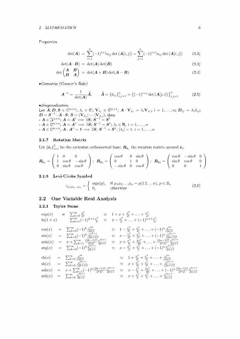
Properties
det(A) =n∑
i=1
(−1)i+jaij det (A[i, j]) =n∑
j=1
(−1)i+jaij det (A[i, j]) (2.2)
det(A ·B) = det(A) det(B) (2.3)
det(
A BB A
)= det(A + B) det(A−B) (2.4)
•Comatrix (Cramer's Rule)
A−1 =1
det(A)A, A = aijn
i,j=1 =(−1)i+j det (A[j, i])
n
i,j=1(2.5)
•DiagonalizationLet A, D, S ∈ Cn×n; λi ∈ C; Vλi ∈ Cn×1; A · Vλi = λiVλi ; i = 1, . . . , n; Dij = λiδij ;D = S−1 ·A · S; S = (Vλ1 | · · · |Vλn
), then- A ∈ Rn×n; A = At =⇒ ∃S; S−1 = St
- A ∈ Cn×n; A = A? =⇒ ∃S; S−1 = S?; λi ∈ R, i = 1, . . . , n- A ∈ Cn×n; A ·A? = 1 =⇒ ∃S; S−1 = S?; |λi| = 1, i = 1, . . . , n
2.1.7 Rotation MatrixLet ei3i=1 be the cartesian orthonormal base; Rei
the rotation matrix around ei.
Re1 =
1 0 01 cos θ − sin θ0 sin θ cos θ
; Re2 =
cos θ 0 sin θ0 1 0− sin θ 0 cos θ
; Re3 =
cos θ − sin θ 0sin θ cos θ 00 0 1
2.1.8 Levi-Civita Symbol
εµ1µ2...µn =
sign(p), if µ1µ2 . . . µn = p(1 2 . . . n), p ∈ Sn
0, otherwise (2.6)
2.2 One Variable Real Analysis2.2.1 Taylor Sums
exp(x) =∑∞
k=0xk
k! ' 1 + x + x2
2! + . . . + xn
n!
ln(1 + x) =∑∞
k=1(−1)k+1 xk
k ' x− x2
2 + . . . + (−1)n+1 xn
n
cos(x) =∑∞
k=0(−1)k x2k
(2k)! ' 1− x2
2! + x4
4! + . . . + (−1)n x2n
(2n)!
sin(x) =∑∞
k=0(−1)k x2k+1
(2k+1)! ' x− x3
3! + x5
5! + . . . + (−1)n x2n+1
(2n+1)!
asin(x) = x +∑∞
k=1(2k−1)!!
2kk!x2k+1
2k+1 ' x + x3
6 + 3x5
40 + . . . + (2n−1)!!2nn!
x2n+1
2n+1
atg(x) =∑∞
k=0(−1)k x2k+1
2k+1 ' x− x3
3 + x5
5 + . . . + (−1)n x2n+1
2n+1
ch(x) =∑∞
k=0x2k
(2k)! ' 1 + x2
2! + x4
4! + . . . + x2n
(2n)!
sh(x) =∑∞
k=0x2k+1
(2k+1)! ' x + x3
3! + x5
5! + . . . + x2n+1
(2n+1)!
ash(x) = x +∑∞
k=1(−1)k (2k−1)!!2kk!
x2k+1
2k+1 ' x− x3
6 + 3x5
40 + . . . + (−1)n (2n−1)!!2nn!
x2n+1
2n+1
ath(x) =∑∞
k=0x2k+1
2k+1 ' x + x3
3 + x5
5 + . . . + x2n+1
2n+1

2 MATHEMATICS 7
11+x =
∑∞k=0(−1)kxk ' 1− x + x2 + . . . + (−1)nxn
1(1+x)2 =
∑∞k=0(−1)k(k + 1)xk ' 1− 2x + 3x2 + . . . + (−1)n(n + 1)xn
√1 + x = 1 +
∑∞k=1(−1)k+1 (2k−1)!!
2kk!xk ' 1 + x
2 − x2
8 + . . . + (−1)n+1 (2n−3)!!2nn! xn
1√1+x
= 1 +∑∞
k=1(−1)k (2k−1)!!2kk!
xk ' 1− x2 + 3x2
8 + . . . + (−1)n (2n−1)!!2nn! xn
(1 + x)α = 1 +∑∞
k=1
∏k−1i=0 (α−i)
k! xk ' 1 + αx + α(α−1)2! x2 + . . . +
∏n−1i=0 (α−i)
n! xn
ln(
1+x1−x
)= 2
∑∞k=0
x2k+1
2k+1 ' 2(x + x3
3 + x5
5 + . . . + x2n+1
2n+1
)∫ x
0dy e−y2
=∑∞
k=0(−1)k x2k+1
k!(2k+1) ' x− x3
3 + x5
2!5 − x7
3!7 + . . . + (−1)n x2n+1
n!(2n+1)
2.2.2 Integrals•Gaussian IntegralsLet α, β, γ ∈ C, Re(α) > 0; x, a ∈ Rd; A : Rd → Rd an operator (matrix); np (nn) thenumber of positive (negative) eigenvalues of A, sign(A) = np − nn.
∫
Rd
ddx exp(−αx2 + βx + γ
)=
(π
α
)d/2
exp(
4αγ + β2
4α
)(2.7)
∫
Rd
ddx exp(− 1
2 〈x|Ax〉+ 〈a|x〉) =(2π)d/2
√det(A)
exp(
12
⟨a|A−1a
⟩)(2.8)
∫
Rd
ddx exp(
i2 〈x|Ax〉) =
(2π)d/2
√det(A)
exp(iπ
4sign(A)
)(2.9)
•Integrals of Gaussian Moments∫
Rd
ddx |x|n e−αx2=
πd/2
αd+n
2
Γ(
d+n2
)
Γ(
d2
) (2.10)∫
Rd
ddx |x|n e−αx2xixj =
πd/2
α(d+n+2)/2
d + n
2d
Γ(
d+n2
)
Γ(
d2
) δij (2.11)∫
Rd
ddx |x|n e−αx2xixjxkxl =
πd/2
α(d+n+4)/2
34
(d + n)(d + n + 2)d(d + 2)
Γ(
d+n2
)
Γ(
d2
)
×
δijkl +13
[δijδkl(1− δik) + δikδjl(1− δij) + δilδjk(1− δij)](2.12)
•Exponential-like Integrals∫ ∞
0
dx xne−αx =n!
αn+1(2.13)
•Angular integralsLet g, σ = (σ1, . . . , σd) ∈ Rd, |σ| = 1. We adopt the notation
∫dσ =
∫|x|=1
ddx . In theintegrals below, the results when θ(σ · g) is absent are obtained upon multiplying the valueof βn by two.
∫dσ θ(σ · g)(σ · g)nσiσj =
βn
n + dgn−2(ngigj + g2δij) (2.14)
∫dσ θ(σ · g)(σ · g)nσi = βn+1g
n−1gi (2.15)
βn =∫
dσ θ(σ · g)(σ · g)n = π(d−1)/2 Γ(
n+12
)
Γ(
n+d2
) (2.16)

2 MATHEMATICS 8
•Hypersphere Integrals∫
|x|≤R
dnx =πn/2
Γ(n/2 + 1)Rn (2.17)
∫
|x|=R
dnx =2πn/2
Γ(n/2)Rn−1 (2.18)
•Trigonometric Functions∫
dx
∫dx
1cos2 x
=∫
dx tg x = − ln (| cosx|) (2.19)∫
dx
∫dx
−1sin2 x
=∫
dx ctg x = ln (| sin x|) (2.20)∫
dx
∫dx
− cos x
sin2 x=
∫dx
1sin x
= ln(∣∣∣tg
(x
2
)∣∣∣)
(2.21)∫
dx
∫dx
sin x
cos2 x=
∫dx
1cos x
= ln(∣∣∣tg
(x
2+
π
4
)∣∣∣)
(2.22)∫
dx
∫dx
1√1− x2
=∫
dx asin x = x asin x +√
1− x2 (2.23)∫
dx
∫dx
−1√1− x2
=∫
dx acosx = x acosx−√
1− x2 (2.24)∫
dx
∫dx
11 + x2
=∫
dx atg x = x atg x− ln(√
1 + x2)
(2.25)∫
dx
∫dx
−11 + x2
=∫
dx actg x = x actg x + ln(√
1 + x2)
(2.26)
•Hyperbolic Functions∫
dx
∫dx
1ch2 x
=∫
dx th x = ln (chx) (2.27)∫
dx
∫dx
−1sh2 x
=∫
dx cthx = ln (| shx|) (2.28)∫
dx
∫dx
1√1 + x2
=∫
dx ashx = x ashx−√
x2 + 1 (2.29)∫
dx
∫dx
1√x2 − 1
=∫
dx ach x = x achx−√
x2 − 1 (2.30)∫
dx
∫dx
11− x2
=∫
dx ath x = x ath x + ln(√
1− x2)
(2.31)∫
dx
∫dx
−11− x2
=∫
dx acth x = x acthx + ln(√
x2 − 1)
(2.32)
•Square Roots∫
dx
∫dx
x√x2 ± a2
=∫
dx√
x2 ± a2 =x
2
√x2 ± a2 ± a2
2ln
(x +
√x2 ± a2
)(2.33)
∫dx
∫dx
−x√a2 − x2
=∫
dx√
a2 − x2 =x
2
√a2 − x2 +
a2
2asin
(x
a
)(2.34)
∫dx
∫dx
−x√(x2 ± a2)3
=∫
dx1√
x2 ± a2= ln
(x +
√x2 ± a2
)(2.35)
∫dx
∫dx
x√(x2 − a2)3
=∫
dx1√
a2 − x2= asin
(x
a
)(2.36)

2 MATHEMATICS 9
•Polynomial Fractions∫
dxx
(x2 ± a)n=
12
(x2 ± a)1−n
1− n(2.37)
∫dx
xp−1
xp + a= 1
p ln (|xp + a|) (2.38)
∫dx
x
(x2 + ax + b)2=
ax + 2b
(x2 + ax + b)(a2 − 4b)− 2a
atg(
2x+a√4b−a2
)
(4b− a2)3/2(2.39)
∫dx
ax + b
x2 + 2cx + s=
a
2ln
(|x2 + 2cx + s|) +b− ca√d− c2
atg(
x + c√d− c2
)(2.40)
∫dx
∫dx
−2(x + a)((x + a)2 + b2)2
=∫
dx1
(x + a)2 + b2=
1b
atg(
x + a
b
)(2.41)
∫dx
∫dx
±2x
(∓x2 ± a2)2=
∫dx
1∓x2 ± a2
=12a
ln(∣∣∣∣
x± a
∓x + a
∣∣∣∣)
(2.42)
•Derivative of an Integral
ddy
∫ g(y)
h(y)
dx f(x, k(y)) = g(1)(y)f(g(y), k(y))−h(1)(y)f(h(y), k(y))+∫ g(y)
h(y)
dxddy
f(x, k(y)) (2.43)
•Spherical Change of Variables in Rn
Let r > 0, ϕ ∈ ]0, 2π[, θi ∈ ]0, π[ ∀ i = 1, . . . , n − 2, then the spherical change of variables inRn is
x1 = r sin θ1 . . . sin θn−2 cosϕx2 = r sin θ1 . . . sin θn−2 sinϕxk = r cos θk−2 sin θk−1 . . . sin θn−2, k = 3, . . . , n− 1xn = r cos θn−2
(2.44)
with the Jacobian
J = rn−1n−2∏
k=1
(sin θk)k. (2.45)
2.2.3 Inequalities
Let ‖f‖p =(∫ b
adx |f(x)|p
)1/p
.
∫ b
a
dx |f(x)g(x)| ≤ ‖f‖p‖g‖q, 1/p + 1/q = 1 (Hölder) (2.46)
‖f + g‖p ≤ ‖f‖p + ‖g‖p, 1 ≤ p < ∞ (Minkowski) (2.47)|〈f |g〉| ≤ ‖f‖ ‖g‖, (Cauchy-Schwartz) (2.48)
‖f‖ ‖g‖ ≤ α‖f‖2 +14α‖g‖2, α > 0 (Young) (2.49)
| 〈f |g〉 | ≤ |f(a)| maxa≤ξ≤b
∣∣∣∣∣∫ ξ
a
dx g(x)
∣∣∣∣∣ , f(a)f(b) ≥ 0, |f(a)| ≥ |f(b)| (Ostrowski) (2.50)

2 MATHEMATICS 10
2.2.4 Dirac Distribution
∀f(x) so that∫
Rdx f(x) = 1, then: lim
ε→0
1εf
(x− x0
ε
)= δ(x− x0) (2.51)
δ(x− x0) =12π
∫
Rdk eik(x−x0) (2.52)
δ(x− x0) =d
dxθ(x− x0) (2.53)
∫
Rdxϕ(x)δ(n)(x− x0) = (−1)nϕ(n)(x0) (2.54)
δ(ax) = 1|a|δ(x), a ∈ R (2.55)
δ (g(x)) =n∑
i=1
1∣∣g(1)(xi)∣∣δ(x− xi),
g(xi) = 0, g(1)(xi) 6= 0
n
i=1(2.56)
∇2(
1r
)= −4πδ (r); ∇ · ( r
r3
)= 4πδ(r);
(∇2 + k2)
eik·rr = −4πδ(r)
2.2.5 Dominated Convergence TheoremLet fn(x)n≥1 ∈ L1(µ); limn→∞ fn(x) = f(x); |fn(x)| ≤ M(X) ∈ L1(µ) ∀x ∈ Ω ⊂ R, ∀n.
limn→∞
∫
Ω
dµ fn =∫
Ω
dµ f (2.57)
2.3 Vector AnalysisNotation: f , g are scalar functions; A, B, C, D are vectors; T is a tensor; ei3i=1 is anorthonormal basis of R3; r =
∑3i=1 xiei; r = |r|; r = r
r .
2.3.1 Vector Identities
A ·B×C = A×B ·C = B ·C×A = B×C ·A = C ·A×B = C×A ·B (2.58)A× (B×C) = (C×B)×A = (A ·C)B− (A ·B)C (2.59)A× (B×C) + B× (C×A) + C× (A×B) = 0 (2.60)(A×B) · (C×D) = (A ·C) (B ·D)− (A ·D) (B ·C) (2.61)(A×B)× (C×D) = (A×B ·D)C− (A×B ·C)D (2.62)∇(fg) = ∇(gf) = f∇g + g∇f (2.63)∇ · (fA) = f∇ ·A + A ·∇f (2.64)∇× (fA) = f∇×A + ∇f ×A (2.65)∇ · (A×B) = B ·∇×A−A ·∇×B (2.66)∇× (A×B) = A (∇ ·B)−B (∇ ·A) + (B ·∇)A− (A ·∇)B (2.67)A× (∇×B) = (∇B) ·A− (A ·∇)B (2.68)∇ (A ·B) = A× (∇×B) + B× (∇×A) + (A ·∇)B + (B ·∇)A (2.69)∇2A = ∇ (∇ ·A)−∇×∇×A (2.70)∇ · (∇f ×∇g) = 0 (2.71)∇×∇f = 0 (2.72)∇ ·∇×A = 0 (2.73)∇r = r (2.74)

2 MATHEMATICS 11
2.3.2 Dierential Operators in Curvilinear Coordinates•Cylindrical CoordinatesDivergence
∇ ·A =1r
∂
∂r(rAr) +
1r
∂Aφ
∂φ+
∂Az
∂z(2.75)
Gradient(∇f)r =
∂f
∂r; (∇f)φ =
1r
∂f
∂φ; (∇f)z =
∂f
∂z(2.76)
Curl
(∇×A)r =1r
∂Az
∂φ− ∂Aφ
∂φ(2.77)
(∇×A)φ =∂Ar
∂z− ∂Az
∂r(2.78)
(∇×A)z =1r
∂
∂r(rAφ)− 1
r
∂Ar
∂φ(2.79)
Laplacian of a scalar function
∇2f =1r
∂
∂r
(r∂f
∂r
)+
1r2
∂2f
∂φ2+
∂2f
∂z2(2.80)
Laplacian of a vector
(∇2A)r
= ∇2Ar − 2r2
∂Aφ
∂φ− Ar
r2(2.81)
(∇2A)φ
= ∇2Aφ +2r2
∂Ar
∂φ− Aφ
r2(2.82)
(∇2A)z
= ∇2Az (2.83)
Components of (A ·∇)B
((A ·∇)B)r = Ar∂Br
∂r+
Aφ
r
∂Br
∂φ+ Az
∂Br
∂z− AφBφ
r(2.84)
((A ·∇)B)φ = Ar∂Bφ
∂r+
Aφ
r
∂Bφ
∂φ+ Az
∂Bφ
∂z+
AφBr
r(2.85)
((A ·∇)B)z = Ar∂Bz
∂r+
Aφ
r
∂Bz
∂φ+ Az
∂Bz
∂z(2.86)
Divergence of a tensor
(∇ · T )r =1r
∂
∂r(rT rr) +
1r
∂T φr
∂φ+
∂T zr
∂z− T φφ
r(2.87)
(∇ · T )φ =1r
∂
∂r(rT rφ) +
1r
∂T φφ
∂φ+
∂T zφ
∂z− T φr
r(2.88)
(∇ · T )z =1r
∂
∂r(rT rz) +
1r
∂T φz
∂φ+
∂T zz
∂z(2.89)
•Spherical CoordinatesDivergence
∇ ·A =1r2
∂
∂r
(r2Ar
)+
1r sin θ
∂
∂θ(sin θAθ) +
1r sin θ
∂Aφ
∂φ(2.90)
Gradient(∇f)r =
∂f
∂r; (∇f)θ =
1r
∂f
∂θ; (∇f)φ =
1r sin θ
∂f
∂φ(2.91)

2 MATHEMATICS 12
Curl
(∇×A)r =1
r sin θ
∂
∂θ(sin θAφ)− 1
r sin θ
∂Aθ
∂φ(2.92)
(∇×A)θ =1
r sin θ
∂Ar
∂φ− 1
r
∂
∂r(rAφ) (2.93)
(∇×A)φ =1r
∂
∂r(rAθ)− 1
r
∂Ar
∂θ(2.94)
Laplacian of a scalar function
∇2f =1r
∂2
∂r2(rf) +
1r2 sin θ
∂
∂θ
(sin θ
∂f
∂θ
)+
1r2 sin2 θ
∂2f
∂φ2(2.95)
Laplacian of a vector
(∇2A)r
= ∇2Ar − 2Ar
r2− 2
r2
∂Aθ
∂θ− 2 ctg θAθ
r2− 2
r2 sin θ
∂Aφ
∂φ(2.96)
(∇2A)θ
= ∇2Aθ +2r2
∂Ar
∂θ− Aθ
r2 sin2 θ− 2 cos θ
r2 sin2 θ
∂Aφ
∂φ(2.97)
(∇2A)φ
= ∇2Aφ − Aφ
r2 sin2 θ+
2r2 sin θ
∂Ar
∂φ+
2 cos θ
r2 sin2 θ
∂Aθ
∂φ(2.98)
Components of (A ·∇)B
((A ·∇)B)r = Ar∂Br
∂r+
Aθ
r
∂Br
∂θ+
Aφ
r sin θ
∂Br
∂φ− AθBθ + AφBφ
r(2.99)
((A ·∇)B)θ = Ar∂Bθ
∂r+
Aθ
r
∂Bθ
∂θ+
Aφ
r sin θ
∂Bθ
∂φ+
AθBr
r− ctg θAφBφ
r(2.100)
((A ·∇)B)φ = Ar∂Bφ
∂r+
Aθ
r
∂Bφ
∂θ+
Aφ
r sin θ
∂Bφ
∂φ+
AφBr
r+
ctg θAφBθ
r(2.101)
Divergence of a tensor
(∇ · T )r =1r2
∂
∂r
(r2T rr
)+
1r sin θ
∂
∂θ(sin θT θr) +
1r sin θ
∂T φr
∂φ− T θθ + T φφ
r(2.102)
(∇ · T )θ =1r2
∂
∂r
(r2T rθ
)+
1r sin θ
∂
∂θ(sin θT θθ) +
1r sin θ
∂T φθ
∂φ+
T θr
r− ctg θT φφ
r(2.103)
(∇ · T )φ =1r2
∂
∂r
(r2T rφ
)+
1r sin θ
∂
∂θ(sin θT θφ) +
1r sin θ
∂T φφ
∂φ+
T φr
r− ctg θT φθ
r(2.104)
2.3.3 Theorems (Green, Ostrogradsky, Stokes)•GreenLet Ω ⊂ R2 be a regular domain; P, Q ∈ C1
(Ω
); Fr(Ω) the frontier positively oriented of Ω.
∮
Fr(Ω)
(PQ
)·(
dxdy
)=
∫
Ω
dxdy
(∂Q
∂x− ∂P
∂y
)(2.105)
•Ostrogradski (Divergence Theorem)Let Ω ⊂ R3 be a regular domain parametrised by Ω = ψ(U); U ⊂ R2; F ∈ C1
(Ω;R3
); Fr(Ω)
the frontier positively oriented of Ω; ν the unitary boundary continuous normal vector of Ω;dσ = ‖D1ψ ×D2ψ‖dx1dx2 .
∮
Fr(Ω)
dσ F · ν =∫
Ω
d3x∇ · F (2.106)
2 MATHEMATICS 13
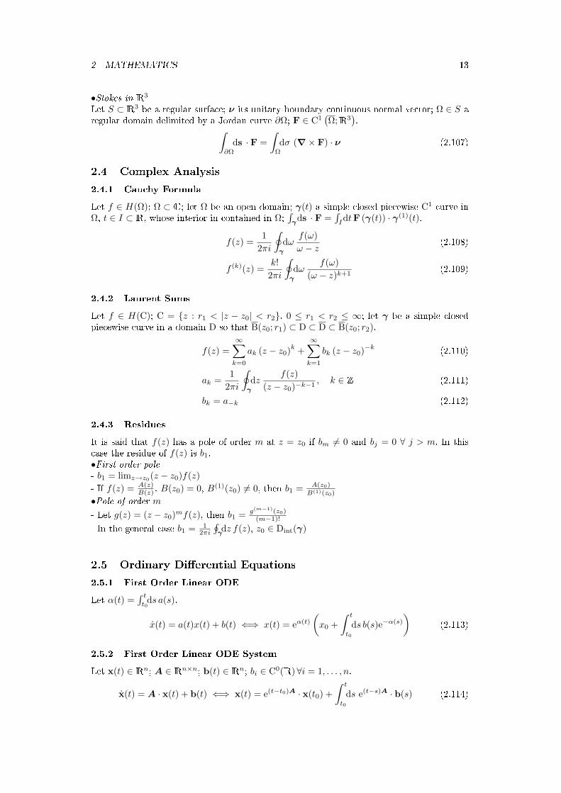
•Stokes in R3
Let S ⊂ R3 be a regular surface; ν its unitary boundary continuous normal vector; Ω ∈ S aregular domain delimited by a Jordan curve ∂Ω; F ∈ C1
(Ω;R3
).
∫
∂Ω
ds · F =∫
Ω
dσ (∇× F) · ν (2.107)
2.4 Complex Analysis2.4.1 Cauchy FormulaLet f ∈ H(Ω); Ω ⊂ C; let Ω be an open domain; γ(t) a simple closed piecewise C1 curve inΩ, t ∈ I ⊂ R, whose interior in contained in Ω;
∫γds · F =
∫IdtF (γ(t)) · γ(1)(t).
f(z) =1
2πi
∮
γ
dωf(ω)ω − z
(2.108)
f (k)(z) =k!2πi
∮
γ
dωf(ω)
(ω − z)k+1(2.109)
2.4.2 Laurent SumsLet f ∈ H(C); C = z : r1 < |z − z0| < r2, 0 ≤ r1 < r2 ≤ ∞; let γ be a simple closedpiecewise curve in a domain D so that B(z0; r1) ⊂ D ⊂ D ⊂ B(z0; r2).
f(z) =∞∑
k=0
ak (z − z0)k +
∞∑
k=1
bk (z − z0)−k (2.110)
ak =1
2πi
∮
γ
dzf(z)
(z − z0)−k−1, k ∈ Z (2.111)
bk = a−k (2.112)
2.4.3 ResiduesIt is said that f(z) has a pole of order m at z = z0 if bm 6= 0 and bj = 0 ∀ j > m. In thiscase the residue of f(z) is b1.•First order pole- b1 = limz→z0(z − z0)f(z)- If f(z) = A(z)
B(z) , B(z0) = 0, B(1)(z0) 6= 0, then b1 = A(z0)B(1)(z0)
•Pole of order m
- Let g(z) = (z − z0)mf(z), then b1 = g(m−1)(z0)(m−1)!
- In the general case b1 = 12πi
∮γdz f(z), z0 ∈ Dint(γ)
2.5 Ordinary Dierential Equations2.5.1 First Order Linear ODELet α(t) =
∫ t
t0ds a(s).
x(t) = a(t)x(t) + b(t) ⇐⇒ x(t) = eα(t)
(x0 +
∫ t
t0
ds b(s)e−α(s)
)(2.113)
2.5.2 First Order Linear ODE SystemLet x(t) ∈ Rn; A ∈ Rn×n; b(t) ∈ Rn; bi ∈ C0(R)∀i = 1, . . . , n.
x(t) = A · x(t) + b(t) ⇐⇒ x(t) = e(t−t0)A · x(t0) +∫ t
t0
ds e(t−s)A · b(s) (2.114)
2 MATHEMATICS 14
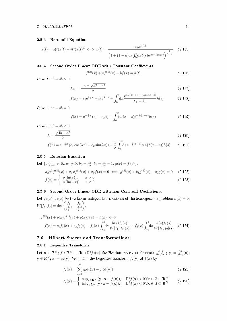
2.5.3 Bernoulli Equation
x(t) = a(t)x(t) + b(t)x(t)n ⇐⇒ x(t) =x0eα(t)
(1 + (1− n)x0
∫ t
t0ds b(s)e(n−1)α(s)
) 1n−1
(2.115)
2.5.4 Second Order Linear ODE with Constant Coecientsf (2)(x) + af (1)(x) + bf(x) = h(t) (2.116)
Case 1: a2 − 4b > 0
λ± =−a±√a2 − 4b
2(2.117)
f(x) = c1eλ+x + c2eλ−x +∫ x
0
dseλ+(x−s) − eλ−(x−s)
λ+ − λ−h(s) (2.118)
Case 2: a2 − 4b = 0
f(x) = e−a2 x (c1 + c2x) +
∫ x
0
ds (x− s)e−a2 (x−s)h(s) (2.119)
Case 3: a2 − 4b < 0
λ =√
4b− a2
2(2.120)
f(x) = e−a2 x (c1 cos(λx) + c2 sin(λx)) +
1λ
∫ x
0
ds e−a2 (x−s) sin(λ(x− s))h(s) (2.121)
2.5.5 Eulerian EquationLet ai3i=1 ∈ R, a2 6= 0, b0 = a0
a2, b1 = a1
a2− 1, g(x) = f (ex).
a2x2f (2)(x) + a1xf (1)(x) + a0f(x) = 0 ⇐⇒ g(2)(x) + b1g
(1)(x) + b0g(x) = 0 (2.122)
f(x) =
g (ln(x)), x > 0g (ln(−x)), x < 0 (2.123)
2.5.6 Second Order Linear ODE with non-Constant CoecientsLet f1(x), f2(x) be two linear independent solutions of the homogeneous problem h(x) = 0;
W [f1, f2] = det(
f1 f2
f(1)1 f
(1)2
).
f (2)(x) + p(x)f (1)(x) + q(x)f(x) = h(x) ⇐⇒
f(x) = c1f1(x) + c2f2(x)− f1(x)∫ x
x0
dsh(s)f2(s)
W [f1, f2](s)+ f2(x)
∫ x
x0
dsh(s)f1(s)
W [f1, f2](s)(2.124)
2.6 Hilbert Spaces and Transformations2.6.1 Legendre Transform
Let x ∈ RN ; f : RN → R; (D2f)(x) the Hessian matrix of elements ∂2f∂xi∂xj
; yi = ∂f∂xi
(x);y ∈ RN ; xi = φi(y). We dene the Legendre transform f∗(y) of f(x) by
f∗(y) =N∑
i=1
yiφi(y)− f (φ(y)) (2.125)
f∗(y) =
supx∈RN (y · x− f(x)), D2f(x) > 0∀x ∈ Ω ⊂ RN
infx∈RN (y · x− f(x)), D2f(x) < 0∀x ∈ Ω ⊂ RN (2.126)
2 MATHEMATICS 15
2.6.2 Laplace TransformLet f : [0,∞[→ C.
L (f(x)) (s) = F (s) =∫ ∞
0
dx f(x)e−sx (2.127)
L (eaxf(x)) = F (s− a) (2.128)L (xnf(x)) = (−1)nF (n)(s) (2.129)
L(f (n)(x)
)= snF (s)−
n∑
k=1
sn−kf (k−1)(0) (2.130)
(f ∗ g)(x) =∫ x
0
dy f(x− y)g(y) =⇒ L (f ∗ g) = L (f)L (g) (2.131)
2.6.3 Fourier TransformLet f : RN → C so that
∫RN dNx |f(x)|2 < ∞.
F (f(x)) (k) = f(k) =1
(2π)N/2
∫
RN
dNx f(x)e−ik·x (2.132)
F−1(f(k)
)(x) = f(x) =
1(2π)N/2
∫
RN
dNx f(k)eix·k (2.133)
F (f(x + h)) (k) = e−ik·hF (f(x)) (k) (2.134)F (f (ax)) (k) = 1
|a|N F (f(x)) (k) (2.135)
F(f (n) (x)
)(k) = (ik)n F (f(x)) (k) (2.136)
F (xnf (x)) (k) = (i)n F (n) (f(x)) (k) (2.137)
(f ∗ g)(x) =∫
RN
dNy f(x− y)g(y) =⇒ F (f ∗ g) = F (f)F (g) (2.138)⟨f∣∣g⟩
=⟨f∣∣g⟩
(2.139)
F(e−
12 〈x|Ax〉
)(k) =
1
(det(A))1/2e−
12
⟨k∣∣A−1k
⟩(2.140)
2.6.4 Bases of L2([a, b])
Let 〈f |g〉 =∫ b
adx f(x)?g(x) be the scalar product of L2([a, b]), then one has the following
orthonormal bases Bi4i=1 of L2([a, b]). B2 leads to the usual Fourier sum.
B1 =
1√b− a
exp(
in
(2π
b− a
)x
)
n∈Z(2.141)
B2 =
1√
b− a,
√2
b− acos
(n
(2π
b− a
)x
),
√2
b− asin
(n
(2π
b− a
)x
)
n∈N∗(2.142)
B3 =
1√
b− a,
√2
b− acos
(n
(π
b− a
)(x− a)
)
n∈N∗(2.143)
B4 =
√2
b− asin
(n
(π
b− a
)(x− a)
)
n∈N∗(2.144)
2 MATHEMATICS 16
2.7 Special Functions2.7.1 Bessel Functions Jν(x), Yν(x), H
(±)ν (x)
•First Kind Bessel Functions Jν(x)Let ν ≥ 0; x ∈]0,∞[; then Jν , J−ν are two linear independent solutions.
x2f (2)(x) + xf (1)(x) + (x2 − ν2)f(x) = 0 ⇐⇒ Jν(x) =∞∑
k=0
(−1)k(x/2)2k+ν
k! Γ(ν + k + 1)(2.145)
•Second Kind Bessel Functions (Neumann Functions) Yν(x)Jν , Yν are two linear independent solutions of Bessel's equation, ν /∈ N.
Yν(x) =1
sin (νπ)(cos (νπJν(x))− J−ν(x)) (2.146)
If ν ∈ NYν(x) =
1π
(∂
∂νJν(x)− (−1)ν ∂
∂νJ−ν(x)
)(2.147)
•Third Kind Bessel Functions (Hankel's Functions) H(±)ν (x)
H(+)ν , H
(−)ν are two linear independent solutions of Bessel's equation.
H(±)ν (x) = Jν(x)± iYν(x) (2.148)
•Asymptotic Behaviour of Jν(x), Yν(x)
Jν(x)x→+∞³
√π
2xcos
(x− π
4− νπ
2
)+
Rν(x)x3/2
, supx≥1
|Rν(x)| < ∞ (2.149)
Yν(x)x→+∞³
√π
2xsin
(x− π
4− νπ
2
)+
Sν(x)x3/2
, supx≥1
|Sν(x)| < ∞ (2.150)
2.7.2 Legendre Polynomials Pn(x)√
n + 1/2 Pn(x) form an orthonormal basis of L2(]− 1, 1[, dx ).
(1− x2)f (2)(x)− 2xf (1)(x) + n(n + 1)f(x) = 0 ⇐⇒ Pn(x) =1
2nn!dn
dxn(x2 − 1)n (2.151)
P0(x) = 1 P1(x) = x P2(x) = 12 (3x2 − 1)
P3(x) = 12x(5x2 − 3) P4(x) = 1
8 (35x4 − 30x2 + 3) P5(x) = 18x(63x4 − 70x2 + 15)
2.7.3 Associated Legendre Polynomials Pmn (x)
(1− x2)f (2)(x)− 2xf (1)(x) +(
n(n + 1)− m2
1− x2
)f(x) = 0
⇐⇒ Pmn (x) = (−1)m(1− x2)m/2 dm
dxmPn(x) (2.152)
P 00 (x) = 1 P 0
1 (x) = x P 02 (x) = 1
2 (3x2 − 1)P 1
0 (x) = 0 P 11 (x) = −√1− x2 P 1
2 (x) = −3x√
1− x2
P 20 (x) = 0 P 2
1 (x) = 0 P 22 (x) = 3(1− x2)
2 MATHEMATICS 17
2.7.4 Hermite Polynomials Hn(x)
(2nπ1/2n!)−1/2Hn(x) form an orthonormal basis of L2(]−∞,∞[, e−x2
dx).
f (2)(x)− 2xf (1)(x) + 2nf(x) = 0 ⇐⇒ Hn(x) = (−1)nex2 dn
dxne−x2 (2.153)
H0(x) = 1 H1(x) = 2x H2(x) = 2(2x2 − 1)H3(x) = 4x(2x2 − 3) H4(x) = 4(4x4 − 12x2 + 3) H5(x) = 8x(4x4 − 20x2 + 15)
2.7.5 Generalized Laguerre Polynomials Lan(x)
√Γ(n+1)
Γ(a+n+1)Lan(x) form an orthonormal basis of L2 (]0,∞[, xae−xdx ); a > −1.
xf (2)(x) + (a + 1− x)f (1)(x) + nf(x) = 0
⇐⇒ Lan(x) = (−1)nexx−a dn
dxn
(e−xxn+a
)=
n∑
j=0
(−1)j
(n + a
n− j
)xj
j!(2.154)
L00(x) = 1 L0
1(x) = 1− x L02(x) = 1− 2x + 1
2x2
L10(x) = 1 L1
1(x) = 2− x L12(x) = 3− 3x + 1
2x2
L20(x) = 1 L2
1(x) = 3− x L22(x) = 6− 4x + 1
2x2
The Sonine polynomials Sn(x) are dened by Sn(x) = Ld/2−1n , where d is the dimension.
2.7.6 Chebyshev Polynomials Tn(x)√
εn
π Tn(x) form an orthonormal basis of L2(]− 1, 1[, (1− x2)−1/2dx
); εn = 2− δn,0.
Tn+1(x)− 2xTn(x) + Tn−1(x) = 0 ⇐⇒ Tn(x) = cos (n acos(x)) =1∑
k=0
(x + i1+2k
√1− x2
)n
2(2.155)
T0(x) = 1 T1(x) = x T2(x) = 2x2 − 1T3(x) = 4x2 − 3x T4(x) = 8x4 − 8x2 + 1 T5(x) = 16x5 − 20x3 + 5x
2.7.7 Spherical Harmonics Y ml (θ, ϕ)
Y ml (θ, ϕ) =
√2l + 1
4π
√(l + m)!(l −m)! eimϕPm
l (cos θ) , l ≥ 0 (2.156)
Y ml (θ, ϕ) = Y m
−(l+1)(θ, ϕ) , l ≤ −1 (2.157)
Y 00 (θ, ϕ) =
1√4π
(2.158)
Y 01 (θ, ϕ) =
√34π
cos θ (2.159)
Y ±11 (θ, ϕ) = ∓
√38π
sin θ e±iϕ (2.160)
Y 02 (θ, ϕ) =
√5
16π(3 cos2 θ − 1) (2.161)
Y ±12 (θ, ϕ) = ∓
√158π
sin θ cos θ e±iϕ (2.162)
Y ±22 (θ, ϕ) =
√1532π
sin2 θ e±2iϕ (2.163)
2 MATHEMATICS 18
2.7.8 Radial Hydrogen Functions Rnl(r)
Let a0 = ~2µe2 = 0.529117 Å; C(n, l) be a numerical coecient; C(1, 0) = 2, C(2, 0) =
√2,
C(2, 1) = 12√
6.
(− ~
2
2µ
d2
dr2+~l(l + 1)
2µr2− e2
r− En
)Rnl = 0
⇐⇒ Rnl(r) = C(n, l)1
a3/20
(r
ao
)l
e−r
a0n Lln−l−1
(r
2a0
)(2.164)
R10(r) =2
a3/20
e−ra0 (2.165)
R20(r) =2
(2a0)3/2
(1− r
2a0
)e−
r2a0 (2.166)
R21(r) =1√
3(2a0)3/2
r
a0e−
r2a0 (2.167)
R30(r) =2
(3a0)3/2
(1− 2
3r
a0+
227
r2
a20
)e−
r3a0 (2.168)
R31(r) =8
9√
2(3a0)3/2
(1− 1
6r
a0
)r
a0e−
r3a0 (2.169)
R32(r) =12
81√
10(3a0)3/2
(ra0
)2
e−r
3a0 (2.170)
2.7.9 Airy Function Ai(x), Bi(x); Asymptotic Behaviour
f (2)(x)− xf(x) = 0 ⇐⇒ f(x) =√
xJ1/3
(23x3/2
)(2.171)
Ai(+∞) = A(1)i (+∞) = 0 Bi(−∞) = B
(1)i (−∞) = 0
Ai(x)x→+∞³ 1
x1/4 exp(− 2
3x3/2)
Bi(x)x→+∞³ 1
x1/4 exp(
23x3/2
)
Ai(x)x→−∞³ 2
(−x)1/4 cos(
23 (−x)3/2 − π
4
)Bi(x)
x→−∞³ 1(−x)1/4 sin
(23 (−x)3/2 − π
4
)
2.7.10 Gamma Function Γ(x)
(x− 1)! = Γ(x) =∫ ∞
0
dy e−yyx−1 (2.172)
Γ (x + 1) = xΓ (x) Γ(x)Γ(1− x) = πsin(πx)
Γ(n + 1/2) =√
π2n (2n− 1)!! Γ(1/2− n) = (−1)n 2n√π
(2n−1)!!
2.7.11 Stirling FormulaLet z ∈ C. In general one uses z! ∼ √
2πzz+1/2e−z.√
2πzz+1/2e−ze1
12z+1 < z! <√
2πzz+1/2e−ze1
12z (2.173)
2 MATHEMATICS 19
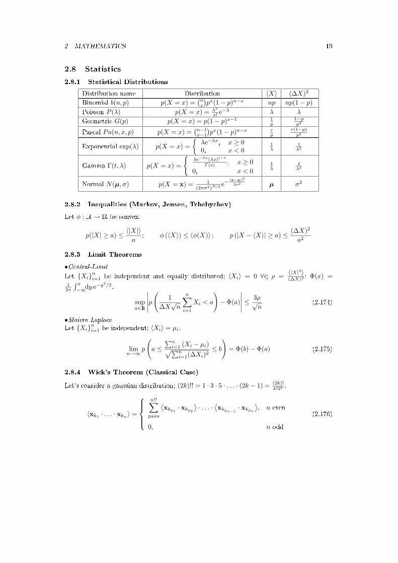
2.8 Statistics2.8.1 Statistical Distributions
Distribution name Distribution 〈X〉 (∆X)2
Binomial b(n, p) p(X = x) =(nx
)px(1− p)n−x np np(1− p)
Poisson P (λ) p(X = x) = λx
x! e−λ λ λ
Geometric G(p) p(X = x) = p(1− p)x−1 1p
1−pp2
Pascal Pa(n, x, p) p(X = x) =(n−1x−1
)px(1− p)n−x r
pr(1−p)
p2
Exponential exp(λ) p(X = x) =
λe−λx, x ≥ 00, x < 0
1λ
1λ2
Gamma Γ(t, λ) p(X = x) =
λe−λx(λx)t−1
Γ(s) , x ≥ 00, x < 0
tλ
tλ2
Normal N(µ, σ) p(X = x) = 1(2πσ2)N/2 e−
(x−µ)2
2σ2 µ σ2
2.8.2 Inequalities (Markov, Jensen, Tchebychev)Let φ : R→ R be convex.
p(|X| ≥ a) ≤ 〈|X|〉a
; φ (〈X〉) ≤ 〈φ(X)〉 ; p (|X − 〈X〉| ≥ a) ≤ (∆X)2
a2
2.8.3 Limit Theorems•Central-LimitLet Xin
i=1 be independent and equally distributed; 〈Xi〉 = 0 ∀i; ρ = 〈|X|3〉(∆X)3 ; Φ(x) =
12π
∫ x
−∞dy e−y2/2.
supa∈R
∣∣∣∣∣p(
1∆X
√n
n∑
i=1
Xi < a
)− Φ(a)
∣∣∣∣∣ ≤3ρ√n
(2.174)
•Moivre-LaplaceLet Xin
i=1 be independent; 〈Xi〉 = µi.
limn→∞
p
(a ≤
∑ni=1 (Xi − µi)√∑n
i=1(∆Xi)2≤ b
)= Φ(b)− Φ(a) (2.175)
2.8.4 Wick's Theorem (Classical Case)
Let's consider a gaussian distribution; (2k)!! = 1 · 3 · 5 · . . . · (2k − 1) = (2k)!k!2k .
〈xk1 · . . . · xkn〉 =
n!!∑
pairs
⟨xkp1
· xkp2
⟩ · . . . · ⟨xkpn−1· xkpn
⟩, n even
0, n odd
(2.176)
3 PHYSICS 20
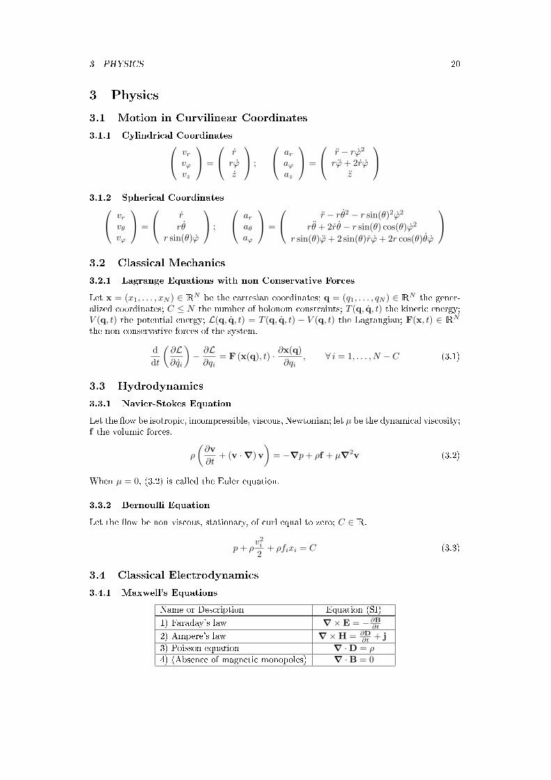
3 Physics3.1 Motion in Curvilinear Coordinates3.1.1 Cylindrical Coordinates
vr
vϕ
vz
=
rrϕz
;
ar
aϕ
az
=
r − rϕ2
rϕ + 2rϕz
3.1.2 Spherical Coordinates
vr
vθ
vϕ
=
r
rθr sin(θ)ϕ
;
ar
aθ
aϕ
=
r − rθ2 − r sin(θ)2ϕ2
rθ + 2rθ − r sin(θ) cos(θ)ϕ2
r sin(θ)ϕ + 2 sin(θ)rϕ + 2r cos(θ)θϕ
3.2 Classical Mechanics3.2.1 Lagrange Equations with non Conservative ForcesLet x = (x1, . . . , xN ) ∈ RN be the cartesian coordinates; q = (q1, . . . , qN ) ∈ RN the gener-alized coordinates; C ≤ N the number of holonom constraints; T (q, q, t) the kinetic energy;V (q, t) the potential energy; L(q, q, t) = T (q, q, t) − V (q, t) the Lagrangian; F(x, t) ∈ RN
the non conservative forces of the system.
ddt
(∂L∂qi
)− ∂L
∂qi= F (x(q), t) · ∂x(q)
∂qi, ∀ i = 1, . . . , N − C (3.1)
3.3 Hydrodynamics3.3.1 Navier-Stokes EquationLet the ow be isotropic, incompressible, viscous, Newtonian; let µ be the dynamical viscosity;f the volumic forces.
ρ
(∂v∂t
+ (v ·∇)v)
= −∇p + ρf + µ∇2v (3.2)
When µ = 0, (3.2) is called the Euler equation.
3.3.2 Bernoulli EquationLet the ow be non viscous, stationary, of curl equal to zero; C ∈ R.
p + ρv2
i
2+ ρfixi = C (3.3)
3.4 Classical Electrodynamics3.4.1 Maxwell's Equations
Name or Description Equation (SI)1) Faraday's law ∇×E = −∂B
∂t
2) Ampere's law ∇×H = ∂D∂t + j
3) Poisson equation ∇ ·D = ρ4) (Absence of magnetic monopoles) ∇ ·B = 0

3 PHYSICS 21
3.4.2 Complementary Basic RelationsName or description Equation (SI)Equation for the vector potential ∇2A− 1
c2∂2A∂t2 = −µ0j
Equation for the scalar potential ∇2V − 1c2
∂2V∂t2 = − ρ
ε0
Poisson Equation ∇2f(x) = g(x) ⇐⇒ f(x) = − 14π
∫Ωd3y g(y)
|x−y|Linear tensorial constitutive relations D = εE; B = µHElectric Force F = χε0∇
(12E
2) |Ω|
Magnetic Force F = χµ0
∇ (12B
2) |Ω|
Energy du = E · dD + H · dB⇐⇒ u(x, t) = 1
2 (E ·D + H ·B)Poynting's Vector S = E×HPoynting's Theorem ∂
∂tu(x, t) + ∇ · S(x, t) = −E · j
3.4.3 Vacuum ElectrostaticsLet Γ ⊂ R3 be a closed path; Σ ⊂ R3 a closed surface.
∇×E = 0 ⇐⇒∮
Γ
dγ E = 0 (3.4)
∇ ·D = 0 ⇐⇒∮
Σ
dσ D =∑
i∈Dint(Σ)
qi (3.5)
E = −∇V ⇐⇒∫
Γ
dγ E =∫ b
a
dsE = Va − Vb (3.6)
∇2V = − ρ
ε0⇐⇒ V (x) =
14πε0
∫
Ω
d3yρ(y)|x− y| (3.7)
δW = qV ⇐⇒ δW = E · dD (3.8)
3.4.4 Linear Theory of Conductors and DielectricsLet Ω ⊂ R3 be a volume of measure |Ω|.
V = QC ; U = 1
2CV 2; U = 12E
2 (3.9)F = χε0∇
(12E
2) |Ω| (3.10)
µ = qδ (3.11)
P =dµ
dΩ; P = χε0E (3.12)
D = ε0E + P ⇐⇒ D = ε0εrE (3.13)
3.4.5 Magnetostatics
∇×H = j ⇐⇒∮
Γ
dγ H =∑
Iint (3.14)
∇ ·B = 0 ⇐⇒∮
Σ
dσ B = 0 (3.15)
∇2A = −µ0j ⇐⇒ A(x) =µ0
4π
∫
Ω
d3yj(y)|x− y| (3.16)
dF = Idl×B ⇐⇒ dB =µ0
4πIdl× r
r2⇐⇒ B(x) =
µ0
4π
∫
Ω
d3yj(y)× (x− y)|x− y|3 (3.17)
δW = H · dB (3.18)
3 PHYSICS 22
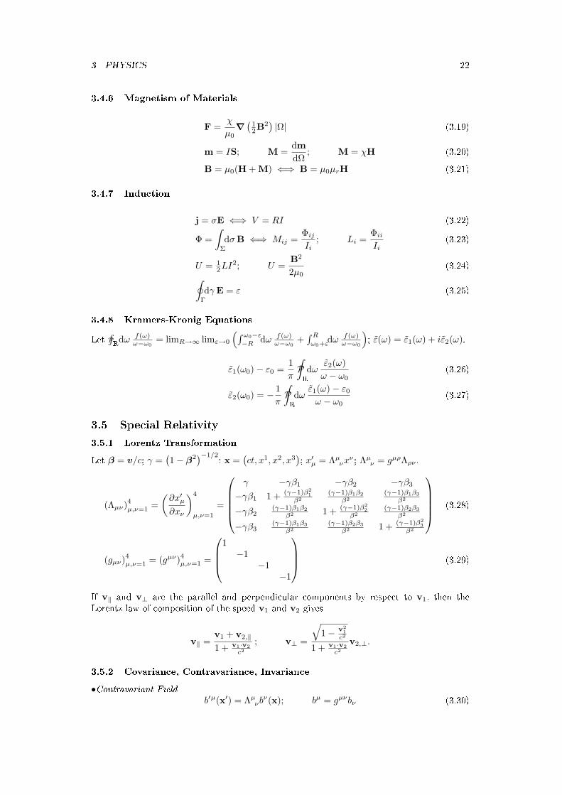
3.4.6 Magnetism of Materials
F =χ
µ0∇ (
12B
2) |Ω| (3.19)
m = IS; M =dmdΩ
; M = χH (3.20)B = µ0(H + M) ⇐⇒ B = µ0µrH (3.21)
3.4.7 Induction
j = σE ⇐⇒ V = RI (3.22)
Φ =∫
Σ
dσ B ⇐⇒ Mij =Φij
Ii; Li =
Φii
Ii(3.23)
U = 12LI2; U =
B2
2µ0(3.24)
∮
Γ
dγ E = ε (3.25)
3.4.8 Kramers-Kronig Equations
Let∫RP dω f(ω)
ω−ω0= limR→∞ limε→0
(∫ ω0−ε
−Rdω f(ω)
ω−ω0+
∫ R
ω0+εdω f(ω)
ω−ω0
); ε(ω) = ε1(ω) + iε2(ω).
ε1(ω0)− ε0 =1π
∫
RP dω
ε2(ω)ω − ω0
(3.26)
ε2(ω0) = − 1π
∫
RP dω
ε1(ω)− ε0
ω − ω0(3.27)
3.5 Special Relativity3.5.1 Lorentz TransformationLet β = v/c; γ =
(1− β2
)−1/2; x =(ct, x1, x2, x3
); x′µ = Λµ
νxν ; Λµν = gµρΛρν .
(Λµν)4µ,ν=1 =(
∂x′µ∂xν
)4
µ,ν=1
=
γ −γβ1 −γβ2 −γβ3
−γβ1 1 + (γ−1)β21
β2(γ−1)β1β2
β2(γ−1)β1β3
β2
−γβ2(γ−1)β1β2
β2 1 + (γ−1)β22
β2(γ−1)β2β3
β2
−γβ3(γ−1)β1β3
β2(γ−1)β2β3
β2 1 + (γ−1)β23
β2
(3.28)
(gµν)4µ,ν=1 = (gµν)4µ,ν=1 =
1−1
−1−1
(3.29)
If v‖ and v⊥ are the parallel and perpendicular components by respect to v1, then theLorentz law of composition of the speed v1 and v2 gives
v‖ =v1 + v2,‖1 + v1·v2
c2
; v⊥ =
√1− v2
1c2
1 + v1·v2c2
v2,⊥.
3.5.2 Covariance, Contravariance, Invariance•Contravariant Field
b′µ(x′) = Λµνbν(x); bµ = gµνbν (3.30)
3 PHYSICS 23
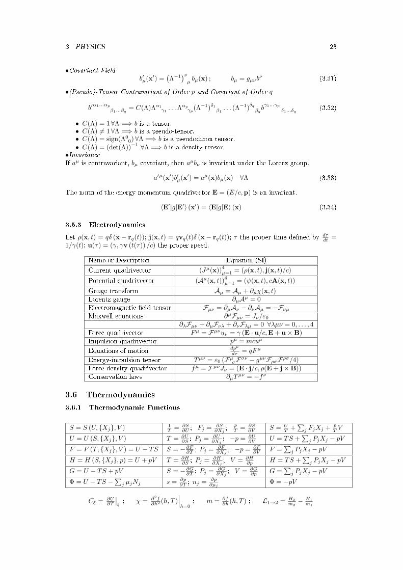
•Covariant Fieldb′µ(x′) =
(Λ−1
)ν
µbµ(x) ; bµ = gµνbν (3.31)
•(Pseudo)-Tensor Contravariant of Order p and Covariant of Order q
b′α1...αp
β1...βq= C(Λ)Λα1
γ1. . . Λαp
γp(Λ−1)δ1
β1. . . (Λ−1)δq
βqbγ1...γp
δ1...δq(3.32)
• C(Λ) = 1 ∀Λ =⇒ b is a tensor.• C(Λ) 6= 1 ∀Λ =⇒ b is a pseudo-tensor.• C(Λ) = sign(Λ0
0)∀Λ =⇒ b is a pseudochron tensor.• C(Λ) = (det(Λ))−1 ∀Λ =⇒ b is a density tensor.
•InvarianceIf aµ is contravariant, bµ covariant, then aµbν is invariant under the Lorenz group.
a′µ(x′)b′µ(x′) = aµ(x)bµ(x) ∀Λ (3.33)
The norm of the energy-momentum quadrivector E = (E/c,p) is an invariant.
〈E′|g|E′〉 (x′) = 〈E|g|E〉 (x) (3.34)
3.5.3 ElectrodynamicsLet ρ(x, t) = qδ (x− rq(t)); j(x, t) = qvq(t)δ (x− rq(t)); τ the proper time dened by dτ
dt =1/γ(t); u(τ) = (γ, γv (t(τ)) /c) the proper speed.
Name or Description Equation (SI)Current quadrivector (Jµ(x))4µ=1 = (ρ(x, t), j(x, t)/c)
Potential quadrivector (Aµ(x, t))4µ=1 = (ψ(x, t), cA(x, t))Gauge transform Aµ = Aµ + ∂µχ(x, t)Lorentz gauge ∂µAµ = 0Electromagnetic eld tensor Fµν = ∂µAν − ∂νAµ = −Fνµ
Maxwell equations ∂µFµν = Jν/ε0
∂λFµν + ∂µFνλ + ∂νFλµ = 0 ∀λµν = 0, . . . , 4Force quadrivector Fµ = Fµνuν = γ (E · u/c,E + u×B)Impulsion quadrivector pµ = mcuµ
Equations of motion dpµ
dτ = qFµ
Energy-impulsion tensor Tµν = ε0 (FµσFσν − gµνFρσFρσ/4)
Force density quadrivector fµ = FµνJν = (E · j/c, ρ(E + j×B))Conservation laws ∂µTµν = −fν
3.6 Thermodynamics3.6.1 Thermodynamic Functions
S = S (U, Xj, V ) 1T = ∂S
∂U ; Fj = ∂S∂Xj
; pT = ∂S
∂V S = UT +
∑j FjXj + p
T V
U = U (S, Xj, V ) T = ∂U∂S ; Pj = ∂U
∂Xj; −p = ∂U
∂V U = TS +∑
j PjXj − pV
F = F (T, Xj, V ) = U − TS S = −∂F∂T ; Pj = ∂F
∂Xj; −p = ∂F
∂V F =∑
j PjXj − pV
H = H (S, Xj, p) = U + pV T = ∂H∂S ; Pj = ∂H
∂Xj; V = ∂H
∂p H = TS +∑
j PjXj − pV
G = U − TS + pV S = −∂G∂T ; Pj = ∂G
∂Xj; V = ∂G
∂p G =∑
j PjXj − pV
Φ = U − TS −∑j µjNj s = ∂p
∂T ; nj = ∂p∂µj
Φ = −pV
Cξ = ∂U∂T
∣∣ξ; χ = ∂2f
∂h2 (h, T )∣∣∣h=0
; m = ∂f∂h (h, T ) ; L1→2 = H2
m2− H1
m1
3 PHYSICS 24
3.7 Classical Statistical Physics3.7.1 Statistical EnsemblesSee sections 3.10.1-3.10.3 page 28.
3.7.2 k-Points Correlation FunctionLet Λ ⊂ Rd; indistinguishable particles; xα = (pα,qα); qα ∈ Λ; pα ∈ Rd; dNω(x) = dNx
N !hdN ;let
A(x1, . . . ,xN ) =1k!
∑
1≤α1≤N
...1≤αk≤N
A(k)(xα1 , . . . ,xαk)
be a k-points observable; let N = k+m; then the k-points correlation function ρ(k)(x1, . . . ,xk)is given by
ρ(k)(x1, . . . ,xk) =∞∑
m=0
∫dmω(y1, . . . ,ym) ρk+m(x1, . . . ,xk,y1, . . . ,ym) (3.35)
〈A〉ρ =∫
dkω(x) ρ(k)(x1, . . . ,xk) A(k)(x1, . . . ,xk) (3.36)
3.7.3 Fokker-Plank EquationLet the stochastic process be a Markov weakly stationary process dened by p(x0|x, t); letx = (x1, . . . , xn) be the n variables of the system; let α > 1;
∫Rndnx (x − x0)i p(x0|x, t) =
ai(x0) t + O(tα);∫Rndnx (x− x0)i(x− x0)j p(x0|x, t) = bij(x0) t + O(tα).
∂
∂tp(x0|y, t) = −
n∑
i=1
∂
∂yi(ai(y)p(x0|y, t)) +
12
n∑
i,j=1
∂2
∂yi∂yj(bij(y)p(x0|y, t)) (3.37)
3.7.4 Master EquationsLet the stochastic process be a discrete Markov weakly stationary process; W(n1|n2) =limt→0
1t p(n1|n2, t); P (n, t) = P (n′|n, t) the conditional probability of state n at time t
granted that the state was n′ at time 0, Ω the space phase.
d
dtp(n, t) =
∑
n′∈Ω
(p(n′, t)W(n′|n)− p(n, t)W(n|n′)) (3.38)
3.8 Quantum Mechanics3.8.1 Stationary Perturbation TheoryLet H = H0 + W ; H0 |ϕn〉 = E0
n |ϕn〉.
En = E0n + 〈ϕn|Wϕn〉+
∑
i 6=n
|〈ϕi|W |ϕn〉|2E0
n − E0i
+ . . . (3.39)
∣∣ϕW 6=0n
⟩= |ϕn〉+
∑
i 6=n
〈ϕi|W |ϕn〉E0
n − E0i
|ϕi〉+ . . . (3.40)
3 PHYSICS 25
3.8.2 Non Stationary Perturbation TheoryLet H(t) = H0 + λW (t); 〈x|ψt〉 = U(t) 〈x|ψ0〉; U0(t) = e−itH0/~; WI(t) = U†
0 (t)W (t)U0(t).
U(t) = U0(t)
(1+
λ
i~
∫ t
0
ds1 WI(s1) +(
λ
i~
)2 ∫ t
0
ds1
∫ s1
0
ds2 WI(s1)WI(s2) + . . .
+(
λ
i~
)n ∫ t
0
dsn WI(sn)n−1∏
k=1
∫ sk+1
0
dsk WI(sk) + . . .
)(3.41)
3.8.3 Fermi's Golden RuleLet H = H0 + W (t); H0 |in〉 = Ein |in〉; H0 |end〉 = Eend |end〉; 〈in|end〉 = 0; let |ν〉ν be anorthonormal base; H0 |ν〉 = Eν |ν〉.
dp(in → end)dt
=2π
~δ(Ein − Eend)
∣∣∣∣ limη→0A(η)
∣∣∣∣2
(3.42)
A(η) =
〈end|W |in〉 , rst order∑
ν
〈end|W |ν〉 〈ν|W |in〉Eν − Ein − iη
, second order (3.43)
3.8.4 Harmonic OscillatorLet |n〉∞n=0 be the eigenstates of the hamiltonian H with eigenvalues En∞n=0, so thatH |n〉 = En |n〉; Hn(x) the nth Hermite polynomial.
H =p2
2m+ 1
2mω2q2 = ~ω(a†a + 1
2
)(3.44)
a = p−imωq√2~mω
a† = p+imωq√2~mω
a |n〉 =√
n |n− 1〉 a† |n〉 =√
n + 1 |n + 1〉a |0〉 = 0
|n〉 = 1√n!
(a†
)n |0〉 ϕn(x) = 〈x|n〉 =(
mωπ~
)1/4 1√2nn!
e−mω2~ x2
Hn
(√mω~ x
)
ϕ0(x) =(
mωπ~
)1/4 e−mω2~ x2
ϕ1(x) =(
4π
(mω~
)3)1/4
x e−mω2~ x2
ϕ2(x) =(
mω4π~
)1/4 (2mω~ − 1
)e−
mω2~ x2
3.8.5 Hydrogen Atom
Let r = |r|; r ∈ R3; µ = memp
me+mp; e2 = q2
4πε0; µB = q~
2me. Rnl(r) and Y m
l (θ, ϕ) are dened inthe sections 2.7.7 and 2.7.8. The complete set of commutating observables is H,L2, L3.
(− ~
2
2µ∇2 − e2
r
)ψ(r) = Eψ(r) (3.45)
ψnlm(r) = Rnl(r)Y ml (θ, ϕ) (3.46)
Hψnlm = Enψnlm n = 1, 2, . . . ,∞ (3.47)L2Y m
l (θ, ϕ) = ~2l(l + 1)Y ml (θ, ϕ) l = 0, 1, . . . , n− 1 (3.48)
L3Yml (θ, ϕ) = ~mY m
l (θ, ϕ) m = −l,−l + 1, . . . , l − 1, l (3.49)

3 PHYSICS 26
En = −EI
n2(3.50)
EI =α2mec
2
2= 13.60580 eV, α =
e2
~c(3.51)
∇2 =1r
∂2
∂r2r − L2
~2r2(3.52)
L± = L1 ± iL2 (3.53)L±Y m
l (θ, ϕ) = ~√
l(l + 1)−m(m± 1)Y m±1l (θ, ϕ) (3.54)
L2 = 12 (L+L− + L−L+) + L2
3 (3.55)L±L∓ = L2 ± ~L3 − L2
3 (3.56)
3.8.6 Pauli's Matrices
σx =(
0 11 0
); σy =
(0 −ii 0
); σz =
(1 00 −1
)
3.8.7 Commutation and Anticommutation RelationsLet q, p, L = q × p be the position, impulsion, orbital kinetic momentum operators; a, a†
the annihilation, creation operators; ª denotes a cyclic permutation.
[qi, pj] = i~δij ; [L1, L2] = i~L3 ª; [L2, L] = [L2, L3] = 0[L3, L±] = ±~L±; [L+, L−] = 2~L3; [L2, L±] = 0[a, a†
]= 1;
[a†a, a
]= −a;
[a†a, a†
]= a†
[σx, σy] = 2iσz ª; σx, σy = 0 ª
[AB, C] = A[B, C] + [A,C]B; [A,BC] = B[A,C] + [A,B]C[AB, C] = A B,C − A,CB; [A,BC] = A,BC −B A,C
eAeB = eA+B+12 [A,B] (3.57)
eA+B = limN→∞
(e
AN e
BN
)N
(3.58)
eλABe−λA =∞∑
n=0
λn
n!Ωn(A,B), Ωn(A,B) =
B, n = 0[A, Ωn−1(A,B)] , n ≥ 1 (3.59)
3.9 Feynman Path Integral3.9.1 Feynman Path IntegralLet L (x(s), x(s)) be the Lagrangian of the system; d its dimension.
〈x|U(t, t0)|x0〉 =∫ x,t
x0,t0
d[x(·)] exp(
i
~S (x(·))
)(3.60)
∫ x,t
x0,t0
d [x(·)] = limN→∞
(m
2πi~ t−t0N+1
)d N+12 ∫
RdN
ddx1 · . . . · ddxN (3.61)
S (x(·)) =∫ t
t0
dsL (x(s), x(s)) (3.62)
〈x|ψt〉 =∫
Rd
ddx0 〈x|U(t, t0)|x0〉 〈x0|ψ0〉 (3.63)
3 PHYSICS 27
3.9.2 Van Vleck's FormulaLet xc(·) be the classical path with boundary conditions x(t0) = x0, x(t) = x; ν (xc(·)) thenumber of times that det
(∂2S(xc(s))∂x0,i∂xj
3
i,j=1
)= ∞, s ∈ [0, t].
〈x|U(t, t0)|x0〉 '∑xc
1(2πi~)3/2
∣∣∣∣∣det
(∂2S(xc(s))∂x0,i∂xj
3
i,j=1
)∣∣∣∣∣
1/2
ei~S(xc(·))e−i π
2 ν(xc(·)) (3.64)
3.9.3 Exact Solutions•3D Free Particle: L = 1
2mx2(s)
〈x|U(t, t0)|x0〉 =∫ x,t
x0,t0
d[x(·)] exp(
im
2~
∫ t
t0
ds x2(s))
=(
m
2πi~(t− t0)
)3/2
ei~S(xc(·)) (3.65)
S (xc(·)) =m
2(x− x0)
2
(t− t0)(3.66)
xc(s) = x0 +s− t0t− t0
(x− x0) (3.67)
•1D Linear Potential: Time Dependent Electrical Field: L = 12mx2(s) + eE(s)x(s)
〈x|U(t, 0)|x0〉 =( m
2πi~t
)1/2
ei~S(xc(·)) (3.68)
xc(s) =s
t(x− x0) + x0 +
e
m
∫ s
0
du
∫ u
0
dv E(v)− es
mt
∫ t
0
du
∫ u
0
dv E(v) (3.69)
•1D Forced Harmonic Oscillator: L = 12mx2(s)− 1
2mω2x2(s) + F (s)x(s)
〈x|U(t, t0)|x0〉 =( m
2πi~
)1/2(
ω
sin (ω(t− t0))
)1/2
ei~S(xc(·)) (3.70)
S (xc(·)) =mω
2 sin (ω(t− t0))
(x2 + x2
0) cos (ω(t− t0))− 2xx0
+2x
mω
∫ t
t0
ds F (s) sin (ω(s− t0)) +2x0
mω
∫ t
t0
dsF (s) sin (ω(t− s))
− 2m2ω2
∫ t
t0
ds
∫ s
t0
duF (u)F (s) sin (ω(t− s)) sin (ω(u− t0))
(3.71)
xc(s) =sin (ω(s− t0))sin (ω(t− t0))
(x− x0 cos (ω(t− t0))− 1
mω
∫ t
t0
duF (u) sin (ω(t− u)))
+x0 cos (ω(s− t0)) +1
mω
∫ s
t0
duF (u) sin (ω(s− u)) (3.72)
3.9.4 Quantum Statistical Physics
Q = Tr(e−βH
), t0 = 0, t = β~ (3.73)
Q =∫
Rdx
∫ x,β~
x,0
dWD exp
(−1~
∫ β~
0
ds V (x(s))
)(3.74)
dWD = d [x(·)] exp
(− 1
4D
∫ β~
0
dσ
(dx(σ)
dσ
)2)
, D =~
2m(3.75)
〈x(t1) · x(t2)〉 = 2D min (t1, t2) (3.76)
3 PHYSICS 28
3.10 Quantum Statistical PhysicsIn the classical case, one replaces Tr(·) by
∑∞N=0
∫ΓN,Λ
dNxN !hdN (·) (the sum appears only in
the grand canonical ensemble), with x = qi, piNi=1; q, p ∈ Rd; and operators by their
eigenvalues.
3.10.1 Microcanonical EnsembleLet P∆
E be the projector on the Hilbert subspace of energy [E −∆, E].
ρ∆(E,N, Λ) =1
Ω∆(E, N, Λ)P∆
E (3.77)
Ω∆(E, N, Λ) = Tr(P∆
E
)(3.78)
S(E, N, Λ) = kB ln(Ω∆(E,N, Λ)
)
3.10.2 Canonical Ensemble
ρ(β, N, Λ) =e−βHN,Λ
Q(β, N, Λ)(3.79)
Q(β,N, Λ) = Tr(e−βHN,Λ
)(3.80)
F (β,N, Λ) = − 1β ln (Q(β,N, Λ)); S(β, N, Λ) = −kBβ2 ∂
∂β
(1β ln (Q(β, N, Λ))
)
〈HN,Λ〉 = − ∂∂β ln (Q(β,N, Λ))
3.10.3 Grand Canonical Ensemble
ρ(β, µ, Λ) =e−β(HΛ−µN)
Q(β, µ, Λ)(3.81)
Q(β, µ, Λ) = Tr(e−β(HΛ−µN)
)(3.82)
p(β, µ, Λ) = 1β
1|Λ| ln (Q(β, µ, Λ)); S(β, µ, Λ) = −kBβ2 ∂
∂β
(1β ln (Q(β, µ, Λ))
)
〈N〉(β,µ,Λ) = 1β
∂∂µ ln (Q(β, µ, Λ)); 〈H〉 = µ 〈N〉 − ∂
∂β ln (Q(β, µ, Λ))∆2
N = 〈N2〉 − 〈N〉2 = 1β
∂∂µ 〈N〉; ∆2
H = 〈H2〉 − 〈H〉2 = − ∂∂β 〈H〉+ µ
β∂
∂µ 〈H〉
3.10.4 Quantum Linear Response Theory•Linear Response Function χAB(t, t′)Let H(t) = H0 + HI(t); HI(t) = −Bf(t); let A,B be observables; χAB(t, t′) = χAB(t − t′);χAB(t) = 0 ∀t < 0.
〈A〉 (t) = 〈A〉ρ0+
∫ t
0
dt′ χAB(t, t′)f(t′) + O(f2) (3.83)
•Fluctuation-Dissipation TheoremLet U0(t) = e−itH0/~; B0(t) = U?
0 (t)BU0(t); let GAB(t) = 12 Tr
(ρ0
(AB0(t) + B0(t)A
))=⟨
AB0(t)⟩be the temporal correlations of A and B; GAB(ω) =
∫Rdt eiωtGAB(t).
limε→0
12i
(χBA(ω + iε)− χ?
AB(ω + iε))
=1~
th(
β~ω2
)GAB(ω) (3.84)
•Kubo's FormulaχAB(t) =
∫ β
0
dτ
⟨d
dsB0(s)
∣∣∣∣s=−i~τ
A0(t)
⟩
ρ0
(3.85)

3 PHYSICS 29
3.11 Dynamical Systems and Fractals3.11.1 Liapunov ExponentsLet x = F(x) ' (
DFDx
)x∗ · x0 = Vt · x0; xn+1 = f(xn) ' (
Dfn
Dx
)(x0) = Df
Dx (xn) · DfDx (xn−1) ·
. . . · DfDx (x0) = Vn(x0). The dynamical system is chaotic in Ω =
x0 ∈ RN |λ1 > 0
.
λ1 = limt→∞
12t
ln(Tr
(Vt
t ·Vt
))(3.86)
λ1 = limn→∞
12n
ln(Tr
(Vt
n ·Vn
))(3.87)
3.11.2 Generalized Multifractal Dimension Dq
Let N(ε) be the number of hyper-box Ci of spatial extension ε needed to cover the object;let µi = µ(Ci) = limT→∞ 1
T
∫ T
0dt χCi (x(t)) be the measure of Ci; q = 0 corresponds to the
usual fractal box-dimension of uniform weight.
Dq =1
1− qlimε→0
ln (I(q, ε))ln
(1ε
) (3.88)
I(q, ε) =N(ε)∑
i=1
µqi (3.89)