appendix 3 - alberta€¦ · appendix 3.6 supporting information for aquatic resources may 2012...
TRANSCRIPT

APPENDIX 3.6 Supporting Information for Aquatic Resources

APPENDIX 3.6 Supporting Information for Aquatic Resources
May 2012 Project No. 10-1346-0001 i
Table of Contents
1.0 INTRODUCTION .............................................................................................................................................................. 1
2.0 CHRONIC EFFECTS BENCHMARKS ............................................................................................................................. 1
2.1 Updated Canadian Council of Ministers of the Environment Protocol ................................................................. 1
2.2 Application ........................................................................................................................................................... 2
2.3 Screening of Constituents for Chronic Effects Benchmark Development ............................................................ 2
2.4 Methods ............................................................................................................................................................... 5
2.4.1 General Approach .................................................................................................................................... 5
2.5 Procedure ............................................................................................................................................................ 8
2.5.1 Step 1: Creation of a Toxicological Database ........................................................................................... 8
2.5.2 Step 2: Statistical Analysis of Toxicity Data ............................................................................................ 13
2.5.3 Step 3: Identification of Chronic Effects Benchmark ............................................................................... 14
2.6 Chronic Effects Benchmark Results for Metals .................................................................................................. 14
2.6.1 Aluminum................................................................................................................................................ 14
2.6.2 Antimony ................................................................................................................................................ 16
2.6.3 Arsenic ................................................................................................................................................... 17
2.6.4 Barium .................................................................................................................................................... 18
2.6.5 Beryllium ................................................................................................................................................. 19
2.6.6 Boron ...................................................................................................................................................... 19
2.6.7 Cadmium ................................................................................................................................................ 19
2.6.8 Chromium ............................................................................................................................................... 21
2.6.9 Cobalt ..................................................................................................................................................... 23
2.6.10 Copper .................................................................................................................................................... 23
2.6.11 Iron ......................................................................................................................................................... 27
2.6.12 Lead ....................................................................................................................................................... 27
2.6.13 Manganese ............................................................................................................................................. 28
APPENDIX 3.6 Supporting Information for Aquatic Resources
May 2012 Project No. 10-1346-0001 ii
2.6.14 Mercury .................................................................................................................................................. 29
2.6.15 Aquatic Benchmark Derivation ............................................................................................................... 29
2.6.16 Molybdenum ........................................................................................................................................... 36
2.6.17 Nickel ...................................................................................................................................................... 39
2.6.18 Silver ...................................................................................................................................................... 41
2.6.19 Strontium ................................................................................................................................................ 44
2.6.20 Vanadium ............................................................................................................................................... 51
2.6.21 Zinc ......................................................................................................................................................... 51
2.7 Chronic Effects Benchmark Results for Polycyclic Aromatic Hydrocarbons ...................................................... 53
2.7.1 Anthracene ............................................................................................................................................. 54
2.7.2 Fluoranthene .......................................................................................................................................... 55
2.7.3 Fluorene ................................................................................................................................................. 57
2.7.4 Naphthalene ........................................................................................................................................... 59
2.7.5 Phenanthrene ......................................................................................................................................... 61
2.7.6 Pyrene .................................................................................................................................................... 64
2.7.7 Application of Polycyclic Aromatic Hydrocarbon Compounds to Groups ................................................ 65
2.8 Chronic Effects Benchmark Results for Other Constituents .............................................................................. 65
2.8.1 Ammonia ................................................................................................................................................ 65
2.8.2 Naphthenic Acids .................................................................................................................................... 66
2.8.3 Sulphide ................................................................................................................................................. 67
2.8.4 Dissolved Solids ..................................................................................................................................... 68
2.8.5 Total Phenolics ....................................................................................................................................... 69
2.9 Selected Chronic Effects Benchmarks............................................................................................................... 70
3.0 UPDATE TO NAPHTHENIC ACIDS DEGRADATION ASSUMPTIONS FOR THE JACKPINE MINE EXPANSION & PIERRE RIVER MINE ........................................................................................................................... 72
3.1 Introduction ........................................................................................................................................................ 72
3.2 Assessment Methods ........................................................................................................................................ 72
3.3 Results and Discussion ..................................................................................................................................... 74

APPENDIX 3.6 Supporting Information for Aquatic Resources
May 2012 Project No. 10-1346-0001 iii
3.4 Summary ........................................................................................................................................................... 79
4.0 UPDATE TO JACKPINE MINE EXPANSION PIT LAKE MODELLING ........................................................................ 79
4.1 Introduction ........................................................................................................................................................ 79
4.2 Assessment Methods ........................................................................................................................................ 79
4.3 Results ............................................................................................................................................................... 80
4.4 Summary ........................................................................................................................................................... 83
5.0 REFERENCES ............................................................................................................................................................... 85
5.1 Personal Communications ................................................................................................................................. 95
TABLES
Table 2.3-1 Water Quality Assessment Constituents for the Assessment ........................................................................ 3
Table 2.5-1 Compounds and Indicators Included in Polycyclic Aromatic Hydrocarbon Groups ...................................... 10
Table 2.6-1 Available Aquatic Toxicity Data for Aluminum ............................................................................................. 15
Table 2.6-2 Available Aquatic Toxicity Data for Arsenic ................................................................................................. 17
Table 2.6-3 Chronic Aquatic Toxicity Data for Cadmium, by Species ............................................................................. 20
Table 2.6-4 Criterion Maximum Concentration Calculated Using Hardness Equation and Biotic Ligand Model ............. 26
Table 2.6-5 Available Aquatic Toxicity Data for Mercury ................................................................................................ 29
Table 2.6-6 Summary of Freshwater Chronic Toxicity Data for Molybdenum ................................................................. 37
Table 2.6-7 Available Aquatic Toxicity Data for Nickel ................................................................................................... 40
Table 2.6-8 Summary of Freshwater Chronic Toxicity Data for Silver ............................................................................ 42
Table 2.6-9 Summary of Freshwater Chronic Toxicity Data for Strontium (All Data Included) ........................................ 48
Table 2.6-10 Summary of Freshwater Chronic Toxicity Data for Strontium ...................................................................... 49
Table 2.6-11 Available Aquatic Toxicity Data for Zinc ...................................................................................................... 52
Table 2.7-1 Available Aquatic Toxicity Data for Anthracene ........................................................................................... 54
Table 2.7-2 Predicted Chronic HC5 Values for Polycyclic Aromatic Hydrocarbons ........................................................ 55
Table 2.7-3 Available Aquatic Toxicity Data for Fluoranthene ........................................................................................ 56
Table 2.7-4 Available Aquatic Toxicity Data for Fluorene ............................................................................................... 58
Table 2.7-5 Available Aquatic Toxicity Data for Naphthalene ......................................................................................... 60
Table 2.7-6 Available Aquatic Toxicity Data for Phenanthrene ....................................................................................... 62
Table 2.7-7 Available Aquatic Toxicity Data for Pyrene .................................................................................................. 64
Table 2.9-1 Chronic Effects Benchmarks Used in the Aquatic Health Assessment ........................................................ 70
Table 3.3-1 Naphthenic Acids Concentrations in Muskeg River Downstream of Stanley Creek and Northwest Pit Lake (MO) .................................................................................................................................................... 75
Table 3.3-2 Naphthenic Acids Concentrations in Muskeg River at the Mouth (M3) ........................................................ 76
APPENDIX 3.6 Supporting Information for Aquatic Resources
May 2012 Project No. 10-1346-0001 iv
Table 3.3-3 Naphthenic Acids Concentrations in Jackpine Creek at the Mouth (J1) ...................................................... 77
Table 3.3-4 Naphthenic Acids Concentrations in Kearl Lake (K1) .................................................................................. 78
Table 4.2-1 Characteristics of Pit Lakes ......................................................................................................................... 80
Table 4.3-1 Predicted Concentrations in Pit Lakes ......................................................................................................... 81
FIGURES
Figure 2.4-1 Procedure Used to Identify Chronic Effects Benchmarks .............................................................................. 6
Figure 2.6-1 Species Sensitivity Distribution Curve for Aluminum ................................................................................... 16
Figure 2.6-2 Species Sensitivity Distribution Curve for Arsenic ....................................................................................... 18
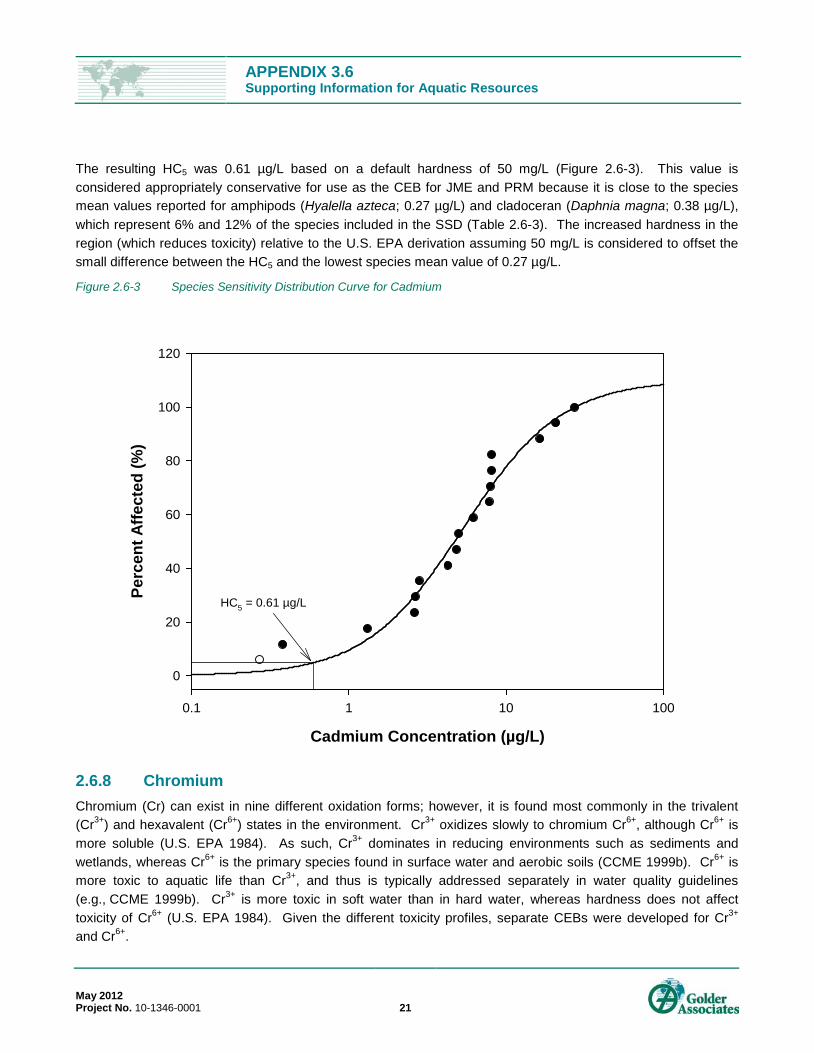
Figure 2.6-3 Species Sensitivity Distribution Curve for Cadmium .................................................................................... 21
Figure 2.6-4 Species Sensitivity Distribution Curve for Hexavalent Chromium ................................................................ 22
Figure 2.6-5 Criterion Maximum Concentration Calculated Using Hardness Equation and Biotic Ligand Model ............. 25
Figure 2.6-6 Species Sensitivity Distribution Curve for Manganese ................................................................................ 28
Figure 2.6-7 Water-Based Species Sensitivity Distribution Curve for Mercury ................................................................ 30
Figure 2.6-8 Concentration-Response for Mercury in Freshwater Invertebrate Tissues .................................................. 32
Figure 2.6-9 Concentration-Response for Mercury in Freshwater Fish Tissues .............................................................. 34
Figure 2.6-10 Species Sensitivity Distribution Curve for Molybdenum ............................................................................... 39
Figure 2.6-11 Species Sensitivity Distribution Curve for Nickel ......................................................................................... 41
Figure 2.6-12 Species Sensitivity Distribution Curve for Silver .......................................................................................... 43
Figure 2.6-13 Species Sensitivity Distribution Curve for Strontium .................................................................................... 50
Figure 2.6-14 Species Sensitivity Distribution Curve for Zinc ............................................................................................ 52
Figure 2.7-1 Species Sensitivity Distribution Curve for Anthracene ................................................................................. 55
Figure 2.7-2 Species Sensitivity Distribution Curve for Fluoranthene .............................................................................. 57
Figure 2.7-3 Species Sensitivity Distribution Curve for Fluorene ..................................................................................... 58
Figure 2.7-4 Species Sensitivity Distribution Curve for Naphthalene ............................................................................... 61
Figure 2.7-5 Species Sensitivity Distribution Curve for Phenanthrene ............................................................................. 63
Figure 2.7-6 Species Sensitivity Distribution Curve for Pyrene ........................................................................................ 65
Figure 3.2-1 Modelled Degradation of a Single Source of Naphthenic Acids .................................................................. 73
ATTACHMENTS
Attachment A: Aquatic Health

APPENDIX 3.6 Supporting Information for Aquatic Resources
May 2012 Project No. 10-1346-0001 1
1.0 INTRODUCTION Appendix 3.6 is prepared in response to technical information requested of Shell during discussions with Environment Canada in 2011, and further supports the Aquatic Resources Assessment presented in Appendix 2. This document consists of two major sections: Section 2.0, Chronic Effects Benchmarks (CEBs), and Section 3.0, Naphthenic Acids. Also included is Attachment A to Section 2.0, which discusses the implications of updated CEBs on the Environmental Impact Assessment (EIA) Aquatic Health Assessment.
2.0 CHRONIC EFFECTS BENCHMARKS This appendix describes the methods and results of CEB derivations applied to the aquatic health assessment of the EIA for the Jackpine Mine Expansion (JME) and Pierre River Mine (PRM). Aquatic health assessments for oil sands developments have traditionally applied a combination of generic federal guidelines from the Canadian Council of Ministers of the Environment (CCME 1999a; updates to 2011) and derivations of site-specific criteria using species sensitivity distributions (CCME 2003a; Posthuma et al. 2002). The EIA included derivations of CEBs, as described in Volume 4B, Appendix 4-2, Section 3. However, while these CEBs were being derived, CCME (2007a) developed a refined stepwise procedure for site-specific derivations that is now preferred by regulators and that provides a consistent framework for future evaluations. This appendix presents updated CEBs that follow the approach described by CCME (2007a). The CEB derivations also include additional datapoints; therefore, the CEBs described herein supersede those presented in the EIA.
Implications to the aquatic health assessment of the EIA Base Case and EIA Application Case are presented in Attachment A.
2.1 Updated Canadian Council of Ministers of the Environment Protocol In the CCME (2007a) protocol, two approaches for deriving water quality guidelines are provided. These approaches depend on the quality and amount of data available for each constituent:
Statistical Extrapolation Method – This approach uses data from multiple species to derive the final guideline and uses the Species Sensitivity Distribution (SSD). This approach establishes an acceptable response (effect) size, fits suitable endpoint data to a specified model, and calculates an exposure concentration that protects a specified percentage of species (e.g., 95%).
Lowest Threshold Method – If the data are insufficient to model an SSD curve, then a second- or third-tier guideline may be developed considering the lowest toxicity value from a high-quality study (and applying an uncertainty or safety factor). This approach is based on the original federal guideline development protocol (CCME 1991).
The SSD approach is preferred (i.e., Type A guidelines) because it considers the range of thresholds derived from valid studies, such that guidelines are not unduly influenced by a single anomalous result. Both approaches require a defined minimum amount of environmental and toxicological data. Where inadequate or insufficient toxicity data exist for deriving a Type A guideline, Type B1 or Type B2 guidelines can be derived based on the quantity and quality of available toxicity data (CCME 2007a). At present, there is no protocol for deriving guidelines when the minimum toxicity data requirement for a Type B guideline is not met.
APPENDIX 3.6 Supporting Information for Aquatic Resources
May 2012 Project No. 10-1346-0001 2
2.2 Application This appendix provides the technical rationale for the development of region-specific CEBs for oil sands developments, with an emphasis on the JME and PRM. The overarching goal was to provide a system for aquatic effects benchmark development that includes the following:
is consistent with updated Canadian (i.e., CCME) federal guidance for development of aquatic effect thresholds;
is customized to general water quality constituents that are reflective of the Athabasca Oil Sands Region;
makes appropriate use of available and relevant toxicity information;
coordinates derivations across multiple projects for consistency and efficiency; and
applies technically defensible assumptions in the derivation procedures.
The CEBs developed in this appendix have general applicability to the Athabasca Oil Sands Region. However, some of the CEBs are refined through customization to watercourse-specific water concentrations. The current project spans the Muskeg River watershed, which comprises the JME Local Study Area (LSA), as well as the watersheds in the adjacent PRM LSA. The environmental characteristics of both areas, which are described as follows, were considered for site-specific customization of CEBs:
JME LSA medians: pH=7.5, temperature=7°C, hardness=149 mg/L calcium carbonate (CaCO3), Dissolved Organic Carbon (DOC)=22 mg/L; and
PRM LSA medians: pH=7.5, temperature=5°C, hardness=143 mg/L CaCO3, DOC=21.8 mg/L.
The most conservative modifiers from the two areas were adopted for customization of CEBs, which were from the PRM LSA (i.e., lower hardness values results in CEBs that are lower and therefore more protective), although the values are very similar for both areas.
2.3 Screening of Constituents for Chronic Effects Benchmark Development
The CEB evaluation began by considering the full list of water quality assessment constituents (Table 2.3-1). Predicted concentrations of these constituents were compared to generic federal Water Quality Guidelines (WQGs; CCME 2007b), if available.
Water quality guidelines represent levels that, if met in any surface water, will provide a high level of protection to aquatic life. In this assessment, the Canadian Water Quality Guidelines for the Protection of Aquatic Life were used; these conservative guidelines are intended to “protect all forms of aquatic life and all aspects of the aquatic life cycles, including the most sensitive life stage of the most sensitive species over the long term” (CCME 1999a). That is, exceedance of a water quality guideline indicates that adverse effects may be possible, but not necessarily likely.

APPENDIX 3.6 Supporting Information for Aquatic Resources
May 2012 Project No. 10-1346-0001 3
Table 2.3-1 Water Quality Assessment Constituents for the Assessment Assessment Constituents(a)(b)
Aluminum Ammonia Antimony Arsenic Barium Beryllium Boron Cadmium Calcium(c) Chloride(c) Chromium Cobalt Copper Dissolved Organic Carbon(c) Iron Lead Magnesium(c)
Manganese Mercury Molybdenum Monomer(d) Naphthenic acids (labile and refractory) Nickel Polycyclic Aromatic Hydrocarbons (PAH) group 1 PAH group 2 PAH group 3 PAH group 4 PAH group 5 PAH group 6 PAH group 7 PAH group 8 PAH group 9 Potassium(c)
Selenium(c) Silver Sodium Strontium Sulphate(c) Sulphide Tainting potential Temperature Total dissolved solids Total nitrogen(c) Total phenolics Total phosphorus(c) Toxicity - acute Toxicity - chronic Vanadium Zinc
(a) All listed metals are considered to be total metals. (b) For a discussion of individual Polycyclic Aromatic Hydrocarbons (PAHs) and linkage to PAH group assignments, see Table 2.5-1. (c) Constituent modelled in the EIA but no chronic effect benchmark developed, due to status as a nutrient or evaluation using an alternate
constituent. (d) Constituent modelled in the EIA but no chronic effect benchmark developed, due to low concentrations predicted by modelling. Note: Table is the same as EIA, Volume 4A, Section 6.5, Table 6.5-1.
To further focus the development of CEBs, a screening procedure was applied to identify the following categories of constituents:
CEBs Available – CEBs already developed from other oil sands developments using the CCME (2007a) procedure, and considered to be relevant to the assessment.
CEBs Unavailable – CEBs not previously derived for other oil sands developments, or that required refinement to be relevant to the assessment.
CEBs Not Required – Constituents that were consistently below screening-level water quality guidelines.
A constituent in either of the first two categories was carried forward unless it was excluded from further consideration for one of the following reasons:
the constituent in question has been shown to have limited potential to affect aquatic health (i.e., innocuous constituents);
the constituent in question is more appropriate assessed through a tissue-based benchmark than a water-based benchmark; or
the constituent in question is a component of another constituent, which is a more suitable focus point for the analysis.
APPENDIX 3.6 Supporting Information for Aquatic Resources
May 2012 Project No. 10-1346-0001 4
Accordingly, the following constituents from Table 2.3-1 were excluded during the first step of the screening process:
selenium;
monomer, due to low concentrations predicted by modelling;
individual nutrients and major ions (e.g., calcium, chloride, magnesium, potassium, sulphate, total nitrogen, total phosphorus);
non-chemical constituents (i.e., fish tainting potential, toxicity – acute and chronic); and
dissolved constituents.
These constituents, and the specific rationales for their exclusion from CEB development, are discussed below.
Selenium Consistent with the current state of the science of selenium toxicology, and recognizing that selenium elicits effects on reproduction due to maternal transfer (Chapman et al. 2010), a water-based CEB was not developed for selenium. Rather, the potential for effects to aquatic health due to predicted selenium concentrations were assessed through predicted tissue concentrations in the indirect exposure – changes to fish tissue quality assessment.
Monomer The modelling predicted that instream concentrations of monomer would be essentially zero at all assessment nodes and during all snapshots (EIA, Volume 4B, Appendix 4-7). Therefore, a benchmark was not derived for this constituent.
Individual Nutrients and Major Ions Phosphorus and nitrogen compounds are nutrients that can exert adverse effects at high concentrations via eutrophication. These nutrients were not evaluated as individual constituents requiring CEB development because potential effects related to eutrophication are assessed separately in the EIA, particularly in terms of the effect on Dissolved Oxygen (DO) demand. Muskeg drainage and overburden dewatering waters have the potential to contain high levels of oxygen-consuming organic constituents and low DO levels.
The effect of JME and PRM on DO levels was discussed in the EIA, Volume 4A, Section 6.5, and an eutrophication assessment was provided in the EIA, Volume 4A, Section 6.6. Notably, because watercourses in the JME and PRM LSAs are relatively nutrient-rich, they are less sensitive to nutrient inputs relative to oligotrophic streams. As such, negligible eutrophication effects on aquatic biota are expected in these watercourses under EIA Application Case conditions. Nevertheless, nitrate and ammonia were screened for toxicity effects using WQGs.
Furthermore, calcium, chloride, magnesium, potassium and sulphate were excluded from CEB development because these individual ions are components of Total Dissolved Solids (TDS), another modelled constituent included in the assessment. For TDS, the mixture of constituents was evaluated using a conservative CEB, which is protective against effects of the individual constituents in the mixture.
APPENDIX 3.6 Supporting Information for Aquatic Resources
May 2012 Project No. 10-1346-0001 5
Predicted changes in sulphate concentrations are expected to have a negligible effect on aquatic biota given the moderately hard waters in these watercourses (which ameliorate sulphate toxicity), and the low predicted concentrations relative to recently derived effects-based water quality limits proposed by the Alberta Government (AENV 2008).
Non-chemical Constituents Taint in fish is defined as an abnormal odour or flavour detected in the edible tissue (LeBlanc et al. 2000). Tainting thresholds were converted to Tainting Potential Units (TPU), which were then compared to standardized benchmarks for the evaluation of fish tainting. Similarly, the assessment constituents related to toxic effects (acute and chronic toxicity) in operational and reclamation water were converted to toxic units (toxic unit - acute [TUa] and toxic unit - chronic [TUc]), as described in EIA, Volume 4A, Section 6.5.2.7. The TU and TPU approaches do not require development of site-specific CEBs.
Dissolved Constituents No CEBs were developed for the dissolved form of metals, metalloids or non-metals because they are a component of the corresponding total metal concentrations. Total metal measurements provide a more conservative basis for assessment than dissolved metals. Some site-specific considerations (i.e., toxicity-modifying factors) implicitly account for the proportion of constituent that is expected to be dissolved, but derivation of CEBs for the dissolved phase was not conducted.
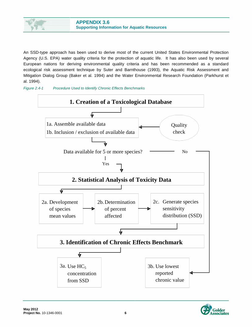
2.4 Methods 2.4.1 General Approach The general procedure for CEB development followed a three-step process which included creating a toxicological database for each constituent, analyzing the available data, and deriving an HC5 value. This value denotes a concentration that is hazardous to no more than 5% of species in the community. Where insufficient data were available, a value was conservatively derived using the lowest reported chronic toxicity test results (Figure 2.4-1). Chronic effect benchmarks were required for any constituent that was carried through the initial screening procedure described in Section 2.3.
The CEBs represent constituent concentrations above which changes to aquatic health could occur on the scale of individual organisms. The benchmarks are less conservative (i.e., more realistic) than generic WQGs, but retain a level of conservatism for the evaluation of population-level effects, which would require concentrations to be higher than the CEBs. Consequently, the CEBs are considered to be conservative thresholds by which potential effects to aquatic health can be assessed.
Consistent with CCME (2007a), the SSD approach was selected as a preferred method to derive a CEB in acknowledgement that there are biological differences among species and that the variation among species sensitivities can be described by a statistical distribution. The distribution can then be used to define an environmental quality criterion, expressed as a concentration that is expected to be safe for the majority of species (Posthuma et al. 2002). The most commonly used criterion is referred to as the HC5 value. A comparison of chronic, single species and experimental ecosystem data for metals, pesticides, surfactants and other organic and inorganic compounds has shown that the HC5 is a conservative threshold for effects to aquatic ecosystems (Versteeg et al. 1999).
APPENDIX 3.6 Supporting Information for Aquatic Resources
May 2012 Project No. 10-1346-0001 6
An SSD-type approach has been used to derive most of the current United States Environmental Protection Agency (U.S. EPA) water quality criteria for the protection of aquatic life. It has also been used by several European nations for deriving environmental quality criteria and has been recommended as a standard ecological risk assessment technique by Suter and Barnthouse (1993), the Aquatic Risk Assessment and Mitigation Dialog Group (Baker et al. 1994) and the Water Environmental Research Foundation (Parkhurst et al. 1994). Figure 2.4-1 Procedure Used to Identify Chronic Effects Benchmarks
1. Creation of a Toxicological Database
2. Statistical Analysis of Toxicity Data
3. Identification of Chronic Effects Benchmark
1a. Assemble available data
1b. Inclusion / exclusion of available data
2a. Development of species mean values
Quality check
2b. Determination of percent affected
2c. Generate species sensitivity distribution (SSD)
3a. Use HC5 concentration from SSD
3b. Use lowest reported chronic value
Data available for 5 or more species?
Yes
No
APPENDIX 3.6 Supporting Information for Aquatic Resources
May 2012 Project No. 10-1346-0001 7
The CCME has used an SSD approach to develop the Canadian water quality guidelines for ammonia and boron for the protection of aquatic life (CCME 2009, 2010). The CCME (2007a) recommends using this approach to develop other Canadian water quality guidelines for the protection of aquatic life. Although the approach has not yet been applied by CCME to the majority of the individual constituents for which WQGs exist for the protection of aquatic life, the basic concepts of the approach are transferable to site- and region-specific guideline derivations. Therefore, the basic principles of CCME (2007a) and many of the specific procedural rules were applied in deriving the CEBs.
Applying the SSD approach provides several advantages in CEB development, because it:
enables more recent studies to be included in the toxicity database;
enables exclusion of non-resident species with poor ecological relevance to the region; and
facilitates the consideration of site-specific modifying factors in the screening of relevant toxicity studies.
These considerations improve the relevance of the CEB to the region.
One disadvantage of the region-specific customization of CEBs is related to the reduction of sample size that occurs when studies are excluded based on regional relevance. Whereas the freshwater SSDs used in the development of generic WQGs can incorporate toxicity test results for numerous species from many ecosystems, the region-specific CEBs filter the toxicity data for relevance. In most cases, this filtering reduces the number of species and endpoints available, and sometimes results in insufficient data for development of an SSD. To compensate for this problem, several mitigating assumptions were applied:
The screening of organisms for regional relevance to the SSD was not highly restrictive (i.e., all freshwater organisms found in Canada were retained, with tropical and subtropical species excluded).
Some subchronic test endpoints that did not meet the test duration constraints of the CCME (2007a) derivation protocol were retained to maintain suitable sample sizes for SSD development.
Where toxicity datasets were screened for relevance to water quality constituents in regional waterbodies, a liberal acceptance range was applied to avoid premature exclusion of data. For example, water hardness in the range of 50 to 450 mg/L CaCO3 was considered relevant to the Oil Sands Region, with only the extremes of soft and hard water excluded.
The above approach provided CEB derivations that are applicable to numerous waterbodies in the Oil Sands Region. Where the above assumptions had the potential to affect the conservatism and uncertainty of the derived CEBs, the derivation procedure qualitatively considered additional factors and context, such as:
the direction of suspected bias (e.g., inclusion of aluminum toxicity data at pH 6.5 would tend to reduce CEBs relative to neutral pH conditions);
the relation of the CEB to the most sensitive and relevant chronic toxicity endpoint;
other toxicity modifying factors (e.g., high DOC) that were not explicitly included in the derivation, but that may influence site-specific bioavailability;
APPENDIX 3.6 Supporting Information for Aquatic Resources
May 2012 Project No. 10-1346-0001 8
the effect size of test endpoints (e.g., EC25 or LC10) used to derive the SSD, particularly for those endpoints close to the fifth percentile of the distribution; and
supporting lines of evidence from other toxicological models and literature not directly incorporated in the SSD.
2.5 Procedure The following subsections outline the technical procedures for the three-step derivation process shown in Figure 2.4-1.
2.5.1 Step 1: Creation of a Toxicological Database 2.5.1.1 Step 1a: Assemble Available Data Metals and Metalloids Available chronic toxicological data for each constituent were summarized, with a focus on data for algae, invertebrates and fish (following the recommendations of CCME 2007a). The development of each toxicity database began with an examination of primary chronic toxicity data from fact sheets used to derive relevant Canadian Water Quality Guidelines (CCME 1999a; 2007b). The toxicity database was then expanded by querying the AQUIRE and ECOTOX databases administered by the U.S. EPA (2007a), and by searching for other available peer-reviewed scientific literature from journal databases (e.g., Cambridge Scientific Abstracts, PubMed). This review was focused on the period after the previous guideline derivations.
The resulting database contained data with various test endpoints, such as mortality, reduced survival, growth, or reproduction, derived from subchronic and chronic studies. The toxicity database contains primary and secondary data that meet the requirements of U.S. EPA and CCME guideline development protocols (CCME 2007a; Stephan et al. 1985).
All life stages were included in the toxicity database; however, for aquatic invertebrates and amphibians with terrestrial adult stages (e.g., non-biting midge), only the aquatic phases were included in the recent SSD analyses. Although the database does not include all available data, it contains primary data that meet the requirements of U.S. EPA and CCME guideline development protocols (CCME 2007a; Stephan et al. 1985).
Polycyclic Aromatic Hydrocarbons The procedure for developing a toxicity database for Polycyclic Aromatic Hydrocarbons (PAHs) began with the selection of indicator PAH compounds spanning a range of molecular structures, including:
anthracene;
fluoranthene;
fluorene;
naphthalene;
phenanthrene; and
pyrene.

APPENDIX 3.6 Supporting Information for Aquatic Resources
May 2012 Project No. 10-1346-0001 9
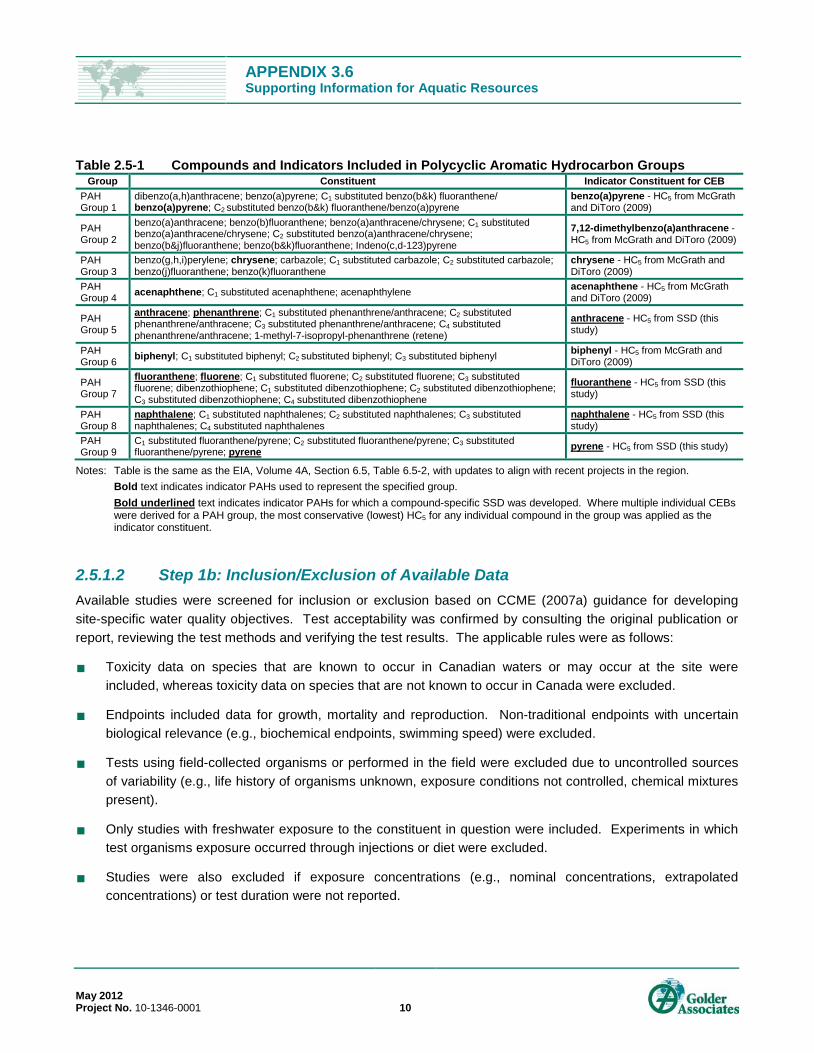
The JME and PRM included compound-specific derivations for these six indicator PAHs, with the objective of comparing the SSD-based CEBs to the threshold values for chronic toxicity summarized in McGrath and DiToro (2009). The latter work entailed an assessment of the Target Lipid Model (TLM) for toxicity assessment of type I narcotic chemicals. The numeric water quality guidelines in McGrath and DiToro (2009) are equivalent to a HC5 (i.e., hazard concentration to 5% of the tested species, or the concentration that protects 95% of the tested species) and therefore compatible with the level of protection specified in CCME (2007a). The TLM derivation procedure differs from the SSD approach; however, the former applies toxic units as a metric for expressing the toxicity of multiple PAHs present in a mixture, and applies an acute to chronic ratio for estimation of chronic sublethal effects.
The TLM has been validated and demonstrated to correctly predict (within the uncertainty bounds) the onset of sublethal effects of edemas, haemorrhaging, and other abnormalities in early life-stage exposure of organisms to PAHs. The authors conclude that computed HC5 values were lower than No Observed Effect Concentrations (NOECs) based on growth, reproduction, and mortality endpoints and sublethal effects. The TLM procedure, therefore, provides an independent validation of the SSD applied to individual PAH toxicity distributions. Once the comparability of the two derivation methods was assessed (and confirmed to be acceptable), remaining PAH groups were assigned CEBs extrapolated from the TLM (Table 2.5-1). This validation step provided an added level of confidence in the CEBs for PAHs, and helped to compensate for limitations in the datasets for specific PAH compounds.
The development of the toxicological database for the individual PAHs began with the examination of the toxicity data for PAHs summarized in McGrath and DiToro (2009). Review of the reported toxicological literature in that study included 34 studies that examined both chronic and acute toxicity of PAHs. Additional studies were also obtained by querying the ECOTOX database (U.S. EPA 2007a) and used to bolster the data set. Test endpoints included mortality, growth and/or reproduction for several species of algae, invertebrate, amphibians and fish.
APPENDIX 3.6 Supporting Information for Aquatic Resources
May 2012 Project No. 10-1346-0001 10
Table 2.5-1 Compounds and Indicators Included in Polycyclic Aromatic Hydrocarbon Groups Group Constituent Indicator Constituent for CEB
PAH Group 1
dibenzo(a,h)anthracene; benzo(a)pyrene; C1 substituted benzo(b&k) fluoranthene/ benzo(a)pyrene; C2 substituted benzo(b&k) fluoranthene/benzo(a)pyrene
benzo(a)pyrene - HC5 from McGrath and DiToro (2009)
PAH Group 2
benzo(a)anthracene; benzo(b)fluoranthene; benzo(a)anthracene/chrysene; C1 substituted benzo(a)anthracene/chrysene; C2 substituted benzo(a)anthracene/chrysene; benzo(b&j)fluoranthene; benzo(b&k)fluoranthene; Indeno(c,d-123)pyrene
7,12-dimethylbenzo(a)anthracene - HC5 from McGrath and DiToro (2009)
PAH Group 3
benzo(g,h,i)perylene; chrysene; carbazole; C1 substituted carbazole; C2 substituted carbazole; benzo(j)fluoranthene; benzo(k)fluoranthene
chrysene - HC5 from McGrath and DiToro (2009)
PAH Group 4 acenaphthene; C1 substituted acenaphthene; acenaphthylene acenaphthene - HC5 from McGrath
and DiToro (2009)
PAH Group 5
anthracene; phenanthrene; C1 substituted phenanthrene/anthracene; C2 substituted phenanthrene/anthracene; C3 substituted phenanthrene/anthracene; C4 substituted phenanthrene/anthracene; 1-methyl-7-isopropyl-phenanthrene (retene)
anthracene
PAH Group 6
- HC5 from SSD (this study)
biphenyl; C1 substituted biphenyl; C2 substituted biphenyl; C3 substituted biphenyl biphenyl - HC5 from McGrath and DiToro (2009)
PAH Group 7
fluoranthene; fluorene; C1 substituted fluorene; C2 substituted fluorene; C3 substituted fluorene; dibenzothiophene; C1 substituted dibenzothiophene; C2 substituted dibenzothiophene; C3 substituted dibenzothiophene; C4 substituted dibenzothiophene
fluoranthene
PAH Group 8
- HC5 from SSD (this study)
naphthalene; C1 substituted naphthalenes; C2 substituted naphthalenes; C3 substituted naphthalenes; C4 substituted naphthalenes
naphthalene
PAH Group 9
- HC5 from SSD (this study)
C1 substituted fluoranthene/pyrene; C2 substituted fluoranthene/pyrene; C3 substituted fluoranthene/pyrene; pyrene pyrene
Notes: Table is the same as the EIA, Volume 4A, Section 6.5, Table 6.5-2, with updates to align with recent projects in the region.
- HC5 from SSD (this study)
Bold text indicates indicator PAHs used to represent the specified group. Bold underlined
2.5.1.2 Step 1b: Inclusion/Exclusion of Available Data
text indicates indicator PAHs for which a compound-specific SSD was developed. Where multiple individual CEBs were derived for a PAH group, the most conservative (lowest) HC5 for any individual compound in the group was applied as the indicator constituent.
Available studies were screened for inclusion or exclusion based on CCME (2007a) guidance for developing site-specific water quality objectives. Test acceptability was confirmed by consulting the original publication or report, reviewing the test methods and verifying the test results. The applicable rules were as follows:
Toxicity data on species that are known to occur in Canadian waters or may occur at the site were included, whereas toxicity data on species that are not known to occur in Canada were excluded.
Endpoints included data for growth, mortality and reproduction. Non-traditional endpoints with uncertain biological relevance (e.g., biochemical endpoints, swimming speed) were excluded.
Tests using field-collected organisms or performed in the field were excluded due to uncontrolled sources of variability (e.g., life history of organisms unknown, exposure conditions not controlled, chemical mixtures present).
Only studies with freshwater exposure to the constituent in question were included. Experiments in which test organisms exposure occurred through injections or diet were excluded.
Studies were also excluded if exposure concentrations (e.g., nominal concentrations, extrapolated concentrations) or test duration were not reported.

APPENDIX 3.6 Supporting Information for Aquatic Resources
May 2012 Project No. 10-1346-0001 11
Studies evaluating synergistic, or antagonistic effects of chemicals or compensatory responses of organisms (such as tolerance [acclimation, adaptation], or reduced density-dependent mortality among juveniles) were excluded.
Included studies must have followed good laboratory practices (e.g., presence of control group), a defensible experimental design, and accepted statistical procedures for data analysis.
If a member of a family of freshwater fish may occur at the site, then toxicity data from any fish species within that family were maintained in the database.
If a member of a family of amphibians may occur at the site, then toxicity data from any amphibian species within that family were maintained in the database.
If a member of a class of freshwater invertebrates may occur at the site, then toxicity data from that invertebrate class were retained in the toxicity database.
If a member of a phylum of freshwater algae may occur at the site, then toxicity data from that phylum were retained in the database.
Tests greater than 96 hours in duration were considered to be chronic for most species. This decision rule differs somewhat from the CCME (2007a) guidance, which specifies a seven-day minimum duration for a chronic designation. During the review it was observed that some tests (such as the three-brood Ceriodaphnia dubia reproduction test) could fall below the 7-day threshold due to the variations in the speed of reproduction of test cultures. This endpoint is considered to be a suitable chronic endpoint even where time to three broods falls below seven days. Some additional exceptions were made to the guidance on test duration, such as for metals exposures to the nematode Caenorhabditis elegans. For this organism, tests 96 hours in duration were considered to be chronic because of their relatively short life span (Carleton-Dodds 2010, pers. comm.).
Site-Specific Screening The CCME (2007a) derivation protocol emphasizes the importance of toxicity modifying factors in the development of water quality guidelines. It is acceptable, indeed preferable, to account explicitly for the physico-chemical factors that mediate the bioavailability or toxicity of constituents. In the context of JME and PRM, it was desirable to screen the toxicity database to include only those studies that are reflective of the general water quality constituents expected in the JME or PRM LSA, both of which are representative of the receiving environment.
Metal speciation in aquatic environments and potential toxicity to aquatic organisms is highly influenced by water quality variables such as pH and water hardness. To derive a site-specific chronic benchmark for metals, studies with no reported pH and water hardness, or with pH and water hardness values outside the expected range of values encountered in the study area (pH = 6.5 to 9.5 and hardness = 50 mg/L to 450 mg/L CaCO3) were excluded. These ranges were considered sufficiently robust to include a range of conditions over the duration of JME and PRM, while simultaneously excluding extremes of these constituents that would not be relevant during the operational life or closure stages of JME and PRM. In addition, for CEBs based on hardness-dependent equations, a central tendency value specific to JME (149 mg/L CaCO3) was applied. Use of this hardness value would result in conservative benchmarks for PRM because water hardness is generally

APPENDIX 3.6 Supporting Information for Aquatic Resources
May 2012 Project No. 10-1346-0001 12
slightly higher in the PRM LSA. For copper, the CEB derived from the Biotic Ligand Model (BLM) was customized to site-specific hardness, DOC and pH.
Photo-enhanced toxicity of PAHs has been demonstrated in laboratory and in a few in situ studies, and the mechanism of toxic action for this process has been well described (Boese et al. 1998; Harrison 2008). Given a certain combination of chemical exposure conditions and lighting conditions (specifically the ultraviolet [UV] light spectrum and degree of light exposure to animal skin surface during contaminant bioaccumulation) photo-enhanced toxicity of PAHs can significantly increase toxicity beyond normal levels. However, in most realistic environmental exposures, this phenomenon is ameliorated by physical, chemical and biotic factors (McDonald and Chapman 2002). Whereas the difference between UV and non-UV LC50 values is at least two orders of magnitude for non-arthropods in laboratory comparisons (Harrison 2008), such laboratory bioassays have been criticized for faults such as exaggerated UV exposure and PAH bioavailability. Swartz et al. (1997) stated that “the importance of phototoxicity in the derivation of PAH SQC may ultimately be determined by the photoecology of benthic ecosystems.” Few if any studies clearly and directly implicate PAH phototoxicity with adverse ecological effects in field populations (McDonald and Chapman 2002).
Whereas the ecological relevance of phototoxicity in field communities remains in question, a number of site-specific factors that mitigate against the influence of photo-enhanced toxicity of PAHs will be present in the scenarios modelled for the EIA. For example, the configuration of pit lakes incorporates an increase in water depth, and watercourses in the LSA are naturally high in the concentrations of water quality constituents such as turbidity, suspended solids and DOC, which result in attenuation of the UV light spectrum. Therefore, PAHs phototoxicity-based endpoints were not included in the SSD derivation. This exclusion matches the approach of McGrath and DiToro (2009) that excludes photo-enhanced toxicity endpoints.
Given that the toxicity of PAHs to aquatic organisms is not known to be influenced by water quality variables such as pH and hardness, all exposure conditions for these constituents were considered appropriate for inclusion in the SSD derivation.
Endpoint Selection For statistical endpoints, the preference ranking (i.e., the most preferred acceptable to the least preferred acceptable endpoint) was conducted following guidance from CCME (2007a):
ECx/ICx representing a no-effects threshold;
EC10/IC10;
EC11-25/IC11-25;
Maximum Allowable Toxicant Concentration (MATC), which was estimated using the geometric mean of the NOEC and the Lowest Observed Effects Concentration (LOEC);
NOEC;
LOEC;
IC26-49 or EC26-49; and
IC50/EC50.

APPENDIX 3.6 Supporting Information for Aquatic Resources
May 2012 Project No. 10-1346-0001 13
Regression-based endpoints, such as Inhibiting Concentration (IC), Effect Concentration (EC) or Lethal Concentration (LC) values, were given preference over hypothesis-based endpoints, such as LOEC and NOEC values. They are also the endpoints favoured by CCME (2007a) and U.S. EPA (2007a). The IC10/EC10 results were given first priority because these results represent a conservative threshold for no negative effect, and are derived by regression analysis. If a study yielded multiple results for a single endpoint, then the results were reduced to a single measurement to avoid biasing the database toward the results of a single study.
Generally, effects on no more than 20% of exposed individuals is considered to be an acceptable threshold level for negative effects (CCME 2007a), and current risk assessment guidance recommended the use of IC20/EC20 as permissible level of effects (Suter et al. 1995). However, IC25/EC25 values are commonly reported in the literature, and such variations are considered to be within the range of natural variability often observed in the field among normal, unexposed populations. Therefore, in the absence of an IC10/EC10 result, IC11-25 or EC11-25
values were used.
In some instances, the primary literature reported NOEC/LOEC concentrations without corresponding ECx/ICx values, but also provided tabular or graphical data that permitted estimation of the ECx/ICx. In these cases, the preference for an effect-size based endpoint outweighed the small uncertainty associated with interpolation or estimation from the raw data. The results of a concentration-response model fit to the study data (i.e., smoothed results) were used preferentially to single concentration test data for estimating ECx/ICx.
2.5.2 Step 2: Statistical Analysis of Toxicity Data Statistical analysis of the assembled data points (and associated model fitting) was completed if data were available for five or more species. The statistical analysis consisted of the following:
developing species mean values;
ranking the species mean values to determine percent affected; and
fitting a statistical distribution to the available dataset, if appropriate.
Species means were calculated by taking the geometric mean of the individual test results. The geometric mean, as opposed to the arithmetic mean, was used to limit the bias of high test results. Species mean values were then ranked from lowest to highest, and the percent of species affected was calculated based on dividing the rank assigned to each species mean by the total number of species. Logistic relationships between the percent of species affected and concentration of the constituent in question were evaluated using SigmaPlot version 11.0 (SPSS 2002).
Minimum data requirements for SSDs that have been recommended by various authorities range from three to more than 20 (Suter et al. 2002). The CCME (2007a) specifies a minimum of seven species, but other jurisdictions differ (e.g., Danish soil quality criteria require a minimum of five species [Suter et al. 2002]). Species sensitivity derivations developed with more species are likely more robust. However, the benefit of basing the CEB on all relevant and available toxicity data (i.e., in an SSD) was considered to outweigh the potential increase in uncertainty arising from having relatively few data.
APPENDIX 3.6 Supporting Information for Aquatic Resources
May 2012 Project No. 10-1346-0001 14
2.5.3 Step 3: Identification of Chronic Effects Benchmark Step 3a – Derivation of the HC5 Concentration After an appropriate regression model was developed, the HC5 value was calculated using the model equation. The HC5 value was then used as the CEB for the constituent in question. In addition, the HC20 value and HC50 value were reported to provide context on the shape and steepness of the concentration-response curve.
Step 3b – Selection of the Lowest Reported Chronic Value For several constituents, toxicity data were available for fewer than five species. Chronic effects benchmarks for these constituents were based on the lowest chronic toxicity result present in the constituent-specific toxicity database.
Previously Evaluated Constituents The list of constituents requiring new SSD derivation was refined to consider the previous work conducted for similar developments such as Syncrude (2009) and Total (2010). These developments provided numerous water quality guidelines that were already consistent with the CCME (2007a) derivation procedure. The CEBs drawn from the technical derivations found in previous assessments included: antimony, barium, beryllium, cadmium, chromium, iron, lead, manganese, molybdenum, strontium and vanadium. Although these derivations were not all site- or region-specific, many of these CEBs were considered to be applicable to JME and PRM as preliminary CEBs. Additional refinement of these CEBs would only be warranted if the predicted concentrations exceeded the CEBs. For completeness, the full derivations for these constituents are included in this appendix.
2.6 Chronic Effects Benchmark Results for Metals 2.6.1 Aluminum Aluminum (Al) can be found in the natural environment and is generally associated with igneous rocks (composed of alumino-silicate minerals); bauxite materials (primarily composed of aluminum hydroxide); silicates and cryolite (Na3AlF6) (Staley and Haupin 1992). Aluminum has only one oxidation state (+3; ATSDR 2008) and may enter aquatic systems by both natural processes (e.g., weathering of rocks) and anthropogenic activities (e.g., metal smelting). The aqueous solubility of aluminum is strongly influenced by the pH of the local environment with increases in aluminum’s solubility occurring as pH decreases (pH less than 5.5). Aluminum can also react and form complexes with chloride, fluoride, sulphate, nitrate, phosphate and negatively charged compounds such as humic materials and clay (ATSDR 2008). This element does not readily bioconcentrate in aquatic organisms (Rosseland et al. 1990).

APPENDIX 3.6 Supporting Information for Aquatic Resources
May 2012 Project No. 10-1346-0001 15
A summary of the toxicity database used to derive a site-specific chronic toxicological benchmark for aluminum is shown in Table 2.6-1. The SSD was conducted using chronic toxicity data for eight aquatic species. Sufficient toxicity data were available for aluminum to develop a SSD, with a logistic regression model providing a good fit to the observed data (r2 = 0.97) (Figure 2.6-1). The logistic model took the following form:
Where:
y = percent of aquatic species affected x = aluminum concentration (µg/L)
Table 2.6-1 Available Aquatic Toxicity Data for Aluminum
Species Scientific Name Species Common Name Chronic Value [µg/L] Rank
Percent Affected
[%] Hyalella azteca scud (amphipod) 529 1 12.5 Oncorhynchus mykiss rainbow trout 779 2 25 Asellus aquaticus aquatic sowbug 5,358 3 37.5 Daphnia pulex water flea 6,042 4 50 Crangonyx pseudogracilis amphipod 10,846 5 62.5 Ceriodaphnia dubia water flea 24,743 6 75 Tubifex tubifex tubificid worm 58,075 7 87.5 Daphnia magna water flea 71,556 8 100
Based on the logistic regression model, the HC5, HC20 and HC50 for aluminum were estimated to be 51, 807 and 7,056 µg/L, respectively (Figure 2.6-1). The toxicity benchmark for aluminum reported by CCME (1999a, updates to 2011) is 5 µg/L if pH is less than 6.5 and 100 µg/L if pH is greater than or equal to 6.5. However, guidance is not clearly provided in CCME (2007b) on how this toxicity benchmark was derived.
The site-specific pH for JME and PRM is about 7.5, which is well within the pH range for which the aluminum guideline becomes 100 µg/L. This threshold is lower than all chronic values considered in the SSD derivation, such that the HC5 is extrapolated below the lowest relevant chronic value.
53.0
27136.8
153.5x
1−
+
=y

APPENDIX 3.6 Supporting Information for Aquatic Resources
May 2012 Project No. 10-1346-0001 16
Figure 2.6-1 Species Sensitivity Distribution Curve for Aluminum
2.6.2 Antimony Two forms of antimony (Sb) can exist in the dissolved phase (ATSDR 1997); however, most antimony released into waterways is associated with particulate matter. Dissolved antimony (Sb3+) occurs under moderately oxidizing conditions, whereas dissolved antimony (Sb5+) predominates in highly oxidizing environments (NWQMS 2000). The toxicity of antimony depends largely upon its chemical form and oxidation state, with Sb3+ exerting greater toxicity than Sb5+ (Hou and Narasaki 1999). Consequently, most toxicity studies focus on Sb3+.
Insufficient data were available to create an SSD for antimony. The lowest reported toxicity value was a 30-day NOEC of 7.5 µg/L for survival and growth of fathead minnow embryos (LeBlanc and Dean 1984); however, this NOEC was unbounded (i.e., a LOEC could not be calculated in the study). It was also very low in comparison to other toxicity estimates. Therefore, the next lowest reported toxicity value of 157 µg/L was selected for use as the CEB for antimony. This value is based on a 28-day LC10 test result generated using rainbow trout (Birge et al. 1979, 1980a) and is considered to be conservative, because it is based on the more toxic form (i.e., Sb3+).
Aluminum concentration (µg/L)
100 1000 10000 100000
Perc
ent a
ffect
ed (%
)
0
20
40
60
80
100
120
HC5 = 51 µg/L
HC20 = 807 µg/L
HC50 = 7056 µg/L

APPENDIX 3.6 Supporting Information for Aquatic Resources
May 2012 Project No. 10-1346-0001 17
2.6.3 Arsenic Arsenic (As) is widely distributed in the natural environment. This element has four oxidation states: As3-, As0, As3+, and As5+; however, in aquatic systems, inorganic arsenic occurs primarily as As5+ and As3+. Both forms generally exist together, although As5+ predominates under oxidizing conditions and As3+ predominates under reducing conditions. Given that As3+ is the most toxic form of arsenic in aquatic environments, limited chronic toxicity data were available for As5+. As a result, both As5+ and As3+ were included in the toxicity database (ATSDR 2007).
A summary of the toxicity database used to derive a site-specific chronic toxicological benchmark for arsenic is shown in Table 2.6-2. The SSD was conducted using chronic toxicity data for eight aquatic species. Sufficient toxicity data were available for arsenic to develop a SSD, with a logistic regression model providing a good fit to the observed data (r2 = 0.96) (Figure 2.6-2). The logistic model took the following form:
Where:
y = percent of aquatic species affected x = arsenic concentration (µg/L)
Table 2.6-2 Available Aquatic Toxicity Data for Arsenic Species Scientific Name Species Common Name Chronic Value
[µg/L] Rank Percent Affected [%]
Hyalella azteca scud (amphipod) 484 1 12.5 Bosmina longirostris water flea 850 2 25 Ceriodaphnia dubia water flea 1,078 3 37.5 Daphnia magna water flea 2,200 4 50 Oncorhynchus mykiss rainbow trout 9,640 5 62.5 Salmo gairdneri rainbow trout 13,300 6 75 Morone saxatilis striped bass 35,146 7 87.5 Daphnia pulex water flea 49,600 8 100
59.0
7117.98
125.98x
1−
+
=y
APPENDIX 3.6 Supporting Information for Aquatic Resources
May 2012 Project No. 10-1346-0001 18
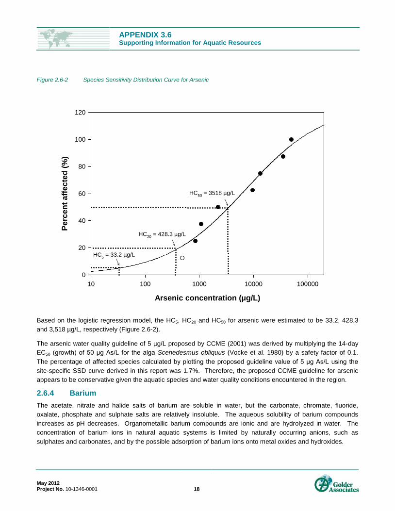
Figure 2.6-2 Species Sensitivity Distribution Curve for Arsenic
Based on the logistic regression model, the HC5, HC20 and HC50 for arsenic were estimated to be 33.2, 428.3 and 3,518 µg/L, respectively (Figure 2.6-2).
The arsenic water quality guideline of 5 µg/L proposed by CCME (2001) was derived by multiplying the 14-day EC50 (growth) of 50 μg As/L for the alga Scenedesmus obliquus (Vocke et al. 1980) by a safety factor of 0.1. The percentage of affected species calculated by plotting the proposed guideline value of 5 μg As/L using the site-specific SSD curve derived in this report was 1.7%. Therefore, the proposed CCME guideline for arsenic appears to be conservative given the aquatic species and water quality conditions encountered in the region.
2.6.4 Barium The acetate, nitrate and halide salts of barium are soluble in water, but the carbonate, chromate, fluoride, oxalate, phosphate and sulphate salts are relatively insoluble. The aqueous solubility of barium compounds increases as pH decreases. Organometallic barium compounds are ionic and are hydrolyzed in water. The concentration of barium ions in natural aquatic systems is limited by naturally occurring anions, such as sulphates and carbonates, and by the possible adsorption of barium ions onto metal oxides and hydroxides.
Arsenic concentration (µg/L)
10 100 1000 10000 100000
Perc
ent a
ffect
ed (%
)
0
20
40
60
80
100
120
HC5 = 33.2 µg/L
HC20 = 428.3 µg/L
HC50 = 3518 µg/L
APPENDIX 3.6 Supporting Information for Aquatic Resources
May 2012 Project No. 10-1346-0001 19
Insufficient data were available to develop an SSD for barium. The lowest reported toxicity value of 5,800 µg/L was, therefore, conservatively selected for use as the CEB for barium. This value is based on an EC16 reproduction test result generated using the water flea Daphnia magna (Biesinger and Christensen 1972).
2.6.5 Beryllium Beryllium toxicity and speciation varies with pH changes in the environment. Formation of solid beryllium hydroxide (Be[OH]2) occurs in most aquatic systems with ranges of pH 6 to 8. Beryllium can also form insoluble carbonates and soluble beryllium sulphates in aquatic environments.
Insufficient data were available for beryllium to develop an SSD. The lowest reported toxicity value of 5.3 μg/L was, therefore, conservatively selected for use as the CEB for beryllium. This value is based on a 28-day MATC for reproduction in Daphnia magna (Kimball 1978).
2.6.6 Boron The CCME water quality guideline for the protection of aquatic life is 1.5 mg/L of boron for long-term exposures (CCME 2009). This value was derived based on an SSD of long-term toxicity endpoints, which yielded a fifth percentile value (HC5) of 1.5 mg/L with confidence limits of 1.2 mg/L and 1.7 mg/L. As this derivation included a number of long-term endpoints for fish, invertebrates, plants and amphibians, the HC5 derivation is considered consistent with the CCME (2007a) derivation procedure. Many of the endpoints were based on NOECs, LOECs or MATCs (which do not convey the effect size and are not preferred endpoints); however, there is not a compelling reason to discard the CCME analysis for an alternative derivation.
Toxicity modifying factors were not applied to the boron guideline because evidence for the influence of water hardness on toxicity is mixed. Some species exhibit reduced toxicity at high hardness, whereas others show no response. Although reduced toxicity has been indicated in natural waters and in waters with elevated organic carbon content, but there is not sufficient information to quantify the relationship is not sufficient (CCME 2009).
2.6.7 Cadmium Cadmium (Cd) is usually found as a mineral combined with other elements, such as oxygen (cadmium oxide), chlorine (cadmium chloride) or sulphur (cadmium sulphate, cadmium sulphide). It may exist in water as a hydrated ion, as inorganic complexes (such as carbonates, hydroxides, chlorides or sulphates) or as organic complexes with humic acids (OECD 1994). Cadmium may enter aquatic systems through weathering and erosion of soils and bedrock, atmospheric deposition, direct discharge from industrial operations, leakage from landfalls and contaminated sites, and the dispersive use of sludge and fertilizers in agriculture. The predominant dissolved form of cadmium in freshwater is the cadmium ion (Cd2+), which is the form that is most bioavailable to aquatic biota (Wright and Welbourn 1994). Upon entry to the aquatic ecosystem, cadmium tends to partition to particulate matter and dissolved organic matter, reducing concentrations of the free ion in the water column, thereby lowering its bioavailability (Jonnalagadda and Rao 1993).
Modifying factors, such as hardness, salinity, pH and DO concentrations, can have a profound effect on cadmium toxicity to aquatic plants and animals. Ions, such as hydrogen and calcium, may compete with cadmium, resulting in reduced cadmium uptake and toxicity (Wright and Welbourn 1994). The toxicity of cadmium to fish is strongly affected by hardness, mainly because of competition for anionic binding sites at the gills between cadmium ions and ions responsible for hardness (i.e., calcium and magnesium) (Parametrix 1995).

APPENDIX 3.6 Supporting Information for Aquatic Resources
May 2012 Project No. 10-1346-0001 20
The U.S. EPA revised their recommended criteria for cadmium in 2001 (U.S. EPA 2001). This revision included an extensive review of the available toxicological literature and their revised criterion included a hardness correction factor. It was deemed to be unnecessary to repeat this work. Instead, the species mean chronic toxicity values from U.S. EPA (2001) were used as the basis for the toxicological database for this constituent (Table 2.6-3).
Table 2.6-3 Chronic Aquatic Toxicity Data for Cadmium, by Species Species Common Name Species Mean Chronic Toxicity Value(a)
[µg/L] Included/ Excluded Reason
Hyalella azteca amphipod 0.27 Included - Daphnia magna cladoceran 0.38 Included - Oncorhynchus mykiss rainbow trout 1.31 Included - Oncorhynchus tshawytscha chinook salmon 2.61 Included - Salvelinus fontinalis brook trout 2.64 Included - Chironomus tentans midge 2.80 Included - Oncorhynchus kisutch coho salmon 4.27 Included - Aplexa hypnorum snail 4.82 Included - Salmo trutta brown trout 5.00 Included - Daphnia pulex cladoceran 6.17 Included - Catostomus commersoni white sucker 7.80 Included - Salmo salar Atlantic salmon 7.92 Included - Salvelinus namaycush lake trout 8.09 Included - Esox lucius northern pike 8.09 Included - Pimephales promelas fathead minnow 16.4 Included - Aeolosoma headleyi oligochaete 20.7 Included - Ceriodaphnia dubia cladoceran 27.2 Included - Jordanella floridae flagfish 5.32 Excluded Non-resident species Micropterus dolomieu smallmouth bass 8.12 Excluded Non-resident species Lepomis macrochirus bluegill 17.4 Excluded Non-resident species Oreochromis aurea blue tilapia 23.6 Excluded Non-resident species
(a) Toxicity values were corrected to a hardness of 50 mg/L as CaCO3. Source: U.S. EPA (2001; Table 3c).
Given that there were mean chronic values for 17 species, sufficient data were available to develop a site-specific SSD for cadmium. The logistic model provided a good fit to the data (r2 = 0.97), and followed the form:
where:
y = percent of aquatic community affected x = cadmium concentration (µg/L)
4.1
3.51
2.110−
+
=x
y
APPENDIX 3.6 Supporting Information for Aquatic Resources
May 2012 Project No. 10-1346-0001 21
The resulting HC5 was 0.61 µg/L based on a default hardness of 50 mg/L (Figure 2.6-3). This value is considered appropriately conservative for use as the CEB for JME and PRM because it is close to the species mean values reported for amphipods (Hyalella azteca; 0.27 µg/L) and cladoceran (Daphnia magna; 0.38 µg/L), which represent 6% and 12% of the species included in the SSD (Table 2.6-3). The increased hardness in the region (which reduces toxicity) relative to the U.S. EPA derivation assuming 50 mg/L is considered to offset the small difference between the HC5 and the lowest species mean value of 0.27 µg/L.
Figure 2.6-3 Species Sensitivity Distribution Curve for Cadmium
2.6.8 Chromium Chromium (Cr) can exist in nine different oxidation forms; however, it is found most commonly in the trivalent (Cr3+) and hexavalent (Cr6+) states in the environment. Cr3+ oxidizes slowly to chromium Cr6+, although Cr6+ is more soluble (U.S. EPA 1984). As such, Cr3+ dominates in reducing environments such as sediments and wetlands, whereas Cr6+ is the primary species found in surface water and aerobic soils (CCME 1999b). Cr6+ is more toxic to aquatic life than Cr3+, and thus is typically addressed separately in water quality guidelines (e.g., CCME 1999b). Cr3+ is more toxic in soft water than in hard water, whereas hardness does not affect toxicity of Cr6+ (U.S. EPA 1984). Given the different toxicity profiles, separate CEBs were developed for Cr3+ and Cr6+.
Cadmium Concentration (µg/L)
0.1 1 10 100
Perc
ent A
ffect
ed (%
)
0
20
40
60
80
100
120
HC5 = 0.61 µg/L

APPENDIX 3.6 Supporting Information for Aquatic Resources
May 2012 Project No. 10-1346-0001 22
Sufficient data were available to develop an SSD for Cr6+. The logistic model provided a good fit to the data (r2 = 0.97), and followed the form:
where:
y = percent of aquatic community affected x = chromium (Cr6+) concentration (µg/L)
The resulting HC5 based on the logistic regression model was 8.3 µg/L (Figure 2.6-4). The SSD was derived using chronic toxicity data for 14 aquatic species.
Figure 2.6-4 Species Sensitivity Distribution Curve for Hexavalent Chromium
Insufficient chronic toxicity data were available for chromium Cr3+ to develop an SSD. The lowest reported toxicity value of 89 μg/L was therefore selected for use as the CEB for Cr3+. This value is based on a LOEC for survival of rainbow trout embryos exposed until 30-day post-swim-up (Stevens and Chapman 1984). This toxicity value is associated with soft water (i.e., hardness of 25 mg/L as CaCO3) and therefore would be a conservative estimate of the toxicity threshold for JME and PRM.
09.1
1.1181
6.96−
+
=x
y
Chromium (VI) Concentration (µg/L)
1 10 100 1000 10000 100000
Perc
ent A
ffect
ed (%
)
0
20
40
60
80
100
120
HC5 = 8.3 µg/L

APPENDIX 3.6 Supporting Information for Aquatic Resources
May 2012 Project No. 10-1346-0001 23
2.6.9 Cobalt Cobalt can exist in six oxidation states; however, the most common states in the aquatic environment are cobalt (III) and cobalt (II), which form numerous organic and inorganic salts. Like most metals, the solubility of cobalt is highly dependent on its form. While cobaltous carbonate is highly insoluble in water, several salts, such as cobalt chloride (CoCl2), are highly soluble. Cobalt is essential in trace amounts, and it forms part of the vitamin B-12.
The British Columbia Ministry of Water, Land and Air Protection (BC MWLAP) recently evaluated the toxicological literature for cobalt (BC MWLAP 2004), and determined that invertebrates are more sensitive than fish to cobalt exposure. These data, although insufficient to develop an SSD-based threshold, were considered adequate to develop a benchmark based on the most sensitive chronic freshwater endpoints (freshwater crustaceans). Thus, the chronic toxicity data reported by BC MWLAP (2004) for species relevant to JME and PRM area were applied to define the CEB for cobalt, using the geometric mean of Daphnia and Ceriodaphnia endpoints. The derivation also included an application factor of 0.5 to account for the difference between an effect and no-effect level; this value was justified BC MWLAP (2004) on the basis of experimental observations and the essential nutrient status of cobalt. The resulting CEB was set to 4 µg/L. This value is close to the reproductive NOEC test result generated using the water flea Daphnia magna (Kimball 1978).
2.6.10 Copper In natural waters, copper (Cu) occurs primarily as the divalent cupric ion in free and complex forms. The cupric ion (Cu2+) is the most readily available (Suedel et al. 1996), and is highly reactive, forming complexes and precipitates with organic and inorganic constituents and suspended solids in the water column (U.S. EPA 1985). Copper can be toxic to aquatic life, but at low concentrations it is an essential nutrient for both aquatic plants and animals (U.S. EPA 1985).
Water quality can also affect the toxicity and bioavailability of copper to aquatic life. Generally, as water hardness increases, toxicity decreases. Water hardness in natural waters is controlled by the presence of calcium and magnesium, which compete with metal cations for binding sites on the gills of aquatic organisms (ICME 1995).
2.6.10.1 Background to Copper Water Quality Guidelines A default screening concentration (conservative water quality guideline) of 2 µg/L is available from CCME (2011) for protection of aquatic life, but this value is substantially overprotective for JME and PRM.
A hardness-adjusted value can be derived from the following formula:
copper chronic effect guideline in µg/L = e(0.8545[lnHardness]-1.465) × 0.2
APPENDIX 3.6 Supporting Information for Aquatic Resources
May 2012 Project No. 10-1346-0001 24
For a site-specific water hardness of 143 to 149 mg/L CaCO3, the calculated CCME copper guideline would be 3.21 to 3.32 µg/L Cu. Even when adjusted for hardness, this guideline is considered overprotective. Like the CCME, the U.S. EPA (2007b) has developed hardness adjusted benchmarks for copper. Specifically, except possibly where a locally important species is very sensitive, freshwater aquatic organisms should be protected if:
the four-day average concentration of copper does not exceed the numerical value (in μg/L) given by the equation:
a. Criterion Continuous Concentration (CCC) = e(0.8545 [ln(Hardness)] –1.702) × 0.960 more than once every three years on the average
the one-hour average concentration does not exceed the numerical value (in μg/L) given by the equation:
b. Criterion Maximum Concentration (CMC) = e(0.9422 [ln(Hardness)] –1.700) × 0.960 more than once every three years on the average
For a water hardness of 143 to 149 mg/L CaCO3, reflective of both the JME and PRM LSA watercourses, the calculated hardness-based U.S. EPA copper guideline (CCC) is 12.2 to 12.6 µg/L Cu.
The above U.S. EPA aquatic life benchmarks for metals address the reported effects of hardness on copper toxicity using empirical regressions of toxic concentrations versus hardness for available toxicity data across a wide range of hardness values (Stephan et al. 1985). However, these regressions have certain limitations. Most notably, these regressions apply best to waters in which the correlations among hardness, pH and alkalinity are similar to the data used in the regressions. The separate effects of these factors are not addressed for exposure conditions in which these correlations are different. In addition, some physicochemical factors affecting metal toxicity, such as organic carbon, are not addressed at all.
Because copper toxicity has been reported to vary markedly because of various physicochemical characteristics of the exposure water, a simple hardness-based derivation is not appropriate. Some of the physicochemical factors that need to be considered are temperature, dissolved organic compounds, suspended particles, pH and various inorganic cations and anions, including those composing hardness and alkalinity. These factors influence the bioavailability of copper with hard water, turbid water and circumneutral pH having lower bioavailability relative to soft, clear, acidic water.
2.6.10.2 The Biotic Ligand Model The Biotic Ligand Model (BLM) provides a means to account for the effect of water chemistry, in addition to hardness, on metal bioavailability and toxicity (i.e., hardness, pH and DOC are used for the BLM). In this manner, one of the principal weaknesses of hardness-based guidelines can be resolved. The U.S. EPA (2007b) has developed the BLM procedure for copper, and the updated freshwater benchmark derivations using the BLM are based on the general guidelines set forth in Stephan et al. (1985).
One of the more sensitive constituents in the BLM is DOC in the water. As shown in Figure 2.6-5 (from U.S. EPA 2007b), the toxicity of copper decreases significantly when DOC rises to 10 mg/L and beyond. Furthermore, the divergence between the BLM and the hardness-based equation increases for high DOC concentrations.

APPENDIX 3.6 Supporting Information for Aquatic Resources
May 2012 Project No. 10-1346-0001 25
Figure 2.6-5 Criterion Maximum Concentration Calculated Using Hardness Equation and Biotic Ligand Model
Source: (U.S. EPA 2007b)
Full specification of the BLM requires parameterization of numerous water quality constituents, including alkalinity, ion concentrations, sulphides, and other constituents. However, U.S. EPA (2007b) has provided a simplified version of the BLM for copper, in which benchmarks can be estimated from approximate values of three driving constituents, specifically pH, hardness and DOC. The simplified BLM calculations provided in U.S. EPA (2007b) assume that alkalinity was correlated with pH, and that other major ions are correlated with hardness based on observed correlations in U.S. EPA synthetic water recipes.
The output from the copper BLM (U.S. EPA 2007b, Appendix G), assuming alkalinity and pH are proportional to hardness is excerpted in Table 2.6-4. The pH of 7.5 is considered representative of the receiving environment; typical hardness (149 mg/L CaCO3 and DOC 22 mg/L or greater) apply to the streams to which the CEBs are being applied. Representative water quality benchmark values using the BLM and the hardness equation approaches are listed in Table 2.6-4. The benchmarks are considered equivalent to the CMC values because they are based on short-term effects, rather than continuous chronic exposure.
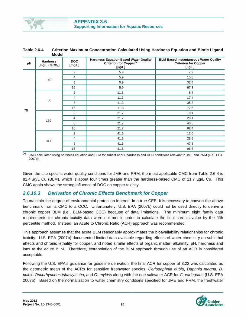
APPENDIX 3.6 Supporting Information for Aquatic Resources
May 2012 Project No. 10-1346-0001 26
Table 2.6-4 Criterion Maximum Concentration Calculated Using Hardness Equation and Biotic Ligand Model
pH Hardness [mg/L CaCO3]
DOC [mg/L]
Hardness Equation Based Water Quality Criterion for Copper(a)
[µg/L]
BLM Based Instantaneous Water Quality Criterion for Copper
[µg/L]
75
40
2 5.9 7.9 4 5.9 15.8 8 5.9 32.4
16 5.9 67.3
80
2 11.3 8.7 4 11.3 17.4 8 11.3 35.3
16 11.3 72.5
159
2 21.7 10.1 4 21.7 20.1 8 21.7 40.5
16 21.7 82.4
317
2 41.5 12.0 4 41.5 23.9 8 41.5 47.8
16 41.5 96.8 (a) CMC calculated using hardness equation and BLM for subset of pH, hardness and DOC conditions relevant to JME and PRM (U.S. EPA
2007b).
Given the site-specific water quality conditions for JME and PRM, the most applicable CMC from Table 2.6-4 is 82.4 µg/L Cu (BLM), which is about four times greater than the hardness-based CMC of 21.7 µg/L Cu. This CMC again shows the strong influence of DOC on copper toxicity.
2.6.10.3 Derivation of Chronic Effects Benchmark for Copper To maintain the degree of environmental protection inherent in a true CEB, it is necessary to convert the above benchmark from a CMC to a CCC. Unfortunately, U.S. EPA (2007b) could not be used directly to derive a chronic copper BLM (i.e., BLM-based CCC) because of data limitations. The minimum eight family data requirements for chronic toxicity data were not met in order to calculate the final chronic value by the fifth percentile method. Instead, an Acute to Chronic Ratio (ACR) approach was recommended.
This approach assumes that the acute BLM reasonably approximates the bioavailability relationships for chronic toxicity. U.S. EPA (2007b) documented limited data available regarding effects of water chemistry on sublethal effects and chronic lethality for copper, and noted similar effects of organic matter, alkalinity, pH, hardness and ions to the acute BLM. Therefore, extrapolation of the BLM approach through use of an ACR is considered acceptable.
Following the U.S. EPA’s guidance for guideline derivation, the final ACR for copper of 3.22 was calculated as the geometric mean of the ACRs for sensitive freshwater species, Ceriodaphnia dubia, Daphnia magna, D. pulex, Oncorhynchus tshawytscha, and O. mykiss along with the one saltwater ACR for C. variegatus (U.S. EPA 2007b). Based on the normalization to water chemistry conditions specified for JME and PRM, the freshwater
APPENDIX 3.6 Supporting Information for Aquatic Resources
May 2012 Project No. 10-1346-0001 27
site-specific acute guideline is 82.4 μg/L which, divided by the final ACR of 3.22, results in a freshwater CEB of 25.6 μg/L Cu.
The generic CCME copper guideline and U.S. EPA’s earlier freshwater copper benchmark recommendations are hardness-dependent values. These default guidelines, although conservative, are expected to substantially overstate copper toxicity for the stream conditions anticipated for JME and PRM. As concluded by U.S. EPA (2007b), a BLM-based benchmark calculation procedure is expected to yield a more appropriate benchmark because it accounts for the important water chemistry factors that affect toxicity, including DOC complexation, where the hardness-only correction does not.
A freshwater CEB of 25.6 μg/L Cu is recommended based on the BLM approach. This value is still considered conservative given that the input DOC of 16 mg/L is lower than the estimated value of 22 mg/L for the receiving waters (JME and PRM LSA).
2.6.11 Iron Iron (Fe) exists in two forms: soluble ferrous (Fe2+) iron and insoluble ferric (Fe3+) iron. Oxidation-reduction reactions determine the chemical behaviour of iron in the aquatic environment. In aerobic systems, the vast majority of iron is present in water as insoluble ferric ion, which is largely non-toxic. Under anaerobic conditions, soluble ferrous iron can form. Although periodic anoxia has been observed in the LSA of both JME and PRM, dissolved oxygen levels tend to be high, and iron exists predominantly as insoluble ferric iron.
Insufficient data were available to develop an SSD for iron. The lowest reported toxicity value of 256 μg/L was, therefore, initially identified for use as the CEB for iron. This value is based on a 21-day reproduction test using the water flea Daphnia magna (Dave 1984). The identified value is very similar to the Canadian water quality guideline of 300 μg/L (CCME 2007b). Thus, the Canadian water quality guideline was carried forward as the CEB for iron.
The toxicity of iron is strongly influenced by the speciation of the metal, whereas the screening value used in this study was the generic guideline for the protection of aquatic life. In most freshwater systems, Fe2+ (the more toxic species) is rapidly oxidized to insoluble Fe3+ oxyhydroxides, resulting in precipitation. The process is influenced by pH, redox potential, amount and type of dissolved organic matter, and other environmental factors, with acidic, non-humic rivers generally having the highest proportion of iron present in the dissolved form (Vuori 1995). The screening threshold used in this study is designed to be protective of all conditions, including those for which bioavailability is maximized. In most field situations, however, the effect of iron as a toxicant is through a physical effect associated with the settling of iron precipitates (e.g., ferric hydroxide). Because the circumneutral conditions in watercourses in the LSA are not amenable to production of significant concentrations of stable Fe2+, the iron screening guidelines described above are highly conservative.
2.6.12 Lead The generic CCME (2007b) guideline for lead is 1 μg/L. However, CCME (1999a, with updates to 2011) provides a hardness-based derivation, which corresponds to 5.0 to 5.3 μg/L at a site-specific hardness range of 143 to 149 mg/L CaCO3. The latter was selected as the CEB for lead, and no SSD-based derivation was necessary for JME and PRM due to the low concentrations of lead predicted by the water quality model.

APPENDIX 3.6 Supporting Information for Aquatic Resources
May 2012 Project No. 10-1346-0001 28
2.6.13 Manganese Manganese (Mn) exists in oxidation states ranging from Mn3- to Mn7+, of which divalent and trivalent manganese are the more important forms in aquatic systems (CCREM 1987). Sufficient data were available to develop an SSD for manganese, as there were chronic toxicity data for five species. The logistic model provided a good fit to the data (r2 = 0.94), and followed the form:
where:
y = percent of aquatic community affected x = manganese concentration (µg/L)
The resulting HC5 based on the logistic regression model was 1,455 µg/L (Figure 2.6-6).
Figure 2.6-6 Species Sensitivity Distribution Curve for Manganese
7.2
41101
9.89−
+
=x
y
Manganese Concentration (µg/L)
1000 10000 100000 1000000
Perc
ent A
ffect
ed (%
)
0
20
40
60
80
100
120
HC5 = 1,455 µg/L
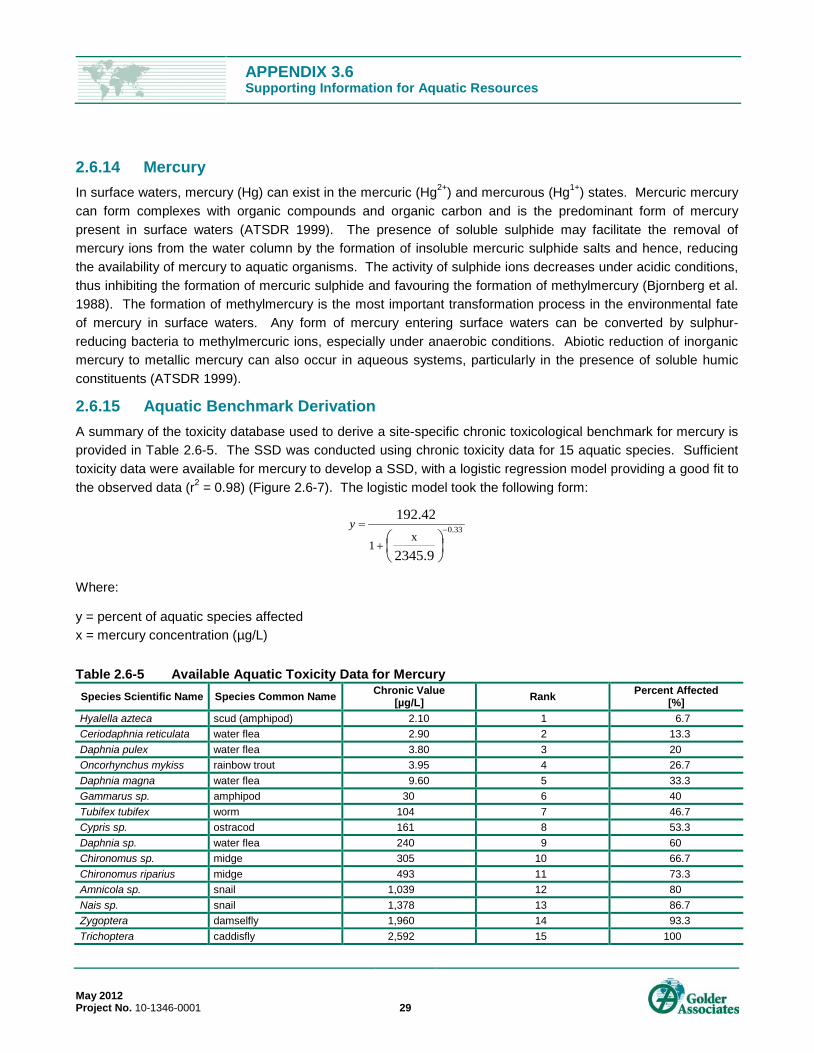
APPENDIX 3.6 Supporting Information for Aquatic Resources
May 2012 Project No. 10-1346-0001 29
2.6.14 Mercury In surface waters, mercury (Hg) can exist in the mercuric (Hg2+) and mercurous (Hg1+) states. Mercuric mercury can form complexes with organic compounds and organic carbon and is the predominant form of mercury present in surface waters (ATSDR 1999). The presence of soluble sulphide may facilitate the removal of mercury ions from the water column by the formation of insoluble mercuric sulphide salts and hence, reducing the availability of mercury to aquatic organisms. The activity of sulphide ions decreases under acidic conditions, thus inhibiting the formation of mercuric sulphide and favouring the formation of methylmercury (Bjornberg et al. 1988). The formation of methylmercury is the most important transformation process in the environmental fate of mercury in surface waters. Any form of mercury entering surface waters can be converted by sulphur-reducing bacteria to methylmercuric ions, especially under anaerobic conditions. Abiotic reduction of inorganic mercury to metallic mercury can also occur in aqueous systems, particularly in the presence of soluble humic constituents (ATSDR 1999).
2.6.15 Aquatic Benchmark Derivation A summary of the toxicity database used to derive a site-specific chronic toxicological benchmark for mercury is provided in Table 2.6-5. The SSD was conducted using chronic toxicity data for 15 aquatic species. Sufficient toxicity data were available for mercury to develop a SSD, with a logistic regression model providing a good fit to the observed data (r2 = 0.98) (Figure 2.6-7). The logistic model took the following form:
Where:
y = percent of aquatic species affected x = mercury concentration (µg/L)
Table 2.6-5 Available Aquatic Toxicity Data for Mercury Species Scientific Name Species Common Name Chronic Value
[µg/L] Rank Percent Affected [%]
Hyalella azteca scud (amphipod) 2.10 1 6.7 Ceriodaphnia reticulata water flea 2.90 2 13.3 Daphnia pulex water flea 3.80 3 20 Oncorhynchus mykiss rainbow trout 3.95 4 26.7 Daphnia magna water flea 9.60 5 33.3 Gammarus sp. amphipod 30 6 40 Tubifex tubifex worm 104 7 46.7 Cypris sp. ostracod 161 8 53.3 Daphnia sp. water flea 240 9 60 Chironomus sp. midge 305 10 66.7 Chironomus riparius midge 493 11 73.3 Amnicola sp. snail 1,039 12 80 Nais sp. snail 1,378 13 86.7 Zygoptera damselfly 1,960 14 93.3 Trichoptera caddisfly 2,592 15 100
33.0
2345.9
192.42x
1−
+
=y
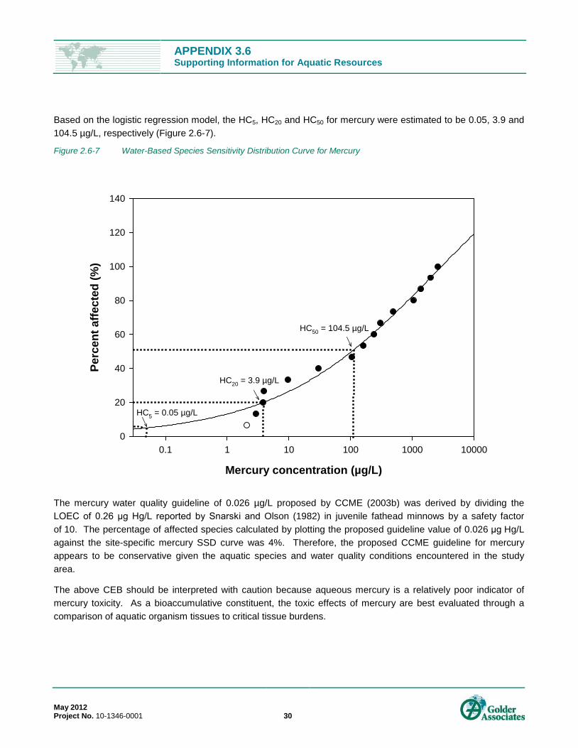
APPENDIX 3.6 Supporting Information for Aquatic Resources
May 2012 Project No. 10-1346-0001 30
Based on the logistic regression model, the HC5, HC20 and HC50 for mercury were estimated to be 0.05, 3.9 and 104.5 µg/L, respectively (Figure 2.6-7).
Figure 2.6-7 Water-Based Species Sensitivity Distribution Curve for Mercury
The mercury water quality guideline of 0.026 µg/L proposed by CCME (2003b) was derived by dividing the LOEC of 0.26 μg Hg/L reported by Snarski and Olson (1982) in juvenile fathead minnows by a safety factor of 10. The percentage of affected species calculated by plotting the proposed guideline value of 0.026 μg Hg/L against the site-specific mercury SSD curve was 4%. Therefore, the proposed CCME guideline for mercury appears to be conservative given the aquatic species and water quality conditions encountered in the study area.
The above CEB should be interpreted with caution because aqueous mercury is a relatively poor indicator of mercury toxicity. As a bioaccumulative constituent, the toxic effects of mercury are best evaluated through a comparison of aquatic organism tissues to critical tissue burdens.
Mercury concentration (µg/L)
0.1 1 10 100 1000 10000
Perc
ent a
ffect
ed (%
)
0
20
40
60
80
100
120
140
HC5 = 0.05 µg/L
HC20 = 3.9 µg/L
HC50 = 104.5 µg/L

APPENDIX 3.6 Supporting Information for Aquatic Resources
May 2012 Project No. 10-1346-0001 31
2.6.15.1 Tissue Benchmark Derivation Because mercury is a strongly bioaccumulative constituent, and biomagnifies in the aquatic food web, the CEB development for mercury was supplemented with an analysis of tissue-based effects observed in freshwater aquatic life. This procedure entailed compiling information that related the exposure of invertebrates and fish to methylmercury and total mercury (measured as a wet weight concentration of mercury in their body tissues) to adverse effects in survival, growth, and reproductive endpoints.
The unique chemical partitioning properties of mercury warranted separate derivations for invertebrates and fish. In fish tissues, mercury is found predominantly in the methylated form, with approximately 95% or more as methylmercury (Wiener and Spry 1996). For this reason, it is common practice to assume that total mercury and methylmercury in fish tissue are equivalent for the purposes of deriving concentration-response relationships. In contrast, the proportion of methylmercury in invertebrate tissues is more variable, with methylmercury usually predominating, but sometimes dropping below 30% of the total mercury present. In general, the proportion of mercury found in organic forms increases with progression up the food web.
The procedure used to develop threshold mercury body residues for mercury entailed the following:
compilation of literature studies that linked the concentrations of mercury in freshwater organisms to chronic lethal and sublethal response endpoints;
conversion of response data to a normalized percent effect by scaling exposure responses to the background/control response and expressing results as a percentage impairment for the specified endpoint;
examining data for systematic differences in sensitivity for certain endpoint types or groups of taxa;
developing a threshold tissue concentration that is protective of both fish and invertebrates, through separate analyses of the statistical fit to the most sensitive endpoint(s) for each biota type; and
comparison of derived values to ecological protection thresholds proposed by other authors.
The data sources included studies that were identified in numerous compendia of tissue effect thresholds (Beckvar et al. 2005; EVS 1999; Jarvinen and Ankley 1999; Sandheinrich and Wiener 2011; Wiener and Spry 1996) and were supported by the results of an online literature review.
Mercury Effects in Invertebrates The concentration-response relationship for invertebrate experiments where the tissue mercury burden was measured in inorganic (upper pane) and organic (lower pane) forms is presented in Figure 2.6-8. The data represent responses to multiple test species including mussels, snails, mayflies and daphnids. For both inorganic and organic mercury, no significant responses were observed for the growth endpoint. However, survival and reproduction were adversely affected at high tissue concentrations of mercury. The data vary substantially reflecting the range of experimental designs and test species, and negative effect levels were observed in some treatments (i.e., indication of a positive response to exposure, likely attributable to natural variability).

APPENDIX 3.6 Supporting Information for Aquatic Resources
May 2012 Project No. 10-1346-0001 32
Figure 2.6-8 Concentration-Response for Mercury in Freshwater Invertebrate Tissues
-40
-20
0
20
40
60
80
100
0.01 0.1 1 10 100
Adv
erse
Effe
ct S
ize
(%)
Tissue Hg (Inorganic, mg/kg ww)
SurvivalReproductionGrowthSmoothed Survival & Reproduction
-40
-20
0
20
40
60
80
100
0.01 0.1 1 10 100
Adv
erse
Effe
ct S
ize
(%)
Tissue Hg (Organic, mg/kg ww)
SurvivalReproductionGrowthSmoothed Survival & Reproduction
APPENDIX 3.6 Supporting Information for Aquatic Resources
May 2012 Project No. 10-1346-0001 33
Despite the variability in individual results, a smoothed model was fit to the combined survival and reproduction data for the concentration-response data for both in organic and organic mercury. Whereas the onset of toxic responses appears to occur in the low mg/kg range for both forms of mercury, the steepness of the concentration-response was greater for the inorganic mercury model, with very large responses observed near 10 mg/kg Hg. Based on the overall response profile shown in Figure 2.6-9, a threshold mercury concentration of 3 mg/kg ww total mercury, or 2 mg/kg ww methylmercury, is proposed as a tissue-based CEB for JME and PRM. These concentrations were chosen based on the estimate of the IC20 from the combined data for the most sensitive endpoints (reproduction and survival).
Mercury Effects in Fish A scatterplot of the tissue effects data for freshwater fish, subdivided into the three main endpoint types (survival, growth and reproduction), is provided in Figure 2.6-9 (upper pane). Unlike invertebrates, there were no major differences in the sensitivity of these three endpoints, with the data highly overlapping and similar model fit (using a logarithmic regression for all endpoints). Again, there is substantial variability in individual data points, reflecting the range of experimental designs and test species, along with natural variability within experiments. However, an increase in response rate with increasing mercury concentration is evident for all three endpoints. Furthermore, the sensitivity of fish to mercury is greater than for invertebrates. At the concentration of 3 mg/kg used for invertebrates, numerous studies have indicated large adverse responses, and the mean (modelled) response for survival and reproduction endpoints exceeds 20%. Although development of a precise threshold is confounded by the high variability, it appears that the magnitude and frequency of adverse responses increases at concentrations close to 1.0 mg/kg total mercury.
Using an IC20 approach applied to the most sensitive endpoint, a concentration of 1.0 mg/kg total mercury was identified. However, the uncertainty associated with the data variability may warrant additional conservatism. Accordingly, a fish tissue CEB of 0.5 mg/kg was selected, which represents a lower level of mean response for survival, and a mean response close to zero for growth and reproduction.
As an additional check on the acceptability of the fish tissue CEB of 0.5 mg/kg, the data were plotted on the basis of species (Figure 2.6-9, lower pane). Mummichog appear to be insensitive to mercury exposure, with no meaningful increase in the incidence of adverse effects across the range of exposures tested. The remaining species (with sufficient data for comparison) suggest similar sensitivity to mercury exposure.

APPENDIX 3.6 Supporting Information for Aquatic Resources
May 2012 Project No. 10-1346-0001 34
Figure 2.6-9 Concentration-Response for Mercury in Freshwater Fish Tissues
-80
-60
-40
-20
0
20
40
60
80
100
0.01 0.1 1 10 100
Adv
erse
Effe
ct M
agni
tude
(%)
Mercury Concentration (mg/kg ww)
Survival Reproduction GrowthSmoothed Survival Smoothed Reproduction Smoothed Growth
-80
-60
-40
-20
0
20
40
60
80
100
0.01 0.1 1 10 100
Perc
ent A
dver
se R
espo
nse
Mercury Concentration (mg/kg ww)
BluegillBrook troutMummichogFathead minnowGolden shinerRainbow troutWalleye
APPENDIX 3.6 Supporting Information for Aquatic Resources
May 2012 Project No. 10-1346-0001 35
Comparison to Other Reviews Because the CEB for the protection of fish is more sensitive than for protection of invertebrates, and because fish tissue concentrations tend to be higher (due to biomagnification), the fish CEB is likely to be the driver for overall environmental protection. The following authors have developed tissue-based thresholds for protection of fish; therefore their results were compared with the CEB based on evaluation of concentration-response data:
Beckvar et al. (2005) – The authors applied a systematic method for deriving protective (i.e., unlikely to have adverse effects) tissue residue-effect concentrations in fish using decision rules that were formulated to provide guidance on selecting studies and obtaining data in a consistent manner. Paired no-effect and low-effect whole-body residue concentrations in fish were identified for mercury and four analytical approaches of simple ranking, empirical percentile, tissue Threshold-Effect Level (t-TEL), and cumulative distribution function were explored. A whole-body mercury t-TEL of 0.2 mg/kg ww was derived, based largely on sublethal endpoints (growth, reproduction, development, behaviour), and was determined to be protective of juvenile and adult fish. The difference between the t-TEL of 0.2 mg/kg ww and the CEB of 0.5 mg/kg ww is partly attributable to the inclusion by Beckvar et al. (2005) of behavioural test endpoints (such as foraging behaviour and predator avoidance) and partly to a recognized "consistent bias toward protective tissue concentrations." Importantly, the authors cautioned against using tissue residue information from only one study of a species that closely is related to the species of interest. This method supports the meta-analysis of multiple species and experimental conditions to help account for inter-experimental variability.
Wiener and Spry (1996) – The authors summarize the information on mercury toxicity to fish available up to the mid 1990s. The review indicated that concentrations of total mercury associated with lethal and sublethal effects in freshwater fish were expected in the concentration range of 5 to 10 mg/kg ww in whole fish, with signs of overt toxicity not expected below this range. Although it was suggested that sensitive species may require a threshold in the low mg/kg range for protection against ecological impairment, there was no indication of adverse responses below 1.0 mg/kg. The authors also conducted an analysis of existing fish egg concentration studies, and concluded that while adverse effects tended to occur at lower concentrations in eggs relative to adult tissue, these differences were compensated by the lower average concentrations in eggs relative to adult body burdens. The study for JME and PRM suggests that the threshold concentration range proposed by Wiener and Spry (1996) is too high, and this opinion is shared by other authors based on more recent scientific findings.
Sandheinrich and Wiener (2011) – The authors summarize a range of fish toxicity studies including evidence for mercury responses associated with biochemistry, gene expression, behaviour, reproduction, histology, and growth endpoints. This compilation serves as an update to the Wiener and Spry (1996) publication, and emphasizes that recent research has led to a reassessment of the concentration threshold previously thought to be protective. The authors conclude, based on an examination of a wide array of laboratory experiments and field studies, that freshwater fish are adversely affected at tissue concentrations of methylmercury below 1.0 mg/kg ww. They conclude that changes in biochemical processes, damage to cells and tissues, and reduced reproduction can occur at methylmercury concentrations of about 0.3 to 0.7 mg/kg ww in the whole body and about 0.5 to 1.2 mg/kg ww in axial muscle tissues. The midpoint of the whole body threshold range proposed by Sandheinrich and Wiener (2011) is equal to the CEB proposed for this assessment of 0.5 mg/kg ww. Furthermore, the lower end of

APPENDIX 3.6 Supporting Information for Aquatic Resources
May 2012 Project No. 10-1346-0001 36
the 0.3 to 0.7 mg/kg ww range appears to be associated with endpoints that have more uncertain ecological relevance. For example, the data presented in Sandheinrich and Wiener (2011) suggest that behavioural responses occur at concentrations slightly lower than reproduction, growth, and developmental responses. Furthermore, biochemistry and gene expression responses can occur at low concentrations, but these responses are indicators of environmental exposure that do not necessarily translate into ecologically significant effects. Given the differences in the choice of endpoints used in this study versus Sandheinrich and Wiener (2011), the findings are in very strong agreement.
EVS Solutions Inc. (EVS 1999) – Eleven studies, focusing on laboratory experiments that dosed with either methylmercury or mercuric chloride in food or water, were reviewed to identify the range of mercury concentrations associated with adverse effects on survival, growth, and reproductive success in fish. Similar to this study, the authors found that the effects and no-effects concentrations were overlapping. No effects concentrations for sublethal test endpoints ranged from 0.25 mg/kg ww in juvenile walleye to 16 mg/kg ww in Japanese medaka eggs. The most common endpoints assessed were growth, survival, and hatching and spawning success, and larval growth and survival appeared to be the most sensitive endpoints. EVS (1999) did not provide a point estimate of the threshold tissue residue-effect concentration; however, their results were in general agreement with the overall findings in this report.
Overall, the results in this report appear to be in alignment with the work of others, particularly recent work investigating sublethal chronic responses of fish to mercury. On this basis the proposed 0.5 mg/kg ww threshold for whole body fish tissue concentrations was retained as a protective CEB for JME and PRM.
2.6.16 Molybdenum Molybdenum (Mo) is widely distributed in the natural environment and occurs primarily as molybdenite (MoS2) and molybdate (MoO4
2-) (CCREM 1987). Molybdenum enters the aquatic environment naturally through weathering of igneous and sedimentary rocks. The largest anthropogenic source is through the use of molybdenum-containing fertilizer; however other sources include mining and milling of molybdenum, use of molybdenum products, the mining and milling of uranium and copper ores, and the burning of fossil fuels.
Molybdenum occurs in several oxidation states including Mo2+, Mo3+, Mo4+, Mo5+ and Mo6+. The tetravalent and hexavalent states are the most common in nature. Dissolved molybdenum occurs mainly as molybdenum sulphide (MoS2), molybdate (MoO4
2-) and bimolybdate (HMoO4-). A pH greater than 7 the molybdate anion is
the predominant form, where at pH less than 7 polymeric species form (CCME 1999a). Water solubility is largely dependent on pH with molybdenum remaining in solution at pH greater than 5 and forming complexes with iron and aluminum at pH less than 5. Molybdenum bioaccumulates in aquatic organisms such as algae, vascular plants and soft tissues of fish (CCREM 1987).
The current Canadian Water Quality Guideline promulgated by CCME (1999a, updates to 2011) for the protection of freshwater aquatic life for molybdenum is 73 µg/L. It was derived by multiplying the lowest chronic toxicity value, a 28-day LC50 of 0.73 mg/L for rainbow trout (Birge 1978; Birge et al. 1979, 1980a) by a safety factor of 0.1 (CCME 1999a).

APPENDIX 3.6 Supporting Information for Aquatic Resources
May 2012 Project No. 10-1346-0001 37
A summary of the toxicity database used to derive a CEB for molybdenum is provided in Table 2.6-6.
Table 2.6-6 Summary of Freshwater Chronic Toxicity Data for Molybdenum Species Scientific Name Species Common Name Chronic Value
[mg/L] Rank Percent Affected [%]
Onchorhynchus mykiss rainbow trout 43 1 13 Ceriodaphnia dubia water flea 51 2 25 Pimephales promelas fathead minnow 60 3 38 Pseudokirchneriella subcapitata green algae 74 4 50 Daphnia magna water flea 89 5 63 Chironomus riparius midge 121 6 75 Lymnaea stagnalis great pond snail 211 7 88 Lemna minor duckweed 242 8 100
The SSD was developed using chronic toxicity data for eight freshwater species. Importantly, the Birge (1978) and Birge et al. (1979, 1980a) data were categorized as unacceptable based on the protocol for guideline derivation provided by the CCME (2007a). These Birge studies have been identified to have data reliability issues by several authors, including De Schamphelaere et al.’s (2010) evaluation of molybdenum toxicity data, which provides a detailed discussion of quality assessment and screening. In brief, the test methods were poorly described, the molybdenum salt that was used in the testing was not reported, molybdenum concentrations were measured but not reported, physiochemical parameters were measured but not reported, and survival of controls was not reported. As well, there is a discrepancy between the results of these studies and the majority of the literature which demonstrate low toxicity of molybdenum to fish. Similar discrepancies have been observed for other trace contaminants evaluated by Birge (1978) and Birge et al. (1979, 1980a), and data have been eliminated as unreliable on this basis.
In 2005, Davies et al. (2005) replicated the experiments of Birge (1978) and Birge et al. (1979, 1980a) in an attempt to resolve the discrepancy described above, using established protocols for chronic toxicity testing. The reproduced tests could not replicate the high molybdenum toxicity reported by Birge (1978) or Birge et al. (1979, 1980a), and the results were comparable to other studies reporting low toxicity of molybdenum to fish. For these reasons, the Birge (1978) and Birge et al. (1979, 1980a) data were not included in the SSD.
Until recently, the data availability for molybdenum toxicity was poor, such that reliable SSD derivations could not be performed. Recognizing these limitations, the International Molybdenum Association sponsored a suite of chronic toxicity tests using multiple freshwater species, with the express purpose of developing an SSD. De Schamphelaere et al. (2010) presents the results of these ecotoxicity experiments, which were conducted to support the derivation of a freshwater probable-no-effect-concentration for molybdenum using the European SSD framework. Ten species were tested, including fish, amphibians, aquatic invertebrates, aquatic plants and algae. These data, as well as the data of GEI (2009) were primarily used to develop the SSD for molybdenum. The SSD analysis in this report differs slightly from that of De Schamphelaere et al. (2010) due to subtle differences in the derivation procedure (CCME versus Europe), and due to the inclusion of additional data from a literature review.
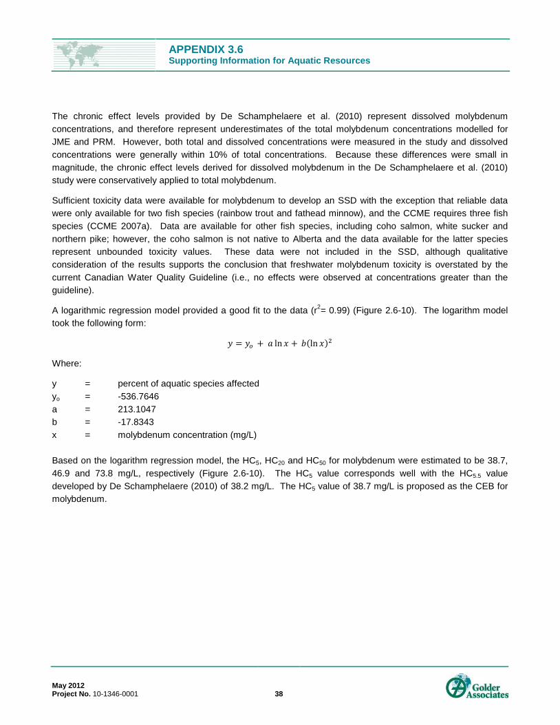
APPENDIX 3.6 Supporting Information for Aquatic Resources
May 2012 Project No. 10-1346-0001 38
The chronic effect levels provided by De Schamphelaere et al. (2010) represent dissolved molybdenum concentrations, and therefore represent underestimates of the total molybdenum concentrations modelled for JME and PRM. However, both total and dissolved concentrations were measured in the study and dissolved concentrations were generally within 10% of total concentrations. Because these differences were small in magnitude, the chronic effect levels derived for dissolved molybdenum in the De Schamphelaere et al. (2010) study were conservatively applied to total molybdenum.
Sufficient toxicity data were available for molybdenum to develop an SSD with the exception that reliable data were only available for two fish species (rainbow trout and fathead minnow), and the CCME requires three fish species (CCME 2007a). Data are available for other fish species, including coho salmon, white sucker and northern pike; however, the coho salmon is not native to Alberta and the data available for the latter species represent unbounded toxicity values. These data were not included in the SSD, although qualitative consideration of the results supports the conclusion that freshwater molybdenum toxicity is overstated by the current Canadian Water Quality Guideline (i.e., no effects were observed at concentrations greater than the guideline).
A logarithmic regression model provided a good fit to the data (r2= 0.99) (Figure 2.6-10). The logarithm model took the following form:
𝑦 = 𝑦𝑜 + 𝑎 ln 𝑥 + 𝑏(ln 𝑥)2
Where:
y = percent of aquatic species affected yo = -536.7646 a = 213.1047 b = -17.8343 x = molybdenum concentration (mg/L) Based on the logarithm regression model, the HC5, HC20 and HC50 for molybdenum were estimated to be 38.7, 46.9 and 73.8 mg/L, respectively (Figure 2.6-10). The HC5 value corresponds well with the HC5.5 value developed by De Schamphelaere (2010) of 38.2 mg/L. The HC5 value of 38.7 mg/L is proposed as the CEB for molybdenum.
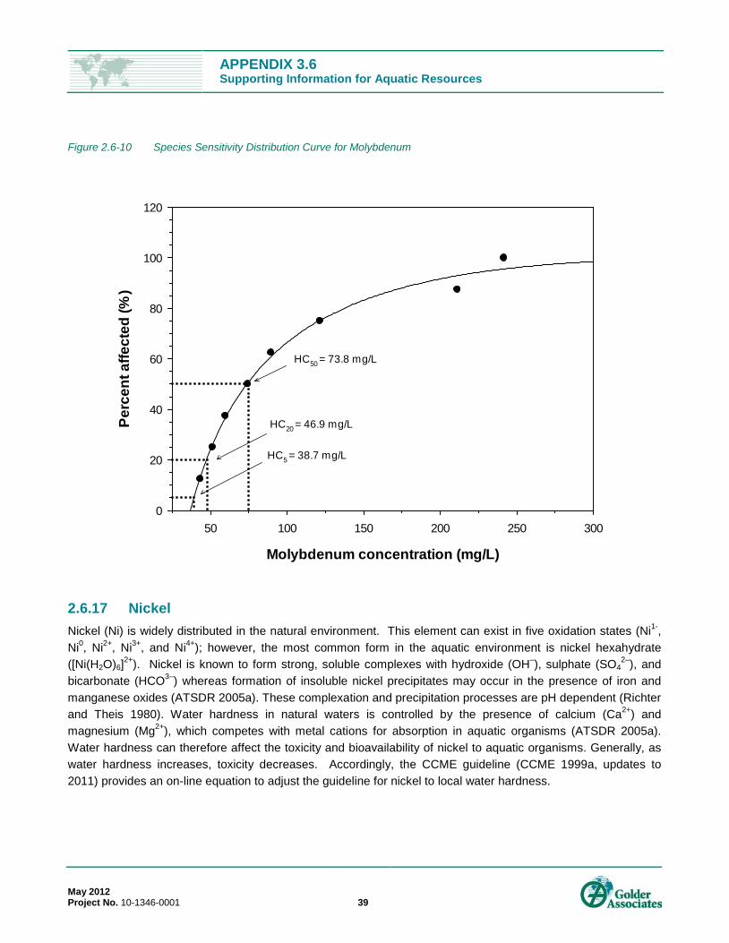
APPENDIX 3.6 Supporting Information for Aquatic Resources
May 2012 Project No. 10-1346-0001 39
Figure 2.6-10 Species Sensitivity Distribution Curve for Molybdenum
2.6.17 Nickel Nickel (Ni) is widely distributed in the natural environment. This element can exist in five oxidation states (Ni1-, Ni0, Ni2+, Ni3+, and Ni4+); however, the most common form in the aquatic environment is nickel hexahydrate ([Ni(H2O)6]2+). Nickel is known to form strong, soluble complexes with hydroxide (OH–), sulphate (SO4
2–), and bicarbonate (HCO3–) whereas formation of insoluble nickel precipitates may occur in the presence of iron and manganese oxides (ATSDR 2005a). These complexation and precipitation processes are pH dependent (Richter and Theis 1980). Water hardness in natural waters is controlled by the presence of calcium (Ca2+) and magnesium (Mg2+), which competes with metal cations for absorption in aquatic organisms (ATSDR 2005a). Water hardness can therefore affect the toxicity and bioavailability of nickel to aquatic organisms. Generally, as water hardness increases, toxicity decreases. Accordingly, the CCME guideline (CCME 1999a, updates to 2011) provides an on-line equation to adjust the guideline for nickel to local water hardness.
Molybdenum concentration (mg/L)
50 100 150 200 250 300
Perc
ent a
ffect
ed (%
)
0
20
40
60
80
100
120
HC20 = 46.9 mg/L
HC50 = 73.8 mg/L
HC5 = 38.7 mg/L
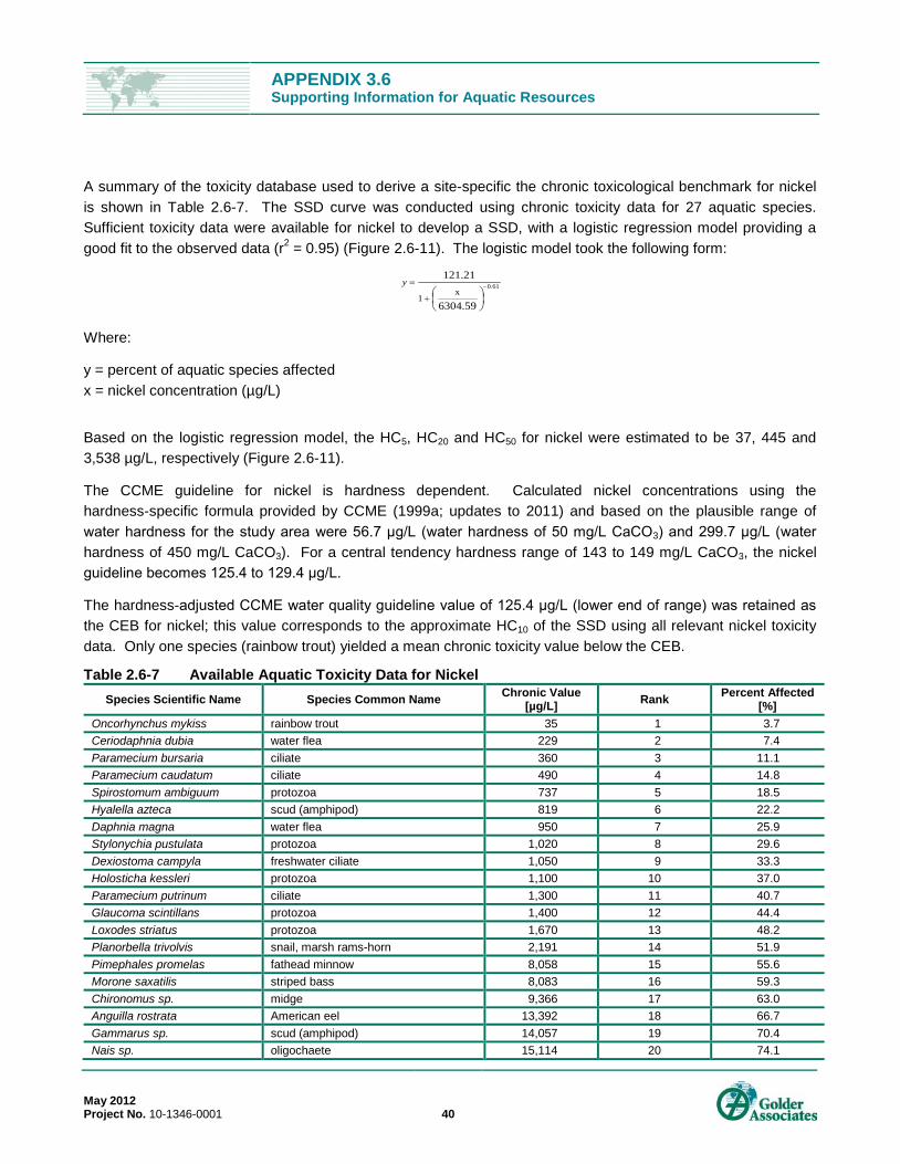
APPENDIX 3.6 Supporting Information for Aquatic Resources
May 2012 Project No. 10-1346-0001 40
A summary of the toxicity database used to derive a site-specific the chronic toxicological benchmark for nickel is shown in Table 2.6-7. The SSD curve was conducted using chronic toxicity data for 27 aquatic species. Sufficient toxicity data were available for nickel to develop a SSD, with a logistic regression model providing a good fit to the observed data (r2 = 0.95) (Figure 2.6-11). The logistic model took the following form:
Where:
y = percent of aquatic species affected x = nickel concentration (µg/L)
Based on the logistic regression model, the HC5, HC20 and HC50 for nickel were estimated to be 37, 445 and 3,538 µg/L, respectively (Figure 2.6-11).
The CCME guideline for nickel is hardness dependent. Calculated nickel concentrations using the hardness-specific formula provided by CCME (1999a; updates to 2011) and based on the plausible range of water hardness for the study area were 56.7 μg/L (water hardness of 50 mg/L CaCO3) and 299.7 μg/L (water hardness of 450 mg/L CaCO3). For a central tendency hardness range of 143 to 149 mg/L CaCO3, the nickel guideline becomes 125.4 to 129.4 μg/L.
The hardness-adjusted CCME water quality guideline value of 125.4 μg/L (lower end of range) was retained as the CEB for nickel; this value corresponds to the approximate HC10 of the SSD using all relevant nickel toxicity data. Only one species (rainbow trout) yielded a mean chronic toxicity value below the CEB.
Table 2.6-7 Available Aquatic Toxicity Data for Nickel Species Scientific Name Species Common Name Chronic Value
[µg/L] Rank Percent Affected [%]
Oncorhynchus mykiss rainbow trout 35 1 3.7 Ceriodaphnia dubia water flea 229 2 7.4 Paramecium bursaria ciliate 360 3 11.1 Paramecium caudatum ciliate 490 4 14.8 Spirostomum ambiguum protozoa 737 5 18.5 Hyalella azteca scud (amphipod) 819 6 22.2 Daphnia magna water flea 950 7 25.9 Stylonychia pustulata protozoa 1,020 8 29.6 Dexiostoma campyla freshwater ciliate 1,050 9 33.3 Holosticha kessleri protozoa 1,100 10 37.0 Paramecium putrinum ciliate 1,300 11 40.7 Glaucoma scintillans protozoa 1,400 12 44.4 Loxodes striatus protozoa 1,670 13 48.2 Planorbella trivolvis snail, marsh rams-horn 2,191 14 51.9 Pimephales promelas fathead minnow 8,058 15 55.6 Morone saxatilis striped bass 8,083 16 59.3 Chironomus sp. midge 9,366 17 63.0 Anguilla rostrata American eel 13,392 18 66.7 Gammarus sp. scud (amphipod) 14,057 19 70.4 Nais sp. oligochaete 15,114 20 74.1
61.0
6304.59
121.21x
1−
+
=y

APPENDIX 3.6 Supporting Information for Aquatic Resources
Table 2.6-7 Available Aquatic Toxicity Data for Nickel (continued)
May 2012 Project No. 10-1346-0001 41
Species Scientific Name Species Common Name Chronic Value [µg/L] Rank Percent Affected
[%] Amnicola sp. spire snail 17,313 21 77.8 Daphnia pulex water flea 19,640 22 81.5 Tubifex tubifex tubificid worm 21,720 23 85.2 Zygoptera damselfly order 23,658 24 88.9 Chironomus riparius midge 25,000 25 92.6 Trichoptera caddisfly order 38,232 26 96.3 Gammarus fasciatus scud (amphipod) 100,000 27 100
Figure 2.6-11 Species Sensitivity Distribution Curve for Nickel
2.6.18 Silver Silver (Ag) has a relatively low abundance but is widely distributed in the earth’s crust (CCREM 1987). It occurs naturally in ores and elemental form (CCREM 1987). It is released to the environment from natural and anthropogenic sources. Mining, silverware manufacturing and the photographic/imaging industry are the greatest anthropogenic contributors (Purcell and Peters 1998). It has been estimated that one fourth to two fifths of the silver released to the environment enters the aquatic component (Scow et al. 1981).
Nickel concentration (µg/L)
10 100 1000 10000 100000
Perc
ent a
ffect
ed (%
)
0
20
40
60
80
100
120
HC5 = 37 µg/L
HC20 = 445 µg/L
HC50 = 3,538 µg/L

APPENDIX 3.6 Supporting Information for Aquatic Resources
May 2012 Project No. 10-1346-0001 42
Silver may exist in the aquatic environment in several chemical forms. However, only the free ionic form of silver (Ag+) is toxic to freshwater organisms (Hogstrand and Wood 1998). In natural waters, the free ionic form is present only at very low concentrations because it readily reacts (binds) with different inorganic and organic ligands that are present in the freshwater environment, including chloride, DOC and sulphides. Silver sulphide is the principal naturally occurring silver compound and is the likely fate of silver discharged into any environment containing a source of sulphide (Kramer et al. 2002). These bound forms of silver are much less toxic than silver nitrate (AgNO3), the form which is frequently used in toxicity testing because it dissociates freely in solution to yield large amounts of Ag+, representing a worst-case simulation of toxicity in the natural environment (Davies et al. 1978; LeBlanc et al. 1984). Recognizing this, recent research has focused on characterizing the role of such ligands in mitigating chronic silver toxicity in the freshwater environment, and development of a BLM for prediction of chronic silver toxicity, analogous to the BLM described above for copper.
The current Canadian Water Quality Guideline for the protection of freshwater aquatic life for silver is 0.1 µg/L, which was derived using the procedure of CCREM (1987) and has not changed since that date. This value is primarily based on the studies of Davies et al. (1978) and Nebeker et al. (1983). In an early life stage test using rainbow trout, Davies et al. (1978) reported a decrease in growth (length) at a silver concentration of 0.17 µg/L. In an early life stage test using steelhead trout, Nebeker et al. (1983) reported a decrease in growth (length) at a silver concentration of 0.1 µg/L.
A summary of the toxicity database used to derive a CEB for silver is provided in Table 2.6-8.
Table 2.6-8 Summary of Freshwater Chronic Toxicity Data for Silver Species Scientific Name Species Common Name Chronic Value
[µg/L] Rank Percent Affected [%]
Salmo trutta brown trout 0.22 1 7 Daphnia pulex water flea 0.56 2 14 Isonychia bicolor mayfly 0.70 3 21 Ceriodaphnia reticulata water flea 0.78 4 29 Oncorhynchus mykiss rainbow trout 0.96 5 36 Pimephales promelas fathead minnow 1.0 6 43 Stenonema modestum mayfly 2.50 7 50 Hyalella azteca amphipod 2.53 8 57 Daphnia magna water flea 4.5 9 64 Lemna minor duckweed 6.0 10 71 Ceriodaphnia dubia water flea 9.5 11 79 Pseudokirchneriella subcapitata green algae 10 12 86 Chlorella vulgaris green algae 23 13 93 Chironomus tentans midge 63 14 100
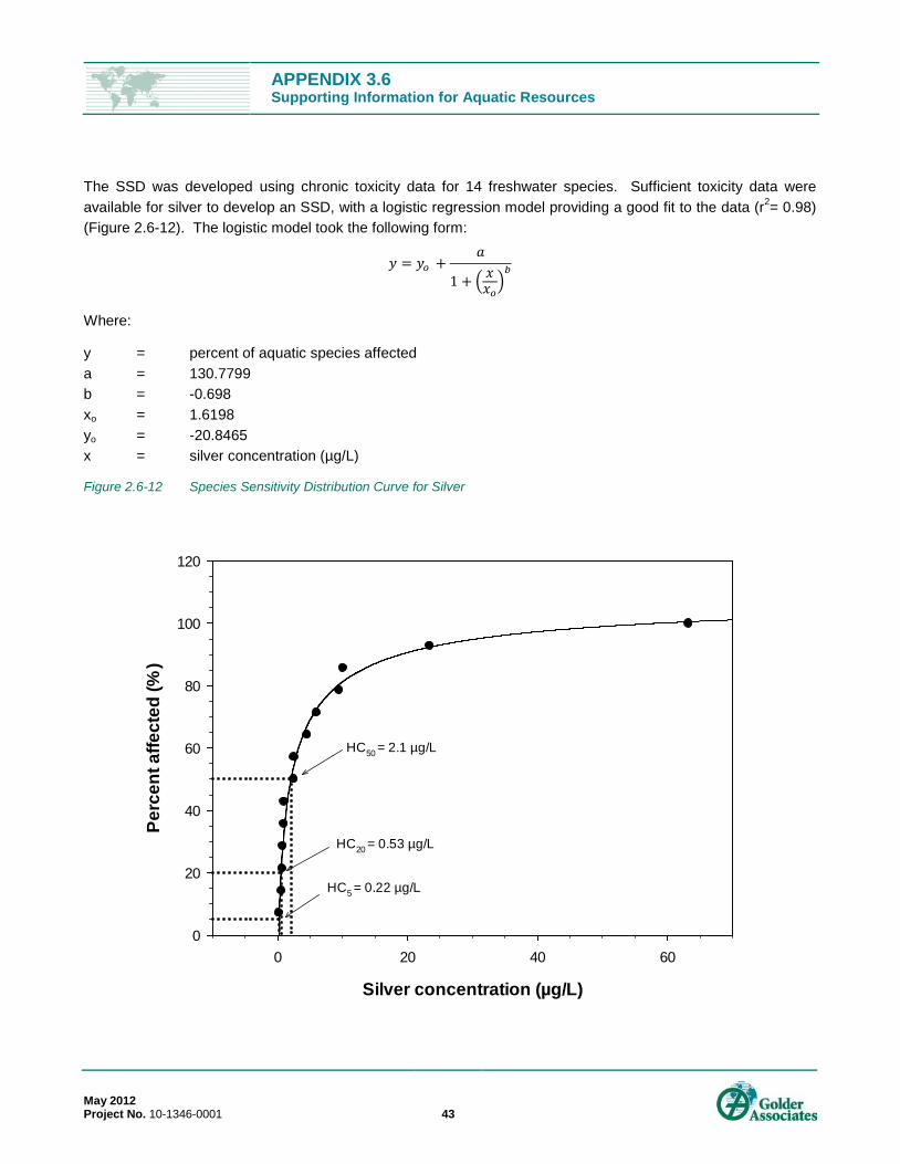
APPENDIX 3.6 Supporting Information for Aquatic Resources
May 2012 Project No. 10-1346-0001 43
The SSD was developed using chronic toxicity data for 14 freshwater species. Sufficient toxicity data were available for silver to develop an SSD, with a logistic regression model providing a good fit to the data (r2= 0.98) (Figure 2.6-12). The logistic model took the following form:
𝑦 = 𝑦𝑜 +𝑎
1 + � 𝑥𝑥𝑜�𝑏
Where:
y = percent of aquatic species affected a = 130.7799 b = -0.698 xo = 1.6198 yo = -20.8465 x = silver concentration (µg/L) Figure 2.6-12 Species Sensitivity Distribution Curve for Silver
Silver concentration (µg/L)
0 20 40 60
Perc
ent a
ffect
ed (%
)
0
20
40
60
80
100
120
HC50 = 2.1 µg/L
HC20 = 0.53 µg/L
HC5 = 0.22 µg/L

APPENDIX 3.6 Supporting Information for Aquatic Resources
May 2012 Project No. 10-1346-0001 44
Based on the logistic regression model, the HC5, HC20 and HC50 for silver were estimated to be 0.22, 0.53 and 2.1 µg/L, respectively (Figure 2.6-12). The HC5 of 0.22 µg/L is proposed as the CEB for silver. This value is close to the lowest species mean chronic value (for brown trout) and thus is protective of the most sensitive freshwater aquatic life.
2.6.19 Strontium Strontium (Sr) can exist in two oxidation states: Sr0 and Sr2+. Under normal environmental conditions, only the Sr2+ oxidation state is stable enough to be of practical importance, since strontium readily reacts with both water and oxygen (Cotton and Wilkinson 1980; Hibbins 1997). There are 26 isotopes of strontium, four of which occur naturally. Naturally occurring strontium is not radioactive and is either referred to as stable strontium or simply as strontium.
Previous assessments of strontium toxicity have identified that, although sufficient data are available to develop an SSD for strontium, the logistic model could not provide a good fit to the data. The apparent reason for the lack of model fit was the disparity between the majority of chronic toxicity estimates (in the range 34,000 μg/L to 465,000 μg/L), and the very low values reported by Birge et al. (1979, 1980a) for rainbow trout embryos (49 μg/L and 200 μg/L). These disparities warranted a detailed critical assessment of the primary data prior to CEB derivation, particularly given concerns regarding data reliability previously identified for the Birge et al. (1979) study reference (compare molybdenum CEB derivation above). Accordingly, this section presents a more detailed presentation of literature findings than is provided for other metals. For a technical summary similar in detail to other metals, the reader may skip to Section 2.6.19.4 of this appendix.
2.6.19.1 Fish Toxicity Pacholski (2009) conducted a 21-day test with juvenile rainbow trout (Oncorhynchus mykiss); additional details of the test procedures were provided in HydroQual (2009). Test fish were approximately 0.3 to 0.5 g wet weight at test initiation, and the exposure system was static-renewal with weekly replacement of test solutions. Control survival after 21 days was 90%, and the results were corrected for control response. Survival was the only endpoint measured; an LC25 of 133,000 µg/L and an LC50 of 286,000 µg/L were reported. The LC25 of 133,000 µg/L was considered to be an acceptable low-effect concentration and was therefore used for the CEB determination.
Birge (1978) conducted a 28-day test with rainbow trout, from fertilization through to four days post-hatch; results of this study were also reported in Birge et al. (1979, 1980a). The exposure system was static-renewal, with replacement of test solutions every 12 hours. Control performance was not reported, but the results were corrected for control response. Survival was the only endpoint measured; an LC01 of 6.0 µg/L and an LC50 of 200 µg/L were reported. The LC01 was considered to be too conservative an estimate of a no-effect concentration for the CEB, as the CCME (2007a) method allows for up to a 10% effect for that estimate, and was also problematic because it was within the range of baseline and/or background strontium concentrations associated with northern Canadian Lakes. Conversely, the LC50 was considered to be insensitive and therefore unsuitable for the CEB; if lethal endpoints are used as low-effect concentrations for the CEB, their effect level should be between 11% and 25%. For the purpose of the CEB determination, a MATC of 35 µg/L was calculated as the geometric mean of the LC01 and LC50 concentrations. This MATC was within the range or lower than background concentrations reported for European and United States streams. Results from this
APPENDIX 3.6 Supporting Information for Aquatic Resources
May 2012 Project No. 10-1346-0001 45
study were also over 1,000 times more sensitive than what Pacholski (2009) reported for juveniles of the same species.
Birge et al. (1980a) conducted a 28-day test with rainbow trout, from fertilization through to four days post-hatch; results of this study were also reported in Birge et al. (1981). The exposure system was static-renewal, with replacement of test solutions every 12 hours. Control survival was 83% to 96%, which was acceptable for this type of test, and the results were corrected for control response. Survival was the only endpoint measured, and the endpoints reported were an LC01 of 13 µg/L, and LC10 of 49 µg/L, and an LC50 of 250 µg/L were reported. The LC10 was used for the CEB determination. Results from this study were consistent with those reported by Birge (1978), but were also within the range or lower than background concentrations reported for European and United States streams.
Birge (1978) conducted a 7-day test with goldfish (Carassius auratus) from fertilization through to four days post-hatch; results of this study were also reported in Birge et al. (1979, 1980a). The exposure system was static-renewal, with replacement of test solutions every 12 hours. Control performance was not reported, but the results were corrected for control response. Survival was the only endpoint measured; an LC01 of 45.3 µg/L and an LC50 of 8,580 µg/L were reported. For reasons previously described, an MATC of 623 µg/L was calculated as the geometric mean of the LC01 and LC50, for use in the CEB determination. The MATC from this study was within the range of background concentrations reported for European and United States streams. Also, although goldfish were introduced over 100 years ago, they are not native to North America.
Pacholski (2009) conducted a standard 7-day survival and growth test with larval (less than 24–hour old) fathead minnow (Pimephales promelas); additional testing details were provided in HydroQual (2009). The 7-day LC50 for survival was 354,000 µg/L and the IC25 for growth was 319,000 µg/L; this latter value was used for the CEB determination.
Hull (2008) provided a collection of worksheets showing calculations used to develop acute and chronic values for strontium for the Michigan Department of Environmental Quality (it was not clear whether these had actually been formally adopted as state water quality standards). These worksheets included tabulated toxicity data from a number of unpublished reports. Cook (2008; cited in Hull 2008) conducted a 7-day test with fathead minnow; it is assumed that this was a standard 7-day larval fish test, but the only endpoints that were reported by Hull (2008) were for survival. The NOEC for survival was 92,870 µg/L and the LOEC was 188,750 µg/L; Hull (2008) used the NOEC and LOEC to calculate an MATC of 132,390 µg/L, which was used for the CEB determination. Survival results from this 7-day fathead minnow test were more sensitive than the Pacholski (2009) 7-day fathead minnow results, but were similar to the Pacholski (2009) results for juvenile rainbow trout, and also consistent with results from three acute 96-hour LC50s for fathead minnow that ranged from 140,180 to 228,470 µg/L (Hull 2008).
Jones (1939) conducted toxicity tests with stickleback (Gasterosteus aculeatus), to determine a survival curve for strontium. The test duration was 10 days, and test solutions were renewed daily. The LT50 for strontium was 1,200,000 µg/L for this 10-day exposure; this result was included in the CEB determination.
Schroder et al. (1995) reported that a 24-hour immersion in a strontium chloride solution is used for marking chum salmon (Oncorhynchus keta) and sockeye salmon (O. nerka) fry prior to their release in the wild. The strontium is deposited in calcified tissues and can easily be detected in otoliths when the fish are older. For this study, chum salmon fry were exposed to three strontium concentrations (120,000, 1,200,000 or 9,000,000 µg/L)
APPENDIX 3.6 Supporting Information for Aquatic Resources
May 2012 Project No. 10-1346-0001 46
for 24 hours, reared for 34 days on a standard hatchery diet, then sacrificed for analyses. Control mortality was 1%; mortality in the 1,200,000 µg/L treatment was 2%, and mortality in the 9,000,000 µg/L treatment was 7%. The geometric mean of these two results was used for the CEB determination. In a second experiment, sockeye salmon were immersed in a 5,000,000 µg/L strontium solution for 24 hours and then reared for 21 months on a standard hatchery diet to determine how long the marked fish could be distinguished from unmarked fish. Although mortality data were not provided for the second experiment, it was presumed that survival was sufficiently high during the 21-month rearing period to provide meaningful test results.
2.6.19.2 Invertebrate Toxicity Biesinger and Christensen (1972) conducted 21-day tests with the water flea, Daphnia magna, to determine effects of strontium exposure on survival and reproduction. They reported a 21-day LC50 of 86,000 µg/L for survival and a 21-day EC50 of 60,000 µg/L for reproduction. In addition, an EC16 of 42,000 µg/L was calculated for reproduction, to represent the lowest effect size that could be distinguished from variability associated with the control response. This EC16 was used for the CEB determination.
Pacholski (2009) conducted a 21-day survival and reproduction test with Daphnia magna, and reported an LC50 of 122,000 µg/L and an IC25 of 49,000 µg/L for reproduction. Additional details regarding testing were provided in HydroQual (2009). This IC25 for reproduction was similar to the EC16 from the Biesinger and Christensen (1972) study, and was included for the CEB determination.
Cook (2008; cited in Hull 2008) conducted a 6-day survival and reproduction test with the water flea, Ceriodaphnia dubia. The NOEC and LOEC for reproduction were 24,570 and 45,890 µg/L, respectively. The MATC calculated from those two values was 33,578 µg/L and was used for the CEB determination.
Pacholski (2009) conducted a 6-day survival and reproduction test with Ceriodaphnia dubia, and reported an LC50 of 206,000 µg/L and an IC25 of 30,000 µg/L for reproduction. Additional details regarding testing were provided in HydroQual (2009). This IC25 for reproduction was consistent with the MATC from the Cook (2008) study, and was included for the CEB determination.
Borgmann et al. (2005) conducted 7-day tests with the amphipod, Hyalella azteca, to determine the effects of strontium on survival. The primary objective of this study was to assess the toxicity of 63 elements in waters at two different hardness levels, and therefore a number of elements were only tested at a few concentrations, starting at 1,000 µg/L and then testing at higher or lower concentrations depending on the initiation result. This was the case for strontium, which was not tested at a full dilution series that would have allowed for determination of LC25 or LC50 values. In soft water, the 7-day LC50 was greater than 1,000 µg/L; there was 18% mortality at 315 µg/L but only 12% mortality at 1,000 µg/L. In the higher-hardness Lake Ontario water, the 7-day LC50 was greater than 3,150 µg/L, and there was only 7% mortality at 1,000 µg/L. The authors reported that control survival was at least 80%, which is reasonable for this test method. However, the results were not corrected for the control response and, given that the survival results that were reported for strontium were all at least 80% it is possible that with correction for the control responses that these effect sizes would have been smaller or even non-existent. For the purpose of the CEB determination, the single-concentration mortality data as LC07, LC12 and LC18 results representing no-effect and low-effect concentrations were used. However, the lack of control response correction means that these results are likely overly conservative estimates of effects. This conclusion is supported by the fact that Hull (2008) reported a 48-hour LC50 of 198,011 µg/L from an acute Hyalella test, a concentration almost 200 times higher than that reported by Borgmann et al. (2005).

APPENDIX 3.6 Supporting Information for Aquatic Resources
May 2012 Project No. 10-1346-0001 47
Boutet and Chaisemartin (1973; cited from Pacholski 2009) reported a 30-day LC50 of 390,000 µg/L for white-clawed crayfish (Austropolmobius pallipes pallipes) and a 30-day LC50 of 860,000 µg/L for spinycheek crayfish (Orconectes limonus). Both these results were included for the CEB determination.
Suzuki (1959) conducted 10-day tests with mosquito larvae (Culex pipiens paliens). The EC25 for time to emergence was 553,000 µg/L and the EC25 for time to pupation was 5,530 µg/L. The EC25 of 553,000 µg/L was included for the CEB determination.
Jones (1940) conducted 48-hour tests with the planarian (Polycelis nigra), and reported LT50s of 3,500,000 and 6,000,000 µg/L for two different strontium salts. The author considered this endpoint to be the threshold of toxicity because with only a slight dilution the survival was extended considerably. Both of these results were included for the CEB determination.
2.6.19.3 Other Organism Toxicity Pacholski (2009) conducted a standard 72-hour algal growth test with Pseudokirchneriella subcapitata; additional testing details were provided in HydroQual (2009). The 72-hour IC25 of 53,000 µg/L was used for the CEB determination. The algae demonstrated a hormetic response, with growth stimulation occurring at strontium concentrations up to 23,000 µg/L, but inhibition of growth at higher concentrations.
Birge (1978) conducted a 7-day test with the narrow-mouthed toad (Gastrophryne carolinensis) from fertilization through to four days post-hatch; results of this study were also reported in Birge et al. (1979, 1980a, 1980b). The exposure system was static-renewal, with replacement of test solutions every 12 hours. Control performance was not reported, but the results were corrected for control response. Survival was the only endpoint measured; an LC01 of 2.4 µg/L and an LC50 of 160 µg/L were reported. The LC01 was considered to be too conservative for use as a no-effect concentration, and the LC50 was not conservative enough as a low-effect concentration. An MATC of 20 µg/L was calculated as the geometric mean of the LC01 and LC50. This study was excluded from the CEB determination, based on the questionable ecological relevance of this species to the region, the fact that the test endpoints were lower than background concentrations associated with European and US streams, and the questions of data acceptability for the Birge studies as discussed earlier.
2.6.19.4 Chronic Effects Benchmark Derivations Chronic toxicity data from 11 studies on 13 aquatic species were considered in the derivation of a strontium CEB. These data represented studies performed on five fish species (including two salmonids), seven invertebrate species (including planktonic crustaceans), and one algal species. This data set was therefore considered sufficiently robust to apply the CCME (2007a) methods for developing a Type A long-term exposure water quality guideline.
The endpoints from the 11 chronic studies on 13 species, along with the calculated Species Mean Chronic Values (SMCVs) that were used to generate the SSD for strontium are summarized in Table 2.6-9. Eight studies conducted with fish, invertebrates or algae had endpoints associated with strontium concentrations in excess of 30,000 µg/L. However, there were three studies that demonstrated much greater sensitivity to strontium, with individual test endpoints ranging from 35 to 1,000 µg/L. Although there were potential technical reliability issues identified with these three studies, their endpoints were initially included in the SSD to provide a conservative estimate of the effects threshold for strontium, albeit with an associated increase in uncertainty.
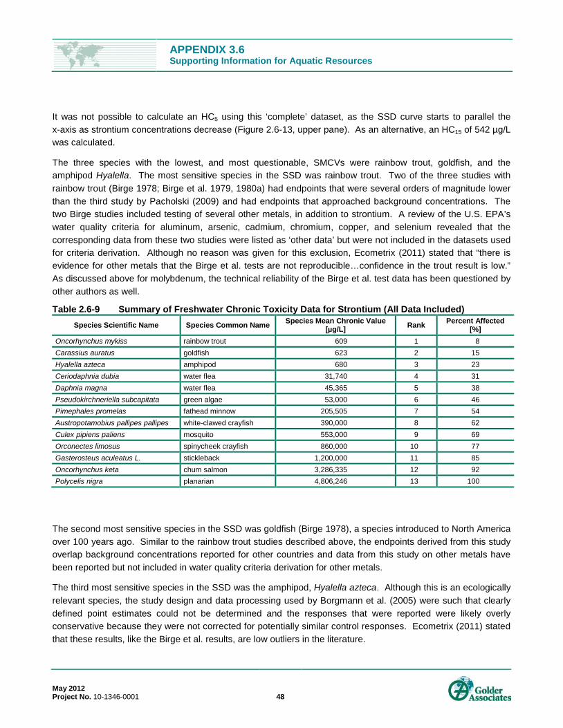
APPENDIX 3.6 Supporting Information for Aquatic Resources
May 2012 Project No. 10-1346-0001 48
It was not possible to calculate an HC5 using this ‘complete’ dataset, as the SSD curve starts to parallel the x-axis as strontium concentrations decrease (Figure 2.6-13, upper pane). As an alternative, an HC15 of 542 µg/L was calculated.
The three species with the lowest, and most questionable, SMCVs were rainbow trout, goldfish, and the amphipod Hyalella. The most sensitive species in the SSD was rainbow trout. Two of the three studies with rainbow trout (Birge 1978; Birge et al. 1979, 1980a) had endpoints that were several orders of magnitude lower than the third study by Pacholski (2009) and had endpoints that approached background concentrations. The two Birge studies included testing of several other metals, in addition to strontium. A review of the U.S. EPA’s water quality criteria for aluminum, arsenic, cadmium, chromium, copper, and selenium revealed that the corresponding data from these two studies were listed as ‘other data’ but were not included in the datasets used for criteria derivation. Although no reason was given for this exclusion, Ecometrix (2011) stated that “there is evidence for other metals that the Birge et al. tests are not reproducible…confidence in the trout result is low.” As discussed above for molybdenum, the technical reliability of the Birge et al. test data has been questioned by other authors as well.
Table 2.6-9 Summary of Freshwater Chronic Toxicity Data for Strontium (All Data Included) Species Scientific Name Species Common Name Species Mean Chronic Value
[µg/L] Rank Percent Affected [%]
Oncorhynchus mykiss rainbow trout 609 1 8 Carassius auratus goldfish 623 2 15 Hyalella azteca amphipod 680 3 23 Ceriodaphnia dubia water flea 31,740 4 31 Daphnia magna water flea 45,365 5 38 Pseudokirchneriella subcapitata green algae 53,000 6 46 Pimephales promelas fathead minnow 205,505 7 54 Austropotamobius pallipes pallipes white-clawed crayfish 390,000 8 62 Culex pipiens paliens mosquito 553,000 9 69 Orconectes limosus spinycheek crayfish 860,000 10 77 Gasterosteus aculeatus L. stickleback 1,200,000 11 85 Oncorhynchus keta chum salmon 3,286,335 12 92 Polycelis nigra planarian 4,806,246 13 100
The second most sensitive species in the SSD was goldfish (Birge 1978), a species introduced to North America over 100 years ago. Similar to the rainbow trout studies described above, the endpoints derived from this study overlap background concentrations reported for other countries and data from this study on other metals have been reported but not included in water quality criteria derivation for other metals.
The third most sensitive species in the SSD was the amphipod, Hyalella azteca. Although this is an ecologically relevant species, the study design and data processing used by Borgmann et al. (2005) were such that clearly defined point estimates could not be determined and the responses that were reported were likely overly conservative because they were not corrected for potentially similar control responses. Ecometrix (2011) stated that these results, like the Birge et al. results, are low outliers in the literature.
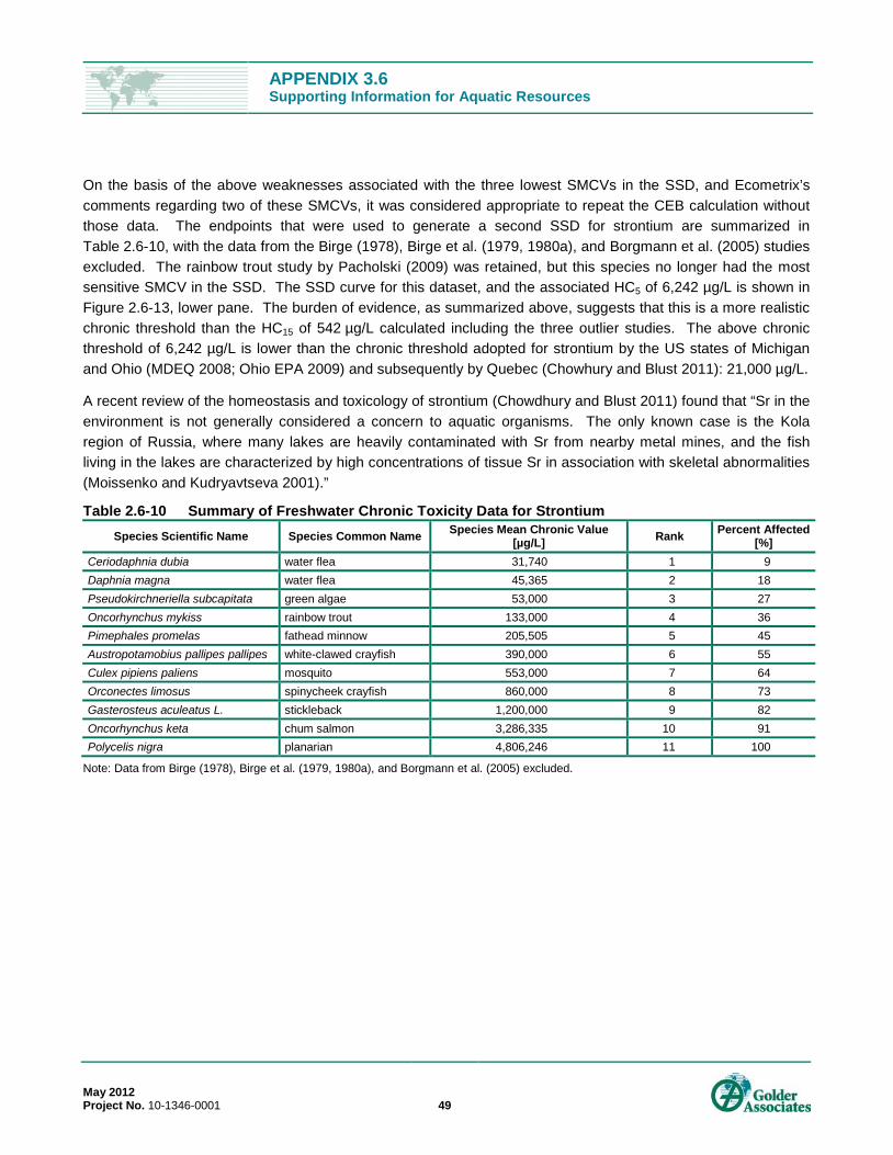
APPENDIX 3.6 Supporting Information for Aquatic Resources
May 2012 Project No. 10-1346-0001 49
On the basis of the above weaknesses associated with the three lowest SMCVs in the SSD, and Ecometrix’s comments regarding two of these SMCVs, it was considered appropriate to repeat the CEB calculation without those data. The endpoints that were used to generate a second SSD for strontium are summarized in Table 2.6-10, with the data from the Birge (1978), Birge et al. (1979, 1980a), and Borgmann et al. (2005) studies excluded. The rainbow trout study by Pacholski (2009) was retained, but this species no longer had the most sensitive SMCV in the SSD. The SSD curve for this dataset, and the associated HC5 of 6,242 µg/L is shown in Figure 2.6-13, lower pane. The burden of evidence, as summarized above, suggests that this is a more realistic chronic threshold than the HC15 of 542 µg/L calculated including the three outlier studies. The above chronic threshold of 6,242 µg/L is lower than the chronic threshold adopted for strontium by the US states of Michigan and Ohio (MDEQ 2008; Ohio EPA 2009) and subsequently by Quebec (Chowhury and Blust 2011): 21,000 µg/L.
A recent review of the homeostasis and toxicology of strontium (Chowdhury and Blust 2011) found that “Sr in the environment is not generally considered a concern to aquatic organisms. The only known case is the Kola region of Russia, where many lakes are heavily contaminated with Sr from nearby metal mines, and the fish living in the lakes are characterized by high concentrations of tissue Sr in association with skeletal abnormalities (Moissenko and Kudryavtseva 2001).”
Table 2.6-10 Summary of Freshwater Chronic Toxicity Data for Strontium Species Scientific Name Species Common Name Species Mean Chronic Value
[µg/L] Rank Percent Affected [%]
Ceriodaphnia dubia water flea 31,740 1 9 Daphnia magna water flea 45,365 2 18 Pseudokirchneriella subcapitata green algae 53,000 3 27 Oncorhynchus mykiss rainbow trout 133,000 4 36 Pimephales promelas fathead minnow 205,505 5 45 Austropotamobius pallipes pallipes white-clawed crayfish 390,000 6 55 Culex pipiens paliens mosquito 553,000 7 64 Orconectes limosus spinycheek crayfish 860,000 8 73 Gasterosteus aculeatus L. stickleback 1,200,000 9 82 Oncorhynchus keta chum salmon 3,286,335 10 91 Polycelis nigra planarian 4,806,246 11 100
Note: Data from Birge (1978), Birge et al. (1979, 1980a), and Borgmann et al. (2005) excluded.

APPENDIX 3.6 Supporting Information for Aquatic Resources
May 2012 Project No. 10-1346-0001 50
Figure 2.6-13 Species Sensitivity Distribution Curve for Strontium
(a) All chronic studies included (an HC5 could not be calculated but the HC15 was 542 µg/L).
(b) Data from Birge (1978), Birge et al. (1979, 1980a), and Borgmann et al. (2005) excluded.
Strontium concentration (µg/L)
10 100 1000 10000 100000 1000000 10000000
Perc
ent a
ffect
ed (%
)
0
20
40
60
80
100
120
Strontium concentration (µg/L)
1000 10000 100000 1000000 10000000
Perc
ent A
ffect
ed (%
)
-20
0
20
40
60
80
100
120
HC5 = 6,264 µg/L

APPENDIX 3.6 Supporting Information for Aquatic Resources
May 2012 Project No. 10-1346-0001 51
2.6.20 Vanadium The transport and speciation of vanadium (V) in water is influenced by pH, redox potential and the presence of particulate matter. In fresh water, vanadium generally exists in solution as the vanadyl ion (V4+) under reducing conditions and the vanadate ion (V5+) under oxidizing conditions, or as an integral part of, or adsorbed onto, particulate matter (Wehrli and Stumm 1989). The partitioning of vanadium between water and sediment is strongly influenced by the presence of particulates in the water. Both vanadate and vanadyl species are known to bind strongly to mineral or biogenic surfaces by adsorption or complexing (Wehrli and Stumm 1989).
Insufficient data were available to develop an SSD for vanadium. The lowest reported toxicity value of 33.8 µg/L was, therefore, selected for use as the CEB for vanadium. This value is based on a 28-day LC10 test result (Birge et al. 1979, 1980a) based on a 28-day LC10 with rainbow trout embryos. As discussed earlier in the context of molybdenum and strontium CEB derivations, the Birge et al. test endpoints should be interpreted with caution due to evidence for other metals that the tests are not reproducible.
2.6.21 Zinc Zinc (Zn) compounds can be found in rocks, certain minerals and carbonate sediments. As a result of weathering of these materials, soluble compounds of zinc may be released into aquatic systems. Urban runoff, mine drainage and industrial effluents may be also a source of zinc to receiving aquatic systems. Zinc exists in the aquatic environment as Zn2+ oxidation state with zinc hydroxide (Zn[OH]3) as the main form present in natural waters (ATSDR 2005b). This element frequently forms complexes with a variety of organic and inorganic compounds (e.g., humic acids). The stability of these zinc complexes depends on the pH of the water with a higher dissociation rate occurring as the pH decreases (Guy and Chakrabarti 1976).
A summary of the toxicity database used to derive a site-specific chronic toxicological benchmark for zinc is shown in Table 2.6-11. The SSD was conducted using chronic toxicity data for 14 aquatic species. Sufficient toxicity data were available for zinc to develop a SSD, with a logistic regression model providing a good fit to the observed data (r2 = 0.98) (Figure 2.6-14). The logistic model took the following form:
Where:
y = percent of aquatic species affected x = zinc concentration (µg/L)
76.1
814.05
118.67x
1−
+
=y
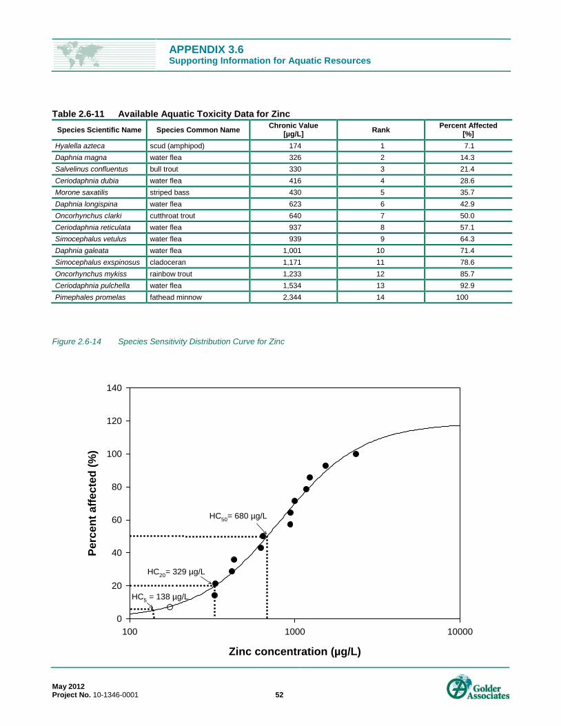
APPENDIX 3.6 Supporting Information for Aquatic Resources
May 2012 Project No. 10-1346-0001 52
Table 2.6-11 Available Aquatic Toxicity Data for Zinc Species Scientific Name Species Common Name Chronic Value
[µg/L] Rank Percent Affected [%]
Hyalella azteca scud (amphipod) 174 1 7.1 Daphnia magna water flea 326 2 14.3 Salvelinus confluentus bull trout 330 3 21.4 Ceriodaphnia dubia water flea 416 4 28.6 Morone saxatilis striped bass 430 5 35.7 Daphnia longispina water flea 623 6 42.9 Oncorhynchus clarki cutthroat trout 640 7 50.0 Ceriodaphnia reticulata water flea 937 8 57.1 Simocephalus vetulus water flea 939 9 64.3 Daphnia galeata water flea 1,001 10 71.4 Simocephalus exspinosus cladoceran 1,171 11 78.6 Oncorhynchus mykiss rainbow trout 1,233 12 85.7 Ceriodaphnia pulchella water flea 1,534 13 92.9 Pimephales promelas fathead minnow 2,344 14 100
Figure 2.6-14 Species Sensitivity Distribution Curve for Zinc
Zinc concentration (µg/L)
100 1000 10000
Perc
ent a
ffect
ed (%
)
0
20
40
60
80
100
120
140
HC5 = 138 µg/L
HC20= 329 µg/L
HC50= 680 µg/L

APPENDIX 3.6 Supporting Information for Aquatic Resources
May 2012 Project No. 10-1346-0001 53
Based on the logistic regression model, the HC5, HC20 and HC50 for zinc were estimated to be 138, 329 and 680 µg/L, respectively (Figure 2.6-14).
The toxicity benchmark for zinc reported by CCME (1999a; updates to 2011) is 30 µg/L. However, guidance is not clearly provided on how this toxicity benchmark was derived. The percentage of affected species calculated by plotting the proposed guideline value of 30 μg Zn/L using the site-specific SSD curve derived in this report was less than 1%. Therefore, the proposed CCME guideline for zinc appears to be conservative given the aquatic species and water quality conditions encountered in the study area.
2.7 Chronic Effects Benchmark Results for Polycyclic Aromatic Hydrocarbons
Polycyclic Aromatic Hydrocarbons (PAHs) are a group of organic compounds that contain two or more benzene rings in their structure. Polycyclic aromatic hydrocarbons are ubiquitous in terrestrial, atmospheric and aquatic environments (ATSDR 1995). In general, PAHs can be grouped as low molecular weight (less than four rings; including acenaphthene, acenaphthylene, anthracene, fluorene, 1-methylnaphthalene, 2-methylnaphthalene, naphthalene and phenanthrene) and high molecular weight (four or more rings; including benzo(a)anthracene, benzo(a)pyrene, benzo(b&j)fluoranthene, benzo(g,h,i)perylene, benzo(k)fluoranthene, chrysene, dibenz(a,h)anthracene, fluoranthene, indeno(1,2,3-cd)pyrene and pyrene). These compounds can enter aquatic systems through atmospheric deposition and from discharges of industrial effluents, municipal waste water, and improper disposal of used motor oil. Transport and partitioning (e.g., Henry’s law constant, soil organic carbon-water partitioning coefficient [KOC] values, and n-octanol/water partition coefficient [KOW] values) of PAHs in aquatic environments are generally related to their molecular weights (ATSDR 1995).
Once in the aquatic environment, PAHs compounds can be removed from the water column by volatilization to the atmosphere (primarily low molecular PAHs), by binding to suspended particles or sediments, or by being accumulated by aquatic biota (McGrath and DiToro 2009). Due to their low solubility and high affinity for organic carbon, PAHs are primarily found sorbed to particles (e.g., humic acids) in aquatic systems. Polycyclic aromatic hydrocarbons can be also chemically transformed by photo-oxidation into metabolites that may be more carcinogenic and toxic than the parental compound (Oris and Giesy 1986). This process and its associated phototoxicity has been observed mainly under laboratory conditions and rarely studied in natural environments, thus the ecological relevance of PAHs photo-oxidation is still unclear (McDonald and Chapman 2002).
Aquatic organisms can accumulate PAHs directly from water, sediments or food with bioconcentration factors generally ranging from 10 to 10,000 (Eisler 1987). In general, bioconcentration is greater for the higher molecular weight than for the lower molecular weight PAHs. Polycyclic aromatic hydrocarbons biomagnification has not been reported to occur in aquatic organisms because of the rapid metabolism and high elimination rate of these compounds in aquatic organisms (Eisler 1987).

APPENDIX 3.6 Supporting Information for Aquatic Resources
May 2012 Project No. 10-1346-0001 54
2.7.1 Anthracene A summary of the toxicity database used to derive a site-specific chronic toxicological benchmark for anthracene is show in Table 2.7-1. The SSD was conducted using chronic toxicity data for seven aquatic species. Sufficient toxicity data were available for anthracene to develop a SSD, with a logistic regression model providing good fit to the data (r2 = 0.90) (Figure 2.7-1). The logistic model took the following form:
Where:
y = percent of aquatic species affected x = anthracene concentration (µg/L)
Based on the logistic regression model, the HC5, HC20 and HC50 for anthracene were estimated to be 5.6, 9.6 and 16 µg/L, respectively (Figure 2.7-1).
The HC5 for anthracene reported in this study was two times lower than the HC5 reported by McGrath and DiToro (2009). The SSD-based derivations correspond strongly to the TLM for toxicity assessment of Type I narcotic chemicals (Table 2.7-2). The small differences in the predicted HC5 concentration may be explained by the inclusion/exclusion criteria to derive SSD relationships followed in this report, such as inclusion of studies to better represent site-specific conditions and the exclusion of aquatic species not relevant to Canadian waters.
Table 2.7-1 Available Aquatic Toxicity Data for Anthracene Species Scientific Name Species Common Name Ranking Chronic Value
[µg/L] Percent Affected
[%] Daphnia magna water flea 1 8.10 14.3 Hydrilla verticillata hydrilla 2 10 28.6 Pimephales promelas fathead minnow 3 15.5 42.9 Selenastrum capricornutum green algae 4 19 57.1 Daphnia pulex water flea 5 754 71.4 Lumbriculus variegatus oligochaete, worm 6 37 85.7 Aedes taeniorhynchus mosquito 7 45 100
95.2
14.37
86.93x
1−
+
=y
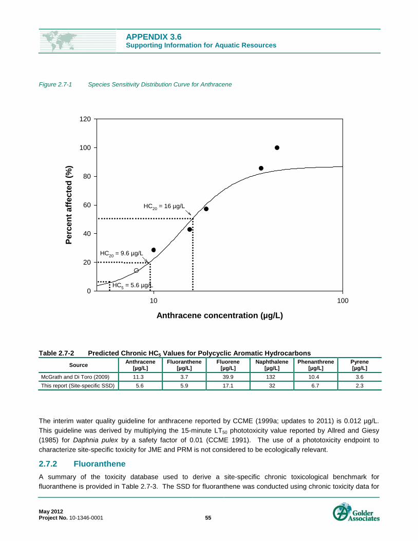
APPENDIX 3.6 Supporting Information for Aquatic Resources
May 2012 Project No. 10-1346-0001 55
Figure 2.7-1 Species Sensitivity Distribution Curve for Anthracene
Table 2.7-2 Predicted Chronic HC5 Values for Polycyclic Aromatic Hydrocarbons Source Anthracene
[µg/L] Fluoranthene
[µg/L] Fluorene
[µg/L] Naphthalene
[µg/L] Phenanthrene
[µg/L] Pyrene [µg/L]
McGrath and Di Toro (2009) 11.3 3.7 39.9 132 10.4 3.6 This report (Site-specific SSD) 5.6 5.9 17.1 32 6.7 2.3
The interim water quality guideline for anthracene reported by CCME (1999a; updates to 2011) is 0.012 µg/L. This guideline was derived by multiplying the 15-minute LT50 phototoxicity value reported by Allred and Giesy (1985) for Daphnia pulex by a safety factor of 0.01 (CCME 1991). The use of a phototoxicity endpoint to characterize site-specific toxicity for JME and PRM is not considered to be ecologically relevant.
2.7.2 Fluoranthene A summary of the toxicity database used to derive a site-specific chronic toxicological benchmark for fluoranthene is provided in Table 2.7-3. The SSD for fluoranthene was conducted using chronic toxicity data for
Anthracene concentration (µg/L)
10 100
Perc
ent a
ffect
ed (%
)
0
20
40
60
80
100
120
HC5 = 5.6 µg/L
HC20 = 9.6 µg/L
HC20 = 16 µg/L

APPENDIX 3.6 Supporting Information for Aquatic Resources
May 2012 Project No. 10-1346-0001 56
19 aquatic species. Sufficient toxicity data were available for fluoranthene to develop a SSD, with a logistic regression model providing a good fit to the observed data (r2 = 0.98) (Figure 2.7-2). The logistic model took the following form:
Where:
y = percent of aquatic species affected x = fluoranthene concentration (µg/L)
Based on the logistic regression model, the HC5, HC20 and HC50 for fluoranthene were estimated to be 5.9, 21.9 and 64.5 µg/L, respectively (Figure 2.7-2). The HC5 for fluoranthene reported in this study was slightly higher than the HC5 reported by McGrath and DiToro (2009) (Table 2.7-3).
The interim water quality guideline for fluoranthene reported by CCME (1999a; updates to 2011) is 0.04 µg/L. This guideline was derived by multiplying the acute LC50 of 4 µg/L reported by Kagan et al. (1985) in Daphnia magna exposed to fluoranthene and UV light by a safety factor of 0.01 (CCME 1991). The use of a phototoxicity endpoint to characterize site-specific toxicity for JME and PRM is not considered to be ecologically relevant.
Table 2.7-3 Available Aquatic Toxicity Data for Fluoranthene Species Scientific Name Species Common Name Rank Chronic Value
[µg/L] Percent Affected
[%] Lumbriculus variegatus oligochaete, worm 1 4.7 5.3 Pimephales promelas fathead minnow 2 15 10.5 Hyalella azteca scud (amphipod) 3 21 15.8 Chironomus tentans midge 4 25 21.1 Daphnia magna water flea 5 31 26.3 Ictalurus punctatus channel catfish 6 36 31.6 Anabaena flosaquae blue-green algae 7 38 36.8 Ceriodaphnia dubia water flea 8 40 42.1 Rana catesbeiana bullfrog 9 60 47.4 Chironomus riparius midge 10 88 52.6 Diporeia sp. scud (amphipod) 11 90 57.9 Oncorhynchus mykiss rainbow trout 12 91 63.2 Gammarus pulex amphipod 13 96 68.4 Utterbackia imbecillis paper pondshell 14 110 73.7 Stylaria lacustris oligochaete 15 159 79.0 Lemna minor duckweed 16 166 84.2 Scenedesmus subspicatus algae 17 192 89.5 Lemna gibba inflated duckweed 18 260 94.7 Pseudokirchneriella subcapitata algae 19 260 100
15.1
93.70
126.94x
1−
+
=y

APPENDIX 3.6 Supporting Information for Aquatic Resources
May 2012 Project No. 10-1346-0001 57
Figure 2.7-2 Species Sensitivity Distribution Curve for Fluoranthene
2.7.3 Fluorene A summary of the toxicity database used to derive a site-specific chronic toxicological benchmark for fluorene is provided in Table 2.7-4. The SSD for fluorene was conducted using chronic toxicity data for 15 aquatic species. Sufficient toxicity data were available for fluorene to develop a SSD, with a logistic regression model providing a good fit to the observed data (r2 = 0.95) (Figure 2.7-3). The logistic model took the following form:
Where:
y = percent of aquatic species affected x = fluorene concentration (µg/L)
Fluoranthene concentration (µg/L)
1 10 100 1000
Perc
ent a
ffect
ed (%
)
0
20
40
60
80
100
120
140
HC5 = 5.9 µg/L
HC20 = 21.9 µg/L
HC50 = 64.5 µg/L
81.0
634.62
97.48x
1−
+
=y

APPENDIX 3.6 Supporting Information for Aquatic Resources
May 2012 Project No. 10-1346-0001 58
Table 2.7-4 Available Aquatic Toxicity Data for Fluorene Species Scientific Name Species Common Name Rank Chronic Value
[µg/L] Percent Affected
[%] Lumbriculus variegatus oligochaete, worm 1 100 6.7 Micropterus salmoides largemouth bass 2 120 13.3 Plankton plankton 2 120 13.3 Daphnia magna water flea 4 125 26.7 Chironomus riparius midge 5 142 33.3 Daphnia pulex water flea 6 212 40.0 Gammarus pseudolimnaeus scud (amphipod) 7 600 46.7 Anabaena flosaquae blue-green algae 8 1,089 53.3 Oncorhynchus mykiss rainbow trout 9 1,473 60.0 M. potosensis snail 10 1,900 66.7 Invertebrates invertebrates 11 2,000 73.3 Lemna gibba inflated duckweed 11 2,000 73.3 Hexagenia bilineata mayfly 13 5,900 86.7 Selenastrum capricornutum green algae 14 800,000 93.3 Pimephales promelas fathead minnow 15 1,000,000 100
Figure 2.7-3 Species Sensitivity Distribution Curve for Fluorene
Fluorene concentration (µg/L)
1 10 100 1000 10000 100000 1000000
Perc
ent a
ffect
ed (%
)
0
20
40
60
80
100
120
HC5 = 17.1µg/L
HC20 = 118.5 µg/L
HC50 = 680 µg/L
APPENDIX 3.6 Supporting Information for Aquatic Resources
May 2012 Project No. 10-1346-0001 59
Based on the logistic regression model, the HC5, HC20 and HC50 for fluorene were estimated to be 17.1, 118.5 and 680 µg/L, respectively (Figure 2.7-3). The HC5 for fluorene reported in this study was slightly higher than the HC5 reported by McGrath and DiToro (2009) (Table 2.7-2).
The interim water quality guideline for fluorene reported by CCME (1999a; updates to 2011) is 3 µg/L. This guideline was derived by multiplying the LOEC of 125 µg/L (nominal concentration) reported by Finger et al. (1985) for phototoxicity responses to Daphnia magna by a safety factor of 0.1 (CCME 1991). The result was then multiplied by a correction factor of 0.24 because the measured fluorene concentration during the chronic tests with daphnids was 24% of the reported nominal LOEC concentration of 125 μg/L. However, the use of a phototoxicity endpoint to characterize site-specific toxicity for JME and PRM is not considered to be ecologically relevant.
2.7.4 Naphthalene A summary of the toxicity database used to derive a site-specific chronic toxicological benchmark for naphthalene is provided in Table 2.7-5. The SSD was conducted using chronic toxicity data for 20 aquatic species. Sufficient toxicity data were available for naphthalene to develop a SSD, with a logistic regression model providing strong fit to the observed data (r2 = 0.98) (Figure 2.7-4). The logistic model took the following form:
Where:
y = percent of aquatic species affected x = naphthalene concentration (µg/L)
Based on the logistic regression model, the HC5, HC20 and HC50 for naphthalene were estimated to be 32, 239.3 and 1,420 µg/L, respectively (Figure 2.7-4). The HC5 for naphthalene reported in this study was four times lower than the HC5 reported by McGrath and DiToro (2009) (Table 2.7-2).
The interim water quality guideline for naphthalene reported by CCME (1999a; updates to 2011) is 1.1 µg/L. This guideline was derived by multiplying the LOEC (survival) of 11 µg/L reported by Black et al. (1983) for rainbow trout embryos by a safety factor of 0.1 (CCME 1991). However, the use of a phototoxicity endpoint to characterize site-specific toxicity for JME and PRM is not considered to be ecologically relevant.
77.0
1480
101.65x
1−
+
=y
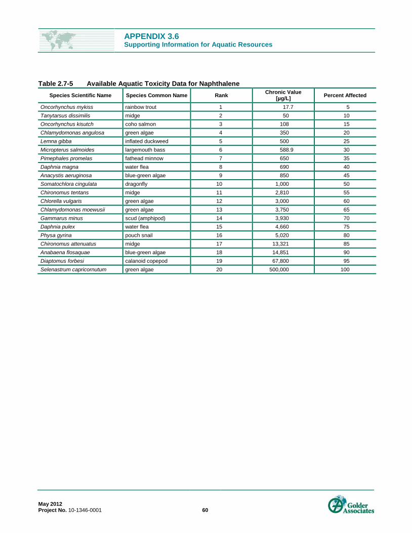
APPENDIX 3.6 Supporting Information for Aquatic Resources
May 2012 Project No. 10-1346-0001 60
Table 2.7-5 Available Aquatic Toxicity Data for Naphthalene Species Scientific Name Species Common Name Rank Chronic Value
[µg/L] Percent Affected
Oncorhynchus mykiss rainbow trout 1 17.7 5 Tanytarsus dissimilis midge 2 50 10 Oncorhynchus kisutch coho salmon 3 108 15 Chlamydomonas angulosa green algae 4 350 20 Lemna gibba inflated duckweed 5 500 25 Micropterus salmoides largemouth bass 6 588.9 30 Pimephales promelas fathead minnow 7 650 35 Daphnia magna water flea 8 690 40 Anacystis aeruginosa blue-green algae 9 850 45 Somatochlora cingulata dragonfly 10 1,000 50 Chironomus tentans midge 11 2,810 55 Chlorella vulgaris green algae 12 3,000 60 Chlamydomonas moewusii green algae 13 3,750 65 Gammarus minus scud (amphipod) 14 3,930 70 Daphnia pulex water flea 15 4,660 75 Physa gyrina pouch snail 16 5,020 80 Chironomus attenuatus midge 17 13,321 85 Anabaena flosaquae blue-green algae 18 14,851 90 Diaptomus forbesi calanoid copepod 19 67,800 95 Selenastrum capricornutum green algae 20 500,000 100
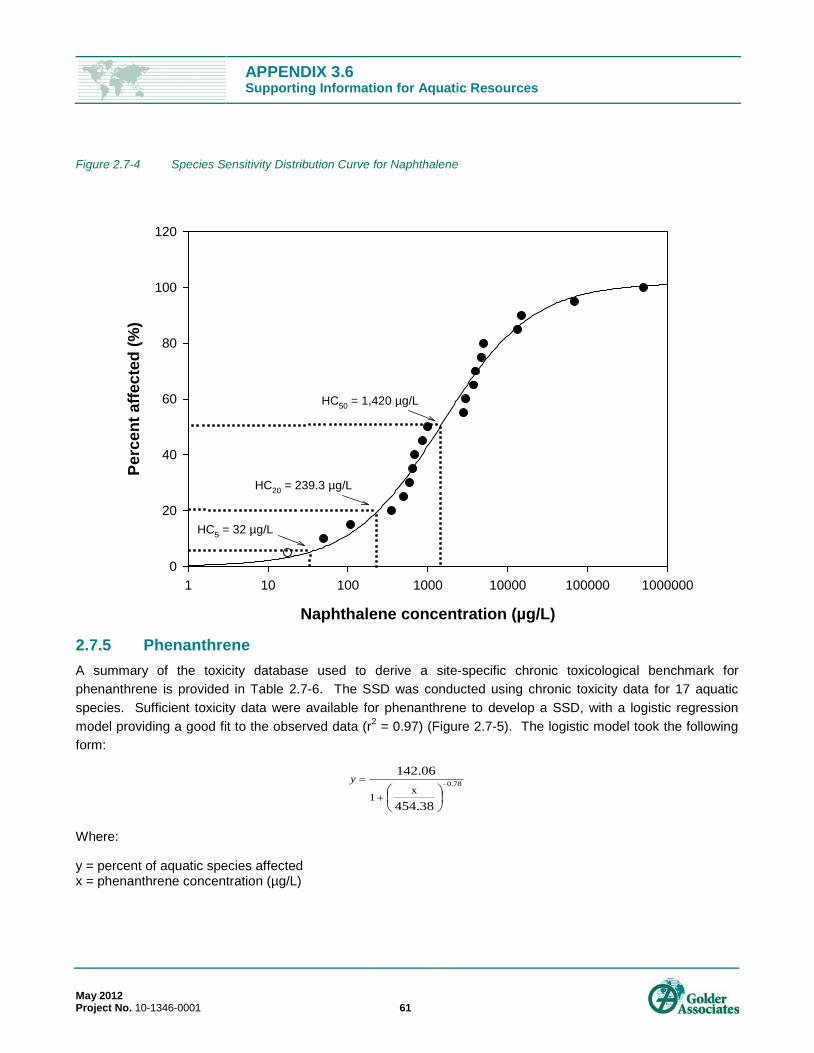
APPENDIX 3.6 Supporting Information for Aquatic Resources
May 2012 Project No. 10-1346-0001 61
Figure 2.7-4 Species Sensitivity Distribution Curve for Naphthalene
2.7.5 Phenanthrene A summary of the toxicity database used to derive a site-specific chronic toxicological benchmark for phenanthrene is provided in Table 2.7-6. The SSD was conducted using chronic toxicity data for 17 aquatic species. Sufficient toxicity data were available for phenanthrene to develop a SSD, with a logistic regression model providing a good fit to the observed data (r2 = 0.97) (Figure 2.7-5). The logistic model took the following form:
Where:
y = percent of aquatic species affected x = phenanthrene concentration (µg/L)
Naphthalene concentration (µg/L)
1 10 100 1000 10000 100000 1000000
Perc
ent a
ffect
ed (%
)
0
20
40
60
80
100
120
HC5 = 32 µg/L
HC20 = 239.3 µg/L
HC50 = 1,420 µg/L
78.0
454.38
142.06x
1−
+
=y
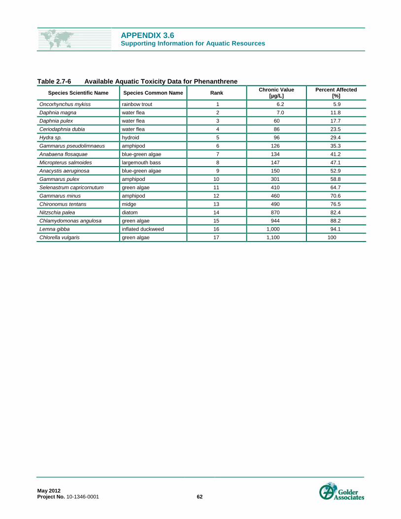
APPENDIX 3.6 Supporting Information for Aquatic Resources
May 2012 Project No. 10-1346-0001 62
Table 2.7-6 Available Aquatic Toxicity Data for Phenanthrene Species Scientific Name Species Common Name Rank Chronic Value
[µg/L] Percent Affected
[%] Oncorhynchus mykiss rainbow trout 1 6.2 5.9 Daphnia magna water flea 2 7.0 11.8 Daphnia pulex water flea 3 60 17.7 Ceriodaphnia dubia water flea 4 86 23.5 Hydra sp. hydroid 5 96 29.4 Gammarus pseudolimnaeus amphipod 6 126 35.3 Anabaena flosaquae blue-green algae 7 134 41.2 Micropterus salmoides largemouth bass 8 147 47.1 Anacystis aeruginosa blue-green algae 9 150 52.9 Gammarus pulex amphipod 10 301 58.8 Selenastrum capricornutum green algae 11 410 64.7 Gammarus minus amphipod 12 460 70.6 Chironomus tentans midge 13 490 76.5 Nitzschia palea diatom 14 870 82.4 Chlamydomonas angulosa green algae 15 944 88.2 Lemna gibba inflated duckweed 16 1,000 94.1 Chlorella vulgaris green algae 17 1,100 100
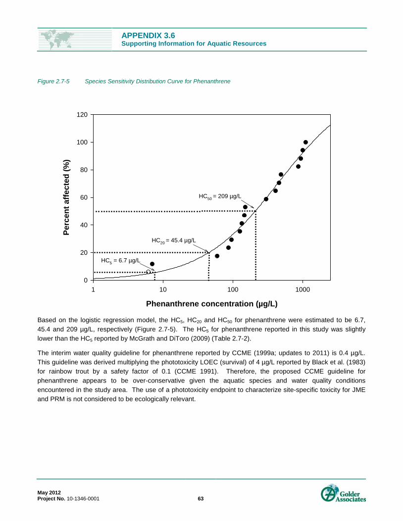
APPENDIX 3.6 Supporting Information for Aquatic Resources
May 2012 Project No. 10-1346-0001 63
Figure 2.7-5 Species Sensitivity Distribution Curve for Phenanthrene
Based on the logistic regression model, the HC5, HC20 and HC50 for phenanthrene were estimated to be 6.7, 45.4 and 209 µg/L, respectively (Figure 2.7-5). The HC5 for phenanthrene reported in this study was slightly lower than the HC5 reported by McGrath and DiToro (2009) (Table 2.7-2).
The interim water quality guideline for phenanthrene reported by CCME (1999a; updates to 2011) is 0.4 µg/L. This guideline was derived multiplying the phototoxicity LOEC (survival) of 4 µg/L reported by Black et al. (1983) for rainbow trout by a safety factor of 0.1 (CCME 1991). Therefore, the proposed CCME guideline for phenanthrene appears to be over-conservative given the aquatic species and water quality conditions encountered in the study area. The use of a phototoxicity endpoint to characterize site-specific toxicity for JME and PRM is not considered to be ecologically relevant.
Phenanthrene concentration (µg/L)
1 10 100 1000
Perc
ent a
ffect
ed (%
)
0
20
40
60
80
100
120
HC5 = 6.7 µg/L
HC20 = 45.4 µg/L
HC50 = 209 µg/L

APPENDIX 3.6 Supporting Information for Aquatic Resources
May 2012 Project No. 10-1346-0001 64
2.7.6 Pyrene A summary of the toxicity database used to derive a site-specific chronic toxicological benchmark for pyrene is shown in Table 2.7-7. The SSD was conducted using chronic toxicity data for five aquatic species. Sufficient toxicity data were available for pyrene to develop a SSD, with a logistic regression model providing a good fit to the observed data (r2 = 0.97) (Figure 2.7-6). The logistic model took the following form:
Where:
y = percent of aquatic species affected x = pyrene concentration (µg/L)
Table 2.7-7 Available Aquatic Toxicity Data for Pyrene Species Scientific Name Species Common Name Rank Chronic Value
[µg/L] Percent Affected
[%] Lumbriculus variegatus oligochaete, worm 1 5.03 20 Ceriodaphnia dubia water flea 2 18.5 40 Daphnia magna water flea 3 22 60 Gammarus pulex amphipod 4 27.1 80 Chlamydomonas angulosa algae 5 132 100
Based on the logistic regression model, the HC5, HC20 and HC50 for pyrene were estimated to be 2.3, 6.8 and 17 µg/L, respectively (Figure 2.7-6). The HC5 for pyrene reported in this study was slightly lower than the HC5 of 3.6 µg/L reported by McGrath and DiToro (2009) (Table 2.7-2).
The interim water quality guideline for pyrene reported by CCME (1999a; updates to 2011) is 0.025 µg/L. This guideline was derived by multiplying the acute value (LC50) of 2.5 µg/L for phototoxicity to mosquito larvae (A. aegypti) (Kagan and Kagan 1986) by a safety factor of 0.01 (CCME 1991). The lowest acute value for phototoxicity to mosquitoes, prior to application of safety factors, is similar to the HC5 for non-phototoxicity endpoints. Therefore, the proposed CCME guideline for phenanthrene appears to be over-conservative given the aquatic species and water quality conditions encountered in the region. The use of a phototoxicity endpoint to characterize site-specific toxicity for JME and PRM is not considered to be ecologically relevant.
10.2
15.73
105.09x
1−
+
=y

APPENDIX 3.6 Supporting Information for Aquatic Resources
May 2012 Project No. 10-1346-0001 65
Figure 2.7-6 Species Sensitivity Distribution Curve for Pyrene
2.7.7 Application of Polycyclic Aromatic Hydrocarbon Compounds to Groups As shown in Table 2.7-2, the correspondence is strong between the SSD-based derivations and the TLM for toxicity assessment of type I narcotic chemicals (McGrath and DiToro 2009). For five of the six compounds evaluated in this study, the SSD approach yielded a lower CEB, indicating that the SSD approach is expected to provide an appropriately conservative threshold for chronic toxic responses. The difference between the two methods was less than a factor of two for most of the individual PAHs. This broad agreement provides validation of the McGrath and DiToro (2009) chronic benchmarks for application to PAH Groups for which no individual PAH was evaluated using the SSD method.
2.8 Chronic Effects Benchmark Results for Other Constituents 2.8.1 Ammonia Ammonia can act as both a nutrient and a toxicant. The toxicity of ammonia is strongly influenced by ammonia speciation, which in turn is influenced by environmental parameters including pH, temperature and ionic strength. The CCME (2010) freshwater guideline for ammonia is for unionized ammonia (0.019 mg/L) rather than total concentration.
Pyrene concentration (µg/L)
1 10 100
Perc
ent a
ffect
ed (%
)
0
20
40
60
80
100
120
HC5 = 2.3 µg/L
HC20 = 6.8 µg/L
HC50 = 17 µg/L

APPENDIX 3.6 Supporting Information for Aquatic Resources
May 2012 Project No. 10-1346-0001 66
Data collected from the Oil Sands Region indicate that the majority of the nitrogen (N) present in process-affected waters is in the form of ammonia, with some organic nitrogen and little or no nitrate or nitrite. In aerobic environments, ammonia is transformed to nitrate or used for growth by aquatic plants.
As the JME and PRM data will likely consist of total ammonia concentrations, it is necessary to consider the site-specific temperature and pH, which are the primary determinants of ammonia speciation. Using the temperature interval (5°C to 10°C) and pH (7.5) values that are representative of the LSA for both JME and PRM, CCME (2010) indicates a water quality guideline range of 3.26 to 4.84 mg/L NH3 for the protection of aquatic life. This number can be converted to total ammonia nitrogen by multiplying by 0.8224, yielding a water quality guideline range of 2.68 to 3.98 mg/L N.
Note that as the temperature rises, the guideline decreases, such that the guideline during summer months (chronic exposure) would decline to about 2.0 mg/L N. To be conservative, the latter number was used.
2.8.2 Naphthenic Acids Naphthenic acids are an environmentally significant group of compounds that result from petroleum extraction from oil sands deposits (Headley and McMartin 2004).
Naphthenic acids are found at concentrations ranging from 40 to 120 mg/L in oil sands process waters (Holowenko et al. 2002). North American guidelines for the protection of aquatic life for naphthenic acids, are not available because chronic toxicity data for exposure to naphthenic acids and their fractionated components are lacking. These compounds have been identified as the agent responsible for most of the acute toxicity observed in tailings water and other process-affected waters (Verbeek et al. 1993). Naphthenic acids act as surfactants, interfering with normal gas exchange across gill membranes in fish. Exposure can result in narcosis, which means that thresholds for sublethal toxicity endpoints such as reduced growth or reproduction in aquatic organisms are quickly surpassed by acute toxicity (i.e., lethality).
Most of the studies documented in the literature are for acute effects, including acute toxicity to freshwater fish, invertebrates, and algae; these data show that naphthenic acids are moderately to highly toxic to fish and other aquatic life. Fish are particularly sensitive to the toxic effects of naphthenic acids in comparison to other aquatic organisms (Nero et al. 2006). Studies documented by API (2003) and Maxxam (2010) indicate acute toxicity to multiple species in the 1 to 5 mg/L range, including zebra fish (Brachydanio rerio) embryos and three-spine sticklebacks (Gasterosteus aculeatus), whereas other species have much higher thresholds. Other authors report LC50 values for naphthenic acids that range from 4 to 78 mg/L, depending on the species, water hardness, water temperature, length of exposure and dissolved oxygen concentration (Verbeek et al. 1993).
API (2003) determined that additional studies would be necessary to adequately characterize the hazard of naphthenic acids, and proposed toxicity testing of fish, aquatic invertebrates, and algae to address the potential aquatic toxicity of these materials. However, there does not currently appear to be sufficient information to develop a chronic effect benchmark using the SSD method. Some individual studies that assessed chronic toxicity endpoints are discussed below.
The age of the process-affected water is also an important consideration because naphthenic acids readily degrade (Herman et al. 1994; MacKinnon and Boerger 1986). The degradation of naphthenic acids results in lower toxicity, as shown by studies of fresh versus aged tailings pond water (Holowenko et al. 2002). As
APPENDIX 3.6 Supporting Information for Aquatic Resources
May 2012 Project No. 10-1346-0001 67
described below, total naphthenic acids can be classified as two fractions, i.e., labile (degradable) naphthenic acids and refractory (non-degradable) naphthenic acids.
Labile Naphthenic Acids The labile, lower molecular weight fraction is primarily responsible for whole effluent toxicity, and is selectively degraded from mixtures of naphthenic acids during aerobic biodegradation (Clemente et al. 2004; Holowenko et al. 2002). Hence, the aquatic health evaluation for watercourses and waterbodies focused on the predicted concentrations of labile naphthenic acids, as well as total concentrations. Due to the changes in the composition of naphthenic acid mixtures, the most relevant toxicity endpoints for labile naphthenic acids are derived from studies of oil sands process-affected water. The latter incorporate the degradation of the mixture, in contrast to the fresh commercial mixtures.
Some early lifestage bioassays have been conducted with yellow perch and Japanese medaka, and these studies have yielded a range of developmental responses (Maxxam 2010). Kavanagh et al. (2011) demonstrated that aged oil sand process-affected waters negatively affected the reproductive physiology of fathead minnows and suggested an effects threshold for impairment of 25 mg/L total naphthenic acids. Exposure of yellow perch to sublethal concentrations (0.9 mg/L commercial naphthenic acids; 1.7 mg/L extracted naphthenic acids) resulted in high levels of gill proliferative (epithelial, mucous, and chloride cell) changes; these concentrations were four-fold lower than those causing acute toxicity (Nero et al. 2006). Other hatching, growth, edema and other deformities have also been observed (Maxxam 2010).
The preferred toxicological endpoints in aquatic assessments are survival, growth, reproduction and development. If the gill anomalies documented by Nero et al. (2006) are conservatively assumed to be ecologically relevant developmental effects, the 1.7 mg/L concentration represents the lowest threshold concentration identified in the literature. Therefore, a concentration of about 1 mg/L may be used as a conservative threshold for the labile (more toxic) fraction of the naphthenic acid mixture.
Refractory Naphthenic Acids The data to develop a site-specific CEB for refractory naphthenic acids is inadequate. However, it is likely that the effects threshold for this constituent group is substantially higher than the threshold described above for labile naphthenic acids.
2.8.3 Sulphide Hydrogen sulphide can be highly toxic in the short term to aquatic life. Long-term exposure of fish to sub-lethal levels can cause slower growth, increase in mortality and reduction in fecundity. Wang and Chapman (1999) summarize aquatic toxicity data for sulphides to benthic invertebrates. The most sensitive endpoint was evaluated was Oseid and Smith (1974); it measured mortality in a long-term (65 to 105 day) exposure to freshwater amphipods of the genus Gammarus. The chronic no effect level was 2 µg/L, whereas other studies reported thresholds for toxicity that were at least 10-fold greater. As such, 2 µg/L represents a conservative screening threshold, particularly given that chronic elevated exposures of sulphide in the water column are unlikely to be maintained given that sulphides are rapidly volatilized.
APPENDIX 3.6 Supporting Information for Aquatic Resources
May 2012 Project No. 10-1346-0001 68
2.8.4 Dissolved Solids Total Dissolved Solids (TDS) is a measure of the combined content of all inorganic and organic substances contained in a liquid, including molecular, ionized and colloidal suspended matter. The principal inorganic anions dissolved in water include carbonates, chlorides, sulphates and nitrates, and the principal cations are sodium, potassium, calcium and magnesium (IDNR 2003).
The operational definition of TDS is that the solids must be small enough to survive filtration through a sieve the size of 2 µm. Total dissolved solids are distinct from Total Suspended Solids (TSS), in that the latter cannot pass through a sieve of 2 µm and yet remain suspended in solution.
The CCME (2002) provides water quality guidelines for the protection of aquatic life, but these guidelines apply to turbidity and TSS, rather than TDS. A Canadian TDS guideline for drinking water quality of 500 mg/L exists (Health Canada 2007), but it is for protection of aesthetic values for human use, not for protection of aquatic life. For aquatic life endpoints, several jurisdictions in the United States report thresholds ranging from 250 to 2,500 mg/L. For example, the Iowa Department of Natural Resources recently repealed a TDS standard of 1,000 mg/L for aquatic life (IDNR 2009). The standard was repealed in favour of guidelines for specific ions such as chloride and sulphate.
The most ecologically relevant studies that were reviewed for this report and were related to the effects of mining-related TDS on freshwater aquatic life are for elevated TDS levels in the vicinity of two northern Canadian mines.
Red Dog Mine, Alaska A series of TDS investigations were conducted at the Red Dog Mine in Alaska (Brix and Grosell 2005). These studies were conducted based on questions regarding the ecological relevance of the site-specific water quality standards for Mainstem Red Dog Creek of:
1,500 mg/L TDS during non-spawning periods of salmonids; and
500 mg/L TDS during spawning based on State of Alaska Water Quality Regulations.
The Brix and Grosell (2005) studies emphasized fertilization effects on two fish species (Arctic grayling [Thymallus arcticus] and Dolly Varden char [Salvelinus malma]) across a gradient of TDS exposures. The test was an early life stage (embryo) test of up to 72 hours duration, which was considered long enough to assess successful fertilization for this sensitive life stage. Previous work by Stekoll et al. (2003a, b) considered fertilization success, embryo development, hatching success and larval growth and survival, but indicated that fertilization success was the most sensitive endpoint of those evaluated despite the short test duration.
For an EC20 and the reproductive endpoint, a geometric mean of available toxicity values was calculated by Brix and Grosell (2005) to derive a species mean value. Species mean values of 1,357 and 1,779 mg/L TDS were estimated for Arctic grayling and Dolly Varden, respectively. On this basis, the authors concluded that the current site-specific limit of 1,500 mg/L TDS (or a value near it), is appropriate for the protection of this endpoint in salmonids.
APPENDIX 3.6 Supporting Information for Aquatic Resources
May 2012 Project No. 10-1346-0001 69
Snap Lake Mine, Northwest Territories Golder (2011) provides a detailed literature review of the effects of TDS on freshwater aquatic biota. The review was conducted as follow up to Golder (2003), which reported on potential effects of increased TDS on aquatic communities in Snap Lake. The results of the literature review indicate that freshwater fish and benthic invertebrates can tolerate exposures to TDS that substantially exceed the lower-bound guideline of 500 mg/L TDS from the State of Alaska Water Quality Regulations (a value commonly used as a conservative screening value).
The literature review identified a species geomean for the most sensitive fish species (for chronic tests in the review) of 1,000 mg/L TDS. The literature review also indicates that freshwater benthic invertebrates are generally tolerant of TDS at this higher concentration. The only taxa group that indicated some adverse responses at 1,000 mg/L TDS was zooplankton, and the sensitivity of the various taxa was highly variable.
Summary of Total Dissolved Solids Studies The literature review of fish and benthic invertebrate toxicity indicates that no significant adverse effects are expected for these species at concentrations below 1,000 mg/L TDS. The potential effects to sensitive zooplankton at this concentration would be mitigated by the chemical composition of the site-specific TDS mixture, and the relative tolerance of other zooplankton species (i.e., a viable zooplankton community would be present even at 1,000 mg/L). This revised screening concentration exceeds the maximum TDS estimate for all nodes at all snapshots. Therefore, the predicted changes in TDS levels in the LSA, resulting from either JME and PRM or approved developments, would have a negligible effect on aquatic health. This conclusion applies over the operational phase of JME and PRM and into the Far Future.
One of the factors influencing the toxicity of the TDS mixture is the composition of major ions. The principal inorganic anions dissolved in water include carbonates, chlorides, sulphates and nitrates, and the principal cations are sodium, potassium, calcium and magnesium (IDNR 2003). Based on an evaluation of the toxicological literature, the chloride and sulphate constituents contribute a significant portion of the toxicity. For this reason, jurisdictions including the Iowa Department of Natural Resources have moved toward assessment of these specific toxic ions. Importantly, the composition of source waters for JME and PRM indicates relatively low proportions of these ions. Based on the composition of source waters, which includes a combination of natural watercourses and process-affected water, the composition of this water during the peak concentration would be about: 10% sodium, 10% calcium, 40% bicarbonate, 30% sulphate and 10% other minor constituents. The sodium, calcium and bicarbonate ions (comprising 60%) are not expected to be as toxic as the sulphate and chloride portions of TDS that comprise a minority of the mixture.
Considering the above, for application to JME and PRM, a screening guideline of 1,000 mg/L TDS would be protective against adverse effects of TDS to freshwater aquatic life.
2.8.5 Total Phenolics Phenols can occur in surface waters from both natural (plant decomposition) and anthropogenic (effluent) influences; this constituent partitions strongly to water. The term phenols relates to a suite of related chemicals including monohydric phenols (including phenol, cresols and xylenols) and dihydric phenols (including catechols, resorcinol and quinol). However, the majority of toxicity data available for guideline derivation are for phenol.
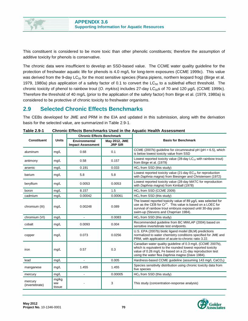
APPENDIX 3.6 Supporting Information for Aquatic Resources
May 2012 Project No. 10-1346-0001 70
This constituent is considered to be more toxic than other phenolic constituents; therefore the assumption of additive toxicity for phenols is conservative.
The chronic data were insufficient to develop an SSD-based value. The CCME water quality guideline for the protection of freshwater aquatic life for phenols is 4.0 mg/L for long-term exposures (CCME 1999c). This value was derived from the 9-day LC50 for the most sensitive species (Rana pipiens, northern leopard frog) (Birge et al. 1979, 1980a) plus application of a safety factor of 0.1 to convert the LC50 to a sublethal effect threshold. The chronic toxicity of phenol to rainbow trout (O. mykiss) includes 27-day LC50s of 70 and 120 µg/L (CCME 1999c). Therefore the threshold of 40 mg/L (prior to the application of the safety factor) from Birge et al. (1979, 1980a) is considered to be protective of chronic toxicity to freshwater organisms.
2.9 Selected Chronic Effects Benchmarks The CEBs developed for JME and PRM in the EIA and updated in this submission, along with the derivation basis for the selected value, are summarized in Table 2.9-1.
Table 2.9-1 Chronic Effects Benchmarks Used in the Aquatic Health Assessment
Constituent Units Chronic Effects Benchmark
Basis for Benchmark Environmental Impact Assessment
May 2012, JME JRP SIR
aluminum mg/L 0.68 0.1 CCME (2007b) guideline for circumneutral pH (pH > 6.5), which is below lowest toxicity value from SSD
antimony mg/L 0.58 0.157 Lowest reported toxicity value (28-day LC10 with rainbow trout) from Birge et al. (1979)
arsenic mg/L 0.191 0.033 HC5 from SSD (this study)
barium mg/L 5.8 5.8 Lowest reported toxicity value (21-day EC16 for reproduction with Daphnia magna) from Biesinger and Christensen (1972)
beryllium mg/L 0.0053 0.0053 Lowest reported toxicity value (28-day MATC for reproduction with Daphnia magna) from Kimball (1978)
boron mg/L 8.157 1.5 HC5 from SSD (CCME 2009) cadmium mg/L 0.00042 0.00061 HC5 from SSD (this study)
chromium (III) mg/L 0.00248 0.089
The lowest reported toxicity value of 89 μg/L was selected for use as the CEB for Cr3+. This value is based on a LOEC for survival of rainbow trout embryos exposed until 30-day post-swim-up (Stevens and Chapman 1984).
chromium (VI) mg/L - 0.0083 HC5 from SSD (this study)
cobalt mg/L 0.0093 0.004 Recommended guideline from BC MWLAP (2004) based on sensitive invertebrate test endpoints.
copper mg/L 0.073 0.0256 U.S. EPA (2007b) biotic ligand model (BLM) predictions normalized to water chemistry conditions specified for JME and PRM, with application of acute-to-chronic ratio 3.22.
iron mg/L 0.57 0.3
Canadian water quality guideline of 0.3 mg/L (CCME 2007b), which is equivalent to the rounded lowest reported toxicity value of 0.26 mg/L Fe based on a 21-day reproduction test using the water flea Daphnia magna (Dave 1984).
lead mg/L - 0.005 Hardness-based CCME guideline (assuming 143 mg/L CaCO3)
manganese mg/L 1.455 1.455 Species sensitivity distribution using chronic toxicity data from five species
mercury mg/L - 0.00005 HC5 from SSD (this study)
mercury (invertebrate)
mg/kg ww tissue
- 3 This study (concentration-response analysis)
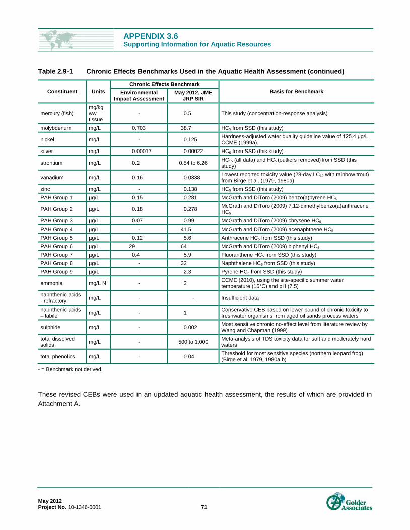
APPENDIX 3.6 Supporting Information for Aquatic Resources
Table 2.9-1 Chronic Effects Benchmarks Used in the Aquatic Health Assessment (continued)
May 2012 Project No. 10-1346-0001 71
Constituent Units Chronic Effects Benchmark
Basis for Benchmark Environmental Impact Assessment
May 2012, JME JRP SIR
mercury (fish) mg/kg ww tissue
- 0.5 This study (concentration-response analysis)
molybdenum mg/L 0.703 38.7 HC5 from SSD (this study)
nickel mg/L - 0.125 Hardness-adjusted water quality guideline value of 125.4 μg/L CCME (1999a).
silver mg/L 0.00017 0.00022 HC5 from SSD (this study)
strontium mg/L 0.2 0.54 to 6.26 HC15 (all data) and HC5 (outliers removed) from SSD (this study)
vanadium mg/L 0.16 0.0338 Lowest reported toxicity value (28-day LC10 with rainbow trout) from Birge et al. (1979, 1980a)
zinc mg/L - 0.138 HC5 from SSD (this study) PAH Group 1 µg/L 0.15 0.281 McGrath and DiToro (2009) benzo(a)pyrene HC5
PAH Group 2 µg/L 0.18 0.278 McGrath and DiToro (2009) 7,12-dimethylbenzo(a)anthracene HC5
PAH Group 3 µg/L 0.07 0.99 McGrath and DiToro (2009) chrysene HC5 PAH Group 4 µg/L - 41.5 McGrath and DiToro (2009) acenaphthene HC5 PAH Group 5 µg/L 0.12 5.6 Anthracene HC5 from SSD (this study) PAH Group 6 µg/L 29 64 McGrath and DiToro (2009) biphenyl HC5 PAH Group 7 µg/L 0.4 5.9 Fluoranthene HC5 from SSD (this study) PAH Group 8 µg/L - 32 Naphthalene HC5 from SSD (this study) PAH Group 9 µg/L - 2.3 Pyrene HC5 from SSD (this study)
ammonia mg/L N - 2 CCME (2010), using the site-specific summer water temperature (15°C) and pH (7.5)
naphthenic acids - refractory mg/L - - Insufficient data
naphthenic acids – labile mg/L - 1 Conservative CEB based on lower bound of chronic toxicity to
freshwater organisms from aged oil sands process waters
sulphide mg/L - 0.002 Most sensitive chronic no-effect level from literature review by Wang and Chapman (1999)
total dissolved solids mg/L - 500 to 1,000 Meta-analysis of TDS toxicity data for soft and moderately hard
waters
total phenolics mg/L - 0.04 Threshold for most sensitive species (northern leopard frog) (Birge et al. 1979, 1980a,b)
- = Benchmark not derived.
These revised CEBs were used in an updated aquatic health assessment, the results of which are provided in Attachment A.

APPENDIX 3.6 Supporting Information for Aquatic Resources
May 2012 Project No. 10-1346-0001 72
3.0 UPDATE TO NAPHTHENIC ACIDS DEGRADATION ASSUMPTIONS FOR THE JACKPINE MINE EXPANSION & PIERRE RIVER MINE
3.1 Introduction In the EIA, naphthenic acids were modelled under the assumption that they could be divided into two sub-classes of compounds: labile naphthenic acids and refractory naphthenic acids. The aerobic degradation rate for labile naphthenic acids was set at 3.2/year based on a study by Scott et al. (2005), and refractory naphthenic acids were assumed not to degrade. Scott et al. (2005) found that about 25% of total naphthenic acids were degraded within 40 to 50 days in a laboratory study. They attributed most of this degradation to removal of naphthenic acids with fewer than 18 carbons, which comprised about 60% to 70% of total naphthenic acids. Process-affected sources of water were thus defined as being 70% labile and 30% refractory for modelling, on the assumption that naphthenic acids with 18 or fewer carbons were best characterized as labile and the remaining naphthenic acids were refractory. Details of the assumptions used in the EIA were provided in Volume 4A, Section 6.5.2.7.
After the EIA had been submitted, Han et al. (2009) published a study that measured naphthenic acids in a test pond containing aged oil sands process waters. The test pond had no major inflows or outflows, so concentrations were not substantially affected by dilution. Thus, changes in concentration were attributed to degradation. They found that after 13 years, total naphthenic acids concentrations had declined by about 50%. To date, no published field or laboratory studies have measured naphthenic acids degradation beyond 13 years. It is likely that some portion of the remaining 50% of naphthenic acids will continue to degrade at rates comparable to those observed by Han et al. (2009), while some portion will be effectively inert within timeframes that can be practically modelled.
This appendix presents an update to the naphthenic acids concentrations that were predicted for all nodes within the JME LSA for the same snapshots and cases reported in the EIA, Volume 4A, Section 6.5. The updated predictions were derived by adjusting degradation rates to align with the studies mentioned above, keeping all other inputs consistent with the EIA. The intent of this appendix is to update naphthenic acid definitions and revise the original water quality predictions in the EIA, as necessary. Naphthenic acids predictions under the EIA and 2012 PDC are also discussed in Appendix 2, Section 3.3.3 of the 2012 PDC.
3.2 Assessment Methods In this update, the findings of Scott et al. (2005) and Han et al. (2009) were adapted to derive kinetic rate constants for modelling the degradation of naphthenic acids. New rates were calculated that account for the degradation rates observed in both of these studies. To apply the results of these studies to long-term predictions of naphthenic acids concentrations, the following approach was used:
For all process-affected inflow sources, such as direct inputs of oil sands process water or groundwater inflows from tailings areas, 25% of total naphthenic acids were assumed to be labile, with a half-life of 0.22 years.
For all process-affected inflow sources, 75% of total naphthenic acids were assumed to be refractory, with a half-life of 23 years (which yields a 50% decline in total naphthenic acids at 13 years).
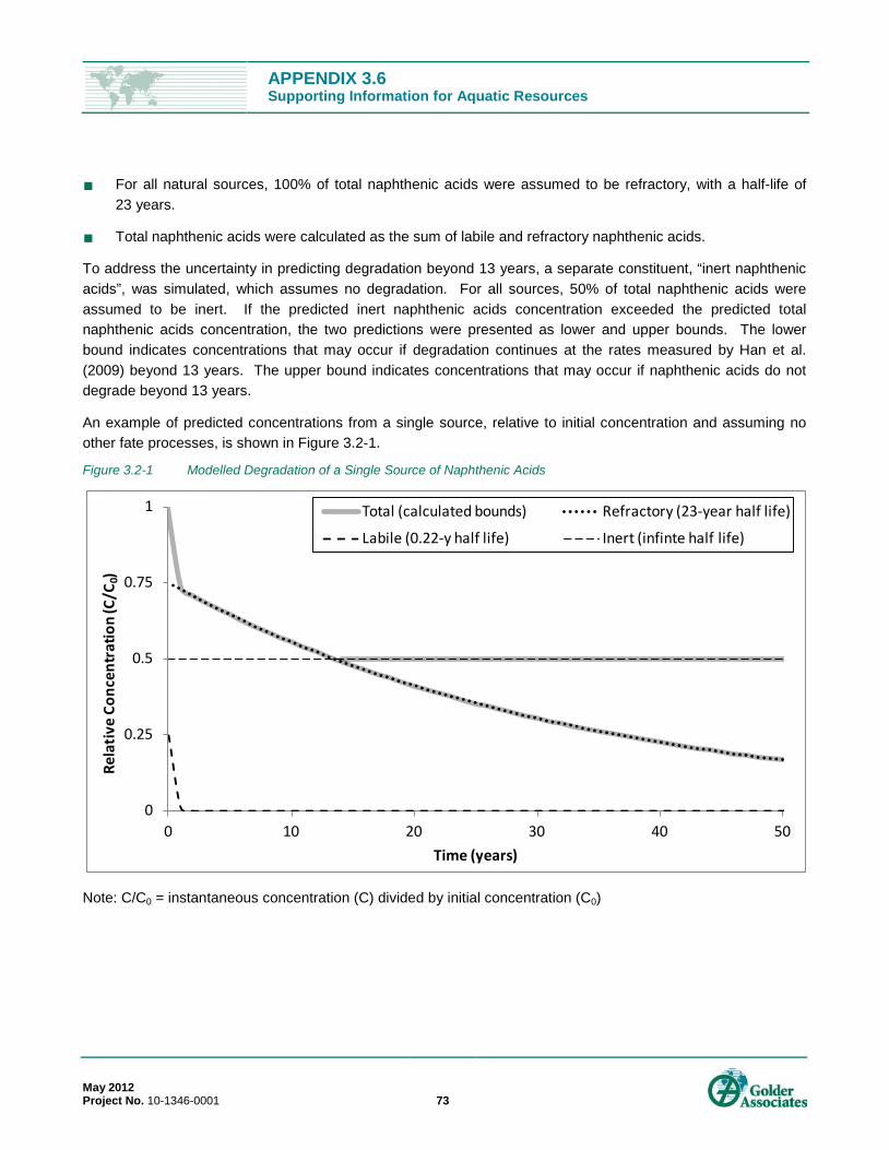
APPENDIX 3.6 Supporting Information for Aquatic Resources
May 2012 Project No. 10-1346-0001 73
For all natural sources, 100% of total naphthenic acids were assumed to be refractory, with a half-life of 23 years.
Total naphthenic acids were calculated as the sum of labile and refractory naphthenic acids.
To address the uncertainty in predicting degradation beyond 13 years, a separate constituent, “inert naphthenic acids”, was simulated, which assumes no degradation. For all sources, 50% of total naphthenic acids were assumed to be inert. If the predicted inert naphthenic acids concentration exceeded the predicted total naphthenic acids concentration, the two predictions were presented as lower and upper bounds. The lower bound indicates concentrations that may occur if degradation continues at the rates measured by Han et al. (2009) beyond 13 years. The upper bound indicates concentrations that may occur if naphthenic acids do not degrade beyond 13 years.
An example of predicted concentrations from a single source, relative to initial concentration and assuming no other fate processes, is shown in Figure 3.2-1.
Figure 3.2-1 Modelled Degradation of a Single Source of Naphthenic Acids
Note: C/C0 = instantaneous concentration (C) divided by initial concentration (C0)
0
0.25
0.5
0.75
1
0 10 20 30 40 50
Rela
tive
Conc
entr
atio
n (C
/C0)
Time (years)
Total (calculated bounds) Refractory (23-year half life)
Labile (0.22-y half life) Inert (infinte half life)
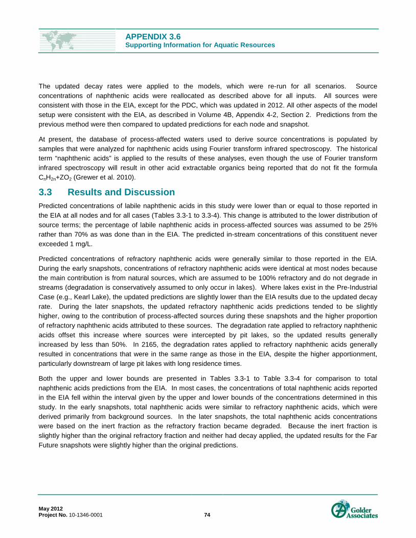
APPENDIX 3.6 Supporting Information for Aquatic Resources
May 2012 Project No. 10-1346-0001 74
The updated decay rates were applied to the models, which were re-run for all scenarios. Source concentrations of naphthenic acids were reallocated as described above for all inputs. All sources were consistent with those in the EIA, except for the PDC, which was updated in 2012. All other aspects of the model setup were consistent with the EIA, as described in Volume 4B, Appendix 4-2, Section 2. Predictions from the previous method were then compared to updated predictions for each node and snapshot.
At present, the database of process-affected waters used to derive source concentrations is populated by samples that were analyzed for naphthenic acids using Fourier transform infrared spectroscopy. The historical term “naphthenic acids” is applied to the results of these analyses, even though the use of Fourier transform infrared spectroscopy will result in other acid extractable organics being reported that do not fit the formula CnH2n+ZO2 (Grewer et al. 2010).
3.3 Results and Discussion Predicted concentrations of labile naphthenic acids in this study were lower than or equal to those reported in the EIA at all nodes and for all cases (Tables 3.3-1 to 3.3-4). This change is attributed to the lower distribution of source terms; the percentage of labile naphthenic acids in process-affected sources was assumed to be 25% rather than 70% as was done than in the EIA. The predicted in-stream concentrations of this constituent never exceeded 1 mg/L.
Predicted concentrations of refractory naphthenic acids were generally similar to those reported in the EIA. During the early snapshots, concentrations of refractory naphthenic acids were identical at most nodes because the main contribution is from natural sources, which are assumed to be 100% refractory and do not degrade in streams (degradation is conservatively assumed to only occur in lakes). Where lakes exist in the Pre-Industrial Case (e.g., Kearl Lake), the updated predictions are slightly lower than the EIA results due to the updated decay rate. During the later snapshots, the updated refractory naphthenic acids predictions tended to be slightly higher, owing to the contribution of process-affected sources during these snapshots and the higher proportion of refractory naphthenic acids attributed to these sources. The degradation rate applied to refractory naphthenic acids offset this increase where sources were intercepted by pit lakes, so the updated results generally increased by less than 50%. In 2165, the degradation rates applied to refractory naphthenic acids generally resulted in concentrations that were in the same range as those in the EIA, despite the higher apportionment, particularly downstream of large pit lakes with long residence times.
Both the upper and lower bounds are presented in Tables 3.3-1 to Table 3.3-4 for comparison to total naphthenic acids predictions from the EIA. In most cases, the concentrations of total naphthenic acids reported in the EIA fell within the interval given by the upper and lower bounds of the concentrations determined in this study. In the early snapshots, total naphthenic acids were similar to refractory naphthenic acids, which were derived primarily from background sources. In the later snapshots, the total naphthenic acids concentrations were based on the inert fraction as the refractory fraction became degraded. Because the inert fraction is slightly higher than the original refractory fraction and neither had decay applied, the updated results for the Far Future snapshots were slightly higher than the original predictions.
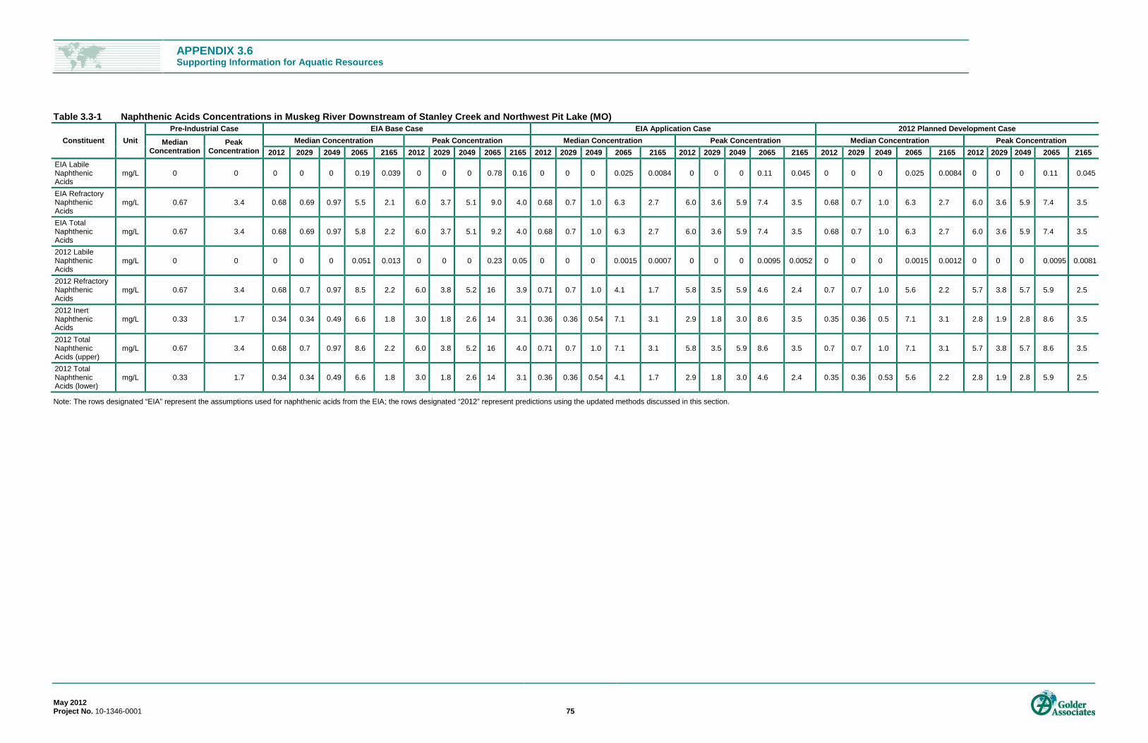
APPENDIX 3.6 Supporting Information for Aquatic Resources
May 2012 Project No. 10-1346-0001 75
Table 3.3-1 Naphthenic Acids Concentrations in Muskeg River Downstream of Stanley Creek and Northwest Pit Lake (MO)
Constituent Unit Pre-Industrial Case EIA Base Case EIA Application Case 2012 Planned Development Case
Median Concentration
Peak Concentration
Median Concentration Peak Concentration Median Concentration Peak Concentration Median Concentration Peak Concentration 2012 2029 2049 2065 2165 2012 2029 2049 2065 2165 2012 2029 2049 2065 2165 2012 2029 2049 2065 2165 2012 2029 2049 2065 2165 2012 2029 2049 2065 2165
EIA Labile Naphthenic Acids
mg/L 0 0 0 0 0 0.19 0.039 0 0 0 0.78 0.16 0 0 0 0.025 0.0084 0 0 0 0.11 0.045 0 0 0 0.025 0.0084 0 0 0 0.11 0.045
EIA Refractory Naphthenic Acids
mg/L 0.67 3.4 0.68 0.69 0.97 5.5 2.1 6.0 3.7 5.1 9.0 4.0 0.68 0.7 1.0 6.3 2.7 6.0 3.6 5.9 7.4 3.5 0.68 0.7 1.0 6.3 2.7 6.0 3.6 5.9 7.4 3.5
EIA Total Naphthenic Acids
mg/L 0.67 3.4 0.68 0.69 0.97 5.8 2.2 6.0 3.7 5.1 9.2 4.0 0.68 0.7 1.0 6.3 2.7 6.0 3.6 5.9 7.4 3.5 0.68 0.7 1.0 6.3 2.7 6.0 3.6 5.9 7.4 3.5
2012 Labile Naphthenic Acids
mg/L 0 0 0 0 0 0.051 0.013 0 0 0 0.23 0.05 0 0 0 0.0015 0.0007 0 0 0 0.0095 0.0052 0 0 0 0.0015 0.0012 0 0 0 0.0095 0.0081
2012 Refractory Naphthenic Acids
mg/L 0.67 3.4 0.68 0.7 0.97 8.5 2.2 6.0 3.8 5.2 16 3.9 0.71 0.7 1.0 4.1 1.7 5.8 3.5 5.9 4.6 2.4 0.7 0.7 1.0 5.6 2.2 5.7 3.8 5.7 5.9 2.5
2012 Inert Naphthenic Acids
mg/L 0.33 1.7 0.34 0.34 0.49 6.6 1.8 3.0 1.8 2.6 14 3.1 0.36 0.36 0.54 7.1 3.1 2.9 1.8 3.0 8.6 3.5 0.35 0.36 0.5 7.1 3.1 2.8 1.9 2.8 8.6 3.5
2012 Total Naphthenic Acids (upper)
mg/L 0.67 3.4 0.68 0.7 0.97 8.6 2.2 6.0 3.8 5.2 16 4.0 0.71 0.7 1.0 7.1 3.1 5.8 3.5 5.9 8.6 3.5 0.7 0.7 1.0 7.1 3.1 5.7 3.8 5.7 8.6 3.5
2012 Total Naphthenic Acids (lower)
mg/L 0.33 1.7 0.34 0.34 0.49 6.6 1.8 3.0 1.8 2.6 14 3.1 0.36 0.36 0.54 4.1 1.7 2.9 1.8 3.0 4.6 2.4 0.35 0.36 0.53 5.6 2.2 2.8 1.9 2.8 5.9 2.5
Note: The rows designated “EIA” represent the assumptions used for naphthenic acids from the EIA; the rows designated “2012” represent predictions using the updated methods discussed in this section.
APPENDIX 3.6 Supporting Information for Aquatic Resources
May 2012 Project No. 10-1346-0001 76
Table 3.3-2 Naphthenic Acids Concentrations in Muskeg River at the Mouth (M3)
Constituent Unit
Pre-Industrial Case EIA Base Case EIA Application Case 2012 Planned Development Case
Median Concentration
Peak Concentration
Median Concentration Peak Concentration Median Concentration Peak Concentration Median Concentration Peak Concentration 2012 2029 2049 2065 2165 2012 2029 2049 2065 2165 2012 2029 2049 2065 2165 2012 2029 2049 2065 2165 2012 2029 2049 2065 2165 2012 2029 2049 2065 2165
EIA Labile Naphthenic Acids
mg/L 0 0 0 0.028 0.093 0.19 0.11 0 0.38 0.39 0.53 0.34 0 0.022 0.11 0.11 0.091 0 0.36 0.47 0.48 0.53 0 0.022 0.11 0.11 0.091 0 0.36 0.47 0.48 0.53
EIA Refractory Naphthenic Acids
mg/L 0.7 3.4 1.0 1.0 1.9 4.1 2.5 4.9 3.4 3.7 6.5 4.4 1.0 1.0 1.1 4.6 2.6 4.9 3.4 3.7 7.2 4.2 1.0 1.0 1.1 4.6 2.6 4.9 3.4 3.7 7.2 4.2
EIA Total Naphthenic Acids
mg/L 0.7 3.4 1.0 1.0 2.0 4.3 2.6 4.9 3.4 3.9 6.6 4.6 1.0 1.1 1.2 4.7 2.7 4.9 3.5 4.0 7.3 4.3 1.0 1.1 1.2 4.7 2.7 4.9 3.5 4.0 7.3 4.3
2012 Labile Naphthenic Acids
mg/L 0 0 0 0.02 0.032 0.053 0.032 0 0.29 0.11 0.16 0.082 0 0.0037 0.023 0.024 0.022 0 0.099 0.11 0.35 0.33 0 0.0037 0.023 0.017 0.015 0 0.1 0.11 0.22 0.26
2012 Refractory Naphthenic Acids
mg/L 0.7 3.5 0.99 1.1 2.3 6.2 3.4 5.0 3.6 4.7 9.7 6.5 1.0 1.1 1.2 4.1 2.7 4.4 3.7 4.6 5.9 4.5 0.97 1.2 1.2 3.8 2.2 4.7 3.5 4.9 5.8 3.8
2012 Inert Naphthenic Acids
mg/L 0.35 1.7 0.49 0.57 1.7 4.8 2.7 2.5 1.9 4.1 10 6.8 0.51 0.59 0.65 4.9 3.1 2.2 2.1 3.0 8.6 5.1 0.5 0.62 0.69 4.6 2.8 2.4 2.3 3.1 8.2 4.4
2012 Total Naphthenic Acids (upper)
mg/L 0.7 3.5 0.99 1.1 2.3 6.3 3.4 5.0 3.9 4.8 10 6.8 1.0 1.1 1.2 4.9 3.1 4.4 3.8 4.7 8.6 5.1 0.97 1.2 1.2 4.6 2.8 4.7 3.6 5.0 8.2 4.4
2012 Total Naphthenic Acids (lower)
mg/L 0.35 1.7 0.49 0.57 1.7 4.8 2.7 2.5 1.9 4.1 9.9 6.6 0.51 0.59 0.65 4.1 2.7 2.2 2.1 3.0 6.3 4.8 0.5 0.62 0.69 3.8 2.2 2.4 2.3 3.1 6.0 4.1
Note: The rows designated “EIA” represent the assumptions used for naphthenic acids from the EIA; the rows designated “2012” represent predictions using the updated methods discussed in this section.

APPENDIX 3.6 Supporting Information for Aquatic Resources
May 2012 Project No. 10-1346-0001 77
Table 3.3-3 Naphthenic Acids Concentrations in Jackpine Creek at the Mouth (J1)
Constituent Unit
Pre-Industrial Case EIA Base Case EIA Application Case 2012 Planned Development Case
Median Concentration
Peak Concentration
Median Concentration Peak Concentration Median Concentration Peak Concentration Median Concentration Peak Concentration 2012 2029 2049 2065 2165 2012 2029 2049 2065 2165 2012 2029 2049 2065 2165 2012 2029 2049 2065 2165 2012 2029 2049 2065 2165 2012 2029 2049 2065 2165
EIA Labile Naphthenic Acids mg/L 0 0 0 0 0 0.11 0.11 0 0 0 1.2 1.2 0 0 0 0.2 0.2 0 0 0 1.2 1.2 0 0 0 0.2 0.2 0 0 0 1.2 1.2
EIA Refractory Naphthenic Acids mg/L 0.67 3.6 0.69 0.73 0.72 1.0 1.0 3.5 3.7 3.3 6.0 6.0 0.69 0.73 0.72 1.1 1.1 3.5 3.7 3.3 4.6 4.6 0.69 0.73 0.72 1.1 1.1 3.5 3.7 3.3 4.6 4.6
EIA Total Naphthenic Acids mg/L 0.67 3.6 0.69 0.73 0.72 1.1 1.1 3.5 3.7 3.3 6.6 6.6 0.69 0.73 0.72 1.3 1.3 3.5 3.7 3.3 5.4 5.4 0.69 0.73 0.72 1.3 1.3 3.5 3.7 3.3 5.4 5.4
2012 Labile Naphthenic Acids mg/L 0 0 0 0 0 0.034 0.034 0 0 0 0.22 0.22 0 0 0 0.052 0.052 0 0 0 0.28 0.28 0 0 0 0.014 0.014 0 0 0 0.21 0.21
2012 Refractory Naphthenic Acids mg/L 0.67 3.7 0.7 0.73 0.72 1.4 1.4 3.6 3.8 3.3 12 12 0.71 0.73 0.72 1.6 1.6 3.3 3.8 3.3 14 14 0.69 0.68 0.69 0.87 0.86 3.4 3.6 3.4 3.6 3.4
2012 Inert Naphthenic Acids mg/L 0.33 1.8 0.34 0.36 0.36 0.9 0.9 1.8 1.9 1.7 9.5 9.5 0.36 0.37 0.36 1.0 1.0 1.7 1.9 1.7 11 11 0.35 0.35 0.35 0.69 0.47 1.7 1.8 1.7 4.7 2.0
2012 Total Naphthenic Acids (upper)
mg/L 0.67 3.7 0.7 0.73 0.72 1.4 1.4 3.6 3.8 3.3 12 12 0.71 0.73 0.72 1.7 1.7 3.3 3.8 3.3 14 14 0.69 0.68 0.69 0.88 0.87 3.4 3.6 3.4 4.7 3.6
2012 Total Naphthenic Acids (lower)
mg/L 0.33 1.8 0.34 0.36 0.36 0.9 0.9 1.8 1.9 1.7 9.5 9.5 0.36 0.37 0.36 1.0 1.0 1.7 1.9 1.7 11 11 0.35 0.35 0.35 0.69 0.47 1.7 1.8 1.7 3.8 2.0
Note: The rows designated “EIA” represent the assumptions used for naphthenic acids from the EIA; the rows designated “2012” represent predictions using the updated methods discussed in this section.

APPENDIX 3.6 Supporting Information for Aquatic Resources
May 2012 Project No. 10-1346-0001 78
Table 3.3-4 Naphthenic Acids Concentrations in Kearl Lake (K1)
Constituent Unit
Pre-Industrial Case EIA Base Case EIA Application Case 2012 Planned Development Case
Median Concentration
Peak Concentration
Median Concentration Peak Concentration Median Concentration Peak Concentration Median Concentration Peak Concentration 2012 2029 2049 2065 2165 2012 2029 2049 2065 2165 2012 2029 2049 2065 2165 2012 2029 2049 2065 2165 2012 2029 2049 2065 2165 2012 2029 2049 2065 2165
EIA Labile Naphthenic Acids
mg/L 0 0 0 0 0 0.0038 0.0001 0 0 0 0.036 0.0005 0 0 0 0.046 0.036 0 0 0 0.29 0.21 0 0 0 0.046 0.036 0 0 0 0.29 0.21
EIA Refractory Naphthenic Acids
mg/L 0.92 1.3 0.89 0.88 0.89 1.8 1.0 1.2 1.0 1.0 3.5 1.4 0.89 0.77 0.79 3.4 2.8 1.2 1.1 1.1 4.6 3.8 0.89 0.77 0.79 3.4 2.8 1.2 1.1 1.1 4.6 3.8
EIA Total Naphthenic Acids
mg/L 0.92 1.3 0.89 0.88 0.89 1.8 1.0 1.2 1.0 1.0 3.5 1.4 0.89 0.77 0.79 3.4 2.8 1.2 1.1 1.1 4.6 3.8 0.89 0.77 0.79 3.4 2.8 1.2 1.1 1.1 4.6 3.8
2012 Labile Naphthenic Acids
mg/L 0 0 0 0 0 0.0021 0.0001 0 0 0 0.013 0.0002 0 0 0 0.012 0.0083 0 0 0 0.084 0.056 0 0 0 0.0039 0.0038 0 0 0 0.027 0.027
2012 Refractory Naphthenic Acids
mg/L 0.81 1.2 0.79 0.78 0.8 2.3 0.34 1.2 0.97 0.93 3.2 0.86 0.73 0.74 0.75 6.1 4.9 1.4 1.2 1.2 7.1 5.7 0.72 0.7 0.77 2.8 2.6 1.5 1.0 1.1 4.3 4.0
2012 Inert Naphthenic Acids
mg/L 0.39 0.72 0.39 0.41 0.49 1.8 0.45 0.72 0.59 0.65 4.1 0.91 0.39 0.42 0.43 5.0 4.0 0.8 0.75 0.74 7.1 5.7 0.38 0.39 0.44 3.1 2.8 0.77 0.54 0.79 4.8 4.5
2012 Total Naphthenic Acids (upper)
mg/L 0.81 1.2 0.79 0.78 0.8 2.3 0.45 1.2 0.97 0.93 4.1 0.91 0.73 0.74 0.75 6.1 4.9 1.4 1.2 1.2 7.2 5.8 0.72 0.7 0.77 3.1 2.8 1.5 1.0 1.1 4.8 4.5
2012 Total Naphthenic Acids (lower)
mg/L 0.39 0.72 0.39 0.41 0.49 1.8 0.34 0.72 0.59 0.65 3.2 0.86 0.39 0.42 0.43 5.0 4.0 0.8 0.75 0.74 7.1 5.7 0.38 0.39 0.44 2.8 2.6 0.77 0.54 0.79 4.3 4.0
Note: The rows designated “EIA” represent the assumptions used for naphthenic acids from the EIA; the rows designated “2012” represent predictions using the updated methods discussed in this section.
APPENDIX 3.6 Supporting Information for Aquatic Resources
May 2012 Project No. 10-1346-0001 79
3.4 Summary Naphthenic acids concentrations were predicted in the EIA using degradation rates derived from Scott et al. (2005). In this update, predictions were made using rates obtained from Han et al. (2009) for refractory naphthenic acids. An inert fraction was also modelled to reflect the uncertainty in long-term predictions. In general, predictions for the early snapshots were similar to what was predicted in the EIA because process-affected sources constitute a very small fraction of total loading to watercourses during these snapshots. In the later years of operations, refractory naphthenic acids were occasionally higher in the update due to the larger portion of naphthenic acids in process-affected waters being attributed to this fraction. In the Far Future, the EIA results for refractory and total naphthenic acids were generally close to the upper bound estimate for these fractions in the updated results. While there are some differences in concentrations, the magnitude of change would not affect the original conclusions drawn in the EIA.
4.0 UPDATE TO JACKPINE MINE EXPANSION PIT LAKE MODELLING 4.1 Introduction Four pit lakes will be created during the closure management phase of the Jackpine Mine – Phase 1 and JME. These lakes are described in the EIA (Volume 4A, Appendix 4-2, Section 2.1.3). The pit lakes presented in the May 2011, Submission of Information to the Joint Review Panel, Section 3.4 were updated by excluding MFT from all four Jackpine pit lakes. In the May 2011, Submission of Information to the Joint Review Panel, hydrodynamic modelling was completed to evaluate meromictic conditions in the deeper pit lakes, but a full suite of water quality constituents was not considered necessary because the water quality was assumed to be improved from previous assessments. The updated modelling described herein does present a full suite of water quality constituents, as the full suite was required for the 2012 PDC small streams assessment.
Because there are no changes to the 2012 PDC upstream of the pit lakes, these predictions represent both the 2012 JME Application Case and 2012 PDC. Thus, the pit lake water quality predictions presented herein supersede all previous submissions for the Application Case.
4.2 Assessment Methods The modelling approach in this assessment is identical to the EIA approach described in EIA Volume 4B, Appendix 4-2, Section 2.1.3, except that the Golder Pit Lake Model (GPLM) was used to model water quality instead of CE-QUAL-W2 (Cole and Wells 2008). Previous work (Golder 2007) has shown that these models produce similar water quality predictions, provided that CE-QUAL-W2 is run first and the hydrodynamic conditions predicted by CE-QUAL-W2 are entered as inputs to GPLM.
All inputs to the models were consistent with the previous modelling, except where changes have been made as part of mine plan updates (e.g., flow rates from the reclaimed mine and exclusion of MFT). The mixing characteristics of lakes were estimated by the hydrodynamic model completed in CE-QUAL-W2 and presented in the May 2011, Submission of Information to the Joint Review Panel. In that update, CE-QUAL-W2 models were used to simulate hydrodynamics, TDS and DO in the pit lakes.
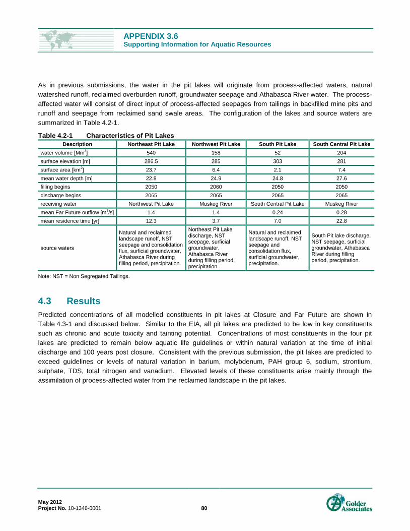
APPENDIX 3.6 Supporting Information for Aquatic Resources
May 2012 Project No. 10-1346-0001 80
As in previous submissions, the water in the pit lakes will originate from process-affected waters, natural watershed runoff, reclaimed overburden runoff, groundwater seepage and Athabasca River water. The process-affected water will consist of direct input of process-affected seepages from tailings in backfilled mine pits and runoff and seepage from reclaimed sand swale areas. The configuration of the lakes and source waters are summarized in Table 4.2-1.
Table 4.2-1 Characteristics of Pit Lakes Description Northeast Pit Lake Northwest Pit Lake South Pit Lake South Central Pit Lake
water volume [Mm3] 540 158 52 204 surface elevation [m] 286.5 285 303 281 surface area [km2] 23.7 6.4 2.1 7.4 mean water depth [m] 22.8 24.9 24.8 27.6 filling begins 2050 2060 2050 2050 discharge begins 2065 2065 2065 2065 receiving water Northwest Pit Lake Muskeg River South Central Pit Lake Muskeg River mean Far Future outflow [m3/s] 1.4 1.4 0.24 0.28 mean residence time [yr] 12.3 3.7 7.0 22.8
source waters
Natural and reclaimed landscape runoff, NST seepage and consolidation flux, surficial groundwater, Athabasca River during filling period, precipitation.
Northeast Pit Lake discharge, NST seepage, surficial groundwater, Athabasca River during filling period, precipitation.
Natural and reclaimed landscape runoff, NST seepage and consolidation flux, surficial groundwater, precipitation.
South Pit lake discharge, NST seepage, surficial groundwater, Athabasca River during filling period, precipitation.
Note: NST = Non Segregated Tailings.
4.3 Results Predicted concentrations of all modelled constituents in pit lakes at Closure and Far Future are shown in Table 4.3-1 and discussed below. Similar to the EIA, all pit lakes are predicted to be low in key constituents such as chronic and acute toxicity and tainting potential. Concentrations of most constituents in the four pit lakes are predicted to remain below aquatic life guidelines or within natural variation at the time of initial discharge and 100 years post closure. Consistent with the previous submission, the pit lakes are predicted to exceed guidelines or levels of natural variation in barium, molybdenum, PAH group 6, sodium, strontium, sulphate, TDS, total nitrogen and vanadium. Elevated levels of these constituents arise mainly through the assimilation of process-affected water from the reclaimed landscape in the pit lakes.

APPENDIX 3.6 Supporting Information for Aquatic Resources
May 2012 Project No. 10-1346-0001 81
Table 4.3-1 Predicted Concentrations in Pit Lakes
Constituent Units Northeast Pit Lake Northwest Pit Lake South Pit Lake South Central Pit Lake
Initial 2065
Far Future 2165
Initial 2065
Far Future 2165
Initial 2065
Far Future 2165
Initial 2065
Far Future 2165
Aluminum mg/L 0.75 0.15 0.99 0.15 0.16 0.13 0.61 0.14 Ammonia - N mg/L 0.0036 0.0069 0.00054 0.0004 0.015 0.015 0.0056 0.0063 Antimony mg/L 0.0010 0.0013 0.00055 0.0013 0.00055 0.00049 0.00057 0.00058 Arsenic mg/L 0.002 0.0016 0.0015 0.0017 0.00076 0.00059 0.0015 0.0011 Barium mg/L 0.079 0.12 0.072 0.12 0.067 0.11 0.074 0.14 Beryllium mg/L 0.00052 0.00031 0.00047 0.00032 0.00053 0.00038 0.00046 0.00039 Boron mg/L 0.55 0.57 0.12 0.6 1.3 1.1 0.73 1.3 Cadmium mg/L 0.00086 0.00096 0.00071 0.00098 0.00089 0.00076 0.00084 0.00091 Calcium mg/L 41 47 36 47 69 80 53 84 Chloride mg/L 30 21 24 22 72 49 45 58 Chromium mg/L 0.0041 0.0023 0.0038 0.0024 0.0022 0.0013 0.0031 0.0016 Cobalt mg/L 0.0018 0.00096 0.0015 0.001 0.00097 0.00066 0.0016 0.0012 Copper mg/L 0.0037 0.0023 0.0035 0.0024 0.0022 0.0019 0.003 0.0021 Dissolved organic carbon mg/L 20 33 11 33 27 35 21 39 Iron mg/L 1.6 1.1 2.2 1.1 0.29 1.3 1.3 1.0 Lead mg/L 0.0015 0.0011 0.0017 0.0011 0.00012 0.00016 0.001 0.00023 Magnesium mg/L 11 14 9.8 14 15 22 13 23 Manganese mg/L 0.088 0.19 0.071 0.19 0.062 0.11 0.083 0.18 Mercury mg/L 0.000016 0.0000043 0.000018 0.0000044 0.0000041 0.0000041 0.000013 0.0000067 Molybdenum mg/L 0.11 0.089 0.017 0.093 0.22 0.18 0.14 0.23 Monomer mg/L <0.0001 <0.0001 <0.0001 <0.0001 <0.0001 <0.0001 <0.0001 <0.0001 Naphthenic acids - labile mg/L 0.044 0.098 0.0057 0.012 0.69 0.64 0.041 0.039 Naphthenic acids - refractory mg/L 4.1 2.6 0.9 2.6 7.3 6.1 3.1 4.0 Total naphthenic acids mg/L 4.2 2.7 0.91 2.6 8.0 6.8 3.1 4.0 Inert naphthenic acids mg/L 3.6 3.1 0.56 3.2 10 9.3 4.3 8.8 Nickel mg/L 0.0089 0.0049 0.007 0.0053 0.013 0.0092 0.0093 0.0096 PAH group 1 ppb 0.00077 0.00085 0.00029 0.00045 0.0059 0.0051 0.0018 0.0013 PAH group 2 ppb 0.0053 0.0063 0.00077 0.0047 0.035 0.031 0.016 0.014 PAH group 3 ppb 0.00011 <0.0001 0.0003 <0.0001 <0.0001 <0.0001 0.000091 <0.0001 PAH group 4 ppb 0.00036 0.00029 0.000046 0.000037 0.0033 0.0027 0.00043 0.0003
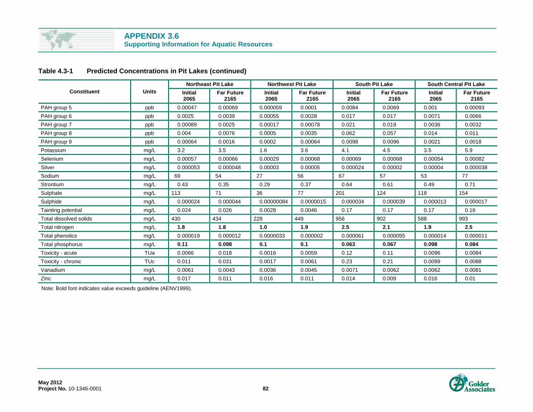
APPENDIX 3.6 Supporting Information for Aquatic Resources
Table 4.3-1 Predicted Concentrations in Pit Lakes (continued)
May 2012 Project No. 10-1346-0001 82
Constituent Units Northeast Pit Lake Northwest Pit Lake South Pit Lake South Central Pit Lake
Initial 2065
Far Future 2165
Initial 2065
Far Future 2165
Initial 2065
Far Future 2165
Initial 2065
Far Future 2165
PAH group 5 ppb 0.00047 0.00069 0.000059 0.0001 0.0084 0.0069 0.001 0.00093 PAH group 6 ppb 0.0025 0.0039 0.00055 0.0028 0.017 0.017 0.0071 0.0066 PAH group 7 ppb 0.00089 0.0025 0.00017 0.00078 0.021 0.019 0.0036 0.0032 PAH group 8 ppb 0.004 0.0076 0.0005 0.0035 0.062 0.057 0.014 0.011 PAH group 9 ppb 0.00064 0.0016 0.0002 0.00064 0.0098 0.0096 0.0021 0.0018 Potassium mg/L 3.2 3.5 1.6 3.6 4.1 4.5 3.5 5.9 Selenium mg/L 0.00057 0.00066 0.00029 0.00068 0.00069 0.00068 0.00054 0.00082 Silver mg/L 0.000053 0.000048 0.00003 0.00005 0.000024 0.00002 0.00004 0.000038 Sodium mg/L 69 54 27 56 67 57 53 77 Strontium mg/L 0.43 0.35 0.29 0.37 0.64 0.61 0.49 0.71 Sulphate mg/L 113 71 36 77 201 124 118 154 Sulphide mg/L 0.000024 0.000044 0.00000084 0.0000015 0.000034 0.000039 0.000013 0.000017 Tainting potential mg/L 0.024 0.026 0.0028 0.0046 0.17 0.17 0.17 0.16 Total dissolved solids mg/L 430 434 228 449 956 902 588 993 Total nitrogen mg/L 1.8 1.8 1.0 1.9 2.5 2.1 1.9 2.5 Total phenolics mg/L 0.000019 0.000012 0.0000033 0.000002 0.000061 0.000055 0.000014 0.000011 Total phosphorus mg/L 0.11 0.098 0.1 0.1 0.063 0.067 0.098 0.084 Toxicity - acute TUa 0.0066 0.018 0.0016 0.0059 0.12 0.11 0.0096 0.0084 Toxicity - chronic TUc 0.011 0.031 0.0017 0.0061 0.23 0.21 0.0099 0.0088 Vanadium mg/L 0.0061 0.0043 0.0036 0.0045 0.0071 0.0062 0.0062 0.0081 Zinc mg/L 0.017 0.011 0.016 0.011 0.014 0.009 0.016 0.01
Note: Bold font indicates value exceeds guideline (AENV1999).
APPENDIX 3.6 Supporting Information for Aquatic Resources
May 2012 Project No. 10-1346-0001 83
The major differences in this submission are predicted concentrations of TDS, major ions, organic constituents and total metals in 2065. Because of the larger proportion of Athabasca River water used to fill the lakes and the lack of MFT porewater inputs, concentrations of TDS, major ions and organic constituents are predicted to be lower than in the EIA. Conversely, concentrations of aluminum, copper, iron, lead, manganese and phosphorus are predicted to increase in the 2012 results compared to the EIA because the Athabasca River is high in these metals. These constituents are predicted to exceed guidelines in one or more pit lakes, primarily due to the high concentrations in the Athabasca River water used to fill the lakes. Since Athabasca River water will be used to fill the lakes, considerable settling and reduction in concentration can be expected as the lakes fill between 2050 and 2065. Settling of total metals was not accounted for in this conservative modelling; therefore, concentrations of these constituents are anticipated to be substantially lower than predicted in the 2012 PDC. Other constituent concentrations are predicted to be similar to those presented in the EIA with respect to exceedances of guidelines and natural variation. In the Far Future, pit lake concentrations under the present plan are predicted to be similar to those presented in the EIA, because the filling source and tailings content have little effect on long-term concentrations.
Similar to the EIA, labile naphthenic acids are predicted to be well below 1 mg/L at the time of initial discharge and beyond for all of the four pit lakes. At Closure in 2065, all forms of naphthenic acids are predicted to be lower in the pit lakes compared to the previous submission because of the additional Athabasca River water and lack of MFT porewater inputs. At 100 years post closure, concentrations of refractory naphthenic acids are predicted to be similar to or less than what was presented in the EIA for a given pit lake. Refractory naphthenic acids were previously assigned to 30% of total naphthenic acids in process-affected waters with no decay; the 2012 PDC modelling assigned 75% with a 23-year half life (Appendix 3.6). Thus, the pit lakes with longer residence times (South Central Pit Lake and Northeastern Pit Lake) have lower Far-Future concentrations of refractory naphthenic acids than were previously predicted. Due to the inclusion of an inert fraction in the calculation of total naphthenic acids (Appendix 3.6), concentrations of total naphthenic acids are predicted to be higher in the 2012 PDC than in the EIA in South Pit Lake and South Central Pit Lake. The higher concentrations are predicted because these pit lakes receive relatively little fresh water inflow; therefore, the inert fraction declines more slowly in these pit lakes. Total naphthenic acids in Northeastern Pit Lake and North West Pit Lake are predicted to be lower than in the EIA at all times.
4.4 Summary All four lakes are predicted to be low in key constituents such as chronic and acute toxicity and tainting potential. These findings are consistent with the JME pit lakes presented in the EIA, even with MFT. Concentrations of most constituents in the pit lakes are predicted to remain below aquatic life guidelines or within natural variation at the time of initial discharge and 100 years post closure. Consistent with the previous submission, the pit lakes are predicted to exceed guidelines or levels of natural variation in barium, molybdenum, PAH group 6, sodium, strontium, sulphate, TDS, total nitrogen and vanadium. Elevated levels of these constituents arise mainly through the assimilation of process-affected water from the reclaimed landscape in the pit lakes.
APPENDIX 3.6 Supporting Information for Aquatic Resources
May 2012 Project No. 10-1346-0001 84
Pit lake concentrations of TDS, major ions and organic constituents are predicted to be lower than in the EIA. Concentrations of aluminum, copper, iron, lead, manganese and phosphorus are predicted to be higher in 2065 compared to predictions in the EIA. All of these constituents are predicted to exceed guidelines in one or more pit lakes, primarily due to the high concentrations in the Athabasca River water used to fill the lakes. Other constituent concentrations are predicted to be similar to those presented in the EIA. In the Far Future, pit lake concentrations are predicted to be similar to those presented in the EIA.
Labile naphthenic acids are predicted to be well below 1 mg/L at the time of initial discharge and beyond for all of the four pit lakes. At Closure in 2065, all forms of naphthenic acids are predicted to be lower in the pit lakes than predicted in the EIA. At 100 years post closure, concentrations of refractory naphthenic acids are predicted to be similar to or less than predicted in the EIA.
APPENDIX 3.6 Supporting Information for Aquatic Resources
May 2012 Project No. 10-1346-0001 85
5.0 REFERENCES Allred, P.M. and J.P. Giesy. 1985. Solar radiation-induced toxicity of anthracene to Daphnia pulex. Environ
Toxicol Chem 4:219–226.
AENV (Alberta Environment). 1999. Surface Water Quality Guidelines for Use in Alberta. Science and Standards Branch. Environmental Assurance Division. Edmonton, AB. Submitted November 1999. 25 pp.
AENV (Alberta Environment). 2008. Muskeg River Interim Management Framework for Water Quantity and Quality. ISBN 978-0-7785-7630-3. June 2008. Edmonton, AB, Canada. 72 pp.
API (American Petroleum Institute). 2003. High Production Volume (HPV) Chemical Challenge Program: Test Plan for Reclaimed Substances: Streams Containing Naphthenic Acids, Phenolics, Disulfides, Acids or Caustics. Submitted to the U.S. EPA by the American Petroleum Institute, Petroleum HPV Testing Group, Washington, DC, USA.
ATSDR (Agency for Toxic Substances and Disease Registry). 1995. Toxicological profile for polycyclic aromatic hydrocarbons. United States Department of Health and Human Services. Public Health Service, Atlanta, GA, USA. 458 pp.
ATSDR. 1997. Toxicological Profiles on CD-ROM. United States Public Health Service. Atlanta, GA, USA.
ATSDR. 1999. Toxicological profile for mercury. United States Department of Health and Human Services. Public Health Service, Atlanta, GA, USA. 610 pp.
ATSDR. 2005a. Toxicological profile for nickel. United States Department of Health and Human Services. Public Health Service, Atlanta, GA, USA. 351 pp.
ATSDR. 2005b. Toxicological profile for zinc. United States Department of Health and Human Services. Public Health Service, Atlanta, GA, USA. 607 pp.
ATSDR. 2007. Toxicological profile for arsenic. United States Department of Health and Human Services. Public Health Service, Atlanta, GA, USA. 489 pp.
ATSDR. 2008. Toxicological profile for aluminum. United States Department of Health and Human Services. Public Health Service, Atlanta, GA, USA. 310 pp.
Baker, J.L., A.C. Barefoot, L.E. Beasley, L. Burns, P. Caukins, J. Clark, R.L. Feulner, J.P. Giesy, R.L. Graney, R. Griggs, H. Jacoby, D. Laskowski, A. Maciorowski, E. Mihaich, H. Nelson, R. Parrish, R.E. Siefert, K.R. Solomon, W. van der Schalie. 1994. Final Report: Aquatic Risk Assessment and Mitigation Dialog Group. SETAC Press. Pensacola, FL, USA.
BC MWLAP (British Columbia Ministry of Water, Land and Air Protection). 2004. Technical Report – Water Quality Guidelines for Cobalt. BC MWLAP. Victoria, BC, Canada. Available at: http://www.env.gov.bc.ca/wat/wq/BCguidelines/cobalt/cobalt_tech.pdf
Beckvar, N., T.M. Dillon and L.B. Read. 2005. Approaches for Linking Whole-body Fish Tissue Residues of Mercury or DDT to Biological Effect Thresholds. Environ Toxicol Chem 24(8):2094-2105.

APPENDIX 3.6 Supporting Information for Aquatic Resources
May 2012 Project No. 10-1346-0001 86
Biesinger, K.E. and G.M. Christensen. 1972. Effects of various metals on survival, growth, reproduction and
metabolism of Daphnia magna. J Fish Res Board Can 29:1691-1700.
Birge, W.J. 1978. Aquatic toxicology of trace elements of coal and fly ash. In J.H. Thorp, J.W. Gibbons (eds),
Energy and Environmental Stress in Aquatic Systems: Selected Papers From a Symposium Held at
Augusta, Georgia, November 2-4, 1977. Dep Energy Symp Ser 48:219-240.
Birge, W.J., J.A. Black and A.G. Westerman. 1979. Evaluation of aquatic pollutants using fish and amphibian
eggs as bioassay organisms. In S.W. Nielsen, G. Migaki, D.G. Scarpelli (eds), Animals as Monitors of
Environmental Pollutants. National Academy of Science, Washington, DC, pp 108-118.
Birge, W.J., J.A. Black and A.G. Westerman and J.E. Hudson. 1980a. Aquatic toxicity tests on inorganic
elements occurring in oil shale. In Gale, C. (ed.)., Oil Shale Symposium: Sampling, Analysis and Quality
Assurance. United States Environmental Protection Agency, Cincinnati, OH, USA. pp. 519-534.
Birge, W.J., J.A. Black and R. Kuehne. 1980b. Effects of organic compounds on amphibian reproduction.
University of Kentucky, Water Resources Institute, Lexington, KY.
Birge, W.J., J.A. Black and B.A. Ramey. 1981. The reproductive toxicology of aquatic contaminants. In J.
Saxena, F. Fisher (eds), Hazard Assessment of Chemicals: Current Developments, Academic Press,
New York, NY. pp 59-115.
Bjornberg A, L. Hakanson and K. Lundbergh. 1988. A theory on the mechanisms regulating the bioavailability of
mercury in natural waters. Environ Pollut 49:53-61.
Black, J.A., W.J. Birge, A.G. Westerman and P.C. Francis. 1983. Comparative aquatic toxicology of aromatic
hydrocarbons. Fundam Appl Toxicol 3:353–358.
Boese, B.L., J.O. Lamberson, R.C. Swartz, R. Ozretich R and F. Cole. 1998 Photoinduced toxicity of PAHs and
alkylated PAHs to a marine in faunal amphipod (Rhepoxynius abronius). Arch Environ Contam Toxicol
34:235-240.
Borgmann, U, Y. Couillard, P. Doyle and D.G. Dixon. 2005. Toxicity of sixty-three metals and metalloids to
Hyalella azteca at two levels of water hardness. Environ Toxicol Chem 24:641-652.
Boutet, C. and C. Chaisemartin. 1973. Specific toxic properties of metallic salts in Austropotamobius pallipes
pallipes and Orconectes limosus (Proprietes toxiques specifiques des sels metalliques chez Austropotamobius pallipes pallipes et Orconectes limosu. C R Seances Soc Biol Fil 167: 1933-1938.
Brix, K.V. and M. Grosell. 2005. Report on the Effects of Total Dissolved Solids on Arctic Grayling and Dolly
Varden Fertilization Success. Prepared for Teck Cominco, Red Dog Mine, Kotzebue, AK by the
University of Miami, Miami, FL, USA. Available at:
http://www.dec.state.ak.us/water/wqsar/wqs/pdfs/final_Brix_TDS_report.pdf
APPENDIX 3.6 Supporting Information for Aquatic Resources
May 2012 Project No. 10-1346-0001 87
CCME (Canadian Council of Ministers of the Environment). 1991. Appendix IX— A protocol for the derivation of
water quality guidelines for the protection of aquatic life (April 1991). In: Canadian water quality
guidelines, Canadian Council of Resource and Environment Ministers, 1987. Prepared by the Task
Force on Water Quality Guidelines. [Updated and reprinted with minor revisions and editorial changes in
Canadian environmental quality guidelines, Chapter 4, Canadian Council of Ministers of the
Environment, 1999, Winnipeg, MB]
CCME. 1999a. (with updates to 2011). Canadian Environmental Quality Guidelines. Canadian Council of
Ministers of the Environment. Winnipeg, MB, Canada. Available at: http://ceqg-rcqe.ccme.ca/
CCME. 1999b. Canadian water quality guidelines for the protection of aquatic life: Chromium – hexavalent
chromium and trivalent chromium. In: Canadian Environmental Quality Guidelines. Canadian Council of
Ministers of the Environment. Winnipeg, MB, Canada. Available at: http://ceqg-
rcqe.ccme.ca/download/en/165/
CCME. 1999c. Canadian water quality guidelines for the protection of aquatic life: Mono- and dihydric phenols.
In: Canadian Environmental Quality Guidelines. Canadian Council of Ministers of the Environment.
Winnipeg, MB, Canada. Available at: http://ceqg-rcqe.ccme.ca/download/en/204/
CCME. 2001. Canadian water quality guidelines for the protection of aquatic life: Arsenic. In: Canadian
Environmental Quality Guidelines, 1999. Canadian Council of Ministers of the Environment. Winnipeg,
MB, Canada. 2001 update. Available at: http://ceqg-rcqe.ccme.ca/download/en/143/
CCME. 2002. Canadian water quality guidelines for the protection of aquatic life: Total particulate matter. In:
Canadian Environmental Quality Guidelines, 1999. Canadian Council of Ministers of the Environment.
Winnipeg, MB, Canada. 2002 update. Available at: http://ceqg-rcqe.ccme.ca/download/en/217/
CCME. 2003a. Guidance on the site-specific application of water quality guidelines in Canada: Procedures for
deriving numerical water quality objectives. In: Canadian Environmental Quality Guidelines. Canadian
Council of Ministers of the Environment. Winnipeg, MB, Canada.
CCME. 2003b. Canadian water quality guidelines for the protection of aquatic life: Mercury - Inorganic mercury
and methylmercury. In: Canadian Environmental Quality Guidelines, 1999. Canadian Council of
Ministers of the Environment. Winnipeg, MB, Canada. 2003 update. Available at: http://ceqg-
rcqe.ccme.ca/download/en/191/
CCME. 2007a. A protocol for the derivation of water quality guidelines for the protection of aquatic life 2007. In:
Canadian Environmental Quality Guidelines, Canadian Council of Ministers of the Environment.
Winnipeg, MB, Canada. Available at: ceqg-rcqe.ccme.ca/download/en/220/
CCME. 2007b. Canadian Water Quality Guidelines for the Protection of Aquatic Life: Summary Table. Update
7.1. December 2007. In: Canadian Environmental Quality Guidelines. Canadian Council of Ministers of
the Environment. Winnipeg, MB, Canada. Available at:
http://www.ccme.ca/assets/pdf/aql_summary_7.1_en.pdf
APPENDIX 3.6 Supporting Information for Aquatic Resources
May 2012 Project No. 10-1346-0001 88
CCME. 2009. Canadian Water Quality Guidelines for the Protection of Aquatic Life: Boron. In: Canadian
Environmental Quality Guidelines. Canadian Council of Ministers of the Environment. Winnipeg, MB,
Canada. Available at: ceqg-rcqe.ccme.ca/download/en/324/
CCME. 2010. Canadian Water Quality Guidelines for the Protection of Aquatic Life: Ammonia. In: Canadian
Environmental Quality Guidelines. Canadian Council of Ministers of the Environment. Winnipeg, MB,
Canada. Available at: ceqg-rcqe.ccme.ca/download/en/141/
CCME. 2011. Canadian Environmental Quality Guidelines. Canadian Water Quality Guidelines for the Protection
of Aquatic Life – Copper. Available at:
http://st-ts.ccme.ca/?lang=en&factsheet=71#aql_fresh_concentration.
CCREM (Canadian Council of Resource and Environment Ministers). 1987. Canadian Water Quality Guidelines
of the Canadian Council of Resource and Environment Ministers (CCREM). Winnipeg, MB, Canada.
Prepared by the Task Force on Water Quality Guidelines of the Canadian Council of Resource and
Environment Ministers. March 1987.
Chapman, P.M., W.J. Adams, M.L. Brooks, C.G. Delos, S.N. Luoma, W.A. Maher, H.M. Ohlendorf, T.S. Presser
and D.P. Shaw. 2010. Ecological Assessment of Selenium in the Aquatic Environment. Society of
Environmental Toxicology and Chemistry (SETAC). Pensacola, FL, USA.
Chowdhury, M.J. and R. Blust. 2011. Strontium. In C.M. Wood, A.P. Farrell, C.J. Brauner (eds), Homeostasis
and Toxicology of Non-Essential Metals. Volume 31 B, Fish Physiology Series. Elsevier, New York, NY,
pp 351-390.
Clemente, J.S., M.D. MacKinnon and P.M. Fedorak. 2004. Aerobic biodegradation of two commercial
naphthenic acids preparations. Environ Sci Technol 38:1009-1016.
Cole, T.M. and S.A. Wells. 2008. CE-QUAL-W2: A Two-Dimensional, Laterally Averaged, Hydrodynamic and
Water Quality Model, Version 3.5. Prepared for U.S. Army Corps of Engineers. 20314-1000.
Washington, DC. 680 pp.
Cook, D. 2008. Chemical-Specific Toxicity Tests to Calculate Tier II Acute-to-Chronic Ratios (ACRs) for Lithium
Chloride (LiCl) and Strontium Chloride (SrCl2) Using Fathead Minnow and Ceriodaphnia dubia.
Unpublished report by Global Environmental Consulting LLC.
Cotton, F.A. and G. Wilkinson (eds). 1980. Advanced Inorganic Chemistry: A Comprehensive Text. John Wiley &
Sons. New York, NY, USA. 1396 pp.
Dave, G. 1984. Effects of waterborne iron on growth, reproduction, survival and haemoglobin in Daphnia magna.
Comp Biochem Physiol 78C:433-438.
Davies, P.H., J.P. Goettl and J.R. Sinley. 1978. Toxicity of silver to rainbow trout (Salmo gairdneri). Water Res
12:113-117.
Davies, T.D., J. Pickard and K.J. Hall. 2005. Acute molybdenum toxicity to rainbow trout and other fish. J
Environ Eng Sci 4:481-485.
APPENDIX 3.6 Supporting Information for Aquatic Resources
May 2012 Project No. 10-1346-0001 89
De Schamphelaere, K.A.C., W. Stubblefield, P. Rodriguez, K. Vleminckx, C.R. and Janssen. 2010. The chronic
toxicity of molybdate to freshwater organisms. I. Generating reliable effects data. Sci Tot Environ
408:5362-5371.
Ecometrix. 2011. Suggested Effluent Quality Criteria for the Snap Lake Diamond Mine. Memorandum from Don
Hart and Ian Collins (Ecometrix Inc.) to the MVLWB. October 19, 2011.
Eisler, R. 1987. Polycyclic aromatic hydrocarbon hazards to fish, wildlife, and invertebrates: A synoptic review.
Laurel, MD: US Fish and Wildlife Service, Patuxent Wildlife Research Center.
EVS. (EVS Solutions Inc). 1999. Review of Tissue Residue Effects Data for Tributylin, Mercury, and
Polychlorinated Biphenyls. Prepared for the Port of Seattle, Lockheed Martin Corporation, Todd
Shipyards, Seattle, WA.
Finger, S.E., E.F. Little, M.G. Henry, J.F. Fairchild and T.P. Boyle. 1985. Comparison of laboratory and field
assessment of fluorene: Part I. Effects of fluorene on the survival, growth, reproduction, and behavior of aquatic organisms in laboratory tests. In: Boyle, TP, ed., Validation and predictability of laboratory
methods for assessing the fate and effects of contaminants in aquatic ecosystems, ASTM STP 865.
Philadelphia PA.
GEI (GEI Consultants). 2009. New molybdenum toxicity data, Appendix A of ambient water quality standards for
molybdenum. Exhibit D of Chevron Mining Inc’s notice of intent to present direct testimony of S.P.
Canton in the matter of the triennial review of water quality standards for interstate and intrastate waters,
20.6.4 NMAC; 2009.
Golder (Golder Associates Ltd.). 2003. Report on Potential Effects of Increased Total Dissolved Solids on
Aquatic Communities in Snap Lake. Submitted to Department of Fisheries and Oceans Canada and the
Mackenzie Valley Environmental Review Board.
Golder. 2007. Pit Lake Modelling Phase II. Prepared by Golder Associates Ltd. Submitted to Cumulative
Environmental Management Association September 2007. Calgary, AB.
Golder. 2011. Total Dissolved Solids (TDS) Study – Task 1 – Literature Review - Final. Technical Memorandum
prepared by Cathy McPherson and James Dwyer (Golder Associates, Burnaby BC) for Jason Ash (De
Beers Canada Inc.). April 6, 2011.
Grewer, D.M., R.F. Young, R.M. Whittal and P.M. Fedorak. 2010. Naphthenic acids and other acid-extractables
in water samples from Alberta: What is being measured? Science of the Total Environment, 408:5997-
6010.
Guy, R.D. and C.L. Chakrabarti. 1976. Studies of metal-organic interactions in model systems pertaining to
natural waters. Can J Chem 54:2600-2611.
Han, X.M., M.D. MacKinnon and J.W. Martin. 2009. Estimating the in situ biodegradation of naphthenic acids in
oil sands process waters by HPLC/HRMS. Chemosphere 76:63-70.

APPENDIX 3.6 Supporting Information for Aquatic Resources
May 2012 Project No. 10-1346-0001 90
Harrison, J. 2008. Benthic macroinvertebrate sensitivity to PAH phototoxicity: patterns and causes. APS 402
Dissertation. University of Sheffield's Ecotoxicology Group. Candidate no: 040196002. Available at:
http://aps.group.shef.ac.uk/level-4-web-sites/l4-students-08/harrison-jesse/aps402-dissertation.pdf
Headley, J.V. and D.W. McMartin. 2004. A review of the occurrence and fate of naphthenic acids in aquatic
environments. J Environ Sci Health, Part A: Environ Sci Eng A39:1989-2010.
Health Canada. 2007. Guidelines for Canadian Drinking Water Quality: Chemical and Physical Parameters.
Available at: http://www.hc-sc.gc.ca/ewh-semt/pubs/water-eau/doc_sup-appui/sum_guide-
res_recom/chemical-chimiques_e.html#4.
Herman, D.C., P.M. Fedorak, M.D. MacKinnon and J.W. Costernon. 1994. Biodegradation of naphthenic acids
by microbial populations indigenous to oil sands tailings. Canadian Journal of Microbiology 40(6):467-
77.
Hibbins, S.G. 1997. Strontium and strontium compounds. In: Kroschwitz, J.I. and M. Howe-Grant (eds.). Kirk-
Othmer Encyclopaedia of Chemical Technology, Volume 22. John Wiley & Sons. New York, NY, USA.
pp. 947-955.
Hogstrand, C., C.M. Wood. 1998. Toward a better understanding of the bioavailability, physiology and toxicity of
silver in fish: Implications for water quality criteria. Environ Toxicol Chem 17:547-561.
Holowenko, F.M., M.D. MacKinnon and P.M. Fedorak. 2002. Characterization of naphthenic acids in oil sands
wastewaters by gas chromatography-mass spectrometry. Water Res 36:2843-2855.
Hou, H and H. Narasaki. 1999. Differential determination of antimony (III) and antimony (V) in river water by
hydride-generation inductively coupled plasma mass spectrometry. Anal Sci 15:911-914.
Hull, C. 2008. Rule 57 Aquatic Values Data Sheet. Michigan Department of Environmental Quality. June 2008.
Available at: http://www.epa.gov/Region5/glic/pdfs/ mi_al_487_06162008.pdf. Accessed September 16,
2011.
HydroQual (HydroQual Laboratories Ltd.). 2009. Aquatic Toxicity Assessment on Strontium. Reported prepared
for Golder Associates Ltd., Calgary, AB, by HydroQual Laboratories Ltd., Calgary, AB. May 8, 2009.
ICME (International Council on Metals and the Environment). 1995. Persistence, bio-accumulation and toxicity of
metals and metal compounds. ICME. Ottawa, ON, Canada.
IDNR (Iowa Department of Natural Resources). 2003. Issue Paper – Total Dissolved Solids (TDS). Available at:
http://www.albuw.ait.ac.th/Group_R/TDS/report-4/Database/Ref%20materials/ tdsissue.pdf
IDNR. 2009. Water Quality Standards Review: Chloride, Sulfate and Total Dissolved Solids. Consultation
Package. February 9, 2009. Available at: http://www.dnr.mo.gov/env/wpp/rules/rir/so4-cl-
ws_review_idnr_so4-cl.pdf
Jarvinen, A.W. and G.T. Ankley. 1999. Linkage of Effects to Tissue Residues: Development of a Comprehensive
Database for Aquatic Organisms Exposed to Inorganic and Organic Chemicals. SETAC Technical
Publication Series, Pensacola, FL.
APPENDIX 3.6 Supporting Information for Aquatic Resources
May 2012 Project No. 10-1346-0001 91
Jones, J.R.E. 1939. The relation between the electrolytic solution pressures of the metals and their toxicity to the
stickleback (Gasterosteus aculeatus L.). J Exp Biol 16: 425-437.
Jones, J.R.E. 1940. A further study of the relation between toxicity and solution pressure, with Polycelis nigra as
test animal. J Exp Biol 17: 408-415.
Jonnalagadda, S.B. and P.V. Rao. 1993. Toxicity, bioavailability and metal speciation. Comp Biochem Physio
Ser C (Pharmacology, Toxicology and Endocrinology) 106:585-595.
Kagan, J, E.D. Kagan, I.A. Kagan, P.A. Kagan and S. Quigley. 1985. The phototoxicity of non-carcinogenic
polycyclic aromatic hydrocarbons in aquatic organisms. Chemosphere 14:1829–1834.
Kagan, J. and E.D. Kagan. 1986. The toxicity of benzo(a)pyrene and pyrene in the mosquito Aedes aegypti, in
the dark and in the presence of ultraviolet light. Chemosphere 15:243–251.
Kavanagh, R.J., R.A. Frank, K.D. Oakes, M.R. Servos, R.F. Young, P.M. Fedorak, M.D. MacKinnon, K.R.
Solomon, D.G. Dixon and G. Van Der Kraak. 2011. Fathead minnow (Pimephales promelas)
reproduction is impaired in aged oil sands process-affected waters. Aquat Toxicol 101:214-220.
Kimball, G. 1978. The effects of lesser known metals and one organic to fathead minnows (Pimephales
promelas) and Daphnia magna. Department of Entomology, Fisheries and Wildlife, University of
Minnesota, USA.
Kramer, J.R., G. Benoit, K.C. Bowles, D.M. DiToro, R.T. Herrin, G.W. Luther III, H. Manolopoulos, K.A. Robillard,
M.M. Shafer and J.R. Shaw. 2002. Environmental Chemistry of Silver. In: Andren, A.W. and Bober,
T.W. (eds.), Silver in the Environment: Transport, Fate and Effects. Research Findings of the Argentum
International Conference Series 1993-2000. pp. 1-20.
LeBlanc, E.L., L.W. Leger, and R.J. LeBlanc. 2000. Final Draft: Evaluation of the potential for Oil Sands CT
water to cause taint in laboratory exposed rainbow trout (Onchorhynchus mykiss) using a selected, screened, trained sensory evaluation panel. Prepared for HydroQual Laboratories Ltd.
LeBlanc, G.A. and J.W. Dean. 1984. Antimony and thallium toxicity to embryos and larvae of fathead minnows
(Pimephales promelas). Bull Environ Contam Toxicol 32:565-569.
LeBlanc, G.C., J.D. Mastone, A.P. Paradice, B.F. Wilson, H.B. Lockhart Jr. and K.A. Robillard. 1984. The
influence of speciation on the toxicity of silver to fathead minnow (Pimephales promelas). Environ
Toxicol Chem 3:37-46.
MacKinnon, M. and H. Boerger. 1986. Description of two treatment methods for detoxifying oil sands tailings
pond water. Water Pollution Research Journal of Canada 21:496-512.
Maxxam. 2010. A review of the nature of naphthenic acid occurrence toxicity and fate in refinery and oil sands
extraction wastewaters. Power Point presentation prepared by Dr. Curtis Eickhoff, presented at Second
International Oil Sands Tailings Conference. Internet:
http://ostrfdownload.civil.ualberta.ca/2nd%20International%20Oil%20Sands%20Tailings%20Conference
%202010/IOSTC%202010%20Dec%207%20presentations/Eickhoff%20et%20al.pdf
APPENDIX 3.6 Supporting Information for Aquatic Resources
May 2012 Project No. 10-1346-0001 92
McDonald, B.G. and P.M. Chapman. 2002. PAH phototoxicity – an ecologically irrelevant phenomenon? Mar
Poll Bull 44:1321-1326.
McGrath, J.A. and D.M. DiToro. 2009. Validation of the target lipid model for toxicity assessment of residual
petroleum constituents: monocyclic and polycyclic aromatic hydrocarbons. Environ Toxicol Chem
28:1130-1148.
MDEQ (Michigan Department of Environmental Quality). 2008. Rule 57 Water Quality Values 2008-12-10.
Surface Water Quality Assessment Section.
Moissenko, T.I. and L.P. Kudryavtseva. 2001. Trace metal accumulation and fish pathologies in areas affected
by mining and metallurgical enterprises in the Kola Region, Russia. Environ Pollut 114:285-297.
NWQMS (National Water Quality Management Strategy). 2000. Australian and New Zealand Guidelines for
Fresh and Marine Water Quality. Prepared by Australia and New Zealand Environment and
Conservation Council (ANZECC) and Agriculture and Resource Management Council of Australia and
New Zealand (ARMCANZ).
Nebeker, A.V, C.K. McAuliffe, R. Mshar and D.G. Stevens. 1983. Toxicity of silver to steelhead and rainbow
trout, fathead minnows and Daphnia magna. Environmental Toxicology and Chemistry 2:95-104.
Nero, V, A. Farwell, L.E. Lee, T. Van Meer, M.D. MacKinnon and D.G. Dixon. 2006. The effects of salinity on
naphthenic acid toxicity to yellow perch: gill and liver histopathology. Ecotoxicol Environ Saf 65:252-264.
Ohio EPA (Ohio Environmental Protection Agency). 2009. Lake Erie Basin Aquatic Life and Human Health Tier I
Criteria, Tier II Values and Screening Values (SV). Chapter 3745-1 of the Ohio Administrative Code.
Division of Surface Water.
OECD (Organisation for Economic Co-operation and Development). 1994. Risk Reduction Monograph No. 5:
Cadmium. OECD Environment Directorate. Paris, France.
Oris, J.T. and J.P. Giesy (Jr). 1986. Photoinduced toxicity of anthracene to juvenile bluegill sunfish (Lepomis
macrochirus Rafinesque): photoperiod effects and predictive hazard evaluation. Environ Toxicol Chem
5:761-768.
Oseid, D.M. and L.L. Smith Jr. 1974. Chronic toxicity of hydrogen sulfide to Gammarus pseudolimnaeus. Am
Fish Soc Trans 103:819-822.
Pacholski, L. 2009. Toxicity of Stable Strontium in Surface Freshwaters of the Oil Sands Region in Alberta,
Canada – Deriving an Aquatic Guideline and Refined Chronic Effects Benchmark. University of Ulster,
Londonderry, Northern Ireland.
Parametrix (Parametrix, Inc.). 1995. Persistence, bioaccumulation and toxicity of metals and metal compounds.
Prepared for the International Council on Metals and the Environment. Ottawa, ON. 93 pp.
Parkhurst, B.R., W. Warren-Hicks, R.D. Cardwell, J. Volosin, T. Etchison, J.B. Butcher and S.M. Covington.
1994. Methodology for Aquatic Ecological Risk Assessment. Contract No. RP91-AER-1. Prepared for
Water Environment Research Foundation. Alexandria, VA, USA.
APPENDIX 3.6 Supporting Information for Aquatic Resources
May 2012 Project No. 10-1346-0001 93
Posthuma, L, G.W. Suter II and T.P. Traas. 2002. Species Sensitivity Distributions in Ecotoxicology. Lewis
Publishers, Boca Raton, FL, USA.
Purcell, T.W. and J.J. Peters. 1998. Sources of silver in the environment. Environ Toxicol Chem 17:539-546.
Richter, R.O. and T.L. Theis. 1980. Nickel. In: Nriagu JO (ed.), Nickel in the Environment. New York, NY: John
Wiley and Sons, Inc. pp. 189-202.
Rosseland, B.O., T.D. Eidhuset, and M. Staurnes. 1990. Environmental effects of aluminum. Environ Geochem
Health 12:17-27.
Sandheinrich, M.B, and J.G. Wiener. 2011. Methylmercury in Freshwater Fish: Recent Advances in Assessing
Toxicity of Environmentally Relevant Exposures. Chapter 4 in Beyer, N.W. and J.P. Meador (eds). 2011.
Environmental Contaminants in Biota, Interpreting Tissue Concentrations (2nd Edition). CRC Press,
Taylor and Francis Group, Boca Raton, Florida.
Schroder, S.L., |C.M. Knudsen, E.C. Volk. 1995. Marking salmon fry with strontium chloride solutions. Can J
Fish Aquat Sci 52: 1141-1149.
Scott, A.C., M.D. MacKinnon and P.M. Fedorak. 2005. Naphthenic acids in Athabasca oil sands tailings waters
are less biodegradable than commercial naphthenic acids. Environmental Science & Technology.
39:8388-8394.
Scow et al. 1981. Exposure risk assessment for silver. Technical Report. US Environmental Protection
Agency, Washington, DC, USA.
Snarski, V.M. and G.F. Olson. 1982. Chronic toxicity and bioaccumulation of mercuric chloride in the fathead
minnow (Pimephales promelas). Aquat Toxicol 2:143-156.
SPSS Inc. 2002. SigmaPlot 8.02. Chicago, Illinois.
Staley, J.T. and W. Haupin. 1992. Aluminum and aluminum alloys. In: Kroschwitz, J.I. and M. Howe-Grant
(eds.), Kirk-Othmer Encyclopedia of Chemical Technology. Vol. 2: Alkanolamines to antibiotics
(glycopeptides). New York: John Wiley & Sons, Inc. pp. 248-249.
Stekoll, M., W. Smoker, I. Wang and B. Failor. 2003a. Salmon as a bioassay model of effects of total dissolved
solids. Final report for ASTF grant #98-1-012. Juneau, Alaska, University of Alaska - Fairbanks: 87 pp.
Stekoll, M, W. Smoker, I. Wang and W. Hayes. 2003b. Final report on the effects of total dissolved solids on
fertilization rates of salmonids in the Red Dog Mine Area. Juneau, Alaska, University of Alaska -
Fairbanks: 27 pp.
Stephan, C.E., D.I. Mount, D.J. Hansen, J.H. Gentile, G.A. Chapman and W.A. Brungs. 1985. Guidelines for
deriving numerical national water quality criteria for the protection of aquatic organisms and their uses.
PB85-227049. National Technical Information Service, Springfield, VA, USA.
Stevens, D.G. and G.A. Chapman. 1984. Toxicity of trivalent chromium to early life stages of steelhead trout.
Environ Toxicol Chem 3:125-133.
APPENDIX 3.6 Supporting Information for Aquatic Resources
May 2012 Project No. 10-1346-0001 94
Suedel, B.C., E. Deaver and J.H. Rodgers. 1996. Experimental factors that may affect toxicity of aqueous and
sediment-bound copper to freshwater organisms. Arch Environ Contam Toxicol 30:40-46.
Suter, G.W. II and L. Barnthouse. 1993. Assessment concepts. In: Suter, G.W. II (ed.), Ecological Risk
Assessment. Lewis Publishers. Chelsea, MI, USA. pp. 21-47.
Suter, G.W. II, B.W. Cornaby, C.T. Hadden, R.N. Hull RN, M. Stack and F.A. Safran. 1995. An approach for
balancing health and ecological risks at hazardous waste sites. Risk Anal 15:221–231.
Suter, G.W. II, T.P. Traas and L. Posthuma. 2002. Issues and practices in the derivation and use of species
sensitivity distributions. In: Posthuma L, G.W. Suter II and T.P. Traas (eds), Species Sensitivity
Distributions in Ecotoxicology. Lewis Publishers, New York, NY, USA.
Suzuki, K. 1959. The toxic influence of heavy metal salts upon mosquito larvae. Hokkaido Univ J Fac Sci Ser 6:
196-209.
Swartz, R.C., S.P. Ferraro J.O. Lamberson, F.A. Cole, R.J. Ozretich, B.L. Boese, D.W. Schults, M. Behrenfeld
and G.T. Ankley. 1997. Photoactivation and toxicity of mixtures of polycyclic aromatic hydrocarbon
compounds in marine sediment. Environ Toxicol Chem 16:2151-2157.
Syncrude (Syncrude Canada Ltd.). 2009. Update to the Approval of the South Aurora Mine. Prepared by Golder
Associates Ltd. for Syncrude Canada Ltd. Submitted to Alberta Energy and Utilities Board and to Alberta
Environment.
Total (Total E&P Canada). 2010. Joslyn North Mine Update. Prepared by Golder Associates Ltd. for Total E&P
Canada. Submitted to Alberta Energy and Utilities Board and to Alberta Environment.
U.S. EPA (United States Environmental Protection Agency). 1984. Ambient water quality criteria for chromium –
1984. EPA 440/5-84-029. Office of Water Regulations and Standards, Criteria and Standards Division.
Washington, DC, USA.
U.S. EPA. 1985. Ambient water quality criteria for copper – 1984. EPA 440/5-84-031. Office of Water
Regulations and Standards, Criteria and Standards Division. Washington, DC, USA.
U.S. EPA. 2001. Update of ambient water quality criteria for cadmium. EPA-822-R-01-001. National Technical
Information Service, Springfield, VA, USA.
U.S. EPA. 2007a. ECOTOX Release 4.0. The ECOTOX (ECOTOXicology) database of single chemical toxicity
information for aquatic and terrestrial life. Available at: http://cfpub.epa.gov/ecotox/ecotox_home.cfm
U.S. EPA. 2007b. Aquatic life ambient freshwater quality criteria – copper, 2007 revision. EPA-822-R-07-001.
U.S. EPA Office of Water. Washington, DC, USA. 204 pp.
Verbeek, R.C., W. MacKay W and M. MacKinnon. 1993. Oil Sands: Our Petroleum Future Conference,
Edmonton, Alberta. April 4-7, 1993. Alberta Oil Sands Technology and Research Authority. Edmonton,
AB.
Versteeg, D.J., S.E. Belanger and G.J. Carr. 1999. Understanding single species and model ecosystem
sensitivity: data-based comparison. Environ Toxicol Chem 18:1329-1346.
APPENDIX 3.6 Supporting Information for Aquatic Resources
May 2012 Project No. 10-1346-0001 95
Vocke, R.W., K.L. Sears, J.J. O’Toole and R.B. Wildman RB. 1980. Growth responses of selected freshwater
algae to trace elements and scrubber ash slurry generated by coal-fired power plants. Water Res
14:141-150.
Vuori, K-M. 1995. Direct and indirect effects or iron on river ecosystems. Ann Zool Fennici 32:317-329.
Wang, F. and P.M. Chapman. 1999. Biological implications of sulfide in sediment—a review focusing on
sediment toxicity. Environ Toxicol Chem 18:2526–2532.
Wehrli, B. and W. Stumm. 1989. Vanadyl in natural waters: adsorption and hydrolysis promote oxygenation.
Geochimica et Cosmochimica Acta. 53:69-77.
Wiener, J.G. and D.J. Spry. 1996. Toxicological significance of mercury in freshwater fish. In Beyer, N.W., G.H.
Heinz, A.W. Redmon-Norwood (eds), Environmental Contaminants in Wildlife, Interpreting Tissue
Concentrations. CRC Press, Boca Raton, Florida. pp. 297-339.
Wright, D.A. and P.M. Welbourn. 1994. Cadmium in the aquatic environment: a review of ecological,
physiological, and toxicological effects on biota. Environ Rev 2:187-214.
5.1 Personal Communications Carleton-Dodds, I. 2010. Personal communication. Electronic mail from I. Carleton-Dodds (Senior
Ecotoxicologist, HydroQual Laboratories Ltd., Calgary, AB, Canada) to Kerrie Serben (Environmental
Scientist, Golder Associates, Saskatoon SK). October 15, 2010.
APPENDIX 3.6 Supporting Information for Aquatic Resources
May 2012 Project No. 10-1346-0001
ATTACHMENT A Aquatic Health
ATTACHMENT A Aquatic Health
May 2012 Project No. 10-1346-0001 i
Table of Contents
1.0 INTRODUCTION ............................................................................................................................................................... 1
1.1 Section Content ................................................................................................................................................... 1
2.0 ASSESSMENT METHODS ............................................................................................................................................... 2
3.0 RESULTS ......................................................................................................................................................................... 4
3.1 Jackpine Mine Expansion .................................................................................................................................... 4
3.1.1 EIA Base Case .............................................................................................................................................. 4
3.1.2 EIA Application Case ..................................................................................................................................... 4
3.2 Athabasca River ................................................................................................................................................ 14
3.2.1 EIA Base Case ............................................................................................................................................ 14
3.2.2 EIA Application Case ................................................................................................................................... 14
4.0 REFERENCES ................................................................................................................................................................ 16
TABLES Table 1 Chronic Effects Benchmarks Used in the Aquatic Health Assessments .................................................................... 2
Table 2 Summary of Substances of Potential Concern Carried Forward to the EIA Jackpine Mine Expansion Application Case Aquatic Health Assessment ........................................................................................................... 5
Table 3 Comparison of Predicted Peak Concentrations in Jackpine Creek With Chronic Effects Benchmarks ..................... 7
Table 4 Comparison of Predicted Peak Concentrations in Muskeg River (M3) With Chronic Effects Benchmarks ................ 7
Table 5 Comparison of Predicted Peak Concentrations in Muskeg River (M0) With Chronic Effects Benchmarks ................ 9
Table 6 Comparison of Predicted Peak Concentrations in Kearl Lake With Chronic Effects Benchmarks ........................... 10
Table 7 Residual Impact Classification for Aquatic Health in Jackpine Creek ...................................................................... 11
Table 8 Residual Impact Classification for Aquatic Health in Muskeg River (M3) ................................................................ 11
Table 9 Residual Impact Classification for Aquatic Health in Muskeg River (M0) ................................................................ 12
Table 10 Residual Impact Classification for Aquatic Health in Kearl Lake ............................................................................. 12
Table 11 Comparison of Predicted Concentrations in Jackpine Mine Expansion Pit Lakes With Chronic Effects Benchmarks ............................................................................................................................................................ 13
Table 12 Residual Impact Classification for Aquatic Health in the Jackpine Mine Expansion Pit Lakes ................................ 14
Table 13 Residual Impact Classification for Aquatic Health in the Athabasca River .............................................................. 15
ATTACHMENT A Aquatic Health
May 2012 Project No. 10-1346-0001 1
1.0 INTRODUCTION This section presents an update to the aquatic health assessment completed for the 2007 Jackpine Mine Expansion (JME) Environmental Impact Assessment (EIA) (Volume 4A, Section 6.6) based on updated Chronic Effects Benchmarks (CEBs). In the EIA, the aquatic health assessment considered how changes in water, sediment and fish tissue quality due to JME would affect aquatic health. The EIA aquatic health assessment was based in part on CEBs that were derived for JME. Derivation of the CEBs was described in the EIA, Volume 4B, Appendix 4-2, Section 3. For the May 2012, Jackpine Mine Expansion, Joint Review Panel Supplemental Information Requests, the CEBs were re-derived as per the guidelines by the Canadian Council of Ministers of Environment (CCME 2007), as detailed in Appendix 3.6 of this submission. This section provides an update to the EIA aquatic health assessment with respect to any conclusions that were drawn from the CEBs. The updated aquatic health assessment considers the linkage between changes in water quality and direct or indirect effects on aquatic health. Potential effects on aquatic health due to changes in sediment and fish tissue quality are outlined in Volume 4A, Section 6.6 of the EIA and are not affected by updates to the CEBs.
This section addresses potential effects of JME, along with operating and approved developments, on aquatic health in the study areas during construction, operation and closure phases of JME. The updated aquatic health assessment described in this section has been prepared in coordination with other EIA components through the linkages described in Volume 4A, Section 6.6 of the EIA. Potential effects on fish relative to fish consumption guidelines and effects on human health are discussed in Volume 3, Section 5 of the EIA. Potential effects to aquatic health due to projects in the 2012 Planned Development Case (PDC) are assessed in Appendix 2, Section 3.3.4 of this submission.
1.1 Section Content The aquatic health assessment is organized as follows:
Section 2.0 describes the approach and methods used in this assessment.
Section 3.1 provides an update to the EIA Application Case assessment which considers the effects of JME activities on aquatic health within the local area, in combination with the EIA Base Case effects and the aquatic viability of the pit lakes.
Section 3.2 provides an update to the EIA Application Case aquatic health assessment for the Athabasca River.
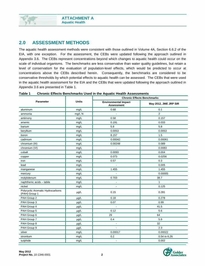
ATTACHMENT A Aquatic Health
May 2012 Project No. 10-1346-0001 2
2.0 ASSESSMENT METHODS The aquatic health assessment methods were consistent with those outlined in Volume 4A, Section 6.6.2 of the EIA, with one exception. For the assessment, the CEBs were updated following the approach outlined in Appendix 3.6. The CEBs represent concentrations beyond which changes to aquatic health could occur on the scale of individual organisms. The benchmarks are less conservative than water quality guidelines, but retain a level of conservatism for the evaluation of population-level effects, which would be predicted to occur at concentrations above the CEBs described herein. Consequently, the benchmarks are considered to be conservative thresholds by which potential effects to aquatic health can be assessed. The CEBs that were used in the aquatic health assessment for the EIA and the CEBs that were updated following the approach outlined in Appendix 3.6 are presented in Table 1.
Table 1 Chronic Effects Benchmarks Used in the Aquatic Health Assessments
Parameter Units Chronic Effects Benchmarks
Environmental Impact Assessment May 2012, JME JRP SIR
aluminum mg/L 0.68 0.1 ammonia mg/L N - 2 antimony mg/L 0.58 0.157 arsenic mg/L 0.191 0.033 barium mg/L 5.8 5.8 beryllium mg/L 0.0053 0.0053 boron mg/L 8.157 1.5 cadmium mg/L 0.00042 0.00061 chromium (III) mg/L 0.00248 0.089 chromium (VI) mg/L - 0.0083 cobalt mg/L 0.0093 0.004 copper mg/L 0.073 0.0256 iron mg/L 0.57 0.3 lead mg/L - 0.005 manganese mg/L 1.455 1.455 mercury mg/L - 0.00005 molybdenum mg/L 0.703 38.7 naphthenic acids – labile mg/L - 1 nickel mg/L - 0.125 Polycyclic Aromatic Hydrocarbons (PAH) Group 1 µg/L 0.15 0.281
PAH Group 2 µg/L 0.18 0.278 PAH Group 3 µg/L 0.07 0.99 PAH Group 4 µg/L - 41.5 PAH Group 5 µg/L 0.12 5.6 PAH Group 6 µg/L 29 64 PAH Group 7 µg/L 0.4 5.9 PAH Group 8 µg/L - 32 PAH Group 9 µg/L - 2.3 silver mg/L 0.00017 0.00022 strontium mg/L 0.2 0.54 to 6.26 sulphide mg/L - 0.002
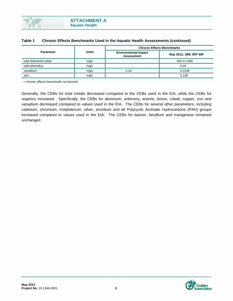
ATTACHMENT A Aquatic Health
Table 1 Chronic Effects Benchmarks Used in the Aquatic Health Assessments (continued)
May 2012 Project No. 10-1346-0001 3
Parameter Units Chronic Effects Benchmarks
Environmental Impact Assessment May 2012, JME JRP SIR
total dissolved solids mg/L - 500 to 1000 total phenolics mg/L - 0.04 vanadium mg/L 0.16 0.0338 zinc mg/L - 0.138
- = chronic effects benchmark not derived.
Generally, the CEBs for total metals decreased compared to the CEBs used in the EIA, while the CEBs for organics increased. Specifically, the CEBs for aluminum, antimony, arsenic, boron, cobalt, copper, iron and vanadium decreased compared to values used in the EIA. The CEBs for several other parameters, including cadmium, chromium, molybdenum, silver, strontium and all Polycyclic Aromatic Hydrocarbons (PAH) groups increased compared to values used in the EIA. The CEBs for barium, beryllium and manganese remained unchanged.
ATTACHMENT A Aquatic Health
May 2012 Project No. 10-1346-0001 4
3.0 RESULTS 3.1 Jackpine Mine Expansion 3.1.1 EIA Base Case The EIA Base Case assessment considered the current state of aquatic health within the study area, with inclusion of existing and approved developments functioning at maximum potential disturbance or effect. This includes developments that have been completed, are under construction or have approval to be built that will result in changes in habitat area or habitat conditions in watercourses or waterbodies within the Local Study Area (LSA), including the Muskeg River watershed.
The assessment methods and format of results for the Base Case assessment closely match the EIA Application Case assessment discussed below. For that reason, and because the interpretation of aquatic health metrics for the EIA Application Case depends on the relative magnitudes of concentrations between the two scenarios, it is important to provide a side-by-side comparison of exposure data. Therefore, for ease of presentation and clarity of results, the predictions for the EIA Base Case are provided alongside the EIA Application Case assessment.
3.1.2 EIA Application Case This section re-evaluates the aquatic health impact assessment in the JME LSA in relation to the EIA Application Case based on the newly derived CEBs. The Application Case refers to existing and approved development conditions (i.e., Base Case) in combination with JME.
3.1.2.1 Effects on Aquatic Health in the Muskeg River Watershed Individual substances that are of potential concern were identified in Volume 4A, Section 6.5 of the EIA. A list of the Substances of Potential Concern (SOPCs) that were identified in the Muskeg River, Jackpine Creek and Kearl Lake during the construction and operational phases and after final reclamation of JME is complete is provided in Table 2.
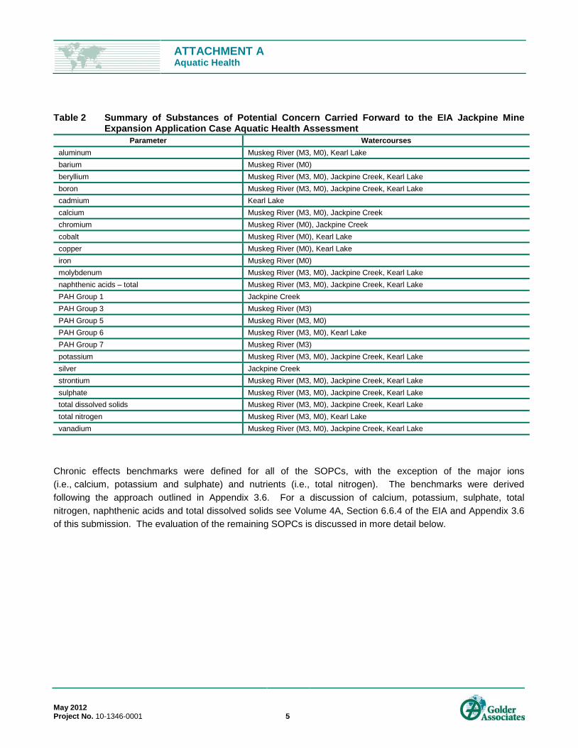
ATTACHMENT A Aquatic Health
May 2012 Project No. 10-1346-0001 5
Table 2 Summary of Substances of Potential Concern Carried Forward to the EIA Jackpine Mine Expansion Application Case Aquatic Health Assessment
Parameter Watercourses aluminum Muskeg River (M3, M0), Kearl Lake barium Muskeg River (M0) beryllium Muskeg River (M3, M0), Jackpine Creek, Kearl Lake boron Muskeg River (M3, M0), Jackpine Creek, Kearl Lake cadmium Kearl Lake calcium Muskeg River (M3, M0), Jackpine Creek chromium Muskeg River (M0), Jackpine Creek cobalt Muskeg River (M0), Kearl Lake copper Muskeg River (M0), Kearl Lake iron Muskeg River (M0) molybdenum Muskeg River (M3, M0), Jackpine Creek, Kearl Lake naphthenic acids – total Muskeg River (M3, M0), Jackpine Creek, Kearl Lake PAH Group 1 Jackpine Creek PAH Group 3 Muskeg River (M3) PAH Group 5 Muskeg River (M3, M0) PAH Group 6 Muskeg River (M3, M0), Kearl Lake PAH Group 7 Muskeg River (M3) potassium Muskeg River (M3, M0), Jackpine Creek, Kearl Lake silver Jackpine Creek strontium Muskeg River (M3, M0), Jackpine Creek, Kearl Lake sulphate Muskeg River (M3, M0), Jackpine Creek, Kearl Lake total dissolved solids Muskeg River (M3, M0), Jackpine Creek, Kearl Lake total nitrogen Muskeg River (M3, M0), Kearl Lake vanadium Muskeg River (M3, M0), Jackpine Creek, Kearl Lake
Chronic effects benchmarks were defined for all of the SOPCs, with the exception of the major ions (i.e., calcium, potassium and sulphate) and nutrients (i.e., total nitrogen). The benchmarks were derived following the approach outlined in Appendix 3.6. For a discussion of calcium, potassium, sulphate, total nitrogen, naphthenic acids and total dissolved solids see Volume 4A, Section 6.6.4 of the EIA and Appendix 3.6 of this submission. The evaluation of the remaining SOPCs is discussed in more detail below.

ATTACHMENT A Aquatic Health
May 2012 Project No. 10-1346-0001 6
3.1.2.1.1 Jackpine Creek Substances of potential concern identified in Jackpine Creek included beryllium, boron, chromium, cobalt, molybdenum, PAH Group 1, silver, strontium and vanadium during 2065 and Far Future (Table 3). For all SOPCs, predicted peak concentrations were less than the corresponding chronic effects benchmark, or the frequency of compliance with the benchmark was equal to or greater than that predicted to occur under the EIA Base Case (Table 3). As such, predicted changes to in-stream concentrations of beryllium, boron, chromium, cobalt, molybdenum, PAH Group 1, silver, strontium and vanadium are expected to result in negligible effects to aquatic health in Jackpine Creek.
3.1.2.1.2 Muskeg River (M3) Substances of potential concern identified in the Muskeg River (M3) included aluminum during 2033 and 2065, and beryllium, boron, molybdenum, strontium, vanadium and PAH Groups 3, 5, 6 and 7 during 2065 and Far Future (Table 4). With the exception of aluminum, predicted peak concentrations of all SOPCs were less than the corresponding chronic effects benchmark, or the frequency of compliance with the benchmark was equal to or greater than that predicted to occur under the EIA Base Case (Table 4). As such, predicted changes to in-stream concentrations of beryllium, boron, molybdenum, strontium, vanadium and PAH Groups 3, 5, 6 and 7 are expected to result in negligible effects to aquatic health in the Muskeg River (M3).
Predicted peak concentrations of aluminum were higher than the CEB in 2033 and 2065. In 2033, aluminum concentrations are predicted to increase as a result of closed-circuiting of natural areas, diversion of upstream reaches and discharges of muskeg drainage and overburden dewatering waters. In 2065, aluminum concentrations are predicted to increase due to outflow from pit lakes and increased low flow periods. The frequencies of compliance with the benchmark are lower under the EIA Application Case than under the EIA Base Case. Potential effects associated with the predicted changes in aluminum concentrations were rated as being low in magnitude, high in frequency and local in geographical extent. Duration was rated as medium-term, because the predicted increase in in-stream concentrations are projected to occur during operations and closure but not Far Future.
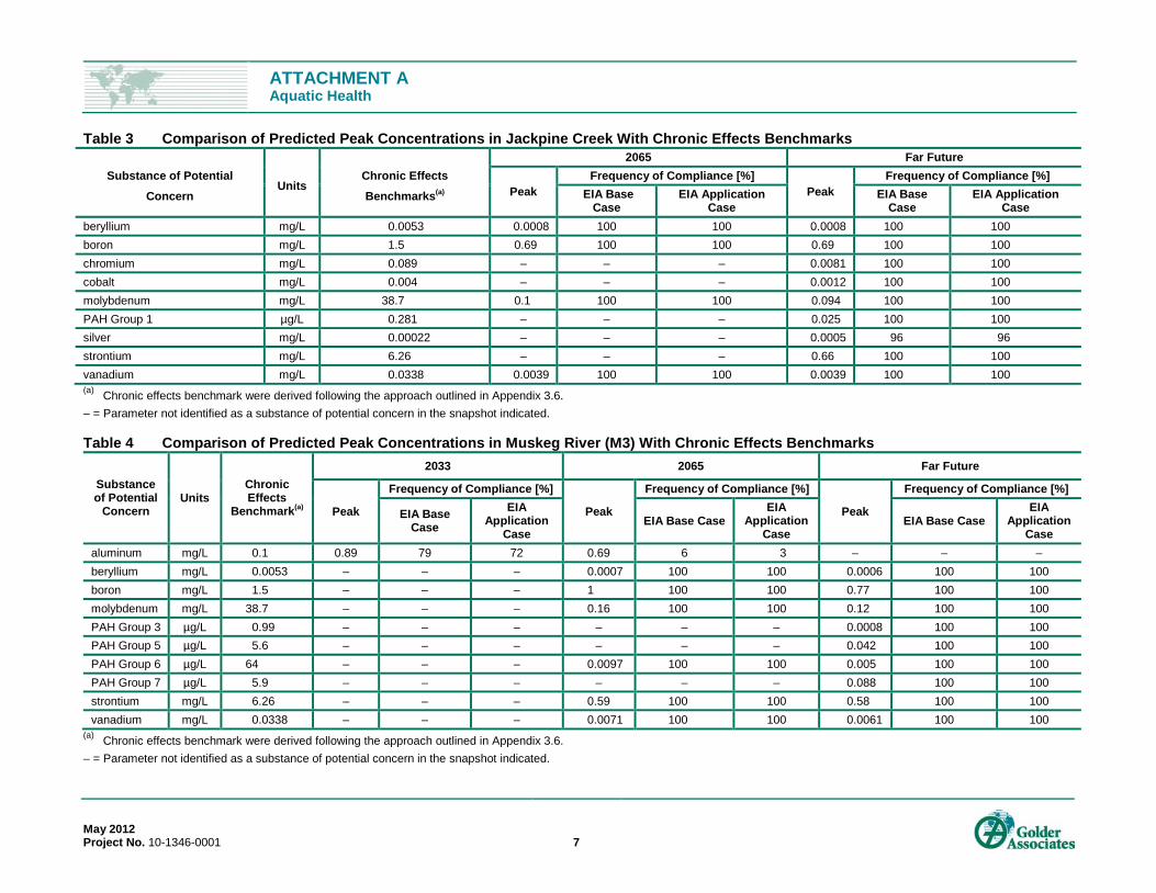
ATTACHMENT A Aquatic Health
May 2012 Project No. 10-1346-0001 7
Table 3 Comparison of Predicted Peak Concentrations in Jackpine Creek With Chronic Effects Benchmarks
Substance of Potential
Concern Units
Chronic Effects
Benchmarks(a)
2065 Far Future
Peak Frequency of Compliance [%]
Peak Frequency of Compliance [%]
EIA Base Case
EIA Application Case
EIA Base Case
EIA Application Case
beryllium mg/L 0.0053 0.0008 100 100 0.0008 100 100 boron mg/L 1.5 0.69 100 100 0.69 100 100 chromium mg/L 0.089 – – – 0.0081 100 100 cobalt mg/L 0.004 – – – 0.0012 100 100 molybdenum mg/L 38.7 0.1 100 100 0.094 100 100 PAH Group 1 µg/L 0.281 – – – 0.025 100 100 silver mg/L 0.00022 – – – 0.0005 96 96 strontium mg/L 6.26 – – – 0.66 100 100 vanadium mg/L 0.0338 0.0039 100 100 0.0039 100 100 (a) Chronic effects benchmark were derived following the approach outlined in Appendix 3.6. – = Parameter not identified as a substance of potential concern in the snapshot indicated.
Table 4 Comparison of Predicted Peak Concentrations in Muskeg River (M3) With Chronic Effects Benchmarks
Substance of Potential
Concern Units
Chronic Effects
Benchmark(a)
2033 2065 Far Future
Peak
Frequency of Compliance [%]
Peak
Frequency of Compliance [%]
Peak
Frequency of Compliance [%]
EIA Base Case
EIA Application
Case EIA Base Case
EIA Application
Case EIA Base Case
EIA Application
Case aluminum mg/L 0.1 0.89 79 72 0.69 6 3 – – – beryllium mg/L 0.0053 – – – 0.0007 100 100 0.0006 100 100 boron mg/L 1.5 – – – 1 100 100 0.77 100 100 molybdenum mg/L 38.7 – – – 0.16 100 100 0.12 100 100 PAH Group 3 µg/L 0.99 – – – – – – 0.0008 100 100 PAH Group 5 µg/L 5.6 – – – – – – 0.042 100 100 PAH Group 6 µg/L 64 – – – 0.0097 100 100 0.005 100 100 PAH Group 7 µg/L 5.9 – – – – – – 0.088 100 100 strontium mg/L 6.26 – – – 0.59 100 100 0.58 100 100 vanadium mg/L 0.0338 – – – 0.0071 100 100 0.0061 100 100
(a) Chronic effects benchmark were derived following the approach outlined in Appendix 3.6. – = Parameter not identified as a substance of potential concern in the snapshot indicated.

ATTACHMENT A Aquatic Health
May 2012 Project No. 10-1346-0001 8
3.1.2.1.3 Muskeg River (M0) Substances of potential concern identified in the Muskeg River (M0) included aluminum, barium, beryllium, boron, chromium, cobalt, copper, iron, molybdenum, strontium, vanadium and PAH Groups 5 and 6 (Table 5). With the exception of aluminum, cobalt and iron, predicted peak concentrations of all SOPCs were below their respective benchmarks, or the frequency of compliance with the benchmark was equal to or greater than that predicted under the EIA Base Case.
Predicted peak concentrations of aluminum were higher than the CEB in 2012 and 2065. The predicted peak concentration of cobalt was higher than the CEB in 2052, while the predicted peak concentration of iron was higher than the CEB in the Far Future. Aluminum concentrations are predicted to increase in 2012 due to closed-circuiting of natural areas, diversion of upstream reaches, and discharges of muskeg drainage and overburden dewatering waters. In 2065, aluminum concentrations are predicted to increase due to outflow from pit lakes and increased low flow periods. Cobalt is predicted to increase as a result of the diversion of upland flows to the downstream reach. Iron is predicted to increase as a result of outflow from pit lakes and increased low flow periods. The frequencies of compliance with the benchmarks are lower under the EIA Application Case than under the EIA Base Case. Potential effects associated with the predicted changes in aluminum and cobalt were rated as being low in magnitude, moderate in frequency and local in geographical extent. Duration was rated as medium-term, because the predicted increase in in-stream concentrations are projected to occur during operations and closure but not Far Future. Potential effects associated with the predicted change in iron concentrations was rated as being low in magnitude, high in frequency and local in geographical extent. Duration was rated as long-term, because the predicted increases in in-stream iron concentrations are projected to occur after final reclamation is complete.
3.1.2.1.4 Kearl Lake In Kearl Lake, SOPCs included aluminum, beryllium, boron, cadmium, cobalt, copper, molybdenum, PAH Group 6, strontium and vanadium (Table 6). With the exception of cadmium, predicted peak concentrations of all SOPCs were less than the corresponding CEB, or the frequency of compliance with the benchmark was equal to or greater than that predicted under the EIA Base Case.
Peak cadmium concentrations were higher than the CEB in 2065 and the Far Future. Cadmium is predicted to increase as a result of outflow from the pit lakes and increased low flow periods. The frequency of compliance with the benchmark is lower under the EIA Application Case than under the EIA Base Case. Potential impacts associated with changes in cadmium concentrations were, therefore, rated as being low in magnitude, high in frequency and local in geographical extent. Duration was rated as long-term, because the predicted increase in in-stream concentrations of cadmium is projected to occur during closure and after final reclamation is complete.
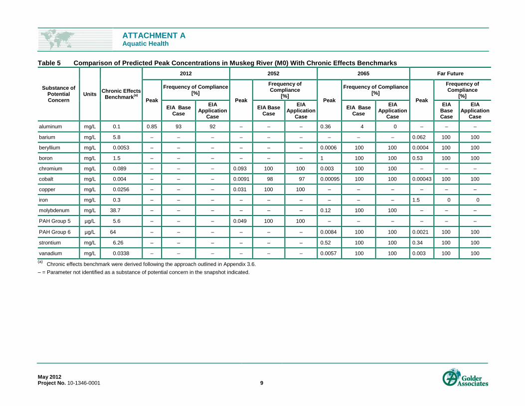
ATTACHMENT A Aquatic Health
May 2012 Project No. 10-1346-0001 9
Table 5 Comparison of Predicted Peak Concentrations in Muskeg River (M0) With Chronic Effects Benchmarks
Substance of Potential Concern
Units Chronic Effects Benchmark(a)
2012 2052 2065 Far Future
Peak
Frequency of Compliance [%]
Peak
Frequency of Compliance
[%] Peak
Frequency of Compliance [%]
Peak
Frequency of Compliance
[%]
EIA Base Case
EIA Application
Case EIA Base
Case EIA
Application Case
EIA Base Case
EIA Application
Case
EIA Base Case
EIA Application
Case
aluminum mg/L 0.1 0.85 93 92 – – – 0.36 4 0 – – –
barium mg/L 5.8 – – – – – – – – – 0.062 100 100
beryllium mg/L 0.0053 – – – – – – 0.0006 100 100 0.0004 100 100
boron mg/L 1.5 – – – – – – 1 100 100 0.53 100 100
chromium mg/L 0.089 – – – 0.093 100 100 0.003 100 100 – – –
cobalt mg/L 0.004 – – – 0.0091 98 97 0.00095 100 100 0.00043 100 100
copper mg/L 0.0256 – – – 0.031 100 100 – – – – – –
iron mg/L 0.3 – – – – – – – – – 1.5 0 0
molybdenum mg/L 38.7 – – – – – – 0.12 100 100 – – –
PAH Group 5 µg/L 5.6 – – – 0.049 100 100 – – – – – –
PAH Group 6 µg/L 64 – – – – – – 0.0084 100 100 0.0021 100 100
strontium mg/L 6.26 – – – – – – 0.52 100 100 0.34 100 100
vanadium mg/L 0.0338 – – – – – – 0.0057 100 100 0.003 100 100 (a) Chronic effects benchmark were derived following the approach outlined in Appendix 3.6. – = Parameter not identified as a substance of potential concern in the snapshot indicated.
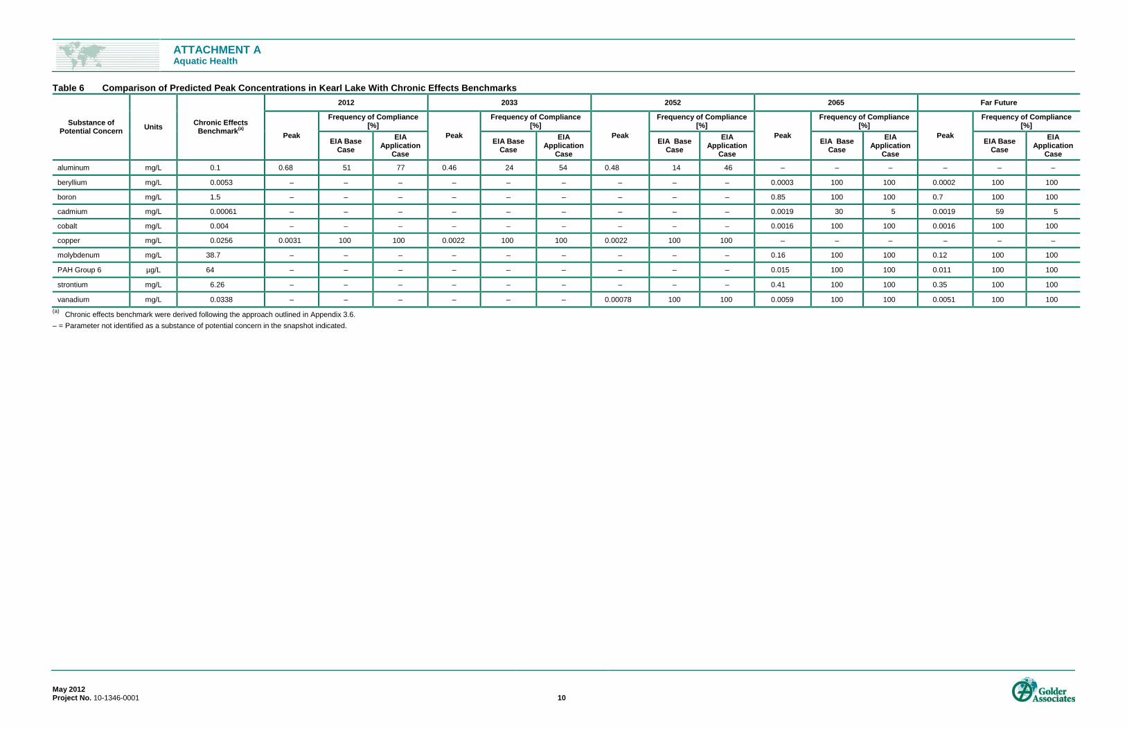
ATTACHMENT A Aquatic Health
May 2012 Project No. 10-1346-0001 10
Table 6 Comparison of Predicted Peak Concentrations in Kearl Lake With Chronic Effects Benchmarks
Substance of Potential Concern Units Chronic Effects
Benchmark(a)
2012 2033 2052 2065 Far Future
Peak
Frequency of Compliance [%]
Peak
Frequency of Compliance [%]
Peak
Frequency of Compliance [%]
Peak
Frequency of Compliance [%]
Peak
Frequency of Compliance [%]
EIA Base Case
EIA Application
Case EIA Base
Case EIA
Application Case
EIA Base Case
EIA Application
Case EIA Base
Case EIA
Application Case
EIA Base Case
EIA Application
Case
aluminum mg/L 0.1 0.68 51 77 0.46 24 54 0.48 14 46 – – – – – –
beryllium mg/L 0.0053 – – – – – – – – – 0.0003 100 100 0.0002 100 100
boron mg/L 1.5 – – – – – – – – – 0.85 100 100 0.7 100 100
cadmium mg/L 0.00061 – – – – – – – – – 0.0019 30 5 0.0019 59 5
cobalt mg/L 0.004 – – – – – – – – – 0.0016 100 100 0.0016 100 100
copper mg/L 0.0256 0.0031 100 100 0.0022 100 100 0.0022 100 100 – – – – – –
molybdenum mg/L 38.7 – – – – – – – – – 0.16 100 100 0.12 100 100
PAH Group 6 µg/L 64 – – – – – – – – – 0.015 100 100 0.011 100 100
strontium mg/L 6.26 – – – – – – – – – 0.41 100 100 0.35 100 100
vanadium mg/L 0.0338 – – – – – – 0.00078 100 100 0.0059 100 100 0.0051 100 100 (a) Chronic effects benchmark were derived following the approach outlined in Appendix 3.6. – = Parameter not identified as a substance of potential concern in the snapshot indicated.
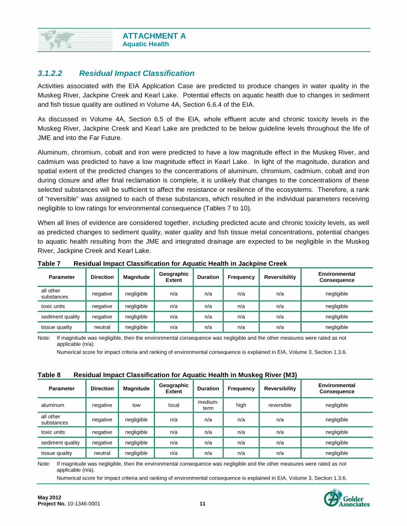
ATTACHMENT A Aquatic Health
May 2012 Project No. 10-1346-0001 11
3.1.2.2 Residual Impact Classification Activities associated with the EIA Application Case are predicted to produce changes in water quality in the Muskeg River, Jackpine Creek and Kearl Lake. Potential effects on aquatic health due to changes in sediment and fish tissue quality are outlined in Volume 4A, Section 6.6.4 of the EIA.
As discussed in Volume 4A, Section 6.5 of the EIA, whole effluent acute and chronic toxicity levels in the Muskeg River, Jackpine Creek and Kearl Lake are predicted to be below guideline levels throughout the life of JME and into the Far Future.
Aluminum, chromium, cobalt and iron were predicted to have a low magnitude effect in the Muskeg River, and cadmium was predicted to have a low magnitude effect in Kearl Lake. In light of the magnitude, duration and spatial extent of the predicted changes to the concentrations of aluminum, chromium, cadmium, cobalt and iron during closure and after final reclamation is complete, it is unlikely that changes to the concentrations of these selected substances will be sufficient to affect the resistance or resilience of the ecosystems. Therefore, a rank of “reversible” was assigned to each of these substances, which resulted in the individual parameters receiving negligible to low ratings for environmental consequence (Tables 7 to 10).
When all lines of evidence are considered together, including predicted acute and chronic toxicity levels, as well as predicted changes to sediment quality, water quality and fish tissue metal concentrations, potential changes to aquatic health resulting from the JME and integrated drainage are expected to be negligible in the Muskeg River, Jackpine Creek and Kearl Lake.
Table 7 Residual Impact Classification for Aquatic Health in Jackpine Creek
Parameter Direction Magnitude Geographic Extent Duration Frequency Reversibility Environmental
Consequence
all other substances negative negligible n/a n/a n/a n/a negligible
toxic units negative negligible n/a n/a n/a n/a negligible
sediment quality negative negligible n/a n/a n/a n/a negligible
tissue quality neutral negligible n/a n/a n/a n/a negligible
Note: If magnitude was negligible, then the environmental consequence was negligible and the other measures were rated as not applicable (n/a).
Numerical score for impact criteria and ranking of environmental consequence is explained in EIA, Volume 3, Section 1.3.6.
Table 8 Residual Impact Classification for Aquatic Health in Muskeg River (M3)
Parameter Direction Magnitude Geographic Extent Duration Frequency Reversibility Environmental
Consequence
aluminum negative low local medium-term high reversible negligible
all other substances negative negligible n/a n/a n/a n/a negligible
toxic units negative negligible n/a n/a n/a n/a negligible
sediment quality negative negligible n/a n/a n/a n/a negligible
tissue quality neutral negligible n/a n/a n/a n/a negligible
Note: If magnitude was negligible, then the environmental consequence was negligible and the other measures were rated as not applicable (n/a).
Numerical score for impact criteria and ranking of environmental consequence is explained in EIA, Volume 3, Section 1.3.6.

ATTACHMENT A Aquatic Health
May 2012 Project No. 10-1346-0001 12
Table 9 Residual Impact Classification for Aquatic Health in Muskeg River (M0) Parameter Direction Magnitude Geographic
Extent Duration Frequency Reversibility Environmental Consequence
aluminum negative low local medium-term moderate reversible negligible cobalt negative low local medium-term moderate reversible negligible iron negative low local long-term high reversible low (+6) all other substances negative negligible n/a n/a n/a n/a negligible toxic units negative negligible n/a n/a n/a n/a negligible sediment quality negative negligible n/a n/a n/a n/a negligible tissue quality negative negligible n/a n/a n/a n/a negligible
Note: If magnitude was negligible, then the environmental consequence was negligible and the other measures were rated as not applicable (n/a).
Numerical score for impact criteria and ranking of environmental consequence is explained in EIA, Volume 3, Section 1.3.6.
Table 10 Residual Impact Classification for Aquatic Health in Kearl Lake Parameter Direction Magnitude Geographic
Extent Duration Frequency Reversibility Environmental Consequence
cadmium negative low local long-term high reversible low (+6) all other substances negative negligible n/a n/a n/a n/a negligible toxic units negative negligible n/a n/a n/a n/a negligible sediment quality negative negligible n/a n/a n/a n/a negligible tissue quality neutral negligible n/a n/a n/a n/a negligible
Note: If magnitude was negligible, then the environmental consequence was negligible and the other measures were rated as not applicable (n/a).
Numerical score for impact criteria and ranking of environmental consequence is explained in EIA, Volume 3, Section 1.3.6.
3.1.2.3 Effects on the Ecological Viability of the Jackpine Mine Expansion Closure Landscape
The capability of the pit lakes to support aquatic life was re-evaluated in consideration of the updated CEBs.
Individual parameters that were identified as SOPCs in one or more of the pit lakes included:
barium; PAH Group 2; sulphate;
boron; PAH Group 6; total dissolved solids;
molybdenum; sodium; total nitrogen; and
naphthenic acids; strontium; vanadium.
Chronic effects benchmarks were defined for all of the SOPCs, with the exception of the major ions (i.e., sodium and sulphate) and nutrients (i.e., total nitrogen). The benchmarks were derived following the approach outlined in Appendix 3.6. For a discussion of sodium, sulphate, total nitrogen, naphthenic acids and total dissolved solids see Volume 4A, Section 6.6.4 in the EIA and Appendix 3.6 of this submission. The remaining seven SOPCs were evaluated, including barium, boron, molybdenum, PAH Group 2 and 6, strontium and vanadium. For each of these SOPCs, predicted concentrations are less than the corresponding CEB (Table 11).
3.1.2.4 Residual Impact Classification Similar to the conclusions put forward in the EIA, the JME pit lakes are expected to be able to support a viable aquatic ecosystem. No residual impacts are predicted (Table 12).

ATTACHMENT A Aquatic Health
May 2012 Project No. 10-1346-0001 13
Table 11 Comparison of Predicted Concentrations in Jackpine Mine Expansion Pit Lakes With Chronic Effects Benchmarks
Substance of Potential Concern Units Chronic Effects
Benchmark(a)
Jackpine South Pit Lake
Jackpine South Central Pit Lake
Jackpine Northwest Pit Lake
Jackpine Northeast Pit Lake
Initial Far Future Initial Far Future Initial Far Future Initial Far Future 2065 2165 2065 2165 2065 2165 2065 2165
barium mg/L 5.8 0.071 0.11 0.091 0.19 0.071 0.095 0.077 0.094 boron mg/L 1.5 1.2 1.1 1.3 1.1 0.21 0.73 1.2 0.65 molybdenum mg/L 38.7 0.21 0.18 0.21 0.18 0.018 0.11 0.12 0.097 PAH Group 2 μg/L 0.278 0.041 0.037 0.039 0.021 0.0044 0.0014 0.03 0.0018 PAH Group 6 μg/L 64 0.02 0.018 0.016 0.0081 0.0017 0.00082 0.012 0.001 strontium mg/L 6.26 0.62 0.61 0.62 0.63 0.29 0.38 0.44 0.35 vanadium mg/L 0.0338 0.0071 0.0061 0.0084 0.0065 0.0034 0.0056 0.0095 0.005
(a) Chronic effects benchmark were derived following the approach outlined in Appendix 3.6.

ATTACHMENT A Aquatic Health
May 2012 Project No. 10-1346-0001 14
Table 12 Residual Impact Classification for Aquatic Health in the Jackpine Mine Expansion Pit Lakes
Parameter Direction Magnitude Geographic Extent Duration Frequency Reversibility Environmental
Consequence
all parameters neutral negligible n/a n/a n/a n/a negligible
Note: If magnitude was negligible, then the environmental consequence was negligible and the other measures were rated as not applicable (n/a).
3.2 Athabasca River 3.2.1 EIA Base Case The EIA Base Case assessment considers the current state of aquatic health within the Athabasca River study area, with inclusion of existing and approved developments functioning at maximum potential disturbance or effect. A list of the existing, approved and planned developments included in the EIA Base, JME Application and PDC cases is provided in Appendix 3.1 of this submission.
Similar to the small streams assessment, the predictions for the EIA Base Case are provided in the EIA Application Case assessment.
3.2.2 EIA Application Case As outlined in Volume 4A, Section 6.5 in the EIA, activities associated with JME in combination with existing and approved developments in the lower Athabasca River watershed have the potential to affect water quality in the Athabasca River. This section re-evaluates the impact assessment for aquatic health in the Athabasca River in relation to the EIA Application Case, based on the newly derived CEBs.
Individual substances that are of potential concern were identified in Volume 4A, Section 6.5 of the EIA. No SOPCs were identified in the Athabasca River upstream of the Embarras River. Individual parameters that were identified as SOPCs in the Athabasca River downstream of the Muskeg River include boron and naphthenic acids.
A CEB was defined for boron following the methods outlined in Appendix 3.6. In both cases, median and peak concentrations in the identified snapshots were less than the corresponding benchmark. The median and peak concentrations of boron predicted in 2065 and the Far Future downstream of the Muskeg River were 0.071 and 0.31 mg/L, respectively (see EIA Volume 4A, Section 6.5, Table 6.5-22). Negligible effects to aquatic health are, therefore, expected to result from the predicted changes in the concentrations of boron.
3.2.2.1 Residual Impact Classification Activities associated with JMEare predicted to produce changes in water quality in the Athabasca River. Potential effects on aquatic health due to changes in sediment and fish tissue quality are outlined in Volume 4A, Section 6.6.6 of the EIA.
Whole effluent acute and chronic toxicity levels in the Athabasca River are predicted to be below guideline levels throughout the life of JME and into the Far Future. Predicted changes to in-stream concentrations of the individual parameters considered in the analysis are either unchanged from existing conditions or the EIA Base Case, or they remain below effects benchmarks. As such, activities associated with JME are expected to result in negligible effects to aquatic health in the Athabasca River (Table 13).

ATTACHMENT A Aquatic Health
May 2012 Project No. 10-1346-0001 15
Table 13 Residual Impact Classification for Aquatic Health in the Athabasca River
Parameter Direction Magnitude Geographic Extent Duration Frequency Reversibility Environmental
Consequence
individual substances negative negligible n/a n/a n/a n/a negligible toxic units negative negligible n/a n/a n/a n/a negligible sediment quality negative negligible n/a n/a n/a n/a negligible tissue quality negative negligible n/a n/a n/a n/a negligible
Note: If magnitude was negligible, then the environmental consequence was negligible and the other measures were rated as not applicable (n/a). Numerical score for impact criteria and ranking of environmental consequence is explained in EIA, Volume 3, Section 1.3.6.
ATTACHMENT A Aquatic Health
May 2012 Project No. 10-1346-0001 16
4.0 REFERENCES CCME (Canadian Council of Ministers of the Environment). 2007. A protocol for the derivation of
water quality guidelines for the protection of aquatic life 2007. In: Canadian Environmental Quality Guidelines, Canadian Council of Ministers of the Environment. Winnipeg, MB, Canada. Available at: ceqg-rcqe.ccme.ca/download/en/220/