appendix 8 detailed results of dilution and dispersion

CAPITAL REGIONAL DISTRICT

CRD CORE AREA WASTEWATER TREATMENT PROGRAM

STAGE 2 ENVIRONMENTAL IMPACT STUDY

307071-00020 : Rev 0 : 18 February 2013 Appendices

Appendix 8 Detailed Results of Dilution and Dispersion Modelling

- 1 -

T E C H N I C A L M E M O R A N D U MT E C H N I C A L M E M O R A N D U M

To: Chris Lowe, Capital Regional DistrictFrom: Donald Hodgins, Ph.D., P.Eng., Scott Tinis, Ph.D., LoraxSubject: Preliminary outfall assessment – Option 1: 33-port designDate: August 31, 2011 (revision 1 October 2011)Copies: Tony Brcic, Capital Regional District

The bottom line: with effluent bacteria concentrations of 400,000 cfu/100 mL the proposed diffuser cannot achieve sufficient dilution to meet the recreational water quality standard of 200 cfu/100 mL in the IDZ, for neither normal operating conditions, nor failure scenarios 1 and 2. The diffuser and its location at M8E do not, however, pose a risk to shellfish resources during normal summer operations, and only a slight, episodic risk during wet weather storms. Similarly there appears to be a slight episodic risk to shellfish during the failure scenarios. Locating the McLoughlin diffuser at the M8E station offers slightly greater dilution efficiency than co-locating it with the Macaulay diffuser, with no significant difference in the risk to shellfish resources.

1.0 PURPOSE

A preliminary assessment of outfall option 1 (33-port design located at M8E) is presented in this report. Two aspects of diffuser performance are considered: (i) dilution and trapping in the initial dilution zone (IDZ), and the related question of whether, or not, the recreational water quality criteria for fecal coliform bacteria is met; and (ii) the potential risk of shellfish exposure to fecal coliforms at sensitive locations outside the current closure area, and the likelihood of exceeding the Environment Canada shellfish criteria at these locations. The results for the M8E diffuser location are also compared with the identical 33-port diffuser located adjacent to the existing Macaulay diffuser. This comparison was intended to show if there are significant differences in diffuser behaviour, or far-field risk, associated with co-locating the new and existing diffusers, instead of placing the McLoughlin outfall along an entirely new route.

From the shellfish perspective there are two principal areas of interest that lie outside of current closure boundaries: (i) Haystock Islets and Witty’s Lagoon immediately south of Albert Head, and (ii) the Chatham and Discovery Islands in Plumper Passage east of Trial Island. Both areas are located proximate to First Nations reserve lands. These areas are the focus of the present discussion.

Two different situations are considered:

1. Proposed treatment conditions with discharge of treated wastewater through the new McLoughlin outfall (normal conditions).

2. Failure conditions associated with the proposed wastewater treatment plant (WWTP) resulting in various combinations of untreated and treated wastewater being discharged through the McLoughlin and Clover/Macaulay outfalls (failure scenarios).

The assessment was carried out using a 3-dimensional water quality model (Hodgins et al., 1998; Li and Hodgins, 2004; Hodgins, 2009) developed and applied over the past 20 years for the CRD. This model (called C3-UM) takes the regional oceanographic properties into account (tides, currents and mixing), as well as simulating the behaviour of the buoyant plumes associated with each of the existing and planned outfall diffusers. The diffuser dynamics are crucial to the analysis since they provide the initial mixing, coliform concentration and depth of dispersion data to the large-scale C3 model.

- 2 -

2.0 OUTFALL SPECIFICATIONS (OPTION 1)

The proposed McLoughlin outfall, designated as option 1 in this report, has the following properties (Table 2.1)1: The outfall length is approximately 2 km, and the orientation places the diffuser downslope, across the bathymetric contours. The water depth is about 55 m. This diffuser design is hydraulically efficient, providing the least impact on the treatment plant design in terms of meeting the hydraulic head requirements for gravity flow.

The location of the diffuser coincides with the Macaulay outfall benthic sampling station M8E, lying approximately 800 m east of the existing Macaulay diffuser (Fig. 2.1). This site is advantageous in that it makes use of existing sampling data for baseline environmental assessment purposes. The diffuser centre-point coordinates are: 48° 25.09’ N, 123° 23.59’ W (NAD83).

Table 2.1: Diffuser specifications for Option 1

Number of ports 33Port diameter 200 mmPort spacing (average) 6.15 mHorizontal discharge angle wrt horizontal 90 degreesDiffuser orientation 180° azimuth

Macaulay M8E

Clover

Macaulay M8E

Clover

Figure 2.1 Map of study area showing the Macaulay, M8E (McLoughlin) and Clover diffuser locations.

1 Van Bastelaere, I., 2010. McLoughlin Point Outfall, Conceptual Diffuser Design, Analysis Summary (Draft). Prepared for Capital Regional District by Indesco Consulting Ltd.

- 3 -

3.0 EFFLUENT FLOW SPECIFICATIONS

3.1 Normal Conditions

Two normal operating conditions were examined: Average Dry Weather Flows (ADWF) representative of summer (August) conditions (Fig. 3.1), and wet weather (WW) flows representative of conditions expected in, say, December or January (Fig. 3.2). Both hydrographs contain storm events during which flows are higher than average for the period. The hydrographs were derived by Kerr Wood Leidel2. Note that the WW flows are about 1.6 times higher on average than the ADWFs.

For ADWFs all of the effluent receives secondary treatment. There are no overflows expected at either Macaulay or Clover based on the design capacity of the McLoughlin WWTP. The maximum fecal coliform concentrations are estimated to be equal to or less than 400,000 cfu/100 mL (by Stantec). This value was used for the simulations.

During the wet weather storm event some overflow of untreated wastewater at Macaulay and Clover is expected (again based on the design capacity of the McLoughlin WWTP). Fecal coliform concentrations in the overflows were specified as 14,000,000 cfu/100 mL to be consistent with the Environment Canada guidance for untreated wastewater in the failure scenarios. 400,000 cfu/100 mL was used here also for the treated wastewater coliform concentration.

0.0

0.5

1.0

1.5

2.0

2.5

0 24 48 72 96 120 144 168 192 216 240 264 288 312 336

Time step (h)

Q (

m^

3/s)

Mcloughlin Macaulay Clover

Figure 3.1 Wastewater flow hydrographs for McLoughlin, Clover and Macaulay used for input to C3-UM for ADWF normal conditions. The graph shows the hydrograph for 14 days.

2 2030 Hydrographs_with SENOB Tanks.xls: worksheet 90th% anal

- 4 -

0.0

0.5

1.0

1.5

2.0

2.5

3.0

3.5

4.0

4.5

0 24 48 72 96 120 144 168 192 216 240 264 288 312 336

Time step (h)

Q (

m^

3/s)

Mcloughlin Macaulay Clover

Figure 3.2 Wastewater flow hydrographs for McLoughlin, Clover and Macaulay used for input to C3-UM for wet weather + storm normal conditions

3.2 Failure Scenarios 1 & 2

The failure scenarios were developed by Stantec (Rev. Jan. 7, 2011). The first scenario concerns total failure of the influent channel and diversion of the Clover stream out the existing Clover outfall, without treatment, for seven days while repairs are made. In this circumstance, untreated wastewater would be discharged through the McLoughlin diffuser for the total flow for 1 h, immediately after failure, followed by 7 days of discharge of untreated wastewater through the Clover Point outfall (~ 50% of the flow) and 7 days of secondary treated wastewater through the McLoughlin outfall (~ 50% of the flow). These flows are shown in Fig. 3.3.

The second scenario concerns failure of the influent pump from Macaulay, resulting in a 2-day discharge of untreated effluent from the existing Macaulay outfall while repairs are made (~ 50% of the flow), and 2 days of treated effluent discharge (~ 50% of the flow) from the McLoughlin outfall. These flows are plotted in Fig. 3.4. Although much shorter in duration than the first scenario, the Macaulay pump failure may have serious implications because the two outfalls are located close together, and closer to shore than the Clover outfall.

Based on guidance from Environment Canada, the effluent flow to be considered in the failure scenarios should be exceeded only 10% of the time. For the present analysis, flow hydrographs were developed by Kerr Wood Leidel (Feb. 11, 2011) based on the wet weather total daily flow volume that meets this guideline. Fecal coliform concentrations were specified as 400,000 cfu/100 mL for secondary treatment (estimated by Stantec) and 14,000,000 cfu/100 mL for untreated wastewater (also based on guidance from Environment Canada).

- 5 -

0.0

0.5

1.0

1.5

2.0

2.5

3.0

0 24 48 72 96 120 144 168 192 216 240 264 288 312 336

Time step

Q (

m^

3/s)

Mcloughlin Clover

Figure 3.3 Effluent discharge rate for the McLoughlin and Clover outfalls for failure scenario 1.

0.0

0.5

1.0

1.5

2.0

2.5

3.0

0 24 48 72 96 120 144 168 192 216 240 264 288 312 336

Time (h)

Q (

m^

3/s)

Mcloughlin Macaulay

Figure 3.4 Effluent discharge rate for the McLoughlin and Macaulay outfalls for failure scenario 2.

- 6 -

4.0 OCEANOGRAPHIC CONDITIONS

4.1 Tides and Density Stratification

Two oceanographic factors play important roles in determining the dispersion characteristics of effluent from all of the CRD outfalls: namely, the tide and the vertical density stratification. The tides contain important fortnightly modulations, which in turn, govern the strength of the currents and the intensity of turbulent mixing. Thus, each model run is a minimum of 14 days so that the effects of at least one complete fortnightly cycle are included.

The vertical stratification results from variations in seawater temperature and salinity. Slightly more brackish water tends to move seaward through Juan de Fuca Strait from the Strait of Georgia in the surface layers. Denser, saltier water originating in the Pacific Ocean lies below this lighter layer. The density contrast between the layers is greatest in summer due to the freshest flows from the Fraser River, and least in winter.

The principal effect of the stratification is felt in the trapping and dilution characteristics for the diffusers. Generally, trapping is deeper and less dilute during periods of stronger stratification, and vice versa for periods of weaker stratification. Note, that these parameters are also affected by the effluent flow rate and so the picture is a little more complicated.

Accordingly, the analyses reported here cover two seasons: winter, for which December 2011 was chosen, and summer, for which August 2011 was chosen. The tidal conditions for these periods are shown in Fig. 4.1. Stratification profiles3 are compared for winter and summer in Fig. 4.2, for a location immediately south of M8E at a water depth of 80 m. These profiles are representative of conditions at the Macaulay diffuser also.

Fortnightly model runs were made for each of the normal conditions, and for each of the failure scenarios. In the case of the failure conditions, the time of failure was chosen to coincide with high effluent flow rates (late morning) and with weak tidal currents over the diffuser. This should represent a worst case in terms of shellfish risk by virtue of surface trapping and dispersion with relatively low dilution.

4.2 Bacterial Die-off Rates

Fecal coliform bacteria die when discharged into marine waters. The rate at which they die depends upon the water temperature, its salinity and incident sunlight. The C3-UM model takes this die-off into account using accepted formula published by the US Environmental Protection Agency. Specifically, decay rates for fecal coliforms are specified using first-order kinetics in the form:

C(t) = C(0) exp (-kt) (1)

where C(t) = concentration at time tC(0) = concentration at time t=0k = disappearance coefficient that is dependent upon temperature, salinity and light (h-1)t = time.

3 Seawater density is expressed as ‘sigma-t’ which is defined as density – 1000 in units of kg/m3.

- 7 -

0

0.5

1

1.5

2

2.5

3

1-Aug 5-Aug 9-Aug 13-Aug 17-Aug 21-Aug 25-Aug 29-Aug

Time

Vic

tori

a t

ide

(m)

(a)

0

0.5

1

1.5

2

2.5

3

3.5

03-Dec 07-Dec 11-Dec 15-Dec 19-Dec 23-Dec 27-Dec 31-Dec

Time

Vic

tori

a ti

de

(m)

(b)

Figure 4.1 Victoria tide for (a) August 2011 and (b) December 2011.

- 8 -

0

10

20

30

40

50

60

70

80

90

23 24 25 26

sigma-t

dep

th (

m)

winter

summer

Figure 4.2 Density stratification input to C3-UM at the beginning of each model run for winter and summer conditions.

Equation (1) is a standard method of modelling bacterial die-off; see, for example, Bowie et al. (1985 – Chapter 8). Mancini (1978) expressed the decay rate function as:

k = (0.8 + 0.006(%SW))/24 × 1.07(T-20) + kL L (2)

where %SW = percent sea waterT = sea water temperature in degrees CelsiuskL = light-dependent disappearance rate (cm2/cal)L = depth-averaged light intensity (cal/cm2 – h)

Typically, the total radiation flux at the sea surface (Lo) is about 80 W/m2 during winter months, increasing to about 280 W/m2 in summer, at Victoria’s latitude. Converting units provides seasonal fluxes of 7 and 24 cal/(cm2-h) respectively. Radiation, which is absorbed rapidly in the water column, is modelled with the relation:

Lz = Lo exp (-αz) (3)

where Lz = flux at depth zα = absorption coefficient.

Integration of (3) between depths z2 and z1, where H = z2 - z1, yields:

Lz = Lo [ exp(-αz2) – exp(-αz1) ] / (-αH) (4)

- 9 -

Based on data in Pickard (1979 – Table 3, p. 57) light attenuation in coastal waters is, approximately, 90% at 10 m depth. This degree of absorption corresponds to α = 0.23 m-1, which when inserted into (4) with z2 and z1 equal to layer boundaries in successive 5-m intervals yields the ratios for L z/Lo, and for k shown in Table 4.1.

Table 4.1: Values for Lz/Lo and k for the uppermost five layers of C3-UM

Layer 1 2 3 4 5

Lz/Lo 0.594 0.188 0.059 0.019 0.006

k (winter) 0.188 0.070 0.033 0.021 0.018

k (summer) 0.620 0.209 0.079 0.038 0.025

In these calculations, we have assumed average values for T = 11.5 °C (summer) and = 8.8 °C (winter), %SW = 3.1 and kL = 0.042 (Mancini, 1978). These values have been used in the simulations discussed here.

Guidance from Environment Canada concerning the failure scenario analyses suggests that a ‘universal’ die-off rate of 0.1951 h-1 should be adopted. This rate corresponds to a T90 = 11.8 h (90% of coliform bacteria have disappeared in 11.8 h). This rate agrees reasonably well with the winter surface layer value calculated above, but would be highly conservative (die-off that is too slow) in summer.

- 10 -

5.0 DISCUSSION OF RESULTS FOR THE 33-PORT DIFFUSER AT M8E


5.1.1 ADWF + Storm

The basic statistics for trapping depth and dilution are shown in Fig. 5.1 to 5.3. In this case, 87% of trapping occurs between 35 and 50 m. Trapping in surface layers (z<15 m) takes place less than 2% of the time. Approximately 70% of the dilutions range from 300:1 to 800:1, which is typical for this type of diffuser and effluent flow rates. The minimum dilution found here was 105:1. The scatter diagram in Fig. 5.3 clearly shows that lowest dilutions coincide with deep trapping (at times of high current speed). When the plume rises to the near-surface layers, dilutions increase to over 700:1.

If secondary treatment yields fecal coliform concentrations of 400,000 cfu/100 mL, then the minimum dilution required to achieve the recreational water quality standard is 2000:1. Clearly the 33-port diffuser and location will not produce sufficient dilution to meet this standard. The predicted coliform concentrations are less than 200 cfu/100 mL less than 2% of the time within the IDZ.

The maximum concentration map for the surface layer is shown in Fig. 5.4. The hot spot over the McLoughlin diffuser corresponds with the surfacing event with the lowest dilution (760:1) and the highest coliform concentration (526 cfu/100 mL). The detectable effluent signature is confined to the area around the diffuser and to the west of Trial Island. There is no apparent risk to shellfish resources at either the Chatham-Discovery Islands, or the Haystock Islets for these conditions.

5.1.2 WW + storm

The trapping and dilution statistics for the wet weather simulation are shown in Fig. 5.5 to 5.7, in the same format as for the ADWF+storm simulation. The time period of the wet weather simulation is in December when stratification is typically less pronounced than in summer. Combined with higher discharge rates, this leads to more frequent surfacing events, about 10% of the time. However, in the winter simulation a wide range of dilutions is associated with near surface trapping (Fig. 5.7), from 245:1 to over 4000:1.

The trapping depth distribution is also broader than in summer with more occurrences between 15 and 35 m. In this case 54% of trapping values lie between 35 and 50 m, compared with 87% during summer. As noted for the summer simulation, the minimum dilution (135:1) corresponds with deep trapping at a time of high current speed. Approximately 70% of dilution values fall in the range 300:1 to 1000:1, similar to summer conditions.

The conclusion is the same as for summer conditions: the Option 1 diffuser and M8E location will not produce sufficient dilution to meet the recreational water quality standard for fecal coliform concentration, both at the surface and at depth.

The maximum coliform concentration distribution for the WW+storm simulation is shown in Fig. 5.8. The greatest concentration is associated with surfacing over the McLoughlin diffuser (approximately 1400 cfu/100 mL), with a band of elevated concentrations around Trial Island. This band is almost certainly the result of the overflow through the Clover outfall. There is some exposure at the Chatham and Discovery Islands, but little apparent exposure at the Haystock Islets.

The time-series of coliform concentrations at Chatham Island and at the Haystock Islets are plotted in Fig. 5.9 and 5.10. There is a very slight risk to shellfish at Chatham Island associated with the storm overflow (peak concentrations of about 40 cfu/100 mL), slight because exposure is episodic and of short duration.

- 11 -

On the other hand, several storms can be expected over winter months leading to Clover overflows. Thus, it is possible for such episodes to recur several times each winter, separated by periods of no exposure.

There is no apparent risk to shellfish at the Haystock Islets.

0%

5%

10%

15%

20%

25%

30%

35%

40%

45%

2.5

12.5

22.5

32.5

42.5

52.5

62.5

72.5

82.5

92.5

103

Trapping depth (m)

freq

uen

cy

ADWF+storm

Figure 5.1 Marginal distribution of trapping depth for the ADWF+storm simulation.

0%

2%

4%

6%

8%

10%

12%

14%

16%

18%

20%

50 550 1050 1550 2050 2550 3050

Dilution

Fre

qu

ency

ADWF+storm

Figure 5.2 Marginal distribution of dilution for the ADWF+storm simulation.

- 12 -

0

500

1000

1500

2000

2500

3000

3500

0 10 20 30 40 50 60

Trapping depth (m)

Dilu

tio

n

ADWF + storm

Figure 5.3 Scatter diagram of dilution versus trapping depth4 for the ADWF+storm simulation.

Figure 5.4 Map of maximum fecal coliform concentration in the surface layer (z=0-5 m) at any time during the ADWF+storm simulation for normal conditions.

4 Trapping depths are determined in increments of 5 m by C3-UM since that is the thickness of the model layers between the surface and the diffusers. In reality the trapping depth would vary continuously.

- 13 -

0%

5%

10%

15%

20%

25%

2.5

12.5

22.5

32.5

42.5

52.5

62.5

72.5

82.5

92.5

103

Trapping depth (m)

freq

uen

cy

WW+storm

Figure 5.5 Marginal distribution of trapping depth for the WW+storm simulation.

0%

2%

4%

6%

8%

10%

12%

14%

50 550 1050 1550 2050 2550 3050

Dilution

Fre

qu

ency

WW+storm

Figure 5.6 Marginal distribution of dilution for the WW+storm simulation.

- 14 -

0

1000

2000

3000

4000

5000

6000

0 5 10 15 20 25 30 35 40 45 50

Trapping depth (m)

Dilu

tio

n

WW+storm

Figure 5.7 Scatter diagram of dilution versus trapping depth for the WW+storm simulation.

Figure 5.8 Map of maximum fecal coliform concentration in the surface layer (z=0-5 m) at any time during the WW+storm simulation for normal conditions.

- 15 -

0

5

10

15

20

25

30

35

40

45


Time

FC

co

nc

en

tra

tio

n (

cfu

/10

0 m

L)

-10

-8

-6

-4

-2

0

2

4

z=0-5 m z=5-10 m z=10-15 m Victoria tide

Figure 5.9 Time-series of fecal coliform concentration on the west shore of Chatham Island in Plumper Passage for the WW+storm simulation for normal conditions.

0

2

4

6

8

10

12

14

16

18

20


Time

FC

co

nce

ntr

atio

n (

cfu

/100

mL

)

-10

-8

-6

-4

-2

0

2

4


Figure 5.10 Time-series of fecal coliform concentration on the east side of the Haystock Islets for the WW+storm simulation for normal conditions.

5.2 Failure Scenarios

5.2.1 Near-Field Conditions in the IDZ

The trapping and dilution characteristics for the McLoughlin outfall for both failure scenarios are summarized in the scatter diagrams shown in Fig. 5.11. Because the effluent flow rates are similar to the WW normal operations (but slightly lower as explained in Section 3.2), and the oceanographic conditions are the same, the trapping-dilution properties are also similar. Minimum dilutions (178:1 for scenario1 and 154:1 for scenario 2) occurred at depths of 30 to 40 m. The lowest dilutions during surface-layer trapping were about 335:1 in both cases, although the average dilutions for these events were over 1500:1.

- 16 -

Thus, as noted in the previous section, the McLoughlin outfall does not achieve sufficient dilution to conform to the recreational water quality criterion even with secondary treatment.

0

1000

2000

3000

4000

5000

6000

7000

0 10 20 30 40 50 60

Trapping depth (m)

Dilu

tio

nscenario 1

(a)

0

1000

2000

3000

4000

5000

6000

0 10 20 30 40 50 60

Trapping depth (m)

Dilu

tio

n

scenario 2

(b)

Figure 5.11 Scatter diagram of dilution versus trapping depth for the (a) scenario 1, and (b) scenario 2 simulations.

- 17 -

During scenario 1 the greatest risk to shellfish contamination is likely posed by the discharge of untreated wastewater for about 7 days through the Clover outfall. The scatter diagram of dilution versus trapping depth is shown in Fig. 5.12. Trapping is deep in the water column (mainly below 40 m), with no surfacing, and dilutions range from about 260:1, to well over 5000:1 during times of high current speed. In view of the effluent fecal coliform concentration of 14,000,000 cfu/100 mL, the recreational water quality criterion would not be met within the Clover outfall IDZ during this failure scenario.

The situation differs in scenario 2, when the untreated wastewater is discharged through the Macaulay outfall (Fig. 5.13). In this case, effluent does surface toward the end of the failure event, with minimum dilutions of about 470:1. There is only one period of surface layer trapping, which may pose a risk of shellfish contamination at the Haystock Islets. Dilutions are not sufficient to meet the recreational water quality standard in the IDZ during the failure scenario.

5.2.2 Far-field Dispersion and Risk to Shellfish

The simulation results for both scenarios are summarized in the surface-layer maximum concentration maps shown in Fig. 5.14. As noted earlier, these maps represent the maximum concentration observed at any time during the model run, sampled every 15 minutes.

The hot spot above the McLoughlin diffuser for scenario 1 (Fig. 5.14a) results from the surfacing untreated effluent at the time of failure (concentrations > 25,000 cfu/100 mL). This outcome was expected since the time of failure was chosen such that peak effluent flows coincided with slack tide. These conditions should provide the greatest risk to shellfish resources near Albert Head. This figure also shows elevated fecal coliform concentrations west of Trial Island, and in Plumper Passage, which are the result of the 7-d discharge of untreated wastewater through the Clover outfall.

Figure 5.15 illustrates the concentration time-series at a location on the west side of Chatham Island. Here again the episodes of high concentration occur on flooding tides, with marked periods of low concentration as the ebb waters from Haro Strait flush the area. There is little concentration variation with depth at this location, and concentrations decrease with time after the Clover discharge is stopped.

During the failure event, maximum concentrations range from 250 to 300 cfu/100 mL, leading to some risk to shellfish resources; however, exposure is limited to the duration of the forcemain failure. After repairs are completed the area is rapidly flushed.

The time-series of fecal coliform concentration on the east side of the Haystock Islets are plotted in Fig. 5.16. Here the exposure is somewhat less tidally modulated than at Chatham Island, the concentrations are lower and there is more variation with depth (lowest concentration in the surface layer). However, concentrations are below about 15 cfu/100 mL and there is no apparent risk to shellfish resources based on the Canadian shellfish criteria.

In scenario 2 the highest surface concentrations over the Macaulay diffuser exceed 25,000 cfu/100 mL giving the hot spot and the elongated elliptical dispersion pattern toward Albert Head shown in Fig. 5.14b. In this case there is little effluent signature in Plumper Passage since there is no discharge through the Clover outfall. The fecal coliform time-series at Chatham Island and the Haystock Islets are shown in Fig. 5.17 and 5.18. There is little or no risk to shellfish resources at Chatham Island, but effluent is present at the Haystock Islets for the period of the failure event. The peak concentrations here are about 100 cfu/100 mL (one peak) following the surfacing event at the Macaulay outfall.

- 18 -

0

1000

2000

3000

4000

5000

6000

7000

8000

0 10 20 30 40 50 60 70

Trapping depth (m)

Dilu

tio

n

Clover scenario 1

Figure 5.12 Scatter diagram of dilution versus trapping depth for the Clover outfall for the scenario 1 simulation.

0

500

1000

1500

2000

2500

3000

0 5 10 15 20 25 30 35 40 45 50

Trapping depth (m)

Dilu

tio

n

Macaulay scenario 2

Figure 5.13 Scatter diagram of dilution versus trapping depth for the Macaulay outfall for the scenario 2 simulation.

- 19 -

(a)

(b)

Figure 5.14 Map of maximum fecal coliform concentration in the surface layer (z=0-5 m) at any time during failure scenario 1 (a) and scenario 2 (b).

- 20 -

0

50

100

150

200

250

300


Time

FC

co

nce

ntr

atio

n (

cfu

/100

m

L)

-10

-8

-6

-4

-2

0

2

4

tid

e (m

)


Figure 5.15 Time-series of fecal coliform concentration on the west shore of Chatham Island in Plumper Passage for scenario 1.

0

5

10

15

20

25

30

03-Dec 07-Dec 11-Dec 15-Dec

Time

FC

co

nce

ntr

atio

n (

cfu

/100

mL

)

-8

-6

-4

-2

0

2

4

tid

e (m

)


Figure 5.16 Time-series of fecal coliform concentration on the east side of Haystock Islets for scenario 1.

- 21 -

0

4

8

12

16

20


Time

FC

co

nce

ntr

atio

n (

cfu

/100

m

L)

-10

-8

-6

-4

-2

0

2

4

tid

e (m

)


Figure 5.17 Time-series of fecal coliform concentration on the west shore of Chatham Island in Plumper Passage for scenario 2.

0

20

40

60

80

100

120

140


Time

FC

co

nc

entr

ati

on

(c

fu/1

00 m

L)

-8

-6

-4

-2

0

2

4

tid

e (m

)


Figure 5.18 Time-series of fecal coliform concentration on the east side of Haystock Islets for scenario 2.

- 22 -

6.0 COMPARISON OF RESULTS FOR M8E WITH A CO-LOCATED DIFFUSER

The issue considered in this section is whether there are benefits to locating the new McLoughlin diffuser adjacent to the existing Macaulay diffuser compared with the M8E location shown in Fig. 2.1. Two aspects are examined here: trapping and dilution in the IDZ, and risk to shellfish resources. Because the water depths are very similar for both locations (58 m for the co-located McLoughlin diffuser and 55 m for M8E) the near-field results are expected to be similar – differences would arise principally from spatial variations in current speed and direction. In this analysis the effluent discharge rates are identical.


6.1.2 Trapping and Dilution in the IDZ

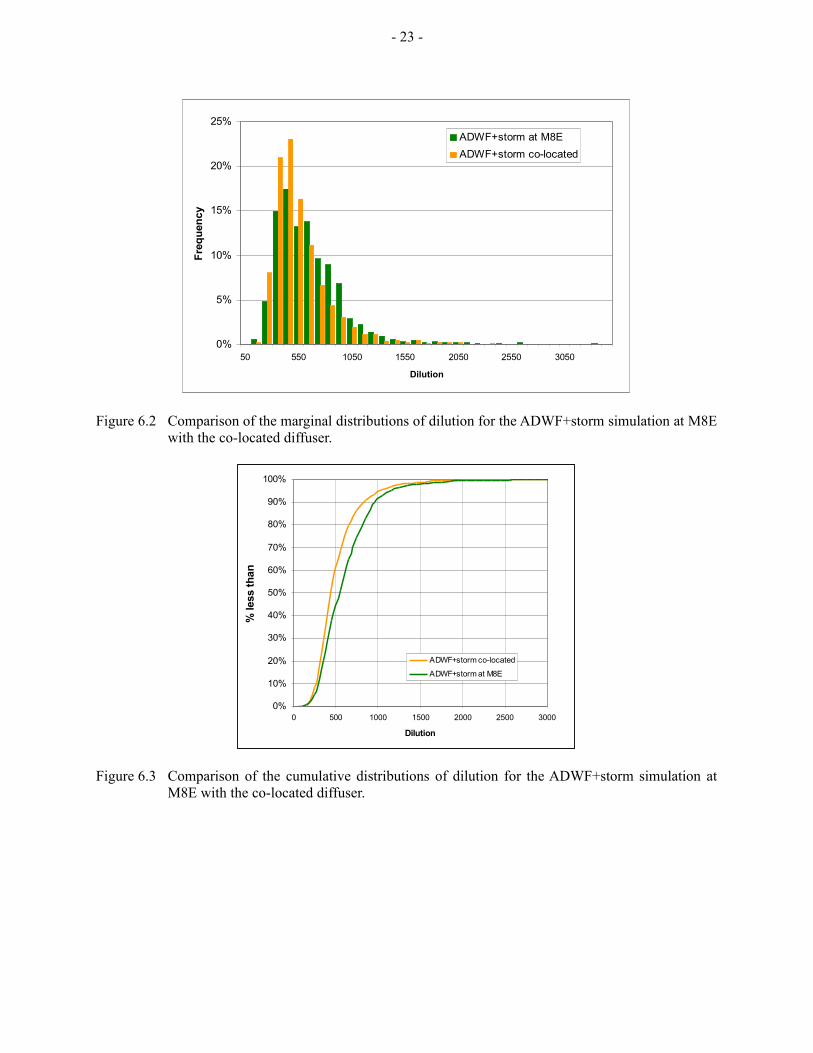
Trapping depth and dilution statistics during ADWF+storm conditions are plotted in Fig. 6.1 and 6.2. The trapping depth characteristics differ very little for these two locations, although there is a slightly higher frequency of surfacing at M8E than at Macaulay (8 events versus 1 event, recognizing that each event lasts only a few minutes). However, the predicted dilutions are greater at M8E than at Macaulay (Fig. 6.3), which presumably reflects the influence of currents on the plume behaviour.

The marginal distributions for trapping depth and dilution are shown in Fig. 6.4 and 6.5 for the WW+storm conditions. Trapping depths are similar for both locations, although the frequency of deep trapping is slightly greater for M8E. As noted for summer conditions, dilution in the IDZ is generally greater at M8E than at Macaulay; this is shown clearly in the cumulative distribution plotted in Fig. 6.6.

These differences in dilution for both seasons are, however, not particularly significant since they are subsumed well within in the range of dilutions at both locations, and are not sufficient to achieve compliance with the recreational water quality standard for fecal coliforms at either location. On balance it appears that the 33-port diffuser is slightly more efficient, in terms of dilution, at M8E than co-located with the Macaulay diffuser.

0%

5%

10%

15%

20%

25%

30%

35%

40%

45%

2.5

12.5

22.5

32.5

42.5

52.5

62.5

72.5

82.5

92.5

103

Trapping depth (m)

freq

uen

cy

ADWF+storm at M8E

ADWF+storm co-located

Figure 6.1 Comparison of the marginal distributions of trapping depth for the ADWF+storm simulation at M8E with the co-located diffuser.

- 23 -

0%

5%

10%

15%

20%

25%

50 550 1050 1550 2050 2550 3050

Dilution

Fre

qu

enc

y

ADWF+storm at M8E


Figure 6.2 Comparison of the marginal distributions of dilution for the ADWF+storm simulation at M8E with the co-located diffuser.

0%

10%

20%

30%

40%

50%

60%

70%

80%

90%

100%

0 500 1000 1500 2000 2500 3000

Dilution

% le

ss t

han


ADWF+storm at M8E

Figure 6.3 Comparison of the cumulative distributions of dilution for the ADWF+storm simulation at M8E with the co-located diffuser.

- 24 -

0%

5%

10%

15%

20%

25%

2.5

12.5

22.5

32.5

42.5

52.5

62.5

72.5

82.5

92.5

103

Trapping depth (m)

freq

uen

cy

WW+storm at M8E

WW+storm co-located

Figure 6.4 Comparison of the marginal distributions of trapping depth for the WW+storm simulation at M8E with the co-located diffuser.

0%

2%

4%

6%

8%

10%

12%

14%

16%

18%

50 550 1050 1550 2050 2550 3050

Dilution

Fre

qu

ency

WW+storm at M8E

WW+storm co-located

Figure 6.5 Comparison of the marginal distributions of dilution for the WW+storm simulation at M8E with the co-located diffuser.

- 25 -

0%

10%

20%

30%

40%

50%

60%

70%

80%

90%

100%

0 500 1000 1500 2000 2500 3000

Dilution

% l

ess

tha

n

WW+storm co-located

WW+storm at M8E

Figure 6.6 Comparison of the cumulative distributions of dilution for the WW+storm simulation at M8E with the co-located diffuser.

A number of statistics are both locations and both seasons are compiled in Table 6.1.

Table 6.1: Summary of dilution statistics for M8E versus the co-located diffuser.

ADWF+storm WW+storm

M8E Co-located M8E Co-located

Minimum 105:1 108:1 135:1 182:1

Median 545:1 430:1 700:1 604:1

Range (105,3310) (108,2280) (135,5500) (182,5500)

Minimum at surface

760 509 245 292

Mean at surface 1445 566 1322 1250

Range at surface (760,3310) (509,622) (245,4000) (292,5000)

6.1.2 Far-field Dispersion and Shellfish Risk

The model simulation for the ADWF+storm condition, with co-located diffuser, indicates a very low level of exposure at the Haystock Isles, with maximum concentrations of less than 20 cfu/100 mL at depths of

- 26 -

10 to 15 m, in one event associated with the storm discharge. Concentrations greater than 14 cfu/100 mL last for less than 3 h. A low level of exposure was also predicted at Chatham and Discovery Islands. Maximum concentrations, also at 10 to 15 m depth, ranged from about 80 to 100 cfu/100 mL over a period of 3 h. At both locations concentrations decreased toward the surface by a factor of about 2. These results differ from the model predictions for the M8E diffuser location, for which no exposure was found.

The simulation results for WW+storm conditions are show in Fig. 6.7 and 6.8. The time scale is expanded to show the exposure episodes at each location. For all practical purposes the difference in diffuser locations makes no difference in exposure for winter storm discharges.

0

5

10

15

20

25

30

35

40

45

04-Dec 05-Dec 06-Dec 07-Dec

Time

FC

co

nc

en

tra

tio

n (

cfu

/10

0 m

L)

-2

-1

0

1

2

3

4

z=10-15 m for M8E z=10-15 m for co-located Victoria tide

Figure 6.7 Comparison of fecal coliform concentration on the west shore of Chatham Island for the WW+storm simulation for diffuser locations at M8E and co-located with Macaulay.

0

5

10

15

20

25

04-Dec 05-Dec 06-Dec 07-Dec 08-Dec

Time

FC

co

nce

ntr

atio

n (

cfu

/100

mL

)

-2

-1

0

1

2

3

4

z=10-15 m for M8E z=10-15 m for co-located Victoria tide

Figure 6.8 Comparison of fecal coliform concentration on the east side of the Haystock Islets for the WW+storm simulation for diffuser locations at M8E and co-located with Macaulay.

- 27 -

6.2 Risk to Shellfish Resources During Failure Scenarios 1 and 2

As noted in Section 5.2.2 the only risk to shellfish resources during Scenario 1 occurs in Plumper Passage along the west shores of Chatham and Discovery Islands (see Fig. 5.15). The high concentrations there (> 250 cfu/100 mL) arise from the discharge of untreated effluent through the Clover outfall; the location of the McLoughlin diffuser would not likely be significant. A comparison of the time-series at Chatham Island, at depths of 10 to 15 m, confirms that there is no change to the risk since the discharge through Clover is identical for both McLoughlin locations (Fig. 6.9 – average difference is 0.2, with a maximum difference of 9 cfu/100 mL).

-15

-10

-5

0

5

10

15


Time

FC

co

nc

en

tra

tio

n (

cfu

/10

0 m

L)

0

0.5

1

1.5

2

2.5

3

3.5

4

difference FC concentration Victoria tide

Figure 6.9 Difference in FC concentration at Chatham Island for failure scenario 1 (FCco-located – FCM8E).

For Scenario 1 there is a very low level of exposure at the Haystock Islets, less than 20 cfu/100 mL, over the failure period (Fig. 5.16). These results are virtually unchanged if the McLoughlin diffuser were to be co-located with the Macaulay diffuser.

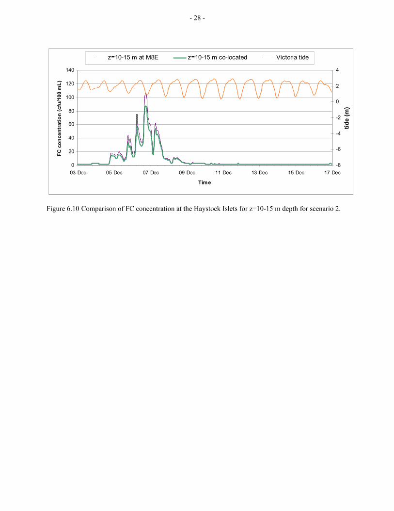
During scenario 2, with no discharge through the Clover outfall, a very low level of exposure was predicted for the Chatham and Discovery Islands (Fig. 5.17 – concentrations < 20 cfu/100 mL). With the McLoughlin diffuser located further west at Macaulay versus M8E, the concentrations were found to be slightly lower (e.g., maximum at 10-15 m depth of 14 (co-located) versus 18 (M8E) cfu/100 mL).

The situation is similar but reversed at the Haystock Islets – see Fig. 5.18 and the comparison for 10-15 m depth in Fig. 6.10. The pattern of exposure is very similar; however, the peak concentrations are marginally lower when the two diffusers are co-located. This outcome is slightly counter-intuitive but probably results from the circulation patterns along Royal Roads, possibly combined with a longer travel time for effluent from the co-located diffuser locations than from M8E (hence slightly more die-off).

Overall the differences in shellfish risk for the two McLoughlin diffuser locations are not significant for either of the failure scenarios, and little or no benefit is associated with the co-located diffuser.

- 28 -

0

20

40

60

80

100

120

140


Time

FC

co

nce

ntr

ati

on

(c

fu/1

00

mL

)

-8

-6

-4

-2

0

2

4

tid

e (m

)

z=10-15 m at M8E z=10-15 m co-located Victoria tide

Figure 6.10 Comparison of FC concentration at the Haystock Islets for z=10-15 m depth for scenario 2.

- 29 -

7.0 REFERENCES

Bowie, G.L., and 9 co-authors, 1985. Rates, Constants, and Kinetics Formulations in Surface Water Quality Modeling. 2nd Ed., EPA/600/3-85/040 June 1985.

Hodgins, D.O., S.W. Tinis and L.A. Taylor, 1998. Marine Sewage Outfall Assessment for the Capital Regional District, British Columiba, Using Nested Three-dimensional Models. Wat. Sci. Tech., 38(10), 301-308.

Hodgins, D.O., 2009. Technical Memorandum, The C3-UM and Sedimentation Modelling Systems and Their Implementation for the Capital Regional District, Prepared for Capital Regional District by Seaconsult Marine Research Ltd.

Li, S. and D.O. Hodgins, 2004. A dynamically coupled outfall plume-circulation model for effluent dispersion in Burrard Inlet, British Columbia. J. Environ. Sci., 3(2004), 433-449.

Mancini, J.L., 1978. Numerical Estimates of Coliform Mortality Rates Under Various Conditions. J. Wat. Poll. Control Fed., 50(11), p. 2477-2484.

Pickard, G.L., 1979. Descriptive Physical Oceanography, 3rd Ed. Pergamon Press, 233 pp.

- 1 -

TT EE CC HH NN II CC AA LL MM EE MM OO RR AA NN DD UU MM

To: Chris Lowe, Capital Regional District

From: Donald Hodgins, Ph.D., P.Eng., Scott Tinis, Ph.D., Lorax

Subject: Baseline outfall assessment – pre-treatment conditions (2011)

Date: August 31, 2011 (Rev February 24, 2012)

Copies: Tony Brcic, Capital Regional District

1.0 PURPOSE

As part of the outfall assessment program for the proposed McLoughlin wastewater treatment plant,

existing conditions with untreated wastewater discharged through the Macaulay and Clover outfalls were

simulated with a numerical model. These conditions were examined for winter effluent discharge rates

to serve as a far-field baseline with which to compare the McLoughlin WWTP operations and outfall.

The parameter of interest in this study was fecal coliform concentration.

As noted in Hodgins and Tinis (2011), there are two principal areas of interest from the shellfish

perspective that lie outside of current closure boundaries: (i) Haystock Islets and Witty’s Lagoon

immediately south of Albert Head, and (ii) the Chatham and Discovery Islands in Plumper Passage east

of Trial Island. Both areas are located proximate to First Nations reserve lands. These areas are the

focus of the present discussion.

The simulations were carried out using a three-dimensional water quality model (Hodgins et al., 1998; Li

and Hodgins, 2004; Hodgins, 2009) developed and applied over the past 20 years for the CRD. This

model (called C3-UM) takes the regional oceanographic properties into account (tides, currents and

mixing), as well as simulating the behaviour of the buoyant plumes associated with each of the existing

and planned outfall diffusers. The diffuser dynamics are crucial to the analysis since they provide the

initial mixing, coliform concentration and depth of dispersion data to the large-scale C3 model.

- 2 -

2.0 OUTFALL SPECIFICATIONS (OPTION 1)

The location of each existing diffuser is shown in Fig. 2.1. For reference the M8E location, one option

proposed for McLoughlin outfall, is also shown on the map.

Table 2.1: Diffuser specifications for the Macaulay and Clover outfalls used in the simulation

Clover Outfall

Number of ports 39

Port diameter 150 mm

Port spacing (average) 3.5 m

Horizontal discharge angle wrt horizontal 5 degrees

Macaulay Outfall

Number of ports 27

Port diameter 140 mm

Port spacing (average) 5.31 m

Horizontal discharge angle wrt horizontal 45 degrees

Macaulay M8E

Clover

Macaulay M8E

Clover

Figure 2.1 Map of study area showing the Macaulay, M8E (McLoughlin option) and Clover diffuser

locations.

- 3 -

3.0 EFFLUENT FLOW SPECIFICATIONS FOR EXISTING CONDITIONS

The wastewater flows were based on hydrographs derived by Kerr Wood Leidel1. These hydrographs

(for Macaulay and Clover) were scaled to agree with total daily flow amounts measured during winter

months in 2008 and 2009. The total daily flows are 55.6 ML/d for Clover and 48.6 ML/d for Macaulay.

After scaling to these totals, the hydrographs are as shown in Fig. 3.1. They were input to the model as

two successive 14-day sequences.

An approximate estimate for fecal coliform concentrations in the wastewater was obtained from effluent

quality measurements made between 1994 and 2000. Averaging data for winter months provided

concentrations of 4,464,000 cfu/100 mL (range 1,600,000 to 7,700,000) for Clover and 5,050,000 cfu

100 mL (range 1,100,000 to 23,000,000) for Macaulay. These values were held constant with time for

the simulations. These averages are a little less than half of the recommended Environment Canada

value of 14,000,000 cfu/100 mL to be applied to potential failure scenarios for the proposed new outfall.

0.0

0.2

0.4

0.6

0.8

1.0

1.2

1.4

1.6

0 24 48 72 96 120 144 168 192 216 240 264 288 312 336

Time step (h)

Q (

m^

3/s

)

Clover Macaulay

Figure 3.1 Wastewater flow hydrographs for Clover and Macaulay used for input to C3-UM for existing

conditions. The graph shows hydrographs for 14 days.

1 2030 Hydrographs_with SENOB Tanks.xls: worksheet 90th% anal

- 4 -

4.0 OCEANOGRAPHIC CONDITIONS

4.1 Tides and Density Stratification

Two oceanographic factors play important roles in determining the dispersion characteristics of effluent

from all of the CRD outfalls: namely, the tide and the vertical density stratification. The tides contain

important fortnightly modulations, which in turn, govern the strength of the currents and the intensity of

turbulent mixing. In any one month there are also subtle variations in the fortnightly cycles. Thus, each

model run is a minimum of 14 days so that the effects of at least one complete fortnightly cycle are

included.

The vertical stratification results from variations in seawater temperature and salinity. Slightly more

brackish water tends to move seaward through Juan de Fuca Strait from the Strait of Georgia in the

surface layers. Denser, saltier water originating in the Pacific Ocean lies below this lighter layer. The

density contrast between the layers is greatest in summer due to the freshet flows from the Fraser River,

and least in winter.

The principal effect of the stratification is felt in the trapping and dilution characteristics for the

diffusers. Generally, trapping is deeper and less dilute during periods of stronger stratification, and vice

versa for periods of weaker stratification. Note, that these parameters are also affected by the effluent

flow rate and so the picture is a little more complicated.

The greatest risk to shellfish is considered to occur during winter months because more effluent tends to

reach the near-surface layers at this time, and logically has a more direct path to the shellfish areas than

when effluent traps deeper in the water column. Therefore existing conditions were simulated only for a

representative winter period; in this case, a 28-d period from December 3 – 31, 2011, was chosen to

cover two complete fortnightly cycles. Two 14-day back-to-back runs were made for this purpose.

During this period the Victoria tide exhibits two distinct fortnightly large tide modulations (Fig. 4.1),

with a neap tide on Dec 17-18. The tides on Dec 24-26 are amongst the largest of the year. The

objective was to see if these large (spring) tides gave rise to wastewater dispersion to the areas of interest

at concentrations sufficient to pose a risk to shellfish.

Stratification profiles2 are compared for winter and summer in Fig. 4.2, for a location immediately south

of M8E at a water depth of 80 m. The winter stratification profile was used for the model simulation.

2 Seawater density is expressed as ‘sigma-t’ which is defined as density – 1000 in units of kg/m

3.

- 5 -

0

0.5

1

1.5

2

2.5

3

3.5


Time

Vic

tori

a t

ide (

m)

Figure 4.1 Victoria tide for December 2011.

0

10

20

30

40

50

60

70

80

90

23 24 25 26

sigma-t

dep

th (

m)

winter

summer

Figure 4.2 Density stratification input to C3-UM at the beginning of each model run for winter.

4.2 Bacterial Die-off Rates

Fecal coliform bacteria die when discharged into marine waters. The rate at which they die depends

upon the water temperature, its salinity and incident sunlight. The C3-UM model takes this die-off into

account using accepted formula published by the US Environmental Protection Agency. Specifically,

decay rates for fecal coliforms are specified using first-order kinetics in the form:

- 6 -

C(t) = C(0) exp (-kt) (1)

where C(t) = concentration at time t

C(0) = concentration at time t=0

k = disappearance coefficient that is dependent upon temperature, salinity and light (h-1

)

t = time.

Equation (1) is a standard method of modelling bacterial die-off; see, for example, Bowie et al. (1985 –

Chapter 8). Mancini (1978) expressed the decay rate function as:

k = (0.8 + 0.006(%SW))/24 1.07(T-20)

+ kL L (2)

where %SW = percent sea water

T = sea water temperature in degrees Celsius

kL = light-dependent disappearance rate (cm2/cal)

L = depth-averaged light intensity (cal/cm2 – h)

Typically, the total radiation flux at the sea surface (Lo) is about 80 W/m2

during winter months,

increasing to about 280 W/m2 in summer, at Victoria’s latitude. Converting units provides seasonal

fluxes of 7 and 24 cal/(cm2-h) respectively. Radiation, which is absorbed rapidly in the water column, is

modelled with the relation:

Lz = Lo exp (-z) (3)

where Lz = flux at depth z

= absorption coefficient.

Integration of (3) between depths z2 and z1, where H = z2 - z1, yields:

Lz = Lo [ exp(-z2) – exp(-z1) ] / (-H) (4)

Based on data in Pickard (1979 – Table 3, p. 57) light attenuation in coastal waters is, approximately,

90% at 10 m depth. This degree of absorption corresponds to = 0.23 m-1

, which when inserted into (4)

with z2 and z1 equal to layer boundaries in successive 5-m intervals yields the ratios for Lz/Lo, and for k

shown in Table 4.1.

Table 4.1: Values for Lz/Lo and k for the uppermost five layers of C3-UM

Layer 1 2 3 4 5

Lz/Lo 0.594 0.188 0.059 0.019 0.006

k (winter) 0.188 0.070 0.033 0.021 0.018

k (summer) 0.620 0.209 0.079 0.038 0.025

In these calculations, we have assumed average values for T = 11.5 C (summer) and = 8.8 C (winter),

%SW = 3.1 and kL = 0.042 (Mancini, 1978). These values have been used in the simulations discussed

here.

- 7 -

Guidance from Environment Canada concerning the failure scenario analyses suggests that a ‘universal’

die-off rate of 0.1951 h-1

should be adopted. This rate corresponds to a T90 = 11.8 h (90% of coliform

bacteria have disappeared in 11.8 h). This rate agrees reasonably well with the winter surface layer value

calculated above, but would be highly conservative (die-off that is too slow) in summer.

- 8 -

5.0 DISCUSSION OF RESULTS

5.1 Existing Conditions – Discharge Through the Macaulay and Clover Outfalls

The simulation results are summarized in the maximum concentration maps shown in Fig. 5.1 to 5.3 for

the top three layers of the model. The layers are 5 m thick. These maps represent the maximum

concentration observed at any time during the model run, sampled every 15 minutes. As expected, high

concentrations (> 8,000 cfu/100 mL) occurred at the surface at Macaulay due to plume trapping in the

top layer. The minimum dilution was 566:1 at this location when surface trapping occurred. There is no

corresponding high-concentration zone at Clover because the plume did not trap in the surface layer; the

minimum rise depth was a little over 5 m and occurred only once during the period of minimum tide on

December 29th. Plume rise depths at Clover ranged from about 35 to 60 m. Trapping depths were

generally a little deeper.

The maximum concentration maps for layers 2 and 3 show evidence of increasing concentrations with

depth, between the diffusers and shore, immediately to the west of Trial Island and on the western side of

Chatham and Discovery Islands in Plumper Passage. Peak concentrations are typically between 80 and

100 cfu/100 mL in these areas. There is some indication of concentrations above 10 cfu/100 mL near the

Haystock Islets.

Figure 5.4 illustrates the concentration time-series at a location on the west side of Chatham Island,

where episodes of high concentration occur on flooding tides, with marked periods of low concentration

as the ebb waters from Haro Strait flush the area. There is little concentration variation with depth at this

location and the highest concentrations are clearly linked to large tides. Flood currents are strongest

during these tidal conditions and thus carry the discharged effluent from both outfalls around Trial Island

into the area around Plumper Passage.

Maximum concentrations were slightly less than 100 cfu/100 mL. Periods of concentrations > 14

cfu/100 mL were generally short, typically about 8 h. However, given the recurrence of exposure over

successive days with concentrations above 14 cfu/100 mL there is some risk to shellfish contamination in

this area.

The concentration time-series for the Haystock Islets are shown in Fig. 5.5. Here the highest

concentrations occur on the building portion of each fortnightly tidal cycle, and are not directly linked to

the largest tides in the cycle as they are in Plumper Passage. This is presumably due to the unique pattern

of ebb tide currents over the outfalls and along Royal Roads toward and around Albert Head in this phase

of the fortnightly tidal cycle. In this simulation, there were no concentrations > 14 cfu/100 mL in the

surface layer. As shown in the time-series there were several episodes when concentrations did exceed

this threshold between 5 and 10 m (layer 2), and 10 and 15 m (layer 3). In these two deeper layers, the

peak concentrations were 35 cfu/100 mL in layer 2, and 41 cfu/100 mL in layer 3; average concentrations

were 19 and 20 cfu/100 mL respectively. These results suggest that there appears to be some risk to

shellfish in the subsurface waters, but not likely in the intertidal zone.

Thus, the 28-day simulation results for existing winter conditions indicate some risk to shellfish

resources outside the current closure area. The risk appears to be slightly greater at Chatham and

Discovery Islands than around the Haystock Islets and Witty’s Lagoon. The principal source of coliform

bacteria in Plumper Passage is the Clover outfall. This is somewhat unexpected from an oceanographic

point of view since trapping depths for Clover were deep (93% of trapping occurred in the range 40 to 65

m), and implies that the flooding currents advect the wastewater up-slope after trapping in the IDZ. The

- 9 -

mid-channel depth in Plumper Passage is about 30 m. This phenomenon is discussed more fully in the

next section.

Figure 5.1 Map of maximum fecal coliform concentration in the surface layer (z=0-5 m) at any time

during the winter simulation for existing conditions.

Figure 5.2 Map of maximum fecal coliform concentration in the second layer (z=5-10 m) at any time


- 10 -

Figure 5.3 Map of maximum fecal coliform concentration in the third layer (z=10-15 m) at any time


0

20

40

60

80

100

120


Time

FC

co

ncen

trati

on

(cfu

/100

mL

)

-10

-8

-6

-4

-2

0

2

4

tid

e (

m)


Figure 5.4 Time-series of fecal coliform concentration on the west shore of Chatham Island in Plumper

Passage for the winter simulation for existing conditions.

- 11 -

Figure 5.5 Time-series of fecal coliform concentration on the east side of the Haystock Islets for the

winter simulation for existing conditions.

5.2 Oceanographic Explanation for Elevated Coliform Concentrations in Plumper Passage

Deep trapping plumes (>30 m), particularly from the diffuser at Clover Point, experience much lower

coliform decay rates than their near-surface counterparts and hold the potential for pooling with high

coliform concentrations. The 50 m contour (Fig. 5.6) shows that Constance Bank forms a partial

southern barrier to deeply trapped plume advection/dispersion, and model simulations show that the

plume is initially confined between the Victoria shoreline and Constance Bank, with the core

concentrated along the 30-60 m contour band close to the diffuser.

During the flood phase of the tide, eastward currents near the diffusers carry the plume south of Trial

Island roughly following the 50 m contour, then turn northward into Plumper Passage and Haro Strait.

Model simulations show that topographic steering of the tidal currents causes a back-eddy to be formed

south of Chatham and Discovery Islands, with a subsequent upslope advection of the plume where it

crosses the 50 m contour into shallower waters. Near the south shore of Discovery Island, the plume is

seen to surface and high concentrations of fecal coliforms are predicted for short periods of the tidal

cycle.

The structure of the eddy is shown in Fig. 5.7. Vertical sections of the coliform concentration and

density fields indicate that the highest concentrations are located within the core of the eddy, which is

evident as a downward displacement of the isopycnals (lines of equal density). Over time, this structure

is pushed into shallow water where the isopyncals are compressed, and the plume is pushed upwards.

The progression of the eddy towards Discovery Island is illustrated in Fig. 5.8 using a series of hourly

cross-sections of fecal coliform concentration. As the flood tide intensifies, the plume core is forced

upwards where it eventually surfaces and shoals near Discovery Island. By the fourth hour, the plume is

already starting to retreat southward prior to the onset of slack tide at Victoria. The sections are not able

to show the process in its entirety, since the eddy is three-dimensional in nature. In addition, it is not

known at this time how the vertical movement of the plume is divided between vertical mixing and

- 12 -

vertical advection due to dynamic processes. The simulations indicate that the largest contributor to the

surfacing plume in Plumper Passage by far is the Clover Point outfall - due both to its proximity to the

Discovery/Chatham Islands, and by the characteristic deep-trapping plume formed by the diffuser.

Figure 5.6 Topography of the receiving water basin south of Victoria showing diffuser locations used

in the simulations and highlighting the 50 m contour which becomes an important factor in

the movement of deep-trapping effluent plumes.

- 13 -

Figure 5.7 Plume4D generated images of the surface coliform concentrations and cross-sections of

coliform and density expressed as sigma-t (density(kg/m3)-1000). The cross-sections are

taken along the white line in the main panel, starting at the southernmost point. The core of

the plume is co-located with the eddy core, seen in the right inset as a depression in the

density contours (isopycnals).

- 14 -

Figure 5.8 Vertical sections of fecal coliform concentration taken through the plume starting south of

Trial Island to the south shore of Discovery Island (see Figure 5.7 for approximate section

location) over a four hour period from 2300h December 9 to 0200h December 10, 2011.

The images show the upslope progression and eventual shoaling of the plume on Discovery

Island during the flood phase of the tide. The tidal elevation at Victoria is shown at the

right for reference (the red lines correspond to the times of the sections on the left).

- 15 -

5.0 REFERENCES

Bowie, G.L., and 9 co-authors, 1985. Rates, Constants, and Kinetics Formulations in Surface Water

Quality Modeling. 2nd

Ed., EPA/600/3-85/040 June 1985.

Hodgins, D.O. and S.W. Tinis, 2011. Preliminary outfall assessment – Option 1: 33-port design.

Technical Memorandum Rev. 1 October 2011. Prepared for Capital Regional District by Lorax

Environmental Services Ltd.

Hodgins, D.O., S.W. Tinis and L.A. Taylor, 1998. Marine Sewage Outfall Assessment for the Capital

Regional District, British Columiba, Using Nested Three-dimensional Models. Wat. Sci. Tech.,

38(10), 301-308.

Hodgins, D.O., 2006. Technical Memorandum, Assessment of Plume Trapping and Dilution at the

Clover Point Outfall and Macaulay Point Outfall. Prepared for Capital Regional District by

Seaconsult Marine Research Ltd.

Hodgins, D.O., 2009. Technical Memorandum, The C3-UM and Sedimentation Modelling Systems and

Their Implementation for the Capital Regional District, Prepared for Capital Regional District by

Seaconsult Marine Research Ltd.

Li, S. and D.O. Hodgins, 2004. A dynamically coupled outfall plume-circulation model for effluent

dispersion in Burrard Inlet, British Columbia. J. Environ. Sci., 3(2004), 433-449.

Mancini, J.L., 1978. Numerical Estimates of Coliform Mortality Rates Under Various Conditions. J. Wat.

Poll. Control Fed., 50(11), p. 2477-2484.

Pickard, G.L., 1979. Descriptive Physical Oceanography, 3rd

Ed. Pergamon Press, 233 pp.

appendix 8 detailed results of dilution and dispersion

Documents