appendix a interactive benchmarking - springer978-1-4614-6043-5/1.pdfto take advantage of modern...

Appendix AInteractive Benchmarking

A.1 Introduction

Modern benchmarking allows us to explore a series of relevant performance issues.In addition, it allows us to analyze a series of operational, tactical and strategicdecisions as we have illustrated in Chap. 6. In fact, the benchmarking frameworkcan serve as a learning lab for managers because it is based on a comprehensivemodel of the complex multiple-input multiple-output relationships derived fromactual practices. To take advantage of modern benchmarking and the associatedframework, one needs either to understand the techniques in some detail or to havea software implementation that combines state-of-the-art methods with an easy andintuitive user interface. Using such software, managers can take advantage of thenewest possibilities without being benchmarking technicians—much like one candrive a car without being a mechanic.

In this Appendix, we give a short introduction to the interactive benchmarkingIB software. This software is, to the best of our knowledge, the only software thatcombines state-of-the-art techniques with the explicit idea of supporting individualperformance evaluation and learning facilities. A more detailed introduction toInteractive Benchmarking, as well as several opportunities to use it on data setsfrom this book, is available on http://www.ibensoft.com. To clearly mark the specifictools and facilities in the IB program, such items will be indicated using thetypewriter font.

A.2 The General Idea

IB is an interactive computer program that organizes and analyzes data with theobjective of improving performance. It combines benchmarking theory, decisionsupport methods and computer software to identify appropriate role models and

P. Bogetoft, Performance Benchmarking: Measuring and Managing Performance,Management for Professionals, DOI 10.1007/978-1-4614-6043-5,© Springer Science+Business Media New York 2012

225

http://www.ibensoft.com

226 A Interactive Benchmarking

Fig. A.1 Interaction in IB

useful performance standards as well as to undertake analyses that can inform andsupport managerial decision-making.

As we have explained in this book, theorists and practitioners have demonstratedmuch interest in benchmarking and relative performance evaluations in the lastdecades. Most analyses, however, rely on a series of presumptions, and the evaluatedunits (firms, divisions, entities, projects, persons) may question these assumptionsand the relevance of the results. Moreover, they may ask a series of what-ifquestions. The basic idea of IB is, therefore, to tailor the benchmarking to thespecific application and users.

To allow tailored benchmarks, IB has embedded state-of-the-art methods in aneasy-to-use software. Thus, IB offers a benchmarking environment rather than abenchmarking report based on more or less arbitrary assumptions made by theanalyst. A user interacts directly with a computer system to make the analysis reflectthe user’s specific focus, conditions, mission and aspirations. This is illustrated inFig. A.1 below.

The user (manager) selects a focus (model) for the analysis. The focus can beshort run or long run, and it can involve the whole firm or some parts of the firm.IB typically comes preloaded with relevant models, but it also allows the user theopportunity to develop his own focus.

The models are defined so as to capture the relevant conditions. However, theuser can make further presumptions about the units to be analyzed (MyUnit) and itsrelevant comparators (Potential Peers). The evaluated unit can be a realized,a budgeted, a merged firm, etc. Similarly, comparison with some of the other unitscan be excluded via filters on the allowed peers. The user may, for example, only beinterested in comparisons with local firms of similar size.

The specific mission or strategy of the user can be further specified by definingsearch directions. The directions reflect how keen the user is to save on the differentinputs (resources) and to expand the different outputs (products and services).

The aspiration level and performance of other units can be examined as well.Although best practice is of particular interest, the user may strive for less, e.g. 25%of best practice. Likewise, the user may be interested in how well the other units dowith respect to the same mission.

A.4 Model 227

A.3 Normal IB Session Flow

IB is available in both a windows and a web-based version. Both systems areorganized in a tab structure. The login procedure determines which tabs the usercan see and which facilities in the individual tabs he can use. User types are definedvia an administration module. Text- and video-based help systems are available toassist the user in using the program and interpreting the results.

A normal IB session flow takes the user from the left to the right tab. This meansthat he will

• Choose a data set.• Choose a model.• Choose who to evaluate and perhaps who to compare to.• Learn about the firm and the industry using KPIs.• Find and adjust the benchmark for the firm, possibly changing the strategy, the

estimated model, the comparison basis etc.• Analyze the most relevant peers.• Do a full analysis of all firms in the industry.• Analyze the dynamic development over time.• Take out relevant reports.

The user can always jump back to a former tab and change his choice. Forexample, he can change the model used to analyze performance or change the unitbeing analyzed. During a session, the tabs will light up when they become available.A user may not use the Benchmark tab, for example, before he has selected aModel, i.e. a focus of the analysis.

A.4 Model

The first stage of an analysis is to select a Data set to analyze and a base model.Model selection is done via the Model tab. The user can rely on a pre-definedmodel, or he can develop his own model.

The user can see the pre-defined models in the Predefined model sub-tab.When he marks a predefined model, a description becomes available on the lowerpart of the screen. The predefined models are developed by the provider, e.g. thebenchmarking technician inside a firm, or an industrial organization that offersbenchmarking services to its members. The pre-defined models are usually thestarting point for the user. The Predefined Model tab is illustrated in Fig. A.2.

The user can, however, define alternative models in the Selfdefined modelsub-tab. A model is, as explained in Chap. 3, defined by inputs, outputs and contextvariables.

• Inputs I represent resources used, costs and so on.• Outputs O represent the products or services generated.


Fig. A.2 A predefined model in IB

• The context variables are non-controllable conditions that may either ease orcomplicate the transformation of inputs into outputs. In the former case, they canbe considered non-controllable inputs, and in the latter case, non-controllableoutputs. Also, they can remain un-classified (Read only R) and be used in asecond stage analysis.

As the inputs and outputs are chosen, the program calculates the relevant (sub-)sample, i.e. the units with data observations for all the chosen variables.

The Selfdefined Model tab is illustrated in Fig. A.3.The data set typically also contains a series of Locked L variables. They

cannot be used as inputs or outputs because they contain non-numerical information.They can however as all the other variables be used in the delineation of relevantcomparators in the Units: Potential Peers tab. Also, they can be used aspossible explanatory variables of performance in the Second stage analysisof the Sector tab.

To turn the chosen model specification, i.e. the inputs and outputs, into agenuine model, we must also determine the relationship between the variables. Theestimation approach used for self-defined models is that of minimal extrapolation.The idea behind the so-called DEA approaches is to extrapolate as little as possiblefrom the data—to find the closest possible approximation to the actual data—asexplained in Chap. 4. It is also possible to use models estimated using parametricPAR econometric approaches like SFA. Such models are, however, best estimatedusing advanced econometric software and then subsequently defined in the datasheet. Estimation of parametric models on the fly is not advisable and PAR istherefore presently not an option in the Selfdefined model tab; rather, it is anoption only in the Predefined model tab.

To have a fully functional benchmarking model, one must also specify thereturns to scale, see the discussion in Chap. 4. The returns to scale expresses the

A.4 Model 229

Fig. A.3 Towards a selfdefined model in IB

user’s a priori beliefs about the effects of increasing and decreasing the scale ofoperations. The question is whether more inputs are required per output bundleas the scale of operation gets larger (large scale disadvantages) or smaller (smallscale disadvantages). In other words, if we increase the inputs by some percentagebut do not believe that the outputs can be increased by the same percentage, thenwe believe there are disadvantages to being larger. Likewise, if we decrease theinput by some percentage and believe that the outputs will decrease by a largerpercentage, then we believe there are disadvantages to being small. A commonreason to expect difficulties when an operation is too large is due to the increasein required coordination and communication tasks. Similarly, a common reason toexpect difficulties when an operation is too small is the presence of fixed costs orthe need to have effective specialization. The possibleReturns To Scale RTSvalues in IB are

• Free disposability hull FHD+ means that we have no ex ante assumptions aboutthe impact of size on the possibility to transform inputs to outputs except possiblyfor some local rescaling allowed in the Benchmark tab discussed below.

• Additive ADD or Free replicability hull FRH means that we have no ex anteassumptions about the impact of size except that we do not believe there is ageneral disadvantage of being large. More specifically, we believe that we canreplicate existing firms and thus create new firms as sums of existing ones.


• Constant return to scale CRSmeans that we do not believe there to be a significantdisadvantage of being small or large.

• Decreasing return to scale DRS means that there may be disadvantages of beinglarge but no disadvantages of being small.

• Increasing return to scale IRS means that there may be disadvantages of beingsmall but no disadvantages of being large.

• Variable return to scale VRS means that there are likely disadvantages ofbeing too small and too large.

If the user later regrets his ex ante specification of RTS, he can change theassumption on the fly in the Benchmark tab, as discussed below.

Before closing the Selfdefined Model tab, the user must Name the modeland provide a description. This allows the user to call the alternative models he haspreviously developed via the Load button.

A.5 Units

The Units tab is used to identify which firm the user wants to analyze: MyUnit. Itis also possible to Merge two or more firms and to limit the Potential Peersto those relevant for comparison.

In MyUnit tab, the user selects the firm to analyze. He can choose between

• Existing Unit: A previously defined firm can be analyzed using the dataprovided in the data set. The firm’s values of the Inputs (I) and Outputs (O) thenshow up in the window below.

• Selfdefined new: A self-defined firm can be analyzed by giving it a nameand by providing the relevant values for the Inputs (I) and Outputs (O) in thetable. If the self-defined unit resembles an existing one, the user can mark thisunit first and then simply modify the numbers of the existing unit.

• Selfdefined update: A previously defined firm can be up-dated with newvalues before being analyzed. IB also have a Scenario/Survey facilitythat can support the calculation of new values for different scenarios, e.g. anoptimistic and a pessimistic scenario, and that can be used to collect data fromfirms that have not previously supplied data.

For the more advanced modeling there is also the possibility to use variabletransformations Vtrans at this stage. This facility allows the user to recalculatethe values of all variable using R-scripts. This can be useful to calibrate the valuesof the units so as to be particularly relevant for MyUnit. n a school model, the usermay for example ask: If all schools had the same set of students as MyUnit, whichresults would they then produce?

The option to define one’s own unit is useful in many cases, including analyses ofthe possibilities to make improvements to an existing budget, in an average year, orafter planned changes (see the discussion in Chap. 6). The MyUnit tab is illustratedin Fig. A.4.

A.5 Units 231

Fig. A.4 MyUnit tab in IB

In Merge the user can define a potential merger of two or more units. Theuser must indicate which of the existing units he would like to be included in thepotential merger. IB then names this unit as Merge Candidate1 + Candidate2 + . . .+ CandidateK and the combined resource usage (sum of the pre-merger inputs) andcombined production (sum of their pre-merger outputs) are calculated. Analyzingthis, the user can obtain an understanding of the overall potential gains from amerger as discussed in Chap. 7. This firm can then be analyzed like any other self-defined unit. The potential of high savings in the merged unit suggest the possibilityof large gains from the merger.

It is also possible to do merger analysis between the analyzed unit and anotherunit in the Benchmark tab. Here, Merger analysis allows the user todecompose the possible gains from a merger into a learning effect, a mix effectand a size effect. We already illustrated this application of IB in Fig. 7.6.

The merger options in IB is directly applicable to horizontal mergers, i.e. theintegration of firms producing the same types of services (outputs) using thesame types of resources (inputs). A vertical merger occurs when an upstreamfirm integrates with a downstream firm. The upstream firm produces services orintermediate products that are used as resources in the downstream firm. Verticalmergers can also be evaluated by IB. To do so, the user should model bothproduction processes as special cases of a combined model. In particular, this canbe done by thinking in terms of netputs, i.e. inputs as negative netputs, and outputsas positive netputs. This approach is also applicable for more advanced networks,where some of the outputs of the upstream units are final products, whereas othersare intermediate products also serving as inputs for the downstream unit.

In Potential Peers, the user can restrict the units he wants to compareto MyUnit. The benchmarking procedure itself will usually generate reasonablecomparators. In fact, this is a good indication that the model is reasonably specified.


Fig. A.5 Defining potential peers in IB

Still, it might be relevant to include additional restrictions, and this is done throughthe Potential Peers tab. This tab is illustrated in Fig. A.5.

The right Peers window gives the potential units that are left for compari-son. Individual units can be excluded by un-checking them, and the user canUndo picking if he regrets his selection. The selection can also be done fromthe Benchmark tab, and particularly interesting groups of potential peers can besaved for easy reference in the KPI and Benchmarking tabs.

The total number of potential peers is given as Potential. The numbermeasures the size of the comparator base, i.e. the number of firms for which wehave full data on the inputs and outputs of the model.

The Included number of potential peers is also calculated and gives thenumber of Potential Peers minus the firms that are excluded by the filters, asdiscussed below, minus any extra firms that have been individually removed.

To define general comparison rules, IB uses Filters. They are defined andmodified in the upper left part of the Potential Peers tab. The user can define a filterby using standard logical expressions. Pressing +, a new condition is generated.Moving the curser over the line gives the possible choices in each position. In theexample, we only want to compare Physicians that have used no more that 20,000Euro in ancillary costs.

The option to make specific restrictions on the analyzed units via filters is usefulin many situations. Classical applications include

A.6 Key Performance Indicators KPI 233

• Nominal variable—e.g. coops or investor owned companies, liberal or conserva-tive regions, east or west, etc.—may call for a splitting of the sample to makethe comparisons more interesting. A cooperative may, for example, be moreinterested in comparisons to other cooperatives than in comparisons to investor-owned firms.

• Ordinal variable—e.g. low quality, medium and high quality, complicated orsimple cases—may, likewise, call for a splitting of the sample. It will typically bethe case that the simple products of low quality produced under easy conditionscan be benchmarked to similar products as well as to more complicated productsof higher quality produced under more difficult conditions. The latter, however,cannot reasonably be benchmarked against the former.

• Time variables—e.g. data from different years—may also be interesting as afilter parameter. For example, the user may evaluate progress compared to a fixedperformance standard such as last year’s best practice.

For the more advanced users, there are also the possibility to use R-scripts to de-fine more peer groups. One possibility is to DefineConditionalPeerGroupwhere the peer group changes dynamically with the firm being analyzed.

A.6 Key Performance Indicators KPI

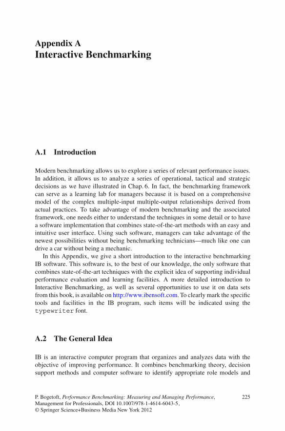
Traditional benchmarking makes use of a selection of key performance indicators.The KPI tab allows the user to explore these one by one and to also get a holisticpicture of several KPIs. This tab is illustrated in Fig. A.6.

The user can select a KPI to analyze via a scroll-down menu. It is possible toselect KPIs on which there is no data for MyUnit.

The top left table provides summary statistics for the KPI, which are selectedand displayed just above the table. The units that these summary statistics cover arethose delineated in the Potential Peers tab. If no filters have been introducedhere and if no units have been deselected in the Benchmark tab, the sampleconsists of all the units for which the data set contains information about the KPI.The summary statics provide information on

• MyUnit, i.e. value of the KPI for MyUnit.• Average value, i.e. the (un-weighted) KPI value around which actual KPIs vary.• St.Dev, i.e. the standard deviation measure of the spread in the KPIs.• Min, i.e. the minimum KPI value in the sample.• Twenty-five percent Quartile, i.e. the KPI value that 25% of the units are below

and 75% are above.• Median, i.e. the KPI value that 50% of the units are below and 50% are above.• Seventy five percent Quartile, i.e. the KPI that 75% of the units are below and

25% are above.• Max, i.e. the maximum KPI value in the sample.


Fig. A.6 Simple KPI analysis in IB

The bar chart graph below the summary statistics table displays the value of theKPI for all Potential Peers. The units are ordered such that high KPIs are to theleft and low values are to the right. MyUnit is, if there is a value for this unit,emphasized as a red bar, shown here in a darker gray.

To get an overview of several KPIs simultaneously, the user can construct aradar diagram. The dimensions in the radar are chosen sequentially by the user byselecting a KPI and then pressing Add to Radar. In each dimension, the radarthen shows not only the minimal and the maximal value of the KPI in question, butalso the average value in the sample and the value of MyUnit. The radar diagramis constructed relative to the maximal value in each dimension. Thus, a value of 0.5in a given direction means 50% of the maximal value.

The user can change the sample that is being analyzed by changing the peer groupin the upper right corner. He can also alter which firms are being displayed—andhow—in the chart graph by using drop-down menus in the lower part of the screen.

A.7 Benchmark 235

A.7 Benchmark

The Benchmark tab is the central screen in IB. It compares MyUnit against acombination of other units and allows the user to control the comparisons in anumber of ways. This tab is illustrated in Fig. A.7.

The table compares the values of MyUnit as given in the Present Valuecolumn, against the values of a combination of Potential Peers as given inBenchmark column. This is like comparing a realized account or developmentagainst a budget or a plan. The Benchmark is constructed by considering all firmsin the current Peer Group and a class of possible combinations thereof. Amongthe resulting, typically infinite number of possible comparators, the program picksthe one that offers the largest potential improvement in the performance of MyUnit.The details of the construction of the Benchmark values depend on benchmarkingcontrols, as discussed below.

The colored Performance bars illustrate the comparison of the present andbenchmark values.

• The red bars show the input side, the costs. It shows the % that theBenchmark uses of the MyUnit values. Eighty nine percent, for example, meansthat the benchmark only uses 89% of what MyUnit does. Put differently, MyUnit

Fig. A.7 Central benchmarking tab in IB


should be able to save 11% of the Present Value. Short red bars therefore indicatelarge savings potential.

• The blue bars, shown here as dark bars and with an “O” in the final columns,represent outputs. They show the percentage MyUnit has been able to produce ofthe Benchmark. A value of 94%, for example, means a 6% output expansion ispossible. Therefore, short blue bars indicate large expansion possibilities.

Observe that the savings potential and expansion possibilities are calculatedsimultaneously.

A.7.1 Improvement Directions

The central controls of the Benchmark tab are the horizontal sliders giving theDirection. They allow the user to introduce his own search direction to expresshis preferences and strategy. If he is interested in saving more on some input thananother, he can simply drag the slider of the former further to the right. Likewise,if he is interested in expanding a given output more than others, he can drags itsslider further to the right. In other words, dragging a slider to the right means thatthe user emphasizes this dimension more and looks for benchmarks that save morein this direction, if it is an input, or to expand more in this direction, if it is anoutput. Essentially, the sliders work like a generalized steering wheel of a car or likefrequency controls on an amplifier. So to speak, the user can steer the benchmark bydriving in different directions.

Instead of using the horizontal sliders, the user can also use the up and downarrows. They have the same effect but they also allow the user to go above 100 andbelow 0. Negative values mean that he is interested in spending more of an input orreducing some output. The meaning of the specific direction values are as explainedin Chaps. 2 and 6. For most users, however, the direction numbers are less important,just like one does not need to understand the detailed calibration of a car’s steeringmechanism to be an excellent driver. What it takes is primarily training and an ideaof where one wants to go. The main practical use of the direction numbers is thatthey allow a more advanced user to reconstruct a given benchmark later.

Two directions are particularly popular and simple to explain, namely: (1)proportional reduction of all inputs and (2) proportional expansion of all outputs.This corresponds to Farrell based input and output efficiencies as introduced inChap. 2. To facilitate the choice of these possibilities, IB contains dedicated buttonsInput prop. and Output prop.

A.7.2 Show and Eliminate Peers

A useful feature of the central Benchmark tab of IB is the option to show peers andto exclude some of these. Pressing Show Peers, the peers behind a constructed

A.7 Benchmark 237

benchmark become visible. The illustration of the peers contains their names, andthe relative importance of the different peers is given by numbers summing to 100.This gives a good first impression of who to learn from.

Another very useful feature is the possibility to eliminate specific peers. Thisis called picking in IB and works like this: The user can click on any of thebars showing the significance of a peer. This will eliminate it as a potential peerand the benchmark will change. If the user is interested in seeing more detailsconcerning the active peers before deciding to eliminate any, he can get full detailsfrom the Peer Units tab. The eliminated peers can be reintroduced by usingUndo picking in the Potential Peers tab as described above.

Picking away individual peers is a convenient way for the user to introduce anysoft and subjective information he may have. He may, for example, know that thedata from a given unit is uncertain or that it is run using a different managementphilosophy that cannot or will not be imitated by MyUnit.

If the user continues to eliminate peers, he will reach a point where noimprovements are possible. When this happens, the Benchmark column will showhow many extra resources are needed or how many services must be given upcompared to the best practice of the remaining units. The InEff score will inthis case become a super-efficiency score and its color will change to red. Alsothe Performance bars will get adjusted colors to make the user aware of this.If the user continues to eliminate Peers, he will eventually reach a point where nocomparisons are possible.

A.7.3 Inefficiency Step Ladder

Instead of eliminating peers one at a time, the user can also do this in an automatedway by pressing the Inefficiency Step Ladder button InESL. This will initiatea process of successive elimination of the most influential peer until no furthercomparisons are possible. The inefficiency will decline as more and more peersare eliminated. The resulting levels of inefficiency are depicted in a step function,as illustrated in Fig. A.8.

The InESL functionality is useful among others to understand the robustnessof estimated improvement potentials. If the InESL function is steep, i.e. declinesquickly, then the elimination of just a few peer units may dramatically lowerthe estimated potentials and, therefore, the initial estimate relies more heavily onthe quality of the first peers. If, on the other hand, the InESL graph is flat, theevaluations are not too dependent on exactly which units we can compare to.

A.7.4 Scale (and Estimation Principle)

The assumed returns to scale and estimation principle can be changed in the pulldown window named Scale.


Fig. A.8 Inefficiency step ladder in IB

The non-parametric options available are CRS, DRS, IRS, VRS, FDH+, and ADDor FRH like we discussed in connection with the Model tab above. Also, in caseone or more parametric models are estimated, they will be indicated as PAR.

It should be noted that when a FDH estimation is activated, it becomes possibleto make additional assumptions about local constant return to scale. This explainsthe name FDH+. The idea is that if some firm has used certain inputs to producecertain outputs, then we could also scale inputs and outputs proportionally by anyfactor in the interval from L to U. Traditional FDH, therefore, is the special casewhere L =U = 1.

The return to scale properties of PAR depends entirely on the properties of theunderlying parametric form. In general, however, it is more restricted than the DEAspecification and certainly more restricted than the FDH specification, as we havediscussed in Chap. 5

A.7.5 Efficiency or Super Efficiency

Another control in the Benchmark tab is the Efficiency pull down. There aretwo possible settings for this.

• Normal efficiency means that the evaluated unit can be compared to itself. Inthat case, it is always possible to find a benchmark at least as good as MyUnit.

• Super efficiency means that the evaluated unit cannot be compared to itself. Inthat case, we are comparing with the best practice of others only. If MyUnitis not a best practice unit, the two calculations coincide. If MyUnit is a bestpractice unit, however, it will usually not be possible to find a benchmark atleast as good as MyUnit. In such cases, the Benchmark may use more of someinput or produce less of some outputs. The interpretation is that these are theincreases in resource usage and the reductions of service provisions that MyUnitcould introduce without losing its status as a best practice unit. Therefore,Super

A.8 Peer Units 239

efficiency is a more informative measure than Normal efficiency. Moreover, thisnotion is very useful in performance-based payment schemes as we discussed inChap. 8.

A related possibility is to set the Aspiration level to match the user’s strategy.The idea is that the user can specify if he is interested in having best practicebenchmarks, or benchmarks corresponding to 10% under best practice or bestpractice plus a 2% productivity improvement, for example.

A.7.6 Exclude Slack and Outliers

The calculated Benchmark gives the maximal possibilities to improve MyUnitin the Improvement Direction chosen. In addition to improvements in theproportions specified by the Direction, there may be possibilities to make individualimprovements in some of the dimensions but not in all of the directions. To see theextra potential to improve in some directions, the user can check the ExSlack box.This will, if possible, determine a new Benchmark that uses the same or fewerinputs and produces the same or more outputs than the original benchmark.

If the analyses of a pre-defined model suggest that some of the observationsare likely outliers, the likely outliers for the given model can be listed in the datafile. When calculating the Benchmark, the user can then choose if he wants toexclude or include the likely outliers. The default setting is that potential outliersare excluded, and the ExOutliers check box is, therefore, checked by default.

A.7.7 Generate a Report

When the user has found an interesting benchmark, he can make a report torecord the comparisons and to generate a convenient presentation of his findings.The Add report feature can be used repeatedly changing for example theDirection or Scale assumptions in the Benchmark tab. Once the user hasadded at least one report, the Reports tab becomes active. It keeps the reports onfile for later printing or editing, as discussed below. Similar reporting capabilitiesare available in the KPI and Sector tabs.

A.8 Peer Units

The Peer Units tab provides additional information about the calculated Bench-mark. Here, the user can see the active peer units, i.e. the firms that MyUnit iscompared to, their relative importance, and all the available information about those


units. Besides the inputs and outputs used in the calculations, this includes all theRead-only and Locked information from the data set.

The additional information is useful to guide and refine the benchmarking via aniterative process.

The information can also contain links to contacts and additional information,e.g. to the peer units’ homepages, the names of CEOs, CFOs, and so on.

A.9 Sector Analysis

In the Sector tab, the user can supplement the analysis of his primary unit,MyUnit, with a parallel analysis of all the units in the data set. This is relevantfor putting the analysis of MyUnit into perspective as well as for evaluating theModel.

More specifically, this tab allows the user to

• Generate the inefficiencies for all the units in the sector under some commonassumptions.

• Save the results in an Excel file.• Illustrate the results in five different graph types, namely Density, Dist-ribution, Sorted InEff, Impact, and Second stage, with addi-tional individual options.

Hence, using Sector, the user can evaluate not only how well his own firm isdoing but also how well everyone else is doing.

The Sector tab with a Density graph is illustrated in Fig. A.9.Density is a simple histogram showing the relative frequency of inefficiency

scores within different intervals. By clicking on one of the bars, the user obtainsthe list of units with their corresponding inefficiency values. The red bar containsMyUnit.Distribution is a usual cumulative distribution of the inefficiencies. The

unit of interest, MyUnit, is marked by a red dot. It is therefore easy to see whichperformance fractile MyUnit belongs to.Sorted InEff simply illustrates the inefficiencies in the different firms in a

bar diagram with the largest inefficiencies first and MyUnit marked in red.Impact diagrams, often referred to as Salter diagrams, plot inefficiency on the

vertical axis, and the individual firms are represented by columns, the horizontalwidth of which is proportional to one of the variables in the data set. The choiceof variable for the horizontal axis is left to the user. MyUnit is represented bya red dot. The diagram is useful to get an idea of the sector-wide losses becauseinefficiency in large units is represented by wider bars. In this way, the total area ofthe bars is proportional to social losses.

The Second stage graph plots inefficiencies against the other availablevariables. The user can choose which variable to plot against. The plot gives an

A.10 Dynamics 241

Fig. A.9 Sector analysis in IB with density graph

idea of omitted variables that may have a systematic impact on inefficiency. Suchvariables can then be included in the Model. The Second stage graph can alsobe used to (roughly) correct the inefficiencies for such omissions as well as forcomplicating or facilitating factors that can not naturally be treated as outputs orinputs, e.g. quality variables as we discussed in Chap. 6. If there is a clear upwardtrend, for example, it suggests that units (firms) with large values of the variableon the horizontal axis cannot be expected to be as efficient as the units with smallvalues of this variable.

A.10 Dynamics

The Dynamic tab, as illustrated in Fig. A.10, allows analysis of performancechanges over time. The tab becomes available whenever there are data from severalperiods. The user can here calculate Malmquist productivity indices and theirdecomposition in Frontier Shift and Catch-Up both for the industry in general andfor the individual firms. Different graphical illustrations are also supported.


Fig. A.10 Dynamic analysis in IB

A.11 Reports

The Reports tab contains references to the reports generated in the KPI, theBenchmark, and the Sector Analysis tabs. The Reports tab is illustratedin Fig. A.11.

The report file format, font and language can be changed to fit the user. The 2012version of IB supports English, German, Dutch and Danish reports.

The automatically generated reports are written as stand-alone reports containingspecific results from the analysis as well as information on how to interpret theresults.

A.12 Bibliographic Notes

More information on IB is available on www.ibensoft.com. Here, visitors can alsotry Interactive Benchmarking IB on several data sets similar to the ones analyzed inthis book.

www.ibensoft.com

A.12 Bibliographic Notes 243

Fig. A.11 Automated reports in IB

The theory behind Interactive Benchmarking is covered in Bogetoft and Nielsen(2005) and Bogetoft et al. (2006a). A more technical discussion of benchmarkingtechniques in general is Bogetoft and Otto (2011). Detailed information on theunderlying programs is provided in Ibensoft (2010b) and Ibensoft (2010a).

References

Afriat SN (1972) Efficiency estimation of production functions. Int Econ Rev 13:568–598Agrell PJ, Bogetoft P (2000) Ekonomisk natbesiktning. Final report stem. Technical report,

SUMICSID AB (In Swedish)Agrell PJ, Bogetoft P (2001a) Incentive regulation. Working PaperAgrell PJ, Bogetoft P (2001b) Should health regulators use DEA? In: Fidalgo Eea (ed) Coordina-

cion e Incentivos en Sanidad, Asociasion de Economia de la Salud, Barcelona, pp.133–154Agrell PJ, Bogetoft P (2003) Norm models. Consultation report, Norwegian Water Resources and

Energy Directorate (NVE)Agrell PJ, Bogetoft P (2004) Nve network cost efficiency model. Technical report, Norwegian

Energy Directorate NVEAgrell P, Bogetoft P (2007) Development of benchmarking models for German electricity and gas

distribution. Consultation report, Bundesnetzagentur, Bonn, GermanyAgrell PJ, Bogetoft P (2008) Electricity and gas dso benchmarking whitepaper. Consulation report,

BundesnetzagenturAgrell P, Bogetoft P (2009) International benchmarking of electricity transmission system

operators - e3grid project. Consultation report, open version, Council of European EnergyRegulators

Agrell PJ, Bogetoft P (2010a) Benchmarking of german gas transmission system operators.Consultation report, Bundesnetzagentur (BNetzA)

Agrell PJ, Bogetoft P (2010b) A primer on regulation and benchmarking with examples fromnetwork industries. Technical Report version 05, SUMICSID AB

Agrell PJ, Tind J (2001) A dual approach to noconvex frontier models. J Productivity Anal16:129–147

Agrell PJ, Bogetoft P, Tind J (2002) Incentive plans for productive efficiency, innovation andlearning. Int J Prod Econ 78:1–11

Agrell PJ, Bogetoft P, Bjørndalen J, Vanhanen J, Syrjanen M (2005a) Nemesys subproject A:system analysis. Consultation report, Nordenergi

Agrell PJ, Bogetoft P, Tind J (2005b) Dea and dynamic yardstick competition in scandinavianelectricity distribution. J Productivity Anal 23:173–201

Agrell P, Bogetoft P, Halbersma R, Mikkers M (2007) Yardstick competition for multi-producthospitals. NZa Research Paper 2007/1, NZa, Netherlands

Agrell PJ, Bogetoft P, Cullmann A, von Hirschhausen C, Neumann A, Walter M (2008) Ergeb-nisdokumentation: Bestimmung der effizienzwerte verteilernetzbetreiber strom. Consultationreport, Bundesnetzagentur

Aigner DJ, Chu SF (1968) On estimating the industry production function. Am Econ Rev58:826–839


245

246 References

Aigner DJ, Lovell CAK, Schmidt P (1977) Formulation and estimation of stochastic frontierproduction function models. J Econom 6:21–37

Andersen J, Bogetoft P (2007) Gains from quota trade: theoretical models and an application tothe Danish fishery. Eur Rev Agric Econ 34(1):105–127

Andersen P, Petersen NC (1993) A procedure for ranking efficient units in data envelopmentanalysis. Manag Sci 39(10):1261–1264

APQC (2011) American productivity and quality center. URL http://www.apqc.org/Asmild M, Bogetoft P, Hougaard JL (2013) Rationalising inefficiency: a study of Canadian bank

branches. Omega 41:80–87Banker RD (1980) A game theoretic approach to measuring efficiency. Eur J Oper Res 5:262–268Banker RD (1984) Estimating most productive scale size using data envelopment analysis. Eur J

Oper Res 17(1):35–54Banker RD, Morey RC (1986) Efficiency analysis for exogenously fixed inputs and outputs. Oper

Res 34(4):513–521Banker RD, Thrall R (1992) Estimation of returns to scale using data envelopment analysis. Eur J

Oper Res 62:74–84Banker RD, Charnes A, Cooper WW (1984) Some models for estimating technical and scale

inefficiencies in data envelopment analysis. Manag Sci 30:1078–1092Banker RD, Charnes A, Cooper WW, Clarke R (1989) Constrained game formulations and

interpretations for data envelopment analysis. Eur J Oper Res 40:299–308Battese G, Coelli T (1992) Frontier production functions, technical efficiency and panel data: with

application to paddy farmers in India. J Productivity Anal 3:153–169Bogetoft P (1986) An efficiency evaluation of Danish police stations (In Danish). Technical reportBogetoft P (1990) Strategic responses to dea-control - a game theoretical analysis. Technical report,

Copenhagen Business SchoolBogetoft P (1994a) Incentive efficient production frontiers: an agency perspective on DEA. Manag

Sci 40:959–968Bogetoft P (1994b) Non-cooperative planning theory. Springer, BerlinBogetoft P (1995) Incentives and productivity measurements. Int J Prod Econ 39:67–81Bogetoft P (1996) DEA on relaxed convexity assumptions. Manag Sci 42:457–465Bogetoft P (1997) DEA-based yardstick competition: the optimality of best practice regulation.

Ann Oper Res 73:277–298Bogetoft P (2000) DEA and activity planning under asymmetric information. J Productivity Anal

13:7–48Bogetoft P, Gammeltvedt TE (2006) Mergers in norwegian electricity distribution: a cost saving

exercise? Working paper, NVE, NorwayBogetoft P, Hougaard JL (2003) Rational inefficiencies. J Productivity Anal 20:243–271Bogetoft P, Katona K (2008) Efficiency gains from mergers in the healthcare sector. Technical

report, Nederlandse Zorgautoriteit NZABogetoft P, Nielsen K (2004) Monitoring farm, herd and cow performance - efficiency analyses.

Technical report, Royal Agricultural University and www.kv\OT1\aegforskning.dkBogetoft P, Nielsen K (2005) Internet based benchmarking. J Group Decis Negotiation

14(3):195–215Bogetoft P, Nielsen K (2008) DEA based auctions. Eur J Oper Res 184:685–700Bogetoft P, Nielsen K (2012) Efficient and confidential reallocation of contracts: how the Danish

sugar industry adapted to the new sugar regime. J Business Econ ZfB 81(2):165–180Bogetoft P, Otto L (2011) Benchmarking with DEA, SFA, and R. Springer, New YorkBogetoft P, Pruzan P (1991) Planning with multiple criteria, 1st edn. North-Holland, AmsterdamBogetoft P, Wang D (2005) Estimating the potential gains from mergers. J Productivity Anal

23:145–171Bogetoft P, Wittrup J (2011) Productivity and education: benchmarking of elementary school in

denmark. Nordic Econ Policy Rev 2:257–294Bogetoft P, Tama J, Tind J (2000) Convex input and output projections of nonconvex production

possibility sets. Manag Sci 46:858–869

http://www.apqc.org/

www.kvOT1ae gforskning.dk

References 247

Bogetoft P, Strange N, Thorsen BJ (2003) Efficiency and merger gains in the Danish forestryextension service. Forest Sci 49(4):585–595

Bogetoft P, Fried H, Eeckaut PV (2004) Power benchmarking: what’s wrong with traditionalbenchmarking and how to do it right. Technical report, Credit Union Research and Advice,Credit Union National Association, http://thepoint.cuna.org/

Bogetoft P, Bramsen JM, Nielsen K (2006a) Balanced benchmarking. Int J Bus Perform Manag8(4):274–289

Bogetoft P, Fare R, Obel B (2006b) Allocative efficiency of technically inefficient production units.Eur J Oper Res 168(2):450–462

Bogetoft P, Boye K, Neergaard-Petersen H, Nielsen K (2007a) Reallocating sugar beet contracts:can sugar production survive in Denmark. Eur Rev Agric Econ 34(1):1–20

Bogetoft P, Fried H, Eeckaut PV (2007b) The university benchmarker: an interactive computerapproach. In: Bonaccorsi A, Daraio C (eds) Universities And Strategic Knowledge Creation,Chap 14. Edward Elgar Publishing, Cheltenham, Northampton

Bogetoft P, Christensen D, Damgard I, Geisler M, Jakobsen T, Krøigaard M, Nielsen J, NielsenJ, Nielsen K, Pagter J, et al. (2009) Secure multiparty computation goes live. Financialcryptography and data security. Springer, Berlin, pp. 325–343

Bogetoft P, Kristensen T, Pedersen KM (2010) Potential gains from hospital mergers in Denmark.Health Care Manag Sci Energy Policy, 30(8):637-647

Bowlin W (1997) A proposal for designing employment contracts for government managers.Socioecon Plann Sci 31:205–216

Brannlund R, Fare R, Grosskopf S (1995) Environmental regulation and profitability: an applica-tion to Swedish pulp and paper mills. Environ Resour Econ 6(1):23–36

Brannlund R, Chung Y, Fare R, Grosskopf S (1998) Emissions trading and profitability: theSwedish pulp and paper industry. Environ Resour Econ 12:345–356

Bundesnetzagentur (2007) Bericht der bundesnetzagentur nach § 112a enwg zur einfuhrung deranreizregulierung nach § 21a enwg. Report, Bundesnetzagentur

Caves DW, Christensen LR, Diewert WE (1982) The economic theory of index numbers and themeasurement of input, output, and productivity. Econometrica 50(6):1393–1414

Chambers RG (1988) Applied production analysis: a dual approach. Cambridge University Press,Cambridge

Chambers RG, Chung Y, Fare R (1998) Profit, directional distance functions, and nerlovianefficiency. J Optim Theory Appl 2:351–364

Chang KP (1999) Measuring efficiency with quasiconcave production frontiers. Eur J Oper Res115:497–506

Chang K, Guh Y (1991) Linear production functions and the data envelopment analysis. Eur JOper Res 52:215–233

Charnes A, Cooper WW, Rhodes E (1978) Measuring the efficiency of decision making units. EurJ Oper Res 2:429–444

Charnes A, Cooper WW, Rhodes E (1979) Short communication: measuring the efficiency ofdecision making units. Eur J Oper Res 3:339

Charnes A, Cooper WW, Lewin AY, Seiford LM (1995) Data envelopment analysis: theory,methodology and applications. Kluwer, Boston

Charnes A, Cooper WW, Wei QL, Huang ZM (1989) Cone ratio data envelopment analysis andmulti-objective programming. Int J Syst Sci 20:1099–1118

Che YK (1993) Design competition through multidimensional auctions. RAND J Econ24(4):668–680

Christensen LR, Jorgenson DW, Lau LJ (1973) Transcendental logarithmic production frontiers.Rev Econ Stat 55:28–45

Coelli T, Prasada Rao DS, Battese G (1998) An introduction to efficiency and productivity analysis.Kluwer, Boston

Coelli T, Estache A, Perelman S, Trujillo L (2003) A primer on efficiency measurement for utilitiesand transport regulators. Technical Report 129, World Bank Publications

Cooper WW, Seiford LM, Tone K (2000) Data envelopment analysis. Kluwer, Boston

http://thepoint.cuna.org/

248 References

Cooper WW, Seiford LM, Tone K (2007) Data envelopment analysis: a comprehensive text withmodels, applications, references and DEA-solver software, 2nd edn. Springer, Secaucus

Cox D, Hinkley D (1974) Theoretical statistics. Chapman and Hall, LondonCUNA CUNA (2010) Cub. URL http://advice.cuna.org/cu benchmarker.htmlDalen DM (1996) Strategic responses to relative evaluation of bureaus: implication for bureaucratic

slack. J Productivity Anal 7:29–39Dalen DM, Gomez-Lobo A (1997) Estimating cost functions in regulated industries under

asymmetric information. Eur Econ Rev 31:935–942Dalen DM, Gomez-Lobo A (2001) Yardstick on the road: regulatory contracts and cost efficiency

in the Norwegian bus industry. Working Paper, Norwegian School of ManagementDebreu G (1951) The coefficient of resource utilization. Econometrica 19(3):273–292Demsetz H (1968) Why regulate utilities? J Law Econ 11(1):55-65Denrell J (2005) Selection bias and the perils of benchmarking. Harvard Bus Rev 83(4):114–119Deprins D, Simar L, Tulkens H (1984) Measuring labor efficiency in post offices. Technical report.

In: Marchand M, Pestieau P, Tulkens H (eds) The performance of public enterprises: conceptsand measurements. North Holland, Amsterdam, pp. 243–267

Dorfman R, Samuelson P, Solow R (1958) Linear programming and economic analysis. McGraw-Hill, New York

Eldenburg LG, Wolcott SK (2005) Cost management - measuring, monitoring, and motivatingperformance. Wiley, New York

Farrell MJ (1957) The measurement of productive efficiency. J Royal Stat Soc 120:253–281Fare R, Grosskopf S (2000) Network DEA. Socioecon Plann Sci 34:35–49Fare R, Primont D (1995) Multi-output production and duality: theory and applications. Kluwer,

BostonFare R, Grosskopf S, Lovell CAK, Yaisawatng S (1993) Derivation of shadow prices for

undesirable outputs: a distance function approach. Rev Econ Stat 75:374–380Fare R, Grosskopf S, Lindgren B, Ross P (1994) Productivity development in swedish hopsitals:

a malmquist output index approach. In: Data envelopment analysis: theory, methodology, andapplication, Chap 13. Kluwer, Boston, pp 253–272

Fare R, Grosskopf S, Lundstrom M, Roos P (2007) Evaluating health care efficiency. ScientificReport 1: 2007, R. R., Institute of Applied Economics

Fethi M, Jackson PM, Weyman-Jones TG (2001) European airlines: a stochastic dea study ofefficiency with market liberalisation. Technical report, University of Leicester Efficiency andProductivity Research Unit

Forsund F, Hjalmarsson L (1979) Generalized farrell measures of efficiency: an application to milkprocessing in Swedish dairy plants. Econ J 89:294–315

Førsund F, Kittelsen S (1998) Productivity development of Norwegian electricity distributionutilities. Resour Energy Econ 20:207–224

Fox KJ (1999) Efficiency at different levels of aggregation: public vs. private sector firms. EconLett 65:173176

Gale D (1960) The theory of linear economic models. McGraw-Hill, New YorkGovernment TF (2007) Verordnung zum erlass und zur anderung von rechtsvorschriften auf dem

gebiet der energieregulierung. Germany Teil I Nr. 55, BundesgesetzblattGreene W (2008) Econometric analysis, 6th edn. Pearson Prentice Hall, Upper Saddle RiverGreene WH (1990) A gamma-distributed stochastic frontier model. J Econom 46:141–164Hadley G (1962) Linear programming. Addison Wesley, ReadingHillier FS, Lieberman GJ (2010) Introduction to operations research, 9th edn. McGraw-Hill, New

YorkIbensoft (2010a) User guide to administration module of interactive benchmarking ib. Technical

report, Ibensoft ApSIbensoft (2010b) User guide to interactive benchmarking ib. Technical report, Ibensoft ApSJacobs R, Smith PC, Street A (2006) Measuring efficiency in health care. Cambrigde University

Press, CambridgeKoopmans T (1951) Activity analysis of production and allocation. Wiley, New York

http://advice.cuna.org/cu_benchmarker.html

References 249

Kumbhakar SC, Lovel CAK (2000) Stochastic frontier analysis. Cambridge University Press,Cambridge

Kuosmanen T (2001) Dea with efficiency classification preserving conditional convexity. Eur JOper Res 132:83–99

Kuosmanen T (2003) Duality theory of non-convex technologies. J Productivity Anal 20:273–304Laffont JJ, Tirole J (1993) A theory of incentives in procurement and regulation. MIT Press,

CambridgeLangset T (2009) Rundskriv eø 4/2009 om beregning av inntektsrammer og kostnadsnorm for

2010. (In Norwegian) NVE 2009 04925-4, The Norwegian Water Resources and EnergyDirectorate (NVE)

Land KC, Lovel CAK, Thore S (1993) Chance-constrained data envelopment analysis. ManagerialDecis Econ 14:541–554

Lazear E, Rosen S (1981) Rank-order tournaments as optimum labor contracts. J Political Econ89:841–864

Lehmann EL (1983) Theory of point estimation. Wiley, New YorkLewin A, Morey RC (1981) Measuring the relative efficiency and output potential of public sector

organizations: an application of data envelopment analysis. J Policy Anal Inf Syst 5:267–285Littlechild S (1983) Regulation of british telecommunications’ profitability: report to the secretary

of state. Technical report, Department of Industry, LondonLovell CAK (1993) Production frontiers and productive efficiency. In: Fried H, Lovell CAK,

Schmidt S (eds) The measurement of productive efficiency: techniques and applications.Oxford University Press, New York

Luenberger DG (1984) Linear and nonlinear programming, 2nd edn. Addison-Wesley, ReadingLuenberger D (1992) Benefit functions and duality. J Math Econ 21:461–481Malmquist S (1953) Index numbers and indifference curves. Trabajos de Estatistica 4:209–242Nalebuff BJ, Stiglitz JE (1983) Prizes and incentives: towards a general theory of compensation

and competition. Bell J Econ 14:21–43OECD (2006) Health care quality indicators project conceptual framework paper. Technical report,

OECD Health Working PapersOlesen O, Petersen NC (1995) Chance constrained efficiency evaluation. Manag Sci 41(3):442–457Olesen O, Petersen NC (2002) The use of data envelopment analysis with probabilistic assurance

regions for measuring hospital efficiency. J Productivity Anal 17:83–109Olesen OB, Petersen NC (2007) Target and technical efficiency in dea – controlling for environ-

mental characteristics. Working Paper, the University of Southern DenmarkParadi JC, Vela S, Yang Z (2004) Assessing bank and bank branch performance: modeling

considerations and approaches. In: Cooper WW, Seiford LM, Zhu J (eds) Handbook on dataenvelopment analysis. Kluwer, Boston

Petersen N (1990) Data envelopment analysis on a relaxed set of assumptions. Manag Sci36(3):305–314

Post GT (2001) Estimating non-convex production sets using transconcave dea. Eur J Oper Res131:132–142

Rao CR (1973) Linear statistical inference and its applications, 2nd edn. Wiley, New YorkResende M (2001) Relative efficiency measurement and prospects for yardstick competition in

brazilian electricity distribution. Energy Policy (In Press)Richmond J (1974) Estimating the efficiency of production. Int Econ Rev 15:515–521Rigby DK (2011a) Management tools 2011 - an executive’s guide. Technical report, Bain &

Company IncRigby DK (2011b) Management tools and trends 2011. Technical report, Bain & Company IncRigsrevisionen (2000) Report to the state auditors on court productivity etc. (In: Danish:beretning

til statsrevisorerne om retternes produktivitet mv.). Technical report, Danish Auditor General‘sOffice

Ruggiero J (1996) On the measurement of technical efficiency in the public sector. Eur J Oper Res90:553–565

250 References

Seiford LM (1994) A dea bibliography (1978–1992). In: Charnes A, Cooper W, Lewin A (eds) Dataenvelopment analysis: theory, methodology, and application, Kluwer, Boston, pp. 437–469

Shephard RW (1953) Cost and production functions. Princeton University Press, Princeton,reprinted as Lecture Notes in Economics and Mathematical Systems, 1st edn, vol. 194(Springer, Berlin, 1981)

Shephard RW (1970) Theory of cost and production functions. Princeton University Press,Princeton

Sheriff G (2001) Using data envelopment analysis to design contracts under asymmetric informa-tion. Technical report, University of Maryland

Shleifer A (1985) A theory of yardstick competition. Rand J Econ 16:319–327Silvey SD (1970) Statistical inference. Chapmann and Hall, London (reprinted with corrections

1975)Smith P (1976) On the statistical estimation of parametric frontier production functions. Rev Econ

Stat 58:238–239Tavaras G (2002) A bibliography of data envelopment analysis (1978–2001). Technical report,

Rutgers Centre of Operations ResearchThanassoulis E (2000) DEA and its use in the regulation of water companies. Eur J Oper Res

127:1–13Thanassoulis E, Portela M, Allen R (2004) Handbook on data envelopment analysis, Kluwer,

Dodrecht, Ch 4 Incorporating Value Judgements in DEA, pp. 99–138Tirole J (1988) The theory of industrial organization. MIT Press, CambridgeTulkens H (1993) On fdh efficiency analysis: some methodological issues and applications to retail

banking, courts and urban transit. J Productivity Anal 4:183–210Varian HR (1992) Microeconomic analysis, 3rd edn. Norton, New YorkWalter M, Cullmann A (2008) Potential gains from mergers in local public transport – an efficiency

analysis applied to germany. Technical report, Technische Universitat DresdenWunsch P (1995) Peer comparison and regulation: an application to urban mass transit firms in

europe. PhD thesis, Department of Economics, UniversitE Catholique de Louvain, p 182

Index

Aacronyms, list of, xixactivity analysis, 81additivity, 65adjusted relative residual, 114adverse selection, 195, 213aggregation, 7allocative efficiency AE, 33, 37, 38application

Canadian bank branches, 55Danish banks, 55Danish bulls, 57Danish courts, 55Danish extension offices, 54Danish hospitals, 186Danish industries, 109Danish police, 55Danish schools, 55, 85, 147Danish sugar beet farmers, 53DSO, 187DSO regulation, 42, 75, 76, 203, 216electricity networks, 18fishery, 31German transport, 56health care, 44hospital, 122, 181partial weights in regulation, 98sugar beets, 17universities, 60US Credit Union, 59waterworks, 15, 31, 66, 79

aspiration, 137assurance region, 93

numerical example, 95asymmetric information, 17, 18auction

second score, 219

BBalanced Scorecards BSC, 130bank branches, 55banks, 55Benchmark, 235benchmarking, 1, 7, 13, 14

inter-organizational, 14interactive, 15intra-organizational, 14learning lab, 127longitudinal, 14model development, 206panel, 14R package, 19relative performance evaluation, 14traditional, 1

Benefit-Cost Advantage, 91Benefit-Cost Ratio, 89best practice, 10bias correction, 99bidding, 218budget, 128, 132

benchmarking based, 133flexible, 133objectives, 138responsibility, 134variance, 133

bulls, 57

Ccatch-up, 41cautious estimate, 72circular test, 41Cobb-Douglas, 180COLS, 11, 115comparative advantage, 144


251

252 Index

Completeness, 51conservative estimate, 72constant returns to scale, 4, 64contextual variables, 50controllability, 44, 188controllable resources, 188convex combination, 61convex hull, 62convexity, 61

pros and cons, 62coordination, 16Corrected Ordinary Least Squares (COLS), 11cost accounting, 133cost efficiency, 33, 34

decomposition, 35cost function, 5, 119, 120cost-benefit analysis, 90Cost-Benefit Ratio, 90cost-recovery regulation, 197courts, 55CPI-X regulation, 198credit union, 59crs, 64

DDANVA, 15data, 49Data Envelopment Analysis (DEA), 11data generation process, 112DEA, 11

assumptions, 73auction, 218comparison of DEA models, 75game problem, 91illustration of technologies, 74incentives, 209maximin program, 91models, 73pros and cons, 13

DEA models, 73DEA-based auction, 218DEA-based yardstick competition, 214dedication, vdegree of freedom, 52density, 240deterministic models, 11directional distance, 29, 129Directional distance function, 236discretionary resources, 188disintegration gains, 190distance function, 121distribution, 240distribution system operator DSO, 18, 42, 187

dominance, 15drs, 64dual program, 144dynamic efficiency, 39dynamic incentives, 215

EE Farrell input efficiency, 9e3GRID, 98EC efficiency change EC, 41effectiveness, 7, 99efficiency, 6, 25

allocative, 33, 37, 38bias, 99choice between measures, 44cost, 33, 34directional, 29directional distance function, 129dynamic, 39Farrell input, 9Farrell output, 10hyper, 87input, 26Koopmans, 25Malmquist, 39measures, 23merger, 44network, 43non-discretionary, 29numerical example, 27output, 26profit, 38revenue, 37scale, 83, 149structural, 16, 43, 149, 217sub-vector, 29super, 86theoretical foundation, 25with prices, 33

efficiency scoreuse of, 45

efficient firm, 25electricity network, 18engineering approach, 12excess function, 30extension offices, 54

FFarrell, 9, 10Farrell input efficiency, 26Farrell measures, 9Farrell output efficiency, 10, 26

Index 253

FDH, 58firm, 14

for-profit, 14non-profit, 14

fishery, 31Fox’s Paradox, 4franchise auction, 201free disposability, 57free disposable hull, 58frontier models, 10

Ggeneral setting, 49German DSO regulation, 203German electricity DSO model, 208German expansion factor, 205German revenue-cap formula, 204

Hheteroscedasticity, 208horizontal integration, 165hospital, 44, 122, 181hospitals, 186

IIB, 225

Benchmark, 235density, 240Direction, 236distribution, 240Dynamics, 241Impact, 240Inefficiency step ladder, 237KPI, 233merge, 231Model, 227Outlier, 239Peer units, 239Peers, 236Potential Peers, 231Report, 242report, 239Returns to scale, 229RTS, 237second stage, 240Sector analysis, 240Slack, 239Super efficiency, 238

IBEN, 15, 31Impact graph, 240incentive problem, 17

incentives, 209adverse selection, 195, 213auctions, 218dynamic, 215moral hazard, 195participation, 195risk aversion, 212super-efficiency, 211

Independence, 52indifference curve, 7individually rational, 73inefficiency, 5InEfficiency Step Ladder IESL, 237inner approximation, 72input, 50input efficiency, 26interactive benchmarking, 15, 31, 129Interactive Benchmarking IB, 225irs, 65isoquant, 6

KKey Performance Indicators KPI

implicit assumptions, 3Key Performance Indicators KPIs, 2Koopmans efficiency, 25KPI, 233

Llearning, 15learning lab, 127log-linear, 122

MMalmquist, 241

decomposition, 41efficiency, 39numerical example, 42

marginal costs, 152marginal products, 152maximum likelihood principle, 111merger, 44, 163, 231

basic decomposition, 170, 172basic idea, 166cost model, 172disintegration gains, 190distribution system operators DSOs, 187DSO regulation, 217horizontal, 165hospitals, 181, 186learning, 171

254 Index

merger (cont.)learning effect, 169numerical example, 173organizational restructuring, 174overall gains, 167parametric model, 180restricted controllability, 188restricted transferability, 188scale, size effect, 170, 172scope, harmony effect, 169, 171sub-vector, 188

minimal extrapolationprinciple, 12, 72

moral hazard, 195, 212most productive scale size MPSS, 83motivation, 17multi criteria decision making MCDM, 94

NNash equilibrium NE, 212ndrs, 65netvolume, 98network efficiency, 43nirs, 64non-discretionary variables, 29Non-redundancy, 52nonparametric models, 11Norwegian Water Resources and Energy

Directorate NVE, 216notation, 49

OOperationally, 52Ordinary Least Square (OLS), 114organizational restructuring, 174organizational structure, 149Outlier, 239outlier, 206outliers

super-efficiency, 206output, 50output efficiency, 26overall gains from merger, 167

Pparametric functions, 104

Cobb-Douglas, 107Linear, 105

parametric models, 11partial evaluations, 4

partial value information, 93participation, 195peers, 15, 77, 140

maximal numbers of, 78police, 55price-cap regulation, 198production account, 24production function, 104production plan, 23production record, 24profit efficiency, 38public transport, 56

Qquality, 154

Rranking

partial, 25rate-of-substitution, 105rates of technical substitution, 94rational ideal evaluation, 6rational inefficiency, 211reallocation

application to sugar beets, 17reference unit, 77regulation, 18, 42, 73, 195

franchise auction, 201price-cap, revenue-cap, CPI-X, 198yardstick, 200best of four model, 205classical regulations, 196cost-recovery, 197European DSO, 202ex ante, 199ex post, 201German DSO, 203Norway, 216outlier, 206Swedish DSOs, 76

relative residual, 114Relevance, 51replicative, 65residual, 113

adjusted relative, 114relative, 114

restricted constant return to scale, 66Returns to scale, 237revenue efficiency, 37revenue-cap regulation, 198risk-aversion, 212

Index 255

SSalter diagram, 240scale efficiency SE, 83schools, 55, 147SE, 83second score auction, 219second stage, 240second-stage analysis, 142, 159selection bias, 143sensitivity analysis, 99SFA, 11

distance functions, 121cost function, 119input distance function, 121pros and cons, 13

Slack, 239software, 19, 80sourcing

insource, 153outsource, 153

stochastic cost function, 119Stochastic Data Envelopment Analysis

(SDEA), 11Stochastic Frontier Analysis SFA, 11stochastic models, 11strategic planning, 128strategic position, 146strategy, 128structural efficiency, 16, 43, 217sub-vector efficiency, 29, 188sugar beet farmers, 53sugar beets, 17Super efficiency, 238

super-efficiency, 86incentives, 211regulation, 86

symbols, list of, xixsystems view, 8

Ttaxonomy, 11technical change TC, 40technology set, 10traditional benchmarking, 1transferability, 188translog, 122

Uuniversity, 60

Vvalue for money, 99

Wwaterworks, 15, 31weight restrictions, 93What-if analysis, 127

Yyardstick regulation, 200

appendix a interactive benchmarking - springer978-1-4614-6043-5/1.pdfto take advantage of modern...

Documents