appendix a. lorentz invariant distributions - home - springer978-3-662-03245-9/1.pdf · appendix a....
TRANSCRIPT

Appendix A. Lorentz Invariant Distributions
Theorem. There are precisely two, linearly indendent, Lorentz invariant distributions Ai (z; m) which obey the Klein-Gordon equation for mass m. These are
A (z. m) . i fd 3 k (e - ikz eikz) LlO , .= - (2n)3 2Wk -, (A.l)
1 fd 3 k 'k 'k A (z'm)'= - -(e-· z +e Z) 1 , . (2n)3 2Wk ' (A.2)
with W k == kO = Jk 2 + m2 • These distributions have the following properties:
(i) {D +m2 }A;(z;m)=0, i = 0,1, (A.3)
(ii) Ao(zO = 0, Z; m) = 0, (A.4a)
(iii) a~oAo(Z;mt~o = - J(z), (A.4b)
(iv) Ao( -z;m)= -Ao(z;m), Ai (- z;m) = Ai (z;m), (A.5)
(v) Ao(z;m) = ° for Z2 < 0. (A.6)
Note, however, that Ai (z; m) does not vanish for spacelike argument, Z2 < O.
Proof Part (i) is obvious because Ai are linear superpositions of exponentials which satisfy the Klein-Gordon equation. Part (ii) is also obvious by noting that, with ZO = 0, the integrand is an odd function. Part (iii) gives minus the sum of the integrals J d3 k exp {± ik'z} divided by 2(2n)3. This is a representation of the three-dimensional delta distribution. Part (iv) is again obvious by noting that the integrand in (A.l) is antisymmetric while that in (A.2) symmetric when z is replaced by - z.
To prove (v) we first note that Ao, (A.1), can also be written as
Ao(z;m) = - (2~)3 f d4 qe-iqzJ (q2 -m2)e(qO), (A. 7)
where e(qO) = qO/lqOI is the sign of the time component of the four-vector q. Note that unlike the variable k in (A.l) and (A.2), the four-vector q is unconstrained, i.e. has four independent components. That (A.7) and (A.1) represent

Appendix A 453
the same distribution is seen by using the equality
b(q2 - m2) = b((qO)2 - (q2 + m2)) = 2~O {b(qO - J q2 + m2) + b(qO + J qO + m2)}
and by doing the integral over the variable qQ. This gives (A.I) with k = q,
kO == w k = J q2 + m2. Now, for time-like z, i.e. for Z2 > 0, both Z2 and the sign of zo, sign ZO are Lorentz invariants. Thus, for time-like arguments the distribution ~O, being itself Lorentz invariant, must be a funtion of Z2 and of sign zoo This is in accord with the antisymmetry noted in the first equation (A.5). For space-like arguments, however, the distinction between positive and negative values of ZO is not Lorentz invariant. Therefore, for space-like z the distribution ~o is a function of the invariant Z2 only. From this observation one concludes that
~(-z;m)= +~(z;m).
As this is in contradiction with the anti symmetry (A.5), we conclude that part (v) of the theorem is true. Regarding the distribution ~1 we note that this argument does not hold: Indeed, ~1 is symmetric under the transformation Zf---> - z, and, hence, does not vanish for space-like z.

Appendix B. S-Matrix, Cross Sections, Decay Probabilities
Write the scattering matrix (somewhat symbolically) as
(B.l)
where f and i are asymptotic free states. bfi means "no scattering" and Rfi is the reaction matrix proper. Rfi necessarily contains a b-distribution expressing conservation of total energy and momentum. Besides this distribution it is convenient to take out a factor i (2n)4 and to define the T-matrix by (Sect. 6.1.3),
Rfi = i (2n)4 b(Pf - Pi) Tr;. (B.2)
The differential cross section for the reaction
a+ b-d +2+ ... +N
(all particles being described asymptotically by plane waves), is given by the general expression
(B.3)
In this expression
Ea = Jia)2 + m;, Eb = Jib)2 + m~, E = -jp(n)2 + m2 . n n'
N
P; = pta) + p(b), Pf = L pIn), n=l
and IVabl is the relative velocity of the incoming particles, d 3 pIn) /2En is the Lorentz invariant volume element in the phase space of particle number n. This term as well as the incoming flux factor in the first denominator is in accord with our covariant normalization (P'lp) = 2Ep b(p' - p). Formula (B.3) holds in all systems of reference where the momenta i a) and i b) are collinear (e.g. the laboratory and centre-of-mass systems). It can be extended to any system by replacing the flux factor (so-called M~ller factor) with the invariant on the r.h.s. of the following equation:
(BA)

Appendix B 455
(One should verify that this equation does indeed hold if the 3-momenta of particles a and b are collinear.)
The observable cross sections are obtained from (B.3) by integration over those momentum variables in the final state which are not observed. Similarly, depending on whether or not particles a and b have nonvanishing spin and are polarized, the appropriate average over spin projections must be taken. If the spin orientations in the final state are not discriminated, (B.3) must be summed over them.
In a similar fashion the differential decay rate of a particle a, with mass rna and momentum q, into a final state with N particles,
a-d+2+···+N,
is given by
(B.5)
Again, depending on what shall be observed, integration over some of the momentum variables and, possibly, sums over spin projections in the final state must be performed. If the decaying particle has non vanishing spin and if the spin orientation is not known, the formula must be averaged over all spin projections.
From (B.5) one sees that the squared decay amplitude has the dimension [ITriIZ] = E Z(3-N). Thus, in a two-body decay the dimension is (energyf, whereas in a three-body decay T is dimensionless. This can be useful in checking calculations.
Let us consider a few examples:
(i) Differential cross section for a + b --+ 1 + 2. The example of elastic scattering of two massive particles (masses m and M, respectively) is worked out in detail in Sect. 2.4.2. Examples of neutrino reactions are treated in Sects. 3.2.4 and 4.1.2e.
(ii) Two-body decay. In the rest system of the decaying particle the two particles in the final state have the momenta
with El + E z = rna' Ei = {m? + KZ)l/Z, and K: = IKI. Integrating over the 3-momentum of particle 2 one obtains from (B.5)
where d 3 p(1) can be expressed in polar coordinates, d 3 p(1)=K2 dKdQ. Noting than KdK = El dEl one can convert the integration over K into an integration

456 Appendix B
over E1• For this we need the derivative of the argument of the <5-distribution with respect to E 1 , viz.
~{ _ }-1 dE2 dK_E1+E2_ ma
d El + E2 ma - + d d - -. E1 K E1 E2 E2
one obtains
The decay probability is independent of the azimuth cp. Integrating over this angle we have
(2n)8 K dr=-s 2 IT(a-d +2Wd(cos8),
ma (B.6)
where 8 is the opening angle between the spin expectation value of the decaying particle a and the momentum of particle 1. Equation (4.96) for the decay of a polarized T into a pion and a neutrino provides an example for this case. If the decaying particle is spinless, or if it has spin but is unpolarized, I TI2 is isotropic. Integrating over d(cos8) one obtains the total decay rate
(2n)8 K r=--2 IT(a~1 +2W·
4ma (B.7)
(iii) Three-body decays. Here we distinguish several situations: If two of the particles in the final state are not observed (cf. the example of ,u ~ evv) one proceeds as described in Sect. 4.1.2a and obtains a differential decay rate
d 2 r jdEd(cos8),
where 8 is the opening angle between the spin of the decaying particle and the momentum of the observed particle in the final state. In other situations one may proceed as follows. Integrate first (B.5) over d 3 p(3) to obtain
d 6 r = (2nf K1 K2IT(a ~ 123W<5(E1 + E2 + E3 - ma) 16ma E3
x dEl dE 2 dOl d02,
where E3 = [m~ + (p(l) + pi2»)2r/2 and Ki : = Ip(i)I. Then integrate over dOl for particle 1 which is emitted isotropically, take p(l) as the 3-axis and make use of the axial symmetry around this direction, viz.
(2n)9 K K d 3r =--~ IT(a~ 123W <5(E1 + E2 + E3 - ma)dEl dE2 d (cos 8), (B.S)
Sma E3
where now
E3 = (m~ + Ki + K~ + 2K1 K2cos82)1/2.

Appendix B 457
This formula may be transformed to the variables E1, E2, E3 by means of the Jacobian
0(E1,E2,coS()2) E3 0(E1,E2,E3) /(1/(2
and finally to the variables s: = E2 + E3 and t: = E2 - E3, giving
d2 r = (2n)9IT(a~ 123WdE1 dt, 16ma
(B.9)
from which the total rate is obtained by integration over the kinematic range of E1 and of t.
Note that T contains a factor (2n) - 3/2 for each external particle. So IT(a~ 1 + 2W produces a factor (2n)-9, IT(a~ 123W produces a factor (2n)-12.

Appendix Ct. Some Feynman Rules for Quantum Electrodynamics of Spin-t/2 Particles f±
The rules hold for the matrix R, as defined by (B.l). The T-matrix is obtained upon comparison with the defining equation (B.2).
(i) Diagrams. One draws all connected diagrams of the process under consideration, at the order n in the coupling constant that one wishes to calculate. External and internal fermion lines are provided with arrows which point in the direction of the flow of negative charge. The momenta of internal lines are chosen such as to follow the arrow. All factors prescribed by the following rules must be written down from right to left following the direction of the arrows.
(ii) External lines. For each external, incoming f- write a spinor in momentum space ue(p), for each incoming f+ write ve(p). Similarly, for an outgoing f- write ue(p), for an outgoing f+ write a ve(p). For an incoming or outgoing photon write a polarization vector clT.(k, A) with the index rt to be contracted with ylT. at the fermion vertex to which it couples. In addition, each external particle obtains a factor (2n)-3f2.
(iii) Vertices. Each vertex (ffy) has a factor eylT. and a 6-distribution for energy-momentum conservation at that vertex.
(iv) Internal fermion lines. An internal fermion line is represented by a propagator
TI + me p2 -m; + ic'
where the direction of p is chosen in accordance with rule (i). (v) Internal photon lines. An internal photon line with momentum k con
nects two vertices (ffy) characterized by the Lorentz indices rt and f3 [cf. rule (iii)] and yields a factor
glT.P
- k2 +ic'
(vi) Integrations. All internal momenta must be integrated over. In all cases this yields a 6-distribution 6(P j - Pc) for conservation of total energy-momentum. In orders of e which are higher than the lowest nontrivial order this rule also gives rise to some nontrivial integrations over internal momenta. Such integrals can turn out to be divergent and must then be analyzed in the framework of renormalization.

Appendix C 459
(vii) Factors. Rfi has a factor (- t where P is the permutation of the fermions in the final state, as well as a factor (_)L if L is the number of closed fermion loops. In addition, Rfi obtains the following factors:
in + /; + b;(2n)4(n - /; - b;),
where n is the order of perturbation theory, h the number of internal fermion lines, bi the number of internal photon lines.
(viii) Closed fermion loops. Closed loops which couple to an odd number of photon lines give a vanishing amplitude. This is a consequence of C-invariance of QED.
(ix) External potentials. An external potential is an approximation for the interaction with a very heavy particle which therefore can absorb or provide an arbitrary amount of 3-momentum. Therefore, for an external potential one has to write a J-distribution only for energy conservation, whilst the vertex factor eya must be replaced by
JaO Ze v(k) (2n)3 k 2 '
where Ze is the total charge that creates the potential, v(k) is the form factor of the corresponding charge distribution,
v(k) = fd3Xe-ikXp(x),
with fp(x)d 3 x = 1.
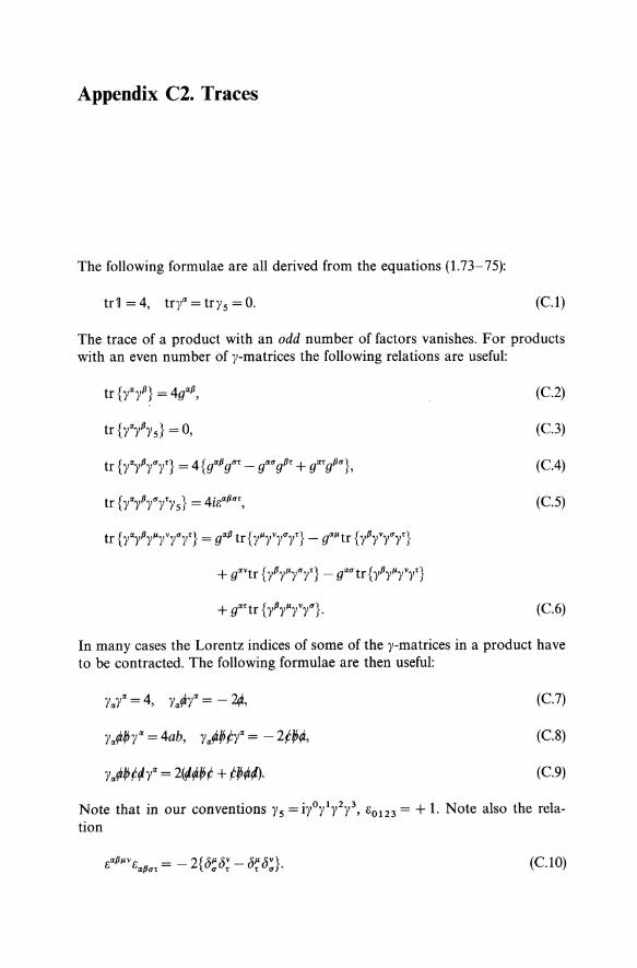
Appendix C2. Traces
The following formulae are all derived from the equations (1.73-75):
td = 4, trya = try 5 = o. (C.1)
The trace of a product with an odd number of factors vanishes. For products with an even number of y-matrices the following relations are useful:
(e.2)
(e.3)
(CA)
(e.S)
(e.6)
In many cases the Lorentz indices of some of the y-matrices in a product have to be contracted. The following formulae are then useful:
(e.7)
(e.S)
(e.9)
Note that in our conventions 1'5 = iyOy1y2y3, 80123 = + 1. Note also the relation
a{Jp.v _ 2{ >p." >p. >v} G Ga{J"t-- U"Ut-UtU". (e.1O)
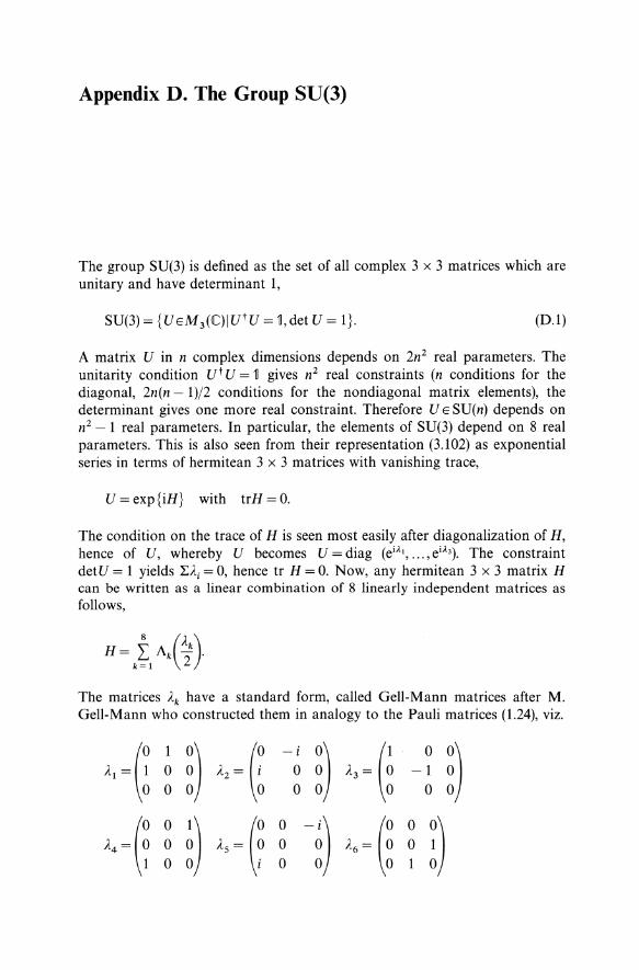
Appendix D. The Group SU(3)
The group SU(3) is defined as the set of all complex 3 x 3 matrices which are unitary and have determinant 1,
(D.1)
A matrix U in n complex dimensions depends on 2n2 real parameters. The unitarity condition U t U = ~ gives n2 real constraints (n conditions for the diagonal, 2n(n - 1)/2 conditions for the nondiagonal matrix elements), the determinant gives one more real constraint. Therefore U E SU(n) depends on n2 - 1 real parameters. In particular, the elements of SU(3) depend on 8 real parameters. This is also seen from their representation (3.102) as exponential series in terms of hermitean 3 x 3 matrices with vanishing trace,
U = exp{iH} with trH = o.
The condition on the trace of H is seen most easily after diagonalization of H, hence of U, whereby U becomes U = diag (eiA1 , ••• ,eiA3). The constraint detU = 1 yields Llli = 0, hence tr H = O. Now, any hermitean 3 x 3 matrix H can be written as a linear combination of 8 linearly independent matrices as follows,
H = f Ak (Ilk). k=l 2
The matrices Ilk have a standard form, called Gell-Mann matrices after M. Gell-Mann who constructed them in analogy to the Pauli matrices (1.24), viz.
A, ~(! 1
~) A, ~ (~ -~ ~) A,~ (~ o 0) 0 -1 0 0 o 0 o 0
A'~(~ 0
~) A; ~ (~ 0
-~) A,~ (~ 0 !) 0 0 0
0 0 1

462 Appendix D
(0 0
A? = 0 0 o i -!) 1 (1 0
As = r; 0 1 y3 0 0
(D.2)
Apart from a factor 2, the matrices (D.2) are the generators in the threedimensional representation 1 called the fundamental representation,
U(~) = (~) with normalization tr {( ~k) (~) } = ~6kj" (D.3)
SU(3) has rank 2. This is seen from eqs. (D.2) which show that two generators, T3 and Ts, are simultaneously diagonal. Furthermore, from the explicit representation (D.2) it is obvious that the generators (TI' T2 , T3) form an SU(2) subgroup of SU(3). In the "eightfold way" where baryons and mesons made up of u, d and s quarks are classified according to the flavour group SUi3), this SU(2) subgroup is the (strong) isospin group. In a similar fashion one verifies that the sets
( U I = T6 , U 2 = ~, U 3 = - ~ T3 + f T3) and
(VI = T4 , V2 = Ts, V3 = ~ T3 + f Ts)
also generate SU(2) subgroups of SU(3). In analogy to the isospin they are called, respectively, U -spin and V-spin.
In SU(3), i.e. when SUf (3) is interpreted as the flavour group classifying light mesons and baryons, the electric charge operator is
1 'h Qe.m. = T3 + 2: Y, WIt (D.4)
Y denoting the operator of hypercharge with respect to strong interactions. One verifies easily that Q commutes with the generators Ui' This means that U -spin connects particles which carry the same electric charge.
Invariant tensors in SU(3) are 67, Cijk and cijk• They are used in constructing irreducible, unitary representations of SU(3) from the fundamental representation 1 where
d. (1 1 2) U(Y)= lag - - --3' 3' 3'
and from its conjugate. The representation conjugate to l is the anti triplet I which cannot be identified with the triplet l- unlike SU(2) where the doublet and its conjugate are equivalent to each other.

Appendix D 463
Important Clebsch - Gordan decompositions of SU(3) are
1 x I = l + ~ 1 x 1 = Ia + [s, 1 x 1 x 1 = La + ~ + ~ + 10 s' (D.S)
where the subscripts 'a' and's' indicate that these states are antisymmetric or symmetric, respectively, under exchange of any two of its constituents. In SUe (3) the triplet 1 is used to classify quarks (u,d,s), its conjugate I then describes their antiparticles (u, if, 8). The singlets L the octets ~ and the dec uplets 10 serve to classify physical hadrons, mesons made up of quarks and antiquarks and baryons made up of three quarks.

Appendix E. Dirac Equation with Central Fields
The Hamiltonian form (1.82a) of the Dirac equation is well adapted for a discussion of interactions with external fields. For the case of an external, spherically symmetric potential V(r) and for stationary states (ex: e - iEt) it reads
E'I'(r) = { - iCl' V + V(r) + mf3} 'I'(r),
with a and 13 as given by (1.81). Using the vector identities
V = r(r· V) - r x (r x V)
A(A ) 1 A I =r r' V --r x r
one has
A 8 i (A l) S A { 8 1 S I} Cl,V=Cl'r---Cl' rx =Ys 'r --- . , 8r r 8r r
where Ys is given by (1.78), whilst the matrix S stands for
Finally, upon introduction of Dirac's angular momentum operator
K:=f3(S'I+~)=(~O) _~(O))
with K(O) = (J • I + ~, equation (E.l) takes the form
{- iysS' r (:r +~ - f3~) + V(r) + f3m}'I' = E'P =:H'I'.
(E.1)
(E.2)
(E.3)
One verifies by explicit calculation that K commutes with H, [H, KJ = 0, but that H neither commutes with the orbital angular momentum nor with the spin. The operator K contains the entire dependence on angular momenta so that (E.3) lends itself to separation into radial and angular coordinates. To see this, we note first that K(O) can be written as

Appendix E 465
Its eigenfunctions are the coupled states
Denote the eigenvalues of K(O) by - K, I.e.
K(O) CfJjlm = - KCfJjlm with K = - j(j + 1) + l(l + 1)-1-
Note also that (K(O))2 = ~ + (1 • 1+ P = l- S2 + ~, from which one deduces K2 = (j + ~y From these formulae one sees that
for K > 0: 1= K,
for K < 0: 1= - K - 1,
in all cases j = IKI -l (E.4)
Therefore, the eigenfunctions of total angular momentum j can be written in the compact notation CfJ jIm == CfJKm, the modulus of K giving the value of j, the sign giving the value of 1= j ±~, according to the rules (E.4). As K(O)CfJKm = - KCfJ Km, the eigenvalues and eigenfunctions of K, (E.2), are
For the eigenfunctions 'I' of (E.1) or (E.3) one makes the ansatz
'I' ( A) (gAr) CfJKm(r) ) Km r,r = i!K(r)CfJ-Km(r) ,
(E.5)
the factor i being introduced for convenience so that the resulting differential equations for the radial functions! and 9 become real. As a last step one verifies by explicit calculation that (1. r) CfJKm = - CfJ _ Km' With these tools at hand one deduces from (E.3) the following system of differential equations:
K-1 !~ = ~!K - (E - V(r) - m)gK'
r
K+1 g~ = ---gK + (E - V(r) + m)!K'
r (E.6)
Clearly, this result does not depend on the specific representation (1.82a) of the Dirac equation we started from. For example in the representation (1.74) we would obtain
[cf. (2.1 07)].

466 Appendix E
Equation (E.5) shows very clearly that the central field solutions are not eigenfunctions of orbital angular momentum: For example for K = - 1, the upper component has 1 = 0, the lower has T = 1. Thus, the relativistic analogue of an s-state has a component proportional to a p-state, cf. the discussing of the Ml-transition 2s --+ Is in Sect. 4.1.3.

Books, Monographs and General Reviews of Data
[ABS72]
[ART31]
[BEB84]
[BJD65]
[CHL84]
[COL84]
[DST63]
[DWS86]
M. Abramovitz and I. A. Stegun, Handbook of Mathematical Functions, (Dover, New York, 1972) E. Artin, Einfiihrung in die Theorie der Gammafunktion, Hamb. math. Einzelschriften 11 (Leipzig 1931) P. Becher, M. B6hm and H. Joos, Gauge Theorie of the Strong and Electroweak Interactions, (J. Wiley, New York, 1984) J. Bjorken and S. Drell, Relativistic Quantum Mechanics, Relativistic Quantum Fields (McGraw-Hill, New York, 1964, 1965) T. -Po Cheng and L. -F. Li, Gauge Theory of Elementary Particle Physics (Clarendon Press, Oxford, 1984) J. C. Collins, Renormalization (Cambridge University Press, Cambridge, 1984) A. de Shalit and I. Talmi, Nuclear Shell Theory (Academic Press, New York, 1963) B. deWit and J. Smith, Field Theory in Particle Physics I (North Holland Publ., Amsterdam, 1986)
[EDM57] A. R. Edmonds, Angular Momentum in Quantum Mechanics (Princeton University Press, 1957)
[FAR59] U. Fano and G. Racah, Irreducible Tensorial Sets (Academic Press, New York, 1959)
[GAS66] S. Gasiorowicz, Elementary Particle Physics (John Wiley & Sons, New York, 1966)
[GRR94] I. S. Gradstheyn and I. M. Ryzhik, Table of Integrals, Series, and Products, (Academic Press, New York, 1994)
[HAM89] M. Hamermesh, Group Theory (Addison-Wesley, Reading, 1989) [HEI53] W. Heitler, The Quantum Theory of Radiation (Oxford University
[HUA92]
[ITZ80]
[JAC75]
[KAL64]
Press, 1953) K. Huang, Quarks, Leptons and Gauge Fields (World Scientific, Singapore, 1992) C. Itzykson and J. -B. Zuber, Quantum Field Theory (McGraw-Hill, New York, 1980) J. D. Jackson, Classical Electrodynamics (John Wiley & Sons, New York, 1975) G. KaJlen, Elementary Particle Physics (Addison-Wesley, Reading, 1964)

468 Books, Monographs and General Reviews of Data
[KOK69] J. J. J. Kokkedee, The Quark Model (W. A. Benjamin, New York 1969)
[LAL75] L. D. Landau and E. M. Lifshitz, Theoretical Physics, Vol. IV b (Pergamon Press, New York, 1975)
[MUP77] C. S. Wu and V. Hughes (editors) Muon Physics, Vols. I-III (Academic Press, New York, 1977)
[NAC90] O. Nachtmann, Elementary Particle Physics: Concepts and Phenomena (Springer, Berlin, 1990)
[OKU82] L. B. Okun, Leptons and Quarks (North Holland, Amsterdam, 1982)
[OMN70] R. Omnes, Introduction a l'Etude des Particules Eif!mentaires (Ediscience, Paris, 1970)
[O'R86] L. O'Raifertaigh, Group Structure of Gauge Theories (Cambridge Monographs on Mathematical Physics, 1986)
[PER87] D. H. Perkins, Introduction to High Energy Physics (Addison Wesley, 1987)
[POR95] B. Povh, K. Rith, Ch. Scholz and F. Zetsche, Particles and Nuclei (Springer, Berlin, 1995)
[RAC64] G. Racah, Group Theory and Spectroscopy, Springer Tracts in Modern Physics, Vol. 37 (Springer, Berlin, 1964)
[ROS55] M. E. Rose, Multipole Fields (John Wiley & Sons, New York, 1955) [ROS61] M. E. Rose, Relativistic Electron Theory (John Wiley & Sons, New
York, 1961) [ROS63] M. E. Rose, Elementary Theory of Angular Momentum (John Wiley
& Sons, New York, 1963) [RPP94] Review of Particle Properties, Phys. Rev. D50 (1994) 1173 [RUE70] W. Ruhl, The Lorentz Group and Harmonic Analysis (W. A. Ben
jamin, New York, 1970) [SAK84] J. J. Sakurai, Advanced Quantum Mechanics (Benjamin/
Cummings, 1984) [SCH68] L. J. Schiff, Quantum Mechanics (McGraw-Hill, New York, 1968) [SCH94] F. Scheck, Mechanics-from Newton's Laws to Deterministic Chaos
(Springer, Heidelberg, 1994) [UEB71] H. Uberall, Electron Scattering from Complex Nuclei (Academic
Press, New York, 1971) [WAT58] G. N. Watson, Theory of Bessel Functions (Cambridge University
Press, 1958) [ZIJ94] J. Zinn-Justin, Quantum Field Theory and Critical Phenomena
(Oxford Science Publications, 1994)

Exercises: Further Hints and Selected Solutions
Chapter 1: Fermion Fields and their Properties
1.1. The Lagrangian density for a Majorana field is given by (1.108). One takes the partial derivatives with respect to, say, 4>; and with respect to 8/14>;,
85l' _ i (~/18 )Bb"- BC,,-* 84>; - 2: a /1 'Pb + mc; 'Pc
85l' _ i (~/1)Bb "-8(8/14>;)- -2: a 'Pb·
The Euler-Lagrange equation which reads (1) - 8P) = 0 yields
i(fr/18/1)Bb4>b + mc;BC4>'t = o.
(1)
(2)
This is (1.107b). Similarly, (1.107a) is obtained by taking the derivatives with respect to 4>b and to 8/14>b.
1.3. With J 2 = a(2)/2 and noting that all even powers of a(i) are equal to the unit matrix, while all odd powers are equal to a(i>,
one finds
With J1 = (1/2, - 1/2) counting the rows, ni = (1/2, -1/2) counting the columns, one has
Let U denote the transformation that effects the transition to contragedience. Regarding rotations, this simply means that U must be such that
(3)

470 Exercises: Further Hints and Selected Solutions
for any rotation matrix D(R). When expressed in terms of the generators, this gives the condition
(4)
and, hence
UJkU- 1 = -Jt, or UJk+JtU=O. (5)
The phase convention which is standard in the theory of angular momentum (and which goes back to Condon and Shortley) yields J 1 real and positive, J 2
pure imaginary, and, of course, J 3 real and diagonal. Therefore the condition (5) is met if we choose
U = D(O, n, 0) = ei1t'z,
because a rotation by n about the 2-axis leaves invariant J 2 but transforms J 1
and J 3 into - J 1 and - J 3' respectively. Applying U twice leads back to the original representation.
1.4. For vanishing mass m = 0, and omitting the spinor indices, (1.69b) reads
i(t/lo/l(e±iPX¢(p)) = o.
The wave function in momentum space obeys the equation
((J0po - (f'p)¢(p) = 0,
with pO = Ipl. Obviously, its solutions describe positive helicity, (f'p/IPI = + 1. In a similar way (l:69a) with m = 0 yields plane wave solutions with negative helicity.
1.6. With ff! as given in (1.163) we calculate the derivatives
off! =~((t/lo )Abd. _m*xA+m*eABd.* o¢! 2 /l 'Pb n 1 'PB
off! _ i (~/l)Abd. o(o/l¢!) - -2 (J 'Pb'
Note that according to the rules (1.56) eAB ¢; = - eab(¢b)* = + ¢*A. Therefore, the Euler-Lagrange equation reads
i((t/lo/l)Ab¢b = m1;xA - m''t¢*A.
Taking derivatives with respect to X* and to o/lX* one obtains in the same way
i((J/lo/l)aBXB = mn¢a + mix:·
1.7. The behaviour of the two-spinors ¢a and XA under P, C, and T is given explicitly in Sect. 1.5. The transformation behaviour of the Lagrangian density (1.163) is studied in the same way as in (3.50), (3.55), and (3.56), and we recommend the reader goes through these first. It then follows that (1.163)
Exercises: Further Hints and Selected Solutions 471
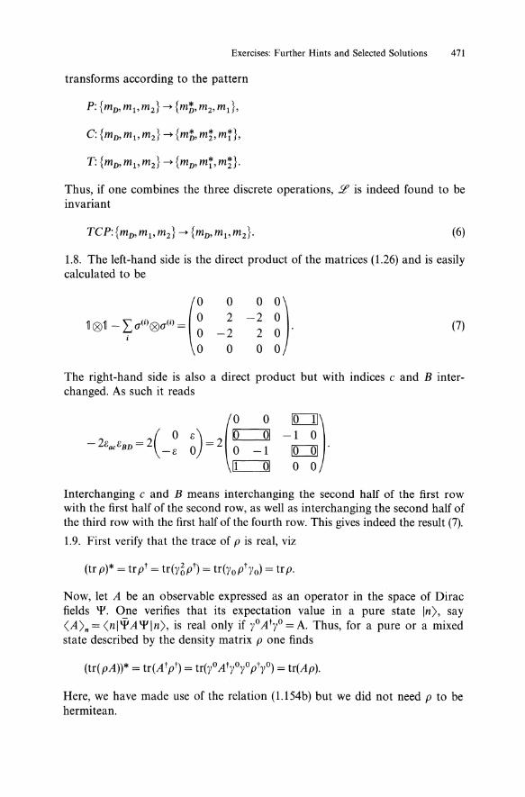
transforms according to the pattern
Thus, if one combines the three discrete operations, !£' is indeed found to be invariant
(6)
1.8. The left-hand side is the direct product of the matrices (1.26) and is easily calculated to be
o 2
-2 o
o 0) -2 0 2 0 .
o 0
(7)
The right-hand side is also a direct product but with indices c and B interchanged. As such it reads
Interchanging c and B means interchanging the second half of the first row with the first half of the second row, as well as interchanging the second half of the third row with the first half of the fourth row. This gives indeed the result (7).
1.9. First verify that the trace of p is real, viz
Now, let A be an observable expressed as an operator in the space of Dirac fields '1'. One verifies that its expectation value in a pure state In), say (A)n = (nl'PA'I'ln), is real only ifyOAtyo=A. Thus, for a pure or a mixed state described by the density matrix p one finds
Here, we have made use of the relation (1.154b) but we did not need p to be hermitean.

472 Exercises: Further Hints and Selected Solutions
1.10. First we work out the explicit form of p. Using the standard representation (1.78) one finds
1 ( (E + m)(~ + ~.(J) p = 2 (p.(J) + (p.~) + i(P x ~).(J
- (p.(J) - (p.~) + i(p x ~).(J )
- (E - m)(1 - (-(J) - E;m(P·~)(P·(J) (8)
Then choose the 3-axis such that p = pe3 • The answer is then read off from the explicit representation (8).
1.12. The matrix AESL(2, q that represents the boost with rapidity parameter A along the direction w is given by
~ (A)2n ~ (A)2n + 1 ~ A = e)./2",., = 1 + 2 (J·wfn+ 2 (J·w)2n+1
= ~ cosh(A/2) + (J·W sinh(A/2). (9)
(Cf. also the solution to exercise 1.3 above). With O"(l)T = 0"(1), 0"(2)T = _ 0"(2),
and 0"(3)T = 0"(3), it is easy to find the transpose of the expression (9) as well as its inverse. The latter is
(10)
(Verify that (10) is indeed the inverse of AT.) From (5), on the other hand, we have
UAU- 1 = exp Gw .U(JU- 1 ) = exp ( -~w.(J*)
= exp( - ~(l~'t 0"(1) - W20"(2) + W3 0"(3»))-
The right-hand side, when expanded as in (9), is identical with (10).
1.13. The momenta conjugate to ¢a and to ¢; are, respectively,
a _ 85l' _ i A.*( d))Ba n - 8(80¢a) -2'f'B 0" ,
*B _ 85l' _ i d) BaA. n - 8(8o¢;) - -2(0") 'f'a·
The Hamiltonian density is
with 5l' as given in (1.108). Making use of the equations of motion (1.107) and taking the integral over 3-space, at constant time, one obtains
H=f d3XYl'=~f d 3x¢;Fo(5Ba¢a. XO = const. 2 XO = const.

Exercises: Further Hints and Selected Solutions 473
It is not difficult to derive from the equations of motions that a plane wave solution must have the form
and that the functions <Pi and "'i satisfy the equations
(Po + P3)<PI (p) + (PI - iP2) '" 2( p) = m<p !(p)
(Po - P3)<P2(P) + (PI + iP2) '" I (p) = m<p 'f(p)
(PO+P3)"'I(P)+(PI -iP2)<P2(P) = -m"'!(p)
(Po - P3)"'2(P) + (PI + iP2) <PI (p) = - m"'!(p).
The latter are seen to be invariant under the replacement
<PI (pO,p) --? <P !(pO, _ p), '" ipO,p) --? _ ",!(pO, _ p).
Thus, I<PI(pO,pW=I<pI(pO,-PW, and 1"'I(pO,pW=I"'2(pO,-PW. Insert now the Fourier decomposition
of the field ¢ and its hermitean conjugate into the expression for Yf and perform the integral over d3x, giving a b distribution in the momentum variables. The result is
Indeed, H vanishes because the integrand is odd.
Chapter 2: Electromagnetic Processes and Interactions
2.1. Reflection with respect to a plane through the origin and perpendicular to the 3-direction inverts the direction of the incident momentum but leaves the spin orientation unchanged. A rotation by 180 0 about, say, the 2-axis, brings back the incident momentum to its initial configuration but interchanges the solutions u+ and u_. If the interaction is invariant the scattering amplitudes for the two spin orientations must be the same.

474 Exercises: Further Hints and Selected Solutions
2.2. Repeat the calculation described in Sect. 2.4.2., inserting the matrix element
<p'Up(O)lp) = (2!)3 F(q2),
instead of (2.46'), and use m ~ O.
2.3. For an infinitesimally small translation four-vector e with lelll« 1, (2.39) gives
F'(x') ~ F(x) + e/3IlF(x) = F(x) + iell[PIl,F(x)].
On the other hand, using [Pll, r] = 0, and expanding the operator U(e) ~ ~ + iellPIl, we find
U(e)F(x) U- 1(e) ~ F(x) + iell[PIl, F(x)].
Now choose e to be ell = ailin for some large n and take the limit
lim (~ + i all PIl)n = eia•P'. n-+oo n
2.4. With x: = Yn - Ye the integral over d3q can be calculated using spherical coordinates in q-space, i.e. d3q=q2 dqd(cos8q)d</>q. The integrand being even in the modulus q of q we extend the integral over q to the interval ( - 00, + 00). With z: = cos 8q and noting that the integral over the azimuth </>q gives a factor 2n, we find
f 3 eiq·x foo f+l i xz n f+OO (e iqX e- iqX ) 2n2 d q-2 =2n dq dze q =-;- dq ---- =-.
q 0 - 1 IX - 00 q q X
In the second step we extended the integral over q to the interval ( - 00, 00), in the last step we made use of Cauchy'S theorem.
2.7. Due to time dilation the effective lifetime that is recorded in the laboratory frame is !Jab = y!, with Y = Elm. The average length over which a particle of energy E can be transported is then estimated from !Jab and its velocity v = pI(my) in the laboratory frame.
2.8. For negative K we have t = - K - 1 and (2.105) read, dropping the index K,
df -t-2 -= f -(E- V-m)g dr r
(11)
dg t -=-g+(E- V+m)f. dr r
(12)
By (12) f can be expressed in terms of 9 and of dgldr. The derivative df I dr can also be expressed in terms 9 and dgldr, by means of (11) and the previous result. We then take the derivative of (12) with respect to r to obtain a second-

Exercises: Further Hints and Selected Solutions 475
order differential equation for the function g alone. One obtains
d2g + (~+ dV/dr )dg dr2 r E - V + m dr
(( _ )2 _ 2 _ t(t + 1) _ t dV/dr ) _ 0 + E V m 2 (E ) g - . r r - V+m
Let 8 be the energy E from which the rest energy is subtracted, E = m + 8. In the limit of 8 and V being small as compared to the rest energy m,
(E - V)2 - m2 ~ 2m(8 - V).
In this limit the second order differential equation for g reduces to
d 2g 2dg (t(t + 1) ) dr2 + -;: dr - r2 + 2m(V - 8) g = O. (13)
The analogous analysis for 1(' = - I( - 1 gives the same value of t and leads to the same differential equation. The result (13) is identical with the nonrelativistic radial equation for the wave function Rtn(r) = Ynk)/r.
2.9. Making use of the identity
1 . {,s = -(/ - (2 _ S2)
2
the angular matrix element for the states t = 1, j = 3/2 or j = 1/2, is easily calculated,
«'s>=~0U+1)-t(t+l)-~). The former has I( = - 2, the latter has I( = 1. In the nonrelativistic limit they have the same radial function (2.145) which, for a circular orbit reads
2n Y = rne -rlna.
n,n-1 nn+1J(2n-1)!ai+ 1/2 .
The expectation value of 1/r3 is calculated in an elementary way,
3 2 1 O/r >n,n-1 = n4(2n-1)(n-1)ar
Thus, the fine structure splitting, when calculated in first order perturbation theory, is found to be
m(Zet)4 LlE = 2n4(n - 1)' (14)
On the other hand, taking the difference of (2.164) for I( = n - 1 and for I( = n - lone finds the same expression (14). Thus, up to terms of higher order in Zet the relativistic result agrees with the perturbative estimate.

476 Exercises: Further Hints and Selected Solutions
2.11. The strategy for solving this exercise is to use partial integration in such a way that the radial part of the Laplacian
appears in the integrand. By Poisson's equation this is then replaced by the difference of the corresponding charge densities. Accordingly, we transform the integral
I: = J: dr(ar2 + br3 + cr4)(Vl - V2)
= J: r2dr (~r2 + 1b2 r3 + ;0 r4)Ll(Vl - V2)·
Making use of Poisson's equation Ll(Vl - V2) = - 4nZe(Pl - P2)' the difference of the potentials is replaced by the difference of the charge distributions. The formula for I now contains the moments Ll <rn) = 4n J r2drrn. This yields the desired formula for LlE,
The coefficients a, b, and c for the 2p state and for the 28 state are obtained by expanding the squared radial functions (2.145) in power of r, viz.
a(2p) = b(2p) = 0, C(2p) =_1_ 12ar
a(2s) = _1_ b(2s) = _ ~ C(2s) = ~ 2ar ar 8ar
2.12. The solution to this exercise is similar to the previous one.
2.14. Using the equations in momentum space pu(p) = m u(p) and u(p) P = m u(P) we calculate
u(p')iaaP( p - p')Pu( p) = -~u(P') [YaP - YaP' - Pra + p'yaJu(p)
= - u(p') [YaP - Pa + p'Ya - P~Ju(p)
= - 2m u(p') Yau(p) + (Pa + p~)u(p')u(p).
In the second step we have used YaP' = - p'Ya + 2p~ and PYa = -YaP + 2Pa· Analogous relations hold with u(p) replaced by v(p) and u(p') by v(p'). In view of weak interactions (Chaps. 3 and 4) it is instructive to derive analogous identities which hold when a ap is multiplied by Y s'

Exercises: Further Hints and Selected Solutions 477
Chapter 3: Weak Interactions and the Standard Model of Strong and Electroweak Interactions
3.1. Applying parity or charge conjugation to one of the indicated states obviously reproduces the same state. The eigenvalues are determined as follows. The parity of a quark-antiquark state contains a factor (- t from the angular part 1jm of the orbital wave function, t being the relative angular momentum, and a factor - 1 from the relative intrinsic parity of quark and antiquark, thus p = (_ )t+ 1.
Charge conjugation interchanges quark and antiquark, hence the spins must be recoupled, giving a factor (- )1/2+1/2-S. Regarding the orbital wave function, we note that interchanging q and if means relabeling coordinates in the relative coordinate r1 - r2 . While the radial part does not change, the angular part changes by a factor ( - t Finally, charge conjugation gives an extra minus sign when applied to a doublet (with respect to an internal symmetry such as strong isospin); cf. Sect. 1.10. Therefore, C = (- )t+s. If the w meson is purely
nonstrange, i.e., if w = (uti - da)/..)2, then ¢ is a purely strange state, i.e., ¢ = ss. This is so because ¢ is an isoscalar and must be orthogonal to w.
From the results above the P and C eigenvalues for low-lying mesons are as follows:
no,/} (t = a,s = 0) : P= -1 C= +1
Po,w,¢(t=O,S=I): P= -1 C= -1
a2 (t = I,S = 1) : P= + 1 C= +1
3.4. The generators fall into two sets, say ~ for SU(P) and Sj for SU(Q), which commute for all k and j, [~,Sj] = 0. Therefore, expressions such as (3.112) for the gauge potential and (3.121) for the field strength tensor will read explicitly
Aa(x) = i[epIB~)(x)~ + eQLC~"l(x)Sj]' Fap(x) = i[epLG~J(x)~ + eQLH~J(x)Sj].
In fact, a more precise way of writing the generators would be Tk®~ and ~®Sj' where the first factor acts on the internal space spanned by representations of SU(P), the second acts on the internal space pertaining to SU(Q). The construction of the gauge theory for the group SU(P) x SU(Q), along the lines of Sect. (3.3), goes through for any choice of the coupling constants ep and eQ.
For example, one verifies that the Lagrangian for the pure gauge fields is just the sum of the corresponding Lagrangians for the SU(P) fields Ba and for the SU(Q) fields Ca,
1 1 1 --F FaP = --G Gap --H HaP 4 ap 4 ap 4 ap .
Here we have used tr {~®~} = tr ~ = ° and likewise for Sj.

478 Exercises: Further Hints and Selected Solutions
3.5. The equation
- (8ag- 1(x)) g(X) = Aa(x)
is interpreted as a differential equation for the gauge transformation g(x), the inhomogeneity being Aa(x). Rewriting this equation
8ag- 1(x) = - Aa(x)g-l(x), (15)
we obtain the integrability condition
(8p8a - 8a8p)g-1(X) = O.
Inserting (15) we find
8a(Ap(x)g-1(X)) - 8P(Aa(x)g-1(x)) = (8aAp - 8pAa)g-1 + Ap8ag- 1 - Aa8pg-l
= (8aAp - 8pAa)g-1 +( - ApAa + AaAp)g-l
= FaP(x)g-l(x) = O.
In the second step we have used (15) to replace 8ag- \ in the last step we have inserted the definition of the field strength tensor. As g -l(X) is not identically zero we conclude: Aa(x) is gauge equivalent to 0 if and only if Fap(x) vanishes identically. Thus, Fap is a measure which tells us to which extent the potential Aa cannot be gauged to zero.
3.6. With G = SO(3) the structure constants are Cijk = Bijk• For simplicity consider a set of real scalar fields
forming an M-dimensional representation of G. The invariant scalar product is M
(<11, <11) = L <Mx)<Mx). k=l
A globally invariant theory involving these fields could have the form
This is turned into a locally gauge invariant theory by introducing gauge fields Aa(x) = ieL;= 1 T;A~)(x) in the adjoint representation of SO(3) and the covariant derivative D(A) which acts on the scalar multiplet. Symbolically, we obtain
5l' = - ~(paP,Fap) + ~ (Da<1l,Da<1l) - m2(<1I,<1I) + ..1.(<11,<11)2, (16)
with c = 1/(e2 K) and tr(T;T,,) = KOik• The second, third, and fourth terms are obvious. We work out the first one explicitly, viz.

Exercises: Further Hints and Selected Solutions 479
1 e =-1" faP --I" '(Aa X AP)
4JaP 2JaP
2
+ ~ {(Aa-Aa)(Ap-AP) - (Aa' AP)(Ap-Aa)}. (17)
Here the boldface notation stands for Aa = (A~), i = 1,2,3) and, likewise, for hp = (f~1 = aaA~) - apA~), i = 1,2,3). (Remember that the gauge fields and the field strengths belong to the adjoint representation of G = SO(3). Thus, they form a triplet and, therefore, are isomorphic to a vector in real, three-dimensional space \R 3 .) We have made use of the identity
and have introduced the well-known scalar and cross products of \R 3 . This theory is perhaps the simplest, nontrivial example of a gauge theory. In the explicit form (16) and (17) it is easy to interpret in terms of interactions between the three gauge bosons and with the scalar fields. In the example studied here, G is both a spectrum symmetry and the structure group from which the gauge group is constructed. Without the gauge principle, i.e., without the geometric framework on which it rests, it would be difficult to guess the specific form (17) of the Lagrangian.
3.7. A priori the mixing matrix between any two generations is a unitary matrix U E U(2) and, hence, depends on four parameters: A common phase ({J
in U = ei",U s and three angles which parametrize the factor with determinant + 1, UsE SU(2). Clearly, the former is irrelevant and may be omitted from the start. In analogy to D(1/2), cf. Sect. 1.8.3.a, the latter must have the form, for the example of mixing between the first and the third generation,
(COS" e;~""'" 0 si"""e;"''-'''' ) 13
U~·3)= 0 1 cos IX ~ - i(P13 + Y13) - sin IX13e - i(P13 - Y13) 0 13
(e;'" 0 ),,,) (co~"" 0 Si~"" ) (e~" 0 o ) = 0 1 1 1 o .
0 0 - SIll IX 13 0 cos IX 13 0 0 e -iY13
What remains to be done is to multiply the three mlXlng matrices, U~1.2) U~,3) U~·3), and to realize that both the initial, unmixed, states, say b(m) == (d,s,b), and the mixed states d(n) can each be multiplied by an unobserv-

480 Exercises: Further Hints and Selected Solutions
able phase, such that the mixing matrix
diag (ei1>l, ei1>2, ei1>3) U~1,2)U~,3)U~ ,3)diag(eil/l 1 , eit/12, eil/l3)
is physically equivalent to U~,2)U~,3)U~1,3). This freedom in the choice of ¢i and t/Ji reduces the number of observable phases to four.
3.8. In this exercise, which we do not write out here, it is important to realize that the coupling of the charged W-bosons to the photon is fixed through the generalized kinetic term (Fap,FaP), so that, in particular, the anomalous magnetic moment of the W can be identified. If the coupling had been constructed from the minimal coupling principle (1.200) of electrodynamics, the W would have obtained no anomalous magnetic moment.
3.9. The neutral partner of the Higgs doublet has y = - 2t3• The right-hand side of (3.173) then becomes
- i(gA~3) - g' A~O)) t3¢o.
When this is inserted into (3.172) we obtain
~(A,O A,O)t2(gA(3) _ g'A(O)) (gA(3)a _ g'A(O)a) == ~M2 A(i)A(k)a i k = 03 2 0/ ,0/ 3 a a 2 lk (J. , , , •
Thus the mass matrix for the neutral gauge bosons is given by
M2 = (¢O,¢O)t~( g'2, - g;,). -gg g
(18)
Diagonalization of this matrix gives m; = 0 and m~ = (¢O,¢O)t~(g2 + g'2). The result for m~ is as given in Sect. 3.4.3c.
3.10. Return to (3.222) and write the second factor in terms of helicity projec-tion operators, viz.
The longitudinal polarization of the outgoing neutrino is easily obtained from this;
(1 - 2) - (1 + 2) PI = (l _ 2) + (1 + 2) = - 2.
3.12. The calculation, which is a little lengthy, may be done along the lines of our calculation with mr = 0, as given in Sect 3.6.3. Alternatively, this might be a good example to tryout an algebraic program such as REDUCE.
3.13. Inserting c~) = 0 and c~=/l) = 0 into (3.242) gives a vanishing asymmetry. Although the electromagnetic and the neutral weak (NC) couplings have negative relative parity, this is not seen in the asymmetry. This interference could only be seen by measuring a spin-momentum correlation.
Exercises: Further Hints and Selected Solutions 481
Chapter 4: Beyond the Minimal Standard Model
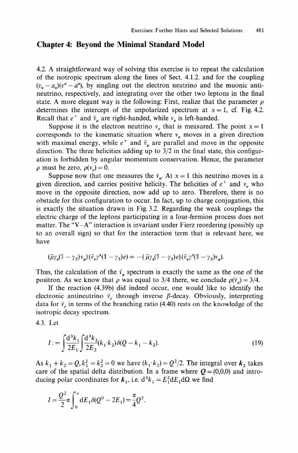
4.2. A straightforward way of solving this exercise is to repeat the calculation of the isotropic spectrum along the lines of Sect. 4.1.2. and for the coupling (va - aa)(va - aa), by singling out the electron neutrino and the muonic antineutrino, respectively, and integrating over the other two leptons in the final state. A more elegant way is the following: First, realize that the parameter p determines the intercept of the unpolarized spectrum at x = 1, cf. Fig. 4.2. Recall that e+ and vI' are right-handed, while Ve is left-handed.
Suppose it is the electron neutrino Ve that is measured. The point x = 1 corresponds to the kinematic situation where ve moves in a given direction with maximal energy, while e+ and vI' are parallel and move in the opposite direction. The three helicities adding up to 3/2 in the final state, this configuration is forbidden by angular momentum conservation. Hence, the parameter p must be zero, p(vJ = o.
Suppose now that one measures the vI'" At x = 1 this neutrino moves in a given direction, and carries positive helicity. The helicities of e + and ve who move in the opposite direction, now add up to zero. Therefore, there is no obstacle for this configuration to occur. In fact, up to charge conjugation, this is exactly the situation drawn in Fig. 3.2. Regarding the weak couplings the electric charge of the leptons participating in a four-fermion process does not matter. The "V -A" interaction is invariant under Fierz reordering (possibly up to an overall sign) so that for the interaction term that is relevant here, we have
Thus, the calculation of the vI' spectrum is exactly the same as the one of the positron. As we know that p was equal to 3/4 there, we conclude p(vl') = 3/4.
If the reaction (4.39b) did indeed occur, one would like to identify the electronic antineutrino ve through inverse f3-decay. Obviously, interpreting data for ve in terms of the branching ratio (4.40) rests on the knowledge of the isotropic decay spectrum.
4.3. Let
]:= _1 -\k1.k2)6(Q-k1-k2). fd3k fd3k 2E1 2E2
(19)
As k1 + k2 = Q,k~ = k~ = 0 we have (k 1·k2) = Q2/2. The integral over k2 takes care of the spatial delta distribution. In a frame where Q = (0,0,0) and introducing polar coordinates for k 1, i.e. d3k 1 = EidE1dQ we find

482 Exercises: Further Hints and Selected Solutions
The integral (4.44b) is best decomposed into covariants which are then isolated by taking various contractions as follows. The momentum Q being the only variable, the integral must be a linear combination of the covariants g"P and Q"QP with Lorentz invariant coefficients. We set
I"P. = fd 3 k 1 fd 3 k2 {k" kP - (k ·k )g"P + k" kP} (j(Q - k - k ) . 2E 2E 1 2 1 2 2 1 1 2 1 2
(20)
and calculate the invariant integrals
From the definition of the tensor integral I"P we find its contraction with the metric tensor g"pl"P = -21, with I as calculated above. Inserting Q = k1 + k2 in the integrand of Q"!,,PQp, the second combination is zero. Thus B = - A, (A + 4B)Q2 = - nQ2/2, and, from these,
n n A=- B=--
6' 6· (21)
4.4. Let k and k' denote the initial and final neutrino four-momenta, respectively, p the electron momentum, q the muon momentum. Neglecting terms quadratic in the electron mass the invariant kinematic variables sand tare expressed in terms of the laboratory energies as follows,
s = (k + p)2 ~ 2meE~b,
t = (k _q)2 = (k' - p)2 ~ - 2meE~ab ~ - 2me(E~b - E~b) ~ -s(1- y).
With dt/dy = s and the fact that the cross section (4.69) is a quadratic function in the variable y, the integration is elementary. Note that it is the integral over y from some value Ymin (that depends on the experimental arrangement), to its maximum y = 1 which is determined in the quoted experiments.
4.5. The calculation is similar to the one of exercise 4.3., except that now one of the neutrinos is massive, say, k~ = It 2 • We first calculate the integral
(22)
say, in a frame where the spatial part of Q vanishes. The integral over d3k 2
eliminates the spatial (j-distribution. In a frame where Q = (0,0,0), this leaves E2 a function of E 1, so that we obtain

Exercises: Further Hints and Selected Solutions 483
with EiE1)=J).2+Ef. The integral over E1 is calculated using the wellknown replacement rule for the delta distribution
1 (") c5(g(E1)) ~ Ig'(E~))1 c5(E D,
where E~) is a simple zero of the function EiE1)' This gives
n Q2 _ ).2 n Q2 _ ).2
10 ="2 (QO)2 ~ 10 ="2 Q2
In the last step we returned to an arbitrary frame (where Q is possibly nonzero), using our knowledge that the integral 10 must be a Lorentz scalar. As the neutrino number 2 is massive, the scalar product of the neutrino fourmomenta becomes (k 1·k2) = (Q2 - ).2)/2 and the integral (19) is given by
n (Q2 _ ).2)2
1="4 Q2 .
The tensor integral (20) is calculated as in exercise 4.3., making use of the result above. One finds
and, from these relations,
n (Q2 _ ).2?(Q2 + 2).2) n (Q2 _ ).2)2(2Q2 + ).2) A = 6" (Q2)3 ,B = - 12 -'-=---( Q-=-2=)3,;::----'-· (23)
Clearly, for ). = 0 the result (23) goes over into the result (21) of exercise 4.3.
4.6. It is simplest to use a Cartesian basis in isospin space and to drop all real factors such as (2n)3/2 so that the ansatz reads
(i) _ , (OIAa (O)lniq) - Fuijqa'
Inserting first T -1 T and then p- 1 P one obtains successively
(OIA~)(O)ln/q) = (0IT- 1(T A~)(O)T -l)Tlniq)
= (_)1 Hao(OIA~)(O)lnMo' - q)*11T
= (_)1 Hao(OI(P A~) (0)p-1)PlnMo, - q)*'1T !
= - (OIA~)t(O)lnMo, q)*'1T'1P
= - F*c5 ijqa'1T'1P
(24)
Here '1P is the intrinsic parity of the pion, '1T is an analogous phase which appears when Tis applied to a one-pion state. The pion has negative intrinsic parity. It is even with respect to charge conjugation, i.e. '1e = 1. With '1p'1p'1e = 1 we conclude that the product '1P'1T is + 1. Thus, F, as defined in (24) is pure imaginary, or, equivalently,f" is pure real.
484 Exercises: Further Hints and Selected Solutions
4.9. It is not difficult to check that this model for the pionic axial current yields the terms represented by the diagrams of Fig. 4.5 and, hence, that the structure terms vanish.
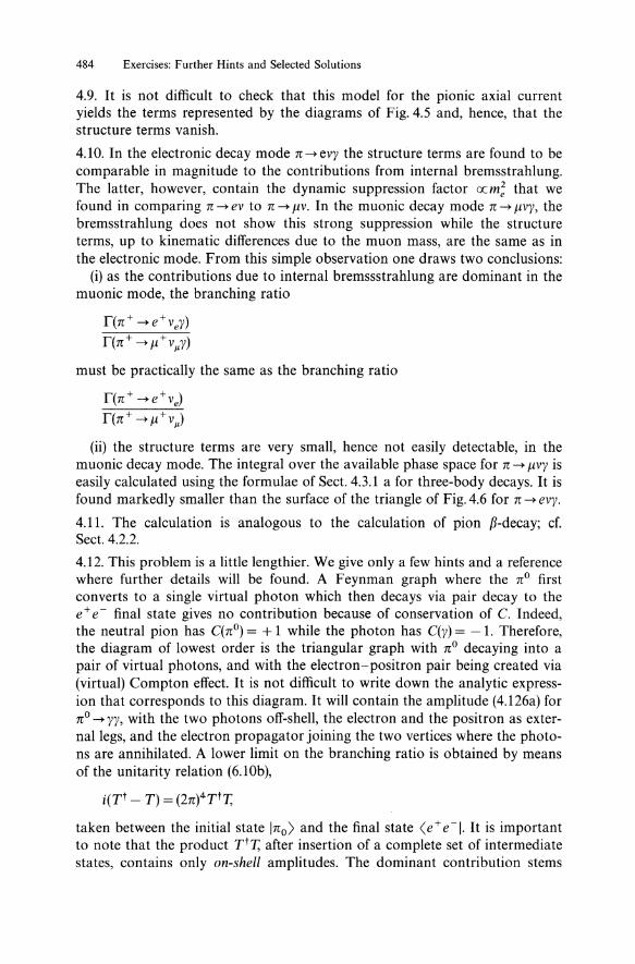
4.10. In the electronic decay mode n --+ evy the structure terms are found to be comparable in magnitude to the contributions from internal bremsstrahlung. The latter, however, contain the dynamic suppression factor ocm; that we found in comparing n --+ ev to n --+ f.1V. In the muonic decay mode n --+ f.1vy, the bremsstrahlung does not show this strong suppression while the structure terms, up to kinematic differences due to the muon mass, are the same as in the electronic mode. From this simple observation one draws two conclusions:
(i) as the contributions due to internal bremssstrahlung are dominant in the muonic mode, the branching ratio
r(n+ --+e+veY)
r(n+ --+ f.1+ VIlY)
must be practically the same as the branching ratio
r(n+ --+e+ve)
r(n+ --+ f.1+ v)
(ii) the structure terms are very small, hence not easily detectable, in the muonic decay mode. The integral over the available phase space for n --+ f.1vy is easily calculated using the formulae of Sect. 4.3.1 a for three-body decays. It is found markedly smaller than the surface of the triangle of Fig. 4.6 for n --+ evy.
4.11. The calculation is analogous to the calculation of pion f3-decay; cf. Sect. 4.2.2.
4.12. This problem is a little lengthier. We give only a few hints and a reference where further details will be found. A Feynman graph where the nO first converts to a single virtual photon which then decays via pair decay to the e + e - final state gives no contribution because of conservation of C. Indeed, the neutral pion has C(nO) = + 1 while the photon has C(y) = -1. Therefore, the diagram of lowest order is the triangular graph with nO decaying into a pair of virtual photons, and with the electron-positron pair being created via (virtual) Compton effect. It is not difficult to write down the analytic expression that corresponds to this diagram. It will contain the amplitude (4.126a) for nO --+ yy, with the two photons off-shell, the electron and the positron as externallegs, and the electron propagator joining the two vertices where the photons are annihilated. A lower limit on the branching ratio is obtained by means of the unitarity relation (6.10b),
i(Tt - T) = (2n)4TtT,
taken between the initial state Ino) and the final state (e+e-I. It is important to note that the product TtT, after insertion of a complete set of intermediate states, contains only on-shell amplitudes. The dominant contribution stems

Exercises: Further Hints and Selected Solutions 485
from the two-photon intermediate state,
i«e+ e-Ino)* - <nole+ e-») = (2n)4<e+ e-Iyy)*<yylno) + "',
with the two photons on their mass shell. This will be a lower limit because the unitarity relation yields only the imaginary part of the no --> e + e - amplitude. If this is worked out one finds the so-called unitarity limit
This gives a lower limit on the branching ratio of 4.75 x 10- 8 (cf., e.g., L.G. Landsberg, Phys. Rep. 128 (1985) 301). Compare this to the present experimental value for the branching ratio: (7.5 ± 2.0) x 10- 8 (Deshpande et aI., Phys. Rev. Lett. 71 (1993) 27, McFarland et aI., ibid. p.31.)
Chapter 5: Scattering of Strongly Interacting Particles on Nuclei
5.1 Set E = m + G, where G is the analogue of the energy of the nonrelativistic limit. The approximation
(E - WO)l = (m + G - WO)l ~ m1 + 2m( G - Wo)
leads to Schrodinger's equation with potential V + WOo
5.2. The essence of the argument is seen in the following example. Calculate the form factor
F(q) = f d 3 rp(r)eiq.r
for the one-body density
per) = f d3rl f d3r2¢*(r l )¢*(r1) itl b(r - r;)¢(rl)¢(r1),
(25)
with and without the center-of-mass condition, for the 1s-wave functions as given in eq. (5.55). Note that the product of two such wave functions can be separated in centre-of-mass and relative coordinates, rc = (rl + rz)/2 and r=r l -rz, respectively, viz.
Next prove the general integral
f (n)3/Z d 3 -ax' ip'x - p'/(4a) xe e = - e , a
(26)
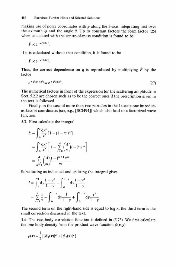
486 Exercises: Further Hints and Selected Solutions
making use of polar coordinates with p along the 3-axis, integrating first over the aximuth ({J and the angle 8. Up to constant factors the form factor (25) when calculated with the centre-of-mass condition is found to be
F -q'/(Scc') oce .
If it is calculated without that condition, it is found to be
F- -q'/(4cc') oce .
Thus, the correct dependence on q is reproduced by multiplying F by the factor
e+ q'/(4Acc') = e+q'/(Scc'). (27)
The numerical factors in front of the expression for the scattering amplitude in Sect. 5.2.2 are chosen such as to be the correct ones if the prescription given in the text is followed.
Finally, in the case of more than two particles in the Is-state one introduces Jacobi coordinates (see, e.g., [SCH94]) which also lead to a factorized wave function.
5.3. First calculate the integral
= IX d~' [1- I: (A)( - txmJ o X .=0 n
Substituting as indicated and splitting the integral gives
1= dy-- - dy--fl 1- yA fl-X 1 - yA
o l-y 0 l-y
A I fl-X 1 fl-X yA L -- dy-+ dy-. v=lV 0 l-y 0 l-y
The second term on· the right-hand side is equal to log x, the third term is the small correction discussed in the text.
5.4. The two-body correlation function is defined in (5.73). We first calculate the one-body density from the product wave function t/I(x,y):
Exercises: Further Hints and Selected Solutions 487
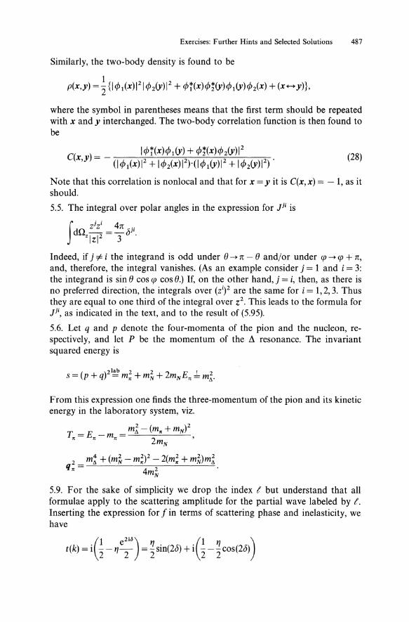
Similarly, the two-body density is found to be
where the symbol in parentheses means that the first term should be repeated with x and y interchanged. The two-body correlation function is then found to be
(28)
Note that this correlation is nonlocal and that for x = y it is C(x, x) = - 1, as it should.
5.5. The integral over polar angles in the expression for pi is
fdn zjzi = 4n c5ji zlzl2 3 .
Indeed, if j "# i the integrand is odd under e ---+ n - e and/or under q> ---+ q> + n, and, therefore, the integral vanishes. (As an example consider j = 1 and i = 3: the integrand is sin e cos q> cos e.) If, on the other hand, j = i, then, as there is no preferred direction, the integrals over (Zi)2 are the same for i = 1,2,3. Thus they are equal to one third of the integral over Z2. This leads to the formula for pi, as indicated in the text, and to the result of (5.95).
5.6. Let q and p denote the four-momenta of the pion and the nucleon, respectively, and let P be the momentum of the A resonance. The invariant squared energy is
( ) 21ab 2 2 2 ! 2 S = P + q = m" + mN + mNE" = m",.
From this expression one finds the three-momentum of the pion and its kinetic energy in the laboratory system, viz.
T = E _ = m~ - (m" + mN)2 " "m" 2 ' mN
5.9. For the sake of simplicity we drop the index t but understand that all formulae apply to the scattering amplitude for the partial wave labeled by t. Inserting the expression for f in terms of scattering phase and inelasticity, we have
(1 e2ib) 1] (1 1] ) t(k) = i - -1]- = -sin(2c5) + i - --cos(2c5) 2 2 2 2 2

488 Exercises: Further Hints and Selected Solutions
and, indeed,
2 ( 1)2 1 2 1 (Re t) + 1m t -"2 = ~rl ::::; 4'
At the resonance, E = Er and c5(kr) = n/2, we find
(k ) i . rei 1 + '1 t r ="2(l+'1)=lr' and r el =-2- r .
Now, let
r x:= ii, 2(E - Er)
1>:= r
The amplitude is then rewritten as follows
t(k) =-1 x 2[ -I>+i], +1>
and, in particular, It - ix/21 = x/2 is independent of 1>. Thus, in the complex plane the amplitude t lies on a circle whose center has coordinates (0,ix/2) and whose radius is x/2. The total cross section as well as the integrated elastic and inelastic cross sections (for the partial wave t) become
t 4n(2t + 1) x (J = --
tot k2 1 + 1>2
t 4n(2t + 1) x 2 t (J el = k2 1 + 1>2 = X(J tot
(J;nel = (1 - x) (J;ot.
These formulae are easy to interpret if one notes that x = rel/r is the probability for the resonance to decay back to the elastic channel, while (1 - x) is the probability for it to decay to anyone of the reaction channels.
5.10. Take the 3-axis along the momentum of the incoming pion and take the spin of the proton to be oriented along the positive 3-direction so that the proton spin projection is + 1/2. Clearly, the reaction is independent of the azimuthal angle cpo Furthermore, as the relative orbital angular momentum vanishes, t = 0, the Ll in the two-step process
is produced in the state Ii = 3/2, j3 = 1/2). Applying space reflection P results in replacing the scattering angle 8 by n - 8. The interaction being assumed to be invariant under P we conclude
d(J(8) = d(J(n - 8).

Exercises: Further Hints and Selected Solutions 489
(One may add a rotation by 1800 about the 2-axis to bring back the incident pion momentum to its initial direction.) The same argument applies to the opposite orientation of the proton spin and, hence, to any superposition of the two orientations.
5.11. We show that the state (1 +, 2°Ne) cannot decay to the configuration (0+, 160 + a). By angular momentum conservation the final state must have total angular momentum j = 1. The a particle and the Oxygen ground state having spin zero, this angular momentum must be equal to the relative orbital angular momentum, j = t = 1. Furthermore, both nuclei have positive parity. Therefore, the parity of the final state is
in contradiction with the parity of zONe which is + 1.
Chapter 6: Hadronic Atoms
6.3. and 6.4. The relative angular momentum t and the total spin S of the two nucleons have fixed values and, for simplicity, we do not write them out. When expressed in terms of states with good isospin we have
1 - -Ipp) = j2 {I(NN) 1 = 1,13 = 0) + I(NN) 1 = 0,13 = O)}
1 - -Inn)= j2{I(NN)I= 1,I3=0)-I(NN)I=O,I3=O)}. (29)
The eigenvalue of charge conjugation C in these states is (- t+ s, while the rotation exp{ in1 z} in isospin space gives the phase ( -l-13 = ( - )1. Therefore, the eigenstate of isospin I(N N)1, 13 = 0) is also an eigenstate of G-parity with eigenvalue (- )t+S+I. Now, (2n) pions in a relative s-state have even G-parity, while (2n + 1) pions have odd G-parity. Therefore, the components with (S = 0,1 = 0) and (S = 1,1 = 1) will decay into an even number of pions, the components with (S = 0, 1 = 1) and (S = 1,1 = 0) will decay into an odd number of pions.
6.5. This exercise is solved most easily by making use of the theorem of Wigner and Eckart, and by using a table of Clebsch-Gordan coefficients or, equivalently, of 3j-symbols.
6.6. Start from (6.24) with K = ke 3 and use j(' x K= - sin e ez. Then, from (6.24) the non-flip amplitude and the spin-flip amplitudes are given by,

490 Exercises: Further Hints and Selected Solutions
respectively, 00
Inoflip(E,O) = L A(PAcos 0), o
00
Iflip(E, 0) = L B(P~(cos 0) sin 0, o
with
A( = tl(_ + (t + 1)1(+, B( = i(j(+ -1(-)·
Assuming j = 3/2 to be the dominant amplitude, that is, 11 _ ~ 0 and 12 + ~ 0, we obtain
(i) for t = 1:
Inoflip(E,O) = 2/1 + cosO, IfliP(E, 0) = ill + sinO,
and for the angular distribution
w(= l(E, 0) = I/noflii + I/flip l2 = 1/1+12(1 + 3 cos2 0);
(ii) for t = 2:
Inoflip(E,O) =/2- (3 cos20 - 1), Iflip(E,O) = - i12- 3 cosOsinO,
and for the angular distribution
wt=iE,O) = 1/2_12(1 + 3 cos2 0).
(30)
(31)
As a result, the angular distribution is the same in the two cases. Its measurement cannot help to distinguish the partial waves (t = 1,j = 3/2) and (t = 2,j = 3/2).
6.8. The formula follows by means of the expansion formula for the plane wave
t
exp{ik·x} =4nLi{jAkx) L Y:m(~)Y{m(x) ( m=-(
and the well-known addition theorem for spherical harmonics
~ * «(") (C\ _ 2t + 1 P «(". £\ m~-( Y(m K Y(m ft.) - 4n (K "').
6.11. Set u: = cot fJ, use the formulae
. s: 1 s: u Stnu= ~' cOSu= ~
v' 1 + u2 v' 1 + u2
and insert u = l/alc + roK to obtain
1= 1 K(U - i)
a

Exercises: Further Hints and Selected Solutions 491
Here the modulus of the three-momentum is related to the energy by K2 = 2mE, with m the reduced mass of the kaon-nucleon system. If there is a bound state the energy is negative, E = - B, B > 0, and K2 is replaced by K2 = - K2, or K = iK. Neglecting the effective range ro, the amplitude has a pole at K = - l/a, and there is bound state with binding energy
1 B~--2·
2J1a
Inserting numbers one finds that this bound state is located at about 12.5 MeV below threshold and that it has a width of about 2 x 13 MeV.
6.12. Define the function
f(r): = N o{ 1 + exp (r ~ c)} -1,
with z = t/( 410g 3). The normalization factor is found from the integral
= - 1 + - - 6 - -- enclz fCO r2dr c3 { (nz)2 (Z)3 00 (-)" }
o l+exp{(r-c)/z} 3 c C n~l n3 . (32)
Note that the third term in the curly brackets of (32) is small and can be neglected in our calculation. Now, if c is replaced by c(1 + f3 Y20) we have
fd3r 1 = fdnfco dxx2~ __ z--;3 __ -c:-
1 +exp{(r-c(l+f3Y20))/Z} 0 l+exp{x-xo}
where we have introduced the abbreviations
r c X:=-, xo:=-(1+f3Y20).
x z
Making use of the formula for the square of Y20 given in Sect. 6.4.1. we can write
3 c3 { 2 2} c3
{ 3 2 ( 2)5 f3) } xO~z31+3f3Y20+3f3Y20~Z3 1+4nf3+3f31+7fo Y20 ,
a formula which is valid up to order f33. After integration over the angular variables the integral above becomes, in the same approximation
492 Exercises: Further Hints and Selected Solutions
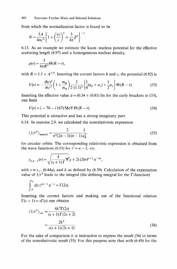
from which the normalization factor is found to be
N = - 1 + - + - [32 . 3A { (nz)2 3 }-1 4nc3 c 4n
6.13. As an example we estimate the kaon-nucleus potential for the effective scattering length (6.97) and a homogeneous nuclear density,
3 p(r) = 4nR30(R - r),
with R = 1.1 x A 1/3. Inserting the correct factors hand c, the potential (6.92) is
V(r) = - ~?: (1 + ::) 2.(:.1)3 H(ao + a1) + ~a1} 0(R - r). (33)
Inserting the effective value ii = (0.34 + iO.81) fm for the curly brackets in (33), one finds
V(r) = ( - 70 - i 167) MeV 0 (R - r).
This potential is attractive and has a strong imaginary part.
6.14. In exercise 2.9. we calculated the nonrelativistic expression
3 2 1 (l/r >nonrel. = n4(2n-l)(n-l)ar
(34)
(35)
for circular orbits. The corresponding relativistic expression is obtained from the wave functions (6.51) for t = n - 1, viz.
Yn,n-1 (r) = J(S +\) r 'I'~X + 2)(2kry+ 1 e- kr ,
with s == s +, (6.44a), and k as defined by (6.39). Calculation of the expectation value of l/r3 leads to the integral (the defining integral for the r -function)
f: dzz2s - 1e- z =r(2s).
Inserting the correct factors and making use of the functional relation r(s + 1) = sr(s) one obtains
3 4k3r(2s) (l/r \el. = (s + 1) r(2s + 2)
2P s(s + 1)(2s + 1)'
(36)
For the sake of comparison it is instructive to express the result (36) in terms of the nonrelativistic result (35). For this purpose note that with (6.49) for the

Exercises: Further Hints and Selected Solutions 493
energy,
we have
3 3 n4( n - 1)( 2n - 1) 1 <1lr >reI. = <1lr )nonrel. s(s + 1)(2s + 1) {(s + 1)2 + (ZIX)2P/2· (37)
As a numerical example take n = 2, t = 1 and Z = 82 so that ZIX ~ 0.6. The factor on the right-hand side of (37) is found to be 1.39. Also, one verifies that this factor tends to 1 as terms of order (ZIX)2 are neglected. Indeed, in this limit s~t=n-1.
6.15. In order to prove the assertion we must verify the following properties:
III + Il2 = ~
IllIl2 = Il2Ill =0
Il? = Ili' i = 1,2.
(38)
(39)
(40)
The first property (38) is obvious. In verifying (39) we make use of the identity
(alJ(aJk) = (6 ik + ia/;jik) tlk = t 2 - (Jo{.
In the second step, we inserted the commutator of ti and t k • The first product (39) is then found to be
III Il2 = (2t ~ W [t(t + 1) - (J·t - t 2 + (J·t],
which, when acting on a state of good t 2 gives indeed zero. In exactly the same way one verifies (40). Finally, we must check that III indeed projects onto j + = t + 1/2, II2 projects onto j _ = t - 1/2. For this purpose we note that the denominator'in their definition can be written as
2t + 1 = j + U + + 1) - j _ U _ + 1).
Furthermore, we replace (J·t by jU + 1) - t(t + 1) - 3/4 and obtain the result
Il = jU+1)-j-U-+1) I j+U++l)-j_(j_+1)
(41)
(42)
from which the assertion is evident.

Subject Index
Abelian gauge theories 205 adjoint representation 67 Adler-Weisberger relation 319 annihilation operators
anticommutation relations 36 anomalous magnetic moment 62 anticommutation relations of creation
and annihilation operators 36 anticommutator 33 antiparticles 39 antisymmetric tensor in three dimensions 65 asymptotic behaviour
of confluent hypergeometric function 137,422
asymptotic freedom 246 axial current 314 axial vector current 173
baryon number 176 Beg's theorem 389 Bessel functions 99 beta-decay of triton 330 biunitary transformation 241 Bohr radius 127, 128 boosts 4,6 Born approximation 73, 76, 103 bottom quark 176 Breit system 60
Cabibbo angle 225 Cabibbo-Kobayashi-Maskawa
mixing matrix 225, 242 causal distribution 32, 452 charge and current densities 103 charge conjugate spinor 28 charge conjugation 68, 195 charge density 73 charge form factor 74 charge operator 38 charge radius 81
of nuclei 73 charged current (CC)
interactions 182, 237
charmed quark 176 chiral symmetry 249,315 chirality 187 Clebsch-Gordan coefficients 98 coherent approximation 380 colour degree of freedom 245 colour quantum numbers 177, 245 compact groups 208 confinement 249 confluent hypergeometric function 128,136,
421 asymptotic behaviour 137, 422
conjugate momenta of Dirac Fields 38 connection form 218 conserved vector current 308 constituent quark masses 250 contact interaction 180 contragredience 14 contravariant vectors 2 Coulomb distortion 109 Coulomb gauge 102 Coulomb interaction
instantaneous 102 Coulomb phases 117 covariant density matrix 47 covariant derivative 64,214
for SU(3) 248 covariant normalization 27,412,454 covariant vector 2 creation operators 37
anticommutation relations 36 cross section asymmetry 252 current conservation 84 current density 38 current quark masses 250 curvature form 218
decay modes n°--->yy 244,328 /.l--->ey 350
decomposition theorem for Lorentz transformations 5
deep inelastic region 76, 168
496 Subject Index
deep inelastic scattering 161 hadronic tensor 164 leptonic tensor 163
density matrix 43 for neutrinos 49
destruction operators 37 differential cross section 454 differential decay rate 455 diffraction minima 110 Dirac equation 20, 21, 24, 464
Hamilton form 24 Dirac field
energy density of 40 Lagrange density of 37 negative frequency part 25 positive frequency part 25 quantization of 33
Dirac mass term 37, 55 Dirac matrices 23 Dirac quantum number 134 Dirac's angular momentum operator 464 dispersion corrections 56, 122 dotted spinors 15 down quark 176
effective ranges 417 eightfold way 462 Eikonal approximation 366 elastic unitarity 412 electric dipole transition 130 electric quadrupole moment 123, 442 electromagnetic current 60, 84 electromagnetic field tensor 59 electron scattering
selection rules for 107 energy density of Dirac field 40 energy-momentum tensor density 40 Euler angles 10, 43 exotic atoms 407 external potentials 459
Fermi constant 221 Fermi density 119 Fermi-Dirac statistics 34 Fermion multiplets in gauge theory 242 Fermion propagator 458 Feynman rules 83, 87, 458 field strength tensor for SU(3) 248 field tensor 214 Fierz transformation 283 flavour quantum numbers 176 form factor 80, 91, 92
electric 91 magnetic 92
forward-backward asymmetry 268 in cross section 263
four-fermion interaction 199, 282
frozen nucleus assumption 374 fundamental representation 67
g-factor 60 G-parity 314 gamma-transitions
time scale of 130 gauge boson masses 234 gauge group 208, 218 gauge invariance of QED 63 gauge theories 205
Abelian and non-Abelian 205 Fermion multiplets in 242
gauge transformation 208 Gell-Mann matrices 244, 461 generators of infinitesimal transformations
65,206 global transformations 208 gluons 248 Goldberger-Treiman relation 318 Goldstone fields 231 Goldstone theorem 231 Gordon identity 85, 89 Green function 79, 357, 361 group orbit 231
hadronic matrix element Lorentz structure of 173
hadronic tensor in deep inelastic scattering 164
hadronic weak interactions 306 Hamilton form of the Dirac equation 24 handedness 187 hard-core correlation function 386 Heisenberg equations of motion 84 helicity 175
eigenstates 78 operator 27 transfer at vertices 188
Helmholtz equation 97 hermiticity of electromagnetic current 86 hidden symmetry 229 Higgs doublet 240 Higgs field 233
vacuum expectation value of 236 Higgs sector of GSW model 238 high-energy representation of Dirac
matrices 23 Horizontal symmetries 352 hydrogen wave functions
nonrelativistic 128 of relativistic hydrogen atom 423
hyperfine structure 159
impact parameter 366 inclusive scattering 109, 161 inelasticity 360 internal spectrum symmetry 177

intrinsic parity 18, 195 invariant cross section 82 invariant tensors in SU(3) 462 inverse muon decay 299 isobar model 399 isomer shift 158 isospin
strong interaction 93, 177 weak interaction 223
Kaonic atoms 423, 438 Klein-Gordon equation 8, 20, 357,
419,429 Kummer's differential equation 136, 421
Lagrange density of the Dirac field 37 of the Maxwell field 58 of the Majorana field 31
Lamb shift and vacuum polarization 152 Laplace operator 19 left-right symmetric theories 298 lepton family numbers 175, 348 lepton mixing 352 lepton universality 223, 274 leptonic processes 179 leptonic tensor in deep inelastic
scattering 163 leptons 174 Lie algebra 65, 206 Lie group 65, 206 Lippmann-Schwinger equation 363 little group 42, 49, 230 local transformations 208 longitudinal polarization in
~-decay 297 Lorentz group
spin or representations of 13 Lorentz invariant distributions 452 Lorentz structure of hadronic matrix
element 173 Lorentz transformation
decomposition theorem for 5 orthochronous 3 proper 3 special 4, 12
Lorentz-Lorenz effect 389
magnetic moment 60, 92, 174 anomalous 92 normal 92 of the muon 127
Majorana fields 31,51 quantization of 30
Majorana mass term 55
Subject Index 497
Majorana neutrino 349 Majorana spinors 30 Mandelstam variables 82 mass eigenstates 225,241 mass matrix 52, 344 masses of W± and zo 202 Maxwell field
Lagrange density of 58 mesonic atoms 423 metric tensor 2 Michel parameter 295 Michel spectrum 295 minimal substitution 59, 63 M~ller factor 87,414,454 M¢ller operators 364 Mott cross section 80 multiple scattering 365, 371 multi pole fields 98
electric 100 longitudinal 100 magnetic 100
multi pole form factors electric 105 magnetic 106
muon capture 318 muon decay 288
inverse 299 longitudinal polarization in 297 observables in 295 transverse polarization in 297
muon neutrino helicity 301
natural units 59 negative frequency part of the Dirac field 25 neutral current (NC) 237, 302
interactions 183 neutrino
masses 330, 333 oscillations 339 scattering 271
neutrino and antineutrino scattering 255
neutrinoless double fJ-decay 349 non-Abelian gauge theories 205 nuclear charge density 57 nuclear polarizability 56 number of leptonic generations 272
observables in muon decay 295 one-body density 382 on-shell scheme 236 optical potential 380, 385, 428 optical theorem 411
p-wave scattering volume 417 parallel transport 210, 213
498 Subject Index
parity 195, 197 violation 183
partial conservation of the axial current 315
partial wave analysis 111, 124 Pauli correlations 389 Pauli matrices 8 Pauli principle 34 Pauli term 62 Pauli-Lubanski vector 42 PCT-theorem 198,282 phase function 371 phase shifts 121 photon propagator 83 pion beta decay 308,311 pion decay constant 314 pionic atoms 428, 432 Poincare sphere 44 Poisson's equation 73 polarizability 153 polarization 270
polarization charge density 150 positive frequency part of Dirac field 25 potential scattering theory 356 profile function 367, 371, 375 projectors onto positive and negative frequency
solutions 47 proton
r.m.s. radius of 94 pseudoscalars 278
QCD Lagrangian 248 quadrupole hyperfine structure 444 quadrupole moment
spectroscopic 123, 161,442 quantization
of Dirac field 33 of Majorana fields 30
quantum chromodynamics 244 quantum electrodynamics 143,458
gauge invariance of 63 quark families 176,224 quarks
weak hypercharge of 227 quasi free scattering 76
radiative corrections to muon decay 299 to W-mass 236
radius of half-density 118 of proton 73
rapidity parameter 6 reaction matrix 411
root-mean-square radius 81 of the pion 321
Rosenbluth formula 90, 169 rotations 4, 10
S-matrix 411 s-wave scattering length 317 Sachs form factors 92 scalar wave equations 357 scalars 278 scaling 246 scattering
equation 361 matrix 454 neutrino and antineutrino 255 phase 116, 119,360
seesaw mechanism 55 selection rules for electron scattering 107 semi-inclusive scattering 109 semileptonic processes 179, 190, 307 SL (2,C) 8 solar neutrino
flux 341 units (SNU) 342
space reflection 3, 17 special linear group 9 special Lorentz transformation 4, 12 spin projection operator 46 spin vector 7 spinor
fields 16 representations of the Lorentz Group 13 time reversed 30
spin-statistics theorem 34 spontaneous symmetry breaking 228 standard representation of Dirac matrices 23 Stokes parameters 44 strange quark 176 strong interaction isospin 177 strongly deformed nuclei 122, 440 structure constants 65, 206 structure functions 165 structure group 208 SU (2) 65, 206 SU(3) 206,244,461
covariant derivative for 64,214 field strength tensor for 248 invariant tensors in 462 vector potential for 210
SU(n) 206 surface thickness 118
T-matrix 412,454 T-operator 364 theorem of Goldstone 231

three-body decays 456 time reversal 3, 17, 195, 197 time reversed spinor 30 time scale of y-transitions 130 top quark 176, 274 trace techniques 89 traces 460 translation formulae 84 transverse polarization in Il-decay 297 triangle anomaly 243 two-body correlation 385
function 382 two-body decay 455 two-body density 382
U(I) 64,206 U-transformation 14 undotted spinors 15 unitarity 204, 411 unitary gauge 240 universality of weak interactions 190 up quark 176
Subject Index 499
V-A interaction 296, 297 vacuum expectation value of Higgs
field 236 vacuum polarization 144, 146 vector current 173 vector potential 210
for SU(3) 247 vector spherical harmonics 98
weak hypercharge 223 of quarks 227
weak interaction eigenstates 224, 241 universality of 190
weak isospin 223 Weinberg angle 201, 222 Weyl equations 20 Whittaker function 437 Wigner-Eckart theorem 93 W-propagator 199
Yukawa coupling 235