59

Appendix A – Notes on Exemptions

Groundwater Regulations 2010

Regulation 8 (i.e. WFD Article 11 (3)(j))

(a) The direct discharge of pollutants into groundwater is prohibited;

(b) The following discharges may be permitted subject to a requirement for prior authorisation

provided such discharges, and the conditions imposed, do not compromise the achievement of

the environmental objectives established for the body of groundwater into which the discharge is

made;

(i) injection of water containing substances resulting from the operations for exploration

and extraction of hydrocarbons or mining activities, and injection of water for technical

reasons, into geological formations from which hydrocarbons or other substances have

been extracted or into geological formations which for natural reasons are permanently

unsuitable for other purposes. Such injections shall not contain substances other than

those resulting from the above operations,

(ii) reinjection of pumped groundwater from mines and quarries or associated with the

construction or maintenance of civil engineering works,

(iii) injection of natural gas or liquefied petroleum gas (LPG) for storage purposes into

geological formations which for natural reasons are permanently unsuitable for other

purposes,

(iv) injection of natural gas or liquefied petroleum gas (LPG) for storage purposes into

other geological formations where there is an overriding need for security of gas supply,

and where the injection is such as to prevent any present or future danger of

deterioration in the quality of any receiving groundwater,

(v) discharges resulting from construction, civil engineering and building works and

similar activities on, or in the ground which come into contact with groundwater. Such

activities may be treated as having been authorised provided that they are conducted in

accordance with general binding rules which are applicable to such activities,

(vi) small quantities of substances for scientific purposes for characterisation, protection

or remediation of water bodies limited to the amount strictly necessary for the purposes

concerned;

(c) Reinjection of water used for geothermal purposes into the same aquifer may be permitted

subject to a requirement for prior authorisation.

60

Regulation 14 (i.e. GWD Article 6(3))

Without prejudice to any more stringent requirements in other Community legislation, Member States

may exempt from the measures required by paragraph 1 inputs of pollutants that are:

Categories of exempted pollutant inputs Comments/Examples

a) inputs that are the result of direct discharges authorised in

accordance with Regulation 8;

Self explanatory.

- prior authorisation is

required.

b) inputs considered to be of a quantity and concentration so small

as to obviate any present or future danger of deterioration in the

quality of the receiving groundwater;

Amount of substance is so

small it cannot be quantified,

e.g. hazardous substances

from single septic tank.

c) inputs that are the consequences of accidents or exceptional

circumstances of natural cause that could not reasonably have

been foreseen, avoided or mitigated;

Weather extremes or natural

events. However, if they can

be foreseen they should be

prevented.

d) inputs that are the result of artificial recharge or augmentation of

bodies of groundwater authorised in accordance with Article

11(3)(f) of Directive 2000/60/EC;

Self explanatory – prior

authorisation is required.

e) inputs considered incapable, for technical reasons, of being

prevented:

i. measures that would increase risks to human health or to

the quality of the environment as a whole, or

ii. disproportionately costly measures to remove quantities of

pollutants from or otherwise control their percolation in,

contaminated ground or subsoil; or

Where full remediation of a

contaminated site may do

more harm than good. This

might include, for example,

contaminated land sites or

old unlined landfills, subject

to case-by-case assessment.

f) inputs that are the result of interventions in surface waters for the

purposes, amongst others, of mitigating the effects of floods and

droughts, and for the management of waters and waterways,

including at international level. Such activities, including cutting,

dredging, relocation and deposition of sediments in surface water,

shall be conducted in accordance with general binding rules, and,

where applicable, with permits and authorisations issued on the

basis of such rules, developed by the relevant authority for that

purpose, provided that such inputs do not compromise the

achievement of the environmental objectives established for the

water bodies concerned.

Self explanatory.

61

Appendix B – Primary Information Sources

General:

General Water Maps: http://watermaps.wfdireland.ie/

WFD groundwater bodies and surface water bodies;

Chemical status of associated groundwater body and related downgradient surface water

bodies.

General mapping by the Ordnance Survey of Ireland: www.osi.ie

Geological Survey of Ireland:

GSI Groundwater Public Viewer: http://spatial.dcenr.gov.ie/imf/imf.jsp?site=Groundwater or relevant

datasets downloaded from http://www.dcenr.gov.ie/

Teagasc subsoil maps;

Groundwater vulnerability;

Groundwater recharge map;

Source protection areas;

Subsoil permeability map;

Groundwater resources: Aquifer and flow types;

Bedrock map;

Karst features (not comprehensive);

Groundwater protection schemes;

GSI groundwater body descriptions at

http://www.gsi.ie/Programmes/Groundwater/Projects/Groundwater+Body+Descriptions.htm

Environmental Protection Agency:

EPA ENVision – Environmental Maps: http://maps.epa.ie/internetmapviewer/mapviewer.aspx

Soil types;

Surface water features;

Location of IPPC and Waste licences.

62

Drinking water supplies: EPA - Groundwater and Hydrometric Division or Office of Environmental

Enforcement;

National groundwater quality and level monitoring network: Groundwater and Hydrometric Section

Potential other point sources of pollution: EPA and local authority licence databases.

National Parks and Wildlife Service:

General Information: www.npws.ie

Appropriate Assessment: http://www.npws.ie/en/WildlifePlanningtheLaw/AppropriateAssessment/

NPWS map viewer: http://www.designatednatureareas.ie/mapviewer/

GWDTEs and Special Areas of Conservation locations and associated SAC descriptions at

http://www.npws.ie/en/ProtectedSites/SpecialAreasofConservationSACs/.

River Flow Data:

EPA ENVision – Environmental Maps: http://maps.epa.ie/internetmapviewer/mapviewer.aspx

EPA Hydrometric Data System: http://watermaps.wfdireland.ie/HydroTool

EPA HYDRONET website: http://hydronet.epa.ie

EPA Estimated Dry Weather Flow and 95-percentile Flow. Available from

http://www.epa.ie/downloads/pubs/water/flows/

OPW Hydro-Data Web-Site: http://www.opw.ie/hydro/index.asp?mpg=main.asp

63

Appendix C – Polluting Substances and Receptor-

based Water Quality Standards

Polluting Substances

Lists of polluting substances can be found in:

Annex VIII of the Water Framework Directive; and

Annex to the Groundwater Directive.

Hazardous and Non-Hazardous Substances

The EPA has listed substances that have been determined as hazardous and those determined to be

non-hazardous, in a report called “Classification of Hazardous and Non-hazardous Substances in

Groundwater” which can be found on the EPA website www.epa.ie.

Receptor-based Water Quality Standards

Hazardous Substances

Hazardous substances are substances or groups of substances that are toxic, persistent and liable to

bio-accumulate, and other substances or groups of substances which give rise to an equivalent level

of concern. Hazardous substances are listed in a document by the EPA (2010).

The default compliance value for hazardous substances is the Minimum Reporting Value (MRV) of the

substance. This is the lowest concentration that can be determined with a known degree of

confidence, and may or may not be equivalent to limits of detection.

Table C.1 presents provisional MRVs for selected hazardous substances. The provisional MRVs are

based on a set of values published by the Environment Agency (EA) H1 Technical Annex to Annex J:

Hydrogeological Risk Assessments for Landfills and the Derivation of Groundwater Control Levels

and Compliance Limits (2010).

Where an MRV is not available, an agreed limit of detection (LoD) for the relevant hazardous

substances should be determined by the regulatory body. LoDs have not been predefined, and so the

LoDs given in the WHO Guidelines for Drinking Water Quality, Third Edition, Volume 1, 2004, as

amended (2008), can be used as a first guide.

Table C.1: Provisional MRVs for Selected Hazardous Substances

Substance MRV (μg/l) Comment

1,1,1-trichloroethane 0.1

1,1,2-trichloroethane 0.1

1,2-dichloroethane 1

2,4 D ester 0.1 methyl, ethyl, isopropyl, isobutyl and butyl each to 0.1

2,4-dichlorophenol 0.1

2-chlorophenol 0.1

4-chloro-3-methylphenol 0.1

aldrin 0.003

atrazine 0.03

azinphos-ethyl 0.02

azinphos-methyl 0.001

64

Substance MRV (μg/l) Comment

benzene 1

cadmium 0.1

carbon tetrachloride 0.1

chlorfenvinphos 0.001

chloroform 0.1

chloronitrotoluenes 1 2,6-CNT; 4,2-CNT; 4,3-CNT; 2,4-CNT; 2,5-CNT each to 1µg/l

PCB (individual congeners) 0.001

demeton 0.05 demeton-s-methyl only

diazinon 0.001

dieldrin 0.003

dimethoate 0.01

endosulfan 0.005 endosulphan a and endosulphan b, each to 0.005 µg/l

endrin 0.003 fenitrothion 0.001 fenthion 0.01 hexachlorobenzene 0.001 hexachlorobutadiene 0.005

hexachlorocyclohexanes 0.001 α-HCH, γ-HCH and δ-HCH each to 0.001μg/l β-HCH to 0.005μg/l

isodrin 0.003 malathion 0.001

mecoprop 0.04 mercury 0.01 mevinphos 0.005 op DDT 0.002 o = ortho; p = para

pp DDT 0.002 op DDE 0.002 pp DDE 0.002 op TDE 0.002 pp TDE 0.002 parathion 0.01 parathion methyl 0.015 pentachlorophenol 0.1 permethrin 0.001 cis and trans-permethrin both to 0.001μg/l

simazine 0.03 tetrachloroethylene 0.1 toluene 4 tributyltin compounds 0.001 trichlorobenzene 0.01 135 tcb; 124 tcb; 123 tcb each to 0.01 µg/l

trichloroethylene 0.1 trifluralin 0.01 triphenyltin compounds 0.001

xylenes 3 o-xylene and m/p-xylene each to 3μg/l. May not be possible to separate m- and p-xylene.

65

Other substances may be added by the EPA at a later time.

Non-Hazardous Substances

Non-hazardous substances are pollutants listed in Annex VIII of the WFD which are not considered

hazardous, and any other non-hazardous pollutants not listed in that Annex that present an existing or

potential risk of pollution. Non-hazardous substances are listed in a document by the EPA (2010a).

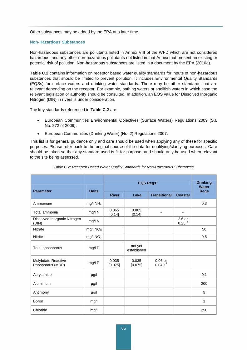
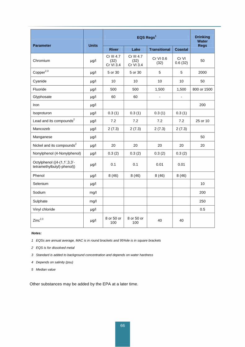
Table C.2 contains information on receptor based water quality standards for inputs of non-hazardous

substances that should be limited to prevent pollution. It includes Environmental Quality Standards

(EQSs) for surface waters and drinking water standards. There may be other standards that are

relevant depending on the receptor. For example, bathing waters or shellfish waters in which case the

relevant legislation or authority should be consulted. In addition, an EQS value for Dissolved Inorganic

Nitrogen (DIN) in rivers is under consideration.

The key standards referenced in Table C.2 are:

European Communities Environmental Objectives (Surface Waters) Regulations 2009 (S.I.

No. 272 of 2009);

European Communities (Drinking Water) (No. 2) Regulations 2007.

This list is for general guidance only and care should be used when applying any of these for specific

purposes. Please refer back to the original source of the data for qualifying/clarifying purposes. Care

should be taken so that any standard used is fit for purpose, and should only be used when relevant

to the site being assessed.

Table C.2: Receptor Based Water Quality Standards for Non-Hazardous Substances

Parameter

Units

EQS Regs1 Drinking

Water Regs

River Lake Transitional Coastal

Ammonium mg/l NH4 0.3

Total ammonia mg/l N 0.065 [0.14]

0.065 [0.14]

- -

Dissolved Inorganic Nitrogen (DIN)

mg/l N

2.6 or 0.25

4

Nitrate mg/l NO3 50

Nitrite mg/l NO2 0.5

Total phosphorus mg/l P

not yet established

Molybdate Reactive Phosphorus (MRP)

mg/l P 0.035 [0.075]

0.035 [0.075]

0.06 or 0.040

5

Acrylamide μg/l

0.1

Aluminium μg/l

200

Antimony μg/l

5

Boron mg/l

1

Chloride mg/l

250

66

Parameter

Units

EQS Regs1 Drinking

Water Regs

River Lake Transitional Coastal

Chromium μg/l Cr III 4.7

(32) Cr VI 3.4

Cr III 4.7 (32)

Cr VI 3.4

Cr VI 0.6 (32)

Cr VI 0.6 (32)

50

Copper2,3

μg/l 5 or 30 5 or 30 5 5 2000

Cyanide μg/l 10 10 10 10 50

Fluoride μg/l 500 500 1,500 1,500 800 or 1500

Glyphosate μg/l 60 60 - -

Iron μg/l

200

Isoproturon μg/l 0.3 (1) 0.3 (1) 0.3 (1) 0.3 (1)

Lead and its compounds2 μg/l 7.2 7.2 7.2 7.2 25 or 10

Mancozeb μg/l 2 (7.3) 2 (7.3) 2 (7.3) 2 (7.3)

Manganese μg/l

50

Nickel and its compounds2 μg/l 20 20 20 20 20

Nonylphenol (4-Nonylphenol) μg/l 0.3 (2) 0.3 (2) 0.3 (2) 0.3 (2)

Octylphenol ((4-(1,1’,3,3’-tetramethylbutyl)-phenol))

μg/l 0.1 0.1 0.01 0.01

Phenol μg/l 8 (46) 8 (46) 8 (46) 8 (46)

Selenium μg/l

10

Sodium mg/l

200

Sulphate mg/l

250

Vinyl chloride μg/l

0.5

Zinc2,3

μg/l 8 or 50 or

100 8 or 50 or

100 40 40

Notes:

1 EQSs are annual average, MAC is in round brackets and 95%ile is in square brackets

2 EQS is for dissolved metal

3 Standard is added to background concentration and depends on water hardness

4 Depends on salinity (psu)

5 Median value

Other substances may be added by the EPA at a later time.

67

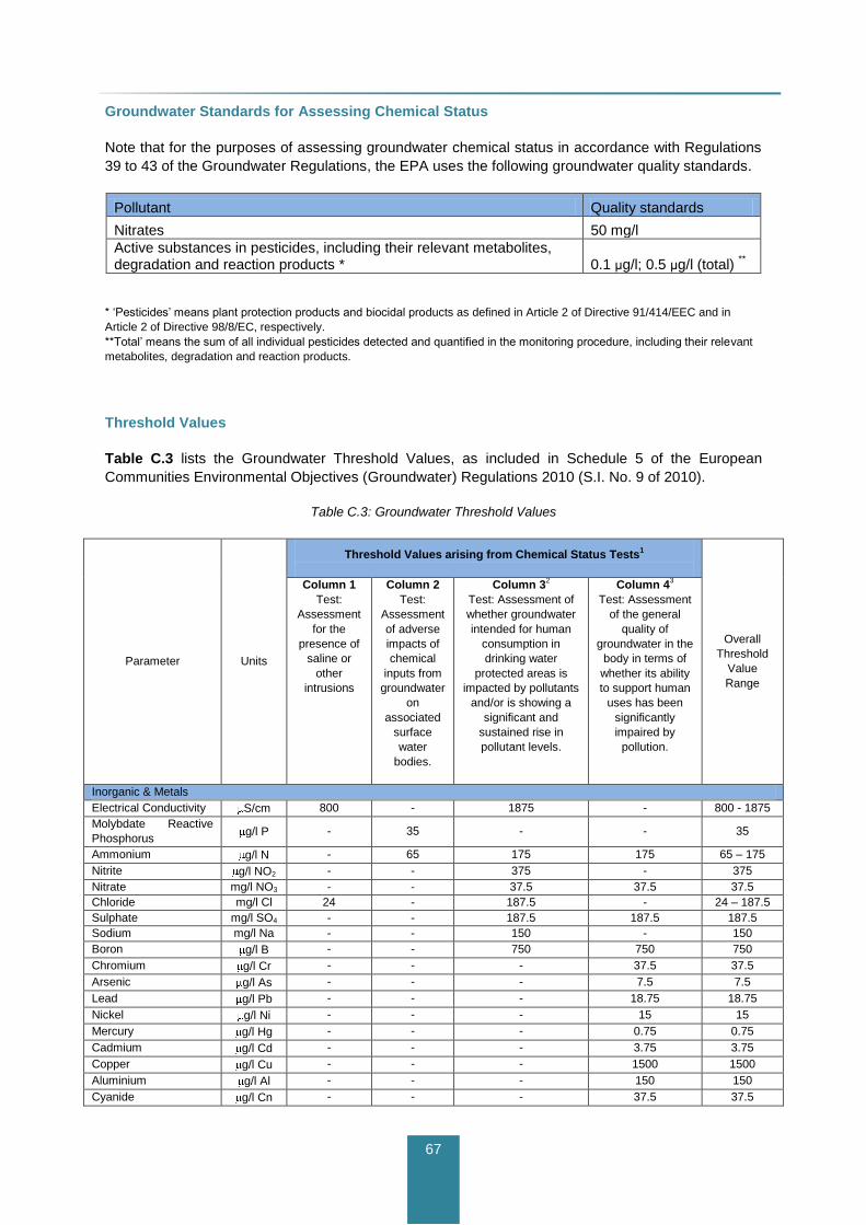
Groundwater Standards for Assessing Chemical Status

Note that for the purposes of assessing groundwater chemical status in accordance with Regulations

39 to 43 of the Groundwater Regulations, the EPA uses the following groundwater quality standards.

Pollutant Quality standards

Nitrates 50 mg/l

Active substances in pesticides, including their relevant metabolites, degradation and reaction products * 0.1 μg/l; 0.5 μg/l (total)

**

* ‘Pesticides’ means plant protection products and biocidal products as defined in Article 2 of Directive 91/414/EEC and in

Article 2 of Directive 98/8/EC, respectively.

**Total’ means the sum of all individual pesticides detected and quantified in the monitoring procedure, including their relevant

metabolites, degradation and reaction products.

Threshold Values

Table C.3 lists the Groundwater Threshold Values, as included in Schedule 5 of the European

Communities Environmental Objectives (Groundwater) Regulations 2010 (S.I. No. 9 of 2010).

Table C.3: Groundwater Threshold Values

Parameter Units

Threshold Values arising from Chemical Status Tests1

Overall

Threshold

Value

Range

Column 1

Test:

Assessment

for the

presence of

saline or

other

intrusions

Column 2

Test:

Assessment

of adverse

impacts of

chemical

inputs from

groundwater

on

associated

surface

water

bodies.

Column 32

Test: Assessment of

whether groundwater

intended for human

consumption in

drinking water

protected areas is

impacted by pollutants

and/or is showing a

significant and

sustained rise in

pollutant levels.

Column 43

Test: Assessment

of the general

quality of

groundwater in the

body in terms of

whether its ability

to support human

uses has been

significantly

impaired by

pollution.

Inorganic & Metals

Electrical Conductivity S/cm 800 - 1875 - 800 - 1875

Molybdate Reactive

Phosphorus g/l P - 35 - - 35

Ammonium g/l N - 65 175 175 65 – 175

Nitrite g/l NO2 - - 375 - 375

Nitrate mg/l NO3 - - 37.5 37.5 37.5

Chloride mg/l Cl 24 - 187.5 - 24 – 187.5

Sulphate mg/l SO4 - - 187.5 187.5 187.5

Sodium mg/l Na - - 150 - 150

Boron g/l B - - 750 750 750

Chromium g/l Cr - - - 37.5 37.5

Arsenic g/l As - - - 7.5 7.5

Lead g/l Pb - - - 18.75 18.75

Nickel g/l Ni - - - 15 15

Mercury g/l Hg - - - 0.75 0.75

Cadmium g/l Cd - - - 3.75 3.75

Copper g/l Cu - - - 1500 1500

Aluminium g/l Al - - - 150 150

Cyanide g/l Cn - - - 37.5 37.5

68

Pesticides

Atrazine g/l - - 0.075 0.075 0.075

Simazine g/l - - 0.075 0.075 0.075

MCPA g/l - - 0.075 0.075 0.075

Lindane g/l - - 0.075 0.075 0.075

Diuron g/l - - 0.075 0.075 0.075

4,4 - DDT g/l - - 0.075 0.075 0.075

Dieldrin g/l - - 0.075 0.075 0.075

Cypermethrin g/l - - 0.075 0.075 0.075

Bentazone g/l - - 0.075 0.075 0.075

Glyphosate g/l - - 0.075 0.075 0.075

Chlortoluron g/l - - 0.075 0.075 0.075

Mecoprop g/l - - 0.075 0.075 0.075

Isoproturon g/l - - 0.075 0.075 0.075

2,4

Dichlorophenoxyacetic

acid

g/l - - 0.075 0.075 0.075

Total Pesticides g/l - - 0.375 0.375 0.375

Organics

1,2-Dichloroethane g/l - - - 2.25 2.25

Vinyl Chloride g/l - - - 0.375 0.375

Total

Tetrachloroethene &

Trichloroethene

g/l - - - 7.5 7.5

Benzene g/l - - - 0.75 0.75

Benzo(alpha)pyrene ng/l - - - 7.5 7.5

Total Polycyclic

Aromatic

Hydrocarbons

g/l

- - - 0.075 0.075

Total Trihalomethanes g/l - - - 75 75

Notes:

1 “Threshold values” have been established for pollutants that are causing a risk to groundwater bodies. Exceedance of a relevant threshold value at a representative monitoring point triggers further investigation to confirm whether the criteria for poor groundwater chemical status are being met. If the criteria for poor chemical status are being met by one or more of the test procedures in Schedule 7, then a body or a group of bodies of groundwater is classified as being at poor chemical status. Threshold values are expressed as annual arithmetic mean concentrations. 2 For the drinking water test, further investigation includes an assessment of significant and sustained upward trends in concentration of the relevant pollutant at the monitoring point. 3 For the general chemical test, further investigation includes the aggregation of data from a representative group of monitoring points, comparison of the aggregated annual arithmetic mean concentration of the relevant pollutant with the threshold value and confirmation of significant impairment of the groundwater body’s ability to support human uses.

69

Appendix D – Substances of Concern and

Attenuation

The estimation of chemical loading to groundwater requires knowledge of the chemical composition

and concentrations of individual substances in the effluent. This appendix outlines the key substances

of concern for different types of effluent.

A useful reference document which details the chemistries of different effluent types is “Guidance,

Procedures and Training on the Licensing of Discharges to Surface Waters and to Sewer for Local

Authorities” (Water Services National Training Group, 2010).

Domestic Waste Water Effluent

Domestic waste water effluent is defined as “wastewater of a composition and concentration

(biological and chemical) normally discharged by a household, and which originates predominantly

from the human metabolism or from day to day domestic type human activities, including washing and

sanitation, but does not include fats, oils, grease or food particles discharged from a premises in the

course of, or in preparation for, providing a related service or carrying on a related trade” (Water

Services Act, 2007).

For domestic waste water inputs to groundwater that exceed 5m3/d in volume, a Section 4 licence is

required from the relevant local authority, under the Local Government (Water Pollution) Acts 1977 to

1990. Domestic waste water not exceeding 5 m3/d in volume, which is discharged to groundwater

from a septic tank or other disposal unit by means of a infiltration area, soakage pit or other method is

exempt from obtaining a Section 4 licence under Article 4 of the Local Government (Water Pollution)

Regulations, 1978. The EPA licenses inputs of domestic sewage to groundwater under IPPC and

waste licensing regimes if there is an input associated with a licensable activity.

Under the Waste Water Discharge (Authorisation) Regulations of 2007 (as amended), the EPA may

issue a licence or certificate of authorisation to water services authorities that discharge waste water

to receiving waters. Discharges from agglomerations with a population equivalent (p.e.) greater than

500 require a licence and those with a p.e. less than 500 require a certificate of authorisation. A

licence is an authorisation with more stringent conditions than a certificate of authorisation.

The waste water regulations of 2007 address discharges to water. In the context of groundwater, the

500 p.e. threshold is considered quite large, equivalent to a maximum discharge rate of approximately

90 m3/d. No water services authorities are currently operating any discharge to groundwater activities

at this scale.

In Ireland, discharges of domestic waste water to ground occur primarily from septic tank systems and

packaged treatment plants, collectively referred as onsite waste water treatment systems (OSWTS).

There are few large discharges to ground from waste water treatment works, but the number of

OSWTSs exceeds 400,000 (Spain and Glasgow, 2009).

The chemical composition of effluent will depend on the source, the type of treatment system (e.g.

septic tank, packaged treatment plant), and the condition of the treatment system. Typical

concentration ranges for key substances in untreated domestic waste water effluents are indicated in

Table D.1, which includes effluent from commercial sources such as hotels, retail shops and offices.

Effluents from commercial activities may contain additional substances that are particularly associated

with that activity, which should be identified during risk screening.

70

Table D.1: Untreated Domestic Waste Water Characteristics

Parameter Domestic Sources*

Commercial Sources

Mean**

BOD5 150-500* 470

COD 300-1,000* 888

Suspended Solids 200-700* 293

Total Phosphorous (as P) 5-20* 8.21

Total Nitrogen (N)*** 40.6** 55

Ammonia (NH4 – N) 22-80* 45.6

Nitrate (NO3 – N) 0.25** 0.27

Nitrite (NO2 – N) 0.04** 0.04

pH 7.5** 7.37

Total Coliforms 106 -

109 10

8

E. Coli 105 10

7

* All values in mg/l, except bacteria counts which are expressed in colony forming units per 100 ml. Ranges sourced from EPA Code of Practice, 2009a. ** All results in mg/l, Source: EPA Waste water Treatment Manual, Treatment for Small Communities, Business, Leisure Centres and Hotels, 1999. ***Total nitrogen is the sum of sum of Total Kjeldahl Nitrogen (organically bound nitrogen and ammonia) and Oxidised Nitrogen (nitrate and nitrite).

The main substances of concern associated with domestic waste water are ammoniacal nitrogen

(NH4), phosphorus (P), and microbiological constituents (pathogens). Table D.2 provides a summary

of performance standards for key substances which are concentrations that are expected in effluents

from OSWTSs (EPA, 2009a). Packaged treatment plants are often quoted to achieve a higher level of

treatment compared to septic tanks.

As identified in the EPA code of practice for OSWTSs (EPA, 2009a), local authorities may set stricter

performance standards, conditional on the results of impact assessment on receiving waters

(including groundwater). Packaged treatment plant manufacturers will often quote the level of

treatment that can be achieved, some claiming that NH4 concentrations can be treated to less than

20 mg/l-N for more expensive and advanced treatment plants.

Table D.2: Performance Standards for Packaged Secondary Treatment Plants Receiving

Domestic Waste Water Effluent

Parameter Standard (mg/l)1 Comment

BOD (mg/l) 20

Suspended solids (mg/l) 30

NH4 as N (mg/l) 20 Unless otherwise specified by local authority

Total nitrogen as N (mg/l) 5 Only for nutrient sensitive locations

Total phosphorus as P (mg/l) 2 Only for nutrient sensitive locations

1 - 95-percentile compliance is required for site monitoring carried out after installation.

71

Ammoniacal nitrogen (NH4

Concentrations of NH4 in domestic waste water are typically much higher than relevant receptor-

based water quality standards, which in the case of surface waters is 0.065 mg/l-N (as a mean value)

for the good-moderate status boundary and 0.04 mg/l-N for the high-good status boundary.

Ammonium may be transformed (nitrified) to nitrate (NO3), which is a key parameter monitored by the

EPA to determine water body status. Elevated nitrate concentrations occur in some Irish groundwater

bodies, but can be virtually absent in others.

Where chemical status is poor as a result of elevated nitrates, or sustained upwards concentration

trends are identified, additional treatment of the effluent may be required prior to discharge.

Phosphorus and phosphates

Several groundwater bodies in the central and western parts of Ireland have been classified as being

at poor status due to elevated phosphate concentrations. Nearly all instances are associated with

extremely vulnerable karstic limestone aquifers. Although the poor status classification is mostly

associated with diffuse pressures, point discharges are also considered to contribute.

The UK TAG has identified limitations in knowledge relating to understanding the origin (natural and

anthropogenic), fate and transport of phosphorus within the sub-surface and in groundwater, with

particular regard to the potential impact on dependent surface waters and terrestrial ecosystems.

Several important research projects in Irish and other research institutions, such as the EPA-

supported Pathways Project involving Irish research institutions, are currently underway to explore

important questions surrounding the fate and transport of P in groundwater.

Microbiological contamination

Harmful micro-organisms are often described as “pathogens”. Public groundwater drinking water

supplies throughout Ireland are routinely tested for pathogens. In the karstified limestone aquifers of

central and western Ireland, microbiological contamination of raw water supplies is frequent, requiring

treatment at the source. Such contamination is the cause for boil water notices most commonly

associated with rural group water schemes that may not yet have adequate treatment at source.

Poor wellhead construction practices contribute to the microbiological contamination of groundwater

resources. Wellheads are commonly constructed without grouting seals which allows polluted surface

runoff to enter groundwater via the annular space between the borehole casing (liner) and the drilled

borehole walls. Wellheads are also frequently constructed in below-ground concrete chambers, where

polluted surface water may pool and enter boreholes directly from the top.

Other

Other contaminants, notably organic compounds (which include hazardous substances) may be

present at low concentrations in domestic waste water. Such effluent may also carry trace

concentrations of pharmaceutical products and their metabolites.

For domestic waste water, the presence of hazardous substances cannot be ruled out owing to poor

disposal practices. However, existing EPA monitoring data from public groundwater supplies suggest

that detections are both rare and sporadic.

Trade Effluent

Trade effluent is “an effluent from any works, apparatus, plant or drainage pipe used for the disposal

to waters or to a sewer of any liquid (whether treated or untreated) either with or without particles of

matter in suspension therein, which is discharged from premises used for carrying on any trade or

industry (including mining), but does not include domestic sewage or storm water” (Water Services

Act, 2007).

72

The chemical composition of trade effluent is a function of the specific industrial or commercial activity

with which it is associated. Substances of concern that may be considered indicative of different

trades are outlined below:

Extraction of minerals and aggregates - metals, as well as suspended solids and

hydrocarbons;

Energy-producing industry – temperature, pH, conductivity (and TDS);

Metals industry - associated metals, as well as suspended solids and hydrocarbons;

Chemicals manufacturing - associated chemicals (e.g. pharmaceutical constituents,

pesticides);

Intensive agriculture sector - nitrates, phosphorus and pesticides; and

Extraction and refining of fossil fuels such as petroleum, natural gas, coal or bituminous shale

- oil, hydrogen sulphide, ammonia and phenols.

A summary of commercial and industrial activities, identifying the main pollutants, priority substances

and priority hazardous substances associated with industrial and commercial activities is provided in

Appendix 6 of the Guidance, Procedures and Training on the Licensing of Discharges to Surface

Waters and to Sewer for Local Authorities (Water Services National Training Group, 2010).

Cases involving trade effluent may require a broader suite of laboratory analyses than those for

domestic waste water, in order to verify the presence or absence of hazardous substances.

Integrated Constructed Wetlands

Integrated constructed wetlands (ICWs) provide for the containment and treatment of waste water

effluent whereby sequential segments of emergent vegetated ponds lead to progressively improved

effluent quality. The ICW concept of enhancing ecological habitat diversity in emergent vegetated

ponds is becoming an increasingly important feature in planning applications involving domestic and

farmyard waste water disposal.

Some of the waste water effluent to ICWs will invariably infiltrate through the bottom of containment

ponds. Provided they are installed to the standards described in DEHLG Guidance (2010), they

should not have a significant impact on groundwater, except where the permeability of the underlying

subsoil is at or close to the upper limit of 1x10-8

m/s when high ammonium concentrations in the

underlying groundwater can pose a threat to ammonium sensitive surface waters. Where they are not

installed to the DEHLG standard, significant loadings of N, P and microbial pathogens to groundwater

can result.

Hydrologic and water quality scenarios associated with ICWs can be extremely variable, both from

one system to another and seasonally within a single system. It is therefore difficult to provide

“reliable” figures for ICW influent and effluent volumes and concentrations. These will mostly have to

be established on a case-by-case basis.

The DEHLG has published guidance on the assessment, design, construction, and maintenance of

ICW systems associated with domestic and soiled farmyard waste water (DEHLG, 2010). The

guidance provides useful indicators of ICW influent characteristics, which is the waste water that flows

into the ICW containment ponds, and therefore would represent the water that could infiltrate to

groundwater.

73

As indicated in Table D.3, ICW influent concentrations of key substances of concern (N and P) are

similar to those presented in Table D.1 for OSWTS, although the reported BOD5 is significantly

higher.

Table D.3: ICW Influent Concentrations of Key Substances of Concern

Parameter Mean

Concentration

(mg/l)

Standard

Deviation No. Samples

ICW influent from domestic source [1]

COD mg/l O2 1178.68 642.09 101

BOD5 mg/l O2 853.86 552.45 99

Ammonia mg/l N 33.99 10.47 108

Nitrate mg/l N 6.38 5.72 98

Molybdate Reactive Phosphate

mg/l P 4.28 2.28 102

ICW influent from soiled farmyard [2]

COD mg/l O2 1908 6119 463

BOD5 mg/l O2 816 3941 386

Ammonia mg/l N 64 127 609

Nitrate mg/l N 2.6 6.2 151

Molybdate Reactive Phosphate

mg/l P 10 8.3 618

1 - Domestic waste water ICW system, Glaslough, Co. Monaghan

2 - Annestown/Dunhill catchment.

Landfills

Landfills are regulated by the EPA under the Waste Management Acts, 1996 to 2011. Planning of

landfills includes consideration of requirements for their design and operation as described in EPA’s

Landfill Site Design Manual (2000), intended to assist local authorities and the waste management

industry in general with the siting and design of landfills.

Landfills invariably produce leachate, a liquid that percolates through the waste and which picks up

suspended and soluble materials that originate in or degrade from the waste.

The primary compounds of concern in landfill leachate are summarised in Table D.4. The chemical

constituents of leachates can vary considerably from one facility to another, and depend on the nature

and age of the waste materials, the degradation processes that take place within the landfill cells, and

any attenuation processes through landfill liners. A helpful overview of landfill leachates is provided in

the EPA’s Landfill Site Design Manual (2000).

74

Table D.4: Key Substances of Concern in Landfill Leachate

Parameter Median* Mean*

Ammoniacal Nitrogen -N 582 922

Sulphate (as SO4) 608 676

Phosphate (as P) 3.3 5

Chloride 1,490 1,805

Magnesium 400 384

Calcium 1,600 2,241

Manganese 22.95 32.94

Iron 475 653.8

Other PAHs, phenols, nickel, mercury

- -

* All results in mg/l

Source: Extract from EPA (2000) - Summary of composition of acetogenic leachates sampled from large landfills with a

relatively dry high waste input

Sustainable Urban Drainage Systems (SuDS)

SuDS are urban stormwater control structures, typically engineered to collect and dispose of urban

runoff through designed conveyance and holding structures, including ponds, french drains,

percolation swales, and/or infiltration basins.

Besides their hydraulic control objectives, SuDs are frequently intended to improve the quality of

urban runoff before associated pollutants can reach potential receptors (such as streams). Urban

stormwater can mobilise pollutants that accumulate on impermeable surfaces such as roads, car

parks, and rooftops. Typical pollutants are hydrocarbons, heavy metals, suspended solids and

organic matter. Urban runoff may also be generated during dry weather periods from washing of

paved surfaces, car washing on hard surfaces, and waste tipping.

Many SuDS are deliberately engineered to enhance infiltration to groundwater as a means of

reducing the volumes of stormwater generated, thereby also reducing the potential for flooding. An

unintended consequence is the risk that pollutants may enter groundwater. As such, SuDS represent

potential inputs to groundwater. This is recognised in the SuDS manual (CIRIA, 2007), which

recommends that infiltration basins should not be used in areas where groundwater is vulnerable.

A high number of planning applications for new developments incorporate some type of SuDS. There

is growing concern about potential (cumulative) impacts on groundwater quality from such

developments, partly because perceived impacts have not been empirically verified or discounted.

One study in Ireland demonstrated that road drainage features such as filter drains can be effective in

removing metals from road runoff, but that inadequate construction practices and lack of maintenance

increases the risk of pollution to receiving waters, including groundwater (Bruen et al., 2006).

SuDS are therefore included in this guidance document as a potential input to groundwater, one that

needs to be addressed during risk screening and technical assessment. In particular, SuDS should be

reviewed where groundwater vulnerability is high or extreme, and direct infiltration to bedrock aquifers

should not be permitted. Similarly, direct discharge of road runoff into swallow holes, dolines and

enclosed depressions in karstified limestone aquifers should be avoided.

Attenuation

Upon discharge, effluents (and leachates) infiltrate vertically towards groundwater. While infiltration

capacity and rates are controlled by subsoil permeability, chemical substances in the effluent are

75

subjected to physical-chemical processes, during their passage, which may reduce the chemical

loading to groundwater.

These processes include filtration, dilution, dispersion, degradation, transformation, and retardation.

Combined, they describe the “attenuation” of substances as they migrate through the subsoil

environment. Attenuation invariably results in the reduction of chemical concentrations.

Attenuation in Subsoils

Soils and subsoils offer the main opportunity for pollutant attenuation. The degree of attenuation that

takes place is a function of many variables, including subsoil thickness, permeability, organic and

mineral content, and even the nature of the chemicals themselves. Certain substances attenuate less

and are commonly referred to as “conservative tracers” (e.g. chloride). Other substances do attenuate

under favorable conditions, such as nitrogen, phosphorus and, in terms of hazardous substances,

volatile organic compounds.

Ammonium and total nitrogen attenuation is sensitive to subsoil lithology, notably clay content, soil

organic carbon, the availability of oxygen, and the chemical composition of the effluent itself. Recent

research in both Ireland (Ó Súilleabhaín, C., 2004 and Gill et al., 2005; 2009) and the UK (BGS,

2007) indicates that ammonium and total nitrogen can be significantly reduced through denitrification

beneath infiltration areas for conventional septic tank systems, and less so for advanced disposal

systems. The degree of attenuation that occurs is strongly linked to the formation of a biomat at the

base and along infiltration (percolation) trenches.

Specifically, Gill et al. (2005; 2008) concluded from field experiments that septic tank systems

provided treatment performance comparable to those of packaged secondary treatment system in

subsoils with relatively fast infiltration characteristics. Nitrogen and viral indicators underwent

enhanced attenuation in subsoils receiving septic tank effluent. Nitrogen loads were halved after less

than 1 m of subsoil depth. Phosphorus removal rates were equally high, although a relationship

between removal rates and soil mineralogy was noted. Table D5 summarises the results of Gill et al.

(2009) and Table D6 presents recommended attenuation factors for both nitrogen and phosphorous.

While phosphous is relative immobile in subsoils such as glacial tills, attenuation in sands/gravels will

be limited, and where the subsoil is thin, the capacity of the subsoil to continue to attenuate may be

finite.

There is a vast body of international research and related publications concerning attenuation

processes generally, as well as prediction methods for attenuation through both subsoils and

groundwater. Most relate to remediation of contaminated land and groundwater. Useful reference

documents to the specific issues described in this discharge to groundwater guidance are Gill et al.

(2004), Smith and Lerner (2007) and Buss et al. (2004). Two research programmes are currently

underway to study nitrogen attenuation in groundwater pathways in Irish aquifers, one involving

QUB/TCD/UCD, the other involving Teagasc and TCD.

Predictions of attenuation processes in subsoils (and aquifers) can be made using various analytical

tools, but require site-specific data. To verify the degree of attenuation that actually takes place in

subsoils, samples are needed of both the effluent and the resulting input directly above the

groundwater receptor, prior to mixing with groundwater. The latter would require having to drill within a

pollution source, and is rarely, if ever, done for reasons of practicality and to avoid creating direct

pathways to groundwater. Instead, samples are collected at the groundwater table adjacent to the

source, immediately after mixing and dilution with groundwater. This sampling would be carried out as

part of compliance monitoring, described in Section 5 of the main guidance text.

Attenuation in Groundwater

Once in groundwater, pollutants are further attenuated, primarily through mixing which results in

dilution (an attenuation process). The degree of mixing that occurs is a function of the hydraulic and

chemical loading of effluent and the natural flux and concentrations in groundwater. Relevant mixing

calculations are presented in Appendix E.

76

As mixing is both a function of the load from the effluent and natural groundwater flow conditions,

maximising the percolation area perpendicular to the natural groundwater flow direction increases the

dilution potential at a site and reduces the concentrations in the pollution plume.

Owing to the predominant fracture and fissure permeability of Irish bedrock aquifers, limited additional

attenuation (beyond dilution) can be expected to occur in groundwater, with three possible

exceptions:

In aquifers where denitrification takes place;

In aquifers where sorption and precipitation of phosphorus takes place; and

In sand and gravel aquifers, where dispersion, degradation, and retardation processes can be

important.

Some limited additional dilution may take place in fractured aquifers due to (unpolluted) recharge from

rainfall along the groundwater flowpath. Alternatively, concentrations may increase in the

downgradient direction if other sources contribute additional pollutant load along the same flow path.

Mixing and dilution is also important for microbial pathogens, although less so. The key factor for

these types of pollutants is time of travel to a receptor (as an attenuation mechanism).

Microorganisms have life-spans and, therefore, potential impact is reduced with longer travel times.

77

Table D5 Changes with Pollutant Loading at 1 m Depth of Subsoil (based on Gill, et. al, 2009)

Type of Treatment System

Site 1 Septic Tank

effluent

Site 2 Septic Tank

effluent

Site 3 Septic Tank

effluent

Site 4 Secondary

treated package

plant effluent

Site 5 Secondary

treated package

plant effluent

Site 6 Secondary

treated package

plant effluent

Mean discharge per capita l/d

119 105 82 90

60 123

Subsoil T-value 3.7 15 33 4.5 29 52

Nitrogen loading (g-N/d) Effluent loading to subsoil (g-N/d) % reduction in loading (attenuation) at 1 m depth

60.4

58.6

28.9

76.5

19.6

89.3

20.2

24.8

18.4

9.2

17.8

23.6

Phosphorus loading (g-P/d) Effluent loading (g/d) % reduction in loading (attenuation) at 1 m depth

13.2

95.5

5.9

89.8

1.2

>99

7.0

97.7

9.5

76.8

2.0

90.0

Table D6 Estimates of N and P Loading from Septic Tanks and Package Treatment Plants

Source Parameter Concentration mg/l (as N or P)

Loading Kg N or P/Person/Year

Percentage Reduction in Loading at 1 m Depth of Suitable Subsoil

Septic Tank Nitrogen Phosphorus

70 17

2.7 0.5

70 90

2

Package Treatment Plant

Nitrogen Phosphorus

62 20

1.8 0.5

10 90

2

Sewage Treatment Plant

1

Nitrogen Phosphorus

20 7

1.1 0.4

Dependent on design Dependent on design

1. Data from Entec (2010)

2. These percentage reductions assume that the capacity of the subsoil to attenuate phosphorus

is infinite. However, where the subsoil is thin, the capacity is likely to be finite and the subsoil

alone should not be relied on in nutrient sensitive areas.

78

Appendix E – Relevant Calculations

This appendix provides a brief description, relevant equations and a sequence of calculations that

should be carried out to: a) check on site suitability for percolation; and b) estimate the resulting

concentration of a substance of concern in groundwater that might result from a new discharge

activity (i.e. predicting an impact to groundwater quality).

The calculations follow a series of steps which are summarised in Figure E1, and involve:

a) Defining or estimating the planned discharge rate and hydraulic loading to groundwater

(Sections 1.1 through 1.4 below);

b) Estimating the infiltration capacity of the site to check that it can “accept” the planned

discharge quantity (Section 1.5 below);

c) Defining the expected chemical loading to groundwater (Section 2 below);

d) Calculating (predicting) the mixing and resulting concentration of a substance of concern that

can be expected in groundwater (Section 2.2 below).

The resulting concentration is subsequently compared against relevant receptor standards or

compliance values. The outcome is judged in terms of whether an authorisation may be granted (with

conditions) or should be denied, or whether more detailed assessment may be necessary to address

specific questions or uncertainties that may arise in the assessment process.

Each calculation step is presented below, with examples.

1. Hydraulic Loading to Groundwater

In the context of this guidance, hydraulic loading to groundwater has two components:

The effluent;

Natural recharge from rainfall.

The hydraulic loading is the quantity of water and/or effluent that percolates to groundwater, and is

typically expressed as a volumetric flow rate over a given percolation area. Unless capped, natural

recharge can be a significant component of the total loading over the input area.

Information about the expected hydraulic loading should be provided by the Applicant, and can be

estimated or checked using the calculations and guidance presented below.

It should be pointed out that for Tier 1 assessments (e.g. single houses), the natural recharge from

the rain is already factored into the design loading rates specified for the different types of on-site

systems in the EPA CoP.

79

Figure E1: Steps in Calculation and Compliance Checking

80

1.1 Effluent Discharge Rate

In the majority of cases, the planned discharge rate is specified by the Applicant.

For a domestic waste water effluent, the discharge rate can be can be estimated from the number of

people to be served by the effluent treatment and discharge facility, whether this is a single septic

system, a polishing filter, or discharge from a waste water treatment plant. For domestic properties,

the following equation applies:

For domestic situations, average water consumption is of the order of 145 to 150 litres per capita per

day (lcd). A detailed study on the performance of OSWTSs for single houses by Gill et al. (2008)

considers 150 lcd as a maximum discharge rate for design purposes.

Effluent discharge rates from commercial and institutional premises will vary according to the specific

activity carried out on the premises. Recommended discharge rates from commercial premises are

outlined in the EPA manual on waste water treatment systems for small communities, business,

leisure centers, and hotels (EPA, 1999).

Annual variations in domestic waste water quantities can occur where there is a seasonal or even

sudden influx of people to a facility, notably hotels. For this reason, the estimated discharge rates

that are stated by an Applicant should be both the average (needed for pollutant loading estimation)

and an estimated maximum (e.g. seasonal maximum (needed for the evaluation of the hydraulic

loading)).

For larger waste water treatment systems involving waste water collection networks, consideration

should be given to potential added waste water quantities from: a) trade effluent discharges to

sewers; b) infiltration/inflow of groundwater where the collection network is constructed below the

groundwater table; and c) stormwater (in networks where stormwater can enter the collection

network).

For periods without rain, the influent volume to a waste water treatment plant is referred to as the Dry

Weather Flow, which is derived from the following equation:

Note: Section 16 authorisations are issued by the Local Authorities for discharges into their sewer.

The local authorities will have details of estimated dry weather flows based on measurements of

inflows to the waste water treatment plant. If collection networks are constructed above the

groundwater table (at all times), there will be no infiltration/inflow of groundwater to the network.

DWF = PQ + I + E

where:

P = Population served;

Q = Domestic effluent generated per person per day;

I = Infiltration/Inflow of groundwater into the collection network;

E = Trade effluent flows into the collection network (from discharge to sewer licences).

Example 1: Seven houses in a single development connected to one OSWTS, average

occupancy 4 persons per household:

Estimated effluent discharge rate = 7 households x 4 people x 150 lcd = 4.2 m3/d

Discharge rate = No. households x No. people per household x Water consumption

81

1.2 Natural Recharge from Rainfall

A certain percentage of rainfall infiltrates naturally through soils and subsoils at any given site. This is

called recharge, and the fraction (percentage) of rainfall that infiltrates is commonly referred to as a

“recharge coefficient” (Rc). The recharge coefficient is site-specific, and is largely dependent on soil

and subsoil characteristics. Sites on low-permeability soils and sediments will have lower recharge

coefficients than those on more sandy and well draining sites, simply because less rain water is able

to percolate/infiltrate.

Useful reference documents for recharge estimation are the existing “Guidance on the Assessment

of Impact of Groundwater Abstractions” (Working Group on Groundwater (WGGW) 2005a, 2005b)

and Misstear et al. (2009). Prepared in the context of WFD implementation in Ireland, these

documents incorporate tables of recharge coefficients for different hydrogeological settings that are

specific to Ireland, and which are rooted in the extensive groundwater vulnerability mapping carried

out by the GSI.

The documents also include step-by step methods for determining which recharge coefficient would

be appropriate for a given site, using information from these sources:

Rainfall (R) – from Met Éireann – 30-year annual average rainfall map for 1961–1990 or

1971–2000;

Potential Evapotranspiration (PE) – from Met Éireann – national map;

Soil drainage type – from Teagasc – distinguishes between poorly drained and well drained

soils;

Groundwater vulnerability – from the GSI – national groundwater vulnerability map;

Subsoil permeability – from the GSI – national map of subsoil permeability.

Table E.1 reproduces the recommended recharge coefficients described by the GWWG (2005a,b)

and Misstear et al. (2009). An example of recharge estimation is provided below.

Example 2: Site involving an onsite waste water treatment system (OSWTS) with a

percolation area of 1,000 m2.

The site location is checked against information from the above-listed sources of information:

Groundwater vulnerability = high (from GSI vulnerability map);

Subsoil permeability = moderate (from GSI subsoil permeability map);

Soil type = well drained soils (from Teagasc soil type map);

Rainfall (R) = 820 mm/yr (from Met Éireann).

Potential evapotranspiration (PE) = 500 mm/yr (from Met Éireann).

Actual evapotranspiration (AE) = PE x 0.95 = 0.95 x 500 = 475 mm/yr.

From Table 1, the inner range of expected recharge coefficients (Rc) = 50-70%; 60% selected on

basis of site (soil/subsoil) characteristics.

Effective Rainfall (ER) = R–AE = 820-475 = 345 mm/yr.

Rc = 60%.

Therefore, recharge = 345 x 0.6 = 207 mm/yr = 0.21 m/yr.

For a percolation area of 1,000 m2, the total estimated recharge (from rainfall) would be

0.21 m/yr x 1,000 m2

= 210 m3/yr.

82

Table E.1: Recharge Coefficients Used in Recharge Estimation

Vulnerability

Category

Hydrogeological Setting

(references to soils relate to Teagasc soil mapping)

Recharge Coefficient (Rc)

Min

(%)

Inner

Range

Max

(%)

Extreme

1.i Areas where rock is at ground surface 60 80-90 100

1.ii Sand/gravel overlain by ‘well drained’ soil

60 80-90 100

Sand/gravel overlain by ‘poorly drained’ (gley) soil

1.iii Till overlain by ‘well drained’ soil

45 50-70 80

1.iv Till overlain by ‘poorly drained’ (gley) soil

15 25-40 50

1.v Sand/ gravel aquifer where the water table is ≤ 3 m

below surface

70 80-90 100

1.vi Peat 15 25-40 50

High

2.i Sand/gravel aquifer, overlain by ‘well drained’ soil 60 80-90 100

2.ii High permeability subsoil (sand/gravel) overlain by ‘well

drained’ soil

60 80-90 100

2.iii High permeability subsoil (sand/gravel) overlain by

‘poorly drained’ soil

2.iv Moderate permeability subsoil overlain by ‘well drained’

soil

35 50-70 80

2.v Moderate permeability subsoil overlain by ‘poorly

drained’ (gley) soil

15 25-40 50

2.vi Low permeability subsoil 10 23-30 40

2.vii Peat 0 5-15 20

Moderate

3.i Moderate permeability subsoil and overlain by ‘well

drained’ soil

25 30-40 60

3.ii Moderate permeability subsoil and overlain by ‘poorly

drained’ (gley) soil

10 20-40 50

3.iii Low permeability subsoil 5 10-20 30

3. iv Basin peat 0 3-5 10

Low 4.i Low permeability subsoil 2 5-15 20

4.ii Basin peat 0 3-5 10

High to Low

5.i High Permeability Subsoils (Sand & Gravels) 60 90 100

5.ii Moderate Permeability Subsoil overlain by well drained

soils

25 60 80

5.iii Moderate Permeability Subsoils overlain by poorly

drained soils

10 30 50

5.iv Low Permeability Subsoil 2 20 40

5.v Peat 0 5 20

Made Ground 6. Disturbed soils in built-up areas 10 20 50

83

1.3 Total Estimated Hydraulic Loading

The total estimated hydraulic loading rate is given by the following equation:

1.4 Hydraulic Loading from Recharge Basins or Ponds

Potential infiltration from discharge activities that involve recharge basins or ponds (such as ICWs)

have to be estimated slightly differently from above since there is no treatment system for the effluent

per se, but rather, effluent infiltrates through the base of basins/ponds as a function of:

Vertical gradient (head of water);

Subsoil permeability.

In reality, the base of the basins/ponds may develop a lower-permeability “mat” due to silting, but for

initial estimates of infiltration, gradient and subsoil permeability drive the infiltration capacity.

1.5 Infiltration Capacity

Even though a discharge rate or loading can be defined, there is no guarantee that the planned

effluent quantities can actually be percolated on account of the hydrogeological characteristics of the

site. The quantity that can be physically percolated over a planned area in the long term reflects the

site’s inherent “infiltration capacity”. The term “infiltration capacity” is sometimes also referred to as a

“long-term acceptance rate”, which is the quantity that can infiltrate from a particular effluent

treatment system without clogging of subsoils or water-logging at the surface.

Example 4: ICW with a one hectare pond. The base of the pond has been lined with a

0.75 m thick clayey subsoil with an average permeability (field-saturated hydraulic

conductivity) of 1x10-8

m/s.

Average depth (head) of water/waste water in pond = 0.2 m (measured onsite);

Vertical hydraulic gradient = (0.75+0.2)/0.75 = 1.27;

Expected Hydraulic Loading from Pond = 10,000 m2 x 1.27 x 1x10

-8 m/s x 86,400 = 11 m

3/d.

Hydraulic loading from basin/pond = Area x Vertical gradient x Subsoil permeability

Example 3: Total Hydraulic Loading combining loading from Examples 1 and 2;

Discharge rate = 4.2 m3/day = 1,533 m

3/yr;

Natural recharge rate = 210 m3/yr (or 0.58 m

3/d);

Total Estimated Hydraulic Loading = 1,533 + 210 = 1,743 m /yr = 4.77 m3/d.

Total hydraulic loading = Discharge rate + Natural recharge rate

84

One of the goals of a Tier 1, 2 or 3 assessment is to estimate the infiltration capacity of a site, which

can be achieved through field testing (e.g. T-tests) or calculations using permeability values of the

underlying geological materials.

In the context of Irish hydrogeology, the reference to permeability relates to both subsoils and

bedrock aquifers. Infiltration capacity at any given site may be compromised if:

Clay layers (even thin clay bands) are present beneath the percolation area;

The groundwater table is naturally shallow (close to the surface), even seasonally;

The subsoils above low-permeability bedrock are very thin; and

In the case of OSWTSs, a biomat is formed due to high BOD of the wastewater (which

lowers the permeability of the geological materials surrounding the OSWTS).

The function of the biomat is crucial to the understanding of the design loading rates set out in the

EPA CoP, where the loading rates are based on the interaction of the biomat and underlying subsoil

hydraulic conductivity.

Regarding the permeability of geological materials, the degree to which permeability has to be

quantified or tested (both in subsoils and aquifers) depends on the risk of impact posed by the

proposed development, as described in Section 4 of the main report. For Tier 1 assessment, T-tests

will mostly be sufficient, using guidance in the EPA CoP on effluent disposal from single houses

(EPA, 2009). For Tier 2 assessment, T-tests may be sufficient, although permeability estimation from

grain-size distribution and falling/rising head tests may also be required. For Tier 3 assessment, in-

situ and/or laboratory testing is likely to be required, as well as test pumping of the aquifer.

A related concept that may be important at some sites is groundwater mounding. When effluent

enters groundwater, groundwater levels may rise and develop a mound beneath the percolation

area. In broad terms, the height of mounding (and risk of ponding) is a function of the permeability

relationships of subsoils and aquifers, the contrast between them, and the effluent percolation rate

and volume.

A more permeable or transmissive aquifer has greater capacity to transmit percolating water away

from the source of percolation and therefore the maximum height of the mound will be less. Mounds

that form beneath a percolation area will change in size and shape with time as a function of

seasonal climatic changes and changes in effluent quantities with time. Mounds that intersect ground

surface will cause localized ponding or flooding and increased surface runoff.

There are few instances where mounding is likely to be a significant concern, however, some Tier 2

and 3 assessments may have to look at the potential for mounding, in which case simple, analytical

techniques exist to predict mounding using site specific hydrogeological data, although more detailed

investigations may be required in circumstances where the hydraulic loading is high and the

infiltration capacity is limited.

Infiltration Capacity and Loading from OSWTS

Sites where the saturated subsoil permeability is estimated to be 1x10-8

m/s or lower are unlikely to

be suitable for percolation of effluent, even for small-scale OSWTSs, as the effluent cannot physically

percolate underground in sufficient quantities to avoid ponding at the surface. As most discharge to

groundwater applications are expected to involve OWSTSs, estimates of infiltration capacity will

mostly be limited to results from T-tests in trial holes.

From the EPA CoP for OSWTSs for single houses (EPA, 2009), T-values should fall in the range

between 3 and 50 for a site to be considered suitable for percolation of septic tank effluent or

between 3 and 75 for the discharge of secondary (or tertiary) treated effluent. The appropriate design

hydraulic loading rates in terms of litres per m2 plan area per day (l/m

2/d) depends upon the quality of

effluent discharged to the subsoil (septic tank or secondary treated) and whether the effluent is

85

discharged by gravity to percolation trenches or pumped to a distribution manifold (EPA, 2009a). It

should be noted that when effluent is discharged by gravity to the percolation trenches, the CoP

states the hydraulic loading rates in terms of the base of the trench (not the overall plan area of the

percolation area). The LTARs (Long Term Acceptance Rates) stated in this report have been

calculated on the basis of the effluent loading onto the overall plan area of the percolation area. The

LTAR is defined as, “the amount of pre-treated effluent which the system can infiltrate during its

lifetime without water logging or clogging” in units, l/m2/d (Gill, 2006).

While T-values remain the primary metric for determining infiltration capacity of sites involving

OSWTS, Tier 2 and 3 assessments require hydraulic loading calculations that make use of site-

specific subsoil permeability values, as described in Section 4 of the main document. The

determination of permeability is a relatively complex field with several different approaches available

(e.g., grain size analyses, falling head tests in piezometers, and laboratory techniques). The different

methods each express percolation rates with their own unique coefficient of hydraulic conductivity

value.

The standard falling head T-test carried out on-site in Ireland, however, does not express the

percolation value in terms of hydraulic conductivity but the mean time for the water level to drop

25 mm over the test. Research carried out by Mulqueen and Rodgers (2001) on the Irish T-test

procedure concluded that it would be more rigorous to convert the T-values into field saturated

hydraulic conductivity (kfs) values. This approach was adopted because, while percolation times

recorded in consecutive tests in the same hole generally increase, kfs values remain relatively

constant. The kfs is then expressed as the inverse of the percolation rate times a constant, thus

allowing the percolation rate to be directly related to the kfs of the soil (Mulqueen and Rodgers, 2001).

For a 0.3 m x 0.3 m trial hole,

where tm is the T-value (i.e. average time to fall 25 mm).

Use of this equation for T values outside of the range 3-75 is not recommended.

Table E.2 provides a summary of the approximate relationships between T-values, permeability and

long-term acceptance rates for small waste water treatment systems, as reported by Gill (2006). As

such, Table E.2 is a useful reference, particularly for Tier 1 assessments. Table E3 gives estimated

permeability values for the subsoils mapped by the GSI as part of the vulnerability mapping process.

Table E.3 Estimated permeability ranges for subsoils

Subsoil type

Permeability

(BS5930) m/d m/s

GRAVEL/SAND >5 5x10-5

SILT 1x10-2

to 5 1x10-7

to 5x10-5

SILT/CLAY 5x10-3

to 5x10-1

5x10-8

to 5x10-6

CLAY <5x10-3

<5x10-8

)/(2.4

dmt

km

fs

86

Table E.2: Approximate Relationships between T-values, Permeability and Long-term Acceptance Rates

T-value K

Design loading rate for effluent

(LTAR) (l/m2/d)

Septic tank Gravity2

Secondary treated gravity2

Septic tank pumped

Secondary treated pumped

< 3 > 1.4 Direct infiltration not authorised

3 to 20 1.4 to 0.21 3.33 10 4 20

20 to 40 0.21 to 0.11 3.33 5 4 10

40 to 50 0.11 to 0.08 3.33 5 4 5

50 to 75 0.08 to 0.06 not permitted 3.2 not

permitted 3

> 75 < 0.06 Discharge to ground not authorised

1 –T-value ranges converted into equivalent permeabilities using the Mulqueen and Rodgers (2001) equation. 2 - All LTARs are based on plan area of percolation area (i.e. not trench base for effluents discharged by gravity).

87

Spatial Considerations

To check the percolation area needed for a given infiltration capacity, the following equation can be

applied:

Alternatively, if the applicant has a limited area available for an infiltration system, the infiltration

capacity that must be verified from field testing or permeability estimates can be calculated by simply

re-arranging the above equation, as follows

The latter is not an uncommon situation, particularly for commercial enterprises operating within

confined property boundaries.

Preferential Flow Pathways

Preferential pathways can be an important site feature that can influence both the hydraulic and

chemical loading to groundwater, whereby infiltration capacity is increased and the attenuation

potential is reduced.

Preferential pathways can be of many different types. They can be macropores formed by root zones

or burrows created by fauna, or they can be cracks and fractures in subsoils that result from

geological processes (e.g., weathering in glacial tills). They can also represent the inherent

heterogeneity (or variability) of subsoil textures, or disturbances caused by tillage or excavation.

A = Q/Inf

Where,

A = percolation area needed (m2);

Q = total hydraulic loading rate (m3/d);

Inf = infiltration capacity (l/m2/d or m

3/m

2/d).

Example 5:

Total estimated discharge rate = 39 m3/d;

Land available as a percolation area = 1,200 m2, or 40 m x 30 m;

Therefore, Inf = 39/1200 = 0.032 m/d, 32 mm/d, as the infiltration rate that has to be verified over

the planned percolation area.

Note – A value of 32 mm/d is very large, but is the required infiltration capacity where there is a

constraint that only 1,200 m2 is available as an infiltration area. Until verified through field testing,

Inf therefore remains theoretical. Field testing may be carried out as T-tests, or calculations made

using permeability values.

Inf = Q/A

Where,

Inf = infiltration rate (m/d) that must be field-tested;

Q = discharge volume/rate (m3/d);

A = area (m2) available for infiltration/percolation.

88

Any subsoil investigation should include a visual examination for the presence of preferential

pathways. This is best accomplished in test trenches where subsoils are exposed. It may not be

possible to directly quantify the influence of preferential pathways at any given site, but where they

are observed, they should be noted and described in the site conceptual model.

A useful review of preferential pathways in the Irish context is provided by Daly (2002) who

concludes that the potential for “bypass flow” would be particularly significant in areas where

thickness of soils and subsoils are thin (<2 m) – e.g. in areas of extreme groundwater vulnerability.

Additionally, the Irish Soil map of 1980 (Gardiner and Radford, 1980) provides lists of soil

associations in which physical characteristics are “conducive to preferential flow”.

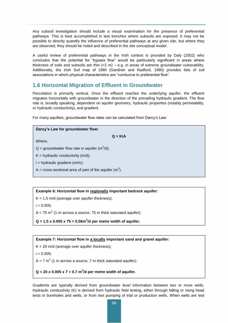
1.6 Horizontal Migration of Effluent in Groundwater

Percolation is primarily vertical. Once the effluent reaches the underlying aquifer, the effluent

migrates horizontally with groundwater in the direction of the prevailing hydraulic gradient. The flow

rate is, broadly speaking, dependent on aquifer geometry, hydraulic properties (notably permeability,

or hydraulic conductivity), and gradient.

For many aquifers, groundwater flow rates can be calculated from Darcy’s Law:

Gradients are typically derived from groundwater level information between two or more wells.

Hydraulic conductivity (K) is derived from hydraulic field testing, either through falling or rising head

tests in boreholes and wells, or from test pumping of trial or production wells. When wells are test

Example 7: Horizontal flow in a locally important sand and gravel aquifer:

K = 20 m/d (average over aquifer thickness);

i = 0.005;

A = 7 m2 (1 m across a source, 7 m thick saturated aquifer);

Q = 20 x 0.005 x 7 = 0.7 m3/d per metre width of aquifer.

Example 6: Horizontal flow in regionally important bedrock aquifer:

K = 1.5 m/d (average over aquifer thickness);

i = 0.005;

A = 75 m2 (1 m across a source, 75 m thick saturated aquifer);

Q = 1.5 x 0.005 x 75 = 0.56m3/d per metre width of aquifer.

Darcy’s Law for groundwater flow:

Q = KiA

Where,

Q = groundwater flow rate in aquifer (m3/d);

K = hydraulic conductivity (m/d);

i = hydraulic gradient (m/m);

A = cross-sectional area of part of the aquifer (m2).

.

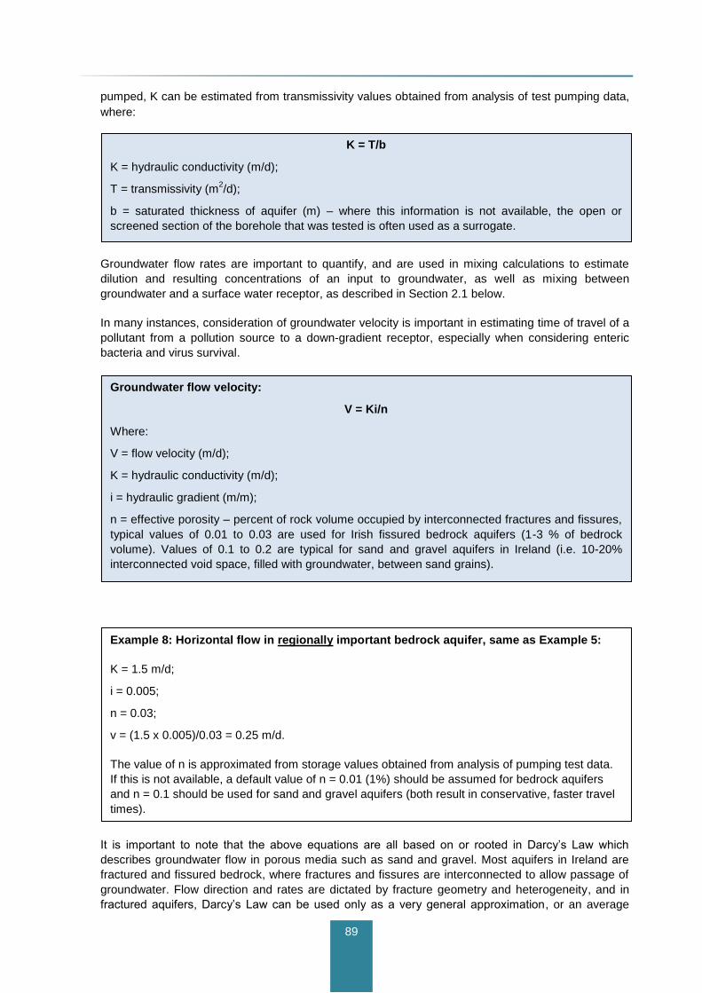
89

pumped, K can be estimated from transmissivity values obtained from analysis of test pumping data,

where:

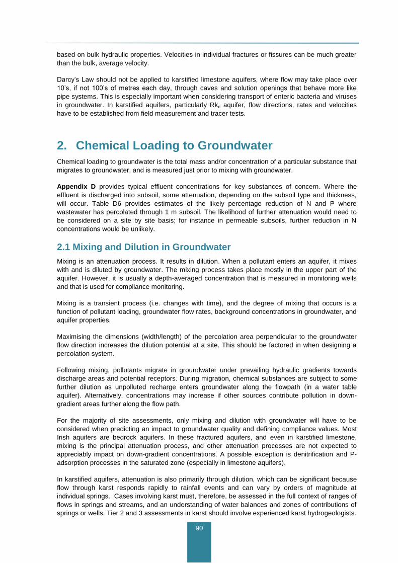
Groundwater flow rates are important to quantify, and are used in mixing calculations to estimate

dilution and resulting concentrations of an input to groundwater, as well as mixing between

groundwater and a surface water receptor, as described in Section 2.1 below.

In many instances, consideration of groundwater velocity is important in estimating time of travel of a

pollutant from a pollution source to a down-gradient receptor, especially when considering enteric

bacteria and virus survival.

It is important to note that the above equations are all based on or rooted in Darcy’s Law which

describes groundwater flow in porous media such as sand and gravel. Most aquifers in Ireland are

fractured and fissured bedrock, where fractures and fissures are interconnected to allow passage of

groundwater. Flow direction and rates are dictated by fracture geometry and heterogeneity, and in

fractured aquifers, Darcy’s Law can be used only as a very general approximation, or an average

Example 8: Horizontal flow in regionally important bedrock aquifer, same as Example 5:

K = 1.5 m/d;

i = 0.005;

n = 0.03;

v = (1.5 x 0.005)/0.03 = 0.25 m/d.

The value of n is approximated from storage values obtained from analysis of pumping test data.

If this is not available, a default value of n = 0.01 (1%) should be assumed for bedrock aquifers

and n = 0.1 should be used for sand and gravel aquifers (both result in conservative, faster travel

times).

Groundwater flow velocity:

V = Ki/n

Where:

V = flow velocity (m/d);

K = hydraulic conductivity (m/d);

i = hydraulic gradient (m/m);

n = effective porosity – percent of rock volume occupied by interconnected fractures and fissures,

typical values of 0.01 to 0.03 are used for Irish fissured bedrock aquifers (1-3 % of bedrock

volume). Values of 0.1 to 0.2 are typical for sand and gravel aquifers in Ireland (i.e. 10-20%

interconnected void space, filled with groundwater, between sand grains).

K = T/b

K = hydraulic conductivity (m/d);

T = transmissivity (m2/d);

b = saturated thickness of aquifer (m) – where this information is not available, the open or

screened section of the borehole that was tested is often used as a surrogate.

90

based on bulk hydraulic properties. Velocities in individual fractures or fissures can be much greater

than the bulk, average velocity.

Darcy’s Law should not be applied to karstified limestone aquifers, where flow may take place over

10’s, if not 100’s of metres each day, through caves and solution openings that behave more like

pipe systems. This is especially important when considering transport of enteric bacteria and viruses

in groundwater. In karstified aquifers, particularly Rkc aquifer, flow directions, rates and velocities

have to be established from field measurement and tracer tests.

2. Chemical Loading to Groundwater

Chemical loading to groundwater is the total mass and/or concentration of a particular substance that

migrates to groundwater, and is measured just prior to mixing with groundwater.

Appendix D provides typical effluent concentrations for key substances of concern. Where the

effluent is discharged into subsoil, some attenuation, depending on the subsoil type and thickness,

will occur. Table D6 provides estimates of the likely percentage reduction of N and P where

wastewater has percolated through 1 m subsoil. The likelihood of further attenuation would need to

be considered on a site by site basis; for instance in permeable subsoils, further reduction in N

concentrations would be unlikely.

2.1 Mixing and Dilution in Groundwater

Mixing is an attenuation process. It results in dilution. When a pollutant enters an aquifer, it mixes

with and is diluted by groundwater. The mixing process takes place mostly in the upper part of the

aquifer. However, it is usually a depth-averaged concentration that is measured in monitoring wells

and that is used for compliance monitoring.

Mixing is a transient process (i.e. changes with time), and the degree of mixing that occurs is a

function of pollutant loading, groundwater flow rates, background concentrations in groundwater, and

aquifer properties.

Maximising the dimensions (width/length) of the percolation area perpendicular to the groundwater

flow direction increases the dilution potential at a site. This should be factored in when designing a

percolation system.

Following mixing, pollutants migrate in groundwater under prevailing hydraulic gradients towards

discharge areas and potential receptors. During migration, chemical substances are subject to some

further dilution as unpolluted recharge enters groundwater along the flowpath (in a water table

aquifer). Alternatively, concentrations may increase if other sources contribute pollution in down-

gradient areas further along the flow path.

For the majority of site assessments, only mixing and dilution with groundwater will have to be

considered when predicting an impact to groundwater quality and defining compliance values. Most

Irish aquifers are bedrock aquifers. In these fractured aquifers, and even in karstified limestone,

mixing is the principal attenuation process, and other attenuation processes are not expected to

appreciably impact on down-gradient concentrations. A possible exception is denitrification and P-

adsorption processes in the saturated zone (especially in limestone aquifers).

In karstified aquifers, attenuation is also primarily through dilution, which can be significant because

flow through karst responds rapidly to rainfall events and can vary by orders of magnitude at

individual springs. Cases involving karst must, therefore, be assessed in the full context of ranges of

flows in springs and streams, and an understanding of water balances and zones of contributions of

springs or wells. Tier 2 and 3 assessments in karst should involve experienced karst hydrogeologists.

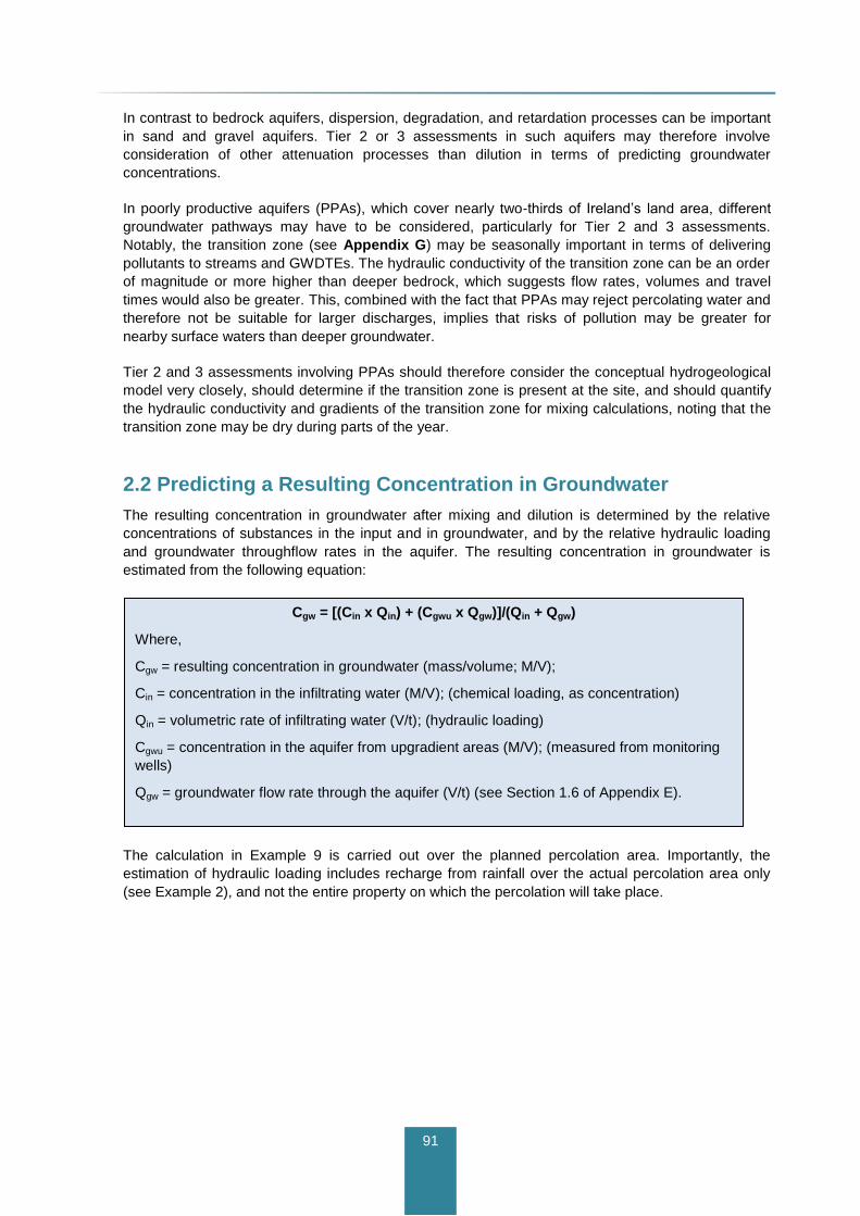
91

In contrast to bedrock aquifers, dispersion, degradation, and retardation processes can be important

in sand and gravel aquifers. Tier 2 or 3 assessments in such aquifers may therefore involve

consideration of other attenuation processes than dilution in terms of predicting groundwater

concentrations.

In poorly productive aquifers (PPAs), which cover nearly two-thirds of Ireland’s land area, different

groundwater pathways may have to be considered, particularly for Tier 2 and 3 assessments.

Notably, the transition zone (see Appendix G) may be seasonally important in terms of delivering

pollutants to streams and GWDTEs. The hydraulic conductivity of the transition zone can be an order

of magnitude or more higher than deeper bedrock, which suggests flow rates, volumes and travel

times would also be greater. This, combined with the fact that PPAs may reject percolating water and

therefore not be suitable for larger discharges, implies that risks of pollution may be greater for

nearby surface waters than deeper groundwater.

Tier 2 and 3 assessments involving PPAs should therefore consider the conceptual hydrogeological

model very closely, should determine if the transition zone is present at the site, and should quantify

the hydraulic conductivity and gradients of the transition zone for mixing calculations, noting that the

transition zone may be dry during parts of the year.

2.2 Predicting a Resulting Concentration in Groundwater

The resulting concentration in groundwater after mixing and dilution is determined by the relative

concentrations of substances in the input and in groundwater, and by the relative hydraulic loading

and groundwater throughflow rates in the aquifer. The resulting concentration in groundwater is

estimated from the following equation:

The calculation in Example 9 is carried out over the planned percolation area. Importantly, the

estimation of hydraulic loading includes recharge from rainfall over the actual percolation area only

(see Example 2), and not the entire property on which the percolation will take place.

Cgw = [(Cin x Qin) + (Cgwu x Qgw)]/(Qin + Qgw)

Where,

Cgw = resulting concentration in groundwater (mass/volume; M/V);

Cin = concentration in the infiltrating water (M/V); (chemical loading, as concentration)

Qin = volumetric rate of infiltrating water (V/t); (hydraulic loading)

Cgwu = concentration in the aquifer from upgradient areas (M/V); (measured from monitoring

wells)

Qgw = groundwater flow rate through the aquifer (V/t) (see Section 1.6 of Appendix E).

92

3. Checking Compliance

3.1 Comparing Resulting Groundwater Concentrations to

Receptor-Based Water Quality Standards

In Example 9, the immediate receptor is a regionally important fractured aquifer which is an existing

resource and used for public water supply (supply from wells and springs). In this case, the

appropriate receptor-based water quality standard is the drinking water standard for nitrate of

11.3 mg/l as N, which would also be considered as the appropriate compliance value.

In Example 9, further attenuation in groundwater is not considered likely as the aquifer is a fractured

bedrock aquifer. The resulting groundwater concentration of 16.2 mg-N/l exceeds the drinking water

standard of 11.3 mg-N/l, so from this comparison, authorisation would not be granted.

In this situation, there are two ways to proceed:

a) Implementing a pollution source control measure to try to improve the effluent water

quality through additional treatment; or

b) Conducting additional field work and sampling to establish whether or not further

attenuation would occur in a down-gradient direction.

In both cases, the onus is on the Applicant to demonstrate to the Licensing body that the input would

be acceptable and comply with groundwater quality and status classification objectives.

Example 9: Computing a Resulting Groundwater Concentration of N in a Regionally

Important Fractured Bedrock Aquifer.

Estimated chemical loading of nitrate (as N) (after percolation through a biomat and free-draining

subsoil) to groundwater = 30 mg/l = Cin.

Total estimated effluent discharge rate (including recharge from rainfall) = 10.3 m3/d (or

10,300 l/d) = Qin.

Infiltration capacity (from field testing) = 20 l/m2/d.

Total percolation area required = 10,300 l/d divided by 20 l/m2/d = 500 m

2 (25 x 20 m).

Percolation area is 25 m wide, perpendicular to the groundwater flow direction (i.e. to maximise

the dilution potential).

Estimated groundwater flow rate past percolation area = 0.56 m3/d per metre width over the

estimated depth of aquifer (from Example 6) = 0.56 x 25 m of percolation area = 14 m3/d = Qgw.

Sampled and measured groundwater concentration of NO3-N in upgradient well = 6 mg/l = Cgwu.

Resulting groundwater concentration:

Cin x Qin = 30.0 mg/l x 10.3 m3/d = 309,000 mg/d;

Cgwu x Qgw = 6.0 mg/l x 14.0 m3/d = 84,000 mg/d.

Qin + Qgw =10.3 +14.0 = 24.3 m3/d

Cgw = [309,000 mg/d + 84,000 mg/d]/24.3 m3/d = 16,173 mg/m

3

= 16.2 mg-N/l.

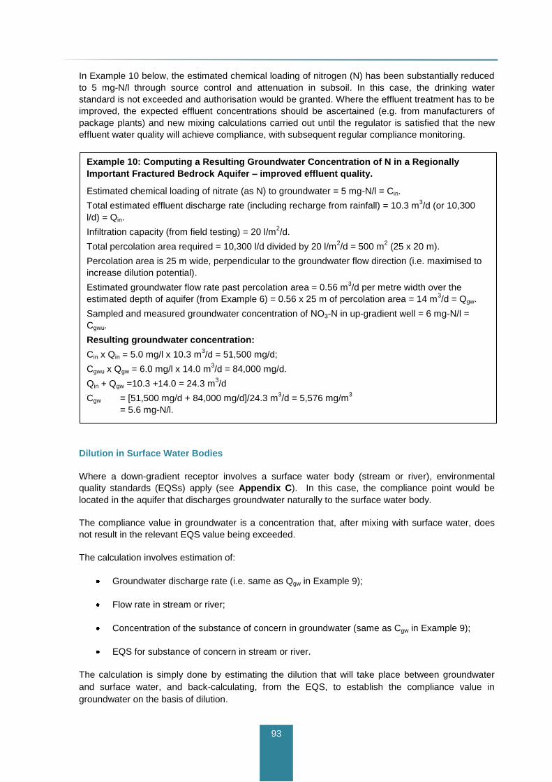
93

In Example 10 below, the estimated chemical loading of nitrogen (N) has been substantially reduced

to 5 mg-N/l through source control and attenuation in subsoil. In this case, the drinking water

standard is not exceeded and authorisation would be granted. Where the effluent treatment has to be

improved, the expected effluent concentrations should be ascertained (e.g. from manufacturers of

package plants) and new mixing calculations carried out until the regulator is satisfied that the new

effluent water quality will achieve compliance, with subsequent regular compliance monitoring.

Dilution in Surface Water Bodies

Where a down-gradient receptor involves a surface water body (stream or river), environmental

quality standards (EQSs) apply (see Appendix C). In this case, the compliance point would be

located in the aquifer that discharges groundwater naturally to the surface water body.

The compliance value in groundwater is a concentration that, after mixing with surface water, does

not result in the relevant EQS value being exceeded.

The calculation involves estimation of:

Groundwater discharge rate (i.e. same as Qgw in Example 9);

Flow rate in stream or river;

Concentration of the substance of concern in groundwater (same as Cgw in Example 9);

EQS for substance of concern in stream or river.

The calculation is simply done by estimating the dilution that will take place between groundwater

and surface water, and back-calculating, from the EQS, to establish the compliance value in

groundwater on the basis of dilution.

Example 10: Computing a Resulting Groundwater Concentration of N in a Regionally

Important Fractured Bedrock Aquifer – improved effluent quality.

Estimated chemical loading of nitrate (as N) to groundwater = 5 mg-N/l = Cin.

Total estimated effluent discharge rate (including recharge from rainfall) = 10.3 m3/d (or 10,300

l/d) = Qin.

Infiltration capacity (from field testing) = 20 l/m2/d.

Total percolation area required = 10,300 l/d divided by 20 l/m2/d = 500 m

2 (25 x 20 m).

Percolation area is 25 m wide, perpendicular to the groundwater flow direction (i.e. maximised to

increase dilution potential).

Estimated groundwater flow rate past percolation area = 0.56 m3/d per metre width over the

estimated depth of aquifer (from Example 6) = 0.56 x 25 m of percolation area = 14 m3/d = Qgw.

Sampled and measured groundwater concentration of NO3-N in up-gradient well = 6 mg-N/l =

Cgwu.

Resulting groundwater concentration:

Cin x Qin = 5.0 mg/l x 10.3 m3/d = 51,500 mg/d;

Cgwu x Qgw = 6.0 mg/l x 14.0 m3/d = 84,000 mg/d.

Qin + Qgw =10.3 +14.0 = 24.3 m3/d

Cgw = [51,500 mg/d + 84,000 mg/d]/24.3 m3/d = 5,576 mg/m

3

= 5.6 mg-N/l.

94

The resulting concentration is very high, and would not be authorised. The reason is that the

groundwater receptor (aquifer) is also a resource that is used for public water supply and for which a

drinking water standard of 25 µg/L applies.

In Example 12, an input of 107 mg/L is considered to be unrealistic, as phosphorus loading from

waste water effluents (or even land leachates) are not expected to exceed a few mg/L. An input on

this magnitude could therefore be authorised with respect to the EQS in the stream. However, there

may be other circumstances associated with the input that would restrict the allowable input, such as

a nearby GWDTE, where associated ecosystems may be sensitive to nutrient enrichment. This would

have to be checked and assessed on a case-by-case basis.

The type of calculations presented in Examples 11 and 12 are to be regarded as indicative only. For

example, they ignore potentially important attenuation processes that may take place in the

hyporheic zone along the margins of surface water bodies, which could influence analysis of

discharge concentrations further. If further attenuation processes are suspected, these would have to

be studied in greater detail through site investigation. In addition, the calculations are based on

average flows; in certain circumstances, the role of ‘seasonality’ and the impact of groundwater

inputs during low flow periods may need to be considered.

Nutrient sensitive surface waters have different capacities to assimilate pollutants, which is described

extensively in the technical guidance on the assessment of surface water discharges (DEHLG,

2010). For nutrient sensitive waters, the principal substances of concern are nitrogen and

phosphorus, as these control eutrophication processes, and both have very low EQS values for

determination of good status (Appendix C), at 0.065 mg/l-N and 0.035 mg/l-P respectively.

Example 12: Back-calculating a Compliance Value in Groundwater from an EQS in a

Stream – for Molybdate Reactive Phosphorus (MRP).

Mean estimated or known flow in stream = 1 m3/s = 86,400 m

3/d.

Mean groundwater discharge rate = 0.56 m3/d per metre width of aquifer.

Length of stream affected by “plume” in groundwater = 50 m;

EQS for MRP in stream = 0.035 mg/L-P.

Dilution Factor = flow in river divide by groundwater discharge over plume width = 86,400 m3/d

divided by (0.56 m3/d x 50 m) = 3,085.

“Allowable” MRP concentration in groundwater from discharge activity that will not result in

exceedance of EQS = 0.035 x 3,085 = 107 mg/L.

Example 11: Back-calculating a Compliance Value in Groundwater from an EQS in a

Stream – for Lead (dissolved).

Mean estimated or known flow in stream = 1 m3/s = 86,400 m

3/d.

Mean groundwater discharge rate = 0.56 m3/d per metre width of aquifer.

Length of stream affected by “plume” in groundwater = 50 m;

EQS for dissolved lead in stream = 7.2 µg/L.

Dilution Factor = flow in river divide by discharge over plume area = 86,400 m3/d divided by (0.56

m3/d x 50 m) = 3,085.

“Allowable” concentration of dissolved Lead in groundwater from discharge activity that will not

result in exceedance of EQS = 7.2 x 3,085 = 22,212 µg/L = 22.2 mg/L.

95

Where nutrient sensitive receptors are involved, careful prediction of the likely impact of related

substances are required as part of the site assessment. Whereas Examples 11 and 12 estimate an

“allowable concentration” in order not to exceed an EQS, the following equation can be used to

estimate the minimum average stream flow required to maintain a stream concentration below an

EQS for a given (known) concentration in groundwater.

Estimating Stream Flows in Ungauged Catchments

Groundwater and surface water flow rates described above represent average (mean) flow

conditions. Whereas the EPA, OPW and local authorities operate networks of hydrometric gauging

stations on many streams and rivers throughout the country, surface water flow data can be difficult

to obtain or derive in ungauged catchments.

Where measured flow data are not available, estimates can be made using rainfall-runoff modeling

techniques. The EPA also has a system for Estimating Flow Duration Curves at

http://watermaps.wfdireland.ie/HydroTool/. This provides an estimate of river flows exceeded for a

percentage of time, in the range 5% to 95%, at a range of ungauged locations. Flows are estimated

based on observed daily mean flows at similar catchments, chosen from a master set of hydrometric

stations throughout the country.

Alternatively, a first, crude approximation of average streamflow in non-karstified catchments can be

made using the following equation (DEHLG, 2010):

Q (l/s) = A x R x 0.5 x 0.032

Where,

A = catchment area (km2) upstream of the discharge point

R = average annual rainfall (mm)

0.5 = factor converting rainfall to effective rainfall

0.032 = conversion factor to l/s

Qu/s = ((Qgw/86.4)(Cgw – Cd/s))/(Cd/s - Cu/s)

Where,

Qu/s = flow rate in the river upstream of the discharge (l/s);

Cu/s = concentration of the substance of concern in the river upstream of the discharge (mg/l);

Qgw = groundwater discharge rate (m3/d);

Cgw = concentration of the substance of concern in groundwater (mg/l);

Cd/s = concentration of the substance of concern in the river downstream of the discharge (mg/l);

86.4 = conversion factor to l/s.

96

3.2 Checking Concentration Trends

In addition to checking groundwater concentrations against compliance values during compliance

monitoring, the chemical loading should also not result in sustained upward trends in concentrations.

An example of a sustained upward concentration trend is shown in Figure E2 below.

Figure E2: Example of Sustained Upward Concentration Trend

A statistically significant trend is one that is identified using a recognised statistical trend assessment

technique. An environmentally significant trend is one that is statistically significant, and which if not

reversed would lead to the failure of one or more of the WFD’s environmental objectives. As

groundwater data have asymmetric or non-normal distributions, non-parametric statistical methods

are required for trend assessment. Many groundwater systems have considerable seasonal

variability in parameter concentrations, which can impact on trend assessments. The non-parametric

Seasonal Kendall test is a statistical method that reduces the impact of seasonality on trend

assessments.

Where significant and sustained upward trends are identified, e.g. from a contaminant plume, the

upward trends need to be reversed to prevent failure of the relevant WFD objectives. The start date

for trend reversal is based on the significance of the trend and the risk associated with failing an

objective of the WFD. By default, Schedule 8 (Part B) of the Regulations indicates that the starting

point for trend reversal is the date when 75% of the Threshold value is likely to be exceeded. Further

details are given in Craig and Daly (2010).

97

4. Evaluation of the Potential Impact of Discharges

to Groundwater on Groundwater Body and

Surface Water Body Status

Where a groundwater body (GWB) is classed as ‘poor’, addition of further quantities of the pollutant

causing this status, will exacerbate the situation; the significance of this will vary with the loading rate

and the level of dilution that will occur. The most common circumstance is where the GWB is classed

as ‘poor’ because of the contribution of pollutants in groundwater to a ‘less than good’ status river.

Figure E3 illustrates the GWB chemical status nationally. Where a GWB is classed as ‘good’,

addition of further quantities of pollutant may result in ‘poor’ status in the GWB, particularly in

circumstances where the available capacity (see Section 3.5) is limited.

Figure E3: Groundwater Body Chemical Status May 2011

98

Allowing any development potentially impacting on groundwater bodies or on surface water bodies

via the groundwater pathway using the following approach assumes that measures will be applied

throughout the catchment either to maintain the GWB at ‘good’ status or to improve the GWB

from ‘poor’ to ‘good’ status, as appropriate, and that there is confidence that the measures

will be successful.

4.1 Recommended Approach

It will be unnecessary to undertake these calculations in circumstances where the available capacity

in the GWB is not restricted, unless the planned discharge is large.

1. Check the pollutants that will be discharged to groundwater. If these pollutants may potentially

be delivered to the GWB and may impact on the status, then an evaluation is required.

2. Note the threshold value (TV) for the pollutant (see Table C3).

3. Determine the GWB within which the proposed discharge will be located.

4. The area that this approach applies to will vary depending on whether the receptor of concern

is the groundwater body or an associated surface water body (SWB). Where the GWB is the

receptor, the area used in the calculations is the total area of the GWB. Where the receptor is

an associated SWB, the area used is the portion of the GWB that is contributing groundwater

to the ‘less than good’ status SWB, i.e., the groundwater catchment area of the ‘less than

good’ status river stretch.

5. If the GWB is at ‘good’ status and the actual (average) background concentration of the

pollutant is known, then this can be used in the calculations.

6. If the GWB is at ‘poor’ status or the background concentration is uncertain, an ‘adjusted

background concentration’ is calculated for the delineated area. The adjusted background

concentration assumes that measures will be applied throughout the catchment to bring the

groundwater body to good status. The adjusted background concentration is calculated as

75% of the TV. The exception to this will be where a ‘high’ status stream is the receptor; 75%

of the high status surface water EQS will be used as the adjusted background concentration.

7. In circumstances where an associated surface water body is the receptor of concern, the

guidance for discharges to surface waters should be considered.

8. The difference between the actual or adjusted background concentration and the TV is

considered to be an approximation of the ‘theoretical available capacity’ of the GWB

(following application of measures to maintain, or return to, good status of the GWB) see

Figure E4. This capacity approach is similar to the ‘headroom’ approach taken in the guidance

for licensing of discharges to surface waters (Water Services Training Group, 2010).

99

0 x TV

0.25 x TV

0.5 x TV

0.75 x TV

1 x TV

Co

nce

ntr

atio

n a

s fr

acti

on

of T

hre

sho

ld V

alu

e

TV

Adjusted Background

Concentration (0.75 x Threshold Value) Or Actual Background Concentration

Permissible Increase for the discharge (25% of theoretical available capacity above actual or

adjusted background concentration). This assumes that measures will be applied to entire catchment to return to or maintain Good Status

Theoretical

Available Capacity

Maximum increase of 25% of theoretical available capacityallowed for individual assessment

Figure E4: Determination of Theoretical Available Capacity

9. A mass balance calculation is used to evaluate the impact of the discharge on the actual or

adjusted background concentration. The calculation of the impact should include assessment

of the pathway susceptibility to groundwater and the use of BAT for the pollutants in question.

10. If the discharge will not use >25% of the theoretical available capacity then the discharge

may be permitted. If the discharge will use >25% of the theoretical available capacity then

refusal of the discharge should be considered. The figure of 25% of the theoretical available

capacity is used to allow capacity for other users and is subject to an assessment of the

catchment. The authorisation body may also wish to take into consideration other factors in

the catchment when making its decision such as the expected future development. If only

minor future development is anticipated then the authorisation body might wish to consider

allowing an increase in the 25% allocation to discharge under consideration. However, if

significant future development is anticipated, then the 25% allocation may be appropriate

(Water Services Training Group, 2010.)

100

Example 14: GWB classed as good with average nitrate concentration of 35 mg/l

Pollutant load = 20 m3/d (7,300 m

3/yr) with concentration of 80 mg/l NO3 = 1.6kg NO3/d =

584 kgNO /yr.

GWB area = 20 km2 with average recharge = 0.3 m/yr = 6,000,000 m

3/yr.

Development located in an area with high permeability subsoil, i.e., pathway susceptibility to

groundwater is high and no attenuation is expected.

TV = 37.5 mg/l NO3.

Mean background concentration = known concentration = 35 mg/l NO3.

Theoretical Available capacity = 2.5 mg/l NO3.

Resultant concentration due to the discharge (using Mass Balance calculation) = 35.055 mg/l

NO3.

Percentage of Theoretical Available Capacity Used = (35.055 mg/l – 35 mg/l)/2.5 mg/l = 2.2%

As the discharge will not use >25% of the theoretical available capacity then the discharge may

be permitted

Example 13: Karst GWB classed as poor as groundwater is the main contributor of MRP to

a moderate status SWB

Pollutant load = 20 m3/d (7,300 m

3/yr) with concentration of 10 mg/l P = 0.2 kgP/d = 73 kgP/yr.

Assume a 90% reduction in loading due to attenuation in the subsoil. Therefore loading to

groundwater = 7.3 kgP/yr.

Recharge volume: GWB area contributing to the SWB (based on surface water sub-catchment)

= 10 km2 with average recharge = 0.4 m/yr = 4,000,000 m

3/yr.

Development located in an area with 4 m subsoil.

TV = 35 ug/l P (this is a mean value).

Adjusted background concentration = 75% of TV = 26.3 ug/l P (assumes measures to return

GWB to Good Status).

Theoretical Available capacity = 8.7 ug/l P.

Resultant concentration due to the discharge (using Mass Balance calculation – see Appendix

E – Relevant Calculations, Section 2.2) = 28 ug/l P

Percentage of Theoretical Available Capacity Used = (28.0 ug/l – 26.3 ug/l)/ 8.7ug/l = 20%

As the discharge will not use >25% of the theoretical available capacity then the discharge may

be permitted.

N.B.: this approach assumes that measures will have been applied throughout the

catchment to restore the GWB from ‘poor’ to ‘good’ status.

Priority should be given to examining existing developments in the critical source areas (CSAs) –

extremely vulnerable areas – and enforcement undertaken where necessary.

The above calculations assume that there is significant attenuation of MRP in the subsoil beneath

the percolation area (Gill et al. (2009) show a 77-99% reduction in P at 1 m depth beneath a

percolation area – see Table D5 and Table D6). However, in areas with shallow bedrock, it is

probable that the capacity of the subsoil to attenuate P will reduce with time. Therefore, a lower

reduction value may be advisable in this circumstance.

101

Appendix F – Groundwater Protection Response

Matrices and Minimum Separation Distances

Introduction

The role of the groundwater response matrix is to provide an initial evaluation (as part of the desk

study) of the general suitability of a site for a particular activity, from a hydrogeological perspective.

The response matrix is intended as an initial screening tool, after which site specific investigations

shall be undertaken to confirm site suitability. The response matrix can also be used to indicate the

measures that may be required to meet the required specification. An explanation of the role of

groundwater protection responses in a groundwater protection scheme is given in Groundwater

Protection Schemes (DELG/EPA/GSI, 1999).

The geological and hydrogeological data that place a site within a response category is general to an

area, and not specific to a site. It is therefore incumbent on the developer to demonstrate that the site

conditions of a specific site are determined, before a decision is taken on the suitability or otherwise

of a site. Examples of uncertainty on available data can include depth to rock values (and hence

vulnerability ratings) and the presence of sand/gravel.

In general the pollution risk is greatest in source protection areas and on regionally important

aquifers. The topsoil and subsoil, depending on their type, permeability and thickness, play a critical

role in preventing groundwater contamination and mitigating the impact of many potential pollutants.

They act as a protecting filtering layer over groundwater.

A risk assessment approach is taken in the development of this response matrix. The appropriate

response to the risk of groundwater contamination from an activity in the different hydrogeological

settings in Ireland is given by the assigned response category (R) appropriate to each protection.

Groundwater Response Matrices are available for:

On-Site (Waste Water treatment) Systems for Single Houses (EPA, 2009);

Integrated constructed wetlands (DEHLG, 2010);

Landfills (EPA, 2006);

Out wintering pads (DAFF, 2007); and

Earth lined slurry/ effluent stores (DAFF, 2005).

The response matrices for these activities are reproduced in this Appendix. These groundwater

protection responses should be read in conjunction with Groundwater Protection Schemes

(DELG/EPA/GSI, 1999) and their respective guidance documents. Additional responses for other

potentially polluting activities are expected to be developed by the EPA and the GSI in the future.

Source protection areas are delineated for public, group and industrial water supplies. These areas

provide additional protection by placing tighter controls on activities within the vicinity of the source.

The matrix in Table F.1 below gives the result of integrating the two regional elements of land

surface zoning (vulnerability categories and resource protection areas). In practice this is achieved by

superimposing the interim vulnerability map on the draft aquifer map. Each zone is represented by a

code e.g. Rf/M, which represents areas of regionally important fissured aquifers where the

groundwater is moderately vulnerable to contamination.

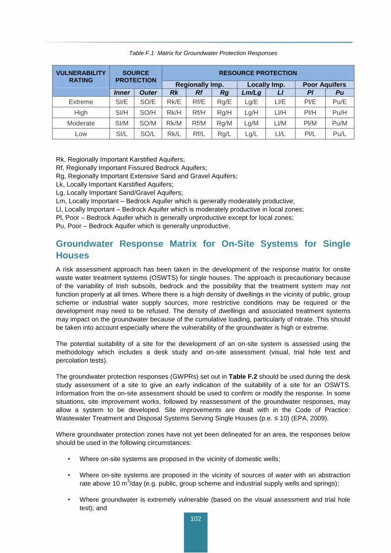
102

Table F.1: Matrix for Groundwater Protection Responses

VULNERABILITY RATING

SOURCE PROTECTION

RESOURCE PROTECTION

Regionally Imp. Locally Imp. Poor Aquifers

Inner Outer Rk Rf Rg Lm/Lg Ll Pl Pu

Extreme SI/E SO/E Rk/E Rf/E Rg/E Lg/E Ll/E Pl/E Pu/E

High SI/H SO/H Rk/H Rf/H Rg/H Lg/H Ll/H Pl/H Pu/H

Moderate SI/M SO/M Rk/M Rf/M Rg/M Lg/M Ll/M Pl/M Pu/M

Low SI/L SO/L Rk/L Rf/L Rg/L Lg/L Ll/L Pl/L Pu/L

Rk, Regionally Important Karstified Aquifers;

Rf, Regionally Important Fissured Bedrock Aquifers;

Rg, Regionally Important Extensive Sand and Gravel Aquifers;

Lk, Locally Important Karstified Aquifers;

Lg, Locally Important Sand/Gravel Aquifers;

Lm, Locally Important – Bedrock Aquifer which is generally moderately productive;

Ll, Locally Important – Bedrock Aquifer which is moderately productive in local zones;

Pl, Poor – Bedrock Aquifer which is generally unproductive except for local zones;

Pu, Poor – Bedrock Aquifer which is generally unproductive.

Groundwater Response Matrix for On-Site Systems for Single

Houses

A risk assessment approach has been taken in the development of the response matrix for onsite

waste water treatment systems (OSWTS) for single houses. The approach is precautionary because

of the variability of Irish subsoils, bedrock and the possibility that the treatment system may not

function properly at all times. Where there is a high density of dwellings in the vicinity of public, group

scheme or industrial water supply sources, more restrictive conditions may be required or the

development may need to be refused. The density of dwellings and associated treatment systems

may impact on the groundwater because of the cumulative loading, particularly of nitrate. This should

be taken into account especially where the vulnerability of the groundwater is high or extreme.

The potential suitability of a site for the development of an on-site system is assessed using the

methodology which includes a desk study and on-site assessment (visual, trial hole test and

percolation tests).

The groundwater protection responses (GWPRs) set out in Table F.2 should be used during the desk

study assessment of a site to give an early indication of the suitability of a site for an OSWTS.

Information from the on-site assessment should be used to confirm or modify the response. In some

situations, site improvement works, followed by reassessment of the groundwater responses, may

allow a system to be developed. Site improvements are dealt with in the Code of Practice:

Wastewater Treatment and Disposal Systems Serving Single Houses (p.e. ≤ 10) (EPA, 2009).

Where groundwater protection zones have not yet been delineated for an area, the responses below

should be used in the following circumstances:

• Where on-site systems are proposed in the vicinity of domestic wells;

• Where on-site systems are proposed in the vicinity of sources of water with an abstraction

rate above 10 m3/day (e.g. public, group scheme and industrial supply wells and springs);

• Where groundwater is extremely vulnerable (based on the visual assessment and trial hole

test); and

103

• Where there are karst features such as swallow holes, caves, etc.

The appropriate response to the risk of groundwater contamination from an OSWTS is given by the

assigned response category (R) appropriate to each protection zone as shown in Table F.2.

Table F.2: Response Matrix for OSWTS

VULNERABILITY RATING

SOURCE PROTECTION*

RESOURCE PROTECTION

Regionally Imp.

Locally Imp. Poor Aquifers

Inner Outer Rk Rf/ Rg Lk Lm/Lg Ll Pl Pu

Extreme R32 R3

1 R2

2 R2

2 R2

2 R2

1 R2

1 R2

1 R2

1

High R24 R2

3 R2

1 R1 R2

1 R1 R1 R1 R1

Moderate R24 R2

3 R1 R1 R1 R1 R1 R1 R1

Low R24 R1 R1 R1 R1 R1 R1 R1 R1

* For public, group scheme or industrial water supply sources where protection zones have not been delineated,

the arbitrary distances given in DELG/EPA/GSI (1999) of 300 m for the Inner Protection Area (SI) and 1,000 m

for the Outer Protection Area (SO) should be used as a guide upgradient of the source.

R1 Acceptable subject to normal good practice (i.e. system selection, construction, operation

and maintenance in accordance with the Code of Practice (EPA, 2009)).

R21 Acceptable subject to normal good practice. Where domestic water supplies are located

nearby, particular attention should be given to the depth of subsoil over bedrock such that

the minimum depths required in the Code of Practice (EPA, 2009) are met and that the

likelihood of microbial pollution is minimised.

R22 Acceptable subject to normal good practice and the following additional condition:

1. There is a minimum thickness of 2 m unsaturated soil/subsoil beneath the invert of the

percolation trench of a septic tank system.

Or,

2. A secondary treatment system as described in sections 8 and 9 of the Code of Practice

(EPA, 2009) is installed, with a minimum thickness of 0.3 m unsaturated soil/subsoil with P/T-

values from 3 to 75 (in addition to the polishing filter which should be a minimum depth of 0.9

m), beneath the invert of the polishing filter (i.e. 1.2 m in total for a soil polishing filter).

R23 Acceptable subject to normal good practice, Condition 1 above and the following additional

condition:

3. The authority should be satisfied that, on the evidence of the groundwater quality of the

source and the number of existing houses, the accumulation of significant nitrate and/or

microbiological contamination is unlikely.

R24 Acceptable subject to normal good practice, Conditions 1 and 2 above and the following

additional condition:

4. No on-site treatment system should be located within 60 m of a public, group scheme or

industrial water supply source.

R31 Not generally acceptable, unless:

A septic tank system as described in section 7 of the Code of Practice (EPA, 2009) is

installed with a minimum thickness of 2 m unsaturated soil/subsoil beneath the invert of the

percolation trench (i.e. an increase of 0.8 m from the requirements in section 6 of the Code of

Practice (EPA, 2009)),

104

Or,

A secondary treatment system, as described in the sections 8 and 9 of the Code of Practice

(EPA, 2009), is installed, with a minimum thickness of 0.3 m unsaturated soil/subsoil with

P/T-values from 3 to 75 (in addition to the polishing filter which should be a minimum depth

of 0.9 m), beneath the invert of the polishing filter (i.e. 1.2 m in total for a soil polishing filter)

and subject to the following conditions:

5. The authority should be satisfied that, on the evidence of the groundwater quality of the

source and the number of existing houses, the accumulation of significant nitrate and/or

microbiological contamination is unlikely

6. No on-site treatment system should be located within 60 m of a public, group scheme or

industrial water supply source

7. A management and maintenance agreement is completed with the systems supplier.

R32 Not generally acceptable unless:

A secondary treatment system is installed, with a minimum thickness of 0.9 m unsaturated

soil/subsoil with P/T-values from 3 to 75 (in addition to the polishing filter which should be a

minimum depth of 0.9 m), beneath the invert of the polishing filter (i.e. 1.8 m in total for a soil

polishing filter) and subject to the following conditions:

8. The authority should be satisfied that, on the evidence of the groundwater quality of the

source and the number of existing houses, the accumulation of significant nitrate and/or

microbiological contamination is unlikely

9. No on-site treatment system should be located within 60 m of a public, group scheme or

industrial water supply source

10. A management and maintenance agreement is completed with the systems supplier.

The responses above assume that there is no significant groundwater contamination in the area.

Should contamination by pathogenic organisms or nitrate (or other contaminants) be a problem in

any particular area, more restrictive responses may be necessary.

Where nitrate levels are known to be high or nitrate-loading analysis indicates a potential problem,

consideration should be given to the use of treatment systems, which include a denitrification unit.

Monitoring carried out by the local authority will assist in determining whether or not a variation in any

of these responses is required. Sites are not suitable for discharge of effluent to ground for very low

permeability subsoils (where T > 90).

Recommended Minimum Separation Distances

Table F.3 provides recommended distances between receptors and percolation areas or polishing

filters, in order to protect groundwater. These distances depend on the thickness and permeability of

subsoil. The depths and distances given in this table are based on the concepts of ‘risk assessment’

and ‘risk management’, and take account, as far as practicable, of the uncertainties associated with

hydrogeological conditions in Ireland. Use of the depths and distances in this table does not

guarantee that pollution will not be caused; rather, it will reduce the risk of significant pollution

occurring.

105

Table F.3: Recommended Minimum Distance between a Receptor and a Percolation Area or Polishing Filter

T or P Value1

Type of soil/subsoil 2

Depth of

soil/subsoil Minimum distance (m) from receptor to percolation area or polishing filter 5

(m) above bedrock (see note 1,2,3,6)

Public Water Supply

Karst feature

downgradient domestic well or flow direction is unknown

(see note 5)

Domestic well

alongside (no

gradient)

upgradient domestic well

>30

CLAY; silty, sandy CLAY (e.g. clayey till); CLAY/SILT.

1.2

>3.0

60

15

40

30

25

15

10 -30

Sandy SILT; clayey, silty SAND; clayey, silty GRAVEL (e.g. sandy till).

1.2

8.0

60

15

45

30

25

15

<10

SAND; GRAVEL; silty SAND.

2.03

2.04

>8.04

60

15

60

40

30

25

15

1The T-value (expressed as min/25 mm) is the time taken for the water to drop a specified distance in a percolation test hole. For shallow subsoils the trial hole requirements

are different and hence the test results are called P-values. 2BS5930 descriptions

3water table 1.2-2.0 m

4water table >2.0 m

5The distance from the percolation area or polishing filter means the distance from the periphery of the percolation area or polishing filter and not the centre.

106

Table F.3 Notes:

1. Depths are measured from the invert level of the percolation trench. 2. Depths and distances can be related by interpolation: e.g. where the thickness of sandy CLAY is

1.2 m, the minimum recommended distance from the well to percolation area is 40 m; where the thickness is 3.0 m, the distance is 30 m; distances for intermediate depths can be approximated by interpolation.

3. Where bedrock is shallow (<2 m below invert of the trench), greater distances may be necessary where there is evidence of the presence of preferential flow paths (e.g. cracks, roots) in the subsoil.

4. Where the minimum subsoil thicknesses are less than those given above, site improvements and systems other than systems, as described in Sections 8 and 9 may be used to reduce the likelihood of contamination.

5. If effluent and bacteria enter bedrock rapidly (within 1-2 days), the distances given may not be adequate where the percolation area is in the zone of contribution of a well. Further site-specific evaluation is necessary.

6. Where bedrock is known to be karstified or highly fractured, greater depths of subsoil may be advisable to minimise the likelihood of contamination.

Where an on-site system is in the zone of contribution of a well, the likelihood of contamination and

the threat to human health depend largely on five factors:

1. The thickness and permeability of subsoil beneath the invert of the percolation trench;

2. The permeability of the bedrock, where the well is tapping the bedrock;

3. The distance between the well or spring and the on-site system;

4. The groundwater flow direction, and

5. The level of treatment of effluent.

Groundwater Response Matrix for Integrated Constructed

Wetlands (ICWs)

The appropriate response to the risk of groundwater contamination from an integrated constructed

wetland is given by the assigned response category (R) appropriate to each protection zone as

shown in Table F.4.

Table F.4: Response Matrix for ICWs

VULNERABILITY RATING

SOURCE PROTECTION

RESOURCE PROTECTION

Regionally Imp. Locally Imp. Poor Aquifers

Inner Outer Rk* Rf Rg Lm/Lg Ll Pl Pu

Extreme R4 R34 R3

3 R3

2 R4 R4 R3

1 R3

1 R3

1

High R24 R2

3 R2

2 R2

1 R2

1 R2

1 R1 R1 R1

Moderate R24 R2

3 R2

2 R1 R1 R1 R1 R1 R1

Low R23 R2

3 R2

2 R1 R1 R1 R1 R1 R1

*A small proportion of the country (~0.6%) is underlain by locally important karstic aquifers (Lk); in these areas,

the groundwater protection responses for the Rk groundwater protection zone shall apply.

R1 Acceptable, subject to meeting the following requirements:

1. The ICW shall be underlain by at least 1000 mm of cohesive subsoil.

2. An upper portion of the subsoil, which will vary in thickness as set out below depending on

the risk posed by the ICW, shall have a permeability of less than 1x10-8

m/s. Where this is

present in situ, (i.e. the subsoil is classed as CLAY (using BS5930) or, in certain situations,

SILT/CLAY, and has a clay content of >13% (where the particle size distribution is adjusted

by excluding materials larger than 20 mm), and is free from preferential flowpaths, the

107

surface of the excavated portion of the pond will require plastering with remoulded subsoil.

Where the subsoil is considered to have a permeability of greater than 1x10-8

m/s (i.e. is

classed as SILT or, in certain situations, SILT/CLAY, and the clay content is <13% but

>10%,) the subsoil must be enhanced by compaction or puddling to achieve the required

permeability standard. Where the subsoil is classed as SAND, GRAVEL or SILT (in

circumstances where the clay content is <10%), suitable subsoil or other material must be

provided for the liner.

3. The upper 500 mm shall have a permeability of less than 1 x 10-8

m/s

4. Where the subsoil is sand/gravel, the upper 750 mm of the liner shall be installed with a

permeability of less than 1x10-8

m/s.

5. The ICW shall be at least 60m away from any well or spring used for potable water.

R21 Acceptable, subject to normal good practice, meeting requirements 1, 2, 4 and 5 above, but

with the following additional requirement

6. The minimum thickness of subsoil with a permeability of less than 1x10-8

m/s shall be 750

mm.

R22 Acceptable, subject to normal good practice, meeting design requirements 1, 2, 4, 5 and 6

above, and the following additional requirements:

7. The ICW shall be at least 15 m away from karst features that indicate enhanced zones of

high bedrock permeability (e.g. swallow holes and dolines (collapse features)).

8. The site assessment shall pay particular attention to the possibility of instability in these karst

areas.

R23 Acceptable, subject to normal good practice, meeting requirements 1, 2, 4, 5, 6, 7 (in karst

areas) and 8 (in karst areas).

R24 Acceptable, subject to normal good practice, meeting requirements 1, 2, 4, 5, 6, 7 (in karst

areas) and 8 (in karst areas) and the following additional requirement:

9. Where microbial pathogens and/or high nitrate concentrations are known to be present in the

water supply source, more detailed site investigation and/or restrictive design requirements

may be necessary.

R31 Not generally acceptable, unless requirements 1, 2, 3, 4 and 5 can be met (Note 1).

R32 Not generally acceptable, unless requirements 1, 2, 4, 5 and 6 can be met (Note 1).

R33 Not generally acceptable, unless requirements 1, 2, 4, 5, 6, 7 and 8 can be met (Note 1).

R34 Not generally acceptable, unless requirements 1, 2, 4, 5, 6, 7 (in karst areas), 8 (in karst

areas), and 9 can be met (Note 1).

R4 Not acceptable

Note 1: Establishing the required minimum subsoil thickness beneath the ponds will be difficult to

achieve.

Groundwater Response Matrix for Landfills

In general terms this response matrix is for the siting of landfills for non-hazardous wastes. The

principles involved may also be applied to the selection process for landfill sites for hazardous and

inert waste. A significant factor in siting all landfills is the protection of groundwater, which is an

important resource and source of water supply in Ireland, particularly in rural areas.

108

The geology and hydrogeology of any region have a major bearing on: (i) the availability of suitable

areas for landfill sites; (ii) the level of natural protection for groundwater from contamination by landfill

leachate; and (iii) the design, operation and monitoring of landfills.

Developers of landfills should have regard to both the resource potential and the vulnerability of the

underlying and adjacent aquifers. The groundwater protection responses combine both of these

factors in a matrix which facilitates rational decisions on the acceptability or otherwise of a landfill

from a hydrogeological point of view. The risk to groundwater from the landfilling of waste is mainly

influenced by the:

Nature of the waste;

Leachate composition;

Volume of leachate generated;

Groundwater vulnerability;

Proximity of a groundwater source;

Value of the groundwater resource;

Landfill design; and

Landfill operation and management practices.

The generation of leachate is one of the main hazards to groundwater from the disposal of waste by

landfilling. Good site selection, design and operation assist in minimising the risk of pollution.

Leachate from landfills for non hazardous waste is a highly polluting liquid and its composition is

dependent on the nature of the waste within the landfill. The pollution potential can be evaluated by

calculating the volume and predicting the composition of leachate that will be generated.

The volume of leachate depends principally on the area of the landfill, the meteorological and

hydrogeological factors and the effectiveness of the capping. It is essential that the volume of

leachate generated be kept to a minimum. The design and operation of the landfill should ensure that

the ingress of groundwater and surface water is minimised and controlled.

Leachate composition varies due to a number of different factors such as the age and type of waste

and operational practices at the site.

The conditions within a landfill vary over time from aerobic to anaerobic thus allowing different

chemical reactions to take place. Most landfill leachates have high BOD, COD, ammonia, chloride,

sodium, potassium, hardness and boron levels. Ammonia is a contaminant, which may be used as an

indicator of contamination, particularly in terms of surface water, as it can be toxic to fish at low

concentrations (1 mg/l). Chloride is a mobile constituent, which is often used as an indicator of

contamination. The leachate from non-hazardous waste landfills may produce reducing conditions

beneath the landfill, allowing the solution of iron and manganese from the underlying deposits.

Leachates from landfill sites for non-hazardous waste often contain complex organic compounds,

chlorinated hydrocarbons and metals at concentrations which pose a threat to groundwater and

surface waters. Solvents and other synthetic organic chemicals are a significant hazard, being of

environmental significance at very low concentrations and resistant to degradation. Moreover, they

may be transformed in some cases into more hazardous compounds.

The siting, design, operation and monitoring of landfills must comply with the guidelines outlined in

the EPA’s Landfill manuals. However, where a waste licence has been issued for an existing landfill,

alternative site specific requirements may be specified.. A Waste Licence is required for all landfills.

The appropriate response to the risk of groundwater contamination is given by the assigned

response category (R) appropriate to each protection zone (Table F.5).

109

From the point of view of reducing the risk to groundwater, it is recommended that all landfills be

located in, or as near as possible to, the zone in the bottom right hand corner of the matrix.

Table F.5: Response Matrix for Landfills

VULNERABILITY RATING

SOURCE PROTECTION

RESOURCE PROTECTION

Regionally Imp. Locally Imp. Poor Aquifers

Inner Outer Rk Rf/ Rg Lm/Lg Ll Pl Pu

Extreme R4 R4 R4 R4 R32 R2

2 R2

2 R2

1

High R4 R4 R4 R4 R31 R2

1 R2

1 R1

Moderate R4 R4 R4 R31 R2

2 R2

1 R2

1 R1

Low R4 R31 R3

1 R3

1 R1 R1 R1 R1

In all cases standards prescribed in the EPA Landfill Site Design Manual (EPA, 2000) or conditions of

a waste licence will apply.

R1 Acceptable subject to guidance outlined in the EPA Landfill Design Manual or conditions of a

waste licence.

R21 Acceptable subject to guidance outlined in the EPA Landfill Design Manual or conditions of a

waste licence.

1. Special attention should be given to checking for the presence of high permeability zones. If

such zones are present then the landfill should only be allowed if it can be proven that the

risk of leachate movement to these zones is insignificant and that special attention has been

given to existing wells down-gradient of the site and to the projected future development of

the aquifer.

R22 Acceptable subject to guidance outlined in the EPA Landfill Design Manual or conditions of a

waste licence.

2. Special attention should be given to checking for the presence of high permeability zones. If

such zones are present then the landfill should only be allowed if it can be proven that the

risk of leachate movement to these zones is insignificant and that special attention has been

given to existing wells down-gradient of the site and to the projected future development of

the aquifer.

3. Groundwater control measures such as cut-off walls or interceptor drains may be necessary

to control high water table or the head of leachate may be required to be maintained at a

level lower than the water table depending on site conditions.

R31 Not generally acceptable, unless it can be shown that:

4. the groundwater in the aquifer is confined; or

5. it is proven that there will not be a significant impact on the groundwater; and

6. it is not practicable to find a site in a lower risk area.

R32 Not generally acceptable, unless it can be shown that

7. there is a minimum consistent thickness of 3 metres of low permeability subsoil present;

8. it is proven that there will not be a significant impact on the groundwater; and

9. it is not practicable to find a site in a lower risk area.

R4 Not acceptable.

110

Regionally Important Aquifers

The siting of landfills on or near regionally important aquifers should only be considered:

Where the hydraulic gradient (relative to the leachate level at the base of the landfill) is

upwards for a substantial proportion of each year (confined aquifer situation).

Where the proposed landfill is located in the discharge area of an aquifer. In this case

surface water may be more at risk.

Where a map showing a regionally important aquifer includes low permeability zones or units

which cannot be delineated using existing geological and hydrogeological information but

which can be found by site investigations. Location of a landfill site on such a unit may be

acceptable provided leakage to the permeable zones or units is insignificant.

Where the wastes types are restricted and the waste acceptance procedures employed are

in accordance with the criteria specified by the EPA.

Investigations

Special attention should be given to checking for the presence of more permeable zones, such as

faults, particularly in fractured bedrock aquifers. Geophysical surveys may be used to identify zones

which should be investigated further by drilling to determine their vertical and lateral extent.

Hydrogeological tests should also be carried out to define the local and regional effects of the zones.

Investigations should be carried out in accordance with the EPA’s Landfill Manual Investigations for

Landfills, 1995.

Groundwater Response Matrix for Earth-Lined Slurry/ Effluent

Stores (ELS)

The appropriate response to the risk of groundwater contamination from an earth-lined slurry/ effluent

stores (ELS) is given by the assigned response category (R) appropriate to each protection zone as

shown in Table F.6.

Table F.6: Response Matrix for ELS

VULNERABILITY RATING

SOURCE PROTECTION

RESOURCE PROTECTION

Regionally Imp Locally Imp. Poor Aquifers

Inner Outer Rk* Rf Rg Lm/Lg Ll Pl Pu

Extreme R4 R34 R3

3 R3

2 R4 R4 R3

1 R3

1 R3

1

High R24 R2

3 R2

2 R2

1 R4 R4 R1 R1 R1

Moderate R23 R2

3 R2

2 R1 R1 R1 R1 R1 R1

Low R23 R2

3 R2

2 R1 R1 R1 R1 R1 R1

*A small proportion of the country (~0.6%) is underlain by locally important karstic aquifers (Lk); in these areas,

the groundwater protection responses for the Rk groundwater protection zone shall apply.

The responses are given below:

R1 Acceptable, subject to normal good practice (i.e. investigation, construction, operation and

maintenance in accordance with DAFF Minimum Specification S131) as set out in the

following requirements:

1. The ELS shall be underlain by at least 1.5 m of cohesive subsoil.

111

2. An upper portion of the subsoil, which will vary in thickness depending on the level of risk

posed by the ELS, shall have a permeability of less than 1x10-9

m/s.

- Where this is present in situ, (i.e. the subsoil is classed as CLAY (using BS5930) and

has a clay content of >18% (where the particle size distribution is adjusted by

excluding materials larger than 20 mm), and is free from preferential flowpaths), the

surface of the excavated portion of the store will require plastering with remoulded

subsoil.

- Where the subsoil is considered to have a permeability of greater than 1x10-9

m/s,

the subsoil must be enhanced by compaction to achieve the required permeability

standard.

3. The upper 0.5m shall have a permeability of less than 1x10-9

m/s.

4. Where the subsoil is sand/gravel in vertical hydraulic continuity with the main water table, an

ELS is not acceptable.

5. The ELS shall be at least 60 m from any well or spring used for potable water.

R21 Acceptable, subject to normal good practice, meeting requirements 1, 2, 4 and 5 above, and

the following additional requirement:

6. The minimum thickness of subsoil with a permeability of less than 1x10-9

m/s shall be 1.0 m.

R22 Acceptable, subject to normal good practice, meeting design requirements 1, 2, 4, 5 and 6

above, and the following additional requirement:

7. The ELS shall be at least 15 m from karst features that indicate enhanced zones of high

bedrock permeability (e.g. swallow holes and dolines (collapse features)).

R23 Acceptable, subject to normal good practice, meeting requirements 1, 2, 4, 5, 6 and 7 (in

karst areas).

R24 Acceptable, subject to normal good practice, meeting requirements 1, 2, 4, 5, 6 and 7 (in

karst areas) above, and the following additional requirement:

8. Where microbial pathogens and/or high nitrate concentrations are known to be present in the

water supply source, more detailed site investigation and/or restrictive design requirements

may be necessary.

R31 Not generally acceptable, unless requirements 1, 2, 3, 4 and 5 can be met (Note: Achieving

the required minimum subsoil thickness beneath the stores (ELSs) is unlikely.)

R32 Not generally acceptable, unless requirements 1, 2, 4, 5 and 6 can be met ((Note: Achieving

the required minimum subsoil thickness beneath the stores (ELSs) is unlikely.)

R33 Not generally acceptable, unless requirements 1, 2, 4, 5, 6, and 7 can be met ((Note:

Achieving the required minimum subsoil thickness beneath the stores (ELSs) is unlikely.)

R34 Not generally acceptable, unless requirements 1, 2, 4, 5, 6, and 7 (in karst areas) can be met

((Note: Achieving the required minimum subsoil thickness beneath the stores (ELSs) is

unlikely.).

R4 Not acceptable.

Note 1: Achieving the required minimum subsoil thickness beneath the stores (ELSs) is unlikely.

Note 2: Where a source protection area has not been delineated by the Local Authority and the

proposed ELS site lies within 300m up-gradient of a public supply abstraction point, the ground water

protection response as per source protection area of Table F.1 applies.

112

Groundwater Response Matrix for Out Wintering Pads (OWP)

The appropriate response to the risk of groundwater contamination from an out wintering pad (OWP)

is given by the assigned response category (R) appropriate to each protection zone as shown in

Table F.7.

Table F.7: Response Matrix for OWP

VULNERABILITY RATING

SOURCE PROTECTION

RESOURCE PROTECTION

Regionally Imp. Locally Imp. Poor Aquifers

Inner Outer Rk* Rf Rg Lm/Lg Ll Pl Pu

Extreme R4 R34 R3

3 R3

2 R3

2 R3

2 R3

1 R3

1 R3

1

High R34 R2

3 R2

2 R2

1 R2

1 R2

1 R1 R1 R1

Moderate R24 R2

3 R2

2 R1 R1 R1 R1 R1 R1

Low R23 R2

3 R2

2 R1 R1 R1 R1 R1 R1

*A small proportion of the country (~0.6%) is underlain by locally important karstic aquifers (Lk); in these areas,

the groundwater protection responses for the Rk groundwater protection zone shall apply.

For an OWP, the release point of contaminants is assumed to be 0.5m to 0.75m below ground

surface. Note: In all responses listed below, a geomembrane-lined out wintering pad may be used in

place of a subsoil-lined out wintering pad except for response R4. The responses are given below:

R1 Acceptable, subject to normal good practice (i.e. investigation, construction, operation and

maintenance in accordance with DAFF Minimum Specification S132) and to meeting the following

requirements:

1. The OWP shall be underlain by either a subsoil liner or a geomembrane liner.

2. In general all subsoil-lined OWPs shall be underlain by at least 0.5m of moderate to low

permeability unsaturated subsoil enhanced by compaction to ensure a maximum

permeability of 1 x 10-8

m/s is achieved. The clay content of the subsoil being used as a

compacted liner shall be at least 10% as determined in the laboratory using a particle size

distribution (PSD) test (BS 1377) and where the particle size distribution is adjusted by

excluding materials larger than 20mm. Additionally, the compacted subsoil liner shall be

underlain by at least 0.25m of unsaturated subsoil (see Note 1 below).

3. Where the subsoil is at least 1.0m thick and is characterised as moderate to low

permeability, unsaturated, impervious, free of preferential flowpaths and has a clay content of

at least 13%, the surface of the excavated portion of the OWP will only require plastering

with remoulded subsoil.

4. The OWP shall not be underlain directly by sand/gravel in vertical hydraulic conductivity with

the main watertable. Therefore, if the underlying subsoil is classed as sand or gravel (or

where the clay content is <10%), suitable subsoil will need to be imported to form the subsoil

liner (see Note 1 below).

5. All geomembrane-lined OWPs shall be underlain by at least 150mm of unsaturated subsoil,

the upper 50mm of which may be a protective fine sand layer depending on the requirements

of the lining contractor. The geomembrane shall be overlain by low to moderate permeability

subsoil with a minimum thickness of 200mm (see Note 1 below).

6. The OWP shall be at least 60m away from any well or spring used for potable water.

R21 As R1 with the following additional requirement:

7. Where the permeability of the subsoil is considered to be greater than 1x10-8

m/s, the

minimum thickness of the compacted unsaturated subsoil liner component shall be 0.75m.

Additionally, the compacted subsoil liner shall be underlain by at least 0.25m of unsaturated

subsoil (see Note 1 below).

113

R22 As R1, also meeting requirements 7 and with the following additional requirements:

8. The OWP shall be at least 15m away from karst features that indicate enhanced zones of

high bedrock permeability (e.g. swallow holes and dolines (collapse features).

9. The site assessment shall pay particular attention to the possibility of instability in these karst

areas.

R23 As R1, also meeting requirements 7, 8 (in karst areas) and 9

(in karst areas).

R24 As R1, also meeting requirements 7, 8 (in karst areas) and with the following additional

requirements:

10. Where microbial pathogens and/or high nitrate concentrations are known to be present in the

water supply source, more detailed site investigation and/or restrictive design requirements

may be necessary.

R31 Not generally acceptable, unless requirements 1, 2, 3, 4, 5, and 6 can be met (see Notes

below).

R32 Not generally acceptable, unless requirements 1, 2, 3, 4, 5, 6 and 7 can be met (see Notes

below).

R33 Not generally acceptable, unless requirements 1, 2, 3, 4, 5, 6, 7, 8 and 9 can be met (see

Notes below).

R34 Not generally acceptable, unless requirements 1, 2, 3, 4, 5, 6, 7, 8 (in karst areas), 9 (in karst

areas) and 10 can be met (see Notes below).

R4 Not acceptable.

Note 1: In cases where sufficient suitable subsoil is not available, suitable subsoil may be imported

for use.

Note 2: Achieving the required minimum subsoil thickness beneath the OWP underdrainage system

may be difficult to achieve in these situations.

114

Appendix G – Conceptual Hydrogeological Models

Introduction

This appendix describes conceptual hydrogeological models and their importance in site

assessment. It also highlights two important and specific hydrogeological environments that are

common in Ireland; poorly productive aquifers and karstified limestone aquifers.

A conceptual hydrogeological model is a simplified representation or working description of how a

real hydrogeological system is believed to behave. In the context of this guidance, it describes

linkages between SPR risk assessment factors, including geological characteristics, groundwater

flow conditions, geochemical processes, anthropogenic influences and, most importantly, their

combined relationships to receptors.

A good conceptual model can help to define how pollutants migrate from a source to a receptor. The

model can be simple or complex, depending on the site and the discharge activity at hand. It may be

purely descriptive in nature or it may incorporate illustrations in the form of geological cross-sections,

drawings, maps, photographs, etc. Conceptual models may also include tabulations and basic

calculations such as groundwater flow calculations and water balances, in which case they are

described as quantitative in nature. An important point to note is that conceptual models only need to

be as complex as the site itself or commensurate with the degree of risk of impact on receptors.

Developing a Conceptual Understanding

Three simple diagrams have been compiled to illustrate the value and complexity of a site specific

conceptual groundwater model.

The beginning of the process of compiling a conceptual model is to gather and correlate the existing

information. Figure G1A shows a sketch map of part of a valley. A river flows along the valley floor. A

spring on the edge of the river flood plain feeds water through a small wetland to the river. A group

scheme water supply borehole is located adjacent to the spring just above the flood plain. It is

proposed that a farm will discharge wastewater into the ground on the valley sides. The farm has its

own water supply borehole. A house above the farm has another private supply borehole.

Groundwater level measurements have been made, and the levels in metres above datum are shown

in red on the map. The groundwater levels are as follows: private borehole is 27 mOD; farm

borehole is 21 mOD; group scheme supply water level is 9 mOD; the spring level is 8 mOD; and the

river is 6 mOD. Figure G1B shows the obvious interpretation of this information in plan view or from

a surface perspective. The groundwater gradient, and flow direction is from the valley sides towards

the river in the valley floor. The proposed farm discharge to groundwater is directly up-gradient of the

group scheme borehole, the spring and wetland, and the river. Therefore, it appears that there is an

obvious potential pathway for flow by gravity underground between the site of the proposed

discharge or ‘Source’, and three receptors, when viewed in a two dimensional plan views, or from the

surface.

Figure G2A illustrates this straightforward conceptual understanding from a subsurface, or vertical,

section, perspective. It shows a simple layer of overburden (soil and subsoil) overlying a bedrock

aquifer containing numerous, evenly distributed fractures. A thin blue line in the overburden shows

the position of the ‘water table’ or groundwater level, derived from the water levels measured in the

boreholes, spring and river. Groundwater flow is from the valley sides to the river. The overburden

and the bedrock are depicted as two homogenous and isotropic porous aquifers that are linked

hydraulically. Figure G2B illustrates the conceptual model of groundwater flow from the proposed

discharge source as a plume along a pathway downhill to the group scheme water supply borehole,

spring and river. It shows how the discharge from the source becomes attenuated and diluted along

the pathway to the three potential receptors. It also shows how the groundwater resource itself

115

becomes a fourth receptor, as well as a pathway. Figure G2A illustrates a ‘natural’ set of conditions,

uninfluenced by, for example, pumping from the group scheme borehole.

Figure G2B illustrates how an artificial alteration of the natural groundwater gradient can change the

risk to different potential receptors, and how changes over time are important in assessing pathways

and risks.

Figure G2B shows the same subsurface section as G2A. It illustrates the effect of pumping from the

group water supply scheme borehole. As pumping commences, the water level in the borehole goes

down to 10 m below datum, and groundwater, in the aquifer at a level above -10 m, flows under

gravity into the borehole. This creates a localised groundwater gradient towards the borehole. The

section shown in Figure G2B shows how the pathway of the plume of contaminants from the source

is intercepted by the creation of this localised lowering of the water level in the subsoil and the

bedrock aquifer. This indicates that few contaminants from the source are likely to reach the spring or

the river, but only as long as the group scheme borehole is pumping. Consideration of the pumping

may appear to alter the conceptual model and reduce the flow from the source to other receptors.

However, it is rare in Ireland for a group scheme water supply borehole to be pumped continuously at

a constant rate. It is common for pumping to take place for a few hours to fill a reservoir. When the

pumps are stopped, water levels will recover, and the ‘natural’ pathway to the spring and the river

maybe temporarily re-established. Figure G2B indicates that pumping can draw the plume deeper

into the bedrock aquifer. Therefore pumping may cause a deeper contamination of the bedrock

groundwater resource. Figure G2B shows that the group scheme borehole consists of a short length

of steel casing through the overburden to stop the sides collapsing. The rest of the borehole consists

of an open hole through the bedrock. Therefore, this ‘old style’ borehole has been constructed in

such a way that a mixture of groundwater from the overburden, shallow bedrock and deep bedrock

can enter the borehole, and ultimately be distributed to the members of the group scheme. Figure

G2B illustrates how the conceptual understanding, derived from the plan view in Figure G1A, is

changed and becomes more complicated when time, and the vertical or subsurface perspective is

considered.

Figure G3A and Figure G3B appear complicated, but simple principles and concepts still apply. The

diagrams show the vertical dimension of a common, or to a greater or lesser degree, normal,

arrangement or system of groundwater flow in Ireland. There are no homogeneous or isotropic

porous bedrock aquifers in Ireland, when considered at a site-specific scale and in the context of

short travel paths. These figures has the same arrangement of boreholes, river, spring and discharge

source as shown in Figures G2A and G2B. There are two differences; the nature and structure of

the overburden and bedrock, and the design and construction of the group water scheme borehole.

Figure G3A illustrates a subsoil that is stratified. The upper layer is soil. This overlies a layer of

sandy till that is free draining or permeable. Within the till there is a thin layer of clay. The clay is

relatively impermeable. Though it is thin, it severely restricts the ease with which water can move

down from the upper part of the till into the lower layer of till. The lower till lies directly above the

bedrock. The bedrock is limestone that has been fractured and weathered. It is common to find that

the lower part of the subsoil and the upper weathered part of the bedrock together form a single,

hydraulic zone along which groundwater can flow easily. The coarse grained material at the bottom

of the till and the broken, rotten rock at the top of the bedrock are often referred to as the ‘transition

zone’ in Ireland. The transition zone appears to fulfill a role similar to an engineered drainage blanket,

below, for example, a car park.

The majority of the bedrock limestone mass is not permeable. However, it is often found that

preferential flow takes place at one or more levels in the rock mass through conduits created by

solution weathering.

116

Figures G3A and G3B, for the sake of illustration, shows conduits at two levels in the rock; a middle

conduit system and a lower conduit system. The age of the genesis of each conduit system in Irish

bedrock is not known, but each probably developed at a different period, in the long geological and

weathering history of the rock, in response to tectonic movement, different climates and sea levels. It

is common to find that the water pressures and water chemistry in conduits are different from the

levels and chemistry in the slightly fractured or jointed mass of the bedrock. They are invariably also

different from the levels, chemistry and microbiology in the subsoil groundwater flow system. Figures

G3A and G3B represents conditions that frequently occur. They illustrate conditions in the

subsurface where flow is not uniform. Instead, flow is discrete and often separate or stratified.

Rapid groundwater flow in the bedrock is usually dominated by conduits. Conduits may be formed by

either, or both, solution weathering (karst processes), or by faulting or intense jointing in rock that is

not susceptible to karst weathering. Thin, coarse, clean gravels also can be regarded as high

transmissive zones in the subsoil above the bedrock.

It is therefore important, in the context of discharges to groundwater and a Source-Pathway-Receptor

risk assessment to focus on understanding the high transmissive zones, as well as the overall

hydraulic characteristics of the subsurface.

Figures G1, G2 and G3 illustrated how the river, spring and the group water supply scheme

borehole were each potential specific receptors, and how the groundwater resource was a fourth

more general receptor. Figure G2B showed how pumping from the water supply borehole could

temporarily or permanently alter the assessment of risk depending upon duration of pumping.

Figures G3A and G3B illustrate how the conceptual model shown in Figure G2B is radically altered

by a combination of a properly constructed water supply borehole and a heterogeneous aquifer with

conduit flow systems.

The EPA supported the publication of the IGI Guidelines on water well construction (IGI, 2007). A

proper, modern water supply borehole must be constructed in such a way as to prevent the ingress

of shallow groundwater that is either susceptible or potentially vulnerable to contamination. This is

achieved by the installation of a pump chamber casing around which the annulus (the gap between

the outside of the casing and the inside of the bored hole) is fully sealed by an injected cement grout.

The group water supply scheme borehole in Figure G3A and Figure G3B is shown with a blue water

well grade PVC pump chamber casing down from the surface to just above the lower conduit system

in the limestone bedrock. The cement grout filled annulus is highlighted in red outside the blue

casing. The diagram shows how water can only enter the borehole from below the casing and grout

seal. Figure G3B illustrates the pumping arrangements for the water supply borehole. It shows the

pump inside the pump chamber casing, and, as the water level during pumping cannot be drawn

down below the pump, the pumping water level (given for example as -10 m) is never below the

bottom of the casing. It shows how the water pumped from the borehole is drawn from the lower

conduit, and how the water from the overburden, transition zone and middle conduit cannot migrate

down to the inflow level at the base of the pump chamber casing. Figure G3B also goes further to

illustrate how pumping, a borehole constructed in this manner, creates a draw down in the water

pressure in the lower conduit system, but does not create a draw down in the water pressure in the

middle conduit, and transition zone or the water table in the till above the clay. Figure G3B illustrates

how the Pathway of the plume of contaminants from the Source is not altered by the pumping.

Figure G3B has been drawn to show how a properly constructed water supply borehole, down

gradient of a proposed discharge Source, need not be a Receptor, and therefore how a proposed

discharge to groundwater can be permitted above a water supply borehole.

117

Figure G1 Plan view of a rural area showing water level contours and a pollution plume

(Source: David Ball)

118

Figure G2 Cross-section showing the effective of pumping well on the development of a pollution plume (Source: David Ball)

119

Figure G3 Cross-section in a karstified showing the role of the subsoil and conduits in the limestone (Source: David Ball)

120

Recommended Approach

All site assessments associated with discharge to groundwater activities should be accompanied by

conceptual models. Tier 2 and Tier 3 assessments should include the preparation (by the applicant)

of a conceptual model report, which would usually be illustrated by cross-sections, such as those

exemplified in Figure G.4 (sourced from Conroy, 2010) and Figure G.5 (CDM, 2010).

Cross sections to illustrate a conceptual model are vital to achieve a proper understanding of the risk

of impact at a given site. The challenge of drawing a credible cross section emphasizes the need to

understand the Pathway linking the Source and the Receptor. It highlights the need to gather

appropriate information on groundwater flow above the Source, between the Source and the

Receptor and at the Receptor. In other words, a Pathway starts as flow up-gradient of the Source,

and not just at the source. Compiling a section also draws attention to how the risk to various

receptors may change as a result of natural seasonal variations, or artificial changes induced by

human interventions and the adequate or inadequate construction of water supply sources.

The recommended approach is to focus on the Pathway(s).

Examples of important questions, depending on the circumstances, to be addressed are:

Is there sufficient information on the hydrogeology, and in particular the Pathway?

What do water levels, or water chemistry/microbiology analyses from boreholes represent in

the vertical dimension?

Is there a temporary or permanent shallow groundwater flow system in the subsoil?

Is there a risk of a direct input occurring?

Can the effluent move away underground without ponding at the surface?

What and where are the potential receptors?

How would pollutants reach a receptor; i.e. the pathways?

Will substances in the effluent be adequately attenuated before reaching a receptor?

How quickly can an impact occur?

What should a groundwater monitoring network look like?

Are the proposed monitoring network boreholes properly designed and constructed to

provide accurate, appropriate information?

Are potential seasonal variations sufficiently accounted for?

Site context – are there other nearby pollution sources?

A useful reference document on the development of conceptual models is the EC-published

document entitled “Guidance on Risk Assessment and the Use of Conceptual Models for

Groundwater” (CIS, 2010).

Conceptual model development is an iterative process as indicated by Figure G.6. Development

should start at the planning phase of a discharge activity to ensure that all relevant information is

considered and prepared in an application process.

121

Figure G.4 – Example of a Conceptual Hydrogeological Cross-Section

122

Figure G. 5 – Example of a Conceptual Hydrogeological Cross-section in a Poorly Productive Bedrock Aquifer

123

Figure G.6 – Principles of Conceptual Model Development

As the site assessment is carried out, the conceptual model should be reviewed as new data and

information become available, and as the hydrogeological understanding of the site progresses. Its

development and refinement is a function of data availability and subsequent findings during field

investigations. As much as summarising what is conceptually understood about a site, the conceptual

model is equally important in highlighting what is not understood or inadequately quantified. The

model therefore serves to steer the site assessment work that may be required.

Poorly Productive Aquifers

Specific hydrogeological environments in Ireland that should receive particular attention in conceptual

models and site investigations are bedrock aquifers classified by the GSI as “poorly productive”.

These are highlighted because they cover nearly two-thirds of the total land area of the republic.

Poorly productive aquifers are bedrock aquifers that exhibit low-permeability characteristics in terms

of groundwater flux and hydraulic behaviour. As defined by the GSI, PPAs include aquifer categories

Pu, Pl, and Ll (DELG/EPA/GSI, 1999; GSI, 2006), as follows:

Pu – bedrock aquifers which are generally unproductive;

Pl – bedrock aquifers which are generally unproductive except for local zones;

Ll - bedrock aquifers which are moderately productive only in local zones.

Although PPAs are generally not regarded as important sources of water for public water supply

(although occasionally high-yielding wells can be drilled in fault zones), they are nonetheless

believed to be environmentally significant in terms of delivering water and associated pollutants to

rivers and lakes via shallow groundwater pathways (EPA, 2006). For this reason, the EPA has

incorporated PPAs into its long-term WFD monitoring programme, but with a focus and means of

monitoring which are very different to those in other more regionally important aquifers.

Their key hydrogeological characteristics and features, as well as a suggested groundwater

monitoring approach, was documented as part of a national study of PPAs (EPA, 2010).

124

As summarised in Figure G.7, PPAs include four potential pathways for groundwater movement:

Subsoils;

A “transition zone” between subsoils and underlying bedrock;

Shallow bedrock;

Deeper bedrock.

Figure G.7 Subsurface Pathways and Monitoring Targets

125

Subsoils are represented by lithologies such as glacial till or alluvial sediments along stream courses.

The “transition zone” (TZ) is the boundary between subsoils and fractured bedrock. Its physical

appearance is often “rubbly”, represented by broken pieces of rock and a dense network of shallow

fractures which may be infilled to varying degrees by subsoil and/or weathered bedrock.

The TZ can transmit relatively large quantities of groundwater quickly (driven by physical gradients)

and has therefore a particular relevance to a discharge to groundwater activity. Depending on the

position within a catchment, the TZ (if present at a site) may or may not be saturated with water. At

higher positions within a catchment, the TZ can dry up periodically during periods of no rainfall and,

as such, would have greater capacity to move effluent away from a site. In contrast, closer to rivers

and streams, the TZ may be filled with water all year around, which in theory would reduce its

hydraulic capacity to move percolating effluent away. The latter is a function of the hydraulic

conductivity and transmissivity of the TZ which can be field tested as described in Section 4 of this

guidance document.

The shallow bedrock zone occurs immediately beneath the TZ. It may or may not be weathered, and

the fractures and joints in the rock may or may not be clogged with residual clays. Like the TZ,

shallow bedrock may be temporarily (seasonally) dry.

Deep bedrock is conceptually a deeper section in which fractures and fissures transmit groundwater

and support baseflow of streams all year around. Conceptually, there are fewer (or less frequent)

fractures and fissures with increasing depth, but this is not always the case.

Groundwater flow in PPAs takes place through fractures and fissures, and is characterised by low

transmissive and storage properties. Groundwater occurrences and flow patterns are determined by

heterogeneities associated with the frequency and geometry of related fractures and fissures.

It is important to note that not all pathways may be present or apparent at all locations within a PPA

catchment. For this reason, sites that involve PPAs should include site investigation to describe site-

specific pathways and permeability of respective pathways (i.e. through hydraulic testing of boreholes

and/or wells).

Karstified Limestone Aquifers

A second hydrogeological environment in Ireland that merits particular attention is the limestone

karst. Karstic limestone aquifers are characterised by groundwater flow through underground solution

cavities and cave systems in addition to flow through fissures and along bedding planes.

Karstified limestone aquifers have been classified by the GSI as “Rkc” aquifers – regionally important

limestone aquifers that are dominated by conduit flow – and as “Rkd” aquifers - regionally important

limestone aquifers where flow is more diffuse through fractures and fissures. Both aquifer types serve

as important sources of public water supply, in many counties, but principally in central and western

parts of the country, including Mayo, Roscommon, Galway, Clare.

Groundwater flow in karstified aquifers is notoriously unpredictable, both in terms of flow rates and

directions. Zones of contributions of discharge points such as springs can therefore be difficult to

define, and extensive tracer tests may be required to prove hydraulic connections between recharge

and discharge points. The input of an experienced karst hydrogeologist is recommended for Tier 2

and 3 site assessments in such aquifers

Figure G8 illustrates the underground pathway of a pollution incident on a limestone pavement.

126

Figure G.8 – Pollution Incident on Limestone Pavement

The vertical passage of the pollutant follows larger fissures in the limestone, without the delaying

factor and attenuation of the soil, thereby creating more rapid transport of the pollutant to the

groundwater and ultimately the spring or stream.