appendix a overview of different business values ...978-3-319-49235-3/1.pdf · overview of...

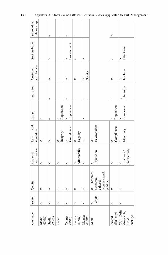
Appendix AOverview of Different Business ValuesApplicable to Risk Management

Here a benchmark of different business values applicable within risk management isprovided (provided by Stedin).

© Springer International Publishing AG 2017R.P.Y. Mehairjan, Risk-Based Maintenance for Electricity Network Organizations,DOI 10.1007/978-3-319-49235-3

129

Com

pany

Safety

Quality

Financial

performance

Law

and

regu

latio

nIm

age

Inno

vatio

nCustomer

satisfaction

Sustainability

Stakeholder

relatio

nship

Stedin

(DNO)

××

××

×–

––

–

Stedin

(201

5)×

××

×–

–×

×–

Eneco

×–

×× Integrity

× Reputation

––

––

Tennet

(TSO

)×

××

× Com

pliance

× Reputation

–×

× Env

iron

ment

–

Enexis

(DNO)

××

× Affordability

× Legality

––

××

–

Liand

er(D

NO)

××

×–

×–

× Service

×–

Shell

× Peop

le×

(Techn

ical,

econ

omic,

cultu

ral,

organisatio

nal,

politics)

× Reputation

× Env

iron

ment

Prorail

(Railway)

××

×× Com

pliance

× Reputation

–×

××

TU

Delft

(Research,

TBM

faculty

)

××

× Efficiency/

prod

uctiv

ity

× Effectiv

ity× Ergon

omic

x Effectiv

ity× Ecology

× Effectiv

ity

130 Appendix A: Overview of Different Business Values Applicable to Risk Management

Appendix BDevelopment Process of MaintenanceManagement Maturity Model

Here the process underlying the development of the maintenance managementmaturity model is given in Fig. B.1. The M4 model is mainly inspired by theInstitute of Asset Management (IAM) Capability Maturity Model which is sug-gested to be used for measuring the capability of organisations when adopting assetmanagement according to PAS 55. When attempting to translate this model to apractical arena and specifically to maintenance management, there were practicalgaps identified. The available models did not satisfy the needs and specific relevantrequirements of maintenance management as such. On the basis of a selectedfocused group approach of experts of multidisciplinary competencies, a brain-storming (inductive method) was adopted to develop the M4 method. The sixorganisation pillars are reached by means of multivoting decision-making approa-ches. The identical focused group has also been interviewed and involved in thedevelopment of the assessment logic of the maturity levels.

StrategicMaintenanceManagementStakeholders

Process

Concepts

Policy

InformationData

Performance

Criteria

Roles

Responsibility

ProfessionalizeMaintenanceManagement

InformationSystems

Inspections

Reporting Finance

Portfolio

Risk

Planning

Schedules

Identification of Organisation Dimensions

Organisation & Processes

Policy & Criteria

Information & Systems

Data Quality

Performance & Portfolio

Developmentof

MaintenanceManagement

MaturityModel based on Identified Dimensions

Identified Dimensions Maturity Model DesignPeople

Fig. B.1 Simplified representation of the development process of the maintenance managementmaturity model design


131

A simplified overview of the levels of assets that are assessed in the maintenancematurity model (M4) is shown in Fig. B.2.

A summary of the number of questions per domain and the overall character-istics of these questions are provided here:

Domain # ofquestions

Characteristics

Organisationand processes

8 Guaranteeing continuous improvement processes with rolesof designated (inter-) departments that are documented- Are processes described, documented and uniform- Are roles uniform, organised and followed- Knowledge and training

Policy andcriteria

10 This domain is concerned with the fact that policies andcriteria are documented, recorded and implemented.Appropriate strategic policies are translated to criteria on thatbasis of which maintenance planning can be performed- Are policies documented and followed- Are criteria adapted and updated on time- Are manufacturer, product and maintenance specificationsavailable and used

Information andsystems

12 This domain is related to the information requirements andinformation systems used for maintenance management foreach asset group and whether required information isavailable and recorded in the systems- Are assets registered, available in systems and structured- How is information gathered- Inspection and failure reports available and used- Is the information supporting lifecycle managementcapabilities

- Is analysis and reporting possible, automated and uniform- Are systems asset centric, uniform, coupled and available

Data quality 6 This domain is related to the degree to which data is suitablefor the purpose for which it is used on strategic, tactical andoperational level of the maintenance processes- Insights into the quality of data such as timely,completeness, correctness

- Are data quality measurements performed and how are theydone

- Are criteria for data quality assessment available- How are data quality issues dealt with

Performance andportfolio

13 This domain is responsible for transparent financial andportfolio planning business rules, suitable for the operationalenvironment, leading to a uniform way to categorisemaintenance activities- How are maintenance and inspection actions scheduled andreported

- Are KPI’s followed and available- Maintenance planning and actions and effect ofmaintenance

- Financial planning and administration

132 Appendix B: Development Process of Maintenance Management Maturity Model

The procedure that is followed during the maturity-level assessment is given inthe flow chart shown in Fig. B.3.

Here a summary results from the internal questionnaire related to “What is atleast needed to grow towards the maturity level “House in Order given:

MaturityMaintenance

Total

Gas Electricity

Pipelines StationsConnections Secundary TertiaryPrimary

Medium Voltage Grid

Sub-transmissionGrid

Medium Voltage Substations SubstationsPublic Lightning TransformersLow Voltage

Fig. B.2 Different asset groups which are assessed by means of the developed maintenancemanagement maturity model

Question n+1Question n

Asset Captain

Questions & Answers related

to Maturity Levels

Best in Class House in Order PracticallyManaged Nothing in Place

Maturity Level assessed

No No No

Yes Yes Yes

Fig. B.3 Flow chart of the procedure that is followed during the assessment of the questions whenestablishing the maturity levels.

Appendix B: Development Process of Maintenance Management Maturity Model 133

What is required to grow towards “House in Order”

Domain Summary

Organisation andprocesses

Formalisation, approval and stability of all maintenance roles andprocesses (inside and outside the asset management department)

Policy and criteria Produce and formalise all the policy, criteria and product specifications.Improvement of the failure data recording process for assets. Draftingand carrying out health assessments for gas network assets, such as isthe case for electricity networks assets


Finalising the project entailing the complete ComputerisedMaintenance Management System (CMMS). Implement a number ofspecific Geographical Information System (GIS) changes and updates.Moreover, the link between static asset data systems and dynamicfailure and inspection data systems is required

Data quality Monitoring data quality in a formal and structured way in order toprevent data pollution and discrepancies


Implement measures to be able to demonstrate the effectiveness ofmaintenance on the following years planning and budgets. Establishingmeans to ensure that maintenance management plans are guidingdecisions and not solely based on budgets

Here a summary of the results from the internal questionnaire related to “What isat least needed to grow towards the maturity level” “Best in Class” is given.

What is required to grow towards “Best in Class”

Domain Summary

Organisation andprocesses

Long-term strategy for maintenance management and using riskmanagement as guiding principle. Internal and external auditing.Creating and securing a line-of-sight throughout the whole companyregarding maintenance management

Policy and criteria Formalise all the policy, criteria and product specifications. Securingthe continuous improvement cycle. Improving and developing lifecycleasset maintenance management models (RAMS) and risk-basedmaintenance management models


Establishing component-level in-depth analytical methods supported byinformation and systems. Integrating CMMS, ERP, GIS and otherspecific information systems with each in a common data architecture

Data quality Securing the current data quality levels. Enriching operational dataquality levels. Creating an awareness on the operational levels (in thefield) for recording field data with precision and useful quality


Linking financial planning with asset planning in order to providelifecycle modelling by means of analysing the risk reduction for everyspend budget. Development and implementation of maintenance keyperformance indicators (KPIs) most favourable based on RAMSphilosophy

134 Appendix B: Development Process of Maintenance Management Maturity Model

In [86] and [87], an extensive overview of different benchmarked maturitymodels is provided. The authors in these references distinguish the maturity modelsbased on the application domain they are developed and applied for. These rangefrom generic to specialised domains such as IT support management. From thisoverview, it is found that a number of maturity models are developed which aredirected to maintenance management. In the following, these reported maintenancematurity models together with the developed with M4 are given.

Literature review of maintenance maturity models together with M4

Reference name Levels Dimensions Assessment items

[88], Maintenance managementbased on organisational maturitylevel

Surveybased

5 Propose 15 assessment areas

[81], Maintenance Maturity Grid 6 10 Generalised assessmentscriteria

[89], Integrated maintenancescorecard

4 4 Based on 4 perspectivesdefined from the balancedscorecard

[54], Maintenance managementmaturity model (M4)

4 5 Based on 49 proposedquestion assessments

Appendix B: Development Process of Maintenance Management Maturity Model 135

Appendix CRevised Risk Priority Numbersfor different Maintenance Policies

A complete list of the identified failure modes with the related failure code is givenhere:

List of the failure mode codes

Failure modecode

Brief description of failure mode

Tap changer-related failure modes

R1 No solid connection between main and selector windings due to impropercontacts (long-term effect LTE)

R3 No solid connection between main and selector windings due to impropercontacts (burn-ins and slack due to short circuits)

R4 No solid connection between main and selector windings due to impropercontacts (wear and tear)

R6 Mechanical slack due to wear and tear of components

R7 Mechanical block due to weariness of material

R8 Vacuum bottle leakage

R9 Bridging resistor defect due to mechanical weariness or overloading due toshort circuits

R10 Contacts defect

R11 Improper (too slow) switching due to weariness of springs

R12 Block in intermediate tap position due to weariness of springs due tomechanical defect

R13 Defect of air dryer due to silica gel saturated due to mechanical defect

R14 Lowered quality due to normal utilisation

R15 Leakage in the conservator

M1 No voltage or command signal

M2 Internal electrical defect

M3 Internal mechanical defect(continued)


137

(continued)


Failure modecode


Core and windings-related failure modes

KE3 Windings do not unsatisfactorily conduct current or do not unsatisfactorilyinduce the magnetic field due to ageing paper insulation

KE6 Windings do not unsatisfactorily conduct current or do not unsatisfactorilyinduce the magnetic field due to defective paper insulation (harmonics)

Oil-type bushing-related failure modes

OD1 Short circuit in insulated oil bushing between the tank and conductor due tocontaminated bushings

OD6 Bad/improper connection between windings and cable termination due tomounting or material defects

OD7 Ring-type current transformers not connected or short-circuited due tomounting or material defect

OD8 Ring-type current transformers not connected or short-circuited due tovibrations

Capacitor-type bushing-related failure modes

CD1 Short circuit in insulated oil bushing between the tank and conductor due tocontaminated bushings

CD5 Short circuit in insulated capacitor bushing between the tank and conductordue to incorrect oil-level packing

CD6 Short circuit in insulated capacitor bushing between the tank and conductordue to ageing of paper insulation

CD7 Bad/improper connection between windings and cable termination due tomounting or material defects

CD9 Ring-type current transformers not connected or short-circuited due tovibrations

Tank and accessories-related failure modes

T1 Oil leakage due to improper sealing of gaskets

T2 Oil leakage due to corrosion of appendages

Oil-related failure modes

OL1 Contaminated oil due to moisture (saturated silica gel)

OL2 Contaminated oil due to moisture (improper working oil lock)

OL3 Contaminated oil due to moisture (leakage)

OL4 Contaminated oil due to moisture (resistance changes)

OL5 Contaminated oil due to moisture (aged paper insulation)

OL6 Chemical and physical ageing of oil due to overloading

OL7 Aged oil due to normal operating conditions

Cooling system related failure modes

KO1 Impaired cooling due to unsatisfactory oil circulation (unsatisfactory openedseal/valve)

KO2 Impaired cooling due to unsatisfactory oil circulation (unsatisfactory ventingof radiator)

(continued)

138 Appendix C: Revised Risk Priority Numbers for different Maintenance Policies

(continued)


Failure modecode


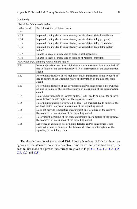
KO3 Impaired cooling due to unsatisfactory air circulation (failed ventilator)

KO4 Impaired cooling due to unsatisfactory air circulation (clogged grate)

KO5 Impaired cooling due to unsatisfactory air circulation (clogged radiator)

KO6 Impaired cooling due to unsatisfactory air circulation (ventilator systemfailure)

KO7 Unable to keep oil inside due to leakage sealing/gaskets

KO8 Unable to keep oil inside due to leakage of radiator (corrosion)

Protection and signalling-related failure modes

BE1 No or unjust detection of too high flow and/or transformer is not switched offdue to failure of the protection relays MR or interruption of the disconnectioncircuit

BE2 No or unjust detection of too high flow and/or transformer is not switched offdue to failure of the Buchholz relays or interruption of the disconnectioncircuit

BE3 No or unjust detection of gas development and/or transformer is not switchedoff due to failure of the Buchholz relays or interruption of the disconnectioncircuit

BE4 No or unjust signalling of lowered oil level (tank) due to failure of the oil-levelmetre (relays) or interruption of the signalling circuit

BE5 No or unjust signalling of lowered oil level (tap changer) due to failure of theoil-level metre (relays) or interruption of the signalling circuit

BE6 Does not provide temperature measurement due to failure of the resistivethermometer or interruption of the signalling circuit

BE7 No or unjust signalling of too high temperature due to failure of the distancethermometer or interruption of the signalling circuit

BE8 Difference in current is not or unjust detected and/or transformer is notswitched off due to failure of the differential relays or interruption of thesignalling or switching circuit

The detailed results of the revised Risk Priority Numbers (RPN) for three cat-egories of maintenance policies (corrective, time based and condition based) foreach failure mode of a power transformer are given in Figs. C.1, C.2, C.3, C.4, C.5,C.6, C.7 and C.8).

Appendix C: Revised Risk Priority Numbers for different Maintenance Policies 139

Fig. C.1 Revised RPN for different maintenance policies for the transformer tap changer failuremodes

Fig. C.2 Revised RPN for different maintenance policies for the transformer protection andsignalling failure modes

Fig. C.3 Revised RPN for different maintenance policies for the transformer oil-type bushingfailure modes


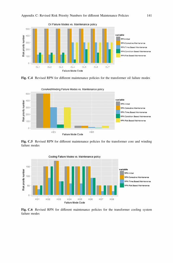
Fig. C.4 Revised RPN for different maintenance policies for the transformer oil failure modes

Fig. C.5 Revised RPN for different maintenance policies for the transformer core and windingfailure modes

Fig. C.6 Revised RPN for different maintenance policies for the transformer cooling systemfailure modes

Appendix C: Revised Risk Priority Numbers for different Maintenance Policies 141

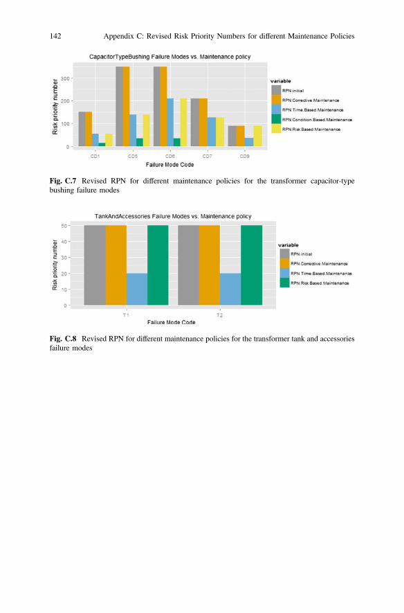
Fig. C.7 Revised RPN for different maintenance policies for the transformer capacitor-typebushing failure modes

Fig. C.8 Revised RPN for different maintenance policies for the transformer tank and accessoriesfailure modes


Appendix DStatistical Lifetime Distributions

From statistical reliability engineering, given a continuous random variable X, thefollowing statistical failure functions can be denoted [71]:

Probability Density Function—The probability density function (pdf) of acontinuous random variable, X, is a function that describes the probability thatX assumes a value in the interval [a, b]. If X is a continuous random variable, thenthe pdf, of X, is a function f(x) such that for two numbers, a and b with a < b:

P a�X � bð Þ ¼Zb

a

f ðxÞdx and f ðxÞ� 0 for all x ðD:2Þ

That is, the probability that X assumes a value in the interval [a, b] is the areaunder the density function.

Cumulative Density Function—A cumulative distribution function, cdf, refersto the probability that the value of a random variable falls within a specific range.The cdf is a function F(x) of a random variable, X, and is defined for a number x by:

F xð Þ ¼ P X� xð Þ ¼Zx

0;�1f ðsÞ ds ðD:2Þ

The cdf is the integral of the pdf and reflects the probability that f(x) will be equalto or less than x.

Reliability Function—The reliability function, R(t), can be derived using theprevious definition of the cdf function. This cdf (3.2) is also called the unreliabilityfunction, Q(t), which is the probability of failure in the region of 0 and t. Fromequation (D.2), the association between F(t) and Q(t) becomes:

FðtÞ ¼ QðtÞ ¼Z t

0

f ðsÞ ds ðD:3Þ


143

In general, there are only two states that can occur: success or failure. These twostates are also mutually exclusive (they cannot occur at the same time). Sincereliability and unreliability are the probabilities of two mutually exclusive states, thesum of both is always equal to unity. Therefore:

QðtÞþRðtÞ ¼ 1

RðtÞ ¼ 1� QðtÞ

RðtÞ ¼ 1�Z t

0

f ðsÞds

RðtÞ ¼Z1

t

f ðsÞds

ðD:4Þ

The Failure Rate Function—The failure rate function, λ(t), is a function of timeand has a probabilistic interpretation, namely λ(t). dt represents the probability thata device of age t will fail in the interval (t, t + dt). The failure rate function is equalto the probability of a component failing if it has not yet failed. Since the pdf is theprobability of a component failing and the cdf is the probability that it has alreadyfailed, the failure rate can be mathematically characterised as follows:

kðtÞ ¼ f ðtÞ1� FðtÞ ¼

f ðtÞ1� R t

0 f ðsÞds¼ f ðtÞ

RðtÞ ðD:5Þ

The failure rate function can be expressed as failures per unit time, e.g. 2 failuresper year. The above-mentioned quantities f(t), F(t), R(t) and λ(t) can be convertedinto each other. Therefore, they contain all information about the failure process ofthe system under consideration.

144 Appendix D: Statistical Lifetime Distributions

Appendix EMonte Carlo Simulation Algorithm

The algorithm for the MCS is programmed in MATLAB. The flow chart shown inFig. E.1 presents the principle of operation of the MATLAB code.

Fig. E.1 Flow chart representing the principle of operation of the MCS algorithm [74].


145

The simulation starts with the generation of random failures of every componentin the radial feeder system. This is done in the MATLAB engine “TTF generator”where a random number for the random variable TTF is generated from the asso-ciated probability distribution of the component. After this, the failure states aredetermined using the “Failure Engine” to define whether the failures occurredwithin the mission time. All failures outside the mission time are neglected. Forfailures within the mission time, a replacement is performed. A failure of either acable or a joint leads to the replacement with two new synthetic joints and a smalllength of XLPE cable. In order to check whether these newly installed componentsfail within the remaining mission time, a TTF is generated and analysed for thesecomponent. All simulated failures within the mission time are summated and storedin a database. The whole process is repeated 5000 times, and finally, the results areshown in a frequency plot of the amount of customer outages is.

146 Appendix E: Monte Carlo Simulation Algorithm

Appendix FNon-technical triggers for riskmanagement

Non-Technical Risks: These risks are not considered in the relatively technicalmaintenance management, but considered by strategy specialists and policy analy-sers. Additionally, these risks are normally for long term, so their probabilities andconsequences are difficult to predict (e.g. the case that Germany abandoned nuclearpower). Consequently, asset managers can only contribute to control these risksthrough providing innovative technical design of assets/asset systems. In the fol-lowing, we discuss each level of AM from a non-technically triggered risk viewpoint.

• At the strategic level,

– Analyse future networks, determine risks with commercial or societalstimuli.

– The solutions to these risks are frequently not optimised in standard riskmanagement system such as risk register. Since they are long term anddifficult to quantify (i.e. unlikely to be included in a KPI system), the assetportfolio should simply be redundant, robust or flexible enough to survive ineach scenario.

– Such robustness or flexibility can be interpreted technically as hardrequirement on asset systems. These requirements are called strategicrequirements.

• At the tactical level, an equally important task is to design new/replaced/refurbished asset systems, as well as their preventive maintenance plans, so thatthey can cope with strategic requirements.

• The operational level should investigate ways to operate and maintain newcomponents and environments introduced by strategic requirements.

The right triangle in Figure 43 represents the management of risks withnon-technical stimuli. It has a larger area at the strategic level (S2), because thediversity (different specialities) and long-term characteristic of these types of risksrequire a wider human resource (knowledge of overall system) to study.


147

Appendix GCase Studies of the Applicationof Condition Monitoring

Case study 1: Experience of Online Partial Discharge Monitoring on aWide-Area Medium Voltage Network

In this case study, the application of a handheld online monitoring device todetect partial discharges (PD) is described. The measurements were performed inthe medium voltage (MV) network of Stedin in the Netherlands [83].

Parts of the MV network have been designed with the principles of unearthedstar-point grounding (floating system). An advantage of such a design is that thevoltage between the phases themselves, in case of a phase-to-ground fault, is hardlyinfluenced. Consequently, the loads are not changed and the system remains inoperation. However, the downside to this is that the absolute voltages of the healthyphases are increased by a factor √3 in the case of a phase-to-earth. As result of adormant fault in an unearthed 10 kV network of Stedin, a long-lasting earth fault(>6 h) occurred. After this dormant fault was finally isolated by the protectionsystem, it was also found from the failure investigation later on that the earth faultwas the cause and had been presented for approximately 6 h. There were especiallyconcerns about possible higher levels of PD activities in surrounding cable joints,terminations and cables. The asset managers then argued that this long-lasting earthfault, which resulted in elevated voltage levels on the healthy phases, might havestressed surrounding assets and caused them to come into a critical state. As a “firstline in defence”, without time consuming or costly investigations, the asset man-agers decided to carry out measurements to get a rough initial result whether thislong-lasting earth fault might had stressed the nearby assets. A quick, low-cost PDscreening was selected.

A two-stage approach was set up:

– Stage 1: A quick PD scan was performed at the primary HV/MV substationassessing the outgoing cables and local switchgear assets.

The quick scan was performed by the PD-handheld device, which comprises acombination of inductive High-Frequency Current Transformer (HFCT) and


149

capacitive Transient Earth Voltage (TEV) sensors. On the basis of the results ofstage 1, Stedin would decide on one or combinations of the following stages:

– Stage 1: Perform offline PD detection and localisation measurement of sus-pected feeders (from stage 1).

– Stage 2: Perform permanent PD monitoring measurements on suspected feeders(from stage 1).

– Stage 3: Perform a wide-area PD-handheld screening on both sides of the cableand all Ring Main Units (RMU’s) in the between the circuit.

Stage 1: Primary substation-level PD-handheld screening: At the primary(25 kV/10 kV) MV substation that energises the feeder that had the previouslydescribed earth fault, a quick PD screening measurement was carried out. In total,27 single cable sections have been diagnosed with the PD-handheld system. At thefirst stage, an HFCT sensor was installed to measure any PD activity on the cablescreen wire which is connected to the main earth point of the substation. Thesemeasurements take about 1–2 min per single feeder. Secondly, the TEV sensor wasused to measure the overall condition of the 10 kV switchgear. Colour-codedcriticality was indicated (LEDs) and digital dB signal (acoustic) on the display. Toreduce background noise level, a 100 kHz filter was used with HFCT sensor.

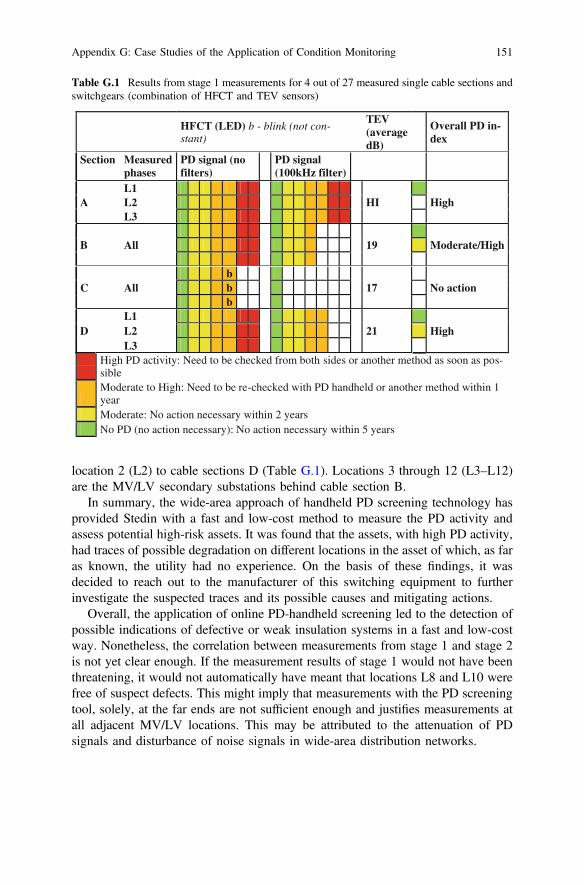
In Table G.1, the combined results from the HFCT and TEV sensors for 4 out ofthe 27 measured cable sections are given. Cable section A, for instance, had highPD magnitudes in both cases, namely with and without high-pass filter. However,this cable is a feeder to a local metro station and the level of high-frequency noise atthis location substantially influenced the measurement results, making it very dif-ficult to draw conclusions from these. Cable section C showed, with filter, nosignificant PD activity and was therefore classified as “no action required”. It wasfound that cable sections B and D have moderate PD magnitudes and also relativelyhigh levels for local (switchgear) dB value (TEV sensor).

Therefore, Stedin decided to carry out a wide-area (far end and multiple RMU)network PD-handheld measurement for sections B and D, in particular from the farend side of the cable and at all RMU’s in the circuit between both ends of the cable.

Stage 2: Monitoring on a Wide-Area Medium Voltage Network: In stage 2, thecable sections B and D were measured from the far end. Section B is an outgoingfeeder with multiple MV/LV secondary stations in between. In total, 12 secondaryMV/LV substations and all intermediate cable sections connecting these MV/LVsubstations (behind cable section B) were measured with the PD-handheld device atthe terminal. From these online measurements, it was found that two MV/LVlocations had high local PD activity. Finally, in collaboration with the maintenancedepartment and the service provider, it was decided to investigate these twoswitchgears (RMU) at these MV/LV locations by means of in-depth visualinspections. Under controlled conditions, in order to continue the electricity supply,they were taken out of service and inspected.

In Fig. G.1, a one-line diagram schematic representation is given of the 12locations. Location 1 (L1) corresponds to cable section B (in Table G.1) and

150 Appendix G: Case Studies of the Application of Condition Monitoring

location 2 (L2) to cable sections D (Table G.1). Locations 3 through 12 (L3–L12)are the MV/LV secondary substations behind cable section B.

In summary, the wide-area approach of handheld PD screening technology hasprovided Stedin with a fast and low-cost method to measure the PD activity andassess potential high-risk assets. It was found that the assets, with high PD activity,had traces of possible degradation on different locations in the asset of which, as faras known, the utility had no experience. On the basis of these findings, it wasdecided to reach out to the manufacturer of this switching equipment to furtherinvestigate the suspected traces and its possible causes and mitigating actions.

Overall, the application of online PD-handheld screening led to the detection ofpossible indications of defective or weak insulation systems in a fast and low-costway. Nonetheless, the correlation between measurements from stage 1 and stage 2is not yet clear enough. If the measurement results of stage 1 would not have beenthreatening, it would not automatically have meant that locations L8 and L10 werefree of suspect defects. This might imply that measurements with the PD screeningtool, solely, at the far ends are not sufficient enough and justifies measurements atall adjacent MV/LV locations. This may be attributed to the attenuation of PDsignals and disturbance of noise signals in wide-area distribution networks.

Table G.1 Results from stage 1 measurements for 4 out of 27 measured single cable sections andswitchgears (combination of HFCT and TEV sensors)

HFCT (LED) b - blink (not con-stant)

TEV (average dB)

Overall PD in-dex

Section Measured phases

PD signal (no filters)

PD signal (100kHz filter)

AL1

HI HighL2L3

B All 19 Moderate/High

C Allb

17 No actionbb

DL1

21 HighL2L3

High PD activity: Need to be checked from both sides or another method as soon as pos-sibleModerate to High: Need to be re-checked with PD handheld or another method within 1 yearModerate: No action necessary within 2 yearsNo PD (no action necessary): No action necessary within 5 years

Appendix G: Case Studies of the Application of Condition Monitoring 151

Case study 2: Continuous Diagnostic Measuring for MV Power CableNetworks

In this case study, an experience with a continuous monitoring system formedium voltage power cable networks is given. At present, 83 systems are beingused, many of these guarding the main feeders in the city of Rotterdam in thenetwork of Stedin. This monitoring system works as described in [23, 82]. Brieflydescribed, two inductive PD sensors are placed in the cable network, one sensor atposition A and the other at position B. These positions can be several kilometres(km) apart from each other. From a defect spot X between these positions A and B,

Fig. G.1 Results of PD measurements for 12 locations. Locations L8 and L10 were taken out ofservice for in-depth inspections. L8 and L10 had a higher TEV (capacitive) and HFCT (inductive)results of PD activity locally. During the inspection of these MV switchgears (RMU’s), suspecttraces were found, which may be a possible source of the higher HFCT and TEV results. However,this was not confirmed


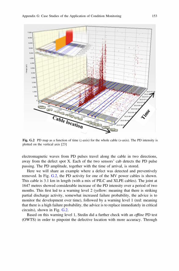
electromagnetic waves from PD pulses travel along the cable in two directions,away from the defect spot X. Each of the two sensors’ cab detects the PD pulsepassing. The PD amplitude, together with the time of arrival, is stored.

Here we will share an example where a defect was detected and preventivelyremoved. In Fig. G.2, the PD activity for one of the MV power cables is shown.This cable is 3.1 km in length (with a mix of PILC and XLPE cables). The joint at1647 metres showed considerable increase of the PD intensity over a period of twomonths. This first led to a warning level 2 (yellow: meaning that there is strikingpartial discharge activity, somewhat increased failure probability, the advice is tomonitor the development over time), followed by a warning level 1 (red: meaningthat there is a high failure probability, the advice is to replace immediately in criticalcircuits), shown in Fig. G.2.

Based on this warning level 1, Stedin did a further check with an offline PD test(OWTS) in order to pinpoint the defective location with more accuracy. Through

Fig. G.2 PD map as a function of time (z-axis) for the whole cable (x-axis). The PD intensity isplotted on the vertical axis [23]

Appendix G: Case Studies of the Application of Condition Monitoring 153

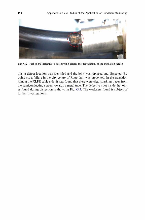
this, a defect location was identified and the joint was replaced and dissected. Bydoing so, a failure in the city centre of Rotterdam was prevented. In the transitionjoint at the XLPE cable side, it was found that there were clear sparking traces fromthe semiconducting screen towards a metal tube. The defective spot inside the jointas found during dissection is shown in Fig. G.3. The weakness found is subject offurther investigations.

Fig. G.3 Part of the defective joint showing clearly the degradation of the insulation screen


References

Goerdin, S. A. V., Mehairjan, R. P. Y., & Smit, J. J. (2015). Monte Carlo Simulation applied tosupport risk-based decision making in electricity distribution networks. Eindhoven, sn

Liyanage, J. P., sd. International Journal of Strategic Engineering Asset Management. sl:International Journal of Strategic Engineering Asset Management.


155

appendix a overview of different business values ...978-3-319-49235-3/1.pdf · overview of...

Documents