appendix a: procedure of the experiment - home - …978-3-319-53904...appendix a: procedure of the...
TRANSCRIPT

Appendix A: Procedure of the Experiment
Introduction
At the beginning of the experiments the participants were welcomed and the
research team introduced themselves. A short description of the experiment was
given—two games and a questionnaire—but no details were provided about the
content or the purpose. The participants were told that the games are common in
this research sector and are played in a similar manner in different countries across
the world. They were also informed that they would play with money provided by
the University of Dresden for research purposes. Anyone was free to leave at any
point before or during the experiment.
The participants were instructed that they were not allowed to talk about the
games at any point during the experiment, otherwise they would have to be
disqualified. They were free to talk about other topics and one research assistant
remained with the participants at all times, ensuring that this rule was followed. We
also assured all participants that the result of the study would be used for research
purposes only and that any personal information would be kept strictly confidential.
Everyone drew a number out of a bag, which allowed for a random order of
participants in the games. At the end of the introduction, the ‘show-up’ fee of 4000Cambodian Riel (USD1) was distributed to each participant.
Risk Game
The first game began with a description of rules. To address issues of low literacy,
the procedures were explained to all participants with the use of graphs. Addition-
ally, the local members of the research team enacted various game situations in
front of the participants. The examples were defined and oriented towards the
examples provided by Schechter (2007). The players were informed that questions
© Springer International Publishing AG 2017
O. Fiala, Natural Disasters and Individual Behaviour in Developing Countries,Contributions to Economics, DOI 10.1007/978-3-319-53904-1
167

were not allowed in the group setting, but could be asked of the researchers in
private. At the beginning of the game, every player was asked if she understood the
game. If they did not, the research team would explain the rules again in private and
answer any questions. The participants were called by the number they had drawn
from the bag. To decrease the length of time needed for the game, it was necessary
to play it simultaneously at two different stations. Both stations were occupied by
two research assistants at all times. As in many experiments in rural areas, to ensure
that participants understood the games, neither the risk nor the trust game was
double blind (Barr 2003; Karlan 2005; Schechter 2007).
The participants were told that everyone would receive 6000 Riel (USD1.50) in
yellow-coloured play money. These looked similar to the real notes, so that the
participants could make the connection to the actual money. They were told that the
play money would be exchanged at the end of the experiment, one-to-one, into real
money. Each player received six 1000 Riel notes for use in the game.
The players were told that they had the opportunity to bet any share of this
money, which included the choice not to bet at all. After the player decided the
amount they wanted to bet, they rolled an unbiased six-sided die. The following
distribution of possible outcomes was given, which is based on previous studies by
Schechter (2007) and Ahsan (2014). If the die landed on one, the player would lose
the money she bet. If the die landed on two, the player would lose half of the money.
If the die showed three, the player would keep the amount she bet. If the die landed
on 4/5/6, the player would receive 1.5/2.0/2.5 times her bet, respectively. Thus, a
roll of one or two would have a negative result, a roll of three would have a neutral
result, and rolls of four, five or six would have positive results. Participants were
reminded that they could finish the game with more or less than the original amount
of 6000 Riel.
After one round, the game was over. The game was played only once with each
participant. Each participant could take away the share she did not bet, plus the
money she won through rolling the die (if any). The total money from the game was
paid out in play money at the end of the round.
Figure A.1 summarises the procedure of the game. A translated version of this
figure was also used by the research team to explain the game.
Trust Game
After the risk game the participants were gathered as one large group again for an
explanation of the second game. The success of the trust game largely depends on
the participants’ understanding of the rules (Ahsan 2014). As in the first game, the
procedures were explained aloud in front of all participants, with the support of
graphs. As before, the local members of the research team enacted various (previ-
ously defined) situations and demonstrated the procedures of the game. The partic-
ipants were not allowed to discuss the game amongst themselves, but they were told
that any questions could be asked to the researchers in private. The explanation of
the trust game was more time-consuming than that of the risk game.
168 Appendix A: Procedure of the Experiment

The game is played by pairs of individuals: player 1 and player 2. Each partic-
ipant played the role of player 1 in the first round and the role of player 2 in the
second round. The players were told that they would always play with other people
from their village, but each time with a different person. Participants were notified
that nobody would know exactly with whom they were playing.
The participants were called again by their number. As in the risk game, the
game was played at two different stations simultaneously, and both stations were
occupied by two research assistants each.
In the first round of the game, each participant was given 6000 Riel (USD1.50) in
red play money, in the form of six 1000 Riel notes. This different colour was used to
prevent confusion and crossover of play money between the two games.
Player 1 then had the opportunity to send a share of their 6000 Riel to an
anonymous player 2. Whatever amount player 1 sent was tripled by the researcher
before it was put in an envelope in front of the participants. Each envelope was
marked with a different letter combination. If no money was sent by player 1, the
envelope remained empty. After every participant played their role as player 1, the
envelopes were shuffled in front of the whole group.
In the next phase, all participants were called again by their number to play their
role as player 2. On the way to the station they took an envelope from the top of the
stack. The players were told that they should not receive their own envelope. If they
had drawn their own, they should return it and pick the next one. The participants
opened the envelopes in front of the research assistants and saw how much (if any)
money was sent from player 1. Then they decided how much money they wanted to
keep and how much they wanted to return to player 1.
Therefore, the participants finished the game with whatever they kept as player
1 (from the original 6000 Riel), plus whatever they kept from the tripled amount in
your money is lost
get 0.5x your money back
get your money back
get 1.5x your money back
get 2x your money back
get 2.5x your money back
6,000 Riel
keep money safe
play with money:
you can win
more, but also
lose some
Fig. A.1 Procedure of risk game
Appendix A: Procedure of the Experiment 169

their role as player 2, plus whatever they found in their original envelope as player
1 (which was returned by another player 2). Each player was informed that they
could finish with more or <6000 Riel as a result of the game.
Figure A.2 summarises the procedure of the game. A translated version of this
figure was also used by the research team to explain the game.
PLAYER 1
6,000 Riel
keep money safe
send money
to player 2any money sent
will be tripled
money is going to
player 2
envelope with money
sent by player 1 (tripled)
PLAYER 2
keep money
send money
back to player 1
Fig. A.2 Procedure of trust game for player 1 and 2
170 Appendix A: Procedure of the Experiment

Questionnaire
After both games the participants were called by their number to one of the six
research assistants, and were asked the questions from the set questionnaire. The
research team asked all questions in person and no questionnaires were distributed
to the participants. The questionnaire took place at the end of the experiment, so
that questions had no influence on the behaviour during the games. They also
received their original envelope from the trust game (as player 1), with the
money (if any) sent back by player 2. After the questionnaires, the participants
approached the author to immediately exchange their play money for real money.
The questionnaire contained the sections household information, experiences with
natural disasters, disaster risk management activities, prevention and preparedness,
and demand for insurance.
Discrete Choice Experiment
The discrete choice experiment comprises 48 alternatives, presented in 24 choice
sets, each consisting of three alternatives (flood insurance A, flood insurance B, no
insurance). A sample of one choice set in English is presented in Fig. A.3.
Insurance A Insurance B No Insurance
Cover for loss 1,000,000 Riel 500,000 Riel –
Weeklypremium
2,000 Riel 2,000 Riel –
Condition forpay-out
Pay-out after a visit ofinsuranceemployee
Pay-out if measuring station has shown flood
–
Credit without loan without loan –
Prevention Noprevention
Preventioneffort –
Provider Village National government –
Fig. A.3 Sample of choice set
Appendix A: Procedure of the Experiment 171

References
Ahsan D (2014) Does natural disaster influence people’s risk preference and trust? An experiment
from cyclone prone coast of Bangladesh. Int J Disaster Risk Reduct 9:48–57.
Barr A (2003) Trust and expected trustworthiness: experimental evidence from Zimbabwean
villages. Econ J 113:614–630.
Karlan DS (2005) Using experimental economics to measure social capital and predict financial
decisions. Am Econ Rev 95:1688–1699.
Schechter L (2007) Traditional trust measurement and the risk confound: an experiment in rural
Paraguay. J Econ Behav Organ 62:272–292.
172 Appendix A: Procedure of the Experiment

Appendix B: Descriptive Statistics: Livelihoods
and Coping with Natural Disasters in Rural
Cambodia
Household Information
Table B.1 summarises the most significant results of the individual statistics. In
total, 209 persons from 5 villages participated.1
37.5% of the participants were male, 62.5% were female (n ¼ 208). Whilst the
average age was 50.9, the youngest participant was 19 and the oldest was 95. 97.6% of
the participants were married (n ¼ 207) and Buddhism was the dominant religion
(96.2%); the rest were Christians (n¼ 209). Two thirds of the respondents were female.
Figure B.1 shows the level of education of the participants (n ¼ 209). While
37.8% of the participants had no formal education at all, only 57.9% had completed
primary or secondary school, although strong differences between the male and
female participants can be observed.
59.6% of participants described themselves as literate (n¼ 203). The results also
differ significantly between genders (Fig. B.2). While 83.3% of the men described
themselves as literate, only 44.4% of women did so. To measure financial literacy,
Clarke and Kalani (2012) asked their participants short mathematical questions and
used the number of correct answers as a proxy for financial literacy. For this
analysis, the same method with the given questions was used.2 22.4% gave no
correct answers, another 22.4% gave one correct answer, 24.9% two correct
answers, 21.5% three correct answers and 8.8% were able to answer all questions
correctly (n ¼ 205).
1Three participants, who were under the age of 18 and did not disclose this fact at the beginning,
were deleted from the sample. Another five participants in one village came to participate, but
finished the experiment too early or did not start at all. They were also deleted from the sample.
The number of answers for each question varies; therefore the actual number of observations is
provided for each question.2The mathematical questions were the following: 5 þ 3 ¼ ?, 3 � 7 ¼?, 1/10th of 300 ¼ ?, 5% of
200 ¼ ?
© Springer International Publishing AG 2017
O. Fiala, Natural Disasters and Individual Behaviour in Developing Countries,Contributions to Economics, DOI 10.1007/978-3-319-53904-1
173

Literate83.3%
Illiterate16.7%
Male
Literate44.4%Illiterate
55.6%
Female
Fig. B.2 Literacy
Table B.1 Individual statistics summary
Characteristics Mean Min Max
Male (%) 37.5%Age 50.9 19 95Married (%) 97.6%Buddhist (%) 96.2%No education (%) 37.8%Literate (%) 59.6%Financially literate 1.7 0 4Household size 5.6 1 17Head of household (%) 67.9%Living in village <15 years (%) 9.7%Households with credit (%) 48.1%Land owned (%) 59.3%Land owned (ha) 2.87 0.08 15Growing rice (%) 55.8%Households with livestock (%) 23.9%Total livestock units, usual year (2012) 0.24 0 6.5Total livestock units, last year (2013) 0.34 0 6.5Per-capita income, usual year (US Dollars) 379 0 16,676Per-capita income, last year (US Dollars) 257 0 5000No. of observations 209
12.8%
60.3%
19.2%
7.7%
0.0%
0.0%
53.1%
37.7%
6.9%
2.3%
0.0%
0.0%
None
Primary
Secondary
High School
College degree
Graduate
0% 20% 40% 60% 80%
male
female
Fig. B.1 Level of education completed
174 Appendix B: Descriptive Statistics: Livelihoods . . .

67.9% of participants answered that they are the head of their households
(n ¼ 209). Figure B.3 shows the average number of household members. The
average size of the total number of household members was 5.6, whilst the smallest
household was formed of 1, and the largest made up of 17 persons (n ¼ 209).
Almost two thirds of the participants had lived in their village for their entire
lives (61.5%). 80 participants moved to their villages later in life, on average 23.9
years ago (min 1, max 40 years). Only 9.6% of the participants had lived in their
village for <15 years (n ¼ 207).
The next questions reveal the living conditions of the participants. Figure B.4
shows the material used to build the walls of participants’ houses. While 28.5%
used different kind of metals, 58.5% had walls of wood or leaves (n ¼ 207). The
majority of the participants (95.2%) used a different kind of metal for their roofs
(n ¼ 208).
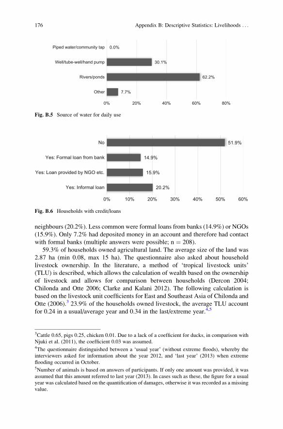
Figure B.5 shows the participants’ sources of water for daily use. 62.2% of the
sample obtained their water from river and ponds, followed by 30.1% who had a
well or hand pump. ‘Other’ (7.7%) includes those who purchased water for daily
use (n ¼ 209). 86.1% of participants had access to electricity (n ¼ 208).
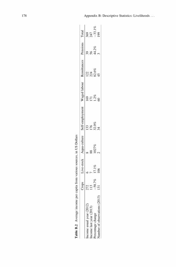
Figure B.6 shows the proportion of participants who had applied for various
types of credit. 51.9% had not borrowed any money. Of those who had borrowed
money, the majority received it from informal sources: family, friends or
4.3%
2.4%
28.5%
37.2%
21.3%
6.3%
Bricks only
Bricks & Wood
Metal (aluminium, iron, zinc)
Wood only
Leaves
Other
0% 10% 20% 30% 40%
Fig. B.4 Materials used to construct house walls
5.6
2.4
1.2
0.4
0.9
0 2 4 6
Total number of household members
Number of family members who are working
Number of children less than 15 years old
Number of children less than 5 years old
Number of family members above 50 years old
Fig. B.3 Number of household members
Appendix B: Descriptive Statistics: Livelihoods . . . 175
neighbours (20.2%). Less common were formal loans from banks (14.9%) or NGOs
(15.9%). Only 7.2% had deposited money in an account and therefore had contact
with formal banks (multiple answers were possible; n ¼ 208).
59.3% of households owned agricultural land. The average size of the land was
2.87 ha (min 0.08, max 15 ha). The questionnaire also asked about household
livestock ownership. In the literature, a method of ‘tropical livestock units’(TLU) is described, which allows the calculation of wealth based on the ownership
of livestock and allows for comparison between households (Dercon 2004;
Chilonda and Otte 2006; Clarke and Kalani 2012). The following calculation is
based on the livestock unit coefficients for East and Southeast Asia of Chilonda and
Otte (2006).3 23.9% of the households owned livestock, the average TLU account
for 0.24 in a usual/average year and 0.34 in the last/extreme year.4,5
0.0%
30.1%
62.2%
7.7%
Piped water/community tap
Well/tube-well/hand pump
Rivers/ponds
Other
0% 20% 40% 60% 80%
Fig. B.5 Source of water for daily use
51.9%
14.9%
15.9%
20.2%
No
Yes: Formal loan from bank
Yes: Loan provided by NGO etc.
Yes: Informal loan
0% 10% 20% 30% 40% 50% 60%
Fig. B.6 Households with credit/loans
3Cattle 0.65, pigs 0.25, chicken 0.01. Due to a lack of a coefficient for ducks, in comparison with
Njuki et al. (2011), the coefficient 0.03 was assumed.4The questionnaire distinguished between a ‘usual year’ (without extreme floods), whereby the
interviewers asked for information about the year 2012, and ‘last year’ (2013) when extreme
flooding occurred in October.5Number of animals is based on answers of participants. If only one amount was provided, it was
assumed that this amount referred to last year (2013). In cases such as these, the figure for a usual
year was calculated based on the quantification of damages, otherwise it was recorded as a missing
value.
176 Appendix B: Descriptive Statistics: Livelihoods . . .

The questionnaire asked about different sources of income,6 including income from:
• Growing crops7
• Raising livestock
• Aquaculture8
• Non-farming/self-employment
• Waged labour
• Remittances
• Pension
Figure B.7 shows the proportion of the various income sources per household.
65.8% of all participants gained income from growing crops, followed by raising
livestock (53.3%) and waged labour (30.2%). Another important source of income
was remittances (22.6%) and income from self-employment (17.1%). Aquaculture
and pensions can be neglected (n ¼ 199).
Table B.2 shows the income from various sources from 199 participants in a
usual year (2012) and last year (2013).9 In 2012 the average income per capita was
65.8%
53.3%
1.0%
17.1%
30.2%
22.6%
1.5%
Crops
Livestock
Aquaculture
Non-farming/self-employment
Waged labour
Remittances
Pension
0% 20% 40% 60% 80%
Fig. B.7 Percentage of participants earning from various sources of income
6The questionnaire asked for annual income. However, many participants are not aware of their
income per year but were able to provide information per month or per day. In the latter case, an
average of 27 working days per month was assumed. The relevant exchange rates are 32.33 Thai
Baht for USD1 and 4000 Cambodian Riel for USD1.7If no income information was provided, the annual household income was calculated on the basis
of the amount of crops produced. If the sales price for 1 t of rice was given in the interview, this
was used for the income calculation. Otherwise the average sales price was calculated and
assumed for the other households in the same village. Because of different types of rice crops
and different sales markets, a generally accessible price cannot be assumed. When crops were
mentioned ‘for consumption’ no amount was attributed and no income was calculated. One
household produced cassava—based on Reuy (2013), 1 t of cassava has the value of USD160.8One household mentioned only the amount of fish sold, but not income. Based on information
from Yady et al. (2012), 1 kg of fish has the value of USD0.44.9All income information was originally recorded per household and transferred to per-capita based
on household sizes. For the various sources of income (except the total income), the conditional
average income was calculated (based on the number of participants who earned money from the
various sources).
Appendix B: Descriptive Statistics: Livelihoods . . . 177
Table
B.2
Averageincomeper
capitafrom
varioussources,in
USDollars
Crops
Live-stock
Aqua-culture
Self-em
ployment
Waged
labour
Rem
ittances
Pensions
Total
Incomeusual
year(2012)
272
68
133
169
122
39
369
Incomelastyear(2013)
113
788
176
171
224
56
247
Percentagechange
�58.7%
17.1%
1027%
32.0%
1.2%
82.6%
44.2%
�33.1%
Number
ofobservations(2013)
131
106
234
60
45
3199
178 Appendix B: Descriptive Statistics: Livelihoods . . .
USD369, which shrank by 33.1% to USD247 in 2013. The average income from
growing crops per capita, livestock income and pensions also decreased. In con-
trast, the average income from other sources increased, particularly average
remittances.
Figure B.8 presents the numbers from the table above and highlights the
differences of the income sources over the 2 years (2012 and 2013). In 2012,
growing crops was the dominant source of income, followed by waged labour,
self-employment and remittances; this picture changed in 2013.
Experiences with Natural Disasters
Part II of the questionnaire was intended to investigate participants’ experienceswith natural disasters. Different questions about experiences, assessments of flood
risks and actual damages were asked. Table B.3 provides a short summary of the
key results.
Crops
Livestock
Aquaculture
Self-employment
Waged labour
Remittances
Pension
Total
$0 $50 $100 $150 $200 $250 $300 $350 $400
Income usual year (per capita)
Income last year (per capita)
Fig. B.8 Average income from various sources and total average income per capita
Table B.3 Summary of participants’ experiences with natural disasters
Characteristics Mean (%)
Experienced flooding in the last 5 years 68.4Observed flooding 97.9Strong fear of danger of damages through floods 67.7Faced severe consequences of flooding 73.0Believes that extreme floods are becoming more frequent 74.6Damage to household property due to extreme flood in 2013 26.4Damage to household production due to extreme flood in 2013 88.7
Appendix B: Descriptive Statistics: Livelihoods . . . 179
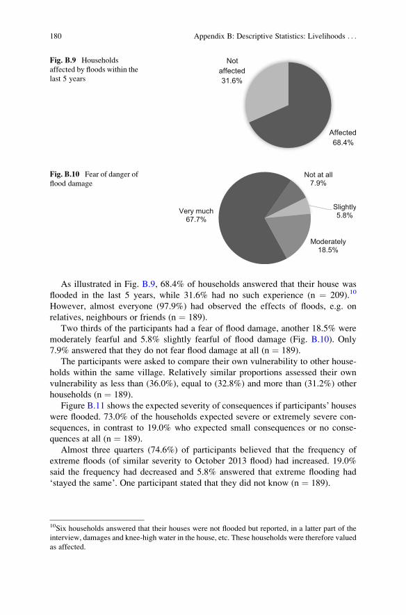
As illustrated in Fig. B.9, 68.4% of households answered that their house was
flooded in the last 5 years, while 31.6% had no such experience (n ¼ 209).10
However, almost everyone (97.9%) had observed the effects of floods, e.g. on
relatives, neighbours or friends (n ¼ 189).
Two thirds of the participants had a fear of flood damage, another 18.5% were
moderately fearful and 5.8% slightly fearful of flood damage (Fig. B.10). Only
7.9% answered that they do not fear flood damage at all (n ¼ 189).
The participants were asked to compare their own vulnerability to other house-
holds within the same village. Relatively similar proportions assessed their own
vulnerability as less than (36.0%), equal to (32.8%) and more than (31.2%) other
households (n ¼ 189).
Figure B.11 shows the expected severity of consequences if participants’ houseswere flooded. 73.0% of the households expected severe or extremely severe con-
sequences, in contrast to 19.0% who expected small consequences or no conse-
quences at all (n ¼ 189).
Almost three quarters (74.6%) of participants believed that the frequency of
extreme floods (of similar severity to October 2013 flood) had increased. 19.0%
said the frequency had decreased and 5.8% answered that extreme flooding had
‘stayed the same’. One participant stated that they did not know (n ¼ 189).
Affected68.4%
Not affected31.6%
Fig. B.9 Households
affected by floods within the
last 5 years
Not at all7.9%
Slightly5.8%
Moderately18.5%
Very much67.7%
Fig. B.10 Fear of danger of
flood damage
10Six households answered that their houses were not flooded but reported, in a latter part of the
interview, damages and knee-high water in the house, etc. These households were therefore valued
as affected.
180 Appendix B: Descriptive Statistics: Livelihoods . . .

Looking to the future, 51.3%of participants believed that their housewould be flooded
more frequently than at present (Fig. B.12). 34.7% believed it would flood the same
amount as at present and 14.0% believed it would happen less frequently (n¼ 150).11
52% of flood-affected households are flooded, to some extent, during the rainy
season every year (n ¼ 150). Figure B.13 shows the maximum height of floodwater
reached during annual floods compared to the height of water during the extreme
floods of 2013. The figure shows the height of water during the annual floods and
the October 2013 flood (n ¼ 91 for annual floods, n ¼ 149 for flood in 2013).
For 2.7% of participants, during the flood in October 2013, the area in and
around the house was flooded for 1 week only, for 17.8% the floodwater remained
for 1 to 2 weeks, for 21.9% between 2 and 4 weeks and for the majority (48.6%), it
took between 1 and 2 months for the floodwater to subside. For 8.9% the flood
lasted for more than 2 months (n ¼ 146).
The last question in part II of the questionnaire focused on the experienced
damages of the 2013 flood. Figure B.14 shows the share of households who suffered
Less frequent than at present14.0%
As frequent
as at present34.7%
More frequent than at present51.3%
Fig. B.12 Participants’ belief in the frequency of future household flooding
5.8%
13.2%
7.9%
31.7%
41.3%
No consequences at all
Small consequences
Neutral
Severe consequences
Extremely severe consequences
0% 10% 20% 30% 40% 50%
Fig. B.11 Participants’ expectation of severity of consequences if house floods
11This and the following questions in this section of the questionnaire were asked only to those
who were flood-affected. Therefore, the number of observations is smaller.
Appendix B: Descriptive Statistics: Livelihoods . . . 181

from this disaster. 106 households reported damages, 88.7% of these to household
production, e.g. their crops or livestock, 26.4% to household property. 12.3%
reported forgone income (opportunity costs), an average of USD73.12 Another
18.9% mentioned medical costs as an additional loss of income due to the flood
(the average cost for medical care was USD179).
Disaster Risk Management Activities
Part III of the questionnaire focused on existing disaster risk management activities.
To assess the degree of organisation of the participants, the initial questions asked
about membership in local organisations and groups. Only 7.2% were members of a
local organisation, only 8.2% were part of a local savings group and 11.1%
Flooding inside yard
Flooding inside house, to ankle height
Flooding inside house, to knee height
Flooding inside house, to waist height
Flooding inside house, to shoulder height
Flooding inside house, above head height
0% 10% 20% 30% 40% 50%
Annual flood
Flood in October 2013
Fig. B.13 Maximum height of water during annual floods and the extreme flood in 2013
26.4%
88.7%
79.2%
18.9%
Damage to household property
Damage to household production
Forgone income
Medical costs etc.
0% 20% 40% 60% 80% 100%
Fig. B.14 Household damage by extreme flooding in October 2013
12If amount of forgone income was not provided, the amount was calculated by multiplying the
level of flood duration by regular income (only wages/self-employment were considered).
182 Appendix B: Descriptive Statistics: Livelihoods . . .
belonged to an agricultural community (n ¼ 207). Flood information was
exchanged regularly between neighbours by 86.9% of the participants.
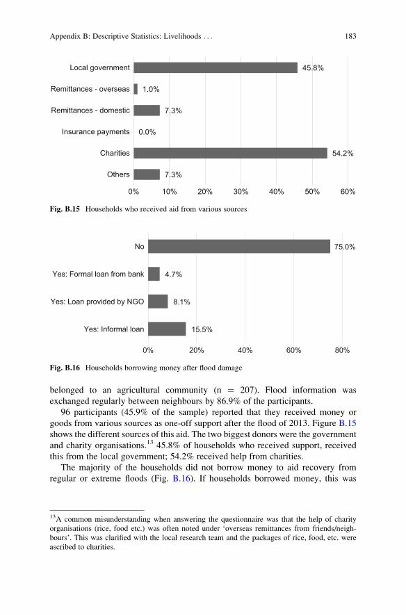
96 participants (45.9% of the sample) reported that they received money or
goods from various sources as one-off support after the flood of 2013. Figure B.15
shows the different sources of this aid. The two biggest donors were the government
and charity organisations.13 45.8% of households who received support, received
this from the local government; 54.2% received help from charities.
The majority of the households did not borrow money to aid recovery from
regular or extreme floods (Fig. B.16). If households borrowed money, this was
45.8%
1.0%
7.3%
0.0%
54.2%
7.3%
Local government
Remittances - overseas
Remittances - domestic
Insurance payments
Charities
Others
0% 10% 20% 30% 40% 50% 60%
Fig. B.15 Households who received aid from various sources
75.0%
4.7%
8.1%
15.5%
No
Yes: Formal loan from bank
Yes: Loan provided by NGO
Yes: Informal loan
0% 20% 40% 60% 80%
Fig. B.16 Households borrowing money after flood damage
13A common misunderstanding when answering the questionnaire was that the help of charity
organisations (rice, food etc.) was often noted under ‘overseas remittances from friends/neigh-
bours’. This was clarified with the local research team and the packages of rice, food, etc. were
ascribed to charities.
Appendix B: Descriptive Statistics: Livelihoods . . . 183

mostly done on an informal basis from relatives, friends or neighbours (multiple
answers were possible; n ¼ 161).
The two final questions examined the sale of production assets or valuable items
as a source of income after the floods. 10.8% of households sold production assets
after the 2013 flood including machines, tools, animals or land; only 3.4% sold
valuable items such as jewellery or gold (n ¼ 148).
Prevention and Preparedness
Part IV of the questionnaire focused on household assessments of prevention against
flood events. For 84.2% of the participants it was somewhat or extremely important to
prevent or reduce the negative consequences of floods (Fig. B.17). 12.9% answered
that prevention has only little importance or is not important at all (n ¼ 209).
Figure B.18 shows the judgement of the participants of their own ability to
protect themselves from the negative consequences of floods. 68.8% of the
7.2%
5.7%
2.9%
31.6%
52.6%
Not important at all
Slightly important
Neutral
Somewhat important
Extremely important
0% 10% 20% 30% 40% 50% 60%
Fig. B.17 Participants’ belief in the importance of prevention/reduction of negative consequences
of floods
41.3%
27.4%
8.7%
20.2%
2.4%
I cannot protect myself at all
I can hardly protect myself
Neutral
I can protect myself well
I can protect myself completely
0% 10% 20% 30% 40% 50%
Fig. B.18 Participants’ judgement of own ability to protect themselves
184 Appendix B: Descriptive Statistics: Livelihoods . . .

households answered that they could not protect themselves at all or could hardly
protect themselves. In contrast, 22.6% said they could protect themselves well or
completely (n ¼ 208). 43.5% of the households were satisfied with their current
level of protection against extreme flood events, while 56.5% answered that they
were dissatisfied in this regard (n ¼ 209).
Figure B.19 shows who participants believe was mainly responsible for provid-
ing flood protection. 66.8% of the participants stated that it is their own responsi-
bility, followed by the village community (18.8%) and national government (10%)
(n ¼ 202).
47.1% of households modified the timing of crop planting so that the harvest
would precede the expected arrival of floods (n ¼ 206) and 55.4% of households
used chemical fertiliser (n ¼ 204). The last question was focused on the partici-
pants’ needs for better preparation against extreme flood events like the one in
October 2013 (multiple answers were possible)—Fig. B.20 displays the answers.
Building infrastructure to prevent floods and financial assistance for flood protec-
tion measures were the most popular responses (51.7 and 50.2% of the participants
mentioned these respectively). Improved knowledge of and information about
coping mechanisms for extreme flooding were emphasised by 34.4%.
64.9%
1.9%
2.4%
9.6%
18.3%
2.9%
I am responsible
District government
Provincial government
National government
Village community
Other
0% 10% 20% 30% 40% 50% 60% 70%
Fig. B.19 Participants’ belief in who is responsible to provide flood protection
50.2%
51.7%
34.4%
1.0%
8.6%
Financial assistance for flood protectionmeasures
Building infrastructure to prevent flooding
Improved knowledge and information abouthow to cope with extreme floods
Provision of insurance against the cost ofdamage caused by extreme floods
Other
0% 10% 20% 30% 40% 50% 60%
Fig. B.20 Participants’ needs for better preparations against extreme floods
Appendix B: Descriptive Statistics: Livelihoods . . . 185

Demand for Insurance
The last part of the questionnaire focused on the individuals’ demand for
microinsurance. Only 1 person reported that they had insurance (n ¼ 120) and
4.9% knew someone with insurance (n ¼ 163). Following the discrete choice
analysis (see Sect. 4.3), several questions were asked to control the results of the
estimation. Respondents who had chosen ‘no insurance’ at least four times (out of
six choice sets) were asked for the reason. Hereby, 19 respondents agreed with the
statement “I am not interested in buying insurance”, while another 19 participants
gave missing affordability as reason. The preferred provider was the village com-
munity, followed by national government and non-governmental organisations
(n¼159). The choice of a preferred provider is illustrated in Fig. B.21.
A overwhelming majority of respondents (92.5%) would be more interested in
insurance if it was paired with a loan; 91.8% would increase their prevention efforts
if the insurance would consequently become cheaper (n ¼ 159). Finally, the
individuals were asked if they would increase their production or try new crops
with higher returns in the case that they would have insurance against flood damage.
Although the truth of the answer cannot be validated in a real world situation,
74.2% of respondents would increase their productive activities (n ¼ 159).
References
Chilonda P, Otte J (2006) Indicators to monitor trends in livestock production at national, regional
and international levels.
Clarke D, Kalani G (2012) Microinsurance decisions: evidence from Ethiopia. Microinsurance
Innovation Facility Research Paper 19, Geneva.
Dercon S (2004) Growth and shocks: evidence from rural Ethiopia. J Dev Econ 74:309–329.
28.3%
6.3%
11.9%
18.9%
34.6%
National government
Provincial government
Private company
NGO
Village
0% 10% 20% 30% 40%
Fig. B.21 Participants’ preference for insurance provider
186 Appendix B: Descriptive Statistics: Livelihoods . . .

Njuki J, Poole J, Johnson N et al (2011) Gender, livestock and livelihood indicators. International
Livestock Research Institute (ILRI), Nairobi.
Reuy R (2013) Cassava production dropped in 2012. Phnom Penh Post. http://www.
phnompenhpost.com/business/cassava-production-dropped-2012. Accessed 11 Nov 2014.
Yady M, Rajabova R, Long Y, Burja K (2012) Cambodia food price and wage bulletin. World
Food Programme, Cambodia Agricultural Marketing Office, Phnom Penh.
Appendix B: Descriptive Statistics: Livelihoods . . . 187
Appendix C: Robustness Checks
The Impact of Natural Disasters on Individuals’Risk-TakingPropensity in Rural Cambodia
Section 3.4 presents empirical evidence for the impact of natural disasters on
individuals’ risk-taking propensity. In addition to the regressions (1) to (4) presentedin Table 3.7 other control variables have been entered and removed, however no
significant impact on the efficiency of the regression model could be found. The
tested control variables include: education, religion, observation of floods, income
distribution within village (Gini coefficient), mean income in village, amount of
time a participant lived in the village, satisfaction with protection, fear of future
floods, flood level in rainy season, post-disaster support by government or charity,
and flood damages to household property or production assets. Tests for
heteroskedasticity and a robust regression also confirmed the results of the
presented regression. Finally, repeating the regressions without respondents who
had not bet anything confirms the main findings, especially regarding disaster
experience.
Identifying income as the core variable, which is significantly different between
the affected and non-affected group, a propensity score matching of the sample
regarding income was conducted. Regression (14) in Table C.1 using this propen-
sity score matching dataset confirmed the direction and scale of the results
presented in Sect. 3.4.
© Springer International Publishing AG 2017
O. Fiala, Natural Disasters and Individual Behaviour in Developing Countries,Contributions to Economics, DOI 10.1007/978-3-319-53904-1
189

The Interest in Microinsurance: First Results from a Poisson
Regression
Section 4.3.1 presents the results from a Poisson regression, investigating the
impact of several social-economic variables on the interest in insurance (expressed
by the amount a respondent chose any insurance contract). No significant effect of
wealth per capita (calculated in ‘tropical livestock units’) can be found in the
regressions (9) and (10), when substituting income per capita by wealth. The effects
of other variables used in Table 4.7 stay consistent in direction of effect and
significance (Table C.2).
Table C.1 Regression for risk game based on propensity score matching sample
Share bet in risk game
(14)
(Constant) 0.079 (0.229)Affected 0.202*** (0.051)Age 0.018* (0.009)Age squared �0.017** (0.008)Gender �0.009 (0.050)Married state �0.320** (0.124)Financial literacy 0.078*** (0.023)Number of people living in the household �0.033*** (0.011)Number of children under 15 years in the household 0.047*** (0.017)Total income per capita in US Dollars (2013) �0.000 (0.000)Number of observations 59
Standard errors in parentheses
***p < 0.01, **p < 0.05, *p < 0.10
Table C.2 Including wealth in Poisson regression for interest in insurance
(9) (10)
Wealth (TLU) per capita (2014) �0.070 (0.221) �0.125 (0.224)Number of observations 126 126
Each column represents the regressions (9) to (10) for interest in insurance. Control variables
included as in 4.7. Standard errors in parentheses
190 Appendix C: Robustness Checks

Appendix D: Research Designs of Selected
Empirical Studies
Section 4.2 analyses the role of 12 determinants for microinsurance demand,
whereof risk aversion, trust and risk exposure are of particular interest for the
empirical analysis of microinsurance demand in Cambodia (Sect. 4.3). Table D.1
combines the references regarding microinsurance demand and risk aversion (4.2),
trust (4.3) and risk exposure (Table 4.4), and provides a short overview of the
various research designs.
Table D.1 Research designs of selected empirical studies
Reference
Relevant
determinantsa Research design
Akter et al.
(2008)
Risk exposure Household survey in six different districts in Bangladesh
facing various levels of exposure to environmental risk.
Discrete choice logit regression model investigates
demand for hypothetical catastrophe insurance product
Households in areas less exposed to environmental risks
are less likely to buy catastrophe insuranceGine et al.
(2008)
Risk aversion,
Trust
Household survey investigates determinants for demand
for rainfall insurance products among smallholder farmers
in India. Probit regression is used in order to explain
decision for insurance purchase
Uncertainty about the product leads to lower demand of
risk-averse households and those with less trust in insur-
ance providerCai et al. (2009) Trust Randomised field experiment in China, investigating take-
up of insurance for sows and the impact on farmers’production decisions (OLS regression)
Lack of trust in government-subsidised microinsurance is
significant barrier for insurance take-up
(continued)
© Springer International Publishing AG 2017
O. Fiala, Natural Disasters and Individual Behaviour in Developing Countries,Contributions to Economics, DOI 10.1007/978-3-319-53904-1
191
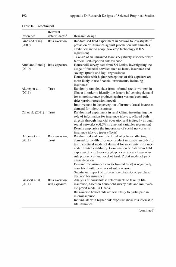
Table D.1 (continued)
Reference
Relevant
determinantsa Research design
Gine and Yang
(2009)
Risk aversion Randomised field experiment in Malawi to investigate if
provision of insurance against production risk animates
credit demand to adopt new crop technology (OLS
regression)
Take-up of an uninsured loan is negatively associated with
farmers’ self-reported risk aversionArun and Bendig
(2010)
Risk exposure Household survey data from Sri Lanka, investigating the
usage of financial services such as loans, insurance and
savings (probit and logit regressions)
Households with higher perceptions of risk exposure are
more likely to use financial instruments, including
insurancesAkotey et al.
(2011)
Trust Randomly sampled data from informal sector workers in
Ghana in order to identify the factors influencing demand
for microinsurance products against various economic
risks (probit regression model)
Improvement in the perception of insurers (trust) increases
demand for microinsuranceCai et al. (2011) Trust Randomised experiment in rural China, investigating the
role of information for insurance take-up, offered both
directly through financial education and indirectly through
social networks (OLS/instrumental variables regression)
Results emphasise the importance of social networks in
insurance take-up (peer effects)Dercon et al.
(2011)
Risk aversion,
Trust
Randomised and controlled trial of policies affecting
demand for health insurance product in Kenya, in order to
test theoretical model of demand for indemnity insurance
under limited credibility. Combination of data from field
experiment with laboratory-type experiments to measure
risk preferences and level of trust. Probit model of pur-
chase decision
Demand for insurance (under limited trust) is negatively
correlated with measures of risk aversion
Significant impact of insurers’ creditability on purchase
decision for insuranceGiesbert et al.
(2011)
Risk aversion,
risk exposure
Analysis of households’ determinants to take up life
insurance, based on household survey data and multivari-
ate probit model in Ghana.
Risk-averse households are less likely to participate in
microinsurance
Individuals with higher risk exposure show less interest in
life insurance
(continued)
192 Appendix D: Research Designs of Selected Empirical Studies
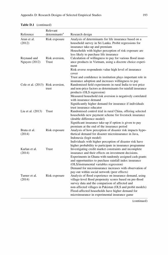
Table D.1 (continued)
Reference
Relevant
determinantsa Research design
Arun et al.
(2012)
Risk exposure Analysis of determinants for life insurance based on a
household survey in Sri Lanka. Probit regressions for
insurance take-up and premium
Households with higher perception of risk exposure are
less likely to purchase life insuranceReynaud and
Nguyen (2012)
Risk aversion,
Trust
Calculation of willingness to pay for various flood insur-
ance products in Vietnam, using a discrete choice experi-
ment
Risk-averse respondents value high level of insurance
cover
Trust and confidence in institution plays important role in
insurance adoption and increases willingness to payCole et al. (2013) Risk aversion,
trust
Randomised field experiments in rural India to test price
and non-price factors as determinants for rainfall insurance
products (OLS regression)
Measured household risk aversion is negatively correlated
with insurance demand
Significantly higher demand for insurance if individuals
trust insurance educatorLiu et al. (2013) Trust Randomised control trial in rural China, offering selected
households new payment scheme for livestock insurance
(double difference model)
Significant insurance take-up if option is given to pay
premium at the end of the insurance periodBrata et al.
(2014)
Risk exposure Analysis of how perception of disaster risk impacts hypo-
thetical demand for disaster microinsurance in Java,
Indonesia (logit model)
Individuals with higher perception of disaster risk have
higher probability to participate in insurance programmeKarlan et al.
(2014)
Trust Investigating credit market constraints and incomplete
insurance and their effects on investment decisions.
Experiments in Ghana with randomly assigned cash grants
and opportunities to purchase rainfall index insurance
(OLS/instrumental variables regression)
Demand for microinsurance increases with observation of
pay-out within social network (peer effects)Turner et al.
(2014)
Risk exposure Analysis of flood experience on insurance demand, using
village-level flood propensity scores based on pre-flood
survey data and the comparison of affected and
non-affected villages in Pakistan (OLS and probit models)
Flood-affected households have higher demand for
microinsurance in experimental insurance game
(continued)
Appendix D: Research Designs of Selected Empirical Studies 193

References
Akotey OJ, Osei KA, Gemegah A (2011) The demand for micro insurance in Ghana. J Risk Financ
12:182–194.
Akter S, Brouwer R, Chowdhury S, Aziz S (2008) Determinants of participation in a Catastrophe
Insurance Programme: empirical evidence from a developing country. Canberra.
Arun T, Bendig M (2010) Risk management among the poor: the case of microfinancial services.
IZA Discussion Paper 5174, Bonn.
Arun T, Bendig M, Arun S (2012) Bequest motives and determinants of micro life insurance in Sri
Lanka. World Dev 40:1700–1711
Brata AG, Rietveld P, de Groot HLF et al (2014) Living with the Merapi Volcano: risks and
disaster microinsurance. ANU Working Papers in Trade and Development 13, Canberra.
Cai H, Chen Y, Fang H, Zhou L-A (2009) Microinsurance, trust and economic development:
evidence from a randomized natural field experiment. NBER Working Paper Series 15396,
Cambridge, MA.
Cai J, De Janvry A, Sadoulet E (2011) Social networks and insurance take-up: evidence from a
randomized experiment in China. Microinsurance Innovation Facility Research Paper
8, Geneva.
Cole S, Gine X, Tobacman J et al (2013) Barriers to household risk management: evidence from
India. Am Econ J Appl Econ 5:104–135.
Dercon S, Gunning J, Zeitlin A (2011) The demand for Insurance Under Limited Trust: evidence
from a field experiment in Kenya. University of Wisconsin, Agriculture and Applied Econom-
ics, Madison.
Table D.1 (continued)
Reference
Relevant
determinantsa Research design
Grislain-
Letremy (2015)
Trust,
Risk exposure
Investigating determinants of demand for insurance cov-
erage, using household-level data on insured and
uninsured households in French overseas departments in
Latin America and the Caribbean. Estimation of theoreti-
cal insurance supply and demand model.
Take-up rate in the neighbourhood directly increases the
individual probability of purchasing insurance (peer
effects)
The probability of purchasing insurance decreases with the
number of past disasters that have occurredLiu et al. (2015) Risk exposure Analysis of willingness to pay for a hypothetical rainfall
index insurance in China (logit and tobit model)
Significantly higher demand for rainfall index insurance
by flood-affected householdsYeboah and
Obeng (2016)
Trust Analysis of financial literacy and other factors and their
effects on willingness to pay for microinsurance among
informal business operators in Ghana, using cross-
sectional survey data (OLS regression)
Negative impact of respondents’ confidence in the contracton insurance demand; positive peer effects
aRelevant determinants for microinsurance demand; one or more of risk aversion, trust and risk
exposure
194 Appendix D: Research Designs of Selected Empirical Studies

Giesbert L, Steiner S, Bendig M (2011) Participation in micro life insurance and the use of other
financial services in Ghana. J Risk Insur 78:7–35.
Gine X, Townsend R, Vickery J (2008) Patterns of rainfall insurance participation in rural India.
World Bank Econ Rev 22:539–566.
Gine X, Yang D (2009) Insurance, credit, and technology adoption: field experimental evidence
from Malawi. J Dev Econ 89:1–11.
Grislain-Letremy C (2015) Natural disasters: exposure and underinsurance. CREST, Paris-
Dauphine University, Paris.
Karlan D, Osei R, Osei-Akoto I, Udry C (2014) Agricultural Decisions after relaxing credit and
risk constraints. Q J Econ 129:597–652.
Liu X, Tang Y, Miranda MJ (2015) Does past experience in natural disasters affect willingness-to-
pay for Weather Index Insurance? Evidence from China. In: Agricultural and Applied Eco-
nomics Association Annual Meeting 2015, San Francisco.
Liu Y, Chen KZ, Hill RV, Xiao C (2013) Borrowing from the insurer: an empirical analysis of
demand and impact of insurance in China. Microinsurance Innovation Facility Research Paper
34, Geneva.
Reynaud A, Nguyen M-H (2012) Monetary valuation of flood insurance in Vietnam. Vietnam
Center of Research in Economics, Management and Environment 01-2012, Hanoi, Ho Chi
Minh City.
Turner G, Said F, Afzal U (2014) Microinsurance demand after a rare flood event: evidence from a
field experiment in Pakistan. Geneva Pap Risk Insur Issues Pract 39:201–223.
Yeboah AK, Obeng CK (2016) Effect of financial literacy on willingness to pay for micro-
insurance by commercial market business operators in Ghana. MPRA Paper 70135, Munich.
Appendix D: Research Designs of Selected Empirical Studies 195