appendix a solutions to selected problems - boston...
TRANSCRIPT

1
Appendix A Solutions to Selected Problems Solutions to Chapter 3 Problems .................................................................................................1 Solutions to Chapter 6 Problems .................................................Error! Bookmark not defined. Solutions to Chapter 3 Problems Problem 1. Let )(f ! , 11 !"!# , be a function of one variable, ),( !"#$ and ),( LLL !"#$ are two unit vectors. Show that )q(sinè4!d)f( L
2!
L =!!•!"+
.
Here
L!•! is the scalar product of two vectors, and q(x), 1x0 !! , is a function of one
variable defined as
!! "+#$+#=
x
0
1
x
ã)]dãx)f(â(ã,x)f(ã),([21dã)(f
21q(x) ,
where 1)x,()x,( =!"+!# , and
2
2
ã1x
x1ãarccos!
1x)â(ã,!
!= .
Solution. Let !
+
""•"#"2!
LL d)f()(g . (1)
In the following derivations we assume that 0
L=! , that is, vector
L! belongs to ZX plane.
This assumption does not limit the generality of the derivations as one always can substitute φ with (
L!"! ) without changing the domain of the integration (i.e., the upper hemisphere). For
convenience of derivations let us transform the original system of coordinates to a new one, where
L! is aligned with Z-direction (Fig. 1). This can be accomplished with rotation by angle
L!" around the Y-axis as specified with the following linear transform,

2
,R)(AR L!"#$ where
!!!
"
#
$$$
%
&
''
'('
)'(
LL
LL
L
cos0sin
010
sin0cos
)(A
and )z,y,x(R = and )z,y,x(R !!!=! are vectors in the original and new coordinate system, respectively. Note the minus sign for angle
L! . This is due to the fact that positive angles are
counted outward from Z-direction. One example of transformation is for the Z-axis, which is transformed from )1,0,0(Z = in the original system into )cos,0,sin(Z LL !!"=# in the new system. To determine the integration domain in the new coordinate system, let
)cos,sinsin,cos(sinv !"!"!= be a unit vector in the new system. The v vector falls into the upper hemisphere of the original system if and only if .0coscossinsin0cossinsinzv
LL!"#"+$"#+$"#"%&'•
Therefore,
.sinsin
coscoscos
L
L
!!
!!"# (2)
Note that the angular domain of the upper hemisphere in the original coordinate system is
],0[ !"# and ]2,0[ !"# . This domain is specified differently in the new coordinate system as shown in Fig. 2. Namely, three sectors with respect to ! can be identified: ]2/,0[ L!"#$! (shown in Red), ]2/,2/[ LL !+"!#"$! (shown in green), and ],2/[ L !"+!#" (shown in blue). The corresponding variations of ! can be derived from the algebraic analysis of Eq. (2). The final expression for the angular domain in the new coordinate system is:
Figure. 1 Coordinate system transform via rotation by angle
L!" around the Y-axis.
Z
Y
X
L!
L!"

3
!!!!!!
"
!!!!!!
#
$
%&'
()+(&)*<))
))))
))*(
))
))&'
)+()*(&)+))
))+*
(&'
)*(&)>))
))
.
],,2(,1
sinsin
coscos
];sinsin
coscosarccos2,
sinsin
coscos[arccos
],2,
2[,1
sinsin
coscos1
];2,0[
),2,0[,1
sinsin
coscos
LL
L
L
L
L
L
LLL
L
LL
L
(3)
In a view that in the new coordinate system the direction
L! coincides with Z! , the argument of
function )(f L !•! in Eq. (1) simplifies, i.e., !="•" cosL
. Therefore, !!
""
""#$
%"=%%•%&%+
sinsin
coscoscos
2!
LL
L
L
d)osc(fd)f()(g
! !!!"+#
"$#
%&
'()
*""""
$#
%&
'()
*""""
#"$#
+"$"++"$"=
L
L
L
L
L
L
L 2
2
sinsin
coscosarccos2
sinsin
coscosarccos
2
0
2
0
d)dcos()osc(fd)dcos()osc(f
)d(sin)ins(f22
L
!
"
#
##"=
!"
"#$
%&'
()*
+,-
.""""
/0"+L
0 L
L )(sindsinsin
coscosarccos22)ins(f
Figure. 2 The upper hemisphere of the original system of coordinates XYZ in a new system of coordinates ZYX !!! . Vector
L! is
aligned with axis Z! of the new system.
L2
!+"
X!
L!
!
L2
!"#
L!
L2
!"# 0
2
!
Z!
X Z
4
.)(sindsinsin
coscosarccos2)ins(-f
L
0 L
L!"
"#$
%&'
()*
+,-
.""""
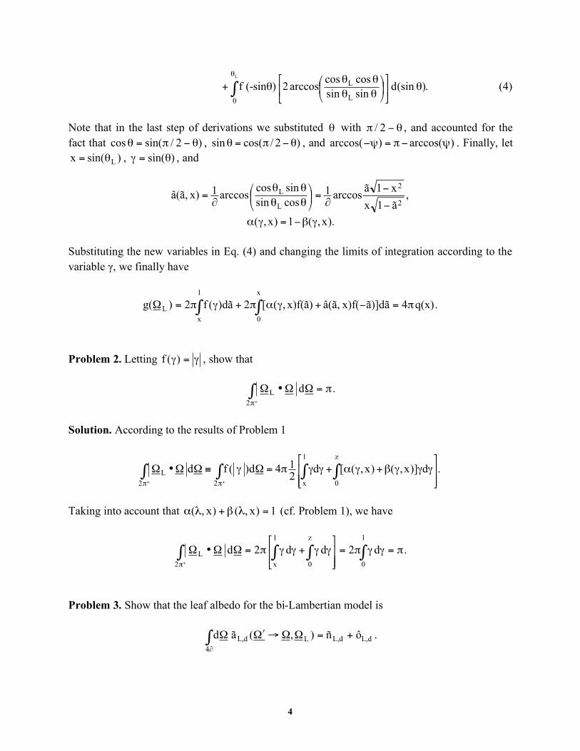
"+ (4)
Note that in the last step of derivations we substituted ! with !"# 2/ , and accounted for the fact that )2/sin(cos !"#=! , )2/cos(sin !"#=! , and )arccos()arccos( !"#=!" . Finally, let
)sin(x L!= , )sin(!=" , and
,ã1x
x1ãarccos!
1cossin
sincosarccos!
1x)â(ã,2
2
L
L
!
!="
#
$%&
'((
((=
).x,(1)x,( !"#=!$ Substituting the new variables in Eq. (4) and changing the limits of integration according to the variable γ, we finally have
.q(x)4ã)]dãx)f(â(ã,x)f(ã),([2dã)(f2)g(
x
0
1
x
L !! "=#+$%"+$"=&
Problem 2. Letting !=!)(f , show that .d
2
L!=""•"#
+!
Solution. According to the results of Problem 1
.d)]x,()x,([d214d)(fd
1
x
z
022
L
!!"
#
$$%
&'''(+')+''*=+',++•+ - ---
++ **
Taking into account that 1)x,()x,( =!"+!# (cf. Problem 1), we have
!! !! "=##"=$$%
&
''(
)##+##"=**•*
+"
1
0
1
x
z
02
L.d2dd2d
Problem 3. Show that the leaf albedo for the bi-Lambertian model is dL,dL,LdL,
4!
ôñ),(ãd +=!!"!#!$ .

5
Solution. The bi-Lambertian model for diffuse leaf scattering phase function is (cf. Chapter 3, Eq. (9))
!"
!#
$
>%•%&%•%%•%
<%•%&%•%%•%=%%'%&
0.))((,ô!
1
0,))((,ñ!
1
),(ã
LLLL,d
LLLL,d
LL,d (1)
Note that the angles !" and
L! are fixed in the integral of interests and integration over whole
sphere can be spitted into two parts, namely, ),(ãd LL,d
4!
!!"!#!$
).,(ãd),(ãd LdL,
0))((
LdL,
0))(( LLLL
!!"!#!+!!"!#!= $$<!•!#!•!>!•!#!•!
(2)
Taking into account Eq. (1), we have
,d1),(ãd L
0))((
d,LLdL,
0))(( LLLL
!•!!"#
=!!$!%! &&>!•!%!•!>!•!%!•!
(3a)
.d1),(ãd L
0))((
d,LLdL,
0))(( LLLL
!•!!"#
=!!$!%! &&<!•!%!•!<!•!%!•!
(3b)
In view that the angles !" and
L! are fixed, the integrals on the right hand side of Eqs. (3a) and
(3b) are identical and equal to the integral over hemisphere ( +!2 or !"2 ). The last integral was evaluated in the Problem 2, namely, .d
L
2
!="•""#+!
(4)
Combining Eqs. (2)-(4) we finally have .11),(ãd d,Ld,Ld,Ld,LLdL,
4!
!+"=#!#
+#"#
=$$%$&$'
Problem 5. Prove Equation (14). Solution. Equation (14) in Chapter 3 states: ,
21),r(Gd
21
2
=!!" #
+"
(1)

6
where (cf. Chapter 3, Eq. (2)) ,)(gd
21),r(G L
2
LLL !•!!!"
=! #+"
(2a)
.1)(gd2!1
LL
2!
L =!!"+
(2b)
Combining Eq. (1)-(2) and result of Problem 2, we have !
+"
##"2
),r(Gd21
! !+ +" "
#•###"
#"
=
2
L
2
LLL )(gd21d
21
! !+ +" "
#•####"
=
2 2
LLLL2d)(gd
41
.2
12
4
12
=!"!!
=
Problem 6. Show that the geometry factor ),r(G ! for spherically distributed leaf normals depends neither r nor ! and is equal to 0.5. Solution. Recall (cf. Chapter 3, Eq. (2)), .)(gd
21),r(G L
2
LLL !•!!!"
=! #+"
Recall also, that for spherically distributed leaf normals 1)(g LL =! (cf. Chapter 3, Eq. (5f)). Combining this result with the result of the Problem 2, we have .
21
21d
21),r(G L
2
L =!"!
=#•##!
=# $+!
Problem 7. Show that µ=G for horizontal leaves, and !"= sin)/2(G for vertical leaves. Solution. Recall (cf. Chapter 3, Eq. (2)), .)(gd
21),r(G L
2
LLL !•!!!"
=! #+"

7
Further, let )cos,sinsin,cos(sin !"!"!=# and )cos,sinsin,cos(sin LLLLLL !"!"!=# . Therefore, ( ) ( ) ( ) ( ) ( ) ( )!"!+#!"#!+#!"#!=$•$ coscossinsinsinsincossincossin
LLLLLL
.coscos)cos(sinsin LLL !!+"#"$!!= For horizontal leaves the derivations for ),r(G ! are as follows. The probability density of leaf normal orientation (cf. Chapter 3, Eq. (4)) is
.sin
)0()(g
L
LLL !
"!#=$
Therefore,
!•!!"##$
=! % %$ $
LLL
2/
0
2
0
LLL )(gddsin21),r(G
! !" "
##+$%$&###
%#'#$#
"=
2/
0
2
0
LLLL
LLLL coscos)cos(sinsinsin
)0(sindd
21
.cos µ!"= Similar derivations can be performed for vertical leaves. In this case the probability density of leaf normal orientation is
.sin
)2/()(g
L
LLL !
"#!$=%
Therefore,
! !" "
##+$%$&###
"%#'#$#
"=(
2/
0
2
0
LLLL
LLLL coscos)cos(sinsin
sin
)2/(sindd
21),r(G
.sin20)cos(sin1d212
0
LL !"
=+#$#%!%#"
= &"

8
Problem 8. Let the polar angle, L! , and azimuth,
L! , of leaf normals be independent (see Eq.
3). Show that
),,(),r(gd),r(G LL
1
0
LL µµ!µµ=µ "
where
LLcos !=µ , !=µ cos , and
! "•"#
=
2!
0
LLLLL dö||)(öh21)ìø(ì, .
Solution. Since the polar angle,
L! , and azimuth angle,
Lö , of leaf normals are independant, the
following representation of the probability density of leaf normal orientation is valid (cf. Chapter 3, Eq. (3)): ),(öh)(ìg)(g LLLLLL =! where L Lg (ì ) and L Lh (ö )/2! are the probability density functions of leaf normal inclination and azimuth, respectively. Therefore, !•!!!
"=µ #
+"
L
2
LLLL ),r(gd21),r(G
!•!"µ"µ#
= $ $#
LLLL
1
0
L
2
0
LL )(h),r(gdd21
!•!""µµ#
= $ $#
LLL
1
0
2
0
LLLL )(hd),r(gd21
.),(),r(gd211
0
LLLL! µµ"µµ#
=
Problem 9. Show that in canopies where leaf normals are distributed uniformly along the azimuthal coordinate [i.e., 1)(h LL =! ], ),( Lµµ! can be reduced to
!"
!#$
%&&'+&%
(=
otherwise,sinì1ì1)(2/1)/!(2ìì
,sinèsinèìì if,ìì)ìø(ì,
,t2L
2tL
LLL
L
where the branch angle
t! is )cotcotarccos( L!"!# .

9
Solution. Recall (cf. Problem 6), .coscos)cos(sinsin LLLL !!+"#"$!!=%•% Therefore,
!•!""#
$µµ% &#
L
2
0
LLLL )(hd21),(
!"
##+$%$##$"
=
2
0
LLLL coscos)cos(sinsind21
!"
##+$%$##$"
=
0
LLLL coscos)cos(sinsind1
( )!"
##+$%##$"
=
0
LLLL ctgctgcossinsind1 (1)
Note that in the above derivations we took into account that 1)(h LL =! and also symmetry of function )b)cos(a( +!" in the interval ]2,0[ !"# . In the derivations to follow we need to consider two cases. First, consider the case, when 1ctgctg L !"" . In this case the expression
)ctgctg(cos LL !!+" in the Eq. (1) does not change the sign over the whole interval of integration, ],0[ ! . Therefore,
( )!"
##+$%##$"
&0
LLLLL ctgctgcossinsind1)ìø(ì,
( )!"
##+$%##$"
=
0
LLLL ctgctgcossinsind1
.coscosL
!!= (2a) Now consider the second case, when 1ctgctg L <!! . Here the value of the expression
)ctgctg(cos LL !!+" in the Eq. (1) is monotonically decreasing in the interval ],0[ !"# . The value of *!=! , where the integrand changes the sign is given by 0ctgctgcos L
* =!!+" [ ].ctgctgarccos L* !!"=#$
Now we can evaluate Eq. (1) by splitting the interval of integration into two parts, where the integrand has the opposite signs,

10
( )!"
##+$%##$"
&0
LLLLL ctgctgcossinsind1)ìø(ì,
( ) ( )!!"
#
#
$$+#$$#%$$+#$$#"
=*
*
ctgcoscossinsindcoscoscossinsind1LLLL
0
LLLL
( ) .2coscossinsinsin21 *
L*
L!"#$$+#$$
!= (2b)
Combined, the Eq. (2a)-(2b) present the solution to the problem. Problem 10. Show that in canopies with constant leaf normal inclination but uniform orientation along the azimuth [cf. Eq. (4)], ),()(G Lµµ!=µ Solution. For canopies with independent polar angle,
L! , and azimuth,
L! , of leaf normals (cf.
Problem 7), we have
),,(),r(gd),r(G LL
1
0
LL µµ!µµ=µ " (1)
where
LLcos !=µ , !=µ cos , and
.dö||)(öh21)ìø(ì,
2!
0
LLLLL ! "•"#
= (2)
The condition of constant leaf normal inclination and uniform orientation along azimuth implies
),(sin
)(),r(g *
LL
*L
LL µ!µ"=#
#!#"=µ
.1)(h LL =! (3) Combining Eqs. (1)-(3), we have
),(),r(gd),r(G LL
1
0
LL µµ!µµ=µ "
),,()(d L*
L
1
0
L µµ!µ"µ#µ= $
.),( *µµ!=

11
Problem 11. Using Eq. (6), derive the )ìø(ì, L in the case of heliotropic orientations. Solution. Recall (cf. Problem 7),
.dö||)(öh21)ìø(ì,
2!
0
LLLLL ! "•"#
$ (1)
In the case when the leaf azimuths have a preferred orientation with respect to the solar azimuth orientation (heliotropism) the
Lh function may be modeled as follows (Chapter 3, Eq. (6)),
.ç)ö(öcos
!
1ö),(öh2!1
L2
LL !!= (2)
Recall also (cf. Problem 6), .coscos)cos(sinsin LLLL !!+"#"$!!=%•% (3) Combining Eq. (1)-(3), we have
! "•"#
$2!
0
LLLLL dö||)(öh21)ìø(ì,
! ""+##""$###%
=
2!
0
LLLL2
L |coscos)-cos(sinins|)--(cosd1
! ""+#""$##%
=
2!
0
LL2 |coscoscossinins|)-(cosd1
,|)tgctgccos(sinins|)-(cosd12!
0
LL
2
! ""+#$""%##&
= (4)
where
L!"!=# . To evalute the above integral we need to consider two cases (cf. Problem 8).
First, consider the case, when 1ctgctg L !"" . In this case the integrand does not change the sign over whole interval of integration. Therefore,
! ""+#""$##%
&2!
0
LL2
L |)soccoscossinins|)-(cosd1)ìø(ì,
[ ]! ""+#""$##%
=
2!
0
LL2 coscoscossinins)-(cosd1
.)-(cosdosccoscos)-(cosdsinins12!
0
2L
2!
0
2L !! "##$$+#"##$$
%= (5)

12
The evaluation of two definite integrals in Eq. (5) requires derivations of corresponding indefinite integrals,
1I and
2I :
!"!+
!##=!"!!##$ %% cos2
)2-cos(21dsininscos)-(cosdsininsI L
2L1
.6
)2-sin(3
2
)2-sin(ins
2
sinins L
!"
#$%
& '(+
'(+(
))= (6a)
!!"#+
#$$="##$$%2
)2-cos(21dosccos)-(cosdosccosI L
2L2
.2
)2-sin(2
2
osccos L
!"
#$%
& '(+(
))= (6b)
Therefore, the corresponding definite integrals over interval ]2,0[ !"# are 0I
2
01=
!="
=" and .osccosI
L
2
02!!"=
"=#
=# (7)
Combining Eqs. (5)-(7), we have .coscos)ìø(ì, LLL µµ!""= (8) Now consider the second case, when 1ctgctg L <!! . In this case the expression under sign of integral in Eq. (4), )tgctgccos( L !!+" , will change sign two times (first at *! and second at
*2 !"# ) over the interval ]2,0[ !"# . The value of *! is given by 0)tgctgccos( L =!!+" [ ].ctgctgarccos L
* !!"=#$ (9) In order to evaluate integral in Eq. (4) we need to consider three intervals, where integrand has constant sign: ],0[ *!"! , ]2,[ ** !"#!$! , and ]2,2[ * !"#!$" . Therefore,
! "#$$+#"#$$#%
=
2!
0
2L
2LL |)-(cossoccos)cos-(cossinins|d1)ìø(ì,
[ ] [ ] [ ] !
"#!
"#!
"
"+++#+
!=
2
221
2
21021 *
*
*
*
IIIIII1
[ ] [ ]*
*
2
21
2
021II2II
1!"#
!
#+$"+
#= (10)
,I2II2I1*
*
*
*
2
2
2
02
2
1
2
01
!"#
!
#!"#
!
#$"+$"
#= (10)

13
where
,)2cos()3sin(31)2cos(sinsin2sinsinI2I ***
L
2
1
2
01
*
*
!"#$
%& '(+'(+()**=)+
(+,
(
, (11a)
( ).)2cos()2sin(2coscosI2I **L
2
2
2
02
*
*
!"+#$"%&&=%$"$#
"
# (11b)
Combining Eqs. (10)-(11), we have
!"#$
%& '(+'(+()
*
++= )2cos()3sin(
31)2cos(sinsin2
sinsin)ìø(ì, ***L
L
( ) ,)2cos()2sin(2coscos
**L !"+#$"%#
&&+ (12)
where *! is given by Eq. (9). Overall, Eqs. (8) and (12) present the complete solution to the problem. Finally, note that in the special case of dia-heliotropic distribution, ( 0=! ), the Eq. (12) reduces to
( ) ,)2sin(2coscos
)3sin(31sin3
sinsin)ìø(ì, **L**L
L !+"#!$"
%%+&'()
*+ !+!$
"
%%=
and in the case of para-heliotropic distribution ( 2/!=" ), to
( ) .)2sin(2coscos
)3sin(31sin2
sinsin)ìø(ì, **L**L
L !"#"!$#
%%+&'()
*+ !"!$
#
%%=
Problem 12. Calculate area scattering phase function for diffuse radiation, )(d !"!#$ , in the case of uniform leaf normal distribution, 1gL = . Solution. Recall (Chapter 3, Eq. (16)-(17)), ,)(Ãô)(Ãñ)(Ã ddL,ddL,d !"!#+!"!#=!"!# +$ (1a) where,
.)()()(ìgdìd2!1)( LLL,LL
2!
0
L
1
0
Ld !•!"!•!##±=!$!"% &&± (1b)

14
The (+) in the above definition indicates that the L
! integration is over that portion of the interval ]2,0[ ! for which the integrand is either positive (+) or negative (−). We need to calculate phase function for the case of uniform leaf normal orientation, 1gL = . In view of the symmetry of the integrand with respect to
L! , the integral over the upper hemisphere is equal to that over
lower hemisphere and,
.)()(d2!1
21)()(d
2!1)( LL
4
LLL
2
Ld!"
!#$
!%
!&'
(•()(•((±=(•()(•((±=(*()+ ,,-+-
± (1c)
The integrand depends on three vectors: ! , !" ,
L! . In order to simplify integration, let us
choose the coordinate system where X-Y plane coincides with the plane of vectors !" and ! ( 0=µ=µ! ). Therefore, ,)0,sin,(cos !!=" ,)0,sin,(cos !"!"=#" (2) .)cos,sinsin,cos(sin LLLLLL !"!"!=# Taking into account Eq. (2) and performing trigonometric transformations, we have .)cos()cos(sin))(( LLL
2LL !"#!!#!$=%•%%"•% (3)
Let !"!#$% , an angle between ! and !" , )arccos( !"•!=# . Let !"#!$%
L, and
Ldd !=" . Therefore,
)cos()cos(d)1(d41
2
0
1
1
L2
L !"+!!µ#µ$
±=% &&$
#
±
[ ])2cos()cos(21d)1(d
41
2
0
L2
1
1
L !+"+!"µ#µ$
±= %%$
#
[ ] .)ycos()cos(21dy)1(d
41
2
0
L2
1
1
L +!µ"µ#
±= $$#
"
(4)
Note, the integrand in Eq. (4) is changing sign two times over the interval ]2;0[ ! : !"#= )cos()ycos( .y !±"= Namely, the integrand is positive over ];0[ !"# , negative over ];[ !+"!#" and again positive over ]2;[ !"+! . Therefore,

15
!"
!#$
!%
!&'
+(++()( **+
(++
(,+
+
2
0
dy)]ycos()[cos(dy)]ycos()[cos(21)(I
!"#$
+"=
0
dy)]ycos()[cos(
,)sin()cos()( !+!!"#= (5a) and
!"+#
"$#
$ +"%" dy)]ycos()[cos(21)(I
!"
#$"
+#= dy)]ycos()[cos(
).sin()cos( !"!!= (5b) Combining Eq. (4) and (5), we have,
.3
)(I)1(d
4
)(I1
1
L2
L !
"±=µ#µ
!
"±=$
±
#
±± % (6)
Finally, substituting Eq. (6) into Eq. (1), we have )(Ãô)(Ãñ)(Ã ddL,ddL,d !"!#+!"!#=!"!#
+$
{ })]sin()cos()[(ô)]sin()cos([ñ31
dL,dL, !+!!"#+!+!!"#
=
.)cos(3
ô)]cos()[sin(
3
dL,d,L!+!!"!
#
$=
Problem 13. Given the direction of incoming, ! , and reflected, !" , fluxes at the leaf surface ( 1=!"=! ) show that the direction of leaf normals ),(n LLL !µ in the case of specular reflection is given by
,)1(2
L!•!"#
µ#µ"=µ
.
cos1cos1
sin1sin1tan
22
22
L
!µ""!#µ#"
!µ""!#µ#"=!
Solution. Consider the geometry of interaction of solar beams with a leaf surface in the case of specular reflection as shown in Fig. (1). Given the incoming, Ù , and reflected, Ù! , directions,

16
the angle between them is given by ÙÙcos !•=" . The leaf normal in the case of specular reflection is
ÙÙ
ÙÙnL !"
!"= . (1)
The norm ÙÙ !" can be calculated as follows (cf. Fig. 1(b)):
.)1(22cos12
2sin2ÙÙ !"•!#=$#=$="# (2)
Let ,)cos,cossin,sin(sin !"!"!=# (3a) ,)cos,cossin,sin(sin !"#"!"#"!"=$" (3b) .)cos,cossin,sin(sinn LLLLLL !"!"!= (3c) Combining Eqs. (1)-(3) we will get formulas for the thee components of vector
Ln , namely,
,)1(2
sinsinsinsinsinsin LL
!"•!#
$"%"#$%=$% (4a)
,)1(2
cossincossincossin LL
!"•!#
$"%"#$%=$% (4b)
.)1(2
coscoscos L!"•!#
$"#$=$ (4c)
The Eq. (4c) directly evaluates
LLcos!=µ . The expression for
L! can be derived dividing Eq.
(4a) by (4b), namely,
Figure. 1 The geometry of interaction of radiation with leaf. Panel (a) shows direc-tion of leaf surface, leaf nor-mal (
Ln ), incoming (! ) and
reflected (!" ) beams. Panel (b) is a schematic plot to eva-luate the norm of ÙÙ !" .
!"
!
Ln
!
1=!
1=!"
(a) (b)
!"#!

17
.
cos1cos1
sin1sin1
cossincossin
sinsinsinsintan
22
22
L
!"µ"##!µ#
!"µ"##!µ#$
!"%"#!%
!"%"#!%=!