appendix a stakeholder newsletters with... · strategies- including specific project identification...

Appendix A

Stakeholder Newsletters

Rehabilitation Plan - AppendicesTar-Pamlico Local Watershed Planning June 2005

September 1

Meeting Summary

Tar-Pamlico Local Watersheds Planning Team

NEXT MEETING

Tuesday, November 16

12:00-2:30

Braswell Center, Tarboro

Please RSVP- The Town of Tarboro will graciously provide lunch

Directions:

From Raleigh:

US 264 East until Exit 485-Tarboro

At Stop sign take left on Western Blvd. Go through 3 stoplights. Braswell Center on right.

From Greenville:

NC43 until you get to stop sign in Tarboro. Right on 258, which will turn into Western. Go through 3 stoplights. Center is on right.

Next meeting

• Update on watershed

assessment

• Hear group’s feedback

about work so far

Watershed Education for Communities and Local Officials www.ces.ncsu.edu/depts/agecon/WECO/tar_pamlico.htm

The Tar-Pamlico Local Watersheds Team met for the first time on Sept. 1 at the Pitt County Agricultural Center.

At this meeting, participants enjoyed a lunch provided by the Pitt County Soil and Water Conservation District, learned about the Ecosystem Enhancement Program’s purpose for watershed planning, learned the results from the first phase of the technical watershed assessment, and identified areas of interest on watershed maps.

This newsletter provides an overview of what was covered in the meeting. To view Powerpoint presentations that were

Watershed Team Meets for First Time

The Ecosystem Enhancement Program’s Tar-Pamlico Debut

Bonnie Duncan provided the group with an overview of the Ecosystem Enhancement Program’s purpose for local watershed planning.

This non-regulatory program’s goals are to restore, enhance, and protect watershed functions that include water quality, aquatic and wildlife habitat, and floodwater prevention.

EEP sponsors Local Watershed Planning to reach these goals. A group of local stakeholders works cooperatively to identify issues, set priorities, develop strategies, secure funding, and implement watershed protection and restoration projects within their communities.

EEP has hired BLUE Land Water Infrastructure to conduct a technical watershed assessment to identify potential

provided at the meeting, go to our website and click on “Presentations and Technical Documents”. You will see presentations from Bonnie Duncan and Rob Breeding with EEP, and Melissa Ruiz from BLUE, Land Water Infrastructure.

Please feel free to copy and share this and future newsletters with anyone that you feel would be interested.

If you have any questions about the planning process, feel free to call Christy Perrin at 919-515-4542 or email her at [email protected]

problems and likely solutions to the problems.

EEP contracted with WECO, Watershed Education for Communities and Local Officials, to convene this local stakeholder group who will review the assessment as it occurs, and provide feedback on solutions that can work. Partnerships will be the key to actually getting the strategies implemented!

The particular watersheds were chosen for the planning effort because of:

Tar-Pamlico Nutrient Sensitive Waters

Impaired waters (303(d))

Altered hydrology

Rapidly changing land uses

Lack of riparian buffers- can be

Tar-Pamlico Local Watersheds

addressed with Tar-Pamlico Buffer Rule funds

Local interest

Projected future DOT Impacts

Testing new planning and coastal plain assessment methods for smaller watersheds

The planning area includes Hendricks and Crisp Creeks watersheds, the Green Mill Run watershed, and the Cow Swamp watershed. Each watershed is a delineated 15 square mile drainge area. The EEP hopes to be able to better measure impacts and improvements by targeting smaller watersheds in this specific planning effort.

Potential elements of a local watershed plan can include:

Watershed assessment

-Phase I: Watershed Characterization – compilation

EEP, continued… Page 2 of 4

of data describing current watershed conditions

-Phase II: Detailed Assessment – collection of detailed field measurements and stream reconnaissance to verify and extrapolate data gathered in Phase I.

-Phase III: Development of Watershed Strategies - including specific project identification

Wetlands, Stream and Buffer restoration and enhancement projects

Local growth management initiatives

Urban/agricultural stormwater management best management practices

Education and technical assistance programs

Funding for implementing projects can come from EEP for many types of projects. Partnerships can also apply for grant funding from other sources to implement projects that EEP may not be able to pay for.

Rob Breeding, (formerly with Division of Water Quality but now with EEP), provided a summary of water quality data that had been collected as part of the watershed characterization. BLUE LWI will use the water quality information in their assessment. Rob explained the methodology for collecting samples. They looked at macro-invertebrates, (insects whose presence or absence is an indicator of water quality), habitat, and water chemistry (nutrients and metals). Some highlights from his findings include:

The macro-invertebrate community suggests severely impacted water quality at sites in Hendricks Creek and Green Mill Run

Crisp Creek had regularly high inputs of nitrogen throughout the sample period

Hendricks Creek had high copper levels in a January baseflow sample

Crisp Creek had high aluminum in a June storm sample

See Rob’s slides online within the EEP Introduction and Overview presentation. Melissa Ruiz, BLUE LWI, provided an overview of the results of the first phase of the watershed assessment, a characterization of the current watershed functions. The complete characterization is available on the project website (the URL is on the front page of this newsletter). Melissa’s presentation is also posted on-line.

BLUE, LWI assessed watershed functions by compiling and analyzing existing data, such as that found in land use plans, water quality reports, floodplain maps, etc. Much of the work involved using GIS mapping techniques. The analysis looked at:

Sediment and nutrient movement in the watersheds

State of stream buffers Wetlands- existing and altered Land use/land cover Population Water quality and flooding Regulations

Melissa showed pictures taken from the watersheds that illustrated stressors they found in the watersheds. These stressors include: Urban issues/findings:

Impervious surfaces adjacent to streams Unbuffered, channelized and/or culverted

streams Eroding/hardened banks Stormwater inputs to streams Opportunities for Best management Practices

(BMPs), buffers, restoration Rural issues/findings:

Deeply channelized/unbuffered streams Agriculture crops in riparian zone Drained wetlands 303(d) listed streams (on state and EPA’s list of

impaired)

The Watershed Characterization

Participants looked at maps of the watersheds, and indicated on the maps where there were areas of concern or interest. Those comments are summarized here. GREEN MILL RUN

A stream restoration project is currently being initiated by NC EEP on an unnamed tributary to Green Mill Run in the Greenville County Club area.

A biorention cell is planned for the Elm Street Park – Greenville Stormwater Management Program.

Flooding problems: Green Mill Run at Evans o Green Mill Run between Charles & 14th o Green Mill Run on west side of Elm o Green Mill Run between 10th and 5th

Severe erosion: Green Mill Run near Reedy Branch FEMA buyout land: Green Mill Run on east side of

Evans New development: Arlington Blvd and Allen Road (west

side of watershed) HENDRICKS CREEK

EEP considering potential stream restoration/BMP project near school, across from McDonald’s on Western.

EEP considering potential stream project on Hendricks Creek in cemetery north of Howard.

Still major bank erosion even after NRCS project on Hendricks Creek and tributary near school and downstream of cemetery.

Potential wetland project on 86 acre Town of Tarboro property between Howard and Wilson

Summary of Feedback From Group: Map Exercise

Opportunities for buffers, preservation, wetland restoration in headwaters

Recommendations are to conduct:

Field assessment Land use/land cover trending Watershed system modeling

Questions and comments: How Detailed will the implementation plan be- will agencies be identified? A: We hope to establish program partnerships and initiatives through this effort, and that agencies will let us know what they can do, which is why stakeholder involvement is so important. We will also identify agencies and potential funding sources for implementation of various projects.

Long term no-till agriculture is a strategy to consider here- it provides considerably less runoff and sediment when used with a filter strip or buffer. We need to encourage a holistic approach in the field and at the edge, with incentives. A: So noted. EEP works to integrate holistic approaches such as the one you suggest wherever possible. Will aquatic insect scales need to be adjusted for coastal plains? We thought about that, but the numbers we found seem to make sense. Will you monitor for phosphorus? Yes, that and 3 forms of nitrogen. Where do the metals found come from? They could have been from applications in farm fields years ago. In urban areas, there are many sources that end up in stormwater runoff.

The Watershed Characterization continued…

Short stream restoration project on Holly Creek in golf course adjacent to Western already completed by NRCS.

Town Park at Indian Lake – potential BMPs (Potential?) detention ponds in Town of Tarboro

property north of Howard Potential parking lot BMPs at Edgecombe

Community College Few problems on tributary in forested area between

Howard and Anaconda. Potential projects in Industrial Park between

Wilson/McNair/US64. New development:

1. New subdivision N of Industrial/S of Indian Lake

2. New development S of drained pond on Anaconda

3. Wilson will be 3-laned and have curb and gutter

4. McNair Rd Ext coming next spring (Wilson to US 258)

Outside watershed: 1. East Tarboro Canal (EEP stream project) 2. Town of Tarboro land north of E Tarboro

Canal 3. FEMA buyout/park east side of Tarboro

COW SWAMP

New K-8 school to open in 2006 on Mills Road about 0.5 miles east of intersection with Hudsons Crossroads Road. Sewer will be extended to school and new residential development expected to follow.

Page 3 of 4 Tar-Pamlico Local Watersheds

Tar-Pamlico Local Watersheds Page 4 of 4

Nancy Baldwin, Edgecombe Co. Planning Mike Bell, US Army Corps of Engineers Tom Blue, BLWI Art Bradley, Edgecombe Cooperative Ext. Rob Breeding, EEP-DENR Mark Brinson, ECU David Brown, City of Greenville David L. Cashwell, Town of Tarboro Amber Coleman, BLWI Bonnie Duncan, EEP-DENR Tim Etheridge, NRCS Pitt County Carolyn Garris, Pitt Co. SWCD Greg Griffin, Edgecombe SWCD Rupert W. Hasty, NRCS Martin Co. Larry Hobbs, BLWI Heather Jacobs, Pamlico-Tar River Foundation Natalie Jones, DSWC

Feedback from Participants on Maps continued

“When one tugs at a single thing in nature, he finds it attached to the rest of the world”

John Muir

Alice Keene, Pitt Co. Margaret Knight, Edgecombe SWCD Stanley Letchworth, Edgecombe Co. SWCD Troy Lewis, Town of Tarboro Chris Lukasina, Upper Coastal Plain COG Chiquita McDowell, Edgecombe Co. SWCD Sam Noble, Town of Tarboro Ola Pittman, Edgecombe Co. Planning Marc Recktenwald, EEP-DENR James Rhodes, Pitt Co. Stephen Smith, Pitt Co. Lisa Smith, City of Greenville Leroy Smith, Clean Water Mgt. Trust Maria Tripp, NC Wildlife Resources Comm. Charles Vandiford, SE Drainage District

Farm – 30 year CREP easement - 35.1 acres FRB (391) = NRCS code for Forested Riparian Buffer. East side of NC11 ~0.4 miles north of intersection with Council.

Farm ( note is in same vicinity as previous) – 778 long term no-till 5 year contract

Farm at end of gravel road that turns east off of NC 42 approximately 0.4 miles south of NC42/Ralston intersection – CREP CP 21 = Grassed Filter Strips.

Farm – CREP candidate. West side of NC42 approximately 1.1 miles south of intersection with NC142.

Outside watershed – all southeast of watershed but north of US64:

Farm – used for human sewage application

Farm – 7.0 acres CREP pasture Farm – 30 year CREP FRB(391)

easement – near US64 Two other CREP areas: CP21 (393)

and CP8A (412) NRCS states that it would be easier to

identify areas if they could borrow the watershed maps.

Meeting Participants

New subdivision development along Blackjack-Simpson Road in north part of watershed. Potential for BMPs.

New development on north and west side of watershed/a lot of new development outside watershed to northwest. Pitt County Planning suggests that Juniper Branch also be assessed.

Pitt County Planning is researching possibility of greenways along drainage district Right of Ways.

Future bypass to pass outside of west side of watershed boundary.

Hog farm and lagoon off of Hudsons Crossroads Road just east of intersection with Lumbuck Road has been closed out according to regulation.

Blackjack is an important crossroads community in the watershed.

CRISP CREEK

Unnamed tributary flowing into Crisp Creek in northern portion of watershed carries sediment load from wooded area (tributary flows under NC142 ~0.75 miles west of intersection with NC11).

Field up to edge of Crisp Creek west side of NC11 (~1.75 miles south of intersection with NC142 ) Possible buffer opportunity.

November 30

Meeting Summary


NEXT MEETING

February 14, 2005 1:00-3:00 p.m.

Pitt County Agricultural Center Auditorium

403 Govt. CircleGreenville, NC

Directions:

264 east to Greenville. Turn left on 264 Bypass and continue north to Exit 80. Take Exit 80 onto Hwy. 11/13 south and travel ¼ mile to Belvoir Rd/Hwy. 33. Turn left onto Belvoir Road/Hwy. 33. Continue straight, crossing Greene St., until you come to Old Creek Road. Turn left onto Old Creek Road and then left into the Pitt County Office Complex. The Pitt County Agricultural Center is located at the far right of the circle .

Next meeting

• Update on watershed

assessment

• Hear group’s feedback

about work so far


Watershed Team Looks to Future Watershed The Tar-Pamlico Local Watersheds Team met on November 30 at the Braswell Center in Tarboro to discuss ideas for a vision of the watershed, and to hear an update on the watershed assessment. This Newsletter contains summaries of the presentations and the results of the group’s discussion.

As usual, all Powerpoint presentations are

posted in Adobe PDF format on the WECO website listed above. There is also a new comment form on the website for you to post anonymous suggestions or comments.

If you have any questions about the planning process, feel free to call Christy Perrin at 919-515-4542 or email her at [email protected]

How Should Our Watersheds Function?

Watersheds perform a number of functions, such as cycling nutrients and storing storm water. The assessment aims to evaluate the watersheds’ abilities to perform a number of functions.

The group was involved in an exercise to discuss how the watersheds should function, and what types of services should be provided from those functions. This information can help the project team to determine potential goals for the planning process. It is also useful to know what the group’s priorities are for the watersheds.

The group broke into subgroups based on the rural and urban watersheds. The initial results are posted here.

Urban Watersheds

Provide Water Supply

Public Water Supply Aquifer Recharge

Protect Wildlife Habitat & Biodiversity

There should be a plethora of diversity.

To provide aquatic and riparian habitat within an urban landscape that represents the least altered condition from an urban reference standard. To be the best (optimal) functioning riparian ecosystem possible in an urban landscape (holistic) Wildlife Habitat Birds -Provide habitat for a variety of songbirds for birdwatchers.

Providing Recreational & Educational Opportunities

Educational Provide areas for class field trips, K12.Green Space RecreationNatural Recreation ActivitiesGreenways

Flood Control

To provide hydrologic stream functions that are the least-disturbed (altered) from an urban reference standard system.


How Should our Watersheds Function continued…Provide stormwater retention at appropriate locations.Find balance between providing stormwater quantity and quality. Control flood into rural storms.Flood Control (4 comments)

Protecting Water Quality

Sediment Control Improvement of stream bank stabilization (aquatic Habitat function) Clean water, which meets its intended uses. Provide storm water treatment, i.e. removal of NPS pollutants Minimal pollution Nutrient removal Clean up run-off before it gets to the sounds

Rural Watersheds

Water Quality

Storm water Management treatment Control storm water run-off (2) Improve water quality (2) Natural filter system Clean water Control nutrients leaving agricultural and individual homesites Retention ponds for existing subdivisions and trailer parks Filter out pollutants Buffer zone

Recreation

Recreation GreenwaysOpen Space & GreenwaysRecreation

Sustainable Agriculture

Enhance Agricultural OpportunitiesAccess for IrrigationSustain agriculture

Flood Control

Flood controlFlood preventionPreserve Floodplain

Improved Drainage Reduce Flooding Retain (slow) water from run off to decrease likelihood of downstream flooding (2 comments)

Human Habitat

Land for housing

Wildlife Habitat

Wildlife Corridors Recreational Fishing Provide habitat for a diverse array of wildlife. Rare Species Habitat Wildlife Habitat (2) Wildlife

Land Preservation

Conservation EasementsForestryOpen SpaceFarmland preservationPreserve Agriculture

Discussion:

The group discussed the merits of ranking the various issues as a tool to help prioritize potential projects in the watershed and to clarify the group’s vision for these watersheds. A ranked list of prioritized issues would be useful for the watershed assessment team. Several participants pointed out that the issues identified through the exercise include a mix of watershed functions and watershed uses, products or services , so ranking the issues as identified would be like ranking apples and oranges.

The project team decided to determine how to organize the information after the meeting and will look into developing a survey for group members to complete at a later date.

of 6 Tar-Pamlico Local Watersheds Overview of a Coastal Plain Landscape from a Restoration Perspective

East Carolina University (ECU) has been working with EEP and Blue Land Water Infrastructure (BLWI) to develop a stream assessment methodology that is appropriate for the coastal plain. Dr. Mark Brinson, of ECU, provided the framework for understanding the stream assessment methodology as it pertains to the coastal plain. His presentation is summarizedbelow- for his complete powerpoint presentation check out our website.

The goals of the assessment development and pilot studies are to:

Determine the condition of streams/riparian ecosystems at the reach scale (~100 yard) Estimate the condition of streams/riparian ecosystems at the sub-watershed scale (5-25 sq. mi.)

A stream, or watershed’s, functions are what the ecosystem actually does, regardless of how people benefit from it. Three functions of forest buffers on streams relate to:

Hydrology o Reduce surface runoff o Stabilize channels with roots and buried

wood Nutrients and sediment

o Plants take up nutrients and store them o Organic matter production drives

denitrification Habitat

o Often the main forest habitat in the landscape

o Types of biodiversity that is absent in other places

Length of Headwaters Streams Headwater streams include the first and second

order streams (the smallest streams that feed into a watershed system). Between 70-80% of stream length in a watershed consists of headwater streams. These

provide a major connection between land and water, and should be an important focus for restoration. Table 1 shows how much of the streams in the focus watersheds are first and second order streams

Landuse and impacts on water quality

Mark described 3 different areas that make up the watersheds: Interstream divides: upland areas that are relatively closed hydrologically are not large sources of nutrient rich water. Not much opportunity here for restoring water quality or hydrology. Agricultural areas: These areas provide potential for forested buffers, although their establishment is complicated by complex land ownership patterns Bottomland floodplain swamps: consist of hardwood forests, and channelized streams mostly without agriculture. Natural channels support productive hardwood forests.

Roadside ditches Represents a fairly strong source of sediment

(which carries phosphorus), and is directly connected to streams. Highways have caused a large expansion of the drainage network.

Urban impervious surfaces 10-15% impervious surface in a watershed is the

threshold for degrading streams. Mark showed a slide that illustrated a developed area with 27% impervious surface development.

Beaver Impoundments These may be providing some mitigation of water

quality problems, such as nitrogen loading. Beaver ponds directly interfere with maintaining forests for timber production.

Table 1: Length of Headwater Streams

watershed watershed stream length by stream order, miles 1st & 2nd name area, mile2 1st 2nd 3rd 4th % of total

Cow Swamp 17.2 16.3 5.1 4.7 3.3 73% Crisp Creek 17.7 14.5 4.0 3.9 3.2 72%

Hendricks Creek 8.8 12.5 5.9 3.4 1.0 81% Green Mill Run 13.3 10.0 6.9 1.8 5.0 71%


Stream Assessment Method

Kevin Miller, of EEP, presented the stream assessment methods that the project team is using to evaluate the watersheds.The objective of the assessment is to characterize individual stream reaches AND the watershed as a whole.

Kevin re-iterated the riparian ecosystem functions, providing specific examples:Hydrologyo Surface water storage and transport o Groundwater discharge/rechargeBiogeochemistry (nutrient, sediment processes)o Carbon production and storage o Nutrient cyclingHabitato Aquatic habitat for fishes, amphibians, invertebrates, etc. o Terrestrial habitat for mammals, birds, reptiles, etc.

The team will be measuring indicators that are intended to evaluate condition of riparian systems. The indicators can provide evidence of the condition, which relates to how the systems are functioning. These indicators include:

Riparian zone condition (~100 ft. wide)Near stream condition (0-10 ft.)Instream woody structureSediment regimeChannel riparian zone connectionOff/onsite factors affecting stream channelOn/off site factors affecting riparian zoneComposition and structure of vegetation in riparian zoneBank stability (high order only)

Biomass is a mega-indicator of condition, relating to all of the functions. Biomass refers to all the living organic matter (trees, shrubs, above ground living organic matter). One can relate the amount of biomass to various land use cover types. The team can look at the cover types in reference reaches (a reach that is intended to be indicative of what is repeated in the landscape), to predict biomass. Basically, the more biomass you see, the better the condition of the riparian system. You would expect the most biomass in forests, and no biomass in impervious surfaces (the more intensely developed, the less amount of biomass).

Kevi n discussed how each of the indicators can be interpreted for the riparian ecosystem functions that they reveal. We are providing an example for one of the indicators, channel - riparian zone connections. For discussion about the remaining indicators, you can view his presentation on our website.

Channel Riparian Zone Connection: this indicator relates to the ability of high streams flows to overflow the banks into a floodplain (which is a natural occurrence). This ability affects ALL FUNCTIONS in both the stream channel and riparian zone

The connection between the stream channel and riparian zone is fundamental to riparian ecosystem functioning This is determined by the degree of incision and evidence of overbank flow

The channel riparian zone connection, when altered, interferes with the functions in the following ways: Hydrology o The greater the channel capacity, the higher flow necessary to reach overbank o Higher flow velocity means more rapid transport of water, nutrients, and sediment during high flows o Whole-system storage volume is reduced and thus transports water more quickly downstream Biogeochemistry or nutrient cycling o Lower water table reduces contact between groundwater and organic soils, reduces denitrification, increases soil

aeration, and inhibits anaerobic processes o Greater oxidation reduces accumulation of organic matter


Stream Assessment Method continued… Habitat o Terrestrial habitat becomes dryer without overflow, and fewer hydrophytes (water dependent species) are

supported o Aquatic habitat becomes degraded with more sediment

Selection of Sampling Reaches A random sampling approach was used to select the stream reaches for investigation in each of the watersheds. The team used various methods of identifying streams to ensure that headwater streams were included in the list of stream reaches from which the random sampling was taken. BLWI staff assessed those reaches based on the indicators chosen.

Assessment Update

Amber Coleman, BLWI, provided an update on the watershed assessment and watershed modeling that will occur. Check out her interesting Powerpoint presentation, including stream photos, on the project website.

Regarding the Coastal Plain Stream Assessment: Field assessment completed July-September 2004 23-46 points sampled per watershed by a 2 person crew Assessed sample locations for the indicator functions discussed by Kevin

Amber showed the average scores calculated for the indicators in each of the four watersheds (see Table 2). She then showed examples of each of the indicator functions and how the stream systems looked based on the degree of degradation. The project team’s next step is to analyze the data collected through the field assessment. These results will be presented to the group for their review and feedback at a future meeting.

Amber briefly introduced MUSIC, a model that will be used in this watershed assessment. MUSIC (Model for Urban Stormwater Improvement Conceptualisation) was developed in Australia and is currently used by Brisbane and Melbourne city governments. MUSIC is a planning level model that simulates the performance of a “treatment train” of stormwater improvement projects and their effect on water quality. More information about MUSIC can be found at: http://toolkit.net.au/music.

Table 2: Average Scores for indicators in Each Watershed

* Scores are average scores across each subwatershed; 1 = Relatively Unaltered to 4 = Severely Altere

Indicator Hendricks Cow Crisp Creek Green Mill Creek Swamp Run

Instream Woody Structure

2 3 3 2

Sediment Regime

2 3 3 3

Channel 2 3 4 3 Riparian Zone Connection Factors Affecting Stream Channel

2 3 3 3

Factors Affecting Riparian Zone

2 3 4 3

Vegetation Left: 3, Right: 2

3 Left: 3, Right: 4

Left: 3, Right: 4

Streambank Stability

3 3 3 3

Watershed Education for

Communities and Officials

NC State University Campus Box 8109 Raleigh, NC 27695

PHONE: (919) 515-4542

E-MAIL: [email protected] [email protected]

We’re on the Web! See us at:

www.ces.ncsu.edu/ WECO

Meeting Participants

Nancy Baldwin, Edgecombe Co. Planning Patrick Beggs, WECO; NCSU Art Bradley, Edgecombe Cooperative Ext. Mark Brinson, ECU David Brown, City of Greenville David L. Cashwell, Town of Tarboro Robert Cheshire , City of Greenville Amber Coleman, BLWI Bonnie Duncan, EEP-DENR Bob Holman, NCDOT Dwane Jones, NC Cooperative Extension Natalie Jones, DSWC Alice Keene, Pitt Co. Margaret Knight, Edgecombe SWCD Amy Lamson, EEP-DENR Troy Lewis, Town of Tarboro Chiquita McDowell, Edgecombe Co. SWCD Kevin Miller, EEP-DENR, ECU Sam Noble, Town of Tarboro

Christy Perrin, WECO; NCSU Lee Perry, Town of Tarboro Parks & Rec. Connell Purvis Marc Recktenwald, EEP-DENR Rick Rheinhardt, ECU James Rhodes, Pitt Co. Planning Dept. Melissa Ruiz, BLWI Dallas Shackleford, Edgecombe Co. SWCD Stephen Smith, Pitt Co. Planning Dept. Lisa Smith, City of Greenville C. Leroy Smith, Clean Water Mgt. Trust Sue Stuart, Daily Southerner Charles R. Vandiford, SE Drainage District

May you and yours enjoy a peaceful holiday season

Watershed Education for Communities and Officials Dept. Agricultural & Resource Economics

Campus Box 8109 Raleigh, NC 27695-8109

February 14, 2005

Meeting Summary

Tar-Pamlico Local Watersheds Planning Group

NEXT MEETING

Wednesday, March 23

1:00- 3:00

Agriculture Subcommittee meets from 11:30- 12:45 Please RSVP to [email protected]

Edgecombe CES will provide subcommittee’s lunch

Location for both meetings: Edgecombe County Center, Tarboro

From the west: Hwy 64 East from Raleigh to Jct. of US 64 & 258 (Exit 486) immediately past Tar River Bridge. Take US 258 right loop to stop light. Left at stop light to stop sign. Left at stop sign to stop light immediately past old Tar River Bridge. Right at the

first floor in the four story

as you pass the left hand curve. The auditorium is in the back. Parking is in the lot on the right.

From the East: Take Exit 487 (hwy 33-Greenville/Princeville Exit). Turn right on Hwy 33 (go less than a mile where it intersects with “old” Hwy 64). Turn left and continue till it crosses the Tar River Bridge into Tarboro.

Watershed Education for Communities and Local Officials www.ces.ncsu.edu/depts/agecon/WECO/rockriv.html

Laying the groundwork for a watershed plan At the February 14 Tar-Pamlico local As a result, an agricultural watersheds meeting, the group heard subcommittee is being formed to an interesting presentation on specifically address the interests of hydrology and stormwater stakeholders in these watersheds. management in the coastal plains, and

At our next meeting, BLUE LWI willsaw a demonstration of the model that BLUE LWI will use to help make

provide their suggestions for specific restoration projects, and participants

recommendations for a watershed management plan. Potential goals and

will discuss the feasibility of these

objectives for the plan that were projects. The agricultural

developed based on the November subcommittee will meet first at 11:30,

meeting results were shared with the to develop an outreach and

group. Finally, a strategy for involvement plan for Crisp Creek and

addressing the unique issues in the Cow Swamp. The main group meets

rural watersheds of Cow Swamp and at 1:00 p.m.

Crisp Creek was discussed. We look forward to seeing you there!

Watershed Hydrology and Stormwater Management in Northern Coastal Plain Tom Blue, Blue Land, Water, Infrastructure (BLWI) provided an interesting presentation about the basic hydrologic cycle, and the impacts that occur when this natural cycle is interrupted by land use change.

stop light. The Edgecombe

building on the right as soon The accompanying graphic is a sample from Tom’s presentation,

hydrologic cycle. Take a look online at his presentation if you were unable to attend the meeting.

Co. Center is located on the

illustrating the

Tar-Pamlico Local Watersheds Page 2 of4

Watershed Hydrology continued… Some highlights from Tom’s presentation:

• 95% of rainfall events are 2 inches or less, so

1 21

41 61

81 101

121 141

161 181

Time (min)

0

5

10

15

20

25

Flow

(cfs

)

Postdevelopment

Predevelopment

Hydrographs

Music Model Presentation

Tom showed how BLUE LWI was using the “MUSIC” model (Model for Urban Stormwater Improvement Conceptualization) in the watershed assessment. The model provides a mathematical representation of land uses and impacts on water quality in the watersheds. He emphasized that this is a planning/decision-level model, and is not necessarily intended to make exact predictions of things like pollutant loadings.

The model does allow the user to input local water quality data to get more accurate projections. The user can also change percentages of impervious surface, properties of soil, infiltration, and other parameters. The model allows for adding “treatment nodes” to estimate how various treatments in various locations will reduce resulting pollutants and runoff. As more data is collected in the watershed, users can improve the model by entering new data and fine-tuning the treatment options.

it makes sense to design stormwater management to address these amounts of rainfall

• Land use changes, particularly impervious surfaces, can drastically change the hydrology cycle (see the Hydrograph illustrating the rate and amount of flow that runs off a site before and after development

• Innovative development methods (low-impact development) are designed to allow stormwater to infiltrate onsite, alleviating potential downstream stormwater runoff impacts. Low-impact development can be designed to meet landowners’ needs, and is usually similar in cost or less expensive than traditional development, due to potential savings of infrastructure costs.

• The cumulative impact of stormwater detention (the conventional engineering approach) can cause downstream erosion. This method lets out the flow over a long time, and the natural system can not handle it. The solution is to use many pockets of on-site infiltration, with more vegetation.

After running the model, BLUE LWI will recommend a suite of treatment options throughout the watersheds for the watershed group to consider. The suite will be based upon existing conditions and what BLUE LWI determines may be the best option based on assessment data and the modeling results.

Questions: Q: Can the model be used for nutrient management? Answer: Yes, it can do many things, and be very specific. This model is not a mechanistic model, but mechanistic models require GREAT amounts of data, not all of which can always be counted on as correct, without spending lots and lots of time and money. This model takes a more general view. A mechanistic model is very specific and requires details like physics info, etc, within the watershed.


Music Model Presentation continued Q: When were the aerial photos you are using taken? A: Using 2003 aerial photos mainly, but we have 3-4 data sets for each watershed, and are also looking at older aerial photos to determine land-use change trends (this is a separate analysis from the MUSIC model).

Q: Is 100% infiltration on a development site a reasonable goal? A: It depends upon the landscape position and other variables.

Q: Does the model allow you to estimate existing projects? A: Yes, that is put into the model as an existing condition.

Q: Do most municipalities know where their stormwater outfalls are? A: Not all- different levels of surveys are done in different municipalities.

Q: How can you tell where areas drain to in the model? A: Topographic information is in the model to define the watersheds, and we field verify them for accuracy.

Participants of February 14 meeting

Nancy Baldwin, Edgecombe County Patrick Beggs, WECO-NCSU

Tom Blue, BLWI Art Bradley, NCCES-Edgecombe

Rob Breeding, NCEEP Mark Brinson, ECU

David Brown, City of Greenville Robert Cheshire, City of Greenville

Carolyn Garris, Pitt SCWD Troy Lewis, Town of Tarboro

Chris Lukasina, Upper Coastal Plain COG Kevin Miller, NCEEP

Christy Perrin, WECO- NCSU Lee Perry, Town of Tarboro

Ola Pittman, Edgecombe County James Rhodes, Pitt County

Melissa Ruiz, BLWI Jeff Schaeffer, NCEEP

Lisa Smith, City of Greenville Mitch Smith, Pitt County Coop. Ext.

Maria Tripp, NCWRC

Tar-Pamlico Local Watershed Plan: Proposed Goals, Objectives

At the last meeting, stakeholders shared their vision of how they thought the watersheds should function. The project team incorporated that information into a table that includes watershed function goals for the plan and how they relate to stakeholder suggestions. Melissa Ruiz, BLUE:LWI presented the table (which is attached to this mailing), and the group discussed it.

One of the items that some stakeholders had wanted addressed in the plan was greenways. Partnerships between local governments and EEP on projects could address this issue- if a local government has a greenway plan, stream restoration projects may be designed to incorporate greenways. Participants were interested in knowing if EEP had discussed greenway requirements with DOT, since DOT requires paving if DOT funds are used. If greenway funding sources include federal funds, the greenway design must meet ADA requirements- some natural/alternative surfaces do not meet ADA. Boardwalks are one option that would likely meet ADA requirements, although are more expensive. Tom Blue suggested that traditional asphalt or concrete could be

used within an innovative design to allow stormwater runoff to be infiltrated alongside the greenway through swales and bioretention areas. Since DOT has a Phase II Stormwater Permit, it’s possible that a demonstration project for such a greenway could meet their Phase II requirement.

Group recommendation: The group agreed that when the time comes to discuss greenway projects potentially associated with stream restoration projects, some negotiation on a proposal to NCDOT should be attempted.


Watershed Improvements in Drainage Districts Kevin Miller discussed a potential approach for addressing rural watershed needs. The project goal is to find ways to meet EEP needs for watershed improvements without interfering with Drainage Commission and landowner requirements. Suggested approach:

• EEP, an agriculture subcommittee of this watershed group, works with the Drainage Commission and others to find solutions

• Develop ways to cooperatively provide financial incentives • Explore the feasibility of improvement projects that won’t cause conflicts • Test the feasibility of potential projects with modeling and a demonstration project.

More detail about potential types of projects is included in Kevin’s presentation that is online at: http://www.ces.ncsu.edu/depts/agecon/WECO/tar_pamlico/ Although the project team thought this approach would be applied in Crisp Creek, some stakeholders felt that this should also be applied in Cow Swamp, since the headwaters are rural and not currently facing development pressure.

Agricultural Subcommittee The goals for the subcommittee are:

• Help hone the goals and objectives for the Crisp Creek and Cow Swamp watersheds • Help us work with the Drainage District Commission to represent their interests in a restoration strategy • Provide a connection with landowners • Report back to the larger committee

The group responded to a question regarding who should serve on the subcommittee:Charles Vandiford SWCDNRCS NC Cooperative Extension (Art Bradley, Edgecombe CES)Connell Purvis Another agricultural landowner who lives on their farmFarm Bureau APNEPDivision of Forest Resources and or private industry forestry – Weyerhauser?Pamlico Tar-River Foundation

Phase II Stormwater Workshops Available in 2005

Christy Perrin informed the group that NC Cooperative Extension is offering workshops for local governments who will have to implement Stormwater Phase II regulations. The workshops will provide guidance for implementing at least 3

Involvement). Mitch Smith, Director of Pitt County Cooperative Extension, offered to host a workshop for local governments in the area. More information

of the minimum required measures (including Public Education and Public

about this workshop will be announced after it is scheduled.

March 29

Meeting Summary


NEXT MEETING

Tuesday,

May 24, 2005

12:30- 3:00

Please RSVP for lunch, graciously provided by Pitt County Planning Dept.

Agriculture Subcommittee will meet separately on June 15 from 11:30-1:30.

Directions to Pitt Co. Emergency Op. Ctr:

From Raleigh. Take 264 E to Greenville. 264E turns into Stantonsburg Rd. Take a left at the 5th stop light (Moye Dr.) At the 2nd stop light, take a right (5th Street). Go approx. 1/4 mile to 1717 West Fifth Steet (Old Hospital Building on the right). The EOC is in the basement. Call Stephen Smith for help with directions:

(252) 902-3257

Next Meeting Agenda

• Determine which

projects are highest

priority to implement


The Agricultural Subcommittee and the Tar-Pamlico Local Watersheds Team both met on March 29 at the Edgecombe County Building in Tarboro. The Agricultural subcommittee met first to discuss issues pertinent to the Cow Swamp and Crisp Creek watersheds. Edgecombe County Cooperative Extension graciously provided lunch.

The entire watershed team then met to review and discuss draft maps indicating potential restoration projects. This Newsletter contains summaries of both meetings (ag subcommittee on page 3-4) and the results of the group’s discussion.

Remember you can post anonymous suggestions or comments.on our website.

Agricultural Subcommittee meets for first time

Restoration Strategies for Watersheds

The Tar-Pamlico Local Watershed Group met to review potential restoration sites that have been identified through the watershed assessment being conducted by BLWI, and to provide initial feedback for them to consider as they compile potential projects for the watershed plan. The Group split into two subgroups. One group reviewed maps for the Crisp Creek and Hendricks Creek watersheds, while the other group reviewed the Green Mill Run and Cow Swamp watersheds. Amber Coleman and Melissa Ruiz, BLWI, provided an overview of the strategies suggested for subwatersheds. Then participants were asked to consider the following questions:

A listserve has been set up as well- the email address to post to the entire group is: [email protected]

If you are not subscribed but would like to be, send an email to: [email protected] with the following in the body of the email: subscribe tarpamwatersheds [email protected]

If you have any questions about the planning process, feel free to call Christy Perrin at 919-515-4542 or email her at [email protected]. Or Contact Rob Breeding with NCEEP at [email protected]

Overall, do the projects make sense? Do you think you know any of the landowners? If so how amenable may they be to participating? Are there reasons why some projects may be better than others?

- Potential partnerships? - Difficulties?

Is anything missing?

Tar-Pamlico Local Watersheds

Restoration Strategies for Watersheds continued…

Page 2 of 6

Riparian Buffer Restoration Projects • Amber, BLUE LWI, clarified that buffer projects

were highlighted as areas to potentially install a woody vegetation community where it has been denuded. EEP may be able to pay for buffer restoration if it meets their program’s criteria. Riparian buffers are protected by the Tar-Pamlico rules.

• When EEP works on a project, they plant 50 feet

from the creek. With cooperation from the CREP Program (Conservation Reserve Enhancement Program), a buffer could possibly be planted up to 300 ft.

• ECU tried not to use artificially created streams in

the watershed assessment, and tried to include only DWQ-recognized streams. A comment was made that the artificial streams are still included on the map. If NC Division of Water Quality (NCDWQ) recognizes it as a stream, it could qualify for stream restoration. Potential joint credit EEP – Greenville (Phase II).

• Greenville requires the developer to determine

whether it is a blue-line stream. Alteration is allowed if unclassified, otherwise proper authorization is needed for alteration.

Stormwater Best Management Practices and Phase II Stormwater Regulations

Greenville must identify 3 retrofits annually. Stormwater retrofits and BMPs would provide many benefits – EEP would like to get alternative mitigation credit for these types of projects. With Tar-Pam nutrient rules, if you can demonstrate nutrient removal, you may be able to get credit from DWQ. It may help if this group makes that as a recommendation. Since Cow Swamp is developing those stormwater projects, this will be relevant there, too (Pitt Co. is on the Phase II list).

Potential Partnerships with ECU and City of Greenville

Participants noticed that a lot of property in this watershed is owned by ECU and Greenville. Amber commented that BLUE LWI did not

identify many projects on ECU property, yet. They were considering that it is difficult (expensive) to implement projects in areas with high imperviousness. A participant pointed out the benefit to partnering with public entities like ECU, since it may be easier to work with them than private landowners.

Drainage District and Riparian Buffer Protection

The group discussed the pine plantation in the drainage district. The plantation owners pay assessments- the amount is based on how much benefit you get from the drainage district, and the plantation pays the lesser amount. EEP did not assess the drainage within since it is not classified as a stream. Charles Vandiford was asked to provide information about the drainage. With urbanization occurring in the district, there are many ownership changes to keep up with. Problems occurs when the developer sells land, and the new lot-owner destroys buffer. NCDWQ is responsible for enforcing the Tar-Pam rules here. The City of Greenville notifies the state if an infraction is noticed.

Preservation Projects and Habitat Connectivity In response to a question, EEP clarified that preservation projects are an option here. The NCWRC suggested that larger riparian areas are best for habitat. There is a good flood plain area upstream of Green Mill Run (N East in Watershed). In Cow Swamp areas w/wide buffers preserved are likely high priority. EEP staff responded that wildlife habitat is a function of the watershed, and that habitat connectedness is important. Restoration strategies continued on page 5

Greenville Mill Run/Cow Swamp Discussion Group This group discussed general policy issues that impact the identified projects, rather than specifics about particular project sites. These discussions included:

Drainage District Discussion The participants shared information about how the drainage districts operated. The following summarizes their discussion. Rob Breeding and Kevin Miller, NCEEP, informed the group that they recognized the local needs for drainage, and want to work with this subcommittee to hear how they may meet the local needs while improving the watersheds. NCEEP is preparing to contract with NCSU’s Department of Biological and Agricultural Engineering to develop a demonstration project to provide an example of how this may work. Maintenance of ditches The districts have an easement for performing maintenance only – otherwise the property is owned by the landowner. The landowner is responsible for any damage to the ditch if they allow others’ access. Maintenance is funded through assessments placed on the landowners. In Crisp Creek (Drainage District #2), Landowners have an annual assessment that is channeled through the county and added to their tax bill.

Agricultural Subcommittee Meeting Summary

Page 3 of 6 Tar-Pamlico Local Watersheds

Forest, agricultural, and residential landowners all pay. According to a participant, drainage maintenance projects have been federally and landowner funded. In Pitt County, the US Army Corps of Engineers completed a project which is now maintained locally. Maintenance is expensive- finding funding to assist with maintenance could help provide incentives for participation in some kind of restoration activities. Changes to Ditches Drainage districts are managed in perpetuity, even as the land around it develops. The ditches saved money and prevented damage from hurricanes. The process to change the structure and channel of a drainage ditch involves a review by NRCS, if expertise is available, and approval by the District’s Commission. In Pitt County, any changes require approval of 100% of upstream landowners. The NCSU demonstration project proposed by NCEEP could provide information to back up a request for a restoration project.

The Agricultural Subcommittee of the Tar-Pamlico Local Watersheds Group met for the first time. The committee first discussed the watershed planning process because some of the participants were new to the process, then moved on to Drainage Districts. They spent the last half of the meeting brainstorming the concerns and needs of agricultural landowners and agencies regarding the watershed plan.

Participants’ answers to this question include:

• Be clear regarding the timeline, the level of landowner participation in projects, and how projects will be chosen. Keep in mind the potential to disappoint people who want to participate.

• Do something to maintain drainage while

improving stormwater flow (less flooding will satisfy landowners)

• With changes, who is responsible for future

maintenance? • Don’t create problems with future maintenance

and leave it for landowners.

• Protection of buffer zones on developed

property. New landowners often cut the buffer– easier to ask forgiveness. (They ignore the 50-ft. easement that is on their lot)

• Buffer and drainage

• Sensitivity to agricultural landowners

• (from marine biologist) fresh water in a primary

nursery is a pollutant. Ex: The freshwater line is moving further downstream in some streams- salinity and productivity are directly related

• Development causes increased runoff.

What may be the concerns and needs of agricultural landowners, agencies regarding the watershed plan?

of 6 Tar-Pamlico Local Watersheds ter Title

Agricultural Subcommittee: Concerns and Interests of Stakeholders continued…

• Need to find common ground and include everybody

• Projects should be designed to remove sediment and nutrients rather than directly discharging runoff into streams.

• Economics of farming is tight, federal and state

programs for cost share may not apply to every project. (Ex – CREP ) If farmer loses cropland, he may not qualify for cost shares, so offset losses that may occur.

• Rules are changing for CREP. There are places

where CREP cannot cost share which would have water quality benefits.

• Make sure there is a contingency plan for a project

that is not working satisfactorily. Don’t leave a problem for someone else.

• Offset financial losses for lost timber or agriculture

production.

• Is the project going to make access to the project site public?

• Concern that projects might conflict with effective

drainage and increase flooding potential. These concerns will need to be addressed while developing restoration plans in the agricultural watersheds. Thanks to everybody for helping make the first agricultural subcommittee meeting so productive! At the next subcommittee meeting on June 15 they will hear from Dr. Robert Evans, NCSU Dept. of Biological and Agricultural Engineering, and discuss an approach for a proposed demonstration project.

Agricultural Subcommittee Meeting Participants

Patrick Beggs, WECO; NCSU Gail Bledsoe, NCDFR Art Bradley, Edgecombe CES Rob Breeding, NCEEP Amber Coleman, BLUE LWI Tim Etheridge, Pitt NRCS Greg Griffin, Edgecombe SWCD Jennifer Johnson, NCDFR Chiquita McDowell, Edgecombe SWCD Christy Perrin, WECO; NCSU Connell Purvis, Martin County Melissa Ruiz, BLUE LWI Bill Swartley, NCDFR Charles Vandiford SE Drainage Jimmy Worsley, Edgecombe Drainage District


Restoration Strategies for Watersheds continued…

Other comments from the group about projects:

• Don’t let BMP’s mess up existing riparian wetlands just above W. Wilson St. –they currently look good

• The city of Tarboro is already looking at many

projects.

• Social Services BMP project is outside this watershed.

• Bill Hunt, NCSU Dept. of Biological and

Agricultural Engineering, been down there talking to David fromTarboro (NCSU Dept. of BAE has a contract with NCEEP)

Participants gave a positive response to: • Public Housing Project (redevelopment committee

has an agreement w/EEP already) • Sprint parking lot project (they have an employee

garden and may be amenable to BMPs)

• Mall BMPs for capturing parking lot runoff

• Tarboro HS/Cemetery Project (already working on these)

• Indian Reach Lakes

• Howard Avenue housing development is probably

good place for BMP’s (on town property)

Crisp Creek/Hendricks Creek Discussion Group Crisp Creek Issues

Nothing was identified for the pine plantation in North, but BLWI proposed capturing the sediment from there. A participant asked where the sediment came from, but since stakeholders informed BLUE about the sediment they are unsure.

A participant commented that it will be hard to get farmers to give up land for wetland projects.

Hendricks Creek Discussion

The Long manufacturing site, a Brownfield Site, was discussed. Since it is in a floodplain there is likely not much that can be developed. Participants discussed whether it was a “hazardous waste site”. Participants (including those from Town of Tarboro) felt that it could be a good site for stream & wetland restoration. Run off from Highway 64 is bad at a site between lower and Upper Holly. It was mentioned that this be a good place for DOT Stormwater Phase 2 retrofit project. This flooding may be due to the borrow pit fill site from building the road. The site now has spines on it.

Watershed Education for

Communities and Officials

NC State University Campus Box 8109 Raleigh, NC 27695

PHONE:

(919) 515-4542

E-MAIL: [email protected] [email protected]

We’re on the Web! See us at:

www.ces.ncsu.edu/WECO

Watershed Education for Communities and Officials Dept. Agricultural & Resource Economics

Campus Box 8109 Raleigh, NC 27695-8109

Nancy Baldwin, Edgecombe Co. Planning Patrick Beggs, WECO; NCSU Art Bradley, Edgecombe CES David Brown, City of Greenville David Cashwell, Town of Tarboro Amber Coleman, BLUE LWI Greg Griffin, Edgecombe SWCD Troy Lewis, Town of Tarboro Chris Lukasina, Upper Coastal Plain COG Chiquita McDowell, Edgecombe SWCD Kathy Paull, NCDWQ Christy Perrin, WECO; NCSU Ola Pittman, Edgecombe Co. Planning Melissa Ruiz, BLUE LWI Rob Breeding, NCEEP Stephen Smith, Pitt Co. Planning Maria Tripp, NCWRC Charles Vandiford, S.E. Drainage

Tar-Pamlico Local Watershed Team March Meeting Participants

Appendix B

NC Division of Water QualityWater Quality Sampling Summary Report


Water Quality Monitoring in Hendricks Creek, Crisp Creek, Greens Mill Run, and Cow Swamp,

Tar River Basin: Summary of Results, December 2003 – January 2005

Division of Water Quality

North Carolina Department of Environment and Natural Resources

April 2005

Prepared for the North Carolina Ecosystem Enhancement Program

I. Introduction Local watershed plans (LWP) developed by the North Carolina Ecosystem Enhancement Program (NCEEP) provide assistance to local governments and stakeholders on local watershed management issues including degradation of water quality, potential impacts of various land use practices, and the identification of opportunities for implementing best management practices and restoration efforts. The NCEEP assists stakeholders in the development of the long-term strategy to implement and evaluate the effectiveness of watershed protection recommendations proposed in the LWP. The NCEEP also assists the North Carolina Department of Transportation (NCDOT) in meeting compensatory mitigation needs for stream, riparian buffer and wetland impacts while minimizing future adverse impacts on water quality. The Division of Water Quality assists in the development of the LWP by monitoring and evaluating the water quality in the local watersheds. This water quality report is a part of the LWP for Hendricks Creek, Crisp, Greens Mill Run, and Cow Swamp, all tributaries of the Tar River (Table 1). Because these local subwatersheds are within the Tar River Basin, they are subject to the Tar-Pamlico River Basin Nutrient Sensitive Water Management Strategy to reduce nutrients to the Pamlico estuary. The mainstems of each of these subwatersheds are classified as C, nutrient sensitive waters (NSW). Additionally, in Greens Mill Run subwatershed, the tributaries Fornes Branch and Reedy Branch are classified as C NSW. Crisp Creek is considered to be impaired due to its biological condition (NCDWQ, 2004a). Cow Swamp is part of the larger Chicod Creek watershed. Chicod Creek is impaired from its source to the Tar River (NCDENR, 2003), however the tributaries including Cow Swamp are not on the 303(d) list. Details of the National Pollutant Discharge Elimination System (NPDES) permits in the subwatersheds are given in the LWP Phase I report (Blue LWI, 2004). Of particular interest in the Hendricks Creek subwatershed are the eight NPDES permits and a closed superfund site. Greens Mill Run has one NPDES permit. Crisp Creek, Greens Mill Run, and Cow Swamp are located in North Carolina's outer coastal plain ecoregion, an area characterized by low velocity streams and extensive swamp areas. Hendricks Creek is located in the inner coastal plain ecoregion that is characterized by slightly greater topological relief than the outer coastal plain, but still has low velocity waters and swamps. Crisp Creek and Cow Swamp are in agricultural areas that are under the jurisdiction of

Draft Water Quality Monitoring for Tar LWP April 21, 2004

2

drainage districts. Greens Mill Run and Hendricks Creek have their headwaters in agricultural areas, but the downstream portions are in urban areas. From December 2003 to January 2005, the Division of Water Quality (DWQ) monitored water quality in Hendricks Creek, Crisp Creek, Greens Mill Run, and Cow Swamp to support the NCEEP planning effort in these areas. This summary documents DWQ’s water quality monitoring and describes the water quality patterns observed during this study. The notable differences in water chemistry among the sampling sites, and between storm flow and base flow, are discussed, and comparisons are made to existing water quality standards and criteria. Summary tables are provided for all monitoring sites. Assessments of the macroinvertebrate communities in this subwatershed are summarized in a separate document (NCDWQ, 2004b). Table 1. Subwatershed summary.

Subwatershed Location 14 digit HU LWP Drainage Area (square miles)

Greens Mill Run Greenville; Pitt County 030305060020 13.2 Hendricks Creek Tarboro; Edgecomb County 030303010020 12.5

Cow Swamp Tributary of Chicod Creek; Pitt County 030305080010 17.9

Crisp Creek Tributary of Conetoe Creek; Edgecomb, Martin, and Pitt Counties

030303050030 18.0

II. Methods Water quality was monitored in two urban streams Hendricks Creek and Green Mill Run, and two rural streams, Crisp Creek and Cow Swamp, from December 2003 through January 2005. Water quality monitoring included field measurements, water chemistry (nutrients, metals, turbidity, suspended solids, and fecal coliform,), and sediment toxicity. Figures 1 and 2 show the locations of the sampling sites. Table 2 shows the numbers and types of samples collected at each site and the sampling period. Figures and tables throughout the text refer to the primary sampling sites where water chemistry data was obtained (GMGM02, CHCS01, CTCP01, HCHC01). Field measurements were taken nine times from December 2003 through January 2005 and included percent saturation of oxygen, concentration of dissolved oxygen, specific conductance, temperature, and pH. Samples for nutrient analysis were taken from December 2003 through November 2004 and were analyzed for total phosphorus, ammonia nitrogen, nitrate plus nitrite nitrogen, and total Kjeldahl nitrogen. Samples for metals analysis were taken from December 2003 through November 2004 and were analyzed for aluminum, arsenic, cadmium, chromium, copper, iron, lead, manganese, nickel, and zinc. Turbidity, suspended solids, and fecal coliform were analyzed from samples taken from December 2003 through November 2004. Sediment samples were taken for toxicity in January 2005. The NCDWQ (2003a) standard methods for water quality monitoring were used to obtain the field measurements and water chemistry samples. Most samples were taken during base flow. Base flow is defined as forty-eight hours without measurable precipitation within the


3

subwatershed. It gives an indication of the water conditions that an aquatic organism may potentially be exposed to for an extended period. One storm sample was obtained from Crisp Creek on June 23, 2004. The four subwatersheds that comprise this study are spread out over a large distance, making it very difficult to collect storm samples when the storms are patchy. Additionally, many storms occurred on weekends when staff was unavailable and the laboratory was not able to analyze the samples. Sediment samples for toxicity analysis used the NCDWQ (Mort, 2004) microtox methods. Nutrient concentrations were compared to reference values from the EPA’s Aggregrate Ecoregion IX, Level 3 Ecoregion 65 for the inner coastal plain (USEPA, 2000a) for Hendricks Creek. This ecoregion spans the inner coastal plain regions from Maryland through North Carolina and to Mississippi. Greens Mill Run, Cow Swamp, and Crisp Creek’s nutrient concentrations were compared to the reference values for Ecoregion 63 (USEPA, 2000b). Ecoregion 63 spans the Middle Atlantic Coastal Plain region from Delaware to South Carolina. These reference values are calculated as the twenty-fifth percentile of all samples from the stream in the inner coastal plain ecoregion. Thus, seventy-five percent of the streams sampled in ecoregion had higher concentrations of nutrients than the reference values. The concentrations of nutrients at the twenty-fifth percentile are used as a proxy for un-impacted streams and are considered protective of aquatic life and recreational activities by the EPA. However, these reference values do not represent the results of toxicological evaluations. Metals concentrations were compared to the EPA’s National Ambient Water Quality Criteria (NAWQC) (USEPA, 1999) and the EPA’s Tier II values (USEPA, 1995). Acute NAWQC were established by the EPA to correspond to concentrations that would cause less than 50 percent mortality in five percent of the exposed populations in a brief exposure. Chronic NAWQC are the acute values divided by the geometric mean of at least three median lethal concentrations (LC50). Tier II values were developed by EPA as part of the Great Lakes Program (USEPA, 1995) for use with chemicals for which NAWQC are not available and are based on fewer data. Chronic NAWQC were used to evaluate the base flow metals concentrations measured in the two urban subwatersheds, Greens Mill Run and Hendricks Creek. The NAWQC for the metals cadmium, chromium III, copper, lead, nickel, and zinc are a function of water hardness. In this study, benchmarks for all of the above metals except chromium were adjusted for site-specific hardness’s using the formulas recommended by the USEPA (1999). The hardness was calculated from the calcium and magnesium concentrations. The NAWQC for chromium VI (which does not require hardness adjustment) was used instead of chromium III, since the former provides a more conservative screening level. However, the metals data and their relationship to the benchmarks must be interpreted cautiously. Since total rather than dissolved concentrations of metals were measured, bioavailability is difficult to assess fully. Additionally, organisms could be adapted to local concentrations of metals. Adjusting benchmarks for hardness only partially addresses this issue. Observed pollutant concentrations can also be compared to the North Carolina’s Water Quality Standards (NCWQS) for freshwater aquatic life, which are important regulatory benchmarks. The present study, however, is not concerned with regulatory compliance but with assessing the risks of site-specific impacts. Thus, in this study we used the more conservative NAQWC and


4

reference values from the EPA. The North Carolina standards for dissolved oxygen and fecal coliform were used.

# Bethel

#

Tarboro

#

Princeville

#

Greenville

Crisp CreekSubwatershed

Hendricks CreekSubwatershed

Greens Mill RunSubwatershed

Cow SwampSubwatershed

Tar River

T ar R

iver

Tar R

iver

Edgec

omb Ct

Pitt Cty

N

EW

S

Figure 1. Subwatersheds in Tar River watershed.


5

A) Greens Mill Run Subwatershed Monitoring Sites

#

#

#

#

Greens Mill Ru nGreens Mill Run

UT

Greens Mill Run

Forne s B

ranc

h

Ree

dy B

r.

5th Street

Arlington BlvdDickinson A

ve

NC

11

Mem

oria

l Dr

Ev a

ns

Alle

n R

d

14th St

GMGM02GMGM04

GMGM06

GMGM08

B) Cow Swamp Subwatershed Monitoring Sites

#

Cow Swamp

Cow S wamp

UT

UT

Cow S

wamp

Ca b in B r

Cow

Swamp

Hudsons Crossroads

JC Galloway Rd

Black jack S

impson Rd

Blackjack

Grim

esla

nd R

d CHCS01

Figure 2. Monitoring sites in the Tar subwatersheds.


6

C) Hendricks Creek Subwatershed Monitoring Sites

##

Hendricks Cr

Hend

ri cks Cr

Holly C

r

Tar River

Tar RiverUT

St. James S

t

US 64

Albemarle Ave

HCHC01

US 64

D) Crisp Creek Subwatershed Monitoring Sites

#

Crisp

Cre

ek

Crisp

Creek

UT

US 64

NC 11

NC 42

Rober son School Rd

CTCP01

Figure 2 (cont.). Monitoring Sites in the Tar subwatersheds.


7

Table 2. Number of samples taken at each site during base flow.

Monitoring Method

Location Site Code

Field Measurements December 2003 –

January 2005

Water Chemistry

December 2003 – November 2004

Sediment Toxicity

January 2005

Urban Streams Greens Mill Run at East 5th Street (Greenville) GMGM02 9 8 1

Greens Mill Run at 14th Street (Greenville) GMGM04 4 0 0

Greens Mill Run at Arlington Blvd.(Greenville) GMGM06 4 0 0

Greens Mill Run at Memorial Dr. (Greenville) GMGM08 4 0 0

Hendricks Creek at St. James Street (Tarboro) HCHC01 9 8 1

Rural Streams Cow Swamp at SR 1756/ JC Galloway Road (near Simpson)

CHCS01 9 8 1

Crisp Creek at SR 1527/ Roberson School Road (near Conetoe)

CTCP01 9* 8* 1

* One additional sample was taken during a storm on June 23, 2004.

III. Chemical and Toxicological Conditions A. General Characterization

A summary of the field measurements of physical characteristics (temperature, pH, specific conductance, percent of oxygen, and concentration of dissolved oxygen) is found in Table 3. Temperature was similar at all of the sites and never exceeded the state standard of 32o C. However, comparisons between the subwatersheds in this study showed that Cow Swamp had the highest temperature. There is a trend of increasing temperature in Greens Mill Run from 14th Street (GMGM06) going downstream to 5th Street (GMGM02). Greens Mill Run at Memorial Drive has less canopy cover than the other sites and thus had a higher temperature. pH is near neutral at all sites ranging from 5.81 at Crisp Creek on March 2, 2004 to 7.34 at Cow Swamp on March 25, 2004. Specific Conductance ranged from 117.8 µS/cm in Hendricks Creek on December 9, 2003 to 216 µS/cm in Cow Swamp on October 7, 2004. Overall, Cow Swamp had a slightly higher specific conductance than the other sites. There was a trend for increasing conductance in Greens Mill Run from Memorial Drive going downstream to 5th Street.


8

Low concentrations of dissolved oxygen (instantaneous measurements of less than or equal to 4 mg/L) did not seem to be a common problem throughout the subwatershed. Further discussion of dissolved oxygen follows. Table 3. Mean values and standard errors of field measurements.1

Urban Rural

Green Mill Run Hendricks Creek

Cow Swamp Crisp Creek

GMGM02 GMGM04 GMGM06 GMGM08 HCHC01 CHCS01 CTCP01 CTCP01 Storm

Temperature (oC) 16.3 + 2.2 (9)

15.6 + 3.1 (4)

15.0 + 3.0 (4)

16.4 + 3.6 (4)

15.9 + 1.9 (9)

17.3 + 2.6 (9)

14.6 + 2.2 (9)

pH (SU) 6.77 + 0.09 (9)

6.49 + 0.11 (4)

6.48 + 0.13 (4)

6.42 + 0.10 (4)

6.51 + 0.10 (9)

6.77 + 0.09 (9)

6.21 + 0.11 (9)

6.58 + 0.00 (1)

Specific Conductance (µS/cm)

153.4 + 3.9 (9)

137.1 + 6.1 (4)

127.2 + 6.1 (4)

125.9 + 4.8 (4)

138.7 + 5.3 (9)

171.1 + 12.8 (9)

125.3 + 7.6 (9)

166.8 + 0.0 (1)

Dissolved Oxygen (mg/L)

9.45 + 0.76 (9)

8.86 + 1.15 (4)

8.62 + 1.00 (4)

7.70 + 1.29 (4)

10.10 + 0.61 (9)

8.20 + 1.12 (9)

9.65 + 0.88 (9)

Dissoved Oxygen (percent)

95.5 + 4.4 (9)

88.7 + 9.4 (4)

84.9 + 7.8 (4)

79.0 + 15.0 (4)

101.0 + 3.1 (9)

83.0 + 10.0 (9)

94.0 + 4.7 (9)

1 Values in parenthesis are the number of samples. See Table 2 for site code descriptions. B. Dissolved Oxygen

Greens Mill Run did not have any low dissolved oxygen concentrations (DO) recorded during this study. The DO ranged from 4.55 mg/L at Greens Mill Run at Memorial Drive on October 7, 2004 to 12.75 mg/L at Greens Mill Run at E. 5th Street on January 8, 2004. There were six instances out of 21 where supersaturation, a DO concentration greater than 100 percent, was measured in the Greens Mill Run subwatershed. Hendricks Creek did not have any low DO concentrations recorded during this study. The DO ranged from 8.45 mg/L on October 7, 2003 to 13.37 mg/L on January 8, 2004. There were four instances of supersaturation . A Crisp Creek investigation by DWQ (NCDWQ, 2003b) concluded that low concentrations of dissolved oxygen (DO) were a likely contributor to impairment. However, the current study did not reveal any low DO problems in Crisp Creek. The previous study was conducted during a locally severe drought where the water levels in Crisp Creek were very low. This may have contributed to the low DO concentrations recorded during that study. In this study the DO ranged from 6.35 mg/L on April 20, 2004 to 13.8 mg/L on January 8, 2004. Additionally, there were three instances of supersaturation. Cow Swamp had one measurement that violated the 4.0 mg/L state standard for instantaneous measurement of dissolved oxygen. On October 7, 2004, Cow Swamp contained 3.05 mg/L of dissolved oxygen. Cow Swamp, while not currently listed as impaired, is part of the larger


9

Chicod Creek watershed that is listed on the 303(d) list as impaired due to low DO. The highest DO concentration measured at Cow Swamp was 12.26 on January 8, 2004. Additionally, there were two instances of supersaturation.

C. Turbidity

Excessive turbidity was not an apparent problem during base flow throughout the subwatersheds in this study. No base flow samples exceeded the state standard of 50 NTU. However, all sites exceeded reference values at least once (6.2 NTU for Hendricks Creek in Ecoregion 65; 3.89 NTU for all other subwatersheds in Ecoregion 63). Cow Swamp exceeded the reference value in four out of eight samples (Figure 3). Crisp Creek exceeded the reference value in five out of eight samples. Greens Mill Run exceeded the reference value in seven out of eight samples. Hendricks Creek exceeded the reference value in one out of eight samples. However, on average these exceedances were not much higher than the reference values (Figure 4). Turbidity was measured during a storm at Crisp Creek on June 23, 2004 using an automated sampling device (ISCO). The turbidity was 150 NTU which not only exceeded the Ecoregion 63 reference value (3.89 NTU) but also the state standard of 50 NTU. This storm sample is discussed in more detail in section H.

Figure 3. Turbidity at Tar sample sites on each base flow sampling date. The solid line indicates the reference value for Ecoregion 63 (Greens Mill Run, Cow Swamp, and Crisp Creek). The dashed line is the reference value for Ecoregion 65 (Hendricks Creek).

Figure 4. Means, standard errors, and medians of turbidity during baseflow at Tar sample sites. Bars indicate the means while the points indicate the medians. Reference lines are the same as in Figure 2.

Date

12/1/03 2/1/04 4/1/04 6/1/04 8/1/04 10/1/04

Turb

idity

(NTU

)

0

2

4

6

8

10

12

GMGM02 HCHC01 CHCS01 CTCP01

Turb

idity

(NTU

)

0

2

4

6

8

10

12

URBAN RURAL

Greens Mill RunHendricks CreekCow SwampCrisp Creek


10

D. Suspended and Dissolved Solids

Total suspended and dissolved solids concentrations were typically low throughout the Tar subwatersheds studied (Table 4). There are no state standards for suspended or dissolved solids for waters that are classified as C NSW. However, the dissolved solids standard in water supply watershed is 500 mg/L. The standard for suspended solids in trout waters and primary nursery areas are 10 mg/L. There are no Ecoregion reference conditions. No base flow sample exceeded either the trout waters or water supply standards for dissolved solids or suspended solids. The one storm sample from Crisp Creek did not exceed the water supply watershed standard. The storm sample did exceed the more stringent state trout water standard, however trout are not found in the coast plain area. Table 4. Mean and standard errors of suspended solids and residue at Tar sampling sites.*

Urban Rural

Residue (mg/L) Greens Mill Run

Hendricks Creek

Cow Swamp

Crisp Creek

Crisp Creek Storm

Total Suspended Solids

2.96 + 0.36 (8)

4.22 + 0.72 (8)

3.13 + 0.20 (8)

3.75 + 0.40 (8)

150 (1)

Fixed Residue 1.78 + 0.26 (8)

2.50 + 0.59 (8)

2.31 + 0.48 (8)

2.25 + 0.40 (8)

120 (1)

Volatile Residue < 2.50 + 0.00 (8)

1.63 + 0.25 (8)

2.09 + 0.48 (8)

< 2.50 + 0.00 (8)

32 (1)

* Values in parenthesis are number of samples. Sites with a value of “<2.50” did not have any samples over the detection limit.

E. Nutrients

Nutrient concentrations were high in comparison to the reference values through out the four subwatersheds investigated (Figure 5). High concentrations of total phosphorus are of particular concern for these subwatersheds since phosphorus is usually the limiting factor for algal growth in freshwater. Greens Mill Run nutrient concentrations higher than reference values for NO2 + NO3, and total phosphorus. Hendricks Creek had nutrient concentrations higher than its reference values for TKN, NO2 + NO3, and total nitrogen. It also has the highest mean concentration of ammonia and total phosphorus of all of the sites sampled in the Tar subwatershed. The high variation between samples at Hendricks Creek could be an indicator of periodic sewage overflows. This needs to be investigated further. Cow Swamp had nutrient concentrations higher than reference values for TKN, NO2 + NO3, and total phosphorus.


11

Crisp Creek had nutrient concentrations higher than reference values for NO2 + NO3, and total nitrogen. Of the four sites sampled for nutrient analysis in the Tar subwatershed, Crisp Creek has the highest concentrations of total nitrogen, TKN, and NO2 + NO3. The percentage of inorganic nitrogen was high at all of the sites during base flow (Table 5). Inorganic nitrogen is the nitrogen that is not part of organic material such as plankton, aquatic plants, or detritus. A high percentage of inorganic nitrogen could indicate an influx of fertilizer to the stream. Because the high percentages of inorganic nitrogen were associated with base flow, nitrogen based fertilizers may be contaminating shallow groundwater or the contamination may be coming from sewage leaks (Hendricks Creek and Greens Mill Run). This is particularly likely at these sites since the soils are very sandy. Nitrogen percolates into shallow groundwater through sandy soils very readily. Table 5. Percentage of inorganic nitrogen at Tar sampling sites.1

Urban Rural

Greens Mill Run

Hendricks Creek

Cow Swamp

Crisp Creek

Crisp Creek Storm

Percent Inorganic Nitrogen2

64.9 + 3.1 (8)

78.5 + 2.6 (8)

48.0 + 10.7 (8)

75.6 + 4.2 (8)

60.2 (1)

1 Means and standard errors are shown. Values in parenthesis are number of samples. 2 Inorganic Nitrogen = Ammonia + Nitrite/Nitrate; Total Nitrogen = TKN + Nitrite/Nitrate; Percent Inorganic Nitrogen = (Inorganic Nitrogen/Total Nitrogen) * 100


12

Figure 5. Means, standard errors, and medians of nutrients from baseflow at Tar sampling sites. The reference values for Ecoregion 63, including Greens Mill Run, Cow Swamp, and Crisp Creek, are solid lines. The reference values for Ecoregion 65, including Hendrricks Creek, are dashed lines.


Tota

l Kje

ldah

l Nitr

ogen

(mg/

L)

0.0

0.2

0.4

0.6

0.8


NO

2 +

NO

3 (m

g/L)

0.0

0.2

0.4

0.6

0.8

1.0

1.2

1.4

1.6

1.8


Tota

l Nitr

ogen

(mg/

L)

0.0

0.5

1.0

1.5

2.0


Am

mon

ia N

itrog

en (m

g/L)

0.0

0.1

0.2

0.3

0.4


Tota

l Pho

spho

rus

(mg/

L)

0.0

0.1

0.2

0.3

0.4

0.5

0.6

URBAN

URBAN

URBAN

URBAN

URBAN RURAL

RURAL

RURAL

RURAL

RURAL

A) B)

C) D)

E)


13

F. Fecal Coliform

Fecal coliform samples were not obtained in a manner that would assess a potential violation of the state standard. Instead single samples at each site were taken on an approximately monthly basis. This assesses the bacteriological water quality over a longer time frame and gives a general indication of chronic water quality problems, potential sewer leaks, septic failures, and animals waste rather than a violation of the state standard. All values are probably an underestimation since the samples were not analyzed within the six-hour holding time. They were analyzed within twenty-four hours, which allows time for bacterial die off. For comparative purposes only, the fecal coliform concentrations in the Tar subwatershed were compared to the higher state standard of 400 cfu/100ml (Figure 6). Fecal coliform concentrations were high in the Cow Swamp, Greens Mill Run, and Hendricks Creek subwatersheds. Greens Mill Run exceeded 400 cfu/100 ml in four of eight samples with a geometric mean of 437 cfu/100 ml. In addition to the possibility of a sewer leak causing the elevated concentrations of fecal coliform, there are many dogs that are walked in the park where the sampling site is located. Encouraging the public to scoop their pet’s waste could potentially lower the fecal coliform concentrations in the waters that go through the park. Hendricks Creek exceeded 400 cfu/100ml in six of eight samples with a geometric mean of 638 cfu/100 ml. The maximum fecal coliform concentrations were recorded on May 10 and October 7, 2004 as greater than 2000 cfu/100ml. These high geometric means and maximums indicate that there may be a sewage leak in the subwatershed. A sewer line runs along the mainstem of the creek near the sampling site and while its access is elevated to prevent overflows during flooding, the fact that these concentrations are recorded at base flow indicates that there is some other leak rather than an overflow. In addition to the human health issues from sewage, if sewage is entering the creek then it is also probable that toxicants that are routinely poured down drains could be entering the creek as well. These types of pollutants were not screened for in this study. Cow Swamp exceeded the standard twice with very high concentrations of fecal coliform (>2200 on 3/2/04 and 1800 on 4/20/04). The geometric mean was elevated at 214.8 cfu/100 ml and thus warrants further investigation. There are known swine lagoons and cattle access points upstream of the study site. These are potentially a cause of the high fecal coliform concentrations. Crisp Creek samples never exceeded 400 cfu/100ml.


14

12/1/03 2/1/04 4/1/04 6/1/04 8/1/04 10/1/04

Feca

l Col

iform

(cfu

/ 10

0 m

l)

0

500

1000

1500

2000

2500

Greens Mill Run (geo. mean=438)Hendricks Creek (geo. mean=634) Cow Swamp (geo. mean=215)Crisp Creek (geo. mean=36)State Standard (400 cfu/100 ml)

Figure 6. Fecal coliform concentrations at base flow from Tar sampling sites.

G. Metals

Metals were analyzed at the two urban sites, Hendricks Creek and Green Mill Run. Arsenic, cadmium, chromium, lead, and nickel were not detected at either site during the sampling period. The undetectable concentrations of these metals are very typical throughout North Carolina. Manganese and zinc did not exceed their respective benchmarks in all samples although they were detected (Figure 7). Copper was only detected in one sample (Hendricks Creek on January 8, 2004) and it exceeded its NAWQC benchmark. It was measured at a concentration of 16 µg/L with a benchmark of 3.4 µg/L. Aluminum and iron were frequently detected at concentrations that exceeded their NAWQC values. Aluminum exceeded its NAWQC benchmark in seven of the eight samples taken from Greens Mill Run. In Hendricks Creek aluminum exceeded its NAWQC benchmark in six of the eight base flow samples. Iron exceeded its NAWQC benchmark in seven of the eight samples taken from Greens Mill Run, while it exceeded its NAWQC benchmark in three of the eight samples taken from Hendricks Creek. Aluminum and iron are widespread in North Carolina’s waters, primarily originating in the soils. Potential effects on benthic organisms are uncertain, since organisms in a given locality may be adapted to local concentrations. All metals data must be interpreted cautiously. Since total rather than dissolved concentrations of metals were measured, bioavailability is difficult to assess fully. Adjusting benchmarks for hardness only partially addresses this issue.


15

NAWQC=47

12/1/03 2/1/04 4/1/04 6/1/04 8/1/04 10/1/04

Man

gane

se C

once

ntra

tion

(ug/

L)

0

20

40

60

80

100

120

140

12/1/03 2/1/04 4/1/04 6/1/04 8/1/04 10/1/04

Zinc

Con

cent

ratio

n (u

g/L)

0

20

40

60

80

100

A) B)

Greens Mill RunHendricks CreekNAWQC Chronic

Greens Mill RunHendricks CreekUpper end of NAWQC rangeLower end of NAWQC range

Figure 7. Manganese and zinc base flow concentrations and their benchmarks at the urban Tar sample sites.

H. Storm versus base flow in Crisp Creek One storm sample was obtained from Crisp Creek on June 23, 2004 using an automated sampling device (ISCO). Due to the automated nature of the sampling device, the only field measurements of water quality that could be done was specific conductance. Specific conductance was slightly higher during the storm than at base flow (166.8 µS/cm during the storm compared to a mean of 123.4 µS/cm during base flow). Turbidity was much higher during the storm than at base flow (150 NTU during the storm versus 7.2 NTU at base flow). Suspended solids were also high during storms at 150 mg/L although they still did not exceed the state standard for drinking water of 500 mg/L. Crisp Creek exceeded the acute criteria for aluminum and the iron concentration was exceptionally high (5400 µg/L). There were no base flow metals data at this site for comparison. TKN and phosphorus concentration were higher during the storm than at base flow. TKN was approximately twice the average base flow concentration (0.86 mg/L during the storm versus a base flow mean of 0.45 mg/L). Phosphorus was nearly ten times higher than the mean base flow concentration (0.37 mg/L during the storm versus a base flow mean of 0.04 mg/L). Phosphorus is often bound to soil particles, and the high turbidity and suspended solids during the storm indicate a large influx of soil into the stream either from runoff or eroding banks. However, ammonia, N02+NO3, and total nitrogen were approximately at the same concentrations at base flow and during the storm. There was a lower inorganic nitrogen concentration in the stream during the storm than during base flow (60.2 percent during the storm versus 75.6 at base flow, Table 5). This may indicate that the agricultural best management practices in use are effective in preventing additional nitrogen from entering the stream during storms. However, this is based on a single storm and needs to be investigated further.

NAWQC= 47


16

I. Sediment Toxicity Microtoxicity testing was done on surface sediments taken at the primary sampling sites in Crisp Creek, Cow Swamp, Hendricks Creek, and Greens Mill Run on January 7, 2005 (Table 6). EC50 (effective concentration) data represents the concentration of sediment where there is a fifty percent reduction in the luminescence of the microtox bacteria. This is the concentration that is commonly reported in toxicity literature. EC20 data represents a twenty percent inhibition and is considered to be a level that may cause a significant ecological effect. None of the sites indicated toxicity at the EC50 level. However at the EC20 level, Cow Swamp did exhibit some adverse ecological effects when compared to the conservative Ringwood criteria (Ringwood, DATE). None of the other sites exhibited these negative ecological effects. Metals concentrations were analyzed in the sediments. These concentrations were compared to criteria from EPA Region 4 (2001) and NOAA (2000), and hazard quotients were calculated (HQ). Hazard quotients are the ratio of the measured pollutant to the criteria concentration. None of the HQ exceeded one indicating a low probability of toxicity from metals in the sediments. However, we did not test for pesticides or any other potential pollutant in the sediments. The stream beds at all of the sites were dominated by sand which does not typically bind toxicants. The toxicants usually are absorbed to the fines and organic carbon in the sediments.

Table 6. Microtoxicity test results for the Tar subwatershed.

Toxicity Classification Criteria

Sample ID Soil pH

Total %

fines

Microtox EC20,

mg/L dry sediment

Microtox EC50,

mg/L dry sediment

Env. Canada, 2002 < 20% fines,

Toxic

Ringwood et al., (conservative) < 20% fines,

Toxic

Ringwood et al (less conservative) < 20% fines, Toxic

CHCS01 6.05 10.83 7,427 19,580 NO YES NO

GMGM02 6.47 5.63 20,240 >154,400 NO NO NO

HCHC02 6.16 6.20 13,730 101,500 NO NO NO

CTCP02 5.68 7.35 66,950 >141,200 NO NO NO

IV. Conclusions A. Greens Mill Run

• Fecal coliform is a concern in Greens Mill Run. Fecal coliform concentrations exceeded 400 cfu/100 ml in four of eight samples (50 percent) with a geometric mean of 437 cfu/100 ml. The high fecal coliform concentrations could be due to


17

sewer leaks or the large number of dogs that are walked in the park where the samples originated.

• Greens Mill Run nutrient concentrations had higher than reference values for nitrite + nitrate and total phosphorus. These high nutrient concentrations might also indicate sewer leaks.

• Turbidity at base flow was higher than reference values.

B. Hendricks Creek • Fecal coliform may be a major health issue in this creek, with six of eight samples

(75 percent) exceeding 400 cfu/100 ml (geometric mean 638 cfu/100ml). It is an indicator that there may be leaks in the sewer line that runs through the flood plain of the creek. If this is the case, then other toxicants in the sewage also could be contaminating the stream.

• Nutrient concentrations are very high in Hendricks Creek with a corresponding high percentage of inorganic nitrogen. There is also a high amount of variation observed in the nutrient concentrations, especially TKN, ammonia, and total phosphorus. The high nutrient concentrations could indicate sewer leaks or periodic sewer overflows and should be investigated.

• Copper exceeded its benchmark in one sample. • Hendricks Creek exceeded the turbidity reference value on one occasion.

C. Cow Swamp • Fecal coliform may be a serious problem sporadically in the Cow Swamp

subwatershed possibly due to upstream swine lagoons and cattle access to the stream.

• Sediment is having a negative ecological effect using the most conservative criteria for toxicity.

• Further investigation of dissolved oxygen is warranted due to one measurement of low dissolved oxygen. However, due to the swampy nature of the site interpretation of low dissolved oxygen measurements must be done cautiously.

• Nitrite + nitrate and total phosphorus concentrations exceed the reference values for the ecoregion. High nutrient concentrations at base flow could indicate that the shallow groundwater may be contaminated, that cattle have access to the stream, or that swine lagoons are leaching into the stream upstream of the sampling site.

• Turbidity at base flow was higher than the reference values.

C. Crisp Creek • Crisp Creek has exceptionally high concentrations of nitrite + nitrate which

results in high total nitrogen concentrations. A high percentage of the nitrogen is inorganic and may be coming from shallow groundwater contamination from fertilizers.

• Sediment toxicity was not observed during this study. • Turbidity at base flow was higher than reference values indicating that some

erosion is occurring.


18

• The one storm sample indicated that turbidity does increase substantially during storms and violates the state standard. The high turbidity is caused from sediment washing into the stream or eroding from the bank during high stream flows. Total phosphorus, TKN, aluminum, and iron were all high during the storm flow. These compounds are typically bound onto the sediments that are being washed into the stream by runoff or being eroded from the bank.


19

References Cited Blue LWI. 2004. Watershed Characterization, Phase I, Tar Pamlico River Basin, Cataloging

Unit 03020103. January. Environment Canada. 2002. Biological test method: reference method for determining the

toxicity of sediment using luminescent bacteria in a solid-phase test. EPS 1/RM/42. April.

NCDENR. 2003. North Carolina Water Quality Assessment and Impaired Waters List

(2002 Integrated 305(b) and 303(d) Report). February. NCDWQ. 2003a. Intensive Survey Unit Standard Operating Procedures. Environmental

Sciences Branch. August. [Available on line at http://h2o.enr.state.nc.us/esb/ISUwww/isgsop.pdf].

NCDWQ. 2003b. Assessment Report: Biological Impairment in the Upper Conetoe Creek

Watershed. Planning Branch. June. NCDWQ. 2004a. Summary of Existing Water Quality Data for Selected Portions of Catalog

Unit 03020103, Tar-Pamlico River Basin. January. NCDWQ. 2004b. Biological Monitoring of Lower Tar River Watersheds (TAR 03 and TAR 05),

Ecosystem Enhancement Program (EEP) Studies. April. NOAA. Microtox Solid-Phase Test (SPT) Ecotox SOP 00-017. December 2000. Mort, S. L. 2004. Draft Sediment Sampling Protocol, TMDL Microtox Sediment Project,

August. Ringwood AH, DeLorenzo ME, Ross PE, Holland AF. 1997. Interpretation of Microtox®

solidphase toxicity tests: The effects of sediment composition. Environ Toxicol Chem 16:1135–1140.

USEPA. 1995. Final Water Quality Guidance for the Great Lakes System. 40 CFR Parts 9,

122, 123, 131, 132. Federal Register. 60:56:15365-15425. March 23. USEPA. 1999. National Recommended Water Quality Criteria—Correction. EPA 822-Z-99-

001. USEPA. 2000a. Ambient Water Quality Criteria Recommendations Rivers and Streams in

Nutrient Ecoregion IX. December. USEPA. 2000b. Ambient Water Quality Criteria Recommendations Rivers and Streams in

Nutrient Ecoregion XIV. December.


20

USEPA. 2001. Supplemental Guidance to RAGS: Region 4 Bulletins, Ecological Risk

Assessment. Originally published November 1995. Website version last updated November 30, 2001: http://www.epa.gov/region4/waste/ots/ecolbul.htm.

Appendix

Tables A1 through A8 summarize the physical and chemical data collected at sampling sites described in the main text. All tables cover sampling during the period December 2003 through January 2005. Column headings for these tables are given below: N number of samples or measurements # Det number of samples exceeding the detection limit Min minimum value Max maximum value Med median Mean mean (geometric mean was calculated for Fecal coliform) S.E. standard error For trace metals: Benchmarks for As, Cd, Cr, Cu, Pb, Ni and Zn are adjusted for hardness of the sample. In calculating means, values below the practical quantitation limit (PQL) (coded as <) were assumed to be one half the PQL. The PQL is about five times the calculated Method Detection Limit (MDL) and represents a practical and routinely available detection level with a relatively good certainty that any reported value is reliable. Additional laboratory information is available on the DWQ Laboratory Section web site at http://h2o.enr.state.nc.us/lab/

Table A1. Water Quality Summary for Hendricks Creek at Saint James Street (HCHC01). Base flow

Parameter N #Det MIN MAX Median Mean S.E. NAWQC or

Reference Value State Standard

Field Parameters Water Temperature (°C) 9 N/A 6.7 22.8 15.8 15.9 1.90 32.0 Specific Cond. (µS/cm) 9 N/A 117.9 171.8 136.1 138.7 5.26 D.O. (mg/L) 9 N/A 8.45 13.37 9.20 10.1 0.61 4.0 D.O. (% Saturation) 9 N/A 89.0 119.6 98.7 101.0 3.12 pH (Standard Units) 9 N/A 6.07 7.03 6.56 6.51 0.10 6.0 – 9.0 Nutrients (mg/L) Ammonia Nitrogen 8 8 0.05 0.92 0.13 0.26 0.10 Total Kjeldahl Nitrogen 8 8 0.29 1.40 0.38 0.57 0.13 0.3 Nitrate + Nitrite Nitrogen 8 8 0.69 0.96 0.80 0.82 0.04 0.095 Total Phosphorus 8 8 0.05 1.80 0.08 0.30 0.21 0.0225 Calculated Nutrients (mg/L)

Total Nitrogen1 8 N/A 1.04 2.12 1.29 1.39 0.12 0.618 Inorganic Nitrogen2 8 N/A 0.79 1.64 1.02 1.08 0.09 Percentage of Inorganic Nitrogen3 8 N/A 67.0 87.0 80.0 78.5 2.60

Residue (mg/L)

Suspended Residue 8 7 < 2.50 8.00 4.50 4.22 0.72 500 drinking water

Fixed Residue 8 4 < 2.50 6.00 2.13 2.50 0.59 Volatile Residue 8 2 < 2.50 3.00 1.25 1.63 0.25 Turbidity (NTU) 8 8 3.2 6.7 5.4 5.1 0.4 6.2 50

Fecal Coliform (cfu/100 ml) 8 8 60 > 2000 735

Mean= 937.5;

geo mean = 633.7

253.3 200 geo mean for 5 samples in 30 days or > 400 in 20%

samples in 30 days

Miscellaneous Inorganics (mg/L)

Calculated Hardness4 8 N/A 29.2 41.9 33.9 35.2 1.57 Ions (mg/L) Calcium 8 8 8.4 13.0 9.95 10.5 0.56 Magnesium 8 8 2.0 2.3 2.15 2.16 0.05 Metals (µg/L) Aluminum 8 8 58 300 175.0 175.2 33.2 87 Arsenic 8 0 < 10 to

< 5 150 Cadmium 8 0 < 2.0 0.9-1.2 Chromium 8 0 < 25 11 Copper 8 1 < 2.0 16.0 1.0 2.88 1.88 9.3 Iron 8 8 620 1500 805 921.2 103.7 1000 Lead 8 0 < 10 0.7-1.1 Manganese 8 8 38 65 57 55.9 3.20 120 Nickel 8 0 < 10 18-25 Zinc 8 8 11 32 17 18.6 2.21 42-57 1 Total Nitrogen = TKN + Nitrite/Nitrate 2 Inorganic Nitrogen = Ammonia + Nitrite/Nitrate 3 Percentage of Inorganic Nitrogen = (Inorganic nitrogen/Total Nitrogen)*100 4 Hardness = [Calcium concentration in mg/L]*2.497+[Magnesium concentration in mg/L]*4.116

Table A2. Water Quality Summary for Greens Mill Run at East 5th Street (GMGM02). Base flow



Field Parameters Water Temperature (°C) 9 N/A 6.2 26.0 15.8 16.3 2.18 32.0 Specific Cond. (µS/cm) 9 N/A 131.8 167.0 152.7 153.4 3.91 D.O. (mg/L) 9 N/A 6.20 12.75 9.18 9.45 0.76 4.0 D.O. (% Saturation) 9 N/A 77.4 117.1 94.6 95.5 4.40 pH (Standard Units) 9 N/A 6.43 7.20 6.72 6.77 0.09 6.0 – 9.0 Nutrients (mg/L) Ammonia Nitrogen 8 8 0.03 0.18 0.10 0.10 0.02 Total Kjeldahl Nitrogen 8 8 0.30 0.54 0.39 0.40 0.03 0.51 Nitrate + Nitrite Nitrogen 8 8 0.33 0.83 0.46 0.49 0.05 0.04 Total Phosphorus 8 8 0.06 0.17 0.12 0.12 0.01 0.0525 Calculated Nutrients (mg/L)


Residue (mg/L)

Suspended Residue 8 6 < 2.50 - < 5.0 4.0 3.0 2.96 0.36 500

Fixed Residue 8 2 < 2.50 - < 5.0 3.0 1.25 1.778 0.26

Volatile Residue 8 0 < 2.50 - < 5.0

Turbidity (NTU) 8 8 5.8 11.0 7.0 7.4 0.6 3.89 50


Mean= 642.5;

geo mean= 437.5


samples in 30 days


Calculated Hardness4 8 N/A 36.1 59.4 52.9 50.8 2.91 Ions (mg/L) Calcium 8 8 11 20 17.5 16.8 1.13 Magnesium 8 8 2.1 2.3 2.2 2.19 0.03 Metals (µg/L) Aluminum 8 8 72 410 160 195.2 37.0 87 Arsenic 8 0 < 10 to

<5 150 Cadmium 8 0 < 2.0 1.1-1.6 Chromium 8 0 < 25 11 Copper 8 0 < 2.0 9.3 Iron 8 8 820 2100 1250 1315 134.2 1000 Lead 8 0 < 10 0.9-1.6 Manganese 8 8 18 65 39.5 38.6 4.86 120 Nickel 8 0 < 10 22-33 Zinc 8 7 < 10 19 15 14 1.65 50-77 1 Total Nitrogen = TKN + Nitrite/Nitrate; 2 Inorganic Nitrogen = Ammonia + Nitrite/Nitrate 3 Percentage of Inorganic Nitrogen = (Inorganic nitrogen/Total Nitrogen)*100 4 Hardness = [Calcium concentration in mg/L]*2.497+[Magnesium concentration in mg/L]*4.116

Table A3. Water Quality Summary for Greens Mill Run at 14th Street (GMGM04). Baseflow



Field Parameters Water Temperature (°C) 4 N/A 8.3 22.9 15.6 15.6 3.07 32.0 Specific Cond. (µS/cm) 4 N/A 122.2 151.2 137.4 137.1 6.10 D.O. (mg/L) 4 N/A 6.4 11.51 8.77 8.86 1.15 4.0 D.O. (% Saturation) 4 N/A 67.5 112.7 87.25 88.7 9.36 pH (Standard Units) 4 N/A 6.22 6.72 6.52 6.49 0.11 6.0 – 9.0 Table A4. Water Quality Summary for Greens Mill Run at Arlington Boulevard (GMGM06).

Baseflow Parameter

N #Det MIN MAX Median Mean S.E. NAWQC or Reference Value State Standard

Field Parameters Water Temperature (°C) 4 N/A 7.1 21.3 15.8 15.0 3.02 32.0 Specific Cond. (µS/cm) 4 N/A 114.1 143.3 125.6 127.2 6.10 D.O. (mg/L) 4 N/A 6.48 10.77 8.63 8.63 1.00 4.0 D.O. (% Saturation) 4 N/A 67.3 105.2 83.5 84.9 7.79 pH (Standard Units) 4 N/A 6.15 6.71 6.52 6.48 0.13 6.0 – 9.0 Table A5. Water Quality Summary for Greens Mill Run at Memorial Drive (GMGM08).

Baseflow Parameter

N #Det MIN MAX Median Mean S.E. NAWQC or Reference Value State Standard

Field Parameters Water Temperature (°C) 4 N/A 7.2 25.0 16.8 16.45 3.64 32.0 Specific Cond. (µS/cm) 4 N/A 113.2 135.8 127.3 125.9 4.81 D.O. (mg/L) 4 N/A 4.55 10.8 7.72 7.70 1.29 4.0 D.O. (% Saturation) 4 N/A 47.5 111.1 78.8 79.1 15.0 pH (Standard Units) 4 N/A 6.17 6.67 6.42 6.42 0.10 6.0 – 9.0

Table A6. Water Quality Summary for Cow Swamp at JC Galloway Road (CHCS01). Baseflow



Field Parameters Water Temperature (°C) 9 N/A 5.4 27.7 17.8 17.3 2.60 32.0 Specific Cond. (µS/cm) 9 N/A 84.0 216.0 175.4 171.1 12.8 D.O. (mg/L) 9 N/A 3.05 12.26 7.80 8.20 1.12 4.0 D.O. (% Saturation) 9 N/A 31.8 120.8 93.5 83.0 10.0 pH (Standard Units) 9 N/A 6.46 7.34 6.78 6.77 0.09 6.0 – 9.0 Nutrients (mg/L) Ammonia Nitrogen 8 8 0.02 0.41 0.06 0.10 0.04 Total Kjeldahl Nitrogen 8 8 0.40 0.89 0.54 0.57 0.05 0.51 Nitrate + Nitrite Nitrogen 8 6 < 0.02 1.50 0.59 0.59 0.17 0.04 Total Phosphorus 8 8 0.07 0.23 0.15 0.15 0.02 0.0525 Calculated Nutrients (mg/L)


Residue (mg/L) Suspended Residue 8 7 < 5.0 4.0 3.0 3.13 0.20 500

Fixed Residue 8 3 < 2.50 - < 5.0 5.0 1.88 2.31 0.48

Volatile Residue 8 2 < 2.50 - < 5.0 5.0 1.25 2.09 0.48

Turbidity (NTU) 8 8 3.3 8.4 6.2 6.1 0.60 3.89 50


Mean=583.2;

geo mean= 214.8


samples in 30 days

1 Total Nitrogen = TKN + Nitrite/Nitrate 2 Inorganic Nitrogen = Ammonia + Nitrite/Nitrate 3 Percentage of Inorganic Nitrogen = (Inorganic nitrogen/Total Nitrogen)*100 4 Hardness = [Calcium concentration in mg/L]*2.497+[Magnesium concentration in mg/L]*4.116

Table A7. Water Quality Summary for Crisp Creek at Roberson School Road (CTCP01). Baseflow Storm

Parameter N #Det MIN MAX Median Mean S.E.

State Standard or NAWQC Acute

or Reference Value

June 23, 2004 (n=1)

Field Parameters Water Temperature (°C) 9 N/A 4.3 23.7 14.0 14.6 2.23 32.05 25.0 Specific Cond. (µS/cm) 9 N/A 69.4 146.0 131.6 125.3 7.64 166.8 D.O. (mg/L) 9 N/A 6.35 13.8 9.64 9.65 0.88 4.05 6.54 D.O. (% Saturation) 9 N/A 72.2 114.2 91.6 94.0 4.71 83.9 pH (Standard Units) 9 N/A 5.81 6.96 6.22 6.21 0.11 6.0 – 9.05 6.58 Nutrients (mg/L) Ammonia Nitrogen 8 7 < 0.02 0.17 0.06 0.06 0.02 0.08 Total Kjeldahl Nitrogen 8 8 0.28 0.70 0.42 0.45 0.05 0.516 0.86 Nitrate + Nitrite Nitrogen 8 8 0.56 1.80 1.55 1.29 0.16 0.046 1.10 Total Phosphorus 8 8 0.02 0.07 0.05 0.04 0.01 0.05256 0.37 Calculated Nutrients (mg/L)

Total Nitrogen1 8 N/A 1.07 2.26 1.86 1.74 0.15 0.876 1.96 Inorganic Nitrogen2 8 N/A 0.65 1.86 1.57 1.35 0.17 1.18 Percentage of Inorganic Nitrogen3 8 N/A 54.0 88.0 82.0 75.6 4.2 60.2

Residue (mg/L) Suspended Residue 8 8 2.50 6.0 4.0 3.75 0.40 500 Drinking water5 150.0 Fixed Residue 8 4 < 2.50 4.0 2.12 2.25 0.39 120.0 Volatile Residue 8 0 < 2.50 32.0 Turbidity (NTU) 8 8 4.7 10.7 7.4 7.2 0.7 505 / 3.896 150.0

Fecal Coliform (cfu/100 ml) 8 8 2 140 50

Mean=59.6; geo

mean= 36.2

16.9 200 geo mean for 5

samples in 30 days or > 400 in 20% samples

in 30 days5


Calculated Hardness4 N/A 69.3 Ions (mg/L) Calcium 0 21.0 Magnesium 0 4.1 Metals (µg/L) Aluminum 0 7507 4300 Arsenic 0 3407 < 10 Cadmium 0 3.07 < 2.0 Chromium 0 167 < 25 Copper 0 9.97 3.0 Iron 0 N/A7 5400 Lead 0 51.27 < 10 Manganese 0 1.47 66 Nickel 0 3447 < 10 Zinc 0 887 19 1 Total Nitrogen = TKN + Nitrite/Nitrate; 2 Inorganic Nitrogen = Ammonia + Nitrite/Nitrate 3 Percentage of Inorganic Nitrogen = (Inorganic nitrogen/Total Nitrogen)*100 4 Hardness = [Calcium concentration in mg/L]*2.497+[Magnesium concentration in mg/L]*4.116 5 State Standard; 6 EPA Reference Value for Ecoregion 63; 7 NAWQC Acute Benchmark

Table A8. Water Quality Summary for Tar Watershed QA/QC (deionized water blanks). Deionized Water Parameter

N #Det MIN MAX Median Mean S.E. Nutrients (mg/L) Ammonia Nitrogen 3 0 < 0.02 Total Kjeldahl Nitrogen 3 0 < 0.2 Nitrate + Nitrite Nitrogen 3 0 < 0.02 Total Phosphorus 3 2 < 0.02 0.02 0.02 0.02 0.005 Ions (mg/L) Calcium 1 0 < 0.10 Magnesium 1 0 < 0.10 Metals (µg/L) Aluminum 3 0 < 50 Arsenic 1 0 < 10 Cadmium 1 0 < 2.0 Chromium 1 0 < 25 Copper 3 0 < 2.0 Iron 1 0 < 50 Lead 3 0 < 10 Manganese 1 0 < 10 Nickel 1 0 < 10 Zinc 3 0 < 10

Table A9. Metals analysis of sediment samples for microtox screening.

Appendix C

ECU Coastal Plain StreamAssessment Protocol and Forms


1

Rural Low Order Riparian Assessment Protocol Background This assessment protocol was designed for assessing the condition of headwater riparian ecosystems (1st – 2nd order) that originate in the coastal plain of North Carolina, with emphasis on landscapes dominated by forest or rowcrop agriculture. It was not explicitly developed for landscapes dominated by urban development or affected by other types of development activities. This assessment method was also not designed for evaluating beaver impoundments that have flooded both the channel and floodplain. However, it can be used to assess beaver-impacted reaches where only the channel has been backed up by a downstream impoundment, i.e., where water has not inundated the adjacent floodplain except following a heavy rainfall event. In such cases, SRC indicators #2 and #3 (page 4) should not be assessed. This assessment method is also not appropriate for higher order riparian systems or for riparian ecosystems in other physiographic provinces. Although initially developed in the Little Contentnea drainage basin, it has been field tested in other coastal plain drainage basins in North Carolina. Therefore, this method would be appropriate for use in other coastal plain drainage basins in North Carolina and probably other coastal plain regions in the Southeast. Headwater streams in the coastal plain include all streams that are fed by ground water for some portion of the year and usually flow from fall to late spring during years of normal rainfall. They tend to stop flowing (surface flow) during summer months when weather is warm and evapotranspiration (ET) is high. However, even these intermittent reaches sometimes flow year-round during particularly wet years. In agricultural landscapes, headwater riparian ecosystems range in condition from natural, un-channelized reaches buffered by forest to channelized reaches with only herbaceous vegetation or rowcrop in their riparian zones. Relatively unaltered riparian ecosystems are rare in the coastal plain, particularly the intermittent ones located at the top of drainages. They are (and were) easily converted to ditches in agricultural fields. Office and Field Methods Topographic maps (USGS 1:24,000), county soil surveys, and DOQQs are recommended for conducting assessments. A GPS, shovel or trowel, hand-held laser level, stiff tape measure or meter stick, and 30-100 yd tape are also needed. For some assessment parameters, we used field data to validate relationships between riparian condition and water quality (biogeochemical and biotic). Some of the relationships are based on information published in scientific literature or best professional judgment where there are as yet no data to validate them. However, all parameters are calibrated and field tested against a range of reference sites (relatively unaltered to severely altered).

2

Guidelines for locating randomly assigned reaches Two sets of randomly chosen GPS coordinates are provided for each drainage basin: a set of primary data points and an alternate list of points. The primary list of GPS points identifies all reaches within a given drainage basin that should be assessed. The alternate list of points should be used if an assigned point should not or can not be accessed (see below for rejection criteria). If a given GPS point does not fall on a stream, it should be moved to the point on the assigned stream that is the shortest distance from the GPS point. Next, determine if the randomly assigned GPS location is on a true stream, or former stream, that has at least intermittent flow. In rare cases, a point may mark a field ditch that never was a true stream, an ephemeral draw (i.e., a flow path that carries surface runoff only during precipitation events), or it may mark an ephemeral flow path originating in a wet flat. In such cases, the point should be rejected with an explanation of why it was rejected. If the random GPS point marks an active beaver impoundment, where both channel and floodplain are inundated, then the reach should not be assessed; however, data boxes in Part A on page 1 should be completed and provided to ECU in the requested format. The GPS point should not be replaced by an alternate point. When a GPS point marks a channelized reach, it can sometimes be difficult to determine whether a reach is a true stream (a channelized former stream) or a field ditch. Typically, a true stream will have one or more of the following attributes: (1) it will occur in the proper topographic position (along a linear depression rather than running parallel to contours or across a flat); (2) it will have a hydric soil type; (3) there will be a high-organic soil layer at the level of the former floodplain (which may be buried under fill from channelization or field grading — this could be verified by augering). Channelized streams may also retain some of the original stream sinuosity, depending on the topography. Field ditches that were never true streams are most difficult to discern where a channelized stream has been extended upgradient beyond its original origin. The field assessor should use his or her judgment based on these criteria and observation of similar points in the same area, rejecting sites that fall on field ditches. Differentiating ephemeral flow paths from intermittent streams can also be challenging. By definition the distinction between the two is based on hydrologic considerations: ephemeral flow paths do not have a groundwater flow component (their flow is all surface runoff), while flow in intermittent streams is driven by groundwater with additional flow from surface runoff. Intermittent streams are therefore able to develop, but don’t always develop, fluvial geomorphologic features similar to those found in perennial streams (such as channels, stream beds, banks, sinuosity, point bars, and so on), Such features, when present, are usually far less evident than in perennial streams, and are typically discontinuous or sporadic, especially at the upper end where they transition to ephemeral. Intermittent streams usually have a floodplain (although it may be very narrow), and there is usually evidence of overbank flow on the floodplain (sediment deposits or silt-stained leaves, wrack, and so on). The channel of intermittent streams also typically support hydric soils and sometimes wetland biota (hydrophytic plants and animals such as crawfish), at least in some places, while ephemeral flow paths have neither. These indicators are intentionally qualitative, although they could be quantified and calibrated against reference sites with known hydrology to form the basis for classification (as in NC DWQ’s Stream Classification Method). The field assessor should

3

use his or her judgment based on these criteria and observation of similar sites in the same area, rejecting sites that fall on ephemeral reaches. If a random point must be rejected because it is a ditch or an ephemeral draw, the point should be replaced by the next random GPS coordinates provided by the alternate list of random points. Likewise, the alternate list should be used if access is denied by a landowner or if the point is inaccessible for some other reason. Substitutions should be made sequentially from the alternate list in the order in which they are provided, i.e., the point at the top of the alternate list is used first, then the second one down, etc. In all cases, you must record WHY the site was rejected. (Page 3, bottom, provides space.) The following list provides rejection criteria that could be recorded. The GPS point marks a reach that is:

1) a field ditch 2) an ephemeral flow path 3) inaccessible due to the land owner denying permission 4) a previously sampled 100-yd reach 5) other (identify)

Impoundments in which both the channel and floodplain are inundated due to a dam are noted by filling out Part A on page 1, and no substitution is made from the alternate list. Data collection and observations on-site Page 1. This page is used to provide general information on the channel along the assessed reach and to sketch the major characteristics within its 60 yd (m) riparian zone (30 yards on each side of stream). A reach may be either homogeneous or heterogeneous with respect to cover types, and may contain a road or other structure within it. Page 1, Upstream and Downstream Influences on Reach (Part A). This category provides information on whether the reach is hydrologically affected by an impoundment or by roadside ditches. In many cases, beaver impoundments show a stepwise pattern in which the upper end of one impoundment is adjacent to the dam of the next impoundment upstream. If the floodplain of more than half of the 100 yd reach length is impounded, treat the entire reach as impounded (see below). If less than half of the 100 yd reach of the floodplain is impounded, move the center point upstream (or downstream if the dam is within the reach) to where none of the floodplain of the reach is impounded and continue. If an entire 100-yd reach can not be found immediately upstream or downstream, treat the reach as impounded. First record if the reach is downstream from any roads or roadside ditches. Roadside ditches are a conduit for excess water, sediment, and nutrients, and thus are expected to adversely affect hydrologic regime and nutrient input and cycling. Next, record if the reach was formerly and recently impounded by beaver, but has been abandoned (or dam removed). An abandoned beaver impoundment should be assessed as un-impounded. Standing, non-flowing water in the channel suggests that there is an impoundment downstream from reach. A channel can be affected by an impoundment without a dam occurring within the assessed reach and even if there is no impounded water on the

4

floodplain. (Note: even an impounded reach may begin to flow during high rainfall events). Record if the channel is backed up by an impoundment, but the adjacent floodplain is not inundated by the impoundment. If so, then the site should be assessed, but SRC indicators #2 and #3 (page 4) should not be assessed. Instead, “Bv” should be recorded in the appropriate data boxes on page 3. Next, record if the both the channel and floodplain of the reach are impounded by a beaver dam. The reach is considered impounded if more than half of the reach is impounded. If impounded, do not continue assessment beyond Part A. Page 1, General Channel Condition (Part B). Part of characterizing channel condition requires determining if there is large downed wood (LDW) in the stream channel. If there is none, search the stream banks for sawed-off pieces of logs in the floodplain. Sawed-off large wood indicates that LDW has been removed from the stream (“de-snagged”) to increase stream flow. Channelization can usually be identified by the presence of spoil piles or berms along one or both sides of the stream, and by the level of the adjacent historic floodplain being positioned below that of the berm. In some 2nd - 4th order systems, the channel was constructed in the floodplain, away from the original channel, i.e., “off-channel.” In such cases, the original stream channel can still be found on the floodplain, but it is much more narrow and shallow than the channelized section and it will usually have little or no water flow. Page 1, Site Sketch. The sketch provides a grid on which to map the relative area of cover types within 90 ft (30 yd) of each side of the stream and for less-detailed information or notes about conditions from 30-100 yds. The grids are 30 x 30 ft (10 yd X 10 yd) cells used to facilitate estimates. The sketch map is to be drawn facing downstream with the center of the reach positioned at the midpoint (+) in the center of the map. Marks are also provided for the 10 ft, 50 ft, and 90 ft riparian zones. Sixty 30 x 30 ft (10 x 10 yd) grids have been pre-drawn on the page to facilitate sketching a 90-ft (30 yd) riparian zone on each side of the stream channel. Notes on the condition of the 30-100 yd zone should be made to the left and right of the grids. Cover types should be marked with abbreviations provided in Part C, page 2, along with a north arrow. If a stream meanders or curves along the 100 yd reach, the sketch should be adjusted so that it is shown as straight. The meander can be drawn in the box located on the right side of the sketch map. Likewise, the channel cross-section can be drawn there as well. Page 2, Riparian Zone Cover (Part C). Two indicators not covered by the stream and riparian condition (SRC) scores are Riparian Zone Cover and Near-stream Cover. Riparian zone cover influences the condition of all aspects of the riparian zone. For hydrology, infiltration in the riparian zone is greater under forest conditions than other land covers. Also, evapotranspiration rates would tend to be higher than some of the other cover types that have reduced biomass and leaf area. Overland flow from adjacent fields may be more effectively intercepted, dispersed, and absorbed by mature forest cover as long as gullying does not occur. (Gullying is not as great a problem in most areas of the coastal plain as it is in piedmont riparian zones.) Consequently, a greater proportion of lateral flow to the channel is more likely to take place through groundwater discharge to the channel and interflow than by overland flow.

5

Biogeochemistry is similarly affected by riparian zone condition because hydrology is the force that transports nutrients from one place to another. Forested riparian zones are well known for their capacity to trap sediments and intercept nutrients transported by surface and ground water through the riparian zone. Microbial processes are maintained by organic matter from above and belowground production, which is greater under forested conditions than other cover types. For habitat maintenance, mature riparian forests provide the structural elements for riparian-dependent animals. In addition to the canopy trees and other strata, snags and downed wood are essential to maintaining a suite of vertebrates and invertebrates that depend upon large detritus for food and cover. Both vertical and horizontal structural complexity is higher in forests than in other cover types. The 90 ft riparian zone outer boundary was chosen for RZC because the riparian zone would likely be influenced by surrounding forest, which in this region, can generally reach 90-100 ft in height. Therefore, if growing within the 90-ft riparian zone, a 90-ft tree would have more than a 50% chance of falling into the riparian zone and would be capable of contributing wood to the stream channel. The 50-ft inner zone was chosen to correspond with the NC buffer rules and the 10-ft zone was chosen to correspond to the zone that would most likely affect channel processes (see Part D, below). To evaluate riparian zone cover, the condition (rows) of each zone (columns) should be identified and circled. Because property boundaries often occur along streams, management activities may differ on each side of the stream. Therefore, riparian cover is assessed for each side separately, with a maximum score of 50 for each side and 100 for both sides. A score of 100 means that riparian zone cover is similar to relatively unaltered reference sites. If two cover types cover more or less the same area within a defined zone, then the mean of the two zone scores should be calculated. Otherwise, you could determine a weighted average. However, if three or more cover types are mapped and two or more of the cover types would each score 3 or less, then it would be preferable to choose one type to represent all of those types. (This is because differences among lower scoring types are insignificant anyway.) An example of scoring is as follows: if Young Forest occurs on the left side of the stream bank from the bank edge to 30 ft, Perennial Herb from 30-50 ft, and Annual Rowcrop extends from 50-90 ft, then 13 should be circled in column 1 (Young Forest), 16 (Young Forest) and 2 (Perennial Herb) should be circled in column 2, and 0 (Annual Rowcrop) should be circled in the last column. Each column should be summed and recorded as the “LEFT RZC (total)” or “RIGHT RZC (total)”. The total LEFT zone score would be 22 = (13 + ((16 + 2)/2) + 0, the sum of all zone score totals. If on the right side, Old Forest occurred to 10 ft, Successional Forest from 10-50 ft, and Annual Rowcrop from 50-90 ft, then the RIGHT zone total score would be 29. The scores for the left and right sides should be entered on page 3. The sum of zone scores for LEFT and RIGHT is used to assign the total riparian zone cover score when computing functioning.

6

Table 2.1. Calculation of the Riparian Zone Cover Index. Total score for the reach is the sum of the left and right sides.

0-10 ft 10-50 ft 50-90 ft 0-10 ft 10-50 ft 50-90 ft

Old Forest (OF) 20 25 5 Old Forest (OF) 20 25 5

Mature Forest (MF) 17 22 4 Mature Forest (MF) 17 22 4

Young Forest (YF) 13 16 3 Young Forest (YF) 13 16 3

Successional Forest (SF) 7 9 2 Successional Forest (SF) 7 9 2

Recently harvested (RH) 3 4 1 Recently harvested (RH) 3 4 1

Shrubs/Saplings (SS) 3 3 1 Shrubs/Saplings (SS) 3 3 1

Perennial Herb, incl. Perennial Herb, incl.residential lawns (PH) residential lawns (PH)

Annual Rowcrop (AR) 1 1 0 Annual Rowcrop (AR) 1 1 0

Impervious (IP) 0 0 0 Impervious (IP) 0 0 0

Zone Score (column) 13 9 0 Zone Score (column) 20 9 0

22 29LEFT RZC (total):

Land use bycover type

RIGHT SIDE ZONE(distance from stream)

2 2 0

LEFT RZC (total):


LEFT SIDE ZONE(distance from stream)

2 2 0

Page 2, Near-stream Cover (Part D). This indicator provides information on the structure of vegetation nearest the stream channel (within 10 ft); it is related to biogeochemistry and habitat functions, but for the stream channel only. Vegetation nearest to the stream channel affects in-stream habitat by providing leaves for shredder biota, a source of LDW to the channel for instream structural habitat complexity, and by providing shade that ameliorates stream water temperature for stream biota. Streamside vegetation is important in stabilizing stream banks, thus reducing erosion and preventing nutrient–laden sediment from entering streams. In addition, vegetation nearest a stream provides the best opportunity for nutrient uptake because it is often closest to the areas of groundwater discharge into streams. In low order streams, tree roots extend into the stream channel, creating small pools that trap leaf litter. Both biogeochemistry and habitat of the stream channel are more greatly influenced by the proximity of the near-stream cover than the riparian zone as a whole. Near-stream cover would tend to contribute to live roots in the stream channel, although this influence is unlikely to be significant in higher order streams. Near-stream vegetation also provides litterfall to the channel as a relatively labile source or organic matter for microbial and other food webs. Scoring for Near-stream Cover (NSC) is obtained from the first column of the riparian zone cover table. Scores on each side can range from 20 (Mature Forest) to 0 (Impervious). As in RZC scoring, if two cover types occur equally along the reach, both cover types are circled and the mean is recorded. The mean is then multiplied by 2.5 to covert the NSC total score to a 0 to 100 scale. Applying the RZC scenario presented above, the Left NSC score would be 32.5 (i.e., 13 * 2.5) and the Right NSC score would be 50 (i.e., 20 * 2.5). Data should be entered on page 3. However, more detailed data entry is required for the excel data file that is to be sent to ECU.

7

Page 3, Summary. This page provides blocks in which data from pages 2, 4, and 5 should be entered. Every block should be filled in. Pages 4 and 5, Stream and Riparian Condition (SRC) scores (Part E). The six indicators in this section are scored to determine the condition of the stream channel and its riparian zone. Scores should be entered on page 3. Stream and Riparian Condition (SRC) scores, along with RZC and NSC scores, can be used to estimate functioning. Each column describes four discrete categories of conditions from relatively unaltered to severely altered. Each category can be further assigned a condition from high to low within a category. In some cases, a slightly different set of criteria is applied to intermittent streams than are used for low order perennial streams. Verbiage in brackets ([ ]) provide some guidance on scoring. Each stream riparian condition indicator is related to slightly different aspects of the three categories of function: hydrology, biogeochemistry, and habitat. Some are related only to stream channel condition, some only to riparian zone condition, and some to both. A general outline of the rationale for the six indicators is provided below. This is followed by the incorporation of the RZC and NSC scores into the functions matrix.

1. Instream woody structure. This indicator is related to all three functions, but for channel condition only. Wood in the stream channel affects hydrology by creating pool and riffle sequences that dissipate energy of flowing water and stores water in pools during low flows. In small, unchannelized streams, live tree roots may play this role. Woody structure affects biogeochemistry by providing a surface for microbial activity and a potential source of dissolved organic carbon (DOC), which is released into the water slowly over time. DOC can be used as an energy source for denitrification and other microbial processes. Instream wood also provides structural habitat complexity for epifauna and epiphytes. In larger streams, fish and invertebrates may use woody structure for resting during high flows and for hiding (shelter).

2. Sediment regime. This indicator is related only to the biogeochemistry of free-flowing stream channels and should not be used to assess channels that have been backed up by an impoundment. Excess sediment in free-flowing headwater reaches may come from roadside ditches that enter streams at road crossings, from field ditches that connect directly to channels, and from overland flows that transport surface water from sparsely vegetated agricultural fields through poorly vegetated riparian zones to stream channels. Thus, excess sediment indicates erosional problems within a reach and upstream from the assessed reach. Sediments influence channel biogeochemistry by acting as a carrier of sediment-bound phosphorus, the major mechanism by which phosphorus (and heavy metals) are transport by fluvial systems. Phosphorus enrichment may change the N/P ratio of the stream and enrichment with heavy metals may harm intolerant aquatic biota. Stream channel habitat is normally compromised when excess sediments lower water transparency, suppress primary production of epiphytic algae, and bury benthic and epiphytic organisms.

8

3. Channel-riparian zone connection. This indicator, based on the degree to which a free-flowing stream channel is incised, is related to all functions for both stream channels and riparian zones. (The indicator should not be used to assess channels that have been backed up by an impoundment.) The indicator’s application to all functions reflects the fact that the connection between channel and riparian zone is fundamental to the characteristic functioning of riparian ecosystems. The degree of channel incision determines the degree to which functioning is impaired in both the stream channel and riparian zone. Channelized streams and channels incised by high flow velocities affect hydrology by transporting water more rapidly through the system during high flows and by increasing the groundwater slope toward the channel during low flows. Both alterations reduce the residence time of water in the system by increasing water flows and reducing storage. The steeper water table slope reduces the soil water storage within the riparian zone, thus requiring greater amounts of water to achieve normal conditions of surface and near-surface saturation of the soil. Greater channel capacity, compared to normal channels, requires greater flow volumes to reach overbank flow stage. This can greatly reduce or eliminate the duration and frequency of flooding, the major mechanism by which the channel and riparian zone are hydrologically connected. This in turn affects biogeochemistry in at least two ways: the lowered water table may eliminate contact of surficial groundwater with the organic rich surface horizons of the soil, thus reducing the potential for denitrification in both the channel and riparian zone. A lowered water table also exposes the soil column to greater aeration, thus suppressing anaerobic processes that are common in the floodplains of headwater streams. For biogeochemical processes as a whole, the system becomes more oxidized which reduces the capacity to accumulate organic matter. Hydrologic alterations caused by channelization or incision also adversely affect habitat for aquatic and wetland-dependent species. In the riparian zone, hydrophytes are less likely to occur. Within the stream, greater flow velocities, especially during storm flows, increase sediment concentrations through re-suspension and scour, thus degrading habitat.

4. On/off site factors affecting the stream. This indicator is related to all three functions, but for channel condition only. Pollutant source for assessment purposes is herein defined as roadside ditches, channelized tributaries originating in agricultural fields, and drainage from impervious surfaces. Pollutant sources affect hydrology by contributing excess water to stream channels. Higher and flashier flows may lead to additional channel incision. Pollutant sources, by definition, contribute excess nutrients (primarily nitrogen and phosphorus) and/or toxic pollutants to stream channels, thus interfering with normal biogeochemical cycling. Habitat is also adversely affected by nutrient or chemical additions. Excess nutrients in the presence of sufficient sunlight can create algal accumulations that may lead to anoxia. Toxic chemicals can directly poison stream organisms. Pollutant sources affect stream channels both by entering a reach from upstream and by entering within a reach itself. We assume that sources within the reach are generally more detrimental than sources upstream from a reach. Regardless, distance upstream and type of source should be taken into consideration. However, beaver impoundments trap sediment and increase the residence time of water, thus allowing time for nutrient processing and removal. Therefore, some pollutant sources may be disregarded if a beaver impoundment occurs between pollutant sources and

9

the assessed reach. However, more egregious inputs such as toxic chemicals, domestic sewage, and animal waste are expected to alter streams even if partially processed through a beaver impoundment before entering reach.

5. On/off site factors affecting riparian zone. This indicator is related to all three functions, but for riparian zone condition only. The rationale is the same as provided above for stream channels. The difference is that sources of degradation are limited to those within or directly adjacent to the reach. (It is assumed that alterations to upstream riparian zones do not directly affect the riparian zone of the assessed reach or that such alterations are taken into account with the previous indicator). Likewise, filling, grading, and excavation are included as alterations to the riparian zone, but not to channels. Variations in scoring of factors affecting riparian condition reflect the degree to which they are believed to alter condition. For example, filling and grading are considered potentially more detrimental than livestock access, which is in turn considered more detrimental than pollutant sources. 6. Composition and structure of vegetation in riparian zone. This indicator is related to the habitat functions of riparian zones. Vegetation composition (evaluated relative to native forest) is a direct measure of plant habitat, which in turn affects animal habitat. It is assumed that mature to old forests represent the least altered condition that is conducive to supporting native communities. The footnote provides a list of canopy species characteristic of native forests. If at least 4 of the listed species are present in the canopy and the understory is intact with minimal cover of invasive species (Table 2.2), then the composition and structure of the forest should be relatively unaltered.

Treesnone to rare

ShrubsLigustrum sinense Chinese privet commonElaeagnus angustifolia Russian olive uncommon1

HerbsLonicera japonica Japanese honeysuckle commonMicrostegium vimineum Japanese stiltgrass commonRosa multiflora multiflora rose uncommon1

Murdannia keisak asiatic dayflower commonPolygonum cuspidatum Japanese knotweed common

VinesLonicera japonica Japanese honeysuckle commonPueraria lobata kudzu uncommon1

1 Uncommon invasive in riparian ecosystems, but sometimes present.

Table 2.2 Invasive, non-native species sometimes found in low order riparian ecosystems.

Rural Low Order Riparian Assessment, Vers. 1.1

Site # DateWatershed Field CrewLatitudeLongitude

Reach moved upstream or downstream due to beaver impoundment in <50% of reach. (Enter 1 for yes, 0 for no)

A. Upstream and Downstream Influences on Reach. (Enter 1 for Yes, 0 for No)

Stream reach is downgradient from at least one roadside ditch without an associated detention basin.

Reach formerly and recently impounded by beaver or man-made dam, but now abandoned and recovering.

Only the channel is backed up by downstream impoundment; the riparian zone is not inundated, except

after a heavy rainfall event. If so, conduct assessment, but do not assess SRC #2 & #3 (page 4).

Both channel and riparian zone are flooded by beaver or other dam. If so, do not continue assessment.

B. General Channel Condition. (Enter 1 for Yes, 0 for No)

Natural, free-flowing stream with large downed wood (LDW) and/or litter and tree roots in channel.

Natural, free-flowing stream, but little or no LDW or leaf litter in channel.

Channelized stream with trees growing in and along channel and LDW or litter present in channel.

Channelized stream with trees growing in and along channel, but lacking much LDW or leaf litter in channel.

Channelized stream with mostly shrubs and/or herbaceous vegetation growing in and along channel, few or no trees.

Unvegetated ditch (recently cleared) or ditch lined with rocks.

LEFT RIGHT

Draw stream's meander

Draw channel x-section

Site Sketch (100-yd in upstream-downstream direction by 60 yds wide). Each square is 10 yd X 10 yd. Identify and label cover types using abbrevs. in Part C. Portray stream as straight. Add stream flow arrow and north arrow.

Notes on 30-100 yds

Notes on 30-100 yds

downstream

upstream

+

50 ft

50 ft

10 ft

10 ft

90 ft

90 ft

1


Site # _______ Watershed Date

C. Riparian Zone Cover

0-10 ft 10-50 ft 50-90 ft 0-10 ft 10-50 ft 50-90 ft





Recently Harvested (RH) 3 4 1 Recently Harvested (RH) 3 4 1





Zone Score (column)

D. Near-stream Cover

Left NSC Score Right NSC Score

1 2 3 Mean

2 2 0

E. Channel Incision Ratio

Calculation of Incision Ratio (from 3 locations)

These measurements are recommended if channel seems incised, but there are no clear indicators of overbank flooding (wrack lines, etc.) and no indicators of channelization (spoil berms). (CIR measurements could help determine how to score SRC #3 (p. 4) between 60 and 90.) Take measurements (see diagram) in places where there are good bankfull indicators present. If spoil berm from channelization is present, define lowest points along berm as top of bank when measuring for CIR. If there is no defined channel, then CIR = 1.0.

RIGHT RZC (total):

Near-stream Cover score is obtained from 0-10 ft "Zone Score" box, multiplied by 2.5 (to convert total score to a 0-100 scale). Transfer scores to page 3.

Circle one number in each column that describes average cover type for each zone along a 100-yd reach. If a zone is equally represented by two cover types, circle both types that occur and enter the mean of the two in each "Zone Score" column. Age classes are Old Forest (>75 yr), Mature Forest (50-75 yr), Young Forest (25-50 yr), Successional Forest (5-25 yr), and Recently Harvested (0-5 yr). Use abbreviations below on sketch map, p. 1. For Mature Forest that has been selectively cut or high graded, record as Young Forest. The sum of column scores should be put in the LEFT and RIGHT Riparian Zone Cover (RZC) boxes and then transferred to page 3.


LEFT RZC (total):

Zone Score (column)




2 2 0

a. Bank height (distance from thalweg to top of bank)

b. Bankfull height (thalweg to top of point bar or other indicator of near-annual flow)

CIR: Channel Incision Ratio (bank height/bankfull height)

Bankfull height

Bank height

2


Site # Watershed Date

Reach moved upstream or downstream due to beaver impoundment in <50% of reach.

C. Riparian Zone Cover, p. 2

LEFT (from "LEFT RZC total")

RIGHT (from "RIGHT RZC total")

D. Near-stream Cover, p. 2 (from 0-10 ft "Zone Score" column multiplied by 2.5 to convert to a 0-100 scale)

LEFT (from left "0-10 ft Zone Score" column, multiplied by 2.5 )

RIGHT (from right "0-10 ft Zone Score" column, multiplied by 2.5 )

E. Channel Incision Ratio (p. 2), if measured

F. Stream and Riparian Condition (SRC) scores (pp. 4 & 5)

1. Instream woody structure

Sub-condition "a or b," if appropriate

2. Sediment regime

Sub-condition "a, b, c, or d," if appropriate. (If channel is backed up by beaver, enter Bv.)

3. Channel-riparian zone connection (If channel is backed up by beaver, enter Bv.)

4. On/off site factors affecting stream channel


5. (LEFT) On/off site factors affecting riparian zone of assessed reach


5. (RIGHT) On/off site factors affecting riparian zone of assessed reach


6. (LEFT) Composition and structure of vegetation in riparian zone

Sub-condition "a, b, c, or d," if appropriate

6. (RIGHT) Composition and structure of vegetation in riparian zone


Notes:

3


Site # __________ Watershed Date

Relatively Unaltered1. Instream woody structure

(a) Several pieces of large downed wood (LDW) are within the channel and along banks, representing a mix of sizes 4 to >15 inches (10-40+ cm) in dia. and decay classes. (Recent treefalls from extreme weather events not applicable.)BUT (b), for streams channels that are dry for long periods, tree roots with hypertrophied lenticels are located at channel surface; large roots in channel create small pools that trap leaf litter when available.

Score = 100 90

2. Sediment regime2

During both base flow and high flows, water is dark (tea colored) due to tannins. Also, channel bottom is mostly sandy or clayey.Little or no silt or sand on floodplain.

Score = 100 90

3. Channel-riparian zone connection2

No channel incision apparent or no well-defined channel; no spoil berm alongside channel. (Channel Incision Ratio3 ranges from 1.0 to 2.5.) Also, evidence of overbank flooding, such as wrack lines, apparent on floodplain surface. [Lack of strong indicators of overbank flooding or CIR 2.0 to 2.5 scores 90.]

Score = 100 90

4 On 2nd order streams, an historic channel may occur on former floodplain.

3 Refer to page 2 for calculating Channel Incision Ratio. If spoil berm from channelization is present, define lowest points along berm as top of bank when calculating Channel Incision Ratio.

F. Stream and Riparian Condition.

For each Condition Indicator, record the Condition Category score and letter (a-d) that best describes the condition. Verbiage in brackets ([ ]) provides guidance on scoring.

Condition Indicator

Condition CategorySomewhat Altered Altered Severely Altered

(a) LDW sparse and/or small in size (few or none >4 inches dia.) or not representing a variety of decay classes.BUT (b) For streams channels that are dry for long periods, tree roots located in stream bottom lack hypertrophied lenticels; few or no large tree roots present in channel capable of creating small pools that could trap leaf litter.

(a) No LDW or LDW represents only one decay class deposited during an extreme storm event; channel frequently de-snagged1.BUT (b) For stream channels that are dry for long periods, and channel has been channelized, it is maintained so infrequently that small trees or shrubs grow in and/or along channel.

Stream is channelized, lined with rocks, or has been frequently excavated or cleared of debris to maintain drainage.[Lowest score should be given to channels that are lined with rocks.]

80 70 60 50 40 30 20 10 0

(a) At high flows, suspended sediment evident in water.OR (b) When water runs clear during base flow, sediment can be re-suspended by shuffling feet in channel.OR (c) Only a thin layer (<1-inch thick) of silt deposited on channel bars or on floodplain surface (use shovel to examine). [Thickest deposits score lower.]OR (d) Sediment >1-inch thick due to recent abandonment of beaver impoundment2.

(a) Water is silt laden, esp. after heavy rains; thick (1-2 inches) sand and silt deposited on channel bottom or on floodplain.BUT (b) for streams that are dry for long periods, sand or silt may collect behind root dams and be deposited on floodplain.

(a) Evidence that deposits in reach are generated by upstream activities. Layers of sand and/or silt on bottom over an artificial stone bottom.BUT (b) for streams that dry for long periods, thick sand or silt deposits (>2 inches) are present on bottom of stream bed and/or in riparian zone.

80 70 60 50 40 30 20 10 0

2 Do not assess SRC #2 and #3 if stream channel is backed up by downstream beaver or man-made impoundment. Assess relic beaver impoundments. For relic impoundments, sediment layer may be deep at upstream end and reduced in depth closer to former dam site.

Some channel incision present, but no apparent spoil berms along channel. Channel Incision Ratio3 ranges from 2.5 to 3.5). Also, evidence for overbank flooding on floodplain is present, but weak.

Channel incision ratio >3.5 or deepening apparent; spoil berms present on floodplain, ranging from low and/or old berms to more recent or taller ones. Also, no evidence of overbank flooding, except possibly after extreme (very rare) flooding events.

(a) Stream deeply channelized with no evidence of overbank flooding and sometimes with high linear spoil berms along floodplain4. (b) On low order streams in agricultural fields, spoil and other material may have been spread over the historic floodplain, entirely covering it.

80 70 60 50 40 30 20 10 0

1 If little or no LDW occurs within channel, check stream banks for sawed-off pieces in floodplain. This indicates de-snagging.

4


Site # __________ Watershed Date

F. Stream and Riparian Condition (cont.)

Relatively Unaltered

4. On/off site factors affecting stream

No on-site or off-site factors affecting stream condition. There are no roadside ditches, stormwater, or other known pollutant-source1 inputs within reach or within 500 yds upstream from reach. Also, no livestock access to channel or waste dumping from confined animal operations (CAO). [If any of the above activities occur 500-1,000 yds upstream, score 90.]

Score = 100 90

5. On/off site factors affecting riparian zone of assessed reach (0-50 ft zone)

No factors affecting riparian zone condition within reach. No pollutant 1 sources empty into riparian zone. Livestock do not have access to riparian zone. No filling, grading, or excavation of riparian zone. No leaking of waste from confined animal operation (CAO) into riparian zone. [Presence of trash or organic waste (clippings. etc.) score 45.]

Score =

Left = Left Bank: 50 45

Right = Right Bank: 50 45

6. Composition and structure of vegetation in riparian zone(0-50 ft)

Riparian zone dominated by native forest (>95% of area) with all strata2 intact. No or low cover of exotic or invasive species. No apparent alterations such as grazing, mowing, or selective harvesting. [Old or mature forest (>50 yr. old) scores 50; slightly younger forest scores 45. Low cover of exotic species (<25% in any stratum) scores 45.]

Score =

Left = Left Bank: 50 45

Right = Right Bank: 50 45

Condition Indicator

Condition Category

Somewhat Altered Altered Severely Altered

10 5 0

(a) More than 25% of riparian zone of reach filled, graded, or excavated. (Fill often originates from spreading material excavated during channelization onto floodplain surface.) OR (b) Discharge from lagoons of confined animal operations enters directly into riparian zone.

10 5 0

Pollutant sources 1 feed into stream upstream from reach within the first 500 yds above the reach. [More than one pollutant source or more proximate source should be scored lower than fewer pollutant source locations or a location close to reach.]

(a) Livestock have access to riparian zone. [5-25% grazed and trampled scores 25, 25-75% scores 20, 75-100% scores 15.] OR (b) From 5-25% of riparian zone (0-50 ft) of reach filled, graded, or excavated. (Fill may be a spoil berm along channel bank.) [Higher proportion of fill scores lower.]

Discharge from lagoons of confined animal operations or from septic or sewage treatment systems enters channel directly or livestock have access to stream within reach.

20 10 0 80 70 60 50 40 30

40 35 30

(a) Forest (with all strata2

intact) covers 75-95% of riparian zone with remainder of area representing other cover types. OR (b) >95% forest canopy cover (all strata intact) with exotic or aggressive species (>25% cover) in at least one stratum. OR (c) >95% forest canopy cover with at least one stratum of native vegetation absent or not well represented.OR (d) >95% forest canopy cover with understory removal, recent timber harvesting, or selective harvesting evident, but succession is not hindered.[Old or mature forest (>50 yr. old) should be scored higher than younger forests.]

(a) Pollutant sources 1 empty into stream reach.[Presence of several alterations should be scored lower than fewer alterations within reach.]OR (b) Stream is channelized within an agricultural field and sheet flow runoff from field can enter channel. [Field edges closer than 10 ft scores 30, 10-50 ft scores 40, >50 ft or depressed, grassy swale (BMP) scores 50.]

40 35 30 25 20 15

25 20 15

Pollutant sources 1 empty directly onto floodplain surface. This includes livestock if there is little evidence of trampling and browsing or <5% of area is affected. [Presence of more than one pollutant source should be scored lower than only one pollutant source within reach.]

2 Intact strata include canopy, midstory, understory, and herb layers. Canopy must be comprised of trees >6 in (15 cm) dbh, including at least 5 of the following species: red maple, sweetgum, blackgum, elm, oak, loblolly pine, and sweetbay. A pine plantation does not count as native forest. Forest cover could be linearly arranged along channel or in blocks scattered within the buffer zones.

(a) Forest (with all strata2 intact) covers 50-75% of riparian zone with remainder of area representing other cover types.OR (b) 75-95% forest canopy cover (all strata intact) with exotic or aggressive species (> 25% cover) in at least one stratum. OR (c) 75-95% forest canopy cover with at least one stratum of vegetation absent or not well represented.OR (d) 75-95% forest canopy cover with recent timber harvesting or selective harvesting evident, but succession is not hindered.[Old or mature forest (> 50 yr. old) should be scored higher than younger forests in all cases.]

(a) Forest (with all strata intact2) covers <50% of riparian zone with remainder of area representing other cover types. OR (b) 50-75% forest canopy cover (all strata intact) with exotic or aggressive species (>25% cover) in at least one stratum.OR (c) 50-75% forest canopy cover with at least one stratum of vegetation absent or not well represented.OR (d) 50-75% forest canopy cover with recent timber harvest-ing or selective harvesting evident within riparian zone, but succession is not hindered. [Old or mature forest (>50 yr. old) covering more than 25% of riparian zone with <25% exotic cover should be scored 10; more than 1 combination above scores 5. No woody vegetation scores 0.]

1 Pollutant sources include runoff from roadside ditches, channelized tributaries originating in agricultural fields, and drainage from impervious surfaces. Note, beaver impoundments largely negate the effects of most pollutant sources, except inputs described in the "altered" and "severely altered" categories. Therefore, other upstream pollutant sources may be disregarded if a beaver impoundment occurs between the pollutant sources and the assessed reach.

40 35 30 25 20 15 10 5 0

40 35 30 25 20 15 10 5 0

5

1

Rural High Order Riparian Assessment Protocol Background This assessment manual is designed for assessing the condition of 3rd to 4th order riparian ecosystems that originate in the coastal plain of North Carolina, with emphasis on landscapes dominated by forest or rowcrop agriculture. It was not explicitly developed for landscapes dominated by urban/suburban development or affected by other types of development activities. This assessment method was also not designed for evaluating active beaver impoundments. This assessment method is not appropriate for riparian ecosystems in other physiographic provinces or for headwater (1st – 2nd order) riparian systems or for larger river systems such as the Tar or Neuse Rivers. Although developed in coastal plain drainage basins in North Carolina, it would probably be applicable to other coastal plain regions in the Southeast. High order streams in the coastal plain include 3rd to 4th order perennial streams. They tend to occur between the flats of inter-stream divides and most are named streams on USGS 1:24,000 topographic maps. In agricultural landscapes, high order riparian ecosystems range in condition from natural, un-channelized stream channels with broad, forested floodplains to deeply channelized systems with only herbaceous vegetation or rowcrop in their riparian zones. Relatively unaltered high order riparian ecosystems are rare in the coastal plain. Most were deeply channelized to rapidly convey water from agricultural areas to major rivers. Most are still actively managed by county drainage districts. Many are impounded by beaver, especially unchannelized reaches. Office and Field Methods Topographic maps (USGS 1:24,000), county soil surveys, and DOQQs would be helpful for conducting assessments. A GPS, shovel or trowel, and 30-100 yd tape are also needed. For some assessment parameters, we used field data to validate relationships between riparian condition and water quality (biogeochemical and biotic). Some of the relationships are based on best professional judgment because there are as yet no data to validate them. However, all parameters are calibrated and field tested against reference sites (unaltered to severely altered). The alternate list should be used if access is denied by a landowner or the point is inaccessible for some other reason. Note that the next random point obtained from the alternate list may prove not to be the same order as the one rejected; it could even be located in an urban drainage basin. That is ok. Substitute the new point for the rejected one.

2

Guidelines for locating randomly assigned reaches Two sets of randomly chosen GPS coordinates are provided for each drainage basin: a set of primary data points and an alternate list of points. The primary list of GPS points identifies all reaches within a given drainage basin that should be assessed. The alternate list of points should be used if an assigned point should not or can not be accessed (see below for rejection criteria). If a given GPS point does not fall on a stream, it should be moved to the point on the stream that is the shortest distance from the assigned point. If the random GPS point marks an active beaver impoundment, where both channel and floodplain are inundated, then the reach should not be assessed; however, data boxes in Part A on page 1 should be completed and provided to ECU in the requested format. The GPS point should not be replaced by an alternate point. If a random reach location must be rejected because access is denied by a landowner or the point is inaccessible for some other reason, the point should be replaced by the next random GPS coordinates provided by the alternate list of random points. Note that the next random point obtained from the alternate list may prove not to be the same order as the one rejected; it could even be located in an urban drainage basin. That is ok. Substitute the new point for the rejected one. Substitutions should be made sequentially in the order in which they are provided, i.e., the point at the top of the alternate list is used first, then the second one down, etc. In all cases, you must record WHY the site was rejected. Data collection and observations on-site Page 1. This page is used to provide general information on the channel along the assessed reach and to sketch the major characteristics within its 60 yd (m) buffer zone (30 yards on each side of stream). A reach may be either homoge neous or heterogeneous with respect to cover types, and may contain a road or other structure within it. Page 1, Upstream and Downstream Influences on Reach (Part A). This category provides information on whether the reach is hydrologically affected by an impoundment or by roadside ditches. In many cases, beaver impoundments show a stepwise pattern in which the upper end of one impoundment is adjacent to the dam of the next impoundment upstream. If the floodplain of more than half of the 100 yd reach length is impounded, treat the entire reach as impounded (see below). If less than half of the 100 yd reach of the floodplain is impounded, move the center point upstream (or downstream if the dam is within the assessment reach) to where none of the floodplain of the reach is impounded and continue. If an entire 100 yd reach can not be found immediately upstream or downstream, treat the reach as impounded. First, record if the reach was formerly and recently impounded by beaver, but has been abandoned (or dam removed). An abandoned beaver impoundment should be assessed as un-impounded. Standing, non-flowing water in the channel suggests that there is an impoundment downstream from reach. A channel can be affected by an impoundment without a dam occurring within the assessed reach and even if there is no impounded water on the floodplain. (Note: even an impounded reach may begin to flow during high rainfall events). Record if the channel is backed up by an impoundment, but the adjacent

3

floodplain is not inundated by the impoundment. If so, then the site should be assessed, but SRC indicators #2, #3 and #6 (pages 4 & 5) should not be assessed. Instead, “Bv” should be recorded in the appropriate data boxes on page 3. Next, record if the both the channel and floodplain of the reach are impounded by a beaver dam. The reach is considered impounded if more than half of the reach is impounded. If impounded, do not continue assessment beyond Part A. Page 1, General Channel Condition (Part B). Part of characterizing channel condition requires determining if there large downed wood (LDW) in the stream channel. If there is none, search the stream banks for sawed-off pieces of logs in the floodplain. Sawed-off large wood indicates that LDW has been removed from the stream (“de-snagged”) to increase stream flow. Channelization can usually be identified by the presence of spoil piles or berms along one or both sides of the stream, and by the level of the adjacent historic floodplain being positioned below that of the berm. In some 2nd - 4th order systems, the channel was constructed in the floodplain, away from the original channel, i.e., “off-channel.” In such cases, the original stream channel can still be found on the floodplain, but it is much more narrow and shallow than the channelized section and it will usually have little or no water flow. Page 1, Site Sketch. The sketch provides a grid on which to map the relative area of cover types within 90 ft (30 yd) of each side of the stream and for less-detailed information or notes about conditions from 30-100 yds. The grids are 30 x 30 ft (10 yd X 10 yd) cells used to facilitate estimates. The sketch map is to be drawn facing downstream with the center of the reach positioned at the midpoint (+) in the center of the map. Marks are also provided for the 10 ft, 50 ft, and 90 ft buffer zones. Sixty 30 x 30 ft (10 x 10 yd) grids have been pre-drawn on the page to facilitate sketching a 90-ft (30 yd) riparian zone on each side of the stream channel. Notes on the condition of the 30-100 yd zone should be made to the left and right of the grids. Cover types should be marked with abbreviations provided in Part C, page 2, along with a north arrow. If a stream meanders or curves along the 100 yd reach, the sketch should be adjusted so that it is shown as straight. The meander can be drawn in the box located on the right side of the sketch map. Likewise, the channel cross-section can be drawn there as well. Page 2, Riparian Zone Cover (Part C). The Riparian Zone Cover (RZC) score is used as one indicator in determining the degree of hydrologic and biogeochemical functioning of the riparian zone and requires information on the general structure of vegetation in zones adjacent to the stream channel. The structure of the riparian zone helps determine how effective it will be in maintaining and enhancing water quality. Vegetation, particularly forests, sequesters nutrients, ameliorates soil erosion, and provides habitat. Calibration within a column was based on data for live aboveground biomass and for detrital biomass (both soil organic matter and aboveground detritus) with differences among cover types related to variations in total biomass. Calibrations across rows (distances from stream) are a rough approximation of expected changes in nutrient concentrations across the buffer zone. An assumption is made here that variations in total biomass and distance from stream channel together combine to affect hydrologic regime, biogeochemistry, and habitat quality.

4

The 90 ft buffer zone outer boundary was chosen for RZC because the riparian zone would likely be influenced by surrounding forest, which in this region, can generally reach 90-100 ft in height. Therefore, if growing within the 90-ft buffer zone, a 90-ft tree would have more than a 50% chance of falling into the buffer zone and would be capable of contributing wood to the stream channel. The 50-ft inner zone was chosen to correspond with the NC buffer rules and the 10-ft zone was chosen to correspond to the zone that would most likely affect channel processes (see Part D, below). To evaluate riparian zone cover, the condition (rows) of each zone (columns) should be identified and circled. Because property boundaries often occur along streams, management activities may differ on each side of the stream. Therefore, riparian cover is assessed for each side separately, with a maximum score of 50 for each side and 100 for both sides. A score of 100 means that riparian zone cover is similar to relatively unaltered reference sites. If two cover types cover more or less the same area within a defined zone, then the mean of the two zone scores should be calculated. Otherwise, you could determine a weighted average. However, if three or more cover types are mapped and two or more of the cover types would each score 3 or less, then it would be preferable to choose one type to represent all of those types. (This is because differences among lower scoring types are insignificant anyway.) An example of scoring is as follows: if Young Forest occurs on the left side of the stream bank from the bank edge to 30 ft, Perennial Herb from 30-50 ft, and Annual Rowcrop extends from 50-90 ft, then 13 should be circled in column 1 (Young Forest), 16 (Young Forest) and 2 (Perennial Herb) should be circled in column 2, and 0 (Annual Rowcrop) should be circled in the last column. Each column should be summed and recorded as the “LEFT RZC (total)” or “RIGHT RZC (total)”. The total LEFT zone score would be 22 = (13 + ((16 + 2)/2) + 0, the sum of all zone score totals. If on the right side, Old Forest occurred to 10 ft, Successional Forest from 10-50 ft, and Annual Rowcrop from 50-90 ft, then the RIGHT zone total score would be 29. The scores for the left and right sides should be entered on page 3. The sum of zone scores for LEFT and RIGHT is used to assign the total riparian zone cover score when computing functioning. Page 2, Near-stream Cover (Part D). This indicator provides information on the structure of vegetation nearest the stream channel (within 10 ft); it is related to biogeochemistry and habitat functions, but for the stream channel only. Vegetation nearest to the stream channel affects in-stream habitat by providing leaves for shredder biota, a source of LDW to the channel for instream structural habitat complexity, and by providing shade that ameliorates stream water temperature for stream biota. Streamside vegetation is important in stabilizing stream banks, thus reducing erosion and preventing nutrient–laden sediment from entering streams. In addition, vegetation nearest a stream provides the best opportunity for nutrient uptake because it is often closest to the areas of groundwater discharge into streams. In 3rd – 4th order streams, streamside trees may contribute LDW, leaves, and twigs to the channel. Both biogeochemistry and habitat of the stream channel are more greatly influenced by the proximity of the near-stream cover than the riparian zone as a whole. Near-stream cover would tend to contribute to live roots in the stream channel, although this influence is unlikely to be significant in higher order streams. Near-stream vegetation also provides litterfall to the channel as a relatively labile source or organic matter for microbial and other food webs.

5

Table 2.1. Calculation of the Riparian Zone Cover Index. Total score for the reach is the sum of the left and right sides.

0-10 ft 10-50 ft 50-90 ft 0-10 ft 10-50 ft 50-90 ft





Recently harvested (RH) 3 4 1 Recently harvested (RH) 3 4 1





Zone Score (column) 13 9 0 Zone Score (column) 20 9 0

22 29LEFT RZC (total):



2 2 0

LEFT RZC (total):



2 2 0

Scoring for Near-stream Cover (NSC) is obtained from the first column of the riparian zone cover table. Scores on each side can range from 20 (Mature Forest) to 0 (Impervious). As in RZC scoring, if two cover types occur equally along the reach, both cover types are circled and the mean is recorded. The mean is then multiplied by 2.5 to covert the NSC total score to a 0 to 100 scale. Applying the RZC scenario presented above, the Left NSC score would be 32.5 (i.e., 13 * 2.5) and the Right NSC score would be 50 (i.e., 20 * 2.5). Data should be entered on page 3. However, more detailed data entry is required for the excel data file that is to be sent to ECU. Page 3, Summary. This page provides blocks in which data from pages 2, 4, and 5 should be entered. Every block should be filled in. Pages 4 and 5, Stream and Riparian Condition (SRC) scores (Part E). The seven indicators in this section are scored to determine the condition of the stream channel and its riparian zone. Scores should be entered on page 3. Stream and Riparian Condition (SRC) scores, along with RZC and NSC scores, can be used to estimate degree of functioning. Each column describes four discrete categories of conditions from relatively unaltered to severely altered. Each category can be further assigned a condition from high to low within a category. Verbiage in brackets ([ ]) provide some guidance on scoring. Each stream riparian condition indicator is related to slightly different aspects of hydrologic, biogeochemical, and habitat functioning. Some are related only to stream channel condition, some only to riparian zone condition, and some to both. A general outline of the rationale for the indicators is provided below.

1. Instream woody structure. This indicator is related to all three functions, but for channel condition only. Wood in the stream channel affects hydrology by creating

6

pool and riffle sequences that dissipate energy of flowing water and stores water in pools during drawdown. Biogeochemistry is affected by providing a surface for microbial activity and a potential source of dissolved organic carbon (DOC), which is released into the water slowly over time. DOC can be used as an energy source by denitrifying bacteria and the detritus food web. Instream wood also provides structural habitat complexity for epifauna and epiphytes. Fish and invertebrates may use woody structure for resting or hiding (shelter).

2. Sediment regime. This indicator is related only to the biogeochemistry of free-

flowing stream channels and should not be used to assess channels that have been backed up by an impoundment. Sediments, particularly those generated in agricultural landscapes, carry phosphorus that is bound to sediments. Excess sediment in riparian reaches comes from roadside ditches that enter streams at road crossings and from field ditches that connect directly to channels. Thus, excess sediment indicates erosion problems within reaches and in drainage basins above reaches. Excessive sediments are harmful to aquatic organisms.

3. Channel-riparian zone connection. This indicator, based on the degree to which a

free-flowing stream channel is incised, is related to all functions for both the stream channel and its adjacent floodplain. (The indicator should not be used to assess channels that have been backed up by an impoundment.) The indicator’s application to all functions reflects the fact that the connection between channel and floodplain is fundamental to the functioning of higher order riparian ecosystems. The degree of channel incision determines the degree to which functioning is impaired in both the stream channel and floodplain. Channelized and incised channels affect hydrology by moving water more rapidly through the system during high flows and intersecting the water table during low flows, thus draining the floodplain and eliminating or reducing the duration and frequency of flooding and soil saturation This in turn affects biogeochemistry by reducing the potential for denitrification in both the channel and floodplain. Hydrologic alterations caused by channelization or incision also adversely affect habitat for aquatic and wetland-dependent species.

4. On/off site factors affecting the stream. This indicator is related to all three

functions, but for channel condition only. Pollutant source for assessment purposes is herein defined as roadside ditches, channelized tributaries originating in agricultural fields, and drainage from impervious surfaces. Pollutant sources affect hydrology by contributing excess water to stream channels. Pollutant sources contribute sediment and excess nutrients (primarily nitrogen and phosphorus) to stream channels, thus interfering with normal biogeochemical cycling. Habitat is also adversely affected by nutrient additions or sediments by making habitat unsuitable to animals and/or plants.

Pollutant sources affect stream channels both by entering a reach from upstream and by entering within a reach itself. We assume that a more proximate source (within reach) is generally more detrimental than a source upstream from a reach, with distance upstream and type of source reflecting degree of alteration. However, beaver impoundments trap sediment and increase the residence time of water, thus allowing time for nutrient processing and removal. Therefore, some pollutant sources may be disregarded if a beaver impoundment occurs between pollutant sources and the assessed reach. However, more egregious inputs such

7

as toxic chemicals, domestic sewage, and animal waste are expected to alter streams even if partially processed through a beaver impoundment before entering reach.

5. On/off site factors affecting riparian zone. This indicator is related to all three

functions, but for riparian zone condition only. The rationale is the same as provided above for stream channels. The difference is that sources of degradation are limited to those that affect the reach (i.e., alterations to the main channel upstream do not affect the assessed reach although tributaries entering the main channel within the reach can). Also, channelization, filling, grading, and excavation are included as potential sources of alteration to the riparian zone. Variations in scoring of factors affecting riparian condition reflect the degree to which they are believed to alter condition. For example, filling and grading are considered potentially more detrimental than a source of pollution.

Channelization drains adjacent floodplains and prevents overbank flow onto the floodplain, thus degrading the riparian zone. However, the loss in functioning of a former floodplain of a deeply channelized stream would be ameliorated somewhat if water that would otherwise bypass the former floodplain via ditches and culverts is instead diverted to a forested riparian zone. Forested riparian zones are capable of trapping sediment and removing nutrients before they reach the channel. Especially egregious pollutant inputs, such as toxic chemicals and sewage, would likely overwhelm a forested buffer and are still treated as a severe alteration. Beaver impoundments trap sediment and increase the residence time of water, thus allowing vegetation time to remove nitrate. Therefore, if a beaver impoundment occurs between pollutant sources and the assessed riparian zone, the such pollutant sources should be disregarded. However, egregious pollutant inputs described in the "extremely altered" category will not be ameliorated much by a beaver impoundment.

6. Stream Bank. This indicator is related to the biogeochemistry and habitat functions of streams in free-flowing streams. (It cannot be used to assess channels backed up by impoundments.) Higher order streams transport much more water than low order streams and thus are much more energetic. Energy is dissipated at the outside bends of channels and on LDW and root wads residing in the channel, if present. However, not all stream energy can be dissipated during high flows and so some erosion is inevitable. In fact, bank erosion and sediment redistribution are natural processes that maintain channel morphology and provide a source for LDW to the channel if the banks are forested. Alteration in condition is assumed if erosion, slumping, and undercutting are excessive (outside the range of unaltered reference reaches). Alterations in bank stability lead to excessive introduction of sediment to the channel and ultimately to downstream ecosystems.

7. Composition and structure of vegetation in riparian zone. This indicator is related

to the habitat functions of riparian zones. Vegetation composition (evaluated relative to native forest) is a direct measure of plant habitat, which in turn affects animal habitat. It is assumed that mature to old forests represent the least altered condition that is conducive to supporting native communities. The footnote

8

provides a list of canopy species characteristic of native forests. If at least 4 of the listed species are present in the canopy and the understory is intact with minimal cover of invasive species (Table 2.2), then the composition and structure of the forest should be relatively unaltered.

Treesnone to rare





1 Uncommon invasive in riparian ecosystems, but sometimes present.

Table 2.2 Invasive, non-native species sometimes found in high order riparian ecosystems.

Rural High Order Riparian Assessment, Vers. 1.1

Site # DateWatershed Field CrewLatitudeLongitude

Reach moved upstream or downstream due to beaver impoundment in <50% of reach. (Enter 1 for yes, 0 for no.)

A. Upstream and Downstream Influences on Reach (Enter 1 for Yes, 0 for No)


Only the channel is backed up by downstream impoundment; the floodplain is not inundated, except after

a heavy rainfall event. If so, conduct assessment, but do not assess SRC #2 , #3, & #6 (pp. 4 & 5).


B. General Channel Condition (Enter 1 for Yes, 0 for No)

Natural, free-flowing stream with large downed wood (LDW) in channel.

Natural, free-flowing stream, but little or no LDW in channel.

Channelized stream with trees growing along channel sides and LDW present in channel.

Channelized stream with trees growing along channel sides, but mostly lacking or no LDW in channel.

Channelized stream with mostly shrubs and/or herbaceous vegetation growing along channel sides, few or no trees, and no LDW in channel.

RIGHTLEFT

Notes on 30-100 yds

Notes on 30-100 yds

Site Sketch (100-yd in upstream-downstream direction by 60 yds wide). Each square is 10 yd X 10 yd. Identifyand label cover types using abbrevs. in Part C. Portray stream as straight. Add stream flow arrow and north arrow.



downstream

upstream

+

50 ft

50 ft

10 ft

90 ft

90 ft

10 ft

1


Site # __________ Watershed____________ Field Crew____________ Date _______


0-10 ft 10-50 ft 50-90 ft 0-10 ft 10-50 ft 50-90 ft

Old Forest (OF) 20 25 5 20 25 5


Young Forest (YF) 13 16 3 13 16 3

Successional Forest (SF)

7 9 2 7 9 2

Recently harvested (RH)3 4 1 3 4 1

Shrubs/Saplings (SS) 3 3 1 3 3 1

Perennial Herb, incl. residential lawns (PH)

2 2 0 2 2 0

Annual Rowcrop (AR) 1 1 0 1 1 0

Impervious (IP) 0 0 0 0 0 0

Zone Score (column)


Left NSC Score Right NSC Score

Notes:

Near-stream Cover score is obtained from 0-10 ft "Zone Score" box, multiplied by 2.5 (to convert total score to a 0-100 scale). Transfer scores to page 3.


LEFT RZC (total):

Impervious (IP)

Zone Score (column)

Shrubs/Saplings (SS)

Perennial Herb, incl. residential lawns (PH)

RIGHT RZC (total):

Recently Harvested (RH)

Circle one number in each column that describes average cover type for each zone along a 100-yd reach. If a zone is equally represented by two cover types, circle both types that occur and enter the mean of the two in each "zone score" column. Age classes are Old Forest (>75 yr), Mature Forest (50-75 yr), Young Forest (25-50 yr), Successional Forest (5-25 yr), and Recently Harvested (0-5 yr). Use abbreviations below on sketch map, p. 1. For Mature Forest that has been selectively cut or high graded, record as Young Forest. The sum of column scores should be put in the LEFT and RIGHT Riparian Zone Cover (RZC) boxes and then transferred to page 3.



Successional Forest (SF)


Old Forest (OF)

Young Forest (YF)

Annual Rowcrop (AR)

2



Reach moved upstream or downstream due to beaver impoundment in <50% of reach.

C. Riparian Zone Cover (RZC), p. 2

LEFT (from "LEFT RZC total") Note: Raw data must be entered in data file.

RIGHT (from "RIGHT RZC total") Note: Raw data must be entered in data file.

D. Near-stream Cover, p. 2 (from 0-10 ft "Zone Score" column multiplied by 2.5 to convert to a 0-100 scale)

LEFT (from left "0-10 ft Zone Score" column, multiplied by 2.5)

RIGHT (from right "0-10 ft Zone Score" column, multiplied by 2.5)

E. Stream and Riparian Condition (SRC) scores (pp. 4 & 5)

1. Instream woody structure

2. Sediment regime

Sub-condition "a, b, c, or d," if appropriate. (If channel is backed up by beaver, enter Bv.)

3. Channel-riparian zone connection (If channel is backed up by beaver, enter Bv.)

If relic channel on former floodplain is observed, record "1"; otherwise record "0" here.

4. On/off site factors affecting stream channel


5. (LEFT) On/off site factors affecting riparian zone reach


5. (RIGHT) On/off site factors affecting riparian zone reach


6. (LEFT) Bank stability (If channel is backed up by beaver, enter Bv.)

Sub-condition "a or b," if appropriate (If channel is backed up by beaver, enter Bv.)

6. (RIGHT) Bank stability (If channel is backed up by beaver, enter Bv.)

Sub-condition "a or b," if appropriate (If channel is backed up by beaver, enter Bv.)

7. (LEFT) Composition and structure of vegetation in riparian zone


7. (RIGHT) Composition and structure of vegetation in riparian zone


3


Relatively Unaltered1. Instream woody structure

Several pieces of large downed wood (LDW) are within the channel and along banks, representing a mix of sizes 4 to >15 inches (10-40+ cm) in dia. and decay classes. (Recent treefalls from extreme weather events not applicable.)

Score = 100 90

2. Sediment regime2

During both base flow and high flows, water is dark (tea colored) due to tannins. Also, channel bottom is mostly sandy with little or no silt on channel bottom or on floodplain.

Score = 100 90

3. Channel-riparian zone connection2

No channel incision apparent or no main channel; no spoil berm alongside channel. [Lack of strong indicators of overbank flooding scores 90.]

Score = 100 90


No on-site or off-site factors affecting stream. Stream is not channelized. There are no roadside ditches or other pollutant-source4 entering directly into the stream within the reach or within 500 yds upstream from reach.

Score = 100 90

1 If little or no LDW occurs within channel, check stream banks for sawed-off pieces in floodplain. This indicates de-snagging.

3 On higher order streams, an historic channel may occur on former floodplain. On data sheet, p. 3, record if relic channel is observed.

E. Stream and Riparian Condition. For each Condition Indicator, record the Condition Category score and letter (a-d) that best describes the condition. Verbiage in brackets ([ ]) provides guidance on scoring.

Condition Indicator

Condition Category

Somewhat Altered Altered Severely AlteredLDW sparse and/or small in size (few or none >4 inches in dia.) or not representing a variety of decay classes.[If large >4 inch dbh trees grow along both channels, score 80, if only along one sidel, score 70, if streamside trees are <4-inch dbh, score 60.]

No LDW in channel or LDW in channel represents only one decay class deposited during an extreme storm event1. [If large >4 inch dbh trees grow along both channels, score 50, if only along one side, score 40, if streamside trees are <4-inch dbh, score 30.]

Stream is channelized and periodically cleared of debris to maintain drainage and no or few large trees (>4 inch dbh) grow along channel banks. [Few trees along bank score 20, no trees score 10, channels lined with rocks or concrete score 0.]

80 70 60 50 40 30 20 10 0

(a) At high flows, suspended sediment evident in water.OR (b) When water runs clear during base flow, sediment can be re-suspended by shuffling feet or otherwise stirring in channel.OR (c) Only a thin layer (<1 inch thick) of silt deposited on channel bars or on floodplain surface (use shovel to examine). [Thickest deposits score lower.]OR (d) Sediment >1 inch thick due to recent abandonment of beaver impoundment2.

Water is silt laden, esp. after heavy rains; thick (1-2 inches) silt deposited on channel bars or thick silt deposited on floodplain.OR (b) In channelized streams, thick (1-2 inches) sand deposited on channel bars or on channel bottom.

(a) Discharge enters stream directly from lagoons of confined animal operations (CAO), from direct input of spray field runoff from CAO, from septic or sewage treatment systems.OR (b) Toxic chemicals are diverted to stream.

Evidence that deposits in reach are generated by upstream activities. Thick layers (>2 inches) silt on channel bars or thick sand or silt deposited on floodplain. OR (b) In channelized streams, thick (>2 inches) sand deposited on channel bars or on channel bottom.

80 70 60 50 40 30

20 10 0

20 10 0

(a) For unchannelized streams, pollutant sources4 feed directly into stream within 500 yds upstream from reach (but not within reach).[More than one pollutant source or more proximate source should be scored lower than fewer point source locations or a location further from reach.]OR (b) For channelized streams, culverts of tributaries and ditches leading to stream are blocked or diverted to such a degree that water resides on former floodplain surface before reaching stream.

Pollutant sources4 empty directly into channel stream reach. [Presence of several alterations should be scored lower than fewer alterations within reach.]

2 Do not assess SRC #2, #3, & #6 if stream is backed up by downstream beaver impoundment. For relic impoundments, sediment layer may be deep at upstream end of unmaintained impoundment and reduced in depth closer to former dam site.

4 Pollutant sources include runoff from roadside ditches, channelized tributaries originating in agricultural fields or nurseries, and drainage from impervious surfaces. Note, beaver impoundments largely negate the effects of most pollutant sources, except inputs described in the "altered" and "severely altered" categories. Therefore, most upstream pollutant sources may be disregarded if a beaver impoundment occurs between the pollutant sources and assessed reach.

80 70 60

Stream channelized with low spoil berms along channel on floodplain, but there is still evidence of occasional overbank flooding on floodplain. Channelization occurs within historic channel.

Stream channelized with spoil berms along channel on floodplain, ranging from low and/or old berms to more recent or taller ones3. No evidence of overbank flooding, except possibly after extreme (rare) flooding events.

Stream deeply channelized with high linear spoil berms along channel on former floodplain3

and no evidence of overbank flooding.

50 40 30 20 10 0

80 70 60 50 40 30

4


Relatively Unaltered5. On/off site factors affecting floodplain or former floodplain of assessed reach (bank to floodplain edge)

No factors affecting floodplain condition within reach: no channelization is present and there are no pollutant sources1

entering floodplain. [Presence of trash or organic waste (clippings. etc.) in floodplain scores 45.]

Score (L) = Left Bank: 50 45

Score (R) = Right Bank: 50 45

6. Stream bank2 Evidence of erosion or bank failure absent or minimal (<5%). Streamside vegetation tightly binds soil along banks, although exposed roots may occur at cut banks of stream channel.[Slight erosion or bank undercutting scores 45.]



7. Composition and structure of vegetation in riparian zone (0-90ft)

Riparian zone dominated by native forest (>95% of area) with all strata3 intact. No or low cover of exotic or invasive species. No apparent alterations such as grazing, mowing, or selective harvesting. [Old or mature forest (>50 yr. old) scores 50; slightly younger forest scores 45. Low cover of exotic species (<25% in any stratum) scores 45.]



E. Stream and Riparian Condition (cont.)

Condition Indicator

Condition Category

Somewhat Altered Altered Severely Altered(a) If stream is unchannelized, pollutant sources1 empty directly onto floodplain surface. [More than one pollutant source should be scored lower than only one pollutant source within reach.]OR (b) If stream is channelized with spoil berms alongside channel, water from tributaries and roadside ditches is diverted to former floodplain surface where it sometimes resides on 25-75% of former floodplain before entering channel. OR (c) Herbicides applied infrequently to maintain a utility right of way that traverses floodplain.

(a) If stream is not channelized, ditches or tributaries from spray fields of CAO diverted onto floodplain.OR (b) Stream is channelized with low spoil berms alongside channel, such that overbank flow sometimes occurs, but is rare.

(a) Stream is so deeply channelized and spoil berms so high that that overbank flow is extremely unlikely even during major storm events. If tributary streams and roadside ditches are present, they are diverted directly to stream channel, thus bypassing former floodplain.OR (b) Sewage or discharge from confined animal operations (COA) or toxic chemicals (e.g., biocides) are discharged onto floodplain or former floodplain. [Excessive amount of sewage and/or lack of forest on former floodplain score lower.]

25 20 15 10 5 040 35 30

(a) Forest with all strata3 intact covers 75-95% of riparian zone with remainder of area representing other cover types.OR (b) Forest canopy >95% cover with all strata intact, but with exotic or aggressive species covering >25% in at least one stratum.OR (c) Forest canopy >95% cover with at least one understory stratum of native vegetation absent or not well represented.OR (d) Forest canopy >95% cover with evidence of understory removal, recent timber harvesting, or selective harvesting, but succession not hindered.[Old or mature forest (>50 yr. old) should be scored higher than younger forests.]

(a) Forest (with all strata3 intact) covers 50-75% of riparian zone with remainder of area representing other cover types.OR (b) Forest canopy covers 75-95% with all strata intact, but with exotic or aggressive species (>25% cover) in at least one stratum. OR (c) Forest canopy 75-95% cover with at least one understory stratum of native vegetation absent or not well represented.OR (d) Forest canopy 75-95% cover with evidence of understory removal, recent timber harvesting, or selective harvesting, but succession not hindered.[Old or mature forest (>50 yr. old) should be scored higher than younger forests.]

(a) Forest (with all strata3 intact) covers <50% of riparian zone with remainder of area representing other cover types. OR (b) Forest canopy covers 50-75% (all strata intact) with exotic or aggressive species (>25% cover) in at least one stratum.OR (c) Forest canopy covers 50-75% with at least one understory stratum of vegetation absent or not well represented.OR (d) Forest canopy covers 50-75% with evidence of recent timber harvesting or selective harvesting. [Old or mature forest (>50 yr. old) covering more than 25% of riparian zone with <25% exotic cover should be scored 10; younger forests score 5. Lack of woody vegetation scores 0.]

40 35 30 25 20 15 10 5 0

5-25% of stream banks eroded or slumping, with a few large (>1 inch dia.) exposed roots; many eroded areas healing over.

25-50% of stream bank eroded; erosion, slumping, and undercutting prevalent, esp. at cut banks; many large (>2 inches in dia.) roots of trees (if trees present) exposed along bank with some trees toppled into stream due to undercutting.

(a) More than 50% of bank eroded; erosion, slumping, and undercutting prevalent; many trees (if present) toppled into stream due to undercutting.OR (b) Banks hardened with rocks, gabions, or concrete.

25 20 15 10 5 0

40 35 30 25 20 15 10 5 0

2 Do not assess SRC #2, #3, & #6 if channel is backed up by downstream beaver impoundment. 3 Intact strata include canopy, midstory, understory, and herb layers. Canopy must be comprised of trees >6 in (15 cm) dbh, including at least 4 of the following species: red maple, bald cypress, sycamore, sweetgum, water tupelo, swamp blackgum, elm, and wetland oaks. A pine plantation does not count as native forest. Forest cover could be linearly arranged along channel or in blocks scattered within the buffer zones.

1 Pollutant sources include runoff from roadside ditches, channelized tributaries originating in agricultural fields, and drainage from impervious surfaces. Note, beaver impoundments largely negate the effects of most pollutant sources, except inputs described in the "altered" and "severely altered" categories. Therefore, other upstream pollutant sources may be disregarded if a beaver impoundment occurs between the pollutant sources and the assessed reach.

40 35 30 25 20 15 10 5 0

40 35 30 25 20 15 10 5 0

40 35 30

5

Urban Low Order Riparian Assessment Protocol, V. 1.0 Background This assessment protocol was designed for assessing the condition of low-order riparian ecosystems (1st – 2nd order streams) that originate in urban areas of the coastal plain of North Carolina. It was modified from the one developed for rural landscapes by adjusting indicators and thresholds to better represent reference sites occurring in urban environments. This assessment method was not designed for evaluating portions of beaver impoundments that have flooded both the channel and floodplain. However, it can be used to assess beaver-impounded reaches where only the channel has been backed up by a downstream dam. In this case the water has not inundated the adjacent floodplain except following a heavy rainfall event. In such cases, Stream and Riparian Condition (SRC) indicators #2, #3, and #6 (pp. 4 & 5) should not be assessed either because fluvial features are underwater or channel processes have been modified. This assessment method is also not appropriate for higher order riparian systems or for riparian ecosystems in other physiographic provinces. It has been field tested principally in the Greenville area, but has not been tested nearly as much as the rural methods developed for agriculturally dominated landscapes. Further use of this method will allow evaluation to see how well it works in other urban areas of the coastal plain. Headwater streams in the coastal plain include all streams that are fed by ground water for some portion of the year and usually flow from fall to late spring during years of normal rainfall. They tend to stop flowing (except for stormwater runoff) during summer months when weather is warm and evapotranspiration is high. However, even these intermittent reaches sometimes flow year-round during particularly wet years. In urban areas, low-order riparian ecosystems range in condition from relatively natural, un-channelized reaches buffered by forest to channelized reaches with stream bank and bed hardened with concrete or other artificial substrate. In fact, many headwater streams in urban areas have been replaced by underground conduits that are connected to stormwater drainages. Moreover, urbanization fundamentally changes stream hydrology from groundwater flows to surface flows. The proliferation of impervious surfaces during urbanization is responsible for this change. Ephemeral overland flows that once fed the upper reaches of intermittent streams during storm events have been obliterated entirely and replaced by rooftops, parking lots, streets, and other impervious surfaces. Many first order intermittent streams have been converted to underground storm drains that convey higher peak flows than they did originally because impervious surfaces cannot effectively detain rainfall nor allow groundwater recharge. Where the construction of stormwater detention basins is required, faulty design, construction, and maintenance can render them ineffective in moderating peak flows and removing sediments, nutrients, and other pollutants. Low order riparian ecosystems are sparse in urban areas, and those that remain are often highly degraded. Office and Field Methods The user should make a preliminary decision of whether to use the urban assessment described here, or the rural assessment. Criteria for determination should be used in the office and during the field visit. Office determinations should be verified in the field, especially in the periphery of urban areas where housing and other development

Urban low order 1

activities can change in a matter of a few months. Below is a list of suggestions. If a reach is determined to be urban in the office, it is unlikely that the determination will be changed in the field. The converse is not as likely. Below is a list of office and field criteria for differentiating urban reaches from rural ones. This guidance is used to determine which protocol should be used to assess a randomly assigned reach. Presence of any one indicator below is sufficient for confirming urban status (either in the office or in the field). Office Determinations (made using USGS 7.5 minute series topographic maps and USGS digital orthophoto quarter quads or higher resolution orthogonalized aerial photographs)

1. >10% impervious surface within a circle centered on random point (low order 200 yd radius; high order 500 yd radius; see template of aerial photographs, in Appendix).

2. Area denoted as urban on USGS topo (brown, purple, or pink color). 3. Housing density >2.37 units/acre1 (for low order, >62 units in 200 yd radius circle;

for high order >384 units in 500 yd radius circle). (Units are dwelling units: single family home = 1 unit, duplex = 2 units, each apartment within a complex = 1 unit.)

Field Determinations

1. Stormwater treatment unit (wet or dry detention/retention, or infiltration basin, etc.) is located in assessment reach or upstream (low order within 200 yd; high order within 500 yd) or within watershed.

2. Stormwater input to stream or floodplain from urban stormwater sources, such as curb-and-gutter street or parking lot, is located in assessment reach or upstream (low order within 200 yd; high order within 500 yd). Here, "stormwater input" does not refer to road ditches or grassed swales. (Grassed swales and ditches in agricultural settings indicate that the rural riparian assessments should be used.)

3. Sewer line right-of-way is in riparian zone within 50 ft of stream channel.

Urban low order 2

4. Three or more dwelling units are located within 90 ft of the stream (either side) along 100 yd assessment reach2.

Scoring of land-use cover types relies upon both field data and the literature. For the rural method, we used biomass as a basis for developing a scale to rank the condition of vegetation types. We modified this approach for urban riparian zones by adapting components of the Land Development Index developed for Florida (Brown et al. unpublished manuscript). The Florida index is based on embodied energy (also called “emergy”) analysis (Odum, HT and EC Odum 2001. A Prosperous Way Down. Univ. Press of Colorado, Boulder, CO) and incorporates total energy flow, corrected for quality that occurs in a unit area of land use. It represents the intensity of human use and

1 The rural-urban threshold housing density (2.37 units/acre) is the mean of the lowest density urban zoning classification for Greenville, NC (R-15S, 3 units/acre) and the rural residential zoning classification for Pitt County, NC (minimum lot size 25,000 ft2, which equals 0.57 acre or 1.74 units/acre). 2 Based on the rural-urban threshold housing density (2.37 units/acre) and the size of the assessment area (300 ft x 180 ft = 54,000 ft2, or 1.24 acre; 1.24 acre x 2.37 units/acre = 2.94 units, or ~3 units within the assessment area).

encompasses such factors as air and water pollutants, alteration of physical structure, hydrologic changes, etc. Some of the land uses in Florida (e.g., orange groves, etc.) do not occur our study area. Others were adapted or combined based on our best judgment. For example, golf courses may include multiple cover types such intensively managed lawns and rooftops. When only portions of golf courses are present in an assessed riparian zone, alternative land uses were chosen, such as intensively managed lawns or golf courses. As yet, there are no data to validate these adaptations. However, we have conducted preliminary assessments in the field along a range of reference sites (relatively unaltered to severely altered) in developing the description of conditions for each of the indicators. We chose to set reference standard conditions for urban areas as high as those for rural areas (e.g., old and mature forest) because timber harvesting is unlikely in built-out suburban areas. However, the most degraded urban conditions are lower than those of rural areas. The net result expands the rural scale to include more degraded conditions commonly found in urban but not rural areas. This allows differentiation between varieties of urban land uses that are absent or rare in rural areas. After determining which field sheets to use (rural or urban), the following items should be used in the field: topographic maps (USGS 1:24,000), county soil surveys, and DOQQs (or equivalent high-resolution photography), a GPS, a shovel or trowel, a hand-held laser level, a stiff tape measure or meter stick, and a 30-100 yd tape. Guidelines for randomly assigned reaches Two sets of randomly chosen GPS coordinates are provided for each drainage basin: a set of primary data points and an alternate list of points. The primary list of GPS points identifies all reaches within a given drainage basin that should be assessed. The alternate list of points should be used if an assigned point should not or cannot be accessed or must be rejected for other reasons (see rejection criteria below). If a given GPS point does not fall on a stream, it should be moved to the point on the assigned channel that is the shortest distance from the GPS point. Next, it should be determined if the randomly assigned GPS location is on a true stream, or former stream, that has at least intermittent flow. In rare cases, a point may mark a ditch that was only an ephemeral draw (i.e., a flow path that carries surface runoff only during precipitation events) or simply a man-made ditch dug in an upland landscape that was never a stream. In such cases, the point should be rejected with an explanation of why it was rejected. If the random GPS point marks an active beaver impoundment, where both channel and riparian zone are inundated, then the reach should not be assessed; however, data boxes in Part A on page 1 of the field sheet should be completed and provided to ECU in the requested format. The GPS point should not be replaced by an alternate point. However, if the random point falls near (within 50 yd), but not in, the impoundment, it should be relocated as described below (see “Relocating random points” next). When a GPS point marks a channelized reach, it can sometimes be difficult to determine whether a reach is a true stream (a channelized former stream) or a man-made ditch. For rural sites, true streams have one or more of the following attributes: (1) they occur in the proper topographic position (along a linear depression rather than running parallel to contours or across a flat); (2) they typically have a hydric soil type; and (3) high-

Urban low order 3

organic soil layer occasionally can be found at the level of the former floodplain (which may be buried under fill from channelization or grading — this can be verified by augering). Because the upper reaches of urban streams may have been converted to storm sewer lines or missed due to different mapping conventions in urban areas, mapped streams are not likely to be ditches (i.e, it is unlikely that they were ever streams), except possibly at the expanding edges of urbanizing areas. Nearly all urban streams have been modified in some way, most commonly by channelization. Since truncation of headwaters is common in urban areas, it is unlikely that sampling points provided by random selection will have to be rejected because they are not or were not intermittent streams. For sampling points on streams that have been converted to underground storm drains, this fact should be noted on page 1, but the reach should be rejected and an explanation recorded. The ecological condition of storm drains is not considered good enough to qualify them as streams for assessment purposes. If ephemeral flow paths are encountered in the random points, they should be omitted from sampling. By definition the distinction between ephemeral and intermittent streams is based on hydrologic considerations: ephemeral flow paths do not have a groundwater flow component (their flow is all surface runoff), while flow in intermittent streams is driven by groundwater (at least some of the time) with additional flow from surface runoff. This distinction becomes less sharp in urban areas because of the transformation of groundwater flowpaths to surface flows as discussed above. Further, while intermittent streams may develop fluvial geomorphologic features similar to those found in perennial streams (such as channels, stream beds, banks, sinuosity, point bars, and so on), these features are often obliterated by channelization and other modifications. The channels of intermittent streams typically support hydric soils and sometimes wetland biota (hydrophytic plants and animals such as crayfish), at least in some places, while ephemeral flow paths have neither. These indicators are intentionally qualitative, although they could be quantified and calibrated against reference sites with known hydrology to form the basis for classification (as in NC DWQ’s Stream Classification Method). The field assessor should use his or her judgment based on these criteria and observation of similar sites in urban settings in the same area, rejecting sites that fall on ephemeral reaches. If a random point must be rejected because the stream no longer exists, it is a ditch, or an ephemeral draw, the point should be replaced by the next random GPS coordinates provided by the alternate list of random points. Likewise, the alternate list should be used if access is denied by a landowner or if the point is inaccessible for some other reason. Substitutions should be made sequentially from the alternate list in the order in which they are provided, i.e., the point at the top of the alternate list is used first, then the second one down, etc. In all cases, you must record WHY the site was rejected. (Page 1, top, provides the check-off box for this.) It is especially important in urban areas to know that a point was rejected because the stream was eliminated by urban development activities. The following list provides rejection criteria that could be recorded. The GPS point marks a reach that is:

1) missing because urban development activities have led to the stream being converted to culverted flow

2) a field ditch 3) an ephemeral flow path 4) inaccessible due to the land owner denying permission

Urban low order 4

5) falls within a previously sampled 100-yd reach, but see “Relocating random points” below

6) other (identify) Impoundments in which both the channel and floodplain are inundated due to a dam are noted by in a check-off box in Part A on page 1, and no substitution is made from the alternate list. Relocating random points Random points that fall near (within 50 yd), but not in, beaver or other impoundments should be relocated up- or downstream a short distance so that the entire assessment reach is outside the impoundment. If such relocation places the random point in or near another impoundment such that some of the reach is now in the second impoundment, the randomly assigned reach should be treated as impounded. Similarly, random points that fall within 50 yd of a previously assessed reach should be relocated so that the assessment reaches do not overlap (random points that fall in a previously assessed reach should be rejected and replaced with an alternate point as described above). Random points that fall within 50 yd of the end of a stream should be relocated downstream far enough that the end of the assessment reach corresponds to the end of the stream. Random points that fall with 50 yd of the confluence of two streams should be relocated up- or downstream so that the entire assessment reach lies along the stream segment on which the random point falls. Data collection and observations on-site Page 1. This page is used to provide general information on the channel along the assessed reach and to sketch the major characteristics within its 180-ft-wide (60 yd) riparian zone (90 feet on each side of stream). A reach may be either homogeneous or heterogeneous with respect to cover types and may contain a road or other structure within it. Page 1, Upstream and Downstream Influences on Reach (Part A). This category provides information on whether the reach is hydrologically affected by stormwater outfalls, streetside ditches, an impoundment, and other inputs that alter hydrology. In some cases, beaver impoundments show a stepwise pattern in which the upper end of one impoundment is adjacent to the dam of another impoundment upstream. If the floodplain of more than half of the 100 yd reach length is impounded (i.e., the random point is <50 yd from an impoundment), treat the entire reach as impounded (see below). If less than half of the 100 yd reach of the floodplain is impounded (i.e., the random point is 50-99 yd from an impoundment), move the center point upstream (or downstream if the dam is within the reach) to where none of the floodplain of the reach is impounded and continue with the assessment. If an entire 100-yd reach cannot be found immediately upstream or downstream, treat the assigned reach as impounded. In conducting the assessment, first record if the reach is downstream from any street crossings, stormwater outfalls, or ditches. These features are a conduit for excess water, sediment, and nutrients, and thus are expected to adversely affect hydrologic regime and nutrient input and cycling. Next, record if the reach was formerly and recently impounded by beaver, but has been abandoned (or dam removed). An abandoned beaver impoundment should be assessed as un-impounded.

Urban low order 5

Standing, non-flowing water in the channel suggests that there is an impoundment downstream from reach. A channel can be affected by an impoundment without a dam occurring within the assessed reach and even if there is no impounded water on the floodplain. (Note: even an impounded reach may begin to flow during high rainfall events). Record if the channel is backed up by an impoundment, but the adjacent floodplain is not inundated by the impoundment. If so, then the site should be assessed, but SRC indicators #2, #3, and #6 (pp. 4 & 5) should not be assessed. Instead, “Bv” should be recorded in the appropriate data boxes on page 3. Care should be taken to make sure standing, non-flowing water is not simply a result of channel bed scour that creates an elongated pool of stagnant water. Next, record if the both the channel and floodplain of the reach are impounded by a beaver dam. The reach is considered impounded if more than half of the reach is impounded. If impounded, do not continue assessment beyond Part A. Page 1, General Channel Condition (Part B). Part of characterizing channel condition requires determining if the stream has been channelized or incised. Both tend to reduce or eliminate the frequency of overbank flow, thus preventing the riparian zone from processing nutrients. Channelization can usually be identified by the presence of spoil piles or berms along one or both sides of the channel, and by the level of the adjacent historic floodplain being positioned below that of the berm. Channel incision can be recognized by a deep channel (deeper than expected for the size of the drainage basin) that lacks adjacent spoil piles. Incision is often caused by an increase in the volume of peak flows due to an increase in the area of impervious surfaces in the drainage basin. Another factor in characterizing channel condition requires determining if there is large downed wood (LDW) in the stream channel. If there is none, search the stream banks for sawed-off pieces of logs in the floodplain. Sawed-off large wood indicates that LDW has been removed from the stream (“de-snagged”) to facilitate flow. Page 1, Site Sketch. The sketch provides a grid on which to map the relative area of cover types within 90 ft of each side of the stream and for less-detailed information or notes about conditions from 90-300 ft (30-100 yd). Sixty 30 x 30 ft (10 x 10 yd) grids have been pre-drawn on the page to facilitate sketching a 90-ft riparian zone on each side of the stream channel. The sketch map is to be drawn facing downstream with the center of the reach positioned at the midpoint (+) in the center of the map. Marks are also provided to designate the 10 ft, 50 ft, and 90 ft riparian zones. Notes on the condition of the 90-300 ft (30-100 yd) zone should be made to the left and right of the grids. Cover types should be marked with abbreviations provided in Part C, page 2, along with a north arrow. If a stream meanders or curves along the 100 yd reach, the sketch should be adjusted so that it is shown as straight. The meander can be drawn in the box located on the right side of the sketch map. Likewise, the channel cross-section can be drawn there as well. Estimates of width and depth may be noted for scale. Page 2, Riparian Zone Cover (Part C). Riparian Zone Cover and Near-stream Cover influence the condition of all aspects of riparian zone. For hydrology, infiltration in the riparian zone is greater under forested conditions than for other land covers. Also, evapotranspiration rates would tend to be higher than some of the other cover types that

Urban low order 6

have reduced biomass and especially those that have impervious surfaces. Overland flow from adjacent land uses may be more effectively intercepted, dispersed, and absorbed by forest cover as long as gullying does not occur. (Gullying is not as great a problem in most areas of the coastal plain as it is in piedmont riparian zones.) Impervious surfaces disrupt groundwater flow paths by preventing infiltration and by shunting water to streams via surface flows. This also contributes to increased flashiness. Biogeochemistry is similarly affected by riparian zone condition because forested riparian zones are well known for their capacity to trap sediments and to intercept nutrients transported by surface and ground water through the riparian zone. In addition, microbial processes are maintained by organic matter produced above and belowground, both of which are greater under forested conditions than other cover types. For habitat maintenance, mature riparian forests provide the structural elements for riparian-dependent animals. In addition to the canopy trees and other strata, snags and downed wood are essential for maintaining a suite of vertebrates and invertebrates that depend upon large detritus for food and cover. Both vertical and horizontal structural complexity is higher in forests than in other cover types, especially those associated with urban land uses. The 90 ft (30 yd) riparian zone outer boundary was chosen for RZC because the riparian zone would likely be influenced by surrounding forest, which can generally reach 90-100 ft in height in this region. Therefore, a 90-ft tree growing within the 90-ft riparian zone would have more than a 50% chance of falling into the riparian zone and could, depending on distance from stream and the direction it falls, be capable of contributing wood to the stream channel. The 50-ft inner zone was chosen to correspond with the NC buffer rules and the 10-ft zone was chosen to correspond to the zone that would most likely affect channel processes (see Part D, below).

To evaluate riparian zone cover, the condition (rows) of each zone (columns) should be identified and circled. Because property boundaries often occur along streams, management activities may differ on each side of the stream. Therefore, riparian cover is assessed for each side separately, with a maximum score of 50 for each side and 100 for both sides. A score of 100 means that riparian zone cover is similar to relatively unaltered reference standard sites. If two cover types encompass more or less the same area within a defined zone, then the mean of the two zone scores should be calculated. Otherwise, you could determine a weighted average based on relative surface areas. However, if three or more cover types are mapped within any one zone and two or more of the cover types are of the medium density residential or a more intensely developed category, then choose the most prevalent development cover type for averaging with the less-intensely developed type. (This guidance is suggested because differences among lower scoring cover types are insignificant anyway.)

An example of scoring is as follows: if Young Forest occurs on the left side of the stream bank from the bank edge to 30 ft, Intensely Managed Lawns from 30-50 ft, and High Density Building Multi-unit extends from 50-90 ft, then 19 should be circled in column 1 (Young Forest), 24 (Young Forest) and 11 (Intensely Managed Lawn) in column 2, and 0 (High Density Building Multi-unit) should be circled in the last column. Each column should be summed and recorded as the “LEFT RZC (total)” or “RIGHT RZC (total)”. The

Urban low order 7

total LEFT zone score would be 36.5 = 19 + ((24 + 11)/2) + 0, the sum of all zone score totals. If on the right side, Shrubs/Saplings occurred to 10 ft (17) and Single Family Residential from 10 – 90 ft (7 and 1, respectively), then the RIGHT zone total score would be 25. The scores for the left and right sides should be entered on page 3. The sum of zone scores for LEFT and RIGHT may be used to assign the total riparian zone cover score.

Table 1. Calculation of the Riparian Zone Cover Index for Urban Low Order. Total score for the reach is the sum of the left and right sides. Scores are circled.

0-10 ft 10-50 ft 50-90 ft 0-10 ft 10-50 ft 50-90 ft

Old Forest, >75 yr old (OF) 20 25 5 20 25 5

Mature Forest, 50-75 yr old (MF) 20 25 5 20 25 5

Young Forest, 25-50 yr old (YF) 19 24 5 19 24 5

Successional Forest, 5-25 yr old (SF) 19 23 5 19 23 5

Recently harvested (RH) 18 22 5 18 22 5


Perennial Herb (PH) 16 20 4 16 20 4

Low intensity pasture with livestock (grazing intensity <3 animals/acre) (LIP) 15 18 4 15 18 4

Annual Rowcrop agriculture (AR) 14 17 3 14 17 3Low-density residential, single family (no more than 2 units per side of 100 yd reach within 90 ft of channel); minimally managed lawns (LDR)

12 15 3 12 15 3

Intensely managed lawns, golf course, recreation field, etc. (IML) 9 11 2 9 11 2

Medium-density residential, single family (3-5 units per side of 100 yd reach within 90 ft of channel) (MDR)

6 7 1 6 7 1

High-density residential, single family (more than 5 units per side of 100 yd reach within 90 ft of channel) (HDR)

5 7 1 5 7 1

Medium-density mobile home (3-5 per units side of 100 yd reach within 90 ft of channel) (MDM) 5 6 1 5 6 1

High-density mobile home (more than 5 units per side of 100 yd reach within 90 ft of channel) (HDM) 4 5 1 4 5 1

High density building, multi-unit; strip mall, commercial mall, condos, manufacturing, motels, institutions, etc. (HDB) 0 0 0 0 0 0


Zone Score (column)

LEFT RZC (total): RIGHT RZC (total)

Land use by cover type LEFT SIDE ZONE

(distance from stream) RIGHT SIDE ZONE

(distance from stream)

19 18.5 3 16 0 0

40.5 16

Urban low order 8

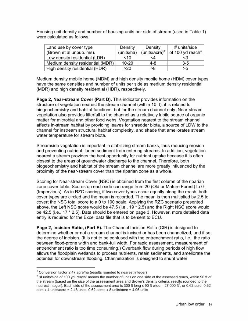
Housing unit density and number of housing units per side of stream (used in Table 1) were calculated as follows:

Land use by cover type (Brown et al unpub. ms).

Density (units/ha)

Density (units/acre)3

# units/side of 100 yd reach4

Low density residential (LDR) <10 <4 <3 Medium density residential (MDR) 10-20 4-8 3-5 High density residential (HDR) >20 >8 >5

Medium density mobile home (MDM) and high density mobile home (HDM) cover types have the same densities and number of units per side as medium density residential (MDR) and high density residential (HDR), respectively.

Page 2, Near-stream Cover (Part D). This indicator provides information on the structure of vegetation nearest the stream channel (within 10 ft); it is related to biogeochemistry and habitat functions, but for the stream channel only. Near-stream vegetation also provides litterfall to the channel as a relatively labile source of organic matter for microbial and other food webs. Vegetation nearest to the stream channel affects in-stream habitat by providing leaves for shredder biota, a source of LDW to the channel for instream structural habitat complexity, and shade that ameliorates stream water temperature for stream biota.

Streamside vegetation is important in stabilizing stream banks, thus reducing erosion and preventing nutrient–laden sediment from entering streams. In addition, vegetation nearest a stream provides the best opportunity for nutrient uptake because it is often closest to the areas of groundwater discharge to the channel. Therefore, both biogeochemistry and habitat of the stream channel are more greatly influenced by the proximity of the near-stream cover than the riparian zone as a whole.

Scoring for Near-stream Cover (NSC) is obtained from the first column of the riparian zone cover table. Scores on each side can range from 20 (Old or Mature Forest) to 0 (Impervious). As in RZC scoring, if two cover types occur equally along the reach, both cover types are circled and the mean is recorded. The mean is then multiplied by 2.5 to covert the NSC total score to a 0 to 100 scale. Applying the RZC scenario presented above, the Left NSC score would be 47.5 (i.e., 19 * 2.5) and the Right NSC score would be 42.5 (i.e., 17 * 2.5). Data should be entered on page 3. However, more detailed data entry is required for the Excel data file that is to be sent to ECU.

Page 2, Incision Ratio, (Part E). The Channel Incision Ratio (CIR) is designed to determine whether or not a stream channel is incised or has been channelized, and if so, the degree of incision. (It is not to be confused with the entrenchment ratio, i.e., the ratio between flood-prone width and bank-full width. For rapid assessment, measurement of entrenchment ratio is too time consuming.) Overbank flow during periods of high flow allows the floodplain wetlands to process nutrients, retain sediments, and ameliorate the potential for downstream flooding. Channelization is designed to shunt water

3 Conversion factor 2.47 acre/ha (results rounded to nearest integer) 4 “# units/side of 100 yd. reach” means the number of units on one side of the assessed reach, within 90 ft of the stream (based on the size of the assessment area and Brown’s density criteria; results rounded to the nearest integer). Each side of the assessment area is 300 ft long x 90 ft wide = 27,000 ft2, or 0.62 acre; 0.62 acre x 4 units/acre = 2.48 units; 0.62 acres x 8 units/acre = 4.96 units

Urban low order 9

downstream quickly and prevent contact with the floodplain, usually so the floodplain can be managed for alternative uses. However, channelization shunts excess nutrients directly to downstream rivers and estuaries, leading to eutrophication.

The figure below the CIR boxes illustrates where bank height and bankfull measurements should be made. Since we have few data on CIR for urban streams, we would like CIR measurements made for all urban streams. The CIR measurements could help us better calibrate SRC #3 (p. 4) using data for urban streams. All measurements should be made in stream reaches that flow or would flow during flow periods (do not attempt to measure in pools).

Measurements (see diagram) should be taken in places where there are good bankfull indicators present. The thalweg is the lowest point in the channel (stream bottom) at a given point along a reach. Bank height is the vertical distance from the thalweg to the top of the lowest bank near the identified thalweg. This is where water would flow from the channel to enter the floodplain during flood conditions. Bankfull height is the vertical distance from the thalweg to indicators of normal full streamflow. Indicators include places along the streambank below which rooted vegetation does not grow or where the stream has cut into the bank. CIR is difficult to measure in channelized streams for two reasons: (1) channelized streams without a forest canopy often are covered with dense herbaceous vegetation making if difficult to see indicators of stream flow and (2) channelization fundamentally alters the relationship between channel morphology and those fluvial processes that create indicators of bankfull flow. Data collected on urban streams will be helpful in calibrating future version of the assessment.

Page 3, Summary. This page provides blocks in which data from pages 2, 4, and 5 should be entered. Every block should be filled in.

Pages 4 and 5, Stream and Riparian Condition (SRC) scores (Part F). The seven indicators in this section are scored to determine the condition of the stream channel and its riparian zone. Scores should be entered on page 3.

Stream and Riparian Condition (SRC) scores, along with RZC and NSC scores, can be used to estimate degree of functioning. Each column describes four discrete categories of conditions from relatively unaltered to severely altered. Each condition indicator can be further assigned a condition from high to low within a category. Verbiage in brackets ([ ]) provide some guidance on scoring.

Each stream riparian condition indicator is related to slightly different aspects of the three categories of function: hydrology, biogeochemistry, and habitat. Some are related only to stream channel condition, some only to riparian zone condition, and some to both. A general outline of the rationale for the seven indicators is provided below. These indicators are used in conjunction with RZC and NSC scores to estimate condition based on degree of functioning relative to unaltered reaches.

1. Instream woody structure. This indicator is related to all three functions, but for channel condition only. Wood in the stream channel affects hydrology by creating pool and riffle sequences that dissipate energy of flowing water and stores water in pools during low flows. In small, unincised streams, live tree roots may play this role. Woody structure affects biogeochemistry by providing a surface for microbial activity and a potential source of

Urban low order 10

dissolved organic carbon (DOC), which is released into the water slowly over time. DOC can be used as an energy source for denitrification and other microbial processes. Instream wood also provides structural habitat complexity for epifauna and epiphytes. In larger streams, fish and invertebrates may use woody structure for resting during high flows and for hiding (shelter). 2. Sediment regime. This indicator is related only to the biogeochemistry of free-flowing stream channels and can not be used to assess channels that have been backed up by an impoundment. In such cases, indicators either fail to develop adequately or are not readily observed. Sediments, particularly those generated from impervious surfaces, carry phosphorus, heavy metals, and other pollutants that are bound to suspended sediments. Excessive sediment deposition may come from a variety of lateral sources and may also indicate erosion problems within reaches and channels above reaches. Excessive sediment supply blocks channel flow and fills pools that would otherwise provide aquatic habitat. Sediments influence channel biogeochemistry by acting as a carrier of sediment-bound phosphorus, the major mechanism by which phosphorus (and heavy metals) are transport by fluvial systems. Phosphorus enrichment may change the N/P ratio of the stream and enrichment with heavy metals may harm intolerant aquatic biota. Stream channel habitat is normally compromised when excess sediments lower water transparency, suppress primary production of epiphytic algae, and bury the habitat of benthic and epiphytic organisms. Often, channels of channelized streams begin to fill over time, especially those in urbanizing areas that are subject to erosional problems upstream. The filling may seem to indicate that the channel is restoring its morphology, but excess sedimentation will still continue to cause problems for biota if not prevented. 3. Channel-riparian zone connection. This indicator, based on the degree to which a free-flowing stream channel is incised, is related to all functions for both stream channels and riparian zones. (The indicator can not be used to assess channels that have been backed up by an impoundment. In such cases, indicators either fail to develop adequately or are not readily observed.) The indicator’s application to all functions reflects the fact that the connection between channel and riparian zone is fundamental to the characteristic functioning of riparian ecosystems. The degree of channel incision determines the degree to which functioning is impaired in both the stream channel and riparian zone. Channelized streams and channels incised by high flow velocities affect hydrology by transporting water more rapidly through the system during high flows and by increasing the groundwater slope toward the channel during low flows. Both alterations reduce the residence time of water in the system by increasing water flows and reducing storage. The steeper water table slope reduces the soil water storage within the riparian zone, thus requiring greater amounts of water to achieve normal conditions of surface and near-surface saturation of the soil. Greater channel capacity, compared to normal channels, requires greater flow volumes to reach overbank flow stage. This can greatly reduce or eliminate the duration and frequency of flooding, the major mechanism by which a channel and its riparian zone are hydrologically connected. This in turn affects biogeochemistry in at least two ways: the lowered water table

Urban low order 11

may eliminate contact of surficial groundwater with the organic rich surface horizons of the soil, thus reducing the potential for denitrification in both the channel and riparian zone. A lowered water table also exposes the soil column to greater aeration, thus suppressing anaerobic processes that are common in floodplains and riparian zones. For biogeochemical processes as a whole, the system becomes more oxidized thus reducing the capacity to accumulate organic matter needed to support denitrification. Hydrologic alterations caused by channelization or incision also adversely affect habitat for aquatic and wetland-dependent species. In the riparian zone, hydrophytes are less likely to occur. Within the stream, greater flow velocities, especially during storm flows, increase suspended sediment concentrations through re-suspension and scour, thus degrading habitat. 4. On/off site factors affecting the stream. This indicator is related to all three functions, but for channel condition only. Pollutant source for assessment purposes is herein defined as drains from streets and detention ponds, roadside ditches, channelized tributaries, and drainage from impervious surfaces. Pollutant sources affect hydrology by contributing excess water to stream channels. Higher and flashier flows may lead to additional channel incision and headward erosion. Pollution sources, by definition, contribute excess nutrients (primarily nitrogen and phosphorus) and/or toxic pollutants to stream channels, thus interfering with normal biogeochemical cycling. Habitat is also adversely affected by nutrient or chemical additions. Excess nutrients in the presence of sufficient sunlight can create algal accumulations that may lead to anoxia. Toxic chemicals can directly poison stream organisms. Pollution affects streams both by transport from upstream and by directly entering a reach. We assume that pollution entering within the reach is generally more detrimental than pollution entering upstream from a reach, with degree of alteration a function of distance upstream, type of source, and opportunities for amelioration. Stormwater detention ponds are meant to moderate peak flows from impervious surfaces and trap sediment and toxic chemicals and so some pollutant sources may be disregarded if a detention pond occurs between the sources of pollution and the assessed reach. However, in some cases storm detention basins are improperly planned, designed, constructed, or maintained, thus rendering them ineffective in moderating flows and/or trapping sediments and pollutants. Therefore, where detention basins occur within 500 yd above an assessed reach (along a contributing tributary), the detention pond(s) should be examined to determine if they are properly designed or managed. If the detention basins are determined to be ineffective, then they should be treated as a source of pollution rather than as a sink (trap). Storm water treatment systems are often sophisticated engineered systems. While there are criteria to determine whether they have been properly designed and constructed, and whether they are being properly operated, they are beyond the

Urban low order 12

scope of this assessment method. The reader is referred to EPA regulatory5 and non-regulatory6 information, NC Division of Water Quality guidelines and regulations7, and the Center for Watershed Protection8 for further information. Beaver impoundments also trap sediment and increase the residence time of water, thus allowing time for nutrient processing and removal. Therefore, some pollutant sources may be disregarded if a beaver impoundment occurs between the sources of pollution and the assessed reach. However, more egregious pollution inputs such as toxic chemicals, leaking sewer lines, and industrial waste are expected to alter streams even if partially processed through a beaver impoundment before entering a reach.

5. On/off site factors affecting riparian zone of assessed reach. This indicator is related to all three functions, but for riparian zone condition only. The rationale is the same as provided above for stream channels. The difference is that sources of degradation are limited to those within or directly adjacent to a reach. (It is assumed that alterations to upstream riparian zones do not directly affect the riparian zone of the assessed reach or that such alterations are taken into account with SRC #4). Likewise, filling, grading, excavation, and activities in non-forest land uses are included as alterations to the riparian zone, but not to channels directly. Variations in scoring of factors affecting riparian condition reflect the degree to which they are believed to alter condition. For example, discharges to the riparian zone from septic or sewer systems are considered potentially more detrimental than intensively managed lawns. Channelization drains adjacent floodplains and increases the capacity of the channel to convey water. This typically eliminates overbank flow onto the floodplain, thus

5 for US EPA stormwater regulatory information see http://www.epa.gov/ebtpages/watestormwater.html; federal stormwater regulations and requirements are included in NPDES regulations 40 CFR Part 122; portions of other regulations are also relevant (see EPA web page for more detail); EPA publishes numerous documents related to stormwater management, including a series of Stormwater Technology Fact Sheets (eg, Wet detention ponds EPA 832-F-99-048, Vegetated swales EPA 832-F-99-027, Stormwater wetlands EPA 832-F-02-020, Bioretention EPA 832-F-99-012, etc.) 6 US EPA Office of Research and Development’s Urban Watershed Management Branch provides non-regulatory information about urban stormwater risks and management (see http://www.epa.gov/ednnrmrl); EPA ORD UWMB publishes numerous documents, journal articles and books related to urban stormwater; a CD compilation of UWMB reports is available from this web page; also available is an electronic copy of Burton, G. Allen, Jr. and Robert E. Pitt. 2001. Stormwater effects manual: A toolbox for watershed managers, scientists and engineers. Lewis Publishers (CRC Press), Boca Raton, FL, USA. 7 see NC DWQ stormwater permitting units web page (http://h2o.enr.state.nc.us/su/stormwater.html); pertinent documents include: NC DENR. 1999. Stormwater best management practices.; state stormwater management program (SSWMP) supplement sheets; stormwater management regulations 15A NCAC 2H .0100 (especially 2H .1008 “Design of stormwater management measures”); and stormwater fact sheets prepared by the Land-of-Sky Regional Council 8 see Center for Watershed Protection web page (http://www.cwp.org); CWP has recently released the Urban Subwatershed Restoration Manual series, an 11-part series of manuals written for a broad audience including planners, engineers and consultants (Schueler, Tom. 2004. An integrated framework to restore small urban watersheds. Urban Subwatershed Restoration Manual No. 1. Center for Watershed Protection, Ellicott City, MD.

Urban low order 13

http://www.epa.gov/ebtpages/watestormwater.html

http://www.epa.gov/ednnrmrl

http://h2o.enr.state.nc.us/su/stormwater.html

http://www.cwp.org/

degrading the riparian zone. However, the loss in functioning of a former floodplain of a deeply channelized stream would be ameliorated somewhat if water that would otherwise bypass the former floodplain via ditches and culverts is instead diverted to a forested riparian zone. Forested riparian zones are capable of trapping sediment and removing nutrients before they reach the channel. Especially egregious pollutant inputs, such as toxic chemicals and sewage, would likely overwhelm the capacity of a forested riparian zone to remove them and are still treated as a severe alteration.

Beaver impoundments trap sediment and increase the residence time of water, thus allowing time to remove nitrate. Therefore, if a beaver impoundment occurs between pollutant sources and the assessed riparian zone, such pollutant sources may be disregarded. However, egregious pollutant inputs described in the "extremely altered" category would not be expected to be ameliorated much by a beaver impoundment. 6. Stream bank. This indicator is related to the biogeochemistry and habitat functions of free-flowing streams. (It cannot be used to assess channels backed up by impoundments. In such cases, indicators either fail to develop adequately or are not readily observed.) As stream discharge increases, hydraulic energy is first dissipated along stream banks and on LDW and roots residing in the channel. Some of this energy results in bank erosion, exposes roots, and causes bank slumping and tree fall, when excessive. If the stream channel is not incised, even higher flows associated with overbank flow transfer total stream energy to the floodplain where it is dissipated without erosion over a large surface area, thus protecting the channel itself from excessive scouring. While some bank erosion and sediment redistribution are natural processes, they are minor in low gradient headwater streams in the coastal plain. Alteration of riparian condition is assumed if erosion, slumping, and undercutting are excessive (outside the range of unaltered reference reaches) and herbaceous vegetation is unable to re-establish on banks after extreme events. Alterations in bank stability lead to excessive introduction of sediment to the channel waters and ultimately to downstream ecosystems.

7. Composition and structure of vegetation in riparian zone. This indicator is related to the habitat functions of riparian zones. Vegetation composition (evaluated relative to native forest) is a direct measure of plant habitat, which in turn affects animal habitat. It is assumed that mature to old forests represent the least altered condition that is conducive to supporting native communities. Footnote #3 in the field data sheet (p. 5) provides a list of canopy species characteristic of native forests. If at least 4 of the listed species are present in the canopy and the understory is intact with minimal cover of invasive species (Table 1), then the composition and structure of the forest should be relatively unaltered. In cases where low-order streams originate on large valley slopes, native forest species may consist principally of upland species due to well-drained conditions in the riparian zone.

Urban low order 14

Treesnone to rare





Table 2. Invasive, non-native species sometimes found in low order riparian ecosystems.

1 Invasivity of this species is uncommon in riparian ecosystems, but sometimes occurs. Appendix

i The rural-urban threshold housing density (2.37 units/acre) is the mean of the lowest density urban zoning classification for Greenville, NC (R-15S, 3 units/acre) and the rural residential zoning classification for Pitt County, NC (minimum lot size 25,000 ft2, which equals 0.57 acre or 1.74 units/acre). ii Based on the rural-urban threshold housing density (2.37 units/acre) and the size of the assessment area (300 ft x 90 ft = 54,000 ft2, or 1.24 acre; 1.24 acre x 2.37 units/acre = 2.94 units, or ~3 units within the riparian zone of the assessment reach). iii Conversion factor 2.47 acre/ha (results rounded to nearest integer) iv “# units/side of 300 ft. reach” means the number of units on one side of the assessed reach, within 90 ft of the stream (based on the size of the assessment area and Brown’s density criteria; results rounded to the nearest integer). Each side of the assessment area is 300 ft long x 90 ft wide = 27,000 ft2, or 0.62 acre; 0.62 acre x 4 units/acre = 2.48 units; 0.62 acres x 8 units/acre = 4.96 units

Urban low order 15

Office and field criteria for differentiating urban from rural reaches This guidance is used to determine which protocol should be used to assess a randomly assigned reach. Presence of any one indicator below is sufficient for confirming urban status (either in the office or in the field). Office Determinations (made using USGS 7.5 minute series topographic maps and USGS digital orthophoto quarter quads or higher resolution orthogonalized aerial photographs)

1) >10% impervious surface within a circle centered on random point (low order 200 yd radius; high order 500 yd (1,500 ft) radius; see template of aerial photographs, in Appendix).

2) Area denoted as urban on USGS topo (brown, purple, or pink color). 3) Housing density >2.37 units/acre (for low order, >62 units in 200 yd radius circle;

for high order >384 units in 500 yd (1,500 ft) radius circle). (Units are dwelling units: single family home = 1 unit, duplex = 2 units, each apartment within a complex = 1 unit.)


1) Stormwater treatment unit (wet or dry detention/retention, or infiltration basin,

etc.) is located in assessment reach or upstream (low order within 200 yd (600 ft); high order within 500 yd) or within watershed.

2) Stormwater input to stream or floodplain from urban stormwater sources, such as curb-and-gutter street or parking lot, is located in assessment reach or upstream (low order within 200 yd; high order within 500 yd). Here, "stormwater input" does not refer to road ditches or grassed swales. (Grassed swales and ditches in agricultural settings indicate that the rural riparian assessments should be used.)

3) Sewer line right-of-way is in riparian zone within 50 ft of stream channel. 4) Three or more dwelling units are located within 90 ft of the stream (either side)

along 100 yd (300 ft) assessment reach.


Urban Low Order Riparian Assessment, V 1.1

Site # Date

Watershed Field CrewLongitudeLatitude If reach rejected, explain why

Reach moved upstream or downstream ( ) yards due to impoundment in <50% of reach due to beaver ( ),


Reach downgradient from at least one street crossing, stormwater outfall, or roadside ditch w/out a detention basin.


Only the channel is backed up by downstream impoundment; the riparian zone is not inundated, except after a heavy rainfall event. If so, conduct assessment, but do not assess SRC #2, #3, and #6 (pp. 4 & 5).



Unincised, free-flowing stream with large downed wood (LDW) and/or litter and tree roots in channel.

Unincised, free-flowing stream with little or no LDW, litter, and tree roots in channel.

Channelized or incised stream with trees growing in and along channel and LDW or leaf litter in channel.

Channelized or incised stream with trees growing in and along channel, but lacking much LDW or leaf litter in channel.

Channelized or incised stream with mostly shrubs and/or herbaceous vegetation growing in and along channel; few or no trees.

Stream channel rip-rapped, bulkheaded, or lined with concrete bottom.

Stream partially or entirely culverted.

LEFT RIGHT



Notes on 90-300 ft

Notes on 90 - 300 ft

Provide North arrow

Reach Sketch Reach is 100 yd (300 ft) in upstream-downstream direction by 60 yd (180 ft) wide. Each square is 10 x 10 yd (30 x 30 ft). Identify and label cover types to 90 ft using abbrevations in Part C. Portray stream as straight. Add stream flow arrow and north arrow.

other impoundment type ( ), or overlap of previous reach ( ). Enter 1 for yes, 0 for no in box, enter distance moved, and check reason.

downstream

upstream

+

50 ft

50 ft

10 ft

10 ft

90 ft

90 ft

1



0-10 ft 10-50 ft 50-90 ft 0-10 ft 10-50 ft 50-90 ft









Annual crop agriculture (AC) 14 17 3 14 17 3Low density residential, single family (no more than 2 houses per one side of 100 yd reach within 90 ft of channel); minimally managed lawns (LDR) 15 3 15 3

Intensely managed lawns, golf course, recreation field, etc. (IML) 9 11 2 9 11 2Medium density residential, single family (3 to 5 houses per one side of 100 ydreach within 90 ft of channel) (MDR) 7 1 7 1

High density residential, single family (more than 5 houses per one side of 100yd reach within 90 ft of channel) (HDR) 7 1 7 1Medium density mobile home (3-5 units per one side of 100 yd reach within90 ft of channel) (MDM) 6 1 6 1High density mobile home (more than 5 units per one side of 100 yd reachwithin 90 ft of channel) (HDM) 5 1 5 1

High density building, multi-unit: strip mall, commercial mall, condos, manufacturing, motels, institutions, etc. (HDB) 0 0 0 0


Zone Score (column)


LEFT NSC Score RIGHT NSC Score

Calculation of Incision Ratio (from 3 locations)Indicator obvious? 1 2 3 Mean

a. Bank height (distance from thalweg to top of bank)

b. Bankfull height (thalweg to top of point bar or other indicator of near-annual flow)

CIR: Channel Incision Ratio (bank height/bankfull height)

Circle one number in each column for each side that describes average cover types for each zone along a 100-yd (300 ft) reach. If a zone is equally represented by two cover types, circle both types and enter the mean of the two in each "zone score" column. If three or more cover types occur, either weight scores by proportion or choose two cover types to represent total cover. Use abbreviations below on sketch map, p. 1. For forest that has been selectively cut or high graded, record as Young Forest. Where shaded types are excluded from 0-10-ft zone, other cover types must be chosen. The sum of column scores should be put in the LEFT and RIGHT Riparian Zone Cover (RZC) boxes and then transferred to page 3.

Near-stream Cover score is obtained from 0-10 ft "Zone score" box, multiplied by 2.5 (to convert score to a 0-100 scale). Transfer scores to page 3.

These measurements are recommended if channel seems incised, but there are no clear indicators of overbank flooding (wrack lines, etc.) and no indicators of channelization (spoil berms). (CIR measurements could help determine how to score SRC #3 (p. 4) between 60 and 90.) Take measurements (see diagram) in places where there are good bankfull indicators present. If spoil berm from channelization is present, define lowest points along berm as top of bank when measuring for CIR. If there is no defined channel, then CIR = 1.0.

Site # Watershed___________________ Field Crew__________________ Date _______




RIGHT RZC (total):

E. Channel Incision Ratio

LEFT RZC (total):

Bankfull height

Bank height

2

Urban Low Order Riparian Assessment, V. 1.1


Reach moved upstream or downstream due to beaver or other type of impoundment in <50% of reach.


LEFT (from "LEFT RZC total" score)

RIGHT (from "RIGHT RZC total" score)

D. Near-stream Cover, p. 2 (from 0-10 ft "zone score" column multiplied by 2.5 to convert to a 0-100 scale)

LEFT (from "Left NSC" score)

RIGHT (from "Right NSC" score)

E. Channel Incision Ratio (p. 2), if measured

CIR

F. Stream and Riparian Condition (SRC) scores (pp. 4 & 5)

1. Instream woody material

Appropriate sub-conditions a-d.

2. Sediment regime (If channel is backed up by beaver, enter "Bv")


3. (LEFT) Channel-riparian zone connection (If channel is backed up by beaver, enter "Bv")


3. (RIGHT) Channel-riparian zone connection (If channel is backed up by beaver, enter "Bv")




5. (LEFT) Factors affecting riparian zone within reach


5. (RIGHT) Factors affecting riparian zone within reach


6. (LEFT) Stream bank stability (If channel is backed up by beaver, enter "Bv")


6. (RIGHT) Stream bank stability (If channel is backed up by beaver, enter "Bv")


7. (LEFT) Habitat quality of riparian zone


7. (RIGHT) Habitat quality of riparian zone


Notes:

3


Relatively Unaltered1. Instream woody material

Much LDW in channel and along banks. (Recent treefalls from extreme weather events or erosion not applicable.) (a) LDW in channel and along banks represents a mix of sizes >4 inch dia. Some LDW > 8 inch dia.(b) LDW represents a mix of decay classes1. BUT (c) For stream channels that are dry for long periods, tree roots with hypertrophied lenticels are located in stream bottom(d) Large (>1 inch) tree roots in channel create small pools that trap leaf litter, when available.

Score = 100 90

2. Sediment regime3, 4

Water runs fairly clear even during periods of high flow. (If originating in flats, water is may be dark (tea colored) due to tannins.)(a) Stream is not channelized. (b) Channel bottom is mostly sandy or clayey with little or no silt on channel bottom or on floodplain.[If sand deposition in channel bottom is due to upstream activities, then see "severely altered" category.]

Score = 100 90

3. Channel-riparian zone connection 4

Strong evidence of overbank flow on floodplain.(a) No apparent channelization or incision. (b) Wrack, sediment, and/or trash on floodplain. [Sparse wrack scores 45.](c) High water marks on trees apparent.(d) No spoil berm alongside channel.

Score (L) = Left Bank: 50 45 Score (R) = Right Bank: 50 45


No on-site or off-site pollution5 affecting stream. (a) There is no pollution entering directly into the stream within the reach or within 200 yd (600 ft) upstream from reach. (b) All stormwater detention basins and ponds within 200 yd, if present, are adequately designed and maintained to reduce peak flows and trap sediment and nutrients. [Condition scores 90.](c) Stream is not channelized.

Score = 100 90

5 See page 5, footnote 1, for definition of pollution.

40 35 3025 20 15 40 35 30 10 5 025 20 15 10 5 0

No LDW in channel(a) Stream is channelized or deply incised and periodically cleared of debris to maintain drainage.(b) No large trees (>4 inch dbh) grow along channel banks.(c) Stream is lined with rocks, rip-rap or concrete.[Lowest score should be given to trapezoidal channels with concrete bottoms.]

80 70 60 50 40 30 20 10 0

Some LDW in channel 2 and along banks.(a) LDW in channel and along banks represents a variety of decay classes.(b) Few or no LDW >8 inch dia. [If large >4 inch dbh trees grow along both banks, score 80, if only along one side, score 70, if streamside trees are <4-inch dbh, score 60.] (c) For streams channels that are dry for long periods, tree roots located in stream bottom lack hypertrophied lenticels(d) Large (>1 inch) tree roots in channel are elevated above channel bottom due to undercutting.

LDW in channel and on banks deposited only during a recent storm.(a) LDW represents only one decay class1. (b) For channelized or deeply incised stream channels that are dry for long periods, channel is maintained so infrequently that small trees or shrubs grow along channel banks. [If large >4 inch dbh trees grow along both banks, score 50, if only along one side, score 40, if streamside trees are <4-inch dbh, score 30.]

F. Stream and Riparian Condition. For each Condition Indicator, record on page 3 the Condition Category score and one or more letters (a-d) that apply. (If a condition is encountered that is not provided, choose a score, and explain alteration and rationale for scoring in notes on p. 3.) Verbiage in brackets ([ ]) provides guidance on scoring.

Condition Indicator


Only off-site pollution5 affecting stream.(a) Pollution feeds directly into stream channel within 200 yd (600 ft) upstream from reach (not within reach).(b) Water from inadequately designed or maintained detention basin enters stream within 200 yd (600 ft) above reach.[More sources or more proximate pollution sources should be scored lower.]

On-site pollution5 affects stream.(a) Pollution from stormwater directly enters stream reach. (b) Water from inadequately designed or maintained detention basin directly empties into reach.(c) Overland-flow from impervious surfaces directly enters reach.(d) Stream culverted for 5-20% of length.[Presence of several pollution sources should be scored lower than fewer sources.]

4 Do not assess SRC #2, #3, and #6 if stream is backed up by downstream beaver impoundment. Assess relic beaver impoundments.

3 Sediment layer of relic beaver impoundments may be deep at upstream end of unmaintained impoundment and reduced in depth closer to former dam site.

80 70 60 50 40 30 20 10 01 Decay classes: (1) bark intact, leaves attached, no evidence of decay, (2) loose bark, no leaves, (3) peeling bark, fungi present, (4) advanced stages of decay, no bark or soft enough for a prod to be easily poked through, and (5) bole decayed into ground. 2 If little or no LDW occurs within channel, check banks for sawed-off pieces in floodplain, which indicates de-snagging. LDW from severe bank erosion not applicable.

Especially egregious pollution or culverting affects stream.(a) Sediment input from construction activities entering channel directly.(b) >20% of reach passes through underground culvert. (c) Evidence of sewer line leaking into stream (note evidence).(d) Hydrocarbons or other toxic chemicals leaking directly into stream (note evidence).

Evidence of occasional overbank flow on floodplain.(a) Some wrack, sediment, trash on floodplain, but sparse and/or old.(b) Stream channelized within historic channel with low spoil berms or breaks in them along channel. (Channel may have been channelized in past, but is filled with sediments to such a degree that overbank flow now occurs.) (c) Channel slightly channelized or incised.

Evidence of overbank flow only after extreme (rare) flood events.(a) No or little wrack on floodplain.(b) Channelization (i.e., spoil berms present and high).(c) Channel deeply incised (not channelized).

Silt and sand carried by stream.(a) Water is silt laden, esp. after heavy rains.(b) Thick (1-2 inches) silt or sand deposited on channel bars, bank edge, or on floodplain (if present).(c) For streams that are dry for long periods, sand or silt may collect behind root dams and be deposited on floodplain (if stream not channelized or incised).

(Heavy sediment load carried by stream. (a) Sediment suspended in water even during low flow. (b) Thick (>2 inch) sand or silt layers recently deposited on channel bars, bank edge, or on floodplain (if present).(c) Evidence that sand or silt deposits in reach are being generated by upstream activities. [Sand or silt on an artificial stone bottom scores lowest.]

20 10 0 80 70 60 50 40 30

Some silt carried by stream. (a) At high flows, suspended sediment evident in water.(b) When water runs clear during base flow, sediment can be re-suspended by shuffling feet in channel.(c) Thin layer (<1 inch thick) of silt deposited on channel bars or on floodplain surface. [Thickest deposits score lower.](d) Sediment >1 inch thick due to recent abandonment of impoundment4.

Overbank flow eliminated.(a) Deep channelization with spoil berms present.(b) Deeply incised (not channelized).(c) Filling and/or leveling of floodplain, some or all of fill may have been derived from spoil from channelization.(d) Presence of high artificial levee or other channel-containment structure.

4

Urban Low Order Riparian Assessment, V 1.1F. Stream and Riparian Condition (cont.)

Relatively Unaltered5. Factors affecting riparian zone within reach(0-50 ft zone)

No factors affecting riparian zone condition within reach. (a) Stream is not channelized and no pollution1 empties into riparian zone. (b) All stormwater detention basins and ponds, if present, are adequately designed and maintained to reduce peak flows and trap sediment and nutrients.[Presence of clippings or organic waste in floodplain scores 45.]


6. Stream bank stability2

Stream bank relatively stable.(a) Evidence of erosion or bank failure absent or minimal (<10%) of length. (b) Streamside vegetation tightly binds soil along banks, although exposed roots may occur at cut banks of stream channel. [Slight erosion or bank undercutting scores 45.]


7. Habitat quality of riparian zone(0-50 ft)

Habitat quality intact.Riparian zone dominated by old or mature native forest (>95% of area) with all strata3 intact. No or low cover of exotic or invasive species. No grazing, mowing, or selective harvesting within riparian zone. [Old or Mature forest (>50 yr. old) scores 50; slightly younger forest scores 45. Exotics in 5-25% in any stratum scores 45.]


3 Intact strata include canopy, midstory, understory, and herb layers. Strata need not be dense to be intact, but no evidence of clearing, grazing, selective harvesting, etc. allowed. Canopy must be comprised of trees >6 inch dbh, including at least 4 of the following species: tulip poplar, red maple, sweetgum, blackgum, elm, oak, loblolly pine, and sweetbay. Forest cover could be linearly arranged along channel or in blocks scattered within the riparian zone.

2 Do not assess SRC #2, #3, and #6 if stream is backed up by downstream beaver impoundment. Assess relic beaver impoundments. For relic impoundments, sediment layer may be deep at upstream end of unmaintained impoundment and reduced in depth closer to former dam site.

Condition Indicator


Factors somewhat affecting riparian zone.(a) Stream is not channelized and water from properly designed and maintained detention facilities emptiesinto riparian zone.(b) Stream is channelized and drainage or stormwater is discharged (or diverted) to riparian zone where it is detained and processed before entering stream.

10 5 0

Especially egregious factors affecting riparian zone.(a) Stream is deeply channelized.(b) More than 25% of riparian zone of reach graded, filled, cultivated, or covered with impervious surface. (c) Septic or sewer system leaking into riparian zone.(d) Hydrocarbons or other toxic chemicals leaking into riparian zone.[Lack of forest in riparian zone scores lower.]

1 Pollution includes runoff from roadside ditches, stormwater drainage, leakage from septic drainfields, runoff from intensely managed lawns or kennels, direct drainage from impervious surfaces including roof tops, and discharge from inadequate detention facilities. Note, beaver impoundments and adequately designed and maintained detention basins largely negate the effects of most pollution, except those described in the "severely altered" category. Therefore, other upstream pollutant sources may be disregarded if an impoundment or properly operating detention basin occurs between the pollutant source(s) and the assessed reach.

10 5 0

Factors affecting riparian zone.(a) Stream not channelized and pollution1 enters directly into riparian zone of reach.(b) Stream is channelized, but no stormwater is diverted to riparian zone.(c) 5-25% of riparian zone (0-50 ft) of reach filled, graded, cultivated, or covered with impervious surface. (d) Combined sewer and storm drain system occurs within riparian zone.[Presence of more categories or greater intensities score lower.]

40 35 30

Habitat quality somewhat degraded.(a) Forest (with all strata3 intact) covers 75-95% of riparian zone with remainder of area representing other cover types.OR (b) >95% forest canopy cover (all strata intact) with exotic or aggressive species (>25% cover) in at least one stratum.OR (c) >95% forest canopy cover with at least one stratum of native vegetation absent or not well represented due to understory removal, recent timber harvesting, or selective harvesting; succession not hindered.[Old or Mature forest (>50 yr. old) should be scored higher than youngerforests.]

40 35 30 25 20 15 25 20 15

Stream bank moderately stable.(a) 10-25% of bank eroded or slumping(b) If trees present along bank, a few large (>1 inch dia.) roots exposed.(c) Most eroded areas recovering.

Stream banks unstable.(a) 25-50% of bank eroded.(b) Erosion, slumping, and undercutting prevalent, especially along cutbanks.(c) If trees present along bank, many large (>1 inch in dia.) roots exposed with some trees toppled into stream due to undercutting.

Habitat quality extremely degraded.(a) Forest (with all strata3 intact) covers <50% of riparian zone with remainder of area representing othercover types. OR (b) 50-75% forest canopy cover (all strata intact) with exotic or aggressive species (>25% cover) in at least one stratum.OR (c) 50-75% forest canopy cover with at least one stratum of vegetation absent or not well represented.OR (d) 50-75% forest canopy cover with recent timber harvesting or selective harvesting evident within riparian zone, but succession is not hindered. [Old or Mature forest (>50 yr. old) covering more than 25% of riparian zone with <25% exotic cover should be scored 10; more than 1 combination above scores 5. Lack ofwoody vegetation scores 0.]

40 35 30 25 20 15 10 5 040 35 30 25 20 15 10 5 0

Habitat quality degraded.(a) Forest (with all strata3 intact) covers 50-75% of riparian zone with remainder of area representing other cover types.OR (b) 75-95% forest canopy cover (all strata intact) with exotic or aggressive species (>25% cover) in at least one stratum. OR (c) 75-95% forest canopy cover with at least one stratum of vegetation absent or not well represented.OR (d) 75-95% forest canopy cover with recent timber harvesting or selective harvesting evident, but succession is not hindered.[Old or Mature forest (>50 yr. old) should be scored higher than younger forests in all cases.]

Stream bank extremely unstable.(a) >50% of bank eroded(b) Erosion, slumping, and undercutting prevalent, esp. along cut banks.(c) If trees present along bank, many toppled into stream due to undercutting.(d) Banks hardened with rip-rap, rocks, gabions, concrete, or bulkheading.

25 20 15 25 20 15 40 35 30 10 5 0

10 5 040 35 30

5

Urban High Order Riparian Assessment Protocol, V. 1.0 Background This assessment manual is designed for assessing the condition of 3rd to 4th order riparian ecosystems that originate in the coastal plain of North Carolina, and are influenced by urban land uses. It was modified from the one developed for rural landscapes by adjusting indicators and thresholds to better represent reference sites occurring in urban environments. This assessment method was not designed for evaluating active beaver impoundments. However, it can be used to assess beaver-impounded reaches where only the channel has been backed up by a downstream impoundment. In this case the water does not inundate the adjacent floodplain except following heavy rainfall events. In such cases, Stream and Riparian Condition (SRC) indicators #2, #3, and #6 (pages 4 and 5) should not be assessed because channel features are underwater or channel processes have been modified. High order streams in the coastal plain include 3rd to 4th order intermittent and perennial streams. This assessment method is not appropriate for riparian ecosystems in other physiographic provinces, low order (1st – 2nd order) riparian systems, or larger river systems such as the Tar or Neuse Rivers. Although developed in coastal plain drainage basins in North Carolina, it would probably be applicable to some other coastal plain regions in the Southeast. High order riparian areas in the coastal plain include those with both intermittent and perennial flow. Intermittent streams tend to cease flow in late summer and early fall when evapotranspiration during the growing season has depressed water tables throughout their drainages, thus reducing surface flows from upstream tributaries and disconnecting the source of local groundwater discharge to the surface. Precipitation from tropical depressions, hurricanes, and convective storms can interrupt periods of low discharge. In comparison with low-order riparian ecosystems, those of unaltered 3rd and 4th order streams have larger floodplains and are wetter. In their unmodified condition, they receive proportionally more water from overbank flow during floods and receive groundwater discharge from larger aquifers than their low-order counterparts. Consequently, they support vegetation adapted to longer periods of saturation and flooding, such as bald cypress and water tupelo in the canopy and lizard’s tail and water willow in the ground layer. In urban locations where channelization has created spoil piles and drained floodplains, Chinese privet is often prevalent. Riparian ecosystems range in condition from relatively natural, un-channelized reaches buffered by forest to channelized reaches with bank and bed hardened with concrete or other artificial substrate. The presence of stormwater outfalls as a water source is one of the signature properties of higher order urban streams. This is partly a consequence of the conversion of low order streams to stormwater drainages that now feed directly to high order riparian floodplains and stream channels. Stormwater drainages may shunt runoff directly from impervious surfaces or from detention ponds. In either case, there is little opportunity for infiltration in the drainage basin. This results in higher peak flows and lower base flows than occurred prior to urbanization. Where the construction of storm detention basins is required, faulty design, construction, and maintenance can render them ineffective in

Urban high order 1

moderating peak flows and removing sediments, nutrients, and other pollutants. In urban areas there is a general pattern of truncated low-order drainages and channelization in the high order streams that remain. The purpose of all of these modifications is to transport water away from urban areas to reduce potential damages due to flooding. Consequently, the drainage network offers little opportunity for ameliorating water quality and reducing peak discharge. The additional hydraulic loading downstream can alter channel morphology. Therefore, riparian ecosystems in urban areas are highly degraded. Office and Field Methods The user should make a preliminary decision of whether to use the urban assessment described here, or the rural assessment. Criteria for determination should be used in the office and during the field visit. Office determinations should be verified in the field, especially in the periphery of urban areas where housing and other development activities can change in a matter of a few months. Below is a list of suggestions. If a reach is determined to be urban in the office, it is unlikely that the determination will be changed in the field. The converse is not as likely. Below is a list of office and field criteria for differentiating urban reaches from rural ones. This guidance is used to determine which protocol should be used to assess a randomly assigned reach. Presence of any one indicator below is sufficient for confirming urban status (either in the office or in the field). Office Determinations (made using USGS 7.5 minute series topographic maps and USGS digital orthophoto quarter quads or higher resolution orthogonalized aerial photographs)

1. >10% impervious surface within a circle centered on random point (low order 200 yd radius; high order 500 yd radius; see template of aerial photographs, in Appendix).

2. Area denoted as urban on USGS topo (brown, purple, or pink color). 3. Housing density >2.37 units/acre1 (for low order, >62 units in 200 yd radius circle;

for high order >384 units in 500 yd radius circle). (Units are dwelling units: single family home = 1 unit, duplex = 2 units, each apartment within a complex = 1 unit.)


1. Stormwater treatment unit (wet or dry detention/retention, or infiltration basin, etc.) is located in assessment reach or upstream (low order within 200 yd; high order within 500 yd) or within watershed.

2. Stormwater input to stream or floodplain from urban stormwater sources, such as curb-and-gutter street or parking lot, is located in assessment reach or upstream (low order within 200 yd; high order within 500 yd). Here, "stormwater input" does not refer to road ditches or grassed swales. (Grassed swales and ditches in agricultural settings indicate that the rural riparian assessments should be used.)

1 The rural-urban threshold housing density (2.37 units/acre) is the mean of the lowest density urban zoning classification for Greenville, NC (R-15S, 3 units/acre) and the rural residential zoning classification for Pitt County, NC (minimum lot size 25,000 ft2, which equals 0.57 acre or 1.74 units/acre).

Urban high order 2

3. Sewer line right-of-way is in riparian zone within 50 ft of stream channel. 4. Three or more dwelling units are located within 90 ft of the stream (either side)

along 100 yd assessment reach2. Scoring of land use cover types relies upon both field data and the literature. For the rural method, we used biomass as a basis for developing a scale to rank the condition of vegetation types. We modified this approach for urban riparian zones by adapting components of the Land Development Index developed for Florida (Brown et al., unpublished manuscript). The Florida index is based on embodied energy (also called “emergy”) analysis (Odum, HT and EC Odum 2001. A Prosperous Way Down. Univ. Press of Colorado, Boulder, CO) and incorporates total energy flow, corrected for quality, that occurs in a unit area of land use. Some of the land uses in Florida (e.g., orange groves, etc.) do not occur our study area. Others were adapted or combined based on our best judgment. For example, golf courses may include multiple cover types such intensively managed lawns and rooftops. When only portions of golf courses are present in an assessed riparian zone, alternative land uses were chosen, such as intensively managed lawn for golf greens. As yet, there are no data to validate these adaptations. However, we have conducted preliminary assessments in the field along a range of reference sites (relatively unaltered to severely altered) in developing the description of conditions for each of the indicators. We chose to set reference standard conditions for urban areas as high as those for rural areas (e.g., old and mature forest). However, the most degraded urban conditions are lower than those of rural areas. The net result expands the rural scale to include more degraded conditions commonly found in urban but not rural areas. This allows differentiation between varieties of urban land uses that are absent or rare in rural areas. After determining which field sheets to use (rural or urban), the following items should be used in the field: topographic maps (USGS 1:24,000), county soil surveys, and DOQQs (or equivalent high-resolution photography), a GPS unit, a shovel or trowel, a hand-held laser level, a stiff tape measure or meter stick, and a 30-100 yd tape. Guidelines for randomly assigned reaches Two sets of randomly chosen GPS coordinates are provided for each drainage basin: a set of primary data points and an alternate list of points. The primary list of GPS points identifies all reaches within a given drainage basin that should be assessed. The alternate list of points should be used if an assigned point should not or cannot be accessed or must be rejected for other reasons (see below for rejection criteria). If a given GPS point does not fall on a stream, it should be moved to the point on the stream that is the shortest distance from the assigned point. If the random GPS point marks an active beaver impoundment, where both channel and floodplain are inundated, then the reach should not be assessed; however, data boxes in Part A on page 1 of the field sheet should be completed and provided to ECU in the requested format. The GPS point should not be replaced by an alternate point.

2 Based on the rural-urban threshold housing density (2.37 units/acre) and the size of the assessment area (300 ft x 180 ft = 54,000 ft2, or 1.24 acre; 1.24 acre x 2.37 units/acre = 2.94 units, or ~3 units within the assessment area).

Urban high order 3

If a random point must be rejected because the stream no longer exists due to urbanization, the point should be replaced by the next random GPS coordinates provided by the alternate list of random points. The alternate list should be used if access is denied by a landowner or the point is inaccessible for some other reason. Note that the next random point obtained from the alternate list may prove not to be the same order as the one rejected; it could even be located in a rural drainage basin. That is okay. Substitute the new point for the rejected one. Substitutions should be made sequentially from the alternate list in the order in which they are provided, i.e., the point at the top of the alternate list is used first, then the second one down, etc. In all cases, you must record WHY the site was rejected. (Page 1, top, provides the check-off box for this.) It is especially important in urban areas to know that a point was rejected because the stream was eliminated by urban development activities. The following list provides rejection criteria that could be recorded. The GPS point marks a reach that is:

1) missing because urban development activities have led to the stream being converted to culverted flow

2) a field ditch 3) an ephemeral flow path 4) inaccessible due to the land owner denying permission 5) falls within a previously sampled 100-yd reach, but see “Relocating random

points” below 6) other (identify)

Impoundments in which both the channel and floodplain are inundated due to a dam are noted by in a check-off box in Part A on page 1, and no substitution is made from the alternate list. Relocating random points Random points that fall near (within 50 yd), but not in, beaver or other impoundments should be relocated up- or downstream a short distance so that the entire assessment reach is outside the impoundment. If such relocation places the random point in or near another impoundment such that some of the reach is now in the second impoundment, the randomly assigned reach should be treated as impounded. Similarly, random points that fall within 50 yd of a previously assessed reach should be relocated so that the assessment reaches do not overlap (random points that fall in a previously assessed reach should be rejected and replaced with an alternate point as described above). Random points that fall within 50 yd of the end of a stream should be relocated downstream far enough that the end of the assessment reach corresponds to the end of the stream. Random points that fall with 50 yd of the confluence of two streams should be relocated up- or downstream so that the entire assessment reach lies along the stream segment on which the random point falls. Data collection and observations on-site Page 1. This page is used to provide general information on the channel along the assessed reach and to sketch the major characteristics within its 180 (60 yd)-ft-wide riparian zone (90 feet on each side of stream). A reach may be either homogeneous or heterogeneous with respect to cover types, and may contain streets, buildings, and other structures within it.

Urban high order 4

, Upstream and Downstream Influences on Reach (Part A). This category provides information on whether the reach is hydrologically affected by an impoundment, by stormwater outfalls, or by streetside ditches. Beaver impoundments may show a stepwise pattern in which the upper end of one impoundment is adjacent to the dam of another impoundment upstream. If the riparian zone of more than half of the 100 yd reach length is impounded (i.e., the random point is <50 yd from an impoundment), treat the entire reach as impounded (see below). If less than half of the 100 yd reach of the riparian zone is impounded (i.e., the random point is 50-99 yd from an impoundment), move the center point upstream (or downstream if the dam is within the assessment reach) to where none of the riparian zone of the reach is impounded and continue. If an entire 100-yd reach cannot be found immediately upstream or downstream, treat the assigned reach as impounded. Next, record whether the reach was formerly and recently impounded by beaver, but has been abandoned (or dam removed). An abandoned beaver or man-made impoundment should be assessed as un-impounded. Standing, non-flowing water in the channel suggests that there is an impoundment downstream from reach. A channel can be affected by an impoundment without a dam occurring within the assessed reach and even if there is no impounded water in the riparian zone. (Note: even an impounded reach may begin to flow during high rainfall events). Record if the channel is backed up by an impoundment, but the adjacent riparian zone is not inundated by the impoundment. If so, then the site should be assessed, but SRC indicators #2, #3 and #6 (pages 4 & 5) should not be assessed. Instead, “Bv” should be recorded in the appropriate data boxes on page 3. Next, record if the both the channel and riparian zone of the reach are impounded by a beaver or man-made dam. The reach is considered impounded if more than half of the reach is impounded. If impounded, do not continue assessment beyond Part A. Page 1, General Channel Condition (Part B). Part of characterizing channel condition requires determining if the stream has been channelized or incised. Both tend to reduce or eliminate the frequency of overbank flow, thus preventing the riparian zone from processing nutrients. Incision is often caused by an increase in the volume of peak flows due to an increase in the area of impervious surfaces in the drainage basin. Channelization can usually be identified by the presence of spoil piles or berms along one or both sides of the channel, and by the level of the adjacent historic floodplain being positioned below that of the berm. Channel incision can be recognized by a deep channel (deeper than expected for the size of the drainage basin) that lacks adjacent spoil piles. In some 3rd - 4th order systems, the channel was constructed in the floodplain, away from the original channel, i.e., “off-channel.” In such cases, the original stream channel can still be found in the riparian zone, but it is much more narrow and shallow than the channelized section and it will usually have little or no water flow. Another factor in characterizing channel condition requires determining if there is large downed wood (LDW) in the stream channel. If there is none, search the stream banks for sawed-off pieces of logs in the floodplain. Sawed-off large wood indicates that LDW has been removed from the stream (“de-snagged”) to increase stream flow. Page 1, Site Sketch. The sketch provides a grid on which to map the relative area of cover types within 90 ft of each side of the stream and for less-detailed information or

Urban high order 5

notes about conditions from 90-300 ft (30-100 yd). Sixty 30 x 30 ft (10 x 10 yd) grids have been pre-drawn on the page to facilitate sketching a 90-ft riparian zone on each side of the stream channel. The sketch map is to be drawn facing downstream with the center of the reach positioned at the midpoint (+) in the center of the map. Marks are also provided to designate the 10 ft, 50 ft, and 90 ft riparian zones. Notes on the condition of the 90-300 ft (30-100 yd) zone should be made to the left and right of the grids. Care should be taken to observe if the floodplain extends beyond the 90 ft zone. The floodplain indicator condition, if it extends beyond 90 ft, is evaluated in the high order assessment only. Cover types should be marked with abbreviations provided in Part C, page 2, along with a north arrow. If a stream meanders or curves along the 100 yd reach, the sketch should be adjusted so that it is shown as straight. The meander can be drawn in the box located on the right side of the sketch map. Likewise, the channel cross-section can be drawn there as well. Estimates of width and depth may be noted for scale. Page 2, Riparian Zone Cover (Part C). The Riparian Zone Cover (RZC) score is used as one indicator in determining the condition of hydrologic and biogeochemical functioning of the riparian zone. It requires information on the general structure of vegetation and other land uses in zones adjacent to the stream channel. The structure of the riparian zone helps determine how effective it will be in maintaining and enhancing water quality. Vegetation, particularly forests, sequesters nutrients, ameliorates soil erosion, and provides habitat. Calibration within a column was based on data for live aboveground biomass and for detrital biomass (both soil organic matter and aboveground detritus) with differences among cover types related to variations in total biomass. Changes in scores decrease per unit zone width as one moves from the inner to outer riparian zone. This is consistent with the concept that near-stream buffer areas are more important to aquatic resources than areas further away. An assumption is made here that variations in total biomass and distance from stream channel together combine to affect hydrologic regime, biogeochemistry, and habitat quality. Both vertical and horizontal structural complexity is higher in forests than in other cover types, especially those associated with urban land uses. The 90 ft (30 yd) riparian zone outer boundary was chosen for RZC because the riparian zone would likely be influenced by surrounding forest that can generally reach 90-100 ft in height which in this region. Therefore, a 90-ft tree growing within the 90-ft riparian zone would have more than a 50% chance of falling into the riparian zone and could, depending on distance from stream and the direction it falls, be capable of contributing wood to the stream channel. The 50-ft inner zone was chosen to correspond with the NC buffer rules and the 10-ft zone was chosen to correspond to the zone that would most likely affect channel processes (see Part D, below). To evaluate riparian zone cover, the condition (rows) of each zone (columns) should be identified and circled. Because property boundaries often occur along streams, management activities may differ on each side of the stream. Therefore, riparian cover is assessed for each side separately, with a maximum score of 50 for each side and 100 for both sides. A score of 100 means that riparian zone cover is similar to relatively unaltered reference standard sites. If two cover types cover more or less the same area within a defined zone, then the mean of the two zone scores should be calculated. Otherwise, you could determine a weighted average. However, if three or more cover types are mapped within any one zone and two or more of the cover types are of the

Urban high order 6

medium density residential or a more intensely developed category, then choose the most prevalent development cover type for averaging with the less-intensely developed type. (This guidance is suggested because differences among lower scoring cover types are insignificant anyway.) An example of scoring is as follows (Table 1): if Young Forest occurs on the left side of the stream bank from the bank edge to 30 ft, Intensely Managed Lawns from 30-50 ft, and High Density Building Multi-unit extends from 50-90 ft, then 19 should be circled in column 1 (Young Forest), 24 (Young Forest) and 11 (Intensely Managed Lawn) in column 2, and 0 (High Density Building Multi-unit) should be circled in the last column. Each column should be summed and recorded as the “LEFT RZC (total)” or “RIGHT RZC (total)”. The total LEFT zone score would be 36.5 = 19 + ((24 + 11)/2) + 0, the sum of all zone score totals. If on the right side, Shrubs/Saplings occurred to 10 ft (17) and Low Density Residential from 10 – 90 ft (7 and 1, respectively), then the RIGHT zone total score would be 25. The scores for the left and right sides should be entered on page 3. The sum of zone scores for LEFT and RIGHT may be used to assign the total riparian zone cover score. Table 1. Calculation of the Riparian Zone Cover Index for Urban High Order. Total score for the reach is the sum of the left and right sides. Scores are circled.

0-10 ft 10-50 ft 50-90 ft 0-10 ft 10-50 ft 50-90 ft









Annual Rowcrop agriculture (AR) 14 17 3 14 17 3Low-density residential, single family (no more than 2 units per side of 100 yd reach within 90 ft of channel); minimally managed lawns (LDR)

12 15 3 12 15 3


Medium-density residential, single family (3-5 units per side of 100 yd reach within 90 ft of channel) (MDR)

6 7 1 6 7 1

High-density residential, single family (more than 5 units per side of 100 yd reach within 90 ft of channel) (HDR)

5 7 1 5 7 1

Medium-density mobile home (3-5 per units side of 100 yd reach within 90 ft of channel) (MDM) 5 6 1 5 6 1

High-density mobile home (more than 5 units per side of 100 yd reach within 90 ft of channel) (HDM) 4 5 1 4 5 1

High density building, multi-unit; strip mall, commercial mall, condos, manufacturing, motels, institutions, etc. (HDB) 0 0 0 0 0 0


Zone Score (column)





19 18.5 3 16 0 0

40.5 16

Urban high order 7

Housing unit density and number of housing units per side of stream (used in Table 1) were calculated as follows:

Land use by cover type (Brown et al unpub. ms).

Density (units/ha)

Density (units/acre)3

# units/side of 100 yd reach4

Low density residential (LDR) <10 <4 <3 Medium density residential (MDR) 10-20 4-8 3-5 High density residential (HDR) >20 >8 >5

Medium density mobile home (MDM) and high density mobile home (HDM) cover types have the same densities and number of units per side as medium density residential (MDR) and high density residential (HDR), respectively. Page 2, Near-stream Cover (Part D). This indicator provides information on the structure of vegetation nearest the stream channel (within 10 ft); it is related to biogeochemistry and habitat functions, but for the stream channel only. Near-stream vegetation also provides litterfall to the channel as a relatively labile source of organic matter for microbial and other food webs. Vegetation nearest to the stream channel affects in-stream habitat by providing leaves for shredder biota, a source of LDW to the channel for instream structural habitat complexity, and shade that ameliorates stream water temperature for stream biota. Streamside vegetation is important in stabilizing stream banks, thus reducing erosion and preventing nutrient–laden sediment from entering streams. In addition, vegetation nearest a stream provides the best opportunity for nutrient uptake because it is often closest to the areas of groundwater discharge to the channel. Therefore, both biogeochemistry and habitat of the stream channel are more greatly influenced by the proximity of the near-stream cover than the riparian zone as a whole. In 3rd – 4th order streams, streamside trees contribute LDW, leaves, and twigs to the channel.

Urban high order 8

Scoring for Near-stream Cover (NSC) is obtained from the first column of the riparian zone cover table. Scores on each side can range from 20 (Old Forest) to 0 (Impervious). As in RZC scoring, if two cover types occur equally along the reach, both cover types are circled and the mean is recorded. The mean is then multiplied by 2.5 to covert the NSC total score to a 0 to 100 scale. Applying the RZC scenario presented above, the Left NSC score would be 47.5 (i.e., 19 * 2.5) and the Right NSC score would be 40 (i.e., 16 * 2.5). Data should be entered on page 3. However, more detailed data entry is required for the Excel data file that is to be sent to ECU.

Page 3, Summary. This page provides blocks in which data from pages 2, 4, and 5 should be entered. Every block should be filled in. Pages 4 and 5, Stream and Riparian Condition (SRC) scores (Part E). The seven indicators in this section are scored to determine the condition of the stream channel and its riparian zone. Scores should be entered on page 3.

3 Conversion factor 2.47 acre/ha (results rounded to nearest integer) 4 “# units/side of 100 yd. reach” means the number of units on one side of the assessed reach, within 90 ft of the stream (based on the size of the assessment area and Brown’s density criteria; results rounded to the nearest integer). Each side of the assessment area is 300 ft long x 90 ft wide = 27,000 ft2, or 0.62 acre; 0.62 acre x 4 units/acre = 2.48 units; 0.62 acres x 8 units/acre = 4.96 units

Stream and Riparian Condition (SRC) scores, along with RZC and NSC scores, can be used to estimate condition based on the degree of functioning relative to unaltered reaches. Each column describes four discrete categories of conditions from relatively unaltered to severely altered. Each category can be further assigned a condition from high to low within a category. Verbiage in brackets ([ ]) provide some guidance on scoring. Each stream riparian condition indicator is related to slightly different aspects of the three categories of function: hydrology, biogeochemistry, and habitat. Some are related only to stream channel condition, some only to riparian zone condition, and some to both. A general outline of the rationale for the seven indicators is provided below. These indicators are used in conjunction with RZC and NSC scores to estimate condition based on the degree of functioning relative to unaltered reaches.

1. Instream woody structure. This indicator is related to all three functions, but for channel condition only. Wood in the stream channel affects hydrology by creating pool and riffle sequences that dissipate energy of flowing water and stores water in pools during drawdown. Biogeochemistry is affected by providing a surface for microbial activity and a potential source of dissolved organic carbon (DOC), which is released into the water slowly over time. DOC can be used as an energy source by denitrifying bacteria and the detritus food web. Instream wood also provides structural habitat complexity for epifauna and epiphytes. Fish and invertebrates may use woody structure for resting or hiding (shelter). 2. Sediment regime. This indicator is related only to the biogeochemistry of free-flowing stream channels and can not be used to assess channels that have been backed up by an impoundment. In such cases, indicators either fail to develop adequately or are not readily observed. Sediments, particularly those generated from impervious surfaces, carry phosphorus, heavy metals, and other pollutants that are bound to suspended sediments. Excessive sediment deposition may also indicate erosion problems within reaches and channels above reaches. Phosphorus enrichment may change the N/P ratio of the stream and heavy metals associated with sediments may harm intolerant aquatic biota. Stream channel habitat is normally compromised when excess sediments lower water transparency, suppress primary production of epiphytic algae, and bury the habitat of benthic and epiphytic organisms. Excessive sediments and pollutants are harmful to aquatic organisms. Often, channels of channelized streams begin to fill over time, especially those in urbanizing areas that are subject to erosional problems upstream. The filling may seem to indicate that the channel is restoring its morphology, but excess sedimentation will still continue to cause problems for biota if not prevented.

3. Channel-riparian zone connection. This indicator, based on the degree to which a free-flowing stream channel is incised, is related to all functions for both the stream channel and its adjacent riparian zone. (The indicator can not be used to assess channels that have been backed up by an impoundment. In such cases, indicators either fail to develop adequately or are not readily observed.) The indicator’s application to all functions

Urban high order 9

reflects the fact that the connection between channel and floodplain is fundamental to the functioning of higher order riparian ecosystems. The degree of channel incision determines the degree to which functioning is impaired in both the stream channel and floodplain. Channelized and incised channels affect hydrology by moving water more rapidly through the system during high flows and intersecting the water table during low flows, thus draining the floodplain and eliminating or reducing the duration and frequency of flooding and soil saturation. This in turn affects biogeochemistry in at least two ways: the lowered water table may eliminate contact of surficial groundwater with the organic rich surface horizons of the soil, thus reducing the potential for denitrification in both the channel and riparian zone. A lowered water table also exposes the soil column to greater aeration, thus suppressing anaerobic processes that are common in floodplains and riparian zones. For biogeochemical processes as a whole, the system becomes more oxidized thus reducing the capacity to accumulate organic matter. Hydrologic alterations caused by channelization or incision also adversely affect habitat for aquatic and wetland-dependent species. In the riparian zone, hydrophytes are less likely to occur. Within the stream, greater flow velocities, especially during storm flows, increase suspended sediment concentrations through re-suspension and scour, thus degrading habitat. Hydrologic alterations caused by channelization or incision also adversely affect habitat for aquatic and wetland-dependent species.

4. On/off site factors affecting the stream. This indicator is related to all three functions, but for channel condition only. Pollutant source for assessment purposes is herein defined as drains from streets and detention ponds, roadside ditches, channelized tributaries, and drainage from impervious surfaces. Pollutant sources affect hydrology by contributing excess water to stream channels. Higher and flashier flows may lead to additional channel incision. Pollution sources, by definition, contribute excess nutrients (primarily nitrogen and phosphorus) and/or toxic pollutants to stream channels, thus interfering with normal biogeochemical cycling. Habitat is also adversely affected by nutrient or chemical additions. Excess nutrients in the presence of sufficient sunlight can create algal accumulations that may lead to anoxia. Toxic chemicals can directly poison stream organisms. Pollution affects streams both by transport from upstream and by directly entering a reach. We assume that pollution entering within the reach is generally more detrimental than pollution entering upstream from a reach, with degree of alteration reflecting distance upstream, type of source, and opportunities for amelioration. Stormwater detention ponds are meant to moderate peak flows from impervious surfaces and trap sediment and toxic chemicals. Some pollutant sources may be disregarded if a detention pond occurs between the sources of pollution and the assessed reach. However, in some cases storm detention basins are improperly planned, designed, constructed, or maintained, thus rendering them ineffective in moderating flows and/or trapping sediments and pollutants. Therefore, where detention basins occur within 500 yd above an assessed reach (along a contributing tributary), the detention pond(s) should be examined to determine if they are properly

Urban high order 10

designed or managed. If the detention basins are determined to be ineffective, then they should be treated as a source of pollution rather than as a sink (trap). Storm water treatment systems are often sophisticated engineered systems. While there are criteria to determine whether they have been properly designed and constructed, and whether they are being properly operated, they are beyond the scope of this assessment method. The reader is referred to EPA regulatory5 and non-regulatory6 information, NC Division of Water Quality guidelines and regulations7, and the Center for Watershed Protection8 for further information. Beaver impoundments also trap sediment and increase the residence time of water, thus allowing time for nutrient processing and removal. Therefore, some pollutant sources may be disregarded if a beaver impoundment occurs between the sources of pollution and the assessed reach. However, more egregious pollution inputs such as toxic chemicals, leaking sewer lines, and industrial waste are expected to alter streams even if partially processed through a beaver impoundment before entering a reach.

5. On/off site factors affecting floodplain or former floodplain. This indicator is related to all three functions, but for riparian zone condition only. The rationale is the same as provided above for stream channels. The difference is that sources of degradation are limited to those that affect a reach. It is assumed that alterations to the main channel upstream do not affect the assessed reach although tributaries entering the main channel within the reach can have an effect. Also, channelization, filling, grading, excavation, and non-forest land uses are included as potential sources of alteration to the riparian zone but not the channel directly. Variations in scoring of factors affecting riparian condition reflect the degree to which

5 for US EPA stormwater regulatory information see http://www.epa.gov/ebtpages/watestormwater.html; federal stormwater regulations and requirements are included in NPDES regulations 40 CFR Part 122; portions of other regulations are also relevant (see EPA web page for more detail); EPA publishes numerous documents related to stormwater management, including a series of Stormwater Technology Fact Sheets (eg, Wet detention ponds EPA 832-F-99-048, Vegetated swales EPA 832-F-99-027, Stormwater wetlands EPA 832-F-02-020, Bioretention EPA 832-F-99-012, etc.) 6 US EPA Office of Research and Development’s Urban Watershed Management Branch provides non-regulatory information about urban stormwater risks and management (see http://www.epa.gov/ednnrmrl); EPA ORD UWMB publishes numerous documents, journal articles and books related to urban stormwater; a CD compilation of UWMB reports is available from this web page; also available is an electronic copy of Burton, G. Allen, Jr. and Robert E. Pitt. 2001. Stormwater effects manual: A toolbox for watershed managers, scientists and engineers. Lewis Publishers (CRC Press), Boca Raton, FL, USA. 7 see NC DWQ stormwater permitting units web page (http://h2o.enr.state.nc.us/su/stormwater.html); pertinent documents include: NC DENR. 1999. Stormwater best management practices.; state stormwater management program (SSWMP) supplement sheets; stormwater management regulations 15A NCAC 2H .0100 (especially 2H .1008 “Design of stormwater management measures”); and stormwater fact sheets prepared by the Land-of-Sky Regional Council 8 see Center for Watershed Protection web page (http://www.cwp.org); CWP has recently released the Urban Subwatershed Restoration Manual series, an 11-part series of manuals written for a broad audience including planners, engineers and consultants (Schueler, Tom. 2004. An integrated framework to restore small urban watersheds. Urban Subwatershed Restoration Manual No. 1. Center for Watershed Protection, Ellicott City, MD.

Urban high order 11

http://www.epa.gov/ebtpages/watestormwater.html

http://www.epa.gov/ednnrmrl

http://h2o.enr.state.nc.us/su/stormwater.html

http://www.cwp.org/

they are believed to alter condition. For example, discharges to the riparian zone from septic or sewer systems are considered potentially more detrimental than intensively managed lawns.

Channelization drains adjacent floodplains and increases the capacity of the channel to convey water. This typically eliminates overbank flow onto the floodplain, thus degrading the riparian zone. However, the loss in functioning of a former floodplain of a deeply channelized stream would be ameliorated somewhat if water that would otherwise bypass the former floodplain via ditches and culverts is instead diverted to a forested riparian zone. Forested riparian zones are capable of trapping sediment and removing nutrients before they reach the channel. Especially egregious pollutant inputs, such as toxic chemicals and sewage, would likely overwhelm the capacity of a forested riparian zone to remove them and are still treated as a severe alteration.

Beaver impoundments trap sediment and increase the residence time of water, thus allowing time to remove some of the nitrate. Therefore, if a beaver impoundment occurs between pollutant sources and the assessed riparian zone, such pollutant sources may be disregarded. However, egregious pollutant inputs described in the "extremely altered" category would not be expected to be ameliorated much by a beaver impoundment.

6. Stream bank. This indicator is related to the biogeochemistry and habitat functions of streams in free-flowing streams. (It cannot be used to assess channels backed up by impoundments. In such cases, indicators either fail to develop adequately or are not readily observed.) Higher order streams transport more water than low order streams and thus are much more energetic. As stream discharge increases, hydraulic energy is first dissipated along stream banks and on LDW and root wads in the bank. Some of this energy results in bank erosion, exposes roots, and causes bank slumping when excessive. If the stream channel is not incised, even higher flows associated with overbank flow transfer total stream energy to the floodplain where it is dissipated without erosion over a large surface area, thus protecting the channel itself from excessive scouring. While some bank erosion and sediment redistribution are natural, excessive amounts deteriorate habitat, cause bank undercutting, and result in excessive tree fall. Alteration of condition is assumed if erosion, slumping, and undercutting are excessive (outside the range of unaltered reference reaches) and herbaceous vegetation is unable to re-establish on banks after extreme events. Alterations in bank stability lead to excessive introduction of sediment to channel water and ultimately to downstream ecosystems.

7. Composition and structure of vegetation in riparian zone. This indicator is related to the habitat functions of riparian zones. Vegetation composition (evaluated relative to native forest) is a direct measure of plant habitat, which in turn affects animal habitat. It is assumed that mature to old forests represent the least altered condition that is conducive to supporting native communities. Footnote #3 in the field data sheet (p. 5) provides a list of canopy species characteristic of native forests. If at least 4 of the listed species are present in the canopy and the understory is intact with minimal cover of invasive species (Table 3.2), then the composition and structure of the forest should be relatively unaltered. Compared to low-order streams, floodplains of relatively unaltered high-order

Urban high order 12

streams tend to be wetter, and thus commonly support obligate wetland species such as bald cypress and water tupelo.

Treesnone to rare





Table 2. Invasive, non-native species sometimes found in low order riparian ecosystems.

1 Invasivity of this species is uncommon in riparian ecosystems, but sometimes occurs.

Appendix

Urban high order 13

Office and field criteria for differentiating urban from rural reaches This guidance is used to determine which protocol should be used to assess a randomly assigned reach. Presence of any one indicator below is sufficient for confirming urban status (either in the office or in the field). Office Determinations (made using USGS 7.5 minute series topographic maps and USGS digital orthophoto quarter quads or higher resolution orthogonalized aerial photographs)

1) >10% impervious surface within a circle centered on random point (low order 200 yd radius; high order 500 yd (1,500 ft) radius; see template of aerial photographs, in Appendix).

2) Area denoted as urban on USGS topo (brown, purple, or pink color). 3) Housing density >2.37 units/acre (for low order, >62 units in 200 yd radius circle;

for high order >384 units in 500 yd (1,500 ft) radius circle). (Units are dwelling units: single family home = 1 unit, duplex = 2 units, each apartment within a complex = 1 unit.)


1) Stormwater treatment unit (wet or dry detention/retention, or infiltration basin,

etc.) is located in assessment reach or upstream (low order within 200 yd (600 ft); high order within 500 yd) or within watershed.

2) Stormwater input to stream or floodplain from urban stormwater sources, such as curb-and-gutter street or parking lot, is located in assessment reach or upstream (low order within 200 yd; high order within 500 yd). Here, "stormwater input" does not refer to road ditches or grassed swales. (Grassed swales and ditches in agricultural settings indicate that the rural riparian assessments should be used.)

3) Sewer line right-of-way is in riparian zone within 50 ft of stream channel. 4) Three or more dwelling units are located within 90 ft of the stream (either side)

along 100 yd (300 ft) assessment reach.


Urban High Order Riparian Assessment, V 1.1

Site # DateWatershed Field CrewLongitude

Latitude If reach rejected, explain why

Reach moved upstream or downstream ( ) yards due to impoundment in <50% of reach due to beaver ( ),


Stream reach is downgradient from at least one street crossing or roadside ditch without a detention basin.


Only the channel is backed up by downstream impoundment; the riparian zone is not inundated, except after a heavy rainfall event. If so, conduct assessment, but do not assess SRC #2, #3, and #6 (pp. 4 & 5).



Unincised, free-flowing stream with large downed wood (LDW) in stream and tree roots along banks.

Unincised, free-flowing stream, but little or no LDW in stream.

Channelized or incised stream with trees growing along channel and LDW in stream.

Channelized or incised stream with trees growing along channel, but lacking much LDW in stream.

Channelized or incised stream with mostly shrubs and/or herbaceous vegetation growing along channel; few or no trees.

Stream channel rip-rapped, bulkheaded , or lined with concrete bottom.

Relic stream channel present on floodplain .

LEFT RIGHT

Draw channel x-section Notes on 90-300 ft

Notes on 90 - 300 ft

other impoundment type ( ), or overlap of previous reach ( ). Enter 1 for yes, 0 for no in box, enter distance moved, and check reason.

Reach Sketch Reach is 100 yd (300 ft) in upstream-downstream direction by 60 yd (180 ft) wide. Each square is 10 x 10 yd (30 x 30 ft). Identify and label cover types to 90 ft using abbrevations in Part C. Portray stream as straight. Add stream flow arrow and north arrow.


Provide North arrow

downstream

upstream

50 ft

50 ft

10 ft

10 ft

90 ft

90 ft

downstream

upstream

50 ft

50 ft

10 ft

90 ft

90 ft

90 ft

+

1



0-10 ft 10-50 ft 50-90 ft 0-10 ft 10-50 ft 50-90 ft







Perennial Herb including powerline right-of-way (PH). 16 20 4 16 20 4


Annual crop agriculture (AC) 14 17 3 14 17 3Low density residential, single family (no more than 2 houses per one side of 100 yd reach), with minimally managed lawns (LDR) 15 3 15 3


Medium density residential, single family (3-5 housed per one side of 100 yd reach) (MDR)

7 1 7 1

High density residential, single family (>5 housed per one side of 100 yd reach) (HDR)

7 1 7 1

Medium density mobile home (3-5 units/one side of 100 yd reach) (MDM) 6 1 6 1

Mobile home, high density (>5 units/one side of 100 yd reach) (HDM) 5 1 5 1

High density building, multi-unit: strip mall, commercial mall, condos, manufacturing, motels, institutions, etc. (HDB) 0 0 0 0


Zone Score (column)


LEFT NSC Score RIGHT NSC Score


Near-stream Cover score is obtained from 0-10 ft "Zone score" box, multiplied by 2.5 (to convert score to a 0-100 scale). Transfer scores to page 3.

Site # Watershed___________________ Field Crew__________________ Date _______

Circle one number in each column for each side that describes average cover types for each zone along a 100-yd (300 ft) reach. If a zone is equally represented by two cover types, circle both types and enter the mean of the two in each "zone score" column. If three or more cover types occur, either weight scores by proportion or choose two cover types to represent total cover. Use abbreviations below on sketch map, p. 1. For forest that has been selectively cut or high graded, record as Young Forest. Where shaded types are excluded from 0-10-ft zone, other cover types must be chosen. The sum of column scores should be put in the LEFT and RIGHT Riparian Zone Cover (RZC) boxes and then transferred to page 3.




2



Reach moved upstream or downstream due to beaver, other impoundment, or overlap in <50% of reach.


LEFT (from "LEFT RZC total" score)

RIGHT (from "RIGHT RZC total" score)

D. Near-stream Cover, p. 2 (multiply column 0-10 ft "zone score" by 2.5 to convert to a 0-100 scale)

LEFT (from "Left NSC" score)

RIGHT (from "Right NSC" score)

E. Stream and Riparian Condition (SRC) scores (pp. 4 & 5)

1. Instream woody material

Appropriate sub-conditions a-b.

2. Sediment regime (If channel is backed up by beaver, enter "Bv")


3. (LEFT) Channel-riparian zone connection (If channel is backed up by beaver, enter "Bv")


3. (RIGHT) Channel-riparian zone connection (If channel is backed up by beaver, enter "Bv")


If relic channel of former floodplain is observed, record '1"; otherwise record "0" here.



5. (LEFT) Factors affecting riparian zone within reach


5. (RIGHT) Factors affecting riparian zone within reach


6. (LEFT) Stream bank stability (If channel is backed up by beaver, enter "Bv")


6. (RIGHT) Stream bank stability (If channel is backed up by beaver, enter "Bv")


7. (LEFT) Habitat quality of riparian zone


7. (RIGHT) Habitat quality of riparian zone


Notes:

3


Relatively Unaltered1. Instream woody material

Much LDW in channel and along banks. (Recent treefalls from extreme weather events or erosion not applicable.) (a) LDW in channel and along banks represents a mix of sizes >4 inch dia. Some LDW >8 inch dia.(b) LDW represents a mix of decay classes1.

Score = 100 90

2. Sediment regime3, 4

Water runs fairly clear even during periods of high flow. (a) Stream is not channelized. (b) Channel bottom is mostly sandy with little or no silt on channel bottom or on floodplain.[If sand deposition in channel bottom is due to upstream activities, then see "severely altered" category.]

Score = 100 90

3. Channel-riparian zone connection3, 4

Strong evidence of overbank flow on floodplain.(a) No apparent channelization or incision. (b) Wrack, sediment, and/or trash on floodplain. [Sparse wrack scores 45.](c) High water marks on trees apparent.(d) No spoil berm alongside channel, but perhaps a natural levee.



No on-site or off-site pollution5

affecting stream. (a) There is no pollution entering directly into the stream within the reach or within 500 yd (1,500 ft) upstream from reach. (b) All stormwater detention basins and ponds within 500 yd (1,500 ft), if present, are adequately designed and maintained to reduce peak flows and trap sediment and nutrients. [Condition scores 90.]

Score = 100 90

4 Sediment layer of relic beaver impoundment may be deep at upstream end of former impoundment and reduced in depth closer to former dam site.5 Pollution includes runoff from roadside ditches, stormwater drainage, leakage from septic drainfields, runoff from intensely managed lawns or kennels, direct drainage from impervious surfaces including roof tops, and discharge from inadequate detention facilities. Note, beaver impoundments and adequately designed and maintained detention basins largely negate the effects of most pollution, except those described in the "severely altered" category. Therefore, other upstream pollutant sources may be disregarded if an impoundment or properly operating detention basin occurs between the pollutant source(s) and the assessed reach.

80 70 601 Decay classes: (1) bark intact, leaves attached, no evidence of decay, (2) loose bark, no leaves, (3) peeling bark, fungi present, (4) advanced stages of decay, no bark or soft enough for a prod to be easily poked through, and (5) bole decayed into ground.

40 35 30 25 20 15 10 5 0

2 If little or no LDW occurs within channel, check banks for sawed-off pieces in floodplain, which indicates de-snagging. LDW from severe bank erosion not applicable. If impossible to determine presence of LDW due to high flow, score 55.

40 35 30 25 20 15 10 5 0

3 Do not assess SRC #2, #3, & #6 if stream is backed up by downstream beaver impoundment. Assess relic beaver impoundments.

Evidence of overbank flow only after extreme (rare) flood events.(a) No or little wrack on floodplain.(b) Channelization (i.e., spoil berms present and high).(c) Channel deeply incised (not channelized).

Overbank flow eliminated.(a) Deep channelization with spoil berms present.(b) Deeply incised (not channelized).(c) Filling and/or leveling of floodplain, some or all of fill may have been derived from spoil from channelization.(d) Presence of high artificial levee or other channel-containment structure.

50 40 30 20 10 0

Some silt carried by stream. (a) At high flows, suspended sediment evident in water.(b) When water runs clear during base flow, sediment can be re-suspended by shuffling feet in channel.(c) Thin layer (<1 inch thick) of silt deposited on channel bars or on floodplain surface. [Thickest deposits score lower.](d) Sediment >1 inch thick due to recent abandonment of

4

Silt and sand carried by stream.(a) Water is silt laden, esp. after heavy rains.(b) Thick (1-2 inches) silt or sand deposited on channel bars, bank edge, or on floodplain (if present).

Especially egregious pollution or culverting affects stream.(a) Sediment input from construction activities entering channel directly.(b) >20% of reach passess through underground culvert. (c) Evidence of sewer line leaking into stream (note evidence).(d) Hydrocarbons or other toxic chemicals leaking directly into stream (note evidence).

Heavy sediment load carried by stream. (a) Sediment suspended in water even during low flow. (b) Thick (>2 inches) sand or silt layers recently deposited on channel bars, bank edge, or on floodplain (if present).(c) Evidence that sand or silt deposits in reach are being generated by upstream activities.

80 70 60 50 40 30 20 10 0

Only off-site pollution5 affecting stream.(a) Pollution feeds directly into stream channel within 500 yd (1,500 ft) upstream from reach (not within reach). (b) Pollution from stormwater or other drainage is discharged (or diverted) to riparian zone where it is detained and processed before entering stream.(c) Water from inadequately designed or maintained detention basin enters stream within 500 yd above reach.

On-site pollution5 affects stream.(a) Pollution from stormwater directly enters stream reach. (b) Water from inadequately designed or maintained detention basin directly empties into stream reach.(c) Overland-flow from impervious surfaces directly enters stream reach.[Presence of several pollution sources should be scored lower

Evidence of occasional overbank flow on floodplain.(a) Some wrack, sediment, trash on floodplain, but sparse and/or old.(b) Stream channelized within historic channel with low spoil berms or breaks in them along channel. (Channel may have been channelized in past, but is filled with sediments to such a degree that overbank flow now occurs.) (c) Channel slightly channelized or incised.

Some LDW in channel 2 and along banks.(a) LDW in channel and along banks represents a variety of decay classes1.(b) Few or no LDW >8 inch dia. [If large >4 inch dbh trees grow along both banks, score 80, if only along one side, score 70, if streamside trees are <4-inch dbh, score 60.]

LDW in channel and on banks deposited only during a recent storm event.(a) LDW represents only one decay class1. [If large >4 inch dbh trees grow along both banks, score 50, if only along one side, score 40, if streamside trees are <4-inch dbh, score 30.]

No LDW in channel(a) Stream is channelized and periodically cleared of debris to maintain drainage(b) No large trees (>4 inch dbh) grow along channel banks. [Lowest score should be given to channels that are partially in culvert or lined with rocks or concrete.]

80 70 60 50 40 30 20 10 0

E. Stream and Riparian Condition. For each Condition Indicator, record on page 3 the Condition Category score and one or more letters (a-d) that apply. (If a condition is encountered that is not provided, choose a score, and explain alteration and rationale for scoring in notes on p. 3.) Verbiage in brackets ([ ]) provides guidance on scoring.

Condition Indicator

Condition Category

Somewhat Altered Altered Severely Altered

4


Relatively Unaltered5. Factors affecting riparian zone1

within reach

No factors affecting riparian zone condition within reach. (a) Stream is not channelized and no pollution2 empties into riparian zone. (b) All stormwater detention basins and ponds, if present, are adequately designed and maintained to reduce peak flows and trap sediment and nutrients.[Presence of clippings or organic waste in floodplain scores 45.]

Score (L) = Left Bank: 50 45 Score (R) = Right Bank: 50 456. Stream bank stability3

Stream bank relatively stable.(a) Evidence of erosion or bank failure absent or minimal (<10%) of length. (b) Streamside vegetation tightly binds soil along banks, although exposed roots may occur at cut banks of stream channel. [Slight erosion or bank undercutting scores 45.]


7. Habitat quality4 of riparian zone (0-90 ft)

Habitat quality intact.Riparian zone dominated by old ormature native forest (>95% of area) with all strata5 intact. No or low cover of exotic or invasive species. No grazing, mowing, or selective harvesting within riparianzone. [Old or Mature forest (>50 yr. old) scores 50; slightly younger forest scores 45. Exotics in 5-25% in anystratum scores 45.]

Score (L) = Left Bank: 50 45 Score (R) = Right Bank: 50 451 Riparian zone is from the stream bank to the floodplain or former floodplain edge. If former floodplain is not discernible, use 90-ft RZC boundary as edge.

5 Intact strata include canopy, midstory, understory, and herb layers. Canopy must be comprised of trees >6 inch (>15 cm) dbh, including at least 4 of the following species: red maple, bald cypress, sycamore, sweetgum, water tupelo, swamp blackgum, elm, and wetland oaks. Forest cover could be linearly arranged along channel or in blocks scattered within the riparian zones.

2 See page 4, footnote 5, for definition of pollution.

40 35 30 25 20 15 10 5 040 35 30 25 20 15 10 5 0

40 35 30 25 20 15 10 5 040 35 30 25 20 15 10 5 0

Habitat quality somewhat degraded.(a) Forest (with all strata5 intact) covers 75-95% of riparian zone with remainder of area representing othercover types.OR (b) >95% forest canopy cover (all strata intact) with exotic or aggressive species (>25% cover) in at least one stratum.OR (c) >95% forest canopy cover with at least one stratum of native vegetation absent or not well represented due to understory removal, recent timber harvesting, or selective harvesting; succession not hindered.[Old or Mature forest (>50 yr. old) should be scored higher than younger forests.]

Habitat quality degraded.(a) Forest (with all strata5 intact) covers 50-75% of riparian zone with remainder of area representing other cover types.OR (b) 75-95% forest canopy cover (all strata intact) with exotic or aggressive species (>25% cover) in at least one stratum. OR (c) 75-95% forest canopy cover with at least one stratum of vegetation absent or not well represented.OR (d) 75-95% forest canopy cover with recent timber harvesting or selective harvesting evident, but succession is not hindered.[Old or Mature forest (>50 yr. old) should be scored higher than younger forests in all cases.]

Habitat quality extremely degraded.(a) Forest (with all strata5 intact) covers <50% of riparian zone with remainder of area representing other cover types. OR (b) 50-75% forest canopy cover (all strata intact) with exotic or aggressive species (>25% cover) in at least one stratum.OR (c) 50-75% forest canopy cover with at least one stratum of vegetation absent or not well represented.OR (d) 50-75% forest canopy cover with recent timber harvesting or selective harvesting evident within riparian zone, but succession is not hindered. [Old or Mature forest (>50 yr. old) covering more than 25% of riparian zone with <25% exotic cover should be scored 10; more than 1 combination above scores 5. Lack of woody vegetation scores 0.]

40 35 30 25 20 15 10 5 0Stream bank moderately stable.(a) 10-25% of bank eroded or slumping(b) If trees present along bank, a few large (>1 inch dia.) roots exposed.(c) Most eroded areas recovering.

Stream banks unstable.(a) 25-50% of bank eroded.(b) Erosion, slumping, and undercuttingprevalent, especially along cutbanks.(c) If trees present along bank, many large (>1 inch in dia.) roots exposed with some trees toppled into stream due to undercutting.

Stream bank extremely unstable.(a) >50% of bank eroded(b) Erosion, slumping, and undercuttingprevalent, esp. along cut banks.(c) If trees present along bank, many toppled into stream due to undercutting.(d) Banks hardened with rocks, gabions, concrete, or bulkheading.

Especially egregious factors affecting riparian zone.(a) More than 25% of riparian zone of reach filled, graded, excavated, or covered with impervious surface.(b) Stream so deeply channelized and spoil berms so high that overbank flow to floodplain is extremely unlikely even during major storm events. (c) Evidence of sewage or toxic chemicals entering riparian zone (note evidence). [Lack of forest on former floodplain scores lower.]

25 20 15 10 5 040 35 30

4 Habitat quality encompasses both plant and animal habitat and includes both quality and area. Quality assumes that mature or old forest with appropriate quality and quantity of LDW, snags, and characteristic 3-D structure.

3 Do not assess SRC #2, #3, & #6 if stream is backed up by downstream beaver impoundment. For relic impoundments, sediment layer may be deep at upstream end of unmaintained impoundment and reduced in depth closer to former dam site.

E. Stream and Riparian Condition (cont.)

Condition Indicator

Condition Category

Somewhat Altered Altered Severely AlteredFactors somewhat affecting riparian zone.(a) Stream is not channelized and water from properly designed and maintained detention facilities empties into riparian zone.(b) Stream is channelized and drainage or stormwater is discharged (or diverted) to riparian zone where it is detained and processed before entering stream. [Forested riparian zone scores higher than other cover types.]

Factors affecting riparian zone.(a) Stream not channelized and pollution2 empties directly into riparian zone. [More than one pollutant source should be scored lower than only one source within reach.](b) Water from tributary streams and roadside ditches is diverted directly to channel, thus bypassing riparian zone. (c) Sewer line or powerline right of way maintained within riparian zone.(d) Combined sewer and storm drain system is within riparian zone.[Forested riparian zone scores higher than other cover types.]

5

Appendix D

US Army Corps of EngineersGreens Mill Run Section 205 Study


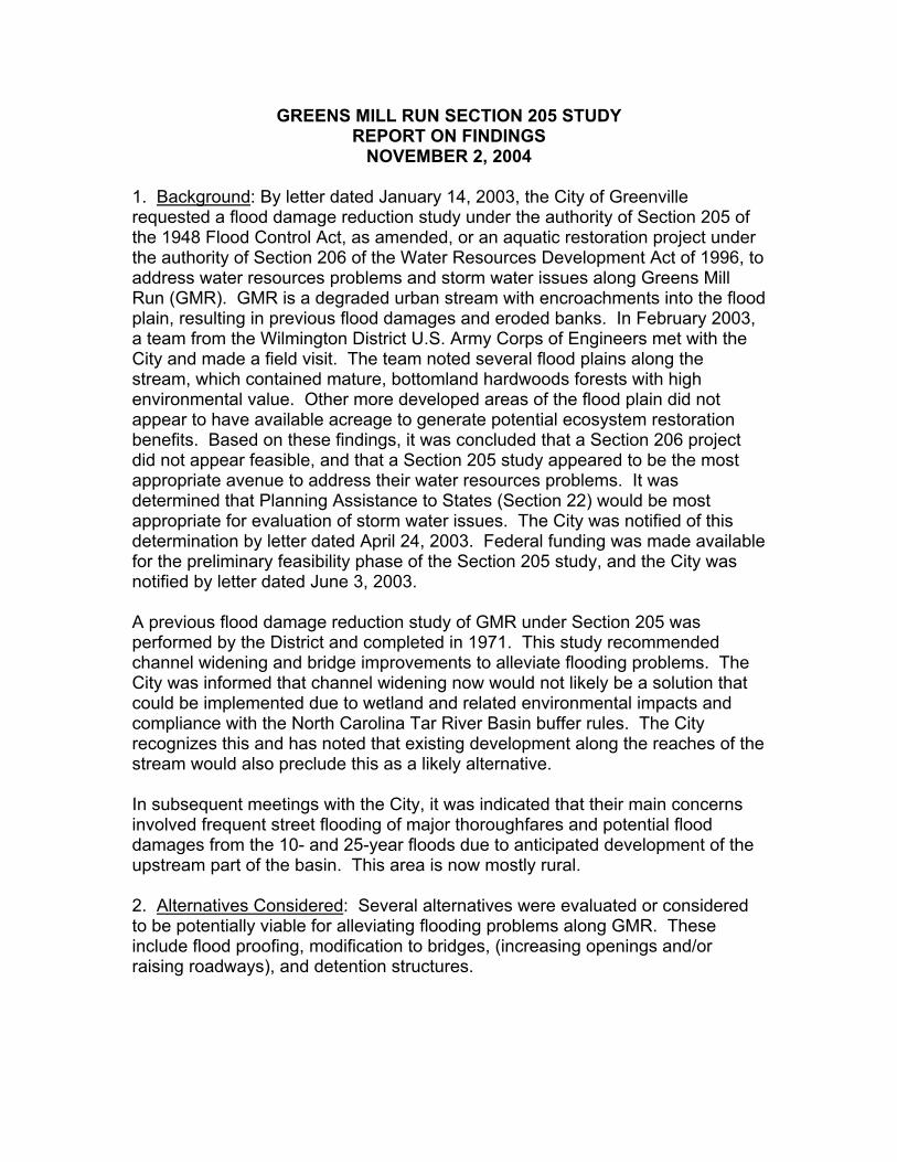
GREENS MILL RUN SECTION 205 STUDY REPORT ON FINDINGS

NOVEMBER 2, 2004

1. Background: By letter dated January 14, 2003, the City of Greenville requested a flood damage reduction study under the authority of Section 205 of the 1948 Flood Control Act, as amended, or an aquatic restoration project under the authority of Section 206 of the Water Resources Development Act of 1996, to address water resources problems and storm water issues along Greens Mill Run (GMR). GMR is a degraded urban stream with encroachments into the flood plain, resulting in previous flood damages and eroded banks. In February 2003, a team from the Wilmington District U.S. Army Corps of Engineers met with the City and made a field visit. The team noted several flood plains along the stream, which contained mature, bottomland hardwoods forests with high environmental value. Other more developed areas of the flood plain did not appear to have available acreage to generate potential ecosystem restoration benefits. Based on these findings, it was concluded that a Section 206 project did not appear feasible, and that a Section 205 study appeared to be the most appropriate avenue to address their water resources problems. It was determined that Planning Assistance to States (Section 22) would be most appropriate for evaluation of storm water issues. The City was notified of this determination by letter dated April 24, 2003. Federal funding was made available for the preliminary feasibility phase of the Section 205 study, and the City was notified by letter dated June 3, 2003. A previous flood damage reduction study of GMR under Section 205 was performed by the District and completed in 1971. This study recommended channel widening and bridge improvements to alleviate flooding problems. The City was informed that channel widening now would not likely be a solution that could be implemented due to wetland and related environmental impacts and compliance with the North Carolina Tar River Basin buffer rules. The City recognizes this and has noted that existing development along the reaches of the stream would also preclude this as a likely alternative. In subsequent meetings with the City, it was indicated that their main concerns involved frequent street flooding of major thoroughfares and potential flood damages from the 10- and 25-year floods due to anticipated development of the upstream part of the basin. This area is now mostly rural. 2. Alternatives Considered: Several alternatives were evaluated or considered to be potentially viable for alleviating flooding problems along GMR. These include flood proofing, modification to bridges, (increasing openings and/or raising roadways), and detention structures.

-2-

Using the steady flow (currently effective) model developed for the Federal Emergency Management Agency (FEMA), which utilized the Corps Hydrologic Engineering Center River Analysis System (HEC-RAS), flood profiles were run for the 2-, 5-, 10-, 25-, 50-, 100-, and 500-yr flood events, under existing (or without project) conditions. A plot of these profiles is attached. In addition to the FEMA model, a very preliminary unsteady flow model was developed for comparison (using the 50-yr peak discharge) and to evaluate the potential effect of detention structures on downstream flood elevations.

a. Floodproofing: The 10-yr flood (based on the FEMA model) was plotted on a photo-based topo map and is included on the enclosed CD ROM. From this plot, about 13 structures between Rockspring Road and Evans Street appeared likely to be subject to damage from this frequency flood. First floor elevations were obtained by field survey and available information. From this survey and the FEMA profile, only one of the 13 structures appeared to be flooded by the 10-year frequency event. It should be noted that this was not considered to be an exhaustive survey of all houses in the area. An additional 6 structures appeared to be flooded up to a depth of approximately one foot by a 25-year flood event. Flood proofing could be considered an alternative, although raising the structures in question may not be practical since they are generally of masonry construction and on a slab. Flood proofing by using sealants and closures may be a possible alternative, on a case-by-case basis.

b. Bridge modifications: An economic evaluation was done to estimate the expected benefits from reduced road overtopping due to bridge modifications at the most promising sites, which included 14th Street and Charles Avenue, discussed below. HEC-RAS model runs were made with increased openings at several of the bridges. A copy of cross section plots from these alternative runs is attached. The effective FEMA model and the models of the various alternatives are included on the enclosed CD ROM. Without major modification (ie. change culverts to bridges), the reduction in upstream flood elevations was generally less than one-half foot. Major modifications would be very expensive (estimated at $1 million minimum) and the effects would be localized. Raising the roadways at 14th and Charles Streets, combined with increased openings, did result in retaining the 10-year or better flood at these locations, as indicated on the cross section plots and in the HEC-RAS models. This would result in benefits from a reduction in the frequency of road overtopping. From the analysis of Charles Street, a substantial modification in the opening would be required to produce this result at that location.

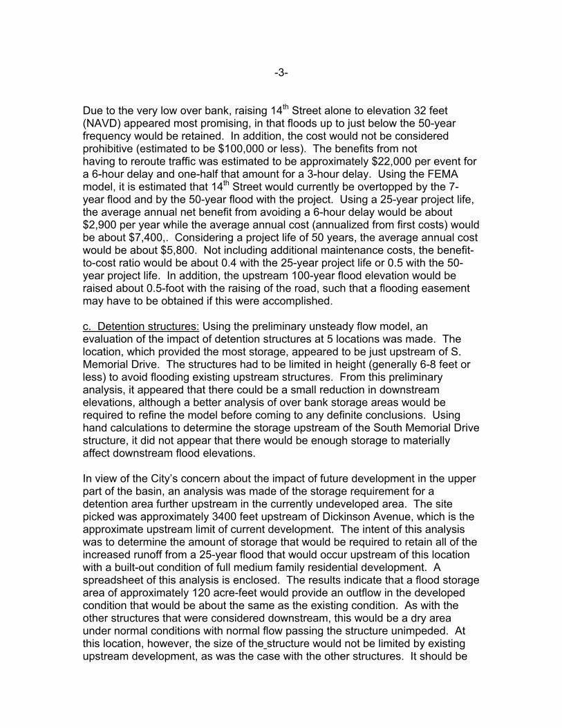
-3-

Due to the very low over bank, raising 14th Street alone to elevation 32 feet (NAVD) appeared most promising, in that floods up to just below the 50-year frequency would be retained. In addition, the cost would not be considered prohibitive (estimated to be $100,000 or less). The benefits from not having to reroute traffic was estimated to be approximately $22,000 per event for a 6-hour delay and one-half that amount for a 3-hour delay. Using the FEMA model, it is estimated that 14th Street would currently be overtopped by the 7-year flood and by the 50-year flood with the project. Using a 25-year project life, the average annual net benefit from avoiding a 6-hour delay would be about $2,900 per year while the average annual cost (annualized from first costs) would be about $7,400,. Considering a project life of 50 years, the average annual cost would be about $5,800. Not including additional maintenance costs, the benefit-to-cost ratio would be about 0.4 with the 25-year project life or 0.5 with the 50-year project life. In addition, the upstream 100-year flood elevation would be raised about 0.5-foot with the raising of the road, such that a flooding easement may have to be obtained if this were accomplished. c. Detention structures: Using the preliminary unsteady flow model, an evaluation of the impact of detention structures at 5 locations was made. The location, which provided the most storage, appeared to be just upstream of S. Memorial Drive. The structures had to be limited in height (generally 6-8 feet or less) to avoid flooding existing upstream structures. From this preliminary analysis, it appeared that there could be a small reduction in downstream elevations, although a better analysis of over bank storage areas would be required to refine the model before coming to any definite conclusions. Using hand calculations to determine the storage upstream of the South Memorial Drive structure, it did not appear that there would be enough storage to materially affect downstream flood elevations. In view of the City’s concern about the impact of future development in the upper part of the basin, an analysis was made of the storage requirement for a detention area further upstream in the currently undeveloped area. The site picked was approximately 3400 feet upstream of Dickinson Avenue, which is the approximate upstream limit of current development. The intent of this analysis was to determine the amount of storage that would be required to retain all of the increased runoff from a 25-year flood that would occur upstream of this location with a built-out condition of full medium family residential development. A spreadsheet of this analysis is enclosed. The results indicate that a flood storage area of approximately 120 acre-feet would provide an outflow in the developed condition that would be about the same as the existing condition. As with the other structures that were considered downstream, this would be a dry area under normal conditions with normal flow passing the structure unimpeded. At this location, however, the size of the structure would not be limited by existing upstream development, as was the case with the other structures. It should be

-4-

noted that rural discharges were used for the existing conditions rather than discharges determined from the current effective FEMA RAS model. It appears that the current model includes effects of urbanization. An alternative to a completely dry pond would be the establishment of wetland areas that would also serve as detention areas. Because of the beneficial nature of wetlands, it is recommended that created wetland areas be incorporated into the detention pond design, if this measure is pursued. 3. Conclusions and Recommendations: Based on the study, an economically favorable solution to the flooding problems along GMR, which would also be environmentally acceptable, was not found. Cost would exceed benefits for an overall nonstructural plan. However, the sponsor may wish to consider implementation of nonstructural alternatives, such as relocation, elevating, or flood proofing, which may be beneficial on a case-by-case basis. The City has been involved in these kinds of nonstructural alternatives as a result of major flooding from Hurricane Floyd in 1999. In addition, it is recommended that the City consider more stringent storm water regulations and require best management practices in order to reduce runoff from future development. Implementation of these features, along with the North Carolina Tar River Basin buffer rules, would be beneficial in reducing storm water runoff and resulting flood stages. Consideration of a detention structure above the currently developed area, perhaps including created wetland areas as discussed in the previous paragraph, is an alternative which appears to have merit in reducing runoff from future development. It is hoped that the information provided will be useful to the City in reducing its flooding problems along Greens Mill Run. 4. List of Attachments: The following is a list of attachments to this report. Attachment 1………………Directory of CD ROM Attachment 2………………Index of HEC-2 Files on CD ROM Attachment 3………………Hydrograph for Retention Pond

Upstream of Dickinson Ave. Attachment 4……………….Flood Profiles, 2-, 5,- 10-, and 25- Yr Attachment 5……………… Natural Flood Profiles from FEMA RAS Model Attachments 6-9………… Bridge/Road Alternative Modifications Attachment 10……………..Alternative Structure at Memorial Drive Attachment 11……………..Alternative Structure at Arlington Blvd.