appendix a the shapiro-wilk test for normality978-1-4419-8724...appendix a the shapiro-wilk test for...

APPENDIX A

The Shapiro-Wilk Test for Normality

Shapiro and Wilk (1965) introduced the test for normality described below.Monte Carlo comparisons by Shapiro et al. (1968) indicate that it has morepower than other procedures for checking the goodness-of-fit of normaldistributions to data.

Suppose you have n observations X l ' X 2 , •• • , Xn • Proceed as follows:

(1) Sort the Xi so that Xi > Xi-I' i = 2,3, ... , n.(2) Calculate

In/21

b= L (Xn- i+ l - Xi)ain,1= 1

where the ain are given in Figure A.I.

X 1 3 4 5 6 7 8 9 10

1 0.7071 0.7071 0.6872 0.6646 0.6431 0.6233 0.6052 0.5888 0.5739

1 0.0000 0.1677 0.2413 0.2806 0.3031 0.3164 0.3244 0.3291

3 0.0000 0.0875 0.1401 0.1743 0.1976 0.2141

4 0.0000 0.0561 0.0947 0.1224

5 0.0000 0.0399

X 11 11 13 14 15 16 17 18 19 10

1 0.5601 0.5475 0.5359 0.5251 0.5150 0.5056 0.4968 0.4886 0.4808 0.4734

1 0.3315 0.3325 0.3325 0.3318 0.3306 0.3290 0.3273 0.3253 0.3232 0.3211

3 0.2260 0.2347 0.2412 0.2460 0.2495 0.2521 0.2540 0.2553 0.2561 0.2565

4 0.1429 0.1586 0.1707 0.1802 0.1878 0.1939 0.1988 0.2027 0.2059 0.2085

5 0.0695 0.0922 0.1099 0.1240 0.1353 0.1447 0.1524 0.1587 0.1641 0.1686

6 0.0000 0.0303 0.0539 0.0727 0.0880 0.1005 0.1109 0.1197 0.1271 0.1334

7 0.0000 0.0240 0.0433 0.0593 0.0725 0.0837 0.0932 0.1013

8 0.0000 0.0196 0.0359 0.0496 0.0612 0.0711

9 0.0000 0.0163 0.0303 0.0422

10 0.0000 0.0140

(continued)

i'..: 21 22 23 24 25 26 27 28 29 30

1 0.4643 0.4590 0.4542 0.4493 0.4450 0.4407 0.4366 0.4328 0.4291 0.4254

2 0.3185 0.3156 0.3126 0.3098 0.3069 0.3043 0.3018 0.2992 0.2968 0.2944

3 0.2578 0.2571 0.2563 0.2554 0.2543 0.2533 0.2522 0.2510 0.2499 0.2487

4 0.2119 0.2131 0.2139 0.2145 0.214 8 0.2151 0.2152 0.2151 0.2150 0.2148

5 0.1736 0.1764 0.1787 0.1807 0.1822 0.1836 0.1848 0.1857 0.1864 0.1870

6 0.1399 0.1443 0.1480 0.1512 0.1539 0.1563 0.1584 0.1601 0.1616 0.1630

7 0.1092 0.1150 0.1201 0.1245 0.1283 0.1316 0.1346 0.1372 0.1395 0.1415

8 0.0804 0.0878 0.0941 0.0997 0.1046 0.1089 0.1128 0.1 162 0.1192 0.1219

9 0.0530 0.0618 0.0696 0.0764 0.0823 0.0876 0.0923 0.0965 0.1002 0.1036

10 0.0263 0.0368 0.0459 0.0539 0.06 10 0.0672 0.0728 0.0778 0.0822 0.0862

11 0.0000 0.0122 0.0228 0.0321 0.0403 0.0476 0.0540 0.0598 0.0650 0.0697

12 0.0000 0.0107 0.0200 0.0284 0.0358 0.0424 0.0483 0.0537

13 0.0000 0.0094 0.0178 0.0253 0.0320 0.0381

14 0.0000 0.0084 0.0159 0.0227IS 0.0000 0.0076

i'..: 31 32 33 34 35 36 37 38 39 40

1 0.4220 0.4188 0.4156 0.4127 0.4096 0.4068 0.4040 0.4015 0.3989 0.3964

2 0.2921 0.2898 0.2876 0.2854 0.2834 0.2813 0.2794 0.2774 0.2755 0.2737

3 0.2475 0.2463 0.2451 0.2439 0.2427 0.2415 0.2403 0.2391 0.2380 0.2368

4 0.2145 0.2 141 0.2137 0.2132 0.2127 0.2121 0.2116 0.2110 0.2104 0.2098

5 0.1874 0.1878 0.1880 0.1882 0.1883 0.1883 0.1883 0.1881 0.1880 0.1878

6 0.1641 0. 1651 0.1660 0.1667 0.1673 0.1678 0.1683 0.1686 0.1689 0. 16917 0.1433 0.1449 0.1463 0.1475 0.1487 0.1496 0.1505 0.1513 0.1520 0.15268 0.1243 0.1265 0.1284 0.1301 0.1317 0.1331 0.1344 0.1356 0.1366 0.13769 0.1066 0.1093 0. 1118 0.1140 0.1160 0.1179 0.1196 0.1211 0.1225 0.1237

10 0.0899 0.0931 0.0961 0.0988 0.1013 0.1036 0.1056 0.1075 0.1092 0.1108

11 0.0739 0.0777 0.0812 0.0844 0.0873 0.0900 0.0924 0.0947 0.0967 0.098612 0.0585 0.0629 0.0669 0.0706 0.0739 0.0770 0.0798 0.0824 0.0848 0.087013 0.0435 0.0485 0.0530 0.0572 0.0610 0.0645 0.0677 0.0706 0.0733 0.075914 0.0289 0.0344 0.0395 0.0441 0.0484 0.0523 0.0559 0.0592 0.0622 0.0651IS 0.0144 0.0206 0.0262 0.0314 0.0361 0.0404 0.0444 0.0481 0.0515 0.0546

16 0.0000 0.0068 0.0131 0.0187 0.0239 0.0287 0.0331 0.0372 0.0409 0.044417 0.0000 0.0062 0.0119 0.0172 0.0220 0.0264 0.0305 0.034318 0.0000 0.0057 0.0110 0.0158 0.0203 0.024419 0.0000 0.0053 0.0101 0.014620 0.0000 0.0049

~ 41 42 43 44 45 46 47 48 49 SO

1 0.3940 0.3917 0.3894 0.3872 0.3850 0.3830 0.3808 0.3789 0.3770 0.37512 0.2719 0.2701 0.2684 0.2667 0.2651 0.2635 0.2620 0.2604 0.2589 0.25743 0.2357 0.2345 0.2334 0.2323 0.2313 0.2302 0.229 1 0.2281 0.2271 0.22604 0.2091 0.2085 0.2078 0.2072 0.2065 0.2058 0.2052 0.2045 0.1038 0.20325 0.1876 0.1874 0.1871 0.1868 0.1865 0.1862 0.1859 0.1855 0.1851 0.1847

6 0.1693 0.1694 0.1695 0.1695 0.1695 0.1695 0.1695 0.1693 0. 1692 0.16917 0.1531 0.1535 0.1539 0.1542 0.1545 0.1548 0.1550 0.1551 0.1553 0.15548 0.1384 0.1392 0.1398 0.1405 0.1410 0.1415 0.1420 0.1423 0.1427 0.14309 0.1249 0.1259 0.1269 0.1278 0.1286 0.1293 0.1300 0.1306 0.1312 0.1317

10 0.1123 0.1136 0.1 149 0.1160 0.1170 0.1180 0.1189 0.1197 0.1205 0.121211 0.1004 0.1020 0.1035 0.1049 0.1062 0.1073 0.1085 0.1095 0.1105 0.111312 0.0891 0.0909 0.0927 0.0943 0.0959 0.0972 0.0986 0.0998 0.1010 0.102013 0.0782 0.0804 0.0824 0.0842 0.0860 0.0876 0.0892 0.0906 0.0919 0.093214 0.0677 0.0701 0.0724 0.0745 0.0765 0.0783 0.0801 0.08 17 0.0832 0.084615 0.0575 0.0602 0.0628 0.065 1 0.0673 0.0694 0.0713 0.0731 0.0748 0.076416 0.0476 0.0506 0.0534 0.0560 0.0584 0.0607 0.0628 0.0648 0.0667 0.068517 0.0379 0.0411 0.0442 0.0471 0.0497 0.0522 0.0546 0.0568 0.0588 0.060818 0.0283 0.0318 0.0352 0.0383 0.0412 0.0439 0.0465 0.0489 0.0511 0.053219 0.0188 0.0227 0.0263 0.0296 0.0328 0.0357 0.0385 0.0411 0.0436 0.045920 0.0094 0.0136 0.0175 0.0211 0.0245 0.0277 0.0307 0.0335 0.0361 0.038621 0.0000 0.0045 0.0087 0.0126 0.0163 0.0197 0.0229 0.0259 0.0288 0.03 1422 0.0000 0.0042 0.0081 0.0118 0.0153 0.0185 0.02 15 0.024423 0.0000 0.0039 0.0076 0.0111 0.0143 0.017424 0.0000 0.0037 0.0071 0.010425 0.0000 0.0035

F igure A.I. Coefficients a in for the Shapiro- Wilk test. (Reproduced by permission fromBiometrika.)

App endix A. The Shapiro- Wilk Test for Normality 305

(3) Calculate

l¥,. = b2/ [ (n - 1)52] ,

where 52 is the sample variance of the X i' Percentage po ints for l¥,. arelisted in Figure A.2. For normal data l¥,. should be near 1; reject theassump tion of normality if l¥,. is small.

Level

0.01 0.02 0.05 0.10 0.50 0.90 0.95 0.98 0.99

3 0 .753 0.756 0.767 0.789 0.959 0.998 0.999 1.000 1.0004 0.687 0.707 0.748 0.792 0.93 5 0.987 0.992 0.996 0.9975 0.686 0.715 0.762 0.806 0.927 0.979 0.986 0.99 1 0.993

6 0.713 0.743 0.788 0.826 0.927 0.974 0.981 0 .986 0.9897 0.730 0.760 0.803 0.838 0.928 0.972 0.979 0 .985 0.9888 0.749 0.778 0.8 18 0.851 0.932 0.972 0.978 0 .984 0.9879 0.764 0.791 0.829 0.859 0.935 0.972 0.978 0.98 4 0.986

10 0.781 0 .806 0.842 0.869 0.938 0.972 0 .978 0.9 83 0.986

11 0.792 0.8 17 0.850 0.876 0.940 0.973 0.979 0.984 0 .98612 0.805 0.828 0.859 0.883 0.943 0.973 0.979 0.98 4 0 .98613 0.814 0.837 0.866 0.889 0 .945 0.974 0.979 0.984 0.98614 0.825 0.846 0.874 0.895 0.947 0.975 0.980 0 .984 0.98615 0.835 0.855 0.88 1 0.90 1 0.950 0.975 0.980 0.984 0 .987

16 0.844 0.863 0.887 0.906 0.952 0.976 0.98 1 0.985 0.98717 0.851 0.869 0.892 0.910 0.954 0.977 0.981 0.985 0.98718 0.858 0.874 0.897 0.914 0.956 0.978 0 .982 0.986 0.98819 0.863 0.879 0.901 0.9 17 0.957 0.978 0.982 0.986 0.98820 0.868 0.884 0.905 0.920 0.959 0.979 0.983 0.986 0.988

21 0.873 0.888 0.908 0.923 0.960 0.980 0.983 0.987 0.98922 0.878 0.892 0.9 11 0.926 0.961 0.980 0.984 0.987 0.98923 0.88 1 0.895 0.9 14 0.928 0.962 0.98 1 0.984 0.987 0.98924 0.884 0.898 0.9 16 0.930 0.963 0.981 0.984 0.987 0 .98925 0.888 0.901 0.9 18 0.93 1 0.964 0.981 0.985 0.988 0.989

26 0.89 1 0.904 0.920 0.933 0.965 0.982 0.985 0.988 0.98927 0.894 0.906 0.92 3 0.935 0.965 0.982 0.985 0.988 0.99028 0.896 0.908 0.924 !J.936 0.966 0.982 0.985 0 .988 0.99029 0.898 0.910 0.926 0.937 0.966 0.982 0.985 0.988 0.99030 0.900 0.9 12 0.927 0.939 0.967 0.983 0.985 0.988 0.900

31 0.902 0.914 0.929 0.9 40 0.967 0.98 3 0.986 0.988 0.99032 0.904 0.9 15 0.930 0.941 0.968 0.983 0.986 0.988 0.99033 0.906 0.9 17 0.931 0.942 0.968 0.983 0.986 0.989 0.99034 0.908 0.9 19 0.933 0.943 0.969 0.983 0.986 0.989 0.99035 0.9 10 0.920 0.934 0.944 0.969 0 .984 0.986 0.989 0.990

36 0.912 0.922 0.935 0.945 0.970 0.984 0.986 0.989 0.99037 0.914 0.924 0.936 0.946 0.970 0.984 0.987 0.989 0.99038 0.9 16 0.925 0.938 0.947 0 .971 0.984 0.987 0.989 0.99039 0.917 0.927 0.939 0.948 0.971 0.984 0.987 0.989 0.99 140 0.919 0.928 0.940 0.949 0.972 0.985 0.987 0.989 0.99 1

41 0.920 0.929 0.941 0.950 0.972 0.985 0.987 0.989 0.99142 0.922 0.930 0.942 0.951 0.972 0.985 0.987 0.989 0.99 143 0.923 0.932 0.943 0.951 0.973 0.98 5 0.987 0.990 0.991

44 0.924 0.933 0.944 0.952 0.973 0.985 0.987 0.990 0.991

45 0.926 0.934 0.945 0.953 0.973 0.98 5 0.988 0.990 0.991

46 0.927 0.935 0.945 0.953 0.974 0.985 0.988 0.990 0.99 1

47 0.928 0.936 0.946 0.954 0.974 0.985 0.988 0.990 0.991

48 0.929 0.937 0.947 0.95 4 0.974 0.985 0.988 0.990 0.991

49 0.929 0.937 0.947 0.955 0.974 0.985 0.988 0.990 0.991

50 0.930 0.938 0.947 0.955 0.974 0.985 0.988 0.990 0.991

FigureA.2. Percentage points for W. for the Shapiro-Wilk test. (Reproduced by

permission from Biometrika.)

APPENDIX L

Routines for Random NumberGeneration

This appendix contains examples of generators, and of routines for calculating and inverting cdfs. Many of the routines presented are discussed inChapters 5 and 6.

All the programs are written in ANSI Fortran. To make them as usefulas possible, we have only used language features which are in both the oldstandard Fortran IV and the new official subset of Fortran 77 [ANSI(1978)J. All the examples have been tested on at least two machines. Errorreporting is summary: in most cases a flag called IFAULT is set to a nonzerovalue if an error is detected, the code used depending on the routine atfault. Names follow the Fortran type conventions, and only dimensionedvariables are explicitly declared. The comment AUXILIARY ROUTINESrefers to routines to be found elsewhere in the appendix.

The appendix contains the following routines:

Functions

1. ALOGAM Evaluates the natural logarithm of rex) (used to set upfurther calls).

2. BETACH Generates a beta deviate using the method of Cheng(1978)-see Section 5.3.10.

3. BETAFX Generates a beta deviate using the method of Fox (1963)see Section 5.3.10.

4. BOXNRM Generates a standard normal deviate using the Box-Mullermethod-see Section 5.2.10.

5. D2 Computes (exp(x) - 1)/x accurately (used as an auxiliaryroutine).

Rout ines for Random Numb er Generation 307

6. GAMAIN

7. IALIAS

8. IVDISC

9. IVUNIP

10. LUKBIN

11. REMPIR

12. RGKM3

13. RGS

14. RSTAB

15. SUMNRM

16. TAN17. TAN218. TRPNRM

19. UNIF

20. UNIFL

21. VBETA22. VCAUCH

23. VCHI2

24. VCHISQ

25. VF26. VNHOMO

Computes the incomplete gamma ratio (used as anauxiliary routine).Generates a discrete random variate by the alias methodsee Section 5.2.8. Initialization is carried out by the subroutine ALSETP.Inverts a discrete cdf using the method of Ahrens andKohrt-see Section 5.2.1. Initialization is carried out bythe subroutine VDSETP.Generates an integer uniform over an interval (1, n) usinginversion-see Section 6.7.1 .Generates a discrete random variate using the methodof Fox (1978b)-see Section 5.2.7. Initialization is carriedout by the subroutine SETLKB.Generates a variate from an empirical distribution with anexponential tail-see Sections 4.6 and 5.2.4.Generates a gamma variate using rejection-see Section5.3.9.Generates a gamma variate using rejection-see Section5.3.9.Generates a stable Paretian variate using the methodof Chambers et al. (1976)-see Section 5.3.3.Generates a standard normal deviate by a not very quickand unnecessarily dirty method : its use is not recommended.Computes tan(x) (used as an auxiliary routine).Computes tan(x)jx (used as an auxiliary routine) .Generates a standard normal deviate using the methodof Ahrens and Dieter-see Example 5.2.2.Generates uniform random numbers. The code is fastand portable-see Section 6.5.2.Generates uniform variates using L'Ecuyer's compositemethod.Calculates the inverse of the beta cdf-see Section 5.3.10.Calculates the inverse of a standard Cauchy cdf-seeSection 5.3.4.Calculates the inverse of the chi-square cdf-see Section5.3.11. This routine can also be used to generate Erlangand gamma variates-see Section 5.3.9. .Calculates the inverse of the chi-square cdf-see Section5.3.11 (faster but less accurate than VCHI2). This routinecan also be used to generate Erlang and gamma variatessee Section 5.3.9.Calculates the inverse of the F cdf-see Section 5.3.12.Generates a deviate from a nonhomogeneous Poissondistribution-see Section 5.3.18.

308

27. VNORM

28. VSTUD

Subroutines

29. BINSRH30. FNORM

31. TBINOM32. TTPOSN

Appendix L

Calculates the inverse of the standard normal cdf using arational approximation.Calculates the inverse of the t cdf-see Section 5.3.13.

Performs a binary search in a tabulated cdf.Calculates areas under a standard normal curve, and alsothe normal loss function.Tabulates the binomial cdf.Tabulates the cdf of a truncated Poisson.

FUNCTION ALOGAM( Y)CC THIS PROCEDURE EVALUATES THE NATURAL LOGARITHM OF GAMMA(Y)C FOR ALL Y>O, ACCURATE TO APPROXIMATELY MACHINE PRECISIONC OR 10 DECIMAL DIGITS, WHICHEVER IS LESS.C STIRLING'S FORMULA IS USED FOR THE CENTRAL POLYNOMIAL PARTC OF THE PROCEDURE.C BASED ON ALG. 291 IN CACM, VOL. 9 , NO. 9 SEPT. 66 , P. 384,C BY M. C. PIKE AND I. D. HILL.C

X = YIF ( X .GE . 7 .0) GO TO 20F = 1.0Z = X - 1.0GO TO 7

5 X = ZF = F* Z

7 Z = Z + 1.IF ( Z .LT . 7) GO TO 5X=X+1.F = - ALOG( F)GO TO 30

20 F = O.30 Z = ( 1.0 / X) ** 2 .0

ALOGAM = F + ( X - 0.5) * ALOG( X) - X + 0.918938533204673 +* (((-0 .000595238095238 * Z + 0.000793650793651) * Z -* 0 .002777777777778) * Z + 0 .083333333333333) / X

RETURNEND

Figure L.l. The funct ion ALOGAM.

Routines for Random Number Generation

FUNCTION BETACH( IY, A, B, CON)REAL CON( 3)

309

CC GENERATE A BETA DEVIATEC REF.: CHENG, R., GENERATING BETA VARIATES WITH NONINTEGRALC SHAPE PARAMETERS, CACM, VOL. 21, APRIL, 1978CC INPUTS:C A, B = THE TWO PARAMETERS OF THE STANDARD BETA,C CON() = A REAL WORK VECTOR OF LENGTH AT LEAST 3.C AT THE FIRST CALL CON( 1) SHOULD BE O.~ IT IS SET TO A FUNCTION OF A & B FOR USE IN SUBSEQUENT CALLSC IY = A RANDOM NUMBER SEED.CC AUXILIARY ROUTINE:C UNIFC

IF ( CON( 1) .GT. 0.) GO TO 200CON ( 1) = AMIN1( A, B)IF ( CON ( 1) . GT . 1.) GO TO 100CON ( 1) = 1./ CON( 1)GO TO 150

100 CON ( 1) = SQRT( ( A + B - 2 . )/( 2.* A* B- A- B»150 CON( 2)= A + B

CON ( 3) = A + 1./ CON( 1)CC SUBSEQUENT ENTRIES ARE HEREC

200 Ul = UNIF( IY)U2 = UNIF( IY)V = CON( 1)* ALOG( Ul/(l.- Ul»W = A* EXP( V)IF « CON( 2»*ALOG« CON( 2»/(B+W» + (CON( 3»

1 *v - 1.3862944 .LT. ALOG( Ul*Ul*U2» GO TO 200BETACH = W/( B + W)RETURNEND

Figure L.2. The function BETACH.

310 Appendix L

FUNCTION BETAFX( IX , NA, NB, WORK)REAL WORK( NA)

CC GENERATE A BETA DEVIATEC REF.: FOX, B.(1963), GENERATION OF RANDOM SAMPLES FROM THEC BETA AND F DISTRIBUTIONS, TECHNOMETRICS, VOL. 5, 269-270.CC INPUTS:C IX = A RANDOM NUMBER SEED,C NA, NB = PARAMETERS OF THE BETA DISTRIBUTION,C MUST BE INTEGERC WORK ( ) "" A WORK VECTOR OF LENGTH AT LEAST NA + NB.CC OUTPUTS :C BETAFX = A DEVIATE FROM THE RELEVANT DISTRIBUTIONCC AUXILIARY ROUTINE;C UNIFCC SETUP WORK VECTOR FOR SORTINGC

DO 100 I 1, NAWORK ( I) 2.

100 CONTINUENAB = NA + NB - 1

CC GENERATE NAB UNIFORMS AND FIND THE NA-TH SMALLESTC

DO 200 I = 1, NABFY = UNIF( IX)IF ( FY .GE . WORK ( 1)) GO TO 200IF ( NA . LE. 1) GO TO 170DO 160 K "" 2, NAIF ( FY .LT. WORK ( K)) GO TO 150WORK ( K - 1) FYGO TO 200

150 WORK ( K - 1) WORK( K)160 CONTINUE170 WORK( NA) "" FY200 CONTINUE

CBETAFX "" WORK( 1)RETURNEND

Figure L.3. The function BETAFX.

Routines for Random Number Generation 311

FUNCTION BOXNRM( IY, Ul)

ON FIRST CALL.

INPUT :IY = RANDOM NUMBER SEEDUl = A WORK SCALER WHICH SHOULD BE > 254

IT STORES DATA FOR SUBSEQUENT CALLSAUXILIARY ROUTINE:

UNIF

CC RETURN A UNIT NORMAL(OR GAUSSIAN) RANDOM VARIABLEC USING THE BOX-MULLER METHOD.CCCCCCCC

IF ( Ul .GE. 254 .) GO TO 100CC A DEVIATE IS LEFT FROM LAST TIMEC

BOXNRM = UlCC INDICATE THAT NONE LEFT. NOTE THAT PROBABILITY THATC A DEVIATE > 254 IS EXTREMELY SMALL.C

Ul = 255.RETURN

CC TIME TO GENERATE A PAIRC

100 Ul = UNIF( IY)Ul = SQRT(-2 .* ALOG( U1))U2 = 6.2831852* UNIF( IY)

CC USE ONE.•.C

BOXNRM = Ul* COS( U2)CC SAVE THE OTHER FOR THE NEXT PASSC

Ul = Ul* SIN( U2)RETURNEND

Figure LA. The function BOXNRM.

312

FUNCTION D2( Z)CC EVALUATE ( EXP( x ) - l) / XC

DOUBLE PRECISION Pl, P2, Ql, Q2, Q3, PV, ZZC ON COMPILERS WITHOUT DOUBLE PRECISION THE ABOVE MUST BEC REPLACED BY REAL Pl, ETC. , AND THE DATA INITIALI ZATIONC MUST USE E RATHER THAN D FORMAT.C

DATA Pl, P2, Ql, Q2, Q3/.8 4006685 253648 3239D3,1 .200011141589964569D2 ,2 .168013370507926648D4,3 .18013370407390023D3 ,4 1.DO/

CC THE APPROXIMATION 1801 FROM HART ET. AL. (1 968, P. 2 13 )C COMPUTER APPROXI MATIO NS, NEW YORK, JOHN WI LEY.C

IF ( ABS( Z) .GT. 0 .1) GO TO 100ZZ = Z * ZPV = Pl + ZZ* P2D2 = 2.DO* PV/( Ql+ ZZ* ( Q2+ ZZ* Q3) - Z* PV)RETURN

100 D2 = ( EXP( Z) - 1 .) / ZRETURNEND

Figure L.S. The function D2.

Append ix L

CCCCCCCCCCC

CCC

FUNCTION GAMAIN( X, P, G, I FAULT)

ALGORITHM AS 32 J.R .STATIST.SOC . C. (1970) VOL.1 9 NO. 3

COMPUTES INCOMPLETE GAMMA RATIO FOR POSITIVE VALUES OFARGUMENTS X AND P . G MUST BE SUPPLIED AND SHOULD BE EQUAL TOLN(GAMMA(P» .

IFAULT = 1 IF P.LE.O ELSE 2 IF X.LT .O ELSE O.USES SERIES EXPANSION -I F P.GT.X OR X. LE. l, OTHERWISE ACONTINUED FRACTION APPROXIMATION.

DIMENSION PN(6)

DEFINE ACCURACY AND INITIALIZE

DATA ACU/l.E-8/, OFLO/l .E30/GIN=O.OIFAULT=O

(continued)


CC TEST FOR ADMISSIBILITY OF ARGUMENTSC

IF(P .LE.O.O) IFAULT=lIF(X.LT.O.O) IFAULT=2IF(IFAULT.GT.O.OR .X .EQ.O.O) GO TO 50FACTOR=EXP(P*ALOG(X)-X-G)IF(X .GT.1.0 .AND.X .GE .P) GO TO 30

CC CALCULATION BY SERIES EXPANSIONC

GIN=l. 0TERM=l. 0RN=P

20 RN=RN+l. 0TERM=TERM*X/RNGIN=GIN+TERMIF(TERM.GT.ACU) GO TO 20GIN=GIN*FACTOR/PGO TO 50

CC CALCULATION BY CONTINUED FRACTIONC

30 A=l.O-PB=A+X+l. 0TERM=O.OPN(l)=l.OPN(2)=XPN(3)=X+1.0PN(4)=X*BGIN=PN(3)/PN(4)

32 A=A+l.OB=B+2.0TERM=TERM+1.0AN=A*TERMDO 33 I=1,2

33 PN(I+4)=B*PN(I+2)-AN*PN(I)IF(PN(6) .EQ.O .O) GO TO 35RN=PN(5)/PN(6)DIF=ABS(GIN-RN)IF(DIF.GT.ACU) GO TO 34IF(DIF.LE.ACU*RN) GO TO 42

34 GIN=RN35 DO 36 I=1,436 PN(I)=PN(I+2)

IF(ABS(PN(5)) .LT.OFLO) GO TO 32DO 41 I=1,4

41 PN(I)=PN(I)/OFLOGO TO 32

42 GIN=1.0-FACTOR*GINC

50 GAMAIN=GINRETURNEND

Figure L.6. The function GAMAIN.

313

314

FUNCTION I ALI AS( PHI, N, A, R)INT EGER A( N)REAL R( N)

CC GENERATE A DISCRETE R. V. BY THE ALIAS METHODCC INPUTS :C PHI = NUMBER BETWEEN 0 AND 1C N = RANGE OF R. V., I.E. , 1, 2, •• . , NC A( I) = ALIAS OF IC R( I) = ALIASING PROBABILIT YCC REF . : KRONMAL AND PETERSON, THE AMERICAN STATISTICIAN,C VOL 33, 1979 .C

Appendix L

C

V = PHI *NJALIAS = V + 1.I F ( JALIAS - V .GT. R( JALIAS» JALIASIALIAS = JALIASRETURNEND

SUBROUTINE ALSETP( N, P, A, R, L)INTEGER A( N) , L( N)REAL P( N), R ( N)

A( J ALIA S )

CC SETUP TABLES FOR USING THE ALIAS METHOD OF GENERATINGC DISCRETE RANDOM VARIABLES USING FUNCTION IALIAS .CC IN PUTS: N = RANGE OF THE RANDOM VARIABLE , I .E. 1 , 2 , .. • , NC P ( I ) = PROBe R. V. = I)C L( ) A WORK VECTOR OF SIZ E NCC OUTPUTS: A( I) = ALIAS OF IC R ( I) ALIASI NG PROBABILIT Y OF IC

LOW = 0MID = N+ 1

CC PUT AT THE BOTTOM, OUTCOMES FOR WHICH THE UNIFORM DISTRIBUTIONC ASSIGNS TOO MUCH PROBABILITY. PUT THE REST AT THE TOP.C

DO 100 I = 1, NA( I) = IR ( I) = N*P( I)IF ( R( I) .GE. 1. ) GO TO 50

CC TOO MUCH PROBABILITY ASS IG NED TO IC

LOW = LOW + 1L(LOW) = IGO TO 100

CC TOO LITTLE PROBABILITY ASSIGNED TO IC

50 MID = MID - 1

(continued)


L( MID) = I100 CONTINUE

315

CC NOW GIVE THE OUTCOMES AT THE BOTTOM(WITH TOO MUCH PROBABILITY)C AN ALIAS AT THE TOP.C

Nl = N - 1DO 200 I = 1, NlK = L( MID)J = L( I)A( J) = KR( K) = R( K) + R( J) - 1 .IF ( R( K) . GE . 1.) GO TO 200MID = MID + 1

200 CONTINUERETURNEND

Figure L.7 . The function IALIAS and its initialization subroutine ALSETP.

316 Append ix L

FUNCTION IVDISC( U, N, M, CDF, LUCKY)REAL CDF( N)INTEGER LUCKY( M)

INVERT A DISCRETE CDF USING AN INDEX VECTOR TO SPEED THINGS UPREF. AHRENS AND KOHRT, COMPUTING, VOL 26, P19, 1981 .

CCCCCCCCCCCCCCCC

C

INPUTS :U = A NUMBER 0 <= U <= 1.N = SIZE OF CDF; = RANGE OF THE RANDOM VARIABLE;M = SIZE OF LUCKYCDF = THE CDF VECTOR.LUCKY = THE POINTER VECTOR, SETUP BY VDSETP

OUTPUT:IVDISC = F INVERSE OF U

TAKE CARE OF CASE U = 1.

IF ( U .LT . CDF( N» GO TO 50IVDISC NRETURN

50 NDX = U* M + 1.JVDISC LUCKY( NDX)

1,2 ... ,N

CC IS U IN A GRID INTERVAL FOR WHICH THERE IS A JVDISCC SUCH THAT CDF( JVDISC - 1) < INTERVAL <= CDF( JVDISC) ?C

IF ( JVDISC .GT. 0) GO TO 300CC HARD LUCK, WE MUST SEARCH THE CDF FOR SMALLEST JVDISCC SUCH THAT CDF( JVDISC) >= U.C

JVDISC = - JVDISCGO TO 200

100 JVDISC = JVDISC + 1200 IF ( CDF( JVDISC) .LT. U) GO TO 100300 IVDISC = JVDISC

RETURNEND

CSUBROUTINE VDSETP( N, M, CDF, l~CKY)

REAL CDF( N)INTEGER LUCKY( M)

CC SETUP POINTER VECTOR LUCKY FOR INDEXED INVERSIONC OF DISCRETE CDF BY THE FUNCTION IVDISC.CC INPUTS:C N = NO . POINTS IN CDFC M = NO. LOCATIONS ALLOCATED FOR POINTERSC CDF = THE CDF VECTORCC OUTPUTS :C LUCKY = THE POINTER VECTOR; > 0 IMPLIES THIS POINTER

(continued)


CCCCCCC

GRID INTERVAL FALLS COMPLETELY WITHIN SOME CDF INTERVAL;< 0 IMPLIES THE GRID INTERVAL IS SPLIT BY A CDF POINT.

DATE 10 SEPT 1986

TAKE CARE OF DEGENERATE CASE OF N 1

DO 25 I = 1, MLUCKY ( I)= 1

25 CONTINUEIF ( N .EQ. 1) RETURN

CC INITIALIZE FOR GENERAL CASEC

NOLD = MI = NDO 300 II = 2, NI = I - 1

CC FIND THE GRID INTERVAL IN WHICH CDF( I) FALLSC

NDX = CDF( I)* M +1IF ( NDX . GT. M) GO TO 300LUCKY ( NDX) = - I

CC ANY GRID INTERVALS FALLING STRICTLY BETWEEN THISC CDF POINT AND THE THE NEXT HIGHER, MAP TO THE NEXT HIGHERC

NDl = NDX +1IF ( NDl .GT . NOLD) GO TO 200DO 100 K = ND1, NOLDLUCKY ( K) = I + 1

100 CONTINUE200 NOLD = NDX - 1300 CONTINUE

RETURNC

END

Figure L,8. The function IVDISC and its initialization subroutine VDSETP.

318

FUNCTION lVUNIP{ IX, L, P)IMPLICIT INTEGER(A-Z)

Appendix L

CC SOME COMPILERS REQUIRE THE ABOVE TO BE INTEGER*4CC PORTABLE CODE TO GENERATE AN INTEGER UNIFORM OVER [ 1, L],C USING INVERSION.CC INPUTS:C IX = A RANDOM INTEGER, 0 =< IX < PCLAN INTEGER, 0 < L < P,C P = AN INTEGER, 1 < P < 2**31 , E.G., MODULUS OF RANDOM NUMBERC GENERATOR.CC OUTPUTS:C lVUNIP ~ INTEGER PART OF{ IX * LIP) + 1,C EFFECTIVELY, A RANDOM INTEGER UNIFORM ON [ 1, L].C PROCEDURE IS VERY SLOW FOR P « 2**31.CC REFERENCE: PROF. A. PERKO, UNIVERSITY OF JYVASKYLA, FINLAND

DATA M/2147483647/, P15/32768/, P16/655361CCOATE 30 SEPT 1986CC CALCULATE IX* L IN DOUBLE PRECISION, I.E., FIND A, B SO:C IX* L A*{2**31) + BC

X LI P16Y L - P16* XU IXI P15V IX - P15* U

CC NOW CALCULATE:C A*{2**31) + B Y * V + V * X * P16 + U * P15 * R * 2C + U * P15 * S + U * P15 * X* P16.C

YV Y * VYVl = WI P15YV2 = YV - P15* YVlR = YI 2S = Y - 2* RUR = U * RURl = URI P15UR2 = UR - P15* URl

CC EXPLOIT THE POSSIBILITY THAT X 0:C

IF ( X .GT. 0) GO TO 100VXl ~ 0VX2 = 0GO TO 200

100 VX = v* XVXl VXI P15VX2 = VX - P15* VXlVXl = VXl + U * X

200 AB = YVl + 2* ( UR2 + VX2) + S* U

(continued)


A2 = ABI P16B = P15 *( AB - P16* A2) + YV2A = A2 + UR1 + VX1

CC NOW THAT WE HAVE A AND BC NOTE THAT ( A * 2**31 + B)I P =C ( A * ( P + IE) + B)I P = A + ( A * IE + B ) I P, SOC COMPUTE K = INTEGER PART OF ( ( A * IE + B )1 P)C NOTE THAT K = SMALLEST INTEGER SATISFYING :C A * IE + B - ( K + 1) * P < 0C

IE = M - P + 1MOE = M I IEINA = AK = 0KUM = B - P

300 IF ( KUM .LT. 0) GO TO 400KUM=KUM-PK = K + 1GO TO 300

CC ADD IN SOME MORE IE'S UNTIL A OF THEM HAVE BEEN ADDEDC

400 IF ( INA .EQ. 0) GO TO 500IEFIT = MIN( MOE, INA)INA = INA - IEFITKUM = KUM + IE * IEFITGO TO 300

C500 lVUNIP = A + K + 1

RETURNEND

Figure L.9. The function IVUNIP.

319

320 Appendix L

FUNCTION LUKBIN( PHI, N, R, T, M, NK)REAL R( N)INTEGER NK( M)

CC THE BUCKET-BINARY SEARCH METHOD OF FOXC REF. OPERATIONS RESEARCH, VOL 25, 1978C FOR GENERATING(QUICKLY) DISCRETE RANDOM VARIABLESCC INPUTS:C PHI = A PROBABILITY, 0 < PHI < 1C N NO. POSSIBLE OUTCOMES FOR THE R. V.C R = A VECTOR SET BY SETLKBC T = A SCALER THRESHOLD SET BY SETLKBC M = NUMBER OF CELLS ALLOWED FOR THE POINTER VECTOR NK( ).C NK = A POINTER VECTOR SET BY SETLKBCC OUTPUTS:C LUKBIN = RANDOM VARIABLE VALUEC

IF ( PHI .GE. T) GO TO 50CC HERE IS THE QUICK BUCKET METHODC

I = M • PHILUKBIN = NK( I + 1)RETURN

CC WE MUST RESORT TO BINARY SEARCHC

50 IF (PHI .LE. R( 1» GO TO 500MAXI = NMINI = 2

100 K = ( MAXI + MINI)/ 2IF ( PHI .GT. R(K») GO TO 300IF ( PHI .GT. R( K - 1)) GO TO 500MAXI = K - 1GO TO 100

300 MINI = K + 1GO TO 100

500 LUKBIN = KRETURNEND

CSUBROUTINE SETLKB( M, N, CDF, T, NK, R)REAL CDF( N), R( N)INTEGER NK( M)

CC SETUP FOR THE LUKBIN METHOD. SEE FUNCTION LUKBINCC INPUTS:C M = NUMBER OF CELLS ALLOWED FOR THE POINTER VECTOR NK( ).C M > O. LARGER M LEADS TO GREATER SPEED.C N = NO. POSSIBLE OUTCOMES FOR THE R. V.C CDF() = CDF OF THE R. V.CC OUTPUTS: T = A THRESHOLD TO BE USED BY LUKBIN

(continued's


C NK() = A POINTER VECTOR WHICH SAVES TIMEC R() = A THRESHOLD PROBABILITY VECTOR.C

EXCESS = O.PO = O.NLIM = 0NUSED = 0DO 400 I = 1, NPI = CDF( I) - POLOT = M* PIPO = CDF( I)IF ( LOT .LE. 0) GO TO 200NUSED = NLIM + 1NLIM = NLIM + LOTDO 100 J = NUSED, NLIMNK( J) = I

100 CONTINUE200 EXCESS = EXCESS + PI - FLOAT(LOT)/FLOAT( M)

R( I) = EXCESS400 CONTINUE

T = FLOAT( NLIM)/ FLOAT( M)DO 500 I = 1, NR( I) = R( I) + T

500 CONTINUERETURNEND

321

Figure L.lO. The function LUKBIN and its initialization subroutine SETLKB.

322 Appendix L

FUNCTION REMPIR( U, N, K, X, THETA, IFAULT)DIMENSION X(N)

CC INVERSION OF AN EMPIRICAL DISTRIBUTION BUT WITH ANC EXPONENTIAL APPROXIMATION TO THE K LARGEST POINTS.CC INPUTS:C U PROBABILITY BEING INVERTEDC N = NO. OF OBSERVATIONSC K = NO . OBS. TO BE USED TO GET EXPONENTIAL RIGHT TAILC X = ORDERED VECTOR OF OBSERVATIONSC THETA = MEAN OF THE EXPONENTIAL TAIL, < 0 ON FIRST CALLCC OUTPUTS :C REMPIR = EMPIRICAL F INVERSE OF UC THETA = MEAN OF THE EXPONENTIAL TAILC IFAULT = 0 IF NO ERROR IN INPUT DATA, 3 OTHERWISEC

IF ( THETA .GT. 0.) GO TO 100CC FIRST CALL; CHECK FOR ERRORS .••C

IF « N .LE. 0) .OR . ( K .GT. N) .OR . ( K . LT . 0)) GO TO 9000XO = o.

CC E.G., IF ORDEREDC

DO 20 I = 1, NIF ( XCI) .LT. XO) GO TO 9000XO = XCI)

20 CONTINUECC INPUT IS OKC

IFAULT = 0IF ( K .GT. 0) GO TO 45

C

C IT IS A PURE EMPIRICAL DISTRIBUTION, FLAG THETAC

THETA = . 0 000 0 1GO TO 100

C

C CALCULATE MEAN OF EXPONENTIAL TAILC TAKE CARE OF SPECIAL CASE OF PURE EXPONENTIALC

4S NK = N - K + 1CC IN PURE EXPONENTIAL CASE, THETA = O.C

C

THETA = O.IF ( K . LT . N) THETA

48 DO 50 I = NK, NTHETA = THETA + XCI)

50 CONTINUETHETA = THETA/ K

- X( N- K)*( K - .5)

(continued)


C HERE IS THE CODE FOR SUBSEQUENT CALLSC

100 IF ( U .LE. 1. - FLOAT(K)/FLOAT(N» GO TO 200CC PULL IT BY(FROM) THE TAILC

XNK = O.IF ( K .LT. N) XNK = X(N - K)REMPIR = XNK - THETA*ALOG(N*(l .- U)/ K)RETURN

CC PULL IT FROM THE EMPIRICAL PARTC

200 V = N* UI = VXO = O.IF ( I .GT . 0) XO X(I)REMPIR XO + ( V - 1)*( X(I+1) - XO)RETURN

C9000 IFAULT 3

RETURNEND

Figure L.II. The function REMPIR.

323

324

FUNCTION RGKM3( ALP, WORK, K, IX )REAL WORK(6)

AppendixL

CC GENERATE A GAMMA VARIATE WITH PARAMETER ALPCC INPUTS:C ALP = DISTRIBUTION PARAMETER, ALP .GE. 1.C WORK() = VECTOR OF WORK CELLS; ON FIRST CALL WORK(l) = -1.C WORK() MUST BE PRESERVED BY CALLER BETWEEN CALLS.C K = WORK CELL. " K MUST BE PRESERVED BY CALLER BETWEEN CALLS.C IX = RANDOM NUMBER SEEDCC OUTPUTS:C RGKM3 = A GAMMA VARIATECC REFERENCES: CHENG, R.C. AND G.M. FEAST(1979) , SOME SIMPLE GAMMAC VARIATE GENERATORS, APPLIED STAT. VOL 28, PP. 290-295 .C TADlKAMALLA, P.R. AND M.E . JOHNSON(1981), A COMPLETE GUIDE TOC GAMMA VARIATE GENERATION, AMER. J. OF MATH. AND MAN . SCI.,C VOL. 1, PP . 213-236.C

IF ( WORK(l) .EQ. ALP) GO TO 100CC INITIALIZATION IF THIS IS FIRST CALLC

WORK(l) = ALPK = 1IF ( ALP .GT . 2.5) K = 2WORK(2) ALP - 1 .WORK(3) = ( ALP - 1 ./( 6.* ALP » / WORK(2)WORK(4) = 2. / WORK(2)WORK(5) = WORK(4) + 2.GO TO ( 1, 11) , K

CC CODE FOR SUBSEQUENT CALLS STARTS HEREC

1 U1 = UNIF( IX)U2 = UNIF( IX)GO TO 20

11 WORK(6) = SQRT( ALP)15 U1 = UNIF( IX)

U = UNIF( IX )U2 = U1 + ( 1. - 1.86* U ) / WORK(6)IF « U2 . LE. 0.) .OR . ( U2 .GE. 1. ) ) GO TO 15

20 W = WORK(3) * U1 / U2IF « WORK(4)* U2 - WORK(5)+ W + 1 . / W) .LE . 0 .) GO TO 200IF « WORK(4)* ALOG( U2)- ALOG( W)+ W - 1 .) . LT . 0.) GO TO 200

100 GO TO ( 1 , 15) , K200 RGKM3 = WORK(2 ) * W

RETURNEND

Figure L.I2. The function RGKM3.

Routines for Random Number Generat ion

FUNCTION RGS( ALP, IX)

325

CC GENERATE A GAMMA VARIATE WITH PARAMETER ALPCC INPUTS:C ALP = DISTRIBUTION PARAMETER ; 0.0 < ALP <= 1 .0.C IX = RANDOM NUMBER SEEDCC OUTPUTS :C RGS = A GAMMA VARIATECC REFERENCES: AHRENS, J.H . AND U. DIETER(1972), COMPUTER METHODS FORC SAMPLING FROM GAMMA, BETA, POISSON AND BINOMIAL DISTRIBUTIONS,C COMPUTING , VOL. 12, PP. 223-246C TADIKAMALLA, P.R. AND M.E . JOHNSON(1981), A COMPLETE GUIDE TOC GAMMA VARIATE GENERATION, AMER. J. OF MATH. AND MAN. SCI.,C VOL. 1 , PP . 213-236.CC DATE 10 SEPT 1986C

1 Ul = UNIF( IX)B = ( 2 .718281828 + ALP) / 2 .718281828P = B * UlU2 = UNIF( IX)IF ( P .GT. 1.) GO TO 3

2 X = EXP( ALOG( P) / ALP)IF ( U2 . GT . EXP( - X» GO TO 1RGS = XRETURN

3 X = - ALOG« B - P) / ALP)IF ( ALOG( U2) .GT . ( ALP - 1 .)* ALOG( X» GO TO 1RGS = XRETURNEND

Figure L.l3. The function RGS.

326 Appendix L

FUNCTION RSTAB( ALPHA, BPRIME, U, W)C GENERATE A STABLE PARETIAN VARIATECC INPUTS:C ALPHA = CHARACTERISTIC EXPONENT, 0<= ALPHA <= 2.C BPRIME = SKEWNESS IN REVISED PARAMETERIZATION, SEE REF.C = 0 GIVES A SYMMETRIC DISTRIBUTION.C U = UNIFORM VARIATE ON (0, 1.)C W = EXPONENTAIL DISTRIBUTED VARIATE WITH MEAN 1.CC REFERENCE: CHAMBERS, J. M., C. L. MALLOWS AND B. W. STUCK(1976),C "A METHOD FOR SIMULATING STABLE RANDOM VARIABLES", JASA, VOL. 71,C NO. 354, PP. 340-344CC AUXILIARY ROUTINES:C D2, TAN, TAN2C

DOUBLE PRECISION DA, DBCC ON COMPILERS WITHOUT DOUBLE PRECISION THE ABOVE MUST BEC REPLACED BY REAL DA, DBC

DATA PIBY2/1.57079633EO/DATA THRI/0.99/EPS = 1. - ALPHA

CC COMPUTE SOME TANGENTSC

PHIBY2 = PIBY2*( U - .5)A = PHIBY2* TAN2( PHIBY2)BB = TAN2( EPS* PHIBY2)B = EPS* PHIBY2* BBIF ( EPS .GT. -.99) TAU = BPRIME/( TAN2( EPS* PIBY2)* PIBY2)IF ( EPS .LE. -.99) TAU = BPRIME*PIBY2* EPS*(I. - EPS) *

1 TAN2(( 1. - EPS)* PIBY2)CC COMPUTE SOME NECESSARY SUBEXPRESSIONSC IF PHI NEAR PI BY 2, USE DOUBLE PRECISION.C

IF ( A .GT. THRl) GO TO 50CC SINGLE PRECISIONC

A2 = A**2A2P = 1. + A2A2 = 1. - A2B2 = B**2B2P = 1. + B2B2 = 1. - B2GO TO 100

CC DOUBLE PRECISIONC

50 DADADB

ADA**2B

(continued)

Routines for Random Number Generat ion 327

DB = DB**2A2 = 1.00 - DAA2P - 1.00 + DAB2 = 1.00 - DBB2P = 1.00 + DB

CC COMPUTE COEFFICIENTC

100 Z = A2P*( B2 + 2.* PHIBY2* BB * TAU)/( w* A2 * B2P)CC COMPUTE THE EXPONENTIAL-TYPE EXPRESSIONC

ALOGZ = ALOG( Z)0= D2( EPS* ALOGZ/(l. - EPS»*( ALOGZ/(l.- EPS»

CC COMPUTE STABLEC

RSTAB = ( 1. + EPS* D) * 2.*« A - B)*(l. + A* B) - PHIBY2*1 TAU* BB*( B* A2 - 2. * A»/( A2 * B2P) + TAU* 0

RETURNEND

Figure L.I4. The function RSTAB.

FUNCTION SUMNRM( IX)

SUM 12 UNIFORMS AND SUBTRACT 6 TO APPROXIMATE A NORMAL***NOT RECOMMENDED!***

CCCCC INPUT:C IX = A RANDOM NUMBERC AUXILIARY ROUTINE:C UNIFC

SEED

SUM = - 6.DO 100 I - 1, 12SUM = SUM + UNIF( IX)

100 CONTINUESUMNRM = SUMRETURNEND

Figure L.IS. The function SUMNRM.

328 Appendix L

FUNCTI ON TAN( XARG)CC EVALUATE THE TANGENT OF XARGC THE APPROXIMATION 42 83 FROM HART ET . AL. ( 1968, P. 251)C COMPUTER APPROXIMATIONS, NEW YORK, JOHN WILEY.C

LOGI CAL NEG, INVDATA PO, PI, P2 , QO, Ql, Q2

1/.129221035E+3,-.887662377E+l, .528644456E-l,2 .164529332E+3 , -.451320561E+2,1 ./

DATA PIBY4/.7 853 98163EO/,PIBY2/1 .57 0796 33EO/DATA PI /3.14159265EO/

CC DATE 13 SEPT 1986C

NEG = .FALSE.INV = .FALSE.X = XARGNEG = X .LT . O.X = ABS ( X)

CC PERFORM RANGE REDUCTI ON IF NECESSARYC

I F ( X .LE. PIBY4 ) GO TO 5 0X = AMOD( X, PI )IF ( X .LE . PIBY2) GO TO 30NEG = .NOT. NEGX = PI - X

30 IF ( X .LE. PIBY4) GO TO 5 0INV = . TRUE.X = PIBY2 - X

50 X = X/ PIBY4CC CONVERT TO RANGE OF RATIONALC

XX = X * XTANT = X*( PO+ XX*( Pl+ XX* P2» /( QO + XX*( Ql+ XX* Q2»IF ( NEG) TANT - TANTIF ( INV) TANT = 1./ TANTTAN = TANTRETURNEND

Figure L.16. The function TAN.


FUNCTION TAN2( XARG)CC COMPUTE TAN( XARG)/ XARGC DEFINED ONLY FOR ABS( XARG) .LE. PI BY 4C FOR OTHER ARGUMENTS RETURNS TAN( XliX COMPUTED DIRECTLY.C THE APPROXIMATION 4283 FROM HART ET. AL(1968, P . 251)C COMPUTER APPROXIMATIONS, NEW YORK, JOHN WILEY.C

DATA PO, Pl , P2, QO, Ql, Q21/.129221035E+3,-.887662377E+l , .528644456E-l,2 . 164529 3 32E+3 , - . 45132 05 61E+2 , 1. 0/

DATA PIBY4/ .785398163EO/CC DATE 13 SEPT 1986C

X = ABS ( XARG)IF ( X . GT . PIBY4) GO TO 200X = X/ PIBY4

CC CONVERT TO RANGE OF RATIONALC

329

XX = X* XTAN2 =( PO+ XX*( Pl + XX* P2»/( PIBY4*( QO+ XX*( Ql+ XX* Q2»)RETURN

200 TAN2 = TAN( XARG)/ XARGRETURNEND

Figure L.17. The function TAN2 .

330 Appendix L

FUNCTION TRPNRM( IX)

DATE 30 SEPT 1986

INPUT:IX = A RANDOM NUMBER SEED

GENERATE UNIT NORMAL DEVIATE BY COMPOSITION METHODOF AHRENS AND DIETERTHE AREA UNDER THE NORMAL CURVE IS DIVIDED INTO 5

DIFFERENT AREAS .

CCCCCCCCCC AUXILIARY ROUTINE:C UNIFCCC

U = UNIF( IX)UO = UNIF( IX)IF ( U .GE •• 91954 4) GO TO 160120

CC AREA A,C

THE TRAPEZOID IN THE MIDDLE

TRPNRM = 2.40376*( UO+ U*.825339)-2.11403RETURNIF ( U .LT•• 965487) GO TO 210

TRPTMP = .28973+ UNIF( IX)*1.55067IF (.398942* EXP(- TRPTMP* TRPTMP/2)-.443299 +

1 TRPTMP*.209694 .LT. UNIF( IX)* 1.59745E-02) GO TO 280GO TO 340TRPTMP = UNIF( I X)*.28973

TRPTMP = 1.8404+ UNIF( IX)*.273629IF (.398942* EXP(- TRPTMP* TRPTMP/2)-.443299 +

1 TRPTMP*.209694 . LT . UNIF( IX)* 4 .27026E-02) GO TO 230GO TO 340IF ( U .LT.• 92585 2) GO TO 310

IX»)GO TO 180

TRPTMP = SQRT(4.46911-2* ALOG( UNIF(IF ( TRPTMP* UNIF( I X) .GT. 2.11403)GO TO 340IF ( U .LT • •949991) GO TO 260

300310

CC AREA E

250260

CC AREA DC

280290

160CC AREA BC

180190200210

CC AREA CC

230240

330 IF (.398942* EXP( - TRPTMP* TRPTMP/2)-.3825451 .LT. UNIF( IX)*1.63977E-02) GO TO 310

340 IF ( UO .GT •. 5) GO TO 370360 TRPTMP = - TRPTMP370 TRPNRM = TRPTMP

RETURNEND

Figure L.I8 . The function TRPNRM.


FUNCTION UNIF( IX)C PORTABLE RANDOM NUMBER GENERATOR USING THE RECURSION:C IX = 16807 * IX MOD (2**(31) - 1)C USING ONLY 32 BITS, INCLUDING SIGN .C SOME COMPILERS REQUIRE THE DECLARATION :C INTEGER*4 IX, K1CC INPUTS:C IX = INTEGER GREATER THAN 0 AND LESS THAN 2147483647CC OUTPUTS:C IX = NEW PSEUDORANDOM VALUE,C UNIF = A UNIFOM FRACTION BETWEEN 0 AND 1.C

K1 = IX/127773IX = 16807*( IX - K1*127773) - K1 * 2836IF ( IX . LT . 0) IX = IX + 2147483647UNIF = IX*4 .656612875E-10RETURNEND

Figure L.19. The function UNIF.

331

332 Appendix L

FUNCTION UNIFL( JX)C INTEGER*4 JX

DIMENSION JX (3)

SET JX(l) = « JX(3) + 2147483562 - JX(2» MOD 2147483562) + 1CCC

CC

CC INPUTS:C JX(2), JX(3) = 2 RANDOM INTEGERS WITH :C 0 < JX(2) < 2147483563C 0 < JX(3) < 2147483399CC OUTPUTS:C JX(l) PSEUDO RANDOM INTEGER, 0 < JX(l) < 2147483563C JX(l) SHOULD BE A HIGH QUALITY RANDOM INTEGER.C PERIOD OF JX(l) IS ABOUT 2.30584 E 18.C JX(2) = PSEUDO RANDOM INTEGER, 0 < JX(2) < 2147483563C JX(3) = PSEUDO RANDOM INTEGER, 0 < JX(3) < 2147483399C UNIFL = PSEUDO RANDOM REAL, O. < UNIFL < 1.CC REF. : L'ECUYER, P. (l986),"EFFICIENT AND PORTABLE COMBINED PSEUDOC RANDOM NUMBER GENERATORS", UNIV. LAVAL, P. Q., CANADA.CC FOR ANY GIVEN SEED FOR STREAM 1, I.E., JX(2), THE FOLLOWINGC SEEDS FOR STREAM 2, I.E., JX(3), WILL GIVE NONOVERLAPPINGC SEQUENCES OF LENGTH 2147483562 FOR THE OUTPUT STREAM, JX(l) :C 1, 1408222472, 905932980, 1185805228, 1749585844, 563802022C 1147463446, 1209938334, 155409276, 617052445,C ETC., I.E ., EVERY 164TH TERM FROM STREAM JX(3).CC INTEGER*4 KC SOME COMPILERS MAY REQUIRE THE INTEGER*4 DECLARATIONS TURNED ONCC DATE 22 SEPT 1986CC GET NEXT TERM IN THE FIRST STREAM = 40014* JX(2) MOD 2147483563C

K = JX( 2)/ 53668JX( 2 ) = 40014 * ( JX( 2) - K * 53668) - K * 12211IF ( JX( 2) .LT . 0) JX( 2) = JX( 2) + 2147483563

GET NEXT TERM IN THE SECOND STREAM = 4069 2* JX(3) MOD 2147483399K = JX( 3)/ 52774JX( 3) = 40692 * ( JX( 3) - K * 52774) - K * 3791IF ( JX( 3) .LT. 0) JX( 3) = JX( 3) + 2147483399

K = JX( 3) - JX( 2)IF ( K . LE . 0) K = K + 2147483562

CC PUT THE COMBINATION BACK INTO JX( 1)

JX( 1) = KCC PUT IT ON THE INTERVAL (0,1)

UNIFL = K * 4 .656613 E -10RETURNEND

Figure L.20. The function UNIFL.


FUNCTION VBETA( PHI, A, B)

INVERSE OF THE BETA CDF

AUXILIARY ROUTINE:VNORM

OUTPUTS :VBETA = INVERSE OF THE BETA CDF

INPUTS:PHI = PROBABILITY TO BE INVERTED, 0 < PHI < 1.A, B = THE 2 SHAPE PARAMETERS OF THE BETA

REF.: ABRAMOWITZ, M. AND STEGUN, I., HANDBOOK OF MATHEMATICALFUNCTIONS WITH FORMULAS, GRAPHS, AND MATHEMATICAL TABLES,NAT. BUR. STANDARDS, GOVT. PRINTING OFF.

CCCCCCCCCCCCCCCCCC ACCURACY: ABOUT 1 DECIMAL DIGITC EXCEPT IF A OR B =1., IN WHICH CASE ACCURACY= MACHINE PRECISION.C

DATA DWARF /.lE-9/CC DATE 30 SEPT 1986C

IF ( PHI .GT. DWARF) GO TO 100VBETA = O.RETURN

100 IF ( PHI . LT . (1. - DWARF» GO TO 150VBETA = 1-RETURN

150 IF ( B .NE. 1 .) GO TO 200VBETA = PHI**(l ./A)RETURN

200 IF ( A .NE. 1.) GO TO 300VBETA = 1 . - (1. - PHI)**(l ./B)RETURN

300 YP = - VNORM( PHI, IFAULT)GL = ( yp* YP - 3 .)/ 6.AD = 1 ./( 2.* A - 1.)BD = 1 ./( 2.* B-1.)H = 2./( AD + BD)W =( yp* SQRT( H+ GL)/ H)-

1( BD- AD)*( GL+.83333333-.66666666/H)VBETA = A/( A + B* EXP(2 .* W»RETURNEND

Figure L.21. The function VBETA.

334 Appendix L

FUNCTION VCAUCH( PHI)CC INVERSE OF STANDARD CAUCHY DISTRIBUTION CDF.CC MACHINE EPSILON

DATA DWARF/ .lE-30/C

ARG=SINARGVCAUCHRETURNEND

3.1415926*( 1. - PHI)AMAXl( DWARF, SIN( ARG))

= COS( ARG)/ SINARG

Figure L.22. The function VCAUCH.

FUNCTION VCHI2( PHI, v, G, IFAULT)CC EVALUATE THE PERCENTAGE POINTS OF THE CHI-SQUAREDC PROBABILITY DISTRIBUTION FUNCTION.C SLOW BUT ACCURATE INVERSION OF CHI-SQUARED CDF.CC BASED ON ALGORITHM AS 91 APPL. STATIST. (1975) VOL.24, NO.3CC INPUTS:C PHI = PROBABILITY TO ·BE INVERTED.C PHI SHOULD LIE IN THE RANGE 0.000002 TO 0.999998,C V = DEGREES OF FREEDOM, AND MUST BE POSITIVE,C G MUST BE SUPPLIED AND SHOULD BE EQUAL TO LN(GAMMA( V/2.0))C E.G. USING FUNCTION ALOGAM.CC OUTPUT:C VCHI2 = INVERSE OF CHI-SQUARE CDF OF PHIC IFAULT = 4 IF INPUT ERROR, ELSE 0CC AUXILIARY ROUTINES:C VNORM, GAMAINCC DESIRED ACCURACY AND LN( 2.):C

DATA E, AA/0.5E-5, 0.6931471805EO/CC DATE 10 SEPT 1986CC CHECK FOR UNUSUAL INPUTC

IF( V .LE. 0.) GO TO 9000IF ( PHI .LE.. 000002 .OR . PHI .GE..999998 ) GO TO 9000IFAULT = 0XX zO.5*V

C=XX-l.O

(continued)


CC STARTING APPROXIMATION FOR SMALL CHI-SQUAREDC

IF ( V .GE. -1.24 * ALOG( PHI» GOTO 1CH = ( PHI * XX * EXP( G + XX * AA» ** (1.0 / XX)IF (CH - E) 6, 4, 4

CC STARTING APPROXIMATION FOR V LESS THAN OR EQUAL TO 0.32C

335

1 IF ( V .GT. 0.32) GOTO 3CH = 0.4A = ALOG(1.0 - PHI)

2 Q = CHP1 = 1.0 + CH * (4.67 + CH)P2 = CH * (6.73 + CH * (6.66 + CH»T = -0.5 + (4.67 + 2.0 * CH) / P1 -

* (6.73 + CH * (13.32 + 3.0 * CH» / P2CH = CH - (1 .0 - EXP(A + G + 0 .5 * CH + C * AA) * P2 / P1) / TIF (ABS(Q / CH - 1 .0) - 0 .01) 4, 4, 2

CC GET THE CORRESPONDING NORMAL DEVIATE:C

3 X = VNORM( PHI, IFAULT)CC STARTING APPROXIMATION USING WILSON AND HILFERTY ESTIMATEC

P1 = 0.222222 / VCH - V * (X * SQRT(P1) + 1.0 - P1) ** 3

CC STARTING APPROXIMATION FOR P TENDING TO 1C

IF (CH .GT. 2.2 * V + 6.0)* CH = -2.0 * (ALOG(1.0 - PHI) - C * ALOG(0 .5 * CH) + G)

CC CALL TO ALGORITHM AS 32 AND CALCULATION OF SEVEN TERMC TAYLOR SERIESC

4 Q = CHP1 = 0.5 * CHP2 = PHI - GAMAIN(P1,XX,G,IF1)IF (IF1 .EQ. 0) GOTO 5IFAULT = 4RETURN

5 T = P2 * EXP(XX * AA + G + P1 - C * ALOG(CH»B = T / CHA = 0.5 * T - B * CSl = (210.0+A*(140.0+A*(105.0+A*(84.0+A*(70.0+60.0*A»») / 420.0S2 = (420.0+A*(735.0+A*(966.0+A*(1141.0+1278.0*A»» / 2520.0S3 = (210.0 + A * (462.0 + A * (707.0 + 932.0 * A») / 2520.0S4 =(252.0+A*(672.0+1182.0*A)+C*(294.0+A*(889.0+1740.0*A)»/5040.0S5 = (84.0 + 264.0 * A + C * (175 .0 + 606.0 * A» / 2520.0S6 = (120.0 + C * (346.0 + 127.0 * C» / 5040.0CH = CH+T*(1.0+0.5*T*Sl-B*C*(Sl-B*(S2-B*(S3-B*(S4-B*(S5-B*S6»»»IF (ABS(Q / CH - 1.0) .GT . E) GOTO 4

C6 VCHI2 = CH

RETURN9000 IFAULT = 4

CC TRY TO GIVE SENSIBLE RESPONSEC

VCHI2 = O.IF ( PHI .GT • • 999998) VCHI2 = V + 4.*SQRT(2.*V)RETURNEND

Figure L.23. The function VCHI2.

336 Appendix L

FUNCTION VCHISQ( PHI, OF)CC INVERSE OF THE CHI-SQUARE C.D.F.C TO GET INVERSE CDF OF K-ERLANG SIMPLY USE:C .S* VCHISQ( PHI, K/2 .) 1C WARNING: THE METHOD IS ONLY ACCURATE TO ABOUT 2 PLACES FORC OF < S BUT NOT EQUAL TO 1. OR 2.CC INPUTS:C PHI = PROBABILITYC DF= DEGREES OF FREEDOM, NOTE, THIS IS REALCC OUTPUTS:C VCHISQ = F INVERSE OF PHI.CC REF.: ABRAMOWITZ AND STEGUNCC SQRT( .S)C

DATA SQPS /.7071067811EO/DATA DWARF /.lE-1S/IF ( OF .NE. 1 .) GO TO 100

CC WHEN DF=l WE CAN COMPUTE IT QUITE ACCURATELYC BASED ON FACT IT IS A SQUARED STANDARD NORMALC

Z = VNORM( 1 . -(1. - PHI)/2., IFAULT)VCHISQ = z* ZRETURN

100 IF ( OF . NE. 2 .) GO TO 200CC WHEN OF = 2 IT CORRESPONDS TO EXPONENTIAL WITH MEAN 2.C

ARG = 1. - PHIIF ( ARG .LT. DWARF) ARG = DWARFVCHISQ = - ALOG( ARG)* 2.RETURN

200 IF ( PHI . GT . DWARF) GO TO 300VCHISQ = O.RETURN

300 Z = VNORM( PHI, IFAULT)SQDF = SQRT(DF)ZSQ = z* ZCH =-«(37S3.*ZSQ+43S3.)*ZSQ-289S17 .)*ZSQ-289717 .)*

1 Z*SQPS/918S400 .CH=CH/SQDF+«(12.*ZSQ-243 .)*ZSQ-923 .)*ZSQ+1472.)/2SS1S .CH=CH/SQDF+«9.*ZSQ+2S6.)*ZSQ-433 .)*Z*SQPS/4860.CH=CH/SQDF-«6.*ZSQ+14 .)*ZSQ-32.)/40S.CH=CH/SQDF+(ZSQ-7.)*Z*SQPS/9.CH=CH/SQDF+2 .*(ZSQ-1.)/3 .CH=CH/SQDF+Z/SQPSVCHISQ = DF*( CH/SQDF + 1 .)RETURNEND

Figure L.24. The function VCHISQ.

Routines for Random Numbe r Generation

FUNCTION VF( PHI, DFN, DFD, W)DIMENSION W(4)

337

CC INVERSE OF THE F CDFC REF. : ABRAMOWITZ AND STEGUNCC INPUTS:C PHI = PROBABILITY TO BE INVERTED. O. < PHI < 1.C DFN= DEGREES OF FREEDOM OF THE NUMERATORC DFD = DEGREES OF FREEDOM OF THE DENOMINATORC OF THE F DISTRIBUTION .C W = WORK VECTOR OF LENGTH 4. W(l) MUST BE SET TO -ION ALLC INITIAL CALLS TO VF WHENEVER DFN = 1 OR DFD = 1. AS LONG ASC DFN AND DFD DO NOT CHANGE, W SHOULD NOT BE ALTERED. IF,C HOWEVER, DFN OR DFD SHOULD CHANGE, W(l) MUST BE RESET TO -1.CC OUTPUTS:C VF = INVERSE OF F CDF EVALUATED AT PHI.C W = WORK VECTOR OF LENGTH 4 . W RETAINS INFORMATION BETWEENC SUCCESSIVE CALLS TO VF WHENEVER DFN OR DFD EQUAL 1.CC ACCURACY : ABOUT 1 DECIMAL DIGIT, EXCEPTC IF DFN OR DFD =1. IN WHICH CASE ACCURACY = ACCURACY OF VSTUD.C ELSE ACCURACY IS THAT 'OF VBETA.C

DATA DWARF /.lE-1S/CC AUXILIARY ROUTINES:C VBETA, VSTUDC

IF ( DFN . NE . 1 .) GO TO 200FV = VSTUD« 1. + PHI)/2., DFD, W, IFAULT)VF = FV* FVRETURN

C

C

200 IF ( DFD .NE. 1.) GO TO 300FV = VSTUD« 2 . - PHI)/2. , DFN , W, IFAULT)IF ( FV .LT. DWARF) FV = DWARFVF = 1 ./(FV* FV)RETURN

300 FV = 1. - VBETA( PHI , DFN/2., DFD/2.)IF ( FV . LT . DWARF) FV = DWARFVF = (DFD/DFN)*( 1. - FV)/( FV)RETURNEND

Figure L.25. The function VF.

338 AppendixL

FUNCTION VNHOMO( U, N, RATE, T, R, K, IFAULT)REAL RATE( N), T( N)

INPUTS:U = PROBABILITY TO BE INVERTEDN = NO. INTERVALS IN A CYCLERATE(K) = ARRIVAL RATE IN INTERVAL K OF CYCLET(K) = END POINT OF INTERVAL K, SO T(N) = CYCLE LENGTHR = CURRENT TIME MOD CYCLE LENGTH, E .G. 0 AT TIME 0K = CURRENT INTERVAL OF CYCLE, E .G. 1 AT TIME 0NOTE : R AND K WILL BE UPDATED FOR THE NEXT CALL

OUTPUTS:VNHOMO = INTERARRIVAL TIMER = TIME OF NEXT ARRIVAL MOD CYCLEK = INTERVAL IN WHICH NEXT ARRIVALIFAULT = 5 IF ERROR IN INPUT, ELSE

CC INVERSE OF THE DYNAMIC EXPONENTIAL,C A.K.A. NONHOMOGENOUS POISSONCCCCCCCCCCCCCCCC

LENGTHWILL OCCURo

IFAULT = 0X = o.

CC GENERATE INTERARRIVAL TIME WITH MEAN 1C

E = - ALOG(l. - U)CC SCALED TO CURRENT RATE DOES IT FALL IN CURRENT INTERVAL?C

100 STEP = T(K) - RIF ( STEP .LT. 0 .) GO TO 900RNOW = RATE( K)IF ( RNOW .GT. 0.) GO TO 110IF ( RNOW . EQ. 0.) GO TO 120GO TO 900

CC INTERARRIVAL TIME IF AT CURRENT RATEC

110 U = E/ RNOWIF ( U . LE. STEP) GO TO 300

CC NO, JUMP TO END OF THIS INTERVALC

120 X = X + STEPE = E - STEP* RNOWIF ( K .EQ. N) GO TO 200R = T(K)K = K+ 1GO TO 100

200 R = O.K = 1GO TO 100

CC YES, WE STAYED IN INTERVAL KC

300 VNHOMO = X + UR = R + URETURN

900 IFAULT = 5RETURNEND

Figure L.26. The function VNHOMO.


FUNCTION VNORM( PHI, IFAULT)

339

CC VNORM RETURNS THE INVERSE OF THE CDF OF THE NORMAL DISTRIBUTION.C IT USES A RATIONAL APPROXIMATION WHICH SEEMS TO HAVE A RELATIVEC ACCURACY OF ABOUT 5 DECIMAL PLACES.C REF.: KENNEDY AND GENTLE, STATISTICAL COMPUTING, DEKKER, 1980.CC INPUTS:C PHI = PROBABILITY, 0 <= PHI <= 1.CC OUTPUTS:C F INVERSE OF PHI, I.E., A VALUE SUCH THATC PROBe X <= VNORM) = PHI.C IFAULT = 6 IF PHI OUT OF RANGE, ELSE 0C

DATA PLIM /1.0E-18/DATA PO/-0.322232431088EO/, P1 / -1.0/, P2 / -0.342242088547EO/DATA P3 / -0.0204231210245EO/, P4/-0.4536422I0148E-4/DATA QO/0.099348462606EO/, Q1/0.588581570495EO/DATA Q2/0.531103462366EO/, Q3/0.10353775285EO/DATA Q4/0.38560700634E-2/ .

CIFAULT = 0P = PHIIF (P.GT.0.5) P = 1. - PIF ( P .GE. PLIM) GO TO 100

CC THIS IS AS FAR OUT IN THE TAILS AS WE GOC

VTEMP = 8.C CHECK FOR INPUT ERROR

IF ( P .LT. 0.) GO TO 9000GO TO 200

100 Y = SQRT(-ALOG(P*P»VTEMP = Y + ««Y*P4 + P3)*Y + P2)*Y + P1)*Y + POll

1 ««Y*Q4 + Q3)*Y + Q2)*Y + Q1)*Y + QO)200 IF ( PHI .LT. 0.5) VTEMP = - VTEMP

VNORM = VTEMPRETURN


Figure L.27. The function VNORM .

340 Appendix L

FUNCTION VSTUD( PHI, OF, W, IFAULT)DIMENSION W(4)

GENERATE THE INVERSE CDF OF THE STUDENT T

REFERENCE: G. W. HILL, COMMUNICATIONS OF THE ACM, VOL. 13, NO. 10,OCT. 1970.

ACCURACY IN DECIMAL DIGITS OF ABOUT:5 IF OF >= 8.,MACHINE PRECISION IF OF = 1. OR 2.,3 OTHERWISE.

INPUTS:PHI = PROBABILITY , 0 <= PHI <= 1OF = DEGREES OF FREEDOMW = WORK VECTOR OF LENGTH 4 WHICH DEPENDS ONLY ON OF.

VSTUD WILL RECALCULATE, E.G., ON FIRST CALL, IFW(l) < O. ON INPUT.

OUTPUTS:VSTUD = F INVERSE OF PHI, I.E., VALUE SUCH THAT

PROBe X <= VSTUD) = PHI.W = WORK VECTOR OF LENGTH 4. W RETAINS INFORMATION BETWEEN CALLS

WHEN OF DOES NOT CHANGE.IFAULT = 7 IF INPUT ERROR, ELSE O.

CCCCCCCCCCCCCCCCCCCCCCCCCC MACHINE EPSILON

DATA DWARF/ .lE-30/CC PI OVER 2

DATA PIOVR2 /1.5707963268EO/CCOATE 30 SEPT 1986CC CHECK FOR INPUT ERRORC

IFAULT = 0IF ( PHI .LT. o..OR. PHI .GT. 1 .) GO TO 9000IF ( OF .LE. 0.) GO TO 9000

CC IF IT IS A CAUCHY USE SPECIAL METHODC

IF ( OF . EQ. 1 .) GO TO 300CC THERE IS ALSO A SPECIAL, EXACT METHOD IF OF 2C

IF ( OF .EQ. 2.) GO TO 400CC CHECK TO SEE IF WE'RE NOT TOO FAR OUT IN THE TAILS.C

IF (PHI.GT.DWARF .AND. (1. - PHI).GT.DWARF) GO TO 205T = 10 .E30GO TO 290

CC GENERAL CASECC FIRST, CONVERT THE CUMULATIVE PROBABILITY TO THE TWO-TAILEDC EQUIVALENT USED BY THIS METHOD.C

205 PHIX2 = 2 . * PHIP2TAIL = AMIN1(PHIX2, 2 .0 - PHIX2)

CC BEGIN THE APROXIMATIONCC IF W(l) >= 0 THEN SKIP THE COMPUTATIONS THAT DEPEND SOLELY ON OF.C THE VALUES FOR THESE VARIABLES WERE STORED IN W DURING A PREVIOUSC CALL.

(continued)


IF ( Well .GT. 0 .) GO TO 250W(2) = 1.Oj(DF - 0 .5)well = 48.0j(W(2) * W(2))W(3) = «20700 .0*W(2)jW(1)-98.)*W(2)-16.)*W(2) + 96.36W(4)=«94 .5j(W(1)+W(3))-3.)jW(1) + 1.)*SQRT(W(2)*PIOVR2)*DF

250 X = W(4) * P2TAILC = W(3)Y = X ** (2.jDF)IF (Y.LE. (.05 + W(2))) GO TO 270

ASYMPTOTIC INVERSE EXPANSION ABOUT NORMAL

C

CCC

260

X = VNORM( P2TAIL * 0.5, IFAULT)Y = X * XIF (DF.LT.5) C = C + 0.3 * (DF - 4 .5) * (X + .6)C = «(.05*W(4)*X-5.)*X-7.)*X-2.)*X+W(1)+CY = ««( .4*Y+6.3)*Y+36 .)*Y+94.5)jC-Y-3.)jW(1)+1 .)*XY = W(2) * Y * YIF (Y.LE.0.002) GO TO 260

Y = EXP(Y) - l.GO TO 280Y = .5 * Y * Y + YGO TO 280

C

C

C

270 Y2 (DF + 6 .)j(DF + Y) - 0.089 * W(4) - .822Y2 Y2"* (DF + 2.) * 3.Y2 (1.jY2 + .5j(DF + 4.)) * Y - 1.Y2 Y2 * (DF + 1.)j(DF + 2 .)Y Y2 + l.jY

280 T = SQRT(DF * Y)290 IF (PHI.LT.0 .5) T - T

VSTUD = T

RETURNCC INVERSE OF STANDARD CAUCHY DISTRIBUTION CDF.C RELATIVE ACCURACY = MACHINE PRECISION, E.G. 5 DIGITSC

300 ARG = 3.1415926*( 1. - PHI)SINARG = AMAX1( DWARF, SIN( ARG))VSTUD = COS( ARG)j SINARGRETURN

CC SPECIAL CASE OF DF = 2.C RELATIVE ACCURACY = MACHINE PRECISION, E.G., 5 DIGITSC

400 IF ( PHI .GT • • 5) GO TO 440T = 2.* PHIGO TO 450

440 T = 2.*( 1 . - PHI)450 IF ( T . LE . DWARF) T = DWARF

VTEMP = SQRT«2.j(T*( 2. - T))) - 2.)IF ( PHI .LE•• 5) VTEMP = - VTEMPVSTUD = VTEMPRETURN


Figure L.28. The function VSTUD .

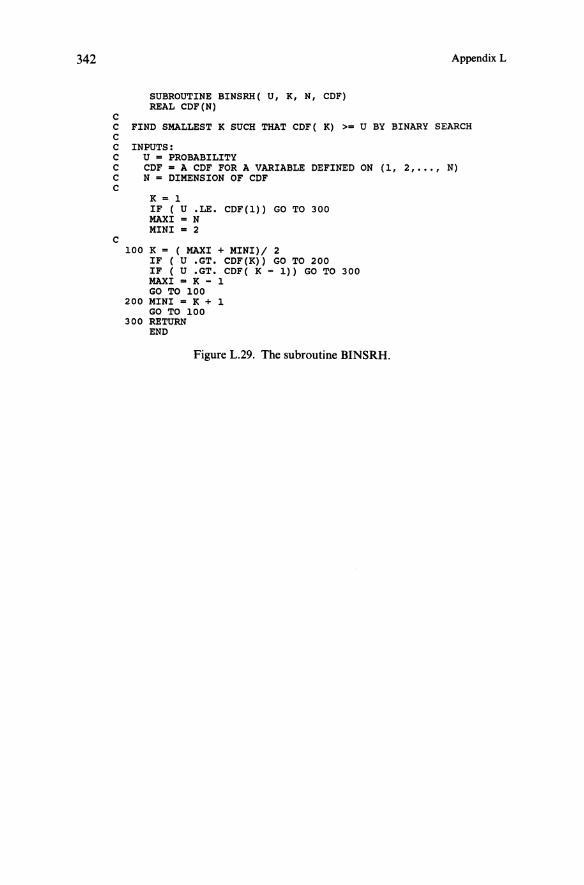
K = 1IF ( U .LE. CDF(l» GO TO 300MAXI = NMINI = 2

INPUTS:U = PROBABILITYCDF = A CDF FOR A VARIABLE DEFINED ON (1, 2, .•• , N)N = DIMENSION OF CDF

342 Appendix L

SUBROUTINE BINSRH( U, K, N, CDF)REAL CDF(N)

CC FIND SMALLEST K SUCH THAT CDF( K) >= U BY BINARY SEARCHCCCCCC

C100 K = ( MAXI + MINI)/ 2

IF ( U .GT. CDF(K» GO TO 200IF ( U .GT. CDF( K - 1» GO TO 300MAXI = K - 1GO TO 100

200 MINI = K + 1GO TO 100

300 RETURNEND

Figure L.29. The subroutine BINSRH .


SUBROUTINE FNORM( X , PHI, UNL)

343

CC EVALUATE THE STANDARD NORMAL CDF AND THE UNIT LINEAR LOSSCC INPUT:C X = A REAL NUMBERVC OUTPUTS:C PHI a AREA UNDER UNIT NORMAL CURVE TO THE LEFT OF X.C UNL = E(MAX(O,X-Z» WHERE Z IS UNIT NORMAL,C I.E., UNL = UNIT NORMAL LOSS FUNCTION =C INTEGRAL FROM MINUS INFINITY TO X OF ( X - Z) F( Z) DZ, WHEREC F(Z) IS THE UNIT NORMAL DENSITY.CC WARNING: RESULTS ARE ACCURATE ONLY TO ABOUT 5 PLACESC

Z = XIF ( Z .LT. 0.) Z = -ZT = 1./(1. + . 2316419 * Z)PHI = T*(.31938153 + T*(-.356563782 + T*(1 .781477937 +

1 T*( -1.821255978 + T*1 .330274429»»E2 = O.

CC 6 S. D. OUT GETS TREATED AS INFINITYC

IF ( Z . LE . 6.) E2 = EXP(-Z*Z/2.)*.3989422803PHI = 1. - E2* PHIIF ( X .LT. 0 .) PHI = 1. - PHIUNL = X* PHI + E2RETURNEND

Figure L.30. The subroutine FNORM.

344 Appendix L

SUBROUTINE TBINOM( N, P, CDF, IFAULT)REAL CDF( N)

TABULATE THE BINOMIAL CDF

TOLERANCE FOR SMALL VALUESDATA TOLR 11.E-101

OUTPUTS:CDF( I) = PROBe X <= 1-1)

= PROBABILITY OF LESS THAN I SUCCESSESIFAULT = 8 IF INPUT ERROR, ELSE 0

INPUTS:N = NO. OF POSSIBLE OUTCOMES(SHIFTED BY 1 SO THEY ARE l,2 • • . N)P = SECOND PARAMETER OF BINOMIAL, 0 <= P <= 1.E.G., A BINOMIAL WITH 10 TRIALS AND A PROBABILITY OFSUCCESS OF . 2 AT EACH TRIAL HAS 11 POSSIBLEOUTCOMES, THUS TBINOM IS CALLED WITH N = 11 AND P = . 2

CCCCCCCCCCCCCCCCC SOMEWHAT CIRCUITOUS METHOD IS USED TO AVOID UNDERFLOWC AND OVERFLOW WHICH MIGHT OTHERWISE OCCUR FOR N > 120.CC

CC DATE 13 SEPT 1986CC CHECK FOR BAD INPUTC

IF « N .LE. O).OR.( P .LT. O.).OR.( P .GT. 1.» GO TO 9000IFAULT - 0

CC WATCH OUT FOR BOUNDARY CASES OF PC

IF ( P .GT. 0.) GO TO 50DO 30 J = l,NCDF( J) = 1.

30 CONTINUERETURN

50 IF ( P .LT. 1.) GO TO 70DO 60 J = 1, NCDF(J) = O.

60 CONTINUECDF( N) = 1.RETURN

CC TYPICAL VALUES OF P START HEREC

70 QOP = ( 1. - P)I PPOQ = P/( 1. - P)R = 1.

CC SET K APPROXIMATELY = MEANC

K - N* P + 1.IF ( K .GT. N) K = NCDF(K) = 1.K1 = K-1TOT = 1.IF ( K1 .LE. 0) GO TO 150J = K

(continued )


CC CALCULATE P.M.F. PROBABILITIES RELATIVE TO P(K).C FIRST BELOW KC

DO 100 I = 1, KlJ = J - 1

CC RELATIVELY SMALL PROBABILITIES GET SET TO O.C

IF ( R .LE. TOLR) R = O.R = R* QOP *J/( N - J)CDF( J) = RTOT = TOT + R

100 CONTINUECC NOW ABOVE KC

150 IF ( K .EQ. N) GO TO 300R =l.Kl = K + 1DO 200 J = Kl , N


IF ( R .LE. TOLR) R O.R = R * POQ*( N - J + 1)/( J -1)TOT = TOT + RCDF( J ) = R

200 CONTINUECC NOW RESCALE AND CONVERT P.M.F. TO C.D.F.C

300 RUN = O.DO 400 J = 1, NRUN = RUN + CDF( J)/ TOTCDF( J) = RUN

4 00 CONTINUERETURN


Figure L.31. The subroutine TBINOM.

345

346 Append ix L

SUBROUTINE TTPOSN( N, NSTART, P, CDF, IFAULT)REAL CDF( N)

CC TABULATE THE TRUNCATED POISSON CDF.CC INPUTS:C N = NUMBER OF VALUES TO TABULATEC NSTART = STARTING VALUEC P = MEAN OF THE DISTRIBUTIONCC OUTPUTS:C CDF( I) = THE CDF OF THE POISON DISTRIBUTIONC SHIFTED SO THAT CDF( I) = PROBe X <= I + NSTART - 1).C IFAULT = 9 IF INPUT ERROR, ELSE 0CC TOLERANCE FOR SMALL VALUES

DATA TOLR/.1E-18/CC CHECK FOR BAD INPUTC

IFAULT = 0IF « N .LE. 0) .OR. ( P .LT. 0 .)

1 .OR . ( NSTART .LT. 0» GO TO 9000CC WATCH OUT FOR BOUNDARY CASES OF PC

IF ( P .GT . 0.) GO TO 50DO 30 J = 1, NCDF( J) = 1.

30 CONTINUERETURN

CC TYPICAL VALUES OF P START HEREC

50 R = 1.TOT = 1.K=P+1.NLIM N + NSTARTIF ( K .GT . NLIM) K = NLIMIF ( K .LE. NSTART) K = NSTART + 1CDF( K - NSTART) = 1.K1 = K - 1 - NSTARTIF ( K1 .LE. 0) GO TO 150J = K

CC CALCULATE P.M.F. PROBABILITIES RELATIVE TO P(K)C FIRST GO DOWN FROM KC

DO 100 I = 1, K1CC RELATIVELY SMALL PROBABILITIES GET SET TO O.C

IF ( R .LE. TO~) R = O.J = J - 1R = R* J/ PCDF( J - NSTART) = RTOT = TOT + R

100 CONTINUE

(continued)


CC NOW GO UPC

150 K1 = K1 + 2IF ( K1 .GT. N) GO TO 300R = 1.JJ = KDO 200 J = K1 , N


IF ( R .LE. TOLR) R = O.R = R* PI JJTOT = TOT + RCDF( J ) = RJJ = JJ + 1

200 CONTINUECC NOW RESCALE AND CONVERT TO C.D.F.C

300 RUN = O.DO 400 J = 1, NRUN = RUN + CDF( J)I TOTCDF( J) = RUN

400 CONTINUERETURN

C9000 IFAULT 9

RETURNEND

Figure L.32. The subroutine TTPOSN.

347

APPENDIX X

Examples of Simulation Programming

This appendix contains most of the programs and examples referred to inChapters 7 and 8. A number of comments are in order.

First and foremost, these programs are illustrations : they are not intendedto be copied slavishly. The Fortran programs, for example, are written inthe current ANSI standard Fortran [ANSI (1978)], using the full language.They will not run on machines still using Fortran IV, nor on compilers whichaccept only the official ANSI subset. Simula programs are presented withkeywords underlined and in lower case, since we believe this is easier toread than the all-upper-case representation imposed by some machines. Allthe programs presented have been tested in one form or another, though notnecessarily with exactly the text given in this appendix.

While writing this book we used a variety ofmachines. Most of the numerical results in Chapter 8 were obtained using a CDC Cyber 173; almost all ofthem were checked on a XDS Sigma 6. The examples in Simula and GPSSwere also run on a Cyber 173. The examples in Simscript were run on an IBM4341. Some of the GPSS programs were also checked on this machine .

The reader should be aware that ifhe doesrun our programs on a differentmachine, he may get different answers despite using the same portable randomnumber generator. Such functions as ERLANG and NXTARR use floatingpoint arithmetic; NXT ARR in particular cumulates floating-point values.A very minor difference in floating-point representations on two differentmachines may be just enough to throw two supposedly identical simulationsout of synchronization: once this happens, all further resemblance betweentheir outputs may be lost.


PROGRAM BOMBERCOMMON /TIMCOM/TIMEINTEGER INRNGE, BOMB, READY, BURST, EN DSIMINTEGER SEED, EVENT, I, N, GOUT, PD OWNREAL TIME, DIST, TOFFLT, NORMAL, UNIF, RLOGICAL PLANOK(5), GUNOK(3), GUNRDY(3), TRACEPARAMETER (INRNGE = I, BOMB = 2, READY = 3,

X BURST = 4, ENDSIM = 5)EXTERNAL PUT, GET, INIT, UNIF, NORMAL, DIST, TOFFLT

CC EXAMPLE 7.1 .1 FROM SECTION 7.1 .4CC TIME IS MEASURED IN SECONDS.C TIME 0 IS WHEN THE FIRST AIRCRAFTC COMES IN TO RANGE .CC CHANGE THE FOLLOWING TO SUPPRESS TRACEC

TRACE = .TRUE.CC INITIALIZE - ALL PLANES ARE OU T OF RANGE, ALL GUNS AREC INTACT AND READY TO FIRE.C NO PLANES HAVE BEEN SHOT DOWN .C

CALL INITDO 1 1=1,5PL ANOK(I) = . FALSE.PDOWN = 0DO 2 1=1,3GUNOK(I) = .TRUE.

2 GUNRDY(I) = .TRUE .GOUT = 0SEED = 1234 5

349

CCCCC

CCCCCCCC

R IS THE RANGE FOR OPENING FIRE.THE SCHEDULE INITIALLY CONTAINS JUST TWO EVENTS: PLANE 1COMES INTO RANGE AND THE END OF THE SIMULATION .

R = 3000 .0CALL PUT(INRNGE, (3900 .0-R)/300.0, 1)CALL PUT(ENDSIM, 50.0, 0)

99 CALL GET(EVENT, N)IF (EVENT .EQ. INRNGE) GO TO 100IF (EVENT . EQ. BOMB) GO TO 200IF lEVENT .EQ. READYl GO TO 300IF EVENT . EQ. BURST GO TO 400IF (EVENT .EQ. ENDSIM) GO TO 500

THIS SECTION SI MULATES AN AIRCRAFT COMING INTO RANGE

IF IT IS NOT THE LAST AIRCRAFT, SCHEDULE ITS SUCCESSOR .IF THERE IS A GUN READY TO FIRE, IT WILL DO SO .WHEN A GUN FIRES, WE MUST SCHEDULE THE BURST AND ALSOTHE TIME WHEN THE GUN IS RELOADED .FINALLY, SCHEDULE AN ARRIVAL AT THE BOMBING POINT .

(continued)

350

C100910

911

101

Appendix X

IF (TRACE) PRINT 910,TIME,NFORMAT (F6.2, ' AIRCRAFT',I4,' IN RANGE')IF (N .LT. 5) CALL PUT(INRNGE, TIME+2.0, N+1)PLANOK(N) = .TRUE.DO 101 1=1,3IF (.NOT. GUNOK(I) .OR •• NOT. GUNRDY(I» GO TO 101IF (TRACE) PRINT 911,TIME,I,NFORMAT (F6.2,' GUN',I4,' FIRES AT AIRCRAFT',I4)CALL PUT(BURST, TIME+TOFFLT(N), N)CALL PUT(READY, TIME+NORMAL(5.0, 0.5, SEED), I)GUNRDY(I) = .FALSE.CONTINUECALL PUT(BOMB, TIME+R/300.0, N)GO TO 99

CC THIS SECTION SIMULATES AN AIRCRAFT DROPPING ITS BOMBSCC IF THE PLANE HAS BEEN DESTROYED, THE EVENT IS IGNORED.C OTHERWISE, WE DECIDE FOR EACH GUN IN TURN IF IT ISC HIT DR NOT.C

200 IF (PLANOK(N» THENIF (TRACE) PRINT 920,TIME,N

920 FORMAT (F6.2,' AIRCRAFT',I4,' DROPS ITS BOMBS')DO 201 1=1,3IF ( (UNIF(SEED) .LE. 0.2) .AND. GUNOK(I) ) THEN

GUNOK(I) = .FALSE.GOUT = GOUT + 1IF (TRACE) PRINT 921,TIME,I

921 FORMAT (F6.2,' GUN',I4,' DESTROYED')ENDIF

201 CONTINUEENDIFGO TO 99

CC THIS SECTION SIMULATES THE END OF LOADING A GUNCC IF THE GUN HAS BEEN DESTROYED, THE EVENT IS IGNORED.C OTHERWISE, LOOK FOR A TARGET: WE TRY FIRST THE NEARESTC ONCOMING PLANE, THEN THE NEAREST RECEDING PLANE. IFC A TARGET IS FOUND, SCHEDULE THE BURST AND THE END OFC RELOADING; OTHERWISE, MARK THE GUN AS READY.C

300

301

302

930

303931

IF (GUNOK(N» THENDO 301 1=1,5IF (PLANOK(I) .AND. DIST(I) .LE. 0) GO TO 303CONTI NUEDO 302 I = 5, 1, -1IF (PLANOK(I) .AND. DIST(I) .LE. 2100.0) GO TO 303CONTINUEIF (TRACE) PRINT 930,TIME,NFORMAT (F6.2,' GUN',I4,' READY - NO TARGET')GUNRDY(N) = .TRUE.GO TO 99IF (TRACE) PRINT 931,TIME,N,IFORMAT (F6.2,' GUN',I4,' FIRES AT AIRCRAFT',I4)CALL PUT(BURST, TIME+TOFFLT(I), I)CALL PUT(READY, TIME+NORMAL(5.0, 0.5, SEED), N)

ENDIFGO TO 99

(continued )

Examples of Simulation Programmmg 351

CC THIS SECTION SIMULATES A SHELL BURSTC

943,TIME,NSHOT AIMED AT AIRCRAFT' ,14,THE AIR')

IF (PLANOK(N)) THENIF (TRACE) PRINT 940,TIME,NFORMAT (F6.2,' SHOT BURSTS BY AIRCRAFT',14)IF (UNIF{SEED).GT.0.3-ABS{DIST{N))/10000.0) THEN

IF (TRACE) PRINT 941,TIME,NFORMAT (F6.2,' AIRCRAFT',I4,' DESTROYED')PLANOK{N) = .FALSE.PDOWN = PDOWN + 1

ELSEIF (TRACE) PRINT 942,TIMEFORMAT (F6.2,' NO DAMAGE')

ENDIFELSE

IF (TRACE) PRINTFORMAT (F6.2,'

I BURSTS IN943

XENDIFGO TO 99

942

941

400

940

CC THIS IS THE END OF THE SIMULATIONC

500 PRINT 9S0,GOUT,PDOWH950 FORMAT (1//,15,' GUNS DESTROYED',/,IS,

X I PLANES SHOT DOWN')STOPEND

Figure X.7.1. A simulation in Fortran.

352 Append ix X

PROGRAM SIMNAICOMMON /TIMCOM/ TIMEINTEGER ARRVAL,ENDSRV,OPNDOR,SHTDORINTEGER ARRSD,SRVSD,TELSD,RNGSDINTEGER QUEUE,TLATW K,TLFREE,NCUST,NSERVINTEGER NREPLS,REPL,EVENT,IREAL TIME,NXTARR,ERLANG,UNIF,XLOGICAL TRACEPARAMETER (ARRVAL = I, ENDSRV = 2, OPNDOR = 3, SHTDOR 4)EXTERNAL NXTARR, UNIF, ERLANG, INIT, PUT, GET, SETARR

CC EXAMPLE 1.4.1 - SEE SECTION 7.1.6CC THE TIME UNIT IS 1 MINUTE.C TIME 0 CORRESPONDS TO 9 A.M.CC CHANGE THE FOLLOWING TO SUPPRESS TRACEC

TRACE = .TRUE.CC SET RANDOM NUMBER SEEDS SPACED 200000 VALUES APARTC

ARRSDSRVSDTELSDRNGSD

123456789019339855442050954260918807827

CC SET NUMBER OF RUNS TO CARRY OUTC

NREPLS = 200DO 9B REPL = I,NREPLS

CC INITIALIZE FOR A NEW RUNCC SET NUMBER OF TELLERS AT WORK.C INITIALLY NO TELLERS ARE FREE SINCE THE DOOR IS NOT OPENC

X = UNIF(TELSD)TlATWK = 3IF (X.LT.0.20) TLATWK = 2IF (X.LT.0.05) TLATWK = 1TlFREE = 0IF (TRACE) PRINT 950,TLATWK

950 FORMAT (13, ' TELLERS AT WORK')CC SET QUEUE EMPTY, NO CUSTOMERS OR SERVI CES SO FARC

QUEUE 0NCUST = 0NSERV = 0

CC SET TIME 0, SCHEDULE EMPTY, ARRIVAL DISTBN INITIALIZEDC

CCCC

CALL INITX = SETARR(O)

INITIALIZE SCHEDULE WITH FIRST ARRIVAL,AND CLOSING OF DOOR ( = END OF 1 RUN)

CALL PUT (ARRVAL, NXTARR(ARRSD))CALL PUT (OPNDOR, 60.0)CALL PUT (SHTDOR, 360.0)

OPEN I NG OF DOO R,

(continued)

Examples of Simulation Programming 353

CCCCCCC

** *** ** * ** * * * * ** * *

START OF MAI N LOO P

************** ****

CCC

CALL PUT (ARRVAL, NXTARR(ARRSD))

99 CALL GET (EVENT)IF (EVENT .EQ. ARRVAL) GO TO 100IF (EVE NT .E Q. ENDSRV) GO TO 200IF (EVEN T .EQ. OPNDOR) GO TO 300IF (EVENT .EQ. SHTDOR) GO TO 400

THIS SECTION SIMULATES THE ARRIVAL OF A CUSTOME R

100 NCUST = NC UST + 1IF (TRACE) PRINT 951, TIM E,NC UST

951 FORMAT (FI0.2,· ARRIVA L OF CUST OM ER ',I 6)CC AT EACH ARRIVAL, WE MUST SCHED ULE THE NEX TC

CC IF TH ERE IS A TELLER FRE E, WE START SERVICEC

I F (TLFRE E.GT.O) THENTLFREE = TLFREE - 1NSERV = NSERV + 1IF (TRACE) PRINT 952,TIME ,NSERV

952 FORMAT (F10.2, ' START OF SERVI CE',I6)CALL PUT (END SRV , TIME + ERLANG(2.0 ,2,SRV SD))

CC OTHERWISE THE CUSTOMER MA Y OR MAY NOT STAY ,C DEPENDING ON THE QUEUE LENGTHC

ELSEIF (UNIF(RNGSD).GT.(QUEUE-5)/5.0) THEN

QUEUE = QUEUE + 1IF (TRACE) PR INT 953,T IM E,QU EUE

953 FORMAT (F10.2,' QUEUE IS NOW' , I6 )ELSE

IF (TRACE) PRINT 954,TIME954 FORMAT (F10.2 , ' CUSTOMER DOES NOT JOIN QUEUE')

ENDIFENDIFGO TO 99

CC IN THIS SECTION WE SIMULATE THE END OF A PER IOD OF SERVICECC IF THE QUEUE IS NOT EMPTY, THE FIRST CUSTOMER WILL STARTC SERVICE AND WE MUST SCHEDULE THE CORRESPONDING ENDC SERVICE. OTHE RWISE THE TE LLER IS NOW FREE.C

200 IF (QUE UE .NE.O) THENNSERV = NSERV + 1QUEUE = QUEUE - 1IF (TRACE) PRINT 955,TIME,NSERV

955 FORMAT (FlO.2,' START OF SERVICE' ,16)I F (TRACE) PRINT 956,TIME,QUEUE

956 FORMAT (F10.2,' QUEUE IS NOW ',I6)CALL PUT (ENDSRV, TIME + ERLANG(2.0,2 ,SRVSD))

(continued)

354

ELSETLFREE = TLFREE + 1IF (TRACE) PRINT 957,TIME,TLFREE

957 FORMAT (FlO.2,' NUMBER OF TELLERS FREE',16)ENDIFGO TO 99

AppendixX

CC THIS IS THE END OF ONE RUNC

CC IN THIS SECTION WE SIMULATE THE OPENING OF THE DOORCC ALL THE TELLERS BECOME AVAILABLE. IF THERE ARE CUSTOMERSC IN THE QUEUE, SOME OF THEM CAN START SERVICE AND WE MUSTC SCHEDULE THE CORRESPONDING END SERVICE EVENTS.C

300 TLFREE = TLATWKIF (TRACE) PRINT 958,TIME

958 FORMAT (F10.2,' THE DOOR OPENS')DO 301 I = I,TLATWKIF (QUEUE.NE.O) THEN

NSERV = NSERV + 1QUEUE = QUEUE -1TLFREE = TLFREE - 1IF (TRACE) PRINT 959,TIME,NSERV

959 FORMAT (FlO.2,' START OF SERVICE',16)IF (TRACE) PRINT 960,TIME,QUEUE

960 FORMAT (FI0.2,' NUMBER IN QUEUE IS NOW ',I6)CALL PUT (ENOSRV, TIME + ERLANG(2.0,2,SRVSO»

ENDIF301 CONTINUE

IF (TRACE) PRINT 961,TIME,TLFREE961 FORMAT (F10.2,' NUMBER OF TELLERS FREE',16)

GO TO 99CC IN THIS SECTION WE SIMULATE THE CLOSING OF THE DOORCC SINCE WE KNOW ALL CUSTOMERS ALREADY IN THE QUEUE WILLC EVENTUALLY RECEIVE SERVICE, WE CAN SIMPLY COUNT THEMC AND STOP SIMULATING AT THIS POINT.C

400 CONTINUEIF (TRACE) PRINT 962,TIME,QUEUE

962 FORMAT (f10.2,' OOOR CLOSES: NUMBER IN QUEUE',16)NSERV = NSERV + QUEUEPRINT 990, TLATWK, NCUST, NSERV

990 FORMAT (16,' TELLERS,',16,' CUSTOMERS,',I6,' WERE SERVED')WRITE (1,991) TLATW K,NCUST ,NSERV

991 FORMAT (316)

98 CONTINUESTOPEND

Figure X.7.2. The standard example in Fortran.

Examples of Simulat ion Programming

REAL FUNCTION ERLANG(MEAN,SHAPE,SEED)REAL MEAN ,UNIF,XINTEGER SHAPE ,SEED,IEXTERNAL UNIFX = 1.°DO 1 I = 1,SHAPEX = X * UNIF(SEED)ERLANG = - MEAN * ALOG(X) / SHAPERETURNEND

Figure X.7.3. The function ERLANG.

REAL FUNCTION NXTARR(SEED)REAL X(4),Y(4),MEAN(4) ,CUMUL ,UNIFINTEGER SEG ,SEEDEXTERNAL UNIFSAVE CUMUL, SEG, X, Y, MEAN

355

CC THIS SUBROUTINE IMPLEMENTS A PROCEDUREC FOR NONSTATIONARY PROCESSES: SEE 5.3.18, 4.9.C CUMUL GIVES THE SUCCESSIVE VALUES OF Y, WHILE SEG TELLS USC WHICH SEGMENT DF THE PIECEWISE-LINEAR INTEGRATED RATEC FUNCTION WE ARE CURRENTLY ON.CC THE TABLE BELOW DEFINES THE PIECEWISE-LINEAR FUNCTION .C THE DUMMY VALUE OF Y(4) SERVES TO STOP US OVER -RUNNINGC THE TABLE.C

DATA X / 45.0,120 .0,300.0, 0.0/DATA Y / 0.0 , 37.5,217.5, 1E10/DATA MEAN / 2.0, 1.0, 2.0, 0.0/CUMUL = CUMUL - ALOG(UNIF(SEED»

CC FIRST WE MUST CHECK IF WE ARE STILL IN THE SAME SEGMENTC

IF (CUMUL .LT.Y(SEG+1» GO TO 2SEG = SEG + 1GO TO 1

CC NOW WE KNOW THE SEGMENT, WE CAN CALCULATE THE INVERSEC

2 NXTARR = X(SEG) + (CUMUL - Y(SEG» * MEAN(SEG)RETURN

CC THIS ENTRY POINT INITIALIZES CUMUL AND SEGC

ENTRY SETARRCUMUL = 0.0SEG = 1SETARR = 0.0RETURNEND

Figure X.7.4. The function NXTARR.

356 Appendix X

" EX AM PLE OF SIMSCR IP T MODE LI NG

" EX AMPLE 7. 2.1 DF SEC TION 7. 2.3

PR EAMB LE

EV ENT NOTIC ES I NCLUOE CUSTO MER . AR RIV AL , NEW.HAMBURG ER,AND STO P. SIMULATIONEVE RY END. SE RVI CE HA S A PATR ON

TEM PORARY ENTITI ESEVERY OROER HAS A SIZE

AND A TIME. OF.ARR I VALAN O MAY BEL ON G TO TH E QU EUE

DE FINE TIME.OF.ARRIVAL AS A REAL VARIABLEUErl NE SI ZE AS AN INTEGER VARIA BLE

THE SYSTE M HA S A SER VER. STATU SAND A TOT AL .CUSTO MERSAND A LDST. CUST OME RSAND A STO CKAND A SER VICE. TIMEAND A STR EAM.NOAN D AN ORDER . SI ZE RANDOM STE P VAR IAB LEAND OWNS TH E QU EU E

DEFINE SERVI CE. TIME AS A REAL VARIABL EDEFINE TOTAL.CU ST OMERS, LOST.CU ST OME RS, STO CK,

SERVE R. ST ATUS AND ST REAM.NO AS I NTEG ER VARIA BLE SDEFI NE OR DE R.SIZ E AS AN INT EGER, STR EAM 7 VA RIABLEDEFI NE QUEU E AS A FIFO SET

AC CUMULATE UTILI ZATION AS THE MEAN OF SERVER. STATUSTALLY MEAN. SERVICE.TIME AS THE MEAN OF SERVI CE.TIME

DE FI NE .B USY TO ME AN 1DEFINE .I OLE TO ME AN 0DEFINE SEC ONDS TO MEAN UN ITSDEFINE MINUTES TO MEAN *60 UNIT SDEFINE HOURS TO MEAN *60 MINUTE S

END "P REAM BLE

MA INLET STREAM.NO = IREAD ORDE R. SI ZESCHE DULE A ST OP. SIMULA TI DN IN 4 HO URSSCH EDU LE A NEW. HAMBURGER IN

UNIFOR M. F(30 . 0 ,50.0 ,S TREAM. ND) SECO ND SSCHEDULE A CUS TO MER. ARRI VAL IN

EXPONENTIAL.F(2.5, STREAM.NO) MINUTE SSTART SIMULATION

END " MAI N

EVENT CU STO MER. ARRI VALADD 1 TO TOTAL. CU STOME RSSCHE OULE A CU STOMER.ARRIVAL IN

EXPONENTIAL.F(2.5,STREAM.NO) MINUTE SIF N.QUEUE = 3,

ADD 1 TO LOST.CUST OMERS(continued)


ELSECREATE AN ORDERLET SIZE(ORDER) = ORDER. SIZELET TIME.Of.ARRIVAL = TIME.VfILE ORDER IN QUEUECALL START.SERVICE

ALWAYSRETURN

END' 'EVENT CUSTOMER.ARRIVAL

ROUTINE TO START.SERVICEIf SERVER. STATUS = .IDLE

AND QUEUE IS NOT EMPTYAND SIZE(f.QUEUE) < STOCKREMOVE fIRST ORDER fROM QUEUESUBTRACT SIZE(ORDER) fROM STOCKLET SERVER. STATUS = .BUSYSCHEDULE AN END. SERVICE GIVING ORDER IN

45.0 + 25.0*SIZE(ORDER) SECONDSALWAYSRETURN

END' 'ROUTINE TO START.SERVICE

EVENT NEW. HAMBURGERADD 1 TO STOC K

SCHEDULE A NEW. HAMBURGER INUNIfORM.f(30.0,5D.0,STREAM.NO) SECONDS

CALL START.SERVI CERETURN

END' 'EVENT NEW. HAMBURGER

EVENT EN D. SE RVICE GIVEN ORDERDEfINE ORDER AS AN I NTEGER VAR IABLELET SERVI CE.TIME = TIME.V - TIME.Of.ARRIVAL(ORDER)DESTROY THIS ORDE RLET SERVER. STATUS = .IDLECALL START.SERVICERETURN

END ' 'EVENT END. SERVI CE

EVENT STOP. SIMULATIO NPR I NT 3 LINES WITH TOTAL.CUST OME RS, LOST.C USTOMERS,

MEA N.SERVI CE.TIME AND UTILI ZA TION THUS*** CUSTOMER S ARRIVED. ***WERE LOST.MEAN SERVI CE TIME WA S *** SECONDS.THE SERVER UTILIZATION WAS *.**

STOPEND' 'STOP.SIMULATION

Figure X.7.5. A simulat ion in Simscript.

357

358

THE STANDARD EXAMPLE IN SIMSCRIPT 11.5

THE T[ME UNIT [S 1 MINUTE, WITH TIME 0 AT 9.00 A.M.

PREAMBLE

EVENT NOTICES INCLUDE ARRIVAL, DEPARTURE, OPENING,AND CLOSING

Appendix X

TEMPORARY ENTITIESEVERY CUSTOMER HAS A TIME.OF.ARRIVAL AND MAY BELONG

TO THE QUEUE

THE SYSTEM OWNS THE QUEUE

DEFINE TEL.FREE, TEL.AT.WORK, NUM.CUSTOMERS,NUM.SERVICES, AND NUM.BALKS AS INTEGER VARIABLES

DEFINE WAITING.TIME AS A REAL VARIABLEDEFINE NEXT.ARRIVAL AS A REAL FUNCTION

DEFINE ARRIVAL.SEED TO MEAN 1DEF[NE SERVICE.SEED TO MEAN 2DEFINE TELLER. SEED TO MEAN 3DEFINE BALK. SEED TO MEAN 4

ACCUMULATE AVG.QUEUE AS THE AVERAGE OF N.QUEUETALLY AVG.WAIT AS THE AVERAGE OF WAITING. TIME

END

MAIN

DEFINE X AS A REAL VARIABLE

LET X = UNIFORM.FIO.O, 1.0, TELLER.SEE~)

LET TEL.AT.WORK = 3 "NOW FIX UP NUMBER OF TELLERSIF X < 0.2 LET TEL.AT.WORK = 2ALWAYS IF X < 0.05 LET TEL.AT.WORK = 1

ALWAYS

LET TEL.FREE = 0LET NUM.CUSTOMERS 0LET NUM.SERVICES 0LET NUM.BALKS 0

SCHEDULE AN OPENING AT 60.0SCHEDULE A CLOSING AT 360.0SCHEDULE AN ARRIVAL AT NEXT.ARRIVALSTART SIMULATION

"CONTROL WILL RETURN WHEN ALL CUSTOMERS HAVE BEEN SERVED

PRINT 3 LINES WITH TEL.AT.WORK,NUM.CUSTOMERS, NUM.SERVICES,

NUM.BALKS, AVG.QUEUE, AND AVG.WAIT THUS** TELLERS AT WORK*** CUSTOMERS, *** SERVICES, *** BALKSAVERAGE QUEUE *.**, AVERAGE WAIT *.** MINUTES

END(continued)


(continued)

EVENT ARRIVALADD 1 TO NUM.CUSTOMERSSCHEDULE AN ARRIVAL AT NEXT.ARRIVALIF (N.QUEUE - 5}/5.0 > UNIFORM.F(D.O, 1.0, BALK. SEED)

ADD 1 TO NUM.BAL KSRETURN

ALWAYSIF TEL.FREE = 0

CREATE A CUSTOMERLET TIME.OF.ARRIVAL(CUSTOMER} TIME.VFILE CUSTOMER IN QUEUE

ELSELET WAITING.TIME = 0.0SCHEDULE A DEPARTURE IN ERLANG.F(2.0, 2, SERVICE.SEED}

UN ITSADD 1 TO NUM.SERVICESSUBTRACT 1 FROM TEL.FREE

ALWAYSRETURN

END

EVENT DEPARTUREIF QUEUE IS EMPTY

ADD 1 TO TEL.FREEELSE

REMOVE FIRST CUSTOMER FROM QUEUELET WAITING.TIME = TIME.V - TIME.OF.ARRIVAL(CUSTOMER}DESTROY CUSTOMERSCHEDULE A DEPARTURE IN ERLANG.F(2.0, 2, SERVICE.SEED}

UNITSADD 1 TO NUM.SERVICES

ALWAYSRETURN

END

EVENT OPENINGDEFINE I AS AN INTEGER VARIABLERESET TOTALS OF N.QUEUEFOR I = 1 TO TEL.AT.WORK DO

SCHEDULE A DEPARTURE NOWLOOP

FREEING AL L THE TELLERS HAS EXACTLY THE SAME EFFECTAS TEL.AT.WORK DEPARTURES

END

EVENT CLOSINGCANCEL THE ARRIVALRET URN

ENDROUTINE NEXT.ARRIVAL

DEFINE X, Y, AND M AS REAL, SAVED, I-DIMENSIONAL ARRAYSDEFINE CUMUL AS A REAL, SAVED VARIABLEDEFINE SEG AS AN INTEGER, SAVED VARIAB LE

IF SEG = 0 I I THIS IS THE FIRST CALL OF THE RO UTINELET SEG = 1LET CUMUL = 0.0RESERVE X(*}, Y(*}, AND M(*} AS 4LET X(I} 45.0LET X(2} = 120 .0

300.00.00.037.5217.599999.92.01.02.00.0

360

END

LET X(3)LET X(4)LET Y(I)LET Y(2)LET Y(3)LET Y(4)LET M(I)LET M( 2)LET M(3)LET M(4)

ALWAYSADD EXPONENTIAL.F(I.0. ARRIVAL. SEED) TO CUMUL'SEARCH' IF CUMUL >= Y(SEG+l)

ADD 1 TO SEGGO TO SEARCH

ALWAYSRETURN WITH X(SEG) + (CUMUL - Y(SEG)) * M(SEG)

Figure X.7.6. The standard example in Simscript.

Appendix X

Examples of Simul at ion Pr ogramm ing

SIMULATE

* EXAMPLE 7.3.1 OF SECTION 7. 3.4* 1 SIMULATE D TIME UNIT REPRE SENT S 100 MSE C.

EXPO FUNCTI ON RN 8, C240.0, 0/ 0. 1, 0. 104/0 . 2 , 0. 222/0 . 3 ,0 . 355/0 . 4 ,0 .509/0 . 5, 0 . 690.6,0.915/0.7,1.2/0.75,1.38/0. 8,1 .6/0. 84,1. 83/ 0. 88, 2.1 20.9,2.3/0.92,2.5 2/0.94 , 2. 81/0.95,2.99/0.9 6,3. 2/0. 97, 3.50.9 8, 3.9/0.99,4.6/0. 995 ,5.3/0.998, 6.2/0.9 99,7. 0/ 0.9 997, 8. 0

361

CLA SS FUN CTION0.6,1/0.9,2/1.0,3

TIME FUN CT I ON1,1/2 ,5/3,20

CORE FUNCTION1,16/2, 32/3,6 4

RN7 ,D3

PF1, L3

PFl,L3

MEMRYALLCLSICLS 2CLS3TOTAL

CYCLE

RR OB

DO NE

STORAGEEQ UQTABLEQTABLEQTABLEQTABLE

GE NE RATETERMINATE

GENERATE

ADVANCEASSIGNASS IGNASSIGNQUEUEQUEUEENTERSE I ZEADVAN CEREL EAS EASSIGNTES T GBUFFE RTRAN SFERLEA VEDEP ARTDEP AR TTRAN SFE R

ST ART

RESETSTAR TEND

2564,Q1,1 0 ,10,1 52, 10 , 10 , 153, 50 , 50 , 10ALL,20 ,20 , 30

6001

" ,2 0,,3PF

100,FN$EXPOI,FN$CLASS,PF2,F N$T IME,PF3 ,FN$CDRE,PFPFIALLMEMRY.PF 3CPU1CPU2-, I, PFPF2,O , DONE

,RROBME MRY, PF3PF IALL, CY CLE

1, NP

10

TIM ER - DE CREME NT SCOUNTER EVERY MINUTE

CREATE 20 TR ANS AC TIONSWITH 3 FUL L-WORDPARAMETERS EA CH.TYPE A COMMAND.

COMMAND TRANSMITT ED.

CONTE ND FOR CO RF.

USE 1 QUANTUM OF CPU.

IF REQ UIR ED TIME IS NO WZERO , GO TO DONE;OTHER WISE GO TO BAC K OFCPU QUEUE AND WAIT TU RN.REL EASE CO RE.REPLY READ Y : ME ASU RERESPO NS E TIME.

INI TI AL I ZE WI THOU TPR INT I NG.REI NI TI ALIZE STATI STI CS.SIMULATE 10 MI NUT ES.

Figure X.7.7. A simulation in GPSS.

362 Appendix X

SIMULATE** THE RUNNING EXAMPLE - SEE SECTION 1.4** THE TIME UNIT IS 1 SECOND, WITH TIME 0 AT 9.45 A.M.* THUS TIME 900 10.00 A.M.* 4500 11.00 A.M.* 15300 = 2.00 P.M.* 18900 = 3.00 P.M.** THE FOLLOWING ENTITIES ARE USED:** FACILITIES - TELLl, TELL2, TELL3 : THE THREE TELLERS* QUEUES BANK KEEPS TRACK OF HOW MANY PEOPLE ARE* IN THE SYSTEM* WLINE KEEPS TRACK OF HOW MANY PEOPLE ARE* IN THE WAITING LINE* SWITCHES DOOR SET WHEN THE DOOR OF THE BANK IS OPEN** NOW DEFINE SOME NECESSARY FUNCTIONS:** THE EXPONENTIAL DISTRIBUTION WITH MEAN 1* THIS IS THE STANDARD APPROXIMATION TAKEN FROM THE* IBM MANUAL*EXPON FUNCTION RNl,C240,0/ • 1 , • 104/ • 2, • 222/ • 3 , • 355/ • 4 , • 509/ • 5, • 69/ .6, .915.7,1.2/.75,1.38/.8,1.6/.84,1.83/.88,2.12/.9,2.3.92,2.52/.94,2.81/.95,2.99/.96,3.2/.97,3.5.98,3.9/.99,4.6/.995,5.3/.998,6.2/.999,7/.9997,8** MEAN INTERARRIVAL TIME OF CUSTOMERS AS A FUNCTION* OF THE TIME OF DAY*MEAN FUNCTION Cl,034500,120/15300,60/18900,120** NUMBER OF TELLERS AT WORK*TELLS FUNCTION RNl,D3.8,3/.95,211,1** PROBABILITY OF BALKING ( TIMES 1000 ) AS A FUNCTION* OF WAITING-LINE LENGTH*BALK FUNCTION Q$WLINE,065,0/6,200/7,400/8,600/9,800/10,1000** THE ERLANG DISTRIBUTION WITH MEAN AND SHAPE 2 :* THIS IS CALCULATED SIMPLY AS THE SUM OF TWO EXPONENTIALS*

*ERLAN FVARIABLE 60*(FN$EXPON+FN$EXPON)

* THE FOLLOWING SECTION GIVES THE CODE FOR A CUSTOMER.* AS DISCUSSED IN THE TEXT, THE ARRIVAL DISTRIBUTION IS* FUDGED AT THE POINTS WHERE THE ARRIVAL RATE CHANGES.* A 'CUSTOMER' TRANSACTION HAS ONE HALF-WORD PARAMETER* USED TO HOLD THE NUMBER OF THE TELLER HE IS USING.* (continued)


GET TE LLER

GET TELLER 2

FN$MEAN ,FN$EXPON", ,IPH

GET TELLER 3LEAVE WAITIN G LINERECEIVE SERVICETELLER IS FREEDLEAVE THE SYSTEM

GENERATE A NEWCUSTOMER

o TO CLEAR THE I GENERATE' BLOCKDOOR IF THE DOOR IS CLOSED, WAITBANK ENTER THE SYSTEM.FN$BALK" BALK BALK IF QUEUE TOO LONGWLINE ENTER WAITING LINEALL ,GETl,GET3,3 TRY ALL THREE TELLERSTELL 11,1, PH,SERVTELL21,2, PH,SERVTELL31,3, PHWLI NEV$ERLANPHIBAN K

GENERATE

ADVA NCEGA TE LSQUEUETRANSFERQU EU ETRANSFE RSEIZEASSIGNTRANSFERSEIZEASSIGNTRANSFERSE lZEASSIGNDEPARTADVANCERELEASEDEPARTTEI{MINATE

*

*

GET3

GET 1

SERV

GET2

BALK DEPART BANKTERM I NA TE

AFTEI{ BALKING , LEAVE THE SYSTEM

** THIS SECTION HANDLES THE SETUP OF TELLERS, OPENS* AND CLOSES THE DOOR OF THE BANK, AND CONTROLS* THE ENDING OF THE SIMULATION*

GENERATE 1.. ,I,127,IPH GENERATE ONE TOP-PRIORITY* TRANSACTION

FUN AVAIL TEL L1- TELL3 AT 9.45 AL L TELLERS ARE* UNAVAILABLE

ADVANCE 899 WAIT UNTIL 10.00LOGIC S DOOR OPEN THE DOORASSIGN I , FN$TE LLS,P HFAVAIL TELL!TEST G PHl,I,*+4 MAKE 1 TO 3 TELLERSFAVAIL TELL 2 AVAILABLETEST G PHl,2,*+ 2FAVAIL TELL3ADVANCE 18000 WAIT UNTIL 3.00LOGIC R DO OR CLOSE THE DOORTEST E Q$BANK,O WAIT UNTIL CUSTOMERS LEAVETERMINATE 1 END RU N

**** CONTROL CARDS ****

STARTEN D

Figure X.7.8. The standard example in GPSS.

364

simulation begin

comment Example 7.4.1 of section 7.4.3 ;

Append ix X

process class passenger;beglnBoo ean taxpaid, repeat ;real timein;taxpaid : = draw (0.75, seeda);timein := time;activate new passenger~ negexp (1, seedb);if not freeclerks.empty then ~eg~n-- --- activate freecTer s. lrst after current;

freecler ks.f irst.out end; -----wait (checkinq) ---end passenger;

process class clerk;beg~

clerkloop: inspect checkinq.firstwhen passenger do~

checkinq.first.out;if repeat then hold (1) else hold (normal

(3,T;'""Seedc) ) ;.!..f. taxpaid then begin

totpass := totpass + 1;totwait : = totwait + time - time in end

else b~¥in ------- ~ not freetaxmen.empty then~

activate freetaxmen.f irst after current;freetaxmen.f irst.out end; -----

this passenger.into (taxq) ene-endotherwise-waTt (free clerks) ; ------goto clerkloopend clerk;

process class taxman;beg~

taxloop: inspect taxq.firstwhen passenger do begi

htaxq.first:out ; old (negexp (2,seedd));taxpaid : = repeat := true;.!..f. ~ fre~clerks.empty then begin

actlvate freeclerKS:Tirst after current;freeclerks.first.out end; -----

this passenger. into (checkinqr-endotherw~wait (freetaxmen); ---90~0 taxloop.!!!- taxman;integer seeda, seedb , seedc, seedd, i;integer nclerks, ntaxmen, totpass;real totwait;ref (head) checkinq, taxq, freeclerks, freetaxmen;

(continued)


seeda : = 12345; {and so on for the other seeds}nclerks : = inint; ntaxmen : = inint; {read these values}checkinq :- new head; freetaxmen : - new head ;for i : = 1 step 1 until nclerks do activate new clerk;for i := 1 ~ 1 untl1 ntaxmen era actlvate "i'ii!'W taxman;activate new passenger~ negexp (1, seedb';-hol d (120"f;outtext ('number of clerks'); outint (nclerks, 6); outimage;outtext ('number of taxmen'); outint (ntaxmen, 6) ; outimage;outtext ('mean wait'); outfix (totwait/totpass, 2,6); outimage

end simulation

Figure X.7.9. A simulation in Simula.

366

begin external class Demos;

comment Example 7.3.1 of section 7.3 .4 recoded in Demos;

Appendix X

Demos~ref (negexp) thinktime;reT (randint) aux ;ref (res) core, cpu ;reT (histogram) overall;reT (histogram) array response [1:3] ;lnteger array time-needed, core neededlnteger --,---;-

comment The unit of time is 1 msec

[1 : 3]

entity class terminal ;beginlnteger class, time left,real time began;hold (thinktime.sample)i := aux .sample ;class := if i < 60 then 1 else

if i ~ then-2 else 3time began := tTme ;time left : = time needed [class] ;core.acquire (core needed [class])while time left> 0 do----- begin cpu.acquire (1) ;

hold (100) ;time left := time left -100cpu.release (1)

end ;core.release (core needed [class])overall.update (time-time began) ;response [cla ss].update (t ime-time began)repeatend terminal;thinktime :- new negexp ("THINK TIME", 0.0001)aux :- ~ randint ("AUXILIARY", 0,99) ;core : - new res ("CORE", 256) ;cpu : - new res ("CPU", 1) ;overall :-:riew histogram ("OVERALL", 0.0, 60000.0, 30)response [1]":-

new histogram ("CLASS 1", 0.0, 15000.0, 15)response [2] :-

new histogram ("CLASS 2", 0.0, 15000.0, 15)response [3] :-

new histogram ("CLASS 3", 0.0, 60000.0, 30)timeneeded [1] : = 100 ;time needed [2] .- 500 ;time needed [3] : = 2000core needed [1] . - 16 ;core needed [2] : = 32 ;core needed [3] := 64 ;

for

end

i : = 1~ 1 unti I 20 ss~ terminal---r"fERMINAL").schedule (0.0)

hold (60000.0) ;reset ;hold (20.0 * 60000.0)end

Figure X.7.1O. A simulation using Demos .


~external class Demos;Demos beg~

367

comment the runn ing example - see section 1.4.

The time unit is one minute with time a at 9.00 a .m.;

integer n;rea 1 x;ref(count) arrivals, services , balks ;ref (erlang) servicetime;reT (res) tellers ;ref (arrd ist) nextarr ival ;ref (balkdist) balk;

rdist class arrdist;begln ---rea cumul; integer seg ;array x, y, mean [1 . 4] ;ref (negexp) aux;

real procedure sample;begl 1cumu : = cumul + aux. sample;while cumul )= y[seg+l] do seg := seg + 1;sample : = x[seg] + (cumul- y[seg]) * mean[seg] - time~;

x[l] : = 45. 0 ; y[l] .- O. 0; mean[l] ·- 2.0 ;x[2] := 120.0; y[2] : = 37.5; mean[2] : = 1. 0;x[3] .- 300.0; y[3] : = 217.5 ; mean[3] ·- 2.0;x[4] .- 0.0; y[4] .- 1. 0&9 ; mean[4] ·- 0.0;

aux : - new negexp ("arr aux ", 1.0);cumul : = 0.0;s eg : = 1end *** definition of arrd ist ***

bdist class balkd ist (pr);ref (re5Jllr;begin

Boolean procedure sample;sample :- (pr.length - 5) / 5 ) zyqsample;

comment - zyqsample is the (0,1) uniform generatorsupplied by Demos;

end *** definition of balkdist ***entity class customer;begin --arrivals.update (1);new customer ("customer") • schedule (nextarrival • sample);~not balk. sample then- beVln --

te ers. acquire (1);services. update (1);hold (servicetime • sample);tellers. release (1)end (continued)

368

else---Oalks • update (1)end *** definition of customer *** ;

AppendixX

trace;arrivalsservicesbalksservicetimenextarrival

:- newnewnewnewnew

count ("arrivals");count ("services");count ("balks");erlang ("servicetime".arrdist ("interval");

2.0. 2);

comment - draw number of tellers;x new uniform ("aux unif". 0.0. 1.0) • sample;n := rr-x < 0.05 then 1

- else if x~.2 then 2--else 3 ; --

comment

tellersba1ktell ers

- set up required tellers, though they are notyet available;

:- new res ("tellers". n);:- new balkdist ("balks ". tellers);• acqui re (n);

comment - schedule first customer;new customer ("customer") • schedule (nextarrival • sample);

comment - open door and make tellers available at 10.00 a.m.;hold (60.0);tellers. release (n);

comment - wait until 3.00 p.m. and wrap up;hold (300.0);services. update (tellers. length)

endend;

Figure X.7.11. The standard example in Demos.


REAL FUNCTION ERLANG (MEAN, SHAPE, SEED)INTEGER I,J,K,SEEDREAL X(25) ,FX(25) ,U,UNIFEXTERNAL UNIFDATA X 1.0,.2,.4,.6,.8,1.0,1.2,1.4,1.6,1.8,2.0,

X 2.2,2.4,2.6,2.8,3.0,3.2,3.4,3.6,3.8,4.0,X 5.0,6.0,7.0,7.799981

DATA FX/.O,.01752,.06155,.12190,.19121,X .26424,.33737,.40817,.47507,.53716,X .59399,.64543,.69156,.73262,.76892,X .80085,.82880,.85316,.87431,.89262,X .90842,.95957,.98265,.99270,1.01

CC THIS FUNCTION GENERATES AN ERLANG WITH MEAN 2.0C AND SHAPE 2 USING LINEAR INTERPOLATION IN A TABLEC OF THE DISTRIBUTIONCC THE PARAMETERS MEAN AND SHAPE ARE NOT USED, BUTC REMAIN FOR COMPATIBILITY WITH THE MAIN PROGRAM.C

U UNIF(SEED)I = 1J = 25

CC BINARY SEARCH FOR U IN TABLEC

K=(I+J)/2IF (FX(K).LE.U) GO TO 2J = K - 1GO TO 1

2 IF (FX(K+l).GT.U) GO TO 3I = K + 1GO TO 1

3 ERLANG = X(K) + (U - FX(K)) * (X(K+l) - X(K)) 1X (FX(K+l) - FX(K))

RETURNEND

Figure X.8.1. A table-driven Erlang generator.

369

370 Appendix X

cC INITIALIZE FOR A NEW RUNC

IF (EVEN) GO TO 96CC ON AN ODD-NUMBERED RUN, WE START A NEW SEGMENTC OF RANDOM NUMBERS AND SET AVGSRV 2.0C

DO 95 I = 1,100X = UNIF(ARRSD)X = UNIF(SRVSD)

95 X = UNIF(RNGSD)HLDARR ARRSDHLDSRV = SRVSDHLDRNG = RNGSDAVGSRV = 2.0GO TO 97

CC ON AN EVEN-NUMBERED RUN, WE USE THE SAME SEEDSC AS BEFORE FOR ALL GENERATORS, BUT SET AVGSRV = 1.8C

C

C

96 ARRSD = HLDARRSRVSD = HLDSRVRNGSD = HLDRNGAVGSERV = 1.8

97 EVEN = .NOT. EVEN

Figure X.8.2. Additional code when using common random numbers .

Examples of Simulat ion Programming 371

PROGRAM STAREGINTEGER NTELL,NARR,NSERV,N,NM,IREAL X(200),Y(200),ZREAL ARR,SERV,SLOPEREAL SIGX,SIGY,SIGXY,SIGX2,SIGY2,SIGZ,SIGZ2

CC REGRESSION OF NSERV = Y AGAINST NARR = XC WE SUBTRACT OFF THE KNOWN MEAN 247.5 OF XC TO MAKE LIFE MORE SIMPLECC ESTIMATION IS BY SPLITTINGC

N = 0SIGX = 0.0SIGY = 0.0SIGXY 0.0SIGX2 = 0.0SIGY2 = 0.0

CC NTELL IS IN FACT CONSTANT = 2C

CC GET THE DATA AND CALCULATE THE APPROPRIATE SUMSC

1 READ (*,900, END = 2) NTELL,NARR,NSERV900 FORMAT (316)

ARR = NARR - 247.5SERV = NSERVN = N + 1SIGX = SIGX + ARRSIGY = SIGY + SERVSIGXY = SIGXY + ARR * SERVSIGX2 = SIGX2 + ARR * ARRSIGY2 = SIGY2 + SERV * SERVX(N) = ARRY(N) = SERVGO TO 1

CC NOW DO REGRESSION WITH SPLITTINGC WE WILL CALL THE OBSERVATIONS ZC

CC START BY PRINTING THE NAIVE ESTIMATE AS A CHECKC

2 PRINT 901,SIGY/N,(SIGY2 - SIGY*SIGY/N) /X (N * (N-1))

901 FORMAT (' NAIVE EST',F10.4,' EST VAR',FIO.4)

NM = N - 1SIGZ = 0.0SIGZ2 = 0.0D03I=l,N

CC SUBTRACT OFF CURRENT X AND YC

CC CALCULATE THE SLOPE USING THE REMAINING VALUES

SIGX = SIGX - X(I)SIGY = SIGY - Y(I)SIGXY SIGXY - X(I)*Y(I)SIGX2 = SIGX2 - X(I)*X(I)SIGY2 = SIGY2 - Y(I)*Y(I)

(continued)

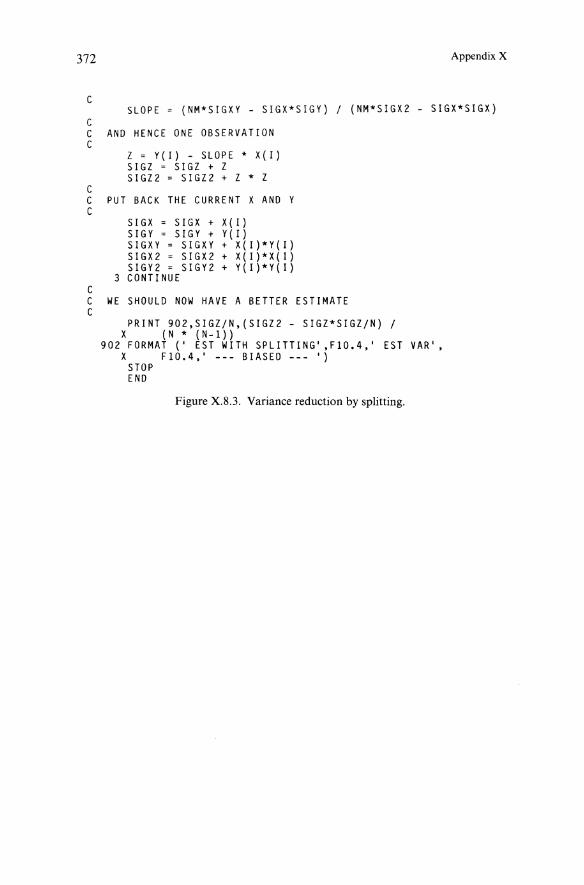
372

C

Append ix X

SLOPE = (NM*SIGXY - SIGX*SIGY) j (NM*SIGX2 - SIGX*SIGX)CC AND HENCE ONE OBSERVATIONC

Z = Y(I) - SLOPE * X(I)SIGZ = SIGZ + ZSIGZ2 = SIGZ2 + Z * Z

CC PUT BACK THE CURRENT X AND YC

SIGX = SIGX + X(I)SIGY = SIGY + Y(I)SIGXY = SIGXY + X(I)*Y(I)SIGX2 = SIGX2 + X(I)*X(I)SIGY2 = SIGY2 + Y(I)*Y(I)

3 CONTINUECC WE SHOULD NOW HAVE A BETTER ESTIMATEC

PRINT 902,SIGZjN ,(SIGZ2 - SIGZ*SIGZjN) jX (N * (N-l))

902 FORMAT (' EST WITH SPLITTING' ,FIO.4,' EST VAR',X FIO.4,' --- BIASED -- - ')

STOPEND

Figure X.8.3. Variance reduction by splitting.


PROGRAM STASPLINTEGER NTELL,NARR,NSERV,N,NM,IREAL X(200),Y(200),ZN,ZREAL ARR,SERV,SLOPEREAL SIGX,SIGY,SIGXY,SIGX2,SIGY2.SIGZ.SIGZ2

CC REGRESSION OF NSERV = Y AGAINST NARR = XC WE SUBTRACT OFF THE KNOWN MEAN 247.5 OF XC TO MAKE LIFE.MORE SIMPLECC ESTIMATION IS BY JACKKNIFINGC

N = 0SIGX = 0.0SIGY = 0.0SIGXY 0.0SIGX2 = 0.0SIGY2 = 0.0

CC GET THE DATA AND CALCULATE THE APPROPRIATE SUMSC

1 READ (*.900. END = 2) NTELL.NARR.NSERV900 FORMAT (316)

CC NTELL IS IN FACT CONSTANT = 2C

ARR = NARR - 247.5SERV = NSERVN = N + 1SIGX = SIGX + ARRSIGY = SIGY + SERVSIGXY = SIGXY + ARR * SERVSIGX2 = SIGX2 + ARR * ARRSIGY2 = SIGY2 + SERV * SERVX(N) = ARRY(N) = SERVGO TO 1

CC START BY PRINTING THE NAIVE ESTIMATE AS A CHECKC

2 PRINT 901.SIGY/N,(SIGY2 - SIGY*SIGY/N) /X (N * (N-l))

901 FORMAT (' NAIVE EST' .FlO.4.' EST VAR' .FlO.4)CC FIRST CALCULATE ZN USING ALL N VALUESC

373

ZN = (SIGY*SIGX2 - SIGX*SIGXY) / (N*SIGX2 - SIGX*SIGX)PRINT 903.ZN

903 FORMAT (' ESTIMATE USING ALL N VALUES' .FI0.4)CC NOW CALCULATE THE PSEUOOVALUESC

NM = N - 1SIGZ = 0.0SIGZ2 = 0.0DO 3 I = I.N

CC SUBTRACT OFF CURRENT X AND YC

SIGX SIGX X(I)SIGY = SIGY - Y(I) (continued)

374

SIGXYSIGX2SIGY2

SIGXY - X( I )*y( I)SIGX2 - X(I)*X(I)SIGY2 - Y(I)*Y(I)

Appendix X

CCC

CCC

CALCULATE AN ESTIMATE USING ONLY N-l VALUES

Z = (SIGY*SIGX2 - SIGX*SIGXY) / (NM*SIGX2 - SIGX*SIGX)

AND HENCE CALCULATE THE NEXT PSEUDOVALUE

Z = N * ZN - NM * ZSIGZ = SIGZ + ZSIGZ2 = SIGZ2 + Z * Z

CC PUT BACK THE CURRENT X AND YC

SIGX = SIGX +SIGY = SIGY +SIGXY = SIGXYSIGX2 = SIGX2SIGY2 = SIGY2

3 CONTINUE

X(I)Y( I )+ X(I)*Y(I)+ X(I)*X(I)+ Y(I)*Y(I)

CC WE SHOULD NOW HAVE A BETTER ESTIMATEC

PRINT 902.SIGZ/N.(SIGZ2 - SIGZ*SIGZ/N) /X (N * (N-l»

902 FORMAT (' EST WITH JACKKNIFING' .F10 .4.' EST VAR' .X FIO.4.' --- BIASED --- ')

STOPEND

Figure X .8A. Variance reduction by jackknifing.

C

REAL FUNCTION B(SRVSD)REAL X,UNIF,ERLANG,BC,BT,BLIM,BMULTINTEGER SRVSDEXTERNAL UNIF. ERLANGCOMMON /BPARAM/ BC,BT,BLIM,BMULT

IF (UNIF(SRVSD).GT.BLIM) THENCC USE TRUNCATED ERLANGC

B = ERLANG(2 .0,2.SRVSD)IF (B.GT.BT) GO TO 1BMULT = BMULT * BC

ELSEcC USE TRUNCATED EXPONENTIALC

B = BT - ALOG(UNIF(SRVSD»BMULT = BMULT * BC * B / BT

ENDIFRETURNEND

Figure X.8.5. Importance sampling-the function B.

References

Abramowitz, M., and Stegun, I. A. (1964). Handbook ofMathematical Functions withFormulas, Graphs, and Mathematical Tables. Dover: New York .

Adelson, R. M. (1966). Compound Poisson distributions. Oper. Res. Quart., 17,73-75 .Ahrens, J. H., and Dieter, U. (1972a). Computer methods for sampling from the

exponential and normal distributions. Commun. ACM, 15, 873-882.Ahrens, J. H., and Dieter, U. (l972b). Computer methods for sampling from gamma,

beta, Poisson and binomial distributions. Computing, 12, 223-246.Ahrens, J. H., and Dieter, U. (1980).Sampling from binomial and Poisson distributions :

a method with bounded computation times. Computing, 25, 193-208.Ahrens, J. H., and Dieter, U. (l982a) . Generating gamma variates by a modified

rejection technique. Commun. ACM, 25, 47-54.Ahrens, J. H., and Dieter, U. (1982b). Computer generation of Poisson deviates from

modified normal distribut ions. ACM Trans. Math . Software, 8, 163-179.Ahrens, J. H., and Kohrt, K. D . (1981). Computer.methods for efficientsampling from

largely arbitrary statistical distributions. Computing, 26, 19-31.Albin, S. L. (1982). On the Poisson approximations for superposition arrival processes

in queues. Manage. Sci., 28, 126-137.Anderson, T. W., and Darling, D. A. (1954). A test of goodness of fit. JASA , 49,

765-769.Andrews, D. F ., Bickel, P. J., Hampel , F. R., Huber, P. J., Rogers, W. H., and Tukey,

J. W. (1972). Robust Estimates ofLocation. Princeton University Press: Princeton ,N.J.

ANSI (1978). American National Standard Programming Language FORTRAN.American National Standards Institute : New York.

Arvidsen, N. I., and Johnsson , T. (1982). Variance reduct ion through negative correlation, a simulation study. J. Stat. Comput. Simul., 15, 119-127.

Asmussen, S. (1985). Conjugate processes and the simulation of ruin problems.Stochastic Process. Appl., 20, 213-229.

Avriel, M. (1976). Nonlinear Programming: Analysis and Methods. Prentice-Hall :Englewood Cliffs, N.J.

Babad, J. M. (1975). The IBM GPSS random number generator. Technical Report ,University of Chicago, Graduate School of Business.

376 References

Barlow, R. E., and Proschan, F . (1965). Mathematical Theory of Reliability. Wiley :New York.

Barr , D. R., and Slezak, N. L. (1972). A comparison of multivari ate normal generators.Commun. ACM, 15, 1048-1049.

Bazaraa, M. S., and Shetty , C. M. (1979). Nonlinear Programming : Theory andAlgorithms. Wiley: New York.

Bennett, C. H. (1979). On random and hard -to-describe numbers . IBM Watson Research Center Report RC 7483 (No. 32272), Yorktown Heights, N.Y.

Bentley, J. L., and Saxe, J. B. (1980). Gener ating sorted lists of random numbers. ACMTrans. Math. Software, 6,359-364.

Bergstrom, H. (1952). On some expansions of stable distribut ions. Ark . Mat . II , 18,375- 378.

Berman, M. B. (1970). Generating random variates from gamma distributions withnon- integer shape parameters. Report R-641-PR, The RAND Corporat ion, SantaMon ica, Calif.

Best, D . J., and Roberts, D . E. (1975). Algorithm AS 91: the percentage points of the X2

distribution. Appl. Stat., 24,385-3 88.Bhattacharjee, G . P. (1970). Algorithm AS 32- The incomplete gamma integral. Appl.

Stat. , 19, 285-287.Billingsley, P. (1968). Convergence of Probability Measures. Wiley: New York.Bil1ingsley, P. (1986). Probability and Measure. Wiley: New York .Birtwhistle, G. M. (1979a). Demos Reference Manual. Dep . of Computer Science,

University of Bradford : Bradford.Birtwhistle, G. M. (1979b). Demos-Discrete Event Modelling on Simula. Macmil1an:

Lond on.Birtwhistle, G. M., Dahl , O.-J., Myhrhaug, B., and Nygaard , K. (1973). Simula Begin.

Studentlitteratur: Oslo.Bobillier, P. A., Kahan, B. c., and Probs t, A. R. (1976). Simulation with GPSS and

GPSS V. Prentice-Hall: Englewood Cliffs, N.J.Boender , C. G. E., Rinnooy Kan, A. H. G. , Timmer, G. T., and Stougie, L. (1982). A

stochastic method for global opt imizat ion. Math. Program., 22, 125-140.Boneh, A. (1983). Preduce- a probabilistic algori thm identifying redunda ncy by a

random feasible point generation. (Lecture Notes in Math emat ics, # 206, Chap.10). Redundancy in Mathematical Programming (M. H. Karm an , V. Lofti, and J.TeIgen, eds.). Sprin ger-Verlag : New York .

Box, G . E. P., H unter, W. G., and Hunter, J. S. (1978). Stat istics fo r Experimenters.Wiley: New York.

Box, G. E. P., and Muller, M. E. (1958). A note on the generation of rand om norm aldeviates. Ann. Math. Stat. , 29, 610-611.

Bratley, P., and Fox , B. L. (1986). Implement ing Sobol's quasirand om sequencegenerat or. Techni cal Report. Universite de Mont real.

Braun , J. E. (editor) (1983). Simscript Il. 5 Ref erence Handbook, 2nd edn ., CACI Inc.:Los Angeles.

Bright , H. S., and Enison , R. L. (1979). Quasi-random number sequences from a longperiod TLP generator with remarks on application to cryptography. Comput.Suru., 11, 357-370 .

Brillinger, D. R. (1981 ). Time Series: Data Analysis and Theory. Holden-Day: SanFrancisco.

Brinch Han sen, P. (1973). Operating System Principles. Prentice-Hall : EnglewoodCliffs, N.J.

Brinch Hansen, P. (1977). The Architecture of Concurrent Programs. Prentice-Hall:Englewood Cliffs, N.J.

Brown, C. A., and Purdom, P. W. (1981). An average time analysis of backtracking .SIAM J. Comput., 10, 583-593.

References 377

Brown, M. , and Solomon, H. (1979). On combining pseudorandom number generators.Ann. Suu., 1, 691-695.

Brown, M., Solomon, H., and Stephens, M. A. (1981). Monte Carlo simulation of therenewal process. J. Appl. Probab., 18,426-434.

Brumelle, S. L. (1971). Some inequalities for parallel service queues. Oper. Res., 19,402--413.

Callaert, H., and Janssen, P. (1981). The convergence rate of fixed-width confidenceintervals for the mean. Sankyii , 43, 211-219.

Carson, J. S. (1978). Variance reduction techniques for simulated queuing processes.Report No . 78-8, Dept. of Industrial Engineering, Un iversity of Wisconsin,Madison .

Carson, J. S. (1980). Linear combinations of indirect estimators for variance reduction inregenerative simulations. Technical Report, Dept. of Industrial and SystemsEngineering, Georgia Institute of Technology, Atlanta.

Carson, J. S., and Law, A. M. (1980). Conservation equations and variance reduction inqueu ing simulations . Oper. Res., 28, 535-546.

Carter, G ., and Ignall, E. J. (1975). Virtual measures : a variance reduction technique forsimulation. Manage. Sci., 21, 607-617.

CDC (1972). MIMIC Digital Simulation Language Reference Manual . Publication No.44610400. Control Data Corporation : Sunnyvale, Calif.

Chambers, J . M., Mallows, C. L., and Stuck, B. W. (1976). A method for simulatingstable random variables. JASA, 71, 340-344.

Chen, H. C., and Asau , Y. (1974). On generating random variates from an empiricaldistribution. AlEE Trans., 6, 163-166.

Cheng, R . C. H. (1978). Generating beta variates with nonintegral shape parameters.Commun . ACM, 21, 317-322.

Cheng, R . C. H. (1981). The use of antithetic control variates in computer simulation.Proceedings 1981 Winter Simulation Conference, pp. 313-318.

Cheng, R . C. H. (1982). The use of antithetic variates in computer simulations. J. Opl.Res. Soc., 33, 229-237.

Cheng, R . C. H ., and Feast, G. M. (1979). Some simple gamma variate generators. Appl .Stat ., 28, 290-295.

Chouinard, A., and McDonald, D. (1982). A rank test for non-homogeneous Poissonprocesses. Manuscript, Dept. of Mathematics, University of Ottawa.

Chow, Y. S., and Robbins, H . (1965). On the asymptotic theory of fixed-width sequentialconfidence intervals for the mean. Ann. Math . Stat ., 36, 457--462.

Chu, Y. (1969). Digital Simulation of Continuous Systems . McGraw-Hill : NewYork .

Cinlar, E. (1972). Superposition of point processes. In Stochastic Point Processes:Statistical Analysis, Theory, and Applications, (P. A. W. Lewis, editor), pp . 549-606.Wiley : New York.

Cinlar, E. (1975). Introduction to Stochastic Processes. Prentice-Hall : Englewood Cliffs,N.J.

Clark, G. M. (1981). Use of Polya distributions in approximate solutions to nonstationary M/M/s queues.Commun. ACM, 24, 206-217.

Clark, R. L. (1973). A linguistic contribution to GOTO-Iess programming. Datamation ,December, 62-63.

Clementson, A.T. (1973). ECSL User's Manual . Department ofEngineering Production,University of Birmingham : Birmingham.

Cochran, W. G. (1977). Sampling Techniques. Wiley : New York . .Conte, S. D., and de Boor, C. (1980). Elementary Numerical Analysis. McGraw-Hill :

New York.Conway, R. W. (1963). Some tactical problems in digital simulation. Manage. Sci., 10,

47-61.

378 References

Cooper, R. B. (1981). Introdu ction to Queueing Theory, 2nd edn. North Holland : NewYork .

Coveyou, R. R., and McPherson , R. D. (1967). Fourier analysis of uniform randomnumber generators. J. ACM, 14,100-119.

Cox, D. R., and Smith, W. L. (1961). Queues. Wiley: New York.Crane , M. A., and Lemoine, A. J . (1977).An Introduction to the Regenerative Methodfor

Simulation Analysis. (Lecture Notes in Control and Information Sciences.)Springer-Verlag : New York, Heidelberg, Berlin.

Dahl , O.-J., Myhrhaug, B., and Nygaard, K. (1970). Common Base Language . Publication S-22. Norwegian Computing Center : Oslo.

Dahl, O.-J., and Nygaard , K. (1967). Simula : A Language for Programming andDescription of Discrete Event Systems. Introduction and user's manual, 5th edn .Norwegian Computing Center : Oslo.

Dannenbring, D. G. (1977). Procedures for estimating optimal solution values forlarge combinatorial problems . Manage . Sci ., 23, 1273-1283.

Davey, D. (1982). Une contribution aux methodes de construction des langages desimulation discrets. Ph.D. Thesis, Departement d'informatique et de rechercheoperationnelle, Universite de Montreal.

Davey, D. , and Vaucher, J. G. (1980). Self-optimizing partitioned sequencing sets fordiscrete event simulation. INFOR, 18, 41-61.

Deak , I. (1980). Three digit accurate multiple normal probabilities. Numer . Math., 35,369-380.

De Millo, R. A., Lipton, R. J., and Perlis, A. J. (1979). Social processes and proofs oftheorems and programs. Commun . ACM, 22, 271-280.

Denardo, E. V., and Fox, B. L. (1979). Shortest-route methods : I, reaching, pruning,and buckets. Oper. Res . 27, 161-186.

Devroye, L. (1979). Inequalities for the completion times of stochastic PERT networks .Math . Oper. Res ., 4, 441-447.

Devroye, L. (1980). The computer generation of binomial random variables. TechnicalReport, School of Computer Science, McGill University, Montreal.

Devroye, L. (198Ia) . The computer generation of Poisson random variables . Computing , 26, 197-207.

Devroye, L. (1981c). Person al communication and unpublished course notes.Devroye , L. (1982). A note on approximations in random variate generation. J. Stat.

Comput. Simul., 14,149-158.Devroye, L. (1984a). Random variate generation for unimodal and monotone

densities. Computing, 32, 43-68.Devroye, L. (1984b). A simple algorithm for generating random variates with a log

concave density. Computing, 33, 247-257.Devroye, L. (1986). Non-un iform Random Variate Generation . Springer-Verl ag : New

York .Dieter, U. (1971). Pseudo-random numbers: the exact distribution of pairs . Math .

Comput ., 25, 855-883.Dieter, U. (1975). How to calculate shortest vectors in a lattice. Math . Comput ., 29,

827-833.Dieter, U. (1982). Personal commun ication .Dieter, U. , and Ahrens , J . (1971). An exact determination of serial correlations of

pseudo-random numbers . Numer. Math ., 17, 101-123.Disney, R. L. (1980). A tutorial on Markov renewal theory, semi-regenerative pro

cesses,and their applications. Technical Report, Virginia Polytechnic Institute andState University, Blacksburg, Va.

Downham, D. Y., and Roberts, F. D. K. (1967). Multiplicative congruential pseudorandom number generators. Comput . J., 10, 74-77.

Draper, N. R., and Smith, H. (1981). Applied Regression Analysis. Wiley: NewYork.

References 379

Duersch, R., and Schruben, L. (1986). An interactive run length control for simulationon PC's. Proceedings Winter Simulation Conference, Was hingto n, D.C.

Duket, S. D., and Pritsker , A. A. B. (1978). Examinat ion of simulat ion output usingspectral methods. Math . Comput. Simul., 20, 53-60.

Du ssault , J .-P. (1980). Reduction du biais des estimateurs de la variance dans uneexperience avec variables de cont r61e. Publication No. 389, Departern ent d'informat ique et de recherche operat ionnelle, Universite de Montreal.

Edward s, P. (1967). The Encyclopedia of Philosophy . Macm illan: New York.Efron , B. (1982). The Jackknife, the Bootstrap and other Resampling Plans. (CBMS-NSF

Series.) SIAM : Philadelphia.Efron , B., and Stein , C. (1981). The jackknife estimate of var iance. Ann. Stat ., 9,586

596.Epstein, B. (1960). Testing for the validi ty of the assumption that the underlying

distr ibution of life is exponential. Technometrics, 2, 83- 101.Fama, E. , and Roll, R. (1968). Some properties of symmetric sta ble distr ibutions. J.

Amer. Stat. Assoc., 63, 817- 836.Fama, E., and Roll , R. (1971). Parameter estimates for symmetric sta ble distributions .

J. Am er. Stat. Assoc., 66,331-338.Fan, C. T ., Muller, M. E., and Rezuch a, 1. (1962). Development of sampling plans by

using sequential (item by item) selection techn iques and digital computers. JASA,57, 387-402 .

Federgruen, A., and Schweitzer , P. J. (1978). A survey of asymptotic value-iteration forundi scounted Markovian decision problems. Working Paper No . 7833, GraduateSchool of Management , Unive rsity of Rochester.

Feller , W. (1971). An Introduction to Probability Theory and Its Applications, Vol. 2,2nd edn. Wiley: New York.

Fishman, G . S. (1977). Achieving specific accuracy in simulation output analysis.Commun. ACM, 20,310-315.

Fishman, G . S. (1978). Principles ofDiscrete Event Simulation. Wiley : New York .Fishman , G. S., and Moore, L. R. (1986). An exhaustive analysis of multiplicative

congruential ran do m number generato rs with modul us 23 1- I. S IAM J. Sci.

Sta tist. Comput., 7, 24-45 .Ford, L. R., Jr. , and Fulkerson , D. R. (1962). Flows in Networks . Princeton Un iversity

Press: Pr inceton, N.J .Forsythe, G . E. (1972). Von Neumann 's comparison method for random sampling

from the normal and other distributions. Math . Comput ., 26, 817-826.Fox, B. L. (1963). Generation of random samples from the beta and F distributions .

Technometrics, 5, 269-270 .Fox , B. L. (1968). Letter to the editor. Technometrics, 10, 883- 884.Fox , B. L. (1978a). Estimation and simulation (communication to the editor) . Manage.

Sci. 24, 860-861.Fox, B. L. (1978b). Data structures and computer science techniques in operations

research. Oper. Res., 26, 686-717 .Fox, B. L. (1981). Fitting ' standa rd' distributions to data is necessar ily good : dogma or

myth? Proceedinqs 1981 Winter Simulation Conference, pp . 305-307.Fox, B. L. (1986). Impl ement at ion and relative efficiency of qu asirandom sequence

generators. ACM Trans. Mat h. Software (to appea r). . . . .Fox, B. L., and Gl ynn , P. W. (I 986a) . Discrete-time conversion for simulating serm

Markov processes. Oper. Res. Lett. , 5, 191-1 96.Fo x, B. L., and Glynn , P. W. (1986b). Estimating time ave rages via randoml y-spaced

observations. SIAM J. Appl. Mat h. (to appear).Fo x, B. L., and Gl ynn , P. W. (1986c). Co nditio nal confidence intervals. Ma nuscript.

University of Wisconsin.Fo x, B. L., and Glynn , P: W. (1986d). Numerical meth ods for transient Mark ov

cha ins. Manuscrip t. Universite de Mon treal.

380 References

Fox, B. L., and Glynn, P. W. (1986e) . Computing Poi sson probabilities. TechnicalReport. Universite de Montreal. ., .

Franta, W.. R . (1975). A note on random variate generators and antithetic sampling.INFOR,13,112-117 .

Franta, W. R. (1977). The Process View ofSimulation . North Holland : New York.Fulkerson, D. R. (1962). Expected critical path lengths in PERT networks . Oper. Res.,

10,808-817.Gafarian, A. V., Ancker, C. J ., Jr ., and Morisaku, T . (1978). Evaluation of commonly

used rules for detecting •steady state' in computer simulation. Nav . Res. LogisticsQuart. , 25, 511-529.

Galambos, J. (1978). The Asymptotic Theory of Extreme Order Statistics. Wiley: NewYork .

Garey, M. R., and Johnson, D. S. (1979). Computers and Intractab ility . Freeman : SanFrancisco.

Gavish, B., and Merchant, D . K. (1978). Binary level testing of pseudo-random numbergenerators. Technical Report, University of Rochester.

Gerontidis, 1., and Smith, R. L. (1982). Monte Carlo generation of order statisticsfrom general distributions . Appl . Stat. 31, 238-243.

Glynn, P. W. (1982a). Some new results in regenerative process theory. TechnicalReport 16, Dept. of Operations Research, Stanford University, Stanford, Calif.

Glynn, P . W. (1982b) . Regenerative aspects of the steady-state simulation problem forMarkov chains. Technical Report 17, Dept. of Operations ' Research, StanfordUniversity, Stanford, Calif.

Glynn, P. W. (I 982c). Regenerative simulation of Harris recurrent Markov chains.Technical Report 18, Dept. ofOperations Research, Stanford University, Stanford,Calif.

Glynn, P. W. (I 982d). Coverage error for confidence intervals in simulation outputanalysis. Technical Report 15, Dept. of Operations Research, Stanford University,Stanford, Calif.

Glynn, P. W. (1982e). Asymptotic theory for non parametric confidence intervals.Technical Report 19, Dept. ofOperations Research, Stanford University, Stanford,Calif.

Gl ynn , P. W. (1986a) . Optimization of stochastic systems. Proceedings WinterSimulation Conference, Wa shington, D.C.

Glynn, P. W. (1986b). Sensitivity analysis for stationary probabilities of a Markovchain. Proceedings Winter Simulation Conference, Washington, D.C.

Glynn, P. W., and Igleh art, D . L. (1985). Large-sample theory for standardized timeseries : an overview. Proceedings Winter Simulat ion Conference.

Glynn, P. W., and Iglehart, D. L. (1986). Consistent variance estimation for steadystate simulation.

Glynn, P. W., and Iglehart, D. L. (1988). The theory of standardized time series. Math.Oper. Res. (to appear).

Glynn, P. W., and Whitt, W. (1986a) . Extensions of the queueing relations L = AWand H = AG.

Glynn, P. W., and Whitt, W. (1986b). A central-limit-theorem-version of L = AW .Queueing Systems, 2,191 -215.

Glynn, P. W., and Whitt, W. (1986c). The efficiency of simulation estimators.Technical report. AT & T Bell Laboratories, Holmdel, New Jersey.

Glynn, P. W., and Whitt, W. (1987). Indirect estimation via L = Aw. OperationsResearch (to appear).

Gorenstein, S. (1967). Testing a random number generator. Commun . ACM, 10,111-118.

Granovsky, B. L. (1981). Optimal formulae of the conditional Monte Carlo. SIAM J.Alg . Discrete Math., 2, 289-294.

References 381

Grassmann, W. K. (1981). The optimal est imation of the expected number in a MJDJooqueueing system. Oper. Res., 29, 1208- 1211.

Gray, H. L. , and Schucany, W. R. (1972). The Generalized Jackknife S tatistic . Dekker :New York .

Greenberger, M. (1961). Notes on a new pseudo-random number generator. J. ACM , 8,163-167 .

Gu ibas, L. J. , and Odlyzko, A. M. (1980). Long repetitive patterns in random sequences.Z . Wahrsch., 53, 241-262.

Gumbel, E. J. (1958). Statistics ofExtremes. Columbia University Press: New York.Gunther, F . L. , and Wolff, R. W. (1980). Th e almost regenerat ive method for stochastic

system simulations. Oper. Res., 28, 375- 386.Halfin, S. (1982). Linear estimators for a class of stationary queu eing processes. Oper.

Res., 30,515-529.Halton, J . (1970). A retrospective and prospective survey of the Monte Carlo method.

SIAM Rev., 12, 1-63.Hammersley, J. M. , and Hand scomb , D. C. (1964). Monte Carlo M ethods . Methuen:

London.Hannan, E. J . (1970). Multiple Time Series. Wiley : New York.Harris, C. M. (1976). A note on testing for exponentiality. Nav. Res. Logistics Quart .,

23. 169-175.Harri son, J. M. , and Lemoine , A. J . (1977). Limit theorems for periodic queues. J. Appl.

Probab., 14, 566-576 .Hart , J. F. et al. (1968). Computer Approxi mations. SIAM Series in Applied Mathemat ics,

Wiley: New York .Heath, D., an d Sanchez, P. (1986). On the adequacy of pseudorandom number

genera to rs. Oper. Res. Lett., 5, 3-6.Heildelberger, P. (1986). Limita tions of infinitesimal perturbati on ana lysis. Technical

Report. IBM T. J. Watson Research Center. Yorktown Heights, N.Y.Heidelberger, P., and Iglehart, D. L. (1979). Compar ing stochastic systems using

regenerat ive simulations with common random numbers. Adv. Appl. Probab., 11,804-8 19.

Heidelberger, P., and Lewis, P.A. W. (1981). Regression-adjusted estimate s for regenerative simulations, with graphics. Comm un. ACM, 24, 260-273.

Heidelberger, P., and Welch, P. D. (198Ia) . A spectral method for simulation confidenceinterval generat ion and run length control. Commun . ACM , 24, 233-245.

Heidelberger, P., and Welch, P. D. (198Ib). Adapti ve spectra l methods for simulationoutput analysis. IB M J . Res. Devel., 25, 860- 876.

Heidelberger, P., and Welch, P. D. (1982). Simulation run length control in the presenceof an initial transient. IBM Technical Report.

Heidelberger, P., and Welch, P. (1983). Simulation run length control in the presenceof an initial transient. Oper. Res. 31, 1109-1144.

Henr iksen, J . O. (1979). An interactiv~ debugging facility for GPSS. ACM SIGSIMSimuletter, 10, 60-67 .

Heyman, D. P., and Sobel, M. J. (1982). Stochastic M odels in Operat ions Research,Vol. 1, McGraw-Hill: New York.

Heyman, D. P., and Sobel, M. J. (1984). Stochastic Mo dels in Operations Research,Vol. 2, McGraw-Hill : New York.

Heyman , D. P., and Stidham, Jr. , S., (1980). The relat ion between customer and timeaverages in queues. Oper. Res., 28, 983- 994.

Hill, G. W. (1970). Algor ithm 395: Student's t-distribution. Commun. ACM, 13,617-619.Hinderer, K . (1978). Approximate solutions of finite-state dynamic programs. In

Dynamic Programming and Its Applications (M. L. Puterman, editor), pp . 289-317,Academic Press : New York.

Hoare , C. A. R. (1981). The emperor's old clothes. Commun. ACM , 24, 75-8 3.

382References

Hobson, E. W. (1957). The Theory ofFunctions ofa Real Variable, Vol. 1. Dover : NewYork (reprint of the 1927 edition).

Hordijk, A., Iglehart, D . L., and Schassber~er, R. (1976). Discrete-time methods ofsimulating continuous-time Markov chams . Adv. Appl. Probab., 8, 772-788: .

IBM (1971). General Purpose Simulation System V User's Manual, 2nd edn . PublicationSH20-0851-1. IBM: New York.

IBM (1972a). SIMPL/1 Program Reference Manual. Publication SHI9-5060-0. IBM :New York.

IBM (1972b). SIMPL/1 Operation Guide. Publication SHI9-5038-0. IBM: New York.Iglehart, D . L. (1978). The regenerative method for simulation analysis . In Current

Trends in Programming Methodology-Software Modeling (K. M. Chandy andR. T. Yeh, editors). Prentice-Hall : Englewood Cliffs, N.J.

Iglehart, D. L., and Lewis, P. A. W. (1979). Regenerative simulation with internalcontrols. J. ACM, 26, 271-282 .

Iglehart, D . L., and Shedler, G. S. (1983). Statistical efficiencyof regenerative simulationmethods for networks of queues . Adv. Appl. Prob. 15, 183-197.

Iglehart, D. L., and Stone, M. L. (1982). Regenerative simulation for estimating extremevalues . Technical Report 20, Dept. of Operations Research, Stanford University,Stanford, Calif.

Ignall, E. J., Kolesar, P., and Walker, W. E. (1978). Using simulation to develop andvalidate analytic models: some case studies . Oper. Res., 26, 237-253.

IMSL (1980).1 MSL Library, Vol. I, 8th edn . Distributed by International Mathematical and Statistical Libraries, Inc ., Houston, Tex.

Jensen, K., and Wirth, N. (1976). PASCAL User Manual and Report, 2nd edn ., 2ndprinting. Springer-Verlag: New York , Heidelberg, Berlin.

Johnk, M. D . (1964).Erzeugung von Betaverteilten und Gammaverteilten Zufallszahlen.Metrika, 8, 5-15 .

Kachitvichyanukul, V., and Schmeiser, B. (1985). Computer generation of hypergeometric random variates. J. Statist. Comput. Simul., 22, 127-145 .

Karlin, S., and Taylor, H. M. (1975). A First Course in Stochastic Processes, 2nd edn.Academic Press : New York .

Katzan, H., Jr., (1971). APL User's Guide. Van Nostrand Reinhold : New York.Kelton, W. D. (1980). The startup problem in discrete-event simulation. Report 80-1,

Dept. of Industrial Engineering, University of Wisconsin, Madison.Kelton, W. D., and Law, A. M. (1984). An analytical evaluation of alternative

strategies in steady-state simulation. Oper. Res., 32,169-184.Kennedy, Jr ., W. J ., and Gentle, J . E. (1980). Statistical Computing. Dekker : New

York.Kershenbaum, A., and Van Slyke, R. (1972). Computing minimum spanning trees

efficiently. Proceedingsof the 25th ACM National Conference, pp. 518-527 .Khintchine, A. Y. (1969). Mathematical Methods in the Theory of Queueing. Hafner :

New York.Kinderman, A. J., and Ramage, J. G . (1976). Computer generation of normal random

variables. JASA, 71, 893-896 .Kleijnen, J. P. C. (1974). Statistical Techniquesin Simulation, Part I . Dekker : New York.Kleijnen, J. P. C. (1975). Statistical Techniques in Simulation, Part 2. Dekker : New York.Kleijnen, J. P. C. (1978). Communication to the editor (reply to Fox (1978a) and

Schruben (1978)). Manage. Sci., 24,1772-1774.Kleinrock, L. (1975). Queueing Systems, Vol. 1. Wiley : New York.Kleinrock, L. (1976). Queueing Systems, Vol. 2. Wiley : New York.Knuth, D. E. (1973). The Art of Computer Programming, Vol. 1, 2nd edn. Addison

Wesley : Reading, Mass .Knuth, D. E. (1975). Estimating the efficiency of backtrack programs. Math . Comp., 29,

121-136.Knuth, D. E. (1981). The Art of Computer Programming, Vol. 2, 2nd edn. Addison

Wesley : Reading, Mass .

References 383

Koopman, B. O. (1977). Intuition in mathematical operations research. Oper. Res., 25,189-206.

Koopman, B. O. (1979). An operational critique of detection. Oper. Res., 27, 115-133.Kronma1, R. A. , and Peterson, A. V. (1979). On the alias method for generating random

variables from a discrete distribution. Amer. Stat., 33, 214-218.Kronmal, R. A., and Peterson, A. V. (1981). A variant of the acceptance/rejection

method for computer generation of random variables. JASA, 76, 446-451.Landauer, J. P. (1976). Hybrid digital /analog computer systems. Computer, 9, 15-24.Landwehr, C. E. (1980). An abstract type for statistics collection in SIMULA. ACM

Trans. Prog. Lang. Syst., 2, 544-563 .Larmouth, J. (1981). Fortran 77 portability. Software-Pract. Exper ., 11, 1071-f117.Lavenberg, S. S., Moeller , T. L., and Welch, P. D. (1982). Statistical results on multiple

control variables with application to queueing network simulation. Oper. Res., 30,182-202.

Lavenbe rg, S. S., and Sauer, C. H . (1977). Sequential stopping rules for the regenerativemethod of simulation. IBM J. Res. Develop., 21, 545-558.

Lavenberg, S. S., and Welch, P. D. (1981). A perspective on the use ofcontrol variablesto increase the efficiency of Monte Carlo simulations. Manage. Sci., 27,322-335 .

Law, A. M. (1975). Efficient estimators for simulated queueing systems. Manage . Sci.,22,30-41.

Law, A. M. (1977). Confidence intervals in discrete-event simulation : a comparison ofreplication and batch means. Nav. Res . Logistics Quart ., 24, 667-678.

Law, A. M. (1979). Statistical Analysis of Simulation Output Data With Simscript II.5 .CACI Inc . : Los Angeles.

Law, A. M., and Carson, J. S. (1979). A sequential procedure for determining the lengthof a steady-state simulation. Oper. Res., 27, 1011-1025.

Law, A. M., and Kelton, W. D. (1984). Confidence intervals for steadystate simulation, I : A survey of fixed sample size procedures. Oper. Res ., 32,1221-1239.

Law, A. M:, and Kelton, W. D. (1982). Confidence intervals for steady-state simulation,II : A survey of sequential procedures. Manage . Sci., 28, 550-562.

L'Ecuyer, P. (1986). Efficient and portable combined pseudorandom number generators. Commun . ACM (to appear).

Lee, Y. T., and Requicha, A. A. G . (1982a). Algorithms for computing the volume andother integral properties of solids, I: Known methods and open issues. Commun .ACM, 25, 635-641.

Lee, Y. T., and Requicha, A. A. G. (1982b). Algorithms for computing the volume andother integral properties of solids, II : A family of algorithms based on representation conversion and cellular approximation. Commun . ACM, 25, 642-650.

Lehmann, E. L. (1966). Some concepts of dependence. Ann . Math. Stat., 37, 11371153.

Leringe, 0., and Sundblad, Y. (1975). Simulafor den som kan Algol (English translation :"Simula for those who know Algol ") . Tekniska Hogskolans Studentkar Kompendieformedlingen: Stockholm.

Lewis, P. A. W., and Shedler, G. S. (1979a). Simulation of nonhomogeneous Poissonprocesses by thinning. Nav . Res . Logistics Quart ., 26, 403-414. .

Lewis, P. A. W., and Shedler, G. S. (1979b). Simulation of nonhomogeneous POissonprocesses with degree-two exponential polynomial rate function. Oper. Res., 27,

1026-1040.Lewis, T. G., and Payne, W. H. (1973). Generalized feedback shift register pseudo-

random number algorithm. J. ACM, 20,456-468.Lilliefors. H. W. (1967) . On the Kolmogorov-Smirnov test for normality with mean and

variance unknown. JASA, 62,399-402.Lilliefors, H. W. (1969). On the Kolmogorov-Smirnov test for the exponential distri

bution with mean unknown. JASA , 64, 387-389.

384 References

Ling, R. E., and Roberts, H. V. (1980). User's Manualfor IDA. Scientific Press: PaloAlto, Calif.

Lurie , D., and Hartley. H. O. (1972). Machine-generation of order statistics for MonteCarlo computations. Amer. Stat., 26, 26-27.

McCormack, W. M., and Sargent, R. G . (1981). Analysis of future event set algorithmsfor discrete-event simulation. Commun . ACM, 24, 801-812.

McKeon, R. (1941). The Basic Works of Aristotle. Random House : New York.MacLaren, M. D ., Marsaglia, G., and Bray, T. A. (1964). A fast procedure for generating

exponential random variables. Commun. ACM, 7, 298-300.MacWilliams, F . J., and Sloane, N . J . A. (1976). Pseudo-random sequences and arrays.

Proc. IEEE, 64, 1715-1729.Mahl, R.. and Boussard, J. C. (1977). Alqorithmique et structures de donnees . Labora

toire d'informatique, Universite de Nice : Nice.Mann, H. B., and Wald, A. (1942). On the choice of the number of class intervals in the

application of the chi-square test. Ann . Math. Stat ., 13, 306-317 .Marsaglia, G. (1961). Expressing a random variable in terms of uniform random

variables. Ann . Math . Stat., 32, 894-899 .Marsaglia, G . (1964). Generating a var iable from the tail of the normal distribution.

Technometrics,6, 101-102.Marsaglia, G . (1968). Random numbers fall mainly in the planes . Proc. Nat . Acad. Sci.,

60,25-28.Marsaglia, G. (1977). The squeeze method for generating gamma variates. Comput .

Math . Appl., 3,321-325.Marsaglia, G., and Bray, T . A. (1968). On-line random number generators and their use

in combinations. Commun . ACM, 11, 757-759 .Marshall, A. W. (1956). In Symposium on Monte Carlo Methods (H . A. Meyer , editor),

p . 14. Wiley: New York.Meilijson, 1., and Nadas, A. (1979). Convex majorization with an application to the

length of critical paths. J. Appl. Probab., 671-677.Meketon, M. S., and Heidelberger, P. (1982). A renewal theoretic approach to bias

reduction in regenerative simulations. Manage. Sci ., 26, 173-181.Meketon, M. S., and Schmeiser, B. (1984). Overlapping batch mean s: something for

nothing? Proceedings Winter Simulation Confer ence, pp. 227-230.Melamed, B. (1979). Characterizations of Poisson traffic streams in Jackson queueing

networks. Adv. Appl. Probab., 11, 422-438 .Melamed, B. (1982). On Markov jump processes imbedded at jump epochs and the ir

queueing-theoretic applications. Math. Oper. Res ., 7, 111-128.Miller, R. G. (1974). The jackknife-a review. Biometrika, 61, 1-5.Miller, R. G. (1981). Simultaneous Statistical Inferenc e. Springer-Verlag : New York,

Heidelberg, Berlin.Mitchell, B. (1973). Variance reduction by antithetic variates in GIGll queueing

simulations. Oper. Res., 21, 988-997 .Morse, P. M. (1977). ORSA twenty-five years later. Oper . Res ., 25,186-188.Mullarney, A., and Johnson, G . D. (1984). Simscr ipt II.5 Programming Language.

CACI Inc. : Los Angeles.Mulvey, J. M. (1980). Reducing the U .S. Treasury's taxpayer data base by optimization.

Interfaces, 10, 101-112 .Nance, R . E., and Overstreet, Jr., C ., (1978). Some observations on the behavior of

composite random number generators. Oper. Res., 26, 915-935.Neuts, M. F. (editor) (1977a). Algorithmic Methods in Probability (TIMS Studies in the

Management Sciences), Vol. 7. North Holland : Amsterdam.Neuts, M. F . (1977b). The mythology of steady state. Working Paper, Dept. of Statistics

and Computer Science, University of Delaware, Newark. Presented at the ORSATIMS Meeting, Atlanta, Ga., November 7-9,1977.

Neuts, M. F. (1981). Matrix-Geometric Solutions in Stochastic Models. Johns HopkinsUniversity Press: Baltimore.

References 385

Niederreiter, H. (1978). Quasi-Monte Carlo methods and pseudo-random numbers.Bull. Amer . Math . Soc., 84, 957-1042 .

Niederreiter, H., and McCurley, K. (1979). Optimization of functions by quasirandom search methods. Computing , 22, 119-123 .

Niederrciter, H., and Peart, P. (1986). Locali zation of search in quasi-Monte Carlomethods for global optimization. SIAM J . Sci. Statist. Comput., 7,660-664.

Nozari, A. (1986). Confidence intervals based on steady-state continuous-timestatistics. Oper. Res. Lett. (to appear).

Odeh, R. E., and Evans, J. O. (1974). Algorithm AS 70: percentage points of thenormal distribution, Appl. Stat ., 23, 96-97 .

Ohlin, M. (1977). Next random-a method of fast access to any number in the randomgenerator cycle. Simula Newslett ., 6, 18-20.

Parzen, E. (1962). Stochastic Processes. Holden-Day : San Francisco.Paulson, A. S., Holcomb, E. W., and Leitch, R. A. (1975). The estimation of parameters

of the stable laws. Biometrika, 62, 163-170.Payne, W. H. (1970). FORTRAN Tausworthe pseudorandom number generator.

Commun. ACM, 13, 57.Payne, W. H., Rabung, J. R., and Bogyo, T. P. (1969). Coding the Lehmer pseudo

random number generator. Commun. ACM, 12, 85-86 .Pike, M. c., and Hill, I. D. (1966). Algorithm 291-logarithm of gamma function.

Commun. ACM, 9, 684-685.Press, W. H., Flannery, B. P., Teukolsky, S. A., and Vetterling, W. T. (1986). Numerical

Recipes, Cambridge University Press : Cambridge.Priestley, M. B. (1981). Special Analysi s and Time Series. Academic Press : London.Pritsker, A. A. B. (1974). The GASP IV Simulation Language. Wiley : New York .Pritsker, A. A. B. (1977). Modeling and Analysis Using Q-GERT Networks. Halsted

Press (a division of Wiley) : New York .Pritsker, A. A. B. (1986). Introduction to Simulation and SLAM II, Wiley: New York.Pritsker, A. A. B., and Kiviat, P. J. (1969). Simulation with Gasp II : A Fortran Based

Simulation Language. Prentice-Hall: Englewood Cliffs, N.J.Proceedings of the Winter Simulation Conference (1981) (available from: Association

for Computing Machinery, 1133Avenue of the Americas, New York, N.Y . 10036).Purdom, P. W. (1978). Tree size by partial backtracking. SIAM J. Comput ., 7, 481-491.Ramberg, J., and Schmeiser, B. (1974). An approximate method for generating asym

metric random variables. Commun. ACM, 17, 78-82 .Rand Corporation (1955). A Million Random Digits with 100,000 Normal Deviates. Free

Press : Glencoe , Ill.Renyi, A. (1953). On the theory of order statistics. Acta Math. Acad. Sci. Hung., 4,

191-231.Reiman, M. 1., and Weiss, A. (1986). Sensitivity analysis for simulations via likeli

hood ratios. Technical Report. AT & T Bell Laboratories : Murray Hill, NewJersey.

Robbins, H., and Munro, S. (1951). A stochastic approximation method. Ann. Math.Stat ., 22, 400-407 .

Rosenblatt, M. (1975). Multiply schemes and shuffling. Math . Comp., 29, 929-934.Ross, S. M. (1970). Applied Probability Models with Optimization Applications. Holden

Day: San Francisco.Ross, S. M. ( 1985). Introduction to Probability Mode/s, Academic Press : Orlando, FL.Rothery, P. (1982). The use of control variates in Monte Carlo estimation of power.

Appl. Stat., 31, 125-129.Rothkopf, M. (1969). A model of rational competitive bidding . Manage. Sci., 15,

362-373 .Rothkopf, M., and Oren, S. S. (1979). A closure approximation for the non stationary

MJMJs queue. Manage. Sci., 25, 522-534 .Russell, E. C. (1983). Building Simulation Models with Simscript II.5. CACI Inc. : Los

Angeles.

386References

Sargent, R . G. (1980). Verification and validation of simulation models. WorkingPaper No. 80-013, College of Engineering, Syracuse University, Syracuse, NewYork.

Scheffe, H . (1959). The Analysis of Variance. Wiley : New York.Schmeiser, B. (1980). Generation of variates from distribution ta ils. Oper. Res., 28,

1012-1017.Schmeiser, B. (1982). Batch size effects in the analysis of simulation output . Oper. Res.,

30, 556-568.Schmeiser, B., and Babu, A. J. G. (1980). Beta variate generation via exponential

majorizing functions . Oper. Res. , 28, 917-926.Schmeiser, B., and Kachitvichyanukul, V. (1981). Poisson random variate generation.

Research Memorandum 81-4, School ofIndustrial Engineering, Purdue University,West Lafayette, Ind .

Schmeiser, B., and Lal, R . (1980). Squeeze methods for generating gamma variates.JASA, 75, 679-682.

Schmeiser, B., and Lal , R . (1982). Bivariate gamma random vectors. Oper. Res. , 30,355-374.

Schmeiser, B., and Kachitvichyanukul (1986) . Correlation induction without theinverse transformation . Proceedings Winter Simulation Conference, Wa sh ington,D.C.

Schrage, L. (1979). A more portable Fortran random number generator. ACM Trans.Math . Software , 5, 132-138.

Schriber, T. J. (1974). Simulation Using GPSS. Wiley : New York.Schruben, L. W. (1978). Communication to the editor (reply to Fox (1978a)) . Manage.

Sci., 24, 862.Schruben, L. W. (1982) . Detecting initi alization bias in simulation output. Oper. Res.,

30, 569-590.Schruben, L. W. (I983a) . Analy sis of simulation event incidence graphs. Comm. ACM,

26, 957-963.Schruben, L. W. (1983b). Confidence interval estimation using standardized time

series. Oper. Res., 31, 1090-1108.Schruben, L. W. (1986a). Simulation optimization using frequency domain methods.

Proceedings Winter Simulation Conference, Wa shington, D .C.Schruben, L. W. (1986b). Sequential simulation run control using standardized time

series . ASA-ACM Interface Meetin g, Colorado.Schruben, L. W ., and Margolin, B. H . (1978). Pseudorandom number assignment in

statistically designed simulation and distribution sampling experiments. JASA, 73,504-525.

Schucany, W. R., (1972). Order statistics in simulation. J. Stat . Compo Simul., 1,281-286.

Shapiro, S. S., and Wilk , M . B. (1965). An analysis of variance test for normality (complete samples). Biometrika , 52, 591-611.

Shapiro, S. S., Wilk , M . B., and Chen, H . J. (1968). A comparative study ofvarious testsof normality. JASA , 63, 1343-1372.

Shearn, D . C. S. (1975). Discrete event simulation in Algol68. Software-i-Pract . Exper .,5,279-293.

Sheil, B. A. (1981). The psychological study of programming. Comput. Surv., 13,101-120.

Siegmund, D . (1976). Importance sampling in the Monte Carlo study of sequentialtests . Ann. Stat., 4, 673-684.

Siklosi, K . (1975). Simula Simulation . Tekniska Hogskolans Studentkar Kompendieformedlingen: Stockholm.

Smith, R. L. (1984). Efficient Monte Carlo procedures for generating points uniformlydistributed over bounded regions. Oper. Res., 32, 1296-1308.

References 387

Sobol' , I. M. (1974). Pseudorandom numbers for constructing discrete Markov chainsby the Monte Carlo meth od. USS R Comput. Moths. Math. Phys., 14, 36-45.

Sobol', I. M. (1982). On an estimate of the accuracy of a simple mult idimensionalsearch. Soviet M ath. Dokl. , 26, 398-401.

Solis, F. J., and Wets, R. J.-8. (1981). Minimization by random search techniques.Math. Oper. Re s., 6, 19-30.

Stahnke, W. (1973). Primitive binary polynomials. Math. Comp., 27, 977-980.Starr, N. (1966). The performance of a sequential procedure for the fixed-width interval

estimation of the mean. Ann. Math . Stat ., 37, 36-50.Stidham, Jr. , S., (1970). On the optimality of single-server queueing systems. Oper,

Res. , 18, 708-732.Strang, G. (1986). Introduct ion to Applied Mathematics. Wellesley- Cambridge Press:

Wellesley, MA.Strauch, R. E. (1970). When a queue looks the same to an arriving customer as to an

observer. Manage. Sci., 17, 140-141.Sunder , S. (1978). Personal communication.Tadikamalla, P. R. (1978). Computer generation of gamma random variables, 11.

Commun. ACM, 21, 925-927.Tadikamalla, P. R. (1980). Random sampling from the exponential power distribution.

JASA. 75. 683-686 .Tadikamalla, P. R., and Johnson, M. E. (1981). A complete guide to gamma variate

generation. Amer. J . Math . Manage . Sci., 1, 213-236 .Tannenbaum, A. S. (1981). Computer Ne twork s. Prentice-Hall: Englewood Cliffs, N.J .Tausworthe , R. C. (1965). Random numbers generated by linear recurrence modulo

two. Math . Comput., 19, 201-209.Theil, H. (1961). Economic Forecasts and Policy. North-Holland : Amsterdam.Thesen, A. (1977). The evolution of a new discrete event simulation language for

inexperienced users (WIDES ). Software-i-Pract. Exper. , 7, 519-533 .Toothill , J. P. R.. Robinson, W. D., and Adams , A. G. (1971). The runs up-and-down

performance of Tausworthe pseudo-random number generators. J. ACM, 18,381-399 .

Van Slyke, R. (1963). Monte Carlo methods and the PERT problem. Oper . Res., 11,839-860 .

Vaucher , J. G . (1973). La programmation avec Simula 67. Document de travail no. 36,Departement d'informatique et de recherche operationnelle, Universite deMontreal, Montreal.

Vaucher , J. G. (1975). Prefixed procedures : a structuring concept for operations.lNFOR. 13. 287-295.

Vaucher, J. G. (1976). On the distribution of event times for the notices in a simulationevent list. INFOR, 15,171 -182 .

Vaucher, J. G. , and Duval, P. (1975). A comparison of simulation event list algorithms.Commun. ACM, 18, 223-230 .

Von Neumann, J. (1951). Various techniques used in connection with random digits.National Bureau of Standards Applied Mathematics, Series 12, pp. 36-38.

Wagner, H. M. (1975). Principles of Operations Research , 2nd edn . Prentice-Hall :Englewood Cliffs, N.J.

Wahba , G. (1980). Automatic smoothing of the log periodogram. JASA , 75,122-132.Walker, A. J. (1977). An efficient method for generating discrete random variables with

general distributions. ACM Trans. Math . Software, 3, 253-256.Weissman , I. (1978a). Estimation of parameters and large quantiles based on the k

largest observations. JASA , 73, 812-815.Weissman, I. (l978b). Private communication.Welsh, J. , and McKeag, M. (1980). Structured System Programming. Prentice-Hall :

Englewood Cliffs, N.J.

388 References

West, J. (1979). S/MGRAPH-A Graphics Package for Simscript us. CACI Inc. : LosAngeles.

Whitt, W. (1976). Bivariate distributions with given marginals. Ann . Stat., 4, 1280-1289.Whitt , W. (1983). Untold horrors of the waiting room : what the steady-state

distribution will never tell about the queue-length process. Manage. Sci., 29,395-408.

Wichmann, B. A., and Hill, 1. D. (1982). An efficient and portable pseudo-randomnumber generator. Appl . Stat ., 31, 188-190.

Wilson, J. R. (1984). Variance reduction techniques for digital simulation. Amer . J.Math. Manag ement Sci., 4,277-312.

Wolff, R. W. (1982). Poisson arrivals see time averages. Oper. Res., 30, 223-231.Woolsey, R. E. D., and Swanson, H. S. (1975). Operations Research for Immediate

Applications . Harper & Row : New York .Wright, R. D., and Ramsay , Jr., T. E. (1979). On the effectivenessof common random

numbers . Manage . Sci., 25, 649-656 .Xerox (1972). SL-/ Reference Manual. Publication 9016 76B, Xerox Corporation,

EI Segundo, Calif.Yakowitz, S., Krimmel, J. E., and Szidarovszky, F. (1978). Weighted Monte Carlo

integration. SIAM J. Numer . Anal. , 15, 1289-1300.Yuen, C. (1982). The inversion method in random variate generation. M.Sc. Thesis,

School of Computer Science, McGill University, Montreal.Zierler, N. (1969). Primitive trinom ials whose degree is a Mersenne exponent. Inf.

Cont., 15, 67-69.

Author Index

Abramowitz, M . 160, 333, 336-337Adelson, R. M . 183Ahrens, J. H. 128,148-150,156,160,

169, In, 181-182,206,316,325,330

Albin, S. L. 139Anderson, T. W. 219Andrews, D. F. 45ANSI 229, 236, 306, 348Arvidsen, N. I. 59Asau, Y. 148Asmussen, S. 46Avriel, M . 29

Babad, 1. M. 198Babu, A. J. G. 174Barlow, R. E. 177Barr, D. R. 165Bazaraa, M. S. 29Bennett, C. H. 193Bentley, J. L. 39Bergstrom, H. 166Berman, M. B. 172-173Bhattacharjee, G. P. 312Billingsley, P. 102-103, 113, 119,

121-122,128,144Birtwhistle, G. M. 271, 274, 276Bobillier, P. A. 247,251Boender, C. G. E. 42Boneh, A. 42Boor, C. de 149Boussard, J. C. 234

Box, G. E. P. 29, 161Bratley, P. 194Braun, J. E. 243Bray , T. A. 204Bright, H . S. 203Brillinger, D. R. 102Brinch Hansen, P. 232, 277Brown, C. A. 36Brown, M. 114, 203Brumelle, S. L. 58

CACI Inc. 243, 250Callaert, H. 41Carson, J. S. 92-94, 109Carter, G. nCDC 19Chambers, J. M . 165-166,307,326Chen, H. C. 148Cheng, R. C. H. 63, 173, 306, 309, 324Chouinard, A. 141Chow, Y. S. 41,81,97Chu, Y. 18Cinlar, E. 12,73,136-137,139Clark, R. L. 60, 244Clementson, A. T. 277Cochran, W. G. 65Conte, S. D. 149Conway, R. W. 91, 94Cooper, R. B. 60,89, 129, 143Coveyou, R. R. 205, 208Cox, D. R. 95Crane, M. A. 114

390

Dahl, O.-J. 263, 275Dannenbring, D. G. 131Darling, D. A. 219Davey, D. 32Deak, I. 46De Millo , R. A. 8Denardo, E. V. 31Devroye, L. 37,40-41 , 126, 128, 132,

146,155,181 -182Dieter, U . 128, 156, 160, 169, 172,

181-182,196,206,208,325,330Disney, R. L. 4, 12Downham, D. Y. 274Draper, N. R. 61Duersch, R. 121Duket, S. D. 103Dussault, J.-P . 61Duval, P. 31

Edwards, P. 6Efron , B. 74-76Enison, R. L. 203Epstein, B. 129Euwe, M. 225Evans, J. O. 161

Fama, E. 166Fan, C. T. 40Feast, G. M. 324Federgruen, A. 39Feller, W. 41, 114-115 , 126, 128, 131,

138Fishman, G. S. 97-98 , 105,225-226Ford Jr , L. R. 37Forsythe, G. E. 162Fox, B. L. 7,31-32,46,64,73,86,90,

113,125,129,135,148,157,173,183, 194,306-307,310

Franta, W. R. 152,276Fulkerson, D. R. 37

Gafarian, A. V. 94Galambos, J. 130-131, 134, 177Garey, M. R. 278Gavish, B. 217Gentle, J. E. 40, 160,339Gerontidis, I. 39Glynn, P. W. 29, 35, 46, 64, 69, 73, 86,

90,100,108-109,113,120,125,129, 183

Gorenstein, S. 218

Author Index

Granovsky, B. L. 70Grassmann, W. K. 89Gray, H. L. 76Greenberger, M. 205Guibas, L. J. 217Gumbel, E. J. 177Gunther, F . L. 99

Halfin , S. 89Halton, J. 39Hammersley, J. M. 35, 46, 63, 65, 70Handscomb, D. C. 35, 46, 63, 65, 70Hannan, E. J. 102, 105Harris, C. M. 129Harrison, J. M. 142Hart, J. F. 312,328-329Hartley, H. O. 39Heath, D. 217Heidelberger, P. 29, 98-99, 103,

120-121Henriksen, J. O. 262Heyman, D. P. 108, 112, 129Hill, G . W. 340Hill, I. D. 43, 203, 214, 308Hinderer, K. 11Hoare, C. A. R. 32-33Hobson, E. W. 54Hordijk, A. 73

IBM 196-198,251,261 -262Iglehart, D. L. 95,97-100, 120Ignall , E. J . 4, 72IMSL Library 18,21 , 196,212

Janssen, P. 41Jensen, K. 241Johnk, M. D. 172-173Johnson, D. S. 278Johnson, G. D. 243Johnson, M. E. 172, 324-325Johnsson, T. 59

Kachitvichyanukul, V. 152, 182, 184Karlin, S. 114-115, 137Katzan Jr , H. 196Kelton, W. D. 27,80- 81,93,98, 103,

106Kennedy Jr, W. J. 40, 160,339Kershenbaum, A. 36Keynes, J. M. 11

Author Index

Khintchine, A. Y. 138Kinderman, A. J. 156Kiviat, P. J. 236Kleijnen, J. P. C. II, 29,46, 65, 225Kleinrock, L. 58, 60, 89, 129Knuth, D. E. 26,35-36,40-41,68,

162, 164, 169, 192, 202, 204-208,210,214-215,218,232,239,271

Kohrt, K. D. 148-150,316Koopman, B. O. 3, 6, 8Kronmal, R. A. 160, 314

Lal, R. 128, 172Landauer, J. P. 24-25Landwehr, C. E. 276Larmouth, J. 279Lavenberg, S. S. 62, 98Law, A. M. 27,80-81,92-94,98, 103,

106, 109, 247L'Ecuyer, P. 43, 204, 214, 226, 332Lee, Y. T. 35Lehmann, E. L. 53Lehmer, D. H. 212Lemoine, A. J. 114, 142Leringe, 6. 276Lewis, P. A. W. 98, 100, 137, 141, 179,

186Lewis, T. G. 202-203Lilliefors , H. W. 135, 218Ling, R. E. 83Lurie, D. 39

MacLaren, M. D. 164MacPherson, R. D. 205, 208MacWilliams, F . J. 200Mahl, R. 234Mallows, C. L. 326Mann, H. B. 218Margolin, B. H. 57Marsaglia, G. 154,156,172,197,204,

208, 215Marshall, A. W. 44McCormack, W. M. 31McCurley, K. 29McDonald, D. 141McKeag, M. 243McKeon, R. 6Meilijson , I. 37Meketon, M. S. 113, 120Melamed, B. 139-140Merchant, D . K. 217Miller, R. G . 76, 84

391

Mitchell, B. 53Moore, L. R. 225-226Morse, P. M. 7Mullarney, A. 243Muller, M. E. 161Mulvey, J. M. 10Munro, S. 69

Nadas, A. 37Nance, R. E. 204Neuts, M. F. 11, 79, 129Niederreiter, H. 26, 29,35, 194,208,

215Nozari, A. 121Nygaard, K. 263

Odeh, R. E. 161Odlyzko, A. M. 217Ohlin, M. 239Oren, S. S. 60Overstreet Jr , C. 204

Parzen, E. 136Paulson , A. S. 167Payne, W. H. 202-203 , 212,215,247Peart, P . 29Perko, A. 222,318Peterson, A. V. 160,314Pike, M. C. 308Press, W. H. 102Priestley, M. B. 104Pritsker, A. A. B. 18, 103,236-237Proschan, F . 177Purdom, P. W. 36

Ramage, J. G . 156Ramberg, J. 178Ramsay Jr, T. E. 55Rand Corporation 195Reiman, M. I. 144Reiser, J. F. 215Ren yi, A. 133Requicha, A. A. G. 35Robbins, H. 41,69, 81,97Roberts, F . D. K. 274Roberts, H. V. 83Roll , R. 166Rosenblatt, M. 205Ross, S. M. 53, 118Rothery, P. 61

392

Rothkopf, M. 60, 177Russell, E. C. 243, 250

Sanchez, P. 217Sargent, R. G . 8, 31Sauer, C. H. 98Saxe, J. B. 39Scheffe, H. 84Schmeiser, B. 93,113,128,152,155,

172,174,178,182,184Schrage, L. E. 213,239Schriber, T. J. 251Schruben, L. W. 13, 27, 29, 57, 90, 94,

120-123Schucany, W. R. 39, 76Schweitzer, P. J. 39Shapiro, S. S. 303Shearn, D. C. S. 243Shedler, G. S. 100,137,141 ,179,186Sheil, B. A. 276Shetty, C. M. 29Siegmund, D. 45Sikl6si, K. 276Slezak , N. L. 165Sloane, N . J. A. 200Smith, H. 61Smith, R. L. 39,42Smith, W. L. 95Sobel , M. J. 108, 129Sobol', 1. M. 29,57, 194Solis, F. J. 42Solomon, H. 203Stahnke, W. 200Starr, N. 81Stegun.T, A. 160,333,336-337Stein, C. 75Stidham Jr , S. 58, 112Stone, M. L. 100Strang, G. 102Strauch, R. E. 140Stuck, B. W. 326Sundblad, Y. 276Sunder, S. 187Swanson, H. S. 107

Author Index

Tadikamalla, P. R. 170, 172,324-325Tannenbaum, A. S. 42Tausworthe, R. C. 201Taylor, H. M. 114-115,137Theil , H. 10Thesen, A. 237Toothill, J. P. R. 202

Van Slyke, R. 36-37Vaucher, J. G. 31-32,271,275von Neumann, J. 151, 162, 195

Wagner, H. M. 3-4Wahba, G. 103Wald , A. 218Walker, A. J. 160Weiss, A. 144Weissman, 1. 133Welch, P. D. 62, 103, 121Welsh , J. 243West , J. 247Wets , R. J.-B. 42Whitt, W. 35,53, 79, 108-109Wichmann, B. A. 43,203,214Wilk , M. B. 303Wilson, J. R. 46, 63, 70Wirth, N. 241Wolff, R. W. 99, 139-140Woolsey, R. E. D. 107Wright, R. D. 55

Xerox, 23

Yakowitz, S. 35Yuen, C. 147

Zierler, N. 200, 202

Subject Index

Absolute performance 48, 77, 82Activities 277Activ ity scanning 31Additive congruential generator 196Aggregation 10, 87, 124, 129Airport simula tion 269Alias method 158, 189, 314Analog-digital conversion 24Anal og simulation 2Anal ytic models 3ANSI Standard Fo rtran 229,306,348Ant i-a ircraft simul at ion 234Antithetic variates 44,47, 56, 65, 224,

289, 300APL 196Approximation 8Asymptotic normality 78,81 , 105, 114,

118, 121, 126Asynchronous simulation 17,31 ,86,

89,230Autocorrelation function 201Autoregressive methods 81, 90, 103

Backtracking 36Balk ing 14,56Bank simulation 14,56, 71, 237, 281

in Demos 274, 367in Fortran 237, 352in GPSS 260,362in Simscript 249, 358

Base-stock policy 94

Batch means 81,90Bayesian inference 5Beta distribution 172, 309-310, 333Bias 27,45, 95

initialization 81,94, 108, 112, 123Binary search 147, 273, 320, 342Binomial distribution 181

tabulation of 344Bivariate dist ributions 53, 128Black box problem 3Bonferroni inequality 84Boundary conditions IIBox- Muller method 161" 223, 311Branch-and-bound 36, 40Buckets 31, 148Busy cycle 95

Cauchy distribution 165, 167,334Censored distributions 124Central limit theorem (see Asymptotic

normality)Certainty equivalence 10,42Champernoune's C 194Channel contention 42Checkpoint-restart 34, 279Chi-square distribution 102, 121-123,

174,334,336Chi-square test 217Classes of generators 194Clock mech anism 30, 32, 230, 245, 273Closure approximations 60

394

Coefficient of varia tion 129Com binations of generators 203, 332COME FROM sta tement 244Common ran dom numbers 47-48, 57,

109,287,301,370Communication interval 23Compositio n 156,297Com pou nd Poisson distribution 183Co mpo und Poisson process 137Computational complexity 35, 59, 120,

189, 278Computer simulation 257Con ditiona l Monte Ca rlo 45, 70, 140,

299Co nfidence ellipsoid 84Confidence interval 41, 49, 78, 81-82,

85,88, 103, 105, 11 9, 121Cons trai ned multiple regression 63Co ntinuous mapping theorem

102-103,1 19,123,1 28Con tinuo us simulatio n 2, 18Control variates 47, 59, 277, 286, 291,

300Co nvergence rates (see Computationa l. complexi ty)

Correlation 46, 152extrema l 46, 53, 55

Co-routine 16,264Coupled renewa l sequences 117Covariance-decomposition lemma 56Covariance stationary 100Co vering hyper planes 197, 208CPM (see Critical path)Critical path 3,30,37,59, 74, 188,

194Cryptog raphy 195CSL 277Cut set 74Cycle length 99, 206

Debugging 26, 33DEC-20 Fortra n 196Demos 229, 271,366Differentia l equatio ns 2, 18Digital simulation 2Discrepancy 29, 57, 59, 194Discrete-event simulation 2Discrete-time conve rsion 73, 112- 113Disjoint sequences 47, 226, 290, 332Distributional approximation 10, 124,

131, 133Dog 19Dynamic programming II , 129

Subject Index

Efficiency 35Elementa ry renewal theorem 117Empirical cdf (see Mixed empirica l

distribution)Entities 244Equilibrium (see Stead y state)Erlang distribution 14, 171, 282Event 12, 15,277

conditio ning 13epochs 12incidence graph 13list (see Clock mechanism)not ice 30notices in Simula 268

Excess life 116Experimenta l design 26Expo nentia l distrib ution 129-131 , 133,

162, 168, 286Exponentia l power distributio n 170Exponent ial smoo thing 11Extrapolat ion 4, 27, 63, 94Extrema l correlations 46, 53, 55Extreme value distr ibut ions 130, 177Extreme values 130, 132

F-distribution 105, 175, 337Fail ure ra te 129Fast Fourier transform 102Fibonacci generator 196Finite horizon 11, 48, 77-78 , 82Fixed sample size 78, 81Flight simulators 3Fo rt ran 196, 229- 230, 233- 234,

236-237,279,281simu latio n program 349, 369

Fo urier tra nsform 101Frequency domain 101Functional ap proximation 9

inverse transform 160

Gamm a dist ribution 171,324- 325GASP 18, 24GAS P-II 236GASP-IV 237General purpose languages 229General ized rejection 153Geomet ric distribution 184Golf simulatio n 22Goodness 26,301Goodness of fit 83, 133, 286, 302, 361GPSS 18,251 ,276,279,281

ran dom number generator 197

Subject Index

GPSS/H 262Gradient estimation 28-29, 68~69,

143-144Greedy algorithm 37Gumbel distribution 177

Hamburger simulation 247Heap 31Hit-or-miss estimator 35Horizon (see Finite horizon, Infinite

horizon)Hybrid generator 203, 333Hybrid simulation 3, 24Hyperexponential distribution 129,

169Hypergeometric distribution 183

Iconic models 2IDA 83Imbedded Markov chain 12

. Importance sampling 65, 296, 300, 374IMSL 18,196Indirect estimation 55, 108, III , 292Infinite horizon (see Steady state)Initial transient (see Bias)Initialization bias (see Bias)Inventory 12, 54, 66, 79, 93Inversion 25,47,126,135,137,

146-147,151 -152,282of discrete cdf 316of empirical distribution 322

Jackson network 60Jackknifing 45,61 , 74,93,97-98, 119,

294, 373

Key renewal theorem 115Knapsack problem 39Kolmogorov-Smirnov test 135,218,

220

Lambda distribution 178Laplace distribution 170Least-squares regre ssion 61Likelihood ratio 69, 144Linear congruential generator 196,

211,221 ,224,331Linear equations 38Linear recursion mod 2 generator (see

Tausworthe generator)

395

Linked list 31, 232-233, 245, 266Logistic distribution 178Lognormal distribution 128, 168Long-run performance (see Steady

state)Low-discrepancy sequences (see

Discrepancy)Low-pass filter 94

M IMII 27,60, 78Markov chain 12-13 ,38,57,69, 73,

113, 129, 185, 189, 194Markov renewal theory 12, 73, 112Martingale 144Matrix generator 13, 113, 189Mersenne exponent 202,208Midsquare method 195MIMIC 18,21Mixed empirical distribution 131, 150,

270, 284Mixing 120Models IModular testing 9Monotonicity 47,51,68,289Monte Carlo 35, 38, 46, 56, 58, 70

solution of linear equations 38Multidimensional Poisson distribution

186Multidimensional uniformity 193,208,

219Multiple comparisons 84Multiplicative generator (see Linear

congruential generator)Multivariate distribution 128Multivariate normal 128, 164

integral 46

Negative binomial distribution 185Network reliability 36Nonhomogeneous Poisson process

135, 178, 338Non-overlapping sequences (see

Disjo int sequences)Nonstandard normal 164Normal

Box-Muller 161,223,297,311cdf 343distribution 126,339expansion 193probability plot 83

NormalityShapiro- Wilk test for 303

396

Normality assumption 83, 126Numerical integration 35, 46, 194

Observati on 86-89Ockh am 's razor 6Orthonormalizati on 46Outliers 43Output analysis 77Overlapping batches 113

Packet tran smission 42Pascal 24 1

distribution 185Par allel Pascal 277Pascal Plus 243

Periodogram 103Pe rmutation test 220PERT (see Critical path)Perturbation a na lysis 28Poisson distrib ut ion 130, 135, 182

tabulation of 346Poststratified estima to r 65Prewhitening 102Prime modulus generat or 212Primitive element mod m 206Primitive polynomi al 199P roportion al sampling 64, 296Pseudorand om

generator 193seq uence 25, 193

Pseudovalu e 75

Q-GERT 237Quasi-empirical distribution (see Mi xed

empirical distribution )Quasirandom (see Discrep an cy)Queueing network 47, 55,60

R2D2 41Rabbit 19Random

devices 195inte gers 220numbers 2, 25, 39, 145, 192obse rve r 139sampling from a file 35, 40

Randomness 192,217RANDU 197Ratio estim at es 75, 83, 96Rati on al approxima tion 161

Subject Index

Regenerative method 88, 95, 118, 142,189

Regre ssiondetermined control va ria tes 61,62,

75with jackknifi ng 294with splitt ing 293

Rejection 151, 153Relative performance 47-48, 84, 99Relaxation time 79Renewal the or y 113Residu al life 116Resources 250, 254, 258Response surface 29Reversing multipliers 225Robustness 282, 285Row generat or (see Matrix genera to r)Runs tests 219Russian ro ulette 46, 64

s, S policy 94Sati sfiability pr obl em 278Scrambling 88Screening 29, 85Seed 26Sensitiv ity 9,28, 125Sequential procedures

for batch mean s 92, 108for regenerative methods 97for samp ling 30, 4 1, 78, 81for sta nda rdized time series 123

Serial correlat ion 79-80, 100in gen erators 205

Shapiro- Wilk test 303Shift register 199Short-run performan ce (see Finite

hori zon)Shuffling 35, 203SIMPL/I 196Simscript 18,243, 276, 356Simula 197,263, 276, 364Simulated annealing 43Simultaneou s confidence intervals 84SL/I 18, 23SLAM 18, 25,237Sor ted rando m numbers 39Spaced batches 113Spectral

analysis 29, 100density 101test 208

Splitting 46,61 , 64, 293,300, 372Squeeze 153

Subject Index

Stable distributions 165, 326Standardized time series 120Stationarity (see Steady state)Statistics gathering 13, 16, 33, 279Steady state 10, 78, 85, 121Stepwise multiple regress ion 62, 106Stochastic program 58Stopping time 114, 144Stratification 63, 295Stress testing 9Superposition 130, 138-139Synchronization 47,49,51,56-57,94,

99, 102, 108, 126, 146, 152,226,274, 288

Synchronousobservations 87simulation 17,31,216,230

r-distribution 50, 62, 83, 85, 91, 103,121, 175, 340

Tables of random numbers 195Tabular approximation to inverse 149Tausworthe generator 198, 208, 215,

226Thinning 179Timings of generators 189Tin estimator 97Trace 9,34

397

Trace-driven simulation 134Transaction-based

estimates 108observations 87, 107

Transactions 252Transient (see Finite horizon and Bias)Tukey-Hanning window 101

Uniformly distributed integers 220

Validation 6,8-9, 11Variance-decomposition lemma 54,61 ,

67Verification 8, 33-34Virtual measures (see Certainty

equivalence)

Wait-until 17, 277-278Wald's equation 115Walking in n-space 41Weibull distribution 130, 176,271,

286-287WIDES 237Window

Tukey-Hanning 101Worst-case bounds 7

appendix a the shapiro-wilk test for normality978-1-4419-8724...appendix a the shapiro-wilk test for...

Documents