1

Appendix A: The Standard Model of Population Growth

Although most writers acknowledge that humans are capable of population growth that if

left unchecked would have greatly exceeded today's population, the issue, implicit or explicit, is

the mechanism(s) for providing that check. Some see a kind of “natural fertility” in which births

and deaths are so closely matched that things just somehow work out (e.g., Fagan 1998). Others

posit vague mechanisms that keep populations stable and well below resource stress, much less

competition or starvation. Often population size is not coupled with the availability of resources

in these models, and we consider this separation highly unlikely for most human populations.

Other models acknowledge the necessity of such links (e.g., Hassan 1981) but posit vague

control mechanisms such as the feeling on the part of some members of society that their

standard of living has become depressed. These models grade into other models that posit a clear

linkage to availability of resources but view homeostasis as being attained with little stress and

ultimately into the argument that there is no evidence that homeostatic mechanisms have ever

worked adequately. We consider all these models versions of the standard model (that is, we

believe that the standard model is implicit in many models that do not address the issue directly).

The standard model seems to have at its heart the unrealistic assumption that population size is

decoupled from carrying capacity or, to put it another way, density-independent. The argument

against density-independent population equilibrium as a feature of human ecological adaptation

is well summed up by Bates and Lees (1979:274): “So pervasive are explanations based upon

this notion, and yet so lacking is it in empirical documentation, that we feel justified in calling it

the ‘myth of population regulation.’ ” Yet this seems implicitly to be the model in use in much of

anthropology today.

Rather than attempt to characterize the positions of individual writers, we simply list

2

examples that we consider as using some form of the standard model, either explicitly or

implicitly: Benedict (1970), Bettinger (1999), Binford (1968), Binford and Chasko (1976),

Birdsell (1968), Blanton (1975), Carneiro (1978), Cowgill (1975a, b, 1996), Ehrlich, Ehrlich,

and Daily (1995), Engelbrecht (1987), Flannery (1969), Gross (1975), Handwerker (1983),

Harris and Ross (1987), Hassan (1975, 1981), Hayden (1972, 1975), Layton, Foley, and

Williams(1991), Maschner (1992), O’Brien (1987), Polgar (1972), and Sahlins (1972). These

writers assume that but do not show how and why stabilization (K*) would take place far below

K and still be linked to it. The issue is subtle but important. For example, Hassan (1981) argues

for populations' being at “optimal carrying capacity” (a level far below carrying capacity) but

being sensitive to minor as well as major changes in carrying capacity so that even slight changes

are enough to bring about demographic changes that keep the population near its supposedly

optimal level. Just how this state of affairs could work is not explicated. Although this

mechanism may work under some circumstances, without an explicit model showing the

circumstances under which stabilization will occur such claims are more realistically seen as

being based on a decoupled model.

Not all writers accept or use the standard model. Counter arguments to it are that growth

and population stress must have been common in the past and are relevant to change in human

cultural systems. This or a similar position is taken by Belovsky (1988), Bronson (1972),

Brookfield and Brown (1963), Cohen (1972, 1977), Harner (1970), Harris (1984), Keeley

(1988), Lee (1987), Redding (1988), and Sanders and Price (1968). The “growth and stress

model” is implicit in work by Glassow (1996) and various cultural ecologists such as Carneiro

(1970, 1981) and Rappaport (1967) and is taken as a given by McNeil (1976). Keeley (1988)

argues, for example, that the various forms of the standard model are speculative and not

3

founded on theory or empirical evidence and that population growth followed by population

stress was common in the past. He seems to favor the view that occasional population crashes

due to famine, disease, etc., were the extrinsic controlling factor for population growth. Whereas

the standard model errs by assuming that the default case is a density-independent population in

equilibrium with carrying capacity, the counterargument errs by assuming that populations are

always subject to growth and hence to constant stress because of population size's reaching

carrying capacity under all conditions.

In sum, we believe that an uncritically held model of population growth and its

relationship to carrying capacity has obscured important factors in human behavior. Rather than

simply rejecting the standard model (or the counterargument), though, we put forth in its stead a

multitrajectory model that we believe is far more realistic and better accounts for variation in

patterns of population growth and stasis.

Sources

BATES, DANIEL G. AND SUSAN H. LEES. 1979. “The myth of population regulation,” in

Evolutionary biology and human social behavior. Edited by N. A. Chagnon and W. Irons, pp.

273-89. North Scituate, Mass.: Duxbury.

BELOVSKY, GARY E. 1988. An optimal foraging-based model of hunter-gatherer population

dynamics. Journal of Anthropological Archaeology 7:329-72.

BENEDICT, BURTON. 1970. “Population regulation in primitive societies,” in Population

control. Edited by A. Allison, pp. 165-80. Harmondsworth, England: Penguin Books.

BETTINGER, ROBERT L. 1999. Comment on: Environmental imperatives reconsidered:

Demographic crises in western America during the medieval warm anomaly, by Current

Anthropology 40:158-59.

4

BINFORD, LEWIS. 1968. “Post-Pleistocene adaptations,” in New perspectives in archaeology.

Edited by S. R. Binford and L. R. Binford, pp. 313-41. Chicago: Aldine.

BINFORD, LEWIS AND W. J. CHASKO. 1976. “Nunamiut demographic history,” in

Demographic anthropology. Edited by E. Zubrow, pp. 63-143. New York: Academic Press.

BIRDSELL, J. B. 1968. “Some predictions for the Pleistocene based upon equilibrium systems

among recent hunters,” in Man the hunter. Edited by R. Lee and I. DeVore, pp. 229-40. Chicago:

Aldine.

BLANTON, RICHARD E. 1975. “The cybernetic analysis of human population growth,” in

Population studies in archaeological and biological anthropology: A symposium. Edited by Alan

C. Swedlund, pp. 116-26. Memoirs of the Society for American Archaeology 30.

BRONSON, BENNET.1972. “The earliest farming: demography as cause and consequent,” in

Population, ecology and social evolution. Edited by S. Polgar, pp. 53-78. The Hague: Mouton.

BROOKFIELD, H. C., AND P. BROWN. 1963. Struggle for land: asgriculture and group

territories among the Chimbu of the New Guinea highlands. Melbourne: Oxford University

Press.

CARNEIRO, R. 1978. “Political expansion as an expression of the principle of competitive

exclusion,” in Origins of the state: The anthropology of political evolution. Edited by R. Cohen

and E. Service, pp. 205-23. Philadelphia: ISHI.

----------. 1981. “The chiefdom: Precursor of the state,” in The transition to statehood in the New

World. Edited by G. D. Jones and R. R. Kautz, pp. 37-79. Cambridge: Cambridge University

Press.

COHEN, MARK NATHAN. 1972. “Population pressure and the origins of agriculture: An

archaeological example from the coast of Peru,” in Population, ecology and social evolution.

5

Edited by S. Polgar, pp. 79-121. The Hague: Mouton.

----------.1977. The food crisis in prehistory: Overpopulation and the origins of agriculture. New

Haven: Yale University Press.

COWGILL, G. 1975a. “Population pressure as a non-explanation,” in Population studies in

archaeology and biological anthropology. Edited by Alan Swedlund, pp. 127-31. Society for

American Archaeology Memoir 30.

----------.1975b On causes and consequences of ancient and modern population changes.

American Anthropologist 77:505-25.

----------. 1996. “Population, human nature, knowing actors, and explaining the onset of

complexity,” in Debating complexity: Proceedings of the 26th Annual Chacmool Conference.

Edited by D. A. Meyer, P. C. Dawson, and D. T. Hanna, pp. 16-22. Calgary: Archaeological

Association of the University of Calgary.

EHRLICH, PAUL R., ANNE H. EHRLICH, AND GRETCHEN C. DAILY. 1995. The stork and

the plow: The equity answer to the human dilemma. New York: Putnam.

ENGELBRECHT, WILLIAM. 1987. Factors maintaining low population density among the

prehistoric Iroquois. American Antiquity 52:13-27.

FAGAN, BRIAN M. 1998. 9th edition. People of the earth: An introduction to world prehistory.

New York: Longman.

FLANNERY, K. V. 1969. “Origins and ecological effects of early domestication in Iran and the

Near East,” in The domestication and exploitation of plants and animals. Edited by P. J. Ucko

and G. W. Dimbleby, pp. 73-100. London: Duckworth.

GLASSOW, MICHAEL A. 1996. Purisimeno Chumash prehistory: Maritime adaptations along

the Southern California coast. Fort Worth: Harcourt Brace.

6

GROSS, DANIEL. 1975. Protein capture and cultural development in the Amazon Basin.

American Anthropologist 77:526-49.

HANDWERKER. W. PENN. 1983. The first demographic transition: An analysis of subsistence

choices and reproductive consequences. American Anthropologist 85:5-27.

HARNER, MICHAEL. 1970. Population pressure and the social evolution of agriculturists.

Southwestern Journal of Anthropology 26:67-86.

HARRIS, MARVIN. 1984. Animal capture and Yanomamo warfare: Retrospect and new

evidence. Journal of Anthropological Research 40:183-201.

HARRIS, M., AND E. B. ROSS. 1987. Death, sex, and fertility: Population regulation in

preindustrial and developing societies. New York: Columbia University Press.

HASSAN, FEKRI. 1975. “Determination of the size, density and growth rate of hunting-

gathering populations,” in Population, ecology and social evolution. Edited by S. Polgar, pp. 27-

52. The Hague: Mouton.

----------. 1981. Demographic archaeology. New York: Academic Press.

HAYDEN, B. 1972. Population control among hunter-gatherers. World Archaeology 4:205-21.

----------. 1975. The carrying capacity dilemma: An alternative approach. American Antiquity

40(2), pt. 2:11-21.

KEELEY, LAWRENCE H. 1988. Hunter-gatherer economic complexity and population

pressure: A cross-cultural analysis. Journal of Anthropological Archaeology 7:373-411.

LAYTON, ROBERT, ROBERT FOLEY, AND ELIZABETH WILLIAMS. 1991.The transition

between hunting and gathering and the specialized husbandry of resources. Current

Anthropology 32:255-74.

LEE, RONALD D. 1987. Population dynamics of humans and other animals. Demography 24:

7

443-65.

McNEIL, WILLIAM H. 1976. Plagues and peoples. Garden City, Anchor Press/Doubleday:

New York.

MASCHNER, HERBERT D. 1992.The origins of hunter and gatherer sedentism and political

complexity: A case study from the northern Northwest Coast. Ph.D. diss., University of

California, Santa Barbara, Calif.

O’BRIEN, MICHAEL J. 1987. Sedentism, population growth, and resource selection in the

Woodland Midwest: A review of co-evolutionary developments. Current Anthropology 28:177-

97.

POLGAR, STEVEN. 1972. Population history and population policies from an anthropological

perspective. Current Anthropology 13: 203-9.

RAPPAPORT, ROY. 1967. Pigs for ancestors. New Haven: Yale University Press.

REDDING, R. W. 1988. A general explanation of subsistence change: From hunting and

gathering to food production. Journal of Anthropological Archaeology 7:56-97.

SAHLINS, MARSHALL D. 1972. Stone Age economics. Chicago: Aldine.

SANDERS, WILLIAM T., AND BARBARA J. PRICE. 1968. Mesoamerica: The evolution of a

civilization. New York: Random House.

8

Appendix B: Decision Model for Interbirth Spacing

Assume that each female has some set of activities or tasks, {A1, A2, …, An},that are done on a

regular basis. Some subset of these tasks, say {S1, S2 …, Sm}, has costs (e.g., energy and/or time)

per unit time the activity is performed that vary positively with population size and relate to

resource procurement and processing (subsistence activities). Another subset of these tasks, say,

{P1, P2…, Pk}, has costs per unit time that vary positively with current family structure (age and

number of offspring) and relate to parenting activities (parenting activities). Finally, the

remaining, other tasks, {O1, O2 …, Oj}, have costs per unit time that are essentially independent

of family structure and/or population size. A females's total costs, on a given day, will be the

sum of the costs for the activities done that day: TC = ΣαiAi, where αi is a coefficient that takes

into account the amount of time allotted to activity Ai on that day.

Let Tmax be the maximum value for TC. If TC > Tmax for the activities to be performed on

a given day, then for at least one activity, Aj, the coefficient αj will be set to (or close to) 0 for

that day. The activity so selected must be consistent with constraints such as the quantity of food

resources the female must procure daily. For simplicity, assume that the set of subsistence

activities represents the minimal food procurement and processing tasks she must perform daily,

and consequently the value of αi cannot be set to 0 for these tasks. Changing the value of αi to 0

for the other tasks (these are largely independent of family structure and population size) will

have only a short-term effect on reduction of the value of TC. Consequently, reduction of the

value of TC derives from altering the parenting activities. In particular, by deferring the next

pregnancy, parenting costs will decrease through time as children become old enough that they

do not need to be carried or brought along while foraging.

9

For the multiagent simulation of !Kung San population dynamics (Read 1998) the food

procurement and processing activities were given a proxy, summary measure based on the

current population size. Other activities were not included since, on average, they are

approximately constant. The parenting activities were given a proxy measure based on the age

of current offspring. The following decision rule was used in accordance with assumptions 1 - 3:

For a given female agent, if her value of TC < Tmax for the current unit of time (e.g., a year), then

do not modify the intrinsic age-specific fertility rate, if TC ≥ Tmax then set her current fertility rate

to 0. This decision rule implies that a female will become pregnant in accordance with the

intrinsic fertility rate so long as her total costs are within the bounds she perceives as acceptable;

she will have as many children as possible (assumption 3) as long as her parenting costs are

acceptable to her. When the (potential) parenting costs in conjunction with the food procurement

and processing costs would be excessive were she to have another offspring, she defers

pregnancy until TC < Tmax, in accordance with assumption 2. Read (1998) demonstrates that this

decision rule accounts for (1) the empirical evidence regarding birth spacing among the !Kung

San and (2) population stabilization as a consequence of this decision model.

Sources

READ, DWIGHT. 1998. Kinship based demographic simulation of societal processes. Journal

of Artificial Societies and Social Simulation. http://jasss.soc.surrey.ac.uk/1/1/1.html

10

Appendix C: Test of Predictions Regarding K and K* Due to Change in Foraging Costs

with Decrease in Resource Density

Two data sources are used to test the model: one relates the area used by a hunter-

gatherer group in Australia to rainfall and the other relates rainfall to net above-ground biomass

productivity (NAGP). The NAGP measure, rather than total biomass, can be related to carrying

capacity, since "the majority of the food resources taken from the plant community are

technically the product of net annual production and not components of the plant community's

standing biomass" (Binford 2001: 175). Hence K ~ NAGP. Binford provides tables (tables 4.01

and 4.07) that give the rainfall value and the NAGP value in the region utilized by each

Australian hunter-gatherer group. The other data source is Birdsell's (1953, 1973) work relating

hunter-gatherer group catchment area to rainfall in Australia and establishing a modal value (of

about 500 persons) for the population size of a dialect group. Birdsell found that the equation

area = 7122.8 (rainfall) - 1.58 fit his data, and this equation is used here to convert the rainfall in an

area used by a hunter-gatherer group to the area used by that group. The modal value permits

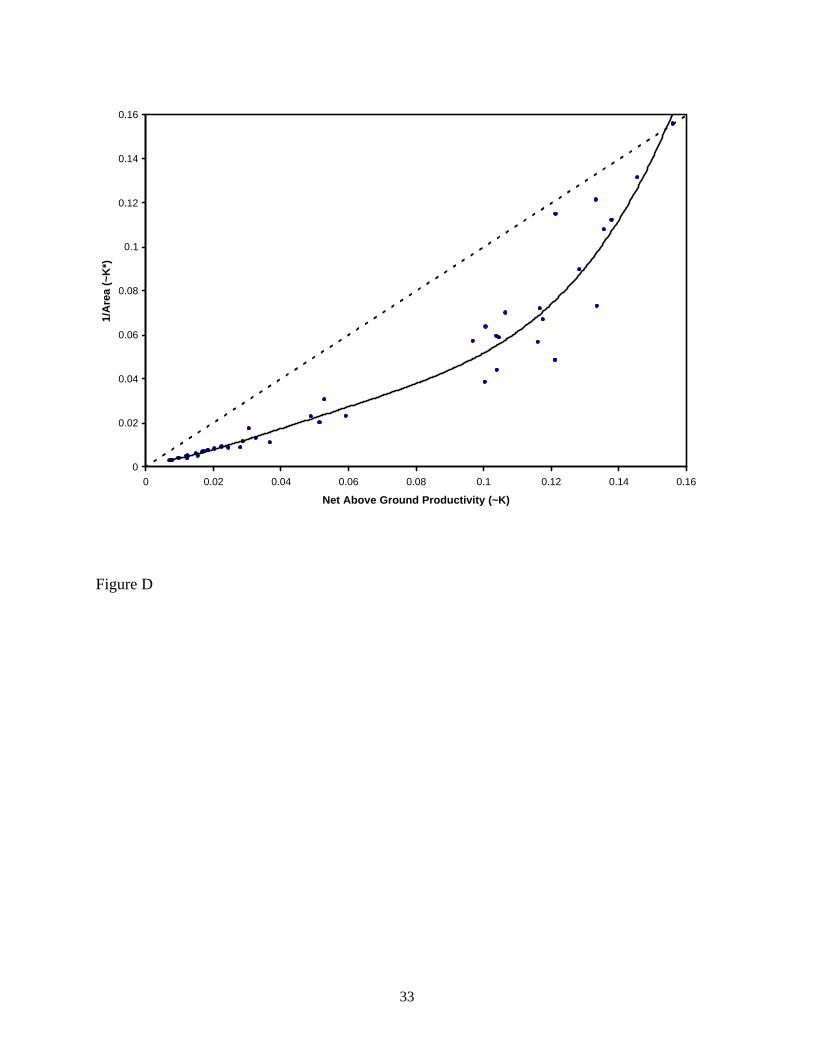
converting the area data into a proxy measure of population density: K* ~ 1/area. Figure D

shows the pattern for the Australian data when comparing K and K*.

Carrying capacity K is assumed to be proportional to net above-ground biomass

productivity. K* is assumed to be proportional to 1/area based on a fixed, modal value of the

population size of Australian hunter-gatherer groups. The curve is a fourth-degree polynomial fit

to the data points solely to show the general trend on the assumption that the left group of data

points (NAGP < 0.06) connects smoothly with the right group of data points (NAGP > 0.1). The

constants in the polynomial have no particular interpretation, and so their values are not shown.

Axis scales are relative and not absolute. Data on rainfall, NAGP, and population size are from

11

Binford (2001: tables 4.01, 4.07, and 5.01); seven data points with population size listed by

Binford as questionable have been excluded, and one further data point (Mineng) has been

excluded as an outlier. The data have been scaled so that the most extreme point (upper right)

has the same K and K* value on the assumption that a group in the environment with the highest

resource density will be close to carrying capacity. The pattern of increasing and then decreasing

values for K - K*, however, does not depend upon the scaling choice.

The pattern of the data shows clearly the initial trend, as predicted by the model, of an increase in

K - K* as the resource density decreases and then convergence between K* and K as resource

density reaches low values. The relationship between (K - K*)/K* and K is shown in figure E.

The trend line was computed excluding the arc of points on the left side of the graph. As

predicted, unutilized resources per person vary inversely and approximately linearly with the

resource density. Axis scales are relative and not absolute. The vertical axis values are

computed from the NAGP (~K) and the 1/area (~K*) values used in figure D. The arc of points

is from groups with low NAGP, hence corresponding to a relatively small value for K. The

small value of K may constrain variation in K* values. Though the trend for these points may be

constrained by low resource density, resource availability per person remains high, as is

predicted for an area with low resource density.

Sources

BINFORD, LEWIS. 2001. Constructing frames of reference: An analytical method for

archaeological theory building using ethnographic and environmental data sets. Berkeley:

University of California Press.

BIRDSELL, J. B. 1953. Some environmental and cultural factors influencing the structuring of

Australian aboriginal populations. American Naturalist 87:171-207.

12

----------. 1973 A basic demographic unit. Current Anthropology 14:337-56.

13

Appendix D: Competition Model

Assume a fixed region for the population so that population density is proportional to population

size. The Lotka competition model is a generalization of the Verhulst-Pearl equation for logistic

growth. Logistic growth is given by the equation

dP/dt = P(a – bP), (1)

where P(t) is the population size at time t, a is the intrinsic growth rate for the population, and b

is a parameter whose value identifies the effect of an increase in population size on the intrinsic

growth rate. When P(t) = a/b, dP/dt = 0 and the population no longer grows. The differential

equation given in equation 1 has the exact solution P(t) = (a/b)/ (1 + exp[-a(t-t0)]), where P(t0) is

the initial population size.

For two populations in competition, each population is assumed to follow the logistic

growth curve with the added factor that the growth of one population affects the growth of the

other. Competition is modeled via the following pair of differential equations:

dP1/dt = P1(a1 – b11 P1– b12P2) and (2)

dP2/dt = P2(a2 – b21P1 – b22P2), (3)

where Pi(t) is the population size of population Pi at time t, ai is the intrinsic growth rate for

population Pi, and bij measures the inhibitory effect of population Pj on population Pi so that b11

is the inhibitory effect that growth of population P1 has on itself, b12 is the inhibitory effect that

population P2 has on population P1, etc., 1 ≤ i, j ≤ 2.

The model assumes a fixed set of relations between P1 and P2 and that all individuals are

affected equally by population growth in terms of the way in which current net fertility is

affected. The pair of differential equations (equations 2 and 3) does not have an exact solution in

terms of an explicit form for the functions P1(t) and P2(t), hence phase-space diagrams in which

14

P1 is plotted against P2 are used to show population size trajectories as determined by these ewo

equations. Equilibrium values for P1 and P2 are also plotted in the phase-space diagram.

Equilibrium values are computed from setting dP1/dt = 0 and dP2/dt = 0. If dP1/dt = 0

then a1 – b11P1 – b12P2 = 0 and this equation defines a linear relationship between P1 and P2

along which P1 has no growth. If dP2/dt = 0, then a2 – b22P2 – b21P1 = 0, and this equation

defines a linear relationship between P1 and P2 along which P2 has no growth. Thus in the phase

space there will be two lines representing equilibrium values, one determined by the first

equation and the second by the second equation.

15

Appendix E: Four Patterns of Competition

We can graph the way in which one population affects the growth trajectory of the other

population by use of a two-dimensional phase-space diagram in which the axes measure the

current population size of each of the two populations and arrows indicate the current net growth

rates of the two populations for each point in the phase space. We can also indicate the curve

along which a population has a net growth rate of zero given its level of competition with the

other population. When one of these curves is determined for each of the two populations, the

intersection of the two curves, if any, represents the point(s) for which both populations have a

net growth rate of zero, that is, in equilibrium with respect to each other.

Depending on the relative magnitudes of the parameters ai and bij, there are four

qualitative patterns for the two populations (figs. F – I). The curve along which a population has

a net growth rate of zero is a straight line (see appendix C). In figure F the two straight lines

intersect and divide the upper right quadrant into four subregions. For all four subregions the net

growth rate of the two populations (indicated by horizontal and vertical arrows) has the overall

effect (indicated by the arrow at an angle) of driving both of the populations in the direction of

the intersection of the two lines. Hence for this configuration the two populations have a stable

equilibrium represented by the intersection of the two lines, and any perturbation from the

equilibrium point will move the population sizes back toward the equilibrium point. For the

assumption that the populations have the same intrinsic growth rate, or a1 = a2, the conditions

under which there is a stable equilibrium may be characterized as competition in which one

population has a greater inhibitory effect on its own growth than on that of the second

population.

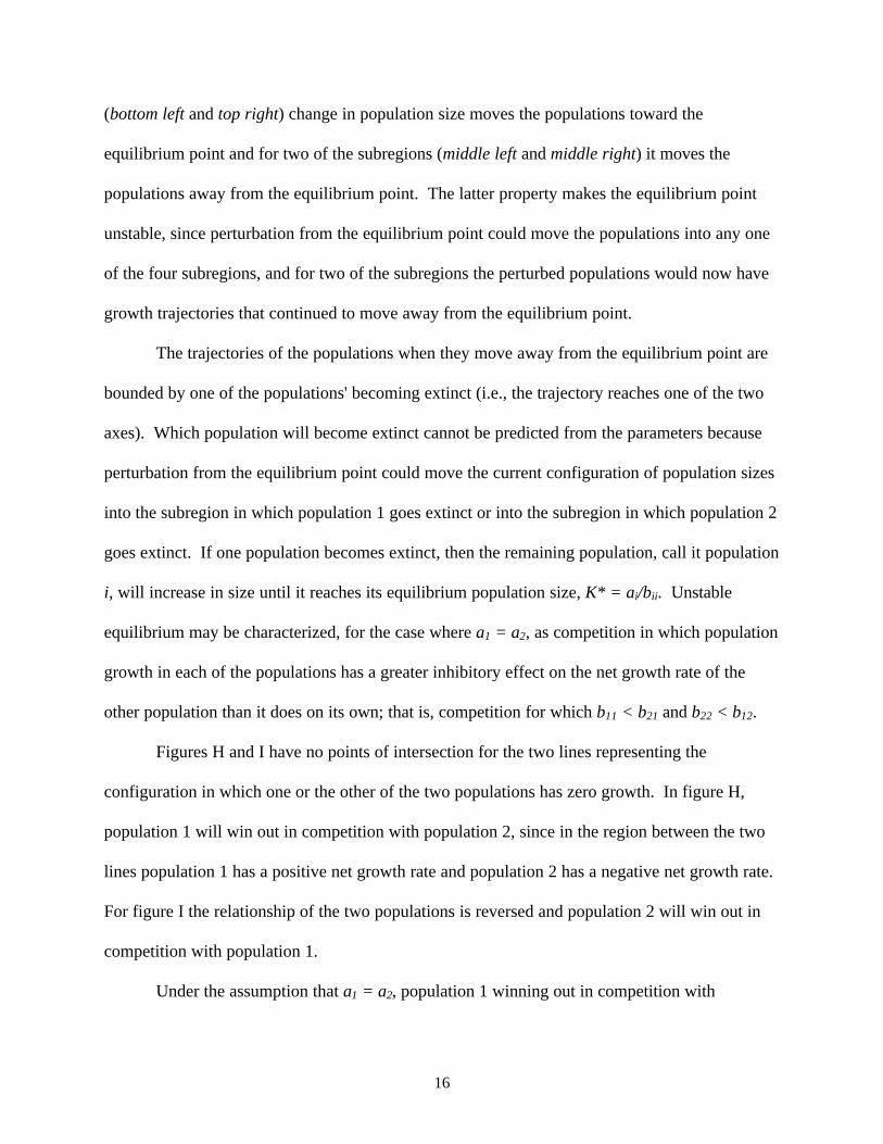
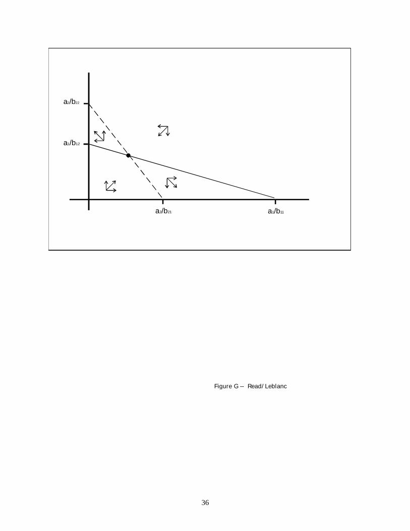
Figure G also has an equilibrium point and four subregions, but for two of the subregions

16

(bottom left and top right) change in population size moves the populations toward the

equilibrium point and for two of the subregions (middle left and middle right) it moves the

populations away from the equilibrium point. The latter property makes the equilibrium point

unstable, since perturbation from the equilibrium point could move the populations into any one

of the four subregions, and for two of the subregions the perturbed populations would now have

growth trajectories that continued to move away from the equilibrium point.

The trajectories of the populations when they move away from the equilibrium point are

bounded by one of the populations' becoming extinct (i.e., the trajectory reaches one of the two

axes). Which population will become extinct cannot be predicted from the parameters because

perturbation from the equilibrium point could move the current configuration of population sizes

into the subregion in which population 1 goes extinct or into the subregion in which population 2

goes extinct. If one population becomes extinct, then the remaining population, call it population

i, will increase in size until it reaches its equilibrium population size, K* = ai/bii. Unstable

equilibrium may be characterized, for the case where a1 = a2, as competition in which population

growth in each of the populations has a greater inhibitory effect on the net growth rate of the

other population than it does on its own; that is, competition for which b11 < b21 and b22 < b12.

Figures H and I have no points of intersection for the two lines representing the

configuration in which one or the other of the two populations has zero growth. In figure H,

population 1 will win out in competition with population 2, since in the region between the two

lines population 1 has a positive net growth rate and population 2 has a negative net growth rate.

For figure I the relationship of the two populations is reversed and population 2 will win out in

competition with population 1.

Under the assumption that a1 = a2, population 1 winning out in competition with

17

population 2 may be characterized as competition in which population 1 has a greater inhibitory

effect on the growth of population 2 than it does on itself and population 2 has a greater

inhibitory effect on itself than it does on population 1 (i.e. b11 < b21 and b22 > b12). In other

words, population 1 can grow at the expense of population 2, and therefore population 2

becomes extinct. Conversely, population 2 winning out in competition with population 1 may be

characterized as competition in which population 2 has a greater inhibitory effect on the growth

of population 1 than it does on itself and population 1 has a greater inhibitory effect on itself than

it does on population 2 (i.e. b11 > b21 and b22 < b12). This might occur if growth in population 1

had little effect on the resource base for population 2 but growth in population 2 had the effect of

removing resources from population 1. An example would be competition between a hunter-

gatherer population and an agricultural group in which the two groups overlapped in the use of

hunted foods and the expansion of agricultural land reduced the availability of foraged foods.

Of these four sets of competitive relationships, we will primarily be interested in the

conditions under which a stable equilibrium can occur and the conditions under which one of the

populations will win out in competition with the other.

Parameter Values

For recent human populations we assume that both populations have the same intrinsic growth

rate (a1 = a2). This is reflected in the fact that when correction is made for reduction in the

fertility rate due to behavioral practices, the same corrected fertility rate of about 10-15 offspring

per reproductive period is obtained, regardless of the population. Assuming that mortality rates

for different populations are comparable prior to the introduction of modern medical practices,

then the inherent growth rates of recent human populations are about the same. Therefore we

will assume throughout the following that a1 = a2 = a, the populations differing only in the b

18

parameters.

The parameters b11 and b22 measure the equilibrium population size of population 1 and

population 2, respectively, in terms of the quantities 1/b11 and 1/b22. The parameters b12 and b21

measure the inhibitory effect of one population on the other population. Since we are comparing

one group with another, we may assume that the nutritional needs of an individual are

independent of the population to which that individual belongs. This assumption allows us to

equate the per person use of food resources in one group with the per person use of food

resources in the other group. Hence if the food resources used per person in population 1 are all

resources that would otherwise be available to population 2, then we may set b21 = b11 and b12 =

b22. If both populations have the same equilibrium population size, then b11 = b22 = b12 = b22.

This configuration will arise when the two populations have the same catchment area and use the

same resources from that catchment area in comparable ways. An example of such a

configuration would be, say, all of the different camps in !Kung San society, since each camp

potentially has access to all resources via rights of camp membership through relatives and the

hxaro system (Wiessner 1982). For culturally distinct groups, however, conditions under which

there is complete overlap of catchment areas are rare.

For distinct groups we can relate the parameters b12 and b21 to the overlap in the

catchment areas of the two populations. Initially, we assume that the two populations use the

same set of resources and resources are uniformly distributed over the catchment areas. We then

relax the first assumption. Let C1 be the catchment area for population 1 and C2 the catchment

area for population 2. Let c be the zone of overlap of these two catchment areas. The proportion

of a group’s catchment area in the zone of overlap measures the extent to which one population

is using resources otherwise available to the other population and therefore the impact of

19

population growth of one population on the other population. More precisely, under the

specified conditions, after suitable scaling of the parameters, b12 = c/C1 and b21 = c/C2.

When C1 = C2 = C, it follows that b12 = b21 = c/C and the two populations have

equivalent effects on each other's growth. If the catchment area for population 1, say, is larger

than the catchment area for population 2, then b12 = c/C1 < b21 = c/C2 and growth in population

1 has a greater effect on population 2 than does growth in population 2 on population 1.

If the resource bases of the two groups are not identical, then we can introduce a term, ri,

representing the proportion of the resources used by population i that are also used by population

j. With this notation, b21 = (r1 c)/C2 and b12 = (r2 c)/C1, since growth in population 1 reduces the

resource base for population 2 in the overlap region, c, only by the proportion of the resources

used by population 1 that otherwise would be used by population 2 (and similarly for the effect

of population 2 on population 1). One implication is that when one group expands its resource

base and the other group does not, the former group will have a greater impact on the latter group

than the latter group has on the former.

Baseline Competition: Two Groups with Identical Parameters

Assume that we start out with, say, two hunter-gatherer populations having the same internal

population dynamics (i.e., a1 = a2 = a and b11 = b22), and using the same mix of resources. The

parameters b12 and b21, as discussed above, measure the impact of one population on the growth

of the other population due to, for example, resources utilized by one population thereby being

made unavailable to the other population. The size of the overlap of the catchment areas, C1 and

C2 (fig. J) for groups 1 and 2, respectively, measures the relative magnitude of the parameters b12

and b21.

If C1 = C2, then the two populations use exactly the same resources and both the same

20

effect on each other as on themselves; hence b12 = b22 = b21 = b11 (fig. K, A), and the two

population sizes at equilibrium will be K* = a/b11 = a/b22. All points along the common line for

the two groups are quasi-stable equilibrium values for the population size of each group. At the

other extreme, if the regions C1 and C2 do not overlap, then the two populations are independent

of each other and b12 = b21 = 0 (fig. K, B). Each group now independently increases to the

carrying capacity of the area from which it obtains resources, and the point representing the

carrying capacity of the area for each of the two groups is a stable equilibrium value. If the

catchment areas only partially overlap and the two populations use the same resource base, then

b12 = b21 < b11 = b22 (fig. K, C). The latter corresponds to the configuration shown in figure F,

namely, stable equilibrium between the two populations. In all cases, the parameters drive the

populations to a stable equilibrium configuration. We now consider in more detail the third and

first possibilities with regard to stability of the configuration. For the third possibility, namely,

incomplete overlap of catchment areas, we consider two subcases: territorial exclusion and lack

of territorial exclusion. For all possibilities we arrive at the same conclusion, namely, that the

only stable configuration is the second one, with non-overlapping catchment areas.i

Partial overlap Although a stable configuration with partial overlap is theoretically

possible, this configuration unrealistically assumes that each population responds only to the

reduction in resources available to it due to the use of resources by the other group as if this were

a feature of its environment over which it had no control. If, however, the members of one

population, say, population 1, begin to practice territorial exclusion, then the parameters b21 and

b12 will be affected. The parameters b11 and b22 will not change, since they measure the

equilibrium population size when only a single population is present. The parameter b12 will

decrease to b12* (i.e., a/b12 < a/b12*), since population 1 is isolating itself from population 2 via

21

territorial exclusion. The parameter b21 will increase to b21* (i.e. a/b21* < a/b21) since population

2 is affected not only by population 1's use of resources but also by its reduction of access to

resources. The effect is to shift the stable equilibrium of figure F in the direction of a

configuration in which population 1 will win out in competition with population 2.

Realistically, population 2 may not become extinct; the ability of population 1 to practice

territorial exclusion may be limited as its catchment area increases in size, or population 2 may

be able to find a catchment area in which it can also practice territorial exclusion. In either case,

stability will reemerge only when the overlap in catchment areas between populations 1 and 2 is

small, thereby making the population dynamics of the two populations essentially independent.

Where neither group is defending its catchment area against the other, partial overlap of

catchment areas assumes that catchment area is bounded for reasons other than the presence of

the other group. Partial overlap may occur, for example, when the two groups exploit different

resources that only partially overlap in their geographical distribution. If, however, the two

groups are utilizing the same resource base and not practicing territorial exclusion, then partial

overlap is not a stable arrangement, since one group can grow by expanding its catchment area

without opposition from the other. Population growth will be expected because the model

implies that both populations are stabilized at a population level below the equilibrium

population size of each group were there no competition. Hence expansion of the catchment area

would reduce the cost of foraging, thereby obviating the need for decisions to increase spacing of

offspring. Consequently, we would expect that in the absence of territorial exclusion, groups

utilizing the same resource base would eventually either completely overlap, be reduced to one

by the extinction of the other, or be geographically isolated with no overlap of their catchment

areas. Complete overlap will be equivalent to neutral equilibrium along the line of overlap of

22

equilibrium values in the phase-space diagram. Any stochastic variation along this line simply

moves the two populations from one equilibrium value to another, and so the two populations

will not return to their previous equilibrium value. Thus by stochastic drift one population may

go to extinction along the line of intersection. The only alternative will be geographic isolation.

!Kung San camps are an example of complete overlap. The rules of camp membership

effectively allow access to resources throughout the territory. This is a stable configuration that

does not lead to intercamp conflict over resources, although the membership of an individual

camp may die out because of drift effects were it not for cultural means through which new camp

members are recruited

Complete Overlap. While the theoretical case of complete overlap of catchment areas

would be a stable arrangement in a fixed, deterministic universe (fig. L, A), change in any one of

the parameters for the two populations will shift the arrangement to a configuration in which one

population will win out in competition with the other (figure L, B). Thus complete overlap is

unstable in the face of long-term change in parameter values, and so we can assume that for there

to be a stable configuration with complete overlap in the catchment areas, any change in

parameter value by one group must be matched by an equivalent change in parameter value by

the other group.

For groups that are part of the same society (e.g., the !Kung San camps), equivalence of

parameter values in all subgroups could arise out of a common cultural context, such as a shared

valuation placed on the well-being of a family. If the two groups are part of different societies,

however, then differences in their cultural contexts make possible long-term differences in

parameter values between the two groups. Hence we would expect that the theoretical pattern of

a stable arrangement with complete overlap in catchment areas would be more likely to occur

23

when the groups are part of the same society.ii

Sources

PIELOU, E. C. 1969. An introduction to mathematical ecology. New York: Wiley-Interscience.

WIESSNER, POLLY. 1982. “Risk, reciprocity and social influences on !Kung San economics,”

in Politics and history in band societies. Edited by Eleanor Leacock, Richard Lee, pp. 61-84.

Cambridge: Cambridge University Press.

24

Appendix F: Warfare Fatalities in Small-Scale Societies

Although it is commonly assumed that warfare in the past, especially nonstate warfare, was

insignificant from a cultural or biological point of view (Braun and Plog 1982, Hassan 1981,

Knauft 1991, Reyna 1994, Service 1975, Turney-High 1949). Keeley’s and others' (e.g., Ember

and Ember 1992) careful assessment of a large body of evidence shows this assumption to be

false. (Other useful considerations of prehistoric or early ethnographic cases of warfare include

Bamforth 1994; Berndt 1964; Bovee and Owsley 1994; Burch 1974, 1988; Chagnon 1988; Feil

1987; Haas 1990; LeBlanc 1999; Manson and Wrangham 1991; Maschner and Maschner 1997;

Meggitt 1977; Milner, Anderson, and Smith 1991; Moss and Erlandson 1992; Owsley 1994;

Rappaport 1967; Redmond 1994; Strathern 1971; Tuck 1978; Vayda 1960). Keeley makes the

very convincing case that “primitive” warfare is neither ritualistic nor nonfatal. He shows that

when warfare is endemic, the cumulative effect of warfare on mortality rates in societies from

bands to chiefdoms is significant. While formal battles in places such as New Guinea may have

resulted in only one casualty in a single battle, such battles were sufficiently common that the

cumulative effect was large. Moreover, formal battles were accompanied by raiding and ambush,

which were much more deadly for women and children and further increased the death rate.

Where the information is relatively good (Berndt 1964, Chagnon 1988, Meggitt 1977, Morren

1984, Shankman 1991, Sillitoe 1977), death rates of adult males (lifetime cause of death) due to

warfare range from 20 to 32%, with 25% probably a reasonable generalization. Death rates for

women due to warfare were from 3 to 16% for reproductive-aged women, with a reasonable

generalization of 4-5%.

Figures for the Ache are instructive: “Death at the hands of another human being was by

far the most common cause of death to forest-dwelling Ache” (Hill and Hurtado 1995:168).

25

Among adult Ache males, external warfare accounted for 35% of all deaths, and more than 40%

of reproductive-aged females died or were captured (removed from the reproductive group)

because of warfare.

Group size is highly significant for success in endemic warfare. Because much of the

warfare is attritional, the larger groups (larger value for a/b) prevailed. Moreover, skill at

warfare cannot be easily turned on and off. Typically, boys are taught techniques of fighting

from a young age, and good war leaders are discovered because of the frequency of fighting.

Any group that avoids warfare, does not train its boys, and does not allow military leadership to

be developed, discovered, and recognized is greatly disadvantaged if attacked. Thus, it is simply

impossible, except on small islands or in other conditions of isolation, for a group to “refuse to

play.” A group cannot simply lower its birth rate so that it does not need more land and then stop

fighting. Unless all the neighboring groups do likewise, it will be at a great disadvantage and an

easy and likely target for another group that is expanding through aggression.

Sources

BAMFORTH, D. B. 1994. Indigenous people, indigenous violence: Precontact warfare on the

North American Great Plains. Man 29: 95-115.

BERNDT, R. M.1964 Warfare in the New Guinea Highlands. American Anthropologist

66:183-203.

BOVEE, DANA L. AND DOUGLAS W. OWSLEY. 1994. “Evidence of warfare at the

Heerwald site,” in Skeletal biology in the Great Plains: Migration, warfare, health, and

subsistence. Edited by D W. Owsley and R. L. Jantz, pp. 355-62. Washington, D. C.:

Smithsonian Institution Press.

BRAUN, DAVID, AND STEPHEN PLOG. 1982. Evolution of “tribal” social networks: theory

26

and prehistoric North American evidence. American Antiquity 47:504-25.

BURCH, E. S. 1974. Eskimo warfare in Northwest Alaska. Anthropological Papers of the

University of Alaska 16:1-14.

----------. 1988. "War and trade," in Crossroads of continents: Cultures of Siberia and Alaska.

Edited by W. W. Fitzhugh and A. Crowell, pp. 227-40. Washington D.C.: Smithsonian

Institution Press.

CHAGNON, N. 1988 Life histories, blood revenge, and warfare in a tribal population. Science

239:985-92.

EMBER, CAROL R. AND MELVIN EMBER. 1992. Resource unpredictability, mistrust, and

war: A cross-cultural study. Journal of Conflict Resolution 36:242-62.

FEIL, D. K. 1987 The Evolution of Highland Papua New Guinea Societies. Cambridge:

Cambridge University Press.

HAAS, JONATHAN. 1990. "Warfare and tribalization in the prehistoric Southwest," in The

anthropology of war. Edited by Jonathan Haas, pp. 171-89. New York: Cambridge University

Press.

HASSAN, FEKRI. 1981. Demographic archaeology. New York: Academic Press.

HILL, KIM, AND A. MAGDALENA HURTADO. 1995. Ache life history: The ecology and

demography of a foraging people. New York: Aldine de Gruyter.

KNAUFT, BRUCE M. 1991. Violence and sociality in human evolution. Current Anthropology

32:391-428.

LEBLANC, STEVEN A. 1999. Prehistoric warfare in the American Southwest. Salt Lake City:

University of Utah Press.

MANSON, J. AND R. WRANGHAM 1991 Intergroup aggression in chimpanzees and humans.

27

Current Anthropology 32:369-90.

MASCHNER, HERBERT D., AND KATHERINE L. REEDY-MASCHNER. 1997. Raid,

retreat, defend (repeat): the archaeology and ethnohistory of warfare on the North Pacific Rim.

Journal of Anthropological Archaeology 17:19-51.

MEGGITT, M. J. 1977 Blood is their argument. Palo Alto, Calif.: Mayfield.

MILNER, G., E. ANDERSON, AND V. SMITH. 1991. Warfare in late prehistoric West-Central

Illinois. American Antiquity 56:581-603.

MORREN, G. E. B. J. 1984 "Warfare on the highland fringe of New Guinea: The case of the

mountain Ok," in Warfare, culture, and environment. Edited by R. B. Ferguson, pp. xxx-xxx.

Orlando: Academic Press.

MOSS, MADONNA L., AND JON M. ERLANDSON. 1992. Forts, refuge rocks, and defensive

sites: the antiquity of warfare along the north Pacific Coast of North America. Arctic

Anthropology 29:73-90.

OWSLEY, DOUGLAS W. 1994. “Warfare in coalescent tradition populations of the Northern

Plains,” in Skeletal biology in the Great Plains: Migration, warfare, health, and subsistence.

Edited by D.W. Owsley and R. L. Jantz, pp. 333-43. Washington, D.C.: Smithsonian Institution

Press.

RAPPAPORT, ROY. 1967. Pigs for ancestors. New Haven: Yale University Press.

REDMOND, ELSA M. 1994. Tribal and chiefly warfare in South America. Memoirs of the

Museum of Anthropology, University of Michigan, Number 28. Studies in Latin American

Ethnohistory and Archaeology, Joyce Marcus, General Editor, Volume V.

REYNA, S. P. 1994. “A mode of domination approach to organized violence,” in Studying war:

Anthropological perspectives. Edited by S. P. Reyna and R. E. Downs, pp. 29-65. Amsterdam:

28

Gordon and Breach Publishers.

SERVICE, ELMAN R. 1975. Origins of the state and civilization: The process of cultural

evolution. New York: Norton.

SHANKMAN, PAUL. 1991. Culture contact, cultural ecology, and Dani warfare. Man (N.S.)

26:229-321.

SILLITOE, P. 1977 Land shortage and war in New Guinea. Ethnology 16:71-81.

STRATHERN, ANDREW. 1971. The rope of Moka: Big-men and ceremonial exchange in

Mount Hagen, New Guinea. Cambridge: Cambridge University Press.

TUCK, JAMES A. 1978. “Northern Iroquoian prehistory,” in Northeast. Edited by B. G.

Trigger, pp. 322-33. Handbook of North American Indians vol. 15. W. C. Sturtevant, general

editor. Washington, D.C.: Smithsonian Press.

TURNEY-HIGH, H. 1949. Primitive war: Its practice and concepts. Reissue with new preface

and afterword. Columbia: University of South Carolina Press, 1971.

VAYDA, ANDREW P. 1960. Maori warfare. Wellington: Polynesian Society.

29

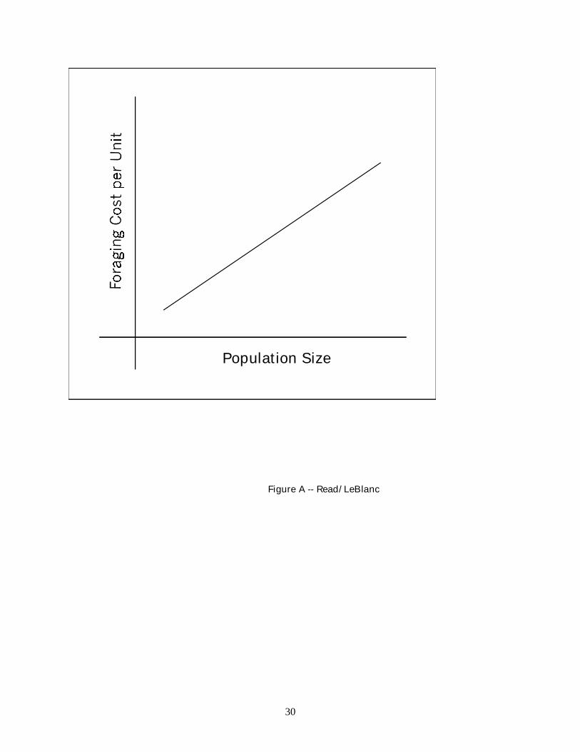
Fig. A. Population density and average foraging cost per unit of resource per female forager, keeping

fixed the resource base and the catchment area (schematic).

Fig. B. Total parenting costs and interbirth spacing (schematic).

Fig. C. Population size and net growth rate (schematic).

Fig. D. K and K* values for Australian hunter-gatherer.

Fig. E. Unutilized resources per person and resource density.

Fig. F. Stable equilibrium. Area where population 2 grows, shown by a vertical arrow pointing upward

(horizontal shading). Area where population 1 grows, shown by horizontal arrow pointing to the right

(vertical shading). Area where both populations grow (double shading). In all three shaded areas and

the unshaded area the increase or decrease in the sizes of the two populations pushes them to the point of

intersection of the two lines (diagonal arrows).

Fig. G. Unstable equilibrium. Population 1 wins out when the populations are in the region at the lower

right; population 2 wins out when the populations are in the region at the upper left.

Fig. H. Population 1 wins out as the populations move in the direction of the vertical axis when the pair

of populations is in the middle region.

Fig. I. Population 2 wins out as the populations move in the direction of the vertical axis when the pair of

populations is in the middle region.

Fig. J. Catchment areas for two populations. The extent of the area of intersection for the two catchment

regions (gray) measures the degree to which each population inhibits the growth of the other.

Fig. K. Phase-space diagram for three patterns of catchment overlap.

Fig. L. Equilibrium with complete overlap of catchment areas (top) and shift in configuration with change

in parameter value (decrease in b12) to one in which population 1 wins out.

30

Population Size

Figure A -- Read/LeBlanc

31

Figure B -- Read/Leblanc

32

Figure C -- Read/Leblanc

33

Figure D

0

0.02

0.04

0.06

0.08

0.1

0.12

0.14

0.16

0 0.02 0.04 0.06 0.08 0.1 0.12 0.14 0.16

Net Above Ground Productivity (~K)

1/A

rea

(~K

*)

34

Figure E

0

0.5

1

1.5

2

2.5

0 0.02 0.04 0.06 0.08 0.1 0.12 0.14 0.16 0.18

Net Above Ground Productivity (~K)

(K -

K*)

/K*

35

a /b1 11

a /b1 12

a /b2 22

a /b2 21

Population 1

Pop

ulat

ion

2

Zero Growth Population 1

Zero Growth Population 2

Figure F -- Read/Leblanc

36

a /b1 11

a /b1 12

a /b2 22

a /b2 21

Figure G -- Read/Leblanc

37

a /b1 11

a /b1 12

a /b2 22

a /b2 21

Figure H -- Read/Leblanc

38

a /b1 11

a /b1 12

a /b2 22

a /b2 21

Figure I -- Read/Leblanc

39

Population 1

Population 2

Area of overlap is a measure of b and b

(A) With 100% overlap, b = b = b = b(B) With 0% overlap, b = 0 = b , the two populations are decoupled(C) With partial overlap, b = b < b = b

12 21

12 11 22 21

12 21

12 21 11 22

Two Identical Populations: b = b , b = b and a = a .11 22 12 21 1 2

Figure J -- Read/Leblanc

40

Lines overlap, equilibriumalong the overlapping lines

Single equilibrium point

a /b2 22

a /b1 11

Population 1

Pop

ulat

ion

2

a /b1 12

= a /b2 22

= a /b2 21a /b1 11

Population 1

Pop

ulat

ion

2

Single equilibrium point

a /b1 12

a /b2 22

a /b1 11 a /b2 21

Stable Equilibrium

Population 1P

opul

atio

n2

(C) Partial overlap: b = b < b = b12 21 11 22

(B) No overlap: b = b = 012 21(A) Complete overlap: b = b = b = b12 21 11 22

Figure K-- Read/LeBlanc

41

equilibrium value

Population 1

Population 1

Pop

ulat

ion

2

Pop

ulat

ion

2

= a /b2 22

a /b2 22

a /b1 12

a /b1 12

a /b2 21

a /b2 21

= a /b1 11

= a /b1 11

Figure L--Read/LeBlanc

42

i We include under nonoverlapping catchment areas a configuration in which there might be

limited overlap in the respective regions for which the impact of one group on the other is within the

range of “noise” or stochastic variation in the population dynamics within a single population. Our

concern here is with effects of one group upon a second group that are more pronounced than background

fluctuations within a single group in isolation.ii Pielou (1969:64) observes that the theoretical possibility of a stable configuration between

different species in competition contradicts the “competitive exclusion principle,” hence “no ‘proof’ of

the principle will ever be had” (p. 64). She does not consider, though, that the theoretical model of stable

equilibrium between two species that are ecological homologues assumes fixed parameters for each of the

two species. Since the pattern of complete overlap is an unstable configuration in the face of parameter

variation, it follows that two species that are ecological homologues can arrive at a stable configuration

only when each species precisely tracks changes in the other's parameter values. The latter is not likely

and so with changes in parameter values a possibility for one or the other of the two species it follows that

the “competitive exclusion principle” is consistent with a model of competition between two species.