appendix b4 variable infiltration capacity (vic ... · appendix b4 — variable infiltration...

Appendix B4 Variable Infiltration Capacity (VIC)

Hydrologic Modeling Methods and Simulations

December 2012 B4-1

Appendix B4 — Variable Infiltration Capacity (VIC) Hydrologic Modeling Methods and Simulations

The Variable Infiltration Capacity (VIC) model (Liang et al., 1994; Liang et al., 1996) is the hydrology model used in the Colorado River Basin Water Supply and Demand Study (Study) to simulate the hydrologic response of the Colorado River Basin (Basin) to historical and future climate. The results from VIC simulations were used to describe the range of streamflows under the Downscaled General Circulation Model (GCM) Projected scenario. Each of the 112 downscaled climate projections was used as input into the VIC hydrology model. The VIC hydrology model uses the climate projections along with land cover, soils, elevation, and other watershed information to simulate hydrologic fluxes. The hydrologic fluxes were then routed to each of the 29 natural flow locations using a routing network derived from the topography. The result of this approach is 112 unique sequences of natural flow under future climate projections. However, the simulated natural flows can contain significant monthly and annual biases when compared to the natural flows of the historical period. These biases are generally small for mainstem Colorado River locations, but can be large for smaller watersheds and in areas where the VIC model was not specifically calibrated. To account and compensate for these biases, the VIC-simulated streamflows for both the historical and future periods were first adjusted for biases before incorporating into systems modeling. This appendix describes the VIC hydrology model, methods, and simulations included in the Study.

1.0 General Description of VIC The VIC model (Liang et al., 1994; Liang et al., 1996) is a spatially distributed hydrologic model that solves the water balance at each model grid cell. It incorporates spatially distributed parameters describing topography, soils, land use, and vegetation classes. VIC is considered a macro-scale hydrologic model in that it is designed for larger basins with fairly coarse grids. In this manner, it accepts input meteorological data directly from global or national gridded databases or from GCM projections. To compensate for the coarseness of the discretization, VIC is unique in its incorporation of sub-grid variability to describe variations in the land parameters as well as precipitation distribution. Parameterization within VIC is performed primarily through adjustments to parameters describing the rates of infiltration and baseflow as a function of soil properties, as well as the soil layers’ depths. When simulating in water balance mode, VIC is driven by daily inputs of precipitation, maximum and minimum temperature, and wind speed. The model internally calculates additional meteorological forcings such as short- and long-wave radiation, relative humidity, vapor pressure, and vapor pressure deficits. Rainfall, snow, infiltration, evapotranspiration (ET), runoff, soil moisture, and baseflow are computed over each grid cell on a daily basis for the entire period of simulation. An offline routing tool then processes the individual cell runoff and baseflow terms and routes the flow to develop streamflow at various locations in the watershed. Figure B4-1 shows the hydrologic processes included in the VIC model.

Colorado River Basin Water Supply and Demand Study

B4-2 December 2012

FIGURE B4-1 Hydrologic Processes Included in the VIC Model

Source: http://www.hydro.washington.edu/Lettenmaier/Models/VIC/Overview/ModelOverview.shtml

The VIC model has been applied to many major basins in the United States, including large-scale applications to California’s Central Valley (Maurer et al., 2002; Brekke et al., 2008; Cayan et al., 2010), Colorado River Basin (Christensen and Lettenmaier, 2007), Columbia River Basin (Hamlet et al., 2010), and for several basins in Texas (Maurer et al., 2002; CH2M HILL, 2008). The VIC model has a number of favorable attributes for the Study, but VIC’s three most significant advantages are that it has a reliable, physically based model of ET, it has a physically based model of snow dynamics, and it has been used for two studies of climate change in the Basin for which calibrated parameters are available.

2.0 VIC Modeling Methods Specific to the Colorado River Basin

2.1 Model Inputs The VIC model was driven by meteorological forcing data. Although the model has some flexibility in what variables are required, forcing files typically include daily values for precipitation, maximum temperature, minimum temperature, and wind speed. The VIC model required that the forcing files be in either American Standard Code for Information Interchange or binary format, with one file for each grid cell of the simulation domain. The model grid for the Basin consists of approximately 4,500 grid cells at a 1/8th-degree latitude by longitude spatial resolution.

Daily gridded observed meteorology data were obtained from Santa Clara University (Maurer et al., 2002) for the period 1950 to 1999. Projections of monthly future climate data were obtained


December 2012 B4-3

from the Lawrence Livermore National Laboratory under the World Climate Research Program’s Coupled Model Intercomparison Project Phase 3 and using the weather general (temporal disaggregation) methods described in appendix B3. Wind speed in the future projections was not adjusted in these analyses because downscaling of this parameter was not available, nor well translated from global climate models to local scales.

2.2 VIC Model Processes and Output The VIC model was simulated in water balance mode. In this mode, a complete land surface water balance is computed for each grid cell on a daily basis for the entire model domain. Unique to the VIC model is its characterization of sub-grid variability. Sub-grid elevation bands enable more-detailed characterization of snow-related processes. Five elevation bands are included for each grid cell. In addition, VIC also includes a sub-daily (1-hour) computation to resolve transients in the snow model. The soil column is represented by three soil zones extending downward from the land surface to capture the vertical distribution of soil moisture. The VIC model represents multiple vegetation types using the National Atmospheric and Space Administration’s Land Data Assimilation System databases as the primary input data set.

For the simulations performed for the Basin, the following water balance parameters were produced as output on a daily and monthly time step: precipitation, runoff, baseflow, ET, soil moisture, and snow water equivalent. The runoff simulated from each grid cell was routed to various river flow locations using VIC’s offline routing tool. The routing tool processes individual cell runoff and baseflow terms and routes the flow based on flow direction and flow accumulation inputs derived from digital elevation models. For the simulations performed for the Basin, intervening streamflow was routed to 29 locations that align with the 29 natural flow locations in the Colorado River Simulation System (CRSS), the Bureau of Reclamation’s (Reclamation) long-term planning model and the primary modeling tool used in the Study. Flows are output in both daily and monthly time steps. Only the monthly flows were used in subsequent analyses. It is important to note that VIC routed flows are considered “naturalized” in that they do not include effects of diversions, imports, storage, or other human management of the water resource.

3.0 Colorado River Basin VIC Model Validation A VIC model of the Basin was previously developed by the University of Washington (Christensen and Lettenmaier, 2007), and was provided to Reclamation for the Study. The VIC model was not further calibrated or refined as part of the Study, but the model performance over the 1950 to 1999 validation period is described in this section.

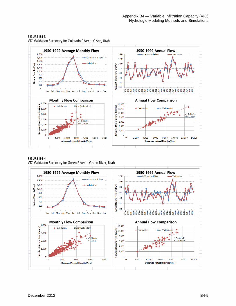
The VIC historical validation run was simulated on a daily time step over the 1950 to 1999 period. Historical observed climate inputs are from Maurer et al. (2002). Streamflow was routed to each of the 29 natural flow locations used by Reclamation in Basin planning. Figure B4-2 shows the validation results for the Colorado River at Lees Ferry, Arizona location. The VIC simulation results in an overestimation of mean annual flows of about 3.9 percent when compared to the Reclamation natural flow estimate. The validation run captured the low and moderate annual flows, but has a slight overestimation of the high annual flows. Simulated flows in April and May flows are higher than Reclamation calculated historical natural flows, while July and August flows are slightly lower. Simulated flows for Colorado River at Cisco, Green River at Green River, Utah, and the San Juan River near Bluff, Utah, are shown in figures B4-3


B4-4 December 2012

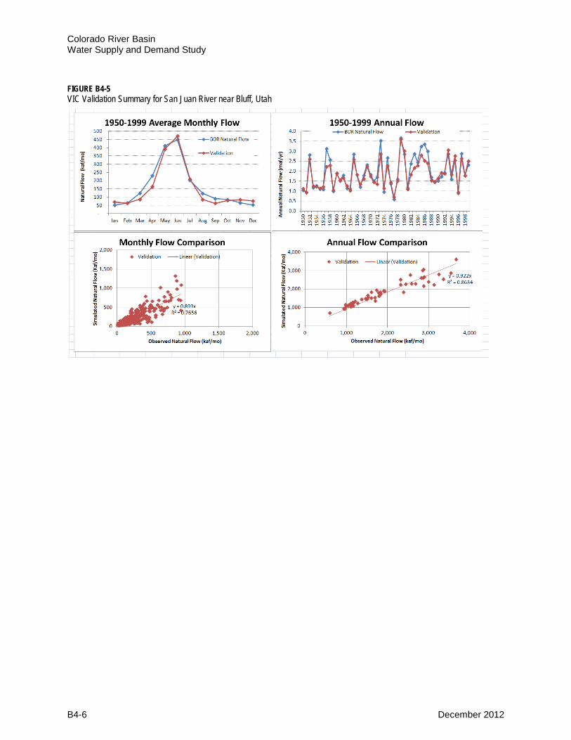
through B4-5. The simulated flows show a slight overestimation for the Colorado River at Cisco and Green River at Green River stations when compared to the Reclamation natural flow estimates, while an underestimation is apparent for the San Juan River near Bluff station. Pearson's linear correlation coefficient, bias, and root mean square error (RMSE) are computed using the observed naturalized and VIC-simulated streamflows as driven by Maurer et al. (2002) over the 1950 to 1999 validation period for all 20 locations in the Upper Basin. These results are summarized in table B4-1. In general, the VIC model appears to have relatively small biases for the larger watersheds as compared to the Reclamation natural flow estimates, but can be larger for smaller watersheds and in areas where the VIC model was not specifically calibrated. The VIC model appears to have higher biases in the upper watersheds and lower biases farther downstream as more watershed contributes to the flow.

FIGURE B4-2 VIC Validation Summary for Colorado River at Lees Ferry, Arizona


December 2012 B4-5

FIGURE B4-3 VIC Validation Summary for Colorado River at Cisco, Utah

FIGURE B4-4 VIC Validation Summary for Green River at Green River, Utah


B4-6 December 2012

FIGURE B4-5 VIC Validation Summary for San Juan River near Bluff, Utah


December 2012 B4-7

TABLE B4-1 Observed Annual Naturalized Streamflow and VIC-simulated Streamflow (with Maurer et. al [2002] historical meteorology) Comparison Statistics (1950–1999)

ID Location

Obs. Nat. Flow

(thousand acre-feet

[kaf])

VIC Nat. Flow (kaf)

Bias (%)

Pearson's Linear Correl. Coef.

RMSE (kaf)

RMSE (% of mean flow)

1 Colorado River at Glenwood Springs, Colorado

2,071 2,192 5.8% 0.9 360.0 17.4%

2 Colorado River near Cameo, Colorado

3,489 3,741 7.2% 0.9 546.4 15.7%

3 Taylor River Below Taylor Park Reservoir, Colorado

148 172 15.9% 0.8 48.2 32.5%

4 Gunnison River at Blue Mesa Reservoir, Colorado

1,045 1,316 26.0% 0.9 332.3 31.8%

5 Gunnison River at Crystal Reservoir, Colorado

1,273 1,494 17.4% 0.9 325.5 25.6%

6 Gunnison River near Grand Junction, Colorado

2,304 2,336 1.4% 0.9 295.2 12.8%

7 Dolores River near Cisco, Utah

789 554 -29.7% 0.9 307.0 38.9%

8 Colorado River near Cisco, Utah

6,647 6,829 2.7% 1.0 640.4 9.6%

9 Green River below Fontenelle Reservoir, Wyoming

1,364 1,079 -20.9% 0.8 396.8 29.1%

10 Green R. near Green River, Wyoming

1,469 1,226 -16.5% 0.8 359.1 24.5%

11 Green River near Greendale, Utah

2,009 1,971 -1.9% 0.8 392.3 19.5%

12 Yampa River near Maybell, Colorado

1,210 1,086 -10.2% 0.9 196.4 16.2%

13 Little Snake River near Lily, Colorado

466 580 24.3% 0.8 173.1 37.1%

14 Duchesne River near Randlett, Utah

778 920 18.2% 0.9 291.1 37.4%

15 White River near Watson, Utah

557 525 -5.7% 0.8 167.1 30.0%

16 Green River at Green River, Utah

5,397 5,440 0.8% 0.9 785.7 14.6%

17 San Rafael River near Green River, Utah

161 273 69.1% 0.7 152.8 94.8%

18 San Juan River near Archuleta, New Mexico

1,028 869 -15.5% 0.9 268.2 26.1%

19 San Juan River Bluff, Utah 1,953 1,856 -5.0% 0.9 292.6 15.0%

20 Colorado River at Lees Ferry, Arizona

14,673 15,248 3.9% 1.0 1550.9 10.6%


B4-8 December 2012

4.0 Application of Streamflow Bias Correction The analysis presented in appendix B3 shows that there are some biases in the VIC streamflows as driven by GMC-simulated historic meteorological forcings in comparison with the naturalized streamflows for the Basin for the overlapping period 1950 to 1999. These biases result from several factors, including spatial and temporal errors in downscaled climate model forcings, complex groundwater interactions, and other complexities normally inherent to VIC hydrologic model parameter calibration. The analysis showed there are some uncertainties in the daily disaggregation method that was used to produce daily meteorological forcings from the monthly downscaled meteorology (see appendix B3). Daily meteorological data are required to drive the VIC. Moreover, there are uncertainties related to VIC model processes and parameter calibration demonstrated through comparisons of VIC-simulated historical streamflows with the naturalized streamflows for the Basin. Bias corrections of the downscaled climate model simulated VIC streamflows are performed to better reflect the statistics of the observed streamflows for the historical simulation period. This document describes the method developed to bias-correct the streamflows for the Basin. The method has been implemented for all 29 river locations for the period 1950 to 1999 for VIC simulation for each of the 112 projections. Results are presented for one particular projection (Trace 44 – sresa2.cccma_cgcm3_1.4) to demonstrate the process. VIC streamflows generated under future climate projections incorporate the same bias correction process before determining the flow projections for use in systems modeling.

The streamflow bias correction accounts for monthly and annual statistical bias at each of the 29 flow locations. Following the station-specific adjustments, the total Basin mass balance is again checked and adjustments are made such that flow continuity is maintained throughout the Basin. The streamflow bias correction involves the following steps:

1. Evaluate the monthly and annual bias in VIC-simulated streamflows as compared to the observed natural flows for each of the 29 locations. See Figure B4-6.

FIGURE B4-6 Comparisons of the January Cumulative Distribution Function (CDF) (left) and Mean Monthly (right) Streamflow Developed from VIC-simulated and Natural Streamflow Colorado River at Parker Dam, Arizona location. Simulated streamflow from VIC simulation is driven by downscaled climate model forcings from Trace 44.

0 200 400 600 800 1000 1200

0

0.2

0.4

0.6

0.8

1

Streamflow (kaf)

F(x)

NaturalFlowsVICraw

J F M A M J J A S O N D0

1000

2000

3000

4000

Stre

amflo

w (k

af)

NaturalFlowsVICraw


December 2012 B4-9

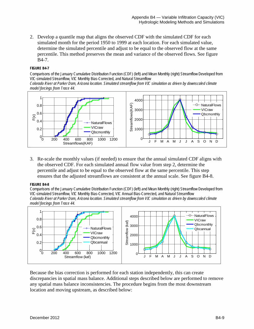
2. Develop a quantile map that aligns the observed CDF with the simulated CDF for each simulated month for the period 1950 to 1999 at each location. For each simulated value, determine the simulated percentile and adjust to be equal to the observed flow at the same percentile. This method preserves the mean and variance of the observed flows. See figure B4-7.

FIGURE B4-7 Comparisons of the January Cumulative Distribution Function (CDF) (left) and Mean Monthly (right) Streamflow Developed from VIC-simulated Streamflow, VIC Monthly Bias-Corrected, and Natural Streamflow Colorado River at Parker Dam, Arizona location. Simulated streamflow from VIC simulation as driven by downscaled climate model forcings from Trace 44.

3. Re-scale the monthly values (if needed) to ensure that the annual simulated CDF aligns with the observed CDF. For each simulated annual flow value from step 2, determine the percentile and adjust to be equal to the observed flow at the same percentile. This step ensures that the adjusted streamflows are consistent at the annual scale. See figure B4-8.

FIGURE B4-8 Comparisons of the January Cumulative Distribution Function (CDF) (left) and Mean Monthly (right) Streamflow Developed from VIC-simulated Streamflow, VIC Monthly Bias-Corrected, VIC Annual Bias-Corrected, and Natural Streamflow Colorado River at Parker Dam, Arizona location. Simulated streamflow from VIC simulation as driven by downscaled climate model forcings from Trace 44.

Because the bias correction is performed for each station independently, this can create discrepancies in spatial mass balance. Additional steps described below are performed to remove any spatial mass balance inconsistencies. The procedure begins from the most downstream location and moving upstream, as described below:

0 200 400 600 800 1000 12000

0.2

0.4

0.6

0.8

1

Streamflows(KAF)

F(x)

NaturalFlowsVICrawQbcmonthly


1000

2000

3000

4000

Stre

amflo

ws(

KA

F)

NaturalFlowsVICrawQbcmonthly

0 200 400 600 800 1000 12000

0.2

0.4

0.6

0.8

1

Streamflow (kaf)

F(x)

NaturalFlowsVICrawQbcmonthlyQbcannual


1000

2000

3000

4000

Stre

amflo

w (k

af)

NaturalFlowsVICrawQbcmonthlyQbcannual


B4-10 December 2012

4. Anchor the calculations at the most downstream location (i.e., bias corrected streamflows athe Imperial Dam are unaltered).

Compare bias corrected flows at upstream locations (including incremental flows) with the downstream location. Compute the difference (Deltamon) as the downstream-computed monthly flow (Qds) minus the upstream-computed monthly flow (Qus), then adjust all upstream flows based on their relative flow contribution.

t

Q1

Q2

5.

Deltamon = Qds - Qus or (e.g. Q3 – (Q1+Q2) )

Adji, mon = Deltamon * |Qi|/sum(|Qi..n|) or

[e.g. Adj1,mon = Delta,mon * |Q1|/(|Q1|+|Q2|) ] Q3

This process results in consistent mass balance on monthly scales (i.e., Q3=Q1+Q2). See figure B4-9.

FIGURE B4-9 Comparisons of the January Cumulative Distribution Function (CDF) (left) and Mean Monthly (right) Streamflow Developed from VIC-simulated Streamflow, VIC Monthly Bias-Corrected, VIC Annual Bias-Corrected, VIC Monthly Spatial Mass Balance Corrected and Natural Streamflow Colorado River at Parker Dam, Arizona location. Simulated streamflow from VIC simulation as driven by downscaled climate model forcings from Trace 44.

0 200 400 600 800 1000 12000

0.2

0.4

0.6

0.8

1

Streamflow (kaf)

F(x)

NaturalFlowsVICrawQbcmonthlyQbcannualQbcmonthlyspatial


1000

2000

3000

4000

Stre

amflo

w (k

af)

NaturalFlowsVICrawQbcmonthlyQbcannualQbcmonthlyspatial

4. Finally, a verification check is performed based on the annual flows to ensure that all mass balance and corrections have been implemented correctly. See figure B4-10.

A summary of the biases for each step in the bias correction process is shown for one climate projection simulation (table B4-2). The process is automated such that each Downscaled GCM Projection streamflow is bias corrected independently. The results from the VIC simulation presented in table B4-2 are different than those presented in table B4-1 because the VIC simulation is driven by two different meteorological datasets. Table B4-2 shows the results when simulated over the historical period with one GMC-simulated historical climate. The bias thus represents both hydrologic and meteorologic bias. The “station” bias correction column shows the resulting biases after conducting steps 1 through 3 in the streamflow bias correction above. The “spatial balance” bias correction column shows the resulting biases after conducting steps 1 through 6, and represents the final residual bias in the model results.


December 2012 B4-11

FIGURE B4-10 Comparisons of the January Cumulative Distribution Function (CDF) (left) and Mean Monthly (right) Streamflow Developed from VIC-simulated Streamflow, VIC Monthly Bias-Corrected, VIC Annual Bias-Corrected, VIC Monthly Spatial Mass Balance Corrected, VIC Annual Spatial Mass Balance Corrected, and Natural Streamflow Colorado River at Parker Dam, Arizona location. Simulated streamflow from VIC simulation as driven by downscaled climate model forcings from Trace 44.

0 200 400 600 800 1000 12000

0.2

0.4

0.6

0.8

1

Streamflow (kaf)

F(x)

NaturalFlowsVICrawQbcmonthlyQbcannualQbcmonthlyspatialQbcannualspatial


1000

2000

3000

4000

Stre

amflo

w (k

af)

NaturalFlowsVICrawQbcmonthlyQbcannualQbcmonthlyspatialQbcannualspatial

TABLE B4-2 Summary of Biases at the 20 Upper Basin Natural Flow Stations at Each Step in the Bias Correction Process

% Differences of Streamflows ID Location Obs Nat Flow VIC Nat Flow % Bias Station Bias-correction Spatial Balance Bias-correction Stn01 Colorado River at Glenwood Springs, CO 2,071 2,181 5.3% 0.0% 1.3% Stn02 Colorado River near Cameo, CO 3,489 3,701 6.1% 0.0% 0.9% Stn03 Taylor River below Taylor Park Reservoir, CO 148 174 17.0% 0.0% 2.4% Stn04 Gunnision River at Blue Mesa Reservoir, CO 1,045 1,314 25.8% 0.0% 1.3% Stn05 Gunnison River at Crystal Reservoir, CO 1,273 1,486 16.7% 0.0% 0.6% Stn06 Gunnison River near Grand Junction, CO 2,304 2,293 -0.5% 0.0% -0.3% Stn07 Dolores River near Cisco, UT 789 537 -32.0% 0.0% -2.5% Stn08 Colorado River near Cisco UT 6,647 6,699 0.8% 0.0% 0.2% Stn09 Green R Bel Fontenelle Res, WY 1,364 1,062 -22.1% 0.0% 2.1% Stn10 Green R. near Green River, WY 1,469 1,198 -18.5% 0.0% 1.7% Stn11 Green River near Greendale, UT 2,009 1,881 -6.4% 0.0% 1.6% Stn12 Yampa River near Maybell, CO 1,210 1,078 -10.9% 0.0% 0.9% Stn13 Little Snake River near Lily, CO 466 558 19.6% 0.0% 0.2% Stn14 Duchesne River near Randlett, UT 778 872 12.1% 0.0% 1.3% Stn15 White River near Watson, UT 557 516 -7.2% 0.0% 1.0% Stn16 Green River at Green River, UT 5,397 5,234 -3.0% 0.0% 1.0% Stn17 San Rafael River near Green River, UT 161 262 62.2% 0.0% -1.3% Stn18 San Juan River near Archuleta, NM 1,028 867 -15.7% 0.0% -0.8% Stn19 San Juan River near Bluff, UT 1,953 1,835 -6.0% 0.0% -0.7% Stn20 Colorado R at Lees Ferry, AZ 14,673 14,839 1.1% 0.0% 0.3%

5.0 VIC-simulated Hydrologic Fluxes Although the primary result of the VIC modeling is streamflow for use in Colorado River system modeling, the model also produces hydrologic fluxes that are important in describing the causes of changes in streamflows. This section provides details on the methods and use of such hydrologic fluxes.

5.1 Climate and Gridded Hydrologic Process Analysis Methods Gridded climate and hydrologic process data were generated by the VIC model for the historical and the 112 climate projection scenarios. These data were converted to a specialized format, allowing for statistical analysis and visualization via spatial mapping. This analysis was performed to better understand the primary factors, both climatological and hydrological, that drive projected changes in streamflows relative to historical conditions.


B4-12 December 2012

5.2 Production of Gridded Data Sets In addition to streamflows, the VIC model exports climate and hydrologic data for each simulation. The climate data include average air temperature (degrees Celsius [°C]) generated during the model simulations and precipitation (millimeters [mm]), which is consistent with the data provided in the model input files. Hydrologic parameters include ET, runoff (surface runoff), baseflow (subsurface runoff), soil moisture (in each of three soil layers), and snow water equivalent (SWE). Both the climate and hydrologic data are stored in American Standard Code for Information Interchange-formatted text files known as “flux files.” One flux file is produced for every grid cell of the Study Area, and each file contains values for the specified parameters at every time step of the simulation.

The flux file output generated by the VIC model was converted to network common data format (netCDF) to more readily evaluate and visualize the data. Developed by the staff at the Unidata Program Center in Boulder, Colorado, netCDF is a machine-independent data format for array-oriented (i.e., multi-dimensional) scientific data. In particular, netCDF is well suited to spatially gridded time series data, such as gridded climate data. Unidata has developed a variety of software libraries and tools that support the creation, manipulation, and analysis of multi-dimensional data. Unidata’s netCDF-Java library was used to develop an application-specific Java program to convert the VIC flux files from American Standard Code for Information Interchange format to netCDF format.

The resulting netCDF files are each three-dimensional, defined by latitude, longitude, and time. The spatial extent of the hydrologic basin spans from latitude 31.3125° to 43.4375° North and from longitude 115.6875° to 105.6875° West. Given a grid cell size of 1/8th-degree, the latitude dimension spans 98 grid cells and the longitude dimension spans 81 grid cells, for a total 7,938 grid cells. The temporal extent of the data is from 1950 to 2099. Given a monthly time step, the time dimension consists of 1,800 values.

The complete list of parameters included in the netCDF files is as follows:

• Average air temperature (°C) • Precipitation (mm) • ET (mm) • Potential ET (mm) • ET Efficiency (percent) • Runoff (surface) (mm) • Baseflow (subsurface) (mm) • Total Runoff (mm) • Total Runoff Efficiency (percent) • Soil Moisture Sum (mm) • Maximum Soil Moisture (mm) • Soil Moisture Fraction (percent) • SWE (mm)

One netCDF file was produced for each climate projection and for the historic scenario, for a total of 113 netCDF files.


December 2012 B4-13

5.3 Statistical Analysis To quantify potential changes between historical and future time periods, the VIC output data were statistically evaluated. For each historical and future time period of interest, statistics were developed for the consolidated dataset consisting of all 112 projections, such that the resulting statistics are representative of the 112-member ensemble. Statistics were generated for a subset of the VIC output parameters and derived parameters described previously. The eight parameters evaluated are as follows:

• Average air temperature (°C) • Precipitation (mm) • ET (mm) • ET Efficiency (percent) • Total Runoff (mm) • Total Runoff Efficiency (percent) • Soil Moisture Fraction (percent) • SWE (mm)

A Java program was developed to process the VIC model output data stored in the netCDF files described previously. The Java program relies heavily on the netCDF-Java library, and on the Descriptive Statistics package of the Apache Commons math library. The statistics generated for each parameter include the mean, standard deviation, variance, skew, minimum, and maximum. In addition, the CDF for each time period was produced. A CDF describes the probability that a data point will be found at a value less than or equal to some value, “x.” For this analysis, “x” values corresponding to all integer percentiles from 1 to 100 (inclusive) were generated for each cumulative distribution function.

5.3.1 Analysis Time Periods Three future periods were selected for comparison to the historical period. Each period, including the historical, consists of 30 years and is identified by the representative middle value that defines that period. For example, the historical period consists of the years 1971 to 2000, and is represented by the year 1985. The historical period of 1971 to 2000 was selected as the reference climate because it was the established climate normal used by the National Oceanic and Atmospheric Administration at the onset of the Study. The three future periods selected for analysis were 2011 to 2040 (represented by the year 2025), 2041 to 2070 (represented by the year 2055), and 2066 to 2095 (represented by the year 2080). Because the last year of the climate projections is 2099, which is 1 year short of a 30-year period starting in 2071, the end year selected for the 2080 period was 2095. Therefore, the 2080 period includes 5 years of overlap (2066 to 2070) with the 2055 period. For each of the four time periods specified, the representative statistics described previously were generated on a monthly, seasonal, and annual basis. In this analysis, the seasons are defined as follows:

• Fall: October, November, and December • Winter: January, February, and March • Spring: April, May, and June • Summer: July, August, and September


B4-14 December 2012

5.3.2 Analysis Spatial Scale The statistical analysis described previously was conducted on both a grid cell and watershed basis. The results of the grid cell analysis produce the most informative map graphics and clearly show spatial variation at the greatest resolution possible. At this spatial scale, the statistics for each grid cell are developed independently.

In contrast, watershed statistics are developed concurrently for all grid cells that are members of a watershed unit. In this case, a time series of watershed data was generated for each parameter prior to conducting the statistical analysis. For a given watershed, this was done by averaging the values of all member grid cells for each time step of the simulation period. The statistical analysis was then applied to the watershed time series, such that the resulting values are representative of the watershed as a whole. The watershed analysis results in a more manageable set of outputs and is useful for evaluating trends in different regions of the basin.

5.3.3 Statistical Analysis Output The resulting statistics were stored in four-dimensional netCDF files, which are defined by latitude, longitude, time, and statistic. The spatial extent of the Study Area spans from latitude 31.3125 ° to 43.4375 °North and from longitutde 115.6875 ° to 105.6875 °West. Given a grid cell size of 1/8th-degree, the latitude dimension spans 98 grid cells and the longitude dimension spans 81 grid cells, for a total 7,938 grid cells. The temporal extent of the data consisted of 17 values, each of which represents a monthly (1 to 12), annual (13), or seasonal (14 to 17) analysis time. The “statistic” dimension contains 111 values. The first 100 values are integer percentiles corresponding to the CDF distribution. The last 11 values represent the general statistics—mean, standard deviation, variance, skewness, minimum, P10, P25, P50, P75, P90, and maximum. Two netCDF files were produced for each of the four time periods—one for the grid cell-based statistics and one for the watershed-based statistics. Each netCDF file contains statistics representative of the 112-member projection ensemble for each of the eight climatological and hydrologic parameters identified previously. For watershed statistics, text files containing the general statistics and CDF values are also produced for each variable and time period. This output allows for ready production of spreadsheet charts, such as those presented in the results section.

5.3.4 Change Metrics Finally, change metrics were generated for each parameter, in which the difference between future period statistics and historical period statistics were calculated on both absolute and percent change bases. These results are again stored in netCDF files, with two files generated for each future period—one for grid cell data and one for watershed data. The format of these files is identical to those containing the results of the statistical analysis.

6.0 VIC Model Limitations The VIC model and simulations described in this appendix include several limitations that should be considered:

• Although the VIC model contains several sub-grid mechanisms, the coarse-grid scale should be noted when considering results and analysis of local-scale phenomenon. The VIC model is currently best applied for the regional scale hydrologic analyses.


December 2012 B4-15

• The VIC model has been applied without re-calibration. As the results suggest, the model is reasonable for capturing flow changes at the larger watersheds in the Basin, but has significant bias at smaller scales. The streamflow bias correction method corrects for much of the bias, but improved VIC calibration would limit the extent of these adjustments.

• The VIC model has been evaluated for monthly and annual time-scales, but daily results have not been assessed. Caution should be exercised with the use of any daily results due to issues related to daily weather generation of inputs, lack of hydrology model evaluation, and inherent limitations with climate bias correction for extreme events.

• The VIC model is only as good as its inputs. There are several limitations to long-term gridded meteorology related to data, spatial-temporal interpolation, and bias correction that should be considered. In addition, the inputs to the model do not include any transient trends in the vegetation or water management that may affect streamflows; they should only be analyzed from a naturalized flow change standpoint.

• Finally, the VIC model includes three soil zones to capture the vertical movement of soil moisture, but does not include groundwater. In areas where groundwater connectivity with surface process or streamflow is important, the VIC model may not have sufficient subsurface characterization to capture hydrologic responses.

7.0 References Brekke, L.D., M.D. Dettinger, E.P. Maurer, and M. Anderson. 2008. “Significance of Model

Credibility in Estimating Climate Projection Distributions for Regional Hydroclimatological Risk Assessments.” Climatic Change Vol. 89 No. 3-4, 371-394, DOI: 10.1007/s10584-007-9388-3.

Cayan, D.R., T. Das, D.W. Pierce, T.P. Barnett, M. Tyree, and A. Gershunov. 2010. “Future dryness in the southwest US and the hydrology of the early 21st century drought.” Proceedings of the National Academy of Sciences, 107(50), 21271-21276, DOI: 10.1073/pnas.0912391107.

CH2M HILL. 2008. Climate Change Study, Report on Evaluation Methods and Climate Scenarios.

Christensen, N.S., and D.P. Lettenmaier. 2007. “A Multimodel Ensemble Approach to Assessment of Climate Change Impacts on the Hydrology and Water Resources of the Colorado River Basin.” Hydrology and Earth System Sciences, 11, 1417–1434.

Hamlet, A.F., P. Carrasco, J. Deems, M.M. Elsner, T. Kamstra, C. Lee, S-Y Lee, G. Mauger, E. P. Salathé, I. Tohver, and L. Whitely Binder. 2010. Final Project Report for the Columbia Basin Climate Change Scenarios Project. Retrieved from http://www.hydro.washington.edu/2860/report/.

Liang, X., D.P. Lettenmaier, E.F. Wood , and S.J. Burges. 1994. “A Simple Hydrologically Based Model of Land Surface Water and Energy Fluxes for General Circulation Models.” Journal of Geophysical Research, Vol. 99, pp. 14415-14428.

Liang, X., D.P. Lettenmaier, and E.F. Wood . 1996. Surface Soil Moisture Parameterization of the VIC-2L Model: Evaluation and Modification.

http://www.hydro.washington.edu/2860/report/


B4-16 December 2012

Maurer, E.P., A.W. Wood, J.C. Adam, D.P. Lettenmaier, and B. Nijssen. 2002. “A Long-Term Hydrologically-Based Data Set of Land Surface Fluxes and States for the Conterminous United States.” Journal of Climate, 15(22), 3237-3251.

appendix b4 variable infiltration capacity (vic ... · appendix b4 — variable infiltration...

Documents