appendix c: assessing water quality processes in puget
TRANSCRIPT
Puget Sound Characterization Appendix C: Water Quality Volume 1: Water Resource Assessments C-1 Oct 2016 Update
Appendix C: Assessing Water Quality Processes in Puget Sound and Western Washington
Table of Contents
INTRODUCTION .................................................................................................................. 2
MODEL 1 – EXPORT POTENTIAL ................................................................................... 4
Sediment Process .............................................................................................................................. 4 Description of the Sediment Process.................................................................................................. 4 Relative Sediment Export Potential of Assessment Units .................................................................. 8 Model of Sediment Export Potential ................................................................................................ 12
Phosphorus Process ........................................................................................................................ 16 Description of the Phosphorus Process ............................................................................................ 16 Relative Phosphorus Export Potential of Assessment Units ............................................................. 18 Model of Phosphorus Export Potential ........................................................................................... 20
Metals Process - .............................................................................................................................. 23 Description of the Metals Process .................................................................................................... 23 Relative Metals Export Potential of Assessment Units ..................................................................... 24 Model of Metals Export Potential .................................................................................................... 25
Nitrogen Process ............................................................................................................................. 27 Description of the Nitrogen Process ................................................................................................. 27 Relative Nitrogen Export Potential of Assessment Units ................................................................. 32 Model of Nitrogen Export Potential ................................................................................................. 33
Pathogen Process - .......................................................................................................................... 35 Description of the Pathogen Process................................................................................................ 35 Relative Pathogen Export Potential of Assessment Units ................................................................ 37 Model of Pathogen Export Potential ................................................................................................ 38
MODEL 2 –DEGRADATION (N-SPECT) ..................................................................... 40
Introduction .................................................................................................................................... 40 N-SPECT Model Options ................................................................................................................... 40 N-SPECT Algorithms .......................................................................................................................... 41 N-SPECT Model Input Datasets......................................................................................................... 42 Grouping and Mapping of AU Degradation ...................................................................................... 47 Results .............................................................................................................................................. 49
References ...................................................................................................................................... 60

Puget Sound Characterization Appendix C: Water Quality Volume 1: Water Resource Assessments C-2 Oct 2016 Update
Introduction The Water Quality Process consists of methods for analyzing the relative export
potential and degradation of assessment units (AU) for sediments, phosphorus, metals, nitrogen, and pathogens. These materials, in excess quantities (for toxins, in any amounts), negatively affect the beneficial uses of the state’s aquatic ecosystems. Two numerical models, Models 1 and 2, are described for each pollutant representing export potential and degradation. For “non-degraded” conditions, Model 1 evaluates how key physical characteristics may control the export potential for a pollutant. For degraded conditions, Model 2 uses an existing NOAA model, N-SPECT, to provide a coarse-scale assessment of pollutant levels generated by existing land uses.
This process has similarities and differences from the Water Flow Process (Figure C-1). In both processes two elements are conceived as continuous variables plotted in two dimensions, with degradation (Model 2) on the horizontal axis. Both processes treat the vertical axis as an expression of an AU’s status with natural Western Washington land
Figure C-1. A comparison of the integration of model 1 and 2 for the water flow and water quality assessments. For the water flow assessment, model 1 generates the “importance” index and model 2 provides the “degradation” index. For the water quality assessments, model 1 generates the “export potential” index and model 2 provides the “degradation” index. cover, generally forested. Otherwise, the vertical axes (Model 1) differ fundamentally in the two processes. In the Water Quality Process, “export potential” is a measure of an AU’s relative capacity, if disturbed, to generate and transport contaminants to aquatic areas downstream, ultimately to Puget Sound. In the Water Flow Process, in contrast, the vertical axis is termed “importance”, representing the relative ability of an AU to contribute to a watershed’s key hydrologic processes of surface water delivery, storage, and groundwater recharge and discharge.
Puget Sound Characterization Appendix C: Water Quality Volume 1: Water Resource Assessments C-3 Oct 2016 Update
Both the Water Flow Process importance model and the Water Quality Process export
potential models comprise: (1) components representing the delivery, movement, and loss of a commodity, which is water in the Water Flow Process and one of the contaminants in the Water Quality Process; (2) mechanisms governing operation of the components; (3) controls on the mechanisms; and (4) indicators representing the controls. In the Water Quality Process models, the source component encompasses both delivery and movement. “Loss” in the water flow process means conveyance of water from the watershed being analyzed to another one, or to the ultimate receiving water. Therefore, the term has no meaning at the AU level for the water flow assessments. In the Water Quality Process, however, pollutant transport can be interrupted within an AU, represented by the ‘sink’ or loss component, a negative term in the models. Export potential thus represents the difference between ‘source’ and ‘sink’ components.
Model results are plotted on the vertical axis in the same fashion in both processes.
An AU with relatively high ability to produce a contaminant and efficiently move it into the flow network, but with low capacity for removal in a sink, ranks highly for protection from disturbance or restoration to remove disturbance, depending upon where the AU falls on the degradation axis. In the Water Quality Process, AU’s are comparatively rated according to the magnitude (not absolute value) of the model score, which can be negative; (e.g., an AU with a score of -0.5 would fall lower on the vertical axis than one scoring +0.5 or another of -0.3).
Common to both Water Flow and Water Quality Processes are “degradation”
modules that bring human influences into the assessment on an AU scale. The degradation and importance models are composed similarly in the Water Flow Process. However, the Water Quality Process degradation model utilizes the Non-Point Source Pollution and Erosion Control Tool (N-SPECT). N-SPECT is a GIS-based screening tool to estimate water pollutant loadings as a function of land use and land cover and associated pollutant export coefficients (mass/unit area).

Puget Sound Characterization Appendix C: Water Quality Volume 1: Water Resource Assessments C-4 Oct 2016 Update
Model 1 – Export Potential
Sediment Process
Description of the Sediment Process The Sediment Process (Figure C-2) is defined as the interaction of sources
(embracing production and movement) and sinks of sediment in a watershed. This process is dependent on elements of the Water Flow Process model outlined in Appendix B. It also plays a crucial role in assessing the sources and sinks of other materials covered in subsequent sections of this appendix.
Sediment Sources
Sediment Production Sediment delivery to aquatic ecosystems is a natural phenomenon with a range of
variability; however, excessive amounts of sediment can undermine the condition of aquatic ecosystems. Under natural conditions, sediment is delivered to aquatic ecosystems via three primary mechanisms:
• Surface erosion, delivering sediments as a result of surficial soil removal through
rainfall impact and shear stresses created by water flowing over land surfaces;
• Mass wasting, delivering sediment en masse from soil creep and slope failures, generally in areas of steep topography and relatively high precipitation quantities; and
• In-channel erosion, delivering sediments directly into the flow from the mass
failure of stream banks and the shear stresses imposed on streambeds and gravel bars by stream flow.
Puget Sound Characterization Appendix C: Water Quality Volume 1: Water Resource Assessments C-5 Oct 2016 Update
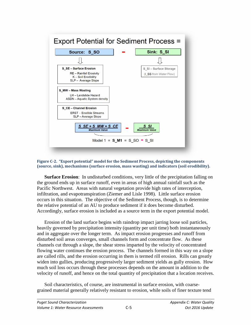
Figure C-2. “Export potential” model for the Sediment Process, depicting the components (source, sink), mechanisms (surface erosion, mass wasting) and indicators (soil erodibility).
Surface Erosion: In undisturbed conditions, very little of the precipitation falling on
the ground ends up in surface runoff, even in areas of high annual rainfall such as the Pacific Northwest. Areas with natural vegetation provide high rates of interception, infiltration, and evapotranspiration (Ziemer and Lisle 1998). Little surface erosion occurs in this situation. The objective of the Sediment Process, though, is to determine the relative potential of an AU to produce sediment if it does become disturbed. Accordingly, surface erosion is included as a source term in the export potential model.
Erosion of the land surface begins with raindrop impact jarring loose soil particles,
heavily governed by precipitation intensity (quantity per unit time) both instantaneously and in aggregate over the longer term. As impact erosion progresses and runoff from disturbed soil areas converges, small channels form and concentrate flow. As these channels cut through a slope, the shear stress imparted by the velocity of concentrated flowing water continues the erosion process. The channels formed in this way on a slope are called rills, and the erosion occurring in them is termed rill erosion. Rills can greatly widen into gullies, producing progressively larger sediment yields as gully erosion. How much soil loss occurs through these processes depends on the amount in addition to the velocity of runoff, and hence on the total quantity of precipitation that a location receives.
Soil characteristics, of course, are instrumental in surface erosion, with coarse-
grained material generally relatively resistant to erosion, while soils of finer texture tend

Puget Sound Characterization Appendix C: Water Quality Volume 1: Water Resource Assessments C-6 Oct 2016 Update
to be moved more easily. However, other soil factors also come into play. Some clays composed of very small particles consolidate and withstand the impact of falling precipitation and the shear stress of flowing water better than soils of coarser texture. With low water infiltration into the soil, though, they can produce more runoff than other soils and as a consequence still be erosive. Elevated organic content is another attribute tending to decrease a soil’s erosivity.
Topography is a third major influence on how much erosion will occur. Greater
steepness allows water to gain greater velocity, and hence shear stress, than on a gentler grade. The length of the slope is key as well. A longer slope permits water to accelerate to a higher velocity than a shorter slope or one with breaks causing deceleration at points along the flow path.
Vegetative cover is the final major factor in the determining the extent of sediment
removal from a natural slope by surface erosion. Plants intercept falling precipitation, reducing raindrop impact. Their roots and the organic layer they create on the surface further reduce impact and also create friction to reduce velocity and shear stress. Vegetation reduces water runoff quantity and its associated erosion potential through several mechanisms: evaporation from intercepted water on needles or leaves, water storage in the organic layer, assistance to infiltration provided by the root structure channeling through soil, and uptake into tissues (with possible subsequent transpiration to the atmosphere). For the Sediment Process, as in the Water Flow Process, a uniform forested condition is assumed as the natural state in western Washington (except in those limited areas with native prairie grasses).
Mass Wasting: The potential for sediment delivery by mass-wasting events is
directly related to the presence of areas susceptible to landslides, particularly those that move relatively rapidly (and commonly affect only the surface soil of a hillslope). In many parts of the landscape of this region, mass-wasting events dominate the delivery of sediment to aquatic ecosystems (Gomi et al. 2002).
Hillslope gradient and form (e.g., concave, convex, planar) play primary roles in
governing the presence and behavior of landslides. Other physical factors, such as hydrologic conditions, soil properties, bedrock geology, and land-use practices, also influence the frequency and timing of landslides. Debris avalanches (e.g., shallow, rapid landslides, excluding those triggered by roads) often occur on steep ground, particularly in concave topography, which forms a collection point for water, soils, and debris. These materials become destabilized when the factors promoting mass movement (e.g., gravity, soil saturation) overcome those resisting motion. Therefore, slope gradient and form are the principal determinants of potential for debris avalanches (Shaw and Johnson 1995).
Channel Erosion: In-channel erosion depends on the capacity of the flow to do
work on the channel materials, countered by their ability to remain in place in the face of the forces in play. It is intimately related to movement within the stream of sediments of terrestrial origin. The most fundamental measure of a stream’s ability to entrain channel bed material is the shear stress created by the flow. Bank erosion is also partially

Puget Sound Characterization Appendix C: Water Quality Volume 1: Water Resource Assessments C-7 Oct 2016 Update
controlled by shear stress, but local bank geometry comes into play, as does riparian vegetation through its ability to shield bank material from elevated velocity and absorb its energy, and from the binding effects of deep roots.
Mathematically, stream flow shear stress (τ) is most directly expressed as the product
of flow depth (normally expressed as hydraulic radius, R, the ratio of cross-sectional area to wetted perimeter) and slope (s), as well as the specific gravity of water (γ), τ = γ R s (Leopold, Wolman, and Miller1992). Channel roughness, created by rocks, cobbles, and bank vegetation, tends to dissipate the energy of any given flow, thus making it less effective in moving sediment.
Critical shear stress defines the state of incipient sediment motion. When shear stress
generated by the flow is greater than critical shear stress sediment transport results, although dynamic equilibrium can still exist with sediment entering a reach equivalent to that exiting. When the shear stress is less than critical shear stress within a reach, or if sediment transport into a reach exceeds that going out, channel aggradation (sediment accumulation) occurs.
Sediment Movement Sediment movement involves transport from the point of production to the channel
network and then through the network to its exit from the AU. Delivery to the channel principally depends on proximity to the source, topographic gradient, and vegetation cover (Goudie 2004).
Sediments entrained in stream flow can be transported as bed load in the form of
sliding and rolling grains or as suspended load carried by the main flow. Suspended sediment is that portion of the total sediment load of rivers that is carried in the water column. It contains the portion termed "wash load," or that component of the suspended load that is too fine ever to be represented in the bed material. In practice, wash load usually comprises the silt, clay, and colloidal fractions whose movement is controlled by their supply rather than by flow energy. Sediments in the sand fraction can be transported as both bed load and suspended load (the latter being termed bed-material suspended load). The bed load also comprises larger material not normally suspended in the flow but instead transported along the bed by sliding, rolling, or hopping (“saltating”).
Sediment Sinks Overland flow carrying sediments can infiltrate into the soil before reaching a water
course. Infiltration removes the particles mobilized by erosion from transport before they can reach a stream or other water body.
As sediment moves through a watershed it is deposited and temporarily or
permanently stored in areas where the water has low transport capacity (i.e., low water velocity). These areas include lakes, depressional wetlands and unconfined and
Puget Sound Characterization Appendix C: Water Quality Volume 1: Water Resource Assessments C-8 Oct 2016 Update
moderately confined flood plains, which are also features entering into the Water Flow Process.
Relative Sediment Export Potential of Assessment Units The preceding section examined mechanisms accounting for the sources and sinks of
sediments in a natural western Washington watershed. The objective of the Sediment Process model is to assess the relative potential of those various mechanisms, operating on the scale of landscape assessment units and working in concert, to deliver sediment to and move it through a portion of a watershed. As in the Water Flow Process model, the intent of the Sediment Process model is to characterize the relative priority of AU’s to receive protection (if in a relatively natural state) or restoration (if degraded to some degree). Because sediments are a water quality impediment when released in higher than natural quantities, priority is given to an AU if it has a comparatively high potential to produce and transport sediments onward if disturbed. Likewise, an AU is less sensitive in this context if it can effectively attenuate the transport of sediments originating within itself or delivered from another one upstream. These judgments have no implication for observance of water quality regulatory standards, which must be met in all circumstances. They are, however, an expression of relative risk of non-compliance with standards in different locations in a watershed.
This section introduces the indicators used to represent sediment source and sink
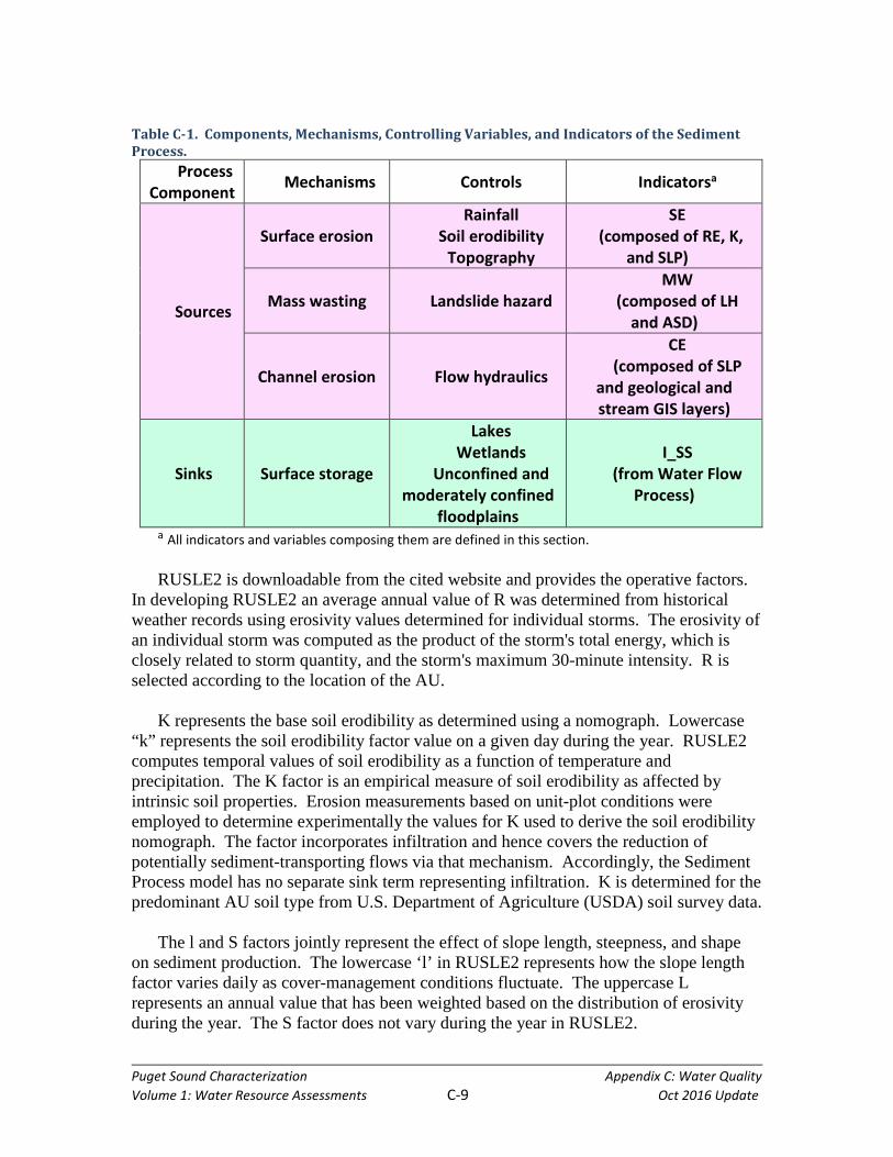
mechanisms, and to model the export potential of the AU in this respect. Table C-1 summarizes the relationships among major components of the Sediment Process model, the mechanisms operating within these components, the controlling variables, and the indicators representing the controls.
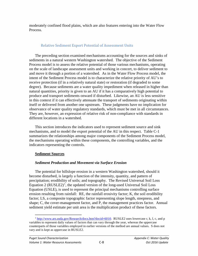
Sediment Sources Sediment Production and Movement via Surface Erosion The potential for hillslope erosion in a western Washington watershed, should it
become disturbed, is largely a function of the intensity, quantity, and pattern of precipitation; erodibility of soils; and topography. The Revised Universal Soil Loss Equation 2 (RUSLE2)1, the updated version of the long-used Universal Soil Loss Equation (USLE), is used to represent the principal mechanisms controlling surface erosion resulting from rainfall: RE, the rainfall erosivity factor; K, the soil erodibility factor; LS, a composite topographic factor representing slope length, steepness, and shape; C, the cover-management factor, and P, the management practices factor. Annual sediment yield estimate per unit area is the multiplication product of these factors.
1 http://www.ars.usda.gov/Research/docs.htm?docid=6010. RUSLE2 uses lowercase r, k, l, c, and p
variables to represent daily values of factors that can vary through the year, whereas the uppercase counterparts of those variables employed in earlier versions of the method are annual values. S does not vary and is kept as uppercase in RUSLE2.
Puget Sound Characterization Appendix C: Water Quality Volume 1: Water Resource Assessments C-9 Oct 2016 Update
Table C-1. Components, Mechanisms, Controlling Variables, and Indicators of the Sediment Process.
Process Component Mechanisms Controls Indicatorsa
Sources
Surface erosion Rainfall
Soil erodibility Topography
SE (composed of RE, K, and SLP)
Mass wasting Landslide hazard MW
(composed of LH and ASD)
Channel erosion Flow hydraulics
CE (composed of SLP
and geological and stream GIS layers)
Sinks Surface storage
Lakes Wetlands
Unconfined and moderately confined
floodplains
I_SS (from Water Flow
Process)
a All indicators and variables composing them are defined in this section. RUSLE2 is downloadable from the cited website and provides the operative factors.
In developing RUSLE2 an average annual value of R was determined from historical weather records using erosivity values determined for individual storms. The erosivity of an individual storm was computed as the product of the storm's total energy, which is closely related to storm quantity, and the storm's maximum 30-minute intensity. R is selected according to the location of the AU.
K represents the base soil erodibility as determined using a nomograph. Lowercase
“k” represents the soil erodibility factor value on a given day during the year. RUSLE2 computes temporal values of soil erodibility as a function of temperature and precipitation. The K factor is an empirical measure of soil erodibility as affected by intrinsic soil properties. Erosion measurements based on unit-plot conditions were employed to determine experimentally the values for K used to derive the soil erodibility nomograph. The factor incorporates infiltration and hence covers the reduction of potentially sediment-transporting flows via that mechanism. Accordingly, the Sediment Process model has no separate sink term representing infiltration. K is determined for the predominant AU soil type from U.S. Department of Agriculture (USDA) soil survey data.
The l and S factors jointly represent the effect of slope length, steepness, and shape
on sediment production. The lowercase ‘l’ in RUSLE2 represents how the slope length factor varies daily as cover-management conditions fluctuate. The uppercase L represents an annual value that has been weighted based on the distribution of erosivity during the year. The S factor does not vary during the year in RUSLE2.

Puget Sound Characterization Appendix C: Water Quality Volume 1: Water Resource Assessments C-10 Oct 2016 Update
For Sediment Process modeling purposes, the slope-gradient effect on sediment
delivery via land erosion is represented by average AU slope, SLP. This variable is determined by averaging over all AU pixels on a digital elevation model (DEM).
The slope-length aspect of topography is expressed as the reciprocal of aquatic
system density (1/ASD). ASD is defined as the stream arc length in the AU, including the flow path length through hydraulically connected lakes and wetlands2, divided by the AU area. Framing as the reciprocal denotes that the distance potentially eroding surface flows can travel before reaching water, and hence the acceleration they can gather, is inversely related to the prevalence of receiving water bodies in the AU. Slope length has much less influence on erosion than gradient (e.g., increasing slope from 1 to 10 percent raises the LS factor by an order of magnitude, but increasing the slope length from 100 to 1000 ft. only increases LS by a factor of about two to four depending on the specific slope3). Therefore, in modeling it would be appropriate to apply a weighting factor, W (< 1), to diminish the importance of slope length relative to gradient. However, that factor would be the same for all AU’s and thus is not instrumental in ranking them as intended in the Sediment Process.
The aforementioned variables all represent sediment production potential. Whether
or not eroded sediments actually reach a receiving water has traditionally been expressed in USLE modeling in terms of the delivery ratio, the sediment mass at a point in the channel network as a fraction of erosion yield. Delivery ratio depends most strongly on steepness, drainage density, and interrupting vegetation (Goudie 2004). Steepness is already incorporated in the Sediment Process through SLP. Vegetation is taken to be uniform among AU’s in the natural state and thus is not a factor in evaluating them relatively. ASD is, therefore, an appropriate expression of sediment delivery for this model.
The Sediment Process model assumes that, once eroded material enters the channel
network, it is transported through the AU, except for that portion lost through sinks, as covered below. Therefore, there is no movement component separate from delivery.
In the natural state in western Washington, human influence is assumed to be absent,
with cover taken to be forested and uniform throughout and no management practices in use. Once disturbed, the forest cover is replaced and management practices are applied according to human choices. The degradation model covers those conditions; hence, the C and P factors are not involved in Sediment Process importance modeling.
Considering the foregoing discussion, a complete indicator of sediment export
potential would be:
2 Included are permanently and intermittently flowing natural streams and wetlands
intermittently saturated at the surface; not included are isolated lakes and wetlands and human-built conveyances or ponds, which are considered in the impairment assessment.
3 http://www.omafra.gov.on.ca/english/engineer/facts/00-001.htm#tab3a

Puget Sound Characterization Appendix C: Water Quality Volume 1: Water Resource Assessments C-11 Oct 2016 Update
𝑆𝑆𝑆𝑆 = 𝑅𝑅𝑆𝑆 ∗ 𝐾𝐾 ∗ 𝑆𝑆𝑆𝑆𝑆𝑆 ∗ �1
𝐴𝐴𝑆𝑆𝐴𝐴� ∗ 𝑊𝑊 ∗ 𝐴𝐴𝑆𝑆𝐴𝐴
ASD cancels and W is equal among AU’s, reducing the indicator to three variables. Sediment Production and Movement via Mass Wasting As stated earlier, landslide hazard in western Washington is mainly a function of
slope gradient and form (curvature). Shaw and Johnson (1995) developed a predictive model based on these two factors that can be used to identify areas at higher risk for mass wasting. The model is applied using GIS methods for analyzing surface topography. Western Washington landslide hazards have been mapped at a scale of 900-m2 pixels color-coded to signify degrees of failure potential. Red indicates those slopes most susceptible to shallow, rapid landsliding; yellow denotes moderate susceptibility; and green indicates low susceptibility. This model is a good initial predictor of the relative risk of mass wasting events; however, actual slope stability conditions at the site level will need to be determined by a qualified expert. In modeling, the AU’s landslide hazard is characterized by the variable LH according to the predominant classification within its boundaries, with integer values 3, 2, or 1 corresponding to high, moderate, and low susceptibility, respectively.
The potential for mass wasting to produce sediments that can be transported into and
through streams and other water bodies depends on the proximity of those waters to landslide hazards. As with the surface erosion sediment source, in modeling this potential is represented by ASD. Once delivered, these sediments are assumed to move through and exit the AU, except as removed by sinks.
Sediment Production and Movement via Channel Erosion The discussion regarding channel erosion mechanisms above under Description of the
Sediment Process provides a basis to model the relative export potential of AU’s for in-channel erosion. It was reasoned that the key variables are shear stress created by the flow, the tendency for geological materials contacted by the flow to erode, and the relative extent of streams within the AU. Shear stress is directly proportional to slope, and thus the SLP variable already presented under the Surface Erosion discussion is also applied in modeling channel erosion. The GIS geology layer was assessed with respect to the relative erosiveness of the various lithological units to quantify a variable, GEO, to
The model indicator of surface erosion created by rainfall, SE, is the product RE * K * SLP.
The indicator of relative mass wasting potential of an AU, MW, is the product LH * ASD.
Puget Sound Characterization Appendix C: Water Quality Volume 1: Water Resource Assessments C-12 Oct 2016 Update
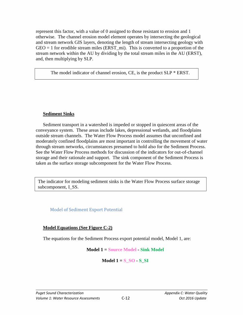
represent this factor, with a value of 0 assigned to those resistant to erosion and 1 otherwise. The channel erosion model element operates by intersecting the geological and stream network GIS layers, denoting the length of stream intersecting geology with GEO = 1 for erodible stream miles (ERST_mi). This is converted to a proportion of the stream network within the AU by dividing by the total stream miles in the AU (ERST), and, then multiplying by SLP.
Sediment Sinks Sediment transport in a watershed is impeded or stopped in quiescent areas of the
conveyance system. These areas include lakes, depressional wetlands, and floodplains outside stream channels. The Water Flow Process model assumes that unconfined and moderately confined floodplains are most important in controlling the movement of water through stream networks, circumstances presumed to hold also for the Sediment Process. See the Water Flow Process methods for discussion of the indicators for out-of-channel storage and their rationale and support. The sink component of the Sediment Process is taken as the surface storage subcomponent for the Water Flow Process.
Model of Sediment Export Potential Model Equations (See Figure C-2) The equations for the Sediment Process export potential model, Model 1, are:
Model 1 = Source Model - Sink Model
Model 1 = S_SO - S_SI
The model indicator of channel erosion, CE, is the product SLP * ERST.
The indicator for modeling sediment sinks is the Water Flow Process surface storage subcomponent, I_SS.
Puget Sound Characterization Appendix C: Water Quality Volume 1: Water Resource Assessments C-13 Oct 2016 Update
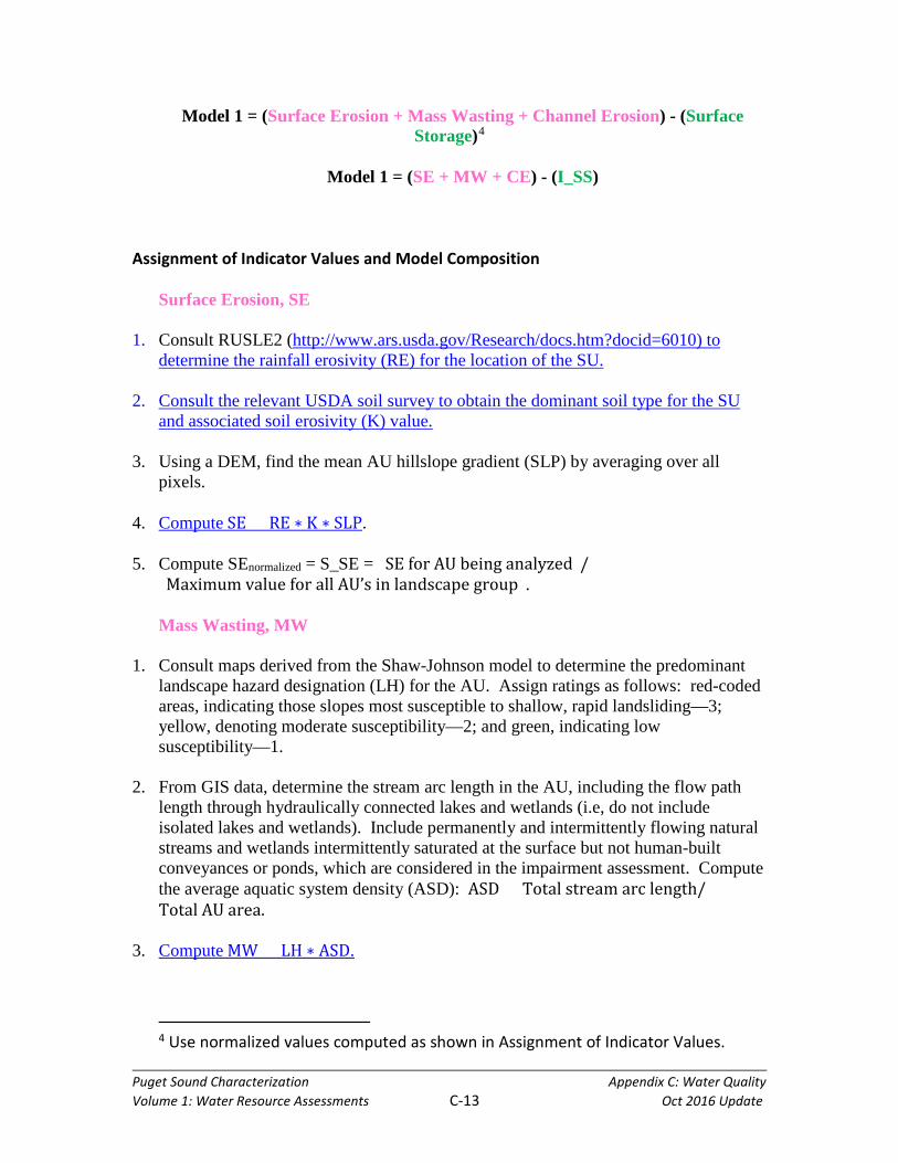
Model 1 = (Surface Erosion + Mass Wasting + Channel Erosion) - (Surface Storage)4
Model 1 = (SE + MW + CE) - (I_SS)
Assignment of Indicator Values and Model Composition Surface Erosion, SE
1. Consult RUSLE2 (http://www.ars.usda.gov/Research/docs.htm?docid=6010) to determine the rainfall erosivity (RE) for the location of the SU.
2. Consult the relevant USDA soil survey to obtain the dominant soil type for the SU and associated soil erosivity (K) value.
3. Using a DEM, find the mean AU hillslope gradient (SLP) by averaging over all pixels.
4. Compute SE = RE ∗ K ∗ SLP.
5. Compute SEnormalized = S_SE = (SE for AU being analyzed)/(Maximum value for all AU’s in landscape group). Mass Wasting, MW
1. Consult maps derived from the Shaw-Johnson model to determine the predominant landscape hazard designation (LH) for the AU. Assign ratings as follows: red-coded areas, indicating those slopes most susceptible to shallow, rapid landsliding—3; yellow, denoting moderate susceptibility—2; and green, indicating low susceptibility—1.
2. From GIS data, determine the stream arc length in the AU, including the flow path length through hydraulically connected lakes and wetlands (i.e, do not include isolated lakes and wetlands). Include permanently and intermittently flowing natural streams and wetlands intermittently saturated at the surface but not human-built conveyances or ponds, which are considered in the impairment assessment. Compute the average aquatic system density (ASD): ASD = Total stream arc length/Total AU area.
3. Compute MW = LH ∗ ASD.
4 Use normalized values computed as shown in Assignment of Indicator Values.

Puget Sound Characterization Appendix C: Water Quality Volume 1: Water Resource Assessments C-14 Oct 2016 Update
4. Compute MWnormalized = S_MW = (MW for AU being analyzed)/(Maximum value for all AU′s in landscape group). Channel Erosion, CE
1. Obtain mean AU hillslope gradient (SLP) from Rainfall Erosion analysis.
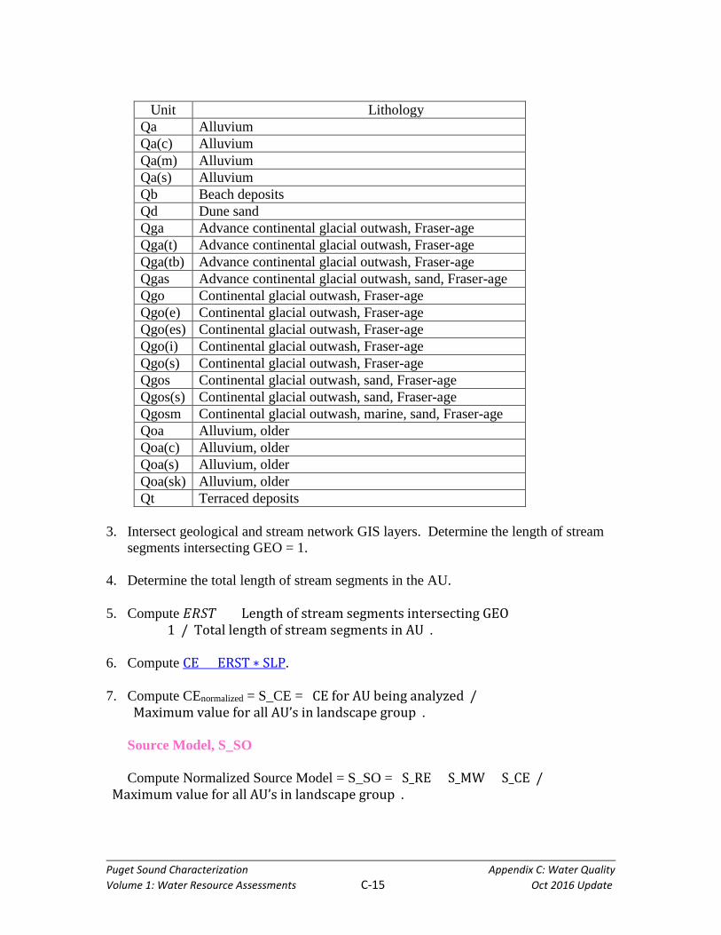
2. Determine the geology parameter (GEO) from the GIS geology layer by assigning a value of 1 to the following geological units and a value of 0 to all others:
Puget Sound Characterization Appendix C: Water Quality Volume 1: Water Resource Assessments C-15 Oct 2016 Update
Unit Lithology
Qa Alluvium Qa(c) Alluvium Qa(m) Alluvium Qa(s) Alluvium Qb Beach deposits Qd Dune sand Qga Advance continental glacial outwash, Fraser-age Qga(t) Advance continental glacial outwash, Fraser-age Qga(tb) Advance continental glacial outwash, Fraser-age Qgas Advance continental glacial outwash, sand, Fraser-age Qgo Continental glacial outwash, Fraser-age Qgo(e) Continental glacial outwash, Fraser-age Qgo(es) Continental glacial outwash, Fraser-age Qgo(i) Continental glacial outwash, Fraser-age Qgo(s) Continental glacial outwash, Fraser-age Qgos Continental glacial outwash, sand, Fraser-age Qgos(s) Continental glacial outwash, sand, Fraser-age Qgosm Continental glacial outwash, marine, sand, Fraser-age Qoa Alluvium, older Qoa(c) Alluvium, older Qoa(s) Alluvium, older Qoa(sk) Alluvium, older Qt Terraced deposits
3. Intersect geological and stream network GIS layers. Determine the length of stream
segments intersecting GEO = 1.
4. Determine the total length of stream segments in the AU.
5. Compute 𝑆𝑆𝑅𝑅𝑆𝑆𝐸𝐸 = (Length of stream segments intersecting GEO = 1)/(Total length of stream segments in AU).
6. Compute CE = ERST ∗ SLP.
7. Compute CEnormalized = S_CE = (CE for AU being analyzed)/
(Maximum value for all AU’s in landscape group). Source Model, S_SO Compute Normalized Source Model = S_SO = (S_RE + S_MW + S_CE)/
(Maximum value for all AU’s in landscape group).

Puget Sound Characterization Appendix C: Water Quality Volume 1: Water Resource Assessments C-16 Oct 2016 Update
Surface Storage (lake, wetland, and unconfined and moderately confined floodplain storage) I_SS
1. Obtain from the Water Flow Process.
Phosphorus Process
Description of the Phosphorus Process The Phosphorus Process (Figure C-3) is defined as the interaction of sources
(embracing production and movement) and sinks of phosphorus in a watershed. This process is dependent on elements of the Water Flow and Sediment Process models outlined previously.
Phosphorus Sources Phosphorus Production Under natural conditions, phosphorus (P) enters a watershed through the production
mechanisms described in the Sediment Process (erosion of terrestrial soils and in-channel substrates, mass wasting), weathering of rocks, and wet- and dry-deposition from the atmosphere. P content varies in soils, aquatic substrates, and rocks depending on their mineralogy, with sedimentary rocks and soils developed from them tending to reach the highest concentrations (Huminicki and Hawthorne 2002). Atmospheric deposition would not vary substantially through the region’s natural watersheds. Hence, no one assessment unit within those watersheds would contribute differently than any other, and this source is not considered further.

Puget Sound Characterization Appendix C: Water Quality Volume 1: Water Resource Assessments C-17 Oct 2016 Update
Figure C-3. Export potential model for the Phosphorous Process, depicting the components, mechanisms and indicators.
Many phosphorus compounds are relatively insoluble, and hence a large fraction of
the P in any watershed is in the solid phase (Stumm and Morgan 1996). In soil, solubility is least at soil pH < 5.5, where aluminum tends to fix P in relatively insoluble compounds, and pH > 7.0, where calcium is the dominant cation reacting with P to produce increasingly insoluble compounds as pH rises. Because soil pH is usually in the circumneutral area, some P enters water in the soluble state, through dissolution, as well as in the particulate form via erosion. The dissolved P form is most available to biota, which makes it the primary concern regarding eutrophication. Soluble P can become particulate through sorption to soil particles (especially, clays) and organic material. This form of phosphorus reaches aquatic ecosystems along the same pathways as fine sediment.
Phosphorus Movement Phosphorus moves in a watershed via channel transport, either dissolved in the water
or, in its particulate form, with the sediments. In water, the solubility of P combined with or sorbed by other materials is controlled by pH and concentrations of the various metals involved. Changes in those variables can result in dissolution of phosphorus. In the water pH range 4.5-6.5, P tends to be bound to the solid phase by iron and aluminum, either by precipitation or adsorption. Very little P becomes sorbed between pH 7.0 and 9.0, but at higher pH the tendency for P precipitation becomes enhanced and appears to be related to the progressively decreasing solubility of calcium phosphate (apatite) (Stumm and Morgan 1996).

Puget Sound Characterization Appendix C: Water Quality Volume 1: Water Resource Assessments C-18 Oct 2016 Update
Phosphorus Sinks While passing overland, before discharge into a water body, some sheet and
concentrated flow infiltrates the soil, the amount depending on many variables. As discussed above, P dissolved in the percolating water sorbs to soil particles mainly as a function of clay and organic content.
Dissolved P reaching a water body can be removed permanently or temporarily via a
number of mechanisms: (1) uptake by biota; (2) adsorption to aluminum and ferric iron oxides and hydroxides, and subsequent precipitation out of solution (Walbridge and Struthers 1993); (3) adsorption to sediment particles; (4) reactions with metal ions (mainly, calcium, magnesium, aluminum, and iron) forming complexes, chelates, or insoluble salts (Stumm and Morgan 1996); and (5) trapping of particles that have adsorbed or reacted with phosphorus. Adsorption to soil particles is most likely to occur in finer soils, such as clays, that have a phosphorus deficit (Sheldon et al. 2005). These soils can occur in either aquatic or upland settings. In general, aquatic settings, such as wetlands with mineral soils, are likely to remove dissolved P from surface water; while upland settings are likely to remove dissolved P from water that percolates into the subsurface deposits (Axt and Walbridge 1999).
Particulate P and dissolved P converted to a particulate form are permanently or
temporarily removed from aquatic ecosystems through the loss component of the Sediment Process. For example, since depressional wetlands are effective at removing sediment, they are also effective at removing phosphorus (Sheldon et al. 2005).
Capture of dissolved P is not necessarily permanent, and often is not. It is released
from the tissues of plants and animals upon death and decomposition. Lakes of any significant depth stratify seasonally and develop a hypolimnetic layer isolated from the atmosphere for months. With oxygen-consuming biological decomposition processes occurring without oxygen replenishment, these layers commonly go fully or nearly anaerobic, especially in more advanced states of eutrophication. With depleted oxygen P residing in lake sediments redissolves into the water column. Wetlands also release phosphorus from sediment during long periods of anoxia (Adamus et al. 1991).
Relative Phosphorus Export Potential of Assessment Units The preceding section examined mechanisms accounting for the sources and sinks of
phosphorus in a natural western Washington watershed. The objective of the Phosphorus Process model is to assess the relative potential of those various mechanisms, operating on the scale of landscape assessment units and working in concert, to deliver P to and move it through a portion of a watershed. As in the Water Flow and Sediment Process models, the intent of the Phosphorus Process model is to characterize the relative priority
Puget Sound Characterization Appendix C: Water Quality Volume 1: Water Resource Assessments C-19 Oct 2016 Update
of AU’s to receive protection (if in a relatively natural state) or restoration (if degraded to some degree). Because phosphorus is a water quality impediment when released in higher than natural quantities, priority is given to an AU if it has a comparatively high potential to produce and transport P onward if disturbed. Likewise, an AU is less sensitive in this context if it can effectively attenuate the transport of phosphorus originating within itself or delivered from another one upstream. These judgments have no implication for observance of water quality regulatory standards, which must be met in all circumstances. They are, however, an expression of relative risk of non-compliance with standards in different locations in a watershed.
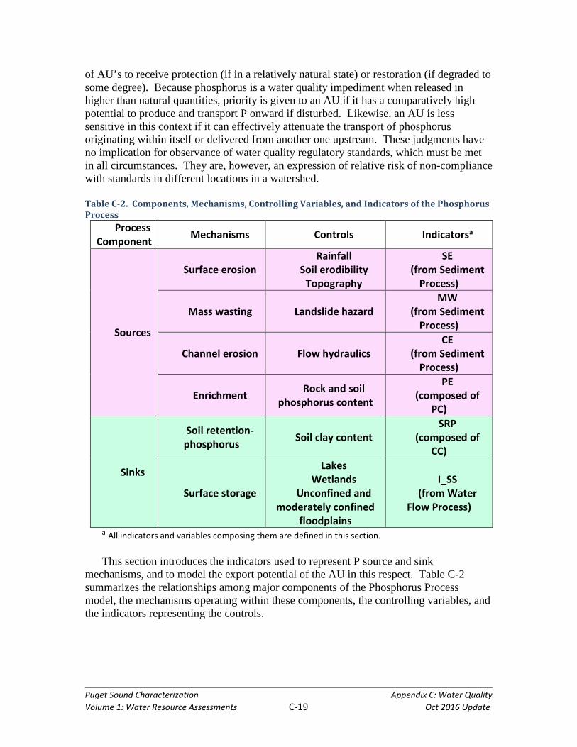
Table C-2. Components, Mechanisms, Controlling Variables, and Indicators of the Phosphorus Process
Process Component Mechanisms Controls Indicatorsa
Sources
Surface erosion Rainfall
Soil erodibility Topography
SE (from Sediment
Process)
Mass wasting Landslide hazard MW
(from Sediment Process)
Channel erosion Flow hydraulics CE
(from Sediment Process)
Enrichment Rock and soil phosphorus content
PE (composed of
PC)
Sinks
Soil retention-phosphorus Soil clay content
SRP (composed of
CC)
Surface storage
Lakes Wetlands
Unconfined and moderately confined
floodplains
I_SS (from Water
Flow Process)
a All indicators and variables composing them are defined in this section. This section introduces the indicators used to represent P source and sink
mechanisms, and to model the export potential of the AU in this respect. Table C-2 summarizes the relationships among major components of the Phosphorus Process model, the mechanisms operating within these components, the controlling variables, and the indicators representing the controls.

Puget Sound Characterization Appendix C: Water Quality Volume 1: Water Resource Assessments C-20 Oct 2016 Update
Phosphorus Sources Since phosphorus is present in some amount in soil and geological material, it enters
water along with sediments through the same sources, surface erosion, mass wasting and in-channel erosion. Therefore, these mechanisms are identical in the Sediment and Phosphorus Processes. However, the quantity of P accompanying sediments differs spatially around western Washington. Therefore, a phosphorus enrichment indicator, PE, is added to the Phosphorus Process source model to distinguish AU’s on this basis. It is quantified in terms of soil P content, PC. GIS mapping currently does not exist for this quantity. Therefore, it can only be taken into account by applying any available local knowledge or data. Without that information, the sources component of the Phosphorus Process reduces to identity with the Sediment Process.
Phosphorus Sinks The Phosphorus Process is based on two assumptions regarding phosphorus removal:
(1) the K factor in the surface erosion mechanism incorporates soil infiltration, particulate P in infiltrating water is removed before entering surface water, and dissolved P is removed in relation to the soil’s clay content (CC); and (2) surface storage sediment sinks have the same potential to capture sediments and phosphorus in equal measure, not distinguishing between particulate and dissolved P forms. In modeling, an AU’s clay content is characterized by the variable CC from GIS mapping and assignment of integer values 3, 2, or 1 corresponding to > 28, 10-28, and < 10 percent clay, respectively, as recommended by Natsuhara (personal communication). GIS mapping is not currently available for organic content, the other soil property primarily governing the tendency to sequester phosphorus. However, mapping does cover peat and muck soils, those highest in organics are mapped and with the greatest ability to capture P. They are taken into account in modeling by grouping with clays in the > 28 percent range.
Model of Phosphorus Export Potential Model Equations (Figure C-3) The equations for the Phosphorus Process export potential model, Model 1, are:
Model 1 = Source Model - Sink Model
The model indicator of phosphorus enrichment, PE, is soil phosphorus content, PC.
The model indicator of phosphorus retention by soils, SRP, is soil clay content, CC. The indicator for modeling surface storage phosphorus sinks is the Water Flow Process surface
storage subcomponent, I_SS.

Puget Sound Characterization Appendix C: Water Quality Volume 1: Water Resource Assessments C-21 Oct 2016 Update
Model 1 = P_SO - P_SI
Model 1 = (Surface Erosion + Mass Wasting + Channel Erosion + Phosphorus
Enrichment) - (Phosphorus-Soil Retention + Surface Storage)5
Model 1 = (S_SE + S_MW + S_CE + PE) - (P_SR + I_SS) Assignment of Indicator Values and Model Composition Surface Erosion, S_SE
1. Obtain from the Sediment Process. Mass Wasting, S_MW
1. Obtain from the Sediment Process. Channel Erosion, S_CE
1. Obtain from the Sediment Process. Phosphorus Enrichment, PE
1. Use local knowledge or data to assign a phosphorus content, PC, rating. For example, areas known to be very high in P could be assigned a rating of 3, moderately high deposits a 2, and other locations a 1. In the absence of such information, assign a value of 0, which makes the Phosphorus Process equivalent to the Sediment Process.
2. Assign PE = PC.
3. Compute PEnormalized = I_PE = (PE for AU being analyzed)/(Maximum value for all AU’s in landscape group). Source Model, P_SO
1. Compute Normalized Source Model = P_SO = (S_SE + S_MW + S_CE +PE)/(Maximum value for all AU’s in landscape group). Soil Retention-Phosphorus, SRP
5 Use normalized values computed as shown in Assignment of Indicator Values.
Puget Sound Characterization Appendix C: Water Quality Volume 1: Water Resource Assessments C-22 Oct 2016 Update
1. Consult the soil type and soil clay content GIS layers. Assign ratings for clay content, CC, as follows: > 28%: 3 (also include peat and muck soils in this category); 10-28%: 2; and < 10%: 1.
2. Assign SRP = CC.
3. Compute SRPnormalized = P_SR = (SRP for AU being analyzed)/(Maximum value for all AU’s in landscape group). Surface Storage (lake, wetland, and unconfined and moderately confined
floodplain storage), I_SS
1. Obtain from the Water Flow Process. Sink Model, P_SI
1. Compute Normalized Sink Model = P_SI = (P_SR + I_SS)/(Maximum value for all AU’s in landscape group).

Puget Sound Characterization Appendix C: Water Quality Volume 1: Water Resource Assessments C-23 Oct 2016 Update
Metals Process
Description of the Metals Process The Metals Process (Figure C-4) is defined as the operation of watershed sinks for
metals. This process is dependent on elements of the Water Flow Process model outlined previously.
Metals exist naturally as copper, lead, zinc, mercury, cadmium, nickel, and others,
many toxic to aquatic life. In western Washington toxic metals are in relatively low concentrations in streams draining watersheds in natural land cover. According to Welch (1998), bedrock type does not influence metal concentrations in streams. While in unusual circumstances acidic pH and atmospheric deposition can result in higher metal levels (Welch 1998), these conditions would not vary substantially through the region’s natural watersheds. Hence, no one assessment unit within those watersheds would contribute differently than any other even when disturbed. Overall, natural processes are not considered to be a significant mechanism, relative to human inputs, for delivery of toxic metals to western Washington aquatic ecosystems. Accordingly, metal sources are considered in the degradation model but not the export potential model.
Figure C-4. Export potential model for the Metals Process, depicting the components, mechanisms and indicators.

Puget Sound Characterization Appendix C: Water Quality Volume 1: Water Resource Assessments C-24 Oct 2016 Update
Metals Sinks
Even though watershed assessment units in natural land cover are not considered to be a significant mechanism for delivery of toxic metals to western Washington aquatic ecosystems, natural processes in these units would mediate the transport and fate of metals introduced by other sources. Metals are present in water in particulate and dissolved forms. Removal of sediments from the water column also subtracts the particulate metals they transport. Dissolved metals can be removed from solution by a number of mechanisms: (1) hydroxide and oxide adsorption and complexation; (2) sediment particle adsorption; (3) ion exchange; and (4) reactions with anionic ligands (mainly, halides, sulfates, sulfites, and carbonates) forming chelates or insoluble salts (Stumm and Morgan 1996). The pH plays a significant role in governing these mechanisms and the distribution of metals between the solid and aqueous states. Metal solubilities tend to be lowest in the circumneutral pH area.
Metals are most likely to be temporarily stored through adsorption to wetland soils
with high cation exchange capacities (Sheldon et al. 2005, Kadlec and Knight 1996). These soils have relatively high organic and clay content, although it is not yet clear whether glacially derived clays provide the same conditions as weathered clays (Sheldon et al. 2005).
Relative Metals Export Potential of Assessment Units The preceding section examined mechanisms accounting for the sinks of metals in a
natural western Washington watershed. The objective of the Metals Process model is to assess the relative potential of those various mechanisms, operating on the scale of landscape assessment units and working in concert, to move metals through a portion of a watershed, or, alternatively, attenuate their movement. As in the Water Flow and Sediment Process models, the intent of the Metals Process model is to characterize the relative priority of AU’s to receive protection (if in a relatively natural state) or restoration (if degraded to some degree). Because metals are water quality impediments when released and transported in higher than natural quantities, priority is given to an AU if it has a comparatively high potential to transport metals onward if disturbed. Likewise, an AU is less sensitive in this context if it can effectively attenuate the transport of metals originating within itself or delivered from another one upstream. These judgments have no implication for observance of water quality regulatory standards, which must be met in all circumstances. They are, however, an expression of relative risk of non-compliance with standards in different locations in a watershed.
This section introduces the indicators used to represent metals sink mechanisms, and
to model the export potential of the AU in this respect. Table C-3 summarizes the relationships among major component of the Metals Process model, the mechanisms operating within this component, the controlling variables, and the indicators representing the controls.

Puget Sound Characterization Appendix C: Water Quality Volume 1: Water Resource Assessments C-25 Oct 2016 Update
Table C-3. Components, Mechanisms, Controlling Variables, and Indicators of the Metals Process.
Process Component Mechanisms Controls Indicatorsa
Sinks
Soil retention-metals
Cation exchange capacity
SRM (composed of
CEC)
Surface storage
Lakes Wetlands
Unconfined and moderately confined
floodplains
I_SS (from Water
Flow Process)
a All indicators and variables comprising them are defined in this section. Metals Sinks The Metals Process is based on two assumptions regarding metals removal: (1) the K
factor in the surface erosion mechanism incorporates soil infiltration, particulate metals in infiltrating water are removed before entering surface water, and dissolved metals are removed in relation to the soil’s cation exchange capacity (CEC); and (2) surface storage sediment sinks have the same potential to capture sediments and metals in equal measure, not distinguishing between particulate and dissolved forms. CEC was estimated for Western Washington based on pH of 7 and soil clay and organic contents and mapped in GIS (Natsuhara personal communication). GIS mapping is not currently available for other soil properties (e.g., texture, various chemical constituents) that also govern the tendency to sequester metals.
Model of Metals Export Potential Model Equations (Figure C-4) The equations for the Metals Process export potential model, Model 1, are:
Model 1 = - Sink Model
Model 1 = - M_S1
Model 1 = - (Soil Retention-Metals + Surface Storage)6 6 Use normalized values computed as shown in Assignment of Indicator Values.
The model indicator of metals retention by soils, SRM, is cation exchange capacity at pH = 7, CEC-7. The indicator for modeling surface storage metals sinks is the Water Flow
Process surface storage subcomponent, I_SS.

Puget Sound Characterization Appendix C: Water Quality Volume 1: Water Resource Assessments C-26 Oct 2016 Update
Model 1 = - (M_SRM + I_SS)
Assignment of Indicator Values and Model Composition
Soil Retention-Metals, SRM
1. Consult the CEC-7 (pH = 7) GIS layer.
2. Assign SRM = CEC-7.
3. Compute SRMnormalized = M_SRM = (SRM for AU being analyzed)/(Maximum value for all AU’s in landscape group). Surface Storage (lake, wetland, and unconfined and moderately confined
floodplain storage), I_SS
1. Obtain from the Water Flow Process. Sink Model, M_SI
1. Compute Normalized Sink Model = M_SI = (M_SRM + I_SS)/(Maximum value for all AU’s in landscape group).
Puget Sound Characterization Appendix C: Water Quality Volume 1: Water Resource Assessments C-27 Oct 2016 Update
Nitrogen Process
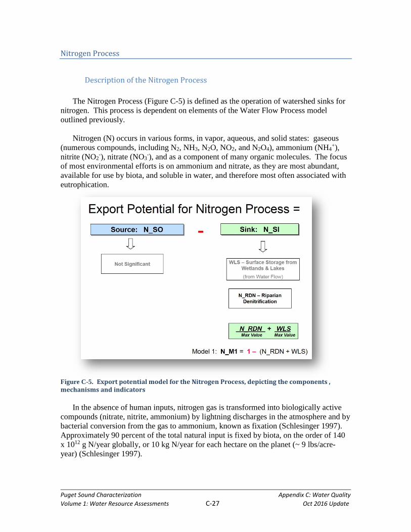
Description of the Nitrogen Process The Nitrogen Process (Figure C-5) is defined as the operation of watershed sinks for
nitrogen. This process is dependent on elements of the Water Flow Process model outlined previously.
Nitrogen (N) occurs in various forms, in vapor, aqueous, and solid states: gaseous
(numerous compounds, including N2, NH3, N2O, NO2, and N2O4), ammonium (NH4+),
nitrite (NO2-), nitrate (NO3
-), and as a component of many organic molecules. The focus of most environmental efforts is on ammonium and nitrate, as they are most abundant, available for use by biota, and soluble in water, and therefore most often associated with eutrophication.
Figure C-5. Export potential model for the Nitrogen Process, depicting the components , mechanisms and indicators
In the absence of human inputs, nitrogen gas is transformed into biologically active
compounds (nitrate, nitrite, ammonium) by lightning discharges in the atmosphere and by bacterial conversion from the gas to ammonium, known as fixation (Schlesinger 1997). Approximately 90 percent of the total natural input is fixed by biota, on the order of 140 x 1012 g N/year globally, or 10 kg N/year for each hectare on the planet (~ 9 lbs/acre-year) (Schlesinger 1997).
Puget Sound Characterization Appendix C: Water Quality Volume 1: Water Resource Assessments C-28 Oct 2016 Update
The operation of these processes in a western Washington watershed in natural land cover would not differ substantially from place to place. Hence, no one assessment unit within those watersheds would contribute differently than any other even when disturbed. Overall, natural processes are not considered to be a significant mechanism, relative to human inputs, for production of nitrogen in western Washington aquatic ecosystems. Accordingly, N production is considered in the degradation model but not the export potential model.
Nitrogen Cycling Even though watershed assessment units in natural land cover are not considered to
be a significant mechanism for delivery of nitrogen to western Washington aquatic ecosystems, natural processes in these units would mediate the transport and fate of nitrogen introduced by other sources. Once it has reached a watershed, nitrogen can be temporarily stored or transformed from one biologically active form to another through three mechanisms: (1) biotic uptake and decomposition, (2) adsorption, and (3) nitrification. As nitrogen moves through a watershed, it will likely be assimilated, transformed, and then released numerous times in a process called nutrient cycling.
In plants, inorganic nitrogen, in the forms of ammonium, nitrite, and nitrate, is
transformed to organic nitrogen (e.g., proteins, urea). When the plants die, this organic nitrogen is converted back into ammonium by bacteria and fungi. Nitrification then transforms the ammonium to nitrite and, subsequently, nitrate. This transformation is important because nitrate can be permanently removed from a watershed through denitrification. Nitrification depends upon two species of bacteria and occurs in uplands and all aquatic areas where oxygen is present (Mitch and Gosselink 2000). In wetlands the location of the oxic/anoxic interfaces governs where nitrification occurs; however, the mechanisms controlling the process in stream ecosystems are not yet understood (Grimm et al. 2003). Some ammonium can become adsorbed to fine sediments in stream bottoms (Peterson et al. 2001) and on upland soils (Grimm et al. 2003). The work by Peterson et al. (2001) indicates that this particular mechanism may account for a major portion of the ammonium removal occurring in small streams.
Denitrification is a process mediated by anaerobic bacteria converting nitrate to
gaseous nitrogen for liberation to the atmospheric sink. As anaerobic zones are most common in wet areas, this nitrogen removal process is more likely to occur in wetlands and other aquatic ecosystems than in terrestrial environments (Grimm et al. 2003). In order for denitrification to occur, a set of conditions must be met:
• Reactive sites in anaerobic conditions and sources of organic carbon providing the
energy for denitrifying microbes must be present. (Denitrification can be high in anoxic areas around the root zones of living plants, which exude dissolved organic carbon, and in detrital deposits, sources of particulate organic matter.)
Puget Sound Characterization Appendix C: Water Quality Volume 1: Water Resource Assessments C-29 Oct 2016 Update
• Water must have time to interact with these reactive sites. (The residence time of water or the rate at which it moves through substrates must allow for interaction between the nitrate-laden water and the carbon deposits.)
• Nitrate must be present in the water. If the first two of the above conditions are met, the role an area plays in the nitrogen
budget of the larger watershed is dependent upon the flux of nitrate to that location. In other words, it is possible for an area to have theoretically high nitrate removal efficiency but to receive little or no nitrate-laden waters much of the year (Vidon and Hill 2004). Nitrate reaches aquatic ecosystems both through transport from land and as a product of the nitrification transformation within the water itself. Ammonium reaching water must be adsorbed and held long enough for the reaction to occur. Therefore, adsorption and then nitrification are prerequisites for nitrogen loss via denitrification.
Transformations that depend upon microbes, such as nitrification and denitrification,
occur at very high rates in “hot spots” within a watershed. Many of these hot spots are located at the interfaces between terrestrial and aquatic ecosystems. Such spots occur because all necessary conditions exist for biogeochemical transformations: movement of water into the area, high material flux, and reactive sites for the transformations (McClain et al. 2003).
The shallow depth and small discharge of headwater streams provide opportunity for
ammonium to become adsorbed to streambed sediments and subsequently converted to nitrate in the aerobic conditions prevailing there (Peterson et al. 2001), making this environment instrumental in nitrogen cycling. The seasonal edges of depressional wetlands are other locations offering the aerobic conditions necessary for nitrification to occur (Sheldon et al. 2005). Nitrate produced in wetlands and headwaters streams can then move and be denitrified when reaching an anaerobic environment.
Nitrogen Loss Under natural conditions, ammonium is removed from a watershed through
volatilization, while nitrate is lost via denitrification. Volatilization occurs as bacteria process decaying organic matter and ammonia (the gas, NH3) is released. It primarily occurs in marshes with excessive algal blooms (Mitsch and Gosselink 2000).
Wetlands are the primary locations of denitrification in a watershed. Other important
locations are lakes and areas where groundwater is anoxic and intersects riparian areas of streams and rivers in permeable alluvial deposits that may not specifically be identified as wetlands.
Wetlands and Lakes Saturated areas within depressional wetlands provide the anaerobic conditions
necessary for denitrification to occur (Sheldon et al. 2005, Mitsch and Gosselink 2000).
Puget Sound Characterization Appendix C: Water Quality Volume 1: Water Resource Assessments C-30 Oct 2016 Update
Wetlands are the one feature in the landscape where anaerobic soils near the surface are found, and thus are the primary source of denitrification in a watershed (Arheimer and Wittgren 1994).
The potential for denitrification in wetland soils is up to six times higher than in other
soils of the floodplain (Ullah and Faulkner 2006). The amount of nitrogen removed by wetlands, however, depends on their relative presence in a watershed. Wetlands making up 1 percent of a watershed can remove 10-16 percent of the nitrogen in the system. This quantity increases to more than 50 percent with 5 percent wetland coverage (Arheimer and Wittgren 1994). In certain small agricultural watersheds, wetlands can denitrify as much as 80 percent of the nitrogen moving through the system, even though they represent less than 1 percent of the total area (Woltemade 2000).
The other major locations for denitrification in a watershed are the anaerobic
hypolimnions of lakes (Arheimer and Wittgren 1994). This condition occurs in lakes that thermally stratify in the summer months, especially those somewhat to highly advanced in eutrophication.
Riparian Areas Research over the past 10 years has taken interest in identifying the hydrogeologic
settings of riparian areas most likely to meet the three conditions for denitrification: the presence of reactive sites in anaerobic conditions, the time for water to interact with the reactive sites, and nitrates in the water. The results of two of these studies are described below.
In the glaciated portion of northeastern United States, researchers from the University
of Rhode Island concluded that nitrate removal occurs primarily in shallow hydric riparian soils and not in deeper deposits (Rosenblatt et al. 2001, Gold et al. 2001, Kellogg et al. 2005). They observed that hydric alluvial and outwash deposits are subject to fluvial action and therefore have buried organic deposits. This condition, in conjunction with higher hydraulic conductivities, provides an opportunity for groundwater to interact with the carbon deposits and for the microbes to perform denitrification. An exception occurs when groundwater is able to move through the riparian area at depth, bypassing the rooting zone or the buried organic deposits. These researchers suggested that denitrification tends to happen in shallow hydric outwash and alluvial deposits underlain by a less permeable deposit, which prevents bypass of the likely areas for denitrification. Of course, anaerobiosis must exist for denitrification actually to occur.
In glaciated Ontario, researchers from York University identified riparian areas as
important nitrogen sinks, if they had a high flux of nitrate (Vidon and Hill 2004, Hill et al. 2004). They found that the yearly flux of nitrogen-laden waters reaching a site is determined in large part by the size of the upland aquifer and its connectivity to the riparian area. Denitrification efficiencies can be high in non-hydric alluvial and outwash deposits, as well as hydric deposits.

Puget Sound Characterization Appendix C: Water Quality Volume 1: Water Resource Assessments C-31 Oct 2016 Update
Using these findings, it can be hypothesized that important areas for denitrification within a watershed are those:
• Adjacent to a deep upland aquifer (The size of this water source governs the
potential magnitude and duration of sub-surface flow from the upland area into the riparian area. Vidon and Hill [2004] suggested that this upland aquifer should be greater than 2 meters deep);
• Connected via a steep slope to the upland area (This setting ensures a large
hydraulic gradient from the upland to the riparian area, thus providing opportunity for a large flux of water and nitrates to move into the riparian area. A good indicator of this condition is incised river valleys [i.e., the area between the valley floor and upland is a steep valley wall]. Vidon and Hill [2004] suggested an overall slope in this transition area of 5 percent but also indicated that it can be over 15 percent in local areas); and
• Relatively shallow, permeable riparian deposits (riparian deposits that are
alluvium or outwash no deeper than 6 meters would be good indicators of these areas [Vidon and Hill 2004, Rosenblatt et al. 2001, Gold et al. 2001, Kellogg et al. 2005]).
Very coarse deposits can have such a high hydraulic conductivity that water moves
very quickly through the deposit. Then, the distance required for a given amount of denitrification to occur would be longer than in finer deposits. As a result, it is possible that a particular riparian area of coarse deposits could have a width that is inadequate to allow large quantities of denitrification to occur. Also, rapid water exchange makes oxygen depletion less likely in such deposits, removing an essential condition for denitrification.
In considering these various clues for the choice of viable indicators for riparian zone
denitrification, Cox (personal communication) confirmed that the best course at this state of knowledge is to pinpoint hydric soils occurring in floodplains. In his experience alluvium rarely provides the combination of adequate organic matter (minimum 10 percent) and anoxia. This simplified procedure would omit upland interactions, but present mapping cannot represent these factors anyway.

Puget Sound Characterization Appendix C: Water Quality Volume 1: Water Resource Assessments C-32 Oct 2016 Update
Relative Nitrogen Export Potential of Assessment Units The preceding section examined mechanisms accounting for the sinks of nitrogen in a
natural western Washington watershed. The objective of the Nitrogen Process model is to assess the relative potential of those various mechanisms, operating on the scale of landscape assessment units and working in concert, to move nitrogen through a portion of a watershed, or, alternatively, attenuate their movement. As in the Water Flow and Sediment Process models, the intent of the Nitrogen Process model is to characterize the relative priority of AU’s to receive protection (if in a relatively natural state) or restoration (if degraded to some degree). Because nitrogen is a water-quality impediment when released and transported in higher than natural quantities, priority is given to an AU if it has a comparatively high potential to transport nitrogen onward if disturbed. Likewise, an AU is less sensitive in this context if it can effectively attenuate the transport of nitrogen originating within itself or delivered from another one upstream. These judgments have no implication for observance of water quality regulatory standards, which must be met in all circumstances. They are, however, an expression of relative risk of non-compliance with standards in different locations in a watershed.
This section introduces the indicators used to represent nitrogen sink mechanisms,
and to model the export potential of the AU in this respect. Table C-4 summarizes the relationships among major component of the Nitrogen Process model, the mechanisms operating within this component, the controlling variables, and the indicators representing the controls.
Table C-4. Components, Mechanisms, Controlling Variables, and Indicators of the Nitrogen Process
Process Component Mechanisms Controls Indicatorsa
Sinks Denitrification
Wetlands Lakes
WLS (from Water Flow
Process)
Riparian denitrification
potential
RDN (unconfined
floodplains in hydric soils GIS layers)
a All indicators and variables comprising them are defined in this section. Nitrogen Sinks The preceding discussion pointed out that volatilization and denitrification are the
principal processes accounting for nitrogen loss in a watershed. Furthermore, adsorption and nitrification are prerequisite processes for effective denitrification but do not remove nitrogen or permanently sequester it, and hence are not modeled.
Puget Sound Characterization Appendix C: Water Quality Volume 1: Water Resource Assessments C-33 Oct 2016 Update
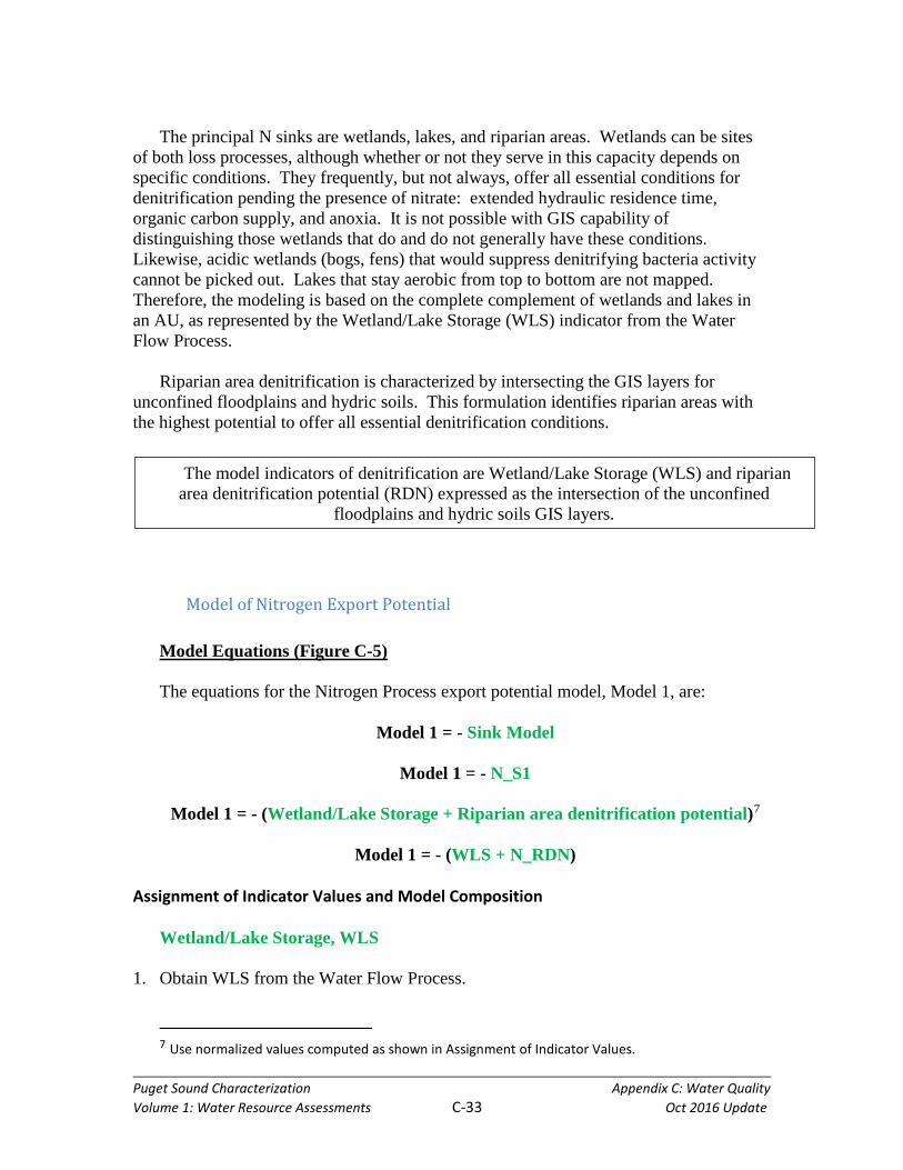
The principal N sinks are wetlands, lakes, and riparian areas. Wetlands can be sites
of both loss processes, although whether or not they serve in this capacity depends on specific conditions. They frequently, but not always, offer all essential conditions for denitrification pending the presence of nitrate: extended hydraulic residence time, organic carbon supply, and anoxia. It is not possible with GIS capability of distinguishing those wetlands that do and do not generally have these conditions. Likewise, acidic wetlands (bogs, fens) that would suppress denitrifying bacteria activity cannot be picked out. Lakes that stay aerobic from top to bottom are not mapped. Therefore, the modeling is based on the complete complement of wetlands and lakes in an AU, as represented by the Wetland/Lake Storage (WLS) indicator from the Water Flow Process.
Riparian area denitrification is characterized by intersecting the GIS layers for
unconfined floodplains and hydric soils. This formulation identifies riparian areas with the highest potential to offer all essential denitrification conditions.
Model of Nitrogen Export Potential Model Equations (Figure C-5) The equations for the Nitrogen Process export potential model, Model 1, are:
Model 1 = - Sink Model
Model 1 = - N_S1
Model 1 = - (Wetland/Lake Storage + Riparian area denitrification potential)7
Model 1 = - (WLS + N_RDN)
Assignment of Indicator Values and Model Composition Wetland/Lake Storage, WLS
1. Obtain WLS from the Water Flow Process. 7 Use normalized values computed as shown in Assignment of Indicator Values.
The model indicators of denitrification are Wetland/Lake Storage (WLS) and riparian area denitrification potential (RDN) expressed as the intersection of the unconfined
floodplains and hydric soils GIS layers.
Puget Sound Characterization Appendix C: Water Quality Volume 1: Water Resource Assessments C-34 Oct 2016 Update
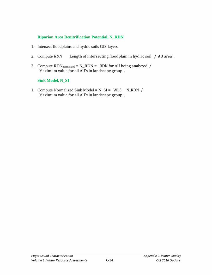
Riparian Area Denitrification Potential, N_RDN
1. Intersect floodplains and hydric soils GIS layers.
2. Compute 𝑅𝑅𝐴𝐴𝑅𝑅 = (Length of intersecting floodplain in hydric soil )/(AU area).
3. Compute RDNnormalized = N_RDN = (RDN for AU being analyzed)/(Maximum value for all AU’s in landscape group). Sink Model, N_SI
1. Compute Normalized Sink Model = N_SI = (WLS + N_RDN)/(Maximum value for all AU’s in landscape group).

Puget Sound Characterization Appendix C: Water Quality Volume 1: Water Resource Assessments C-35 Oct 2016 Update
Pathogen Process -
Description of the Pathogen Process The Pathogen Process (Figure C-6) is defined as the operation of watershed sinks for
pathogenic organisms. This process is dependent on an element of the Water Flow Process model outlined previously.
Pathogens are potentially disease-causing organisms, including bacteria, protozoans,
and viruses. Under natural conditions, the primary input of pathogens is the fecal material of wildlife deposited within upland areas that drain into aquatic ecosystems or deposited directly into them (Sherer et al. 1992). This source would not differ substantially from place to place in a western Washington watershed in natural land cover. Hence, no one assessment unit within those watersheds would contribute differently than any other even when disturbed. Overall, natural processes are not considered to be a significant mechanism, relative to human inputs, for production of pathogens in western Washington aquatic ecosystems. Accordingly, pathogen production is considered in the degradation model but not the export potential model.
Figure C-6. Export potential model for the Pathogen Process, depicting the components, mechanisms and indicators.
Pathogens are generally represented by indicator groups of bacteria in water quality
analysis and regulation, and this discussion focuses on bacteria. Most commonly employed are the fecal coliforms or one species among them, Escherichia coli. The feces of all warm-blooded animals carry bacteria in this group. While it contains human disease-causing organisms and is invariably associated with others, the group also includes bacteria not introduced to the environment in feces but generated independently, especially in soils (Doyle and Erickson 2006). Total coliforms embrace even more
Puget Sound Characterization Appendix C: Water Quality Volume 1: Water Resource Assessments C-36 Oct 2016 Update
organisms of natural origin and are, accordingly, less useful as an indicator group for pathogenesis. The Enterococci group is increasingly being measured and assigned regulatory standards. Two species are common in the intestines of humans, and they and others are recognized as disease-producing (Gilmore et al. 2002). These organisms are believed to provide a higher correlation than fecal coliforms with many of the human pathogens often found in wastewater effluents and storm runoff (Jin et al. 2004). Fecal streptococci sometimes receive attention in environmental studies but are not used as a regulatory indicator group.
Pathogen Dynamics in a Watershed Fecal pathogens tend to survive for considerably longer periods of time in water with
sediment than without (Sherer et al. 1992). Thus, sediments provide a transport medium and increase bacteria viability in aquatic transport. Bacteria do not tend to pass from their point of origin to the ultimate sink (e.g., marine waters) rapidly and without change (McDonald, Kay, and Jenkins 1982; Struck 1988; Gerba and McLeod 1976; Horner, Brenner, and Jones 1989). In contrast, they cycle dynamically, sometimes depositing in sediments with the particles to which they are attached, and perhaps going dormant, and other times reproducing again and being released from the sediments into the flow. These events depend on a number of factors, such as temperature, changes in flow quantity and velocity, and sediment composition. The point is that bacteria discharged into an aquatic environment at one time and place can influence that environment over an extended time into the future and at other locations affected by the discharge.
Pathogen Loss The preceding discussion portrayed bacteria as generally not directly flowing through
aquatic systems, but instead coming to rest temporarily in sediments, from which they can subsequently be released back to the water under the control of flow and temperature, perhaps after having grown in numbers. Therefore, quiescent environments mediating particle settling and having sediments retentive of bacteria can interrupt their transport and provide an opportunity for extinguishment. Depressional wetlands are the leading landscape features fitting this description. They remove pathogen-bearing sediment in surface waters through the mechanisms of filtration and sedimentation and contain mineral and organic hydric soils that have high adsorptive capacity. Velocity reduction and vegetative filtration also occur in low gradient, unconfined floodplains (Borst et al. 2001, Sherer et al. 1992, Sheldon et al. 2005).
Pathogens are removed from a watershed via mortality. The primary factors causing death of these organisms are ultraviolet radiation, temperature, pH, salinity, predation, and starvation (Roszak and Colwell 1987). Marino and Gannon (1991) reported that the extent of bacterial and protozoan predation is a major factor determining fecal coliform and fecal streptococci survival. Tate (1978) demonstrated that protozoans played a significant role in reducing E. coli populations in muck soils over a 10-day period.
Puget Sound Characterization Appendix C: Water Quality Volume 1: Water Resource Assessments C-37 Oct 2016 Update
Increasing the residence time of water is a critical mechanism by which pathogens can be removed from the ecosystem. Studies conducted in stormwater treatment wetlands indicate that standing water promotes physical, chemical, and biological processes that increase the removal of bacteria from surface waters (Borst et al. 2001). Death may be due to increased microbial competition with or predation on pathogenic organisms (Marino and Gannon 1991). Cox et al. (2005) reported a 99.8 percent die off of E. coli bacteria during the first 65 days in 8 liters of stream sediment held under quiescent conditions and supplemented with 3 liters of dairy barnyard manure. Hemond and Benoit (1988) reported that detention time and predation by microorganisms in wetlands results in the loss of pathogens. These results suggest that aquatic ecosystems that allow predation of pathogens to occur over a longer period of time play an important role in eliminating pathogens. Due to their ability to hold water back, depressional wetlands provide longer residence time for surface waters than streams and rivers.
Relative Pathogen Export Potential of Assessment Units The preceding section examined mechanisms accounting for the sinks of pathogens in
a natural western Washington watershed. The objective of the Pathogen Process model is to assess the relative potential of those various mechanisms, operating on the scale of landscape assessment units and working in concert, to move pathogens through a portion of a watershed, or, alternatively, attenuate their movement. As in the Water Flow and Sediment Process models, the intent of the Pathogen Process model is to characterize the relative priority of AU’s to receive protection (if in a relatively natural state) or restoration (if degraded to some degree). Because pathogens are water-quality impediments when released and transported in higher than natural quantities, priority is given to an AU if it has a comparatively high potential to transport pathogens onward if disturbed. Likewise, an AU is less sensitive in this context if it can effectively attenuate the transport of pathogens originating within itself or delivered from another one upstream. These judgments have no implication for observance of water quality regulatory standards, which must be met in all circumstances. They are, however, an expression of relative risk of non-compliance with standards in different locations in a watershed.
This section introduces the indicator used to represent pathogen sink mechanisms,
and to model the export potential of the AU in this respect. Table C-5 summarizes the relationships among major component of the Pathogen Process model, the mechanism operating within this component, the controlling variable, and the indicator representing the control.

Puget Sound Characterization Appendix C: Water Quality Volume 1: Water Resource Assessments C-38 Oct 2016 Update
Table C-5. Component, Mechanism, Controlling Variable, and Indicator of the Pathogen Process
Process Component Mechanism Control Indicatora
Sink Mortality Depressional wetlands
DPWT (composed of
dpwt_pct from Water Flow
Process) a The indicator and variable comprising it are defined in this section. Pathogen Sink Because of their ability to cycle through stages of transport, dormancy, regeneration,
and reproduction, elimination of pathogens from a watershed requires their mortality. Extinguishing bacteria, in turn, requires their capture with the sediments constituting their transport mechanism and adsorption in a medium capable of holding them for a sufficient time for predation and other factors to kill them. Depressional wetlands are unique in furnishing all of the essential conditions and control an AU’s role in pathogen mortality to a much greater degree than any other feature.
Model of Pathogen Export Potential Model Equations (Figure C-6) The equations for the Pathogen Process export potential model, Model 1, are:
Model 1 = - Sink Model
Model 1 = - PA_S1
Model 1 = - (Depressional Wetland Presence)8
Model 1 = - (DPWT)
8 Use normalized values computed as shown in Assignment of Indicator Values.
The model indicator of bacterial mortality is the relative depressional wetlands presence, DW, as quantified in the Water Flow Process by dpwt_pct.

Puget Sound Characterization Appendix C: Water Quality Volume 1: Water Resource Assessments C-39 Oct 2016 Update
Assignment of Indicator Values and Model Composition Depressional Wetland Presence, DPWT
1. Obtain dpwt_pct from the Water Flow Process.
2. Assign DPWT = dpwt_pct.
3. Compute DPWTnormalized = (DPWT for AU being analyzed)/(Maximum value for all AU’s in landscape group). Sink Model, PA_SI
1. PA_SI = DPWT

Puget Sound Characterization Appendix C: Water Quality Volume 1: Water Resource Assessments C-40 Oct 2016 Update
Model 2 –Degradation (N-SPECT)
Introduction
The degradation models for all of the water quality processes use an existing model, the Non-Point Source Pollution and Erosion Control Tool (N-SPECT). N-SPECT is a GIS-based screening tool to estimate water pollutant loadings as a function of land use and land cover and associated pollutant export coefficients (mass/unit area). Because the N-SPECT model is an existing peer reviewed model with extensive documentation on its methods and application, we have not duplicated that information in this section. This information can be accessed at the following links:
http://www.csc.noaa.gov/digitalcoast/tools/nspect/_pdf/N-SPECT_TechnicalGuide.pdf http://www.csc.noaa.gov/digitalcoast/tools/nspect/_pdf/N-SPECT_UsersManual.pdf
N-SPECT Model Options
Two basic N-SPECT options were exercised in the application of the model to the Puget Sound Basin. The first option was to use the single storm runoff and load calculation instead of the average annual runoff and load calculation. The two reasons were to make more correct use of the NRCS curve number method for calculating runoff, and to avoid the insurmountable problem of identifying appropriate, consistent numbers of storms to go along with an annual rainfall input. In applying the single storm option, a 2-yr, 24-hr design storm with SCS (NRCS) Type 1-A distribution was selected. Selection of this design storm was based on the judgment that the storm frequency should be neither too low, nor too high to produce runoff from a range of land uses yet also to represent overall pollutant generation. However, no pretense is made that the 2-yr event has much advantage over a 1.01-year event of 5-yr event for the comparative modeling purposes of the PSC project.
The second N-SPECT option invoked was to compute “local” rather than “routed”
runoff and pollutant loads. N-SPECT has the ability to “route” water and pollutant loads using DEM data and simple summation. While this capability may be of interest in future applications, it is not consistent with current logical framework of the PSC project which is oriented toward treating and comparing AU’s as autonomous units rather than as a hierarchical network. Therefore, local runoff and pollutant loads were calculated for all 30-meter square pixels within each AU and summed to obtain AU-total runoff and load.

Puget Sound Characterization Appendix C: Water Quality Volume 1: Water Resource Assessments C-41 Oct 2016 Update
N-SPECT Algorithms To calculate runoff, N-SPECT utilizes the SCS Curve number methodology:
S).(PS).(PRpixel 80
20 2
+−
= 101000−=
CNS (eqs. 1 and 2)
In which R = “direct storm runoff” in inches, P = storm precipitation in inches, S =
retention or storage in inches, and CN = SCS Curve Number appropriate to the soil-cover complex and antecedent moisture condition.
As discussed earlier, in N-SPECT, for the annual runoff option, annual P is used with
an estimate of the # of significant storms. For this option, N-SPECT divides the annual P by the number of storms to estimate a typical storm and multiplies the calculated runoff from typical storm by the number of storms to produce an annual runoff estimate. As we know, this is an extrapolation of the curve number runoff procedure unique to N-SPECT that was not intended by the USDA-SCS (now USDA NRCS), the original developer of the curve number method.
Pollutant Modeling – Excluding Sediment With the exception of sediment, N-SPECT calculates all pollutant loads for each land
use pixel by a simple multiplication of user input Event Mean Concentration and runoff volume.
Loadp = Ap x Rp/12 x 62.4 x EMC
(eq. 3) In which Loadp = the pixel load in lbs for all non-sediment constituents except
pathogens, Ap is the pixel area in square feet, Rp/12 is the runoff from the curve number calculation converted to feet, and 62.4 converts runoff volume (Ap x Rp/12) to runoff weight in lbs, and EMC is the concentration in ppm (=~ mg/l) of the pollutant of interest.
For pathogens, the user must recognize that N-SPECT does not specifically
accommodate typical pathogen units (e.g. counts per liter), and it is up to the user to either interpret the output as a relative indicator or convert it to meaningful physical units.
Sediment (Erosion) Modeling Sediment modeling in N-SPECT is computed using the Revised Universal Soil Loss
Equation (RUSLE, Renard et al, 1991) for average annual loads and the Modified USLE (MUSLE, Williams and Berndt, 1977)) for storm loads. As mentioned earlier, the single storm-event option was selected for the runoff calculation, therefore the MUSLE was selected as the pixel sediment-production model. Like the RUSLE and the original

Puget Sound Characterization Appendix C: Water Quality Volume 1: Water Resource Assessments C-42 Oct 2016 Update
USLE (Wischmeier and Smith, 1978), the MUSLE uses a factorial equation to compute soil loss per unit area, except that it substitutes a power function of the product of event runoff volume and peak flow for the average annual rainfall erosion parameter, R. Thus, the sediment yield is expressed in tons, not tons per acre per year:
SY = 95 (Q x qp)0.56 K LS C P (eq. 4)
in which SY = the sediment yield from an individual storm in tons, Q = the storm runoff volume in ac-ft, qp = the peak runoff rate in ft3/sec, K = soil-erodibility factor, LS = the slope length and gradient factor, C = the crop management or cover factor, and P = the erosion-control-practice factor. This last factor is not used by N-SPECT (i.e., it is effectively assigned an invariant value of 1.0)
N-SPECT Model Input Datasets The N-SPECT model requires land cover or land use, landscape slope, precipitation
and soils datasets as well as EMC values for each land use to simulate pollutant loading. A key requirement for the N-SPECT in the PSC project is that datasets cover the entire Puget Sound Basin. Table C-7 below lists datasets that meet this criterion.
Runoff and Sediment Parameters Table C-7 summarizes input parameters for both the runoff and sediment calculations.
For the MUSLE calculation, the storm volume and peak flow values were derived from the curve number runoff calculation which is implemented on a time varying basis using the type 1A storm distribution. As shown, GIS-based datasets covering most if not all of the Puget Sound basin were available for land use, storm rainfall totals, elevation (used to calculate pixel slope) and USLE K-factors. In the case of the K-factors, there were holes in the coverage within national parks and forests that were filled with median values for the K-factor and for the hydrologic soil group (0.20 and C-type soil, respectively).
One item to note is that 2-yr, 24-hr precipitation polygons from Oregon Climate
Service (OCS) do not distinguish rain from snow, and snow tends to increasingly dominate with increasing elevation above 1500 feet in the in the Puget Sound basin. Additionally, even when rain occurs at higher elevations, snow cover may significantly attenuate pollutant entrainment and transport. To correct for what would be anomalous results for mountain areas, OCS 2-yr, 24 hour precipitation was reduced by 20%, 40%, and 60% in the WADNR rain-on-snow zone, snow dominated zone, and highland zones which generally correspond to elevation bands of 1500-3000, 3000-4000, and above 4000 feet, respectively.

Puget Sound Characterization Appendix C: Water Quality Volume 1: Water Resource Assessments C-43 Oct 2016 Update
Table C-7: GIS and Tabular Input Datasets Utilized for N-SPECT Model Application.
GIS Datasets Original Data Source Comment • Land Use or Land Cover NOAA C-CAP 30-meter pixel • Sub-Basins (Analysis
Units for PSC) NIFC SSHIAP, provided by
Ecology Used for post-processing of
N-SPECT model output • 2-year 24-hour Storm
event precipitation Oregon Climate Service
(OCS) PRISM Model, provided by WSDOT
Original polygon data converted to raster format
• Digital Elevation Model (DEM)
USGS, provided by University of Washington
Original 10-meter pixels aggregated to 30-meters
• K-Factor Grid NRCS SSURGO Database, “kwfact” attribute
Original polygon data converted to raster upon import to N-SPECT
• NRCS Hydrologic Soils Group (A, B, C, D)
NRCS SSURGO Database, “hydgrp” attribute
Original polygon data converted to raster upon import to N-SPECT
Tabular Datasets • Curve Number per land
use Handbook of Hydrology
• Pollutant Event Mean Concentrations (EMCs) for each land use
Multiple, see discussion
All GIS datasets for both N-SPECT input and output are spatially referenced
using the Washington State Plane South Zone projection, North American Datum of 1983 horizontal datum, and units of feet. Depth and elevation units for the DEM and precipitation datasets were converted to inches and feet respectively.
Table C-8 summarizes runoff curve number values and USLE/MUSLE cover
factor values implemented in the N-SPECT runoff and sediment yield calculations in this project. Curve number values for different C-CAP land classes NRCS soils groups are based on typical literature values (e.g., Maidment, 1993). C-factor values were derived largely from N-SPECT documentation with some interpretation and minor adjustments. The slope length and gradient factor, LS is determined by N-SPECT using a combination of pixel size and average gradient determined using the DEM.

Puget Sound Characterization Appendix C: Water Quality Volume 1: Water Resource Assessments C-44 Oct 2016 Update
Table C-8: NRCS Curve Number and Cover Factor by C-CAP Land Class Name.
C-CAP Class Name NRCS Hydrologic Soil Group
USLE Cover Factor
A B C D High Intensity Developed 89 92 94 95 0.005 Medium Intensity Developed 77 85 90 92 0.006 Low Intensity Developed 61 75 83 87 0.03 Open Spaces Developed 49 69 79 84 0.03 Cultivated Land 67 78 85 89 0.24 Pasture/Hay 49 69 79 84 0.24 Grassland 30 58 71 78 0.05 Deciduous Forest 30 48 65 73 0.004 Evergreen Forest 30 48 65 73 0.004 Mixed Forest 30 48 65 73 0.004 Scrub/Shrub 30 48 65 73 0.014 Palustrine Forested Wetland 0 0 0 0 0.003 Palustrine Scrub/Shrub Wetland 0 0 0 0 0.003 Palustrine Emergent Wetland 0 0 0 0 0.003 Estuarine Emergent Wetland 0 0 0 0 0.003 Unconsolidated Shore 0 0 0 0 0.5 Water 0 0 0 0 0
Palustrine Aquatic Bed 0 0 0 0 0.5 Estuarine Aquatic Bed 0 0 0 0 0.5 Snow/Ice 0 0 0 0 0 Non-Mountainous Bare Land (< 2000 feet) 77 86 91 94 0.7 Mountainous Bare Land (> 2000 feet) 30 48 65 73 0.1
“EMC” Values and PSC Relative Load Modeling Approach The N-SPECT user defines the number and type of pollutants to be tracked for
each land use pixel. For each land use class and pollutant, the user must provide a typical concentration value. EMC values and the overall approach to EMC-based evaluation of comparative pollutant generation for Puget Sound AU’s were developed using a multi-pronged approach: a review of literature and national databases that provide typical loads or concentrations by land use, review of recent EMC data developed for land uses within the Puget Sound basin, and finally by convening a workshop (held at the office of Northwest Hydraulic Consultants on May 19, 2011) of local and regional experts to review the project’s water quality modeling objectives, approach and assignment of EMC values to land uses. Consensus was achieved

Puget Sound Characterization Appendix C: Water Quality Volume 1: Water Resource Assessments C-45 Oct 2016 Update
concerning two significant issues: 1) the need to group some C-CAP land use classes due to the lack of data or rationale for distinguishing individual EMC values within the groups, and 2) that among several key data sets there was more consistency (and logic) in the ratios of EMC values among land use groups than in the absolute values themselves.
The practical outcome of the first consensus item is illustrated in Table C-9 by the
first two columns which show how 21 C-CAP land use classes are grouped into 10 PSC pollutant generation classes. The second consensus item, was that use of physical units (e.g., mg/l or ppm) in N-SPECT for PSC modeling should be abandoned in favor of a relative index ranging from 0.0 to 10.0 with no units for each EMC-based pollutant. This approach was suggested by the objective of the modeling—to characterize the relative degradation of AU’s associated with land use within the AU, rather than to predict actual pollutant loads from each AU. Values in the columns for TP, TN, TSS, Cu, Zn, and Pathogen in Table C-9 reflect this approach. The values represent average ratios scaled to assign the land use group which most consistently exhibited the highest concentration in multiple studies (Lowe, 2011; Roberts, 2011; Inkpen and Embry, 2008; King County, 2007; Brandenberger et al, 2007; Hart Crowser et al, 2007; LA County, 2006; Strecker, 1997; Chandler 1996; and Chandler, 1993) within the Puget Sound basin, the region and nationally.
As shown in Table C-9 cultivated agricultural land ranks at the top among the
EMC classes for TP, TN, and Cu while Commercial/Industrial/Highway is at the top for Zn, ranks second for Cu, and ties for second with other urban classes for TP, & TN.

Puget Sound Characterization Appendix C: Water Quality Volume 1: Water Resource Assessments C-46 Oct 2016 Update
Table C-9: Relative EMC Values by C-CAP Land Class Name.
C-CAP Class Name PSC EMC Class Name
Relative EMCs by Constituent
TP TN TSS Cu Zn Pathogens
High Intensity Developed
Comm./Ind./ Highway 2.7 4.5 1.5 6.5 10. 10
Medium Intensity Developed
High Density Residential 2.7 4.5 1.3 3.3 5. 10
Low Intensity Developed
Low Density Residential 2.7 4.5 1.2 1.6 2.5 5
Open Spaces Developed Urban Open 1.3 2.7 0.6 1.2 0.4 2
Cultivated Land Agriculture 10 10 2 10. 4.6 3 Pasture/Hay
Natural Open w/ Pasture
1.3 2.7 1 1.2 0.4 2 Grassland 1.3 2.7 1 1.2 0.4 2 Scrub/Shrub 1.3 2.7 1 1.2 0.4 2 Palustrine Forested Wetland 1.3 2.7 1 1.2 0.4 2
Palustrine Scrub/Shrub Wetland 1.3 2.7 1 1.2 0.4 2
Palustrine Emergent Wetland 1.3 2.7 1 1.2 0.4 2
Estuarine Emergent Wetland 1.3 2.7 1 1.2 0.4 2
Water 1.3 2.7 1 1.2 0.4 2 Palustrine Aquatic Bed 1.3 2.7 1 1.2 0.4 2 Estuarine Aquatic Bed 1.3 2.7 1 1.2 0.4 2 Snow/Ice 1.3 2.7 1 1.2 0.4 2 Deciduous Forest
Forest 0.8 0.2 0.2 0.4 0.4 1
Evergreen Forest 0.8 0.2 0.2 0.4 0.4 1 Mixed Forest 0.8 0.2 0.2 0.4 0.4 1
Unconsolidated Shore Unconsolidated Shore 3 2.7 10 0.4 0.4 1
Bare Land1
Non-Mountainous Bare Land (< 2000 feet)
3 2.7 10 0.4 0.4 1
Mountainous Bare Land (> 2000 feet)
1.3 2.7 1 0 0 2
1CCAP Bare Land has been split into two types, low elevation which is a relatively rare occurrence but applies to severely disturbed bare soil areas such as quarries and landfills, and high elevation which is more evident in some areas of the Cascades and generally represents natural exposed bedrock and talus.
Puget Sound Characterization Appendix C: Water Quality Volume 1: Water Resource Assessments C-47 Oct 2016 Update
Normalization and Aggregation of N-SPECT Output to AU Level Degradation at both the 30-meter pixel and AU level is represented on a scale of
zero to one in which zero represents a condition with no increase in load due to land use/cover alteration within the pixel or AU and 1.0 represents the maximum level of degradation within the degradation comparison area (DCA). In the PSC project, two DCAs and therefore two sets of AU rankings are considered, the WRIA-Level and the Puget Sound basin-wide DCA. Relative degradation (0 to 1) for a specific pollutant for a DCA is first computed for each 30-meter grid cell within an AU.
Pixel and AU Degradation Calculation The relative 30-meter pixel degradation for either DCA is: Di,j = (Existing Li,j – Pre-development Li,j)/(Existing Li – Pre-development Li)max
(eq. 5) In which Di,j is the relative degradation associated with specific pollutant i (0 – 1)
in pixel j expressed as a ratio of the increase in pollutant load per unit area (LPA) caused by land use/cover change for the pixel j divided by the maximum increase in load per unit area calculated for all pixels within either the WRIA DCA or the Puget Sound Basin-wide DCA. GIS processing is used to compute the average value of Di over all pixels within an AU in order to represent relative AU degradation. As an example, a value of 0.20 for AU total phosphorus (TP) means that the increase in TP load per unit area associated with land use/cover change within the AU is 20% as large as the maximum increase in TP load per unit area caused by land use/cover change within the WRIA or the entire Puget Sound Basin.
Grouping and Mapping of AU Degradation
AU degradation results are categorized into four groups corresponding to “low”, “medium low”, “medium high”, and “high” levels of relative degradation for mapping purposes. Originally, these groups were defined by simple quartiles determined by the rank of AU’s with respect to increase in relative load per unit area (LPA) caused by land use/cover change. That is, 25% of the AU’s with the highest LPAs were categorized as “high, the next lower 25% of AU’s were classified as “medium high” etc. This method assures that there would be an even number AU’s in each group. After an examination of the distribution of LPA values for most of the pollutants, it was decided that a more informative grouping might be achieved by grouping results using ratios of the average LPA value for either the entire DCA (Puget Sound Basin or individual WRIA). In this scheme “low”, “medium low”, “medium high”, and “high” are defined by LPA ranges bounded by the following ratios to the DCA average, 0 - 0.50, .50 - 1.00, 1.00 - 2.00, and >2.00 respectively. Figure C-8 compares the two schemes using total phosphorus results for the Puget Sound Basin DCA as an example. In the map on the left, by definition, the same

Puget Sound Characterization Appendix C: Water Quality Volume 1: Water Resource Assessments C-48 Oct 2016 Update
number of AU’s are placed into each category. However, this approach was found to put an extreme range of LPA values in the same “high” category. The map on the right places a majority of AU’s in the “low” category (likely where they belong), while also providing better discrimination and highlighting of AU’s producing higher loads.
Figure C-8. Example of categorizing AUs by standard quartiles (left), or by ranges defined by ratios to the average value (right).
Low
Medium-Low
Medium-High
High

Puget Sound Characterization Appendix C: Water Quality Volume 1: Water Resource Assessments C-49 Oct 2016 Update
Results All of the sample results in these figures use quartile mapping based on
degradation rankings for the entire Puget Sound Basin. However, the GIS datasets with the N-SPECT and post-processing results include both basin-wide and within-WRIA rankings of both AU’s and C-CAP pixels.
Figures C-9 through C-15 map relative degradation for TP, TN, Zn, Cu,
Pathogens, TSS and Erosion. With the exception of erosion, maps of all the other relative pollutant LPAs show a great deal of consistency. AU’s with the highest concentration of high intensity development (commercial–industrial) are generally the most degraded across all pollutants, but AU’s that are nearly or totally dominated by cultivated agriculture are also very high producers. For example, looking at copper, the AU with the largest relative load in the Puget Sound basin include those containing the Bremerton Naval Base, and the Seattle and Olympia port areas which are all mapped with very high levels of C-CAP’s “high intensity development” class. However, loads per unit area are nearly as high for AU’s with very high percentages of cultivated land such as agricultural fields in the Nooksack and lower Skagit watersheds.
The erosion map is quite distinct from all the other maps including TSS in that
“high” areas are not the most urbanized. Instead, the erosion map tends to flag areas with a combination of high runoff, steep slopes, and removal of forest cover resulting in more erosion prone land cover classes such as scrub shrub, grassland, or bare soil. Clearly, many of the “high” AU’s show the impacts of logging. However, it should be noted that unlike TSS which is an urban runoff indicator for fine sediments/solids which are transported to streams or other receiving waters, erosion in forestry zones, as calculated by N-SPECT on 30-meter pixels does not account for factors that can greatly reduce the delivery of sediment to streams.
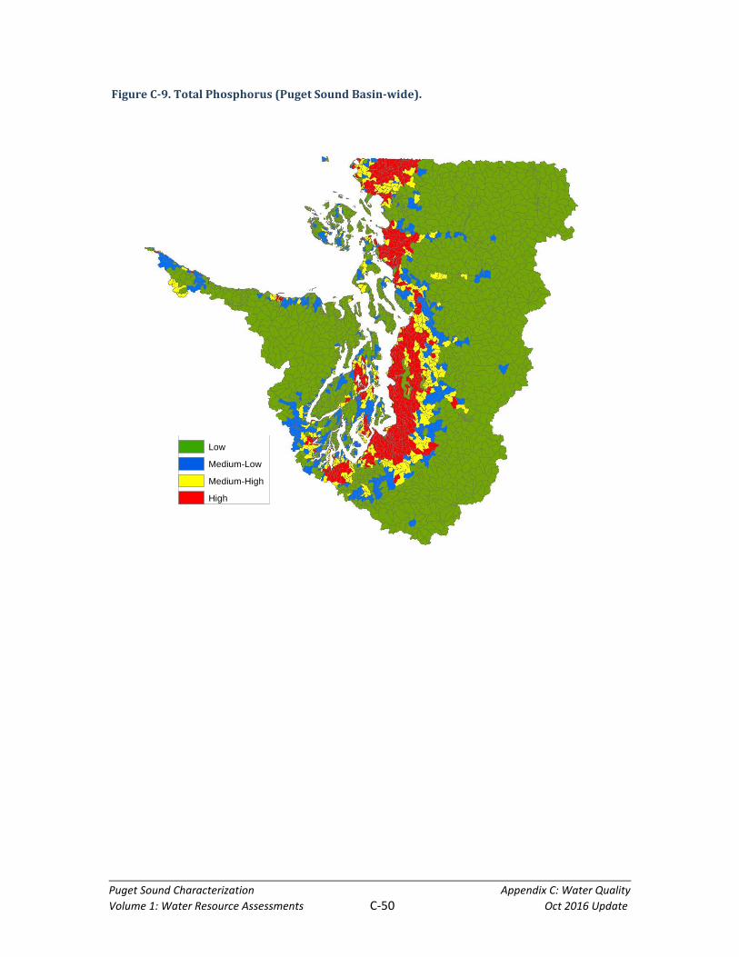
Puget Sound Characterization Appendix C: Water Quality Volume 1: Water Resource Assessments C-50 Oct 2016 Update
Low
Medium-Low
Medium-High
High
Figure C-9. Total Phosphorus (Puget Sound Basin-wide).
Low
Medium-Low
Medium-High
High
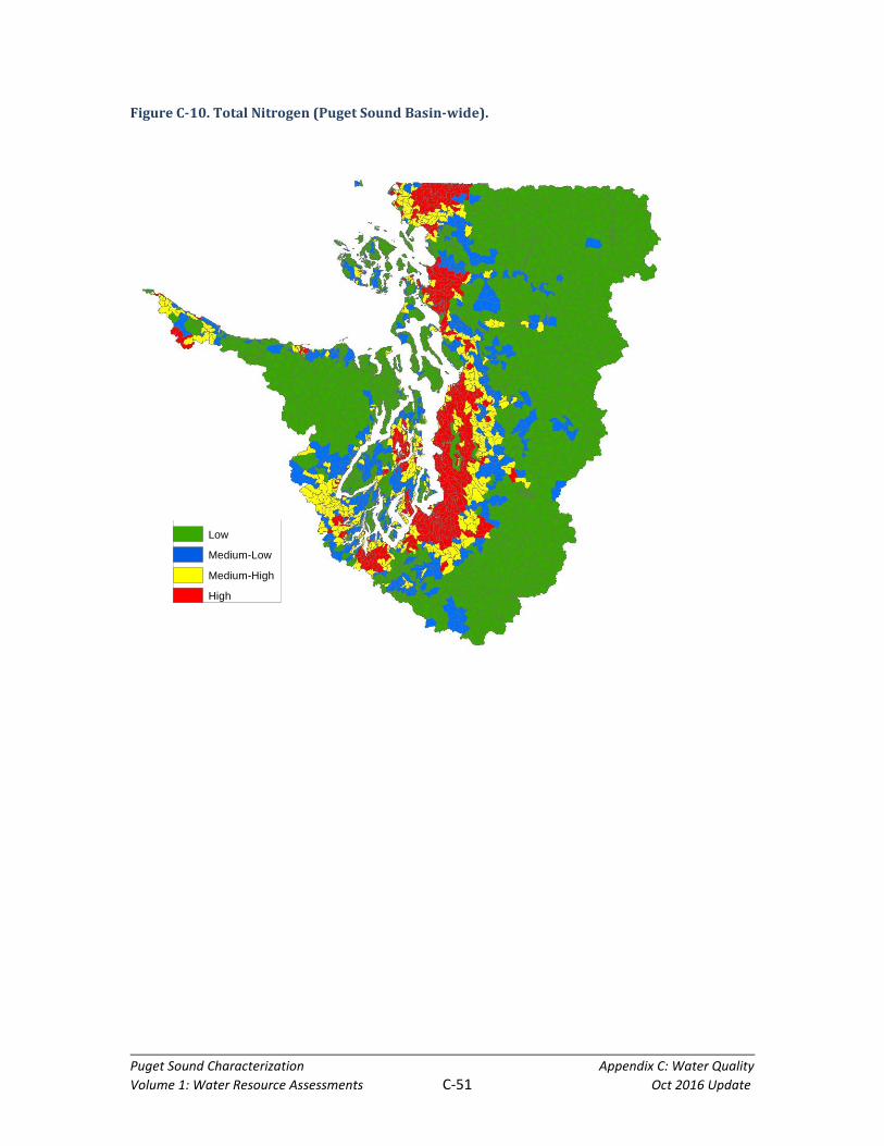
Puget Sound Characterization Appendix C: Water Quality Volume 1: Water Resource Assessments C-51 Oct 2016 Update
Figure C-10. Total Nitrogen (Puget Sound Basin-wide).
Low
Medium-Low
Medium-High
High
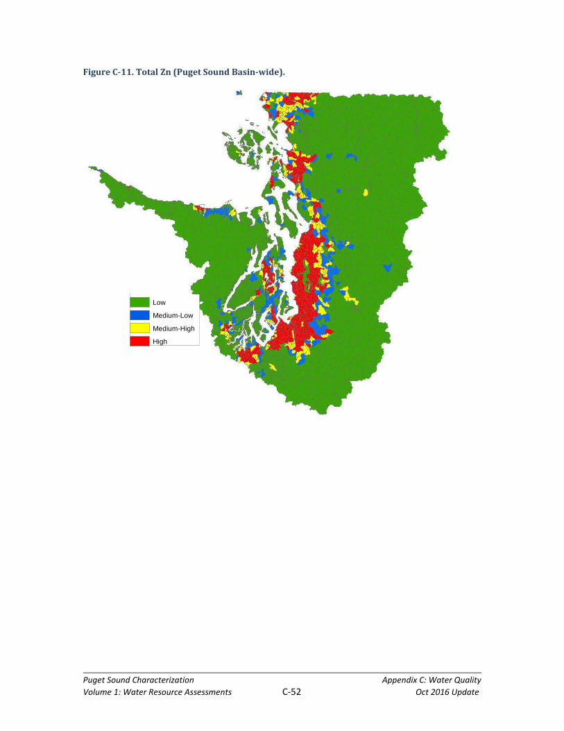
Puget Sound Characterization Appendix C: Water Quality Volume 1: Water Resource Assessments C-52 Oct 2016 Update
Figure C-11. Total Zn (Puget Sound Basin-wide).
Low
Medium-Low
Medium-High
High
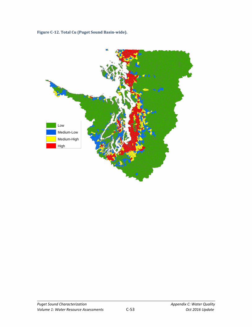
Puget Sound Characterization Appendix C: Water Quality Volume 1: Water Resource Assessments C-53 Oct 2016 Update
Low
Medium-Low
Medium-High
High
Figure C-12. Total Cu (Puget Sound Basin-wide).

Puget Sound Characterization Appendix C: Water Quality Volume 1: Water Resource Assessments C-54 Oct 2016 Update
Low
Medium-Low
Medium-High
High
Figure C-13. Pathogens (Puget Sound Basin-wide).
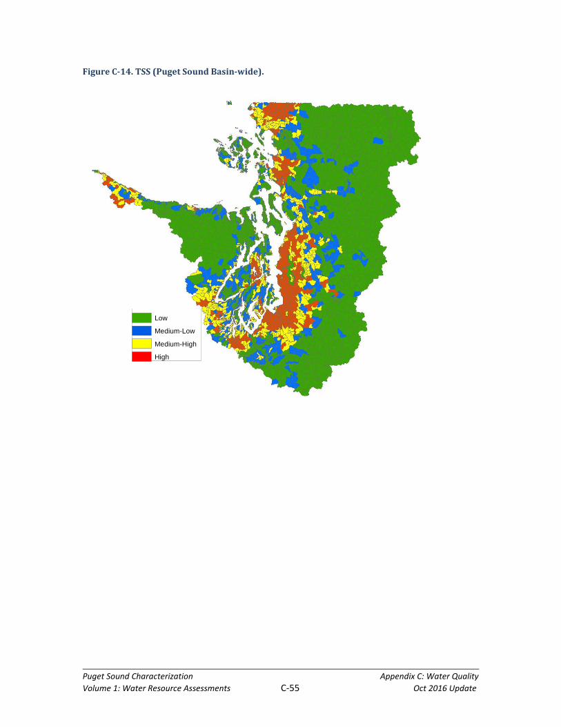
Puget Sound Characterization Appendix C: Water Quality Volume 1: Water Resource Assessments C-55 Oct 2016 Update
Figure C-14. TSS (Puget Sound Basin-wide).
Low
Medium-Low
Medium-High
High

Puget Sound Characterization Appendix C: Water Quality Volume 1: Water Resource Assessments C-56 Oct 2016 Update
Figure C-15. Erosion (Puget Sound Basin-wide).
Low
Medium-Low
Medium-High
High

Puget Sound Characterization Appendix C: Water Quality Volume 1: Water Resource Assessments C-57 Oct 2016 Update
AU’s with maximum Puget Sound-wide loads Table C-10 lists AU’s that exhibit maximum load per unit area for at least one
constituent (denoted by a value of 1.00) within the entire Puget Sound basin. Additionally, relative values in the table that are within 10% of the sound-wide maximum value are shaded. Note that maxima may result from several different types of land uses depending primarily on land class but also hydrology (soils, cover, and storm rainfall). While the C-CAP “high intensity developed” (i.e., commercial-industrial) certainly dominates the highest pollutant producing AU’s, mixed urban, cultivated agriculture, and industrial forestry-dominated AU’s also produce maxima for TSS, TP, and Erosion.
The case of the AU with maximum erosion bares some explanation because the
method of the distinctly different approach to calculating erosion compared to EMC-based pollutants as discussed earlier. The AU map for erosion reflects clearing of forest cover and its replacement by scrub-shrub, grassland, and non-mountainous bare land- especially in areas with high rainfall and soils with higher runoff potential. This is exemplified by AU 50207 in the Hoko-Lyre watershed (WRIA 19) which is estimated to have highest Puget Sound-wide erosion associated with land use and cover change. As shown in Figure C-16, a large fraction of the forest in this AU which forms the headwater of the Hoko River has been cleared and is classified as scrub-shrub and grassland. In addition there are patches of bare land (yellow) in this AU. This C-CAP land use class has the highest cover factor (C-factor) of all classes.
Drilling Down into Maps Using GIS Functions The GIS database for degradation modeling allows for great flexibility in analysis
and diagnosis of results at the sound-wide, WRIA, or AU scale. Using GIS sorting and selection functions, AU’s with relatively large unit loads can easily be identified either sound-wide (as with Table C-10) or within individual WRIAs. More detailed analysis and diagnosis of results are also available at the sub-AU scale by querying the C-CAP raster data or air photos. Additionally, 30-meter scale N-SPECT input and output databases can be used to diagnose overall AU average results and identify specific pollutant loading hot-spots within individual AU’s.

Puget Sound Characterization Appendix C: Water Quality Volume 1: Water Resource Assessments C-58 Oct 2016 Update
Figure C-16. C-CAP Land Use in Hoko River Headwater AU #60207.

Puget Sound Characterization Appendix C: Water Quality Volume 1: Water Resource Assessments C-59 Oct 2016 Update
Table C-10. AU’s with Maximum Relative Load per Unit Area of Modeled Pollutants Caused by Land Use Change. (AU relative loads greater 90% or greater of Puget Sound Basin-wide maximum are shaded)
WRIA AU_ID River Basin Location Dominant
Land Use (s) Sq Mi Runoff TP TN TSS Zn Cu Pathogen
Count Erosion
15 71534 Sinclair Inlet
Bremerton Naval Base
Commercial-Industrial 1.6 1.00 0.66 1.00 0.91 0.90 0.90 1.00 0.01
13 60025 Deschutes Port of
Olympia and downtown
Commercial-Industrial 0.5 1.00 0.65 0.99 0.93 1.00 1.00 0.99 0.02
1 51305 Nooksack East of Sumas Cultivated Agriculture 4.0 0.38 1.00 0.93 0.58 0.22 0.76 0.14 0.15
19 60207 Hoko Headwater Area
Industrial Forestry/Scrub
Shrub/Grassland 6.8 0.12 0.11 0.28 0.61 0.00 0.08 0.06 1.00
18 60255 Elwha Port Angeles Mixed Urban 0.8 0.47 0.30 0.39 1.00 0.22 0.23 0.30 0.08

Puget Sound Characterization Appendix C: Water Quality Volume 1: Water Resource Assessments C-60 Oct 2016 Update
References
Adamus, P.R., E.J. Clairain, Jr., M.E. Morrow, L.P. Rozas, and R.D. Smith. 1991. Wetland Evaluation Technique (WET), Volume I: Literature Review and Evaluation, WRP-DE-2. U.S. Army Corps of Engineers Waterways Experiment Station, Vicksburg, MS.
Arheimer, B. and H.B. Wittgren. 1994. Modeling the Effects of Wetlands and Regional
Nitrogen Transport. Ambio 23(6):378-386. Axt, J.R. and M.R.Walbridge. 1999. Phosphate Removal Capacity of Palustrine
Forested Wetlands and Adjacent Uplands in Virginia. Soil Science Society of America Journal 63:1019-1031.
Borst, M., M. Krudner, M.L. O’Shea, J.M. Perdek, D. Reasoner, and M.D. Royer. 2001.
Chapter 4: Source Water Protection: Its Role in Controlling Disinfection By-products (DBPs) and Microbial Contaminants. Pp. 4-1 – 4-35 in R.M. Clark and B.K. Boutin (eds.), Controlling Disinfection By-products and Microbial Contaminants in Drinking Water, EPA/600/R-01/110, US Environmental Protection Agency, National Risk Management Research Laboratory. Available at http://www.epa.gov/ORD/NRMRL/Pubs/600R01110/600r01110.pdf.
Cox, S., U.S. Geological Survey, Tacoma, WA, personal communication. Cox, S.E., F.W. Simonds, L. Doremus, R.L. Huffman, and R.M. Defawe. 2005. Ground
Water/Surface Water Interactions and Quality of Discharging Ground Water in Streams of the Lower Nooksack River Basin, Whatcom County, Washington. U.S. Geological Survey Scientific Investigations Report 2005-5255.
Doyle, M.P., and M.C. Erickson. 2006. Closing the door on the Fecal Coliform Assay.
Microbe 1:162-163. Ecology (2010), Puget Sound Characterization Project: Description of Methods, Models
and Analysis. Version 1 (Draft for Peer Review). Ecology Publication #10-06-XX http://www.ecy.wa.gov/biblio/0506027.html. February 2010.
EPA (2001), PLOAD Version 3.0 User’s Manual Appendix IV. Event Mean Concentrations (EMCs) and Export Coefficients. January 2001.
EPA (2010), Better Assessment Science Integrating point and Nonpoint Sources
(BASINS) Version 4.0 User’s Manual, October 2010 Update. Gerba, C.P. and J.S. McLeod. 1976. Effects of Sediments on the Survival of Escherichia
coli in Marine Waters. Applied and Environmental Microbiology 32:114-120.

Puget Sound Characterization Appendix C: Water Quality Volume 1: Water Resource Assessments C-61 Oct 2016 Update
Gilmore, M.S., P.S. Coburn, S.R. Nallapareddy, and B.E. Murray. 2002. Enterococcal Virulence. Pp. 301-354 in M.S. Gilmore et al. (eds.), The Enterococci: Pathogenesis, Molecular Biology, and Antibiotic Resistance, American Society for Microbiology, Washington, DC.
Gold, A.J., P.M. Groffman, K. Addy, D.Q. Kellogg, M. Stolt, and A.E. Rosenblatt. 2001.
Landscape Attributes as Controls on Ground Water Nitrate Removal Capacity of Riparian Zones. Journal of the American Water Resources Association 37(6):1457-1464.
Gomi, T., R.C. Sidle, and J.S. Richardson. 2002. Understanding processes and
downstream linkages of headwater systems. Bioscience 52(10): 905-917. Goudie, A.S. (ed.). 2004. Encyclopedia of Geomorphology, Vol. 2. Routledge,
Cornwall, U.K. Grimm, N.B., S.E. Gergel, W.H. McDowell, E.W. Boyer, C.L. Dent, P. Groffman, S.C.
Hart, J. Harvey, C. Johnston, E. Mayorga, M.E. McClain, and G. Pinay. 2003. Merging Aquatic and terrestrial Perspectives of Nutrient biogeochemistry. Oecologia 442:485-501.
Hemond, H.F. and J. Benoit. 1988. Cumulative Impacts on Water Quality Functions of
Wetlands. Environmental Management 12(5):639-653. Hill, A.R., P G.F. Vidon, and J. Langat. 2004. Denitrification Potential in Relation to
Lithology in Five Headwater Riparian Zones. Journal Of Environmental Quality 33(3):911-919.
Horner, R.R., M.V. Brenner, and C.A. Jones. 1989. Design of Monitoring Programs for
Determining Sources of Shellfish Bed Bacterial Contamination Problems. Report to Washington State Department of Ecology by Department of Civil Engineering, University of Washington, Seattle, WA.
Huminicki, D.M.C. and F.C. Hawthorne. 2002. The Crystal Chemistry of the Phosphate
Minerals. Reviews in Mineralogy and Geochemistry 48(1):123-253. Jin G., H.W. Jeng, H. Bradford, and A.J. Englande. 2004. Comparison of E. coli,
Enterococci, and Fecal Coliform as Indicators for Brackish Water Quality Qssessment. Water Environment Research 76 (3): 245–255.
Kadlec, R.H. and R.L. Knight. 1996. Treatment Wetlands. CRC Lewis Publishers, Boca
Raton, FL. Kellogg, D.Q., A.J. Gold, P.M. Groffman, K. Addy, M.H. Stolt, and G. Blazejewski.
2005. In Situ Ground Water Denitrification in Stratified, Permeable Soils Underlying Riparian Wetlands. Journal of Environmental Quality 34(2):524-533.

Puget Sound Characterization Appendix C: Water Quality Volume 1: Water Resource Assessments C-62 Oct 2016 Update
Leopold, L.B., M.G. Wolman, and J.P. Miller. 1992. Fluvial Processes in
Geomorphology. Dover Publications, Inc., New York, NY. Marino, R.P. and J.J. Gannon. 1991. Survival of fecal Coliforms and Fecal Streptococci
in Storm Drain Sediments. Water Research 25:1089–1098. McClain, M.E., E.W. Boyer, C.L. Dent, S.E. Gergel, N.B. Grimm, P.M. Groffman, S.C.
Hart, J.W. Harvey, C.A. Johnston, E. Mayorga, W.H. McDowell, and G. Pinay. 2003. Biogeochemical Hot Spots and Hot Moments at the Interface of Terrestrial and Aquatic Ecosystems. Ecosystems 6:301-312.
McDonald, A., D. Kay, and A. Jenkins. 1982. Generation of Fecal and Total Coliform
Surges by Stream Flow Manipulation in the Absence of Normal Hydrometeorological Stimuli. Applied and Environmental Microbiology 44:292-300.
Mitsch, W.J. and J.G. Gosselink. 2000. Wetlands. Van Nostrand Reinhold, New York,
NY. Natsuhara, C., Natural Resources Conservation Service, Puyallup, WA, personal
communication. NOAA (2004), Nonpoint Source Pollution and Erosion Comparison Tool (N-SPECT)
Technical Guide. Version 1.0 Release 1, November 2004 PB Americas, Inc. and Northwest Hydraulic Consultants, Inc. (2008). Model Selection
and Recommendation Report for Central Oahu Watershed Study, Phase 2 – Part A. Prepared for U.S. Army Corps of Engineers, Honolulu District, and City and County of Honolulu, Department of Environmental Services. November 2008.
Peterson, B.J., W.M. Wollheim, P.J. Mulholland, J.R. Webster, J.L. Meyer, J.L. Tank, E.
Marti, W.B. Bowden, H.M. Valett, A.E. Hershey, W.H. McDowell, W.K. Dodds, S.K. Hamilton, S. Gregory, and D.D. Morrall. 2001. Control of Nitrogen Export from Watersheds by Headwater Streams. Science 292:86-90.
Renard, K.G., G.R. Foster, G.A. Weesies, and J.P. Porter (1991). RUSLE - Revised
universal soil loss equation. Journal of Soil and Water Conservation, 1991(1):30-33. Rosenblatt, A.E., A.J. Gold, M.H. Stolt, P.M. Groffman, and D.Q. Kellogg. 2001.
Identifying Riparian Sinks for Watershed Nitrate Using Soil Surveys. Journal of Environmental
Quality 30:1596-1604. Roszak, D.B., and R.R. Colwell. 1987. Survival Strategies of Bacteria in the Natural
Environment. Microbiological Reviews 53:365-379.
Puget Sound Characterization Appendix C: Water Quality Volume 1: Water Resource Assessments C-63 Oct 2016 Update
Sherer, B.M., J.R. Miner, J.A. Moore, and J.C. Buckhouse. 1992. Indicator Bacterial
Survival in Stream Sediments. Journal of Environmental Quality 21:591-595. Tate, R. L., III. 1978. Cultural and Environmental Factors Affecting the Longevity of
Escherichia coli in Histosols. Applied Environmental Microbiology 35:925-929. Schlesinger, W.H. 1997. Biogeochemistry: An analysis of global change. San Diego:
Academic Press. Shaw, S.C. and D.H. Johnson. 1995. Slope morphology model derived from digital
elevation data. Proceedings Northwest Arc/Info Users Conference, Coeur d’Alene, ID, October 23-25, 1995, 12 pp.
Sheldon, D.T., T. Hruby, P. Johnson, K. Harper, A. McMillan, T. Granger, S. Stanley, E.
Stockdale. 2005. Freshwater Wetlands in Washington State, Volume I: A Synthesis of the Science, Publication #05-06-006. Washington State Department of Ecology, Olympia, WA.
Struck, P.H. 1988. The Relationship Between Sediment and Fecal Coliform Levels in a
Puget Sound Estuary. Journal of Environmental Health 50:403-407. Stumm, W. and J.J. Morgan. 1996. Aquatic Chemistry, Chemical Equilibria and Rates
in Natural Waters, 3rd Ed. John Wiley & Sons, Inc., New York, NY. Ullah, S and S.P. Faulkner. 2006. Use of Cotton Gin Trash to Enhance Denitrification in
Restored Forested Wetlands. Forest Ecology and Management 237:557-563. Vidon, P.G.F. and A.R. Hill. 2004. Landscape Controls on Nitrate Removal in Stream
Riparian Zones. Water Resources Research 40 (3):1-14. Walbridge, M.R. and J.P. Struthers. 1993. Phosphorus retention in non-tidal palustrine
forested wetlands of the mid-Atlantic region. Wetlands, 13:84-94 Welch, E.B. 1998. Chap 4: Stream Quality. In: R.J. Naiman and R.E. Bilby (eds).
River Ecology and Management: Lessons from the Pacific Northwest. Springer-Verlag Press, Inc., New York, NY.
Williams, J.R., and H.D. Berndt (1977). Sediment yield prediction based on watershed
hydrology. Trans. of the ASAE. pp 1100-1104. Woltemade, C.J. 2000. Ability of Restored Wetlands to Reduce Nitrogen and
Phosphorus Concentrations in Agricultural Drainage Water. Journal of Soil and Water Conservation, 55(3):303-309.

Puget Sound Characterization Appendix C: Water Quality Volume 1: Water Resource Assessments C-64 Oct 2016 Update
Ziemer, R.R., and T.E. Lisle. 1998. Chapter 3, Hydrology, pp. 43-68, in: Naiman, R.J., and R.E. Bilby, eds., River Ecology and Management: Lessons from the Pacific Coastal Ecoregion, Springer-Verlag, New York, NY.
Lowe, Julie, Department of Ecology, Personal Communication, May 24, 2011 Roberts, Mindy, Department of Ecology, Personal Communication, May 9, 2011.