appendix c. preliminary quantitative risk analysis of the texas … · 2018-12-26 · -i-quest...
TRANSCRIPT

Appendix C. Preliminary Quantitative Risk Analysis of the Texas Clean Energy Project

QUEST
PRELIMINARY QUANTITATIVE RISK ANALYSIS (QRA)
OF THE TEXAS CLEAN ENERGY PROJECT
Prepared For CH2M Hill
9191 South Jamaica Street Englewood, CO 80112-5946
Prepared By Quest Consultants Inc. 908 26th Avenue, N.W. Post Office Box 721387
Norman, OK 73070-8069 Telephone: 405-329-7475
Fax: 405-329-7734
November 15, 2010 10-11-6773
-i- QUEST
PRELIMINARY QUANTITATIVE RISK ANALYSIS (QRA) OF THE TEXAS CLEAN ENERGY PROJECT
Table of Contents
Page
1.0 Introduction ....................................................................................................................... 1-1 1.1 Hazards Identification.................................................................................................. 1-1 1.2 Failure Case Definition ................................................................................................ 1-2 1.3 Failure Frequency Definition ....................................................................................... 1-3 1.4 Hazard Zone Analysis ................................................................................................. 1-3 1.5 Public/Industrial Risk Quantification ........................................................................... 1-3 1.6 Risk Assessment.......................................................................................................... 1-3 2.0 Facility Location, Pipeline Routes, Pipeline Data, and Well Data ............................................. 2-1 2.1 TCEP Facility Location ............................................................................................... 2-1 2.2 TCEP Process Description ........................................................................................... 2-1 2.3 Population Data ........................................................................................................... 2-3 2.4 Meteorological Data .................................................................................................... 2-3 3.0 Potential Hazards ..................................................................................................................... 3-1 3.1 Physiological Effects of Hydrogen Sulfide ................................................................... 3-2 3.1.1 H2S Probit Relation from Perry and Articola ................................................... 3-2 3.2 Physiological Effects of Ammonia ............................................................................... 3-5 3.3 Physiological Effects of Hydrogen Cyanide ................................................................. 3-7 3.4 Physiological Effects of Sulfuric Acid ......................................................................... 3-8 3.5 Physiological Effects of Sulfur Dioxide ..................................................................... 3-11 3.6 Physiological Effects of Hydrogen Chloride .............................................................. 3-12 3.7 Physiological Effects of Carbon Monoxide ................................................................ 3-14 3.8 Physiological Effects of Carbonyl Sulfide .................................................................. 3-15 3.9 Physiological Effects of Carbon Dioxide ................................................................... 3-16 3.10 Physiological Effects of Exposure to Thermal Radiation form Fires ........................... 3-18 3.11 Physiological Effects of Overpressure........................................................................ 3-20 3.12 Consequence Analysis ............................................................................................... 3-23 3.12.1 Toxic Concentration Limits for Process Streams Containing More Than One Toxic Compound ............................................... 3-24 3.12.2 Example Consequence Analysis Results ........................................................ 3-24 3.12.2.1 Toxic Release and Dispersion Calculations for the Ammonia Production Line ......................................................... 3-24 3.12.2.2 Flammable Release Calculations for the Clean Syngas Line Entering the Ammonia Synthesis Unit .................... 3-25 3.12.2.3 Torch Fire Radiation Hazards Following Flammable Fluid Release ............................................................................. 3-26 3.12.2.4 Vapor Cloud Explosion Overpressure Hazards ........................... 3-26 3.13 Summary of Consequence Analysis Results ............................................................... 3-26

-ii- QUEST
Table of Contents (continued)
Page 4.0 Accident Frequency ........................................................................................................... 4-1 4.1 Piping Failure Rates .................................................................................................... 4-1 4.1.1 Welded Piping ................................................................................................ 4-1 4.1.2 Screwed Piping ............................................................................................... 4-2 4.2 Gaskets ....................................................................................................................... 4-2 4.3 Valves ....................................................................................................................... 4-3 4.3.1 Check Valve Failures ...................................................................................... 4-3 4.4 Pressure Vessel Failure Rates ...................................................................................... 4-3 4.4.1 Leaks ........................................................................................................... 4-3 4.4.2 Catastrophic Failures ...................................................................................... 4-4 4.5 Heat Exchanger Failure Rates ...................................................................................... 4-4 4.6 Pump Failure Rates ..................................................................................................... 4-4 4.7 Compressor Failure Rates ............................................................................................ 4-5 4.8 Pipeline Failure Rates .................................................................................................. 4-5 4.8.1 Steel Pipelines ................................................................................................ 4-5 4.8.2 Surface Equipment .......................................................................................... 4-6 4.9 Common Cause Failures .............................................................................................. 4-6 4.10 Human Error ........................................................................................................... 4-7 4.11 Hazardous Events Following Gas Releases .................................................................. 4-8 5.0 Risk Analysis Methodology ..................................................................................................... 5-1 5.1 Risk Quantification...................................................................................................... 5-1 5.2 Assumptions Employed in Risk Quantification ............................................................ 5-3 6.0 Risk Analysis Results and Conclusions .................................................................................... 6-1 6.1 Summary of Maximum Toxic Impact Zones ................................................................ 6-1 6.2 Measures of Risk Posed by TCEP Process Units, Ammonia Storage Tanks and Pipelines ..................................................................................................... 6-1 6.2.1 Hazard Footprints and Vulnerability Zones for TCEP Process Units ................ 6-1 6.2.2 TCEP Pipeline Hazard Footprints and Vulnerability Zones.............................. 6-2 6.2.3 Risk Contours ................................................................................................. 6-4 6.2.3.1 Terminology and Numerical Values for Representing Risk Levels .................................................................. 6-4 6.2.3.2 Risk Contours for TCEP and Associated Pipelines .............................. 6-6 6.2.3.3 Results for the Natural Gas and Carbon Dioxide Pipelines .................. 6-7 6.3 Risk Acceptability Criteria .......................................................................................... 6-7 6.4 Conservatism Built Into the Risk Analysis Study ....................................................... 6-10 6.5 Study Conclusions ..................................................................................................... 6-12 7.0 References ....................................................................................................................... 7-1 Appendix A CANARY by Quest® Model Descriptions ................................................................... A-1

-iii- QUEST
List of Figures Figure Page 1-1 Overview of Risk Analysis Methodology ................................................................................. 1-2 2-1 Plot Plan and Property Line for TCEP ...................................................................................... 2-2 2-2 Block Flow Diagram for TCEP ................................................................................................ 2-5 2-3 Block Flow Diagram Identifying Major Lines Containing Hazardous Materials in TCEP .................................................................................................. 2-6 2-4 Process Unit Layout for TCEP ................................................................................................. 2-7 2-5 Pipeline Routes for TCEP ........................................................................................................ 2-8 2-6 Wind Rose for Midland, TX ..................................................................................................... 2-9 3-1 Hydrogen Sulfide Probit Functions .......................................................................................... 3-4 3-2 Ammonia Probit Functions ...................................................................................................... 3-6 3-3 Hydrogen Cyanide Probit Functions ......................................................................................... 3-8 3-4 Sulfuric Acid Probit Functions ............................................................................................... 3-10 3-5 Sulfur Dioxide Probit Functions ............................................................................................. 3-12 3-6 Hydrogen Chloride Probit Functions ...................................................................................... 3-14 3-7 Carbon Monoxide Probit Functions ........................................................................................ 3-15 3-8 Carbon Dioxide Probit Functions ........................................................................................... 3-18 3-9 Incident Radiation Probit Functions ....................................................................................... 3-20 3-10 Explosion Overpressure Probit Function ................................................................................ 3-23 3-11 Overhead View of Toxic Vapor Dispersion Cloud .................................................................. 3-30 4-1 Event Tree for a Flammable/Toxic Release from 30-Inch Syngas Line ................................... 4-10 5-1 Representative Range of Wind Speed/Atmospheric Stability Categories ................................... 5-3 6-1 Hazard Footprint and Vulnerability Zone Rupture of 3-Inch Line Leaving the Ammonia Synthesis Unit ................................................................... 6-3 6-2 Hazard Footprint and Vulnerability Corridor Rupture of 10-Inch Carbon Dioxide Export Pipeline .................................................................................. 6-5 6-3 Risk Contours for the Proposed TCEP ...................................................................................... 6-8 6-4 Pipeline Risk Transects for the Incoming Natural Gas and Export Carbon Dioxide Pipelines ............................................................................................. 6-9 6-5 International Risk Acceptability Standards ............................................................................. 6-11 6-6 Risk Contours for the TCEP Facility ...................................................................................... 6-14
-iv- QUEST
List of Tables Table Page 2-1 Summary of Pipeline Data ....................................................................................................... 2-3 3-1 Physiological Response to Various Concentrations of Hydrogen Sulfide (H2S) ......................... 3-3 3-2 Hazardous H2S Concentration Levels for Various Exposure Times Using the Perry and Articola [1980] H2S Probit ....................................................................................... 3-4 3-3 Effects of Different Concentrations of Ammonia ...................................................................... 3-5 3-4 Hazardous NH3 Concentration Levels for Various Exposure Times Using the Perry and Articola [1980] NH3 Probit ....................................................................................... 3-6 3-5 Hazardous HCN Concentration Levels for Various Exposure Times Using the Perry and Articola [1980] HCN Probit ..................................................................................... 3-7 3-6 Effects of Different Concentrations of Sulfuric Acid ................................................................ 3-9 3-7 Hazardous H2SO4 Concentration Levels for Various Exposure Times Using the Mudan [1990] H2SO4 Probit ................................................................................................... 3-10 3-8 Hazardous SO2 Concentration Levels for Various Exposure Times Using the Perry and Articola [1980] SO2 Probit ..................................................................................... 3-11 3-9 Effects of Different Concentrations of Hydrogen Chloride ..................................................... 3-13 3-10 Hazardous HCl Concentration Levels for Various Exposure Times Using the Perry and Articola [1980] HCl Probit ..................................................................................... 3-13 3-11 Hazardous CO Concentration Levels for Various Exposure Times Using the TNO [1989] CO Probit........................................................................................................... 3-15 3-12 Hazardous COS Concentration Levels for Various Exposure Times According to NAC/AEGL Committee .................................................................................... 3-16 3-13 Effects of Different Concentrations of Carbon Dioxide .......................................................... 3-17 3-14 Hazardous CO2 Concentration Levels for Various Exposure Times Using the HSE [2009] CO2 Probit ......................................................................................................... 3-17 3-15 Hazardous Thermal Radiation Levels for Various Exposure Times Using the Tsao and Perry [1979] Thermal Radiation Probit .................................................................... 3-19 3-16 Damage Produced by Blast Waves [Clancey, 1972] ............................................................... 3-22 3-17 Hazardous Overpressure Levels for Various Exposure Times Using the HSE [1991] Overpressure Probit ............................................................................................ 3-22 3-18 NH3 Dispersion Results – Aerosol Jet Model Rupture of Line Leaving Ammonia Synthesis Unit ................................................................. 3-27 3-19 NH3 Dispersion Results – Aerosol Jet Model 1-Inch Hole in Line Leaving Ammonia Synthesis Unit ........................................................... 3-28 3-20 NH3 Dispersion Results – Aerosol Jet Model 1/4 –Inch Hole in Line Leaving Ammonia Synthesis Unit ...................................................... 3-29 3-21 Flammable Dispersion Results – Momentum Jet Model Rupture of Syngas Line Entering Ammonia Synthesis Unit .................................................... 3-31 3-22 Flammable Dispersion Results – Momentum Jet Model 1-Inch Hole in Syngas Line Entering Ammonia Synthesis Unit .............................................. 3-32 3-23 Summary of Immediate Torch Fire Impacts for a Release from Syngas Line Entering the Ammonia Synthesis Unit........................................... 3-33 3-24 Summary of Delayed Torch Fire Impacts for a Release from Syngas Line Entering the Ammonia Synthesis Unit........................................... 3-34 3-25 Summary of Consequence Modeling Results for “Worst Case” and “Average” Meteorological Conditions ....................................................... 3-35

-v- QUEST
List of Tables (continued)
Table Page 6-1 Ten Largest Hazard Distances for Releases from TCEP Units and Pipelines ............................. 6-2 6-2 Maximum Hazard Footprint Distances ..................................................................................... 6-6 6-3 Risk Level Terminology and Numerical Values ....................................................................... 6-6 6-4 Risk Evaluation Criteria ......................................................................................................... 6-13

1-1 QUEST
SECTION 1 INTRODUCTION
Quest Consultants Inc. was retained by CH2MHill to perform a preliminary quantitative risk analysis (QRA) of the proposed Texas Clean Energy Project and associated pipelines and anhydrous ammonia storage operations to be located near the town of Penwell, Texas. The primary objectives of the QRA were to identify the potential risk to persons outside of the TCEP and to compare those risks to internationally accepted risk criteria. With this objective in mind, the TCEP process units and associated pipelines in-cluded in the study were limited to those that transport or process flammable, acutely toxic, or asphyxiant materials. The primary TCEP process units, associated pipelines, and storage facilities handling these materials included in this study can be identified as follows.
Ammonia synthesis unit Mercury removal and acid gas removal unit Sulfuric acid plant Carbon dioxide compression and drying unit Gasification unit Sour shift and gas cooling units Blowdown and sour water system Urea synthesis Air separation unit Gas turbine unit Anhydrous ammonia storage Carbon dioxide pipeline Natural gas pipeline
The QRA was divided into three primary tasks. First, determine potential releases that could result in significant hazardous conditions along the pipelines and near the TCEP. Second, for those potential re-leases identified, derive an annual probability of release. Third, using consistent, accepted methodology, combine the potential release consequences with the annual release probabilities to arrive at a measure of the risk posed to the public. Figure 1-1 illustrates the steps in the QRA procedure required to complete the three primary tasks. 1.1 Hazards Identification The potential hazards associated with the TCEP process units, pipelines, and ammonia storage options are common to similar processes worldwide, and are a function of the materials being processed, processing systems, procedures used for operating and maintaining the equipment, and hazard detection and mitigation systems provided. The hazards that are likely to exist are identified by the physical and chemical proper-ties of the materials being handled, and the process conditions. For facilities handling flammable, toxic, and asphyxiant fluids, the common hazards are:
torch fires flash fires vapor cloud explosions toxic gas clouds (e.g., fluids containing hydrogen sulfide) asphyxiant gas clouds (e.g., fluids containing an asphyxiant such as carbon dioxide)

1-2 QUEST
The hazards identification step is discussed in Sections 2 and 3.
QUANTITATIVE RISK ANALYSIS STEPS TOOLS UTILIZED
Hazards Identification and Failure Case Definition
Industrial accident histories Review of project design information
Review of hazard detection and mitigation systems
Failure Frequency Definition Single component failure rates
Fault Tree Analysis (FTA)
Hazard Zone Analysis Hazard computation models for fires,
explosions, and gas clouds
Hazard contours for people
Public/Industrial Risk Quantification
Population distribution near the site Local weather conditions
Local topography
Risk Assessment Acceptable risk values
Figure 1-1 Overview of Risk Analysis Methodology
1.2 Failure Case Definition The potential release sources of process materials or working fluids are determined from a combination of past history of releases from similar facilities and facility-specific information, including Process Flow Diagrams (PFDs), Piping and Instrumentation Diagrams (P&IDs), accident data, and engineering analysis by system safety engineers. Other methods that may be used in selected instances include Failure Modes and Effects Analysis (FMEA) and Hazards and Operability (HAZOP) studies. This step in the analysis defines the various release sources and conditions of release for each failure case. The release conditions include:
fluid composition, temperature, and pressure release rate and duration
1-3 QUEST
location and orientation of the release type of surface over which released liquid (if any) spreads
The failure case definition step is included in Section 3. 1.3 Failure Frequency Definition The frequency with which a given failure case is expected to occur can be estimated by using a combination of:
historical experience failure rate data on similar types of equipment service factors engineering judgment
For single component failures (e.g., pipe rupture), the failure frequency can be determined from industrial failure rate data bases. For multiple component failures (e.g., failure of a high pressure alarm and shut-down of a compressor discharge line), Fault Tree Analysis (FTA) techniques can be used. The single component failure rates used in constructing the fault tree are obtained from industrial failure rate data bases. The failure frequency step is included in Section 4. 1.4 Hazard Zone Analysis The release conditions (pressure, composition, temperature, hole size, inventory, etc.) from the failure case definitions are then processed, using the best available hazard quantification technology, to produce a set of hazard zones for each failure case. The CANARY by Quest® computer software hazards analysis package is used to produce profiles for the fire, explosion, toxic, and asphyxiant hazards associated with the failure case. The models that are used account for:
release conditions ambient weather conditions (wind speed, air temperature, humidity, atmospheric stability) effects of the local terrain (diking, vegetation) mixture thermodynamics
The hazard zone analysis step is included in Section 3. 1.5 Public/Industrial Risk Quantification The methodology used in this study follows internationally accepted guidelines and has been successfully employed in QRA studies that have undergone regulatory review in countries worldwide. This method-ology is described in Section 5. The result of the analysis is a prediction of the risk posed by the TCEP process units, pipelines, and an-hydrous ammonia storage options. Risk may be expressed in several forms (risk contours, average indi-vidual risk, societal risk, etc.). For this analysis, the focus was on the prediction of risk contours. 1.6 Risk Assessment Risk indicators enable decision makers (corporate risk managers or regulatory authorities) to evaluate the potential risks associated with the TCEP and ancillary operations. Risk contours for the TCEP process

1-4 QUEST
components and associated pipelines can be compared to internationally accepted risk criteria which can assist decision makers in making judgments about the acceptability of the risk associated with the project. Results of the risk analysis and conclusions drawn from this study are presented in Section 6.

2-1 QUEST
SECTION 2 FACILITY LOCATION, PIPELINE ROUTES,
PIPELINE DATA, AND WELL DATA 2.1 TCEP Facility Location The Texas Clean Energy Plant (TCEP) is located just north of the town of Penwell, Texas. The portions of the project to be evaluated include the coal gasification plant, power generation block, ammonia and urea production facilities, the pipelines that consist of one incoming natural gas pipeline from the south and one carbon dioxide pipeline leaving the north end of the site, and anhydrous ammonia storage. A preliminary plot plan of the site is presented in Figure 2-1. 2.2 TCEP Process Description A brief summary of the TCEP process is presented in this section. This summary is drawn from an extensive process description presented in CH2MHill’s report titled Texas Clean Energy Project Initial Conceptual Design Report [CH2MHill, 2010]. Coal, which has been dried and ground, is gasified by combusting coal with purified oxygen in a gasifier to produce raw syngas (primarily carbon monoxide) and molten slag. The syngas and molten slag are cooled by contact with quench water. The slag and excess quench water form “black water” and are removed for further dewatering and slag disposal. The cooled raw syngas is further processed to remove fine ash, chlorides and soot. The remaining syngas is converted to a hydrogen rich syngas using a water gas shift reaction. During the water shift process, carbonyl sulfides are converted into hydrogen sulfide. The resultant hot sour syngas containing hydrogen, carbon dioxide, and hydrogen sulfide is cooled and passed through a mercury removal unit to remove up to 95 percent of the mercury in the gas. After mercury removal, the sour syngas is processed in the Acid Gas Removal (AGR) unit to remove carbon dioxide and hydrogen sulfide. The recovered carbon dioxide is further cleaned, compressed and piped to locations for enhanced oil recovery operations. The hydrogen sulfide is processed to produce a saleable molten sulfur product. The high hydrogen content syngas can be used as a fuel for power generation or a raw feedstock for production of urea. To produce power, the syngas is combusted in a turbine generator to produce electricity. The syngas feed to the turbine is diluted with nitrogen before combustion to reduce formation of nitrous oxides. The exhaust gas from the turbine generator contains water, carbon monoxide and hydrogen sulfide with trace amounts of carbonyl sulfide and ammonia. Urea is produced by first converting the syngas into ammonia and then converting the ammonia to urea. Syngas is purified to remove trace impurities such as carbon monoxide, methane, and argon using a liquid nitrogen wash. Nitrogen is added to the syngas (now mostly hydrogen) to produce a stoichiometric nitrogen to hydrogen ratio for ammonia production. The hydrogen-nitrogen mixture is compressed, cooled, and reacted in a multi-bed catalytic reactor to produce ammonia. The reactor product, ammonia, is cooled and liquefied. The liquid ammonia product is temporarily stored prior to conversion to urea. Urea is produced by reacting ammonia with carbon dioxide to form ammonium carbamate, which slowly decomposes into urea and water. The concentrated urea solution is sprayed into a fluidized bed (granulator) to produce urea particles of the desired size. The urea is stored prior to shipping out in rail cars.

2-2 QUEST
Figure 2-1 Plot Plan and Property Line for TCEP
2-3 QUEST
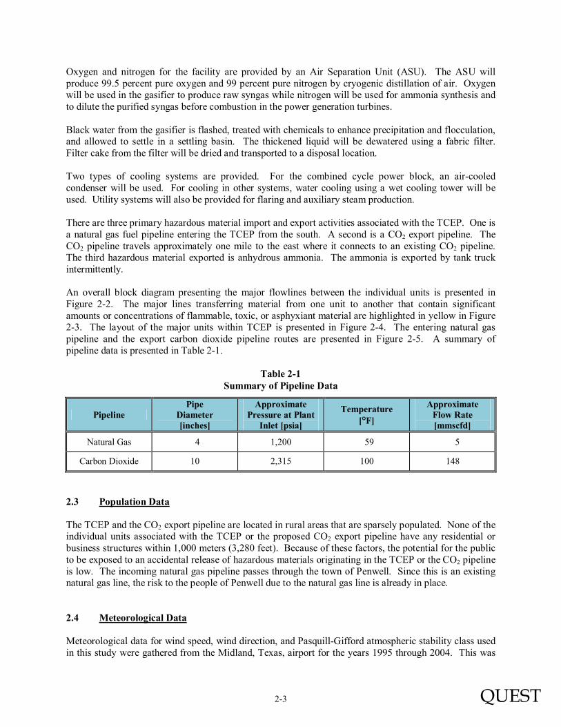
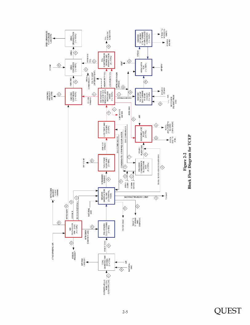
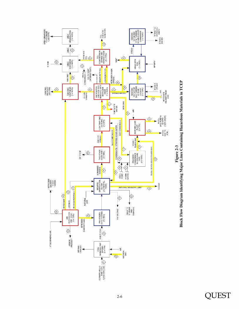
Oxygen and nitrogen for the facility are provided by an Air Separation Unit (ASU). The ASU will produce 99.5 percent pure oxygen and 99 percent pure nitrogen by cryogenic distillation of air. Oxygen will be used in the gasifier to produce raw syngas while nitrogen will be used for ammonia synthesis and to dilute the purified syngas before combustion in the power generation turbines. Black water from the gasifier is flashed, treated with chemicals to enhance precipitation and flocculation, and allowed to settle in a settling basin. The thickened liquid will be dewatered using a fabric filter. Filter cake from the filter will be dried and transported to a disposal location. Two types of cooling systems are provided. For the combined cycle power block, an air-cooled condenser will be used. For cooling in other systems, water cooling using a wet cooling tower will be used. Utility systems will also be provided for flaring and auxiliary steam production. There are three primary hazardous material import and export activities associated with the TCEP. One is a natural gas fuel pipeline entering the TCEP from the south. A second is a CO2 export pipeline. The CO2 pipeline travels approximately one mile to the east where it connects to an existing CO2 pipeline. The third hazardous material exported is anhydrous ammonia. The ammonia is exported by tank truck intermittently. An overall block diagram presenting the major flowlines between the individual units is presented in Figure 2-2. The major lines transferring material from one unit to another that contain significant amounts or concentrations of flammable, toxic, or asphyxiant material are highlighted in yellow in Figure 2-3. The layout of the major units within TCEP is presented in Figure 2-4. The entering natural gas pipeline and the export carbon dioxide pipeline routes are presented in Figure 2-5. A summary of pipeline data is presented in Table 2-1.
Table 2-1 Summary of Pipeline Data
Pipeline Pipe
Diameter [inches]
Approximate Pressure at Plant
Inlet [psia]
Temperature [°F]
Approximate Flow Rate [mmscfd]
Natural Gas 4 1,200 59 5
Carbon Dioxide 10 2,315 100 148
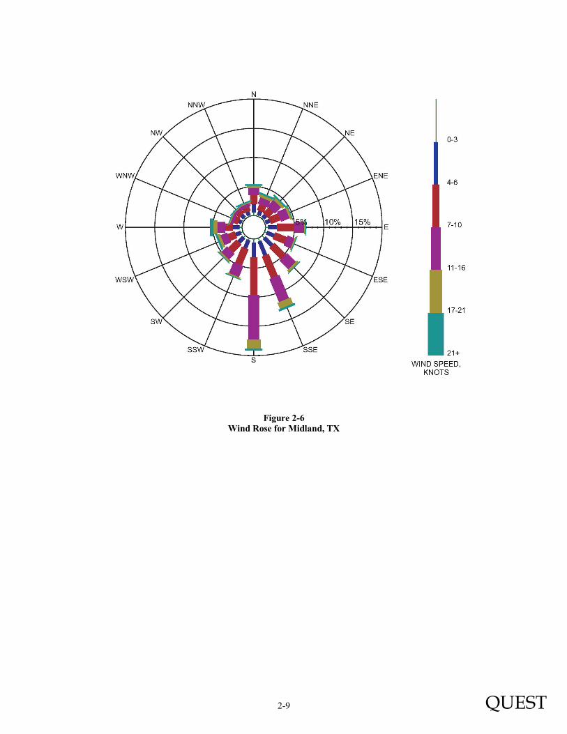
2.3 Population Data The TCEP and the CO2 export pipeline are located in rural areas that are sparsely populated. None of the individual units associated with the TCEP or the proposed CO2 export pipeline have any residential or business structures within 1,000 meters (3,280 feet). Because of these factors, the potential for the public to be exposed to an accidental release of hazardous materials originating in the TCEP or the CO2 pipeline is low. The incoming natural gas pipeline passes through the town of Penwell. Since this is an existing natural gas line, the risk to the people of Penwell due to the natural gas line is already in place. 2.4 Meteorological Data Meteorological data for wind speed, wind direction, and Pasquill-Gifford atmospheric stability class used in this study were gathered from the Midland, Texas, airport for the years 1995 through 2004. This was

2-4 QUEST
the nearest available reporting station with a complete data set and is approximately 30 miles northeast of Penwell, Texas. Figure 2-6 presents the annual wind rose data for all stability classes. The length and width of a particular arm of the rose define the frequency and speed at which the wind blows from the direction the arm is pointing. As an example, reviewing Figure 2-6 shows that the most common wind blows from south to north.
Fig
ure
2-2
B
lock
Flo
w D
iagr
am f
or T
CE
P
2-5 QUEST
Fig
ure
2-3
B
lock
Flo
w D
iagr
am I
den
tify
ing
Maj
or L
ines
Con
tain
ing
Haz
ard
ous
Mat
eria
ls i
n T
CE
P
2-6 QUEST

2-7 QUEST
Figure 2-4 Process Unit Layout for TCEP
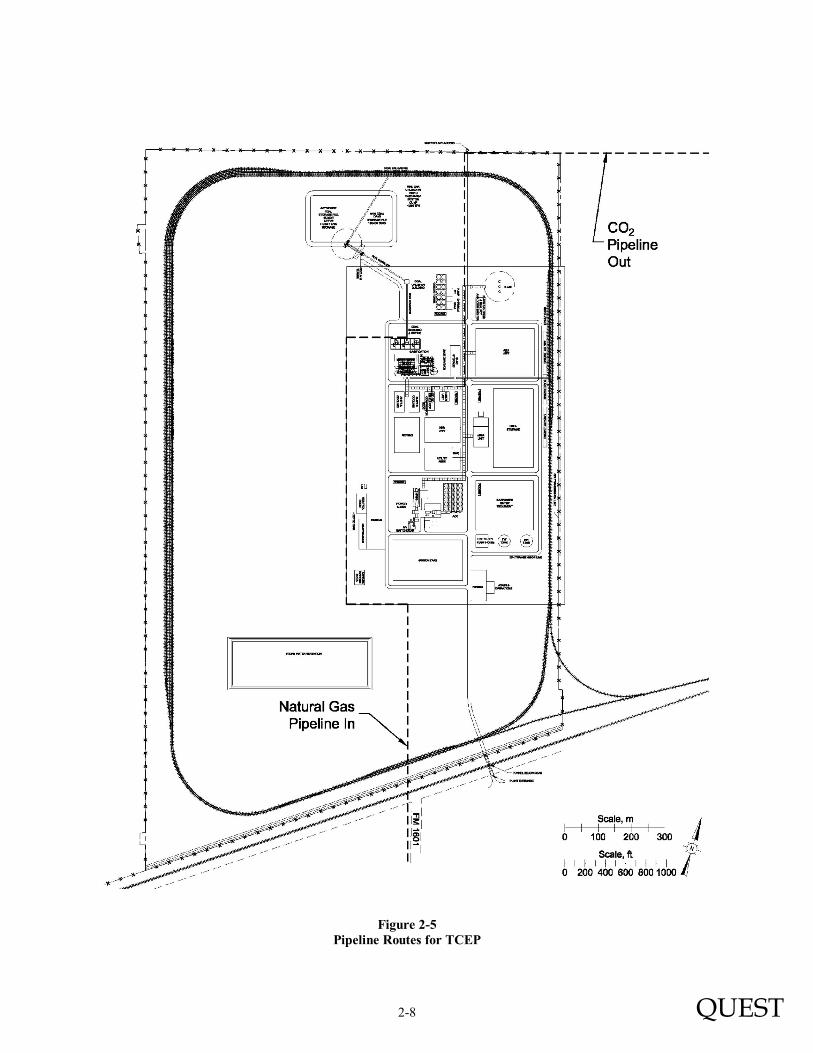
2-8 QUEST
Figure 2-5 Pipeline Routes for TCEP
2-9 QUEST
Figure 2-6 Wind Rose for Midland, TX

3-1 QUEST
SECTION 3 POTENTIAL HAZARDS
Quest reviewed the TCEP preliminary process design and proposed pipeline routes in order to determine credible hazardous release events involving flammable and toxic fluids. As a result of this review, the following potential releases were selected for evaluation. TCEP Process Units (1) Full rupture of the piping or associated equipment, resulting in rapid depressurization of an
individual system. (2) A 1-inch hole (2.54 cm) in the piping or associated equipment. This hole could be the result of
material defect or puncture. (3) A 1/4-inch hole (0.635 cm) in the piping or associated equipment. This release would simulate a
corrosion hole or a damaged fitting on the equipment. Anhydrous Ammonia Storage (1) Full rupture of the piping or associated equipment, resulting in a release from storage. (2) A 1-inch hole (2.54 cm) in the piping or associated equipment. This hole could be the result of
material defect or puncture. (3) A 1/4-inch hole (0.635 cm) in associated equipment. This release would simulate a corrosion
hole or a damaged fitting on the equipment. Natural Gas and Carbon Dioxide Pipeline Releases (1) Full rupture of the pipeline or associated equipment, resulting in rapid depressurization of the
line. This is considered the maximum credible release that might occur along a pipeline. (2) A 2-inch hole (5.08 cm) in one of the pipelines or associated equipment. This hole could be the
result of material defect or puncture. (3) A 1/4-inch hole (0.635 cm) in one of the pipelines or associated equipment. This release would
simulate a corrosion hole in the pipeline. Hazards Created by Releases The release scenarios described above define the range of credible releases that might occur within or between the TCEP process units and along the pipeline routes. Each of these releases may create one or more of the following hazards. (1) Exposure to gas containing a toxic compound (e.g., hydrogen sulfide) (2) Exposure to asphyxiant levels caused by the presence of a non-toxic gas (e.g., carbon dioxide) (3) Exposure to flammable gas that could result in a flash fire or torch fire (4) Exposure to explosion overpressure following the ignition of a flammable cloud The remainder of Section 3 defines the techniques used to quantify the hazards, while Section 4 quantifies the frequencies at which these releases might occur.

3-2 QUEST
3.1 Physiological Effects of Hydrogen Sulfide Hydrogen Sulfide (H2S) is a colorless, flammable gas with a strong, irritating odor. H2S has a low threshold limit value (TLV) and is detectable by odor at concentrations significantly lower than those necessary to cause physical harm or impairment (odor detectable from 0.13 B 1 ppm). The most serious hazard presented by H2S is exposure to a large release from which escape is impossible. Table 3-1 describes various physiological effects of H2S. The physiological effects of airborne toxic materials depend on the concentration of the toxic vapor in the air being inhaled, and the length of time an individual is exposed to this concentration. The combination of concentration and time is referred to as “dosage.” In risk studies that involve toxic gases, probit equations are commonly used to quantify the expected rate of fatalities for the exposed population. Probit equations are based on experimental dose-response data and take the following form. �� = � + �ln(�� �) where: Pr = probit
C = concentration of toxic vapor in the air being inhaled (ppm)
t = time of exposure (minutes) to concentration C a, b, and n = constants The product Cn
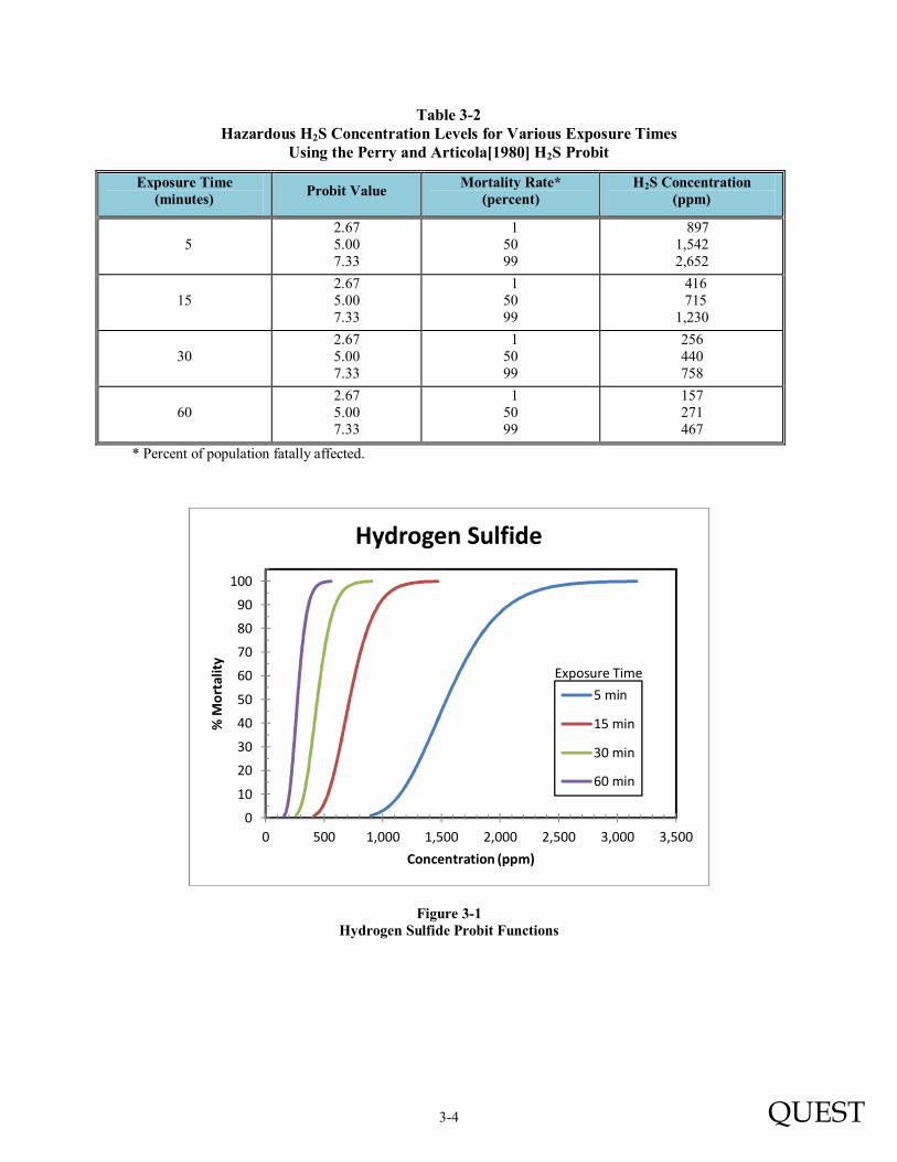
t is often referred to as the dose factor. According to probit equations, all combinations of concentration (C) and time (t) that result in equal dose factors also result in equal values for the probit (Pr) and therefore produce equal expected mortality rates for the exposed population. 3.1.1 H2S Probit Relation from Perry and Articola A probit equation for H2S has been presented by Perry and Articola [1980]. This probit uses the values of -31.42, 3.008, and 1.43 for the constants a, b, and n, respectively. Substituting these values into the general probit equation yields the following probit equation for H2S. �� = −31.42 + 3.008ln(��.�� �) Dispersion calculations are often performed assuming a 60-minute exposure to the gas. This is particularly true when dealing with air pollution studies since they are typically concerned with long-term exposures to low concentration levels. For accidental releases of toxic gases, shorter exposure times are warranted since the durations of many accidental releases are less than an hour. In this study, calculations were performed for various exposure times and concentration levels, dependent on the duration and nature of the release. When using a probit equation, the value of the probit (Pr) that corresponds to a specific dose factor must be compared to a statistical table to determine the expected mortality rate. If the value of the probit is 2.67, the expected mortality rate is one percent. Using this probit equation, the H2S concentration that equates to a one percent mortality rate is 157 ppm for 60 minutes exposure, 256 ppm for 30 minutes exposure, or 416 ppm for 15 minutes exposure, etc. Table 3-2 presents the probit values, mortality rates, and H2S concentrations for various exposure times, while Figure 3-1 presents the same information in graphical form.

3-3 QUEST
Table 3-1
Physiological Response to Various Concentrations of Hydrogen Sulfide (H2S)
H2S Concentration
(ppm)
Duration of Exposure
0-2 min 2-15 min 15-30 min 30 min to 1 hr
1-4 hr 4-8 hr 8-48 hr
5-100
Mild conjunctivitis,
respiratory tract irritation.
100-150
Coughing, irritation of eyes, loss of
sense of smell.
Disturbed respiration, pain in eyes, sleepiness.
Throat irritation.
Salivation and mucous discharge,
sharp pain in eyes,
coughing.
Increased symptoms.*
Hemorrhage and death.*
150-200 Loss of sense of smell.
Throat and eye
irritation.
Throat and eye irritation.
Difficult breathing,
blurred vision, light
shy.
Serious irritating effect.*
Hemorrhage and death.*
250-350
Irritation of eyes, loss of
sense of smell.
Irritation of eyes.
Painful secretion of
tears, weariness.
Light shy, pain in eyes,
difficult breathing.
Hemorrhage and death.*
340-450
Irritation of eyes, loss of
sense of smell.
Difficult respiration, coughing,
irritation of eyes.
Increased irritation of
eyes and nasal tract, dull pain
in head, weariness, light shy.
Dizziness, weakness, increased irritation,
death.
Death.*
500-600
Coughing, collapse,
and unconscio-
usness.
Respiratory disturbances, irritation of
eyes, collapse.*
Serious eye irritation, light shy,
palpitation of heart, a few
cases of death.
Severe pain in eyes and
head, dizziness,
trembling of extremities,
great weakness and
death.*
600 or greater
Collapse, unconscio-
usness, death.*
*Data secured from experience on dogs that have a susceptibility similar to man. Source: National Safety Council data sheet D-chem 15.
3-4 QUEST
Table 3-2 Hazardous H2S Concentration Levels for Various Exposure Times
Using the Perry and Articola[1980] H2S Probit
Exposure Time (minutes)
Probit Value Mortality Rate*
(percent) H2S Concentration
(ppm)
5 2.67 5.00 7.33
1 50 99
897 1,542 2,652
15 2.67 5.00 7.33
1 50 99
416 715 1,230
30 2.67 5.00 7.33
1 50 99
256 440 758
60 2.67 5.00 7.33
1 50 99
157 271 467
* Percent of population fatally affected.
Figure 3-1 Hydrogen Sulfide Probit Functions
0
10
20
30
40
50
60
70
80
90
100
0 500 1,000 1,500 2,000 2,500 3,000 3,500
% M
ort
alit
y
Concentration (ppm)
Hydrogen Sulfide
5 min
15 min
30 min
60 min
Exposure Time

3-5 QUEST
3.2 Physiological Effects of Ammonia Ammonia (NH3) is a colorless, toxic gas with a low threshold limit value (TLV). NH3 is detectable by odor at concentrations much less than those necessary to cause harm. This allows persons who smell the gas to escape. The most serious hazard presented by NH3 is from a large release from which escape is not possible. Table 3-3 describes various physiological effects of NH3.
Table 3-3 Effects of Different Concentrations of Ammonia
Description Concentration
(ppmv) Reference
TLV (Threshold Limit Value) 25 ACGIH
IDLH B This level represents a maximum concentration from which one could escape within 30 minutes without any escape-impairing symptoms or any irreversible health effects.
300 NIOSH
Concentration causing severe irritation of throat, nasal passages, and upper nasal tract.
400 Matheson
Concentration causing severe eye irritation. 700 Matheson
Concentration causing coughing and bronchial spasms. Possibly fatal for exposure of less than one-half hour.
1,700 Matheson
Minimum concentration for the onset of lethality after 30-minute exposure (fatal to 1% of exposed population).
1,883 Perry and Articola
Minimum concentration for 50% lethality after 30-minute exposure (fatal to 50% of exposed population).
4,005 Perry and Articola
Minimum concentration for 99% lethality after 30-minute exposure (fatal to 99% of exposed population).
8,519 Perry and Articola
ACGIH - Threshold Limit Values for 1976 (HSE, 1977 EH 15). Matheson B Matheson Gas Data Book (Matheson Company, 1961). NIOSH - APocket Guide to Chemical Hazards.@ Publication No. 94-116, 1994, Superintendent of Documents,
Washington, D.C. Perry, W. W., and W. P. Articola - AStudy to Modify the Vulnerability Model of the Risk Management System.@
U.S. Coast Guard, Report CG-D-22-80, February, 1980. A probit equation for NH3 uses the values of -28.33, 2.27, and 1.36 for the constants a, b, and n, respectively [Perry and Articola, 1980]. Substituting these values into the general probit equation yields the following probit equation for NH3. �� = −28.33 + 2.27ln(��.�� �) Using this probit equation, the NH3 concentration that equates to a one percent mortality rate is 1,131 ppm for 60 minutes exposure, 1,883 ppm for 30 minutes exposure, or 3,135 ppm for 15 minutes exposure, etc., as shown in Table 3-4. Table 3-4 presents the mortality rates, dosage levels, and NH3 concentrations for various exposure times, while Figure 3-2 presents the same information in graphical form.

3-6 QUEST
Table 3-4 Hazardous NH3 Concentration Levels for Various Exposure Times
Using the Perry and Articola [1980] NH3 Probit
Exposure Time (minutes)
Probit Value Mortality Rate*
(percent) NH3 Concentration
(ppm)
5 2.67 5.00 7.33
1 50 99
7,031 14,955 31,809
15 2.67 5.00 7.33
1 50 99
3,135 6,667 14,182
30 2.67 5.00 7.33
1 50 99
1,883 4,005 8,519
60 2.67 5.00 7.33
1 50 99
1,131 2,406 5,117
* Percent of population fatally affected.
Figure 3-2 Ammonia Probit Functions
0
10
20
30
40
50
60
70
80
90
100
0 10,000 20,000 30,000 40,000 50,000
% M
ort
alit
y
Concentration (ppm)
Ammonia
5 min
15 min
30 min
60 min
Exposure Time

3-7 QUEST
3.3 Physiological Effects of Hydrogen Cyanide Hydrogen Cyanide (HCN) is a colorless, flammable, toxic gas. It is extremely poisonous and can cause fatality before a person is aware of its presence. HCN is said to have an odor similar to bitter almonds. It is extremely poisonous because it binds irreversibly to the iron atom in hemoglobin. This process reduces the ability of hemoglobin to transport oxygen to the body’s cells and tissues. At relatively low concentrations, HCN can cause impaired vision, vomiting, nausea, or even death. The effect of HCN exposure can vary greatly from person to person depending on their age and health, and the concentration and length of exposure. Many people cannot detect HCN, hence odor does not provide adequate warning of hazardous concentrations. A probit equation for HCN has been presented by Perry and Articola [1980]. This probit uses the values of -29.4224, 3.008 and 1.43 for the constants a, b, and n, respectively. Substituting these values into the general probit equation yields the following probit equation for HCN.
�� = −29.4224 + 3.008 ln(��.�� �)
Using this probit equation, the HCN concentration that equates to a one percent mortality rate is 99 ppm for 60 minutes exposure, 161 ppm for 30 minutes exposure, or 262 ppm for 15 minutes exposure, etc., as shown in Table 3-5. Table 3-5 presents the probit values, mortality rates, and HCN concentration for various exposure times, while Figure 3-3 presents the same information in graphical form.
Table 3-5 Hazardous HCN Concentration Levels for Various Exposure Times
Using the Perry and Articola [1980] HCN Probit
Exposure Time (minutes)
Probit Value Mortality Rate*
(percent) HCN Concentration
(ppm)
5 2.67 5.00 7.33
1 50 99
564 970 1,667
15 2.67 5.00 7.33
1 50 99
262 450 773
30 2.67 5.00 7.33
1 50 99
161 277 476
60 2.67 5.00 7.33
1 50 99
99 171 293
* Percent of population fatally affected.

3-8 QUEST
Figure 3-3 Hydrogen Cyanide Probit Functions
3.4 Physiological Effects of Sulfuric Acid Sulfuric acid (H2SO4) normally exists as a colorless, oily liquid that is odorless. The most serious hazard presented by H2SO4 is exposure to a large release from which an acid mist is formed and escape is impossible. Table 3-6 describes various physiological effects of H2SO4 mist. A probit equation for H2SO4 uses the values of -34.214, 4.178, and 1.00 for the constants a, b, and n, respectively [Mudan, 1990]. Substituting these values into the general probit equation yields the following probit equation for H2SO4. �� = −34.214 + 4.178ln(��.�� �) Using this probit equation, the H2SO4 concentration that equates to a one percent mortality rate is 114 ppm for 60 minutes exposure, 227 ppm for 30 minutes exposure, or 455 ppm for 15 minutes exposure, etc., as shown in Table 3-7. Table 3-7 presents the mortality rates and H2SO4 concentrations for various exposure times, while Figure 3-4 presents the same information in graphical form.
0
10
20
30
40
50
60
70
80
90
100
0 500 1,000 1,500 2,000 2,500
% M
ort
alit
y
Concentration (ppm)
Hydrogen Cyanide
5 min
15 min
30 min
60 min
Exposure Time

3-9 QUEST
Table 3-6 Effects of Different Concentrations of Sulfuric Acid
Description Concentration (mg/m3) [ppm]
Reference
TLV-TWA. The time-weighted average concentration for a normal 8-hour work day and a 40-hour work week, to which nearly all workers may be repeatedly exposed, day after day, without adverse effect.
1.0 [0.25] ACGIH
ERPG-1. The maximum airborne concentration below which it is believed that nearly all individuals could be exposed for up to one hour without experiencing other than mild, transient adverse health effects or without perceiving a clearly defined objectionable odor.
2.0 [0.50] AIHA
TEL-STEL. The concentration to which workers can be exposed con-tinuously for a short period of time without suffering from 1) irritation, 2) chronic or irreversible tissue damage, or 3) narcosis of sufficient degree to increase the likelihood of accidental injury, impair self-rescue, or materially reduce work efficiency, and provided that the daily TLV-TWA is not exceeded. A STEL is defined as a 15-minute TWA exposure which should not be exceeded at any time during a work day, even if the 8-hour TWA is within the TLV-TWA.
3.0 [0.75] ACGIH
ERPG-2. The maximum airborne concentration below which it is believed that nearly all individuals could be exposed for up to one hour without experiencing or developing irreversible or other serious health effects or symptoms which could impair an individual's ability to take protective action.
10.0 [2.5] AIHA
Minimum concentration for the onset of lethality after 30-minute exposure (fatal to 1% of exposed population).
[3.53] Mudan
Minimum concentration for the onset of lethality after 30-minute exposure (fatal to 50% of exposed population).
[6.16] Mudan
ERPG-3. The maximum airborne concentration below which it is believed that nearly all individuals could be exposed for up to one hour without experiencing or developing life-threatening health effects.
30.0 [7.5] AIHA
Minimum concentration for the onset of lethality after 30-minute exposure (fatal to 99% of exposed population).
[10.76] Mudan
IDLH. This level represents a maximum concentration from which one could escape within 30 minutes without any escape-impairing symptoms or any irreversible health effects.
80.0 [20.0] NIOSH
ACGIH - ATLV's - Threshold Limit Values and Biological Exposure Indices for 1986-1987.@ American
Conference of Governmental Industrial Hygienists, Cincinnati, Ohio, 1986: p. 21. AIHA - AEmergency Response Planning Guidelines.@ American Industrial Hygiene Association, 1988. Mudan, K. S. - Quantitative Risk Assessment of Generic Hydrofluoric Acid and Sulfuric Acid Alkylation for
Phillips Petroleum Company (Appendix D, AToxicology@). Technica Inc., 355 East Campus Boulevard, Suite 170, Columbus, Ohio 43235, 1990: p. D.19.
NIOSH - APocket Guide to Chemical Hazards.@ Publication No. 78-210, Superintendent of Documents, Washington, D.C.

3-10 QUEST
Table 3-7 Hazardous H2SO4 Concentration Levels for Various Exposure Times
Using the Mudan [1990] H2SO4 Probit
Exposure Time (minutes)
Probit Value Mortality Rate*
(percent) H2SO4 Concentration
(ppm)
5 2.67 5.00 7.33
1 50 99
1,364 2,383 4,162
15 2.67 5.00 7.33
1 50 99
455 794 1,387
30 2.67 5.00 7.33
1 50 99
227 397 694
60 2.67 5.00 7.33
1 50 99
114 199 347
* Percent of population fatally affected.
Figure 3-4 Sulfuric Acid Probit Functions
0
10
20
30
40
50
60
70
80
90
100
0 1,000 2,000 3,000 4,000 5,000 6,000
% M
ort
alit
y
Concentration (ppm)
Sulfuric Acid
5 min
15 min
30 min
60 min
Exposure Time

3-11 QUEST
3.5 Physiological Effects of Sulfur Dioxide Sulfur Dioxide (SO2) is a colorless, nonflammable, toxic gas with a strong, irritating odor. SO2 is so irritating that it provides its own warning of toxic concentration (odor detectable from 0.3 – 1 ppm). Similar to H2S, the most serious hazard presented by SO2 is exposure to a large release from which escape is impossible. The principle toxic effects of SO2 are due to the formation of sulfurous acid when SO2 comes into contact with water in bodily fluids. A probit equation for SO2 has been presented by Perry and Articola [1980]. This probit uses the values of -15.67, 2.100, and 1.00 for the constants a, b, and n, respectively. Substituting these values into the general probit equation yields the following probit equation for SO2.
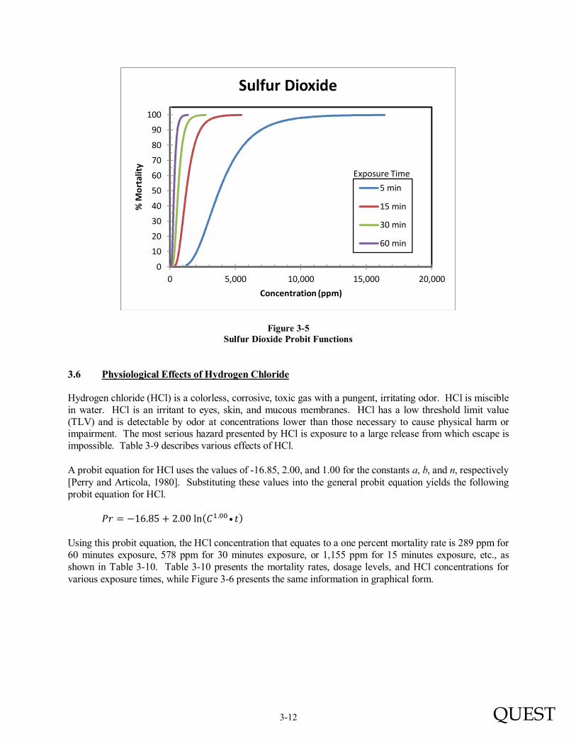
�� = −15.67 + 2.100 ln (��.�� �) Using this probit equation, the SO2 concentration that equates to a one percent mortality rate is 103 ppm for 60 minutes exposure, 207 ppm for 30 minutes exposure, or 414 ppm for 15 minutes exposure, etc., as shown in Table 3-8. Table 3-8 presents the probit values, mortality rates, and SO2 concentrations for various exposure times, while Figure 3-5 presents the same information in graphical form.
Table 3-8
Hazardous SO2 Concentration Levels for Various Exposure Times Using the Perry and Articola [1980] SO2 Probit
Exposure Time [minutes]
Probit Value Mortality Rate*
[percent] SO2 Concentration
[ppm]
5 2.67 5.00 7.33
1 50 99
1,241 3,765 11,418
15 2.67 5.00 7.33
1 50 99
414 1,255 3,806
30 2.67 5.00 7.33
1 50 99
207 628 1,903
60 2.67 5.00 7.33
1 50 99
103 314 952
*Percent of exposed population fatally affected.
3-12 QUEST
Figure 3-5 Sulfur Dioxide Probit Functions
3.6 Physiological Effects of Hydrogen Chloride Hydrogen chloride (HCl) is a colorless, corrosive, toxic gas with a pungent, irritating odor. HCl is miscible in water. HCl is an irritant to eyes, skin, and mucous membranes. HCl has a low threshold limit value (TLV) and is detectable by odor at concentrations lower than those necessary to cause physical harm or impairment. The most serious hazard presented by HCl is exposure to a large release from which escape is impossible. Table 3-9 describes various effects of HCl. A probit equation for HCl uses the values of -16.85, 2.00, and 1.00 for the constants a, b, and n, respectively [Perry and Articola, 1980]. Substituting these values into the general probit equation yields the following probit equation for HCl. �� = −16.85 + 2.00ln(��.�� �) Using this probit equation, the HCl concentration that equates to a one percent mortality rate is 289 ppm for 60 minutes exposure, 578 ppm for 30 minutes exposure, or 1,155 ppm for 15 minutes exposure, etc., as shown in Table 3-10. Table 3-10 presents the mortality rates, dosage levels, and HCl concentrations for various exposure times, while Figure 3-6 presents the same information in graphical form.
0
10
20
30
40
50
60
70
80
90
100
0 5,000 10,000 15,000 20,000
% M
ort
alit
y
Concentration (ppm)
Sulfur Dioxide
5 min
15 min
30 min
60 min
Exposure Time

3-13 QUEST
Table 3-9
Effects of Different Concentrations of Hydrogen Chloride
Description Concentration
(ppm) Reference
TLV (Threshold Limit Value). 5 ACGIH
IDLH. This level represents a maximum concentration from which one could escape within 30 minutes without any escape-impairing symptoms or any irreversible health effects.
50 NIOSH
ERPG-3. The maximum airborne concentration below which it is believed that nearly all individuals could be exposed for up to one hour without experiencing or developing life-threatening health effects.
100 AIHA
Minimum concentration for the onset of lethality after 30-minute exposure (fatal to 1% of exposed population).
578 Perry and Articola
Minimum concentration for 50% lethality after 30-minute exposure (fatal to 50% of exposed population).
1,852 Perry and Articola
Minimum concentration for 99% lethality after 30-minute exposure (fatal to 99% of exposed population).
5,936 Perry and Articola
ACGIH - ATLV's - Threshold Limit Values and Biological Exposure Indices for 1986-1987.@ American
Conference of Governmental Industrial Hygienists, Cincinnati, Ohio, 1986: p. 21. AIHA - AEmergency Response Planning Guidelines.@ American Industrial Hygiene Association, 1988. NIOSH - APocket Guide to Chemical Hazards.@ Publication No. 94-116, 1994, Superintendent of Documents,
Washington, D.C. Perry, W. W., and W. P. Articola - AStudy to Modify the Vulnerability Model of the Risk Management System.@
U.S. Coast Guard, Report CG-D-22-80, February, 1980.
Table 3-10 Hazardous HCl Concentration Levels for Various Exposure Times
Using the Perry and Articola [1980] HCl Probit
Exposure Time [minutes]
Probit Value Mortality Rate*
[percent] HCl Concentration
[ppm]
5 2.67 5.00 7.33
1 50 99
3,465 11,110 35,616
15 2.67 5.00 7.33
1 50 99
1,155 3,703 11,872
30 2.67 5.00 7.33
1 50 99
578 1,852 5,936
60 2.67 5.00 7.33
1 50 99
289 926 2,968
*Percent of exposed population fatally affected.

3-14 QUEST
Figure 3-6 Hydrogen Chloride Probit Functions
3.7 Physiological Effects of Carbon Monoxide Carbon Monoxide (CO) is a colorless, odorless, flammable, toxic gas. Due to these properties, CO can cause fatality before a person is aware of its presence. At low concentrations or exposures, CO may have only a mild impact, and may be mistaken for the flu. At higher concentrations, CO can cause impaired vision, nausea, or even death. Acute effects are due to the formation of carboxyhemoglobin in the blood, which limits oxygen intake. The effect of CO exposure can vary greatly from person to person depending on their age and health, and the concentration and length of exposure. A probit equation for CO has been presented by TNO [1989]. This probit uses the values of -7.265, 1.000, and 1.00 for the constants a, b, and n, respectively. Substituting these values into the general probit equation yields the following probit equation for CO.
�� = −7.265 + 1.000 ln(��.�� �) Using this probit equation, the CO concentration that equates to a one percent mortality rate is 344 ppm for 60 minutes exposure, 688 ppm for 30 minutes exposure, or 1,376 ppm for 15 minutes exposure, etc., as shown in Table 3-11. Table 3-11 presents the probit values, mortality rates, and CO concentrations for various exposure times, while Figure 3-7 presents the same information in graphical form.
0
10
20
30
40
50
60
70
80
90
100
0 10,000 20,000 30,000 40,000 50,000 60,000
% M
ort
alit
y
Concentration (ppm)
Hydrogen Chloride
5 min
15 min
30 min
60 min
Exposure Time

3-15 QUEST
Table 3-11 Hazardous CO Concentration Levels for Various Exposure Times
Using the TNO [1989] CO Probit
Exposure Time [minutes]
Probit Value Mortality Rate*
[percent] CO Concentration
[ppm]
5 2.67 5.00 7.33
1 50 99
4,128 42,428 436,072
15 2.67 5.00 7.33
1 50 99
1,376 14,143 145,357
30 2.67 5.00 7.33
1 50 99
688 7,071 72,679
60 2.67 5.00 7.33
1 50 99
344 3,536 36,339
*Percent of exposed population fatally affected.
Figure 3-7 Carbon Monoxide Probit Functions
3.8 Physiological Effects of Carbonyl Sulfide Carbonyl Sulfide (COS) is a colorless, flammable gas with an odor. Pure COS has no odor, but commercial grade has a typical sulfur odor and is detectable by odor at concentrations significantly lower than those necessary to cause physical harm or impairment, odor threshold of 0.1 ppm [U.S. EPA, 1992].
0
10
20
30
40
50
60
70
80
90
100
0 200,000 400,000 600,000 800,000 1,000,000
% M
ort
alit
y
Concentration (ppm)
Carbon Monoxide
5 min
15 min
30 min
60 min
Exposure Time

3-16 QUEST
The most serious hazards presented by COS are exposure to a large release from which escape is impossible. Table 3-12 describes various physiological effects of COS. A probit equation for COS has not been developed. A review of Table 3-12 would allow for the use of 190 ppm of COS to be conservatively used as the 1%, 50%, and 100% mortality level for exposure to COS for exposure time ranging from 10 to 30 minutes.
Table 3-12 Hazardous COS Concentration Levels for Various Exposure Times
According to NAC/AEGL Committee
AEGL Exposure
Time = 10 min Exposure
Time = 30 min Exposure
Time = 1 hr
AEGL-1 is the airborne concentration (expressed as parts per million or milligrams per cubic meter [ppm or mg/m3]) of a substance above which it is predicted that the general population, including susceptible individuals, could experience notable discomfort, irritation, or certain asymptomatic, non-sensory effects. However, the effects are not disabling and are transient and reversible upon cessation of exposure.
NR NR NR
AEGL-2 is the airborne concentration (expressed as ppm or mg/m3) of a substance above which it is predicted that the general population, including susceptible individuals, could experience irreversible or other serious, long-lasting adverse health effects or an impaired ability to escape.
69 ppm (170 mg/m3)
69 ppm (170 mg/m3)
55 ppm (130 mg/m3)
AEGL-3 is the airborne concentration (expressed as ppm or mg/m3) of a substance above which it is predicted that the general population, including susceptible individuals, could experience life-threatening health effects or death.
190 ppm (470 mg/m3)
190 ppm (470 mg/m3)
150 ppm (370 mg/m3)
NR: Not Recommended due to insufficient data. The absence of AEGL-1 values does not imply that concentrations below AEGL-2 are without effect. Carbonyl sulfide has poor warning properties; it may cause serious effects or lethality at concentrations causing no signs or symptoms.
3.9 Physiological Effects of Carbon Dioxide Carbon Dioxide (CO2) is a colorless, odorless gas. The major hazard associated with CO2 is asphyxiation. At low concentrations CO2 may only have mild effects. At high concentrations, CO2 can cause nausea, vomiting, asphyxiation and even death. The acute effects are due to displacement of oxygen by CO2 resulting in reduced oxygen. Table 3-13 describes in detail the various effects of CO2 concentrations. A probit equation for CO2 uses the values of -90.80, 1.01, and 8 for the constants a, b, and n, respectively [HSE, 2009]. Substituting these values into the general probit equation yields the following probit equation for CO2. �� = −90.80 + 1.01ln(�� �)

3-17 QUEST
Table 3-13 Effects of Different Concentrations of Carbon Dioxide
Oxygen Concentration
Effects and Symptoms (Due to Depleted Oxygen Content in Air [1])
Required Carbon Dioxide Concentration
15 - 19 % Decreased ability to perform tasks. May impair coordination and may induce early symptoms in persons with head, lung, or circulatory problems.
28.6 - 9.5 % 286,000 - 95,000 ppmv
12 -14 % Breathing increases, especially in exertion. Pulse up. Impaired coordination, perception, and judgment.
42.9 - 33.3 % 524,000 - 333,333 ppmv
10 - 12 % Breathing further increases in rate and depth, poor coordination and judgment, lips slightly blue.
52.4 - 42.9 % 524,000 - 429,000 ppmv
8 - 10 % Mental failure, fainting, unconsciousness, ashen face, blueness of lips, nausea (upset stomach), and vomiting.
61.9 - 52.4 % 619,000 - 524,000 ppmv
6 - 8 % 8 minutes, may be fatal in 50 to 100% of cases; 6 minutes, may be fatal in 25 to 50% of cases; 4-5 minutes, recovery with treatment.
71.4 - 61.9 % 714,000 - 619,000 ppmv
4 - 6 % Coma in 40 seconds, followed by convulsions, breathing failure, death.
80.9 - 71.4 % 809,000 - 714,000 ppmv
[1] Compressed Gas Association Safety Bulletin [SB-2 - 1992]
Using this probit equation, the CO2 concentration that equates to a one percent mortality rate is 63,340 ppm for 60 minutes exposure, 69,073 ppm for 30 minutes exposure, or 75,325 ppm for 15 minutes exposure, etc., as shown in Table 3-14. Table 3-14 presents the mortality rates, dosage levels, and CO2 concentrations for various exposure times, while Figure 3-8 presents the same information in graphical form.
Table 3-14 Hazardous CO2 Concentration Levels for Various Exposure Times
Using the HSE [2009] CO2 Probit
Exposure Time [minutes]
Probit Value Mortality Rate*
[percent] CO2 Concentration
[ppm]
5 2.67 5.00 7.33
1 50 99
86,413 115,296 153,833
15 2.67 5.00 7.33
1 50 99
75,325 100,502 134,094
30 2.67 5.00 7.33
1 50 99
69,073 92,160 122,965
60 2.67 5.00 7.33
1 50 99
63,340 84,511 112,759
*Percent of exposed population fatally affected.

3-18 QUEST
Figure 3-8
Carbon Dioxide Probit Functions 3.10 Physiological Effects of Exposure to Thermal Radiation from Fires The physiological effect of fire on humans depends on the rate at which heat is transferred from the fire to the person, and the time the person is exposed to the fire. Even short-term exposure to high heat flux levels may be fatal. This situation could occur when persons wearing ordinary clothes are inside a flammable vapor cloud (defined by the lower flammable limit) when it is ignited. Persons located outside a flammable cloud when it is ignited will be exposed to much lower heat flux levels. If the person is far enough from the edge of the flammable cloud, the heat flux will be incapable of causing fatal injuries, regardless of exposure time. Persons closer to the cloud, but not within it, will be able to take action to protect themselves (e.g., moving farther away as the flames approach, or seeking shelter inside structures or behind solid objects). In the event of a continuous torch fire during the release of flammable gas or gas/aerosol, or a pool fire, the thermal radiation levels necessary to cause fatal injuries to the public must be defined as a function of exposure time. This is typically accomplished through the use of probit equations, which are based on experimental dose-response data.
�� = � + �ln(� ��)
where: Pr = probit K = intensity of the hazard t = time of exposure to the hazard a, b, and n = constants
0
10
20
30
40
50
60
70
80
90
100
0 50,000 100,000 150,000 200,000
% M
ort
alit
y
Concentration (ppm)
Carbon Dioxide
5 min
15 min
30 min
60 min
Exposure Time
3-19 QUEST
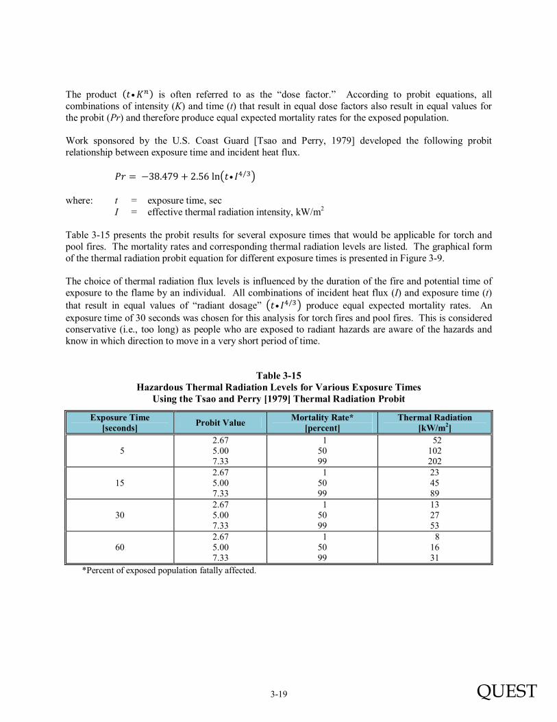
The product (� ��) is often referred to as the “dose factor.” According to probit equations, all combinations of intensity (K) and time (t) that result in equal dose factors also result in equal values for the probit (Pr) and therefore produce equal expected mortality rates for the exposed population. Work sponsored by the U.S. Coast Guard [Tsao and Perry, 1979] developed the following probit relationship between exposure time and incident heat flux.
�� = −38.479 + 2.56ln�� ��/��
where: t = exposure time, sec I = effective thermal radiation intensity, kW/m2 Table 3-15 presents the probit results for several exposure times that would be applicable for torch and pool fires. The mortality rates and corresponding thermal radiation levels are listed. The graphical form of the thermal radiation probit equation for different exposure times is presented in Figure 3-9. The choice of thermal radiation flux levels is influenced by the duration of the fire and potential time of exposure to the flame by an individual. All combinations of incident heat flux (I) and exposure time (t)
that result in equal values of “radiant dosage” �� ��/�� produce equal expected mortality rates. An exposure time of 30 seconds was chosen for this analysis for torch fires and pool fires. This is considered conservative (i.e., too long) as people who are exposed to radiant hazards are aware of the hazards and know in which direction to move in a very short period of time.
Table 3-15
Hazardous Thermal Radiation Levels for Various Exposure Times Using the Tsao and Perry [1979] Thermal Radiation Probit
Exposure Time [seconds]
Probit Value Mortality Rate*
[percent] Thermal Radiation
[kW/m2]
5 2.67 5.00 7.33
1 50 99
52 102 202
15 2.67 5.00 7.33
1 50 99
23 45 89
30 2.67 5.00 7.33
1 50 99
13 27 53
60 2.67 5.00 7.33
1 50 99
8 16 31
*Percent of exposed population fatally affected.

3-20 QUEST
Figure 3-9 Incident Radiation Probit Functions
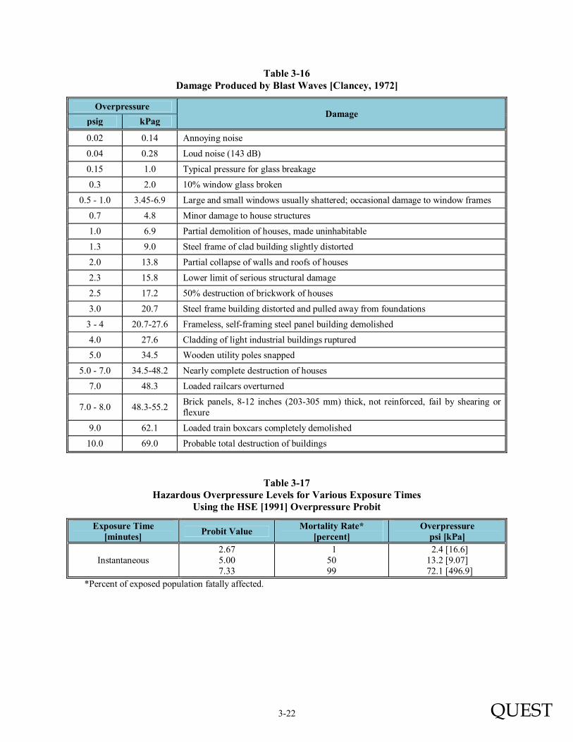
3.11 Physiological Effects of Overpressure The damaging effect of overpressure on buildings depends on the peak overpressure that reaches a given structure, and the method of construction of that structure, as illustrated by Table 3-16. Similarly, the physiological effects of overpressure depend on the peak overpressure that reaches the person. Exposure to high overpressure levels may be fatal. If the person is far enough from the source of the explosion, the overpressure is incapable of causing fatal injuries. The vapor cloud explosion (VCE) calculations in this analysis were made with the Baker-Strehlow-Tang model. This model is based on the premise that the strength of the blast wave generated by a VCE is dependent on the reactivity of the flammable gas involved; the presence (or absence) of structures such as walls or ceilings that partially confine the vapor cloud; and the spatial density of obstructions within the flammable cloud [Baker, et al., 1994, 1998]. This model reflects the results of several international research programs on vapor cloud explosions and deflagrations, which show that the strength of the blast wave generated by a VCE increases as the degree of confinement and/or obstruction of the cloud increases. The following quotations illustrate this point.
“On the evidence of the trials performed at Maplin Sands, the deflagration [explosion] of truly unconfined flat clouds of natural gas or propane does not constitute a blast hazard.” [Hirst and Eyre, 1982] (Tests conducted by Shell Research Ltd. in the United Kingdom.) “Both in two- and three-dimensional geometries, a continuous accelerating flame was observed in the presence of repeated obstacles. A positive feedback mechanism between the flame front and a disturbed flow field generated by the flame is responsible for this.
0
10
20
30
40
50
60
70
80
90
100
0 20 40 60 80 100 120 140 160
% M
ort
alit
y
Incident Radiant Flux (kW/m2)
Incident Radiation
5 sec
15 sec
30 sec
60 sec
Exposure Time

3-21 QUEST
The disturbances in the flow field mainly concern flow velocity gradients. Without repeated obstacles, the flame front velocities reached are low both in two-dimensional and three-dimensional geometry.” [van Wingerdan and Zeeuwen, 1983] (Tests conducted by TNO in the Netherlands.) “The current understanding of vapor cloud explosions involving natural gas is that combustion only of that part of the cloud which engulfs a severely congested region, formed by repeated obstacles, will contribute to the generation of pressure.” [Johnson, Sutton, and Wickens, 1991] (Tests conducted by British Gas in the United Kingdom.)
Researchers who have studied case histories of accidental vapor cloud explosions have reached similar conclusions.
“It is a necessary condition that obstacles or other forms of semi-confinement are present within the explosive region at the moment of ignition in order to generate an explosion.” [Wiekema, 1984] “A common feature of vapor cloud explosions is that they have all involved ignition of vapor clouds, at least part of which have engulfed regions of repeated obstacles.” [Harris and Wickens, 1989]
In the event of an ignition and deflagration of a flammable gas or gas/aerosol cloud, the overpressure levels necessary to cause injury to the public are often defined as a function of peak overpressure. Unlike potential fire hazards, persons who are exposed to overpressure have no time to react or take shelter; thus, time does not enter into the hazard relationship. Work by the Health and Safety Executive, United Kingdom [HSE, 1991], has produced a probit relationship based on peak overpressure. This probit equation has the following form. �� = −23.8 + 2.92ln(�) where: p = peak overpressure, psig Table 3-17 presents the probit results for exposure time that would be applicable for a vapor cloud explosion. The mortality rates and corresponding overpressure levels are listed. The graphical form of the overpressure probit equation for exposure time is presented in Figure 3-10.
3-22 QUEST
Table 3-16 Damage Produced by Blast Waves [Clancey, 1972]
Overpressure Damage
psig kPag
0.02 0.14 Annoying noise
0.04 0.28 Loud noise (143 dB)
0.15 1.0 Typical pressure for glass breakage
0.3 2.0 10% window glass broken
0.5 - 1.0 3.45-6.9 Large and small windows usually shattered; occasional damage to window frames
0.7 4.8 Minor damage to house structures
1.0 6.9 Partial demolition of houses, made uninhabitable
1.3 9.0 Steel frame of clad building slightly distorted
2.0 13.8 Partial collapse of walls and roofs of houses
2.3 15.8 Lower limit of serious structural damage
2.5 17.2 50% destruction of brickwork of houses
3.0 20.7 Steel frame building distorted and pulled away from foundations
3 - 4 20.7-27.6 Frameless, self-framing steel panel building demolished
4.0 27.6 Cladding of light industrial buildings ruptured
5.0 34.5 Wooden utility poles snapped
5.0 - 7.0 34.5-48.2 Nearly complete destruction of houses
7.0 48.3 Loaded railcars overturned
7.0 - 8.0 48.3-55.2 Brick panels, 8-12 inches (203-305 mm) thick, not reinforced, fail by shearing or flexure
9.0 62.1 Loaded train boxcars completely demolished
10.0 69.0 Probable total destruction of buildings
Table 3-17 Hazardous Overpressure Levels for Various Exposure Times
Using the HSE [1991] Overpressure Probit
Exposure Time [minutes]
Probit Value Mortality Rate*
[percent] Overpressure
psi [kPa]
Instantaneous 2.67 5.00 7.33
1 50 99
2.4 [16.6] 13.2 [9.07]
72.1 [496.9]
*Percent of exposed population fatally affected.

3-23 QUEST
Figure 3-10 Explosion Overpressure Probit Function
3.12 Consequence Analysis When performing site-specific consequence analysis studies, the ability to accurately model the release, dilution, and dispersion of gases and aerosols is important if an accurate assessment of potential exposure is to be attained. For this reason, Quest uses a modeling package, CANARY by Quest®, that contains a set of complex models that calculate release conditions, initial dilution of the vapor (dependent upon the release characteristics), and the subsequent dispersion of the vapor introduced into the atmosphere. The models contain algorithms that account for thermodynamics, mixture behavior, transient release rates, gas cloud density relative to air, initial velocity of the released gas, and heat transfer effects from the surrounding atmosphere and the substrate. The release and dispersion models contained in the QuestFOCUS package (the predecessor to CANARY by Quest) were reviewed in a United States Environmental Protection Agency (EPA) sponsored study [TRC, 1991] and an American Petroleum Institute (API) study [Hanna, Strimaitis, and Chang, 1991]. In both studies, the QuestFOCUS software was evaluated on technical merit (appropriateness of models for specific applications) and on model predictions for specific releases. One conclusion drawn by both studies was that the dispersion software tended to overpredict the extent of the gas cloud travel, thus resulting in too large a cloud when compared to the test data (i.e., a conservative approach). A study prepared for the Minerals Management Service [Chang, et al.,1998] reviewed models for use in modeling routine and accidental releases of flammable and toxic gases. CANARY by Quest received the highest possible ranking in the science and credibility areas. In addition, the report recommends CANARY by Quest for use when evaluating toxic and flammable gas releases. The specific models (e.g., SLAB) contained in the CANARY by Quest software package have also been extensively reviewed. Technical descriptions of the CANARY models used in this study are presented in Appendix A.
0
10
20
30
40
50
60
70
80
90
100
0 20 40 60 80 100 120 140
% M
ort
alit
y
Overpressure (psig)
Explosion Overpressure

3-24 QUEST
3.12.1 Toxic Concentration Limits for Process Streams Containing More Than One Toxic Compound
In many of the TCEP process streams, the fluid being transported or processed contains more than one toxic component. In some cases, the concentration of one of the toxic components is so much larger than the other toxic component(s), that the decision to model the impact from the dominant single component is easy to justify. This is because the hazard zone produced by the dominant toxic component will be large enough to completely engulf the hazard zone(s) produce by the other toxic component(s) in the fluid release. For some process streams, identifying the toxic component that dominates or defines the impact zone is not as straight-forward. In the absence of data on the combined effect of these toxic gases on humans, the toxic hazards of each gas must be determined individually. In these cases, multiple runs of the consequence modeling software were conducted, using the component-specific probit concentration endpoints in order to identify the dominant toxic hazard. 3.12.2 Example Consequence Analysis Results This section presents two sets of consequence analysis results for two of the process streams in TCEP. The first set of calculations describes how the toxic impacts are derived and the second set describes how the flammable (flash fire, torch fire, and explosion overpressure) impacts are defined. 3.12.2.1 Toxic Release and Dispersion Calculations for the Ammonia Production Line Dispersion analyses were performed to determine the extent of ammonia gas clouds resulting from the ammonia line leaving the ammonia synthesis plant going to storage. The calculations were performed when ammonia was being produced at the maximum rate (328 STPD). The release scenario involves a rupture or hole in the piping. All releases are assumed to last until ammonia inventory is depleted. For this study, sixty minutes is considered the upper time limit within which a release begins, detection occurs, and corrective action is taken to stop the release. In light of the uncertainties in the available experimental data and probit equations in general, a minimum exposure time of five minutes is used in this study. Thus, even if the duration of a particular release is less than five minutes, the time a person may be exposed is assumed to be five minutes. Mathematical models are used to calculate the time-varying release rates from the break or leak source. Most of the NH3 releases modeled in this study are liquid releases in which part of the liquid flashes to vapor upon release. This behavior produces an aerosol of vapor, air, and small liquid drops that remain suspended; and larger liquid drops that fall to the ground (i.e., the “rainout” from the atmosphere). The ratio of vapor to aerosol to rainout varies according to the pressure, temperature, and composition of the liquid being released. The rainout portion forms a pool on the ground, and the pool is assumed to spread unconfined. The rate of vapor evolution from this pool is also modeled. Release rate and liquid vaporization calculations are completed first, then dispersion calculations are performed. A momentum jet model is used to predict the dispersion of the gas and aerosol-laden vapor clouds because gas and aerosol releases have high velocities relative to the surrounding atmosphere and quickly entrain air into the plume. The entrainment of air is due to the momentum exchange and results in initial rapid dilution of the cloud. For aerosol releases, the rapid expansion of the plume and entrainment of air into the aerosol cloud cause the temperature of the plume to decrease as the liquid droplets are evaporating. These pressurized releases are described by the momentum jet aerosol model employed in this study.
3-25 QUEST
For releases that result in a significant liquid portion reaching the ground (rainout), a second vapor cloud will be created. Dispersion of the second cloud is modeled using the SLAB dense gas dispersion model. Dense gas models are specifically designed to calculate the rate of dispersion of negatively buoyant gases in the atmosphere. In all cases where a second cloud developed, the downwind extent of the second cloud was markedly shorter than the extent of the aerosol-laden momentum jet cloud. Tables 3-18, 3-19, and 3-20 illustrate how the dispersion results vary with atmospheric conditions and hole size. These tables provide the dispersion results from calculations performed for a full line rupture, one-inch puncture, and 1/4-inch leak in the piping associated with the ammonia production line leaving the ammonia synthesis unit. These tables contain the maximum downwind travel distances to the three NH3 concentrations of interest for each cloud, using an accident duration of five minutes (time to deinventory the NH3 from piping and terminate the release for a full line rupture) to 60 minutes for the 1/4-inch leak. For the full line rupture, these concentrations represent exposures to 7,031 ppm (exposure time (∆t) = 5 min = 1% mortality); 14,955 ppm (∆t = 5 min = 50% mortality); and 31,809 ppm (∆t = 5 min = 99% mortality), respectively. As can be seen in Tables 3-18, 3-19, and 3-20, the maximum downwind extent of a vapor cloud occurs when the atmosphere is stable and the wind speed is low (i.e., F stability and a wind speed of 1 to 3 m/s). A summary of the maximum distances achieved by the 19 releases evaluated under low wind and average wind conditions is presented in Table 3-25. A graphical example drawn from the dispersion results is presented in Figure 3-11. Figure 3-11 presents a plan view of the momentum jet cloud under moderate winds (4.63 m/s) and D stability following a rupture of the ammonia line leaving the ammonia synthesis unit. The outlines of the 7,031 ppm (1% mortality), 14,955 ppm (50% mortality), and 31,809 ppm (99% mortality) concentration levels within the cloud are presented. In all cases, when two clouds were formed during a release, the maximum extent of the aerosol-laden (momentum jet) cloud was much greater than the extent of the cloud evolving from the liquid pool; therefore, the results from the momentum jet model dominate the analysis. 3.12.2.2 Flammable Release Calculations for the Clean Syngas Line Entering the Ammonia
Synthesis Unit In addition to the toxic dispersion calculations made, dispersion analyses were performed to determine the extent of flammable gas clouds resulting from the releases selected. These release scenarios involve holes in vessels and piping, seal failures, gasket failures, etc., in all areas of TCEP. Release rate and liquid vaporization calculations are completed first, then dispersion calculations are performed to identify the size of the flash fire zone and the source terms for the torch fire, pool fire, and vapor cloud explosion scenarios. Tables 3-21 and 3-22 illustrate how the flammable dispersion results vary with atmospheric conditions and hole size. These tables give the dispersion results from calculations performed for a line rupture and 1-inch puncture in the clean syngas line (99+% hydrogen) leaving the mercury and acid gas removal unit on its way to the ammonia synthesis unit. The leak scenarios produced impact zones less than 3 meters and not presented. These tables contain the maximum downwind travel distances to lower flammable limit (LFL) for each cloud.
3-26 QUEST
3.12.2.3 Torch Fire Radiation Hazards Following Flammable Fluid Release The extent of the potential torch fire hazards following a release from the clean syngas line is determined by many of the same parameters that define the flash fire for dispersion analysis. For torch fire calculations, the atmospheric stability is not an important parameter; thus, for each hole size, fewer thermal radiation calculations need to be made (one for each combination of hole size, wind speed, and release rate). A maximum of 36 torch fire radiation calculations are made for each release location (3 hole sizes x 6 wind speeds x 2 rates [immediate and delayed ignition]). The distinction between immediate and delayed torch fires is based upon when the flammable cloud ignites following release. In general, the immediate torch fire will create a larger hazard because of the high mass flow during the initial seconds of a release. If a flammable fluid is ignited at some time after the release begins, the mass flow rate that feeds the torch fire is generally less. Thus, two torch fire outcomes are evaluated for each flammable gas/aerosol release scenario and each hole size. If a pool is created during the release, the opposite is true. The longer the ignition of the flammable vapors is delayed, the larger the pool may be, resulting in a larger radiant impact once ignited. Results of the torch fire radiation calculations for the release of syngas feeding the ammonia synthesis unit are summarized in Tables 3-23 and 3-24 for the rupture and puncture scenarios. Since the fire radiation calculations are not a function of atmospheric stability, the matrix is defined differently. The rupture and puncture results for immediate torch fires are represented in Table 3-23. Delayed torch fire results are shown in Table 3-24. Thermal radiation endpoints defined by the probit analysis for 30-second exposure are listed in Tables 3-23 and 3-24 as 7.27 kW/m2 (1% mortality), 14.39 kW/m2 (50% mortality), and 28.47 kW/m2 (99% mortality). The ¼-inch leak fires are so small relative to the ruptures and punctures, they are not presented. 3.12.2.4 Vapor Cloud Explosion Overpressure Hazards The extent of a potential explosion overpressure hazard zone is initially influenced by the same parameters as the flash fire hazard zones. Once a flammable cloud develops, it then requires an ignition source and some degree of confinement or congestion in order to develop significant overpressure. Areas within TCEP that provide this congestion or confinement are associated with the process equipment, piping and piperacks, and infrastructure components. As part of the analysis, potential areas of congestion were identified as those where sufficient confinement of a flammable cloud might be possible and the vapor cloud explosion calculations were performed accordingly. The results of the vapor cloud explosion calculations, for the vapor cloud ignitions that could result in overpressures high enough to cause a fatality, are listed in Table 3-25. 3.13 Summary of Consequence Analysis Results
Table 3-25 presents a summary of the largest impacts from each of the major process lines transporting flammable or toxic materials from one process unit to another. Incoming and outgoing pipeline releases as well as anhydrous ammonia storage releases are also used in Table 3-25. In each table, the maximum ground level distances to the specified mortality endpoints are listed for ruptures, punctures, and leaks from project equipment.
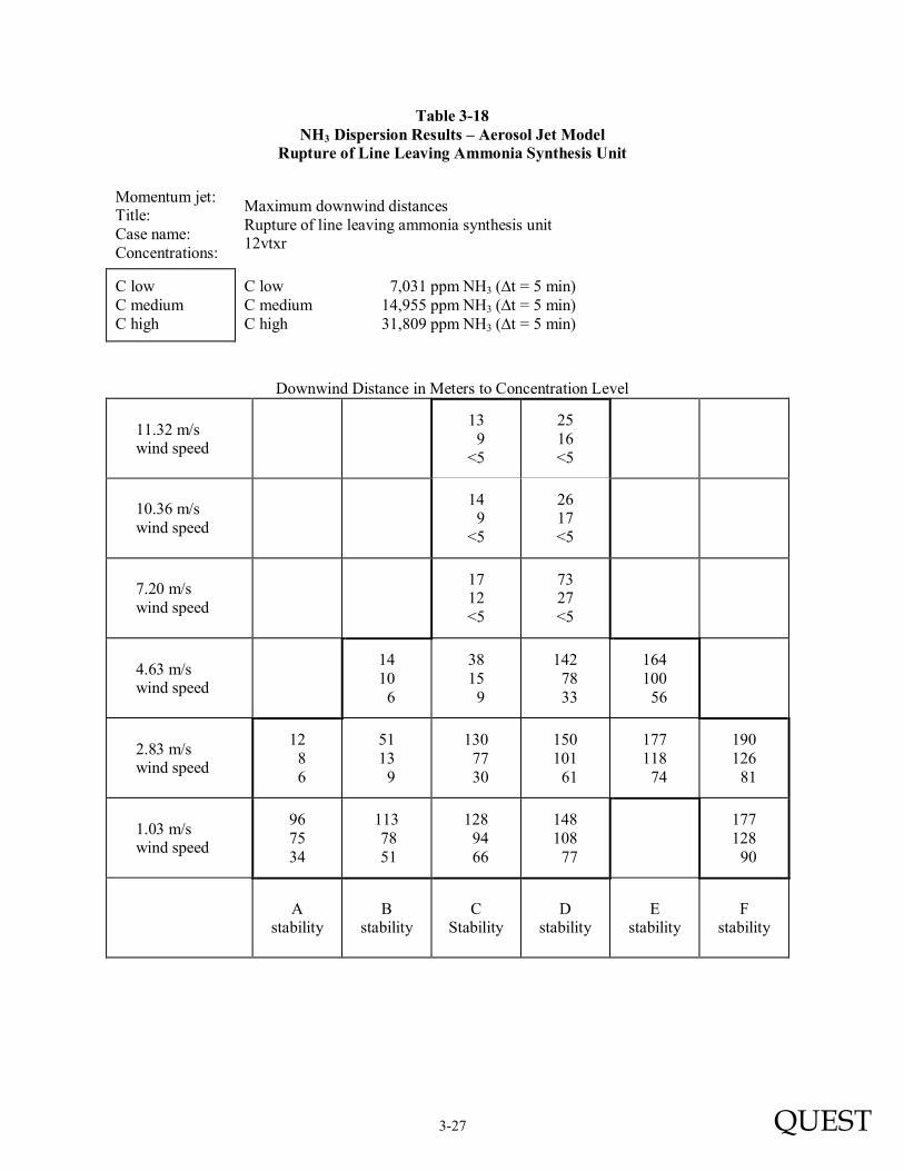
3-27 QUEST
Table 3-18 NH3 Dispersion Results – Aerosol Jet Model
Rupture of Line Leaving Ammonia Synthesis Unit
Momentum jet: Title: Case name: Concentrations:
Maximum downwind distances Rupture of line leaving ammonia synthesis unit 12vtxr
C low C medium C high
C low C medium C high
7,031 ppm NH3 (∆t = 5 min) 14,955 ppm NH3 (∆t = 5 min) 31,809 ppm NH3 (∆t = 5 min)
Downwind Distance in Meters to Concentration Level
11.32 m/s wind speed
13 9 <5
25 16 <5
10.36 m/s wind speed
14 9 <5
26 17 <5
7.20 m/s wind speed
17 12 <5
73 27 <5
4.63 m/s wind speed
14 10 6
38 15 9
142 78 33
164 100 56
2.83 m/s wind speed
12 8 6
51 13 9
130 77 30
150 101 61
177 118 74
190 126 81
1.03 m/s wind speed
96 75 34
113 78 51
128 94 66
148 108 77
177 128 90
A
stability B
stability C
Stability D
stability E
stability F
stability

3-28 QUEST
Table 3-19 NH3 Dispersion Results – Aerosol Jet Model
1-Inch Hole in Line Leaving Ammonia Synthesis Unit
Momentum jet: Title: Case name: Concentrations:
Maximum downwind distances 1-inch hole in line leaving ammonia synthesis unit 12vtxp
C low C medium C high
C low C medium C high
3,983 ppm NH3 (∆t = 11 min) 8,472 ppm NH3 (∆t = 11 min) 18,020 ppm NH3 (∆t = 11 min)
Downwind Distance in Meters to Concentration Level
11.32 m/s wind speed
18 12 8
67 24 15
10.36 m/s wind speed
19 13 9
93 46 16
7.20 m/s wind speed
23 16 11
158 96 53
4.63 m/s wind speed
18 13 9
179 106 51
203 131 82
217 140 89
2.83 m/s wind speed
73 11 8
167 106 63
198 140 93
233 161 109
266 180 118
290 194 126
1.03 m/s wind speed
167 142 82
172 146 120
195 151 124
220 163 120
266 192 138
A
stability B
stability C
stability D
stability E
stability F
stability

3-29 QUEST
Table 3-20 NH3 Dispersion Results – Aerosol Jet Model
1/4-Inch Hole In Line Leaving Ammonia Synthesis Unit
Momentum jet: Title: Case name: Concentrations:
Maximum downwind distances 1/4-inch hole in line leaving ammonia synthesis unit 12vtxq
C low C medium C high
C low C medium C high
1,883 ppm NH3 (∆t = 30 min) 4,005 ppm NH3 (∆t = 30 min) 8,519 ppm NH3 (∆t = 30 min)
Downwind Distance in Meters to Concentration Level
11.32 m/s wind speed
11 7 <5
22 14 <5
10.36 m/s wind speed
12 8 <5
23 15 <5
7.20 m/s wind speed
14 10 6
89 48 20
4.63 m/s wind speed
11 8 5
19 13 9
158 103 65
167 110 72
2.83 m/s wind speed
9 6 5
92 42 8
169 118 75
188 130 86
212 142 92
237 158 100
1.03 m/s wind speed
120 86 61
139 107 82
161 119 93
183 135 100
224 159 111
A
stability B
stability C
stability D
stability E
stability F
stability

3-30 QUEST
Figure 3-11 Overhead View of Toxic Vapor Dispersion Cloud

3-31 QUEST
Table 3-21 Flammable Dispersion Results – Momentum Jet Model
Rupture of Syngas Line Entering Ammonia Synthesis Unit
Momentum jet: Title: Case name: Concentrations:
Maximum downwind distances Rupture of syngas line entering ammonia synthesis unit 11vfxr
C C LFL (4.0 mol %)
Downwind Distance in Meters to Concentration Level
11.32 m/s wind speed
13 20
10.36 m/s wind speed
14 21
7.20 m/s wind speed
17 23
4.63 m/s wind speed
16 20 26 30
2.83 m/s wind speed
15 20 24 29 32 34
1.03 m/s wind speed
23 27 30 33 35
A
stability B
stability C
stability D
stability E
stability F
stability

3-32 QUEST
Table 3-22 Flammable Dispersion Results – Momentum Jet Model
1-Inch Hole in Syngas Line Entering Ammonia Synthesis Unit
Momentum jet: Title: Case name: Concentrations:
Maximum downwind distances 1-inch hole in syngas line entering ammonia synthesis unt 11vfxp
C C LFL (4.0 mol %)
Downwind Distance in Meters to Concentration Level
11.32 m/s wind speed
<5 <5
10.36 m/s wind speed
<5 <5
7.20 m/s wind speed
<5 <5
4.63 m/s wind speed
<5 <5 <5 <5
2.83 m/s wind speed
<5 <5 <5 <5 <5 <5
1.03 m/s wind speed
<5 <5 <5 <5 <5
A
stability B
stability C
stability D
stability E
stability F
stability
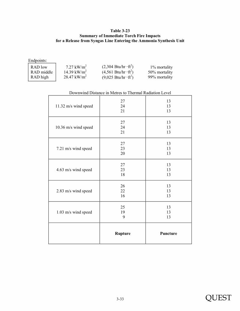
3-33 QUEST
Table 3-23 Summary of Immediate Torch Fire Impacts
for a Release from Syngas Line Entering the Ammonia Synthesis Unit Endpoints:
RAD low RAD middle RAD high
7.27 kW/m2 14.39 kW/m2 28.47 kW/m2
(2,304 Btu/hr·ft2) (4,561 Btu/hr·ft2) (9,025 Btu/hr·ft2)
1% mortality 50% mortality 99% mortality
Downwind Distance in Metres to Thermal Radiation Level
11.32 m/s wind speed 27 24 21
13 13 13
10.36 m/s wind speed 27 24 21
13 13 13
7.21 m/s wind speed 27 23 20
13 13 13
4.63 m/s wind speed 27 23 18
13 13 13
2.83 m/s wind speed 26 22 16
13 13 13
1.03 m/s wind speed 25 19 9
13 13 13
Rupture Puncture

3-34 QUEST
Table 3-24 Summary of Delayed Torch Fire Impacts
for a Release from Syngas Line Entering the Ammonia Synthesis Unit Endpoints:
RAD low RAD middle RAD high
7.27 kW/m2 14.39 kW/m2 28.47 kW/m2
(2,304 Btu/hr·ft2) (4,561 Btu/hr·ft2) (9,025 Btu/hr·ft2)
1% mortality 50% mortality 99% mortality
Downwind Distance in Metres to Thermal Radiation Level
11.32 m/s wind speed 23 20 18
13 13 13
10.36 m/s wind speed 23 20 18
13 13 13
7.21 m/s wind speed 23 20 17
13 13 13
4.63 m/s wind speed 23 19 15
13 13 13
2.83 m/s wind speed 22 18 12
13 13 13
1.03 m/s wind speed 21 16 7
13 13 13
Rupture Puncture

Tab
le 3
-25
Su
mm
ary
of
Co
nse
qu
ence
Mod
elin
g R
esu
lts
for
“Wor
st C
ase”
an
d “
Ave
rage
” M
eteo
rolo
gica
l C
on
dit
ion
s
Rel
ease
Loc
ati
on
[Tox
ic/A
sph
yxia
nt]
Hol
e S
ize
(Eff
ecti
ve
Dia
met
e r)
Wea
ther
(W
ind
Sp
eed
(m
/s)/
S
tab
ilit
y)
Gra
de
Lev
el
Imp
act
Dis
tan
ce
(m)
to F
lash
Fir
e E
nd
poi
nt
Gra
de
Lev
el I
mp
act
Dis
tan
ce (
m)
to T
oxic
or
Asp
hyx
ian
t P
rob
it
En
dp
oin
ts
Gra
de
Lev
el I
mp
act
Dis
tan
ce (
m)
to
Ove
r pre
ssu
re P
rob
it
En
dp
oin
ts
Gra
de
Lev
el I
mp
act
Dis
tan
ce (
m)
to R
adia
tion
P
rob
it E
nd
poi
nts
Mor
tali
ty L
evel
M
orta
lity
Lev
el
Mor
tali
ty L
evel
M
orta
lity
Lev
el
100%
1%
50
%
99%
1%
50
%
99%
1%
50
%
99%
Scr
ubb
ed s
yng
as t
o sh
ift
[Car
bon
Mon
oxid
e]
32"
1.0
3/F
<
5
199
0 0
22
5 3
90
88
85
4.6
3/D
<
5
155
0 0
21
5 3
90
88
85
1"
1.0
3/F
<
5
101
0 0
2 2
0 12
12
12
4.6
3 /D
<
5
45
0 0
2 2
0 12
12
12
1/4"
1.0
3/F
<
5
29
0 0
1 1
1 0
0 0
4.6
3 /D
<
5
0 0
0 1
1 1
0 0
0
Sh
ifte
d sy
ng
as t
o ac
id g
as
rem
oval
30"
1.0
3/F
63
0
0 0
51
12
6 99
96
91
4.6
3/D
48
0
0 0
45
11
6 99
96
91
1"
1.0
3 /F
<
5
0 0
0 6
1 1
16
15
0
4.6
3/D
<
5
0 0
0 5
1 1
16
15
0
1/4"
1.0
3/F
<
5
0 0
0 1
1 1
0 0
0
4.6
3/D
<
5
0 0
0 1
1 1
0 0
0
Cle
an s
ynga
s to
am
mon
ia
syn
thes
is
12"
1.0
3/F
35
0
0 0
34
8 4
25
19
9
4.6
3/D
26
0
0 0
29
7 4
27
23
18
1"
1.0
3 /F
<
5
0 0
0 10
2
1 13
13
13
4.6
3 /D
<
5
0 0
0 9
2 1
13
13
13
1/4"
1.0
3/F
<
5
0 0
0 2
2 0
5 0
0
4.6
3/D
<
5
0 0
0 2
2 0
5 0
0
3-35 QUEST
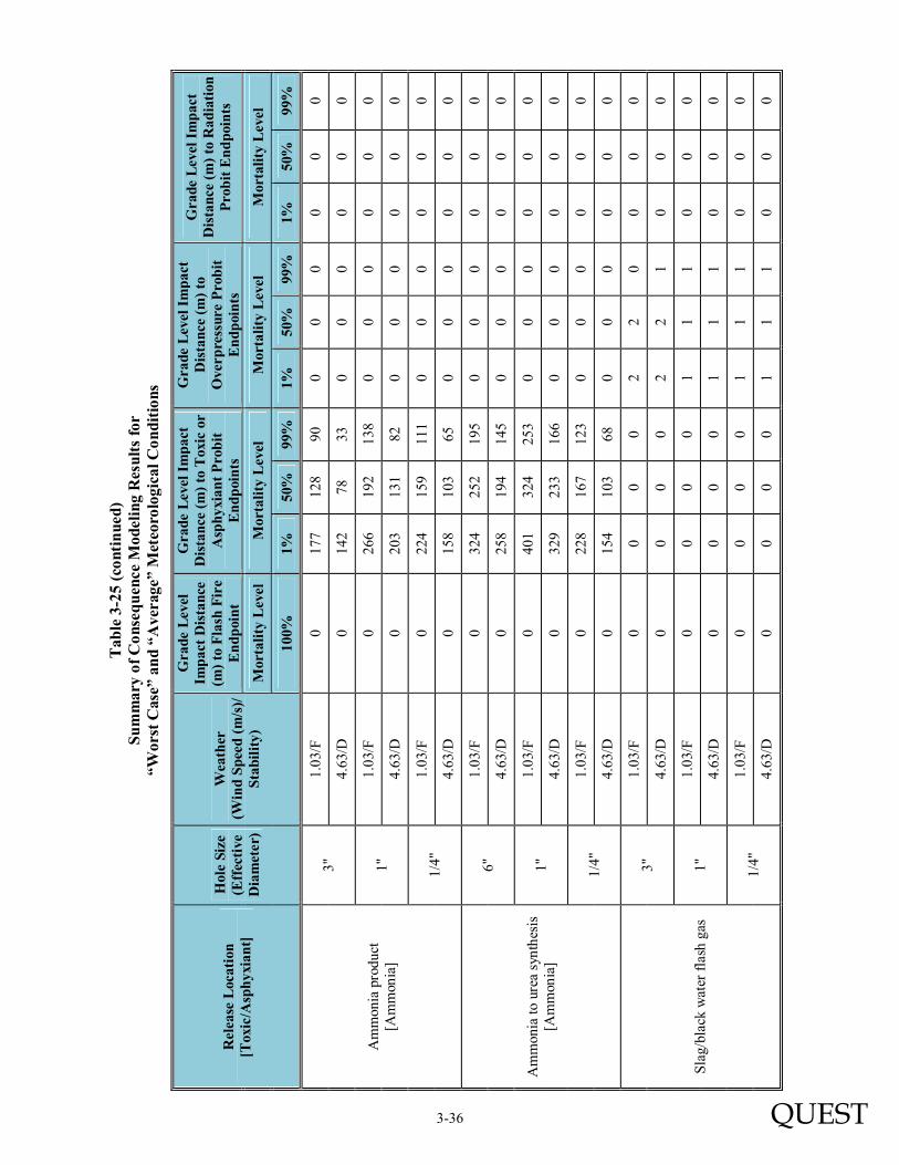
Tab
le 3
-25
(co
nti
nu
ed)
Su
mm
ary
of
Co
nse
qu
ence
Mod
elin
g R
esu
lts
for
“Wors
t C
ase”
an
d “
Ave
rage
” M
eteo
rolo
gica
l C
on
dit
ion
s
Rel
ease
Loc
ati
on
[Tox
ic/A
sph
yxia
nt]
Hol
e S
ize
(Eff
ecti
ve
Dia
met
e r)
Wea
ther
(W
ind
Sp
eed
(m
/s)/
S
tab
ilit
y)
Gra
de
Lev
el
Imp
act
Dis
tan
ce
(m)
to F
lash
Fir
e E
nd
poi
nt
Gra
de
Lev
el I
mp
act
Dis
tan
ce (
m)
to T
oxic
or
Asp
hyx
ian
t P
rob
it
En
dp
oin
ts
Gra
de
Lev
el I
mp
act
Dis
tan
ce (
m)
to
Ove
r pre
ssu
re P
rob
it
En
dp
oin
ts
Gra
de
Lev
el I
mp
act
Dis
tan
ce (
m)
to R
adia
tion
P
rob
it E
nd
poi
nts
Mor
tali
ty L
evel
M
orta
lity
Lev
el
Mor
tali
ty L
evel
M
orta
lity
Lev
el
100%
1%
50
%
99%
1%
50
%
99%
1%
50
%
99%
Am
mon
ia p
rodu
ct
[Am
mon
ia]
3"
1.0
3/F
0
177
128
90
0 0
0 0
0 0
4.6
3/D
0
142
78
33
0 0
0 0
0 0
1"
1.0
3/F
0
266
192
138
0 0
0 0
0 0
4.6
3 /D
0
203
131
82
0 0
0 0
0 0
1/4"
1.0
3/F
0
224
159
111
0 0
0 0
0 0
4.6
3 /D
0
158
103
65
0 0
0 0
0 0
Am
mon
ia t
o ur
ea s
ynth
esis
[A
mm
onia
]
6"
1.0
3/F
0
324
252
195
0 0
0 0
0 0
4.6
3/D
0
258
194
145
0 0
0 0
0 0
1"
1.0
3 /F
0
401
324
253
0 0
0 0
0 0
4.6
3/D
0
329
233
166
0 0
0 0
0 0
1/4"
1.0
3/F
0
228
167
123
0 0
0 0
0 0
4.6
3/D
0
154
103
68
0 0
0 0
0 0
Sla
g/b l
ack
wat
er f
lash
gas
3"
1.0
3/F
0
0 0
0 2
2 0
0 0
0
4.6
3/D
0
0 0
0 2
2 1
0 0
0
1"
1.0
3 /F
0
0 0
0 1
1 1
0 0
0
4.6
3 /D
0
0 0
0 1
1 1
0 0
0
1/4"
1.0
3/F
0
0 0
0 1
1 1
0 0
0
4.6
3/D
0
0 0
0 1
1 1
0 0
0
3-36 QUEST
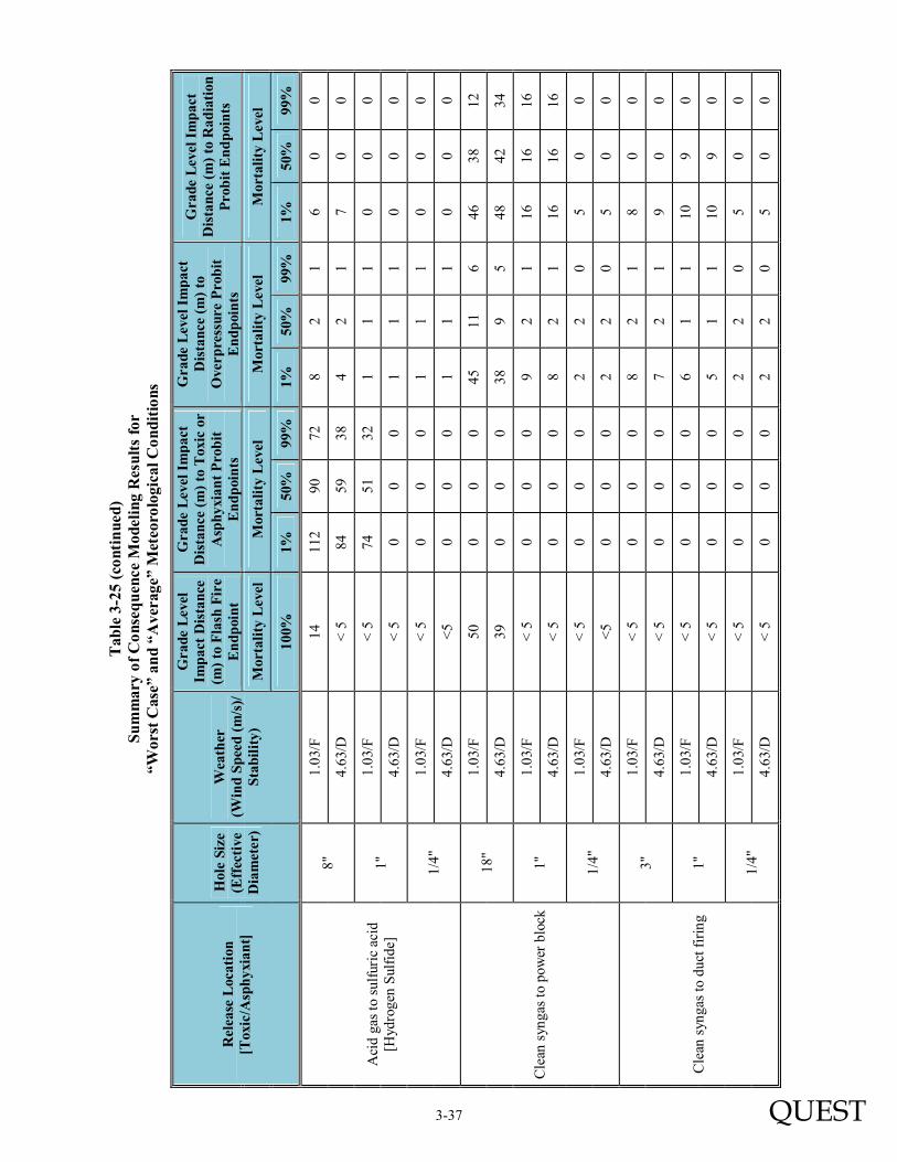
Tab
le 3
-25
(co
nti
nu
ed)
Su
mm
ary
of
Co
nse
qu
ence
Mod
elin
g R
esu
lts
for
“Wors
t C
ase”
an
d “
Ave
rage
” M
eteo
rolo
gica
l C
on
dit
ion
s
Rel
ease
Loc
ati
on
[Tox
ic/A
sph
yxia
nt]
Hol
e S
ize
(Eff
ecti
ve
Dia
met
e r)
Wea
ther
(W
ind
Sp
eed
(m
/s)/
S
tab
ilit
y)
Gra
de
Lev
el
Imp
act
Dis
tan
ce
(m)
to F
lash
Fir
e E
nd
poi
nt
Gra
de
Lev
el I
mp
act
Dis
tan
ce (
m)
to T
oxic
or
Asp
hyx
ian
t P
rob
it
En
dp
oin
ts
Gra
de
Lev
el I
mp
act
Dis
tan
ce (
m)
to
Ove
r pre
ssu
re P
rob
it
En
dp
oin
ts
Gra
de
Lev
el I
mp
act
Dis
tan
ce (
m)
to R
adia
tion
P
rob
it E
nd
poi
nts
Mor
tali
ty L
evel
M
orta
lity
Lev
el
Mor
tali
ty L
evel
M
orta
lity
Lev
el
100%
1%
50
%
99%
1%
50
%
99%
1%
50
%
99%
Aci
d ga
s to
su
lfur
ic a
cid
[Hyd
rog
en S
ulfi
de]
8"
1.0
3/F
14
11
2 90
72
8
2 1
6 0
0
4.6
3/D
<
5
84
59
38
4 2
1 7
0 0
1"
1.0
3/F
<
5
74
51
32
1 1
1 0
0 0
4.6
3 /D
<
5
0 0
0 1
1 1
0 0
0
1/4"
1.0
3/F
<
5
0 0
0 1
1 1
0 0
0
4.6
3 /D
<
5 0
0 0
1 1
1 0
0 0
Cle
an s
yng
as t
o po
wer
blo
ck
18"
1.
03 /
F
50
0 0
0 45
11
6
46
38
12
4.6
3/D
39
0
0 0
38
9 5
48
42
34
1"
1.0
3 /F
<
5
0 0
0 9
2 1
16
16
16
4.6
3/D
<
5
0 0
0 8
2 1
16
16
16
1/4"
1.0
3/F
<
5
0 0
0 2
2 0
5 0
0
4.6
3/D
<
5 0
0 0
2 2
0 5
0 0
Cle
an s
ynga
s to
duc
t fi
rin
g
3"
1.0
3/F
<
5
0 0
0 8
2 1
8 0
0
4.6
3/D
<
5
0 0
0 7
2 1
9 0
0
1"
1.0
3 /F
<
5
0 0
0 6
1 1
10
9 0
4.6
3 /D
<
5
0 0
0 5
1 1
10
9 0
1/4"
1.0
3/F
<
5
0 0
0 2
2 0
5 0
0
4.6
3/D
<
5
0 0
0 2
2 0
5 0
0
3-37 QUEST

Tab
le 3
-25
(co
nti
nu
ed)
Su
mm
ary
of
Co
nse
qu
ence
Mod
elin
g R
esu
lts
for
“Wors
t C
ase”
an
d “
Ave
rage
” M
eteo
rolo
gica
l C
on
dit
ion
s
Rel
ease
Loc
ati
on
[Tox
ic/A
sph
yxia
nt]
Hol
e S
ize
(Eff
ecti
ve
Dia
met
e r)
Wea
ther
(W
ind
Sp
eed
(m
/s)/
S
tab
ilit
y)
Gra
de
Lev
el
Imp
act
Dis
tan
ce
(m)
to F
lash
Fir
e E
nd
poi
nt
Gra
de
Lev
el I
mp
act
Dis
tan
ce (
m)
to T
oxic
or
Asp
hyx
ian
t P
rob
it
En
dp
oin
ts
Gra
de
Lev
el I
mp
act
Dis
tan
ce (
m)
to
Ove
r pre
ssu
re P
rob
it
En
dp
oin
ts
Gra
de
Lev
el I
mp
act
Dis
tan
ce (
m)
to R
adia
tion
P
rob
it E
nd
poi
nts
Mor
tali
ty L
evel
M
orta
lity
Lev
el
Mor
tali
ty L
evel
M
orta
lity
Lev
el
100%
1%
50
%
99%
1%
50
%
99%
1%
50
%
99%
Nit
rog
en w
ash
off
gas
[Car
bon
Mon
oxid
e]
10"
1.0
3/F
<
5
46
0 0
5 1
1 10
8
6
4.6
3/D
<
5
23
0 0
4 2
1 10
8
7
1"
1.0
3/F
<
5
30
0 0
1 1
1 4
0 0
4.6
3 /D
<
5
0 0
0 1
1 1
4 0
0
1/4"
1.0
3/F
<
5
0 0
0 1
1 1
0 0
0
4.6
3 /D
<
5
0 0
0 1
1 1
0 0
0
Sta
ck g
as t
o at
mos
pher
e [N
itro
gen
]
20"
1.
03/
F
0 69
62
55
0
0 0
0 0
0
4.6
3/D
0
31
27
23
0 0
0 0
0 0
1"
1.0
3 /F
0
9 7
6 0
0 0
0 0
0
4.6
3/D
0
0 0
0 0
0 0
0 0
0
1/4"
1.0
3/F
0
0 0
0 0
0 0
0 0
0
4.6
3/D
0
0 0
0 0
0 0
0 0
0
Pu
rifi
ed C
O2
to u
rea
syst
em
[Car
bon
Dio
xid
e]
3"
1.0
3/F
0
64
56
48
0 0
0 0
0 0
4.6
3/D
0
29
24
20
0 0
0 0
0 0
1"
1.0
3 /F
0
51
37
26
0 0
0 0
0 0
4.6
3 /D
0
0 0
0 0
0 0
0 0
0
1/4"
1.0
3/F
0
0 0
0 0
0 0
0 0
0
4.6
3/D
0
0 0
0 0
0 0
0 0
0
3-38 QUEST

Tab
le 3
-25
(co
nti
nu
ed)
Su
mm
ary
of
Co
nse
qu
ence
Mod
elin
g R
esu
lts
for
“Wors
t C
ase”
an
d “
Ave
rage
” M
eteo
rolo
gica
l C
on
dit
ion
s
Rel
ease
Loc
ati
on
[Tox
ic/A
sph
yxia
nt]
Hol
e S
ize
(Eff
ecti
ve
Dia
met
e r)
Wea
ther
(W
ind
Sp
eed
(m
/s)/
S
tab
ilit
y)
Gra
de
Lev
el
Imp
act
Dis
tan
ce
(m)
to F
lash
Fir
e E
nd
poi
nt
Gra
de
Lev
el I
mp
act
Dis
tan
ce (
m)
to T
oxic
or
Asp
hyx
ian
t P
rob
it
En
dp
oin
ts
Gra
de
Lev
el I
mp
act
Dis
tan
ce (
m)
to
Ove
r pre
ssu
re P
rob
it
En
dp
oin
ts
Gra
de
Lev
el I
mp
act
Dis
tan
ce (
m)
to R
adia
tion
Pro
bit
En
dp
oin
ts
Mor
tali
ty L
evel
M
orta
lity
Lev
el
Mor
tali
ty L
evel
M
orta
lity
Lev
el
100%
1%
50
%
99%
1%
50
%
99%
1%
50
%
99%
CO
2 t
o E
OR
[C
arbo
n D
ioxid
e]
10"
1.0
3/F
0
139
101
77
0 0
0 0
0 0
4.6
3/D
0
131
114
97
0 0
0 0
0 0
1"
1.0
3/F
0
110
79
29
0 0
0 0
0 0
4.6
3 /D
0
66
54
43
0 0
0 0
0 0
1/4"
1.0
3/F
0
31
24
0 0
0 0
0 0
0
4.6
3 /D
0
0 0
0 0
0 0
0 0
0
Nit
roge
n d
ilu
ents
to
gas
turb
ine
[Nit
roge
n]
60"
1.0
3/F
0
9 7
4 0
0 0
0 0
0
4.6
3/D
0
13
10
7 0
0 0
0 0
0
1"
1.0
3 /F
0
0 0
0 0
0 0
0 0
0
4.6
3/D
0
0 0
0 0
0 0
0 0
0
1/4"
1.0
3/F
0
0 0
0 0
0 0
0 0
0
4.6
3/D
0
0 0
0 0
0 0
0 0
0
Gas
tur
bin
e ex
haus
t to
HR
SG
[N
itro
gen
]
198"
1.0
3/F
0
10
9 9
0 0
0 0
0 0
4.6
3/D
0
13
12
10
0 0
0 0
0 0
1"
1.0
3 /F
0
0 0
0 0
0 0
0 0
0
4.6
3 /D
0
0 0
0 0
0 0
0 0
0
1/4"
1.0
3/F
0
0 0
0 0
0 0
0 0
0
4.6
3/D
0
0 0
0 0
0 0
0 0
0
3-39 QUEST

Tab
le 3
-25
(co
nti
nu
ed)
Su
mm
ary
of
Co
nse
qu
ence
Mod
elin
g R
esu
lts
for
“Wors
t C
ase”
an
d “
Ave
rage
” M
eteo
rolo
gica
l C
on
dit
ion
s
Rel
ease
Loc
ati
on
[Tox
ic/A
sph
yxia
nt]
Hol
e S
ize
(Eff
ecti
ve
Dia
met
e r)
Wea
ther
(W
ind
Sp
eed
(m
/s)/
S
tab
ilit
y)
Gra
de
Lev
el
Imp
act
Dis
tan
ce
(m)
to F
lash
Fir
e E
nd
poi
nt
Gra
de
Lev
el I
mp
act
Dis
tan
ce (
m)
to T
oxic
or
Asp
hyx
ian
t P
rob
it
En
dp
oin
ts
Gra
de
Lev
el I
mp
act
Dis
tan
ce (
m)
to
Ove
r pre
ssu
re P
rob
it
En
dp
oin
ts
Gra
de
Lev
el I
mp
act
Dis
tan
ce (
m)
to R
adia
tion
P
rob
it E
nd
poi
nts
Mor
tali
ty L
evel
M
orta
lity
Lev
el
Mor
tali
ty L
evel
M
orta
lity
Lev
el
100%
1%
50
%
99%
1%
50
%
99%
1%
50
%
99%
HR
SG
ven
t [N
itro
gen
]
132
" 1.
03/
F
0 19
17
16
0
0 0
0 0
0
4.6
3/D
0
27
23
20
0 0
0 0
0 0
1"
1.0
3/F
0
0 0
0 0
0 0
0 0
0
4.6
3 /D
0
0 0
0 0
0 0
0 0
0
1/4"
1.0
3/F
0
0 0
0 0
0 0
0 0
0
4.6
3 /D
0
0 0
0 0
0 0
0 0
0
Nat
ural
gas
to
coal
gri
ndi
ng
and
dry
ing
4"
1.0
3/F
<
5
0 0
0 6
0 0
17
15
15
4.6
3/D
<
5
0 0
0 5
0 0
17
15
15
1"
1.0
3 /F
<
5
0 0
0 6
0 0
16
16
16
4.6
3/D
<
5
0 0
0 5
0 0
16
16
16
1/4"
1.0
3/F
<
5
0 0
0 3
0 0
10
9 9
4.6
3/D
<
5 0
0 0
2 0
0 10
9
9
Pre
ssur
ized
am
mon
ia s
tora
ge
[Am
mon
ia]
6"
1.0
3/F
74
14
15
972
750
86
21
11
96
95
94
4.6
3/D
13
3 11
74
845
622
236
56
30
96
95
94
1"
1.0
3 /F
0
498
419
294
20
5 3
22
22
21
4.6
3 /D
0
435
310
215
16
4 2
22
22
21
1/4"
1.0
3/F
0
204
147
102
0 0
0 0
0 0
4.6
3/D
0
130
81
47
0 0
0 0
0 0
3-40 QUEST
4-1 QUEST
SECTION 4 ACCIDENT FREQUENCY
The likelihood of a particular accident occurring within some specific time period can be expressed in different ways. One way is to state the statistical probability that the accident will occur during a one-year period. This annual probability of occurrence can be derived from failure frequency data bases of similar accidents that have occurred with similar systems or components in the past. Most data bases (e.g., CCPS [1989], OREDA [1984]) that are used in this type of analysis contain failure frequency data (e.g., on the average, there has been one failure of this type of equipment for 347,000 hours of service). By using the following equation, the annual probability of occurrence of an event can be calculated if the frequency of occurrence of the event is known.
1t
p e
where: p annual probability of occurrence (dimensionless)
annual failure frequency (failures per year) t time period (one year) If an event has occurred once in 347,000 hours of use, its annual failure frequency is computed as fol-lows.
1 8,760
0.0252 /347,000
event hoursx events year
hours year
The annual probability of occurrence of the event is then calculated as follows.
-0.0252·11 0.0249p e
Note that the frequency of occurrence and the probability of occurrence are nearly identical. (This is al-ways true when the frequency is low.) An annual probability of occurrence of 0.0249 is approximately the same as saying there will probably be one event per forty years of use. Due to the scarcity of accident frequency data bases, it is not always possible to derive an exact probabil-ity of occurrence for a particular accident. Also, variations from one system to another (e.g., differences in design, operation, maintenance, or mitigation measures) can alter the probability of occurrence for a specific system. Therefore, variations in accident probabilities are usually not significant unless the varia-tion approaches one order of magnitude (i.e., the two values differ by a factor of ten). The following subsections describe the basis and origin of failure frequency rates used in this analysis. 4.1 Piping Failure Rates 4.1.1 Welded Piping
4-2 QUEST
WASH-1400 [USNRC, 1975] lists the failure rates for piping as 1.0 x 10⁻¹⁰/hour for pipes greater than three inches in diameter, and 1.0 x 10⁻⁹/hour for smaller pipes. These rates are based on a “section” of pipe, i.e., 1.0 x 10⁻¹⁰ failures per section of >three-inch pipe/hour. A section of pipe is defined as any straight portion of pipe of welded construction between any two fittings (such as flanges, valves, strainers, elbows, etc.). CCPS [1989] gives a mean pipe failure rate of 2.68 x 10⁻⁸/mile/hour (4.45 x 10⁻⁸/foot/year). This would be approximately the same as the WASH-1400 rate, 1.0 x 10⁻⁹/section/hour (8.76 x 10-
6/section/year), if the average section of pipe were about 200 feet in length. Most data bases of pipe failure rates are not sufficiently detailed to allow a determination of the failure frequency as a function of the size of the release (i.e., size of the hole in the pipe). However, British Gas has gathered such data on their gas pipelines [Fearnehough, 1985]. Their data show that well over 90% of all failures are less than a one-inch diameter hole, and only 3% are greater than a three-inch diameter hole. Since most full ruptures of piping systems are caused by outside forces, full ruptures are expected to occur more frequently on small-diameter pipes. Based on the above discussion, the expected failure rates for aboveground, metallic piping with no threaded connections are assumed to be as follows. For pipes from one inch to three inches in diameter: Hole size 1/4 inch 1/4 to 2 inch 2 inch to full rupture Expected failure rate 2.25 x 10⁻⁸/foot/year 1.8 x 10⁻⁸/foot/year 4.5 x 10⁻⁹/foot/year For pipes from four inches to ten inches in diameter: Hole size 1/4 inch 1/4 to 2 inch 2 inch to full rupture Expected failure rate 2.25 x 10⁻⁸/foot/year 2.0 x 10⁻⁸/foot/year 2.5 x 10⁻⁹/foot/year 4.1.2 Screwed Piping CCPS [1989] also gives a value of 5.7 x 10⁻⁷/hour for the failure rate of metal piping connections. The specific types of connections are not listed, but threaded connections are implied since failures in welded piping systems with flanged connections are either classified as piping failures or gasket failures. Failure rates for piping in aboveground, metallic piping systems with screwed connections are assumed to be the same as the failure rates listed in Section 4.1.1 for welded piping systems. For screwed fittings, the ex-pected failure rates are as follows. Hole size 0 to 1/4 inch 1/4 inch to full rupture Expected failure rate 4.0 x 10⁻³/fitting/year 1.0 x 10⁻³/fitting/year 4.2 Gaskets According to WASH-1400 [USNRC, 1975], the median failure rate (leak or rupture) for gaskets at flanged connections is 3.0 x 10⁻⁷/hour. Green and Bourne [1972] reported 5.0 x 10⁻⁷/hour as the failure rate for gaskets. The data from both sources are thought to include small leaks that would not create sig-nificant hazards. Unfortunately, the data are not broken down by gasket type. It is generally believed that spiral-wound, metallic-reinforced gaskets are less prone to major leaks than ordinary composition gaskets. Also, it is

4-3 QUEST
nearly impossible to “blow out” all, or even a section, of a metallic-reinforced gasket. In consideration of these factors, a failure rate of 3.0 x 10⁻⁸/hour is thought to be conservative for loss of 1/4 of a metallic-reinforced gasket. Based on continuous service, the annual expected failure rate for metallic-reinforced gaskets is 2.6 x 10⁻⁴ failures/year/gasket. For ordinary composition gaskets, the expected failure rate is 2.6 x 10⁻³ failures/year/gasket. 4.3 Valves WASH-1400 [USNRC, 1975] lists a failure rate of 1.0 x 10⁻⁸ failures/hour for external leakage or rupture of valves. Assuming continuous service, the annual leakage/rupture rate is approximately 8.8 x 10⁻⁵/year. Unfortunately, this number includes very small leaks as well as valve body ruptures. This reduces the usefulness of this failure rate since the probability of a small leak from a valve bonnet gasket is obviously much greater than the probability of a two-inch hole in the valve body. To overcome this difficulty, the valve body can be considered similar to pipe, and the valve bonnet gasket can be treated like other gas-kets. To be conservative, each flanged valve is considered to have a failure rate equal to a ten-foot sec-tion of pipe and one gasket. Similarly, a threaded valve is treated like ten feet of pipe, one gasket, and one screwed fitting. 4.3.1 Check Valve failures The CCPS [1989] lists a value for the failure of a check valve to prevent reverse flow upon demand. This value is 2.2 failures per 1,000 demands, or 2.2 x 10⁻³/d. 4.4 Pressure Vessel Failure Rates 4.4.1 Leaks CCPS [1989] reports a failure rate of 1.09 x 10⁻⁸/hour for pressure vessels. For continuous service, the annual expected failure rate for pressure vessels would be 9.5 x 10⁻⁵ failures/year. Bush [1975] made an in-depth study of pressure vessels of many types, including boilers. In Bush's study, the rate of “disrup-tive” failures of pressure vessels was 1.0 x 10⁻⁵/year, i.e., a factor of ten less than the CCPS value. The explanation for this difference lies in the definition of “failure.” Bush's number is based on “disruptive” failures which are assumed to be failures of such magnitude that the affected vessel would need to be tak-en out of service immediately for repair or replacement. The data base reported by the CCPS most likely includes smaller leaks that Bush categorized as “noncritical.” Smith and Warwick [1981] analyzed the failure history of a large number of pressure vessels (about 20,000) in the United Kingdom. They present a short description of each failure, thus allowing the fail-ures to be categorized by size. Most of the failures were small leaks (approximately half can be catego-rized as smaller than a one-inch diameter hole). Based on the previous discussion, the following failure rates are proposed for pressurized process vessels. Equivalent hole diameter 1/4 inch 1/4 to 2 inch >2 inch Expected failure rate 3.0 x 10⁻⁵/year 4.0 x 10⁻⁵/year 5.0 x 10⁻⁶/year
4-4 QUEST
4.4.2 Catastrophic Failures For this study, a catastrophic failure is defined as the sudden, nearly instantaneous rupture of a pressure vessel, resulting in nearly instantaneous release of the vessel's contents. Catastrophic failures of pressure vessels can be roughly divided into two types—cold catastrophic failures and BLEVE's. If a pressure vessel ruptures when the contents of the vessel are at, or near, ambient temperature, the fail-ure is a cold catastrophic failure. Such failures might occur as the result of improper metallurgy, defec-tive welds, overpressurization, etc. Most products that are stored at ambient temperature in pressure ves-sel storage tanks are superheated liquefied gases. If the contents of the tank are released into the atmos-phere nearly instantaneously, an aerosol cloud will be formed as some of the liquid flashes to vapor. If the material is flammable, the cloud might be ignited (either instantaneously or after some delay) or will dissipate without being ignited. Sooby and Tolchard [1993] conducted an analysis of cold catastrophic failures of pressurized LPG stor-age tanks in Europe. They found that no such failure had ever been recorded during more than twenty-five million tank-years of service. From this data, they derived a frequency of 2.7 x 10⁻⁸ cold catastrophic failures per vessel per year for pressurized storage tanks. 4.5 Heat Exchanger Failure Rates Failure rate data for shell-and-tube heat exchangers that are designed and constructed much like other pressurized process vessels are sometimes reported with the data for pressure vessels. However, shell-and-tube heat exchangers are expected to have higher failure rates than simple pressure vessels because they are more complex than pressure vessels and are subject to additional stresses caused by temperature-induced expansion and contraction. To account for the additional complexity and stresses, the failure rates of the reboilers are assumed to be twice the rates listed previously for pressure vessels. Based on this discussion, the following failure rates are proposed. Equivalent hole diameter 1/4 inch 1/4 to 2 inch >2 inch Expected failure rate 6.0 x 10⁻⁵/year 8.0 x 10⁻⁵/year 1.0 x 10⁻⁵/year 4.6 Pump Failure Rates Green and Bourne [1972] list the failure rate for “rotating seals” as 7.0 x 10⁻⁶/hour. Assuming continuous operation (i.e., 8,760 hours/year), the annual expected failure rate is 6.0 x 10⁻² failures/year/seal. For pumps fitted with double mechanical seals, a major seal leak occurs only if both seals fail. If the two seal failures were always caused by independent events, the failure rate for a double seal configuration would be the square of the single seal failure rate, i.e., about 3.6 x 10⁻³ failures/year. However, some causes of seal failure can result in the simultaneous failure of both seals (e.g., bearing failures, excessive vibration, improper installation, etc.). Thus, the failure rate is somewhere between 6.0 x 10⁻²/year and 3.6 x 10⁻³/year. In the absence of hard data, we have assumed the failure rate for double mechanical seals is 5.0 x 10⁻³/year. Rotating seal failures do not occur with sealless pumps because such pumps do not have rotating seals. However, sealless pumps are still subject to many of the non-seal types of failures that can occur with any pump (e.g., cracks in the pump housing).

4-5 QUEST
The common sources of failure rate data (OREDA, WASH-1400, CCPS) do not present data for failures of pump housings, although such failures have occurred. In the absence of such data, we assume the fail-ure rate for a pump housing is equal to the failure rate of a ten-foot section of pipe of similar diameter. 4.7 Compressor Failure Rates Data on the frequency of releases from compressors are very rare, and contain little detailed information. A report from The Oil Industry International Exploration and Production Forum (E&P Forum) includes data from four sources, but the total sample size of all four data bases is only 1,875 compressor years of service [E&P, 1992]. The number of reported releases was 119, which translates to a release frequency of 6.35 x 10⁻²/compressor/year. Only seven of the 119 releases were classified as “major.” Based on this limited data, the expected failure rates are as follows.
Hole size <1/4 inch 1/4 to 1 inch 1 inch to full rupture Expected failure rate 6.0 x 10⁻²/compr/yr 3.2 x 10⁻³/compr/yr 5.3 x 10⁻⁴/compr/yr
4.8 Pipeline Failure Rates 4.8.1 Steel Pipelines Department of Transportation (DOT) data for underground liquid pipelines in the United States indicate a failure rate of 1.35 x 10⁻³ failures/mile/year [DOT 1988]. Data compiled from DOT statistics on failures of gas pipelines show a failure rate of 1.21 x 10⁻³ failures/mile/year for steel pipelines in the United States [Jones, et al., 1986]. In addition to failures of buried pipe, these data include failures of buried pipeline components, such as block valves and check valves, when the failure resulted in a release of fluid from the pipeline. Data gathered by operators of gas transmission pipelines in Europe indicate a failure rate of 1.13 x 10⁻³ failures/mile/year [EGPIDG, 1988]. These data sets are not sufficiently detailed to allow a determination of the failure frequency as a function of the size of the release (i.e., the size of hole in the pipeline). However, British Gas has gathered such data on their gas pipelines [Fearnehough, 1985]. These data indicate that well over 90% of all failures are less than a one-inch diameter hole, and only 3% are greater than a three-inch diameter hole. Data compiled from DOT data on gas pipelines in the United States show a trend toward higher failure rates as pipe diameter decreases [Jones, et al., 1986]. (Smaller diameter pipes have thinner walls; thus, they are more prone to failure by corrosion and by mechanical damage from outside forces.) Based on the data sets described above, the expected failure rates for steel pipelines are assumed to be as follows. For pipelines from six to twelve inches in diameter: Hole size <1/4 inch 1/4 to 1 inch 1 inch to full rupture
Expected failure rate 0.76 x 10⁻³/mile/year 0.61 x 10⁻³/mile/year 0.15 x 10⁻³/mile/year For pipelines from fourteen to twenty-two inches in diameter:

4-6 QUEST
Hole size <1/4 inch 1/4 to 1 inch 1 inch to full rupture Expected failure rate 0.65 x 10⁻³/mile/year 0.52 x 10⁻³/mile/year 0.13 x 10⁻³/mile/year
For pipelines from twenty-four to twenty-eight inches in diameter:
Hole size <1/4 inch 1/4 to 1 inch 1 inch to full rupture Expected failure rate 0.28 x 10⁻³/mile/year 0.224 x 10⁻³/mile/year 0.056 x 10⁻³/mile/year
For pipelines from thirty to thirty-six inches in diameter:
Hole size <1/4 inch 1/4 to 1 inch 1 inch to full rupture Expected failure rate 0.10 x 10⁻³/mile/year 0.08 x 10⁻³/mile/year 0.02 x 10⁻³/mile/year
In the absence of applicable data, the injection pipelines in this study were assumed to have failure rates similar to the ones presented above for gas transmission pipelines. In addition, failure rates for the 4-inch pipeline were assumed to be similar to those of the 6-inch to 12-inch gas transmission pipelines. 4.8.2 Surface Equipment Some types of pipeline equipment (such as pig launchers and receivers) are always located aboveground. In some instances, other types of pipeline equipment might also be located aboveground (e.g., block valves and blowdown valves). Failure rates for such equipment have been reported by Canada’s Energy Resources Conservation Board [ERCB, 1990]. The reported rate for full-bore ruptures is 8.12 x 10⁻⁵ fail-ures/equipment piece/year; and the reported rate for “leaks” is 2.95 x 10⁻⁴ failures/equipment piece/year. Based on these data, the failure rates for surface equipment are expected to be as follows. Hole size <1/4 inch 1/4 to 1 inch 1 inch to full rupture Expected failure rate 1.65 x 10⁻⁴/piece/year 1.30 x 10⁻⁴/piece/year 8.12 x 10⁻⁵/piece/year 4.9 Common Cause Failures Components that are exposed to a common working environment may be susceptible to common cause failures if they contain a common design error (e.g., wrong materials of construction specified) or a com-mon manufacturing defect (e.g., improper welding technique). Thus, within a particular unit or facility, the failure rates of components such as pipes, valves, pump seals, gaskets, etc., may be higher than the rates obtained from typical failure rate data bases, if the components are susceptible to common cause failures. However, common cause failures seldom exert a large influence on the actual failure rate of a specific type or class of component. Design reviews, quality control and quality assurance programs, process hazards analyses, accident investigations, etc., will generally reveal the sources of common cause failures either before such failures occur, or after only one or two such failures have occurred. The sus-ceptible components are then respecified, repaired, or replaced, as required. Failures of sensing and control devices seldom lead directly to an accident. In most cases, the failure of such a device would lead to an accident only if other events occur simultaneously or sequentially. The contribution of such failures to the frequency of specific accidents can sometimes be estimated by tech-niques such as fault tree analysis. The presence of common cause failures in a fault tree will increase the complexity of the analysis.
4-7 QUEST
In the analysis that is the subject of this report, each accident of interest involves the failure of a physical component of a process system. Available data bases for component failures include failures that oc-curred as the result of common causes. Hence, the expected frequencies of occurrence of the accidents of interest can be based directly on component failure rates obtained from historical data bases, and there is no need to resort to fault tree analysis or to adjust the estimated failure rates to account for common cause failures. 4.10 Human Error The probability of occurrence of any specific accident can be influenced by human error. However, in most situations, it is not possible to quantify this influence. Fortunately, it is seldom necessary to attempt such quantification. There are two general forms in which human error can contribute to the failure of a component or system of components. The first form, which is implicit in nature, includes poor component design, improper specification of components, flawed manufacturing, improper selection of materials of construction, and similar situations that result in the installation and use of defective components or the improper use of non-defective components. The second form, which is explicit in nature, includes improper operation and improper maintenance. Most of the available equipment failure rate data bases do not categorize the causes of the failures. Whether the rupture of a pipe is due to excessive corrosion, poor design, improper welding procedure, or some other cause, the rupture is simply added to the data base as one “pipe failure.” Thus, since implicit human errors manifest themselves in the form of component failures, they are already included in the failure rate data bases for component failures. Many types of explicit human errors also manifest themselves in the form of component failures. There-fore, like implicit human errors, component failures caused by explicit human errors are already included in the failure rate data bases for component failures. For example, if a pump seal is improperly installed (improper maintenance) and it begins to leak after several hours of operation, it would simply be recorded in a failure rate data base as one “pump seal failure.” Similarly, if an operator responds improperly (im-proper operation) to a high pressure alarm and the pressure continues to increase, ultimately resulting in the rupture of a pipe, the event is recorded in a failure rate data base as a “pipe rupture.” Except in rare cases, there is little reason to believe that equipment failures due to implicit or explicit hu-man errors will occur more often or less often in a specific facility than in the facilities that contributed failure rate data to the data bases. Therefore, component failure rates obtained from historical data bases can nearly always be used without being modified to account for human error. Accidents that are the result of explicit human errors, but do not involve failures of components, are not included in typical failure rate data bases. Examples of such accidents include overfilling a tank (result-ing in a liquid spill), opening a flanged connection on a piping system that has not been properly drained and purged (resulting in a leak of gas or liquid), opening a water-draw-off valve on an LPG tank and then walking away (resulting in a release of LPG), etc. The contribution of explicit human error to the frequency of accidents that do not involve the failure of components can sometimes be estimated by techniques such as fault tree analysis or event tree analysis. These techniques are used to illustrate how the occurrence of an accident is the result of a chain of events or the simultaneous occurrence of several events. These events can be component failures or human fail-

4-8 QUEST
ures. Using these techniques, the probability of occurrence of the accident can be quantified IF the prob-ability of occurrence of EVERY event that contributes to the accident can be quantified. In many cases, there is insufficient historical data for some of the events. (This is particularly true for human error events.) Thus, assumed values must often be used. This inevitably leads to questions regarding the accu-racy or applicability of the estimated probability of occurrence of the accident. In the analysis that is the subject of this report, the accidents of interest all involve the failure of a physi-cal component of a process system. Thus, frequencies of occurrence of these accidents (which are based on component failure rates obtained from historical data bases) need not be increased or decreased to ac-count for human error. 4.11 Hazardous Events Following Gas Releases A release of hazardous gas to the atmosphere may create one or more hazardous conditions, depending on events that occur subsequent to the release. For a gas that is flammable and toxic/asphyxiant, the possi-bilities are: (a) No ignition. If a flammable/toxic/asphyxiant vapor cloud forms but never ignites, the only hazard
is due to the toxic or asphyxiant characteristics of the cloud. (b) Immediate ignition. If ignition occurs nearly simultaneously with the beginning of the release,
the hazard may be heat radiation from a torch fire. (c) Delayed ignition. If there is a time delay between the start of the release and ignition of the re-
lease, a flammable/toxic vapor cloud will form. Before ignition, the cloud may present a toxic hazard. After ignition, there will be a vapor cloud fire (flash fire) and possibly a vapor cloud ex-plosion, possibly followed by a torch fire.
Each of these three possibilities has some probability of occurring, once a release has occurred. The sum of these three probabilities must equal one. The ignition/explosion probabilities employed in this study are taken from an Institution of Chemical Engineers report [IChemE, 1990]. Estimated values are a func-tion of the “size” of the release. Consequences of the hazardous events that may occur subsequent to a release of hazardous fluid are also proportional to the “size” of the release. Therefore, when calculating the accident probability, it is neces-sary to estimate the distribution of releases of various sizes. This is typically done by applying a hole size distribution, such as the one presented in Section 4.4 for pressure vessels. The estimates used for hole size and ignition probability are best illustrated by event trees, with a release of gas as the initial event. One event tree prepared for this study is presented in Figure 4-1. The event tree describes the risk associated with a release of gas from a welded metal pipe that has a nominal diame-ter of 30 inches. Moving from left to right, the tree first branches into three hole sizes, each being defined by the diameter of the hole through which the gas is being released. Each of these three branches divides into three branches based on ignition timing and probability. At the far right of the event tree are the nine “out-comes” that have some probability of occurring if the initiating release occurs. The estimated annual probability of occurrence of each possible outcome, per meter of pipe, is also listed on the event tree. In general, small releases are the most likely to occur, the least likely to be ignited (small probability of reaching an ignition source), and least likely to result in vapor cloud explosions (insufficient mass of gas in the flammable gas cloud). The largest releases are the least likely to occur, the most likely to be ignited

4-9 QUEST
(highest probability of reaching an ignition source), the most likely to be ignited immediately (the force needed to cause a large release may also be capable of igniting the release), and the most likely to result in a vapor cloud explosion. Since the ignition and explosion probabilities in the event tree are not derived from a historical data base, it could be argued that these probabilities should be increased or decreased. However, even large changes (50%) in the individual probabilities will not make a significant change in the overall analysis. This is due to several factors. First, if the frequency of one event is increased, the frequency of some other event must be lowered. Thus, depending on the magnitude of the potential hazard zones, the overall risk may increase or decrease due to changes in the event frequencies. As illustrated by the event tree in Figure 4-1, there are three possible outcomes (torch fire, flash fire/torch fire/VCE, and toxic/asphyxiant cloud) for each of the three release sizes (rupture, puncture, and leak). To arrive at the annual probability of a specific outcome, the overall failure rate is modified by the probabil-ity at each applicable branching of the event tree. The annual probabilities per meter of pipe for the spe-cific outcomes are presented on the far right of the event tree. From a review of Figure 4-1, it is found that the most likely outcome following a release from the syngas line leaving the low temperature gas cooling unit is a leak that does not ignite and results in a small gas cloud containing carbon dioxide. This release is defined to have an annual probability of 7.31 x 10⁻⁸ per meter of pipe (about once every 13,700,000 years). A review of the event tree also defines a leak from the syngas line which ultimately leads to a vapor cloud explosion to be the most unlikely outcome. This outcome has an annual probability of 7.38 x 10⁻¹¹ per meter of pipe (about once every 13,500,000,000 years). It should be kept in mind that a specific outcome probability does not account for the wind speed, direction, or stability. These weather factors are accounted for in the risk mapping phase of the analysis described in Section 5. Similar event trees were constructed for releases of hazardous fluids from a range of pipe sizes throughout the TCEP process units and pipelines. The outcome probabilities from the event trees are combined with consequence outcomes in the risk mapping analysis described in Section 5.

Hol
e S
ize
and
P
rob
ab
ilit
y Ig
nit
i on
Typ
e P
rob
abil
ity
Con
dit
ion
al
Pro
bab
ilit
y O
utc
ome
An
nu
al P
rob
abil
ity
Per
Met
er o
f P
ipe
Imm
edia
te
0.27
0 0.
0150
T
orch
Fir
e 2.
21E
-09
R
uptu
r e
Del
ayed
0.
030
0.00
17
Fla
sh F
ire/
Tor
ch F
ire
2.46
E-1
0
0.0
56
Vap
or C
loud
Exp
losi
on
N
one
0.70
0 0.
0389
T
oxic
/Asp
hyx
ian
t C
loud
5.
74E
-09
Rel
ease
of
Syn
gas
fro
m
30-i
nch
[76
2 m
m]
proc
ess
pip
ing
Im
med
iate
0.
033
0.01
49
Tor
ch F
ire
2.20
E-0
9
P
unct
ure
Del
ayed
0.
004
0.00
17
Fla
sh F
ire/
Tor
ch F
ire
2.44
E-1
0
1.47
6E-0
7 0.
444
Vap
or C
loud
Exp
losi
on
fa
ilur
es/m
/yr
N
one
0.96
3 0.
4279
T
oxic
/Asp
hyx
ian
t C
loud
6.
32E
-08
Im
med
iate
0.
009
0.00
45
Tor
ch F
ire
6.64
E-1
0
Lea
k D
elay
ed
0.00
1 0.
0005
F
lash
Fir
e/T
orch
Fir
e 7.
38E
-11
0.5
00
Vap
or C
loud
Exp
losi
on
Non
e 0.
990
0.49
50
Tox
ic/A
sph
yxia
nt
Clo
ud
7.31
E-0
8
Fig
ure
4-1
E
ven
t T
ree
for
a F
lam
mab
le/T
oxic
Rel
ease
fro
m 3
0-In
ch S
ynga
s L
ine
4-10 QUEST

5-1 QUEST
SECTION 5 RISK ANALYSIS METHODOLOGY
The TCEP process units and associated pipelines pose no health hazards to the public as long as the equipment does not release flammable, toxic, or asphyxiant fluids into the environment. In the event of an accident that results in a release of hazardous material, persons near the release point may be at risk due to the properties of the vapor cloud created by the release. The objective of a quantitative risk analysis (QRA) is to calculate the level of risk to people. Once the risk level is calculated, it can be evaluated against applicable risk criteria. The risk posed by hazardous materials is expressed as a product of the probability of occurrence of a hazardous event and the consequences of that event. Therefore, in order to quantify the risk associated with hazardous fluids, it is necessary to quantify the probabilities of accidents that would release fluids into the environment, and the consequences of such releases. The probability of each outcomes and its potential consequences must then be combined using a consistent, accepted methodology that accounts for the influence of weather conditions and other pertinent factors. The risk quantification methodology developed by Quest has been successfully employed in QRA studies that have undergone regulatory review in several countries worldwide. The following is a brief description of the steps involved in quantifying the risk imposed by a facility handling hazardous materials. 5.1 Risk Quantification Conceptually, performing a risk analysis is straightforward. For releases of flammable, toxic, and/or asphyxiant fluids, the analysis can be divided into the following steps. Step 1. Within each “area” of the facility being considered in the study, determine the potential credible
events that would create a flammable, toxic, or asphyxiant gas cloud, vapor cloud explosion, torch fire, pool fire, or BLEVE. Potential release sources are determined from a combination of historical accident data, site-specific information, and engineering analyses by process safety engineers. Some of the factors that contribute to the selection of each unique event are:
a. Fluid composition, temperature, and pressure b. Fluid inventory in the process c. Hole size d. Release orientation e. Release location f. Process controls and emergency shutdown systems
Step 2. Determine the frequency of occurrence of each of these events. The frequency of occurrence is a
summation of the failure frequencies of all components of the process where a release of hazardous fluid would result in a similar hazard. Individual failure frequencies are based on historical experience, failure rate data for similar equipment, and engineering judgment.
Step 3. Use the following equation to convert the frequency of occurrence of each event to an annual probability of occurrence.

5-2 QUEST
1t
p e
where: p annual probability of occurrence (dimensionless)
annual failure frequency (failures per year)
t time period (one year) Step 4. Calculate the size of each potentially fatal hazard zone created by each of the releases identified
in Step 1.
i. The hazards of interest are:
a. Thermal radiation from flash fires, torch fires, pool fires, and BLEVE fireballs, b. Overpressure from vapor cloud explosions, and c. Toxic and asphyxiant vapor clouds.
ii. The size of each hazard zone is a function of one or more of the following factors.
a. Orientation of the release (e.g., vertical or horizontal) b. Wind speed c. Atmospheric stability d. Local terrain (including diking and drainage) e. Composition, pressure, and temperature of fluid being released f. Hole size g. Vessel inventories h. Diameter of the liquid pool i. Presence of regions of confinement or congestion Step 5. Determine the risk in the vicinity of the hazardous materials facilities.
i. The potential exposure of an individual to a specific hazard zone depends on the following factors.
a. Size (area) of the hazard zone. b. Location of the individual, relative to the release location. c. Wind direction.
ii. Determine the exposure of an individual to each potential hazard zone.
a. Perform toxic vapor cloud, asphyxiant vapor cloud, flash fire, and vapor cloud explosion hazard zone calculations for all hole sizes, wind directions, wind speeds, atmospheric stabilities, and release orientations.
b. Perform torch fire and pool fire hazard zone calculations for all hole sizes, release orientations, wind speeds, and wind directions. (Fire radiation hazard zones are not dependent on atmospheric stability.)
c. Perform BLEVE hazard zone calculations
iii. Modify each annual probability of occurrence to develop the annual probability for each unique event outcome using event trees. The annual probability, P(acc), as identified in Step 3, is modified by conditional probabilities, such as ignition or non-ignition, and

5-3 QUEST
probabilities of specific weather conditions. These probabilities are divided into the following groups.
a. P(wd,ws,stab) probability that the wind blows from a specified direction (wd), with
a certain wind speed (ws), and a given atmospheric stability class, A through F (stab). Meteorological data are generally divided into sixteen wind directions, six wind speed classes, and six Pasquill-Gifford atmospheric stability categories. Although all 576 combinations of these conditions do not exist, a significant number will exist for each meteorological data set. Figure 1 represents a typical wind speed versus stability distribution.
b. P(ii) probability of immediate ignition (i.e., probability that ignition occurs nearly simultaneously with the release).
c. P(di) probability of delayed ignition (i.e., probability that ignition occurs after a vapor cloud has formed).
d. P(orientation) probability that hazardous fluid is released into the atmosphere in a particular orientation.
iv. Sum the potential exposures from each of the hazards for all releases identified in Step 1.
This summation involves applying the annual probability of occurrence of each potential hazard zone to the areas covered by that zone. For example, the annual probability of a unique flash fire outcome (delayed ignition of a flammable vapor cloud following release from a process system) is P(acc) • P(orientation) • P(ws,wd,stab) • P(di).
Figure 5-1 Representative Range of Wind Speed/Atmospheric Stability Categories
5.2 Assumptions Employed in Risk Quantification In this preliminary analysis, several assumptions were necessary to complete the overall project design and to reduce the computation requirements of the study. In each case, the simplifying assumption led to an overprediction of the potential risk to people outside the facility. These assumptions include:

5-4 QUEST
(1) Process unit data. Several of the process units to be employed in TCEP are not in the final design stage. The primary piping inputs and outputs with their associated mass balances were available for this work. Quest experience with project of similar function and capacity allowed us to develop equipment estimates for these preliminary design units. In all cases, the equipment “counts” were overestimated to provide a conservative result.
(2) Consequence modeling. Similar to the equipment count estimates above, the process variables
(mass flow, pressure, temperature, inventory, etc.) were not available for all units. In those cases where process data was not available, the consequences associated with the incoming and outgoing process streams were used to develop the consequence results for the unit. This assumption provides a conservative risk result since the piping transferring the materials from one unit to another contain the largest inventories of flammable, toxic, and asphyxiant materials.
(3) Ammonia storage. The preliminary design did not include any anhydrous ammonia storage. It is unlikely that TCEP will operate without some amount of intermediate ammonia storage. As the decision to employ refrigerated and/or pressurized storage has not been made, Quest assumed one refrigerated and one pressurized (bullet) anhydrous ammonia storage vessel would be located on site. This assumption should overpredict the overall risk results since no project-specific safety systems were assumed to be in place. If one or both of the ammonia storage vessels are removed from the product or the standard safety systems are put in place, the predicted risk level will be lower than those presented.
(4) Local terrain. Although the terrain outside the facility or along the pipeline route is generally uniform, obstructions to vapor travel within the area are potentially significant. In this analysis, no additional dilution due to obstructions being in the travel path of the vapor cloud was taken into account. This assumption is applicable to all releases studied and results in an overprediction of the size of the potential hazard zones.
(5) Meteorologic data. The weather conditions (wind speed, atmospheric stability, and atmospheric temperature) existing at the time of a release all influence the dispersion of the released fluid. In this analysis, average weather conditions were assumed for all releases.
The result of the analysis is a prediction of the risk posed by the facility. Risk may be expressed in several forms (e.g., risk contours, average individual risk, societal risk, etc.). For this analysis, the focus was on the prediction of risk contours.

6-1 QUEST
SECTION 6 RISK ANALYSIS RESULTS AND CONCLUSIONS
This section presents a summary of the results of the preliminary risk analysis. These results are based on the consequence analysis presented in Section 3, the accident frequency analysis presented in Section 4, and the risk analysis methodology presented in Section 5. The analysis results are presented primarily in the form of risk contours for the facility and risk transects for the carbon dioxide and natural gas pipelines 6.1 Summary of Maximum Toxic Impact Zones Differences in the toxic impact zones generated by potential releases from the various sections of the facility are due primarily to differences in the composition of the toxic fluid, operating pressure, process flow rates, and available inventory. In this study, the emphasis is on calculating the potential lethal exposure of the public to concentrations of H2S, NH3, H2SO4, HCN, HCl, SO2, and COS as well as fatal exposure to common asphyxiants such as CO2 and N2. For this reason, the toxic and asphyxiant dispersion calculations were performed using probit relationships that account for time-varying effects. The 1% fatality probit level was used to define the maximum extent that a hazard may extend and cause a fatality (1% of the exposed population at the extent of the hazard). The 50% probit level was used to define a zone within which 50% of the exposed members of the public were assumed to be fatalities. The extent of the 99% probit hazard level defined a zone within which all of the exposed members of the public were assumed to be fatalities due to the release of fluid containing a toxic component or a significant asphyxiant concentration. Table 6-1 presents a list of the ten accidental releases that generate the largest flammable, toxic, or asphyxiant impacts. The maximum predicted distances to the mortality probit levels are listed for each release. 6.2 Measures of Risk Posed by TCEP Process Units, Ammonia Storage Tanks and Pipelines Several different methods can be used to evaluate the risk of the TCEP and pipeline system. Professionals in risk analysis recognize there is no single measure of risk that completely describes the risk a project poses to the public. Regulatory agencies have used methods such as hazard footprints, risk contours, f/N curves, and risk matrices to evaluate the risk posed by a project. This section of the report describes the risk measurement techniques that were applied to TCEP and evaluates the risk posed by the full system. 6.2.1 Hazard Footprints and Vulnerability Zones for TCEP Process Units Generating hazard footprints and vulnerability zones for all potential accidents within the TCEP does not represent a true measure of the risk posed by the facility. A hazard footprint generally defines the maximum possible zone or area that could be affected by one or more accidents. The size of the maximum footprint will often be much larger than the hazard footprint associated with any other accident. The total area encompassed by rotating the footprint around the point of release will not accurately represent the potential hazard zone since the whole area within the circle cannot be affected by a single

6-2 QUEST
accident. These circles are often referred to as “vulnerability zones.” An example is provided in Figure 6-1. Figure 6-1 is the cloud map for the largest toxic vapor cloud which can be produced by a rupture of the 3-inch ammonia line leaving ammonia synthesis unit and going to storage. The maximum distance achieved by the cloud is 190 m (see Table 3-18). The 1% mortality toxic hazard vulnerability zone for this accident is represented by the circle drawn on Figure 6-1.
Table 6-1 Ten Largest Hazard Distances for Releases from TCEP Units and Pipelines
Release from [Largest Hazard]
Hole Size (Effective Diameter)
Weather (Wind Speed (m/s)/
Stability)
Distance [m] from Release Point to Fatality Level
1% 50% 99%
Pressurized ammonia storage [Toxic] 6" 1.03/F 1415 972 750
Pressurized ammonia storage [Toxic] 6" 4.63/D 1174 845 622
Pressurized ammonia storage [Toxic] 1" 1.03/F 498 419 294
Pressurized ammonia storage [Toxic] 1" 4.63/D 435 310 215
Ammonia to urea synthesis [Toxic] 1" 1.03/F 401 324 253
Ammonia to urea synthesis [Toxic] 1" 4.63/D 329 233 166
Ammonia to urea synthesis [Toxic] 6" 1.03/F 324 252 195
Ammonia product [Toxic] 1" 1.03/F 266 192 138
Ammonia to urea synthesis [Toxic] 6" 4.63/D 258 194 145
Ammonia product [Toxic] 1" 4.63/D 203 131 82
It is important to note that the cloud map in Figure 6-1 has a specific frequency associated with it. The size of the toxic ammonia cloud outlined in Figure 6-1 depicts the maximum possible area that the cloud might cover IF there is a full rupture, AND the wind speed is low, AND a stable atmospheric environment exists, AND the wind is blowing from the northeast. Thus, for the hazardous ammonia cloud to reach its maximum possible size, many different factors must be present during the course of the accident. For the cloud drawn (i.e., a cloud evolving from the rupture of the 3-inch ammonia line leaving the ammonia synthesis unit, with wind out of the northeast at 1 m/s, and Pasquill F (stable) atmospheric conditions), the annual probability of occurrence is 2.73 x (10)-9/year (approximately one chance in 366,300,000 per year that the cloud will form as shown). When the hazard vulnerability zone (the circle) on Figures 6-1 is presented, there is no associated probability since the cloud cannot cover the entire area at one time. Thus, circular vulnerability zones are not a meaningful measure of risk. The circular vulnerability zone simply provides information about which areas could potentially be exposed, but provides no information about the likelihood of exposure. 6.2.2 TCEP Pipeline Hazard Footprints and Vulnerability Zones A hazard footprint does not represent a true measure of the risk posed by a pipeline. The hazard footprint produced following a pipeline release will often be much larger than all but one single potential

6-3 QUEST
Figure 6-1
Hazard Footprint and Vulnerability Zone Rupture of 3-inch Line Leaving the Ammonia Synthesis Unit

6-4 QUEST
accident. This is the case for all of outgoing CO2 and incoming natural gas pipeline sections. For each pipeline section, a unique accident will generate the largest potentially fatal hazard zone along that pipeline route. For example, along the CO2 export pipeline, a full rupture of the line will create an asphyxiant impact (defined by the 1% fatality CO2 probit) up to 81 meters away from the pipeline. No other potential accident will generate a hazard farther away than 81 meters from the pipeline. A similar analysis was made for the incoming natural gas pipeline. The largest fatal hazard posed by the natural gas pipeline is a torch fire following a rupture. A full rupture of the line and subsequent ignition will create a radiant impact (defined by the 1% fatality incident radiation probit) up to 17 meters away from the pipeline. Generating a continuous hazard footprint for the CO2 pipeline simply requires drawing a line parallel to the pipeline at a distance of 81 meters. An example of this type of hazard footprint, or more appropriately for a pipeline, a hazard corridor, is shown in Figure 6-2. It is important to note that the size of the hazard corridor is defined by the single worst possible accident. A second precaution is necessary when reviewing hazard footprints. As stated above, the size of a potential impact resulting from an accidental release is generally much smaller than the defined maximum footprint. This is particularly true for pipeline hazard corridors. As seen in Figure 6-1, the area of the largest toxic impact zone defined by the 1% fatality CO2 probit is much smaller than the area contained within the hazard corridor along the route. The asphyxiant impact zone outlined in Figure 6-1 (shown as the cross-hatched area) depicts the maximum possible area the toxic cloud might cover in the event of a full rupture, AND the wind blowing perpendicular to the pipeline, AND the wind speed is low, AND the atmosphere is calm. Thus, for the asphyxiant impact zone to reach its maximum possible size, many different factors must be present during the course of the accident. For these reasons, hazard footprints and corridors are not meaningful measures of the risk posed by a pipeline. A hazard footprint simply provides information about which area could potentially be exposed, but provides no information about the chances of exposure. Nevertheless, the maximum distances that define the hazard corridors for the carbon dioxide and natural gas pipelines are presented in Table 6-2. 6.2.3 Risk Contours 6.2.3.1 Terminology and Numerical Values for Representing Risk Levels Once each release event has been fully assessed (annual probability of occurrence and consequences of that occurrence) the results can be presented in a concise manner. There are several methods available to present the risk associated with the potential release of flammable, toxic, and asphyxiant fluids from the TCEP configuration. Most methods define the level of exposure of the surrounding population in terms of annual probability of exposure (e.g., fatality) on an individual or societal basis. In this study, the emphasis is on calculating the potential exposure of the public to lethal hazards posed by flammable, toxic, and asphyxiant materials. For this reason, flammable, toxic, and asphyxiant dispersion calculations as well as radiant and explosion calculations were performed for a wide range of releases representing a full range of mortality levels (1%, 50%, 99%). The result of the analysis is then a prediction of the maximum extent and frequency at which the public may be exposed to a lethal flammable, toxic, or asphyxiant hazard due to an accidental release from one of the TCEP units or pipelines.

6-5 QUEST
Figure 6-2
Hazard Footprint and Vulnerability Corridor Rupture of 10-inch Carbon Dioxide Export Pipeline

6-6 QUEST
Table 6-2 Maximum Hazard Footprint Distances
Equipment Maximum Distance [m] Defining Hazard Corridor
Inlet Natural Gas Pipeline (torch fire) 17
Export CO2 Pipeline (asphyxiant) 81
The risk an individual is potentially exposed to by events that originate in TCEP or the associated pipelines can be represented by a numerical measure. This numerical measure represents the chance, or probability, that an individual will be exposed to a fatal hazard during a year-long period. For example, a value of 1.0 x 10⁻⁶ (or 10-6 in shorthand notation) represents one chance in 1,000,000 (one million) per year of being fatally affected by a release originating in the TCEP facility or associated pipelines. If this risk level is predicted to occur at a particular location, it represents the annual chance of fatality at that location due to any of the potential releases from the TCEP equipment. Risk contours present levels of risk based on annual exposure. For any risk level identified at a specific location, that level of risk is contingent upon one's presence 24 hours a day, 365 days per year. For this reason, risk contours do not describe the risk to populations that are inherently mobile, such as traffic on roadways or employees within a facility. Table 6-3 lists the numerical value, the short-hand representation of that value as it is used in this report, and the value expressed in terms of chances per year.
Table 6-3
Risk Level Terminology and Numerical Values
Numerical Value Shorthand Notation Chance per Year of Fatality
1.0 x 10⁻⁴ 10-4 One chance in 10,000 of being killed per year
1.0 x 10⁻⁵ 10-5 One chance in 100,000 of being killed per year
1.0 x 10⁻⁶ 10-6 One chance in 1,000,000 of being killed per year
1.0 x 10⁻⁷ 10-7 One chance in 10,000,000 of being killed per year
1.0 x 10⁻⁸ 10-8 One chance in 100,000,000 of being killed per year
6.2.3.2 Risk Contours for TCEP and Associated Pipelines The risk associated with potential flammable, toxic, and asphyxiant fluid releases from the TCEP process units can be thought of as the probability that an individual would be exposed to defined levels of toxic, asphyxiant, radiant, or overpressure hazards at a particular location. This risk is determined by summing the risk of all potential releases, outcomes, and atmospheric combinations. The results of the risk analysis calculations, which were described in Section 5, are best presented graphically. Combining the potential flammable, toxic, and asphyxiant hazard zones from releases evolving from the proposed process units with the annual probabilities of occurrence and local weather data results in the risk contour plot presented in Figure 6-3. The contour lines on Figure 6-3 represent levels of risk of

6-7 QUEST
exposure to a lethal dose of a toxic material or exposure to a lethal asphyxiant level or exposure to a lethal radiant or overpressure exposure for all the potential releases evaluated. This figure is interpreted as follows. If an individual were located on the contour line labeled 10-6, that individual has an annual probability of 1.0 x 10⁻⁶ (one chance in one million per year) of being exposed to a fatal impact as a result of any flammable, toxic, or asphyxiant fluid release occurring within the TCEP or the entering natural gas pipeline or the CO2 export pipeline. Risk contour plots contain the magnitudes of possible accidents and the annual probabilities of occurrence of these accidents. The risk contours contain the hazard maps defined in the consequence portion of the analysis and match them with the probability that conditions exist which would allow the hazard zone to be created. In this manner, the maximum hazard distances which define the hazards described earlier are matched with the probability that the release occurs; the gas cloud does or does not ignite immediately upon release; the winds are low, moderate, or high; the air is calm or unstable; and the wind is blowing in a particular direction, etc. The risk contour technique also considers potential releases that have little or no impact on the public. An example would be a small corrosion leak on the natural gas line, resulting in a release of flammable gas into the atmosphere on a day when the wind is blowing at 11 m/s under neutral (Pasquill D) atmospheric stability conditions. Clearly, such a release poses little risk to the public. Note that the low (1.0 x 10⁻⁷ and 1.0 x 10⁻⁸) individual risk contours extend outside the TCEP project property line to the east. These low probability risk contours are composed entirely of the large hazards (rupture events) that have low probabilities of occurrence. 6.2.3.3 Results for the Natural Gas and Carbon Dioxide Pipelines The risk contours presented in Figure 6-3 show the risk contributions from the TCEP itself, and from the incoming and departing pipelines. Although this provides an overall picture of the risk, it is not helpful in determining the risk associated with either one of the pipelines. Another method of presenting the risk posed by a pipeline is the risk transect. A risk transect plots the annual risk of fatality due to a release from the pipeline against the perpendicular distance from the pipeline. This method of risk presentation provides a simple method of risk comparison for multiple pipelines. Figure 6-4 presents the calculated risk transects for the incoming 4-inch natural gas and 10-inch export carbon dioxide pipelines associated with the TCEP. Figure 6-4 clearly demonstrates how rapidly the risk associated with the pipelines decays as the distance from the pipeline increases. 6.3 Risk Acceptability Criteria There have been a few attempts to define acceptability criteria for public risk. In general, the risk criteria have been developed to help regulatory agencies define where permanent housing should be developed near industrial areas. Several recognized international standards are described below. Western Australia The Environmental Protection Agency of Western Australia uses the following definitions of acceptable and unacceptable risk limits for new industrial installations.
Risk levels lower than 1.0 x 10⁻⁶ per year are defined as acceptable. Risk levels greater than 1.0 x 10⁻⁵ per year are defined as unacceptable.

6-8 QUEST
Figure 6-3
Risk Contours for the Proposed TCEP

6-9 QUEST
Figure 6-4
Pipeline Risk Transects for the Incoming Natural Gas and Export Carbon Dioxide Pipelines The use of a “band” between the two limits suggests there is some uncertainty in the calculation of absolute risk. This band (between 1.0 x 10⁻⁵ and 1.0 x 10⁻⁶) allows for some judgment in what is acceptable or unacceptable. New South Wales Department of Urban Affairs and Planning The New South Wales Department of Urban Affairs and Planning uses the following definitions of acceptable and unacceptable risk limits for new industrial installations located near residential developments.
Risk levels lower than 1.0 x 10⁻⁶ per year are defined as acceptable for residential areas. Risk levels greater than 1.0 x 10⁻⁶ per year are defined as unacceptable.
Hong Kong Risk guidelines have been developed by the government of Hong Kong for potentially hazardous installations. The guidelines are to be applied to new facilities and the expansion of existing facilities. The purpose of the guidelines was to limit the expansion of housing developments near potentially hazardous installations. In general, development of new housing near an existing facility, or expansion of a facility near existing housing, would be restricted if the risk of fatality contour of 1.0 x 10⁻⁵ per year encroaches onto the housing development. Thus, the Hong Kong criteria can be defined as:
6-10 QUEST
Risk levels lower than 1.0 x 10⁻⁵ per year are defined as acceptable. Risk levels greater than 1.0 x 10⁻⁵ per year are defined as unacceptable.
United Kingdom The Health and Safety Executive (HSE) is the regulatory authority for hazard identification and risk assessment studies in the United Kingdom. In 1989, the HSE published a document entitled Risk Criteria for Land Use Planning in the Vicinity of Major Industrial Hazards. The risk criteria proposed by the HSE are:
Risk levels lower than 1.0 x 10⁻⁶ per year are defined as acceptable. Risk levels greater than 1.0 x 10⁻⁵ per year are unacceptable for small developments. Risk levels greater than 1.0 x 10⁻⁶ per year are unacceptable for large developments.
The HSE has also published a document that discusses their process for risk-based decision making. In Reducing Risks, Protecting People (2001), the HSE presents another set of risk tolerability limits that are intended as guidelines to be applied with common sense, not with regulatory rigidity.
Risk levels lower than 1.0 x 10⁻⁶ per year for any population group are defined as acceptable. For members of the public, risk levels greater than 1.0 x 10⁻⁴ per year are unacceptable. Risk levels between 1.0 x 10⁻⁴ and 1.0 x 10⁻⁶ for the public are considered tolerable if the risk is
“in the wider interest of society” and the risk is demonstrated to be as low as reasonably practicable (ALARP).
Netherlands The Dutch Ministry for Housing, Spatial Planning, and the Environment passed a decree in 2004 that defines the acceptable risk levels associated with industrial activities. For facility siting, the regulatory requirements are:
Risk levels lower than 1.0 x 10⁻⁶ per year are defined acceptable for new facilities. Risk levels greater than 1.0 x 10⁻⁶ per year are unacceptable for new facilities.
Figure 6-5 presents a summary of the risk acceptability criteria. 6.4 Conservatism Built Into the Risk Analysis Study As with any consequence or risk analysis study, assumptions and engineering approximations are made in order to calculate the risk associated with the project components. In general, assumptions are made that tend to overpredict the risk due to releases from the project components. Thus, Quest believes that the predictions of risk presented in this report are conservative – in other words, they show the risk to be higher than it really may be.
A few of the conservative assumptions (that lead to risk overprediction) are listed below. The contributions of these factors cannot be explicitly quantified. They are presented here to provide qualitative reasons why the actual risk would be expected to be lower than predicted.

6-11 QUEST
Figure 6-5 International Risk Acceptability Standards
The risk calculations assume that people are present 24 hours a day, 365 days a year, at locations surrounding the TCEP. The population data available show that there are no permanent public buildings (houses, schools, etc.) within 1.0 kilometer of the facility. Thus, the risk to any member of the public is extremely small since there are no members of the public continuously present near the facility.
Most releases were assumed to be oriented such that they are pointing horizontally in the direction the wind is blowing. This orientation allows the released material to travel the maximum distance before diluting below the lower flammable limit or below the toxic or asphyxiant concentration endpoint. Any other release direction (upwind, crosswind, etc.) would result in smaller impact zones. The net effect is an overprediction of risk.
If a release did not ignite immediately upon release, it was assumed to grow (travel) to its full extent (maximum downwind distance) before igniting. This overestimates the risk by not allowing for intermediate ignition and subsequently smaller hazard zones.
For persons exposed to fire radiation from a pool fire or torch fire, it was assumed that the duration of exposure was equal to thirty (30) seconds. This means that no protective or evasive action is taken by that individual for a full thirty seconds. If an individual moves away from the fire or finds shelter behind a solid object, their exposure to radiant energy will be reduced. Thus, the assumption of a 30-second exposure results in an overprediction of risk.
Due to the preliminary nature of the QRA, many of the final design parameters for the
individual process units are not finalized. The major inventories, and often the highest
6-12 QUEST
concentrations of flammable, toxic, and asphyxiant fluids are located in the transfer piping between the major process units. As part of this analysis, the annual probabilities of release were developed from generic data for the proposed units. The consequences of the releases were equated to those of the incoming and outgoing process flow lines. This approach serves to overpredict the risk associated with the process unit releases by forcing the use of the larger impact zones associated with the large inventory release cases. The net result is to overpredict the consequences associated with each proposed unit, thereby overpredicting the risk.
6.5 Study Conclusions The overall objective of this study was to quantitatively determine the level of risk posed to the public by potential flammable, toxic, and asphyxiant releases originating within the proposed TCEP and associated pipelines, as expressed by risk contours. The study consisted of three primary tasks. Task 1. Select potential events that could lead to releases of flammable, toxic, and asphyxiant fluids at
rates sufficient to create toxic or asphyxiant vapor clouds, flash fires, torch fires, pool fires, and vapor cloud explosions. This task was described in Sections 2 and 3.
Task 2. Determine the annual probability of occurrence of each event defined in Task 1. This task was presented in Section 4.
Task 3. Perform a consequence analysis for each event defined in Task 1 to determine how far the toxic and asphyxiant vapor clouds could travel to lethal concentrations and the extent of all flammable hazards to lethal levels with the available mitigation systems in place. This task was presented in Section 3. Combine the consequence modeling results with the annual probabilities from Task 2 to calculate the risk to the public from the proposed TCEP and associated pipelines. This task was described in Section 5 and the results presented earlier in Section 6.
In summary, the preliminary quantitative risk analysis of the proposed TCEP and associated pipelines near Penwell, Texas, resulted in four primary findings:
1. The risk levels posed by potential releases of flammable, toxic, and asphyxiant fluids from the proposed TCEP and associated pipelines would be considered acceptable by several international standards. This is demonstrated in Table 6-4.
2. The closest residence in Penwell is located over 1,000 m to the south of the proposed TCEP
site. The residents in Penwell are not exposed to any risk levels greater than 1 x 10⁻⁸ from the TCEP. The TCEP risk contours are presented in Figure 6-6 on an aerial photograph of the site and surrounding area. The location of the TCEP, relative to the Penwell would be acceptable by all international standards.
3. The high consequence/low probability accidental releases associated with the ammonia
storage operations drive the outer (1.0 x 10⁻⁷ and 1.0 x 10⁻⁸) risk contours. At the time of this analysis, the anhydrous ammonia storage options and designs were not completed. Quest assumptions involving the inventory and location options that may be employed were purposely conservative. The actual risk associated with the ammonia storage options will most certainly be lower when the design is finalized. When the actual design is incorporated into the analysis, the 1.0 x (10)-7 and 1.0 x 10)-8 risk contours should contract back toward the TCEP.

6-13 QUEST
4. The risks associated with the natural gas and carbon dioxide pipeline operations are low, below 1.0 x 10⁻⁶ in the immediate vicinity of the pipeline. This is not an unexpected result as pipeline operations for both natural gas and carbon dioxide are well understood and there is significant historical data to support this finding.
This preliminary quantitative risk analysis found the hazards and risks associated with the proposed TCEP and associated pipelines to be similar to those of other process plant operations worldwide that handle low concentrations of toxic materials in gas streams. The risks posed by flammable fluids are small due to the majority of the flammable fluids being processed in the gaseous phase. The location of the TCEP results in public risk levels that are clearly acceptable by published international standards.
Table 6-4
Risk Evaluation Criteria
Reference Authority
Location of Public Criteria Evaluation
Acceptable Requires
Examination Unacceptable
EPA of Western Australia
Public outside the TCEP property line. The 1 x (10)-6 contour extends 200 m past the east TCEP property boundary but there are no public residences in that area)
New South Wales Department of Urban Affairs and Planning
Public outside the TCEP property line. The 1 x (10)-6 contour extends 200 m past the east TCEP property boundary but there are no public residences in that area)
Hong Kong
Public outside the TCEP property line. The 1 x (10)-6 contour extends 200 m past the east TCEP property boundary but there are no public residences in that area)
United Kingdom
Public outside the TCEP property line. The 1 x (10)-6 contour extends 200 m past the east TCEP property boundary but there are no public residences in that area)
Netherlands
Public outside the TCEP property line. The 1 x (10)-6 contour extends 200 m past the east TCEP property boundary but there are no public residences in that area)

6-14 QUEST
Figure 6-6
Risk Contours for the TCEP Facility

7-1 QUEST
SECTION 7 REFERENCES
Bush, S. H. (1975), APressure Vessel Reliability.@ Journal of Pressure Vessel Technology, No. 97, Series
J, February, 1975: pp. 54-70. CCPS (1989), Guidelines for Process Equipment Reliability Data, with Data Tables. Center for Chemical
Process Safety of the American Institute of Chemical Engineers, 345 East 47th Street, New York, New York 19917, 1989.
CCPS (1989), Guidelines for Chemical Process Quantitative Risk Analysis. Center for Chemical Process
Safety of the American Institute of Chemical Engineers, 345 East 47th Street, New York, New York, 1989.
Chang, Joseph C., Mark E. Fernau, Joseph S. Scire, and David G. Strimaitis (1998), A Critical Review of
Four Types of Air Quality Models Pertinent to MMS Regulatory and Environmental Assessment Missions. Mineral Management Service, Gulf of Mexico OCS Region, U.S. Department of the Interior, New Orleans, November, 1998.
Clancey, V. J. (1972), “Diagnostic Features of Explosion Damage.” Sixth International Meeting on
Forensic Sciences, Edinburgh, Scotland, 1972. DOT (1988), Hazardous Materials Information System. U.S. Department of Transportation, Materials
Transportation Bureau, Washington, D.C., 1988. E&P Forum (1992), Hydrocarbon Leak and Ignition Data Base. The Oil Industry International
Exploration and Production Forum, Report No. 11.4/180, London, United Kingdom, May, 1992. EGPIDG (1988), Gas Pipeline Incidents. A report of the European Gas Pipeline Incident Data Group,
April, 1988. ERCB (1990), Risk Approach: An Approach for Estimating Risk to Public Safety from Uncontrolled Sour
Gas Releases (Volume 6). Energy Resources Conservation Board, Report 90-B, Calgary, Alberta, Canada, October, 1990.
Fearnehough, G. D. (1985), AThe Control of Risk in Gas Transmission Pipelines.@ Presented at the
Institution of Chemical Engineers Symposium on Assessment and Control of Major Hazards, Manchester, United Kingdom, April, 1985
Green, A. E., and A. J. Bourne (1972), Reliability Technology. John Wiley and Sons, Ltd., New York,
New York, 1972. Hanna, S. R., D. G. Strimaitis, and J. C. Chang (1991), AUncertainties in Hazardous Gas Model
Predictions@. International Conference and Workshop on Modeling and Mitigating the Consequences of Accidental Releases of Hazardous Materials, Center for Chemical Process Safety of the American Institute of Chemical Engineers, New Orleans, Louisiana, May 20-24, 1991
7-2 QUEST
Harris, R. J., and M. J, Wickens (1989), Understanding Vapour Cloud Explosions—An Experimental Study. The Institution of Gas Engineers, Communication No. 1408, 1989.
Hirst, W. J. S., and J. A. Eyre (1982), “Maplin Sands Experiments 1980: Combustion of Large LNG and
Refrigerated Liquid Propane Spills on the Sea.” Proceedings of the Second Symposium on Heavy Gases and Risk Assessment, Frankfurt am Main, May 25-26, 1982: pp. 211-224.
HSE (1991), Major Hazard Aspects of the Transport of Dangerous Substances. Health and Safety Exec-
utive, Advisory Committee on Dangerous Substances, London, United Kingdom, 1991. HSE (2009), Comparison of Risks From Carbon Dioxide and Natural Gas Pipelines. Prepared by the
Health and Safety Laboratory for the Health and Safety Executive 2009. Research Report RR749. IChemE (1990), A. W. Cox, F. P. Lees, and M. L. Ang, Classification of Hazardous Locations. The
Institution of Chemical Engineers, 1990. Johnson, D. M., P. Sutton, and M. J. Wickens (1991), “Scaled Experiments to Study Vapour Cloud
Explosions.” IChemE Symposium Series No. 124, Hazards XI, New Directions in Process Safety, Manchester, United Kingdom, April, 1991: pp. 67-85.
Jones, D. J., G. S. Kramer, D. N. Gideon, and R. J. Eiber (1986), An Analysis of Reportable Incidents for
Natural Gas Transmission and Gathering Lines, 1970 through June 1984. Prepared for the Pipeline Research Committee, American Gas Association, NG-18, Report No. 158, March, 1986.
Mudan, K. S. (1990), Quantitative Risk Assessment of Generic Hydrofluoric Acid and Sulfuric Acid
Alkylation for Phillips Petroleum Company (Appendix D, “Toxicology”). Technica Inc., 355 East Campus Boulevard, Suite 170, Columbus, Ohio 43235, 1990: p. D.19.
OREDA (1984), OREDA, Offshore Reliability Data Handbook (First Edition). OREDA, Post Office Box
370, N-1322 Hovik, Norway, 1984. Perry, W. W., and W. P. Articola (1980), “Study to Modify the Vulnerability Model of the Risk
Management System.” U.S. Coast Guard, Report CG-D-22-80, February, 1980. Smith, T. A., and R. G. Warwick (1981), A Survey of Defects in Pressure Vessels in the United Kingdom for
the Period 1962-1978 and Its Relevance to Nuclear Primary Circuits. Safety and Reliability Directorate, SRD R-203, United Kingdom Atomic Energy Authority, December, 1981.
Sooby, W., and J. M. Tolchard (1993), AEstimation of Cold Failure Frequency of LPG Tanks in Europe.@
Paper presented at the Conference on Risk and Safety Management in the Gas Industry, Hong Kong, October, 1993.
Stiver, W., and D. Macay (1983), AEvaporation Rates of Chemical Spills.@ Environment Canada First
Technical Spills Seminar, Toronto, Canada, 1983. TNO Green Book (1989), Methods for the Determination of Possible Damage to People and Objects
Resulting from Releases of Hazardous Materials. The Netherlands Organization of Applied Scientific Research, Voorburg, The Netherlands, December, 1989.

7-3 QUEST
TRC (1991), Evaluation of Dense Gas Simulation Models. Prepared for the U.S. Environmental Protection Agency by TRC Environmental Consultants, Inc., East Hartford, Connecticut, 06108, EPA Contract No. 68-02-4399, May, 1991.
Tsao, C. K., and W. W. Perry (1979), Modifications to the Vulnerability Model: A Simulation System for
Assessing Damage Resulting from Marine Spills. U.S. Coast Guard Report CG-D-38-79, Washington, D.C., March, 1979.
USNRC (1975), Reactor Safety Study: An Assessment of Accident Risks in U.S. Commercial Nuclear
Power Plants. WASH 1400, U.S. Nuclear Regulatory Commission, Washington, D.C., October, 1975.
van Wingerden, C. J. M., and J. P. Zeeuwen (1983), “Flame Propagation in the Presence of Repeated
Obstacles: Influence of Gas Reactivity and Degree of Confinement.” Journal of Hazardous Materials, Vol. 8, 1983: pp. 139-156.
VROM (2004), Besluit Externe Veiligheid Inrichtingen (External Safety (Establishments) Decree),
Staatscourant Sept. 23, 2004, nt. 183, 2004. Wiekema, B. J. (1984), “Vapour Cloud Explosions—An Analysis Based on Accident” (Part I). Journal of
Hazardous Materials, Vol. 8, 1984: pp. 285-311. Wiekema, B. J. (1984), “Vapour Cloud Explosions – An Analysis Based on Accident” (Part II). Journal of
Hazardous Materials, Vol. 8, 1984: pp. 313-329.

A-1 QUEST
APPENDIX A CANARY by QUEST® MODEL DESCRIPTIONS
The following model descriptions are taken from the CANARY by Quest User Manual. Section A Engineering Properties Section B Pool Fire Radiation Model Section C Torch Fire and Flare Radiation Model Section D Fireball Model Section E Fluid Release Model Section F Momentum Jet Dispersion Model Section G Heavy Gas Dispersion Model Section I Vapor Cloud Explosion Model

CANARY by Quest User’s Manual Section A. Engineering Properties
October, 2009 Section A - Page 1
Engineering Properties Purpose The purpose of this model is to provide an accurate means of computing physical and thermodynamic prop-erties of a wide range of chemical mixtures and pure components using a minimum of initial information. Required Data (a) Fluid composition (b) Temperature and pressure of the fluid prior to release Methodology Basic thermodynamic properties are computed using the Peng-Robinson equation of state [Peng and Robinson, 1976]. The necessary physical and thermodynamic properties are calculated in the following manner. Step 1: The temperature and pressure of the fluid at storage conditions and the identity and mole fraction of
each component of the fluid are obtained. Mixture parameters are determined using data from the extensive properties data base within CANARY.
Step 2: Each calculation begins with the computation of the vapor and liquid fluid composition. For cases
where the temperature and pressure result in only one phase being present, the vapor or liquid com-position will be the same as the initial feed composition. The composition calculation is an iterative procedure using a modification of the techniques described by Starling [1973].
Step 3: Once the vapor and liquid compositions are known, the vapor and liquid densities, enthalpies,
entropies, and heat capacities can be computed directly. Other physical properties (viscosity, thermal conductivity, surface tension, etc.) are computed using correlations developed in Reid, Prausnitz, and Poling [1987].
Step 4: A matrix of properties is computed over a range of temperatures and pressures. Physical and thermo-
dynamics properties required by other models within CANARY are then interpolated from this table. Basic Thermodynamic Equations
( ) ( ) ( )3 2 2 2 31 3 2Z B Z A B B Z A B B B− − + − − − − −i i i i i = 0 (1)
where: Z = fluid compressibility factor, P VR Ti
i, dimensionless
P = system pressure, kPa V = fluid specific volume, m3/kmol

CANARY by Quest User’s Manual Section A. Engineering Properties
October, 2009 Section A - Page 2
R = gas constant, 8.314 m3i kPa/(kmol i K)
T = absolute temperature, K
A = 2 2
a PR T
i
i
a = 2 2
0.45724c
R TP
αi
i i
α = ( )20.51 1 rm T⎡ ⎤+ −⎣ ⎦i
m = 20.37464 1.54226 0.26992ω ω+ −i i ω = acentric factor
rT = c
TT
cT = pseudo-critical temperature, K
cP = pseudo-critical pressure, kPa
B = b PR Ti
i
b = 0.0778 c
c
TRP
i i
H = 20
o P P dH R T P TT
ρ
ρ
ρρ ρ
∂⎡ ⎤⎛ ⎞ ⎛ ⎞+ − + − ⎜ ⎟⎢ ⎥ ⎜ ⎟∂⎝ ⎠ ⎝ ⎠⎣ ⎦
⌠⎮⌡
i i i (2)
where: H = enthalpy of fluid at system conditions, kJ/kg
oH = enthalpy of ideal gas at system temperature, kJ/kg
S = ( ) 20
lno P dS R R T RT
ρ
ρ
ρρ ρρ
∂⎡ ⎤⎛ ⎞ ⎛ ⎞− + − ⎜ ⎟⎢ ⎥ ⎜ ⎟∂⎝ ⎠ ⎝ ⎠⎣ ⎦
⌠⎮⌡
i i i i i (3)
where: S = entropy of fluid at system conditions, kJ/(kg i K)
oS = entropy of ideal gas at system temperature, kJ/(kg iK)
ln io
i
fR Tf
⎛ ⎞⎜ ⎟⎝ ⎠
i i = ( ) ( )o oi i i iH H T S S⎡ ⎤− − −⎣ ⎦i (4)
where: if = fugacity of component ,i kPa
oif = standard state reference fugacity, kPa

CANARY by Quest User’s Manual Section A. Engineering Properties
October, 2009 Section A - Page 3
References Peng, D., and D. B. Robinson, “New Two-Constant Equation of State.” Industrial Engineering Chemistry
Fundamentals, Vol. 15, No. 59, 1976. Reid, R. C., J. M. Prausnitz, and B. E. Poling, The Properties of Gases and Liquids (Fourth Edition).
McGraw-Hill Book Company, New York, New York, 1987. Starling, K. E., Fluid Thermodynamic Properties for Light Petroleum Systems. Gulf Publishing Company,
Houston, Texas, 1973.

CANARY by Quest User’s Manual Section B. Pool Fire Radiation Model
October, 2009 Section B - Page 1
Pool Fire Radiation Model Purpose The purpose of this model is to predict the impact of fire radiation emitted by flames that are fueled by vapors emanating from liquid pools. Specifically, the model predicts the maximum radiant heat flux incident upon a target as a function of distance between the target and the flame. Required Data (a) Composition of the liquid in the pool (b) Temperature of the liquid in the pool (c) Wind speed (d) Air temperature (e) Relative humidity (f) Elevation of the target (relative to grade) (g) Elevation of the pool (relative to grade) (h) Dimensions of the free surface of the pool (i) Orientation of the pool (relative to the wind direction) (j) Spill surface (land or water) Methodology Step 1: The geometric shape of the flame is defined. The flame column above a circular pool, square pool, or
rectangular pool is modeled as an elliptical cylinder. Step 2: The dimensions of the flame column are determined. The dimensions of the base of the flame are
defined by the pool dimensions. An empirical correlation developed by Thomas [1965] is used to calculate the length (height) of the flame.
L = ( )
0.61
0.542 ha h
mDg Dρ
⎛ ⎞⎜ ⎟⎝ ⎠
i ii i
where: L = length (height) of the flame, m hD = hydraulic diameter of the liquid pool, m m = mass burning flux, kg/(m2
i s) aρ = density of air, kg/m3 g = gravitational acceleration, 9.8 m/s2
Notes: Mass burning fluxes used in the Thomas equation are the steady-state rates for pools on land
(soil, concrete, etc.) or water, whichever is specified by the user.

CANARY by Quest User’s Manual Section B. Pool Fire Radiation Model
October, 2009 Section B - Page 2
For pool fires with hydraulic diameters greater than 100 m, the flame length, ,L is set equal to the length calculated for 100 m.hD =
Step 3: The angle ( )Φ to which the flame is bent from vertical by the wind is calculated using an empirical correlation developed by Welker and Sliepcevich [1970].
tan( )cos ( )
ΦΦ
=0.70.07 0.62
3.2 h a v
a h a
D u ug D
ρ ρµ ρ
−⎛ ⎞⎛ ⎞ ⎛ ⎞⎜ ⎟⎜ ⎟ ⎜ ⎟
⎝ ⎠ ⎝ ⎠ ⎝ ⎠
i ii i i
i
where: Φ = angle the flame tilts from vertical, degrees u = wind speed, m/s aµ = viscosity of air, kg/(m i s) vρ = density of fuel vapor, kg/m3
Step 4: The increase in the downwind dimension of the base of the flame (flame drag) is calculated using a generalized form of the empirical correlation Moorhouse [1982] developed for large circular pool fires.
wD =0.0692
1.5 xx
uDg D
⎛ ⎞⎜ ⎟⎝ ⎠
i ii
where: wD = downwind dimension of base of tilted flame, m
xD = downwind dimension of the pool, m Step 5: The flame is divided into two zones: a clear zone in which the flame is not obscured by smoke; and a
smoky zone in which a fraction of the flame surface is obscured by smoke. The length of the clear zone is calculated by the following equation, which is based on an empirical correlation developed by Pritchard and Binding [1992].
cL = ( )1.13 2.49
0.1790.655.05 1ha
m CD uHρ
−− ⎛ ⎞ ⎛ ⎞+ ⎜ ⎟⎜ ⎟ ⎝ ⎠⎝ ⎠
i i i i
where: cL = length of the clear zone, m
CH = carbon/hydrogen ratio of fuel, dimensionless
Step 6: The surface flux of the clear zone is calculated using the following equation.
c zq = ( )1 hb Ds mq e−− ii
where: c zq = surface flux of the clear zone, kW/m2
s mq = maximum surface flux, kW/m2 b = extinction coefficient, m-1
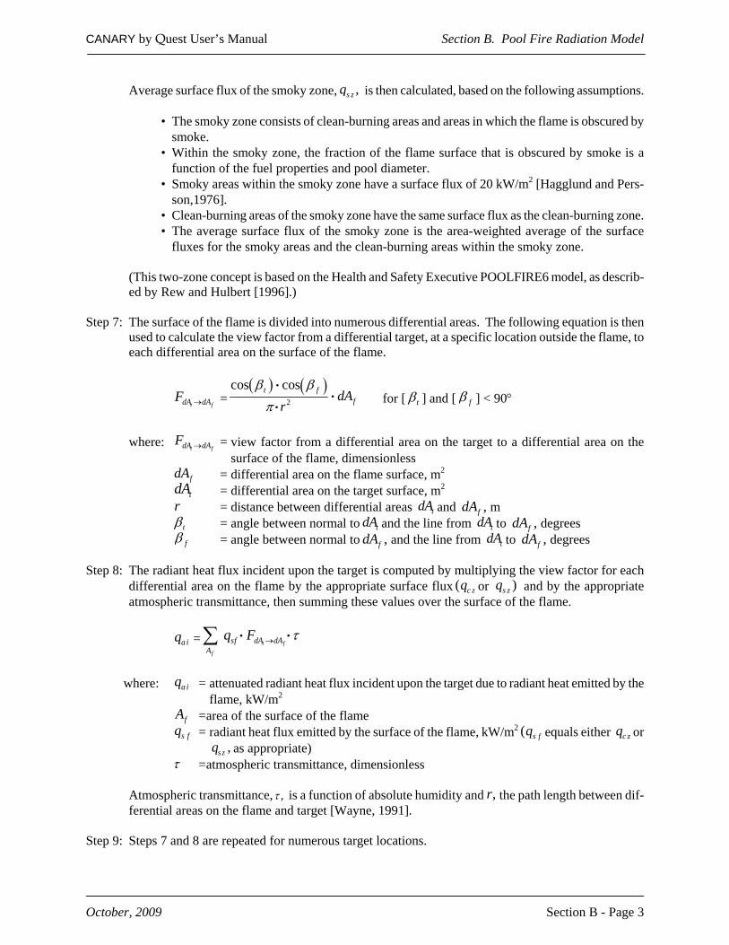
CANARY by Quest User’s Manual Section B. Pool Fire Radiation Model
October, 2009 Section B - Page 3
Average surface flux of the smoky zone, ,s zq is then calculated, based on the following assumptions.
• The smoky zone consists of clean-burning areas and areas in which the flame is obscured by smoke.
• Within the smoky zone, the fraction of the flame surface that is obscured by smoke is a function of the fuel properties and pool diameter.
• Smoky areas within the smoky zone have a surface flux of 20 kW/m2 [Hagglund and Pers-son,1976].
• Clean-burning areas of the smoky zone have the same surface flux as the clean-burning zone. • The average surface flux of the smoky zone is the area-weighted average of the surface
fluxes for the smoky areas and the clean-burning areas within the smoky zone.
(This two-zone concept is based on the Health and Safety Executive POOLFIRE6 model, as describ-ed by Rew and Hulbert [1996].)
Step 7: The surface of the flame is divided into numerous differential areas. The following equation is then
used to calculate the view factor from a differential target, at a specific location outside the flame, to each differential area on the surface of the flame.
t fdA dAF → =( ) ( )
2
cos cost ffdA
rβ βπ
ii
i for [ tβ ] and [ fβ ] < 90°
where:
t fdA dAF → = view factor from a differential area on the target to a differential area on the surface of the flame, dimensionless
fdA = differential area on the flame surface, m2 tdA = differential area on the target surface, m2 r = distance between differential areas tdA and ,fdA m tβ = angle between normal to tdA and the line from tdA to ,fdA degrees fβ = angle between normal to ,fdA and the line from tdA to ,fdA degrees
Step 8: The radiant heat flux incident upon the target is computed by multiplying the view factor for each differential area on the flame by the appropriate surface flux ( c zq or )s zq and by the appropriate atmospheric transmittance, then summing these values over the surface of the flame.
a iq = t f
f
sf dA dAA
q F τ→∑ i i
where: a iq = attenuated radiant heat flux incident upon the target due to radiant heat emitted by the
flame, kW/m2 fA = area of the surface of the flame s fq = radiant heat flux emitted by the surface of the flame, kW/m2 ( s fq equals either c zq or
,s zq as appropriate) τ = atmospheric transmittance, dimensionless
Atmospheric transmittance, ,τ is a function of absolute humidity and ,r the path length between dif-ferential areas on the flame and target [Wayne, 1991].
Step 9: Steps 7 and 8 are repeated for numerous target locations.

CANARY by Quest User’s Manual Section B. Pool Fire Radiation Model
October, 2009 Section B - Page 4
Validation Several of the equations used in the Pool Fire Radiation Model are empirical relationships based on data from medium- to large-scale experiments, which ensures reasonably good agreement between model predictions and experimental data for variables such as flame length and tilt angle. Comparisons of experimental data and model predictions for incident heat flux at specific locations are more meaningful and of greater interest. Unfortunately, few reports on medium- or large-scale experiments contain the level of detail required to make such comparisons. One source of detailed test data is a report by Welker and Cavin [1982]. It contains data from sixty-one pool fire tests involving commercial propane. Variables that were examined during these tests include pool size (2.7 to 152 m2) and wind speed. Figure B-1 compares the predicted values of incident heat flux with experimental data from the sixty-one pool fire tests.
0 2000 4000 6000 8000 10000
Pool Fire Test Data, Btu/hr-ft2
0
2000
4000
6000
8000
10000
CAN
ARY
Pre
dict
ions
, Btu
/hr-
ft2
40 x 40 ft20 x 20 ft10 x 10 ft5 x 5 ft
Figure B-1
In another series of tests, fire radiation measurements were taken for large liquefied natural gas (LNG) pool fires. The Montoir tests are the largest tests of LNG fires, involving pools up to 35 meters in diameter [Nédelka, Moorhouse, and Tucker, 1989]. Figure B-2 compares the radiation isopleths predicted by CANARY with the actual measurements taken in Test 2 of the Montoir series.
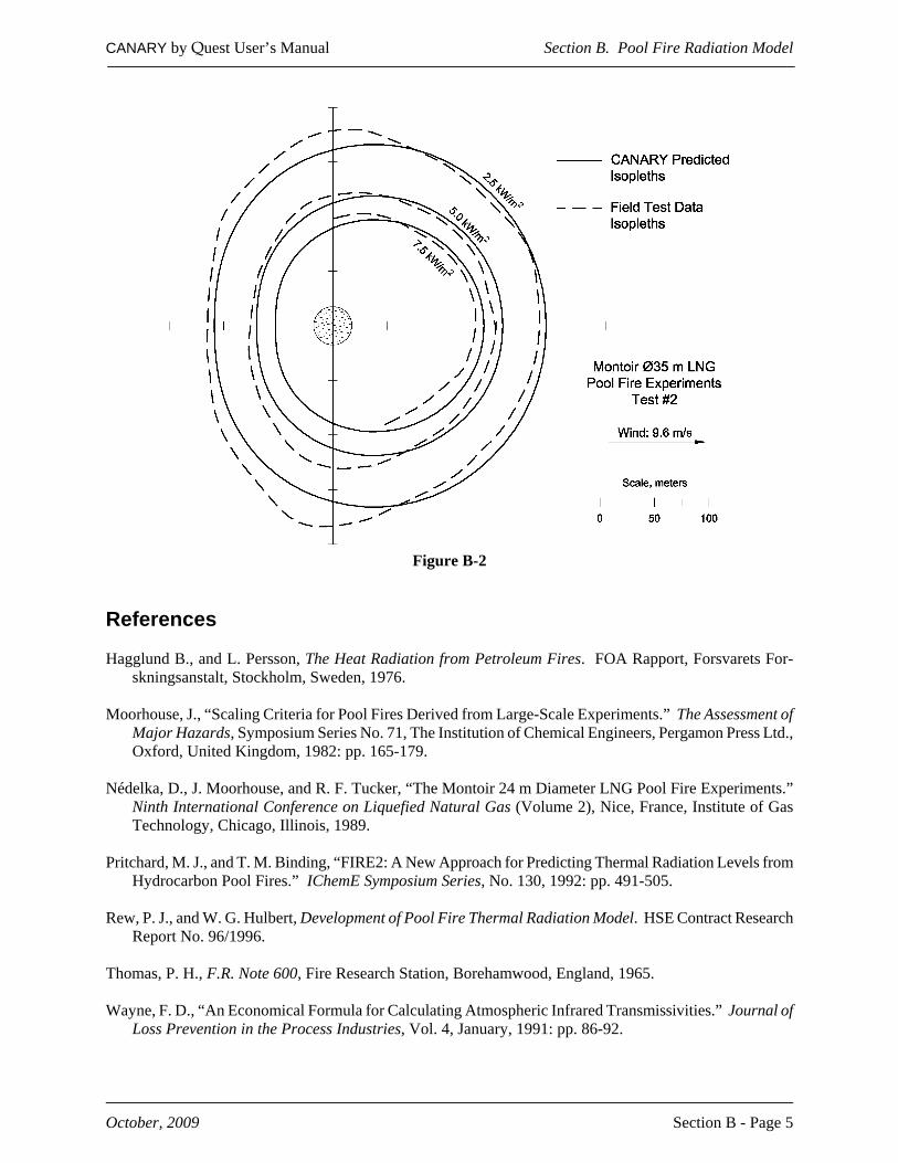
CANARY by Quest User’s Manual Section B. Pool Fire Radiation Model
October, 2009 Section B - Page 5
Figure B-2 References Hagglund B., and L. Persson, The Heat Radiation from Petroleum Fires. FOA Rapport, Forsvarets For-
skningsanstalt, Stockholm, Sweden, 1976. Moorhouse, J., “Scaling Criteria for Pool Fires Derived from Large-Scale Experiments.” The Assessment of
Major Hazards, Symposium Series No. 71, The Institution of Chemical Engineers, Pergamon Press Ltd., Oxford, United Kingdom, 1982: pp. 165-179.
Nédelka, D., J. Moorhouse, and R. F. Tucker, “The Montoir 24 m Diameter LNG Pool Fire Experiments.”
Ninth International Conference on Liquefied Natural Gas (Volume 2), Nice, France, Institute of Gas Technology, Chicago, Illinois, 1989.
Pritchard, M. J., and T. M. Binding, “FIRE2: A New Approach for Predicting Thermal Radiation Levels from
Hydrocarbon Pool Fires.” IChemE Symposium Series, No. 130, 1992: pp. 491-505. Rew, P. J., and W. G. Hulbert, Development of Pool Fire Thermal Radiation Model. HSE Contract Research
Report No. 96/1996. Thomas, P. H., F.R. Note 600, Fire Research Station, Borehamwood, England, 1965. Wayne, F. D., “An Economical Formula for Calculating Atmospheric Infrared Transmissivities.” Journal of
Loss Prevention in the Process Industries, Vol. 4, January, 1991: pp. 86-92.

CANARY by Quest User’s Manual Section B. Pool Fire Radiation Model
October, 2009 Section B - Page 6
Welker, J. R., and W. D. Cavin, Vaporization, Dispersion, and Radiant Fluxes from LPG Spills. Final Report No. DOE-EP-0042, Department of Energy Contract No. DOE-AC05-78EV-06020-1, May, 1982 (NTIS No. DOE-EV-06020-1).
Welker, J. R., and C. M. Sliepcevich, Susceptibility of Potential Target Components to Defeat by Thermal
Action. University of Oklahoma Research Institute, Report No. OURI-1578-FR, Norman, Oklahoma, 1970.
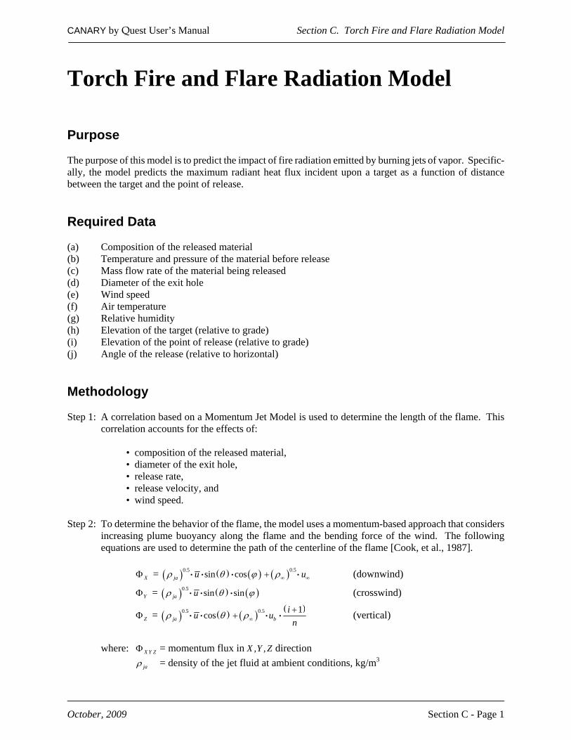
CANARY by Quest User’s Manual Section C. Torch Fire and Flare Radiation Model
October, 2009 Section C - Page 1
Torch Fire and Flare Radiation Model Purpose The purpose of this model is to predict the impact of fire radiation emitted by burning jets of vapor. Specific-ally, the model predicts the maximum radiant heat flux incident upon a target as a function of distance between the target and the point of release. Required Data (a) Composition of the released material (b) Temperature and pressure of the material before release (c) Mass flow rate of the material being released (d) Diameter of the exit hole (e) Wind speed (f) Air temperature (g) Relative humidity (h) Elevation of the target (relative to grade) (i) Elevation of the point of release (relative to grade) (j) Angle of the release (relative to horizontal) Methodology Step 1: A correlation based on a Momentum Jet Model is used to determine the length of the flame. This
correlation accounts for the effects of:
• composition of the released material, • diameter of the exit hole, • release rate, • release velocity, and • wind speed.
Step 2: To determine the behavior of the flame, the model uses a momentum-based approach that considers
increasing plume buoyancy along the flame and the bending force of the wind. The following equations are used to determine the path of the centerline of the flame [Cook, et al., 1987].
XΦ = ( ) ( ) ( ) ( )0.50.5 sin cosja u uρ θ ϕ ρ∞ ∞+i i i i (downwind)
YΦ = ( ) ( ) ( )0.5 sin sinja uρ θ ϕi i i (crosswind)
ZΦ = ( ) ( ) ( )( )0.50.5 1cosja biu u
nρ θ ρ∞
++i i i i (vertical)
where: X Y ZΦ = momentum flux in , ,X Y Z direction
jaρ = density of the jet fluid at ambient conditions, kg/m3
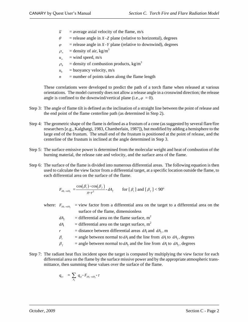
CANARY by Quest User’s Manual Section C. Torch Fire and Flare Radiation Model
October, 2009 Section C - Page 2
u = average axial velocity of the flame, m/s θ = release angle in X Z− plane (relative to horizontal), degrees ϕ = release angle in X Y− plane (relative to downwind), degrees ρ∞ = density of air, kg/m3 u∞ = wind speed, m/s
bρ = density of combustion products, kg/m3
bu = buoyancy velocity, m/s n = number of points taken along the flame length
These correlations were developed to predict the path of a torch flame when released at various orientations. The model currently does not allow a release angle in a crosswind direction; the release angle is confined to the downwind/vertical plane (i.e.,ϕ = 0).
Step 3: The angle of flame tilt is defined as the inclination of a straight line between the point of release and
the end point of the flame centerline path (as determined in Step 2). Step 4: The geometric shape of the flame is defined as a frustum of a cone (as suggested by several flare/fire
researchers [e.g., Kalghatgi, 1983, Chamberlain, 1987]), but modified by adding a hemisphere to the large end of the frustum. The small end of the frustum is positioned at the point of release, and the centerline of the frustum is inclined at the angle determined in Step 3.
Step 5: The surface emissive power is determined from the molecular weight and heat of combustion of the
burning material, the release rate and velocity, and the surface area of the flame. Step 6: The surface of the flame is divided into numerous differential areas. The following equation is then
used to calculate the view factor from a differential target, at a specific location outside the flame, to each differential area on the surface of the flame.
t fdA dAF → =( ) ( )
2
cos cost ffdA
rβ βπ
ii
i for [ tβ ] and [ fβ ] < 90°
where:
t fdA dAF → = view factor from a differential area on the target to a differential area on the surface of the flame, dimensionless
fdA = differential area on the flame surface, m2
tdA = differential area on the target surface, m2 r = distance between differential areas tdA and ,fdA m
tβ = angle between normal to tdA and the line from tdA to ,fdA degrees
fβ = angle between normal to fdA and the line from tdA to ,fdA degrees Step 7: The radiant heat flux incident upon the target is computed by multiplying the view factor for each
differential area on the flame by the surface missive power and by the appropriate atmospheric trans-mittance, then summing these values over the surface of the flame.
a iq =
t f
f
sf dA dAA
q F τ→∑ i i

CANARY by Quest User’s Manual Section C. Torch Fire and Flare Radiation Model
October, 2009 Section C - Page 3
where: a iq = attenuated radiant heat flux incident upon the target due to radiant heat emitted by the flame, kW/m2
fA = area of the surface of the flame
s fq = radiant heat flux emitted by the surface of the flame, kW/m2 τ = atmospheric transmittance, dimensionless
Atmospheric transmittance, ,τ is a function of absolute humidity and ,r the path length between differential areas on the flame and target [Wayne, 1991].
Step 8: Steps 6 and 7 are repeated for numerous target locations. Validation Several of the equations used in the Torch Fire and Flare Radiation Model are empirical relationships based on data from medium- to large-scale experiments, which ensures reasonably good agreement between model predictions and experimental data for variables such as flame tilt angle. Comparisons of experimental data and model predictions for incident heat flux at specific locations are more meaningful and of greater interest. Unfortunately, few reports on medium- or large-scale experiments contain the level of detail required to make such comparisons. One reasonable source of test data is a report by Chamberlain [1987]. It contains data from seven flare tests involving natural gas releases from industrial flares, with several data points being reported for each test. Variables that were examined during these tests include release diameter (0.203 and 1.07 m), release rate and velocity, and wind speed. Figure C-1 compares the predicted values of incident heat flux with experimental data from the seven flare tests.
0 2 4 6 8 10
Flare Test Data, kW/m2
0
2
4
6
8
10
CAN
AR
Y Pr
edic
tions
, kW
/m2
Test Series 3Test Series 4
Figure C-1
CANARY by Quest User’s Manual Section C. Torch Fire and Flare Radiation Model
October, 2009 Section C - Page 4
References Chamberlain, G. A., “Developments in Design Methods for Predicting Thermal Radiation from Flares.”
Chemical Engineering Research and Design, Vol. 65, July, 1987. Cook, D. K., M. Fairweather, G. Hankinson, and K. O’Brien, “Flaring of Natural Gas from Inclined Vent
Stacks.” IChemE Symposium Series #102, Pergamon Press, 1987. Kalghatgi, G. T., “The Visible Shape and Size of a Turbulent Hydrocarbon Jet Diffusion Flame in a Cross
Wind.” Combustion and Flame, Vol. 52, 1983: pp. 91-106. Wayne, F. D., “An Economical Formula for Calculating Atmospheric Infrared Transmissivities.” Journal of
Loss Prevention in the Process Industries, Vol. 4, January, 1991: pp. 86-92.
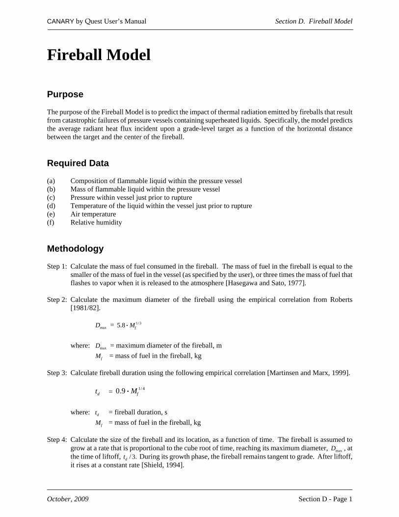
CANARY by Quest User’s Manual Section D. Fireball Model
October, 2009 Section D - Page 1
Fireball Model Purpose The purpose of the Fireball Model is to predict the impact of thermal radiation emitted by fireballs that result from catastrophic failures of pressure vessels containing superheated liquids. Specifically, the model predicts the average radiant heat flux incident upon a grade-level target as a function of the horizontal distance between the target and the center of the fireball. Required Data (a) Composition of flammable liquid within the pressure vessel (b) Mass of flammable liquid within the pressure vessel (c) Pressure within vessel just prior to rupture (d) Temperature of the liquid within the vessel just prior to rupture (e) Air temperature (f) Relative humidity Methodology Step 1: Calculate the mass of fuel consumed in the fireball. The mass of fuel in the fireball is equal to the
smaller of the mass of fuel in the vessel (as specified by the user), or three times the mass of fuel that flashes to vapor when it is released to the atmosphere [Hasegawa and Sato, 1977].
Step 2: Calculate the maximum diameter of the fireball using the empirical correlation from Roberts
[1981/82].
maxD = 1/ 35.8 fMi
where: maxD = maximum diameter of the fireball, m
fM = mass of fuel in the fireball, kg Step 3: Calculate fireball duration using the following empirical correlation [Martinsen and Marx, 1999].
dt = 1/ 40.9 fMi
where: dt = fireball duration, s fM = mass of fuel in the fireball, kg
Step 4: Calculate the size of the fireball and its location, as a function of time. The fireball is assumed to
grow at a rate that is proportional to the cube root of time, reaching its maximum diameter, maxD , at the time of liftoff, / 3.dt During its growth phase, the fireball remains tangent to grade. After liftoff, it rises at a constant rate [Shield, 1994].

CANARY by Quest User’s Manual Section D. Fireball Model
October, 2009 Section D - Page 2
Step 5: Estimate the surface flux of the fireball. The fraction of the total available heat energy that is emitted as radiation is calculated using the equation derived by Roberts [1981/82].
f = 0.320.0296 Pi
where: f = fraction of available heat energy released as radiation, dimensionless
P = pressure in vessel at time of rupture, kPa
The total amount of energy emitted as radiation is then calculated.
rE = f cf M H∆i i
where: rE = energy emitted as radiation, kJ
cH∆ = heat of combustion, kJ/kg
The surface flux is estimated by dividing rE by the average surface area of the fireball and the fireball duration, but it is not allowed to exceed 400 kW/m2.
Step 6: Calculate the maximum view factor from a differential target (at specific grade level locations outside
the fireball) to the fireball, using the simple equation for a spherical radiator [Howell, 1982].
F =2
2
RH
where: F = view factor from differential area to the fireball, dimensionless
R = radius of the fireball, m H = distance between target and the center of the fireball, m
R and H vary with time due to the growth and rise of the fireball. Therefore, the duration of the fireball is divided into time intervals and a view factor is calculated at the end of each interval.
Step 7: Compute the attenuated radiant heat flux at each target location, at the end of each time interval,
by multiplying the appropriate view factor by the surface flux of the fireball and by the appropriate atmospheric transmittance. The transmittance of the atmosphere is a function of the absolute humid-ity and path length from the fireball to the target [Wayne, 1991]. For each target location, calculate the average attenuated heat flux over the duration of the fireball.
Step 8: Calculate the absorbed energy at each target location. For a given location, the energy absorbed
during each time interval is computed by multiplying the length of the interval by the average attenuated radiant heat flux for that interval. The absorbed energies for all time intervals are then summed to determine the radiant energy absorbed over the duration of the fireball.
Step 9: Calculate the integrated dosage at each target location. This is computed in the same manner as
absorbed energy is computed in Step 8, except that the average attenuated radiant heat flux for each time interval is taken to the 4/3rds power before it is multiplied by the time interval. This allows the dosage to be used in the probit equation for fatalities from thermal radiation [Eisenberg, Lynch, and Breeding, 1975].

CANARY by Quest User’s Manual Section D. Fireball Model
October, 2009 Section D - Page 3
Pr = ( )4 /338.4785 2.56 ln q t− + i i
where: Pr = probit q = radiant heat flux, W/m2 t = exposure time, s
Validation Several of the equations used in the Fireball Model are empirical relationships based on data from small- to medium-scale experiments, which ensures reasonably good agreement between model predictions and experimental data for variables such as maximum fireball diameter. Comparisons of experimental data and model predictions for average incident heat flux, absorbed energy, or dosage are more meaningful and of greater interest. Unfortunately, very few reports on small- or medium-scale fireball experiments contain the level of detail required to make such comparisons, and no such data are available for large-scale experiments. One of the most complete sources of test data for medium-scale fireball tests is a report by Johnson, Pritchard, and Wickens [1990]. It contains data on five BLEVE tests that involved butane and propane, in quantities up to 2,000 kg. Figure D-1 compares the predicted values of absorbed energy with experimental data from those five BLEVE tests.
Figure D-1

CANARY by Quest User’s Manual Section D. Fireball Model
October, 2009 Section D - Page 4
References Eisenberg, N. A., C. J. Lynch, and R. J. Breeding, Vulnerability Model: A Simulation System for Assessing
Damage Resulting from Marine Spills. U.S. Coast Guard, Report CG-D-136-75, June, 1975. Hasegawa, K., and K. Sato, “Study on the Fireball Following Steam Explosion of n-Pentane.” Proceedings of
the Second International Symposium on Loss Prevention and Safety Promotion in the Process Industries, Heidelberg, Germany, September, 1977: pp. 297-304.
Howell, John R., A Catalog of Radiation Configuration Factors. McGraw-Hill Book Company, 1982. Johnson, D. M., M. J. Pritchard, and M. J. Wickens, Large-Scale Catastrophic Releases of Flammable
Liquids. Commission of European Communities, Report EV4T.0014, 1990. Martinsen, W. E., and J. D. Marx, “An Improved Model for the Prediction of Radiant Heat from Fireballs.”
Presented at the 1999 International Conference and Workshop on Modeling Consequences of Accidental Releases of Hazardous Materials, San Francisco, California, September 28 - October 1, 1999.
Roberts, A. F., “Thermal Radiation Hazards from Releases of LPG from Pressurized Storage.” Fire Safety
Journal, Vol. 4, 1981/82: pp. 197-212. Shield, S. R., Consequence Modeling for LPG Distribution in Hong Kong. Thornton Research Centre, Safety
and Environment Department, United Kingdom, TNRN 95.7001, December 13, 1994. Wayne, F. D., “An Economical Formula for Calculating Atmospheric Infrared Transmissivities.” Journal of
Loss Prevention in the Process Industries, Vol. 4, January, 1991: pp. 86-92.

CANARY by Quest User’s Manual Section E. Fluid Release Model
October, 2009 Section E - Page 1
Fluid Release Model Purpose The purpose of the Fluid Release Model is to predict the rate of mass release from a breach of containment. Specifically, the model predicts the rate of flow and the physical state (liquid, two-phase, or gas) of the release of a fluid stream as it enters the atmosphere from a circular breach in a pipe or vessel wall. The model also computes the amount of vapor and aerosol produced and the rate at which liquid reaches the ground. Required Data (a) Composition of the fluid (b) Temperature and pressure of the fluid just prior to the time of the breach (c) Normal flow rate of fluid into the vessel or in the pipe (d) Size of the pipe and/or vessel (e) Length of pipe (f) Area of the breach (g) Angle of release relative to horizontal (h) Elevation of release point above grade Methodology Step 1: Calculation of Initial Flow Conditions
The initial conditions (before the breach occurs) in the piping and/or vessel are determined from the input data, coupled with a calculation to determine the initial pressure profile in the piping. The pressure profile is computed by dividing the pipe into small incremental lengths and computing the flow conditions stepwise from the vessel to the breach point. As the flow conditions are computed, the time required for a sonic wave to traverse each section is also computed. The flow in any length increment can be all vapor, all liquid, or two-phase (this implies that the sonic velocity within each section may vary). As flow conditions are computed in each length increment, checks are made to determine if the fluid velocity has exceeded the sonic velocity or if the pressure in the flow increment has reached atmospheric. If either condition has been reached, an error code is generated and compu-tations are stopped.
Step 2: Initial Unsteady State Flow Calculations
When a breach occurs in a system with piping, a disturbance in flow and pressure propagates from the breach point at the local sonic velocity of the fluid. During the time required for the disturbance to reach the upstream end of the piping, a period of highly unsteady flow occurs. The portion of the piping that has experienced the passage of the pressure disturbance is in accelerated flow, while the portion upstream of the disturbance is in the same flow regime as before the breach occurred.
To compute the flow rate from the breach during the initial unsteady flow period, a small time increment is selected and the distance that the pressure disturbance has moved in that time increment is computed using the sonic velocity profile found in the initial pressure profile calculation. The

CANARY by Quest User’s Manual Section E. Fluid Release Model
October, 2009 Section E - Page 2
disturbed length is subdivided into small increments for use in an iterative pressure balance calcula-tion. A pressure balance is achieved when a breach pressure is found that balances the flow from the breach and the flow in the disturbed section of piping. Another time increment is added, and the iterative procedure continues. The unsteady period continues until the pressure disturbance reaches the upstream end of the pipe.
Step 3: Long-Term Unsteady State Flow Calculations
The long-term unsteady state flow calculations are characterized by flow in the piping system that is changing more slowly than during the initial unsteady state calculations. The length of accelerated flow in the piping is constant, set by the user input pipe length. The vessel contents are being deplet-ed, resulting in a potential lowering of pressure in the vessel. As with the other flow calculations, the time is incremented and the vessel conditions are computed. The new vessel conditions serve as input for the pressure drop calculations in the pipe. When a breach pressure is computed that balances the breach flow with the flow in the piping, a solution for that time is achieved. The solu-tion continues until the ending time or other ending conditions are reached.
The frictional losses in the piping system are computed using the equation:
h = 24
2ls
c e
f L Ug D
⎛ ⎞⎜ ⎟⎝ ⎠
i i i
i i (1)
where: h = head (pressure) loss, ft of fluid
f = friction factor L = length of system, ft U = average flowing velocity, ft/sec
cg = gravitational constant, 32.2 lbm i ft/(lbf i sec2) eD = equivalent diameter of duct, ft
The friction factor is computed using the following equation:
1f
= 102 18.71.74 2.0 log
eD Re fε⎡ ⎤− +⎢ ⎥
⎣ ⎦
ii
i (2)
where: ε = pipe roughness, ft
Re = Reynolds number, /eD U ρ µi i , dimensionless ρ = fluid density, lb/ft3 µ = fluid viscosity, lb/(ft i sec)
Equations (1) and (2) are used for liquid, vapor, and two-phase flow regimes. Since the piping is subdivided into small lengths, changes in velocity and physical properties across each segment are assumed to be negligible. At each step in the calculation, a check is made to determine if the fluid velocity has reached or exceeded the computed critical (sonic) velocity for the fluid. If the critical velocity has been exceeded, the velocity is constrained to the critical velocity and the maximum mass flow rate in the piping has been set.
If the fluid in the piping is in two-phase flow, the Lockhart and Martinelli [1949] modification to Equation (1) is used. The Lockhart and Martinelli equation for head loss is shown below:

CANARY by Quest User’s Manual Section E. Fluid Release Model
October, 2009 Section E - Page 3
TPh = 2
2 42
ls
c e
f L Ug D
⎛ ⎞Φ ⎜ ⎟
⎝ ⎠
i i ii
i i (3)
where: TPh = head loss for two-phase flow, ft of fluid
Φ = empirical parameter correlating single- and two-phase flow, dimensionless lsU = superficial liquid velocity (velocity of liquid if liquid filled the pipe), ft/sec
This equation is valid over short distances where the flowing velocity does not change appreciably.
Validation Validation of fluid flow models is difficult since little data are available for comparison. Fletcher [1983] presented a set of data for flashing CFC-11 flowing through orifices and piping. Figures E-1 through E-4 compare calculations made using the Fluid Release Model with the data presented by Fletcher. Figure E-1 compares fluid fluxes for orifice type releases. These releases had length-to-diameter (L/D) ratios less than 0.88. Figure E-2 compares computed and experimental release fluxes for an L/D ratio of 120 at several levels of storage pressure. Figure E-3 compares similar releases for an L/D of 37.5. Figure E-4 shows predicted and experimental release fluxes at a given pressure for L/D ratios from 1 to 200. Figures E-5 and E-6 compare computed and experimental gas discharge rates for the complete breach of two pipes. One pipe had an internal diameter of 6.2 inches (0.157 m); the other had a diameter of 12 inches (0.305 m). These pipes were initially pressurized to 1,000 psia with air and then explosively ruptured. The experimental values were reported in a research paper for Alberta Environment, authored by Wilson [1981]. Aerosols and Liquid Droplet Evaporation Liquids stored at temperatures above their atmospheric pressure boiling point (superheated liquids) will give off vapor when released from storage. If the temperature of storage is sufficiently above the normal boiling point, the energy of the released vapor will break the liquid stream into small droplets. If these droplets are small enough, they will not settle, but remain in the vapor stream as aerosol droplets. The presence of aerosol droplets in the vapor stream changes its apparent density and provides an additional source of vapor. Droplets large enough to fall to the ground will lose mass due to evaporation during their fall. The prediction of aerosol formation and amount of aerosol formed is based on the theoretical work performed for the Center for Chemical Process Safety (CCPS) by CREARE. CREARE=s work has been extended and corrected by Quest. The extension to the model computes the non-aerosol drop evaporation. In Figure E-7, the four experimental data sets available for comparison (chlorine (Cl2), methylamine (MMA), CFC-11, and cyclohexane) are compared to the values computed by the CANARY Aerosol Model.

CANARY by Quest User’s Manual Section E. Fluid Release Model
October, 2009 Section E - Page 4
0 1 2 3 4 5System Pressure, barg
0
5000
10000
15000
20000
Mas
s Fl
ux, k
g/(m
2 -s)
ExperimentalComputed
Figure E-1
Comparison of CFC-11 Orifice Releases as a Function of System Pressure
0 1 2 3 4System Pressure, barg
0
1000
2000
3000
4000
5000
6000
7000
Mas
s Fl
ux, k
g/(m
2 -s)
ExperimentalComputed
Figure E-2
CFC-11 Release Rate Comparison with L/D of 120

CANARY by Quest User’s Manual Section E. Fluid Release Model
October, 2009 Section E - Page 5
0 1 2 3 4System Pressure, barg
0
1000
2000
3000
4000
5000
6000
7000
Mas
s Fl
ux, k
g/(m
2 -s)
ExperimentalComputed
Figure E-3
CFC-11 Release Rate Comparison with L/D of 37.5
0 20 40 60 80 100 120 140 160 180 200
Length/Diameter Ratio
0
4000
8000
12000
16000
Mas
s Fl
ux, k
g/(m
2 -s)
ExperimentalComputed
Figure E-4
CFC-11 Release Rate Comparison at Varying L/D Ratios

CANARY by Quest User’s Manual Section E. Fluid Release Model
October, 2009 Section E - Page 6
0 10 20 30 40 50 60 70Time, sec
10
100
2
3
4
5
6
789
2
3
4
Mas
s R
ate,
kg/
sec
ExperimentalComputed
Figure E-5
Air Discharge Rates for 0.157 m Diameter Piping
0 20 40 60 80 100Time, sec
100
1000
8
9
2
3
4
5
6
7
8
9
Mas
s R
ate,
kg/
sec
ExperimentalComputed
Figure E-6
Air Discharge Rates for 0.305 m Diameter Piping

CANARY by Quest User’s Manual Section E. Fluid Release Model
October, 2009 Section E - Page 7
230 250 270 290 310 330 350 370 390 410
Temperature, K
0
10
20
30
40
50
60
70
80
90
100
110
Perc
ent o
f Liq
uid
to G
roun
d (N
orm
aliz
ed to
100
% a
t NB
P)
Cl2 MMA CFC-11 Cyclohexane
Figure E-7
Aerosol Formation as a Function of Storage Temperature References Fletcher, B., “Flashing Flow Through Orifices and Pipes.” Paper presented at the AIChE Loss Prevention
Symposium, Denver, Colorado, 1983. Lockhart, R. W., and R. C. Martinelli, “Proposed Correlation of Data for Isothermal Two-Phase, Two-
Component Flow in Pipes.” Chemical Engineering Progress, Vol. 45, 1949: p. 39. Wilson, D. J., “Expansion and Plume Rise of Gas Jets from High Pressure Pipeline Ruptures.” Research
Paper, Pollution Control Division, Alberta Environment, April, 1981.

CANARY by Quest User’s Manual Section F. Momentum Jet Dispersion Model
October, 2009 Section F - Page 1
Momentum Jet Dispersion Model Purpose The purpose of this model is to predict the dispersion of a jet release into ambient air. It is used to predict the downwind travel of a flammable or toxic gas or aerosol momentum jet release. Required Data (a) Composition and properties of the released material (b) Temperature of released material (c) Release rate of material (d) Vertical release angle relative to wind direction (e) Height of release (f) Release area (g) Ambient wind speed (h) Ambient Pasquill-Gifford stability class (i) Ambient temperature (j) Relative humidity (k) Surface roughness scale Methodology Step 1: An assumption is made that flow perpendicular to the main flow in the plume is negligible, that the
velocity and concentration profiles in the jet are similar at all sections of the jet, that molecular trans-port in the jet is negligible, and that longitudinal turbulent transport is negligible when compared to longitudinal convective transport. The coordinate system is then defined in s and ,r where s is the path length of the plume and r is the radial distance from the plume centerline. The angle between the plume axis and horizontal is referred to as .θ Relationships between the downwind coordinate,
,x vertical coordinate, ,y and plume axis are given simply by:
dxds
= ( )cos θ (1)
and d yd s
= ( )sin θ (2)
Step 2: Velocity, concentration, and density profiles are assumed to be cylindrically symmetric about the
plume axis and are assumed to be Gaussian in shape. The three profiles are taken as:
( ), ,u s r θ = ( ) ( ) ( )
2
2*cosr
b saU u s eθ
−
+i i (3)
where: u = plume velocity, m/s

CANARY by Quest User’s Manual Section F. Momentum Jet Dispersion Model
October, 2009 Section F - Page 2
aU = ambient wind speed, m/s *u = plume velocity relative to the wind in the downwind direction at the plume axis, m/s ( )b s = characteristic width of the plume at distance s from the release, m
( ), ,s rρ θ = ( ) ( )
2
2 2*rb s
a s eλρ ρ−
+ ii (4)
where: ρ = plume density, kg/m3
aρ = density of ambient air, kg/m3 ( )* sρ = density difference between plume axis and ambient air, kg/m3
2λ = turbulent Schmidt number, 1.35
( ), ,c s r θ = ( ) ( )
2
2 2*r
b sc s eλ−ii (5)
where: c = pollutant concentration in the plume, kg/m3
( )*c s = pollutant concentration at plume centerline, kg/m3 Step 3: The equation for air entrainment into the plume and the conservation equations can then be solved.
The equation for air entrainment is:
( )2
02bd u dr
dsρ π∫ i i i i (6)
= ( ) ( ) ( ){ }*1 2 32 sin cosa ab u s U uπ ρ α α θ θ α ′+ +i i i i i i i i⏐ ⏐ ⏐ ⏐
where: 1α = entrainment coefficient for a free jet, 0.057
2α = entrainment coefficient for a line thermal, 0.5
3α = entrainment coefficient due to turbulence, 1.0 u′ = turbulent entrainment velocity (root mean square of the wind velocity fluctuation is
used for this number), m/s Step 4: The equations of conservation of mass, momentum, and energy are given as:
( )2
02bd c u dr
dsπ∫ i i i i = 0 (7)
( )( )( )2 2
0cos 2bd u dr
dsρ θ π∫ i i i i i (8)
= ( ) ( ) ( ){ }*1 2 32 sin cosa ab u s U uπ ρ α α θ θ α ′+ +i i i i i i i i i
+ ( )2 sind a aC b Uπ ρ θi i i i

CANARY by Quest User’s Manual Section F. Momentum Jet Dispersion Model
October, 2009 Section F - Page 3
( )( )2 2
0cos 2
bd u drds
ρ θ π∫ i i i i i (9)
= ( ) ( ) ( )2 2
0sin cos
b
a d a ag r dr C b Uρ ρ π π ρ θ θ− ±∫ i i i i i i i i i
2
00
1 1 2b
a
d u r drd s
ρ πρ ρ
⎛ ⎞⎛ ⎞−⎜ ⎟⎜ ⎟⎝ ⎠⎝ ⎠
∫ i i i i i (10)
= ( ) ( ) ( ){ }*1 2 3
0
1 12 | | sin | cosa aa a
b u s U úρ π α α θ θ αρ ρ
⎛ ⎞− + +⎜ ⎟⎝ ⎠
i i i i i i i i
The subscript 0 refers to conditions at the point of release. These equations are integrated along the path of the plume to yield the concentration profiles as a function of elevation and distance down-wind of the release.
Step 5: After the steady-state equations are solved, an along-wind dispersion correction is applied to account
for short-duration releases. This is accomplished using the method outlined by Palazzi, et al. [1982]. Step 6: If the plume reaches the ground, it is coupled to the Heavy Gas Dispersion Model (described in
Section G) and the dispersion calculations continue. Validation The Momentum Jet Dispersion Model used in CANARY was validated by comparing results obtained from the model with experimental data from field tests. Data used for this comparison and the conditions used in the model were taken from an American Petroleum Institute (API) study [Hanna, Strimaitis, and Chang, 1991]. For this model, comparisons were made with the Desert Tortoise, Goldfish, and Prairie Grass series of dispersion tests. Results of these comparisons are shown in Figure F-1. References Astleford, W. J., T. B. Morrow, and J. C. Buckingham, Hazardous Chemical Vapor Handbook for Marine
Tank Vessels (Final Report B Phase II). U.S. Coast Guard Report No. CG-D-12-83, April, 1983. Hanna, S. R., D. G. Strimaitis, and J. C. Chang, Hazard Response Modeling Uncertainty (A Quantitative
Method), Evaluation of Commonly Used Hazardous Gas Dispersion Models, Volume II. Study co-sponsored by the Air Force Engineering and Services Center, Tyndall Air Force Base, Florida, and the American Petroleum Institute; performed by Sigma Research Corporation, Westford, Massachusetts, September, 1991.
Havens, J., and T. Spicer, LNG Vapor Dispersion Prediction with the DEGADIS Dense Gas Dispersion
Model. Gas Research Institute Contract No. 5086-252-1287 with the University of Arkansas, September, 1990: pp. 37-48.
Ooms, G., “A New Method for the Calculation of the Plume Path of Gases Emitted by a Stack.” Atmospheric
Environment, Vol. 6, 1972: pp. 889-909.

CANARY by Quest User’s Manual Section F. Momentum Jet Dispersion Model
October, 2009 Section F - Page 4
10-2 10-1 100 101 102 103 104 105 10610-2
10-1
100
101
102
103
104
105
106
Desert Tortoise (NH3)Goldfish (HF)Prarie Grass (SO2)
OVERPREDICTION
UNDERPREDICTION
Flammable RangeTrace Gas Range
Field Data Concentration (ppm)
CA
NA
RY
Pre
dict
ed C
once
ntra
tion
(ppm
)
Figure F-1
Ooms, G., A. P. Mahieu, and F. Zelis, “The Plume Path of Vent Gases Heavier than Air.” First International
Symposium on Loss Prevention and Safety Promotion in the Process Industries, C. H. Buschman, Editor, Elsevier Press, 1974.
Palazzi, E., M. De Faveri, G. Fumarola, and G. Ferraiolo, “Diffusion from a Steady Source of Short Dura-
tion.” Atmospheric Environment, Vol. 16, No. 12, 1982: pp. 2785-2790.

CANARY by Quest User’s Manual Section G. Heavy Gas Dispersion Model
October, 2009 Section G - Page 1
Heavy Gas Dispersion Model Purpose The purpose of this model is to predict the dispersion and gravity flow of a heavy gas released into the air from liquid pools or instantaneous gas releases. It is used to predict the downwind travel of a flammable or toxic vapor cloud. Required Data (a) Composition and properties of the released material (b) Temperature of released material (c) Vapor generation rate (d) Vapor source area (e) Vapor source duration (f) Ambient wind speed (g) Ambient Pasquill-Gifford atmospheric stability class (h) Ambient temperature (i) Relative humidity (j) Surface roughness scale Methodology Step 1: For a steady-state plume, released from a stationary source, the Heavy Gas Dispersion Model solves
the following equations:
( )d U B h mdx
ρ i i i i = s s sW Bρ i i (1)
( )d U B hdx
ρ i i i = ( )a e e s s sV h W B W Bρ ρ+ +i i i i i (2)
( )pd U B h C Tdx
ρ i i i i i = ( )a e e pa a s s s ps s tV h W B C T W B C T fρ ρ+ + +i i i i i i i i i (3)
( )d U B h Udx
ρ i i i i
= ( ) ( )20.5 g a a e e a udg B h V h W B U fdx
α ρ ρ ρ⎡ ⎤− − + + +⎣ ⎦i i i i i i i i i
(4)
( )gd U B h Vdx
ρ i i i i = ( ) 2a vgg h fρ ρ− +i i (5)
cdZU
dxi = c
gZVB
− i (6)

CANARY by Quest User’s Manual Section G. Heavy Gas Dispersion Model
October, 2009 Section G - Page 2
dBUdxi = a
e gV Vρρ
+i (7)
Tρ i = ( )a a s
s a s
T MM M M m
ρ+ −⎡ ⎤⎣ ⎦
i i
i (8)
where: x = downwind distance, m
ρ = density, kg/m3 U = velocity in the direction of the wind, m/s B = cloud width parameter, m h = cloud height parameter, m m = mass fraction of source gas T = temperature, K
pC = specific heat, J/(kg iK)
tf = ground heat flux, J/(m is)
uf = downwind friction term, kg/s2
vf = crosswind friction term, kg/s2
eV = horizontal entrainment rate, m/s
gV = horizontal crosswind gravity flow velocity, m/s
eW = vertical entrainment rate, m/s
sW = vertical source gas injection velocity, m/s M = molecular weight, kg/kmole s = refers to source properties a = refers to ambient properties
The first six equations are crosswind-averaged conservation equations. Equation (7) is the width equation, and Equation (8) is the equation of state.
Step 2: All of the gas cloud properties are crosswind averaged. The three-dimensional concentration distri-
bution is calculated from the average mass concentration by assuming the following concentration profile:
( ), ,C x y z = ( ) ( ) ( )
1 2C x C y C zi i (9)
( )C x = ( )
( ) ( )a
s a s
M m xM M M m x+ −
i
i (10)
( )1C y = 14 2 2
y b y berf erfb β β
⎧ ⎫+ −⎪ ⎪⎛ ⎞ ⎛ ⎞−⎨ ⎬⎜ ⎟ ⎜ ⎟⎪ ⎪⎝ ⎠ ⎝ ⎠⎩ ⎭i
i i i (11)
2B = 2 23b β+ i (12)
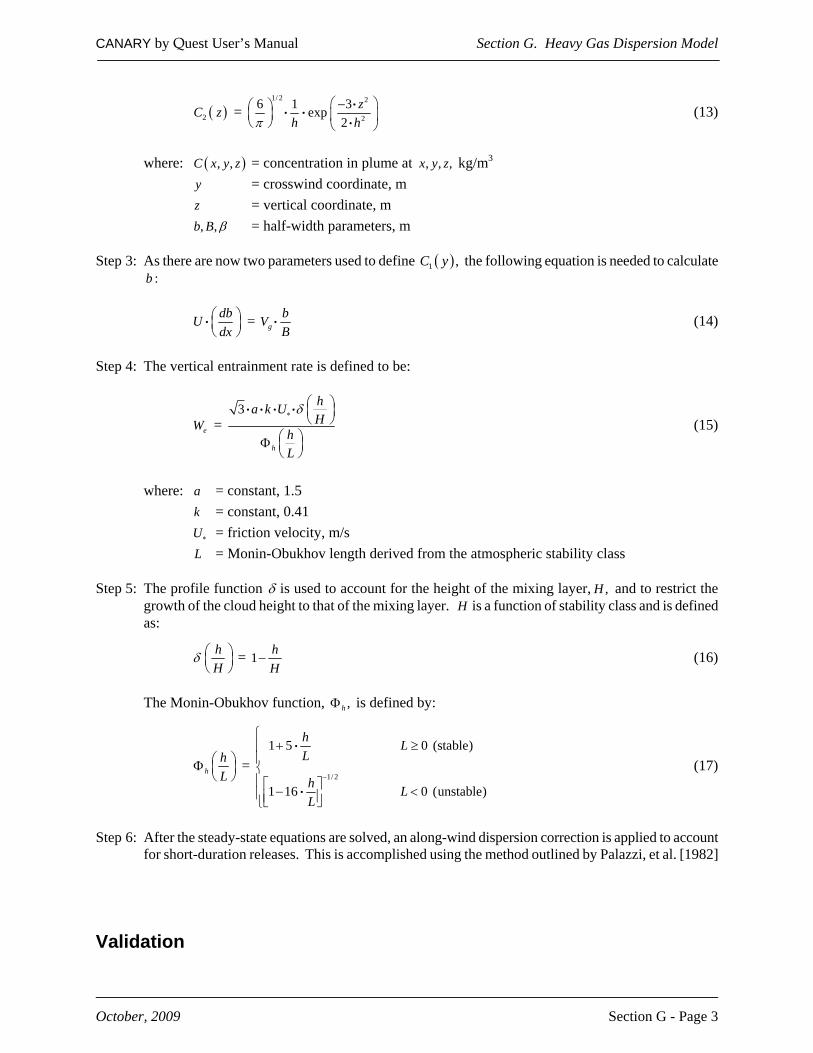
CANARY by Quest User’s Manual Section G. Heavy Gas Dispersion Model
October, 2009 Section G - Page 3
( )2C z = 1/ 2 2
2
6 1 3exp2
zh hπ
⎛ ⎞−⎛ ⎞⎜ ⎟ ⎜ ⎟⎝ ⎠ ⎝ ⎠
ii i
i (13)
where: ( ), ,C x y z = concentration in plume at , , ,x y z kg/m3
y = crosswind coordinate, m z = vertical coordinate, m , ,b B β = half-width parameters, m
Step 3: As there are now two parameters used to define ( )1 ,C y the following equation is needed to calculate
:b
dbUdx
⎛ ⎞⎜ ⎟⎝ ⎠i = g
bVB
i (14)
Step 4: The vertical entrainment rate is defined to be:
eW = 3
h
ha k UH
hL
δ∗⎛ ⎞⎜ ⎟⎝ ⎠
⎛ ⎞Φ ⎜ ⎟⎝ ⎠
i i i i
(15)
where: a = constant, 1.5
k = constant, 0.41 U∗ = friction velocity, m/s L = Monin-Obukhov length derived from the atmospheric stability class
Step 5: The profile function δ is used to account for the height of the mixing layer, ,H and to restrict the
growth of the cloud height to that of the mixing layer. H is a function of stability class and is defined as:
hH
δ ⎛ ⎞⎜ ⎟⎝ ⎠
= 1 hH
− (16)
The Monin-Obukhov function, ,hΦ is defined by:
hhL
⎛ ⎞Φ ⎜ ⎟⎝ ⎠
= 1/ 2
1 5 0 (stable)
1 16 0 (unstable)
h LL
h LL
−
⎧+ ≥⎪
⎪⎨⎪⎡ ⎤− <⎪⎢ ⎥⎣ ⎦⎩
i
i
(17)
Step 6: After the steady-state equations are solved, an along-wind dispersion correction is applied to account
for short-duration releases. This is accomplished using the method outlined by Palazzi, et al. [1982] Validation
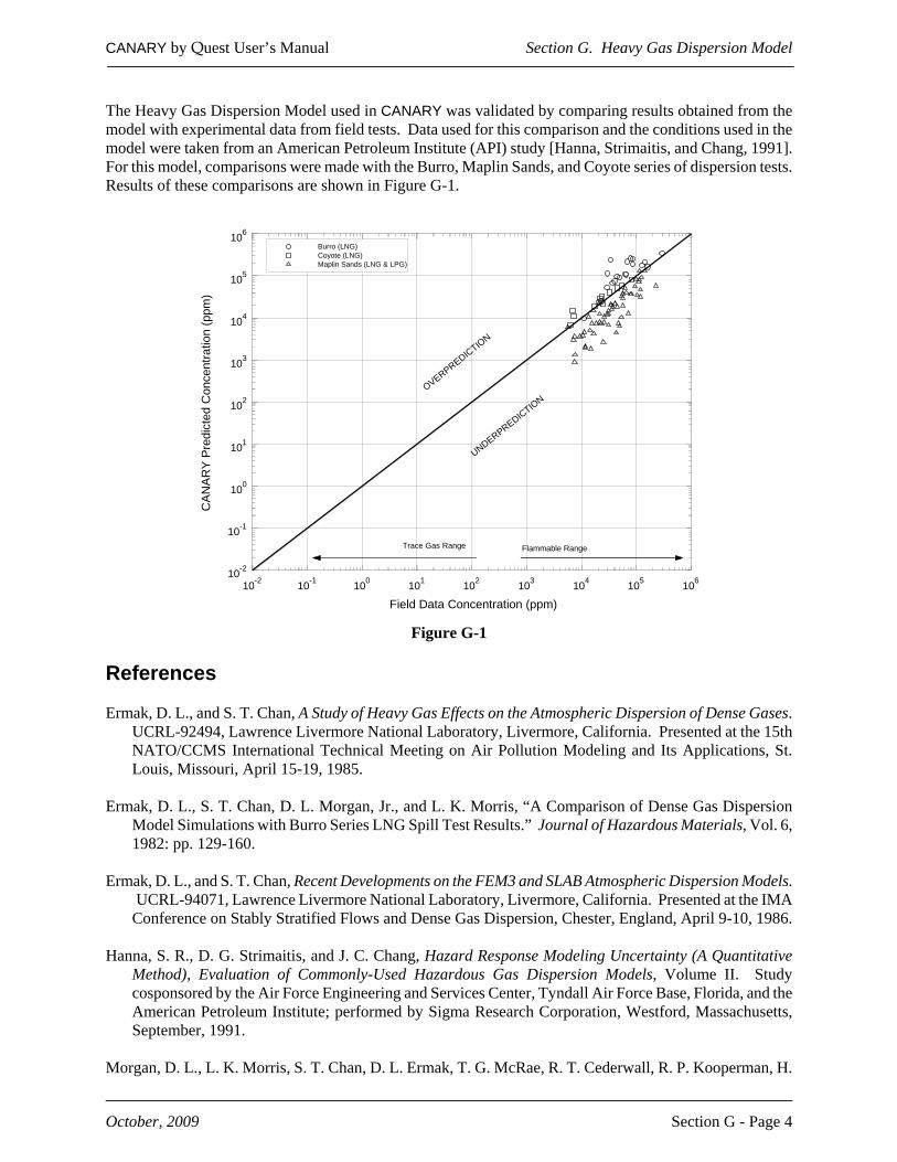
CANARY by Quest User’s Manual Section G. Heavy Gas Dispersion Model
October, 2009 Section G - Page 4
The Heavy Gas Dispersion Model used in CANARY was validated by comparing results obtained from the model with experimental data from field tests. Data used for this comparison and the conditions used in the model were taken from an American Petroleum Institute (API) study [Hanna, Strimaitis, and Chang, 1991]. For this model, comparisons were made with the Burro, Maplin Sands, and Coyote series of dispersion tests. Results of these comparisons are shown in Figure G-1.
10-2 10-1 100 101 102 103 104 105 10610-2
10-1
100
101
102
103
104
105
106
Burro (LNG)Coyote (LNG)Maplin Sands (LNG & LPG)
OVERPREDICTION
UNDERPREDICTION
Flammable RangeTrace Gas Range
Field Data Concentration (ppm)
CA
NA
RY
Pre
dict
ed C
once
ntra
tion
(ppm
)
Figure G-1
References Ermak, D. L., and S. T. Chan, A Study of Heavy Gas Effects on the Atmospheric Dispersion of Dense Gases.
UCRL-92494, Lawrence Livermore National Laboratory, Livermore, California. Presented at the 15th NATO/CCMS International Technical Meeting on Air Pollution Modeling and Its Applications, St. Louis, Missouri, April 15-19, 1985.
Ermak, D. L., S. T. Chan, D. L. Morgan, Jr., and L. K. Morris, “A Comparison of Dense Gas Dispersion
Model Simulations with Burro Series LNG Spill Test Results.” Journal of Hazardous Materials, Vol. 6, 1982: pp. 129-160.
Ermak, D. L., and S. T. Chan, Recent Developments on the FEM3 and SLAB Atmospheric Dispersion Models.
UCRL-94071, Lawrence Livermore National Laboratory, Livermore, California. Presented at the IMA Conference on Stably Stratified Flows and Dense Gas Dispersion, Chester, England, April 9-10, 1986.
Hanna, S. R., D. G. Strimaitis, and J. C. Chang, Hazard Response Modeling Uncertainty (A Quantitative
Method), Evaluation of Commonly-Used Hazardous Gas Dispersion Models, Volume II. Study cosponsored by the Air Force Engineering and Services Center, Tyndall Air Force Base, Florida, and the American Petroleum Institute; performed by Sigma Research Corporation, Westford, Massachusetts, September, 1991.
Morgan, D. L., L. K. Morris, S. T. Chan, D. L. Ermak, T. G. McRae, R. T. Cederwall, R. P. Kooperman, H.

CANARY by Quest User’s Manual Section G. Heavy Gas Dispersion Model
October, 2009 Section G - Page 5
C. Goldwire, Jr., J. W. McClure, and W. J. Hogan, Phenomenology and Modeling of Liquefied Natural Gas Vapor Dispersion. UCRL-53581, Lawrence Livermore National Laboratory, Livermore, California, 1982.
Morgan, D. L., Jr., L. K. Morris, and D. L. Ermak, SLAB: A Time-Dependent Computer Model for the
Dispersion of Heavy Gases Released in the Atmosphere. UCRL-53383, Lawrence Livermore National Laboratory, Livermore, California, 1983.
Palazzi, E., M. De Faveri, G. Fumarola, and G. Ferraiolo, “Diffusion from a Steady Source of Short Dura-
tion.” Atmospheric Environment, Vol. 16, No. 12, 1982: pp. 2785-2790.
CANARY by Quest User’s Manual Section I. Vapor Cloud Explosion Model
October, 2009 Section I - Page 1
Vapor Cloud Explosion Model Purpose The purpose of this model is to predict the overpressure field that would be produced by the explosion of a partially confined and/or obstructed fuel-air cloud, based on the Baker-Strehlow-Tang methodology. Specifically, the model predicts the magnitude of the peak side-on overpressure and specific impulse as a function of distance from the source of the explosion. Required Data (a) Composition of the fuel (flammable fluid) involved in the explosion (b) Total mass of fuel in the flammable cloud at the time of ignition or the volume of the partially-con-
fined/obstructed area (c) Fuel reactivity (high, medium, or low) (d) Obstacle density (high, medium, or low) (e) Flame expansion (1-D, 2-D, 22-D, or 3-D) (f) Reflection factor Methodology Step 1: The combustion energy of the cloud is estimated by multiplying its mass by the heat of combustion.
If the volume of the flammable cloud is input, the mass is estimated by assuming that a stoichiometric mixture of gas and air exists within that volume.
Step 2: The combustion energy is multiplied by the reflection factor to account for blast reflection from the
ground or surrounding objects. Step 3: Flame speed is determined from the fuel reactivity, obstacle density, and flame expansion parameters,
as presented in Baker, et al. [1994, 1998, 1999, 2005].
Fuel reactivity and obstacle density each have low, medium, and high choices. The flame expansion parameter allows choices of 1-D, 2-D, 2.5-D, and 3-D. The choices for these three parameters create a matrix of 36 possibilities, thus allowing locations that have differing levels of congestion or con-finement to produce different overpressures. Each matrix possibility corresponds to a flame speed, and thus a peak (source) overpressure. The meanings of the three parameters and their options are:
Fuel Reactivity (High, Medium, or Low). Some of the fuels considered to have high reactivity are acetylene, ethylene oxide, propylene oxide, and hydrogen. Low reactivity fuels are (pure) methane and carbon monoxide. Most other fuels are medium reactivity. If fuels from different reactivity categories are mixed, the model recommends using the higher category unless the amount of higher reactivity fuel is less than 2% of the mixture.
CANARY by Quest User’s Manual Section I. Vapor Cloud Explosion Model
October, 2009 Section I - Page 2
Obstacle Density (High, Medium, or Low). High obstacle density is encountered when objects in the flame=s path are closely spaced. This is defined as multiple layers of obstruc-tion resulting in at least a 40% blockage ratio (i.e., 40% of the area is occupied by obstacles). Low density areas are defined as having a blockage ratio of less than 10%. All other blockage ratios fall into the medium category.
Flame Expansion (1-D, 2-D, 2.5-D, or 3-D). The expansion of the flame front must be char-acterized with one of these four descriptors. 1-D expansion is likened to an explosion in a pipe or hallway. 2-D expansion can be described as what occurs between flat, parallel sur-faces. An unconfined (hemispherical expansion) case is described as 3-D. The additional descriptor of 2.5-D is used for situations that begin as 2-D and quickly transition to 3-D or situations where the confinement is made by either a frangible panel or by a nearly-solid confining plane.
Step 4: Based on the calculated flame speed, appropriate blast curves are selected from the figures in Baker,
et al., 1999. For flame speeds not shown on the graph, appropriate curves are prepared by interpola-tion between existing curves.
Step 5: The Sachs scaled distance, ,R is calculated for several distances using the equation:
R = 1/ 3
0
R
EP
⎛ ⎞⎜ ⎟⎝ ⎠
where: R = distance from the center of the explosion
E = total energy calculated in step 2, above
0P = atmospheric pressure Step 6: The peak side-on overpressure and specific impulse at each scaled distance are determined from the
blast curves in Baker, et al., 1999. References Baker, Q. A., M. J. Tang, E. Scheier, and G. J. Silva, “Vapor Cloud Explosion Analysis.” 28th Loss Preven-
tion Symposium, AIChE, 1994. Baker, Q. A., C. M. Doolittle, G. A. Fitzgerald, and M. J. Tang, “Recent Developments in the Baker-Strehlow
VCE Analysis Methodology.” Process Safety Progress, 1998: p. 297. Pierorazio, A.J., J.K.Thomas, Q.A.Baker, and D.E.Ketchum, “An Update to the Baker-Strehlow-Tang Vapor
Cloud Explosion Prediction Methodology Flame Speed Table,” Process Safety Progress, 2005: v.24, no.1.
Tang, M.J. and Q.A. Baker, “A New Set of Blast Curves from Vapor Cloud Explosion,” Process Safety
Progress, 1999: p. 235.