appendix - dnrec change 2013-2014...delaware climate change impact assessment | 2014 appendix:...

Delaware Climate Change Impact Assessment | 2014

Appendix:

Climate Projections – Data, Models, and Methods (Katharine Hayhoe, Anne Stoner, and Rodica Gelca) Climate Projection Indicators

DELAWAREClimate Change

Impact AssessmentPREPARED BY

Division of Energy and ClimateDelaware Department of Natural Resources and Environmental Control

A-2 Delaware Climate Change Impact Assessment | 2014

Appendix Climate Projections – Data, Models, and Methods

Appendix Climate Projections – Data, Models, and MethodsAuthors: Dr. Katharine Hayhoe, Dr. Anne Stoner, and Dr. Rodica Gelca, ATMOS Research & Consulting

This section describes the specific data sets and methods used to assess projected changes in Delaware climate in response to human-induced global change. These data sets, models, and methods include future scenarios, global climate models, long-term station records, and a statistical downscaling model. The methods and the assessment framework used here are consistent with—and, in general, represent updated versions of—those used in the 2007 Northeast Climate Impact Assessment,1 the 2009 Second U.S. National Climate Assessment2 and the upcoming 2013 Third U.S. National Climate Assessment.3 (Note: For definitions of key terms, see Chapter 4.)

A.1. Historical and Future Climate ScenariosThe scenarios used in this analysis were the RCP 8.5 (higher) and 4.5 (lower) concentration pathways and SRES A1fi (higher) and B1 (lower) emission scenarios. These scenarios were chosen because they cover a broad range of plausible futures in terms of human emissions of carbon dioxide (CO2) and other radiatively active species and resulting impacts on climate. Results shown in this report are based on the newer RCP scenarios only. Plots of results from both RCP and SRES scenarios are provided in the Excel files included with this Appendix.

In historical climate model simulations, climate in each year is affected by external forcings or climate drivers (including atmospheric levels of greenhouse gases, solar radiation, and volcanic eruptions) consistent with observed values for that year. The historical forcings used by the global

climate model (GCM) simulations in this project are the Coupled Model Intercomparison Project’s “20thCenturyClimateinCoupledModels”or 20C3M total forcing scenarios.4, 5 These simulations provide the closest approximation to actual climate forcing from the beginning of the historical simulation to the year 2000 for older CMIP3 simulations, and the year 2005 for newer CMIP5 simulations. Where multiple 20C3M simulations were available, the first was used here (“run1”forCMIP3and“r1i1p1”forCMIP5)unless complete daily outputs were not available for that simulation, in which case the next available was used.

The historical simulation provides the starting conditions for future simulations. To ensure the accuracy of the inputs used in the historical scenarios, it is customary in the climate modeling community for historical simulations to end at least 5 years before present. So although the CMIP3 GCM simulations were typically conducted after 2005, the CMIP3 historical total-forcingscenarioendsand“future”scenariosbeginin 2000. CMIP5 historical scenarios end in 2005 and“future”scenariosbeginin2006.Inthefuturescenarios, most external natural climate drivers are fixed, and human emissions correspond to a range of plausible pathways rather than observed values.

Future scenarios depend on a myriad of factors, including how human societies and economies will develop over the coming decades; what technological advances are expected; which energy sources will be used in the future to generate electricity, power transportation, and serve industry; and how all these choices will affect future emissions from human activities.

Delaware Climate Change Impact Assessment | 2014 A-3


To address these questions, in 2000 the Intergovernmental Panel on Climate Change (IPCC) developed a series of scenarios described in the Special Report on Emissions Scenarios (SRES).6 These scenarios describe internally consistent pathways of future societal development and corresponding emissions. The carbon emissions and global temperature change that result from the SRES scenarios are shown in Figure 1 (left).

At the higher end of the range, the SRES higher-emissions or fossil fuel–intensive scenario (A1FI or A1fi, for fossil-intensive) represents a world with fossil fuel–intensive economic growth and a global population that peaks mid-century and then declines. New and more efficient technologies are introduced toward the end of the century. In this scenario, atmospheric CO2 concentrations reach 940 parts per million by 2100, more than triple preindustrial levels of 280 ppm. At the lower end, the SRES lower-emissions scenario (B1) also represents a world with high economic growth and a global population that peaks mid-century and then declines. However, this scenario includes a shift to less fossil fuel–intensive industries and the introduction of clean and resource-efficient technologies. Emissions of greenhouse gases peak around mid-century and then decline. Atmospheric CO2 levels reach 550 parts per million by 2100, about double preindustrial levels.

Associated temperature changes by end of century range from 4 to 9oF, based on the best estimate of climate sensitivity.

For this project, climate projections were based on the A1FI higher (dark red) and B1 (blue) lower scenarios. Because of the decision of IPCC Working Group 1 to focus on the A2, A1B, and B1 scenarios, only four GCMs had A1FI scenarios available. For other models, daily outputs were not available for all scenarios. Table 1, in the next section on Global Climate Models, summarizes the combinations of GCM simulations and emission scenarios used in this work.

In 2010, the IPCC released a new set of scenarios, called Representative Concentration Pathways (RCPs).7 In contrast to the SRES scenarios, the RCPs are expressed in terms of CO2 concentrations in the atmosphere, rather than direct emissions. The RCP scenarios are named in terms of their change in radiative forcing (in watts permetersquared)byendofcentury:+8.5W/m2 and+4.5W/m2.

RCP scenarioscanbeconverted“backwards,”into the range of emissions consistent with a given concentration trajectory, using a carbon cycle model (Figure 1, center). Four RCP scenarios were developed to span a plausible range of future CO2 concentrations, from lower to higher. At the

Figure 1. There are two families of future scenarios: the 2000 Special Report on Emission Scenarios (SRES, left) and the 2010 Representative Concentration Pathways (RCP, center). This figure compares 2000 SRES (left), 2010 RCP (center), and observed historical annual carbon emissions (right) in gigatons of carbon (GtC). At the top end of the range, the SRES and RCP scenarios are very similar. At the bottom end of the range, the RCP 2.6 scenario is much lower, because it includes the option of using policies to reduce CO2 emissions, while SRES scenarios do not.

SRES (2000) RCP (2010) ACTUAL



higher end of the range, atmospheric CO2 levels under the RCP 8.5 scenario reach more than 900 parts per million by 2100. At the lowest, under RCP 2.6, policy actions to reduce CO2 emissions below zero before the end of the century (i.e., to the point where humans are responsible for a net uptake of CO2 from the atmosphere) keep atmospheric CO2 levels below 450 parts per million by 2100. Associated temperature changes by end-of-century range from 2 to 8oF, based on the best estimate of climate sensitivity.

In this Assessment, climate projections were developed for the RCP 8.5 higher (dark red) and 4.5 lower (blue) scenarios, because these closely match the SRES A1fi and B1 scenarios. Although the CMIP5 archive contains simulations from more than 40 models, a much smaller subset (only 16 individual models, from 13 modeling groups) archived daily temperature and precipitation for both the RCP 8.5 and 4.5 scenarios and even fewer of these models (9, total) represented updated versions of models already available in the CMIP3 archive. The CMIP5 models used in this study are summarized in Table 1.

As diverse as they are, neither the SRES nor the RCP scenarios cover the entire range of possible

futures. Since 2000, CO2 emissions have already been increasing at an average rate of 3% per year. If they continue at this rate, emissions will eventually outpace even the highest of the SRES and RCP scenarios (Figure 1, right).8,9 On the other hand, significant reductions in emissions—on the order of 80% by 2050, as already mandated by the state of California—could reduce CO2 levels below the lower B1 emission scenario within a few decades.10 Nonetheless, the substantial difference between the higher and lower scenarios used here provides a good illustration of the potential range of climate changes that can be expected in the future, and how much these depend on future emissions and human choices.

A.2. Global Climate ModelsTo generate high-resolution daily projections of temperature and precipitation, this analysis used CMIP3 global climate model simulations from four different models, and CMIP5 simulations from nine different models. Plots of projections for CMIP5 models are provided in the Excel files included with this Appendix.

Origin CMIP3 model(s)

CMIP3 scenarios

CMIP5 model(s) CMIP5 scenario(s)

National Center for Atmospheric Research, USA CCSM3PCM

A1FI, B1 A1FI, B1

CCSM4 4.5, 8.5

Centre National de Recherches Meteorologiques, France CNRM-CM5 4.5, 8.5

Commonwealth Scientific and Industrial Research Organisation, Australia

CSIRO-MK3.6.0 4.5, 8.5

Geophysical Fluid Dynamics Laboratory, USA GFDL CM2.1 A1FI, B1 - -

Max Planck Institute for Meteorology, Germany MPI-ESM-LR, MR 4.5, 8.5

UK Meteorological Office Hadley Centre HadCM3+ A1FI, B1 HadGEM2-CC^+ 4.5, 8.5

Institute for Numerical Mathematics, Russian INMCM4 4.5, 8.5

Institut Pierre Simon Laplace, France IPSL-CM5A-LR 4.5, 8.5

Agency for Marine-Earth Science and Technology, Atmosphere and Ocean Research Institute, and National Institute for Environmental Studies, Japan

MIROC5 4.5, 8.5

Meteorological Research Institute, Japan MRI-CGCM3 4.5, 8.5

Table 1. CMIP3 and CMIP5 global climate modeling groups and their models used in this analysis. Those marked with a (+) have only 360 days per year. All other models archived full daily time series from 1960 to 2099 (for CMIP3 simulations) and 1950 to 2100 (for CMIP5 simulations).



Future scenarios are used as input to GCMs, which are complex, three-dimensional coupled models that are continually evolving to incorporate the latest scientific understanding of the atmosphere, oceans, and earth’s surface. As output, GCMs produce geographic grid-based projections of temperature, precipitation, and other climate variables and daily and monthly scales. These physical models were originally known as atmosphere-ocean general circulation models (AO-GCMs). However, many of the newest generation of models are now more accurately described as global climate models (GCMs) as they incorporate additional aspects of the earth’s climate system beyond atmospheric and oceanic dynamics.

Because of their complexity, GCMs are constantly being enhanced as scientific understanding of climate improves and as computational power increases. Some models are more successful than others at reproducing observed climate and trends over the past century.11 However, all future simulations agree that both global and regional temperatures will increase over the coming century in response to increasing emissions of greenhouse gases from human activities.12

Historical GCM simulations are initialized in thelate1800s,externally“forced”bythehumanemissions, volcanic eruptions, and solar variations represented by the historical scenario described above. They are also allowed to develop their own pattern of natural chaotic variability over time. This means that, although the climatological means of historical simulations should correspond to observations at the continental to global scale, no temporal correspondence between model simulations and observations should be expected on a day-to-day or even year-to-year basis. For example, although a strong El Niño event occurred from 1997 to 1998 in the real world, it may not occur in a model simulation in that year. However, over several decades, the average number of simulated El Niño events should be similar to those observed. Similarly, although the central United States suffered the effects of an unusually intense heat wave during summer 1995, a model simulation for 1995 might show that year as

average or even cooler than average. However, a similarly intense heat wave should be simulated some time during the climatological period centered around 1995.

In this study, we used global climate model simulations archived by the Program for Climate Model Intercomparison and Diagnosis (PCMDI). The first collection of climate model simulations, assembled between 2005 and 2006, consists of models that contributed to phase 3 of the Coupled Model Intercomparison Project (CMIP3).13 These are the results presented in the 2007 IPCC Third and Fourth Assessment Reports (TAR and AR4).

The CMIP3 GCM simulations used in this analysis consist of all model outputs archived by PCMDI with daily maximum and minimum temperature and precipitation available for the SRES A1fi and B1 scenarios. Additional simulations were obtained from the archives of the Geophysical Fluid Dynamics Laboratory, the National Center for Atmospheric Research, and the U.K. Meteorological Office. The list of GCMs used, their origin, the scenarios available for each, and the time periods covered by their output are given in Table 1.

From 2011 through the end of 2012, PCMDI began to collect and archive new GCM simulations that contributed to the fifth phase of CMIP and are used in the IPCC Fifth Assessment Report (AR5).14 The CMIP3 and CMIP5 archives are similar in that most of the same international modeling groups contributed to both. Both provide daily, monthly, and yearly output from climate model simulations driven by a wide range of future scenarios. However, the archives are also different from each other in three key ways. First, many of the CMIP5 models are new versions or updates of previous CMIP3 models and some of the CMIP5 models are entirely new. Some of theCMIP5modelsare“EarthSystemModels”that include both traditional components of the CMIP3 Atmosphere-Ocean General Circulation Models as well as new components such as atmospheric chemistry or dynamic vegetation. Second, the CMIP5 simulations use the RCP scenarios as input for future simulations, while



the CMIP3 simulations use the SRES scenarios as input (Figure 1). Third, the CMIP5 archive contains many more output fields than the CMIP3 archive did.

The CMIP5 GCM simulations used in this project consist of nine sets of model outputs archived by the Earth System Grid with continuous daily maximum and minimum temperature and precipitation outputs available for historical and the RCP 8.5 future scenario and 14 available for historical and the RCP 4.5 future scenario. No additional simulations were obtained from individual modeling group archives. The full list of CMIP5 GCMs used, their origin, the scenarios available for each, and the time periods covered by their output are given in Table 1.

The GCMs used in this study were chosen based on several criteria. First, only well established models were considered, those already extensively described and evaluated in the peer-reviewed scientific literature. Models must have been evaluated and shown to adequately reproduce key features of the atmosphere and ocean system. Second, the models had to include the greater part of the IPCC range of uncertainty in climate sensitivity (2 to 4.5oC).15 Climate sensitivity is defined as the temperature change resulting from a doubling of atmospheric CO2 concentrations relative to preindustrial times, after the atmosphere has had decades to adjust to the change. In other words, climate sensitivity determines the extent to which temperatures will rise under a given increase in atmospheric concentrations of greenhouse gases.16 The third and last criterion is that the models chosen must have continuous daily time series of temperature and precipitation archived for the scenarios used here (SRES A1FI and B1; RCP 8.5 and 4.5). The GCMs selected for this analysis are the only models that meet these criteria.

For some regions of the world (including the Arctic, but not the continental United States), there is some evidence that models better able to reproduce regional climate features may produce different future projections.17 Such characteristics include large-scale circulation features or feedback

processes that can be resolved at the scale of a global model. However, it is not valid to evaluate a global model on its ability to reproduce local features, such as the bias in temperature over a given city or region. Such limitations are to be expected in any GCM, because they are primarily the result of a lack of spatial resolution rather than any inherent shortcoming in the physics of the model. Here, no attempt was made to select a subset of GCMs that performed better than others, because previous literature has showed that it is difficult, if not impossible, to identify such a subset for the continental United States.18,19

A.3. Statistical Downscaling ModelThis project used the statistical Asynchronous Regional Regression Model (ARRM). It was selected because it can resolve the tails of the distribution of daily temperature and precipitation to a greater extent than the more commonly used Delta and BCSD methods, but is less time-intensive and therefore able to generate more outputs as compared to a high-resolution regional climate model.

Global models cannot accurately capture the fine-scale changes experienced at the regional to local scale. GCM simulations require months of computing time, effectively limiting the typical grid cell sizes of the models to 1 or more degrees of latitude and longitude per side. And although the models are precise to this scale, they are actually skillful, or accurate, to an even coarser scale.20

Dynamical and statistical downscaling represent two complementary ways to incorporate higher-resolution information into GCM simulations to obtain local- to regional-scale climate projections. Dynamical downscaling, often referred to as regional climate modeling, uses a limited-area, high-resolution model to simulate physical climate processes at the regional scale, with grid cells typically ranging from 10 to 50 km per side. Statistical downscaling models capture historical relationships between large-scale weather features and local climate, and use these to translate



future projections down to the scale of any observations—here, both individual weather stations as well as a regular grid.

Statistical models are generally flexible and less computationally demanding than regional climate models, able to use a broad range of GCM inputs to simulate future changes in temperature and precipitation for a continuous period covering more than a century. Hence, statistical downscaling models are best suited for analyses that require a range of future projections that reflect the uncertainty in future scenarios and climate sensitivity, at the scale of observations that may already be used for planning purposes. If the study is more of a sensitivity analysis, where using one or two future simulations is not a limitation, or if it requires multiple surface and upper-air climate variables as input (and has a generous budget!), then regional climate modeling may be more appropriate.

In this project we used a relatively new statistical downscaling model, the Asynchronous Regional Regression Model, or ARRM.21 ARRM uses asynchronous quantile regression, originally developed by Koenker and Bassett,22 to estimate conditional quantiles of the response variable in econometrics. Dettinger et al.23 was the first to apply this statistical technique to climate projections to examine simulated hydrologic

responses to climate variations and change, as well as to heat-related impacts on health.24

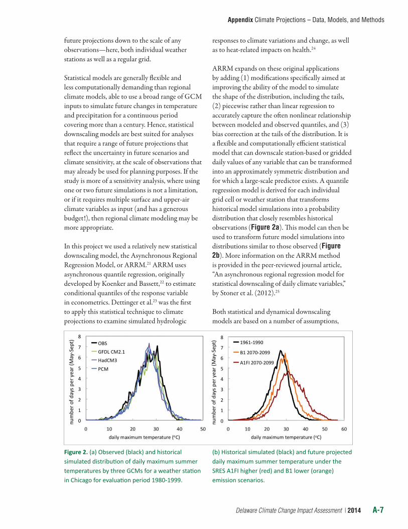
ARRM expands on these original applications by adding (1) modifications specifically aimed at improving the ability of the model to simulate the shape of the distribution, including the tails, (2) piecewise rather than linear regression to accurately capture the often nonlinear relationship between modeled and observed quantiles, and (3) bias correction at the tails of the distribution. It is a flexible and computationally efficient statistical model that can downscale station-based or gridded daily values of any variable that can be transformed into an approximately symmetric distribution and for which a large-scale predictor exists. A quantile regression model is derived for each individual grid cell or weather station that transforms historical model simulations into a probability distribution that closely resembles historical observations (Figure 2a). This model can then be used to transform future model simulations into distributions similar to those observed (Figure 2b). More information on the ARRM method is provided in the peer-reviewed journal article, “Anasynchronousregionalregressionmodelforstatisticaldownscalingofdailyclimatevariables,”by Stoner et al. (2012).25

Both statistical and dynamical downscaling models are based on a number of assumptions,

Figure 2. (a) Observed (black) and historical simulated distribution of daily maximum summer temperatures by three GCMs for a weather station in Chicago for evaluation period 1980-1999.

(b) Historical simulated (black) and future projected daily maximum summer temperature under the SRES A1FI higher (red) and B1 lower (orange) emission scenarios.



some shared, some unique to each method. Two important shared assumptions are the following: first, that the inputs received from GCMs are reasonable—that is, that they adequately capture the large-scale circulation of the atmosphere and ocean at the skillful scale of the global model; and second, that the information from the GCM fully incorporates the climate change signal over that region. All statistical models are based on a crucial assumption often referred to as stationarity. Stationarity assumes that the relationship between large-scale weather systems and local climate will remain constant over time. This assumption may be valid for lesser amounts of change, but could lead to biases under larger amounts of climate change.

In a separate project, we are currently evaluating the stationarity of three downscaling methods, including the ARRM method used here. Preliminary analyses show that the assumption of stationarity holds true over much of the world for the lower and middle parts of the distribution. The only location where ARRM performance is systematically non-stationary (i.e., relationships based on historical observations and simulations do not hold true in the future) is at extremely high temperatures (at and above the 99.9th quantile) along coastal areas, with warm biases up to 6oC. This may be due to the statistical model’s inability to capture dynamical changes in the strength of the land-sea breeze as the temperature differences between land and ocean are exacerbated under climate change; the origins of this feature are currently under investigation.

This bias has important implications for the climate projections generated for Delaware, because several of the station locations used in this study would be considered coastal. It suggests that estimated changes in days hotter than the 1-in-100 hottest historical day (e.g., the historical ~3 to 4 hottest days of the year) may be subject to temperature biases that increase in magnitude such that biases for the 1-in-1,000 hottest days (e.g., the hottest day in 3 years) may be as large as the projected changes in the temperature of those days by end of century under a higher emissions scenario. For precipitation, the ARRM method is characterized by a spatially variable bias at all quantiles that

is generally not systematic, and varies from approximately-30to+30%,dependingonlocation.

A.4. Station ObservationsLong-term weather station records were obtained from the Global Historical Climatology Networka and supplemented with additional records from the National Climatic Data Center cooperative observer programb and the state climatologist for Delaware.27 All station data were quality-controlled to remove questionable data points before being used to train the statistical downscaling model.

To train the downscaling model, the observed record must be of adequate length and quality. To appropriately sample from the range of natural climate variability at most of the station locations, and to produce robust results without overfitting, each station used in the analysis was required to have a minimum of 20 consecutive years of daily observations overlapping GCM outputs with less than 50% missing data after quality control. When these limits were applied, the number of usable stations for Delaware totaled 14 for maximum and minimum temperature and precipitation. The latitude, longitude, and station names of the weather stations for which downscaled projections were generated are provided in Table 2 and are plotted in Figure 3.

Although GHCN station data have already undergone a standardized quality control,28 these stations were additionally filtered using a quality control algorithm to identify and remove erroneous values that had previously been identified in the GHCN database as well as elsewhere. The quality control process consists of two steps: first, individual quality control for each station; and second, a nearest-neighbor approach to validate outliers identified relative to the climatology of each month.

a GHCN data is available online at: http://www.ncdc.noaa.gov/oa/climate/ghcn-daily/

b NCDC-COOP data is available online at: http://www.ncdc.noaa.gov/land-based-station-data/cooperative-observer-network-coop

http://www.ncdc.noaa.gov/oa/climate/ghcn-daily/

http://www.ncdc.noaa.gov/oa/climate/ghcn-daily/

http://www.ncdc.noaa.gov/land-based-station-data/cooperative-observer-network-coop





Individual quality control identified and replaced with“N/A”anyvaluesthatfailedoneormoreofthese three tests:

1. Days when the daily reported minimum temperature exceeds the reported maximum.

2. Temperature values above or below the highest recorded values for North America (-50 to 70oC) or with precipitation below zero or above the highest recorded value for the continental United States (915 mm in 24 h).

3. Repeated values of more than five consecutive days with identical temperature or nonzero precipitation values to the first decimal place.

In the second step of the quality control process, upto10“nearestneighbors”foreachindividualweather station were queried to see if the days with anomalously high and low values were also days in which anomalous values occurred at the neighboring station, plus or minus one day on either side to account for weather systems that may be moving through the area close to midnight. The resulting files were then scanned to identify any stations with less than 3,650 real

Figure 3. This report generated future projections for 14 weather stations in Delaware with long-term historical records. Weather stations that did not have sufficiently long and/or complete observational records to provide an adequate sampling of observed climate variability at their locations were eliminated from this analysis.

Station Name Latitude Longitude Beginning of Record GHCN ID

Bear 39.5917 -75.7325 Apr 2003 USC00071200

Bridgeville 38.75 -75.6167 Jan 1893 USC00071330

Dover 39.2583 -75.5167 Jan 1893 USC00072730

Georgetown 38.6333 -75.45 Sept 1946 USC00073570

Greenwood 38.8161 -75.5761 Jan 1986 USC00073595

Lewes 38.7756 -75.1389 Feb 1945 USC00075320

Middletown 39.45 -75.6667 Sept 1952 USC00075852

Milford 38.8983 -75.425 May 1893 USC00075915

Newark University Farm 39.6694 -75.7514 Apr 1894 USC00076410

Selbyville 38.4667 -75.2167 Jan 1954 USC00078269

Wilmington Porter 39.7739 -75.5414 Jan 1932 USC00079605

Dover AFB 39.1333 -75.4667 Jul 1946 USW00013707

Georgetown Sussex Airport 38.6892 -75.3592 Feb 1945 USW00013764

Wilmington New Castle Airport 39.6728 -75.6008 Jan 1948 USW00013781

Table 2. Latitude, longitude, and identification numbers for the 14 weather stations used in this analysis.



values and less than 200 values for any given month. After the quality control and filtering process was complete, a total of 14 stations were available to be downscaled using the ARRM model described previously and the GCM inputs listed in Table 1.

A.5. UncertaintyThe primary challenge in climate impact analyses is the reliability of future information. A common axiom warns that the only aspect of the future that can be predicted with any certainty is the fact that it is impossible to do so. However, although it is not possible to predict the future, it is possible to project it. Projections can describe what would be likely to occur under a set of consistent and clearly articulated assumptions. For climate change impacts, these assumptions should encompass a broad variety of the ways in which energy, population, development, and technology might change in the future.

There is always some degree of uncertainty inherent to any future projections. To accurately interpret and apply future projections for planning purposes, it is essential to quantify both the magnitude of the uncertainty as well as the reasons for its existence. Each of the steps involved in generating projections—future scenarios, global modeling, and downscaling—introduces a degree of uncertainty into future projections; how to address this uncertainty is the focus of this section.

Another well-used axiom states that all models are wrong (but some can be useful). The earth’s climate is a complex system. It is possible to simulate only those processes that have been observed and documented. Clearly, there are other feedbacks and forcing factors at work that have yet to be documented. Hence, it is a common tendency to assign most of the range in future projections to model, or scientific, uncertainty.

Future projections will always be limited by scientific understanding of the system being predicted. However, there are other important sources of uncertainty that must be considered;

some even outweigh model uncertainty for certain variables and timescales.

Uncertainty in climate change at the global to regional scale arises primarily due to three different causes: (1) natural variability in the climate system, (2) scientific uncertainty in predicting the response of the earth’s climate system to human-induced change, and (3) socioeconomic or scenario uncertainty in predicting future energy choices and hence emissions of heat-trapping gases.29

It is important to note that scenario uncertainty is very different, and entirely distinct, from scientific uncertainty in at least two important ways. First, although scientific uncertainty can be reduced through coordinated observational programs and improved physical modeling, scenario uncertainty arises due to the fundamental inability to predict future changes in human behavior. It can be reduced only by the passing of time, as certain choices (such as depletion of a nonrenewable resource) can eliminate or render certain options less likely. Second, scientific uncertainty is often characterized by a normal distribution, where the mean value is more likely than the outliers. However, scenario uncertainty hinges primarily on whether or not the primary emitters of heat-trapping gases, including traditionally large emitters such as the United States as well as nations with rapidly growing contributions such as India and China, will enact binding legislation to reduce their emissions or not. If they do enact legislation, then the lower emission scenarios become more probable. If they do not, then the higher scenarios become more probable. The longer such action is delayed, the less likely it becomes to achieve a lower scenario because of the emissions that continue to accumulate in the atmosphere. Hence, scenario uncertainty cannot be considered to have a normal distribution. Rather, the consequences of a lower versus a higher emissions scenario must be considered independently to isolate the role that human choices are likely to play in determining future impacts.

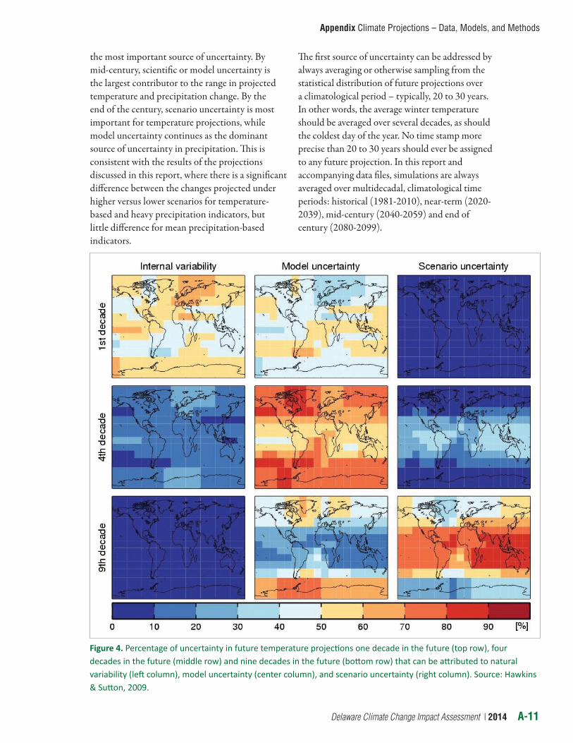
Figure 4 illustrates how, over timescales of years to several decades, natural chaotic variability is



the most important source of uncertainty. By mid-century, scientific or model uncertainty is the largest contributor to the range in projected temperature and precipitation change. By the end of the century, scenario uncertainty is most important for temperature projections, while model uncertainty continues as the dominant source of uncertainty in precipitation. This is consistent with the results of the projections discussed in this report, where there is a significant difference between the changes projected under higher versus lower scenarios for temperature-based and heavy precipitation indicators, but little difference for mean precipitation-based indicators.

The first source of uncertainty can be addressed by always averaging or otherwise sampling from the statistical distribution of future projections over a climatological period – typically, 20 to 30 years. In other words, the average winter temperature should be averaged over several decades, as should the coldest day of the year. No time stamp more precise than 20 to 30 years should ever be assigned to any future projection. In this report and accompanying data files, simulations are always averaged over multidecadal, climatological time periods: historical (1981-2010), near-term (2020-2039), mid-century (2040-2059) and end of century (2080-2099).

Figure 4. Percentage of uncertainty in future temperature projections one decade in the future (top row), four decades in the future (middle row) and nine decades in the future (bottom row) that can be attributed to natural variability (left column), model uncertainty (center column), and scenario uncertainty (right column). Source: Hawkins & Sutton, 2009.



The second source of uncertainty, model or scientific uncertainty, can be addressed by using multiple global climate models to simulate the response of the climate system to human-induced change (here, nine newer CMIP5 and four older CMIP3 models). As noted above, the climate models used here cover a range of climate sensitivity; they also cover an even wider range of precipitation projections, particularly at the local to regional scale.

Again, although no model is perfect, most models are useful. Only models that demonstratively fail to reproduce the basic features of large-scale climate dynamics (e.g., the jet stream or El Niño) should be eliminated from consideration. Multiple studies have convincingly demonstrated that the average of an ensemble of simulations from a range of climate models (even ones of varied ability) is generally closer to reality than the simulations from one individual model--even one deemed “good”whenevaluatedonitsperformanceovera given region.30, 31 Hence, wherever possible, impacts should be summarized in terms of the values resulting from multiple climate models, while uncertainty estimates can be derived from the range or variance in model projections. This is why most plots in this report show both multimodel mean values as well as a range of uncertainty around each value.

The third and final primary source of uncertainty in future projections can be addressed through generating climate projections for multiple futures: forexample,a“higheremissions”futureinwhichthe world continues to depend on fossil fuels as the primary energy source (SRES A1FI or RCP 8.5), ascomparedtoa“loweremissions”futurefocusingon sustainability and conservation (SRES B1 or RCP 4.5).

Over the next two to three decades, projections can be averaged across scenarios, because there is no significant difference between scenarios over that time frame due to the inertia of the climate system in responding to changes in heat-trapping gas levels in the atmosphere.32 Past mid-century, however, projections should never be averaged across scenarios; rather, the difference in impacts resulting from a higher as compared to a lower scenario should always be clearly delineated. That is why, in this report, future projections are always summarized in terms of what is expected for each scenario individually.



AppendixList of Bar Graphs for All Climate Indicators All temperature values in ˚F, all precipitation values in inches

TEMPERATURE INDICATORS

Annual – Seasonal Temperature Indicators:

Maximum Temperatures• Winter Maximum Temperature

• Winter Maximum Temperature Change

• Spring Maximum Temperature

• Spring Maximum Temperature Change

• Summer Maximum Temperature

• Summer Maximum Temperature Change

• Fall Maximum Temperature

• Fall Maximum Temperature Change

• Annual Maximum Temperature

• Annual Maximum Temperature Change

Minimum Temperatures• Winter Minimum Temperature

• Winter Minimum Temperature Change

• Spring Minimum Temperature

• Spring Minimum Temperature Change

• Summer Minimum Temperature

• Summer Minimum Temperature Change

• Fall Minimum Temperature

• Fall Minimum Temperature Change

• Annual Minimum Temperature

• Annual Minimum Temperature Change

Average Temperatures• Winter Average Temperature

• Winter Average Temperature Change

• Spring Average Temperature

• Spring Average Temperature Change

• Summer Average Temperature

• Summer Average Temperature Change

• Fall Average Temperature

• Fall Average Temperature Change

• Annual Average Temperature

• Annual Average Temperature Change

Temperature Range• Winter Temperature Range

• Spring Temperature Range

• Summer Temperature Range

• Fall Temperature Range

• Annual Temperature Range

Standard Deviation of Temperature• Standard Deviation of Winter Maximum Temperature

• Standard Deviation of Spring Maximum Temperature

• Standard Deviation of Summer Maximum Temperature

• Standard Deviation of Fall Maximum Temperature

• Standard Deviation of Annual Maximum Temperature

• Standard Deviation of Winter Minimum Temperature

• Standard Deviation of Spring Minimum Temperature

• Standard Deviation of Summer Minimum Temperature

• Standard Deviation of Fall Minimum Temperature

• Standard Deviation of Annual Minimum Temperature



Other Temperature Indicators: Temperature Extremes• Nights with Minimum Temperatures < 20˚F

• Changes in Nights with Minimum Temperatures < 20˚F

• Nights with Minimum Temperatures < 32˚F

• Changes in Nights with Minimum Temperatures < 32˚F

• Days with Maximum Temperatures > 90˚F

• Changes in Days with Maximum Temperatures > 90˚F


• Days with Maximum Temperatures > 100F



• Nights with Minimum Temperatures > 80˚F



• Number of 4+ Day Heat Waves per Year

• Longest Sequence of Days with Maximum Temperatures > 90˚F



Growing Season• Date of Last Frost in Spring

• Change in Date of Last Spring Frost (days)

• Date of First Frost in Fall

• Change in Date of First Frost in Fall (days)

Energy-Related Temperature Indicators• Mean Annual Cooling Degree-Days

• Mean Annual Heating Degree-Days

Temperature Extreme Percentiles• Nights with Minimum Temperatures < Historic 1-in-100

Coldest (1 percentile)

• Nights with Minimum Temperatures < Historic 1-in-20 Coldest (5th percentile)

• Days with Maximum Temperatures > Historic 1-in-20 Hottest (95th percentile)

• Days with Maximum Temperatures > Historic 1-in-100 Hottest (99th percentile)

PRECIPITATION INDICATORS

Annual – Seasonal Precipitation Indicators: Average Precipitation• Winter Precipitation (inches)

• Winter Precipitation Change (%)

• Spring Precipitation (inches)

• Spring Precipitation Change (%)

• Summer Precipitation (inches)

• Summer Precipitation Change (%)

• Fall Precipitation (inches)

• Fall Precipitation Change (%)

• Annual Precipitation (inches)

• Annual Precipitation Change (%)

3-Month Precipitation Change• January-March 3-Month Precipitation Change (%)

• February-April 3-Month Precipitation Change (%)

• March-May 3-Month Precipitation Change (%)

• April-June 3-Month Precipitation Change (%)

• May-July 3-Month Precipitation Change (%)

• June-August 3-Month Precipitation Change (%)

• July-September 3-Month Precipitation Change (%)

• August-October 3-Month Precipitation Change (%)

• September-November 3-Month Precipitation Change (%)

• October-December 3-Month Precipitation Change (%)

• November-January 3-Month Precipitation Change (%)

• December-February 3-Month Precipitation Change (%)

6- and 12-Month Precipitation Change• January-June 6-Month Precipitation Change (%)

• February-July 6-Month Precipitation Change (%)

• March-August 6-Month Precipitation Change (%)



• April-September 6-Month Precipitation Change (%)

• May-October 6-Month Precipitation Change (%)

• June-November 6-Month Precipitation Change (%)

• July-December 6-Month Precipitation Change (%)

• August-January 6-Month Precipitation Change (%)

• September-February 6-Month Precipitation Change (%)

• October-March 6-Month Precipitation Change (%)

• November-April 6-Month Precipitation Change (%)

• December-May 6-Month Precipitation Change (%)

• January-December 12-Month Precipitation Change (%)

Other Precipitation Indicators:Dry Days• Annual Average Dry Days per Year

• Change in Dry Days per Year (%)

• Longest Dry Period of the Year (days)

• Change in Longest Dry Period (%)

Precipitation Indices• Precipitation Intensity (inches/day)

• Change in Precipitation Intensity (%)

• Standardized Precipitation Index

Extreme Precipitation• Days per Year > 0.5”

• Days per Year > 1”








• Precipitation on Wettest 1 Day/Year (inches)

• Precipitation on Wettest 5 Days/Year (inches)

• Precipitation on Wettest 2 Weeks/Year (inches)

• Precipitation on Wettest 1 Day in 2 Years (inches)

• Precipitation on Wettest 5 Days in 2 Years (inches)

• Precipitation on Wettest Two Weeks in 2 Years (inches)

• Precipitation on Wettest 1 Day in 10 Years (inches)

• Precipitation on Wettest 5 Days in 10 Years (inches)

• Precipitation on Wettest Two Weeks in 10 Years (inches)

• Days per Year > Historical 2-day Maximum



• Percentage of Precipitation Falling as Rain vs. Snow (%)

HUMIDITY HYBRID INDICATORSDewpoint Indicators• Winter Dewpoint Temperature (˚F)

• Winter Dewpoint Temperature Change (˚F)

• Spring Dewpoint Temperature (˚F)

• Spring Dewpoint Temperature Change (˚F)

• Summer Dewpoint Temperature (˚F)

• Summer Dewpoint Temperature Change (˚F)

• Fall Dewpoint Temperature (˚F)

• Fall Dewpoint Temperature Change (˚F)

• Annual Dewpoint Temperature (˚F)

• Annual Dewpoint Temperature Change (˚F)

Relative Humidity• Average Winter Relative Humidity (%)

• Change in Winter Relative Humidity (%)

• Average Spring Relative Humidity (%)

• Change in Spring Relative Humidity (%)

• Average Summer Relative Humidity (%)

• Change in Summer Relative Humidity (%)

• Average Fall Relative Humidity (%)

• Change in Fall Relative Humidity (%)

• Average Annual Relative Humidity (%)

• Change in Annual Relative Humidity (%)



Heat Indices• Summer Heat Index (˚F)

• Change in Summer Heat Index (˚F)

• Number of Hot Dry Days per Year

• Number of Cool Wet Days per Year

Potential Evapotranspiration• Winter Potential Evapotranspiration (mm)

• Spring Potential Evapotranspiration (mm)

• Summer Potential Evapotranspiration (mm)

• Fall Potential Evapotranspiration (mm)

• Annual Potential Evapotranspiration (mm)

Sources (Endnotes)

1 Frumhoff, P.C., McCarthy, J. J., Melillo, J. M., Moser, S. C., & Wuebbles, D. J. (2007). Confronting climate change in the U.S. Northeast: Science, impacts, and solutions. Synthesis report of the Northeast Climate Impacts Assessment (NECIA). Cambridge, MA: Union of Concerned Scientists (UCS).

2 U.S. Global Change Research Program (USGCRP). (2009). Global climate change impacts in the United States. Cambridge University Press. http://www.globalchange.gov/usimpacts/

3 Walsh, J., Wuebbles, D., Hayhoe, K., Kunkel, K., Somerville, R., Stephens, G., … Kennedy, J. (2014). Chapter 2: Our Changing Climate. In: The Third U.S. National Climate Assessment. In press.

4 Meehl, G. A., Covey, C., Delworth, T., Latif, M., McAvaney, B., Mitchell, J. F. B., … Taylor, K. E. (2007). The WCRP CMIP3 multi-model dataset: A new era in climate change research. Bulletin of the American Meteorological Society, 88, 1383-1394.

5 Taylor, K. E., Stouffer, R. J., & Meehl, G. A. (2012). An overview of CMIP5 and the experiment design. Bulletin of American Meteorological Society, 93, 485–498. doi: http://dx.doi.org/10.1175/BAMS-D-11-00094.1

6 Nakicenovi, N., Alcamo, J., Davis, G., de Vries, B., Fenhann, J., Gaffin, S. … Dadi, Z. (2000). Intergovernmental Panel on Climate Change special report on emissions scenarios. Cambridge University Press, Cambridge, U.K.

7 Moss, R. H., Edmonds, J. A., Hibbard, K. A., Manning, M. R., Rose, S. K., Van Vuuren, D. P. … Wilbanks, T. J. (2010). The next generation of scenarios for climate change research and assessment. Nature, 463, 747-756.

8 Raupach, M. R., Marland, G., Ciais, P., Le Quere, C., Canadell, J. G., Klepper, G., & Field, C. B. (2007). Global and regional drivers of accelerating CO2 emissions. Proceedings of the National Academy of Sciences, 104(24), 10288-10293.

9 Myhre, G., Alterskjaer, K., & Lowe, D. (2009). A fast method for updating global fossil fuel carbon dioxide emissions. Environmental Research Letters, 4, doi:10.1088/1748-9326/4/3/034012

10 Meinshausen, M., Hare, B., Wigley, T. M. M., Van Vuuren, D., Den Elzen, M. G. J., & Swart, R. (2006). Multi-gas emissions pathways to meet climate targets. Climatic Change 75, 151-194.

11 Randall, D. A., Wood, R. A., Bony, S., Colman, R., Fichefet, T., Fyfe, J., … Taylor, K. E. (2007). Cilmate models and their evaluation. In: Climate change 2007: The physical science basis. Contribution of Working Group I to the Fourth Assessment Report of the Intergovernmental Panel on Climate Change. [Solomon, S., Qin, D., Manning, M., Chen, Z., Marquis, M., Averyt, K.B., Tignor, M., & Miller, H.L. (Eds.)]. Cambridge University Press, Cambridge, U.K.

12 IPCC. (2007). Summary for policymakers. In: Climate change 2007: The physical science basis. Contribution of Working Group I to the Fourth Assessment Report of the Intergovernmental Panel on Climate Change. [Solomon, S., Qin, D., Manning, M., Chen, Z., Marquis, M., Averyt, K.B., Tignor, M., & Miller, H.L. (Eds.)]. Cambridge University Press, Cambridge, U.K.

13 Meehl, G. A., Covey, C., Delworth, T., Latif, M., McAvaney, B., Mitchell, J. F. B., … Taylor, K. E. (2007). The WCRP CMIP3 multi-model dataset: A new era in climate change research. Bulletin of the American Meteorological Society, 88, 1383-1394.

14 Taylor, K. E., Stouffer, R. J., & Meehl, G. A. (2012). An overview of CMIP5 and the experiment design. Bulletin of American Meteorological Society, 93, 485–498. doi: http://dx.doi.org/10.1175/BAMS-D-11-00094.1

15 IPCC. (2007). Summary for policymakers. In: Climate change 2007: The physical science basis. Contribution of Working Group I to the Fourth Assessment Report of the Intergovernmental Panel on Climate Change. [Solomon, S., Qin, D., Manning, M., Chen, Z., Marquis, M., Averyt, K.B., Tignor, M., & Miller, H.L. (Eds.)]. Cambridge University Press, Cambridge, U.K.

http://dx.doi.org/10.1175/BAMS-D-11-00094.1

http://dx.doi.org/10.1175/BAMS-D-11-00094.1



16 Knutti, R., & Hegerl, G. (2008). The equilibrium sensitivity of the Earth’s temperature to radiation changes. Nature Geoscience, 1, 735-743.

17 Overland, J. E., Wang, M., Bond, N. A., Walsh, J. E., Kattsov, V. M., & Chapman, W. L. (2011) Considerations in the selection of global climate models for regional climate projections: The Arctic as a case study. Journal of Climate, 24, 1583-1597.

18 Knutti, R. (2010). The end of model democracy? Climatic Change, 102, 395-404.

19 Randall, D. A., Wood, R. A., Bony, S., Colman, R., Fichefet, T., Fyfe, J., … Taylor, K. E. (2007). Climate models and their evaluation. In: Climate change 2007: The physical science basis. Contribution of Working Group I to the Fourth Assessment Report of the Intergovernmental Panel on Climate Change. [Solomon, S., Qin, D., Manning, M., Chen, Z., Marquis, M., Averyt, K.B., Tignor, M., & Miller, H.L. (Eds.)]. Cambridge University Press, Cambridge, U.K.

20 Grotch, S., & MacCracken, M. (1991). The use of general circulation models to predict regional climatic change. Journal of Climate, 4, 286-303.

21 Stoner, A., Hayhoe, K., Yang, X., & Wuebbles, D. (2012). An asynchronous regional regression model to downscale daily temperature and precipitation climate projections. International Journal of Climatology, 33, 11, 2473-2494. Article first published online: 4 October 2012.

22 Koenker, R., & Bassett, G. (1978). Regression quantiles. Econometrica, 46, 33-50.

23 Dettinger, M. D., Cayan, D. R., Meyer, M. K., & Jeton, A. E. (2004). Simulated hydrologic responses to climate variations and change in the Merced, Carson, and American River basins, Sierra Nevada, California, 1900-2099. Climatic Change, 62, 283-317.

24 Hayhoe, K., Cayan, D., Field, C. B., Frumhoff, P. C., Maurer, E. P., Miller, N. L. … Verville, J. H. (2004). Emission pathways, climate change, and impacts on California. Proceedings of the National Academy of Sciences, 101, 12423-12427.

25 Stoner, A., Hayhoe, K., Yang, X., & Wuebbles, D. (2012). An asynchronous regional regression model to downscale daily temperature and precipitation climate projections. International Journal of Climatology, 33, 11, 2473-2494. Article first published online: 4 October 2012.

26 Vrac, M., Stein, M., Liang, X., & Hayhoe, K. (2007). A general method for validating statistical downscaling methods under future climate change. Geophysical Research Letters, 34(18).

27 Leathers, D. J., University of Delaware, Office of the Delaware State Climatologist. [personal communication, August, 2013].

28 Durre, I., Menne, M. J., & Vose, R. S. (2008). Strategies for evaluating quality-control procedures. Journal of Climate and Applied Meteorology, 47, 1785-1791.

29 Hawkins & Sutton. (2009). The potential to narrow uncertainty in regional climate predictions. Bulletin of American Meteorological Society, 90, 1095.

30 Weigel, A., Knutti, R., Liniger, M., & Appenzeller, C. (2010). Risks of model weighting in multimodel climate projections. Journal of Climate, 23, 4175-4191.

31 Knutti, R. (2010). The end of model democracy? Climatic Change, 102, 395-404.

32 Stott, P., & Kettleborough, J. (2002). Origins and estimates of uncertainty in predictions of twenty-first century temperature rise. Nature, 416, 723-725.

appendix - dnrec change 2013-2014...delaware climate change impact assessment | 2014 appendix:...

Documents