appendix d retrospective data tables d.1. d.2. d.3. d.4...
TRANSCRIPT

Appendix D
Retrospective Data TABLES D.1. Annual maximum one-hour average ozone, 1992-2000 D.2. Annual maximum eight-hour average ozone, 1992-2000 D.3. Number of annual exceedance days for one-hour ozone, 1992-2000 D.4. Number of annual exceedance days for eight-hour ozone, 1992–2000 D5. Regression equations for correlation analysis of one-hour vs. eight-hour D6. Climatological equivalency (S: Standard, E: Equivalency calculated with standard) D7. Regression Equation for Correlation Analysis between 1hr CO and 8hr CO D8. Climatological equivalency (S: Standard, E: Equivalency calculated with standard) D9. Regional analysis of ozone exceeding days for Cincinnati, Dayton, Toledo, Columbus
(Maple Canyon), Cleveland, Akron, Marietta and Columbus (Chesapeake): 1992-2000 in ppb
D10. High Concentration and High Frequency in Correlation With Wind Direction. FIGURES D1. High ozone days exceeding 1-hour threshold level, 1992-2000 D2 (a&b). 24-hour averaged PM10 levels: (a) Cincinnati urban site, 1992-1999 (b) Maple
Canyon suburban site D2 (c&d). 24-hour averaged PM10 levels 1992-2000: (c) Columbus (Chesapeake) suburban
site, (d) Cleveland suburban D2 (e). 24-hour averaged PM10 levels in 1992-2000: (e) Steubenville urban Site D3. 2nd Highest 1hr Averaged CO in 1992-20 D4-1 (a & b). Hourly CO distribution: (a) Cincinnati and (b) Dayton D4-1 (c & d). Hourly CO distribution: (c) Columbus (Chesapeake) and (d) Columbus (Maple
Canyon) D4-1 (e & F). Hourly CO distribution: (e) Akron and (f) Cleveland D4-2 (a & b). Hourly SO2 distribution: (a) Cincinnati and (b) Dayton D4-2 (c & d). Hourly SO2 distribution in: (c) Chesapeake and (d) Cleveland D4-2 (e & f). Hourly SO2 distribution: (e) Akron and (f) Steubenville D4-3 (a & b). Hourly NO2 distribution: (a) Cincinnati and (b) Cleveland D4-3 (c). Hourly NO2 distribution: (c) Steubenville D5-1 (a&b). Correlation between CO and Ozone Concentration in 1992-2000: (a) Cincinnati and
(b) Dayton D5-1 (c&d). Correlation between CO and Ozone Concentration: (c) Columbus (Chesapeake),
1992-2000 and (d) Columbus (Maple Canyon), 1993-2000 D5-2 (a&b). Correlation between SO2 and Ozone Concentration in 1992-2000: (a) Cincinnati and
(b) Dayton D6-1. Spatial Coordination plots of PM10, 1992-2000
360 Appendix D
D6-2. Spatial Coordination plots of CO, 1992-2000 D6-3. . Spatial Coordination plots of SO2 , 1992-2000 D6-3. Spatial Coordination plots of SO2, 1992-2000 D6-4. Spatial Coordination plots of NO2, 1992-2000 D7 (a & b). KZ Filter of ozone levels in (a) Cincinnati and (b) Dayton, 1992-2000 D7 (c & d). KZ Filter of ozone levels in (c) Columbus (Maple Canyon) and (d) Columbus
(Chesapeake), 1992-2000 D7 (e & f). KZ Filter of ozone levels in (e) Akron and (f) Cleveland, 1992-2000 D7 (g & h). KZ Filter of ozone levels in (g) Marietta and (h) Toledo, 1992-2000 D7 (i). KZ Filter of ozone levels in (i) Steubenville, 1992-2000 D8 (a & b). KZ Filter of PM10 levels in (a) Cincinnati, 1992-1999 and (b) Maple Canyon, 1992-
2000 D8 (c & d). KZ Filter of PM10 levels in (c) Columbus (Chesapeake) and (d) Cleveland, 1992-
2000 D8 (e). KZ Filter of PM10 levels in (e) Steubenville, 1992-2000 D9 (a & b). KZ Filter of CO levels in (a) Cincinnati and (b) Dayton, 1992-2000 D9 (c & d). KZ Filter of CO levels in (c) Columbus (Chesapeake) and (d) Columbus (Maple
Canyon), 1993-2000 D9 (e & f). KZ Filter of CO levels in (e) Akron and (f) Cleveland, 1992-2000 D10 (a & b). KZ Filter of SO2 levels in (a) Cincinnati and (b) Dayton, 1992-2000 D10 (c & d) KZ Filter of SO2 levels in (c) Columbus (Chesapeake) and (d) Cleveland, 1992-
2000 D10 (e & f) KZ Filter of SO2 levels in (e) Akron and (f) Steubenville, 1992-2000 D11 (a & b) KZ Filter of NO2 levels in (a) Cincinnati, 1992-2000 and (b) Cleveland, 1992-1999 D11 (c) KZ Filter of NO2 at (c) Steubenville, 1992-1997 D12. Co-relational plots of maximum eight-hour vs. one-hour ozone concentrations at the
six monitoring site, 1992-2000 D13. Co-relational plots of maximum eight-hour vs. one-hour ozone
concentrations at the six monitoring site, 1992-2000 D14. Correlation between 1 Hour and 8 Hour CO1992-2000: (a) Cincinnati, (b) Dayton,
(c) Columbus (Chesapeake), (d) Columbus (Maple Canyon), (e) Akron and (f) Cleveland
D15 (a & b). Correlations between PM10 and weather components at Columbus (Maple Canyon), Ohio in 1992-2000: (a) PM10 vs. wind speed and (b) PM10 vs. wind direction
D15 (c). Correlations between PM10 and weather components at Columbus (Maple Canyon), Ohio in 1992-1999: (c) PM10 vs. temperature
D16 (a & b). Correlations between PM10 and weather components at Columbus (Chesapeake), Ohio in 1992-1999: (a) PM10 vs. wind speed and : (b) PM10 and wind direction.
D16 (c). Correlations between PM10 and weather components at Columbus (Chesapeake), Ohio in 1992-2000 and (c) PM10 vs. temperature
D17 (a & b). Correlations between PM10 and weather components at Cleveland, Ohio in 1992-2000: (a) PM10 vs. wind speed and (b) PM10 vs. wind direction
D17 (c). Correlations between PM10 and weather components at Cleveland, Ohio in 1992-2000: (c) PM10 vs. temperature.

Appendix D 361
D18 (a & b). Correlations between PM10 and weather components at Steubenville, Ohio in 1992-2000: (a) PM10 vs. wind speed and (b) PM10 vs. wind direction
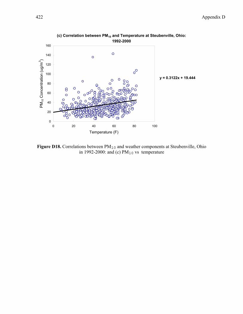
D18 (c). Correlations between PM10 and weather components at Steubenville, Ohio in 1992-2000: and (c) PM10 vs temperature.
D19. Correlations between CO and weather components at Cincinnati, Ohio in 1992-2000: (a) CO vs. wind speed and (b) CO vs. wind direction
D20. Correlations between CO and weather components at Dayton, Ohio in 1992-2000: (a) CO vs. wind speed and (b) CO vs. wind direction
D21. Correlations between CO and weather components at Columbus (Chesapeake), Ohio in 1992-2000: (a) CO vs. wind speed and (b) CO vs. wind direction
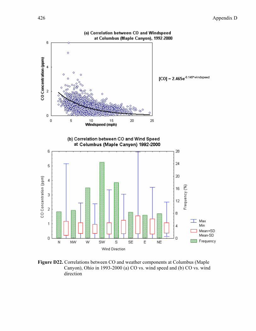
D22. Correlations between CO and weather components at Columbus (Maple Canyon), Ohio in 1993-2000 (a) CO vs. wind speed and (b) CO vs. wind direction
D23. Correlations between CO and weather components at Akron, Ohio in 1992-2000: (a) CO vs. wind speed and (b) CO vs. wind direction
D24. Correlations between CO and weather components at Cleveland, Ohio in 1992-2000: (a) CO vs. wind speed and (b) CO vs. wind direction
D25. Correlations between SO2 and weather components at Cincinnati, Ohio in 1992-2000: (a) SO2 vs. wind speed and (b) SO2 vs. wind direction
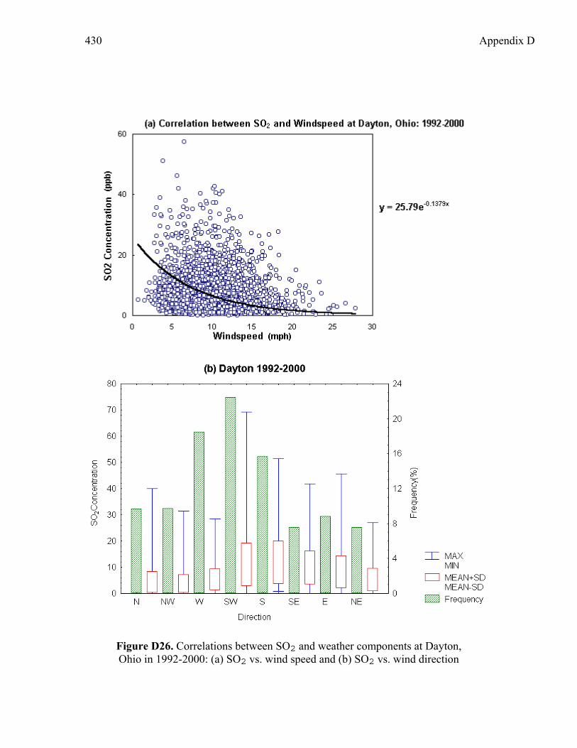
D26. Correlations between SO2 and weather components at Dayton, Ohio in 1992-2000: (a) SO2 vs. wind speed and (b) SO2 vs. wind direction
D27. Correlations between SO2 and weather components at Columbus (Chesapeake), Ohio in 1992-2000: (a) SO2 vs. wind speed and (b) SO2 vs. wind direction
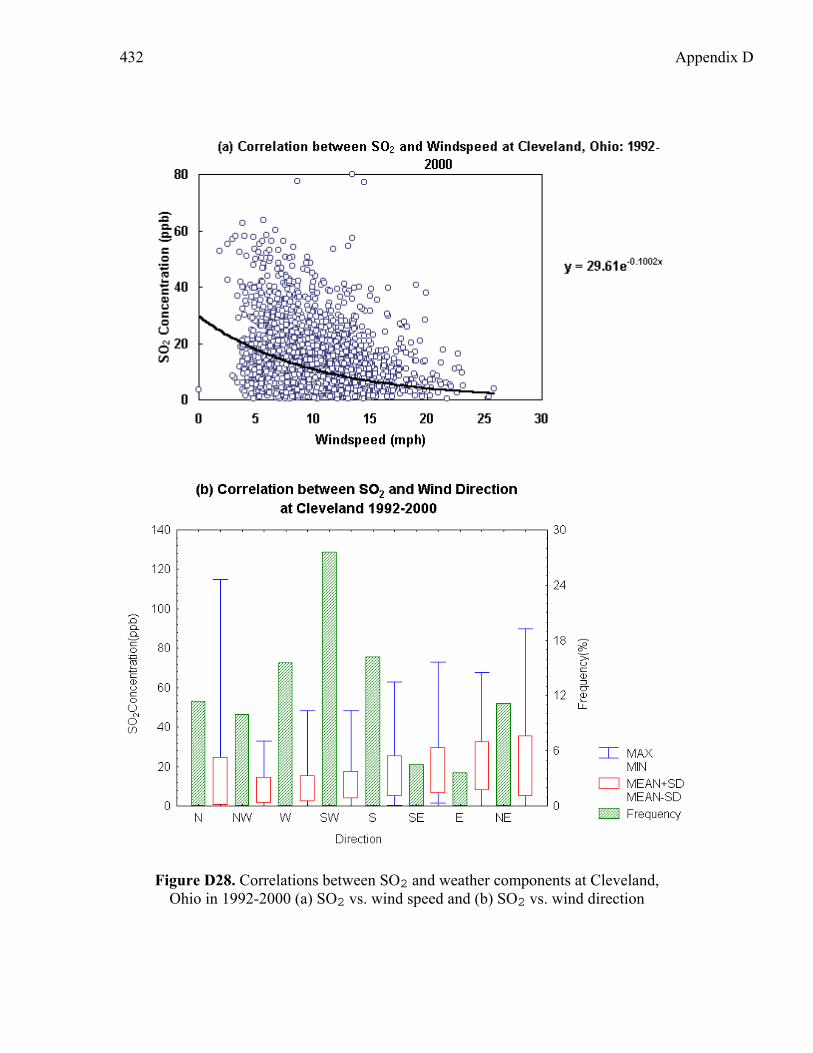
D28. Correlations between SO2 and weather components at Cleveland, Ohio in 1992-2000 (a) SO2 vs. wind speed and (b) SO2 vs. wind direction
D29. Correlations between SO2 and weather components at Akron, Ohio in 1992-2000: (a) SO2 vs. wind speed and (b) SO2 vs. wind direction
D30. Correlations between SO2 and weather components at Steubenville, Ohio in 1992-2000: (a) SO2 vs. wind speed and (b) SO2 vs. wind direction
D31. orrelations between NO2 and weather components at Cincinnati, Ohio in 1995-2000: (a) NO2 vs. wind speed and (b) NO2 vs. wind direction
D32. orrelations between NO2 and weather components at Dayton, Ohio in 1992-1999: (a) NO2 vs. wind speed and (b) NO2 vs. wind direction
D33. orrelations between NO2 and weather components at Steubenville, Ohio in 1992-1997: (a) NO2 vs. wind speed and (b) NO2 vs. wind direction
D34 (a & b). Back trajectories for high CO days at the monitoring sites selected in Ohio, 1992-2000: (a) Cincinnati and (b) Dayton
D34 (c & d). Back trajectories for high CO days at the monitoring sites selected in Ohio: (c) Columbus (Chesapeake), 1992-2000 and (d) Columbus (Maple Canyon), 1993-2000
D34 (e & f). Back trajectories for high CO days at the monitoring sites selected in Ohio, 1992-2000: (e) Akron and (f) Cleveland
D35. (a) Cluster plot at Cincinnati, 1992-2000 (b) Frequencies and average CO concentrations by cluster at Cincinnati, 1992-2000
D36. (a) Cluster plot at Dayton, 1992-2000 (b) Frequencies and average CO concentrations by cluster at Dayton, 1992-2000
362 Appendix D
D37. (a) Cluster plot at Columbus (Chesapeake), 1992-2000 (b) Frequencies and average CO concentrations by cluster at Columbus (Chesapeake), 1992-2000
D38. (a) Cluster plot at Columbus (Maple Canyon), 1993-2000 (b) Frequencies and average CO concentrations by cluster at Columbus (Maple Canyon), 1993-2000
D39. (a) Cluster plot at Akron 1992-2000 (b) Frequencies and average CO concentrations by cluster at Akron, 1992-2000
D40. (a) Cluster plot at Cleveland, 1992-2000 (b) Frequencies and average CO concentrations by cluster at Cleveland, 1992-2000
D41 (a & b). Back trajectories for high SO2 days at the monitoring sites selected in Ohio, 1992-2000: (a) Cincinnati and (b) Dayton
D41 (c & d). Back trajectories for high SO2 days at the monitoring sites selected in Ohio, 1992-2000: (c) Columbus (Chesapeake) and (d) Cleveland.
D41 (e & f). Back trajectories for high SO2 days at the monitoring sites selected in Ohio, 1992-2000: (e) Akron and (f) Steubenville
D42. (a) Cluster plot at Cincinnati, 1992-2000 (b) Frequencies and average SO2 concentrations by cluster at Cincinnati, 1992-2000
D43. (a) Cluster plot at Dayton, 1992-2000 (b) Frequencies and average SO2 concentrations by cluster at Dayton, 1992-2000
D44. (a) Cluster plot at Columbus (Chesapeake), 1992-2000 (b) Frequencies and average SO2 concentrations by cluster at Columbus (Chesapeake), 1992-2000
D45. (a) Cluster plot at Cleveland, 1992-2000 (b) Frequencies and average SO2 concentrations by cluster at Cleveland, 1992-2000
D46. (a) Cluster plot at Akron 1992-2000 (b) Frequencies and average SO2 concentrations by cluster at Akron, 1992-2000
D47. (a) Cluster plot at Steubenville, 1992-2000 (b) Frequencies and average SO2 concentrations by cluster at Steubenville, 1992-2000
D48. Back trajectories for high NO2 days at the monitoring sites selected in Ohio: Cleveland, 1992-1999
D49. Back trajectories for high NO2 days at the monitoring sites selected in Ohio: Steubenville, 1992-1997
D50. (a) Cluster plot at Cincinnati, 1995-2000 (b) Frequencies and average NO2 concentrations by cluster at Cincinnati, 1995-2000
D51. a) Cluster plot at Cleveland, 1995-2000 (b) Frequencies and average NO2 concentrations by cluster at Cleveland, 1995-2000
D52. (a) Cluster plot at Steubenville, 1992-1997 (b) Frequencies and average NO2 concentrations by cluster at Steubenville, 1992-1997

Appendix D 363
Table D.1. Annual maximum one-hour average ozone, 1992-2000
Cincinnati Dayton
Columbus (Maple
Canyon)
Columbus (Chesapeake Akron Cleveland Marietta Toledo Steubenville
1992 87 99 89 130 117 109 105 96 113 1993 110 125 108 109 110 126 137 131 110 1994 109 118 98 106 110 127 126 113 153 1995 128 115 104 130 124 113 112 130 118 1996 115 117 98 118 113 110 113 108 100 1997 117 130 98 101 112 97 110 118 106 1998 115 116 122 113 128 112 125 116 93 1999 104 128 118 123 115 99 125 122 113 2000 109 112 111 - 110 94 113 97 103
Table D.2. Annual maximum eight-hour average ozone, 1992-2000
Cincinnati Dayton Columbus
(Maple Canyon)
Columbus (Chesapeake) Akron Cleveland Marietta Toledo Steubenville
1992 78 83 79 114 99 87 116 88 87 1993 88 99 94 95 100 103 108 101 101 1994 87 106 88 94 88 104 106 93 136 1995 115 104 96 108 99 91 99 115 102 1996 101 113 91 114 99 103 100 97 92 1997 98 106 90 97 99 81 97 95 94 1998 97 97 112 104 114 100 106 101 83 1999 95 113 107 110 95 92 118 101 102 2000 98 102 97 100 89 98 88 96
Table D.3. Number of annual exceedance days for one-hour ozone, 1992-2000
Cincinnati Dayton
Columbus (Maple
Canyon)
Columbus (Chesapeake) Akron Cleveland Marietta Toledo Steubenville
1992 0 0 0 0 0 0 2 0 0 1993 0 1 0 0 0 1 1 1 0 1994 0 0 0 0 0 2 1 0 1 1995 1 0 0 1 0 0 0 1 0 1996 0 0 0 0 0 0 0 0 0 1997 0 1 0 0 0 0 0 0 0 1998 0 0 0 0 1 0 1 0 0 1999 0 2 0 0 0 0 1 0 0 2000 0 0 0 0 0 0 0 0

364 Appendix D
Table D.4. Number of annual exceedance days for eight-hour ozone, 1992–2000
Cincinnati Dayton
Columbus (Maple Canyon)
Columbus (Chesapeake) Akron Cleveland Marietta Toledo Steubenville
1992 0 0 0 0 5 1 4 1 1 1993 2 10 6 5 10 7 18 3 1 1994 1 9 1 6 5 2 13 5 3 1995 4 7 7 5 10 3 9 7 11 1996 5 14 4 10 9 4 4 8 2 1997 4 4 3 4 5 0 3 5 1 1998 6 8 12 14 14 1 12 6 0 1999 7 11 11 13 12 1 12 3 6 2000 4 3 1 3 1 3 1 3
0
1
2
3
4
4 5 6 7 8 9 10Month
Tota
l Num
ber o
f Day
s ov
er 1
25 p
pb fo
r 1-
hour
Ozo
ne
Cincinnati
Dayton
Columbus
Columbus
Cleveland
Toledo
Akron
Marietta
Steubenville
(Chesapeake)
(Maple Canyon)
Figure D.1. High ozone days exceeding 1-hour threshold level, 1992-2000

Appendix D 365
(a)
0
25
50
75
100
125
150
1/926/92
10/922/93
6/9310/93
2/947/94
11/943/95
7/9511/95
3/967/96
11/963/97
7/9711/97
3/987/98
11/983/99
Date
PM10
Con
cent
ratio
n (u
g/m
3 ) PM10 NAAQS (24-hour averaged)
(b)
0
25
50
75
100
125
150
1/925/92
9/921/93
5/939/93
1/945/94
9/941/95
5/959/95
1/965/96
9/961/97
6/979/97
2/987/98
11/983/99
7/991/00
5/009/00
Date
PM10
Con
cent
ratio
n (u
g/m
3 ) PM10 NAAQS (24-hour averaged)
Figure D.2. 24-hour averaged PM10 levels: (a) Cincinnati urban site, 1992-1999 (b) Columbus
(Maple Canyon) suburban site.

366 Appendix D
(c)
0
25
50
75
100
125
150
1/925/92
9/921/93
6/9310/93
2/946/94
11/943/95
7/9511/95
3/967/96
11/963/97
7/9711/97
4/988/98
12/984/99
9/991/00
5/00
Date
PM10
Con
cent
ratio
n (u
g/m
3 ) PM10 NAAQS (24-hour averaged)
(d)
0
25
50
75
100
125
150
1/925/92
12/925/93
9/931/94
5/949/94
1/956/95
10/952/96
6/9610/96
2/976/97
10/972/98
6/9810/98
2/996/99
10/992/00
6/008/00
10/00Date
PM10
Con
cent
ratio
n (u
g/m
3 )
PM10 NAAQS (24-hour averaged)
Figure D.2. 24-hour averaged PM10 levels 1992-2000: (c) Columbus (Chesapeake) suburban site,
(d) Cleveland suburban

Appendix D 367
(e)
0
25
50
75
100
125
150
1/925/92
8/9212/92
4/939/93
1/945/94
9/941/95
5/959/95
1/965/96
9/961/97
5/977/98
3/997/99
11/993/00
7/0011/00
Date
PM10
Con
cent
ratio
n (u
g/m
3 ) PM10 NAAQS (24-hour averaged)
Figure D.2. 24-hour averaged PM10 levels in 1992-2000: (e) Steubenville urban Site

368 Appendix D
Figure D.3. 2nd Highest 1hr Averaged CO in 1992-2000

Appendix D 369
Figure D4-1. Hourly CO distribution: (a) Cincinnati and (b) Dayton

370 Appendix D
Figure D4-1. Hourly CO distribution: (c) Columbus (Chesapeake) and (d) Columbus
(Maple Canyon)
Appendix D 371
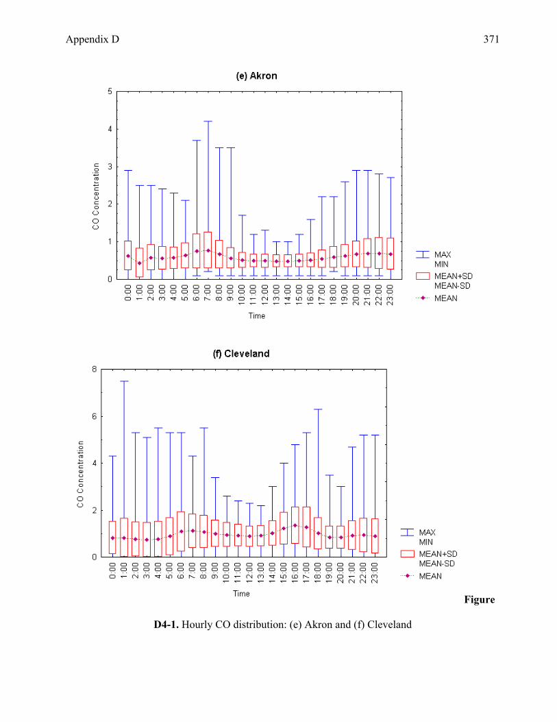
Figure
D4-1. Hourly CO distribution: (e) Akron and (f) Cleveland

372 Appendix D
Figure D4-2. Hourly SO2 distribution: (a) Cincinnati and (b) Dayton

Appendix D 373
Figure D4-2. Hourly SO2 distribution in: (c) Columbus (Chesapeake) and (d) Cleveland

374 Appendix D
Figure D4-2. Hourly SO2 distribution: (e) Akron and (f) Steubenville
Appendix D 375
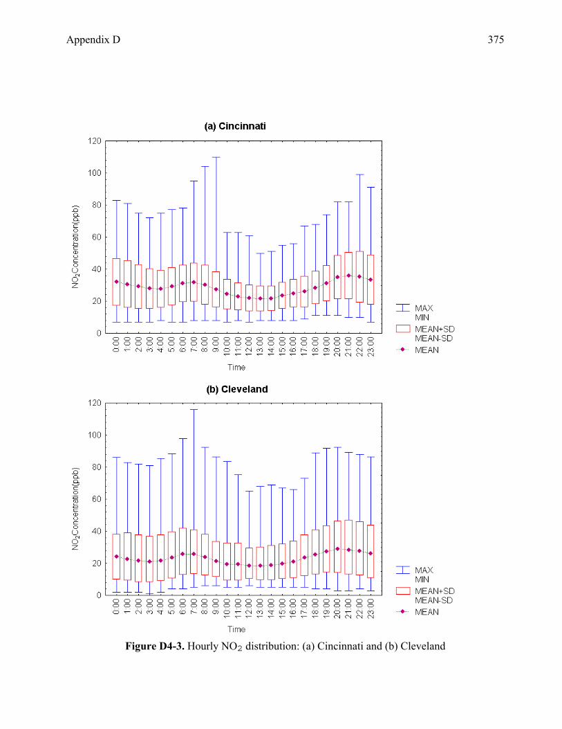
Figure D4-3. Hourly NO2 distribution: (a) Cincinnati and (b) Cleveland

376 Appendix D
Figure D4-3. Hourly NO2 distribution: (c) Steubenville

Appendix D 377
Figure D5-1. Correlation between CO and Ozone Concentration in 1992-2000: (a) Cincinnati and
(b) Dayton.
378 Appendix D
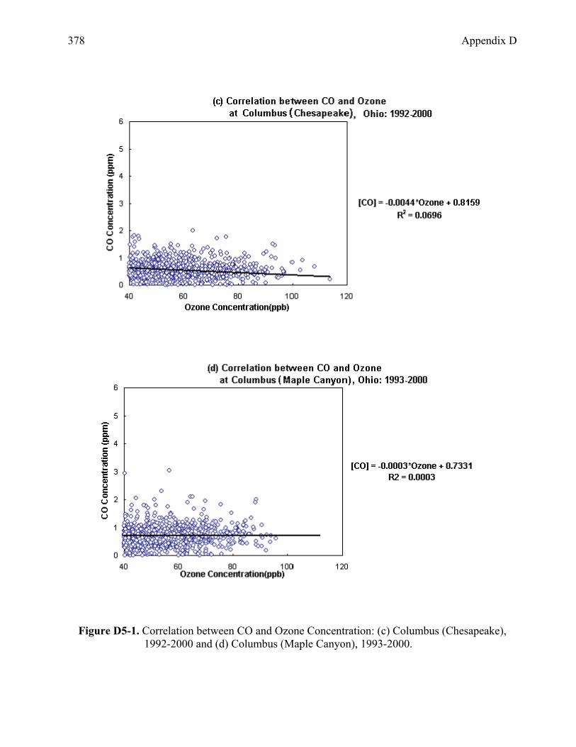
Figure D5-1. Correlation between CO and Ozone Concentration: (c) Columbus (Chesapeake), 1992-2000 and (d) Columbus (Maple Canyon), 1993-2000.
Appendix D 379
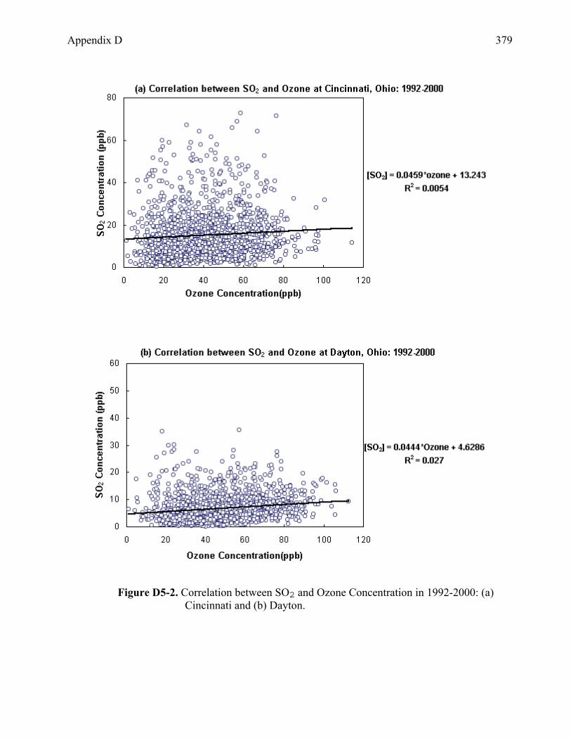
Figure D5-2. Correlation between SO2 and Ozone Concentration in 1992-2000: (a) Cincinnati and (b) Dayton.

380 Appendix D
Figure D6-1. Spatial Coordination plots of PM10, 1992-2000

Appendix D 381
Figure D6-2. Spatial Coordination plots of CO, 1992-2000
382 Appendix D
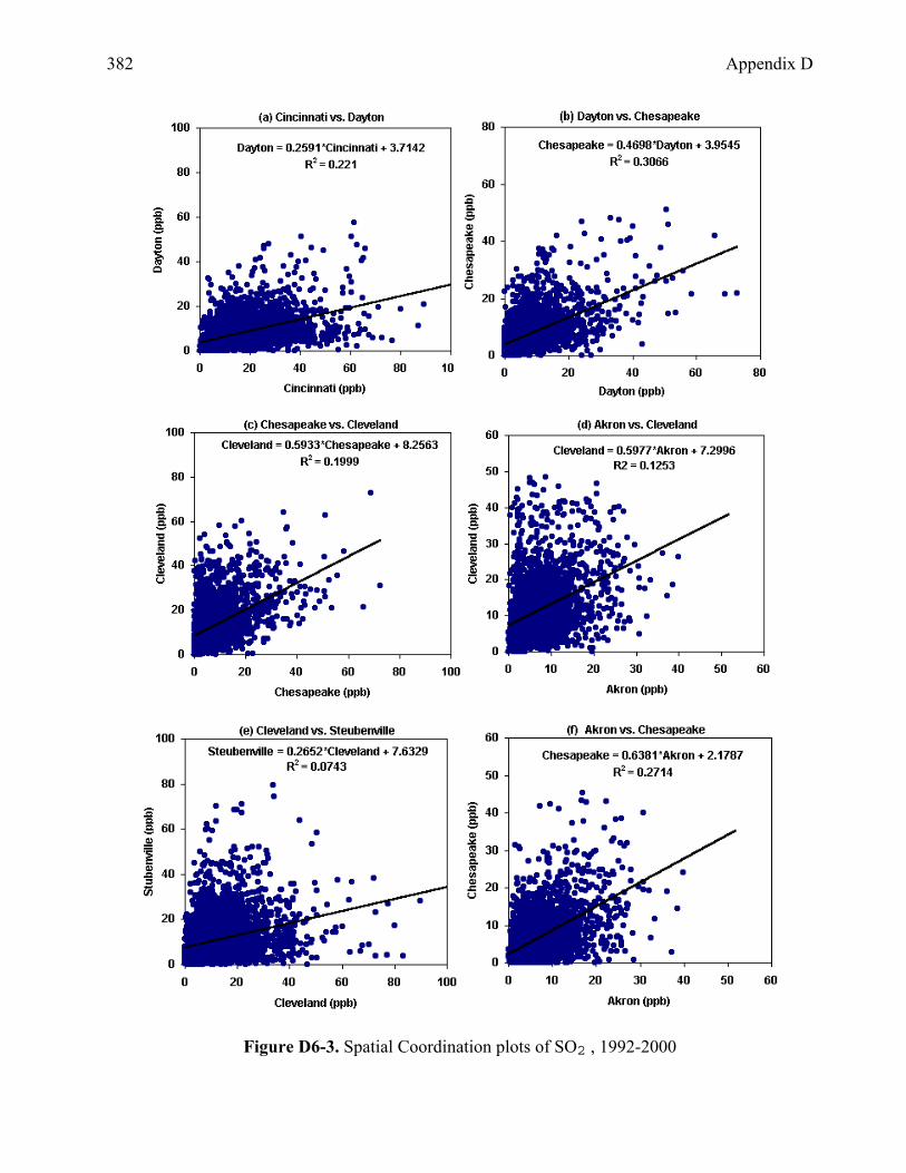
Figure D6-3. Spatial Coordination plots of SO2 , 1992-2000

Appendix D 383
Figure D6-3. Spatial Coordination plots of SO2, 1992-2000
384 Appendix D
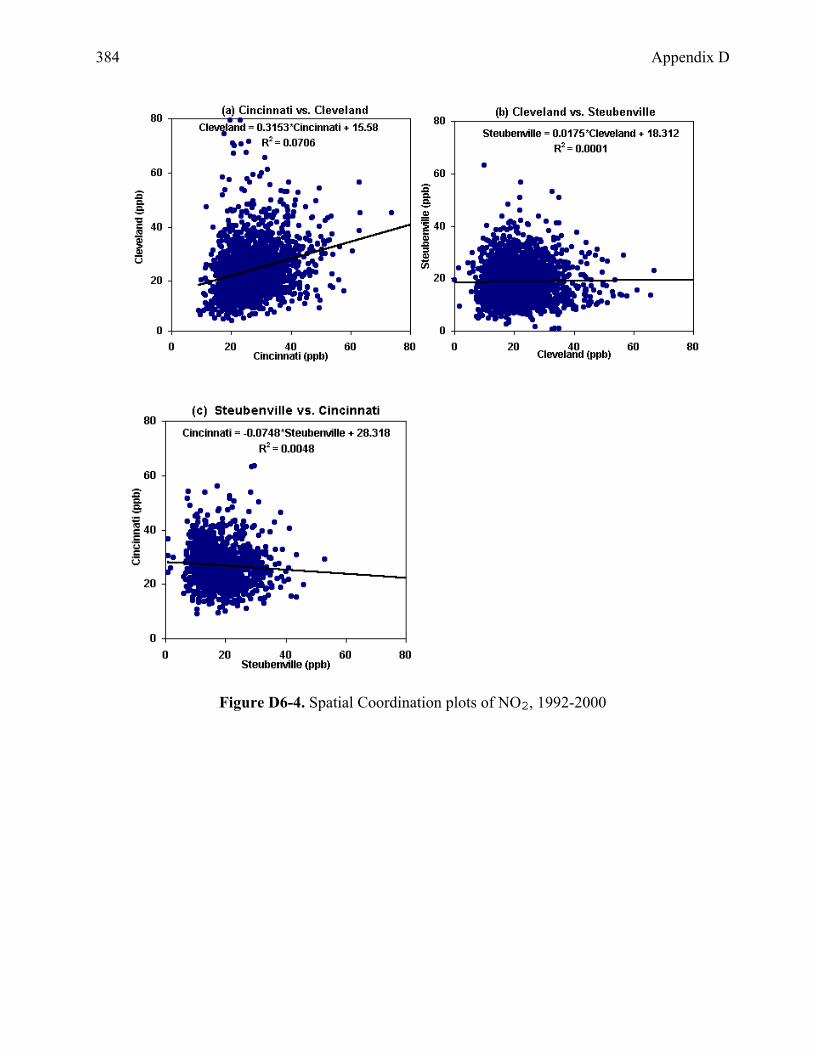
Figure D6-4. Spatial Coordination plots of NO2, 1992-2000
Appendix D 385
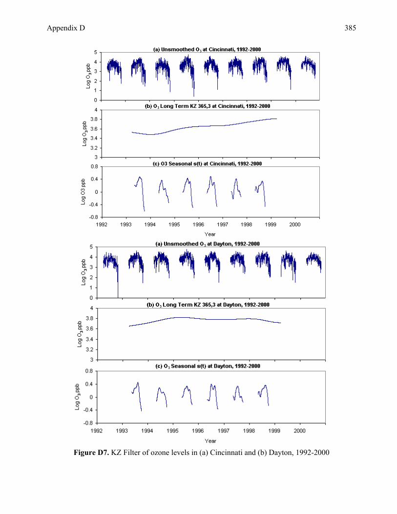
Figure D7. KZ Filter of ozone levels in (a) Cincinnati and (b) Dayton, 1992-2000

386 Appendix D
Figure D7. KZ Filter of ozone levels in (c) Columbus (Maple Canyon) and (d) Columbus
(Chesapeake), 1992-2000
Appendix D 387
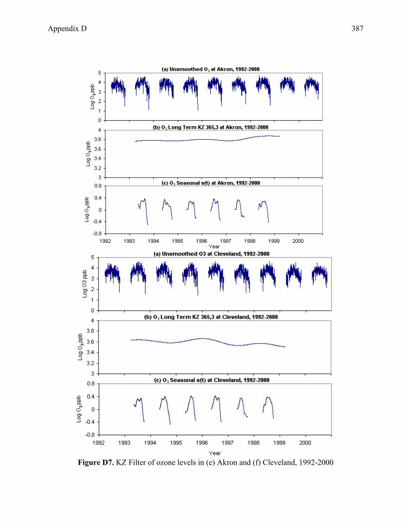
Figure D7. KZ Filter of ozone levels in (e) Akron and (f) Cleveland, 1992-2000

388 Appendix D
Figure D7. KZ Filter of ozone levels in (g) Marietta and (h) Toledo, 1992-2000
Appendix D 389
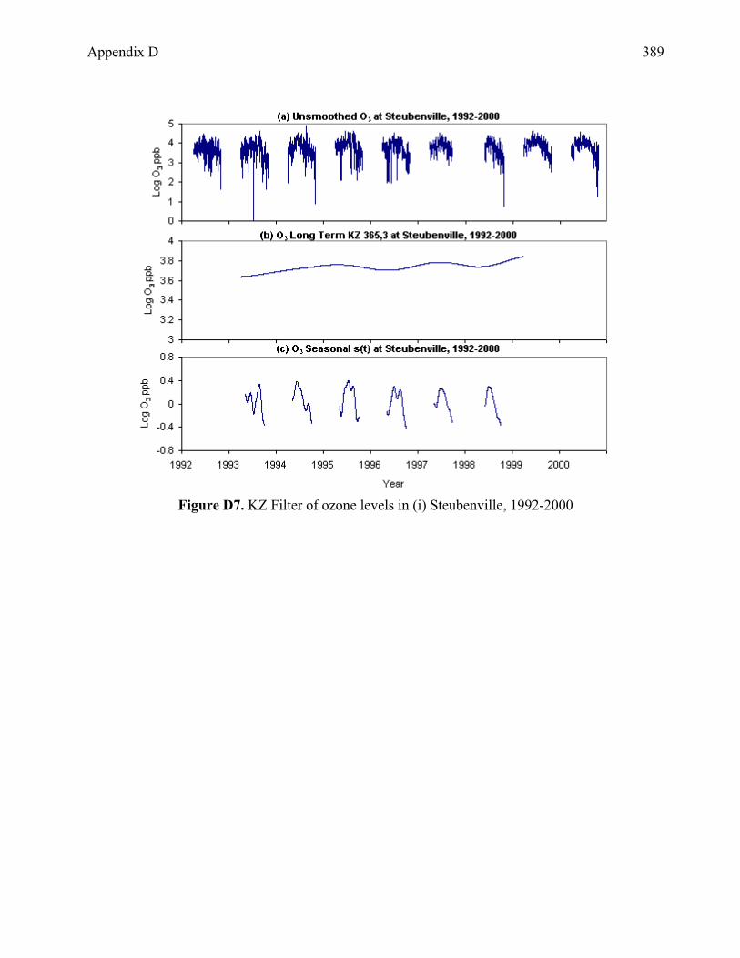
Figure D7. KZ Filter of ozone levels in (i) Steubenville, 1992-2000

390 Appendix D
Figure D8. KZ Filter of PM10 levels in (a) Cincinnati, 1992-1999 and (b) Columbus (Maple
Canyon), 1992-2000
Appendix D 391
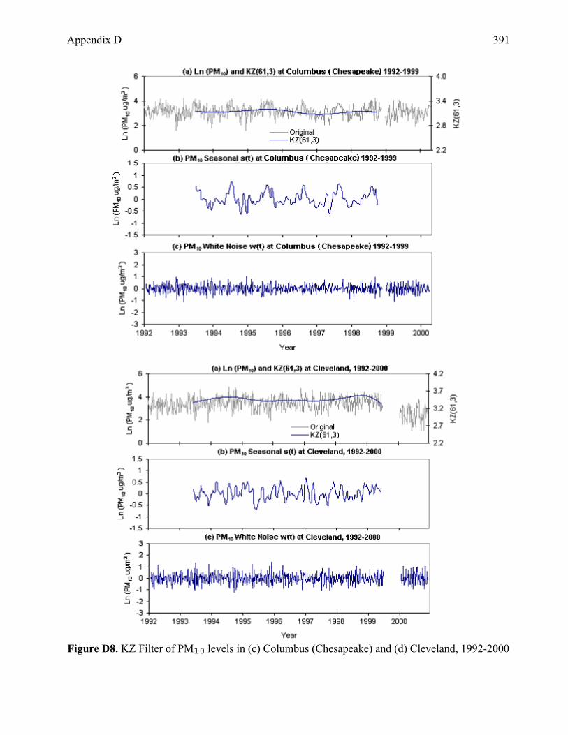
Figure D8. KZ Filter of PM10 levels in (c) Columbus (Chesapeake) and (d) Cleveland, 1992-2000

392 Appendix D
Figure D8. KZ Filter of PM10 levels in (e) Steubenville, 1992-2000

Appendix D 393
Figure D9. KZ Filter of CO levels in (a) Cincinnati and (b) Dayton, 1992-2000
394 Appendix D
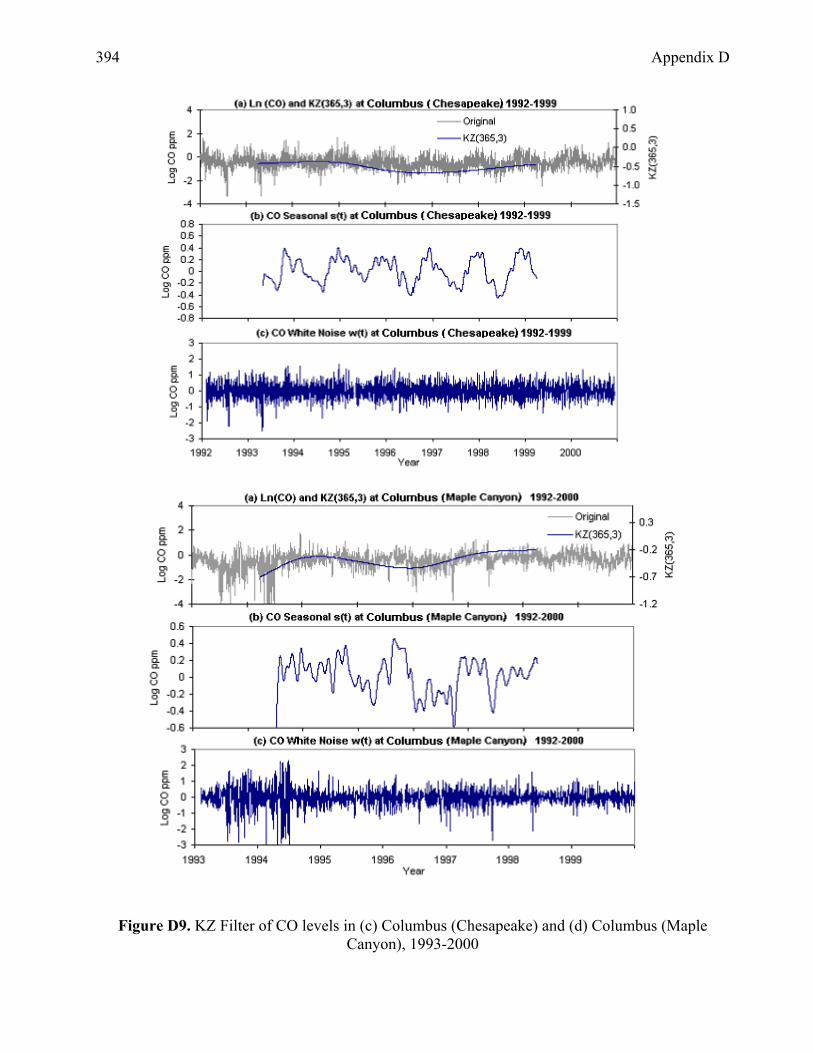
Figure D9. KZ Filter of CO levels in (c) Columbus (Chesapeake) and (d) Columbus (Maple
Canyon), 1993-2000

Appendix D 395
Figure D9. KZ Filter of CO levels in (e) Akron and (f) Cleveland, 1992-2000

396 Appendix D
Figure D10. KZ Filter of SO2 levels in (a) Cincinnati and (b) Dayton, 1992-2000
Appendix D 397
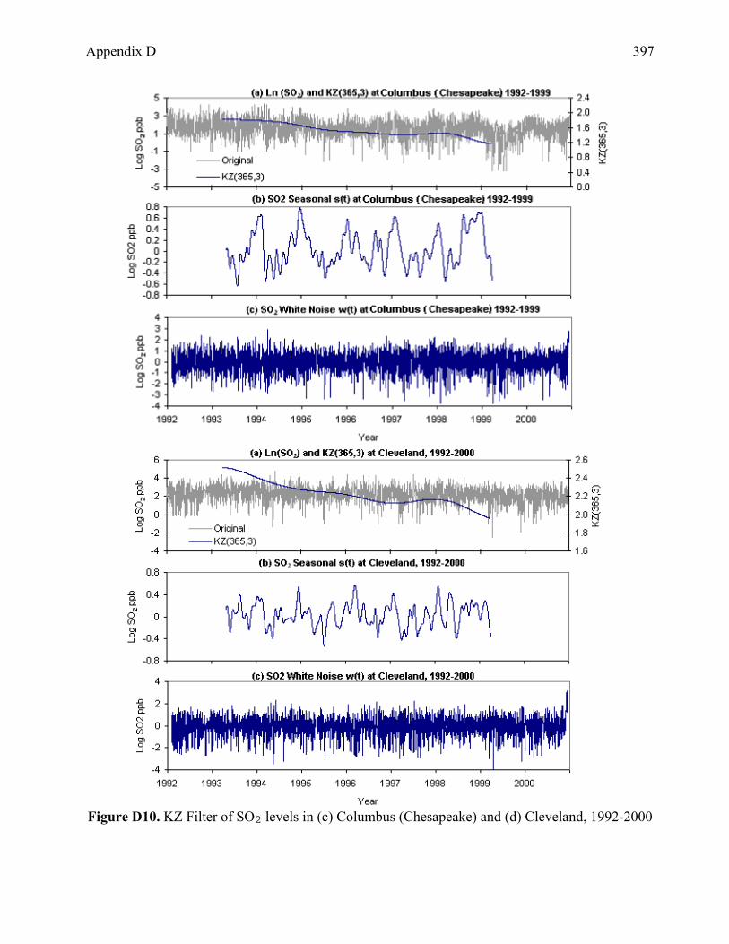
Figure D10. KZ Filter of SO2 levels in (c) Columbus (Chesapeake) and (d) Cleveland, 1992-2000

398 Appendix D
Figure D10. KZ Filter of SO2 levels in (e) Akron and (f) Steubenville, 1992-2000
Appendix D 399
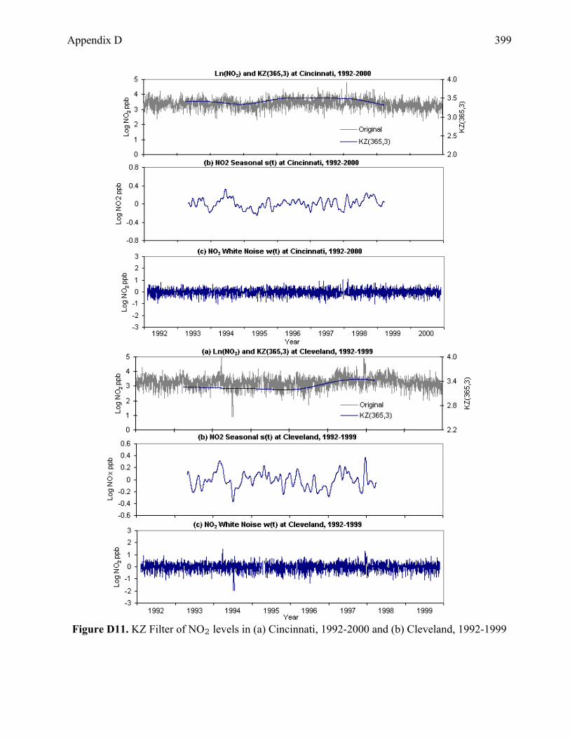
Figure D11. KZ Filter of NO2 levels in (a) Cincinnati, 1992-2000 and (b) Cleveland, 1992-1999
400 Appendix D
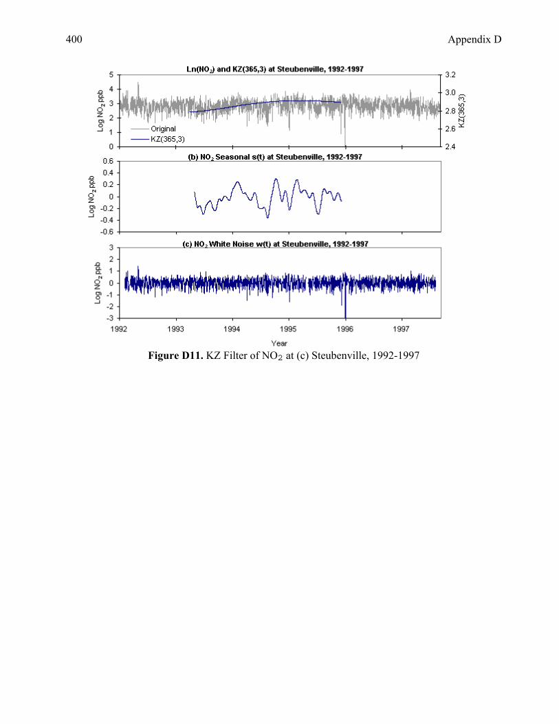
Figure D11. KZ Filter of NO2 at (c) Steubenville, 1992-1997

Appendix D 401
Figure D12. Co-relational plots of maximum eight-hour vs. one-hour ozone concentrations at the
six monitoring site, 1992-2000

402 Appendix D
Figure D13. Co-relational plots of maximum eight-hour vs. one-hour ozone
concentrations at the six monitoring site, 1992-2000

Appendix D 403
Figure D14. Correlation between 1 Hour and 8 Hour CO1992-2000: (a) Cincinnati, (b) Dayton,
(c) Chesapeake, (d) Maple Canyon, (e) Akron and (f) Cleveland
404 Appendix D
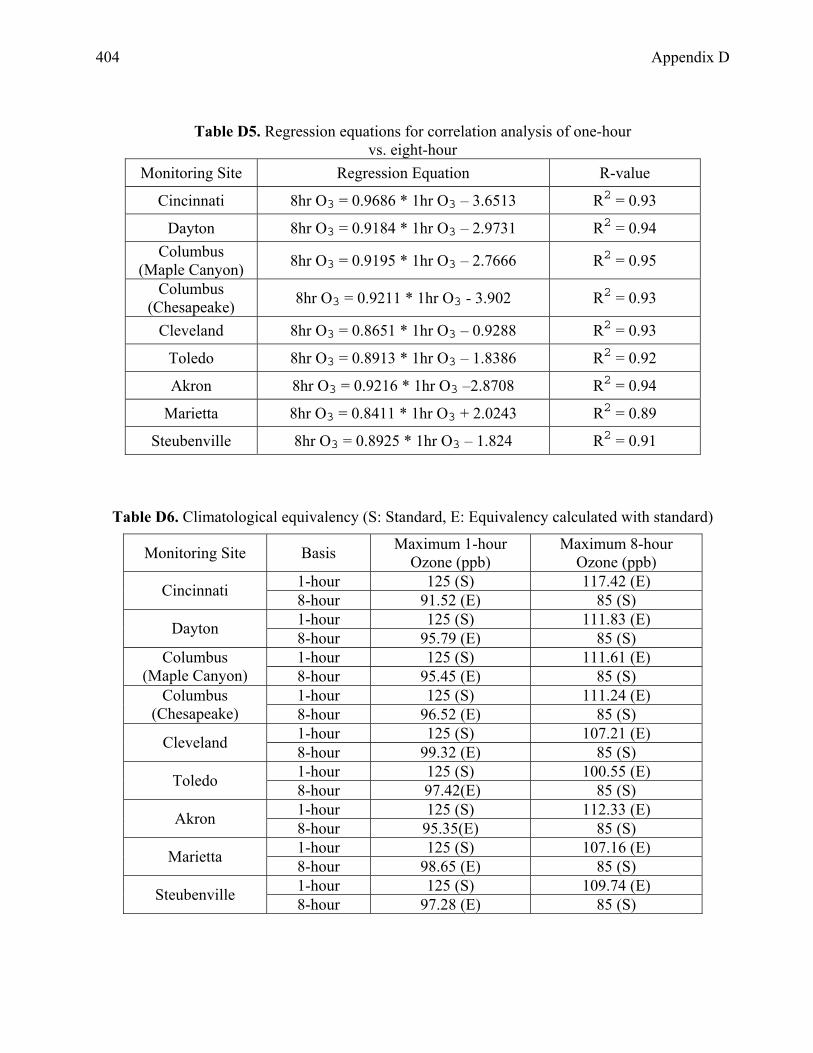
Table D5. Regression equations for correlation analysis of one-hour
vs. eight-hour Monitoring Site Regression Equation R-value
Cincinnati 8hr O3 = 0.9686 * 1hr O3 – 3.6513 R2 = 0.93
Dayton 8hr O3 = 0.9184 * 1hr O3 – 2.9731 R2 = 0.94 Columbus
(Maple Canyon) 8hr O3 = 0.9195 * 1hr O3 – 2.7666 R2 = 0.95
Columbus (Chesapeake) 8hr O3 = 0.9211 * 1hr O3 - 3.902 R2 = 0.93
Cleveland 8hr O3 = 0.8651 * 1hr O3 – 0.9288 R2 = 0.93
Toledo 8hr O3 = 0.8913 * 1hr O3 – 1.8386 R2 = 0.92
Akron 8hr O3 = 0.9216 * 1hr O3 –2.8708 R2 = 0.94
Marietta 8hr O3 = 0.8411 * 1hr O3 + 2.0243 R2 = 0.89
Steubenville 8hr O3 = 0.8925 * 1hr O3 – 1.824 R2 = 0.91
Table D6. Climatological equivalency (S: Standard, E: Equivalency calculated with standard)
Monitoring Site Basis Maximum 1-hour Ozone (ppb)
Maximum 8-hour Ozone (ppb)
1-hour 125 (S) 117.42 (E) Cincinnati 8-hour 91.52 (E) 85 (S) 1-hour 125 (S) 111.83 (E) Dayton 8-hour 95.79 (E) 85 (S) 1-hour 125 (S) 111.61 (E) Columbus
(Maple Canyon) 8-hour 95.45 (E) 85 (S) 1-hour 125 (S) 111.24 (E) Columbus
(Chesapeake) 8-hour 96.52 (E) 85 (S) 1-hour 125 (S) 107.21 (E) Cleveland 8-hour 99.32 (E) 85 (S) 1-hour 125 (S) 100.55 (E) Toledo 8-hour 97.42(E) 85 (S) 1-hour 125 (S) 112.33 (E) Akron 8-hour 95.35(E) 85 (S) 1-hour 125 (S) 107.16 (E) Marietta 8-hour 98.65 (E) 85 (S) 1-hour 125 (S) 109.74 (E) Steubenville 8-hour 97.28 (E) 85 (S)

Appendix D 405
Table D7. Regression Equation for Correlation Analysis between
1hr CO and 8hr CO Monitoring Site Regression Equation R-value
Cincinnati 8hr CO = 0.5135 * 1hr CO + 0.2151 R2 = 0.7968
Dayton 8hr CO = 0.5048 * 1hr CO + 0.1574 R2 = 0.805 Columbus
(Chesapeake) 8hr CO = 0.4863 * 1hr CO + 0.1567 R2 = 0.8309
Columbus (Maple Canyon) 8hr CO = 0.5061 * 1hr CO + 0.1729 R2 = 0.7882
Akron 8hr CO = 0.4608 * 1hr CO + 0.1588 R2 = 0.7702
Cleveland 8hr CO = 0.5663 * 1hr CO + 0.3835 R2 = 0.7717
Table D8. Climatological equivalency (S: Standard, E: Equivalency calculated with standard)
Monitoring Site Basis Maximum 1-hour CO (ppm)
Maximum 8-hour CO (ppm)
1-hour 35 (S) 18.19 (E) Cincinnati 8-hour 17.11 (E) 9 (S) 1-hour 35 (S) 17.83 (E) Dayton 8-hour 17.52 (E) 9 (S) 1-hour 35 (S) 17.18 (E) Columbus
(Chesapeake) 8-hour 18.19 (E) 9 (S) 1-hour 35 (S) 17.89 (E) Columbus
(Maple Canyon) 8-hour 17.44 (E) 9 (S) 1-hour 35 (S) 16.29 (E) Akron 8-hour 19.19(E) 9 (S) 1-hour 35 (S) 20.2 (E) Cleveland 8-hour 15.22 (E) 9 (S)

406
App
endi
x D
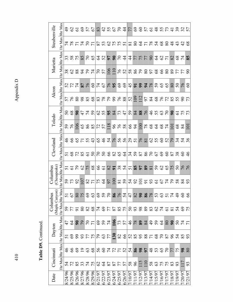
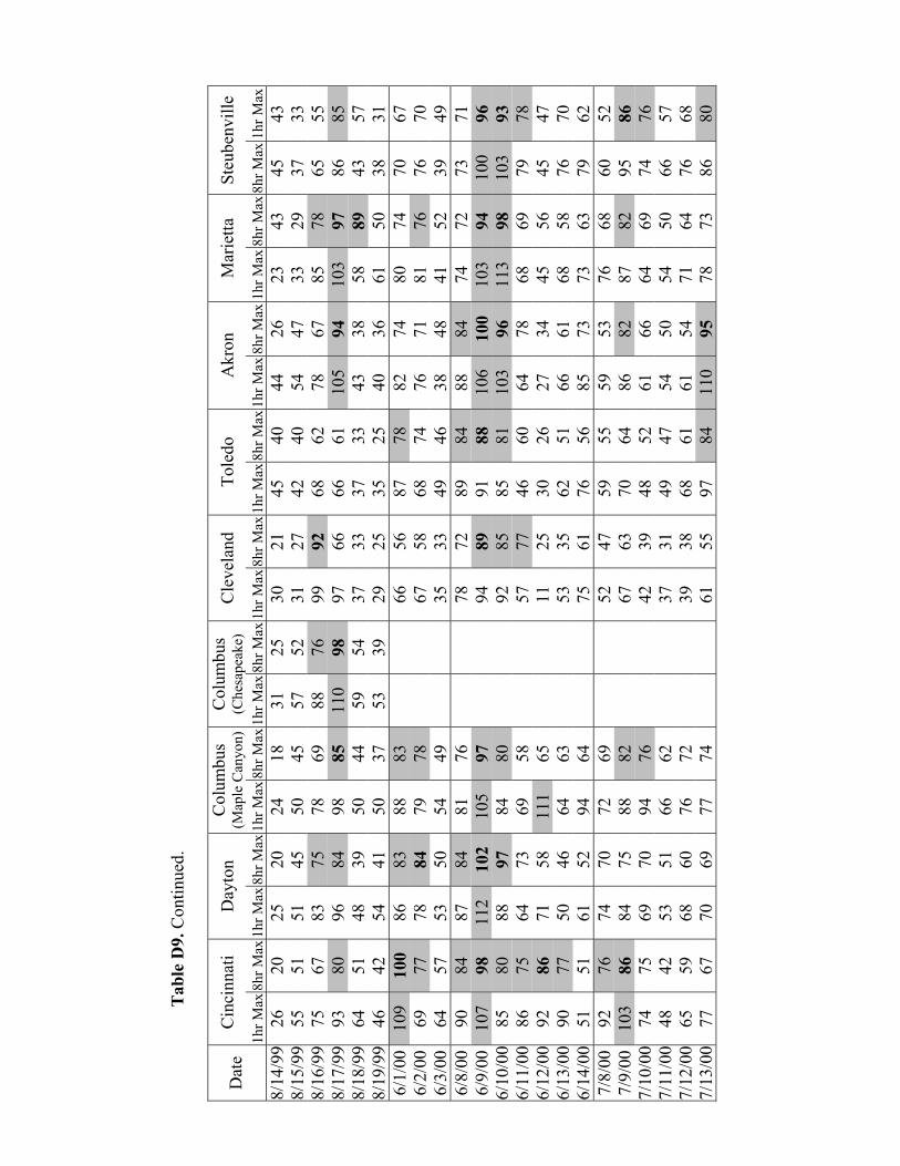
Tab
le D
9. R
egio
nal a
naly
sis o
f ozo
ne e
xcee
ding
day
s for
Cin
cinn
ati,
Day
ton,
Tol
edo,
Col
umbu
s (M
aple
Can
yon)
, C
leve
land
, Akr
on, M
arie
tta a
nd C
olum
bus (
Che
sape
ake)
, 199
2-20
00 in
ppb
Dat
e C
inci
nnat
i D
ayto
n C
olum
bus
(Map
le C
anyo
n)C
olum
bus
(Che
sape
ake)
C
leve
land
To
ledo
A
kron
M
arie
tta
Steu
benv
ille
1h
r Max
8hr
Max
1hr
Max
8hr
Max
1hr
Max
8hr M
ax1h
r Max
8hr M
ax1h
r Max
8hr M
ax1h
r Max
8hr
Max
1hr M
ax8h
r Max
1hr M
ax8h
r Max
1hr M
ax8h
r Max
5/9/
92
56
50
52
41
39
32
43
39
31
27
62
40
41
32
41
29
38
33
5/10
/92
67
57
57
54
69
63
68
62
49
41
70
63
84
71
63
59
64
58
5/11
/92
78
71
72
70
64
62
72
64
103
87
96
88
80
77
84
77
72
66
5/12
/92
75
52
74
58
78
71
82
76
83
80
88
63
88
81
93
87
70
59
5/13
/92
52
46
49
44
45
37
47
38
59
38
53
47
53
43
62
54
67
60
6/16
/93
71
62
83
75
69
63
82
73
43
34
94
79
77
67
103
95
76
72
6/17
/93
69
63
100
93
10
1 94
86
82
92
87
85
78
10
4 95
12
4 10
8 31
30
6/
18/9
3 87
70
77
68
89
71
92
76
73
63
76
65
90
80
93
82
27
25
6/
19/9
3 81
72
10
5
88
91
78
103
89
85
74
88
79
84
80
93
77
33
30
6/20
/93
41
33
42
38
67
61
66
55
69
59
32
27
72
60
91
81
59
54
6/21
/93
44
41
50
45
45
37
46
39
55
48
52
45
47
39
44
36
45
26
6/22
/93
84
67
62
59
73
57
58
43
66
52
80
64
77
65
75
70
77
73
6/23
/93
68
61
83
75
62
56
80
75
51
42
80
73
70
62
86
57
74
66
6/24
/93
68
60
103
88
94
89
91
75
10
3 87
89
80
98
92
92
82
49
40
6/
25/9
3 30
27
57
46
81
73
58
53
65
57
42
37
76
66
91
86
69
64
7/
22/9
3 68
61
72
60
60
36
70
57
39
35
74
63
65
50
40
36
84
73
7/
23/9
3 80
75
65
56
96
70
73
60
50
39
77
71
96
69
40
38
82
62
7/
24/9
3 95
77
10
5
89
95
91
81
70
66
55
121
10
1 10
2 93
11
0 86
76
69
7/
25/9
3 97
85
95
82
97
92
91
77
10
5 92
10
3
84
106
92
124
106
55
52
7/26
/93
75
63
62
56
70
62
60
53
72
59
76
43
73
60
* *
94
83
8/13
/93
53
43
63
58
83
66
71
61
85
57
* *
78
68
87
81
43
37
8/14
/93
87
72
77
71
108
91
84
78
70
60
94
80
108
92
90
85
86
82
8/15
/93
110
88
10
1
95
98
89
93
82
109
92
95
88
105
100
100
95
84
71
8/16
/93
72
45
66
57
72
65
65
61
65
59
* *
65
60
106
84
72
64
8/17
/93
44
37
60
56
73
68
62
56
71
65
* *
74
70
59
48
74
62
8/18
/93
75
69
84
74
57
53
62
41
59
47
* *
62
51
78
70
70
64
8/19
/93
89
76
125
99
85
78
86
81
84
70
13
1
89
79
72
91
80
54
46
8/20
/93
48
44
60
58
69
60
65
53
70
57
54
47
82
68
60
57
84
64

Tab
le D
1. C
ontin
ued.
Dat
e C
inci
nnat
i D
ayto
n C
olum
bus
(Map
le C
anyo
n)C
olum
bus
(Che
sape
ake)
C
leve
land
To
ledo
A
kron
M
arie
tta
Steu
benv
ille
1h
r Max
8hr
Max
1hr
Max
8hr
Max
1hr
Max
8hr M
ax1h
r Max
8hr M
ax1h
r Max
8hr M
ax1h
r Max
8hr
Max
1hr M
ax8h
r Max
1hr M
ax8h
r Max
1hr M
ax8h
r Max
6/3/
94
38
34
72
67
60
53
58
53
34
30
78
69
58
48
68
64
83
82
6/4/
94
54
49
87
83
94
83
92
85
62
50
84
79
101
86
100
94
78
74
6/5/
94
48
45
116
10
6
85
83
100
94
84
67
101
92
88
86
11
1 10
6 66
63
6/
6/94
63
45
66
57
81
74
76
71
77
61
55
44
71
68
77
70
50
40
6/
7/94
62
41
80
71
87
79
80
63
70
64
32
13
91
84
10
4 78
71
57
6/
8/94
45
31
37
27
61
38
35
19
42
30
30
23
61
35
68
48
73
68
6/
9/94
60
45
63
58
75
65
67
58
54
44
62
51
64
59
78
70
97
83
6/
10/9
4 76
68
97
89
82
69
98
92
60
51
95
87
70
64
10
1 95
69
64
6/
11/9
4 45
43
90
84
89
84
90
86
10
3 85
82
78
89
85
91
80
80
71
6/
12/9
4 36
29
82
73
67
62
79
77
61
56
65
57
66
61
10
8 93
73
64
6/
13/9
4 55
48
83
76
72
69
66
61
69
59
66
60
75
67
80
72
82
69
6/
14/9
4 51
46
85
76
76
70
66
38
57
45
66
60
78
72
79
70
90
80
6/
15/9
4 68
57
76
71
78
72
62
45
58
46
73
67
78
64
10
9 83
98
83
6/
16/9
4 61
37
78
69
81
51
10
1 53
80
69
68
57
88
72
10
2 89
10
9 93
6/
17/9
4 87
71
96
84
72
68
85
77
69
63
92
79
92
85
11
2 93
82
73
6/
18/9
4 10
9
83
89
76
87
65
86
79
92
84
98
77
86
74
90
78
80
73
6/19
/94
89
78
94
90
82
68
80
74
69
56
88
81
110
88
110
90
71
55
6/20
/94
82
69
98
78
85
72
102
75
93
72
92
77
95
78
126
105
68
62
6/21
/94
62
52
97
80
68
63
85
74
83
78
75
68
87
77
87
79
72
59
6/22
/94
98
87
103
95
81
70
89
83
40
35
11
3
93
78
62
85
66
43
38
6/23
/94
66
57
67
53
89
83
58
42
46
30
72
56
78
69
100
83
30
29
7/11
/94
62
52
76
67
55
48
55
51
58
51
87
69
65
52
49
45
88
81
7/12
/94
66
59
118
10
1
76
73
87
83
125
98
103
87
81
79
73
67
45
32
7/
13/9
4 21
14
45
34
94
88
*
* 93
64
37
26
96
84
41
34
60
49
7/
14/9
4 33
24
61
57
62
51
62
55
66
52
50
44
56
47
29
25
56
54
7/
15/9
4 24
16
65
59
52
16
61
47
68
61
43
34
67
62
54
43
77
68

408
App
endi
x D
Dat
e C
inci
nnat
i D
ayto
n C
olum
bus
(Map
le C
anyo
n)C
olum
bus
(Che
sape
ake)
C
leve
land
To
ledo
A
kron
M
arie
tta
Steu
benv
ille
1h
r Max
8hr
Max
1hr
Max
8hr
Max
1hr
Max
8hr M
ax1h
r Max
8hr M
ax1h
r Max
8hr M
ax1h
r Max
8hr
Max
1hr M
ax8h
r Max
1hr M
ax8h
r Max
1hr M
ax8h
r Max
6/16
/95
75
64
76
52
69
65
95
80
34
30
97
84
89
75
86
77
114
102
6/17
/95
84
75
87
83
100
94
91
81
46
43
115
92
10
9 99
95
85
10
0 91
6/
18/9
5 10
3
97
90
86
104
96
87
83
50
48
97
90
96
93
94
91
72
62
6/19
/95
103
94
87
83
98
93
95
87
65
53
96
87
10
0 92
10
9 98
78
40
6/
20/9
5 59
41
87
70
90
80
76
58
86
67
59
49
92
78
11
0 99
87
71
6/
21/9
5 86
53
82
57
92
81
94
70
70
59
95
66
83
70
25
13
62
52
6/
22/9
5 78
57
89
74
83
76
76
68
67
62
90
75
11
9 92
76
63
53
50
6/
23/9
5 55
50
71
52
77
70
71
62
91
77
73
61
72
66
52
38
60
47
6/
24/9
5 54
44
62
52
62
47
51
46
50
42
73
54
63
48
67
58
78
62
6/
25/9
5 89
76
93
85
61
49
65
56
60
51
66
58
67
51
71
62
62
50
6/
26/9
5 56
45
67
51
73
59
70
61
58
44
68
50
59
36
10
0 64
53
45
7/
11/9
5 93
69
78
72
90
80
90
72
65
59
91
79
97
80
86
49
10
8 98
7/
12/9
5 10
1
91
115
10
4
87
84
130
108
78
66
130
11
5 96
89
83
80
10
9 96
7/
13/9
5 86
76
10
1
93
91
88
95
85
103
91
91
78
90
86
* *
100
87
7/14
/95
86
79
93
90
93
83
101
97
88
76
87
67
89
82
108
79
79
74
7/15
/95
101
76
10
3
69
98
84
107
80
91
82
101
72
10
1 84
91
38
60
47
7/
29/9
5 74
66
67
63
63
62
64
59
77
67
79
71
68
66
64
60
86
82
7/
30/9
5 87
80
94
78
10
0 87
86
77
64
57
99
88
87
80
78
73
10
2 93
7/
31/9
5 12
8
115
10
9
85
92
85
76
72
79
65
109
97
87
84
11
2 99
11
1 91
8/
1/95
58
42
95
75
91
89
97
81
96
87
71
55
95
89
11
1 94
70
65
8/
2/95
78
62
80
67
87
78
74
71
65
56
96
82
77
73
95
81
17
15
8/
18/9
5 65
36
60
45
78
63
53
45
62
50
54
43
85
50
93
69
11
8 10
1 8/
19/9
5 74
50
74
61
89
81
93
79
10
1 87
70
60
10
5 87
69
61
83
72
8/
20/9
5 71
64
70
63
83
72
83
76
88
75
78
71
11
7 94
85
76
44
42
8/
21/9
5 82
64
76
65
76
63
10
8 74
89
66
65
59
78
70
88
83
80
59
8/
22/9
5 57
52
49
38
46
39
46
36
40
28
59
52
41
39
56
52
88
82
8/
23/9
5 81
68
78
69
68
56
81
67
47
39
79
73
70
63
74
62
68
57
8/
24/9
5 10
9
81
79
61
67
55
101
83
40
28
93
81
58
52
83
44
108
78
8/25
/95
83
68
62
53
68
54
54
50
41
39
86
72
59
47
84
70
101
93
8/26
/95
83
71
81
71
101
88
98
81
83
69
88
76
124
98
110
90
90
37
8/27
/95
65
58
94
84
90
84
90
85
74
67
70
57
88
71
96
84
15
14

Tab
le D
9. C
ontin
ued.
Dat
e C
inci
nnat
i D
ayto
n C
olum
bus
(Map
le C
anyo
n)C
olum
bus
(Che
sape
ake)
C
leve
land
To
ledo
A
kron
M
arie
tta
Steu
benv
ille
1h
r Max
8hr
Max
1hr
Max
8hr
Max
1hr
Max
8hr M
ax1h
r Max
8hr M
ax1h
r Max
8hr M
ax1h
r Max
8hr
Max
1hr M
ax8h
r Max
1hr M
ax8h
r Max
1hr M
ax8h
r Max
6/15
/96
83
77
84
81
90
79
92
84
67
59
70
64
93
84
85
71
82
79
6/16
/96
106
93
93
90
89
84
94
89
84
73
88
84
92
87
10
5 93
69
63
6/
17/9
6 80
64
85
78
84
76
97
73
71
54
84
68
82
67
79
72
71
59
6/
18/9
6 60
41
62
54
70
57
68
55
51
47
65
50
60
46
67
62
70
64
6/
19/9
6 71
63
69
56
78
70
79
71
77
67
62
55
71
67
61
44
72
63
6/
20/9
6 58
56
67
55
65
62
63
60
71
64
56
53
74
66
79
62
68
65
6/
21/9
6 10
2
77
84
77
79
70
83
75
65
59
69
54
81
77
67
62
56
49
6/22
/96
70
66
79
70
68
63
76
71
72
63
79
72
71
67
76
70
66
46
6/23
/96
115
96
98
87
66
62
76
74
40
26
92
78
70
64
65
63
41
35
6/
24/9
6 51
38
66
63
59
43
68
50
83
69
71
56
60
48
76
58
47
40
6/
25/9
6 60
51
55
51
44
39
55
38
51
39
56
51
50
42
54
50
57
44
6/
26/9
6 78
67
68
62
58
48
68
62
38
34
74
65
62
52
61
55
78
75
6/
27/9
6 10
3
96
98
86
95
75
101
91
85
64
106
97
79
72
78
74
86
80
6/
28/9
6 10
7
98
112
10
6
92
86
100
91
110
84
96
91
113
99
113
100
85
69
6/29
/96
106
10
1
101
95
94
91
11
8 11
4 92
82
10
7
96
96
93
99
92
71
64
6/30
/96
72
67
86
79
81
70
89
81
88
85
78
74
84
76
83
79
80
71
7/1/
96
75
65
97
90
74
69
77
75
49
43
98
86
84
71
75
67
40
32
7/2/
96
82
74
91
86
85
78
91
73
87
82
91
82
98
91
79
67
51
45
7/3/
96
52
44
52
48
43
32
55
51
40
35
49
42
43
38
43
35
69
59
7/4/
96
73
66
65
60
51
44
56
52
59
54
62
56
57
51
27
25
100
92
7/5/
96
84
72
87
84
72
68
89
84
76
68
88
78
76
73
50
45
94
86
7/6/
96
90
85
117
11
3
89
85
101
97
94
88
108
92
98
91
67
61
63
59
7/
7/96
81
69
10
7
99
98
89
104
95
108
103
90
74
103
96
46
43
47
47
7/8/
96
77
61
77
70
70
63
80
71
72
48
76
65
66
62
33
31
53
47
8/3/
96
72
67
88
84
74
69
76
68
85
78
82
75
79
74
75
70
77
61
8/4/
96
85
76
87
75
72
68
92
86
91
85
88
83
86
75
84
76
78
72
8/5/
96
74
65
106
89
90
81
85
79
94
82
91
75
94
82
85
75
87
75
8/
6/96
97
71
*
* 84
80
96
88
10
0 81
90
80
94
89
97
82
82
58
8/
7/96
76
69
10
7
89
88
79
89
70
86
81
84
80
87
80
97
87
41
35
8/8/
96
40
20
67
60
71
52
65
46
62
57
56
43
63
49
76
51
42
34
410
App
endi
x D
Tab
le D
9. C
ontin
ued.
Dat
e C
inci
nnat
i D
ayto
n
Col
umbu
s (M
aple
Can
yon)
Col
umbu
s (C
hesa
peak
e)
Cle
vela
nd
Tole
do
Akr
on
Mar
ietta
St
eube
nvill
e
1hr M
ax 8
hr M
ax 1
hr M
ax 8
hr M
ax 1
hr M
ax8h
r Max
1hr M
ax8h
r Max
1hr M
ax8h
r Max
1hr M
ax 8
hr M
ax1h
r Max
8hr M
ax1h
r Max
8hr M
ax1h
r Max
8hr M
ax8/
24/9
6 54
46
51
47
59
51
59
51
51
46
59
50
57
52
38
33
74
49
8/
25/9
6 72
66
69
64
77
67
73
61
68
66
76
68
76
72
62
58
78
62
8/
26/9
6 85
69
99
90
91
80
92
79
72
65
10
6
90
80
74
88
75
71
61
8/27
/96
33
19
93
79
80
75
107
62
85
71
65
47
98
87
94
85
74
69
8/28
/96
74
63
77
70
82
69
82
75
61
55
86
74
85
76
79
70
70
57
8/29
/96
75
68
75
71
68
63
71
68
50
43
85
59
68
60
74
65
71
67
6/21
/97
62
56
79
69
74
69
75
66
70
65
72
62
83
74
70
64
87
83
6/22
/97
64
60
63
59
69
59
64
61
50
46
57
55
78
67
57
52
53
42
6/23
/97
87
74
77
74
77
70
97
82
66
54
118
95
79
76
10
6 97
62
55
6/
24/9
7 87
72
13
0
106
87
86
10
0 91
82
76
96
84
99
95
11
0 90
75
67
6/
25/9
7 77
71
82
73
85
76
81
38
65
56
76
73
76
69
76
70
75
70
6/
26/9
7 57
52
66
57
75
54
59
54
64
56
58
47
88
69
52
44
51
44
7/
10/9
7 58
54
52
46
50
47
54
51
34
29
66
59
52
45
58
44
81
77
7/
11/9
7 96
86
85
78
93
82
92
85
59
51
94
84
10
9 91
86
77
80
69
7/
12/9
7 11
5
98
95
89
98
90
101
97
87
76
100
88
11
2 99
79
75
64
60
7/
13/9
7 11
0
97
88
84
89
86
91
89
86
81
78
76
97
94
80
77
71
57
7/14
/97
58
48
71
49
83
78
93
81
70
62
68
46
84
78
97
90
78
61
7/15
/97
63
53
68
59
62
53
61
59
67
55
64
55
68
59
68
64
54
48
7/16
/97
75
65
70
64
74
63
67
62
69
60
68
63
76
65
66
62
68
55
7/17
/97
75
70
87
80
61
51
74
65
60
52
74
70
72
65
80
71
80
73
7/18
/97
83
77
96
90
81
74
79
75
87
79
101
90
85
80
89
82
48
41
7/
19/9
7 93
75
54
50
54
49
58
50
38
34
68
61
55
50
77
68
43
39
7/
20/9
7 11
7
98
85
74
69
60
84
76
60
54
84
75
90
76
77
74
42
32
7/21
/97
93
80
93
71
75
66
93
76
46
36
101
73
73
60
90
85
68
57

Tab
le D
9. C
ontin
ued.
Dat
e C
inci
nnat
i D
ayto
n C
olum
bus
(Map
le C
anyo
n)C
olum
bus
(Che
sape
ake)
C
leve
land
To
ledo
A
kron
M
arie
tta
Steu
benv
ille
1h
r Max
8hr
Max
1hr
Max
8hr
Max
1hr
Max
8hr M
ax1h
r Max
8hr M
ax1h
r Max
8hr M
ax1h
r Max
8hr
Max
1hr M
ax8h
r Max
1hr M
ax8h
r Max
1hr M
ax8h
r Max
5/13
/98
76
72
96
77
55
49
68
59
40
29
92
73
59
47
80
68
* *
5/14
/98
88
74
95
86
101
90
105
94
85
73
87
78
110
98
80
73
* *
5/15
/98
97
76
102
91
12
2 11
2 10
4 93
73
69
10
5
89
128
114
115
103
* *
5/16
/98
73
68
70
67
77
67
75
69
63
53
64
61
82
77
62
59
* *
5/17
/98
82
76
80
74
75
72
77
74
58
53
69
67
79
78
78
74
* *
5/18
/98
75
62
82
77
79
73
73
52
57
52
83
70
84
80
85
77
* *
5/19
/98
115
97
10
1
95
102
97
109
103
72
68
109
85
11
4 10
5 10
3 92
*
* 5/
20/9
8 60
54
69
61
74
70
77
72
55
51
57
33
98
88
79
63
*
* 5/
21/9
8 70
63
65
60
57
51
57
55
35
32
70
61
64
58
61
58
*
* 6/
22/9
8 65
52
71
63
82
78
82
70
65
57
67
57
86
82
53
52
74
66
6/
23/9
8 56
48
66
61
57
49
56
50
67
60
58
53
55
46
47
38
51
45
6/
24/9
8 87
75
93
79
98
85
82
74
98
83
93
83
10
4 89
89
74
85
75
6/
25/9
8 10
0
86
94
78
100
89
105
96
86
76
86
80
96
87
97
81
89
83
6/26
/98
63
58
75
70
77
59
81
70
81
73
68
63
84
79
85
79
86
70
6/27
/98
57
51
53
49
65
59
64
61
47
36
55
49
67
55
66
56
53
43
6/28
/98
62
56
55
49
68
58
76
64
80
65
51
46
68
58
61
50
68
57
7/11
/98
64
62
55
53
62
53
59
56
37
36
65
60
61
53
61
52
63
50
7/12
/98
87
81
77
73
67
61
82
76
61
56
79
77
83
75
70
65
79
69
7/13
/98
85
77
97
93
97
92
100
91
88
69
116
10
1 10
5 98
10
3 90
72
55
7/
14/9
8 25
18
52
43
88
85
61
52
84
82
49
40
92
85
83
72
93
82
7/
15/9
8 39
27
56
41
71
63
66
59
59
53
43
31
70
55
61
53
41
32
8/
2/98
81
72
75
72
84
77
80
76
61
56
79
73
74
70
71
66
66
59
8/
3/98
72
65
73
67
10
7 93
84
75
75
65
74
69
98
91
95
87
62
58
8/
4/98
65
54
70
44
10
2 90
82
62
74
65
*
* 96
89
93
87
66
60
8/
5/98
74
66
63
39
10
6 88
71
53
76
52
47
29
60
55
89
85
62
57
8/
6/98
81
68
11
2
82
107
102
98
89
84
79
88
69
99
94
104
93
50
41
8/7/
98
101
89
92
83
11
3 10
3 10
7 96
11
2 10
0 10
2
77
107
99
88
83
55
47
8/8/
98
74
66
106
89
82
74
10
3 93
88
79
93
66
85
75
49
47
41
36
8/
9/98
45
41
59
51
77
66
61
54
49
38
53
44
69
58
78
56
39
32

412
App
endi
x D
Tab
le D
9. C
ontin
ued.
Dat
e C
inci
nnat
i D
ayto
n
Col
umbu
s (M
aple
Can
yon)
Col
umbu
s (C
hesa
peak
e)
Cle
vela
nd
Tole
do
Akr
on
Mar
ietta
St
eube
nvill
e
1hr M
ax 8
hr M
ax 1
hr M
ax 8
hr M
ax 1
hr M
ax8h
r Max
1hr M
ax8h
r Max
1hr M
ax8h
r Max
1hr M
ax 8
hr M
ax1h
r Max
8hr M
ax1h
r Max
8hr M
ax1h
r Max
8hr M
ax9/
11/9
865
56
77
68
74
67
85
76
60
55
82
71
76
71
78
71
48
43
9/
12/9
885
76
93
84
92
84
10
9 10
0 76
66
95
85
87
82
97
90
64
55
9/
13/9
810
1
88
102
96
98
89
11
3 10
4 96
84
10
2
91
102
94
125
106
58
48
9/14
/98
74
61
96
74
114
85
108
91
87
79
79
65
101
83
100
81
50
35
9/15
/98
51
41
58
53
78
67
61
56
50
38
57
51
60
53
84
80
38
36
5/28
/99
89
78
85
80
80
75
79
75
43
38
42
40
84
81
87
81
88
81
5/29
/99
103
95
10
6
98
109
95
99
93
40
38
43
40
79
75
93
90
77
75
5/30
/99
83
80
100
96
10
3 98
10
1 96
63
58
53
49
98
90
99
96
92
82
5/
31/9
955
47
64
51
59
52
63
58
37
33
26
23
77
70
72
67
83
79
6/
1/99
46
38
44
34
39
34
49
44
32
28
20
18
38
33
41
44
50
55
6/
8/99
86
79
79
74
71
68
74
72
79
74
40
27
93
83
79
72
79
74
6/
9/99
85
68
10
7
85
111
99
112
94
60
48
69
54
112
95
89
83
74
56
6/10
/99
103
93
12
7
113
11
8 10
7 12
3 11
0 77
70
12
2
98
102
95
123
102
111
101
6/11
/99
93
86
128
11
1
102
94
98
92
94
74
110
10
1 10
3 92
97
86
11
3 10
2 6/
12/9
995
69
96
73
11
1 91
11
4 95
96
78
85
72
10
1 93
75
65
94
87
6/
13/9
989
82
91
77
10
4 95
98
92
72
68
73
60
86
80
83
70
63
68
6/
14/9
956
54
58
55
54
47
54
51
50
40
52
50
61
49
46
53
53
46
6/
20/9
987
83
84
81
89
83
89
84
67
62
81
77
78
73
83
73
79
77
6/
21/9
984
79
94
89
92
86
86
82
59
49
77
73
63
58
82
73
73
67
6/
22/9
910
2
88
84
78
86
78
88
79
61
55
90
80
85
76
60
65
79
73
6/23
/99
83
69
110
96
97
91
10
4 97
72
64
93
88
93
86
82
78
77
64
6/
24/9
944
33
42
38
56
52
57
52
49
43
57
48
68
65
74
69
72
64
7/
13/9
963
54
75
69
81
73
78
72
64
58
54
32
81
71
69
61
75
55
7/
14/9
991
72
91
81
96
87
88
82
91
80
*
* 98
85
76
60
62
56
7/
15/9
995
88
95
83
86
76
89
83
68
66
*
* 88
84
10
7 98
85
83
7/
16/9
978
72
97
89
76
72
82
79
72
65
83
80
10
2 95
12
5 11
8 96
92
7/
17/9
982
66
72
67
80
74
89
80
64
59
75
68
80
79
84
97
86
81
Tab
le D
9. C
ontin
ued.
Dat
e C
inci
nnat
i D
ayto
n C
olum
bus
(Map
le C
anyo
n)C
olum
bus
(Che
sape
ake)
C
leve
land
To
ledo
A
kron
M
arie
tta
Steu
benv
ille
1h
r Max
8hr
Max
1hr
Max
8hr
Max
1hr
Max
8hr M
ax1h
r Max
8hr M
ax1h
r Max
8hr M
ax1h
r Max
8hr
Max
1hr M
ax8h
r Max
1hr M
ax8h
r Max
8hr M
ax1h
r Max
8/14
/99
26
20
25
20
24
18
31
25
30
21
45
40
44
26
23
43
45
43
8/15
/99
55
51
51
45
50
45
57
52
31
27
42
40
54
47
33
29
37
33
8/16
/99
75
67
83
75
78
69
88
76
99
92
68
62
78
67
85
78
65
55
8/17
/99
93
80
96
84
98
85
110
98
97
66
66
61
105
94
103
97
86
85
8/18
/99
64
51
48
39
50
44
59
54
37
33
37
33
43
38
58
89
43
57
8/19
/99
46
42
54
41
50
37
53
39
29
25
35
25
40
36
61
50
38
31
6/1/
00
109
100
86
83
88
83
66
56
87
78
82
74
80
74
70
67
6/2/
00
69
77
78
84
79
78
67
58
68
74
76
71
81
76
76
70
6/3/
00
64
57
53
50
54
49
35
33
49
46
38
48
41
52
39
49
6/8/
00
90
84
87
84
81
76
78
72
89
84
88
84
74
72
73
71
6/9/
00
107
98
112
102
105
97
94
89
91
88
106
100
103
94
100
96
6/10
/00
85
80
88
97
84
80
92
85
85
81
103
96
113
98
103
93
6/11
/00
86
75
64
73
69
58
57
77
46
60
64
78
68
69
79
78
6/12
/00
92
86
71
58
111
65
11
25
30
26
27
34
45
56
45
47
6/13
/00
90
77
50
46
64
63
53
35
62
51
66
61
68
58
76
70
6/14
/00
51
51
61
52
94
64
75
61
76
56
85
73
73
63
79
62
7/8/
00
92
76
74
70
72
69
52
47
59
55
59
53
76
68
60
52
7/9/
00
103
86
84
75
88
82
67
63
70
64
86
82
87
82
95
86
7/10
/00
74
75
69
70
94
76
42
39
48
52
61
66
64
69
74
76
7/11
/00
48
42
53
51
66
62
37
31
49
47
54
50
54
50
66
57
7/12
/00
65
59
68
60
76
72
39
38
68
61
61
54
71
64
76
68
7/13
/00
77
67
70
69
77
74
61
55
97
84
110
95
78
73
86
80

414 Appendix D
Table D10. High Concentration and High Frequency in Correlation With Wind Direction.
Cincinnati Dayton
Columbus (Maple
Canyon)
Columbus (Chesapeake) Akron Cleveland Marietta Toledo Steubenville
PM10 *E/SW - S/SW E/SW S/SW - - S/SW
CO E/SW SW/SW SE/SW E/SW N/SW NW/SW - - -
SO2 SW/SW S/SW - W/SW W/SW NE/SW - - S/SW NO2 S/SW - - - - SE/SW - - NW/SW
* E/SW means East High Directional Concentration / Southwest High Directional Frequency of Wind.
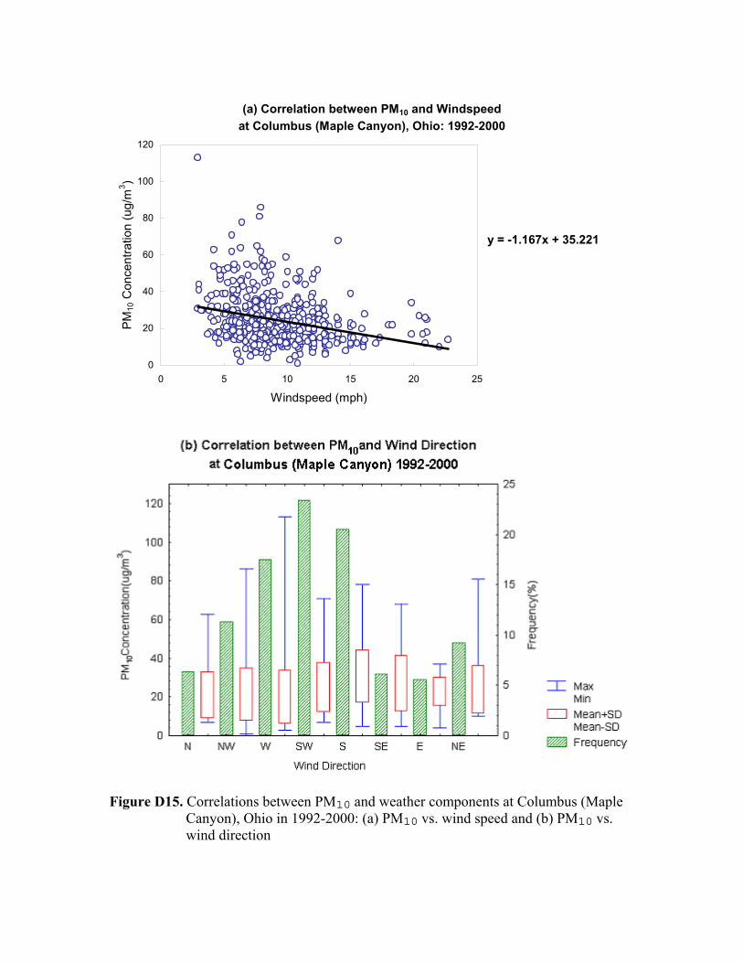
(a) Correlation between PM10 and Windspeed at Columbus (Maple Canyon), Ohio: 1992-2000
y = -1.167x + 35.221
0
20
40
60
80
100
120
0 5 10 15 20 25
Windspeed (mph)
PM10
Con
cent
ratio
n (u
g/m
3 )
Figure D15. Correlations between PM10 and weather components at Columbus (Maple Canyon), Ohio in 1992-2000: (a) PM10 vs. wind speed and (b) PM10 vs. wind direction

416 Appendix D
(c) Correlation between PM10 and Temperature at Columbus (Maple Canyon), Ohio: 1992-2000
y = 0.2472x + 12.274
0
20
40
60
80
100
120
0 20 40 60 80 100
Temperature (F)
PM10
Con
cent
ratio
n (u
g/m
3 )
Figure D15. Correlations between PM10 and weather components at Columbus (Maple Canyon), Ohio in 1992-1999: (c) PM10 vs. temperature

(a) Correlation between PM10 and Windspeed at Columbus (Chesapeake), Ohio: 1992-2000
y = -0.6192x + 30.217
0
10
20
30
40
50
60
70
80
0 5 10 15 20 25Windspeed (mph)
PM10
Con
cent
ratio
n (u
g/m
3 )
Figure D16. Correlations between PM10 and weather components at Columbus (Chesapeake), Ohio in 1992-1999: (a) PM10 vs. wind speed and: (b) PM10 and wind direction.

418 Appendix D
(c) Correlation between PM10 and Temperature at Columbus (Chesapeake), Ohio: 1992-2000
y = 0.2642x + 11.586
0
10
20
30
40
50
60
70
80
0 20 40 60 80 100
Temperauture (F)
PM10
Con
cent
ratio
n (u
g/m
3 )
Figure D16. Correlations between PM10 and weather components at Columbus (Chesapeake), Ohio in 1992-2000 and (c) PM10 vs. temperature
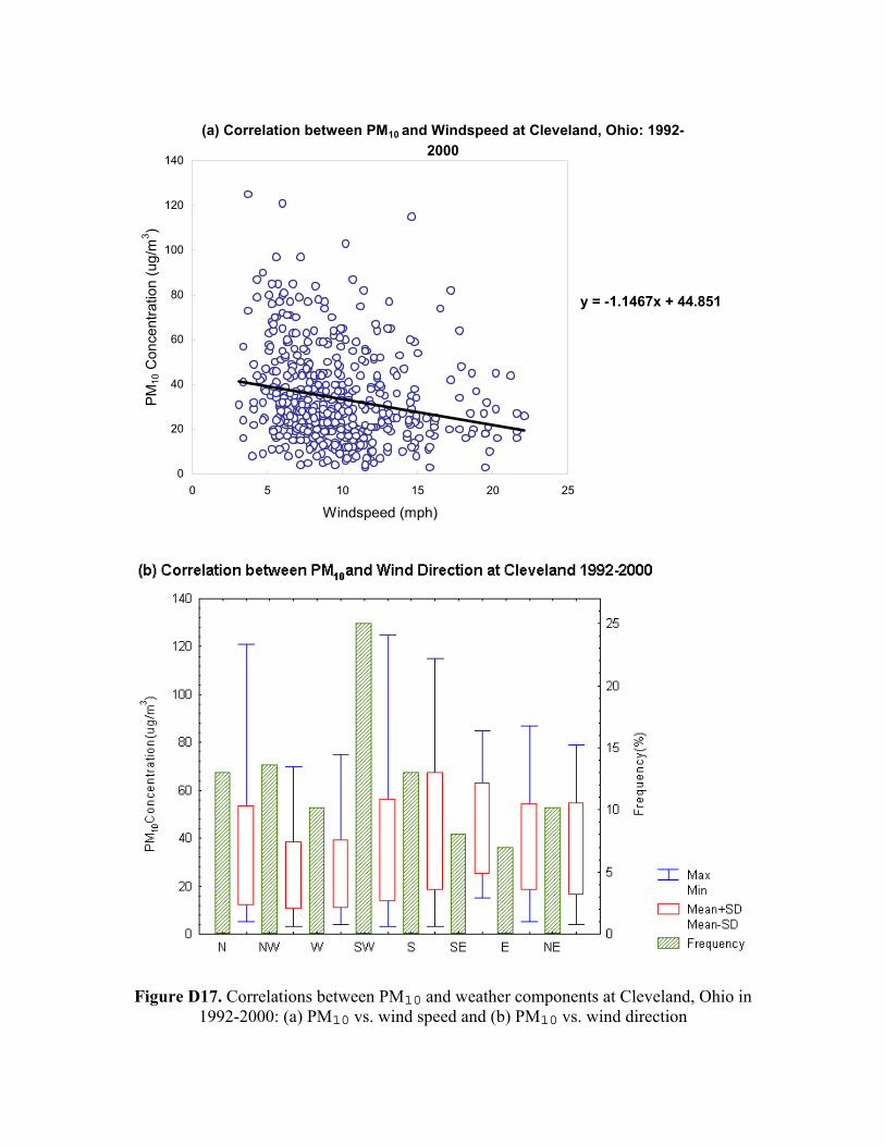
(a) Correlation between PM10 and Windspeed at Cleveland, Ohio: 1992-2000
y = -1.1467x + 44.851
0
20
40
60
80
100
120
140
0 5 10 15 20 25
Windspeed (mph)
PM10
Con
cent
ratio
n (u
g/m
3 )
Figure D17. Correlations between PM10 and weather components at Cleveland, Ohio in 1992-2000: (a) PM10 vs. wind speed and (b) PM10 vs. wind direction

420 Appendix D
(c) Correlation between PM10 and Temperature at Cleveland, Ohio: 1992-2000
y = 0.2567x + 18.622
0
20
40
60
80
100
120
140
0 20 40 60 80 100Temperature(F)
PM10
Con
cent
ratio
n (u
g/m
3 )
Figure D17. Correlations between PM10 and weather components at Cleveland, Ohio in 1992-2000: (c) PM10 vs. temperature.

(a) Correlation between PM10 and Windspeed at Steubenville, Ohio: 1992-2000
y = -1.2113x + 44.757
0
20
40
60
80
100
120
140
160
0 5 10 15 20Windspeed (mph)
PM10
Con
cent
ratio
n (u
g/m
3 )
Figure D18. Correlations between PM10 and weather components at Steubenville, Ohio in 1992-2000: (a) PM10 vs. wind speed and (b) PM10 vs. wind direction
422 Appendix D
(c) Correlation between PM10 and Temperature at Steubenville, Ohio: 1992-2000
y = 0.3122x + 19.444
0
20
40
60
80
100
120
140
160
0 20 40 60 80 100
Temperature (F)
PM10
Con
cent
ratio
n (u
g/m
3 )
Figure D18. Correlations between PM10 and weather components at Steubenville, Ohio in 1992-2000: and (c) PM10 vs temperature
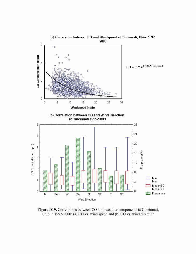
Figure D19. Correlations between CO and weather components at Cincinnati, Ohio in 1992-2000: (a) CO vs. wind speed and (b) CO vs. wind direction

424 Appendix D
Figure D20. Correlations between CO and weather components at Dayton, Ohio in 1992-2000: (a) CO vs. wind speed and (b) CO vs. wind direction

Figure D21. Correlations between CO and weather components at Chesapeake, Ohio in 1992-2000: (a) CO vs. wind speed and (b) CO vs. wind direction
426 Appendix D
Figure D22. Correlations between CO and weather components at Columbus (Maple Canyon), Ohio in 1993-2000 (a) CO vs. wind speed and (b) CO vs. wind direction
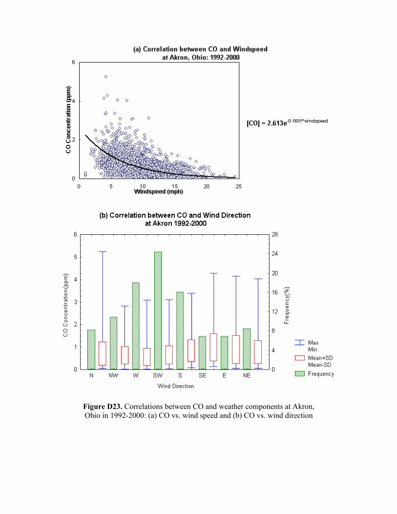
Figure D23. Correlations between CO and weather components at Akron, Ohio in 1992-2000: (a) CO vs. wind speed and (b) CO vs. wind direction

428 Appendix D
Figure D24. Correlations between CO and weather components at Cleveland,
Ohio in 1992-2000: (a) CO vs. wind speed and (b) CO vs. wind direction

Figure D25. Correlations between SO2 and weather components at Cincinnati, Ohio in 1992-2000: (a) SO2 vs. wind speed and (b) SO2 vs. wind direction
430 Appendix D
Figure D26. Correlations between SO2 and weather components at Dayton, Ohio in 1992-2000: (a) SO2 vs. wind speed and (b) SO2 vs. wind direction

Figure D27. Correlations between SO2 and weather components at Columbus (Chesapeake), Ohio in 1992-2000: (a) SO2 vs. wind speed and (b) SO2 vs. wind direction
432 Appendix D
Figure D28. Correlations between SO2 and weather components at Cleveland, Ohio in 1992-2000 (a) SO2 vs. wind speed and (b) SO2 vs. wind direction

Figure D29. Correlations between SO2 and weather components at Akron, Ohio in 1992-2000: (a) SO2 vs. wind speed and (b) SO2 vs. wind direction

434 Appendix D
Figure D30. Correlations between SO2 and weather components at Steubenville, Ohio in 1992-2000: (a) SO2 vs. wind speed and (b) SO2 vs. wind direction
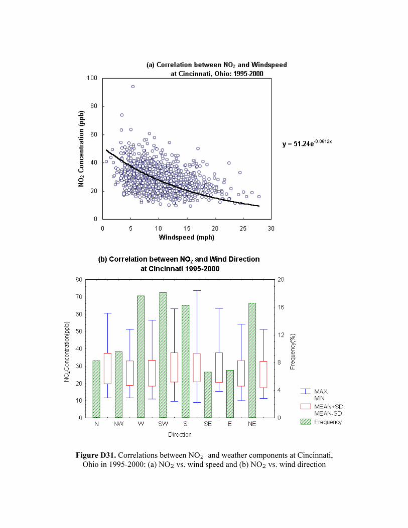
Figure D31. Correlations between NO2 and weather components at Cincinnati, Ohio in 1995-2000: (a) NO2 vs. wind speed and (b) NO2 vs. wind direction

436 Appendix D
Figure D32. Correlations between NO2 and weather components at Dayton, Ohio in 1992-1999: (a) NO2 vs. wind speed and (b) NO2 vs. wind direction
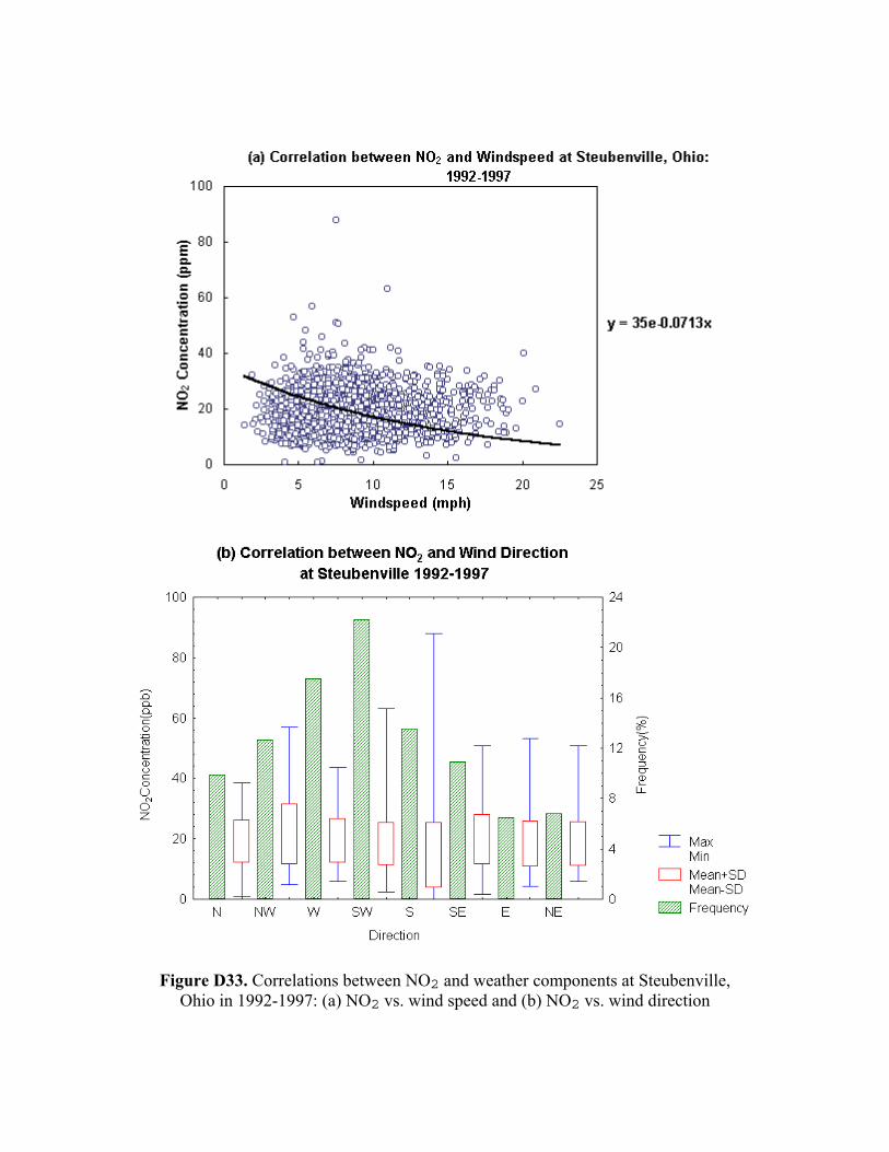
Figure D33. Correlations between NO2 and weather components at Steubenville, Ohio in 1992-1997: (a) NO2 vs. wind speed and (b) NO2 vs. wind direction

438 Appendix D
Figure D34. Back trajectories for high CO days at the monitoring sites selected in Ohio, 1992-2000: (a) Cincinnati and (b) Dayton
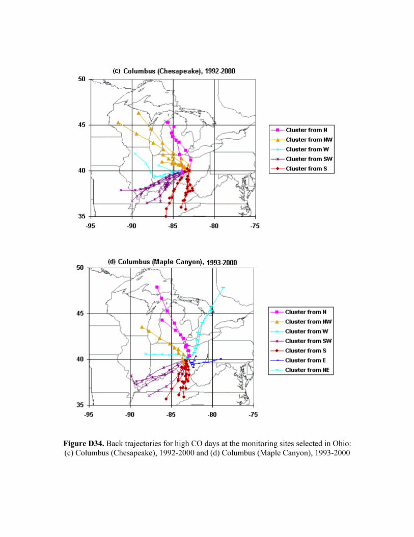
Figure D34. Back trajectories for high CO days at the monitoring sites selected in Ohio: (c) Columbus (Chesapeake), 1992-2000 and (d) Columbus (Maple Canyon), 1993-2000

440 Appendix D
Figure D34. Back trajectories for high CO days at the monitoring sites selected in Ohio, 1992-2000: (e) Akron and (f) Cleveland

Figure D35. (a) Cluster plot at Cincinnati, 1992-2000 (b) Frequencies and average CO concentrations by cluster at Cincinnati, 1992-2000

442 Appendix D
Figure D36. (a) Cluster plot at Dayton, 1992-2000 (b) Frequencies and average CO concentrations by cluster at Dayton, 1992-2000

Figure D37. (a) Cluster plot at Columbus (Chesapeake), 1992-2000 (b) Frequencies and
average CO concentrations by cluster at Columbus (Chesapeake), 1992-2000

444 Appendix D
Figure D38. (a) Cluster plot at Columbus (Maple Canyon), 1993-2000 (b) Frequencies
and average CO concentrations by cluster at Columbus (Maple Canyon), 1993-2000

Figure D39. (a) Cluster plot at Akron 1992-2000 (b) Frequencies and average CO concentrations by cluster at Akron, 1992-2000

446 Appendix D
Figure D40. (a) Cluster plot at Cleveland, 1992-2000 (b) Frequencies and average CO concentrations by cluster at Cleveland, 1992-2000

Figure D41. Back trajectories for high SO2 days at the monitoring sites selected in Ohio, 1992-2000: (a) Cincinnati and (b) Dayton

448 Appendix D
Figure D41 Back trajectories for high SO2 days at the monitoring sites selected in Ohio, 1992-2000: (c) Columbus (Chesapeake) and (d) Cleveland.

Figure D41. Back trajectories for high SO2 days at the monitoring sites selected in Ohio, 1992-2000: (e) Akron and (f) Steubenville
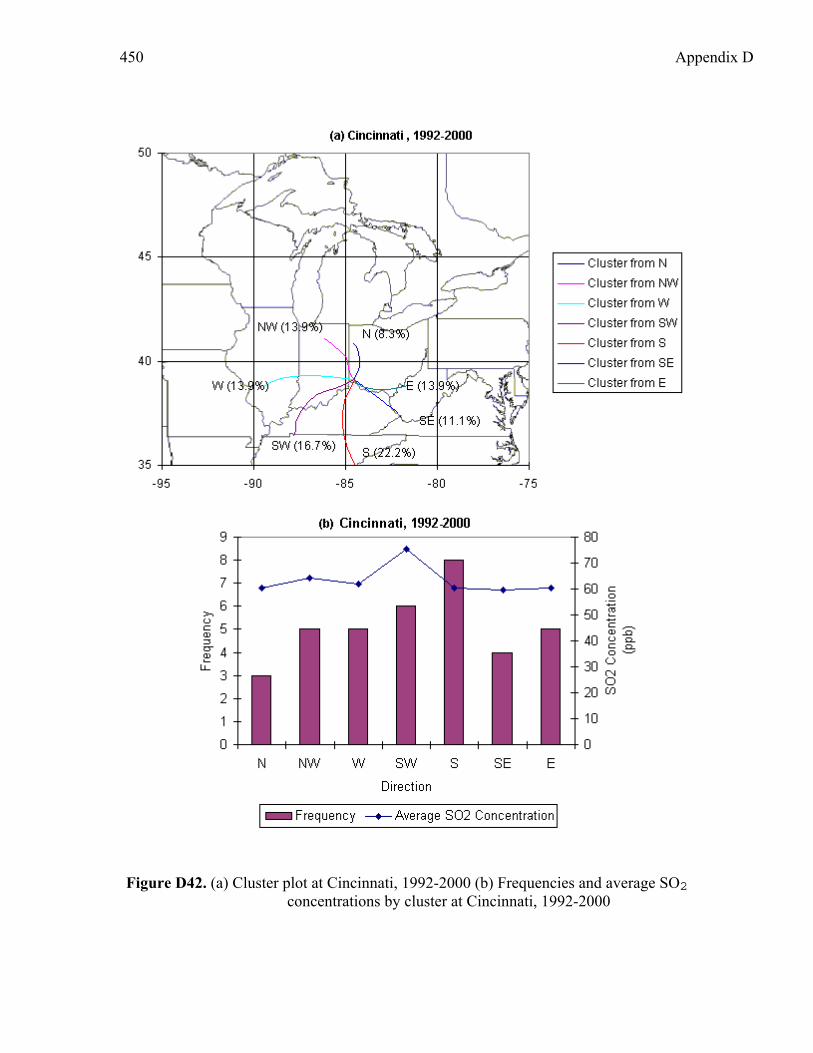
450 Appendix D
Figure D42. (a) Cluster plot at Cincinnati, 1992-2000 (b) Frequencies and average SO2
concentrations by cluster at Cincinnati, 1992-2000

Figure D43. (a) Cluster plot at Dayton, 1992-2000 (b) Frequencies and average SO2
concentrations by cluster at Dayton, 1992-2000

452 Appendix D
Figure D44. (a) Cluster plot at Columbus (Chesapeake), 1992-2000 (b) Frequencies and
average SO2 concentrations by cluster at Columbus (Chesapeake), 1992-2000
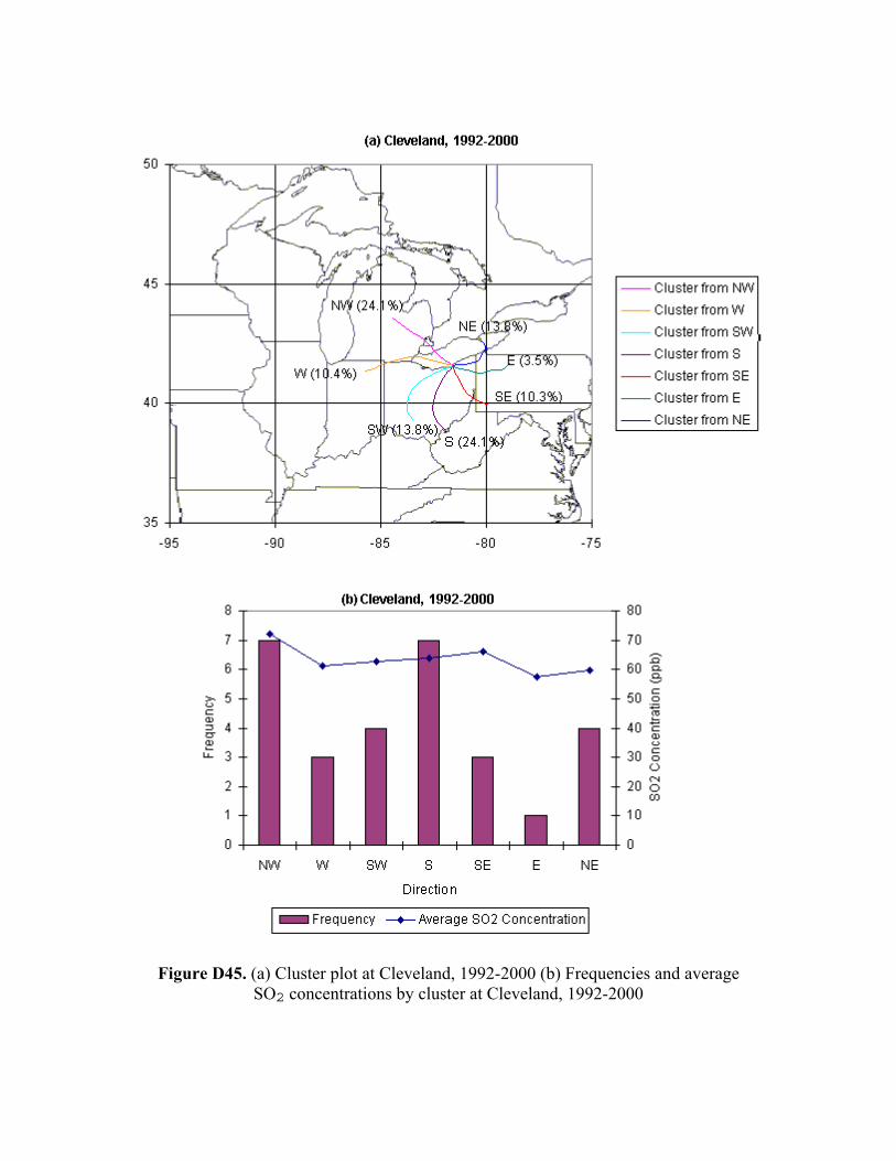
Figure D45. (a) Cluster plot at Cleveland, 1992-2000 (b) Frequencies and average SO2 concentrations by cluster at Cleveland, 1992-2000

454 Appendix D
Figure D46. (a) Cluster plot at Akron 1992-2000 (b) Frequencies and average SO2 concentrations by cluster at Akron, 1992-2000

Figure D47. (a) Cluster plot at Steubenville, 1992-2000 (b) Frequencies and average SO2 concentrations by cluster at Steubenville, 1992-2000

456 Appendix D
Figure D48. Back trajectories for high NO2 days at the monitoring sites selected in Ohio: Cleveland, 1992-1999
Figure D49. Back trajectories for high NO2 days at the monitoring sites selected in Ohio: Steubenville, 1992-1997
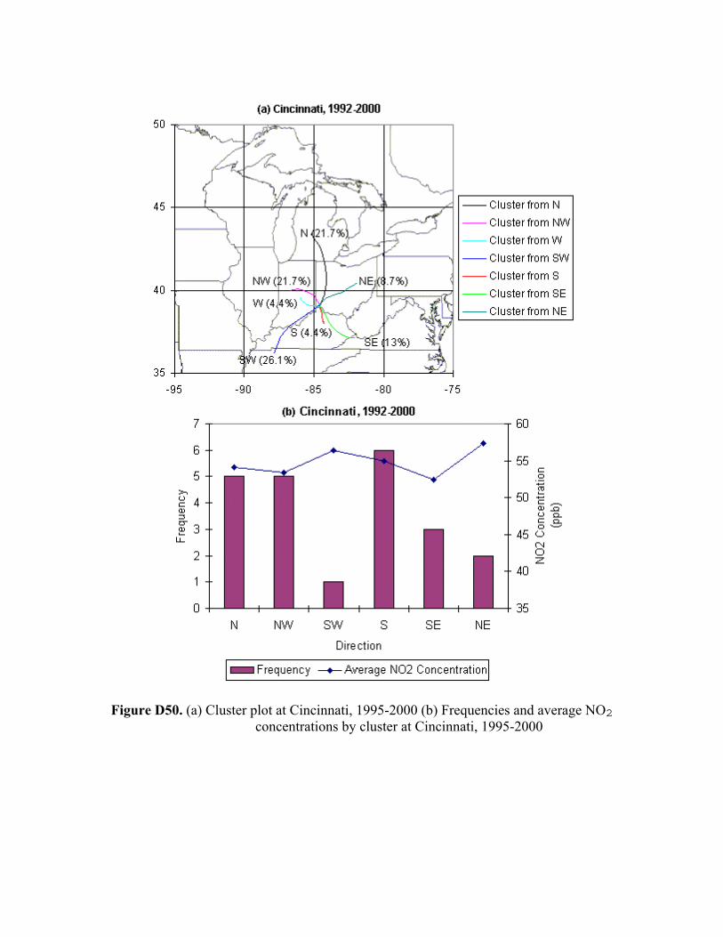
Figure D50. (a) Cluster plot at Cincinnati, 1995-2000 (b) Frequencies and average NO2
concentrations by cluster at Cincinnati, 1995-2000

458 Appendix D
Figure D51. (a) Cluster plot at Cleveland, 1995-2000 (b) Frequencies and average NO2
concentrations by cluster at Clevland, 1995-2000
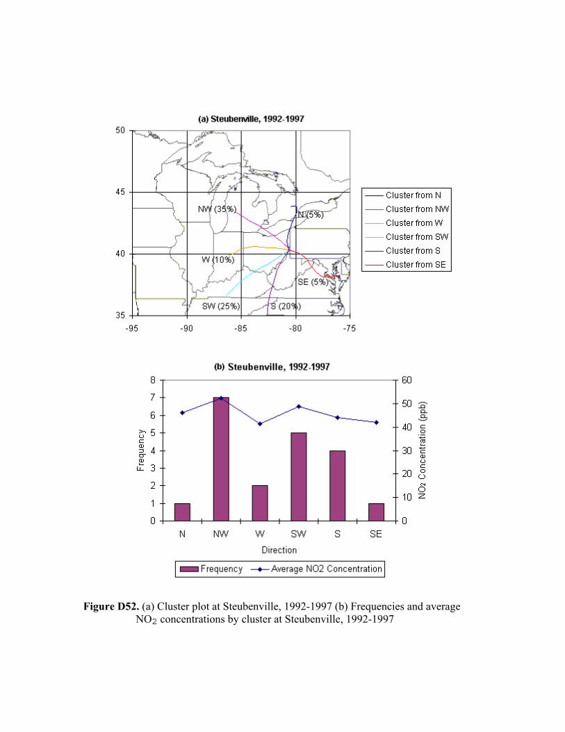
Figure D52. (a) Cluster plot at Steubenville, 1992-1997 (b) Frequencies and average NO2 concentrations by cluster at Steubenville, 1992-1997

460 Appendix D