appendix d – summary of existing simplified...

APPENDIX D – SUMMARY OF EXISTING SIMPLIFIED METHODS

D-1

An extensive literature search revealed many methods for the calculation of live

load distribution factors. This appendix will discuss, in detail, the procedures outlined in

the AASHTO LRFD Specifications (6) since the accuracy of most newly developed

methods are compared to this method. Other simple and/or more accurate methods

available will also be discussed in detail. Extensive research has shown that these

methods compare favorably with refined methods of analysis. Detailed calculations for

each method presented in this appendix are performed on a simple bridge and compared

to finite element analysis. These calculations can be found in Appendix E.

AASHTO LRFD Method

The AASHTO LRFD presents a set of equations for calculation of live load

distribution factors for interior and exterior beams for both moment and shear. In

addition to these equations, skew reduction and increase factor equations are presented

for moment and shear, respectively. Most variables in each set of equations contain

ranges of applicability. These variables include span length, beam spacing, slab

thickness, beam stiffness, and number of beams. When the variables are within their

range of applicability, the distribution factors calculated from these equations are

considered as accurate. However, the equations become less accurate when the ranges of

applicability are exceeded. The AASHTO LRFD Specifications state that a refined

analysis should be pursued for the distribution factors of bridge beams when the

requirements and/or ranges of applicability of the equations are not met.

Like any simplified method, the AASHTO LRFD method outlines several

conditions that a bridge must conform to in order to sustain a reasonable level of

accuracy. Section 4.6.2.2 of the specifications lists the conditions that must be met in

D-2

addition to any condition identified in the tables of distribution factors. The conditions

are as follows:

• Width of deck is constant;

• Unless otherwise specified, the number of beams is not less than four;

• Beams are parallel and have approximately the same stiffness;

• Unless otherwise specified, the roadway part of the overhang, de, does not exceed

3.0 ft;

• Curvature in plan is less than the limit specified in Article 4.6.1.2, which states:

segments of horizontally curved superstructures with torsionally stiff closed

sections whose central angle subtended by a curved span or portion thereof is less

than 12.0° may be analyzed as if the segment were straight; and

• Cross-section is consistent with one of the cross-sections shown in Table

4.6.2.2.1-1 of the specifications.

Distribution of Live Load Moment

The live load moment distribution factor equations for selected bridges are shown

in Table D-1 and Table D-2 for interior and exterior beams, respectively. The equations

for slab bridges are shown in Table D-3. The range of applicability of each equation is

also included in these tables. The corresponding skew correction factors for each bridge

type are shown in Table D-4.

D-3

Table D-1. Distribution of Live Loads per Lane for Moment in Interior Beams

Type of Superstructure

Applicable Cross-Section

from Table 4.6.2.2.1-1

Distribution Factors Range of Applicability

One Design Lane Loaded:

Two or More Design Lanes Loaded:


Two or More Design Lanes Loaded: If N c > 8 use N c = 8


Two or More Design Lanes Loaded:

Use Lever Rule S > 11.5Regardless of Number of Loaded Lanes:Concrete Deck on

Multiple Steel Box Girders

b, c

a, e, k and also i, j if

sufficiently connected to act as a unit

use lesser of the values obtained from the equation above with N b = 3 or the lever rule

Multicell Concrete Box Beam

d

Concrete Deck, Filled Grid, or Partially Filled Grid on Steel or Concrete Beams; Concrete T-Beams, T- and Double T- Sections

N b = 3

Concrete Deck on Concrete Spread Box Beams

b, c

1.0

3

3.04.0

0.121406.0 ⎟⎟

⎠

⎞⎜⎜⎝

⎛⎟⎠⎞

⎜⎝⎛

⎟⎠⎞

⎜⎝⎛+

s

g

LtK

LSS

1.0

3

2.06.0

0.125.9075.0 ⎟⎟

⎠

⎞⎜⎜⎝

⎛⎟⎠⎞

⎜⎝⎛

⎟⎠⎞

⎜⎝⎛+

s

g

LtK

LSS

4 240 2012.0 4.516.0 3.5

≥≤≤≤≤≤≤

b

s

NLtS

45.035.0 113.6

1.75 ⎟⎟⎠

⎞⎜⎜⎝

⎛⎟⎠⎞

⎜⎝⎛

⎟⎠⎞

⎜⎝⎛ +

cNLS

25.03.01

5.813

⎟⎠⎞

⎜⎝⎛

⎟⎠⎞

⎜⎝⎛

⎟⎟⎠

⎞⎜⎜⎝

⎛L

SNc

3 240 6013.0 7.0

≥≤≤≤≤

cNLS

25.0

2

35.0

12.03.0⎟⎠⎞

⎜⎝⎛

⎟⎠⎞

⎜⎝⎛

LSdS

125.0

2

6.0

12.06.3⎟⎠⎞

⎜⎝⎛

⎟⎠⎞

⎜⎝⎛

LSdS

3 65 18140 2011.5 6.0

≥≤≤≤≤≤≤

cNdLS

Lb

L

NNN 0.425 0.85 05.0 ++

1.5 5.0 ≤≤b

L

NN

D-4

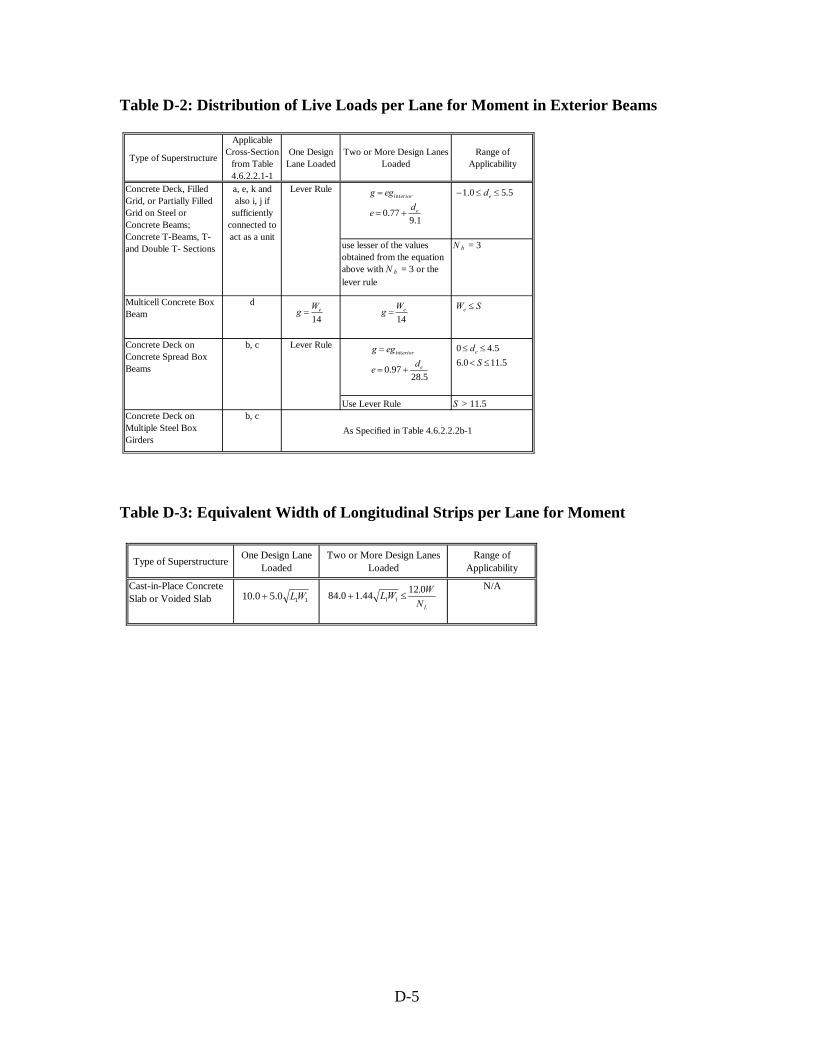
Table D-2: Distribution of Live Loads per Lane for Moment in Exterior Beams




One Design Lane Loaded

Two or More Design Lanes Loaded

Range of Applicability

Use Lever Rule S > 11.5

use lesser of the values obtained from the equation above with N b = 3 or the lever rule

N b = 3


b, c

Lever Rule

Lever Rule




d


Concrete Deck on Multiple Steel Box Girders

b, cAs Specified in Table 4.6.2.2.2b-1

9.1 0.77

int

e

erior

de

egg

+=

= 5.5 0.1 ≤≤− ed

14 eWg =

14 eWg =

SWe ≤

11.5 6.04.5 0

≤<≤≤

Sde

28.5 0.97

int

e

erior

de

egg

+=

=

Table D-3: Equivalent Width of Longitudinal Strips per Lane for Moment

Type of Superstructure One Design Lane Loaded



N/ACast-in-Place Concrete Slab or Voided Slab 115.0 0.10 WL+

LNW.WL 012 1.44 0.84 11 ≤+

D-5

Table D-4: Reduction of Load Distribution Factors for Moment in Longitudinal Beams on Skewed Supports




Any Number of Design Lanes Loaded


Cast-in-Place Concrete Slab or Voided Slab

N/A N/A

Concrete Deck on Concrete Spread Box Beams, Concrete Box Beams, and Double T- Sections used in Multibeam Decks

b, c, f, g




( )5.025.0

31

511

0.1225.0

tan1

⎟⎠⎞

⎜⎝⎛

⎟⎟⎠

⎞⎜⎜⎝

⎛=

−

LS

LtK

c

θc

s

g

.

°=°>=°<60 use 60 If

0.0 then 30 If 1

θθcθ

4 240 2016.0 3.560 30

≥≤≤≤≤

°≤≤°

bNLSθ

°=°>

≤

60 use 60 If

1.0 tan0.25 - 05.1

θθ

θ °≤≤ 60 0 θ

1.0 tan0.25 - 05.1 ≤θ

The multiple presence factors shown in Table D-5 have already been incorporated

into the tabulated distribution factor equations previously shown.

Because diaphragms were not considered in the models, the specifications include

an interim provision that states:

“In beam-slab bridge cross-sections with diaphragms or cross-frames, the

distribution factor for the exterior beam shall not be taken to be less than that

which would be obtained by assuming that the cross-section deflects and rotates

as a rigid cross-section.”

The procedure is the same as the conventional approximation for loads on piles.

The distribution factor is determined by the following equation:

D-6

∑

∑+=

b

L

N

N

ext

b

L

x

eX

NNR

2 (D-1)

where,

R = reaction on exterior beam in terms of lanes;

NL = number of loaded lanes under consideration;

Table D-5: Multiple Presence Factors

1 1.202 1.003 0.85

4 or more 0.65

Number of Loaded Lanes

Multiple Presence Factor

"m"

e = eccentricity of a design truck or a design lane load from the center of

gravity of the pattern of girders (ft);

x = horizontal distance from the center of gravity of the pattern of girders to

each girder (ft);

Xext = horizontal distance from the center of gravity of the pattern of girders to

the exterior girder (ft); and

Nb = number of beams.

Distribution of Live Load Shear

The live load shear distribution factor equations for selected bridges are shown in

Table D-6 and Table D-7 for interior and exterior beams, respectively. The equations for

D-7

slab bridges are the same as shown in Table D-3. The range of applicability of each

equation is also included in these tables. The corresponding skew correction factors for

each bridge type are shown in Table D-8.

Table D-6: Distribution of Live Loads per Lane for Shear in Interior Beams





Two or More Design Lanes

LoadedRange of Applicability

Lever Rule Lever Rule N b = 3

Lever Rule Lever Rule S > 11.5

As specified in Table 4.6.2.2.2b-1Concrete Deck on Multiple Steel Box Girders

b, c


d



b, c



4

7,000,000 10,000240 2012.0 4.516.0 3.5

≥

≤≤≤≤≤≤≤≤

b

g

s

N

KLtS

3 110 35240 2013.0 6.0

≥≤≤≤≤≤≤

cNdLS

3 65 18140 2011.5 6.0

≥≤≤≤≤≤≤

cNdLS

25.0 36.0 S

+0.2

35 -

12 2.0 ⎟

⎠⎞

⎜⎝⎛+

SS

1.06.0

0.125.9⎟⎠⎞

⎜⎝⎛

⎟⎠⎞

⎜⎝⎛

LdS 1.09.0

0.123.7⎟⎠⎞

⎜⎝⎛

⎟⎠⎞

⎜⎝⎛

LdS

1.06.0

0.1210⎟⎠⎞

⎜⎝⎛

⎟⎠⎞

⎜⎝⎛

LdS 1.08.0

0.124.7⎟⎠⎞

⎜⎝⎛

⎟⎠⎞

⎜⎝⎛

LdS

D-8

Table D-7: Distribution of Live Loads per Lane for Shear in Exterior Beams





Two or More Design Lanes

Loaded


Lever Rule S > 11.5

Lever Rule

Lever RuleMulticell Concrete Box Beam




d


b, c

Concrete Deck on Multiple Steel Box Girders

b, cAs Specified in Table 4.6.2.2.2b-1

Lever Rule

10 0.6

int

e

erior

de

egg

+=

= 5.5 0.1 ≤≤− ed

4.5 0 ≤≤ ed

10 0.8

int

e

erior

de

egg

+=

=

5.0 0.2 ≤≤− ed

12.5 0.64

int

e

erior

de

egg

+=

=

Table D-8: Correction Factors for Load Distribution Factors for Support Shear of the Obtuse Corner







b, c





d

θK

Lt.

g

s tan0120.20 0.13.0

3

⎟⎟⎠

⎞⎜⎜⎝

⎛+

4 240 2016.0 3.5

60 0

≥≤≤≤≤

°≤≤°

bNLSθ

θS

Ld

tan612.0 0.1 +

3 110 35240 2013.0 0.660 0

≥≤≤≤≤≤<

°≤<°

cNdLSθ

θdL tan

7012.0 0.25 0.1 ⎥

⎦

⎤⎢⎣

⎡⎟⎠⎞

⎜⎝⎛++

3 65 18140 2011.5 0.660 0

≥≤≤≤≤≤<

°≤<°

bNdLSθ

D-9

The variables in Table D-1 through Table D-4 and Table D-6 through Table D-8 are

defined as follows:

A = area of beam (in2);

d = depth of beam (in);

de = distance from exterior web of exterior beam and the interior edge of curb

or traffic barrier (ft);

e = correction factor;

eg = distance between the centers of gravity of the basic beam and deck (in.);

g = distribution factor;

I = moment of inertia of beam (in4);

Kg = n(I + Aeg2) = longitudinal stiffness parameter (in4);

L = span length (ft);

L1 = modified span length taken equal to the lesser of the actual span or 60.0 ft;

n = modular ratio;

Nb = number of beams;

Nc = number of cells in a concrete box girder;

NL = number of design lanes;

S = beam spacing (ft);

ts = slab thickness (in);

θ = skew angle (deg);

D-10

W = physical edge-to-edge width of bridge (ft);

W1 = modified edge-to-edge width of bridge taken equal to the lesser of the

actual width or 60.0 ft for multilane loading, or 30.0 ft for single-lane

loading (ft); and

We = half the web spacing, plus the total overhang (ft).

D-11

Canadian Highway Bridge Design Code Method

The simplified method presented in the Canadian Highway Bridge Design Code

(CHBDC) (27) for live load analysis is applicable, provided that the bridge in question

satisfies the following conditions:

• The width is constant;

• The support conditions are closely equivalent to line support, both at the ends of

the bridge and, in the case of multispan bridges, at intermediate supports;

• For slab bridges and slab-on-girder bridges with skew, the following provisions

are met:

o For solid and voided slab bridges, the skew parameter

( ) ( )[ ]61

LengthSpan Angle Skewtan WidthBridge ≤=ε

o For slab-on-girder bridges, the skew parameter

( ) ( )[ ] ;181

LengthSpan Angle SkewtanSpacingGirder ≤=ε

• For bridges that are curved in plan, the radius of curvature, span, and width satisfy

the following provisions:

o ( )( )( ) 1.0

Curvature of Radius WidthBridge5.0LengthSpan 2

≤

o There are at least two intermediate diaphragms per span;

D-12

• A solid or voided slab is of substantially uniform depth across a transverse

section, or tapered in the vicinity of a free edge provided that the length of the

taper in the transverse direction does not exceed 2.5 m;

• For slab-on-girder bridges, there shall be at least three longitudinal girders that are

of equal flexural rigidity and equally spaced, or with variations from the mean of

not more than 10% in each case;

• For a bridge having longitudinal girders and an overhanging deck slab, the

overhang does not exceed 60% of the mean spacing between the longitudinal

girders or the spacing of the two outermost adjacent webs for box girder bridges

and, also, is not more than 1.80 m;

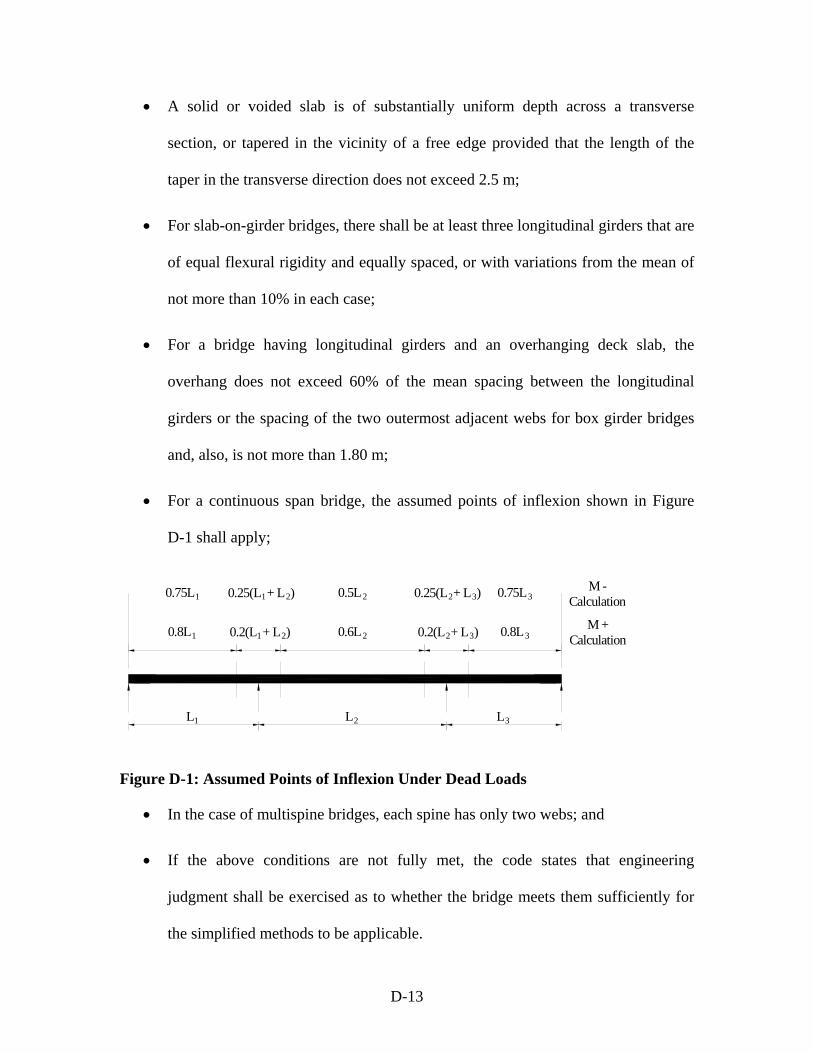
• For a continuous span bridge, the assumed points of inflexion shown in Figure

D-1 shall apply;

L1 L2 L3

0.8L1 0.2(L + L )1 0.6L2 0.8L32 0.2(L + L )2 3

0.75L 0.25(L + L )1 1 2 0.5L2 20.25(L + L )3 0.75L3M -

Calculation

M +Calculation

Figure D-1: Assumed Points of Inflexion Under Dead Loads

• In the case of multispine bridges, each spine has only two webs; and

• If the above conditions are not fully met, the code states that engineering

judgment shall be exercised as to whether the bridge meets them sufficiently for

the simplified methods to be applicable.

D-13

Superstructure types are grouped into two categories, which include shallow

superstructure and multispine bridges. Shallow superstructures include the following

bridge types:

• Slab;

• Voided Slab, including multicell box girders meeting diaphragm requirements;

• Slab-on-girder;

• Steel grid deck-on-girder;

• Wood deck-on-girder;

• Wood deck on longitudinal wood beam;

• Stress-laminated wood deck bridges spanning longitudinally;

• Longitudinal nail-laminated wood deck bridges;

• Longitudinal laminates of wood-concrete composite decks; and

• Shear-connected beam bridges in which the interconnection of adjacent beams is

such as to provide continuity of transverse flexural rigidity across the cross-

section.

Multispine bridges include:

• Box girder bridges in which the boxes are connected by only the deck slab and

transverse diaphragms, if present; and

D-14

• Shear-connected beam bridges in which the interconnection of adjacent beams is

such as not to provide continuity of transverse flexural rigidity across the cross-

section.

Longitudinal Bending Moments for Ultimate and Serviceability Limit States

Girder-Type Bridges. The longitudinal moment per girder, Mg, is determined by using

the following equations:

N

RnMM LTg avg = (D-2)

1.05

100 1

≥

⎟⎟⎠

⎞⎜⎜⎝

⎛+

=f

m µCF

SNF (D-3)

avggmg MFM = (D-4)

where,

Mg avg = the average moment per girder determined by sharing equally the total

moment on the bridge cross-section among all girders in the cross-

section;

MT = the maximum moment per design lane at the point of the span under

consideration;

n = the number of design lanes;

D-15

RL = the modification factor for multilane loading equal to 1.0 for 1 lane

loaded, 0.90 for two lanes loaded, 0.80 for three lanes loaded, 0.70 for

four lanes loaded, 0.60 for five lanes loaded, and 0.55 for six or more

lanes loaded;

N = the number of girders;

Fm = an amplification factor to account for the transverse variation in

maximum longitudinal moment intensity, as compared to the average

longitudinal moment intensity;

µ = 1.0; 0.6

3.3 - ≤eW

We = width of a design lane (m);

S = center-to-center girder spacing (m);

Cf = a correction factor (%); and

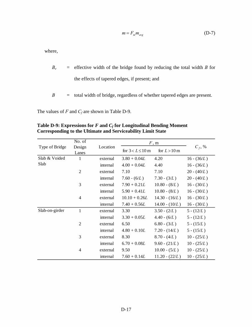
F = a width dimension that characterizes load distribution for a bridge.

The values of F and Cf are shown in Table D-9.

Slab and Voided Slab Bridges.

e

LTavg B

RnMm = (D-5)

1.05

100 1

≥

⎟⎟⎠

⎞⎜⎜⎝

⎛+

=f

m µCF

BF (D-6)

D-16

avgmmFm = (D-7)

where,

Be = effective width of the bridge found by reducing the total width B for

the effects of tapered edges, if present; and

B = total width of bridge, regardless of whether tapered edges are present.


Table D-9: Expressions for F and Cf for Longitudinal Bending Moment Corresponding to the Ultimate and Serviceability Limit State

1 external 3.80 + 0.04L 4.20 16 - (36/L )internal 4.00 + 0.04L 4.40 16 - (36/L )

2 external 7.10 7.10 20 - (40/L )internal 7.60 - (6/L ) 7.30 - (3/L ) 20 - (40/L )

3 external 7.90 + 0.21L 10.80 - (8/L ) 16 - (30/L )internal 5.90 + 0.41L 10.80 - (8/L ) 16 - (30/L )


1 external 3.30 3.50 - (2/L ) 5 - (12/L )internal 3.30 + 0.05L 4.40 - (6/L ) 5 - (12/L )




Type of Bridge

Slab & Voided Slab

Slab-on-girder

F , mNo. of Design Lanes

Location C f , %m 10 3for ≤< L m 10 for >L

D-17

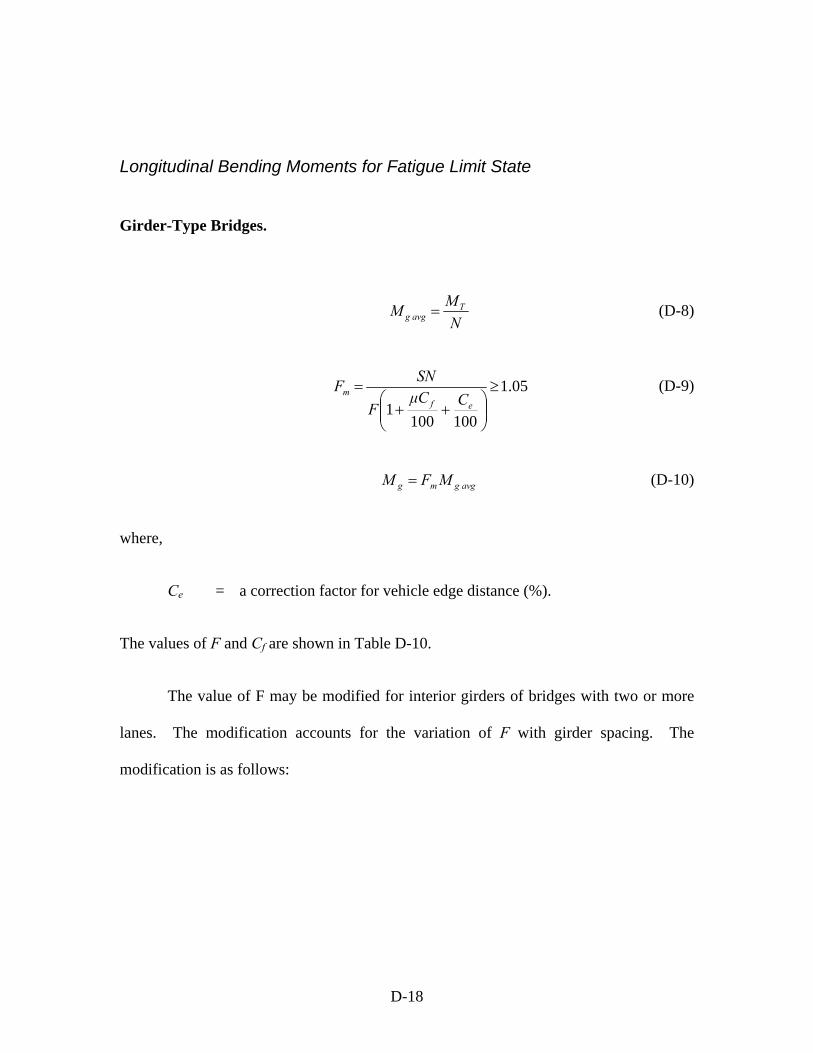
Longitudinal Bending Moments for Fatigue Limit State

Girder-Type Bridges.

N

MM Tg avg = (D-8)

1.05

100

100 1

≥

⎟⎟⎠

⎞⎜⎜⎝

⎛++

=ef

m CµCF

SNF (D-9)

avggmg MFM = (D-10)

where,

Ce = a correction factor for vehicle edge distance (%).


The value of F may be modified for interior girders of bridges with two or more

lanes. The modification accounts for the variation of F with girder spacing. The

modification is as follows:

D-18

For m 50 m 10 ≤≤ L

( ) ⎥⎦

⎤⎢⎣

⎡⎟⎠⎞

⎜⎝⎛+=

4010 - 0.35 - 0.29 00.1 LSFF tab (D-11)

For L > 50 m

( )0.65 0.29 += SFF tab (D-12)

where,

Ftab = value of F found for the internal girders from Table D-10. The girder

spacing S is limited to m. 3.6 m 2.1 ≤≤ S A value of S equal to 3.6 m

may be used if S exceeds 3.6 m.

Slab and Voided Slab Bridges.

e

Tavg B

Mm = (D-13)

1.05

100 1

≥

⎟⎟⎠

⎞⎜⎜⎝

⎛+

=f

m µCF

BF (D-14)

avgmmFm = (D-15)

The values of F and Cf are found in Table D-10.

D-19

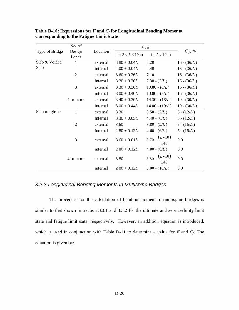
Table D-10: Expressions for F and Cf for Longitudinal Bending Moments Corresponding to the Fatigue Limit State

1 external 3.80 + 0.04L 4.20 16 - (36/L )internal 4.00 + 0.04L 4.40 16 - (36/L )

2 external 3.60 + 0.26L 7.10 16 - (36/L )internal 3.20 + 0.30L 7.30 - (3/L ) 16 - (36/L )


4 or more external 3.40 + 0.30L 14.30 - (16/L ) 10 - (30/L )internal 3.00 + 0.44L 14.00 - (10/L ) 10 - (30/L )



3 external 3.60 + 0.01L 0.0

internal 2.80 + 0.12L 4.80 - (8/L ) 0.0

4 or more external 3.80 0.0

internal 2.80 + 0.12L 5.00 - (10/L ) 0.0

Slab-on-girder

Slab & Voided Slab

Type of BridgeNo. of Design Lanes

LocationF , m

C f , %m 10 3for ≤< L m 10 for >L

( )140

10 - 70.3 L+

( )140

10 - 80.3 L+

3.2.3 Longitudinal Bending Moments in Multispine Bridges

The procedure for the calculation of bending moment in multispine bridges is

similar to that shown in Section 3.3.1 and 3.3.2 for the ultimate and serviceability limit

state and fatigue limit state, respectively. However, an addition equation is introduced,

which is used in conjunction with Table D-11 to determine a value for F and Cf. The

equation is given by:

D-20

5.0

⎟⎟⎠

⎞⎜⎜⎝

⎛⎟⎠⎞

⎜⎝⎛=

xy

x

DD

LBπβ (D-16)

where,

B = width of bridge for ULS and SLS, but no greater than three times the

spine spacing S for FLS;

Dx = total bending stiffness, EI, of the bridge cross-section divided by the

width of the bridge; and

Dxy = total torsional stiffness, GJ, of the cross-section divided by the width

of the bridge.

Table D-11: Expressions for F and Cf for Longitudinal Moments in Multispine Bridges

Limit State Number of Design Lanes F , m C f , %ULS or SLS 2 8.5 - 0.3β 16 - 2β

3 11.5 - 0.5β 16 - 2β4 14.5 - 0.7β 16 - 2β

FLS 2 or more 8.5 - 0.9β 16 - 2β

3.2.4 Longitudinal Vertical Shear for Ultimate and Serviceability Limit States

Girder Type Bridges. The longitudinal shear per girder, Vg, is determined by using the following equations:

N

RnVV LTavgg = (D-17)

F

SNFv = (D-18)

avggvg VFV = (D-19)

D-21

where,

Vg avg = the average shear per girder determined by sharing equally the total

shear on the bridge cross-section among all girders in the cross-

section;

VT = the maximum shear per lane at the points of the span under

consideration; and

Fv = an amplification factor to account for the transverse variation in

maximum longitudinal vertical shear intensity, as compared to the

average longitudinal vertical shear intensity.

The values of F are found in Table D-12. When the girder spacing is less than

2.00 m, the value of F shall be multiplied by the following reduction factor:

25.0

00.2 ⎥⎦⎤

⎢⎣⎡ S (D-20)

Slab and Voided Slab Bridges. The longitudinal vertical shear per meter of width is

calculated from the following:

e

LTavg B

RnVv = (D-21)

1.05 ≥=FBFv (D-22)

D-22

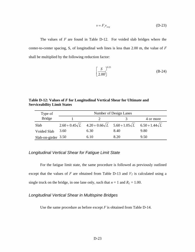
avgvvFv = (D-23)

The values of F are found in Table D-12. For voided slab bridges where the

center-to-center spacing, S, of longitudinal web lines is less than 2.00 m, the value of F

shall be multiplied by the following reduction factor:

25.0

00.2 ⎥⎦⎤

⎢⎣⎡ S (B-24)

Table D-12: Values of F for Longitudinal Vertical Shear for Ultimate and Serviceability Limit States

1 2 3 4 or m

SlabVoided Slab 3.60 6.30 8.40 9.80

Slab-on-girder 3.50 6.10 8.20 9.50

Type of Bridge

Number of Design Lanesore

L0.45 60.2 + L0.66 20.4 + L1.05 60.5 + L1.44 50.6 +

Longitudinal Vertical Shear for Fatigue Limit State

For the fatigue limit state, the same procedure is followed as previously outlined

except that the values of F are obtained from Table D-13 and VT is calculated using a

single truck on the bridge, in one lane only, such that n = 1 and RL = 1.00.

Longitudinal Vertical Shear in Multispine Bridges

Use the same procedure as before except F is obtained from Table D-14.

D-23

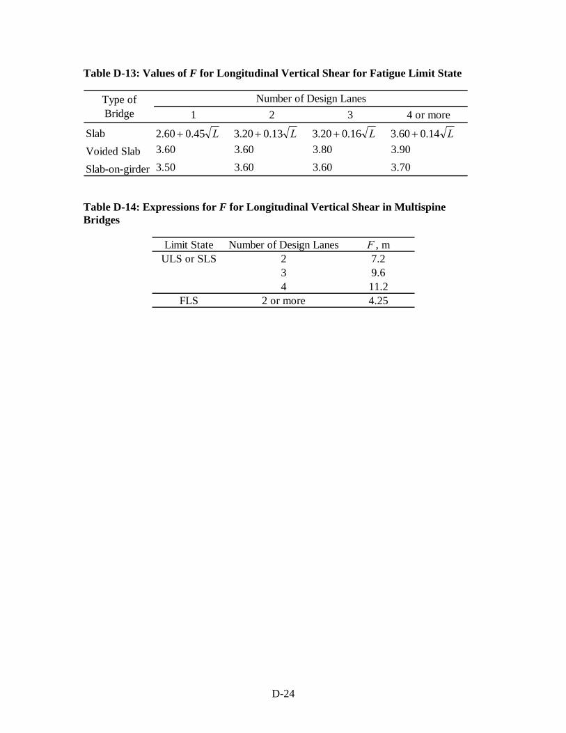
Table D-13: Values of F for Longitudinal Vertical Shear for Fatigue Limit State

1 2 3 4 or m

SlabVoided Slab 3.60 3.60 3.80 3.90

Slab-on-girder 3.50 3.60 3.60 3.70

Type of Bridge

Number of Design Lanesore

L0.45 60.2 + L0.13 20.3 + L0.16 20.3 + L0.14 60.3 +

Table D-14: Expressions for F for Longitudinal Vertical Shear in Multispine Bridges

Limit State Number of Design Lanes F , mULS or SLS 2 7.2

3 94 11.2

FLS 2 or more 4.25

.6

D-24

Henry’s Equal Distribution Factor Method

Henry’s equal distribution factor (EDF) method is by far the simplest of all

methods previously discussed. Because the EDF method requires only the width of the

roadway, number of traffic lanes, number of beam lines, and the multiple-presence factor

of the bridge, it can be applied without difficulty to different types of superstructures and

beam arrangements. The procedure for the calculation of distribution factors is as

follows (60):

Step 1: Reinforced Concrete I-beams, Reinforced Concrete Box Beams, Precast

Box Beams:

(a) Divide roadway width by 10 ft to determine the fractional number of traffic

lanes.

(b) Reduce the value from (a) by a factor obtained from a linear interpolation for

intensity to determine the total number of traffic lanes considered for carrying

live load on bridge. Table D-15 shows the multiple-presence factor for a

specific number of loaded lanes.

(c) Divide the total number of lanes by the number of beams to determine the

number of lanes of live load per beam, or the distribution factor of lane load per

beam.

Step 2: Steel and Prestressed I-beams:

(d) Proceed with steps (a) through (c) above.

(e) Multiply the value from (c) by a ratio of 6/5.5 or 1.09 to determine the

D-25

distribution factor of lane load per beam

Table D-15: Multiple Presence Factors

2 1.003 0.90

4 or more 0.75

Number of Loaded Lanes

Multiple Presence Factor "m"

Modified Henry’s Method

Modification factors to Henry’s method were developed based on a comparison

and evaluation study conducted by Huo et al. (59). Distribution factors from Henry’s

method were compared to the AASHTO Standard and AASHTO LRFD methods in

addition to finite element analysis. Two sets of modification factors for moment and

shear distribution were recommended. The first set includes moment modification

factors based on superstructure type along with a single shear factor applicable to all

structure types. The second set of modification factors includes separate sets of factors

for moment and shear. The effects of skew and span length are included in the second set

of modification factors.

Modification Factors for Live Load Moment and Shear (Set 1). The

procedure for the calculation of moment and shear distribution factors using set 1

modification factors is as follows:

Step 1: Basic Equal Distribution Factor - follow (a) through (c) in Section 3.3.

Step 2: Superstructure Type Modification - Moment Distribution Factors

D-26

(d) Multiply the value from (c) by the appropriate moment modification factor

from Table D-16 to determine the moment distribution factor.

Step 3: Superstructure Type Modification – Shear Distribution Factors

(e) Multiply the value from (d) by the shear factor in Table D-16 to determine the

shear distribution factor.

Modification Factors for Live Load Moment and Shear (Set 2). The

procedure for the calculation of moment and shear distribution factors using set 2

modification factors is as follows:

Step 1: Basic Equal Distribution Factor - follow (a) through (c) in Section 3.3.

For Moment Distribution Factor:

Step 2: Superstructure Type Modification

(d) Multiply the value from (c) by the appropriate structure type modification factor

from Table D-17.

Step 3: Skew Angle and Span Length Modification

(a) If applicable, multiply the value from (d) by the skew angle and/or span length

modification factor from Table D-17 to determine the final moment distribution

factor.

For Shear Distribution Factor:

Step 2: Superstructure Type Modification

(e) Multiply the value from (c) by the appropriate structure type modification factor

from Table D-18.

D-27

Step 3: Skew Angle Modification

(b) If applicable, multiply the value from (d) by the skew angle modification factor

from Table D-18 to determine the final shear distribution factor.

Table D-16: Structure Type Modification Factors (Set 1)

Moment Shear Precast Spread Box Beam b 1.00Precast Concrete I-Sections k 1.10CIP Concrete T-Beam e 1.05CIP Concrete Box Beam d 1.05Steel I-Beam a 1.10Steel Open Box Beam c 1.00

Structure Type

1.15

Modification FactorAASHTO LRFD Cross Section Type

Table D-17: Modification Factors for Live Load Moment (Set 2)

θ < 30o θ > 30o L < 100 ft L > 100 ftPrecast Spread Box Beam b 1.00Precast Concrete I-Sections k 1.15CIP Concrete T-Beam e 1.10CIP Concrete Box Beam d 1.10Steel I-Beam a 1.15Steel Open Box Beam c 1.10

Modification Factor

Structure TypeAASHTO LRFD

Cross Section TypeSkew Angle Span Length

1.00 0.94 1.00 0.94

Structure Type

Table D-18: Modification Factors for Live Load Shear (Set 2)

Structure Type Skew AnglePrecast Spread Box Beam b 1.05Precast Concrete I-Sections k 1.20CIP Concrete T-Beam e 1.05CIP Concrete Box Beam d 1.20Steel I-Beam a 1.15Steel Open Box Beam c 1.15

Modification FactorAASHTO LRFD Cross Section Type

1.0 + 0.2tanθ

Structure Type

D-28

Sanders and Elleby Method

The method proposed by Sanders and Elleby (106) follows the simple S/D

approach, which has been utilized in the AASHTO Standard Specifications for many

years. The exception is the calculation of the D constant. The value of D is determined

by the following relationships:

3For ≤C

2

31

723

105 ⎟

⎠⎞

⎜⎝⎛ −⎟

⎠⎞

⎜⎝⎛ −++=

CNND LL (D-25)

3For >C

10

5 LND += (D-26)

where,

NL = total number of design traffic lanes; and

C = a stiffness parameter that depends on the type of bridge, bridge and beam

properties, and material properties.

The stiffness parameter, C is calculated as follows, for beam and slab and multi-

beam bridges:

21

1

1

2 ⎥⎦

⎤⎢⎣

⎡+

=tJJ

IGE

LWC (D-27)

For concrete box girder bridges:

D-29

( )21

121

2 ⎥⎦

⎤⎢⎣

⎡+⎟⎟

⎠

⎞⎜⎜⎝

⎛+=

dg NG

EWdN

LWC (D-28)

where,

W = overall bridge width (ft);

L = span length (distance between live load points of inflection for continuous

span) (ft);

E = modulus of elasticity of the transformed beam section;

G = modulus of rigidity of the transformed beam section;

I1 = flexural moment of inertia of the transformed beam section per unit width;

J1 = torsional moment of inertia of the transformed beam section per unit

width;

Jt = ½ of the torsional moment of inertia of a unit width of bridge deck slab;

d = depth of the bridge from center of top slab to center of bottom slab;

Ng = number of girder stems; and

Nd = number of interior diaphragms.

For preliminary designs of beam and slab bridges, the parameter C can be approximated

by using the values given in Table D-19.

D-30

Table D-19: Values of K to be used in C = K(W/L)

Bridge Type Beam Type and Deck Material K Concrete deck: Beam and slab (includes

concrete slab bridge) Noncomposite steel I-beams 3.0 Composite steel I-beams 4.8

Nonvoided concrete beams (prestressed or reinforced) 3.5

Separated concrete box-beams 1.8 Concrete slab bridge 0.6

The following two parameters were considered the most important regarding

lateral distribution of a wheel line:

42 y

x

DD

LWθ = (D-29)

⎟⎟

⎠

⎞

⎜⎜

⎝

⎛ +=

yx

yxxy

DDDD

α21 (D-30)

where,

θ = flexural parameter;

α = torsional parameter;

L = span length (ft);

W = bridge width (ft);

Dxy = torsional stiffness in the longitudinal direction (lb-in2/ft);

Dyx = torsional stiffness in the transverse direction (lb-in2/ft);

Dx = flexural stiffness in the longitudinal direction (lb-in2/ft); and

D-31

Dy = flexural stiffness in the transverse direction (lb-in2/ft).

For simplification, these two parameters were combined into one

parameter defined by:

yxxy

x

DDD

LW

αθC

+==

22 (D-31)

The calculation of this parameter is based on the following assumptions:

(1) A typical interior beam or diaphragm shall include a portion of the deck slab

equal to the beam or diaphragm spacing.

(2) Full transverse flexural and torsional continuity of the diaphragms is assumed

only when they are rigidly connected to the longitudinal beams.

(3) The torsional rigidity of the steel beams or diaphragms is ignored.

(4) For flexural and torsional rigidity calculations of steel beam-concrete deck bridge

types, the steel cross-sectional area should be expressed as an equivalent area of

concrete.

(5) The uncracked gross area of the concrete cross section may be used for rigidity

calculations involving prestressed or reinforced concrete structural members.

(6) Standard engineering procedures are used for computing the torsional and flexural

rigidities of typical bridge systems.

To consider the effect of diaphragms, the torsional stiffness in the transverse

direction, Dyx, should be increased by the torsional stiffness of the diaphragm divided by

its spacing.

D-32

Alternate Distribution Factor Method for Moments

None of the simplified methods listed above performed well for moment

distribution for an interior girder with one lane loaded. An effort was made to develop a

simplified method to address this problem. A parametric equation was developed for use

in this case. In the interest of being thorough, the method was applied to all loading and

girder position cases, and it was discovered that it performed well for several cases.

The equation takes the form of

321 1Exp

g

ExpExp

NLS

DSg ⎟

⎟⎠

⎞⎜⎜⎝

⎛⎟⎠⎞

⎜⎝⎛

⎟⎠⎞

⎜⎝⎛=

where Exp1, Exp2, Exp3, and D are constants that vary with bridge type,

S = the girder spacing in feet,

L = the span length in feet,

and Ng = the number of girders or number of cells + 1 for the bridge.

This parametric equation was developed by combining terms for the one lane

loaded interior girder moment distribution factor equations for I section and cast-in-place

box girder bridges. The terms that were dependent on the stiffness of the section were

dropped. By varying the values of the three exponents and the D constant, this equation

form produced reasonable results for the various bridge types. In cases where one of the

exponents was determined to be near zero, the term was dropped (exponent was set equal

to zero) in order to simplify the application of this equation as much as possible

D-33

appendix d – summary of existing simplified...

Documents