1

APPENDIX

The derivation of the equation for Reynolds Number for use in the sizing of control valves for non-turbulent flow (laminar and transitional)

The role of Fd and CVRTL in calculating Rev for control valves. The definition of the valve style modifier Fd, can be found in IEC std. 60534-2-1. In Reynolds Number the characteristic dimension “J” for control valves is the hydraulic mean diameter dH. dH = 4 x effective area of the conduit / the wetted perimeter. For a circular pipe or orifice with no restrictions or irregularities dH = the pipe or orifice diameter. Fd = dH/de where dH = the hydraulic mean diameter of the controlling orifice (valve trim) and de = the equivalent circular diameter for the valve trim. For a single stage, single path trim the diameter of the vena contracta dVC is considered to be the same as de making Fd = dH/dVC.

The rated CV of a control valve is: L

apCV

2

S

4

VRTF

1KKKd.10625.4C

ds = metres CVRT = USGPM 2

vcC

2

s dK.d giving

apV

LVRT

3

VCK.K

1F.C1065.4d

CVRT is the rated CV for a valve to pass the required flow, but in the turbulent regime. As explained earlier an estimate must be made at this stage of the size of valve required to pass the specified flow but in the non-turbulent regime. CVRT is increased by a factor somewhere between 35% and 150% depending on the viscosity of the fluid. A valve is then selected with a rated CV nearest to this inflated CVRT. The selected rated CV is identified as CVRTL.

The vena contracta for this larger valve is: LVRTL

3

VC F.C1065.4d

The product of the velocity and approach coefficients may be accepted as approximately unity. To obtain the characteristic dimension l (hydraulic mean diameter) in control

valve terminology: J LVRTLd

3

dVC F.CF1065.4Fd

In reviewing the technical literature it is found that various authors indicate

that 1/ apVKK has a minimal effect on dVC.Fd. It therefore been omitted.

The fundamental equation for Reynolds Number is: υ

v.R ev

J

where v = the velocity at the vena contracta vvc. m/sec J = characteristic dimension = dVC.Fd. m υ= coef. of kinematic viscosity. m2/sec

Q= volumetric flow. m3/sec

2

VC

2

VC

vcd

Q273.1

.d

Q.4v

2

LVRTL

3

ddVC2

VC

evF.C1065.4

1

υ

1.273.Q.F.Fd.

d.υ

Q.273.1R

LVRTL

dev

F.Cυ

Q.F.76.273R Q= m3/sec, CVRTL= USGPM, υ= m2/sec

LVRTL

dev

F.Cυ

Q.F.076.0R * Q= m3/ hr, CVRTL= USGPM, υ= m2/sec

LVRTL

dev

F.Cυ

Q.F.000,76R Q= m3/ hr, CVRTL= USGPM, υ= centistokes

(centistokes = m2/ sec x10-6) * This is equation (A1) in IEC 60534-2-1 but omitting the bracket holding the velocity of approach term ) Approximate values of K may be calculated from:

for standard trims where 016.0d

C2

1

V 2

2

1

V

-3

d

C

102.14K

for reduced size trims where 001.0016.0d

C2

1

V

36.1

2

1

V3

d

C101.3841K

when 001.0d

C2

1

V K = 1 constant

Values of K (turbulent) calculated from these equations may differ slightly from the turbulent K values indicated in figures 7 and 8 which are considered to be the more realistic.

For high capacity valves where 047.0d

C2

1

V K (turbulent) as calculated from

the equation K

1014.2

d

C3

2

1

V

will result in values less than 1. This initially

seems strange since K is an indication of a valve’s resistance to flow so it is reasonable to expect its value to be in excess of 1.The low value is due to these valves having very high velocity of approach factors Kap and very low pressure recovery factors FL.

3

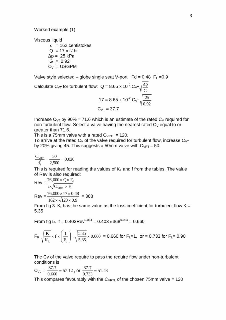
Worked example (1) Viscous liquid = 162 centistokes

Q = 17 m3/ hr Δp = 25 kPa G = 0.92 CV = USGPM Valve style selected – globe single seat V-port Fd = 0.48 FL =0.9

Calculate CVT for turbulent flow: Q = 8.65 X 10-2.CVTG

p

17 = 8.65 X 10-2.CVT0.92

25

CVT = 37.7 Increase CVT by 90% = 71.6 which is an estimate of the rated CV required for non-turbulent flow. Select a valve having the nearest rated CV equal to or greater than 71.6. This is a 75mm valve with a rated CVRTL = 120. To arrive at the rated CV of the valve required for turbulent flow, increase CVT by 20% giving 45. This suggests a 50mm valve with CVRT = 50.

020.0500,2

50

d

C2

1

VRT

This is required for reading the values of KL and f from the tables. The value of Rev is also required:

Rev =LVRTL

d

FC

FQ000,76

Rev =9.0120162

48.017000,76

= 368

From fig 3. KL has the same value as the loss coefficient for turbulent flow K = 5.35 From fig 5. f = 0.403Rev0.084 = 0.403 x 3680.084 = 0.660

FR 660.05.35

5.35

F

1f

K

K

LL

= 0.660 for FL=1, or = 0.733 for FL= 0.90

The Cv of the valve require to pass the require flow under non-turbulent conditions is

CVL = 12.57660.0

7.37 , or 43.51

733.0

7.37

This compares favourably with the CVRTL of the chosen 75mm valve = 120

4

If, in some cases, the CVRTL indicates a valve greater than the one selected at the beginning of the procedure, the calculation must be repeated with CVT increased by more than 90%. Worked example(2): Highly viscous liquid = 1,100 centistokes

Q = 17 m3/ hr Δp = 25 kPa G = 0.92 CV = USGPM Valve style selected – globe single seat V-port Fd = 0.48 FL =0.9

Calculate CVT for turbulent flow: Q = 8.65 X 10-2.CVTG

p

17 = 8.65 X 10-2.CVT0.92

25

CVT = 37.7 Increase CVT by 120% = 83 which is an estimate of the rated CV required for non-turbulent flow. Select a valve having the nearest rated CV equal to or greater than 83. This is a 75mm valve with a rated CVRTL = 120. To arrive at the rated CV of the valve required for turbulent flow, increase CVT by 20% giving 45. This suggests a 50mm valve with CVRT = 50.

020.0500,2

50

d

C2

1

VRT

This is required for reading the values of KL and f from the tables. The value of Rev is also required:

Rev =LVRTL

d

FC

FQ000,76

Rev =9.0120100,1

48.017000,76

= 54

From fig 3. KL = 610 / Rev = 610 / 54 =11.29 K = 5.35 From fig 4. f = 0.63

FR = 63.011.29

5.35

F

1f

K

K

LL

= 0.43 for FL=1, or = 0.48 for FL= 0.9

The Cv of the valve require to pass the require flow under non-turbulent conditions is:

5

CVL = 54.780.48

37.7or,67.87

43.0

7.37

This compares favourably with the CVRTL of the chosen 75mm valve = 120

6

7

8

KL Equations Standard size trims

2

1d

Vc

Rev

Rev

Rev

0.016

1 – 60 KL=Rev

944

60 – 250 KL = 0.44

Rev

41.93

250 KL = K = 8.50

0.020

1 – 70 KL= Rev

610

70 – 250 KL = 0.38Rev

00.44

250 KL = K = 5.35

0.033

1 –100 KL=Rev

515

100 – 500 KL = 0.60Rev

62.81

500 KL = K =1.96

0.040

1–150 KL=Rev

468

150 – 500 KL = 0.70

Rev

14.105

500 KL = K = 1.34

0.047

1– 250 KL=Rev

420

250–1,000 KL = 0.26

Rev

34.7

1,000 KL = K =1.16

0.052

1– 350 KL=Rev

386

350–1,000 KL = 0.32Rev

00.7

1,000 KL = K = 0.79

0.065

1– 400 KL=Rev

320

400–1,500 KL = 0.36Rev

71.6

1,500 KL = K = 0.50

Reduced size trims

2

1d

Vc

Rev

Rev

Rev

0.001

1-250 KL= 0.861Rev

197

250 –700 KL = 0.51

Rev

23.28

700 KL = K =1.0

0.002

1–280 KL=0.861

Rev

269

280–1,800 KL = 0.40

Rev

77.19

1,800 KL = K =1.0

0.003

1–300 KL= 0.861Rev

425

300–1,850 KL = 0.40

Rev

35.31

1,850 KL = K =1.5

0.005

1–300 KL= 0.861Rev

638

300–2,000 KL = 0.45

Rev

73.60

2,000 KL = K = 2.0

0.011

1–350 KL= 0.861Rev

054,1

350–2,000 KL = 0.30

Rev

35.40

2,000 KL = K = 4.0

Fig 3 Table of loss coefficients K and KL

9

Tabulated values for “f” the correction factor for KL

Standard size trims

2

1d

vc

Rev

Laminar

0.016

1 – 70 f = 0.81

0.020

1 – 70 f = 0.63

0.033

1 – 250 f = 0.60

0.040

1 – 300 f = 0.57

0.047

1 – 400 f = 0.53

0.052

1 – 600 f = 0.48

0.065

1 – 640 f = 0.45

2

1d

vc

Rev

Turbulent

0.016 3,500 turbulent

0.020 4,000 turbulent

0.033 4,000 turbulent

0.040 5,000 turbulent

0.047 5,500 turbulent

0.052 5,500 turbulent

0.065 5,500 turbulent

2

1d

vc

Rev

Transitional Phase 2

0.016

>70 – 111 f = 0.810

0.020 >70 – 114 f = 0.630

0.033

>250 – 262 f = 0.600

0.040

>300 – 349 f = 0.570

0.047

>400 – 1,800 f = 0.110 Rev0.260

0.052

>600 – 2,000 f = 0.084 Rev0.279

0.065

>640 – 2,400 f = 0.064 Rev0.301

2

1d

vc

Rev

Transitional Phase 1a

0.016

>111 – 600 f = 0.498 Rev0.072

0.020

>114 – 600 f = 0.403 Rev0.084

0.033

>262 – 700 f = 0.400 Rev0.067

0.040

>349 – 1,000 f = 0.372 Rev0.073

0.047

>1,800–5,500 f = 0.112 Rev0.244

0.052

>2,000–5,500 f = 0.083 Rev0.280

0.065

>2,400–5,500 f = 0.044 Rev0.351

2

1d

vc

Rev

Transitional Phase 1b

0.016

>600 – 3,500 f = 0.337 Rev0.133

0.020

>600 – 4,000 f = 0.210 Rev0.188

0.033

>700 – 4,000 f = 0.103 Rev0.274

0.040

>1,000 – 5,000 f = 0.080 Rev0.296

Fig 4. Table of correction factors f for standard size trims.

10

Tabulated values for “f” the correction factor for KL

Reduced size trims

2

1d

vc

Rev

Laminar

0.011

1 – 90 f = 0.866Rev0.027

0.005

1 -110 f = 0,711Rev0.028

0.003

1 – 120 f = 0.661Rev0.032

0.002

1 – 215 f = 0.537Rev0.054

0.001

1 – 300 f = 0.395Rev0.092

2

1d

vc

Rev

Transitional 2

0.011

>90 – 350 f = 0.935

0.005

>110 – 500 f = 0.910

0.003

>120 – 550 f = 0.837

0.002

>215 – 700 f = 0.725

0.001

>300 – 1,000 f = 0.059

2

1d

vc

Rev

Transitional 1

Rev

Turbulent

0.011 >350 – 3,000 f = 0.779 Rev

0.031 3,000 Turbulent

0.005

>500 – 4,500 f = 0.714 Rev0.040

4,500 Turbulent

0.003

>550 – 5,000 f = 0.512 Rev0.078

5,000 Turbulent

0.002

>700 – 6,000 f = 0.312 Rev0.134

6,000 Turbulent

0.001

>1,000 – 7,000 f = 0.152 Rev0.213

7.000 Turbulent

Fig 5 Table of correction factor f for reduced size trims

11

12

13

14

Nomenclature Cv = valve flow coefficient – USGPM d1 = valve inlet diameter – mm dH = hydraulic mean diameter – m dS = valve trim effective diameter - mm f = KL correction factor FP = piping geometry factor. FR = Reynolds Number factor

G = specific gravity K = valve turbulent loss coefficient KL = valve non-turbulent loss coefficient l = characteristic dimension in Rev - m N = numerical constant p = pressure - kPa abs. Δp = pressure drop across valve - kPa Q = volumetric flow rate – m3/hr v = velocity – m/sec

υ = kinematic viscosity – m2/sec or centistokes

References (1) IEC -- Std 60534 2 1 - International Electrotechnical Commission,3 rue de Varembé, PO Box 131, CH-1211,Geneva 20, Switzerland. (2) ISA / ANSI -- Std 75.01. The ISA, 67 Alexandra Drive, Research Triangle Park, NC, 27709 USA. (3) J.Kiesbauer -- Calculation of the flow behaviour of micro control valves. – Paper published by Samson AG, D-60314 Frankfurt am Main, Germany. (4) H.D.Baumann – What’s new in valve sizing? Chemical Engineering (1995)McGraw – Hill inc. (5) H.D.Baumann – Viscosity flow correction for small control valve trims. - ISA, paper 90-618, Research Triangle Park, NC, 27709 USA. (6) H.D.Baumann – A unifying method for sizing throttling valves under laminar or transitional flow conditions.- Transactions of the ASME Journal of fluids Engineering, March 1993, pp166-169. (7) J.A.George – Evolution and status of non-turbulent flow sizing for control valves. The ISA, 67Alexander Drive, Research Triangle Park,NC, 27709 USA. (8) G. Stiles - Liquid viscosity effects on control valve sizing. Technical Manual TM17, Fisher Controls International, Marshalltown, IA, USA. (9) D. S. Miller - Internal flow systems. – British Hydromechanics Research Association,Fluids Engineering Series. (10) H.D.Baumann - Control valve primer. – ISA, 67 Alexander Drive, 12277 Research Triangle Park,NC, 27709 USA