Appendix AQuantum-Mechanical Background

A.1 Spherical Single-Particle Wave Functions

A.1.1 General Form

In nuclear, atomic, and cluster physics the case of spherically symmetric systems hasalways been attractive for getting an understanding of the underlying phenomenabecause of its simplicity both in analytic and in computational applications. Thisappendix summarizes some properties of single-particle wave functions in spheri-cally symmetric potentials.

The single-particle Hamiltonian for this case can be written in spherical coordi-nates as

h = − �2

2m∇2 + V (r ) = − �

2

2m

1

r2

∂

∂r

(r2 ∂

∂r

)+ L2

2mr2+ V (r ).

An important consequence of spherical symmetry is that the stationary wave func-tions can be chosen also as eigenfunctions of the angular momentum operators L2

and L z . As is known from elementary quantum mechanics the corresponding eigen-functions are the spherical harmonics and the single-particle wave function can bedecomposed as

ϕnlm(r) = fn(r )Ylm(Ω),

with n indicating the quantum numbers associated with the radial wave function. Itfulfills the eigenvalue relations

hϕnlm = εnlϕnlm

L2ϕnlm = �2l(l + 1)ϕnlm

L zϕnlm = �mϕnlm .

Note that the single-particle energies must be degenerated with respect to the quan-tum number m.

J.A. Maruhn et al., Simple Models of Many-Fermion Systems,DOI 10.1007/978-3-642-03839-6, C© Springer-Verlag Berlin Heidelberg 2010

243

244 Appendix A

The radial wave functions then are solutions of the ordinary differential equation

[− �

2

2m

1

r2

d

dr

(r2 d

dr

)+ �

2l(l + 1)

2mr2+ V (r )

]fn(r ) = εnl fn(r ).

In the Hamiltonian as written down above spin does not play a role. The eigen-states including the spin degree of freedom therefore simply have to be multipliedby a spinor,

ϕnlms(x) = fn(r )Ylm(Ω)χs .

In this case spin practically only influences the theories by allowing double occu-pation of these single-particle states. It becomes a more active participant in thetheory only if it is present in the Hamiltonian, for example, via a spin–orbit couplingcontaining the operator L · s.

A.1.2 Harmonic Oscillator

The most important set of spherical wave functions is the one for the harmonicoscillator potential. For V (r ) = 1

2 mω2r2 the complete wave functions are given by

ψnlm(r,Ω) =√

2n+l+2

n!(2n + 2l + 1)!!√

πx30

× rl

xl0

Ll+1/2n (r2/x2

0 ) exp−r2/2x20 Ylm(Ω).

with x0 = √�/mω. Here n = 1, 2, . . . and, as usual, l = 0, 1, . . . and m = −l,−l+

1, . . . + l.The symbol Lm

n (x) stands for the generalized Laguerre polynomial (for someproperties see Appendix B.2). The eigenenergies are determined by the principalquantum number N = 2(n − 1) + l as

EN = �ω(N + 3

2

)(A.1)

The computational effectiveness of these functions is due to the fact that manyintegrals involving them can be calculated analytically. In addition, many recursionrelations found in the mathematical handbooks make the calculation of derivativesand specific values quite efficient.

An alternative treatment of the spherical harmonic oscillator can be done inCartesian coordinates. The Hamiltonian is decomposed into three parts correspond-ing to the three coordinate directions

Appendix A 245

h = − �2

2m

d2

dx2+ 1

2mω2x2 − �

2

2m

d2

dy2+ 1

2mω2 y2 − �

2

2m

d2

dz2+ 1

2mω2z2,

so that the eigenfunction becomes a product of three eigenfunctions of the 1D har-monic oscillator:

ϕnx ny nz = ϕnx (x)ϕny (y)ϕnz (z)

with

ϕn(x) = 1√2nn!

√πx0

Hn(x/x0) exp(− 12 x/x2

0 )

and the Hn the Hermite polynomials (for properties again see Appendix B.2). Theeigenenergy in this case is

εnx ny nz = �ω(nx + ny + nz + 3

2

).

The advantage of this formulation is that for the Hermite polynomials even moreuseful properties are known than for the Laguerre ones. The drawback is that thefunctions are no longer angular momentum eigenstates.

In cylindrical coordinates (ρ, z) the eigenfunctions of the harmonic oscillator canalso be constructed in a simple way. If the z-axis is the symmetry axis, we still havea quantum number m from L z , and in the z-direction there is a simple 1D harmonicoscillator with quantum number nz , while for ρ things are a bit more complicated.Its excitation is given by nρ = 0, 1, . . .. The complete solution is

ψnznρμ(z, ρ, φ) = N exp[− 1

2 k2(z2 + ρ2)]

Hnz (kz) ρ|μ| L |μ|nρ

(kρ2) eiμφ

with N an unspecified normalization constant and k = mω/�. The energy of thelevels is given by

E = �ω(nz + 2nρ + |μ| + 3

2

).

Note that the number of “quanta” nρ in the ρ direction counts twice in the energy for-mula because it contains two oscillator directions and that the angular-momentumprojection contributes to the energy because of the centrifugal potential.

Of course the degeneracy of the levels is the same independent of the coordinatesystem used, and the principal quantum number N can be split up in three ways:

N = nx + ny + nz = nz + 2nρ + |μ| = 2n + l.

The degeneracy can be computed most easily from the Cartesian form. The dif-ferent possibilities of choosing 0 ≤ nx , ny, nz ≤ N with nx + ny + nz = N fixed

246 Appendix A

is given by choosing a value for nx and then one for ny from the remaining choices,which determines nz completely, this we get

N =N∑

nx =0

N−nx∑ny=0

1 =N∑

nx =0

(N − nx + 1) = 12 (N + 1)(N + 2). (A.2)

The various coordinate systems are useful in different situations; for example, thespherical basis makes the spin–orbit coupling diagonal, while non-spherical but stillaxially symmetric systems are often treated more simply in the cylindrical basis.

A.1.3 The Hydrogen Atom

In the hydrogen atom the potential is V (r ) = −e2/r . This problem can be solvedanalytically only in spherical coordinates. The solution of the radial part leads to aradial quantum number nr = 0, 1, 2, . . ., which is, however, replaced by the prin-cipal quantum number n = nr + l + 1, since the energy eigenvalues are found todepend only on n. The familiar angular momentum quantum numbers are, of course,also present, so that the set of quantum numbers becomes:

n = 1, 2, 3, . . . l = 0, 1, . . . , n − 1, m = −l,−l + 1, . . . ,+l

The energy eigenvalues are given by

EN = −e4me

2�2

1

n2= −Ry

n2,

defining the Rydberg constant Ry ≈ 13.6 eV. The normalized eigenfunctions are

ϕ(r, θ, φ) =√(

2

na0

)3 (n − l − 1)!

2n(n + l)!e−r/2 rl L2l+1

n−l−1(r ) Ylm(θ, φ).

They again contain the generalized Laguerre polynomials (see Appendix B.2).The states discussed here are all bound. For positive energies there is a continuous

spectrum with distorted plane waves as eigenfunctions, which will not be used inthis book.

A.1.4 The Spherical Square Well (Box)

The radial wavefunctions for the spherical box potential (as given in Table 3.1) aredetermined by

Appendix A 247

Table A.1 Left: The zeroes of the spherical Bessel functions jnl (x). Right: The lowest states inthe spectrum of the spherical box potential with quantum numbers n and l, momentum knl , andsingle-particle energy εnl . The last column shows the multiplicity of the states including spin

Zeroes of jnl (x)

l\n 1 2 3 40 3.142 6.283 9.425 12.5661 4.493 7.725 10.904 14.0662 5.764 9.095 12.3233 6.988 10.417 13.6984 8.183 11.7055 9.356 12.9676 10.513 14.2077 11.6578 12.7919 13.916

Spectrum of spherical box

n l knl [R−1] εnl [ �2

2m ] 2(2l+1)1 0 3.142 9.872 21 1 4.493 20.187 61 2 5.764 33.224 102 0 6.283 39.476 21 3 6.988 48.832 142 1 7.725 59.676 61 4 8.183 66.961 182 2 9.095 82.719 101 5 9.356 87.535 223 0 9.425 88.831 2

[− �

2

2m

1

r2

∂

∂r

(r2 ∂

∂r

)+ �

2l(l+1)

2mr2

]fnl(r ) = εnl fnl(r ), (A.3a)

fnl(R) = 0. (A.3b)

These are free spherical waves, except for the boundary condition (A.3b). Solutionsare the spherical Bessel functions

fnl(r ) = jnl(knlr ), εnl = �2

2mk2

nl , (A.3c)

where the knl are determined such that the boundary condition (A.3b) is fulfilled.The zeroes of the jnl can only be found numerically. They are given for small l andn on the left part of Table A.1. The resulting spectrum is shown on the right part.

A.2 Angular Momentum

A.2.1 Angular Momentum Algebra

In this and the following section a few facts about angular momenta and their cou-pling are presented. For anything going beyond the elementary treatment given here,the reader is directed to one of the many excellent textbooks on the field, e.g., [31]or [108].

The basis for all of angular momentum theory lies in the commutation relationsbetween the components,

[ Jx , Jy] = i� Jz, [ Jy, Jz] = i� Jx , [ Jz, Jx ] = i� Jy, (A.4)

248 Appendix A

which define the angular momentum algebra. The algebra is independent of whetherJ is replaced by the orbital angular momentum operator L = −i�r × ∇ or the spinoperator s = 1

2 �σ .As should be familiar, an immediate consequence is that the square of the angular

momentum operator

J2 = J 2

x + J 2y + J 2

z

commutes with all of the components and can therefore be diagonalized togetherwith one of them, for which conventionally Jz is chosen. In a spherically symmetricsystem, for which [J, H ] = 0 holds, we can therefore select eigenstates |α J M〉fulfilling

H |α J M〉 = Eα|α J M〉,J

2|α J M〉 = �2 J (J + 1)|α J M〉, (A.5)

Jz|α J M〉 = �M |α J M〉.

Here α summarizes all non-angular momentum quantum numbers. The derivationof the eigenvalues J = 0, 1

2 , 1, 32 , . . . and M = −J,−J + 1, . . . ,+J can be found

in quantum-mechanics textbooks [70, 24].An especially useful alternative set of operators is given by Jz together with the

combinations

J+ = Jx + i Jy, J− = Jx − i Jy . (A.6)

Their commutation relations are

[J2, J±] = 0, [ Jz, J±] = ± J±.

These operators have the simple effect of raising or lowering the angular-momentumprojection by one:

J±|J M〉 =√

(J ∓ M)(J ± M + 1)|J, M ± 1〉.

The matrix element contained in the equation corresponds to a specific choice ofrelative phases of the angular momentum eigenstates according to Condon andShortley.

It is also worth keeping in mind that rotation of wave functions can be done usingangular momentum operators. A rotation of a state |Ψ 〉 around the x-axis throughan angle ϕ, e.g., can be written as

Appendix A 249

|Ψ ′〉 = exp(− i

�Jxϕ)|Ψ 〉,

and Jx therefore describes infinitesimal rotations.

A.2.2 Angular Momentum Coupling

A new problem arises when there is more than one angular momentum in a system.This can occur in two ways: a single particle can have internal angular momentum,i.e., spin, in addition to its orbital angular momentum, or there may be more thanone particle, each contributing its own orbital angular momentum and spin.

Let us first examine the case of several particles. As long as they all are affectedonly by a spherical external potential, they are completely independent of each otherand their angular momenta are seperately conserved. As soon as they interact witheach other, however, the rotational symmetry is fulfilled only for rotating all theparticles together, which is described by the total angular momentum operator. Fortwo particles it is given by

J = J1 + J2.

Calculating the commutation relations for the components of total angular momen-tum reveals that they again fulfill the angular momentum algebra as defined in (A.4).This is very important, because the sum of any number of angular momenta behavesthe same as an elementary angular momentum operator — the eigenvalues andeigenstates of the total angular momentum of a complete atom or nucleus just followthe same rule (A.5) as that of an elementary particle.

Rotational symmetry assures us that [J, H ] = 0, so that eigenstates of the Hamil-

tonian can also be constructed to be eigenstates of the operators J2

and Jz ,

H |α, J, M〉 = Eα|α, J, M〉J

2|α, J, M〉 = �2 J (J + 1)|α, J, M〉

Jz|α, J, M〉 = �M |α, J, M〉.

For the spin and orbital angular momentum of a single particle things are quiteanalogous, since as soon as the two are coupled, rotational invariance will be validonly for rotations involving both orbital and internal rotation, so again the totalangular momentum operator, in this case J = L + s, will be a conserved quantityand produce good quantum numbers. Things are thus completely analogous to thecoupling of two different particles.

250 Appendix A

A.2.3 Coupled and Uncoupled Basis

In constructing states of good angular momentum, normally one has to start with theeigenstates of the individual angular momenta. Thus we have eigenstates |α1 j1m1〉for particle 1 fulfilling

J21|α1 j1m1〉 = �

2 j1( j1 + 1)|α1 j1m1〉, J1z|α1 j1m1〉 = �m1|α1 j1m1〉,

where α1 summarizes all other quantum numbers of particle 1. Similarly for particle2 the same properties hold with the index replaced by 2. A set of basis states, theuncoupled basis, can then be constructed from the direct products,

|α1 j1m1〉|α2 j2m2〉,

and they are eigenstates of all four operators.To make the transition to a coupled basis we have to investigate which operators

can still be diagonal together with the total angular operators J2

and Jz . Since J1

and J2 refer to different degrees of freedom and thus commute trivially, we get

[J1,2, J2] = 0 and [J1,2, Jz] = 0, while J1z and J2z do not commute with the total

angular momentum operators. A complete set of commuting operators is thus givenby

J2, Jz, , J

21, J

22.

The corresponding quantum numbers are J , M , j1, and j2 and lead to the coupledbasis

|J M, j1 j2〉.

The linear transformation between the coupled and uncoupled bases is given bythe so-called Clebsch–Gordan coefficients, but since they are not used in this bookwe refer the reader to the angular momentum theory textbooks mentioned above.

The physical meaning of the angular momentum coupling as the addition of twovectors implies some restrictions on the quantum numbers involved. First, becauseJz = J1z + J2z , the corresponding quantum numbers must also add up: M = m1 +m2.

Second, there is the triangle rule concerning the lengths of the vectors: this canvisualized geometrically in that the length of the sum must lie between the differ-ence and the sum of lengths, corresponding to limiting possible angles between thevectors. This is expressed as

| j1 − j2| ≤ J ≤ j1 + j2.

Appendix A 251

A.2.4 Spin Coupling

An important special case is the coupling of the spins of two spin 1/2 particles.According to the triangle rule, the resulting total spin S is either 0 or 1. The explicitformulas are for S = 0

|S = 0, M = 0〉 = 1√2

(χ

(1)

+ 12

χ(2)

− 12

− χ(1)

− 12

χ(2)

+ 12

),

where χ(1,2)

± 12

are the basis spinors of the two particles. This wave function is anti-

symmetric under exchange of the two particles. On the other hand, for S = 1 thewave functions are symmetric:

|S = 1, M = +1〉 = χ(1)

+ 12

χ(2)

+ 12

,

|S = 1, M = 0〉 = 1√2

(χ

(1)

+ 12

χ(2)

− 12

+ χ(1)

− 12

χ(2)

+ 12

),

|S = 1, M = −1〉 = χ(1)

− 12

χ(2)

− 12

.

A.2.5 Matrix Element of L · s

In some simple cases properties of the coupled state can be calculated withoutexplicit construction of the pertinent eigenstates. We consider the case of an orbitalangular momentum L coupled with spin s to a resulting J. The coupled basic statesare |α J M, l 1

2 〉.Now in many physical systems there is a spin–orbit interaction term in the

Hamiltonian proportional to L · s. The matrix element of this in the coupled statescan be calculated by noting

J2 = (L + s)2 = L

2 + s2 + 2L · s,

so that

L · s = 12 (J

2 − L2 − s2).

The operators on the right-hand side are all diagonal in the coupled basis and sub-stituting the eigenvalues yields the diagonal matrix elements

〈α J M, l 12 |L · s|α J M, l 1

2 〉 = �2

2

(J (J + 1) − l(l + 1) − 3

4

)

with all other matrix elements zero.

252 Appendix A

A.3 Independent-Particle Wave Functions

The simplest kind of many-particle system, which serves as the basis for most of themore complex theories, is one of identical non-interacting particles: an independent-particle model. In this case the Hamiltonian H of the N -particle system is just thesum of the identical single-particle Hamiltonians h for the individual particles,

H (x1, x2, . . . xN ) =N∑

k=1

h(xk). (A.7)

Here we have introduced the super-vector x = (r, ν) which stands for both theconfiguration space coordinate r and the spin projection ν = ± 1

2 .Clearly for this Hamiltonian an eigenfunction for the many-body case can be

obtained simply as a product of single-particle eigenfunctions: if we have eigen-states fulfilling

h(x)ϕα(x) = εαφα(x), (A.8)

the many-body wave function

Ψ (x1, . . . xN ) =N∏

k=1

φαk (xk) (A.9)

corresponds to a state with the particles in the orbitals labeled αk , k = 1, . . . N , andfulfilling

HΨ = EΨ, with E =N∑

k=1

εk . (A.10)

In general there will be an infinite number of single-particle eigenstates of hopforming a complete basis, and the many-particle wave function is determined by theset of occupied states chosen from them. We will always assume that the single-particle states are orthonormal,

∫d3x ϕ∗

α(x)ϕβ(x) = δαβ.

Here the “integration” over x is meant to include the integration over configurationspace as well the scalar product of the spinors. If the single-particle wave functionsare orthonormal, then the many-body one is also normalized.

As it stands, however, the product wave function is not correct, since we aredealing with Fermions and the many-body wave function must be antisymmetricunder exchange of two-particle coordinates. This can be achieved by using a Slaterdeterminant

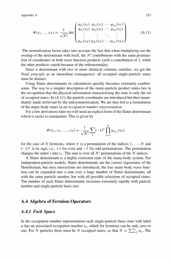
Appendix A 253

Ψ (x1, . . . xN ) = 1√N !

det

⎛⎜⎜⎜⎝

ϕα1 (x1) ϕα2 (x1) · · · ϕαN (x1)ϕα1 (x2) ϕα2 (x2) · · · ϕαN (x2)

......

. . ....

ϕα1 (xN ) ϕα2 (xN ) · · · ϕαN (xN )

⎞⎟⎟⎟⎠ . (A.11)

The normalization factor takes into account the fact that when multiplying out theoverlap of the determinant with itself, the N ! contributions with the same permuta-tion of coordinates in both wave function products yield a contribution of 1, whilethe other products vanish because of the orthonormality.

Since a determinant with two or more identical columns vanishes, we get thePauli principle as an immediate consequence: all occupied single-particle statesmust be distinct.

Using Slater determinants in calculations quickly becomes extremely cumber-some. The way to a simpler description of the many-particle product states lies inthe recognition that the physical information characterizing the state is only the setof occupied states: In (A.11), the particle coordinates are introduced but then imme-diately made irrelevant by the antisymmetrization. We are thus led to a formulationof the many-body states in an occupation number representation.

For a few derivations later we will need an explicit form of the Slater determinantwhich is easier to manipulate. This is given by

Ψ (x1, x2, . . . , xN ) = 1√N !

∑π

(−1)πN∏

k=1

ϕαkπ(xk),

for the case of N fermions, where π is a permutation of the indices 1, . . . , N and(−1)π is its sign, i.e., +1 for even and −1 for odd permutations. The permutationchanges the index i into iπ . The sum is over all N ! permutations of the N indices.

A Slater determinant is a highly restricted state of the many-body system. Forindependent-particle models, Slater determinants are the correct eigenstates of theHamiltonian, but once interactions are introduced, the true many-body wave func-tion can be expanded into a sum over a large number of Slater determinants, allwith the same particle number, but with all possible selections of occupied states.The number of such Slater determinants increases extremely rapidly with particlenumber and single-particle basis size.

A.4 Algebra of Fermion Operators

A.4.1 Fock Space

In the occupation number representation each single-particle basis state with labelα has an associated occupation number nα which for fermions can be only zero orone. For N particles there must be N occupied states, so that N = ∑∞

α=1 nα . The

254 Appendix A

many-body states are denoted by ket vectors as |n1, n2, . . .〉 and the Slater deter-minant of (A.11) would correspond to nαk = 1 for k = 1, . . . N and all otheroccupation numbers equal to zero.

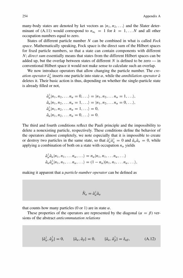
States of different particle number N can be combined in what is called Fockspace. Mathematically speaking, Fock space is the direct sum of the Hilbert spacesfor fixed particle numbers, so that a state can contain components with differentN ; direct sum essentially means that states from the different Hilbert spaces can beadded up, but the overlap between states of different N is defined to be zero — inconventional Hilbert space it would not make sense to calculate such an overlap.

We now introduce operators that allow changing the particle number. The cre-ation operator a†

α inserts one particle into state α, while the annihilation operator adeletes it. Their basic action is thus, depending on whether the single-particle stateis already filled or not,

a†α|n1, n2, . . . nα = 0, . . .〉 = |n1, n2, . . . nα = 1, . . .〉,

aα|n1, n2, . . . nα = 1, . . .〉 = |n1, n2, . . . nα = 0, . . .〉,a†

α|n1, n2, . . . nα = 1, . . .〉 = 0,

aα|n1, n2, . . . nα = 0, . . .〉 = 0.

The third and fourth conditions reflect the Pauli principle and the impossibility todelete a nonexisting particle, respectively. These conditions define the behavior ofthe operators almost completely, we note especially that it is impossible to createor destroy two particles in the same state, so that a†

α a†α = 0 and aα aα = 0, while

applying a combination of both on a state with occupation nα yields

a†α aα|n1, n1, . . . nα, . . .〉 = nα|n1, n1, . . . nα, . . .〉

aα a†α|n1, n1, . . . nα, . . .〉 = (1 − nα)|n1, n1, . . . nα, . . .〉,

making it apparent that a particle-number operator can be defined as

Nα = a†α aα

that counts how many particles (0 or 1) are in state α.These properties of the operators are represented by the diagonal (α = β) ver-

sions of the abstract anticommutation relations

{a†α, a†

β} = 0, {aα, aβ} = 0, {aα, a†β} = δαβ, (A.12)

Appendix A 255

where the anticommutator of two operators is defined as { A, B} = A B + B A. Itshould be noted as a consequence that

a†α a†

β = −a†β a†

α. (A.13)

The nondiagonal versions of these relations imply that creating or annihilatingparticles in two different single-particle states in order α → β or β → α producesthe same many-particle wave function, but with opposite sign. This expresses theantisymmetry for fermions.

We thus have set up a second-quantization formalism for fermions characterizedby the anticommutation rules A.12. Many-particle states can now be produced outof the vacuum |0〉, which is simply the state with all nα = 0, by the application ofcreation operators. Thus, the state corresponding to the Slater determinant A.11 canbe written as

a†α1

a†α2

. . . a†αN

|0〉. (A.14)

The final sign depends on the ordering of the operators, but that is usually no prob-lem. A convention is, e.g., that the order of the creation operators be the same asthe order of the states in the columns of the Slater determinant. We then have aone-to-one correspondence between the Slater determinants in configuration spaceand the Fock-space states as defined in (A.14).

A.4.2 Operators in Fock Space

For the use of the formalism in actual calculations it is necessary to also trans-form operators into the second-quantization formalism. To that end it is sufficient toconstruct an operator that yields the same matrix elements between the Slater deter-minants as between the corresponding Fock states. The form of such an operatorwill depend on its type, the two most useful being

• one-body operators depending only on the coordinates of one particle, but foridentical particles summed over identical contributions for all particles. An exam-ple is the kinetic energy

T =N∑

k=1

tk =N∑

k=1

−�2

2m∇2

k .

A general one-body operator will have the form

F =N∑

k=1

f (xk).

256 Appendix A

• two-body operators depending on the coordinates of two particles. A typicalexample is the interaction potential given by

V (x1, . . . xN ) = 12

N∑j,k=1

v(x j , xk).

The matrix elements of these expressions have to be evaluated between two Slaterdeterminants and an operator in second-quantization notation must be constructedthat produces identical matrix elements. We take two Slater determinants

Ψ (x1, . . . , xN ) = 1√N !

∑π

(−1)πN∏

j=1

ϕα jπ(x j ),

Ψ ′(x1, . . . , xN ) = 1√N !

∑π ′

(−1)π′

N∏j ′=1

ϕ′j ′π ′ (x j ′ ).

with the indices α′j ′ and α j describe the different choices of N occupied single-

particle wave functions from a complete orthonormal set ϕk(x), k = 1, . . . ,∞. Thematrix element becomes

〈Ψ | f |Ψ ′〉 =N∑

k=1

1

N !

∫d3x1 · · ·

∫d3xN

∑ππ ′

(−1)π+π ′( N∏j=1

ϕ∗α jπ

(x j ))

f (xk)( N∏

j ′=1

ϕα′j ′π ′

(x j ′ )).

From the products we can form single-particle integrals by taking the single-particlewave functions with identical arguments together. For the special case j = j ′ = kthe matrix element

∫d3xk ϕ∗

αkπ(xk) f (xk) ϕα′

kπ ′

(xk) = fαkπ α′kπ ′

, (A.15)

results, whereas the others simply reduce to

∫d3x j ϕ∗

α jπ(x j ) ϕα′

j ′π ′

(x j ) = δα jπ α′j ′π ′

.

The many-body matrix element becomes

〈Ψ | f |Ψ ′〉 =∑

k

1

N !

∑ππ ′

(−1)π+π ′fkπ kπ ′

N∏j, j ′=1

j �=k, j ′ �=k

δ jπ j ′π ′ .

Appendix A 257

For this matrix element not to vanish, the Kronecker symbols require that the samestates must be occupied in Ψ as in Ψ ′ with a single exception. This implies that asingle-particle operator changes the state of a single particle only.

Now if at most one single-particle state is different between the two occupations,for a given permutation π there is only one π ′ that makes all Kronecker symbolsnonzero; so the sum over π ′ can be dropped by choosing π ′ correctly for each π .How is the total sign to be determined? As π and π ′ are the permutations needed tobring the states numbered by i and i ′ from their original ordering into the same order(with the indices kπ and kπ ′ also in the same position), the factor σ = (−1)π+π ′

tellswhether an even or odd permutation is needed to transform these original orderingsinto each other and it does not depend on π or π ′. The sum over permutations π theneffectively runs only over the various ways to number the N − 1 states occupied inboth Ψ and Ψ ′.

The matrix element is totally independent of the permutation. It only contains thefactor σ , and the single-particle matrix element fkπ kπ ′ always has the same indices:those of the two single-particle states which differ between Ψ and Ψ ′; let us simplycall them j and j ′. The matrix element is now

〈Ψ | f |Ψ ′〉 =N∑

k=1

1

N !σ f j j ′

∑π, j fixed

1 = 1

N !σ N f j j ′ (N − 1)! = σ f j j ′ .

What should the equivalent operator in second quantization look like? It mustremove one particle from state j ′ and put it into the state j while not doing anythingto the other states, the resulting matrix element being f j j ′ . Since this must operatefor all combinations of j and j ′ we are led to

F =∑

j j ′f j j ′ a†

j a j ′ .

It has to be checked whether the signs are correct. The Fock-space states are

|Ψ 〉 = a†α1

· · · a†αN

|0〉 , |Ψ ′〉 = a†α′

1· · · a†

α′N|0〉,

and the matrix element is

〈Ψ |F |Ψ ′〉 =∑

j j ′f j j ′ 〈0|aαN · · · aα1 a†

j a j ′ a†α′

1· · · a†

α′N|0〉.

It is clear that again the set of indices α must denote the same states as α′, exceptthat j replaces j ′. Permute the i ′ in such a way that they are in the same order asthe i (and with j ′ at the same place as j), and this will yield the same sign factorσ as defined above for the Slater determinants. Permuting the operator combinationa†

j a j ′ in front of a†j ′ does not change the sign, and we get

258 Appendix A

〈Ψ |F |Ψ ′〉 =∑

j j ′f j j ′ 〈0|aαN · · · aα1 a†

α1· · · a†

j a j ′ a†j ′ · · · a†

αN|0〉.

In this expression the operator combinations a†i ai ′ all yield factors of 1, and the final

result is

〈Ψ |F |Ψ ′〉 = σ f j j ′

in agreement with the result calculated in the Slater-determinant formulation.The rule for transcribing a single-particle operator into second-quantized form is

thus

F =∑

j j ′f j j ′ a†

j a j ′ with f j j ′ = 〈ϕ j | f |ϕ j ′ 〉.

The analogous result for two-body operators such as the potential energy

V = 12

∑k �=k ′

v(xk, xk ′ )

can be obtained in a similar way. Each individual term in the sum can change thestates of two particles now, so that a product of two creation and two annihilationoperators is needed. The calculation can be done in a similar way as above, but is ofcourse more complex. We skip the cumbersome details and give the final form forthe second-quantized operator:

V = 12

∑i jkl

vi jkl a†i a†

j al ak , (A.16)

with the two-particle matrix element defined by

vi jkl =∫

d3x∫

d3x ′ ϕ∗i (x) ϕ∗

j (x′) v(x, x ′) ϕk(x) ϕl(x

′).

Note the opposite ordering of the last two indices in the matrix element as comparedto the operators in (A.16).

In many calculations the evaluation of the matrix elements leads to an antisym-metric combination, which is therefore given a special abbreviation:

Appendix A 259

vi jkl = vi jkl − vi jlk .

Note also the symmetry of the matrix element under the interchange of the two pairsof single-particle wave functions:

vi jkl = v j ilk .

Two more general properties of these second-quantized expressions are worthmentioning: they conserve particle number, since both contain the same number ofcreation as annihilation operators in each term, and they do not explicitly depend onthe number of particles anymore: this is instead supplied by the Fock-space states.

A.4.3 Field Operators

The creation and annihilation operators discussed up to now have affected particlesin specific states. It is sometimes useful to construct operators for particles at aspecific location in space by defining

ψ†(r) =∑

k

a†kϕ

∗k (r), ψ(r) =

∑k

akϕk(r). (A.17)

These field operators fulfill the anticommutation relations

{ψ†(r), ψ†(′)} = 0,

{ψ(r), ψ(r′)} = 0,

{ψ(r), ψ†(r′)} = δ(r − r′).

The last relation can be probed using the completeness of the single-particle basis.These definitions also show the origin of the name “second quantization”: the

wave functions themselves become field operators.

A.5 Hierarchy of Density Operators

A.5.1 The One-Body Density

From the many-body wave function it is relatively straightforward to calculate theprobability to find one particle at the location r; this probability is normalized toone and has to be multiplied by the total number of particles N to obtain the density.Since we are not interested in the positions of the other particles, they have to beintegrated over and the result is

260 Appendix A

�(r) = N∫

Ψ ∗(r, r2, . . . rN )Ψ (r, r2, . . . rN ) d3r2 . . . d3rN . (A.18)

If Ψ is a Slater determinant built out of the single-particle states φk , k = 1, . . . N ,this can be reduced to

�(r) =N∑

k=1

|ϕk(r)|2

by using the orthonormality of the single-particle wave functions. It can also beformulated as the matrix element of an operator

�(r) =N∑

j=1

δ(r − r j ),

so that

�(r) = 〈Ψ |�|Ψ 〉.

A useful generalization of this concept is the nondiagonal density

�(r, r′) = N∫

Ψ ∗(r′, r2, . . . rN )Ψ (r, r2, . . . rN ) d3r2 . . . d3rN . (A.19)

This concept can be carried over to second quantization. The density can be obtainedby finding the number of particles in a single-particle state, multiplying it by thecorresponding density, and summing over all states,

�(r) =∞∑j=1

ϕ∗j (r)ϕ j (r)〈Ψ |a†

j a j |Ψ 〉 = 〈Ψ |ψ†(r)ψ(r)|Ψ 〉,

where the result was also expressed through field operators.For the nondiagonal density we get similarly

�(r, r′) =∞∑

j,k=1

ϕ∗j (r

′)ϕk(r)〈Ψ |a†j ak |Ψ 〉 = 〈Ψ |ψ†(r′)ψ(r)|Ψ 〉. (A.20)

This also motivates the definition of a nondiagonal density operator

�(r, r′) = ψ†(r′)ψ(r).

Appendix A 261

A.5.2 The One-Body Density Matrix

We are thus naturally led to introduce the operator combination just discussed asthe Fock-space version of the nondiagonal one-body density. Given a many-particlestate |Ψ 〉, the one-body density matrix is defined as

�kl = 〈Ψ |a†l ak |Ψ 〉, (A.21)

where k and l run over the single-particle basic states. |Ψ 〉 need not be a simpleSlater determinant built out of these states but can be a general many-body wavefunction, a superposition of such Slater determinants. Note that the one-body densitymatrix depends both on the state |Ψ 〉 and on the single-particle basis defining theoperators a†

k and al . It is customary to use the shorter term “density matrix” forthe one-body density matrix if no confusion with other types of density matrix ispossible.

The following elementary properties of the density matrix are easily derived:

• �kl is hermitian:

�lk = 〈Ψ |a†k al |Ψ 〉 = 〈Ψ |(a†

l ak)†|Ψ 〉 = �∗kl .

• Expectation values of single-particle operators such as

t =∑

kl

tkl a†k al

can be calculated via

〈Ψ |t |Ψ 〉 =∑

kl

tkl〈Ψ |a†k al |Ψ 〉 =

∑kl

tkl �lk,

which can be rewritten using matrix trace notation:

〈Ψ |t |Ψ 〉 = Tr{�t}.

This also explains why in the definition (A.21) the order of indices is chosenoppositely on both sides.

262 Appendix A

Here t on the right-hand side stands for the matrix tkl representing the operatort .1

• If the state |Ψ 〉 is a simple Slater determinant, the form of the density matrix isquite restricted. We first regard the case that |Ψ 〉 is built out of the same single-particle states as those contained in the single-particle basis defining the densitymatrix. Then we must have

�kl ={

δkl for k and l occupied in |Ψ 〉0 otherwise

.

Thus � is diagonal in this case with ones and zeroes on the diagonal dependingon whether the corresponding single-particle state is occupied or empty. Further-more it fulfills the important relation

�2 = �, (A.22)

which follows immediately from the special form of the matrix. It is importantthat this relation continues to hold in the more general case. If the single-particlestates that make up |Ψ 〉 are not included in the basis defining �, they may in anycase be expanded in those using some unitary matrix U ,

βk =∑

k ′Ukk ′ ak ′ ,

where βk now denotes the second-quantization operator for these states occupiedin |Ψ 〉. The density matrix � defined in the basis of the βk now is given by

� = U�U †,

so that conversely � = U †�U . Since � fulfills (A.22), we get

�2 = U †�UU †�U = U †�2U = U †�U = �.

So �2 = � holds for a Slater determinant |Ψ 〉 no matter what single-particle basisis used for defining �.

This relation for one-body density matrices should not be confused with theanalogous equation for a general density matrix. A general density matrix fulfilling�2 = � describes a pure state, a totally different implication.

The relation (A.22) shows that � is a projection matrix: it projects any vectordescribing a superposition of the basis states onto the subspace of occupied ones.

1 The following notation is used: t denotes an operator, t the corresponding matrix, and tkl theelements of the matrix.

Appendix A 263

A.5.3 The Two-Body Density

The one-body density is suited for the description of one-body operators. Since theinteractions between particles always depend on at least two-particle coordinates, itis necessary to introduce a two-body density as well. In configuration space it is thesimple generalization of (A.19)

�(r1, r2; r′1, r′

2) =∫

Ψ ∗(r1, r2, r3, . . . rN )Ψ (r′1, r′

2, r3, . . . rN ) d3r3 . . . d3rN .

(A.23)

(In fact, this process can be carried further to yield higher and higher densities up tothe full N -body density |Ψ (r1, . . . rN )|2)

We can now define operators and matrices as in the one-body case. In terms offield operators the two-body density is given by

�(r1, r2; r′1, r′

2) = 〈Ψ |ψ†(r′1)ψ†(r′

2)ψ(r2)ψ(r1)|Ψ 〉.

Going over to creation and annihilation operators and a matrix formulation we getthe definition of the two-body density matrix

� jklm = 〈Ψ |a†l a†

mak a j |Ψ 〉, (A.24)

which is, however, not as useful for the purposes of this book. The most importantproperty of the two-body density is that for a Slater-determinant state |Ψ 〉 it can besplit up into products of single-particle densities:

�(r1, r2, r′1, r′

2) = �(r1, r′1)�(r2, r′

2) − �(r1, r′2)�(r2, r′

1).

This result can be shown by using a basis containing the occupied states, evaluatingthe matrix element in (A.24) as shown in Chap. 5 and going back to coordinatespace.

A.6 Time Reversal and Kramers Degeneracy

Time-reversal invariance is usually not treated thoroughly in elementary quantum-mechanics courses, because it is somewhat more complicated than space inversion.For fermionic systems, however, it has important consequences which we will derivehere.

Time reversal is defined by its effect on the principal physical quantities position,momentum, angular momentum, spin, and time itself:

264 Appendix A

r → r , p → −p , s → −s , L → −L , t → −t .

Hamiltonians should be time-reversal invariant, so that, for example, a term such asr · p cannot be allowed. This leads to the usual property in microscopic physics thatthe evolution of a system and its time-reversed analogue should both be possible.

Time reversal has unusual properties compared with the other symmetries. Denot-ing the time-reversal operator by T , the commutator of position and momentumtransforms as

T[x, px

]T −1 = [x,−px

] = −i�,

so that we must demand T i�T −1 = −i�! The only way to achieve this is to assumethat the time reversal operator includes complex conjugation. This also works forthe Schrodinger equation, where the time-reversal invariance of the Hamiltoniandemands that i�∂/∂t be invariant, too.

The operator for time reversal, T , thus cannot be unitary, because it is not evenlinear. A linear operator commutes with an arbitrary c number, so that one shouldhave

T i�T −1 = i�T T −1 = i�,

whereas we need as the transformation of the constant T i�T −1 = −i�. Operatorswith the property T α = α∗T for an arbitrary complex number α are called antilin-ear operators.

Special care needs to be taken when constructing the eigenstates of T , becausemany of the familiar operator properties do not hold. Assume that |A〉 is an eigen-state of T with eigenvalue A. Applying T 2 then yields

T 2|A〉 = T A|A〉 = A∗T |A〉 = |A|2|A〉.

Now the basic definition of time reversal shows that it must satisfy T 2 = 1, so thatthe eigenvalue A must have a magnitude of unity:

A = expiφA

with some phase angle φA. This angle actually depends on the choice of phase forthe eigenstate, because if |A〉 is replaced by a new state

|A′〉 = exp12 iφA |A〉,

the eigenvalue also changes:

T |A′〉 = T exp12 iφA |A〉 = exp− 1

2 iφA T |A〉 = exp− 12 iφA expiφA |A〉 = |A′〉.

Appendix A 265

So it is possible to make the eigenvalue of T equal to 1 by a change of phase. Itis interesting to note that the properties of time reversal are thus intimately linkedto the phases of the wave functions, which otherwise play little role in quantummechanics.

For spherical systems the interplay between angular momentum and time reversalis interesting. Let us look at total angular momentum J = L + s, although thearguments are equally valid for spin and orbital angular momenta. T inverts thesign of J, so that it commutes with J 2 but not with Jz . If time reversal is combinedwith a rotation R that inverts the direction of the z-axis, it should commute withboth:

[RT , J 2] = 0,

[RT , Jz

] = 0,

and this operator RT can then be diagonalized together with J 2 and Jz . The possibleeigenvalues, by the same argument as for T , must have the form exp(iφA) and canagain be made equal to 1 by a change of phase of the wave function. Denoting anyadditional quantum numbers by α, we can thus construct a system of eigenfunctions|α J M〉 such that

RT |α J M〉 = |α J M〉

This works with the usual angular momentum eigenstates, but requires a specialchoice of phase for the basic functions.

The rotation R is arbitrary except for the condition of inverting the z-axis. It iscustomary to choose a rotation by an angle π about the y-axis, R = Ry(π ).

Let us now examine the action of (RT )2. On the one hand, since its eigenvalueis 1, we have

(RT )2|α J M〉 = |α J M〉.

On the other hand, R commutes with T , because the rotation Ry(π ) can beexpressed as exp(iπ Jy) and T inverts the signs of both Jy and the imaginary factoriπ . Thus we can also write

(RT

)2 |α J M〉 = R2T 2|α J M〉 = Ry(2π )T 2|α J M〉.

Now comes the crucial part. The rotation by 2π is the identity for wave functionswith integral spin, but produces a −1 for half-integer spins. The result is thus

T 2 ={

+1 for integral spin,

−1 for half-integer spin.

Here we are only interested in the latter case. An eigenvalue of −1 is not possiblebecause T 2 is the identity operator and thus has only eigenvalues of +1.

266 Appendix A

The solution for this apparent contradiction is that for fermions there are noeigenvectors of T , or, in other words, T |A〉 is always linearly independent of |A〉.As the Hamiltonian is invariant under time reversal and commute with T , |A〉 andT |A〉 have the same energy: there are thus two linearly independent but degenerateeigenstates of the Hamiltonian.

This twofold degeneracy of fermionic states is called Kramers degeneracy. In thesingle-particle wave functions, for example, consequences appear in the followingway: for a wave function with orbital angular momentum projection M combiningwith spin projection s to total angular momentum projection Ω , the state producedby time reversal has quantum numbers (−M,−s,−Ω). In the case of sphericalsymmetry, this is hidden by the degeneracy of all angular momentum projections(for other quantum numbers identical), but if the system deviates from spherical tocylindrical geometry, Kramers degeneracy implies that there will still be degeneratestates with opposite Ω projection.

This general result also applies to many-body states. If the Hamiltonian for asystem consisting of an odd number of fermions (and thus having a fractional spin)is invariant under time reversal, its eigenstates will always show twofold degeneracywith the two states being time reversed with respect to each other.

Appendix BUseful Tables

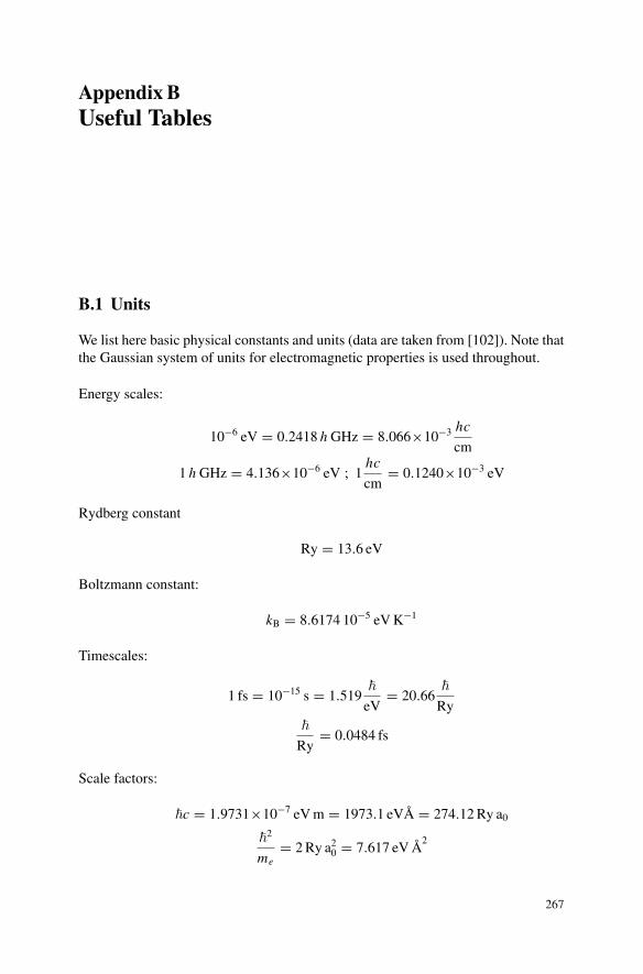
B.1 Units

We list here basic physical constants and units (data are taken from [102]). Note thatthe Gaussian system of units for electromagnetic properties is used throughout.

Energy scales:

10−6 eV = 0.2418 h GHz = 8.066×10−3 hc

cm

1 h GHz = 4.136×10−6 eV ; 1hc

cm= 0.1240×10−3 eV

Rydberg constant

Ry = 13.6 eV

Boltzmann constant:

kB = 8.6174 10−5 eV K−1

Timescales:

1 fs = 10−15 s = 1.519�

eV= 20.66

�

Ry�

Ry= 0.0484 fs

Scale factors:

�c = 1.9731×10−7 eV m = 1973.1 eVA = 274.12 Ry a0

�2

me= 2 Ry a2

0 = 7.617 eV A2

267

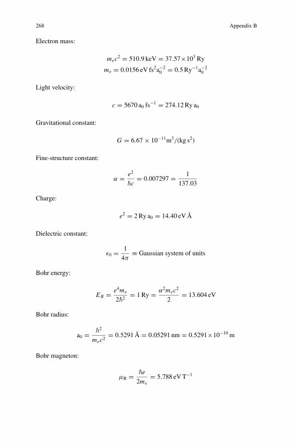
268 Appendix B

Electron mass:

mec2 = 510.9 keV = 37.57×103 Ry

me = 0.0156 eV fs2a−20 = 0.5 Ry−1a−2

0

Light velocity:

c = 5670 a0 fs−1 = 274.12 Ry a0

Gravitational constant:

G = 6.67 × 10−11m3/(kg s2)

Fine-structure constant:

α = e2

�c= 0.007297 = 1

137.03

Charge:

e2 = 2 Ry a0 = 14.40 eV A

Dielectric constant:

ε0 = 1

4π≡ Gaussian system of units

Bohr energy:

EB = e4me

2�2= 1 Ry = α2mec2

2= 13.604 eV

Bohr radius:

a0 = �2

mec2= 0.5291 A = 0.05291 nm = 0.5291×10−10 m

Bohr magneton:

μB = �e

2me= 5.788 eV T−1

Appendix B 269

A few nuclear quantities [29]:

Proton:

m pc2 = 938.2 MeV = 1836.1 me

�2

m p= 41.494 MeV fm2

μp = 2.7928 μN

Nuclear magneton:

μN = e�

2m pc= 0.3152 ∗ 10−11 eV

Gs= 0.5446 ∗ 10−3μe

Neutron:

mnc2 = 939.5 MeV = 1838.9 me

Deuteron:

mdc2 = 1875.4 MeV = 3670.8 me

μd = 0.8574 μN

B.2 Hermite and Laguerre Polynomials

Othogonal polynomials occur in the solutions of many differential equations inphysics. Distinct polynomials arise for different boundary conditions and dimen-sionalities. Because many useful properties can be derived for them, they are usedextensively in analytic calculations. The most important properties are the differ-ential equations they obey, their normalization integrals, and simple recursion rela-tions.

For more information on special functions the classic reference is [118], down-loadable from http://www.math.sfu.ca/cbm/aands/.

B.2.1 The Hermite Polynomials

These occur most prominently in the solution of the 1D oscillator. The differentialequation

d2

dx2f (x) − 2x

d

dxf (x) + 2n f (x) = 0

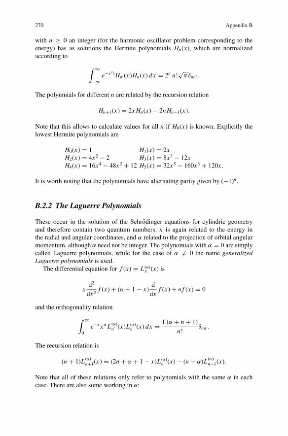
270 Appendix B

with n ≥ 0 an integer (for the harmonic oscillator problem corresponding to theenergy) has as solutions the Hermite polynomials Hn(x), which are normalizedaccording to

∫ ∞

−∞e−x2) Hn′ (x)Hn(x) dx = 2n n!

√πδnn′ .

The polynmials for different n are related by the recursion relation

Hn+1(x) = 2x Hn(x) − 2nHn−1(x).

Note that this allows to calculate values for all n if H0(x) is known. Explicitly thelowest Hermite polynomials are

H0(x) = 1 H1(x) = 2xH2(x) = 4x2 − 2 H3(x) = 8x3 − 12xH4(x) = 16x4 − 48x2 + 12 H5(x) = 32x5 − 160x3 + 120x .

It is worth noting that the polynomials have alternating parity given by (−1)n .

B.2.2 The Laguerre Polynomials

These occur in the solution of the Schrodinger equations for cylindric geometryand therefore contain two quantum numbers: n is again related to the energy inthe radial and angular coordinates, and α related to the projection of orbital angularmomentum, although α need not be integer. The polynomials with α = 0 are simplycalled Laguerre polynomials, while for the case of α �= 0 the name generalizedLaguerre polynomials is used.

The differential equation for f (x) = L (α)n (x) is

xd2

dx2f (x) + (α + 1 − x)

d

dxf (x) + n f (x) = 0

and the orthogonality relation

∫ ∞

0e−x xα L (α)

n′ (x)L (α)n (x) dx = Γ(α + n + 1)

n!δnn′ .

The recursion relation is

(n + 1)L (α)n+1(x) = (2n + α + 1 − x)L (α)

n (x) − (n + α)L (α)n−1(x).

Note that all of these relations only refer to polynomials with the same α in eachcase. There are also some working in α:

Appendix B 271

L (α+1)n (x) = 1

x

[(x − n)L (α)

n (x) + (α + n)L (α)n−1(x)

],

L (α−1)n (x) = L (α)

n (x) − L (α)n−1(x).

Special cases are

L (α)0 (x) = 1,

L (α)1 (x) = −x + α + 1,

L (α)2 (x) = 1/2 a2 + 3/2 a + 1 − xa − 2 x + 1/2 x2.

Clearly these become quite complicated quickly but can readily be generated usingthe recursion relations.

References

1. M. Abramowitz, I.A. Stegun, Handbook of Mathematical Functions with Formulas, Graphs,and Mathematical Tables, ninth Dover printing, tenth GPO printing edn. (Dover, New York,1964)

2. A. Artemyev, E.V. Ludena, V. Karasiev, J. Mol. Struct.: THEOCHEM 580, 47 (2002)3. N.W. Ashcroft, N.D. Mermin, Solid State Physics (Saunders College, Philadelphia, 1976)4. P.W. Atkins, Physical Chemistry (Oxford University, Oxford, 1977)5. M. Baldo, C. Maieron, P. Schuck, X. Vinas, Nucl. Phys. A 736, 241 (2004)6. R. Balian, C. Bloch, Ann. Phys. 85, 514 (1974)7. J. Bardeen, L.N. Cooper, J.R. Schrieffer, Phys. Rev. 108, 1175 (1957)8. M. Bender, P.H. Heenen, P.G. Reinhard, Rev. Mod. Phys. 75, 121 (2003)9. G.F. Bertsch, The Practitioner’s Shell Model (North-Holland, Amsterdam, 1972)

10. G.F. Bertsch, R. Broglia, Oscillations in Finite Quantum Systems (Cambridge UniversityPress, Cambridge, 1994)

11. G.F. Bertsch, S. Das Gupta, Phys. Rep. 160, 190 (1988)12. K. Binder, Encyclopedia of Mathematics (Kluwer Academic, Dordrecht, 2001)13. J.P. Blaizot, G. Ripka, Quantum Theory of Finite Systems (MIT Press, Cambridge Mas-

sachusetts and London England, 1985)14. I. Bloch, J. Dalibart, W. Zwerger, Rev. Mod. Phys. 80, 885 (2008)15. O. Bohigas, A.M. Lane, J. Martorell, Phys. Rep. 51, 267 (1979)16. D. Bohm, D. Pines, Phys. Rev. 92, 609 (1953)17. A. Bohr, B.R. Mottelson, Struktur der Atomkerne I. Einteilchenbewegung (Akademie Verlag,

Berlin, 1975)18. A. Bohr, B.R. Mottelson, Struktur der Atomkerne II. Kerndeformationen (Akademie Verlag,

Berlin, 1980)19. M. Brack, Rev. Mod. Phys. 65, 677 (1993)20. M. Brack, R.K. Bhaduri, Semiclassical Physics (Addison-Wesley, Reading, 1997)21. D.M. Ceperley, B.J. Alder, Phys. Rev. Lett. 45, 566 (1980)22. E. Chabanat, P. Bonche, P. Haensel, J. Meyer, R. Schaeffer, Nucl. Phys. A 627, 710 (1997)23. J.P. Coe, A. Sudbery, I. D’Amico, Phys. Rev. B 77, 205122 (2008)24. C. Cohen-Tanuudji, B. Diu, F. Laloe, Quantum Mechanics (Wiley, New York, 2006)25. P.M. Dinh, J. Navarro, E. Suraud, Oceans et gouttelettes quantiques (CNRS Editions, Paris,

2007)26. J.F. Dobson, Phys. Rev. Lett. 73, 2244 (1994)27. R.M. Dreizler, E.K.U. Gross, Density Functional Theory: An Approach to the Quantum

Many-Body Problem (Springer-Verlag, Berlin, 1990)28. R. Dorner, V. Mergel, O. Jagutzki, L. Spielberger, J. Ullrich, R. Moshammer, H. Schmidt-

Bocking, Phys. Rep. 330, 95 (2000)29. G. Eder, Kernkrafte (Verlag G. Braun, Karlsruuhe, 1965)

273

274 References

30. A.R. Edmonds, Angular Momentum in Quantum Mechanics (Princeton University Press,Princeton, 1960)

31. A.R. Edmonds, Angular Momentum in Quantum Mechanics (Princeton University Press,Princeton, 1996)

32. R. Englman, The Jahn-Teller Effect in Molecules and Crystals (Wiley, London, 1972)33. T.E.O. Ericson, W. Weise, Pions and Nuclei (Clarendon, Oxford, 1988)34. E. Fermi, Z. Phys. 48, 73 (1928)35. S. Flugge, Practical Quantum Mechanics (Springer, Heidelberg, 1974)36. H.S. Friedrich, Theoretical Atomic Physics (Springer, Heidelberg, 2006)37. J. Friedrich, N. Vogler, Nucl. Phys. A 373, 192 (1982)38. S. Giorgini, L.P. Pitaevski, S. Stringari, Rev. Mod. Phys. 80, 1216 (2008)39. N.K. Glendenning, Compact Stars (Springer, Heidelberg, 1997)40. H. Goldstein, Classical Mechanics (Addison-Wesley, Cambridge MA, 1950)41. S. Grebenev, B. Sartakov, J.P. Toennies, A.F. Vilesov, Science 289, 1532 (2000)42. W. Greiner, J.A. Maruhn, Kernmodelle, Theoretische Physik, vol. 11 (Verl. Harri Deutsch,

Thun, Frankfurt am Main, 1995)43. E.K.U. Gross, E. Runge, O. Heinonen, Many–Particle Theory (Adam Hilger, Bristol,

Philadelphia, New York, 1991)44. H. Haberland (ed.), Clusters of Atoms and Molecules 1- Theory, Experiment, and Clusters of

Atoms, vol. 52 (Springer Series in Chemical Physics, Berlin, 1994)45. H. Haken, Introduction to Laser Physics (Springer, Berlin, 1991)46. H. Haken, H.C. Wolf, The Physics of Atoms and Quanta (Springer, Berlin, 2000)47. R. Haussmann, W. Rantner, S. Cerrito, W. Zwerger, Phys. Rev. A 75, 023610 (2007)48. K.L.G. Heyde, The Nuclear Shell Model, 1st edn. (Springer, Berlin, Heidelberg, New York,

1990)49. S. Hofmann, G. Munzenberg, Rev. Mod. Phys. 72, 733 (2000)50. P. Hohenberg, W. Kohn, Phys. Rev. 136, 864 (1964)51. G. Jaeger, Quantum Information: An Overview (Springer, Berlin, 2006)52. H.A. Jahn, E. Teller, Proc. Roy. Soc. A 161, 220 (1937)53. W.R. Johnson, Atomic Structure Theory (Springer, Berlin, 2007)54. R.O. Jones, O. Gunnarsson, Rev. Mod. Phys. 61, 689 (1989)55. C. Kohl, P.G. Reinhard, Z. Phys. D 39, 225 (1997)56. W. Kohn, Rev. Mod. Phys. 71, 1253 (1999)57. W. Kohn, L.J. Sham, Phys. Rev. 140, 1133 (1965)58. M. Koskinen, P.O. Lipas, M. Manninen, Nucl. Phys. A 591, 421 (1995)59. U. Kreibig, M. Vollmer, Optical Properties of Metal Clusters, vol. 25 (Springer Series in

Materials Science, Berlin, 1993)60. A. Kumar, S.E. Laux, F. Stern, Phys. Rev. B 42, 5166 (1990)61. S. Kummel, L. Kronik, Rev. Mod. Phys. 80, 3 (2008)62. L.D. Landau, E.M. Lifshitz, J. Menzies, Quantum Mechanics: Non-Relativistic Theory

(Butterworth-Heinemann, Oxford, 1991)63. J.M. Lattimer, M. Prakash, Science 304, 536 (2004)64. H.J. Lipkin, N. Meshkov, A.J. Glick, Nucl. Phys. 62, 188 (1965)65. B.D. Marco, S.B. Papp, D.S. Jin, Phys. Rev. Lett. 86, 5409 (2001)66. E.S.P. Marmier, Physics of Nuclei and Particles, Vol I (Academic, New York, 1969)67. J. Maruhn, W. Greiner, Z. Physik 251, 431 (1972)68. J. Maruhn, P.G. Reinhard, P. Stevenson, I. Stone, M. Strayer, Phys. Rev. C 71, 064328 (2005)69. E. Merzbacher, Quantum Mechanics (Wiley, New York, 1997)70. A. Messiah, Quantum Mechanics (Dover, New York, 2000)71. G. Mie, Ann. Phys. (Leipzig) 25, 377 (1908)72. A. Mourachkine, High-Temperature Superconductivity in Cuprates (Springer, Heidelberg,

2007)73. J. Navarro, P.G. Reinhard, E. Suraud, Euro. Phys. J. A 30, 333 (2006)74. J.W. Negele, Rev. Mod. Phys. 54, 913 (1982)

References 275

75. S.G. Nilsson, Mat.-Fys. Medd. Dan. Vid. Selsk. 29, 16 (1955)76. D.P. O’Neill, P.M.W. Gill, Phys. Rev. A 68, 022505 (2003)77. T. Padmanabhan, Theoretical Astrophysics Volume II: Stars and Stellar Systems (Cambridge

University Press, Cambridge, 2001)78. V.R. Pandharipande, I. Sick, P.K.A. deWitt Huberts, Rev. Mod. Phys. 69, 981 (1997)79. R.D. Parks. (ed.), Superconductivity (Dekker, New York, 1969)80. R.G. Parr, W. Yang, Density-Functional Theory of Atoms and Molecules (Oxford University

Press, Oxford, 1989)81. J.P. Perdew, K. Burke, M. Ernzerhof, Phys. Rev. Lett. 77, 3865 (1996)82. J.P. Perdew, Y. Wang, Phys. Rev. B 45, 13244 (1992)83. J.P. Perdew, A. Zunger, Phys. Rev. B 23, 5048 (1981)84. D. Pettifor, Bonding and Structure of Molecules and Solids (Clarendon, Oxford, 1995)85. D. Pines, P. Nozieres, The Theory of Quantum Liquids (Benjamin, New York, 1966)86. S. Raman, C. Nestor, P. Tikkanen, At. Data Nucl. Data Tab. 78, 1 (2001)87. S.M. Reimann, M. Manninen, Rev. Mod. Phys. 74 1283 (2002)88. P.G. Reinhard, E.W. Otten, Nucl. Phys. A 420, 173 (1984)89. P.G. Reinhard, E. Suraud, Introduction to Cluster Dynamics (Wiley, New York, 2003)90. P.G. Reinhard, C. Toepffer, Int. J. Mod. Phys. E 3, 435 (1994)91. G. Rickayzen, Theory of Superconductivity (Interscience, New York, 1965)92. P. Ring, P. Schuck, The Nuclear Many-Body Problem (Springer-Verlag, New York, Heidel-

berg, Berlin, 1980)93. D.J. Rowe, Nuclear Collective Motion (Methuen, London, 1970)94. U. Rossler, Solid State Theory (Springer, Berlin, 2004)95. E.R. Scerri, The Periodic Table: Its Story and Its Significance (Oxford University Press,

Oxford, 2006)96. L.I. Schiff, Quantum Mechanics (McGraw Hill, New York, 1968)97. M. Schmidt, H. Haberland, Eur. Phys. J. D 6, 109 (1999)98. T.H.R. Skyrme, Nucl. Phys. 9, 615 (1959)99. J.C. Slater, Phys Rev. 81, 385 (1951)

100. A. Szabo, N.S. Ostlund, Modern Quantum Chemistry (Dover, New York, 1996)101. L. Szasz, Pseudopotential Theory of Atoms and Molecules (Wiley, New York, 1985)102. G. Sussmann, Einfuhrung in die Quantenmechanik I (Bibliographisches Institut, Mannheim,

1963)103. B. Talukdar, A. Sarkar, S. Roy, P. Sarkar, Chem. Phys. Lett. 381, 67 (2003)104. S. Tarucha, D.G. Austing, T. Honda, R.J. van der Haage, L. Kouwenhoven, Phys. Rev. Lett.

77, 3613 (1996)105. L. Thomas, Proc. Camb. Phil. Soc. 23, 195 (1926)106. T. Tietz, Ann. Physik 15, 6, 186 (1955)107. D. Varsano, R. di Felice, M. Marques, A. Rubio, Science 110, 7129 (2006)108. D.A. Varshalovich, A.N. Moskalev, V.K. Khersonskii, Quantum Theory of Angular Momen-

tum (World Scientific Pub. Co., Singapore, 1988)109. D. Vautherin, D.M. Brink, Phys. Rev. C 5, 626 (1972)110. G. Vignale, Phys. Rev. Lett. 74, 3233 (1995)111. G.E. Volovik, The Universe in a Helium Droplet (Clarendon, Oxford, 2003)112. E. Wahlstrom, E.K. Vestergaard, R. Schaub, A. Ronnau, M. Vestergaard, E. Laegsgaard, I.

Stensgaard, F. Besenbacher, Science 303, 511 (2004)113. S. Weinberg, The Quantum Theory of Fields, Vol. II (Cambridge University Press, Cam-

bridge, 1996)114. M. Weissbluth, Atoms and Molecules (Academic Press, San Diego, 1978)115. B. Yoon, J.W. Negele, Phys. Rev. A 16, 1451 (1977)116. J. Zinn-Justin, Quantum Field Theory and Critical Phenomena (Oxford Science Publishers,

Oxford, 2002)117. W.A. de Heer, Rev. Mod. Phys. 65, 611 (1993)118. J. von Neumann, E. Wigner, Z. Phys. 30, 467 (1929)

Index

Aa0, see Bohr radiusAlkalies, 11–13, 17, 39, 105Atom traps, 190Atomic clusters, 118Atomic compounds, see moleculesAtomic traps, 76, 118, 224Atoms, 1, 2, 4, 8–11, 17–21, 24, 27, 28, 30, 31,

39, 43, 73, 118, 155–159Average potential, 125

BBCS model, 159, 165, 231–238Benzene, 169Bohr radius, 268Born-Oppenheimer approximation, 181Bose-Einstein condensate, 159, 238Box potential, see square-well potential

CChandrasekhar mass, 63, 65Chiral symmetry breaking, 180Clemenger-Nilsson model, 76, 77, 79, 80, 82Clusters, 73Compact stars, see white dwarfs, neutron starsConfiguration interaction, 93, 115l2-correction, 78, 80, 85, 87, 88Coulomb blockade, 84Coulomb energy, direct part, 66Coulomb energy, exchange part, 67Covalent bond, 13, 14, 220

DDensity

one-body, 260two-body, 56–57, 263

Density functional theory, 72, see DFTDensity matrix, 40–41

one-body, 40, 53–55, 129–130, 223, 260,261

two-body, 40, 263DFT, 28, 37, 55, 143–155, 189, 200–202, 221Direct term, 125Dissociation energy, 103Droplets, see helium droplets, 73

EEffective interaction, 143, 152Effective mass, 83Electron gas, metal, 66Entanglement, 223Exchange energy, 69Exchange term, 125Excitations 1ph, 187

FFermi distribution, 60Fermi energy, 45, 51–53Fermi gas, 226

charged, 66–69finite temperature, 59–63kinetic energy, 57–58level density, 59one-dimensional, 47–50relativistic, 64–65two-dimensional, 50–51

Fermi liquid, 46Fermi momentum, 45, 51–53Fermi pressure, 69Fermi sphere, 50Fermion traps, 1, 2, 22–25, 27, 42, 45, 46,

159–160, 211, 237Fock space, 254fs, 268

GGap equation, 234–236GDR, see giant dipole resonance, 206

277

278 Index

Generalized gradient approximation, 147Giant dipole resonance, 187Giant resonances, 187Goldstone modes, 215Guanine, 33

HHuckel model, 94, 105–110, 115Halogens, 11–13, 105Harmonic oscillator, 74–81

axially symmetric, 75, 76, 81circular, 75potential, 72spherical, 75, 87triaxial, 75two-center, 89–91

Harmonic-potential theorem, 212Hartree approximation, 125, 137, 140, 143Hartree-Fock, 117–135, 165, 188

approximation, 137–140energy, 126equations, 121–126Hamiltonian, 124multi-configuration, 93

Helium atom, 135–140, 149–151, 223Helium clusters, 164Helium droplets, 2, 12, 21–22, 26–29, 45, 118,

224HF, see Hartree-FockHiggs mechanism, 180HO, see harmonic oscillatorHohenberg-Kohn theorem, 144–145, 154HOMO, 33, 39HOMO-LUMO gap, 39, 108, 215Hooke’s atom, 220–224Hubbard model, 163, 166Hulthen potential, 73Hund’s rules, 215Hybridization, 98, 99Hylleraas ansatz, 223

IIncompressibility, 153Independent-particle model, 119, 252Ionic binding, 103, 104, 220Ionization potential, 10, 12, 17, 18, 30, 31, 128IP, see ionization potentialIsing model, 166Isomer, 177

JJahn-Teller effect, 147, 180–182, 188, 215

dynamical, 181

Jellium approximation, 16, 55, 66, 72, 182,189, 212

KKohn theorem, 211–212Kohn-Sham approach, 147–149, 151, 154, 189,

202Koopman’s theorem, 127, 151, 153Kramers degeneracy, 225, 231, 266KS, see Kohn-Sham

LLattice gas models, 166LCAO, 94, 99–105, 110–115, 119, 139LDA, 46, 55, 145–155, 182Lennard-Jones potential, 219Level crossings, 88Level density, 34–35Linear combination of atomic orbitals, see

LCAOLipkin-Meshkov-Glick modes, see LMG

modelLMG model, 164, 165, 169, 177, 178, 197,

202–205Local-density approximation, see LDALUMO, 33, 39

MMagic numbers, 7, 17, 30, 34, 41, 73, 77,

79–81, 83–89, 91, 164, 180, 181Mean field, 2, 4, 5, 7, 9, 11, 22, 28, 29, 31, 35,

125Mean free path, 5, 17, 18, 28Metal clusters, 1, 2, 14–19, 22, 26–31, 33, 45,

55, 76, 77, 80–83, 164, 180, 187, 188,206, 209–212

Metal drop, 212–213Metallic bond, 13, 14, 18, 220Mie plasmon, 187, 190, 208–213Mie plasmon resonance, 8, 18, 19, 33, 82Molecules, 1, 2, 12–14, 18, 26, 31, 33, 73,

93–116, 118, 180dimer, 94–95, 100–105, 111–114polyatomic, 97–100, 105

Multi-configuration Hartree-Fock, 93

NNambu-Jona-Lasinio model, 143Negele-Yoon model, 130–135Neon atom, 152Neutron stars, 22–25, 27, 28, 45Nilsson model, 78, 80, 87–88Nuclear fission, 147Nuclear matter, 153

Index 279

Nuclei, 1, 2, 4, 4–8, 11, 16–18, 22, 27–31,34–35, 41, 42, 45, 73, 85–91, 118, 164,187, 190, 206, 224, 230, 236, 237

OOblate deformation, 8, 17Odd-even staggering, 229–231One-particle one-hole excitation, see 1ph

excitationOperator

annihilation, 37–40, 254creation, 37–40, 254field, 259one-body, 255, 258particle number, 38, 254two-body, 256, 258

π -orbitals, 95–97σ -orbitals, 95–97Overlap integral, 100

PPairing correlations, 76, 224–238Pairing gap, 181, 224, 229, 230Particle-hole excitation, 128Pauli pressure, 58PAV, see projection after variationPhenomenological shell model, 711ph excitation, 39, 128, 2162ph excitation, 128Projection after variation, 184Prolate deformation, 8, 16Promotion mechanism, 98Pseudo-potentials, 73–74

QQuantum dots, 1, 2, 19–21, 22, 27, 30, 31, 46,

73, 76–77, 79, 83, 118, 164–166, 190,208, 211, 221, 223

Quasispin, 163–185, 197, 226–229

RRandom-phase approximation, see RPARare gases, 2, 4, 8–10, 12, 21, 30, 31, 39, 164,

216, 220bond, 12–14

Residual interaction, 125, 129Ritz variational principle, 119, 137RPA, 129, 166, 189, 192–208, 225

equations, 197, 198Ry, 267

SSaturating systems, 5–8, 22, 27, 45, 49, 71–73,

211Second quantization, 255

Self-consistency, 126Self-interaction correction, 151, 158Seniority model, 226–229

quantum number, 229Separation energy, 128SIC, see self-interaction correctionSkyrme force, 125, 143, 153–154Slater approximation, 143, 146Slater determinant, 36–38, 40, 47, 93, 115,

118, 119, 130, 178, 193, 253Slater state, see Slater determinantSpin-orbit coupling, 78, 85–88, 153, 154Spontaneous symmetry breaking, 177–185Square-well potential, 48, 72, 79, 246, 247Strength distributions, 199Sum rules, 206–213Superconductivity, 224, 229Superfluidity, 224, 229Symmetry breaking, 134–135, 165

spontaneous, 215Symmetry restoration, 178, 183–185

TTDHF, 190–192TF, see Thomas-Fermi approximationThomas-Fermi approximation, 143, 146, 147,

154, 202Tietz approximation, 158Tight-binding model, 73, 105–110, 169Time-dependent Hartree-Fock, see TDHFTime reversal, 263Transition moments, 199Translational Invariance, 134Traps, see fermion traps, 73Two-center shell model, 89

VValence-bond theory, 94–99, 110, 115Van der Waals force, 104Van der Waals interaction, 216–220VAP, see variation after projectionVariation after projection, 184Variational principle, time-dependent, 190, 191VB, see valence-bond theoryVlasov equation, 192Volume conservation, 73, 74, 77, 80

WWhite dwarfs, 22–25, 45Wigner-Seitz radius, 77Woods-Saxon potential, 72, 88

Zzero-force theorem, 212