applicability and accuracy of quantitative forecasting models applied...
TRANSCRIPT
Applicability and accuracy of quantitative
forecasting models applied in actual firms A case study at The Company
Master of Science Thesis
in the Management and Economics of Innovation Programme
JOHAN EGNELL
LINNEA HANSSON
Department of Technology Management and Economics
Division of Innovation Engineering and Management
CHALMERS UNIVERSITY OF TECHNOLOGY
Göteborg, Sweden, 2013
Report No. E 2013:115

MASTER’S THESIS E 2013:115
Applicability and accuracy of quantitative forecasting
models applied in actual firms A case study at The Company
JOHAN EGNELL
LINNEA HANSSON
Tutor, Chalmers: Jan Wickenberg
Department of Technology Management and Economics
Division of Innovation Engineering and Management
CHALMERS UNIVERSITY OF TECHNOLOGY
Göteborg, Sweden 2013

Applicability and accuracy of quantitative forecasting models applied in actual firms
Johan Egnell and Linnea Hansson
© Johan Egnell and Linnea Hansson, 2013
Master’s Thesis E 2013:115
Department of Technology Management and Economics
Division of Innovation Engineering and Management
Chalmers University of Technology
SE-412 96 Göteborg, Sweden
Telephone: + 46 (0)31-772 1000
Chalmers Reproservice
Göteborg, Sweden 2013

Abstract
Taking off from an in-depth case study, this thesis deals with the concept of business
forecasting. Business forecasting is the task of predicting future trends and demand in
order for managers to make better decisions. Business forecasting as an academic
subject has been studied extensively, and researchers have proposed numerous
methods on how companies should approach forecasting effectively. A lion share of
the methods studied by researchers involves manipulation of historical data by the use
of quantitative models. Quantitative models are based on the assumptions that
patterns can be found in historical data, and that the past pattern can be used to
forecast future pattern.
The Company is a global B2B manufacturing firm with operations in more than 100
countries. As of today, their forecasting is constructed locally in each country through
a judgmental approach where managers use their experience to estimate future order
intake. This thesis describes how experiments were set up where the accuracy of a
number of quantitative forecasting models was compared to the accuracy of the
judgemental forecast.
The thesis makes three main theoretical contributions. Firstly, the findings of the
thesis support the claim made by other researchers that quantitative models, on
average, perform better compared to judgmental forecasts. The results of the
experiments show that a quantitative approach to forecasting outperforms the
judgmental forecast constructed by The Company with 50%.
Secondly, the result of the thesis show that a combination of quantitative models
improve the forecasting accuracy compared to each of the individual models used in
the combination. This is believed to be caused by the inherent bias within each model
that is smoothed out when combining a number of different quantitative models.
Lastly, the authors of the thesis argue that the quantitative models that others
researchers study and propose may be too complex to be of any use to those firms that
wish to construct and control their own forecasting model. Many models, such as the
ARIMA-models, require know-how on statistics and econometrics that are hard to
find in many firms. Research on business forecasting is however relevant in the sense
that complex models will eventually become available to firms in commercially
software packages, making research on business forecasting relevant for actual firms.

Acknowledgements
Firstly, we would like to extend our gratitude to Professor Jan Wickenberg, whom in
the role as tutor has guided us away from the sins of improper methodology and
wrongful purposes. Jan also deserves recognition for his excellent work as lecturer
and examiner at Chalmers University of Technology. We consider his course among
the best, a statemenmt we know for sure that our fellow classmates agree with.
Secondly, we would like to thank Professor Patrik Jonsson for his guidance during the
initial stages of this thesis. When we were stumbling in the dark, it was utter
happiness when Patrik lit the candle.
Finally, to our anonymous supervisor at The Company, your help was invaluable, and
our gratefulness unmeasurable.
Table of content
1. Introduction ......................................................................................... 1
1.1. Background ..................................................................................................... 1 1.2. Purpose ............................................................................................................ 2 1.3. Delimitations ................................................................................................... 2
1.4. Thesis outline .................................................................................................. 3
2. Literature review ................................................................................. 4
2.1. Background and history of business forecasting ............................................. 4 2.2. Quantitative forecasts ...................................................................................... 4
2.2.1 Decomposition .............................................................................................. 5
2.2.2 Identifying outliers ........................................................................................ 7
2.2.3 Quantitative forecasting methods ................................................................. 8
2.2.4 Accuracy of quantitative forecasts .............................................................. 14
2.3. Combination of quantitative forecasting methods ........................................ 15
2.4. Measures of forecasting accuracy ................................................................. 16
2.4.1 Scale-dependent measures .......................................................................... 16
2.4.2 Scale-independent measures ....................................................................... 16
2.4.3 Relative errors ............................................................................................. 17
2.4.4 Relative measure ......................................................................................... 18
2.4.5 Scaled errors ............................................................................................... 18
2.5. Judgmental forecasts ..................................................................................... 19
2.5.1 Judgmental forecasting methods ................................................................. 19
2.5.2 Accuracy of judgmental forecasts ............................................................... 20
2.6. Combination of judgemental forecasts and quantitative methods ................ 21 2.7. Theoretical framework - Summary ............................................................... 22
3. Method .............................................................................................. 23
3.1. Scope and general outline of the work conducted within this thesis ............ 23
3.2. Literature review ........................................................................................... 26 3.3. Data collection............................................................................................... 26
3.3.1 Quantitative data ......................................................................................... 26
3.4. Qualitative data ............................................................................................. 27
3.4.1 Validity in qualitative interviews ................................................................ 27
3.5. Experiments ................................................................................................... 28
3.5.1 Forecasting methods ................................................................................... 29
3.5.2 Measurements of forecasting accuracy ....................................................... 30
3.5.3 Identifying outliers ...................................................................................... 31
4. Empirical findings – The Company .................................................. 32
4.1. The Company – general information, products and market characteristics .. 32 4.2. Current forecasting processes at The Company ............................................ 32
4.2.1 UK ............................................................................................................... 33
4.2.2 France .......................................................................................................... 33
4.2.3 Germany ...................................................................................................... 34
4.3. Evaluation of forecast made by The Company ............................................. 34 4.4. Data decomposition ....................................................................................... 36
4.4.1 Autocorrelation ........................................................................................... 37
4.4.2 Model split .................................................................................................. 38
4.5. Accuracy of quantitative models ................................................................... 39
4.5.1 Accuracy of quantitative models – three months forecast .......................... 39
4.5.2 Accuracy of quantitative methods – six months forecast ........................... 40
4.5.3 Combination of quantitative forecasts ........................................................ 40
4.6. Comparison between actual forecasts made by The Company and a
combination of quantitative forecasting models ...................................................... 42
5. Discussion ......................................................................................... 44
5.1. Empirical findings compared to Hypotheses identified in academic literature
44 5.2. Do researchers study forecasting methods that are too statistically complex,
and demand too much resource to be of any use for actual firms? .......................... 45
6. Conclusion ........................................................................................ 49
7. Bibliography...................................................................................... 50
8. Appendix I: Recommendations to The Company ................................ I

1
1. Introduction
This chapter gives an introduction to the subject of business forecasting, followed
by the purpose of the thesis. Furthermore, the delimitations and general outline of
the thesis are presented.
“Tell us what the future holds, so we may know that you are gods”
(-Isaiah 41:23 )
Background
Predicting the future has been a part of human lives since the dawn of humanity, and
many different methods have been used in the past, some of them being fairly
dysfunctional. In ancient Babylon, the future was predicted by the amount of maggots
in a rotten sheep’s liver while people in the Nordic countries turned to patterns in the
fire to foretell future events.
As the prophet Isaiah expressed it in the beginning of the chapter, a person whom
excelled at foretelling was considered to possess godlike skills, and for those
excelling in foretelling the future, the opportunity of fortune and fame was
considerable. Today, the usage of dysfunctional methods and the godly context has
deteriorated, but the possibility of fortune and fame is still present for those that
forecast accurately. Consequently, bad forecasting might have serious consequences.
An example of forecasting going wrong are the alleged words of Ken Olsen, president
of Digital Equipment Corporation (DEC) in 1977: “There is no reason for any
individual to have a computer in their home”. Subsequently, DEC entered the
personal computer market too late and struggled until they were acquired in 1992.
For businesses working in the global and competitive environment of today, the need
of accurate forecasting is as important as ever before. Short lead-time, just-in-time-
delivery and cost effectiveness are all drivers of success that are directly linked to an
understanding of customer demand, making accurate forecasts an integral part of a
firm’s general competiveness.
Business forecasting is defined as a management tool that aims at predicting the
uncertainties of business trends in order for managers to make better decisions (Hanke
& Wichern, 2005). A quantitative approach to business forecasting relies heavily on
statistics and the manipulation of historical data. Quantitative forecasting has been
studied extensively in the last decades, and various methods on how to manipulate
and interpret data have been proposed.
Quantitative forecasting methods have been found to produce more accurate forecasts
than judgemental, or qualitative, forecasts (Pant & Starbuck, 1990). However, despite

2
the advanced computers we have today, and the constant development of quantitative
models and methods, most scholars emphasises the involvement of logic thinking and
judgemental adjustment to quantitative forecasts (Pant & Starbuck, 1990; Hanke &
Wichern, 2005; Fildes, et al., 2009).
There is a scarcity of resources within all firms, and companies cannot undertake all
projects (Maylor, 2010, p.56). Researchers studying business forecasting rarely take
this fact into account, as the methods researchers construct tend to become more and
more advanced, and thus more costly (Makridakis & Hibon, 2000). The risk
associated to researchers not taking the boundaries of resource-reality of actual firms
into consideration might be that the research becomes focused on forecasting methods
that have few practical implications, as they are too expensive and too difficult to
implement in actual firms. As the actual definition of business forecasting is rather
practical, one might also argue that the scholarly community is moving away from the
actual object the community claims to be studying.
Purpose
The purpose of this report is to contribute to the existing knowledge on business
forecasting through a case study. In the case study, different quantitative forecasting
models are applied on historical data in order to compare them to the judgemental
forecasting processes used today at The Company.
The findings of the case study will be compared to hypotheseses identified in the
academic literature. The thesis also aim at contributing theoretically by discussing if
the quantitative forecasting models studied and proposed by other researchers have
limited practical implications, as the methods might be too statistically complex to be
of any use of actual firms.
Delimitations
When given the task to identify a quantitative forecasting model for The Company,
the model needed to be easy to understand, easy to implement and easy to explain.
The model also needed to be simple enough so that changes in the model, (e.g. values
of variables), could be made in-house, and would not require experts/consultants. The
improvement in forecasting accuracy also needed to be significant; otherwise changes
in the forecasting process would be unnecessary when considering the cost/benefits of
changing the current processes.
The Company has five differentiated product groups according to their respective field
of application. We were asked to produce a forecast for one of the groups; Product
group 1.

3
Thesis outline
This thesis is divided into six chapters. Chapter 2 presents an outline of the research
on business forecasting that affects this thesis. Emphasis is placed on the introduction
of different forecasting models, data decomposition, judgemental forecasts and
measures of accuracy. The methods used in order to reach a valid conclusion are
presented in chapter 3.
The empirical findings of the thesis are introduced in Chapter 4, being briefly
introduced by a short presentation of The Company and their current forecasting
processes. Chapter 5 presents a discussion regarding the relation between the
theoretical and the empirical findings in order to fully reach the purpose of the thesis.
Lastly, the conclusion drawn in from the thesis, along with suggestions regarding
further research is found in chapter 6.
4
2. Literature review
This chapter include a comprehensive guide to the research done within the field
business forecasting. Initially, a short introduction of the history and development of
business forecasting will be given, followed by a presentation of the research related
to the scope and aim of this thesis, such as different quantitative and judgmental
forecasting methods and methods on how to measure forecasting accuracy.
“Prediction is very difficult, especially about the future.”
(- Niels Bohr, as quoted in Pant & Starbuck, 1990, p. 433)
Background and history of business forecasting
When business forecasting was introduced as a subject of academic interest, the
method used most widely within the business sector was exponential smoothing
methods. A practitioner, Robert G. Brown, introduced the methods in the late 50s
(Lapide, 2009). These exponential smoothing methods still live on today. Later, more
advanced methods taking seasonality and trend into account were brought forward in
the 60’s and 70’s by scholars such as Holt (trend) and Winter (seasonality and trend)
(Lapide, 2009).
As managers later understood that actions such as promotional activities, competitor
action and product introduction would shape and create demand, these variables
needed to be understood and incorporated into the forecasts. One method to
incorporate explanatory variables was the ARIMA-model. Pioneers within the field of
ARIMA-models were statisticians George Box and Gwilym Jenkins who 1970
created the Box-Jenkins methodology to find the best fit of a model in order to
forecast (Lapide, 2009).With the introduction of computers, more advanced
forecasting measures has emerged. In the latest of the M-competitions, were different
forecasting methods are compared, seven (out of 24) were software-run commercially
available packages (Makridakis & Hibon, 2000).
Quantitative forecasts
The features of quantitative forecasting models vary greatly, as they have been
developed for different purposes. The results are a number of techniques varying both
in complexity and structure. However, a common notion is that quantitative forecasts
can be applied when three conditions are met (Makridakis, et al., 1998, p. 9):
1. There is information about the past
2. The information can be quantified

5
3. It can be assumed that the past pattern will reflect the future pattern.
Once it has been specified that the data available respond well to the three conditions
above, the actual recognition of an appropriate forecasting technique can begin. This
is mainly done by initially investigating the data, a task known as Decomposition
(Hanke & Wichern, 2005, pp. 5-7).
2.2.1 Decomposition
Quantitative forecasting methods are based on the concept that patterns in historical
data exist, and that this pattern can be used when predicting future sales (Makridakis,
et al., 1998). Most of the forecasting methods break down the pattern into
components, where every component is analysed separately. This breakdown of
pattern is also called the decomposition of a pattern. Decomposition is usually divided
as follows:
Where:
Yt = the time series value at period t
St = the seasonal component at period t
Tt = the trend-cycle component at period t
Et = the error component at time t
The method that calculates the time series value can have an additive or a
multiplicative form. The additive form is appropriate when the magnitude of the
seasonal fluctuations does not vary with the level of the series. The multiplicative
form is thus appropriate when seasonal fluctuations increase and decrease with the
level of the series.
The additive decomposition equation has the form:
While the multiplicative decomposition has the form:
Seasonally adjusted data
Seasonally adjusted data can easily be calculated by subtracting the seasonal
component from the additive formula, or by dividing it from the multiplicative
formula. Calculating the seasonal component can be done in many ways, and involves
comparing seasonal data to the average value. For example, if the average value over
a year is 100, while the value for January is 125, the seasonal component is 25 for an
additive approach, and 1.25 for a multiplicative approach.
6
Once the data has been seasonally adjusted, only the trend-cycle and irregular
components remain. Most economic time-series are seasonally adjusted as seasonality
variations are generally not of primary interest. When the seasonally adjusted
component has been removed, it is easier to compare values to each other.
Trend adjusted data
Trend-cycle components can be calculated by excluding the seasonality and irregular
component. There are many different methods to identify a trend-cycle but the basic
idea is to eliminate the irregular component from a series (as the seasonality
component has already been removed – see above) by smoothing historical data. The
simplest and oldest trend-cycle analysis model is the moving average model. There
are several different moving average models such as simple moving average, double
moving average and weighted moving average (Makridakis, et al., 1998)
Error adjusted data
Simple moving average assumes that observations that are adjacent in time are likely
to be close in value. Through a smooth trend-cycle component, simple moving
average will eliminate some of the randomness that occurs (Makridakis, et al., 1998).
When using simple moving average the first thing to be decided is the order of the
moving average. Order means how many different checkpoints to use in the analysis.
Common orders to use are 3 or 5. The more order of numbers included, the smoother
forecast you get. The likelihood of randomness in the data will also be eliminated
with a large number of orders. Simple moving average can be used for any odd order.
Order is defined as k, and the trend cycle component by the use of simple moving
average is computed as:
∑
where
t is the period which trend component is estimated, and t is also the centred number.
This means that in a three-order average, the third is the period that follows the
period that is being measured. Every new calculation drops the oldest number and
include a new number, that why that is called moving average. Because of this, it is
not possible to calculate the trend-cycle in the beginning and in the end of a time
series. To overcome this problem a shorter length moving average can be used in the
initiating phase, which means that the first number can be estimated by using an
average of m.
7
Autocorrelation
Another way to decompose a data series is to perform an autocorrelation analysis.
Autocorrelation analysis allows you to investigate patterns in the data by studying the
autocorrelation coefficients. The coefficient shows the correlation between a variable
lagged a number of periods and itself. The autocorrelation can be used to answer four
questions regarding patterns in a time series (Hanke & Wichern, 2005):
1. Is the data random?
2. Do the data have a trend?
3. Is the data stationary?
4. Is the data seasonal?
The autocorrelation coefficient (rk) is computed as:
∑
∑
Where k is the lag and Y is the observed value.
If rk is close to zero, the series can be assumed to be random. That means that for any
lag k the series are not related to each other.
If rk is significantly different from zero for the first time lags and then slowly drop
towards zero as the number of lags increases, the series can be assumed to have a
trend.
If rk reappears in cycles, the series can be assumed to have a seasonal pattern. The
coefficient will reoccur in a pattern as for example four or twelve lags. A seasonal lag
of four means that the data-series is quarterly, while a significant value twelve means
that the series is yearly.
The definition of autocorrelation close to zero is that the distribution of the
autocorrelation coefficient is approximated as a normal distribution with a mean of
zero and has an approximated standard deviation of 1/√n (Hanke & Wichern, 2005).
To calculate the critical values, Makridakis et. al. (1998) propose to use a 95%
confidence interval, meaning that 95% of all samples of autocorrelations coefficients
will be within ±1.96/√n for the series to be counted as close to zero.
2.2.2 Identifying outliers
An important aspect of setting up a quantitative forecasting model is that of
identifying outliers. Outliers are values outside a lower and upper limit (typically 95%
confidence interval around the mean of the data set) that depend on an external factor.
In business forecasting, an outlier usually means that seasonal factors (such as the end
of a budget year, or vacations) or single events (large tender orders from a big
8
company) for a specific month/week/day affect the order intake heavily. The extreme
value in order intake will not reflect normal demand, and should therefore not be
considered when setting up quantitative forecasting models (Hanke & Wichern, 2005,
pp. 72-74).
Consider a firm that has a price increase in December each year. The price increase
makes the demand for the company’s product increase by 200% in November. If the
November value should be used when forecasting future demand, the forecast will be
too high, as future demand will depend on a data set that doesn’t reflect normal
demand. Researchers have identified numerous ways of identifying outliers. Two
methods are called trimming and winsorizing. When trimming data, the top and
bottom values are excluded determined by a fixed value in per cent. For example, a 10
per cent trimming means that the top 5 percent and the bottom 5 percent are discarded
from the data set. Winsorizing is similar to trimming, but it replaces extreme values
instead of discarding them. A 10 per cent winsorization means that the data below the
5th percentile of the data is set to the 5th percentile and the values above the 95th
percentile is set to the 95th percentile (Jose & Winkler, 2008).
2.2.3 Quantitative forecasting methods
A major factor influencing the selection of forecasting method is what pattern that can
be identified within the data. Depending on characteristics such as seasonality, trend
and cyclical patterns in the data series, different models are better optimized to deal
with the patterns found in the data. The concept of choosing a forecasting method is
based on trial and error (Hanke & Wichern, 2005). The trial is set up by applying
historical data to a forecasting model to measure how accurate the model would have
forecasted. The forecasting method that produces the most accurate and the one with
the least error will be used for the future (Hanke & Wichern, 2005).
This chapter will present a number of forecasting methods that are introduced by
Makridakis, Wheelwright and Hyndman in their book Forecasting: methods and
applications (1998). For further discussion regarding the choice of forecasting
methods, please see chapter 3.
Moving averages forecast
Moving average is one of the most basic forecasting models. It uses the averages of
the latest k periods of known data to forecast, which means that the model requires
data to be stored from the k latest periods.
∑

9
Where is the forecast, and is the actual value at time t. The model is simple to
understand and use but at the same time the model does not handle any trend or
seasonality fluctuations.
Exponential smoothing methods
Exponential smoothing methods have the properties that recent values are given more
weight in forecasting than the older observations. The methods use weighted average
from past observations using weights that decay smoothly. There are several
exponential smoothing methods and most of them don’t take seasonality or trend into
account with the exception of Holt’s method, which identifies trend within a series,
and Holt-Winters’ method, which involves three parameters taking smoothing factors,
trend and seasonality into account.
Single exponential smoothing
Single exponential smoothing (SES) utilizes the forecast made for the previous
period, in combination with the forecast error, to estimate future values. The form of
SES looks as follows:
or,
In this form, the new forecast ( ) is the old forecast ( ) adjusted by α times the
error of the old forecast. can in turn be substituted by:
This way, the most recent observation is given the largest weight, the second most
recent less weight and so forth. A small α will give little weight to the most recent
observation (but still more weight than the second most recent observation), making
the new forecast similar to the old forecast, giving the latest observation a small
impact on the forecast. A big α represents a small number of historical data and a
small α represents a large number of historical data. Therefore, a small value of α
require a better optimized first value since it will influence the rest of the forecasts
more than it would if α were large.
The initial problem of using SES is to optimize α. The optimal α should be chosen so
that it minimizes the forecasting error. There are algorithms calculating the best α, but
it is however quite simple to identify a good α simply by comparing a number of
values between zero and one (Makridakis, et al., 1998, pp. 154-162).

10
Compared to moving average, single exponential smoothing lacks need of storage of
historical data as you only need the old forecast and the most recent actual value,
which makes SES easy to use when historical data is missing.
Adaptive-response-rate single exponential smoothing
A modification of SES is the adaptive-response-rate single exponential smoothing
(ARRSES). Possible advantage with ARRSES, compared to SES, is that α can be
modified as changes in data occur. ARRSES takes both a smoothed estimated forecast
error and a smoothed estimated absolute forecast error into account. Except α, the
ARRSES model use β as a parameter between 0 and 1 to calculate those two
estimated errors.
As can be seen in the formulas, α depends on β. It is common that a small β is chosen,
which means that α will not fluctuate very much. When using ARRSES, the forecast
is completely automatic and together with the advantages of SES gives ARRSE useful
when the data set shows no seasonality or no trend. As with SES, the variables α and
β has to be optimized initially with regards to the forecasting error. Optimizing
variables can either be done through a computerized algorithm, or by a matrix where
the forecasting accuracy from using different values of α and β are placed in a matrix,
thus highlighting what combinations produce accurate forecasts.
Holt’s linear method
Holt’s linear method is a method that takes trend into account and this method is
found using two smoothing constants, α and β and following equations:
Lt denotes an estimate of the level of the series at time t and bt denotes an estimate of
the slope of the series at time t and Ft+m is the forecast for m periods ahead.
11
There are a few different alternatives to estimate L1 and b1 in the initialization phase.
One is to set L1 =Y1, another is to use least squared regression on the first few values
of the series and b1 can be defined as the difference between Y1 and Y2 or as average
of the first few difference values of the series.
As for SES and ARRSES, α and β can be optimized by using a non-linear
optimization algorithm with regards to minimizing the forecasting error.
Holt-Winters’ trend and seasonality method
Holt-Winters’ method is, in addition to Holt’s linear method, a method that takes both
trend and seasonality into account. The equations for Holt-Winters’ method are
similar to Holt’s equations; the difference being that there is an additional variable
dealing with seasonality. The equations below are for Holt-Winters’ multiplicative
method, the additive method is less common, but will shortly be presented later.
St denotes the seasonal component, and s is the length of seasonality while γ is the
seasonal factor.
In the initialization phase Ls, bs and Ss are being calculated as:
As for other methods, using a non-linear optimization algorithm can optimize α, β and
γ.
Holt-Winters’ additive method is less common than the multiplicative method. The
two methods look nearly the same, the difference is that seasonality is added and
subtracted instead of taking products and ratios as in the multiplicative method.
12
The initializations values for Ls and bs are calculated the same way as for the
multiplicative method, while the initialization value for Ss is estimated as:
Box-Jenkins: ARMA and ARIMA models
ARIMA models are a class of models that produces forecasts based on a description
of historical pattern in the data ARIMA stands for Autoregressive integrated moving
average and are models used when the series is non-stationary, different from ARMA
models that are used when data are stationary. Data is stationary when there are no
changes in the mean or in variance over time, and vice versa for non-stationary data
(Hanke & Wichern, 2005, pp.215-267).
ARIMA (p, d, q) has the notations of:
AR: p = order of the autoregressive part
I: d = degree of first differencing involved
MA: q = order of the moving average part
The Box-Jenkins methodology is not a specific forecasting method per-se, but it is
instead an iterative method to identify a fitting ARIMA model to the data set. The
fitting is mainly done in three steps (see Figure 1). In the first step, model
identification, the data is investigated in order to determine whether the data is
stationary. This is done by looking at a plot of the time series, along with looking at
an autocorrelation function of the data. If the time series is non-stationary, it can be
converted to a stationary series by differencing. Differencing means that the original
series will be replaced by a series of differences (between Yt and Yt-1) in order to
make the series stationary. This process of differencing represents the I (integral) in
ARIMA (Hanke & Wichern, Business forecasting, 2005).
The second part of step 1 is to compare the autocorrelation function to a number of
theoretical ARIMA models. Researchers have computed guidelines that show what
forecasting models are appropriate depending on the look of the autocorrelation
function. There are too many ARIMA and ARMA models to be described in this
chapter, but most models include either an autoregressive component, a moving
average component, or both.
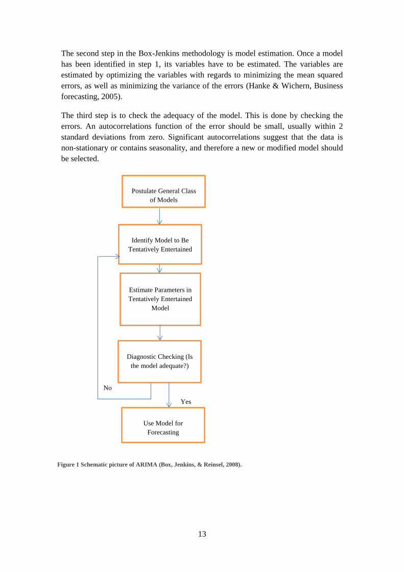
13
The second step in the Box-Jenkins methodology is model estimation. Once a model
has been identified in step 1, its variables have to be estimated. The variables are
estimated by optimizing the variables with regards to minimizing the mean squared
errors, as well as minimizing the variance of the errors (Hanke & Wichern, Business
forecasting, 2005).
The third step is to check the adequacy of the model. This is done by checking the
errors. An autocorrelations function of the error should be small, usually within 2
standard deviations from zero. Significant autocorrelations suggest that the data is
non-stationary or contains seasonality, and therefore a new or modified model should
be selected.
Postulate General Class
of Models
Diagnostic Checking (Is
the model adequate?)
Estimate Parameters in
Tentatively Entertained
Model
Identify Model to Be
Tentatively Entertained
Yes
Use Model for
Forecasting
No
Figure 1 Schematic picture of ARIMA (Box, Jenkins, & Reinsel, 2008).
14
2.2.4 Accuracy of quantitative forecasts
There have been a number of studies where different (quantitative) forecasting
methods have been compared to each other. Makridakis and Hibon have led three
competitions called M-competitions, where researchers all over the world were
invited to construct a forecast from a given set of time series data. In the first M-
competition held in 1982, 15 forecasting methods (and nine variations) computed
forecast from 1001 real-life time series. The second competition, held in 1991 was
designed to run on a real-time basis in collaboration with four companies designated
to provide both data and to answer questions on factors and variables the participating
researchers wanted to know more about (such as competitors, product mix etc.). The
competition ran for two years and also involved estimating six macro-economic
series. After one year, the researchers were allowed to change their forecasts. The
findings from each of these two competitions were practically identical and were
summoned by Makridakis and Hibon as (Makridakis, et al., 1993):
a) Statistically complex methods do not necessarily provide a more accurate
forecast
b) The relative ranking of the methods varied when different methods were
used to measure the forecast accuracy.
c) A combination of forecasts outperform, on average, the individual
methods being combined
d) The accuracy of the methods varies according to the time horizon being
forecasted
Despite these findings (which were validated by many of the participating
researchers), theoretical forecasters have (according to Makridakis and Hibon) largely
ignored this and continued to put effort into building more complex methods. A final
attempt to settle the issue was made in 2000 when the M3 competition was launched,
where 24 different models utilized 3003 different time series covering industry,
micro, macro, finance, demographics, as well as yearly, quarterly and monthly data.
The results from the M3 competition once again confirmed the previous findings from
the M1 and M2 competition. These findings have been examined and confirmed by
other researchers who have used the same set of data as the one used in the M-
competitions; (Geurts & Kelly, 1986; Clemen, 1989; Flores & Pearce, 2000; Konig et
al., 2005).
The reason why sophisticated and well-fitted models do not perform better than
simple models is explained by Makridakis and Hibon (2000) by the fact that future
data is usually never as predictable as quantitative models suggests and that past data
cannot predict upcoming event and changes. The fact that sophisticated models are
fitted against past events creates a bias within the model as the variables change with
unforeseen and low predictability events such as competitor action, technological
changes and macro-economic changes.
15
Combination of quantitative forecasting methods
Combining more than one forecast has been shown to reduce forecasting errors
(Makridakis & Hibon, 2000; Ringuest & Tang, 1989). The improvement accuracy
tends to greater be when the individual forecasts have poor accuracy themselves
(Makridakis & Hibon, 2000). Researchers have tried to identify optimum ways of
combining forecasts, but empirical studies has shown that the accuracy can be
increased significantly simply by putting equal weight to a number of forecasts that is
combined, or by a median combination method (Ringuest & Tang, 1989).
The general form of a combined forecast is:
Where: is the combined forecast,
is the forecast from the jth method,
is the weight applied to the jth forecast,
n is the total number of forecasts available for combining
A simple average combined forecast is computed by putting equal weights to all
forecast by dividing the weight with the total number of forecasts:
A median combined forecast is constructed by putting if the jth method yields
the median value of the tested models. Otherwise, .
Ringuest and Tang (1989) write that taking historical forecasting experience into
account when combining forecasts (which average and median combination doesn’t)
can increase the accuracy even further. They suggest a combination that is built on the
notion that a forecast that produced the most accurate forecast the previous period, is
most likely to produce the most accurate forecast the following period. Thus the
weight is computed as:
; if the forecast from the jth period produced the least
forecasting error in the previous period.
and
; otherwise
Versions of this method to combine forecasts include:
16
; if the jth method was in bottom xth percentile the previous
period.
and,
; otherwise
Measures of forecasting accuracy
There are many different ways of evaluating forecasting methods. Rob J. Hyndman
and Anne B. Koehler have summarized many of the existing measures in an article
published in 2006. The disadvantages and advantages of each method are also pointed
out. They have divided the measures into five different groups: Scale-dependent
measures, Scale-independent measures, relative error relative measures and scaled
error measures.
2.4.1 Scale-dependent measures
Scaled-dependent measures are accuracy measures whose scale depends on the scale
of the data. A scale-dependent measure is not preferable when comparing different
data sets. Examples of the most commonly used scale-dependent measures are:
∑
√
∑
∑
Since RMSE and MSE will be more sensitive to extreme values than MAE or MdAE,
MAE and MdAE might be better when measure forecasting accuracy for a volatile
observed data set.
2.4.2 Scale-independent measures
Scaled-independent measures are accuracy measures whose scale does not depend on
the scale of the data. A scale-dependent measure can be preferable when comparing

17
across data set (Hyndman & Koehler, 2006). Examples of the most commonly used
scale-independent measures are:
∑
(
)
√
∑
√
∑
The most common measure is MAPE, and many textbooks and articles recommend
MAPE when comparing the accuracy of different forecasts, largely because of the
variables relevance in statistical modelling (Hanke & Reitsch, 1995, p. 120;
Bowerman, et al., 2004, p. 18). Other researchers point out that using scale-
independent measures there will appear some difficulties when time series contains a
zero-value, and for Yt is close to zero (Makridakis, et al., 1998, p. 45). Coleman and
Swanson (2004) argue that logarithmic scale can help measures based on percentage
errors to be less skewed.
2.4.3 Relative errors
Relative error measures are an alternative way of scaling the data by dividing each
error by an error obtained using a different forecasting method. The error obtained
from the method of comparison method is denoted with a*. The usage of relative error
is usually a way to compare how different forecasting methods perform against one
single method (usually a naïve1 method). The different forecasting methods are then
ranked according to their performance against the method of comparison. Examples
of the most common used relative error measures are:
1 Naïve method is when the last known actual is used to forecast future all future values (Makridakis, et
al., 1998).

18
∑
(
)
The greatest disadvantage with relative error is that the models have a statistical
distribution with undefined mean and infinite variance (Hyndman & Koehler, 2006).
2.4.4 Relative measure
An alternative to use relative error is to use a relative measure. This is also a method
to compare different forecasting method with each other, but instead of comparing
errors, a relative measure compares the actual measurements of accuracy. For
example, MAE of a forecast can be compared with the MAE for a benchmarked
forecast to show how different methods perform against a one single method (again, a
naïve method is usually chosen as the method of comparison).
When the benchmarked forecast is a naïve method and the relative measure value is
RMSE, the method is called Theil’s U statistics (Makridakis, et al., 1998). When
Theil’s U statistic (or any other relative measure) gives a value less than one, it
indicates that the forecasting method is better than a naïve method, and vice versa.
2.4.5 Scaled errors
Scaled error uses a meaningful scale when measure the forecast accuracy and it is also
widely applicable compared to relative errors with undefined mean and infinite
variance and relative measures which only can be computed when there are several
forecasts on the same series (Hyndman & Koehler, 2006).
Scaled error is defined as:
∑
Using this definition of scaled errors, different comparison variables can be defined as
for example:
√
19
Hyndeman and Koheler propose that measures based on scaled errors should be the
standard approach for measuring forecasting accuracy. They have also applied a
scaled error measure to the M3-competition, showing that the results it provided were
more consistent with the actual conclusions of the M3 competition. Hyndeman and
Koheler also suggest that it is less sensitive to outliers and more easily interpreted
than RMSSE, and less variable on small sample than MdASE. In the latest of large
forecasting competition held in 2010, tourism data was used, the researchers who set
up the competition endorsed the opinion of Hyndman and Koehler; that MAScE
should replace MAPE as the standard measure of forecast accuracy (Athanasopoulos,
et al., 2011).
A value of MASE greater than one shows that the proposed forecast, on average,
gives smaller errors than the benchmarked forecast, and vice versa.
Judgmental forecasts
Even if a firm has the ambition of using quantitative models as the primary mean to
forecasting, there should always a measure of judgement involved in the forecasting
process (Hanke & Wichern, 2005, p. 463). Good judgement is required when deciding
if the data that is available is relevant. The interconnection between the future and the
past might change (e.g. change of technological base in society) and thus the variables
used in the model will not be optimized to predict future outcome. In those cases,
theoretical models must be changed according to judgement and knowledge of the
different market factors.
There is a wide range of possibilities on how a firm can utilize judgemental
adjustments to forecasts. On one end, there is the possibility of firms’ historical data
series, and adjustment is a very small part of the forecasting process. On the other
end, circumstances might make it impossible to use a quantitative model, or the use of
one might not be practical. Circumstances that make the use of theoretical models
impossible might be that there are no data available, or that the analyst’s opinion is
that the historical data is directly irrelevant to future demand (Harvey, 1995).
2.5.1 Judgmental forecasting methods
The methods described below are not subject to empirical testing later in this report.
Instead, they are presented simply to show alternatives to quantitative forecasts that
are strictly based on judgement.
The Delphi Method
Group dynamics is a critical issue when a group of people is asked to jointly reach a
consensus about the future. The result of an exercise like that is that the group will
reach “consensus”, even though all participants may not agree to the decision,

20
because of high-ranking members or of vocal members of the group (Hanke &
Wichern, 2005, p. 464). One method to avoid the aspects related to group dynamics
from the forecasting process is the Delphi method. Initially, members of the group
reply in writing what they’re thought are on the questions posed by an investigation
team. The opinions and then summed up and e-mailed to all members who can answer
and defend or change their opinion. This usually goes on for another two or three
round until the investigation feels that they have information on all aspects of the
future (Rowe & Wright, 1999).
Bottom up/ Top down forecasts
Bottom-up and Top-Down forecasts are two sides of the same judgmental-
forecasting-coin. The forecast is made in-house by either salespersons (bottom-up) or
managers (top down) to estimate sales. Top-Down forecasts is usually believed to be
more focused on the general knowledge of the business, while bottom-up forecasts are
believed to have an advantage because of salespersons knowledge on the local market
(Kahn, 1998).
2.5.2 Accuracy of judgmental forecasts
Research has shown that whenever historical data is available, the interference of
judgemental modifications on average reduces the accuracy of the forecast (Jain,
1990; Flores & Pearce, 2000). Graham and Harvey (1996) showed that three quarters
of all newsletter recommendations made by (supposedly) knowledgeable
professionals for investments on the financial market performed worse than a random
selection of stocks. Professional managers investing in stocks and funds also
consistently underperform when compared to the S&P 500 index (Makridakis, et al.,
1998, p. 485). A common explanation to this finding is attributed to bias on the part of
the forecaster, possibly because of a tendency to be overly optimistic or pessimistic
(Graham & Harvey, 1996). It has also been shown that a judgemental component
within a forecasting process increases the cost of forecasting (Makridakis, 1986, p.
45).
A number of judgemental forecasts made for areas other than financial investments
have been shown to perform worse than a naïve method. Salesperson’s forecasts have
for example been shown to be notoriously inaccurate (Walker & McKlelland, 1991;
Winklhofer, et al., 1996; Makridakis, et al., 1998). Salespeople’s forecasts fluctuate
considerably depending on the mood of the salespeople and whether the rate of
success of sales calls made close before forecasting (Walker & McKlelland, 1991).
There is also a possibility that salespeople are rewarded if selling more than their
target, which increases bias. At the same time, sales managers want to set high targets
as motivation for the salespeople, thus adjusting the forecasts upward.
Management forecasts are much as likely as being inaccurate as salespeople forecast.
Managers tend not to see how competitive threats or new technologies will affect the

21
market, and (Walker & McKlelland, 1991) has shown that managers are
overoptimistic and that they have difficulties setting personal and political interests
aside. In line with the general knowledge on judgemental forecast, management
forecast are inferior to statistical models, as long as data is available. The same result
has been observed when researchers have compared “expert” (business analysts,
researchers etc.) forecasts with those if statistical models (Makridakis, et al., 1998, p.
492). Another interesting aspect of judgemental forecasting is that biases cannot be
avoided by making decisions made in groups. Instead, groups amplify the effect of
bias (Janis, 1972) as members become supportive of the leader and each other.
Another problematic aspect of group decisions is that responsibility for the decision
cannot be traced back to one single individual.
Combination of judgemental forecasts and quantitative methods
The notion of judgemental forecasts being inferior to statistical models has hopefully
become clear to the reader at this point. With that said, salespersons and managers do
possess valuable information that could greatly improve a firm ability to estimate
future demand. One way to take advantage of the objectiveness of theoretical models,
while capitalizing from judgemental information and management knowledge is a
procedure called anchoring (Makridakis, et al., 1998). When anchoring, a number of
key people are shown the forecast made by the quantitative model. To this, they add
or subtract a percentage to the forecast depending on circumstances and variables they
feel that the theoretical model does not take into account. The proposed changes must
be explained and the factors involved must be written down. The adjustments are
made anonymously in order to avoid being influenced by high-ranking members of
the group.
An investigation Fildes et. al. (2009) of more than 60,000 quantitative forecasts and
their accuracy made by four companies, known as being good at forecasting, showed
that 80 per cent of all forecasts made had a judgemental adjustment to the initial
forecast calculated by a computer. The result of the adjustment was three times out of
four a more accurate forecast. The investigation shows that larger adjustment increase
accuracy while small adjustments tend to decrease the accuracy. This is explained by
the fact that large adjustments are based on specific knowledge of larger events
(marketing campaigns, price increase etc.) while smaller adjustments tend to be based
more on “gut-feeling”. When studying positive and negative adjustment where
positive adjustment decreases the accuracy and vice versa for negative adjustment.
Fildes et al. (2009) explain this attribute by a general over-optimism in management
judgement.
Other circumstances when judgemental adjustments increase the accuracy are when
the volatility of sales is high. (Sanders & Ritzman, 1992) has shown that a coefficient
of variation (ratio of the standard deviation of the data divided with the overall mean)
reached 30 per cent, adjustments started to increase the accuracy. As the volatility
22
increases, the accuracy has been shown to increase even further. But, this relation is
only true as long as the volatility in a series does not reflect unanticipated events
(O'Connor, et al., 1993).
Reasons for judgemental adjustment decreasing the accuracy include the fact that
analysts adjust forecasts based on unreliable data, and that adjustments (with or
without reason) tend to give the analyst more confidence in the forecast (Harvey,
1995; Kottemann, et al., 1994).
Theoretical framework - Summary
In order to contribute to the existing knowledge base on business forecasting, three
hypotheses has been identified that will be compared to the empirical findings made
within this thesis:
H1: Quantitative forecasts outperform, on average, judgmental forecasts.
H2: A combination of forecasting methods will increase the accuracy when
compared to the individual methods that.
H3: The relative ranking varies depending on which accuracy measure
through which the forecasting method is measured.
A fourth hypothesis has been identified in the academic literature, but it will not be
compared to any empirical findings, as an empirical investigation on how much the
accuracy increases because judgemental adjustments to a quantitative model. It will
instead be discussed in relation to the capabilities of key personnel at The Company.
H4: Judgmental adjustments to a quantitative method increase the accuracy.
23
3. Method
This section provides a description on how the report was conducted. In order to
reach the objective of this thesis the methodology was divided into four distinct
sections:
A literature review on the subject was conducted in order to gain enough
knowledge on the subject to be able to draw valid conclusions when
looking at the results of the experiments and from the interviews.
Knowledge on the subject was also crucial when setting up experiments,
as well as the outline of the interviews (Dalen, 2007, p. 12).
Secondly, we collected data on The Company. The data collected consisted
of both quantitative and qualitative data. Examples of quantitative
information are sales figures, external order intake and previous forecast
made by The Company. Qualitative data was mainly collected through
interviews with personnel within the organization.
An effort has been made to “clean” the quantitative data from outliers in
order to optimize the third step of the process, which was to apply
historical data on different forecasting models presented in the academic
literature to see which would have the most potential to increase the
forecasting accuracy.
The last section in the methodology was to discuss the empirical findings
in relation to the theoretical framework as well as the overall purpose and
aim of the thesis.
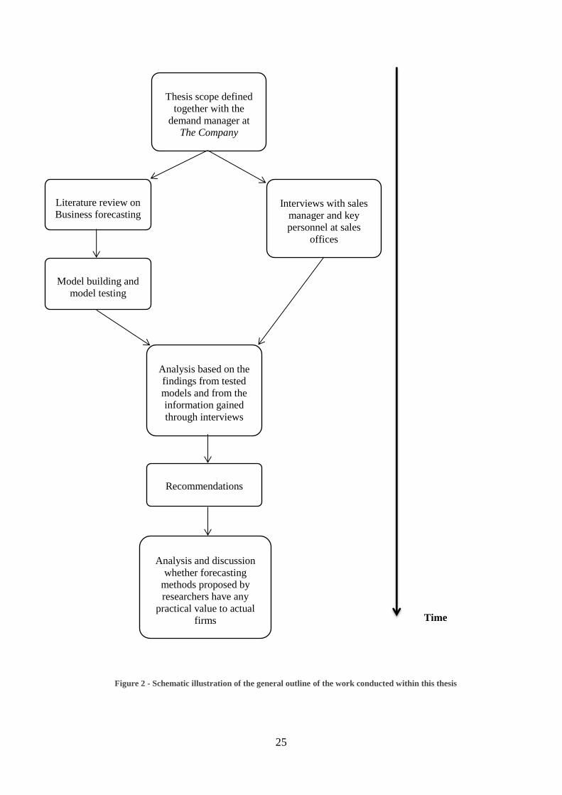
Scope and general outline of the work conducted within this thesis
The scope of the thesis was discussed at an initial meeting at The Company. It was
decided that the thesis would study what the current forecasting process at The
Company looks like, and to investigate whether a quantitative forecast based on
historical data could improve the current forecasting process. Within the scope, it was
also decided that the quantitative method that were to be studied, needed to be simple
enough for The Company to implement them without having to hire consultants to do
it, or spending much time understanding the underlying theory of the forecasting
method. The decision which methods to test were decided jointly by the authors, the
demand manager and the data intelligence manager.
Contact was taken with Patrik Jonsson, professor in Operations and Supply Chain
Management at the Division of Logistics and Transportations at Chalmers University
of Technology. He was of great help much help by proposing books and articles. Prof.
Jonsson also explained the methodology behind testing and evaluating different
forecasting methods. It is believed that without his help, the result of the thesis would
not have been as valid as otherwise.

24
Information on the current forecasting process was mainly gained through interviews
with the demand manager, and with sales managers and business controllers at
various sales offices in Europe.
To test whether a quantitative forecasting method is a mean to increase forecasting
accuracy, an extensive literature review on business forecasting was launched.
Information gained from textbooks and articles published in scientific journals were
used to construct a number of different quantitative forecasting models in order to
identify methods that could increase the accuracy of the forecast at The Company.
The constructed methods were evaluated and the results were later compared to the
forecast made by The Company.
Quite early in the process of working with the thesis, an intricate feeling emerged that
researchers are studying forecasting models that are too complex to be of any use to
actual firms. Deriving from this feeling, the task to investigate whether research on
business forecasting has limited practicality started, and became part of the purpose of
the thesis. The investigation is strictly based on the normative opinion of the authors.
25
Interviews with sales
manager and key
personnel at sales
offices
Literature review on
Business forecasting
Model building and
model testing
Thesis scope defined
together with the
demand manager at
The Company
Analysis based on the
findings from tested
models and from the
information gained
through interviews
Recommendations
Time
Analysis and discussion
whether forecasting
methods proposed by
researchers have any
practical value to actual
firms
Figure 2 - Schematic illustration of the general outline of the work conducted within this thesis
26
Literature review
The literature that has been studied lies mainly within the field of business
forecasting. Initially, a comprehensive understanding on the subject was reached by
reading textbooks. The work of Makridakis et al. (1998), seen by many as one of the
best comprehensive introductions to business forecasting (Faria, 2002; Briggs, 1999),
has been of great help to understand the basics principles of business forecasting, as
well as to provide information on which areas that required further research. Others
textbooks studied include Manufacturing, Planning and Control (2009) by Patrik
Jonsson and Stig-Arne Mattson and Business Forecasting (2005) by John E. Hanke
and Dean W. Wichern
For deepened understanding, scientific articles were studied. The articles were
obtained mostly through web-based search engines using key words. Emphasis has
been put into studying high-cited articles. The most important journal on forecasting
is International Journal of Forecasting with an impact factor of 1.424, and many
articles used in the thesis has been published in this journal.
Many of the articles studied within this thesis studies the M-competitions. M-
competitions are three competitions held in 1982, 1993 and 2000 where a number of
researchers have been led by Spiros Makridakis and Michele Hibon to conduct
forecasts on a given set of time series data. The advantages of these competitions are
that they focus on empirical validation, which simplified comparison between
different forecasting methods.
Data collection
Both quantitative and qualitative data was collected within the thesis. Quantitative
data consisted mainly of numerical data such as sales and external order intake of The
Company, while qualitative data consisted of data retained through interviews with
key personnel at The Company.
3.3.1 Quantitative data
The quantitative data was provided by the demand manager and the data intelligence
manager at The Company. This means that the data from The Company might have
been manipulated, as we have not been given access to look at the raw data sent in
from front-line salespersons. However, it is not likely that the data does not reflect
actual sales and order intake as we have identified no strong incentives for the
demand manager and the data intelligence manager to provide us with false data.
27
Qualitative data
Qualitative data was collected through a number of interviews held with employees of
The Company. The interviews were conducted through face-to-face meetings with
local representatives at sales offices in UK, France and Germany. In UK, the
employees that participated in the interview were the UK sales manager and three
business controllers. In France the attendees where the District Area Manager (DAM)
(responsibilities included France as well as Spain and Italy) and a regional controller,
while the participants in Germany where the DAM and a controller.
The interviewees where recommended to us by the demand manager at The
Company. They were all familiar with the local process of forecasting, and all of the
individuals the demand manager recommended did attend the meetings except for a
financial controller in Germany. The DAM explained that his absence would not be a
problem, as he and the controller being present were familiar with the process and
with his work.
The ambitious for the interviews were for them to be relatively open, characterised by
discussions rather than a questioning. The interviews proved to be valuable as they
confirmed some of the information obtained in the literature review. The interviews
also clarified what capabilities and the resources where available at each sales office,
which helped as it highlighted which potential changes that would be realistic and
possible.
Despite the open interviews, a questionnaire was constructed that functioned as a
template in order to make sure that we didn’t forget to ask question we had discussed
in beforehand as being important. The questionnaire was pre-tested during a
telephone meeting with the sales manager of the Swedish sales office. The
information he provided to us has been used in the thesis, but not as extensively as the
data obtained from the face-to-face meetings in UK, France and Germany. The reason
for this is that his time was quite limited, thus the information was not very thorough,
and partly because we found out that the first draft of the questionnaire was not good
enough; the questions we were asking did not provided us with misaligned answers
compared to the general scope and aim of the thesis.
3.4.1 Validity in qualitative interviews
Researchers have pointed out issues regarding the validity when using interviews as a
source of data (Kvale & Bryman, 2002). According to Dalen (2007), there are four
different factors that are related to validity in qualitative interviews:
1. Validity regarding the researcher (and his/her relationship to the
phenomena being studied)
2. Sample

28
3. Validity regarding the data (eg: The data obtained does not reflect the
reality)
4. Validity regarding (the scientists) interpretation and analytical methods
(different researchers might interpret the data differently, thus drawing
different conclusions)
Factor 1 is not believed to be of any relevance to this thesis as the authors have no
relationship to The Company, and that the task given to them was to study the
company from a theoretical standpoint without much guiding from the company.
Factor 2 – 4 is believed to be more serious threats to the validity of the findings. As
mentioned before, the demand manager of The Company picked the interviewees,
minimizing our control of the sample. Still, the interviewees are believed to be of high
relevance to this thesis as they were very familiar with the process of forecasting. The
reason why UK, France and Germany were chosen as the countries to visit was both
logical and practical. All three countries are large markets and are important to The
Company, but there are differences among them. They have different sales
organizations and their respective customers behave differently. The difference makes
the data provided by them valuable as they cover many of the different types of
market behaviour where The Company is present. The practical side of it was that the
three countries are located relatively close to Sweden, and also close to each other,
making it possible to visit all three countries during one trip at a reasonable cost.
There is always a possibility of the raw data being wrong (Dalen, 2007). The
interviewees might intentionally give the wrong answer to avoid being criticised
(Hanke & Wichern, 2005). The interviewee might also not be certain of the answer,
but still answering (e.g. guessing), which also might affects the validity. In the
interviews held within this thesis, the benefits of a more accurate forecasting were
understood by all participants, increasing the possibility of the answers being correct
and honest. In UK and Germany, the time was of no factor and the answers were
thorough. The sales office in France had recently implemented a new ERP-system,
and the DAM and the controller seemed to be a somewhat stressed, making the
interview not as thorough compared to the ones conducted in UK or Germany.
Being novices in the subject, we have tried to use the information given to us during
the interviews as they have been told to us. We have avoided interpreting what was
told in a way that could affect the validity to much extent.
Experiments
One of the key elements of this thesis was to investigate the possibilities of adding a
quantitative time-series forecasting model to the current forecasting process at The
Company. A number of different quantitative forecasting methods presented in the
29
academic literature on external order intake between January 2010 and May 2013
have been tested.
The test was constructed in such a way that historical data was applied to a
quantitative model who forecasted value for time periods in the past. This way the
forecast from the quantitative model can be compared to known actuals in the past.
The test measured the accuracy on three and six months’ time frame, as those
intervals was used among the staff at The Company. For a three months forecast, the
first month that was forecasted differed depending on the model, but generally the
first month forecasted was April 2010, and for a six months forecast the first forecast
was usually made for July 2010. The accuracy of each forecast has then been
evaluated through a number of different measures to see which performed the best.
The quantitative forecasts have also been compared to the forecasts that The Company
has made between May 2012 and May 2013 in order to see whether they have any
potential to increase the accuracy (there is no data available for forecasting accuracy
made by The Company prior to May 2012).
3.5.1 Forecasting methods
Historical data was compiled in MS Excel in order to test the different models and to
conclude which model that performed the best. The result of those tests, in
combination with information gained through academic literature review and
information from the interviews with employees, was the foundation of the discussion
and final recommendation to The Company.
The models we chose to test were
3 Months Moving Average (3MA)
5 Months Moving Average (5MA)
Last Year Actual (LYA) (e g. Forecast for July 2011 is set as the actual value
of July 2010)
Single Exponential Smoothing (SES)
Adaptive response rate single exponential smoothing (ARRESES)
Holt’s method
Holt-Winter’s trend and seasonality measure
Holt-Winter’s measure, trend excluded
All of these methods are well known within the field of business forecasting. They are
presented in Makridakis et.al. (1998), and they were also used in the M-competitions
(Makridakis & Hibon, 2000). The level of difficulty also varies among the different
30
methods, from simple methods such as MA and LYA, to more advanced methods
such as Holt-Winter’s trend and seasonality measure.
A number of methods have of course been excluded from this report. The reason why
they have been excluded is simply because they were too complex, and also not
included in the work of Makridakis et. al. (1998). Examples of methods being deemed
as too complex are the ARIMA-models. The guideline from the beginning was to
come up with a forecasting method that would be simple to understand for The
Company. ARIMA-methods need an understanding of autocorrelation and how to
interpret data to change the model according to changes in the data. This is an
understanding that The Company does not have in-house, thus it was excluded from
the report.
As mentioned earlier in the report, the decision on which forecasting methods to
construct and to test was made by the authors, the demand manager and the data
intelligence managers in consensus. However, the authors had deeper understanding
of different forecasting methods, and the process can be described as the authors
presenting different forecasting methods to the demand manager and the data
intelligence manager. During the presentation, it was explained how the method
should be constructed, and how many variables it contained. The data manager and
the demand manager asked clarifying questions, and later decided whether or not the
particular method would be too difficult for The Company to implement. If it was
deemed too difficult, the authors did not proceed constructing and testing the method
in MS Excel.
In many of the forecasting methods, initial values of the first forecast have been
estimated by the average of the first 12 months. Where variables have been optimized
(such as in SES) the solver function in MS Excel has been used.
3.5.2 Measurements of forecasting accuracy
The measurements used to analyse the accuracy of each forecasting methods used in
this thesis were:
Mean Error (ME)
Mean Absolute Error (MAE)
Mean Squared Error (MSE)
Mean Absolute Percentage Error (MAPE)
Theil’s U-statistics
Mean Absolute Scaled Error (MAScE)

31
The reason why these measures were chosen was that all of them, except MAScE, are
presented in Jonsson & Mattson (2009), Makridakis et. al. (1998, pp. 43-49) as well
as in Hanke & Wichern (2005, pp. 78-82), and can thus be considered to be well-
known and easy to understand. MAScE is used because of the arguments made, and
empirical evidence presented by Hyndeman and Koehler (2010) saying that MAScE
provide consistent results.
As described in the theory-chapter, different models may perform differently
depending on which measurement is used. Our hopes were that one single method
would outperform the other methods in all measurements. If a superior model was not
found, MAScE was decided to be the measurement to use when benchmarking the
result of different forecasting methods. We have not found consensus in the literature
saying that MAScE is superior to other measurements, but we believe that the benefits
of MAScE (mentioned in Chapter 2), as well as the findings that MAScE provided a
more consistent result on the M3-data to be very convincing.
3.5.3 Identifying outliers
Workwise, a lot of time has been spent on transforming raw-data into valid and
reliable data suited for forecasting. We found that trimming and winsorizing are
inconsistent ways of identifying and replacing outliers. The point of transforming
raw-data into reliable data is not to exclude extreme values simply because they are
extreme values, there must also be a reason (seasonal, or external) for the extreme
value to become an outlier.
This thesis used a similar approach to that of winsorizing with the difference that each
extreme value was investigated. In order to determine whether the extreme value
could be explained by an external factor, each value was discussed together with sales
managers and demand manager. If an extreme value was identified as an outlier, the
outlier was substituted by an average of the two previous and two following months.
32
4. Empirical findings – The Company
This chapter includes a brief presentation of The Company and their current
forecasting process. The decomposition of the data is presented to show the trend and
seasonal component in the data set. Finally, the results of the quantitative models are
compared to the forecast made by The Company to determine if a quantitative model
can improve the forecasting accuracy.
The Company – general information, products and market characteristics
The Company is a global manufacturer of B2B products with sales and service
location in 120 countries, with sales totalling approximately 900 million euro in 2012.
The product line is divided into five different groups. The products in the each
different group are not very similar to the products in another group, and the products
within each group also cover a wide range of price and applications. Despite the
differences, most products share the same type of end user. This thesis only constructs
a quantitative forecast based for one of the different product groups; Product group 1.
The products in product group 1 can be categorized as premium in comparison to the
products of competitors, and lie within the prize-range of €2,500-€196,000 depending
on model. The expected lifespan of the products is 8-10 years (normal usage). The
buyer differs depending on country of sales. In some markets, such as Sweden, the
buyer is usually the same as the end-user, while in other countries the buyer is a large
company purchasing large quantities. In some countries it is also common that the
buyer is a dealer that offers a “complete package” to the end-user, in which The
Company’s product is one part.
There are a number of competitors active in each market. Except for a few other truly
global companies, many competitors are strong in one or two markets.
Current forecasting processes at The Company
The Company’s forecasting process is constructed locally in each country/region and
consists of a 24-month forecast where external order intake for each model is
forecasted. The demand manager has a meeting with the District Area Manager where
the forecast is discussed before the forecast is passed on to the head of market of The
Company.
There are no specific guidelines provided by The Company to the local sales offices
on how a forecast should be done, and how each country or region forecasts is
decided in each specific country. How forecasting is done is different countries varies,
but it is generally a bottom-up forecast where the opinion of salespersons and
distributors is taken into account, and later adjusted by a manager before the final
forecast is set.

33
According to the demand manager, the intellectual input into the forecast process
varies depending on country. Some countries take the forecasting process seriously,
having well-founded arguments regarding customer and competitor activity, while
other countries spend little time and effort. Some countries even fail to report their
forecast. The sales manager speculates that the reason behind the lack of input into the
forecasting process is that some sales offices are busier, while some lack interest into
spending the resources needed to produce a well-founded forecast.
4.2.1 UK
The UK-market is characterized by large tender-orders from large companies. The
sales organization consists of a number of sales-offices spread around the country.
When estimating future sales, the sales are divided in known and unknown sales. The
part which is known derives from a simple CRM-system, in which salespersons
reports quotations, including quantity, the likelihood of reaching an agreement and
date of expected order. From this, a forecast is produced. The unknown part consists
of future sales that haven’t been reported in by salespersons. Customers being familiar
with the product line characterize unknown sales, and orders are placed on the spot.
The national sales manager makes the forecast of the unknown part, and process
could be described as “advanced guessing”, as he uses his experience and the input of
other employees. The unknown part increases as the time horizon gets longer, and a
forecast of more than six month into the future consists mostly of experience and gut
feeling.
When asked about what actions they feel could improve the forecasting process, the
UK-office pointed out the large amount of time consuming reporting that have to be
done. They feel that forecasting each model 24 months into the future is irrelevant as
it is impossible to accurately predict order intake for that long. They also favour a
process where all the data they have to report, such as financials and order intake,
deliveries should be done on a “master document”. Their opinion was also that a
quantitative model based on historical data is not compatible with the reality as it is
today. The volatility in sales requires a judgemental approach, as a theoretical model
is inferior to experience when it comes to understanding customer behaviour and
upcoming events.
4.2.2 France
The sales organization in France is different from the organization in UK. Most of the
sales in France are made through dealers instead of salespeople employed by The
Company. The forecast is constructed by the DAM and a financial controller. The
DAM and the financial controller mainly use the opinion of key account customers
(who are even more dominant in France than in UK) to estimate future demand. The
forecaster in France do not use any quantitative model and they feel that dealers are
not very trustworthy when asked about future sales, as they tend to be over-optimistic.

34
In line with the opinions of the UK-office, the France-office thinks that the reporting
is too thorough. They also expressed the opinion that it is very difficult to perform
monthly forecast, especially as they have many key account customers who might
decide to postpone their order. A postponed order will highly affect the forecast
negatively, but the France-office felt that they were “punished” in a way that was not
fair, as they knew an order was coming, just not the exact date of order. France also
expressed a concern regarding the “reward” for producing accurate forecasts. They
pointed out that even when forecasting is accurate, the lead time does not change from
the factories.
4.2.3 Germany
Different from the France and UK customers, the average customer in Germany did
not order a large quantity. When large tender orders are made, the customers are
focused on prize where The Company is unable to compete with customers. The sales
office in Germany wins one large tender order per year on average. They have dealers
spread out over Germany, as well as employed sales persons as well. The DAM and
two financial controllers construct the forecast. They base their forecast on
judgement, but also with the aid of different indexes and indicators. Examples of
indicators they use are the forecasts made by industry associations of products that are
related to the products of The Company. They also study the amount of offers they
have sent out at the moment, and try to draw conclusions from those. They do not
have any statistics on hit rate among the offers, but they use their experience instead.
As with France and UK, Germany felt that the time horizon was far too long. They
also feel that the forecast is too detailed, as they have to forecast each specific model.
A forecast horizon of more than six months is more guessing and experience than a
forecast made on a shorter time horizon, which is more based on actual figures and
data.
Evaluation of forecast made by The Company
The Company started to log their forecasts in February 2012. That means that their
first three-month forecast was for May 2012, and the first six-month forecast was
made in February for August 2012. The result of the three-month the forecast is
heavily affected by quotation for a very large order, which was believed at that time
to be won and the order to be in place in August 2012. This can be seen in Figure 3.
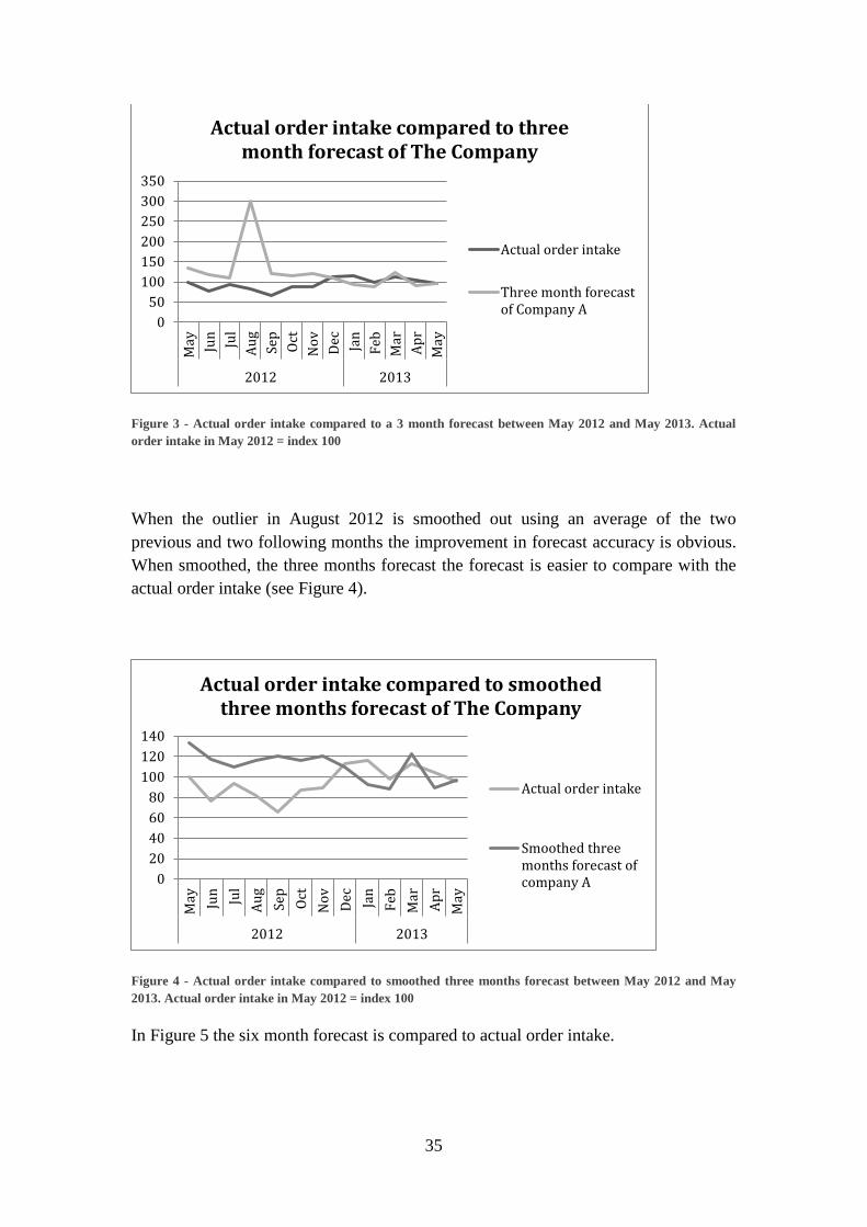
35
Figure 3 - Actual order intake compared to a 3 month forecast between May 2012 and May 2013. Actual
order intake in May 2012 = index 100
When the outlier in August 2012 is smoothed out using an average of the two
previous and two following months the improvement in forecast accuracy is obvious.
When smoothed, the three months forecast the forecast is easier to compare with the
actual order intake (see Figure 4).
Figure 4 - Actual order intake compared to smoothed three months forecast between May 2012 and May
2013. Actual order intake in May 2012 = index 100
In Figure 5 the six month forecast is compared to actual order intake.
0
50
100
150
200
250
300
350M
ay Jun
Jul
Au
g
Sep
Oct
No
v
Dec Jan
Feb
Mar
Ap
r
May
2012 2013
Actual order intake compared to three month forecast of The Company
Actual order intake
Three month forecastof Company A
0
20
40
60
80
100
120
140
May Jun
Jul
Au
g
Sep
Oct
No
v
Dec Jan
Feb
Mar
Ap
r
May
2012 2013
Actual order intake compared to smoothed three months forecast of The Company
Actual order intake
Smoothed threemonths forecast ofcompany A

36
Figure 5 - Actual order intake compared to six months forecast between Aug 2012 and May 2013. Actual
order intake in Aug 2012 = index 100
The accuracy for the smoothed three and six months forecast can be seen in the table
below (Table 1).
As can be seen in Figure 4 and Figure 5, the forecast is generally too positive for
forecasts on three and six months’ time horizon. The U-statistics highlight that the
forecast was more or less unnecessary, as a naïve method, on average, performed
better than the forecast.
Evaluation - forecast of The Company ME MAE MAPE MSE U-stat MAScE
3 months forecast 120 182 27% 47737 1,01 0,70
6 months forecast 170 214 31% 65638 1,48 0,99
Table 1 - Evaluation of The Company's actual forecast between May 2012 and May 2013
Data decomposition
When looking at Figure 6, it can be seen that the external order intake varies over
time, and that there is no clear trend. The fact that there is no trend suggests that a
fitting forecasting model does not require a variable taking trend into account.
0
50
100
150
200
Aug Sep Oct Nov Dec Jan Feb Mar Apr May
2012 2013
Actual order intake compared to six months forecast of The Company
Actual order intake
Six months forecastof Company A
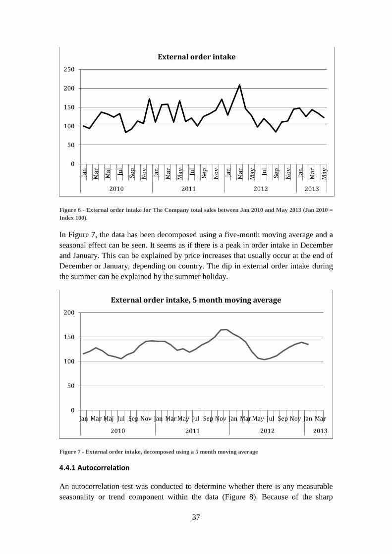
37
Figure 6 - External order intake for The Company total sales between Jan 2010 and May 2013 (Jan 2010 =
Index 100).
In Figure 7, the data has been decomposed using a five-month moving average and a
seasonal effect can be seen. It seems as if there is a peak in order intake in December
and January. This can be explained by price increases that usually occur at the end of
December or January, depending on country. The dip in external order intake during
the summer can be explained by the summer holiday.
Figure 7 - External order intake, decomposed using a 5 month moving average
4.4.1 Autocorrelation
An autocorrelation-test was conducted to determine whether there is any measurable
seasonality or trend component within the data (Figure 8). Because of the sharp
0
50
100
150
200
250
Jan
Mar
Maj Ju
l
Sep
No
v
Jan
Mar
May Ju
l
Sep
No
v
Jan
Mar
May Ju
l
Sep
No
v
Jan
Mar
May
2010 2011 2012 2013
External order intake
0
50
100
150
200
Jan Mar Maj Jul Sep Nov Jan Mar May Jul Sep Nov Jan Mar May Jul Sep Nov Jan Mar
2010 2011 2012 2013
External order intake, 5 month moving average
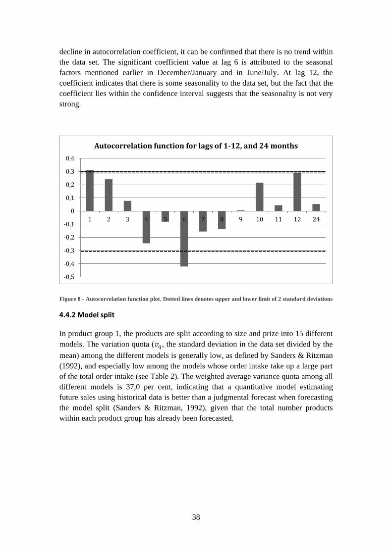
38
decline in autocorrelation coefficient, it can be confirmed that there is no trend within
the data set. The significant coefficient value at lag 6 is attributed to the seasonal
factors mentioned earlier in December/January and in June/July. At lag 12, the
coefficient indicates that there is some seasonality to the data set, but the fact that the
coefficient lies within the confidence interval suggests that the seasonality is not very
strong.
Figure 8 - Autocorrelation function plot. Dotted lines denotes upper and lower limit of 2 standard deviations
4.4.2 Model split
In product group 1, the products are split according to size and prize into 15 different
models. The variation quota ( , the standard deviation in the data set divided by the
mean) among the different models is generally low, as defined by Sanders & Ritzman
(1992), and especially low among the models whose order intake take up a large part
of the total order intake (see Table 2). The weighted average variance quota among all
different models is 37,0 per cent, indicating that a quantitative model estimating
future sales using historical data is better than a judgmental forecast when forecasting
the model split (Sanders & Ritzman, 1992), given that the total number products
within each product group has already been forecasted.
-0,5
-0,4
-0,3
-0,2
-0,1
0
0,1
0,2
0,3
0,4
1 2 3 4 5 6 7 8 9 10 11 12 24
Autocorrelation function for lags of 1-12, and 24 months

39
Model % of total
orders Variance quota
G 6,60% 25,50%
E 28,80% 28,20%
F 12,70% 28,50%
J 2,20% 30,70%
A 11,80% 34,10%
C 3,40% 34,50%
I 0,40% 38,50%
B 2,50% 39,00%
D 18,50% 43,60%
H 1,70% 44,50%
O 5,50% 51,00%
L 2,20% 67,00%
M 2,70% 80,40%
K 0,60% 124,20%
N 0,40% 137,30%
Table 2 – Distributions, variance quota and weighted average variance quota of the models within product
group 1
Accuracy of quantitative models
4.5.1 Accuracy of quantitative models – three months forecast
The accuracy of the different models varies quite differently (see Table 1). The
simplest models such as moving average and last year’s value does not perform very
well compared to more advanced methods. Holt Winters methods that take trend into
account are also not very accurate. The fact that there is no trend component in the
data probably account for this. Single Exponential Smoothing (SES), a relatively
simple method, is among the more accurate methods. This can be attributed to the
high level volatility in the data, and a smoothing method, in this case alpha is very
small, is likely to be accurate. The same is true for Holt’s method, whose trend
component was optimized to be very small, which means that Holt’s method is quite
similar to SES.
The autocorrelation test indicated some seasonality to the data set, which is likely to
explain why Holt Winters methods, where seasonality is included but where trend has
been excluded are the most accurate.
∑
Weighted average variance quota =
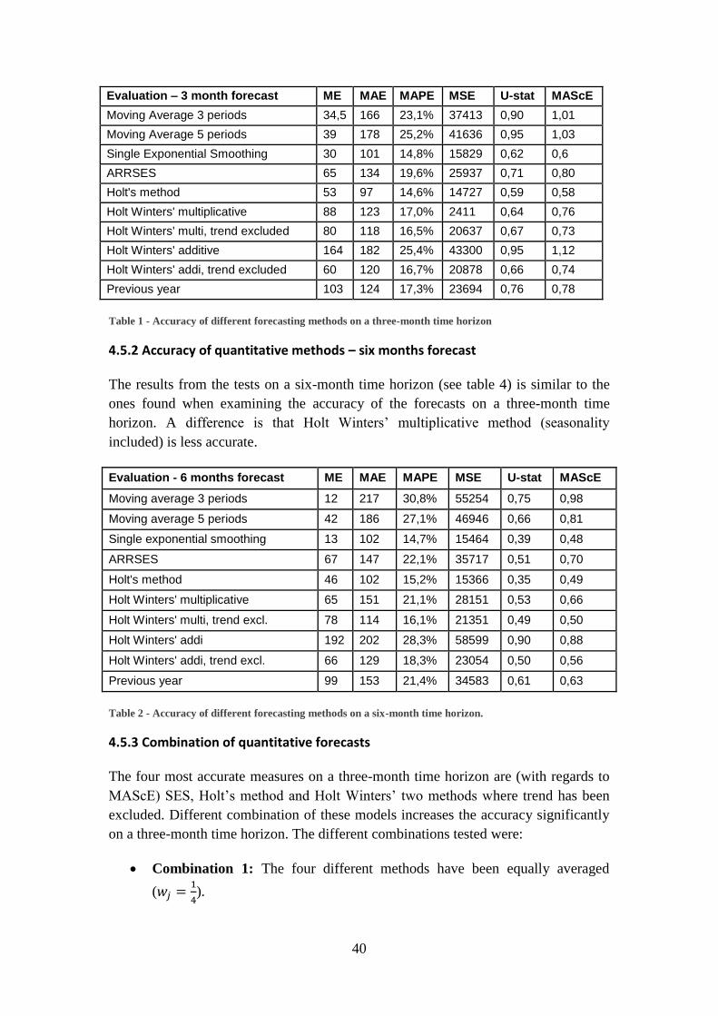
40
Evaluation – 3 month forecast ME MAE MAPE MSE U-stat MAScE
Moving Average 3 periods 34,5 166 23,1% 37413 0,90 1,01
Moving Average 5 periods 39 178 25,2% 41636 0,95 1,03
Single Exponential Smoothing 30 101 14,8% 15829 0,62 0,6
ARRSES 65 134 19,6% 25937 0,71 0,80
Holt's method 53 97 14,6% 14727 0,59 0,58
Holt Winters' multiplicative 88 123 17,0% 2411 0,64 0,76
Holt Winters' multi, trend excluded 80 118 16,5% 20637 0,67 0,73
Holt Winters' additive 164 182 25,4% 43300 0,95 1,12
Holt Winters' addi, trend excluded 60 120 16,7% 20878 0,66 0,74
Previous year 103 124 17,3% 23694 0,76 0,78
Table 1 - Accuracy of different forecasting methods on a three-month time horizon
4.5.2 Accuracy of quantitative methods – six months forecast
The results from the tests on a six-month time horizon (see table 4) is similar to the
ones found when examining the accuracy of the forecasts on a three-month time
horizon. A difference is that Holt Winters’ multiplicative method (seasonality
included) is less accurate.
Evaluation - 6 months forecast ME MAE MAPE MSE U-stat MAScE
Moving average 3 periods 12 217 30,8% 55254 0,75 0,98
Moving average 5 periods 42 186 27,1% 46946 0,66 0,81
Single exponential smoothing 13 102 14,7% 15464 0,39 0,48
ARRSES 67 147 22,1% 35717 0,51 0,70
Holt's method 46 102 15,2% 15366 0,35 0,49
Holt Winters' multiplicative 65 151 21,1% 28151 0,53 0,66
Holt Winters' multi, trend excl. 78 114 16,1% 21351 0,49 0,50
Holt Winters' addi 192 202 28,3% 58599 0,90 0,88
Holt Winters' addi, trend excl. 66 129 18,3% 23054 0,50 0,56
Previous year 99 153 21,4% 34583 0,61 0,63
Table 2 - Accuracy of different forecasting methods on a six-month time horizon.
4.5.3 Combination of quantitative forecasts
The four most accurate measures on a three-month time horizon are (with regards to
MAScE) SES, Holt’s method and Holt Winters’ two methods where trend has been
excluded. Different combination of these models increases the accuracy significantly
on a three-month time horizon. The different combinations tested were:
Combination 1: The four different methods have been equally averaged
(
).
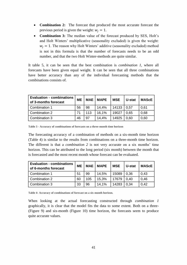
41
Combination 2: The forecast that produced the most accurate forecast the
previous period is given the weight: .
Combination 3: The median value of the forecast produced by SES, Holt’s
and Holt Winters’ multiplicative (seasonality excluded) is given the weight:
. The reason why Holt Winters’ additive (seasonality excluded) method
is not in this formula is that the number of forecasts needs to be an odd
number, and that the two Holt Winter-methods are quite similar.
It table 5, it can be seen that the best combination is combination 1, where all
forecasts have been given equal weight. It can be seen that all three combinations
have better accuracy than any of the individual forecasting methods that the
combinations consists of.
Evaluation - combinations
of 3-months forecast ME MAE MAPE MSE U-stat MAScE
Combination 1 56 98 14,4% 14133 0,57 0,61
Combination 2 71 113 16,1% 19027 0,65 0,68
Combination 3 46 97 14,4% 14925 0,60 0,60
Table 3 - Accuracy of combinations of forecasts on a three-month time horizon
The forecasting accuracy of a combination of methods on a six-month time horizon
(Table 4) is similar to the results from combinations on a three-month time horizon.
The different is that a combination 2 is not very accurate on a six months’ time
horizon. This can be attributed to the long period (six month) between the month that
is forecasted and the most recent month whose forecast can be evaluated.
Evaluation - combinations
of 6-months forecast ME MAE MAPE MSE U-stat MAScE
Combination 1 51 99 14,5% 15089 0,36 0,43
Combination 2 60 105 15,3% 17679 0,40 0,46
Combination 3 33 96 14,1% 14283 0,34 0,42
Table 4- Accuracy of combinations of forecast on a six-month horizon.
When looking at the actual forecasting constructed through combination 1
graphically, it is clear that the model fits the data to some extent. Both on a three-
(Figure 9) and six-month (Figure 10) time horizon, the forecasts seem to produce
quite accurate values.
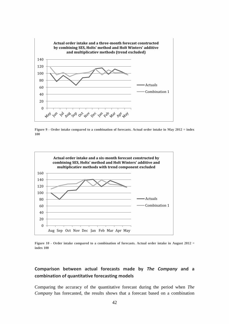
42
Figure 9 - Order intake compared to a combination of forecasts. Actual order intake in May 2012 = index
100
Figure 10 - Order intake compared to a combination of forecasts. Actual order intake in August 2012 =
index 100
Comparison between actual forecasts made by The Company and a
combination of quantitative forecasting models
Comparing the accuracy of the quantitative forecast during the period when The
Company has forecasted, the results shows that a forecast based on a combination
0
20
40
60
80
100
120
140
Actual order intake and a three-month forecast constructed by combining SES, Holts' method and Holt Winters' additive
and multiplicatiev methods (trend excluded)
Actuals
Combination 1
0
20
40
60
80
100
120
140
160
Aug Sep Oct Nov Dec Jan Feb Mar Apr May
Actual order intake and a six-month forecast constructed by combining SES, Holts' method and Holt Winters' additive and
multiplicatiev methods with trend component excluded
Actuals
Combination 1

43
between different quantitative models is far superior to the actual forecast made by
The Company. The improvement is close to 50 per cent for both 3 and 6 months
forecasts (see
Forecast horizon Combination 1 The Company's forecast Improvement
3 months 14% 27% 48,3%
6 months 16% 31% 48,5%
Table 5). Worth noticing is that all quantitative methods tested within this thesis
outperforms the judgmental forecast made by The Company, both on a 3- and 6-
month horizon.
Forecast horizon Combination 1 The Company's forecast Improvement
3 months 14% 27% 48,3%
6 months 16% 31% 48,5%
Table 5 - Comparison between Combination 1, and the forecast made by The Company.

44
5. Discussion
The discussion is divided into two parts where the first part covers the findings of the
thesis and whether they reject or confirm the hypotheseses presented in chapter 2.
The second part consists of the findings and feelings if researchers are possible to
follow with regards to the resources available of normal companies.
Empirical findings compared to Hypotheses identified in academic literature
In this section, a discussion regarding the four hypotheseses presented at the end of
chapter 2 is made. The results support two of the hypotheseses, while our results
neither support nor reject the third of the hypotheseses. The fourth hypothesis is
supported in general terms, and is discussed, but has not been empirically tested.
H:1. Quantitative forecast outperforms judgemental forecasts
The findings of this thesis show that all quantitative forecasting models
applied on historical data produces a more accurate forecast than the forecast
produced by managers and salespeople at The Company between May 2012
and May 2013. The best quantitative model was proved to be a combination of
four individual models, where each model was given similar weight. This
combination improved the forecasting accuracy by 50%.
The forecasts produced by The Company are generally too optimistic. At The
Company, the final version of the forecast produced in each country/region is done by
a sales manager. This might be a possible explanation to the optimistic forecasts, as
researchers have found that managers tend to be too optimistic about the future
(Walker & McKlelland, 1991).
H:2. A combination of forecasting methods increases the accuracy when
compared to the individual methods that the combination consists of.
Researchers have found when studying the M-competitions that a combination
of forecasting methods reduces the forecasting error (Makridakis & Hibon,
2000). Our results show that a combination of the four most accurate
forecasting methods increases the accuracy, thus confirming the findings of
researchers.
A combination of forecast will smooth out the bias built inside each forecasting
method. Even though the future may resemble the history to some extent, it is likely
that the relationship isn’t absolute. Each forecasting method interprets historical data
to optimize its components, but the future will probably not look like the way the
method assumes it will. This “error” in optimization will then be smoothed out when
models are combined (Makridakis et al, 1998).
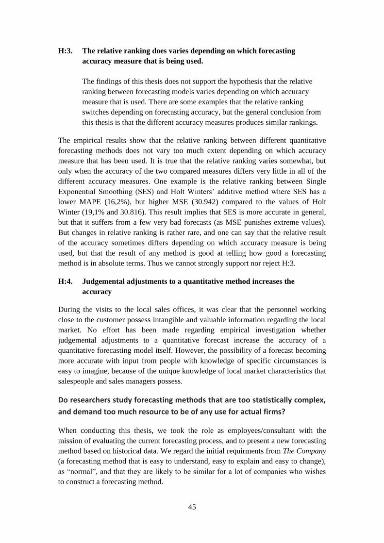
45
H:3. The relative ranking does varies depending on which forecasting
accuracy measure that is being used.
The findings of this thesis does not support the hypothesis that the relative
ranking between forecasting models varies depending on which accuracy
measure that is used. There are some examples that the relative ranking
switches depending on forecasting accuracy, but the general conclusion from
this thesis is that the different accuracy measures produces similar rankings.
The empirical results show that the relative ranking between different quantitative
forecasting methods does not vary too much extent depending on which accuracy
measure that has been used. It is true that the relative ranking varies somewhat, but
only when the accuracy of the two compared measures differs very little in all of the
different accuracy measures. One example is the relative ranking between Single
Exponential Smoothing (SES) and Holt Winters’ additive method where SES has a
lower MAPE (16,2%), but higher MSE (30.942) compared to the values of Holt
Winter (19,1% and 30.816). This result implies that SES is more accurate in general,
but that it suffers from a few very bad forecasts (as MSE punishes extreme values).
But changes in relative ranking is rather rare, and one can say that the relative result
of the accuracy sometimes differs depending on which accuracy measure is being
used, but that the result of any method is good at telling how good a forecasting
method is in absolute terms. Thus we cannot strongly support nor reject H:3.
H:4. Judgemental adjustments to a quantitative method increases the
accuracy
During the visits to the local sales offices, it was clear that the personnel working
close to the customer possess intangible and valuable information regarding the local
market. No effort has been made regarding empirical investigation whether
judgemental adjustments to a quantitative forecast increase the accuracy of a
quantitative forecasting model itself. However, the possibility of a forecast becoming
more accurate with input from people with knowledge of specific circumstances is
easy to imagine, because of the unique knowledge of local market characteristics that
salespeople and sales managers possess.
Do researchers study forecasting methods that are too statistically complex,
and demand too much resource to be of any use for actual firms?
When conducting this thesis, we took the role as employees/consultant with the
mission of evaluating the current forecasting process, and to present a new forecasting
method based on historical data. We regard the initial requirments from The Company
(a forecasting method that is easy to understand, easy to explain and easy to change),
as “normal”, and that they are likely to be similar for a lot of companies who wishes
to construct a forecasting method.
46
Even though the specifications may be similar between companies, the actual
forecasting process that is constructed may not look the same because of different
capabilities and a difference in available resources between firms. Some, especially
larger firms, are likely to have employees with profound skills in both statistics and
coding which enables them to construct advanced forecasting methods. In The
Company, the resources available are limited, and the demand manager and sales
managers have little room for spending additional time on forecasting. The same is
also true for the people working with the ERP-system (in which the forecasting
method will be incorporated). An advanced forecasting method is likely to demand
resources, not only when the method is coded, but also if the ERP-system is updated
or changed. Even though the level of knowledge varies among firm, we propose that
the conclusions made in thesis, which derives from the capabilities of The Company,
can be seen as general, as we are confident in the fact that the capabilities of many
firms are similar to those of The Company.
Using a theoretical framework when identifying a fitting method according to the
specifications of The Company, we have been able to draw the following conclusions
regarding the research hypothesis; that researchers study forecasting models that are
too complex to be implemented, thus being of no use, in most firms.
The more simple methodologies on how to decompose a time series are
relevant to the type of work an employee/consultant might be assigned to
do.
An integral part of constructing a forecasting method is to decompose the data in
order to identify the properties and components of the data set. To reach an
understanding, and to draw valid conclusions, you need to be certain about
seasonality, trend and the error-pattern.
Textbooks on the subject usually devote one or two chapters to the process of
decomposition. The chapters usually contain a number of different methods to
decompose a data set, and the level of complexity varies among the methods. The
more simple ones, such as moving average, are easy to understand and to apply to a
data set. The same can be said for an autocorrelation test, whose outcome, the
autocorrelation function, is easy to interpret, and not very difficult to construct. An
autocorrelation test provides the forecaster with quite specific knowledge on trend and
seasonality.
There are many more complex method of decomposition which has not been covered
in this thesis, simply because they are too statistically complex to fit with the needs
and specifications of The Company. In Forecasting – Method and application
(Makridakis et al. 1998), STL and X-12-ARIMA, two more recently developed and
complex methods are discussed, and the discussion ends with:
47
“The computer source code for both X-12-ARIMA and STL is publicly
available for other researchers to adapt. Executive versions of X-12-ARIMA
are available from the same Internet site. STL is also available as an option in
the package S-plus.” (Makridakis et al. 1998:125)
This phrase, as will be seen later in this chapter, in some way sums up how
“unpractical” statistically complex methods are. The fact that the code, according to
the authors, “is available for other researchers” implies that the method is statistically
complex, and to be understood only by people who regard themselves as researchers,
and not as pracitioners. The methods are available in software packages, but if a firm
uses decomposition software, they must be ready to have limited understanding of the
forecasting process, as well as rely on help from experts brought in from outside the
firm for updates and implementation.
Many forecasting methods are too statistically complex for firms lacking
profound skills in statistics and coding.
As with decomposition methods, textbooks present a large number of forecasting
methods, varying from simple methods such as Moving Average to complex ARIMA
models. There are also a number of methods which has not been described in this
thesis. The main reason why they haven’t been described is that they are too complex
to be of any interest to the thesis, given the initial specifications from The Company.
The identification of methods that are “too complex” has been made together with the
demand manager of The Company. Methods deemed to be too difficult to implement
include all ARIMA-models. When learning about ARIMA, in is not hard to
understand why the Demand Manager discarded the models, as initial autocorrelation-
tests followed by partial correlation tests have to be conducted. To that, you have to
interpret the autocorrelation function and find a suitable model, which in turn have to
be fitted to the model by an autoregressive approach, as well as with a moving
average approach. We believe the feeling of complexity and impracticality of many
models that the demand manager felt are shared with managers and other personnel
engaged in estimating future demand at other companies
Many forecasting methods demand non-linear optimization. A non-linear
optimization is not very difficult if there is only one variable that has to be optimized,
as there are no combinations of variables that need to be considered. For more
variables, the process of identifying extreme values (e.g. the best forecast) becomes
more and more difficult, as the number of combinations increases by a factor of 10. It
is possible to optimize through a script constructed when coding the forecasting
method, but the people writing code at The Company expressed concern that it might
be too difficult. There are also commercial software packages available that can
optimize, but that was not an option according to representatives of The Company.
Instead, it was decided that methods containing two variables (such as Holt’s method
or Holt Winters’ with trend excluded) should serve as upper limit for the complexity

48
regarding non-linear optimization. This agreement meant that many of the forecasting
methods proposed and discussed by researchers were excluded from this thesis,
further highlighting the impracticability of many forecasting models that is being
studied by researchers.
The research of business forecasting is relevant, and the research is not
moving away from the actual definition of business forecasting.
Despite our normative opinion that many of the forecasting models discussed by
researchers are too complex for many companies who wishes to construct a
forecasting method in-house, the research itself is relevant in many ways. As
mentioned earlier, advanced forecasting methods are available for everyone in
commercial software packages. Developing a forecasting method in-house is costly,
and an alternative might be to look for forecasting methods externally. The software
packages available on the market derive from the work of researchers. This shows
that the research made have obviously had practical implications, undermining the
statement made in the introduction chapter that the research community is moving
away from the actual area it claims to be studying. Obviously, the findings from the
research made in business forecast are trickling down and eventually reach actual
companies.

49
6. Conclusion
We have been able to empirically confirm two of the four hypotheseses identified in
the theoretical framework of this thesis. Firstly, the findings of this thesis support the
claim that quantitative approaches are superior to a judgmental approach as long as
data is available. Secondly, the hypothesis that a combination of quantitative forecast
increases the accuracy is supported as well.
Our empirical findings have not been able to support nor reject H:3, as the relative
ranking is mostly the same, independent of which accuracy measure is used. H:4 has
not been tested empirically, but our findings from interviews with sales managers and
controllers in sales offices in UK, Germany and France indicate support of this
hypothesis. Sales managers and employees in contact with key account possess
valuable information that could be of great help when forecasting.
The findings regarding researcher’s inability to study forecasting models that are of
use to actual firms are strictly based on the capacities of The Company, and the
capabilities of the authors as employees/consultants. Despite the small and
questionable sample, it became obvious that many of the forecasting models that
researchers discuss and evaluate are too difficult to implement for companies who
wishes to use models that they control and understand. One can question this finding
rather easy by arguing that a case study of a single company, conducted through a
“fake-employment” by two graduates does not produce valid conclusions. With that
being said, we are certain that our capabilities, as well as the capabilities of The
Company, are not unusual compared to the capabilities found in other companies
similar to The Company. Thus, the findings are relevant to companies with equal, or
worse capabilities than that of The Company.
Even though we are firm in our opinion that our findings are relevant, research would
benefit from larger of samples and sets. We recommend that further research be
conducted where researchers empirically test what models are the most suitable for,
depending on the setting and the capabilities of the company. By doing this,
researchers can develop models instructing companies that: “If you lack capability X,
and have access to Y resources, method Z is likely to produce a large increase in
forecasting accuracy, while not putting constraints on the current organization.” A
development in this direction would be of much help to demand planners in
companies, which, according to the definition, is what business forecasting is all
about.

50
7. Bibliography
Athanasopoulos, G., Hyndman, R. J., Song, H. & Wu, D. C., 2011. The tourism
forecasting competition. International Journal of Forecasting, Volume 27, pp. 822-
844.
Bowerman, B. L., O'Connoll, R. T. & Koehler, A. B., 2004. Forecasting, time series
and regression: an applied approach. Belmonth: Thomson Brooks/Cole.
Box, G. E. P., Jenkins, G. M. & Reinsel, G. C., 2008. Time Series Analysis:
Forecasting and Control. 4th ed. Hoboken: John Wiley & Sons Inc..
Briggs, M. W., 1999. Forecasting Methods and Applications by Spyros Makridakis;
Steven C. Wheelwright; Ro J. Hyndman. American Statistical Association, 94(445),
pp. 345-346.
Clemen, R. T., 1989. Combining forecasts: A review and annotated bibliography.
International Journal of Forecasting, 5(4), pp. 559-583.
Coleman, C. D. & Swanson, D. A., 2007. On MAPE-R as a measure of cross-
sectional estimation and forecast accuracy. Journal of Economic and Social
Measurements, 32(4th), pp. 219-233.
Dalen, M., 2007. Intervju som metod. 2nd ed. Malmö: Gleerups Utbildning.
Faria, A. E., 2002. Forecasting Methods and Applications by Spyros Makridakis;
Steven C Wheelwright; Rob J. Hyndman. International Journal of Forecasting, 18(1),
pp. 158-159.
Fildes, R., Goodwin, P., Lawrence, M. & Nikolopoulos, K., 2009. Effective
forecasting and judgmental adjustments: an empirical evaluation and strategies for
improvement in supply-chain planning. International Journal of Forecasting, 25(1),
pp. 3-23.
Flores, B. E. & Pearce, S. L., 2000. The use of an expert system in the M3
competition. International Journal of Forecasting, 16(4), p. 485–496.
Geurts, M. D. & Kelly, P. J., 1986. Forecasting retail sales using alternative models.
International Journal of Forecasting, 2(3), pp. 261-272.
Graham, J. R. & Harvey, C. R., 1996. Market timing ability and volatility implied in
investment newsletters' asset alocation recommendation. Journal of Financial
Economics, 42(3), pp. 397-421.
Hanke, J. E. & Reitsch, A. G., 1995. Business forecasting. 5th ed. Englewood Cliffs:
Prentice-Hall.
51
Hanke, J. E. & Wichern, D. W., 2005. Business forecasting. 8th ed. Upper Saddle
River: Rearson.
Harvey, N., 1995. Why Are Judgments Less Consistent in Less Predictable Task
Situations?. Organizational Behavior and Human Decision Processes, 63(3), p. 247–
263.
Hyndman, R. J. & Koehler, A. B., 2006. Another Look at Measures of Forecast
Accuracy. International Journal of Forecasting, 22(4), pp. 679-688.
Jain, C. L., 1990. Myths and realities of forecasting. Journal of Business Forecasting
Methods and Systems, p. 101.
Janis, I. L., 1972. Victims of groupthink: A psychological study of foreign policy
decisions and fiascoes. Oxford UK: Houghton Mifflin.
Jonsson, P. & Mattsson, S.-A., 2009. Manufacturing, planning and control.
Berkshire: McGraw-Hill Education.
Kahn, K. B., 1998. Revisiting top-down versus bottom-up forecast. The Journal of
Business Forecasting , Issue summer issue, pp. 14-19.
Kottemann, J. E., Davis, F. D. & Remus, W. E., 1994. Computer-Assisted Decision
Making: Performance, Beliefs, and the Illusion of Control. Organizational Behavior
and Human Decision Processes, 57(1), p. 26–37.
Kvale, I. & Bryman, A., 2002. Samhällsvetenskapliga metoder. Malmö: Liber AB.
Lapide, L., 2009. history to demand-driven forecasting. The Journal of Business,
2(28), pp. 18-19.
Makridakis, S., 1986. The art and science of forecasting: an assessment and future
directions. International Journal of Forecasting, 2(1), pp. 15-39.
Makridakis, S. et al., 1993. The M2-competition: A real-time judgmentally based
forecasting study. International Journal of Forecasting, 9(1), pp. 5-22.
Makridakis, S. & Hibon, M., 2000. The M3-Competition: results, conclusions and
implications. International Journal of Forecasting, 16(4), p. 451–476.
Makridakis, S., Wheelwriight, S. C. & Hyndman, R. J., 1998. Forecasting methods
and applications. 3rd ed. New ork: John Wiley & Sons, Inc..
O'Connor, M., Remus, W. & Griggs, K., 1993. Judgemental forecasting in times of
change. International Journal of Forecasting, 9(2), pp. 163-172.

52
Pant, N. P. & Starbuck, W. H., 1990. Innocents in the Forest: Forecasting and
Research Methods. Journal of Management, 16(2), pp. 433-460.
Quenouille, M. H., 1949. Approximate tests of correlation in time-series 3.
Mathematical Proceedings of the Cambridge Philosophical Society, 45(3), pp. 483-
484.
Ringuest, J. L. & Tang, K., 1989. An empirical comparison of five procedures for
combining (or selecting) forecasts. Socio-Economic Planning Sciences, 23(4), p. 217–
225.
Rowe, G. & Wright, G., 1999. The Delphi technique as a forecasting tool: issues and
analysis. International Journal of Forecasting, 15(4), p. 353–375.
Sanders, N. R. & Ritzman, L. P., 1992. The need for contextual and technical
knowledge in judgmental forecasting. Behavioral Decision Making, 5(1), pp. 39-52.
Walker, K. B. & McKlelland, L. A., 1991. Forecast in Corporate Budgeting.
Management Forecasts and Statistical Prediction Model Forecasts in Corporate
Budgeting, 2(2), pp. 371-381.
Winklhofer, H., Diamantopoulos, A. & Witt, S. F., 1996. Forecasting practice: A
review of the empirical literature and an agenda for future research. International
Journal of Forecasting, 12(2), pp. 193-221.

I
8. Appendix : Recommendations to The Company
We suggest that The Company introduces a centralized forecast process based on
historical data where the external order intake for all countries are combined
Our results show that a quantitative forecast based on historical data increases the
forecast accuracy by more than 50 per cent when compared to the judgemental
forecasts currently produced by sales offices
We argue that a centralized forecast is easier to understand and also easier to evaluate.
When the external order intake is summed up, the forecast deals with only one time
series, which has a smaller variation than the external order intake-values of each
country. Since there are no clear benefits for The Company to forecast each country as
the production does not take the origin of the order into account, there is no reason to
make separate forecasts for each country.
The quantitative forecast should be supplemented with a judgemental
component where sales offices have the ability to adjust the forecast when event
will happen that will affect the order intake.
We found that Holt’s method, Holt Winters’ additive method, Holt Winters’
multiplicative method and single exponential smoothing gave the best result, but a
combination of these methods increased the accuracy even further. A combined
forecast showed an improvement of 50 per cent, from an average error of 27 per cent
to 14 per cent. We expect the accuracy to increase even further if local sales offices
are given the possibility to influence the forecast when they have knowledge of
certain events, such as large tender order, price increases etc. that the quantitative
method cannot predict. We believe that sales persons and sales managers have
intangible and valuable knowledge of the local market. We propose that they share
their view of the market during the monthly reviews. We also suggest that sales
managers can always adjustment the forecast downwards. To adjust the forecast
upwards should be more difficult and should only be made if the manager have strong
arguments for it. This is because of the findings made by researchers that adjustments
upwards tend to increase the error, unless the adjustment is largest and can be well
explained.
Even though sales managers can and should propose adjustment to the forecast, the
ownership lies with the demand manager. Only the sales manager can make the final
decision whether to change the quantitative forecast. We strongly suggest that the
model split is not forecasted judgementally, but that the average of the last twelve
months is used instead. This derives from the fact that on an aggregated level, the
deviation of each model is not very large, and research has shown that a quantitative
approach outperform judgemental forecasts in those cases. But, the input of sales

II
managers should always be considered if they possess knowledge of larger events that
will affect the model split.
The recommendations proposed in this chapter will not introduce any large changes
from the process of today since there already is a review meeting each month where
demand manager discuss the judgmental forecast with sales offices. We believe that
the sales managers will appreciate if the review meeting more functioned as a
discussion between them and demand manager, instead having to present specific
numbers for each models. To not make the forecasting activities decline at the sales
offices; we propose that the current system where part of their bonus is based on the
forecasting accuracy remains as it today.