APPLICABILITY OF CONTROL CHARTS TO CONCRETE PRODUCTION AND INSPECTION John B. DiCocco, New York State Department of Transportation

The concepts of process control and their applicability to concrete produc­tion are discussed. The commonly used types of process control charts are reviewed, and concurrent use of R- and X-charts is recommended. Par­ticular attention is given to selection of producer's risk, rational subgroup, and subgroup size and to correct procedures for determining the variation needed to set control limits. In addition, operating characteristic curves are presented to show how the number of rational subgroups used in setting up these charts affects the probability of falsely declaring a process in con­trol. Other operating characteristic curves are presented to show the ef­fect of rational subgroup size on the ability of R- and X-charts to detect respectively changes in process variation and slippages in process means. Guidelines for initial use are offered for producers who wish to institute formalized process control in concrete plants but who lack the necessary data. The paper also discusses the applicability of acceptance control charts to concrete inspection. Their concepts and assumptions are con­sidered in light of concrete properties, and it is concluded that they are not appropriate for concrete inspection. Specifically, it is shown that as­sumptions necessary for proper use of acceptance control charts are not satisfied by concrete properties and that, even if they were, there would be no advantage in using them instead of equivalent acceptance sampling plans because the amounts of sampling and testing required would be the same.

•DURING the last decade, highway engineers have sought better ways to ensure that construction materials comply with specification requirements. In the process, some confusion has resulted. Some have attempted to use process control charts instead of acceptance sampling plans, perhaps in the mistaken belief that there is no difference between acceptance control charts and process control charts and that either type can be substituted for acceptance sampling plans. In fact, this is not the case.

As Juran and Gryna (1) see it, "process control or 'correction' refers to the se­quence of events by which a process is kept free of sporadic troubles, i.e., the means by which the status quo is maintained." This is in contrast to acceptance sampling, which is defined by the American Society for Quality Control (in ASQC Standard A2-1970) as the "sampling inspection in which decisions are made to accept or reject a product." Similarly, acceptance control charts are used to judge the acceptability of a process and are similar to acceptance sampling plans. If specific conditions are met, ac­ceptance control charts can be used instead of acceptance sampling plans, but they can never replace process control charts. The function of process control charts is to keep a process in a state of statistical control, whereas the function of acceptance sampling plans and acceptance control charts is to judge the acceptability of either a product or a process, and no pretense is made that the process judged is in a state of statistical control.

Sponsored by Committee on Quality Assurance and Acceptance Procedures.

42

43

The differences between acceptance sampling and process control are well known. The necessary conditions for proper use of acceptance control charts as substitutes for acceptance sampling plans are also well understood. But unfortunately, the liter­ature dealing with these subjects seldom reaches practicing highway engineers, and therefore valuable information goes unused. Consequently, engineers responsible for ensuring quality concrete hold basic misconceptions, which although not specifically stated are implied in the literature available on attempts made to ensure concrete qual­ity. These misconceptions can be summarized as follows:

1. Process control charts can be substituted for acceptance sampling plans or ac-ceptance control charts and sampling can thus be reduced,

2. Acceptance control charts are interchangeable with process control charts, and 3. Buyers can successfully perform process control.

A review of basic process control concepts and the conditions necessary for proper use of acceptance control charts is usually enough to show that process control has nothing in common with inspection or acceptance control charts and that process con­trol can be successfully performed only by producers. It also shows that the amount of sampling for process control could exceed that necessary for inspection and that, in practice, process control is a difficult task.

Thus, in hope of dispelling some of these misconceptions, the major objective of this paper is briefly to review, in a form easily available to highway engineers, the basic concepts and types of control charts for their applicability to concrete production, in order to prepare for the eventual, almost certain, introduction of formalized pro­cess control by the concrete industry. A secondary objective is to suggest guidelines for initial use to those producers who wish to initiate process control but who lack the appropriate data because public agencies and other buyers have assumed responsibility for testing all output from their plants.

No new theory is presented-rather, well-established concepts are reviewed to see how they can be applied to concrete. In this respect, the references given are im­portant and should be consulted wherever the paper dwells only briefly on any of the topics discussed.

PROCESS CONTROL CHARTS

Concrete is a manufactured product. As such, its production must be systematically controlled if compliance with specification requirements is not to be left to chance. As for any other product, acceptance sampling will reject most or all concrete produced if its production cannot be controlled to attain the desired properties and property levels. Thus, prospective sellers must ensure that their concrete can consistently and economically satisfy market requirements.

Ensuring that concrete can be economically manufactured involves capability studies; ensuring that it constantly meets buyer demands requires process control. Both capa­bility studies and process control involve physical manipulation of machines and ma­terials, and for that reason they are the responsibility of the manufacturer. The buyer can observe these functions and use the resulting information, but seldom can he per­form either for two reasons. First, the buyer and his inspectors may be removed from the manufacturing process. Second, inspectors rarely have the many skills necessary for effective process control, which involves such tasks as sharpening tools, calibrating measuring devices, blending materials, and operating machinery as well as a knowledge of applied statistics. Most inspectors are not that knowledgeable, and, even if men with the necessary skills could be found, producers might prevent their interfering with production. This, however, does not mean buyers should ignore process control. Buyers should encourage it and understand it well to analyze process control data and make informed decisions. Process control data are usually available in the form of control charts, and buyers or their representatives must be familiar with the types of control charts and concepts involved to take advantage of the infor­mation they provide.

44

Concepts and Nomenclature

In simplest terms, control charts are graphical tests of hypotheses. These charts are based on the idea that in a manufacturing process variations are inevitable but can be minimized by eliminating causes of large variations. According to control chart theory, total variation in process output is composed of two parts: variation due to assignable causes and random or inherent variation . The former is the variation that can be identified and eliminated by removing the assignable causes. The latter is that variation that cannot be attributed to any single factor and cannot be economically elim­inated. When all variation due to assignable causes is removed and only random vari­ation remains, the process is said to be in control. Control charts are used to test graphically the hypothesis that differences in properties of the process output are due only to random variation, i.e., that the process is in control.

When the process is in statistical control, variation is at a minimum, and computed statistics of the output properties assume predictable patterns, which in most cases can be characterized closely by known frequency distributions . Control charts make use of these facts in a simple, systematic way. To set up a control chart, variation due to assignable causes is eliminated, the magnitude of the random variation is com­puted, and the frequency distributions of the properties of the process output are deter­mined. Then, the sample size and statistic to be used in testing the hypothesis of con­trol are chosen along with a confidence interval. Once these parameters are known, the critical values for the hypothesis that only chance variation exists can be computed and plotted. The result is a control chart in which the limiting lines correspond to critical values that the controlled statistics cannot exceed in order not to reject the hypothesis of control.

Control charts can be used for different purposes and based on a number of statis­tics. Control charts are commonly used for process control, for process acceptance, and for analysis of past data. These uses give rise to the nomenclature of process control charts, acceptance control charts, and control charts to analyze past data. Besides taking their names from their intended function, control charts are also named for the statistics used. The process control charts most commonly used, which take their names from the statistics used, are the following:

1. Control charts for fraction defective (p-charts); 2 . Control charts for number of defects (c-charts); 3. Difference control charts; 4. Cumulative sum control charts ("cusum" charts); 5. Standard deviation control charts (er-charts); 6. Control charts for sample ranges (R-charts); and 7. Control charts for sample means (X-charts).

Charts Applicable to Concrete

The choice of the statistic to be used in a control chart depends on the nature of the product and process to be controlled, nature and ease of testing, reproducibility of test methods, and expertise of the control chart users. Thus, to decide which sta­tistic is most appropriate, the advantages and shortcomings of each must be viewed in light of the product's properties eligible for control.

In the case of concrete, producers could choose to control the same properties that concrete buyers measure for acceptance sampling: slump, air content, and cylinder strength. But their choice is not and should not be limited to these properties. Among other variables eligible for control are the amounts and quality of ingredients used in making concrete. The choice depends on the producer and on his knowledge of the re­lations between chosen control variables and desired properties of the final product. For concrete, it is possible to control slump and strength by controlling the water­cement ratio and air content by controllin~ the amount of air-entraining agent. Thus, the properties likely to be chosen for control can all be measured on a continuous scale, and statistics such as mean, standard deviation, and ran~, as well as fraction defective, can be computed for each property. This means that X-charts, er-charts,

45

R-charts and p-charts as well as others are all theoretically applicable to concrete production. Although applicable, all of these charts do not offer the same advantages.

p-Charts-Charts to control the fraction defective (p-charts) are desirable from a management point of view. They provide a continuous record of quality for economic studies and management decisions. However, they are not very helpful to the quality control engineer because a production unit can be out-of-specification for more than one property and because, by controlling the total fraction defective, he does not know which property is causing defects or in what proportion. Thus, information essential to prevent defects is not readily available. Moreover, p-charts require large sample sizes, and, unless testing is relatively inexpensive and nondestructive, they are eco­nomically undesirable. Because concrete testing is time-consuming and expensive and because concrete can be defective for more than one property, p-charts are not the most appropriate for control of its production.

c-Charts-Number-of-defects-per-unit control charts are used when one single pro­duction unit can have a large number of defects that are not necessarily detrimental to performance of the production unit but are nevertheless undesirable, for example, numbers of blemishes per square yard of cloth, scratches on a refrigerator, or minor defects in a car. This type of control chart requires that the testing be by attributes. It is not the most appropriate to control such variables as are encountered in concrete production.

Difference Control Charts-Difference control charts are used to test the hypothesis that a process output is no different than material in a standard lot kept under the same environmental conditions as the process output being judged. They are employed when test results are sensitive to such conditions. The process is said to be in control if the control statistic of an output sample does not differ from the corresponding sta­tistic computed from a sample taken from the standard lot by more than the difference expected due to sampling variations. For concrete, no standard lot can be kept because it hardens, and thus this type of control chart is not appropriate.

Cusum Charts-Cumulative sum control charts can be used for control of both the process average and fraction defective. These charts are statistically more discrim­inating than the corresponding Shewhart charts, or X- and p-charts. But their limits depend on the average run length (ARL) and are difficult to compute without the aid of a computer or such monographs and tables as those given by Kemp (2, 3). Although these charts, in principle, are applicable to concrete production, it is-believed that they will not be well received by the concrete industry. What is gained in statistical efficiency with cusum charts does not compensate for the simplicity and clear graph­ical display of the process operation lost by not using the corresponding classical Shew hart charts.

a-Charts-Standard deviation control charts (a-charts) are adaptable for control of the variability of output properties that can be measured on a continuous scale, such as those of concrete, and thus they could be used. However, they require large sample sizes. If the sample is less than 10, the range is preferable as a measure of variabil­ity. Because in concrete testing it is very difficult to sample 10 or more consecutive production units, a-charts are not the most appropriate. The range control chart is more effective because it allows judging variability at more frequent intervals.

R-Charts-Control charts for sample ranges (R-charts) are widely used to control the variability of process output. They are applicable to concrete properties and are considered the most appropriate for control of concrete variability.

X-Charts-Perhaps the most widely used and misused of all control charts are those for sample means. These are simple to construct and provide self-explanatory dis­plays of process conditions with time. Because of their simplicity and because the theory for these charts is widely published, X-charts are considered the most appro­priate to control the levels of concrete properties.

R- and X-charts then emerge as the most logical choices for control of concrete production. Next, it must be determined whether they should be used separately or concurrently. The ultimate goal of process control is the elimination of defective pro­duction units. In the case of concrete properties, defectives can be caused both by shifts in means and by increases in variability. Thus, for effective control of the

46

process, R- and X-charts must be used concurrently. To illustrate this point, con­sider air content. If mean air content coincides with that desired, but its variability as measured by the standard deviation is larger than allowed, some concrete batches will have air contents outside the desired limits. This is shown in Figure la, where cr 0 is the desired standard deviation and X 0 is the desired mean. If the process mean and standard deviation coincide with those desired, no results will exceed the toler­ances. However, if X0 approaches the desired but cr 0 increases to cr 1, some results will exceed the limits as represented by the shaded areas. Similarly, if the mean of the process shifts to X0 ± o while the process standard deviation remains approxi­mately equal to that desired, results will again fall outside the limits as shown in Figure lb. If the mean increases to X0 + o, some re~lts will exceed the upper limit as represented by the area A2 • If the mean shifts to X0 - o, a fraction of the results represented by area A

1 will exceed the lower limit. Thus, to ensure that the process

output meets specification tolerances, both the process mean and the variability must be controlled, and R- and X-charts must be used concurrently.

Information Required for R- and X-Charts

Choosing the types of control charts to be used is only the first step. Next comes the more difficult task of gathering the necessary information. Constructing R- and X-charts requires knowing the frequency distribution of sample means and sample ranges, the frequency distribution of the control properties, the desired process mean, the standard deviation of the control properties when the process is operating at the level of control desired, the probability of falsely looking for trouble in lhe procei:;s when none exists, and the size of the rational subgroup to be used.

The frequency distributions of sample means and sample ranges are well known. Their parameters are extensively labulaled in lhe quality control literature and present no problem. The literature also indicates that the frequency distributions of concrete properties are approximately normal (4). The desired process mean is usually set in the specifications and needs no attention at this stage, but the remaining parameters are not so readily obtainable. The selections of subgroup size and the probability of falsely looking for process trouble depend on costs, whereas standard deviations to be used must either be determined from given standards or obtained through process capability studies.

The choice of producer's risk (the probability of falsely looking for assignable causes when none may exist) depends on the economic consequences of not discovering assign­able causes in those instances where they do exist. To stop the process and look for trouble adds to production costs, but so does rejection of production units. In choosing the probability of falsely looking for trouble, the cost of looking for assignable causes and discovering none must be balanced against that of rejection resulting from assign­able causes going undetected. If looking for assignable causes is inexpensive, whereas the cost of rejection is high, the probability of falsely looking for trouble should be relatively large, say, 5 to 10 percent. However, if the cost of looking for trouble in the process is high whereas the cost of rejections is low, this probability should be chosen to be low.

For concrete, the cost of rejections can be very high; for example, rejection of a 6-yd3 load of concrete means a loss of at least $90. A few rejections can quickly dis­sipate a day's profit. But chasing nonexistent assignable causes on 5 percent of the occasions when a sample is recovered from the process can be more expensive yet, especially if work must stop. This suggests that initially setting the probability of falsely looking for trouble at approximately 1 percent and using the customary 3cr limits is still appropriate. This risk could then be changed, based on actual cost data.

The choice of the rational subgroup must be consistent with the objective of control charting and must be based on both economic and process considerations. The objec­tive of the range chart is continuous testing of the hypothesis that process variation does not differ from its variation when in control by more than expected due to sampling variation alone. For proper testing of this hypothesis, R-chart limits must be based on random variation alone, i.e., on the variation representing control. If other than

47

random variation were included, the resulting limits would be wider, with loss of sensitivity of the R-chart to changes in process variation (5, ch. 13, p. 42). Simi­larly, the intent of an X-chart is to detect shifts in process average greater in magni­tude than those expected due to random variation. This is accomplished by continuously testing the hypothesis that the process mean at any time does not differ from that of the process when in control by more than expected due to random variation. The limiting values of the expected shifts, which are the X-chart limits, depend on the random vari­ation. Again, if these limits were computed based on a standard deviation including other than random variation, they would be wider and would result in loss in sensitivity of the X-chart to shifts in process average.

Thus, for control chart purposes, it will be necessary to obtain a sample reflecting only random variation. Such a sample is also known as the rational subgroup, and most quality control books offer guidelines for its proper selection. These guidelines can be succinctly summarized: Include in the subgroup only consecutive production units manufactured with the same materials and under essentially the same conditions. It is reasoned that such a sample is most likely to reflect random variation alone be­cause the process mean and variation are likely to remain stable over short periods.

Unfortunately, this golden rule cannot always be easily applied because recovery of samples from consecutive production units can be physically difficult or even impossible. For concrete, testing consecutive production units is difficult because it takes about 20 minutes to sample and test one production unit. During that time, a plant in full production can mix at least 10 batches, and concrete testing cannot be postponed. Thus, sampling consecutive units is a remote possibility unless more than one tester is pro­vided, or variables other than those inspected for acceptance sampling are used for control-probably an unlikely case. However, if production of nonconsecutive units occurred under essentially the same conditions and within a relatively short time, variation among them might approach that of consecutive units. Under these circum­stances, a sample approaching the rational subgroup would still be obtainable with one tester. Thus, when sampling for process control, care should be taken to ensure that sampling is performed as quickly as possible, and during sampling that aggregates, cement, admixtures, and personnel remain unchanged.

A subgroup consisting of consecutive or nearly consecutive production units is also desirable from a practical point of view and preferable to a random sample. The practical importance is that such a sample facilitates the identification of assignable causes. For example, assume that a random sample of size n is recovered over 2 hours and has to be used for control chart purposes. Further assume that the mean computed from this sample shows a lack of control when plotted on the X-chart, that individual test results are not available, and that the problem is to identify what caused the process mean to shift.

Under these circumstances, it is not known at what point during production the pro­cess first came under the influence of assignable causes. Thus, all factors present during the 2-hour period, but not before, must be suspected and investigated. In con­crete production many things can change in 2 hours, and the list of suspects may be large, making it difficult to isolate the culprit if it has not disappeared meanwhile. But if the sample consisted of consecutive or nearly consecutive production units, the search would be limited to factors present during a very short time. The list of sus­pects would be smaller, and chances of the culprit disappearing would be minimized. Thus, random sampling that is essential for acceptance sampling is undesirable in sampling for process control.

Another factor influencing the control limits is sample size. The larger the sample size is, the tighter the limits and greater the sensitivity of the charts. Choice of sub­group size depends chiefly on economics. In choosing sample size, testing costs must be balanced against the consequences of producing defectives. Thus, optimum sample size and sampling frequency should be determined for each separate process. However, findings of theoretical studies can serve as a .guide until enough information is accu­mulated from case studies. A. J. Duncan made one such study of sample sizes for X­and R-charts (~ p. 398), summarizing his findings as follows:

48

"l. The customary sample sizes of 4 or 5 are close to optimum if the shifts to be detected are relatively large, e.g., if the assignable cause produces a shift of 2cr' or more in the process average. If it is the aim of the chart to detect shifts in the pro­cess average as small as lcr', sample sizes of 15 to 20 are more economical than sample sizes of 4 or 5.

"2. If a shift in the process average causes a high rate of loss, i.e., high relative to the cost of inspection, it is better to take small samples quite frequently than large samples less frequently. For example, when the rate of loss is high, samples of 4 or 5 taken every half hour are better than samples of 8 or 10 taken every hour.

"3. Under certain circumstances charts using 2cr or even 1.5cr limits are more eco­nomical than charts using the conventional 3cr limits. This is true if it is possible to decide very quickly and inexpensively that nothing is wrong with the process when a point (just by chance) happens to fall outside the control limits, i.e., when the cost of looking for trouble when none exists is low. Contrariwise, it will be more economical to use charts with 3.5cr to 4cr limits if the cost of looking for trouble is very high.

"4. If the unit cost of inspection is relatively high, the most economical design is one that takes small samples (say samples of 2) at relatively long intervals (say every 4 to 8 hours) with narrow control limits, say at ±1.5cr."

If the concrete properties conventionally tested were chosen for process control, which is likely to be the case, it is suspected that assignable causes would produce large shifts in process average. But this is only a conjecture, which cannot be sub­stantiated with available data. The bulk of the data available to the author for the tra­ditionally measured concrete properties were obtained under random sampling. They thus reflect random as well as assignable cause variation and preclude determining the magnitude of changes in process averages due to assignable causes. If for process control producers chose other than the conventionally tested properties, the magnitude of shifts in mean due to assignable causes would still be unknown because data on other than conventionally tested properties are almost nonexistent. This precludes choosing sample size on the basis of the expected magnitude of shifts in process mean, and the choice must be made on the basis of cost of rejection, which can be high. Thus, it appears desirable to test small subgroups at frequent intervals, and samples of four taken at least every hour are a good starting point in accumulating the data necessary for determining optimum sample size.

Regardless of the sample size ultimately chosen, its effect on sensitivity of X- and R-charts can be shown with operating characteristic curves (6, p. 391). The OC­curves shown in Figure 2a show how sample size affects the X-chart 's ability to detect a shift in mean of a given magnitude. The QC-curves shown in Figure 2b show how sample size affects the R-chart's ability to detect changes in process variation. It can be seen that the probability of not catching a shift in process average of the same magnitude increases as sample size decreases. For example, the probability of not detecting a shift in mean of magnitude 2 .Ocr', on taking the first sample after the shift has occurred, varies approximately from 0.04 for n = 6 to 0.55 for n = 2. Similarly, Figure 3 shows that the probability of not detecting a change in process standard de­viation when it doubles (>- = 2) varies from 0.52 for n = 6 to 0.82 for n = 2. The OC­curves also show that the probability of not catching large changes in process average and variation, upon taking the first sample after the changes have occurred, is rela­tively high with small subgroups. But the probability of not catching changes in pro­cess average and variation on the first and / or second sample after the changes have occurred is the product of the probability of not detecting the change for each individ­ual sample, and generally the probability of not catching a change with any of g con­secutive subgroups is P', where P is the probability of not catching the change with a single subgroup. Because P is a fraction, the probability of not detecting a change in either process average or process variation in any of g subgroups quickly becomes small even for moderate values of g. For this reason, sampling for pror.P.88 r.ontrol should occur at frequent intervals.

Having chosen the producer's risk and rational subgroup size, the value of the stan­dard deviation to be used must still be determined before R- and X-charts can be

Figure 1. Effects on fraction defective of changes in standard deviation and shifts in mean.

(a) STANDARD DEVIATION(o)

LOWER SPEC. LIMIT - - UPPER SPEC. LIMIT

__ ...

( b) MEAN (x)·

LOWER SPEC. LIMIT -UPPER SPEC. LIMIT

o 0 =DESIRED STD DEVIATION ii o = DESIRED MEAN 111 =ACTUAL STD DEVIATION A = AREA (PROPORTION OF RESULTS

EXCEEDING SPECS)

Figure 3. QC-curves for control charts of sample mean.

..J 1.00 0 m= TOTAL SUBGROUPS a: n = SIZE OF EACH ... z SUBGROUP 0 TR\Jf OC CURVE " UPP R BOUND ;!!; 0 .80

"' z i;j m

"' .. ~ 0.60

"' u 0 a: m • 2 ..

n • 5

"' z ;:: 0 .40 .. "' I u

" I .. ... I 0 I >- 0.20 m• 3 !:: ..J I n=5 iii

\•m= 25 .. m 0 n • 5 a: " .. 0

0 '2 3 9 j

Oj "" size of shift in mean from the desired process mean in terms of the process standard deviation.

4

Figure 2. QC-curves for process control charts for 3a limits.

(a) l<-CHART

0 .80

..J 0 0.60 a: ... z 0

" 0.40

"' ~ 0 .20 --++--\·H--\- -T--------m

"' .. "' "' "' u 0 a: 0.

"' z

11' 2o" 3cr' 4cr' 5cr' 60" MAGNITUDE OF SHIFT IN X

(b) R-CHART ;:: .. t.00 - - -..;::------------

"' u u .. ... 0 .. ~ 0.60 -----\'!·'r'.----:>ir-----­iii .. m ~ o.4o ------¥rr~=---"'-::::-­..

2 4

Figure 4. Example of process control chart when standards are not given.

I><

a:

!al X-CHART

-------t---- ---UCL

ft Kd2 Vlr

~--~---''---------x I __A_

IC dt V1i

-------!-------LCL

2345678 SUBGROUP

(b) R-CHART

------1-------UCL

K~R dz

I ~~~~~~-:-~~~~~~ii

I K.'!J.R

d i

-------~-------LCL 2 3 4 5 6

SUBGROUP 7 8

6

50

constructed. This variation may be known from past experience, derived from given standards, determined through process capability studies, or approximated from recent process output. In setting up R- and X-charts, two situations can arise. In the first, with no standards given, the minimum achievable process variation is unknown, and the process must be brought into control with respect to itself. In the second, stan­dards are given and the process must be controlled to meet the standards but need not necessarily be brought into control with respect to itself. When no standards are given, the process must be manipulated until all assignable cause variations are elim­inated and the properties conlrolled assume predictable patterns. For correct de­termination of whether a process has reached a state of control, the decision must be based on test results from a large number of rational subgroups. But because testing is usually costly, it is customary Lo accepl the hypothesis that a process has reached control solely on the basis of limited data from the recent past and to estimate the standard deviation to be used in setting control limits from these same data . This procedure, which involves some risks, consists of the following steps (discussed fu1·ther in~' ch. 13, pp. 46-63):

1. Test a predetermined number of subgroups of size n ; 2. Compute the mean and range for each subgroup; 3. Using appropriale formulas based on the data collected and the subgroup size,

calculate upper and lower limits for both the R- and X-charts; 4. Plot the subgroup ranges and means respectively on R- and X-charts; and 5. If all plotted points fall within the control limits , accept the hypothesis of con­

trol; otherwise reject it.

However, a process thus declared in control may in fact not be. The probability of the process not having reached a state of statistical control depends on the number of rational subgroups and the subgroup size. King (7, 8) has computed these probabilities for a number of subgroups of size five as a function-of shifts in process average. The resulting QC-curves and OC-curve upper bounds are shown in Figure 3, in which a process whose mean has shifted from the true but unknown process mean by 1.0a' would be accepted as being in control with respect to itself only 3 percent of the time, if the X-chart were based on 25 subgroups of 5. However, if the mean had shifted the same amount, the process would be accepted as in control approximately 90 percent of the time, if the mean control chart were based on two subgroups of five. Thus, of the OC-curves shown, that based on 25 subgroups of 5 gives the lowest probability of de­claring a process in control with respect to itself when in fact it is not. This is one reason why most books on quality control recommend basing the X- and R-charts on at least 25 subgroups of 5. Another reason is that such control charts have been ob­served to work well in practice.

In some cases, particularly as producers accumulate data, the standard deviation is known, and control limits can be easily determined. More frequently, standards are given, and the standard deviation to be used for process control is derived from them. This is usually the case when the sole objective of process control is to meet the buyer's (or inspecting agency's) requirements, and producers choose the same properties for control that will be tested for acceptance sampling. In those situations, the standard deviation to be used in construction of X- and R-charts is taken as one­sixth the specification range for each control property. This approach assumes that the process is capable of producing outputs whose properties have standard deviations equal to or less than one-sixth the respective specification ranges.

For concrete properties, standards are given in the form of specifications, and bringing the process into control with respect to itself could appear to be superfluous work. It is desirable, however , to ensure that the process is capable of meeting the specifications. When a process is brought into control with respect to itself, the pro­cess mean may differ from that specified, but process variation is close to a minimum and represents that economically achievable. Thus, bringing the process into control with respect to itself will reveal whether it can meet specifications; if it cannot, de­fectives will result. Undertaking production under these circumstances is very risky if the buyer is using statistical acceptance sampling plans (as defined in ASQC Standard

51

A2-1970) for inspection. Consequently, producers should bring the process into con­trol with respect to itself whenever possible. However, because concrete testing is costly and difficult, it is suggested that initially producers use a minimum of five sub­groups of five to establish control limits instead of customary 25 subgroups of 5. This gives a probability of falsely declaring the process in control of approximately 50 per­cent (Fig. 3) when the mean shifts by 1.0cr. But producers could revise the limits and reduce this probability by using results from subgroups tested subsequently to monitor the process and falling within the control limits.

Constructing R- and X-Charts

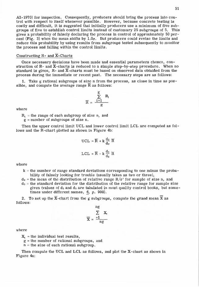
Once necessary decisions have been made and essential parameters chosen, con­struction of R- and X-charts is reduced to a simple step-by-step procedure. When no standard is given, R- and X-charts must be based on observed data obtaided from the process during the immediate or recent past. The necessary steps are as follows:

1. Take g rational subgroups of size n from the process, as close in time as pos­sible, and compute the average range Ras follows:

R =

where

g L ~

i =l g

R1 = the range of each subgroup of size n, and g =number of subgroups of size n.

Then the upper control limit UCL and lower control limit LCL are computed as fol­lows and the R-chart plotted as shown in Figure 4b:

where

- d3 -UCL = R +k- R dz

LCL = R - k d3 R d2

k =the number of range standard deviations corresponding to one minus the proba­bility of falsely looking for trouble (usually taken as two or three),

d2 =the mean of the distribution of relative range R/cr' for sample of size n, and d3 = the standard deviation for the distribution of the relative range for sample size

given (values of d2 and d3 are tabulated in most quality control books, but some­times under different names, .§_, p. 908).

2. To set up the X-chart from the g subgroups, compute the grand mean X as follows:

where

Xi =the individual test results,

ng

L Xi X = ::!__

ng

g =the number of rational subgroups, and n = the size of each rational subgroup.

Then compute the UCL and LCL as follows, and plot the X-chart as shown in Figure 4a:

52

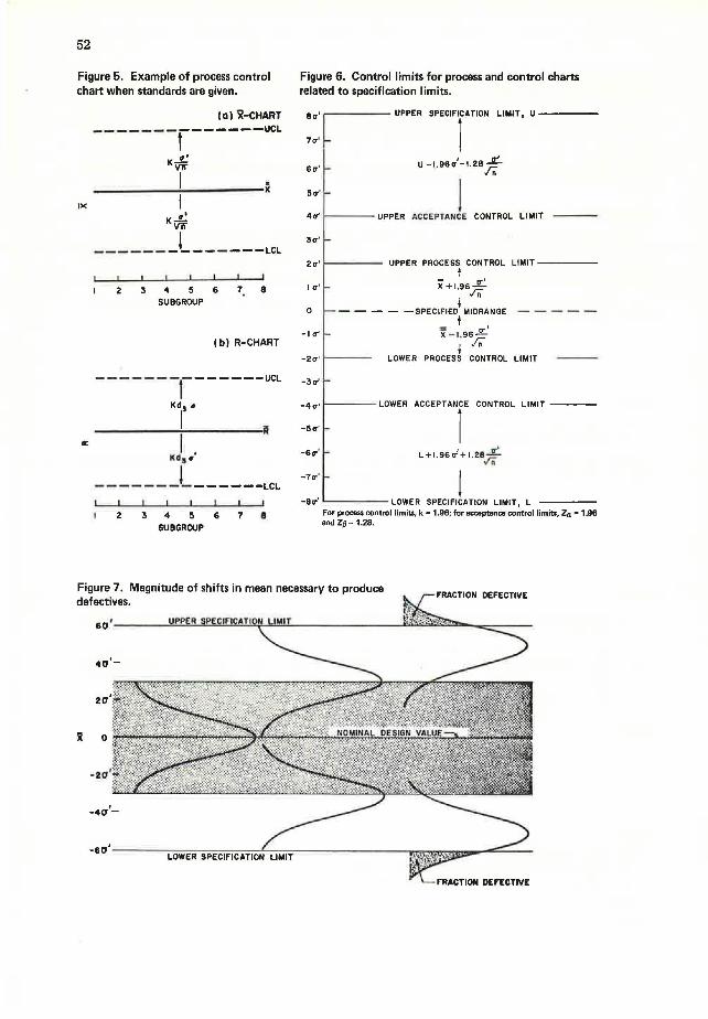
Figure 5. Example of process control chart when standards are given.

I><

ac

(a) ~-CHART

-------r------UCL

o' Ki/if

--------~! _______ ; I o' Kvn

----- - _l_ - -- ---LCL

2 3 4 5 6 7. 8 SUBGROUP

(bl R-CHART

- - - - - - -1- - - - - - -UCL

Kd5 o

I ----------.....,----------~ I .

Kd 5 o

- - - - - - _l_ - - - - - -LCL

2 3 4 5 6 7 e SUBGROUP

Figure 6. Control limits for process and control charts related to specification limits.

Bir' ~----- UPPER SPECIFICATION LIMIT, U -----

1 7a1 -

6rr' -u -1.9sir'-1.2B ..L... .rn

50"' - l 4cr' 1-----UPPER ACCEPTANCE CONTROL LIMIT - ---

3a' -

2cr' >-----

la' -

UPPER PROCESS CONTROL LIMIT----­t

= D'"' x + 1.96,rn

+ 0 - - - - - -SPECIFIED MIDRANGE - - - - -t

= IT' X - l. 96J;;""

+

-lcr' -

-2a'>---- LOWER PROCESS CONTROL LIMIT

-3cr' -

-4cr' t----- LOWER

-5ir'

-6tr' t-

-70"' I-

ACCEPTANr CONTROL LIMIT ----

' ~ L+ 1.96IT+1.28.fii

! -Bir' ~----- LOWER SPECIFICATION LIMIT, L

For process control limits, k = 1.96; for acceptance control limits, Za = 1.96 and z~ = 1.28.

Figure 7. Magnitude of shifts in mean necessary to produce defectives.

ii 0

I -4a-

= R UCL = X + k - ­

d2 ./fi

= R. LCL =X- k-­d2 ./fi

53

When the mean and standard deviation of control properties are known or derived from specification limits, the procedure for setting up R- and X-charts for subgroups of size n becomes very simple. Letting a' equal the known or derived standard de­viation, the procedure for constructing R-charts reduces to the following steps:

1. Compute R by R = d2o', where R =the average range, d2 =the mean of the rela­tive range, and a' =the known or assumed process standard deviation.

2. Compute the R-chart UCL and LCL as follows-UCL = d2a' + kd30' and LCL = d20'' - kd30''.

3. Plot the R-chart as shown in Figure 5b.

Similarly, letting the given or specification mean equal X, the procedure in setting up an X-chart for standard given reduces to the following steps:

1. Compute the UCL and LCL as follows-

= a' UCL =X +k­.fo

= a' LCL =X - k­

,/ll"

2. Plot the X-chart as shown in Figure 5a.

Both the procedure for no standard given and the procedure for standard given as­sume that the control properties are normally distributed. This assumption is usually of no great consequence unless the properties controlled follow distributions deviating markedly from normality. As already mentioned, concrete properties can be taken to be approximately normally distributed, and this assumption should not result in dif­ficulties.

Operation of R- and X-Charts

Consistent with the objective of using control charts graphically to test the hypothesis that the control statistic does not fall outside the allowed intervals, the operation of R­and X-charts reduces to three steps:

1. Sampling and testing rational subgroups, 2. Computing subgroup means and ranges, and 3. Plotting subgroup means and ranges on the appropriate control charts to see

whether they fall within the chosen confidence intervals (which are represented graphi­cally by the control limits).

If the values of subgroup ranges and means fall within the corresponding control chart limits, the process is considered in control, and routine testing is continued. If either the mean or range of one or more subgroups plots outside the control limits, the process is taken to be out of control. When a point on either plot is out of control, assignable causes are sought, and if found they are identified and eliminated. During the search for assignable causes, testing frequencies are increased, and testing con­tinues until there is reason to believe that the process is back in control and likely to remain there. When there is evidence that control has been restored, routine testing is resumed until another point again plots out of control, and the cycle then starts again.

Experienced quality control personnel have refined the basic rules for operation of control charts in attempts to prevent the process from going out of control at all. They have established criteria for action before assignable causes can cause trouble. For

54

example, 2cr limits are often used as a warning limit for action when too many points approach or exceed those limits. Other criteria are also used. Duncan summarizes the common action criteria as follows (.§_, p. 347):

"l. One or more points outside the control limits. "2. One or more points in the vicinity of a warning limit. This suggests the need

for immediately taking more data to check on the possibility of the process being out of control.

"3. A run [defined as successive items of the same class] of 7 or more points. This might be a run up or run down or simply a run above or below the central line on the control chart.

"4. Cycles or other nonrandom patterns in the data. Such patterns maybe of great help to the experienced operator. Other criteria that are sometimes used are the following:

"5. 11. run of 2 or 3 points outside of 2cr limits. "6. A run of 4 or 5 points outside of 1cr limits."

This multiplicity of criteria increases the chances of falsely looking for trouble, and the choice among action criteria should be based on economics.

R- and X-Charts Suggested for Inilialion of Formalized Process Control in Concrete Plants

The properties to be controlled, size of the rational subgroup, and probability of falsely looking for trouble are the responsibilities and choices of producers. They should also choose whether to control each process with respect to given standards or with respect to itself. To make these decisions, producers must rely on data sys­tematically collected and properly analyzed. To the writer's knowledge, however, few concrete producers practice formalized statistical process control, as defined in ASQC Standard A3. For this reason, it seems appropriate for public agencies to suggest process control charts for producers to use until they can accumulate enough informa­tion to set up quality control systems properly on an individual plant basis. Such sug­gestions follow, based on the points discussed, which it is believed may provide a good starting point and yield good results:

1. Bring the process into control with respect to itself to ensure that specifications can be met;

2. When the process is in control with respect to itself and variation is consistent with the specification ranges, set up R- and X-charts based on the standard deviation derived from the specifications, i.e., one-sixth the range for the property inspected;

3. Use a probability of falsely looking for assignable causes of approximately 1 percent by using 3cr limits control charts (k = 3); and

4. Use both R- and X-charts to minimize rejections and a rational subgroup of size four.

Were these suggestions taken, most concrete plants could be controlled to meet specifications. In New York, control charts based on these guidelines were used in three case studies with good results (4). There is every reason to believe that results would be similar using these guidelines for other plants.

ACCEPTANCE CONTROL CHARTS

In some instances, the specification range is much greater than six process standard deviations, and the process output can meet the specification limits even when the pro­cess mean has shifted out of control. When this occurs, there is little chance of pro­ducing defectives, and it may be desirable to use the kinds of X-charts known as ac­ceptance control charts.

Their construction requires that the process standard deviation be lmown. Their control limits do not coincide with those of X-charts for process control based on the same sample sizes and standard deviations. Unlike process control charts, ac­ceptance control charts are not designed to detect lack of process control. Their only goal is to ensure with known risks that the percentage of defective output is limited

55

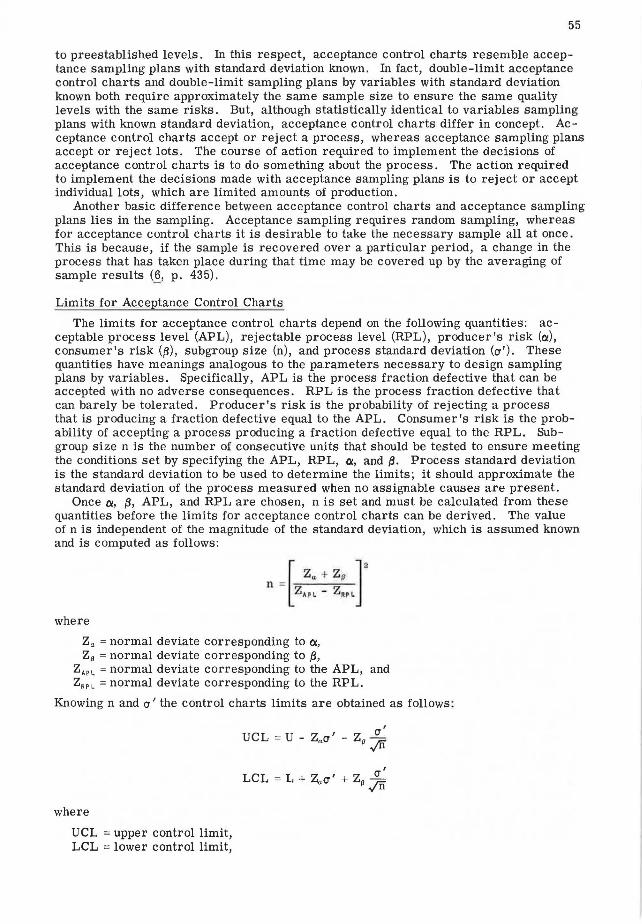
to preestablished levels. In this respect, acceptance control charts resemble accep­tance sampling plans with standard deviation known. In fact, double-limit acceptance control charts and double-limit sampling plans by variables with standard deviation known both require approximately the same sample size to ensure the same quality levels with the same risks. But, although statistically identical to variables sampling plans with known standard deviation, acceptance control charts differ in concept. Ac­ceptance control charts accept or reject a process, whereas acceptance sampling plans accept or reject lots. The course of action required to implement the decisions of acceptance control charts is to do something about the process. The action required to implement the decisions made with acceptance sampling plans is to reject or accept individual lots, which are limited amounts of production.

Another basic difference between acceptance control charts and acceptance sampling plans lies in the sampling. Acceptance sampling requires random sampling, whereas for acceptance control charts it is desirable to take the necessary sample all at once. This is because, if the sample is recovered over a particular period, a change in the process that has taken place during that time may be covered up by the averaging of sample results (§_, p. 435).

Limits for Acceptance Control Charts

The limits for acceptance control charts depend on the following quantities: ac­ceptable process level (APL), rejectable process level (RPL), producer's risk (01), consumer's risk ((3), subgroup size (n), and process standard deviation (a'). These quantities have meanings analogous to the parameters necessary to design sampling plans by variables. Specifically, APL is the process fraction defective that can be accepted with no adverse consequences. RPL is the process fraction defective that can barely be tolerated. Producer's risk is the probability of rejecting a process that is producing a fraction defective equal to the APL. Consumer's risk is the prob­ability of accepting a process producing a fraction defective equal to the RPL. Sub­group size n is the number of consecutive units that should be tested to ensure meeting the conditions set by specifying the APL, RPL, a, and {3. Process standard deviation is the standard deviation to be used to determine the limits; it should approximate the standard deviation of the process measured when no assignable causes are present.

Once Cll, {3, APL, and RPL are chosen, n is set and must be calculated from these quantities before the limits for acceptance control charts can be derived. The value of n is independent of the magnitude of the standard deviation, which is assumed known and is computed as follows:

where

Za = normal deviate corresponding to OI,

Z~ = normal deviate corresponding to {3, ZAPL = normal deviate corresponding to the APL, and ZRPL =normal deviate corresponding to the RPL.

Knowing n and a 1 the control charts limits are obtained as follows:

where

UCL =upper control limit, LCL = lower control limit,

56

U = upper specification limit, L = lower specification limit,

Za = normal deviate corresponding to Cl,

Z~ =normal deviate corresponding to {J,

0 ' = known standard deviation, and n = sample size.

It should be emphasized that these limits are derived using the specification limits as reference points, whereas the reference point for process control chart limits is the design or specified mean, as shown in Figure 6 (9). This is not accidental. It is consistent with the assumptions that the specification-range should be greater than 6cr' to use acceptance control charts and that the process mean can shift about the design mean without producing defectives so long as the standard deviation remains unchanged.

Applicability to Concrete

The objective of acceptance control charts is to reject processes whose output equals or exceeds the RPL. This objective limits their applicability to only those properties that can be measured immediately after manufacturing. If those properties cannot be measured immediately after production, use of these charts leads to two difficulties. First, if the process shifts to the rejectable level, defectives will be produced during the time lag between production and testing. Depending on the time elapsed, this can result in accepting substantial amounts of inferior product. Second, a process op­erating at a rejectable process level at the time the sample is produced can shift back to an acceptable level while waiting for test results. When this happens, rejecting the process on the basis of the last available data leads to rejecting an acceptable process and causes unnecessary manufacturing delays.

Concrete properties that can be measured immediately after mixing are slump and air content, and in principle acceptance control charts can be used for these properties provided that sampling and testing are performed at the plant site. But, although ap­plicable in theory, the use of acceptance control charts for slump and air content is neither practical nor desirable. They are not practical because no saving in testing is realized, and they are not desirable because conditions for the use of acceptance control charts do not exist.

Acceptance control charts are desirable if the following conditions are satisfied:

1. The specification range is wide enough to accommodate shifts in process averages of considerable magnitude without resulting in defectives,

2. The process standard deviation is known and stable, 3. The production units included in the subgroup represent consecutive production,

and 4. The decision of rejection can be enforced.

Neither slump nor air content meets these conditions, for reasons that will now be discussed.

Specification Range-Acceptance control charts are used to give producers of a uni­form product an advantage when the specification range is considerably greater than six times the process standard deviation. If the specification range is very large, compared to the six standard deviations needed to meet the specifications, the pro­cess average can be allowed to shift considerably without resulting in defectives. Under these circumstances both acceptance sampling and process control can be re­laxed (Fig. 7). The specification range is 12 process standard deviations. But for most properties the specification limits need provide only a range of six standard de­viations to eliminate nearly all defectives. This means that the process average shown in Figure 7 can shift to ±30'' from the nominal design value while producing almost no defectives. Only when the process average moves outside the shaded area will de­fectives begin to be produced. But large shifts are not likely to occur, and thus the chances for defectives are almost nonexistent. Because production of defectives is unlikely, the producer need not be particularly meticulous about process control. He needs only to prevent very large shifts in the process average, which usually take very

57

little effort to avoid. Similarly, the buyer is not likely to receive defectives and can afford to accept the material so long as the process is monitored to prevent large shifts in process level. To ensure this , he can rely on acceptance control charts , using his own data or the producer's data. But for slump and air content, the specification range usually approximates the needed six standard deviations (4). This means that small shifts in the process level are likely to result in large fractions defective. For this reason, to ensure that process control is pursued, concrete buyers should use accep­tance sampling and rely completely on their own data, and acceptance control charts are inappropriate.

Standard Deviation-In the preceding discussion, it was tacitly assumed that the process standard deviation was known. In fact, the process standard deviation for slump and air content changes from plant to plant (4). Moreover, there is no impar­tial way to assume a safe value. If small standard-deviations are assumed, producers of unacceptable quality are rewarded and buyers penalized . If large standard devia­tions are assumed, producers of uniform quality will suffer unnecessary and unfair rejection. These points are most important, and one may convince himself of their validity with a few simple sketches. This means that, to be fair in setting up accep­tance control charts, the standard deviation should be determined for each separate concrete plant, and control chart limits would have to change from plant to plant. The result would be an administrative nightmare.

Subgroup-For acceptance control charts, the sample should consist of consecutive production units. Recovery of such a sample is a difficult task for concrete, even if the sample size is small. The sample size for acceptance control charts depends on e1, {3, APL, and RPL and can be relatively large. For example, for an APL of 0.003 and RPL of 0.036, the necessary sample size is 10 if el = 0.05 and f3 = 0.10. If higher quality levels were required, the sample size would be larger. These relatively large sample sizes make recovery of samples consisting of consecutive or almost con­secutive production units a difficult task. This is another drawback for acceptance control charts.

Enforcement of the Rejection Decision-As already discussed, acceptance control charts accept or reject a process and not a finite or tangible amount of material. If the buyer uses acceptance control charts, he can encounter difficulties in enforcing re­jection. When a process is rejected, a producer can refuse to look for assignable causes. In such cases, the buyer cannot really enforce his decision. He can stop buying the product, but, if the producer has an alternative, less demanding market, he may not care. Because the decision does not involve material, but rather doing something totally under the producer's control, the buyer must depend on the producer's cooperation . Within the same company, acceptance control charts can work because the producer and those responsible for process acceptance report to the same manager. In such cases, disputes can be quickly resolved with no necessity for litigation. But in a vendor-vendee relationship, this arrangement can lead to problems.

Amount of Sampling-From the point of view of testing and sampling, there is no advantage in using acceptance control charts. If a point on the acceptance control chart represents the amount of material as a lot, then to ensure the same quality levels with the same risks, acceptance control charts and sampling plans by variables with standard deviation known require the same sample size. In fact, sample size is computed with the same formula. But for an acceptance sampling plan, sample size must consist of a random sample. This is an advantage because sampling of consecu­tive concrete production units is difficult, and acceptance sampling plans by variables with standard deviations known are preferable to acceptance control charts.

To summarize, then, acceptance control charts lose on all accounts, and their use in concrete inspection is not appropriate.

SUMMARY

It is hoped that this paper has served to stress that for concrete

1. Process control is a difficult task requiring (a) constant sampling and testing, (b) constant attention of plant managers, and (c) constant care by manufacturing per­sonnel; and

58

2. Concrete buyers should avoid assuming responsibility for process control be­cause (a) it requires interfering with management of the production process, (b) it requires skills that concrete inspectors cannot be expected to possess, (c) it requires decisions that are properly the responsibility of plant managers, and (d) it could re­quire more sampling than acceptance sampling.

It is also hoped that the discussion of acceptance control charts makes it clear that process control charts and acceptance control charts cannot be used interchangeably and that acceptance control charts are not appropriate as a replacement for acceptance sampling in concrete inspection.

Finally, the author hopes that those responsible for buying concrete will read the literature referenced in this paper before deciding to use process control or acceptance sampling to ensure quality concrete. The author is confident that the informed buyer, except on rare occasions, will choose acceptance sampling.

ACKNOWLEDGMENTS

This paper was prepared under administrative supervision of William C. Burnett and Peter J. Bellair, New York State Department of Transportation, and derives in part from literature surveys carried on under research projects made in cooperation with the U.S. Department of Transportation, Federal Highway Administration. Its contents reflect the opinions, findings, and conclusions of the author and not necessarily those of the New York State Department of Transportation or the Federal Highway Ad­ministration.

REFERENCES

1. Juran, J. M., and Gryna, F. M., Jr. Quality Planning and Analysis From Product Development Through Usage. McGraw-Hill Book Co., New York, 1970, p. 276.

2. Kemp, K. W. The Average Run Length of Cumulative Sum Charts When a V-Mask Is Used. Jour. Royal Statistical Society, Series B, Vol. 23, No. 1, 1961, pp. 149-153.

3. Kemp, K. W. The Use of Cumulative Sums for Sampling Inspection Schemes. Applied Statistics, Vol. 1, No. 1, March 1962, pp. 16-31.

4. DiCocco, J . B. Quality Assurance for Portland Cement Concrete. Engineering Research and Development Bureau, New York State Department of Transportation, Res. Rept. 10, (in preparation).

5. Juran, J.M., Seder, L.A., and Gryna, F. M., Jr. Quality Control Handbook, 2nd Ed. McGraw-Hill Book Co., New York, 1967.

6. Duncan, A. J. Quality Control and Industrial Statistics, 3rd Ed. Richard D. Irwin, Inc., Homewood, Ill., 1965.

7. King, E. P. The Operating Characteristics of the Average Chart. Industrial Quality Control, Vol. 9, No. 3, Nov. 1952, pp. 30-32.

8. King, E. P. The Operating Characteristic of the Control Chart for Sample Means. Annals of Mathematical Statistics, Vol. 23, No. 3, Sept. 1952, pp. 384-395.

9. Freund, R. A. Acceptance Control Charts. Industrial Quality Control, Vol. 14, No. 4, Oct. 1957, pp. 13-23.