applicability of dzerdzeevski´s atmospheric circulation classification to northern-hemispheric...
TRANSCRIPT

Applicability of Dzerdzeevski´s atmospheric circulation classification to northern-hemispheric climate variations
Andreas Hoy, Mait Sepp

2
Structure
1) Background and Classification Concept
2) Discussion• Frequency Variations• Applicability on Temperature
3) Conclusions and Outlook
Andreas Hoy | [email protected] | EMS/ECAM 07–11 September 2015 | Sofia
3
1) Background and Classification Concept
2) Discussion• Frequency Variations• Applicability on Temperature
3) Conclusions and Outlook
Andreas Hoy | [email protected] | EMS/ECAM 07–11 September 2015 | Sofia
Structure

4
• Developed by the Soviet meteorologist Boris Lvovich Dzerdzeevski in 1950s/60s
• Data available from 1899, updated until 2015 (used here: 1901–2010)
• Atmospheric circulation classification for the non-tropical latitudes of the entire northern hemisphere only known hemispheric concept, justifies closer look
• Focus on very large-scale hemispheric circulation characteristics – based on 1) number/location of blockings of the prevailing westerlies by polar intrusions and 2) trajectories of cyclones/anticyclones and troughs/ridges
• NB! Focus on macro processes instead of individual fronts/disturbances
• Utilisation of upper air data at 500/700 hPa level as indicator of the main mid-tropospheric steering currents
• Pronounced seasonal differences, which are accounted for by frequency distribution of the 41 subtypes (include 98% of all days, 2% not assigned)
• Drawbacks: 1) manual classification with likely homogeneity issues in time series (methodical changes, person in charge); 2) unsatisfactory correlations with local weather conditions due to high level of generalisation? (weak regional focus)
• So far very little information about applicability on climate variations
Andreas Hoy | [email protected] | EMS/ECAM 07–11 September 2015 | Sofia
Background

5
• 41 subtypes (Elementary Circulation Mechanisms; ECM), merged into 13 circulation types (CT), summarised by four circulation groups (CG)
• Zonal (Z): polar high pressure, no blocking, 5 ECM´s in 2 CT´s [7%]
• Zonal disturbed (ZD): polar high pressure, 1 blocking situation, 13 ECM´s in 5 CT´s [25%]
• Meridional north (MN): polar high pressure, 2-4 blocking situations, 21 ECM´s in 5 CT´s [54%]
• Meridional south (MS): polar low (!) pressure, no blocking, 2 ECM´s [13%]
Andreas Hoy | [email protected] | EMS/ECAM 07–11 September 2015 | Sofia
Z ZD MN MS
Classification Concept
6
1. Which frequency variations occur within the classification and how reliable are they?
2. Where does (the current version) of Dzerdzeevski´s classification supports explaining regional climate variability? (here: focus on air temperature variations)
shall be approached in this presentation (ongoing work!)
Andreas Hoy | [email protected] | EMS/ECAM 07–11 September 2015 | Sofia
Research Questions

7
Structure
1) Background and Classification Concept
2) Discussion• Frequency Variations• Applicability on Temperature
3) Conclusions and Outlook
Andreas Hoy | [email protected] | EMS/ECAM 07–11 September 2015 | Sofia
8Andreas Hoy | [email protected] | EMS/ECAM 07–11 September 2015 | Sofia
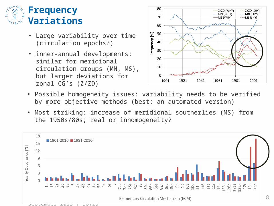
• Large variability over time (circulation epochs?)
• inner-annual developments: similar for meridional circulation groups (MN, MS), but larger deviations for zonal CG´s (Z/ZD)
• Possible homogeneity issues: variability needs to be verified by more objective methods (best: an automated version)
• Most striking: increase of meridional southerlies (MS) from the 1950s/80s; real or inhomogeneity?
Frequency Variations

9Andreas Hoy | [email protected] | EMS/ECAM 07–11 September 2015 | Sofia
• Alternative approach: grouping of ECM´s with similar characteristics in a selected target region
• Regionally more meaningful than using the 4 CG´s or 13 CT´s?
• here, selection of ECM´s with a NAO like temperature pattern during the cold season (winter, DJFM, WHY) in the polar region (dipole between “warm” Svalbard and “cold” southern Greenland)
• Two indices, resembling NAO+ (SEL+; 13w, 12d, 11a, 8cw, 5a, 5b, 5c) and NAO- (SEL-; 12a, 12bw, 12cw, 11b, 9b, 8dw, 8bw, 8a)
• Next step: comparing frequency variations of the NAO with a combined Dzerdzeevski index: SEL = [SEL+] – [SEL-]
• Average SEL frequency of about 70%
Frequency Variations

10Andreas Hoy | [email protected] | EMS/ECAM 07–11 September 2015 | Sofia
1901191719331949196519811997-1.5
-0.7
0.0
0.8
1.5
-20
-5
10
25
40
r (annual basis)NAOI (Li/Wang)SEL (Dzerdzeevski)
NA
O-I
ndex
SE
L-I
nd
ex
1901191819351952196919862003-2.0
-1.0
0.0
1.0
2.0
-20
-5
10
25
40
r (annual basis)
NAOI (Li/Wang)
NA
O-I
nd
ex
SE
L-I
ndex
• Good agreement between SEL and NAO
• proves usability of the SEL index for target regions
• Spatial applicability on air temperature?
11 years smoothing, WHY 31 years smoothing, WHY
Frequency Variations (SEL index)

11
• Circulation groups (CG´s), consisting of many CT´s/ECM´s, yield little information on air temperature due to large generalisation (focus on similar processes, like blocking number, NOT their similar spatial location different climate impacts in same spatial areas
• Some individual ECM´s include pronounced and meaningful signals, especially in the polar region, Siberia and Northern America – yet, they often have a too small frequency or large within-type variability
• one way may be to focus on circulation types (CT´s)
Andreas Hoy | [email protected] | EMS/ECAM 07–11 September 2015 | Sofia
Zonally Disturbed (ZD); winter; n=2098 (21%)
Meridional North (MN); winter; n=6162 (61%)
Applicability on Temperature

12Andreas Hoy | [email protected] | EMS/ECAM 07–11 September 2015 | Sofia
CT5; winter; n=1085 (11%)CT5; autumn; n=694 (7%)
• CT 5; disturbed zonal flow (ZD)
• Occurs from September to March
• Example of spatially/temporally quite consistent ECM signals, leading to pronounced/meaningful CT signals
Applicability on Temperature

13Andreas Hoy | [email protected] | EMS/ECAM 07–11 September 2015 | Sofia
CT11; winter; n=3093 (32%)CT11; autumn; n=1189 (12%)
• CT 11; meridional northern flow (MD)
• Occurs from September to April
• Example of spatially/temporally inconsistent ECM signals, leading to weak/meaningless CT signals
ECM11b; winter; n=733 (7%)
ECM11a; winter; n=1520 (15%)
Applicability on Temperature

14Andreas Hoy | [email protected] | EMS/ECAM 07–11 September 2015 | Sofia
• SEL index: larger correlations than NAO or continental-scale European circulation classifications (e.g., Grosswetterlagen, Vangengeim-Girs classif.) with average winter temperature in a) Svalbard (e.g., Barencburg/ Bjoernoeya r~0.6
1961-2010) and b) the Black/Caspian Sea region (e.g., Sotchi r~-0.6)
• SEL is further well applicable in Scandinavia (r up to 0.6), north-western Russia (r up to 0.5) and to the Baltic Sea Ice extent (r >0.5); and probably other regions
SEL+; winter; n=4011 (41%)
SEL-; winter; n=2930 (30%)
Applicability on Temperature (SEL index)
L HHL
H
HL
L

15
Structure
1) Background and Classification Concept
2) Discussion• Frequency Variations• Applicability on Temperature
3) Conclusions and Outlook
Andreas Hoy | [email protected] | EMS/ECAM 07–11 September 2015 | Sofia

16
1. Which frequency variations occur within the classification and how reliable are they?
•Large fluctuations over time (so-called circulation epochs)
• Strong increase of southerly air masses into the polar region is the most remarkable feature (homogeneity?)
• The presented SEL index displays similar variations over time like indices of the NAO (and Westerlies in certain European continental-scale classifications)
Andreas Hoy | [email protected] | EMS/ECAM 07–11 September 2015 | Sofia
Conclusions

17
2. Where does (the current version) of Dzerdzeevski´s classification supports explaining regional air temperature variability?
• Distinctive temperature anomalies form paramount in the polar region/over the continents (most pronounced in North America and over Siberia)
• Yet, existing groups, types and sub-types (ECM´s) do hardly justify using this classification over other alternatives (like the NAO, or regional-/continental-scale approaches), despite strong signals of some types/sub-types
• Way to be more successful: combining selected ECM´s with certain characteristics in a chosen target region in mid or high latitudes
• The presented SEL index yields larger correlations with average winter temperature in Svalbard and b) the Black/Caspian Sea areas than a range of other indices/classifications
• SEL is further well applicable in Scandinavia/north-western Russia and probably Greenland/central North America
Andreas Hoy | [email protected] | EMS/ECAM 07–11 September 2015 | Sofia
Conclusions
18Andreas Hoy | [email protected] | EMS/ECAM 07–11 September 2015 | Sofia
Further research ideas
• Using sector data (six sectors available: Atlantic, European, Siberian, Far East, Pacific, American) may allow more regional applicability, yet moves away from hemispheric concept
• More detailed comparison with other classifications/indices (e.g., with large-scale classification approaches of the Cost733 catalogue within the Atlantic-European area)
• Investigation of so-far unknown teleconnections
• Preparation of an automated version based on specifications of the original concept, thus avoiding/clarifying current homogeneity issues and allowing a backward-extension of time series
Outlook


20
Data: Temperature data: gridded set of daily averages in ~1.9 x 1.9°
worldwide resolution (Twentieth Century Global Reanalysis dataset – Compo et al. 2011), www.esrl.noaa.gov/psd/data/gridded/data.20thC_ReanV2.html
Dzerdzeevski CG´s/CT´s/ECM´s: daily data via www.atmospheric-circulation.ru (Nina Kononova)
Methods: Analysis of daily data (circulation types and air temperature) Calculation of daily air temperature anomalies per grid point for
1901-2010; consideration of annual cycle) Visualisation of average temperature anomaly fields per
circulation type (via mapping program SURFER)
Andreas Hoy | [email protected] | EMS/ECAM 07–11 September 2015 | Sofia
Air temperature: signal maps

21Andreas Hoy | [email protected] | EMS/ECAM 07–11 September 2015 | Sofia
Monthly Temperature Anomaly SignalsSEL+ SEL-
October 54%
January 68%
November 65%
December70%
February 74%
March 65%

Circulation Types (CT´s)
1 2,9% WHY
2 4,3% SHY
Elementary Circulation Mechanisms (ECM´s)
1a 1,5% WHY
1б 1,4% WHY
2a 1,3% SHY
2б 2,0% SHY
2в 1,0% SHY
Anticyclonic conditions at Arctic region; 2-4 southern cyclone outlets in 2-4 (of 6) sectors; no blocking
Third column describes main occurrence of CT´s/ECM´s; WHY = Winter half year; SHY = Summer half year
Zonal Circulation Group (Z)

Circulation Types (CT´s)
3 3,1% SHY
4 6,0% SHY
5 5,4% WHY
6 1,9% SHY
7 8,2% Year
Elementary Circulation Mechanisms (ECM´s)
3 3,1% SHY4a 0,8% WHY4б 3,2% SHY4в 2,0% SHY5a 1,6% WHY5б 2,2% WHY5в 0,5% WHY5г 1,0% WHY6 1,9% SHY7аз 2,7% WHY7ал 2,4% SHY7бз 1,7% WHY7бл 1,4% SHY
Anticyclonic conditions at Arctic region; 2-4 southern cyclone outlets in 2-4 (of 6) sectors; one blocking over the hemisphere
Zonally Disturbed Circulation Group (ZD)
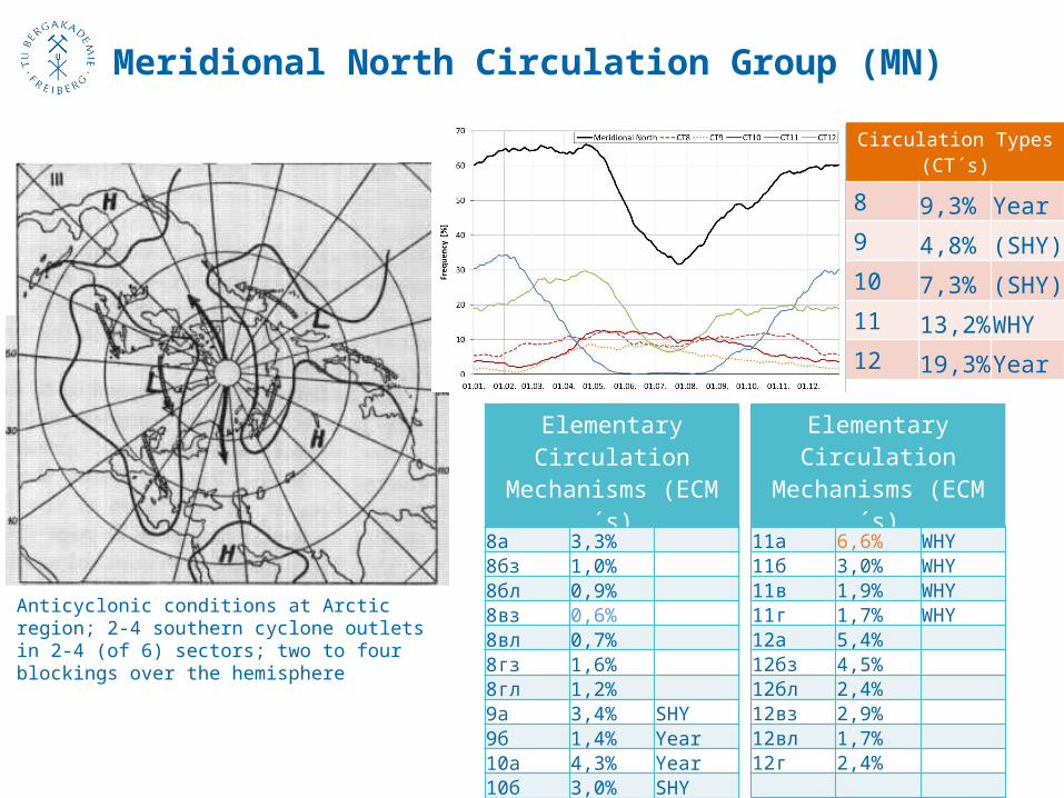
Circulation Types (CT´s)
8 9,3% Year
9 4,8% (SHY)
10 7,3% (SHY)
11 13,2% WHY
12 19,3% Year
Anticyclonic conditions at Arctic region; 2-4 southern cyclone outlets in 2-4 (of 6) sectors; two to four blockings over the hemisphere
Elementary Circulation Mechanisms (ECM´s)
8a 3,3%8бз 1,0%8бл 0,9%8вз 0,6%8вл 0,7%8гз 1,6%8гл 1,2%9a 3,4% SHY9б 1,4% Year10a 4,3% Year10б 3,0% SHY
Elementary Circulation Mechanisms (ECM´s)
11a 6,6% WHY11б 3,0% WHY11в 1,9% WHY11г 1,7% WHY12a 5,4%12бз 4,5%12бл 2,4%12вз 2,9%12вл 1,7%12г 2,4%
Meridional North Circulation Group (MN)

Elementary Circulation Mechanisms (ECM´s)
13з 5,9% WHY
13л 6,9% SHY
Anticyclonic conditions at Arctic region; 3-4 southern cyclone outlets in 3-4 (of 6) sectors; no blocking
Meridional South Circulation Group (MS)

Summer half year; n=2889 (15%)
Winter half year; n=2302 (12%)
Meridional South Circulation Group

27Andreas Hoy | [email protected] | EMS/ECAM 07–11 September 2015 | Sofia
NAO ≥+1 (Index after Li and Wang 2003); data: winter half year 1951-2010
L HH L
MS (southerly intrusion into Arctic); data: winter half year 1951-2010
L HH L
The increase of Meridional Southerlies (MS)
• Hemispheric temperature distribution: similar between MS and NAO+
• (MS temperature anomaly fields northward shifted by definition)
• Both observed temperature trends and variability of NAO index tend to justify frequency increase in MS since the 1950s/80s