application of a fractional-step method to … cfd/59-308.pdf · joijrnal of computational physics...

JOIJRNAL OF COMPUTATIONAL PHYSICS 59, 308-323 (1985)

Application of a Fractional-Step Method to Incompressible Navier-Stokes Equations

J. KIM AND P. MCIIN

Computational Fluid Dynamics Branch, NASA Ames Research Center, Moffett Field, Californin 94035

Received March 15, 1984; revised September 4, 1984

A numerical method for computing three-dimensional, time-dependent incompressible flows is presented. The method is based on a fractional-step, or time-splitting, scheme in conjunction with the approximate-factorization technique. It is shown that the use of velocity boundary conditions for the intermediate velocity field can lead to inconsistent numerical solutions. Appropriate boundary conditions for the intermediate velocity field are derived and tested. Numerical solutions for flows inside a driven cavity and over a backward-facing step are presented and compared with experimental data and other numerical results. I@- 1985

Academic Press, Inc.

1. INTRODUCTION

In this paper we present a numerical method for solving three-dimensional, time- dependent incompressible Navier-Stokes equations. The major difficulty in obtain- ing a time-accurate solution for an incompressible flow arises from the fact that the continuity equation does not contain the time-derivative explicitly. The constraint of mass conservation is achieved by an implicit coupling between the continuity equation and the pressure in the momentum equations. One can use an explicit time-advancement scheme which obtains the pressure at the current time-step such that the continuity equation at the next step is satisfied. However, for fully implicit or semi-implicit schemes, the aforementioned difficulty prevents the use of the con- ventional alternating-direction-implicit (ADI) scheme to advance in time as is the case for compressible flows. This difficulty can be avoided in two-dimensional cases by reformulating the problem in terms of the vorticity and stream-function. For three-dimensional problems, one can introduce an artificial compressibility into the continuity equation to include the required time-derivative for an ADI scheme. This is satisfactory, however, only for the steady-state solutions [ 11. For unsteady problems, since the effect of the artificial compressibility has to be minimized, this approach produces a highly stiff system for numerical solutions [2].

The objective of the present work is to develop a numerical method for solving the incompressible Navier-Stokes equations satisfying the conservation of mass exactly (within machine round-off). It will also be required that the numerical

308 0021-9991/85 $3.00 Copyrlghf 0 1985 by Academic Press, Inc. All rights of reproductmn in any form reserved.

FRACTIONAL-STEP METHOD 309

scheme preserve the global conservation of momentum, kinetic energy, and circulation in the absence of time-differencing errors and viscosity. It can be shown that failure to preserve these conservation properties can lead to numerical instabilities [3]. To stabilize the calculations using methods that do not preserve these properties, artificial viscosity is often introduced either explicitly or implicitly by using dissipative finite-difference schemes, especially for high-Reynolds-number flows. It is possible that for low-Reynolds-number flows, a nonconservative scheme can produce a stable solution without artificial viscosity, since the viscous terms are relatively large and can quickly annihilate the error terms introduced. However, for high-Reynolds-number flows, the lack of mass or energy conservations probably leads to the numerical instabilities.

The method developed herein is based on a fractional-step method (e.g., [4, 53) in conjunction with the approximate-factorization technique [6, 71. The flow field is represented on a staggered grid [8]. The problem of concocting boundary conditions for the intermediate (split) velocity field is addressed and it is shown that the use of velocity boundary conditions can lead to inconsistent and erroneous results. Appropriate boundary conditions for the intermediate-velocity field are derived using a technique similar to that of LeVeque and Oliger [9]. The Poisson equation for the pressure correction is solved by a direct method based on trigonometric expansions. In this way the continuity equation is satisfied to machine accuracy at every time-step.

The numerical procedures used in the present method are described in Section 2. Section 3 provides a derivation of the boundary conditions for the intermediate- velocity field, and numerical results for two different flow geometries are presented in Section 4; a summary is given in Section 5.

2. NUMERICAL METHOD

In this section we present a variant of the fractional-step method used by Chorin [4] for time-advancement of the Navier-Stokes and continuity equations for incompressible viscous flows:

auj a ap I a a at+ax."iuj= --+---q, axj Re axj axj J

Here, all variables are nondimensionalized by a characteristic velocity and length scale, and Re is the Reynolds number.

The fractional step, or time-split method, is in general a method of approximation of the evolution equations based on decomposition of the operators

310 KIM AND MOIN

they contain. In application of this method to the Navier-Stokes equations, one can interpret the role of pressure in the momentum equations as a projection operator which projects an arbitrary vector field into a divergence-free vector field. A two- step time-advancement scheme for Eqs. (1) and (2) can be written as

2;.-u7 1 -‘=Z’3H’-H:-‘)+;& g+-$+;

At ( > (a,+U:), (3)

3

UV+’ , -22; At

= -G(qY’+ ’ ),

with

D(uy+‘)=O, (5)

where Hi = -(6/6x,) uiui is the convective terms, 4 is a scalar to be determined, 6/6xi represents discrete finite difference operators, and G and D represent discrete gradient and divergence operators, respectively. We used the second-order-explicit Adams-Bashforth scheme for the convective terms and the second-order-implicit Crank-Nicholson for the viscous terms. Implicit treatment of the viscous terms eliminates the numerical viscous stability restriction. This restriction is particularly severe for low-Reynolds-number flows and near boundaries where stretched meshes are used. Equation (3) is a second-order-accurate approximation of Eq. (1) with @/axi excluded. By substituting Eq. (4) into (3), one can easily show that the overall accuracy of the splitting method is still second order. Note that $ is different from the original pressure: in fact, p = 4 + (At/2 Re) V*d. All the spatial derivatives are approximated with second-order central differences on a staggered grid [S]. Figure 1 illustrates the staggered grid. With the staggered mesh, the momentum

u2 (i, j + X, k)

V A

u1 (i-1/, j, k) )(

G Ci.‘i. k)

)(ul (i+%,j,k)

X2 V

I

A

9 (i, j-X, k)

FIG. 1. The staggered mesh in two dimensions.


equations are evaluated at velocity nodes, and the continuity equation is enforced for each cell. One important advantage of using the staggered mesh for incompressible flows is that ad hoc pressure boundary conditions are not required. Furthermore, it can be shown [lo] that with this approximation of spatial derivatives and in the absence of time-differencing errors and viscosity, global conservations of momentum, kinetic energy, and circulation are preserved. It should be pointed out that schemes that do not require ad hoc boundary conditions on non- staggered grids have been developed, but those schemes are based on spectral methods [ll, 121. The main disadvantages of staggered grids are that some of the velocity components are not defined on the boundaries and extension to higher orders is difficult.

Equation (3) can be rewritten as

(1-A,-A,-A,)(li,-ul)=~(3Hf-H:~‘)

+ 2(A, + A, + A,) uy, (6)

where A, = (At/2 Re)(6’/6x:), A, = (At/2 Re)(s2/Jx:), A) = (At/2 Re)(62/6x$. The left-hand side of Eq. (6) is then approximated as follows:

(l-A,)(1--A,)(I--A,)(lii-u:)=~(3H1-H1-’)

+2(A,+A,+A,)u;. (7)

Equation (7) is an O(dt3) approximation to Eq. (6). However, it requires inversions of tridiagonal matrices rather than inversion of a large sparse matrix, as in the case of Eq. (6). This results in a significant reduction in computing cost and memory.

Equations (4) and (5) can be solved as coupled system of equations for u;+ ’ and 4 ’ + ’ with boundary conditions for u; + l. Note that since 4” + ’ is defined at the center of each cell, there is a sufficient number of equations for u; + l and @‘+ ’ without the need for boundary condition for @‘+ ‘. Equations (4) and (5) can be combined to eliminate u;” and thus obtain a set of equations for @‘+ ‘. For the cells not adjacent to the boundaries, these equations take the form of the discrete Poisson equation,

for i = 2, 3 ,..., N, - 1, j = 2, 3 ,..., N, - 1, k = 2, 3 ,..., N, - 1. For the cells adjacent to the boundaries, incorporation of the velocity boundary conditions yields a modified set of equations. For example, for the cells adjacent to the lower boundary (j= l), we obtain

312 KIM AND MOIN

(-$+-$)rn~+Y, l,k)+~,3,2)~x,,l,2)~~+“~~~~(~~~~~;1’:~~ lTk)

1 u;+‘(i, l/2, k) - z&(i, l/2, k) ‘;DLdc

x,(3/2) - x2( l/2)

E Q(i, 1, k) (9)

for i = 2, 3,..., N, - 1, k = 2, 3,..., N, - 1. A solution to Eq. (8) and the corresponding boundary equations can be easily obtained using transform methods [ 131. Let

N, - I Nj - 1 @+‘(i,j, k)= c 1 &ki m)cos I=0 m=O

[$-+;)]cos[T(k-;)] (10)

for i=l,2 ,..., N,, j=l,2 ,..., N,, k = 1, 2 ,..., N,. Substituting Eq. (10) and the corresponding expansion for Q into (8) and (9) and using the orthogonality property of cosines, we obtain

where k; = 2[ 1 - cos(xl/N,)]/dx~ and k; = 2[ 1 - cos(xm/N,)]/dx~ are the modified wave numbers. For each set of wave numbers, the above tridiagonal system of equations can be easily inverted, and dn+ ’ is obtained from Eq. (10). The final velocity field u; + ’ is then obtained from

q+‘= zi, - AtG(qP + ‘). (12)

Note that 4 is determined to within an additive constant. When kk = k; = 0 in Eq. (ll), this arbitrary constant is prescribed as the average of 4 in the (xi, x3) plane adjacent to the lower boundary. It can be shown that the expression for Q is consistent with the compatibility condition which guarantees existence of a solution for 4. This compatibility condition is analogous to the well-known solvability condition for the Poisson’s equation with Neumann boundary condition; and in the case of kk = k; = 0, it provides for prescription of the arbitrary constant for I$ in addition to enforcing all the boundary equations such as (9). In solving the system of linear algebraic equations for 4 using the series expansion (lo), we have assumed that uniform mesh spacings are used in the streamwise and spanwise directions (xi and x3). If nonuniformly spaced mesh points are used in these directions or com- plicated domains are considered, one has to resort to iterative techniques such as multigrid methods to solve for 4.

3. BOUNDARY CONDITIONS

Boundary conditions for the intermediate velocity fields in time-splitting methods are generally a source of ambiguity. At each complete time-step, only the boundary


conditions for the velocity field are given and those of the intermediate velocity field are unknown. We will show in this section that except when the boundary conditions for the intermediate velocity field are chosen to be consistent with the gover- ning equations, the solution may suffer from appreciable numerical errors. In the present work, we derive the appropriate boundary conditions for the intermediate velocity field using a method suggested by LeVeque and Oliger [9].

To construct the proper boundary conditions for iii, we regard tii as an approximation to u*(x, t n + i), where the continuous function u*(x, t) satisfies

ui*(x, t,) = Ui(X, t,).

Hence

z&x24*(x, t, + At)

a*ll* =u*(x, tJ+Atfg+fArz- (32 + ...

=u,?(x,t,)+At H:+&V’u: )2 d )

+1At2d If~+&V*@ + . .._

Since u:(x, t,) = ui(x, t,),

(14)

(15)

=ui(X, t,+ 1) + At g+ O(At2). I

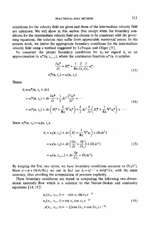
By keeping the first two terms, we have boundary conditions accurate to @At*). Since p = 4 + O(At/Re), we can in fact use fii= uy+ ’ + At$Y’/axi with the same accuracy, thus avoiding the computation of pressure explicitly.

These boundary conditions are tested in computing the following two-dimensional unsteady flow which is a solution to the Navier-Stokes and continuity equations [14,15]:

uI(xI, x2, t) = -cos x, sinx, e-*’

24,(x,, x2, t) = sin x1 cos x2 eP2r

p(x,, x2, t) = - +(cos 2x, + cos 2x2) eC4’.

(16)

314 KIM AND MOIN

TABLE I

Maximum Error after 30 Steps: E,,,/u,,,

Boundary conditions

20x20 8.172 x 1O-4 1.085 x 1O-4 40x40 1.127 x 10m3 7.678 x 1O-5

Computations are carried out in the domain, 0 6 x,, x2 < rc. The maximum difference between the exact and numerical solutions from four different runs are listed in Table I. The superiority of the results using boundary conditions (15) over the results using the velocity boundary condition, zi, = u; + ’ , is clearly evident. In fact, the error for the latter case increases when the mesh is refined. This indicates that the fractional-step method with the latter boundary condition is an inconsistent scheme. To determine the overall accuracy of the scheme using the boundary condition (15), three calculations are performed with three different mesh sizes but keeping the Courant number constant. The variation of the maximum error in uI with mesh refinement is plotted in Fig. 2; it shows that the scheme is indeed second- order accurate. Similar plots for u2 and p yield the same results. As a further check,

1 2 4 AxJAn

‘ref

FIG. 2. Maximum error as a function of mesh refinement.


the two-dimensional unsteady flow given by Eq. (16) is computed with u1 and u2 interchanged and p with the opposite sign, and the second-order accuracy is also achieved.

Since the boundary condition derived in Eq. (15) is extrapolative, numerical experiments are performed to determine whether the implicit part of the scheme with the boundary condition (15) is unconditionally stable. The following equations are numerically integrated in 0 < x1, x2 6 1.

au, -= -$+57&, at l Re

az.4, ap 1 -= --+-v2u2 at 2 Re

u,(O, x*) = u*( 1, x*) = 2+(X1) 0) = U2(XI) 1) = 0.

This is essentially the driven cavity problem (see Section 4.1) without the nonlinear terms. Stable solutions are obtained for all the time steps considered (as large as dt/(Re Ax’) = 104) indicating that the implicit part of the numerical scheme presented in this paper is indeed unconditionally stable. The nonlinear terms are treated explicitly and impose a restriction on the largest time step that can be used.

4. NUMERICAL EXAMPLES

In this section we present numerical results obtained from applications of the aforementioned numerical method to two laminar flow problems. Both problems

Xl u, =u2=0

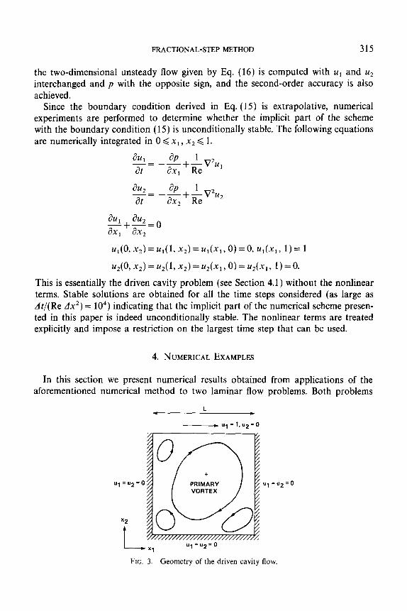
3. Geometry of the driven cavity flow.

316 KIM AND MOlN

,A: : : : :

STREAMLINE ‘/

a) VORTICITY

STREAMLINE (b)

VORTICITY

STREAMLINE VORTICITY

FIG. 4. Streamlines and contours of constant vorticity. (a) Re = 1, (b) Re = 400, (c) Re = 2,W.

MACTIONAL-STEP METHOD

(b)

Fro. 5. Velocity vectors. (a) Re= 1, (b) Re= 100, (c) Re=400, (d) Re= loo0, (e) Re=‘2OW (f) Re = 5000.

318 KIM AND MOIN

have been used widely as standard test cases for evaluating the stability and accuracy of numerical methods for incompressible flow problems.

4.1. Flow in a Driven Cavity

Figure 3 shows the geometry and the boundary conditions for the flow in a driven cavity together with the appropriate nomenclature. Flow is driven by the upper wall, and several standing vortices exist inside the cavity whose charac- teristics are functions of Reynolds numbers. Figures 4 and 5 show the computed results of streamlines, contours of constant vorticity, and velocity vectors for several Reynolds numbers. The purpose of the velocity-vector figures is to show the corner eddies, which are too weak to be displayed clearly by the streamlines. They are drawn parallel to the flow direction at each mesh point. At Re = 1, this flow is almost symmetric with respect to the centerline, and two corner eddies are visible. As Reynolds number increases, the center of the main vortex moves toward the downstream corner before it returns toward the center at higher Reynolds numbers. In the Reynolds number range, 1000-2000, the third corner eddy is formed at the upper left corner. At Re = 5000, a tertiary corner eddy is visible. In Fig. 6, the velocity at the middle of the cavity for Re = 400 is shown in comparison with other computed results. Two numerical results with different grid sizes are shown from the present computations. Both results, 21 x 21 and 31 x 31, are in good agreement with those of Rurggraf [ 161 and Goda [ 171. Although not shown here, Goda

-1 0 1

9

Re=400

FIG. 6. Profile of streamwise velocity at the midplane of the cavity (x1 =O.SL.) for Re =400: -, 31 x 31, Burggraf [16], Coda [17]; 0, 21 x21; II, 31 x 31, present results.


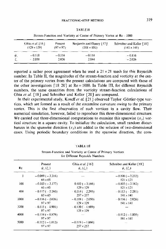
TABLE II

Stream-Function and Vorticity at Center of Primary Vortex at Re = 1000

Ghia et a/. 1163 Present Benjamin and Denny [ 171 Schreiber and Keller [ 181 (129 x 129) (97 x 97) (101 x 101) (141 x 141)

*, -0.118 -0.116 -0.118 -0.116 r 5, - 2.050 - 2.026 - 2.044 - 2.026

reported a rather poor agreement when he used a 21 x 21 mesh for this Reynolds number. In Table II, the magnitudes of the stream-function and vorticity at the center of the primary vortex from the present calculations are compared with those of the other investigators [ 18-201 at Re = 1000. In Table III, for different Reynolds numbers, the same quantities from the vorticity stream-function calculations of Ghia et al. [IS] and Schreiber and Keller [20] are compared.

In their experimental study, Koseff et al. [21] observed Taylor-Gortler-type vortices, which are formed as a result of the streamline curvature owing to the primary vortex. This is the first observation of such vortices in a cavity flow. Their numerical simulation, however, failed to reproduce this three-dimensional structure. We carried out three-dimensional computations to examine this spanwise (xX) vor- tical structure in a square cavity. To initialize the calculation, small random distur- bances in the spanwise direction (.x3) are added to the solution of two-dimensional cases. Using periodic boundary conditions in the spanwise direction, the com-

TABLE III

Stream-Function and Vorticity at Center of Primary Vortices for Different Reynolds Numbers

Re Present *, (5‘)

Ghia et al. 1163 Schreiber and Keller [ 1 S] $, (i‘) *< (ir,,)

1 -0.099 (-3.316) -0.100 (-3.232) 65 x 65 121 x 121

100 -0.103 (-3.177) -0.103 (-3.166) -0.103 (-3.182) 65 x 65 129 x 129 121 x 121

400 -0.112 (-2.260) -0.114(-2.295) -0.113 (-2.281) 65 x 65 257 x 257 141 x 141

1000 -0.116(-2.026) -0.118 (-2.050) -0.116 (-2.026) 91 x 97 129 x 129 141 x 141

3200 -0.115 (-1.901) -O.lZO(-1.989) 97x97 129x 129

4000 -0.114 (- 1.879) -0.112 (- 1.805) 97 x 97 161x161

5000 -0.112 (- 1.812) -0.119(-1.860) 97 x 97 257 x 257

320 KIM AND MOIN

FIG. 7. Velocity vectors in an (.Y~-.Y~) plane through the geometric center of the cubic cavity (x, =0.52).

putations are carried out for various Reynolds numbers. The spanwise vertical structure are observed only for high-Reynolds-number flows (Re 2900). In Fig. 7, the velocity vectors in the plane perpendicular to the primary vortex show the existence of the counterrotating vortices at Re = 1000. This case is computed using 32 x 32 x 32 grid points. The maximum spanwise (x3) velocity in this plane is uj = 0.043, which indicates the vertical structure is very weak. Although Goda [ 173 calculated the flow in a three-dimensional cavity, no such three-dimensional structure was reported.

4.2. Flow over a Backward-Facing Step

The flow over a backward-facing step in a channel provides an excellent test case for the accuracy of numerical method because of the dependence of the reattachment length x, on the Reynolds number. Excessive numerical smoothing in favor of stability will result in failure to predict the correct reattachment length.

PARABOLIC INFLOW u, = u2 = 0 ON WALLS

BOUNDARY DIVIDING STREAMLINE

x2

t

REATTACHMENT

FIG. 8. Flow over a backward-facing step (1:2 expansion ratio).


14 -

12 -

10 -

Jz 8-

2

6-

4-

2-

I I I 0 200 400 600 800

Re

FIG. 9. Reattachment length as a function of Reynolds number: 0, data from Armaly el al. [22]; ---; computation of Armaly ef al.; -, present results.

In this paper we report our two-dimensional computations of laminar flow over a backward-facing step. The geometry and boundary conditions for this flow are shown in Fig. 8. At the inflow boundary, located at the step, a parabolic profile is prescribed. All the results presented are obtained using 101 x 101 grid points and the downstream boundary was located at x = 30/z, where h is the step height. Both Neumann and Dirichlet outflow boundary conditions are used, and the two results are identical. In Fig. 9, numerical results for different Reynolds numbers are shown in comparison with the experimental and computational results of Armaly et al. [22]. The dependence of the reattachment length on Reynolds number is in good agreement with the experimental data up to about Re = 500. At Re = 600, the computed results start to deviate from the experimental values. A mesh-refinement study, as well as variation of the location of downstream boundary at this Reynolds number, showed that the difference between the experimental and computational results is not a result of numerical errors. It is most likely, as Armaly et al. [22] have pointed out, that the difference is due to the three-dimensionality of the experimental flow at this Reynolds number. Three-dimensional computations of the flow over a backward-facing step, which demand extensive computational time, are

FIG. 10. Streamlines at Re = 600.

322 KIM AND MOIN

currently under way and will be reported in a future article. In comparison with the numerical results of Armaly et al. [22] (using TEACH code), however, the present results show a much higher reattachment length.

Armaly et al. [22] reported the existence of a secondary separation bubble on the no-step wall at Re = 1000. The length of the secondary bubble at Re = 1000 was 10.4 step-heights and the length decreased for higher Reynolds numbers. Figure 10 shows the computed streamlines at Re = 600, indicating the secondary separation bubble on the no-step wall; the bubble length is 7.8 step-heights. At Re = 800, the length increased to 11.5 step-heights.

5. SUMMARY

A numerical method was presented for solving three-dimensional, time-dependent incompressible flows; the method is based on the fractional-step method used in conjunction with the approximate-factorization scheme. The three-dimensional Poisson equations were solved directly by a transform method, and the velocity field satisfied the continuity equation up to machine accuracy. The method is second-order accurate in both space and time. Proper boundary conditions for the intermediate (split) velocity field were derived and tested against a known solution, and laminar flows in a driven cavity and over a backward-facing step were calculated at several Reynolds numbers. The numerical results are in good agreement with experimental data and other numerical solutions.

ACKNOWLEDGMENTS

The authors express their thanks to Dr. Robert F. Warming for helpful comments on a draft of this paper. We are also grateful to D. Nagi N. Mansour for carrying out some of the computations reported here.

REFERENCES

1. A. J. CHORIN, J. Comput. Phys. 2 (1967), 12. 2. J. L. STEGER AND P. KUTLER, AIAA J. 15 (1977), 581. 3. N. A. PHILLIPS, in “The Atmosphere and Sea in Motion,” Rockefeller Inst. Press, New York, 1959. 4. A. J. CHORIN, Math. Compur. 23 (1969), 341. 5. R. TEMAM, “Navier-Stokes Equations. Theory and Numerical Analysis,” 2nd ed., North-Holland,

Amsterdam, 1979. 6. R. M. BEAM AND R. F. WARMING, J. Comput. Phys. 22 (1976), 87. 7. W. R. BRILEY AND H. MCDONALD, J. Compui. Phys. 24 (1977), 428. 8. F. H. HARLOW AND J. E. WELCH, Phys. Fluids 8 (1965), 2182. 9. R. L. LEVEQUE AND J. OLIGER, “Numerical Analysis Project,” Manuscript NA-81-16, Computer

Science Department, Stanford University, Stanfbrd, Calif., 1981. IO. D. K. LILLY, Mon. Weather Rev. 93 (1965), 11.


11. P. MOIN AND J. KIM, J. Compur. Phys. 35 (1980) 381. 12. L. KLEISER AND U. SCHUMANN, in “Proceedings, Third GAMM-Conference on Numerical Methods

in Fluid Mechanics” (E. H. Hirschel, Ed.), pp. 165-173, Braunschweig, 1980. 13. F. W. DORR, SIAM Rev. 12(2) (1970), 248. 14. A. J. CHORIN, “The Numerical Solution of the Navier-Stokes Equations for an Incompressible

Fluid,” AEC Research and Development Report, NYO-1480-82, New York University, New York, 1967.

15. C. E. PEARSON, Report No. SRRC-RR-64-17, Sperry-Rand Research Center, Sudbury, Mass., 1964. 16. 0. R. BURGGRAF, J. Fluid Mech. 24 (1966) 113. 17. K. GODA, J. Comput. Phys. 30 (1979), 76. 18. U. GHIA, K. N. GHIA, AND C. T. SHIN, J. Compuf. Phys. 48 (1982). 387. 19. A. S. BENJAMIN AND V. E. DENNY, J. Comput. Phys. 33 (1979) 340. 20. R. SCHREIBER AND H. B. KELLER, J. Comput. Phys. 49 (1983), 310. 21. J. R. KOSEFF, R. L. STREET, P. M. GRESHO, C. D. UPSON, J. A. C. HUMPHREY, AND W.-M. To,

“Proceedings, Third International Conference on Numerical Methods in Laminar and Turbulent Flows, Seattle, Wash., Aug. 8-11, 1983,” (C. D. Taylor, Ed.), p. 564.

22. B. F. ARMALY, F. DURST, AND J. C. F. PEREIRA, J. Fluid Ma-h. 127 (1983) 473.

5X1/59/2-10

application of a fractional-step method to … cfd/59-308.pdf · joijrnal of computational physics...

Documents