application of airborne and surface-based em/laser measurements

Canadian Technical Report of Hydrography and Ocean Sciences #249

2006

Application of Airborne and Surface-based EM/Laser Measurements to Ice/Water/Sediment Models

at Mackenzie Delta Sites

by

J. Scott Holladay*

Department of Fisheries and Oceans Canada Maritimes Region

Ocean Sciences Division Bedford Institute of Oceanography Dartmouth, Nova Scotia, B2Y 4A2

* Geosensors Inc., 66 Mann Ave., Toronto, Ontario M4S 2Y3 Canada

© Her Majesty the Queen in Right of Canada, 2006 Cat. No. Fs 97-18/249E ISSN 0711-6764

Correct Citation for this publication: Holladay, J. Scott. 2006. Application of Airborne and Surface-based EM/Laser Measurements to Ice/Water/Sediment Models at Mackenzie Delta Sites. Can. Tech. Rep. Hydrogr. Ocean Sci. #249: iv + 47p.

ii

Table of Contents Table of Contents................................................................................................. iii Abstract................................................................................................................ iv Introduction ...........................................................................................................1 Overview...............................................................................................................2 Relevant Models ...................................................................................................4 Instrumentation .....................................................................................................6

Electromagnetic Measurement of Ice Thickness and Bathymetry:.....................6 IcePic™ Instrument Specifications:....................................................................9

Sensitivity Analysis .............................................................................................10 EM Profile Inversion Results ...............................................................................16 Discussion ..........................................................................................................26

Detection of frozen sediments beneath bottom-fast ice: ..................................26 Fresh water bathymetry: ..................................................................................27 Depth Estimation to Conductive Layers Beneath Fresh Water and Ice: ..........28 Real-Time Applications: ...................................................................................28

Conclusions ........................................................................................................30 Acknowledgements.............................................................................................31 References .........................................................................................................32 Appendix A .........................................................................................................33

Application of Surface EM Sensors to Sea Ice Measurement..........................33 Sensitivity Studies—Surface EM Systems.......................................................34 Simulated Dualem-4™ and Surface Ice Sounder™ Profile Inversion ..............36 Conclusions .....................................................................................................38

Appendix B .........................................................................................................39 Sensitivity Analysis Plots .................................................................................39

iii

Abstract Holladay, J. Scott. 2006. Application of Airborne and Surface-based EM/Laser Measurements to Ice/Water/Sediment Models at Mackenzie Delta Sites. Can. Tech. Rep. Hydrogr. Ocean Sci. #249: iv + 47p. This report presents a new inversion methodology capable of displaying shallow coastal morphology properties by reprocessing Electromagnetic – Laser (EM) data collected by helicopter-borne sensors. The analysis used the EM data collected during the CASES program (Coastal Arctic Shelf Exchange Study) and showed that zones of frozen sediment beneath bottom-fast ice could be easily distinguished from adjacent zones where the sediments were not frozen. It also appeared that such zones had a spatial signature that distinguished them from areas where substantial thicknesses of fresh water were present beneath the ice. Processing of EM data using the new methodology can easily be carried out in the field on a laptop computer.

Résumé Holladay, J. Scott. 2006. Application of Airborne and Surface-based EM/Laser Measurements to Ice/Water/Sediment Models at Mackenzie Delta Sites. Can. Tech. Rep. Hydrogr. Ocean Sci. #249: iv + 47p. On présente dans ce rapport une nouvelle méthodologie d’inversion permettant la représentation de propriétés morphologiques littorales à faible profondeur par nouveau traitement de données électromagnétiques – laser (EM) recueillies au moyen de capteurs héliportés. L’analyse a porté sur les données EM recueillies dans le cadre du programme d’étude des échanges sur la plate-forme côtière arctique (CASES, Coastal Arctic Shelf Exchange Study) et a montré que les zones de sédiments congelés sous la glace reposant sur le fond peuvent être facilement distinguées des zones adjacentes dans lesquelles les sédiments ne sont pas congelés. Il est en outre devenu apparent que ces zones présentent une signature spatiale qui les distinguent des étendues où une couche d’eau douce d’une épaisseur substantielle est présente sous la glace. Le traitement des données EM au moyen de nouveaux algorithmes peut s’effectuer facilement sur le terrain à l’aide d’un ordinateur portatif.

iv

Application of Airborne and Surface-based EM/Laser Measurements

to Ice/Water/Sediment Models at Mackenzie Delta Sites

Introduction This report documents the interpretation of a unique set of survey data acquired under winter conditions by the DFO IcePic™ system in shallow parts of the lower Mackenzie Delta, where fresh water ice and water conditions, shallow water depth, and the presence of Stamukhi are important factors. The principal focus of this study was to evaluate the system’s ability to distinguish frozen from unfrozen sub-ice sediments in bottom-fast ice conditions, and to identify other properties of the ice/water/sediment system that could be characterised. Sensitivity analyses were used to clarify which ice/water/sediment properties could be most easily determined for a variety of situations. The field observations presented were acquired during the spring of 2004 as part of the Canadian Arctic Shelf Exchange Study (CASES). The object of the CASES IcePic™ field work as a whole was to collect pack ice data with helicopter-borne sensors, first to validate SAR imagery identification algorithms (a project supported by the Canadian Space Agency), and second to support CASES marine habitat studies. A third objective was to collect land-fast ice observations from the Mackenzie Delta in support of Oil and Gas developments through a project funded by PERD, the Panel of Energy and Research Development. This is the particular data set of interest to this report, as survey lines did cross over shallow coastal regions. During the survey, sea ice thickness and surface ice roughness were measured with a helicopter-borne sensor platform called the “IcePic”, consisting of a cigar-shaped sensor housing hard-mounted on the nose of a BO-105 Canadian Coast Guard helicopter. The platform’s electromagnetic (EM) sensor provides the distance from the sensor to the top of the seawater surface (or nearest electrically conductive layer), while its laser altimeter provides the distance to the surface of the snow, ice or open water. Together, under normal offshore conditions, the sensor data yield the snow-plus-ice thickness over seawater1. The laser altimeter data is also used to provide pack ice surface roughness profiles. IcePic™ data sets have the advantages of high coverage rates, the ability to operate far from base camps, and can easily profile over difficult ice conditions, zones of thin ice and open water. The system has been used in a variety of settings and modes ranging from detailed acquisition at very low altitudes over short survey lines close to shore, to surveying long lines in an offshore environment. 1 Prinsenberg et al., 2002

1

Overview Airborne electromagnetic (EM) methods have been successfully applied to a range of problems relevant to oceanographic, hydrographic and geological studies, particularly the measurement of sea ice thickness2 over relatively deep, uniform seawater, and bathymetric measurements3 of seawater depth, particularly in turbid and ice-covered waters where LIDAR-based methods cannot be applied. These applications were successful because the numerical models used for data interpretation were relatively simple, incorporating only two or three layers, and because the required high-accuracy EM measurements were carefully specified, acquired and processed to resolve the key model parameters, particularly ice thickness and water depth. In the case of airborne EM bathymetry, auxiliary data (including conductivity-temperature-depth profiles and tidal measurements or predictions) at selected locations and times within the survey area were used to improve the accuracy of those key parameters. In shallow water, EM bathymetry measurements were also expected to yield estimates of sea bottom conductivity and hence some rough measure of sea bottom composition, but the required studies for assessment of the accuracy of such measurements were not carried out. This research effort has therefore focused on assessing the potential of an airborne electromagnetic-laser altimeter system for investigation of sub-ice sediment properties, fresh water bathymetry through sea ice and salinity stratification beneath ice. The primary dataset used for this study was acquired with the IcePic™ survey system, which is owned and operated by the Department of Fisheries and Oceans. These data were collected under winter conditions over the lower Mackenzie Delta, in the transition zone between the inshore regime, where fresh water ice and water conditions dominate, and the offshore regime, where typical Beaufort Sea pack ice overlies seawater, with depths in the tens of metres. The map shown in Figure 1 below provides some indication of the complexity of the delta environment. During the winter, the principal flow (95%) of the Mackenzie River follows the southern portion of the Middle Channel, with less than 1% following the East Channel. The Middle Channel then divides again: 25% flows east in Neklek Channel, into the East Channel, and into Kittigazuit Bay, 40% flows west through Reindeer Channel, and 35% continues north as Middle Channel4. 2 Routine ice thickness measurements have been made since the mid-1990’s using airborne systems developed for DFO such as the “Ice Probe” and IcePic™ and, more recently, using sled-based EM measurement systems. 3 The only “commercial” measurements of this type were acquired with the Canadian Hydrographic Service (CHS) Through Ice Bathymetry System or TIBS, during a series of CHS surveys for the in the 1990’s, but other systems have been used to acquire research data sets. 4 Fassnacht and Conly, 2000.

2

The survey line numbers shown on the map were acquired during two flights executed on April 26, 2004. Lines 4077-4078 were collected at the end of an extended flight that originated in Franklin Bay, well to the east of the map area. After refueling the helicopter at the inactive CPSP Tuktoyaktuk base, line 4079 was flown, starting just east of the Middle Channel discharge, running roughly parallel to the Garry Island shoreline, and continuing northwest to a point just southeast of the Devon Oil ice camp. Line 4080 was then initiated and continued to the northeast, followed by line 4082 that ran back to the southeast, ending to the northeast of Pelly Island. Line 4083 started near Hooper Island, running to the northeast to the 30m depth contour. The line direction was then briefly reversed before running south into Kugmallit Bay.

2

2

2

2

2

2

2 2 2

2

2

2

2 2

2

2

2

2

2 3

3

3

3 3

3 3

3

3

3 4

4

4

4

4 4 4 4 4

4 4

4

5

5

5

5

5

55 5

5

0

10 10

10 10

10

20

20

20 20

20

30 30 30

30 30 30

30

30

40

40

40

40

50

50 50

50

50

40

40

2

3 3 3 3

4 4

5

2 2

22 2 3 234

3

5

1

68.8

69

69.2

69.4

69.6

69.8

70

70.2

70.4

Beaufort Sea

East ChannelMiddle Channel

Neklek Channel

Richards I.

.

Shallow Bay

Kittigazuit Bay

Mackenzie River

Kugmallit Bay

4080

40

3

. .

Tuktoyaktuk

Figure 1(black).

2Reindeer Channel

3

1

Pelly I.

Garry I

MackenzieBay

-36.5

-136

: Lower MaThe Tuktoy

4

0 1 4082

79

-

135.5 -

135 -

134.5 1

ckenzie delta, showing baktuk town site, where th

3 4 5408

-34

-133.5

athymetry (e helicopte

3

20 4077

4078
Pullen I Hooper I
-

133 -

132.5 -

132

blue) and IcePicTM survey tracks r was refuelled, is also shown.

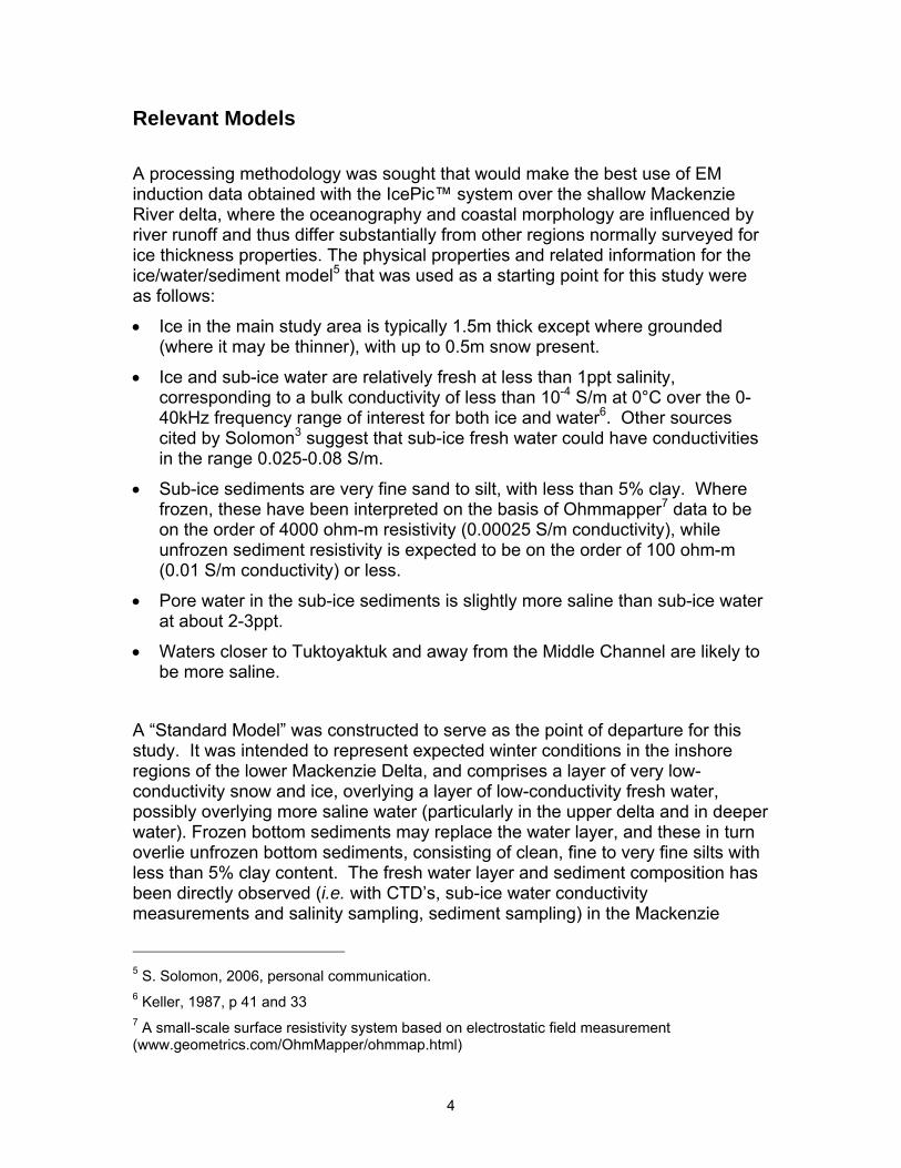
Relevant Models A processing methodology was sought that would make the best use of EM induction data obtained with the IcePic™ system over the shallow Mackenzie River delta, where the oceanography and coastal morphology are influenced by river runoff and thus differ substantially from other regions normally surveyed for ice thickness properties. The physical properties and related information for the ice/water/sediment model5 that was used as a starting point for this study were as follows:

• Ice in the main study area is typically 1.5m thick except where grounded (where it may be thinner), with up to 0.5m snow present.

• Ice and sub-ice water are relatively fresh at less than 1ppt salinity, corresponding to a bulk conductivity of less than 10-4 S/m at 0°C over the 0-40kHz frequency range of interest for both ice and water6. Other sources cited by Solomon3 suggest that sub-ice fresh water could have conductivities in the range 0.025-0.08 S/m.

• Sub-ice sediments are very fine sand to silt, with less than 5% clay. Where frozen, these have been interpreted on the basis of Ohmmapper7 data to be on the order of 4000 ohm-m resistivity (0.00025 S/m conductivity), while unfrozen sediment resistivity is expected to be on the order of 100 ohm-m (0.01 S/m conductivity) or less.

• Pore water in the sub-ice sediments is slightly more saline than sub-ice water at about 2-3ppt.

• Waters closer to Tuktoyaktuk and away from the Middle Channel are likely to be more saline.

A “Standard Model” was constructed to serve as the point of departure for this study. It was intended to represent expected winter conditions in the inshore regions of the lower Mackenzie Delta, and comprises a layer of very low-conductivity snow and ice, overlying a layer of low-conductivity fresh water, possibly overlying more saline water (particularly in the upper delta and in deeper water). Frozen bottom sediments may replace the water layer, and these in turn overlie unfrozen bottom sediments, consisting of clean, fine to very fine silts with less than 5% clay content. The fresh water layer and sediment composition has been directly observed (i.e. with CTD’s, sub-ice water conductivity measurements and salinity sampling, sediment sampling) in the Mackenzie

5 S. Solomon, 2006, personal communication. 6 Keller, 1987, p 41 and 33 7 A small-scale surface resistivity system based on electrostatic field measurement (www.geometrics.com/OhmMapper/ohmmap.html)

4

delta8, but sediment pore water salinities in the area covered by the airborne data (or, better yet, in situ sediment conductivity measurements) were not available. Similar salinity stratification in the water column has been observed in estuaries such as that near Botwood, Newfoundland, on the Exploits River9. At Botwood, the large salinity (and hence density) contrast between the freshwater and seawater layers appeared to inhibit mixing in the quiet sub-ice environment. This complex, multi-layer model would be difficult to characterise adequately using real-world laser/electromagnetic measurements, owing to its numerous parameters and weak contrasts, particularly between ice, fresh water and frozen sediments. Practical experience with quantitative interpretation of EM data from different systems over layered structures suggests that airborne data over models with as few as three layers are difficult to interpret unless a priori simplifying assumptions are made. Fortunately, in this case the ice and fresh water layers are expected to be so low in conductivity relative to seawater or unfrozen bottom sediments that (subject to field validation) they can be merged into a single equivalent layer. In fact, unless the conductivity of frozen sediments beneath the ice is much higher than the 2.5x10-4 S/m estimated from inversion of Geometrics Ohmmapper™ data10, it is unlikely that their EM response can be resolved from that of the overlying ice using standard IcePic™ measurements. Sub-ice seawater under deep-water Arctic conditions is usually relatively uniform in its properties, with conductivities of approximately 2.5 S/m. Conductivity-Temperature-Depth (CTD) profiles obtained in April-May of 198711 and 1991 during the low-flow winter period bear this out12. In the principal inshore study area, seawater is not present, which further simplifies the model. A provisional Standard Model is therefore proposed consisting of the following: 1. Very resistive ice and snow (nominal conductivity 10-4 S/m, thickness 2m)

overlying a variable thickness (nominal value 0m) of fresh water (nominal conductivity ranging up to 0.08 S/m), with total composite thickness T1 and average conductivity Sig1 (nominal value 10-4 to 10-3 S/m).

2. A frozen sediment layer, assumed to be uniform, with variable thickness T2 (nominal value 1m) and conductivity Sig2 (nominal value 2.5x10-4 S/m).

3. A basal unfrozen sediment layer, assumed to be thick and uniform, with conductivity Sig3 (as low as10-2 S/m, higher where clay and/or seawater is present or pore waters are otherwise more saline than expected.)

8 S. Solomon, 2006, personal communication 9 Rossiter, Holladay and Lalumiere, 1992 10 S. Solomon, 2006, personal communication 11 Macdonald and Carmack, 1991 12 Macdonald et al, 1992

5

An optional water layer may be substituted for the frozen sediment layer, of variable thickness T2 (nominal value 1m) and conductivity Sig2 (nominal value 0.025 S/m).

Instrumentation Electromagnetic Measurement of Ice Thickness and Bathymetry: Low-frequency electromagnetic measurements, particularly airborne electromagnetics, provide a valuable means of probing the subsurface over large areas. Historically, EM methods were developed for detection and characterisation of conductive mineral deposits and geological structures. As EM sensors became more quantitative and easily deployed during the 1980’s, interest developed in detailed mapping of other features, such as sea ice thickness13 and water depth. Since that time, dedicated airborne systems were developed for measurement of sea ice thickness and bathymetry, each optimised in some sense for their particular mission. This section briefly discusses the geophysics underlying EM-based sea ice and bathymetric measurements. A “generic” EM induction sea ice measurement system comprises an electromagnetic induction sensor operating at one or more frequencies, a laser altimeter, a GPS receiver and a real-time ice properties processor, mounted on or towed beneath an aircraft. The processing unit estimates the distance between the EM sensor and the sub-ice seawater based on the strength of the EM signal reflected from the water surface, and subtracts the laser-derived height of the EM sensor above the ice/snow surface. Factors Affecting Accuracy: All EM measurements are subject to attenuation effects, due to the nature of practical EM transmitters and to the fact that materials such as seawater and, to a lesser extent, sea ice and bottom sediments, are electrically conductive. The “transmitted” signal amplitude arising from an EM transmitter falls off as the cube of distance from the transmitter, as long as the transmitter’s physical dimensions are small relative to that distance. The transmitted signal must also “reflect” from subsurface interfaces, such as ice/seawater, or seawater/sea bottom, and the “reflected” or “received” signal must propagate back up to the EM receiver, further reducing signal strength arising from the subsurface. This effect is usually referred to as “geometric” attenuation, since it relates to the geometric relationship between the sensor and the subsurface structure. EM signals are also attenuated in conductive materials by the so-called “skin effect”, in which the energy of the transmitted signal is progressively converted to heat as its induced eddy current system circulates in the material. For a plane 13 Kovacs and Holladay, 1990

6

electromagnetic wave, this type of attenuation is inversely proportional to the square root of the product of transmitter frequency F and the conductivity of the material σ, embodied in a property called the “skin depth” δ = (2/(2πµ0σF))1/2. A plane electromagnetic wave amplitude is attenuated by 1/e in one skin depth, 1/e2 in two skin depths, and so on (“e” is the base of the natural logarithm, approximately 2.718). The fields transmitted by transmitters which are small relative to system dimensions (such as are used in airborne EM systems, hand-held or sled-borne surface systems) attenuate even more rapidly than this “skin depth” rule of thumb implies. The combination of geometrical and skin effect attenuation diminishes the sensitivity of EM measurements to subsurface features very rapidly as sensor altitude increases, particularly at high frequencies. This means that survey measurements need to be made at relatively low altitudes in order to achieve good signal/noise characteristics. Low-altitude operation has the added benefit of minimising the EM sensor’s “footprint”14, which reflects the spatial averaging of features such as ridge keels at the ice/seawater interface by the EM sensing and data inversion process, and is proportional to sensor altitude. Calibration and base level stability are important factors in the accuracy of EM measurements. Most electromagnetic sensors exhibit calibration variation in both amplitude and phase of the received signal, as well as base level drift and electrostatic disturbances. Since these errors are systematic, they bias subsurface properties estimated from the EM measurements; minimising these errors in survey data is thus a high priority in system and survey design. These effects can be mitigated to some extent by careful system design and shielding, but major additional improvements are obtained through the use of active calibration systems, such as the one used in the IcePic™ and Dualem™ sensors15. Accurate bird pitch and roll sensors are important elements of towed-bird systems, owing to their tendency to swing and pitch beneath the helicopter. The DFO Ice Probe system is the only towed-bird system that incorporates such a device. The AWI bird and all others rely on flying smooth, straight profiles with no crosswind in order to approach their theoretical accuracy. This effect is substantial, with thickness errors of 10-20cm or more being commonplace. The IcePic™ system also incorporates pitch and roll sensors, although these measurements are much less critical to the ice thickness estimates, due to the system’s low operating height and the sensor’s proximity to the helicopter. Noise in the received signal is a function of ambient noise levels generated by sferics (lightning flashes), cultural noise such as that due to power lines and radio transmitters, noise arising from the aircraft (both direct emissions and variations in secondary field arising from vibration of the helicopter’s conductive structure and blades), vibration of the receiver coil in the earth’s magnetic field, and noise

14 Kovacs et al, 1995 15 Holladay and Lee, US patent 6,534,985, Canadian patent pending.

7

arising from thermal and electronic effects in the receiver coil and preamplifier. Operationally, in regions remote from settlements and power installations and for frequencies at which noise is not being emitted by the helicopter, most noise arises from sferic effects. This noise can be reduced to tolerable levels by increasing transmitted field strength. The IcePic™ system was designed to exhibit noise levels of approximately 1 ppm or less, which mainly arise from sferic sources. Transmitter-receiver separation affects EM measurements in multiple ways. Since all16 practical EM sensors used for ice-related work utilise so-called “coupling ratios” of the form (received signal)/(transmitted signal at receiver location), which are usually expressed in parts-per-million (ppm) or rarely parts-per-thousand (ppt), their sensitivity to subsurface structures increases as the cube of transmitter-receiver separation, for a given receiver effective area and gain. Two EM sensors of different lengths which offer identical noise levels expressed in ppm are thus not equivalent in sensitivity. However, using short coil separations can sometimes improve overall sensitivity by reducing system error levels, particularly in a high-vibration environment. Taken together, the above effects impose limits on the effective depth of investigation of EM sensors, particularly in highly conductive materials such as seawater. Given the broad range of possible scales and operating conditions, it is necessary to perform numerical modelling and use sensitivity analysis techniques to assess which model parameters a given sensor should or should not be able to resolve. To place the IcePic™ system in context, consider some of the other systems that have been used for EM-based sea ice and bathymetric measurements. The “Through Ice Bathymetry System” (TIBS), also owned by DFO through the Canadian Hydrographic Service, is over 7m long and almost 1m in diameter, and weighs about 400 kg. It uses an extremely low minimum operating frequency of 45 Hz, flies at 15-20m survey altitude, and is able to accurately measure seawater depth to approximately 50m. Its primary function is the estimation of seawater depth from the air in ice-covered waters. At a smaller scale are the DFO Ice Probe and the Alfred Wegener Institute (AWI)17 helicopter-towed ice measurement birds, with coil separations on the order of 3m, bird weights of about 100 kg, and nominal operating heights of about 15m. These systems operate at frequencies between 3.68 and 150 kHz. The lightweight, fixed-mount IcePic™ system operates at heights between 1 and 10m, employs a coil separation of 1.2m, and uses 4 frequencies between 1674 and 35156 Hz18. Two versions of the IcePic™ system are shown in Figure 2 below. 16 Surface EM sensors such as the Dualem and the EM-31 utilise coupling ratios internally, but may express quadrature response in equivalent apparent conductivity units of milliSiemens/m. 17 Haas et al, 1997 18 At the smallest end of the scale, there are surface-based systems that operate at heights as low as of 0.2m, with one or two receiver coil separations, and typically use a single frequency of approximately 9 kHz, with coil separations ranging from 1m to 4m. These systems are limited in

8

Towed-bird systems display a number of strengths and weaknesses. A towed bird operates relatively far from the helicopter, with its moving blades and electromagnetic emissions. Such systems also have the advantage of being “button-on”—they can be deployed from a suitable helicopter using its cargo hook. However, towed birds substantially complicate helicopter operations and require special pilot skills. Takeoffs and landings (especially on icebreakers), as well as flight under sub-optimal weather conditions, can be problematic. These and other shortcomings of towed-bird systems motivated the development of the hard-mounted IcePic™ system, which can acquire data either “touched down” on the ice surface, or in low altitude flight above the surface, heights much lower than those at which even a small towed helicopter EM sensor such as the Ice Probe or the AWI bird can be safely operated. The IcePic™ system offers high sensitivity, a wide range of frequencies, extremely stable calibration, very low-altitude data acquisition, and has a negligible effect on helicopter fuel consumption, payload and general operation (easing landings on icebreakers and in other difficult situations).

Figure 2: IcePic™ installed on MBB BO105 (left) and Bell 206L (right) helicopters

IcePic™ Instrument Specifications: The IcePic™ system, originally called EISFlow™, was developed by Geosensors Inc. for DFO in 1999-2001, and has been in active service since that time. The sensor consists of an EM sensor array mounted at the helicopter’s nose, with control, data acquisition and processing being performed on an electronics console mounted inside the helicopter. The instrument operates at frequencies of 1.7, 5.0, 11.7 and 35.2 kHz, and records EM responses in phase and out of phase with the transmitted field to 0.1 ppm precision. The EM array is in the form of a miniature Helicopter EM system, with a transmitter and receiver coil separated by a centre to centre distance of 1.2m, mounted in the horizontal coplanar orientation. Its nominal noise level is 1 part per million of the primary field at the receiver location. Base levels are measured by flying the system out

survey range and by their inability to cross open water or extremely rough ice, but are less costly to acquire and, for small surveys, to operate than airborne systems.

9

of ground effect. The system incorporates an Optech laser altimeter with an accuracy of 1 cm over the 1 to 10m operating altitude range and output at 20 Hz, as well as pitch and roll sensors with accuracy of approximately 1 degree.

Sensitivity Analysis

A series of sensitivity analyses were conducted to evaluate the sensitivity of inverted model parameters to noise in the observed data. Similar studies have been performed by the author in earlier reports for DFO. That methodology has been used here without substantial modification. The following passage, adapted from one such report, describes the background and method as applied to an analysis of sea ice thickness estimation.

The EM inverse problem is non-linear in the parameters of interest, ie sea ice conductivity and thickness. As such, the error estimates available from methods like the damped SVD technique must be used with caution. In particular, parameter variances estimated on the basis of data variances are only meaningful when they are small, so that they represent minor perturbations of the model. Expressions are given below for linear parameter variance estimates. When more substantial parameter variances must be investigated, non-linear searches of the parameter space become necessary. Numerical procedures for performing such searches are available, but lie outside the scope of this analysis. However, certain aspects of non-linear testing may be carried out using an inversion routine

During the SVD inversion process, the relationship between the parameter corrections ∆p and the misfit ∆c between the computed model response and the observed data is

∆ ∆p = d-1A c

=V I U tΛ Λ ∆/ ( )2 + λ c

where λ is the stabilisation or damping parameter used for the pseudo-inversion of the Jacobian matrix A. This defines the variance of the parameter corrections as

var( ) / ( )∆ Λ Λp = E Vij jj jjj

n2 2 2 2

1

+=∑ λ 2

where E2 is the data variance estimate, i.e. (1 ppm)2. Once the fitting process has been completed, this parameter variance estimate provides guidance (within the limits mentioned above) as to how the variance in the calculated response is distributed amongst the model parameters. For the purposes of this report, the Standard Error (SE) of the parameters is defined as the square root of var(∆p).

The quantification of performance can be performed at two levels. Linear estimates of parameter error can be formulated for small variations away from defined models with reasonable accuracy, while for large variations a non-linear search may be necessary. For the purposes of this analysis, the former approach will be applied, as small changes in the model parameters fall into the linear regime.

10

To summarise, the methodology used for this analysis was as follows:

1. A base model was defined to serve as a starting point for the analysis.

• The effects of introducing auxiliary or a priori information (knowledge of the values of specific parameters) into the analysis were considered.

• The effects of damping during pseudo-inversion of the Jacobian matrix were investigated. At the damping levels typically used, the effect was negligible. Data plots for this case were therefore not presented.

2. […]

3. Sensitivity estimates based on pseudo-inversion of the models’ Jacobian matrices were computed and used to estimate the parameter errors to be expected for specified levels of error in the observed EM response.

4. […]

The EM system is assumed to yield data with a 1 ppm noise level having zero mean and stationary statistics. Noise levels which differ from this value propagate directly through to the output standard errors. Sensor elevation and orientation were considered to be exact.

Violation of these assumptions yields fairly predictable results, at least for small perturbations. For example, if the noise level is 10 ppm rather than 1 ppm, the predicted error levels in the model parameters T1, σ1 and σ2 (see below) will increase in direct proportion. If the error distribution is slightly skewed, the output noise distributions should show an approximately similar deviation. Errors in the sensor elevation above the snow or ice surface will add directly to errors in the ice thickness, but should have only weak effects on the conductivities. Sensor orientation effects can be corrected for, provided that an accurate measurement of the orientation is available. Calibration and drift errors, as long as they are small, have a similar effect on the output parameters.

The first round of sensitivity studies examined the accuracy with which the “free” model parameters can be determined using the standard system output at a single sensor height. Each variation of the sensitivity study was designated with a model number, which corresponds to the models specified in Table 1 below. In this table, key EM system specifications are listed, as well as the sensor height and a model definition. A “C” suffix to a model parameter value in this table indicates that the parameter was “constant” or “fixed,” i.e. that it was considered to be known a priori, which typically has the effect of reducing predicted errors for the remaining parameters. In the following, the i’th layer conductivity Sigi is equivalent to the symbol σ, used earlier. Sensitivity study 1-1 is for an IcePic™ configuration over the standard model with nominal values for all parameters except T1, which was varied in order to evaluate the predicted errors of all parameters as a function of that parameter. Study 1-2 is for the same system and model configuration, but with a higher Sig2 value of .025 S/m. All parameters were free to vary. In Study 1-3, Sig1 was considered to be known a priori. In Study 1-4, Sig1 and Sig2 were considered to be known a priori. Studies 1-5 – 1-6 are comparable to 1-3 – 1-4, but with a Sig3 value of 0.5 S/m.

11

The second round of studies are for the same configuration, but employ a two-layer model in which the intermediate water layer is absent. The three variations are 2-1, with all parameters free, 2-2 with Sig1 known a priori, and 2-3 with Sig1 and Sig2 known a priori. In 2-4, the basal halfspace conductivity was increased to 0.5 S/m. The third round are also for the same configuration, but with seawater being substituted for the relatively resistive bottom layer. The first three variations are 3-1, with all parameters free, 3-2 with Sig1 known a priori, and 3-3 with Sig1 and Sig2 known a priori. The last two variations, 3-4 and 3-5, were computed for a lower sensor height of 1m, corresponding to the IcePic™ system being operated in a “touch down” mode with the helicopter skids just above the ice surface. In the interests of clarity and brevity, only excerpts from these sensitivity analyses will be discussed in this report.

10-1 100 101 10210-3

10-2

10-1

100

101

102

103

T1 Value (m)

Sta

ndar

d E

rror (

para

met

er u

nits

)

SE's for 3-Layer Model Params: Model 12

Sig1 Sig2 Sig3 T1 T2

Degrees of Freedom

Figure 3: Study 1-2. IcePic™ at 5m over three layer model with medium-conductivity (Sig2=0.025 S/m) fresh water.

In this example, the Standard Error (SE) estimates for the various parameters are presented as a function of the thickness T1 of the first layer, assuming relatively low conductivities of 0.0001, 0.025 and 0.01 S/m for the ice, water and bottom layers, as indicated in Table 1. With the exception of Sig3 (bottom layer conductivity), these error estimates far exceed the actual parameter value (except Sig1 for T1 values exceeding the unrealistic value of 20m.) This indicates that, for a situation where all parameters are unconstrained, only Sig3 may be estimated with any degree of confidence. Resolution of certain parameters can be increased by reducing model complexity, or by providing a priori estimates of one or more model parameters, which has the effect of improving the resolution of some or all of the remaining “free” parameters. The figure for Study 1-3 below shows the effect of fixing the upper layer conductivity Sig1 to 10-4 S/m.

12

Table 1: Sensitivity study summary

Study Number

Meas't Class

No. of Freq's

No. of Rx's

Coil Sep(s)

(m)Sensor

Height (m) Model DescriptionS1 (S/m) T1 (m) S2 (S/m) T2 (m) S3 (S/m)

1-1 Single 4 1 1.2 5 0.0001 2 0.00025 1 0.011-2 Single 4 1 1.2 5 0.0001 2 0.025 1 0.011-3 Single 4 1 1.2 5 0.0001C 2 0.025 1 0.011-4 Single 4 1 1.2 5 0.0001C 2 0.025C 1 0.011-5 Single 4 1 1.2 5 0.0001C 2 0.025 1 0.51-6 Single 4 1 1.2 5 0.0001C 2 0.025C 1 0.5

2-1 Single 4 1 1.2 5 0.0001 2 0.012-2 Single 4 1 1.2 5 0.0001C 2 0.012-3 Single 4 1 1.2 1 0.0001C 2 0.01C2-4 Single 4 1 1.2 1 0.0001C 2 0.5

3-1 Single 4 1 1.2 5 0.0001 2 2.53-2 Single 4 1 1.2 5 0.0001C 2 2.53-3 Single 4 1 1.2 5 0.0001 2 2.5C3-4 Single 4 1 1.2 1 0.0001 2 2.53-5 Single 4 1 1.2 1 0.0001C 2 2.5

10-1 100 101 10210-3

10-2

10-1

100

101

102

103

T1 Value (m)

Sta

ndar

d E

rror (

para

met

er u

nits

)


Sig2 Sig3 T1 T2

Degrees of Freedom

Figure 4: Study 1-3. IcePic™ at 5m over three layer model with medium-conductivity (Sig2=0.025 S/m) fresh water, Sig1 fixed

In this case, the SE’s for the T1 and T2 estimates are improved, and there is some improvement in the Sig2 SE’s, but Sig3 is still the only parameter resolved. In Study 1-4 below, assuming an a prio i value of 0.025 S/m for Sigr 2 improves the SE’s for the remaining parameters.

13

10-1 100 101 10210-3

10-2

10-1

100

101

102

T1 Value (m)

Sta

ndar

d E

rror (

para

met

er u

nits

)


Sig3 T1 T2

Degrees of Freedom

Figure 5: Study 1-4. IcePic™ at 5m for 3 layer model with Sig2=0.025 S/m (fresh water), Sig1 and Sig2 fixed The T1 and T2 SE’s drop below 1m for T1 values of up to 3m and 1m, respectively, and the SE for Sig3 falls to almost 10-3 S/m. If we consider the case of 2m snow plus ice (indicated by the vertical black line) over 1m of fresh water, the upper black arrow indicates a T2 (water thickness) error estimate of about ±1.5m, while the lower arrow indicates the lower T1 (snow plus ice) error estimate of ±.6m. The T2 value is poorly resolved, while T1 is somewhat better estimated. If the bottom layer is more conductive than 0.01 S/m (say 0.5 S/m) the situation changes considerably.

10-1 100 101 10210-4

10-3

10-2

10-1

100

101

102

T1 Value (m)

Sta

ndar

d E

rror (

para

met

er u

nits

)


Sig3 T1 T2

Degrees of Freedom

Figure 6: Study 1-6. IcePic™ at 5m for 3 layer model with Sig3=0. 5 S/m layer 3, Sig1 and Sig2 fixed.

In this case (with the same a priori values for Sig1 and Sig2), the SE’s for both T1 and T2 drop below 0.1m for T1 = 2m and T2 = 1m, and the SE for Sig3 drops still further. This is the result of the stronger EM response from the bottom layer improving the signal/noise ratio of the EM measurement. Given the results

14

displayed in the next section, it appears that this is a fairly representative model for at least one profile of IcePic™ data from the 2004 Mackenzie Delta flights. Simplifying the model from three layers to two layers also increases the resolution of model parameters, assuming that the model remains applicable. In the case of resistive fresh water ice overlying a fresh water layer that in turn overlies conductive bottom sediments or conductive seawater, the previous examples indicate that the fresh ice and fresh water layers are indistinguishable from each other. Under these circumstances, a two layer model comprising an upper layer (representing snow plus ice plus fresh water) of thickness T1 and conductivity Sig1, overlying a more conductive halfspace of conductivity Sig2, should also fit the data. Sensitivity analyses 2-1 to 2-4 address this situation for the ice over sediment case, while analyses 3-1 to 3-5 relate to the corresponding case over seawater. Consider the plot for Study 2-4 below, for which the sediment conductivity Sig2 is 0.5 S/m. In this example, the SE’s for T1 are less than 0.007m for T1 values in the 1 to 2m range. The SE’s for Sig2 are less than 1% (0.005 S/m) for T1 values less than 6m. Even the Sig1 values are well constrained for thick ice/water: for a T1 value of 1m, the SE for Sig1 is 0.001 S/m, somewhat lower than was obtained for the relatively constrained values in Study 1-6 above. As expected, Sig1 SE’s rise for small values of T1, since there is progressively less response from the thinning upper layer. The improved parameter resolution obtained with the 2-layer model is accompanied in practice by more rapid and robust convergence of the inversion algorithm. These results suggest that, where possible, a 2-layer model should be used for inversion of IcePic™ data, although 3-layer inversions may be used with care, at least where some model parameters may be specified a priori.

10-1 100 101 10210-5

10-4

10-3

10-2

10-1

100

101

T1 Value (m)

Sta

ndar

d E

rror (

para

met

er u

nits

)


Sig1 Sig2 T1

Degrees of Freedom

Figure 7: Study 2-4. IcePic™ at 5m for 2 layer model with Sig2=0. 5 S/m, all parameters free. For a T1 value of 2m, parameter errors are on the order of 3x10-4 and 1x10-3 S/m for Sig1 and Sig2, and 6x10-3 m for T1. At a T1 value of 10m, Sig1 errors have decreased tenfold, while T1 and Sig2 errors have increased by similar factors. These error levels are still low enough to provide useful information for ice plus fresh water depths of 10m.

15

EM Profile Inversion Results

In this section, a detailed discussion of dataset FEM04079, acquired over the central portion of the Mackenzie Delta on April 26, 2004, is followed by less detailed discussions of a series of similar datasets acquired to the north and east of FEM04079’s track on April 26. The IcePic™ data file FEM04079 was inverted using a two-layer model derived from the Standard Model discussed above, using the following starting parameters: Sig1 = 10-4 S/m (assumed to be known a priori), Sig2 = 0.01 S/m, and T1 = 2m. The results are shown in Figure 8 below.

100 200 300 400 500 600 700 800 900 1000 11000

1

2

3

4

5

6

7

8

9

Time (sec)

Par

amet

ers

1 to

3

Inverted Parameters from File FEM04079PPR

Laser rmn SigIce*1000Tice SigW Bathymetry

Frozen sediments Fresh water beneath ice Stamukhi 6m depthcontour

2m depthcontour

10m depthcontour

Figure 8: 2 Layer model with Sig1=10-4 S/m (fixed), from SE to NW, plotted vs time in seconds. Bathymetry (see text) from a CHS acoustic survey has also been plotted for this line; note the close correspondence between T1 and bathymetry near 200 seconds and between 300 and 630 seconds.

This figure includes a bathymetric profile (magenta dashed line) provided by Ingrid Peterson, who extracted it using a nearest-neighbour interpolation method from a bathymetric dataset for the Beaufort Sea provided by Steve Solomon. Within the bathymetric dataset, the data for the profile in Fig. 8 are from CHS field sheets 1300872 and 1300962 acquired in 1971 and 1974 respectively. She also determined that a 1.26m correction was required to account for tidal variation, ice freeboard and estimated snow depth at the profile location. As suggested by the annotations in this figure, there are four distinct zones sampled by this profile. The inshore zone is characterised by T1 values in the 2 to 3.5m range, with a pair of abrupt thickenings in T1 to about 6.5m just after 100 seconds and just before 300 seconds. These features are coincident with shallow zones in the known bathymetry, plotted in magenta. These features correspond to high-probability locations for sub-ice frozen sediments, based on known bathymetry and SAR interpretations. In the section between 190 and 220 seconds, the T1 value corresponds closely to the known bathymetry. The inshore zone extends to the vicinity of the 2m bathymetric contour (3.26m depth

16

on this plot, which includes tide, freeboard and snow depth correction). In the next zone, just to seaward of the inshore zone (from 310 to 630 seconds), theT1 values correspond closely to the bathymetry profile. In this zone, fresh water ice overlies fresh water, which in turn overlies a relatively conductive sediment layer, consistent with a nearby CTD sounding from 1991. In the third zone, T1 values decrease and the heavily ridged Stamukhi begins. The decrease in T1 is due to the presence of layers of denser, more saline water beneath the fresh water. These saline layers are interpreted by the inversion program as a basal conductive layer, similar to the role played by the conductive sediments in the first two zones. The fresh water and the more-saline water layers, being less dense than seawater, are ponded behind the deep keels of ridges running approximately parallel to the depth contours within the Stamukhi. These additional layers are again consistent with expected CTD structure as seen in nearby 1987 and 1991 observations. In the fourth zone, there is little or no fresh water remaining beneath the ice—it has been replaced by brackish water of approximately 1.1 S/m conductivity. This layer is thick and conductive enough to mask the presence of normal seawater beneath it, which may be present at the seaward end. If the profile had continued for another few kilometres to the northwest, the transition to sea ice overlying normal seawater at 2.5 S/m would probably have been observed—such a transition was seen in another line that will be discussed below. Over the full length of this profile, small amplitudes of the fitting parameter RMN indicate that this model fits the EM/laser data well (to within a few percent). A small feature, with basal layer conductivity approaching that of seawater, is seen between 873 and 877 seconds. It is interpreted as a small zone of remnant surface seawater that was not replaced by buoyant, low salinity plume water, because of ice ridges surrounding the small zone. This feature is shown in enlarged form in Figure 9 below.

840 850 860 870 880 890 9000

2

4

6

8

10

Time (sec)

Par

amet

ers

1 to

3



High-salinity water "cell"trapped by deep ridge keels

Weak positive correlationbetween T1 and Sig2

Negative correlation betweenT1 and Sig2

Figure 9: Detail from line 4079, showing high-salinity feature surrounded by deep ridge keels. Note the positive and negative correlation between T1 and SigW (Sig2) along the indicated sections of this plot.

17

Sensitivity analysis 1-4 suggests that, if the conductivities of the two upper layers are known a priori, the thicknesses of the upper layers and the basal layer conductivity can be interpreted for layered structures with accuracy on the order of decimetres in T1 and T2, and milliSiemens per metre for Sig3. This was tested by inverting line 4079 with fixed conductivities of 10-4 and 0.6 S/m for these layers, with T1, T2 and Sig3 as free parameters; these layer conductivities were applicable to the third zone discussed above. Figure 10 below shows the same portion of the line as in Figure 9, but with this 0.6 S/m intermediate layer included.

845 850 855 860 865 870 875 880 885 890 8950

2

4

6

8

10

12

Time (sec)

Par

amet

ers

1 to

3


Laser rmn SigIce*1000Tice SigW Tw SigB Ti+Tw

0.6 S/m layer 2 thickness

Layer 1+2 thickness

Layer 1 (ice) thickness

Basal layer conductivity

High-salinity"cell"

Thick intermediate layer No intermediatelayer Thin ~1m

intermediate layer above brackish water ~1.5 S/m

No intermediatelayer

Thick intermediatelayer (brackish+rubble?) over brackish water~1.5 S/m

Figure 10: 3 Layer model: Sig1 and Sig2 fixed. . T1+T2 (solid green) is expected to be more accurate than T2 alone (magenta). Note the reduced correlation between T1+T2 and the basal layer conductivity Sig3, compared to the previous figure. In this figure, the solid green trace is the sum of T1+T2. The estimated T1+T2 and Sig3 values are very similar to T1 and Sig2 for some portions of the 2 layer detail section shown above, but differ substantially in others. On initial inspection, the resolution of the intermediate layer thickness T2 does not appear to be as stable as that of T1, given the large excursions in T2 beneath some thickness variations, but these do appear to have some validity. Under certain circumstances, correlation between T1 and the basal conductivity could be regarded as an indication of model inadequacy. Comparison of the basal halfspace conductivity in these two figures (green dashed line in this figure, cyan solid line in previous figure) shows that much of the correlation and anti-correlation seen between T1 and the basal conductivity in the 2 layer model has been reduced in the 3 layer model, which supports the choice of ~0.6 S/m for the intermediate brackish water layer on the left side of the figure. In the zone of thicker ice between 860 and 870 seconds, T1 peaks are mirrored by T2 troughs of similar amplitude, as would be expected if T1 represents ice thickness and T2 the thickness of a brackish water layer lying beneath the ice and above more saline water at depth. For the largest values of T1 in this time range, the T2 profile drops to near-zero values and becomes blocky, indicating that the contribution of the intermediate layer to the overall model response in these locations is approaching the negligible level. The complementary behaviour of T1 and T2 strongly suggest that in this band of ice ridges, there is little saline water incorporated into the block structure of the ridge keels, such

18

that the keels are thoroughly consolidated and resistive. This would be expected if these ridges were formed from fresh water ice overlying fresh water. On the right side of the figure between 882 and 888 seconds, the inversion yields a thinner intermediate layer of ~0.6 S/m water beneath a level ice section. No indication of this intermediate layer remains at 897 seconds, to seaward of the next band of heavily deformed ice. In contrast to the inshore band of ice ridges between 860 and 870 seconds, where the ridge keels are electrically resistive, giving rise to a negative correlation between T1 and T2, there is generally positive correlation between T1 and T2 in the region between 888 and 896 seconds. This may be interpreted as a conductive “root” of the rubble zone, consisting of an unconsolidated mixture of rubble and relatively conductive water, and acting as a dam behind which the brackish intermediate layer seen between 882 and 888 seconds was ponded. This interpretation also explains the negative correlation observed for the 2 layer model in this vicinity between upper layer thickness and basal layer conductivity that was noted in the previous figure: the 2 layer model was inadequate in this region, and distorted the basal layer conductivity value to compensate for the lack of a required intermediate layer. The high-salinity zone observed in the basal conductivity between seconds 873 and 877 in the previous figure is still present in Figure 10, as expected. This suggests that essentially no low-salinity water has entered this zone. The sensing footprint of the EM system, which is on the order of 15m for a 5m survey altitude, corresponds to a time interval of about 0.5 second. All of the features described in this section are 1 second or more wide, and so cannot be interpreted as EM footprint effects. It is, however, likely that the values of T1 estimated over narrow peaks have been underestimated due to this effect. The same two-layer model used to prepare Figure 8 above was used to invert all data files from April 26, 2006. These profiles, for which tracks are plotted in Figure 1, are presented as time series profiles in Figure 11 to Figure 15.

0 200 400 600 800 1000 1200

1

2

3

4

5

6

7

8

9

10

Time (sec)

Par

amet

ers

1 to

3


Laser rmn SigIce*1000Tice SigW

Normal offshorewater salinity

Reduction of apparentwater salinity beneath stamukhi

OFFSHORE INSHORE

Open water

Figure 11: 2-layer inversion results for file 4077. This profile starts north of the Tuktoyaktuk Peninsula and runs SW toward Kugmallit Bay. Note the open lead beginning at 606 seconds, with normal 2.5 S/m seawater present at surface.

19

0 100 200 300 400 5000

1

2

3

4

5

6

7

8

9

10

Time (sec)

Par

amet

ers

1 to

3Inverted Parameters from File FEM04078PPR


Progressive reductionof apparent water salinity

Step reductions of apparentwater salinity beneath stamukhi

Apparent fresh water pondingbeneath ice~0.4-0.5m ~0.8m

OFFSHORE INSHORE

Figure 12: Survey line 4078, extending south from end of Line 4077 toward Kugmallit Bay.

0 100 200 300 400 500 600 700 800 9000

1

2

3

4

5

6

7

8

9

10

Time (sec)

Par

amet

ers

1 to

3



Figure 13: Line 4080, extending NNE from the end of line 4079.

0 100 200 300 400 500 600 700 800 900 10000

1

2

3

4

5

6

7

8

9

Time (sec)

Par

amet

ers

1 to

3



Figure 14: Line 4082, extending SE from the end of line 4080 toward Richards Island.

20

0 500 1000 1500 2000 2500 3000 3500 40000

1

2

3

4

5

6

7

8

9

10

Time (sec)

Par

amet

ers

1 to

3Inverted Parameters from File FEM04083PPR


Figure 15: Line 4083, extending NE from the vicinity of Hooper Island, with a second leg starting at time 2200 running south into Kugmallit Bay.

Figure 16: View at 1430 local time (approximately 1500 seconds on profile above) during fourth background measurement in FEM04083, altitude ~200m. Note zones of open water and thin ice, which appear on profile at about 1600 seconds.

For line 4083, note the thin (1m) surface layer sections at approximately 1600 seconds (Fig. 15). These correspond to leads covered with open water, new or grey ice (Fig. 16), implying 0.8-1.0m fresh water at the surface, overlying a 0.5 S/m saline layer. By comparison with Line 4079 (Fig. 8), fresh water layers are

21

present up to 1900 seconds and after 2400 seconds, with substantial thicknesses of fresh water at both ends of the line. The two-layer inversion results shown above, which were all acquired on April 26, 2004, are shown in plan view, merged with 1991 CTD results (which arose under a different pack ice configuration), coastal outlines and bathymetric contours, in Figure 17.

Figure 17: EM-derived upper layer thickness (red) and basal layer conductivity (black) estimates, with bathymetric contours and 1991 CTD information. The CTD results, which arose under different pack ice conditions than were present in 2004, are plotted with the low-conductivity upper layer, including ice thickness, represented as red bars with the same scale factors as for the ice thickness profiles, and the lower layer conductivity are plotted as black bars using the conductivity scale from the profiles (courtesy of I. Peterson).

22

The profile and bathymetry data of Figure 17 were also merged with satellite SAR imagery, as shown in Figure 18 below.

Figure 18: Two-layer EM model results (upper layer thickness in red, basal layer conductivity in yellow) and bathymetric contours as in previous figure, superimposed on ENVISAT SAR imagery (courtesy of Ingrid Peterson).

23

Figure 19: Detail of two-layer EM model results results (upper layer thickness in red, basal layer conductivity in green) and bathymetric contours for Line 4079, superimposed on ENVISAT SAR imagery as in previous figure (courtesy of Ingrid Peterson).

In the image above, the two zones of frozen sub-ice sediments in Line 4079, which were discussed above, are visible as spatially narrow thickenings in T1 near 69.5 N, 135.5 W. The zone of ice overlying a thick sub-ice fresh water layer is visible between the shoreline of Garry Island and the 6m bathymetric contour, while the heavily ridged zone corresponds to the Stamukhi is visible from NW of the 6m contour to well beyond the 10m contour. Note that this survey line was terminated just short of a large refrozen lead, which shows as a dark band running SSW – NNE. The localised zone of high basal layer conductivity

24

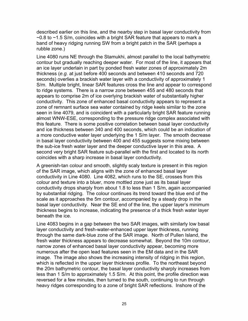
described earlier on this line, and the nearby step in basal layer conductivity from ~0.8 to ~1.5 S/m, coincides with a bright SAR feature that appears to mark a band of heavy ridging running SW from a bright patch in the SAR (perhaps a rubble zone.) Line 4080 runs NE through the Stamukhi, almost parallel to the local bathymetric contour but gradually reaching deeper water. For most of the line, it appears that an ice layer underlain in part by ponded fresh water zones of approximately 2m thickness (e.g. at just before 400 seconds and between 410 seconds and 720 seconds) overlies a brackish water layer with a conductivity of approximately 1 S/m. Multiple bright, linear SAR features cross the line and appear to correspond to ridge systems. There is a narrow zone between 455 and 480 seconds that appears to comprise 2m of ice overlying brackish water of substantially higher conductivity. This zone of enhanced basal conductivity appears to represent a zone of remnant surface sea water contained by ridge keels similar to the zone seen in line 4079, and is coincident with a particularly bright SAR feature running almost WNW-ESE, corresponding to the pressure ridge complex associated with this feature. There is some positive correlation between basal layer conductivity and ice thickness between 340 and 400 seconds, which could be an indication of a more conductive water layer underlying the 1 S/m layer. The smooth decrease in basal layer conductivity between 400 and 455 suggests some mixing between the sub-ice fresh water layer and the deeper conductive layer in this area. A second very bright SAR feature sub-parallel with the first and located to its north coincides with a sharp increase in basal layer conductivity. A greenish-tan colour and smooth, slightly scaly texture is present in this region of the SAR image, which aligns with the zone of enhanced basal layer conductivity in Line 4080. Line 4082, which runs to the SE, crosses from this colour and texture into a bluer, more mottled zone just as its basal layer conductivity drops sharply from about 1.8 to less than 1 S/m, again accompanied by substantial ridging. The colour continues its trend toward the blue end of the scale as it approaches the 5m contour, accompanied by a steady drop in the basal layer conductivity. Near the SE end of the line, the upper layer’s minimum thickness begins to increase, indicating the presence of a thick fresh water layer beneath the ice. Line 4083 begins in a gap between the two SAR images, with similarly low basal layer conductivity and fresh-water-enhanced upper layer thickness, running through the same dark-blue zone of the SAR image. North of Pullen Island, the fresh water thickness appears to decrease somewhat. Beyond the 10m contour, narrow zones of enhanced basal layer conductivity appear, becoming more numerous after the open lead features seen in the EM data and in the SAR image. The image also shows the increasing intensity of ridging in this region, which is reflected in the upper layer thickness profile. To the northeast beyond the 20m bathymetric contour, the basal layer conductivity sharply increases from less than 1 S/m to approximately 1.5 S/m. At this point, the profile direction was reversed for a few minutes, then turned to the south, continuing to run through heavy ridges corresponding to a zone of bright SAR reflections. Inshore of the

25

10m depth contour, the SAR image colour trends back toward blue, crossing a bright and fairly broad feature at the 9m depth contour that corresponds to ridging visible in the upper layer thickness. For the rest of this profile, the upper layer thickens while the basal layer conductivity continues to fall, as expected where a thickening fresh water layer is present beneath the ice. Finally, near the 5m contour, a broad peak is observed in the upper layer thickness that corresponds closely to that seen at a similar depth on line 4079. The total upper layer thickness matches the bathymetry well from the 3m contour to below the 2m level: evidently there is a more substantial thickness of saline water at depths of less than 5m in this area than was seen near Garry Island. Lines 4077 and 4078 were acquired prior to 4079, during the initial approach to Tuktoyaktuk after a long data acquisition run around Cape Bathurst from Franklin Bay. In deep water, the basal layer conductivity is 2.5 S/m, corresponding to normal seawater. A large open lead was crossed between 600 and 640 seconds, with 2.5 S/m water present at the surface. The first significant conductivity reduction occurs at a band of ridges near the 30m contour, followed by another drop near the 20m contour. At this point, line 4077 was terminated and 4078 started. Further drops in basal layer conductivity occurred at a band of ridges that are just visible at the eastern edge of the SAR image, followed by another drop at the south edge of a further series of E-W trending ridges. At this point, the SAR image colour became blue with a relatively smooth texture, and the upper layer’s minimum thickness started to increase, signalling the presence of almost 1m of fresh water beneath the ice at the end of the line.

Discussion Detection of frozen sediments beneath bottom-fast ice: The inversion results above, supported by sensitivity analyses, suggest that zones where the presence of bottom-fast ice has resulted in freezing of sub-ice sediments can be effectively mapped with IcePic™ data, provided that suitable models and assumptions (using an a prio i estimate of snow/ice/frozen sediment conductivity while allowing upper layer thickness and the lower layer conductivity to vary) are used during inversion of the data. The accuracy of this interpretation will drop where the unfrozen sediments assumed to be present at the bottom of this layered model assume low electrical conductivities.

r

The conductivity enhancement seen in shallow unfrozen sediments is a persistent and stable feature in inversions of IcePic™ data from this area, and its existence is supported by similar results in W.J. Scott’s report19 on inversion of

19 Scott, W.J., Inversion of EM Profiles, Mackenzie Delta Area, NWT

26

EM31 and EM34 profiles in the area, indicating a conductive feature that frequently appeared beneath inshore fresh water ice. In the Scott study, the same feature appeared whether or not fresh water was present between the ice and the bottom, and where bottom sediments were apparently unfrozen (so that the surficial resistive layer was in the normal ~2m thickness range) or frozen beneath bottom-fast ice (in which case the surficial resistive layer could be much thicker). The interpreted conductivity for unfrozen sediments is high relative to the expected values for porous sediments based on inshore pore water salinities, but as expected, this parameter value trends higher as the survey line progresses offshore into more saline environments. An interesting feature of the inverted model in the vicinity of the interpreted thick zones of frozen sediments is the thickening of T1 on the inshore side (eg up to 100 seconds and between 220 and 280 seconds) of these features, and a smaller section of thick T1 between 150 and 185 seconds. These features could simply represent ice and snow buildup, or possibly zones where bottom sediments started to freeze later in the winter, resulting in shallower interfaces between frozen and unfrozen sediments. The interpretation of thickness and conductivity profiles was considerably enhanced by overlaying them on the SAR image and bathymetric contours. The sharp jump in the estimated Sig2 value to approximately 1.1 S/m near the 10m bathymetric contour is consistent with the presence of a brackish transition zone between the fresh water ponded inshore of the Stamuhki and the seawater present on the seaward side of the Stamuhki. This enhanced apparent conductivity does not vary systematically with water depth, indicating that the EM measurement is no longer sensing the much lower conductivity of the bottom sediments. Thus, the response of the 8 metre thickness of this brackish water masks the presence of the lower conductivity sea bottom for the instrument’s frequency range. The lower layer of the inversion model effectively shifts from representing bottom sediments (beneath 10 metres of fresh water and ice corresponding to the top layer) to a thick layer of brackish water. This effect is even more strongly seen on lines that cross from the deep-water sea ice regime into the near-shore Stamukhi environment, such as 4077 and 4078. Fresh water bathymetry: Sensitivity analysis 2-4 (Figure 7) predicts that useful estimates for T1, corresponding to snow plus ice plus fresh water layer thickness, as well as Sig1, corresponding to the conductivity of that composite layer, and Sig2, the conductivity of the basal layer, can be obtained from IcePic™ data. Constraining the value of Sig1, which is reasonable for this application, further improves the quality of the estimates for T1 and Sig2. This prediction is borne out by the close correspondence between T1 and corrected bathymetry along line 4079 in Figure 8 above. The T1 and bathymetric results for depths less than 6.5m diverge only in the vicinity of the (interpreted) frozen sediments near 100 and 300 seconds. These

27

divergences are almost certainly artifacts of the nearest-neighbor method whereby the bathymetric profile was extracted from the bathymetric survey grid: since there are no bathymetric data on the grid over the two sandbars traversed at 100 and 300 seconds, this method selects the nearest non-zero bathymetric values and plots them where values reflecting the true depth over the sandbars should be reported instead. As expected, three-layer inversion (with T1, T2, Sig2 and Sig3 free to vary) of the IcePic™ data in this case did not yield valuable additional information regarding the fresh water layer lying between the ~2m snow/ice layer and the bottom inshore of the Stamukhi, and led to occasional instability in the inversion process. However, by using a three-layer model with a priori estimates derived in part from CTD information obtained in previous years for upper, intermediate and lower layer conductivities (Figure 10), it was possible to trace the presence of a moderately conductive (0.6 S/m) intermediate layer between the upper ice layer and a lower, more saline water layer, to see it thin out in a zone of deep, consolidated ice ridges and finally disappear at the seaward edge of a second zone of deformed ice or rubble that appears to have been much less consolidated than the inshore ridges. With a few minor exceptions near the (interpreted) frozen sediments, this three-layer model also reproduced the two-layer inversion results in the fresh water zone. This method should work well in suitable river and lake environments, provided that a strong conductivity contrast exists between ice/water and sediment. Since lake-bottom sediments often contain a substantial clay component, this method may prove to be relatively widely applicable. However, the presence of resistive or magnetic rock formations at the bottom or under a thin veneer of sediments will degrade accuracy by decreasing the observed inphase EM response. Depth Estimation to Conductive Layers Beneath Fresh Water and Ice: For depths greater than 6.5m, the T1 values diverge rapidly from the observed bathymetry. This is due to a conductive zone of brackish water located between the bottom of the fresh water layer and the top of the sediments, which increases rapidly in thickness at the expense of the fresh water layer’s thickness, which is ponded behind the deep keels of the Stamukhi. Similar features are seen on all of the survey lines that cross from fresh to saline environments. It is also possible to identify salinity stratification in sections of open water or thin ice: compare ~1m of fresh water layer overlying 0.5 S/m saline water near 1600 seconds in line 4083 with 2.5 S/m seawater at surface after 606 seconds in line 4077. Real-Time Applications: The signal/noise levels present in the IcePic™ measurements at 5m nominal survey height over the inshore portions of this line were relatively high, on the order of 14-35% of values obtained over sea ice of comparable thickness at the

28

same survey height. Using a suitable model configuration and careful survey procedures (mainly comprising acquisition of more frequent background measurements and keeping survey altitudes as low as permitted by safety considerations), real-time two-layer inversion of IcePic™ for near-shore applications should be practical. It is anticipated that such inversion will be able to distinguish zones of bottom-fast ice over thick frozen sediments from similar zones of bottom-fast ice that lack frozen sub-ice sediments, and to estimate fresh-water sub-ice bathymetry where conditions are suitable. Frozen sub-ice sediment zones display a distinctive spatial character compared to zones where ice and significant thicknesses of fresh water overlie unfrozen, conductive sediments. These different signatures can also be confirmed given known bathymetric data. Identification and characterisation of ponded fresh, brackish and seawater zones beneath Stamukhi should also be possible through observation of variations in the estimated conductivity of the lower layer, or through later interpretation of three-layer inversion results. Operating at lower altitudes is desirable because it considerably improves signal levels, as well as spatial and model resolution. Additional subsurface parameter accuracy may thus be obtained, for relatively short profiles, by profiling at lower altitude (where this can be done safely.) In addition to true real-time processing, in which T1 and Sig2 estimates can be viewed and acted upon in-flight, near-real-time processing of the data to obtain additional accuracy and printed map products can be easily and quickly performed with a laptop computer at the survey base, or even at the refuelling site between survey flights.

29

Conclusions

Inversion studies on a shallow-water IcePic™ data set from the Mackenzie Delta, motivated and informed by a series of parameter sensitivity analyses, suggest that: 1. IcePic™ data sets can distinguish zones where bottom-fast ice overlies

frozen sediments from similar zones where bottom-fast ice overlies unfrozen sediments.

2. Such data sets can also yield estimates of fresh water bathymetry in the inshore zone where ice and fresh water overlie conductive bottom sediments. This approach cannot be applied where a saline water layer with conductivity comparable to or higher than the sediment conductivity is present. However, it could prove useful for airborne bathymetric estimates over fresh water lakes and rivers where a suitable conductivity contrast exists. Quantitative tests of this approach would be straightforward and relatively inexpensive.

3. In open water, layers of fresh water overlying more saline waters can be readily identified.

4. Through the use of a constrained three-layer model, it proved possible to identify the properties of a saline intermediate layer beneath the upper ice/fresh water layer and a conductive lower layer, which in turn clarified the nature of sub-ice water ponding within the Stamukhi. These features could be deduced in part from the behaviour of the basal-layer conductivity estimate obtained from a two-layer inversion of the same dataset, but the three-layer inversion resolved ambiguities remaining in that two-layer interpretation.

5. This study also confirmed the presence of a high-conductance zone, also detected in an earlier surface-based study, which corresponds to unfrozen sediments located beneath the upper ice/frozen sediment or ice/fresh water layer. The presence of this zone improves the expected accuracy of thickness estimates for the upper layer.

6. It should be possible to perform real-time surveys for these features, particularly frozen sediments beneath bottom-fast ice and fresh-water bathymetry in shallow water, using a standard IcePic™ system on which the inversion configuration has been modified for this task.

7. Field processing of such survey data to obtain improved accuracy can be performed rapidly on a laptop computer.

30

Acknowledgements The author gratefully acknowledges information, insights, suggestions, data and graphics provided by Steven Solomon and Ingrid Peterson, and Ms. Peterson’s careful review of this report. Field data acquisition was greatly facilitated by CCGS Amundsen Captain Bernard Tremblay, with flight support by helicopter pilot Yvon Coté and helicopter engineer Bertrand Murray. ENVISAT ASAR data were provided by the European Space Agency under AO Project 178. Financial support was provided by CASES (L. Fortier and D. Barber), through the Can. Space Agency-GRIP program, the Panel of Energy and Research Development and through Geo. Service Canada Atlantic Region (G. Mason) and Devon Oil Canada (D. Scott and B. Wright).

31

References Fassnacht, S.R. and F. M. Conly, 2000. Persistence of a scour hole on the East Channel of the Mackenzie Delta, N.W.T., Can. J. Civ. Eng. Vol. 27: 798:804. Haas, C., Gerland, S., Eicken, H. and Miller, H., 1997, Comparison of sea ice thickness measurements under summer and winter conditions in the Arctic using a small electromagnetic induction device: Geophysics 62, 749-757. Keller, G.V. 1987, Rock and Mineral Properties, in Electromagnetic Methods in Applied Geophysics, V1, Theory, Misac N. Nabighian, ed., Society of Exploration Geophsicists. Kovacs, A. and Holladay, J.S., 1990, Sea ice thickness measurement using a small airborne electromagnetic sounding system, Geophysics 55, 1327-1337 Kovacs, A, Holladay, J.S., and Bergeron, C, 1995, The footprint/altitude ratio for helicopter sounding of sea-ice thickness: Comparison of theoretical and field estimates, Geophysics 60, 374-380. Macdonald, R.W. and E.C. Carmack. 1991. The role of large-scale under-ice topography in separating estuary and ocean on an Arctic shelf. Atmosphere-Ocean 29:37-53. Macdonald, R.W., R. Pearson, D. Sieberg, F.A. McLaughlin, M.C. O'Brien, D.W. Paton, E.C. Carmack, J.R. Forbes, J.Barwell-Clarke, 1992. NOGAP B.6, Physical and chemical data collected in the Beaufort Sea and Mackenzie River delta, April-May 1991, Can. Data Rep. Hydrogr. Ocean Sci.: 104, 154 pp Prinsenberg, S. J., S. Holladay, and J. Lee. 2002, Measuring Ice Thickness with EISFlow™, a Fixed-mounted Helicopter Electromagnetic-laser System, Proceedings of the Twelfth (2002) International Offshore and Polar Engineering Conference, Kitakyushu, Japan, May 26-May 31, 2002, Vol. 1, pp. 737-740 Rossiter, J.R., J.S. Holladay and L.A. Lalumiere, 1992, Validation of airborne sea ice thickness measurement using electromagnetic induction during LIMEX ’89, Can. Contractor Rep. Hydrog. And Ocean Sci. 41. Scott, W.J., Inversion of EM Profiles, Mackenzie Delta Area, NWT, Report under SSC Contract 23420-01M465/001/HAL, prepared for S. Solomon by GeoScott Exploration Consultants Inc.

32

Appendix A Application of Surface EM Sensors to Sea Ice Measurement Surface-based EM measurements, originally developed for near-surface geological and environmental investigations, have been used since the 1980’s for sea ice measurements, as reported by Kovacs and Morey20 and more recently by Hass et al21 and Reid et al22. These investigators all used a commercial device called the Geonics EM-31, a single-receiver, single-frequency EM device designed in the 1970’s. A new EM device known as the Dualem-4 was introduced in 2000, with shorter 2m and 1m versions introduced in 2001 and 2004. W. Scott analysed data from an EM31, along with the larger-scale EM34, for permafrost studies in the Mackenzie Delta region23. The Dualem-4™ system is a commercially available sensor used for terrain conductivity mapping, comprising a horizontal coplanar coil pair with a 4m coil separation augmented by a perpendicular-configuration receiver at a coil separation of 4.1m. The two coil configurations display substantially different sensitivity functions to layered conductivity structures in the ground, with the perpendicular configuration mainly sensitive from 0 to 2m beneath the sensor, while the horizontal coplanar configuration is most sensitive over a wider range, from about .2 to 6m. These complementary sensitivity distributions permit substantial improvements in the resolution of inverted parameters compared to those inverted from just one configuration. The sensor exhibits a noise level of about 5 ppm under quiet ambient noise conditions, and typically exhibits long-term base level stability of better than ± 20 ppm in the horizontal coplanar inphase and quadrature; the perpendicular quadrature typically exhibits even better base level stability. The Geosensors Sea Ice Sensor™ (SIS™) uses the same coil configuration as the Dualem-4, but with coil separations of 1.0 and 1.1m, and incorporates a GPS receiver and a real-time data inversion processor to yield ice and sub-ice water (or bottom) property estimates. The package also includes a purpose-designed sled, a snowmobile towbar and a harness for manual towing. A photograph of the SIS™ in use is provided below. 20 Kovacs, A. and Morey, R. M., 1991, Sounding sea ice thickness using a portable

electromagnetic induction instrument: Geophysics, 56, 1992-1998. 21 Haas, C., Gerland, S., Eicken, H. and Miller, H., 1997, Comparison of sea ice thickness

measurements under summer and winter conditions in the Arctic using a small electromagnetic induction device: Geophysics 62, 749-757.

22 Reid, J. E., J. Vrbancich, and A. P. Worby, 2003, A comparison of shipborne and airborne electromagnetic methods for Antarctic sea ice thickness measurements: 16th ASEG Geophysical Conference and Exhibition, Extended Abstracts

23 Scott, W.J., Inversion of EM Profiles, Mackenzie Delta Area, NWT, Report under SSC Contract 23420-01M465/001/HAL, prepared for S. Solomon by GeoScott Exploration Consultants Inc.

33

Figure A-1: Surface Ice Sensor™ system in operation on ice in the Northumberland Strait south of Prince Edward Island. Sensitivity Studies—Surface EM Systems The fourth group of sensitivity studies (see Appendix B) examines a profiling measurement with a single-frequency, dual-receiver configuration corresponding to a Dualem-4™ system. These studies were designated Study 4-1, 4-2 … 4-4. A fifth round of studies examined the results of a vertical sounding with a single-frequency, dual-receiver configuration with 4m transmitter-receiver separation, corresponding to a Dualem-4™ system. These studies were designated Study 5-1, 5-2 … 5-5. The expected error levels for making a similar measurement on the ice surface over the same 2-layer model as in Study 2-4, using a Dualem-4™ instrument mounted on a sled, were also examined. The results are shown in the figure for Study 4-3 below. The results were surprisingly good in comparison with the airborne results, even with all parameters “free”, in part because the instrument was located so much closer to the ice (the same effect is seen when IcePic™ data are acquired at low altitudes), and in part because the Dualem-4™ coil separation is large relative to that of the airborne system.

34

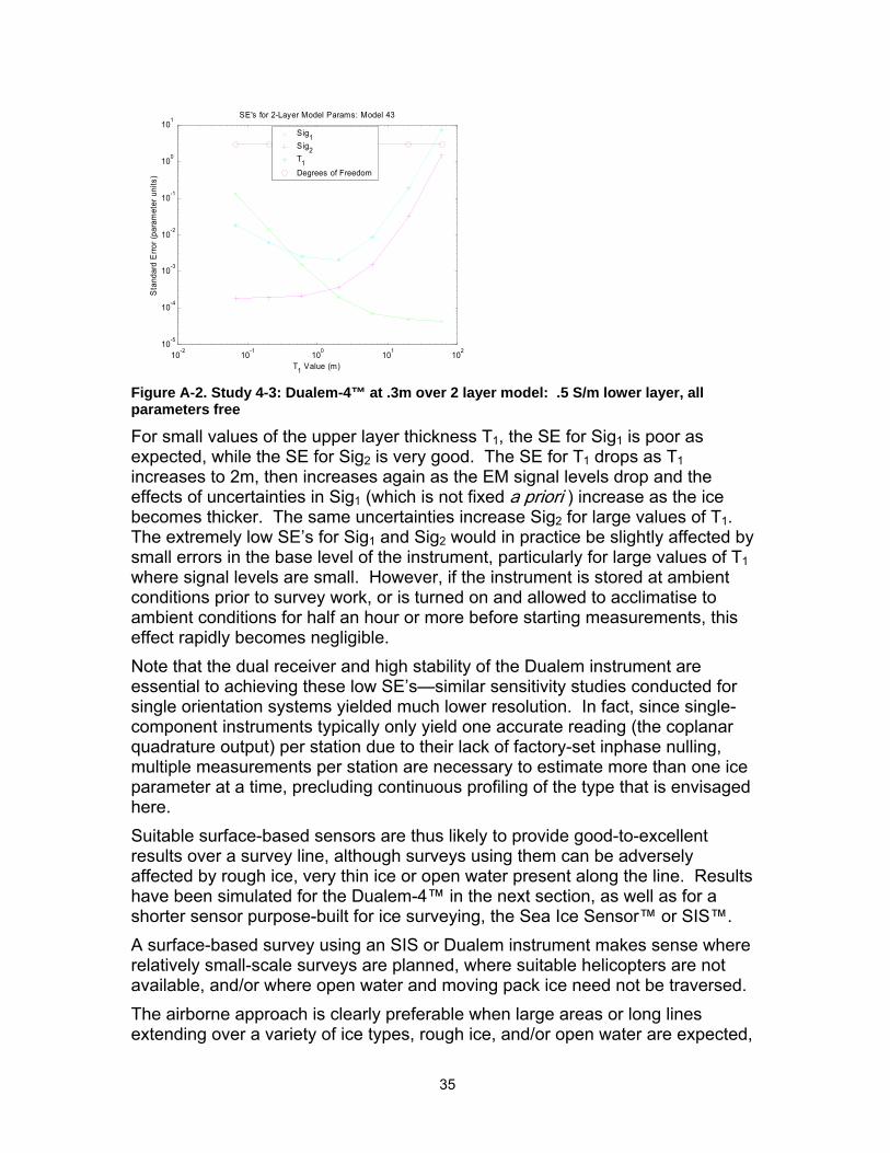
10-2 10-1 100 101 10210-5

10-4

10-3

10-2

10-1

100

101

T1 Value (m)

Sta

ndar

d E

rror (

para

met

er u

nits

)


Sig1 Sig2 T1

Degrees of Freedom

Figure A-2. Study 4-3: Dualem-4™ at .3m over 2 layer model: .5 S/m lower layer, all parameters free For small values of the upper layer thickness T1, the SE for Sig1 is poor as expected, while the SE for Sig2 is very good. The SE for T1 drops as T1 increases to 2m, then increases again as the EM signal levels drop and the effects of uncertainties in Sig1 (which is not fixed a prio i ) increase as the ice becomes thicker. The same uncertainties increase Sig

r2 for large values of T1.

The extremely low SE’s for Sig1 and Sig2 would in practice be slightly affected by small errors in the base level of the instrument, particularly for large values of T1 where signal levels are small. However, if the instrument is stored at ambient conditions prior to survey work, or is turned on and allowed to acclimatise to ambient conditions for half an hour or more before starting measurements, this effect rapidly becomes negligible. Note that the dual receiver and high stability of the Dualem instrument are essential to achieving these low SE’s—similar sensitivity studies conducted for single orientation systems yielded much lower resolution. In fact, since single-component instruments typically only yield one accurate reading (the coplanar quadrature output) per station due to their lack of factory-set inphase nulling, multiple measurements per station are necessary to estimate more than one ice parameter at a time, precluding continuous profiling of the type that is envisaged here. Suitable surface-based sensors are thus likely to provide good-to-excellent results over a survey line, although surveys using them can be adversely affected by rough ice, very thin ice or open water present along the line. Results have been simulated for the Dualem-4™ in the next section, as well as for a shorter sensor purpose-built for ice surveying, the Sea Ice Sensor™ or SIS™. A surface-based survey using an SIS or Dualem instrument makes sense where relatively small-scale surveys are planned, where suitable helicopters are not available, and/or where open water and moving pack ice need not be traversed. The airborne approach is clearly preferable when large areas or long lines extending over a variety of ice types, rough ice, and/or open water are expected,

35

or when surveys must be conducted at considerable distance from the base camp. The IcePic™ also operates at multiple frequencies, and can be used to conduct vertical soundings (not discussed here) over substantial height ranges.

Simulated Dualem-4™ and Surface Ice Sounder™ Profile Inversion The three profiles on the preceding page were constructed by using the inverted model parameters from the three-layer case as inputs to a forward modelling program for two different configurations of surface EM systems. This procedure is reasonable but not rigorous, since the frequency range and field geometry from the IcePic™ system are different from those of the ground systems. However, it should provide at least a good first-order sense of the likely performance of the surface-based systems.

100 200 300 400 500 600 700 800 900 10000

1

2

3

4

5

6

7

8

9

Time (sec)

Laye

r Par

amet

ers

File DU404079: 2 layer inversion, 2 parameters free, 10ppm noise added

Laser Sig1*100T1 Sig2

Figure A-3. Simulated Dualem-4™ profile constructed from 3 layer IcePic™ inversion results. The T1 and Sig2 estimates are essentially unaffected by the addition of 10 ppm noise.

0 100 200 300 400 500 600 700 800 900 10000

1

2

3

4

5

6

7

8

9

Time (sec)

Laye

r Par

amet

ers

File DU104079: 2 layer inversion, 2 parameters free, 10ppm noise added


Figure A-4. Simulated SIS™ (1m coil separation) profile constructed as in previous figure. The T1 and Sig2 estimates are slightly affected by the addition of 10 ppm noise.

36

0 100 200 300 400 500 600 700 800 900 10000

1

2

3

4

5

6

7

8

9

10

Time (sec)

Laye

r Par

amet

ers


Figure A-5. Simulated SIS™ (1m coil separation) as previous, but a 20 ppm base level offset has been added. The effect of this offset on the T1 and Sig2 estimates is minimal. The first example is for a Dualem-4, comprising a horizontal coplanar coil pair with a 4m coil separation augmented by a perpendicular-configuration receiver at a coil separation of 4.1m. The two coil configurations display substantially different sensitivity functions to layered conductivity structures in the ground, with the perpendicular configuration mainly sensitive from 0 to 2m beneath the sensor, while the horizontal coplanar configuration is most sensitive over a wider range, from about .2 to 6m. These complementary sensitivity distributions permit substantial improvements in the resolution of inverted parameters compared to those inverted from just one configuration. 10 ppm of noise was added to the simulated EM data for this profile, with negligible impact on the inverted parameters. The second simulation is of an SIS™ sensor, which uses the same complementary receiver configurations as the Dualem-4™, but with coil separations of 1 and 1.1m. Adding 10 ppm (about twice the nominal EM noise level for the SIS) of noise to this data generates visible additional noise in the inverted T1 estimates in the zones of largest T1. This was expected because the main source of EM response is the conductive feature represented by Sig2—where the sensor is farthest away from this feature, the EM signal is weakest and the relative size of the added EM noise strongest. The third simulation is again of an SIS™ sensor, but with an additional base level shift of 20 ppm added to all of the data. This systematic error corresponds to the upper limit of the specified stability range for this sensor. Its effect is again strongest for large T1 values, but overall it is minimal and perhaps negligible in the context of other likely errors. This result arises mainly because of the presence of the relatively conductive sediments observed as Sig2. For the much lower Sig2 values that were expected at the outset of this study, T1 errors due to this simulated base level shift would be larger.

37

Conclusions

1. Simulations of Dualem-4™ and SIS™ data, supported by parameter sensitivity analyses, suggest that surface-based electromagnetic measurements performed with these instruments can be interpreted in a similar manner to map frozen sub-ice sediments. The advantage of these systems over single-component systems such as the Geonics EM-31 is that they can acquire multiple useful data components simultaneously, permitting continuous profiling. Their inphase stability is also high enough to permit use of the inphase in data inversion, which further improves ice property resolution.

2. IcePic™ data sets, as compared to surface EM measurements, have the advantages of high coverage rates, the ability to operate far from base camps, and can easily profile over difficult ice conditions, zones of thin ice and open water. The system has been used in a variety of settings and modes ranging from detailed acquisition at very low altitude over short survey lines close to shore, to surveying long lines in an offshore environment. Surface-based measurements are well suited to surveys along shorter profiles or smaller areas, particularly where ice conditions are sufficiently smooth and thick to be passable on foot or by snow machine.

38

Appendix B Sensitivity Analysis Plots A series of sensitivity analyses were conducted to assess the resolving capabilities of the IcePic™ and Dualem-4 EM systems for variants on the “standard model”. The results are presented below. Discussions of some of these analysis plots are provided in the main body of this report.

Table 2: Sensitivity study summary

Study Number

Meas't Class

No. of Freq's

No. of Rx's

Coil Sep(s)

(m)Sensor

Height (m) Model DescriptionS1 (S/m) T1 (m) S2 (S/m) T2 (m) S3 (S/m)

1-1 Single 4 1 1.2 5 0.0001 2 0.00025 1 0.011-2 Single 4 1 1.2 5 0.0001 2 0.025 1 0.011-3 Single 4 1 1.2 5 0.0001C 2 0.025 1 0.011-4 Single 4 1 1.2 5 0.0001C 2 0.025C 1 0.011-5 Single 4 1 1.2 5 0.0001C 2 0.025 1 0.51-5 Single 4 1 1.2 5 0.0001C 2 0.025C 1 0.5

2-1 Single 4 1 1.2 5 0.0001 2 0.012-2 Single 4 1 1.2 5 0.0001C 2 0.012-3 Single 4 1 1.2 1 0.0001C 2 0.01C2-4 Single 4 1 1.2 1 0.0001C 2 0.5

3-1 Single 4 1 1.2 5 0.0001 2 2.53-2 Single 4 1 1.2 5 0.0001C 2 2.53-3 Single 4 1 1.2 5 0.0001 2 2.5C3-4 Single 4 1 1.2 1 0.0001 2 2.53-5 Single 4 1 1.2 1 0.0001C 2 2.5

4-1 Single 1 2 4, 4.1 0.3 0.0001 3 0.014-2 Single 1 2 4, 4.1 0.3 0.0001C 3 0.014-3 Single 1 2 4, 4.1 0.3 0.0001 2 0.54-4 Single 1 2 4, 4.1 0.3 0.0001 2 2.5

5-1 Multi-ht 1 2 4, 4.1 1-2.2 0.0001C 2 0.00025 1 0.015-2 Multi-ht 1 2 4, 4.1 1-2.2 0.0001 3 0.015-3 Multi-ht 1 2 4, 4.1 1-2.2 0.0001C 3 0.015-4 Multi-ht 1 2 4, 4.1 1-2.2 0.0001 2 0.55-5 Multi-ht 1 2 4, 4.1 1-2.2 0.0001 2 2.5

39

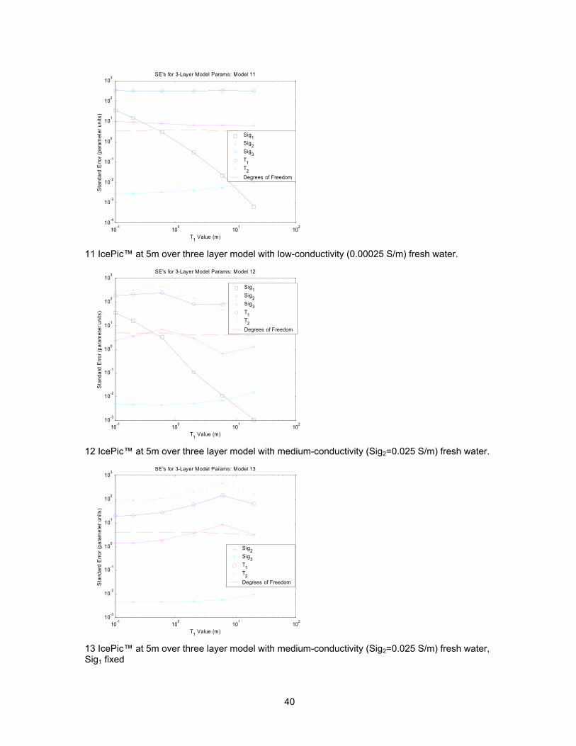
10-1 100 101 10210-4

10-3

10-2

10-1

100

101

102

103

T1 Value (m)

Sta

ndar

d E

rror (

para

met

er u

nits

)



Degrees of Freedom

11 IcePic™ at 5m over three layer model with low-conductivity (0.00025 S/m) fresh water.

10-1 100 101 10210-3

10-2

10-1

100

101

102

103

T1 Value (m)

Sta

ndar

d E

rror (

para

met

er u

nits

)



Degrees of Freedom

12 IcePic™ at 5m over three layer model with medium-conductivity (Sig2=0.025 S/m) fresh water.

10-1 100 101 10210-3

10-2

10-1

100

101

102

103

T1 Value (m)

Sta

ndar

d E

rror (

para

met

er u

nits

)


Sig2 Sig3 T1 T2

Degrees of Freedom

13 IcePic™ at 5m over three layer model with medium-conductivity (Sig2=0.025 S/m) fresh water, Sig1 fixed

40

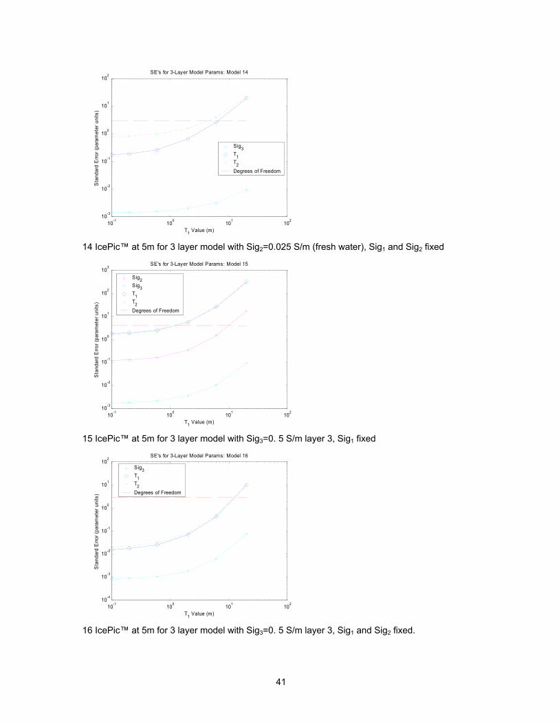
10-1 100 101 10210-3

10-2

10-1

100

101

102

T1 Value (m)

Sta

ndar

d E

rror (

para

met

er u

nits

)


Sig3 T1 T2

Degrees of Freedom

14 IcePic™ at 5m for 3 layer model with Sig2=0.025 S/m (fresh water), Sig1 and Sig2 fixed

10-1 100 101 10210-3

10-2

10-1

100

101

102

103

T1 Value (m)

Sta

ndar

d E

rror (

para

met

er u

nits

)


Sig2 Sig3 T1 T2

Degrees of Freedom

15 IcePic™ at 5m for 3 layer model with Sig3=0. 5 S/m layer 3, Sig1 fixed

10-1 100 101 10210-4

10-3

10-2

10-1

100

101

102

T1 Value (m)

Sta

ndar

d E

rror (

para

met

er u

nits

)


Sig3 T1 T2

Degrees of Freedom

16 IcePic™ at 5m for 3 layer model with Sig3=0. 5 S/m layer 3, Sig1 and Sig2 fixed.

41

10-1 100 101 10210-4

10-3

10-2

10-1

100

101

102

103

T1 Value (m)

Sta

ndar

d E

rror (

para

met

er u

nits

)SE's for 2-Layer Model Params: Model 21

Sig1 Sig2 T1

Degrees of Freedom

21 IcePic™ at 5m, 2 layer model, all parameters free

10-1 100 101 10210-4

10-3

10-2

10-1

100

101

T1 Value (m)

Sta

ndar

d E

rror (

para

met

er u

nits

)

SE's for 2-Layer Model Params, Sig1 fixed: Model 22

Sig2 T1

Degrees of Freedom

22 IcePic™at 5m, 2 layer model, T1 fixed

10-1

100

101

102

10-2

10-1

100

101

T1 Value (m)

Sta

ndar

d E

rror (

para

met

er u

nits

)


T1

Degrees of Freedom

23 IcePic™ at 5m, 2 layer model, T1 and T2 fixed

42

10-1 100 101 10210-5

10-4

10-3

10-2

10-1

100

101

T1 Value (m)

Sta

ndar

d E

rror (

para

met

er u

nits

)


Sig1 Sig2 T1

Degrees of Freedom

24. IcePic™ at 5m for 2 layer model with Sig2=0. 5 S/m, all parameters free. For a T1 value of 2m, parameter errors are on the order of 3x10-4 and 1x10-3 S/m for Sig1 and Sig2, and 6x10-3 m for T1.

10-1 100 101 10210-4

10-3

10-2

10-1

100

101

T1 Value (m)

Sta

ndar

d E

rror (

para

met

er u

nits

)


Sig1 Sig2 T1

Degrees of Freedom

31 IcePic™ at 5m, 2 layer model, fresh ice over seawater—all parameters free

10-1 100 101 10210-3

10-2

10-1

100

101

T1 Value (m)

Sta

ndar

d E

rror (

para

met

er u

nits

)


Sig2 T1

Degrees of Freedom

32 IcePic™ at 5m, 2 layer model, fresh ice over seawater—σ1 fixed

43

10-1 100 101 10210-4

10-3

10-2

10-1

100

T1 Value (m)

Sta

ndar

d E

rror (

para

met

er u

nits

)


T1

Degrees of Freedom

33 IcePic™ at 5m, 2 layer model, fresh ice over seawater— σ1 and σ2 fixed

10-1 100 101 10210-5

10-4

10-3

10-2

10-1

100

101

T1 Value (m)

Sta

ndar

d E

rror (

para

met

er u

nits

)


Sig1 Sig2 T1

Degrees of Freedom

34 IcePic™ at 1m, 2 layer model, fresh ice over seawater—all parameters free

10-1

100

101

102

10-5

10-4

10-3

10-2

10-1

100

101

T1 Value (m)

Sta

ndar

d E

rror (

para

met

er u

nits

)


Sig2 T1

Degrees of Freedom

35 IcePic™ at 1m, 2 layer model, fresh ice over seawater—σ1 fixed

44

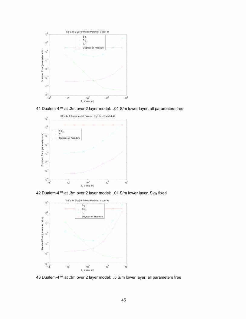
10-2 10-1 100 101 10210-5

10-4

10-3

10-2

10-1

100

101

102

T1 Value (m)

Sta

ndar

d E

rror (

para

met

er u

nits

)


Sig1 Sig2 T1

Degrees of Freedom

41 Dualem-4™ at .3m over 2 layer model: .01 S/m lower layer, all parameters free

10-2 10-1 100 101 10210-6

10-5

10-4

10-3

10-2

10-1

100

101

T1 Value (m)

Sta

ndar

d E

rror (

para

met

er u

nits

)


Sig2 T1

Degrees of Freedom

42 Dualem-4™ at .3m over 2 layer model: .01 S/m lower layer, Sig1 fixed

10-2 10-1 100 101 10210-5

10-4

10-3

10-2

10-1

100

101

T1 Value (m)

Sta

ndar

d E

rror (

para

met

er u

nits

)


Sig1 Sig2 T1

Degrees of Freedom

43 Dualem-4™ at .3m over 2 layer model: .5 S/m lower layer, all parameters free

45

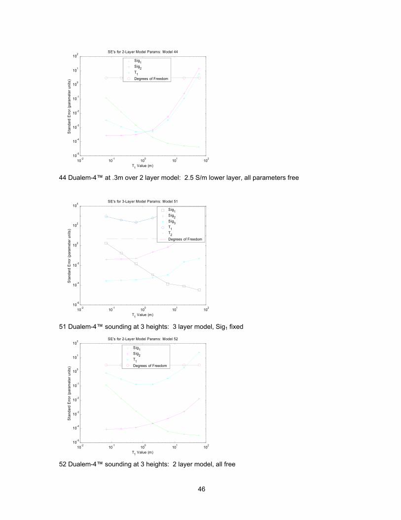
10-2 10-1 100 101 10210-5

10-4

10-3

10-2

10-1

100

101

102

T1 Value (m)

Sta

ndar

d E

rror (

para

met

er u

nits

)


Sig1 Sig2 T1

Degrees of Freedom

44 Dualem-4™ at .3m over 2 layer model: 2.5 S/m lower layer, all parameters free

10-2 10-1 100 101 10210-6

10-4

10-2

100

102

104

T1 Value (m)

Sta

ndar

d E

rror (

para

met

er u

nits

)



Degrees of Freedom

51 Dualem-4™ sounding at 3 heights: 3 layer model, Sig1 fixed

10-2 10-1 100 101 10210-5

10-4

10-3

10-2

10-1

100

101

102

T1 Value (m)

Sta

ndar

d E

rror (

para

met

er u

nits

)


Sig1 Sig2 T1

Degrees of Freedom

52 Dualem-4™ sounding at 3 heights: 2 layer model, all free

46

10-2 10-1 100 101 10210-6

10-5

10-4

10-3

10-2

10-1

100

101

T1 Value (m)

Sta

ndar

d E

rror (

para

met

er u

nits

)


Sig2 T1

Degrees of Freedom

53 Dualem-4™ sounding at 3 heights: 2 layer model, Sig1 fixed

10-2 10-1 100 101 10210-5

10-4

10-3

10-2

10-1

100

101

T1 Value (m)

Sta

ndar

d E

rror (

para

met

er u

nits

)


Sig1 Sig2 T1

Degrees of Freedom

54 Dualem-4™ sounding at 3 heights: 2 layer model, Sig2=0.5 S/m

10-2 10-1 100 101 10210-5

10-4

10-3

10-2

10-1

100

101

T1 Value (m)

Sta

ndar

d E

rror (

para

met

er u

nits

)


Sig1 Sig2 T1

Degrees of Freedom

55 Dualem-4™ sounding at 3 heights: 2 layer model, Sig2=2.5 S/m

47

application of airborne and surface-based em/laser measurements

Documents