application of artificial intelligence (artificial neural ...€¦ · thesis summary title:...
TRANSCRIPT

School of Management
Blekinge Institute of Technology
Application of Artificial Intelligence (Artificial
Neural Network) to Assess Credit Risk:
A Predictive Model For Credit Card Scoring
Authors: Md. Samsul Islam, Lin Zhou, Fei Li
Supervisor: Mr. Anders Hederstierna
Thesis for the Degree of MSc in Business Administration
Spring 2009
Abstract
Credit Decisions are extremely vital for any type of financial institution because it can
stimulate huge financial losses generated from defaulters. A number of banks use judgmental
decisions, means credit analysts go through every application separately and other banks use
credit scoring system or combination of both. Credit scoring system uses many types of
statistical models. But recently, professionals started looking for alternative algorithms that
can provide better accuracy regarding classification. Neural network can be a suitable
alternative. It is apparent from the classification outcomes of this study that neural network
gives slightly better results than discriminant analysis and logistic regression. It should be
noted that it is not possible to draw a general conclusion that neural network holds better
predictive ability than logistic regression and discriminant analysis, because this study covers
only one dataset. Moreover, it is comprehensible that a “Bad Accepted” generates much
higher costs than a “Good Rejected” and neural network acquires less amount of “Bad
Accepted” than discriminant analysis and logistic regression. So, neural network achieves
less cost of misclassification for the dataset used in this study. Furthermore, in the final
section of this study, an optimization algorithm (Genetic Algorithm) is proposed in order to
obtain better classification accuracy through the configurations of the neural network
architecture. On the contrary, it is vital to note that the success of any predictive model
largely depends on the predictor variables that are selected to use as the model inputs. But it
is important to consider some points regarding predictor variables selection, for example,
some specific variables are prohibited in some countries, variables all together should
provide the highest predictive strength and variables may be judged through statistical
analysis etc. This study also covers those concepts about input variables selection standards.

Acknowledgement
We would like to express our deepest gratitude to our supervisor Anders Hederstierna for his
patience and guidance during the thesis works.
We would also like to show our gratitude to our friends, who helped us a lot through sharing
the knowledge on the thesis topic.
At last, we would like to express many special thanks to our families, who were always there
to give us support and understanding.
Thesis Summary
Title: Application of Artificial Intelligence (Artificial Neural Network) to Assess Credit Risk:
A Predictive Model for Credit Card Scoring.
Authors: Md. Samsul Islam, Lin Zhou, Fei Li
Supervisor: Mr. Anders Hederstierna
Department: School of Management, Blekinge Institute of Technology
Course: MScBA Thesis, 15 credits.
Problem Statement: Credit Decisions are extremely vital for any type of financial institution
because it can stimulate huge financial losses provoked from defaulters. A number of banks
use judgmental decisions, means credit analysts go through every application separately and
other banks use credit scoring system or combination of both. It primarily depends on the type
of the product. In the case of small amount of credits like consumer credits (especially in
credit cards), banks try to pursue automated system (credit scoring). The system provides
decision based on the pattern recognition that is known from the previous customer’s
database. Many types of algorithms are used in credit scoring. But recently, professionals
started looking for more effective (more accurate decisions) alternatives, for example Neural
Network. But there are few guidelines on this topic and its application in credit decisions.
Purpose: The primary purpose of this study is to introduce the variables those are most
frequently used in credit card scoring systems. And the secondary purpose is to initiate the
comparison of the neural networks performance with other widely used statistical methods.
Research Method: This is a quantitative research mostly. The objective is to use extensive
credit card related data to classify characteristics of the customers, observed by the statistical
methods and neural network algorithm. All aspects of the research are carefully designed
before data collection procedure. And the analysis is targeted for the precise measurements.
Literature Review: Previous literatures are reviewed to cover up two important components.
First of all, it is attempted to come across important concepts and publication in the field of
credit scoring and to study its relatedness with neural network applications. And in the second
phase of the literature review, the prime focus is to study the predictor variables those are
most widely used in theory and real life applications, and thus to re-assess the concepts.
Findings: It is important to consider some points regarding predictor variables selection, for
example, some specific variables are prohibited in some countries, variables all together
should provide the highest predictive strength and variables may be judged through statistical
analysis etc. Moreover, it is found that neural network gives slightly better results than
discriminant analysis and logistic regression. It should be noted that it is not possible to draw
a general conclusion that neural network holds better predictive ability than logistic regression
and discriminant analysis, because this study covers only one dataset. Furthermore, it is
apparent that neural network (equals to 61) acquired less amount of “Bad Accepted” than
discriminant analysis (equals to 143) and logistic regression (equals to 140). So, neural
network obtains less cost of misclassification than discriminant analysis or logistic regression.
In addition, neural network can obtain better predictive ability if the parameters are optimized.

Table of Contents
ABSTRA CT
ACK NOWL EDG EMENT
THESI S S UMMARY
1 INTR OD UC TI ON
BACKGROUND 1
NEURA L NE TW ORK IN CRE DIT SCORIN G 1
MOTIVA TION (GROUNDS FOR TOP IC SE LECTION) 1
2 STUD Y D ESIG N
RESEA RCH OBJECTIVE 2
RESEA RCH QUESTIONS 2
TA RGE T POPU LATION 2
SA MPLE S IZE 2
RELAT IONSHIP TO BE A NA LYZE D 2
JUST IFICAT ION OF THE RE SEARCH 2
3 LITERA TUR E REVI EW ON C REDI T SC ORI NG 3
4 LITERA TUR E REVI EW ON VAR IAB LES SELECTION 6
5 DATA C OL LECTION A ND P REPA RATION
DA TA COLLECTION 9
DA TA PREPA RA TION
META DA TA PRE PA RATION 10
DA TA VA L IDATION 10
MODE L PREPA RA TION 11
6 PREDIC TI VE MOD EL S D EVEL OP MENT
DISCRIMINANT ANA LYSIS
MEA SURE MENT OF M ODE L PERFORMA NCE 12
IMPORTA NCE OF INDEPE NDENT VA RIA BLE S 12
LOG ISTIC REGRE SSION
MEA SURE MENT OF MODE L PERFORMA NCE 14
IMPORTA NCE OF INDEPE NDENT VA RIA BLE S 15
ARTIFICIA L NEU RA L NE TW ORK
NEURA L NE TW ORK STRUC TU RE (A RCHITECTU RE) 16
MEA SURE MENT OF MODE L PERFORMA NCE 17
IMPORTA NCE OF INDEPE NDENT VA RIA BLE S 17

7 COMPA RIS ON OF THE PR ED IC TI VE ABI LI TY
D i scr im i nan t A nal ys i s 18
Log i s t i c Regr ess i o n 18
Ar t i f i c i a l Neur a l Networ k 19
8 OPTI MIZATI ON OF N N P ER FOR MA NC E 20
9 MA NAGERIAL I MP LICA TI ONS 21
10 FI NDI NGS A ND C O NCL US ION 23
REFERENCES

1
Chapter 1: Introduction
Credit Scoring is another area of finance where neural network has useful applications.
Nowadays neural network is being used as a proper substitute for the existing statistical
techniques. The study will be a managerial knowledge gaps in using this type of algorithm.
1.1 Background:
Assessment of Credit Risk is very important for any type of financial institution for avoiding
huge amount of losses that may be associated with any type of inappropriate credit approval
decision (Yu, Wang et al. 2008). In the case of frequent credit decisions like thousands,
financial institution will not take any judgmental decision for every individual case manually,
but it will try to adopt the automated credit scoring system to easier and accelerate the
decision making process. So, here comes the concept of the “Credit Scoring Model”.
Credit Scoring is a method of measuring the risk incorporated with a potential customer by
analyzing his data (Lawrence and Solomon 2002). Usually, in a credit scoring system,
an applicant’s data are assessed and evaluated, like his financial status, preceding past
payments and company background to distinguish between a “good” and a “bad” applicant
(Xu, Chan et al. 1999). This is usually done by taking a sample of past customers
(Thomas, Edelman et al. 2004). Typically, credit scoring models deal with two classes of
credit, consumer loans and commercial loans (Thomas, Edelman et al. 2002). In the field of
credit risk management, many models and algorithms have been applied to support credit
scoring, including statistical, genetic algorithms and neural networks (Yu, Wang et al. 2008).
1.2 Neural Network in Credit Scoring:
Neural Network (NN) is being used in business arena for different applications. For example,
it is used in finance in bankruptcy classification, fraud detection (Smith and Gupta 2003).
Credit Scoring is another area of finance where it has useful applications (Kamruzzaman,
Begg et al. 2006). Nowadays neural network is being used as a proper substitute for the
existing statistical techniques, especially if the underlying analytic relationship between
dependent and independent variables is unknown (Yu, Wang et al. 2008). Although it is often
difficult to understand the classifications decision of neural network (Perner and Imiya 2005).
1.3 Motivation (Grounds for Topic Selection):
Classification plays a crucial role in business planning, especially in Credit Scoring. But,
conventional methods suffer from several limitations, for example, many conventional
methods assume linear relationship among the variables although there may be non-linear
relationship in reality and non-linear models like the multiple regression models require
model selection which is based on trial and error process (Leondes 2005). So, forecasting
using Neural Network can be a suitable alternative. The higher predictive ability of Neural
Network applications can be attributed to their ability of reproducing human intelligence
(Bocij, Chaffey et al. 2009) and to their powerful pattern recognition capability (Zhang 2003).
They have demonstrated effectiveness in different business applications (Smith and Gupta
2003). Unfortunately, business community has not adopted it properly because of its
mathematical nature although it is very popular in Engineering Discipline (Smith and Gupta
2003). This is the main reason of choosing NN technique for model creation. And another
main focus is to develop the model for the credit card market. Because, it is logically assumed
and expected that the predictor variables will be different in the scenario of product lines.

2
Chapter 2: Study Design
Credit Scoring follows the concept of “Pattern Recognition”. The patterns of the “Accepted
Customers” and the “Rejected Customers” are identified based on the previous applicants.
2.1 Research Objective:
The objective of the thesis is to classify and compare the predictive accuracy of the artificial
neural network algorithm with the traditional and widely used statistical models. Moreover, it
will provide the concepts and theories that should be reviewed and considered during the
selection of the predictor variables for the development of any type of credit scoring system.
2.2 Research Questions:
Which generic variables are notable for the development of a credit card scoring system?
What is the Standard Neural Network (NN) Architecture for the Model Development?
What is the predictive ability of the NN in comparison with the Statistical Techniques?
How to optimize the NN parameters using evolutionary algorithm (Genetic Algorithm)?
2.3 Target Population:
Risk factors are different in all places because of the difference in the characteristics of the
borrowing populations. So, every credit scoring model is different from each other (Caouette,
Altman et al. 1998). And it is important to map out the scope of the market covered by the
model, including geography, company size, and industry. The main target population of this
study will be the universal consumers who use different types of credit cards, and who exhibit
common (shared) characteristics in the different geographical locations or markets.
2.4 Sample Size:
A real world credit card dataset is used in this study which represents a financial institution in
the Germany. The dataset is extracted from the UCI Machine Learning Repository. There are
total 1,000 cases (applicants) in the dataset. Out of these 1,000 available customers data, 700
applicants are the “Creditworthy” and the rest 300 applicants are the “Non-creditworthy”.
2.5 Relationship to Be Analyzed:
Credit Scoring System follows the concept of “Pattern Recognition”. The patterns of the
“Accepted Customers” and the “Rejected Customers” are identified based on the data of the
previous applicants. And the identified pattern is used to predict the behavior of the future
applicants based on the input or independent variables like income, job, debt etc. The same
concept is going to be applied in this study also for the default risk prediction of applicants.
2.6 Justification of the Research:
This research intends to study the success stories of Neural Network in classification; it will
be very useful to new managers in the banking industry. The study will identify managerial
knowledge gaps in using advanced algorithm and will help to cover these gaps in readiness
for managerial roles. And at the same time, this thesis will work as guidelines for the financial
institutions that deal with credit card, and those want to develop credit scoring models.
3
Chapter 3: Literature Review on Credit Scoring
The fundamental of all types of credit scoring models are same, similar types of borrowers
will behave in a similar way and sophisticated tools are used to identify similar categories of
borrowers and thus predict future credit performance so that bank can avoid future losses.
Risk is everywhere. May be, risk components have been increased dramatically in the recent
years in comparison with the past, especially in the case of health and safety issues, it is also
true in the case of financial products, for example, credit risk (Culp 2001). And this credit risk
develops from the probability that the borrowers may be unwilling or unable to fulfill their
contractual obligations (Jorion 2000). The most important tool for the assessment of credit
risk is credit scoring and credit scoring attempts to summarize a borrower’s credit history by
using credit scoring model (Fabozzi, Davis et al. 2006). Credit scoring models are decision
support systems that take a set of predictor variables as input and provide a score as output
and creditors use these models to justify who will get credit and who will not (Jentzsch 2007).
The fundamental of all credit scoring models are same, similar types of borrowers will behave
in a similar way and sophisticated tools are used to identify similar categories of borrowers
and thus predict credit performance (Fabozzi 1999). But the meaning of credit scoring has
been changed for the last couple of years, now a days they are used to find out possible fraud,
potential bankruptcy rather than only for the justification of the creditworthiness, according to
the author an altering definition will be like “...credit scoring is the use of a numerical formula
to assign points to specific items of information to predict an outcome” (Mays 1998:25).
The prescription of credit scoring is to recognize patterns in the population based on the
similarities. Fisher (1936) introduced the concept in the statistics and Durand (1941)
identified that it might be applied to recognize good and bad loans, as cited by Thomas,
Edelman et al. (2002). Credit scoring was first used in consumer banking in the 1960 among
the finance companies, after that gradually retailers and credit card companies started using
the concept (Anderloni, Braga et al. 2006). At that moment, the tremendously increasing
number of applicants for credit cards forced the lenders to automate their credit decisions
because of the economic and manpower related reasons, ultimately these organizations found
credit scoring system more accurate than judgmental systems (default rate dropped by 50% or
more) (Thomas, Edelman et al. 2002). Moreover, according to Mays (1998) based on opinions
of several industry experts, the first one was the Montgomery Ward’s scoring system for
credit card application, and at present, mortgage industry started adopting the same theory.
And this Montgomery Ward was one of best clients of Fair Issac Company that invented the
credit score to help lenders to better analyze applicant’s creditworthiness and this company
introduced the first credit scoring model in the year of 1958 (Rosenberger and Nash 2009).
The way credit scoring works is simple theoretically. According to the author Jentzsch (2007),
the basic working procedure can be explained in the following way: the dependent variable
(Y) represents credit risk (the probability of repayment). The independent variables (predictor
variables or Xi) are used to explain the dependent variable. The list and the value of the
independent variables are extracted from the ”Application Form” generally, or sometimes
from the credit report (available in the USA especially). The list of independent variables may
be like payment history, number of accounts, types of accounts with other things. Then the
performance of a specific customer is decided based on the performance of the similar types
of customers by using credit scoring system, credit scoring system awards points on every
possible factor to calculate the probability of repayment. After adding these awarded points,
credit score comes up. Normally, the higher the achieved points, the lower the risk is.

4
Credit scoring systems use different types of models. A credit scoring model is a complicated
set of algorithms that creditors use to evaluate the creditworthiness of a specific customer
(Burrell 2007). These models give unique advantages, for example, they provide a rigorous
way of screening credit applications and save huge amount of time and cost (providing
salaries to credit analysts) (Colquitt 2007). Among the available models, four approaches are
most widely used and those are Linear Discriminant Analysis, Logistic Regression and Probit,
K-nearest Neighbor Classifier, Support Vector Machine Classifier (Servigny and Renault
2004). All of these algorithms have one similarity, all of them include parameters that are
defined by the variables and the variables can be obtained from a credit report or an
application form. The variables can be different types, for example credit history, income,
outstanding debt among others, those are explained in detail in the next chapter of this study.
On the other hand, some of these methods have severe limitations (statistical restrictions). For
example, in discriminant analysis, assumption of normality, assumption of linearity and
assumption of homogeneity of variance have to be satisfied and violation of these
assumptions may stimulate problems in the reliable estimation (Anderloni, Braga et al. 2006).
In addition to these models, new types of mathematical and statistical models have been
developed for the last couple of years to address credit risk in different perspectives, for
example, linear programming, integer programming, neural network and genetic algorithm
with others, among these models, it has been noted that neural networks are capable of
separating the classes (good and bad credit risk) in a better way (Abrahams and Zhang 2008).
For an example, Hecht-Nielson Co. developed a credit scoring system using neural network
that was able to increase the profitability by 27% by separating good credit risks and bad
credit risks in an effective way (Harston, 1990) as cited by Kamruzzaman, Begg et al. (2006).
Here is a short-summary and review of the writings related with credit scoring algorithms and
corresponding classification success as cited by (Liao and Triantaphyllou 2008). Shi et al.
(2002) utilized Multiple Criteria Linear Programming (SAS Software) to classify credit card
database into two groups (good and bad) and three groups (good, normal and bad). Ong et al.
(2005) applied Genetic Programming to classify good and bad customers. Wang et. Al (2005)
used Fuzzy Support Vector Machine (Fuzzy SVM) on the credit database, based on the
assumption that one customer can’t be absolutely good or bad. And the study also included
other algorithms like Linear Regression, Logistic Regression and BP-network. Lee et al.
(2006) employed Classification and Regression Tree (CART) and Multivariate Adaptive
Regression Splines (MARS) and identified better performance in comparison with the
Discriminant Analysis, Logistic Regression, Neural Network and Support Vector Machine.
Here, credit card dataset was used. Sexton et al. (2006) used GA-based algorithm, called
Neural Network Simultaneous Optimization Algorithm on a credit dataset. The performance
was satisfactory and the model was able to identify significant variables among the other
existing variables. In the following, there is a quick review of the authors in a tabular format:
Reference Goal Database /
Description
Data Size Preprocessing Algorithm
Ong et al. (2005) To build credit
scoring models
UCI data bases Australian credit scoring data
and German credit data
Discretization Genetic
programming
Wang et. Al
(2005)
To discriminate good
credits from bad ones
Credit card
applicants data
Three datasets. The largest
contains 1,225 applicants
with 12 variables each
Fuzzy Support
Vector Machine
Lee et al. (2006) To classify
credit applicants
Bank credit
card dataset
8,000 customers with 9 inputs
and one output
CART 4.0 and
MARS 2.0
Sexton et al.
(2006)
To classify whether
to grant a credit card
UCI credit
screening dataset
690 records with 51inputs
and 2 outputs
Genetic
Algorithm
Table 1: Summary of credit scoring related studies, cited by Liao and Triantaphyllou (2008)

5
According to the authors Blattberg, Kim, & Neslin (2008), Fahrmeir once conducted a study
with 1000 customers of a German bank. Here, the total number of cases is divided equally,
but randomly. As a result, 500 customers are taken for model construction and the rest 500
cases are kept alone for model validation. The dependent variable is “DEFAULT”, that is
coded as 0 (creditworthy) and 1 (non-creditworthy). The total number of predictor variables
are 8. Some justify the demographic characteristics of the customers, like SEX (male/female),
MARRIAGE (marital status). The other variables are used to rationalize the behaviors, like
BAD (bad account), GOOD (good account), DURATION (duration of credit in months), PAY
(payment of previous credits), PRIVATE (professional / private use) and CREDIT (line of
credit). Here, Multilayer Perceptron Algorithm is used and the total number of hidden layer is
1 that possesses two neurons. In the architectural point of view, it is an 8-2-1 Neural Network,
means 8 independent variables, 2 neurons in the hidden layer and 1 dependent variable.
Backpropagation is used to estimate the Synaptic Weights. SAS Enterprise Miner is adopted.
In another study by the authors Xu, Chan, King, & Fu (1999), Neural Network model is
constructed with multilayer perceptron algorithm and backpropagation is adopted. The total
number of samples is divided into Training Sample (40%), Testing Sample (30%) and
Validation Sample (30%). The output variable is like Good Indicator (for example, .9 if it is a
good customer) or Bad Indicator (for example, .1 if it is a bad customer). Hence, the value of
all dependent and independent variables fall into the category of 0 and 1, all are treated as
Interval Level Variables. Activation Function and Combination Function is used in the model
building. To test the predictive ability of the model, 100 cases (50 good and 50 bad) is used to
generate forecasting. The performance of the model is very brilliant. The authors of this study
expect that Artificial Neural Network Models can be a good substitute for the traditional
statistical techniques when the predictor variables require non-linear transformation.
A study carried out in the year of 1998 found that more than 60% of the largest banks of the
USA are using credit scoring models to provide loans to small businesses and among them,
only 12% have developed their own (Proprietary) models and 42% of the companies using
these models to make automatic credit approval or rejection decisions (Frame, Srinivasan, and
Woosley, 2001) as cited by Acs and Audretsch (2003). Credit scoring models require huge
amount of past data of customers to make a scoring system and small companies (financial
institutions) don’t have that database to make a proprietary model. These credit scoring
models are becoming popular day by day. Moreover, although there is a rising trend of using
different types of credit scoring models to classify good and bad customers, these models are
not without limitations. One of the most important limitations is that credit scoring models
take decision based on the data those are used for "Extended Loan", so it suffers from the
"Selection Bias" (Greenbaum and Thakor 2007). According to the same author, to avoid the
selection bias, the best way is to include those samples that are accepted rather than only
including the rejected samples. Another criticism of credit scoring models is that it doesn’t
take into account the changing behavior of borrowers. The borrower’s behavior is changing
from time to time. Moreover, the nature of the relationship among the variables might change
with the progression of the time and new types of variables can come into existence that may
be proved useful for better prediction accuracy (Jentzsch 2007). So, the author recommended
to re-estimate the models classification accuracy from time to time, and to re-adjust if needed.
Although credit scoring is a good choice for automating the decision process, but not every
lender can use it. First of all, credit scoring system has high fixed costs (technological
equipments and data), that must be justified by the volume, and second of all, it can be used
only for very standardized loan products like credit cards (Sawyers, Schydlowsky et al. 2000).
6
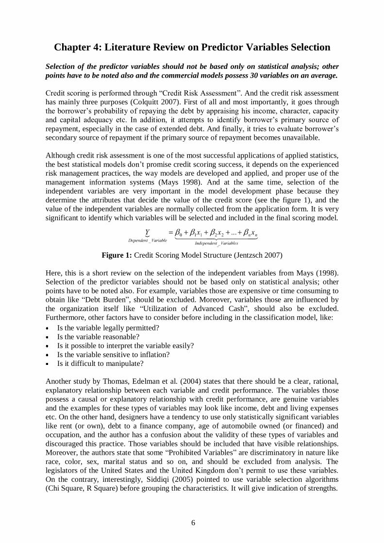
Chapter 4: Literature Review on Predictor Variables Selection
Selection of the predictor variables should not be based only on statistical analysis; other
points have to be noted also and the commercial models possess 30 variables on an average.
Credit scoring is performed through “Credit Risk Assessment”. And the credit risk assessment
has mainly three purposes (Colquitt 2007). First of all and most importantly, it goes through
the borrower’s probability of repaying the debt by appraising his income, character, capacity
and capital adequacy etc. In addition, it attempts to identify borrower’s primary source of
repayment, especially in the case of extended debt. And finally, it tries to evaluate borrower’s
secondary source of repayment if the primary source of repayment becomes unavailable.
Although credit risk assessment is one of the most successful applications of applied statistics,
the best statistical models don’t promise credit scoring success, it depends on the experienced
risk management practices, the way models are developed and applied, and proper use of the
management information systems (Mays 1998). And at the same time, selection of the
independent variables are very important in the model development phase because they
determine the attributes that decide the value of the credit score (see the figure 1), and the
value of the independent variables are normally collected from the application form. It is very
significant to identify which variables will be selected and included in the final scoring model.
Figure 1: Credit Scoring Model Structure (Jentzsch 2007)
Here, this is a short review on the selection of the independent variables from Mays (1998).
Selection of the predictor variables should not be based only on statistical analysis; other
points have to be noted also. For example, variables those are expensive or time consuming to
obtain like “Debt Burden”, should be excluded. Moreover, variables those are influenced by
the organization itself like “Utilization of Advanced Cash”, should also be excluded.
Furthermore, other factors have to consider before including in the classification model, like:
Is the variable legally permitted?
Is the variable reasonable?
Is it possible to interpret the variable easily?
Is the variable sensitive to inflation?
Is it difficult to manipulate?
Another study by Thomas, Edelman et al. (2004) states that there should be a clear, rational,
explanatory relationship between each variable and credit performance. The variables those
possess a causal or explanatory relationship with credit performance, are genuine variables
and the examples for these types of variables may look like income, debt and living expenses
etc. On the other hand, designers have a tendency to use only statistically significant variables
like rent (or own), debt to a finance company, age of automobile owned (or financed) and
occupation, and the author has a confusion about the validity of these types of variables and
discouraged this practice. Those variables should be included that have visible relationships.
Moreover, the authors state that some “Prohibited Variables” are discriminatory in nature like
race, color, sex, marital status and so on, and should be excluded from analysis. The
legislators of the United States and the United Kingdom don’t permit to use these variables.
On the contrary, interestingly, Siddiqi (2005) pointed to use variable selection algorithms
(Chi Square, R Square) before grouping the characteristics. It will give indication of strengths.

7
The study of Jentzsch (2007) reviews some important considerations regarding the selection
of the explanatory variables. The author briefs that commercial models possess 30 variables
on an average and those models are good at estimating the probability of debt repayment.
Additionally, some specific variables are prohibited in some countries, as presented in the
table 2. Here, in the table, “0” signifies “No Legal Restriction” and “1” represents “Legal
Restrictions”. So, it differs from country to country which variables are restricted. For an
example, age is allowed in the European countries, but it is not authorized in the USA unless
credit scoring models assign a positive value. Similarly, gender is allowed in the European
countries but it is not permitted in the USA. On the other hand, credit behavior of Americans
differ from the behavior of the Australians and there is more credit information available in
the USA than European countries. So, credit scoring models differ from each other critically.
Table 2: Prohibited variables in the countries (Jentzsch 2007)
Abrahams and Zhang (2009) drew attention to the importance of the “Sequence” of the
independent variables selection. The authors report that credit scoring models handle 6 to 12
independent variables. In the initialization process of the variables selection, the variable
which is enjoying the “Highest Predictive Strength”, should be chosen first. The next variable
has to be chosen in such a way that it will give the “Highest Predictive Strength” in
combination with the first one, but may not be strong enough on its own. Among the
remaining variables, for an example, debt ratio is highly related with the projection of the
credit risk, so it can be chosen in the third place. The next possible candidate can be the
“Number of Years at the Present Address”, it can provide very good forecasting of credit risk
in combination with other included variables. But it’s a weaker variable on its own; it means
that a person can change his residential address for a number of reasons like promotion,
movement to a better place where universities are available etc. So, this variable can be a
measure of the stability, but financial capacity is a better measure of the ability of repayment.
The authors Fabozzi, Davis et al. (2006) attempted to summarize the variables that have been
found very helpful for the prediction of the future credit performance based on a large sample
of customers, are the number of late payments of loans within a specified time period, the
amount of time credit has been established, the amount of credit used compared to the amount
of credit available, the length of time at the current residence, the employment history and
bankruptcy, charge-offs and collections. On the other hand, Anderloni, Braga et al.(2006)
focused on statistical analysis to select the best set of variables in predicting the credit
performance. Statistical analysis will also help to identify the weights for each chosen variable
in comparison with the credit performance. According to the authors some variables may have
relationship with default risk, for example, applicant’s monthly income, financial assets,
outstanding debts, net cash flow of the firm, whether the applicant has defaulted on a previous
loan, whether the applicant owns or rents a home are all important variables for consideration.

8
Thomas, Edelman et al. (2002) grounded some principles for variables selection. The practical
concepts of credit scoring stress to include all the variables related with applicant or
applicant’s environment that will aid in predicting the default risk. Some attributes offer
information about the stability of the applicant (for example, time at present address, time at
present employment), some characteristics present information about the financial capacity of
the applicant (for example, having a current or checking account, having credit cards, time
with current bank), some variables provide information about the applicant’s resources (for
example, residential status, employment status, spouse’s employment) and the rest of the
variables offer information on the possible outgoings (for example, number of children,
number of dependents). Moreover, it is illegal to use some characteristics like race, religion
and gender etc. Furthermore, there are some specific types of variables those are not illegal
but culturally unacceptable (for example, poor health records or lots of driving convictions).
And sometimes, creditors look for insurance protection against the credit card debts during the
change of the employment status (suppose, unemployment). So, all variables are subjective.
Table 3: Reasons for data collection (Thomas, Edelman et al. 2002)
Beares, Beck et al. (2001) stated that judgmental system and scoring system use best subset of
variables to identify default risk. There are 5 categories of variables those are used usually:
Character: It attempts to identify the applicant whether she is really willinging to repay
the loan or not. Lots of factors have to be considered to recognize the character like
understanding the applicant’s job stability and residential stability, credit history and
personal characteristics. Character is the most important factor but it is hard to measure.
Capacity: It measures the applicant’s financial capability to repay the money according to
the agreement. That’s why, lenders assess the applicant’s income statement, dividend and
other types of incomes. Applicant’s regular expenses are also considered in measurement.
Capital: It measures the net value of the applicant’s assets. Actually, the lenders want to
recognize the backup capacity if unfavorable situation develops. Capital is usually
assessed in the case of huge consumer loans, for example, boats and airplanes etc.
Collateral: Collateral is the asset that the applicant pledges to the financial institution. If
the primary source of repayment fails, then the collateral will work as a secondary source
of repayment. It means, the lender can repossess the collateral and can sell it in the market.
Condition (General Economic Conditions): It focuses on the macro-economic
conditions that can impact the applicant’s ability to repay the loan. Actually, it assesses
the applicant’s job type and the nature of the firm where the applicant is doing the job.

9
Chapter 5: Data Collection and Preparation
The dataset contains 1,000 cases, 700 applicants are considered as “Creditworthy” and the
rest 300 applicants are treated as “Non-creditworthy”. Data preparation allows identifying
unusual cases, invalid cases, erroneous variables and the incorrect data values in dataset.
5.1 Data Collection:
A real world credit card dataset is used in this study. The dataset is extracted from the UCI
Machine Learning Repository1 (http://archive.ics.uci.edu/ml/). The name of the Financial
Institution is ignored in the repository for protecting the sensitive customer data. The dataset
is referred as “German Credit Dataset” in the database. After preparing or cleaning the
dataset, it is used in the subsequent sections for conducting the analysis with Logistic
Regression, Discriminant Analysis, and Neural Network. Data description is given in next.
Data Set
Characteristics: Multivariate
Number of
Instances: 1000 Area: Financial
Attribute
Characteristics:
Categorical, Integer
Number of
Attributes: 20
Associated
Tasks: Classification
Table 4: Summary of the German Credit Card Dataset (Hofmann 1994)
No. Variable Type Scale Description
1 Case_ID Case Identifier Nominal Case ID
2 Attribute_1 Input Variable Nominal Status of Existing Checking A/C
3 Attribute_2 Input Variable Scale Duration in Month
4 Attribute_3 Input Variable Nominal Credit History
5 Attribute_4 Input Variable Nominal Credit Purpose
6 Attribute_5 Input Variable Scale Credit Amount
7 Attibute_6 Input Variable Nominal Savings Account/Bonds
8 Attribute_7 Input Variable Nominal Present Employment Since
9 Attribute_8 Input Variable Scale Installment Rate in...
10 Attribute_9 Input Variable Nominal Personal Status and Sex
11 Attribute_10 Input Variable Nominal Other Debtors / Guarantors
12 Attribute_11 Input Variable Scale Present Residence Since
13 Attribute_12 Input Variable Nominal Property
14 Attribute_13 Input Variable Scale Age in Years
15 Attribute_14 Input Variable Nominal Other Installment Plans
16 Attribute_15 Input Variable Nominal Housing
17 Attribute_16 Input Variable Scale Number of Existing Credits ...
18 Attribute_17 Input Variable Nominal Job
19 Attribute_18 Input Variable Scale Number of People Being...
20 Attribute_19 Input Variable Nominal Telephone
21 Attribute_20 Input Variable Nominal Foreign Worker
22 Creditworthiness Output Variable Nominal Status of the Credit Applicant
Table 5: German Credit Card Dataset’s Description
1 The UCI Machine Learning Repository is a collection of databases. It is widely used by researchers. It has
been cited over 1000 times, making it one of the top 100 most cited "papers" in all of computer science.
10
The dataset contains 1,000 cases, 700 applicants are considered as “Creditworthy” and the
rest 300 applicants are treated as “Non-creditworthy”. The dataset holds 22 variables
altogether. Among the variables, 14 variables are “Categorical” and the rest 7 variables are
“Numerical”. Moreover, there are 20 independent variables (input variables) and 1 dependent
variable (output variable) in the dataset. Furthermore, one more variable is added later on to
be used as a “Case Identifier Variable” in the further analysis in the subsequent parts of study.
5.2 Data Preparation2:
Data preparation is important before developing any predictive model. Data preparation
allows identifying unusual cases, invalid cases, erroneous variables and the incorrect data
values in the dataset. If the data is prepared properly, the models will be able to give better
results because of the cleaned data and at the same time, right models will be created that
represent the right scenarios. Here, in this study, data preparation is accomplished in three
modules. All these modules are interconnected with each other and each module represents a
separate and distinct process, and it starts from basic level (data review) to outlier analysis.
5.2.1 Metadata Preparation:
Metadata is all about data of the data. Here, in this module, all variables are reviewed couple
of times to identify their valid values, appropriate levels and correct data measurement scales.
For example, the variable “Creditworthiness” can only intake value either 1 (Good or
Accepted Customer) or 2 (Bad or Rejected Customer), but it can’t obtain any other values
like 3 or 4 or something else. Moreover, the variable is suitable for “Nominal Level Data
Measurement Scale”, but not appropriate for assigning ordinal level (rank or order or
sequence) or scale level (continuous). Furthermore, the label (description) of the variable
should include only the final outcome or status of the applicant, but not any other explanation.
On the other hand, to comply with these rules, especially for the data values, data validation
rules are defined in this stage. The rules are constructed for each nominal variable separately
because nominal level variables are easier to check for out of range values in active dataset.
5.2.2 Data Validation:
In this stage of data preparation, three basic checks are defined by the SPSS Software for all
of the categorical variables (nominal level variables) only, because it is easier to check for
basic rule violations by these types of variables where there are specific categories (groups). If
any of the basic checks is violated, the SPSS output will notify it. The first basic check is that
any of the categorical variables can’t possess more than 70% missing values. The second
basic check is that the maximum amount of cases in a single category should not be more than
95%. The third basic check is that the maximum amount of categories with count of one (1)
should not be more than 90%. Moreover, it is also prepared to check for “Incomplete ID” and
“Duplicate ID” in the dataset. Incomplete ID means that any of the cases is missing one or
more value(s) for the variables. Duplicate ID means that two cases are same in the all related
values, that is unlikely to be true. Furthermore, the software is instructed to check for
validation rule violations, for example, the variable “Creditworthiness” can only intake value
either 1or 2, but it can’t obtain any other values rather than the specified two categories.
According to the SPSS generated output, three basic checks and validation rules are passed by
all the cases and data values in the active dataset. Moreover, three new indicator variables are
created that provide information about incomplete ID and duplicate ID. And all the variables
are showing 0 (not 1) as the values, means that there is no incomplete ID and duplicate ID.
2 For analyzing and writing the data preparation section, SPSS manual “Data Preparation 17.0” is used.

11
5.2.3 Model Preparation:
Identification of the outliers is very important before the construction of the predictive
models, especially for the statistical models. Anomaly detection procedure can be used to
discover the unusual cases (outliers). This algorithm attempts to find out unusual cases based
on their deviations from the cluster groups (each group contains similar types of cases). A
case is considered to be an outlier if its anomaly index value is more than a cut-off point.
Here, the cut-off point is assumed to be 2. According to the following table, there is no outlier
in the active dataset. Moreover, it is showing that the indicator variables created by the
previous module of data validation, are excluded from the anomaly checking procedure. Now,
the checked dataset is prepared for the predictive models construction and further analysis.
Table 6: SPSS Output: Anomaly Checking Results
12
Chapter 6: Predictive Models Development
After development of any type of predictive model, the most important and appropriate task
is to check the usefulness (utility) of the model. Some independent variables are
significantly related with the dependent variable and others are not associated strongly.
6.1 Discriminant Analysis3:
Discriminant analysis is a statistical technique to classify the target population (in this study,
credit card applicants) into the specific categories or groups (here, either creditworthy
applicant or non-creditworthy applicant) based on the certain attributes (predictor variables or
independent variables) (Plewa and Friedlob 1995). Discriminant analysis requires fulfilling
definite assumptions, for example, assumption of normality, assumption of linearity,
assumption of homoscedasticity, absence of multicollinearity and outlier, but this method is
fairly robust to the violation of these assumptions (Meyers, Gamst et al. 2005). Here, in this
study, it is assumed that all required assumptions are fulfilled to use the predictive power of
the discriminant analysis for classification of the applicants. At this point, “creditworthiness”
is the dependent variable (or, grouping variable) and the rest 20 variables are the independent
variables (or, input variables). Here, the output of the discriminant analysis is reported below.
6.1.1 Measurement of Model Performance:
It is important to be aware of the usefulness of a discriminant model through classification
accuracy which compares the predicted group membership (calculated by the discriminant
model) to the known (actual) group membership. A discriminant model is identified as
“Useful” if there is at least 25% more improvement achievable over the by chance accuracy
rate alone. “By Chance Accuracy” means that if there is no relationship between the
dependent variable and the independent variables, it is still possible to achieve some
percentage of correct group membership. Here, “By Chance Accuracy Rate” is 58% and 25%
increase of this value equals to 72%, and the cross validated accuracy rate is 75%. Hence,
cross validated accuracy rate is greater than or equal to the proportional by chance accuracy
rate, it is possible to declare that the discriminant model is useful for the classification goal.
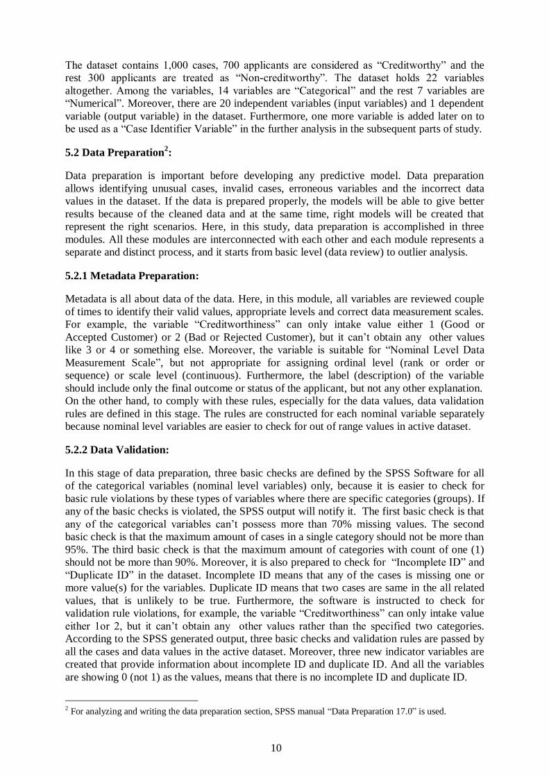
Moreover, Wilks' lambda is a measure of the usefulness of the model. The smaller
significance value indicates that the discriminant function does better than chance at
separating the groups. Here, Wilks' lambda test has a probability of <0.001 which is less than
the level of significance of .05, means that predictors significantly discriminate the groups.
Table 7: SPSS Output: Model Test Checking Usefulness of the Derived Model
6.1.2 Importance of Independent Variables:
One of the most important tasks is to identify the independent variables that are important in
the predictive model development. It can be identified from the “Structure Matrix”. Based on
the structure matrix, the predictor variables strongly associated with the discriminant model,
are the “Status of Existing Checking A/C”, “Credit History”, “Duration in Month” and
“Saving Accounts/Bonds”. These variables possess the loadings of .30 or higher in the model.
3 The tutorials of A. James Schwab is followed, he is a faculty member of the The University of Texas at Austin.
13
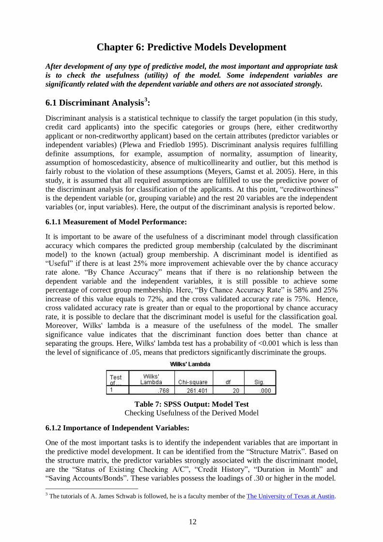
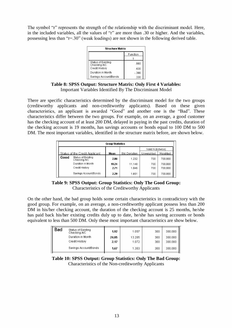
The symbol “r” represents the strength of the relationship with the discriminant model. Here,
in the included variables, all the values of “r” are more than .30 or higher. And the variables,
possessing less than “r=.30” (weak loadings) are not shown in the following derived table.
Table 8: SPSS Output: Structure Matrix: Only First 4 Variables:
Important Variables Identified By The Discriminant Model
There are specific characteristics determined by the discriminant model for the two groups
(creditworthy applicants and non-creditworthy applicants). Based on these given
characteristics, an applicant is awarded “Good” and another one is the “Bad”. These
characteristics differ between the two groups. For example, on an average, a good customer
has the checking account of at least 200 DM, delayed in paying in the past credits, duration of
the checking account is 19 months, has savings accounts or bonds equal to 100 DM to 500
DM. The most important variables, identified in the structure matrix before, are shown below.
Table 9: SPSS Output: Group Statistics: Only The Good Group:
Characteristics of the Creditworthy Applicants
On the other hand, the bad group holds some certain characteristics in contradictory with the
good group. For example, on an average, a non-creditworthy applicant possess less than 200
DM in his/her checking account, the duration of the checking account is 25 months, he/she
has paid back his/her existing credits duly up to date, he/she has saving accounts or bonds
equivalent to less than 500 DM. Only these most important characteristics are show below.
Table 10: SPSS Output: Group Statistics: Only The Bad Group:
Characteristics of the Non-creditworthy Applicants
14
6.2 Logistic Regression4:
Logistic Regression is the most important tool in the social science research for the
categorical data (binary outcome) analysis and it is also becoming very popular in the
business applications, for example, credit scoring (Agresti 2002). The algorithm assumes that
a customer’s default probability is a function of the variables (income, marital status and
others) related with the default behavior (Blattberg, Kim et al. 2008). Logistic regression is
now widely used in credit scoring and more often than discriminant analysis because of the
improvement of the statistical software’s for logistic regression (Greenacre and Blasius 2006).
Moreover, logistic regression is based on an estimation algorithm that requires less
assumptions (assumption of normality, assumption of linearity, assumption of homogeneity of
variance) than discriminant analysis (Jentzsch 2007). This study is not performing those.
6.2.1 Measurement of Model Performance:
After the predictive model development, the most important task is to check the usefulness
(utility) of the model. It can be accomplished in two ways. First one is the significance test.
The significance test for the model chi-square is the statistical evidence of the presence of a
relationship between the dependent variable and the combination of the independent variables.
In this analysis, the probability of the model chi-square (259.936) is <0.001, less than or equal
to the level of significance of .05. The null hypothesis that there is no difference between the
model with only a constant and the model with independent variables is rejected. The
existence of a relationship between the independent variables and the dependent variable is
supported. So, usefulness of the model is confirmed. The table 11 is referred for the test.
Table 11: SPSS Output: Model Test:
Checking Usefulness of the Derived Model
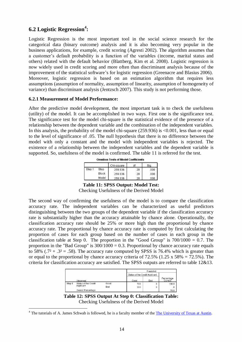
The second way of confirming the usefulness of the model is to compare the classification
accuracy rate. The independent variables can be characterized as useful predictors
distinguishing between the two groups of the dependent variable if the classification accuracy
rate is substantially higher than the accuracy attainable by chance alone. Operationally, the
classification accuracy rate should be 25% or more high than the proportional by chance
accuracy rate. The proportional by chance accuracy rate is computed by first calculating the
proportion of cases for each group based on the number of cases in each group in the
classification table at Step 0. The proportion in the "Good Group" is 700/1000 = 0.7. The
proportion in the "Bad Group" is 300/1000 = 0.3. Proportional by chance accuracy rate equals
to 58% (.7² + .3² = .58). The accuracy rate computed by SPSS is 76.4% which is greater than
or equal to the proportional by chance accuracy criteria of 72.5% (1.25 x 58% = 72.5%). The
criteria for classification accuracy are satisfied. The SPSS outputs are referred to table 12&13.
Table 12: SPSS Output At Step 0: Classification Table: Checking Usefulness of the Derived Model
4 The tutorials of A. James Schwab is followed, he is a faculty member of the The University of Texas at Austin.
15
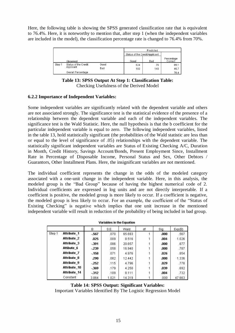
Here, the following table is showing the SPSS generated classification rate that is equivalent
to 76.4%. Here, it is noteworthy to mention that, after step 1 (when the independent variables
are included in the model), the classification percentage rate is changed to 76.4% from 70%.
Table 13: SPSS Output At Step 1: Classification Table: Checking Usefulness of the Derived Model
6.2.2 Importance of Independent Variables:
Some independent variables are significantly related with the dependent variable and others
are not associated strongly. The significance test is the statistical evidence of the presence of a
relationship between the dependent variable and each of the independent variables. The
significance test is the Wald Statistic. Here, the null hypothesis is that the b coefficient for the
particular independent variable is equal to zero. The following independent variables, listed
in the table 13, hold statistically significant (the probabilities of the Wald statistic are less than
or equal to the level of significance of .05) relationships with the dependent variable. The
statistically significant independent variables are Status of Existing Checking A/C, Duration
in Month, Credit History, Savings Account/Bonds, Present Employment Since, Installment
Rate in Percentage of Disposable Income, Personal Status and Sex, Other Debtors /
Guarantors, Other Installment Plans. Here, the insignificant variables are not mentioned.
The individual coefficient represents the change in the odds of the modeled category
associated with a one-unit change in the independent variable. Here, in this analysis, the
modeled group is the “Bad Group” because of having the highest numerical code of 2.
Individual coefficients are expressed in log units and are not directly interpretable. If a
coefficient is positive, the modeled group is more likely to occur. If a coefficient is negative,
the modeled group is less likely to occur. For an example, the coefficient of the “Status of
Existing Checking” is negative which implies that one unit increase in the mentioned
independent variable will result in reduction of the probability of being included in bad group.
Table 14: SPSS Output: Significant Variables:
Important Variables Identified By The Logistic Regression Model

16
6.3 Artificial Neural Network5:
A neural network is an advanced type of traditional regression model and calculates weights
(here, score points) for the independent variables from the previous cases of creditworthy and
non-creditworthy applicants (Mays 2001). The network is constructed with three layers: input
layer, hidden layer and output layer; each node in the input layer represents one independent
variable and brings the value in the network, the nodes in the hidden layer combines and
transforms the values in such a way to match with the target variables in the output layer, and
each node in the output layer represents one dependent variable (Xu, Chan et al. 1999). There
are some disadvantages of the neural network. Most importantly, the internal structure of the
neural network is hidden and it is very difficult to duplicate even using the same input
variables (Saunders and Allen 2002); and it doesn’t explore the direction of the variables used.
6.3.1 Neural Network Structure (Architecture):
Here, neural network model is constructed with the multilayer perceptron algorithm. In the
architectural point of view, it is a 20-10-1 neural network, means that there are total 20
independent variables, 10 neurons in the hidden layer and 1 dependent (output) variable.
SPSS software is used. SPSS procedure can choose the best architecture automatically and it
builds the network with one hidden layer. It is also possible to specify the minimum (by
default 1) and maximum (by default 50) number of units allowed in the hidden layer, and the
automatic architecture selection procedure finds out the “best” number of units (10 units are
selected for this analysis) in the hidden layer. Automatic architecture selection uses the default
activation functions for the hidden layer (Hyperbolic Tangent) and output layers (softmax).
Predictor variables consist of “Factors” and “Covariates”. Factors are the categorical
dependent variables (13 nominal variables) and the covariates are the scale dependent
variables (7 continuous variables). Moreover, standardized method is chosen for the rescaling
of the scale dependent variables to improve the network training. Further, 70% of the data is
allocated for the training (training sample) of the network and to obtain a model; and 30% is
assigned as testing sample to keep tracks of the errors and to protect the from the overtraining.
Different types of training methods are available like batch, online and minibatch. Here, batch
training is chosen because it directly minimizes the total error and it is most useful for
“smaller” datasets. Moreover, Optimization algorithm is used to estimate the synaptic weights
and “Scaled Conjugate Gradient” optimization algorithm is assigned because of the selection
of the batch training method. Batch training method supports only this algorithm.
Additionally, stopping rules are used to determine the stopping criteria for the network
training. According to the rule definitions, a step corresponds to an iteration for the batch
training method. Here, one (1) maximum step is allowed if the error is not decreased further.
Here, it is important to note that, to replicate (repeat) the neural network results exactly, data
analyzer needs to use the same initialization value for the random number generator, the same
data order, and the same variable order, in addition to using the same procedure settings.
5 For analyzing and writing the Neural Network section, SPSS manual “SPSS Neural Network 16.0” is used.

17
6.3.2 Measurement of Model Performance:
The following model summary table displays information about the results of the neural
network training. Here, cross entropy error is displayed because the output layer uses the
softmax activation function. This is the error function that the network tries to minimize
during training. Moreover, the percentage of incorrect prediction is equivalent to 16.1% in the
training samples. So, percentage of correct prediction is nearer to 83.9%, that is quite high.
If any dependent variable has scale measurement level, then the average overall relative error
(relative to the mean model) is displayed. On the other hand, if the defined dependent
variables are categorical, then the average percentage of incorrect predictions is displayed.
Table 15: SPSS Output: Model Summary: Checking Usefulness of the Derived Model
6.3.3 Importance of Independent Variables:
The following table performs an analysis, which computes the importance and the normalized
importance of each predictor in determining the neural network. The analysis is based on the
training and testing samples. The importance of an independent variable is a measure of how
much the network’s model-predicted value changes for different values of the independent
variable. Moreover, the normalized importance is simply the importance values divided by the
largest importance values and expressed as percentages. From the following table, it is evident
that “Foreign Worker” contributes most in the neural network model construction, followed
by “Credit Amount”, “Age in Years”, “Duration in Month”, “Credit History”, “Housing” etc.
Table 16: SPSS Output: Independent Variable Importance:
Only The Nine Most Important Variables:
Important Variables Identified By The Neural Network Model
The above mentioned variables have the greatest impact on how the network classifies the
prospective applicants. But it is not possible to identify the direction of the relationship
between these variables and the predicted probability of default. This is one of the most
prominent limitations of the neural network. So, statistical models will help in this situation.

18
Chapter 7: Comparison of the Model’s Predictive Ability
Models can be compared and evaluated based on the classification accuracy of each of the
group of the dependent variable and it is also important to justify the overall accuracy rate.
7.1 Discriminant Analysis:
In the discriminant analysis model development phase, a statistically significant model is
derived which possess a very good classification accuracy capability. In the following table, it
is shown that the discriminant model is able to classify 621 good applicants as “Good Group”
out of 700 good applicants. Thus, it holds 88.7% classification accuracy for the good group.
On the other hand, the same discriminant model is able to classify 143 bad applicants as “Bad
Group” out of 300 bad applicants. Thus, it holds 47.67% classification accuracy for the bad
group. Thus, the model is able to generate 76.4% classification accuracy in combined groups.
Table 17: SPSS Output: Classification Results:
Predictive Ability of the Discriminant Model
7.2 Logistic Regression:
In the logistic regression analysis model development stage, a statistically significant model is
derived which enjoys a very good classification accuracy capability. In the following table, it
is shown that the logistic model is able to classify 624 good applicants as “Good Group” out
of 700 good applicants. Thus, it holds 89.1% classification accuracy for the good group. On
the other hand, the same logistic model is able to classify 140 bad applicants as “Bad Group”
out of 300 bad applicants. Thus, it holds 46.7% classification accuracy for the bad group.
Thus, the model is able to generate 76.4% classification accuracy for the both groups.
Table 18: SPSS Output: Classification Results:
Predictive Ability of the Logistic Model

19
7.2 Artificial Neural Network:
In the artificial neural network model development stage, a predictive model is derived which
enjoys a very good classification accuracy capability. In the following table, it is shown that
the neural network model is able to classify 422 good applicants as “Good Group” out of 473
good applicants. Thus, it holds 89.2% classification accuracy for the good group. On the other
hand, the same neural network model is able to classify 160 bad applicants as “Bad Group”
out of 221 bad applicants. Thus, it holds 72.4% classification accuracy for the bad group.
Thus, the model is able to generate 83.86% classification accuracy for the both groups. Here,
the training sample is taken into account, because statistical models don’t use testing sample.
Table 19: SPSS Output: Classification Results:
Predictive Ability of the Artificial Neural Network

20
Chapter 8:
Optimization of Neural Network Performance
&
Future Research Scope
Genetic Algorithm can be used as an optimization method for improving NN performance.
There are two main issues about the performance of the neural network. First of all, it is
important to determine its structure and secondly, it is also vital to specify the weights of the
neural network that help to minimize the total errors (Deb, Poli et al. 2004). These are
optimization issues. Evolutionary algorithm (genetic algorithm) is a kind of optimization
technique that uses selection and recombination as the main instruments to deal with
optimization problems (Kamruzzaman, Begg et al. 2009). For example, genetic algorithm is
the main available method that can be used to find well suited network architecture for a given
task or problem (Patel, Honavar et al. 2001). According to the genetic algorithm theory, all
combinations of the parameters of the possible solutions of a given problem (in this analysis,
all the possible combinations of the parameters of the neural network architecture) must be
coded into a gene and by a process of the selection of the fittest (in this case, the best neural
network architecture that provides better classification) only the best solutions are selected for
the reproduction, and after each subsequent generation, new solutions (only selected if they
provide better classification accuracy) are generated by means of the reproduction between
solutions and their related mutations (Mira, Cabestany et al. 2009).
Genetic algorithm is especially suitable for complex optimization problems. Many researchers
tried to optimize the weights of the neural network using genetic algorithm alone (or, with
backpropagation algorithm) and others attempted to find out a good network architecture or
structure (the number of units and their interconnections) (Deb, Poli et al. 2004). Instruments
or tools used by the genetic algorithm are selection, crossover and mutation (Larose, 2006).
Selection indicates the technique of selecting chromosomes that will be used for reproduction.
The fitness function appraises each of the chromosome (candidate solutions), and the better
(fitter) the chromosome, the more probability that it will be selected for the reproduction
purpose. The central task of crossover is to perform recombination, means that the creation of
the two new offspring by randomly choosing a locus and exchanging subsequences to the left
and right of that locus between two chromosomes chosen during the selection process.
Mutation randomly modifies the bits or digits at a particular locus in a chromosome, most of
the time with very low likelihood. Mutation brings new information to the genetic pool and
protects against finding too quickly to a local optimum. The concepts are from Larose (2006).
There are some unique benefits of using Genetic Algorithm as searching and optimization
technique. For example, it is efficient, adaptive, and robust search technique, that is capable of
generating optimal (or, near optimal) solutions (Pal and Wang 1996). For these characteristics
and advantages, genetic algorithms applications in pattern recognition problems (which
require robust, fast and close appropriate solutions) are perfect and almost natural.
Although this study is to provide an overview of application of the neural network in the
classification of the credit card customers, its scope of coverage is limited by the selection and
comparison of the statistical models with neural network model. Future research efforts can
certainly go beyond this limitation in order to have a more comprehensive review of genetic
algorithm related literatures and to use the same dataset for the optimization of the network.

21
Chapter 9: Managerial Implications
It requires careful considerations to develop decision support systems for credits approvals.
Credit scoring models are decision support systems that help managers to assess a potential
customer to accept or reject his application. But it requires careful considerations to develop
and use these types of decision support systems. Anderson (2007) reviews some important
factors regarding the practical development and implementation of the credit scoring systems.
The following is a review of author’s suggestions, summarized with the views of this study:
9.1 Project Preparation:
The first part of project preparation is the “Goal Definition”. It consists of customer
characteristics (whether they require personalized services or high speed decisions),
competitor analysis (what is the current practice of the competitors) and legislation (whether
law permits automated decision support systems or not). The second part of project
preparation is the “Feasibility Study” that judges the limitations of the organization like data
(availability of sufficient data), resources (availability of the people and money) and
technology (availability of the technology to support the proposed decision support system).
9.2 Data Preparation:
Data preparation and sample design is very important. The first factor regarding data
preparation is the “Project Scope” that defines the representative cases or similar types of
cases. “Good / Bad Definition” provides the output variable (what the model is trying to
predict) and will describe the expected behavior (there is no missing payment or no repetition
of exceeding the credit limit). “Sample Window” describes the period that will be used to
draw the sample and it should not be too old or too recent to reflect the current business
scenario. It is required to have minimum 1,500 goods and 1,500 bads “Sample Size”, but
sometimes it is difficult to collect sufficient amount of bads as those are rare and fewer cases
will result in over-fitting. “Matching” refers the indicators that are used to match the data that
are collect from different sources like application processing system, account management
system or credit bureau etc. Matching key can be used to match the customer data, it can be
internal (customer number) or it can be national (personal number) or it can be date of birth
etc. And data preparation must provide the “Training and Validation Data”. Training sample
is used to create the model and the validation sample is used to test the model ultimately.
9.3 Predictive Model Development (Scorecard Modeling):
The subsequent step is the development of a predictive model. The first step of model
development is the choosing of the “Modeling Technique” that depends on lots of factors, for
example, decision tree is a good selection if there is missing data, linear regression is good for
continuous output variable, binary logistic regression is the best choice if there is binary
outcome or binary dependent variable. Moreover, the chosen model should be transparent.
Another important task is to select the “Predictor Variables”. Some developers try to select
only those variables that have relationships with the output variable only, not with each other,
in order to minimize multicollinearity problem. This can be achieved by using factor analysis
and even, it is possible to use the factors in the model development purpose. Fair Issac
company’s Fico Score shows that most important predictor variable is the payment history
(35%), followed by amounts owed (30%), length of credit history (15%) (Jentzsch, 2007).

22
Credit scoring models should include similar types of cases, and those cases may have
dissimilarities for other scoring models. So, segmentation in the dataset is possible. After
deciding the segmentation, training is started. Training is completed with either a parametric
model (Discriminant Analysis or Logistic Regression) or a non-parametric model (NN).
9.4 Finalization:
After completion of the model training, finalization stage starts. “Validation” refers that the
model works well with the targeted population, it is accomplished by the validation sample
and it is also achieved by comparing the model’s predictive ability with other external credit
scoring models. “Calibration” refers that the scores calculated by the different models have
the same meaning, and it is achieved by making a range of the scores of the different models.
Setting a “Cut-off Point” for credit decisions is strategically important. The strategy is chosen
in such a way that the business policy of profit making is not hampered/ overlooked.
It is important to load the credit scoring model into the intended system. In the modern days,
credit scoring models are uploaded in the parameterized system to fine tune the settings
according to the necessity of the strategies of the company. Once the system is uploaded, it is
time to verify it to ensure that it is working according to plan, especially in the case of
automatic calculations. Loading and testing can be done in a separately designed environment.
9.5 Decision Making and Strategy:
Once the model is developed, it is important to make decisions about how the model will be
implemented. The first important factor is the “Level of Automation”, refers the degree of
automation the lender requires. Automation requires fixed cost and variable cost per
application assessment. So, this is a trade-off decision for the lender. But most of the times,
high volume lenders try to automate everything from data acquisition and score calculation to
decision delivery, that is already initiated by some financial institutions, especially for the
credit cards. Whenever any organization goes for significant changes, it is necessary to apply
“Change Management Strategies” to improve its acceptance by informing staffs about the
desired level of changes. Moreover, it is important to initiate “New Policies” regarding
product rule (which determines the eligibility of the applicant for the particular product),
credit rule (which determines the factors that are not mentioned in the credit scoring model)
and the fraud-prevention rule (which determines the conditions that require verification).
9.6 Security:
It is vital to ensure the security of the developed credit scoring model from the internal and
external threats. The first part of the security is the “Documentation” of the derived model.
Every credit scoring model is developed based on lots of assumptions and decisions in the
development stage. And it is required to document those assumptions and decisions,
especially the project scope and objectives, sample design, scoring modeling and strategies.
The second part of security is the “Confidentiality”. Credit scoring models require lots of
investments in the infrastructure and organization should try to make confidentiality
agreements with the staffs, contractors and consultants to protect the proprietary information
from the possible industrial espionage. Information is valuable to competitors and fraudsters.
Appropriate authority level should be declared for each staff of the organization to maintain
proper access to the documentation of the processes and strategies. And highly sensitive and
printed documentations should be kept strictly confidential by managing the key and the lock.

23
Chapter 10: Findings and Conclusion
Appropriate predictor variables selection is one of the conditions for successful credit scoring
models development. This study reviews several considerations regarding the selection of the
predictor variables. Moreover, using the Multilayer Perceptron Algorithm of Neural Network,
network architecture is constructed for predicting the probability that a given customer will
default on a loan. The model results are comparable to those obtained using commonly used
techniques like Logistic Regression or Discriminant Analysis, as described in the following:
German Credit Card Dataset
Models Good
Accepted
Good
Rejected
Bad
Accepted
Bad
Rejected
Success
Rate
Discriminant Analysis 621 79 157 143 76.4%
Logistic Regression 624 76 160 140 76.4%
Neural Network 422 51 61 160 83.86%
Table 20: Predictive Models Comparison
There are two noteworthy and interesting points about this table. First of all, it shows the
predictive ability of each model. Here, the column 2 and 5 (“Good Accepted” and “Bad
Rejected”) are the applicants that are classified correctly. Moreover, the column 3 and 4
(“Good Rejected” and “Bad Accepted”) are the applicants that are classified incorrectly.
Furthermore, it shows that neural network gives slightly better results than discriminant
analysis and logistic regression. It should be noted that it is not possible to draw a general
conclusion that neural network holds better predictive ability than logistic regression and
discriminant analysis, because this study covers only one dataset. On the other hand, statistical
models can be used to further explore the nature of the relationship between the dependent
and each independent variable, and statistical models are preferred than neural network if
there is tiny difference in predictive ability of the neural network and the statistical models.
Secondly, the above provided table gives an idea about the cost of misclassification. In order
to introduce the costs of misclassification it is assumed that a “Bad Accepted” generates much
higher costs than a “Good Rejected”, because there is a chance to lose the whole amount of
credit while accepting a “Bad” and only losing the interest payments while rejecting a “Good”
(Schader, Gaul et al. 2009). Here, in this analysis, it is apparent that neural network (equals to
61) acquired less amount of “Bad Accepted” than discriminant analysis (equals to 143) and
logistic regression (equals to 140). So, neural network achieves less cost of misclassification.
In the above table, statistical models contain the same number of cases for the model
construction, but the NN holds less number of cases because a portion of the cases is kept for
the “Testing Sample” to prevent the network from overtraining/ over-fitting. Furthermore,
statistical models don’t use anything like testing samples. So, the classification results are
slightly incomparable because of the uneven number of cases used in all models. After
re-running the analysis, without any testing sample in the NN, with the equal number of
sample sizes in all the models, it is found that "Bad Accepted" is decreased further to 27 from
61. Because, neural network over trained itself. Moreover, overall percentage correct is
increased to 96% from 83.86%. So, for the German dataset, NN is giving good results always.
In the final section, Genetic Algorithm is proposed to obtain better classification accuracy
through the configurations of the neural network architecture and weights. Moreover, it is
suggested as future research scope that the same dataset can be used for neural network
performance improvement and the results can be compared with before optimization results.

24
References
ABRAHAMS, C. R. & ZHANG, M. (2008) Fair Lending Compliance: Intelligence and Implications for
Credit Risk Management, Wiley. ABRAHAMS, C. R. & ZHANG, M. (2009) Credit Risk Assessment: The New Lending System for
Borrowers, Lenders, and Investors, Wiley. ACS, Z. J. & AUDRETSCH, D. B. (2003) Handbook of Entrepreneurship Research: An Interdisciplinary
Survey and Introduction, Springer. AGRESTI, A. (2002) Categorical Data Analysis, Wiley-Interscience. ANDERLONI, L., BRAGA, M. D. & CARLUCCIO, E. M. (2006) New Frontiers in Banking Services:
Emerging Needs and Tailored Products for Untapped Markets, Springer. ANDERSON, R. (2007) The Credit Scoring Toolkit: Theory and Practice for Retail Credit Risk
Management and Decision Automation, Oxford University Press. BEARES, P. R., BECK, R. E. & SIEGEL, S. M. (2001) Consumer Lending, American Bankers Association. BLATTBERG, R. C., KIM, B.-D. & NESLIN, S. A. (2008) Database Marketing: Analyzing and Managing
Customers, Springer. BOCIJ, P., CHAFFEY, D., GREASLEY, A. & HICKIE, S. (2009) Business Information Systems: Technology,
Development & Management for the E-business, FT Press. BURRELL, J. (2007) How to Repair Your Credit Score Now: Simple No Cost Methods You Can Put to
Use Today, Atlantic Publishing Company. CAOUETTE, J. B., ALTMAN, E. I. & NARAYANAN, P. (1998) Managing Credit Risk: The Next Great
Financial Challenge, Wiley. COLQUITT, J. (2007) Credit Risk Management, McGraw-Hill. CULP, C. L. (2001) The Risk Management Process: Business Strategy and Tactics, Wiley. DEB, K., POLI, R., BANZHAF, W., BEYER, H.-G., BURKE, E., DARWEN, P., DASGUPTA, D., FLOREANO, D.,
FOSTER, J., HARMAN, M., HOLLAND, O., LANZI, P. L., SPECTOR, L., TETTAMANZI, A. & THIERENS, D. (2004) Genetic and Evolutionary Computation - GECCO 2004, Springer.
FABOZZI, F. J. (1999) Subprime Consumer Lending, Wiley. FABOZZI, F. J., DAVIS, H. A. & CHOUDHRY, M. (2006) Introduction to Structured Finance, Wiley. GREENACRE, M. & BLASIUS, J. (2006) Multiple Correspondence Analysis and Related Methods,
Chapman & Hall/CRC. GREENBAUM, S. I. & THAKOR, A. V. (2007) Contemporary Financial Intermediation, Academic Press. HOFMANN, D. H. (1994) Statlog (German Credit Data) Data Set. UCI Machine Learning Repository.

25
JENTZSCH, N. (2007) Financial Privacy: An International Comparison of Credit Reporting Systems (Contributions to Economics), Springer.
JORION, P. (2000) Value at Risk: The New Benchmark for Managing Financial Risk, McGraw-Hill. KAMRUZZAMAN, J., BEGG, R. K. & SARKER, R. A. (2006) Artificial Neural Networks in Finance and
Manufacturing, Idea Group Publishing. LAROSE, D. T. (2006) Data Mining Methods and Models, Wiley-IEEE Press. LAWRENCE, D. & SOLOMON, A. (2002) Managing a Consumer Lending Business, Solomon Lawrence
Partners. LEONDES, C. T. (2005) Intelligent Knowledge-Based Systems: Business and Technology in the New
Millennium, Kluwer Academic Publishers. LIAO, T. W. & TRIANTAPHYLLOU, E. (2008) Recent Advances In Data Mining Of Enterprise Data:
Algorithms and Applications, World Scientific Publishing Company. MAYS, E. (1998) Credit Risk Modeling: Design and Application, CRC. MAYS, E. (2001) Handbook of Credit Scoring, Global Professional Publishing. MEYERS, L. S., GAMST, G. C. & GUARINO, A. J. (2005) Applied Multivariate Research: Design and
Interpretation, Sage Publications. MIRA, J., CABESTANY, J. & PRIETO, A. (2009) New Trends in Neural Computation, Springer. PAL, S. K. & WANG, P. P. (1996) Genetic Algorithms for Pattern Recognition, CRC-Press. PATEL, M., HONAVAR, V. & BALAKRISHNAN, K. (2001) Advances in the Evolutionary Synthesis
of Intelligent Agents, The MIT Press. PERNER, P. & IMIYA, A. (2005) Machine Learning and Data Mining in Pattern Recognition, Springer. PLEWA, F. J. & FRIEDLOB, G. T. (1995) Understanding Cash Flow, Wiley. POLIT, D. F. (1996) Data Analysis and Statistics for Nursing Research, Prentice Hall. ROSENBERGER, L. E., NASH, J & Graham A. (2009) The Deciding Factor: The Power of Analytics to
Make Every Decision a Winner, Jossey-Bass. SAUNDERS, A. & ALLEN, L. (2002) Credit Risk Measurement: New Approaches to Value at Risk
and Other Paradigms, Wiley. SAWYERS, L., SCHYDLOWSKY, D. & NICKERSON, D. (2000) Emerging Financial Markets in the Global
Economy, World Scientific Publishing Company. SERVIGNY, A. D. & RENAULT, O. (2004) The Standard & Poor's Guide to Measuring and Managing
Credit Risk, McGraw-Hill. SIDDIQI, N. (2005) Credit Risk Scorecards: Developing and Implementing Intelligent Credit Scoring,
Wiley.

26
SMITH, K. A. & GUPTA, J. N. D. (2003) Neural Networks in Business: Techniques and Applications, Irm
Press. THOMAS, EDELMAN, D. & CROOK, J. (2002) Credit Scoring & Its Applications, Society for Industrial
Mathematics. THOMAS, L. C., EDELMAN, D. B. & CROOK, J. N. (2004) Readings in Credit Scoring: Foundations,
Developments, and Aims, Oxford University Press. XU, L., CHAN, L.-W., KING, I. & FU, A. (1999) Intelligent Data Engineering and Learning (IDEAL 98):
Perspectives on Financial Engineering and Data Mining, Springer. YU, L., WANG, S., LAI, K. K. & ZHOU, L. (2008) Bio-Inspired Credit Risk Analysis: Computational
Intelligence with Support Vector Machines, Springer. ZHANG, G. P. (2003) Neural Networks in Business Forecasting, Information Science Publishing.