July 2012

NASA/CR-2012-217588 NIA Report No. 2012-04

Application of Benchmark Examples to Assess the Single and Mixed-Mode Static Delamination Propagation Capabilities in ANSYS® Ronald Krueger National Institute of Aerospace, Hampton, Virginia

NASA STI Program . . . in Profile

Since its founding, NASA has been dedicated to the advancement of aeronautics and space science. The NASA scientific and technical information (STI) program plays a key part in helping NASA maintain this important role.

The NASA STI program operates under the auspices of the Agency Chief Information Officer. It collects, organizes, provides for archiving, and disseminates NASA’s STI. The NASA STI program provides access to the NASA Aeronautics and Space Database and its public interface, the NASA Technical Report Server, thus providing one of the largest collections of aeronautical and space science STI in the world. Results are published in both non-NASA channels and by NASA in the NASA STI Report Series, which includes the following report types:

TECHNICAL PUBLICATION. Reports of

completed research or a major significant phase of research that present the results of NASA Programs and include extensive data or theoretical analysis. Includes compilations of significant scientific and technical data and information deemed to be of continuing reference value. NASA counterpart of peer-reviewed formal professional papers, but having less stringent limitations on manuscript length and extent of graphic presentations.

TECHNICAL MEMORANDUM. Scientific

and technical findings that are preliminary or of specialized interest, e.g., quick release reports, working papers, and bibliographies that contain minimal annotation. Does not contain extensive analysis.

CONTRACTOR REPORT. Scientific and

technical findings by NASA-sponsored contractors and grantees.

CONFERENCE PUBLICATION.

Collected papers from scientific and technical conferences, symposia, seminars, or other meetings sponsored or co-sponsored by NASA.

SPECIAL PUBLICATION. Scientific, technical, or historical information from NASA programs, projects, and missions, often concerned with subjects having substantial public interest.

TECHNICAL TRANSLATION. English-language translations of foreign scientific and technical material pertinent to NASA’s mission.

Specialized services also include organizing and publishing research results, distributing specialized research announcements and feeds, providing information desk and personal search support, and enabling data exchange services. For more information about the NASA STI program, see the following: Access the NASA STI program home page

at http://www.sti.nasa.gov

E-mail your question to help@sti.nasa.gov

Fax your question to the NASA STI Information Desk at 443-757-5803

Phone the NASA STI Information Desk at 443-757-5802

Write to: STI Information Desk NASA Center for AeroSpace Information 7115 Standard Drive Hanover, MD 21076-1320

National Aeronautics and Space Administration Langley Research Center Prepared for Langley Research Center Hampton, Virginia 23681-2199 under Contract NNL09AA00A

July 2012

NASA/CR-2012-217588 NIA Report No. 2012-04

Application of Benchmark Examples to Assess the Single and Mixd-Mode Static Delamination Propagation Capabilities in ANSYS® Ronald Krueger National Institute of Aerospace, Hampton, Virginia

Available from:

NASA Center for AeroSpace Information 7115 Standard Drive

Hanover, MD 21076-1320 443-757-5802

Trade names and trademarks are used in this report for identification only. Their usage does not constitute an official endorsement, either expressed or implied, by the National Aeronautics and Space Administration.

APPLICATION OF BENCHMARK EXAMPLES TO ASSESS THE SINGLE AND MIXED-MODE STATIC DELAMINATION PROPAGATION CAPABILITIES IN ANSYS

Ronald Krueger*

ABSTRACT

The application of benchmark examples for the assessment of quasi-static delamination propagation capabilities is demonstrated for ANSYS®. The examples are independent of the analysis software used and allow the assessment of the automated delamination propagation in commercial finite element codes based on the virtual crack closure technique (VCCT). The examples selected are based on two-dimensional finite element models of Double Cantilever Beam (DCB), End-Notched Flexure (ENF), Mixed-Mode Bending (MMB) and Single Leg Bending (SLB) specimens. First, the quasi-static benchmark examples were recreated for each specimen using the current implementation of VCCT in ANSYS®. Second, the delamination was allowed to propagate under quasi-static loading from its initial location using the automated procedure implemented in the finite element software. Third, the load-displacement relationship from a propagation analysis and the benchmark results were compared, and good agreement could be achieved by selecting the appropriate input parameters. The benchmarking procedure proved valuable by highlighting the issues associated with choosing the input parameters of the particular implementation. Overall the results are encouraging, but further assessment for three-dimensional solid models is required.

1. INTRODUCTION

Over the past two decades, the use of fracture mechanics has become common practice to characterize the onset and growth of delaminations. In order to predict delamination onset or growth, the calculated strain energy release rate components are compared to interlaminar fracture toughness properties measured over a range from pure mode I loading to pure mode II loading.

The virtual crack closure technique (VCCT) is widely used for computing energy release rates based on results from continuum (2D) and solid (3D) finite element (FE) analyses. The virtual crack closure technique is also useful for its ability to calculate the mode separation required when using the mixed-mode fracture criterion [1, 2]. The virtual crack closure technique was recently implemented into several commercial finite element codes. As new methods for analyzing composite delamination are incorporated into finite element codes, the need for comparison and benchmarking becomes important since each code requires specific input parameters unique to its implementation. These parameters are unique to the numerical approach chosen and do not reflect real physical differences in delamination behavior.

An approach for assessing the mode I, and mixed-mode I and II, delamination propagation capabilities in commercial finite element codes under static loading was recently presented and demonstrated for the VCCT implementation in Abaqus/Standard®1 [3-5] as well as MD Nastran™ and Marc™2 [6]. First, benchmark results were created manually for finite element models of the *R. Krueger, National Institute of Aerospace, 100 Exploration Way, Hampton, VA, 23666, resident at Durability, Damage Tolerance and Reliability Branch, MS 188E, NASA Langley Research Center, Hampton, VA, 23681, USA. 1 Abaqus/Standard® is a product of Dassault Systèmes Simulia Corp. (DSS), Providence, RI, USA 2 MD Nastran™ and Marc™ are manufactured by MSC.Software Corp., Santa Ana, CA, USA. NASTRAN® is a registered trademark of NASA.

1

mode I Double Cantilever Beam (DCB), the mode II End Notched Flexure (ENF) as well as the mixed-mode I/II Single Leg Bending (SLB) and Mixed-Mode Bending (MMB) specimens. Second, the delamination was allowed to propagate under quasi-static loading from its initial location using the automated procedure implemented in the finite element software. The approach was then extended to allow the assessment of the delamination fatigue growth prediction capabilities in commercial finite element codes [4,7]. As for the static case, benchmark results were created manually first for the mode I Double Cantilever Beam (DCB) and the mode II End Notched Flexure (ENF) specimen. Second, the delamination was allowed to grow under cyclic loading in a finite element model of a commercial code. For all cases, input control parameters were varied to study the effect on the computed delamination propagation and growth. The benchmarking procedure proved valuable by highlighting the issues associated with choosing the input parameters of the particular implementation. Consequently, the benchmark enabled the selection of the appropriate input parameters that yielded good agreement between the results obtained from the growth analysis and the benchmark results. Once the parameters have been identified, they may then be used with confidence to model delamination growth for more complex configurations.

The objective of the present study was to apply existing benchmark examples and assess the quasi-static delamination propagation capabilities in ANSYS®1. To recreate the benchmark results in ANSYS®, existing two-dimensional finite element models were used for simulating the DCB, ENF, SLB and MMB specimens with different delamination lengths a0. For each of the specimens and for each of the delamination lengths modeled, the load and the displacement were monitored. The total strain energy release rate, GT, and mixed-mode ratio, GII/GT, were calculated for a fixed applied displacement. It is assumed that the delamination propagates when the computed energy release rate, GT, reaches the mixed-mode fracture toughness Gc. Thus, critical loads and critical displacements for delamination onset were calculated for each delamination length modeled. From these critical load/displacement results, benchmark solutions were created for each of the specimens. It is assumed that the load/displacement relationship computed during automatic propagation should closely match the benchmark solution.

These benchmark solutions were used to assess the automated delamination propagation capability implemented in ANSYS®. Starting from an existing front, the delamination was allowed to propagate under quasi-static loading based on the algorithms implemented into the software. Input control parameters were varied to study the effect on the computed delamination propagation. Comparison of these results to the benchmark enabled the selection of the appropriate input parameters that yielded good agreement between the results obtained from the propagation analysis and the benchmark results. Once the parameters have been identified, they may then be used with confidence to model delamination growth for more complex configurations.

In this paper, the development of the benchmark cases for the assessment of the quasi-static delamination propagation prediction capabilities is presented for the DCB, ENF, SLB and MMB specimens. Examples of automated propagation analyses are shown, and the selection of the required code specific input parameters are discussed.

2. SPECIMEN CONFIGURATIONS SELECTED AS BENCHMARK CASES For the current numerical investigation, several simple specimens used for fracture toughness

testing were selected. These specimens had been used previously to develop the current approach for assessment of the quasi-static delamination propagation simulation capabilities in commercial 1 ANSYS® is a product of ANSYS, Inc., Canonsburg, PA, USA

2

finite element codes [3-5,7]. The Double Cantilever Beam (DCB) specimen, as shown in Figure 1, was chosen since it only exhibits the mode I opening fracture mode. Besides the previously developed benchmark case of the DCB specimen [3], an additional example was used for which experimental data also exist for comparison. This example was published by NAFEMS - an independent not-for-profit body with the sole aim of promoting the effective use of engineering simulation methods - as part of their benchmark cases [8]. The three-point End-Notched Flexure (ENF) specimen, as shown in Figure 2, was chosen since it only exhibits the mode II sliding fracture mode. Two specimens that exhibit the mixed-mode I/II fracture were selected: The Single Leg Bending (SLB), as shown in Figure 3, which exhibits a mixed-mode fracture at nearly constant 40% mode II and the Mixed-Mode Bending (MMB) specimen, as shown in Figure 4, which was studied for 20%, 50% and 80% mode II. The material and overall specimen dimensions including initial crack length, a0, are shown in the respective figures. All configurations had layups of [0]24. The material properties are given in Tables I through III. A methodology for delamination propagation, onset and growth was applied to the specimens to create the benchmark examples [9, 10]. 3. METHODOLOGY BASED ON FRACTURE MECHANICS

A quasi-static mixed-mode fracture criterion is discussed first, since the parameters are required input to the VCCT implementation in ANSYS®. The input details are discussed in the appendix. The mixed-mode fracture criterion for a material is determined by plotting the interlaminar fracture toughness, Gc, versus the mixed-mode ratio, GII/GT, as shown in Figure 5 for a typical carbon/epoxy material (C12K/R6376). The fracture criterion is generated experimentally using pure Mode I (GII/GT=0) Double Cantilever Beam (DCB) tests (as shown in Figure 1), pure Mode II (GII/GT=1) End-Notched Flexure (ENF) tests (as shown in Figure 2), and Mixed Mode Bending (MMB) tests (as shown in Figure 4), of varying ratios of GI and GII. For one material used in this study (C12K/R6376), the mean values (filled blue circles) are shown in Figure 5. A 2D fracture criterion was suggested by Benzeggah and Kenane [11] using a simple mathematical relationship between Gc and GII/GT

!!  = !!"  + !!!" − !!"  !!!!!

!

                                                                                                               (1)

In this expression, typically called the B-K criterion, GIc and GIIc are the experimentally determined fracture toughness data for mode I and II as shown in Figure 5. The exponent !  was determined by a curve fit using the Levenberg-Marquardt algorithm in the KaleidaGraphTM graphing and data analysis software [12]. The parameters GIc, GIIc and ! are required input to perform a VCCT analysis in ANSYS®, as discussed in the appendix.

During an automated propagation analysis, the total strain energy release rate, GT, and the mixed-mode ratio GII/GT are computed using VCCT. The failure index, GT/Gc, is calculated by correlating the computed total energy release rate, GT, with the mixed-mode fracture toughness, Gc, of the graphite/epoxy material. As shown in equation (1) the mixed-mode fracture toughness, Gc, is a function of the mixed-mode ratio GII/GT (see also Figure 5). It is assumed that the delamination propagates when the failure index, GT/Gc, reaches unity.

3

4. PROCEDURE FOR DEVELOPING QUASI-STATIC BENCHMARK CASES Based on the approach developed earlier [3], quasi-static benchmark results can be created for

any analysis software used. The procedure is outlined using the load/displacement plots for a DCB specimen, as an example.

• First, finite element models of the specimen with different delamination lengths, a0, have to be created

• For each delamination length, a0, modeled, the load, P, and opening displacement, δ/2, at the load point are plotted as shown in Figure 6 (colored lines)

• For each delamination length, a0, modeled, the total energy release rate, GT, and the mixed-mode ratio, GII/GT, component are calculated. The total energy release rate is a function of the delamination length, a0, and the applied opening displacement, δ/2, as indicated in Figure 6, thus GT= GT (a0, δ/2). For the simple case of the mode I DCB specimen shown, the mixed-mode ratio is zero (GII /GT =0).

• For each delamination length, a0, modeled, a failure index, GT/Gc, is calculated by correlating the computed total energy release rate, GT, with the mixed-mode fracture toughness, Gc, of the material. For the simple case of the DCB specimen shown, the failure index is simply calculated as GI /GIc. It is assumed that the delamination propagates when the failure index reaches unity.

• Therefore, the critical load, Pcrit, and critical opening displacement, δcrit /2 can be calculated - for each delamination length, a0, modeled - based on the relationship between load, P, and the energy release rate, G [13],

! =!!

2 ∙!!!!"                                                                                                                                  (2)

 In equation (2), CP is the compliance of the specimen, and ∂A is the increase in surface area corresponding to an incremental increase in load or displacement at fracture. The critical load, Pcrit, and critical opening displacement, δcrit /2 can be calculated for each delamination length, a0, modeled

!!!!

=!!

!!"#$!  ⇒  !!"#$ = !!!!!;    !!"#$/2 = !/2

!!!!                                                          (3)

and the results can be included in the load/displacement plots as shown in Figure 7 (solid red circles).

• By fitting a curve through these critical load/displacement results (solid red circles), a benchmark solution (solid red line) can be created as shown in Figure 7.

During the automated propagation analysis, the computed load/displacements results are expected to follow the benchmark solution.

5. FINITE ELEMENT MODELING 5.1 Model description

Two-dimensional finite element models of the specimens are shown in Figures 8 through 12. All models were translated from existing Abaqus/Standard® input files (.inp) using a translation

4

utility in ANSYS® [14]. Details are discussed in the appendix. The specimens were modeled with plane strain elements (PLANE182) in ANSYS® 13.0 beta and 14.0 beta. Along the length, all models were divided into different sections with different mesh refinement as shown in Figures 8 through 12. A typical finite element model of a DCB specimen is shown in Figure 8. The DCB specimen was modeled with six elements through the specimen thickness (2h) as shown in the detail of Figure 8b. The resulting element length at the delamination tip was Δa=0.5 mm. A finer mesh, resulting in Δa=0.25 mm, was also generated, as shown in Figure 8c. Additionally, two coarser meshes with a reduced number of elements in the length direction were also generated, resulting in Δa=1.0 mm (Figure 8d) and Δa=2.0 mm (Figures 9a, b). Further, a mesh with variable length, Δa, was generated to study the effect of non-uniform element length along the propagation path as shown in Figures 9c and d.

For all models, the plane of delamination was modeled as a discrete discontinuity in the center of the specimen. For the analysis with ANSYS® 13.0 beta and 14.0 beta, the models were created as separate meshes for the upper and lower part of the specimens with identical nodal point coordinates in the plane of delamination. For the analyses where only the energy release rate was calculated for each delamination length, contact was used to define the intact section of the specimen. For the analyses where automated propagation into the intact section was activated, this intact section was modeled with interface elements and contact elements were used to prevent penetration after debonding as discussed in detail in the appendix.

A deformed model of the mode II ENF specimen is shown in Figure 10. The ENF specimen was modeled with six elements through the specimen thickness as discussed earlier. A model of the mixed-mode SLB specimen is shown in Figure 11. For convenience, a model of SLB a specimen from a previous study [3] was used here. The SLB model had ten elements through the specimen thickness. Two plies on each side of the delamination were modeled individually using one element for each ply as shown in the detail of Figure 11b. The remaining plies in each arm were modeled with three elements through the specimen thickness. To model the test correctly, only the upper arm was supported in the analysis as shown in Figure 11a.

Examples of two-dimensional finite element models of MMB specimens with boundary conditions are shown in Figure 12. Along the length, all models were divided into different sections with different mesh refinement as discussed earlier. The MMB specimen was also modeled with six elements through the specimen thickness. The resulting element length at the delamination tip was Δa=0.5 mm. The load apparatus was modeled explicitly using rigid beam elements (MPC184) as shown in Figure 12. Multi-point constraints were used to connect the rigid elements with the planar model of the specimen and enforce the appropriate boundary conditions. The mixed-mode ratio GII/GT is controlled by the length, c, of the loading arm. Configurations were developed that yielded mode ratios of 20% mode II (GII/GT =0.2), 50% mode II (GII/GT =0.5), and 80% mode II (GII/GT =0.8). The mesh of the specimen was kept the same for all three mode ratios. Only the lengths of the rigid elements used to simulate the load apparatus were changed as indicated in the respective models shown in Figures 12a to c.

5.2 Quasi-Static delamination propagation analysis

For the automated delamination propagation analysis, the VCCT implementation in ANSYS® 13.0 beta and 14.0 beta was used. The plane of delamination in two-dimensional analyses is modeled using the ANSYS® crack propagation capability based on cohesive interface elements [15,16,17]. The underlying finite element mesh and model does not have to be modified. It is implied that the energy release rate at the crack tip is calculated at the end of a converged increment.

5

Once the energy release rate exceeds the critical strain energy release rate (including the user-specified mixed-mode criteria as shown in Figure 5), the node at the crack tip is released in the following increment, which allows the crack to propagate.

For automated propagation analysis, it was assumed that the computed behavior should closely match the benchmark results created below. For all analyses, the elastic constants and the input to define the fracture criterion (given in Tables I to III) were kept constant. The following parameters were varied to study the effect on the automated delamination propagation behavior during the analysis:

• The initial time step size and maximum step size for crack growth (cgrow) were varied. The parameters are called dtime and dtmax.

• The automated time stepping (autots) was also studied in detail. The input parameters, which were varied are also called dtime and dtmax2.

• Models with different element length at the crack tip/delamination front, Δa, were used. • Models with non-uniform crack tip element length, Δa, along the propagation path were

also used.

6. QUASI-STATIC ANALYSIS BENCHMARKING 6.1 Quasi-Static Benchmark Case for Mode I 6.1.1 Development of a benchmark case for mode I based on the DCB specimen

The DCB specimen with a unidirectional layup (as shown in Figure 1) was chosen as a benchmark case for mode I. This specimen configuration was chosen, since it is simple and a number of numerical studies had been performed previously to evaluate the critical strain energy release rates. To avoid unnecessary complications, experimental anomalies such as fiber bridging were not addressed. Two-dimensional finite element models simulating DCB specimens with 17 different delamination lengths a0 were created (30.5 mm≤a0≤69.5 mm). For each delamination length modeled, the load, P, and applied opening displacement, δ /2, were monitored as shown in Figure 13 (colored and grey lines). Using VCCT, the mixed-mode strain energy release rate components were computed for applied displacements δ /2 =1 mm (for a0<45.4 mm), and δ /2 =3 mm (for 45.4 mm≤ a0<65.4 mm) and δ /2 =5 mm (for 65.4 mm≤ a0≤69.5 mm). As expected, the results were predominantly mode I. Therefore, a failure index GI/GIc was calculated by correlating the results with the mode I fracture toughness, GIc, of the graphite/epoxy material. It is assumed that the delamination propagates when the failure index reaches unity. Hence for each of the 17 different delamination lengths a0, the critical load, Pcrit, and critical opening displacement, δcrit /2 can be calculated using the relationships expressed in equation (3). The results were included in the load/displacement plots as shown in Figure 14 (solid red circles). A curve fit through the critical load/displacement results was used as a benchmark (solid red line). It was assumed that the computed load-displacement relationship from the automated propagation analysis should closely match the benchmark results.

A comparison of the benchmark result created using the VCCT implementation in ANSYS® (open red circles) with the previously created benchmark in Abaqus/Standard® (solid black diamonds and solid black line) is shown in Figure 15. The observed discrepancy occurred because

2 Note that the input parameters for both crack growth time step (cgrow) and automated time stepping (autots) are called dtime and dtmax. For more clarity dtimea and dtmaxa were used for the parameters for automated time stepping (autots).

6

solid brick elements were used in the original benchmarking study using Abaqus/Standard® [3]. This discrepancy between the results was practically eliminated when the benchmark example was recreated in Abaqus/Standard® using enhanced plane strain elements (CPR4I) to model the specimen (solid blue diamonds and solid blue line). The enhanced plane strain elements in Abaqus/Standard® closely resemble the 2D planar elements PLANE182 in ANSYS®.

6.1.2 Automated delamination propagation analysis using the DCB benchmark case 6.1.2.1 First automated analyses

The automated propagation analysis was performed in one step. Starting from an initial delamination length, a0=30.5 mm, the delamination was allowed to propagate based on the algorithms implemented into ANSYS®. A total crack opening displacement δ/2=2.0 mm was applied to each cantilever arm. Results from the first set of propagation analysis are shown in Figure 16. For the first propagation analysis (dashed red line), the stiffness of the specimen remained unchanged once the critical point was reached and load and displacement kept increasing. Later the stiffness decreased as the delamination propagated, the load started to drop and the computed load/displacement path converged to the benchmark result (solid grey circles and solid grey line). In order to minimize the undesirable overshoot and to closely capture the critical point, additional parameters (dtime and dtmax) had to be introduced to control the time step for crack growth (cgrow). For an initial time step, dtime=0.001, and maximum allowable time step, dtmax=0.01 - so that the analysis could adjust the parameter as needed - the result (solid blue line) was in good agreement with the benchmark result. Improved results (solid red line) could be obtained when the maximum allowable time step was limited to dtmax=0.001.

The influence of the crack growth time step parameters (dtime and dtmax) was studied in detail3. For all the analyses, the input parameters for automated time stepping (autots) were kept constant (dtimea=dtmaxa=0.001). First, the parameters to control the time step for crack growth (cgrow) were set to be equal (dtime=dtmax) during the entire analysis. Analyses were performed for a range of time step values 0.1 ≤ dtime ≤10-6. For time steps, dtime=dtmax=0.1 and 0.01, the results obtained from automated analysis were identical (solid blue line and solid green line) however slightly higher than the benchmark result (solid grey circles and solid grey line) as shown in Figure 17. Improved and consistent results could be obtained when the time steps were smaller than 10-3 as shown in Figure 17 (solid red line for 10-3, solid black line for 10-4, solid purple line for 10-5 and solid orange line for 10-6). A saw tooth pattern was observed, which will be discussed in detail later.

During the analyses, it was also observed that the input parameters (dtimea and dtmaxa) for automated time stepping (autots) had an influence on the computed results. The influence was studied in detail while – based on the study from above - the input to control the time step for crack growth was kept constant (dtime=dtmax=10-6). For automated time steps dtimea=dtmaxa=0.1 (dtmina=10-6), the results (solid red line) overshot the critical point as shown in Figure 18. Once delamination propagation started, the load instantly dropped and the analysis continued to follow the benchmark (solid grey circles and solid grey line). For dtimea=dtmaxa=0.01, the overshoot was less pronounced (solid blue line). It appears that crack propagation starts at the time step after which the critical point has been exceeded for the first time. As shown in the plots, this time step depends on the step size (red dots and blue diamonds). There is no apparent automated cut back procedure

3 Note that the input parameters for both crack growth time step (cgrow) and automated time stepping (autots) are called dtime and dtmax. For more clarity dtimea and dtmaxa were used for the parameters for automated time stepping (autots).

7

that forces a reanalysis of the last step with a smaller step time, which would allow the analysis to zero in on the critical point.

In summary, input parameters for automated time stepping (autots) need to be chosen by the user such that the time steps are sufficiently small to capture the critical point for propagation onset (first node release) correctly. The input parameters which control the time step for crack growth however, appear to have an effect only on the quality of results during propagation. The results suggest that small time steps are required to obtain accurate results. However, such small steps cause an increase in computation time as discussed later. Long computation times, however, may be avoided by splitting the analysis in two parts. During the first part, the analysis remains subcritical and the delamination does not propagate so that large time steps can be used for automated time stepping. The first part of the analysis is set to end just before the analysis reaches the critical point. During the second part of the analysis, the time steps for automated time stepping are reduced to accurately capture the critical point. Additionally, the time steps for crack growth are selected to be sufficiently small to assure a proper propagation analysis.

6.1.2.2 Influence of crack tip element length and mesh size on computed results

The influence on the results caused by different crack tip element length, Δa, was also studied in detail. The crack tip element length was varied 0.25 mm ≤ Δa ≤ 2.0 mm and the respective models are shown in Figures 8 and 9. Results from automated propagation analyses are shown in Figure 19. With increasing element length, Δa, the saw-tooth behavior becomes more exaggerated. For all cases studied, the peak saw tooth values are in good agreement with the benchmark results. Therefore, if a coarse mesh is desired, the peak saw tooth results may be used. The cause of the saw tooth pattern will be discussed in detail later.

Further, the influence of a mesh with non-uniform crack tip element length, Δa, along the propagation path was also studied. The finite element model is shown in Figures 9c and 9d and the corresponding results from automated propagation analyses are shown in Figure 20. For the fine and coarse mesh, different saw tooth patterns are observed as discussed above (see Figure 19). The peak saw tooth values are always in good agreement with the benchmark results. At the transition between the meshes, however, a sharp increase in computed load occurs, yielding unreliable results. This is an indication that the current VCCT implementation in ANSYS® does not account for the case where the element in front of the crack tip has a different element length, Δa, compared to the element behind the crack tip. It is therefore suggested to use meshes with uniform crack tip element length, Δa, along the entire length of the anticipated propagation path. 6.1.2.3 Origin of observed saw tooth behavior

The saw tooth behavior - evident in the results plotted in Figures 19 and 20 - is an artifact of the VCCT implementation. To illustrate the behavior, the crack tip propagation from an initial crack length, a, to a+Δa and finally a+2Δa as shown in Figure 21a is discussed step by step. Initially, the computed load, P, increases with applied opening displacement, δ/2, and the analysis (dashed black line) follows along the load/displacement curve for crack length a (solid green line) until the critical energy release rate is reached (path 1→2) as shown in Figure 21b. During automated propagation, the crack tip node is released when the critical energy release rate/fracture toughness, Gc, is reached (point 2). The associated opening of the entire crack tip element length, Δa, causes a load drop while δ/2 remains constant until the load/displacement curve for crack length a+Δa (solid red line) is reached (path 2→3). With increasing applied opening displacement, δ/2, the load, P, increases

8

along the load/displacement curve for crack length a+Δa (solid red line) until the benchmark curve (grey line) is reached (path 3→4). This cycle is followed by the next node release (path 4→5) and the next load increase along the load/displacement curve for crack length a+2Δa (solid blue line) until the benchmark curve is reached again (path 5→6) and so on. It becomes obvious that longer crack tip elements cause a larger saw tooth behavior. However, if a coarse mesh is desired, the peak saw tooth results (2,4,6) may be used. 6.1.3 NAFEMS DCB benchmark case for mode I

Another DCB specimen with slightly different dimensions and material properties (shown in Figure 1) was selected as an additional mode I benchmark since experimental as well as analytical results were available. This example was published by NAFEMS - an independent not-for-profit body with the sole aim of promoting the effective use of engineering simulation methods - as part of their benchmark examples [8]. The experiments exhibited only a negligible amount of fiber bridging so that comparison with the analysis appeared justified [8]. Following the same procedure outlined above, two-dimensional finite element models simulating DCB specimens with 18 different delamination lengths a0 were created (30.0 mm≤a0≤69.5 mm). For each delamination length modeled, the load, P, and applied opening displacement, δ , were monitored as shown in Figure 22 (colored lines). Critical loads, Pcrit, and critical opening displacements, δcrit , for delamination onset were calculated for each delamination length modeled (red dots in Figure 22). As shown in the plots of Figure 23, the computed benchmark results (open red circles and solid red line) compared well with previously generated benchmark results (solid black diamond and solid black line) [6] as well as with the experimental data (solid blue squares) and the analytical results (solid green line) published in reference 8.

An alternative way to plot the benchmark is shown in Figure 24 where the applied opening displacement, δ, is plotted versus the increase in delamination length a*. This way of presenting the results is shown, since it may be of advantage for large structures where local delamination propagation may have little effect on the global stiffness of the structure and may therefore not be visible in a global load/displacement plot. However, extracting the delamination length a from the finite element results required more manual, time consuming post-processing of the results compared to the relatively simple and readily available output of nodal displacements and forces. The results plotted in Figure 24 are the same cases that were discussed above and were shown in the global load/displacement plot of Figures 23. The conclusions that can be drawn from this plot are identical to those discussed above. Due to the time consuming manual post-processing required, this additional presentation of results was not repeated and not used for the following analyses and examples. 6.1.4 Automated delamination propagation analysis using the NAFEMS DCB benchmark case

As before, the automated propagation analysis was performed in one step. Starting from an initial delamination length, a0=30.0 mm, the delamination was allowed to propagate based on the algorithms implemented into ANSYS®. A total crack opening displacement δ=8.0 mm was applied. Results from the propagation analysis are shown in Figure 25. For the first propagation analysis (dashed red line), the load decreased once the critical point was reached. However, the analysis then followed a path parallel to the benchmark (solid grey circles and solid grey line) up to an applied crack opening displacement δ≈2.5 mm. For increasing δ, the load dropped rapidly and the computed load/displacement converged to the benchmark result for δ >5.0 mm. In order to closely capture the

9

critical point and follow the benchmark curve more closely, additional parameters had to be introduced and their influence on the results was studied in detail.

First, for all the analyses, the input parameters for automated time stepping (autots) were kept constant (dtimea=dtmaxa=0.001). The parameters to control the time step for crack growth (cgrow) were set to be equal (dtime=dtmax) to avoid any change during the analysis. Analyses were performed for a range of cgrow time step values 0.1 ≤ dtime ≤10-6. For time steps dtime=dtmax=0.1 and 0.01, the result obtained from automated analysis were identical (thick dashed blue line and solid green line), but were higher than the benchmark result, as shown in Figure 25. The results converged to the benchmark and then followed the benchmark curve for the applied crack opening displacements δ >5.0 mm. Improved and consistent results could be obtained when the time steps were smaller than 10-3 as shown in Figure 25 (solid red line for 10-3, solid black line for 10-4, solid purple line for 10-5 and solid orange line for 10-6).

Second, the influence of the parameters (dtimea and dtmaxa) for automated time stepping (autots) was studied in detail. Based on the results above, the parameters to control the time step for crack growth (cgrow) were set to dtime=dtmax=10-6 for all analyses. Time steps for automated time stepping (autots; dtimea=dtmaxa=0.1 with dtmina=10-6) yielded results (solid red line) that overshot the critical point as shown in Figure 26. Once delamination propagation started, the load instantly dropped and the analysis continued to follow the benchmark (solid grey circles and solid grey line). For dtimea=dtmaxa=0.01, there was no visible overshoot (solid blue line). These results confirm the observations made earlier. 6.2 Quasi-Static Benchmark Case for Mode II 6.2.1 Development of a benchmark case for mode II based on the ENF specimen

The static benchmark case for mode II is based the ENF specimen (see Figure 2) and was created following the procedure discussed in detail in section 4. Two-dimensional finite element models simulating ENF specimens with 15 different delamination lengths a0 were created (25.4 mm≤ a0≤76.2 mm). An example of a finite element model is shown in Figure 10. For each delamination length modeled, the load, Q, and displacement, w, were monitored as shown in Figure 27 (colored and grey lines). Using VCCT, the mixed-mode strain energy release rate components were computed for applied displacements w=2 mm (for a0<55.9 mm) and w=5 mm (for 55.9 mm≤ a0≤76.2 mm). As expected, the results were predominantly mode II. Therefore, a failure index GII/GIIc was calculated by correlating the results with the mode II fracture toughness, GIIc, of the graphite/epoxy material. It is assumed that the delamination propagates when the failure index reaches unity. Therefore, the critical load, Qcrit, can be calculated based on the relationship between load, Q, and the energy release rate, G, shown earlier in equation (2)

! =!!

2 ∙!!!!"                                                                                                                                  (4)

In equation (4), CQ is the compliance of the specimen, and ∂ A is the increase in surface area corresponding to an incremental increase in load or displacement at fracture. Using equation (4), the critical load, Qcrit, and critical displacement, wcrit, were calculated for each delamination length modeled

10

!!!!!!"

=!!

!!"#$!  ⇒  !!"#$ = !!!!"!!!

;    !!"#$ = !!!!"!!!

                                                         (5)

and the results were included in the load/displacement plots as shown in Figure 27 (solid red circles). These critical load/displacement results indicated that, with increasing delamination length, less load is required to extend the delamination. For the first ten delamination lengths, a0, investigated, the values of the critical displacements also decreased at the same time. This means that the ENF specimen exhibits unstable delamination propagation under load as well as displacement control in this region. The remaining critical load/displacement results pointed to stable propagation.

From these critical load/displacement results (dashed red line in Figure 27), two benchmark solutions can be created as shown in Figure 28. During the analysis, either prescribed displacements, w, or nodal point loads, Q, are applied. For the case of prescribed displacements, w, (dashed blue line), the applied displacement must be held constant over several increments once the critical point (Qcrit, wcrit) is reached, and the delamination front is advanced during these increments. Once the critical path (solid grey line, solid circles) is reached, the applied displacement is increased again incrementally. For the case of applied nodal point loads (dashed red line), the applied load must be held constant while the delamination front is advanced during these increments. Once the critical path (solid grey line, solid circles) is reached, the applied load is increased again incrementally. 6.2.2 Automated delamination propagation analysis for applied displacement

As before, the automated propagation analysis was performed in one step. Starting from an initial delamination length, a0=25.4 mm, the delamination was allowed to propagate based on the algorithms implemented into ANSYS®. A total center deflection w=5.0 mm was applied at the load point. For the first propagation analysis (dashed red line) as shown in Figure 29, the load and displacement overshot the critical point. Later, the load/displacement path ran parallel to the constant deflection branch of the benchmark result (solid grey line). Once this path intersected with the benchmark results, it followed the stable propagation branch of the benchmark result. In order to minimize the undesirable overshoot and to closely capture the critical point, additional parameters (dtime and dtmax) had to be introduced to control the time step for crack growth (cgrow). The results were improved when an initial time step, dtime=0.001, and a maximum allowable time step, dtmax=0.001 were chosen (solid red line), however a small overshoot could still be observed. Therefore, the influence on the results caused by the parameters was studied in detail.

First, for all the analyses, the input parameters for automated time stepping (autots) were kept constant (dtimea=dtmaxa=0.001). The parameters to control the time step for crack growth (cgrow) were set to be equal (dtime=dtmax) to avoid any change during the analysis. Analyses were performed for a range of time step values 0.1 ≤ dtime ≤10-6. For time steps dtime=dtmax=0.1 and 0.01, the results obtained from automated analyses were identical (thick dashed blue line and solid green line), but were higher than the benchmark result, as shown in Figure 30. The results converged towards the benchmark only once applied displacements w>3.5 mm were reached. Improved results could be obtained for dtime=dtmax=0.001 as shown in Figure 30 (solid red line). Further improved and repeatedly consistent results could be obtained when the time steps were equal to or smaller than 10-4 as shown in Figure 30 (thick solid black line for 10-4, solid purple line for 10-5 and solid orange line for 10-6).

11

Second, the influence on the results caused by the parameters (dtime and dtmax) for automated time stepping (autots) was studied in detail. Based on the results above, the parameters to control the time step for crack growth (cgrow) were set to dtime=dtmax=10-6 for all analyses. Time steps for automated time stepping (autots; dtimea=dtmaxa=0.1 with dtmina=10-6) yielded results (solid red line) that overshot the critical point as shown in Figure 31. Once delamination propagation started, the load instantly dropped and the analysis continued to follow the benchmark (solid grey circles and solid grey line). For dtimea=dtmaxa=0.01, the overshoot was less pronounced (solid blue line). These results confirm the observations made earlier. 6.2.3 Automated delamination propagation analysis for applied quasi-static center load

The propagation analysis was performed in one step for an initial delamination length, a0=25.4 mm using the model shown in Figure 10. A total center load Q=1800 N was applied. Based on the results obtained for applied displacement (discussed above), the time step was controlled from the beginning and the influence of the parameters for crack growth (cgrow) (dtime and dtmax) was studied in detail. First, for all the analyses, the input parameters for automated time stepping (autots) were kept constant (dtimea=dtmaxa=0.001). The parameters to control the time step for crack growth (cgrow) were set to be equal (dtime=dtmax) to avoid any change during the analysis. Analyses were performed for a range of time step values 0.1 ≤ dtime ≤10-6. For time steps, dtime=dtmax=0.1 and 0.01, the result obtained from automated analysis were identical (thick dashed blue line and solid green line) as shown in Figure 32. The load and displacement, however, kept increasing after reaching the critical point and the analysis terminated after reaching the applied load (Q=1800 N). Improved results could be obtained for dtime=dtmax=0.001 as shown in Figure 32 (solid red line). The load did not remain constant but the analysis was able to continue through the unstable section and into the stable part of the benchmark. Further improvements and repeatedly consistent results could be obtained when the time steps were equal or smaller than 10-4 as shown in Figure 32 (thick solid black line for 10-4, solid purple line for 10-5 and solid orange line for 10-6) when the automated analysis was able to capture the unstable nature of the crack propagation.

The influence of the parameters (dtimea and dtmaxa) for automated time stepping (autots) was also studied in detail. Based on the results above, the parameters to control the time step for crack growth (cgrow) were set to dtime=dtmax=10-6 for all analyses. Time steps for automated time stepping (autots; dtimea=dtmaxa=0.1 with dtmina=10-6) yielded results (solid red line) that overshot the critical point as shown in Figure 33. The analysis continued along a path with the same initial stiffness and subsequently terminated before the first node release when it reached the applied load (Q=1800 N). For dtimea=dtmaxa=0.01, no overshoot was observed (solid blue line) and the analysis followed the benchmark case (solid grey line). These results confirm the observations made earlier. 6.3 Quasi-Static Benchmark Cases for Mixed-Mode I/II 6.3.1 Development of a benchmark case for mixed-mode I/II based on the SLB specimen

The Single Leg Bending (SLB) specimen was originally chosen to study mode I/mode II delamination propagation [3]. For the current creation of a mixed-mode I/II benchmark, the specimen dimensions and the material properties were taken from reference 3 as shown in Figure 3. The layup, however, was changed from multi-directional to unidirectional ([0]24) to keep the input for 2D models simple. The quasi-static benchmark case was created based on the approach discussed earlier [3]. Two-dimensional finite element models simulating SLB specimens with 15 different delamination lengths a0 were created (35.3 mm≤ a0≤94.6 mm). An example of a finite

12

element model is shown in Figure 11. For each delamination length modeled, the load, Q, and displacement (center deflection), w, were monitored as shown in Figure 34 (grey and colored lines). Using VCCT, the total strain energy release rate, GT, and the mixed-mode ratio GII/GT were computed at the end of the analysis as shown in Figure 34. The failure index GT/Gc was calculated by correlating the computed total energy release rate, GT, with the mixed-mode fracture toughness, Gc, of the graphite/epoxy material. As discussed before (see Figure 5), the mixed-mode fracture toughness, Gc, is a function of the mixed-mode ratio GII/GT. Hence, the mixed-mode fracture toughness, Gc for each computed mixed-mode ratio (GII/GT) was obtained from the curve fit of the material data (solid red curve) shown in Figure 5. It is assumed that the delamination propagates when the failure index GT/Gc reaches unity. Therefore, the critical load, Qcrit, can be calculated based on the relationship between load, Q, and the energy release rate, G, shown earlier in equation (4)

! =!!

2 ∙!!!!"                                                                                                                                  (6)

In equation (6), CQ is the compliance of the specimen, and ∂A is the increase in surface area

corresponding to an incremental increase in load or displacement at fracture. Using equation (5), the critical load, Qcrit, and critical displacement, wcrit, were calculated for each delamination length modeled

!!!!

=!!

!!"#$!  ⇒  !!"#$ = !!!!!;    !!"#$ = !

!!!!                                                          (7)

and the results were included in the load/displacement plots as shown in Figure 34 (solid red circles). These critical load/displacement results indicated that, with increasing delamination length, less load is required to extend the delamination. At the same time also, the values of the critical center deflection decreased. This means that the SLB specimen exhibits unstable delamination propagation under load as well as displacement control (dashed red line). From these critical load/displacement results, a benchmark solution can be created. For an applied displacement (solid red line), the displacement must be held constant over several increments once the critical point is reached and the delamination front is advanced during these increments. Once the critical path (dashed red line) is reached, the applied displacement is increased again incrementally. It is assumed that the load/displacement relationship computed during automatic propagation should closely match the benchmark case. 6.3.2 Automated delamination propagation analysis using the SLB benchmark case

As before, the automated propagation analysis was performed in one step. Starting from an initial delamination length, a0=35.3 mm, the delamination was allowed to propagate based on the algorithms implemented into ANSYS®. A total displacement (center deflection) w=6.0 mm was applied at the load point. For the first propagation analysis (dashed red line), the load and displacement overshot the critical point as shown in Figure 35. As the displacements increased, the load/displacement path ran parallel to the constant deflection branch of the benchmark result (solid grey line). Once this computed path intersected with the benchmark results, it followed the stable propagation branch of the benchmark result. In order to minimize the undesirable overshoot and to

13

closely follow the benchmark case, additional parameters (dtime and dtmax) had to be introduced to control the time step for crack growth (cgrow). The results were improved when an initial time step, dtime=0.001, and a maximum allowable time step, dtmax=0.001 were chosen (solid red line), however a small overshoot could still be observed. Further reducing the input parameters to dtime=0.0001 and dtmax=0.0001 yielded better agreement (solid blue line) with the benchmark result. Again, a saw tooth pattern was observed, as had been observed in earlier analysis.

The influence of the parameters (dtime and dtmax) to control the time step for crack growth (cgrow) was also studied in detail. For all the analyses, the input parameters for automated time stepping (autots) were kept constant (dtimea=dtmaxa=0.001). Additionally, the parameters to control the time step for crack growth (cgrow) were set to be equal (dtime=dtmax) to avoid any change during the analysis. Analyses were performed for a range of time step values 0.1 ≤ dtime ≤10-6. For time steps, dtime=dtmax=0.1 and 0.01, the result obtained from automated analysis were identical (thick dashed blue line and solid green line) as shown in Figure 36. The load and displacement, however, kept increasing after reaching the critical point and never converged towards the benchmark solution (solid grey line). Improved results were obtained for dtime=dtmax=0.001 as shown in Figure 36 (solid red line). The displacement did not stay constant after reaching the critical point, but the analysis was able to continue through the unstable section and the stable part of the benchmark. Further improvements and repeatedly consistent results could be obtained when the time steps were equal to or smaller than 10-4 as shown in Figure 36 (thick solid black line for 10-4, solid purple line for 10-5 and solid orange line for 10-6) when the automated analysis was able to capture the unstable nature of the crack propagation.

The influence of the parameters (dtimea and dtmaxa) for automated time stepping (autots) was also studied. Based on the results above, the parameters to control the time step for crack growth (cgrow) were set to dtime=dtmax=10-6 for all analyses. Time steps for automated time stepping (autots; dtimea=dtmaxa=0.1 with dtmina=10-6) yielded results (solid red line) that overshot the critical point as shown in Figure 37. For dtime=dtmax=0.01, the overshoot was much less pronounced (solid blue line) and the analysis closely followed the benchmark case (solid grey line). These results confirm the observations made earlier. 6.3.3 Development of a benchmark case for 20% mode II based on the MMB specimen

The static benchmark case was created based on the approach developed earlier [3]. Two-dimensional finite element models simulating MMB specimens with 18 different delamination lengths a0 were created (25.4 mm≤ a0≤73.3 mm). An example of a finite element model is shown in Figure 12a. For each delamination length modeled, the load, Q, and displacement, w, were monitored as shown in Figure 38 (grey and colored lines) for the case of 20% mode II (GII/GT =0.2). Using VCCT, the total strain energy release rate, GT, and the mixed-mode ratio GII/GT were computed at the end of the analysis as shown in Figure 38. The failure index GT/Gc was calculated by correlating the computed total energy release rate, GT, with the mixed-mode fracture toughness, Gc, of the graphite/epoxy material. As discussed before (see Figure 5), the mixed-mode fracture toughness, Gc, is a function of the mixed-mode ratio GII/GT. Hence, the mixed-mode fracture toughness, Gc for each computed mixed-mode ratio (GII/GT ≈0.2) was obtained from the curve fit of the material data. It is assumed that the delamination propagates when the failure index GT/Gc reaches unity. Therefore, the critical load, Qcrit, can be calculated based on the relationship between load, Q, and the energy release rate, G as shown earlier in equation (4)

14

! =!!

2 ∙!!!!"                                                                                                                                  (6)

In equation (6), CQ is the compliance of the specimen, and ∂ A is the increase in surface area corresponding to an incremental increase in load or displacement at fracture. The critical load, Qcrit, and critical displacement, wcrit, were calculated for each delamination length modeled

!!!!

=!!

!!"#$!  ⇒  !!!"# = !!!!!;    !!"#$ = !

!!!!                                                          (7)

and the results were included in the load/displacement plots as shown in Figure 38 (solid red circles). These critical load/displacement results indicated that, with increasing delamination length, less load is required to extend the delamination.

From these critical load/displacement results (solid black dots) shown in Figure 39, a benchmark solution (solid red line) for applied displacement, w, can be created. It is assumed that the load/displacement, relationship computed during automatic propagation should closely match the benchmark case. 6.3.4 Automated delamination propagation analysis for 20% mode II using the MMB benchmark case

The propagation analysis was performed in one step using the model shown in Figure 12a starting from an initial delamination length, a0=25.4 mm. During the analysis, the applied displacement was increased to w=10.0 mm and the delamination was allowed to propagate based on the algorithms implemented into ANSYS®. Based on previous results, the first propagation analysis was performed without additional user specifications. The computed load initially overshot the critical point and then quickly dropped as shown in Figure 40 (dashed red line) where the computed resultant force (load Q) is plotted versus the applied displacement, w. Once the computed path intersected with the benchmark results (solid grey line), it started following the benchmark result. In order to minimize the undesirable overshoot and to closely follow the benchmark case, additional parameters (dtime and dtmax) were introduced to control the time step for crack growth (cgrow). For time steps dtime=dtmax=0.1, the result obtained from automated analysis (dashed blue line) overshot the critical point and never converged to the benchmark result. Improved results were obtained for dtime=dtmax=0.001 as shown in Figure 40 (solid black line) where the computed results followed the benchmark curve. Additionally, a case was studied for an initial time step, dtime=10-6 and a maximum allowable time step, dtmax=0.1 so that the analysis could adjust the parameter as needed. The result plotted in Figure 40 (dashed green line) is identical to the one obtained previously for the automated case without additional user specifications (dashed red line). The results suggested that keeping the time steps small and constant provided better results. It was therefore decided to focus on the effects of the crack growth (cgrow) and automated time stepping (autots) parameters. For the remainder of the study, the use of the automated case without additional user specifications as well as input settings that allowed the analysis to adjust the parameters as needed were discontinued.

To gain a better understanding, the effect of the crack growth (cgrow) parameters (dtime and dtmax) was studied in detail. For all the analyses, the input parameters for automated time stepping (autots) were kept constant (dtimea=dtmaxa=0.001). Additionally, the parameters to control the

15

time step for crack growth (cgrow) were set to be equal (dtime=dtmax) to avoid any change during the analysis. Analyses were performed for a range of time step values 0.1 ≤ dtime ≤10-6. For time steps, dtime=dtmax=0.1 and 0.01, the result obtained from automated analysis were identical (thick dashed blue line and solid green line) as shown in Figure 41. As already shown in Figure 40, the computed loads and displacements kept increasing after reaching the critical point and never converged towards the benchmark solution (solid grey line). Improved results could be obtained for dtime=dtmax=0.001 as shown in Figure 41 (solid red line). Repeatedly consistent results could be obtained when the time steps were equal or smaller than 10-3 as shown in Figure 41 (solid black line for 10-4, solid purple line for 10-5 and solid orange line for 10-6) when the automated analysis was able to capture the entire range of the benchmark.

The influence of the parameters (dtimea and dtmaxa) for automated time stepping (autots) was also studied. Based on the results above, the parameters to control the time step for crack growth (cgrow) were set to dtime=dtmax=10-6 for all analyses. Time steps for automated time stepping (autots; dtimea=dtmaxa=0.1 with dtmina=10-6) yielded results (solid red line) that overshot the critical point as shown in Figure 42. For dtimea=dtmaxa=0.01, only a small initial overshoot was observed (solid blue line) and the analysis followed the benchmark case (solid grey line). These results confirm the observations made earlier. 6.3.5 Development of a benchmark case for 50% mode II based on the MMB specimen

The benchmark case for 50% mode II (GII/GT =0.5) was created as outlined above for 20% mode II. Two-dimensional finite element models simulating MMB specimens with 17 different delamination lengths a0 were created (25.4 mm≤ a0≤79.1 mm) to study the case of GII/GT =0.5. An example of a finite element model is shown in Figure 12b. For each delamination length modeled, the load, Q, and displacement, w, were monitored as shown in Figure 43 (grey and colored lines). Using VCCT, the total energy release rate, GT, and the mixed-mode ratio GII/GT were computed at the end of the analysis as shown in Figure 43. The mixed-mode fracture toughness, Gc for each computed mixed-mode ratio (GII/GT ≈0.5) was obtained from the curve fit of the material data. For each of the 17 finite element models representing 17 delamination lengths, the critical load, Qcrit, and critical displacement, wcrit, were calculated using equation (7) and the results were included in the load/displacement plots as shown in Figure 43 (solid red circles).

These critical load/displacement results indicated that, with increasing delamination length, less load is required to extend the delamination. For the first five delamination lengths, a0, investigated, the calculated critical displacements simultaneously also decreased a very small amount. This means that the MMB specimen exhibits unstable delamination propagation under load as well as displacement control in a small region for GII/GT =0.5. The remaining critical load/displacement results pointed to stable propagation. From these critical load/displacement results (solid grey circles and dashed line) shown in Figure 44, two benchmark solutions can be created. During the analysis, either prescribed displacements, w, or nodal point loads, Q, are applied. For the case of prescribed displacements, w, (dashed blue line), the applied displacement must be held constant over several increments once the critical point (Qcrit, wcrit) is reached, and the delamination front is advanced during these increments. Once the critical path (dashed grey line) is reached, the applied displacement is increased again incrementally. For the case of applied nodal point loads (dashed red line), the applied load must be held constant while the delamination front is advanced during these increments. Once the critical path (dashed grey line) is reached, the applied load is increased again incrementally. It is assumed that the load/displacement, relationship computed during automatic propagation should closely match the benchmark case.

16

6.3.6 Automated delamination propagation analysis for 50% mode II for applied displacement The propagation analysis was performed in one step using the model shown in Figure 12b

starting from an initial delamination length, a0=25.4 mm. During the analysis, the applied displacement was increased to w=8.0 mm and the delamination was allowed to propagate based on the algorithms implemented into ANSYS®. Based on previous results, the effect of the crack growth (cgrow) parameters (dtime and dtmax) was studied in detail. For all the analyses, the input parameters for automated time stepping (autots) were kept constant (dtimea=dtmaxa=0.001). Additionally, the parameters to control the time step for crack growth (cgrow) were set to be equal (dtime=dtmax) to avoid any change during the analysis. Analyses were performed for a range of time step values 0.1 ≤ dtime ≤10-6. For time steps, dtime=dtmax=0.1 and 0.01, the results obtained from automated analyses were identical (thick dashed blue line and solid green line) as shown in Figure 45 where the computed resultant force (load Q) is plotted versus the applied displacement w. The computed loads and displacements kept increasing after reaching the critical point and did not converge to the benchmark solution (solid grey line) until the end of the analysis (w=8.0 mm). Improved results were obtained for dtime=dtmax=0.001 as shown in Figure 45 (solid red line). Further improved and repeatedly consistent results were obtained when the time steps were equal to or smaller than 10-4 as shown in Figure 45 (solid black line for 10-4, solid purple line for 10-5 and solid orange line for 10-6) when the automated analysis was able to capture the entire range of the benchmark including the short unstable crack growth after the critical point.

The influence of the autots parameters (dtimea and dtmaxa) for automated time stepping was also studied. Based on the results above, the parameters to control the time step for crack growth (cgrow) were set to dtime=dtmax=10-6 for all analyses. Time steps for automated time stepping (autots; dtimea=dtmaxa=0.1 with dtmina=10-6) yielded results (solid red line) that overshot the critical point, as shown in Figure 46. For dtimea=dtmaxa=0.01, no overshoot was observed (solid blue line) and the analysis followed the benchmark case (solid grey line). These results confirm the observations made earlier. 6.3.7 Automated delamination propagation analysis for 50% mode II for applied quasi-static load

The propagation analysis was performed in one step using the model shown in Figure 12b starting from an initial delamination length, a0=25.4 mm. During the analysis, the total load was allowed to increase to Q=600 N and the delamination was allowed to propagate based on the algorithms implemented into ANSYS®. Based on previous results, the effect of the cgrow parameters (dtime and dtmax) on the results was studied in detail. For all the analyses, the input parameters for automated time stepping (autots) were kept constant (dtimea=dtmaxa=0.001). Additionally, the parameters to control the time step for crack growth (cgrow) were set to be equal (dtime=dtmax) to avoid any change during the analysis. Analyses were performed for a range of time step values 0.1 ≤ dtime ≤10-6. For time steps, dtime=dtmax=0.1 and 0.01, the result obtained from automated analysis were identical (thick dashed blue line and solid green line) as shown in Figure 47 where the computed resultant force (load Q) is plotted versus the applied displacement w. The computed loads and displacements kept increasing after reaching the critical point and never converged towards the benchmark solution (solid grey line). As discussed above, improved results could be obtained using dtime=dtmax=0.001 as shown in Figure 47 (solid red line). Further improved and repeatedly consistent results could be obtained when the time steps were equal to or smaller than 10-4 as shown in Figure 47 (solid black line for 10-4, solid purple line for 10-5 and solid orange line for 10-6) when the automated analysis was able to capture the entire range of the

17

benchmark including the unstable crack path after the critical point. These results confirm the observations made earlier.

The influence of the autots parameters (dtimea and dtmaxa) for automated time stepping was also studied. Based on the results above, the parameters to control the time step for crack growth (cgrow) were set to dtime=dtmax=10-6 for all analyses. Time steps for automated time stepping (autots; dtimea=dtmaxa=0.1 with dtmina=10-6) yielded results (solid red line) that for this particular case did not overshoot the critical point, as shown in Figure 48. For dtimea=dtmaxa=0.01, also no overshoot was observed (solid blue line) and the analysis followed the benchmark case (solid grey line). These results confirm the observations that crack propagation starts at the time step after which the critical point has been exceeded for the first time. If this time step coincides with or is close to the critical point, overshoot is very small or is eliminated (solid red dots and open blue diamonds). 6.3.8 Development of a benchmark case for 80% mode II based on the MMB specimen

The benchmark case for 80% mode II (GII/GT =0.8) was created based on the approach discussed above for 20% and 50% mode II. Two-dimensional finite element models simulating MMB specimens with 21 different delamination lengths a0 were created (25.4 mm≤ a0≤70.6 mm) to study the case of GII/GT =0.8. An example of a finite element model is shown in Figure 12c. For each delamination length modeled, the load, Q, and displacement, w, were monitored as shown in Figure 49 (colored and grey lines). Using VCCT, the total energy release rate, GT, and the mixed-mode ratio GII/GT were computed at the end of the analysis as shown in Figure 49. The mixed-mode fracture toughness, Gc for each computed mixed-mode ratio (GII/GT ≈0.8) was obtained from the curve fit of the material data. For each of the 21 finite element models representing 21 delamination lengths, the critical load, Qcrit, and critical displacement, wcrit, were calculated using equation (7) and the results were included in the load/displacement plots as shown in Figure 49 (solid red circles).

These critical load/displacement results indicated that, with increasing delamination length, less load is required to extend the delamination. For the first seven delamination lengths, a0, investigated, the values of the critical displacements also decreased at the same time. This means that the MMB specimen exhibits unstable delamination propagation under load as well as displacement control in this region for GII/GT =0.8. The remaining critical load/displacement results indicated stable propagation. From these critical load/displacement results (solid grey circles and dashed line), two benchmark solutions can be created as shown in Figure 50. During the analysis, either prescribed displacements, w, or nodal point loads, Q, are applied. For the case of prescribed displacements, w, (dashed blue line), the applied displacement must be held constant over several increments once the critical point (Qcrit, wcrit) is reached, and the delamination front is advanced during these increments. Once the critical path (dashed grey line) is reached, the applied displacement is increased again incrementally. For the case of applied nodal point loads (dashed red line), the applied load must be held constant while the delamination front is advanced during these increments. Once the critical path (dashed grey line) is reached, the applied load is increased again incrementally. It is assumed that the load/displacement relationship computed during automatic propagation should closely match the benchmark case. 6.3.9 Automated delamination propagation analysis for applied displacement

The propagation analysis was performed in one step using the model shown in Figure 12c and starting from an initial delamination length, a0=25.4 mm. During the analysis, the applied displacement was increased to w=8.0 mm and the delamination was allowed to propagate based on

18

the algorithms implemented into ANSYS®. Based on previous results, the effect of the cgrow parameters (dtime and dtmax) was studied in detail as before. For all the analyses, the input parameters for automated time stepping (autots) were kept constant (dtimea=dtmaax=0.001). Additionally, the parameters to control the time step for crack growth (cgrow) were set to be equal (dtime=dtmax), to avoid any change during the analysis. Analyses were performed for a range of time step values 0.1 ≤ dtime ≤10-6. For time steps dtime=dtmax=0.1, 0.01 and 0.001, the result obtained from automated analysis were identical (thick dashed blue line, solid green line and thin solid red line) as shown in Figure 51 where the computed resultant force (load Q) is plotted versus the applied displacement w. For all three cases, the load dropped once the critical point was reached, however the instability was not captured correctly and the displacement kept increasing. Once the computed path intersected with the benchmark results (solid grey line), it followed the benchmark result. Improved and repeatedly consistent results could be obtained when the time steps were equal to or smaller than 10-4 as shown in Figure 51 (solid black line for 10-4, solid purple line for 10-5 and solid orange line for 10-6) when the automated analysis was able to capture the entire range of the benchmark including the short unstable crack growth after the critical point.

The influence of the autots parameters (dtimea and dtmaxa) was also studied. Based on the results above, the parameters to control the time step for crack growth (cgrow) were set to dtime=dtmax=10-6 for all analyses. Time steps for automated time stepping (autots; dtimea=dtmaxa=0.1 with dtmina=10-6) yielded results (solid red line) that overshot the critical point as shown in Figure 52. For dtimea=dtmaxa=0.01, no initial overshoot was observed (solid blue line), and the results ran closer to the benchmark, however the load drop and unstable propagation immediately following the critical point was still not captured completely. Only reducing dtimea=dtmaxa=0.001 yielded satisfactory results (solid green line). These results confirm the observations made earlier.

The total computation times4 are shown in Figure 53 as an example. Small input values for crack growth time (cgrow) cause an increase in computation time as shown by the hashed black bars for fixed autots parameters (dtimea=dtmaxa=0.001). The colored edges correspond to the colors used in plots in Figures 51 and 52. An increase in computation time is also observed for small automated time stepping (filled red bar for dtimea=dtmaxa=0.1; blue vertical hashed bar for dtimea=dtmaxa=0.01; black hashed bar for dtimea=dtmaxa=0.001) and fixed input for crack growth (cgrow) parameters (dtime=dtmax=10-6). Long computation times, however, may be avoided by splitting the analysis in two parts. During the first part, the analysis remains subcritical and the delamination does not propagate so that large time steps can be used for automated time stepping. The first part of the analysis is set to end just before the analysis reaches the critical point. During the second part of the analysis, the time steps for automated time stepping are reduced to accurately capture the critical point (dtimea=dtmaxa≤0.001). Additionally, the time steps for crack growth are selected to be sufficiently small to assure a proper propagation analysis (dtime=dtmax≤10-4).

6.3.10 Automated delamination propagation analysis for applied quasi-static load

The propagation analysis was performed in one step using the model shown in Figure 12c and starting from an initial delamination length, a0=25.4 mm. During the analysis, the total load was allowed to increase to Q=1100 N and the delamination was allowed to propagate based on the algorithms implemented into ANSYS®. Based on previous results, the effect of the cgrow

4 CPU time on Dual-Core AMD Opteron(tm) Processor 8220 SE running openSUSE 11.3 (x86_64)

19

parameters (dtime and dtmax) was studied in detail as before. For all the analyses, the input parameters for automated time stepping (autots) were kept constant (dtimea=dtmaxa=0.001). Additionally, the parameters to control the time step for crack growth (cgrow) were set to be equal (dtime=dtmax) to avoid any change during the analysis. Analyses were performed for a range of time step values 0.1 ≤ dtime ≤10-6. For time steps, dtime=dtmax=0.1, 0.01 and 0.001, the results obtained from automated analyses were identical (thick dashed blue line, solid green line and thin solid red line) as shown in Figure 54 where the computed resultant force (load Q) is plotted versus the applied displacement w. The computed loads and displacements kept increasing after reaching the critical point and never converged towards the benchmark solution (solid grey line). For displacements w> 5.5 mm, the results followed a path that ran parallel to the benchmark. Somewhat improved and repeatedly consistent results could be obtained when the time steps were equal or smaller than 10-4 as shown in Figure 54 (solid black line for 10-4, solid purple line for 10-5 and solid orange line for 10-6) when the automated analysis was able to capture most of the unstable part of the propagation where the load remained constant. As the analysis progressed however, the load started to increase prematurely and the results followed the same path described above for the smaller time step values. It remains somewhat unclear why, even for small time steps - that had yielded excellent results for all the other examples - the analysis did not follow the benchmark. This behavior may be caused in part by the complex contact state of the two delaminated surfaces once the delamination propagates under the point of load application, which had caused problems during the analyses [18]. This issue needs further discussion with the software developers.

The influence of the autots parameters (dtimea and dtmaxa) was also studied. Based on the results above, the parameters to control the time step for crack growth (cgrow) were set to dtime=dtmax=10-6 for all analyses. Time steps for automated time stepping (autots; dtimea=dtmaxa=0.1 with dtmina=10-6) yielded results (solid red line) that overshot the critical point as shown in Figure 55. For dtimea=dtmaxa=0.01, no overshoot was observed (solid blue line) and the analysis was able to capture most of the unstable part of the propagation where the load remained constant. As the analysis progressed however, the load started to increase prematurely and the results followed the same path described above for the time step for crack growth (cgrow). This behavior needs further discussion with the developers as mentioned above.

7. SUMMARY AND CONCLUSIONS The application of benchmark examples for the assessment of quasi-static delamination

propagation capabilities was demonstrated for ANSYS®. The examples selected were based on two-dimensional finite element models of Double Cantilever Beam (DCB), End-Notched Flexure (ENF), Mixed-Mode Bending (MMB) and Single Leg Bending (SLB) specimens.

First, quasi-static benchmark results were created based on the approach developed in reference 3, using two-dimensional finite element models for simulating the specimens with different initial delamination lengths, a0. For each delamination length modeled, the load and displacements were monitored. The mixed-mode I/II strain energy release rate was calculated for a fixed applied displacement. It was assumed that the delamination propagated when the total strain energy release rate reached the mixed-mode fracture toughness value. Thus, critical loads and critical displacements for delamination propagation were calculated for each initial delamination length modeled. From these critical load/displacement results, benchmark solutions were created. It was assumed that the load/displacement relationship computed during automatic propagation should closely match the benchmark cases.

20

Second, the delamination was allowed to propagate under quasi-static loading from its initial location using the automated procedure implemented in ANSYS®. Input control parameters were varied to study the effect on the computed delamination propagation.

The results showed the following: • The benchmarking procedure was capable of highlighting the issues associated with

the input parameters of a particular implementation. • In general, good agreement between the results obtained from the propagation analysis

and the benchmark results could be achieved by selecting the appropriate input parameters. However, selecting the appropriate input required an iterative procedure.

• The results for automated delamination propagation analysis under static loading showed the following:

o Automated analysis generally resulted in a converged solution, however, it led to undesired overshoot of the result.

o User input to control the time step for crack growth (cgrow) is required to obtain more accurate results, in particular for the propagation phase of the analysis. Repeatedly consistent results could be obtained when the initial time step, dtime, and the maximum allowable time step, dtmax, were equivalent and were equal to or smaller than 10-4 (dtime=dtmax≤10-4).

o User input to control the automated time stepping (autots) is also required, in particular to capture the critical point of propagation onset or first node release. Repeatedly consistent results could be obtained when the initial time step, dtimea, and the maximum allowable time step, dtmaxa, were equivalent and were equal to or smaller than 10-3 (dtimea=dtmaxa≤10-3).

o Meshes with different element length, Δa, exhibited different saw tooth behavior of the plotted load/displacement results. The peak saw tooth values were consistently in good agreement with the benchmark results.

o At the transition between different meshes, a sharp increase in computed load occurred, yielding unreliable results. It is therefore suggested that meshes with uniform crack tip element length, Δa, be used along the entire length of the anticipated propagation path.

Overall, the benchmarking procedure proved valuable by highlighting the issues associated with choosing the appropriate input parameters for the VCCT implementation in ANSYS®. Currently, only the load/displacement behavior observed during the propagation analysis for a MMB specimen with 80% mode II under applied load remains an unresolved issue. Additional analyses are also required to study the development of the front shape during delamination propagation in three-dimensional models of simple specimens. Further studies should also include the assessment of the propagation capabilities in more complex specimens and on a structural level.

ACKLOWLEDGEMENTS

The author would like to thank ANSYS, Inc. for supporting this study. In particular, the analyses could not have been successfully performed without Guoyu Lin, Jobie Gerken and Anil Kumar who provided documentation, assistance, and support during this study.

This research was supported by the Subsonic Rotary Wing Project as part of NASA’s

21

Fundamental Aeronautics Program. The analyses were performed at the Durability, Damage Tolerance and Reliability Branch at

NASA Langley Research Center, Hampton, Virginia, USA.

REFERENCES 1. E. F. Rybicki and M. F. Kanninen, A Finite Element Calculation of Stress Intensity Factors by a Modified

Crack Closure Integral," Eng. Fracture Mech., Vol. 9, pp. 931-938, 1977. 2. R. Krueger, "Virtual Crack Closure Technique: History, Approach and Applications," Applied Mechanics

Reviews, Vol. 57, pp. 109-143, 2004. 3. R. Krueger, "An Approach to Assess Delamination Propagation Simulation Capabilities in Commercial Finite

Element Codes," NASA/TM-2008-215123, 2008. 4. R. Krueger, "Development and Application of Benchmark Examples for Mode II Static Delamination

Propagation and Fatigue Growth Predictions," NASA/CR-2011-217305, NIA report no. 2011-02, 2011. 5. R. Krueger, "Development and Application of Benchmark Examples for Mixed-Mode I/II Quasi-Static

Delamination Propagation Predictions," NASA/CR-2012-217562, NIA report no. 2012-01, 2012. 6. A. C. Orifici and R. Krueger, "Assessment of Static Delamination Propagation Capabilities in Commercial

Finite Element Codes Using Benchmark Analysis," NASA/CR-2010-216709, NIA report no. 2010-03, 2010. 7. R. Krueger, "Development of a Benchmark Example for Delamination Fatigue Growth Prediction,"

NASA/CR-2010-216723, NIA report no. 2010-04, 2010. 8. G. A. O. DAVIES, "Benchmarks For Composite Delamination," Publication R00084: NAFEMS, 2002. 9. T. K. O'Brien, W. M. Johnston, and G. Toland, "Mode II Interlaminar Fracture Toughness and Fatigue

Characterization of a Graphite Epoxy Composite Material," NASA/TM-2010-216838, 2010. 10. I. S. Raju and T. K. O'Brien, "Fracture Mechanics Concepts, Stress Fields, Strain Energy Release Rates,

Delamination and Growth Criteria," in Delamination Behavior of Composites, S. Sridharan, Ed.: Woodhead Publishing in Materials, 2008.

11. M. L. Benzeggagh and M. Kenane, "Measurement of Mixed-Mode Delamination Fracture Toughness of Unidirectional Glass/Epoxy Composites with Mixed-Mode Bending Apparatus," Composites Science and Technology, Vol. 56, pp. 439-449, 1996.

12. KaleidaGraph: Version 4.1, 2009. 13. D. Broek, The Practical Use of Fracture Mechanics: Kluwer Academic Publishers, 1991. 14. ANSYS, Inc. Structural Analysis Guide, 2010. 15. G. Lin, "Crack Growth Simulation with VCCT techniques in ANSYS", draft ANSYS, Inc., 2011. 16. G. Lin, "VCCT and Crack Growth Simulation in ANSYS", presentation ANSYS, Inc., 2010. 17. Jobie Gerken, personal communication 18. Anil Kumar, personal communication

22

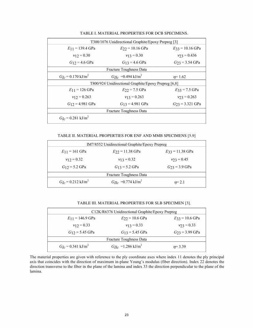
TABLE I. MATERIAL PROPERTIES FOR DCB SPECIMENS.

T300/1076 Unidirectional Graphite/Epoxy Prepreg [3] E11 = 139.4 GPa E22 = 10.16 GPa E33 = 10.16 GPa

ν12 = 0.30 ν13 = 0.30 ν23 = 0.436

G12 = 4.6 GPa G13 = 4.6 GPa G23 = 3.54 GPa

Fracture Toughness Data

GIc = 0.170 kJ/m2 GIIc =0.494 kJ/m2 η= 1.62 T800/924 Unidirectional Graphite/Epoxy Prepreg [6,8]

E11 = 126 GPa E22 = 7.5 GPa E33 = 7.5 GPa

ν12 = 0.263 ν13 = 0.263 ν23 = 0.263

G12 = 4.981 GPa G13 = 4.981 GPa G23 = 3.321 GPa

Fracture Toughness Data

GIc = 0.281 kJ/m2

TABLE II. MATERIAL PROPERTIES FOR ENF AND MMB SPECIMENS [5,9]

IM7/8552 Unidirectional Graphite/Epoxy Prepreg

E11 = 161 GPa E22 = 11.38 GPa E33 = 11.38 GPa

ν12 = 0.32 ν13 = 0.32 ν23 = 0.45

G12 = 5.2 GPa G13 = 5.2 GPa G23 = 3.9 GPa

Fracture Toughness Data

GIc = 0.212 kJ/m2 GIIc =0.774 kJ/m2 η= 2.1

TABLE III. MATERIAL PROPERTIES FOR SLB SPECIMEN [3].

C12K/R6376 Unidirectional Graphite/Epoxy Prepreg E11 = 146.9 GPa E22 = 10.6 GPa E33 = 10.6 GPa

ν12 = 0.33 ν13 = 0.33 ν23 = 0.33

G12 = 5.45 GPa G13 = 5.45 GPa G23 = 3.99 GPa

Fracture Toughness Data

GIc = 0.341 kJ/m2 GIIc =1.286 kJ/m2 η= 3.39

The material properties are given with reference to the ply coordinate axes where index 11 denotes the ply principal axis that coincides with the direction of maximum in-plane Young’s modulus (fiber direction). Index 22 denotes the direction transverse to the fiber in the plane of the lamina and index 33 the direction perpendicular to the plane of the lamina.

23

APPENDIX Conversion of existing models to ANSYS® Two-dimensional planar finite element models of the DCB, ENF, MMB and SLB specimens had been created previously during the creation of the benchmark examples in Abaqus/Standard® [3,4,5,6]. In an effort to preserve the topology of the models, the ABTOANS command in ANSYS® was used to translate the models and create an ANSYS® input file (.dat) [14,17]. To ensure the appropriate translation of the data, Abaqus/Standard® input file (.inp) had to be changed manually prior to executing the ABTOANS command in ANSYS®. Since ANSYS® requires the nodes to be defined before they are used in element definitions, the data in the Abaqus/Standard® input file (.inp) had to be arranged accordingly. Also, the planar elements (CPE4, CPS4, CPE4I) in Abaqus/Standard® had to be changed to an element type (e.g. S4R) recognized by the ABTOANS command in ANSYS®. In the resulting ANSYS® input file (.dat) the element type had to be manually changed to the plane strain elements (PLANE182) in order to be compatible with the current VCCT implementation in ANSYS®. Additional manual input was required to input the material data, local element coordinate systems, the contact definitions, the applied boundary conditions and specific input for the energy release rate computation using VCCT and the automated propagation as shown in the example input files below. Energy release rate computation using VCCT without automated propagation in ANSYS®

To create the benchmark examples of the simple specimens, analyses were performed where only the mixed-mode energy release rate at the crack tip was calculated. For all models, the plane of delamination was modeled as a discrete discontinuity in the center of the specimen. The models were created as separate meshes for the upper and lower part of the specimens with identical nodal point coordinates in the plane of delamination. The delamination interface then must be defined in the model as shown in Figure A1. Here, the crack tip node pair at which the mixed-mode energy release rate is calculated using VCCT is defined a component group N_CRFRONT. Note, that the nodes on both sides of the interface must be included in the component group. Otherwise only half of the energy release rate is computed. The intact section is defined as a contact zone with contact and target elements as shown in Figure A1. To initiate the energy release rate computation using VCCT, the following commands need to be added to the input file [14,15,16,17]: ! VCCT crack calculation specifications cint,new,1 cint,type,VCCT cint,ctnc,N_CRFRONT ! crack tip node component group cint,symm,off ! symmetry off cint,norm,0,1 ! crack plane normal

Note that in the printed output a sign (positive or negative) is assigned to the values of the energy release rate components for mode I and II. To calculate the total energy release rate from these results the absolute values need to be added to obtain the correct value.

An input file is given to provide an overview of an entire analysis and assist the readers in creating their own analyses. The ANSYS® commands shown in bold type were discussed in detail in the previous paragraphs.

24

Input file for energy release rate calculation using VCCT at user defined crack tip node /PREP7 /NOPR SHPP,OFF ! KEYWORD: *HEADING /title, DCB-UD-T300/1076, a=30.5 mm ! KEYWORD: *NODE, NSET=NTOP NSEL,NONE ! Only newly input nodes will be selected N, 5, 0., 150., 12.5 N, 6, 0.5, 150., 12.5 ... ... ... N, 975, 1., 0., 12.5 N, 976, 1.5, 0., 12.5 CM,n_NTOP,NODE NSEL,ALL ! KEYWORD: *NODE, NSET=NBOT NSEL,NONE ! Only newly input nodes will be selected N, 4, 0., 150., 12.5 N, 3, -0.5, 150., 12.5 ... ... ... N, 970, -1., 0., 12.5 N, 969, -1.5, 0., 12.5 CM,n_NBOT,NODE NSEL,ALL ! KEYWORD: *ELEMENT, TYPE=S4R , ELSET=EALL ESEL,NONE ! Only newly input elements will be selected ET,1,PLANE182 keyopt,1,1,2 ! enhanced strain keyopt,1,3,2 ! plane strain TYPE,1 EN, 1, 1, 9, 10, 2 EN, 2, 9, 17, 18, 10 ... ... ... EN, 725, 959, 967, 968, 960 EN, 726, 967, 975, 976, 968 CM,e_EALL,ELEMENT ESEL,ALL ! KEYWORD: *ELSET, ELSET=LY01, GENERATE ESEL,NONE ESEL,A,ELEM,, 1, 121, 1 CM,e_LY01,ELEMENT ESEL,ALL ! KEYWORD: *ELSET, ELSET=LY02, GENERATE ESEL,NONE ESEL,A,ELEM,, 122, 242, 1 CM,e_LY02,ELEMENT ESEL,ALL ! KEYWORD: *ELSET, ELSET=LY03, GENERATE ESEL,NONE ESEL,A,ELEM,, 243, 363, 1 CM,e_LY03,ELEMENT

25

ESEL,ALL ! KEYWORD: *ELSET, ELSET=LY04, GENERATE ESEL,NONE ESEL,A,ELEM,, 364, 484, 1 CM,e_LY04,ELEMENT ESEL,ALL ! KEYWORD: *ELSET, ELSET=LY05, GENERATE ESEL,NONE ESEL,A,ELEM,, 485, 605, 1 CM,e_LY05,ELEMENT ESEL,ALL ! KEYWORD: *ELSET, ELSET=LY06, GENERATE ESEL,NONE ESEL,A,ELEM,, 606, 726, 1 CM,e_LY06,ELEMENT ESEL,ALL ! KEYWORD: *ELSET, ELSET=ELCRBOT ESEL,NONE ESEL,A,ELEM,,263 ESEL,A,ELEM,,264 CM,e_ELCRBOT,ELEMENT ESEL,ALL ! KEYWORD: *ELSET, ELSET=ELCRTOP ESEL,NONE ESEL,A,ELEM,,384 ESEL,A,ELEM,,385 CM,e_ELCRTOP,ELEMENT ESEL,ALL ! KEYWORD: *ELSET, ELSET=EL_BOT, GENERATE ESEL,NONE ESEL,A,ELEM,, 243, 363, 1 CM,e_EL_BOT,ELEMENT ESEL,ALL ! KEYWORD: *ELSET, ELSET=EL_TOP, GENERATE ESEL,NONE ESEL,A,ELEM,, 364, 484, 1 CM,e_EL_TOP,ELEMENT ESEL,ALL ! KEYWORD: *NSET, NSET=BONDED, GENERATE NSEL,NONE NSEL,A,NODE,, 173, 973, 8 CM,n_BONDED,NODE NSEL,ALL ! KEYWORD: *NSET, NSET=CRFRONT NSEL,NONE NSEL,A,NODE,,173 NSEL,A,NODE,,172 CM,n_CRFRONT,NODE NSEL,ALL ! KEYWORD: *NSET, NSET=MPC NSEL,NONE NSEL,A,NODE,,172 CM,n_MPC,NODE NSEL,ALL ! KEYWORD: *NSET, NSET=LFRONT, UNSORTED NSEL,NONE ! **** DCB loading NSEL,A,NODE,,1

26

NSEL,A,NODE,,8 ! ** CM,n_LFRONT,NODE NSEL,ALL ! KEYWORD: *NSET, NSET=LFRONTP NSEL,NONE NSEL,A,NODE,,8 CM,n_LFRONTP,NODE NSEL,ALL ! KEYWORD: *NSET, NSET=LFRONTM NSEL,NONE NSEL,A,NODE,,1 CM,n_LFRONTM,NODE NSEL,ALL ! KEYWORD: *BOUNDARY ! **** boundary for DCB, 2D-full model D,972,UX,0.0 D,971,UY,0.0 D,974,UY,0.0 ! - - - - manual input - - - - - - - - - - - - - - - - - - - - - - - - - - - cmlist ! Anisotropic Material for element layers T300/1076 MP,Ex,1,0.13940E+06 MP,Ey,1,10160. MP,Ez,1,10160. MP,PRxy,1,0.300 MP,PRyz,1,0.43600 MP,PRxz,1,0.300 !MP,PRyz,1,0.300 !MP,PRxz,1,0.43600 MP,Gxy,1,4600. MP,Gyz,1,3537.6 MP,Gxz,1,4600. !MP,Gyz,1,4600. !MP,Gxz,1,3537.6 ! Coordinate systems to orient Anisotropic materials LOCAL,11,0,,,,90 LOCAL,12,0,,,,90 LOCAL,13,0,,,,90 LOCAL,14,0,,,,90 LOCAL,15,0,,,,90 LOCAL,16,0,,,,90 CSYS,0 ! reset active system to be global cartesian ! Change the material ID and element coordinate system for the element layer groups ESEL,S,ELEM,,E_LY01 EMODIF,ALL,MAT,1 EMODIF,ALL,ESYS,11 ESEL,S,ELEM,,E_LY02

27

EMODIF,ALL,MAT,1 EMODIF,ALL,ESYS,12 ESEL,S,ELEM,,E_LY03 EMODIF,ALL,MAT,1 EMODIF,ALL,ESYS,13 ESEL,S,ELEM,,E_LY04 EMODIF,ALL,MAT,1 EMODIF,ALL,ESYS,14 ESEL,S,ELEM,,E_LY05 EMODIF,ALL,MAT,1 EMODIF,ALL,ESYS,15 ESEL,S,ELEM,,E_LY06 EMODIF,ALL,MAT,1 EMODIF,ALL,ESYS,16 ! Set up contact between top and bottom sections ! Element types for contact ET,3,TARGE169 ET,4,CONTA171 KEYOPT,4,12,5 ! bonded ! Mesh the contact surfaces ESEL,S,ELEM,,E_EL_BOT NSLE,S NSEL,R,LOC,X,0 NSEL,R,LOC,Y,0,119.51 TYPE,3 REAL,3 ESURF ESEL,S,ELEM,,E_EL_TOP NSLE,S NSEL,R,LOC,X,0 NSEL,R,LOC,Y,0,119.51 TYPE,4 REAL,3 ESURF ! Applied displacement Boundary Conditions NSEL,S,NODE,,N_LFRONTM D,all,Ux,-1.5 NSEL,S,NODE,,N_LFRONTP D,all,Ux,1.5 ! Solution /solu ! Static analysis antype,static

28

! Non-linear geometry NLGEOM,ON ! Output for postprocessing outres,all,all ! time stepping autots,on ! automatic time step adjustment DELTIM,0.0100000 , 1.0000000E-18, 0.150000 time,1.0 ! simulated final time ! VCCT crack calculation specifications cint,new,1 cint,type,VCCT cint,ctnc,N_CRFRONT ! crack tip node component group cint,symm,off ! symmetry off cint,norm,0,1 ! crack plane normal allsel,all solve finish ! postprocessing /post1 prcint,1 ! print out VCCT calculation ! Use *GET to get the VCCT information NSEL,S,NODE,,N_CRFRONT ctn = ndnext(0) *get,G_1 ,CINT,1,ctip,ctn,,1,,G1 *get,G_2 ,CINT,1,ctip,ctn,,1,,G2 /post26 ! enter time-history post processor NSEL,S,NODE,,N_LFRONTP ! select node component group named N_LFRONTP nd = ndnext(0) ! set nd to node number of 1st node NSOL,2,nd,u,x,apl_dsp ! store x displac. in variable #2, name it apl_dsp RFORCE,3,nd,f,x ! get reaction force, variable #3 prvar,2,3 ! print variables 2 & 3 to screen NSEL,S,NODE,,N_CRFRONT ! select crack tip node group ctn = ndnext(0) ! set ctn to node # of 1st node cisol,5,1,ctn,1,g1 ! get G1 for crack #1, variable #5 cisol,6,1,ctn,1,g2 ! get G2 for crack #1, variable #6 prvar,5,6 ! print variables 5,6 to screen prvar,2,3,5,6 ! print variables 2-6 to screen /eof

29

Automated delamination propagation analysis in ANSYS®

For automated delamination or crack propagation analysis, the same models were used but the input to define the delamination interface was slightly altered as shown in Figure A2. Here, the intact section is defined as an interface with cohesive elements (INTER202), which are used to define the crack path as shown in Figure A1. The intact region is defined by first joining the mesh, inserting the interface elements along the entire interface and then deleting the elements along the already existing, open crack face as shown in Figure A1. The material definition for the cohesive elements is not used and propagation is determined by a mixed-mode fracture criterion such as the BK criterion [11] as shown in Figure A3 for the example of C12K/R6376 (see also Figure 5). To perform automated propagation analysis the following commands also need to be added to the input file [14,15,16,17]: ! VCCT crack calculation specifications cint,new,1 cint,type,VCCT cint,ctnc,N_CRFRONT ! crack tip node component group cint,symm,off ! symmetry off cint,norm,0,1 ! crack plane normal ! crack growth specifications cgrow,new,2 ! new crack growth number cgrow,dtime,0.001 cgrow,dtmin,0.001 cgrow,dtmax,0.001 cgrow,cid,1 ! cint ID for VCCT calculation cgrow,cpath,crkpath ! crack path component cgrow,fcop,mtab,2 ! table number for mixed mode fracture criterion

The manually required input is given to provide an overview of the analysis and assist the

readers in creating their own analyses. The topology remains the same as above. The ANSYS® commands shown in bold type were discussed in detail in the previous paragraphs. Input file for automated delamination propagation analysis ! - - - - manual input - - - - - - - - - - - - - - - - - - - - - - - - - - - cmlist ! Anisotropic Material for element layers T300/1076 MP,Ex,1,0.13940E+06 MP,Ey,1,10160. MP,Ez,1,10160. MP,PRxy,1,0.300 MP,PRyz,1,0.43600 MP,PRxz,1,0.300 !MP,PRyz,1,0.300 !MP,PRxz,1,0.43600 MP,Gxy,1,4600. MP,Gyz,1,3537.6 MP,Gxz,1,4600. !MP,Gyz,1,4600.

30

!MP,Gxz,1,3537.6 ! Coordinate systems to orient Anisotropic materials LOCAL,11,0,,,,90 LOCAL,12,0,,,,90 LOCAL,13,0,,,,90 LOCAL,14,0,,,,90 LOCAL,15,0,,,,90 LOCAL,16,0,,,,90 CSYS,0 ! reset active system to be global cartesian ! Change the material ID and element coordinate system for the element layer groups ESEL,S,ELEM,,E_LY01 EMODIF,ALL,MAT,1 EMODIF,ALL,ESYS,11 ESEL,S,ELEM,,E_LY02 EMODIF,ALL,MAT,1 EMODIF,ALL,ESYS,12 ESEL,S,ELEM,,E_LY03 EMODIF,ALL,MAT,1 EMODIF,ALL,ESYS,13 ESEL,S,ELEM,,E_LY04 EMODIF,ALL,MAT,1 EMODIF,ALL,ESYS,14 ESEL,S,ELEM,,E_LY05 EMODIF,ALL,MAT,1 EMODIF,ALL,ESYS,15 ESEL,S,ELEM,,E_LY06 EMODIF,ALL,MAT,1 EMODIF,ALL,ESYS,16 !- - - - - - - - - - - - - - - - - - - - - - - - - - - - - - - - - - - - ! Start: Crack plane interface elements ! merge nodes on crack plane nsel,s,loc,x,0 nummrg,node ! Set up interface between top and bottom sections ET,2,INTER202 ! 2d 4-node cohesive zone element KEYOPT,2,2,2 ! Multi point constraint (no compliance) KEYOPT,2,3,2 ! plane strain ! component groups for rows of elements along crack plane ESEL,S,CENT,X, -0.5, 0 CM,EL_BOT,ELEMENT

31

ESEL,S,CENT,X, 0, 0.5 CM,EL_TOP,ELEMENT ! Mesh the interface TYPE,2 MAT,2 ESEL,ALL CZMESH,EL_BOT,EL_TOP ! Delete elements at crack face nsel,s,loc,x,0 nsel,r,loc,y,119.5,150 ESLN,S,1 ESEL,R,TYPE,,2 EDELE,ALL ! Component group for crack interface elements ESEL,S,ENAME,,202 CM,CRKPATH,ELEM ESEL,S,ELEM,,CRKPATH ! Interface failure parameters !** Fracture toughness T300/1076: GIc = 0.17 GIIc = 0.494 ! GIIIc = 0.0 ! unused !** B-K parameter: eta=1.75 ! Table to define mixed mode fracture TB,CGCR,2,,,BK !* BK mixed mode fracture criterion TBDATA,1,GIc, GIIC, eta ! Finished: Crack plane interface elements !- - - - - - - - - - - - - - - - - - - - - - - - - - - - - - - - - - - - ! Applied displacement Boundary Conditions NSEL,S,NODE,,N_LFRONTM D,all,Ux,-2.0 NSEL,S,NODE,,N_LFRONTP D,all,Ux,2.0 ! Solution /solu ! Static analysis antype,static ! Non-linear geometry NLGEOM,ON

32

! Output for postprocessing outres,all,all outres,cint,all ! time stepping autots,on ! no automatic time step adjustment DELTIM,0.001,0.000001,0.01 time,1.0 ! simulated final time ! VCCT crack calculation specifications cint,new,1 cint,type,VCCT cint,ctnc,N_CRFRONT ! crack tip node component group cint,symm,off ! symmetry off cint,norm,0,1 ! crack plane normal ! crack growth specifications cgrow,new,2 ! new crack growth number cgrow,dtime,0.001 cgrow,dtmin,0.001 cgrow,dtmax,0.001 cgrow,cid,1 ! cint ID for VCCT calculation cgrow,cpath,crkpath ! crack path component cgrow,fcop,mtab,2 ! table number for mixed mode fracture criterion allsel,all solve finish save !------------------------------------------------------------------------ ! postprocessing /post1 prcint,1 ! print out VCCT calculation ! Use *GET to get the VCCT information NSEL,S,NODE,,N_CRFRONT ctn = ndnext(0) *get,G_1 ,CINT,1,ctip,ctn,,1,,G1 *get,G_2 ,CINT,1,ctip,ctn,,1,,G2 *vwrite, (' *------------------------------------------------------------------------') *vwrite, (' *') *vwrite, (' *',2x,'G1 from ANSYS') *vwrite,G_1 (' *',12x,'G1 = ',3x,F9.3) *vwrite,G_2 (' *',12x,'G2 = ',3x,F9.3)

33

*vwrite, (' *') *vwrite, (' *------------------------------------------------------------------------') /post26 ! enter time-history post processor NSEL,S,NODE,,N_LFRONTP ! select node group named N_LFRONTP nd = ndnext(0) ! set nd node number of 1st node NSOL,2,nd,u,x,apl_dsp ! store x displac. as#2, name it apl_dsp RFORCE,3,nd,f,x ! reaction force at node, variable #3 prvar,2,3 ! print variables 2 & 3 to screen NSEL,S,NODE,,N_CRFRONT ! select crack tip node component group ctn = ndnext(0) ! set ctn to node # of 1st node in group cisol,5,1,ctn,1,g1 ! get G1 for crack #1, variable #5 cisol,6,1,ctn,1,g2 ! get G2 for crack #1, variable #6 prvar,5,6 ! print variables 5,6 to screen prvar,2,3,5,6 ! print variables 2-6 to screen /eof

34

P

P a0

h

2L

2h

B

+θ

y

z

x

Krueger example [3]B 25.0 mm2h 3.0 mm2L 150.0 mma0 30.0 mm

δ

material and layup:T300/1076 [0]24

Figure 1. Double Cantilever Beam Specimen (DCB).

NAFEMS example [8]B 30.0 mm2h 3.0 mm2L 150.0 mma0 30.0 mm material and layup: T800/924 [0]24

Q

2h

+θ

yz

x dimensionsB 25.4 mm2h 4.5 mm2L 101.6 mma0 25.4 mm

Figure 2. End-Notched Flexure Specimen (ENF) [4].

a02LL

wmaterial and layup: IM7/8552 [0]24

Figure 3. Single Leg Bending Specimen (SLB) [3].

yz

2LLaB

t1t2

dimensionsB 25.4 mm t1 2.032 mm t2 2.032 mm 2L 177.8 mma 34.29 mm

w

x

material and layup: C12K/R6376 [0]24

Q

B

35

Figure 4. Mixed Mode Bending Specimen (MMB) (dimensions from [5])

material and layup: IM7/8552 [0]24

dimensionsb 25.4 mm2h 4.5 mm2L 100.8 mm2L* 152.4 mma0 25.4 mm

Q

2LL

a0

w

c

base

loading arm

specimen 2h

width b

2L*

0

200

400

600

800

1000

1200

1400

1600

0 0.2 0.4 0.6 0.8 1

mean values

mixed mode ratio GII/GT

Gc ,

J/m2

DCB, Mode I MMB, Mode I and II ENF, Mode II

curve fit: Gc = G

Ic + (GIIc-GIc)(GII/GT)η

Figure 5. Mixed-mode failure criterion for C12K/R6376.

η = 3.39

GIc =340.5

GIIc =1285.9

36

critical, G=Gc

benchmark

load P Pcrit

δ1/2 δ

2/2 δ

3/2

Figure 7. Calculated critical behavior and resulting benchmark case.

δcrit /2

applied opening displacement δ/2

a1

8_UX_1818_UX_1898_UX_1978_UX_2058_UX_2138_UX_2218_UX_2298_UX_2378_UX_1738_UX_2538_UX_3338_UX_4138_UX_4938_UX_5738_UX_6538_UX_7338_UX_805u_crit

load P

applied opening displacement δ/2

G= G(a1,δ

1/2)δ

1/2 δ

2/2 δ

3/2

G= G(a12,δ

2/2)

G= G(a16,δ

3/2)

Figure 6. Computed load-displacement behavior for specimen with different crack lengths ai.

G= G(a13,δ

2/2)

G= G(a17,δ

3/2)

G= G(a10,δ

1/2)

G= G(a3,δ

1/2)

G= G(a6,δ

1/2)

37

Figure 8. Typical 2D FE-models of a DCB specimen.

(a). View of full model.

(b). Detail of crack tip zone for Δa=0.5 mm.

intact sectioninitial delamination front

δ/2

a0

2h

Δax,u

z,w

δ/2

(c). Detail of crack tip zone for Δa=0.25 mm.

(d). Detail of crack tip zone for Δa=1.0 mm.

x,u

z,w

x,u

z,w

2h

Δa

Δa

2h

38

Figure 9. Additional 2D FE-models of a DCB specimen.

(a). View of full model for Δa=2.0 mm.

(b). Detail of crack tip zone for Δa=2.0 mm.

intact sectioninitial delamination front

a0

2h

Δa

δ/2

(d). Detail of crack tip zone for non-uniform Δa.x,u

z,w

Δa

2h

x,u

z,w

(c). View of full model with non-uniform Δa in propgation zone.

Δa

a0

δ/2

δ/2

δ/2

39

initial delamination front

2L

a0

x,u

z,w

u,w=0w=0

Figure 10. Deformed 2D finite element model of an ENF specimen

Figure 11. Deformed 2D finite element model of a SLB specimen

w

x,u

z,w

w

2L

a0

u,w=0

w=0

a. Deformed FE-model of a SLB specimen with initial delamination before growth

b. Detail of a FE-model of a SLB specimen

initial delamination front

t1

t2

two plies adjacent to the plane of delamination modeled with one element each through the thickness

40

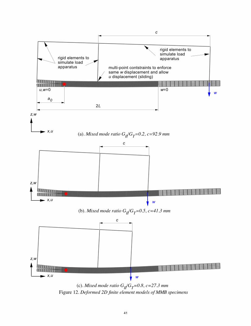
Figure 12. Deformed 2D finite element models of MMB specimens

(a). Mixed mode ratio GII/GT=0.2, c=92.9 mm

(b). Mixed mode ratio GII/GT=0.5, c=41.3 mm

(c). Mixed mode ratio GII/GT=0.8, c=27.3 mm

rigid elements to simulate load apparatus

w

2L

a0

w=0

c

rigid elements to simulate load apparatus

u,w=0

x,u

z,w

x,u

z,w

x,u

z,w

w

w

c

c

multi-point contstraints to enforce same w displacement and allow u displacement (sliding)

41

critical, G= GIc =0.17 kJ/m2

benchmark

0.0 1.0 2.0 3.0 4.0 5.00

10

20

30

40

50

60

70

80

90

100

110

120

130

load P,N

δ1/2 δ

2/2 δ

3/2

applied opening displacement δ/2, mm

Figure 14. Calculated critical behavior and resulting benchmark case for a DCB specimen.

Pcrit=62.0

δcrit /2=0.76

0.0 1.0 2.0 3.0 4.0 5.00

10

20

30

40

50

60

70

80

90

100

110

120

130

a0= 30.5 mm

a0= 45.4 mm

a0= 65.1 mm

load P, N

applied opening displacement δ/2, mmFigure 13. Computed load-displacement behavior of a DCB specimen

for different delamination lengths a0.

δ/2=1.5 δ/2=3.0G= 0.66 kJ/m2

G= 0.43 kJ/m2

G= 0.61 kJ/m2

δ/2=5.0

42

0.0 0.5 1.0 1.50

10

20

30

40

50

60

70

benchmarkfirst automated propagationcgrow: dtime=0.001, dtmax=0.01cgrow: dtime=0.001, dtmax=0.001

load P, N

applied opening displacement δ/2, mmFigure 16. Load/displacement behavior for a benchmark case and automated

propagation analysis for a DCB specimen (autots: dtimea=0.001, dtmaxa=0.001).

autots: dtimea=0.001, dtmaxa=0.001

0.0 0.5 1.0 1.50

10

20

30

40

50

60

70

benchmark analysis [3]

benchmark analysis (ANSYS)

repeated benchmark analysis with enhanced plane strain elements

load P, N

applied opening displacement δ/2, mm

G= GIc =0.17 kJ/m2

Figure 15. Comparison of benchmark cases for a DCB specimen using different finite element software.

43

0.0 0.5 1.0 1.50

10

20

30

40

50

60

70

benchmarkautots: dtimea=0.1, dtmaxa=0.1autots: dtimea=0.01, dtmaxa=0.01

load P, N

applied opening displacement δ/2, mmFigure 18. Influence of step time parameters for automated time stepping (autots) on computed

load/displacement behavior during automated propagation analysis for a DCB specimen.

cgrow: dtime=10-6, dtmax=10-6

0.0 0.5 1.0 1.50

10

20

30

40

50

60

70

benchmarkcgrow: dtime=0.1, dtmax=0.1cgrow: dtime=0.01, dtmax=0.01cgrow: dtime=0.001, dtmax=0.001cgrow: dtime=10-4, dtmax=10-4

cgrow: dtime=10-5, dtmax=10-5

cgrow: dtime=10-6, dtmax=10-6

load P, N

applied opening displacement δ/2, mmFigure 17. Influence of step time parameters for crack growth (cgrow) on computed

load/displacement behavior during automated propagation analysis for a DCB specimen.

autots: dtimea=0.001, dtmaxa=0.001

44

0.0 0.5 1.0 1.50

10

20

30

40

50

60

70benchmarkΔa mixed, FE model Fig. 9c,d

load P, N

applied opening displacement δ/2, mmFigure 20. Influence of varying crack tip element length, Δa, on computed load/displacement

behavior during automated propagation analysis for a DCB specimen.

fine mesh coarse meshtransition

0.0 0.5 1.0 1.50

10

20

30

40

50

60

70

benchmarkΔa=0.5mm , FE model Fig. 8 a and b Δa=0.25mm , FE model Fig. 8 cΔa=1.0 mm , FE model Fig. 8 dΔa=2.0 mm , FE model Fig. 9 a and b

load P, N

applied opening displacement δ/2, mmFigure 19. Influence of crack tip element length, Δa, on computed load/displacement

behavior during automated propagation analysis for a DCB specimen.

45

a a Δa Δa Δaa

(b). Computed load/displacement behavior during automated propagation for a DCB specimen.

(a). Detail of crack propagation from length a to a+Δa to a+2Δa.

• Initial loading until critical energy release rate is reached 1 → 2• Sudden nodal release and opening along entire element length Δa for constant displacement 2 → 3 • Next loading cycle 3 → 4 followed by nodal release 4 → 5 and so on …• If a coarse mesh is desired, peak saw tooth results (2,4,6) may be used

Figure 21. Origin of observed saw tooth behavior during automated propagation.

benchmarkanalysis

load P

applied opening displacement δ/2

a

a+Δa

a+2Δa

2

3

4

5

6

1

46

0.0 1.0 2.0 3.0 4.0 5.0 6.0 7.0 8.0 9.0 10.0 11.0 12.0 13.00

20

40

60

80

100

experimental results (NAFEMS) [8]beam theory (NAFEMS) [8]benchmark analysis [6]benchmark analysis (ANSYS)

load P, N

applied opening displacement δ, mm

Figure 23. Benchmark case for NAFEMS DCB specimen.

G= GIc =0.281 kJ/m2=const.

0.0 2.0 4.0 6.0 8.0 10.0 12.00

50

100

150

a0=30 mm

a0=40 mm

a0=55 mm

a0=69.5mm

load P, N

applied displacement δ, mm

Figure 22. Load-displacement and calculated critical behavior for the NAFEMS DCB specimen.

δ=3.0 δ=6.0 δ=10.0 δ=12.0

G= GIc =0.281 kJ/m2

δcrit =1.98

Pcrit=92.335

G= 0.64 kJ/m2

G= 0.74 kJ/m2

G= 0.44 kJ/m2

G= 0.88 kJ/m2

47

0.0 2.0 4.0 6.0 8.0 10.00

20

40

60

80

100

benchmarkfirst automated propagationcgrow: dtime=0.1, dtmax=0.1cgrow: dtime=0.01, dtmax=0.01cgrow: dtime=0.001, dtmax=0.001cgrow: dtime=10-4, dtmax=10-4

cgrow: dtime=10-5, dtmax=10-5

cgrow: dtime=10-6, dtmax=10-6

load P, N

applied opening displacement δ, mmFigure 25. Influence of step time parameters for crack growth (cgrow) on computed

load/displacement behavior during propagation analysis for the NAFEMS DCB specimen.

autots: dtimea=0.001, dtmaxa=0.001

0.0 10.0 20.0 30.0 40.0 50.0 60.00.0

1.0

2.0

3.0

4.0

5.0

6.0

7.0

8.0

9.0

10.0

11.0

12.0

13.0

beam theory (NAFEMS) [8]benchmark analysis [6]benchmark analysis (ANSYS)

increase in delamination length a*, mm

appliedopening

displacementδ, mm

Figure 24. Benchmark case for NAFEMS DCB specimen plotted as applied opening displacement δ versus increase in delamination length a*.

48

0.0 1.0 2.0 3.0 4.0 5.0 6.00

400

800

1200

1600

2000

2400

a0= 25.4 mm

a0= 55.9 mm

a0= 76.2 mm

critical, G=GIIc

load Q, N

applied displacement w, mm

GII=1.54 kJ/m2

Figure 27. Computed load-displacement behavior for different delamination lengths a

0 and calculated critical behavior for ENF specimen.

Qcrit

=1535

wcrit

=1.42 w=2.0 w=5.0

GII= 4.9

GII= 0.9

0.0 2.0 4.0 6.0 8.0 10.00

20

40

60

80

100

120

benchmark

autots: dtimea=0.1, dtmaxa=0.1

autots: dtimea=0.01, dtmaxa=0.01

load P, N

applied opening displacement δ, mmFigure 26. Influence of step time parameters for automated time stepping (autots) on computed

load/displacement behavior during propagation analysis for NAFEMS DCB specimen.

cgrow: dtime=10-6, dtmax=10-6

49

0.0 1.0 2.0 3.0 4.0 5.0 6.00

400

800

1200

1600

2000

2400

critical, G=GIIc

first automated propagation

cgrow: dtime=0.001, dtmax=0.001

load Q, N

applied displacement w, mm

Qcrit

=1535

wcrit

=1.42

benchmark

Figure 29. Load/displacement behavior for benchmark case and automated propagation analysis for an ENF specimen (autots: dtimea=0.001, dtmaxa=0.001).

autots: dtimea=0.001, dtmaxa=0.001

0.0 1.0 2.0 3.0 4.0 5.0 6.00

400

800

1200

1600

2000

2400

critical, G=GIIc

benchmark for applied load Qbenchmark for applied displacement w

load Q, N

displacement w, mmFigure 28. Calculated critical behavior and resulting benchmark cases

for applied displacement w and load Q for an ENF specimen.

Qcrit

=1535

wcrit

=1.42

50

0.0 1.0 2.0 3.0 4.0 5.0 6.00

400

800

1200

1600

2000

2400

critical

autots: dtimea=0.1, dtmaxa=0.1

autots: dtimea=0.01, dtmaxa=0.01

load Q, N

applied displacement w, mm

Qcrit

=1535

wcrit

=1.42

benchmark

Figure 31. Influence of step time parameters for automated time stepping (autots) on computed load/displacement behavior during propagation analysis for an ENF specimen .

cgrow: dtime=10-6, dtmax=10-6

0.0 1.0 2.0 3.0 4.0 5.0 6.00

400

800

1200

1600

2000

2400

critical, G=GIIccgrow: dtime=0.1, dtmax=0.1cgrow: dtime=0.01, dtmax=0.01cgrow: dtime=0.001, dtmax=0.001cgrow: dtime=10-4, dtmax=10-4

cgrow: dtime=10-5, dtmax=10-5

cgrow: dtime=10-6, dtmax=10-6

load Q, N

applied displacement w, mm

Qcrit

=1535

wcrit

=1.42

Figure 30. Influence of step time parameters for crack growth (cgrow) on computed load/displacement behavior during automated propagation analysis for an ENF specimen.

benchmarkautots: dtimea=0.001, dtmaxa=0.001

51

0.0 1.0 2.0 3.0 4.0 5.0 6.00

400

800

1200

1600

2000

2400

criticalautots: dtimea=0.1, dtmaxa=0.1autots: dtimea=0.01, dtmaxa=0.01

appliedload Q, N

displacement w, mm

Qcrit

=1535

wcrit

=1.42

Figure 33. Influence of parameters for automated time stepping (autots) on computed load/displacement behavior during propagation analysis for an ENF specimen subjected to a load.

benchmark

cgrow: dtime=10-6, dtmax=10-6

0.0 1.0 2.0 3.0 4.0 5.0 6.00

400

800

1200

1600

2000

2400

critical, G=GIIcdtime=0.1, dtmax=0.1dtime=0.01, dtmax=0.01dtime=0.001, dtmax=0.001 dtime=10-4, dtmax=10-4

dtime=10-5, dtmax=10-5

dtime=10-6, dtmax=10-6

appliedload Q, N

displacement w, mm

Qcrit

=1535

wcrit

=1.42

Figure 32. Influence of step time parameters for crack growth (cgrow) on computed load/displacement behavior during propagation analysis for an ENF specimen subjected to a load.

benchmark

autots: dtimea=0.001, dtmaxa=0.001

52

0.0 1.0 2.0 3.0 4.0 5.00

100

200

300

400

500

criticalfirst automated propagationcgrow: dtime=0.001, dtmax=0.001cgrow: dtime=0.0001, dtmax=0.0001

load Q, N

applied displacement w, mm

Figure 35. Calculated benchmark case and automated propagation analysis for a SLB specimen.

benchmark

wcrit

=2.88

Qcrit

=408

autots: dtimea=0.001, dtmaxa=0.001

0.0 1.0 2.0 3.0 4.0 5.00

100

200

300

400

500

a0=35.3 mm

a0=60.3 mm

a0=94.6 mm

critical, G=Gc

load Q, N

applied displacement w, mm

wcrit

=2.88

Qcrit

=408

Figure 34. Calculated critical behavior and resulting benchmark case for a SLB specimen.

w=3.0 w=5.0

G= 0.4 kJ/m2

G= 1.03 kJ/m2

G= 0.53 kJ/m2

benchmark

53

0.0 1.0 2.0 3.0 4.0 5.00

100

200

300

400

500

criticalautots: dtime=0.1, dtmax=0.1autots: dtime=0.01, dtmax=0.01

load Q, N

applied displacement w, mm

Figure 31b. Calculated benchmark case and automated propagation analysis for SLB specimen.

benchmark

wcrit

=2.88

Qcrit

=408

Figure 37. Influence of step time parameters for automated time stepping (autots) on computed load/displacement behavior during propagation analysis for a SLB specimen.

cgrow: dtime=10-6, dtmax=10-6

0.0 1.0 2.0 3.0 4.0 5.00

100

200

300

400

500

dtime=0.1, dtmax=0.1dtime=0.01, dtmax=0.01dtime=0.001, dtmax=0.001dtime=10-4, dtmax=10-4

dtime=10-5, dtmax=10-5

dtime=10-6, dtmax=10-6

load Q, N

applied displacement w, mm

wcrit

=2.88

Qcrit

=408

critical, GT=Gc

benchmark

Figure 36. Influence of step time parameters for crack growth (cgrow) on computed load/displacement behavior during propagation analysis for a SLB specimen.

autots: dtimea=0.001, dtmaxa=0.001

54

0.0 2.0 4.0 6.0 8.0 10.00

20

40

60

80

100

120

140

160

critical, GT = Gc

benchmark

load Q, N

applied displacement w, mmFigure 39. Calculated critical behavior and resulting benchmark case for applied displacement

for a MMB specimen (GII

/GT=0.2).

wcrit

=1.65

Qcrit

=128.6

0.0 2.0 4.0 6.0 8.0 10.00

20

40

60

80

100

120

140

160

a0=25.4 mm

a0=51.4mm

a0=73.3 mm

critical, GT= G

c

load Q, N

applied displacement w, mm

Figure 38. Calculated critical load-displacement behavior for a MMB specimen (GII/G

T=0.2).

Qcrit

=128.6

wcrit

=1.65

GT = 0.33 kJ/m2

GT = 0.5 kJ/m2

w=3.0 w=4.0 w=6.0

55

0.0 2.0 4.0 6.0 8.0 10.00

102030405060708090

100110120130140150160170

critical, benchmarkcgrow: dtime=0.1, dtmax=0.1cgrow: dtime=0.01, dtmax=0.01cgrow: dtime=0.001, dtmax=0.001cgrow: dtime=10-4, dtmax=10-4

cgrow: dtime=10-5, dtmax=10-5

cgrow: dtime=10-6, dtmax=10-6

load Q, N

applied displacement w, mm

wcrit

=1.65

Qcrit

=128.6

Figure 41. Influence of step time parameters for crack growth (cgrow) on computed load/displacement behavior during propagation analysis for a MMB specimen (G

II /G

T=0.2) .

autots: dtimea=0.001, dtmaxa=0.001

0.0 2.0 4.0 6.0 8.0 10.00

102030405060708090

100110120130140150160170

critical, GT=Gc, benchmark

cgrow: dtime=0.1, dtmax=0.1cgrow: dtime=0.001, dtmax=0.001

first automated propagation

cgrow: dtime=10-6, dtmax=0.1

load Q, N

applied displacement w, mm

wcrit

=1.65

Qcrit

=128.6

Figure 40. Calculated benchmark case and automated propagation analysis for a MMB specimen (G

II /G

T=0.2 - autots: dtimea=0.001, dtmaxa=0.001).

autots: dtimea=0.001, dtmaxa=0.001

56

0.0 2.0 4.0 6.0 8.0 10.00

100

200

300

400

500

600

a0=25.4 mm

a0=46.9 mm

a0=55.4 mm

a0=79.1 mm

critical, GT=G

c

load Q, N

applied displacement w, mm

Qcrit

=375

wcrit

=1.33 w=3.0 w=4.0 w=6.0

GT = 0.7 kJ/m2

GT = 0.83 kJ/m2

GT = 1.2 kJ/m2

Figure 43. Computed load-displacement behavior for different delamination lengths a

0 and calculated critical behavior for a MMB specimen (G

II/G

T=0.5).

0.0 2.0 4.0 6.0 8.0 10.00

102030405060708090

100110120130140150160170

critical, GT=Gc, benchmarkautots: dtimea=0.1, dtmaxa=0.1autots: dtimea=0.01, dtmaxa=0.01

load Q, N

applied displacement w, mm

wcrit

=1.65

Qcrit

=128.6

Figure 42. Influence of step time parameters for automated time stepping (autots) on computed load/displacement behavior during propagation analysis for a MMB specimen (G

II /G

T=0.2).

cgrow: dtime=10-6, dtmax=10-6

57

0.0 2.0 4.0 6.0 8.0 10.00

100

200

300

400

500

600

critical, GT=Gc

cgrow: dtime=0.1, dtmax=0.1cgrow: dtime=0.01, dtmax=0.01cgrow: dtime=0.001, dtmax=0.001cgrow: dtime=10-4, dtmax=10-4

cgrow: dtime=10-5, dtmax=10-5

cgrow: dtime=10-6, dtmax=10-6

benchmark for applied displacement

load Q, N

applied displacement w, mm

Qcrit

=375

wcrit

=1.33

Figure 45. Influence of step time parameters for crack growth (cgrow) on computed load/displacement behavior during propagation analysis for a MMB specimen (G

II /G

T=0.5).

autots: dtimea=0.001, dtmaxa=0.001

0.0 2.0 4.0 6.0 8.0 10.00

100

200

300

400

500

600

critical, GT=Gc

benchmark for applied displacement wbenchmark for applied load Q

load Q, N

displacement w, mm

Qcrit

=375

wcrit

=1.33

Figure 44. Calculated critical behavior and resulting benchmark cases for applied displacement w and load Q for a MMB specimen (G

II /G

T=0.5).

58

0.0 2.0 4.0 6.0 8.0 10.00

100

200

300

400

500

600

critical, GT=Gc

benchmarkcgrow: dtime=0.1, dtmax=0.1cgrow: dtime=0.01, dtmax=0.01cgrow: dtime=0.001, dtmax=0.001cgrow: dtime=10-4, dtmax=10-4

cgrow: dtime=10-5, dtmax=10-5

cgrow: dtime=10-6, dtmax=10-6

appliedload Q,

N

displacement w, mm

Qcrit

=375

wcrit

=1.33

Figure 47. Influence of step time input for crack growth (cgrow) on computed load/displacementbehavior during propagation analysis for a MMB specimen (G

II /G

T=0.5) subjected to a load Q.

autots: dtimea=0.001, dtmaxa=0.001

0.0 2.0 4.0 6.0 8.0 10.00

100

200

300

400

500

600

critical, GT=Gcbenchmarkautots: dtimea=0.1, dtmaxa=0.1autots: dtimea=0.01, dtmaxa=0.01

load Q, N

applied displacement w, mm

Qcrit

=375

wcrit

=1.33

Figure 46. Influence of step time parameters for automated time stepping (autots) on computed load/displacement behavior during propagation analysis for a MMB specimen (G

II /G

T=0.5).

cgrow: dtime=10-6, dtmax=10-6

59

0.0 2.0 4.0 6.0 8.0 10.00

200

400

600

800

1000

a0=25.4 mm

a0=49.9 mm

a0=55.4 mm

a0=79.1 mm

critical, GT=G

c

load Q, N

applied displacement w, mm

Qcrit

=729

wcrit

=1.63

GT = 0.78 kJ/m2

GT = 1.1kJ/m2

GT = 2.2 kJ/m2

Figure 49. Computed load-displacement behavior for different delamination lengths a

0 and calculated critical behavior for a MMB specimen (G

II/G

T=0.8).

w=3.0 w=6.0

0.0 2.0 4.0 6.0 8.0 10.00

100

200

300

400

500

600

critical, GT=Gcbenchmarkautots: dtimea=0.1, dtmaxa=0.1autots: dtimea=0.01, dtmaxa=0.01

appliedload Q,

N

displacement w, mm

Qcrit

=375

wcrit

=1.33

Figure 48. Influence of input for automated time stepping (autots) on computed load/displacement behavior during propagation analysis for a MMB specimen (G

II /G

T=0.5) subjected to a load.

cgrow: dtime=10-6, dtmax=10-6

60

0.0 2.0 4.0 6.0 8.0 10.00

200

400

600

800

1000

critical, GT=Gcbenchmark for applied displacementcgrow: dtime=0.1, dtmax=0.1cgrow: dtime=0.01, dtmax=0.01cgrow: dtime=0.001, dtmax=0.001cgrow: dtime=10-4, dtmax=10-4

cgrow: dtime=10-5, dtmax=10-5

cgrow: dtime=10-6, dtmax=10-6

load Q, N

applied displacement w, mm

wcrit

=1.63

Qcrit

=729

Figure 51. Influence of step time parameters for crack growth (cgrow) on computed load/displacement behavior during propagation analysis for a MMB specimen (G

II /G

T=0.8).

autots: dtimea=0.001, dtmaxa=0.001

0.0 2.0 4.0 6.0 8.0 10.00

200

400

600

800

1000

critical, GT=Gc

benchmark for applied displacement wbenchmark for applied load Q

load Q, N

applied displacement w, mmFigure 50. Calculated critical behavior and resulting benchmark cases for

applied load Q and displacement w for a MMB specimen (GII/G

T=0.8).

wcrit

=1.63

Qcrit

=729

61

0

500

1000

1500

2000

2500

3000

3500

4000

4500

5000

0.1 0.01 0.001 1e-4 1e-5 1e-6

CPU-time

autots: dtimea=0.1, dtmaxa=0.1autots: dtimea=0.01, dtmaxa=0.01autots: dtimea=0.001, dtmaxa=0.001

time, seconds

cgrow (dtime=dtmax)Figure 53. Influence of step time parameters for crack growth (cgrow)

on analysis time for a MMB specimen (GII

/GT=0.8).

0.0 2.0 4.0 6.0 8.0 10.00

200

400

600

800

1000

1200

critical, GT=Gcbenchmarkautots: dtimea=0.1, dtmaxa=0.1autots: dtimea=0.01, dtmaxa=0.01autots: dtimea=0.001, dtmaxa=0.001

load Q, N

applied displacement w, mm

wcrit

=1.63

Qcrit

=729

Figure 52. Influence of step time parameters for automated time stepping (autots) on computed load/displacement behavior during propagation analysis for a MMB specimen (G

II /G

T=0.8).

cgrow: dtime=10-6, dtmax=10-6

62

0.0 2.0 4.0 6.0 8.0 10.00

200

400

600

800

1000

critical, GT=Gc

benchmarkautots: dtimea=0.1, dtmaxa=0.1autots: dtimea=0.01, dtmaxa=0.01

appliedload Q, N

displacement w, mm

wcrit

=1.63

Qcrit

=729

Figure 55. Influence of input for automated time stepping (autots) on computed load/displacement behavior during propagation analysis for a MMB specimen (G

II /G

T=0.8) subjected to a load.

cgrow: dtime=10-6, dtmax=10-6

0.0 2.0 4.0 6.0 8.0 10.00

200

400

600

800

1000

critical, GT=Gcbenchmarkcgrow: dtime=0.1, dtmax=0.1cgrow: dtime=0.01, dtmax=0.01cgrow: dtime=0.001, dtmax=0.001cgrow: dtime=10-4, dtmax=10-4

cgrow: dtime=10-5, dtmax=10-5

cgrow: dtime=10-6, dtmax=10-6

appliedload Q, N

displacement w, mm

wcrit

=1.63

Qcrit

=729

Figure 54. Influence of step time input for crack growth (cgrow) on computed load/displacementbehavior during propagation analysis for a MMB specimen (G

II /G

T=0.8) subjected to a load.

autots: dtimea=0.001, dtmaxa=0.001

63

Figure A1. FE-model of a DCB specimen used for computation of energy release rates.

(a). View of full model.

(b). Detail of specimen tip and crack tip zone and respective input data.

N_CRFRONT

δ/2

a0

x,u

z,w

δ/2

N_CRFRONT

E_EL_TOPCONTA171

E_EL_BOTTARGE169

NSEL,NONE NSEL,A,NODE,,173NSEL,A,NODE,,172CM,N_CRFRONT,NODENSEL,ALL

! Element types for contactET,3,TARGE169ET,4,CONTA171KEYOPT,4,12,5 ! bonded

! Mesh the contact surfacesESEL,S,ELEM,,E_EL_BOTNSLE,SNSEL,R,LOC,X,0NSEL,R,LOC,Y,0,119.51TYPE,3REAL,3ESURF

ESEL,S,ELEM,,E_EL_TOPNSLE,SNSEL,R,LOC,X,0NSEL,R,LOC,Y,0,119.51TYPE,4REAL,3ESURF

64

Figure A2. FE-model of a DCB specimen used for automated propagation analysis.

(a). View of full model.

(b). Detail of specimen tip and crack tip zone and respective input data.

δ/2

a0

x,u

z,w

δ/2

CRKPATHINTER202

! merge nodes on crack planensel,s,loc,x,0nummrg,node! Set up interface between top and bottom sectionsET,2,INTER202 ! 2d 4-node cohesive zone elementKEYOPT,2,2,2 ! Multi point constraint (no compliance)KEYOPT,2,3,2 ! plane strain! component groups for rows of elements along crack planeESEL,S,CENT,X, -0.5, 0CM,EL_BOT,ELEMENTESEL,S,CENT,X, 0, 0.5CM,EL_TOP,ELEMENT! Mesh the interfaceTYPE,2MAT,2ESEL,ALLCZMESH,EL_BOT,EL_TOP! Delete cohesive zone elements at crack facensel,s,loc,x,0nsel,r,loc,y,119.5,150ESLN,S,1ESEL,R,TYPE,,2EDELE,ALL! Component group for crack interface elementsESEL,S,ENAME,,202CM,CRKPATH,ELEMESEL,S,ELEM,,CRKPATH

65

0

200

400

600

800

1000

1200

1400

1600

0 0.2 0.4 0.6 0.8 1

mean values

mixed mode ratio GII/GT

Gc ,

J/m2

DCB, Mode I MMB, Mode I and II ENF, Mode II

Figure A3. Mixed-mode failure criterion for C12K/R6376 and input for ANSYS®.

GIc =340.5

GIIc =1285.9

curve fit: Gc = G

Ic + (GIIc-GIc)(GII/GT)η η = 3.39

GIc = 0.3405GIIc = 0.12859eta=3.39TB,CGCR,2,,,BKTBDATA,1,GIc, GIIC, eta

66

REPORT DOCUMENTATION PAGEForm Approved

OMB No. 0704-0188

2. REPORT TYPE

Contractor Report 4. TITLE AND SUBTITLE

Application of Benchmark Examples to Assess the Single and Mixed-Mode Static Delamination Propagation Capabilities in ANSYS

5a. CONTRACT NUMBER

6. AUTHOR(S)

Krueger, Ronald

7. PERFORMING ORGANIZATION NAME(S) AND ADDRESS(ES)

NASA Langley Research CenterHampton, VA 23681-2199

9. SPONSORING/MONITORING AGENCY NAME(S) AND ADDRESS(ES)

National Aeronautics and Space AdministrationWashington, DC 20546-0001

8. PERFORMING ORGANIZATION REPORT NUMBER

NIA Report No. 2012-04

10. SPONSOR/MONITOR'S ACRONYM(S)

NASA

13. SUPPLEMENTARY NOTES

Langley Technical Monitor: Jonathan B. Ransom

12. DISTRIBUTION/AVAILABILITY STATEMENTUnclassified - UnlimitedSubject Category 24Availability: NASA CASI (443) 757-5802

19a. NAME OF RESPONSIBLE PERSON

STI Help Desk (email: help@sti.nasa.gov)

14. ABSTRACT

The application of benchmark examples for the assessment of quasi-static delamination propagation capabilities is demonstrated for ANSYS®. The examples are independent of the analysis software used and allow the assessment of the automated delamination propagation in commercial finite element codes based on the virtual crack closure technique (VCCT). The examples selected are based on two-dimensional finite element models of Double Cantilever Beam (DCB), End-Notched Flexure (ENF), Mixed-Mode Bending (MMB) and Single Leg Bending (SLB) specimens. First, the quasi-static benchmark examples were recreated for each specimen using the current implementation of VCCT in ANSYS®. Second, the delamination was allowed to propagate under quasi-static loading from its initial location using the automated procedure implemented in the finite element software. Third, the load-displacement relationship from a propagation analysis and the benchmark results were compared, and good agreement could be achieved by selecting the appropriate input parameters. The benchmarking procedure proved valuable by highlighting the issues associated with choosing the input parameters of the particular implementation. Overall the results are encouraging, but further assessment for three-dimensional solid models is required.

15. SUBJECT TERMS

benchmarking; composites; delamination; finite element analysis; fracture mechanics; virtual crack closure technique

18. NUMBER OF PAGES

71

19b. TELEPHONE NUMBER (Include area code)

(443) 757-5802

a. REPORT

U

c. THIS PAGE

U

b. ABSTRACT

U

17. LIMITATION OF ABSTRACT

UU

Prescribed by ANSI Std. Z39.18Standard Form 298 (Rev. 8-98)

3. DATES COVERED (From - To)

5b. GRANT NUMBER

NNL09AA00A5c. PROGRAM ELEMENT NUMBER

5d. PROJECT NUMBER

5e. TASK NUMBER

5f. WORK UNIT NUMBER

877868.02.07.07.05.01.01

11. SPONSOR/MONITOR'S REPORT NUMBER(S)

NASA/CR-2012-217588

16. SECURITY CLASSIFICATION OF:

The public reporting burden for this collection of information is estimated to average 1 hour per response, including the time for reviewing instructions, searching existing data sources, gathering and maintaining the data needed, and completing and reviewing the collection of information. Send comments regarding this burden estimate or any other aspect of this collection of information, including suggestions for reducing this burden, to Department of Defense, Washington Headquarters Services, Directorate for Information Operations and Reports (0704-0188), 1215 Jefferson Davis Highway, Suite 1204, Arlington, VA 22202-4302. Respondents should be aware that notwithstanding any other provision of law, no person shall be subject to any penalty for failing to comply with a collection of information if it does not display a currently valid OMB control number.PLEASE DO NOT RETURN YOUR FORM TO THE ABOVE ADDRESS.

1. REPORT DATE (DD-MM-YYYY)

07 - 201201-