application of data mining in medical applications
DESCRIPTION
TRANSCRIPT

Application of Data mining in
Medical Applications
by
Arun George Eapen
A thesis presented to the University of Waterloo
in fulfillment of the thesis requirement for the degree of
Master of Applied Science in
Systems Design Engineering
Waterloo, Ontario, Canada, 2004
©Arun George Eapen 2004

ii
AUTHOR’S DECLARATION
I hereby declare that I am the sole author of this thesis. This is a true copy of the thesis,
including any required final revisions, as accepted by my examiners.
I understand that my thesis may be made electronically available to the public.

iii
Abstract Data mining is a relatively new field of research whose major objective is to acquire
knowledge from large amounts of data. In medical and health care areas, due to regulations
and due to the availability of computers, a large amount of data is becoming available. On the
one hand, practitioners are expected to use all this data in their work but, at the same time,
such a large amount of data cannot be processed by humans in a short time to make
diagnosis, prognosis and treatment schedules. A major objective of this thesis is to evaluate
data mining tools in medical and health care applications to develop a tool that can help make
timely and accurate decisions.
Two medical databases are considered, one for describing the various tools and the
other as the case study. The first database is related to breast cancer and the second is related
to the minimum data set for mental health (MDS-MH). The breast cancer database consists
of 10 attributes and the MDS-MH dataset consists of 455 attributes.
As there are a number of data mining algorithms and tools available we consider only
a few tools to evaluate on these applications and develop classification rules that can be used
in prediction. Our results indicate that for the major case study, namely the mental health
problem, over 70 to 80% accurate results are possible.
A further extension of this work is to make available classification rules in mobile
devices such as PDAs. Patient information is directly inputted onto the PDA and the
classification of these inputted values takes place based on the rules stored on the PDA to
provide real time assistance to practitioners.

iv
Acknowledgment
My deepest gratitude and appreciation goes to Professor Kumaraswamy
Ponnambalam and Professor Jose Arocha for their guidance, patience, support and
encouragement throughout my study at the University of Waterloo, which led to this thesis.
I would like to thank my thesis readers, Professory Bovas Abraham and Professor
Hamid Tizhoosh for reviewing my thesis and providing knowledgeable comments and
suggestions.
My sincere appreciation goes to Professor Romy Shioda and Professor James Hirdes
for their suggestions and helpful assistance during the experimental stages of this thesis. My
thanks to the department of Systems Design and especially Ms. Vicky Lawrence for her
patience and help provided.
I would like to thank my parents, brother, sister and especially my aunt, Ms. Annama
Abraham for their undying prayers, love, encouragement and moral support. ‘Thank you’
Mom and Dad for standing behind me and encouraging me always to take a step forward,
you are the greatest people in the world. Last but not least I want to thank all my friends and
colleagues both in India and in Waterloo who stayed by me throughout this period of time
constantly encouraging me to work hard and at the same time who made my stay and work at
the University of Waterloo a very pleasurable one.

v
Table of Contents
Chapter 1 Introduction…………………………………………………………………… 1
1.1 Motivations….………………………………………………………….… 3
1.2 Goals and Objectives …………………………………………………….. 4
1.3 Thesis Outline…………………………………………………………….. 5
Chapter 2 Background and Literature Review………………………………………………6
2.1 Machine Learning……………………………………………………………….7
2.1.1 Knowledge Discovery in databases [KDD] and data mining…………9
2.1.2 The KDD Process……………………………………………………. 10
2.1.3 Data Mining …………………………………………………………. 12
2.1.4 Text Mining………………………………………………………….. 13
2.2 Health informatics……………………………………………………………… 15
2.2.1 Inter - Resident assessment instrument (Inter- RAI)……..…………. 16
2.3 Summary……………………………………………………………………….. 21
Chapter 3 System Architecture and Model………………………………………………… 22
3.1 System Architecture……………………………………………………………. 22
3.2 Data preprocessing……………………………………………………………. 24
3.2.1 Raw Data…………………………………………………………….. 25
3.2.2 Machine understandable format in WEKA………………………….. 26
3.2.3 Machine understandable format in CRUISE………………………….27
3.2.4 Machine understandable format in Discover*E …………………….. 28
3.2.5 Machine understandable format in Learning Vector Quantization…. 29
3.2.6 Filling up missing and incomplete values…………………………... 30
vi
3.3 Different data mining algorithms and tools……………………………………. 31
3.3.1 WEKA...................................................................................................34
3.3.2 Classification Rule with Unbiased Interaction Selection and Estimation
(CRUISE) ............................................................................................... 37
3.3.3 Discover*E............................................................................................ 37
3.3.4 LVQ_PAK............................................................................................ 40
3.4 Summary……………………………………………………………………….. 42
Chapter 4 Experiments and case study………………………………………………… 43
4.1 Case Study for the Wisconsin breast cancer database………………………….43
4.1.1 Experiments using WEKA…………………………………………… 44
4.1.2 Experiments using CRUISE…………………………………………. 52
4.1.3 Experiments using Discover* E……………………………………… 53
4.1.4 Experiments using Learning vector quantization……………………. 61
4.1.5 Conclusion…………………………………………………………… 62
4.2 Minimum data set – Mental Health Case Study………………………………. 64
4.2.1 Base case for Experiments using MDS-MH…………………………. 66
4.2.2 Classification of MDS-MH …………………………….....................69
4.2.3 Different partitions in the dataset for decision trees experiments…….78
4.3 Summary……………………………………………………………………….. 83
Chapter 5 Conclusion and Future Work……………………………………………........... 84
5.1 Conclusion……………………………………………………………………... 84
5.2 Future Work……………………………………………………………………. 86
Appendix A………………………………………………………………………………… 87
Appendix B………………………………………………………………………………… 89
Appendix C………………………………………………………………………………… 93
Appendix D…………………………………………………………………………………101
Bibliography……………………………………………………………………………….. 104

vii
List of Figures
Figure 1 Overview of the steps involved in the KDD process [1]........................................................ 10
Figure 2 Assessment format for the Inter-RAI system......................................................................... 17
Figure 3 System Architecture............................................................................................................... 22
Figure 4 Detailed architecture of the system........................................................................................ 23
Figure 5 Decision Tree ......................................................................................................................... 32
Figure 6:- Decision tree for the contact lens data [14]. ........................................................................ 34
Figure 7 WEKA software of the main screen....................................................................................... 44
Figure 8 Classifier output of the ZeroR method................................................................................... 45
Figure 9 Classifier output based on decision trees. .............................................................................. 46
Figure 10 Decision Tree created using WEKA................................................................................... 47
Figure 11 Classification output for the Naïve bayes method. .............................................................. 48
Figure 12 Classifier output of the decision table.................................................................................. 49
Figure 13 Importer tool for Discover*E software. ............................................................................... 53
Figure 14 Decision tree using Discover*E........................................................................................... 54
Figure 15 Hyperbolic visualizer for the decision tree. ......................................................................... 55
Figure 16 Dependence tree used in Discover*E software.................................................................... 56
Figure 17 Association Discover Tool classifier ................................................................................... 57
Figure 18 Rule based classifier............................................................................................................. 58
Figure 19 Classification tool in discover *E ........................................................................................ 60
Figure 20 Accuracy for the different tools tested................................................................................. 62
Figure 21 Graph with respect to the accuracy obtained using ZeroR................................................... 67
Figure 22 Accuracy with regard to decision trees. ............................................................................... 70
Figure 23 Accuracy obtained for the Rule based classifier. ................................................................ 72

viii
Figure 24 Association discovery tool in Discover*E ........................................................................... 73
Figure 25 Accuracy obtained with respect to probability and regression. ........................................... 75
Figure 26 Accuracy obtained using the LVQ tool................................................................................ 77
Figure 27 Decision tree created using Discover*E .............................................................................. 80
Figure 28 Experiment using the different tools available in decision tree ........................................... 81
Figure 29 Experiment using the different tools available in decision tree for BCW database............. 82
Figure 30 Accuracy when eleven rules are used for Classification.................................................... 101
Figure 31 Accuracy when 121 rules are used for Classification ........................................................ 102
Figure 32 Accuracy when 508 rules are used for classification ......................................................... 103

ix
List of Tables
Table 1 Accuracy for the WEKA software .......................................................................................... 50
Table 2 Example of Confusion matrix ................................................................................................. 50
Table 3 Confusion matrix of the WEKA software ............................................................................... 51
Table 4 Accuracy obtained with respect to the CRUISE software....................................................... 52
Table 5 Confusion matrix of Cruise Software...................................................................................... 52
Table 6 Accuracy of the Discover*E software..................................................................................... 60
Table 7 Confusion matrix with respect to the Discover*E tools .......................................................... 60
Table 8 Accuracy of the LVQ algorithm.............................................................................................. 61
Table 9 Confusion matrix for the LVQ algorithm................................................................................ 61
Table 10 Incremental accuracy of the various methods ....................................................................... 63
Table 11 Accuracy obtained for MDS-MH database using ZeroR ...................................................... 66
Table 12 Accuracy for the Decision tree based tools for MDS-MH .................................................... 69
Table 13 Accuracy obtained for the rule based classifier..................................................................... 71
Table 14 Accuracy of the tools that are based on Probability and regression...................................... 74
Table 15 Accuracy obtained while running the LVQ tool. .................................................................. 76
Table 16 Experiment using Cruise ....................................................................................................... 79
Table 17 Experiment using WEKA...................................................................................................... 79
Table 18 Experiment using Decision tree in Discover*E..................................................................... 80
Table 19 Experiments conducted using decision trees. ........................................................................ 82

x
Table of Acronyms
PDA:- Personal Digital Assistant.
KDD :- Knowledge Discovery in Data bases.
RAI :- Resident Assessment Instrument.
MDS:- Minimum Data Set.
MDS-MH:- Minimum Data Set – Mental Health
RAP :- Resident Assessment Protocol.
CRUISE :- Classification Rule with Unbiased Interaction Selection and Estimation.
CSV:- Comma Separated Format.
WEKA :- Waikato Environment for Knowledge Analysis.
LVQ :- Learning Vector Quantization.
OLVQ :- Optimized Learning Vector Quantization.
FACT :- Fast Algorithm for Classification Trees.
CART:- Classification and Regression Tree

1
Chapter 1
Introduction
The Healthcare industry is among the most information intensive industries. Medical
information, knowledge and data keep growing on a daily basis. It has been estimated that an
acute care hospital may generate five terabytes of data a year [1]. The ability to use these data
to extract useful information for quality healthcare is crucial.
Medical informatics plays a very important role in the use of clinical data. In such
discoveries pattern recognition is important for the diagnosis of new diseases and the study of
different patterns found when classification of data takes place. It is known that “Discovery
of HIV infection and Hepatitis type C were inspired by analysis of clinical courses
unexpected by experts on immunology and hepatology, respectively” [2].
Computer assisted information retrieval may help support quality decision making and to
avoid human error. Although human decision-making is often optimal, it is poor when there
are huge amounts of data to be classified. Also efficiency and accuracy of decisions will
decrease when humans are put into stress and immense work. Imagine a doctor who has to
examine 5 patient records; he or she will go through them with ease. But if the number of
records increases from 5 to 50 with a time constraint, it is almost certain that the accuracy
with which the doctor delivers the results will not be as high as the ones obtained when he
had only five records to be analyzed.
Structured query languages (SQL) are well known software tools with very little freedom
for manipulations and SQL is useful for finding information, as long as the user knows
perfectly what he or she is searching for. Once the user provides the Query the processor will
provide the user with the exact answer that is required for the solution. Sometimes we come
across cases where the patient has symptoms of fever and sweating. SQL cannot provide us
2
with a diagnosis or decision about whether the patient is having a headache or a cold based
on the information provided.
This lead to the use of data mining in medical informatics, the database that is found in
the hospitals, namely, the hospital information systems (HIS) containing massive amounts of
information which includes patients information, data from laboratories which keeps on
growing year after year. With the help of data mining methods, useful patterns of information
can be found within the data, which will be utilized for further research and evaluation of
reports. The other question that arises is how to classify or group this massive amount of
data. Automatic classification is done based on similarities present in the data. The automatic
classification technique is only proven fruitful if the conclusion that is drawn by the
automatic classifier is acceptable to the clinician or the end user.
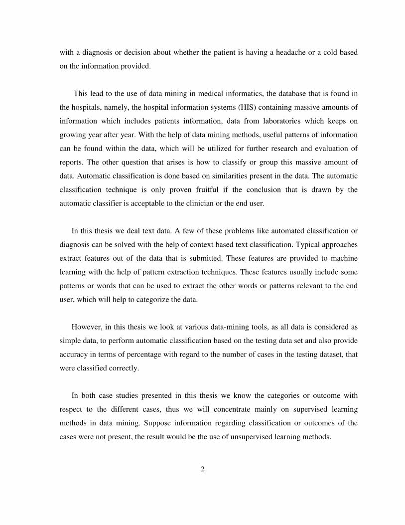
In this thesis we deal text data. A few of these problems like automated classification or
diagnosis can be solved with the help of context based text classification. Typical approaches
extract features out of the data that is submitted. These features are provided to machine
learning with the help of pattern extraction techniques. These features usually include some
patterns or words that can be used to extract the other words or patterns relevant to the end
user, which will help to categorize the data.
However, in this thesis we look at various data-mining tools, as all data is considered as
simple data, to perform automatic classification based on the testing data set and also provide
accuracy in terms of percentage with regard to the number of cases in the testing dataset, that
were classified correctly.
In both case studies presented in this thesis we know the categories or outcome with
respect to the different cases, thus we will concentrate mainly on supervised learning
methods in data mining. Suppose information regarding classification or outcomes of the
cases were not present, the result would be the use of unsupervised learning methods.

3
Although none of the data makes any sense to the complier or the machine learning
algorithms, text data are rather easier for classification and categorization than other types of
data. Also with text data, results are more accurate and are obtained more quickly than with
other types of data.
With mobile computing dominating the market it is possible to build software on mobile
or hand held devices such as a PDA or a smart phone. These devices are handier than
laptops and allow for easier access at all times. The drawback of today’s PDAs is that they
have low computing power and small storage capacity. Thus, running these algorithms on
PDA is not feasible due to these factors.
Lastly, some of the data mining algorithms make use of rules, which are required for
categorization. Rules are obtained based on patterns present in the training data set, which are
extracted by the various data mining algorithms. This rule-based stage can be performed on a
desktop. Once these rules are obtained they can be stored on a PDA. Inputs regarding the
patient can be fed to the PDA and classification of the input can take place based on the rules
stored in the device in real time.
1.1 Motivation:
There are numerous data mining tools and methods available today. Although
machine intelligence tools have been used for flying airplanes, sending rockets to space, the
use of machine intelligence with health related databases has been limited. Machine
intelligence can be used as a second opinion for clinical classification. In this thesis, we will
compare two case studies, both of which are related to health care.
The first database is used to classify data that is related to breast cancer and the
second is related to mental health care. The main case study is related to mental healthcare
and has 455 attributes for classification. The system we are trying to automate is the
minimum data set for mental health (MDS-MH). The MDS-MH system can be considered as

4
the minimum number of questions that need to be answered for a proper diagnosis of mental
health.
Although there are a number of data mining tools in the market today, we use a few
of these tools to evaluate and draw to a conclusion on which is the best tool that can be used
for the MDS-MH database.
1.2 Goals and Objectives:
The application of artificial intelligence in healthcare is relatively new. The aim of
this thesis is to show that data mining can be applied to the medical databases, which will
predict or classify the data with a reasonable accuracy. For a good prediction or classification
the learning algorithms must be provided with a good training set from which rules or
patterns are extracted to help classify the testing dataset.
A number of data mining algorithms will be used in this work to show the drawbacks
and advantages. One of the tools has a built in preprocessing tool. A preprocessing tool is
used to convert raw data into a format understandable by the data-mining algorithm. The rest
of the tools require data to be sent to the algorithms in various formats. This will be
explained in detail in Chapter 2 of this thesis.
Once the testing data is classified with reasonable accuracy, the rules that are required
for classification can be extracted and placed on a mobile computing device such as a
handheld computer. Thus, once the data is inputted into the handheld, classification can be
done based on the rules that are stored in them. This will result in classification of data based
on the rules which does not require a lot of computation and is suitable for PDAs.

5
1.3 Thesis Outline:
Chapter 2 provides the general background and reviews the literature on data mining
models. Some of the models using similar problems are described. The background literature
of knowledge discovery, health informatics, data mining and the different types of tools that
are used in text mining are mentioned in detail.
Chapter 3 presents the system architecture and the model that was used for
implementation in the thesis. This chapter is mainly used for understanding the process in
getting the data till producing results using the data mining tools.
Chapter 4 consists of experiments that are designed for the two case studies using
different data mining tools that are described in Chapter 3. We show the accuracy obtained
for various classifications for the different tools. We draw some conclusion in Chapter 5
about the suitability of the tools for health informatics.

6
Chapter 2
Background and Literature Review
With the evolution of machines, we have found that some tiring and routine or
complex mathematical calculations can be done using calculators, finding specific
information in a large database can be done using machines fast and easily. We use machines
for storing information, remind us of appointments, and so on. As the size of the data was
increasing computer storage has increased. Due to the vast amount of data that was being
created humans invented algorithms that produce results once a query is supplied. Although
these tools perform very well, they can be used to perform only routine tasks. Automatic
classifications and other machine intelligence algorithms cannot be done using standard
database languages. This has led to the creation of machine intelligence algorithms that can
perform tasks supplied by humans and make decisions without human supervision. From the
evolution of machine intelligence came data mining. In data mining, algorithms seek out
patterns and rules within the data from which sets of rules are derived. Algorithms can
automatically classify the data based on similarities (rules and patterns) obtained between the
training on the testing data set.
Today, data mining has grown so vast that they can be used in many applications;
examples include predicting costs of corporate expense claims, in risk management, in
financial analysis, in insurance, in process control in manufacturing, in healthcare, and in
other fields.
Let us consider an example in health care. The number of people feeling sick and
getting admitted into clinics and hospitals are increasing proportionally. The growing number
of patients indirectly increases amount of data that are required to be stored. If a small
number of patients, visit a doctor during a given redundant, the doctor will be able to work
efficiently and provide proper care of the patient. Now consider the case when there is a large

7
number of patients’ coming to meet this doctor in the same period. We will find the quality
of care of the doctor will decrease. If the doctor has another colleague at his side he can at
times ask him for a second opinion before making decisions about the patient.
The idea of having a colleague next door at all times is not a feasible solution. Using
computers to provide a second opinion to the doctor can be a feasible solution. The
computers will search for patterns within the database and will provide the doctor with a fast
opinion of what the diagnosis of the patient could be.
2.1 Machine Learning:
Machine Learning is the study of computer algorithms that improve automatically
through experience [3]. Applications of machine learning range from data mining programs
that discover general rules in large data sets, to information filtering systems that
automatically learn users' interests. Machine learning can be used to develop systems
resulting in increased efficiency and effectiveness of the system.
Machine learning is also called concept learning. That is, computers can learn
concepts and patterns within the data. Machine learning is considered successful when it can
correctly find all the instances that consist of the right patterns and concepts. Although at
times a machine cannot categorize correctly all the instances due to high variations in
attributes present in the data.
8
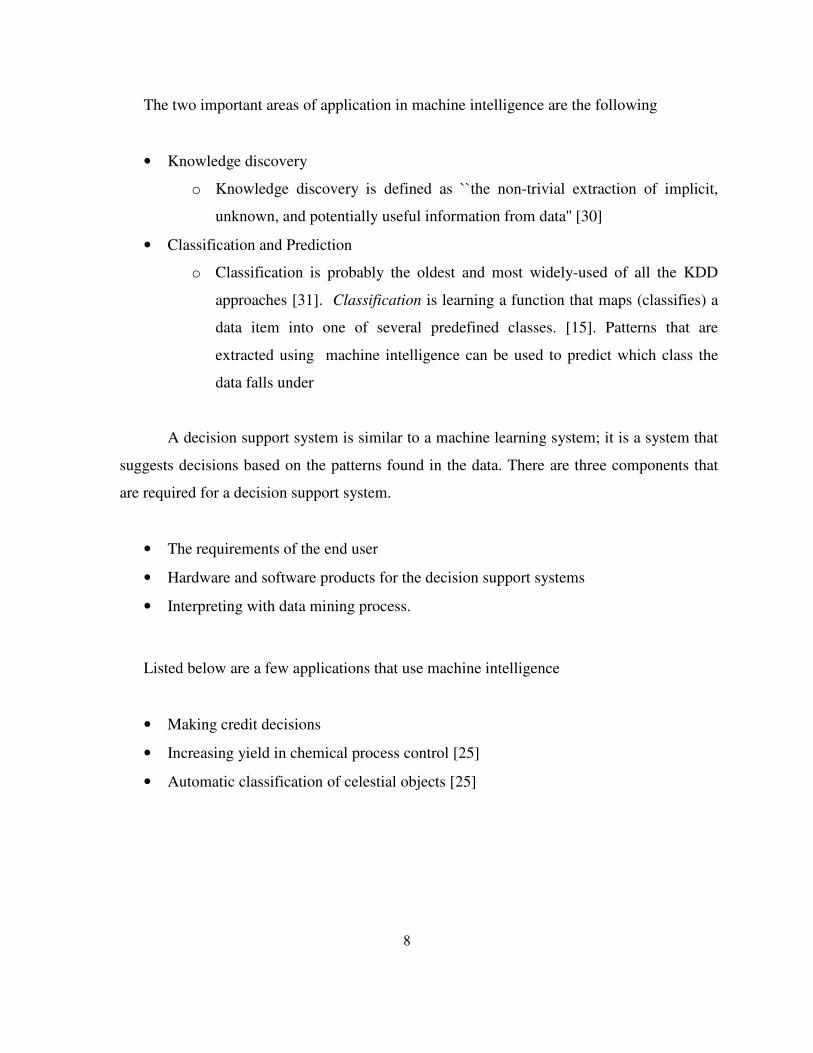
The two important areas of application in machine intelligence are the following
• Knowledge discovery
o Knowledge discovery is defined as `̀the non-trivial extraction of implicit,
unknown, and potentially useful information from data'' [30]
• Classification and Prediction
o Classification is probably the oldest and most widely-used of all the KDD
approaches [31]. Classification is learning a function that maps (classifies) a
data item into one of several predefined classes. [15]. Patterns that are
extracted using machine intelligence can be used to predict which class the
data falls under
A decision support system is similar to a machine learning system; it is a system that
suggests decisions based on the patterns found in the data. There are three components that
are required for a decision support system.
• The requirements of the end user
• Hardware and software products for the decision support systems
• Interpreting with data mining process.
Listed below are a few applications that use machine intelligence
• Making credit decisions
• Increasing yield in chemical process control [25]
• Automatic classification of celestial objects [25]

9
2.1.1 Knowledge Discovery in databases [KDD] and data mining:
Traditional methods (Methods used before computers where introduced into
healthcare) use manual analysis to find patterns or extract knowledge from the database. For
example in the case of health care, the health organizations (E.g. The Center for Disease
Control in the US) analyze the trends in diseases and the occurrence rates. This helps health
organizations take precautions in future in decision making and planning of health care
management.
The traditional method is used to analyze data manually for patterns for the extraction
of knowledge. Take any field like banking, mechanic, healthcare, and marketing; there will
always be a data analyst to work with the data and analyzing the final results. The analyst
acts like an interface between the data and knowledge. We can, using machine intelligence
assist the analyst to produce similar results or knowledge from the data.
When we encounter patterns within a database we state the findings (patterns or rules)
as data mining, information retrieval or knowledge extraction and so on. The term data
mining is used mostly by statisticians, data analysts and the management information
systems (MIS) [7]. The difference between data mining and knowledge discovery is that the
latter is the application of different intelligent algorithms to extract patterns from the data
whereas knowledge discovery is the overall process that is involved in discovering
knowledge from data. There are other steps such as data preprocessing, data selection, data
cleaning, and data visualization, which are also a part of the KDD process.

10
2.1.2 The KDD Process
Knowledge discovery is the process of automatically generating information
formalized in a form “understandable” to humans [8].
Figure 1 Overview of the steps involved in the KDD process [1]
Three components are required for the KDD process, which are the following:
• A goal is the outcome we need to find from analyzing the data; Example: how many
people with X Y Z symptoms died with cancer?
• A database is where all the data and information about the system is located. Usually
this stage is used to know the background information. This information provided
will be related with the training data or examples provided which is used for the next
stage. Example, what does this attribute in the database stand for?
• A set of training examples, as described earlier, the system that is created is
automated, meaning the user only have to put in the database and information about
what he needs to find. First the system should be trained so that it can analyze the
similarities between various attributes of the training examples. The rules obtained
can be used to predict the outcomes in the testing examples.

11
An outline of the steps that are in Figure 1 will be adequate for understanding the
concepts required for the KDD process. The following are the steps involved :
STEP 1:- The first step is to predefine our mission or a goal before discovering
knowledge. We also have to point out from which database we can obtain the knowledge.
STEP2:- Consider a case where we have millions of data points. We have to select a
subset of the database to perform the required knowledge discovery steps. Selection is the
process of selecting the right data from the database on which the tools in data mining
can be used to extract information, knowledge and pattern from the provided raw data.
STEP3:- Data preprocessing and data cleaning. In this step we try to eliminate noise that
is present in the data. Noise can be defined as some form of error within the data. Some
of the tools used here can be used for filling missing values and elimination of duplicates
in the database.
STEP 4:- Transformation of data in this step can be defined as decreasing the
dimensionality of the data that is sent for data mining. Usually there are cases where there
are a high number of attributes in the database for a particular case. With the reduction of
dimensionality we increase the efficiency of the data-mining step with respect to the
accuracy and time utilization.
STEP 5:- The data mining step is the major step in data KDD. This is when the cleaned
and preprocessed data is sent into the intelligent algorithms for classification, clustering,
similarity search within the data, and so on. Here we chose the algorithms that are
suitable for discovering patterns in the data. Some of the algorithms provide better
accuracy in terms of knowledge discovery than others. Thus selecting the right
algorithms can be crucial at this point.
12
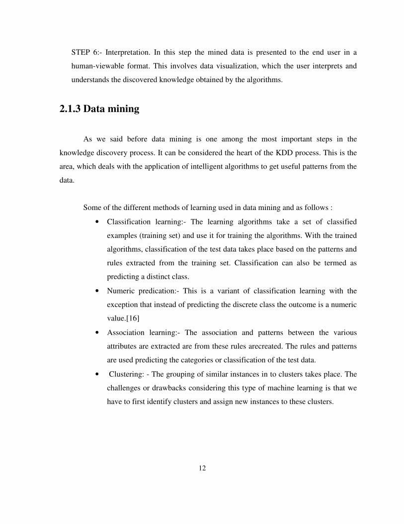
STEP 6:- Interpretation. In this step the mined data is presented to the end user in a
human-viewable format. This involves data visualization, which the user interprets and
understands the discovered knowledge obtained by the algorithms.
2.1.3 Data mining
As we said before data mining is one among the most important steps in the
knowledge discovery process. It can be considered the heart of the KDD process. This is the
area, which deals with the application of intelligent algorithms to get useful patterns from the
data.
Some of the different methods of learning used in data mining and as follows :
• Classification learning:- The learning algorithms take a set of classified
examples (training set) and use it for training the algorithms. With the trained
algorithms, classification of the test data takes place based on the patterns and
rules extracted from the training set. Classification can also be termed as
predicting a distinct class.
• Numeric predication:- This is a variant of classification learning with the
exception that instead of predicting the discrete class the outcome is a numeric
value.[16]
• Association learning:- The association and patterns between the various
attributes are extracted are from these rules arecreated. The rules and patterns
are used predicting the categories or classification of the test data.
• Clustering: - The grouping of similar instances in to clusters takes place. The
challenges or drawbacks considering this type of machine learning is that we
have to first identify clusters and assign new instances to these clusters.

13
There are several learning methods that can be used within each type of learning
methods (E.g. Decision Tree can be considered as a classification technique, Kth Nearest
Neighbor is considered as a clustering technique) but regardless of the learning methods,
concept is given to the notation on what is to be learned and concept description is the
outcome produced by the instance after the learning procedure.
Out of these four types of learning methods we will be only concentrating our work
on two, namely the classification learning and association rules. A number of different types
of classification and association techniques are mentioned in the next chapter. Classification
type of learning is also called supervised learning and clustering is called un-supervised
learning.
2.1.4 Text mining
Data can exist in many forms such as videos, images and text. Data mining can be
used to extract useful information from any form of data. Text mining is the application of
intelligent algorithms to extract useful information from unstructured text.
In text mining the goal is to discover unknown information. Thus to convert the KDD
process to map in the text mining process we will have to replace all the instances of the
word data in Figure 1 by text in all the steps of the KDD process.
Text mining is important given that many systems include databases with attributes
present in text format. The algorithms in data mining need not be modified for each type of
data. Typically data has to be converted either to text format or to binary format by the
compiler before being classified by the algorithms.

14
Similarly to data mining, text mining has many applications. Some of them are the following:
Retrieving documents: Query processing plays a very important role in efficient
information retrieval. With the help of text mining we will be able to effectively produce
queries that generate better results with respect to the completeness and the effectiveness of
the retrieval process.
Document identification: The goal of automatic-learning algorithms is to analyze
documents based on patterns and categorize them accordingly. This goal is accomplished by
means of keywords, which are used to identify which author has written the document and
also can be used for automatic classification of research papers and journals. This is done by
comparing technical taxonomies, linguistics or even using the frequency count method
(Depending on the frequency of certain words used we can sometimes identify the author) .
Prediction or forecasting: Based on time series, we can use text mining for prediction,
which will prove useful in forecasting and finding the changes that need to be made using
time sensitive patterns.
Other advance cases for the use of text mining are in the area of genomic analysis and
DNA study.
One important issue in text mining is the existence of duplicates and inconsistencies
in the data. Usually there are cases when text is repeated or some attributes are present in two
different scales. There are cases when there are missing attributes. With the help of
preprocessing, we can eradicate to a certain extent most of the noise present in the data. Data
processing results in greater efficiency in running the intelligent algorithms.

15
2.2 Health informatics [17]
Healthcare is a very research intensive field and the largest consumer of public funds.
With the emergence of computers and new algorithms, health care has seen an increase of
computer tools and could no longer ignore these emerging tools. This resulted in uniting of
healthcare and computing to form health informatics (Health informatics exists since the
1950’s). This is expected to create more efficiency and effectiveness in the health care
system, while at the same time, improve the quality of health care and lower cost.
Health informatics is an emerging field. It is especially important as it deals with
collection, organization, storage of health related data. With the growing number of patient
and health care requirements, having an automated system will be better in organizing,
retrieving and classifying of medical data. Physicians can input the patient data through
electronic health forms and can run a decision support system on the data input to have an
opinion about the patient’s health and the care required. An example in the advances in
health informatics can be the diagnosis of a patient is health by a doctor practicing in another
part of the world. Thus healthcare organizations can share information regarding a patient
which will cut costs for communication and at the same time be more efficient in providing
care to the patient.
There are other issues like data security and privacy, which is equally important when
considering health related data. Thus Health informatics "deals with biomedical information,
data, and knowledge--their storage, retrieval, and optimal use for problem solving and
decision making"[17]. This is a highly interdisciplinary subject where fields in medicine,
engineering, statistics, computer science and many more come together to form a single field.
With the help of smart algorithms and machine intelligence we can provide the
quality of healthcare by having, problem solving and decision-making systems. Information
systems can help in supporting clinical care in addition to helping administrative tasks. Thus

16
the physicians will have more time to spend with the patients rather than filling up manual
forms.
First the paper forms that are filled by the physicians are converted into electronic
forms. Programs can be built around these forms to help in input validations. Some of the
validation steps can be in the form of cautions provided when fields are inputted with invalid
values; another type of validation can be to make sure attributes of high priority are not left
empty by the user.
The informatics part of health care can take care of the structuring; searching,
organizing and decision making with the emergence in health informatics came many
important research ideas and fields of study. One among them is the Resident Assessment
Instrument (RAI).
2.2.1 Inter-Resident Assessment Instrument (Inter-RAI):
The Inter-RAI is a comprehensive standardized instrument for evaluating the needs,
strengths and preferences of psychiatric patients in institutional settings [10]. Inter-RAI aims
at patients with acute care and long term needs. Inter-RAI consists of a collection of patient
assessment instruments, which are used to gather information, such as patient’s strengths and
needs, and are also used to develop individual care plans for different patients. These
assessments can be updated according to the patients’ health which should improve the care
that is provided to the patient. The Inter-RAI is basically a structured idea of how to produce
a well-defined approach to identify the problem with respect to treating a patient who
requires long-term care. There are more than eight different types of Inter-RAI assessment
instruments. These set of assessments are customized according to the patients requirements,
thus not all the patients will have the same assessment form, which means a patient with
acute care needs with regard to old age facilities will have different assessment forms as
compared to one who requires acute care in mental health. The forms have all the
information or questions that are related for a particular assessment.

17
In Inter-RAI there are a number of forms that are required for diagnosis
corresponding to certain health care issues such as with some acute care or diagnosis of
patients with mental health. The Inter-RAI collection of instruments is also a kind of
minimum data set instruments. This can be considered as the minimum number of questions
that are required to make a proper diagnosis of a patient with respect to a certain acute
problem.
All well-defined problem identification process follows similar steps as mentioned
below where RAP is the resident assessment protocol.
Figure 2 Assessment format for the Inter-RAI system
The end result of implementing these forms is, improved resident care and better
quality of life due to the thorough diagnosis of the patient with the help of the Inter-RAI
forms. Increasing attention provided to each resident should result in the patient responding
better to treatment. Clinical staff will have a clearer picture having all the documentations of
the patient in hand and thus producing effective communication between staff members and
individual residents. The documentation of the Inter-RAI is clear and there will be only one
answer to each question. With proper documentation there should be fewer clerical errors
and, at the same time, educating new staff members will be easier.
Assessment (MDS / other)
Decision –Making (RAPs / other)
Care Plan Development
Care Plan Implementation
Evaluation

18
The RAI consists of three basic components they are as follows
• Minimum data set (MDS)
MDS, as the name suggests is the minimum data which is required to consider a
proper care of a patient with long term health care need with regard to diagnosis in mental
healthcare, acute care or assessment of chronic care/ nursing home. The patients’ needs with
respect to care, problems and conditions of medication are mentioned within this
documentation. The MDS can also be viewed as a screening questionnaire, which can be
used for initial classification or categorization of the patient. The conditions, illness and care
that were provided to the patient before his admission are considered or mentioned within
this set of documents. The questionnaire with regard to MDS Version 2.0, which is available
online, is affixed in the appendix of this thesis. With the help of this questionnaire, we have a
thorough analysis of the patient’s illness and needs with regard to his long term care.
Triggers:- Sometimes during the period of examination, it is found that some
residents respond better to one or the other combinations of MDS attributes. These triggers
are used to identify patients who have the risk in developing some specific functional
problem and require further evaluation using the resident assessment protocol (RAP).
• Resident Assessment protocols (RAP).
Every attribute in the MDS form can be considered as a question that required to be
answered to assess a patient’s needs. Some times the data that is obtained for a particular
attribute will not be sufficient for proper complete assessment, thus we need to provide more
information with regard to this particular attribute.
Thus RAPS can be used to provide individual care to each patient with respect to
social, medical and psychological problems.
19
• Utilization Guidelines
This can be considered as the documentation of the RAI system. Thus there will be no
misunderstanding with regard to attributes and training that will have to be given to
newcomers for completing the RAI-MDS forms. This is very important as this will help
prevent misunderstanding or misrepresentation of attributes during the form filling
procedures.
There are many forms of RAI that have been classified for different sectors of
healthcare. These are a set of forms that will help proper assessment of a patient.
Some of the different types of assessment instruments are as mentioned below
• RAI 2.0 used for assessment in chronic care/ nursing home [10]
• RAI-HC used in home care [10]
• RAI-MH used in diagnosis of mental health [10]
• RAI-AC for Acute care [10]
• RAI-PAC Post-Acute Care- Rehabilitation [10]
The advantage of the RAI system is that they are integrated with one another. There
are a number of applications for the RAI systems. RAI/MDS data is mainly used for care
planning, determining quality indicators, outcome measurement, case-mix-based funding and
determining eligibility for services. [10]
In this thesis we are concentrating on the use of data that is obtained from RAI-MH.
The MDS-MH is an assessment instrument for psychiatric patients. The presence of an
accurate MDS-MH assessment lays the groundwork for the tasks that will follow : problem
identification, determining problem cause, consequence and specification of care goals and
necessary approach to the case [12]. The assessment form deals with all the information that
is required to give proper health care to patients with long time mental problem and care. The

20
assessment forms give information regarding which of the four categories will a patient be
admitted looking at the various attributes in the assessment form.
The four categories of patient classification are
• Acute Care
• Longer term patient
• Forensic patient
• Psychogeriatric patient
The RAI-MH has data obtained from 43 hospitals with around 4000 patients. There
are 455 attributes that are used for the classification of the patient into the four major
categories in mental healthcare.
Some of the sections that are present in the minimum data set for mental health
(MDS-MH) are the following:
• Name and identification numbers
• Referral items
• Mental health service history
• Assessment information
• Mental state indicators
• Substance use and extreme behavior
• Harm to self and others
• Behavior disturbance
• Self care
• Medications
• Health conditions and possible medication side effects
• Service utilization and treatment

21
An advantage of the MDS-MH is some of the attributes with respect to the patient are
based on time series. Thus we can refer to an attribute of importance to the clinician over a
particular period to check on the improvements and changes that need to be made with
respect to patient care. In most cases the information is obtained from the patient or a person
representing the patient, this means that all the information obtained in first hand.
2.3 Summary
This chapter provides an overview of the different components that are required for
the architecture of the PDS based system. It also overviews different components such as,
MDS-MH and machine intelligence. The case study which will be explained in the following
chapters will focus mainly on the data obtained from the MDS-MH database. The next
chapter is focused on the different types of the data mining algorithms and tools that will be
used for running different experiments described in this thesis. The next chapter also includes
the preprocessing stages, and forms the center of the thesis.
22
Chapter 3
System Architecture and model 3.1 System architecture
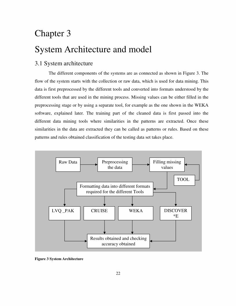
The different components of the systems are as connected as shown in Figure 3. The
flow of the system starts with the collection or raw data, which is used for data mining. This
data is first preprocessed by the different tools and converted into formats understood by the
different tools that are used in the mining process. Missing values can be either filled in the
preprocessing stage or by using a separate tool, for example as the one shown in the WEKA
software, explained later. The training part of the cleaned data is first passed into the
different data mining tools where similarities in the patterns are extracted. Once these
similarities in the data are extracted they can be called as patterns or rules. Based on these
patterns and rules obtained classification of the testing data set takes place.
Figure 3 System Architecture
Raw Data
CRUISE
Preprocessing the data
LVQ _PAK
Filling missing values
WEKA
Formatting data into different formats required for the different Tools
DISCOVER*E
Results obtained and checking accuracy obtained
TOOL
23
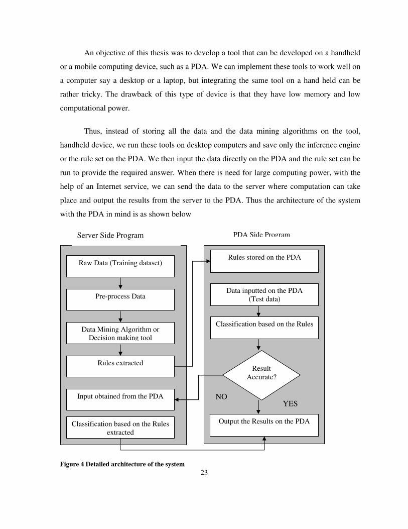
An objective of this thesis was to develop a tool that can be developed on a handheld
or a mobile computing device, such as a PDA. We can implement these tools to work well on
a computer say a desktop or a laptop, but integrating the same tool on a hand held can be
rather tricky. The drawback of this type of device is that they have low memory and low
computational power.
Thus, instead of storing all the data and the data mining algorithms on the tool,
handheld device, we run these tools on desktop computers and save only the inference engine
or the rule set on the PDA. We then input the data directly on the PDA and the rule set can be
run to provide the required answer. When there is need for large computing power, with the
help of an Internet service, we can send the data to the server where computation can take
place and output the results from the server to the PDA. Thus the architecture of the system
with the PDA in mind is as shown below
Figure 4 Detailed architecture of the system
Data Mining Algorithm or Decision making tool
Raw Data (Training dataset)
Pre-process Data
Rules extracted
Data inputted on the PDA (Test data)
PDA Side Program
Rules stored on the PDA
Classification based on the Rules
Output the Results on the PDA
Input obtained from the PDA
Classification based on the Rules extracted
Result Accurate?
YES NO
Server Side Program

24
3.2 Data preprocessing
Each algorithm requires data to be submitted in a specified format. The generation of raw
data into machine understandable format is called preprocessing. Other steps that are
performed during preprocessing are the transformation of the attributes in the database into a
single scale and the replacement of all the missing values in the data.
• Machine understandable format
Raw data can be stored in several formats, including text, Excel or other database
types of files. Sometimes the raw data is not in any format.
Having data already in a format understandable by algorithms can result in better time
efficiency with respect to processing of the data. In most cases the rows represent a single
case and columns represent the attributes that are present within this case. In some of the free
databases that are available online most of them are in comma separated value (CSV) format.
That is all the attributes are separated by commas and two commas simultaneously stands for
a missing data attribute. Sometimes when attributes are missing, instead of finding an empty
space we may find a question mark in place of the missing attribute.
In the WEKA tool for example, the data should be stored in the Attribute-Relation
File Format (.ARFF format) as the data type of the attributes must be declared. The system
does not automatically classify the attribute as being real or categorical. An example of the
ARFF format will be described in the next section of the chapter.
The Wisconsin breast cancer database is described below to illustrate how the
preprocessing is done to provide inputs to each of the machine intelligent tools that were
used.

25
3.2.1 Raw data
The raw data usually has a great deal of noise. Raw data cannot be used
directly for processing, with the machine-learning algorithms. They first need to be
preprocessed into machine understandable format. The breast cancer database of Wisconsin
[29] is considered as an example to demonstrate preprocessing.
The data type of the attributes with the raw data are given below
# Attribute Domain
-- -----------------------------------------
1. Sample code number id number
2. Clump Thickness 1 - 10
3. Uniformity of Cell Size 1 - 10
4. Uniformity of Cell Shape 1 - 10
5. Marginal Adhesion 1 - 10
6. Single Epithelial Cell Size 1 - 10
7. Bare Nuclei 1 - 10
8. Bland Chromatin 1 - 10
9. Normal Nucleoli 1 - 10
10. Mitoses 1 - 10
11. Class: (2 for benign, 4 for malignant)
A row represents one patient’s case with values of attributes mentioned above separated by a
comma. Examples of a few cases in the data set are as follows:
1016277,6,8,8,1,3,4,3,7,1,2
1017023,4,1,1,3,2,1,3,1,1,2
1017122,8,10,10,8,7,10,9,7,1,4
26
In the database the attribute ID number will not contribute any information towards
the machine intelligence in determining whether the person has cancer or not so that column
will be removed from all the cases within the database.
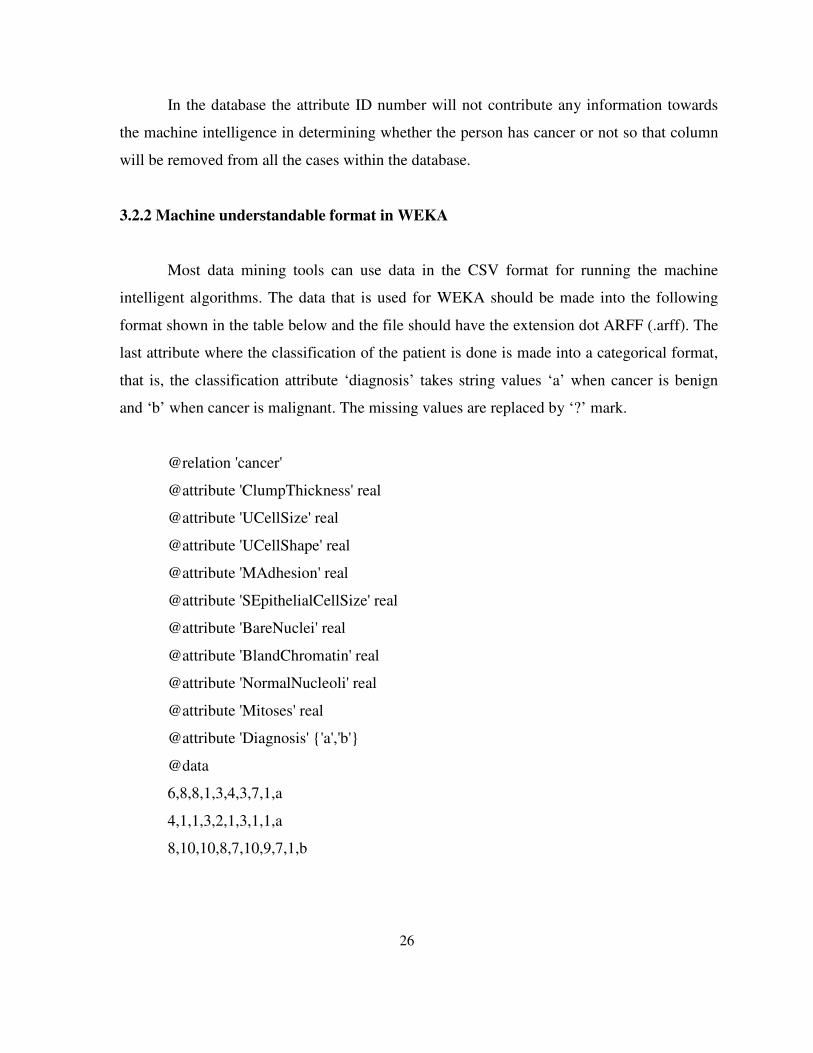
3.2.2 Machine understandable format in WEKA
Most data mining tools can use data in the CSV format for running the machine
intelligent algorithms. The data that is used for WEKA should be made into the following
format shown in the table below and the file should have the extension dot ARFF (.arff). The
last attribute where the classification of the patient is done is made into a categorical format,
that is, the classification attribute ‘diagnosis’ takes string values ‘a’ when cancer is benign
and ‘b’ when cancer is malignant. The missing values are replaced by ‘?’ mark.
@relation 'cancer'
@attribute 'ClumpThickness' real
@attribute 'UCellSize' real
@attribute 'UCellShape' real
@attribute 'MAdhesion' real
@attribute 'SEpithelialCellSize' real
@attribute 'BareNuclei' real
@attribute 'BlandChromatin' real
@attribute 'NormalNucleoli' real
@attribute 'Mitoses' real
@attribute 'Diagnosis' {'a','b'}
@data
6,8,8,1,3,4,3,7,1,a
4,1,1,3,2,1,3,1,1,a
8,10,10,8,7,10,9,7,1,b

27
3.2.3 Machine understandable format in CRUISE
Two files are required for the compilation of the database with respect to the CRUISE
software. One file contains the description of the attribute and the other file consists of all the
data that is present in the database. In the description file “bcancerwis.txt”, is the file where
the data is located and ‘?’ is used as a code for missing values. The rest of the data consists of
information about the different attributes, e.g. ‘c’ in vartype means the attributes is
categorical. In these cases ‘n’ means the attribute is numerical and‘d’ means that the attribute
is dependent and so on.
The description file appears as follows
bcancerwis.txt
?
column,varname,vartype
1,ClumpThickness,n
2,UCellSize,n
3,UCellShape,n
4,MAdhesion,n
5,SEpithelialCellSize,n
6,BareNuclei,n
7,BlandChromatin,n
8,NormalNucleoli,n
9,Mitoses,n
10,Diagnosis,d
The data file is a CSV format file
6,8,8,1,3,4,3,7,1,a
4,1,1,3,2,1,3,1,1,a
8,10,10,8,7,10,9,7,1,b

28
The data used as input in CRUISE looks similar to the one used in WEKA. The
difference between the two is that, in WEKA the descriptive file of the attributes is present
within the dataset and in the case of CRUISE there are two files which need to be inputted to
the tool, one containing the description of the attributes and another containing the dataset as
shown above.
3.2.4 Machine understandable format in Discover*E
For the Discover*E tool the data is provided in a similar format as the CSV
file with the name of the attributes at the first line of the data set. This data set is first sent
through the Importer tool which automatically converts the data into the machine
understandable format for the Discover*E tool. The file that is created has a dot mining
(.mining) as the extension of the processed file.
Raw data in CSV format provided to the importer tool.
ClumpThickness,UCellSize,UCellShape,MAdhesion,SEpithelialCellSize,BareNuclei,
BlandChromatin,NormalNucleoli,Mitoses,Diagnosis
6,8,8,1,3,4,3,7,1,a
4,1,1,3,2,1,3,1,1,a
8,10,10,8,7,10,9,7,1,b
Preprocessor tool that is present in Discover*E software.
Unlike the other tools, the data need not be stored in a particular format. The data, which
is provided above, is in the CSV format with “?” representing the missing data in the
database. This tool makes the data into a format suitable for this tool to provide data analysis
easily. Some of the functions performed in this tool are the following :

29
• Data sampling
• Attribute exclusion
• Feature attribute selection
The preprocessor creates two files one in Text format and another file with the extension
‘miningdata’. The text file contains the case where the user can see what is used as an input
to the Discover *E tool. The miningdata file is used as the input to the various tools that is
present in the Discover*E tool.
3.2.5 Machine understandable format in Learning Vector Quantization
In the LVQ the data presented to the tool is not in the CSV format. The attributes are
separated by space and the missing value is represented by ‘x’. The number of attributes that
are present to make the diagnosis should also be specified. If we look at the example of the
raw data given below we see that there are 9 attributes that are required for the classification
attribute mentioned in the last column. Thus the number 9 has to be mentioned in the first
line of the dataset, which relates to the number of attributes that are present. Also all the
attributes should be given in real numbers.
The first few lines of the data looks like this :
9
6.0,8.0,8.0,1.0,3.0,4.0,3.0,7.0,1.0,a
4.0,1.0,1.0,3.0,2.0,1.0,3.0,1.0,1.0,a
8.0,10.0,10.0,8.0,7.0,10.0,9.0,7.0,1.0,b

30
3.2.6 Filling up missing and incomplete values
Sometimes there are attributes that are incomplete or missing. A common method of
representing missing data, is inputting values that cannot be found in the data e.g. represent
missing data as “-1”. If an attribute is empty usually one may think that the case is less
useful than the rest of the cases in the data set. This is not true as each of the other attributes
contributes useful information towards the set of attribute category. When there are missing
values, instead of leaving them as missing, there are a number of methods that can be used
for filling these missing attributes.
Having efficient methods to fill up missing values extends the applicability in terms of
accuracy for many data mining methods. The accuracy of the tool is increased and with a
larger training set better rules and decision trees can be developed which contributes towards
better classification of the data.
The most common method of filling the attributes quickly and without too much
computation is to replace all the missing values with the arithmetic mean or the mode with
respect to that attribute. The other methods are to run a clustering algorithm and replace the
missing attributes with the attributes of cases that appear close in an n-dimensional space. In
the WEKA tool the latter method is implemented. The other tools that are used in this thesis
can handle missing values but we have not found instances where the missing values were
replaced by other quantities such as the one displayed in the WEKA tool.

31
3.3 Different Data mining Algorithms and Tools
There are a number of machine intelligent tools that are available in the market but at
the same time not all tools are the best for all problems in the data set. Different data sets will
produce different results based on the algorithms used. In this thesis we will be testing some
algorithms based on decision trees, rule based classification, probability and soft computing.
Our aim is to find the best tool that is available for the RAI-MH tool.
Decision Tree
Decision tree is one of the easier data structure to understand data mining. Rules from
the training dataset are first extracted to form the decision tree which is then used for
classification of the testing dataset. A decision tree is necessarily a tree with an arbitrary
degree that classifies instances. They are a powerful tool for classification and predication
but require extensive computation. Creating the tree based on the training set takes time
although making decisions once the tree is made is not time consuming. Classification tree
algorithms may be divided into two groups: one whose result is a binary tree and other that
yields non-binary trees (also called multiway) splits [13].
In decision trees, the leaf node represents the complete classification of a given
instance of the attribute and the decision node specifies the test that is conducted to produce
the leaf node. Thus with a decision tree, the sub tree that is created after any node is
necessarily the outcome of the test that was conducted.
A decision tree is used to classify a certain instance from the root of the tree till the
leaf node which provides the outcome of that instance. A major issue in using decision tree is
to find out how deep the tree should grow and when it should stop. Usually if all the
attributes are different and lead to the same outcome, the decision tree might not be the most
effective in making decision and, at the same time, the size of the tree will be large.

32
There are a number of algorithms that are based on decision trees. We will be
comparing results of different decision tree based tools to evaluate each for a given dataset.
We hope to determine the decision tree or algorithm that provides better accuracy for the
particular dataset. Some of the most common and effective types of algorithms based on
decision trees are C 4.5, FACT and Classification and Regression Tree (CART) [27].
Discover*E and Weka are based on the C4.5 learning algorithm and Cruise is based on
FACT. The C4.5 is a modified version of the basic ID3 algorithm. (See Appendix A for the
algorithm)
Figure 5 Decision Tree
Before creating the decision tree we create rules that correspond to the paths on the
decision tree. Once the rules are created the decision tree is made. From Figure 5 it is noted
that the decision node is actually an attribute, which is characterized by the values present in
it to describe a symptom or take a decision.
Decision Node Leaf Node

33
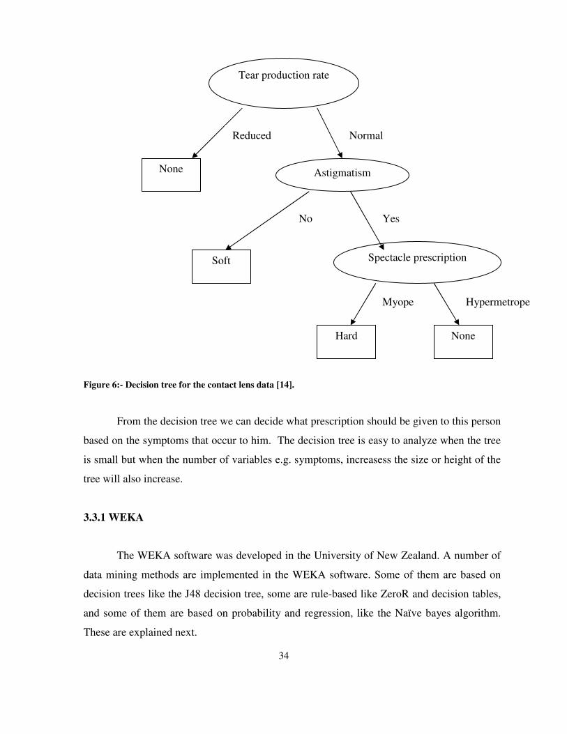
Figure 6 shows a decision tree that used in making decisions about contact lens
research. The subset of the database that is used to create this decision tree and the attributes
that are present in the database are as follows:
Example of the data that is present in the database is
1 1 1 1 1 3
2 1 1 1 2 2
3 1 1 2 1 3
4 1 1 2 2 1
5 1 2 1 1 3
The attributes present in each column represent the following,
Index number
Age of the patient: (1) young, (2) pre-presbyopic, (3) presbyopic
Spectacle prescription: (1) myope, (2) hypermetrope
Astigmatic: (1) no, (2) yes
Tear production rate: (1) reduced, (2) normal
Classification (1) Hard contact lens (2) Soft Contact Lens (3) No Contact Lens
First the rules are extracted from the database. Once the rules are extracted, the rules
are converted into nodes and paths for the tree. Figure 6 represents the decision tree that is
created and the rules that are present in creating the tree can be easily understood and
visualized. This is one of the advantages of a decision tree. Created below is a binary tree
using the rules extracted or provided. Sometimes decision trees are not in binary format when
the attributes are increased and there is a lot of correlation between the data.
34
Figure 6:- Decision tree for the contact lens data [14].
From the decision tree we can decide what prescription should be given to this person
based on the symptoms that occur to him. The decision tree is easy to analyze when the tree
is small but when the number of variables e.g. symptoms, increasess the size or height of the
tree will also increase.
3.3.1 WEKA
The WEKA software was developed in the University of New Zealand. A number of
data mining methods are implemented in the WEKA software. Some of them are based on
decision trees like the J48 decision tree, some are rule-based like ZeroR and decision tables,
and some of them are based on probability and regression, like the Naïve bayes algorithm.
These are explained next.
Tear production rate
Astigmatism
Spectacle prescription
None
Soft
Hard None
Normal Reduced
Yes No
Hypermetrope Myope
35
J48 algorithm method in Weka
The C4.5 algorithm is a part of the multiway split decision tree. C 4.5 yields a binary
split if the selected variable is numerical, but if there are other variables representing the
attributes it will result in a categorical split. That is, the node will be split into C nodes where
C is the number of categories for that attribute [13]. The J4.8 decision tree in WEKA is based
on the C4.5 decision tree algorithm. The C4.5 learning algorithm is described in Appendix
A. In section 4.1.1 more details are given on the tree that is obtained using the J4.8 tool.
ZeroR method in Weka
In the ZeroR method, the result is the class that is in majority when the attributes are
categorical and, when they are numerical. For example, when we consider the data for
Cancer if there is an attribute with just Yes and No options, if the Yes class occurs for a
majority then the output for ZeroR for this attribute is always Yes. Thus the ZeroR is always
considered as the base case for data mining. Applications that work on the principles of data
mining should not provide results worse than ZeroR.
Decision table method in Weka
Machine learning algorithms are designed to educate themselves based on the
patterns and rules extracted from the training dataset. Thus having a good training set can
improve the efficiency with respect to the extraction of rules and patterns. There are two
ways to selecting the attribute subset. The first consists of using the “filter method” where
attributes are filtered to have the best set of outcome before the learning procedure. The
second consists of the “wrapper method” where the learning method is placed within the
selection procedure. The decision table that is used in WEKA does attribute selection using
the wrapper method. Attributes are based on measuring the cross validation performance for
different subsets of attributes and choosing the best performing subset. If some of the cases
are not classified using the wrapper method in the decision table, the majority class from the
36
training dataset is assigned to these cases. There is also an option in WEKA where one can
set the closest match to that instance, which improves performance of the tool significantly.
Naïve Bayes method in Weka
This method is based on probabilistic knowledge. This method goes by the name
Naïve Bayes, because it’s based on Bayes’s rule and “naively” assumes independence- it is
only valid to multiply probabilities when the events are independent [16]. Thus the naïve
bayes rule outputs probabilities for the predicted class of each member of the set of test
instance. Naïve Bayes is based on supervised learning. The goal is to predict the class of the
test cases with class information that is provided in the training data.
The Naïve Bayes classification reads a set of examples from the training set and uses
the Bayes theorem to estimate the probabilities of all classifications. For each instance, the
classification with the highest probability is chosen as the prediction class.
The naïve Bayesian classifier traditionally makes the assumption that a single
Gaussian distribution generates numeric attributes [12]. Two types of Naïve Bayes
algorithms are mentioned below:
• Naïve Bayes (NB)
• Simple Naïve Bayes (SNB)
The difference between the two is that in NB the probability of the attributes are
calculated based on normal distribution’s mean, standard deviation, weighted sum, and
precision but SNB is only based on mean and standard deviation. In this thesis we use NB
method while running the experiments.

37
3.3.2 Classification Rule with Unbiased Interaction Selection and Estimation
(CRUISE).
CRUISE is a powerful data-mining tool based on decision tree classification. It is
based on an older classification tree algorithm called Fast Algorithm for classification trees
(FACT) [28]. It has fast computational speed because it employs multiway splits; this
precludes the use of greedy search methods [11]. (In greedy methods at each stage in a
problem we don’t have to find solutions of the sub problems, we just assign what solution
looks best at the moment). There are some unique features in the FACT tree as compared to
the Binary split type of tree. For instance, unlike some decision trees the nodes in FACT are
split according to the number of classes that are present for the attribute. Therefore, there will
a path or a permutation for all possible combination of the attributes.
There are a number of different formats that can be implemented in decision
algorithm tree, for instance, there are decision trees with a univariate split and there are other
trees with a linear combination split and others with multiway split.
3.3.3 Discover* E.
The Discover*E tool is similar to WEKA in the sense that it includes number of
decision making algorithms built in. This tool is used to explore the different data mining
activities, utilizing algorithms that where developed by Pattern Discovery Software Systems
Ltd and the PAMI lab of the University of Waterloo. Algorithms that are used in this
software are based on probability, decision trees and association rules.
There are three tools that are used for classification :
• Decision tree
• Rule based
• Dependence tree

38
Decision tree Classification.
Similarly to the WEKA software, the decision tree that is used in Discover*E is based
on the C4.5 algorithm with some changes. The decision tree creates a classification tree that
is based on the categorical and classification objects that are present in the database. Once the
classification tree is created, rules are extracted from the tree and the classification of the test
data is conducted. There is also a graphical image of the tree that is provided which will help
us in understanding and traversing the tree. ( See Appendix A for a description of the C4.5
algorithm.)
The decision tree for Discover*E works as follows,
The decision tree tool reads the data that is provided to it in the ‘miningdata’ file
format. The tree is created based on the rules extracted. The results obtained are stored in an
XML file where as, the rule set extracted are stored in a rule-set file in the ‘miningdata’
format.
Rule based classification
Rule based classification is another alternative in data mining to the decision tree method.
Thus a rule can be broken up into two parts, the condition (IF) can be considered as one of
the tests that are used at the decision node of the decision tree and the conclusion (THEN)
that is drawn stands for the classification of the case when this rule is considered. An
example of a rule is If A = 1 and B = 3 then C = True. Thus in the above example “If A = 1
and B = 3” can be considered as a test and the conclusion that is drawn “C = True” is
considered as the conclusion or the classification of the test conducted.
Another point that needs to be made is that there exists another kind of rule-based
classification called the association rule. Although the association rule is very similar to the
classification rule, a difference is that association rule can predict any attribute as well as the

39
final classification and it can be also used to predict any combination of attributes. Thus there
can be a number of association rules that are obtained from a small database. This is the
principle used in the Association discover tool in Discover*E.
For the rule based classification method in Discover*E there are two components that
are required simultaneously: Association discovery and rule based classifier.
• Association discovery
This is used to extract the patterns and rules that are present within the data. A
relationship between the attributes is created. For example, when attribute A has a certain
value the attribute B will have this value. Relations like this are developed and once a
relation is created between the attributes it is easy for categorization and classification.
The tool discovers higher order event association between the attributes and the algorithm
is based on the US patent 5809299.
• Rule classifier model
In this tool, the patterns are provided with weights (scores or points) and significant
patterns are converted to rules. The weights are allocated based on the number of times
each pattern is discovered. If similar patterns are discovered more than once the weights
allocated to them are increased. The rules are also provided with weights and then each
object in the test data is classified one at a time with this tool. This algorithm is also a
part of the patent mentioned above.

40
Dependence Tree Classification:
The dependence tree is based on probability, which is based on the second order
mutual information and maximum spanning tree. With the obtained probabilities the tool
classifies the test data. A tree, similar to a decision tree is created but based on the
probability of occurrence of different attributes. Once the higher order probabilities and the
dependence tree is created the classification then takes place.
3.3.4 LVQ_PAK[20]
The Learning Vector Quantization (LVQ) aims at defining the decision surfaces
between the competing classes. The decision surfaces obtained by a supervised stochastic
learning process of the training data are piecewise-linear hyper planes that approximate the
Bayesian minimum classification error (MCE) probability [19]. This tool is considered a
supervised version of the self-organizing map algorithm [20]. The goal of the algorithm is to
approximate the distribution of the class using a reduced number of class vectors, thus
resulting in minimization of classification errors. This algorithm is similar to the back
propagation algorithm in neural networks [20].
LVQ is based on feed forward neural network algorithm [20].( Feed forward Neural
network is one which has one or more inputs that are propagated through a variable number
of hidden layers where each layer contains a variable number of nodes, which finally reaches
the output layer which contains more than one or more output nodes.) The vector
quantization algorithm sets a number of reference vectors or also called codebook vectors
into a high dimensional space. This is to set the dataset supplied to the algorithm into an
orderly form. The main purpose of learning vector quantization is for statistical classification
that defines class regions in the input data space. A subset of similar vectors is placed into
each class region.

41
There are a number of different implementations with respect to the Learning vector
quantization algorithm a few of them are mentioned below :
• LVQ1
• OLVQ1
• LVQ2.1
• LVQ3
• OLVQ3
The tool implemented in LVQ_PAK can work using most of the above algorithms.
The one used in this research is the OLVQ1, which is the optimized version of the LVQ1
method. In the LVQ1 method a single best matching unit is selected and moved closer or
further away from the testing data set per iteration. In the case of optimized learning vector
quantization each of the codebook vectors has its own learning rate.
A description of the LVQ method along with the formulas are given below,
Assume many of the codebook vectors are assigned to each class of x values and x is
determined to be the same class to which the nearest im belongs. (The variable im is a
parametric reference of code book vector for node i.) Let ||}{||minarg iimxc −= be
defined as the index of the nearest im to ix . c depends on x and all the values of im .and
where t is an integer, that is a discrete time coordinate.
The following equations define the basic LVQ process
• )]()([)()()1( tmtxttmtm ccc −+=+ α if x and cm belongs to the same class
• )]()([)()()1( tmtxttmtm ccc −−=+ α if x and cm belongs to different class
• )()1( tmtm ii =+ for ci ≠ . Here 1)(0 ≤≤ tα where )(tα is the learning rate

42
In the case of OLVQ1 the code book vectors have individual learning rate denoted by
)(tiα and it is assigned to each cm and the following equations are obtained
• )]()([)()()1( tmtxttmtm cccc −+=+ α if x is classified correctly
• )]()([)()()1( tmtxttmtm cccc −−=+ α if x is not classified correctly
• )()1( tmtm ii =+ for ci ≠
The above equation can be expressed as )()()()()]()(1[)( txttstmttstm cccc αα +−=
Where )(ts = +1 if the classification is done correctly and )(ts = -1 if they are
classified wrong.
It is important to know that the training set should be on an average four times larger
than in the testing phase because larger the size of testing set, better will be the accuracy of
the system.
3.4 Summary:
There are a number of data mining algorithms that are found useful for automatic
classification of data. Most of them produce results that are variable in nature. Some
algorithms might work better than others while running one type of data as compared to the
rest. Thus finding the best type of algorithm is an interesting and time consuming work. In
the next chapter we will be running the data mining algorithms mentioned in this chapter on
two medical data sets. One of the data sets is based on breast cancer and the other is based on
the minimum data set for mental health.

43
Chapter 4
Experiments and case study
The experiments will be run on a smaller dataset before addressing the main case
study with respect to the minimum data set that consists of more than 455 attributes. This
will help in understanding the different stages that are used in various data mining
algorithms. The database used is briefed in Chapter 2 and it is related to the breast cancer
Wisconsin data. The database was obtained from the University of Wisconsin Hospitals,
Madison (From Dr. William H. Wolberg [29]).
4.1 Case study for the Wisconsin breast cancer database The objective of this study is to predict whether the tumor or tissue is malignant or
benign from data obtained from the Wisconsin breast cancer database.
Tools that will be tested are as follows:
1. WEKA
a. ZeroR
b. Decision Tree
c. Decision Table
d. Naïve Bayes
2. CRUISE
a. Univariate Split
b. Linear Split
3. Discover*E
a. Decision Tree
b. Dependence Tree
c. Association Rules
4. Learning Vector Quantization

44
The Wisconson database consists of 699 cases. A section from this database will be
used for the testing stage and the rest for training. It is always a good practice to have a larger
set of data for training than for testing. In this case we divide the data set into 500 training
cases and the rest 199 cases for testing the different mining algorithms.
4.1.1 Experiments using WEKA
The front screen of the WEKA software is shown in Figure 7. All the attributes in this
database are displayed in row format in the left half of the screen and on the right side of the
screen the bar graphs represent the distributions of the different attributes that are considered
for data mining.
Figure 7 WEKA software of the main screen

45
a. ZeroR method
The screen shots for the classification tool looks similar to Figure 8. Some of the
screen shots of the WEKA software are shown below. Here the classification tool that is
implemented is the ZeroR. All the classification tools will have similar screens. The bottom
right section of the screen marked with X displays the classifier output.
The classifier outputs results based on the majority class, that is, the outcome of the
experiment which is always the class with maximum number of cases. This is considered the
base case in this thesis and also takes the least computation time.
Figure 8 Classifier output of the ZeroR method
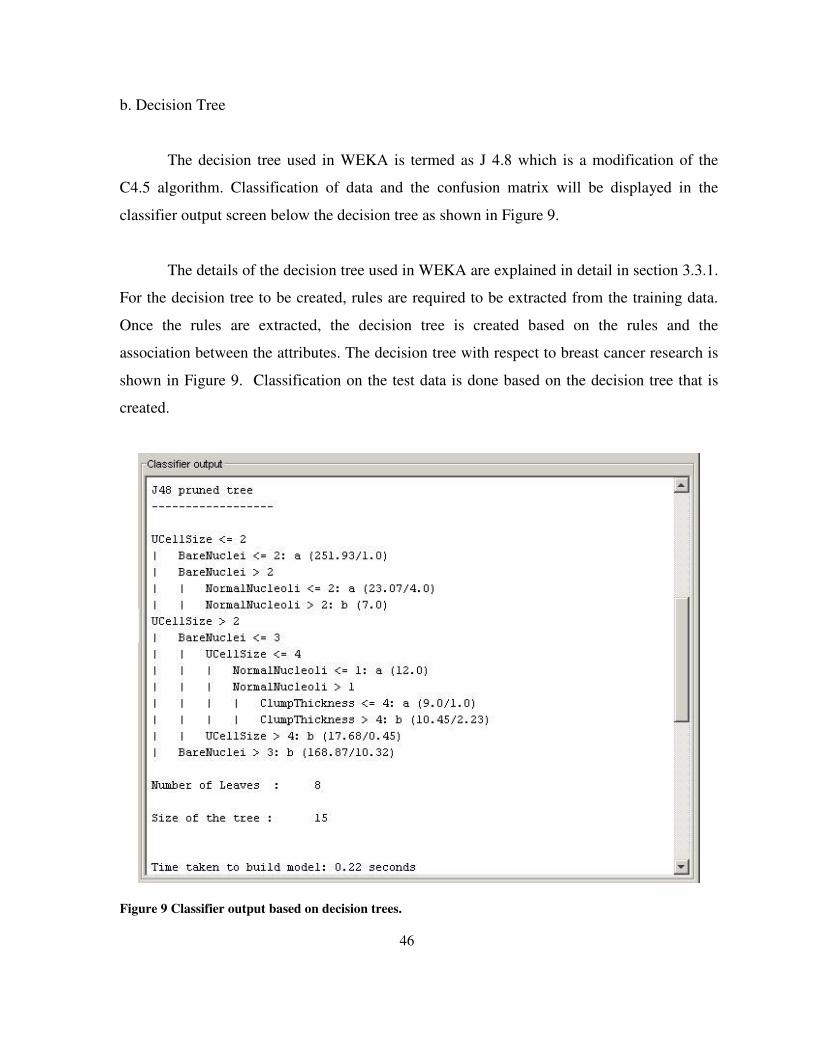
46
b. Decision Tree
The decision tree used in WEKA is termed as J 4.8 which is a modification of the
C4.5 algorithm. Classification of data and the confusion matrix will be displayed in the
classifier output screen below the decision tree as shown in Figure 9.
The details of the decision tree used in WEKA are explained in detail in section 3.3.1.
For the decision tree to be created, rules are required to be extracted from the training data.
Once the rules are extracted, the decision tree is created based on the rules and the
association between the attributes. The decision tree with respect to breast cancer research is
shown in Figure 9. Classification on the test data is done based on the decision tree that is
created.
Figure 9 Classifier output based on decision trees.
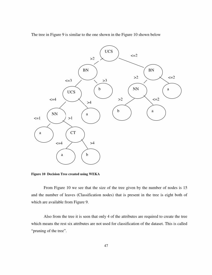
47
The tree in Figure 9 is similar to the one shown in the Figure 10 shown below
Figure 10 Decision Tree created using WEKA
From Figure 10 we see that the size of the tree given by the number of nodes is 15
and the number of leaves (Classification nodes) that is present in the tree is eight both of
which are available from Figure 9.
Also from the tree it is seen that only 4 of the attributes are required to create the tree
which means the rest six attributes are not used for classification of the dataset. This is called
“pruning of the tree”.
UCS
BN BN
a NN
a b
b UCS
a NN
a CT
a b
>2 <=2
<=2 >2 <=3 >3
>4 <=4
<=1 >1
>4 <=4
<=2 >2

48
c. Naïve Bayes method
Naïve Bayes algorithm is a kind of concept learning method. It uses the Bayes
theorem to find the probability of all the classification in the database. Figure 11 shows the
classification output that was generated from the WEKA software. For each of the attributes,
the normal distribution mean, standard deviation and weighted sum are calculated to estimate
the probability of each class. The highest probability for each class is chosen for prediction.
In the case of Naïve Bayes Algorithm in WEKA the following is the classifier output.
Figure 11 Classification output for the Naïve bayes method.
As mentioned before, we used the Naïve Bayes method mentioned in the WEKA tool
similar to the one explained in section 3.3.1

49
d. Decision Table
Given a training data Table (R,c) try to reduce the number of features and the number
of samples without reducing accuracy.
The decision rule is
Find all reduced R = reduced x, predict majority of R class.
Search techniques are used to reduce the number of features. If reduced x does not
match any R in that table, the majority class is predicted. In the decision table, a selection of
features and instances are done using theoretical measures and searching is done using the
best-fit technique. From Figure12, the classification output shows that only 19 rules are
required for the classification of the training data.
Figure 12 Classifier output of the decision table
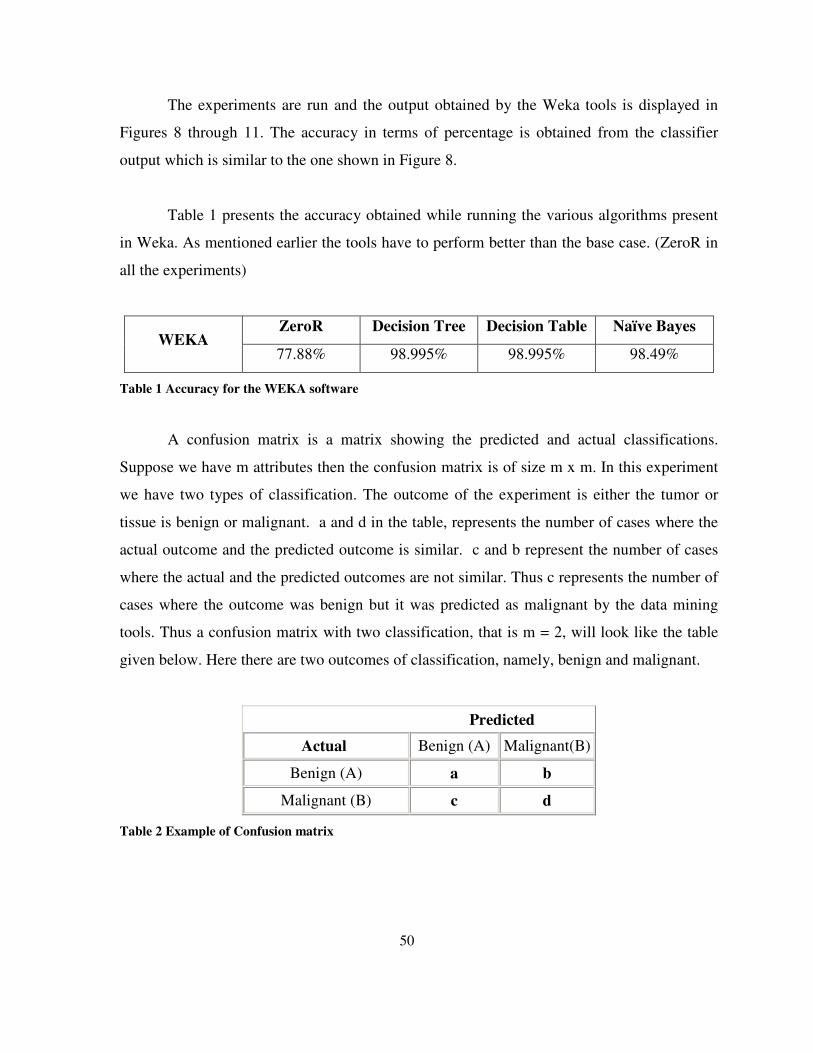
50
The experiments are run and the output obtained by the Weka tools is displayed in
Figures 8 through 11. The accuracy in terms of percentage is obtained from the classifier
output which is similar to the one shown in Figure 8.
Table 1 presents the accuracy obtained while running the various algorithms present
in Weka. As mentioned earlier the tools have to perform better than the base case. (ZeroR in
all the experiments)
ZeroR Decision Tree Decision Table Naïve Bayes WEKA
77.88% 98.995% 98.995% 98.49%
Table 1 Accuracy for the WEKA software
A confusion matrix is a matrix showing the predicted and actual classifications.
Suppose we have m attributes then the confusion matrix is of size m x m. In this experiment
we have two types of classification. The outcome of the experiment is either the tumor or
tissue is benign or malignant. a and d in the table, represents the number of cases where the
actual outcome and the predicted outcome is similar. c and b represent the number of cases
where the actual and the predicted outcomes are not similar. Thus c represents the number of
cases where the outcome was benign but it was predicted as malignant by the data mining
tools. Thus a confusion matrix with two classification, that is m = 2, will look like the table
given below. Here there are two outcomes of classification, namely, benign and malignant.
Predicted
Actual Benign (A) Malignant(B)
Benign (A) a b
Malignant (B) c d
Table 2 Example of Confusion matrix

51
In Table 3, 5 and 7, ‘A’ represents class where tumor is benign and ‘B’ represents
class where tumor is malignant. Also From Table 2 it is seen that in the table (matrix) shown
the columns represent the predicted result and the rows represent the true or actual result.
For example, from Table 3, for Decision tree tool the number 153 and 44 indicates
the number of cases where the actual and predicted values are similar. The number 2
represents the number of cases where the actual outcome was benign but was classified as
being malignant by the WEKA Decision tree tool. Similarly the rest of the predictions are
shown in the Table 3.
Zero R Decision Tree Decision Table Naïve Bayes
A B A B A B A B
A 155 0 153 2 154 1 152 3 WEKA
B 44 0 0 44 1 43 0 44
Table 3 Confusion matrix of the WEKA software
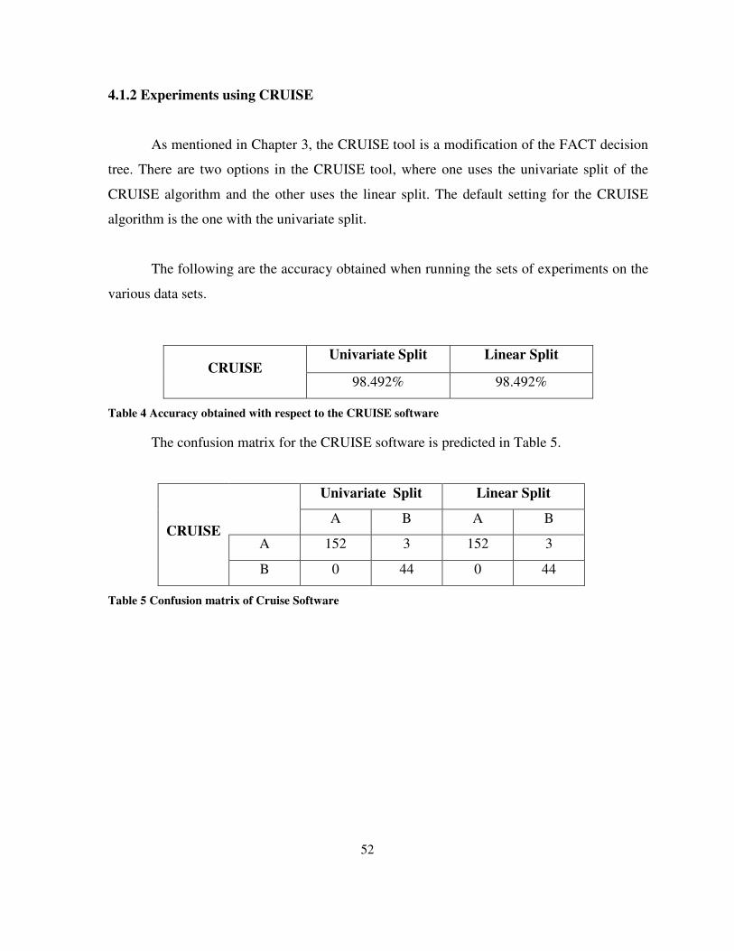
52
4.1.2 Experiments using CRUISE
As mentioned in Chapter 3, the CRUISE tool is a modification of the FACT decision
tree. There are two options in the CRUISE tool, where one uses the univariate split of the
CRUISE algorithm and the other uses the linear split. The default setting for the CRUISE
algorithm is the one with the univariate split.
The following are the accuracy obtained when running the sets of experiments on the
various data sets.
Univariate Split Linear Split CRUISE
98.492% 98.492%
Table 4 Accuracy obtained with respect to the CRUISE software
The confusion matrix for the CRUISE software is predicted in Table 5.
Univariate Split Linear Split
A B A B
A 152 3 152 3 CRUISE
B 0 44 0 44
Table 5 Confusion matrix of Cruise Software
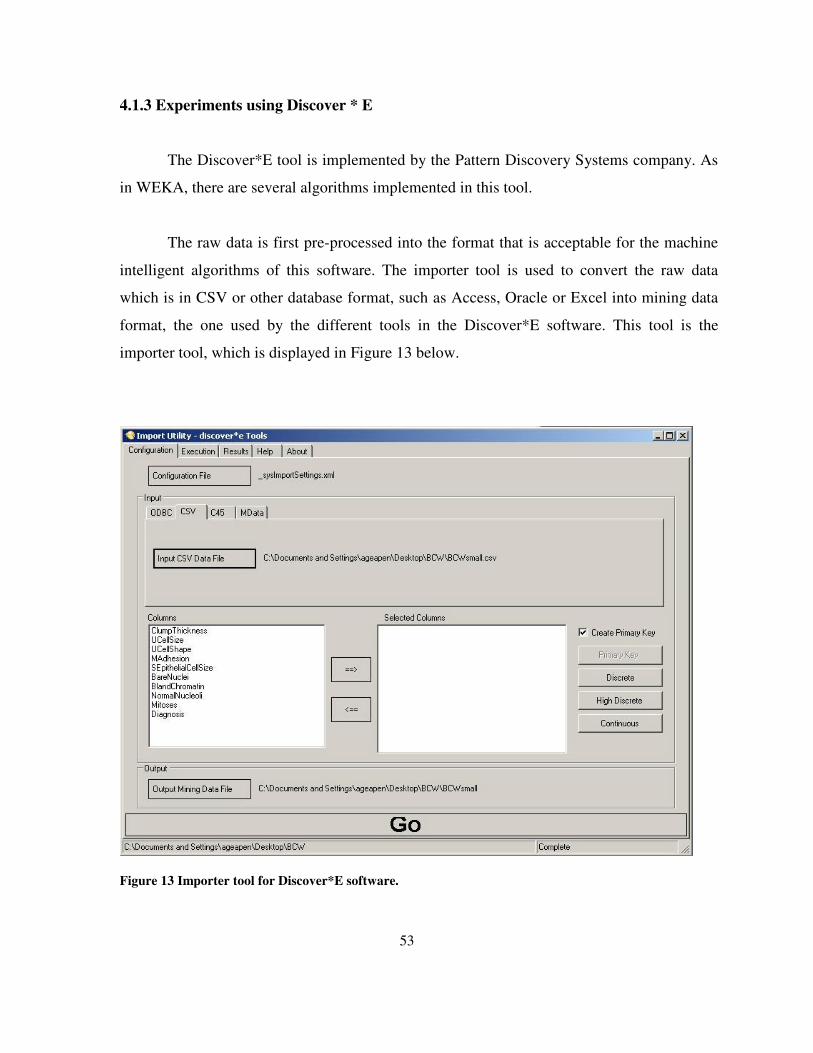
53
4.1.3 Experiments using Discover * E
The Discover*E tool is implemented by the Pattern Discovery Systems company. As
in WEKA, there are several algorithms implemented in this tool.
The raw data is first pre-processed into the format that is acceptable for the machine
intelligent algorithms of this software. The importer tool is used to convert the raw data
which is in CSV or other database format, such as Access, Oracle or Excel into mining data
format, the one used by the different tools in the Discover*E software. This tool is the
importer tool, which is displayed in Figure 13 below.
Figure 13 Importer tool for Discover*E software.

54
a. Decision Tree
The decision tree creates a classification tree based on categorical and classification
objects present in the database. Once the classification tree is created rules are extracted
from the tree and the classification of the test data is conducted. A graphical image of the
tree is also provided which will help us in understanding and traversing the tree. The
decision tree tool is created on the basis of the C4.5 decision tree. Figure 14 provides a
screen shot of the decision tree tool box (the training data for the Classification tree is
provided in this tool box).
Figure 14 Decision tree using Discover*E

55
The tool represented in Figure 15 is called the hyperbolic visualizer tool where multi
dimensional scaling on hyperbolic space is done to illustrate the data set. The GUI
interface allows the user to change viewpoints on the high dimensional space.
The hyperbolic viewer can be used in terms of finding correlations between the
attributes. When moving the trees towards the corners of the viewer the attributes with
higher correlation will be closer or will appear together. The hyperbolic viewer displayed
below shows how the different attributes are connected together to form a decision-
making unit. Figure 15 displays the tree resulting from running the breast cancer
Wisconsin database. Hyperbolic visualizer is just a tool that helps us view the decision
tree created for classification in a very high dimensional surface.
Figure 15 Hyperbolic visualizer for the decision tree.

56
b. Dependence Tree
The dependence tree is based on probability. The tree is based on the second order mutual
information and maximum spanning tree. With the probabilities obtained the tool classifies
the test data. The dependence tree created for the breast cancer case is shown in Figure16
where the left text box is where all the roots or the attributes of the data file are located. The
right hand side of the Figure 16 shows all the information that contains the dependence tree
created with the diagnosis attribute as its root.
From Figure 16, we notice that the tool provides functions that can be used to change
the root of the tree. Thus a dependence tree can be created with respect to the user. The
different trees displayed in the right screen can be saved for further computation and
classification can be done based on the tree that is saved.
Figure 16 Dependence tree used in Discover*E software

57
c. Rule Classifier
As mentioned in Chapter 3 there are two components of the rule-based classification.
The first one is the Association Discovery tool and the other is the rule based classifier.
Figure 17 shows the main screen of the Association Discover tool. By default, the
number of rules and patterns that are extracted using this tool is 1000. Weights are
provided to each rule depending on the number of times that a rule is used. The rules that
are repeatedly used have higher weight than the other and the rules with the most weights
are extracted using the association discover tool.
Figure 17 Association Discover Tool classifier

58
Figure 18 Rule based classifier.
Once the rule set is extracted from the association discovery, the testing data set along
with the rule set is passed through the second component in the rule based classifier model as
shown in Figure 18. Classification of the testing data is then made based on the rules that are
obtained.
In brief, rule based mining in Discover *E consists of two tools, Association discovery
tools which extracts rules and patterns from the training set based on the association between
the different attributes present in the data, where classification takes place and rule based
classifier where once the rules are extracted these rules are implemented on the testing data
set.

59
A number of small changes can be made in the system to improve the accuracy rate for
classification. All changes that are present are in the tool box. An example of such a change
is explained below.
• Input, estimated percentage as 1.0, Estimated Occurrence as 0.1, Prune results was
unchecked and upper order as 6 the result obtained was 99.49% accuracy.
• Input, estimated percentage as 3.0, Estimated Occurrence as 1.0, Prune results was
checked and upper order as 3 the result obtained was 97.98% accuracy.
Thus there are a number of tools that are present in the tool box that will help improve
results with respect to the classification.
In all the classification tools that are present in the Discover*E software, there exists a
classifier verification tool. This tool is used to display the result that is obtained from the
different data mining tools in the software. Another thing that can be obtained from the
classifier tool is the creation of the confusion matrix. The confusion matrix that is created
will help in understanding the variations that is present in the data and hopefully will help the
end user understand why the data was classified wrong and into which category it was
actually put in during classification. A misclassification is caused when data is classified into
a wrong class.
The classification based on the rule based mining algorithm is shown in the classifier
verification tool in Figure 19. Similarly the rest of the results using the other data mining
tools that are present in the Discover*E software can be displayed.

60
Figure 19 Classification tool in discover *E
The results based on the classification and confusion matrices are displayed in the
table below. As mentioned before, the training set is first provided to the data mining
algorithms and then the rules or the tree generated will be applied to the testing data set to
obtain the results shown below. Table 6 shows the accuracy obtained and Table 7 consists of
the confusion matrix that is generated when running these tools on the breast cancer
database.
Decision Tree Dependence Tree Association Rules Discover*E
99.49% 97.98% 99.49%
Table 6 Accuracy of the Discover*E software
Decision Tree Dependence Tree Rule based Classifer
A B A B A B
A 154 1 153 2 154 1 Discover*E
B 0 43 2 41 0 43
Table 7 Confusion matrix with respect to the Discover*E tools
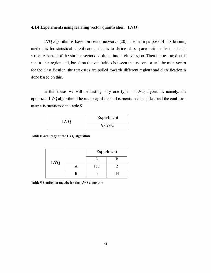
61
4.1.4 Experiments using learning vector quantization (LVQ)
LVQ algorithm is based on neural networks [20]. The main purpose of this learning
method is for statistical classification, that is to define class spaces within the input data
space. A subset of the similar vectors is placed into a class region. Then the testing data is
sent to this region and, based on the similarities between the test vector and the train vector
for the classification, the test cases are pulled towards different regions and classification is
done based on this.
In this thesis we will be testing only one type of LVQ algorithm, namely, the
optimized LVQ algorithm. The accuracy of the tool is mentioned in table 7 and the confusion
matrix is mentioned in Table 8.
Table 8 Accuracy of the LVQ algorithm
Experiment
A B
A 153 2 LVQ
B 0 44
Table 9 Confusion matrix for the LVQ algorithm
Experiment LVQ
98.99%

62
4.1.5 Conclusion.
In Figure 20 we show the bar graph of the accuracy obtained for the different tools. The
lowest accuracy is found by the ZeroR method. Thus it is considered also the base case. All
the other tools tested have performed much better than the ZeroR method. The accuracy on
an average for the rest of the tools are 98.80%.
70
75
80
85
90
95
100
Per
cent
age
W Z
eroR
W D
ecis
ion
Tree
W D
ecis
ion
Tabl
e
W N
aïve
Bay
es
C U
niva
riate
Spl
it
C L
inea
r Spl
it
D*E
Dec
isio
n Tr
ee
D*E
Dep
Tre
e
D*E
Rul
e cl
assi
fier
LVQ
Experiments
Accuracy obtained
Experiments
Figure 20 Accuracy for the different tools tested

63
Another way to show the accuracy is to show the incremental accuracy over the base
method, ZeroR.
Incremental accuracy = accuracy ZeroR
accuracy ZeroR-accuracy Method in percentage, and it is shown in
Table 10
Data mining Method Incremental Accuracy in Percentage
WEKA Decision Tree 27.10%
WEKA Decision Table 27.10%
WEKA Naïve Bayes 26.46%
CRUISE Univariate Split 26.46%
CRUISE Linear Split 26.46%
Discover*E Decision Tree 27.74%
Discover*E Dependence Tree 25.80%
Discover*E Rule based Classifier 27.74%
Linear Vector Quantization 27.10%
Table 10 Incremental accuracy of the various methods

64
4.2 Minimum Data Set – Mental Health Case
Study A major objective of this thesis is to evaluate data mining techniques in the area of
medical informatics. The data we are considering in this case is related to the Minimum data
Set (MDS) with respect to the mental health patients. The MDS-MH is a standard assessment
tool for evaluating patients having problems related to mental health. There are a number of
MDS tools as mentioned in Section 2.2.1 One of their advantages is that they are cross
applicable to the other forms of MDS databases, so that with this knowledge we can apply
the same tools to all the different types of data that are obtained and expect to get the same
outcome in terms of accuracy.
There are 455 attributes present in the MDS-MH system, which was considered for a
proper assessment of a patient with respect to mental health. The outcome of the diagnosis is
mentioned at the last column of the dataset. As mentioned in section 2.2.1, there are four
final classifications. In the database that was provided for research purpose there were 4000
cases. For all the experiments the data set is divided into 500 cases for testing the data and
the rest is used for training the dataset.
There are nine experiments that are conducted
• Experiment 1:- The MDS-MH is used for classifying, patients into four
categories. The four categories to predict are Acute care, Longer-term patient,
Forensic patient or Psychogeriatic patient.
• Experiment 2:- Classification is based on the attribute cc3a (Under referral
items- Current Problem – Patient is Threat or danger to self), in which, we check
the prediction of whether the patient is a threat to himself or not.

65
• Experiment 3:- Similarly to the above case study, we classify patients based
on cc3b (Under referral items – Current Problems – Patient is a threat or danger to
others), i.e., the prediction of whether the patient is a threat to others.
• Experiment 4:- Experiments 3 & 4 are based on the referral data and not
actual facts. The variable d1a is based on actual facts (Self injury). Classification
here is to predict this variable.
• Experiment 5:- Similarly to Experiment 4, here the test is made on variable
d2a which is an actual fact. Classification prediction is done on this variable.
• Experiment 6:- This experiment is the same as Experiment 4, except that in in
this case, the classification attribute is divided into two i.e if the patient is violent
to self or not.
• Experiment 7:- This experiment is the same as Experiment 5. The only change
here is the classification attribute is divided into two i.e if the patient is violent to
others or not.
• Experiment 8:- In this Experiment we included the variable cc3a, that is threat
to self (referred result) and removed attribute d1a (Under harm to self or others –
Self injury, which is based on the actual fact).
• Experiment 9:- Similarly to the above experiment we have removed the
attribute d2a (Under harm to self or others- Violence to others) which is based on
the actual fact and run the experiment to classify the data based on the referred
result (cc3b).
Experiments 8 and 9 are expected to be the most difficult ones.

66
The tools that will be used for this case study will be similar to the ones that are used
in the case study for breast cancer described in Section 4.1.
4.2.1 Base case for Experiments using MDS-MH
Similar to the above breast cancer database case, the ZeroR is considered as the base
case in the MDS-MH data set. The experiments run on with similar setups as the ones
performed in the breast cancer database. Here however, the data size with respect to the
training set and the testing set are much bigger.
The ZeroR algorithm is applied to the nine experiments that are described in the
previous section and the accuracies obtained for running this machine intelligence algorithm
on them are displayed in Table 11.
WEKA ZeroR
Experiment Accuracy
Experiment 1 75.75 %
Experiment 2 70.74 %
Experiment 3 75.69 %
Experiment 4 62.72 %
Experiment 5 66.53 %
Experiment 6 62.72 %
Experiment 7 66.53 %
Experiment 8 70.74 %
Experiment 9 75.75 %
Table 11 Accuracy obtained for MDS-MH database using ZeroR

67
The graph in Figure 21, shows the accuracy of the ZeroR algorithm on the nine
experiments.
Accuracy obtained
0
10
20
30
40
50
60
70
80
90
100E
xpt 1
Exp
t 2
Exp
t 3
Exp
t 4
Exp
t 5
Exp
t 6
Exp
t 7
Exp
t 8
Exp
t 9
Experiments
Acc
urac
y
Zero R
Figure 21 Graph with respect to the accuracy obtained using ZeroR
The average accuracy of the tool when the experiments are done was equal to
69.68%. This is the base case for the experiments that are conducted. The rest of the tools
evaluated in the coming sections are expected to perform better than the ZeroR tool.

68
Algorithms similar to those used with the Breast cancer database are used in the
MDS-MH dataset. The list of the algorithms other than the ZeroR method is listed below.
1. Using the WEKA software
a. J48 algorithm in Weka
b. Decision table in Weka
c. Naïve Bayes in Weka
2. Using Discover*E software
a. Decision tree
b. Rule based
c. Dependence tree
3. Using Learning Vector Quantization method.
4. Using the Cruise tool
a. Univatiate Split
b. Linear combination split
In the MDS-MH database we are categorizing the tools based on the method being used. The
categories and the intelligent algorithms that are implemented are displayed below.
• Decision Tree
o Cruise one of the variation of the decision Tree ‘FACT ’
o Discover*E based on the C 4.5 decision Tree
o Weka J 4.8 based on the C 4.5 decision Tree
• Rule based Classifier
o Rule based classification for Discover *E
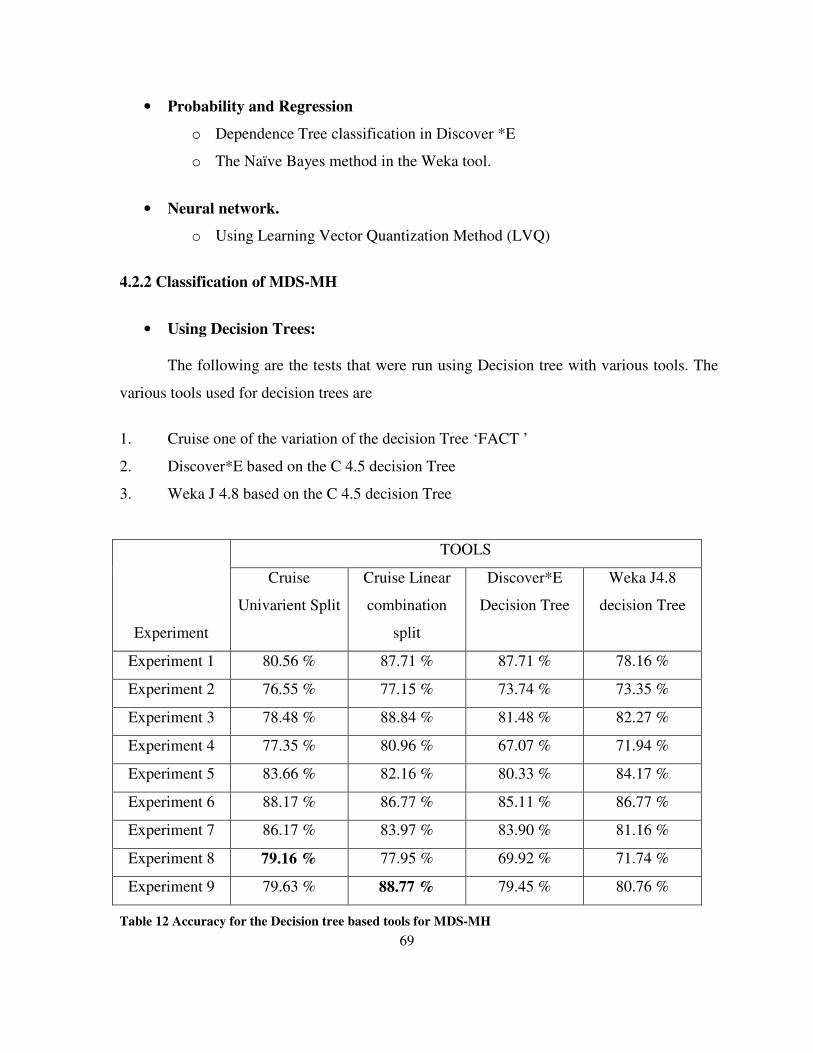
69
• Probability and Regression
o Dependence Tree classification in Discover *E
o The Naïve Bayes method in the Weka tool.
• Neural network.
o Using Learning Vector Quantization Method (LVQ)
4.2.2 Classification of MDS-MH
• Using Decision Trees:
The following are the tests that were run using Decision tree with various tools. The
various tools used for decision trees are
1. Cruise one of the variation of the decision Tree ‘FACT ’
2. Discover*E based on the C 4.5 decision Tree
3. Weka J 4.8 based on the C 4.5 decision Tree
TOOLS
Experiment
Cruise
Univarient Split
Cruise Linear
combination
split
Discover*E
Decision Tree
Weka J4.8
decision Tree
Experiment 1 80.56 % 87.71 % 87.71 % 78.16 %
Experiment 2 76.55 % 77.15 % 73.74 % 73.35 %
Experiment 3 78.48 % 88.84 % 81.48 % 82.27 %
Experiment 4 77.35 % 80.96 % 67.07 % 71.94 %
Experiment 5 83.66 % 82.16 % 80.33 % 84.17 %
Experiment 6 88.17 % 86.77 % 85.11 % 86.77 %
Experiment 7 86.17 % 83.97 % 83.90 % 81.16 %
Experiment 8 79.16 % 77.95 % 69.92 % 71.74 %
Experiment 9 79.63 % 88.77 % 79.45 % 80.76 %
Table 12 Accuracy for the Decision tree based tools for MDS-MH

70
Table 12 shows the accuracy obtained while running tools and algorithms based on
decision trees and the graph shown in Figure 22 shows the degree of accuracy of the tools.
As mentioned earlier, Experiments 8 and 9 are the toughest to predict and the highest
accuracy for Experiment 8 is 79.16 % and for Experiment 9 is 88.77%.
Accuracy obtained
0
10
20
30
40
50
60
70
80
90
100
Exp
t 1
Exp
t 3
Exp
t 5
Exp
t 7
Exp
t 9
Experiments
Acc
urac
y
CruiseUnivarient Split
Cruise LinearcombinationsplitDiscover*EDecision Tree
Weka J4.8decision Tree
Zero R
Figure 22 Accuracy with regard to decision trees.
From the graph in Figure 22 we see for all the experiments the accuracy obtained for
decision tree is more than the ZeroR method shown in bold in the graph. Thus all the tools
perform better than the base case.

71
• Classification based on rule based classifier
The following are the test results using association rules. The tool for analyzing the
rule based classifier is
1. Rule based classification for Discover *E
Experiment Discover*E
Experiment 1 79.95 %
Experiment 2 65.38 %
Experiment 3 66.30 %
Experiment 4 53.59 %
Experiment 5 69.12 %
Experiment 6 69.50 %
Experiment 7 64.57 %
Experiment 8 67.00 %
Experiment 9 72.40 %
Table 13 Accuracy obtained for the rule based classifier.
Among the tools we used for testing only one tool has a data mining algorithm
that is based on rule based classification. This rule based classification is implemented in the
Discover*E software. Table 13 provides the results of the experiments run with the rule
based classifier. The graph displayed in Figure 23 is based on the comparison between the
rule based classifier and the ZeroR method.

72
Accuracy obtained
0
10
20
30
40
50
60
70
80
90
100
Exp
t 1
Exp
t 2
Exp
t 3
Exp
t 4
Exp
t 5
Exp
t 6
Exp
t 7
Exp
t 8
Exp
t 9Experiments
Acc
urac
y
Discover*E Rulebased classifierZero R
Figure 23 Accuracy obtained for the Rule based classifier.
From the graph we see that the ZeroR method at times perform better than the rule based
classifier. The ZeroR cannot be considered as an ideal, machine intelligent algorithm, as it is
based on the majority class distribution, and we have considered this to be the base case.

73
The reason why rule based classification performed worse is explained with an example
below. For Experiment 1, 31236 rules were extracted from the dataset using the association
discover tool. In the configuration screen shown in Figure 17 of the Association Discovery
tool we have set the tool to extract the best 1000 rules and patterns and classification is based
on these 1000 rules extracted. We see in Figure 24 the total number of rules and patterns
(31236) that were extracted and exported (1000).
Increasing the number of rules extracted increases the accuracy of the system. (Appendix
D) Figure 24 shows the output screen obtained from the association discovery tool.
Figure 24 Association discovery tool in Discover*E

74
• Classification based on Probability and Regression
The machine intelligence algorithms based on probability and regression are the
following
1. Dependence tree in Discover*E software
2. Bayes method present in the WEKA software.
Experiment Discover * E method this is
based on Dependence tree
Weka method that is based
on Naïve Bayes method
Experiment 1 75.75 % 81.56 %
Experiment 2 76.35 % 74.75 %
Experiment 3 75.07 % 89.24 %
Experiment 4 56.51 % 37.27 %
Experiment 5 78.16 % 73.34 %
Experiment 6 88.18 % 54.71 %
Experiment 7 84.57 % 79.16 %
Experiment 8 67.74 % 74.75 %
Experiment 9 75.75 % 89.19 %
Table 14 Accuracy of the tools that are based on Probability and regression
Table 14 provides the accuracy of the tools based on Probability and regression. The
dependence tree proved to be better in 5 sets of experiments as compared to the Naïve Bayes
method. The average accuracy when considering the 9 experiments for Dependence tree is
75.34% and using Naïve Bayes algorithm is 72.66%.

75
Accuracy obtained
0
10
20
30
40
50
60
70
80
90
100
Exp
t 1
Exp
t 2
Exp
t 3
Exp
t 4
Exp
t 5
Exp
t 6
Exp
t 7
Exp
t 8
Exp
t 9
Experiments
Acc
urac
y
Discover* E -Dependence treeWEKA NaïveBayesZero R
Figure 25 Accuracy obtained with respect to probability and regression.
Figure 25 presents a comparison between the three algorithms namely ZeroR,
dependence tree and Naïve Bayes method. Both algorithms performed better in the majority
of the cases when compared to the ZeroR method.
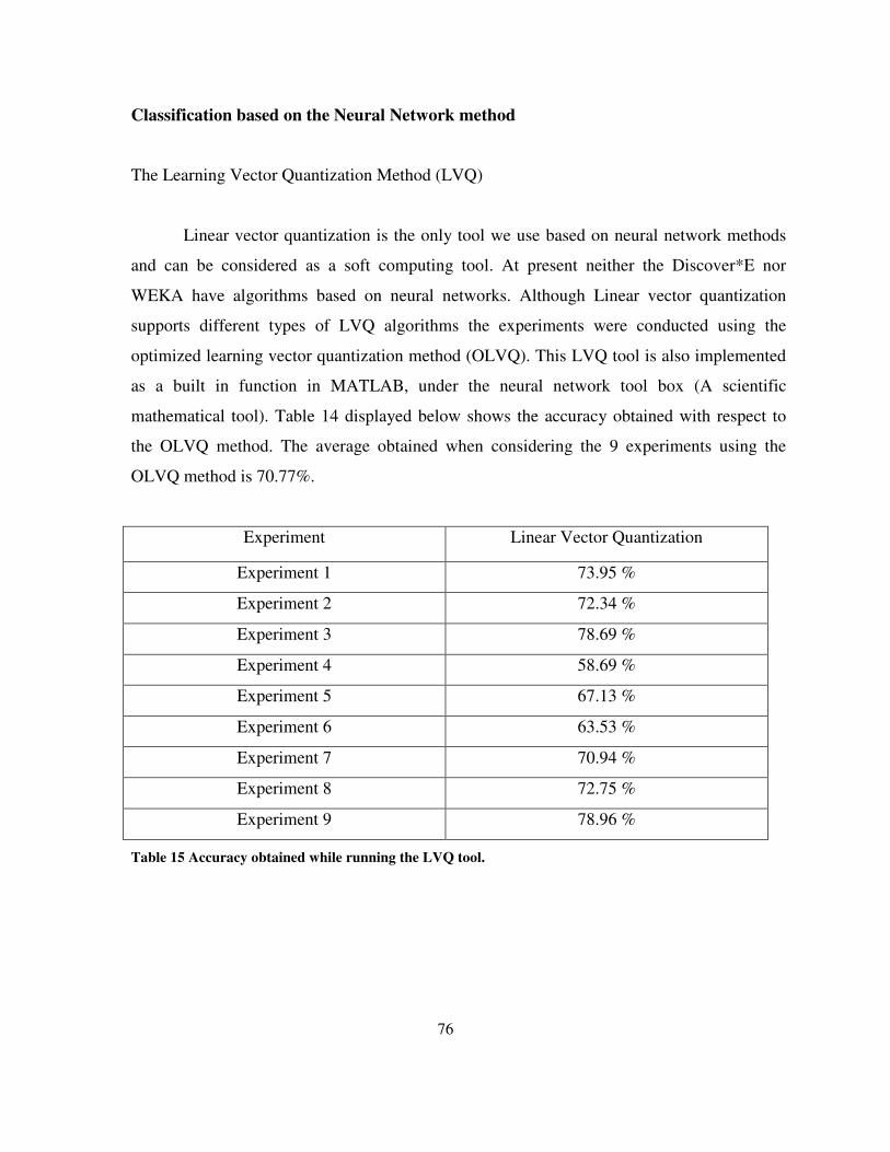
76
Classification based on the Neural Network method
The Learning Vector Quantization Method (LVQ)
Linear vector quantization is the only tool we use based on neural network methods
and can be considered as a soft computing tool. At present neither the Discover*E nor
WEKA have algorithms based on neural networks. Although Linear vector quantization
supports different types of LVQ algorithms the experiments were conducted using the
optimized learning vector quantization method (OLVQ). This LVQ tool is also implemented
as a built in function in MATLAB, under the neural network tool box (A scientific
mathematical tool). Table 14 displayed below shows the accuracy obtained with respect to
the OLVQ method. The average obtained when considering the 9 experiments using the
OLVQ method is 70.77%.
Experiment Linear Vector Quantization
Experiment 1 73.95 %
Experiment 2 72.34 %
Experiment 3 78.69 %
Experiment 4 58.69 %
Experiment 5 67.13 %
Experiment 6 63.53 %
Experiment 7 70.94 %
Experiment 8 72.75 %
Experiment 9 78.96 %
Table 15 Accuracy obtained while running the LVQ tool.

77
Accuracy obtained
0
10
20
30
40
50
60
70
80
90
100
Exp
t 1
Exp
t 2
Exp
t 3
Exp
t 4
Exp
t 5
Exp
t 6
Exp
t 7
Exp
t 8
Exp
t 9
Experiments
Acc
urac
y
Linear QuantizationVectorZero R
Figure 26 Accuracy obtained using the LVQ tool
Figure 26 shows a comparison between the ZeroR and the linear quantization method.
From the graph we see that the tools don’t have too much variation in terms of the accuracy
with respect to the experiments conducted. Comparing the accuracy of the LVQ tool and the
ZeroR tool we see that the LVQ tool performed only slightly better in seven out of nine
experiments

78
4.2.3 Different partitions in the dataset for decision trees experiments.
+Some decision trees produce results based on the dataset supplied. Thus they are
assumed to be biased with respect to the training set. The better the dataset, the better are the
results in terms of classification that is obtained using decision trees.
To help understand that there is not much variation with respect to classification, the
data set provided for Experiment 9 (Considered in section 4.2) is taken into consideration.
This database is partitioned into seven different test and training data sets to conduct this test.
Therefore in each case 500 was the test set and the rest were used for training.
The different machine intelligent tools based on the decision tree are used for these
experiments
• CRUISE linear Split
• WEKA using decision tree
• Discover*E using the decision tree
The accuracy with respect to the classification is described in the following tables.
The average in terms of the accuracy for classification when the seven experiments are
conducted together for CRUISE is 81.19% , decision tree using WEKA is 78.74% and for
Discover*E is 79.37% .
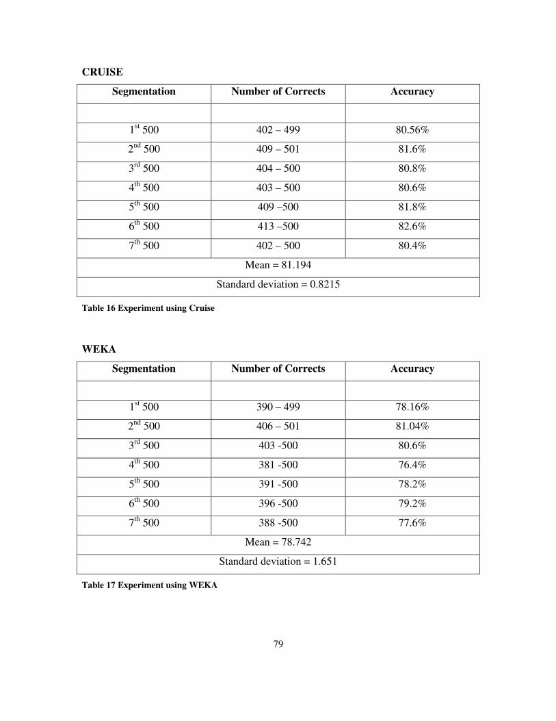
79
CRUISE
Segmentation Number of Corrects Accuracy
1st 500 402 – 499 80.56%
2nd 500 409 – 501 81.6%
3rd 500 404 – 500 80.8%
4th 500 403 – 500 80.6%
5th 500 409 –500 81.8%
6th 500 413 –500 82.6%
7th 500 402 – 500 80.4%
Mean = 81.194
Standard deviation = 0.8215
Table 16 Experiment using Cruise
WEKA
Segmentation Number of Corrects Accuracy
1st 500 390 – 499 78.16%
2nd 500 406 – 501 81.04%
3rd 500 403 -500 80.6%
4th 500 381 -500 76.4%
5th 500 391 -500 78.2%
6th 500 396 -500 79.2%
7th 500 388 -500 77.6%
Mean = 78.742
Standard deviation = 1.651
Table 17 Experiment using WEKA

80
PDS ( Discover *E )
Segmentation Number of Corrects Accuracy
1st 500 438-499 87.71%
2nd 500 389 -501 77.80%
3rd 500 378-500 75.60%
4th 500 387 – 500 77.40%
5th 500 402 – 500 80.40%
6th 500 422 -500 84.40%
7th 500 361 -500 72.20%
Mean = 79.358
Standard deviation = 5.289
Table 18 Experiment using Decision tree in Discover*E
The decision tree created by the Discover*E software is shown in the hyperbolic
viewer in Figure 27. The decision tree is not as clear as the one shown in Figure 15 due to
the high number of attributes that are present in the MDS-MH dataset.
Figure 27 Decision tree created using Discover*E

81
From the above tables the graph mentioned in Figure 28 was obtained. From also the
graph we can draw the conclusion that there is not much fluctuation with respect to
classification.
Accuracy obtained
0
10
20
30
40
50
60
70
80
90
100
Exp
t 1
Exp
t 2
Exp
t 3
Exp
t 4
Exp
t 5
Exp
t 6
Exp
t 7
Experiments
Acc
urac
y
CRUISE
WEKA
Discover*E
Figure 28 Experiment using the different tools available in decision tree
A similar study was conducted to the breast cancer Wisconsin (BCW) database. The
dataset consists of 699 cases. Here the dataset was partitioned into 7 sets. Therefore in each
case 100 was the test set and the rest were used for training. Dataset 7 has only 99 cases used
for testing and the rest is considered for training. The accuracy of the various tools are
mentioned in Table19.

82
WEKA CRUISE Discover*E
Data Set 1 90% 84% 91%
Data Set 2 95% 96% 93%
Data Set 3 95% 94% 90%
Data Set 4 92% 94% 90%
Data Set 5 95% 97% 94%
Data Set 6 99% 95% 99%
Data Set 7 96.96% 95.95% 97.97%
Table 19 Experiments conducted using decision trees.
From the above table the graph mentioned in Figure 29 is obtained.
Accuracy obtained
0
10
20
30
40
50
60
70
80
90
100
Exp
t 1
Exp
t 2
Exp
t 3
Exp
t 4
Exp
t 5
Exp
t 6
Exp
t 7
Experiments
Acc
urac
y
CRUISE
WEKA
Discover*E
Figure 29 Experiment using the different tools available in decision tree for BCW database.

83
To give an example of computation time with regard to the above experiments the
time elapsed with regard to computation are given below for the 7th dataset mentioned in
Section 4.2.3. CRUISE took 47 seconds to build the decision tree and classify the instances.
The decision tree based on WEKA produced results in 34.12 seconds. Decision tree based in
Discover*E produced the tree in 25 seconds while classification of the decision tree took 110
seconds.
4.3 Summary
A comparative study was conducted in this project, for two types of medical
databases. Results have shown that most of decision tree based methods implemented have
outperformed the base case we used i.e. WEKA’s ZeroR method. An added advantage of
decision tree based methods is that it is easier to produce interpretrability for the medical
practitioners and may help in both the validation of the method and in developing further
knowledge of the problem. Also in this chapter the CPU time of some of the experiments
were presented.
84
5. Conclusion and future work
5.1 Conclusion
Machine intelligence algorithms are improving as the number of data mining tools
and algorithms increase. Healthcare data is a good test bed for data mining. A great deal of
data in health care is still being gathered and organized using pen and paper. In this thesis,
we have used the MDS-MH as the case study that consists of 455 attributes and over 4000
cases.
The minimum dataset that was analyzed is in the area of mental health. There are a
number of other tools that are based on MDS and have been made mandatory in different
parts of Canada. The advantage of the MDS assessment tools is that they can be integrated
with each other, resulting in a much bigger set of data. Thus soon there will be a number of
other integrated tools in the MDS system for data mining.
In this thesis, we used ZeroR as the base case. Some times it outperformed some of
the other data-mining algorithms and one reason being that ZeroR implements the majority
class to be the output with regard to the final output of the tool. If we can classify the testing
data set into 2 categories say X and Y, and in the test data set there are more cases present in
category X than Y, then the ZeroR tool will be trained to predict the category for any test
case as X as the tool is trained to classify all the outcomes based on the majority class.
Similarly in experiment 1 in table 9, 75.75% was the accuracy obtained for ZeroR method,
which means 75.75% of the test data, represents the majority class of the training set. Thus
the time required for computation and classification in this method is minimal.
An Example where the ZeroR could perform better is, consider a case where 99 out of
100 cases belong to the majority class of the training dataset. In this the prediction rate of the
ZeroR tool is 99%. But incase in the testing dataset there is only one instance of the majority

85
class of the training dataset then the prediction of this tool will be 1%. Thus the tool is
completely biased on the distribution of the training dataset.
The Naïve Bayes algorithm provides very fluctuating results in the MDS-MH data
set. This is an algorithm commonly used to produce classified results at a very high speed.
Accurate prediction with the Naïve Bayes algorithm comes when all the independent
variables are statistically independent of each other. Accuracy with respect to the rule based
classification can be increased by using more rules for the classification of the test data.
The decision tree experiments that were conduced were the most useful and
informative experiments. One of the questions was whether the number of attributes in the
database could be decreased.
To answer the above question we look at the experiments conducted by WEKA on
using decision tree in section 4.1.1 . We find here that for the breast cancer research the total
number of attributes used were four out of the ten that were available which provided an
accuracy of 98.995% as mentioned in Table 1. Also for the MDS-MH data set for
Experiment 9 that is provided in Appendix B and C the number of attributes that where used
for the experiment were 163 out of 455 present in the database, which provided an accuracy
of 80.76% as shown in Table 12. The number 163 was obtained from the tree using a Java
program.

86
5.2 Future work.
Mobile computing plays a very important role in today’s information retrieval system.
Some of the new handheld devices, cellular phones, PDAs, the Blackberry and others can be
connected to the Internet and information can be received and sent from servers.
There are a number of different data mining algorithms that produce rules that can be
stored in mobile devices and used for data classification. A possibility for future work could
be to implement a local interface for the device where user can input data directly into their
mobile devices, and based on the rule set, can deliver the answer back, i.e. classification is
done using rules stored in the database of the PDA. This can be a handy tool for medical
practitioners.

87
Appendix A Naïve bayes algorithm
Assumption:- Let 1,....., nx x x=< > be an instance of the example language and c C∈ a
possible classification. Then { }i i1,..,Prob (x|c)= Prob(x |c)nΠ ∈
This assumption is justified, if the attributes are independent from each other.
Using this assumption the classification c C∈ with maximum posterior probability
Prob (c|x) is the one that maximizes the expression { }i i1,..,P(c)* Prob(x |c)nΠ ∈
The learner estimates the required probabilities by calculating the corresponding frequencies
observed in the example set.
ID3 decision tree This is based on a tree induction algorithm.
The basic idea is to pick an attribute A with values a1, a2, ..., ar, split the training instances
into subsets Sa1, Sa2, ..., Sar consisting of those instances that have the corresponding attribute
value.
If a subset has only instances in a single class, that part of the tree stops with a leaf node
labeled with the single class.
If not, then the subset is split again, recursively, using a different attribute.

88
C4.5 decision tree algorithm.[24]
1. Build the decision tree from the training set (conventional ID3)
2. Convert the resulting tree into an equivalent set of rules. The number of rules is
equivalent to the number of possible paths from the root to a leaf node.
3. Prune each rule by removing any preconditions that result in improving its accuracy,
according to a validation set.
4. Sort the pruned rules in descending order according to their accuracy, and consider
them in this sequence when classifying subsequent instances.

89
Appendix B
Few of the pages that are taken from the RAI MDS version 2.0. This is similar to the
ones that are used in the RAI-MH
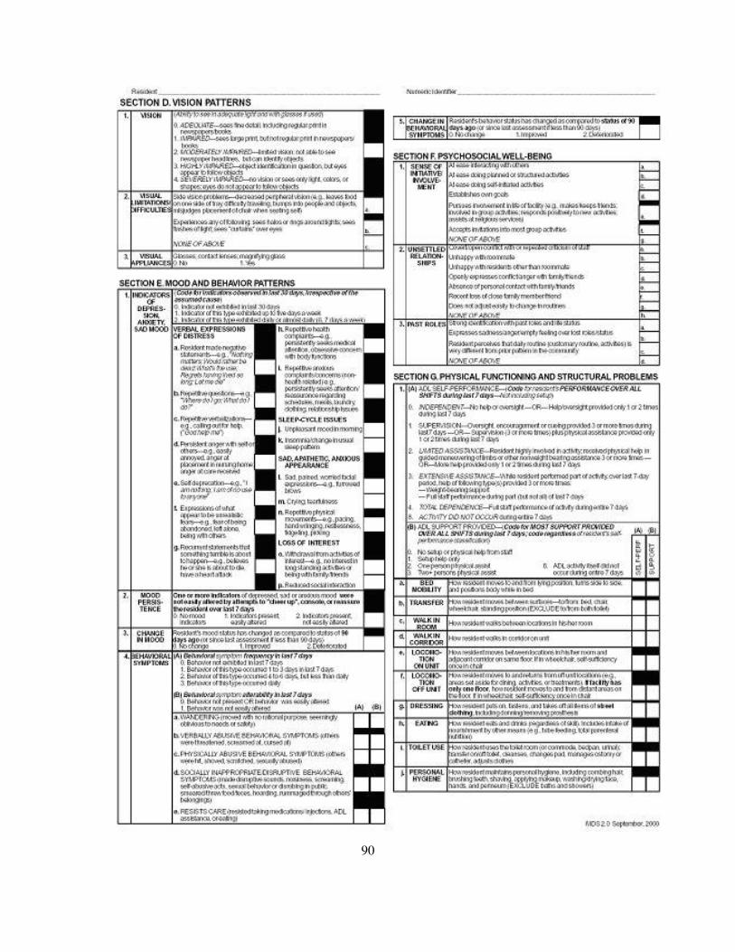
90

91

92

93
Appendix C Given below is a pruned decision tree that was created using the Weka J 4.8. The
attributes that are correlated to each other are connected by an edge in the tree. The decision
tree shown below is for Experiment nine for the MDS-MH system. a6h <= 0 | d2a <= 0 | | j1o <= 0 | | | s5b <= 0 | | | | e2 <= 0.341138 | | | | | d2c <= 1 | | | | | | a4c <= 0 | | | | | | | t5ab <= 5 | | | | | | | | f3c <= 0 | | | | | | | | | k2b <= 0: b (1406.0/37.0) | | | | | | | | | k2b > 0 | | | | | | | | | | k4b <= 0.431102: b (42.0/1.0) | | | | | | | | | | k4b > 0.431102 | | | | | | | | | | | l1db <= 0 | | | | | | | | | | | | dd1 <= 7: a (5.0) | | | | | | | | | | | | dd1 > 7: b (2.0) | | | | | | | | | | | l1db > 0: b (4.0) | | | | | | | | f3c > 0 | | | | | | | | | o1b <= 108 | | | | | | | | | | k2p <= 0: b (80.0/5.0) | | | | | | | | | | k2p > 0 | | | | | | | | | | | cc4 <= 2: b (3.0) | | | | | | | | | | | cc4 > 2: a (2.0) | | | | | | | | | o1b > 108: a (5.0/1.0) | | | | | | | t5ab > 5 | | | | | | | | cc5ja <= 0 | | | | | | | | | b1t <= 1 | | | | | | | | | | h2 <= 1: b (30.0) | | | | | | | | | | h2 > 1: a (3.0/1.0) | | | | | | | | | b1t > 1: a (2.0) | | | | | | | | cc5ja > 0: a (3.0) | | | | | | a4c > 0 | | | | | | | i2a <= 0 | | | | | | | | n1i <= 0 | | | | | | | | | f3a <= 1 | | | | | | | | | | dd8 <= 0: b (33.0) | | | | | | | | | | dd8 > 0 | | | | | | | | | | | l1db <= 0: b (4.0) | | | | | | | | | | | l1db > 0: a (2.0) | | | | | | | | | f3a > 1: a (3.0/1.0) | | | | | | | | n1i > 0: a (4.0/1.0) | | | | | | | i2a > 0: a (4.0/1.0) | | | | | d2c > 1 | | | | | | g1g <= 1 | | | | | | | i2b <= 0 | | | | | | | | u1l <= 0 | | | | | | | | | l2a <= 2 | | | | | | | | | | cc6 <= 0: b (18.0) | | | | | | | | | | cc6 > 0 | | | | | | | | | | | aa5 <= 26: b (2.0) | | | | | | | | | | | aa5 > 26: a (2.0) | | | | | | | | | l2a > 2: a (2.0) | | | | | | | | u1l > 0: a (2.0)
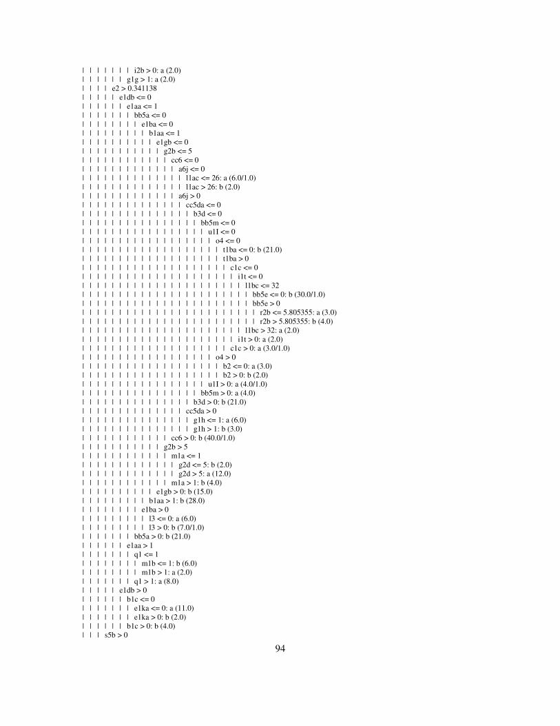
94
| | | | | | | i2b > 0: a (2.0) | | | | | | g1g > 1: a (2.0) | | | | e2 > 0.341138 | | | | | e1db <= 0 | | | | | | e1aa <= 1 | | | | | | | bb5a <= 0 | | | | | | | | e1ba <= 0 | | | | | | | | | b1aa <= 1 | | | | | | | | | | e1gb <= 0 | | | | | | | | | | | g2b <= 5 | | | | | | | | | | | | cc6 <= 0 | | | | | | | | | | | | | a6j <= 0 | | | | | | | | | | | | | | l1ac <= 26: a (6.0/1.0) | | | | | | | | | | | | | | l1ac > 26: b (2.0) | | | | | | | | | | | | | a6j > 0 | | | | | | | | | | | | | | cc5da <= 0 | | | | | | | | | | | | | | | b3d <= 0 | | | | | | | | | | | | | | | | bb5m <= 0 | | | | | | | | | | | | | | | | | u1I <= 0 | | | | | | | | | | | | | | | | | | o4 <= 0 | | | | | | | | | | | | | | | | | | | t1ba <= 0: b (21.0) | | | | | | | | | | | | | | | | | | | t1ba > 0 | | | | | | | | | | | | | | | | | | | | c1c <= 0 | | | | | | | | | | | | | | | | | | | | | i1t <= 0 | | | | | | | | | | | | | | | | | | | | | | l1bc <= 32 | | | | | | | | | | | | | | | | | | | | | | | bb5e <= 0: b (30.0/1.0) | | | | | | | | | | | | | | | | | | | | | | | bb5e > 0 | | | | | | | | | | | | | | | | | | | | | | | | r2b <= 5.805355: a (3.0) | | | | | | | | | | | | | | | | | | | | | | | | r2b > 5.805355: b (4.0) | | | | | | | | | | | | | | | | | | | | | | l1bc > 32: a (2.0) | | | | | | | | | | | | | | | | | | | | | i1t > 0: a (2.0) | | | | | | | | | | | | | | | | | | | | c1c > 0: a (3.0/1.0) | | | | | | | | | | | | | | | | | | o4 > 0 | | | | | | | | | | | | | | | | | | | b2 <= 0: a (3.0) | | | | | | | | | | | | | | | | | | | b2 > 0: b (2.0) | | | | | | | | | | | | | | | | | u1I > 0: a (4.0/1.0) | | | | | | | | | | | | | | | | bb5m > 0: a (4.0) | | | | | | | | | | | | | | | b3d > 0: b (21.0) | | | | | | | | | | | | | | cc5da > 0 | | | | | | | | | | | | | | | g1h <= 1: a (6.0) | | | | | | | | | | | | | | | g1h > 1: b (3.0) | | | | | | | | | | | | cc6 > 0: b (40.0/1.0) | | | | | | | | | | | g2b > 5 | | | | | | | | | | | | m1a <= 1 | | | | | | | | | | | | | g2d <= 5: b (2.0) | | | | | | | | | | | | | g2d > 5: a (12.0) | | | | | | | | | | | | m1a > 1: b (4.0) | | | | | | | | | | e1gb > 0: b (15.0) | | | | | | | | | b1aa > 1: b (28.0) | | | | | | | | e1ba > 0 | | | | | | | | | l3 <= 0: a (6.0) | | | | | | | | | l3 > 0: b (7.0/1.0) | | | | | | | bb5a > 0: b (21.0) | | | | | | e1aa > 1 | | | | | | | q1 <= 1 | | | | | | | | m1b <= 1: b (6.0) | | | | | | | | m1b > 1: a (2.0) | | | | | | | q1 > 1: a (8.0) | | | | | e1db > 0 | | | | | | b1c <= 0 | | | | | | | e1ka <= 0: a (11.0) | | | | | | | e1ka > 0: b (2.0) | | | | | | b1c > 0: b (4.0) | | | s5b > 0

95
| | | | v1a <= 0 | | | | | l1ec <= 18: a (9.0) | | | | | l1ec > 18: b (2.0) | | | | v1a > 0 | | | | | cc5da <= 0: b (15.0) | | | | | cc5da > 0: a (2.0) | | j1o > 0 | | | b1w <= 0 | | | | b3d <= 0 | | | | | cc5ia <= 0 | | | | | | b1h <= 0 | | | | | | | j1i <= 0 | | | | | | | | g2a <= 4 | | | | | | | | | cc3k <= 0 | | | | | | | | | | bb5k <= 0 | | | | | | | | | | | cc3i <= 0 | | | | | | | | | | | | b1bb <= 0 | | | | | | | | | | | | | l2a <= 5 | | | | | | | | | | | | | | s6 <= 1 | | | | | | | | | | | | | | | bb3 <= 3: a (3.0) | | | | | | | | | | | | | | | bb3 > 3: b (2.0) | | | | | | | | | | | | | | s6 > 1: b (17.0) | | | | | | | | | | | | | l2a > 5: a (2.0) | | | | | | | | | | | | b1bb > 0: a (2.0) | | | | | | | | | | | cc3i > 0: a (2.0) | | | | | | | | | | bb5k > 0: a (2.0) | | | | | | | | | cc3k > 0: b (11.0) | | | | | | | | g2a > 4: a (4.0) | | | | | | | j1i > 0: a (3.0) | | | | | | b1h > 0: a (4.0) | | | | | cc5ia > 0: a (5.0) | | | | b3d > 0: b (10.0) | | | b1w > 0: a (5.0) | d2a > 0 | | cc5ia <= 0 | | | l4e <= 1 | | | | e1kb <= 0 | | | | | e1cb <= 1 | | | | | | d2d <= 1 | | | | | | | u1c <= 0 | | | | | | | | cc3h <= 0 | | | | | | | | | k2u <= 0 | | | | | | | | | | k2d <= 0 | | | | | | | | | | | j1b <= 0 | | | | | | | | | | | | g1f <= 0 | | | | | | | | | | | | | b1n <= 0 | | | | | | | | | | | | | | cc5cb <= 0 | | | | | | | | | | | | | | | cc5bb <= 0 | | | | | | | | | | | | | | | | l1eb <= 2 | | | | | | | | | | | | | | | | | b3b <= 0 | | | | | | | | | | | | | | | | | | k2o <= 0 | | | | | | | | | | | | | | | | | | | l2a <= 6 | | | | | | | | | | | | | | | | | | | | n1w <= 0 | | | | | | | | | | | | | | | | | | | | | j1i <= 0 | | | | | | | | | | | | | | | | | | | | | | l2a <= 1 | | | | | | | | | | | | | | | | | | | | | | | a6j <= 0: a (7.0) | | | | | | | | | | | | | | | | | | | | | | | a6j > 0 | | | | | | | | | | | | | | | | | | | | | | | | i1b <= 0 | | | | | | | | | | | | | | | | | | | | | | | | | b1p <= 1 | | | | | | | | | | | | | | | | | | | | | | | | | | e1da <= 1 | | | | | | | | | | | | | | | | | | | | | | | | | | | b1i <= 0 | | | | | | | | | | | | | | | | | | | | | | | | | | | | u1j <= 0 | | | | | | | | | | | | | | | | | | | | | | | | | | | | | b1aa <= 0 | | | | | | | | | | | | | | | | | | | | | | | | | | | | | | b3e <= 0: b (7.0)

96
| | | | | | | | | | | | | | | | | | | | | | | | | | | | | | b3e > 0 | | | | | | | | | | | | | | | | | | | | | | | | | | | | | | | h2 <= 0 | | | | | | | | | | | | | | | | | | | | | | | | | | | | | | | | j1d <= 0 | | | | | | | | | | | | | | | | | | | | | | | | | | | | | | | | | b1f <= 0 | | | | | | | | | | | | | | | | | | | | | | | | | | | | | | | | | | e1db <= 0 | | | | | | | | | | | | | | | | | | | | | | | | | | | | | | | | | | | l3 <= 2 | | | | | | | | | | | | | | | | | | | | | | | | | | | | | | | | | | | | i6 <= 1: b (3.0) | | | | | | | | | | | | | | | | | | | | | | | | | | | | | | | | | | | | i6 > 1: a (23.0/2.0) | | | | | | | | | | | | | | | | | | | | | | | | | | | | | | | | | | | l3 > 2: b (3.0) | | | | | | | | | | | | | | | | | | | | | | | | | | | | | | | | | | e1db > 0: b (2.0) | | | | | | | | | | | | | | | | | | | | | | | | | | | | | | | | | b1f > 0: b (2.0) | | | | | | | | | | | | | | | | | | | | | | | | | | | | | | | | j1d > 0: b (3.0) | | | | | | | | | | | | | | | | | | | | | | | | | | | | | | | h2 > 0: b (4.0) | | | | | | | | | | | | | | | | | | | | | | | | | | | | | b1aa > 0: a (3.0) | | | | | | | | | | | | | | | | | | | | | | | | | | | | u1j > 0: a (7.0) | | | | | | | | | | | | | | | | | | | | | | | | | | | b1i > 0: b (6.0) | | | | | | | | | | | | | | | | | | | | | | | | | | e1da > 1: a (6.0) | | | | | | | | | | | | | | | | | | | | | | | | | b1p > 1: a (11.0) | | | | | | | | | | | | | | | | | | | | | | | | i1b > 0: a (4.0) | | | | | | | | | | | | | | | | | | | | | | l2a > 1: a (13.0) | | | | | | | | | | | | | | | | | | | | | j1i > 0: a (8.0) | | | | | | | | | | | | | | | | | | | | n1w > 0: b (6.0/1.0) | | | | | | | | | | | | | | | | | | | l2a > 6 | | | | | | | | | | | | | | | | | | | | k2a <= 0: a (2.0) | | | | | | | | | | | | | | | | | | | | k2a > 0 | | | | | | | | | | | | | | | | | | | | | dd3 <= 3: b (13.0/1.0) | | | | | | | | | | | | | | | | | | | | | dd3 > 3: a (3.0/1.0) | | | | | | | | | | | | | | | | | | k2o > 0 | | | | | | | | | | | | | | | | | | | u1j <= 0: b (11.0) | | | | | | | | | | | | | | | | | | | u1j > 0: a (2.0) | | | | | | | | | | | | | | | | | b3b > 0 | | | | | | | | | | | | | | | | | | k2o <= 0 | | | | | | | | | | | | | | | | | | | e1da <= 3 | | | | | | | | | | | | | | | | | | | | cc5da <= 0 | | | | | | | | | | | | | | | | | | | | | g1d <= 0 | | | | | | | | | | | | | | | | | | | | | | n1w <= 0 | | | | | | | | | | | | | | | | | | | | | | | t1eb <= 0 | | | | | | | | | | | | | | | | | | | | | | | | t1aa <= 0: b (7.0) | | | | | | | | | | | | | | | | | | | | | | | | t1aa > 0: a (4.0) | | | | | | | | | | | | | | | | | | | | | | | t1eb > 0: b (27.0) | | | | | | | | | | | | | | | | | | | | | | n1w > 0: a (2.0) | | | | | | | | | | | | | | | | | | | | | g1d > 0: a (3.0/1.0) | | | | | | | | | | | | | | | | | | | | cc5da > 0: a (4.0/1.0) | | | | | | | | | | | | | | | | | | | e1da > 3: a (3.0) | | | | | | | | | | | | | | | | | | k2o > 0: a (3.0) | | | | | | | | | | | | | | | | l1eb > 2 | | | | | | | | | | | | | | | | | c3 <= 0 | | | | | | | | | | | | | | | | | | cc3d <= 0: a (2.0) | | | | | | | | | | | | | | | | | | cc3d > 0: b (2.0) | | | | | | | | | | | | | | | | | c3 > 0: b (11.0) | | | | | | | | | | | | | | | cc5bb > 0 | | | | | | | | | | | | | | | | f3b <= 0: b (9.0) | | | | | | | | | | | | | | | | f3b > 0: a (3.0/1.0) | | | | | | | | | | | | | | cc5cb > 0 | | | | | | | | | | | | | | | k2a <= 0: b (2.0) | | | | | | | | | | | | | | | k2a > 0: a (12.0) | | | | | | | | | | | | | b1n > 0 | | | | | | | | | | | | | | j2c <= 0: a (2.0) | | | | | | | | | | | | | | j2c > 0: b (17.0/1.0) | | | | | | | | | | | | g1f > 0 | | | | | | | | | | | | | cc5ca <= 0 | | | | | | | | | | | | | | n1s <= 0: a (18.0) | | | | | | | | | | | | | | n1s > 0: b (2.0) | | | | | | | | | | | | | cc5ca > 0: b (2.0)
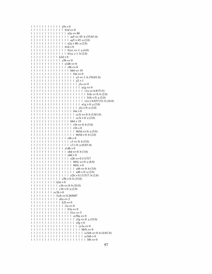
97
| | | | | | | | | | | j1b > 0 | | | | | | | | | | | | b1d <= 0 | | | | | | | | | | | | | u2a <= 80 | | | | | | | | | | | | | | aa5 <= 45: b (35.0/1.0) | | | | | | | | | | | | | | aa5 > 45: a (2.0) | | | | | | | | | | | | | u2a > 80: a (2.0) | | | | | | | | | | | | b1d > 0 | | | | | | | | | | | | | b1cc <= 1: a (4.0) | | | | | | | | | | | | | b1cc > 1: b (2.0) | | | | | | | | | | k2d > 0 | | | | | | | | | | | c5b <= 0 | | | | | | | | | | | | e1db <= 0 | | | | | | | | | | | | | r4b <= 0 | | | | | | | | | | | | | | bb4 <= 19 | | | | | | | | | | | | | | | l4n <= 0 | | | | | | | | | | | | | | | | a3 <= 1: b (70.0/1.0) | | | | | | | | | | | | | | | | a3 > 1 | | | | | | | | | | | | | | | | | j1a <= 0 | | | | | | | | | | | | | | | | | | u1g <= 0 | | | | | | | | | | | | | | | | | | | v1a <= 0.837132 | | | | | | | | | | | | | | | | | | | | b1k <= 0: b (2.0) | | | | | | | | | | | | | | | | | | | | b1k > 0: a (2.0) | | | | | | | | | | | | | | | | | | | v1a > 0.837132: b (16.0) | | | | | | | | | | | | | | | | | | u1g > 0: a (2.0) | | | | | | | | | | | | | | | | | j1a > 0: a (2.0) | | | | | | | | | | | | | | | l4n > 0 | | | | | | | | | | | | | | | | cc3i <= 0: b (5.0/1.0) | | | | | | | | | | | | | | | | cc3i > 0: a (2.0) | | | | | | | | | | | | | | bb4 > 19 | | | | | | | | | | | | | | | r1b <= 0: b (5.0) | | | | | | | | | | | | | | | r1b > 0 | | | | | | | | | | | | | | | | bb5d <= 0: a (5.0) | | | | | | | | | | | | | | | | bb5d > 0: b (2.0) | | | | | | | | | | | | | r4b > 0 | | | | | | | | | | | | | | c3 <= 0: b (5.0) | | | | | | | | | | | | | | c3 > 0: a (8.0/1.0) | | | | | | | | | | | | e1db > 0 | | | | | | | | | | | | | o6d <= 0: b (3.0) | | | | | | | | | | | | | o6d > 0 | | | | | | | | | | | | | | o2b <= 0.111517 | | | | | | | | | | | | | | | bb5c <= 0: a (8.0) | | | | | | | | | | | | | | | bb5c > 0 | | | | | | | | | | | | | | | | a4b <= 0: b (3.0) | | | | | | | | | | | | | | | | a4b > 0: a (2.0) | | | | | | | | | | | | | | o2b > 0.111517: b (2.0) | | | | | | | | | | | c5b > 0: b (15.0) | | | | | | | | | k2u > 0 | | | | | | | | | | c1b <= 0: b (24.0) | | | | | | | | | | c1b > 0: a (2.0) | | | | | | | | cc3h > 0 | | | | | | | | | l1cb <= 0.265687 | | | | | | | | | | d1a <= 2 | | | | | | | | | | | k2l <= 0 | | | | | | | | | | | | i1a <= 0 | | | | | | | | | | | | | b3a <= 0 | | | | | | | | | | | | | | l1cc <= 5 | | | | | | | | | | | | | | | cc5ba <= 0 | | | | | | | | | | | | | | | | s5g <= 0: a (35.0) | | | | | | | | | | | | | | | | s5g > 0 | | | | | | | | | | | | | | | | | cc3a <= 0 | | | | | | | | | | | | | | | | | | bb5i <= 0 | | | | | | | | | | | | | | | | | | | cc5eb <= 0: b (4.0/1.0) | | | | | | | | | | | | | | | | | | | cc5eb > 0 | | | | | | | | | | | | | | | | | | | | l4b <= 0
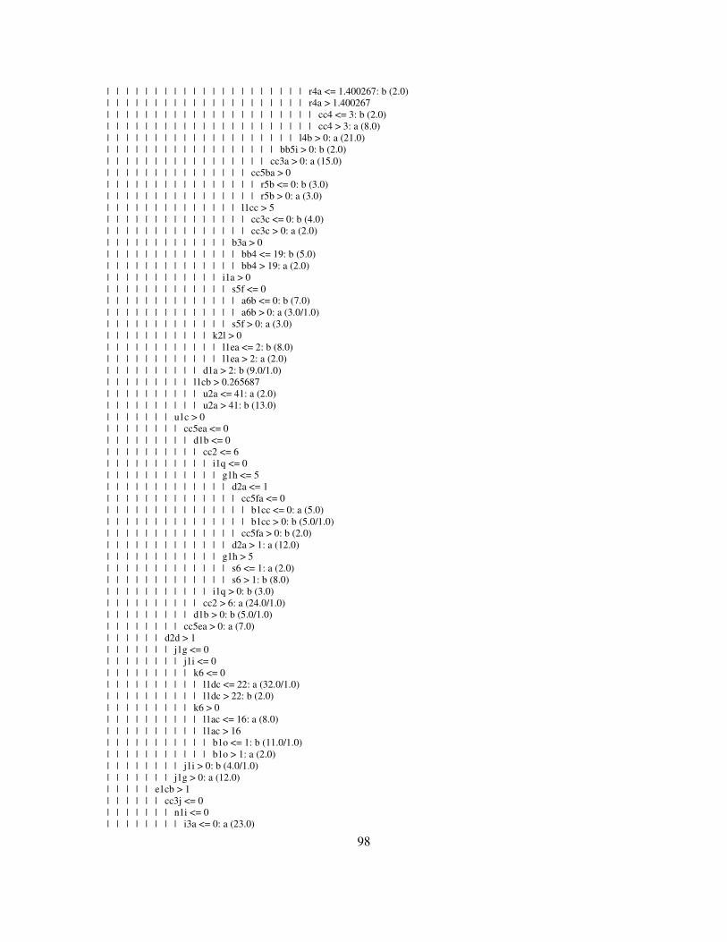
98
| | | | | | | | | | | | | | | | | | | | | r4a <= 1.400267: b (2.0) | | | | | | | | | | | | | | | | | | | | | r4a > 1.400267 | | | | | | | | | | | | | | | | | | | | | | cc4 <= 3: b (2.0) | | | | | | | | | | | | | | | | | | | | | | cc4 > 3: a (8.0) | | | | | | | | | | | | | | | | | | | | l4b > 0: a (21.0) | | | | | | | | | | | | | | | | | | bb5i > 0: b (2.0) | | | | | | | | | | | | | | | | | cc3a > 0: a (15.0) | | | | | | | | | | | | | | | cc5ba > 0 | | | | | | | | | | | | | | | | r5b <= 0: b (3.0) | | | | | | | | | | | | | | | | r5b > 0: a (3.0) | | | | | | | | | | | | | | l1cc > 5 | | | | | | | | | | | | | | | cc3c <= 0: b (4.0) | | | | | | | | | | | | | | | cc3c > 0: a (2.0) | | | | | | | | | | | | | b3a > 0 | | | | | | | | | | | | | | bb4 <= 19: b (5.0) | | | | | | | | | | | | | | bb4 > 19: a (2.0) | | | | | | | | | | | | i1a > 0 | | | | | | | | | | | | | s5f <= 0 | | | | | | | | | | | | | | a6b <= 0: b (7.0) | | | | | | | | | | | | | | a6b > 0: a (3.0/1.0) | | | | | | | | | | | | | s5f > 0: a (3.0) | | | | | | | | | | | k2l > 0 | | | | | | | | | | | | l1ea <= 2: b (8.0) | | | | | | | | | | | | l1ea > 2: a (2.0) | | | | | | | | | | d1a > 2: b (9.0/1.0) | | | | | | | | | l1cb > 0.265687 | | | | | | | | | | u2a <= 41: a (2.0) | | | | | | | | | | u2a > 41: b (13.0) | | | | | | | u1c > 0 | | | | | | | | cc5ea <= 0 | | | | | | | | | d1b <= 0 | | | | | | | | | | cc2 <= 6 | | | | | | | | | | | i1q <= 0 | | | | | | | | | | | | g1h <= 5 | | | | | | | | | | | | | d2a <= 1 | | | | | | | | | | | | | | cc5fa <= 0 | | | | | | | | | | | | | | | b1cc <= 0: a (5.0) | | | | | | | | | | | | | | | b1cc > 0: b (5.0/1.0) | | | | | | | | | | | | | | cc5fa > 0: b (2.0) | | | | | | | | | | | | | d2a > 1: a (12.0) | | | | | | | | | | | | g1h > 5 | | | | | | | | | | | | | s6 <= 1: a (2.0) | | | | | | | | | | | | | s6 > 1: b (8.0) | | | | | | | | | | | i1q > 0: b (3.0) | | | | | | | | | | cc2 > 6: a (24.0/1.0) | | | | | | | | | d1b > 0: b (5.0/1.0) | | | | | | | | cc5ea > 0: a (7.0) | | | | | | d2d > 1 | | | | | | | j1g <= 0 | | | | | | | | j1i <= 0 | | | | | | | | | k6 <= 0 | | | | | | | | | | l1dc <= 22: a (32.0/1.0) | | | | | | | | | | l1dc > 22: b (2.0) | | | | | | | | | k6 > 0 | | | | | | | | | | l1ac <= 16: a (8.0) | | | | | | | | | | l1ac > 16 | | | | | | | | | | | b1o <= 1: b (11.0/1.0) | | | | | | | | | | | b1o > 1: a (2.0) | | | | | | | | j1i > 0: b (4.0/1.0) | | | | | | | j1g > 0: a (12.0) | | | | | e1cb > 1 | | | | | | cc3j <= 0 | | | | | | | n1i <= 0 | | | | | | | | i3a <= 0: a (23.0)
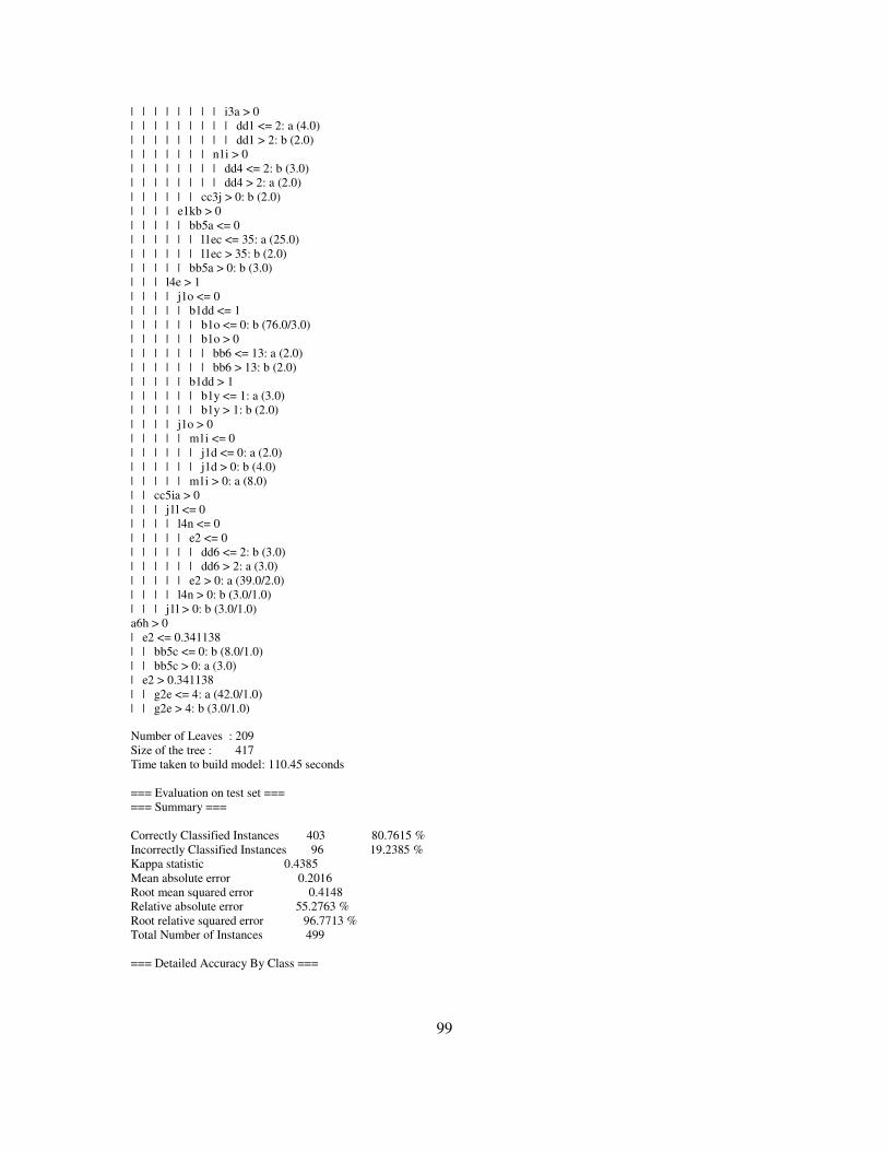
99
| | | | | | | | i3a > 0 | | | | | | | | | dd1 <= 2: a (4.0) | | | | | | | | | dd1 > 2: b (2.0) | | | | | | | n1i > 0 | | | | | | | | dd4 <= 2: b (3.0) | | | | | | | | dd4 > 2: a (2.0) | | | | | | cc3j > 0: b (2.0) | | | | e1kb > 0 | | | | | bb5a <= 0 | | | | | | l1ec <= 35: a (25.0) | | | | | | l1ec > 35: b (2.0) | | | | | bb5a > 0: b (3.0) | | | l4e > 1 | | | | j1o <= 0 | | | | | b1dd <= 1 | | | | | | b1o <= 0: b (76.0/3.0) | | | | | | b1o > 0 | | | | | | | bb6 <= 13: a (2.0) | | | | | | | bb6 > 13: b (2.0) | | | | | b1dd > 1 | | | | | | b1y <= 1: a (3.0) | | | | | | b1y > 1: b (2.0) | | | | j1o > 0 | | | | | m1i <= 0 | | | | | | j1d <= 0: a (2.0) | | | | | | j1d > 0: b (4.0) | | | | | m1i > 0: a (8.0) | | cc5ia > 0 | | | j1l <= 0 | | | | l4n <= 0 | | | | | e2 <= 0 | | | | | | dd6 <= 2: b (3.0) | | | | | | dd6 > 2: a (3.0) | | | | | e2 > 0: a (39.0/2.0) | | | | l4n > 0: b (3.0/1.0) | | | j1l > 0: b (3.0/1.0) a6h > 0 | e2 <= 0.341138 | | bb5c <= 0: b (8.0/1.0) | | bb5c > 0: a (3.0) | e2 > 0.341138 | | g2e <= 4: a (42.0/1.0) | | g2e > 4: b (3.0/1.0) Number of Leaves : 209 Size of the tree : 417 Time taken to build model: 110.45 seconds === Evaluation on test set === === Summary === Correctly Classified Instances 403 80.7615 % Incorrectly Classified Instances 96 19.2385 % Kappa statistic 0.4385 Mean absolute error 0.2016 Root mean squared error 0.4148 Relative absolute error 55.2763 % Root relative squared error 96.7713 % Total Number of Instances 499 === Detailed Accuracy By Class ===

100
TP Rate FP Rate Precision Recall F-Measure Class 0.504 0.095 0.629 0.504 0.56 a 0.905 0.496 0.851 0.905 0.877 b === Confusion Matrix === a b <-- classified as 61 60 | a = a 36 342 | b = b
The tree displayed in this Appendix is similar to the one displayed in Figure 9. The number of nodes present in this tress is 417 and the number of leaf nodes is 209.
Using code written in Java the following was extracted from the above tree. The number of unique attributes in the tree is 163. The table below shows the number of times the different attributes are repeated. b1d 2 d2d 2 a6b 2 b1w 2 l1eb 2 u1l 2 k2p 2 s6 4 bb5m 2 dd6 2 cc3k 2 e1ba 2 u1c 2 b1h 2 c1b 2 aa5 4 bb5e 2 e1kb 2 n1w 4 o1b 2 b3e 2 e1ka 2 i1q 2 g2d 2 r4a 2 cc5cb 2 c5b 2 bb5c 4 j1b 2 g2e 2 t1ba 2 dd8 2 bb6 2 cc5eb 2 l4e 2 l4b 2 i3a 2 cc5ca 2 j2c 2 k2a 4 l1bc 2 s5f 2 k2d 2 b3d 4 k2o 4 n1i 4 b1i 2 j1d 4 cc5da 6 i6 2 cc3d 2 b1y 2 e1da 4 i2a 2 bb4 4 b1o 4 r1b 2 b1p 2 o6d 2 s5b 2 l1cc 2 k2b 2 j1l 2 e1cb 2 b3b 2 cc6 4 cc5fa 2 cc3h 2 l1ac 4 o4 2 d2c 2 d1a 2 b1c 2 b1dd 2 l1ec 4 u2a 4 i1t 2 cc2 2 a4b 2 dd4 2 cc5bb 2 u1j 4 a6h 2 u1g 2 cc3i 4 e1aa 2 r5b 2 b1cc 4 e1gb 2 d2a 4 k2l 2 c3 4 m1a 2 a3 2 v1a 4 cc3j 2 b1bb 2 g1g 2 l1db 4 cc4 4 k4b 2 b1t 2 d1b 2 i2b 2 cc5ia 4 n1s 2 l3 4 f3b 2 l4n 4 bb3 2 dd3 2 m1i 2 m1b 2 cc3a 2 i1a 2 g2a 2 e1db 6 c1c 2 b1f 2 k2u 2 bb5i 2 e2 6 g1h 4 j1i 6 l1ea 2 k6 2 q1 2 b3a 2 g1f 2 r2b 2 j1o 4 f3c 2 u1i 2 i1b 2 b1aa 4 b1n 2 bb5a 4 s5g 2 j1a 2 b1k 2 t1eb 2 l1cb 2 dd1 4 h2 4 a4c 2 t5ab 2 g2b 2 l1dc 2 f3a 2 g1d 2 cc5ja 2 cc5ba 2 j1g 2 r4b 2 cc3c 2 cc5ea 2 o2b 2 t1aa 2 a6j 4 b2 2 bb5d 2 bb5k 2 l2a 8

101
Appendix D
An example to show how increasing the number of rules extracted from the training
set using the Association Discovery, increases the accuracy with regard to classification of
the test data set.
CASE 1
This appendix uses the breast cancer database from Wisconsin. 500 cases are used as
the training data set and 198 cases are used as the test data set. Using Association Discovery
tool it is found that there are 508 patterns within the training data set. From the 508 rules the
tool is made to extract 121 of the best rules. Figure 30 shows the accuracy obtained when 11
Rules where used to classify the 198 test data set.
Figure 30 Accuracy when eleven rules are used for Classification

102
CASE 2
Similar to the above case, here out of 508 rules, 121 of the best rules are used for
classification.
Figure 31 Accuracy when 121 rules are used for Classification

103
CASE 3
All the 508 rules where used for classifying the test data set.
Figure 32 Accuracy when 508 rules are used for classification
From the above three cases it is found that in CASE 1 the accuracy of the rule based
classification was 78.28%, similarly CASE 2 produced an accuracy of 97.98% and in CASE
3 an accuracy of 99.49% was obtained. This suggests that increasing the number of rules
will increase the accuracy of the system during classification.

104
Bibliography
[1] Huang, H. et al. “Business rule extraction from legacy code”, Proceedings of 20th
International Conference on Computer Software and Applications, IEEE
COMPSAC’96, 1996, pp.162-167
[2] Anthony S. Fauci, et al 1997. “Harrison's Principles of Internal Medicine ed. New
York”: McGraw-Hill.
[3] Tom Mitchell 1997 “Machine Learning”, McGraw Hill,.
[4] Lloyd-Williams,M. “Case studies in the data mining approach to health information
analysis”, Knowledge Discovery and Data Mining (1998/434), IEEE Colloquium on,8
May1998, 1996 Page(s): 1/1 -1/4
[5] IBM Guide Business Rules Project, “Defining Business Ruls – What are they are
really”, http://www.guide.org/pubs.htm, 1996
[6] ILOG Rules white paper, http://www.ilog.com/resources/whitepapers.cfm
[7] Kan, S.H. 1995 “Metrics and Models in Software Quality Engineering”, Addison-
Wesley.
[8] B. Wuthrich. “Knowledge Discovery in Databases”. Technical Report CS-95-4, The
Hong Kong University of Science & Technology, 1995.
http://citeseer.nj.nec.com/89234.html
[9] U Fayyad, P.Shaptro and P.Smyth. “From data mining to knowledge discovery in
databases”, American Association of Artificial intelligence. 1996.
http://www.kdnuggets.com/gpspubs/aimag-kdd-overview-1996-Fayyad.pdf
[10] Hirdes JP, Fries BE, Morris JN, et al. "Integrated Health Information Systems Based on
the RAI/MDS Series of Instrument" Healthcare Management Forum 12(4):30-40, 1999

105
[11] Hirdes JP, Marhaba M, Smith, TF et al. 2001 Development of the Resident Assessment
Instrument - Mental Health (RAI-MH), Hospital Quarterly, 4(2), 44-51
[12] Hirdes J.P., Perez E., Curtin-Telegdi N., et al, 1999. RAI-Mental Health (RAI-MH)
Training manual and resource Guide Version 1.0.
[13] Kim, H. and Loh, W.-Y. 2001, Classification trees with unbiased multiway splits,
Journal of the American Statistical Association, vol. 96, pp. 589-604.
[14] George H. John and Pat Langley 1995. Estimating Continuous Distributions in
Bayesian Classifiers. Proceedings of the Eleventh Conference on Uncertainty in
Artificial Intelligence. pp. 338-345. Morgan Kaufmann, San Mateo.
[15] Weiss, S. M., and Kulikowski, C. A.: Computer Systems That Learn, Morgan
Kaufmann Publishers, San Mateo (1991)
[16] Witten, T.H and Frank, E. 2000 Data mining: Practical machine learning tools and
techniques with Java implementations. Morgan Kaufmann, San Francisco.
[17] Shortliffe, EH.,Perrault, LE., (Eds.). Medical informatics: Computer applications in
health care and biomedicine (2nd Edition). New York: Springer, 2000
[18] Wong, A.K.C. and Yang Wang; High-order pattern discovery from discrete-valued
data, IEEE Transactions on Knowledge and Data Engineering, Volume: 9 , Issue: 6 ,
Nov.-Dec. 1997 Pages:877 – 893
[19] Wang, Y. and Wong, A.K.C.;From association to classification: inference-using weight
of evidence, IEEE Transactions on Knowledge and data engineering , Volume: 15 ,
Issue: 3 , May-June 2003 Pages:764 – 767
[20] Teuvo Kohonen, Jussi Hynninen, Jari Kangas, Jorma Laaksonen, and Kari Torkkola
LVQ_PAK: The Learning Vector Quantization Program Package. Technical Report
A30, Helsinki University of Technology, Laboratory of Computer and Information
Science, FIN-02150 Espoo, Finland, 1996.

106
[21] Kohonen, 1986b Learning vector quantization for pattern recognition.
Report TKK-F-A601, Helsinki University of Technology, Espoo, Finland.
[22] McQueen R.J., Neal D.L., DeWar R.E., Garner S.R., Nevill-Manning C.G. (1994) “The
WEKA Machine Learning Workbench : Its Application to a Real World Agricultural
Database” Proc Canadian Machine Learning Workshop, Banff, Alberta, Canada.
[23] Holmes G., Donkin A. and Witten I.H. (1994) “WEKA: A Machine Learning
Workbench” Proc Second Australia and New Zealand Conference on Intelligent
Information Systems, Brisbane, Australia.
[24] Witten I.H., Cunningham S.J. and Holmes G. (1995)Intelligent data analysis using the
WEKA workbench Tutorial Notes, Conference on Artificial Neural Networks and
Expert Systems, Dunedin, NZ.
[25] Garner S.R. (1995) “WEKA: The Waikato Environment for Knowledge Analysis Proc”
New Zealand Computer Science Research Students Conference, University of Waikato,
Hamilton, New Zealand, pp 57-64.
[26] Thamar Solorio and Olac Fuentes, “Improving Classifier Accuracy using Unlabeled
Data”. Proceedings of the IASTED International Conference on Artificial Intelligence
and Applications (AIA2001), Marbella, Spain, Sept. 2001.
[27] Breiman et al., 1984 “Classification and Regression Trees”. Wadsworth International
Group, Belmont, CA.
[28] W.-Y. Loh and N. Vanichsetakul 1988. Tree-structured classification via generalized
discriminant analysis, Journal of the American Statistical Association, 83, 715-728
[29] Wolberg,W.H., & Mangasarian,O.L. 1990. “Multisurface method of pattern separation
for medical diagnosis applied to breast cytology”. In Proceedings of the National
Academy of Sciences, 87, 9193-9196. [http://pbil.univ-
lyon1.fr/library/mlbench/html/BreastCancer.html]

107
[30] Frawley, W.J., Piatetsky-Shapiro, G., and Matheus, C. Knowledge Discovery In
Databases: An Overview. In Knowledge Discovery In Databases, eds. G. Piatetsky-
Shapiro, and W. J. Frawley, AAAI Press/MIT Press, Cambridge, MA., 1991, pp. 1-30.
[31] Quinlan, J.R. C4.5: Programs For Machine Learning. San Mateo, CA: Morgan
Kaufmann, 1993