12th World Congress on Structural and Multidisciplinary Optimisation 05th - 09th, June 2017, Braunschweig, Germany

1

Application of Digital Image Correlation to Material Parameter Identification

Nielen Stander1, Katharina Witowski2, Christian Ilg2, Andre Haufe2, Martin Helbig2, David Koch2

1 Livermore Software Technology Corporation, Livermore, California, USA. nielen@LSTC.com 2 DYNAmore GmbH, Stuttgart, Germany

1. Abstract This paper expounds the parameter identification of material models using simulation-based optimization and experimental results obtained using Digital Image Correlation (DIC). DIC is an optical method which provides full-field displacement measurements for mechanical tests of materials and structures. It can be used to obtain strain field histories from an experimental coupon which can be combined with the corresponding fields obtained from a Finite Element Analysis to identify constitutive properties. The methodology, which involves the solution of an inverse problem, has been implemented in the optimization code LS-OPT®. A core feature is multi-point curves: response curves which are evaluated at multiple locations and extracted from simulations and experimental data. An interface to a commercial optical measurement package was created and an example of a tensile test was used to demonstrate the methodology based on the measurement of point-wise strains vs. tensile force. The Hockett-Sherby flow curve function, using two parameters, was used to model the material. The example validated the code but revealed potential problem areas requiring further investigation. A prominent issue is the method used for matching the experimental and computational curves. To identify sources of ill-posedness of the regression problem, several diagnostic tools are suggested. Some of these tools, notably sensitivity analysis will be demonstrated at the conference. 2. Keywords: Material parameter identification, Digital Image Correlation, material calibration, full-field calibration 3. Introduction The goal of material parameter identification is to characterize the constitutive behavior using experimental results in combination with structural modeling of the test samples. Although rather well established, it is a complex subject which may involve material nonlinearity [3,9], hysteretic behavior (loading and unloading) [9], strain localization [3] as well as instability of the calibration [1]. The testing component may also involve full-field optical measurement [2,3,4,5,6,7,8]. A common and simple approach for identifying material parameters is to use the tensile test in which a coupon is subjected to a force while being measured for deformation. Both are global quantities. To extract the material properties, the coupon, usually of simple geometry, can be modeled using the Finite Element Method which incorporates the constitutive model to be calibrated. The methodology for conducting a calibration requires the construction of a distance functional to quantify the distance between the experimental and computational results:

𝑓𝑓(𝒙𝒙) = ��𝜑𝜑𝑗𝑗(𝒙𝒙) − 𝜑𝜑�𝑗𝑗�2

𝑛𝑛

𝑗𝑗=1

(1)

where 𝜑𝜑𝑗𝑗(𝒙𝒙) are the components of a force history or force-displacement vector and 𝑛𝑛 is the number of observation states. The vector 𝒙𝒙 represents the unknown material parameters and the ~ designates the experimental results. The distance functional is minimized using optimization. Further investigation is required to find a method suitable for interpolating values 𝜑𝜑𝑗𝑗 which correspond to 𝜑𝜑�𝑗𝑗. This depends on whether 𝜑𝜑 represents a mathematical function (each input has exactly one output), or not. In most cases these functions can be handled using a least squares functional in which the interpolation of the computed curve is ordinate-based. For non-functions, such as when loading-unloading occurs, more sophisticated techniques are required such as Partial Curve Mapping [9,10]. In this method both curves are traced based on preservation of the interval length along the target curve. While simple material models can typically be uniquely identified using a tensile and/or shear test, a major difficulty in parameter identification is ill-posedness of the observation equation [1]:

2

𝐴𝐴(𝑥𝑥) = 𝑑𝑑 ;𝑥𝑥 ∈ X (2)

in which the mapping 𝐴𝐴 represents the modeling (e.g. a FE model), 𝑥𝑥 ∈ X represents the model parameters (the material constants) bounded by the parameter space X and 𝑑𝑑 represents the data (experimental data) in the observable data space D. This problem is typically solved with a minimization problem [1]:

𝑑𝑑 = arg{Min𝑑𝑑′

𝐽𝐽(𝑑𝑑′; 𝑥𝑥)} ≡ 𝐴𝐴(𝑥𝑥) (3) In Reference [1] Bui lists important issues to check when solving the inverse problem, namely (i) stability of the solution with respect to variations in the data 𝑑𝑑 as well as with respect to modeling errors and small changes in the model space X (robustness). It should be mentioned that the inverse problem to determine the parameters 𝑥𝑥, for given experimental data 𝑑𝑑, is generally ill-posed. In material parameter identification, various conditions can cause ill-posedness, for example [1]:

• False experimental data (measurement errors or erroneous data files) • Incompatible data, i.e. there is no set of material parameters that will cause the model to produce results in

data space D. • Noise in the experimental data • Modeling errors e.g. in the constitutive model or coarse approximation of the model A

These problems are manifested because of the lack of suitable information provided by the chosen test. E.g. providing global information such as a force-displacement curve representing a chosen point or cross-section of a coupon may not be sufficient to characterize a nonlinear material model which involves material flow, failure and/or damage. It is also typical of failure behavior to be localized, which eludes capture by global force-displacement data [3]. It is probably safe to assume that the more sophisticated the material model and the phenomena it is intended to model, the more parameters it possesses and the greater the need exists for full-field calibration to capture localized behavior. While optimization always yields a solution to the unconstrained regression problem, the deficiency in the distribution of the input data may result in instability of that solution. It is with this problem, as well as accuracy, in mind that experimental mechanicians, over the last three decades, have introduced full field optical measurement techniques. These allow more comprehensive sampling in order to capture phenomena to which the material parameters have non-zero sensitivity, thereby improving stability of the calibration. The purpose of these non-contact methods is to measure the spatial distribution of physical quantities such as displacement or strain. Much of the development in this area arose from the improvements made to camera and computer technology as well as analysis techniques such as the Finite Element Method. Multiple optical measurement methods have been forthcoming such as digital holography and speckle interferometry. Magnetic Resonance Imaging (MRI) has been used to characterize myocardial material, see e.g. [7]. The focus of the current paper is an optical measurement method referred to as Digital Image Correlation [8].

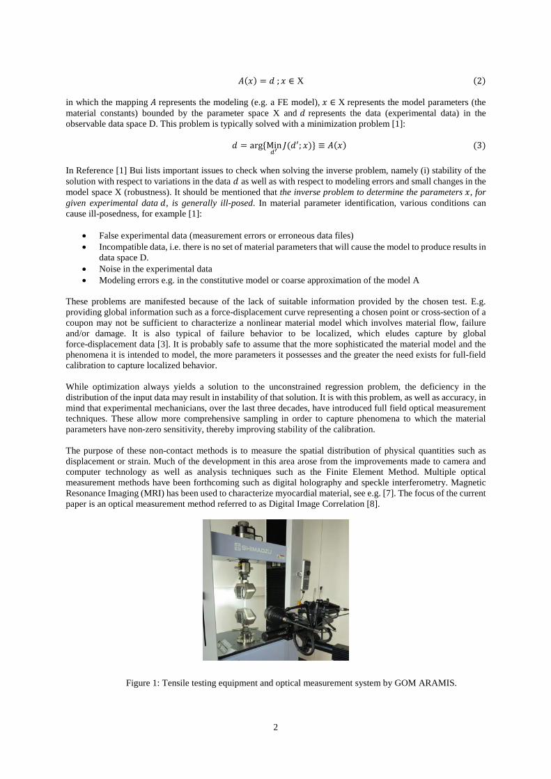
Figure 1: Tensile testing equipment and optical measurement system by GOM ARAMIS.

3

Figure 2: Full field measurement of a shear test using Digital Image Correlation. On the left is the DIC

image (GOM ARAMIS) while a strain contour plot is featured on the right (LS-PrePost®).

Digital Image Correlation (DIC) started to appear in the early 1980s and is an optical measurement method (see Fig. 1 for test setup) which provides full-field displacement measurements for mechanical tests of materials and structures. A specific advantage of this tool is that it exploits numerical images acquired at difference stages of loading. As such, it can be used to obtain temporal displacement, deformation or strain fields from an experimental coupon and can be combined with Finite Element Analysis to identify the constitutive properties of a material (see Fig. 2). Using DIC results, optimization is used to obtain the parameters which will minimize the distance functional involving the measured field and the computed field as components. As expressed for instance in Mahnken et al [3] the functional used is:

𝑓𝑓(𝒙𝒙) = ��𝝋𝝋𝑗𝑗(𝒙𝒙) − 𝝋𝝋�𝑗𝑗�2

𝑛𝑛

𝑗𝑗=1

(4)

where 𝝋𝝋𝒋𝒋(𝒙𝒙) is a vector of nodal displacements or strains with dimension equal to the number of spatially distributed observation points and 𝑛𝑛 is the number of observation states. The functional can be augmented to incorporate global force-displacement measurements or any other functional resulting in parameter identification based on a multi-scale DIC (see e.g. [5]). 2. Methodology and software features While LS-OPT® has included parameter identification features since its first commercial release, the current development goal is to significantly enhance these capabilities to enable LS-OPT to accommodate modern testing techniques such as DIC. While full field calibration has been conducted using LS-OPT in the past [7], the current implementation generalizes the feature to enable it to address a greater diversity of problems. A summary of essential features, most of which have now been implemented in LS-OPT, follows:

4

1. A core feature of the methodology is the multi-point history, a basic mathematical entity representing both

spatial and temporal dimensions. Multi-point histories are curves which are evaluated at multiple locations (possibly thousands) and extracted from simulations and experimental data.

2. To access test data, an interface to the GOM ARAMIS DIC software was developed. 3. An algorithm was developed to map a test point cloud to an FE model. 4. The ability to interpolate fields within a finite element is incorporated into the mapping approach. 5. MSE distance functionals for multi-point histories can be used as objective functions. 6. Error analysis enables the user to assess the size of the mismatch as well as the resulting uncertainty of the

parameters. 7. Graphical features are available to enhance the prior inspection and editing of test results. 8. Distance contour maps are provided for post-processing the discrepancy between computed values and

experimental quantities (not yet implemented). 9. Confidence intervals of the material parameters enable the user to quantify their uncertainty (not yet

implemented). 10. The DynaStats feature of LS-OPT [10] provides sensitivity analysis and stochastic influence tools to identify

spatial strain or displacement sensitivities to individual material parameters. Aside from the obvious use of locating suitable measurement areas, sensitivity analysis also allows the user to compare the significance of different strain measures, e.g. 𝜀𝜀𝑥𝑥𝑥𝑥, 𝜀𝜀𝑦𝑦𝑦𝑦 and 𝜀𝜀𝑥𝑥𝑦𝑦.

A more detailed discussion is provided in the following sub-sections. 2.1. GOM ARAMIS interface and alignment of DIC points Since the following test example uses the GOM ARAMIS measurement software, an LS-OPT GOM interface was implemented to define input files, result components and alignment data. The alignment is computed using the least squares formulation shown in the equation:

min𝑻𝑻‖𝑿𝑿Test𝑻𝑻 − 𝑿𝑿FE‖ (5)

to match any number of test points 𝑿𝑿Test to corresponding coordinates on the FE mesh 𝑿𝑿FE. The points in 𝑿𝑿Test and 𝑿𝑿FE respectively do not have to correspond exactly as the alignment is based on a least squares principle that will minimize the fitting error for any number of points. The solution of Eq. (5), using Singular Value Decomposition, yields the transformation matrix 𝑻𝑻 which is then used to transform all the test points (see e.g. Fig. 7). The data can also be specified as nodal/point IDs. Three or four points normally suffice, but any number can be specified. Alternatively, the alignment step can be omitted, since post-processing software can be used to pre-align the point set. To enable the creation of cross-plots from the GOM data, both the X- and Y-components shown in Fig. 3 can be histories or multi-point histories. E.g. a multi-point 𝑥𝑥𝑥𝑥-strain can be crossed with a multi-point 𝑦𝑦𝑦𝑦-strain to create multi-point stress-strain cross-plots or, as in the example that follows in the next section (Fig. 11), the full-field 𝑥𝑥𝑥𝑥-strain can be crossed with the global force history to create multi-point strain-force cross-plots. The same applies to cross-plots of computational fields.

5

Figure 3: GOM ARAMIS interface in LS-OPT showing alignment input and verification plot of selected

test value X- and Y-components.

2.2. Multi-point histories In the GOM ARAMIS option in the multi-point histories interface, each history is computed at a location selected from the test point set in the original, undeformed state. Features are provided to preview the test point alignment (see Fig. 4). Fig. 5 shows three representative deformation states representing 4557 points extracted from the GOM database for a plate with a hole while Fig. 6 shows the FE mesh with corresponding test points. Fig. 7 shows the effect of the least squares point alignment using Eq. (5).

Figure 4: Multi-point history interface enabling the definition of the response type and location data.

Location type can be defined as 'nearest node' or 'element'. In the latter option, the result is interpolated at the precise location within the nearest element.

6

Figure 5: Selected deformation states from GOM output.

Figure 6: Example of test point mapping showing test point set (red) of 4557 points in relation to the Finite Element mesh.

Figure 7: Interactive feature for verification of least squares test point alignment. The starting test point

location (in bright red) is shown on the left.

2.3. Mapping of test points to a FE mesh After alignment, the test points are mapped to the FE mesh. The algorithm enables mapping in 3 dimensions using a binary tree algorithm. The approach allows for an exact nearest neighbor search with the capacity to map 107 query points to 107 reference points in reasonable time (suitable for interactive use). Practical examples

7

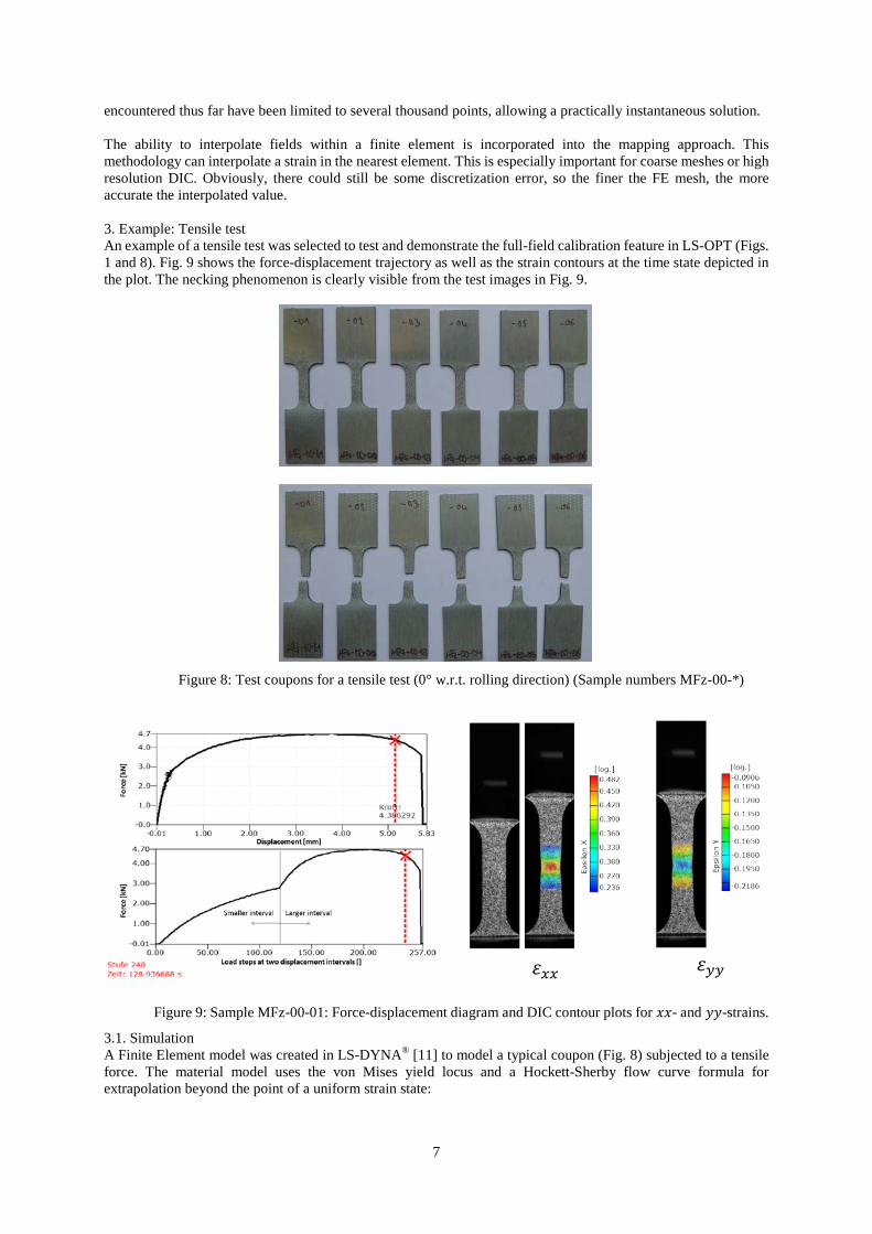
encountered thus far have been limited to several thousand points, allowing a practically instantaneous solution. The ability to interpolate fields within a finite element is incorporated into the mapping approach. This methodology can interpolate a strain in the nearest element. This is especially important for coarse meshes or high resolution DIC. Obviously, there could still be some discretization error, so the finer the FE mesh, the more accurate the interpolated value. 3. Example: Tensile test An example of a tensile test was selected to test and demonstrate the full-field calibration feature in LS-OPT (Figs. 1 and 8). Fig. 9 shows the force-displacement trajectory as well as the strain contours at the time state depicted in the plot. The necking phenomenon is clearly visible from the test images in Fig. 9.

Figure 8: Test coupons for a tensile test (0° w.r.t. rolling direction) (Sample numbers MFz-00-*)

𝜀𝜀𝑥𝑥𝑥𝑥

𝜀𝜀𝑦𝑦𝑦𝑦

Figure 9: Sample MFz-00-01: Force-displacement diagram and DIC contour plots for 𝑥𝑥𝑥𝑥- and 𝑦𝑦𝑦𝑦-strains.

3.1. Simulation A Finite Element model was created in LS-DYNA® [11] to model a typical coupon (Fig. 8) subjected to a tensile force. The material model uses the von Mises yield locus and a Hockett-Sherby flow curve formula for extrapolation beyond the point of a uniform strain state:

8

𝑓𝑓�𝜀𝜀𝑝𝑝� = 𝐴𝐴 − 𝐵𝐵𝑒𝑒−𝐶𝐶𝜀𝜀𝑝𝑝𝑝𝑝

𝑁𝑁 (6)

where 𝐴𝐴, 𝐵𝐵 𝐶𝐶 and 𝑁𝑁 are material constants. 𝐶𝐶1-continuity is assumed at the flow transition following the uniform strain state which removes the requirement to incorporate 𝐴𝐴 and 𝐵𝐵 in the optimization that follows. 3.2. Optimization The LS-OPT setup required alignment of the 391 measured points with the FE mesh as shown in Fig. 10. The force vs. point-wise 𝜀𝜀𝑥𝑥𝑥𝑥 strain curves are shown in the previewing feature depicted in Fig. 11. Each curve represents a measuring point as shown in black in Fig. 10. For the optimization, a cross-plot was defined using multi-point histories to represent the global force vs. point-wise strains. The incorporation of the force ensures that both statics and kinematics are incorporated into the behavior. The optimization problem was set up with parameters 𝐶𝐶 and 𝑁𝑁 as variables and with the objective to minimize the distance functional 𝑓𝑓 [Equation (4)]. This defines the ideal of matching 𝜀𝜀𝑥𝑥𝑥𝑥 at each point and each deformation state. The optimization was conducted using the Sequential Response Surface method of LS-OPT [10] using standard settings.

Figure 10: Finite element model of the coupon specimen (red) shown with 391 superimposed optically measured points at the center (black).

Figure 11: Preview of the multi-point curve: the force (AD-0) vs. full-field logarithmic 𝑥𝑥𝑥𝑥-strain as rendered in a previewing feature of the GOM interface in LS-OPT. Each curve represents a single

measuring point.

9

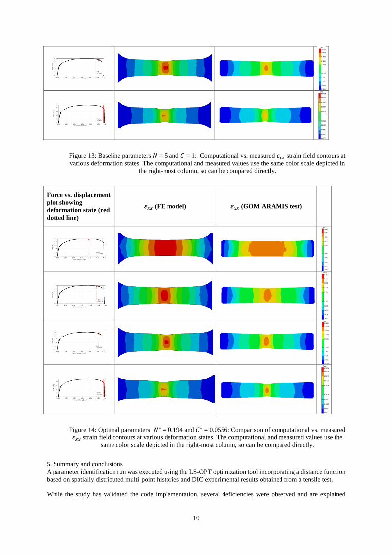
4. Results and observations The optimization history of the distance functional is shown in Fig. 12. The value of the distance functional (the graph ordinate) [Eq.(4)] has been normalized with the maximum absolute value of the experimental values. The table in Fig. 13 represents a comparison of the 𝑥𝑥𝑥𝑥 strain contours obtained from the GOM software with the contours obtained from the LS-DYNA FE simulation for a set of initially estimated values of 𝑁𝑁 = 5 and 𝐶𝐶 = 1. The optimization yields values 𝑁𝑁 = 0.194 and 𝐶𝐶 = 0.0556 which corresponds to the results of Fig. 14. It can be seen that the computational result in the latter figure is significantly closer to the experimental result. A second optimization run from a different starting point (not shown here) yielded values 0.226 and 0.0717 for 𝑁𝑁 and 𝐶𝐶 respectively. Several observations can be made:

1. The optimization result converges to a solution around the 10th iteration. 2. Different starting points may yield different optimal parameters which, while not excessive, cannot be

ignored entirely. 3. The objective value varying between 0.0396 (baseline) and 0.0377 (It. 10) is a relatively small variation.

Figure 12: Optimization history of the normalized distance functional showing convergence achieved

between 10 and 15 iterations. The points represent LS-DYNA results while the line represents the response surface approximation values.

Force vs. displacement plot showing deformation state (red dotted line)

𝜺𝜺𝒙𝒙𝒙𝒙 (FE model) 𝜺𝜺𝒙𝒙𝒙𝒙 (GOM ARAMIS test)

10

Figure 13: Baseline parameters 𝑁𝑁 = 5 and 𝐶𝐶 = 1: Computational vs. measured 𝜀𝜀𝑥𝑥𝑥𝑥 strain field contours at various deformation states. The computational and measured values use the same color scale depicted in

the right-most column, so can be compared directly.

Force vs. displacement plot showing deformation state (red dotted line)

𝜺𝜺𝒙𝒙𝒙𝒙 (FE model) 𝜺𝜺𝒙𝒙𝒙𝒙 (GOM ARAMIS test)

Figure 14: Optimal parameters 𝑁𝑁∗ = 0.194 and 𝐶𝐶∗ = 0.0556: Comparison of computational vs. measured 𝜀𝜀𝑥𝑥𝑥𝑥 strain field contours at various deformation states. The computational and measured values use the

same color scale depicted in the right-most column, so can be compared directly.

5. Summary and conclusions A parameter identification run was executed using the LS-OPT optimization tool incorporating a distance function based on spatially distributed multi-point histories and DIC experimental results obtained from a tensile test. While the study has validated the code implementation, several deficiencies were observed and are explained

11

below, with a view to address them in future development:

1. Stability and Uniqueness. It was shown that different starting points for the optimization procedure yield slightly different results which presumably affect the accuracy of the calibration result. Possible reasons are (i) the inability of the SRSM optimization algorithm to converge sharply, (ii) the presence of local minima (mathematical non-uniqueness) and (iii) instability of the solution. Reasons (i) and (ii) can only be addressed by switching to a global optimization algorithm, such as the Genetic Algorithm available in LS-OPT. Point (iii) can only be addressed by investigating the suitability and location of the result fields measured in the formulation of the objective. It should be noted that only 𝜀𝜀𝑥𝑥𝑥𝑥 was used in the calibration, while 𝜀𝜀𝑦𝑦𝑦𝑦 was neglected, a factor which may have significantly influenced the stability of the solution. The computation of spatial sensitivities and confidence intervals can be used to detect sources of ill-posedness.

2. Sensitivity. A methodology that can be used to investigate sources of instability is sensitivity analysis. It is therefore suggested that a study be done, using LS-OPT DynaStats [10], in which the spatial sensitivity (or stochastic influence) contours can be studied to determine locations where sensitivities of response types such as 𝜀𝜀𝑥𝑥𝑥𝑥 and 𝜀𝜀𝑦𝑦𝑦𝑦 to the individual material parameters are highest. DynaStats is a general tool for previewing the suitability of response field types by allowing the user to study the evolution, over time, of their spatial distribution and relative importance.

3. Confidence intervals of the parameters. It is also suggested that confidence intervals be calculated for the parameters, a function which requires the calculation of the gradients (with respect to the parameters) of the multi-point histories at the optimal solution 𝒙𝒙∗. The confidence intervals quantify the degree to which the optimal value of a parameter can be trusted. The computation of confidence intervals requires response surfaces to be constructed at every location and deformation state.

4. Noise. The very slight improvement of the objective function (0.0396 vs. 0.0377 or about 5%) seems to suggest that a significant component of the residual error (of the distance functional) contains noise so that fitting the material model to the test always yields a non-zero residual. The noise may emanate from discretization error and/or experimental error.

5. Modeling error. It is possible that, in addition to noise, the material flow model does not represent the experimental response with absolute accuracy. This causes a bias or modeling error which remains a residual error even after finding a converged solution to the regression problem.

6. Curve matching technique. It is apparent from Fig. 11 that some of the curves have very steep, near vertical, post-yield behavior which presents a difficulty for ordinate-based interpolation. As a consequence, some of the curve data may be inadvertently neglected. A possible solution would be to extend the Partial Curve Mapping capability in LS-OPT (see Witowski and Stander [9]), currently available for simple histories, to multi-point curves.

7. Finite Element discretization error. The FE mesh provided for the example is somewhat coarse, possibly resulting in a discretization error. This may be especially true because triangular elements are used in the transitions. An obvious remedy would be to increase the fineness of the mesh and to use only higher order triangles or quadrilateral elements.

Since experiments rarely involve a single coupon, future work will also focus on incorporating replicated experiments to assess their influence on the variability of the optimal parameters. 6. References [1] Bui, H.D. Inverse Problems in the Mechanics of Materials, An Introduction, CRC Press, Boca Raton,

London, 1994). [2] Pagnacco, E., Moreau, A., Lemosse, D. Inverse Strategies for the identification of elastic and viscoelastic

material properties using full-field measurements, Materials Science and Engineering, Vol. 452-453, 737-745, 2007

[3] Mahnken, R., Stein, E. Parameter Identification for Finite Deformation Elasto-Plasticity in Principal Directions, Comput. Methods Appl. Mech. Engrg, 147, 17-39, 1997.

[4] Leclerc, H., Périé, J.-N., Roux, S., Hild, F. Integrated Digital Image Correlation for the Identification of Mechanical Properties, MIRAGE 2009, LNCS 5496, 161-171, 2009, A Gagalowicz and W. Philips (Eds.), Springer-Verlag, 2009.

[5] Passieux, J.C., Bugarin, F., David, C., Périé, J.-N., Robert, L. Multiscale Displacement Field Measurement Using Digital Image Correlation: Application to the Identification of Elastic properties, https://hal.archives-ouvertes.fr/hal-00949038, 2014.

[6] Gu, J., Cooreman, S., Smits, A., Bossuyt, S., Sol, H., Lecompte, D. and Vantomme, J. Full-field optical measurement for material parameter identification with inverse methods, High Performance Structures and

12

Materials III, WIT Transactions on the Built Environment, 85, 2006. doi10.2495/HPSM06024. [7] Stander, N. The identification of myocardial material parameters from spatial tagged MRI strain data using

LS-OPT and LS-DYNA, Report, LSTC In cooperation with J. Guccione, Cardiac Mechanics Lab, UCSF, 2006.

[8] Bornert, M., Hild, F., Orteu, J.-J., Roux, S. Full Field Measurements and Identification in Solid Mechanics, Chapter 6: Digital Image Correlation, 157-190, Eds. Grédiac, M., Hild, F., Wiley, 2013.

[9] Witowski, K., Stander, N. Parameter Identification of Hysteretic Models Using Partial Curve Mapping, Proceedings of the 12th AIAA Aviation Technology Integration and Operations Conference and 14th AIAA/ISSMO Multidisciplinary Analysis and Optimization Conference, Indianapolis, Indiana, 2012.

[10] Stander, N., Roux, W.J., Basudhar, A., Eggleston, T, Craig, K.-J. LS-OPT Users Manual, Version 5.2. December 2015.

[11] Hallquist, J.O. LS-DYNA Users Manual, Livermore Software Technology Corporation.