application of dynamic upscaling for thermal reservoir
TRANSCRIPT

University of Calgary
PRISM: University of Calgary's Digital Repository
Graduate Studies The Vault: Electronic Theses and Dissertations
2014-03-26
Application of Dynamic Upscaling for Thermal
Reservoir Simulation
Picone, Matteo M.
Picone, M. M. (2014). Application of Dynamic Upscaling for Thermal Reservoir Simulation
(Unpublished master's thesis). University of Calgary, Calgary, AB. doi:10.11575/PRISM/24960
http://hdl.handle.net/11023/1390
master thesis
University of Calgary graduate students retain copyright ownership and moral rights for their
thesis. You may use this material in any way that is permitted by the Copyright Act or through
licensing that has been assigned to the document. For uses that are not allowable under
copyright legislation or licensing, you are required to seek permission.
Downloaded from PRISM: https://prism.ucalgary.ca

UNIVERSITY OF CALGARY
Application of Dynamic Upscaling for Thermal Reservoir Simulation
By
Matteo Mario Picone
A THESIS
SUBMITTED TO THE FACULTY OF GRADUATE STUDIES
IN PARTIAL FULFILMENT OF THE REQUIREMENTS FOR THE
DEGREE OF MASTER OF ENGINEERING
DEPARTMENT OF CHEMICAL AND PETROLEUM ENGINEERING
CALGARY, ALBERTA
March 2014
© Matteo M. Picone 2014

Abstract
Reservoir simulation is inherently an imperfect tool for forecasting. However, given sufficient
analysis and post-processing, the areas of uncertainty can be quantified and effort can be made to
mitigate their impact and improve the confidence in the prediction. The focus of the research
documented here is to analyze the extent to which grid size definition and the location and
quantity of reservoir heterogeneities impact the performance of a simulation-based recovery
process. In analysing two different sets of models (binary and facies-based), a new methodology
was developed and applied to mitigate the observed difference in the forecasted result. When the
observations are coupled, it suggests that an increase in near wellbore reservoir heterogeneity, as
indicated by a reduction in gridblock connectivity, has an increased impact upon the simulation
results when compared to the impact of strictly length scale definition of heterogeneity.
Additionally, the impact of length scales can be normalized when the focus is upon connectivity
within the reservoir model.
ii

Acknowledgements
I would like to thank Arnfinn Kjosavik for helping to conceive this idea. Our original
conversations serve as the foundation to this work. Secondly, I would like to thank Dr. Ian Gates
who not only served as an academic mentor and was instrumental in fine tuning many of the
details, but was also very kind and patient during the entire process.
Finally, I would like to thank my family. To my parents who always empowered my brother and
I to achieve our goals. They are the foundation to my life and represent everything good I have
accomplished thus far. Life is nothing if not for family.
And to my wife, Kim, you are the other half, the missing piece. And our love is unconditional.
iii

Table of Contents
Abstract ........................................................................................................................... ii Acknowledgements ........................................................................................................ iii Table of Contents ........................................................................................................... iv List of Tables ................................................................................................................. vi List of Figures and Illustrations ..................................................................................... xi List of Symbols, Abbreviations and Nomenclature .................................................... xvii Epigraph ....................................................................................................................... xix
CHAPTER 1 – INTRODUCTION ......................................................................................1 1.1 Background and Introductory Concepts ....................................................................1 1.2 Problem Statement .....................................................................................................8 1.3 Organization of Thesis ...............................................................................................8
CHAPTER 2 – LITERATURE REVIEW .........................................................................10 2.1 Upscaling for Reservoir Simulation ........................................................................10 2.2 Upscaling for Thermal Reservoir Models ...............................................................16
CHAPTER 3 – MODELLING CONCEPTS .....................................................................19 3.1 Numerical Modelling Process ..................................................................................19 3.2 Modelling Tools .......................................................................................................19 3.3 Model Grid Definitions ............................................................................................20 3.4 Editing an Existing Grid ..........................................................................................22 3.5 Reservoir Parameters ...............................................................................................24
3.5.1 SAGD Circulation, Constraint Set-Up ............................................................25 3.5.2 SAGD Production Phase, Constraint Set-Up ..................................................26
3.6 Key Performance Metrics ........................................................................................29 3.7 Binary-Geostatistical Models ..................................................................................32 3.8 Facies-based Models ................................................................................................34 3.9 Vertical Proportion Curves ......................................................................................41 3.10 Dynamic Upscaling Concept .................................................................................45 3.11 Impact of Reservoir Heterogeneities on SAGD Performance ...............................49
CHAPTER 4 – DYNAMIC UPSCALING: RESULTS ....................................................59 4.1 Dynamic Upscaling Parameters ...............................................................................59
4.1.1 Permeability .....................................................................................................60 4.1.2 Heat Transfer – Thermal Conductivity ............................................................63
4.2 History Matching Process ........................................................................................65 4.2.1 Parameters .......................................................................................................67 4.2.2 Optimization Method .......................................................................................67 4.2.3 Objective Function ..........................................................................................68 4.2.4 Influence Matrix ..............................................................................................68 4.2.5 Constraints .......................................................................................................69 4.2.6 Run Configurations .........................................................................................70
4.3 Comparison of Preliminary Results .........................................................................70
iv

4.4 Non-Unique Solutions .............................................................................................75 4.5 Organization of Raw Data .......................................................................................79 4.6 Normalization of Length Scale Impact ....................................................................93
CHAPTER 5 – EVALUATION CRITERIA ...................................................................100 5.1 SAGD Productivity Index ......................................................................................100
5.1.1 SAGD Productivity Set-Up ...........................................................................101 5.2 Application of Equations to Facies-based Models ................................................110 5.3 Modelling Assumptions and Limitations ...............................................................116 5.4 Impact on Commercial Projects .............................................................................125
CHAPTER 6 – CONCLUSIONS AND RECOMMENDATIONS .................................127 6.1 Conclusions ............................................................................................................127 6.2 Recommendations ..................................................................................................131 6.3 Pareto Principle, 80-20 Rule ..................................................................................134
REFERENCES ................................................................................................................136
APPENDICES .................................................................................................................144 Appendix A Governing Equations for Reservoir Simulation ......................................144 A.1 Explicit Discretization of One-Dimensional Flow Equation (x-direction) ...........147 A.2 Implicit Discretization of One-Dimensional Flow Equation (x-direction) ...........148 Appendix B CMOSTTM Input Files .............................................................................149 Appendix C Ranking Geostatistical Realizations for SAGD Process .........................150 Appendix D Production Profile Summary ...................................................................151 Appendix E Formation Heating by Steam Injection: Marx-Langenheim Model ........158
v

List of Tables
Table 3.4.1 – Comparison of Simulation Time for Different Refinement Techniques .....23
Table 3.5.1 – Single Well Pair Reservoir Simulation Properties and Input Parameters ....25
Table 3.5.1.1 – Circulation Well, Constraint Configuration..............................................26
Table 3.5.1.2 – Circulation Heater Configuration .............................................................26
Table 3.5.2.1 – SAGD Production Phase, Constraint Set-Up - Injection Well .................26
Table 3.5.2.2 – SAGD Production Phase, Constraint Set-Up - Production Well ..............27
Table 3.5.2.3 – Comparison of Simulation Time for Different Sub-cool Model ..............28
Table 3.6.1 – 2012 In-situ Progress Reports Published from the ERCB ...........................31
Table 3.7.1 – Depositional Quantities................................................................................33
Table 3.7.2 – BuilderTM Generated Geostatistical Model ..................................................34
Table 3.9.1 – Standard Distribution Parameters ................................................................43
Table 3.11.1 – Comparison of Length Scales and Heterogeneity on Coarse Model
Performance .......................................................................................................................57
Table 3.11.2 – Comparison of Length Scales and Heterogeneity on Relative
Performance .......................................................................................................................58
Table 4.1.2.1 – Thermal Properties within STARSTM for a Single Rock Type .................65
Table 4.2.1.1 – Parameter Inputs .......................................................................................67
Table 4.2.4.1 – Influence Matrix .......................................................................................69
Table 4.3.1 – Binary Model Results, 5% Shale Distribution (Model A) ...........................70
Table 4.3.2 – Binary Model Results, 5% Shale Distribution (Model A) ...........................71
Table 4.3.3 – Matching Parameters Assigned by CMOSTTM, 5% Shale Distribution
(Model A)...........................................................................................................................72
vi

Table 4.4.1 – Alternative Binary Model Results, 5% Shale Distribution (Model A) ........76
Table 4.4.2 – Alternative Matching Parameters Assigned by CMOSTTM, 5% Shale
Distribution (Model A) ......................................................................................................76
Table 4.4.3 – Binary Model Results, 1% Shale Distribution (Unique Solution #1) ..........76
Table 4.4.4 – Matching Parameters Assigned by CMOSTTM, 1% Shale Distribution
(Unique Solution #1)..........................................................................................................76
Table 4.4.5 – Binary Model Results, 1% Shale Distribution (Unique Solution #2) ..........77
Table 4.4.6 – Matching Parameters Assigned by CMOSTTM, 1% Shale Distribution
(Unique Solution #2)..........................................................................................................77
Table 4.5.1 – Outliers in the ‘Original Error’ Cases (4m, 100m, 1m) ...............................82
Table 4.5.2 – Outliers in the ‘Delta Error’ Cases (4m, 100m, 1m) ...................................83
Table 4.5.3 – Binary Model Results, 5% Shale Distribution (Model #1), ‘Original
and Final Error’ ..................................................................................................................88
Table 4.5.4 – Binary Model Results, 5% Shale Distribution (Model #1), ‘Delta
Error’ ..................................................................................................................................89
Table 4.5.5 – Matching Parameters Assigned by CMOSTTM, 5% Shale Distribution
(Model #1) .........................................................................................................................89
Table 4.5.6 – Binary Model Results, 5% Shale Distribution (Model #2) ..........................89
Table 4.5.7 – Binary Model Results, 5% Shale Distribution (Model #2) ..........................89
Table 4.5.8 – Matching Parameters Assigned by CMOSTTM, 5% Shale Distribution
(Model #2) .........................................................................................................................90
Table 4.5.9 – ‘Best Job’ Matching Parameters Assigned by CMOSTTM ..........................90
Table 4.5.10 – ‘Best Job’ Matching Parameters Assigned by CMOSTTM ........................90
vii

Table 4.6.1 – Revisited Comparison of Length Scales and Heterogeneity on Coarse
Model Performance ............................................................................................................96
Table 4.6.2 – Revisited Comparison of Length Scales and Heterogeneity on Relative
Performance .......................................................................................................................97
Table 5.1.1.1 – Model Options with CMG’s SAGD Productivity Index (SPI),
(4m, 100m, 1m) Grid Dimensions ...................................................................................102
Table 5.1.1.2 – Comparison of SPI of Model #1, Model #2 and Model A .....................102
Table 5.1.1.3 – Error Band and Variation in SPI for a Given Shale Content ..................104
Table 5.1.1.4 – Binary Models, 1% Distribution .............................................................105
Table 5.1.1.5 – Binary Models, 2% Distribution .............................................................105
Table 5.1.1.6 – Binary Models, 3% Distribution .............................................................105
Table 5.1.1.7 – Binary Models, 4% Distribution .............................................................105
Table 5.1.1.8 – Binary Models, 5% Distribution .............................................................106
Table 5.1.1.9 – Binary Models, 10% Distribution ...........................................................106
Table 5.1.1.10 – Binary Models, 20% Distribution .........................................................106
Table 5.1.1.11 – Equations Representing the Relationship between SPI and
Parameter Values .............................................................................................................109
Table 5.2.1 – Facies-based Sensitivity .............................................................................110
Table 5.2.2 – Type A’ Facies-based Model Associations (Forecasted Values) ..............111
Table 5.2.3 – Type A’ Facies-based Model Associations (Forecasted Percent
Improvement) ...................................................................................................................112
Table 5.2.4 – Type A’ Facies-based Model Associations (History Match Values) ........112
viii

Table 5.2.5 – Type A’ Facies-based Model Associations (HM Percent
Improvement) ...................................................................................................................112
Table 5.2.6 – Type B’ Facies-based Model Associations (Forecasted Values) ...............113
Table 5.2.7 – Type B’ Facies-based Model Associations (Forecasted Percent
Improvement) ...................................................................................................................113
Table 5.2.8 – Type C’ Facies-based Model Associations (Forecasted Values) ...............113
Table 5.2.9 – Type C’ Facies-based Model Associations (Forecasted Percent
Improvement) ...................................................................................................................113
Table 5.2.10 – Type D’ Facies-based Model Associations (Forecasted Values) ............114
Table 5.2.11 – Type D’ Facies-based Model Associations (Forecasted Percent
Improvement) ...................................................................................................................114
Table 5.2.12 – Type E’ Facies-based Model Associations (Forecasted Values) .............114
Table 5.2.13 – Type E’ Facies-based Model Associations (Forecasted Percent
Improvement) ...................................................................................................................114
Table 5.2.14 – Type F’ Facies-based Model Associations (Forecasted Values) .............115
Table 5.2.15 – Type F’ Facies-based Model Associations (Forecasted Percent
Improvement) ...................................................................................................................115
Table 5.3.1 – Revisited Parameter Inputs ........................................................................123
Table 5.3.2 – Revisited Depositional Quantities .............................................................124
Table 5.4.1 – Representative Simulation Run-Times for Binary Models........................126
Table 5.4.2 – Representative Simulation Run-Times for Facies-based Models ..............126
Table B.1 – Keywords for Manipulation of Permeability Parameters in CMOSTTM ......149
ix

Table B.2 – Keywords for Manipulation of Thermal Conductivity Parameters in
CMOSTTM ........................................................................................................................149
x

List of Figures and Illustrations
Figure 1.1.1 – Schematic Highlighting the Three Major Oil Sands Areas within
Alberta..................................................................................................................................2
Figure 1.1.2 - Cross-sectional View of the Steam-Assisted Gravity Drainage Process ......3
Figure 1.1.3 – Geoscience-Engineering Work-flow ............................................................6
Figure 2.1.1 – Multi-scale Computational Model ..............................................................15
Figure 3.3.1 – Standard Dimensional Notation .................................................................21
Figure 3.4.1 – Schematic of Grid Refinement Process, View in the Cross-Well
Direction (i, j-direction) .....................................................................................................22
Figure 3.4.2 – Comparison of Production Profiles for Different Refinement
Techniques .........................................................................................................................24
Figure 3.5.2.1 – Comparison of Production Profiles for Different Sub-cool Model .........29
Figure 3.6.1 – Representative Type Well Injection and Production Profile ......................32
Figure 3.7.1 – Schematic Representing the Distribution of Facies for 1% Shale by
Volume, Type-A ................................................................................................................33
Figure 3.8.1 – Discrete Facies Distribution per Interval for the Uniform Distribution
Model (Layers 1-30) ..........................................................................................................36
Figure 3.8.2 – Discrete Facies Distribution per Interval for the Fining Upwards Model
(Layers 1-30) ......................................................................................................................37
Figure 3.8.3 – Discrete Facies Distribution per Interval for the Coarsening Upwards
Model (Layers 1-30) ..........................................................................................................37
Figure 3.8.4 – Discrete Facies Distribution per Interval for the Channel Depositional
Model (Layers 1-30) ..........................................................................................................38
xi

Figure 3.8.5 – Normal Oil Saturation Distribution per Facies ...........................................39
Figure 3.8.6 – Normal Porosity Distribution per Facies ....................................................40
Figure 4.1.7 – Normal Vertical Permeability Distribution per Facies ...............................40
Figure 3.9.1 – Vertical Proportion Curves for each Model Configuration ........................41
Figure 3.9.1.A – Uniform Distribution .........................................................................41
Figure 3.9.1.B – Coarsening Upwards Distribution ......................................................42
Figure 3.9.1.C – Fining Upwards Distribution .............................................................42
Figure 3.9.1.D – Channel Distribution ..........................................................................43
Figure 3.9.2 – BuilderTM Generated, Channel Depositional Model (4m, 100m, 1m) .......44
Figure 3.10.1 – Schematic of Temperature Gradients within Varying Block Volumes
at Time, t ............................................................................................................................46
Figure 3.10.2 – Coarse Model Representation of Chamber Development
(4m, 50m, 1m) Facies-based at 1 Year ..............................................................................48
Figure 3.10.3 – Fine Model Representation of Chamber Development
(4m, 50m, 1m) Facies-based at 1 Year ..............................................................................48
Figure 3.10.4 – Temperature Gradient within the Models at Time, t ................................49
Figure 3.11.1 – Comparison of Homogenous Model of Different Length Scales
(Coarse Model and Fine, Base Case Model), 0% Shale Content .......................................50
Figure 3.11.2 – Coarse Model, Chamber Conformance at 5 Years, Temperature ............51
Figure 3.11.3 – Fine Model, Chamber Conformance at 5 Years, Temperature ................51
Figure 3.11.4 – Comparison of Heterogeneous Model of Different Length Scales
(Coarse Model and Fine, Base Case Model), 10% Shale Content.....................................52
Figure 3.11.5 – Coarse Model, Chamber Conformance at 5 Years, Temperature ............52
xii

Figure 3.11.6 – Fine Model, Chamber Conformance at 5 Years, Temperature ................53
Figure 3.11.7 – Comparison of Homogenous Model of Different Length Scales
(Coarse Model and Fine, Base Case Model), 0% Shale Content .......................................54
Figure 3.11.8 – Coarse Model, Chamber Conformance at 5 Years, Temperature ............55
Figure 3.11.9 – Fine Model, Chamber Conformance at 5 Years, Temperature ................55
Figure 3.11.10 – Comparison of Heterogeneous Model of Different Length Scales
(Coarse Model and Fine, Base Case Model), 10% Shale Content.....................................56
Figure 3.11.11 – Coarse Model, Chamber Conformance at 5 Years, Temperature ..........56
Figure 3.11.12 – Fine Model, Chamber Conformance at 5 Years, Temperature ..............57
Figure 4.1.1.1 – Normalized Relative Permeability Curves ..............................................62
Figure 4.3.1 – Production Profile of Coarse Model, Fine Model and Matched Coarse
Model Performance, 5% Shale Distribution (Model A) ....................................................73
Figure 4.3.2 – Coarse Model, Chamber Conformance at 5 Years, Temperature ..............73
Figure 4.3.3 – Fine Model, Chamber Conformance at 5 Years, Temperature ..................74
Figure 4.3.4 – Matched Model, Chamber Conformance at 5 Years, Temperature ............75
Figure 4.4.1 – Production Profile of Coarse Model, Fine Model and Matched Coarse
Models Performance for both Unique Solution Sets, 1% Shale Distribution
(Optimal ‘Best Job’) ..........................................................................................................78
Figure 4.5.1 - Relationship between Shale Content by Volume and Error Correlations
for Binary Model (4m, 100m, 1m).....................................................................................80
Figure 4.5.2 – Cross-Plot of Parameter Values and ‘Original Error’ (%) .........................81
Figure 4.5.3 – Cross-Plot of Parameter Values and ‘Delta Error’ (%) ..............................82
xiii

Figure 4.5.4 – Production Profile of Coarse and Fine Model Performance, 5% Shale
Distribution (Model #1) .....................................................................................................85
Figure 4.5.5 – Production Profile of Coarse and Fine Model Performance, 5% Shale
Distribution (Model #2) .....................................................................................................86
Figure 4.5.6 – Production Profile of Coarse Model #1 and Coarse Model #2
Performance (5% Shale Distribution) ................................................................................87
Figure 4.5.7 – Production Profile of Fine Model #1 and Fine Model #2 Performance
(5% Shale Distribution) .....................................................................................................88
Figure 4.5.8 – Vertical Permeability Distribution of Binary Models (i, k direction),
5% Shale Content ...............................................................................................................91
Figure 4.5.9 – Vertical Permeability Distribution of Binary Models (i, j direction),
5% Shale Content ...............................................................................................................91
Figure 4.5.10 – Production Profile of Coarse Model #1, Model #2 and Model A
Performance (5% Shale Distribution) ................................................................................92
Figure 4.6.1 – Heterogeneous Model, Facies Distribution (i, k-direction), 10% Shale
Content ...............................................................................................................................94
Figure 4.6.2 – Heterogeneous Model, Facies Distribution (i, j-direction), 10% Shale
Content ...............................................................................................................................95
Figure 4.6.3 – Heterogeneous Model, Facies Distribution (i, k-direction), 10% Shale
Content ...............................................................................................................................95
Figure 4.6.4 – Heterogeneous Model, Facies Distribution (i, j-direction), 10% Shale
Content ...............................................................................................................................96
xiv

Figure 4.6.5 – Production Profile of Reconfigured Heterogeneous Distribution
(Type-A, 10% Shale Content)............................................................................................98
Figure 4.6.6 – Production Profile of Reconfigured Heterogeneous Distribution
(Type-F, 10% Shale Content) ............................................................................................99
Figure 5.1.1.1 – Relationship between Shale Content by Volume and SAGD
Productivity Index for all Binary Models ........................................................................103
Figure 5.1.1.2 – Cross-Plot of SPI and Parameter Values ...............................................107
Figure 5.3.1 – Schematic of Well Definition Parallel the Wellbore ................................118
Figure 5.3.2 – Temperature Distribution upon Conversion to SAGD .............................118
Figure 5.3.3 – Energy Investment during the Circulation Period ....................................118
Figure C.1 – Ranking Geostatistical Realizations for SAGD Process .............................150
Figure D.1.A – Production Profile, Type-A’ Uniform (Actual History Match) ..............151
Figure D.1.B – Production Profile, Type-A’ Uniform (Proposed Match) .......................151
Figure D.2.A – Production Profile, Type-A’ Coarsening Upwards (Actual History
Match) ..............................................................................................................................152
Figure D.2.B – Production Profile, Type-A’ Coarsening Upwards (Forecasted
Match) ..............................................................................................................................152
Figure D.3.A – Production Profile, Type-A’ Fining Upwards (Actual History
Match) ..............................................................................................................................153
Figure D.3.B – Production Profile, Type-A’ Fining Upwards (Forecasted Match) ........153
Figure D.4.A – Production Profile, Type-A’ Channel (Actual History Match) ..............154
Figure D.4.B – Production Profile, Type-A’ Channel (Forecasted Match) .....................154
Figure D.5 – Production Profile, Type-B’ Uniform (Forecasted Match) ........................155
xv

Figure D.6 – Production Profile, Type-B’ Channel (Forecasted Match) .........................155
Figure D.7 – Production Profile, Type-C’ Coarsening Upwards (Forecasted
Match) ..............................................................................................................................156
Figure D.8 – Production Profile, Type-D’ Fining Upwards (Forecasted Match) ............156
Figure D.9 – Production Profile, Type-E’ Coarsening Upwards (Forecasted
Match) ..............................................................................................................................157
Figure D.10 – Production Profile, Type-F’ Fining Upwards (Forecasted Match) ...........157
Figure E.1 - Marx-Langenheim Model, Heating within Reservoirs ................................159
xvi

List of Symbols, Abbreviations and Nomenclature
Symbol Definition 𝐴 Area 𝐵 Oil Formation Volume Factor 𝑐 Compressibility 𝑐𝑝 Heat Capacity 𝐶𝑚𝑎𝑥 Optimum Connectivity for the Given Cell ∇ Derivative Operator 𝑓 ̅ Face-Averaged Fractional Flow 𝑓𝑖 Fractional Flow 𝑔 Acceleration due to Gravity ℎ Height 𝑘 Thermal Conductivity Constant of the Material 𝑖 Gridblock Notation 𝑘𝑎𝑏𝑠 Absolute Permeability 𝑘𝑒𝑓𝑓 Effective Permeability 𝑘𝑒𝑥 Effective Permeability 𝐾𝑒𝑞 Equivalent Permeability 𝐾ℎ Horizontal Permeability 𝑘𝑟𝑙 Relative Liquid Permeability 𝐾𝑣 Vertical Permeability 𝐿 Length n Number of Outcomes 𝑛 Time-step Notation 𝑁𝐼 Steam Chamber Development, x-direction 𝑁𝐽 Steam Chamber Development, y-direction 𝑁𝐾 Steam Chamber Development, z-direction 𝑃 Pressure P Probability of Occurrence or Weight p𝑙 Liquid Pressure 𝑞 Sink (production) or Source (injection) Term 𝑄 Volumetric Rate 𝑆𝑔 Gas Saturation 𝑆𝑜 Oil Saturation 𝑆𝑤 Water Saturation Sor Residual Oil Saturation Swirr Irreducible Water Saturation T Temperature t Time 𝐾𝑇𝐻 Thermal Conductivity 𝑡ℎ𝑐𝑜𝑛𝑔 Thermal Conductivity, Gas 𝑡ℎ𝑐𝑜𝑛𝑜 Thermal Conductivity, Oil
xvii

𝑡ℎ𝑐𝑜𝑛𝑟 Thermal Conductivity, Rock 𝑡ℎ𝑐𝑜𝑛𝑠 Thermal Conductivity, Solid 𝑡ℎ𝑐𝑜𝑛𝑤 Thermal Conductivity, Water 𝑇 Transmissibility TR Reservoir Temperature TS Saturation Temperature 𝑉 Volume 𝑉𝑐 Condensate Convective Velocity 𝑣𝑙𝑐 Convective Liquid Velocity of the System x Value Assignment 𝑥 x-direction
Greek Symbol Definition ∆ Delta (Change in Quantity) 𝛿 Partial Derivative 𝜅𝑚𝑖𝑥 Thermal Conductivity, Volume Weighted 𝜆 Mobility �̅�𝑡 Face-Averaged Total Mobility μ Mean 𝜇 Viscosity 𝜇𝑙 Liquid Viscosity 𝑣 Velocity 𝜌𝑙 Liquid Density 𝜌𝒗 Mass Velocity Vector σ Standard Deviation 𝛴 Summation 𝜙 Porosity 𝜙𝑒 Effective Porosity 𝜑𝑓 Fluid Porosity 𝜑𝑣 Void Porosity 𝜔 Averaging Constant (Arithmetic, Harmonic, or
Geometric) 𝜔𝑖 Weight Assignment
xviii

Epigraph
“Lost to the treasures that compel us…”
Alert Status Red
Matthew Good, White Light Rock & Roll Review
Copyright, June 15 2004
xix

CHAPTER 1 – INTRODUCTION
1.1 Background and Introductory Concepts
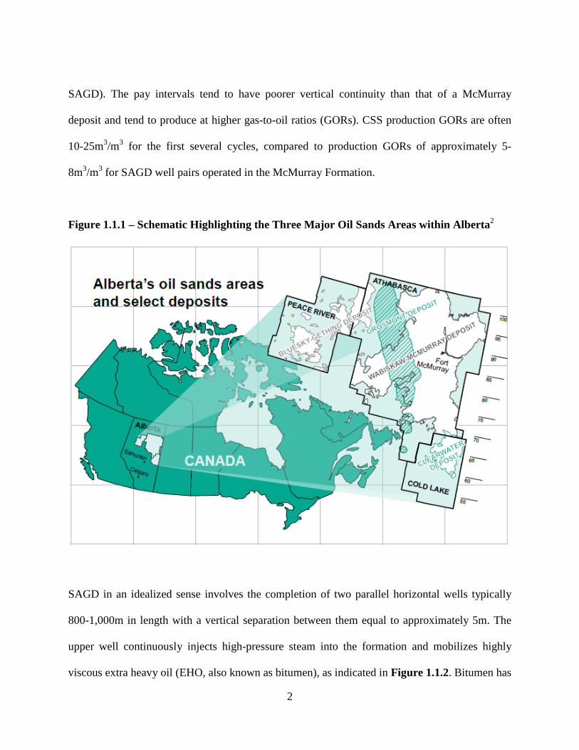
The process of thermal oil recovery is an evolving tertiary production technique commonly used
for oil sands reservoirs in Western Canada. Thermal recovery processes target hydrocarbon plays
where the fluid is immobile at in-situ reservoir conditions and consequently requires heat to
achieve flow. The heat is often in the form of the enthalpy of vaporized water. The Athabasca
Oil Sands region is one of three significant oil sands deposits within the province of Alberta. The
Athabasca region mainly consists of the Wabiskaw-McMurray (clastic) and Grosmont
(carbonate) Formations. The other two major oil sands plays in Alberta are the Cold Lake deposit
which mainly consists of the Clearwater Formation and the Peace River deposit which comprises
the Bluesky-Gething Formations, as indicated in Figure 1.1.1. According to the Alberta Energy
Regulator (AER), formerly known as the Energy Resources Conservation Board (ERCB),
Alberta’s Energy Reserves for 2012 and the Supply/Demand forecasts for 2013-2022 highlight
that Alberta has approximately 26.68 billion m3 of established remaining crude bitumen
reserves1. Approximately 80% of those reserves are considered recoverable by in-situ
technologies, such as Steam-Assisted Gravity Drainage (SAGD) and Cyclic Steam Stimulation
(CSS). Due to the location, depth, reservoir architecture and in-situ properties of the bitumen,
SAGD is the most viable commercial thermal recovery technology currently operated in the
Athabasca Wabiskaw-McMurray region. Conversely, CSS is mostly practiced in Cold Lake and
Peace River where the oil sands formations are deeper and are overlain by a thick, competent
caprock which is required for the elevated injection pressures (often 2-5MPa greater than
1
SAGD). The pay intervals tend to have poorer vertical continuity than that of a McMurray
deposit and tend to produce at higher gas-to-oil ratios (GORs). CSS production GORs are often
10-25m3/m3 for the first several cycles, compared to production GORs of approximately 5-
8m3/m3 for SAGD well pairs operated in the McMurray Formation.
Figure 1.1.1 – Schematic Highlighting the Three Major Oil Sands Areas within Alberta2
SAGD in an idealized sense involves the completion of two parallel horizontal wells typically
800-1,000m in length with a vertical separation between them equal to approximately 5m. The
upper well continuously injects high-pressure steam into the formation and mobilizes highly
viscous extra heavy oil (EHO, also known as bitumen), as indicated in Figure 1.1.2. Bitumen has
2

an API (American Petroleum Institute) gravity of approximately 8-10°API. The viscosity of
bitumen reduces by up to five orders of magnitude after it is heated to saturated steam
conditions, often in excess of 200°C, and flows downward under the action of gravity into the
producer well. The mobilized bitumen is produced in combination with water and formation
gases often in the form of an oil-in-water emulsion. The produced water consists of formation,
lean or transition zone, bottom water and condensed steam. The formation gases consist of free
reservoir gas, gases that evolve out of solution, or gases generated through the process of
aquathermolysis. The formation depth and reservoir pressure are such that the emulsion stream
must often be lifted to surface by using an artificial lift technique, such as Gas Lift (GL) or
Electric Submersible Pumps (ESP).
Figure 1.1.2 - Cross-sectional View of the Steam-Assisted Gravity Drainage Process3
3

Provided the reservoir geology is favourable, a uniform steam chamber can grow along the
horizontal section of the well pair and significant heat conformance can develop in the pay
interval. However, even in this idealized state, SAGD is extremely energy intensive as natural
gas is consumed as fuel to vaporize the water into steam for injection. Unfortunately, this process
is required to develop communication between the pair and to maintain operation and production
until a wind-down or blow-down phase is implemented. In addition to the energy requirement,
the steam is the principle medium in which the energy is transferred into the reservoir. In some
instances solvent can be injected simultaneously with steam (Solvent Co-Injection, SCI) to
improve the mobility of the bitumen by reducing viscosity, however, 100% steam injection is a
common operational methodology with many of the current producers in Alberta. As a result,
SAGD is energy and water intensive and on average requires three units of injected steam on a
cold water equivalent (CWE) basis to produce one unit of bitumen. This relationship and concept
is further indicated in Section 3.5, Figure 3.5.1. While the input requirement is significant, the
produced water volumes and the required handling is equally challenging, as produced water cuts
often range from 70 to 85% of the produced emulsion stream.
The success and economic viability of SAGD is dependent on the ability to efficiently deliver
high quality steam to the reservoir and transfer latent to the bitumen and reduce its in-situ
viscosity to enhance mobility. This continuous cycle is improved when thermal losses are
minimized. From a subsurface perspective, a principle operational challenge associated with
SAGD is the reservoir geology and proportions and distribution of facies. Variation in geology
and depositional environment impacts production efficiency and daily operation. If the pay
interval is discontinuous with variable roof intervals and is characterized by higher proportions
4

of reservoir heterogeneities, then the ability to develop a uniform steam chamber efficiently and
maximize well utilization is reduced. The variation in performance can be observed with respect
to wellbore subcool. Subcool represents the temperature difference between the injector and
producer well and the degree to which an area has developed a steam chamber. Provided a
conventional liner completion, subcool targets for a given well pair are approximately 10-15oC.
Subcool represents the liquid inventory and heat conformance in that particular location along
the well pair. SAGD well pairs with homogenous properties tend to have consistent subcool
values. SAGD well pairs with poorer geology tend to have variable heat conformance and larger
variation in subcool distribution. It should be noted that other reservoir features can significantly
impact SAGD operations such as bottom and top thief zones, but for the purpose of this thesis
that topic will not be explored further.
Therefore, in practice, it is important to characterize the reservoir fully to capture features of the
geology that challenge steam injectivity, steam flow, oil mobilization, and oil drainage in SAGD.
This often entails analysis and integration of petrophysics, geophysics, geology, geochemistry,
production, reservoir and drilling engineering to properly characterize the reservoir.
As part of the multidisciplinary analysis, reservoir engineering via reservoir simulation, can
optimize recovery performance and facilitate field development planning. For subsurface
operations, key field development decisions are often made based on the results of numerical
reservoir simulation. A typical work-flow, which includes a continuous feed-back loop of
dynamic data into the geological model in order to tune and improve the reservoir
characterization, is presented in Figure 1.1.34. While numerical modelling is one component to
5

the geoscience-engineering work-flow, it is fundamental to capture anticipated field behaviour.
These simulation studies are often the foundation of many business plans and reserves reports,
which are directly linked to economics and project viability.
Figure 1.1.3 – Geoscience-Engineering Work-flow4
Historically, a geological model is constructed from reservoir evaluation data such as well logs,
core data, three-dimensional (3D) and four-dimensional (4D) seismic interpretations, and outcrop
studies. Often, geological models that are constructed in geological modelling software packages
encompass several millions cells (a cell is the fundamental discretization unit in a geological
model). However, direct conversion of these geological models to reservoir simulation models is
not possible due to hardware and software limitations. Given modern computational capabilities,
reservoir models which hope to achieve practical execution times must remain below about 5-10
6

million gridblocks, which is also dependent on PVT characterization and numerical tuning. One
way to deal with the conversion of a detailed geological model to a reservoir simulation model,
and still provide a reasonable representation of the geological environment, is through upscaling.
Upscaling is the exercise where a coarse grid is generated with properties that provide a
reasonable representation of a fine-gridded property distribution.
Extensive publications have been written on the development of techniques for scaling
petrophysical properties between the reservoir simulation and geological models, as is the
upscaling and downscaling notation used in Figure 1.1.3. Those publications will be discussed in
detail in Section 2.1 and 2.2.
Within the work-flow, one of the challenges faced by SAGD reservoir simulation is that fine grid
resolution is required to track temperature fronts in the reservoir. This is especially true when
thermal fronts lead to high temperature gradients spanning a few meters or less. Simulation of
finely gridded reservoir models is very computational intensive and impractical to run for
Optimization, Sensitivity Analysis (SA) or History Matching (HM) studies where hundreds to
thousands of runs are required. Consequently, modelling of the SAGD process is done with fine
gridding perpendicular to the wellbore where the temperature gradients are largest, typically
dimensions of 1m in the cross-well direction by 1m in the vertical direction or 2m in the cross-
well direction by 1m in the vertical direction. However, grid resolution parallel the wellbore
tends to be coarser, typically between 25m to 100m per gridblock.
7
1.2 Problem Statement
The research documented here focuses on the differences in the numerical solutions obtained
from a reservoir simulator as a function of length scales and distribution and quantity of reservoir
facies. Therefore, for the research documented in this thesis, the term dynamic upscaling is being
used to refer to this process. Coarse gridblock size along the wellbore is reasonable
simplification provided the temperature gradient is not significant in that direction. However,
with the introduction of facies-based reservoir models with reservoir heterogeneities, large
temperature gradients parallel the wellbore can be introduced. To capture the movement of the
temperature advance in steam chamber, it is necessary to introduce dynamic upscaling
parameters to more accurately model the movement of the thermal front in the coarse
heterogeneous simulation model.
The purpose of the research documented in this thesis is to highlight the impact of dynamic
upscaling on reservoir models and discuss the techniques that can be used to offset the impact of
grid coarsening while still taking advantage of the reduction in simulation time and improved
accuracy of the coarse models.
1.3 Organization of Thesis
The thesis consists of six chapters which highlight the progression of ideas and learnings when
discussing and applying dynamic upscaling parameters to a thermal simulation work-flow.
8

Chapter 1 is intended to discuss the background information and fundamental concepts for
SAGD performance, both operationally and how it is approximated in numerical modelling.
Chapter 2 affords a detailed literature review on all the work that has come before and supports
the purpose and motivation of this thesis in exploring a previously undiscussed area. Chapter 3
discusses all the modelling inputs and various data required to populate a geological model for
import into reservoir simulation software. The configuration of the data-set is the most important
step as the quality of the input impacts the degree to which the data is applicable and useable on
a larger scale. Chapter 3 also begins to introduce the concept of dynamic upscaling and the
fundamental definitions that shape the technical approach. Chapter 4 is the heart of the report, in
that it organizes and presents all the results from the work-flow and quantifies the magnitude of
the outcome. Chapter 4 further expands upon the concepts in Chapter 3 and details the specifics
of the history matching process, which was the approach used to evaluate the impact of reservoir
heterogeneities and length scales in simulation. Chapter 5 further synthesizes the date presented
in Chapter 4 by applying the SAGD Productivity Index tool to the work-flow. Chapter 5 is a
natural progression from Chapter 4 in that it answers several needs and identifies restrictions in
analyzing the data that has be summarized to that point. It includes the final application of the
analytical solution and the modelling assumptions and limitations that are inherent in the thesis.
Chapter 6 is focused on the inferences and conclusions developed from the information
documented in the thesis, but also provides recommendations to expand the work-flow and
strengthen the work moving forward. Finally, the Appendices section is intended to support and
provide specific detail about certain sections of the thesis. It is supplemental to the information
provided in the aforementioned chapters.
9

CHAPTER 2 – LITERATURE REVIEW
In this chapter, a literature review on the techniques that have been developed in the past to
handle uncertainty associated with grid coarsening is discussed. Stochastic geological modelling
involves the generation of several realizations of equal probability for a distribution of various
petrophysical values, such as fluid saturations and directional permeability. These geostatistical
models can successfully represent the geological variation within a depth interval on a fine scale.
However, due to hardware and software limitations, this intense level of detail is unmanageable
for export to flow simulations. As a result, to reduce the number of data points and
corresponding grid density, averaging techniques are applied to upscale the fine scale
petrophysical values to larger grid scales appropriate for dynamic studies. Ultimately, the
ambition is that results obtained from the representative coarser grid perform comparably to that
of the fine grid.
2.1 Upscaling for Reservoir Simulation
The first several approaches for upscaling focus on conventional oil reservoir simulation, such as
the black oil formulation. Of which emphasis will be placed on numerical techniques as opposed
to analytical techniques, such as arithmetic or harmonic means. For example, single-phase
upscaling, as described by Beggs et al. (1989)5, is an algorithm that calculates an effective
permeability, while maintaining the same total flow of the single-phase fluid through the coarse,
homogenous block as that which was obtained from the fine, heterogeneous block. It is
considered the simplest form of upscaling. Specifically, the application of the Pressure-Solver
10
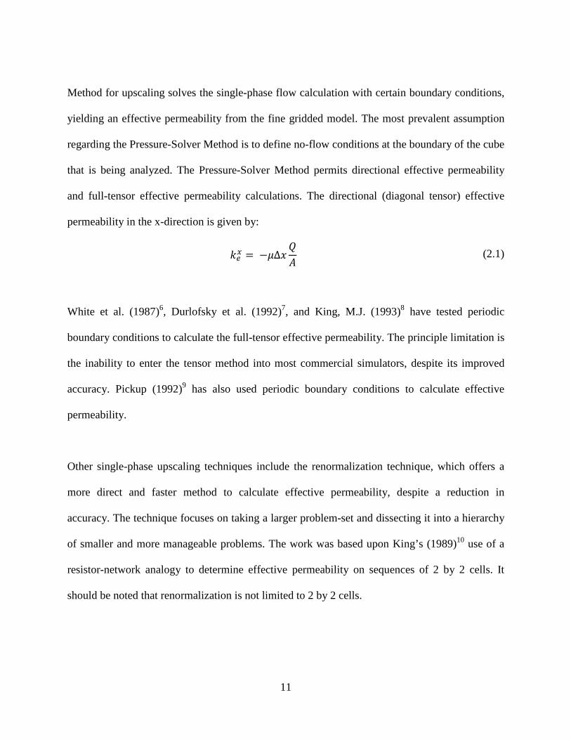
Method for upscaling solves the single-phase flow calculation with certain boundary conditions,
yielding an effective permeability from the fine gridded model. The most prevalent assumption
regarding the Pressure-Solver Method is to define no-flow conditions at the boundary of the cube
that is being analyzed. The Pressure-Solver Method permits directional effective permeability
and full-tensor effective permeability calculations. The directional (diagonal tensor) effective
permeability in the x-direction is given by:
𝑘𝑒𝑥 = −𝜇Δ𝑥𝑄𝐴
(2.1)
White et al. (1987)6, Durlofsky et al. (1992)7, and King, M.J. (1993)8 have tested periodic
boundary conditions to calculate the full-tensor effective permeability. The principle limitation is
the inability to enter the tensor method into most commercial simulators, despite its improved
accuracy. Pickup (1992)9 has also used periodic boundary conditions to calculate effective
permeability.
Other single-phase upscaling techniques include the renormalization technique, which offers a
more direct and faster method to calculate effective permeability, despite a reduction in
accuracy. The technique focuses on taking a larger problem-set and dissecting it into a hierarchy
of smaller and more manageable problems. The work was based upon King’s (1989)10 use of a
resistor-network analogy to determine effective permeability on sequences of 2 by 2 cells. It
should be noted that renormalization is not limited to 2 by 2 cells.
11

In two-phase upscaling, the absolute permeability is inadequate to fully describe the
heterogeneous medium. Therefore, King et al. (1993)11 developed a methodology to utilize
renormalization for two-phase upscaling. Christie et al. (1996)12 would later expand upon the
original renormalization approach, which is built upon the single-phase normalization method.
The production from each gridblock, that has modeled a miniature flow simulation through each
heterogeneous sub-grid at each level and cell, is monitored and the effective relative permeability
is calculated as a function of face-averaged fractional flow and total mobility:
𝑓̅ = ∑𝑓𝑖𝑣𝐴 ∑𝑣𝐴� (2.2)
𝜆𝑡� = ∑𝜆𝑡𝑖𝑘𝑖𝐴𝑖 ∑𝑘𝑖𝐴𝑖� (2.3)
In addition, the use of pseudo function techniques is a diverse area in upscaling. Many different
versions of pseudo functions have been applied over the years. Pseudo function techniques, as
summarized by Soedarmo (1994)13 can be classified into three categories dependent on the
magnitude of: (1) viscous forces, (2) gravitational forces and (3) capillary forces.
The categories can be defined as follows:
(a) Horizontal displacement as a function of viscous forces dominant,
(b) Gravity segregation and viscous cross-flow dominant,
(c) Dynamic pseudo function which simultaneously account for all viscous, gravitational and
capillary interactions.
12

However, these methods can be restrictive, especially the first two. Instead, the use of numerical
modelling to obtain useable solutions is preferred. Dynamic (space and time) pseudo functions
have been proposed by Jacks et al. (1973)14 and Kyte and Berry (1975)15 for improved upscaling
by replacement of a fine gridded model based upon original saturation dependent functions with
a coarser mesh of effective or representative properties. Darcy’s Law was required to calculate
the pseudo functions for Kyte and Berry (1975). Lasseter et al. (1986)16 further expanded upon
the Kyte and Berry (1975) method by presenting a multi-scale upscaling methodology suitable
for heterogeneous reservoirs. Lasseter et al. work was scaled up from laboratory data. Kossack et
al. (1989)17 proposed a scale up procedure from various flow regimes and geological
descriptions. The numerical work performed was designed to verify the effects of different flow
regimes on pseudo function curves in the homogenous, layered and random geological types.
Additionally, Stone (1991)18 introduced the use of average total mobility to avoid the need to
calculate phase potential on a coarser gird, as required by Kyte and Berry (1975). Stone (1991)
also introduced fractional flow formulation instead of calculating the flow using Darcy’s Law.
These effective properties can be thought of as pseudo relative permeability and capillary
pressure functions, represented as a pseudo fraction flow curve.
Alabert and Corre (1991)19 explored three-phase flow in an environment of 3D models of
varying heterogeneity. The flow parameters are directionally dependent. Guérillot and Verdiére
(1995)20 and Verdiére and Thomas (1996)21 utilized two grids to determine the appropriate
upscaled solution. The pressure equation was determined from a coarse grid solution and the
13

saturation distribution was determined by the fine grid solution. The methodology was later
referred to as the Dual Mesh Method.
A major limitation in the application of dynamic pseudo functions is the inherent length or time
dependency of fluid dynamics across the simulated grid boundaries. Therefore, length-dependent
pseudo functions have been proposed to improve upon the dynamic pseudo functions. Taggart et
al. (1995)22 have shown that superior recovery and flow predictions can be obtained with length-
dependent functions by incorporating the curvature of the characteristic fine grid simulation
curves, as opposed to those based upon velocity models.
Unfortunately, despite the large number of pseudo function approaches, there is not one agreed
upon method to perform upscaling in this way. This discrepancy has motivated the need for other
approaches and further research.
An emerging area is the application of an adaptive process within the reservoir models, as
proposed by Guedes et al (1999)23, and is focused on managing a higher volume of data within
the dynamic model than originally proposed with the earlier methods by the solution of the sub-
domain (SD) and coarse grid. This multi-scale computational model for multiphase flow
implicitly treats upscaling without the use of pseudo functions. Fundamentally, Figure 2.1.1
describes the main processes executed, at each time step, by the multi-scale computational
method.
14

Figure 2.1.1 – Multi-scale Computational Model23
It should also be noted that while a Cartesian grid has been applied in the work-flow developed
here, as the geological features are aligned with the grid definition, there has been advancements
within industry to implement a Corner Point Geometry (CPG) as the depositional features of
most models are often not aligned with the choice of gird, impacting the representation of the
effective properties. This methodology was first proposed by Ponting (1989)24, whereby a more
flexible CPG can be implemented to handle more complex reservoir boundaries and reservoir
heterogeneities. The CPG grid can be constructed by using three techniques: (1) streamline
technique as proposed by Agut et al. (1998)25, (2) elastic adjustment as proposed by Garcia et al.
(1990)26 or (3) geological modelling built from stochastic simulations. This grid definition is
coupled with averaging techniques to upscale fine resolution permeability to larger scales
15

appropriate for simulation. The application of power law averaging is implemented on CPG
meshes:
𝐾𝑒𝑞 = �1𝑛�𝑘𝑖𝜔𝑛
𝑖=1
�
1 𝜔�
,𝜔 𝜖 [−1, 1 ] (2.4)
Ultimately, the literature review thus far has been focused on the early methods for upscaling,
often as it relates to representing the fine gridded result as a coarse gridded proxy for
conventional oil and gas models. But the literature does not focus on the impact of varying
length scales within simulation after upscaling. What error is associated with a coarse grid
definition compared to a fine grid definition of identical petrophysical properties when
simulated? This is different than the upscaling presented above. For the purpose of the thesis, the
approach can be thought of as analyzing the difference after a fine gridded model is upscaled and
exported at a specific grid definition. How does the performance change if the model was further
subdivided?
To ensure this approach has not be studied before, further research was performed to analyze the
extent to which upscaling has been applied for thermal simulation, while focusing on work that
could improve the predictive ability of the coarse dynamic model.
2.2 Upscaling for Thermal Reservoir Models
The use of upscaling for thermal models is of most interest and relevance to the work-flow
proposed in the thesis. Of the published literature, the approach that has garnered the most
16

momentum is dynamic sub-gridding. This topic has been reviewed as it relates to SAGD.
Dynamic gridding has been further analyzed by Lacroix et al. (2003)27 as a tool to update the
mesh definition throughout the run-life of the model but is performed external to the reservoir
simulator as opposed to within the simulator. The overriding motivation for this approach is that
it is easier to develop a mesh generator than to implement the sub-gridding directly in the
reservoir model. Alternatively, Lacroix et al. (2003) commented on the ability to have the sub-
gridding directly developed in the model. Given that updating the actual reservoir model
dynamically has the most application to this thesis, it will be discussed further. Christensen et al.
(2004)28 presented a paper focused on the use on dynamic gridding within a 3D SAGD model,
whereby fine gridding is reserved for the bitumen-chamber interface, and coarser gridding is
reserved for areas with lesser change (such as, areas of the steam chamber with constant
temperature). However, the application of the dynamic gridding feature has several limitations
and can be difficult to implement. For example, when applying this technique, the user is advised
to simulate a fine gridded model to study the behaviour of several parameters, such as
temperature, molar fractions and saturation. Only after this preliminary study and review of the
magnitude of the gradients of these variables, can the user accurately define the thresholds which
force amalgamation and de-amalgamation. There is the risk that cells may be amalgamated
across the steam-bitumen interface, resulting in reduced accuracy of the forecast. Therefore
thresholds should be as small as possible to ensure proper dynamic gridding, consequently
increasing simulation time.
While the implementation of this technique has a lot of potential, especially if the user has a
strong understanding of SAGD dynamics, the author wanted to more closely study the impact of
17

geological variation on performance and the movement of the temperature and steam fronts in
homogenous and heterogeneous simulation models. Additionally, the technique proposed offers
the user a tool to screen and filter large sets of static models, representing multiple realizations.
Characterization and understanding of the impact of the reservoir variations as a function of
length scale was as important of a deliverable as proposing an alternative technique to dynamic
gridding.
The research presented in this thesis attempts to answer several questions, which have been
perceived as absent in the published literature for SAGD simulations. Such as, to what extent can
we relate the variation in reservoir quality to performance? How does varying the grid definition
impact our forecasts, when the petrophysical properties remain unchanged? To what extent does
block volume impact the heat and fluid transfer? By performing the exercise outlined in this
thesis, the reader will enhance their understanding of the physics of SAGD.
18

CHAPTER 3 – MODELLING CONCEPTS
3.1 Numerical Modelling Process
In the research done for this thesis, the simulation study was designed to encompass both binary
models and facies-based geological models to quantify the impact of reservoir heterogeneities for
different length scales. The static model (the geological model) is fundamental in the modelling
process as the quality of the result will be a function of the input parameters. It is necessary to
capture any uncertainty and assumptions in the construction phase to identity potential errors or
inconsistencies upon completion of the simulations. These assumptions are further elaborated on
in Section 5.3. The following section highlights the fundamental tools and inputs used to define
models used in the research.
3.2 Modelling Tools
Computer Modelling Group’s (CMG) suite of reservoir simulation tools was the primary
software used in this study. The reservoir models were built by using BuilderTM (Versions
2011.10 and 2012.10)29 and simulated by using the thermal reservoir simulator, Steam, Thermal
and Advanced Processes Reservoir Simulator, STARSTM (Versions 2011.10 and 2012.10)30. The
STARSTM models were coupled with the Computer Assisted History Matching, Optimization,
Sensitivity and Uncertainty Assessment Tool, CMOSTTM (Versions 2011.10 and 2012.10)31.
CMOSTTM automates simulation runs from the base case model and then submits and analyzes
the data from a range of sensitivity parameters and values to achieve an optimal solution set.
19

Ultimately, it permits the reservoir engineer to identify uncertainty and improve simulation
forecasts. Finally, all results were analyzed by using the CMG Results post-processing tools
(Versions 2011.10 and 2012.10)32.
STARSTM is the thermal software commonly used for SAGD processes within the oil sands
industry. For the purpose of this study, FlexWellTM was not employed and sink-source model
approximation was favoured because the foundation of this report focuses on reservoir
performance and interaction of gridblocks and not wellbore hydraulics. Also, no geomehanical
assumptions were implemented into the study.
3.3 Model Grid Definitions
The methodology to create simulation models was to generate representative 3D binary models
and representative 3D facies-based models. Universal to all models was three reservoir inputs:
(1) PVT characterization, (2) relative permeability curves and (3) thermal properties. These
datasets were not manipulated during the course of the study. They were sourced from a
combination of literature33-35 and default parameters outlined in the CMG data-manuals. In this
way, the input parameters should simply been seen as constant inputs across the set of models. It
should also be noted that nominal numerical tuning was performed on the models in the study,
however, a small sub-set of coarse and fine models were reviewed to ensure the run performance
metrics were favourable, such as total time step cuts, solver failures and material balance error.
Given this sample of performance, it was decided that the configuration was appropriate for
global use. The numerical configuration was based upon CMG recommended parameters and
20

ranges, which represent the default for STARSTM related simulations. The parallelization
configuration (including number of processors) was identical for all model types.
The models were constructed with one of six grid definitions. For example, the primary grid
definition as defined on an (i, j, k) basis was (4m, 100m, 1m) and gridblock counts in each
direction equal to (25, 3, 30) gridblocks = 2,250 gridblocks. These models represent one-third the
average length of a SAGD well pair to accelerate run time and reduce the dependence on
hardware and software. This approximation represents the upper limit in reservoir simulation
coarseness when simulating the SAGD process and is referred to as a coarse model
approximation. A fine model approximation involves refining the grid to a (1m, 1m, 1m)
discretization. Additional details of the grid configurations are described in Section 3.7. The
dimensional notation used in this thesis is depicted in Figure 3.3.1.
Figure 3.3.1 – Standard Dimensional Notation
21

3.4 Editing an Existing Grid
Each coarse gridded model will have a unique distribution of reservoir facies, however, their
corresponding find gridded models (1m, 1m, 1m) are simply a manipulation of the coarse
gridded distribution. In that way, the location and quantity of reservoir properties from the coarse
grid to the fine grid are maintained. For example, Figure 3.4.1 idealizes the fundamental process
of grid refinement within the contexts of this paper. The colour palate represents a particular set
of petrophysical values and its distribution within the grid. Also, the placement of the wells
within the schematic (injector and producer well) are idealized, as all the injection and
production nodes are centered in their respective gridblock.
Figure 3.4.1 – Schematic of Grid Refinement Process, View in the Cross-Well Direction (i, k-direction)
Coarse Grid Distribution Fine Grid Distribution
The models were originally refined by using two techniques within BuilderTM. Split grid plane
and Cartesian refine. The split grid plane feature permits the user to specify a uniform or non-
uniform number of blocks divisions in each respective direction. The Cartesian refine feature
also permits the user to specify a uniform or non-uniform number of blocks divisions in each
respective direction. However, Cartesian refine will not refine non-reservoir blocks, which will
22

be represented as Facie Type B in Section 3.7. Based upon the sensitivity analysis that was
performed on several type models, there is no major distinction between the production results
with split grid plane and Cartesian refine. For the purpose of comparison, coarse models were
refined to selective dimensions to generate a quick comparison when compared to simulating the
fine grid definition. The results are presented in Figure 3.4.2. However, as part of the tuning
process to ensure reduced simulation time, the split grid plane method tended to have the fastest
simulation times, as highlighted in Table 3.4.1. In addition to the acceleration in run-time, the
inability of Cartesian refine to segment non-reservoir blocks could have an impact upon the rate
of thermal conductivity in that given cell, when comparing the performance between coarse and
fine gridded reservoir blocks of different block volumes. This option may potentially impact
future results.
Therefore, the split grid plane feature was employed as the local refined grid technique due to its
ease of use and complete refinement of the entire grid. It eliminated the inconsistency between
variable shale content and the number of gridblocks refined on a model basis.
Table 3.4.1 – Comparison of Simulation Time for Different Refinement Techniques
Binary Model Association
Shale Volume
(%)
Dimensions i, j, k (m)
Split Grid Plane Simulation Time
(hh:mm:ss)
Cartesian Refine Simulation Time
(hh:mm:ss) Type-C 5 4, 25, 1 00:07:06 00:07:09 Type-D 5 2, 100, 1 00:01:39 00:01:52 Type-F 5 2, 25, 1 00:17:00 00:25:33
23
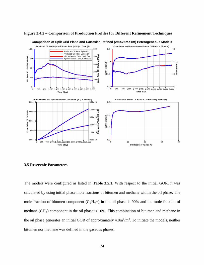
Figure 3.4.2 – Comparison of Production Profiles for Different Refinement Techniques
3.5 Reservoir Parameters
The models were configured as listed in Table 3.5.1. With respect to the initial GOR, it was
calculated by using initial phase mole fractions of bitumen and methane within the oil phase. The
mole fraction of bitumen component (C2H6+) in the oil phase is 90% and the mole fraction of
methane (CH4) component in the oil phase is 10%. This combination of bitumen and methane in
the oil phase generates an initial GOR of approximately 4.8m3/m3. To initiate the models, neither
bitumen nor methane was defined in the gaseous phases.
Comparison of Split Grid Plane and Cartesian Refined (2mX25mX1m) Heterogeneous Models
Produced Oil and Injected Water Rate (m3/d) v. Time (d)
Time (day)
Oil
Rate
SC
- Dai
ly (m
3/da
y)
Wat
er R
ate
SC -
Daily
(m3/
day)
0 365 730 1,095 1,460 1,825 2,190 2,555 2,920 3,285 3,6500
25
50
75
100
0
100
200
300
400
500Produced Oil Rate, Split GridProduced Oil Rate, CartesianInjected Water Rate, Split GridInjected Water Rate, Cartesian
Produced Oil and Injected Water Cumulative (m3) v. Time (d)
Time (day)
Cum
ulat
ive
Oil
SC (m
3)
Cum
ulat
ive
Wat
er S
C (m
3)
0 365 730 1,095 1,460 1,825 2,190 2,555 2,920 3,285 3,6500.00e+0
1.00e+5
2.00e+5
3.00e+5
4.00e+5
0.00e+0
1.00e+5
2.00e+5
3.00e+5
4.00e+5
5.00e+5
Cumulative and Instantaneous Steam Oil Ratio v. Time (d)
Time (day)
cSO
R (m
3/m
3)
iSO
R (m
3/m
3)
0 365 730 1,095 1,460 1,825 2,190 2,555 2,920 3,285 3,6500.0
1.0
2.0
3.0
0.0
2.0
4.0
6.0
Cumulative Steam Oil Ratio v. Oil Recovery Factor (%)
Oil Recovery Factor (%)
cSO
R (m
3/m
3)
0 20 40 60 800.0
1.0
2.0
3.0
24

Table 3.5.1 – Single Well Pair Reservoir Simulation Properties and Input Parameters
Parameter Unit Value Base Case, Cell Definition (i, j, k) cells 25, 3, 1
Base Case, Grid Dimensions (i, j, k) m 4, 100, 1 SAGDable Interval (k-direction) m 30 Reference Depth (k-direction) mTVD 400 Initial Reservoir Temperature oC 12
Initial Reservoir Pressure kPa 2,000 Initial Gas-to-Oil Ratio m3/ m3 4.8
Upper Interval (k-direction) m (vertical cell layers) 10 (1-10) Middle Interval (k-direction) m (vertical cell layers) 10 (11-20) Lower Interval (k-direction) m (vertical cell layers) 10 (21-30)
Depth of Injector m (vertical cell layer) 22.5 (23) Depth of Producer (2.5m off base) m (vertical cell layer) 27.5 (28)
3.5.1 SAGD Circulation, Constraint Set-Up
During the SAGD circulation phase, both the injection and production well inject steam for a
specified period of time to establish communication between the two wells to condition the well
pairs for conversion to SAGD. Within STARSTM the process is idealized with nodal heaters that
simulate the behaviour of injecting steam uniformly along the wellbore without the actual
injection of steam. Both wells were shut-in during the circulation phase and the details of the
well configuration are outlined in Table 3.5.1.1 and 3.5.1.2.
25

Table 3.5.1.1 – Circulation Well, Constraint Configuration
Parameter Unit Value or Parameter Well Geometry - j-direction
Max Steam Constraint m3/d 3.0 Maximum Bottom-Hole Pressure kPa 3,500
Maximum Total Liquid Rate (water and oil phase) m3/d 1,000
Well Radius m 0.086 Geometric Factor for the Well Element unitless 0.249
Inflow Fraction (wfrac) unitless 1.0 Well Skin Factor unitless 0.0
Table 3.5.1.2 – Circulation Heater Configuration
Parameter Unit Value or Parameter Well Heater Duration days 90
Heating Rate J/day-m 2.40E+9 Heater Target Temperature oC 240
3.5.2 SAGD Production Phase, Constraint Set-Up
During the SAGD production phase, the injection well continuously injects high pressure steam
whereas the production well is controlled by pressure and fluid intake constraints. The details of
the injection and production well constraints are outlined in Tables 3.5.2.1 and 3.5.2.2.
Table 3.5.2.1 – SAGD Production Phase, Constraint Set-Up - Injection Well
Parameter Unit Value or Parameter Well Geometry - j-direction
Temperature oC 242.5 Maximum Bottom-Hole Pressure kPa 3,500
Quality unitless 0.95 Maximum Total Water Phase Rate m3/d 1,000
Well Radius m 0.086 Geometric Factor for the Well Element unitless 0.249
Inflow Fraction (wfrac) unitless 1.0 Well Skin Factor unitless 0.0
26

Table 3.5.2.2 – SAGD Production Phase, Constraint Set-Up - Production Well
Parameter Unit Value or Parameter Well Geometry - j-direction
Max Steam Constraint (*STEAM) m3/d 3.0 Minimum Bottom-Hole Pressure kPa 1,000
Maximum Total Liquid Rate (water and oil phase) m3/d 1,000
Well Radius m 0.086 Geometric Factor for the Well Element unitless 0.249
Inflow Fraction (wfrac) unitless 1.0 Well Skin Factor unitless 0.0
The maximum steam constraint defined within this section approximates the sub-cool notation
discussed within the introduction and is used in favour of the steam trapping mode within
STARSTM. The sub-cool constraint in this case is focused on producing a certain volume of live
steam on a daily basis, as opposed to the steam trapping mode that is able to target a specific
temperature difference between the injector and the producer. Operationally, it is easier to speak
to the steam trapping mode, however, numerically the models converged better with the
maximum steam constraint keyword. It should be noted that the instability in the steam trapping
mode is the result of violating the temperature constraint that leads to liquid pooling above the
producer well.
The maximum steam constraint value assigned to the simulations (3m3/d) is comparable to the
target sub-cool values as suggested with conventional liner systems (10-15oC) and the steam
trapping mode as mentioned prior.
The results are presented in Table 3.5.2.3, in which the maximum steam constraint run-time is
comparable to steam trapping mode case of 10oC. However, the production profiles presented in
27
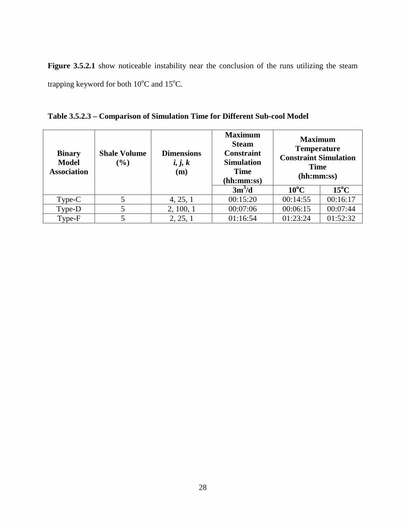
Figure 3.5.2.1 show noticeable instability near the conclusion of the runs utilizing the steam
trapping keyword for both 10oC and 15oC.
Table 3.5.2.3 – Comparison of Simulation Time for Different Sub-cool Model
Binary Model
Association
Shale Volume (%)
Dimensions i, j, k (m)
Maximum Steam
Constraint Simulation
Time (hh:mm:ss)
Maximum Temperature
Constraint Simulation Time
(hh:mm:ss)
3m3/d 10oC 15oC Type-C 5 4, 25, 1 00:15:20 00:14:55 00:16:17 Type-D 5 2, 100, 1 00:07:06 00:06:15 00:07:44 Type-F 5 2, 25, 1 01:16:54 01:23:24 01:52:32
28

Figure 3.5.2.1 – Comparison of Production Profiles for Different Sub-cool Model
3.6 Key Performance Metrics
SAGD performance is measured by several metrics, and those metrics are important in terms of
quantifying the efficiency of SAGD on a well pair basis. Examples are oil rate, cumulative oil
production, produced water rate and cumulative water produced with respect to time. Another
principle indicator for the SAGD process is the Steam-to-Oil Ratio (SOR). SOR can be
represented in terms of the cumulative-SOR (cSOR) or instantaneous-SOR (iSOR). cSOR takes
into consideration the cumulative volume of steam injected, on a CWE basis, and the cumulative
volume of bitumen produced over the period the well pair is on-line. cSOR measurements within
Comparison of Different Sub-cool Keywords (2mX25mX1m) Heterogeneous Model
Produced Oil and Injected Water Rate (m3/d) v. Time (d)
Time (day)
Oil
Rat
e SC
- D
aily
(m3/
day)
Wat
er R
ate
SC -
Dai
ly (m
3/da
y)
0 365 730 1,095 1,460 1,825 2,190 2,555 2,920 3,285 3,6500
10
20
30
40
50
60
70
80
0
100
200
300Produced Oil Rate, 3 m3/dProduced Oil Rate, 15CProduced Oil Rate, 10CInjected Water Rate, 3 m3/dInjected Water Rate, 15CInjected Water Rate, 10C
Produced Oil and Injected Water Cumulative (m3) v. Time (d)
Time (day)
Cum
ulat
ive
Oil
SC (m
3)
Cum
ulat
ive
Wat
er S
C (m
3)
0 365 730 1,095 1,460 1,825 2,190 2,555 2,920 3,285 3,6500.00e+0
1.00e+5
2.00e+5
3.00e+5
4.00e+5
0.00e+0
1.00e+5
2.00e+5
3.00e+5
4.00e+5
5.00e+5
Cumulative and Instantaneous Steam Oil Ratio v. Time (d)
Time (day)
cSO
R (m
3/m
3)
iSO
R (m
3/m
3)
0 365 730 1,095 1,460 1,825 2,190 2,555 2,920 3,285 3,6500.0
1.0
2.0
3.0
4.0
0.0
2.0
4.0
6.0
Cumulative Steam Oil Ratio v. Oil Recovery Factor (%)
Oil Recovery Factor (%)
cSO
R (m
3/m
3)
0 20 40 60 800.0
1.0
2.0
3.0
29

industry include the carbon intensive circulation period. In the simulations done within this
thesis, the circulation stage is modelled with block heaters and thus the actual amount of steam
used in the circulation stage is not taken into account in this work-flow. iSOR takes into
consideration the volume of steam injected, on a CWE basis, and bitumen produced for a given
time period, typically a day.
SOR is an important key performance indicator because it provides insight into efficiency of
steam usage for a period in time or lifetime of the well. For example, if steam injection is being
increased to a particular tubing string and the downhole instrumentation suggests the heat is
being displaced into the producer well because of a vertical barrier, then more heat will be
recycled to surface. This indicates that the additional energy associated with the increased steam
volume is not being used for chamber growth and will hurt thermal efficiency. This trend
manifests itself as gradual increase in cSOR but with a more sudden increase in iSOR.
Alternatively, if steam injection is being increased to a particular tubing string and the downhole
instrumentation suggests that the pressure and temperature are stable, then it is likely that the
incremental steam is being used to grow the chamber. This will often result in greater bitumen
production and potentially a stabilization or reduction in SOR. Historically, industry has targeted
cSOR of 3.0m3/m3 or less, however, due to the start-up of more marginal drainage areas within
the McMurray formation, it is becoming increasingly more challenging target to achieve. The
results of several SAGD projects in Alberta are listed in Table 3.6.136.
30
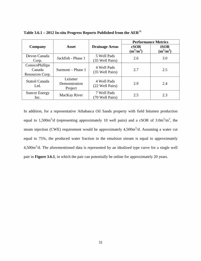
Table 3.6.1 – 2012 In-situ Progress Reports Published from the AER36
Company Asset Drainage Areas Performance Metrics
cSOR (m3/m3)
iSOR (m3/m3)
Devon Canada Corp. Jackfish - Phase 1 5 Well Pads
(35 Well Pairs) 2.6 3.0
ConocoPhillips Canada
Resources Corp. Surmont – Phase 1 4 Well Pads
(35 Well Pairs) 2.7 2.5
Statoil Canada Ltd.
Leismer Demonstration
Project
4 Well Pads (22 Well Pairs) 2.9 2.4
Suncor Energy Inc. MacKay River 7 Well Pads
(70 Well Pairs) 2.5 2.3
In addition, for a representative Athabasca Oil Sands property with field bitumen production
equal to 1,500m3/d (representing approximately 10 well pairs) and a cSOR of 3.0m3/m3, the
steam injection (CWE) requirement would be approximately 4,500m3/d. Assuming a water cut
equal to 75%, the produced water fraction in the emulsion stream is equal to approximately
4,500m3/d. The aforementioned data is represented by an idealized type curve for a single well
pair in Figure 3.6.1, in which the pair can potentially be online for approximately 20 years.
31

Figure 3.6.1 – Representative Type Well Injection and Production Profile
3.7 Binary-Geostatistical Models
Binary reservoir simulation models were generated by using CMG’s BuilderTM geostatistical
object modelling tool (with a uniform probability distribution) to populate gridblocks with
rectangular parallelepiped geological bodies. The object modelling tool was employed for a 3D
distribution of shale bodies of specific dimensions and content. The fluvial depositional37 model
is appropriate for this choice of object modelling, and can often be linked to fining upward
sequences which are very common within the McMurray formation.
32

To clarify the notation assigned to these models, a binary model consists of a discrete
distribution representing one or another variable, in this case: Facies A (sand-dominated) or
Facies B (shale-dominated). The values are binary from the perspective of the object modelling
value (1 or 0, sand or shale). The petrophysical values assigned to each facies type are
deterministic.
Table 3.7.1 – Depositional Quantities
Binary Model Association
Coarse Dimensions i, j, k (m)
Fine Dimensions i, j, k (m)
Non-Reservoir Content
(Percent by Volume) Type-A (Base Case) 4, 100, 1 1, 1, 1 1, 2, 3, 4, 5, 10, 15, 20
Type-B 4, 50, 1 1, 1, 1 1, 5, 10, 20 Type-C 4, 25, 1 1, 1, 1 1, 5, 10, 20 Type-D 2, 100, 1 1, 1, 1 1, 5, 10, 20 Type-E 2, 50, 1 1, 1, 1 1, 5, 10, 20 Type-F 2, 25, 1 1, 1, 1 1, 5, 10, 20
Figure 3.7.1 – Schematic Representing the Distribution of Facies for 1% Shale by Volume, Type-A
4m, 100m, 1m (i, k-direction) 4m, 100m, 1m (i, j-direction)
ProdP1aProdP1b
0 10 20 30 40 50 60 70 80 90 100
0 10 20 30 40 50 60 70 80 90 100380
390400
410420
430440
450
370
380
390
400
410
420
430
440
4500.00 40.00 80.00 feet
0.00 15.00 30.00 meters
File: SingleWell_MoUser: MAPIDate: 7/3/2013Scale: 1:618Z/X: 1.00:1Axis Units: m
0.0
0.0
0.0
0.0
0.0
0.0
0.0
0.0
0.0
0.0
0.0
SingleWell_Model_4mX100mX1mCMGLCustom_Shale_1% 2014-01-01 J layer: 1
ProdP1aProdP1b
0 100 200 300
0 100 200 300
400410
420430
400
410
420
430
0.00 155.00 310.00 feet
0.00 50.00 100.00 meters
File: SingleWell_MoUser: MAPIDate: 7/3/2013Scale: 1:2410Z/Y: 8.00:1Axis Units: m
0.0
0.0
0.0
0.0
0.0
0.0
0.0
0.0
0.0
0.0
0.0
SingleWell_Model_4mX100mX1mCMGLCustom_Shale_1% 2014-01-01 I layer: 13
33

Table 3.7.2 – BuilderTM Generated Geostatistical Model
Inputs Units Facies A Facies B Sand-Dominated Shale-Dominated
Object Modelling Value (Assignment) unitless 1 0
Oil Saturation fraction 0.80 0.00 Residual Oil Saturation fraction 0.10 0.00
Water Saturation fraction 0.20 0.00 Irreducible Water Saturation fraction 0.10 0.00
Gas Saturation fraction 0.00 0.00 Porosity fraction 0.33 0.00
Shale Dimensions (i, j, k) m - 4, 100, 1 Shale Volume fraction 0.00 (0.01, 0.20)
Permeability (i-direction) mD 5,000 0.00 Permeability (j-direction) mD 5,000 0.00
kv/kh fraction 0.80 0.00 Permeability (k-direction) mD 4,000 0.00
3.8 Facies-based Models
The statistical software package used to populate the petrophysical inputs for facies-generated
models within BuilderTM was Palisade’s risk analysis tool, @RISKTM 5.0 Standard (Version
5.5)38. Risk analysis is utilized within industry to determine the frequency of occurrence of
particular events and the magnitude of their outcome. However, risk and risk quantification can
also be used to study the spread for a particular variable. Here, @RISKTM was used in two
capacities: (1) to generate a discrete distribution for each facies type and (2) to generate a normal
distribution for the petrophysical properties as a function of the facies type.
Four generic models were generated for the facies-based modelling approach: (1) Uniform
Distribution model, (2) Fining Upwards model, (3) Coarsening Upwards model and (4) Channel
34

Deposition model. The coarsening upwards sequence can be found in a deltaic environment.
Deltas prograde (build out) and form where rivers carry more sediment into the sea than marine
erosion can carry away39. The fining upwards sequence can be found in a braided fluvial system
environment and is defined as any body of water that is flowing but has insufficient discharge to
carry its load of sediment. Here, the reservoir quality of a coarsening upwards sequence
improves as you decrease depositional depth, whereas, the reservoir quality of the fining
upwards sequence improves as you increase depth40. The uniform distribution model is defined
as an area of decreased reservoir heterogeneity across the targeted interval and would be
supported by logs showing continuous high resistivity and low gamma ray log readings. The
channel depositional model is most closely related to the uniform depositional model, however,
there is a greater distinction between base of pay (top of Devonian or basal McMurray) and top
of pay (transition to roof or regional caprock)41.
For the reservoir simulation models, an understanding of the depositional environments was
coupled together with these four generate generic reservoir profiles to enable the ability of
@RISKTM to model a specific distribution. As a result, the final values selected for the
petrophysical inputs (mean and standard deviation) were not specific to a particular location. The
goal was to emphasize universality of the trends and the lack of uniformity observed within the
reservoir. The facies-based models are also intended to be more representative of geological
models of the Athabasca Oil Sands region.
The facies proportions were determined by using a RiskDiscrete model. A RiskDiscrete
distribution has a number of outcomes equalling n. Each outcome has a particular value
35

assignment (x) and probability of occurrence or weight (p)42. The weight must be a value greater
than or equal to zero. The RiskDiscrete formulation is given by:
𝑓(𝑥) = 𝑝𝑖 𝑓𝑜𝑟 𝑥 = 𝑥𝑖 (3.8.1)
Figures 3.8.1 – 3.8.4 features the four different model configurations for the distribution of
facies. The number associated with each facies type is the value and the probability of
occurrence is a function of the vertical proportion curve for that particular distribution. The
vertical proportion curves are defined per interval, with one interval representing the specified
vertical reservoir layers. Due to the resolution of the images, the first figure is enlarged as the
notation for the x-axis (facies type) and y-axis (probability of occurrence) is maintained for all
the discrete distributions.
Figure 3.8.1 – Discrete Facies Distribution per Interval for the Uniform Distribution Model (Layers 1-30)
Layers 1-30
36

Figure 3.8.2 – Discrete Facies Distribution per Interval for the Fining Upwards Model (Layers 1-30)
Layers 1-10 Layers 11-20 Layers 21-30
Figure 3.8.3 – Discrete Facies Distribution per Interval for the Coarsening Upwards Model (Layers 1-30)
Layers 1-10 Layers 11-20 Layers 21-30
37

Figure 3.8.4 – Discrete Facies Distribution per Interval for the Channel Depositional Model (Layers 1-30)
Layers 1-5 Layers 6-20 Layers 21-25 Layers 26-30
The petrophysical values were presented using a RiskNormal model given by:
𝑓(𝑥) = 1
√2𝜋𝜎 𝑒−
12�𝑥−𝜇𝜎 �
2
(3.8.2)
A RiskNormal distribution is a typical Gaussian (normal) distribution curve. It is a symmetric
continuous distribution which is unbounded on both sides (-∞ < x < +∞) and is described by a
mean (μ) and standard deviation (σ)43. All petrophysical parameters have a lower limit of 0.0 and
the curves are truncated at that value to ensure no non-real values are generated.
Figure 3.8.5 – 3.8.7 highlights the RiskNormal distribution for oil saturation, porosity and
vertical permeability per facies type. Based on the mean and standard deviation a unique value
will be generated per gridblock representing that particular facies. Each numerical model will
represent one particular realization based on the particular arrangement of values. Therefore, the
purpose of the facie-based models was to generate a data-set that is more representative of
geomodelling output for benchmark of the dynamic upscaling parameters. Due to the resolution
38

of the images, the first figure is enlarged as the notation for the x-axis (petrophysical value
assignment) and y-axis (frequency of occurrence) is maintained for all the continuous
distributions.
Figure 3.8.5 – Normal Oil Saturation Distribution per Facies
Facies 1 Distribution
Facies 2 Distribution Facies 3 Distribution
39

Figure 3.8.6 – Normal Porosity Distribution per Facies
Facies 1 Distribution Facies 2 Distribution Facies 3 Distribution
Figure 3.8.7 – Normal Vertical Permeability Distribution per Facies
Facies 1 Distribution Facies 2 Distribution Facies 3 Distribution
Given the distribution of oil saturation, the water saturation distribution is given by:
𝑆𝑤 = 1.0 − 𝑆𝑜,𝑎𝑠 𝑆𝑔 = 0.0 (3.8.3)
The ratio of the vertical to horizontal permeability is constant and equal to 0.8. The values
assigned for oil saturation, porosity, and vertical permeability for each facies type are stochastic
in nature. Ideally, several realizations would be generated for each type to minimize anomalous
distributions.
40

3.9 Vertical Proportion Curves
Vertical proportion curves provide an estimate as to the variation in facies amounts vertically
within the reservoir interval. The vertical proportion curves for the given model are applied in
each plane perpendicular the wellbore. The distribution of petrophysical values is controlled by
the distributions described in the aforementioned sections. The aspect ratio notation refers to the
length-to-width ratio of the shale layers with respect to the parallel and perpendicular flow
direction. Therefore, for the base case models (4m, 100m, 1m), the aspect ratio is equal to
100m:4m or 25m/m.
Figure 3.9.1 – Vertical Proportion Curves for each Model Configuration A. Uniform Distribution Model
41

B. Coarsening Upwards Model
C. Fining Upwards Model
42

D. Channel Depositional Model
Table 3.9.1 – Standard Distribution Parameters
Inputs Units Facies 1 Facies 2 Facies 3
Mean (μ)
Deviation (σ)
Mean (μ)
Deviation (σ)
Mean (μ)
Deviation (σ)
Oil Saturation fraction 0.80 0.05 0.50 0.10 0.10 0.05
Porosity fraction 0.35 0.05 0.20 0.05 0.08 0.02 Vertical
Permeability mD 4,500 1,000 2,000 1,000 200 100
As an example of how the vertical proportion curves are populated within BuilderTM, the
Channel Depositional model was selected to illustrate how the facies-based datasets are more
representative of geological model exports than the binary models. The objective was to target
more realistic realizations in which to benchmark the dynamic upscaling parameters.
43

Figure 3.9.2 – BuilderTM Generated, Channel Depositional Model (4m, 100m, 1m)
Facies Distribution (i, k-direction) Facies Distribution (i, j-direction)
Vertical Permeability (i, k-direction)
Vertical Permeability(i, j-direction)
Horizontal Permeability (i, k-direction)
Horizontal Permeability (i, j-direction)
ProdP1aProdP1b
0 10 20 30 40 50 60 70 80 90 100
0 10 20 30 40 50 60 70 80 90 100
380390
400410
420430
440450
370
380
390
400
410
420
430
440
4500.00 40.00 80.00 feet
0.00 15.00 30.00 meters
File: SW_Model_4mUser: MAPIDate: 6/11/2013Scale: 1:618Z/X: 1.00:1Axis Units: m
1.00
1.20
1.40
1.60
1.80
2.00
2.20
2.40
2.60
2.80
3.00
SW1_Model_4mX100mX1m_DistributionHCMGLCustom_FaciesType 2014-01-01 J layer: 1
ProdP1aProdP1b
0 100 200 300
0 100 200 300
400410
420430
400
410
420
430
0.00 155.00 310.00 feet
0.00 50.00 100.00 meters
File: SW_Model_4mUser: MAPIDate: 6/11/2013Scale: 1:2364Z/Y: 8.00:1Axis Units: m
1.00
1.20
1.40
1.60
1.80
2.00
2.20
2.40
2.60
2.80
3.00
SW1_Model_4mX100mX1m_DistributionHCMGLCustom_FaciesType 2014-01-01 I layer: 13
ProdP1aProdP1b
0 10 20 30 40 50 60 70 80 90 100
0 10 20 30 40 50 60 70 80 90 100
380390
400410
420430
440450
370
380
390
400
410
420
430
440
4500.00 40.00 80.00 feet
0.00 15.00 30.00 meters
File: SW_Model_4mUser: MAPIDate: 6/11/2013Scale: 1:618Z/X: 1.00:1Axis Units: m
2
832
1,662
2,492
3,322
4,152
4,982
5,812
6,642
7,472
8,302
SW1_Model_4mX100mX1m_DistributionHPermeability K (md) 2014-01-01 J layer: 1
ProdP1aProdP1b
0 100 200 300
0 100 200 300
400410
420430
400
410
420
430
0.00 155.00 310.00 feet
0.00 50.00 100.00 meters
File: SW_Model_4mUser: MAPIDate: 6/11/2013Scale: 1:2364Z/Y: 8.00:1Axis Units: m
2
832
1,662
2,492
3,322
4,152
4,982
5,812
6,642
7,472
8,302
SW1_Model_4mX100mX1m_DistributionHPermeability K (md) 2014-01-01 I layer: 13
ProdP1aProdP1b
0 10 20 30 40 50 60 70 80 90 100
0 10 20 30 40 50 60 70 80 90 100
380390
400410
420430
440450
370
380
390
400
410
420
430
440
4500.00 40.00 80.00 feet
0.00 15.00 30.00 meters
File: SW_Model_4mUser: MAPIDate: 6/11/2013Scale: 1:618Z/X: 1.00:1Axis Units: m
2
1,040
2,077
3,115
4,152
5,190
6,227
7,265
8,303
9,340
10,378
SW1_Model_4mX100mX1m_DistributionHPermeability I (md) 2014-01-01 J layer: 1
ProdP1aProdP1b
0 100 200 300
0 100 200 300
400410
420430
400
410
420
430
0.00 155.00 310.00 feet
0.00 50.00 100.00 meters
File: SW_Model_4mUser: MAPIDate: 6/11/2013Scale: 1:2364Z/Y: 8.00:1Axis Units: m
2
1,040
2,077
3,115
4,152
5,190
6,227
7,265
8,303
9,340
10,378
SW1_Model_4mX100mX1m_DistributionHPermeability I (md) 2014-01-01 I layer: 13
44

Porosity (i, k-direction) Porosity (i, j-direction)
Oil Saturation (i, k-direction)
Oil Saturation (i, j-direction)
3.10 Dynamic Upscaling Concept
A coarse gridblock definition along the wellbore is a reasonable simplification provided the
temperature gradient is small. However, with introduction of facies-based reservoir models with
a variable magnitude of reservoir heterogeneities, large temperature gradients parallel the
wellbore are often the norm rather than the exception. To capture the movement of temperature
fronts in the SAGD well pair, it is necessary to refine the grid or introduce dynamic upscaling
parameters in coarser models to more accurately model the movement of the temperature and
ProdP1aProdP1b
0 10 20 30 40 50 60 70 80 90 100
0 10 20 30 40 50 60 70 80 90 100
380390
400410
420430
440450
370
380
390
400
410
420
430
440
4500.00 40.00 80.00 feet
0.00 15.00 30.00 meters
File: SW_Model_4mUser: MAPIDate: 6/11/2013Scale: 1:618Z/X: 1.00:1Axis Units: m
0.01
0.06
0.11
0.17
0.22
0.27
0.32
0.37
0.43
0.48
0.53
SW1_Model_4mX100mX1m_DistributionHPorosity 2014-01-01 J layer: 1
ProdP1aProdP1b
0 100 200 300
0 100 200 300
400410
420430
400
410
420
430
0.00 155.00 310.00 feet
0.00 50.00 100.00 meters
File: SW_Model_4mUser: MAPIDate: 6/11/2013Scale: 1:2364Z/Y: 8.00:1Axis Units: m
0.01
0.06
0.11
0.17
0.22
0.27
0.32
0.37
0.43
0.48
0.53
SW1_Model_4mX100mX1m_DistributionHPorosity 2014-01-01 I layer: 13
ProdP1aProdP1b
0 10 20 30 40 50 60 70 80 90 100
0 10 20 30 40 50 60 70 80 90 100
380390
400410
420430
440450
370
380
390
400
410
420
430
440
4500.00 40.00 80.00 feet
0.00 15.00 30.00 meters
File: SW_Model_4mUser: MAPIDate: 6/11/2013Scale: 1:618Z/X: 1.00:1Axis Units: m
0.00
0.10
0.20
0.30
0.40
0.50
0.60
0.70
0.80
0.90
1.00
SW1_Model_4mX100mX1m_DistributionHOil Saturation 2014-01-01 J layer: 1
ProdP1aProdP1b
0 100 200 300
0 100 200 300
400410
420430
400
410
420
430
0.00 155.00 310.00 feet
0.00 50.00 100.00 meters
File: SW_Model_4mUser: MAPIDate: 6/11/2013Scale: 1:2364Z/Y: 8.00:1Axis Units: m
0.00
0.10
0.20
0.30
0.40
0.50
0.60
0.70
0.80
0.90
1.00
SW1_Model_4mX100mX1m_DistributionHOil Saturation 2014-01-01 I layer: 13
45

steam front due to the change in block volumes. This concept is different than what was
proposed in Sections 2.1 and 2.2, in that the petrophysical values and realization are already
finalized for export to the flow simulator and length scales are predetermined. Therefore, how
does that combination of properties behave at different dimensions and block volumes?
The challenge is in determining the time to achieve the threshold (steam) temperature as well as
the rate of mobilization from the larger gridblocks, especially as the chamber develops vertical
and horizontally and growth occurs around the geological baffles, as indicated in Figure 3.10.1.
Effectively, a smaller volume will heat faster and hydrocarbon will drain quicker than in a larger
volume, even when the reservoir parameters are identical. There exists a relationship between the
reduction in gridblock volume and the time to achieve the steam temperature and pressure.
Figure 3.10.1 – Schematic of Temperature Gradients within Varying Block Volumes at Time, t
Homogenous Coarse Model Homogenous Fine Model
46

Heterogeneous Coarse Model Heterogeneous Fine Model
Based upon the analysis performed for this thesis, it is understood that temperature propagation
within the model will be most similar in a homogenous environment despite the introduction of
grid refinement. The coarse homogenous model will behave very closely to the fine homogenous
model. As indicated in Figure 3.10.1, the rate of temperature migration is considered equivalent.
This temperature signature has also been supported by the small differences observed in the
production profiles for homogenous models of varying length scale, in that the rate of chamber
growth and bitumen drainage is comparable. However, upon the introduction of variable
reservoir quality and a higher fraction of heterogeneities, the temperature signature and nature in
which the temperature propagates within the model is much different. The poorer reservoir
quality can act as a baffle and delay heat development, especially as the grid refinement is
varied. This phenomenon is further supported in Figures 3.10.2 and 3.10.3.
In successive sections, effort will be made to document the impact of reservoir heterogeneities
and the impact of different block dimensions (volumes) on performance of SAGD chambers.
47

Figure 3.10.2 – Coarse Model Representation of Chamber Development (4m, 50m, 1m) Facies-based at 1 Year
Vertical Permeability Temperature
Figure 3.10.3 – Fine Model Representation of Chamber Development (4m, 50m, 1m) Facies-based at 1 Year
Vertical Permeability Temperature
By manipulating the thermal conductivity and permeability values within the simulation, the
hope is that rate of bitumen mobilization and the temperature gradient specific to that volume is
achieved at comparable times. By achieving comparable performance at comparable times, we
are increasing the likelihood that we are matching the performance. A schematic highlighting
InjI1ProdP1ProdP1aProdP1b
0 100 200 300
0 100 200 300
400410
420430
400
410
420
430
0.00 155.00 310.00 feet
0.00 50.00 100.00 meters
File: sw_model_4mxUser: MAPIDate: 8/26/2013Scale: 1:2371Z/Y: 8.00:1Axis Units: m
0
811
1,621
2,432
3,243
4,053
4,864
5,675
6,485
7,296
8,107
SingleWell_Model_4mX50mX1mPermeability K (md) 2015-01-01 I layer: 13
InjI1ProdP1ProdP1aProdP1b
0 100 200 300
0 100 200 300
400410
420430
400
410
420
430
0.00 155.00 310.00 feet
0.00 50.00 100.00 meters
File: sw_model_4mxUser: MAPIDate: 8/26/2013Scale: 1:2371Z/Y: 8.00:1Axis Units: m
12
35
58
81
104
127
150
173
196
219
242
SingleWell_Model_4mX50mX1mTemperature (C) 2015-01-01 I layer: 13
InjI1ProdP1ProdP1aProdP1b
0 100 200 300
0 100 200 300
400410
420430
400
410
420
430
0.00 155.00 310.00 feet
0.00 50.00 100.00 meters
File: sw_model_1mxUser: MAPIDate: 8/26/2013Scale: 1:2376Z/Y: 8.00:1Axis Units: m
0
811
1,621
2,432
3,243
4,053
4,864
5,675
6,485
7,296
8,107
SingleWell_Model_4mX50mX1mPermeability K (md) 2015-01-01 I layer: 51
InjI1ProdP1ProdP1aProdP1b
0 100 200 300
0 100 200 300
400410
420430
400
410
420
430
0.00 155.00 310.00 feet
0.00 50.00 100.00 meters
File: sw_model_1mxUser: MAPIDate: 8/26/2013Scale: 1:2376Z/Y: 8.00:1Axis Units: m
12
35
58
81
104
127
150
173
196
219
242
SingleWell_Model_4mX50mX1mTemperature (C) 2015-01-01 I layer: 51
48

that desired effect is presented in Figure 3.10.4. Alternatively, a one-dimensional (1D) heat
equation could be solved to more rigorously capture the diffusion and advancement of heat on a
block basis, in favour of the qualitative representation.
Figure 3.10.4 – Temperature Gradient within the Models at Time, t
Coarse Model Fine Model Coarse Model with Matching Parameters
3.11 Impact of Reservoir Heterogeneities on SAGD Performance
One key observation early on during the analysis of simulation results was the relationship
between reservoir heterogeneities and length scales. If the model was completely homogenous,
being represented as a two-dimensional (2D) model, then the performances of the steam chamber
and production profile were comparable. Fundamentally, different grid definitions will impact
results, but as shown in Figures 3.11.1 and 3.11.2, the impact is less pronounced until reservoir
heterogeneity is introduced. The primary differences were noted in the first few years of SAGD,
in particular with respect to oil and water production rates. The energy required to achieve
mobilization temperature in a gridblock is volume dependent. Therefore, most variation is
expected during the first several years when the steam chamber-cold bitumen interface is
growing most rapidly. This trend was observed despite different operational and petrophysical
constraints, such as at different injection pressures and a spectrum of constant petrophysical
values (such as, high, medium and low saturation, porosity and permeability profiles). Only upon
49

the introduction of variable reservoir quality did length scale effects begin to significantly impact
performance. Even then the impact of the length scale can be absorbed into the impact of
geology and potential productivity for that pair.
Figure 3.11.1 – Comparison of Homogenous Model of Different Length Scales (Coarse Model and Fine, Base Case Model), 0% Shale Content
Comparison of Fine (1mX1mX1m) and Coarse (4mX100mX1m) Homogenous DistributionProduced Oil and Injected Water Rate (m3/d) v. Time (d)
Time (day)
Oil
Rate
SC
- Dai
ly (m
3/da
y)
Wat
er R
ate
SC -
Daily
(m3/
day)
0 365 730 1,095 1,460 1,825 2,190 2,555 2,920 3,285 3,6500
20
40
60
80
100
120
0
100
200
300Produced Oil Rate, FINEProduced Oil Rate, COARSEInjected Water Rate, FINEInjected Water Rate, COARSE
Produced Oil and Injected Water Cumulative (m3) v. Time (d)
Time (day)
Cum
ulat
ive
Oil
SC (m
3)
Cum
ulat
ive
Wat
er S
C (m
3)
0 365 730 1,095 1,460 1,825 2,190 2,555 2,920 3,285 3,6500.00e+0
1.00e+5
2.00e+5
3.00e+5
4.00e+5
0.00e+0
1.00e+5
2.00e+5
3.00e+5
4.00e+5
5.00e+5
Cumulative and Instantaneous Steam Oil Ratio v. Time (d)
Time (day)
cSO
R (m
3/m
3)
iSO
R (m
3/m
3)
0 365 730 1,095 1,460 1,825 2,190 2,555 2,920 3,285 3,6500.0
1.0
2.0
3.0
4.0
0.0
2.0
4.0
6.0
Cumulative Steam Oil Ratio v. Oil Recovery Factor (%)
Oil Recovery Factor (%)
cSO
R (m
3/m
3)
0 20 40 60 800.0
1.0
2.0
3.0
50

Figure 3.11.2 – Coarse Model, Chamber Conformance at 5 Years, Temperature
i, k-direction i, j-direction
Figure 3.11.3 – Fine Model, Chamber Conformance at 5 Years, Temperature
i, k-direction i, j-direction
InjI1ProdP1ProdP1aProdP1b
0 10 20 30 40 50 60 70 80 90 100
0 10 20 30 40 50 60 70 80 90 100
380390
400410
420430
440450
370
380
390
400
410
420
430
440
4500.00 40.00 80.00 feet
0.00 15.00 30.00 meters
File: singlewell_mUser: MAPIDate: 6/11/2013Scale: 1:618Z/X: 1.00:1Axis Units: m
13
36
59
82
105
128
150
173
196
219
242
SingleWell_Model_4mX100mX1mTemperature (C) 2018-12-31 J layer: 1
0 100 200 300
0 100 200 300
400410
420430
400
410
420
430
0.00 150.00 300.00 feet
0.00 50.00 100.00 meters
File: singlewell_mUser: MAPIDate: 6/11/2013Scale: 1:2354Z/Y: 8.00:1Axis Units: m
13
36
59
82
105
128
150
173
196
219
242
SingleWell_Model_4mX100mX1mTemperature (C) 2018-12-31 I layer: 19
InjI1ProdP1ProdP1aProdP1b
0 10 20 30 40 50 60 70 80 90 100
0 10 20 30 40 50 60 70 80 90 100
380390
400410
420430
440450
370
380
390
400
410
420
430
440
4500.00 40.00 80.00 feet
0.00 15.00 30.00 meters
File: SingleWell_MUser: MAPIDate: 6/11/2013Scale: 1:618Z/X: 1.00:1Axis Units: m
13
36
59
82
105
128
151
173
196
219
242
SingleWell_Model_4mX100mX1mTemperature (C) 2018-12-31 J layer: 1
0 100 200 300
0 100 200 300
400410
420430
400
410
420
430
0.00 150.00 300.00 feet
0.00 50.00 100.00 meters
File: singlewell_mUser: MAPIDate: 6/20/2013Scale: 1:2350Z/Y: 8.00:1Axis Units: m
12
35
58
81
104
127
150
173
196
219
242
SingleWell_Model_4mX100mX1mTemperature (C) 2018-12-31 I layer: 76
51

Figure 3.11.4 – Comparison of Heterogeneous Model of Different Length Scales (Coarse Model and Fine, Base Case Model), 10% Shale Content
Figure 3.11.5 – Coarse Model, Chamber Conformance at 5 Years, Temperature
i, k-direction i, j-direction
Comparison of Fine (1mX1mX1m) and Coarse (4mX100mX1m) Heterogeneous Distribution
Produced Oil and Injected Water Rate (m3/d) v. Time (d)
Time (day)
Oil
Rat
e SC
- D
aily
(m3/
day)
Wat
er R
ate
SC -
Dai
ly (m
3/da
y)
0 365 730 1,095 1,460 1,825 2,190 2,555 2,920 3,285 3,6500
10
20
30
40
50
60
70
80
0
100
200
300Produced Oil Rate, FINEProduced Oil Rate, COARSEInjected Water Rate, FINEInjected Water Rate, COARSE
Produced Oil and Injected Water Cumulative (m3) v. Time (d)
Time (day)
Cum
ulat
ive
Oil
SC (m
3)
Cum
ulat
ive
Wat
er S
C (m
3)
0 365 730 1,095 1,460 1,825 2,190 2,555 2,920 3,285 3,6500.00e+0
1.00e+5
2.00e+5
3.00e+5
4.00e+5
0.00e+0
1.00e+5
2.00e+5
3.00e+5
4.00e+5
5.00e+5
Cumulative and Instantaneous Steam Oil Ratio v. Time (d)
Time (day)
cSO
R (m
3/m
3)
iSO
R (m
3/m
3)
0 365 730 1,095 1,460 1,825 2,190 2,555 2,920 3,285 3,6500.0
1.0
2.0
3.0
4.0
0.0
2.0
4.0
6.0
Cumulative Steam Oil Ratio v. Oil Recovery Factor (%)
Oil Recovery Factor (%)
cSO
R (m
3/m
3)
0 20 40 60 800.0
1.0
2.0
3.0
InjI1ProdP1ProdP1aProdP1b
0 10 20 30 40 50 60 70 80 90 100
0 10 20 30 40 50 60 70 80 90 100
380390
400410
420430
440450
370
380
390
400
410
420
430
440
4500.00 40.00 80.00 feet
0.00 15.00 30.00 meters
File: singlewell_mUser: MAPIDate: 6/11/2013Scale: 1:618Z/X: 1.00:1Axis Units: m
12
35
58
81
104
127
150
173
196
219
242
SingleWell_Model_4mX100mX1mTemperature (C) 2018-12-31 J layer: 1
-100 0 100 200 300 400
-100 0 100 200 300 400
400410
420430
400
410
420
430
0.00 205.00 410.00 feet
0.00 65.00 130.00 meters
File: singlewell_mUser: MAPIDate: 6/11/2013Scale: 1:3173Z/Y: 10.00:1Axis Units: m
12
35
58
81
104
127
150
173
196
219
242
SingleWell_Model_4mX100mX1mTemperature (C) 2018-12-31 I layer: 19
52

Figure 3.11.6 – Fine Model, Chamber Conformance at 5 Years, Temperature
i, k-direction i, j-direction
This observation is the foundation of the research documented in this thesis and the desire to
seek an analytical solution to the noted differences. As identified in the Section 1.1, fine grid
resolution is required to track temperature fronts in the reservoir. As a result, fine gridding is
reserved for the gridblocks perpendicular to the wellbore and coarser gridblocks are an
acceptable approximation parallel to the wellbore. However, as the degree of reservoir
heterogeneity increases, the coarse gridding assumption parallel to the well is less valid as the
temperature gradients in all dimensions are significant.
As an additional investigation the performance of a (2m, 25m, 1m) model was analyzed in the
same capacity as the (4m, 100m, 1m) model above. The (2m, 25m, 1m) model typically
represents the maximum degree of refinement acceptable for geoscience-engineering work-
flows within industry. In many practical cases, finer gridding makes execution times excessive,
especially for pad scale models consisting of up to 10 well pairs. As a result, the work presented
InjI1ProdP1ProdP1aProdP1b
0 10 20 30 40 50 60 70 80 90 100
0 10 20 30 40 50 60 70 80 90 100
380390
400410
420430
440450
370
380
390
400
410
420
430
440
4500.00 40.00 80.00 feet
0.00 15.00 30.00 meters
File: SingleWell_MUser: MAPIDate: 6/11/2013Scale: 1:618Z/X: 1.00:1Axis Units: m
12
35
58
81
104
127
150
173
196
219
242
SingleWell_Model_4mX100mX1mTemperature (C) 2018-12-31 J layer: 1
0 100 200 300
0 100 200 300
400410
420430
400
410
420
430
0.00 155.00 310.00 feet
0.00 50.00 100.00 meters
File: SingleWell_MUser: MAPIDate: 6/20/2013Scale: 1:2391Z/Y: 8.00:1Axis Units: m
12
35
58
81
104
127
150
173
196
219
242
SingleWell_Model_4mX100mX1mTemperature (C) 2018-12-31 I layer: 76
53

in this thesis was designed to evaluate the extremes for grid coarsening and its relative impact to
understand the magnitude of influence.
Figure 3.11.7 – Comparison of Homogenous Model of Different Length Scales (Coarse Model and Fine, Base Case Model), 0% Shale Content
Comparison of Fine (1mX1mX1m) and Coarse (2mX25mX1m) Homogenous DistributionProduced Oil and Injected Water Rate (m3/d) v. Time (d)
Time (day)
Oil
Rat
e SC
- D
aily
(m3/
day)
Wat
er R
ate
SC -
Dai
ly (m
3/da
y)
0 365 730 1,095 1,460 1,825 2,190 2,555 2,920 3,285 3,6500
20
40
60
80
100
0
100
200
300Produced Oil Rate, FINEProduced Oil Rate, COARSEInjected Water Rate, FINEInjected Water Rate, COARSE
Produced Oil and Injected Water Cumulative (m3) v. Time (d)
Time (day)
Cum
ulat
ive
Oil
SC (m
3)
Cum
ulat
ive
Wat
er S
C (m
3)
0 365 730 1,095 1,460 1,825 2,190 2,555 2,920 3,285 3,6500.00e+0
1.00e+5
2.00e+5
3.00e+5
4.00e+5
0.00e+0
1.00e+5
2.00e+5
3.00e+5
4.00e+5
5.00e+5
Cumulative and Instantaneous Steam Oil Ratio v. Time (d)
Time (day)
cSO
R (m
3/m
3)
iSO
R (m
3/m
3)
0 365 730 1,095 1,460 1,825 2,190 2,555 2,920 3,285 3,6500.0
1.0
2.0
3.0
4.0
0.0
2.0
4.0
6.0
Cumulative Steam Oil Ratio v. Oil Recovery Factor (%)
Oil Recovery Factor (%)
cSO
R (m
3/m
3)
0 20 40 60 800.0
1.0
2.0
3.0
54

Figure 3.11.8 – Coarse Model, Chamber Conformance at 5 Years, Temperature
i, k-direction i, j-direction
Figure 3.11.9 – Fine Model, Chamber Conformance at 5 Years, Temperature
i, k-direction i, j-direction
InjI1ProdP1ProdP1aProdP1b
0 10 20 30 40 50 60 70 80 90 100
0 10 20 30 40 50 60 70 80 90 100
380390
400410
420430
440450
370
380
390
400
410
420
430
440
4500.00 40.00 80.00 feet
0.00 15.00 30.00 meters
File: SingleWell_MUser: MAPIDate: 6/20/2013Scale: 1:618Z/X: 1.00:1Axis Units: m
12
35
58
81
104
127
150
173
196
219
242
SingleWell_Model_2mX25mX1mTemperature (C) 2018-12-31 J layer: 1
0 100 200 300
0 100 200 300
400410
420430
400
410
420
430
0.00 150.00 300.00 feet
0.00 50.00 100.00 meters
File: SingleWell_MUser: MAPIDate: 6/20/2013Scale: 1:2354Z/Y: 8.00:1Axis Units: m
12
35
58
81
104
127
150
173
196
219
242
SingleWell_Model_2mX25mX1mTemperature (C) 2018-12-31 I layer: 38
InjI1ProdP1ProdP1aProdP1b
0 10 20 30 40 50 60 70 80 90 100
0 10 20 30 40 50 60 70 80 90 100
380390
400410
420430
440450
370
380
390
400
410
420
430
440
4500.00 40.00 80.00 feet
0.00 15.00 30.00 meters
File: singlewell_mUser: MAPIDate: 6/20/2013Scale: 1:618Z/X: 1.00:1Axis Units: m
12
35
58
81
104
127
150
173
196
219
242
SingleWell_Model_2mX25mX1mTemperature (C) 2018-12-31 J layer: 1
0 100 200 300
0 100 200 300
400410
420430
400
410
420
430
0.00 150.00 300.00 feet
0.00 50.00 100.00 meters
File: singlewell_mUser: MAPIDate: 6/20/2013Scale: 1:2354Z/Y: 8.00:1Axis Units: m
12
35
58
81
104
127
150
173
196
219
242
SingleWell_Model_2mX25mX1mTemperature (C) 2018-12-31 I layer: 76
55

Figure 3.11.10 – Comparison of Heterogeneous Model of Different Length Scales (Coarse Model and Fine, Base Case Model), 10% Shale Content
Figure 3.11.11 – Coarse Model, Chamber Conformance at 5 Years, Temperature
i, k-direction i, j-direction
Comparison of Fine (1mX1mX1m) and Coarse (2mX25mX1m) Heterogeneous Distribution
Produced Oil and Injected Water Rate (m3/d) v. Time (d)
Time (day)
Oil
Rat
e SC
- D
aily
(m3/
day)
Wat
er R
ate
SC -
Dai
ly (m
3/da
y)
0 365 730 1,095 1,460 1,825 2,190 2,555 2,920 3,285 3,6500
10
20
30
40
50
60
70
80
0
100
200
300Produced Oil Rate, FINEProduced Oil Rate, COARSEInjected Water Rate, FINEInjected Water Rate, COARSE
Produced Oil and Injected Water Cumulative (m3) v. Time (d)
Time (day)
Cum
ulat
ive
Oil
SC (m
3)
Cum
ulat
ive
Wat
er S
C (m
3)
0 365 730 1,095 1,460 1,825 2,190 2,555 2,920 3,285 3,6500.00e+0
1.00e+5
2.00e+5
3.00e+5
4.00e+5
0.00e+0
1.00e+5
2.00e+5
3.00e+5
4.00e+5
Cumulative and Instantaneous Steam Oil Ratio v. Time (d)
Time (day)
cSO
R (m
3/m
3)
iSO
R (m
3/m
3)
0 365 730 1,095 1,460 1,825 2,190 2,555 2,920 3,285 3,6500.0
1.0
2.0
3.0
4.0
0.0
2.0
4.0
6.0
Cumulative Steam Oil Ratio v. Oil Recovery Factor (%)
Oil Recovery Factor (%)
cSO
R (m
3/m
3)
0 20 40 60 800.0
1.0
2.0
3.0
InjI1ProdP1ProdP1aProdP1b
0 10 20 30 40 50 60 70 80 90 100
0 10 20 30 40 50 60 70 80 90 100380
390400
410420
430440
450
370
380
390
400
410
420
430
440
4500.00 40.00 80.00 feet
0.00 15.00 30.00 meters
File: singlewell_mUser: MAPIDate: 6/20/2013Scale: 1:618Z/X: 1.00:1Axis Units: m
13
36
59
81
104
127
150
173
196
219
242
SingleWell_Model_2mX25mX1mTemperature (C) 2018-12-31 J layer: 1
0 100 200 300
0 100 200 300
400410
420430
400
410
420
430
0.00 150.00 300.00 feet
0.00 50.00 100.00 meters
File: singlewell_mUser: MAPIDate: 6/20/2013Scale: 1:2354Z/Y: 8.00:1Axis Units: m
13
36
59
81
104
127
150
173
196
219
242
SingleWell_Model_2mX25mX1mTemperature (C) 2018-12-31 I layer: 38
56

Figure 3.11.12 – Fine Model, Chamber Conformance at 5 Years, Temperature
i, k-direction i, j-direction
Table 3.11.1 – Comparison of Length Scales and Heterogeneity on Coarse Model Performance
Model Type
Objective Function (Equation 4.2.3.1), Original Error
Coarse Model (%)
Fine Model (%)
4m, 100m, 1m
0% Shale Content (Homogenous
Properties) 4.77 Reference
10% Shale Content (Heterogeneous
Properties) 8.46 Reference
2m, 25m, 1m
0% Shale Content (Homogenous
Properties) 1.10 Reference
10% Shale Content (Heterogeneous
Properties) 3.41 Reference
InjI1ProdP1ProdP1aProdP1b
0 10 20 30 40 50 60 70 80 90 100
0 10 20 30 40 50 60 70 80 90 100
380390
400410
420430
440450
370
380
390
400
410
420
430
440
4500.00 40.00 80.00 feet
0.00 15.00 30.00 meters
File: SingleWell_MUser: MAPIDate: 6/20/2013Scale: 1:618Z/X: 1.00:1Axis Units: m
13
36
59
81
104
127
150
173
196
219
242
SingleWell_Model_2mX25mX1mTemperature (C) 2018-12-31 J layer: 1
0 100 200 300
0 100 200 300
400410
420430
400
410
420
430
0.00 150.00 300.00 feet
0.00 50.00 100.00 meters
File: SingleWell_MUser: MAPIDate: 6/20/2013Scale: 1:2354Z/Y: 8.00:1Axis Units: m
13
36
59
81
104
127
150
173
196
219
242
SingleWell_Model_2mX25mX1mTemperature (C) 2018-12-31 I layer: 76
57

Table 3.11.2 – Comparison of Length Scales and Heterogeneity on Relative Performance
Model Type
Objective Function (Equation 4.2.3.1),
Difference in Error as a function of Shale Content (%)
4m, 100m, 1m
0% Shale Content (Homogenous Properties) 3.69 10% Shale Content
(Heterogeneous Properties)
2m, 25m, 1m
0% Shale Content (Homogenous Properties) 2.31 10% Shale Content
(Heterogeneous Properties)
The objective function and ‘Original Error’ notation will be explained in more detail in Sections
4.3 and 4.4, respectively. The same relative effect is observed as previously mentioned, in that
the different grid definitions will impact results, but it is more pronounced in the heterogeneous
cases than the homogenous cases. However, at this point it is not known with confidence what
controls the exact behaviour of models with different length scales and quantity of non-reservoir
facies relative to the location within the model.
58

CHAPTER 4 – DYNAMIC UPSCALING: RESULTS
The two dynamic upscaling parameters that were selected for this study were permeability and
thermal conductivity. The motivation for selecting these two parameters will be highlighted in
detail in the following sections. However, to fully understand the impact of multipliers on
simulation, a discussion on how some of these fundamental parameters can affect simulation
processes is presented.
4.1 Dynamic Upscaling Parameters
Two critical phenomena that drive thermal recovery processes are fluid flow and heat transfer.
Fundamental to SAGD is the mobilization of the bitumen followed by the production of the
mobilized emulsion. Two key parameters that influence those events, and are linked to the
gridblock size defined in the models, are permeability and thermal conductivity. By suggesting
multipliers to these base values, an acceleration of heat and/or fluid flow can be induced.
It may not seem logical to apply such drastic corrections to the base values, however, the
justification is three-fold. Firstly, geological models inherently have a high degree of uncertainty.
Dependent on the well control in a given area, and the parameters for geostatistical simulation
(channel directions, channel dimensions, variogram parameters) a high degree of ambiguity is
assumed relative to the actual reservoir, with robust characterization a top challenge. Therefore,
geoscience teams construct multiple realizations of a given area to try to capture the range of
uncertainty in the geology. Secondly, most of the reservoir simulation models are limited in their
59

degree of grid refinement, as a function of software and hardware limitations, and so are the
geological models. Therefore, the property of a gridblock represents the effective value of the
property over the size of the gridblock. The actual distribution of values (within the gridblock) is
smeared. In other words, the values assigned to gridblocks are approximate.
Finally, no history matching exercise is perfect but simply attempts to calibrate a model to
represent reality. The objective of this report is not to focus so much on the magnitude of the
parameter value, but rather which parameters are analyzed to offset the differences observed as a
function of length scale and reservoir quality.
4.1.1 Permeability
Darcy’s Law is the fundamental equation to describe fluid flow within porous medium44:
𝑣𝑙𝑐 = −𝑘 𝑘𝑟𝑙𝜇𝑙
(∇p𝑙 − 𝛾𝑙∇ℎ) (4.1.1.1)
A common representation of Darcy’s Law in the horizontal flow direction is presented as:
𝑞𝑙 = 𝑘 𝑘𝑟𝑙 𝐴𝜇𝑙
𝑝1 − 𝑝2
𝐿 (4.1.1.2)
And a common representation of Darcy’s Law while dominated by gravity is given by:
𝑞𝑙 = 𝑘 𝑘𝑟𝑙 𝐴𝜇𝑙
𝜌𝑙𝑔 (4.1.1.3)
60

There are several assumptions in Darcy’s Law, such as the fluid is homogenous, single-phase,
and Newtonian. However, it is a fundamental component of all reservoir simulation models as it
describes the convective velocity of the system and is associated with the movement of the entire
phase, such as a liquid (𝑣𝑙𝑐).
Therefore, Darcy’s Law and permeability have a significant impact upon steam chamber growth
and bitumen production within SAGD. Fundamentally, permeability is defined as a rock’s ability
to transmit fluids. In this sense, permeability is often considered as absolute permeability, and is
in the absence of other fluids within the reservoir. Effective permeability is the flow of the given
fluid in the presence of other immiscible fluids. Consequently, the relative permeability of a
given fluid is the relationship of the effective permeability divided by the absolute permeability,
as indicated by:
𝑘𝑟𝑙 =𝑘𝑒𝑓𝑓𝑘𝑎𝑏𝑠
(4.1.1.4)
Relative permeability plots are required to be defined in the reservoir input section of the
STARSTM data-set and shows the relative permeability of a fluid to another fluid at a given
saturation. The reservoir system is considered to be water-wet and is reflected in the permeability
curves.
61

Figure 4.1.1.1 – Normalized Relative Permeability Curves
Oil-Water Relative Permeability Gas-Liquid Relative Permeability
For the purpose of matching the coarse reservoir models to the fine reservoir models, the in-situ
permeability (represented as the absolute permeability) was manipulated, but did not influence
the relative permeability curves. The effective permeability and absolute permeability can be
thought of as being scaled together, to maintain the relative permeability values. While a
normalized relative permeability curve was generated, the irreducible water saturation (Swirr =
0.10) and residual oil saturation (Sor = 0.10) were defined on a gridblock basis, but constant and
independent of facies type. The motivation for modifying the absolute permeability was to
accelerate fluid transfer within the blocks, but not the relationship between flows of different
fluids.
The transmissibility of the system takes into consideration the relationship of permeability and
gridblock dimensions, as seen by Equation 4.1.1.5. As a result, the expectation is that the
modification to the gridblocks dimensions is impacting the transmissibility of the system despite
the same defined permeability. In response to a change in grid dimensions, by manipulating the
62

permeability in the coarse model the goal is to achieve comparable interface transmissibility to
the fine model. The mobility is defined by:
𝜆 = 𝑘𝜇𝐵
(4.1.1.5)
The transmissibility, in the x-direction, is given by:
𝑇 = 𝑘𝐴𝜇𝐵∆𝑥
= 𝜆𝐴∆𝑥
(4.1.1.6)
4.1.2 Heat Transfer – Thermal Conductivity
Fourier’s Law of heat conduction states that the heat transfer rate is proportional to a temperature
difference in the direction of heat flow with the thermal conductivity constant of the material and
area45:
𝑞 = −𝑘𝐴 𝑑𝑇𝑑𝑥
(4.1.2.1)
Where k is the thermal conductivity constant, A is the cross-sectional area open to heat transfer,
and dT/dx is the temperature gradient. Dr. Roger Butler describes two major mechanisms for
heat transfer within thermal recovery processes: thermal conduction and convective fluid
transport46. On its own, thermal conduction is inadequate to transfer heat to large reservoir
volumes. However, it is most effective at the bitumen-chamber interface. Therefore, it is a
combination of convective flows and thermal conductivity that permit continual development of
a SAGD chamber. However, in the majority of analysis performed on transfer of heat at the
bitumen-chamber interface, it was concluded that the primary mode of heat transfer in SAGD is
63

conduction47-53, especially when the chamber temperature is assumed constant. It can be
enhanced in several capacities, which include: (1) increasing the thermal conductivity of the oil
sands, and (2) maximizing the heat transfer surface area by voiding the reservoir faster. The
focus here is to analyze temperature and chamber development as a function of heat transfer at
the bitumen-steam interface and how the process is affected by varying reservoir quality and grid
dimensions. Therefore, the enhancements mentioned above can be accomplished with
modification to thermal conductivity and permeability.
A summary of thermal properties is presented Figure 4.1.2.1, which form the base case values
that will be manipulated with the multipliers. Appendix B captures the necessary syntax that is
required to manipulate these base values within the simulation software.
64

Table 4.1.2.1 – Thermal Properties within STARSTM for a Single Rock Type 54
Thermal Conductivity
Keyword Description Units Value
PRPOR Reference Pressure kPa 2,000 CPOR Effective Formation Compressibility kPa-1 1.45E-6
ROCKCP Rock Heat Capacity J/m3-oC 2.35E+6 THCONR Thermal Conductivity of Reservoir Rock J/m-day-oC 2.74E+5 THCONW Thermal Conductivity of Water Phase J/m-day-oC 5.35E+4 THCONO Thermal Conductivity of Oil Phase J/m-day-oC 1.15E+4 THCONG Thermal Conductivity of Gas Phase J/m-day-oC 2,892
THCONMIX Rule Used to Mix Thermal Conductivities of Rock and Phases - SIMPLE
HLOSST Overburden Temperature oC 12 HLOSSTDIFF Critical Temperature Difference oC 1.0 HLOSSPROP Directional Dependency for Heat-loss - - HLOSSPROP,
OVERBUR Heat-loss Properties to the Outer
Gridblock Faces at the Reservoir Top - -
HLOSSPROP, OVERBUR
(dnurol)
Volumetric Heat Capacity of Formation Adjacent to the Reservoir in the
Indicated Direction J/m3-oC 2.35E+6
HLOSSPROP, OVERBUR
(hconl)
Thermal Conductivity of Formation Adjacent to the Reservoir in the
Indicated Direction J/m-day-oC 1.50E+5
HLOSSPROP, UNDERBUR
Heat-loss Properties to the Outer Gridblock Faces at the Reservoir Bottom - -
HLOSSPROP, UNDERBUR
(dnurol)
Volumetric Heat Capacity of Formation Adjacent to the Reservoir in the
Indicated Direction J/m3-oC 2.35E+6
HLOSSPROP, UNDERBUR
(hconl)
Thermal Conductivity of Formation Adjacent to the Reservoir in the
Indicated Direction J/m-day-oC 1.50E+5
4.2 History Matching Process
The determination of dynamic parameter values for application with the coarse model was
performed within CMOSTTM. CMOSTTM states that a Global Objective Function (GOF) is
required for History Matching (HM) and is always the weighted average of all the Local
65

Objective Functions (LOF). The LOF, as it relates to History Matching Error (HME), is the
relative difference between the simulation results and the historical data (fine model, reference
case). The weighted average formulation will average all values using the weight assigned for
each LOF. For the purpose of this report, the weight is equally assigned to all three parameters of
interest: (1) cumulative oil production, (2) cumulative water production and (3) cumulative
steam injection.
𝐺𝑂𝐹 = ∑𝑤𝑖 𝐿𝑂𝐹𝑖∑𝑤𝑖
(4.2.3.1)
Therefore, the GOF or Objective Function (OF), as tabulated in this report, is given by the
following equation and represented on a percentage basis:
𝑂𝐹 (%) =13�𝐻𝑀𝐸𝐶𝑢𝑚𝑢𝑙𝑎𝑡𝑖𝑣𝑒 𝑂𝑖𝑙 𝑃𝑟𝑜𝑑𝑢𝑐𝑡𝑖𝑜𝑛 + 𝐻𝑀𝐸𝐶𝑢𝑚𝑢𝑙𝑎𝑡𝑖𝑣𝑒 𝑊𝑎𝑡𝑒𝑟 𝑃𝑟𝑜𝑑𝑢𝑐𝑡𝑖𝑜𝑛
+ 𝐻𝑀𝐸𝐶𝑢𝑚𝑢𝑙𝑎𝑡𝑖𝑣𝑒 𝑆𝑡𝑒𝑎𝑚 𝐼𝑛𝑗𝑒𝑐𝑡𝑒𝑑�
(4.2.3.1)
Further details of History Matching Error (HME) calculation is outlined in the CMOSTTM data-
manual.
The process that was involved to configure CMOSTTM is outlined below and requires several
steps. First, the coarse and fine models had to be simulated to completion, which corresponded to
10 years of simulation time. Based upon the characteristics of the production profiles, 10 years
was sufficient to capture the ramp-up, plateau and decline periods for each well pair. The fine
model production data or reference historical data was then exported and loaded into a Field
History File (.FHF) as required by CMOSTTM. Second, the original coarse data file had to be
66

conditioned to include the necessary CMOSTTM keywords to run a range of values for a given
parameter.
As no grid refinement occurs in the k-direction, no justification exists to manipulate the
permeability and thermal conductivity in that direction. The remaining inputs for a CMOSTTM
task file (.CMT) are highlighted below and in the order they are required within the software.
Supplemental information is presented in Appendix B.
4.2.1 Parameters
The parameters section is devoted to allowing the user to define different value ranges for each
parameter that will later be used to substitute into the master data-set (.CMM).
Table 4.2.1.1 – Parameter Inputs
Parameter Name
Default Multiplier
Value Generator
Method
Minimum Multiplier
Maximum Multiplier
Number of Values
PERM, i 1 Arithmetic Sequence 1 2.5 25
PERM, j 1 Arithmetic Sequence 1 10 25
TH, i 1 Arithmetic Sequence 1 5 25
TH, j 1 Arithmetic Sequence 1 15 25
4.2.2 Optimization Method
Four different optimization methods exist for use in CMOSTTM: (1) Brute force, (2) Random
search, (3) Particle Swarm Optimization (PSO) and (4) CMG Designed Exploration Controlled
Evolution (DECE) Optimization55. The method employed for all models was the CMG DECE
67

Optimization Method as it is well-suited for engineering-related problems. This is due to the
need to run multiple models with multiple configurations, while focusing on practicality with
respect to execution speed. The DECE method is configured to successively eliminate parameter
values until the best possible solution set remains. The strength of the DECE method allows it to
identify the cause of the improvement or deterioration of a solution. The results of all simulation
runs are analysed and used by the algorithm. Finally, it tends to converge faster than other
optimization methods, particularly the PSO method. Considering all these factors, it was
identified as an appropriate choice for the purpose of this study.
4.2.3 Objective Function
An objective function (weighted average of objective terms) is an expression of a single or
multiple quantities that is designed to achieve a certain goal, which is often a minimum or
maximum value. For example, the purpose of the history matching exercise for this report is to
minimize the error between the historical data (fine gridded models) with the simulated data
(coarse gridded models). As previously mentioned, the quantities that were targeted were
cumulative production values: (1) cumulative oil production, (2) cumulative water production
and (3) cumulative steam injection. The weighting assigned to each parameter was identical
because the target is to minimize the ‘Total Error’ for the history match while honouring all three
parameters with equal importance. This preference was also honoured with the influence matrix.
4.2.4 Influence Matrix
The influence matrix is a feature that permits the DECE method insight into which parameters
will impact the objective function the greatest. The aim is to improve convergence times of the
68

runs. The CMG Manual states that the more likely a parameter is to affect the OF, the higher the
value should be, with a maximum value assignment of 1.0. As engineering judgment is required
to pre-identify the impact upon certain parameters to the objective function, it was concluded
that the possibility of influence for all parameters should be held constant and uniform, so as not
to introduce a basis based upon the conclusions of select models. Since no sensitivity analysis
was performed to evaluate of the impact of the certain variables, no basis was formed to make
such decisions. In addition, the number of parameters is relatively small, given some history
matching exercises, so the DECE method was given control over the extent of influence. As
indicated in Table 4.2.4.1, the influence matrix is configured in the following manner, with the
value ‘1’ representing ‘Definitively Yes (1.0)’ possibility of influence.
Table 4.2.4.1 – Influence Matrix
Cumulative Oil Produced
Cumulative Water Produced
Cumulative Steam Injected
PERM, i 1 1 1 PERM, j 1 1 1
TH, i 1 1 1 TH, j 1 1 1
4.2.5 Constraints
No constraints on the optimization parameters were employed during the history matching
exercise. The purpose of the constraints is to prevent unnecessary simulation runs and allow the
user to change objective function values if constraints are violated. However, based upon the
parameter ranges provided in the ‘Parameter’ section the use of hard or soft constraints was not
employed.
69
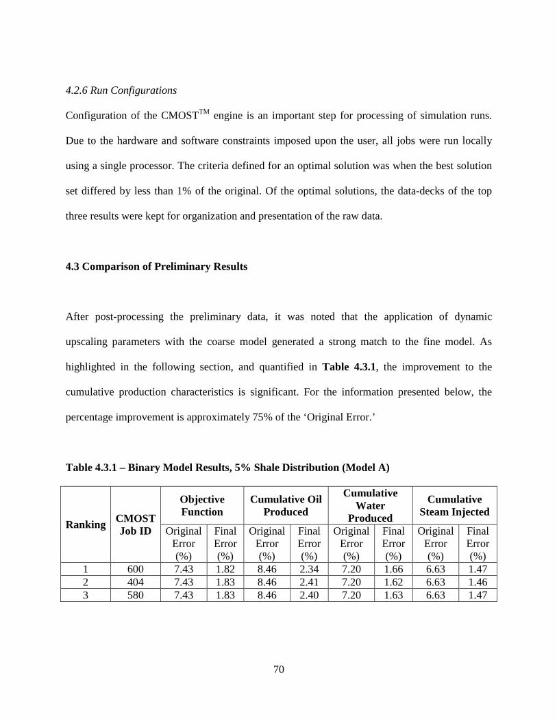
4.2.6 Run Configurations
Configuration of the CMOSTTM engine is an important step for processing of simulation runs.
Due to the hardware and software constraints imposed upon the user, all jobs were run locally
using a single processor. The criteria defined for an optimal solution was when the best solution
set differed by less than 1% of the original. Of the optimal solutions, the data-decks of the top
three results were kept for organization and presentation of the raw data.
4.3 Comparison of Preliminary Results
After post-processing the preliminary data, it was noted that the application of dynamic
upscaling parameters with the coarse model generated a strong match to the fine model. As
highlighted in the following section, and quantified in Table 4.3.1, the improvement to the
cumulative production characteristics is significant. For the information presented below, the
percentage improvement is approximately 75% of the ‘Original Error.’
Table 4.3.1 – Binary Model Results, 5% Shale Distribution (Model A)
Ranking CMOST Job ID
Objective Function
Cumulative Oil Produced
Cumulative Water
Produced
Cumulative Steam Injected
Original Error (%)
Final Error (%)
Original Error (%)
Final Error (%)
Original Error (%)
Final Error (%)
Original Error (%)
Final Error (%)
1 600 7.43 1.82 8.46 2.34 7.20 1.66 6.63 1.47 2 404 7.43 1.83 8.46 2.41 7.20 1.62 6.63 1.46 3 580 7.43 1.83 8.46 2.40 7.20 1.63 6.63 1.47
70

The method of error calculation is an important process, so it is valuable to discuss the various
details. The ‘Original Error’ is the error between the coarse and fine models prior to application
of matching parameters, as computed by CMOSTTM. The ‘Final Error’ is the error between the
coarse and fine models when applying the matching parameters as suggested by the ‘best job’
scenarios to the base coarse model. This is the primary output of the CMOSTTM results file
(.CMR). The ‘Delta Error’ can be thought of the improvement in result by applying the matching
parameters. If a model distribution gives a small ‘Delta Error’, then the parameter values were
less successful in mitigating the impact of the variation in gridding and reservoir properties
relative to a large ‘Delta Error’. However, inherently, the matching parameters can only improve
the base model a certain percentage and a perfect ‘Final Error’ can never be obtained.
The same rules apply for cumulative oil produced, cumulative water produced and cumulative
steam injected error notation. Also, the CMOSTTM Job ID varies from one history matching
exercise to another, as it represents the particular run that achieved that solution, which is to be
expected to vary in such a process. For example, in the aforementioned model, the ‘best job’ or
‘best case’ was achieved after the 600th simulation.
Table 4.3.2 – Binary Model Results, 5% Shale Distribution (Model A)
Ranking CMOST Job ID
Objective Function
Cumulative Oil Produced
Cumulative Water
Produced
Cumulative Steam
Injected Delta Error (%)
1 600 5.61 6.12 5.54 5.16 2 404 5.60 6.05 5.58 5.17 3 580 5.60 6.04 5.57 5.16
71

The matching parameters generated by CMOSTTM are highlighted in Table 4.3.3, in which the
multiplier values were selected from the range provided in the parameters section of the
CMOSTTM task file.
Table 4.3.3 – Matching Parameters Assigned by CMOSTTM, 5% Shale Distribution (Model A)
Ranking CMOST Job ID PERM, i PERM, j TH, i TH, j
1 600 1.56 8.13 1.00 7.42 2 404 1.56 9.25 1.00 13.83 3 580 1.56 9.63 1.00 10.92
An obvious observation in the result between Job ID 600 and 404 is that almost a nominal
change in the ‘Delta Error’ results despite significant changes in the PERM, j and TH, j
multipliers. Approximately a 12% reduction in PERM, j and a 46% reduction in TH, j resulted in
a ~0.01% improvement to the match. In this way, the values generated by any particular case
should not been seen as absolute but a guideline in terms of predicting matching success.
The application of the results as indicated above is presented as a production profile in Figure
4.3.1 and visually in Figures 4.3.2 – 4.3.4.
72

Figure 4.3.1 – Production Profile of Coarse Model, Fine Model and Matched Coarse Model Performance, 5% Shale Distribution (Model A)
Figure 4.3.2 – Coarse Model, Chamber Conformance at 5 Years, Temperature
i, k-direction i, j-direction
Comparison of Fine (1mX1mX1m) and Coarse (4mX100mX1m) 5% Shale Content, Model A
Produced Oil and Injected Water Rate (m3/d) v. Time (d)
Time (day)
Oil
Rat
e SC
- D
aily
(m3/
day)
Wat
er R
ate
SC -
Dai
ly (m
3/da
y)
0 365 730 1,095 1,460 1,825 2,190 2,555 2,920 3,285 3,6500
10
20
30
40
50
60
70
80
0
100
200
300
Produced Oil Rate, FINEProduced Oil Rate, COARSEProduced Oil Rate, Matched
Produced Oil and Injected Water Cumulative (m3) v. Time (d)
Time (day)
Cum
ulat
ive
Oil
SC (m
3)
Cum
ulat
ive
Wat
er S
C (m
3)
0 365 730 1,095 1,460 1,825 2,190 2,555 2,920 3,285 3,6500.00e+0
1.00e+5
2.00e+5
3.00e+5
4.00e+5
0.00e+0
1.00e+5
2.00e+5
3.00e+5
4.00e+5
5.00e+5
Cumulative and Instantaneous Steam Oil Ratio v. Time (d)
Time (day)
cSO
R (m
3/m
3)
iSO
R (m
3/m
3)
0 365 730 1,095 1,460 1,825 2,190 2,555 2,920 3,285 3,6500.0
1.0
2.0
3.0
0.0
2.0
4.0
6.0
Cumulative Steam Oil Ratio v. Oil Recovery Factor (%)
Oil Recovery Factor (%)
cSO
R (m
3/m
3)
0 20 40 60 800.0
1.0
2.0
3.0
InjI1ProdP1ProdP1aProdP1b
0 10 20 30 40 50 60 70 80 90 100
0 10 20 30 40 50 60 70 80 90 100
380390
400410
420430
440450
370
380
390
400
410
420
430
440
4500.00 40.00 80.00 feet
0.00 15.00 30.00 meters
File: singlewell_mUser: MAPIDate: 6/11/2013Scale: 1:618Z/X: 1.00:1Axis Units: m
12
35
58
81
104
127
150
173
196
219
242
SingleWell_Model_4mX100mX1mTemperature (C) 2018-12-31 J layer: 1
0 100 200 300
0 100 200 300
400410
420430
400
410
420
430
0.00 155.00 310.00 feet
0.00 50.00 100.00 meters
File: singlewell_mUser: MAPIDate: 6/11/2013Scale: 1:2439Z/Y: 8.00:1Axis Units: m
12
35
58
81
104
127
150
173
196
219
242
SingleWell_Model_4mX100mX1mTemperature (C) 2018-12-31 I layer: 19
73

Figure 4.3.3 – Fine Model, Chamber Conformance at 5 Years, Temperature
i, k-direction i, j-direction
Figure 4.3.4 – Matched Model, Chamber Conformance at 5 Years, Temperature
i, k-direction i, j-direction
InjI1ProdP1ProdP1aProdP1b
0 10 20 30 40 50 60 70 80 90 100
0 10 20 30 40 50 60 70 80 90 100
380390
400410
420430
440450
370
380
390
400
410
420
430
440
4500.00 40.00 80.00 feet
0.00 15.00 30.00 meters
File: SingleWell_User: MAPIDate: 6/11/2013Scale: 1:618Z/X: 1.00:1Axis Units: m
12
35
58
81
104
127
150
173
196
219
242
SingleWell_Model_4mX100mX1mTemperature (C) 2018-12-31 J layer: 1
0 100 200 300
0 100 200 300
400410
420430
400
410
420
430
0.00 160.00 320.00 feet
0.00 50.00 100.00 meters
File: SingleWell_User: MAPIDate: 6/11/2013Scale: 1:2465Z/Y: 8.00:1Axis Units: m
12
35
58
81
104
127
150
173
196
219
242
SingleWell_Model_4mX100mX1mTemperature (C) 2018-12-31 I layer: 75
InjI1ProdP1ProdP1aProdP1b
0 10 20 30 40 50 60 70 80 90 100
0 10 20 30 40 50 60 70 80 90 100
380390
400410
420430
440450
370
380
390
400
410
420
430
440
4500.00 40.00 80.00 feet
0.00 15.00 30.00 meters
File: SingleWell_User: MAPIDate: 6/11/2013Scale: 1:618Z/X: 1.00:1Axis Units: m
12
35
58
81
104
127
150
173
196
219
242
SingleWell_Model_4mX100mX1mTemperature (C) 2018-12-31 J layer: 1
0 100 200 300
0 100 200 300
400410
420430
400
410
420
430
0.00 155.00 310.00 feet
0.00 50.00 100.00 meters
File: SingleWell_User: MAPIDate: 6/11/2013Scale: 1:2439Z/Y: 8.00:1Axis Units: m
12
35
58
81
104
127
150
173
196
219
242
SingleWell_Model_4mX100mX1mTemperature (C) 2018-12-31 I layer: 19
74

4.4 Non-Unique Solutions
During the course of the analysis, it was also observed the DECE optimization method was
capable of generating non-unique solutions for the same model distributions. Based upon how
the process searches for the optimal solution, it is possible this phenomenon could occur. For
example, the distribution emphasised in the prior section was analysed with two separate history-
matching runs. Based upon those two unique runs, a different set of output was generated. The
optimal ‘best job’ values and the third ‘best job’ values were the same, but the second ‘best job’
values were different. Additionally, for another distribution, while the third ‘best job’ of the first
unique solution was the second ‘best job’ from the second solution set the remaining results were
different.
However, for both sets of distributions the ‘Delta Error’ generated for each solution set were the
same. To iterate Section 4.3, it can be further concluded that different combinations of the
parameters can generate comparable, if not identical results. This is an important conclusion
prior to the organization and analysis of the data. The user can manipulate some of the results, as
long as the improvement to the base models is maximized.
Tables 4.4.1 – 4.4.2 summarizes the variation in history matching runs as mentioned above. The
rows that are highlighted in red represent those solutions that are the same in terms of error
assignment. Whereas, Tables 4.4.3 – 4.4.6 highlight the exact same issue with a different
percentage shale distribution for a different set of runs.
75

Table 4.4.1 – Alternative Binary Model Results, 5% Shale Distribution (Model A)
Ranking CMOST Job ID
Objective Function
Cumulative Oil Produced
Cumulative Water
Produced
Cumulative Steam Injected
Original Error (%)
Final Error (%)
Original Error (%)
Final Error (%)
Original Error (%)
Final Error (%)
Original Error (%)
Final Error (%)
1 881 7.43 1.82 8.46 2.34 7.20 1.66 6.63 1.47 2 906 7.43 1.83 8.46 2.55 7.20 1.50 6.63 1.43 3 800 7.43 1.83 8.46 2.40 7.20 1.63 6.63 1.47
Table 4.4.2 – Alternative Matching Parameters Assigned by CMOSTTM, 5% Shale Distribution (Model A)
Ranking CMOST Job ID PERM, i PERM, j TH, i TH, j
1 881 1.56 8.13 1.00 7.42 2 906 1.63 8.88 1.00 9.17 3 800 1.56 9.63 1.00 10.92
Table 4.4.3 – Binary Model Results, 1% Shale Distribution (Unique Solution #1)
Ranking CMOST Job ID
Objective Function
Cumulative Oil Produced
Cumulative Water
Produced
Cumulative Steam Injected
Original Error (%)
Final Error (%)
Original Error (%)
Final Error (%)
Original Error (%)
Final Error (%)
Original Error (%)
Final Error (%)
1 826 5.26 1.40 5.41 1.59 5.34 1.38 5.02 1.23 2 950 5.26 1.40 5.41 1.54 5.34 1.43 5.02 1.25 3 707 5.26 1.41 5.41 1.58 5.34 1.40 5.02 1.24
Table 4.4.4 – Matching Parameters Assigned by CMOSTTM, 1% Shale Distribution (Unique Solution #1)
Ranking CMOST Job ID PERM, i PERM, j TH, i TH, j
1 826 1.13 8.13 1.17 2.17 2 950 1.13 8.13 1.17 5.67 3 707 1.13 3.63 1.17 6.25
76

Table 4.4.5 – Binary Model Results, 1% Shale Distribution (Unique Solution #2)
Ranking CMOST Job ID
Objective Function
Cumulative Oil Produced
Cumulative Water
Produced
Cumulative Steam Injected
Original Error (%)
Final Error (%)
Original Error (%)
Final Error (%)
Original Error (%)
Final Error (%)
Original Error (%)
Final Error (%)
1 655 5.26 1.40 5.41 1.59 5.34 1.38 5.02 1.23 2 623 5.26 1.41 5.41 1.58 5.34 1.40 5.02 1.24 3 659 5.26 1.41 5.41 1.63 5.34 1.37 5.02 1.24
Table 4.4.6 – Matching Parameters Assigned by CMOSTTM, 1% Shale Distribution (Unique Solution #2)
Ranking CMOST Job ID PERM, i PERM, j TH, i TH, j
1 655 1.13 3.25 1.17 6.25 2 623 1.13 3.63 1.17 6.25 3 659 1.13 3.25 1.17 7.42
77

Figure 4.4.1 – Production Profile of Coarse Model, Fine Model and Matched Coarse Models Performance for both Unique Solution Sets, 1% Shale Distribution (Optimal ‘Best Job’)
Despite different solution sets resulting in a different combination of parameter values, the
impact to the ‘Final Error’ is nominal, as well as the improvement to the production profile.
While the production profiles are not identical for different parameter values of the same ‘Final
Error’, the cumulative profiles are effectively identical and all work to minimize the ‘Final
Error.’
Comparison of Fine (1mX1mX1m) and Coarse (4mX100mX1m), 1% Shale Content
Produced Oil and Injected Water Rate (m3/d) v. Time (d)
Time (day)
Oil
Rat
e SC
- D
aily
(m3/
day)
Wat
er R
ate
SC -
Dai
ly (m
3/da
y)0 365 730 1,095 1,460 1,825 2,190 2,555 2,920 3,285 3,650
0
20
40
60
80
100
120
0
100
200
300Produced Oil Rate, FINEProduced Oil Rate, COARSEProduced Oil Rate, MATCHED #1Produced Oil Rate, MATCHED #2
Produced Oil and Injected Water Cumulative (m3) v. Time (d)
Time (day)
Cum
ulat
ive
Oil
SC (m
3)
Cum
ulat
ive
Wat
er S
C (m
3)
0 365 730 1,095 1,460 1,825 2,190 2,555 2,920 3,285 3,6500.00e+0
1.00e+5
2.00e+5
3.00e+5
4.00e+5
0.00e+0
1.00e+5
2.00e+5
3.00e+5
4.00e+5
5.00e+5
Cumulative and Instantaneous Steam Oil Ratio v. Time (d)
Time (day)
cSO
R (m
3/m
3)
iSO
R (m
3/m
3)
0 365 730 1,095 1,460 1,825 2,190 2,555 2,920 3,285 3,6500.0
1.0
2.0
3.0
0.0
1.0
2.0
3.0
4.0
Cumulative Steam Oil Ratio v. Oil Recovery Factor (%)
Oil Recovery Factor (%)
cSO
R (m
3/m
3)
0 20 40 60 800.0
1.0
2.0
3.0
78

4.5 Organization of Raw Data
After successful completion of all the simulation runs, the raw data was organized and the
extensive exercise of post-processing begun. Several approaches were conceived to best
represent the data without biasing or influencing the results. The objective was to analyze the
impact of different length scales for altered petrophysical arrangements to determine if an
analytical relationship could be generated to more accurately track temperature fronts in the
reservoir. Ideally, the history matching exercise would also indirectly serve as a sensitivity
analysis from the perspective that multiple runs with different inputs would enable the user to
identify if one parameter was being weighted more heavily than other, which would be assumed
to have the biggest impact upon performance. This would also be achieved by introducing no
influence on parameter selection, and weighting their potential contribution equally.
Firstly, a linear relationship was generated to ensure that an increase in reservoir heterogeneities
for a given grid dimension, resulted in an increase to ‘Original Error’. This behaviour can also be
assumed for ‘Delta Error’ provided that an increase in reservoir heterogeneity would allow more
opportunity for improvement and only those models with the greatest ‘Original Error’ could be
improved the greatest. That data is depicted in Figure 4.5.1.
79

Figure 4.5.1 - Relationship between Shale Content by Volume and Error Correlations for Binary Model, (4m, 100m, 1m)
80

Secondly, cross-plots were generated for each parameter and their corresponding value with
respect to ‘Original Error’ and ‘Delta Error’ was organized. Those results are summarized in
Figures 4.5.2 and 4.5.3 for the (4m, 100m, 1m) binary set of models. Data was organized for the
other binary gird dimensions as well as the facies-based models, however, for ease of
presentation and discussion only the (4m, 100m, 1m) cases are presented. The conclusions for
the (4m, 100m, 1m) cases are applicable to the other type models.
Figure 4.5.2 – Cross-Plot of Parameter Values and ‘Original Error’ (%)
81

Figure 4.5.3 – Cross-Plot of Parameter Values and ‘Delta Error’ (%)
The principal challenge with this approach is it only partially takes into consideration the
location of the reservoir heterogeneities relative to the injector and producer well. Therefore,
there is some scatter present in the results that is difficult to build a correlation around. For
example, the ‘Original Error’ plots have an instance of high reservoir quality (1% Shale Content)
showing significantly more aggressive multipliers than a low reservoir quality case (10% Shale
Content). This result is supported in Table 4.5.1.
82

Table 4.5.1 – Outliers in the ‘Original Error’ Cases (4m, 100m, 1m)
Type-A Binary Model
Association
Original Error (%)
Parameters
PERM, i PERM, j TH, i TH, j
1% Shale Content 7.46 1.19 5.67 1.17 9.25
10% Shale Content 12.82 1.44 3.33 1.17 4.75
Additionally, the ‘Delta Error’ plots for the same parameters show a different observation. For a
smaller magnitude of parameter values, a larger improvement in ‘Delta Error’ occurs, with the
effect normalized by the Percent Improvement from ‘Original Error’ reference. This result is
supported in Table 4.5.2.
Table 4.5.2 – Outliers in the ‘Delta Error’ Cases (4m, 100m, 1m)
Type-A Binary Model
Association
Delta Error (%)
Percent Improvement
from Original
Error (%)
Parameters
PERM, i PERM, j TH, i TH, j
1% Shale Content 4.25 43.0 1.19 5.67 1.17 9.25
10% Shale Content 6.73 47.5 1.44 3.33 1.17 4.75
In general, there is no discernible trend between the ‘Original Error’ and the matching
parameters. In that, the ‘best job’ values assigned do not offer any indication of which
configurations have the most or least significant variation from the coarse to the fine models.
However, the ‘Delta Error’ plots provide a clearer trend. The ‘Delta Error’ plots are effective in
showing that an increase in parameter magnitude has a more significant impact upon reducing
83

the error between the coarse and fine models. There is a dependency of the magnitude of the
parameters on matching the models, even if it is not understood which models are most likely to
see certain values. Therefore, the goal moving forward is to refine this approach in order to
enhance the relationship between parameter value and reservoir quality with gridding
dependency.
Due to the petrophysical values assigned to the shale (Facies B) in the binary models or high
proportion shale (Facies 3) in the facies-based models, no models have any inter-well gridblocks
of these properties. As the occurrence of those facies types would prevent chamber development
in that particular plane, and the overall performance would be independent of the distribution
within the rest of the model. However, proximity of these reservoir facies relative to the well pair
(such as, proximity above the injector well) will have significant impact on chamber signature
and ultimate recovery. For example, if we review the coarsening upwards and fining upwards
models generated in the facies-based exercise, the reservoir quality of a coarsening upwards
sequence improves as you decrease depositional depth, whereas, the reservoir quality of the
fining upwards sequence improves as you increase depth. Therefore, it is expected that the
performance of the fining upwards model will tend to be better than the coarsening upwards
model, as the best reservoir quality is closer to the well pair where the need to establish
communication is of paramount importance for future chamber growth. Consequently, the poorer
reservoir quality is closer to the overburden of the model which would only affect the later
portion of the production profile. While the models may have the identical proportions of
reservoir facies, the location alone will be the overriding factor for performance. The relative
84

performance of the coarse and fine model will be captured with respect the ‘Original and Final
Error’, however, it is for that unique case.
Therefore, it can be concluded that the relationship of the fine model to the coarse models
performance will vary with respect to the location of these heterogeneities within the model,
despite identical proportions. For example, the performance of two models of identical
proportions but distributed differently as presented in Figures 4.5.4 – 4.5.7. Upon review of the
steam signatures and production profiles, it is easy to appreciate the spatial impact.
Figure 4.5.4 – Production Profile of Coarse and Fine Model Performance, 5% Shale Distribution (Model #1)
Comparison of Fine (1mX1mX1m) and Coarse (4mX100mX1m), 5% Shale Content, Model #1
Produced Oil and Injected Water Rate (m3/d) v. Time (d)
Time (day)
Oil
Rat
e SC
- D
aily
(m3/
day)
Wat
er R
ate
SC -
Dai
ly (m
3/da
y)
0 365 730 1,095 1,460 1,825 2,190 2,555 2,920 3,285 3,6500
20
40
60
80
100
0
100
200
300Produced Oil Rate, FINEProduced Oil Rate, COARSEInjected Water Rate, FINEInjected Water Rate, COARSE
Produced Oil and Injected Water Cumulative (m3) v. Time (d)
Time (day)
Cum
ulat
ive
Oil
SC (m
3)
Cum
ulat
ive
Wat
er S
C (m
3)
0 365 730 1,095 1,460 1,825 2,190 2,555 2,920 3,285 3,6500.00e+0
1.00e+5
2.00e+5
3.00e+5
4.00e+5
5.00e+5
0.00e+0
1.00e+5
2.00e+5
3.00e+5
4.00e+5
5.00e+5
Cumulative and Instantaneous Steam Oil Ratio v. Time (d)
Time (day)
cSO
R (m
3/m
3)
iSO
R (m
3/m
3)0 365 730 1,095 1,460 1,825 2,190 2,555 2,920 3,285 3,650
0.0
1.0
2.0
3.0
4.0
0.0
2.0
4.0
6.0
Cumulative Steam Oil Ratio v. Oil Recovery Factor (%)
Oil Recovery Factor (%)
cSO
R (m
3/m
3)
0 20 40 60 800.0
1.0
2.0
3.0
85

Figure 4.5.5 – Production Profile of Coarse and Fine Model Performance, 5% Shale Distribution (Model #2)
Comparison of Fine (1mX1mX1m) and Coarse (4mX100mX1m), 5% Shale Content, Model #2
Produced Oil and Injected Water Rate (m3/d) v. Time (d)
Time (day)
Oil
Rat
e SC
- D
aily
(m3/
day)
Wat
er R
ate
SC -
Dai
ly (m
3/da
y)
0 365 730 1,095 1,460 1,825 2,190 2,555 2,920 3,285 3,6500
20
40
60
80
100
0
100
200
300Produced Oil Rate, FINEProduced Oil Rate, COARSEInjected Water Rate, FINEInjected Water Rate, COARSE
Produced Oil and Injected Water Cumulative (m3) v. Time (d)
Time (day)
Cum
ulat
ive
Oil
SC (m
3)
Cum
ulat
ive
Wat
er S
C (m
3)
0 365 730 1,095 1,460 1,825 2,190 2,555 2,920 3,285 3,6500.00e+0
1.00e+5
2.00e+5
3.00e+5
4.00e+5
5.00e+5
0.00e+0
1.00e+5
2.00e+5
3.00e+5
4.00e+5
5.00e+5
Cumulative and Instantaneous Steam Oil Ratio v. Time (d)
Time (day)
cSO
R (m
3/m
3)
iSO
R (m
3/m
3)
0 365 730 1,095 1,460 1,825 2,190 2,555 2,920 3,285 3,6500.0
1.0
2.0
3.0
4.0
0.0
2.0
4.0
6.0
Cumulative Steam Oil Ratio v. Oil Recovery Factor (%)
Oil Recovery Factor (%)
cSO
R (m
3/m
3)
0 20 40 60 800.0
1.0
2.0
3.0
86

Figure 4.5.6 – Production Profile of Coarse Model #1 and Coarse Model #2 Performance (5% Shale Distribution)
Comparison of Coarse (4mX100mX1m) and Coarse (4mX100mX1m), 5% Shale ContentProduced Oil and Injected Water Rate (m3/d) v. Time (d)
Time (day)
Oil
Rat
e SC
- D
aily
(m3/
day)
Wat
er R
ate
SC -
Dai
ly (m
3/da
y)
0 365 730 1,095 1,460 1,825 2,190 2,555 2,920 3,285 3,6500
20
40
60
80
100
0
100
200
300Produced Oil Rate, COARSE, Model #1Produced Oil Rate, COARSE, Model #2Injected Water Rate, COARSE, Model #1Injected Water Rate, COARSE, Model #2
Produced Oil and Injected Water Cumulative (m3) v. Time (d)
Time (day)
Cum
ulat
ive
Oil
SC (m
3)
Cum
ulat
ive
Wat
er S
C (m
3)
0 365 730 1,095 1,460 1,825 2,190 2,555 2,920 3,285 3,6500.00e+0
1.00e+5
2.00e+5
3.00e+5
4.00e+5
5.00e+5
0.00e+0
1.00e+5
2.00e+5
3.00e+5
4.00e+5
Cumulative and Instantaneous Steam Oil Ratio v. Time (d)
Time (day)
cSO
R (m
3/m
3)
iSO
R (m
3/m
3)
0 365 730 1,095 1,460 1,825 2,190 2,555 2,920 3,285 3,6500.0
1.0
2.0
3.0
4.0
0.0
2.0
4.0
6.0
Cumulative Steam Oil Ratio v. Oil Recovery Factor (%)
Oil Recovery Factor (%)
cSO
R (m
3/m
3)
0 20 40 60 800.0
1.0
2.0
3.0
87

Figure 4.5.7 – Production Profile of Fine Model #1 and Fine Model #2 Performance (5% Shale Distribution)
Table 4.5.3 – Binary Model Results, 5% Shale Distribution (Model #1), ‘Original and Final Error’
Ranking CMOST Job ID
Objective Function
Cumulative Oil Produced
Cumulative Water
Produced
Cumulative Steam Injected
Original Error (%)
Final Error (%)
Original Error (%)
Final Error (%)
Original Error (%)
Final Error (%)
Original Error (%)
Final Error (%)
1 558 7.46 1.46 7.98 1.90 7.42 1.23 6.99 1.24 2 744 7.46 1.46 7.98 1.64 7.42 1.42 6.99 1.33 3 823 7.46 1.46 7.98 1.91 7.42 1.23 6.99 1.25
Comparison of Fine (1mX1mX1m) and Fine (1mX1mX1m), 5% Shale Content
Produced Oil and Injected Water Rate (m3/d) v. Time (d)
Time (day)
Oil
Rat
e SC
- D
aily
(m3/
day)
Wat
er R
ate
SC -
Dai
ly (m
3/da
y)
0 365 730 1,095 1,460 1,825 2,190 2,555 2,920 3,285 3,6500
20
40
60
80
100
120
0
100
200
300Produced Oil Rate, FINE, Model #1Produced Oil Rate, FINE, Model #2Injected Water Rate, FINE, Model #1Injected Water Rate, FINE, Model #2
Produced Oil and Injected Water Cumulative (m3) v. Time (d)
Time (day)
Cum
ulat
ive
Oil
SC (m
3)
Cum
ulat
ive
Wat
er S
C (m
3)
0 365 730 1,095 1,460 1,825 2,190 2,555 2,920 3,285 3,6500.00e+0
1.00e+5
2.00e+5
3.00e+5
4.00e+5
5.00e+5
0.00e+0
1.00e+5
2.00e+5
3.00e+5
4.00e+5
5.00e+5
Cumulative and Instantaneous Steam Oil Ratio v. Time (d)
Time (day)
cSO
R (m
3/m
3)
iSO
R (m
3/m
3)
0 365 730 1,095 1,460 1,825 2,190 2,555 2,920 3,285 3,6500.0
1.0
2.0
3.0
4.0
0.0
2.0
4.0
6.0
Cumulative Steam Oil Ratio v. Oil Recovery Factor (%)
Oil Recovery Factor (%)
cSO
R (m
3/m
3)
0 20 40 60 800.0
1.0
2.0
3.0
88

Table 4.5.4– Binary Model Results, 5% Shale Distribution (Model #1), ‘Delta Error’
Ranking CMOST Job ID
Objective Function
Cumulative Oil Produced
Cumulative Water
Produced
Cumulative Steam
Injected Delta Error (%)
1 558 6.00 6.08 6.19 5.75 2 744 6.00 6.34 6.00 5.66 3 823 6.00 6.07 6.19 5.74
Table 4.5.5 – Matching Parameters Assigned by CMOSTTM, 5% Shale Distribution (Model #1)
Ranking CMOST Job ID PERM, i PERM, j TH, i TH, j
1 558 1.56 9.25 1.00 1.58 2 744 1.50 10.00 1.00 14.42 3 823 1.56 9.25 1.00 2.75
Table 4.5.6 – Binary Model Results, 5% Shale Distribution (Model #2)
Ranking CMOST Job ID
Objective Function
Cumulative Oil Produced
Cumulative Water
Produced
Cumulative Steam Injected
Original Error (%)
Final Error (%)
Original Error (%)
Final Error (%)
Original Error (%)
Final Error (%)
Original Error (%)
Final Error (%)
1 648 7.35 1.82 7.36 2.12 7.57 1.75 7.10 1.58 2 538 7.35 1.82 7.36 2.15 7.57 1.73 7.10 1.58 3 627 7.35 1.82 7.36 2.14 7.57 1.74 7.10 1.58
Table 4.5.7 – Binary Model Results, 5% Shale Distribution (Model #2)
Ranking CMOST Job ID
Objective Function
Cumulative Oil Produced
Cumulative Water
Produced
Cumulative Steam
Injected Delta Error (%)
1 648 5.53 5.24 5.82 5.52 2 538 5.53 5.21 5.84 5.52 3 627 5.53 5.22 5.83 5.52
89

Table 4.5.8 – Matching Parameters Assigned by CMOSTTM, 5% Shale Distribution (Model #2)
Ranking CMOST Job ID PERM, i PERM, j TH, i TH, j
1 648 1.31 8.50 1.17 11.50 2 538 1.31 10.00 1.17 12.67 3 627 1.31 9.63 1.17 10.33
Table 4.5.9 – ‘Best Job’ Matching Parameters Assigned by CMOSTTM
Model CMOST Job ID PERM, i PERM, j TH, i TH, j
#1 558 1.56 9.25 1.00 1.58 #2 648 1.31 8.50 1.17 11.50
Fundamentally, these are very similar models yet the matching values proposed by CMOSTTM
vary significantly for thermal conductivity in the j-direction. The other values are fairly
comparable, however, the difference in value for the thermal conductivity parallel the wellbore is
significant. While noted here for the first time, this observation is a re-occurring trend within the
analysis portion of the report that the thermal conductivity in the j-direction often has the most
variation. A review of the results reported in Sections 4.3 and 4.4 supports this conclusion. The
values generated for those versions of binary models with 5% shale distribution are comparable
to above.
Table 4.5.10 – ‘Best Job’ Matching Parameters Assigned by CMOSTTM
Model CMOST Job ID PERM, i PERM, j TH, i TH, j
A 600 1.56 8.13 1.00 7.42
90
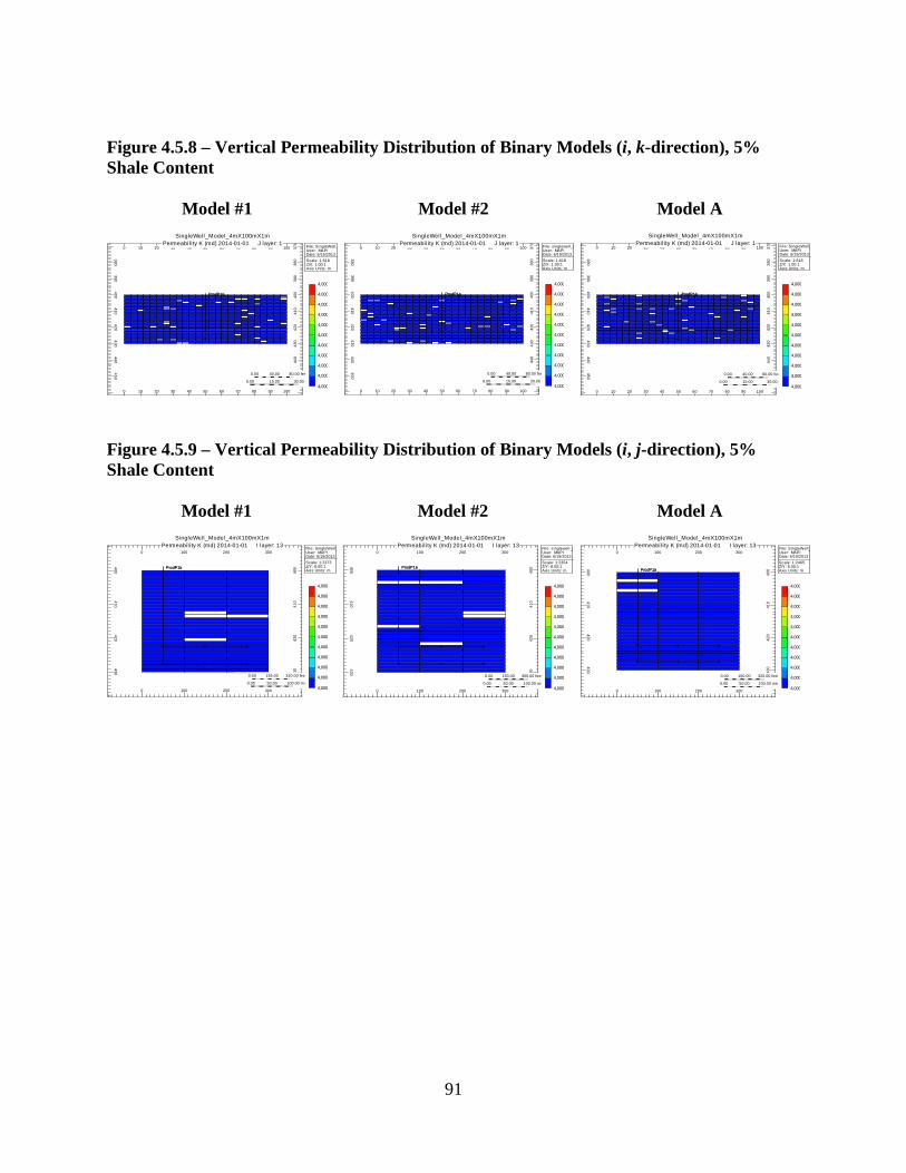
Figure 4.5.8 – Vertical Permeability Distribution of Binary Models (i, k-direction), 5% Shale Content
Model #1 Model #2 Model A
Figure 4.5.9 – Vertical Permeability Distribution of Binary Models (i, j-direction), 5% Shale Content
Model #1 Model #2 Model A
ProdP1aProdP1b
0 10 20 30 40 50 60 70 80 90 100
0 10 20 30 40 50 60 70 80 90 100
380390
400410
420430
440450
370
380
390
400
410
420
430
440
4500.00 40.00 80.00 feet
0.00 15.00 30.00 meters
File: SingleWell_User: MAPIDate: 6/19/2013Scale: 1:618Z/X: 1.00:1Axis Units: m
4,000
4,000
4,000
4,000
4,000
4,000
4,000
4,000
4,000
4,000
4,000
SingleWell_Model_4mX100mX1mPermeabil ity K (md) 2014-01-01 J layer: 1
ProdP1aProdP1b
0 10 20 30 40 50 60 70 80 90 100
0 10 20 30 40 50 60 70 80 90 100
380390
400410
420430
440450
370
380
390
400
410
420
430
440
4500.00 40.00 80.00 feet
0.00 15.00 30.00 meters
File: singlewell_mUser: MAPIDate: 6/19/2013Scale: 1:618Z/X: 1.00:1Axis Units: m
4,000
4,000
4,000
4,000
4,000
4,000
4,000
4,000
4,000
4,000
4,000
SingleWell_Model_4mX100mX1mPermeabil ity K (md) 2014-01-01 J layer: 1
ProdP1aProdP1b
0 10 20 30 40 50 60 70 80 90 100
0 10 20 30 40 50 60 70 80 90 100
380390
400410
420430
440450
370
380
390
400
410
420
430
440
4500.00 40.00 80.00 feet
0.00 15.00 30.00 meters
File: SingleWell_User: MAPIDate: 6/19/2013Scale: 1:618Z/X: 1.00:1Axis Units: m
4,000
4,000
4,000
4,000
4,000
4,000
4,000
4,000
4,000
4,000
4,000
SingleWell_Model_4mX100mX1mPermeabil ity K (md) 2014-01-01 J layer: 1
ProdP1aProdP1b
0 100 200 300
0 100 200 300
400410
420430
400
410
420
430
0.00 155.00 310.00 feet
0.00 50.00 100.00 meters
File: SingleWell_User: MAPIDate: 6/19/2013Scale: 1:2373Z/Y: 8.00:1Axis Units: m
4,000
4,000
4,000
4,000
4,000
4,000
4,000
4,000
4,000
4,000
4,000
SingleWell_Model_4mX100mX1mPermeabil ity K (md) 2014-01-01 I layer: 13
ProdP1aProdP1b
0 100 200 300
0 100 200 300400
410420
430
400
410
420
430
0.00 150.00 300.00 feet
0.00 50.00 100.00 meters
File: singlewell_mUser: MAPIDate: 6/19/2013Scale: 1:2354Z/Y: 8.00:1Axis Units: m
4,000
4,000
4,000
4,000
4,000
4,000
4,000
4,000
4,000
4,000
4,000
SingleWell_Model_4mX100mX1mPermeabil ity K (md) 2014-01-01 I layer: 13
ProdP1aProdP1b
0 100 200 300
0 100 200 300
400410
420430
400
410
420
430
0.00 160.00 320.00 feet
0.00 50.00 100.00 meters
File: SingleWell_User: MAPIDate: 6/19/2013Scale: 1:2465Z/Y: 8.00:1Axis Units: m
4,000
4,000
4,000
4,000
4,000
4,000
4,000
4,000
4,000
4,000
4,000
SingleWell_Model_4mX100mX1mPermeabil ity K (md) 2014-01-01 I layer: 13
91

Figure 4.5.10 – Production Profile of Coarse Model #1, Model #2 and Model A Performance (5% Shale Distribution)
As observed in Figures 4.5.4 – 4.5.7, the distribution of non-reservoir relative to reservoir rock
will impact early SAGD development. The impact to the rate of chamber growth will manifest
itself by calling for more or less aggressive multipliers to offset the presence of those non-
reservoir gridblocks. However, the exact choice of those multiplier values is not expertly known.
Therefore, an additional technique to process the numerical results needs to be developed to
confirm the quantity of reservoir heterogeneities and impact of the location. In developing a
secondary approach for analyzing the data, the hope is additional observations will become
apparent. CMG has recently developed a tool that can analyze several realizations of a static
Comparison of Coarse (4mX100mX1m) Models for #1, #2 and A, 5% Shale Content
Produced Oil and Injected Water Rate (m3/d) v. Time (d)
Time (day)
Oil
Rat
e SC
- D
aily
(m3/
day)
Wat
er R
ate
SC -
Dai
ly (m
3/da
y)
0 365 730 1,095 1,460 1,825 2,190 2,555 2,920 3,285 3,6500
20
40
60
80
100
120
0
100
200
300Produced Oil Rate, COARSE, Model #1Produced Oil Rate, COARSE, Model #2Produced Oil Rate, COARSE, Model AInjected Water Rate, COARSE, Model #1Injected Water Rate, COARSE, Model #2Injected Water Rate, COARSE, Model A
Produced Oil and Injected Water Cumulative (m3) v. Time (d)
Time (day)
Cum
ulat
ive
Oil
SC (m
3)
Cum
ulat
ive
Wat
er S
C (m
3)
0 365 730 1,095 1,460 1,825 2,190 2,555 2,920 3,285 3,6500.00e+0
1.00e+5
2.00e+5
3.00e+5
4.00e+5
5.00e+5
0.00e+0
1.00e+5
2.00e+5
3.00e+5
4.00e+5
Cumulative and Instantaneous Steam Oil Ratio v. Time (d)
Time (day)
cSO
R (m
3/m
3)
iSO
R (m
3/m
3)
0 365 730 1,095 1,460 1,825 2,190 2,555 2,920 3,285 3,6500.0
1.0
2.0
3.0
4.0
0.0
2.0
4.0
6.0
Cumulative Steam Oil Ratio v. Oil Recovery Factor (%)
Oil Recovery Factor (%)
cSO
R (m
3/m
3)
0 20 40 60 800.0
1.0
2.0
3.0
92

reservoir model and provide an indication of productivity. CMG refers to this tool as the SAGD
Productivity Index (SPI).
4.6 Normalization of Length Scale Impact
As described in Section 3.11, the concept of length scale relative to facies proportions was
introduced. Given the magnitude of various parameters and the impact of reservoir
heterogeneities relative to well placement, the following two concepts can be revisited:
- To what extent is reservoir quality over-riding the impact of length scales?
- To what extent do length scales drive reservoir performance?
To iterate Tables 3.11.1 and 3.11.2, the following result was proposed for two binary models.
Table 3.11.1 – Comparison of Length Scales and Heterogeneity on Coarse Model Performance
Model Type Objective Function, Original Error
Coarse Model (%)
Fine Model (%)
4m, 100m, 1m (Type-A)
0% Shale Content (Homogenous
Properties) 4.77 Reference
10% Shale Content (Heterogeneous
Properties) 8.46 Reference
2m, 25m, 1m (Type-F)
0% Shale Content (Homogenous
Properties) 1.10 Reference
10% Shale Content (Heterogeneous
Properties) 3.41 Reference
93

Table 3.11.2 – Comparison of Length Scales and Heterogeneity on Relative Performance
Model Type
Objective Function, Difference in Error as a
function of Shale Content (%)
4m, 100m, 1m (Type-A)
0% Shale Content (Homogenous Properties) 3.69 10% Shale Content
(Heterogeneous Properties)
2m, 25m, 1m (Type-F)
0% Shale Content (Homogenous Properties) 2.31 10% Shale Content
(Heterogeneous Properties)
Upon review of these models, it was observed that placement of reservoir heterogeneities was a
dominant feature, in terms of its impact upon performance and the magnitude of the error values.
For example, the aforementioned case has the following distribution of facies.
Figure 4.6.1 – Heterogeneous Model, Facies Distribution (i, k-direction), 10% Shale Content
4m, 100m, 1m Model 2m, 25m, 1m Model
ProdP1aProdP1b
0 10 20 30 40 50 60 70 80 90 100
0 10 20 30 40 50 60 70 80 90 100
380390
400410
420430
440450
370
380
390
400
410
420
430
440
4500.00 40.00 80.00 feet
0.00 15.00 30.00 meters
File: SingleWell_MoUser: MAPIDate: 7/5/2013Scale: 1:618Z/X: 1.00:1Axis Units: m
0.0
0.0
0.0
0.0
0.0
0.0
0.0
0.0
0.0
0.0
0.0
SingleWell_Model_4mX100mX1mCMGLCustom_Shale_10% 2014-01-01 J layer: 1
ProdP1aProdP1b
0 10 20 30 40 50 60 70 80 90 100
0 10 20 30 40 50 60 70 80 90 100
380390
400410
420430
440450
370
380
390
400
410
420
430
440
4500.00 40.00 80.00 feet
0.00 15.00 30.00 meters
File: SingleWell_MoUser: MAPIDate: 7/5/2013Scale: 1:618Z/X: 1.00:1Axis Units: m
0.0
0.0
0.0
0.0
0.0
0.0
0.0
0.0
0.0
0.0
0.0
SingleWell_Model_2mX25mX1mCMGLCustom_Shale_10% 2014-01-01 J layer: 1
94

Figure 4.6.2 – Heterogeneous Model, Facies Distribution (i, j-direction), 10% Shale Content
4m, 100m, 1m Model 2m, 25m, 1m Model
While it has been observed that there is a dependency on length scale when you normalize the
volume of non-reservoir, it has also been observed that that dependency can be offset based upon
re-alignment of those same proportions. The following set of models highlights that impact upon
SAGD performance.
Figure 4.6.3 – Heterogeneous Model, Facies Distribution (i, k-direction), 10% Shale Content
4m, 100m, 1m Model 2m, 25m, 1m Model
ProdP1aProdP1b
0 100 200 300
0 100 200 300
400410
420430
400
410
420
430
0.00 155.00 310.00 feet
0.00 50.00 100.00 meters
File: SingleWell_MoUser: MAPIDate: 7/5/2013Scale: 1:2388Z/Y: 8.00:1Axis Units: m
0.0
0.0
0.0
0.0
0.0
0.0
0.0
0.0
0.0
0.0
0.0
SingleWell_Model_4mX100mX1mCMGLCustom_Shale_10% 2014-01-01 I layer: 13
ProdP1aProdP1b
0 100 200 300
0 100 200 300
400410
420430
400
410
420
430
0.00 155.00 310.00 feet
0.00 50.00 100.00 meters
File: SingleWell_MoUser: MAPIDate: 7/5/2013Scale: 1:2388Z/Y: 8.00:1Axis Units: m
0.0
0.0
0.0
0.0
0.0
0.0
0.0
0.0
0.0
0.0
0.0
SingleWell_Model_2mX25mX1mCMGLCustom_Shale_10% 2014-01-01 I layer: 25
ProdP1aProdP1b
0 10 20 30 40 50 60 70 80 90 100
0 10 20 30 40 50 60 70 80 90 100
380390
400410
420430
440450
370
380
390
400
410
420
430
440
4500.00 40.00 80.00 feet
0.00 15.00 30.00 meters
File: SingleWell_MoUser: MAPIDate: 7/5/2013Scale: 1:618Z/X: 1.00:1Axis Units: m
0.0
0.0
0.0
0.0
0.0
0.0
0.0
0.0
0.0
0.0
0.0
SingleWell_Model_4mX100mX1mCMGLCustom_Shale_10% 2014-01-01 J layer: 1
ProdP1aProdP1b
0 10 20 30 40 50 60 70 80 90 100
0 10 20 30 40 50 60 70 80 90 100
380390
400410
420430
440450
370
380
390
400
410
420
430
440
4500.00 40.00 80.00 feet
0.00 15.00 30.00 meters
File: SingleWell_MoUser: MAPIDate: 7/5/2013Scale: 1:618Z/X: 1.00:1Axis Units: m
0.0
0.0
0.0
0.0
0.0
0.0
0.0
0.0
0.0
0.0
0.0
SingleWell_Model_2mX25mX1mCMGLCustom_Shale_10% 2014-01-01 J layer: 1
95

Figure 4.6.4 – Heterogeneous Model, Facies Distribution (i, j-direction), 10% Shale Content
4m, 100m, 1m Model 2m, 25m, 1m Model
Table 4.6.1 – Revisited Comparison of Length Scales and Heterogeneity on Coarse Model Performance
Model Type Objective Function, Original Error
Coarse Model (%)
Fine Model (%)
4m, 100m, 1m (Type-A)
0% Shale Content (Homogenous
Properties) 4.77 Reference
10% Shale Content (Heterogeneous
Properties) 5.41 Reference
2m, 25m, 1m (Type-F)
0% Shale Content (Homogenous
Properties) 1.10 Reference
10% Shale Content (Heterogeneous
Properties) 3.71 Reference
ProdP1aProdP1b
0 100 200 300
0 100 200 300
400410
420430
400
410
420
430
0.00 155.00 310.00 feet
0.00 50.00 100.00 meters
File: SingleWell_MoUser: MAPIDate: 7/5/2013Scale: 1:2380Z/Y: 8.00:1Axis Units: m
0.0
0.0
0.0
0.0
0.0
0.0
0.0
0.0
0.0
0.0
0.0
SingleWell_Model_4mX100mX1mCMGLCustom_Shale_10% 2014-01-01 I layer: 13
ProdP1aProdP1b
0 100 200 300
0 100 200 300
400410
420430
400
410
420
430
0.00 155.00 310.00 feet
0.00 50.00 100.00 meters
File: SingleWell_MoUser: MAPIDate: 7/5/2013Scale: 1:2389Z/Y: 8.00:1Axis Units: m
0.0
0.0
0.0
0.0
0.0
0.0
0.0
0.0
0.0
0.0
0.0
SingleWell_Model_2mX25mX1mCMGLCustom_Shale_10% 2014-01-01 I layer: 25
96

Table 4.6.2 – Revisited Comparison of Length Scales and Heterogeneity on Relative Performance
Model Type
Objective Function, Difference in Error as a
function of Shale Content (%)
4m, 100m, 1m (Type-A)
0% Shale Content (Homogenous Properties) 0.64 10% Shale Content
(Heterogeneous Properties)
2m, 25m, 1m (Type-F)
0% Shale Content (Homogenous Properties) 2.61 10% Shale Content
(Heterogeneous Properties)
Given the same content of reservoir and non-reservoir rock types, the placement of the non-
reservoir had a significant impact to the heterogeneous model relative to the fine model or
reference case. The coarse model error for Type-A was significantly different, 8.46% and 5.41%
respectively. However, the difference in coarse error was significantly less for the Type-F
models, 3.41% and 3.71% respectively. The significant reduction in error for Type-A binary
model and the increase in error for the Type-F binary model suggest the overriding impact of
location of these reservoir heterogeneities as opposed to the length scale assignment itself. The
author is not implying that length scale impact is negligible, but through the course of the
analysis the hope is an error bar can be assigned to a given shale content for variable length
scales, and the magnitude of length scale impact can be quantified. Given a realistic band of
uncertainty, the analysis can be simplified for industry models with this variation perpendicular
(4m or 2m) and parallel (100m, 50m or 25m) the wellbore.
97

This implication further motivates the need for a robust tool. The implementation of CMG’s
SAGD Productivity Index will help quantify the impact of different facies types and proportions
while validating the use of these two parameters to recommend upscaling parameters,
independent of the length scales discussed within the content of this report.
Figure 4.6.5 - Production Profile of Reconfigured Heterogeneous Distribution (Type-A, 10% Shale Content)
Comparison of Fine (1mX1mX1m) and Coarse (4mX100mX1m) Type-A, 10% Shale Content
Produced Oil and Injected Water Rate (m3/d) v. Time (d)
Time (day)
Oil
Rat
e SC
- D
aily
(m3/
day)
Wat
er R
ate
SC -
Dai
ly (m
3/da
y)
0 365 730 1,095 1,460 1,825 2,190 2,555 2,920 3,285 3,6500
20
40
60
80
100
0
50
100
150
200
250Produced Oil Rate, FINEProduced Oil Rate, COARSEInjected Water Rate, FINEInjected Water Rate, COARSE
Produced Oil and Injected Water Cumulative (m3) v. Time (d)
Time (day)
Cum
ulat
ive
Oil
SC (m
3)
Cum
ulat
ive
Wat
er S
C (m
3)
0 365 730 1,095 1,460 1,825 2,190 2,555 2,920 3,285 3,6500.00e+0
1.00e+5
2.00e+5
3.00e+5
4.00e+5
0.00e+0
1.00e+5
2.00e+5
3.00e+5
4.00e+5
5.00e+5
Cumulative and Instantaneous Steam Oil Ratio v. Time (d)
Time (day)
cSO
R (m
3/m
3)
iSO
R (m
3/m
3)
0 365 730 1,095 1,460 1,825 2,190 2,555 2,920 3,285 3,6500.0
1.0
2.0
3.0
4.0
0.0
2.0
4.0
6.0
Cumulative Steam Oil Ratio v. Oil Recovery Factor (%)
Oil Recovery Factor (%)
cSO
R (m
3/m
3)
0 20 40 60 800.0
1.0
2.0
3.0
98

Figure 4.6.6 – Production Profile of Reconfigured Heterogeneous Distribution (Type-F, 10% Shale Content)
Comparison of Fine (1mX1mX1m) and Coarse (2mX25mX1m) Type-F, 10% Shale Content
Produced Oil and Injected Water Rate (m3/d) v. Time (d)
Time (day)
Oil
Rat
e SC
- D
aily
(m3/
day)
Wat
er R
ate
SC -
Dai
ly (m
3/da
y)
0 365 730 1,095 1,460 1,825 2,190 2,555 2,920 3,285 3,6500
10
20
30
40
50
60
70
80
0
50
100
150
200
250Produced Oil Rate, FINEProduced Oil Rate, COARSEInjected Water Rate, FINEInjected Water Rate, COARSE
Produced Oil and Injected Water Cumulative (m3) v. Time (d)
Time (day)
Cum
ulat
ive
Oil
SC (m
3)
Cum
ulat
ive
Wat
er S
C (m
3)
0 365 730 1,095 1,460 1,825 2,190 2,555 2,920 3,285 3,6500.00e+0
1.00e+5
2.00e+5
3.00e+5
4.00e+5
0.00e+0
1.00e+5
2.00e+5
3.00e+5
4.00e+5
Cumulative and Instantaneous Steam Oil Ratio v. Time (d)
Time (day)
cSO
R (m
3/m
3)
iSO
R (m
3/m
3)
0 365 730 1,095 1,460 1,825 2,190 2,555 2,920 3,285 3,6500.0
1.0
2.0
3.0
4.0
0.0
2.0
4.0
6.0
Cumulative Steam Oil Ratio v. Oil Recovery Factor (%)
Oil Recovery Factor (%)
cSO
R (m
3/m
3)
0 20 40 60 800.0
1.0
2.0
3.0
99

CHAPTER 5 – EVALUATION CRITERIA
5.1 SAGD Productivity Index
The SAGD Productivity Index tool was developed so geostatistical realizations can be quickly
preprocessed to provide an indication of SAGD productivity prior to simulation. Based upon the
ranking procedure implemented by many geomodellers, such as a net-continuous bitumen or
bulk oil weight script, there can be a disconnect between the static ranking and the dynamic
result, as location of reservoir heterogeneities with respect to well placement is not captured.
Provided three realizations are generated for reservoir simulation studies (p10, p50 and p90), the
results might not show a high, medium and low profile. Therefore, CMG has developed this
mathematical tool to help streamline the process. The SAGD Productivity Index (SPI) for a
realization is determined from the average optimum connectivity of the cells in the realization:
𝑆𝑃𝐼 = ∑𝐼𝑝𝑟𝑜𝑑+𝑁𝐼𝑖=𝐼𝑝𝑟𝑜𝑑−𝑁𝐼 ∑𝐽𝑡𝑜𝑒
𝑗=𝐽ℎ𝑒𝑒𝑙 ∑ 𝐶𝑚𝑎𝑥(𝑖, 𝑗, 𝑘)𝐾𝑝𝑟𝑜𝑑𝑘=𝐾𝑝𝑟𝑜𝑑−𝑁𝐾
(2 ∗ 𝑁𝐼 + 1) ∗ (𝐽𝑡𝑜𝑒 − 𝐽ℎ𝑒𝑒𝑙 + 1) ∗ (𝑁𝐾 + 1) (5.1.1)
As provided from CMG, Iprod, Jheel, Jtoe and Kprod indicate well pair location, with (i, j, k)
indicating the location of the gridblock. Additionally, NI, NK indicates the approximate steam
chamber size at the conclusion of the well pair’s life, relative to the gridblock size56. Further
details of the tool are attached in Appendix C in which CMG has published a brief description
of all the components to the process.
100
5.1.1 SAGD Productivity Set-Up
The CMG SAGD ranking tool is a very straightforward instrument and only requires a few
fundamental inputs. Firstly, the BuilderTM data files (.DAT) must be conditioned with the
appropriate keywords. All the data arrays of interest, such as porosity or permeability, require the
read option keyword ‘*ALL’ be employed. For example, the porosity array is defined on the
following basis:
*POR *ALL
Number of Gridblocksi*Property Valuei Number of Gridblocksi+1*Property Valuei+1
The ‘Model Options’ section within the tool requires an indication of growth potential as well as
the directional permeability. The steam chamber size estimation was based upon a review of
several representative models of different dimensions. It was concluded that chamber growth
was approximately 80% of the vertical and 80% of the horizontal dimension during the life of the
SAGD pair. That is a function of the fact that steam chamber development is first dominated by
vertical chamber rise, then horizontal chamber development upon communication with the
overburden. Table 5.1.1.1 highlights the various inputs required to allow the model to have an
SPI computed.
101

Table 5.1.1.1 – Model Options with CMG’s SAGD Productivity Index (SPI), (4m, 100m, 1m) Grid Dimensions
Estimated Steam Chamber Size Height (gridblocks) Width (gridblocks)
24 20
Gridblock Size i-direction (meters) j-direction (meters) k-direction (meters)
4 100 1
Clean Sand Permeability PERM, i (mD) PERM, j (mD) PERM, k (mD)
5,000 5,000 4,000
As a preliminary check, the productivity index of the three models mentioned earlier (Model A,
Model #1 and Model#2) that have identical distributions (5% shale by volume) but with different
spatial orientations, were first compared to ensure a difference in result was noted as a function
of heterogeneity location,
Table 5.1.1.2 – Comparison of SAGD Productivity Index (SPI) of Model #1, Model #2 and Model A
Model Productivity Index Model #1 0.93397 Model #2 0.96063 Model A 0.95021
As indicated by the production profiles, Model #2 performs better in terms of production and
thermal efficiency, so the incremental increase in productivity index is honoured in the well
pair’s performance. Whereas, the performance of Model #1 and Model A are very similar, which
is reflected in their similar productivity index values.
102

Upon grouping all the productivity indexes for the binary models and facies-based models, there
is a strong correlation between shale context and potential productivity.
Figure 5.1.1.1 – Relationship between Shale Content by Volume and SAGD Productivity Index for all Binary Models
103

Table 5.1.1.3 – Error Band and Variation in SPI for Given Shale Content
Shale Content by Volume (%)
Error Band for Given Shale Content (High Value, Low
Value) (%)
Maximum Variation in SPI (High Value, Low Value)
(fraction)
1 (+0.00,-4.42) (+0.00,-0.05) 2 (+0.00,-0.40) (+0.00,-0.00) 3 (+1.54,0.00) (+0.03,-0.00) 4 (+8.31,0.00) (+0.08,-0.00) 5 (+11.29,+3.20) (+0.10,+0.03) 10 (+13.35,-6.69) (+0.09,-0.04) 15 (+0.00,-13.36) (+0.00,-0.06) 20 (+38.83,-24.11) (+0.09,-0.05)
The error bands can be thought of as the variation observed in the models as a function of length
scale relative to shale content. The impact of the location of reservoir heterogeneities is captured
in the degree of connectivity or SPI. However, it was observed that there was not a strong impact
between length scales and shale content in skewing the result because manipulation in length
scale could also affect connectivity by limiting or increasing lateral continuity of reservoir
barriers. Therefore, for the purpose of the analysis the impact of the length scales can be
minimized. Of the 28 binary model data-points available 22 were selected, because some models
were not appropriate due to numerical convergence problems or non-representative SAGD
chamber behaviour. For the remaining 22 data-points, like model types were lumped together
and an average term was taken to improve the strength of the correlation. Below are the groups
of data, organized into like-distributions.
104

Table 5.1.1.4 – Binary Models, 1% Distribution
Binary Model
Association
Productivity Index
Parameters
PERM, i PERM, j TH, i TH, j Type-A 1.0000 1.13 8.13 1.17 2.17 Type-B 1.0000 1.19 5.13 1.17 2.17 Type-C 0.9994 1.19 7.75 1.17 5.67 Type-D 1.0000 1.06 1.38 1.00 10.92 Type-E 1.0000 1.06 6.63 1.00 9.75 Type-F 0.9995 1.25 5.88 1.17 8.58 Average 0.9999 1.15 5.81 1.11 6.54
Table 5.1.1.5 – Binary Models, 2% Distribution
Binary Model
Association
Productivity Index
Parameters
PERM, i PERM, j TH, i TH, j Type-A 1.0000 1.19 2.88 1.17 10.33
Table 5.1.1.6 – Binary Models, 3% Distribution
Binary Model
Association
Productivity Index
Parameters
PERM, i PERM, j TH, i TH, j Type-A 0.9746 1.56 6.63 1.00 3.33
Table 5.1.1.7 – Binary Models, 4% Distribution
Binary Model
Association
Productivity Index
Parameters
PERM, i PERM, j TH, i TH, j Type-A 0.9949 1.19 7.00 1.17 12.08
105

Table 5.1.1.8 – Binary Models, 5% Distribution
Binary Model
Association
Productivity Index
Parameters
PERM, i PERM, j TH, i TH, j Type-A 0.9803 1.56 8.13 1.00 7.42 Type-C 0.9408 1.25 9.25 1.17 13.25 Type-D 0.9600 1.13 8.50 1.00 9.17 Type-E 0.9706 1.13 4.38 1.00 12.08 Type-F 0.9076 1.25 6.25 1.17 9.17 Average 0.9524 1.26 7.30 1.07 10.22
Table 5.1.1.9 – Binary Models, 10% Distribution
Model Productivity Index
Parameters PERM, i PERM, j TH, i TH, j
Type-A 0.7816 1.69 2.13 1.00 12.67 Type-C 0.6106 1.63 10.00 1.00 12.67 Type-D 0.7405 1.19 9.25 1.00 13.83 Type-F 0.5792 1.19 4.00 1.00 13.83 Average 0.6789 1.42 6.34 1.00 13.25
Table 5.1.1.10 – Binary Models, 20% Distribution
Model Productivity Index
Parameters PERM, i PERM, j TH, i TH, j
Type-C 0.3002 1.56 9.25 1.17 11.50 Type-D 0.2013 1.31 9.63 1.00 10.33 Type-E 0.1805 1.31 8.13 1.00 15.00 Type-F 0.1814 1.25 6.25 1.00 13.83 Average 0.2120 1.36 8.31 1.04 12.67
The performance indexes for each distribution were tabulated and organized into figures.
106

Figure 5.1.1.2 – Cross-Plot of SPI and Parameter Values
107

108

As presented earlier, a parameter that will be used to judge the extent to which the data is
correlatable will be the Coefficient of Determination (R-Squared, R2). The Coefficient of
Determination is a statistical measure that evaluates the proximity of the data points from the
proposed linear regression. The better the linear regression fits the data the greater the likelihood
the R2 term will converge to 1. A principle limitation in our work is the size of the sample set.
Due to the limited data-points, any single data-point will have a greater effect on the trend for the
data-set. As a result, it is assumed the Coefficient of Determination could be improved if more
models and data was available for review, however, it is anticipated that it would not have a big
impact upon the suggested parameters. It should be noted that while the Coefficient of
Determination is much lower in the i-direction metrics, the absolute deviation is relatively small
and therefore would have much lower impact than the j-direction metrics which would have the
biggest impact.
Table 5.1.1.11 – Equations Representing the Relationship between SPI and Parameter Values
Parameter Equation PERM, i Parameter Value = (-0.185*SPI) + 1.442 PERM, j Parameter Value = (-2.701*SPI) + 8.724
TH, i Parameter Value = (0.088*SPI) + 0.999 TH, j Parameter Value = (-6.274*SPI) + 15.059
Based upon the variability observed with the thermal conductivity parameter parallel the
wellbore (j-direction), it was anticipated that the TH, j parameter would afford the greatest
variability and scatter – which is presented in Figure 5.1.1.2.
109

5.2 Application of Equations to Facies-based Models
The intention of the report was to develop a work-flow based upon the binary models, after
which the results could be tested against the more representative “geomodel” (geological model)
types, which are dependent on different facies proportions. The binary models were easier to
evaluate but have less applicability to industrial projects. Binary model types are most relevant to
preliminary decision gates and projects in their infancy where coarse forecasts are acceptable and
type-well representations are frequently used. Therefore, all four facies-based models proposed
earlier will be analyzed with the recently presented equations. Table 5.2.1 highlights the
sensitivity analysis that will be performed. It is assumed this combination of models is an
acceptable sample size.
Table 5.2.1 – Facies-based Sensitivity
Sensitivity Facies-based Model Association Depositional Environment
1 Type-A’ (4m, 100m, 1m)
Uniform Coarsening Upwards
Fining Upwards Channel
2 Type-B’ (4m, 50m, 1m)
Uniform Channel
3 Type-C’ (4m, 25m, 1m) Coarsening Upwards
4 Type-D’ (2m, 100m, 1m) Fining Upwards
5 Type-E’ (2m, 50m, 1m) Coarsening Upwards
6 Type-F’ (2m, 25m, 1m) Fining Upwards
110

The equations representing the relationship between the SAGD Productivity Index and parameter
values will be utilized to project the magnitude of the matching parameters required. It is
hypothesized that the proposed parameter values will noticeably improve the match of the coarse
models to the fine models. The results will then be compared against the ‘Original Error’
relationship defined earlier as a quantitative indicator for success. An ‘Absolute Percent
Improvement’ value can be seen as the improvement from applying the matching parameters to
the coarse models, however, the absolute relationship does not differentiate if the projection is
higher or lower than the fine model reference. Only if the projection worsens the result will it be
noted as a negative result. In addition, the actual history matched models (History Matched
Values) for the Type-A’ sub-set will be highlighted to show the significant improvement if this
exercise could be run on an individual model basis and not generalized (Forecasted Values).
Table 5.2.2 – Type A’ Facies-based Model Associations (Forecasted Values)
Sensitivity Depositional Environment
Productivity Index
Forecasted Parameter Values PERM, i PERM, j TH, i TH, j
1
Uniform 0.6105 1.33 7.07 1.05 11.23 Coarsening Upwards 0.2767 1.39 7.98 1.02 13.32
Fining Upwards 0.7260 1.31 6.76 1.06 10.50
Channel 0.8192 1.29 6.51 1.07 9.92
111

Table 5.2.3 – Type A’ Facies-based Model Associations (Forecasted Percent Improvement)
Sensitivity Depositional Environment
Productivity Index
Coarse Model
Original Error (%)
Modified Coarse Model
Original Error (%)
Absolute Percent
Improvement (%)
1
Uniform 0.6105 9.90 3.34 66.3 Coarsening Upwards 0.2767 2.21 1.98 10.4
Fining Upwards 0.7260 8.11 2.66 67.2
Channel 0.8192 6.79 3.64 46.4
Table 5.2.4 – Type A’ Facies-based Model Associations (History Matched Values)
Sensitivity Depositional Environment
Productivity Index
Forecasted Parameter Values PERM, i PERM, j TH, i TH, j
1
Uniform 0.6105 1.44 9.63 1.17 12.67 Coarsening Upwards 0.2767 1.38 1.00 1.50 4.50
Fining Upwards 0.7260 1.19 4.38 1.50 1.58
Channel 0.8192 1.31 9.63 1.33 12.67
Table 5.2.5 – Type A’ Facies-based Model Associations (HM Percent Improvement)
Sensitivity Depositional Environment
Coarse Model Original Error
(%)
Actual History Matched
Original Error (%)
Absolute Percent Improvement
(%)
1
Uniform 9.90 0.97 90.2 Coarsening Upwards 2.21 0.52 76.5
Fining Upwards 8.11 0.96 88.1 Channel 6.79 1.12 83.5
112

Table 5.2.6 – Type B’ Facies-based Model Associations (Forecasted Values)
Sensitivity Depositional Environment
Productivity Index
Forecasted Parameter Values PERM, i PERM, j TH, i TH, j
2 Uniform 0.5971 1.33 7.11 1.05 11.31 Channel 0.7876 1.30 6.60 1.07 10.12
Table 5.2.7 – Type B’ Facies-based Model Associations (Forecasted Percent Improvement)
Sensitivity Depositional Environment
Productivity Index
Coarse Model
Original Error (%)
Modified Coarse Model
Original Error (%)
Absolute Percent
Improvement (%)
2 Uniform 0.5971 12.81 1.61 87.4 Channel 0.7876 6.12 1.00 83.7
Table 5.2.8 – Type C’ Facies-based Model Associations (Forecasted Values)
Sensitivity Depositional Environment
Productivity Index
Forecasted Parameter Values PERM, i PERM, j TH, i TH, j
3 Coarsening Upwards 0.3657 1.37 7.74 1.03 12.76
Table 5.2.9 – Type C’ Facies-based Model Associations (Forecasted Percent Improvement)
Sensitivity Depositional Environment
Productivity Index
Coarse Model
Original Error (%)
Modified Coarse Model
Original Error (%)
Absolute Percent
Improvement (%)
3 Coarsening Upwards 0.3657 11.33 3.71 67.3
113

Table 5.2.10 – Type D’ Facies-based Model Associations (Forecasted Values)
Sensitivity Depositional Environment
Productivity Index
Forecasted Parameter Values PERM, i PERM, j TH, i TH, j
4 Fining Upwards 0.7077 1.31 6.81 1.06 10.62
Table 5.2.11 – Type D’ Facies-based Model Associations (Forecasted Percent Improvement)
Sensitivity Depositional Environment
Productivity Index
Coarse Model
Original Error (%)
Modified Coarse Model
Original Error (%)
Absolute Percent
Improvement (%)
4 Fining Upwards 0.7077 2.16 3.01 -39.4
Table 5.2.12 – Type E’ Facies-based Model Associations (Forecasted Values)
Sensitivity Depositional Environment
Productivity Index
Forecasted Parameter Values PERM, i PERM, j TH, i TH, j
5 Coarsening Upwards 0.3593 1.38 7.75 1.03 12.80
Table 5.2.13 – Type E’ Facies-based Model Associations (Forecasted Percent Improvement)
Sensitivity Depositional Environment
Productivity Index
Coarse Model
Original Error (%)
Modified Coarse Model
Original Error (%)
Absolute Percent
Improvement (%)
5 Coarsening Upwards 0.3593 8.47 6.27 26.0
114

Table 5.2.14 – Type F’ Facies-based Model Associations (Forecasted Values)
Sensitivity Depositional Environment
Productivity Index
Forecasted Parameter Values PERM, i PERM, j TH, i TH, j
6 Fining Upwards 0.5495 1.34 7.23 1.05 11.61
Table 5.2.15 – Type F’ Facies-based Model Associations (Forecasted Percent Improvement)
Sensitivity Depositional Environment
Productivity Index
Coarse Model
Original Error (%)
Modified Coarse Model
Original Error (%)
Absolute Percent
Improvement (%)
6 Fining Upwards 0.5495 6.03 6.69 -10.9
As indicated by the ‘Percent Improvement’ metric, the application of the SPI-Parameter
formulation has provided a noticeable improvement to the original coarse model, despite the
relationship to length scales. It should be noted that two instances highlighted the need for
further refinement as the analytical solution worsened the result, which will be addressed further
in Section 6.1. Ultimately, the coarse model ‘Original Error’ varied significantly throughout the
models, with no discernible relationship or logic between length scale and depositional type. In
this way, the user can have confidence that their model definition and configuration is
appropriate for this application.
All production profiles are presented in Appendix D, Figures D.1 – D.10. The production
profiles afford a visual appreciation as to the improvement in the coarse model with upscaling
parameters relative to the fine model output.
115

5.3 Modelling Assumptions and Limitations
Inherent to many studies, there are assumptions that impact the validity and applicability of the
results. The purpose of this section is to highlight those assumptions and make suggestions as to
strengthen this body of work and enhance its value for the future while notating obvious
limitations.
Some fundamental assumptions include:
(1) Dynamic SAGD Parameters
The dynamic parameters or operating constraints within the models were held constant, for
example, bottom-hole injection pressure, maximum and minimum liquid rates, producer pressure
(inter-well ΔP), steam quality, maximum steam production, etc. A simple sensitivity analysis
was performed at the start of the study to access the impact of varying these simulation
parameters. The overall observation is that only the bottom-hole pressure and steam quality
could potentially have an impact upon the universality of the results, as it affected the rate of
temperature development within the models. An increase in bottom-hole injection pressure and
saturated steam temperature accelerated chamber development and rate of recovery within all
models. Despite a reduction in thermal efficiency, the SAGD process was effectively enhanced,
however, the relative change from the coarse model approximation to the fine model
approximation was held constant and the impact of the injection pressure could be normalized in
this sense. Ultimately, representative operating parameters were selected based upon published
industry documentation57-59, and it was believed this was the most appropriate value to carry
forward. An improvement for future work-flows could be to consider a wider range of well and
116

operating constraints to verify the impact is nominal and ensure no systematic bias is being built
into the analytical approximation. Regardless, throughout the duration of the report an overriding
thought was that if a parameter was held constant throughout the period of the analysis, then its
impact could be minimized and results were relative.
(2) STARSTM Sink-Source Modelling Approach
As mentioned in prior sections, the type of simulation configuration used during this study was
sink-source modelling. Whereby, each gridblock with a well definition acts as a node for either
steam injection or emulsion production. The performance of that node is independent of the
wellbore nodes adjacent to them, and there is no dependence on wellbore hydraulics.
Fundamentally, this assumption is an acceptable approach for modelling SAGD performance
within a pay interval, as indicated by the work performed in industry33. However, for the benefit
of the study, verifying the result with a discretized well would be useful. Only if certain reservoir
features were not being honoured as understood operationally, would the result potentially
change.
In addition, it was verified within the models that the wellbore configuration was equivalent in
the coarse and the fine model. For example, as the gridblock count increased parallel the
wellbore, additional injection and production nodes were added to the reduced gridblock
volumes, as highlighted in Figure 5.3.1 – 5.3.2. The rate of energy input and temperature for the
entire length of the well was comparable for the different configurations, with the only variation
occurring as a function of reservoir properties and grid size.
117

Figure 5.3.1 – Schematic of Well Definition Parallel the Wellbore
Coarse Grid Distribution Fine Grid Distribution
Figure 5.3.2 – Temperature Distribution upon Conversion to SAGD for Type-B’ Model
Coarse Model Fine Model
Figure 5.3.3 – Energy Investment during the Circulation Period
ProdP1aProdP1b
0 100 200 300
0 100 200 300
400410
420430
400
410
420
430
0.00 155.00 310.00 feet
0.00 50.00 100.00 meters
File: sw_model_4mxUser: MAPIDate: 7/26/2013Scale: 1:2392Z/Y: 8.00:1Axis Units: m
12
35
58
80
103
126
149
172
194
217
240
SingleWell_Model_4mX50mX1mTemperature (C) 2014-03-22 I layer: 13
ProdP1aProdP1b
0 100 200 300
0 100 200 300
400410
420430
400
410
420
430
0.00 155.00 310.00 feet
0.00 50.00 100.00 meters
File: sw_model_1mxUser: MAPIDate: 7/26/2013Scale: 1:2370Z/Y: 8.00:1Axis Units: m
12
35
58
80
103
126
149
172
194
217
240
SingleWell_Model_4mX50mX1mTemperature (C) 2014-03-22 I layer: 51
Single Well Model
Comparison of Cumulative Energy Input of Fine (1mX1mX1m) and Coarse (4mX50X1m), Uniform Model
Time (day)
HTR
WEL
L, H
EAT
CU
M (P
rodP
1a a
nd P
rodP
1b)
0 30 60 90 1200.00e+0
2.00e+12
4.00e+12
6.00e+12
8.00e+12
1.00e+13
Formula: CUMENERGY_Coarse: ENERGY from HeaterFormula: CUMENERGY_Fine: ENERGY from Heater
118

It should be noted that Figure 5.3.2 – 5.3.3 supports the fundamental statement of this paper, that
given normalized production parameters, the temperature signature is inherently different in the
model as a function of grid definition. The heater well configuration can achieve the temperature
set-point (240oC) in the fine model quicker than the coarse model. The difference in energy
required on a block-basis changes the timing and sequencing of the SAGD process.
(3) Fine Gridding as Reference Data
When reviewing core analysis, some geological features are on the magnitude of centimeters and
significant variation can occur over small dimensions. Therefore, it is fair to say the grid
coarseness of (1m, 1m, 1m) could still be inappropriate for being considered the reference case
or case representative of reality. However, due to the nature of the simulations and the effective
properties for each gridblock, the fine gridded models are the maximum limit for grid refinement
for numerical modelling. It would be impossible given current resources to capture geological
features on a finer scale. Therefore, no recommendations are made for further improvement on
the reference cases.
(4) Fundamental Reservoir Inputs
The fundamental reservoir inputs for the simulations (PVT, relative permeability curves and
thermal properties) were all based upon default parameters or sourced from representative files
within the CMG data-base. In addition, the property assignment per facies type was maintained
and universally applied. There was no specific rock type assignment. In this sense, the inputs are
highly generalized but were necessary for performing this type of analysis. However, for further
refinement of this work, more effort can be made into PVT characterization and impact on
119

manipulating these parameters. For example, the viscosity profile will have a big impact on
energy requirement for bitumen mobilization, which will affect the rate of heat development
within the model. Therefore, PVT characterization in its own right will impact the production
profiles significantly. Additionally, the thermal conductivity multipliers are directly linked to the
default or base values, which would likely change as the magnitude of the base values are
altered. While the permeability multipliers are a function of absolute permeability, the relative
permeability inputs, including end-point definitions, will have an effect on the flow of bitumen
production and the ability to void the chamber to allow further chamber growth. In that way,
temperature propagation is directly linked to convective flows. It is not expertly known how
manipulation of these fundamental inputs would affect the result. As a result, it would be a
beneficial exercise to examine a wider range of reservoir inputs, including GOR impact and
directional relative permeability.
(5) CMOSTTM Optimization Method
The process of history matching was based upon one method within CMOSTTM, referred to as
the Designed Exploration Controlled Evolution (DECE) Optimization method. While extensive
justification was sought to employ this technique, other techniques could be considered in the
future to verify the validity of the parameters, such as use of the Particle Swarm Optimization
(PSO) and Brute Force methods. The justification for Brute Force is to better understand the non-
unique solution sets being generated by DECE. By running Brute Force all combination of
parameter values are tested so there is no risk of non-unique solutions. However, the application
of the Brute Force method would have to be selective as the simulation time associated with that
work would not be practicable for all cases.
120

Whereas, the PSO method would be better served as a practical full-scale alternative than to the
Brute Force search method. The PSO method is most similar with the evolutionary computing
techniques such as Genetic Algorithms (GA). It is initially populated with random solutions and
searches for optima by updating generations. Effectively, potential solutions (particles) ‘fly’
through problem space by following current optimum particles. There are several advantages to
PSO approach which include the fact that the PSO approach will continue searching for optimum
values until the maximum number of simulation calls is reached. The PSO method also employs
the use of a repository to reduce the number of simulation calls required for a given number of
solutions. This repository option enables the user to restart the optimization if necessary to see if
a better optimum can be achieved, or revert back to a previously constructed repository of
results. This technique is absent with the DECE method. As the performance of the PSO to the
DECE is not known, this is a good area of study in the future. The focus would be to run the
same cases using the two approaches to determine if the distribution of result is the same. If
differences are noted, further investigation can be performed, such as, considering selective use
of the Brute Force method which is more expensive to run but would improve the understanding
of non-unique solution sets.
(6) SAGD Productivity Index and Ranking Method
The most challenging part of the work-flow was developing an approach to consider the impact
of gridding with respect to reservoir quality. It was concluded that the effect of gridding could be
minimized if the reservoir quality was emphasized. As a result, the SAGD Productivity Index
was employed to rank the connectivity of the cells within the models. The tool focuses on
connectivity of cells to be able to be reached by stream chamber growth and allow for bitumen
121

production into the producer. If the grid dimensions vary significantly, but the reservoir quality is
high then the connectivity of the cell, which is the ratio of the average permeability for the actual
gridblock to the average permeability for the clean sand (as indicated in Appendix C), has
nominal dependence on gridblock sizes. Ultimately, the ability to transmit heat and drain fluids is
mostly comparable. This inference is indicated in more detail in Section 3.11. Fundamentally,
the assumption is that the index is properly treating the connectivity of these cells which directly
effects the analytical approximation.
(7) History Matching Approach
As mentioned earlier in the modelling and project assumptions section, the results are a function
of the CMOSTTM history matching process. However, if the user were to still normalize the
impact of different history matching optimization methods, then the configuration is still limited
in the values that can be proposed. A fundamental assumption was the extent of the parameter
inputs. As indicated in Figure 5.3.1, the minimum or default multiplier was 1, which would
imply no change to the values. However, the maximum multiplier was assumed based upon the
gridding dimensions and understanding of the physical process. In only a few instances was the
upper limit on any multiplier achieved, so it can be assumed that the magnitude and the
increment of each multiplier (for example, 0.1 increment in the PERM, i parameter instance) is
valid and no further sensitivity work needs to be performed. As a validation for the process,
those ‘best job’ cases that were returning multiplier values near the upper or maximum multiplier
limit could be re-assessed using a broader range and/or smaller increments. Ultimately, the goal
was to achieve universal multipliers that improved overall performance whereby more refined
increments would not be necessary.
122

Table 5.3.1 – Revisited Parameter Inputs
Parameter Name
Default Multiplier
Value Generator
Method
Minimum Multiplier
Maximum Multiplier
Number of Values
PERM, i 1 Arithmetic Sequence 1 5 100
PERM, j 1 Arithmetic Sequence 1 20 100
TH, i 1 Arithmetic Sequence 1 10 100
TH, j 1 Arithmetic Sequence 1 30 100
A fundamental limitation includes:
(8) Number and Type of Models
The nature in which the models were constructed is unique to this study. The objective of
building two unique model types (binary and facies-based) was two-fold. Firstly, the binary
configuration focused on control and awareness of the impact of reservoir and non-reservoir with
respect to length scale. As the values were discrete, it would allow the user to focus on the
impact of non-reservoir rock in systematically defined increments, and forecast any challenges or
limitations early on. However, these types of models are neither representative of reality nor
comparable to geological models. Therefore, a second approach employing facie-based models
was proposed to broaden the applicability of the values and verify the binary models could
capture the influence properly. Inherent in this approach is potentially the biggest limitation of
the work, and that is if the binary models do not properly capture the effect of the reservoir and
non-reservoir rock types with respect to varying length scales, then the foundation of the
analytical work is incorrect. However, in expanding the approach more confidence could be
developed as to the precision of these approximations. Another weakness of the data-set it is it is
123

limited in the number of data-points that could be generated, as a result of the extensive
simulation time required for the models. For example, the run-time to generate the ‘best-job’
simulation parameters for the (4m, 25m, 1m) 10% shale distribution was approximately 95
hours.
Regardless, the number and type of models used should be expanded to develop a more robust
data-set in which to tune the current correlations. Additional data would support the ability of the
binary models to be able to predict the correct impact of reservoir heterogeneities coupled with
variable dimensions.
As an example, Table 4.0.1 proposes an updated set of binary model configurations, and
expands upon Table 5.3.2.
Table 5.3.2 – Revisited Depositional Quantities
Model Association Coarse Dimensions (i, j, k)
Fine Dimensions (i, j, k)
Non-Reservoir Content in
Increments of 1% (Percent by
Volume) Type-A (Base Case) 4m, 100m, 1m 1m, 1m, 1m [1, 20]
Type-B 4m, 50m, 1m 1m, 1m, 1m [1, 20] Type-C 4m, 25m, 1m 1m, 1m, 1m [1, 20] Type-D 2m, 100m, 1m 1m, 1m, 1m [1, 20] Type-E 2m, 50m, 1m 1m, 1m, 1m [1, 20] Type-F 2m, 25m, 1m 1m, 1m, 1m [1, 20]
Additionally, variations on the facies-based models could be produced and ran to replicate a
different set of realizations like one would expect from a geological work-flow.
124

5.4 Impact on Commercial Projects
The perceived benefit of this work-flow may be limited, but the ability to improve one’s forecast
has significant implications. Firstly, from a full field production profile, many business planning
decisions are based upon a certain vintage of reservoir models. However, the grid coarseness
decision is often taken with less thought and without full understanding of its implication.
Routinely, the grid coarseness is a function of hardware and software limitations, but tends to
stay rigid for the duration of the project. In that way, older model vintages can be compared
more easily to earlier vintages provided other parameters are not manipulated significantly.
The decision to maintain grid resolution is more significant when more marginal drainage areas
with greater reservoir heterogeneities are considered for production and included in forecasts.
The increase in reservoir variability will result in greater disparity between the coarse and fine
grid cases and more error. It has been shown that approximately 10% uplift in cumulative
production can occur and 5% improvement in thermal efficiency parameters, such as cSOR when
this discrepancy is acknowledged. As mentioned in Section 3.5, these models represent one-third
a conventional well pair. If you extrapolate this one-third of the production to a well with a
standard well length (~900m) and 100% well contribution, the 10% mentioned prior becomes
significant. More relevant is when the uplift associated with a single well pair is extrapolated
amongst several well pads. For example, the cumulative bitumen uplift suggested earlier
corresponds to 12,250 m3 for one-third a pair and 36,750 m3 for 100% well conformance of a
900m horizontal. This contribution multiplied over a 50 well pair (approximately a 5 well pad
configuration) results in a total bitumen contribution of 1.8375 million m3. This can significantly
change project economics and the economic viability of certain areas.
125

Of equal interest is the impact of simulation run-times. As highlighted in Figure 5.4.1 – 5.4.2,
whereby several models are compared between their coarse model and their fine model run-time,
it becomes obvious that it is less expensive to run coarse models in favour of fine models. But
the ability to run a coarse model coupled with upscaling parameters, allows the engineer to
improve their forecast while running with the greatest efficiency. This is increasingly more
important when multiple well pair models want to be simulated with complex PVT
characterization, such as the introduction of solvent with steam, where the interaction between
pairs is of paramount importance, but the improved predictive ability allows for tuning of solvent
use and recovery. In addition, the improved accuracy of the models will benefit the engineer in
terms of generating a history match, as the prediction already couples some elements of a history
matching exercise.
Table 5.4.1 – Representative Simulation Run-Times for Binary Models
Binary Model Association
Non-Reservoir Content
(%)
Coarse Model (hh:mm:ss)
Fine Model (hh:mm:ss)
Type-A 5 00:00:47 92:05:24 Type-A 10 00:00:46 101:02:36 Type-F 5 00:30:40 125:08:57 Type-F 10 00:31:40 146:47:44
Table 5.4.2 – Representative Simulation Run-Times for Facies-based Models
Facies-based Model
Association
Depositional Environment
Productivity Index
Coarse Model (hh:mm:ss)
Fine Model (hh:mm:ss)
Type-A’ Channel 0.8192 00:01:13 51:18:27 Type-F’ Fining Upwards 0.5495 00:19:13 190:18:27
126

CHAPTER 6 – CONCLUSIONS AND RECOMMENDATIONS
6.1 Conclusions
While reservoir simulation inherently has limitations, it is still a widely used and respected
forecasting tool for companies to evaluate different resource plays. As a result, efforts are
continually made to improve the processes in which we apply to simulation work-flows.
Throughout the report, observations were made as to the impact of different grid definitions or
length scales relative to variation in reservoir quality. The work also took into consideration the
location of heterogeneities on the performance of SAGD wells and how it impacts numerical
forecasts.
The primary focus of the conclusion section is to revisit the observations made during the report
coupled with the limitations already identified, to highlight the extent to which this work-flow is
applicable.
- It was observed that there is a strong correlation between shale content by volume and the
‘Original Error’ parameter. Indicating that ‘Original and Delta Error’ increases as the reservoir
becomes less homogenous.
- The original plot of parameter values with respect to ‘Original and Delta Error’ for all
binary model types was poor, motivating the need for a different tool to generate a correlation.
127

- The SAGD Productivity Index built by CMG is a valuable tool for generating a
relationship between different reservoir qualities, as it relates to connectivity of gridblocks and
thus its impact on ‘Original Error’.
- The impact of different length scales in homogenous models is evident when you review
the geometry of the steam chamber and impact on production. However, relative to models with
reservoir heterogeneities, these differences are minor and are often negligible from a project
perspective. The impact of different length scales in homogenous models is most evident in the
ramp-up period of SAGD as the steam chamber is growing most rapidly.
- The location and quantity of reservoir heterogeneities relative to well location has a
significant impact upon performance. As noted in Section 3.11 the difference can be
approximately 1-5% of the Objective Function ‘Original Error’ difference, which is a function of
shale content, despite identical length scales.
- While length scales do have a quantifiable impact upon simulation, for the purpose of this
project and to generalize the correlations for the size of the given sample set, they were absorbed
into the productivity index parameter. Specifically, based upon error bars in Section 5.1, the
impact of length scales could be normalized when considering grid variation of 4m to 2m
perpendicular to the well and 100m to 25m parallel the well. However, it should be noted that the
error bars associated with higher shale content tended to have the largest variation and
uncertainty.
- If fine grid resolution cannot be utilized within a SAGD reservoir simulation, thermal
conductivity and permeability multipliers can be employed to improve the predictive ability of
the coarse model.
128

- During the course of the analysis, it was also observed the DECE optimization method
was capable of generating non-unique solutions for the same model distributions. It was
concluded that different combination of the parameters can generate comparable, if not identical
results. The user can manipulate some of the results, as long as the improvement to the base
models is maximized, further supporting generalized equations for matching purposes.
- Despite different initial length scales for different depositional types, there was the
possibility to generate similar SPI values, and therefore similar forecast parameter values.
However, as each model had a unique ‘Original Error’ value, the magnitude of the improvement
would vary. It is understood that the two values are fundamentally linked, but the magnitude of
impact would need to be analyzed on a case-by-case basis. A larger subset of samples would
help verify the magnitude of its impact for certain cases.
- As hypothesized, the scatter associated with the SPI and parameter values was greatest
for the j-direction (parallel to the well pair) as the variation in length scale was greatest.
Additional models would help tune these values further. However, for the SPI and parameter
values in the i-direction (perpendicular to the well pair), the values had little variation. In the
case of the permeability multiplier the values fluctuated between approximately 1.2 and 1.4
while the values thermal conductivity multiplier fluctuated between approximately 1.0 and 1.15.
In this way, it was concluded that future forecasted values could be assigned constants (average
values of the ranges highlighted above) for the multipliers in the i-direction and not sourced from
the SPI and parameter value formulation in Section 5.1.1.
- Ultimately, the upscaling parameters were effective in matching the three cumulative
metrics as well as improving oil rate and the steam-oil ratio both with respect to time and
129

recovery factor. For example, Appendix D, Figure D.1 – Figure D.10 highlights the
improvement to the rate data on a yearly basis, which is intended to smooth the daily oscillations.
- The results from employing the upscaling parameters is promising with the ‘Absolute
Percent Improvement’ representing an improvement as significant as 85% on some models with
the average improvement being approximately 50%.
- However, those instances where the upscaling parameters were ineffective or less
effective should also be noted. When the coarse model ‘Original Error’ was small, like in the
Type A’ Coarsening Upwards facies-based model case, the improvement was small (~10%).
Additionally, in the Type D’ fining upwards facies-based model case, the parameter values over-
estimated the result. It was reasoned that an ‘Original Error’ less than or equal to 3.0 started to
neutralize the effectiveness in the correlations and should not be used in these instances.
- Additionally, the instance of Type F’ fining upwards facies-based model, the ‘Original
Error’ was appropriate for application of the parameters, indicating a difference between the
coarse and fine model, despite the most refined coarse (i, j) grid dimensions of (2m, 25m).
However, it can’t be explained why this particular combination of depositional model, ‘Original
Error’ value and forecasted parameter values yielded a small negative result. This result is
considered erroneous to the data-set. Upon review of the production profile in Appendix D,
Figure D.10, it is an instance of over-prediction of the productive potential. Therefore,
additional model types need to be simulated to confirm this threshold of behaviour and support
the universal use of upscaling parameters on all coarse models.
- On average the upscaling parameters systematically over-predicted the performance of
the fine model. Though often a significant absolute improvement on the coarse model, the
parameters were often optimistic. By scaling down the magnitude of the parameters by a set
130
percentage, it is reasoned that the matches could be improved by minimizing cases of
exaggerated prediction. This would also benefit Type A’ and D’ cases, as indicated above, as the
degree of improvement required is less significant. The extent to which the parameters should be
scaled is not expertly known.
- An alternative procedure for checking the accuracy of the coarse gridded model result
without running the fine gridded model case is to consider models from producing fields with a
significant amount of historical data, which effectively represents what is being captured with the
fine gridded model. By comparing the forecast of the coarse model, as exported by the
geomodeller, with the coarse model coupled with upscaling parameters, the user can identify
improvements relative to the historical data. This process could be applied prior to the history
matching sensitivity and save efforts during history matching.
6.2 Recommendations
(1) Test Dynamic Upscaling with One Parameter
All runs were performed by coupling the multipliers for permeability and dynamic upscaling, in
both the i-direction and j-direction. However, to get a better appreciation for the ability of one
parameter to improve upon the ‘Original Error’ the optimization runs could be run with a single
parameter, in one direction as well as both directions. For example, permeability multiplier in the
j-direction could be ran then the permeability multiplier for both the i-direction and j-direction
(TH, i and TH, j) could be implemented. Additionally, the parameters in strictly the i-direction
could be run (PERM, i and TH, i) as well as the j-direction (PERM, j and TH, j). In this way,
more effort is made to understand the relative impact of each parameter in each respective
131

direction. This would also likely influence the magnitude of the values, so a significant amount
of new raw data would have to be post-processed. For the confines of this report, it would have
been impractical to perform such an analysis.
(2) Directional Parameters
As an alternative to applying parameters with specific magnitudes, directional parameters could
be assigned per facies type. This would require a more robust understanding of relative
permeability and thermal conductivity characterization, and it would be insufficient to apply
generic values or definitions. However, if each rock type was assigned a certain configuration for
each direction, and that data was tuned based upon different distribution and quantity of reservoir
rock types on a block basis, then multipliers would not be required in favour of this single
solution. The concern is that it could potentially generalize the solution and lose relevance but
would be easier to implement and could also offer more applicability.
(3) Examination of Convection in the Steam Chamber
A major element of this study was the growth of the steam chamber at the bitumen-steam
interface, in which conduction was considered dominant. Heat transfer into the block volume and
the time required to achieve mobilization was analyzed extensively. However, some thought can
be given to the application of convection or convective multipliers in these models. It was
assumed that the temperature within the simulated chambers is constant, so no temperature
gradient exists within the steam zone itself (as highlighted by the Marx-Langenheim Model in
Appendix E), and therefore be stated that convective heating is negligible within the chamber.
However, convective heating can occur at the bitumen-steam interface and is an important heat
132

transfer mechanism within the SAGD process. Sharma and Gates (2011)60 explained this
behaviour through initial water mobility. It was stated that while the results demonstrated
convective heating is a significant contributor to heat transfer at the boundary of the steam
chamber, it does not necessarily increase oil production if limited by the relative oil permeability.
In addition, Mazda and Gates (2013)61 analyzed the role of convective heat flux parallel and
normal to the steam chamber-bitumen interface. They concluded that the results supported the
idea that outflow convection plays a minor role in heat transfer within the SAGD process and the
heat flux is approximately less than 10% of the conductive heat flux normal to the chamber edge.
The role of convective heat transfer within SAGD could be considered for future studies and the
possibility of adapting the mode(s) of heat transfer within the study.
(4) Sensitivity on Specific Placement of Reservoir Heterogeneities
While outside the scope of the original study, a sensitivity analysis could have been performed to
better understand the impact of reservoir heterogeneities relative to placement within the
reservoir interval. It had been identified throughout the course of the study that as low quality
reservoir grouped around the wellbore, performance decreased significantly, but it was never
explicitly quantified. A relationship could be developed with respect to the change in the coarse
model ‘Original Error’ value to understand the link between the percentage of poor quality
reservoir and location to the change observed in the ‘Original Error’. It would enhance the
understanding of what drives changes in the ‘Original Error’ parameter.
133

(5) Application of a Dynamic Upscaling Tool
As indicated in Sections 2.1 and 2.2, the implementation of a dynamic gridding feature, ideally a
commercially tuned and widely tested and calibrated feature, would be a valuable check to this
work-flow. Knowledge and an extensive review about gradient thresholds would have to be
performed in order to properly apply the dynamic gridding algorithm of choice, however, it can
help determine the frequency and quantity of amalgamated and de-amalgamated cells and the
predictive ability of the coarse models coupled with upscaling parameters.
Ultimately, the user knows there is limitation in this work, but that it is still able to provide
significant insight into the impact of reservoir heterogeneities with respect to varying grid
dimensions. Ideally, with new information and models this study could be further tuned.
6.3 Pareto Principle, 80-20 Rule
Throughout the thesis research, the author was motivated by the Pareto Principle, or 80-20 Rule.
An interpretation of the Pareto Principle suggests “80% of all constructive results originate from
the most focused 20% effort.” The focus was on the project details that afforded the greatest
benefit to future users. By placing emphasis on the information most relevant to future users, the
conclusions would more practical. The principle fear was developing a work-flow that had a
limited scope in terms of applicability and usability. But by focusing on a certain configuration
of models, it would allow the user to filter and screen large sets of data in a timely manner.
Furthermore, the author has tried to allow others to build and analyze a comparable approach to
verify or improve upon the base objective. As suggested in Section 6.1, the application of this
134

work-flow could be applied prior to the process of history matching, which is often extensive and
considers a significant amount of variables. Ideally, it can help minimize the amount of history
matching related work and improve the front-end of that task. As highlighted in the Section 5.3
and 6.2, there are many areas where this work could further develop and evolve, but those details
were less relevant to the big picture. Ultimately, the author was seeking to understand from the
process and apply the results than derive a perfect solution.
135

REFERENCES
(1) Energy Resources Conservation Board ST98-2013. 2013. Alberta’s Energy Reserves
2012 and Supply/Demand Outlook 2013–2022, Section 3 – Crude Bitumen (accessed September
2, 2013).
(2) Energy Resources Conservation Board ST98-2013. 2013. Alberta’s Energy Reserves
2012 and Supply/Demand Outlook 2013–2022, Section 3 – Crude Bitumen, 3-2 (accessed
September 2, 2013).
(3) Card, C.C., Chakrabarty, N., Gates, I.D. 2006. Automated Global Optimization of
Commercial SAGD Operations. Paper SPE 2006-157-EA presented at the Canadian International
Petroleum Conference, 13 – 15 June 2006, Calgary, Alberta.
(4) Johnston, D.H. 2013. Practical Applications of Time-lapse Seismic Data. Society of
Exploration and Geophysicists (SEG) 2013 Distinguished Instructor Short Course. Practical
Applications of Time-lapse Seismic Date: 160-163.
(5) Begg, S.H., Carter, R.R., and Dranfield, P. 1989. Assigning Effective Values to
Simulator Gridblock Parameters for Heterogeneous Reservoirs. SPE Res Eng 4 (4): 455-463.
SPE 16754-PA.
(6) White, C.D. and Horne, R.N. 1987. Computing Absolute Transmissibility in the Presence
of Fine-Scale Heterogeneity, Paper SPE 16011 presented at the SPE Symposium on Reservoir
Simulation, 1 – 4 February 1987, San Antonio, Texas.
(7) Durlofsky, L.J. 1992. Representation of Gridblock Permeability in Coarse Scale Models
of Randomly Heterogeneous Porous Media. Water Resources Research, 28 (7): 1791-1800.
136

(8) King, M.J. 1993. Application and Analysis of Tensor Permeability to Cross-Bedded
Reservoirs. Paper SPE 26118-MS presented at the SPE Western Regional Meeting, 26-28 May
1993, Anchorage, Alaska.
(9) Pickup, G.E. et al. 1992. A Method for Calculating Permeability Tensors Using Perturbed
Boundary Conditions. Presented at the Third European Conference on the Mathematics of Oil
Recovery, 17 – 19 June 1992, Delft, Netherlands.
(10) King, P.R. 1989. The Use of Renormalization for Calculating Effective Permeability.
Transport in Porous Media. 4 (1): 37-58.
(11) King, P.R., Muggeride, A.H. and Price, W.G. 1993. Renormalization Calculations of
Immiscible Flow. Transport in Porous Media. 12 (3): 237-240.
(12) Christie, M.A. 1996. Upscaling for Reservoir Simulation. J. Cdn. Pet. Tech 48 (11):
1004-1010. SPE 37324-MS.
(13) Soedarmo, E. 1994. Length-Dependent Pseudo Function: An Improved Up-scaling
Method in Black Oil Simulation. Paper SPE 28754-MS presented at the SPE Asia Pacific Oil and
Gas Conference, 7-10 November 1994, Melbourne, Australia.
(14) Jacks, H.H., Smith, O.J.E., Mattax, C.C. 1973. The Modeling of a Three-Dimensional
Reservoir with a Two-Dimensional Reservoir Simulator – The Use of a Dynamic Pseudo
Functions. SPE Journal 13 (3): 175-185. SPE 4071-PA.
(15) Kyte, J.R., Berry, D.W. 1975. New Pseudo Functions to Control Numerical Dispersion.
SPE Journal 15 (4): 269-276. SPE 5105-PA.
(16) Lasseter, T.J., Waggoner, J.R., Lake, L. W. 1986. Reservoir Heterogeneities and their
Influence on Ultimate Recovery. Reservoir Characterization. Academic Press, Orlando.
137

(17) Kossack, C.A., Aasen, J.O., Opdal, S.T. 1989. Scaling-Up Laboratory Permeability and
Rock Heterogeneities with Pseudo Functions for Field Simulations. Paper SPE 18436-PA
presented at the SPE Symposium on Reservoir Simulation, 6 – 8 February 1989, Houston, Texas.
(18) Stone, H.L. 1991. Rigorous Black Oil Pseudo Functions. Paper SPE 21207-MS presented
at the SPE Symposium on Reservoir Simulation, 17 – 20 February 1991, Anaheim, California.
(19) Alabert, F.G., Corre, B. 1991. Heterogeneity in a Complex Turbiditic Reservoir: Impact
on Field Development. Paper SPE 22902-MS, presented at the SPE Annual Technical
Conference & Exhibition, 6 – 9 October, 1991, Dallas, Texas.
(20) Guérillot, D., Verdiére, S. Different Pressure Grids for Reservoir Simulation in
Heterogeneous Reservoirs. Paper SPE 29148-MS presented at the SPE Symposium on Reservoir
Simulation, 12 – 15 Feb 1995, San Antonio, Texas.
(21) Verdiére, S., Guérillot, D., Thomas, J.M. 1996. Dual Mesh Method for Multiphase Flows
in Heterogeneous Reservoirs. Presented at the Fifth European Conference on the Mathematics of
Oil Recovery, 3 – 6 September 1996, Leoben, Austria.
(22) Taggart, I.J., Soedarmo, E. 1995. Limitations in the Use of Pseudo Functions for
Upscaling Reservoir Simulation Models. Paper SPE 29126-MS presented at the SPE Reservoir
Simulation Symposium, 12 – 15 February 1996, San Antonio, Texas.
(23) Guedes, S.S., Schiozer, D.J. 1999. An Implicit Treatment of Upscaling in Numerical
Reservoir Simulation. Paper SPE 51937-MS presented at the SPE Reservoir Simulation
Symposium, 14-17 February 1999, Houston, Texas.
(24) Ponting, D.K. 1989. Corner Point Geometry in Reservoir Simulation. Presented at the
First European Conference on the Mathematics of Oil Recovery, 1 – 4 July 1989, Oxford,
England.
138

(25) Agut, I. 1998. Flexible Streamline Grids for Reservoir Simulation. Paper SPE 49072-
MSpresented at the SPE Annual Technical Conference and Exhibition, 27 –30 September, New
Orleans, Louisiana.
(26) Garcia, M., Ecole, N., Andre, G., Aziz, K. 1990. An Automatic Grid Generation and
Adjustment Method for Modelling Reservoir Heterogeneities. SPE Res Eng 7 (7): 278-284. SPE
21471-PA.
(27) Lacroix, S., Renard, G., Lemonnier, P., Taieb, C. 2003. Enhanced Numerical Simulations
of IOR Processes Through Dynamic Sub-Gridding. Paper SPE 2003-087 presented at the
Canadian International Petroleum Conference, 10 – 12 June 2003, Calgary, Alberta.
(28) Christensen, J.R., Darche, G., Dechelette, B., Ma, H., Sammon, P.H. 2004, Applications
of Dynamic Gridding to Thermal Simulations. Paper SPE 86969-MS presented at the SPE
International Thermal Operations and Heavy Oil Symposium and Western Regional Meeting, 16
– 18 March 2004, Bakersfield, California.
(29) BuilderTM Pre-Processing Applications, Version 2012 User Guide. 2012. Calgary,
Alberta: Computer Modeling Group Ltd.
(30) STARSTM Advanced Process and Thermal Reservoir Simulator, Version 2012 User
Guide. 2012. Calgary, Alberta: Computer Modeling Group Ltd.
(31) CMOSTTM Computer Assisted History Matching, Optimization and Uncertainty
Assessment Tool, Version 2012 User Guide. 2012. Calgary, Alberta: Computer Modeling Group
Ltd.
(32) Results Graph and Results Report, Version 2012 User Guide. 2012. Calgary, Alberta:
Computer Modeling Group Ltd.
139

(33) Gillis, K.A., Palmgren, C., Thimm, H.F. 2000. Simulation of Gas Production in SAGD.
Paper SPE 65500-MS presented at the SPE/CIM International Conference on Horizontal Well
Technology, 6-8 November 2000, Calgary, Alberta.
(34) Deng, X., Huang. H., Zhao, L. et al. 2010. Simulating the ES-SAGD Process with
Solvent Mixture in Athabasca Reservoirs. J. Cdn. Pet. Tech 49 (1): 38-46. SPE 132488-PA.
(35) Law, D.H.S. and Nasr, T.N. 2003. Field-Scale Numerical Simulation of SAGD Process
with Top-Water Zone. J. Cdn. Pet. Tech 42 (8): 32-38. JCPT Paper No. 03-08-01.
(36) Alberta Energy Regulator (AER). 2013. In-situ Progress Reports,
2013. http://www.ercb.ca/data-and-publications/activity-and-data/insitu-progress (accessed
September 2, 2013)
(37) Fustic, M., Hubbard, S.M., Spencer, R. et al. 2012. Recognition of down-valley
translation in tidally influenced meandering fluvial deposits, Athabasca Oil Sands (Cretaceous),
Alberta, Canada. Elsevier Marine and Petroleum Geology, 29 (2012): 219-232.
(38) @RISKTM Risk Analysis and Simulation Add-In for Microsoft Excel, Version 5.5. 2010.
Ithaca, NY: Palisade Corp.
(39) Prothero, D.R., Schwab, F. 1996. Sedimentary Geology: An Introduction to Sedimentary
Rocks and Stratigraphy. United States: W.H. Freeman and Company: 159-168.
(40) Prothero, D.R., Schwab, F. 1996. Sedimentary Geology: An Introduction to Sedimentary
Rocks and Stratigraphy. United States: W.H. Freeman and Company: 134-140.
(41) Gates, I.D., Wang, J. 2011. Evolution of In Situ Oil Sands Recovery Technology in the
Field: What Happened and What's New? Paper SPE 150686-MS presented at SPE Heavy Oil
Conference and Exhibition, 12-14 December 2011, Kuwait City, Kuwait.
140

(42) @RISKTM Risk Analysis and Simulation, Version 5.5. 2010. Ithaca, NY: Palisade Corp.
Risk Discrete Formulation: 488-490.
(43) @RISKTM Risk Analysis and Simulation, Version 5.5. 2010. Ithaca, NY: Palisade Corp.
Risk Normal Formulation: 544-546.
(44) Aziz, K., Settari, A. 1979. Petroleum Reservoir Simulation. 11-14, 2002. Calgary,
Alberta: Blitzprint Ltd.
(45) Holman, J.P. 1963. Heat Transfer Ninth Edition. 1-24, Ninth Edition 2002. New York,
NY: McGraw-Hill
(46) Butler, R.M. 1997. Thermal Recovery of Oil and Bitumen. 285-300, Fifth Printing 2008.
Calgary, Alberta: GravDrain Inc.
(47) Akin, S. 2005. Mathematical Modeling of Steam-Assisted Gravity Drainage. SPE Res
Eval & Eng 8 (5): 372-376. SPE 86963-PA.
(48) Butler, R.M. 1985. A New Approach to the Modeling of Steam-Assisted Gravity
Drainage. J. Cdn. Pet. Tech. 24 (3): 42-51. JCPT Paper No. 85-03-01.
(49) Ferguson, F.R.S., Butler, R.M. 1988. Steam-Assisted Gravity Drainage Model
Incorporating Energy Recovery from a cooling Steam Chamber. J. Cdn. Pet. Tech. 27 (5): 75-83.
(50) Gotawala, D.R., Gates, I.D. 2008. Steam Fingering at the Edge of a Steam Chamber in a
Heavy Oil Reservoir. Cdn. J. Chem. Eng. 86 (10): 1011-1022.
(51) Reis, J.C. 1992. A Steam-Assisted Gravity Drainage Model for Tar Sands: Linear
Geometry. J. Cdn. Pet. Tech. 31 (10): 14-20. JCPT Paper No. 92-10-01.
(52) Reis, J.C. 1993. A Steam-Assisted Gravity Drainage Model for Tar Sands: Radial
Geometry. J. Cdn. Pet. Tech. 32 (8): 43-48. JCPT Paper No. 93-05-05.
141

(53) Sharma, J., Gates, I.D. 2010. Multiphase Fluid Flow at the Edge of a Steam Chamber.
Cdn. J. Chem. Eng. 88 (3): 312-321.
(54) STARSTM Advanced Process and Thermal Reservoir Simulator, Version 2012 User
Guide. 2012. Calgary, Alberta: Computer Modeling Group Ltd. Other Reservoir Properties –
Rock Types: 273.
(55) CMOSTTM Computer Assisted History Matching, Optimization and Uncertainty
Assessment Tool, Version 2012 User Guide. 2012. Calgary, Alberta: Computer Modeling Group
Ltd. Designed Exploration Controlled Evolution (DECE) Optimization: 227-228.
(56) Computer Modeling Group Ltd. Ranking Geostatistical Realizations for SAGD Process.
2013.
(57) Ito, Y., Hirata, T., Ichikawa. M. 2004. The Effect of Operating Pressure on the Growth of
the Steam Chamber Detected at the Hangingstone SAGD Project. J. Cdn. Pet. Tech. 43 (1): 47-
53. JCPT Paper No. 04-01-05.
(58) Collins, P. M. 2007. The False Lucre of Low-Pressure SAGD. J. Cdn. Pet. Tech. 46 (1):
20-27. JCPT Paper No 07-01-02.
(59) Shin, H., Polikar, M. 2007. Review of Reservoir Parameters to Optimize SAGD and Fast-
SAGD Operating Conditions. J. Cdn. Pet. Tech. 46 (1): 35-41. JCPT Paper No 07-01-04.
(60) Sharma, J., Gates, I.D. 2011. Convection at the Edge of a Steam-Assisted-Gravity-
Drainage Steam Chamber. SPE Journal 16 (3): 503:512. SPE 142432-PA.
(61) Mazda, I., Gates, I.D. 2013. Understanding the Convection Heat-Transfer Mechanism in
the Steam-Assisted Gravity Drainage Process. SPE Journal 18 (6): 1202-1215. SPE 167258-PA.
(62) Settari, A. 2009. Topics in Reservoir Simulation, 2012. Formulation of Flow Equations,
Section 1.2 – Flow Equations for Multiphase, Multicomponent Flow.
142

(63) Carlslaw, H.S., Jaeger, J.C. 1959. Conduction of Heat in Solids. Second Edition 1986.
Oxford, U.K.: Oxford University Press.
(64) Marx, J.W., Langenheim, R.H. 1959. Reservoir Heating by Hot Fluid Injection Petroleum
Transactions. In Transactions of the Society of Petroleum Engineers, Vol. 216: 312-315.
143

APPENDICES
Appendix A Governing Equations for Reservoir Simulation
In reservoir simulation, the basis for numerical modelling involves segmenting the reservoir into
gridblocks of predetermined dimensions. During a dynamic reservoir simulation, the flow
equations are applied between neighbouring gridblocks while honouring and solving the material
balance equation (equation of continuity). The reservoir flow equations are a function of the
conservation of mass, which states that for any volume element that the rate of mass
accumulation is equal to the mass into the system minus the mass out of the system.
The equation of continuity describes the rate of change of density of a fixed point due to the
changes in the mass velocity vector, 𝜌𝒗P
62. In vector notation, the equation of continuity is given
by:
−∇ ⋅ (𝜌𝒗) = 𝛿𝛿𝑡
(𝜌𝜙) ∓ 𝑞 (A.1)
Where ∇ represents the gradient operator with units of reciprocal length, 𝜌𝒗 is the mass velocity
vector with units of mass/area-time, t represents time, 𝜌𝜙 is the density-porosity term with units
mass/volume.
These processes can also include a sink (production) and source (injection) component in the
given gridblock, as denoted by 𝑞 with units of volume/time.
144

With respect to hydrocarbon reservoirs, the equation of continuity must be defined to consider
multiphase, multimechanism and/or multicomponent flow. To solve the equation of continuity in
space and time, an appropriate procedure must be applied to update the pressure and saturations
versus time. For example, consider single phase fluid flow, such as oil, in the x-direction with no
sink or source term:
𝛿𝛿𝑥
�𝜆𝛿𝑃𝛿𝑥� =
𝛿𝛿𝑡�𝜙𝐵� (A.2)
The flow equation can be solved implicitly or explicitly. The explicit formulation and implicit
formulation of the flow equation are described in detail in Appendices A.1 and A.2.
Due to the conditional instability associated with the explicit method (IMPES, implicit pressure
and explicit saturation) most simulators can switch from IMPES to fully implicit method. The
explicit method tends to be unstable at larger time steps and the gridblock with the smallest value
determines the limiting time-step, as indicated in Equation A.3. Whereas, the implicit method is
unconditionally stable regardless of the time step-size employed, but is often associated with
longer numerical run-times.
∆𝑡 ≤ 12�𝜇𝜙𝐶𝑘�∆𝑥2 = Stability Criteria (A.3)
Additionally, the aforementioned conditions are assumed isothermal. However, SAGD involves
the injection of high-pressure steam at saturation temperature, so heat transfer theory must also
be coupled within the reservoir simulator. The heat transfer theory presented will included the
conductive and convective terms as proposed by Carslaw and Jaeger (1959)63. For example,
145

consider the temperature gradient in the horizontal direction (perpendicular to the steam-bitumen
interface):
𝐾𝑇𝐻 �𝛿2𝑇𝛿𝑥2
� − 𝑉𝑐𝜌𝑐𝑐𝑃𝑐 �𝛿𝑇𝛿𝑥� = 𝜌𝑟𝑐𝑃 �
𝛿𝑇𝛿𝑡�
(A.4)
Where 𝐾𝑇𝐻 represents the thermal conductivity with units of mass-length/time3-temp, 𝑉𝑐
represents the condensate convective velocity normal to the chamber edge with units
distance/time, 𝜌𝑟 represents the reservoir (oil sand) density with units of mass/volume, 𝑐𝑃
represents the heat capacity with units of mass/time2-length-temp.
146

A.1 Explicit Discretization of One-Dimensional Flow Equation (x-direction)
𝛿𝛿𝑥
�𝜆𝛿𝑃𝛿𝑥� =
𝛿𝛿𝑡�𝜙𝐵� (A.2)
1∆𝑥
�𝜆𝛿𝑃𝛿𝑥�𝑖+12
− 𝜆𝛿𝑃𝛿𝑥�𝑖−12
�𝑛
= 1∆𝑡��𝜙𝐵�𝑖
𝑛+1
− �𝜙𝐵�𝑖
𝑛
� (A.1.1)
1∆𝑥
�𝜆𝑖+12
(𝑃𝑖+1 − 𝑃𝑖)𝑛
∆𝑥− 𝜆
𝑖−12
(𝑃𝑖 − 𝑃𝑖−1)𝑛
∆𝑥� =
1∆𝑡��𝜙𝐵�𝑖
𝑛+1
− �𝜙𝐵�𝑖
𝑛
� (A.1.2)
𝑇 = 𝑘𝐴𝜇𝐵∆𝑥
= 𝜆𝐴∆𝑥
(4.2.1.5)
𝑇𝑖+12
(𝑃𝑖+1 − 𝑃𝑖)𝑛 − 𝑇𝑖−12
(𝑃𝑖 − 𝑃𝑖−1)𝑛 = 𝑉∆𝑡��𝜙𝐵�𝑖
𝑛+1
− �𝜙𝐵�𝑖
𝑛
� (A.1.3)
�𝑇𝑖+12
(𝑃𝑖+1 − 𝑃𝑖)𝑛 − 𝑇𝑖−12
(𝑃𝑖 − 𝑃𝑖−1)𝑛�𝑥−𝑑𝑖𝑟𝑒𝑐𝑡𝑖𝑜𝑛
= �𝑉𝑐∆𝑡
[𝑃𝑖𝑛+1 − 𝑃𝑖𝑛]�𝑥−𝑑𝑖𝑟𝑒𝑐𝑡𝑖𝑜𝑛
(A.1.4)
Where x represents the direction of interest with units of length, λ represents the mobility ratio
with units of volume/mass-time, P represents the pressure with units of mass/length-time2, t
represents time, 𝜙 represents the porosity term in fractional terms, B represents the formation
volume factor with units of volume/volume, 𝑐 represents the compressibility within the block
with units of reciprocal pressure, V represents the volume of the element, and T represents the
temperature in the interface of the element.
147

A.2 Implicit Discretization of One-Dimensional Flow Equation (x-direction)
𝛿𝛿𝑥
�𝜆𝛿𝑃𝛿𝑥� =
𝛿𝛿𝑡�𝜙𝐵� (A.2)
1∆𝑥
�𝜆𝛿𝑃𝛿𝑥�𝑖+12
− 𝜆𝛿𝑃𝛿𝑥�𝑖−12
�𝑛+1
= 1∆𝑡��𝜙𝐵�𝑖
𝑛+1
− �𝜙𝐵�𝑖
𝑛
� (A.2.1)
1∆𝑥
�𝜆𝑖+12
(𝑃𝑖+1 − 𝑃𝑖)𝑛+1
∆𝑥− 𝜆
𝑖−12
(𝑃𝑖 − 𝑃𝑖−1)𝑛+1
∆𝑥� =
1∆𝑡��𝜙𝐵�𝑖
𝑛+1
− �𝜙𝐵�𝑖
𝑛
� (A.2.2)
1∆𝑥2
�𝜆𝑖+12
(𝑃𝑖+1 − 𝑃𝑖)𝑛+1 − 𝜆𝑖−12
(𝑃𝑖 − 𝑃𝑖−1)𝑛+1� = 1∆𝑡��𝜙𝐵�𝑖
𝑛+1
− �𝜙𝐵�𝑖
𝑛
� (A.2.3)
𝑇 = 𝑘𝐴𝜇𝐵∆𝑥
= 𝜆𝐴∆𝑥
(4.2.1.5)
𝑇𝑖+12
(𝑃𝑖+1 − 𝑃𝑖)𝑛+1 − 𝑇𝑖−12
(𝑃𝑖 − 𝑃𝑖−1)𝑛+1 = �𝑉𝑐∆𝑡
[𝑃𝑖𝑛+1 − 𝑃𝑖𝑛]� (A.2.4)
�𝑇𝑖+12
(𝑃𝑖+1)𝑛+1 − �𝑇𝑖+12
+ 𝑇𝑖−12
−𝑉𝑐Δ𝑡�𝑃𝑖𝑛+1 + 𝑇
𝑖−12 (𝑃𝑖−1)𝑛+1�
𝑥−𝑑𝑖𝑟𝑒𝑐𝑡𝑖𝑜𝑛
= �−𝑉𝑐Δ𝑡
𝑃𝑖𝑛�𝑥−𝑑𝑖𝑟𝑒𝑐𝑡𝑖𝑜𝑛
(A.2.5)
The notation for the implicit discretization is the same as the explicit discretization.
148

Appendix B CMOSTTM Input Files
BuilderTM data files (.DAT) were converted to the CMOSTTM master file (.CMM) with the
necessary syntax. Permeability and thermal conductivity parameters were modified within the
data file and summarized in Table B.1 and B.2.
Table B.1 – Keywords for Manipulation of Permeability Parameters in CMOSTTM
Parameters Units .CMM File Notation
Permeability, i-direction mD *PERMI CON <cmost>this[5,000]=PERMI</cmost>
Permeability, j-direction mD *PERMJ CON <cmost>this[5,000]=PERMJ</cmost>
Table B.2 – Keywords for Manipulation of Thermal Conductivity Parameters in CMOSTTM
Parameters Units .CMM File Notation Temperature oC 12
Rock, i-direction J/m-day-oC <cmost>this[1]=TH_IMULT*2.74e+5</cmost> Rock, j-direction J/m-day-oC <cmost>this[1]=TH_JMULT*2.74e+5</cmost> Water, i-direction J/m-day-oC <cmost>this[1]=TH_IMULT*5.35e+4</cmost> Water, j-direction J/m-day-oC <cmost>this[1]=TH_JMULT*5.35e+4</cmost>
Oil, i-direction J/m-day-oC <cmost>this[1]=TH_IMULT*1.15e+4</cmost> Oil, j-direction J/m-day-oC <cmost>this[1]=TH_JMULT*1.15e+4</cmost> Gas, i-direction J/m-day-oC <cmost>this[1]=TH_IMULT*2,892</cmost> Gas, j-direction J/m-day-oC <cmost>this[1]=TH_JMULT*2,892</cmost>
Solid, i-direction J/m-day-oC <cmost>this[1]=TH_IMULT*2.74e+5</cmost> Solid, j-direction J/m-day-oC <cmost>this[1]=TH_JMULT*2.74e+5</cmost>
149

Appendix C Ranking Geostatistical Realizations for SAGD Process56
150

Appendix D Production Profile Summary
Figure D.1.A – Production Profile, Type-A’ Uniform (Actual History Match)
Figure D.1.B – Production Profile, Type-A’ Uniform (Forecasted Match)
Single Well ModelComparison of Fine (1mX1mX1m) and Coarse (4mX100mX1m) Facie Based - Uniform (HM)
Produced Oil and Injected Water Rate (m3/d) v. Time (d)
Time (day)
Oil
Rat
e SC
- Ye
arly
(m3/
day)
Wat
er R
ate
SC -
Year
ly (m
3/da
y)
0 365 730 1,095 1,460 1,825 2,190 2,555 2,920 3,285 3,6500
10
20
30
40
50
60
0
50
100
150
200
250
300Oil, COARSE Water, COARSEOil, FINE Water, FINEOil, Matched Water, Matched
Produced Oil and Injected Water Cumulative (m3) v. Time (d)
Time (day)
Cum
ulat
ive
Oil
SC (m
3)
Cum
ulat
ive
Wat
er S
C (m
3)
0 365 730 1,095 1,460 1,825 2,190 2,555 2,920 3,285 3,6500.00e+0
5.00e+4
1.00e+5
1.50e+5
2.00e+5
2.50e+5
3.00e+5
0.00e+0
1.00e+5
2.00e+5
3.00e+5
4.00e+5
5.00e+5
Cumulative and Instantaneous Steam Oil Ratio v. Time (d)
Time (day)
cSO
R (m
3/m
3)
iSO
R (m
3/m
3)
0 365 730 1,095 1,460 1,825 2,190 2,555 2,920 3,285 3,6500.0
1.0
2.0
3.0
4.0
5.0
6.0
7.0
8.0
0.0
1.0
2.0
3.0
4.0
5.0
6.0
Cumulative Steam Oil Ratio v. Oil Recovery Factor (%)
Oil Recovery Factor (%)
cSO
R (m
3/m
3)
0 20 40 60 800.0
1.0
2.0
3.0
4.0
5.0
6.0
Single Well ModelComparison of Fine (1mX1mX1m) and Coarse (4mX100mX1m) Facie Based - Uniform
Produced Oil and Injected Water Rate (m3/d) v. Time (d)
Time (day)
Oil
Rat
e SC
- Ye
arly
(m3/
day)
Wat
er R
ate
SC -
Year
ly (m
3/da
y)
0 365 730 1,095 1,460 1,825 2,190 2,555 2,920 3,285 3,6500
10
20
30
40
50
60
0
50
100
150
200
250
300Oil, COARSE Water, COARSEOil, FINE Water, FINEOil, Matched Water, Matched
Produced Oil and Injected Water Cumulative (m3) v. Time (d)
Time (day)
Cum
ulat
ive
Oil
SC (m
3)
Cum
ulat
ive
Wat
er S
C (m
3)
0 365 730 1,095 1,460 1,825 2,190 2,555 2,920 3,285 3,6500.00e+0
5.00e+4
1.00e+5
1.50e+5
2.00e+5
2.50e+5
3.00e+5
0.00e+0
1.00e+5
2.00e+5
3.00e+5
4.00e+5
5.00e+5
Cumulative and Instantaneous Steam Oil Ratio v. Time (d)
Time (day)
cSO
R (m
3/m
3)
iSO
R (m
3/m
3)
0 365 730 1,095 1,460 1,825 2,190 2,555 2,920 3,285 3,6500.0
1.0
2.0
3.0
4.0
5.0
6.0
7.0
8.0
0.0
1.0
2.0
3.0
4.0
5.0
6.0
Cumulative Steam Oil Ratio v. Oil Recovery Factor (%)
Oil Recovery Factor (%)
cSO
R (m
3/m
3)
0 20 40 60 800.0
1.0
2.0
3.0
4.0
5.0
6.0
151

Figure D.2.A – Production Profile, Type-A’ Coarsening Upwards (Actual History Match)
Figure D.2.B – Production Profile, Type-A’ Coarsening Upwards (Forecasted Match)
Single Well ModelComparison of Fine (1mX1mX1m) and Coarse (4mX100mX1m) Facie Based - Coarsening Upwards (HM)
Produced Oil and Injected Water Rate (m3/d) v. Time (d)
Time (day)
Oil
Rat
e SC
- Ye
arly
(m3/
day)
Wat
er R
ate
SC -
Year
ly (m
3/da
y)
0 365 730 1,095 1,460 1,825 2,190 2,555 2,920 3,285 3,6500.0
5.0
10.0
15.0
20.0
0
50
100
150
200
250Oil, COARSE Water, COARSEOil, FINE Water, FINEOil, Matched Water, Matched
Produced Oil and Injected Water Cumulative (m3) v. Time (d)
Time (day)
Cum
ulat
ive
Oil
SC (m
3)
Cum
ulat
ive
Wat
er S
C (m
3)
0 365 730 1,095 1,460 1,825 2,190 2,555 2,920 3,285 3,6500
25,000
50,000
75,000
0.00e+0
5.00e+4
1.00e+5
1.50e+5
2.00e+5
Cumulative and Instantaneous Steam Oil Ratio v. Time (d)
Time (day)
cSO
R (m
3/m
3)
iSO
R (m
3/m
3)
0 365 730 1,095 1,460 1,825 2,190 2,555 2,920 3,285 3,6500.0
1.0
2.0
3.0
4.0
5.0
6.0
7.0
8.0
9.0
10.0
0.0
1.0
2.0
3.0
4.0
5.0
6.0
7.0
Cumulative Steam Oil Ratio v. Oil Recovery Factor (%)
Oil Recovery Factor (%)
cSO
R (m
3/m
3)
0 5 10 15 20 250.0
1.0
2.0
3.0
4.0
5.0
6.0
Single Well ModelComparison of Fine (1mX1mX1m) and Coarse (4mX100mX1m) Facie Based - Coarsening Upwards
Produced Oil and Injected Water Rate (m3/d) v. Time (d)
Time (day)
Oil
Rat
e SC
- Ye
arly
(m3/
day)
Wat
er R
ate
SC -
Year
ly (m
3/da
y)
0 365 730 1,095 1,460 1,825 2,190 2,555 2,920 3,285 3,6500.0
5.0
10.0
15.0
20.0
0
50
100
150
200Oil, COARSE Water, COARSEOil, FINE Water, FINEOil, Matched Water, Matched
Produced Oil and Injected Water Cumulative (m3) v. Time (d)
Time (day)
Cum
ulat
ive
Oil
SC (m
3)
Cum
ulat
ive
Wat
er S
C (m
3)
0 365 730 1,095 1,460 1,825 2,190 2,555 2,920 3,285 3,6500
25,000
50,000
75,000
0.00e+0
5.00e+4
1.00e+5
1.50e+5
2.00e+5
Cumulative and Instantaneous Steam Oil Ratio v. Time (d)
Time (day)
cSO
R (m
3/m
3)
iSO
R (m
3/m
3)
0 365 730 1,095 1,460 1,825 2,190 2,555 2,920 3,285 3,6500.0
1.0
2.0
3.0
4.0
5.0
6.0
7.0
8.0
9.0
10.0
0.0
1.0
2.0
3.0
4.0
5.0
6.0
7.0
Cumulative Steam Oil Ratio v. Oil Recovery Factor (%)
Oil Recovery Factor (%)
cSO
R (m
3/m
3)
0 5 10 15 20 250.0
1.0
2.0
3.0
4.0
5.0
6.0
152
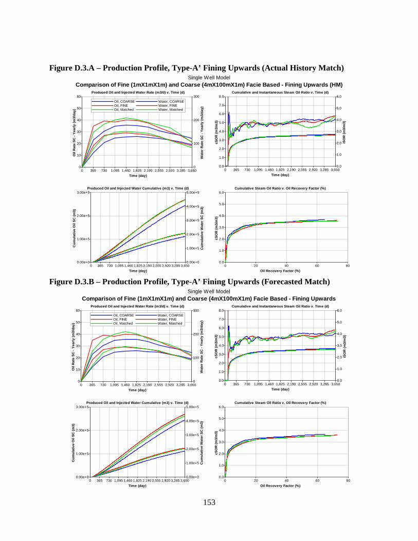
Figure D.3.A – Production Profile, Type-A’ Fining Upwards (Actual History Match)
Figure D.3.B – Production Profile, Type-A’ Fining Upwards (Forecasted Match)
Single Well ModelComparison of Fine (1mX1mX1m) and Coarse (4mX100mX1m) Facie Based - Fining Upwards (HM)
Produced Oil and Injected Water Rate (m3/d) v. Time (d)
Time (day)
Oil
Rat
e SC
- Ye
arly
(m3/
day)
Wat
er R
ate
SC -
Year
ly (m
3/da
y)
0 365 730 1,095 1,460 1,825 2,190 2,555 2,920 3,285 3,6500
10
20
30
40
50
60
0
100
200
300Oil, COARSE Water, COARSEOil, FINE Water, FINEOil, Matched Water, Matched
Produced Oil and Injected Water Cumulative (m3) v. Time (d)
Time (day)
Cum
ulat
ive
Oil
SC (m
3)
Cum
ulat
ive
Wat
er S
C (m
3)
0 365 730 1,095 1,460 1,825 2,190 2,555 2,920 3,285 3,6500.00e+0
1.00e+5
2.00e+5
3.00e+5
0.00e+0
1.00e+5
2.00e+5
3.00e+5
4.00e+5
5.00e+5
Cumulative and Instantaneous Steam Oil Ratio v. Time (d)
Time (day)
cSO
R (m
3/m
3)
iSO
R (m
3/m
3)
0 365 730 1,095 1,460 1,825 2,190 2,555 2,920 3,285 3,6500.0
1.0
2.0
3.0
4.0
5.0
6.0
7.0
8.0
0.0
1.0
2.0
3.0
4.0
5.0
6.0
Cumulative Steam Oil Ratio v. Oil Recovery Factor (%)
Oil Recovery Factor (%)
cSO
R (m
3/m
3)
0 20 40 60 800.0
1.0
2.0
3.0
4.0
5.0
6.0
Single Well ModelComparison of Fine (1mX1mX1m) and Coarse (4mX100mX1m) Facie Based - Fining Upwards
Produced Oil and Injected Water Rate (m3/d) v. Time (d)
Time (day)
Oil
Rat
e SC
- Ye
arly
(m3/
day)
Wat
er R
ate
SC -
Year
ly (m
3/da
y)
0 365 730 1,095 1,460 1,825 2,190 2,555 2,920 3,285 3,6500
10
20
30
40
50
60
0
100
200
300Oil, COARSE Water, COARSEOil, FINE Water, FINEOil, Matched Water, Matched
Produced Oil and Injected Water Cumulative (m3) v. Time (d)
Time (day)
Cum
ulat
ive
Oil
SC (m
3)
Cum
ulat
ive
Wat
er S
C (m
3)
0 365 730 1,095 1,460 1,825 2,190 2,555 2,920 3,285 3,6500.00e+0
1.00e+5
2.00e+5
3.00e+5
0.00e+0
1.00e+5
2.00e+5
3.00e+5
4.00e+5
5.00e+5
Cumulative and Instantaneous Steam Oil Ratio v. Time (d)
Time (day)
cSO
R (m
3/m
3)
iSO
R (m
3/m
3)
0 365 730 1,095 1,460 1,825 2,190 2,555 2,920 3,285 3,6500.0
1.0
2.0
3.0
4.0
5.0
6.0
7.0
8.0
0.0
1.0
2.0
3.0
4.0
5.0
6.0
Cumulative Steam Oil Ratio v. Oil Recovery Factor (%)
Oil Recovery Factor (%)
cSO
R (m
3/m
3)
0 20 40 60 800.0
1.0
2.0
3.0
4.0
5.0
6.0
153

Figure D.4.A – Production Profile, Type-A’ Channel (Actual History Match)
Figure D.4.B – Production Profile, Type-A’ Channel (Forecasted Match)
Single Well ModelComparison of Fine (1mX1mX1m) and Coarse (4mX100mX1m) Facie Based - Channel (HM)
Produced Oil and Injected Water Rate (m3/d) v. Time (d)
Time (day)
Oil
Rat
e SC
- Ye
arly
(m3/
day)
Wat
er R
ate
SC -
Year
ly (m
3/da
y)
0 365 730 1,095 1,460 1,825 2,190 2,555 2,920 3,285 3,6500
10
20
30
40
50
60
70
80
0
100
200
300
400Oil, COARSE Water, COARSEOil, FINE Water, FINEOil, Matched Water, Matched
Produced Oil and Injected Water Cumulative (m3) v. Time (d)
Time (day)
Cum
ulat
ive
Oil
SC (m
3)
Cum
ulat
ive
Wat
er S
C (m
3)
0 365 730 1,095 1,460 1,825 2,190 2,555 2,920 3,285 3,6500.00e+0
1.00e+5
2.00e+5
3.00e+5
0.00e+0
1.00e+5
2.00e+5
3.00e+5
4.00e+5
5.00e+5
Cumulative and Instantaneous Steam Oil Ratio v. Time (d)
Time (day)
cSO
R (m
3/m
3)
iSO
R (m
3/m
3)
0 365 730 1,095 1,460 1,825 2,190 2,555 2,920 3,285 3,6500.0
1.0
2.0
3.0
4.0
5.0
6.0
7.0
8.0
0.0
1.0
2.0
3.0
4.0
5.0
6.0
Cumulative Steam Oil Ratio v. Oil Recovery Factor (%)
Oil Recovery Factor (%)
cSO
R (m
3/m
3)
0 20 40 60 80 1000.0
1.0
2.0
3.0
4.0
5.0
6.0
Single Well ModelComparison of Fine (1mX1mX1m) and Coarse (4mX100mX1m) Facie Based - Channel
Produced Oil and Injected Water Rate (m3/d) v. Time (d)
Time (day)
Oil
Rat
e SC
- Ye
arly
(m3/
day)
Wat
er R
ate
SC -
Year
ly (m
3/da
y)
0 365 730 1,095 1,460 1,825 2,190 2,555 2,920 3,285 3,6500
10
20
30
40
50
60
70
80
0
100
200
300
400Oil, COARSE Water, COARSEOil, FINE Water, FINEOil, Matched Water, Matched
Produced Oil and Injected Water Cumulative (m3) v. Time (d)
Time (day)
Cum
ulat
ive
Oil
SC (m
3)
Cum
ulat
ive
Wat
er S
C (m
3)
0 365 730 1,095 1,460 1,825 2,190 2,555 2,920 3,285 3,6500.00e+0
1.00e+5
2.00e+5
3.00e+5
0.00e+0
1.00e+5
2.00e+5
3.00e+5
4.00e+5
5.00e+5
Cumulative and Instantaneous Steam Oil Ratio v. Time (d)
Time (day)
cSO
R (m
3/m
3)
iSO
R (m
3/m
3)
0 365 730 1,095 1,460 1,825 2,190 2,555 2,920 3,285 3,6500.0
1.0
2.0
3.0
4.0
5.0
6.0
7.0
8.0
0.0
1.0
2.0
3.0
4.0
5.0
6.0
Cumulative Steam Oil Ratio v. Oil Recovery Factor (%)
Oil Recovery Factor (%)
cSO
R (m
3/m
3)
0 20 40 60 80 1000.0
1.0
2.0
3.0
4.0
5.0
6.0
154

Figure D.5 – Production Profile, Type-B’ Uniform (Forecasted Match)
Figure D.6 – Production Profile, Type-B’ Channel (Forecasted Match)
Single Well ModelComparison of Fine (1mX1mX1m) and Coarse (4mX50mX1m) Facie Based - Uniform
Produced Oil and Injected Water Rate (m3/d) v. Time (d)
Time (day)
Oil
Rat
e SC
- Ye
arly
(m3/
day)
Wat
er R
ate
SC -
Year
ly (m
3/da
y)
0 365 730 1,095 1,460 1,825 2,190 2,555 2,920 3,285 3,6500
10
20
30
40
50
60
0
50
100
150
200
250Oil, COARSE Water, COARSEOil, FINE Water, FINEOil, Matched Water, Matched
Produced Oil and Injected Water Cumulative (m3) v. Time (d)
Time (day)
Cum
ulat
ive
Oil
SC (m
3)
Cum
ulat
ive
Wat
er S
C (m
3)
0 365 730 1,095 1,460 1,825 2,190 2,555 2,920 3,285 3,6500.00e+0
1.00e+5
2.00e+5
3.00e+5
4.00e+5
0.00e+0
1.00e+5
2.00e+5
3.00e+5
4.00e+5
5.00e+5
Cumulative and Instantaneous Steam Oil Ratio v. Time (d)
Time (day)
cSO
R (m
3/m
3)
iSO
R (m
3/m
3)
0 365 730 1,095 1,460 1,825 2,190 2,555 2,920 3,285 3,6500.0
1.0
2.0
3.0
4.0
5.0
6.0
7.0
8.0
0.0
1.0
2.0
3.0
4.0
5.0
6.0
Cumulative Steam Oil Ratio v. Oil Recovery Factor (%)
Oil Recovery Factor (%)
cSO
R (m
3/m
3)
0 20 40 60 800.0
1.0
2.0
3.0
4.0
5.0
6.0
Single Well ModelComparison of Fine (1mX1mX1m) and Coarse (4mX50mX1m) Facie Based - Channel
Produced Oil and Injected Water Rate (m3/d) v. Time (d)
Time (day)
Oil
Rat
e SC
- Ye
arly
(m3/
day)
Wat
er R
ate
SC -
Year
ly (m
3/da
y)
0 365 730 1,095 1,460 1,825 2,190 2,555 2,920 3,285 3,6500
10
20
30
40
50
60
70
80
0
100
200
300
400Oil, COARSE Water, COARSEOil, FINE Water, FINEOil, Matched Water, Matched
Produced Oil and Injected Water Cumulative (m3) v. Time (d)
Time (day)
Cum
ulat
ive
Oil
SC (m
3)
Cum
ulat
ive
Wat
er S
C (m
3)
0 365 730 1,095 1,460 1,825 2,190 2,555 2,920 3,285 3,6500.00e+0
1.00e+5
2.00e+5
3.00e+5
4.00e+5
0.00e+0
1.00e+5
2.00e+5
3.00e+5
4.00e+5
5.00e+5
Cumulative and Instantaneous Steam Oil Ratio v. Time (d)
Time (day)
cSO
R (m
3/m
3)
iSO
R (m
3/m
3)
0 365 730 1,095 1,460 1,825 2,190 2,555 2,920 3,285 3,6500.0
1.0
2.0
3.0
4.0
5.0
6.0
7.0
8.0
0.0
1.0
2.0
3.0
4.0
5.0
6.0
Cumulative Steam Oil Ratio v. Oil Recovery Factor (%)
Oil Recovery Factor (%)
cSO
R (m
3/m
3)
0 20 40 60 80 1000.0
1.0
2.0
3.0
4.0
5.0
6.0
155

Figure D.7 – Production Profile, Type-C’ Coarsening Upwards (Forecasted Match)
Figure D.8 – Production Profile, Type-D’ Fining Upwards (Forecasted Match)
Single Well ModelComparison of Fine (1mX1mX1m) and Coarse (4mX25mX1m) Facie Based - Coarsening Upwards
Produced Oil and Injected Water Rate (m3/d) v. Time (d)
Time (day)
Oil
Rat
e SC
- Ye
arly
(m3/
day)
Wat
er R
ate
SC -
Year
ly (m
3/da
y)
0 365 730 1,095 1,460 1,825 2,190 2,555 2,920 3,285 3,6500
10
20
30
40
50
0
50
100
150
200
250Oil, COARSE Water, COARSEOil, FINE Water, FINEOil, Matched Water, Matched
Produced Oil and Injected Water Cumulative (m3) v. Time (d)
Time (day)
Cum
ulat
ive
Oil
SC (m
3)
Cum
ulat
ive
Wat
er S
C (m
3)
0 365 730 1,095 1,460 1,825 2,190 2,555 2,920 3,285 3,6500.00e+0
5.00e+4
1.00e+5
1.50e+5
2.00e+5
0.00e+0
1.00e+5
2.00e+5
3.00e+5
4.00e+5
Cumulative and Instantaneous Steam Oil Ratio v. Time (d)
Time (day)
cSO
R (m
3/m
3)
iSO
R (m
3/m
3)
0 365 730 1,095 1,460 1,825 2,190 2,555 2,920 3,285 3,6500.0
1.0
2.0
3.0
4.0
5.0
6.0
7.0
8.0
9.0
10.0
0.0
1.0
2.0
3.0
4.0
5.0
6.0
7.0
Cumulative Steam Oil Ratio v. Oil Recovery Factor (%)
Oil Recovery Factor (%)
cSO
R (m
3/m
3)
0 10 20 30 40 50 600.0
1.0
2.0
3.0
4.0
5.0
6.0
Single Well ModelComparison of Fine (1mX1mX1m) and Coarse (2mX100mX1m) Facie Based - Fining Upwards
Produced Oil and Injected Water Rate (m3/d) v. Time (d)
Time (day)
Oil
Rat
e SC
- Ye
arly
(m3/
day)
Wat
er R
ate
SC -
Year
ly (m
3/da
y)
0 365 730 1,095 1,460 1,825 2,190 2,555 2,920 3,285 3,6500
10
20
30
40
50
60
70
0
100
200
300Oil, COARSE Water, COARSEOil, FINE Water, FINEOil, Matched Water, Matched
Produced Oil and Injected Water Cumulative (m3) v. Time (d)
Time (day)
Cum
ulat
ive
Oil
SC (m
3)
Cum
ulat
ive
Wat
er S
C (m
3)
0 365 730 1,095 1,460 1,825 2,190 2,555 2,920 3,285 3,6500.00e+0
5.00e+4
1.00e+5
1.50e+5
2.00e+5
2.50e+5
0.00e+0
1.00e+5
2.00e+5
3.00e+5
4.00e+5
5.00e+5
Cumulative and Instantaneous Steam Oil Ratio v. Time (d)
Time (day)
cSO
R (m
3/m
3)
iSO
R (m
3/m
3)
0 365 730 1,095 1,460 1,825 2,190 2,555 2,920 3,285 3,6500.0
1.0
2.0
3.0
4.0
5.0
6.0
7.0
8.0
0.0
1.0
2.0
3.0
4.0
5.0
6.0
Cumulative Steam Oil Ratio v. Oil Recovery Factor (%)
Oil Recovery Factor (%)
cSO
R (m
3/m
3)
0 20 40 60 800.0
1.0
2.0
3.0
4.0
5.0
6.0
156

Figure D.9 – Production Profile, Type-E’ Coarsening Upwards (Forecasted Match)
Figure D.10 – Production Profile, Type-F’ Fining Upwards (Forecasted Match)
Single Well ModelComparison of Fine (1mX1mX1m) and Coarse (2mX50mX1m) Facie Based - Coarsening Upwards
Produced Oil and Injected Water Rate (m3/d) v. Time (d)
Time (day)
Oil
Rat
e SC
- Ye
arly
(m3/
day)
Wat
er R
ate
SC -
Year
ly (m
3/da
y)
0 365 730 1,095 1,460 1,825 2,190 2,555 2,920 3,285 3,6500
10
20
30
40
50
0
50
100
150
200
250
300Oil, COARSE Water, COARSEOil, FINE Water, FINEOil, Matched Water, Matched
Produced Oil and Injected Water Cumulative (m3) v. Time (d)
Time (day)
Cum
ulat
ive
Oil
SC (m
3)
Cum
ulat
ive
Wat
er S
C (m
3)
0 365 730 1,095 1,460 1,825 2,190 2,555 2,920 3,285 3,6500.00e+0
1.00e+5
2.00e+5
3.00e+5
4.00e+5
0.00e+0
1.00e+5
2.00e+5
3.00e+5
4.00e+5
Cumulative and Instantaneous Steam Oil Ratio v. Time (d)
Time (day)
cSO
R (m
3/m
3)
iSO
R (m
3/m
3)
0 365 730 1,095 1,460 1,825 2,190 2,555 2,920 3,285 3,6500.0
1.0
2.0
3.0
4.0
5.0
6.0
7.0
8.0
0.0
1.0
2.0
3.0
4.0
5.0
6.0
7.0
Cumulative Steam Oil Ratio v. Oil Recovery Factor (%)
Oil Recovery Factor (%)
cSO
R (m
3/m
3)
0 10 20 30 40 50 600.0
1.0
2.0
3.0
4.0
5.0
6.0
Single Well ModelComparison of Fine (1mX1mX1m) and Coarse (2mX25mX1m) Facie Based - Fining Upwards
Produced Oil and Injected Water Rate (m3/d) v. Time (d)
Time (day)
Oil
Rat
e SC
- Ye
arly
(m3/
day)
Wat
er R
ate
SC -
Year
ly (m
3/da
y)
0 365 730 1,095 1,460 1,825 2,190 2,555 2,920 3,285 3,6500
10
20
30
40
50
60
70
0
100
200
300
400Oil, COARSE Water, COARSEOil, FINE Water, FINEOil, Matched Water, Matched
Produced Oil and Injected Water Cumulative (m3) v. Time (d)
Time (day)
Cum
ulat
ive
Oil
SC (m
3)
Cum
ulat
ive
Wat
er S
C (m
3)
0 365 730 1,095 1,460 1,825 2,190 2,555 2,920 3,285 3,6500.00e+0
1.00e+5
2.00e+5
3.00e+5
4.00e+5
0.00e+0
1.00e+5
2.00e+5
3.00e+5
4.00e+5
5.00e+5
Cumulative and Instantaneous Steam Oil Ratio v. Time (d)
Time (day)
cSO
R (m
3/m
3)
iSO
R (m
3/m
3)
0 365 730 1,095 1,460 1,825 2,190 2,555 2,920 3,285 3,6500.0
1.0
2.0
3.0
4.0
5.0
6.0
7.0
8.0
0.0
1.0
2.0
3.0
4.0
5.0
6.0
Cumulative Steam Oil Ratio v. Oil Recovery Factor (%)
Oil Recovery Factor (%)
cSO
R (m
3/m
3)
0 20 40 60 800.0
1.0
2.0
3.0
4.0
5.0
6.0
157

Appendix E Formation Heating by Steam Injection: Marx-Langenheim Model
The principle advantage to use of steam for bitumen recovery is the latent heat steam possess in
addition to sensible heat. Conversely, hot water simply carries sensible heat. Steam can transfer
all of its latent heat without a change in temperature.
Prior to steam injection into a bitumen rich formation, the initial reservoir temperature is TR.
Once steam is injected, bitumen is displaced and a quantity of oil is produced, creating a void
within the reservoir. The steam will then condense while heating the surrounding reservoir rock
and fluids. The condensate, while still at saturation temperature TS, moves ahead of the new
wave of steam and preheats the rock at a point beyond the steam front.
It was postulated that the heated zone is at constant steam temperature and a step-change in
temperature occurs at the interface between the steam chamber and bitumen interval. The
postulation is based upon several assumptions, including:
- Constant injection rate,
- Absence of gravity segregation and pressure drop in the steam zone, and
- Homogenous reservoir interval with uniform thickness,
This profile is highlighted in Figure E.1, and is the foundation of the Marx-Langenheim model.
Marx-Langenheim (1959)64 provided a model to explain heating within reservoirs. The growing
steam zone is limited in terms of its heat loss rate to the overburden and underburden as well as
the heating rate of the rock and fluids to steam temperature, TS (equivalent to condensed steam).
158
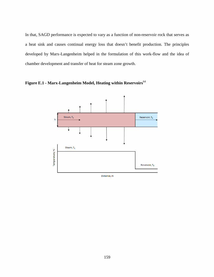
In that, SAGD performance is expected to vary as a function of non-reservoir rock that serves as
a heat sink and causes continual energy loss that doesn’t benefit production. The principles
developed by Marx-Langenheim helped in the formulation of this work-flow and the idea of
chamber development and transfer of heat for steam zone growth.
Figure E.1 - Marx-Langenheim Model, Heating within Reservoirs64
159