application of flushing tanks in simple sewer … · application of flushing tanks in simple sewer...

1

11

Application of flushing tanks in simple sewer networks for in-sewer sediment

erosion and transport Reza H.S.M. Shirazi, Patrick Willems and Jean Berlamont

The principal objective of urban drainage systems is to transport the aqueous

and solid wastes emanating from domestic, industrial and storm sources for

treatment and disposal. The solids that enter the system are often a cause for

concern as they may settle out to form permanent or semi-permanent

deposits on sewer inverts which can generate problems such as hydraulic

restrictions, reduction in the design flow capacity of the sewers, and increase

of the risks of surcharging during storm events. Generally, in-pipe deposits

result from accumulation of sediments during dry weather flow (DWF)

periods and during the recession of storms (Skipworth et al., 2001). Solid

materials largely originate from domestic and industrial wastewater and

from unpaved catchment areas (Dettmar et al., 2002). The sediment

deposition tendency is different depending on the location of a sewer in a

network and the characteristics of the conduit such as size, gradient and

shape. Deposition will occur at a rate depending upon the flow

characteristics, the nature of the particles and their concentration in

suspension near the bed (Fraser & Ashley, 1999).

To account for the effects of sediments in sewer systems, an appropriate

sediment transport modeling should be carried out which needs to consider

the following (Fraser et al., 2005):

2

• To produce rapid, detailed, continuous hydraulic simulations for sewer

flows with long-term durations;

• To determine the most likely locations of sediment deposition using a

pipe-by-pipe analysis;

• To predict approximate depths of sedimentation at locations identified

previously so as to rank potentially problematic locations;

• To predict sediment concentrations during dry weather and storm events

allowing for potential erosion volumes from deposited beds.

The major requirement in urban drainage design is to ensure that

sediment would be transported through sewer pipes at the same rate that it

approaches the sewer network without any long-term build-up of sediment

deposits (May, 2001). It is important to note that since flow rates and

sediment loads in sewer systems can vary considerably with time, it is

unrealistic to expect to be able to design a sewer network so that no

deposition would occur under various flow conditions. Accordingly, sewers

should be designed to transport sediment at a rate sufficient to limit the

depth of deposition to a specified proportion of the pipe section to maintain

the required hydraulic characteristics of the conduit. According to Bertrand-

Krajewski (2002), two important issues regarding sewer system design are:

• How to avoid or at least limit deposition in new sewers by means of

appropriate rules based on sewer shapes, slopes and flow velocities;

• How to cleanse deposits by means of appropriate flushing and

mechanical devices.

In fact, avoiding deposition is not always promising, particularly in flat

regions, where the necessary slopes for sewer pipes to be self-cleansing are

not available due to the costs of deep excavations and pumping systems

(especially in the most upstream parts of the network). Nevertheless, the

deposited particles (see Figure 11.1) may be re-entrained later by means of

higher flows in the network. The magnitude of erosion varies in response to

the time varying hydraulics. Along with sufficient flow velocity and bottom

shear stress, successive occurrence of high flow conditions, which would

force deposited particles to unhinge, has a substantial effect on re-

entrainment of the deposits. In this regard, the shear stress is the key

parameter responsible for the start of sediment transport when its critical

value for certain sediment characteristics is exceeded.

3

In addition, given that designing sewer systems to be self-cleansing is not

always possible, particularly in flat regions, the use of flush tanks that

generate controlled flush waves into the connected sewer system could be

suitable. Flushing is able to realize a preventive strategy under economical

and ecological conditions by generating flush waves continuously or quasi-

continuously (Dettmar & Staufer, 2005). The operation of the flushing

devices is usually based on the storage and successive release of flushing

volumes, able to scour deposited sediments and to transport them

downstream towards steeper sewer sections (Campisano et al., 2004).

Figure 11.1 Deposits in sewers.

Characteristics of the flushing tank

A flushing tank is evaluated in this paper regarding its capabilities for

generating the required scouring forces (i.e. shear stresses) throughout sewer

pipes, as a result of the flush waves (outflow discharges) released in flushing

cycles. The flushing device (provided by Keramo-Steinzeug, Belgium) is

comprised of a tank of 1 m high, with a diameter of 1.2 m and a volume of

about 450 L, releasing a flushing discharge in between 27 and 19 L/s that

lasts for at least 20 seconds. Surface runoff reaches the flushing device by

means of a connection on the side wall of the tank. In rainy periods the water

level in the tank rises until the water height exceeds a given level. Then the

excess flow is bypassed through a pipe toward the exit section, and then by

means of a hydraulic process, the stored water flows through the outfall of

the device and initiates a flush wave into the connected pipe. The flushing

device is illustrated in Figure 11.2. There is a variation in outflow discharge

while the flushing occurs, which is due to the reduction in the initial water

level in the tank. Hence, based on Bernoulli’s equation, head loss

computations and the geometrical characteristics of the flushing device, the

4

outflow from the flushing device (flush wave) is calculated (Bouteligier et

al., 2006) as shown in Figure 11.3.

Figure 11.2 Illustrations of the flushing tank.

0

0.005

0.01

0.015

0.02

0.025

0.03

0 10 20 30

time [s]

outflo

w [m

3/s

]

Figure 11.3 The outflow hydrograph for a flushing cycle.

Implementing the flushing tank in sewer networks

The idea of using the mentioned type of flushing device is to benefit from its

capacity to generate a relatively high volume of inflow into parts of a sewer

network in a relatively short period of time. This high volume of flow assists

in scouring the settled particles and transporting them towards the

downstream parts of the network. In fact, as the generated outflow discharge

of each flush is about 20 L/s, the characteristics of the pipes receiving the

flushes (pipe diameter and bottom slope) could be important. There would

be notable difference in the generated flush characteristics in the connected

pipes with various diameters and slopes. Also, pipe length is an important

parameter influencing the flush characteristics propagating through the

network. If the lengths of the pipes are too long, flushing might not be

effective. Therefore, it is important to install flushing devices in proper

locations to generate the required shear stresses where the existing situation

1.2 m

1

.1 m

5

does not comply with self-cleansing conditions (H.S.M. Shirazi et al., 2008).

The objective of this paper is to assess whether by implementing flushing

tanks in a simple network, erosion of the settled particles and their removal

from the sewer system could be achieved.

11.1 Methodology

11.1.1 InfoWorks CS

Recently, the field of urban drainage design has benefited from the

availability of sewer flow quality modeling tools together with

hydrodynamic simulation packages. Thus, together with general hydraulic

results generated by hydrodynamic modeling, the possibility to properly

model the impact of sediment accumulation in sewer systems as well as the

amount of sediments and pollutants that are transported into receiving waters

or treatment plants has been developed. These lead to an enhanced design

and management of urban drainage systems. In this study, an evaluation

based on simulations carried out with version 9.0 of InfoWorks CS

(Wallingford Software, UK) regarding application of a flushing tank as a

tool for eroding deposited sediments from a simple sewer network is

presented. The hydrodynamic modeling was comprised of implementing

InfoWorks CS to assess the eroding capability of the generated flush waves

regarding sediment removal and transport, applying the model based on the

shear stress estimation in the software (the KUL model developed by

Bouteligier et al., 2002). This model will be discussed in section 11.1.2.

11.1.2 Sediment transport modeling

Sediment deposit could result in the change in the hydrodynamic behavior of

the network due to pipe cross sectional modifications, and could possibly

lead to the occurrence of surcharging or even flooding. Reliable modeling

requires the effect of sediments on the hydraulic features of the flow to be

considered. This indeed demands comprehensive knowledge of the sediment

behavior inside the sewer pipes and the related phenomena linked to

sediment transport (entrainment, deposition, and re-entrainment). For a

proper sediment transport model a precise definition of sediment

characteristics (particle size, density, concentration, etc.) in the catchment

and in the sewer network is required. Particle characteristics and the

6

prevailing hydraulic conditions are important factors regarding proper

estimations of the mode of transport.

It is known that at high enough shear stresses, the re-entrainment of

sediment particles starts to occur with small particles that have high rate of

mobility compared to the larger and heavier ones (Bouteligier et al., 2006).

Fine silt particles and low-density organic materials can be transported

relatively easily by the flow velocities typical of gravity sewers. However,

uneconomically steep gradients would be required to achieve this transport

mode for the heavier inorganic fractions such as medium/coarse sand and

gravel (May, 2001). The flow characteristics are important regarding the

start of the sediment transport phenomenon. For instance the inorganic

granular material moving along the bed in sewers, which may be considered

as bed-load, will rarely travel in true suspension during dry weather flow

(Ashley & Verbanck, 1996).

As it is acknowledged by many researchers (Ashley et al., 1998 and

Skipworth et al., 2001), sewer sediment deposits are heterogeneous. Even in

the same location within a sewer network in-pipe deposits with significantly

different characteristics can develop. Therefore, assigning valid sediment

characteristics in water quality modeling is a rather uncertain task.

Nevertheless, sediment transport modeling cannot be achieved without

setting these parameters, and some relevant values need to be specified for

sediment characteristics. As an example, the characteristic of typical sewer

sediment classes explained by Stovin et al. (2005) is presented in Table 11.1.

Table 11.1 Characteristic of typical sewer sediment classes (Stovin et

al., 2005).

In-Sewer Sediment

Type

d50

[mm]

Density

[kg/m3]

Estimated Fall Velocity

[mm/s]

Gravel 10 2650 756

Sand 3 2650 380

Grit 0.75 2650 136

Gross Solids 2 1030 25

Sanitary – Stormwater 0.06 2500 3

Sanitary – DWF 0.04 1400 0.3

Generally, the main objective of sediment transport modeling is to obtain

the track of sediment accumulation in a sewer system. InfoWorks CS

accomplishes this by offering the water quality simulation module

comprised of three different sediment transport models: Ackers-White based

on concentration comparison (Ackers, 1991), Velikanov based on energy

7

dissipation (Zug et al., 1998), and KUL based on shear stress comparison

(Bouteligier et al., 2002).

For sediment transport modeling in this paper, the KUL model was

implemented. According to the KUL model, which is based on Shields

concept, if the actual shear stress τ is below the critical shear stress for

deposition (τcr-deposition), then deposition will occur. If the actual shear stress

value τ is in-between the critical shear stress for deposition and the one for

erosion (i.e. τcr-deposition < τ < τcr-erosion), then neither erosion nor deposition

occurs and all suspended sediments are transported along the conduit. If the

actual shear stress τ exceeds the critical shear stress for erosion τcr-erosion (i.e.

τ > τcr-erosion) then erosion would occur. The shear stress is calculated as a

function of the water head, the hydraulic radius and the (friction) slope of the

flow according to Eq. 1. The velocity is assumed to be uniform and is

computed according to Eq. 2.

2

8

c vλ

τ ρ= (1)

0

8

c

gv RS

λ= (2)

where τ is the shear stress [N/m2],

cλ the composite friction factor [-],

ρ the water density [kg/m3], v the flow velocity [m/s], g the gravitational

acceleration [m/s2], R is the hydraulic radius [m], and 0S the pipe invert

slope [m/m].

The critical shear stresses for deposition and erosion are calculated based

on the formula in Eq. 3 and Eq. 4 (Bouteligier et al., 2002).

, 50

( 1) /1000cr deposition deposition

g s dτ γ ρ= − (3)

, 50( 1) /1000cr erosion erosion g s dτ γ ρ= − (4)

where deposition

γ is the deposition parameter [-], erosion

γ the erosion

parameter [-] ( deposition erosionγ γ≤ ), s the specific sediment density [-], and d50

the sediment particle size [mm]. In fact, deposition

γ and erosion

γ are the

8

dimensionless critical shear stresses which specify the boundaries for

deposition and erosion respectively.

The median sediment particle size (d50) for InfoWorks modeling in this

paper was assumed to be equal to 0.1 mm for sanitary sediment and 0.2-1.5

mm for catchment sediment. This is compatible with the data presented in

Table 11.1. To verify the effect of variations in sewer network

characteristics on the evolution of sediment depths throughout the network

(sediment transport), various combinations of these characteristics were

considered. The various sewer network combinations are presented in Table

11.2.

Table 11.2 The characteristics of the sewer network.

Sewer Network Slope

[m/m]

DWF

[m3/s]

Sediment

Type

Concentration

[mg/l]

d50

[mm]

Particle

Density

[kg/m3]

Conduit/Network 0 0.003 SF1 150 0.2-1.5 2650

SF2 150 0.1 1800

Conduit/Network 0.001 0.003 SF1 150 0.2-1.5 2650

SF2 150 0.1 1800


SF2 150 0.1 1800


SF2 150 0.1 1800


SF2 150 0.1 1800


SF2 150 0.1 1800

In the previous table, SF1 accounts for the catchment sediment and SF2

corresponds to sanitary sediment.

9

11.1.3 Model set-up

11.1.3.1 Conduit model

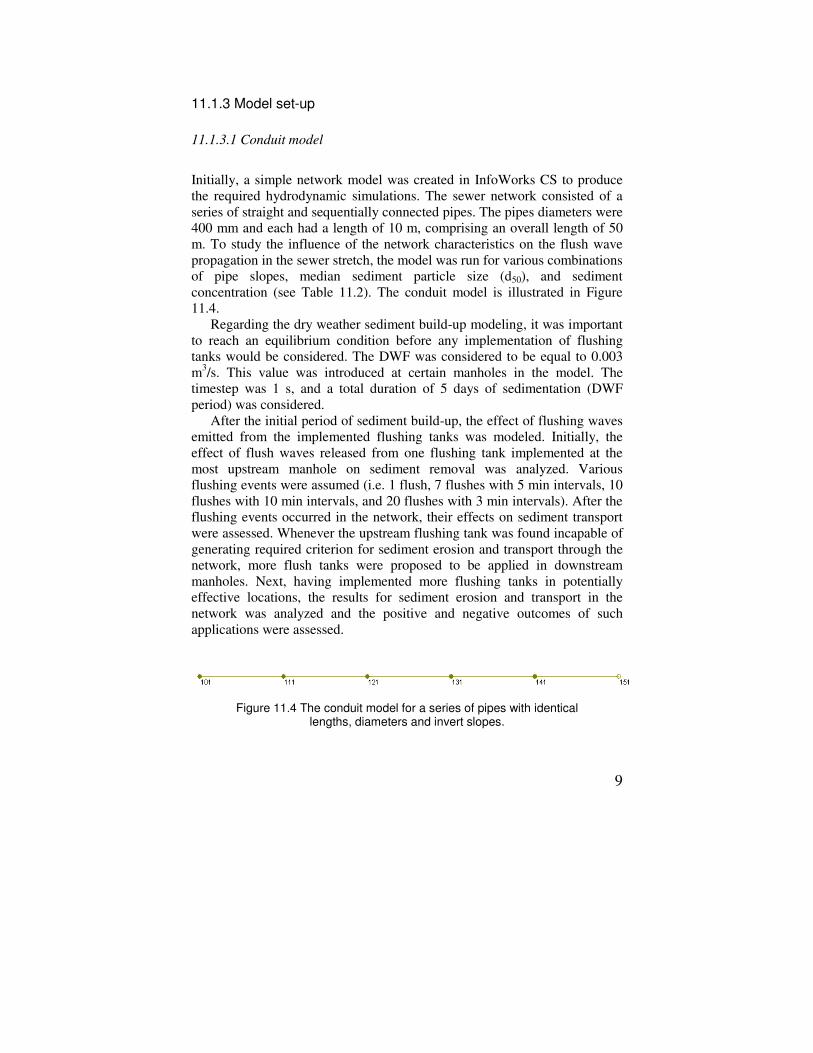
Initially, a simple network model was created in InfoWorks CS to produce

the required hydrodynamic simulations. The sewer network consisted of a

series of straight and sequentially connected pipes. The pipes diameters were

400 mm and each had a length of 10 m, comprising an overall length of 50

m. To study the influence of the network characteristics on the flush wave

propagation in the sewer stretch, the model was run for various combinations

of pipe slopes, median sediment particle size (d50), and sediment

concentration (see Table 11.2). The conduit model is illustrated in Figure

11.4.

Regarding the dry weather sediment build-up modeling, it was important

to reach an equilibrium condition before any implementation of flushing

tanks would be considered. The DWF was considered to be equal to 0.003

m3/s. This value was introduced at certain manholes in the model. The

timestep was 1 s, and a total duration of 5 days of sedimentation (DWF

period) was considered.

After the initial period of sediment build-up, the effect of flushing waves

emitted from the implemented flushing tanks was modeled. Initially, the

effect of flush waves released from one flushing tank implemented at the

most upstream manhole on sediment removal was analyzed. Various

flushing events were assumed (i.e. 1 flush, 7 flushes with 5 min intervals, 10

flushes with 10 min intervals, and 20 flushes with 3 min intervals). After the

flushing events occurred in the network, their effects on sediment transport

were assessed. Whenever the upstream flushing tank was found incapable of

generating required criterion for sediment erosion and transport through the

network, more flush tanks were proposed to be applied in downstream

manholes. Next, having implemented more flushing tanks in potentially

effective locations, the results for sediment erosion and transport in the

network was analyzed and the positive and negative outcomes of such

applications were assessed.

Figure 11.4 The conduit model for a series of pipes with identical

lengths, diameters and invert slopes.

10

As already mentioned, the KUL model was utilized for the sediment

transport modeling (see 11.1.2). In order to model deposition and erosion as

two distinct criteria regarding in-sewer sediment behavior, it was necessary

to specify the required boundaries in the modeling procedure. The

boundaries between settlement of particles and their erosion (re-entrainment)

were defined by means of γ parameters in the KUL model, which are

principally the Shields dimensionless shear stress parameter (see equations 3

and 4).

In order to obtain the dimensionless shear stresses (Shields parameters)

regarding the deposition boundary conditions (γdeposition), the particle

Reynolds number for each sediment particle size (within the range of 0.1-

1.5mm) and for each of the considered slopes was calculated and then the

Shields parameter was detained from the Shields graph (see Figure 11.5 and

Table 11.3). Then, for the dimensionless shear stresses for the erosion

boundary conditions, the corresponding values of γdeposition were modified in

a way to create the required domain for sediment transport in between

deposition and erosion. The results are illustrated in Figure 11.6.

Figure 11.5 The Shields Diagram for sediment deposition-erosion,

ASCE (1975).

11

Table 11.3 Flow characteristics for diverse invert slopes in the conduit.

Slope

Average

Water Depth

Hydraulic

Radius

Mean

Velocity

Reynolds

Number Average Bed

Shear Stress

[N/m2] [mm/m] [m] [m] [m/s] [-]

0 0.12 0.0684 0.16 43776 0.0812

1 0.075 0.0482 0.29 55912 0.2737

2 0.065 0.0372 0.35 52080 0.4207

3 0.05 0.0301 0.398 47919.2 0.5713

4 0.045 0.0277 0.433 47976.4 0.6881

5 0.035 0.0245 0.461 45178 0.8046

0.02

0.03

0.04

0.05

0.06

0.07

0.08

0 1 2 3 4 5

Sh

ield

s p

ara

mete

r [-

]

invert slope [mm/m]

0.1mm 0.2mm 0.3mm 0.4mm 0.5mm

0.6mm 0.7mm 0.8mm 0.9mm 1mm

1.1mm 1.2mm 1.3mm 1.4mm 1.5mm

0.08

0.1

0.12

0.14

0.16

0.18

0.2

0.22

0.24

0 1 2 3 4 5

Sh

ield

s p

ara

me

ter

[-]

invert slope [mm/m]

0.1mm 0.2mm 0.3mm 0.4mm 0.5mm

0.6mm 0.7mm 0.8mm 0.9mm 1mm

1.1mm 1.2mm 1.3mm 1.4mm 1.5mm

Figure 11.6 The dimensionless shear stress boundary conditions for deposition (left) and erosion (right) from the Shields diagram based on

the prevailing hydraulic conditions.

11.1.3.2 Network model

In the second phase, a few more branch pipes were added to the initial

network and the same analyses were repeated to evaluate the overall effects

of added parts on sediment build-up and transport. Again, in the performed

sediment transport modeling, the effect of implementing numerous flush

tanks in various parts of the network over sediment bed modifications

(sediment entrainment, transport, and re-deposition) and changes in bed

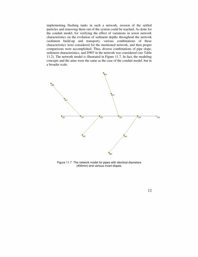
profiles was evaluated. The final objective was to evaluate whether by

12

implementing flushing tanks in such a network, erosion of the settled

particles and removing them out of the system could be reached. As done for

the conduit model, for verifying the effect of variations in sewer network

characteristics on the evolution of sediment depths throughout the network

(sediment build-up and transport), various combinations of these

characteristics were considered for the mentioned network, and then proper

comparisons were accomplished. Thus, diverse combinations of pipe slope,

sediment characteristics, and DWF in the network was considered (see Table

11.2). The network model is illustrated in Figure 11.7. In fact, the modeling

concepts and the aims were the same as the case of the conduit model, but in

a broader scale.

Figure 11.7 The network model for pipes with identical diameters (400mm) and various invert slopes.

13

11.2 Results and Discussion 11.2.1 Sediment build-up along the conduit during DWF period

The main objective in this study was to model the evolution of sedimentation

and erosion in a simple sewer network. In order to reach to a proper

conclusion, it was important to see the sediment build-up along sewers in a

way to comply with physical measures. For such a purpose, a constant DWF

equal to 0.003 m3/s within a 5-day period was assumed in order to leave

enough time for the inflowing particles from the catchment to settle on sewer

inverts before any simulation of the effects of flushes would be done. In fact,

the effect of flushes could not be assessed if the initial conditions were not

modeled properly. Therefore, the modeling attempts were managed in a way

to reach the sediment build-up all over the considered network, i.e. to reach

an equilibrium condition for the sediment layer along sewer inverts.

The problem to deal with was the fact that sediment build-up and

entrainment was very sensitive to the prevailing hydraulic features of the

network. In fact, various network characteristics would lead to diverse

sediment build-up scenarios. Therefore, to reach to an equilibrium condition

for sediment build-up, it was important to change the sediment and flow

characteristics in different networks with dissimilar pipe slopes. In other

words, due to the large effect of invert slopes on the possibility of forming

deposits on the sewer invert levels, only for certain pipe configurations the

particle settlement was reached. Another important issue was the fact that

moving from the upstream toward the downstream part of the network, the

amount of flow would increase due to the existence of manholes which

would provide excessive flow into the network. This in turn would affect the

sedimentation in downstream pipes and as a result less sediment would settle

in those pipes in the network. In fact, the sedimentation was noticed only in

cases where the actual shear stresses at bed were below the critical shear

stresses for deposition (based on the Shields diagram). For the mentioned

model, the sedimentation occurred only in the following cases (the dashed

lines) as indicated in Table 11.4. Some results of sediment build-up for pipes

with various slopes can be observed in the following figures (Figure 11.8

through 11.10).

14

Table 11.4 The dashed lines indicate the situation where deposition of particles were modeled along the pipe invert level.

d50

[mm]

Slope

[mm/m]

0.2 0.3 0.4 0.5 0.6 0.7 0.8 0.9 1.0 1.1 1.2 1.3 1.4 1.5

0

1

2

3

4

5

0

0.05

0.1

0.15

0.2

0.25

0.3

0 10 20 30 40 50

distance from upstream (m)

se

dim

en

t d

ep

th (

m)

0hr 1hr 5hr 10hr 20hr30hr 40hr 50hr 60hr 70hr80hr 90hr 100hr 110hr 120hr

0

0.05

0.1

0.15

0.2

0.25

0.3

0 10 20 30 40 50


se

dim

en

t d

ep

th (

m)


Figure 11.8 Sediment build-up in the conduit with a slope of 0.001 m/m

for particles with d50 equal to 0.6 mm (left) and 1.2 mm (right).

0

0.05

0.1

0.15

0.2

0.25

0.3

0 10 20 30 40 50


se

dim

en

t d

ep

th (

m)


0

0.05

0.1

0.15

0.2

0.25

0.3

0 10 20 30 40 50


se

dim

en

t d

ep

th (

m)


Figure 11.9 Sediment build-up in conduits with slopes equal to 0.001

m/m (left) and 0.002 m/m (right) and particles with d50 equal to 0.9 mm.

15

0

0.05

0.1

0.15

0.2

0.25

0.3

0 10 20 30 40 50


se

dim

en

t d

ep

th (

m)


0

0.05

0.1

0.15

0.2

0.25

0.3

0 10 20 30 40 50


se

dim

en

t d

ep

th (

m)


Figure 11.10 Sediment build-up in conduits with slopes equal to 0.003 m/m (left) and 0.005 m/m (right) and particles with d50 equal to 1.5 mm.

By observing the results, the effect of various particle sizes and invert

slopes can be clearly noticed. In fact, the previous figures show that any

increase in the invert slope would result in lower deposition rate along the

conduit, and illustrate the fact that the erosion of the settled particles would

be eased especially in downstream parts of the sewer length. Besides, larger

particles would form higher sediment bed depths along the pipes inverts.

11.2.2 Sediment erosion by means of flushes in the conduit model

After the DWF sediment build-up period was over, it was time to assess the

effect of flushing waves on sediment removal. In general, to properly

evaluate the effect of flush waves on sediment erosion, it was important to

observe the evolution of the sediment massflow and concentration

throughout the network, and to compare the changes in hydraulic

characteristics such as flow velocity, discharge, sediment concentration and

flux, etc.

It is expected that at the moment the flush wave passes along the pipes,

the sediment depth would be reduced (due to re-entrainment of deposited

particles by the flush wave) and the suspended sediment concentration

would be increased. Later, when the peak of the flush wave diminishes from

its maximum, sedimentation starts to occur due to the reduction in the

energy of the wave. In other words, the reduction in the carrying capacity of

the flow, which coincides with the decrease in flow velocity, would lead to

the decline in the sediment concentration and simultaneously to the

development of sediment deposit layer.

16

For the required evaluations, various types of flushing events were

assumed and their effects were compared (i.e. 1 flush, 7 flushes with 5 min

intervals, 10 flushes with 10 min intervals, and 20 flushes with 3 min

intervals). The comparisons are depicted in Figure 11.11(a) through 11.13.

These figures show that the rate of sediment erosion depends mainly on the

invert slope of the sewers and also on the median size of the drifting

sediment (d50). It was noticed that the ability of flushing waves to entrain

and transport sediment particle was in direct relation with the invert slope of

the sewer pipes. In fact, the aggravated shear stresses due to the flushes

seemed to be unable to overcome the influence of lack of enough slopes in

flat pipes and could not act much on sediment removal. In pipes with higher

slopes (e.g. 0.003 m/m or higher) the effects of flushes were clearly noticed

and sediments were transported in an appropriate rate. In fact, weak flushing

effects occurred in the network with relatively low pipe slopes (less than

0.002 m/m) and comparatively large sediment particles (d50 larger than 1

mm) (see Figure 11.12), while strong erosion occurred in the case of higher

slopes (0.002 m/m and higher) and finer sediments (d50 of 0.9 mm and finer)

(see Figure 11.13).

0

0.05

0.1

0.15

0.2

0.25

0.3

0 10 20 30 40 50


se

dim

en

t d

ep

th (

m)

0hr 0.1hr 0.5hr 1hr 1.5hr 2hr

2.5hr 3hr 3.5hr 4hr 4.5hr 5hr

0

0.05

0.1

0.15

0.2

0.25

0.3

0 10 20 30 40 50


se

dim

en

t d

ep

th (

m)

0hr 0.1hr 0.5hr 1hr 1.5hr 2hr2.5hr 3hr 4hr 5hr 6hr 7hr8hr 9hr 10hr

Figure 11.11(a) Sediment erosion by means of flushes in the conduit

with slope equal to 0.001 m/m and particle d50 equal to 0.9 mm: 1 flush (left), 7 flushes with 5 min intervals (right).

17

0

0.05

0.1

0.15

0.2

0.25

0.3

0 10 20 30 40 50


se

dim

en

t d

ep

th (

m)


0

0.05

0.1

0.15

0.2

0.25

0.3

0 10 20 30 40 50


se

dim

en

t d

ep

th (

m)


Figure 11.11(b) Sediment erosion by means of flushes in the conduit with slope equal to 0.001 m/m and particle d50 equal to 0.9 mm: 10

flushes with 10 min intervals (left), and 20 flushes with 3 min intervals (right).

0

0.05

0.1

0.15

0.2

0.25

0.3

0 10 20 30 40 50


se

dim

en

t d

ep

th (

m)



0

0.05

0.1

0.15

0.2

0.25

0.3

0 10 20 30 40 50


se

dim

en

t d

ep

th (

m)


0

0.05

0.1

0.15

0.2

0.25

0.3

0 10 20 30 40 50


se

dim

en

t d

ep

th (

m)


0

0.05

0.1

0.15

0.2

0.25

0.3

0 10 20 30 40 50


se

dim

en

t d

ep

th (

m)


Figure 11.12 Sediment erosion in the conduit with slope equal to 0.001 m/m and particle d50 equal to 1.2 mm due to the effect of flushes: 1 flush (up-left), 7 flushes with 5 min intervals (up-right), 10 flushes with 10 min intervals (bottom-left), and 20 flushes with 3 min intervals (bottom-right).

18

0

0.05

0.1

0.15

0.2

0.25

0.3

0 10 20 30 40 50


se

dim

en

t d

ep

th (

m)



0

0.05

0.1

0.15

0.2

0.25

0.3

0 10 20 30 40 50


se

dim

en

t d

ep

th (

m)


0

0.05

0.1

0.15

0.2

0.25

0.3

0 10 20 30 40 50


se

dim

en

t d

ep

th (

m)


0

0.05

0.1

0.15

0.2

0.25

0.3

0 10 20 30 40 50

distance from upstream (m)s

ed

ime

nt

de

pth

(m

)0hr 0.1hr 0.5hr 1hr 1.5hr 2hr2.5hr 3hr 4hr 5hr 6hr 7hr8hr 9hr 10hr

Figure 11.13 Sediment erosion in the conduit with slope equal to 0.002 m/m and particle d50 equal to 0.9 mm due to the effect of flushes: 1 flush (up-left), 7 flushes with 5 min intervals (up-right), 10 flushes with 10 min intervals (bottom-left), and 20 flushes with 3 min intervals (bottom-right).

11.2.3 Sediment build-up in DWF period in network

The results for sediment build-up during DWF for the network model were

also obtained and they were compatible with the ones for the conduit model.

Therefore, the model could generate the sediment build-up along sewers in

the network model in an acceptable way. The results corresponding to one

certain network configuration is presented in Figure 11.14.

19

0

0.05

0.1

0.15

0.2

0.25

0.3

0 10 20 30 40 50


se

dim

en

t d

ep

th (

m)


0

0.05

0.1

0.15

0.2

0.25

0.3

0 5 10 15 20


se

dim

en

t d

ep

th (

m)


0

0.05

0.1

0.15

0.2

0.25

0 2 4 6 8 10


se

dim

en

t d

ep

th (

m)


0

0.05

0.1

0.15

0.2

0.25

0 5 10 15 20

distance from upstream (m)s

ed

ime

nt

de

pth

(m

)0hr 1hr 5hr 10hr 20hr30hr 40hr 50hr 60hr 70hr80hr 90hr 100hr 110hr 120hr

0

0.05

0.1

0.15

0.2

0.25

0 5 10 15 20


se

dim

en

t d

ep

th (

m)


Figure 11.14 Sediment build-up in the sewer network with pipe slopes equal to 0.002 m/m and particles with d50 equal to 0.9 mm, top-left: the

main conduit (101-111-121-131-141-151), top-right: 201-211-111, middle-left: 301-121, middle-right: 401-411-131, bottom 501-511-141.

20

11.2.4 Sediment erosion by means of flushes in network

The same as the conduit model, flushing events were modeled for the

network model and the results were compared. The results showed that the

model could generate the sediment erosion along sewers by means of

flushing events in the network model in an acceptable way. One situation is

presented in Figure 11.15.

0

0.05

0.1

0.15

0.2

0.25

0.3

0 10 20 30 40 50


se

dim

en

t d

ep

th (

m)


0

0.05

0.1

0.15

0.2

0.25

0.3

0 10 20 30 40 50


se

dim

en

t d

ep

th (

m)


0

0.05

0.1

0.15

0.2

0.25

0.3

0 10 20 30 40 50


se

dim

en

t d

ep

th (

m)


0

0.05

0.1

0.15

0.2

0.25

0.3

0 10 20 30 40 50


se

dim

en

t d

ep

th (

m)


Figure 11.15 Sediment erosion in the main conduit (101-111-121-131-141-151) due to the effect of flushes in the sewer network with pipe

slopes equal to 0.002 m/m and particles with d50 equal to 0.9 mm: 1 flush (up-left), 7 flushes with 5 min intervals (up-right), 10 flushes with

10 min intervals (bottom-left), and 20 flushes with 3 min intervals (bottom-right) (refer to Figure 11.7).

21

11.3 Conclusions It was discovered that modeling the DWF sediment build-up accurately was

a preceding requirement in assessing the implementation of flushing tanks in

sewer networks, because if the former part was not fulfilled properly, the

latter one dealing with the erosion of the same settled particles cannot be

accomplished in a reasonable way. In fact, sediment deposition modeling

was a very sensitive task and required considered choice of the model

parameters with physical basis. For instance, it was realized that the

propensity for sediment deposition was different depending upon the

location of a sewer in the network (i.e. the relative type of flow input) and

the physical characteristics of the conduit especially its gradient.

Regarding the flushing tank implementations, various parameters such as

network and sediment characteristics and flushing intervals were important

in assessing whether the flushing tank was efficient in removing and

transporting sediments in the considered sewer network. This study revealed

that the type of sediment and main characteristics such as particle size and

density, needed to be carefully considered in sediment transport modeling in

order to obtain appropriate results.

In addition, frequent flushing had obvious effects on sediment erosion

and transport in pipes; the higher the frequency of subsequent flushes, the

less the chance for sediments to settle down in pipes. In fact, the subsequent

flushes would intensify the hydraulic effects of the previous ones in removal

and transport of the sediment through sewer pipes. Dettmar et al. (2002)

mentioned that many small flow waves were able to move non-compact

deposits and to work against new deposits, while big flow waves were able

to loosen compact sediments. Moreover, the first flushes produce minor

transport of deposited particles (but a more evident lowering) while for the

successive flushes, the scoured section length increases more rapidly

(Campisano et al., 2004).

By obtaining the simulation results and evaluating them, the

compatibility of what was modeled with what would be expected was

observed. The results showed that the model was moderately able to

simulate the sedimentation of particles and their erosion by means of the

flushes emitted from implemented flushing tanks. Also, the effect of various

particle sizes and the pipe invert slopes on the processes of deposition and

erosion has been modeled in a satisfactory way.

The effect of flush tank implementations on the modification of initial

sediment beds and on sediment transport was noticeable. However, the effect

22

of the flushing waves was restricted to a rather limited distance downstream

of the flush tank due to effect of headlosses on the flow characteristics, i.e.

gradual reductions in carrying capacity of the flush wave. Nonetheless, in an

overall perspective, the capability of such flushing tanks to produce effective

forces for removal of the settled particles in sewer pipes is well accepted.

Acknowledgements

The authors express their gratitude to Keramo-Steinzeug to have given the

opportunity to the Hydraulics Laboratory of the Katholieke Universiteit

Leuven to accomplish the experiments on the flushing tank and also are

thankful to Wallingford Software for providing the essential software tool

InfoWorks CS.

References

Ackers P. (1991). Sediment Aspects of Drainage and Outfall Design. In: Proceedings of

the International Symposium on Environmental Hydraulics, edited by A.A. Balkema,

Hong Kong. 16-18 December 1991.

American Society of Civil Engineers (ASCE) (1975). Sedimentation Engineering.

Manuals and Reports on Engineering Practice, No. 54, edited by Vito A. Vanoni,

New York, USA.

Ashley R.M. and Verbanck M. (1996). Mechanics of sewer sediment erosion and

transport. Journal of Hydraulic Research, Vol. 34, No 6, pp. 753-769.

Ashley R., Bertrand-Krajewski J.-L., Hvitved-Jacobsen T. (1998). Quo vadis sewer

process modelling? In: Proceedings of the 4th International Conference on

Developments in Urban Drainage Modelling (UDM'98), London, UK. 21-24

September 1998.

Ashley R.M., Bertrand-Krajewski J.-L., Hvitved-Jacobsen T. and Verbanck M. (2004).

Solids in Sewers: Characteristics, Effects and Control of Sewer Solids and Associated

Pollutants. Scientific and Technical Report No. 14. Joint Committee on Urban

Drainage, Sewer Systems and Processes Working Group, IWA Publishing, London,

United Kingdom. May 2004. ISBN: 1900222914.

Bertrand-Krajewski J.-L. (2002). Sewer Sediment Management: Some Historical Aspects

of Egg-Shape Sewers and Flushing Tanks. In: Proceedings of the 3rd International

Conference on Sewer Processes and Networks, Paris, France. 15-17 April 2002.

Bouteligier R., Vaes G. and Berlamont J. (2002). Transport Models for Combined Sewer

Systems. Research project commissioned by Aquafin NV and Severn Trent Water

Ltd., Hydraulics Laboratory, Katholieke Universiteit Leuven, Leuven, Belgium.

Bouteligier R., H.S.M. Shirazi R. and Berlamont J. (2006). Evaluation of the cleansing

capacity of a flushing tank in (sanitary) sewer systems. In: Proceedings of the 7th

23

International Conference on Urban Drainage Modelling and the 4th International

Conference on Water Sensitive Urban Design, edited by A. Deletic and T. Fletcher,

Melbourne, Australia. 2-7 April 2006.

Campisano A. and Modica C. (2002). Flow velocities and shear stresses during flushing

operations in sewer collectors. In: Proceedings of the 3rd International Conference on

Sewer Processes and Networks, Paris, France. 15-17 April 2002.

Campisano A., Creaco E., Modica C. and Ragusa F. (2004). Laboratory Experiments on

Bed Deposit Scouring during Flushing Operations. In: Proceedings of the 4th

International Conference on Sewer Processes and Networks, Funchal, Madeira,

Portugal. 22-24 November 2004.

Dettmar J., Rietsch B. and Lorenz U. (2002). Performance and Operation of Flushing

Devices - Results of a Field and Laboratory Study. In: Proceedings of the 9th

International Conference on Urban Drainage, edited by E.W. Strecker and W.C.

Huber, Portland, Oregon, USA. 8-13 September 2002.

Dettmar J. and Staufer P. (2005). Behaviour of the Activated Storage-Volume of Flushing

Waves on Cleaning Performance. In: Proceedings of the 10th International

Conference on Urban Drainage, edited by Eriksson E., Genc-Fuhrman H., Vollertsen

J., Ledin A., Hvitved-Jacobsen T. and Mikkelsen P.S., Copenhagen, Denmark. 21-26

August 2005.

Fraser A. and Ashley R. (1999). A Model for the Prediction and Control of Problematic

Sediment Deposits. In: Proceedings of the 8th International Conference on Urban

Storm Drainage, Sydney, Australia. 30 August – 3 September 1999.

Fraser A., Schellart A., Ashley R., Tait S. (2005). Prediction of sediment transport and

filling rates of invert traps in combined sewers. In: Proceedings of the 10th

International Conference on Urban Drainage (10ICUD), Copenhagen, Denmark. 21-

26 August 2005.

Gerard C. and Chocat B. (1998). An Aid for the Diagnosis of Sewerage Networks:

Analysis and Modelling of the Links between Networks' Physical Structure and the

Risk of Sediment Build-up. In: Proceedings of the 4th International Conference on

Developments in Urban Drainage Modelling, London, UK. 21-24 September 1998.

H.S.M. Shirazi R., Bouteligier R., Willems P. and Berlamont J. (2008). Preliminary

Results of Investigating Proper Location of Flushing Tanks in Combined Sewer

Networks for Optimum Effect. In: Proceedings of the 11th International Conference

on Urban Drainage (11 ICUD), Edinburgh, Scotland, UK. 31st August – 5th

September 2008.

H.S.M. Shirazi R., Bouteligier R. and Berlamont J. (2008). Evaluation of Sediment

Removal Efficiency of Flushing Devices Regarding Sewer System Characteristics.

In: Proceedings of the International Conference on Hydro-science and Engineering,

Nagoya, Japan. 8-12 September 2008.

May R.W.P. (2001). Minimum Self-cleansing Velocities for Inverted Sewer Siphons. In:

Proceedings of the Urban Drainage Modelling (UDM) Symposium, part of the World

Water Resources & Environmental Resources Congress, edited by R.W. Brashear and

C. Maksimovic, Orlando, Florida, USA. 20-24 May 2001.

Skipworth P.J., Tait S.J., Saul A.J., Ashley R. (2001). Sewer flow quality modelling

based on a novel deposit erosion model. In: Proceedings of the Urban Drainage

24

Modeling (UDM) Symposium, part of the World Water Resources & Environmental

Resources Congress, Orlando, Florida, USA. 20-24 May 2001.

Stovin V.R., Schellart A.N.A., Tait S., Ashley R.M., Burkhard R. (2005). Sewer invert

trap design using laboratory and CFD models and continuous simulation. In:

Proceedings of the 10th International Conference on Urban Drainage (10ICUD),

Copenhagen, Denmark. 21-26 August 2005.

Wallingford Software (2008). InfoWorks CS Help, Wallingford Software Ltd., United

Kingdom.

Zug M., Bellefleur D., Phan L. and Scrivener O. (1998). Sediment Transport Model in

Sewer Networks - a New Utilisation of the Velikanov Model. Water Science and

Technology, 37(1), pp 187–196.

application of flushing tanks in simple sewer … · application of flushing tanks in simple sewer...

Documents