application of hierarchical matrices for solving ... · application of hierarchical matrices for...
TRANSCRIPT

Application of Hierarchical Matrices For SolvingMultiscale Problems
Von der Fakultat fur Mathematik und Informatikder Universitat Leipzig
angenommene
DISSERTATION
zur Erlangung des akademischen GradesDOCTOR RERUM NATURALIUM
(Dr. rer. nat.)
im Fachgebiet
Numerische Mathematik
vorgelegt
von Diplommathematiker Alexander Litvinenko
geboren am 31.08.1979 in Almaty, Kasachstan
Die Annahme der Dissertation haben empfohlen:
1. Prof. Dr. Dr. h.c. Wolfgang Hackbusch (MPIMN Leipzig)
2. Prof. Dr. Ivan G. Graham (University Bath, UK)
3. Prof. Dr. Sergey Rjasanov (Universitat des Saarlandes)
Die Verleihung des akademischen Grades erfolgt auf Beschlussdes Rates der Fakultat fur Mathematik und Informatikvom 20.11.2006 mit dem Gesamtpradikat cum laude.

- 2 -
Acknowledgement
I would like to thank the following people:
• Prof. Dr. Dr. h.c. Wolfgang Hackbusch for inviting me to the Max Planck In-stitute for Mathematics in the Sciences in Leipzig, for the very modern theme,for his ideas and for obtaining financial support. I am thankful for his enjoy-able lecture courses: “Elliptic Differential Equations”, “Hierarchical Matrices”and “Iterative Solution of Large Sparse Systems of Equations”. These courseswere very useful during my work.
• PD DrSci. Boris N. Khoromskij (PhD) for his supervisory help at all stagesof my work, for useful corrections and fruitful collaboration in certain applica-tions, and also for his inspiring lecture courses “Data-Sparse Approximationof Integral Operators” and “Introduction to Structured Tensor-Product Rep-resentation”.
• Dr. Lars Grasedyck and Dr. Steffen Borm for their patience in explaining theH-matrix technique and details of HLIB,
• Dr. Ronald Kriemann for his advice in programming,
• Prof. Dr. Dr. h.c. Wolfgang Hackbusch, Prof. Dr. Ivan G. Graham (Uni-versity of Bath, England) and Prof. Dr. Sergey Rjasanov (Universitat desSaarlandes, Germany) for agreeing to referee this thesis.
This PhD work was done in the Max Planck Institute for Mathematics in theSciences. I am deeply appreciative of the help of Mrs. Herrmann, Mrs. Hunnigerand Mrs. Rackwitz from the personnel department of the institute. I am equallygrateful to the DFG fond for the program “Analysis, Modelling and Simulation ofMultiscale problems”.
I would like to thank all my colleagues and friends Mike Espig, Isabelle Greff, LehelBanjai, Petya Staykova, Alexander Staykov, Michail Perepelitsa, Graham Smith andall the others for making my time in Leipzig so enjoyable.
Particular thanks go to Henriette van Iperen for her moral support and the count-less hours spent correcting the English version of this text.
And last, but certainly not least I would like to thank my wife for her unfailing,loving support during all these years.

- 4 -

Contents
1 Introduction 11
2 Multiscale Problems and Methods for their Solution 192.1 Introduction . . . . . . . . . . . . . . . . . . . . . . . . . . . . . . . . 192.2 Multiscale Methods . . . . . . . . . . . . . . . . . . . . . . . . . . . . 202.3 Applications . . . . . . . . . . . . . . . . . . . . . . . . . . . . . . . . 24
3 Classical Theory of the FE Method 273.1 Sobolev Spaces . . . . . . . . . . . . . . . . . . . . . . . . . . . . . . 27
3.1.1 Spaces Ls(Ω) . . . . . . . . . . . . . . . . . . . . . . . . . . . 273.1.2 Spaces Hk(Ω), Hk
0 (Ω) and H−1(Ω) . . . . . . . . . . . . . . . 283.2 Variational Formulation . . . . . . . . . . . . . . . . . . . . . . . . . 283.3 Inhomogeneous Dirichlet Boundary Conditions . . . . . . . . . . . . . 293.4 Ritz-Galerkin Discretisation Method . . . . . . . . . . . . . . . . . . 303.5 FE Method . . . . . . . . . . . . . . . . . . . . . . . . . . . . . . . . 32
3.5.1 Linear Finite Elements for Ω ⊂ R2 . . . . . . . . . . . . . . . 323.5.2 Error Estimates for Finite Element Methods . . . . . . . . . . 35
4 Hierarchical Domain Decomposition Method 374.1 Introduction . . . . . . . . . . . . . . . . . . . . . . . . . . . . . . . . 374.2 Idea of the HDD Method . . . . . . . . . . . . . . . . . . . . . . . . . 38
4.2.1 Mapping Φω = (Φgω,Φ
fω) . . . . . . . . . . . . . . . . . . . . . 40
4.2.2 Mapping Ψω = (Ψgω,Ψ
fω) . . . . . . . . . . . . . . . . . . . . . 41
4.2.3 Φω and Ψω in terms of the Schur Complement Matrix . . . . . 414.3 Construction Process . . . . . . . . . . . . . . . . . . . . . . . . . . . 42
4.3.1 Initialisation of the Recursion . . . . . . . . . . . . . . . . . . 424.3.2 The Recursion . . . . . . . . . . . . . . . . . . . . . . . . . . . 434.3.3 Building of Matrices Ψω and Φω from Ψω1 and Ψω2 . . . . . . 464.3.4 Algorithm “Leaves to Root” . . . . . . . . . . . . . . . . . . . 474.3.5 Algorithm “Root to Leaves” . . . . . . . . . . . . . . . . . . . 474.3.6 HDD on Two Grids . . . . . . . . . . . . . . . . . . . . . . . . 48
4.4 Modifications of HDD . . . . . . . . . . . . . . . . . . . . . . . . . . 504.4.1 Truncation of Small Scales . . . . . . . . . . . . . . . . . . . . 504.4.2 Two-Grid Modification of the Algorithm “Leaves to Root” . . 514.4.3 HDD on two grids and with Truncation of Small Scales . . . . 524.4.4 Repeated Patterns . . . . . . . . . . . . . . . . . . . . . . . . 534.4.5 Fast Evaluation of Functionals . . . . . . . . . . . . . . . . . . 544.4.6 Functional for Computing the Mean Value . . . . . . . . . . . 574.4.7 Solution in a Subdomain . . . . . . . . . . . . . . . . . . . . . 58
- 5 -

Contents
4.4.8 Homogeneous Problems . . . . . . . . . . . . . . . . . . . . . 58
5 Hierarchical Matrices 59
5.1 Introduction . . . . . . . . . . . . . . . . . . . . . . . . . . . . . . . . 59
5.2 Notation . . . . . . . . . . . . . . . . . . . . . . . . . . . . . . . . . . 60
5.3 H-Matrix for an Elliptic Boundary Value Problem. . . . . . . . . . . 60
5.4 Building of H-Matrices . . . . . . . . . . . . . . . . . . . . . . . . . . 60
5.4.1 Cluster Tree . . . . . . . . . . . . . . . . . . . . . . . . . . . 61
5.4.2 Block Cluster Tree . . . . . . . . . . . . . . . . . . . . . . . . 63
5.5 Admissibility . . . . . . . . . . . . . . . . . . . . . . . . . . . . . . . 64
5.5.1 Standard Admissibility Condition (Admη) . . . . . . . . . . . 64
5.5.2 Weak Admissibility Condition (AdmW ) . . . . . . . . . . . . . 65
5.6 Low-rank Matrix Format . . . . . . . . . . . . . . . . . . . . . . . . . 68
5.7 Hierarchical Matrix Format . . . . . . . . . . . . . . . . . . . . . . . 71
5.8 Filling of Hierarchical Matrices . . . . . . . . . . . . . . . . . . . . . 73
5.8.1 H-Matrix Approximation of BEM Matrix . . . . . . . . . . . 73
5.8.2 H-Matrix Approximation of FEM Matrix . . . . . . . . . . . . 74
5.8.3 Building of an H-Matrix from other H-Matrices . . . . . . . . 74
5.9 Arithmetics of Hierarchical Matrices . . . . . . . . . . . . . . . . . . 74
5.9.1 Matrix - Vector Multiplication . . . . . . . . . . . . . . . . . . 77
5.9.2 Matrix - Matrix Multiplication . . . . . . . . . . . . . . . . . 77
5.9.3 Hierarchical Approximation T R←Hk . . . . . . . . . . . . . . . 77
5.9.4 H-Matrix Inversion . . . . . . . . . . . . . . . . . . . . . . . . 79
5.9.5 Other Operations With an H-Matrix . . . . . . . . . . . . . . 80
5.9.6 Extracting a Part of an H-Matrix . . . . . . . . . . . . . . . . 80
5.9.7 Matrix - Matrix Conversion . . . . . . . . . . . . . . . . . . . 82
5.9.8 Adding Two H-Matrices With Different Block Cluster Trees . 85
5.10 Complexity Estimates . . . . . . . . . . . . . . . . . . . . . . . . . . 85
6 Application of H-matrices to HDD 91
6.1 Notation and Algorithm . . . . . . . . . . . . . . . . . . . . . . . . . 91
6.2 Algorithm of Applying H-Matrices . . . . . . . . . . . . . . . . . . . 92
6.3 Hierarchical Construction on Incompatible Index Sets . . . . . . . . . 98
6.3.1 Building (Ψgω)H from (Ψg
ω1)H and (Ψg
ω2)H . . . . . . . . . . . . 98
6.3.2 Building (Ψfω)H from (Ψf
ω1)H and (Ψf
ω2)H . . . . . . . . . . . . 105
7 Complexity and Storage Requirement of HDD 111
7.1 Notation and Auxiliary Lemmas . . . . . . . . . . . . . . . . . . . . . 111
7.2 Complexity of the Recursive Algorithm ”Leaves to Root” . . . . . . . 115
7.3 Complexity of the Recursive Algorithm ”Root to Leaves” . . . . . . . 117
7.4 Modifications of the HDD Method . . . . . . . . . . . . . . . . . . . . 120
7.4.1 HDD with Truncation the Small Scales - Case (b) . . . . . . . 120
7.4.2 HDD on Two Grids - Case (c) . . . . . . . . . . . . . . . . . . 123
7.4.3 HDD on Two Grids and with Truncation of Small Scales -Case (d) . . . . . . . . . . . . . . . . . . . . . . . . . . . . . . 124
- 6 -

Contents
8 Parallel Computing 1258.1 Introduction . . . . . . . . . . . . . . . . . . . . . . . . . . . . . . . . 1258.2 Parallel Algorithms for H-Matrix Arithmetics . . . . . . . . . . . . . 1268.3 Parallel Complexity of the HDD Method . . . . . . . . . . . . . . . . 129
8.3.1 Complexity of the Algorithm “Leaves to Root” . . . . . . . . 1298.3.2 Complexity of Algorithm “Root to Leaves” . . . . . . . . . . . 132
9 Implementation of the HDD package 1359.1 Data Structures . . . . . . . . . . . . . . . . . . . . . . . . . . . . . . 1359.2 Implementation of the Hierarchy of Grids . . . . . . . . . . . . . . . . 1379.3 Implementation of the HDD Method . . . . . . . . . . . . . . . . . . 1409.4 Conclusion . . . . . . . . . . . . . . . . . . . . . . . . . . . . . . . . . 144
10 Numerical Results 14510.1 Notation . . . . . . . . . . . . . . . . . . . . . . . . . . . . . . . . . 14510.2 Preconditioned Conjugate Gradient Method . . . . . . . . . . . . . . 14710.3 Smooth Coefficients . . . . . . . . . . . . . . . . . . . . . . . . . . . . 15010.4 Oscillatory Coefficients . . . . . . . . . . . . . . . . . . . . . . . . . . 15210.5 Comparison of HDD With H-Matrix Inverse and Inverse by Cholesky
Decomposition . . . . . . . . . . . . . . . . . . . . . . . . . . . . . . 15710.6 Memory Requirements for Φg and Φf . . . . . . . . . . . . . . . . . . 16010.7 Approximation of Φg and Φf . . . . . . . . . . . . . . . . . . . . . . . 16110.8 Jumping Coefficients . . . . . . . . . . . . . . . . . . . . . . . . . . . 16210.9 Skin Problem . . . . . . . . . . . . . . . . . . . . . . . . . . . . . . . 16410.10 Problems With Many Right-Hand Sides . . . . . . . . . . . . . . . . 16810.11 Computing the Functionals of the Solution . . . . . . . . . . . . . . 169
10.11.1 Computing the Mean Value in ω ∈ TTh. . . . . . . . . . . . . 169
10.12 Conclusion to Numerics . . . . . . . . . . . . . . . . . . . . . . . . . 171
11 Appendix 173
Bibliography 177
- 7 -

Notation
Ω, ω polygonal domains∂Ω, ∂ω external boundaries of Ω and ωΓ a part of the external boundary ∂ωγω, γ interface in ωC∞0 (Ω) infinitely differentiable functions with compact supportsf right-hand sideh,H mesh sizesHk(Ω), Hk
0 (Ω) Sobolev spacesI, J index sets, e.g., I = 0, 1, 2, ..., n− 1L differential operatorA stiffness matrix
h grid step sizeLh, A matrix of a finite system of equationsL∞ space of essentially bounded functionsL2 space of square-integrable functionsO(·) Landau symbol: f(x) = O(g(x)) if |f(x)| ≤ const |g(x)|R, R+ real numbers, positive real numberssupp f support of the function fu analytic solutionuh discrete solutionc discrete right-hand sideVh finite-element space∂Ω, ∂ω external boundaries of the domains Ω and ω∆ the Laplace operator(·, ·)L2(Ω) scalar product on L2(Ω)| · |L2(Ω) norm on L2(Ω)‖ · ‖2 Euclidean norm or spectral norm‖ · ‖∞ maximum normTI , TJ cluster treesTI×J block cluster treeH, H(TI×J , k) class of hierarchical matrices with a maximalA−H H-matrix approximant to the inverse of A
low-rank k and with a block cluster tree TI×JR(k, n,m) class of low-rank matrices with n rows, m columns and with a rank k⊕,⊖,⊙ formatted arithmetic operations in the class of hierarchical matrices⊕k,⊖k,⊙k formatted arithmetic with the fixed rank kPh←H prolongation matrixα(x) coefficients in a differential equation, e.g. jumping or oscillating onesFh, FH discrete solution operators, applied to the right-hand side.GH discrete solution operator, applied to the Dirichlet datad spatial dimension, e.g. Rd, d = 1, 2, 3ν frequency, e.g. sin(νx)
- 8 -

x, y nodal points in Ω, e.g. x = (x1, ..., xd)u solution vector u = (u1, ..., uN )T
log natural logarithm based 2dof degree of freedomnh(ωi) number of nodal points in a domain ωi
with the grid step size hnh,x,nh,y number of nodal points in ox and oy directionsq number of processorscond(A) condition number of a matrix Aλmax(A),λmin(A) maximal and minimal eigenvalues of a matrix AΨg, Ψg
ω boundary-to-boundary mappingΨf , Ψf
ω domain-to-boundary mappingΦg, Φg
ω boundary-to-interface mappingΦf , Φf
ω domain-to-interface mappingTh, TH triangulations with the grid step sizes h and HTTh
, TTHdomain decomposition trees with the triangulations Th, TH
T≥HTh, T<HTh
two parts of the domain decomposition tree TTh
Nf , Ng computational complexities of Φf and Φg
S(Φ) storage requirement for a mapping Φglobal k maximal rank of the non-diagonal admissible
subblocks in an H-matrixuk solution obtained by the HDD method;
the subindex k indicates that the fixed rank arithmeticis used (see Def. 5.9.3)
uε solution obtained by the HDD method; the subindex εindicates that the adaptive rank arithmetic is used (see Def. 5.9.3)
uL solution of Au = c, A = LLT , uL = (LT )−HL−Hcεcg the value which is used for the stopping criterium in CGucg solution obtained by the PCG method
(with H-Cholesky preconditioner)εa parameter for the adaptive rank arithmeticεh discretisation errorεH H-matrix approximation errornmin minimal size of an inadmissible block
(see Section 5.5.2), by default, nmin = 32I(ωh) index set of nodal points in ωI(∂ωh) index set of nodal points on ∂ωI(γ), I(γω) index set of nodal points on γ and γω respectivelyHMM Hierarchical Multiscale MethodHDD Hierarchical Domain Decomposition methodCG conjugate gradientPCG preconditioned conjugate gradient.
- 9 -

- 10 -

1 Introduction
Zu neuen Ufern lockt ein neuer Tag,J.W. von Goethe
In this work we combine hierarchical matrix techniques and domain decompositionmethods to obtain fast and efficient algorithms for the solution of multiscale prob-lems. This combination results in the hierarchical domain decomposition method(HDD).
• Multiscale problems are problems that require the use of different length scales.Using only the finest scale is very expensive, if not impossible, in computertime and memory.
• A hierarchical matrix M ∈ Rn×m (which we refer to as anH-matrix) is a matrixwhich consists mostly of low-rank subblocks with a maximal rank k, wherek ≪ minn,m. Such matrices require only O(kn log n) (w.l.o.g. n ≥ m) unitsof memory. The complexity of all arithmetic operations with H-matrices isO(kαn logα n), where α = 1, 2, 3. The accuracy of theH-matrix approximationdepends on the rank k.
• Domain decomposition methods decompose the complete problem into smallersystems of equations corresponding to boundary value problems in subdo-mains. Then fast solvers can be applied to each subdomain. Subproblemsin subdomains are independent, much smaller and require less computationalresources as the initial problem.
The model problem we shall consider in this thesis is the elliptic boundary valueproblem with L∞ coefficients and with Dirichlet boundary condition:
Lu = f in Ω,u = g on ∂Ω,
(1.1)
whose coefficients may contain a non-smooth parameter, e.g.,
L = −2∑
i,j=1
∂
∂jαij
∂
∂i(1.2)
- 11 -

1 Introduction
with αij = αji(x) ∈ L∞(Ω) such that the matrix function A(x) = (αij)i,j=1,2 satisfies0 < λ ≤ λmin(A(x)) ≤ λmax(A(x)) ≤ λ for all x ∈ Ω ⊂ R2. This setting allows usto treat oscillatory as well as jumping coefficients.
This equation can represent incompressible single-phase porous media flow orsteady state heat conduction through a composite material. In the single-phaseflow, u is the flow potential and α is the permeability of the porous medium. Forheat conduction in composite materials, u is the temperature, q = −α∇u is the heatflow density and α is the thermal conductivity.
Examples of the typical problems
Suppose the solution on the boundary ∂Ω (Fig. 1 (a)) is given. Denote the solu-tion on the interface γ by u|γ.In the domain decomposition society a fast and efficient procedure for computing
Ω ΩΩ
a) b) c)
u|∂Ωγ
ω
u|∂ω
u|γ
the solution u|γ, which depends on both the right-hand side and the boundary datau|∂Ω is of interest. In another problem setup (Fig. 1 (b)) the solution in a smallsubdomain ω ⊂ Ω is of interest. For example, the initial domain is an airplane andfor constructive purposes the solution (or flux) in the middle of both wings is ofinterest. At the same time, to compute the solution in the whole airplane is veryexpensive. To solve the problem in ω the boundary values on ∂ω are required. Howdo we produce them efficiently from the global boundary data u|∂Ω and the givenright-hand side f? To solve the initial problem in parallel (e.g., on a machine witheight processors) the solution on the interface (see Fig. 1 (c)) is required. How dowe compute the solution on this interface effectively? The last problem setup is alsorequired for multiscale problems. E.g., the interface in Fig. 1 (c) may be consideredas a coarse grid. In multiscale problems often only the solution on a coarse grid isof interest. The subdomains can be considered as “cells” with periodic structures.In this work we explain how the offered method (HDD) can be applied for solvingsuch problems.
Review of classical methods
After an FEM discretisation of (1.1), we obtain the system of linear equations
Au = c, (1.3)
- 12 -
where the stiffness matrix A is large and sparse (e.g., A ∈ R106×106for the Laplace
operator). There exist different methods for solving this system, for example, directmethods (Gauss elimination, method of H-matrices, direct domain decomposition),iterative methods (multigrid, Conjugate Gradients), and combinations of the previ-ous methods (CG with the hierarchical LU factorization as a preconditioner).
The direct methods (Gauss, LU) do not have convergence problems, but theyrequire a computational cost of O(n3), where n is the number of unknowns. Forthe same reason, they are insufficient if the coefficients of the operator L belongto different scales. Iterative methods produce approximations un converging to theexact solution u∗, but do not compute the matrix A−1. Multigrid methods computethe solution on the coarsest grid and then extend the solution from the coarse toa fine grid. The multigrid iterations use a smoothing procedure to decrease theapproximation error from one grid to another.
The H-matrix method takes into account the structure and properties of thecontinuous operator and builds a special block matrix where almost all blocks areapproximated by low-rank matrices. The method of H-matrices was developed byHackbusch and others [33]. Papers [9], [46] have shown that H-matrices can beused as preconditioners (e.g., the hierarchical LU factorisation, denoted by H-LU).The preconditioners based on the H-matrices are fast to compute (the cost beingO(n log2 n)). As the accuracy of the H-matrix approximation increases fewer iter-ation steps are required. The H-matrix approximation with high accuracy can beused as a direct solver.
Domain decomposition methods together with H-matrix techniques were appliedin [35], [38].
A brief description of the HDD method
The idea of the HDD method belongs to Hackbusch ([34]). Let k be the maximalrank which is used for H-matrices (see Chapter 5), nh and nH the numbers ofdegrees of freedom on a fine grid and on a coarse grid, respectively. In order tobetter understand the HDD method, we now list its properties:
1. The complexities of the one-grid version and two-grid version of HDD are
O(k2nh log3 nh) and O(k2√nhnH log3√nhnH)
respectively.
2. The storage requirements of the one-grid version and two-grid version of HDDare
O(knh log2 nh) and O(k√nhnH log2√nhnH)
respectively.
3. HDD computes two discrete hierarchical solution operators Fh and Gh suchthat:
uh = Fhfh + Ghgh, (1.4)
- 13 -

1 Introduction
where uh(fh, gh) is the FE solution of (1.1), fh the FE right-hand side, and ghthe FE Dirichlet boundary data. Both operators Fh and Gh are approximatedby H-matrices.
4. HDD allows one to compute two operators FH and Gh such that:
uh = FHfH + Ghgh, (1.5)
where FH := FhPh←H , Ph←H is the prolongation matrix (see Section 4.3.6),fH the FE right-hand side defined on a coarse scale with step size H and FHrequires much less computational resources as Fh.
5. A very low cost computation of different functionals of the solution is possible,for example:
a) Neumann data ∂uh
∂nat the boundary,
b) mean values∫ωuhdx, ω ⊂ Ω, solution at a point or solution in a small
subdomain ω,
c) flux∫C∇u−→n dx, where C is a curve in Ω.
6. It provides the possibility of finding uh restricted to a coarser grid with reducedcomputational resources.
7. Because of (1.4), HDD shows big advantages in complexity for problems withmultiple right-hand sides and multiple Dirichlet data.
8. HDD is easily parallelizable.
9. If the initial problem contains repeated patterns then the computational re-sources can be drastically reduced.
In particular, the HDD method is well-suited for solving multiscale problems.
- 14 -
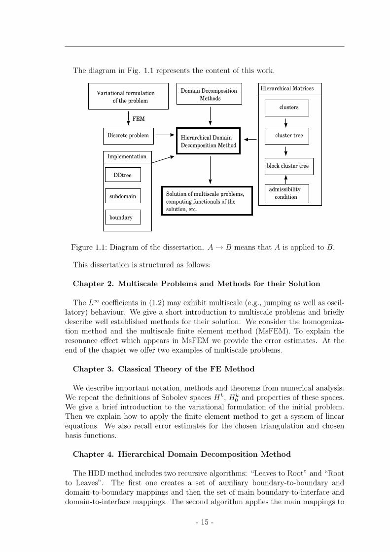
The diagram in Fig. 1.1 represents the content of this work.
Variational formulation
of the problem
Discrete problem cluster tree
clusters
FEM
block cluster tree
admissibility
conditionSolution of multiscale problems,
computing functionals of the
solution, etc.
Hierarchical Domain
Decomposition Method
Domain Decomposition
Methods
DDtree
subdomain
boundary
Implementation
Hierarchical Matrices
Figure 1.1: Diagram of the dissertation. A→ B means that A is applied to B.
This dissertation is structured as follows:
Chapter 2. Multiscale Problems and Methods for their Solution
The L∞ coefficients in (1.2) may exhibit multiscale (e.g., jumping as well as oscil-latory) behaviour. We give a short introduction to multiscale problems and brieflydescribe well established methods for their solution. We consider the homogeniza-tion method and the multiscale finite element method (MsFEM). To explain theresonance effect which appears in MsFEM we provide the error estimates. At theend of the chapter we offer two examples of multiscale problems.
Chapter 3. Classical Theory of the FE Method
We describe important notation, methods and theorems from numerical analysis.We repeat the definitions of Sobolev spaces Hk, Hk
0 and properties of these spaces.We give a brief introduction to the variational formulation of the initial problem.Then we explain how to apply the finite element method to get a system of linearequations. We also recall error estimates for the chosen triangulation and chosenbasis functions.
Chapter 4. Hierarchical Domain Decomposition Method
The HDD method includes two recursive algorithms: “Leaves to Root” and “Rootto Leaves”. The first one creates a set of auxiliary boundary-to-boundary anddomain-to-boundary mappings and then the set of main boundary-to-interface anddomain-to-interface mappings. The second algorithm applies the main mappings to
- 15 -

1 Introduction
compute the solution. There are three modifications of the HDD method: HDDwith the right-hand side fh ∈ VH ⊂ Vh, HDD with truncation of the small scalesand a combination of the first and the second modifications. One may see the com-parison of HDD with truncation of the small scales with the known MsFEM method[40]. We show that HDD is appropriate for the problems with repeated patterns.In conclusion we show how to apply HDD to compute different functionals of thesolution.
Chapter 5. Hierarchical Matrices
The hierarchical matrices (H-matrices) have been used in a wide range of appli-cations since their introduction in 1999 by Hackbusch [33]. They provide a formatfor the data-sparse representation of fully-populated matrices. The main idea inH-matrices is the approximation of certain subblocks of a given matrix by low-rankmatrices. At the beginning we present two examples of H-matrices (see Fig. 5.1).Then we list the main steps which are necessary for building hierarchical matrices:construction of the cluster tree, choice of the admissibility condition and construc-tion of the block cluster tree. We introduce the class of low-rank matricesR(k, n,m),where k, n, m are integers, k ≪ minn,m, and then the low-rank arithmetic. Webriefly describe how to perform the hierarchical matrix operations efficiently (withalmost linear complexity). It will be shown that the cost of the basic H-matrixarithmetic (matrix-matrix addition, matrix-matrix multiplication, inversion of ma-trices) is not greater than O(n logα n), α = 1, 2, 3 (see Theorem 5.10.1). We thenpresent two procedures for extracting a part of a hierarchical matrix (see Algorithm5.9.3) and converting one H-matrix format to another one. The last two proceduresare needed for adding two hierarchical matrices with different block structures (seeLemma 5.10.8).
Chapter 6. Application of H-Matrices to HDD
The exact matrix arithmetic in the HDD method can be replaced by the approx-imate H-matrix arithmetic to improve efficiency. Here we will explain the construc-tion of H-matrix approximations for the domain-to-boundary (denoted by Ψf ) andboundary-to-boundary (denoted by Ψg) mappings, which are essential for the defini-tion of the HDD method. It will be shown that the boundary-to-interface mapping(denoted by Φg) can be approximated by a low-rank matrix and the domain-to-interface mapping (denoted by Φf ) by an H-matrix. Letting ω = ω1 ∪ ω2, whereω, ω1, ω2 ⊂ Ω, we also provide the algorithms for building Ψg
ω from Ψgω1
and Ψgω2
(seeAlgorithms 6.3.1 and 6.3.2) and the algorithms for building Ψf
ω from Ψfω1
and Ψfω2
(see Algorithms 6.3.3 and 6.3.4).
Chapter 7. Complexity and Storage Requirement of HDD
The HDD method consists of two algorithms “Leaves to Root” and “Root toLeaves”. Using the costs of the standard H-matrix operations, we estimate thecomputational complexities of both algorithms. The first algorithm produces a set
- 16 -
of domain-to-interface mappings and boundary-to-interface mappings. The secondalgorithm applies this set of mappings to compute the solution (only matrix-vectormultiplications are required).
Let nh, nH be the respective numbers of degrees of freedom of the fine grid Th andof the coarse grid TH . We prove that the complexities of the algorithms “Leaves toRoot” and “Root to Leaves” are
O(k2nh log3 nh) and O(knh log2 nh),
respectively (cf. Lemmas 7.2.3 and 7.3.3) and the storage requirement isO(knh log2 nh)(see Lemma 7.3.4). As we show in Lemmas 7.4.4 and 7.4.3, the complexities of thesame algorithms for the two-grid modification are
O(k2√nhnH log3√nhnH) and O(k√nhnH log
√nh log
√nH)
The storage requirement for the two-grid modification of HDD is (cf. Lemma 7.4.1)
O(k√nhnH log
√nh log
√nH).
Chapter 8. Parallel Computing
We present the parallel HDD algorithm and estimate parallel complexities of thealgorithms “Leaves to Root” and “Root to Leaves”. We consider the parallel model,which consists of q processors and a global memory which can be accessed by allprocessors simultaneously. The communication time between processors is negligiblein comparison with the computational time. For a machine with q processors theparallel complexity of the algorithm “Leaves to Root” is estimated (Lemma 8.3.3)by
C ′k2√nh log2√nh + Ck2nhq0.45
+ C ′′(1− 3r
4r)√nhn
2min + Ck2nh
qlog3 nh
q
where C, C ′, C ′′, C ∈ R+.The parallel complexity of the algorithm “Root to Leaves” on a machine with qprocessors is estimated (Lemma 8.3.6) by
Ck2nhq
log2 nhq
+28k√nh
q0.45, C ∈ R+.
Chapter 9. Implementation of the HDD Package
The result of the implementation is a package of programs which uses the fol-lowing libraries: HLIB, LAPACK, BLAS and external triangulators (for complexgeometry). We present the data structures for the triangulation, the grid hierarchyand the HDD method. We describe the connection between the data structures“vertex”, “triangle”, “edge”, “subdomain”, “boundary” and “hierarchical decompo-sition tree”. Then, we present the algorithms of the hierarchical decomposition andof the mesh refinement.
Four modifications of HDD (numbered by subindex) which require less computa-tional resources than the original HDD were implemented. HDD1 works with the
- 17 -

1 Introduction
right-hand side defined only on a coarse scale (see Section 4.3.6). HDD2 computesthe solution in all ω with diam(ω) ≥ H, and the mean value of the solution insideall ω with diam(ω) < H. The mean value is a functional of the right-hand side andthe Dirichlet data (see Section 4.4.5). HDD3 is a combination of HDD1 and HDD2.HDD4 is developed for problems with a homogeneous right-hand side (see Section4.4.8).
Chapter 10. Numerical Results
We demonstrate numerical experiments to confirm the estimates of the H-matrixapproximation errors (Chapter 5), the computational times and the needed storagerequirements (Chapter 7).
We demonstrate almost linear complexities of the algorithms “Leaves to Root”and “Root to Leaves”. We also show an almost linear dependence of the memoryrequirement and the executing time on the number of degrees of freedoms. Next,we apply HDD to the problem with highly jumping coefficients (e.g., skin problem)and to problems with strong oscillatory coefficients, e.g.,
α(x, y) = 2 + sin(ν · x) sin(ν · y),
where ν is the frequency (see Table 10.17).The solution, obtained by the HDD method, is compared with the solutions ob-
tained by the preconditioned conjugate gradient (PCG) method and the direct H-Cholesky method. It is shown that the HDD method requires less memory thanthe direct H-matrix inverse and a little bit more than the PCG method with H-Cholesky preconditioner. But note that HDD computes the solution operators Fhand Gh in (1.4) whereas PCG only the solution. Other experiments demonstrate thepossibility of obtaining a solution on a coarse scale and the possibility of truncationof the small scales. Finally, it will be shown that HDD is very efficient for problemswith many right-hand sides.
- 18 -

2 Multiscale Problems and Methodsfor their Solution
2.1 Introduction
In the last years, we have seen large growth of activities in multiscale modelingand computating, with applications in material sciences, fluid mechanics, chemistry,biology, astronomy and other branches of science.
The basic set-up of a multiscale problem is as follows. We have a system whosemicroscopic behaviour, denoted by the state variable u, is described by a givenmicroscopic model. This microscopic model is too expensive to be used in densedetail. Instead, we are interested in the macroscopic behaviour of the system. Wewant to use the microscopic model to extract all microscale details to build a goodapproximation for the macroscale behaviour of the system. Our purpose is notto solve dense microscale problems in detail, but to use a more efficient combinedmacro-micro modeling technique.
There has been a long history of studying multiscale problems in applied math-ematics and computational science (see [7]). Multiscale problems are multiphysicalin nature; namely, the processes at different scales are governed by physical lawsof different characters: for example, quantum mechanics at one scale and classicalmechanics at another. Well-known examples of problems with multiple length scalesinclude turbulent flows, mass distribution in the universe, weather forecasting andocean modeling. Another example is an elliptic equation with a highly oscillatorycoefficient arising in material science or flow through porous media.
On the computational side, several numerical methods have been developed whichaddress explicitly the multiscale nature of the solutions. These include the upscal-ing method ([21]), the averaging method, the homogenization method, the hetero-geneous multiscale method [18], [4] the finite difference heterogeneous multiscalemethod [3] (see also [19], [20]).
Another interesting approach is offered in [39]. The authors consider an elliptichomogenization problems in a domain Ω ⊂ Rd with n+1 separated scales and reduceit to elliptic one-scale problems in dimension (n+ 1)d.
Example 2.1.1 An example in Fig. 2.1 shows the solution of a multiscale problem.On the fine scale we see a complex behaviour of the solution, but on the coarse scalethe solution looks like the function sin(x). For many practical applications, the fineproperties of the solution are of no interest and it suffices to find the macro propertiesof the solution.
Despite significant progress, purely analytical techniques are still very limited whenit comes to problems of practical interest.
- 19 -

2 Multiscale Problems and Methods for their Solution
0,6
0,2
-0,6
0,4
0
x
621
-0,4
-0,2
3 4 50
Figure 2.1: An example of a multiscale solution (wavy curve) and its macroscopicapproximation.
2.2 Multiscale Methods
Homogenization
There exist a lot of composite materials with a large number of heterogeneties(inclusions or holes). One can try to characterise the properties of such a mate-rial locally, i.e., on the microscale. But in practice, it is much more important toknow macroscale characteristics. In the frame of the heterogenization theory, theheterogeneous material is replaced by a fictitious one - the homogenized material.The behaviour of this homogenized material should be as close as possible to thebehaviour of the composite itself. One tries to describe the global properties of thecomposite by taking into account the local properties of its constituents.Homogenization is a way of extracting an equation for the coarse scale behaviourthat takes into account the effect of small scales (see [12], [42]). The fine scalescannot be just ignored because the solution on the coarser scales depends on thefine scales. After homogenization the initial equation does not contain fine scalesand is therefore much easier to solve.For the periodic case, the homogenization process consists in replacing the initialpartial differential equation with rapidly oscillating coefficients that describe thecomposite material by a partial differential equation with the fictitious homogenizedcoefficients. The homogenized coefficients are obtained by solving a non oscillatingpartial differential equation on a period of reference.Let Ω = (0, 1) × (0, 1) and f ∈ L2(Ω). Let α ∈ L∞(Ω) be a positive function suchthat
0 < α ≤ α(x
ε) ≤ α < +∞,
where α and α are constants. We denote the nodal point in Ω by the bold shrift(e.g., x, y). Assume α = α(x
ε) is periodic with period ε. ε characterizes the small
scale of the problem. We assume α(y) is periodic in Y and smooth. The modelproblem is:
−∇α(x)∇u = f in Ω,u = 0 on ∂Ω.
(2.1)
Definition 2.2.1 We denote the volume average over Y as 〈·〉 = 1‖Y ‖∫Ydy.
- 20 -

2.2 Multiscale Methods
For an analysis of this and many other equations see [12], [17].With classical finite element methods, one can obtain a good approximation onlyif the mesh size h is smaller than the finest scale, i.e., h ≪ ε. But the memoryrequirements and CPU time grow polynomially with h−1 and soon become too large.One of the homogenization methods is the so-called multiple-scale method. Recentlythere have been many contributions on multiscale numerical methods, including thepapers [6] and [17]. It seeks an asymptotic expansion of uε of the form
uε(x) = u0(x) + εu1(x,x
ε)− εθε +O(ε2), (2.2)
where xε
is the fast variable. The value of uε at the point x depends on two scales.The first one corresponds to x, which describe the position in Ω. The other scalecorresponds to x
ε, which describe the local position of the point. The first variable,
x, is called the macroscopic (or slow) variable. The second one, xε, is called the
microscopic (or rapidly oscillating) variable. u0 is the solution of the homogenizedequation
∇α∗∇u0 = f in Ω, u0 = 0 on ∂Ω, (2.3)
α∗ is the constant effective coefficient, given by (see Def. 2.2.1)
α∗ij = 〈αik(y)(δkj −∂
∂ykχj)〉,
and χj is the periodic solution of
∇yα(y)∇yχj =
∂
∂yiαij(y)
with zero mean, i.e., 〈χj〉 = 0. It is known that α∗ is symmetric and positive definite.Moreover, we have
u1(x,y) = −χj ∂u0
∂xj.
Since in general u1 6= 0 on ∂Ω, the boundary condition u|∂Ω = 0 is enforced throughthe first-order correction term θε, which is given by
∇α(x
ε)∇θε = 0 in Ω, θε = u1(x,
x
ε) on ∂Ω.
Under certain smoothness conditions, one can also obtain point-wise convergence ofu to u0 as ε → 0.The condition can be weakened if the convergence is consideredin the L2(Ω) space. In [41] the authors use the asymptotic structure (2.2) to revealthe subtle details of the multiscale method and obtain sharp error estimates.
Heterogeneous multiscale method and multiscale finite element method
The heterogeneous multiscale method (HMM) [18],[19], [4] and the multiscale fi-nite element method (MsFEM) [15] have been developed during the last time forsolving, in particular, elliptic problems with multiscale coefficients. Comparison of
- 21 -

2 Multiscale Problems and Methods for their Solution
these two methods is done in [50]. Three examples when HMM can fail, are illus-trated in [22] pp.105-107.The main idea behind the Multiscale Finite Element Method is to build the localbehaviour of the differential operator into the basis functions in order to capture thesmall scale effect while having a relative coarse grid over the whole domain. This isdone by solving the equation on each element to obtain the basis functions, ratherthan using the linear basis functions. In [55], the authors apply MsFEM to thesingularly perturbed convection-diffusion equation with periodic as well as randomcoefficients. They also consider elliptic equations with discontinuous coefficients andnon-smooth boundaries. Both methods (HMM and MsFEM) solve only a subclassof the common multiscale problem. For example, HMM works like a fine scale solverwithout scale separation or any other special assumptions of the problem. Bothmethods for problems without scale separation do not give an answer with reason-able accuracy. In [50] the authors show that MsFEM incurs an O(1) error if thespecific details of the fine scale properties are not explicitly used. They show alsothat for problems without scale separation HMM and MsFEM may fail to converge.HMM offers substantially savings of cost (compared to solve the full fine scale prob-lems) for problems with scale separation. The advantage of both methods is theirparallelizability.
Resonance Effect in MsFEM
For more information see please the original [40]. The variational problem of (2.1)is to seek u ∈ H1
0 (Ω), such that
a(u, v) = f(v), ∀v ∈ H10 (Ω), (2.4)
where
a(u, v) =
∫
Ω
αij∂v
∂xi
∂u
∂xjdx and f(v) =
∫
Ω
fvdx. (2.5)
A finite element method is obtained by restricting the weak formulation (2.4) toa finite-dimensional subspace of H1
0 (Ω). Let an axi-parallel rectangular grid Th begiven (Fig. 3.1). In each element K ∈ Th, we define a set of nodal basis φiK , i =1, ..., d with d being the number of nodes of the element. Let xi = (xi, yi) (i =1, ..., d) be the nodal points in K. We neglect the subscript K when bases in oneelement are considered. The function φi satisfies
∇α(x)∇φi = 0 in K ∈ Th. (2.6)
Let xj ∈ K (j = 1, ..., d) be the nodal points of K. As usual the author requiresφi(xj) = δij. One needs to specify the boundary conditions to make (2.6) a well-posed problem. The authors assume in [40] that the basis functions are continuousacross the boundaries of the elements, so that Vh = spanφi : i = 1, ..., N ⊂ H1
0 (Ω).Then they rewrite the problem (2.4): find uh ∈ Vh such that
a(uh, v) = f(v), ∀v ∈ Vh. (2.7)
In [40] the authors describe two methods how to set up the boundary conditions for(2.6). We do not describe these methods here because there are many other variantsand this is technical. In [41] the authors proved the following result.
- 22 -

2.2 Multiscale Methods
Theorem 2.2.1 Let u be the solution of the model problem (2.1) and uh the solutionof the corresponding equation in weak form (2.7). Then, there exist positive constantsC1 and C2 independent of ε and h, such that
‖u− uh‖1,Ω ≤ C1h‖f‖0,Ω + C2(ε/h)12 , (ε < h). (2.8)
Proof: see [15], [40], [55].To prove (2.8) the authors use the fact that the base functions defined by (2.6) havethe same asymptotic structure as that of u; i.e.,
φi = φi0 + εφi1 − εθi + ... (i = 1, ..., d),
where φi0, φi1, and θi are defined similarly as u0, u1, and θε (see (2.2)), respectively.
Note that applying the standard finite element analysis to MsFEM gives an pes-simistic estimate O(h
ε) in the H1 norm, which is only useful for h ≪ ε. In [40] the
authors prove that in the case of periodic structure the MsFEM method convergesto the correct effective solution as ε→ 0 independent of ε.The following L2-norm error estimate
‖u− uh‖0,Ω ≤ C1h2‖f‖0,Ω + C2ε+ C3‖uh − uh0‖l2(Ω), (2.9)
is obtained from (2.8) by using the standard finite element analysis (see [40]). Hereuh0 is the solution of (2.3), Ci > 0, (i = 1, 2, 3) are constants and ‖uh‖l2(Ω) =(∑
i uh(xi)
2h2)1/2. It is also shown that ‖uh − uh0‖l2(Ω) = O(ε/h). Thus, we have
‖u− uh‖0,Ω = O(h2 + ε/h). (2.10)
It is clear that when h ∼ ε, the multiscale method attains large errors in both H1
and L2 norms. This fact is called the resonance effect, the effect between the gridscale h and the small scale ε. To learn more about the resonance effect see [40].In the same work, the authors propose an over-sampling technique to remove theresonance effect. After application of this over-sampling technique, the convergencein L2 norm is O(h2 + ε| log(h)|) for ε < h.
- 23 -

2 Multiscale Problems and Methods for their Solution
2.3 Applications
Below we briefly consider two examples of multiscale problems to show that usualnumerical approaches are unsufficient and other efficient multiscale methods arerequired. We hope that the HDD method, offered in this work, after some modifi-cations can be applied for solving such types of problems.
A multiple scale model for porous media
Very important in modeling porous media is the use of different length scales.Figure 2.2 shows an example of porous media consisting of different types of stoneson two length scales. Figure (a) demonstrates macroscale (the order is 10 meters),figure (b) microscale (10−3 meters). On the large scale, we identify different typesof sand (stones). On the microscale, grains and pore channels are visible. In thefigure we see the transition zone from a fine sand to a coarse sand. The void spaceis supposed to be filled with water. The behaviour of the liquid flow is influencedby effects on these different length scales.On each scale different physical processes are appearing and different mathematicalequations, which describe this processes are being used. More about the solving ofthis problem see [8], [21].
(a)macroscopic scale (b)microscopic scale
Figure 2.2: Two scales in a porous medium (see [8]).
A multiple scale model for tumor growth
In spite of the huge amount of resources that have been devoted to cancer research,many aspects remain obscure for experimentalists and clinicials, and many of thecurrently used therapeutic strategies are not entirely effective. One can divide themodels for modeling cancer into two approaches: continuum models, mathematicallyformulated in terms of partial differential equations, and cellular automation (CA)models. Significant progress in developing mathematical models was done with theintroduction of multiscale models. The tumor growth has an intrinsic multiple scalenature. It involves processes occurring over a variety of time and length scales: fromthe tissue scale to intracellular processes. The scheme of time and length scales isfigured in Fig. 2.3. The multiscale tumor model include: blood flow, transport intothe tissue of bloodborne oxygen, cell division, apoptosis etc. In the paper [5] theauthors have proposed a multiple scale model for vascular tumor growth in whichthey have integrated phenomena at the tissue scale (vascular structural, adaptation,
- 24 -

2.3 Applications
10 s-6
10 s-3
10 s0
10 s3
10 m-12
10 m-9
10 m-6
10 m-3
Atom Protein Cell Tissue
molecular events(ion channel gating)
diffusion cell signalling
mitosis
Figure 2.3: Example of time and length scales for modeling tumor growth.
and blood flow), cellular scale (cell-to-cell interaction), and the intracellular scale(cell-cycle, apoptosis). To get more details see [5].
- 25 -

2 Multiscale Problems and Methods for their Solution
- 26 -

3 Classical Theory of the FE Method
This Chapter contains classical results [31], [14]. We will hold on the original nota-tion as in [31].
3.1 Sobolev Spaces
In this section we describe well known classical notation. Almost all material istaken from the book [31].Let Ω be a open subset of Rn. L2(Ω) consists of all Lebesque-measurable functionswhose squares on Ω are Lebesque-integrable.
3.1.1 Spaces Ls(Ω)
L1(Ω) = f : Ω→ R measurable | ‖f‖L1(Ω) =∫
Ω|f |dx <∞.
Let 1 < s <∞. Then
Ls(Ω) = f : Ω→ R | |f |s ∈ L1, ‖f‖Ls(Ω) = (
∫
Ω
|f |sdx)1/s <∞.
Let s =∞ and f : Ω→ R be measurable. Then define
‖f‖L∞(D) := infsup|f(x)| : x ∈ D\A : A is a set of measure zero .
The definition of the space L∞(Ω) is:
L∞(Ω) = f : Ω→ R measurable | ‖f‖L∞ <∞
Theorem 3.1.1 L2(Ω) forms a Hilbert space with the scalar product
(u, v)0 := (u, v)L2(Ω) :=
∫
Ω
u(x)v(x)dx
and the norm
|u|0 := ‖u‖L2(Ω) :=
√∫
Ω
|u(x)|2dx.
Definition 3.1.1 u ∈ L2(Ω) has a weak derivative v := Dαu ∈ L2(Ω) if for thelatter v ∈ L2(Ω) holds:
(w, v)0 = (−1)|α|(Dαw, u)0 for all w ∈ C∞0 (Ω).
- 27 -

3 Classical Theory of the FE Method
3.1.2 Spaces Hk(Ω), Hk0(Ω) and H−1(Ω)
Let k ∈ N ∪ 0. Let Hk(Ω) ⊂ L2(Ω) be the set of all functions having weakderivatives Dαu ∈ L2(Ω) for |α| ≤ k:
Hk(Ω) := u ∈ L2(Ω) : Dαu ∈ L2(Ω) for |α| ≤ k.
Theorem 3.1.2 Hk(Ω) forms a Hilbert space with the scalar product
(u, v)k := (u, v)Hk(Ω) :=∑
|α|≤k(Dαu,Dαv)L2(Ω)
and the (Sobolev) norm
‖u‖k := ‖u‖Hk(Ω) :=
√∑
|α|≤k‖Dαu‖2L2(Ω). (3.1)
Definition 3.1.2 The completion of C∞0 (Ω) in L2(Ω) with respect to the norm (3.1)is denoted by Hk
0 (Ω).
Theorem 3.1.3 H00 (Ω) = H0(Ω) = L2(Ω).
Proof: see p.117 in [31].
The Sobolev space denoted here by Hk(Ω) is denoted by W k2 (Ω) in other sources.
Definition 3.1.3 H−1(Ω) is the dual of H10 (Ω), i.e., H−1(Ω) = f |f is a bounded
linear functional on H10 (Ω).
and the norm is
|u|−1 = sup|(u, v)L2(Ω)|/|v|1 : 0 6= v ∈ H10 (Ω).
3.2 Variational Formulation
Let us consider the following elliptic equation
Lu = f in Ω, (3.2)
L =∑
|α|≤m
∑
|β|≤m(−1)|β|Dβaαβ(x)Dα. (3.3)
We assume the homogeneous Dirichlet boundary conditions
u = 0,∂u
∂n= 0 , ..., (
∂
∂n)m−1u = 0 on Γ = ∂Ω, (3.4)
which are only meaningful if Γ is sufficiently smooth. Let u ∈ C2m(Ω) ∩ Hm0 (Ω)
be a classical solution of (3.2) and (3.4). To derive the variational formulation of(3.2)-(3.4) we multiply equation (3.2) by v ∈ C∞0 (Ω) and integrate the result over
- 28 -

3.3 Inhomogeneous Dirichlet Boundary Conditions
the domain Ω.Since v ∈ C∞0 (Ω), the integrand vanishes in the proximity of Γ. After integrationby parts we obtain the variational formulation (the so-called ’weak’ formulation):
∑
|α|,|β|≤m
∫
Ω
aαβ(Dαu(x))(Dβv(x))dx =
∫
Ω
f(x)v(x)dx (3.5)
for all v ∈ C∞0 (Ω).
Definition 3.2.1 The bilinear form and the functional are
a(u, v) :=∑
|α|,|β|≤m
∫
Ω
aαβ(Dαu(x))(Dβv(x))dx, (3.6)
ϕ(v) :=
∫
Ω
f(x)v(x)dx.
Theorem 3.2.1 Let aαβ ∈ L∞(Ω). The bilinear form defined by (3.6) is boundedon Hm
0 (Ω)×Hm0 (Ω).
Proof: see p.146 in [31].
Definition 3.2.2 The variational formulation ( or weak formulation) of the bound-ary value problem (3.2)-(3.4) is:
find u ∈ Hm0 (Ω) with a(u, v) = ϕ(v) for all v ∈ C∞0 (Ω). (3.7)
The existence and uniqueness of the solution in the weak form can be proved by theLax-Milgram Lemma.
Theorem 3.2.2 (Lax-Milgram lemma)Let V be a Hilbert space, let a(·, ·) : V × V → R be a continuous V-elliptic bilinearform, and let ϕ : V → R be a continuous linear form. Then the abstract variationalproblem: Find an element u such that
u ∈ V and ∀v ∈ V, a(u, v) = ϕ(v),
has one and only one solution.
Proof: see [16].
3.3 Inhomogeneous Dirichlet Boundary Conditions
Let us consider the boundary value problem
Lu = f in Ω, u = g on Γ, (3.8)
where L is a differential operator of second order. The variational formulation ofthe boundary value problem reads:
find u ∈ H1(Ω) with u = g on Γ such that (3.9)
a(u, v) = ϕ(v) for all v ∈ H10 (Ω). (3.10)
- 29 -

3 Classical Theory of the FE Method
Remark 3.3.1 For the solvability of Problem (3.9),(3.10) it is necessary that:
there exists a function u0 ∈ H1(Ω) with u0|Γ = g. (3.11)
If such function u0 is known, then we obtain the following weak formulation:
Let u0 satisfy (3.11); find w ∈ H10 (Ω), such that (3.12)
a(w, v) = ϕ(v) := ϕ(v)− a(u0, v) for all v ∈ H10 (Ω). (3.13)
The advantage of this formulation is that the functions w and v are from the samespace H1
0 (Ω).
Remark 3.3.2 In this work we assume that g and Ω are such that u0 from the aboveremark exists.
Theorem 3.3.1 (Existence and uniqueness)Let the following problem
find u ∈ Hm0 (Ω) with a(u, v) = ϕ(v) for all v ∈ Hm
0 (Ω) (3.14)
(with homogeneous boundary values) be uniquely solvable for all ϕ ∈ H−1(Ω). ThenCondition (3.11) is sufficient, and necessary, for the unique solvability of Problem(3.9),(3.10).
Proof: see Theorem 7.3.5 in [31].
The variational formulation is the foundation of the Ritz-Galerkin discretisationmethod.
3.4 Ritz-Galerkin Discretisation Method
Suppose we have a boundary value problem in its variational formulation:
Find u ∈ V, so that a(u, v) = ϕ(v) for all v ∈ V, (3.15)
where we are thinking, in particular, of V = Hm0 (Ω) or V = H1(Ω).
We assume that a(·, ·) is a bounded bilinear form defined on V × V , and that ϕ isfrom the dual space V ′:
|a(u, v)| ≤ Cs‖u‖V ‖v‖V for u, v ∈ V, Cs ∈ R+
|ϕ(v)| ≤ C‖v‖V for v ∈ V, Cs ∈ R+.(3.16)
The Ritz-Galerkin discretisation consists in replacing the infinite-dimensional spaceV with a finite-dimensional space VN :
VN ⊂ V, dimVN = N <∞. (3.17)
Since VN ⊂ V , both a(u, v) and ϕ(v) are defined for u, v ∈ VN . Thus, we pose thefollowing problem:
Find uN ∈ VN , so that a(uN , v) = ϕ(v) for all v ∈ VN . (3.18)
- 30 -

3.4 Ritz-Galerkin Discretisation Method
Definition 3.4.1 The solution of (3.18), if it exists, is called the Ritz-Galerkinsolution (belonging to VN) of the boundary value problem (3.15).
To calculate a solution we need a basis of VN . Let b1, b2, ..., bN be such a basis,
VN = spanb1, ..., bN. (3.19)
For each coefficient vector v = v1, ..., vNT we define
P : Rn → VN ⊂ V, Pv :=N∑
i=1
vibi. (3.20)
Thus, we can rewrite the problem (3.18):
Find uN ∈ VN , so that a(uN , bi) = ϕ(bi) for all i = 1, ..., N. (3.21)
Proof: see [31], p.162.
We now seek u ∈ RN so that uN = Pu.
Theorem 3.4.1 Assume (3.19). The N × N -matrix A = (Aij) and the N -vectorc = (c1, ..., cN)T are defined by
Aij := a(bj, bi) (i, j = 1, ..., N), (3.22)
ci := ϕ(bi) (i = 1, ..., N), (3.23)
Then the problem (3.18) andAu = c (3.24)
are equivalent.
If u is a solution of (3.24), then uN =N∑
j=1
ujbj solves the problem (3.18). In the
opposite direction, if uN is a solution of (3.18), then u := P−1uN is a solution of(3.24).Proof: see [31], p.162.The following theorem estimates the Ritz-Galerkin solution.
Theorem 3.4.2 (Cea) Assume that (3.16),(3.17) and
infsup|a(u, v)| : v ∈ VN , ‖v‖V = 1 : u ∈ VN , ‖u‖V = 1 = ǫN > 0 (3.25)
hold. Let u ∈ V be a solution of the problem (3.15), and let uN ∈ VN be the Ritz-Galerkin solution of (3.18). Then the following estimate holds:
‖u− uN‖V ≤ (1 +CsǫN
)infw∈VN‖u− w‖V (3.26)
with Cs from (3.16). Note that infw∈VN‖u − w‖V is the distance from the function
u to VN .
Proof: see [31], p.168.
- 31 -
3 Classical Theory of the FE Method
3.5 FE Method
3.5.1 Linear Finite Elements for Ω ⊂ R2
The method of finite elements (FE) is very common for the numerical treatment ofelliptic partial differential equations. This method is based on the variational formu-lation of the differential equation. Alternative methods to FE are finite differencemethods and finite volume methods, but FE can be applied to the problems withmore complicated geometry.
First, we partition the given domain Ω into (finitely many) subdomains (elements).In 2D problems we use triangles.
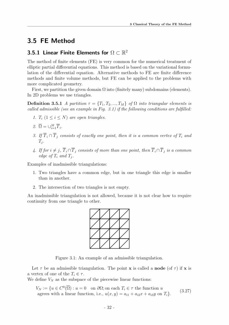
Definition 3.5.1 A partition τ = T1, T2, ..., TM of Ω into triangular elements iscalled admissible (see an example in Fig. 3.1) if the following conditions are fulfilled:
1. Ti (1 ≤ i ≤ N) are open triangles.
2. Ω = ∪Mi=1T i.
3. If T i ∩ T j consists of exactly one point, then it is a common vertex of Ti andTj.
4. If for i 6= j, T i∩T j consists of more than one point, then T i∩T j is a commonedge of Ti and Tj.
Examples of inadmissible triangulations:
1. Two triangles have a common edge, but in one triangle this edge is smallerthan in another.
2. The intersection of two triangles is not empty.
An inadmissible triangulation is not allowed, because it is not clear how to requirecontinuity from one triangle to other.
Figure 3.1: An example of an admissible triangulation.
Let τ be an admissible triangulation. The point x is called a node (of τ) if x isa vertex of one of the Ti ∈ τ .We define VN as the subspace of the piecewise linear functions:
VN := u ∈ C0(Ω) : u = 0 on ∂Ω; on each Ti ∈ τ the function uagrees with a linear function, i.e., u(x, y) = ai1 + ai2x+ ai3y on Ti.
(3.27)
- 32 -

3.5 FE Method
Remark 3.5.1 In the case of inhomogeneous boundary conditions, e.g. u = g on∂Ω we delete the requirement u = 0 on ∂Ω.
Let xi (1 ≤ i ≤ N) be the nodes of τ . For an arbitrary set of numbers uii=1..N
there exists exactly one u ∈ VN with u(xi) = ui. It may be written as u =N∑
i=1
uibi,
where the basis functions bi are characterised by
bi(xi) = 1, bi(x
j) = 0 j 6= i. (3.28)
If T ∈ τ is a triangle with the vertices xi = (xi, yi) and x′ = (x′, y′), x′′ = (x′′, y′′),then
bi(x, y) =(x− x′)(y′′ − y′)− (y − y′)(x′′ − x′)(xi − x′)(y′′ − y′)− (yi − y′)(x′′ − x′)
on T. (3.29)
We are interested in the bilinear form, associated to the initial equation:
a(u, v) =
∫
Ω
α(x)〈∇u,∇v〉dx. (3.30)
The coefficients of the stiffness matrix A are computed by the following formula:
Aij = a(bj, bi) =∑
k
∫
Tk
α(x)〈∇bj,∇bi〉dx. (3.31)
1. If i = j, we have to integrate by all triangles which meet the vertex xi.
2. If i 6= j, we have to integrate by all triangles which contain both vertices xi
and xj.
3. Aij = 0 if xi and xj are not directly connected by the side of a triangle.
Thus, we obtain a data-sparse matrix.
Example 3.5.1 If we choose the basis functions as in (3.29) and the bilinear formby a(u, v) =
∫Ω〈∇u,∇v〉dx, then for inner nodes
Lii = 4, Aij = −1 xi−xj = (0,±h) or (±h, 0), Aij = 0 otherwise; (3.32)
Remark 3.5.2 To calculate Aij =
∫
Tk
α(x)〈∇bj,∇bi〉dx numerically we use the
basic three points quadrature formula on a triangle (see Table 3.1).If bi ∈ P 1, then ∇bi = const,∇bj = const and the coefficients Aij are
Aij =
∫
Tk
α(x)〈∇bj,∇bi〉dx = 〈∇bj,∇bi〉 ·3∑
k=1
α(vk)wk, where
vk = vk(x, y) from (3.35), wk from Tables (3.1),(3.2)
(3.33)
- 33 -

3 Classical Theory of the FE Method
i weights wi di1 di2 di3
1 0.33(3) 0.5 0.5 0.02 0.33(3) 0.0 0.5 0.53 0.33(3) 0.5 0.0 0.5
Table 3.1: The coefficients of the basic 3-point quadrature rule for a triangle (usedin (3.35) and (3.33)). This rule calculates exactly the value of integralsfor polynomial degree 2 (see [16], [54]).
Remark 3.5.3 We compute the FE right-hand side c by the following formula:
cj :=
∫
supp bj
fbjdx, (3.34)
where j = 1, ..., N and f is the right-hand side in (3.8). For non-zero Dirichletboundary data see (3.13).
Remark 3.5.4 It makes sense to apply 12-point quadrature rule if the discretisationerror is smaller than the quadrature error. If the discretisation error is larger thanthe quadrature error, it is reasonable to apply the 3-point quadrature rule.
i weights wi di1 di2 di3
1 0.050844906370207 0.873821971016996 0.063089014491502 0.0630890144915022 0.050844906370207 0.063089014491502 0.873821971016996 0.0630890144915023 0.050844906370207 0.063089014491502 0.063089014491502 0.8738219710169964 0.116786275726379 0.501426509658179 0.249826745170910 0.2498267451709105 0.116786275726379 0.249826745170910 0.501426509658179 0.2498267451709106 0.116786275726379 0.249826745170910 0.249826745170910 0.5014265096581797 0.082851075618374 0.636502499121399 0.310352451033785 0.0531450498448168 0.082851075618374 0.636502499121399 0.053145049844816 0.3103524510337859 0.082851075618374 0.310352451033785 0.636502499121399 0.05314504984481610 0.082851075618374 0.310352451033785 0.053145049844816 0.63650249912139911 0.082851075618374 0.053145049844816 0.310352451033785 0.63650249912139912 0.082851075618374 0.053145049844816 0.636502499121399 0.310352451033785
Table 3.2: The coefficients of the basic 12-point quadrature rule for a triangle (usedin (3.35) and (3.33)). This rule calculates exactly the value of integralsfor polynomial degree 6 (see [16], [54]).
If (x1, y1), (x2, y2), (x3, y3) are coordinates of the vertices of triangle, then we definethe new quadrature points:
vi(x, y) := (di1x1 + di2x2 + di3x3, di1y1 + di2y2 + di3y3), i = 1, 2, 3, (3.35)
where the coefficients dij are defined in Table 3.2.
- 34 -

3.5 FE Method
3.5.2 Error Estimates for Finite Element Methods
In this subsection we use the notation uh besides uN in (3.18).We suppose that
τ is an admissible triangulation of Ω ⊂ R2,VN is defined by (3.27), if V = H1
0 (Ω),VN is as in Remark (3.5.1), if V = H1(Ω),
(3.36)
There are two important theorems which allow to estimate |u− uh|.
Theorem 3.5.1 Assume that conditions (3.36) hold for τ , VN , and V . Let α0 bethe smallest interior angle of all Ti ∈ τ , while h is the maximum length of the sidesof all Ti ∈ τ . Then
infv∈VN‖u− v‖Hk(Ω) ≤ C ′(α0)h
2−k‖u‖H2(Ω) for k = 0, 1 and all u ∈ H2(Ω) ∩ V.(3.37)
Proof: see [31], pp.187-188.For the next theorem we need a new regularity condition on the adjoint problem to(3.15).
Definition 3.5.2 The following problem is called the adjoint problem to (3.15).
Find u ∈ V, so that a∗(u, v) = ϕ(v) for all v ∈ V, (3.38)
where a∗(u, v) := a(v, u).
The new regularity condition is:
For each ϕ ∈ L2(Ω) the problem (3.38)has a solution u ∈ H2(Ω) ∩ V with |u|2 ≤ CR|ϕ|0. (3.39)
Theorem 3.5.2 (Aubin-Nitsche)Assume (3.39), (3.16),
infsup|a(u, v)| : v ∈ VN , ‖v‖V = 1 : u ∈ VN , ‖u‖V = 1 = ǫN ≥ ǫ > 0, (3.40)
andinfv∈VN
|u− v|1 ≤ C0h|u|2 for all u ∈ H2(Ω) ∩ V. (3.41)
Let the problem (3.15) have the solution u ∈ V . Let uh ∈ VN ⊂ V be the finite-element solution and VN is the space of finite elements of an admissible triangulation.With a constant C1 independent of u and h, we get:
|u− uh|0 ≤ C1h|u|1. (3.42)
If the solution u also belongs to H2(Ω)∩V , then there is a constant C2, independentof u and h, such that
|u− uh|0 ≤ C2h2|u|2. (3.43)
Proof: see [31], pp.190-191.
- 35 -

3 Classical Theory of the FE Method
- 36 -

4 Hierarchical DomainDecomposition Method
The idea of the HDD method belongs to Hackbusch ([34]). This Chapter containsthe main results of this work: the HDD method and its modifications.
4.1 Introduction
We repeat the initial boundary value problem to be solved:
−
2∑i,j=1
∂∂jαij
∂∂iu = f in Ω ⊂ R2,
u = g on ∂Ω,
(4.1)
with αij = αji(x) ∈ L∞(Ω) such that the matrix function A(x) = (αij)i,j=1,2 satisfies0 < λ ≤ λmin(A(x)) ≤ λmax(A(x)) ≤ λ for all x ∈ Ω ⊂ R2.After a FE discretisation we obtain a system of linear equations Au = c.In the past, several methods have been developed to combine theH-matrix techniquewith the domain decomposition (DD) method (see [35], [38], [47]).
In [35] Hackbusch applies H-matrices to the direct domain decomposition (DDD)method to compute A−1. In this method he decomposes the initial domain Ω intop subdomains (proportional to the number of parallel processors). The respectivestiffness matrix A ∈ RI×I , I := I(Ω), is represented in the block-matrix form:
A =
A11 0 ... 0 A1Σ
0 A22 ... 0 A2Σ...
.... . .
......
0 0 ... App ApΣAΣ1 AΣ2 ... AΣp AΣΣ
. (4.2)
Here Aii ∈ RIi×Ii , where Ii is the index set of interior degrees of freedom in Ωi.AiΣ ∈ RIi×IΣ , where IΣ := I \∪pi=1Ii is the index set of the degrees of freedom on theinterface. E.g., in the case of finite elements. Assume that A and all submatricesAii are invertible, i.e., the subdomain problems are solvable. Let S := AΣΣ −∑p
i=1AΣiA−1ii AiΣ. Then the inverse of A−1 can be defined by the following formula:
A−1 =
A−111 0 0 0
0. . . 0 0
0 0 A−1pp 0
0 0 0 0
+
A−111 A1Σ
...A−1pp ApΣ−I
[S−1AΣ1A
−111 , · · · , S−1AΣpA
−1pp ,−S−1].
(4.3)
- 37 -

4 Hierarchical Domain Decomposition Method
This DDD method is easily parallelizable. Let d be the spatial dimension. Then thecomplexity will be
O(n
plog np) +O(p1/dnd−1/d), or
O(nd/d+1 log nd/d+1), for p = O(1/d+ 1).
In [38], the authors start with the representation (4.2), apply the so-called directSchur complement method, which is based on the H-matrix technique and the do-main decomposition method to compute the inverse of the Schur complement matrixassociated with the interface. Building the approximate Schur complements corre-sponding to the subdomains Ωi costs O(NΩ logqNΩ) for an FEM discretisation,where NΩ is the number of degrees of freedom in the domain Ω.
In [47] the authors introduce the so-called H-LU factorization which is based onthe nested dissection method [24]. The initial domain Ω is decomposed hierarchicallyinto three parts: Ωleft, γ and Ωright, such that
Ωleft ∩ Ωright = ∅ and Ωleft ∪ Ωright ∪ γ = Ω.
Such a decomposition yields a block structure in which large off-diagonal subblocksof the finite element stiffness matrix are zero and remain zero during the computationof the H-LU factorization. In this approach the authors compute the solution u asfollows u = U−1L−1c, where the factors L and U are approximated in the H-matrixformat.
The HDD method, unlike the methods described above, has the capability tocompute the solution on different scales retaining the information from the finestscales. HDD in the one-scale settings performs comparable to the methods from[35], [38], [47] with regards to the computational complexity.
4.2 Idea of the HDD Method
After Galerkin FE discretisation of (4.1) we construct the solution in the followingform
uh(fh, gh) = Fhfh + Ghgh, (4.4)
where uh(fh, gh) is the FE solution of the initial problem (1.1), fh the FE right-handside, and gh the FE Dirichlet boundary data. The hierarchical domain decomposi-tion (HDD) method computes both operators Fh and Gh. .
Domain decomposition tree (TTh)
Let Th be a triangulation of Ω. First, we decompose hierarchically the givendomain Ω (cf. [24]). The result of the decomposition is the hierarchical tree TTh
(seeFig. 4.1). The properties of the TTh
are:
• Ω is the root of the tree,
• TThis a binary tree,
- 38 -

4.2 Idea of the HDD Method
• If ω ∈ TThhas two sons ω1, ω2 ∈ TTh
, thenω = ω1 ∪ ω2 and ω1, ω2 have no interior point in common,
• ω ∈ TThis a leaf, if and only if ω ∈ Th.
The construction of TThis straight-forward by dividing Ω recursively in pieces. For
practical purposes, the subdomains ω1, ω2 must both be of size ≈ |ω|/2 and theinternal boundary
γω := ∂ω1\∂ω = ∂ω2\∂ω (4.5)
must not be too large (see Fig. 4.2).
1
2
3
4
5
6
7
910
11
12
13
14
15
8
5
6
7
11
12
13
14
15
8
1
2
3
4
5
6
7
910
3
4
19
10
......
5
611
12
13
14
15
6
7
11
15
8
......
26
2
6
Figure 4.1: An example of the hierarchical domain decomposition tree TTh.
Set of nodal points
Let I := I(Ω) and xi, i ∈ I, be the set of all nodal points in Ω (including nodalpoints on the boundary). We define I(ω) as a subset of I with xi ∈ ω = ω. Similarly,
we define I(ω), I(Γω), I(γω), where Γω := ∂ω,
ω = ω\∂ω, for the interior, for the
external boundary and for the internal boundary.
Idea
We are interested in computing the discrete solution uh of (4.1) in Ω. This isequivalent to the computation of uh on all γω, ω ∈ TTh
, since I(Ω) = ∪ω∈TThI(γω).
These computations are performed by using the linear mappings Φfω, Φg
ω defined forall ω ∈ TTh
. The mapping Φgω : RI(∂ω) → RI(γω) maps the boundary data defined on
∂ω to the data defined on the interface γω. Φfω : RI(ω) → RI(γω) maps the right-hand
side data defined on ω to the data defined on γω.
Notation 4.2.1 Let gω := u|I(∂ω) be the local Dirichlet data and fω := f |I(ω) be thelocal right-hand side.
The final aim is to compute the solution uh along γω in the form uh|γω = Φfωfω +
Φgωgω, ω ∈ TTh
. For this purpose HDD builds the mappings Φω := (Φgω,Φ
fω), for all
- 39 -

4 Hierarchical Domain Decomposition Method
ω ∈ TTh. For computing the mapping Φω, ω ∈ TTh
, we, first, need to compute theauxiliary mapping Ψω := (Ψg
ω,Ψfω) which will be defined later.
Thus, the HDD method consists of two steps: the first step is the constructionof the mappings Φg
ω and Φfω for all ω ∈ TTh
. The second step is the recursivecomputation of the solution uh. In the second step HDD applies the mappings Φg
ω
and Φfω to the local Dirichlet data gω and to the local right-hand side fω.
Notation 4.2.2 Let ω ∈ TThand
dω :=((fi)i∈I(ω) , (gi)i∈I(∂ω)
)= (fω, gω) (4.6)
be a composed vector consisting of the right-hand side from (4.1) restricted to ω andthe Dirichlet boundary values gω = uh|∂ω (see also Notation 4.2.1).
Note that gω coincides with the global Dirichlet data in (4.1) only when ω = Ω. Forall other ω ∈ TTh
we compute gω in (4.6) by the algorithm “Root to Leaves” (seeSection 4.3.5).
Assuming that the boundary value problem (4.1) restricted to ω is solvable, wecan define the local FE solution by solving the following discrete problem in thevariational form (see (3.7)):
aω(Uω, bj) = (fω, bj)L2(ω) , ∀ j ∈ I(
ω),
Uω(xj) = gj, ∀ j ∈ I(∂ω).(4.7)
Here, bj is the P 1-Lagrange basis function (see (3.29)) at xj and aω(·, ·) is the bilin-ear form (see (3.30)) with integration restricted to ω and (fω, bj) =
∫ω
fω bj dx.
Let Uω ∈ Vh be the solution of (4.7) in ω. The solution Uω depends on the Dirichletdata on ∂ω and the right-hand side in ω. Dividing problem (4.7) into two subprob-lems (4.8) and (4.9), we obtain Uω = U f
ω + U gω, where U f
ω is the solution of
aω(U
fω , bj) = (fω, bj)L2(ω) , ∀ j ∈ I(
ω),
U fω (xj) = 0, ∀ j ∈ I(∂ω)
(4.8)
and U gω is the solution of
aω(U
gω, bj) = 0, ∀ j ∈ I( ω),
U gω(xj) = gj, ∀ j ∈ I(∂ω).
(4.9)
If ω = Ω then (4.7) is equivalent to the initial problem (4.1) in the weak formulation.
4.2.1 Mapping Φω = (Φgω,Φ
fω)
We consider ω ∈ TThwith two sons ω1, ω2. Recall that we used γω to denote the
interface in ω (see (4.5)). Considering once more the data dω from (4.6), U fω from
(4.8) and U gω from (4.9), we define Φf
ω(fω) and Φgω(gω) by
(Φfω(fω)
)i:= U f
ω (xi) ∀i ∈ I(γω) (4.10)
- 40 -

4.2 Idea of the HDD Method
and(Φg
ω(gω))i := U gω(xi) ∀i ∈ I(γω). (4.11)
Since Uω = U fω + U g
ω, we obtain
(Φω(dω))i := Φgω(gω) + Φf
ω(fω) = U fω (xi) + U g
ω(xi) = Uω(xi) (4.12)
for all i ∈ I(γω).Hence, Φω(dω) is the trace of Uω on γω. Definition in (4.12) says that if the data dωare given then Φω computes the solution of (4.7). Indeed, Φωdω = Φggω + Φffω.Note that the solution uh of the initial global problem coincide with Uω in ω, i.e.,uh|ω = Uω.
4.2.2 Mapping Ψω = (Ψgω,Ψ
fω)
Let us, first, define the mappings Ψfω from (4.8) as
(Ψfω(dω)
)i∈I(∂ω)
:= aω(Ufω , bi)− (fω, bi)L2(ω) , (4.13)
where U fω ∈ Vh, U f
ω |∂ω = 0 and
a(U fω , bi)− (f, bi) = 0, for ∀i ∈ I( ω).
Second, we define the mapping Ψgω from (4.9) by setting
(Ψgω(dω))i∈I(∂ω) := aω(U
gω, bi)− (fω, bi)L2(ω) = aω(U
gω, bi)− 0 = aω(U
gω, bi), (4.14)
where U gω ∈ Vh and (Ψg
ω(dω))i = 0 for ∀i ∈ I( ω).The linear mapping Ψω, which maps the data dω given by (4.6) to the boundary
data on ∂ω, is given in the component form as
Ψω(dω) = (Ψω(dω))i∈I(∂ω) := aω(Uω, bi)− (fω, bi)L2(ω) . (4.15)
By definition and (3.11)-(3.13), Ψω is linear in (fω, gω) and can be written asΨω(dω) = Ψf
ωfω + Ψgωgω. Here Uω is the solution of the local problem (4.7) and
it coincides with the global solution on I(ω).
4.2.3 Φω and Ψω in terms of the Schur Complement Matrix
Let the linear system Au = Fc for ω ∈ TThbe given. In Sections 4.3.1 and 4.3.3
we explain how to obtain the matrices A and F . A is the stiffness matrix for the
domain ω after elimination of the unknowns corresponding to I(ω \γω). The matrix
F comes from the numerical integration.We will write for simplicity γ instead of γω. Thus, A : RI(∂ω∪γ) → RI(∂ω∪γ), u ∈RI(∂ω∪γ), F : RI(ω) → RI(∂ω∪γ) and c ∈ RI(ω). Decomposing the unknown vector uinto two components u1 ∈ RI(∂ω) and u2 ∈ RI(γ), obtain
u =
(u1
u2
).
- 41 -

4 Hierarchical Domain Decomposition Method
The component u1 corresponds to the boundary ∂ω and the component u2 to theinterface γ. Then the equation Au = Fc becomes
(A11 A12
A21 A22
)(u1
u2
)=
(F1
F2
)c, (4.16)
whereA11 : RI(∂ω) → RI(∂ω), A12 : RI(γ) → RI(∂ω),
A21 : RI(∂ω) → RI(γ), A22 : RI(γ) → RI(γ),
F1 : RI(ω) → RI(∂ω), F2 : RI(ω) → RI(γ).
The elimination of the internal points is done as it is shown in (4.17). To eliminatethe variables u2, we multiply both sides of (4.16) by A12A
−122 , subtract the second
row from the first, and obtain(A11 − A12A
−122 A21 0
A21 A22
)(u1
u2
)=
(F1 − A12A
−122 F2
F2
)c. (4.17)
We rewrite the last system as two equations
Au1 := (A11 − A12A−122 A21)u1 = (F1 − A12A
−122 F2)c,
A22u2 = F2c− A21u1.(4.18)
The unknown vector u2 is computed as follows
u2 = A−122 F2c− A−1
22 A21u1. (4.19)
Equation (4.19) is analogous to (4.43). The explicit expressions for the mappingsΨω and Φω follow from (4.18):
Ψgω := A11 − A12A
−122 A21, (4.20)
Ψfω := F1 − A12A
−122 F2, (4.21)
Φgω := −A−1
22 A21, (4.22)
Φfω := A−1
22 F2. (4.23)
4.3 Construction Process
4.3.1 Initialisation of the Recursion
Our purpose is to get, for each triangle ω ∈ Th, the system of linear equations
A · u = c := F · c,
where A is the stiffness matrix, c the discrete values of the right-hand side in thenodes of ω and F will be defined later. The matrix coefficients Aij are computed bythe formula
Aij =
∫
ω
α(x)〈∇bi · ∇bj〉dx (4.24)
- 42 -

4.3 Construction Process
For ω ∈ Th, F ∈ R3×3 comes from the discrete integration and the matrix coefficientsFij are computed using (4.28). The components of c can be computed as follows:
ci =
∫
ω
fbidx ≈f(x1)bi(x1) + f(x2)bi(x2) + f(x3)bi(x3)
3· |ω|, (4.25)
where xi, i ∈ 1, 2, 3, are three vertices of the triangle ω ∈ TTh, bi(xj) = 1 if i = j
and bi(xj) = 0 otherwise. Rewrite (4.25) in matrix form:
c =
c1c2c3
≈ 1
3
b1(x1) b1(x2) b1(x3)b2(x1) b2(x2) b2(x3)b3(x1) b3(x2) b3(x3)
f(x1)f(x2)f(x3)
, (4.26)
where f(xi), i = 1, 2, 3, are the values of the right-hand side f in the vertices of ω.Let
F :=1
3
b1(x1) b1(x2) b1(x3)b2(x1) b2(x2) b2(x3)b3(x1) b3(x2) b3(x3)
. (4.27)
Using the definition of basic functions, we obtain
c1c2c3
≈ 1
3
1 0 00 1 00 0 1
f(x1)f(x2)f(x3)
. (4.28)
Thus, Ψgω corresponds to the matrix A ∈ R3×3 and Ψf
ω to F ∈ R3×3.
4.3.2 The Recursion
The coefficients of Ψω can be computed by (4.15). Let ω ∈ TThand ω1, ω2 be two
sons of ω. The external boundary Γω of ω splits into (see Fig. 4.2)
Γω,1 := ∂ω ∩ ω1, Γω,2 := ∂ω ∩ ω2. (4.29)
For simplicity of further notation, we will write γ instead of γω.
Notation 4.3.1 Recall that I(∂ωi) = I(Γω,i) ∪ I(γ). We denote the restriction ofΨωi
: RI(∂ωi) → RI(∂ωi) to I(γ) by γΨω := (Ψω)|i∈I(γ).
Suppose that by induction, the mappings Ψω1 , Ψω2 are known for the sons ω1, ω2.Now, we explain how to construct Ψω and Φω.
Lemma 4.3.1 Let the data d1 = dω1, d2 = dω2 be given by (4.6).d1 and d2 coincide w.r.t. γω, i.e.,• (consistency conditions for the boundary)
g1,i = g2,i ∀i ∈ I(ω1) ∩ I(ω2), (4.30)
• (consistency conditions for the right-hand side)
f1,i = f2,i ∀i ∈ I(ω1) ∩ I(ω2). (4.31)
- 43 -

4 Hierarchical Domain Decomposition Method
ω1 ω2
ωγω
Γω,1 Γω,2
Γω
Figure 4.2: The decomposition of ω into ω1 and ω2. Here γω is the internal boundaryand Γω,i, i = 1, 2, parts of the external boundaries, see (4.29).
If the local FE solutions uh,1 and uh,2 of the problem (4.7) for the data d1, d2 satisfythe additional equation
γΨω1(d1) + γΨω2(d2) = 0, (4.32)
then the composed solution uh defined by assembling
uh(xi) =
uh,1(xi) for i ∈ I(ω1),uh,2(xi) for i ∈ I(ω2)
(4.33)
satisfies (4.7) for the data dω = (f, g) where
fi =
f1,i for i ∈ I(ω1),f2,i for i ∈ I(ω2),
(4.34)
gi =
g1,i for i ∈ I(Γω,1),g2,i for i ∈ I(Γω,2). (4.35)
Proof: Note that the index sets in (4.33)-(4.35) overlap. Let ω1 ∈ TTh, f1,i = fi,
i ∈ I(ω1), and g1,i = gi, i ∈ I(∂ω1). Then the existence of the unique solutions of
(4.7) gives uh,1(xi) = uh(xi), ∀i ∈ I(ω1).
In a similar manner we get uh,2(xi) = uh(xi) , ∀i ∈ I( ω2). Equation (4.15) gives
( γΨω1(d1))i∈I(γ) = aω1(uh, bi)− (fω1 , bi)L2(ω1) (4.36)
and( γΨω2(d2))i∈I(γ) = aω2(uh, bi)− (fω2 , bi)L2(ω2) . (4.37)
The sum of the two last equations (see Figure 4.3) and (4.32) give
0 = γΨω(dω)i∈I(γ) = aω(uh, bi)− (fω, bi)L2(ω). (4.38)
We see that uh satisfies (4.7).
Note that
uh,1(xi) = g1,i = g2,i = uh,2(xi) holds for i ∈ I(ω1) ∩ I(ω2).
Next, we use the decomposition of the data d1 into the components
d1 = (f1, g1,Γ, g1,γ), (4.39)
- 44 -

4.3 Construction Process
ω
ω
ω
1
2
xjγω
xj
Figure 4.3: The supports of bj, xj ∈ ω1 and xj ∈ ω2.
whereg1,Γ := (g1)i∈I(Γω,1), g1,γ := (g1)i∈I(γ) (4.40)
and similarly for d2 = (f2, g2,Γ, g2,γ).The decomposition g ∈ RI(∂ωj) into gj,Γ ∈ RI(Γω,j) and gj,γ ∈ RI(γ) implies thedecomposition of Ψg
ωj: RI(∂ωj) → RI(∂ωj) into ΨΓ
ωj: RI(Γω,j) → RI(∂ωj) and Ψγ
ωj:
RI(γ) → RI(∂ωj), j = 1, 2. Thus,
Ψgω1gω1 = ΨΓ
ω1g1,Γ + Ψγ
ω1g1,γ and Ψg
ω2gω2 = ΨΓ
ω2g2,Γ + Ψγ
ω2g2,γ .
The maps Ψω1 , Ψω2 become
Ψω1d1 = Ψfω1f1 + ΨΓ
ω1g1,Γ + Ψγ
ω1g1,γ , (4.41)
Ψω2d2 = Ψfω2f2 + ΨΓ
ω2g2,Γ + Ψγ
ω2g2,γ . (4.42)
Definition 4.3.1 We will denote the restriction of Ψγωj
: RI(γ) → RI(∂ωj) to I(γ) by
γΨγωj
: RI(γ) → RI(γ),
where j = 1, 2 and ∂ωj = Γω,j ∪ γ.Restricting (4.41), (4.42) to I(γ), we obtain from (4.32) and g1,γ = g2,γ =: gγ that
(γΨγ
ω1+ γΨγ
ω2
)gγ = (−Ψf
ω1f1 −ΨΓ
ω1g1,Γ −Ψf
ω2f2 −ΨΓ
ω2g2,Γ)|I(γ).
Next, we set M := −( γΨγω1
+ γΨγω2
), and after computing M−1, we obtain:
gγ = M−1(Ψfω1f1 + ΨΓ
ω1g1,Γ + Ψf
ω2f2 + ΨΓ
ω2g2,Γ)|I(γ). (4.43)
Remark 4.3.1 The inverse matrix M−1 exists since it is the sum of positive definitematrices corresponding to the mappings γΨγ
ω1, γΨγ
ω2.
Remark 4.3.2 Since gγ,i = uh(xi), i ∈ I(γ), we have determined the map Φω (itacts on the data dω composed by f1, f2, g1,Γ, g2,Γ).
Remark 4.3.3 We have the formula Ψω(dω) = Ψω1(d1) + Ψω2(d2), where
dω = (fω, gω), d1 = (f1, g1,Γ, g1,γ), d2 = (f2, g2,Γ, g2,γ),g1,γ = g2,γ = M−1(Ψf
ω1f1 + ΨΓ
ω1g1,Γ + Ψf
ω2f2 + ΨΓ
ω2g2,Γ)|I(γ).
(4.44)
Here (fω, gω) is build as in (4.34)-(4.35) and (4.30),(4.31) are satisfied.
Conclusion:Thus, using the given mappings Ψω1 , Ψω2 , defined on the sons ω1, ω2 ∈ TTh
, we cancompute Φω and Ψω for the father ω ∈ TTh
. This recursion process terminates assoon as ω = Ω.
- 45 -

4 Hierarchical Domain Decomposition Method
4.3.3 Building of Matrices Ψω and Φω from Ψω1and Ψω2
Let ω, ω1 and ω2 ∈ TThwhere ω1, ω2 are sons of ω. Recall that ∂ωi = Γω,i ∪ γ.
Suppose we have two linear systems of equations for ω1 and ω2 which can be writtenin the block-matrix form:
(A
(i)11 A
(i)12
A(i)21 A
(i)22
)(u
(i)1
u(i)2
)=
(F
(i)11 F
(i)12
F(i)21 F
(i)22
)(c
(i)1
c(i)2
), i = 1, 2, (4.45)
where γ := γω,
A(i)11 : RI(Γω,i) → RI(Γω,i), A
(i)12 : RI(γ) → RI(Γω,i),
A(i)21 : RI(Γω,i) → RI(γ), A
(i)22 : RI(γ) → RI(γ),
F(i)11 : RI(ωi\γ) → RI(∂ωi), F
(i)12 : RI(γ) → RI(∂ωi),
F(i)21 : RI(ωi\γ) → RI(γ), F
(i)22 : RI(γ) → RI(γ).
Both the equations in (4.45) are analogous to (4.41) and (4.42). Note that c(1)2 = c
(2)2
and u(1)2 = u
(2)2 because of the consistency conditions (see (4.30),(4.31)) on the
interface γ. The system of linear equations for ω be
A
(1)11 0 A
(1)12
0 A(2)11 A
(2)12
A(1)21 A
(2)21 A
(1)22 + A
(2)22
u
(1)1
u(2)1
u(1)2
=
F
(1)11 0 F
(1)12
0 F(2)11 F
(2)12
F(1)21 F
(2)21 F
(1)22 + F
(2)22
c
(1)1
c(2)1
c(1)2
.
(4.46)Using the notation
A11 :=
(A
(1)11 0
0 A(2)11
), A12 :=
(A
(1)12
A(2)12
),
A21 := (A(1)21 , A
(2)21 ), A22 := A
(1)22 + A
(2)22 ,
u1 :=
(u
(1)1
u(2)1
), u2 := u
(1)2 = u
(2)2 ,
F1 :=
(F
(1)11 0 F
(1)12
0 F(2)11 F
(2)12
), F2 :=
(F
(1)21 , F
(2)21 , F
(1)22 + F
(2)22
),
c1 :=
(c
(1)1
c(2)1
), c2 := c
(1)2 = c
(2)2 , c :=
(c1
c2
).
The system (4.46) can be rewritten as
(A
(i)11 A
(i)12
A(i)21 A
(i)22
)(u1
u2
)=
(F1
F2
)c. (4.47)
The system (4.47), indeed, coincides with (4.16).
- 46 -

4.3 Construction Process
4.3.4 Algorithm “Leaves to Root”
The scheme of the recursive process of computing Ψω and Φω from Ψω1 and Ψω2 forall ω ∈ TTh
is shown in Fig. 4.4. We call this process “Leaves to Root”.
..... .....
..... .....
Leaves to R
oot
Ψω11 Ψω12
Ψω1Ψω2
Figure 4.4: Recursive process “Leaves to Root”. A mapping Ψω1 is a linear functionof the mappings Ψω11 ,Ψω12 , ω1 = ω11 ∪ ω12.
“Leaves to Root”:
1. Compute Ψfω ∈ R3×3 and Ψg
ω ∈ R3×3 on all leaves of TTh(triangles of Th) by
(4.24) and (4.28).
2. Recursion from the leaves to the root:
a) Compute Φω and Ψω from Ψω1 ,Ψω2 .
b) Store Φω. Delete Ψω1 ,Ψω2 .
3. Stop if ω = Ω.
Remark 4.3.4 The result of this algorithm will be a collection of mappings Φω :ω ∈ TTh
. The mappings Ψω, ω ∈ TTh, are only of auxiliary purpose and need not
stored.
4.3.5 Algorithm “Root to Leaves”
This algorithm applies the mappings Φω = (Φgω,Φ
fω) to compute the solution. Since
this algorithm starts from the root and ends on the leaves, we will use the name“Root to Leaves”. Figure 4.5 presents the scheme of this algorithm.Let the set Φω : ω ∈ TTh
already be computed and the data dω = (fω, gω), ω = Ω,be given. We can then compute the solution uh of the initial problem as follows.Recursion from the root to the leaves:
- 47 -

4 Hierarchical Domain Decomposition Method
1. Given dω = (fω, gω), compute the solution uh on the interior boundary γω byΦω(dω).
2. Build the data dω1 = (fω1 , gω1), dω2 = (fω2 , gω2) from dω = (fω, gω) andgγω := Φω(dω).
3. Repeat the same for the sons of ω1 and ω2.
4. End if ω does not contain internal nodes.
Since uh(xi) = gγ,i, the set of values (gγω), for all ω ∈ TTh, results the solution of the
initial problem (4.1) in the whole domain Ω.
..... .....
..... .....
Root to
Leaves
Φω1 Φω2
Φω11 Φω12
uγ1 uγ2
uγ
Figure 4.5: The algorithm ’Root to Leaves’. Φωiis applied for computing the solution
on the interior boundary γi.
4.3.6 HDD on Two Grids
In (4.4) the operator Fh requires larger computational resources compared to Gh.To reduce these requirements we compute uh in the following way
uh(fH , gh) = FHfH + Ghgh,
where FH := FhPh←H , H and h are two different scales and Ph←H is a prolongationmatrix.Now, FH requires less resources (computational time and storage requirement) thanFh. If the coefficients α(x) oscillate, the grid step size should be small enough tocatch these oscillations (denote this step size by ”h” and corresponding finite spaceby Vh). At the same time the right-hand side f(x) is often smooth and thereforecan be discretised on a coarse grid with step size H, where H > h (see Fig. 4.6).Another possible problem setup is when the right-hand side is only given at thenodes of the coarse grid.
- 48 -

4.3 Construction Process
The algorithm of computing the prolongation matrix P := Ph←H
Note that we compute prolongation matrices only for triangles of TH . For sim-plicity we write P instead of Ph←H . Let h = H
2. To compute fh = PfH we perform
the following steps.
1. In each vertex vj, j = 0, 1, 2, of ω ∈ TH we compute the piecewise linear basisfunction bHj (x) by (3.29).
2. We compute the prolongation matrix P ∈ R3×3, where Pij = bHj (xi), xi arenodes of the fine grid Th in ω (e.g., middle points of edges). The value of theright-hand side f at a node of Th is defined as a linear combination of thevalues f at the nodes of TH (see an example in Fig. 4.7).
Remark 4.3.5 Now, we compute the solution by (cf. 4.43):
gγ = M−1(Ψfω1f1 + ΨΓ
ω1g1,Γ + Ψf
ω2f2 + ΨΓ
ω2g2,Γ)|I(γ), (4.48)
where Ψfωi
:= ΨfωiPi, i = 1, 2, and Pi is a prolongation matrix. The size of the
matrix Ψfωi
is smaller than the size of the matrix Ψfωi
, i = 1, 2. The size of thematrix Φf
ωiPi is smaller than the size of Φf
ωi, i = 1, 2. The matrices P1 and P2 are
data-sparse, since basis functions have a local support. Thus, memory requirementscan be strongly diminished.
hH
TH Th
Figure 4.6: The right-hand side f is given at the grid points of TH (marked by ())and has to be interpolated at the nodes of the fine grid Th (right).
H
h
x
y
z
x0
Figure 4.7: ω ∈ TH and a basis function at x0. For example, the value of f at thepoint z a linear combination on the values of f at the vertices x,y of ω(e.g., f(z) = 0.75f(y) + 0.25f(x)).
- 49 -

4 Hierarchical Domain Decomposition Method
4.4 Modifications of HDD
4.4.1 Truncation of Small Scales
The standard version of HDD deals with one grid with step size h. In this subsectionwe consider HDD on two grids with step sizes h and H, h < H. Often, only thesolution on the coarse scale is of interest, but to build this solution accurately oneshould take into account the fine scale details.
Notation 4.4.1 Let us denote the pruned domain decomposition tree by T≥HThand
the part removed by pruning by T<HTh(for this part diam(ω) ≤ H). Thus, we have
TTh= T<HTh
∪ T≥HTh(see Fig. 4.8).
Ω
h
H
T≥HTh
TTh
T<HTh
Figure 4.8: Truncation of the small scales.
Remark 4.4.1 The algorithm “Root to Leaves” determines uh in all ω ∈ T≥HThand
terminates on the level corresponding to a medium scale H (see Fig. 4.8). Themappings Φω, ω ∈ T<HTh
, are not computed and not stored. This truncation of the
small scales does not imply any additional error to the solution in ω ∈ T≥HTh.
Remark 4.4.2 In Chapter 10, we compute the complexities of the algorithms “Leavesto Root”, “Root to Leaves” and their modifications.
Now, we compare our method with the multiscale finite element method (MsFEM)(see [50], [40]):
• MsFEM requires two different triangulations. The first triangulation is neededfor solving the appropriate homogenized problem inside a cell and the secondone for solving the macroscale problem. HDD requires one coarse triangulationand its refinement.
• The solution which MsFEM computes on the coarse scale with step size H doesnot coincide with the solution which the standard FEM with step size h wouldproduce. In MsFEM the accuracy of the solution on the coarse scale dependson the accuracy of the solver in the cell (different from HDD). The solution,produced by HDD with truncation of the small scales, does not contain anyadditional error.
- 50 -

4.4 Modifications of HDD
• In MsFEM it is not obvious how to build the boundary data for the homoge-nized problem in 2D and 3D cases in a non-periodic case.
• The offered version of HDD is applicable only in 2D. In the present time the3D version of HDD is under construction.
• MsFEM requires periodicity (unlike HDD) and as a sequence the complexity ofMsFEM is O(nH+ns), where nH is the number of cells (equal to the number ofdegrees of freedom on the coarse grid) and ns the number of degrees of freedomin the cell. HDD with repeated patterns (see Section 4.4.4) has complexityO(nH log3 nH) + O(ns log3 ns). Note that MsFEM applies multigrid methodand computes a particular solution, whereas HDD computes the mappings,i.e., HDD is appropriate for the many right-hand sides.
• HDD can compute different functionals of the solution.
• HDD has linear complexity for homogeneous problems (Section 4.4.8).
Both HDD and MsFEM have the advantage that they are easy parallelizable.
4.4.2 Two-Grid Modification of the Algorithm “Leaves to Root”
The purposes of this modification are:
1. to decrease the memory requirements of the matrices Ψfω and Φf
ω,
2. to speed up the construction of the matrix Ψfω from the matrices Ψf
ω1and Ψf
ω2,
where ω = ω1 ∪ ω2.
Let us introduce some new notation:
1. The subindex h indicates a fine grid.
2. The subindex H indicates a coarse grid.
3. The numbers of grid points in ω are denoted by nh(ω) := |I(ωh)| and nH(ω) :=|I(ωH)| respectively.
4. The index sets of indices in ωi are denoted by I(ωi,h) and I(ωi,H) respectively.
5. Pi : RI(ωi,H) → RI(ωi,h), i = 1, 2, are the prolongation matrices.
Compression of the Mapping Ψfω
The algorithm “Leaves to Root” computes the mappings:
Ψfω : RI(ωh) → RI(∂ωh), for all ω ∈ TTh
.
Taking into account the results from Section 4.3.6, the modified version of the algo-rithm computes the new mappings:
Ψfω : RI(ωH) → RI(∂ωh), for all ω ∈ TTh
.
- 51 -

4 Hierarchical Domain Decomposition Method
. .Ψfω1
Ψfω2
Ψfω1
Ψfω2
Ψfω
P1 P2
Figure 4.9: The matrix Ψfω is constructed from the matrices Ψf
ω1and Ψf
ω2(one step
of the algorithm “Leaves to Root”).
The new scheme of the construction of Ψfω from Ψf
ω1and Ψf
ω2is shown in Fig. 4.9.
The number of columns in Ψfω is by a factor nH(ω)
nh(ω)smaller than the number of
columns in Ψfω.
Remark 4.4.3 In practice, we construct prolongation matrices only for leaves ofTTh
. Then we construct Ψfω directly from Ψf
ω1and Ψf
ω2.
Compression of the mapping Φfω
The algorithm “Leaves to Root” computes also the mappings:
Φfω : RI(ωh) → RI(γh), for all ω ∈ TTh
.
Taking into account the results from Section (4.3.6), we compute the new mappings:
Φfω : RI(ωH) → RI(γh), for all ω ∈ TTh
.
The idea of the compression is shown in Fig. 4.10. There an additional prolongationmatrix P is applied. As a result the number of columns in the new matrix Φf
ω is in
a factor nH(ω)nh(ω)
smaller than in Φfω.
.=
ΦfωΦf
ω P
Figure 4.10: Compression of the matrix Φfω.
4.4.3 HDD on two grids and with Truncation of Small Scales
An application of HDD on two grids with truncation of the small scales results inthe optimal performance. The realization of the HDD method stays the same withthe difference that the domain of definition of both mappings Ψf
ω and Φfω is RI(ωH),
instead of RI(ωh). COMPLEXITY!!!
- 52 -

4.4 Modifications of HDD
4.4.4 Repeated Patterns
Elliptic partial differential equations with periodically oscillating coefficients wereconsidered in [23, 52, 53, 42]. For solving such equations the authors used thetheory of homogenization and different modifications of multigrid methods.The domain with repeated patterns can be decomposed into subdomains (we callthem cells), where the computations are equivalent up to translation. In this case,only one cell has to be considered in the computation (see Fig. 4.12 (a)). Thisreduces the work required in the part T<HTh
(see Fig. 4.8) significantly. For simplicity,suppose that the decomposition into cells forms a coarse scale with the grid step sizeH.The modified HDD method is as follows:
1. Build a triangulation of the domain Ω so that the repeated cells have anidentical triangulation.
2. Build the hierarchical domain decomposition tree T≥HTh(for each subdomain
its internal and external boundary nodes must be known). The leaves of thistree are cells.
3. Build the hierarchical domain decomposition tree Tv := TTh(v) just for one cell
v.
4. Run algorithm “Leaves to Root” for the tree Tv (see Fig. 4.12(a)). Thisalgorithm computes the mappings Φf
ω and Φgω for all ω ∈ Tv.
5. If the symmetry allows, we compute Ψω and Φω on each level l of T≥HThonly
for one node and then copy them to other nodes at the same level (see Fig.4.12(b)).
6. Taking into account translation of indices, “Root to Leaves ” computes thesolution in all ω ∈ TTh
.
cells
Figure 4.11: The given domain is decomposed into m cells and then each cell isdecomposed independently into nc finite elements. The oscillatory co-efficients inside cells are equal.
- 53 -

4 Hierarchical Domain Decomposition Method
Ω
v
T
repeated cells
Ω
v
(a) (b)
v
Figure 4.12: HDD with repeated patterns. (a) Φfω and Φg
ω, ω ∈ Tv, are computedonly for the tree Tv; (b) Φf
ω and Φgω, ω ∈ T≥HTh
, are computed only onceon each level and then copied to other nodes.
4.4.5 Fast Evaluation of Functionals
In this subsection we describe how to use the mappings Φfω and Φg
ω for buildingdifferent linear functionals of the solution (see examples below). Indeed, λ is deter-mined in the same way as Ψω.If the solution u in a subdomain ω ∈ TTh
is known, the mean value µ(ω) can becomputed by the following formula
µ(ω) =
∫ωu(x)dx
|ω| =
∑t∈Th(ω)
|t|3(u1 + u2 + u3)
|ω| , (4.49)
where u is affine on each triangle t with values u1, u2, u3 at the three corners andTh(ω) is the collection of all triangles in ω. If the solution u is unknown, we wouldlike to have a linear functional λω(f, g), ω ∈ TTh
, which computes the mean value µωof the solution in ω.Below we list some examples of problems which can be solved by using linear func-tionals.
Example 4.4.1 Dirichlet data on ∂ω, ω ⊂ Ω, are given and one needs to evaluatethe Neumann data ∂uh
∂non ∂ω.
Example 4.4.2 The given domain Ω is decomposed into p subdomains Ω =⋃pi=1 Ωi
(see (4.2)). We denote the set of nodal points on the interface by IΣ. The computa-tion of the solution in the whole domain Ω can be expensive (or even impossible ina reasonable time) and, therefore, as an alternative, HDD offers the solution on theinterface IΣ and the mean values inside Ωi, i = 1, ..., p.
Example 4.4.3 To compute the FE solution uh(xi) in a fixed nodal point xi ∈ Ω,i.e., to define how the solution uh(xi) depends on the given FE Dirichlet data gh ∈RI(∂Ω) and the FE right-hand side fh ∈ RI(Ω).
Let ω = ω1 ∪ ω2, ω1 ∩ ω2 6= ∅, with ω, ω1, ω2 ∈ TTh. To simplify the notation we
will write di := dωiand (fi, gi) instead of (fωi
, gωi), i = 1, 2. Recall the following
notation (see (4.39), (4.40)):
Γ := ∂ω, Γω,1 := ∂ω ∩ ω1, Γω,2 := ∂ω ∩ ω2, then
- 54 -

4.4 Modifications of HDD
d1 = (f1, g1) = (f1, g1,Γ, g1,γ), d2 = (f2, g2) = (f2, g2,Γ, g2,γ), where (4.50)
g1,Γ = (g1)|Γω,1 , g1,γ = (g1)|γ,g2,Γ = (g2)|Γω,2 , g2,γ = (g2)|γ. (4.51)
We consider a linear functional λω with the properties:
λω(dω) = (λgω, gω) + (λfω, fω), (4.52)
λω(dω) = c1λω1(dω1) + c2λω2(dω2), (4.53)
where λgω : RI(∂ω) → R, λfω : RI(ω) → R and (·, ·) is the scalar product of two vectors.
Definition 4.4.1 Let ω1 ⊂ ω, λfω1: RI(ω1) → R. a) We define the following exten-
sion of λfω1
(λfω1|ω)i :=
(λfω1
)i for i ∈ I(ω1),0 for i ∈ I(ω \ ω1),
where (λfω1|ω) : RI(ω) → R. b) The extension of the functional λg1,Γ : RI(Γω,1) → R is
defined as
(λg1,Γ|Γ)i :=
(λg1,Γ)i for i ∈ I(Γω,1),0 for i ∈ I(Γ \ Γω,1),
where (λg1,Γ|Γ) : RI(Γ) → R.
Definition 4.4.2 Using (4.51), we obtain the following decompositionsλgω1
= (λg1,Γ, λg1,γ) and λgω2
= (λg2,Γ, λg2,γ), where λg1,Γ : RI(Γω,1) → R, λg1,γ : RI(γ) → R,
λg2,Γ : RI(Γω,2) → R, λg2,γ : RI(γ) → R.
Lemma 4.4.1 Let λω(dω) satisfy (4.52) and (4.53) with ω = ω1 ∪ω2. Let λgω1, λgω2
,λfω1
and λfω2be the vectors for the representation of the functionals λω1(dω1) and
λω2(dω2). Then the vectors λfω, λgω for the representation
λω(dω) = (λfω, fω) + (λgω, gω), where fω ∈ RI(ω), gω ∈ RI(∂ω), (4.54)
are given byλfω = λfω + (Φf
ω)Tλgγ,
λgω = λgω + (Φgω)Tλgγ,
λfω := c1λfω1|ω + c2λ
fω2|ω, (4.55)
λgΓ := c1λg1,Γ|Γ + c2λ
g2,Γ|Γ, (4.56)
λgγ = c1λg1,γ + c2λ
g2,γ . (4.57)
Proof: Let dω1 , dω2 be the given data and λω1 and λω2 be the given functionals.Then the functional λω satisfies
λω(dω)(4.53)= c1λω1(dω1) + c2λω2(dω2)
(4.52)= c1((λ
fω1, f1) + (λgω1
, g1)) + c2((λfω2, f2) + (λgω2
, g2)).
- 55 -

4 Hierarchical Domain Decomposition Method
Using the decomposition (4.50), we obtain
λω(dω) = c1(λfω1, f1) + c2(λ
fω2, f2) + c1((λ
g1,Γ, g1,Γ) + (λg1,γ , g1,γ)) (4.58)
+c2((λg2,Γ, g2,Γ) + (λg2,γ , g2,γ)).
The consistency of the solution implies g1,γ = g2,γ =: gγ. From the Definition 4.4.1follows
(λfω1, f1) = (λfω1
|ω, fω), (λfω2, f2) = (λfω2
|ω, fω),(λg1,Γ, g1,Γ) = (λg1,Γ|Γ, gω), (λg2,Γ, g2,Γ) = (λg2,Γ|Γ, gω).
Then, we substitute last expressions in (4.58) to obtain
λω(dω) = (c1λfω1|ω + c2λ
fω2|ω, fω) + (c1λ
g1,Γ|Γ + c2λ
g2,Γ|Γ, gω) (4.59)
+(c1λg1,γ + c2λ
g2,γ , gγ).
Set λfω := c1λfω1|ω + c2λ
fω2|ω, λgΓ := c1λ
g1,Γ|Γ + c2λ
g2,Γ|Γand λgγ := c1λ
g1,γ + c2λ
g2,γ.
From the algorithm “Root to Leaves” we know that
gγ = Φω(dω) = Φgω · gω + Φf
ω · fω. (4.60)
Substituting gγ from (4.60) in (4.59), we obtain
λω(dω) = (λfω, fω) + (λgω, gω) + (λgγ,Φgωgω + Φf
ωfω)
= (λfω + (Φfω)Tλgγ, fω) + (λgω + (Φg
ω)Tλgγ, gω).
We define λfω := λfω + (Φfω)Tλgγ and λgω := λgω + (Φg
ω)Tλgγ and obtain
λω(dω) = (λfω, fω) + (λgω, gω). (4.61)
Example 4.4.4 Lemma 4.4.1 with c1 = |ω1||ω| , c2 = |ω2|
|ω| can be used to compute themean values in all ω ∈ TTh
.
- 56 -

4.4 Modifications of HDD
4.4.6 Functional for Computing the Mean Value
Below we describe two algorithms which are required for computing mean values.These algorithms compute λgω and λfω respectively.
AlgorithmThe initialisation is λgω := (1
3, 1
3, 1
3), λfω := (0, 0, 0) for all leaves of TTh
. For allω ∈ TTh
which have internal nodes the algorithms for building λgω and λfω, ω ∈ TTh,
are the following:
Algorithm 4.4.1 (Building of λgω)build functional g(λg1, λ
g2, Φg
ω,...)begin
allocate memory for λgω;for all i ∈ I(Γω,1) doλgω[i]+ = c1λ
g1[i];
for all i ∈ I(Γω,2) doλgω[i]+ = c2λ
g2[i];
for all i ∈ I(γ) doz[i] = c1λ
g1[i] + c2λ
g2[i];
v := (Φgω)T · z;
for all i ∈ I(∂ω) doλgω[i] := λgω[i] + v[i];
return λgω;end;
Algorithm 4.4.2 (Building of λfω)build functional f(λf1 , λ
f2 , Φf
ω,...)begin
for all i ∈ I(ω1\γ) doλfω[i]+ = c1λ
f1 [i];
for all i ∈ I(ω2\γ) doλfω[i]+ = c2λ
f2 [i];
for all i ∈ I(γ) doz[i] = c1λ
f1 [i] + c2λ
f2 [i];
v := (Φfω)T · z;
for all i ∈ I(ω) doλfω[i] := λfω[i] + v[i];
return λfω;end;
Remark 4.4.4 a) If only the functionals λω, ω ∈ TTh, are of interest, the maps Φω
need not be stored.b) For functionals with local support in some ω0 ∈ TTh
, it suffices that Φω is given forall ω ∈ TTh
with ω ⊃ ω0, while λω0(dω0) is associated with ω0 ∈ TTh. The computation
of Λ(uh) = λ(d) starts with the recursive evaluation of Φω for all ω ⊃ ω0. Then thedata dω0 are available and λω0 can be applied.
- 57 -

4 Hierarchical Domain Decomposition Method
4.4.7 Solution in a Subdomain
Suppose that the solution is only required in a small subdomain ω ∈ TTh. For
this purpose the HDD method requires much less computational resources as usual.An example is shown in Fig. 4.13. The algorithm “Leaves to Root” is performedcompletely, but the algorithm “Root to Leaves” computes the solution only on theinternal boundaries (dotted lines) which are necessary for computing the solutionin ω. The storage requirements are also significantly reduced. We only store themappings Φf
ω and Φgω for all ω ∈ TTh
that belong to the path from the root of TTh
to ω. The storage requirement is O(nh log nh), where nh is the number of degrees offreedom in Ω. The computational cost of the “Root to Leaves” is O(nh log nh) be-cause the storage of an H-matrix and as well as the H-matrix - vector multiplicationrequires O(nh log nh)) (see Table 5.3).
ω
Figure 4.13: The solution in a subdomain ω ∈ TThis required. HDD computes the
solution only on the dotted lines.
4.4.8 Homogeneous Problems
In the case of a zero right-hand side in (4.1), the mappings Ψfω and Φf
ω, ω ∈ TTh, do
not need to be computed at all. Thus, only the mappings Ψgω and Φg
ω are of interest.The complexity of the HDD method in this case is O(k2nh) and storage requirementsO(knh), where nh is the number of degrees of freedom in Ω. The application of theweak admissibility condition (see Subsection 5.5.2) results in multiplications of low-rank matrices and vectors for the algorithm “Root to Leaves”. Numerical examplesconfirm the linear cost of the HDD method with a homogeneous right-hand side,instead of the “almost” linear cost O(nh logq nh) for an inhomogeneous right-handside. In particular, for the discrete problem the CPU times for computing thesolution on grids of sizes 257 × 257 and 513 × 513 with the relative error 10−3 are37.0 sec. and 176.0 sec., correspondingly. The rate is 176.0
37.0= 4.76 (factor 4 means a
linear dependence).
- 58 -

5 Hierarchical Matrices
Almost all results of this Chapter were already published in [33], [30], [27], [11], [37],[29]. The new material is presented in Sections 5.9.5, 5.9.6, 5.9.7 and 5.10.
5.1 Introduction
The difficulty with the exact matrix arithmetic is that except for the diagonal matri-ces (or diagonal after a certain cheap transformation), there isn’t a class of matriceswhich allows the standard matrix operations: Ax, A + B, A · B, A−1 in O(N) op-erations.
The hierarchical matrices (H-matrices) were introduced in 1999 by Hackbusch [33]and since then H-matrices have been applied in a wide range of applications. Theyprovide a format for the data-sparse representation of fully-populated matrices. Themain idea in the H-matrices is to approximate certain subblocks of a given matrixM by low-rank matrices. Let R ∈ Rn×m be a subblock of M and rank(R)=k,k ≪ min(n,m). Suppose that we find matrices A ∈ Rn×k and B ∈ Rm×k so thatR = ABT . The storage requirement for matrices A and B is k(n+m) instead of n·mfor matrix R. Later on will be shown that the cost of the basic matrix arithmetic(matrix-matrix addition, matrix-matrix multiplication, inversion of matrices) is notgreater than O(n logα n). One of the biggest advantages of H-matrices is the almostlinear complexity of the H-matrix addition, multiplication and inversion.In this section we give two examples of H-matrices (see Fig. 5.1). The dark blocksare dense matrices and the light blocks are low-rank matrices. The steps in thegrey blocks show the decay of the singular values in a logarithmic scale. The size ofboth matrices is 4096 × 4096. The first example is an H-matrix approximation ofthe stiffness matrix of the Poisson problem for the grid as shown in Fig. 3.1. Thesecond matrix is an H-matrix approximation of the inverse of the stiffness matrix ofthe Poisson problem. The approximation error is ‖M−1
H M − I‖2 = 2.1 · 10−3.In Section 5.4 we define auxiliary structures: clusters, cluster trees and the blockcluster trees. After that we introduce the admissibility criterion and explain how tobuild a cluster tree and a block cluster tree. We give the definition of H-matricesand define the low-rank arithmetic and the H-matrix arithmetic. We describe howto convert one H-matrix into another with a different block cluster tree. Finally, weestimate the computational complexities of the main arithmetic operations.
- 59 -
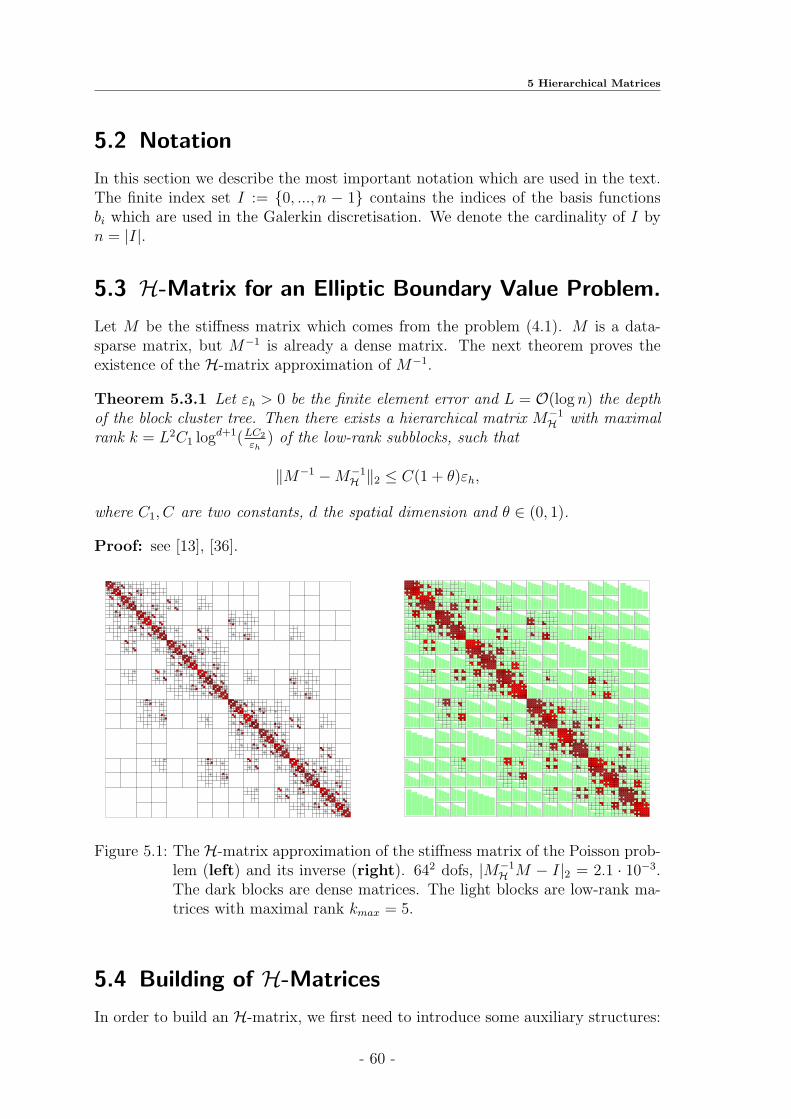
5 Hierarchical Matrices
5.2 Notation
In this section we describe the most important notation which are used in the text.The finite index set I := 0, ..., n − 1 contains the indices of the basis functionsbi which are used in the Galerkin discretisation. We denote the cardinality of I byn = |I|.
5.3 H-Matrix for an Elliptic Boundary Value Problem.
Let M be the stiffness matrix which comes from the problem (4.1). M is a data-sparse matrix, but M−1 is already a dense matrix. The next theorem proves theexistence of the H-matrix approximation of M−1.
Theorem 5.3.1 Let εh > 0 be the finite element error and L = O(log n) the depthof the block cluster tree. Then there exists a hierarchical matrix M−1
H with maximalrank k = L2C1 logd+1(LC2
εh) of the low-rank subblocks, such that
‖M−1 −M−1H ‖2 ≤ C(1 + θ)εh,
where C1, C are two constants, d the spatial dimension and θ ∈ (0, 1).
Proof: see [13], [36].
32 32
32 32
32 32
32 32
32 32
32 32
32 32
32 32
32
32 32
32
32 32
32
32 32
32
32 32
32 32
32
32 32
32
32 32
32
32 32
32
32 32
32 32
32 32
32 32
32 32
32 32
32 32
32 32
32 32
32 32
32
32 32
32 32
32
32 32
32 32
32 32
32 32
32
32 32
32 32
32
32 32
32 32
32 32
32 32
32 32
32 32
32 32
32 32
32 32
32 32
32
32 32
32
32 32
32
32 32
32
32 32
32 32
32
32 32
32
32 32
32
32 32
32
32 32
32 32
32 32
32 32
32 32
32 32
32 32
32 32
32
32 32
32
32 32
32
32 32
32
32 32
32
32 32
32
32 32
32
32 32
32
32 32
32
32 32
32
32 32
32 32
32
32 32
32
32 32
32
32 32
32
32 32
32
32 32
32
32 32
32
32 32
32
32 32
32
32 32
32
32 32
32 32
32 32
32 32
32 32
32 32
32 32
32 32
32
32 32
32
32 32
32
32 32
32
32 32
32 32
32
32 32
32
32 32
32
32 32
32
32 32
32 32
32 32
32 32
32 32
32 32
32 32
32 32
32 32
32 32
32
32 32
32 32
32
32 32
32 32
32 32
32 32
32
32 32
32 32
32
32 32
32 32
32 32
32 32
32 32
32 32
32 32
32 32
32 32
32 32
32
32 32
32
32 32
32
32 32
32
32 32
32 32
32
32 32
32
32 32
32
32 32
32
32 32
32 32
32 32
32 32
32 32
32 32
32 32
32 32
32 32
32 32
32
32 32
32 32
32
32 32
32 32
32
32 32
32 32
32
32 32
32 32
32
32 32
32 32
32
32 32
32 32
32 32
32 32
32
32 32
32 32
32
32 32
32 32
32
32 32
32 32
32
32 32
32 32
32
32 32
32 32
32
32 32
32 32
32 32
32 32
32 32
32 32
32 32
32 32
32 32
32 32
32
32 32
32
32 32
32
32 32
32
32 32
32 32
32
32 32
32
32 32
32
32 32
32
32 32
32 32
32 32
32 32
32 32
32 32
32 32
32 32
32 32
32 32
32
32 32
32 32
32
32 32
32 32
32 32
32 32
32
32 32
32 32
32
32 32
32 32
32 32
32 32
32 32
32 32
32 32
32 32
32 32
32 32
32
32 32
32
32 32
32
32 32
32
32 32
32 32
32
32 32
32
32 32
32
32 32
32
32 32
32 32
32 32
32 32
32 32
32 32
32 32
32 32
32
32 32
32
32 32
32
32 32
32
32 32
32
32 32
32
32 32
32
32 32
32
32 32
32
32 32
32
32 32
32 32
32
32 32
32
32 32
32
32 32
32
32 32
32
32 32
32
32 32
32
32 32
32
32 32
32
32 32
32
32 32
32 32
32 32
32 32
32 32
32 32
32 32
32 32
32
32 32
32
32 32
32
32 32
32
32 32
32 32
32
32 32
32
32 32
32
32 32
32
32 32
32 32
32 32
32 32
32 32
32 32
32 32
32 32
32 32
32 32
32
32 32
32 32
32
32 32
32 32
32 32
32 32
32
32 32
32 32
32
32 32
32 32
32 32
32 32
32 32
32 32
32 32
32 32
32 32
32 32
32
32 32
32
32 32
32
32 32
32
32 32
32 32
32
32 32
32
32 32
32
32 32
32
32 32
32 32
32 32
32 32
32 32
32 32
32 32
32 32
32
32 32
32
32 32
32
32 32
32
32 32
32
32 32
32
32 32
32
32 32
32
32 32
32
32 32
32
32 32
32
32 32
32
32 32
32
32 32
32
32 32
32
32 32
32
32 32
32
32 32
32
32 32
32
32 32
32
32 32
32
32 32
32
32 32
32 32
32
32 32
32
32 32
32
32 32
32
32 32
32
32 32
32
32 32
32
32 32
32
32 32
32
32 32
32
32 32
32
32 32
32
32 32
32
32 32
32
32 32
32
32 32
32
32 32
32
32 32
32
32 32
32
32 32
32
32 32
32
32 32
32
32 32
32 32
32 32
32 32
32 32
32 32
32 32
32 32
32
32 32
32
32 32
32
32 32
32
32 32
32 32
32
32 32
32
32 32
32
32 32
32
32 32
32 32
32 32
32 32
32 32
32 32
32 32
32 32
32 32
32 32
32
32 32
32 32
32
32 32
32 32
32 32
32 32
32
32 32
32 32
32
32 32
32 32
32 32
32 32
32 32
32 32
32 32
32 32
32 32
32 32
32
32 32
32
32 32
32
32 32
32
32 32
32 32
32
32 32
32
32 32
32
32 32
32
32 32
32 32
32 32
32 32
32 32
32 32
32 32
32 32
32
32 32
32
32 32
32
32 32
32
32 32
32
32 32
32
32 32
32
32 32
32
32 32
32
32 32
32
32 32
32 32
32
32 32
32
32 32
32
32 32
32
32 32
32
32 32
32
32 32
32
32 32
32
32 32
32
32 32
32
32 32
32 32
32 32
32 32
32 32
32 32
32 32
32 32
32
32 32
32
32 32
32
32 32
32
32 32
32 32
32
32 32
32
32 32
32
32 32
32
32 32
32 32
32 32
32 32
32 32
32 32
32 32
32 32
32 32
32 32
32
32 32
32 32
32
32 32
32 32
32 32
32 32
32
32 32
32 32
32
32 32
32 32
32 32
32 32
32 32
32 32
32 32
32 32
32 32
32 32
32
32 32
32
32 32
32
32 32
32
32 32
32 32
32
32 32
32
32 32
32
32 32
32
32 32
32 32
32 32
32 32
32 32
32 32
32 32
32 32
32 32
32 32
32
32 32
32 32
32
32 32
32 32
32
32 32
32 32
32
32 32
32 32
32
32 32
32 32
32
32 32
32 32
32 32
32 32
32
32 32
32 32
32
32 32
32 32
32
32 32
32 32
32
32 32
32 32
32
32 32
32 32
32
32 32
32 32
32 32
32 32
32 32
32 32
32 32
32 32
32 32
32 32
32
32 32
32
32 32
32
32 32
32
32 32
32 32
32
32 32
32
32 32
32
32 32
32
32 32
32 32
32 32
32 32
32 32
32 32
32 32
32 32
32 32
32 32
32
32 32
32 32
32
32 32
32 32
32 32
32 32
32
32 32
32 32
32
32 32
32 32
32 32
32 32
32 32
32 32
32 32
32 32
32 32
32 32
32
32 32
32
32 32
32
32 32
32
32 32
32 32
32
32 32
32
32 32
32
32 32
32
32 32
32 32
32 32
32 32
32 32
32 32
32 32
32 32
32
32 32
32
32 32
32
32 32
32
32 32
32
32 32
32
32 32
32
32 32
32
32 32
32
32 32
32
32 32
32 32
32
32 32
32
32 32
32
32 32
32
32 32
32
32 32
32
32 32
32
32 32
32
32 32
32
32 32
32
32 32
32 32
32 32
32 32
32 32
32 32
32 32
32 32
32
32 32
32
32 32
32
32 32
32
32 32
32 32
32
32 32
32
32 32
32
32 32
32
32 32
32 32
32 32
32 32
32 32
32 32
32 32
32 32
32 32
32 32
32
32 32
32 32
32
32 32
32 32
32 32
32 32
32
32 32
32 32
32
32 32
32 32
32 32
32 32
32 32
32 32
32 32
32 32
32 32
32 32
32
32 32
32
32 32
32
32 32
32
32 32
32 32
32
32 32
32
32 32
32
32 32
32
32 32
32 32
32 32
32 32
32 32
32 32
32 32
32 32
Figure 5.1: The H-matrix approximation of the stiffness matrix of the Poisson prob-lem (left) and its inverse (right). 642 dofs, |M−1
H M − I|2 = 2.1 · 10−3.The dark blocks are dense matrices. The light blocks are low-rank ma-trices with maximal rank kmax = 5.
5.4 Building of H-Matrices
In order to build an H-matrix, we first need to introduce some auxiliary structures:
- 60 -

5.4 Building of H-Matrices
1. the cluster tree (denoted by TI),
2. the block cluster tree (denoted by TI×I),
3. the admissibility condition (denoted by Admη or AdmW ).
5.4.1 Cluster Tree
We consider different partitions of I into disjoint subsets including coarse and finepartitions. The set of these partitions is hierarchically structured and is uniquelydefined by the tree T = TI , which is called cluster tree.
Notation 5.4.1 We denote all vertices of a tree T by V (T ) and all sons of a vertext by S(t).
Definition 5.4.1 A vertex v ∈ V (T ) is a leaf if sons(v) = ∅ and we define
L(T ) := v ∈ V (T )| v is a leaf.
Notation 5.4.2 The uniquely determined predecessor (father) of a non-root vertexv ∈ TI is denoted by F(v).
Definition 5.4.2 We define the levels l ∈ N0 of T recursively
T(0)I = I, T (l) := t ∈ TI |F(v) ∈ T l−1
I
and we write level(v)=l if v ∈ T (l)I .
The leaves of T on level l are denoted by
L(T, l) := T (l) ∩ L(T ).
Let the mappingˆ : TI → r | r ⊆ I labels vertices of the tree TI , i.e., if t ∈ TIand t ⊆ I thenˆ : t 7→ t.Thus, for each t ∈ TI , we denote its label by t ⊆ I.
Definition 5.4.3 A finite tree TI is a cluster tree over the index set I if the followingconditions hold:
• I is the root of T and t ⊆ I holds for all t ∈ TI .
• If t ∈ TI is not a leaf, then S(t) contains disjoint subsets of I and t is the
disjoint union of its sons, t =⋃
s∈S(t)
s.
• If t ∈ TI is a leaf, then |t| ≤ nmin for a fixed number nmin.
Definition 5.4.4 If |S(t)| = 2 for all t ∈ TI \L(TI), then TI is called a binary tree.
- 61 -

5 Hierarchical Matrices
0,1,2,3,4,5,6,7
0,1,2,3 4,5,6,7
0,1 2,3 4,5 6,7
Figure 5.2: An example of a cluster tree over the index set I = 0, 1, 2, 3, 4, 5, 6, 7.Each leaf contains nmin = 2 elements.
Definition 5.4.5 The vertices t ∈ V (T ) of a cluster tree are called clusters.
A cluster tree for I is usually denoted by TI . We write t ∈ TI for t ∈ V (TI).In [27], [13], [36] the reader can find two different algorithms for building cluster treesfor a given set of basis functions. The first one is based on a geometrical splittingand the second one on a cardinality splitting. Which one to choose depends, forexample, on the discretisation of a given problem.Each index i ∈ I is associated with the basis function bi of the Galerkin ansatz
space Vh := spanbii∈I , so that the support of the basis functions is denoted by
Ωi := supp(bi) for i ∈ I.
We generalize Ωt to cluster t ∈ TI by setting
Ωt :=⋃
i∈t
Ωi, t ∈ TI . (5.1)
Construction of a cluster tree
Since dealing directly with the supports will be too complicated, we choose a pointxi ∈ Ωi for each index i ∈ I and work with these points instead of the supports. Thissimplification will not significantly harm the performance of the algorithm, since thesupports of the typical finite element basis function is small.Our construction of the cluster tree starts with the dense index set I, which is theroot of the cluster tree by definition. After that we apply a suitable technique tofind a disjoint partition of the index set and use this partition to create the sonclusters. We apply the procedure recursively to the sons until the index sets aresmall enough. To make the partition easier we define for the given domain Ωt from(5.1) a minimal axes-parallel bounding box Qt =
∏di=1[ai, bi], where Qt ⊃ Ωt. The
coordinates ai and bi can be defined as following
for i=1 to dai := minj∈t xj,ibi := maxj∈t xj,i
(5.2)
Each index i ∈ t corresponds to a point xi ∈ Rd. There are some variants ofsplitting the boundary box Qt. For example, we can choose the coordinate directionof the maximal extent and split the box perpendicular to this direction into twosubdomains. This gives us the partition t0, t1 of t (respectively Qt = Qt1 ∪Qt2).
- 62 -

5.4 Building of H-Matrices
Remark 5.4.1 See the algorithms of splitting based on the geometry of Ωt and thecardinality in Sections 5.5.2 , 5.5.3 in [36] and [13].
The building of the special cluster tree TI
The input data for the building of the cluster tree TI is the index set I. In this workwe use the geometrically balanced clustering (see other variants of the clustering in[28], [27]). This means that for building cluster trees we use the geometry of thegiven domain.Let I, I11, I12 and I2 be given index sets such that I = I11 ∪ I12 ∪ I2. Let TI11 , TI12 ,TI2 be given cluster trees, based on I11, I12 and I2. We want to build the binarycluster tree TI such that I11, I12, I2 ∈ TI (see Fig. 5.3). For this purpose we buildcluster I1 which has two sons I11, I12 and cluster I which has sons I1 and I2.
...
......
TI
TI1 TI2
TI11 TI12
Figure 5.3: The structure of the cluster tree TI .
5.4.2 Block Cluster Tree
While the vector components are indexed by i ∈ I, the entries of a matrix haveindices from the index set I × J . The block-cluster tree is nothing but a specialcluster tree over the product index set I × J . The vertices (“blocks”) b ∈ TI×J areof the form b = (t, s) with t ∈ TI , s ∈ TJ .
Definition 5.4.6 Let TI and TJ be cluster trees over the index sets I and J . Afinite tree T is a block cluster tree based on TI and TJ if the following conditionshold:
• root(T ) = I × J .
• Each vertex b ∈ V (T ) has the form b = (t, s) for cluster t ∈ TI and s ∈ TJ .
• For each vertex (t, s) ∈ V (T ) with sons(t, s) 6= ∅, we have
sons(t, s) =
(t, s′) : s′ ∈ sons(s), if sons(t) = ∅ ∧ sons(s) 6= ∅
(t′, s) : t′ ∈ sons(t), if sons(t) 6= ∅ ∧ sons(s) = ∅
(t′, s′) : t′ ∈ sons(t), s′ ∈ sons(s), otherwise(5.3)
• The label of a vertex (t, s) ∈ V (T ) is given by (t, s) = t× s ⊆ I × J .
- 63 -

5 Hierarchical Matrices
A block cluster tree based on TI and TJ is denoted by TI×J . We will use the
abbreviation (t, s) ∈ TI×J for (t, s) ∈ V (TI×J). We can see that root(TI×J) = I × J .This implies that the set of leaves L(TI×J) is a partition of I×J . An implementationof the block cluster tree can be found in [28].
Definition 5.4.7 Let TI×J be a block cluster tree. We call P a partition (or a blockpartition) of I × J if:
P ⊂ TI×J ,b, b′ ∈ P ⇒ (b = b′ or b ∩ b′ = ∅),⋃
b∈P = I × J.(5.4)
5.5 Admissibility
The admissibility condition helps us to find a balance between the storage require-ments of an H-matrix and its approximation accuracy. It also helps us to identifythe blocks which can be approximated well by a low-rank matrices. Let t ∈ TI ,s ∈ TJ and t× s ∈ TI×J .
Definition 5.5.1 The admissibility condition is a Boolean function
Adm : TI×J 7→ true, false (5.5)
with the consistency requirement
Adm(b)⇒ Adm(b′) for all sons b′ of b ∈ TI×J
and the property Adm(b)=true for all leaves b ∈ TI×J .
5.5.1 Standard Admissibility Condition (Admη)
Definition 5.5.2 The standard admissibility criterion for b = (t, s) is
mindiam(Ωt), diam(Ωs) ≤ ηdist(Ωt,Ωs), (5.6)
where η > 0 is a fixed parameter.The admissibility condition (5.5) now takes the form of
Admη(b) = true for b = (t, s) ∈ TI×J :⇐⇒(b is a leaf) or (5.6) holds.
In practice it is difficult to define the Euclidean diameter diam(Ωt) and the Euclideandistance of two clusters dist(Ωt,Ωs). This is the reason why we rewrite the standardadmissibility criterion for the bounding boxes.We define a minimal axis-parallel box Qt ⊆ R2 such that Ωt ⊆ Qt holds.This box will be called the bounding box of the cluster t.
Definition 5.5.3 The standard admissibility criterion for Qt and Qs is:
- 64 -

5.5 Admissibility
mindiam(Qt),diam(Qs) ≤ η dist(Qt, Qs).
Let d be the spatial dimension. We can compute the distances and diameters asfollows:If Qt = [a1, b1]× ...× [ad, bd] and Qs = [c1, d1]× ...× [cd, dd] then
diam(Qt) =√∑d
l=1 (bl − al)2, diam(Qs) =√∑d
l=1 (dl − cl)2 and
dist(Qs, Qt) =√∑d
l=1 dist([al, bl], [cl, dl])2.
Where does the admissibility condition come from?Suppose the following propositions are true:
• B1 ⊂ Rd and B2 ⊂ Rd are compact.
• χ(x, y) is defined for (x, y) ∈ B1 ×B2 with x 6= y.
Let K be an integral operator with an asymptotic smooth kernel K in the domainB1 ×B2:
(Kv)(x) =
∫
B2
χ(x, y)v(y)dy (x ∈ B1).
Suppose that χ(k)(x, y) is an approximation of χ in B1 ×B2 of the separate form:
χ(k)(x, y) =k∑
ν=1
ϕ(k)ν (x)ψ(k)
ν (y),
where k is the rank of separation (index (k) is not a derivative!).Then, under some conditions (see Paragraph 4.6.3 [36],[13]) we have
‖χ− χ(k)‖∞,B1×B2 ≤ c1
[c2 mindiam(B1), diam(B2)
dist(B1, B2)
]k. (5.7)
Proof: See Paragraph 4.6.3 in [36].Now, if
mindiam(B1), diam(B2) ≤1
c2dist(B1, B2). (5.8)
there is an exponential convergence in (5.7).
Definition 5.5.4 Let η > 0 and t, s be two clusters, Ωt and Ωs are supports of tand s. The block b = (t, s) is called η-admissible, if
mindiam(t), diam(s) ≤ dist(t, s). (5.9)
5.5.2 Weak Admissibility Condition (AdmW )
Definition 5.5.5 In the 1D case AdmW (b) = true for b = (t, s) ∈ TI×J :⇔ ((b is aleaf) or t and s are different clusters.
In the following remark we list properties of the weak admissibility condition.
- 65 -
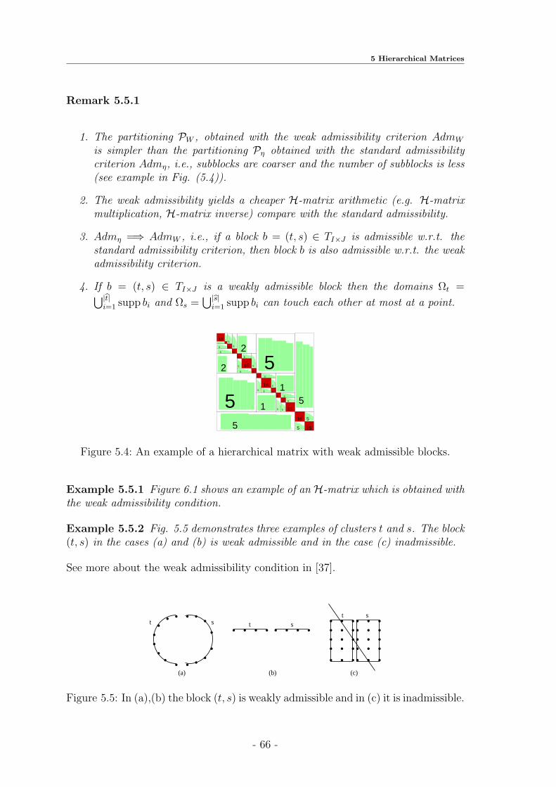
5 Hierarchical Matrices
Remark 5.5.1
1. The partitioning PW , obtained with the weak admissibility criterion AdmW
is simpler than the partitioning Pη obtained with the standard admissibilitycriterion Admη, i.e., subblocks are coarser and the number of subblocks is less(see example in Fig. (5.4)).
2. The weak admissibility yields a cheaper H-matrix arithmetic (e.g. H-matrixmultiplication, H-matrix inverse) compare with the standard admissibility.
3. Admη =⇒ AdmW , i.e., if a block b = (t, s) ∈ TI×J is admissible w.r.t. thestandard admissibility criterion, then block b is also admissible w.r.t. the weakadmissibility criterion.
4. If b = (t, s) ∈ TI×J is a weakly admissible block then the domains Ωt =⋃|bt|i=1 supp bi and Ωs =
⋃|bs|i=1 supp bi can touch each other at most at a point.
13 4
4 45
5 8 5
5 82
28 5
5 16 5
5 85
5
8 5
5
16 5
5 81
18 5
5
8 5
5 15
5
516 5
5 15
Figure 5.4: An example of a hierarchical matrix with weak admissible blocks.
Example 5.5.1 Figure 6.1 shows an example of an H-matrix which is obtained withthe weak admissibility condition.
Example 5.5.2 Fig. 5.5 demonstrates three examples of clusters t and s. The block(t, s) in the cases (a) and (b) is weak admissible and in the case (c) inadmissible.
See more about the weak admissibility condition in [37].
....... . . . ...
...t s . . . . . . . . . . .. . .. . .. . .
. . .
. . .. . .. . .
. . .
. . .
(a) (b) (c)
t st s
Figure 5.5: In (a),(b) the block (t, s) is weakly admissible and in (c) it is inadmissible.
- 66 -
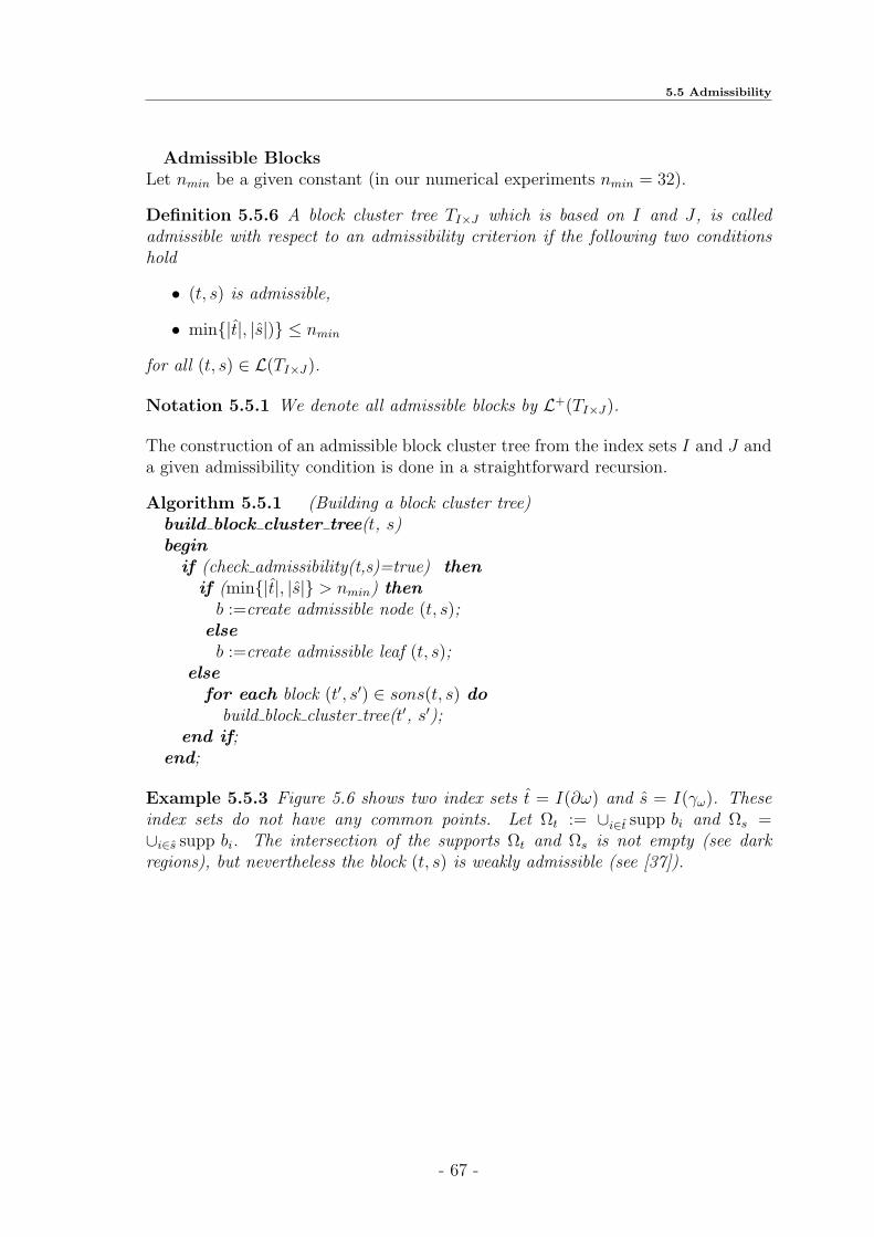
5.5 Admissibility
Admissible BlocksLet nmin be a given constant (in our numerical experiments nmin = 32).
Definition 5.5.6 A block cluster tree TI×J which is based on I and J , is calledadmissible with respect to an admissibility criterion if the following two conditionshold
• (t, s) is admissible,
• min|t|, |s|) ≤ nmin
for all (t, s) ∈ L(TI×J).
Notation 5.5.1 We denote all admissible blocks by L+(TI×J).
The construction of an admissible block cluster tree from the index sets I and J anda given admissibility condition is done in a straightforward recursion.
Algorithm 5.5.1 (Building a block cluster tree)build block cluster tree(t, s)begin
if (check admissibility(t,s)=true) thenif (min|t|, |s| > nmin) thenb :=create admissible node (t, s);
elseb :=create admissible leaf (t, s);
elsefor each block (t′, s′) ∈ sons(t, s) do
build block cluster tree(t′, s′);end if;
end;
Example 5.5.3 Figure 5.6 shows two index sets t = I(∂ω) and s = I(γω). Theseindex sets do not have any common points. Let Ωt := ∪i∈t supp bi and Ωs =∪i∈s supp bi. The intersection of the supports Ωt and Ωs is not empty (see darkregions), but nevertheless the block (t, s) is weakly admissible (see [37]).
- 67 -

5 Hierarchical Matrices
∂ω
γω
Figure 5.6: The intersection of supports Ωs and Ωt of two clusters t and s, wheret = I(∂ω) and s = I(γω) is not empty (see dark regions), but neverthelessthe weak admissible criterion can be applied and the block b = (t, s) isweakly admissible.
Inadmissible Blocks
Definition 5.5.7 A block (t, s) for which an admissibility criterion (standard, weakor some other) is false, is called inadmissible. We denote the set of all inadmissibleblocks in L(TI×J) by L−(TI×J).
Recall that parameter nmin is responsible for the maximal size of inadmissible blocks.If a block b = (t, s) does not satisfy to the first condition in Def. 5.5.6, butmin|t|, |s|) ≤ nmin, then b is approximated by a dense matrix. If the parame-ter nmin is small (e.g. nmin < 16), then the matrix has a deeper hierarchy and thecomplexity of all arithmetic operations increases. On the other hand, if nmin is toolarge, the fully-populated matrix arithmetic begins to dominate.
5.6 Low-rank Matrix Format
Sometimes the name rank-k matrix format is used.The rank-k matrices are very important for the construction of H-matrices. We givethe definition of rank-k matrices and we describe the low-rank arithmetic. Then weestimate the complexity of arithmetic operations and their implementation.
Let M ∈ RI×J be a matrix, I, J two index sets. Consider the factorization
M = ABT where A ∈ RI×1,...,k, B ∈ RJ×1,...,k, k ∈ N0. (5.10)
Definition 5.6.1 We say that matrix M is a rank-k matrix if the representation(5.10) is given. We denote the class of all rank-k matrices for which factors Aand BT in (5.10) exist by R(k, I, J) or R(k, n,m), where n := |I|, m := |J |. IfM ∈ R(k, I, J) we say that M has a low-rank representation.
Remark 5.6.1 If A,B and C are matrices and A := B · C thenRank(A) ≤ minRank(B), Rank(C). As a sequence we have Rank(M) = Rank(ABT ) ≤k for matrices from (5.10).
Remark 5.6.2 Note that we do not state that the matrix M from the representation(5.10) has a rank k, but if Rank(M) = k0 then there exists a factorization (5.10)with k := k0.
- 68 -

5.6 Low-rank Matrix Format
Proof: see Remark 2.2.2 in [36].
Definition 5.6.2 M ∈ R(k, I, J) :⇐⇒M ∈ RI×J is represented in format (5.10).
Remark 5.6.3 To store a matrix M ∈ R(k, n,m) we need k(n+m) units of mem-ory. A dense matrix M ∈ Rn×m requires n ·m units of memory. For k ≪ minn,mthe profit nm− k(n+m) is especially remarkable.
To introduce an approximate arithmetic in R(k, I, J) we recall the singular valuedecomposition.
Definition 5.6.3 A dense matrix M ∈ Rn×m has a singular value decomposition(SVD) M = UΣV T , if U ∈ Rn×n, V ∈ Rm×m are unitary and Σ ∈ Rn×m is diagonalwith singular values Σii (w.l.o.g. we can suggest that Σ11 ≥ Σ22 ≥ ... ≥ Σnn,n = minn,m).
To get the reduced singular value decomposition we omit all singular values, whichare smaller than some level ε or we leave a fixed number of singular values (seeFigure 5.7). After truncation we speak about reduced singular value decomposition(denoted by rSVD) M = UΣV T , where U ∈ Rn×k contains the first k columns of U ,V ∈ Rm×k contains the first k columns of V and Σ ∈ Rk×k contains the k-biggestsingular values of Σ (see Fig. 5.7).
U VΣ T=M
UVΣ∼
∼ ∼ T
=M∼
Figure 5.7: Reduced SVD, only k biggest singular values are taken.
Lemma 5.6.1 Let M ∈ Rn×m and M = UΣV T (U,V orthogonal, Σ diagonal withsingular values σi = Σii and σ1 ≥ σ2 ≥ ...). Then
R := UΣV T with Σij =
σi for i = j ≤ mink, n,m,0 otherwise,
(5.11)
U := U |n×k, V := V |m×k is the solution of the following two problems:
minRank(R)≤k
‖M −R‖2 and minRank(R)≤k
‖M −R‖F . (5.12)
The errors are
‖M −R‖2 = σk+1 and ‖M −R‖F =
√√√√minn,m∑
i=k+1
σ2i . (5.13)
- 69 -

5 Hierarchical Matrices
Proof: see [51] or [25].
Let M = ABT ∈ Rn×m be a matrix in the rank-k matrix format, i.e. A and Bare given. An rSVD M = UΣV T can be computed efficiently in three steps:
1. Compute (reduced) a QR-factorization of A = QARA and B = QBRB, whereQA ∈ Rn×k, QB ∈ Rm×k, and upper triangular matrices RA, RB ∈ Rk×k.
2. Compute an rSVD of RARTB = U ′ΣV ′T .
3. Compute U := QAU′, V := QAV
′T .
For the realization of these steps the linear algebra packages LAPACK and BLASare used. The first and third steps need O((n + m)k2) operations and the secondstep needs O(k3). The total complexity of rSVD is O((n +m)k2 + k3). Hence, wecan compute rSVD of M with a linear complexity.In HLIB one can find an implementation of this algorithm.Now we introduce the rank-k matrix arithmetic. Later on we will use these opera-tions for the definition of the H-matrix arithmetic.
Lemma 5.6.2 The product of a rank-k matrix and a dense matrix is again a rank-kmatrix. Let R ∈ R(k, n,m), N ∈ Rn′×n and M ∈ Rm×m′
. Then
NR ∈ R(k, n′,m), RM ∈ R(k, n,m′). (5.14)
Proof: If R = ABT then NR = (NA)BT and RM = A(MTB)T .
Lemma 5.6.3 Let R1 ∈ R(k1, n,m) and R2 ∈ R(k2, n,m). Then R1+R2 ∈ R(k1+k2, n,m).
Proof: If R1 = ABT and R1 = CDT then R1 + R2 = [AC][BD]T , where matrix[AC] ∈ Rn×(k1+k2) and matrix [BD] ∈ Rm×(k1+k2). Adding two rank-k matrices doesnot require arithmetic operations, but the result matrix has a larger rank. This iswhy we introduce the operation truncation.
Definition 5.6.4 (Truncation Tk)Let k′ < k and M ∈ R(k, n,m) be a rank-k matrix. We define the truncation
operatorT Rk′←k : R(k, n,m)→ R(k′, n,m) by M = T Rk′←k(M),
where M is a best approximation of M in the set R(k, n,m) (not necessarily unique).
Notation 5.6.1 If in Def. 5.6.4 the rank of the source matrix is not important wewill write Tk′.Lemma 5.6.4 (Multiplication of rank-k matrices).Let M1 ∈ R(k1, I, J) and M2 ∈ R(k2, J,K) be given:
M1 = A1BT1 , M2 = A2B
T2 .
The product M := M1M2 can be represented as1. M ∈ R(k2, I,K) with A = A1B
T1 A2 and B = BT
2 . The computation of A costs2k1k2(|I|+ |J |)− k2(|I|+ k1);2. M ∈ R(k1, I,K) with A = A1 and B = B2A
T2B1. The computation of A costs
2k1k2(|J |+ |K|)− k1(|K|+ k2).
- 70 -

5.7 Hierarchical Matrix Format
Proof: see ,e.g., [36].
Definition 5.6.5 The formatted addition ⊕ in the set R(k, n,m) is
A⊕B := Tk(A+B), A,B ∈ R(k, n,m).
Remark 5.6.4 Note that ⊕ is commutative, but in general not distributive (i.e.,(A⊕B)⊕ C and A⊕ (B ⊕ C) may differ).
Theorem 5.6.1 Let k ∈ N be a maximal rank, and I, J , K be index sets. Table5.1 shows storage requirements and computational complexities for rank-k matrices.
Operation Description Complexity
storage(M) M ∈ R(k, I, J), M = ABT k(|I|+ |J |)Mx M ∈ R(k, I, J),M = ABT , x ∈ RJ 2k(|I|+ |J |)− |I| − kM ′ +M ′′ M ′ ∈ R(k′, I, J),M ′′ ∈ R(k′′, I, J) (|I|+ |J |)(k′ + k′′)M ′M ′′ M ′ ∈ R(k′, I, J),M ′′ ∈ R(k′′, I, J) 2k′k′′(|I|+ |J |)− k′′(|I|+ k′)rSVD(M) M = ABT ∈ R(k, I, J) 6k2(|I|+ |J |) + 22k3
T Rk′←k(M) T Rk′←k : R(k, I, J)→ R(k′, I, J) 6k2(|I|+ |J |) + 22k3
M ′ ⊕k M ′′ M ′,M ′′ ∈ R(k, I, J) 24k2(|I|+ |J |) + 176k3
Table 5.1: Storage requirements and computational complexities for rank-k matrices.
Proof: see [33], [27], [13], [36].
5.7 Hierarchical Matrix Format
Definition 5.7.1 Let M ∈ RI×J and I ′×J ′ be a subset of I×J , then the submatrixM |I′×J ′ := (Mi,j)(i,j)∈I′×J ′. For a superset I
′′ × J′′ ⊃ I × J we define the matrix
M′′
:= M |I′′×J ′′
∈ RI′′×J ′′
such that
M′′
ij :=
Mij if (i, j) ∈ I × J,0 otherwise.
(5.15)
Definition 5.7.2 Let I and J be two finite index sets, T := TI×J a block clustertree, P a block partition, k : P → N a given mapping, nmin a small integer. The setof H-matrices H(T, k) ⊂ RI×J (with the partition P and the mapping k) consists ofall M ∈ RI×J with
rank(M |b) ≤ k(b) for all b ∈ L+(T ) and (5.16)
for all b ∈ L+(T ) the factors A, B in M |b = ABT are given explicitly. The matrixblocks b ∈ L−(T ) are given in the standard full matrix representation and are small(the rank is smaller than nmin).
- 71 -

5 Hierarchical Matrices
If ∀b ∈ T k(b) = k then we speak about fixed rank, otherwise, about adaptive rank.
Let us write A ∈ H(TI×J , k,P) if we want to underline that matrix A has thepartitioning P (we denote the weak partitioning by the subindex W and the standardpartitioning by the subindex η).
Definition 5.7.3 Let TI×J be a block cluster tree for the index sets I and J . Amatrix M ∈ H(TI×J , k) is said to be stored in the H-matrix representation if thesubmatrices corresponding to inadmissible leaves are stored as dense matrices andthose corresponding to admissible leaves are stored in the rank-k matrix representa-tion.
To measure the sparsity property of a block cluster tree we introduce the following
Definition 5.7.4 Let TI×J be a block cluster tree based on TI and TJ . We definethe sparsity constant Csp of TI×J by
Csp := maxmaxt∈TI
|s|(t, s) ∈ L(T )|,maxs∈TJ
|t|(t, s) ∈ L(T )|.
Remark 5.7.1 The complexities of all H-matrix arithmetic operations depend onCsp. For a model integral equation, which is discretised by BEM with the standardadmissibility criterion, the constant Csp takes values 3, 27, 189 for 1D, 2D, 3Dproblems accordingly.
Remark 5.7.2 Numerical experiments show that matrices from H(TI×J , k,Pη) andH(TI×J , 3k,PW ) give approximate similar accuracy. The storage and computationaltime for the matrices from H(PW , 3k) are smaller than the corresponding storageand time for H(Pη, k) .
Lemma 5.7.1 1. Let A ∈ H(TI×J , kA,PW ) and B ∈ H(TI×J , kB,PW ), then theexact product A ·B belongs to H(TI×J , kA + kB,PW ).
2. Let A ∈ H(TI×J , k,PW ) be invertible, then A−1 ∈ H(TI×J , k,PW ).
3. Let A ∈ H(TI×I , k,PW ) and I ′ ⊂ I, then the Schur complement isSI′ = A|I′×I′−A|I′×I′′ ·(A|I′′×I′′)−1·A|I′′×I′, I ′′ = I\I ′, provided that (A|I′′×I′′)−1
exists.
Proof: See [37].
Remark 5.7.3 In HLIB we use the structures supermatrix forH-matrices, rkmatrixfor rank-k matrices and fullmatrix for dense matrices.
- 72 -

5.8 Filling of Hierarchical Matrices
5.8 Filling of Hierarchical Matrices
Suppose we have cluster trees TI , TJ , |I| > |J |, a block cluster tree TI×J and anadmissibility criterion. Below we show how we compute elements of M ∈ H(TI×J , k)with complexity O(|I| log |I|) (see more in [33], [29], [28]). Depending on the defini-tion of M , different algorithms for the determinations of the matrix representationsare needed.
Example 5.8.1 1. The matrix M comes from an integral equation.
2. The matrix M comes from a partial differential equation.
3. The matrix M is built from the H-matrices M1 and M2 (our case).
5.8.1 H-Matrix Approximation of BEM Matrix
Consider the following integral equation
∫ 1
0
log |x− y|U(y)dy = F (x), x ∈ (0, 1).
After discretisation by Galerkin’s method we obtain
∫ 1
0
∫ 1
0
φi(x) log |x− y|U(y)dydx =
∫ 1
0
φi(x)F (x)dx, 0 ≤ i < n,
in the space Vn := spanφ0, ..., φn−1, where φi, i = 1, ..., n − 1, are some basisfunctions in BEM. The discrete solution Un in the space Vn is Un :=
∑n−1j=0 ujφj with
uj being the solution of the linear system
Gu = f, Gij :=
∫ 1
0
∫ 1
0
φi(x) log |x− y|φj(y)dydx, fi :=
∫ 1
0
φi(x)F (x)dx.
(5.17)We replace the kernel function g(x, y) = log |x− y| by a degenerate kernel
g(x, y) =k−1∑
ν=0
gν(x)hν(y). (5.18)
Then we substitute g(x, y) = log |x− y| in (5.17) for g(x, y)
Gij :=
∫ 1
0
∫ 1
0
φi(x)k−1∑
ν=0
gν(x)hν(y)φj(y)dydx.
After easy transformations
Gij :=k−1∑
ν=0
(
∫ 1
0
φi(x)gν(x)dx)(
∫ 1
0
hν(y)φj(y)dy).
- 73 -

5 Hierarchical Matrices
Now, all admissible blocks G|(t,s) can be represented in the form
G|(t,s) = ABT , A ∈ R|t|×k, B ∈ R|s|×k,
where the entries of the factors A and B are
Aiν :=
∫ 1
0
φi(x)gν(x)dx, Bjν :=
∫ 1
0
φj(y)hν(y)dy.
We use the fact that the basis functions are local and obtain for all inadmissibleblocks:
Gij :=
∫ (i+1)/n
i/n
∫ (j+1)/n
j/n
log |x− y|dydx.
5.8.2 H-Matrix Approximation of FEM Matrix
The finite element discretisation of a partial differential equation leads to a data-sparse matrix with O(n) elements. For an elliptic equation
−u = g, in Ω ⊂ Rd
u = 0, on ∂Ω
the linear system is (see Section 3.4)
Au = c, Aij :=
∫
Ω
〈∇bi(x),∇bj(x)〉dx, ci :=
∫
Ω
bigdx,
where A is sparse. If the LU decomposition of A or A−1 is required, then A isconverted to the H-matrix format and the efficient H-matrix arithmetic is applied(see HLIB).
5.8.3 Building of an H-Matrix from other H-Matrices
Let I ′, I ′′ ⊂ I and J ′, J ′′ ⊂ J be index sets, T ′I′×J ′ , T ′′I′′×J ′′ and TI×J be three blockcluster trees. Let M1 ∈ H(T ′I′×J ′ , k1), M2 ∈ H(T ′′I′′×J ′′ , k2) and M ∈ H(TI×J , k),then we can define
M := M1|I×J +M2|I×J .For more details see Subsection 5.9.8.
5.9 Arithmetics of Hierarchical Matrices
In this section we describe the algorithms that perform the addition, multiplicationand inversion in the hierarchical matrix format. The reader can get more infor-mation in [33], [29], [13] (English) and [27], [36] (German). Here, we also explainhow to sum and multiply hierarchical matrices which have different block structures.
- 74 -

5.9 Arithmetics of Hierarchical Matrices
Remark 5.9.1 In this Section and further, for simplicity of the notation, we posethat t and t are equivalent and we do not separate between t and t. For instance,|t| = |t|, M |t×s = M |(t,s).
In Section 5.6 we have defined the operator T Rk′←k, which truncates a rank-k matrixto the rank-k′ matrix, k′ < k. An extension of this operator to H-matrices is asfollows:
Definition 5.9.1 (truncation of H-matrices)Let T := TI×J be a block cluster tree and n := |I|, m := |J |. Let M ∈ Rn×m,M ′ ∈ H(T, k). We define the truncation operator
T Hk : Rn×m → H(T, k), M 7→M ′,
where M ′ = T Hk (M) and M ′|(r,s) = T Rk (M |(r,s)) for all (r, s) ∈ L+(T ) and M ′|(r,s) =M |(r,s) for all (r, s) ∈ L−(T ).
Definition 5.9.2 An alternative truncation operator Tε is defined in the followingway:
Tε(M) := argminrank(R)|‖R−M‖2‖M‖2≤ ε,
where the parameter ε is a desired accuracy.
Definition 5.9.3 If the rank k of M ∈ H(TI×J , k) (see Definition 5.7.2) is fixeda priory then we speak about fixed rank arithmetic. If the rank k depends on ablock b ∈ TI×J and is chosen as follows
k = mini : σi ≤ εaσ1,
where σi are the singular values of M |b then we speak about adaptive rankarithmetic (see [13] or Section 6 in [27]).
The use of both truncation operators makes the matrix arithmetic more flexible.
Definition 5.9.4 (Formatted addition of two hierarchical matrices)Let A,B,C ∈ H(TI×J , k), k ∈ N. The formatted addition of the matrices A and Bis defined by
C := A⊕B := Tk(A+B).
If the rank k under consideration is not evident then we write ⊕k instead of ⊕.
Definition 5.9.5 (Formatted multiplication of two hierarchical matrices)Let A ∈ H(TI×J , k), B ∈ H(TJ×K , k), C ∈ H(TI×K , k), k ∈ N. The formattedmultiplication of the matrices A,B is defined by
C = A⊙B := Tk(A ·B).
- 75 -

5 Hierarchical Matrices
The block structure of theH-matrix product A·B does not retain either the structureof matrices A or B and can become rather complicated. See more details about H-matrix multiplication in [13], [36] and [27].Let J , J1 and J2 be three index sets and J = J1 ∪ J2, J1 ∩ J2 = ∅. Let M ∈ RI×J ,M1 ∈ RI×J1 and M2 ∈ RI×J2 be three matrices and M = [M1M2] ∈ RI×J . Theformatted agglomeration of matrices M1 and M2 is defined by:
[M1M2] := M1|I×J +M2|I×J . (5.19)
Definition 5.9.6 Let k1, k2 ∈ N0, M1 ∈ R(k1, I, J1),M2 ∈ R(k2, I, J2) and J =J1∪J2, J1∩J2 = ∅. Then M = T Rk←k1+k2
([M1M2]) = M1|I×J⊕kM2|I×J ∈ R(k, I, J)is called formatted agglomeration.
In the general case there are more than two terms of the agglomeration.
Definition 5.9.7 Let Mi ∈ R(ki, I, J), i = 1, ..., q. The operation
M := T Rk←Pqi=1 ki
(
q∑
i=1
Mi) (5.20)
is the truncated agglomeration of q terms.
Lemma 5.9.1 If in (5.20) k1 = k2 = ... = kq = k, then the complexity of thetruncated agglomeration of q terms is O(k2q2n), n = max|I|, |J |.Proof: The cost of the truncation Tk←2k is O((2k)2n). For q terms the cost isO((kq)2)n) = O(k2q2n).
Remark 5.9.2 A second possibility of a truncated agglomeration for q > 2 is thepairwise truncation:
M = T Rk←k1+kM1 + ...+ T Rk←kq−2+k(Mq−2 + T Rk←kq−1+kq(Mq−1 +Mq))...). (5.21)
Lemma 5.9.2 The complexity of the truncated addition as in (5.21) is
O(k2max(q − 1)n), (5.22)
where k′max := maxki + k| i = 1, ..., q − 2 and kmax := maxk′max, kq−1 + k.Proof: The cost of the truncation Tki←ki+1+ki+2
is O((ki+1 + ki+2)2n).
Let kmax := ki + ki+1, i = 1, ..., q − 1. For q terms the cost is O(k2max(q − 1)n).
Remark 5.9.3 The pairwise truncated addition of q terms is cheaper than the directtruncated addition (5.20) of q terms. For k1 = ... = kq the profit is
(q2 · k2 − (2k)2 · (q − 1))n = (q2 − 4q + 4)k2n.
But practical experiments show that the accuracy of the pairwise truncated additionis worse than the truncated addition of q terms.
Remark 5.9.4 It is also may be possible that the following truncated addition
M = T Rk←k1+k2+k(M1 +M2 + ...+ T Rk←kq−4+kq−3+k(Mq−4 +Mq−3
+T Rk←kq−2+kq−1+kq(Mq−2 +Mq−1 +Mq))...).
is cheaper than the pairwise truncated addition.
- 76 -

5.9 Arithmetics of Hierarchical Matrices
5.9.1 Matrix - Vector Multiplication
Let M ∈ H(TI×J , k), n = |I|, m = |J |, v ∈ Rm and w ∈ Rn. The matrix-vector(denote by MV) multiplication w = Mv is realized in a recursive way. The procedureMV (M [i], v[i], w[i]), where M [i], v[i] and w[i] are corresponding parts of M , v andw calls itself recursively.
Remark 5.9.5 Implementation of MV multiplication in HLIB iseval supermatrix(M, v, w).
5.9.2 Matrix - Matrix Multiplication
The H-matrix multiplication (denote by MM) A · B = C, where A ∈ H(TI×J , k),B ∈ H(TJ×K , k) and C ∈ H(TI×K , k) is realized block-wise recursively. Supposethat A and B are 2× 2 blocks matrices, then
(A11 A12
A21 A22
)(B11 B12
B21 B22
)= Tk
(A11 ⊙B11 ⊕ A12 ⊙B21 A11 ⊙B12 ⊕ A12 ⊙B22
A21 ⊙B11 ⊕ A22 ⊙B21 A22 ⊙B22 ⊕ A21 ⊙B12
).
Remark 5.9.6 In the case when the matrices A and B have different block struc-tures the H-matrix multiplication of A and B is possible after conversion of A or Bto the respective format.
Thus, the product of two H-matrices or their sum can require the truncation ofthe rank.
Lemma 5.9.3 (complexity of the H-matrix truncation)Let T := TI×J be a block cluster tree, based on the cluster trees TI and TJ . Atruncation T Hk′←k(M) of M ∈ H(TI×J , k) can be computed with the complexity
Nk′←k ≤ 6kNSt(T, k) + 23k3|L(T )|,
where NSt is the storage requirement for M .
Proof: see Lemma 2.9 in [29].
5.9.3 Hierarchical Approximation T R←Hk
The hierarchical approximation is applied for the MM multiplication and for theMM conversion.
Notation 5.9.1 We denote an operator which truncates a dense matrix M ∈ RI×J
to a rank-k matrix by T R←Fk .
Note that T R←Fk (M) is done by the singular value decomposition (see Section 5.6).
Notation 5.9.2 We denote the operator, which hierarchically convert M ∈ H(TI×I , k)to a rank-k matrix in p+ 1 steps (see Fig. 5.8) by T R←Hk .
- 77 -

5 Hierarchical Matrices
Definition 5.9.8 (Hierarchical Approximation) Let TI×I be a block cluster tree, p :=depth(TI×I), M ∈ H(TI×I , k). Let P be a partitioning. We define the hierarchicalapproximation MH of M in p+ 1 steps as follows:
T R←Hk :=
T R←Fk (M |b) if b ∈ L(TI×J) ∧ b is inadmissible,T Rk (M |b) if b ∈ L(TI×J) ∧ b is admissible,T Rk←k·|S(b)|(M |b) if b ∈ P ∧ b /∈ L(TI×J),
where |S(b)| is the number of sons of b.
The hierarchical approximation (see Fig. 5.8) contains two subprocedures:
1. The conversion a given dense matrix to a rank-k matrix(addfull2 rkmatrix(..) in HLIB).
2. Adding two or more rank-k matrices with truncation to a rank-k matrix(addparts2 rkmatrix(..) in HLIB).
Lemma 5.9.4 Let M ∈ H(TI×J , k), R ∈ R(k, I, J). The complexity of the trunca-tion R = T R←Hk (M) is O(k2n log n), where n = max|I|, |J |.
Proof: see Lemma 6.4.4 in [36].
F RR R
R R
RR
RR R
R
R
Figure 5.8: Three steps of the hierarchical approximation. The first step is the con-version of a dense matrix F to a rank-k matrix R. In the second stepfour rank-k matrices are converted to a larger rank-k matrix. In stepthree two low-rank matrices are converted to a global rank-k matrix.
Lemma 5.9.5 (Hierarchical Approximation Error)Let p := depth(TI×J), M ∈ H(TI×J , k) and MH be a hierarchical approximation ofM , then
‖M −MH‖F ≤ (2p+1 + 1)‖M − T Hk (M)‖F . (5.23)
‖M −MH‖2 ≤ (23p2
+1 + 2p2 )‖M − T Hk (M)‖2.
Proof: see [27], [13], [36].
- 78 -

5.9 Arithmetics of Hierarchical Matrices
5.9.4 H-Matrix Inversion
Theorem 5.9.1 Let M ∈ H(TI×I , k) be an H-matrix with parameter nmin = k. Theblock cluster tree TI×I is based on a binary cluster tree TI and for all (r, s) ∈ TI×Iwe define
S(r × s) =
r′ × s′|r′ ∈ S(r), s′ ∈ S(s) if r = s,∅ otherwise.
(5.24)
Let M be invertible and p := depth(TI×I). Then the exact inverse M−1 to M fulfils
M−1 ∈ H(TI×I , kp).
Proof: see Section 3.1 in [29].
Recursive formula
Let A ∈ H(TI×I , k) be given as a 2 × 2 block matrix. Let A and A11 be regularmatrices. Then the inversion of
A =
(A11 A12
A21 A22
)(5.25)
can be computed by the following recursive formula:
A−1 =
(A−1
11 + A−111 A12S
−1A21A−111 −A−1
11 A12S−1
−S−1A21A−111 S−1
), (5.26)
where S := A22−A21A−111 A12. This formula is obtained by block Gauss-elimination.
Here all arithmetic operations are done in the H-matrix format. See more [36], [13].
Remark 5.9.7 The matrix inversion is cheaper if the partitioning is obtained withthe weak admissibility criterion. The reason is that the Schur complement S−1 in(5.26) can be computed with the use of the Sherman-Morrison-Woodbury formula(see more in [37]).
H-matrix Inversion by the DD Method
One can use the domain decomposition idea for the inversion (see Section 4.1).
H-matrix Inversion by LU decomposition
Numerical results show that inversion by a hierarchical LU decomposition (denoteby H-LU) is faster than the recursive formula (5.26). Here we briefly describe theH-LU decomposition of a matrix A (see [48],[9],[47]). Assume that all minors of Aare non-zero, then A can be decomposed in a product of a lower triangular matrix Land an upper triangular matrix U . L and U can be approximated by the H-matricesLH and UH if any Schur complement in matrix A has this property (see proof in[10]).
- 79 -

5 Hierarchical Matrices
A ≈ LHUH implies A−1 ≈ U−1H L−1
H .Suppose that
A =
[A11 A12
A21 A22
]=
[L11 0L21 L22
] [U11 U12
0 U22
].
If A is a small dense matrix we use the standard pivoted LU decomposition. Other-wise we proceed as follows:
1. Compute L11 and U11 as H-LU decomposition of A11.
2. Compute U12 from L11U12 = A12 (use a recursive block forward substitution).
3. Compute L21 from L21U11 = A21 (use a recursive block backward substitution).
4. Compute L22 and U22 as H-LU decomposition of L22U22 = A22 − L21U12.
All steps are executed in the class of H-matrices.The complexity of the H-LU decomposition is O(n log2 n). See for more theoryand numerical experiments in [9]. One can find realizations of the H-LU and theH-Cholesky decompositions in HLIB.
Remark 5.9.8 If the initial matrix A is symmetric (i.e., L = UH) then we computethe H-Cholesky decomposition.
5.9.5 Other Operations With an H-Matrix
Let M ∈ H(TI×J , k), n := |I| and m := |J |. The following operations can beperformed recursively.1) Extracting a column (row) from M ,2) The removal of a column (row) from M ,3) Adding a rank-1 matrix to M .
Remark 5.9.9 In order to delete a column i from a rank-k matrix R = ABT , oneshould delete the column i from the matrix BT .
5.9.6 Extracting a Part of an H-Matrix
Let I, J , I ′ and J ′ be four index sets, TI and TJ be two cluster trees, T := TI×J ,M ∈ H(TI×J , k). Let t ∈ TI , s ∈ TJ two clusters such that I ′ ⊆ t and J ′ ⊆ s. Theproblem is to extract M |I′×J ′ .M |I′×J ′ can be a) a fully populated matrix, b) a rank-k matrix, and c) an H-
matrix (see an example in Fig. 5.10).In Case (a) a part of a fully populated submatrix should be copied (is evident).Case (b). Let M |t×s = ABT ∈ R(k, t, s) be a rank-k matrix. The restriction R′ =R|I′×J ′ of the matrix R is also a rank-k matrix with the rank k′ = min(k, |I ′|, |J ′|)(see Figure 5.9) and R′ := A|I′B|TJ ′ .Case (c). If M |t×s is an H-matrix, then the index sets I ′ and J ′ define the restrictionof the block cluster tree T := T |I′×J ′ (see Section 5.9.7).
- 80 -

5.9 Arithmetics of Hierarchical Matrices
Remark 5.9.10 The following procedures are used in HLIB for extracting a part ofan H-matrix:1. addpart fullmatrix(..) copies a part of a dense matrix (see HLIB).2. addpart2 rkmatrix(..) copies a part of a rank-k matrix (see HLIB).3. cut Hmatrix(..) copies a part of an H-matrix (see HDD package).
=
A
BT
*
R
k
k
n
m
n
m
R’
Figure 5.9: A part R′ of a rank-k matrix R = ABT is the product of A|I′ and BT |J ′ .
9 4
4 4 4
4 48
8 8 8
8 89
98 8
8 89
98 3
3 89
98 8
8 8 9
98 7
7 8
9
98 8
8 8 9
98 8
8 8
1
1
8 8
8 8 9
98 8
8 89
9
8 8
8 8 9
9
8 8
812 4
4 48
8 89
98 8
8 8
9
98 8
8 8 9
98 8
8 8
9
9
8 8
8 8 9
98 8
8 89
9
8 8
8 8 9
9
8 8
8
12 4
4 48
8 89
98 8
8 89
98 8
8 8 9
98 7
7 8
1
1
8 8
8 8 9
98 8
8 89
9
8 8
8 8 9
98 8
8 89
9
8 3
3 8 9
9
8 8
8 8 9
9
8 8
8
8 8
8
4 4
4 11
9
9
8 8
8 8 9
98 8
8 89
98 8
8 8 9
98 8
8 89
9
8 8
8 8 9
98 8
8 89
98 8
8 8 9
98 7
7 7
360
205
639
7 3
3 8 3
38 3
3 8 3
3
8 3
3 8 3
3
8 3
312 3
3 43
3 83
38 3
3 8
3
38 3
3 8 3
38 3
3 8
33
8 3
3 8 3
38 3
3 83
3
8 3
3 8 3
3
8 3
3
12 3
3 43
3 73 3
Figure 5.10: Starting from the position (130,120), we take 205 rows and 360 columnsfrom H ∈ R639×639. H ′ ∈ R205×360 is a part of the matrix H.
Another way of extracting a submatrix M ′ ∈ RI′×J ′
from an H-matrix M ∈ RI×J ,I ′ ⊆ I, J ′ ⊆ J , is demonstrated in Fig. 5.11. The idea is to multiply the original H-matrixM from left and from right on the special matrices T1 ∈ RI′×J and T2 ∈ RI×J ′
.The lack of this method is that the result matrix will be in the dense matrix format.
- 81 -
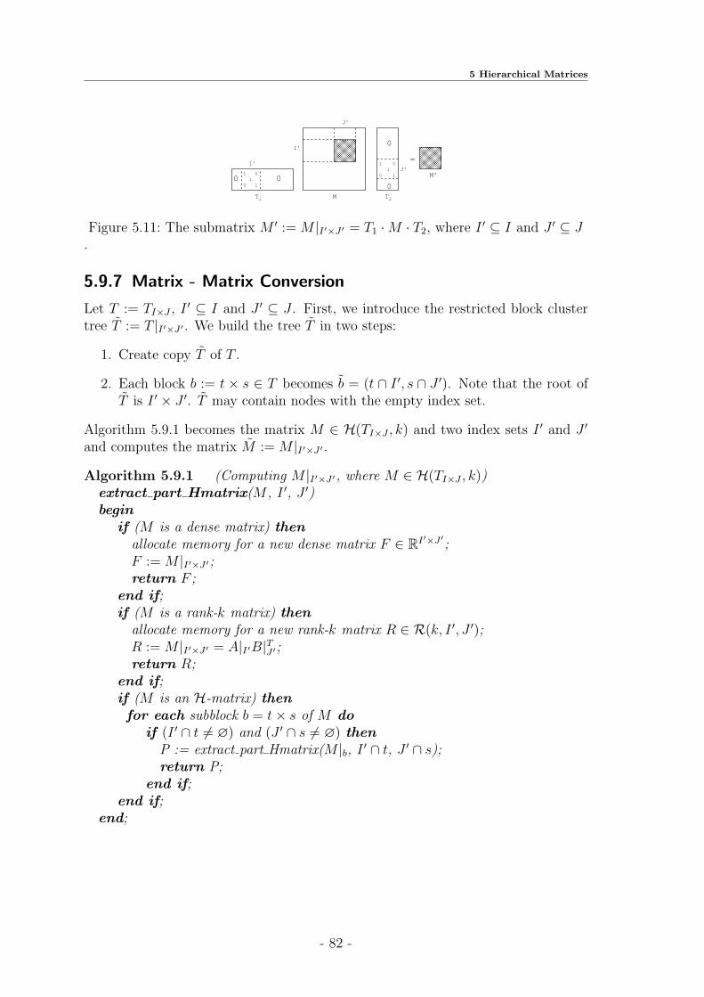
5 Hierarchical Matrices
111
0
00 0
11
1
0
0
=0
0
T M
M’
T1 2
J’
I’
I’J’
Figure 5.11: The submatrix M ′ := M |I′×J ′ = T1 ·M · T2, where I ′ ⊆ I and J ′ ⊆ J.
5.9.7 Matrix - Matrix Conversion
Let T := TI×J , I′ ⊆ I and J ′ ⊆ J . First, we introduce the restricted block cluster
tree T := T |I′×J ′ . We build the tree T in two steps:
1. Create copy T of T .
2. Each block b := t × s ∈ T becomes b = (t ∩ I ′, s ∩ J ′). Note that the root ofT is I ′ × J ′. T may contain nodes with the empty index set.
Algorithm 5.9.1 becomes the matrix M ∈ H(TI×J , k) and two index sets I ′ and J ′
and computes the matrix M := M |I′×J ′ .
Algorithm 5.9.1 (Computing M |I′×J ′, where M ∈ H(TI×J , k))extract part Hmatrix(M , I ′, J ′)begin
if (M is a dense matrix) thenallocate memory for a new dense matrix F ∈ RI′×J ′
;F := M |I′×J ′;return F ;
end if;if (M is a rank-k matrix) then
allocate memory for a new rank-k matrix R ∈ R(k, I ′, J ′);R := M |I′×J ′ = A|I′B|TJ ′;return R;
end if;if (M is an H-matrix) thenfor each subblock b = t× s of M do
if (I ′ ∩ t 6= ∅) and (J ′ ∩ s 6= ∅) thenP := extract part Hmatrix(M |b, I ′ ∩ t, J ′ ∩ s);return P;
end if;end if;
end;
- 82 -
5.9 Arithmetics of Hierarchical Matrices
Consider a more difficult case. Suppose M ∈ H(TI×J , k),
I ⊇ I ′ =
p⋃
i=1
Ii, Ij ∩ Ik = ∅, j 6= k, (5.27)
J ⊇ J ′ =
q⋃
j=1
Jj, Ji ∩ Jk = ∅, i 6= k (5.28)
and n = max|I|, |J |, n′ = max|I ′|, |J ′|. Let M ∈ H(T ′I′×J ′ , k). The problem is
to convert M to M . We set up M by Algorithm 5.9.2.
Algorithm 5.9.2 (Conversion M ∈ H(TI×J , k) to M ′ := M |I′×J ′ ∈ H(T ′I′×J ′ , k))h2h(M , M ′,
⋃pi=1 Ii,
⋃qj=1 Jj)
beginif (M ′ is a dense matrix) then
h2f(M , M ′,⋃pi=1 Ii,
⋃qj=1 Jj);
if (M ′ is a rank-k matrix) thenh2r(M , M ′,
⋃pi=1 Ii,
⋃qj=1 Jj);/∗see Algorithm 5.9.3∗/
if (M ′ is an H-matrix) thenfor each subblock b = t× s of M ′ do
h2h(M , M ′|b,⋃pi=1(Ii ∩ t),
⋃qj=1(Jj ∩ s));
end if;end;
The conversion of an H-matrix to a dense matrix (procedure h2f(..) in Algorithm5.9.2) is done elementwise. The conversion of an H-matrix to a rank-k matrix(procedure h2r(..) in Algorithm 5.9.2) is done by Algorithm 5.9.3.
- 83 -

5 Hierarchical Matrices
Algorithm 5.9.3 (Converting M ∈ H(TI×J , k) to R ∈ R(k, I ′, J ′))h2r(M , R,
⋃pi=1 Ii,
⋃qj=1 Jj)
beginif (M is a dense matrix)
allocate memory for F ∈ RI′×J ′
;for all i ∈ I ′ and j ∈ J ′ doFij := Mij;
convert F to R; /∗ SVD is used ∗/end if;if (M is a rank-k matrix, i.e. M = ABT ) then
allocate memory for R = CDT ∈ R(k, I ′, J ′);C := A, D := B;
end if;if (M is an H-matrix) thenl = 0;for each subblock b = t× s of M doR[l]:=h2r(M |b,
⋃pi=1(Ii ∩ t),
⋃qj=1(Jj ∩ s));
l + +;end forR:=(R[0]⊕k (R[1]⊕k ...⊕k (R[l − 2]⊕k R[l − 1])..);/∗see pairwise truncation in (5.21)∗/
end if;end;
- 84 -

5.10 Complexity Estimates
5.9.8 Adding Two H-Matrices With Different Block Cluster
Trees
The addition of two hierarchical matrices with compatible block cluster trees hasbeen described in [33]. Let I, J , I ′, J ′, I ′′ and J ′′ be given index sets such thatI ′, I ′′ ⊆ I, J ′, J ′′ ⊆ J , and M ∈ H(TI×J , k). Let TI′×J ′ and TI′′×J ′′ be block clustertrees. The sum of M1 ∈ H(TI′×J ′ , k1) and M2 ∈ H(TI′′×J ′′ , k2) with the result matrixM is defined as follows (see Fig. 5.12):
M = M ′ ⊕M ′′, where M ′ := M1|I×J and M ′′ := M2|I×J (see Def. 5.7.1).
The adding procedure applies the list of procedures from Table 5.2.
Remark 5.9.11 Note that M1|I×J and M2|I×J have the block cluster tree TI×J . Tocompute M ′ := M1|I×J and M ′′ := M2|I×J we apply Algorithm 5.9.2.
+ + =
Figure 5.12: Transformation of H-matrices M1, M2 to H-matrices M1|I×J , M2|I×Jand their addition.
procedure description
add fullmatrix(F, F1, F2) Adding two dense matricesadd rkmatrix(R,R1, R2) Adding two rank-k matricesaddfullpart2 rkmatrix(F ,R) Addition of a dense matrix to a rank-k matrixaddrk2 fullmatrix(R,F ) Addition of a rank-k matrix to a dense matrixaddfull2 supermatrix(F,M) Addition of a dense matrix to an H-matrixaddrk2 supermatrix(R,M) Addition of a rank-k matrix to an H-matrixadd supermatrix(M,M1,M2) Adding of H-matrices M := M1 ⊕M2
h2h(M1,M2,...) Conversion of an H-matrix M1 to the H-matrix M2
h2r(M,R,...) Conversion an H-matrix to an rank-k matrixh2f(M,F ,...) Conversion an H-matrix to an dense matrix
Table 5.2: The procedures which are applied for adding two H-matrices with differ-ent block structures. M , Mi are H-matrices, R, Ri are rank-k matrices,F , Fi are dense matrices, i = 1, 2.
5.10 Complexity Estimates
Lemma 5.10.1 Let I be an index set, n := |I| and TI a balanced, binary clustertree and T := TI×I a block cluster tree. Let the depth of the tree is p(T ) = O(log n).
Then the number of clusters on the level i is |T (i)I | = 2i for 0 ≤ i ≤ p(T ) and
|V (TI)| = 2|T | − 1 = O(n).
- 85 -

5 Hierarchical Matrices
Proof: see [27].
Theorem 5.10.1 Let n := max|I|, |J |, |K|, m := |J |, n ≥ m. Let T := TI×J ,TI×K, TK×J be block cluster trees, depth(T ) = log n, M ∈ H(T, k), k := maxk, nmin.The storage requirement and the computational costs of H-matrix operations aregiven in Table 5.3.
Operation Description Complexity
storage(M) M ∈ H(TI×J , k) O(Cspkn log n
Mx M ∈ H(TI×J , k), x ∈ R|J | O(Cspkn log n)M ′ ⊕M ′′ M ′,M ′′ ∈ H(TI×J , k) O(Cspk
2n log n)
M ′ ⊙M ′′ M ′ ∈ H(TI×K , k), O(C3spk
2n log2 n)M ′′ ∈ H(TK×J , k)
M−1 M ∈ H(TI×I , k) O(C3spk
2n log2 n)
H-LU M ∈ H(TI×I , k) O(C3spk
2n log2 n)
M ⊕R M ∈ H(TI×J , k), R ∈ R(k, I, J) O(k2(n+m))
Table 5.3: The costs of H-matrix arithmetical operations, n := max|I|, |J |, |K|.
Proof: See Lemma 5.13 for the MV multiplication and the MM addition. SeeLemmas 2.10, 2.17, 2.19 in [29] for the MM multiplication. See also [33], [27].
Lemma 5.10.2 Let T := TI×J be a block cluster tree. The cost of the multiplicationof a matrix M ∈ H(T, k) and a vector v ∈ R|J | is
NH·v(T, k) ≤ 2NSt(T, k), (5.29)
where NSt(T, k) is the storage requirement for M .
Proof: The scalar product of two vectors u, v ∈ Rm costs m+ (m− 1) < 2m (therearemmultiplications andm−1 additions). The storage of a rank-k matrix R = ABT
is NSt,R(k, n,m) = k(n+m) and the cost of R·v is 2k(n−1)+2k(m−1) ≤ 2k(n+m).The storage requirement of a dense matrix F ∈ Rn×m is n ·m and the computationalcost of F · v is (2m − 1) · n ≤ 2n ·m. Summing the costs for all admissible blockswe prove the lemma.
Lemma 5.10.3 Let T := TI×J , n := |I| ≥ |J |. The removal of i-th row from amatrix M ∈ H(T, k) costs 2Cspkn.
Proof: This removal procedure updates the old data structure. Let p := depth(TI×J).algorithm goes through the whole tree TI×J and removes i-th row from blocks(t, s) ∈ L(T ), i ∈ t. Therefore, the complexity is
p∑
l=0
∑
(t,s)∈L(T,l),i∈t(|t| − 1)kCsp
|t|=2p−l
≤ Cspk
p∑
l=0
(2p−l − 1) (5.30)
- 86 -
5.10 Complexity Estimates
≤ Cspk
p∑
l=0
2l ≤ 2Cspkn. (5.31)
Similarly, the cost of the removal of a column is bounded by 2Cspkn.
Lemma 5.10.4 Let TI be a cluster tree. Adding a rank-1 matrix R ∈ R(1, I, I) tothe hierarchical matrix M ∈ H(TI×I , k) costs O(k2n), where n = |I|.
Proof: Let p := depth(TI×I). We know that the truncated addition of two rank-kmatrices M |t×s and R|t×s costs O(k2(|t|+ |s|)). Thus, the complexity is
N =∑
t∈TI
O(k2|t|) = O(k2|I|). (5.32)
Lemma 5.10.5 Extracting a column j from a matrix M ∈ H(TI×J , k) costs O(k|I|).
Proof: Let n := |I| ≥ |J |. Extracting a column j from M is equivalent to themultiplication M · ej, ej = (0, 0, ...0, 1, 0..., 0) and costs O(kn log n). But it can bedone with the complexity O(kn). Let TJ be a cluster tree, L(TJ) the set of allleaves of TJ and s0 the biggest cluster, such that j ∈ s0 ∈ TJ . Denote the set of allsuccessors of s0 by S ′(s0). Let
L′(TI×J) := (t, s) ∈ L(TI×J)|t ∈ TI , s ∈ TJ and s ∈ S ′(s0). (5.33)
Then the complexity is
N =∑
t×s∈L′(TI×J ),
k(|t|+ |s|) ≤∑
t∈L(TI)
2k|t| = O(k|I|). (5.34)
Similarly, the extraction of a row costs O(k|J |).
Lemma 5.10.6 Let M ∈ H(TI×J , k), I′ ⊆ I, J ′ ⊆ J , n′ = max|I ′|, |J ′|. The
hierarchical conversion (see (5.21)) of M |I′×J ′ to R ∈ R(k, I ′, J ′) is of complexity
N ≤ O(k2qn′ log n), where q := maxl
∑
(I ′ × J ′) ∩ (t× s) 6= ∅
(t× s) ∈ T (l)I×J
1. (5.35)
Proof: Here q is the maximal number of subblocks on the same level which haveto be summed. The conversion (see Section 5.9.3) at one level is of complexityO(k2qn′). There are log n levels and the total complexity is N ≤ O(k2qn′ log n).
- 87 -

5 Hierarchical Matrices
Definition 5.10.1 Let I ′ ⊆ I, J ′ ⊆ J be index sets, T := TI×J , T′ := T ′I′×J ′
block cluster trees. Let q be the maximal number of subblocks which form a block(t′ × s′) ∈ L(T ′I′×J ′). The value q is defined as following
q := max(t×s)∈L(T )
∑
(t× s) ∩ (t′ × s′) 6= ∅
(t′ × s′) ∈ L(T ′)
1. (5.36)
Lemma 5.10.7 Let I ′ ⊆ I, J ′ ⊆ J be index sets, T := TI×J , T′ := TI′×J ′ the block
cluster trees, p := depth(T ), M ∈ H(T, k) and M ′ ∈ H(T ′, k). The complexity ofcomputing M := M ′|I×J is
N = O(k2qn log n log n′),
where n := max|I|, |J |, n′ := max|I ′|, |J ′|, depth(T ′) = log n′ and q is definedin (5.36).
Proof: Suppose that for each leaf b = (t× s) ∈ L(T ) there are q(b) subblocks in T ′
which contain elements from M |b. The search of q(b) subblocks costs in the worstcase q(b) · depth(T ′) = q(b) log n1 ≤ q log n1.By Lemma 5.10.6 the cost of the hierarchical conversion R|t×s = T R←H(M) isC1qk
2(|t|+ |s|) log n′.Using Lemma 5.10.6 and decomposing all leaves of T on admissible and inadmissibleleaves, we obtain
N ≤∑
(t×s)∈L+(T )
Cqk2(|t|+ |s|) log n′ +∑
(t×s)∈L−(T )
C1(|t| · |s|)
≤∑
(t×s)∈L+(T )
Cqk2(|t|+ |s|) log n′ +∑
(t×s)∈L−(T )
C1nmin(|t|+ |s|)
≤p∑
i=0
∑
(t×s)∈T (i)
maxCqk2 log n′, C1nmin(|t|+ |s|)
Cqk2 logn′>C1nmin= Cqk2 log n′(
p∑
i=0
∑
(t×s)∈T (i)
|t|+p∑
i=0
∑
(t×s)∈T (i)
|s|)
≤ 2Cqk2 log n′p∑
i=0
∑
t∈T (i)
|t|
≤ 2Cqk2 log n′p∑
i=0
|I|
= 2Cqk2(p+ 1) log n′|I| = O(k2qn log n log n′).
Lemma 5.10.8 Let I ′ ⊆ I, I ′′ ⊆ I, J ′ ⊆ J , J ′′ ⊆ J be index sets, T := TI×J ,T ′ := TI′×J ′, T ′′ := TI′′×J ′′ the block cluster trees, p := depth(T ), n := max|I|, |J |.
- 88 -
5.10 Complexity Estimates
Let M ∈ H(T, k), M1 ∈ H(T ′, k) and M2 ∈ H(T ′′, k) two H-matrices with differentblock cluster trees. The complexity of computing
M = M1|I×J ⊕M2|I×J
is O(qk2n log2 n), where q is defined in (5.36).
Proof: Let depth(T ′) = log n1 and depth(T ′′) = log n2. From Lemma 5.10.7 followsthat the cost of computing M ′ := M1|I×J and M ′′ := M2|I×J is
O(q(log n1 + log n2)k2n log n).
The cost of adding M ′ ⊕k M ′′ is O(k2n log n). Taken into account that n1 ≃ n2
andn2 ≃ n
2the total cost is
O(q(log n1 + log n2)k2n log n) +O(k2n log n) ≤ O(qk2n log2 n).
- 89 -

5 Hierarchical Matrices
- 90 -

6 Application of H-matrices to HDD
The HDD method from Chapter 4 requires the exact matrix arithmetic, which isexpensive. To avoid it we approximate all matrices by the corresponding H-matricesand then apply the efficientH-matrix technique. Thus, we reduce the computationalcost and storage requirements extremely.
In this section we explain how to apply H-matrices for the approximation ofΨω and Φω. We explain the algorithm “Leaves to Root” in terms of the Schurcomplements defined on ω1, ω2 and ω.
6.1 Notation and Algorithm
In Table 6.1 we recall four types of mappings which are present in the HDD method.All of them will be approximated in the H-matrix format.
Name Mapping
domain-to-boundary Ψfω : RI(ω) → RI(∂ω)
boundary-to-boundary Ψgω : RI(∂ω) → RI(∂ω)
domain-to-interface Φfω : RI(ω) → RI(γ)
boundary-to-interface Φgω : RI(∂ω) → RI(γ)
Table 6.1: Four mappings, which are used in HDD. ω ∈ TTh.
The properties of these mappings are:
1. The mappings Ψfω and Φf
ω are approximated by H-matrices with the standardadmissibility condition (see Section 5.5.1).
2. The mapping Ψgω is approximated by an H-matrix with the weak admissibility
condition (see Section 5.5.2).
3. The mapping Φgω is approximated by a low-rank matrix (as a consequence of
using the weak admissibility condition).
4. The algorithm “Leaves to Root” builds the mappings Ψgω and Ψf
ω. The map-pings Ψg
ω and Ψfω are computed automatically.
5. If the global stiffness matrix after discretisation of the initial problem (4.1) isself-adjoint, then all matrices Ψg
ω, ω ∈ TTh, are positive definite and symmetric.
- 91 -
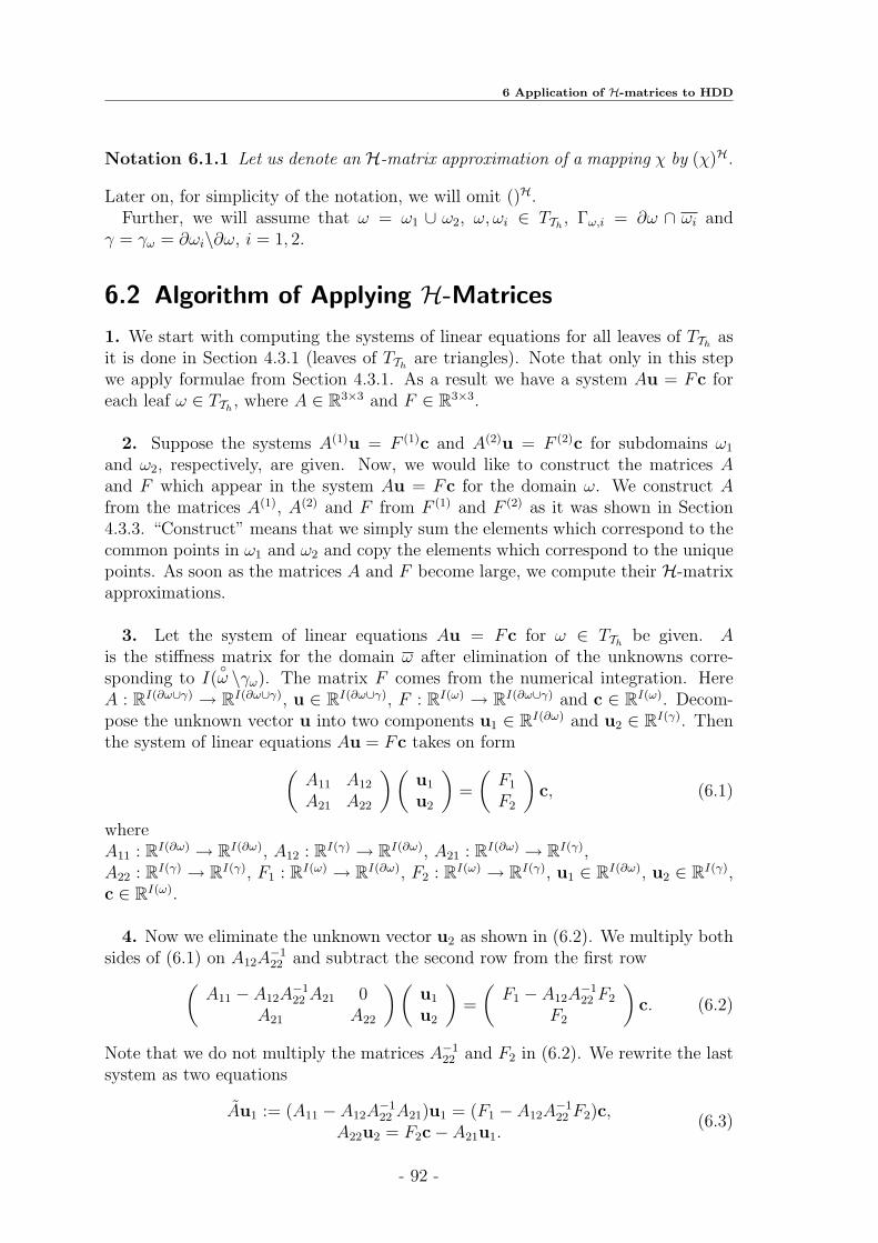
6 Application of H-matrices to HDD
Notation 6.1.1 Let us denote an H-matrix approximation of a mapping χ by (χ)H.
Later on, for simplicity of the notation, we will omit ()H.Further, we will assume that ω = ω1 ∪ ω2, ω, ωi ∈ TTh
, Γω,i = ∂ω ∩ ωi andγ = γω = ∂ωi\∂ω, i = 1, 2.
6.2 Algorithm of Applying H-Matrices
1. We start with computing the systems of linear equations for all leaves of TThas
it is done in Section 4.3.1 (leaves of TThare triangles). Note that only in this step
we apply formulae from Section 4.3.1. As a result we have a system Au = Fc foreach leaf ω ∈ TTh
, where A ∈ R3×3 and F ∈ R3×3.
2. Suppose the systems A(1)u = F (1)c and A(2)u = F (2)c for subdomains ω1
and ω2, respectively, are given. Now, we would like to construct the matrices Aand F which appear in the system Au = Fc for the domain ω. We construct Afrom the matrices A(1), A(2) and F from F (1) and F (2) as it was shown in Section4.3.3. “Construct” means that we simply sum the elements which correspond to thecommon points in ω1 and ω2 and copy the elements which correspond to the uniquepoints. As soon as the matrices A and F become large, we compute their H-matrixapproximations.
3. Let the system of linear equations Au = Fc for ω ∈ TThbe given. A
is the stiffness matrix for the domain ω after elimination of the unknowns corre-sponding to I(
ω \γω). The matrix F comes from the numerical integration. Here
A : RI(∂ω∪γ) → RI(∂ω∪γ), u ∈ RI(∂ω∪γ), F : RI(ω) → RI(∂ω∪γ) and c ∈ RI(ω). Decom-pose the unknown vector u into two components u1 ∈ RI(∂ω) and u2 ∈ RI(γ). Thenthe system of linear equations Au = Fc takes on form
(A11 A12
A21 A22
)(u1
u2
)=
(F1
F2
)c, (6.1)
whereA11 : RI(∂ω) → RI(∂ω), A12 : RI(γ) → RI(∂ω), A21 : RI(∂ω) → RI(γ),A22 : RI(γ) → RI(γ), F1 : RI(ω) → RI(∂ω), F2 : RI(ω) → RI(γ), u1 ∈ RI(∂ω), u2 ∈ RI(γ),c ∈ RI(ω).
4. Now we eliminate the unknown vector u2 as shown in (6.2). We multiply bothsides of (6.1) on A12A
−122 and subtract the second row from the first row
(A11 − A12A
−122 A21 0
A21 A22
)(u1
u2
)=
(F1 − A12A
−122 F2
F2
)c. (6.2)
Note that we do not multiply the matrices A−122 and F2 in (6.2). We rewrite the last
system as two equations
Au1 := (A11 − A12A−122 A21)u1 = (F1 − A12A
−122 F2)c,
A22u2 = F2c− A21u1.(6.3)
- 92 -

6.2 Algorithm of Applying H-Matrices
The unknown vector u2 is computed as follows (compare with (4.43))
u2 = A−122 F2c− A−1
22 A21u1.
The explicit expressions for the mappings Ψω and Φω follow from (6.3):
Ψgω := A11 − A12A
−122 A21, (6.4)
Ψfω := F1 − A12A
−122 F2, (6.5)
Φgω := −A−1
22 A21, (6.6)
Φfω := A−1
22 F2, (6.7)
As soon as the rank of A22 is larger than parameter nmin (see Section 5.5.2), weapply SVD to convert A and F from the dense matrix format to the H-matrixformat. Denote the standard operations − and · in the class of H-matrices by ⊖and ⊙. After approximation of all matrices in (6.4)-(6.7) by H-matrices we obtain
(Ψgω)H := (A11)
H ⊖ (A12)H ⊙ (A−1
22 )H ⊙ (A21)H, (6.8)
(Ψfω)H := (F1)
H ⊖ (A12)H ⊙ (A−1
22 )H ⊙ (F2)H, (6.9)
(Φgω)H := −(A−1
22 )H ⊙ (A21)H, (6.10)
(Φfω)H := (A−1
22 )H ⊙ (F2)H. (6.11)
Note that we multiply H-matrices only in (6.8) and (6.9). In (6.10) and (6.11) westore the multipliers and later on perform only two times matrix-vector multiplica-tions.
5. We repeat steps 2-5 for all other ω ∈ TThand stop when ω = Ω.
Remark 6.2.1 The matrices A−122 , F1, F2, A11 are approximated in the H-matrix
format, A12 and A21 are approximated in the low-rank matrix format. For simplicityof the further notation we omit the superscript H.
Example 6.2.1 Examples of the matrices A and F (Ψgω and Ψf
ω) from (6.1) areshown in Figures 6.1 and 6.2. In Fig. 6.1 one can see that off-diagonal blocks arelow-rank matrices (grey blocks). In Fig. 6.2 the off-diagonal blocks are H-matrices.The white blocks indicate zero matrices and the dark blocks indicate dense matrices.
Remark 6.2.2 The fact that the matrix A is approximated by an H-matrix withweakly admissible blocks plays an important role. From this fact follows that thematrices A12 and A21 are low-rank matrices and multiplications in A12 ⊙ A−1
22 andin A−1
22 ⊙ A21 are therefore quite cheap.
The following Theorem 6.2.1 (see [47]) is important for the application of the H-matrix technique to HDD. This theorem proves the existence of an H-matrix ap-proximation of the Schur complement.
- 93 -

6 Application of H-matrices to HDD
Notation 6.2.1 Let t, s ∈ TI be two clusters, TI×I a block cluster tree and s× t ∈TI×I . We denote the restriction of the block cluster tree TI×I to s× t by T |s×t
Assumption 6.2.1 (Existence of an H-matrix approx. to the inverse)Let A ∈ H(TI×I , k), n := |I|. For any ε > 0 and r := 1, ..., n1, n1 ≤ n, the minorB := A|r×r is invertible and there exists an H-matrix B−1
H ∈ H(T |r×r, kinv) with
kinv := (log2 n)| log ε|3 and ‖B−1 −B−1H ‖2 ≤ Cinvε, Cinv ∈ R+. (6.12)
Proof: (see Assumption 2 in [47]).
Theorem 6.2.1 (Approximation of Schur complements)Let TI be a cluster tree, T := TI×I and p be depth of T . Let A ∈ H(T, kinv) withkinv from (6.12), b := s× t ∈ T and r ∈ TI . Then the Schur complement
S(s, t) = A|s×t − A|s×r(A|r×r)−1A|r×t
can be approximated by SH(s, t) ∈ H(T |s×t, k′) where k′ . (p+ 1)2kinv, such that
‖S(s, t)− SH(s, t)‖2 < Cinv‖A‖22ε, Cinv ∈ R+.
Proof: see Theorem 1 in [47].
25 4
4 85
5 16 5
5 165
5 32 6
6 325
532 5
5 326
632 5
5 321
1
32 5
5 32 5
5
32 5
5
16 4
4 32 5
5 165
5 325
532 5
5 32
12
12
32 5
5 32 5
5
32 5
5
16 5
5
32 4
4 165
5 325
532 5
5 321
1
32 5
5 32 6
6
32 5
5 32 6
6
32 5
5
32 5
5
16 5
5
16 4
4 31
Figure 6.1: An H-matrix approximation to Ψgω ∈ RI×I , I := I(∂ω). The dark blocks
are dense matrices and grey blocks are low-rank matrices. The numbersinside the blocks indicate ranks of these blocks.
- 94 -

6.2 Algorithm of Applying H-Matrices
17 17
16 16
517 17
16 16
5 5
16 5
55 5
16 5
5 16
55 55 5
5 5
55
5
5 16
55 5
5 5
16 168 5
24 24
5 5
5 245 5
8 5
24 24
5 5
24 2416 16 16
5 5
5
5
16
5
16 16
5 55 5
5 23
5 8
5 23
16 165 5
23 23
8 8
23 23
16
16 16 516 16
5 15 5
Figure 6.2: An H-matrix approximation to (Ψfω)H ∈ RI×J , I := I(∂ω), J := J(ω),
|I| = 256, |I| = 4225. The dark blocks are dense matrices and greyblocks are low-rank matrices. The numbers inside the blocks are ranksof these blocks. The white blocks are zero blocks.
Remark 6.2.3 In order to build a rank-k approximation of the matrix Φgω we use
the fact that the singular values σ1 ≥ σ2 ≥ ... ≥ σk ≥ σk+1 ≥ ... ≥ σn of Φgω
decay exponentially (see Fig. 6.3). We only consider the k largest singular valuesσ1 ≥ σ2 ≥ ... ≥ σk (see Section 5.6).
Recall that for simplicity of the notation we write γ instead of γω.
Lemma 6.2.1 We denote the Schur complement A11 − A12A−122 A21 by Sω, where
A11 ∈ H(TI(∂ω)×I(∂ω), k), A12 ∈ R(I(∂ω), I(γ), k), A21 ∈ R(I(γ), I(∂ω), k),A22 ∈ H(TI(γ)×I(γ), k). Let nh,γ := |I(γ)|. Let the model domain be as in Remark7.1.2. The computation of Sω, ω ∈ TTh
, costs
N(Sω) ≤ Ck2nh,γ log2 nh,γ , C ∈ R+. (6.13)
Proof: Due to Table 5.3 the complexity of the inversion A−122 is C1k
2nh,γ log2 nh,γ ,C1 ∈ R+. The complexity of the multiplication A12 · A−1
22 is k-times the MV multi-plication, i.e., C2k
2nh,γ log nh,γ , C2 ∈ R+.We assume that for the domain in Remark 7.1.2 |I(∂ω)| ≤ 6 · |I(γ)| hold. Thecomplexity of the multiplication (A12A
−122 ) · A21 (product of two low-rank matrices)
is2k2(|I(∂ω)|+ |I(γ)|) +O(k3) ≤ 14k2nh,γ +O(k3).
The complexity of the subtraction A11 − A12A−122 · A21 is
C3k2|I(∂ω)| log |I(∂ω)| ≤ C4k
2nh,γ log nh,γ , C3, C4 ∈ R+.
Thus,
N(Sω) ≤ (C1+C2+C4)k2nh,γ log nh,γ+14k2nh,γ+O(k3) ≤ Ck2nh,γ log2 nh,γ , C ∈ R+.
(6.14)
- 95 -
6 Application of H-matrices to HDD
Algorithm 6.2.1 (Elimination of ui, i ∈ I(γ))elimination( H-matrix M , index set I(γ))beginM11 := M [0];M21 := M [1];M12 := M [2];M22 := M [3]; /∗ Corresponds to I(γ) ∗ /M11 := M11 ⊖M12 ⊙M−1
22 ⊙M21;return M11;
end;
Lemma 6.2.2 Let Zω := F1 − A12A−122 F2, where A12 ∈ R(I(∂ω), I(γ), k),
F1 ∈ H(TI(∂ω)×I(ω), k), F2 ∈ H(TI(γ)×I(ω), k), A22 ∈ H(TI(γ)×I(γ), k), nh,γ := |I(γ)|and nh := |I(ω)|. Let the model domain be as in Remark 7.1.2. The computation ofZω, ω ∈ TTh
, costsN(Zω) ≤ Ck2nh log2 nh, C ∈ R+. (6.15)
Proof: The complexity of the multiplication A12 · A−122 is k-times the MV mul-
tiplication, i.e., C1k2nh,γ log nh,γ , C1 ∈ R+. The complexity of the multiplica-
tion (A12A−122 ) · F2 (the product of a low-rank matrix and an H-matrix) is equal
to C2k2nh log nh, C2 ∈ R+. The complexity of the subtraction F1 − A12A
−122 F2 is
C3k2nh log nh, C3 ∈ R+. Thus,
N(Zω) = C1k2nh,γ log nh,γ +C2k
2nh log nh+C3k2nh log nh ≤ Ck2nh log nh, C ∈ R+.
0 20 40 60 80 100 120 140−40
−35
−30
−25
−20
−15
−10
−5
0
sigm
a
Figure 6.3: Exponential decay of the singular values σi of the matrix (Φgω)H in a log
scale. The index i is shown on the horizontal axis and the singular valuesσi on the vertical logarithmic axis, e.g., σ20 ≈ 10−7.
- 96 -
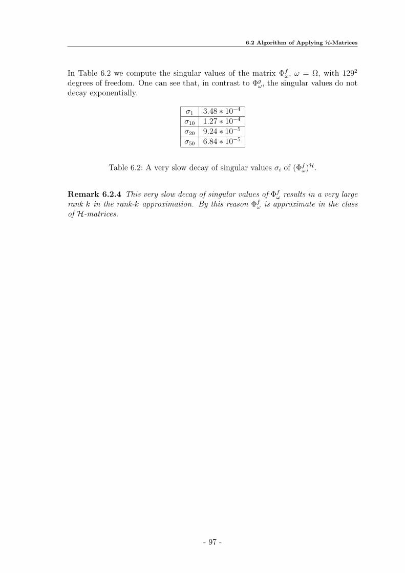
6.2 Algorithm of Applying H-Matrices
In Table 6.2 we compute the singular values of the matrix Φfω, ω = Ω, with 1292
degrees of freedom. One can see that, in contrast to Φgω, the singular values do not
decay exponentially.
σ1 3.48 ∗ 10−4
σ10 1.27 ∗ 10−4
σ20 9.24 ∗ 10−5
σ50 6.84 ∗ 10−5
Table 6.2: A very slow decay of singular values σi of (Φfω)H.
Remark 6.2.4 This very slow decay of singular values of Φfω results in a very large
rank k in the rank-k approximation. By this reason Φfω is approximate in the class
of H-matrices.
- 97 -

6 Application of H-matrices to HDD
6.3 Hierarchical Construction on Incompatible Index
Sets
This Section contains technical details about H-matrix constructions of (Ψgω)H from
(Ψgω1
)H, (Ψgω2
)H and (Ψfω)H from (Ψf
ω1)H, (Ψf
ω2)H.
Let TThbe a domain decomposition tree (the root has level 0). Let us suppose
that we have a domain ω on level l−1 with two sons ω1 and ω2 on level l. In the nexttwo subsections we show the efficient constructions of (Ψg
ω)H from (Ψg
ω1)H, (Ψg
ω2)H
and (Ψfω)H from (Ψf
ω1)H, (Ψf
ω2)H.
Let us change the notation:
I(Γ1) := I(Γω,1) = I(∂ω ∩ ω1),
I(Γ2) := I(Γω,2) = I(∂ω ∩ ω2).
Now, we have the following decompositions:
I(∂ω1) = I(Γ1) ∪ I(γ) and I(∂ω2) = I(Γ2) ∪ I(γ).
6.3.1 Building (Ψgω)H from (Ψg
ω1)H and (Ψg
ω2)H
Let H ∈ H(TI(∂ω∪γ)×I(∂ω∪γ), k). Define the following matrices:
H1 := (Ψgω1
)H ∈ H(TI(∂ω1)×I(∂ω1), k), H2 := (Ψgω2
)H ∈ H(TI(∂ω2)×I(∂ω2), k), (6.16)
H := (Ψgω)H ∈ H(TI(∂ω)×I(∂ω), k), (6.17)
where I(∂ω∪γ) = I(∂ω1∪∂ω2) (see Remark 4.3.3 and Figures 6.4, 6.5). We want toconstruct the matrix H from H1 and H2. First, we build a new cluster tree TI(∂ω∪γ)from the clusters TI(∂ω) and TI(γ). There are many variants of how to build it, butwe want such a cluster tree, which makes it easier to eliminate the unknowns xi,i ∈ I(γ), i.e, one of the sons of the cluster I(∂ω ∪ γ) should coincide with the indexset I(γ). As soon as the cluster tree TI(∂ω∪γ) is built, we build the block cluster treeTI(∂ω∪γ)×I(∂ω∪γ). The block cluster tree TI(∂ω∪γ)×I(∂ω∪γ) defines the block structure
of H. We consider two variants of the block structures:
I(Γi)× I(Γi), I(γ)× I(γ) ∈ TI(∂ωi)×I(∂ωi), i = 1, 2. (6.18)
I(Γi)× I(Γi) /∈ TI(∂ωi)×I(∂ωi) or I(γ)× I(γ) /∈ TI(∂ωi)×I(∂ωi), i = 1, 2. (6.19)
- 98 -

6.3 Hierarchical Construction on Incompatible Index Sets
Building algorithm in case (6.18):Let H1 and H2 be defined as in (6.16) and H as in (6.17).
Algorithm 6.3.1 Building H := (Ψgω)H from H1 := (Ψg
ω1)H and H2 := (Ψg
ω2)H
build Ψg(H1, H2,... )begin
allocate memory for H;H|I(Γ1)×I(Γ1) := H1|I(Γ1)×I(Γ1);
H|I(Γ2)×I(Γ2) := H2|I(Γ2)×I(Γ2);
H|I(Γ1)×I(Γ2) := 0;
H|I(Γ2)×I(Γ1) := 0;/∗ in Fig. 6.4 denoted by d+ h ∗/H|I(γ)×I(γ) := H1|I(γ)×I(γ) ⊕H2|I(γ)×I(γ);H|I(γ)×I(Γ1)∪I(Γ2) := (H1|I(γ)×I(Γ1) ⊕H2|I(γ)×I(Γ2)); /∗ Sum of two low-rank ma-
trices ∗//∗ in Fig. 6.4 denoted by b+ f ∗/
H|I(Γ1)∪I(Γ2)×I(γ) := H1|I(Γ1)×I(γ) ⊕ H2|I(Γ2)×I(γ); /∗ Sum of two low-rank ma-trices ∗/
H:=extract rows(H, r1, r2, i1, i2); /∗ The output is r1, r2 ∗/H:=extract columns(H, c1, c2, j1, j2); /∗ The output is c1, c2 ∗/H:=add rows(H, r1, r2, i3, i4);H:=add columns(H, c1, c2, j3, j4);H:=elimination(H, I(γ)); /∗ see Algorithm 6.2.1∗/return H;
end;
Remark 6.3.1 Since I(Γ1)∩I(Γ2) = I(x, y) 6= ∅, we should remove two repeatedcolumns and two repeated rows from H. The indices i1, i2, j1, j2 indicate the posi-tions of two rows and two columns which have to be extracted. i3, i4 and j3, j4 arepositions of two rows and two columns to which the removed rows and columns r1,r2, c1 and c2 have to be added.
- 99 -

6 Application of H-matrices to HDD
a b
c d
e f
g h
c+g
b+f
d+h
a 0
0 e
c’+g’
b’+f’
d+h
a’
e’
. ...x
y
.
.
Schur Complement
=:
ω1 ω2Γ1 Γ2γ
γ∂ω
I(Γ1)
I(Γ1)
I(Γ1)
I(Γ1)
I(Γ1)
I(Γ1)
I(Γ1)
I(Γ1)
I(Γ2)
I(Γ2)
I(Γ2)
I(Γ2)
I(Γ2)
I(Γ2)
H H
I(γ)
I(γ)
I(γ)I(γ)
I(γ)I(γ)
I(γ)
I(γ)
H1 H2
H
Figure 6.4: Building H := (Ψgω)H ∈ RI(∂ω)×I(∂ω) from H1 := (Ψg
ω1)H ∈ RI(∂ω1)×I(∂ω1)
and H2 := (Ψgω2
)H ∈ RI(∂ω2)×I(∂ω2), where I(∂ωi) = I(Γi)∪ I(γ), i = 1, 2,
I(∂ω) = I(Γ1)∪ I(Γ2), x, y are two common points and I(Γ1) := I(Γ1)\I(x, y). The small letters show the appearance of blocks in differentmatrices. The dotted lines in H present 2 rows and 2 columns.
Remark 6.3.2 Figure 6.4 illustrates Algorithm 6.3.1. The first step is the con-struction of H and then, according to (6.4),
(Ψgω)H = H11 ⊖H12 ⊙H−1
22 ⊙H21,
with H11 := H|I(∂ω)×I(∂ω), H12 := H|I(∂ω)×I(γ),
H21 := H|I(γ)×I(∂ω), H22 := H|I(γ)×I(γ).
- 100 -

6.3 Hierarchical Construction on Incompatible Index Sets
Lemma 6.3.1 The cost of building theH-matrix H (see (6.17)) from theH-matricesH1 and H2 (see (6.16)) in case (6.18) by Algorithm 6.3.1 is
N ≤ Ck2nγ log nγ, where nγ = |I(γ)|, C ∈ R+.
Proof: We follow Algorithm 6.3.1 (see the scheme in Fig. 6.4). Let n1 := |I(∂ω1)|,n2 := |I(∂ω2)|, n := |I(∂ω)|.
1. From Table 5.3 follows that the complexity of addingH1|I(γ)×I(γ) andH2|I(γ)×I(γ)(in Fig. 6.4 denoted by d+ h) is O(k2nγ log nγ).
2. From Table 5.1 follows that the complexity of adding the low-rank matri-ces H1|I(γ)×I(Γ1) and H2|I(γ)×I(Γ2) as well as H1|I(Γ1)×I(γ) and H2|I(Γ2)×I(γ) isO(k2|I(∂ω)|) = O(k2n) (see Table 5.1).
3. The removal of two columns and two rows from H1 by Lemma 5.10.3 costsO(k log n1).
4. Adding four rank-1 matrices to H by Lemma 5.10.4 costs O(k2n2).
5. Adding four elements to the matrix H|I(Γ2)×I(Γ2) in general by Lemma 5.10.4costs O(k2|I(Γ2)|). In our case these elements belong to diagonal blocks andshould be added to dense matrices. The cost is O(1).
6. The cost of computing the Schur complement by Lemma 6.2.1 isO(k2nγ log2 nγ).
Since the complexity of adding two H-matrices dominates, the total complexity is
N ≤ Ck2nγ log nγ , C ∈ R+.
Building algorithm in case (6.19):Let H1 and H2 be defined as in (6.16), H as in (6.17) and I := I(∂ω).
Algorithm 6.3.2 Building H := (Ψgω)H from H1 := (Ψg
ω1)H and H2 := (Ψg
ω2)H
build Ψg(H1, H2,...)begin
allocate memory for H, H;H ′:=copy block structure(H);H ′′:=copy block structure(H);h2h(H1, H
′,...);/∗ Convert H1 to H ′ ∗ /h2h(H2, H
′′,...);/∗ Convert H2 to H ′′ ∗ /H := H ′′ ⊕H ′; /∗ See (6.17) ∗/H:=elimination(H, I(γ12)); /∗ see Algorithm 6.2.1 ∗/return H;
end;
- 101 -

6 Application of H-matrices to HDD
=:
conversion conversion
Schur Complement
ω1 ω2γ12
γ12Γ
γ
I(Γ)
I(Γ)
I(Γ)
I(Γ)
I(Γ)
I(Γ) I(γ)
I(γ)
I(γ)
I(γ)
I(γ)
I(γ)
H1H2
H ′ H ′′
I(∂ω1)
I(∂ω1)
I(∂ω2)
I(∂ω2)
I(γ12)
I(γ12)
I(γ12)
I(γ12)
H := H ′ ⊕H ′′
H
Figure 6.5: Building H := (Ψgω)H ∈ RI(∂ω)×I(∂ω) from H1 := (Ψg
ω1)H ∈ RI(∂ω1)×I(∂ω1)
and H2 := (Ψgω2
)H ∈ RI(∂ω2)×I(∂ω2), I(∂ωi) = I(Γi) ∪ I(γ12), i =1, 2, I(∂ω) = I(Γ) ∪ I(γ). We obtain H after computing H ′ ⊕ H ′′
and the Schur complement, where H ′ := H1|I(∂ω∪γ12)×I(∂ω∪γ12), H ′′ :=H2|I(∂ω∪γ12)×I(∂ω∪γ12).
Remark 6.3.3 Figure 6.5 illustrates Algorithm 6.3.2. First, it shows how H isconstructed. Here
H ′ := H1|I(∂ω∪γ12)×I(∂ω∪γ12), H ′′ := H2|I(∂ω∪γ12)×I(∂ω∪γ12), and H = H ′ ⊕H ′′
with γ12 := ∂ω1 \ ∂ω. Then, according to (6.4),
(Ψgω)H = H11 ⊖H12 ⊙H−1
22 ⊙H21,
with H11 := H|I(∂ω)×I(∂ω), H12 := H|I(∂ω)×I(γ12),
H21 := H|I(γ12)×I(∂ω), H22 := H|I(γ12)×I(γ12).
- 102 -

6.3 Hierarchical Construction on Incompatible Index Sets
Lemma 6.3.2 The cost of building the H-matrix H (see (6.17)) from H-matricesH1 and H2 (see (6.16)) in case (6.19) by Algorithm 6.3.2 is
N ≤ Ck2n log2 n, where n = |I(∂ω)|, C ∈ R+.
Proof: We follow the scheme in Fig. 6.5. Let I := I(∂ω), H ′ := H1|I×I andH ′′ := H2|I×I , where H ′ and H ′′ have the same block cluster structure as H. Weconvert H1 to the matrix H ′ and H2 to the matrix H ′′. The block structure of His important and is shown in Fig. 6.5. As soon as the matrices H ′ and H ′′ areready, we consider the construction of the matrix H as the addition H ′ ⊕H ′′ withfurther elimination of the unknowns with indices i ∈ I(γ12). Using the inequalityn ≤ 2 · |I(∂ω1)| and Lemma 5.10.8 we obtain that the complexity of this additionis O(k2n log2 n). By Lemma 6.2.2 the elimination costs O(k2n log n). The termO(k2n log2 n) dominates.
Example 6.3.1 Figure 6.6 shows an example of building (Ψgω)H ∈ R512×512 from
(Ψgω1
)H ∈ R384×384 and (Ψgω2
)H ∈ R384×384. Let I := I(∂ω ∪ γ). The construction isperformed in three steps: 1) build H ′ := (Ψg
ω1)H|I×I and H ′′ := (Ψg
ω2)H|I×I ,
2) compute H = H ′ ⊕H ′′,3) compute the Schur complement as in Statement 6.3.3.Note that H ′, H ′′, H have the same block structures. The symmetries of (Ψg
ω1)H,
(Ψgω2
)H and (Ψgω)H are used.
- 103 -

6 Application of H-matrices to HDD
13 4
4 45
5 8 5
5 82
28 5
5 16 5
5 85
5
8 5
5
16 5
5 81
18 5
5
8 5
5 15
5
516 5
5 15
255 8
6 16
6 16
6 32
7 32
3216
3216
32
6
32
6
16
6
325 16
6 32
32
3216
16
31
1932
5 32
632
5 31
258
16
16
32
32
132
6
16
6 326 16
6 32
5
3216
3216
32
132
6
32
5
16
6
16
5 31
2032
5 32
632
5 31
25 7
7 89
9 16 10
10 1611
11 32 18
18 3215
1532 17
17
16 10
10
32 8
8 1611
11 3219
1932 11
11 32 14
1432 12
12 31
17 8
8 16 11
11
16 8
8 32 10
10 1617
17 3214
1432 16
16
17 6
6 16 9
9
16 10
10
16 8
8 31
20
2032 12
12 32 13
1332 11
11 31
25 5
5 86
6 16 6
6 166
6 32 7
7 321
132 6
6
16 6
6 32 6
6 166
6 3211
11
32 6
6
16 6
6
32 5
5 166
6 321
132 6
6
32 5
5
16 6
6
16 5
5 31
32
3232 10
10 32 12
1232 10
10 31
(Ψgω1
)H
(Ψgω2
)H
(Ψgω1
)H|I×I
(Ψgω2
)H|I×I
(Ψgω)H ∈ H(TI×I , k)
H
Figure 6.6: Building (Ψgω)H ∈ R512×512 from (Ψg
ω1)H and (Ψg
ω2)H from R384×384. H ∈
R639×639 is an auxiliary matrix. The maximal size of the diagonal blocksis 32× 32. The grey blocks indicate low-rank matrices. The steps insidethe grey blocks show an exponential decay of the corresponding singularvalues. The white blocks indicate zero blocks. For the acceleration ofbuilding the symmetry of Ψg
ω is used.
- 104 -

6.3 Hierarchical Construction on Incompatible Index Sets
6.3.2 Building (Ψfω)H from (Ψf
ω1)H and (Ψf
ω2)H
Denote
H1 := (Ψfω1
)H ∈ H(TI(∂ω1)×I(ω1), k), H2 := (Ψfω2
)H ∈ H(TI(∂ω2)×I(ω2), k) (6.20)
andH ∈ H(TI(∂ω∪γ)×I(ω), k), H := (Ψf
ω)H ∈ H(TI(∂ω)×I(ω), k). (6.21)
Let T := TI(∂ω∪γ)×I(ω). We want to construct the matrix H from H1 and H2 (seeRemark 4.3.3). Note that ∂ω ∪ γ = ∂ω1 ∪ ∂ω2, I(∂ωi) = I(Γi)∪ I(γ), Γ1 ∪Γ2 = ∂ω.To build the matrix H we need two cluster trees TI(∂ω∪γ) and TI(ω). The first clustertree was already built for (Ψg
ω)H. There are many possibilities of how to build TI(ω),
but we want a tree which makes a further elimination of unknowns xi, i ∈ I(γ)easier, i.e., one of the sons of the block cluster tree T has to coincide with the blockI(γ)× I(γ). Therefore we choose the following decomposition:
I(ω) = I(ω1 \ γ) ∪ I(ω2 \ γ) ∪ I(γ).
There are two cases:
I(Γi)× I(ωi \ γ) ∈ TI(∂ωi)×I(ωi) and I(γ)× I(γ) ∈ TI(∂ωi)×I(ωi), i = 1, 2. (6.22)
I(Γi)× I(ωi \ γ) /∈ TI(∂ωi)×I(ωi) or I(γ)× I(γ) /∈ TI(∂ωi)×I(ωi), i = 1, 2. (6.23)
Building algorithm in case (6.22):Let H1 and H2 be defined as in (6.20), H as in (6.21) and A12A
−122 as in (6.1).
Algorithm 6.3.3 Build H := (Ψfω)H from H1 := (Ψf
ω1)H and H2 := (Ψf
ω2)H
build Ψf(H1, H2, A12A−122 )
beginallocate memory for H, H;H|I(γ)×I(γ) := H1|I(γ)×I(γ) ⊕H2|I(γ)×I(γ);H|I(Γ1)×I(ω1\γ) := H1|I(Γ1)×I(ω1\γ);
H|I(Γ2)×I(ω2\γ) := H2|I(Γ2)×I(ω2\γ);
H|I(Γ1)×I(ω2\γ) := 0;
H|I(Γ2)×I(ω1\γ) := 0;/∗ in Fig. 6.7 denoted by [cg] ∗/H|I(γ)×I(ω\γ) := H1|I(γ)×I(ω1\γ) ⊕H2|I(γ)×I(ω2\γ);
/∗ in Fig. 6.7 denoted by b+ f ∗/H|I(Γ1)∪I(Γ2)×I(γ) := H1|I(Γ1)×I(γ)⊕H2|I(Γ2)×I(γ); /∗sum of two low-rank matrices∗/H:=extract rows(H, r1, r2, i1, i2);/∗ The output is r1, r2 ∗/H:=extract columns(H, c1, c2, j1, j2);/∗ The output is c1, c2 ∗/H:=add rows(H, r1, r2, i3, i4);H:=add columns(H, c1, j3, c2, j4);H1 := H|I(∂ω)×I(ω));
H2 := H|I(γ)×I(ω));
return H := H1 ⊖ A12 ⊙ A−122 ⊙ H2;
end;
- 105 -

6 Application of H-matrices to HDD
Again, I(Γ1) ∩ I(Γ2) = I(x, y) 6= ∅. This is the reason why we, first, removetwo columns and two rows from H and then add them to other blocks of H. Theindices i1, i2, j1, j2 are the positions of two rows and two columns which have to beextracted. The indices i3, i4 and j3, j4 indicate the positions of two rows and twocolumns to which the extracted rows and columns r1, r2, c1 and c2 have to be added.
Lemma 6.3.3 The cost of building theH-matrix H (see (6.21)) from theH-matricesH1 and H2 (see (6.20)) in case (6.22) by Algorithm 6.3.3 is
N ≤ Ck2n log n, where n = |I(ω)|, C ∈ R+.
Proof: We follow the scheme in Fig. 6.7. Let n0 = |I(∂ω)| and ni = |I(ωi)|,i = 1, 2.
1. From Table 5.3 follows that the complexity of addingH1|I(γ)×I(γ) andH2|I(γ)×I(γ)(denoted by d+ h in Fig. 6.7) is O(k2nγ log nγ).
2. From Table 5.1 follows that the complexity of adding two low-rank matricesb := H1|I(Γ1)×I(γ) and f := H1|I(Γ2)×I(γ) (see Fig. 6.7) is O(k2n0).
3. Building the newH-matrix [cg] ∈ H(TI(γ)×I(ω1\γ)∪I(ω2\γ), k) from twoH-matricesc := H1|I(γ)×I(ω1\γ), g := H2|I(γ)×I(ω2\γ) costs O(1).
4. The removal of two columns and two rows from H1 (see dotted lines in Fig.6.7) by Lemma 5.10.3 costs O(k log n1).
5. Adding two columns and two rows to matrixH by Lemma 5.10.4 costsO(k2n2)units. After that the 0-blocks become rank-2 matrices (denoted by R2).
6. Adding four elements to the matrix H|I(Γ2)×I(ω2\γ) in the general case byLemma 5.10.4 costs O(k2n2). In our case these elements are added to thedense matrices and the cost is O(1).
7. The cost of computing F1 − A12A−122 F2 by Lemma 6.2.2 is O(k2n log n).
Since the complexity O(k2n log n) dominates, the total complexity is O(k2n log n).
- 106 -

6.3 Hierarchical Construction on Incompatible Index Sets
a 0
0 eb+f
[c g] d+h
a b
c d
e f
g h
a’
e’
d+h
x
y
=:
replacemen
Γ1
Γ1
Γ2
Γ2
γ
γ
ω
I(ω \ γ)
I(Γ2)
I(Γ2)
I(∂ω)
H H
I(ω1 \ γ)
I(ω1 \ γ) I(ω2 \ γ)
I(ω2 \ γ)
I(Γ1)
I(Γ1)
H
I(γ)
I(γ)I(γ)
I(γ)I(γ)
I(γ)
I(γ)
H1 H2
ω1 ω2
Figure 6.7: Building (Ψfω)H ∈ RI(∂ω)×I(ω) from (Ψf
ω1)H ∈ RI(∂ω1)×I(ω1) and (Ψf
ω2)H ∈
RI(∂ω2)×I(ω2), I(Γi) ∪ I(γ) = I(∂ωi), i = 1, 2, I(Γ1) ∩ I(Γ2) = I(x, y).The small letters show the appearance of blocks in different matrices.The dotted lines in H correspond to 2 rows and 2 columns, which wereremoved from H and then added to other positions.
Remark 6.3.4 Figure 6.7 illustrates Algorithm 6.3.3. First, it shows the construc-tion of H, and then, according to (6.5),
(Ψfω)H = F1 ⊖ A12 ⊙ A−1
22 ⊙ F2
with A12, A22 from (6.1) and F1 := H|I(∂ω)×I(ω) and F2 := H|I(γ12)×I(ω).
- 107 -

6 Application of H-matrices to HDD
Building algorithm in case (6.23):Let I := I(∂ω), J := J(ω) be two index sets and H1 and H2 be defined as in (6.20),H as in (6.21) and A12A
−122 as in (6.1).
Algorithm 6.3.4 Build H := (Ψfω)H from H1 := (Ψf
ω1)H and H2 := (Ψf
ω2)H
build Ψf(H1, H2, A12A−122 )
beginallocate memory for H, H;H ′:=copy block structure(H);H ′′:=copy block structure(H);h2h(H1, H
′,...); /∗convert H1 to H ′ by Algorithm 5.9.2∗/h2h(H2, H
′′,...);H := H ′′ ⊕H ′;H1 := H|I(∂ω)×I(ω));
H2 := H|I(γ12)×I(ω));
return H := H1 ⊖ A12 ⊙ A−122 ⊙ H2;
end;
H2
H = H ′ ⊕H ′′
I(ω \ γ)
I(ω \ γ)
I(ω \ γ)
ω1 ω2
∂ω1 ∂ω2
γ12
Γγ
I(γ12)I(γ12)
I(γ)
I(γ)
I(γ)
I(γ)
I(γ)
I(γ)
H ′′
H1
I(ω1) I(ω2)
I(Γ)
I(Γ)
I(Γ)
H ′
I(∂ω1) I(∂ω2)
Figure 6.8: Building H := (Ψfω)H ∈ RI×J , I := I(Γ) ∪ I(γ), J := I(ω \ γ) ∪ I(γ),
from H1 := (Ψfω1
)H ∈ RI(∂ω1)×I(ω1) and H2 := (Ψfω2
)H ∈ RI(∂ω2)×I(ω2).
Remark 6.3.5 Figure 6.8 illustrates Algorithm 6.3.4. First, it shows the construc-tion of H. H = H ′ ⊕H ′′ with
H ′ := H1|I(∂ω∪γ12)×I(∂ω∪γ12), H ′′ := H2|I(∂ω∪γ12)×I(∂ω∪γ12) and γ12 := ∂ω1 \ ∂ω.
Then, according to (6.5),
(Ψfω)H = F1 ⊖ A12 ⊙ A−1
22 ⊙ F2,
- 108 -

6.3 Hierarchical Construction on Incompatible Index Sets
where A12, A22 are defined in (6.1) and F1 := H|I(∂ω)×I(ω) and F2 := H|I(γ12)×I(ω).
Lemma 6.3.4 The cost of building theH-matrix H (see (6.21)) from theH-matricesH1 and H2 (see (6.20)) in case (6.23) using Algorithm 6.3.4 is
N ≤ Ck2n log2 n, where n = |I(ω)|, C ∈ R+.
Proof: We follow the scheme in Fig. 6.8. Let I := I(∂ω), J := J(ω), n := |I(ω)|.Building of H is equivalent to the addition H ′ ⊕ H ′′, where H ′ := H1|I×J andH ′′ := H2|I×J and the further elimination of the unknowns xi, i ∈ I(γ12). It followsfrom Lemma 5.10.8 that adding H ′ and H ′′ costs O(k2n log2 n). It follows fromLemma 6.2.2 that the cost of the elimination is O(k2n log n).
Building (Ψfω)H from (Ψf
ω1)H and (Ψf
ω2)H for the two-grid modification
The index h indicates the quantities of the fine grid and the index H of the coarsegrid. Denote
H1 := (Ψfω1
)H ∈ H(TI(∂ω1,h)×I(ω1,H), k), (6.24)
H2 := (Ψfω2
)H ∈ H(TI(∂ω2,h)×I(ω2,H), k). (6.25)
We want to construct the matrix
H := (Ψfω)H ∈ H(TI(∂ωh)×I(ωH), k). (6.26)
Note that I(∂ωh) ∪ I(γh) = I(∂ω1,h) ∪ I(∂ω2,h), I(∂ωi,h) = I(Γi,h) ∪ I(γh). Weconstruct the tree TI(ωH) so that the further elimination of the unknowns ui, i ∈I(γH) becomes easier, i.e., we want that I(γh) × I(γH) ∈ TI(∂ωh)×I(ωH). We choosethe following decomposition
I(ω) = I(ω1,H \ γH) ∪ I(ω2,H \ γH) ∪ I(γH),
I(∂ωh) = I(Γ1,h) ∪ I(Γ2,h).
There are two cases:
I(Γi,h)× I(ωi,H\ωH), I(γh)× I(γH) ∈ TI(∂ωi,h)×I(ωH), i = 1, 2, (6.27)
I(Γi,h)× I(ωi,H\ωH) /∈ TI(∂ωi,h)×I(ωH) or I(γh)× I(γH) /∈ TI(∂ωi,h)×I(ωH), i = 1, 2.(6.28)
Algorithms 6.3.3, 6.3.4 with small modifications are used for cases (6.27) and (6.28)accordingly.
Lemma 6.3.5 Let matrix H be as in (6.26) and H1 and H2 as in (6.24), (6.25),then the cost of building H from H1 and H2 is
N = O(k2n log n) in case (6.27)N = O(k2n log2 n) in case (6.28),
where n = max|I(∂ωh)|, |I(ωH)|.Proof: Analogous to the proofs of Lemmas 6.3.3, 6.3.4.
- 109 -
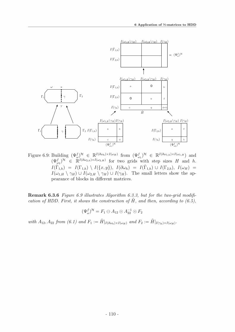
6 Application of H-matrices to HDD
a b
c d
e f
g h
a
e
b
c d+h
f
g
0
0
x
y
=:
Γ1
Γ1
Γ2
Γ2
γ
γ
ω
I(γh)I(γh)
I(Γ1,h)
I(Γ1,h)
I(Γ1,h)
I(γH)
I(γH)
I(γH)I(γH)
I(Γ2,h)
I(Γ2,h)
I(Γ2,h)
H
(Ψfω1
)H
I(ω1,H\γH)
I(ω1,H\γH)
I(ω1,H\γH)
I(ω2,H\γH)
I(ω2,H\γH)
I(ω2,H\γH)
(Ψfω2
)H
(Ψfω)H
I(γh)
Figure 6.9: Building (Ψfω)H ∈ RI(∂ωh)×I(ωH) from (Ψf
ω1)H ∈ RI(∂ω1,h)×I(ω1,H ) and
(Ψfω2
)H ∈ RI(∂ω2,h)×I(ω2,H) for two grids with step sizes H and h.
I(Γ1,h) = I(Γ1,h) \ I(x, y), I(∂ωh) = I(Γ1,h) ∪ I(Γ2,h), I(ωH) =I(ω1,H \ γH) ∪ I(ω2,H \ γH) ∪ I(γH). The small letters show the ap-pearance of blocks in different matrices.
Remark 6.3.6 Figure 6.9 illustrates Algorithm 6.3.3, but for the two-grid modifi-cation of HDD. First, it shows the construction of H, and then, according to (6.5),
(Ψfω)H = F1 ⊖ A12 ⊙ A−1
22 ⊙ F2
with A12, A22 from (6.1) and F1 := H|I(∂ωh)×I(ωH) and F2 := H|I(γh)×I(ωH).
- 110 -

7 Complexity and StorageRequirement of HDD
Let us recall four types of mappings which are present in the HDD method: domain-to-boundary Ψf
ω, boundary-to-boundary Ψgω, domain-to-interface Φf
ω and boundary-to-interface Φg
ω, for all domains ω ∈ TTh. In this Chapter we estimate the compu-
tational complexities of HDD and its modifications. We estimate also the storagerequirements of Φf
ω and Φgω. Finally, in the conclusion, we consider a special case,
namely, when the right-hand side is equal to 0.
7.1 Notation and Auxiliary Lemmas
Let x ∈ D ⊂ Rn, y ∈ Rm. Let ψ : x 7→ y be a given mapping. An algorithmfor computing ψ(x) is a sequence of elementary operations. The computationalcomplexity of the algorithm is characterised by the number of elementary operationsNψ. We take into account only the addition and the multiplication of real numbers,but in some special cases (e.g., the removal of a column from an H-matrix) we alsotake the cost of the coping into account.
Definition 7.1.1 If the computational complexity depends linearly on the data sizen, the algorithm has a linear computational complexity.
Definition 7.1.2 If the storage requirement depends linearly on the data size n, thealgorithm has a linear storage complexity.
Definition 7.1.3 We call the complexity O(n logq n), where q = 1, 2, 3, an almostlinear complexity.
Remark 7.1.1 For large input vectors (e.g., n = 1000000 is very common nowa-days) the time for an algorithm with linear complexity can be one hour and for analgorithm with quadratic complexity one month. This is the reason why it is impor-tant to develop and to use the algorithms with a linear complexity.
There is an empirical observation that says that there is a linear dependence be-tween the computer memory and the processor frequency. To get the optimal ratio(productivity) / (computational resources) the complexity of the algorithm mustbe a linear function of the computer memory and the processor frequency. This isanother reason to develop and to use algorithms with linear complexity.
In this section we show that the HDD method (Case (a)) and its three modifica-tions (Cases (b),(c),(d)) have almost linear complexity. We characterise each case
- 111 -

7 Complexity and Storage Requirement of HDD
by the domain of definition and range of Ψω and Φω.
Case (a) - The standard HDD methodΨfω : RI(ωh) → RI(∂ωh), ω ∈ TTh
,Ψgω : RI(∂ωh) → RI(∂ωh), ω ∈ TTh
,Φfω : RI(ωh) → RI(γh), ω ∈ TTh
,Φgω : RI(∂ωh) → RI(γh), ω ∈ TTh
.
Case (b) - HDD with truncation of the small scalesΨfω : RI(ωh) → RI(∂ωh), ω ∈ TTh
,Ψgω : RI(∂ωh) → RI(∂ωh), ω ∈ TTh
,Φfω : RI(ωh) → RI(γh), ω ∈ T≥HTh
,
Φgω : RI(∂ωh) → RI(γh), ω ∈ T≥HTh
.
Let P : RI(ωH) → RI(ωh) be a prolongation matrix as it is defined in Section 4.3.6.
Case (c) - HDD on two gridsΨfω := Ψf
ωPh←H , where Ψfω : RI(ωh) → RI(∂ωh), Ψf
ω : RI(ωH) → RI(∂ωh), ω ∈ TTh,
Ψgω : RI(∂ωh) → RI(∂ωh), ω ∈ TTh
,Φfω := Φf
ωPh←H , where Φfω : RI(ωh) → RI(γh), Φf
ω : RI(ωH) → RI(γh), ω ∈ TTh,
Φgω : RI(∂ωh) → RI(γh), ω ∈ TTh
.
Case (d) - HDD on two grids and with truncation of the small scalesΨfω := Ψf
ωPh←H , where Ψfω : RI(ωh) → RI(∂ωh), Ψf
ω : RI(ωH) → RI(∂ωh), ω ∈ TTh,
Ψgω : RI(∂ωh) → RI(∂ωh), ω ∈ TTh
,Φfω := Φf
ωPh←H , where Φfω : RI(ωh) → RI(γh), Φf
ω : RI(ωH) → RI(γh), ω ∈ T≥HTh,
Φgω : RI(∂ωh) → RI(γh), ω ∈ T≥HTh
.
h h h
H
h
H
one scale two scales
(a) (b) (c) (d)
Ψf
ΨfΨf
Ψf Ψg ΨgΨgΨg
Figure 7.1: Four cases of the HDD method: (a) the standard HDD method with afine scale h, (b) HDD with a fine scale h and with truncation of the smallscales, (c) HDD on two grids, (d) HDD on two grids and with truncationof the small scales.
We consider four modifications of the HDD method (see Figure 7.1). Case (a) isHDD without any modifications, i.e., there is only one scale h and no truncation.
- 112 -

7.1 Notation and Auxiliary Lemmas
In Case (b) there is one scale, but the algorithm “Root to Leaves” stops at a coarsescale H. Case (c) is HDD on two grids and a right-hand side f given at a coarsescale H. The fourth Case (d) is the same as the third case, but the algorithm “Rootto Leaves” truncates the scales smaller than H. Case (d) is the cheapest one.The long arrows show the algorithms “Leaves to Root” and “Root to Leaves”, theshort arrow in (c) indicates that the algorithm starts not with the smallest scale h,but with a scale H. The short arrow in (d) indicates that there is truncation of thesmall scales. The dotted lines mean that in the corresponding parts of the domaindecomposition tree TTh
the right-hand side is given on the coarse space VH ⊂ Vh andthe prolongation matrix is used.
0
1
1
h
H
.
.
.
.
.
.
.
.
.
.
.
.
.
.
.
.
.
.
.
.
.
.
.
.... .
.
0 x
y nh,x
nh,y
Figure 7.2: Model domain Ω = (0, 1)2 with rectangular grid and its hierarchicaldecomposition. nh,x and nh,y are the numbers of grid points in 0x and0y directions.
Remark 7.1.2 (Model Domain)To keep further theoretical calculations simple, we consider the model domain Ω =
(0, 1)2 with the rectangular grid and its hierarchical decomposition as in Fig. 7.2.
Consider the model problem as in Remark 7.1.2.Let nh,x(ω) and nh,y(ω) be the numbers of grid points in ω ∈ TTh
in the 0x and 0ydirections.The number of grid points in the domain ω ∈ TTh
is nh(ω) = nh,x(ω) · nh,y(ω).A domain ω on the level i of TTh
we denote by ωi. The root of TThhas level 0.
Suppose that nh,x(Ω) = nh,y(Ω) = 2p + 1 and nH,x(Ω) = nH,y(Ω) = 2q + 1. Then thenumber of nodal points in Ω is nh := nh(Ω) = (2p + 1)2 and if the grid step size isH, then nH := nH(Ω) = (2q + 1)2.The number of nodal points on the interface (see Fig. 7.4) is denoted by nh,H andnh,H ≤ 2nh,xnH,x = 2
√nhnH .
Suppose that |I(∂ωi)| ≤ 6nh,x(ωi) andnγωi
:= |I(γωi)| = nh,x(ωi)− 2.
The number of subdomains on each level i of TThis 2l, i = 0, ..., 2p.
- 113 -

7 Complexity and Storage Requirement of HDD
The depth of TThis not larger than log2 nh(Ω) + 2.
Note that 2p ≤ log2 nh(Ω) ≤ 2p+ 1, p ≥ 2.The depth of the domain decomposition tree with scale H (denoted by T≥HTh
) is
2q ≤ depth(T≥HTh) := log2 nH(Ω) ≤ 2q + 1.
level 0
level 1
level 2
level 2p
..................
leaves are triangles
level 2qH
.
.
.
.
.
..................h
.
Figure 7.3: Two levels 2q and 2p of the domain decomposition tree TTh.
Definition 7.1.4 The storage for all mappings Φω, ω ∈ TTh, is denoted by
S(Φ) :=∑
ω∈TTh
S(Φω).
Definition 7.1.5 The number of arithmetic operations for computing all mappingsΨω, ω ∈ TTh
, is denoted by
N(Ψ) :=∑
ω∈TTh
N(Ψω).
For further estimates we will need the following equalities (proofs of these facts seein Appendix):
p∑
i=0
i2 =1
3p3 +O(p2), (7.1)
p∑
i=0
i2i = (p− 1)2p+1 + 2, (7.2)
p∑
i=0
(p− i)2i = 2p+1 − p− 2, (7.3)
p∑
i=0
(p− i)22i ≤ 3 · 2p+1, (7.4)
- 114 -

7.2 Complexity of the Recursive Algorithm ”Leaves to Root”
p∑
i=0
i22i = (p2 − 2p+ 3)2p+1 − 6. (7.5)
Remark 7.1.3 In the following we will assume that
|I(∂ωi)| ≈ 2|I(∂ωi+2)| and
|I(ωi)| ≈ 2|I(ωi+1)|.
7.2 Complexity of the Recursive Algorithm ”Leaves
to Root”
Now we would like to compute the computational cost of the algorithm ”Leaves toRoot”. The Algorithm 7.2.1 computes recursively the mappings Φg
ω and Φfω for all
ω ∈ TTh. The domain decomposition tree TTh
(Ω) is an input parameter.
Algorithm 7.2.1 (Leaves to Root)leaves to root(structure TTh
(ω))begin
T1 :=get left son(TTh(ω));
T2 :=get right son(TTh(ω));
if (T1! = ∅) and (T2! = ∅) thenif (T1 is not computed) then
leaves to root(T1);if (T2 is not computed) then
leaves to root(T2);Ψgω := build Ψg(Ψg
ω1,Ψg
ω2); /∗ See Algorithms 6.3.1, 6.3.2 ∗/
Ψfω := build Ψf (Ψf
ω1,Ψf
ω2); /∗ See Algorithms 6.3.3, 6.3.4 ∗/
Φgω := compute Φg(..);
Φfω := compute Φf (..);
delete(Ψω1);delete(Ψω2);
end if;end;
Lemma 7.2.1 Let k be the rank which is used in the H-matrix arithmetic. Forthe model domain from Remark 7.1.2 the computational complexity of all mappingsΨgω : RI(∂ω) → RI(∂ω), ω ∈ TTh
, has the following upper bound:
N(Ψg) ≤ Ck2nh, C ∈ R+.
Proof: Let N(Ψgω) be the cost of building Ψg
ω from Ψgω1
and Ψgω2
, where ω, ω1, ω2 ∈TTh
and ω1, ω2 are sons of ω. Note that all ω at a fixed level of TThhave the same
- 115 -

7 Complexity and Storage Requirement of HDD
number of degrees of freedom. The total complexity is
N(Ψg) :=∑
ω∈TTh
N(Ψgω)
= N(Ψgω0
) + 2N(Ψgω1
) + 4N(Ψgω2
) + 8N(Ψgω3
) + ...+ 22p+1N(Ψgω2p+1
)
≤ 3N(Ψgω0
) + 12N(Ψgω2
) + ...+ (22p + 22p+1)N(Ψgω2p
)
≤p∑
i=0
(22i+1 + 22i)N(Ψgω2i
)
Lem.6.2.1=
p∑
i=0
(22i+1 + 22i)(C2ik2nh,x(ω2i) log2 nh,x(ω2i))
≤ 3 maxiC2ik
2
p∑
i=0
2i · 2inh,x2i
log2 nh,x2i
C′:=maxi C2i= 3C ′k2nh,x
p∑
i=0
2i · (log nh,x − i)2
≤ 3C ′k2nh,x
p∑
i=0
2i(p+ 1− i)2 = 6C ′k2nh,x
p−1∑
i=−1
2i(p− i)2
(7.4)
≤ Ck2nh,x · 2p ≤ Ck2nh, C ∈ R+.
Lemma 7.2.2 Let k be the rank which is used in the H-matrix arithmetic. Forthe model domain from Remark 7.1.2 the computational complexity of all mappingsΨfω : RI(ω) → RI(∂ω), ω ∈ TTh
, has the following upper bound:
N(Ψf ) ≤ Ck2nh log3 nh, C ∈ R+.
Proof: Let N(Ψfω) be the complexity of building Ψf
ω from Ψfω1
and Ψfω2
, whereω, ω1, ω2 ∈ TTh
and ω1, ω2 are sons of ω. Lemma 6.3.4 yieldsN(Ψfωi
) ≤ Cik2nh(ωi) log2 nh(ωi).
Since all ω at a fixed level of TThare equal, the following estimate holds
N(Ψf ) :=∑
ω∈TTh
N(Ψfω)
= N(Ψfω0
) + 2N(Ψfω1
) + 4N(Ψfω2
) + 8N(Ψfω3
) + ...+ 22pN(Ψfω2p
)
≤2p∑
i=0
2i(Cik2nh(ωi) log2 nh(ωi))
≤2p∑
i=0
2iC ′ik2nh2i
log2 nh2i
C′:=maxi C′i≤ C ′k2nh
2p∑
i=0
(2p+ 1− i)2
(7.1)
≤ C ′k2nh(1
3(2p+ 1)3) ≤ Ck2nh log3 nh, C ∈ R+.
- 116 -
7.3 Complexity of the Recursive Algorithm ”Root to Leaves”
Lemma 7.2.3 Let k be the rank which is used in the H-matrix arithmetic. For themodel domain from Remark 7.1.2 the computational complexity of all mappings Ψω,ω ∈ TTh
, has the following upper bound:
N(Ψ) = N(Ψf) +N(Ψg) ≤ Ck2nh log3 nh, C ∈ R+.
Proof: See Lemmas 7.2.1 and 7.2.2.
7.3 Complexity of the Recursive Algorithm ”Root to
Leaves”
The Algorithm 7.3.1 computes recursively the solution u|I(γω) for all ω ∈ TTh. The
input data are the domain decomposition tree TTh(Ω), the mappings Φg
ω and Φfω for
all ω ∈ TTh, and the solution u|I(∂ω) for a current subdomain ω.
u(x) =
g(x) for all x ∈ ∂ω,0 otherwise.
(7.6)
Note that in the Algorithm 7.3.1 gω and fω are the Dirichlet data and the right-handside for the local problem, defined on ω ∈ TTh
.
Algorithm 7.3.1 (Root to Leaves)root to leaves(TTh
(ω), u)beginT1 :=left son(TTh
(ω));T2 :=right son(TTh
(ω));uγω := Φg
ω · gω + Φfω · fω;
for all i ∈ I(γω) dou[local to global[i]]:=uγω [i];
if (T1! = ∅) thenroot to leaves(T1, u);
if (T2! = ∅) thenroot to leaves(T2, u);
end;
Here local to global[...] is an auxiliary index mapping, which for each global indexin I(Ω) returns its local index in I(ω). Note that we computed the mappings Φg
ω
and Φfω, ω ∈ TTh
, during the computation of the auxiliary mappings Ψfω and Ψg
ω.Below we estimate the complexity of computing the solution u.
Notation 7.3.1 We denote by Ng the complexity of all matrix-vector multiplicationsΦgω · gω, where Φg
ω ∈ RI(γω)×I(∂ω), g ∈ RI(∂ω).We denote by Nf the complexity of all matrix-vector multiplications Φf
ω · fω, whereΦfω ∈ RI(γω)×I(ω), f ∈ RI(ω).
Lemma 7.3.1 Let k be the rank which is used in the H-matrix arithmetic. For themodel domain from Remark 7.1.2 the computational complexity of all matrix-vector
- 117 -

7 Complexity and Storage Requirement of HDD
multiplications Φgω · gω, where Φg
ω : RI(∂ω) → RI(γ), ω ∈ TTh, g ∈ RI(∂ω), has the
following upper bound:Ng ≤ 21knh.
Proof: We have nh,γ ≤ nh,x(ω) for the model problem as in Remark 7.1.2. Thematrix Φg
ω is approximated in the low-rank format and belongs to R(k, I(γ), I(∂ω)).The complexity of the matrix-vector multiplication can be estimated as follows:
Ng(ω) ≤ 2k · (|I(γ)|+ |I(∂ω)|) ≤ 2k(nh,x(ω) + 6nh,x(ω)) = 14knh,x(ω).
The total complexity is
Ng =∑
ω∈TTh
Ng(ω)
≤p−2∑
i=0
(22i+1 + 22i)(14knh,x(ωi))
≤ 42k
p−2∑
i=0
22inh,x2i
= 42knh,x
p−2∑
i=0
2i ≤ 21knh,x2p ≤ 21knh.
Lemma 7.3.2 Let k be the rank which is used in the H-matrix arithmetic. For themodel domain from Remark 7.1.2 the computational complexity of all matrix-vectorproducts Φf
ω · fω, where Φfω : RI(ω) → RI(γ), ω ∈ TTh
, fω ∈ RI(ω), has the followingupper bound:
Nf ≤ Cknh log2 nh, C ∈ R+.
Proof: Each level i ∈ [0, 2p−3] of the tree TThcontains 2i matrices and each matrix
is multiplied by a vector fω. The complexity is
Nf =
2p−3∑
i=0
2iNf (ωi)
=
2p−3∑
i=0
2i(Ciknh(ωi) log nh(ωi))
≤ k ·2p−3∑
i=0
2i(C ′inh2i
lognh2i
)
C′:=maxi C′i≤ C ′nhk
2p−3∑
i=0
(2p+ 1− i) ≤ C ′nhkp(2p+ 4).
We recall that 4p2 ≤ log2 nh, and obtain Nf ≤ Cknh log2 nh.
- 118 -

7.3 Complexity of the Recursive Algorithm ”Root to Leaves”
Lemma 7.3.3 Let k be the rank which is used in the H-matrix arithmetic. Forthe model domain from Remark 7.1.2 the computational complexity of the algorithm“Root to Leaves” has the following upper bound:
N = Nf +Ng ≤ Cknh log2 nh, C ∈ R+.
Proof: See Lemmas 7.3.1, 7.3.2.
Lemma 7.3.4 Let k be the rank which is used in the H-matrix arithmetic. For themodel domain from Remark 7.1.2 the storage of all mappings Φω, ω ∈ TTh
, has thefollowing upper bound:
S(Φ) := S(Φg) + S(Φf ) ≤ Cknh log2 nh.
Proof: From Φgω : RI(∂ω) → RI(γ), Φf
ω : RI(ω) → RI(γ), |I(∂ω)| ≤ |I(ω)| follows thatS(Φg
ω) ≤ S(Φfω). Therefore it is enough to estimate only the second term
S(Φf ) =∑
ω∈TTh
S(Φfω)
=
2p∑
i=0
2iS(Φfωi
)
=
2p∑
i=0
2i(Ciknh(ωi) log nh(ωi))
≤2p∑
i=0
2iC ′iknh2i
lognh2i
C′:=maxi C′i≤ C ′knh
2p∑
i=0
(2p+ 1− i)
≤ C ′knhp(2p+ 2) ≤ Cknh log2 nh, C ∈ R+.
Table 7.1 compares the memory requirement of HDD with the memory requirementsof H-Cholesky factorisation and the direct H-matrix inverse. The memory neededfor HDD is close to the memory needed for H-Cholesky and much smaller than thememory for the direct H-matrix inverse.
Let us in Lemma 7.3.5 estimate the storage requirements of HDD if only thefunctionals which compute the mean values in all ω ∈ TTh
are of interest (see Section4.4.6).
Lemma 7.3.5 Let k be the rank which is used in the H-matrix arithmetic. Let themodel domain be as in Remark 7.1.2. HDD requires S ≤ Cknh log nh, C ∈ R+,units of memory for storing all functionals λfω : RI(ω) → R and λgω : RI(∂ω) → R.
- 119 -
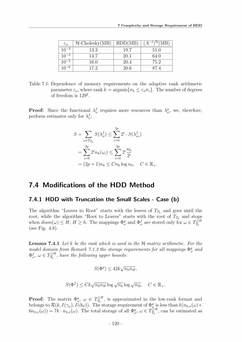
7 Complexity and Storage Requirement of HDD
εa H-Cholesky(MB) HDD(MB) (A−1)H(MB)
10−3 13.3 19.7 51.010−4 14.7 20.1 64.010−5 16.0 20.4 75.210−6 17.2 20.6 87.4
Table 7.1: Dependence of memory requirements on the adaptive rank arithmeticparameter εa, where rank k = argminσk ≤ εaσ1. The number of degreesof freedom is 1292.
Proof: Since the functional λfω requires more resources than λgω, we, therefore,perform estimates only for λfω:
S =∑
ω∈TTh
S(λfω) ≤2p∑
i=0
2i · S(λfωi)
=
2p∑
i=0
2inh(ωi) ≤2p∑
i=0
2inh2i
= (2p+ 1)nh ≤ Cnh log nh, C ∈ R+.
7.4 Modifications of the HDD Method
7.4.1 HDD with Truncation the Small Scales - Case (b)
The algorithm “Leaves to Root” starts with the leaves of TThand goes until the
root, while the algorithm “Root to Leaves” starts with the root of TThand stops
when diam(ω) ≤ H, H ≥ h. The mappings Φgω and Φf
ω are stored only for ω ∈ T≥HTh
(see Fig. 4.8).
Lemma 7.4.1 Let k be the rank which is used in the H-matrix arithmetic. For themodel domain from Remark 7.1.2 the storage requirements for all mappings Φg
ω andΦfω, ω ∈ T≥HTh
, have the following upper bounds:
S(Φg) ≤ 42k√nhnH ,
S(Φf ) ≤ Ck√nhnH log
√nh log
√nH , C ∈ R+.
Proof: The matrix Φgω, ω ∈ T≥HTh
, is approximated in the low-rank format andbelongs toR(k, I(γω), I(∂ω)). The storage requirement of Φg
ω is less than k(nh,x(ω)+6nh,x(ω)) = 7k · nh,x(ω). The total storage of all Φg
ω, ω ∈ T≥HTh, can be estimated as
- 120 -

7.4 Modifications of the HDD Method
follows
S(Φg) :=∑
ω∈T≥HTh
S(Φgω)
= S(Φgω0
) + 2S(Φgω1
) + 4S(Φgω2
) + 8S(Φgω3
) + ...+ 22q+1S(Φgω2q+1
)
≤ 3S(Φgω0
) + 12S(Φgω2
) + ...+ (22q + 22q+1)N(Φgω2q
)
≤q∑
i=0
(22i+1 + 22i)S(Φgω2i
)
≤q∑
i=0
(22i+1 + 22i)(7k · nh,x(ω2i))
= 21k
q∑
i=0
22i(nh,x2i
)
= 21knh,x
q∑
i=0
2i < 21knh,x2q+1
≤ 42knh,xnH,x = 42k√nhnH .
The total storage of all Φfω, ω ∈ T≥HTh
, can be estimated as follows
S(Φfω) =
∑
ω∈T≥HTh
S(Φfω)
=
2q∑
i=0
2i(Ci · 2knh,x(ωi) · nH,x(ωi) log 2nh,x(ωi) · nH,x(ωi))
≤2q∑
i=0
2i(C ′i2knh,x · nH,x
2ilog(
2nh,x · nH,x2i
))
C′:=maxi C′i= 2C ′knh,xnH,x
2q∑
i=0
(log(nh,xnH,x)− i+ 1)
≤ 2C ′knh,xnH,x
2q∑
i=0
(p+ 1 + q + 1− i+ 1)
≤ 2C ′knh,xnH,x(p+ 3)(2q + 1) ≤ Ck√nhnH log
√nh · log
√nH , C ∈ R+.
- 121 -

7 Complexity and Storage Requirement of HDD
H
h
Figure 7.4: An example with two grids. Level 2q corresponds to the scale H andlevel 2p to the scale h. The solution in ω ∈ TTh
with diam(ω) ≥ H is ofinterest.
Lemma 7.4.2 Let k be the rank which is used in the H-matrix arithmetic. For thedomain from Remark 7.1.2 the following two statements hold. a) The computationalcomplexity of all matrix-vector multiplications Φg
ω · gω, where Φgω : RI(∂ωh) → RI(γh),
ω ∈ T≥HTh, gω ∈ RI(∂ωh), has the following upper bound:
Ng ≤ 84k√nhnH .
b) The computational complexity of all matrix-vector multiplications Φfω · fω, where
Φfω : RI(ωh) → RI(γh), ω ∈ T≥HTh
, fω ∈ RI(ωh), has the following upper bound:
Nf ≤ Ck√nhnH log
√nh log
√nH , C ∈ R+.
Proof: Let R ∈ R(k, n,m) be a low-rank matrix and v ∈ Rm a vector. Recall thatthe storage S(R) is equal to k(n+m) and the cost N of R · v is less than 2k(n+m),i.e., N(R · v) ≤ 2S(R). Then Lemma 7.4.1 yields
Ng ≤ 2 · 42k√nhnH .
b) Let M be an H-matrix and v a vector. Due to Lemma 5.10.2, N(M ·v) ≤ 2S(M),where N(M ·v) is the cost of the multiplication and S(M) is the storage requirementof M . From Lemma 7.4.1 follows that
Nf ≤ 2S(Φf ) ≤ 2C ′k√nhnH log
√nh log
√nH , C ′ ∈ R+.
Lemma 7.4.3 Let k be the rank which is used in the H-matrix arithmetic. For thedomain from Remark 7.1.2 the computational complexity of the algorithm “Root toLeaves” on two grids with step sizes h and H has the following upper bound:
N = Nf +Ng ≤ Ck√nhnH log
√nh log
√nH , C ∈ R+.
Proof: Use the fact Nf > Ng and Lemma 7.4.2.
- 122 -
7.4 Modifications of the HDD Method
7.4.2 HDD on Two Grids - Case (c)
We construct Ψgω and Φg
ω as in Case (a) (Sections 7.2, 7.3). If the right-hand sidef is smooth, then it is enough to consider the right-hand side f in a coarse spaceVH ⊂ Vh. In this case we construct the mappings Ψf
ω : RI(ωH) → RI(∂ωh) andΦfω : RI(ωH) → RI(γh) from Ψf
ωi: RI(ωi,H) → RI(∂ωi,h), i = 1, 2, ω, ω1, ω2 ∈ TTh
.
Remark 7.4.1 Note that in this modification of HDD the matrices Ψfω, Φf
ω have asmaller number of columns (|I(ωH)| ≤ |I(ωh)|) than the respective matrices in Cases(a) and (b). The number of degrees of freedom on the fine grid is nh = nh,xnh,x, thenumber of degrees of freedom on the interface (see Fig. 7.4) is nh,H ≤ 2 · nh,xnH,x,where nH,x ≤ nh,x.
Lemma 7.4.4 Let k be the rank which is used in the H-matrix arithmetic. Forthe model domain from Remark 7.1.2 the computational complexity of all mappingsΨfω : RI(ωH) → RI(∂ωh), ω ∈ T≥HTh
, has the following upper bound:
N(Ψf) ≤ Ck2√nHnh log3√nHnh, C ∈ R+.
Proof: Due to Lemma 7.2.2, the computational complexity of all mappings Ψfω,
ω ∈ TTh, is estimated by C ′k2nh log3 nh. On the interface (see Fig. 7.4) the number
of nodal points is 2√nhnH . We substitute nh in C ′k2nh log3 nh by 2
√nhnH and
obtain
N(Ψf) ≤ C ′k2 · 2√nhnH log3(2√nhnH) ≤ Ck2√nHnh log3√nHnh.
Lemma 7.4.5 Let k be the rank which is used in the H-matrix arithmetic. For themodel domain from Remark 7.1.2 the storage of all mappings Φf
ω : RI(ωH) → RI(γh),ω ∈ T≥HTh
, has the following upper bound:
S(Φf ) ≤ Ck√nHnh log2√nHnh, C ∈ R+.
Proof: From Lemma 7.3.4 follows that the storage requirement for all mappingsΦfω, ω ∈ TTh
, is estimated by C ′knh log2 nh, C′ ∈ R+. Now the number of nodal
points is not nh, but 2√nhnH . Therefore
S(Φfω) ≤ C ′k · 2√nhnH log2(2
√nhnH) ≤ Ck
√nhnH log2√nhnH .
In Table 7.2 we present the dependences of the storage requirements for the mappingsΦg, Φf on h and H (domain Ω as in Remark 7.1.2). Here
‖u− uk‖2 / ‖u‖2 ≈ 10−5, ‖u− uk‖∞ ≈ 10−5,
where u is the exact solution and uk the approximated solution. We see that Φg hasa linear memory requirement and Φf an almost linear memory requirement. Thememory requirement of HDD on two grids with step sizes H = 0.5 and h is in afactor ∼ 2 smaller (the third column) than the memory requirements of the standardHDD (the first column). For H = 0.125 the factor is ∼ 1.4 (the forth column).
- 123 -

7 Complexity and Storage Requirement of HDD
h Φg,Φf ,H = h,kB Φg,Φf ,H = 0.5,kB Φg,Φf ,H = 0.125,kB
1/33 2.45 ∗ 102, 4 ∗ 102 9.1 ∗ 10, 1.7 ∗ 102 2 ∗ 102, 2.8 ∗ 102
1/65 1.1 ∗ 103, 2.4 ∗ 103 2.9 ∗ 102, 1.2 ∗ 103 7.9 ∗ 102, 1.8 ∗ 103
1/129 5 ∗ 103, 1.4 ∗ 104 6.8 ∗ 102, 8 ∗ 103 2.6 ∗ 103, 1.2 ∗ 104
1/256 2.1 ∗ 104, 7.86 ∗ 104 1.4 ∗ 103, 4.1 ∗ 104 7.4 ∗ 103, 6.9 ∗ 104
Table 7.2: The dependence of the memory requirements for Φg and Φf on the gridstep sizes h,H.
7.4.3 HDD on Two Grids and with Truncation of Small Scales -Case (d)
This case combines Cases (b) and (c). Suppose that the right-hand side f is givenin the space VH ⊂ Vh. We prolongate fH ∈ VH onto the fine space Vh and obtainfh := Ph←HfH . After that we construct the mappings Ψf
ω : RI(ωH) → RI(∂ωh) andΦfω : RI(ωH) → RI(γh) for all ω ∈ T≥HTh
.
Lemma 7.4.6 Let k be the rank which is used in the H-matrix arithmetic. Forthe model domain from Remark 7.1.2 the computational complexity of the algorithm“Leaves to Root” has the following upper bound:
N(Ψ) = N(Ψfω) +N(Ψg
ω) ≤ Ck2√nHnh log3√nhnH , C ∈ R+.
Proof: Analogously to Case (c). See the proof of Lemma 7.4.4.
Lemma 7.4.7 Let k be the rank which is used in the H-matrix arithmetic. Forthe model domain from Remark 7.1.2 the computational complexity of the algorithm“Root to Leaves” has the following upper bound:
N = Ng +Nf ≤ Ck√nhnH log
√nh log
√nH , C ∈ R+.
Proof: Analogously to Case (b). See the proof of Lemma 7.4.2.
Lemma 7.4.8 Let k be the rank which is used in the H-matrix arithmetic. For themodel domain from Remark 7.1.2 the storage requirements of the mappings Φg
ω andΦfω for all ω ∈ T≥HTh
have the following upper bounds:
S(Φgω) ≤ 42k
√nhnH and
S(Φfω) ≤ Ck
√nhnH log
√nh log
√nH .
Proof: These storage requirements are the same as in Case (b). See the proof ofLemma 7.4.1.
- 124 -

8 Parallel Computing
In this chapter we present the parallel HDD algorithm and estimate its complexity.
8.1 Introduction
In this chapter we consider the parallel computers with the shared memory archi-tecture (although the distributed memory architecture is also possible). We willconsider the parallel RAM (PRAM) model, which consists of q processors and aglobal memory which can be accessed simultaneously by all processors. All datatransfers between different processors are handled by this memory system. Thecommunication time between processors is negligible small in comparison with thecomputational time.To characterize parallel algorithms we introduce the following notation:
Definition 8.1.1 Let t(q) be the execution time of the parallel algorithm A on a
machine with q processors. Then we denote the parallel speedup by S(q) := t(1)t(q)
and
the parallel efficiency of A by E(q) := S(q)q
= t(1)q·t(q) .
To parallelize the HDD method one needs to do the following:
1. Perform the triangulation Th of the domain Ω and construct the hierarchicaldecomposition tree TTh
in parallel.
2. Perform the parallelization of theH-matrix arithmetic (described by R.Kriemannin his dissertation [44]).
3. Perform the parallelization of the algorithm “Leaves to Root”.
4. Perform the parallelization of the algorithm “Root to Leaves” ( requires theparallel H-matrix-vector multiplication).
The time for item (1) is much smaller than the time needed for items (3) and (4).The parallel H-matrix arithmetic is used in items (3) and (4).
- 125 -

8 Parallel Computing
8.2 Parallel Algorithms for H-Matrix Arithmetics
The parallel algorithms for the matrix-vector multiplication, matrix-matrix addition,matrix-matrix multiplication and LU-decomposition for dense matrices can be foundin [25]. The parallel versions of the respective algorithms forH-matrices can be foundin [44].
Theorem 8.2.1 Let T := TI×I be a block cluster trees, M,M ′,M ′′ ∈ H(TI×I , k),n := |I|, x ∈ Rn. Suppose nmin > k. Let |L(T )|, |V (T )| be the numbers of leaves andof nodes in the block cluster tree TI×I , q = 2r is the number of parallel processors.Then the computational complexities in Table 8.1 hold.
Operation Sequential Complexity Parallel Complexity
building(M) N = O(n log n) Nq
+O(|V (T )\L(T )|)storage(M) N = O(kn log n) N
q
Mx N = O(kn log n) Nq
M ′ ⊕M ′′ N = O(k2n log n) Nq
M ′ ⊙M ′′ N = O(k2n log2 n) Nq
+O(Csp(T )|V (T )|)M−1 N = O(k2n log2 n) N
q+O(nn2
min)
H-LU N = O(k2n log2 n) Nq
+O(k2n log2 nn1/d )
Table 8.1: Computational complexities for sequential and parallel algorithms.
Proof: For the proof of the estimates from the second column see [27] or [33]. Forthe proof of the estimates from the third column see [45] or [44].
Definition 8.2.1 Let v be a vertex of TTh, then we denote the subtree which has
vertex v as a root by TTh(v). The set of all nodes at the level l of TTh
we denote by
T(l)Th
.
Remark 8.2.1 Since the parallel efficiency for small matrices is much smaller thanfor large matrices, we divide TTh
into two parts T(l<r)Th
and T(l≥r)Th
(see Fig. 8.1),
where r := log q. T(l<r)Th
contains domains with a large number of degrees of freedom
and T(l≥r)Th
with a small number. The parallel arithmetic is applied only for levels0, .., r − 1. The matrices which appear on the levels r, ..., 2p are small enough andare computed by one processor.
Assumption 8.2.1 Let ω1 be a son of ω. We suppose that |I(ω1)| ≈ 12|I(ω)|,
|I(∂ω1)| ≤ 34|I(∂ω)| and |I(∂ω)| ≤ 6|I(γω)|.
- 126 -

8.2 Parallel Algorithms for H-Matrix Arithmetics
r
[0,...,q-1]
[q/2,...,q-1][0,...,q/2-1]
[0,...,q/4-1] [3q/4,...,q-1]
0 1 2 q-1step size H
step size h
q/2
q/4
1
q ..
.
.
computed
by 1 processor
number of processors
per node
[..][..]T
(l<r)Th
T(l≥r)Th
TTh(v)
Figure 8.1: (left) Decomposition of the TThinto T
(l<r)Th
and T(l≥r)Th
and distributionof q processors. (right) The matrices at the level l ∈ [0, .., r − 1] arecomputed by q
2l processors. The subtree TTh(v) is computed by one
processor.
The parallel version of the algorithm “Leaves to Root”
On each level l < r of TTh(the root has level l = 0) every node gets 2r−l processors.
Every subtree TTh(v), v ∈ T (r)
Th, is computed by one processor (see Fig. 8.1 (right)).
Lemma 8.2.1 Let Sω := A11 − A12A−122 A21 (see (6.1)), where
A11 ∈ H(TI(∂ω)×I(∂ω), k), A12 ∈ R(k, I(∂ω), I(γω)), A21 ∈ R(k, I(γω), I(∂ω)),A22 ∈ H(TI(γω)×I(γω), k), ω ∈ TTh
, and nh,γ := |I(γω)|. The parallel complexity of thecomputation of Sω has the following upper bound:
N(Sω, q) ≤C1k
2nh,γ log2 nh,γq
+ C2n2minnh,γ , C1, C2 ∈ R+. (8.1)
Proof: Due to Table 5.3 the parallel complexity of the inversion A−122 is
C1k2nh,γ log2 nh,γ
q+ C0n
2minnh,γ , C0, C1 ∈ R+.
The parallel complexity of the multiplication A12 · A−122 is k-times the MV multipli-
cation, i.e.,C2k2nh,γ lognh,γ
q, C2 ∈ R+. The parallel complexity of the multiplication
(A12A−122 ) · A21 (product of two low-rank matrices defined in Lemma 5.6.4) is
2k2
q(|I(∂ω)|+ |I(γω)|)
Assum. 8.2.1
≤ 14k2nh,γq
.
The parallel complexity of the subtraction A11 − A12A−122 · A21 is
C3k2|I(∂ω)| log |I(∂ω)|
q
Assum. 8.2.1
≤ C4k2nh,γ log nh,γ
q, C3, C4 ∈ R+.
- 127 -
8 Parallel Computing
Thus,
N(Sω, q) ≤1
q(C4k
2nh,γ log nh,γ + C1k2nh,γ log2 nh,γ) + C0n
2minnh,γ
≤ Ck2nh,γ log2 nh,γq
+ C0n2minnh,γ , C0, C ∈ R+. (8.2)
Lemma 8.2.2 Let Zω := F1 − A12A−122 F2 (see Lemma 6.2.2), where ω ∈ TTh
,
A12 ∈ R(k, I(∂ω), I(γω)), A22 ∈ H(TI(γω)×I(γω), k),
F1 ∈ H(TI(∂ω)×I(ω), k), F2 ∈ H(TI(γω)×I(ω), k),
nh := |I(ω)|. Let the model domain be as in Remark 7.1.2. The parallel complexityof the computation of Zω on a machine with q processors has the following upperbound:
N(Zω, q) ≤Ck2nh log nh
q, C ∈ R+. (8.3)
Proof: A12 ·A−122 was computed in parallel for Ψg
ω (Lemma 8.2.1). The complexity ofthe multiplication (A12A
−122 ) ·F2 (the product of a low-rank matrix and an H-matrix
is k-times the H-matrix-vector multiplication) is estimated by C1k2nh lognh
q, C1 ∈ R+.
The complexity of the subtraction F1 − A12A−122 F2 is C2k2nh lognh
q, C2 ∈ R+. Thus,
N(Zω, q) ≤1
q(C1k
2nh log nh + C2k2nh log nh) ≤
Ck2nh log nhq
, C ∈ R+.
Lemma 8.2.3 Let Ψgω ∈ RI(∂ω)×I(∂ω), Ψf
ωi∈ RI(∂ωi)×I(∂ωi), ω, ωi ∈ TTh
, i = 1, 2,ω = ω1 ∪ ω2. For the model domain from Remark 7.1.2 the parallel computationalcomplexity of building Ψg
ω from Ψgω1
and Ψgω2
has the following upper bound:
N(Ψg, q) ≤ Ck2nh,γ log2 nh,γq
+ C1nh,γn2min, C, C1 ∈ R+, nh,γ := |I(γω)|.
Proof: Lemma 5.10.8 states that building Ψgω1|I(∂ω)×I(∂ω), Ψg
ω2|I(∂ω)×I(∂ω) and their
adding on a machine with one processor costs
N(Ψg, 1) ≤ C0k2|I(∂ω)| log2 |I(∂ω)| ≤ C ′k2nh,γ log2 nh,γ , C0, C
′ ∈ R+.
Theorem 8.2.1 states that the parallel complexity of theH-matrix addition is N(q) =N(1)q
. From these two facts follows that adding Ψgω1|I(∂ω)×I(∂ω)⊕Ψg
ω2|I(∂ω)×I(∂ω) costs
C′k2nh,γ log2 nh,γ
q. After the elimination of the unknowns with indices from I(γω), we
obtain Ψgω. By Lemma 8.2.1 this elimination costs
C2k2nh,γ log2 nh,γ
q+ C1n
2minnh,γ , C1, C2 ∈ R+. (8.4)
- 128 -

8.3 Parallel Complexity of the HDD Method
The total complexity is
N(Ψg, q) ≤ Ck2nh,γ log2 nh,γq
+ C1n2minnh,γ with C = C2 + C ′. (8.5)
Lemma 8.2.4 Let Ψfω ∈ RI(∂ω)×I(ω), Ψf
ωi∈ RI(∂ωi)×I(ωi), ω, ωi ∈ TTh
, i = 1, 2,ω = ω1 ∪ω2 and nh := |I(ω)|. For the model domain from Remark 7.1.2 the parallelcomputational complexity of building Ψf
ω from Ψfω1
and Ψfω2
has the following upperbound:
N(Ψf , q) ≤ Ck2nh log2 nhq
, C ∈ R+.
Proof: In Lemma 5.10.8 we proved that the building of Ψfω1|I(∂ω)×I(ω) and Ψf
ω2|I(∂ω)×I(ω)
and their truncated addition on a machine with one processor cost N(Ψf , 1) ≤C1k
2nh log2 nh, C1 ∈ R+. Theorem 8.2.1 states that the parallel complexity ofthe H-matrix addition is N(q) = N(1)
q. From these two facts follows that adding
Ψfω1|I(∂ω)×I(ω)⊕Ψf
ω2|I(∂ω)×I(ω) costs C1k2nh log2 nh
q. The computation of Zω from Lemma
8.2.2 costs C2k2nh lognh
q, C2 ∈ R+.
Thus, the total complexity is
N(Ψf , q) ≤ C1k2nh log2 nhq
+C2k
2nh log nhq
≤ Ck2nh log2 nhq
, C ∈ R+. (8.6)
8.3 Parallel Complexity of the HDD Method
8.3.1 Complexity of the Algorithm “Leaves to Root”
Lemma 8.3.1 Let q be the number of parallel processors. The model domain andthe domain decomposition tree TTh
is the same as in Remark 7.1.2. The parallelcomputational complexity of all mappings Ψg
ω, ω ∈ TTh, has the following upper
bound:
N(Ψg, q) ≤ 3r
2r·C′k2√nh log2√nh + Ck2nh
q+C ′′(1− 3r
4r)√nhn
2min, C ′, C ′′, C ∈ R+.
Proof: We decompose N(Ψg, q) into two terms (see the reason in Remark 8.2.1)
N(Ψg, q) =r−1∑
l=0
N(Ψgωl,q
2l) +
∑
ω∈TTh(v)
N(Ψgω, 1), v ∈ T (r)
Th. (8.7)
- 129 -

8 Parallel Computing
Note that if ω = ω1 ∪ ω2 then |I(∂ω)| ≤ |I(∂ω1)| + |I(∂ω2)|. The first term can beestimated as follows:
r−1∑
l=0
N(Ψgωl,q
2l)
Lem.8.2.3
≤ C1k2nh,γ log2 nh,γ
q+ C ′1nh,γn
2min
+ C2
k2 3nh,γ
4log2 3nh,γ
4q2
+ C ′23nh,γ
4n2min + ...
+ Crk2(3
4)r−1nh,γ log2(3
4)r−1nh,γ
q2r−1
+ C ′r3r−1
4r−1nh,γn
2min
≤ 2 · (3r
2r− 1) max
i=1..rCi ·
k2nh,γ log2 nh,γq
+ 4 maxi=1..r
C ′i · (1−3r
4r)nh,γn
2min
≤ C ′3r
2r· k
2nh,γ log2 nh,γq
+ C ′′(1− 3r
4r)nh,γn
2min,
where C ′ := 2 maxi=1..r Ci and C ′′ := 4 maxi=1..r C′i. Note that for each subtree
TTh(v), v ∈ T
(r)Th
, we have just one processor and therefore (see Definition 8.2.1,Assumption 8.2.1)
∑
ω∈TTh(v)
N(Ψgω, 1)
Lemma 7.2.1
≤ Ck2 3r
4rnh,
where 3r
4rnh is the number of nodal points in the root of TTh(v), C ∈ R+. Taking
into account the facts q = 2r, nh,γ ≤√nh, we obtain
N(Ψg, q) ≤ 3r
2r· C′k2√nh log2√nh + Ck2nh
q+ C ′′(1− 3r
4r)√nhn
2min.
Lemma 8.3.2 Let q be the number of parallel processors. The model domain andthe domain decomposition tree TTh
is the same as in Remark 7.1.2. The parallelcomputational complexity of all mappings Ψf
ω, ω ∈ TTh, has the following upper
bound:
N(Ψf , q) ≤ Ck2nhq
log3 nhq, C ∈ R+.
Proof: We decompose N(Ψf , q) into two terms (see the reason in Remark 8.2.1)
N(Ψf , q) =r−1∑
l=0
N(Ψfωl,q
2l) +
∑
ω∈TTh(v)
N(Ψfω, 1), v ∈ T (r)
Th. (8.8)
- 130 -

8.3 Parallel Complexity of the HDD Method
Recall that |I(ω1)| ≈ 12|I(ω)|. The first term can be estimated as follows:
r−1∑
l=0
N(Ψfωl,q
2l)
Lem.8.2.4
≤ C1k2nh log2 nh
q+ C2
k2 nh
2log2 nh
2q2
+ ...+ Crk2 nh
2r−1 log2 nh
2r−1
q2r−1
C = maxi=1..r
Ci
≤ Ck2nhq
(log2 nh + log2 nh2
+ ...+ log2 nh2r−1
)
≤ Ck2nhq
((2p+ 1)2 + (2p)2 + ...+ (2p− r + 2)2)
≤ Ck2nhq
(1
3((2p+ 1)3 − (2p− r + 1)3)
≤ Ck2nh3q
· (4(2p+ 1)2r − 4(2p+ 1)r2 + r3)
≤ C ′k2nh(log nh − log q) log nh · log q
q.
Note that for each ω ∈ TTh(v) we have just one processor and therefore (see Definition
8.2.1 and Assumption 8.2.1)
∑
ω∈TTh(v)
N(Ψfω, 1)
Lem. 7.2.2
≤ Ck2nh(v) log3 nh(v)
≤ Ck2nh2r
log3 nh2r, C ∈ R+.
We take into account the following inequality
C ′k2nh(log nh − log q) log nh · log q
q≤ C2k
2nhq
log3 nhq
and obtain the statement of the lemma.
Lemma 8.3.3 Let q be the number of parallel processors. The model domain andthe domain decomposition tree TTh
is the same as in Remark 7.1.2. The parallelcomputational complexity of all mappings Ψω, ω ∈ TTh
, has the following upperbound:
N(Ψ, q) ≤ C ′k2√nh log2√nh + Ck2nhq0.45
+ C ′′(1− 3r
4r)√nhn
2min + Ck2nh
qlog3 nh
q,
where C, C ′, C ′′, C ∈ R+.
Proof: Using Lemmas 8.3.1, 8.3.2, compute N(Ψ, q) = N(Ψf , q) +N(Ψg, q). Notethat 3r
4r ≈ 1q0.45 and nh,γ ≤
√nh.
- 131 -

8 Parallel Computing
8.3.2 Complexity of Algorithm “Root to Leaves”
The input data for this algorithm is a set of mappings Φgω and Φf
ω for all ω ∈ TTh.
The algorithm “Root to Leaves” performs the multiplications Φgω · gω and Φf
ω · fω.
Notation 8.3.1 The cost of the multiplication Φgω · gω on a computer with q proces-
sors we denote by Ng(ω, q). The cost of all multiplications Φgω · gω, ω ∈ TTh
, on acomputer with q processors we denote by Ng(q). Similarly, we define Nf (ω, q) andNf (q).
Lemma 8.3.4 Let q be the number of parallel processors. The model domain andthe domain decomposition tree TTh
is the same as in Remark 7.1.2. The parallelcomputational complexity of all matrix-vector products Φg
ω · gω, where Φgω : RI(∂ω) →
RI(γω), gω ∈ RI(∂ω), ω ∈ TTh, has the following upper bound:
Ng(q) ≤28k√nh
q
3r
2r+
21knhq
.
Proof: We divide Ng(q) into two terms (see the reason in Remark 8.2.1)
Ng(q) =r−1∑
l=0
Ng(ωl,q
2l) +
∑
ω∈TTh(v)
Ng(ω, 1), where v ∈ T (r)Th. (8.9)
Φgω is approximated in the low-rank format and belongs to R(k, I(γω), I(∂ω)). As-
sumption 8.2.1 gives |I(∂ω)| ≤ 6nh,x, where |I(γω)| = nh,γ ≤ nh,x ≃√n. The
parallel complexity of the multiplication Φgω · gω can be estimated as follows:
2k · (|I(∂ω)|+ |I(γω)|)q
≤ 2k · (6nh,x + nh,x)
q=
14knh,x(ω)
q. (8.10)
Suppose that the number of external boundary points decreases by a factor 34
aftereach division, i.e., |I(∂ω1)| ≤ 3
4|I(∂ω)|. Taken into account (8.10), the first term in
(8.9) can be estimated as follows:
r−1∑
l=0
Ng(ωl,q
2l) ≤ 14knh,x
q+
14k3nh,x
4q2
+ ...+14k
3r−1nh,x
4r−1
q2r−1
= 14knh,xq
(1 +3
2+ ...+
3r−1
2r−1)
q=2r
≤ 28k√nh
q(3r
2r− 1) ≤ 28k
√nh
q
3r
2r.
The second term in (8.9) can be estimated by Lemma 7.3.1 as follows
∑
ω∈TTh(v)
Ng(ω, 1) ≤ 21knhq
,
where nh
qis the number of degrees of freedom in the root of TTh
(v).
- 132 -
8.3 Parallel Complexity of the HDD Method
Lemma 8.3.5 Let q be the number of parallel processors. The model domain andthe domain decomposition tree TTh
is the same as in Remark 7.1.2. The parallelcomputational complexity of the matrix-vector products Φf
ω · fω, where Φfω : RI(ω) →
RI(γω), fω ∈ RI(ω), ω ∈ TTh, has the following upper bound:
Nf (q) ≤ Ck2nhq
log2 nhq, C ∈ R+.
Proof: Each level i ∈ [0, 2p − 3] of the tree TThcontains 2i matrices and every
matrix is to be multiplied by vector f . The parallel arithmetic is applied only forlevels 0, .., r− 1 (see Figure 8.1). The matrices which appear on the levels l ≥ r aresmall enough and are computed by one processor. Suppose that |I(ω1)| ≤ 1
2|I(ω)|
(see Assumption 8.2.1). We divide Nf (q) into two parts
Nf (q) =r−1∑
l=0
Nf (ωl,q
2l) +
∑
ω∈TTh(v)
Nf (ω, 1), where v ∈ T (r)Th. (8.11)
The first term in (8.11) can be estimated as follows
r−1∑
l=0
Nf (ωl,q
2l)Lem.7.3.2
≤ C1k2nh log nh
q+ C2
k2 nh
2log nh
2q2
+ ...+ Crk2 nh
2r−1 log nh
2r−1
q2r−1
C′= maxi=1..r
Ci
≤ C ′ · k2nhq
(2p+ 1 + 2p+ ...+ 2p− r + 2)
r=log q
≤ C ′k2nh((2p+ 1)(2p+ 2)− (2p− r + 1)(2p− r + 2))
2q
≤ Ck2nh(4pr − r2)
2qr=log q
≤ Ck2nh(2 log nh − log q) log q
q, C ∈ R+.
By Lemma 7.3.2 the second term in (8.11) can be estimated as follows
∑
ω∈TTh(v)
Nf (ω, 1) ≤ Cknhq
log2 nhq.
We take into account the inequality
Ck2nh(2 log nh − log q) log q
q≤ C ′′k2nh
qlog2 nh
q
and obtain the statement of the lemma.
- 133 -

8 Parallel Computing
Lemma 8.3.6 Let q be the number of parallel processors. The model domain andthe domain decomposition tree TTh
is the same as in Remark 7.1.2. The parallelcomputational complexity of the algorithm “Root to Leaves” has the following upperbound:
N(q) = Nf (q) +Ng(q)
≤ Ck2nhq
log2 nhq
+28k√nh
q
3r
2r, C ∈ R+.
Proof: See Lemmas 8.3.4, 8.3.5 and use the inequality
21knhq≤ Ck2nh
qlog2 nh
q.
- 134 -
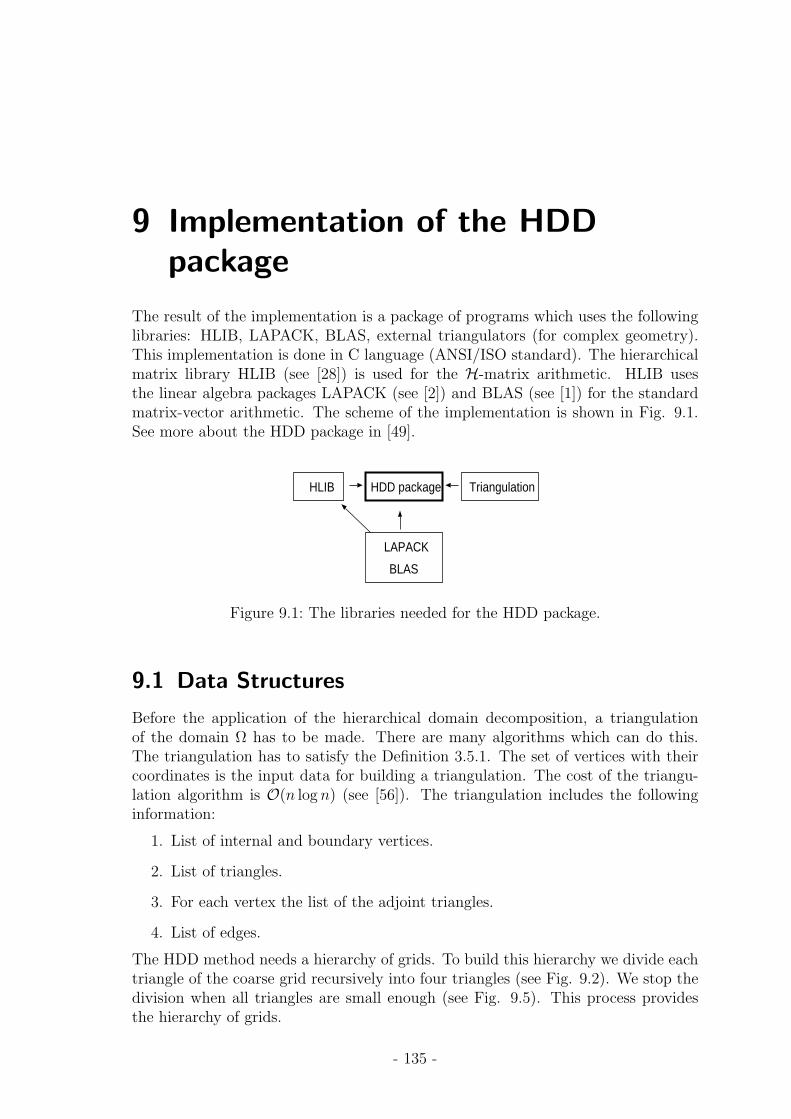
9 Implementation of the HDDpackage
The result of the implementation is a package of programs which uses the followinglibraries: HLIB, LAPACK, BLAS, external triangulators (for complex geometry).This implementation is done in C language (ANSI/ISO standard). The hierarchicalmatrix library HLIB (see [28]) is used for the H-matrix arithmetic. HLIB usesthe linear algebra packages LAPACK (see [2]) and BLAS (see [1]) for the standardmatrix-vector arithmetic. The scheme of the implementation is shown in Fig. 9.1.See more about the HDD package in [49].
BLAS
LAPACK
HLIB HDD package Triangulation
Figure 9.1: The libraries needed for the HDD package.
9.1 Data Structures
Before the application of the hierarchical domain decomposition, a triangulationof the domain Ω has to be made. There are many algorithms which can do this.The triangulation has to satisfy the Definition 3.5.1. The set of vertices with theircoordinates is the input data for building a triangulation. The cost of the triangu-lation algorithm is O(n log n) (see [56]). The triangulation includes the followinginformation:
1. List of internal and boundary vertices.
2. List of triangles.
3. For each vertex the list of the adjoint triangles.
4. List of edges.
The HDD method needs a hierarchy of grids. To build this hierarchy we divide eachtriangle of the coarse grid recursively into four triangles (see Fig. 9.2). We stop thedivision when all triangles are small enough (see Fig. 9.5). This process providesthe hierarchy of grids.
- 135 -

9 Implementation of the HDD package
Vertex Structureindexlist of adjoining trianglesproperty (internal, external)coordinates[2]
Triangle Structureindexvertices[3]edges[3]propertystiffness matrix[3][3]father*sons*
Edge Structureindexsons*vertices[2]propertyfather*
Table 9.1: Fields of the basic structures (see Remark 9.1.1).
Remark 9.1.1 The notation x[N ] means that x is an array, which contains Nelements. The notation y∗ means that y is either a pointer or an array. The notationz[N ][M ] means that matrix z ∈ RN×M .
Remark 9.1.2 Note that the structure grid contains only pointers to the real ver-tices, triangles and edges.
h
H
e1 e2
e10
e11
e20
e21
Figure 9.2: Coarse and fine triangulations. Each triangle and each edge of the finegrid contains data about their father.
The structures vertex, triangle and edge are present in Table 9.1. The Diagramin Fig. 9.3 shows the connection between these structures.
- 136 -

9.2 Implementation of the Hierarchy of Grids
vertexlistel
next*
previous*
v*
vertexlist
size
first*
last*property
vertex
index
tlist*
coordinates[2]
property
tlistel
next*
previous*
element
tlist
size
first*
last*
telement
index
ver[3]
property
edges[3]
bij[3][3]
DATA BASE
father*edges
index
vertices[2]
father*
sons*
property
array of edges
GRID
Figure 9.3: Implementation of the structures for storing vertices, triangles and edges.
9.2 Implementation of the Hierarchy of Grids
Until now we had one or two grids. Below we discuss how to implement the hierarchyof grids Th ⊂ Th/2 ⊂ ... ⊂ Th/2q . All grids must be connected with each other. Itmeans that each finite element has to know his father and vice versa. We build agrid Th with step size h, refine it, obtain a grid Th/2, refine it again and so on.In this work we use two grids Th/2i and Th/2j , 0 ≤ i, j ≤ q but for more difficultproblems more scales should be used. If we are only interested in two scales withH/h > 2, we refine the given scale recursively and do not store intermediate grids.After each recursive step, we reorganize the connections sons↔ father. The schemeof this process is shown in Figures 9.4 and 9.5.
List of vertices 1
List of triangles 1
Array of edges 1
grid with the step size H
..... List of vertices 2
List of triangles 2
Array of edges 2
grid with the step size H/2
List of vertices
List of triangles
Array of edges
grid with the step size h
Figure 9.4: Connection of the grids TH , TH/2,..., Th.
- 137 -

9 Implementation of the HDD package
H
h
...
Figure 9.5: All elements of the finest grid have links to the elements of the coarsestgrid and vice versa.
Let Th0 be the initial grid, TH the current grid which has to be refined, Th thefine grid which we obtain after refinement of TH . Let i be the index of the currentrefinement and imax the maximal number of refinements (i.e., 0 ≤ i < imax). Thenthe algorithm of the recursive mesh refinement will be as follows:
Algorithm 9.2.1 (Refinement of the grid TH imax times)/∗ TH is given, Th0 := TH , i = 0, imax ≥ i. ∗/build fine grid(Th0, TH , i, imax)beginTh:=new grid();if (i = 0)and(imax = 1) thenTh:=refine grid(TH);
elseif (i < imax − 1) thenT ′h:=new grid();T ′h:=refine grid(TH);copy links(Th0, TH , T ′h);delete grid(TH);build fine grid(Th0, T ′h, Th, i+ 1, imax);
elseif (i = imax − 1)
refine grid(TH , Th);copy links(Th0, TH , Th);delete grid(TH);
end if;end if;return Th;
end
Here
• new grid() allocates memory for a new grid.
- 138 -
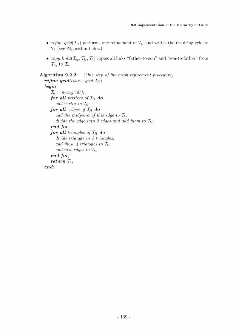
9.2 Implementation of the Hierarchy of Grids
• refine grid(TH) performs one refinement of TH and writes the resulting grid toTh (see Algorithm below).
• copy links(Th0 , TH , Th) copies all links “father-to-son” and “son-to-father” fromTh0 to Th.
Algorithm 9.2.2 (One step of the mesh refinement procedure)refine grid(coarse grid TH)beginTh :=new grid();for all vertices of TH do
add vertex to Th;for all edges of TH do
add the midpoint of this edge to Th;divide the edge into 2 edges and add them to Th;
end for;for all triangles of TH do
divide triangle in 4 triangles;add these 4 triangles to Th;add new edges to Th;
end for;return Th;
end;
- 139 -

9 Implementation of the HDD package
9.3 Implementation of the HDD Method
Suppose that the triangulation Th of the domain Ω is constructed. In this sectionwe describe how to perform the hierarchical decomposition of Ω (see Fig. 4.1) andimplement the HDD method. The scheme of the structures, which are involved inthe implementation of the HDD method is shown in Fig. 9.6.The recursive procedure which performs the hierarchical decomposition is nameddivide(...) (see Algorithm 9.3.1). The input data for the procedure divide(...) arethe root of TTh
and the domain Ω. This procedure divides the set of all triangles,the set of all nodes, the external and internal boundary nodes into two parts (leftson and right son).As it was mentioned in Chapter 5, for building an H-matrix we need a cluster tree,but to build this cluster tree we need to know the coordinates of the nodal pointsxi ∈ Ω. At the same time the admissibility condition requires knowledge about thedistance between two clusters and diameters of the clusters (see Section 5.4).
- 140 -

9.3 Implementation of the HDD Method
DDtree
subdomain
vertexlist
tlist
supermatrix rkmatrix
clustertree
fullmatrix
boundary
cluster
bl.clustertree
edges
H-matrix structures
Grid structure
HDD structures
Figure 9.6: The scheme of the structures, which are used for the implementation ofthe HDD method.
Algorithm 9.3.1 (Hierarchical decomposition)divide(DDtree* Tω, subdomain* ω);begin
ω1 :=new domain();ω2 :=new domain();if (ω contains more than 3 vertices) then
divide vertices(ω, ω1, ω2);divide elements(ω, ω1, ω2);Tω →leftson := new DDtree(ω1);Tω →rightson := new DDtree(ω2);divide(Tω →leftson, ω1);divide(Tω →rightson, ω2);
elseTω →leftson=∅;Tω →rightson=∅;
end if;end;
Here
• divide vertices(ω, ω1, ω2) divides the set of all nodal points of ω into twosubsets V1 := v|v ∈ ω1 and V2 := v|v ∈ ω2. Note that V1∩V2 = v|v ∈ γω.
- 141 -

9 Implementation of the HDD package
• divide elements(ω, ω1, ω2) divides the set of all triangles in ω into two subsetsT1 := t|t ∈ τ(ω1) and T2 := t|t ∈ τ(ω2). Note that T1 ∩ T2 = ∅.
We use the structure subdomain to store the data of ω ∈ TTh(see below). This
structure contains the list of all vertices, list of all triangles (on both scales), itsboundary box and lists of internal and external boundary vertices (on both scales).The boundary boxes are used for an easier division of a domain into two parts.
To store the data about the interface and the external boundary we use the struc-ture boundary (see below). This structure contains the following fields: lists ofvertices (vl, cvl) on both scales and a pointer to the right-hand side matrix (frhs).Since each vertex contains the list of joint triangles we can compute its support((tl)).
The main structure for the hierarchical domain decomposition is DDtree. Thisstructure combines the information about the current level, the “father” level andits children. DDtree is used in both algorithms “Leaves to Root” and “Root toLeaves”.
The fields of the structure DDtree are shown below. For describing a subdomainω ∈ TTh
the structure domain is used.
Program 9.3.1typedef struct _domain domain;
typedef _domain* pdomain;
struct _domain
long index; /* Index of the domain */
tlist* tl; /* List of triangles at the fine scale */
tlist* ctl; /* List of triangles at the coarse scale */
vertexlist* vl; /* List of vertices at the fine grid */
vertexlist* cvl; /* List of vertices at the coarse grid */
double area; /* Area of the domain */
double minx,maxx,miny,maxy; /* Describe the boundary box */
For describing the external ∂ω and internal γω boundaries the structure boundary
is used.
Program 9.3.2typedef struct _boundary boundary;
typedef _boundary* pboundary;
struct _boundary
vertexlist* vl; /* List of vertices at the fine grid */
vertexlist* cvl; /* List of vertices at the coarse grid */
tlist* tl; /* List of triangles at the fine scale */
psupermatrix frhs; /* To store the corresponding hierarchical matrix */
For describing the HDD tree TThthe structure DDTree is used.
- 142 -
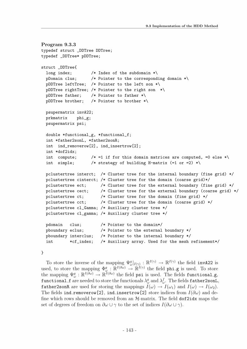
9.3 Implementation of the HDD Method
Program 9.3.3typedef struct _DDTree DDTree;
typedef _DDTree* pDDTree;
struct _DDTree
long index; /* Index of the subdomain *\
pDomain clus; /* Pointer to the corresponding domain *\
pDDTree leftTree; /* Pointer to the left son *\
pDDTree rightTree; /* Pointer to the right son *\
pDDTree father; /* Pointer to father *\
pDDTree brother; /* Pointer to brother *\
psupermatrix invA22;
prkmatrix phi_g;
psupermatrix psi;
double *functional_g, *functional_f;
int *father2sonL, *father2sonR;
int ind_removerow[2], ind_insertrow[2];
int *dof2idx;
int compute; /* =1 if for this domain matrices are computed, =0 else *\
int simple; /* strategy of building H-matrix (=1 or =2) *\
pclustertree interct; /* Cluster tree for the internal boundary (fine grid) */
pclustertree cinterct; /* Cluster tree for the domain (coarse grid)*/
pclustertree ect; /* Cluster tree for the external boundary (fine grid) */
pclustertree cect; /* Cluster tree for the external boundary (coarse grid) */
pclustertree ct; /* Cluster tree for the domain (fine grid) */
pclustertree cct; /* Cluster tree for the domain (coarse grid) */
pclustertree cl_Gamma; /* Auxiliary cluster tree */
pclustertree cl_gamma; /* Auxiliary cluster tree */
pdomain clus; /* Pointer to the domain*/
pboundary eclus; /* Pointer to the external boundary */
pboundary interclus; /* Pointer to the internal boundary */
int *cf_index; /* Auxiliary array. Used for the mesh refinement*/
To store the inverse of the mapping Ψgω|I(γ) : RI(γ) → RI(γ) the field invA22 is
used, to store the mapping Φgω : RI(∂ω) → RI(γ) the field phi g is used. To store
the mapping Ψgω : RI(∂ω) → RI(∂ω) the field psi is used. The fields functional g,
functional f are needed to store the functionals λgω and λfω. The fields father2sonL,father2sonR are used for storing the mappings I(ω) → I(ω1) and I(ω) → I(ω2).The fields ind removerow[2], ind insertrow[2] store indices from I(∂ω) and de-fine which rows should be removed from an H-matrix. The field dof2idx maps theset of degrees of freedom on ∂ω ∪ γ to the set of indices I(∂ω ∪ γ).
- 143 -

9 Implementation of the HDD package
9.4 Conclusion
The main steps of the implementation of HDD are:
1. Read the coarse grid TH .
2. Refine TH by Algorithm 9.2.1 imax times.
3. Build the HDD tree TThby Algorithm 9.3.1.
4. Execute “Leaves to Root” by Algorithm 7.2.1. For each ω ∈ TTh
a) build Ψgω and Ψf
ω for leaves of TTh,
b) build Ψgω from Ψg
ω1and Ψg
ω2by Algorithms 6.3.1 and 6.3.2,
c) build Ψfω from Ψf
ω1and Ψf
ω2by Algorithms 6.3.3 and 6.3.4,
d) build Φgω and Φf
ω by Algorithm 7.3.1,
e) compute the functionals λgω, λfω by Algorithms 4.4.1 and 4.4.2.
5. Execute “Root to Leaves” by Algorithm 7.3.1:
a) compute uγω := Φgω · gω + Φf
ω · fω, ω ∈ TTh,
b) compute (e.g., the mean value) λω(dω) = (λfω, fω) + (λgω, gω), ω ∈ TTh.
6. Compute solution by the PCG method and compare it with the solution com-puted by HDD.
The following modifications of the HDD method were implemented:
1. HDD1 works with the right-hand side from VH ⊂ Vh. For this modification theprolongation matrix Ph←H was applied.
2. HDD2 computes the solution on all internal boundaries γω, diam(ω) ≥ H, andthe mean value of the solution inside all domains ω with diam(ω) < H. Inthis modification the algorithm “Root to Leaves” works only for domains withdiam(ω) ≥ H.
3. HDD3 is a combination of HDD1 and HDD2.
4. HDD4 for problems with the homogeneous right-hand side (the mappings Ψfω
and Φfω are not computed at all).
5. HDD5 for problems with periodic coefficients (see Section 4.4.4).
- 144 -

10 Numerical Results
Numerical experiments are used for the confirmation of the theoretical results andfor the discovering of the invisible patterns of relationships.
In this Chapter we
• compare the solution, obtained by the HDD method, with the solutions ob-tained by the PCG-method and by the H-Cholesky factorization (see Tables10.12, 10.13, 10.15, 10.16);
• demonstrate the dependence of the solution uh on the maximal H-matrix rankk (see Tables 10.5, 10.6, 10.8).
• research the needed computational time and the storage requirement (see Ta-bles 10.14, 10.19, 10.20);
• show the accuracy of the solution for different oscillatory coefficients (see Ta-bles 10.9, 10.10, 10.11, 10.17, 10.18);
• research the accuracy of theH-matrix approximation of Φgω and Φf
ω on differentlevels of the tree TTh
(Tables 10.21, 10.22);
• show the absolute and relative errors for the solution of the so-called skinproblem with discontinuous coefficients (see Tables 10.25, 10.26, 10.27);
• solve a problem with many right-hand sides by the HDD method and comparethe computational time with the time required by PCG (see Table 10.28).
10.1 Notation
Let us introduce the following notation:
• u is an analytic solution;
• u is the FE exact solution, ui = u(xi);
• Ω is the model domain and the model grid is shown in Fig. 10.1;
• A is the global stiffness matrix computed for Ω;
• c is the discrete right-hand side, Au = c;
• k is the maximal rank used in Definition 5.7.2 of H-matrices. If the rank k inH(TI×J , k) is fixed then we call this rank the H-matrix rank;
- 145 -

10 Numerical Results
• uk is the solution obtained by the HDD method. The subindex k indicatesthat the fixed rank arithmetic is used (see Def. 5.9.3);
• uε is the solution obtained by the HDD method. The subindex ε indicatesthat the adaptive rank arithmetic is used (see Def. 5.9.3);
• uL is the solution obtained by the H-Cholesky decomposition (Au = c ⇒uL = (LLT )−1c);
• εcg is the value which is used for the stopping criterium for PCG, i.e., PCGstops as soon as ‖Au(m) − c‖2 ≤ εcg;
• ucg is the solution obtained by the PCG method (with the H-Cholesky pre-conditioner). As stopping criterium we use the residual ‖Aucg − c‖2 ≤ εcg;
• εa is the parameter for the adaptive rank arithmetic with the propertyk = mini : σi ≤ εaσ1, where σi is the i-th singular value;
• εh is the discretisation error;
• εH is the H-matrix approximation error;
• nmin is the minimal size of an inadmissible block. nmin tells us when we shouldstop divide subblocks further (see Section 5.5.2). By default, the minimal sizenmin = 32 is used for inadmissible blocks;
• A−H is the H-matrix approximant to the inverse of A.
nh,x
nh,y
Figure 10.1: The model grid on Ω = (0, 1)2. The number of degrees of freedom isnh,x · nh,y, nh,x = nh,y.
The model elliptic boundary value problem to be solved is
div(α(x)∇u) = f in Ω = (0, 1)2,u = g on ∂Ω.
(10.1)
Further, in all experiments, we will use the grid shown in Fig. 10.1.All numerical experiments were performed on the computers from Table 10.1.
The notebook was used for small applications and Kepler for large ones. In order tocompute a double integral in a triangle we apply the 12 points quadrature rule (seeTable (3.2)).
- 146 -

10.2 Preconditioned Conjugate Gradient Method
Name Model OS Speed, Ghz Memory, GbNotebook Celeron M Fedora 1.3-1.9 0.5
Kepler Intel PC Linux 2.4 3.0 2.0
Table 10.1: Used computers.
We use the domain decomposition as in Proposition 7.1.2. The error ε = ‖u− uk‖2(or ε = ‖u− uk‖∞) which we obtain after applying the HDD method is contributedby two errors: the discretization error εh and the H-matrix approximation errorεH. From the definition of H-matrices it is clear that εH −→ 0, when the rank k isincreasing. In the standard case the discretisation error is εh = O(h) (see Section3.5.2). It is sensible to take the maximal rank k for H-matrices in a way to have thesame order of errors εh and εH. There is no sense to take larger rank k (or smallerεa for the adaptive rank arithmetic) to decrease εH, because εh stays the same andwill dominate.
Remark 10.1.1 Note that to approximate a weak admissible block (see Section5.5.2) we use the rank 3 · k.
Remark 10.1.2 Contrary to the fixed rank arithmetic, in the adaptive rank arith-metic the needed rank k is chosen as follows k = mini : σi ≤ εaσ1.
10.2 Preconditioned Conjugate Gradient Method
Usually, the exact solution of the problem (10.1) is unknown. We use the PCGmethod to estimate the accuracy of the HDD method.
Lemma 10.2.1 The minimal and maximal singular values of the stiffness matrixof the Poisson-model problem on the rectangular quasi-uniform grid (Fig. 10.1) are:
λmin = 8h−2sin2(πh/2),λmax = 8h−2cos2(πh/2).
The matrix A is positive definite and the condition number is
cond(A) = ‖A‖2‖A−1‖2 =λmaxλmin
or
cond(A) =cos2(πh/2)
sin2(πh/2)= O
(1
h2
).
The discontinuous coefficients α(x) of the operator div(α(x)∇) for the domain as inFig. 10.8 can increase the condition number of the stiffness matrix dramatically andas a consequence increase the number of iterations. To estimate the upper bound ofthe condition number one can use the following inequality ([26]):
cond(A) ≤ maxi,j
(α(i)
α(j)
)h−2,
- 147 -

10 Numerical Results
where i, j ∈ Th.Table 10.2 shows the dependence of the condition number of the operator div(α(x)∇)
(for domain as in Fig. 10.8) on the jumping coefficient α. One can see an exponen-tial increasing of cond(A) with decreasing of α. Table 10.3 shows the dependenceof the condition number of the operator div(α(x)∇) on the number of degrees offreedom.
Remark 10.2.1 To compute the condition number of A we need the minimal andthe maximal eigenvalues. It is easy to estimate the maximal eigenvalue and difficultthe minimal eigenvalue. For small matrices (Tables 10.2, 10.3) we compute theeigenvalues exact.
α cond(A)10−1 8.4 ∗ 103
10−2 3.4 ∗ 104
10−3 2.8 ∗ 105
10−4 2.7 ∗ 106
10−5 2.7 ∗ 107
Table 10.2: Dependence of the condition number cond(A) on α. The domain Ω isshown in Fig. 10.8 with β = 1, a = 4h and 652 dofs.
dofs cond(A)92 6.8 ∗ 104
172 5.1 ∗ 105
332 6.1 ∗ 106
652 2.7 ∗ 107
Table 10.3: Dependence of the condition number on the number of degrees of free-dom. The domain Ω is shown in Fig. 10.8 with α = 10−5, β = 1,a = 4h.
Remark 10.2.2 The disadvantage of the CG method is its slow convergence becauseof a possibly large the condition number of A.
The next theorem describes the convergence speed of the CG method.
Theorem 10.2.1 Let Φ be a symmetric iteration. Its matrix W of the third normalform (i.e., W (um+1 − um) = Aum − c) is assumed to satisfy
λW ≤ A ≤ ΛW (λ > 0).
Then the iterates um of the CG method applied to Φ fulfil the energy norm estimate
‖em‖A ≤2cm
1 + c2m‖e0‖A,
- 148 -

10.2 Preconditioned Conjugate Gradient Method
with c :=√κ−1√κ+1
=√λmax−
√λmin√
λmax+√λmin
and em = um − u∗, u∗ is the exact solution of thesystem.
Proof: see [32] p.274.PCG Algorithm
We introduce the following notation: pm is the search direction, rm = c − Aum,m = 0, 1, ..., n− 1, is the residual. We stop the CG iterations when ‖rm‖2 = εcg. Ifthe matrix A is symmetric (A = AT ) and positive definite, i.e., (Av, v) > 0, the CGmethod can be applied. Let W−1 be a preconditioning.
Remark 10.2.3 It is possible that AW−1 is not symmetric and therefore we ap-ply the CG method to the system W−1/2AW−1/2u′ = W−1/2b. If A and W−1 aresymmetric, then W−1/2AW−1/2 is also symmetric.
1. Start: u0 := 0, r0 := c− Au0, p0 := W−1r0, ρ := 〈p0, r0〉,
2. Iteration for m = 0, 1, ...(as long as m < n and ‖rm‖2 ≤ εcg):
am := Apm, λopt := ρm/〈am, pm〉,
um+1 := um + λoptpm,
rm+1 := rm − λoptam,qm+1 := W−1rm+1, ρm+1 := 〈qm+1, rm+1〉,
pm+1 := qm+1 +ρm+1
ρmpm.
Remark 10.2.4 One step um → um+1 of the CG method requires one multiplicationApm and, in addition, only simple vector operations and scalar products. The matrixA, the vectors um, rm and pm have to be stored.
An implementation of the PCG method for the model problem is available in HLIB[28].
Remark 10.2.5 The number of iterations of the CG method without precondition-ing is proportional to
√cond(A) and the number of iterations with preconditioning
is proportional to√cond(W−1A). If the preconditioning is chosen successfully, then√
cond(W−1A)≪√cond(A).
To demonstrate how the CG method solves the problem (10.1) with f = 1, g = 0and α(x, y) = 1 + 1
2sin(20x)sin(20y) on the model grid (Fig. 10.1) we offer Table
10.4. The stiffness matrix A was approximated by an H-matrix with the adaptiverank arithmetic (εa = 10−4). Table 10.4 shows the preparation time (in sec.), thecomputational time (in sec.), the residual and the number of iterations for differentnumbers of degrees of freedom.
- 149 -

10 Numerical Results
dofs Preparation time Computational time ‖Aucg − c‖2 #iter
332 0.2 1.9 7.7 ∗ 10−5 82652 0.92 18.8 9.3 ∗ 10−5 1781292 50.23 165.0 9.3 ∗ 10−5 381
Table 10.4: Computational time, residual and number of iterations for different num-bers of degrees of freedom.
10.3 Smooth Coefficients
Table 10.5 shows that the HDD method works very well on the model Poissonproblem (frequency ν = 0). The analytic solution u = x2 + y2 is given. The relativeand absolute errors show exponential decay with increasing the rank k in the H-matrix arithmetic.
Table 10.6 shows that for different numbers of degrees of freedom (1292 and 2572)the relative and absolute errors decrease when the rank k increases. In the rowsk = 7, 8 the sum of the discretisation error εh and the quadrature error becomescomparable with the H-matrix approximation error.
k ‖u− uk‖2 / ‖u‖2 ‖u− uk‖∞2 7.2 ∗ 10−1 8.6 ∗ 10−1
3 4.8 ∗ 10−2 1.2 ∗ 10−1
4 3.3 ∗ 10−3 1.5 ∗ 10−2
5 3.6 ∗ 10−4 2.0 ∗ 10−3
8 4.1 ∗ 10−7 3.92 ∗ 10−6
12 1.2 ∗ 10−10 3.1 ∗ 10−9
Table 10.5: Dependence of the relative and absolute errors on the rank k. 1292 dofs,α = 1, f = 4, u = x2 + y2.
- 150 -
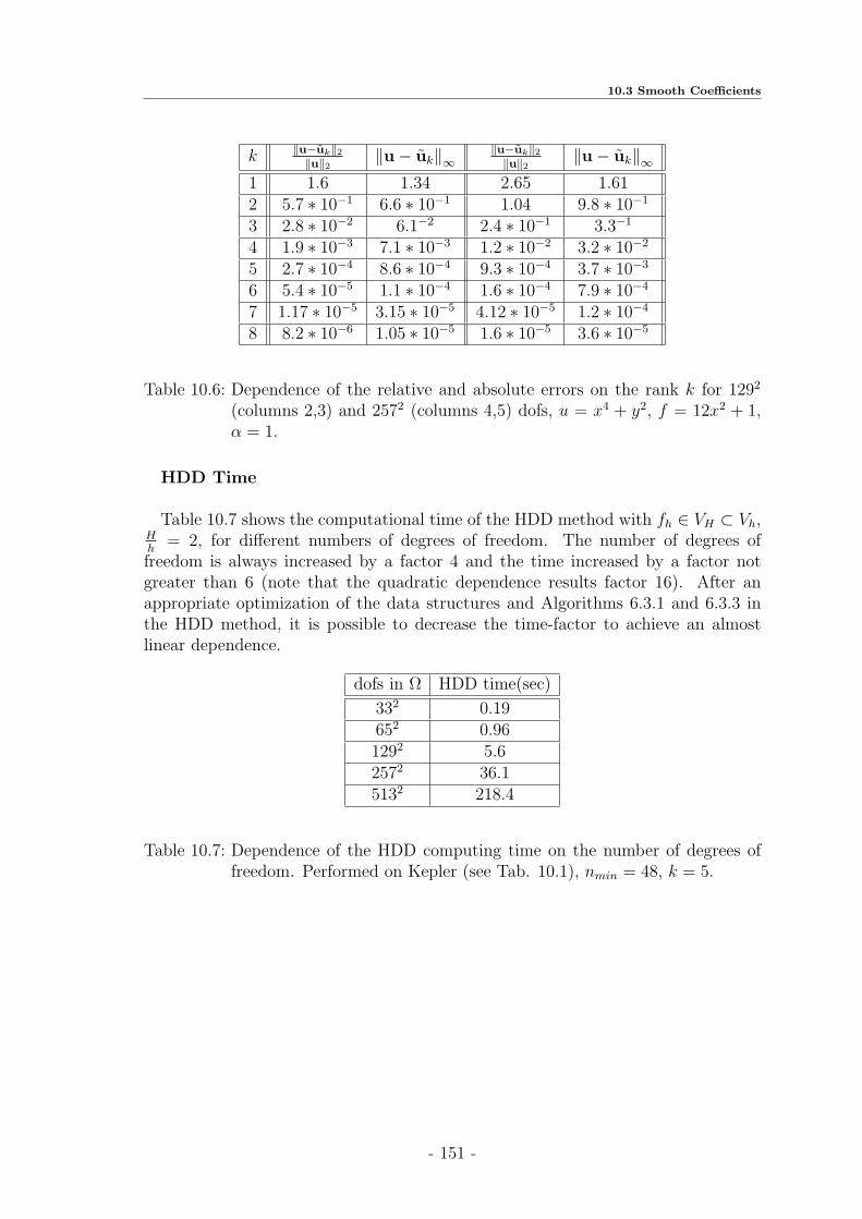
10.3 Smooth Coefficients
k ‖u−uk‖2‖u‖2 ‖u− uk‖∞
‖u−uk‖2‖u‖2 ‖u− uk‖∞
1 1.6 1.34 2.65 1.612 5.7 ∗ 10−1 6.6 ∗ 10−1 1.04 9.8 ∗ 10−1
3 2.8 ∗ 10−2 6.1−2 2.4 ∗ 10−1 3.3−1
4 1.9 ∗ 10−3 7.1 ∗ 10−3 1.2 ∗ 10−2 3.2 ∗ 10−2
5 2.7 ∗ 10−4 8.6 ∗ 10−4 9.3 ∗ 10−4 3.7 ∗ 10−3
6 5.4 ∗ 10−5 1.1 ∗ 10−4 1.6 ∗ 10−4 7.9 ∗ 10−4
7 1.17 ∗ 10−5 3.15 ∗ 10−5 4.12 ∗ 10−5 1.2 ∗ 10−4
8 8.2 ∗ 10−6 1.05 ∗ 10−5 1.6 ∗ 10−5 3.6 ∗ 10−5
Table 10.6: Dependence of the relative and absolute errors on the rank k for 1292
(columns 2,3) and 2572 (columns 4,5) dofs, u = x4 + y2, f = 12x2 + 1,α = 1.
HDD Time
Table 10.7 shows the computational time of the HDD method with fh ∈ VH ⊂ Vh,Hh
= 2, for different numbers of degrees of freedom. The number of degrees offreedom is always increased by a factor 4 and the time increased by a factor notgreater than 6 (note that the quadratic dependence results factor 16). After anappropriate optimization of the data structures and Algorithms 6.3.1 and 6.3.3 inthe HDD method, it is possible to decrease the time-factor to achieve an almostlinear dependence.
dofs in Ω HDD time(sec)
332 0.19652 0.961292 5.62572 36.15132 218.4
Table 10.7: Dependence of the HDD computing time on the number of degrees offreedom. Performed on Kepler (see Tab. 10.1), nmin = 48, k = 5.
- 151 -

10 Numerical Results
10.4 Oscillatory Coefficients
In this subsection we consider the model problem (10.1) with f = 1, g = 0, α(x, y) =1+Asin(νx)sin(νy). The aim is to show how the accuracy of the solution producedby HDD depends on the frequency ν and the amplitude A. Note that we researchapproximation properties of HDD and we do not care about the discretisation error.We suppose that the enough accurate discretisation is already done.
Example 10.4.1 To demonstrate the oscillatory effect we plotted (Figure 10.2) thesolution of the problem
div(α(x)∇u) = 1 in Ω = (0, 1)2,u = 0 on ∂Ω
(10.2)
with α = 11.001+sin(150x)sin(150y)
.
Very often the small details of the solution is out of interest and only the globalbehaviour of the solution is wanted!
Figure 10.2: The solution of the problem (10.2).
- 152 -

10.4 Oscillatory Coefficients
Example 10.4.2 Figures 10.3, 10.4 show the function α(x, y) = 1+12sin(νx)sin(νy)
for ν = 2 and ν = 20.
00.2
0.40.6
0.81
00.2
0.4
0.60.8
11
1.1
1.2
1.3
1.4
1.5
Figure 10.3: The coefficient function α(x, y) = 1 + 12sin(2x)sin(2y).
00.2
0.40.6
0.81
00.2
0.4
0.60.8
10.5
1
1.5
Figure 10.4: The coefficient function α(x, y) = 1 + 12sin(20x)sin(20y).
- 153 -

10 Numerical Results
Since sin(νx) has period 2πν
(see Fig. 10.5), the interval [0, 2πν
] should contain at
least 5 points, i.e., 2πν≥ 4h, where h = 1
(N−1). Thus, for ν ≤ 2π(N−1)
4there are more
than 5 points in the interval [0, 2πν
] (upper figure) and for ν > 2π(N−1)4
less then 5points (lower figure).
h L
Lh
Figure 10.5: An P 1 approximation of sin(x) on [0, L] by 5 points (up) and by 3points (bottom). In the last case, the approximating function is ≡ 0and the discretisation error is large.
Table 10.8 shows how the HDD method solves the problems with oscillatory right-hand side. The analytic solution to the problem with oscillatory coefficients hasbeen chosen to be non-oscillatory u = x2 + y2. The discrete analytic solution u iscompared with the solution uk, obtained by the HDD method. One can see that fork = 2, 3, 4, 5 the both relative and absolute errors decrease. But for k = 8, 12 thequadrature errors (see (3.33)) and discretisation errors come into play and becometo dominate.
k ‖u− uk‖2 / ‖u‖2 ‖u− uk‖∞2 7.4 ∗ 10−1 8.8 ∗ 10−1
3 4.9 ∗ 10−2 1.3 ∗ 10−1
4 6.7 ∗ 10−3 3 ∗ 10−2
5 8.7 ∗ 10−4 4.9 ∗ 10−3
8 2.8 ∗ 10−4 6.9 ∗ 10−4
12 2.8 ∗ 10−4 6.9 ∗ 10−4
Table 10.8: Dependence of the absolute and relative errors on the rank k. 1292
dofs, α(x, y) = 1 + 12sin(νx)sin(νy), f = 4 + 2sin(νx)sin(νy) +
xνcos(νx)sin(νy) + yνsin(νx)cos(νy), ν = 50, u = x2 + y2.
- 154 -

10.4 Oscillatory Coefficients
Recall that the solution obtained by HDD with the maximal H-matrix rank k isdenoted by uk. The solution obtained by HDD with the maximal rank 40 be u40.Such large rank 40 results the almost exact matrix arithmetic. Tables 10.9, 10.10,10.11 show how the accuracy of the HDD method depends on the accuracy of theH-matrix approximation. Table 10.9 contains the relative and absolute errors of thesolution to the problem 10.1 with α = 1+ 1
2sin(50x)sin(50y) for 1292 dofs (columns
2-3) and for 2572 dofs (columns 4,5). One can see an exponential decay of botherrors with increasing the H-matrix rank k.
k ‖u40 − uk‖2 / ‖u40‖2 ‖u40 − uk‖∞ ‖u40 − uk‖2 / ‖u40‖2 ‖u40 − uk‖∞2 1.3 4.8 ∗ 10−2 6.1 6.8 ∗ 10−2
3 5.0 ∗ 10−2 4.2 ∗ 10−3 0.6 3.2 ∗ 10−2
4 4.5 ∗ 10−3 7.9 ∗ 10−4 1.7 ∗ 10−2 2.4 ∗ 10−3
6 1.8 ∗ 10−4 1.9 ∗ 10−5 2.2 ∗ 10−3 3.1 ∗ 10−4
7 7.3 ∗ 10−5 7.76 ∗ 10−6 5.7 ∗ 10−4 5.6 ∗ 10−5
8 1.6 ∗ 10−5 1.8 ∗ 10−6 1.5 ∗ 10−4 1.6 ∗ 10−5
9 4.9 ∗ 10−6 5.3 ∗ 10−7 5.8 ∗ 10−5 5.5 ∗ 10−6
10 1.36 ∗ 10−6 2.0 ∗ 10−7 6 ∗ 10−6 6.5 ∗ 10−7
12 10−7 1.6 ∗ 10−8 7.1 ∗ 10−7 8.6 ∗ 10−8
14 6.9 ∗ 10−9 1.2 ∗ 10−9 4.8 ∗ 10−8 8.2 ∗ 10−9
Table 10.9: Dependence of the absolute and relative errors on the rank k. f = 1,α(x, y) = 1 + 1
2sin(50x)sin(50y). (2-3 columns) 1292 dofs, ‖u40‖2 =
5.4, (4-5 columns) 2572 dofs, ‖u40‖2 = 11.0.
Tables 10.10, 10.11 demonstrate an exponential decay of both relative and ab-solute errors for the problem (10.1) with the oscillatory coefficient α(x, y) = 1 +12sin(10x)sin(10y). The experiments in Table 10.10 are done for 332, 652 degrees of
freedom and in Table 10.11 for 1292, 2572 degrees of freedom.
k ‖u40 − uk‖2 / ‖u40‖2 ‖u40 − uk‖∞ ‖u40 − uk‖2 / ‖u40‖2 ‖u40 − uk‖∞2 1.88 ∗ 10−2 1.95 ∗ 10−3 1.7 ∗ 10−1 1.37 ∗ 10−2
3 6.4 ∗ 10−3 6.6 ∗ 10−4 8.6 ∗ 10−3 7.4 ∗ 10−4
4 1.74 ∗ 10−3 1.9 ∗ 10−4 3.1 ∗ 10−3 2.9 ∗ 10−4
5 1.6 ∗ 10−4 2.2 ∗ 10−5 4.8 ∗ 10−4 5.4 ∗ 10−5
6 1.14 ∗ 10−5 2.27 ∗ 10−6 6.73 ∗ 10−5 8.9 ∗ 10−6
7 2.43 ∗ 10−6 4.9 ∗ 10−7 1.8 ∗ 10−5 2.54 ∗ 10−6
8 2.64 ∗ 10−7 4.6 ∗ 10−8 4.34 ∗ 10−6 6.9 ∗ 10−7
9 7.55 ∗ 10−10 1.65 ∗ 10−10 1.1 ∗ 10−6 1.9 ∗ 10−7
Table 10.10: Dependence of the absolute and relative errors on the rank k. f = 1,α(x, y) = 1 + 1
2sin(10x)sin(10y). (2-3 columns) 332 dofs, ‖u40‖2 =
1.36; (4-5 columns) 652 dofs, ‖u40‖2 = 2.74.
- 155 -

10 Numerical Results
k ‖u40 − uk‖2 / ‖u40‖2 ‖u40 − uk‖∞ ‖u40 − uk‖2 / ‖u40‖2 ‖u40 − uk‖∞3 2.5 ∗ 10−2 2.3 ∗ 10−3 2.7 ∗ 10−1 2 ∗ 10−2
4 5.1 ∗ 10−3 4.3 ∗ 10−4 2.1 ∗ 10−2 2 ∗ 10−3
5 7.3 ∗ 10−4 6.8 ∗ 10−5 1.2 ∗ 10−3 1.3 ∗ 10−4
6 1.65 ∗ 10−4 1.76 ∗ 10−5 2.9 ∗ 10−4 2.6 ∗ 10−5
7 6.3 ∗ 10−5 10−6 1.1 ∗ 10−4 1.1 ∗ 10−5
8 1.94 ∗ 10−5 2.3 ∗ 10−6 4.6 ∗ 10−5 4.5 ∗ 10−6
9 4.67 ∗ 10−6 6.2 ∗ 10−7 1.2 ∗ 10−5 1.4 ∗ 10−6
10 1.0 ∗ 10−6 1.6 ∗ 10−7 3.3 ∗ 10−6 4.1 ∗ 10−7
12 1.0 ∗ 10−7 1.7 ∗ 10−8 4.3 ∗ 10−7 5.5 ∗ 10−8
14 1.1 ∗ 10−8 2.1 ∗ 10−9 5.9 ∗ 10−8 9.5 ∗ 10−9
16 9.0 ∗ 10−10 2.13 ∗ 10−10 7.4 ∗ 10−9 1.3 ∗ 10−9
Table 10.11: Dependence of the absolute and relative errors on the rank k. f = 1,α(x, y) = 1 + 1
2sin(10x)sin(10y). (2-3 columns) 1292 dofs, ‖u40‖2 =
5.5; (4-5 columns) 2572 dofs, ‖u40‖2 = 11.0.
In Table 10.12 we compare the solution of the initial problem (10.1), obtainedby the HDD method with the solution obtained by the PCG method. The maxi-mal number of iterations for the PCG method is 600, the admissible value of theresidual ‖Aucg − c‖2 = 10−6. Thus, we can assume that the PCG method gives an‘exact’ FE solution. The errors in columns 2 and 3 increase because the H-matrixapproximation error εH becomes larger. As a preconditioner we use the H-Choleskyfactorization.
dofs ‖ucg − uε‖∞ ‖ucg−uε‖2‖uε‖2 ‖Aucg − c‖2 timeHDD, (sec)
172 4.42 ∗ 10−10 4.34 ∗ 10−9 9.1 ∗ 10−7 0.06332 8.56 ∗ 10−7 5.1 ∗ 10−6 7.2 ∗ 10−7 0.27652 4.21 ∗ 10−6 3.3 ∗ 10−5 9.6 ∗ 10−7 1.61292 1.32 ∗ 10−5 1.3 ∗ 10−4 9.7 ∗ 10−7 10.0
Table 10.12: Comparison of the HDD solution uε with the PCG solution ucg,α(x, y) = 1 + 1
2sin(50x)sin(50y), εa = 10−6.
In Table 10.13 we consider the problem (10.1) with
α(x, y) =2 + P sin(2πx/ε)
2 + P sin(2πy/ε)+
2 + P sin(2πy/ε)
2 + P sin(2πx/ε),
f = 1, P = 1.8, ε = 1/512 and g = 0. The domain Ω and its triangulation areshown in Proposition 7.1.2. We assume that the solution, obtained by the PCG-method with the H-Cholesky preconditioning is the exact solution (of course, up tothe discretisation error). The residual for the PCG-method is ‖Aucg − c‖2 = 10−6
and the number of iterations is shown in brackets. The H-matrix computations were
- 156 -

10.5 Comparison of HDD With H-Matrix Inverse and Inverse by Cholesky Decomposition
done with the adaptive rank arithmetic εa = 10−5 (see Def. 5.9.3). One can see thatHDD achieves the same accuracy as PCG with a similar computational time. Notethat both methods does not take into account the discretisation error.
dofs ‖ucg − uε‖2 ‖ucg − uε‖∞ PCG sec.(iter) HDD sec.
332 5.7 ∗ 10−4 4.5 ∗ 10−5 0.17(4) 0.39652 2.8 ∗ 10−4 1.1 ∗ 10−5 1.18(4) 1.841292 1.4 ∗ 10−4 2.86 ∗ 10−6 9.6(6) 10.5
Table 10.13: Dependence of the absolute error on the number of degrees of freedom.εa = 10−5.
10.5 Comparison of HDD With H-Matrix Inverse and
Inverse by Cholesky Decomposition
In this section we compare the computational time and memory requirement ofHDD with the times and memory requirements of the H-Matrix inverse and theH-Cholesky decomposition.Table 10.14 demonstrates the dependence of memory requirements and the compu-tational times on the parameter εa (see the adaptive rank arithmetic in Def. 5.9.3).One can see that the computational time and storage requirement of theH-Choleskyfactorisation are the best. The HDD shows almost the same time as H-Choleskyand a much better time as the direct H-matrix inverse. HDD requires more memorythan H-Cholesky and much less than the direct H-matrix inverse. The memory re-quirements for HDD can be decreased after optimization of the Algorithms 6.3.1 and6.3.3. Note that HDD computes the solution operators, but after the H-Choleskyfactorization one still needs to solve two systems of linear equations Lv = c andLTu = v.
εa H− LLT -time(sec);size(MB) HDD-time;size time(A−H);size
10−3 2.1;(13.3) 9.2;(19.7) 21.4;(51.0)10−4 2.6;(14.7) 9.8;(20.1) 29.6;(64.0)10−5 3.0;(16.0) 10.6;(20.4) 37.3;(75.2)10−6 3.4;(17.2) 11.6;(20.6) 47.4;(87.4)
Table 10.14: Comparison of the H-Cholesky factorisation, HDD and the H-matrixinverse. Dependence of time and memory requirements on εa, 1292
dofs.
- 157 -

10 Numerical Results
Table 10.15 shows the dependence of the computational time for the H-Choleskyfactorisation on the number of degrees of freedom. The complexity of the H-matrixarithmetic (see Table 5.3) depends on the factor k2 and it is why we do not seealmost linear factor in time. It is shown ([46], [47]) that for a smaller H-matrixrank k an almost linear complexity can be achieved. Note that it is not enoughmemory for computing H-Cholesky factorization with 5132 dofs and k = 8. Theerror
∥∥(LLT )−1A− I∥∥
2grows up because the H-matrix approximation error grows
up.
dofs∥∥(LLT )−1A− I
∥∥2‖u− uL‖2 / ‖uL‖2 t, sec
332 2.03 ∗ 10−14 1.5 ∗ 10−15 0.08652 5.6 ∗ 10−11 6.1 ∗ 10−13 0.81292 9.0 ∗ 10−10 1.1 ∗ 10−11 6.682572 6.7 ∗ 10−9 9.9 ∗ 10−11 75.05132 n.e.m. n.e.m. not enough memory
Table 10.15: The computational time and accuracy of the solution uL, obtained bythe H-Cholesky decomposition, u = (x2 − 1)(y2 − 1), k = 8.
Table 10.16 compares the computational times of the HDD method and the PCGmethod with H-Cholesky preconditioner. Column 3 contains the measurementsof times for: (a) computing the stiffness matrix A in the data-sparse format; (b)computing the H-Cholesky decomposition of A (used as a preconditioner); (c) PCGiterations.Note that for 5132 dofs there is not enough memory to compute the stiffness matrixA and perform its H-Cholesky factorization. The advantage of the HDD method isthat it does not require agglomeration of the whole stiffness matrix. The memory isdynamically allocated and deallocated.
dofs HDD PCG
332 0.19 0.1=0.03+0.04+0.02652 0.96 0.6=0.2+0.26+0.11292 5.6 5=2.6+1.8+0.62572 36.1 53=38.0+11.4+3.45132 218 n.e.m.
Table 10.16: Comparison of times for the skin problem with α = 10−5, εa = 10−8,εcg = 10−8, H
h= 2. Performed on Kepler from Table 10.1.
Table 10.17 shows how the absolute and relative errors depends on the frequencyν. One can see the errors of the same order, i.e., the HDD method is stable withrespect to the frequency ν. Here u40 is the solution computed by HDD in the class ofH-matrices with the maximal rank 40. Since the exact solution is unknown, we use
- 158 -

10.5 Comparison of HDD With H-Matrix Inverse and Inverse by Cholesky Decomposition
u40 as a good approximation of the exact solution (up to the discretisation error).Here it is quite appropriate to quote the work [11] about existence of H-matrixapproximants to the inverse FE-matrix of elliptic operators with L∞-coefficients. In
ν ‖u40 − uk‖2 / ‖u40‖2 ‖u40 − uk‖∞10 1.65 ∗ 10−4 1.76 ∗ 10−5
50 1.8 ∗ 10−4 1.9 ∗ 10−5
Table 10.17: Dependence of the relative and absolute errors on the frequency ν, 2572
dofs, f = 1, α(x, y) = 1 + 12sin(νx)sin(νy), εa = 10−6.
Table 10.18 we compare the HDD method with the PCG method. Here uε is theHDD solution, ucg the solution obtained by the PCG method with the H-Choleskypreconditioner. The fourth and fifth columns present the computational times. TheHDD time is comparable with the PCG time, but for 5132 dofs PCG requires toomuch memory.
dofs ‖ucg − uε‖2 ‖ucg − uε‖∞ PCG with LLT sec.(iter) HDD sec.
332 4.16 ∗ 10−7 6.68 ∗ 10−8 0.22(2) 0.35652 2.28 ∗ 10−5 1.42 ∗ 10−6 1.66(2) 2.51292 2.38 ∗ 10−4 9.35 ∗ 10−6 17(2) 132572 2.35 ∗ 10−3 2.85 ∗ 10−5 63(11) 60.65132 n.e.m. n.e.m. not enough memory 270.3
Table 10.18: Dependence of the absolute errors on the number of dofs, f = 1,α(x, y) = 1/(1.0001+sin(500x)sin(500y)). All computations were per-formed on Notebook (see Table 10.1) with the adaptive rank arithmetic(see Def. 5.9.3), εa = 10−5, H
h= 2.
Remark 10.5.1 Note that the computational time of the H-Cholesky factorisationdepends on the rank k used in the H-matrix arithmetic (see [47], [46]). If k becomessmaller than the computational time and the accuracy decreases also.
Remark 10.5.2 The later experiments for discontinuous coefficients [43] show thatit is better (in the sense of timing performances) to take a smaller rank k witha larger number of PCG iterations as a larger k with a smaller number of PCGiterations.
- 159 -

10 Numerical Results
10.6 Memory Requirements for Φg and Φf
Tables 10.19, 10.20 show the total storage requirements for all matrices Φgω and Φf
ω,ω ∈ TTh
in the case of one grid and two grids. In Table 10.19 we see an almost lineardependence of the storage requirements on the number of degrees of freedom. Thecolumns S(Φg) and S(Φf ) present memory requirements for all mappings Φg
ω andΦfω, ω ∈ TTh
, respectively. We see a factor ≈ 4 in the column S(Φg) and a factor≈ 5.6 in S(Φf ). Here the factor 4 shows a linear dependence. The numbers in thistable are in accordance with the theoretical estimates in Lemma 7.3.4. We do notsee a linear factor because there is an additional log factor.
dofs S(Φg), Kb S(Φf ), Kb ‖u− uk‖2 / ‖u‖2 ‖u− uk‖∞332 2.45 ∗ 102 4 ∗ 102 3.3 ∗ 10−5 8.47 ∗ 10−5
652 1.1 ∗ 103 2.4 ∗ 103 5.75 ∗ 10−5 1.0 ∗ 10−4
1292 5 ∗ 103 1.4 ∗ 104 7.4 ∗ 10−5 1.1 ∗ 10−4
2572 2.1 ∗ 104 7.86 ∗ 104 8.3 ∗ 10−5 1.3 ∗ 10−4
Table 10.19: Dependence of the total memory requirements for all Φgω and Φf
ω on thenumber of degrees of freedom, k = 7, u = x2 + y2.
Table 10.20 shows the storage requirements for all Φgω and Φf
ω in dependenceon the compression factor H
h. The storage requirement for all Φg
ω stays the same(column S(Φg)) since for all mappings Φg
ω we use only one scale with step size h.Lemmas 7.3.4 and 7.4.5 state that S(Φ) ≤ C1knh log2 nh for one grid and S(Φf ) ≤C2k√nHnh log2√nHnh for two grids.
All computations in Table 10.20 were performed with the adaptive rank arithmeticεa = 10−8.
Hh
S(Φg), MB S(Φf ), MB time, sec
1 2.2 ∗ 101 2.9 ∗ 102 2182 2.2 ∗ 101 8.7 ∗ 101 834 2.2 ∗ 101 3.2 ∗ 101 418 2.2 ∗ 101 1.8 ∗ 101 3216 2.2 ∗ 101 1.5 ∗ 101 26
Table 10.20: The computational time and the total storage requirements for allΦgω and Φf
ω. 2572 dofs, εa = 10−8, α(x, y) = 1 + 12sin(50x)sin(50y),
f(x, y) = x(x− 1) + y(y − 1).
- 160 -

10.7 Approximation of Φg and Φf
10.7 Approximation of Φg and Φf
To estimate the accuracy of the H-matrix approximation to the inverse of the globalstiffness matrix A we compute the error ‖A · A−H − I‖2. But in the HDD methodwe do not have the global matrix A, we have a set of matrices Φg
ω and Φfω, ω ∈ TTh
.The matrices Φg
ω (as well as Φfω) on the l-th level of TTh
are equivalent. It is whywe consider the accuracy of the H-matrix approximation only for one of them. Themappings Φg := Φg
127 and Φf := Φf127 are computed with the H-matrix rank k = 127
(up to almost machine precision 10−16). Tables 10.21, 10.22 show the maximaloperator errors ‖Φg − Φg
21‖2 and ‖Φf − Φf7‖2 on different levels of TTh
. Φg21 and
Φf7 are the H-matrix approximations of Φg and Φf with the maximal ranks 21 and
7 correspondingly. The second column shows the size of the matrix and the thirdcolumn shows the corresponding level of the hierarchical domain decomposition treeTTh
. The maximal error appears at 0-level (root). It can be explained by the factthat an H-matrix approximation of Φg
ω (Φfω) on the 0-level contains more low-rank
blocks and they are bigger. Note that the errors in Tables 10.21, 10.22 do not dependon the right-hand side.Tables 10.21, 10.22 show that it is a nice idea to choose an adaptive rank for each
‖Φg − Φg21‖2 size of Φg level of TTh
4.8 ∗ 10−1 255× 1024 05.5 ∗ 10−3 127× 512 14.22 ∗ 10−5 63× 256 24.55 ∗ 10−8 31× 128 32.58 ∗ 10−17 15× 64 4
Table 10.21: The error ‖Φg−Φg21‖2 on different levels of TTh
. Φg21 is an approximation
of Φg by a rank-21 matrix. The matrix size is |I(γω)|×|I(∂ω)|, α(x, y) =1 + 1
2sin(50x)sin(50y), 1272 dofs.
‖Φf − Φf7‖2 size of Φf level of TTh
2.1 ∗ 10−7 255× 2572 03.6 ∗ 10−9 127× 1292 11.04 ∗ 10−9 63× 652 22.04 ∗ 10−10 31× 332 31.47 ∗ 10−20 15× 172 4
Table 10.22: The error ‖Φf −Φf7‖2 on different levels of TTh
, Φf7 is an approximation
of Φf by rank-7 matrix. The matrix size is |I(γω)| × |I(ω)|, α(x, y) =1 + 1
2sin(50x)sin(50y), 1272 dofs
level of TTh. For example, if TTh
has L levels, than one may take k0 > k1 > k2... >kL−1, where ki is the H-matrix rank on the i-th level. The adaptive rank arithmetic(see Def. 5.9.3) realizes this idea.
- 161 -

10 Numerical Results
10.8 Jumping Coefficients
In this section we consider the class of problems with jumping coefficients. Suchproblems appear in the material sciences (electrical fields through materials withdifferent conductivities), in medicine (the so-called skin problem) etc. An simpleexample is shown in Fig. 10.6. This domain Ω has areas with jumping coefficients:α = 10 and β = 10−2.
Ω
α
β
0.1 0.2 0.8 0.9
0.1
0.2
0.80.9
Figure 10.6: Domain Ω = (0, 1)2 with jumping coefficients α and β.
Table 10.23 shows that the parameter εa (for the adaptive rank arithmetic) has tobe smaller for problems with jumping coefficients than the corresponding parameter(denote by εmodel
a ) for the model problem. A priori one can take
εa := maxωi,ωj∈Th
αωi
αωj
∗ εmodela .
Here maxωi,ωj∈Th
describes the maximal jump between two finite elements ωi and ωj
(leaves of the tree TTh).
εa ‖AA−H − I‖2 time (sec.)
10−6 1.2 63.710−8 3.0 ∗ 10−1 87.110−10 3.4 ∗ 10−4 111.610−12 3.7 ∗ 10−6 156.8
Table 10.23: Dependence of the H-matrix approximation error ‖AA−H − I‖2 on εafor the domain as in Fig. 10.6 with coefficients α = 10 and β = 0.01,1292 dofs.
Table 10.23 shows the total time for the H-matrix approximation (denoted byA−H) to the inverse A−1. Here the time of building the block cluster tree is negli-gible small in comparison with the time of computing A−H. We see also that theaccuracy of the H-matrix approximation to A−1 increases with decreasing the pa-rameter εa.
- 162 -

10.8 Jumping Coefficients
Table 10.24 compares the HDD method with the PCG method for different εa.The domain Ω is shown in Fig. 10.6. Such domains are typical, for instance, in elec-trostatics. The jumping coefficients α and β model electroconductivity in differentmaterials. This table compares also the computational times. We see that the HDDtime is larger. The reason is that HDD computes the solution operators, but PCGonly the solution.
εa ‖Aucg − c‖2 PCG-time (sec) HDD-time ‖ucg−uε‖2‖uε‖2 ‖ucg − uε‖∞
10−4 2 ∗ 10−4 5.3 8.9 6.7 ∗ 10−1 1.410−6 4.8 ∗ 10−7 5.0 10.1 1.8 ∗ 10−4 9.5 ∗ 10−4
10−8 1.4 ∗ 10−8 5.7 11.5 1.1 ∗ 10−6 1.48 ∗ 10−5
10−10 1.45 ∗ 10−8 6.7 12.3 5.3 ∗ 10−7 10−5
10−12 1.2 ∗ 10−8 7.4 13.5 5.2 ∗ 10−7 10−5
Table 10.24: Dependence of the relative and the absolute errors on εa for the modelproblem on the domain as in Fig. 10.6 with coefficients α = 10, β =0.01 and 1292 dofs.
- 163 -

10 Numerical Results
10.9 Skin Problem
The problem in Fig. 10.7 models a more difficult problem (so-called the skin prob-lem). In this problem an ointment penetrates through the skin. The diffusion processis very slow inside the cells and much faster in the channels in between (so-calledthe lipid layer). We choose a rectangular quasi-uniform grid on Ω = (0, 1)2 whichis compatible with the lipid layer. The condition number cond(A) in problems with
jumping coefficients is proportional to h−2 maxωi,ωj∈Th
α(ωi)
α(ωj), where α(ωi) is the jumping
coefficient in ωi, h the grid step size and ωi, ωj ∈ Th.
a b
Lipid layer
α
β
Figure 10.7: Model of a skin fragment Ω = (0, 1)2. The coefficient of the penetrationinside the cells is very small (α), but is large in between (β).
We model this difficult geometry by a simpler one as it shown in Fig. 10.8.
0 10.25 0.75
0.5
1
4h
Figure 10.8: Model domain Ω = (0, 1)2. The coefficient of penetration inside thecells is very small (α), but is large in between (β = 1).
- 164 -

10.9 Skin Problem
Table 10.25 shows the accuracy of the HDD method for different jumping coeffi-cients α (Fig. 10.8). We compare the solution, obtained by the HDD method, withthe solution, obtained by PCG. For a small α (e.g., α = 10−5) the adaptive rankparameter εa = 10−6 (Def. 5.9.3) is not good enough. For highly jumping coefficientone should choose very small parameter εa.
α ‖Aucg − c‖2 ‖ucg−uε‖2‖uε‖2 ‖ucg − uε‖∞
10−1 1.4 ∗ 10−10 8.0 ∗ 10−6 4.5 ∗ 10−6
10−2 3.1 ∗ 10−10 1.6 ∗ 10−5 6.2 ∗ 10−5
10−3 7.7 ∗ 10−8 5.7 ∗ 10−5 2.8 ∗ 10−3
10−4 1.3 ∗ 10−9 7.0 ∗ 10−3 1.510−5 8.9 ∗ 10−9 7.7 ∗ 10−1 8.8 ∗ 102
Table 10.25: Dependence of the absolute and relative errors on the coefficient α.1292 dofs, εa = 10−6, domain as in Fig. 10.8 with β = 1 and thicknessa = 4h.
- 165 -

10 Numerical Results
Table 10.26 shows that the larger the jump is (∼ the smaller α is) the larger are therelative and the absolute errors in the infinity, energy and spectral norms. We recallthat A is the stiffness matrix for the whole domain Ω, ucg is the solution computedby the PCG method and uε is the solution computed by the HDD method.
α ‖ucg−uε‖2‖ucg‖2 ‖ucg − uε‖∞ ‖ucg − uε‖A ‖Aucg − Auε‖2 ‖A‖2
1.0 6.6 ∗ 10−9 7.1 ∗ 10−10 2.3 ∗ 10−7 2.8 ∗ 10−5 1.27 ∗ 105
10−1 2.0 ∗ 10−8 1.4 ∗ 10−8 2.0 ∗ 10−6 1.1 ∗ 10−4 1.22 ∗ 105
10−2 6.6 ∗ 10−8 2.6 ∗ 10−7 1.7 ∗ 10−5 6.9 ∗ 10−4 1.22 ∗ 105
10−3 7.4 ∗ 10−7 1.8 ∗ 10−5 4.2 ∗ 10−4 8.8 ∗ 10−3 1.22 ∗ 105
10−4 4.2 ∗ 10−6 1.8 ∗ 10−3 1.4 ∗ 10−2 7.5 ∗ 10−2 1.22 ∗ 105
10−5 7.0 ∗ 10−5 2.3 ∗ 10−1 9.0 ∗ 10−1 1.0 1.22 ∗ 105
Table 10.26: Dependence of the absolute and relative errors on the jumping coef-ficient α. Ω as in Fig. 10.8, 1292 dofs, thickness a = 4h, β = 1.εa = 10−8, residual ‖Aucg − c‖2 = 10−10.
The accuracy of the solution uε depends on the accuracy of the H-matrix ap-proximation. We use the adaptive rank arithmetic, i.e., we choose the rank for eachsubmatrix as follows k = mini : σi ≤ εaσ1, where σ1 ≤ σ2 ≤ ... ≤ σk ≤ ... are thesingular values.Table 10.27 shows the dependence of the absolute and relative errors on the param-eter εa (for the adaptive rank arithmetic). One can see that the accuracy of HDDcan be improved by decreasing εa.
The comparison of the solution uL computed by the direct H-Cholesky with ucg(computed by PCG) is given in the last column. We assume that PCG after a largenumber of iteration steps produces the ’exact’ FE solution ucg.
εa‖ucg−uε‖2‖ucg‖2 ‖ucg − uε‖∞ ‖ucg − uε‖A ‖Aucg − Auε‖2 ‖ucg−uL‖2
‖ucg‖210−6 4.4 ∗ 10−1 6.67 ∗ 102 1.1 ∗ 103 1.8 ∗ 102 4.7 ∗ 10−4
10−8 7.27 ∗ 10−5 2.3 ∗ 10−1 9.0 ∗ 10−1 1.0 6 ∗ 10−7
10−10 5.1 ∗ 10−7 1.0 ∗ 10−3 3.0 ∗ 10−3 6.1 ∗ 10−3 1.1 ∗ 10−8
10−12 3.9 ∗ 10−9 1.2 ∗ 10−5 2.9 ∗ 10−5 3.8 ∗ 10−5 1 ∗ 10−11
10−14 1.2 ∗ 10−11 6.6 ∗ 10−7 1.2 ∗ 10−7 3.7 ∗ 10−7 1.5 ∗ 10−13
10−16 1.6 ∗ 10−12 1.1 ∗ 10−8 1.7 ∗ 10−8 5.3 ∗ 10−7 2.1 ∗ 10−14
Table 10.27: Dependence of the absolute and relative errors on εa. Ω as in Fig.10.8, 1292 dofs, thickness a = 4h, α = 10−5, β = 1. The residual is‖Aucg − c‖2 = 10−10, ‖A‖2 = 1.22 ∗ 105.
- 166 -

10.9 Skin Problem
In the figure below one can see the spectra of the operator div(α(x)∇) for β = 1,α = 1, α = 10−2 and α = 10−4 (three curves in log-scale). The number of degreesof freedom is 332. This Figure helps us to understand why the condition number ofthe stiffness matrix for the skin problem (Figure 10.8) is large. All three maximaleigenvalues are almost the same and the minimum eigenvalues are differ by a factorproportional to the jump.
0 50 100 150 200 25010
−3
10−2
10−1
100
101
102
103
eigenvalues lambdai
valu
es
alpha=1
alpha=0.01
alpha=1e−4
Decay of singular values of the stiffness matrix A for α = 1, α = 10−2 andα = 10−4.
- 167 -
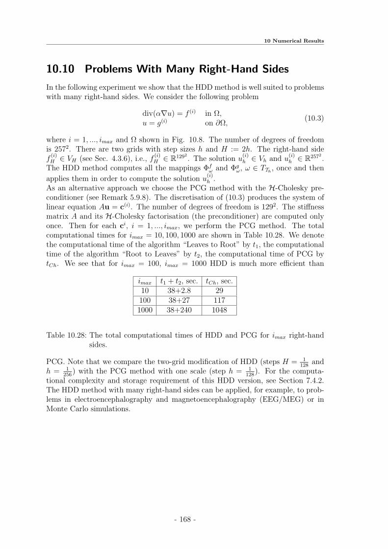
10 Numerical Results
10.10 Problems With Many Right-Hand Sides
In the following experiment we show that the HDD method is well suited to problemswith many right-hand sides. We consider the following problem
div(α∇u) = f (i) in Ω,u = g(i) on ∂Ω,
(10.3)
where i = 1, ..., imax and Ω shown in Fig. 10.8. The number of degrees of freedomis 2572. There are two grids with step sizes h and H := 2h. The right-hand sidef
(i)H ∈ VH (see Sec. 4.3.6), i.e., f
(i)H ∈ R1292
. The solution u(i)h ∈ Vh and u
(i)h ∈ R2572
.The HDD method computes all the mappings Φf
ω and Φgω, ω ∈ TTh
, once and then
applies them in order to compute the solution u(i)h .
As an alternative approach we choose the PCG method with the H-Cholesky pre-conditioner (see Remark 5.9.8). The discretisation of (10.3) produces the system oflinear equation Au = c(i). The number of degrees of freedom is 1292. The stiffnessmatrix A and its H-Cholesky factorisation (the preconditioner) are computed onlyonce. Then for each ci, i = 1, ..., imax, we perform the PCG method. The totalcomputational times for imax = 10, 100, 1000 are shown in Table 10.28. We denotethe computational time of the algorithm “Leaves to Root” by t1, the computationaltime of the algorithm “Root to Leaves” by t2, the computational time of PCG bytCh. We see that for imax = 100, imax = 1000 HDD is much more efficient than
imax t1 + t2, sec. tCh, sec.10 38+2.8 29100 38+27 1171000 38+240 1048
Table 10.28: The total computational times of HDD and PCG for imax right-handsides.
PCG. Note that we compare the two-grid modification of HDD (steps H = 1128
andh = 1
256) with the PCG method with one scale (step h = 1
128). For the computa-
tional complexity and storage requirement of this HDD version, see Section 7.4.2.The HDD method with many right-hand sides can be applied, for example, to prob-lems in electroencephalography and magnetoencephalography (EEG/MEG) or inMonte Carlo simulations.
- 168 -

10.11 Computing the Functionals of the Solution
10.11 Computing the Functionals of the Solution
Very often dimension of the initial multiscale problem is huge, the geometry is com-plex and not the whole solution is of interest, but the solution in a small subdomainω ∈ Ω. Moreover it is interesting how the solution in ω changes when the right-handside f and the Dirichlet boundary data g are changed. For this purposes one maycompute different functionals of the solution (see Section 4.4.5). These functionalsdepend on f , g and the mappings Φg and Φf . Below we give an example.
10.11.1 Computing the Mean Value in ω ∈ TTh
In this section we realize the algorithm from Section 4.4.6 and compare the computedmean value of the solution u in a subdomain ω ∈ TTh
with the exact mean valuein ω. We choose scales H = 1/4 and h = 1/256. The scale H = 1/16 gives adecomposition of the initial domain Ω into 16 cells (see Fig. 10.9). The problem to
13
10
14h
H
11
6 7
16
41
15
12
8
32
5
9
Figure 10.9: Model domain Ω = (0, 1)2 and its subdivision into 16 subdomains.
be considered is:div(α(x)∇u) = 1 in Ω = (0, 1)2,
u = 0 on ∂Ω.
We compute the exact mean value by the following formula:
µ =
∫
ω
udx =∑
t∈Th(ω)
|t|3
(u1 + u2 + u3),
where ui, i = 1, 2, 3, is the solution computed by the PCG-method in vertices of thetriangle t.We compute the exact mean value µ and the approximate mean value µHDD (seeSection 4.4.6) in each cell. Tables 10.29 and 10.30 compare these both values. Wesee from the second column (Tables 10.29, 10.30) that there are three patterns ofsubdomains: internal (6,7,10,11), angular (1,4,13,16) and border (2,3,5,8,9,12,14,15).
- 169 -

10 Numerical Results
|µHDD − µ| |µHDD − µ|/|µHDD| N of subdomain in Fig. 10.91.73 ∗ 10−3 1.38 ∗ 10−1 61.71 ∗ 10−3 1.4 ∗ 10−1 71.71 ∗ 10−3 1.4 ∗ 10−1 101.71 ∗ 10−3 1.4 ∗ 10−1 11
1.71 ∗ 10−3 3.3 ∗ 10−2 11.71 ∗ 10−3 3.3 ∗ 10−2 41.71 ∗ 10−3 3.3 ∗ 10−2 131.71 ∗ 10−3 3.3 ∗ 10−2 16
1.71 ∗ 10−3 7 ∗ 10−2 21.71 ∗ 10−3 7 ∗ 10−2 31.70 ∗ 10−3 7 ∗ 10−2 51.71 ∗ 10−3 7 ∗ 10−2 81.71 ∗ 10−3 6.9 ∗ 10−2 91.71 ∗ 10−3 7 ∗ 10−2 121.71 ∗ 10−3 7 ∗ 10−2 141.71 ∗ 10−3 7 ∗ 10−2 15
Table 10.29: Comparison of the approximate mean value with the exact mean value.α = 1.0/(1.001+sin(50x)sin(50y)), 257 dofs, ‖uε−ucg‖2 = 1.43∗10−9,‖uε − ucg‖∞ = 3.72 ∗ 10−11.
|µHDD − µ| |µHDD − µ|/|µHDD| subdomain in Fig. 10.92.21 ∗ 10−3 1.38 ∗ 10−1 62.23 ∗ 10−3 1.38 ∗ 10−1 72.23 ∗ 10−3 1.4 ∗ 10−1 112.23 ∗ 10−3 1.39 ∗ 10−1 10
2.22 ∗ 10−3 3.4 ∗ 10−2 12.22 ∗ 10−3 3.4 ∗ 10−2 42.23 ∗ 10−3 3.4 ∗ 10−2 132.23 ∗ 10−3 3.4 ∗ 10−2 16
2.22 ∗ 10−3 7.06 ∗ 10−2 22.22 ∗ 10−3 7.07 ∗ 10−2 32.22 ∗ 10−3 7.04 ∗ 10−2 82.23 ∗ 10−3 7.07 ∗ 10−2 52.23 ∗ 10−3 7.07 ∗ 10−2 92.23 ∗ 10−3 7.07 ∗ 10−2 122.23 ∗ 10−3 7.07 ∗ 10−2 142.23 ∗ 10−3 7.07 ∗ 10−2 15
Table 10.30: Comparison of the approximate mean value with the exact mean value.α = 1.0 + 1
2sin(50x)sin(50y), 257 dofs, ‖uε − ucg‖2 = 7.97 ∗ 10−10,
‖uε − ucg‖∞ = 2.37 ∗ 10−11.
- 170 -

10.12 Conclusion to Numerics
10.12 Conclusion to Numerics
By default we use the H-Cholesky preconditioner in the PCG method.
1. The computational time of HDD is smaller than the time required for the directH-matrix inverse and slightly larger than the time of the PCG method (Tables10.13, 10.14, 10.18, 10.24). But HDD solves problems with multiple right-handside and multiple Dirichlet data faster than PCG does (Table 10.28).
2. For a smooth right-hand side f the HDD method with f ∈ VH ⊂ Vh (Sections4.3.6, 7.4.2) is very efficient (Tables 10.28, 10.20). In fact, this modificationof HDD requires less memory (Table 10.16) and smaller computational timethan the PCG method for large numbers of degrees of freedom (Section 10.6).
3. The accuracy of the H-matrix approximation increases with increasing the H-matrix rank k (Tables 10.5, 10.6, 10.8, 10.9, 10.10, 10.11). Here it is importantto have a balance between the discretisation error, the quadrature error andthe H-matrix approximation error because the total error depends on all ofthem.
4. The HDD method is stable for problems with oscillatory and jumping coef-ficients (Section 10.4). HDD is in the state to achieve the same accuracy asthe accuracy of the exact PCG scheme (Tables 10.18, 10.25, 10.26). But thecomputation of the H-Cholesky preconditioner is expensive or even impossiblefor a large number of degrees of freedom (Table 10.18).
5. The accuracy of the solution of problems with highly jumping coefficients canbe improved (Tables 10.23, 10.24, 10.27) by decreasing the H-matrix approxi-mation error (by decreasing the parameter εa or by increasing the rank k).
6. HDD solves the simplified skin problem with highly jumping coefficients up tothe discretisation error (Tables 10.25,10.26,10.27).
7. The HDD method may compute different functionals of the solution with smallcomputational resources and a required accuracy (Tables 10.29, 10.30). If onlythe functionals are of interest, then there is no need to store the mappings Φg
ω
and Φfω, ω ∈ TTh
, and the storage requirements of HDD will even be fewer.
8. The computational time of HDD depends on many factors: a) the accuracy ofthe H-matrix approximation, b) the ratio H
h, c) whether one or two grids are
used, d) whether small scales are truncated or not.
- 171 -

10 Numerical Results
- 172 -

11 Appendix
Lemma 11.0.1p∑
i=0
i2 =1
3p3 +O(p2).
Proof: Let S(p) =∑p
i=0 i2 = ap3 + bp2 + cp+ d. Then
S(p+ 1) =
p+1∑
i=0
i2 = S(p) + (p+ 1)2.
We compare the corresponding coefficients in
ap3 + bp2 + cp+ d+ (p+ 1)2 = a(p+ 1)3 + b(p+ 1)2 + c(p+ 1) + d.
and obtain a = 13.
Lemma 11.0.2p∑
i=0
i2i = (p− 1)2p+1 + 2.
Proof: Consider
S(x) =
p∑
i=0
2ix =2x(p+1) − 1
2x − 1.
Then the derivative is
S ′(x) =
p∑
i=0
i2ix loge 2,
or
S ′(x) =
(2x(p+1)−1
2x − 1
)′=
(p+ 1)2x(p+1) loge 2− 2x(2x(p+1) − 1) loge 2
(2x − 1)2.
Comparing the expressions for the derivatives in x = 1
S ′(1) = (p+ 1)2(p+1) loge 2− 2(2(p+1) − 1) loge 2
and
S ′(1) =
p∑
i=0
i2i loge 2,
we obtain
(p+ 1)2(p+1) loge 2− 2(2(p+1) − 1) loge 2 =
p∑
i=0
i2i loge 2,
p∑
i=0
i2i = (p− 1)2(p+1) + 2.
- 173 -

11 Appendix
Lemma 11.0.3p∑
i=0
(p− i)2i = 2p+1 − p− 2.
Proof:
p∑
i=0
(p− i)2i = p
p∑
i=0
2i −p∑
i=0
i2i = p2p+1 − p− (p− 1)2p+1 − 2 = 2p+1 − p− 2.
Lemma 11.0.4p∑
i=0
(p− i)22i = 3 · 2p+1 +O(p2).
Proof:p∑
i=0
(p− i)22i =
p∑
i=0
(p22i − 2pi2i + i22i)
≤ p22p+1 − 2p(p− 1)2p+1 + (p2 − 2p+ 3)2p+1 = 3 · 2p+1 +O(p2).
Lemma 11.0.5p∑
i=0
i22i = (p2 − 2p+ 3)2p+1 − 6.
- 174 -

Conclusion
The hierarchical domain decomposition method is a flexible tool for solving 2Delliptic boundary value problems with L∞ coefficients. HDD computes the hierar-chical solution operators Fh and Gh and allows the representation of the FE solutionof the initial problem in the form
uh = Fhfh + Ghgh, (11.1)
where fh is the FE right-hand side, and gh is the FE Dirichlet boundary data. Theoperators Fh and Gh are efficiently approximated in the H-matrix format.Representation (11.1) allows HDD to solve problems with multiple right-hand sideand multiple Dirichlet data with reduced computational costs.HDD may compute different functionals of the solution (the solution on the skeletonor at a single point and a mean value
∫ωuhdx, ω ⊂ Ω ⊂ R2, or a flux
∮∇u−→n dx
etc.) with less resources.The application of the H-matrix technique to HDD (see Chapter 5) results in the
computational cost O(k2nh log3 nh) and the storage cost O(knh log2 nh), where nhis the number of degrees of freedom on a fine scale. In the case of two grids theestimates are O(k2√nhnH log3√nhnH) and O(k
√nhnH log2√nhnH), respectively,
where nH is the number of degrees of freedom on a coarse scale.The accuracy of the H-matrix approximation depends on the maximal rank k.The cost of solving homogeneous problems (fh ≡ 0) is O(k2nh), i.e., linear becausein this case the HDD method does not compute the more expensive discrete operatorFh in (11.1). Thus, only the operator Gh is computed.
HDD was successfully applied to problems with the right-hand side from a coarsersubspace VH ⊂ Vh, to problems with strongly oscillatory coefficients and to problemswith highly jumping coefficients.
As we mentioned in Chapter 8, the hierarchical background of the HDD methodprovides its effective parallelization. For a machine with q = 2r processors, theparallel complexity of the algorithm “Leaves to Root” is estimated (Lemma 8.3.3)by
C ′k2√nh log2√nh + Ck2nhq0.45
+ C ′′(1− 3r
4r)√nhn
2min + Ck2nh
qlog3 nh
q
where C ′, C, C ′′, C ∈ R+.The parallel complexity of the algorithm “Root to Leaves” on a machine with qprocessors is estimated (Lemma 8.3.6) by
Ck2nhq
log2 nhq
+28k√nh
q0.45, C ∈ R+.
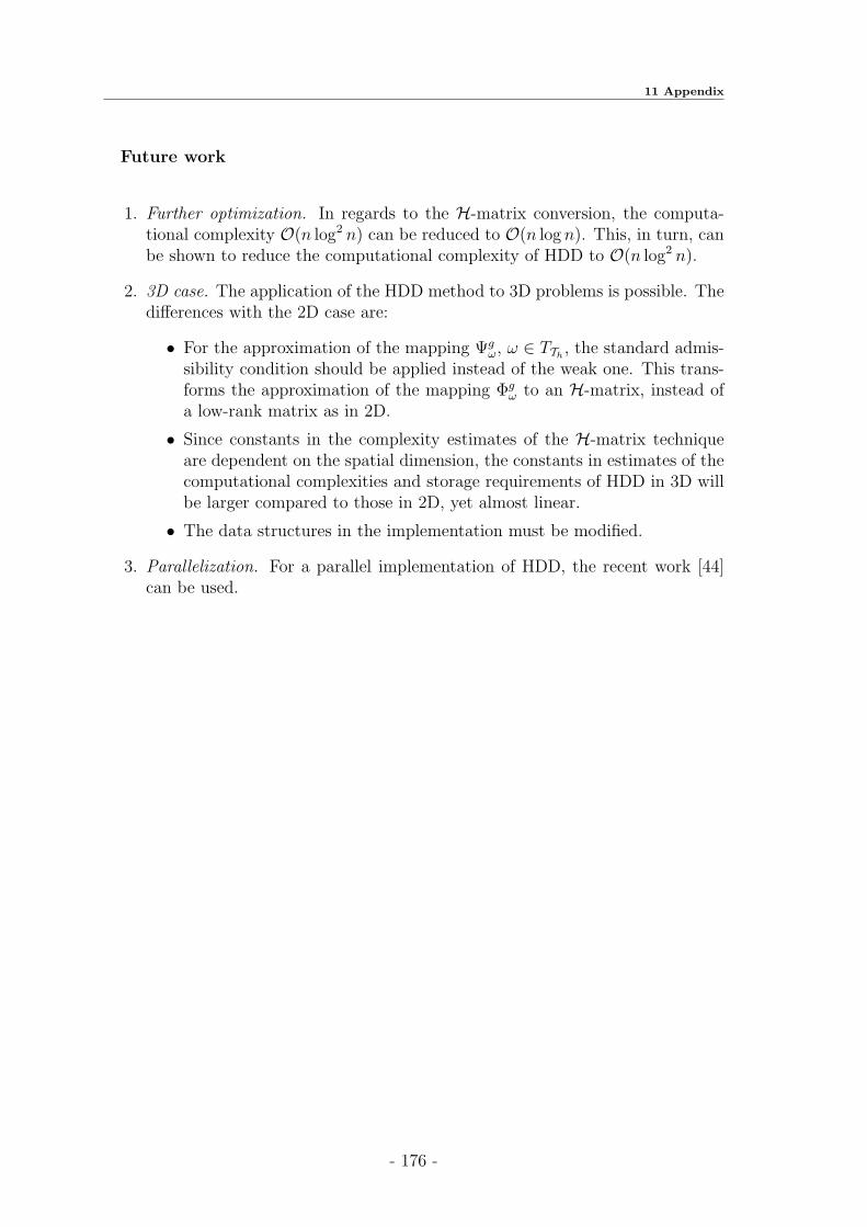
11 Appendix
Future work
1. Further optimization. In regards to the H-matrix conversion, the computa-tional complexity O(n log2 n) can be reduced to O(n log n). This, in turn, canbe shown to reduce the computational complexity of HDD to O(n log2 n).
2. 3D case. The application of the HDD method to 3D problems is possible. Thedifferences with the 2D case are:
• For the approximation of the mapping Ψgω, ω ∈ TTh
, the standard admis-sibility condition should be applied instead of the weak one. This trans-forms the approximation of the mapping Φg
ω to an H-matrix, instead ofa low-rank matrix as in 2D.
• Since constants in the complexity estimates of the H-matrix techniqueare dependent on the spatial dimension, the constants in estimates of thecomputational complexities and storage requirements of HDD in 3D willbe larger compared to those in 2D, yet almost linear.
• The data structures in the implementation must be modified.
3. Parallelization. For a parallel implementation of HDD, the recent work [44]can be used.
- 176 -
Bibliography
[1] Basic linear algebra subroutines. www.netlib.org/blas/.
[2] Linear algebra package. www.netlib.org/lapack/.
[3] Assyr Abdulle and Weinan E. Finite difference heterogeneous multi-scalemethod for homogenization problems. J. Comput. Phys., 191(1):18–39, 2003.
[4] Assyr Abdulle and Christoph Schwab. Heterogeneous multiscale FEM for diffu-sion problems on rough surfaces. Multiscale Model. Simul., 3(1):195–220 (elec-tronic), 2004/05.
[5] T. Alarcon, H. M. Byrne, and P. K. Maini. A multiple scale model for tumorgrowth. Multiscale Model. Simul., 3(2):440–475 (electronic), 2005.
[6] Gregoire Allaire and Robert Brizzi. A multiscale finite element method fornumerical homogenization. Multiscale Model. Simul., 4(3):790–812 (electronic),2005.
[7] Ivo Babuvska. Homogenization and its application. Mathematical and com-putational problems. In Numerical solution of partial differential equations,III (Proc. Third Sympos. (SYNSPADE), Univ. Maryland, College Park, Md.,1975), pages 89–116. Academic Press, New York, 1976.
[8] P. Bastian. Numerical computation of multiphase flow in porous media. Habil-itationsschrift, Heidelberg, Germany, 1999.
[9] M. Bebendorf. Hierarchical LU decomposition-based preconditioners for BEM.Computing, 74(3):225–247, 2005.
[10] M. Bebendorf. Why approximate lu decompositions of finite element discreti-sations of elliptic operators can be computed with almost linear complexity.Technical report in Max-Planck-Institut MIS www.mis.mpg.de, Leipzig, Ger-many, 8, 2005.
[11] M. Bebendorf and W. Hackbusch. Existence of H-matrix approximants to theinverse FE-matrix of elliptic operators with L∞-coefficients. Numer. Math.,95(1):1–28, 2003.
[12] Lions J-L. Bensoussan, A. and G. Papanicolaou. Asymptotic analysis for peri-odic structures. 1978.
[13] S. Borm, L. Grasedyck, and W. Hackbusch. Hierarchical Matrices, vol-ume 21 of Lecture Note. Max-Planck Institute for Mathematics, Leipzig, 2003.www.mis.mpg.de.
- 177 -

Bibliography
[14] Dietrich Braess. Finite elements. Cambridge University Press, Cambridge,second edition, 2001. Theory, fast solvers, and applications in solid mechanics,Translated from the 1992 German edition by Larry L. Schumaker.
[15] Zhiming Chen and Thomas Y. Hou. A mixed multiscale finite element methodfor elliptic problems with oscillating coefficients. Math. Comp., 72(242):541–576(electronic), 2003.
[16] Philippe G. Ciarlet. The finite element method for elliptic problems. North-Holland Publishing Co., Amsterdam, 1978. Studies in Mathematics and itsApplications, Vol. 4.
[17] Doina Cioranescu and Jeannine Saint Jean Paulin. Homogenization of reticu-lated structures, volume 136 of Applied Mathematical Sciences. Springer-Verlag,New York, 1999.
[18] Weinan E and Bjorn Engquist. The heterogeneous multiscale methods. Com-mun. Math. Sci., 1(1):87–132, 2003.
[19] Weinan E and Bjorn Engquist. Multiscale modeling and computation. NoticesAmer. Math. Soc., 50(9):1062–1070, 2003.
[20] Weinan E, Xiantao Li, and Eric Vanden-Eijnden. Some recent progress inmultiscale modeling. In Multiscale modelling and simulation, volume 39 ofLect. Notes Comput. Sci. Eng., pages 3–21. Springer, Berlin, 2004.
[21] Jens Eberhard. Upscaling und mehrgitterverfahren fur stromungen in hetero-genen porosen medien. Ph.D. Thesis, University of Heidelberg, Germany, 2003.
[22] Bjorn Engquist, Per Lotstedt, and Olof Runborg, editors. Multiscale methods inscience and engineering, volume 44 of Lecture Notes in Computational Scienceand Engineering. Springer-Verlag, Berlin, 2005. Papers from the conferenceheld in Uppsala, January 26–28, 2004.
[23] Bjorn Engquist and Erding Luo. Convergence of a multigrid method for el-liptic equations with highly oscillatory coefficients. SIAM J. Numer. Anal.,34(6):2254–2273, 1997.
[24] Alan George. Nested dissection of a regular finite element mesh. SIAM J.Numer. Anal., 10:345–363, 1973. Collection of articles dedicated to the memoryof George E. Forsythe.
[25] Gene H. Golub and Charles F. Van Loan. Matrix computations. Johns Hop-kins Studies in the Mathematical Sciences. Johns Hopkins University Press,Baltimore, MD, third edition, 1996.
[26] I.G. Graham, P. Lechner, and R. Scheichl. Domain decomposition for multiscalepdes. Bath Institute for Complex Systems, Preprint 11, www.bath.ac.uk/math-sci/BICS, 2006.
- 178 -

Bibliography
[27] L. Grasedyck. Theorie und anwendungen hierarchischer matrizen. Ph.D. Thesis,University of Kiel, Germany, 2001.
[28] L. Grasedyck and S. Borm. H-matrix library: www.hlib.org.
[29] L. Grasedyck and W. Hackbusch. Construction and arithmetics of H-matrices.Computing, 70(4):295–334, 2003.
[30] Khoromskij B. N. Hackbusch, W. A sparseH-matrix arithmetic. II. Applicationto multi-dimensional problems. Computing, 64(1):21–47, 2000.
[31] W. Hackbusch. Elliptic differential equations, volume 18 of Springer Seriesin Computational Mathematics. Springer-Verlag, Berlin, 1992. Theory andnumerical treatment, Translated from the author’s revision of the 1986 Germanoriginal by Regine Fadiman and Patrick D. F. Ion.
[32] W. Hackbusch. Iterative solution of large sparse systems of equations, volume 95of Applied Mathematical Sciences. Springer-Verlag, New York, 1994. Translatedand revised from the 1991 German original.
[33] W. Hackbusch. A sparse matrix arithmetic based onH-matrices. I. Introductionto H-matrices. Computing, 62(2):89–108, 1999.
[34] W. Hackbusch. H-matrix techniques and multi-scale problems. Workshop:Numerical methods for multiscale Problems, MPIMS, Leipzig, Germany, 2002.
[35] W. Hackbusch. Direct domain decomposition using the hierarchical matrixtechnique. In Domain decomposition methods in science and engineering, pages39–50 (electronic). Natl. Auton. Univ. Mex., Mexico, 2003.
[36] W. Hackbusch. Hierarchical Matrizen - Algoritmen und Analysis, volume 22.Max-Planck-Institut fr Mathematik, Leipzig, 2004. www.mis.mpg.de.
[37] W. Hackbusch, B. N. Khoromskij, and R. Kriemann. Hierarchical matricesbased on a weak admissibility criterion. Computing, 73(3):207–243, 2004.
[38] W. Hackbusch, B.N. Khoromskij, and R. Kriemann. Direct Schur complementmethod by domain decomposition based on H-matrix approximation. Comput.Vis. Sci., 8(3-4):179–188, 2005.
[39] Viet Ha Hoang and Christoph Schwab. High-dimensional finite elements forelliptic problems with multiple scales. Multiscale Model. Simul., 3(1):168–194(electronic), 2004/05.
[40] Thomas Y. Hou and Xiao-Hui Wu. A multiscale finite element method forelliptic problems in composite materials and porous media. J. Comput. Phys.,134(1):169–189, 1997.
[41] Thomas Y. Hou, Xiao-Hui Wu, and Zhiqiang Cai. Convergence of a multiscalefinite element method for elliptic problems with rapidly oscillating coefficients.Math. Comp., 68(227):913–943, 1999.
- 179 -

Bibliography
[42] V. V. Jikov, S. M. Kozlov, and O. A. Oleuınik. Homogenization of differentialoperators and integral functionals. Springer-Verlag, Berlin, 1994. Translatedfrom the Russian by G. A. Yosifian.
[43] B.N Khoromskij and A. Litvinenko. Domain decomposition based H-matrixpreconditioner for the skin problem in 2d and 3d. Max-Planck Institute, onlinepreprint www.mis.mpg.de/preprints, (95), 2006.
[44] R. Kriemann. Parallele algorithmen fur H-matrizen. Ph.D. Thesis, Universityof Kiel, Germany, 2004.
[45] R. Kriemann. Parallel H-matrix arithmetics on shared memory systems. Com-puting, 74(3):273–297, 2005.
[46] S. Le Borne and L. Grasedyck. H-matrix preconditioners in convection-dominated problems. SIAM J. Matrix Anal. Appl., 27(4):1172–1183 (elec-tronic), 2006.
[47] S. Le Borne, L. Grasedyck, and R. Kriemann. Parallel black box domain de-composition based H − lu preconditioning. Max-Planck-Institut MIS, Leipzig,www.mis.mpg.de, Preprint 115:(electronic), 2005.
[48] M. Lintner. The eigenvalue problem for the 2D Laplacian in H-matrix arith-metic and application to the heat and wave equation. Computing, 72(3-4):293–323, 2004.
[49] A. Litvinenko. Documentation for the HDD method. Technical report in Max-Planck-Institut MIS, www.mis.mpg.de/preprints/tr/index.html, Leipzig, Ger-many, 5, 2006.
[50] Pingbing Ming and Xingye Yue. Numerical methods for multiscale ellipticproblems. J. Comput. Phys., 214(1):421–445, 2006.
[51] L. Mirsky. Symmetric gauge functions and unitarily invariant norms. Quart. J.Math. Oxford Ser. (2), 11:50–59, 1960.
[52] N. Neuss, W. Jager, and G. Wittum. Homogenisierung und mehrgitter. Ph.D.Thesis, Universiteat of Heidelberg, Heidelberg, Germany, 1995.
[53] N. Neuss, W. Jager, and G. Wittum. Homogenization and multigrid. Comput-ing, 66(1):1–26, 2001.
[54] Jeff Ovall. Duality-based adaptive refinement for elliptic pdes. Ph.D. Thesis,University of California at San Diego, 2004.
[55] Peter J. Park and Thomas Y. Hou. Multiscale numerical methods for singularlyperturbed convection-diffusion equations. International Journal of Computa-tional Methods, 1(1):17–65, 2004.
[56] A.V. Skvorcov. Review of algorithms for delaunay triangulation building. Com-putation methods and programming, T.3, 2002.
- 180 -

Index
Hk(Ω), Hk0 (Ω) and H−1(Ω), 28
S(t), Sons of t, 61
T(i)I i-th level of TI , 61TI×J , block cluster tree, 63TI , TJ , cluster trees, 61V (T ), Vertices of T , 61H-matrix, 71H-matrix format, 71L(T, l) leaves of T at level l, 61t, subset of indices, 61t, s, clusters, 61
adaptive rank arithmetic, 75admissibility, standard, 64admissibility, weak , 65admissible blocks, 67algorithm “Leaves to Root”, 47algorithm “Root to Leaves”, 47Aubin-Nitsche’s theorem, 35
block cluster tree, 63Building of λfω, Algorithm, 57Building of λgω, Algorithm, 57
cluster tree, 61
data dω, 40Data structures, 135domain decomposition tree TTh
, 38
FE method, 32fixed rank arithmetic, 75formatted addition, 75formatted multiplication, 75functional λfω, 55functional λgω, 55functional λω, 54
HDD method, 38HDD on two grids, 52
HDD with repeated patterns, 53HDD with truncation of small scales,
52HMM, 21homogenization, 20
Implementation of HDD, 140inadmissible blocks, 68
low-rank matrix, 68
mapping Φω = (Φgω,Φ
fω), 40
mapping Ψω = (Ψgω,Ψ
fω), 41
MsFEM, 21
parallel H-matrix arithmetics, 126parallel efficiency, 125parallel speedup, 125PCG, 147
rank-k matrix, 68resonance effect, 22Ritz-Galerkin discretisation method, 30
Sobolev spaces Ls(Ω),, 27sparsity constant Csp, 72structure boundary, 142structure DDTree, 142structure domain, 142
truncation Tk, 70Truncation operator Tε, 75
variational formulation, 28
- 181 -
Lebenslauf
Alexander Litvinenko
Geboren am 31.08.1979 in Almaty, Kasachstan1986 bis 1994 Besuch der Schule 90 in Almaty.1994 bis 1995 Besuch der Physikalische-Mathematische Schule von NSU in Akadem-gorodok, Novosibirsk, Abitur 1996.1996 bis 2000 Studium an der Staatlichen Universitat Novosibirsk (NSU).2000 Bachelor Diplom in Mathematik.2000 bis 2002 Studium an der Staatlichen Universitat Novosibirsk und Sobolev In-stitut fur Mathematik.2002 Magister Diplom in Mathematik.2002 bis 2006 Doktorand am Max-Planck-Institut fur Mathematik in den Naturwis-senschaften.

Hiermit erklare ich, die vorliegende Dissertation selbstandig und ohne unzulassigefremde Hilfe angefertigt zu haben. Ich habe keine anderen als die angefuhrtenQuellen und Hilfsmittel benutzt und samtliche Textstellen, die wortlich oder sin-ngemas aus veroffentlichten oder unveroffentlichten Schriften entnommen wurden,und alle Angaben, die auf mundlichen Auskunften beruhen, als solche kenntlichgemacht. Ebenfalls sind alle von anderen Personen bereitgestellten Materialen odererbrachten Dienstleistungen als solche gekennzeichnet.
10.04.2006
(Unterschrift)