Science Journal of Applied Mathematics and Statistics 2015; 3(5): 225-229 Published online September 16, 2015 (http://www.sciencepublishinggroup.com/j/sjams) doi: 10.11648/j.sjams.20150305.12 ISSN: 2376-9491 (Print); ISSN: 2376-9513 (Online)

Application of Logistic Regression Model in an Epidemiological Study

Renhao Jin, Fang Yan, Jie Zhu

School of Information, Beijing Wuzi University, Beijing, China

Email address: Renhao.jin@outlook.com (Renhao Jin)

To cite this article: Renhao Jin, Fang Yan, Jie Zhu. Application of Logistic Regression Model in an Epidemiological Study. Science Journal of Applied

Mathematics and Statistics. Vol. 3, No. 5, 2015, pp. 225-229. doi: 10.11648/j.sjams.20150305.12

Abstract: This paper use the logistic regression model to an epidemiological study, i.e. bovine tuberculosis (bTB) occurrence in cattle herds, together with well-established risk factors in the area known as West Wicklow, in the east of Ireland. The binary target variable is whether the herd is in the restricted status, which is defined by whether any bTB reactor is detected in the herd. With the stepwise variables selection procedure, a final logistical regression model is found to adequately describe the data. Herd bTB incidence was positively associated with annual total rainfall, herd size and a herd bTB history in the previous three years, and presence /absence of commonage.

Keywords: Logistic Regression, Bovine Tuberculosis, Stepwise Variables Selection

1. Introduction

Logistic regression is firstly developed by statistician D.R. Cox in 1958 as a statistical method, and after that it is used widely in many fields, including the medical and social sciences. Recent years as the big data society comes, Logistic regression model is also extensively used in many data mining applications, such as, credit risk models in banking industry, customer preference models in retails, and even segment of customers in all areas of business. For example, in economics it can be used to predict the likelihood of a person's choosing to be in the labor force, and a business application would be to predict the likelihood of a homeowner defaulting on a mortgage. Logistic regression is a direct probability model, which is called as logit regression or logit model. Unlike regression model, which is used to model or predict a continuous target variable, the logit model is applied for binary target variable.

Logistic regression measures the relationship between the binary dependent variable and one or more independent variables (explanation variables), which are usually (but not necessarily) continuous, by estimating probabilities. More detailed, for a binary dependent variable y with value 0 or 1, corresponding to the status of an observation, the logit model is written as

logit�Ey = �� + ���� + ���� (1)

where Ey is the expect value of y, i.e., the probability of y = 1 , logit�Ey = ������ �1 − ��⁄ , and the part of �� + ���� + ���� is the linear part of independent variables. The equation (1) is also can be transformed to be

Ey = �������� ! ��"!"���������� ! ��"!" (2)

The important feature of the logit function is that it produces values that lie only between 0 and 1, just as the probability of response and non-response dependent variables, as shown in equation (2).

The approach to fit logit model is often based on maximum likelihood method, as logit model predicts probabilities rather than just classes. For each observation with explanation variables marked as #$ and target variable �$ , let E�$ =%�#$ . The likelihood function for n observations can be written as

L�� =(%��$)*+1 − %��$,�-)*.

$/�

With the procedure of maximum likelihood estimation, the parameters’ estimates and their variances all can be obtained from likelihood method.

The epidemiological study in this paper is based on aggregated bovine tuberculosis (bTB) data in cattle herds from 2005 to 2009, together with well-established risk factors in the area known as West Wicklow, in the east of Ireland. The bTB

Science Journal of Applied Mathematics and Statistics 2015; 3(5): 225-229 226

data is from the first author’s Ph.D thesis, and the other related part of the bTB study has been published in Veterinary Record (2013).

Bovine tuberculosis (bTB), caused by infection with Mycobacterium bovis, affects approximately 0.3% of cattle annually in Ireland, with 18,531 reactor cattle identified in 2011. This has major financial implications both for the farmer whose herd is restricted from trading and cattle slaughtered, and for the exchequer that compensates the farmer and implements measures to control the disease. Data for the bTB study were obtained from three sources: herd data from the national databases of bTB testing herd and animal history (Animal Health Computer System, AHCS); land usage from Herdfinder, a unique multi-layered purpose built spatial mapping system whereby farms shapes submitted by farmers to DAFM under the EU Single Farm Payment Scheme are recorded and weather data from Met Éireann, all for West Wicklow. Both AHCS and Herdfinder databases use the same herd ID number so that farm, geographic location and testing data may be linked. The spatial distribution of herds and rainfall stations, and the study areas is shown in Figure 4.1.

Figure 1. The spatial distribution of herd observations and rainfall stations.

Out of 14 rainfall stations, nine were the nearest to any one herd and they are

shown in the map indexed by station numbers.

2. Statistical Methods

A logistic regression model was built to determine the relationship between bTB incidence in cattle herds and potential risk factors (explanatory variables) from 2005 to 2009. The herd target variable is binary, indicating whether any bTB reactor is detected in the herd, and the herd with target value 1 is with restriction status. So the response variable Y12 is binary: restriction status of the ith herd in year j (1=restricted, 0=not restricted), where j 1,⋯ ,5 denoting the years 2005-2009. In this paper, the observations from different herds were set to be independent and yearly outcomes observed on the same herd were also independent. This assumption has been verified by

first author’s Ph.D thesis. A logistic linear model was used to fit the data with a logit

link function:

logit+π12, logit+E9Y12:, X12β (3)

where the matrix X12 was the design matrix for the explanatory variables and β is a vector of unknown explanatory parameters. A model selection method similar to Ma et al. (2010) was carried out. As we have more than 30 explanatory variables, before building the logit model, we first examined associations between the response variableY and each explanatory variable in a univariate analysis using Spearman’s rank correlation coefficient. Many explanatory variables were skewed and outliers were present and Spearman’s rank correlation was chosen as it is not sensitive to outliers. Explanatory variables were considered for inclusion in the logit model if an association significant at the 0.1 level was found from the univariate analysis. Then a forward stepwise approach was used to build a logit model by adding explanatory variables step by step keeping only those significant at the 5% level until the best-fit model was found. Stepwise approach adjusted for possible effects of collinearity among significant variables in the univariate analysis. Herd bTB history variables, weather variables and geographical variables (total farm area and total farm perimeter) formed three classes of possibly correlated explanatory variables. The correlation among variables in each class was tested using Pearson’s or Spearman’s rank correlation whichever was appropriate. Firstly, the significant variables in the univariate analysis but not in these three classes were found for the logit model. Then for the three classes, starting with the geographical class, only the significant variables in the univariate analysis were considered for inclusion in the multivariate model. A stepwise procedure was used to choose which of these should be retained in the multivariate model as many were correlated. Then the non-significant variables in the univariate analysis and interactions were tested by adding them to the reduced multivariable model, one at a time. This process was continued with the herd bTB history class variables added next and then the weather class variables. The order of entering classes into the model did not change the final model. Transformations including the natural logarithmic (log) and square root (sqrt) transformations were made on the skewed variables or those with extreme values to check whether it could improve model fit. The variable herd size has been found to be an important risk factor in many studies and in the final model log (herd size) or sqrt (herd size) were checked for linearity by the inclusion of quadratic terms. The variable number of introduced cattle was positively skewed with many zeros. However, it was not significant in any model. Categorizing it as 0 or greater than 0 (or transforming it) also did not lead to significance in any model.

Models were fitted using the Logistic procedure and Enterprise Miner in SAS version 9.4 (SAS Institute Inc., Cary, NC, USA).

3. Results

From 2005 to 2009, there were 609 distinct herds in the

227 Renhao Jin et al.: Application of Logistic Regression Model in an Epidemiological Study

study, giving 2666 observations. Table 1 presents the number of herds and the percentage restricted on an annual basis, and the total herds and percentage restricted for each year keep stable and are around 540 and 4% respectively. Table 2 shows summary statistics for selected covariates used in the study, and these results are displayed by two distinct groups as restricted and non-restricted. As shown in Table 2, these covariates, except for the weather variables, are skewed to the right. Comparing the covariates between in two groups, the herd size, total farm area and farm perimeter are all relatively greater in restricted group then those in non-restricted group.

Table 1. Number of herds and percentage of these herds with confirmed

restrictions for tuberculosis in West Wicklow, Ireland from 2005 to 2009. A

herd was considered restricted if any bTB reactor was found on any bTB test

in the year.

Year Total herds Number of restricted herds Percentage restricted*

2005 555 25 0.045 2006 550 22 0.04 2007 530 17 0.032 2008 517 29 0.056 2009 514 29 0.056

*Percentage restricted= Number of herds restricted/ Total number of herds.

Table 2. Summary statistics of selected variables for both non-restricted and restricted herds. There were 2544 observations for non-restricted herds and 122

observations for restricted herds.

Variable name Unit Non-restricted herds Restricted herds

Mean Median 1st quartile 3rd quartile Mean median 1st quartile 3rd quartile

Herd size 71 42 18 98 139 91 50 198 Number of introduced adult cattle 15 3 0 13 23 3 0 16 Annual total rainfall dm 12 12.2 9.6 13.8 12.8 12.5 9.6 15.1 Annual maximum monthly rainfall dm 1.8 1.7 1.5 2.1 1.9 1.8 1.5 2.1 Annual mean monthly temperature ℃ 10 10.2 9.7 10.3 10 10.2 9.7 10.3 Annual averages of monthly average VPD hPa 2.3 2.3 2.2 2.3 2.3 2.3 2.2 2.3 total farm area km2 1.8 0.5 0.2 1.2 2.5 1 0.5 1.8 total farm perimeter km 12.1 8.6 4.3 15.6 17.5 14.9 7.9 22.6 % herds with commonage % 17.7

km, kilometer; dm, decimeter=0.1 meters; VPD, vapour pressure deficit (a measure of atmospheric dryness); herd size was the total number of cattle in a herd.

In the univariate analysis, herd bTB restriction status was significantly associated with 15 explanatory variables (Table 3 (a)). The remaining variables which were not significantly associated herd bTB restriction status are listed in Table 3 (b). Herd size and presence /absence of commonage were entered the regression model first followed by geographical variables, herd bTB history variables and weather variables together with interactions.

Table 3. Spearman’s rank correlation between explanatory variables and herd

bTB restriction status (1=restricted, 0=not restricted). The variables with p

value<0.1 and p value>0.1 are listed in Table 3 (a) and (b) respectively. A1,

A2, A3, P1, P2, and P3 were the amplitude and phase of the first, second, and

third annual cycle of change related to monthly average temperature and

monthly average vapour pressure deficit (VPD) respectively.

Table 3 (a).

Explanatory variables Spearman’s

correlation coefficient P value

Herd size 0.14 <.0001

Presence /absence of commonage 0.03 0.08

Total farm area 0.11 <.0001

Total farm perimeter 0.12 <.0001

Herd bTB history 1 0.09 <.0001

Herd bTB history 2 0.09 <.0001

Herd bTB history 3 0.08 <.0001

Herd bTB history of past 3 years 0.12 <.0001

Annual total rainfall 0.05 0.01

Annual max monthly rainfall 0.04 0.03

Annual mean monthly temperature -0.04 0.04

Temperature.A3 0.04 0.04

Annual mean monthly VPD -0.04 0.05

VPD.A2 -0.04 0.03

VPD.P3 0.04 0.05

Table 3 (b).

Explanatory variables Spearman’s

correlation coefficient P value

Herd type 0.0007 0.97 Number of introduced adult cattle 0.0044 0.82 Presence /absence of introduced adult cattle 0.0099 0.61 Annual maximum monthly temperature 0.0018 0.93 Annual minimum monthly temperature -0.0190 0.34 Annual maximum monthly VPD 0.0018 0.93 Annual minimum monthly VPD 0.0253 0.20 Annual range of monthly temperature 0.0096 0.63 Annual range of monthly VPD -0.0131 0.51 Temperature.A1 0.0096 0.63 Temperature.A2 0.0229 0.25 Temperature.P1 0.0296 0.14 Temperature.P2 0.0006 0.97 Temperature.P3 0.0229 0.25 VPD.A1 0.0063 0.75 VPD.A3 -0.0199 0.31 VPD.P1 0.0078 0.69 VPD.P2 0.0295 0.14

Three years herd bTB history was highly correlated with other history variables (Pearson correlation coefficients > 0.50, p-value < 0.001) while correlations among the yearly history variables were low. Farms with large area typically have large perimeters, and thus the correlation coefficient between area and perimeter is high at 0.636 (p-value < 0.0001). For some herds, rainfall variables from the nearest rainfall station were not available and in such cases data from the second nearest rainfall station were substituted. Of the 14 rainfall stations, nine were found to be the nearest stations for some herd, and in the total of 2666 herd observations, 1008 used rainfall data from the Glen of Imaal station. There were 18 weather variables in our study and many were inter-related with each other. Six were significant in the univariate selection

Science Journal of Applied Mathematics and Statistics 2015; 3(5): 225-229 228

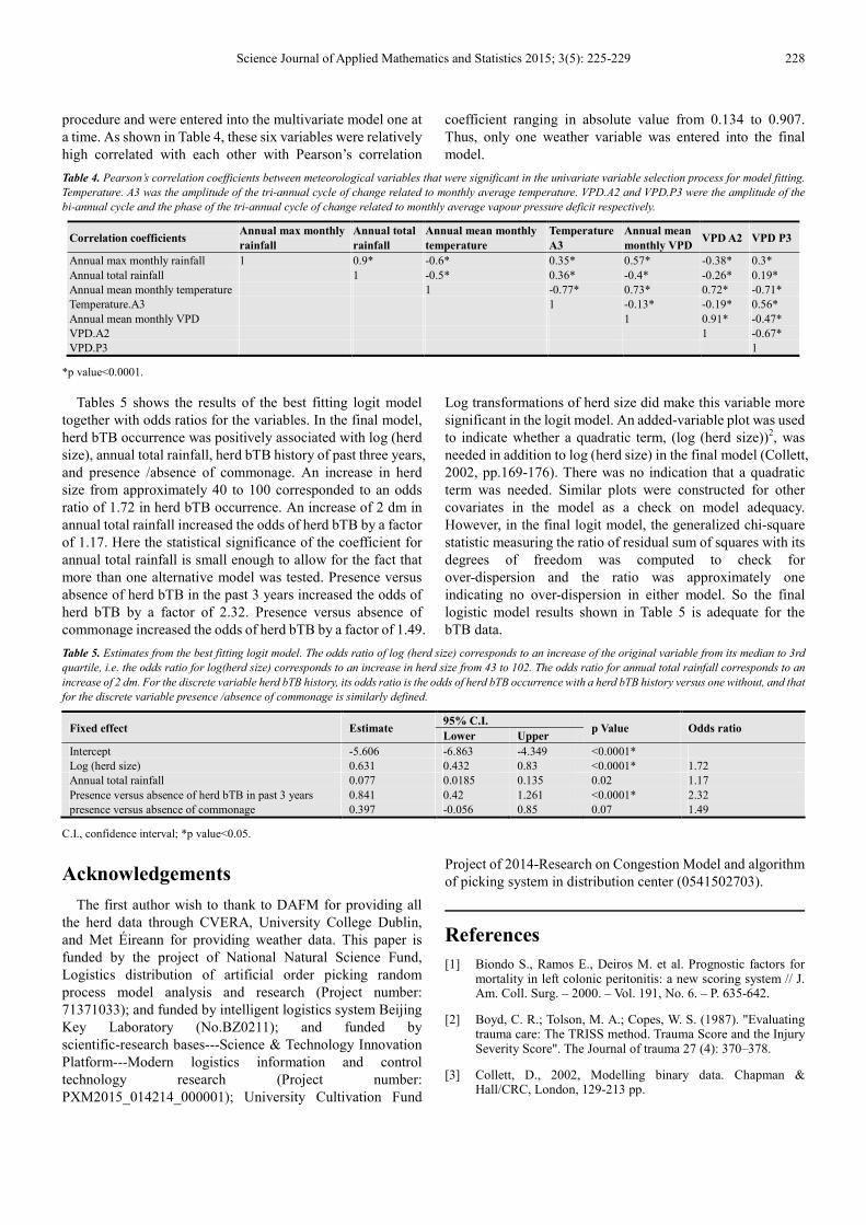
procedure and were entered into the multivariate model one at a time. As shown in Table 4, these six variables were relatively high correlated with each other with Pearson’s correlation

coefficient ranging in absolute value from 0.134 to 0.907. Thus, only one weather variable was entered into the final model.

Table 4. Pearson’s correlation coefficients between meteorological variables that were significant in the univariate variable selection process for model fitting.

Temperature. A3 was the amplitude of the tri-annual cycle of change related to monthly average temperature. VPD.A2 and VPD.P3 were the amplitude of the

bi-annual cycle and the phase of the tri-annual cycle of change related to monthly average vapour pressure deficit respectively.

Correlation coefficients Annual max monthly

rainfall

Annual total

rainfall

Annual mean monthly

temperature

Temperature

A3

Annual mean

monthly VPD VPD A2 VPD P3

Annual max monthly rainfall 1 0.9* -0.6* 0.35* 0.57* -0.38* 0.3* Annual total rainfall 1 -0.5* 0.36* -0.4* -0.26* 0.19* Annual mean monthly temperature 1 -0.77* 0.73* 0.72* -0.71* Temperature.A3 1 -0.13* -0.19* 0.56* Annual mean monthly VPD 1 0.91* -0.47* VPD.A2 1 -0.67* VPD.P3 1

*p value<0.0001.

Tables 5 shows the results of the best fitting logit model together with odds ratios for the variables. In the final model, herd bTB occurrence was positively associated with log (herd size), annual total rainfall, herd bTB history of past three years, and presence /absence of commonage. An increase in herd size from approximately 40 to 100 corresponded to an odds ratio of 1.72 in herd bTB occurrence. An increase of 2 dm in annual total rainfall increased the odds of herd bTB by a factor of 1.17. Here the statistical significance of the coefficient for annual total rainfall is small enough to allow for the fact that more than one alternative model was tested. Presence versus absence of herd bTB in the past 3 years increased the odds of herd bTB by a factor of 2.32. Presence versus absence of commonage increased the odds of herd bTB by a factor of 1.49.

Log transformations of herd size did make this variable more significant in the logit model. An added-variable plot was used to indicate whether a quadratic term, (log (herd size))2, was needed in addition to log (herd size) in the final model (Collett, 2002, pp.169-176). There was no indication that a quadratic term was needed. Similar plots were constructed for other covariates in the model as a check on model adequacy. However, in the final logit model, the generalized chi-square statistic measuring the ratio of residual sum of squares with its degrees of freedom was computed to check for over-dispersion and the ratio was approximately one indicating no over-dispersion in either model. So the final logistic model results shown in Table 5 is adequate for the bTB data.

Table 5. Estimates from the best fitting logit model. The odds ratio of log (herd size) corresponds to an increase of the original variable from its median to 3rd

quartile, i.e. the odds ratio for log(herd size) corresponds to an increase in herd size from 43 to 102. The odds ratio for annual total rainfall corresponds to an

increase of 2 dm. For the discrete variable herd bTB history, its odds ratio is the odds of herd bTB occurrence with a herd bTB history versus one without, and that

for the discrete variable presence /absence of commonage is similarly defined.

Fixed effect Estimate 95% C.I.

p Value Odds ratio Lower Upper

Intercept -5.606 -6.863 -4.349 <0.0001* Log (herd size) 0.631 0.432 0.83 <0.0001* 1.72 Annual total rainfall 0.077 0.0185 0.135 0.02 1.17 Presence versus absence of herd bTB in past 3 years 0.841 0.42 1.261 <0.0001* 2.32 presence versus absence of commonage 0.397 -0.056 0.85 0.07 1.49

C.I., confidence interval; *p value<0.05.

Acknowledgements

The first author wish to thank to DAFM for providing all the herd data through CVERA, University College Dublin, and Met Éireann for providing weather data. This paper is funded by the project of National Natural Science Fund, Logistics distribution of artificial order picking random process model analysis and research (Project number: 71371033); and funded by intelligent logistics system Beijing Key Laboratory (No.BZ0211); and funded by scientific-research bases---Science & Technology Innovation Platform---Modern logistics information and control technology research (Project number: PXM2015_014214_000001); University Cultivation Fund

Project of 2014-Research on Congestion Model and algorithm of picking system in distribution center (0541502703).

References

[1] Biondo S., Ramos E., Deiros M. et al. Prognostic factors for mortality in left colonic peritonitis: a new scoring system // J. Am. Coll. Surg. – 2000. – Vol. 191, No. 6. – Р. 635-642.

[2] Boyd, C. R.; Tolson, M. A.; Copes, W. S. (1987). "Evaluating trauma care: The TRISS method. Trauma Score and the Injury Severity Score". The Journal of trauma 27 (4): 370–378.

[3] Collett, D., 2002, Modelling binary data. Chapman & Hall/CRC, London, 129-213 pp.

229 Renhao Jin et al.: Application of Logistic Regression Model in an Epidemiological Study

[4] Cox, DR (1958). "The regression analysis of binary sequences (with discussion)". J Roy Stat Soc B 20: 215–242.

[5] David A. Freedman (2009). Statistical Models: Theory and Practice. Cambridge University Press. p. 128.

[6] Gareth James; Daniela Witten; Trevor Hastie; Robert Tibshirani (2013). An Introduction to Statistical Learning. Springer. p. 6.

[7] Gordejo, R. F. J., Vermeersch, J. P., 2006. Towards eradication of bovine tuberculosis in the European Union. European Union Veterinary Microbiology 112, 101-109.

[8] Griffin, J. M., Hahesya, T., Lyncha, T., M. D. Salmanb, M. D., McCarthya, J., Hurleya, T., 1993. The association of cattle husbandry practices, environmental factors and farmer characteristics with the occurence of chronic bovine tuberculosis in dairy herds in the Republic of Ireland. Preventive Veterinary Medicine 17, 145-160.

[9] Griffin, J. M., Williams, D. H., Kelly, G. E., Clegg, T. A., O’ Boyle, I., Collins, J. D., More, S. J., 2005. The impact of badger removal on the control of tuberculosis in cattle herds in Ireland. Preventive Veterinary Medicine 67, 237–266.

[10] Hahesy, T., Kelleher, D. L., Doherty, J., 1992. An investigation of a possible association between the occurrence of bovine tuberculosis and weather variables. Irish Veterinary Journal 45, 127-128.

[11] Kattamuri Sarma, 2013. Predictive Modeling with SAS Enterprise Miner: Practical Solutions for Business Applications, Second Edition. NC: SAS Institute Inc, Cary.

[12] Kologlu M., Elker D., Altun H., Sayek I. Valdation of MPI and OIA II in two different groups of patients with secondary peritonitis // Hepato-Gastroenterology. – 2001. – Vol. 48, No. 37. – P. 147-151.

[13] Ma, E., Lam, T., Wong, C., Chuang, S. K., 2010. Is hand, foot and mouth disease associated with meteorological parameters?. Epidemiology and Infection 138, 1779-1788.

[14] Mardia, K. and Marshall, R. (1984). Maximum likelihood estimation of models for residual covariance in spatial regression. Biometrika 71, 135--146.

[15] Richardson, S. and He´ mon, D. (1981). On the variance of the sample correlation between two independent lattice processes. Journal of Applied Probability 18, 943--948.

[16] SAS Institute Inc, 2013. SAS/STAT® 9.4 User’s Guide: The GLIMMIX Procedure (Book Excerpt). NC: SAS Institute Inc, Cary.

[17] SAS Institute Inc, 2013. SAS/STAT® 9.4 User’s Guide: The Logistic Procedure (Book Excerpt). NC: SAS Institute Inc, Cary.

[18] Tiefelsdorf, M. and Boots, B. (1995). The exact distribution of Moran’s I. Environment and Planning A 27, 985--999.

[19] Walker, SH; Duncan, DB (1967). "Estimation of the probability of an event as a function of several independent variables". Biometrika 54: 167–178.