application of mixed-integer programming in chemical
TRANSCRIPT

Application of Mixed-Integer
Programming in Chemical
Engineering
Thomas Pogiatzis
Homerton College
University of Cambridge
This dissertation is submitted for the degree of
Doctor of Philosophy
November 2012

^En tzeinon th tsiliac p�s> stä bolÐtzin
EÐsen ênan tzi> êpeyen täg giìn tou na spoud�sh. VAman rtem poÌ tàc
spoudèc tou, âkartèran ton å tzÔrhc tou t�n �llh �mèran n� shkwsth
n� mpoukk¸soun ... âkartèran, âkartèran ... tÐpote. �N� p�w, lalei,
na doumen eÐnta> m k�mnei.�
P�ei, jwrei ton, gr�fei tzaÈ sb nnh, tzaÈ tä dein tou p�s> st�b bolÐkwshn.
- EÐnta > m poÌ k�mneic, giè mou, lalei tou, tzi> àn êrkesai n� mpoukk¸soumen;
- ^Ahs> me, papa lalei tou, tzi> êto k�mnw loarkoÔc n� dw eÐnta lohc
âkìrtwsen å bouc täg kwlon tou tzi> âphren th tsili�n tou p�s> tzein
to bolÐtzin.
- Krima st� rð�lia, giè mou, lalei tou, poÌ xìkiasa n� sà spoud�sw.
^Eto tä bolÐtzin eÐsem p�nw tou t� tsili�n tzi> å qtÐsthc êbalèn to
p�s> st�b bolÐkwshn, qwrÐc n� tä kajarÐsh.
Cypriot fable
�'Oqi! 'Oqi! Potè mhn anagnwrÐseic ta sÔnora tou anjr¸pou! Na spac
ta sÔnora! N> arnièsai ì,ti jwroÔn ta m�tia sou. Na pejaÐneic kai na
lec: J�natoc den up�rxei!�
Askhtik , NÐkoc Kazantz�khc
(The Saviours of God: Spiritual Exercises, Nikos Kazantzakis)

Preface
The work in this dissertation was undertaken at the Department of
Chemical Engineering and Biotechnology, University of Cambridge,
between October 2009 and November 2012. It is the original work of
the author, except where specifically acknowledged in the text, and
includes nothing that is the outcome of work done in collaboration.
No part of this dissertation has been submitted for a degree, diploma
or other qualification at any other university.
The dissertation is approximately 47000 words in length, including
figures, tables, references, equations and the appendix. It contains
exactly 30 figures.
Thomas A. Pogiatzis
29 November 2012

Acknowledgements
I would like to express my deep gratitude to my supervisors, Drs.
Vassilis Vassiliadis and Ian Wilson, for their guidance and support
during the course of this work. I wish to thank Dr. Ian Wilson for
his kindness and patience. I thank Dr. Vassiliadis for the long and
helpful discussions we had on Mathematical Programming.
Financial support from the Onassis Foundation and Cambridge Eu-
ropean Trust is gratefully acknowledged.
I am very grateful to all my friends with whom I shared my University
years, whether in Athens or in Cambridge. I would always recall our
memorable moments.
I would like to thank my friends Christos and Michalis for they have
always been there for me.
Special thanks are reserved for Evangelia Andreou for her never-
ending encouragement and support. She has been my excellent com-
panion for many years.
Last I wish to thank my family for their continuous support through-
out the years. I am very grateful to them for providing me with the
opportunities to pursue my aspirations.

Abstract
Mixed-Integer Programming has been a vital tool for the chemical engineer
in the recent decades and is employed extensively in process design and control.
This dissertation presents some new Mixed-Integer Programming formulations
developed for two well-studied problems, one with a central role in the area of
Optimisation, the other of great interest to the chemical industry. These are the
Travelling Salesman Problem and the problem of scheduling cleaning actions for
heat exchanger networks subject to fouling.
The Travelling Salesman Problem finds a plethora of applications in many
scientific disciplines, Chemical Engineering included. None of the mathematical
programming formulations proposed for solving the problem considers fewer than
O(n2) binary degrees of freedom. The first part of this dissertation introduces a
novel mathematical description of the Travelling Salesman Problem that succeeds
in reducing the binary degrees of freedom to O(ndlog2(n)e). Three Mixed-Integer
Linear Programming formulations are developed and the computational perfor-
mance of these is tested through computational studies.
Sophisticated methods are now available for scheduling the cleaning actions
for networks of heat exchangers subject to fouling. In the majority of these, only
one form of cleaning is used, which restores the performance of the exchanger
back to its clean level. Ishiyama et al. [2011b] recently revised the scheduling
problem for the case where there are several cleaning methods available. The
second part of this dissertation extends their approach, developed for individual
units, to heat exchanger networks and explores the concept of selection of cleaning
techniques further. Mixed-Integer Programming formulations are proposed for
the scheduling task, for two fouling scenarios: (i) chemical reaction fouling and
(ii) biological fouling. A series of results are presented for the implementation of
the scheduling formulations to networks of different sizes.
Table of contents
List of Algorithms x
List of Figures xi
List of Tables xiii
Nomenclature xxiii
1 Introduction 1
I Travelling Salesman Problem 4
2 Basic aspects of the problem 5
2.1 History of problem . . . . . . . . . . . . . . . . . . . . . . . . . . 5
2.2 Problem formulations . . . . . . . . . . . . . . . . . . . . . . . . . 7
2.2.1 Classical formulation . . . . . . . . . . . . . . . . . . . . . 8
2.2.2 Sequential formulations . . . . . . . . . . . . . . . . . . . . 8
2.2.3 Commodity flow formulations . . . . . . . . . . . . . . . . 9
2.2.4 Time dependent formulations . . . . . . . . . . . . . . . . 10
2.2.5 Comparison of TSP formulations . . . . . . . . . . . . . . 11
2.3 Searching for an optimal tour . . . . . . . . . . . . . . . . . . . . 13
2.3.1 Exact methods . . . . . . . . . . . . . . . . . . . . . . . . 13
2.3.1.1 Cutting-plane method . . . . . . . . . . . . . . . 13
2.3.1.2 Branch-and-Bound method . . . . . . . . . . . . 14
2.3.1.3 Hybrid methods . . . . . . . . . . . . . . . . . . 18
vi

Table of contents
2.3.2 Heuristic approaches . . . . . . . . . . . . . . . . . . . . . 19
2.4 Travelling Salesman & Computational Complexity Theory . . . . 19
2.5 Applications in Chemical Engineering . . . . . . . . . . . . . . . . 20
2.6 Conclusions . . . . . . . . . . . . . . . . . . . . . . . . . . . . . . 21
3 Formulations & computational studies 22
3.1 Inspiration . . . . . . . . . . . . . . . . . . . . . . . . . . . . . . . 22
3.2 Novel formulation . . . . . . . . . . . . . . . . . . . . . . . . . . . 24
3.2.1 Basics . . . . . . . . . . . . . . . . . . . . . . . . . . . . . 24
3.2.2 Adjacency of binary leaves . . . . . . . . . . . . . . . . . . 27
3.2.3 Asymmetric Travelling Salesman model . . . . . . . . . . . 33
3.2.4 Manhattan Travelling Salesman model . . . . . . . . . . . 34
3.3 Computational studies . . . . . . . . . . . . . . . . . . . . . . . . 37
3.3.1 ATSP case studies . . . . . . . . . . . . . . . . . . . . . . 37
3.3.2 Manhattan-TSP case studies . . . . . . . . . . . . . . . . . 39
3.3.3 Comparison with existing formulations . . . . . . . . . . . 40
3.4 Conclusions . . . . . . . . . . . . . . . . . . . . . . . . . . . . . . 42
II Scheduling cleaning actions for heat exchanger net-works subject to fouling 43
4 Background 44
4.1 Fouling & heat transfer processes . . . . . . . . . . . . . . . . . . 44
4.2 Fouling in heat exchangers . . . . . . . . . . . . . . . . . . . . . . 45
4.2.1 Mechanisms of heat exchanger fouling . . . . . . . . . . . . 47
4.2.2 Ageing . . . . . . . . . . . . . . . . . . . . . . . . . . . . . 49
4.2.3 Fouling models . . . . . . . . . . . . . . . . . . . . . . . . 50
4.2.4 Cleaning fouled heat exchangers . . . . . . . . . . . . . . . 52
4.3 Scheduling of cleaning actions . . . . . . . . . . . . . . . . . . . . 53
4.3.1 Single heat exchanger . . . . . . . . . . . . . . . . . . . . . 54
4.3.2 Heat exchanger networks . . . . . . . . . . . . . . . . . . . 55
4.3.2.1 Non-convex formulations . . . . . . . . . . . . . . 56
4.3.2.2 Convex formulations . . . . . . . . . . . . . . . . 58
vii

Table of contents
4.4 Motivating study . . . . . . . . . . . . . . . . . . . . . . . . . . . 59
4.5 Conclusions . . . . . . . . . . . . . . . . . . . . . . . . . . . . . . 60
5 Chemical reaction fouling: formulation & solution methods 62
5.1 Heat transfer analysis . . . . . . . . . . . . . . . . . . . . . . . . . 63
5.2 Fouling analysis . . . . . . . . . . . . . . . . . . . . . . . . . . . . 64
5.3 Time representation . . . . . . . . . . . . . . . . . . . . . . . . . . 67
5.4 Mathematical programming formulation . . . . . . . . . . . . . . 69
5.4.1 Constraints . . . . . . . . . . . . . . . . . . . . . . . . . . 70
5.4.1.1 Simulation constraints . . . . . . . . . . . . . . . 70
5.4.1.2 Process constraints . . . . . . . . . . . . . . . . . 74
5.4.2 Objective function . . . . . . . . . . . . . . . . . . . . . . 75
5.4.3 Characteristics of the proposed scheduling formulation . . 78
5.4.4 The MILP formulation of Lavaja & Bagajewicz . . . . . . 79
5.5 Solution methods . . . . . . . . . . . . . . . . . . . . . . . . . . . 80
5.5.1 Outer approximation/Equality relaxation . . . . . . . . . . 81
5.5.2 Generalised Benders Decomposition algorithm . . . . . . . 82
5.5.3 Receding Horizon heuristic . . . . . . . . . . . . . . . . . . 85
5.6 Conclusions . . . . . . . . . . . . . . . . . . . . . . . . . . . . . . 87
6 Chemical reaction fouling: computational studies 90
6.1 Introductory remarks . . . . . . . . . . . . . . . . . . . . . . . . . 90
6.2 Isolated heat exchanger . . . . . . . . . . . . . . . . . . . . . . . . 91
6.3 Heat exchanger networks . . . . . . . . . . . . . . . . . . . . . . . 94
6.3.1 Heat exchanger network I . . . . . . . . . . . . . . . . . . 96
6.3.2 Heat exchanger network II . . . . . . . . . . . . . . . . . . 103
6.3.3 Solution statistics . . . . . . . . . . . . . . . . . . . . . . . 110
6.4 Conclusions . . . . . . . . . . . . . . . . . . . . . . . . . . . . . . 112
7 Biological fouling: formulations & computational studies 114
7.1 Introductory remarks . . . . . . . . . . . . . . . . . . . . . . . . . 114
7.2 Fouling analysis . . . . . . . . . . . . . . . . . . . . . . . . . . . . 115
7.3 Mathematical programming formulations . . . . . . . . . . . . . . 119
7.3.1 MINLP formulation . . . . . . . . . . . . . . . . . . . . . . 119
viii
Table of contents
7.3.2 MILP formulation . . . . . . . . . . . . . . . . . . . . . . . 121
7.3.3 Objective function . . . . . . . . . . . . . . . . . . . . . . 126
7.4 Computational studies . . . . . . . . . . . . . . . . . . . . . . . . 127
7.4.1 Solution statistics . . . . . . . . . . . . . . . . . . . . . . . 135
7.5 Conclusions . . . . . . . . . . . . . . . . . . . . . . . . . . . . . . 135
8 Conclusions & Recommendations 138
8.1 Travelling Salesman Problem . . . . . . . . . . . . . . . . . . . . . 138
8.1.1 Asymmetric formulations . . . . . . . . . . . . . . . . . . . 139
8.1.2 Manhattan formulation . . . . . . . . . . . . . . . . . . . . 140
8.1.3 Recommendations for future work . . . . . . . . . . . . . . 140
8.2 Scheduling cleaning actions for heat exchanger networks subject
to fouling . . . . . . . . . . . . . . . . . . . . . . . . . . . . . . . 141
8.2.1 Networks subject to chemical reaction fouling . . . . . . . 141
8.2.2 Networks subject to biological fouling . . . . . . . . . . . . 142
8.2.3 Numerical methods . . . . . . . . . . . . . . . . . . . . . . 143
8.2.4 Recommendations for future work . . . . . . . . . . . . . . 144
Appendix A 146
References 149
ix

List of Algorithms
3.1 Nodal binary string analysis . . . . . . . . . . . . . . . . . . . . . 25
5.1 Generalized Benders Decomposition . . . . . . . . . . . . . . . . . 86
5.2 Receding Horizon heuristic . . . . . . . . . . . . . . . . . . . . . . 87
x

List of Figures
2.1 Branch-and-bound example: solution tree after stage 2 . . . . . . 16
2.2 Branch-and-bound example: solution tree after stage 3 . . . . . . 16
2.3 Branch-and-bound example: solution tree after stage 4 . . . . . . 18
3.1 Binary tree with 8 leaves . . . . . . . . . . . . . . . . . . . . . . . 23
3.2 Manhattan distance on a system of Cartesian coordinates . . . . . 35
3.3 Optimal itinerary for Manhattan-TSP case studies . . . . . . . . . 40
4.1 Simplified representation of a heat exchanger, co-current flow . . . 46
4.2 Idealised evolution of thermal fouling resistance . . . . . . . . . . 51
5.1 Schematic representation of a shell-and-tube heat exchanger (counter-
current mode) . . . . . . . . . . . . . . . . . . . . . . . . . . . . . 63
5.2 Growth of gel and coke layers in time . . . . . . . . . . . . . . . . 66
5.3 Schematic representation of a discrete time period (filled circles:
collocation nodes) . . . . . . . . . . . . . . . . . . . . . . . . . . . 68
5.4 Orthogonal (Radau) collocation over finite element . . . . . . . . 69
5.5 Units in serial configuration (solid line: cold stream; dashed line:
hot stream) . . . . . . . . . . . . . . . . . . . . . . . . . . . . . . 74
5.6 Units in parallel configuration (solid line: cold stream; dashed line:
hot stream) . . . . . . . . . . . . . . . . . . . . . . . . . . . . . . 75
5.7 Example of a preheat train (solid line: cold stream; dashed lines:
hot streams . . . . . . . . . . . . . . . . . . . . . . . . . . . . . . 76
5.8 Variation of heat duty with time for unit i in time period j (1: heat
exchanged, 2: energy losses and 3: lost-production opportunity) . 77
xi
List of Figures
5.9 Iterative structure of decomposition algorithms . . . . . . . . . . 80
5.10 Invalid Benders cut (underestimator) . . . . . . . . . . . . . . . . 85
6.1 Time profile of gel and coke thickness: isolated heat exchanger . . 93
6.2 Heat exchanger network I . . . . . . . . . . . . . . . . . . . . . . 96
6.3 Time profile of Tf : heat exchanger network I . . . . . . . . . . . . 102
6.4 Heat exchanger network II . . . . . . . . . . . . . . . . . . . . . . 104
6.5 Time profile of Tf : heat exchanger network II . . . . . . . . . . . 109
6.6 Distribution of solutions generated by the GBD algorithm for 50
random starting points . . . . . . . . . . . . . . . . . . . . . . . . 111
7.1 Progression of thermal fouling resistance after cleaning . . . . . . 116
7.2 Heat exchanger network subject to biological fouling . . . . . . . . 127
7.3 Time profile of Rf : case study A . . . . . . . . . . . . . . . . . . 132
7.4 Time profile of Rf : case study B . . . . . . . . . . . . . . . . . . 133
7.5 Time profile of Rf : case study C . . . . . . . . . . . . . . . . . . 134
7.6 Distribution of solutions generated by the GBD algorithm for 100
random starting points . . . . . . . . . . . . . . . . . . . . . . . . 136
xii

List of Tables
2.1 Size of different ATSP formulations . . . . . . . . . . . . . . . . . 12
2.2 Comparison of ATSP formulations . . . . . . . . . . . . . . . . . . 13
3.1 Size of proposed ATSP formulations . . . . . . . . . . . . . . . . . 34
3.2 Solution report for ATSP case studies . . . . . . . . . . . . . . . . 38
3.3 Solution report for Manhattan-TSP case studies . . . . . . . . . . 39
3.4 Comparison of LP-relaxations: optimal objective function value . 41
6.1 Cleaning parameters . . . . . . . . . . . . . . . . . . . . . . . . . 91
6.2 Operating parameters: isolated heat exchanger . . . . . . . . . . . 92
6.3 Fouling parameters: isolated heat exchanger . . . . . . . . . . . . 92
6.4 Optimal cleaning schedule: isolated heat exchanger (open circles:
chemical actions; filled circles: mechanical action) . . . . . . . . . 92
6.5 Objective value for the optimal schedule and for the no-cleaning
situation: isolated heat exchanger . . . . . . . . . . . . . . . . . . 92
6.6 Problem parameters for heat exchanger network I . . . . . . . . . 97
6.7 Cleaning schedule for heat exchanger network I: case study AI
(open circles: chemical actions) . . . . . . . . . . . . . . . . . . . 98
6.8 Cleaning schedule for heat exchanger network I: case study BI
(open circles: chemical actions; filled circles: mechanical actions) . 100
6.9 Problem parameters for heat exchanger network II . . . . . . . . . 105
6.10 Cleaning schedule for heat exchanger network II: GBD algorithm
– case study AII (open circles: chemical actions) . . . . . . . . . . 106
6.11 Cleaning schedule for heat exchanger network II: RH heuristic –
case study AII (open circles: chemical actions) . . . . . . . . . . . 107
xiii

List of Tables
6.12 Size of studied scheduling problems . . . . . . . . . . . . . . . . . 110
6.13 Execution times . . . . . . . . . . . . . . . . . . . . . . . . . . . . 110
7.1 Operating and design parameters for heat exchanger network sub-
ject to biological fouling . . . . . . . . . . . . . . . . . . . . . . . 128
7.2 Parameters for biological fouling model . . . . . . . . . . . . . . . 128
7.3 Cleaning parameters . . . . . . . . . . . . . . . . . . . . . . . . . 129
7.4 Cleaning schedule for heat exchanger network subject to biologi-
cal fouling (open circles: water flush; filled grey circles: chemical
cleaning; filled black circles: chemical disinfection) . . . . . . . . . 130
A.1 Cost matrix for ATSP case study: n = 8 . . . . . . . . . . . . . . 146
A.2 Cost matrix for ATSP case study: n = 10 . . . . . . . . . . . . . 146
A.3 Cost matrix for ATSP case study: n = 12 . . . . . . . . . . . . . 147
A.4 Coordinates for Manhattan-TSP case study: n = 8 . . . . . . . . 147
A.5 Coordinates for Manhattan-TSP case study: n = 10 . . . . . . . . 148
xiv

Nomenclature
Roman Symbols
A set of arcs in Part I; area in Part II
a constant in equation (4.5)
B binary tree
b constant in equation (4.6)
Bk set of binary variables that are equal to one at iteration k
C cost matrix in Part I; constant defined by equation (5.5) in Part II;
cost vector in Part II
c constant in equation (4.9)
ch index denoting chemical action
cijk cost in time dependent formulation of the travelling salesman prob-
lem
cij length of arc (i, j)
Ck set of binary variables that are equal to zero at iteration k
cm cost of cleaning action m
Cp,c specific heat capacity of cold stream
Cp,h specific heat capacity of hot stream
xv

Nomenclature
dE Euclidean distance
cd index denoting chemical disinfection
dM Manhattan distance (rectilinear metric)
E set of elements
eijl continuous variable indicating whether cities i and j have the same
or opposite directions at level l of binary tree representation
F configuration correction factor
f function
fe energy cost
fl index denoting water flush cleaning
G graph
g function
h function
hcold film heat transfer coefficient of cold stream
hhot film heat transfer coefficient of hot stream
hk length of time element k
i general index; index of vertex (city) in Part I; index of unit in Part II
I1 integral of process costs
j general index; index of vertex (city) in Part I; index of time period
in Part II
K set of iterations in Generalised Benders Decomposition algorithm
xvi

Nomenclature
k general index; index of leaf in Part I; index of element in Part II;
index of iteration in Generalised Benders Decomposition; constant
rate introduced in equation (7.2)
kc coke formation rate
kg gel formation rate
L set of levels for a binary tree
l general index; index of level in Part I; index of node in Part II
l′ index in Theorem 3.1
l′′ index in proof of Theorem 3.1
l∞ infinity norm
l(x)k x-distance between leaves k and k + 1 of binary tree
l(y)k y-distance between leaves k and k + 1 of binary tree
M set of cleaning actions
m general index; index of cleaning mode in Part II; maintenance costs
function in Part II
mc mass flow rate of cold stream
me index denoting mechanical action
mh mass flow rate of hot stream
n general index; number of vertices in graph (cities in travelling sales-
man problem); exponent in equation (7.4)
nl number of levels of a binary tree
np number of leaves of a binary tree in Part I; number of time periods
in Part II
xvii
Nomenclature
nRH number of periods in receding horizon heuristic procedure
nu number of units
nx dimension of vector x
ny dimension of vector y
O set of collocation nodes
P set of leaves for a binary tree in Part I; set of time periods in Part II
p general index; function of process costs in Part II
posi position of city i in decimal base
Q set of vertices (cities) in Part I; heat duty in Part II
Q0 heat duty for a clean heat exchanger
qi Lagrange interpolation polynomial
rc coke formation rate
Rf thermal fouling resistance
rf function defined by equation (7.7)
Rf,cold thermal fouling resistance of layer deposited on the cold side of the
heat transfer wall
Rf,hot thermal fouling resistance of layer deposited on the hot side of the
heat transfer wall
Rf∞ asymptotic value of thermal fouling resistance
Rf,tot total thermal fouling resistance
rg gel formation rate
rijk binary variable in time dependent formulation of the travelling sales-
man problem
xviii

Nomenclature
ril binary variable indicating the direction of city i at level l of the binary
tree
Rw thermal resistance of heat transfer wall
t time
t0 starting time
tch duration of chemical cleaning
Tc,in inlet temperature of cold stream
tcl cleaning time
Tc,o outlet temperature of cold stream
Tf final temperature of cold stream
tf time horizon
T limitf lower limit on final temperature of cold stream
Th,in inlet temperature of hot stream
Th,o outlet temperature of hot stream
tI initiation or induction time
tkl parameter defining the target binary strings in the proposed mathe-
matical description of the travelling salesman problem
tchle leap time after chemical cleaning
tflle leap time after water flush cleaning
tme duration of mechanical cleaning
top operating time
Ttarget target temperature for cold stream
xix

Nomenclature
U overall heat transfer coefficient
U ′ set of units
U0 overall heat transfer coefficient for a clean heat exchanger
ui continuous variable in sequential formulation of the travelling sales-
man problem
V set of vertices (cities)
v continuous variable
w function
wij continuous variable in multi-commodity formulation of the travelling
salesman problem
x x -coordinate in Part I; continuous variable in Part II
x(0)i x-coordinate of city i
xij binary variable in Chapter 2/continuous variable in Chapter 3 indi-
cating the presence of arc (i, j) in travelling salesman’s tour
xk x-coordinate of leaf k of the binary tree
y binary vector
y(0)i y-coordinate of city i
yijm binary variable indicating the cleaning of unit i at period j with
action m
yk y-coordinate of leaf k of the binary tree
z objective variable
z∗ optimal objective function value
z∗GBD best objective function value found by the Generalised Benders De-
composition algorithm
xx

Nomenclature
zij continuous variable in single commodity formulation of the travelling
salesman problem
zik continuous variable indicating the allocation of city i on leaf k of the
binary tree
zIP optimal objective function value for integer programming problem
zrelLP optimal objective function value for linear programming relaxation
problem
zno objective function value for the no-cleaning situation
zkPr objective variable in primal problem (NLP-Pr) at iteration k
zR objective variable in relaxed problem (NLP-R)
zRH objective function value by the receding horizon heuristic procedure
Greek Symbols
α function defined by equation (3.12)
β function defined by equation (3.13)
δ thickness
δc thickness of coke layer
δg thickness of gel layer
∆Tlm logarithmic mean temperature difference
θk objective variable in master problem (MILP-M) at iteration k
λc thermal conductivity of coke layer
λkc Lagrange multiplier at iteration k
λg thermal conductivity of gel layer
λkg Lagrange multiplier at iteration k
xxi
Nomenclature
τ collocation time
τk collocation node k
tijkl sigmoid time
Acronyms
ATSP asymmetric travelling salesman problem
BM basic model for asymmetric travelling salesman problem
CPU central processing unit
DFJ Dantzig, Fulkerson and Johnson travelling salesman problem formu-
lation
ER equality relaxation
GBD generalised Benders decomposition
GG Gavish and Graves travelling salesman problem formulation
IP integer programming
LP linear programming
MILP mixed-integer linear programming
MINLP mixed-integer nonlinear programming
MIP mixed-integer programming
MPC model predictive control
MTZ Miller, Tucker and Zemlin travelling salesman problem formulation
NLP nonlinear programming
NP non-deterministic polynomial class of problems
OA outer approximation
xxii

Nomenclature
P polynomial class of problems
RH receding horizon
TDTSP time dependent travelling salesman problem
TSP travelling salesman problem
xxiii

Chapter 1
Introduction
Mathematical programming has become an indispensable tool for the chemical
engineer over the past 40 years. Optimisation is widely used in process design,
process control, process identification, model development [Biegler, 2010] and
more recently in product and molecule design [Pistikopoulos et al., 2010].
The class of optimisation problems that involve both continuous variables and
discrete variables are generally known as Mixed-Integer Programming problems.
Mixed-Integer Programming finds a plethora of applications in Chemical Engi-
neering. These include the scheduling of batch processes, the synthesis of complex
reactor networks and the retrofit of heat exchanger networks [Floudas, 1995].
In this work, some new Mixed Integer Programming formulations are pre-
sented for two very different problems, one of great theoretical and practical
value, and the other a real industrial problem. The dissertation is divided into
two parts:
I. Travelling Salesman Problem
II. Scheduling cleaning actions for heat exchanger networks subject to fouling
The Travelling Salesman Problem has a central role in Mathematical Pro-
gramming. It was the systematic study of the problem that led to the devel-
opment of the areas of Integer Programming and Mixed-Integer Programming
and directed the way for the discovery of many rigorous and heuristic optimisa-
tion tools. Today, the problem finds numerous applications across all scientific
1

1. Introduction
disciplines. Those related to Chemical Engineering include the vehicle routing
problem, machine scheduling problem and genome mapping.
Hitherto, all existing mathematical formulations of the Travelling Salesman
Problem have required O(n2) binary degrees of freedom or more. The aim of the
current work is the development of a mathematical description for the problem
that involves fewer than O(n2) binary variables.
Chapter 2 reviews the basic aspects of the Travelling Salesman Problem. A
major part of the chapter is devoted to the description of some well-accepted for-
mulations found in the literature. The basic rigorous algorithms used to identify
optimal tours are introduced briefly and some successful tour searching heuristic
procedures are mentioned.
Chapter 3 introduces the novel mathematical description of the Travelling
Salesman Problem. A new class of mathematical programming formulations is
developed, based on work in Binary Arithmetic. The detailed presentation of
the proposed Mixed-Integer Programming formulations is followed by computa-
tional studies, which aim to test their computational performance in practice.
At the end of the chapter, their relationship to other well-known formulations is
discussed.
The second part of this dissertation revisits the problem of scheduling the
cleaning actions for heat exchanger networks subject to fouling. Fouling remains
a long-standing problem in industrial process heat transfer. It dominates the
performance of heat transfer devices and causes acute financial losses. An effec-
tive mitigation strategy for the rectification of the negative effects of fouling is
the regular cleaning of the dirty devices. In recent years, decision-making tools
have been used to schedule the cleaning actions in an attempt to minimise the
associated losses.
A novel scheduling study, presented by Ishiyama et al. [2011b] for an isolated
heat exchanger, introduced the important problem of competition between two
alternative cleaning techniques on the basis of length, cost and effectiveness. The
aims of the current work are to extend the approach of Ishiyama et al. [2011b] to
heat exchanger networks and to explore the concept of choice of cleaning methods
further.
Chapter 4 introduces the phenomenon of fouling and discusses its negative im-
2

1. Introduction
pact on heat transfer processes. The focus is primarily on heat exchangers. Sub-
sequent sections of the chapter review previous scheduling approaches presented
for isolated heat exchangers or networks of units. It is decided to investigate
the problem of scheduling the cleaning actions for: (i) heat exchanger networks
subject to chemical reaction fouling and (ii) heat exchanger networks subject to
biological fouling.
Chapter 5 describes in detail the Mixed-Integer Programming formulation
proposed for the scheduling task for networks subject to chemical reaction fouling.
The chapter includes a description of the fouling model used to quantify the
negative effect of the deposits on heat transfer performance. It concludes with a
discussion regarding appropriate solution methods for the scheduling problem.
In Chapter 6 the proposed scheduling formulation is tested in practice. Case
studies are presented where it is used to generate cleaning schedules for an isolated
unit and two heat exchanger networks. A series of results is presented in each
case, considering the impact of variations in the fouling parameters.
Chapter 7 is concerned with the novel study of scheduling cleaning actions
for heat exchanger networks subject to biological fouling. Two Mixed-Integer
Programming formulations are presented for this scheduling task, which involves
the choice between three cleaning methods. A series of results are obtained for
a small network, using one of the scheduling formulations. These are presented
and discussed at the end of the chapter.
Chapter 8 presents conclusions and recommendations for future work.
3
Part I
Travelling Salesman Problem

Chapter 2
Basic aspects of the problem
This chapter reviews the basic aspects of the Travelling Salesman Problem. The
first section presents a brief history of the problem. Section 2.2, which is of prime
interest for this work, focuses on the mathematical description of the problem
and an overview of some well-established Mathematical Programming formula-
tions is provided. Subsequent sections give a short description of some of the
most important solution methods and establish the importance of the problem
in the areas of Applied Mathematics, Engineering and Computer Science. Some
applications of the problem related to Chemical Engineering are also provided.
2.1 History of problem
“Given a finite set of discrete points and the distance between each pair of them,
find the shortest route to visit all of them exactly once and return to the starting
point”. This humble-sounding task is one of the most notorious and intensively
studied problems of computational mathematics, namely the Travelling Salesman
Problem (TSP). It remains unknown who coined this nifty name for the problem.
In the paragraphs that follow, some of the most important moments in the de-
velopment of the TSP are retraced. The source is the detailed historical survey
by Cook [2011].
Leonard Euler was the first person to study tour problems while trying to
solve a puzzle known as ‘The Bridges of Konigsberg’. Euler also studied the re-
5
2. Basic aspects of the problem
lated Knight’s Tour problem in chess, where one needs to find a closed tour for
the knight to visit all the squares in the board and return to its initial position.
Naturally, he managed to solve both puzzles and in doing so he laid the founda-
tions for Graph Theory [Aldous and Wilson, 2000]. One century later, another
mathematician, Sir William Rowan Hamilton, was investigating possible tours
through all twenty corners of a dodecahedron. He drew the construction known
as the Icosian graph and was trying to identify closed walks that touched all the
vertices (corners) only once. Such a tour is called a Hamiltonian circuit. Follow-
ing this, the salesman’s problem is defined, in mathematical terminology, as the
task of finding the Hamiltonian circuit of minimum weight on a given graph.
Graph Theory is esoteric for the salesman on the road. For him, the search
for the shortest possible tour still continues. To his aid came the Austrian mathe-
matician Karl Menger, who was the person who introduced the TSP to the mathe-
matical community. Menger, in the 1920s, began investigating the closely-related
problem of finding the shortest path without the need to return to the initial
point. He called this the ‘Messenger Problem’. It is speculated that Menger ex-
changed ideas on the matter with the American mathematician Hassler Whitney
during a visit at Harvard University. Afterwards, Whitney posed the problem to
the mathematical community at one seminar given in Princeton University, and,
by the late 1940’s, it was a recognised challenge.
The first systematic treatment of the TSP appeared in [Dantzig et al., 1954],
where the authors presented the first mathematical formulation for the problem
and crafted a computational method to solve it. These prominent mathematicians
identified the shortest route for travelling through the capitals of all 49 states of
the U.S. This was a challenge that had beset the research community for 15 years.
The interest of a wider research community was sparked by a TV commercial
in 1962 by Procter & Gamble, which promoted a competition with a $10000 prize,
enough money to buy a house at the time. The task was to identify the shortest
route starting from Chicago, travelling through 32 destinations across the U.S.
and finally return back to the starting point. The research community responded
enthusiastically to the challenge and at the end there was a tie between a number
of contestants.
Until today, the travelling salesman problem remains an open challenge and
6

2. Basic aspects of the problem
the interest of researchers has increased rather than diminished. The validity of
the statement is apparent when one considers the numerous articles written on
the problem every year.
2.2 Problem formulations
Adopting the notation employed in Graph Theory, the task is to find the Hamil-
tonian circuit of minimum weight for a graph G = (V,A), where V = {1, 2, . . . , n}is the set of vertices (cities) and A = {(i, j) : i, j ∈ V } the set of arcs (connecting
lines).
Let us focus our interest on the different formulations proposed for the Asym-
metric Travelling Salesman Problem (ATSP). In this variant of the problem the
length of an arc depends on the direction in which it is travelled. This is the
general case and it includes the special case of the symmetric problem where the
distance between two cities is independent of the direction of travel.
There are a number of excellent reviews in the literature, such as [Langevin
et al., 1990], [Orman and Williams, 2007] and [Oncan et al., 2009], which describe
and compare the large number of proposed formulations. This section considers
a selection of the most well-known.
It is essential at this point to review the terms Integer Programming (IP),
Linear Programming (LP) and Mixed Integer Programming (MIP). An IP prob-
lem involves only integer variables, whereas an MIP one involves both continuous
and integer variables. Finally, an LP problem involves only continuous variables
which are related to each other by linear constraints only.
The basic model (BM) [Dantzig et al., 1954] for the ATSP is as follows:
min.n∑i=1
n∑j=1
cijxij (2.1)
s.t.n∑i=1
xij = 1 (2.2)
n∑j=1
xij = 1 (2.3)
7

2. Basic aspects of the problem
xij = {0, 1}; i, j = 1, 2, . . . , n (2.4)
{(i, j) : xij = 1, i, j = 2, 3, . . . , n} does not contain subtours (2.5)
where the binary variables xij are equal to 1 if and only if the arc (i, j) is present
in the optimal solution and cij is the length of arc (i, j). Constraints (2.2), (2.3)
and (2.5) eliminate subtours for all vertices.
The key aspect of a TSP formulation is how to formulate the constraints that
break subtours. A subtour is a closed loop that does not contain all the cities.
The majority of TSP formulations have this basic model in common and the only
difference is found at the subtour elimination constraints. There are however
some formulations, such as the time-dependent models, that do not follow this
line drawn by Dantzig et al. [1954]. In the description of the various formulations
that follows, the objective function is given only when the (BM) does not apply.
2.2.1 Classical formulation
The classical TSP formulation was proposed by Dantzig et al. [1954] (DFJ for-
mulation). The set of elimination constraints for their IP model is given by
n∑i∈Q
n∑j∈Q
xij ≤ |Q| − 1 for all Q ⊆ {1, 2, . . . , n} and 2 ≤ |Q| ≤ n− 1. (2.6)
Equation (2.6) defines O(2n) constraints, a very large number even for small prob-
lems (∼ 1 million for 20 cities). Nevertheless, the ingenuity of their proposal lies
in the fact that only a relatively small number of these facet defining inequalities
[Grotchel and Padberg, 1985] needs to be added progressively to the model to
reach the optimal solution. Dantzig et al. [1954] managed to solve by hand a
42-cities problem by incorporating only 9 inequalities out of a two trillion set of
constraints.
2.2.2 Sequential formulations
An extended category of formulations is based on a model first presented by Miller
et al. [1960] (MTZ formulation) for a vehicle routing problem. Firstly, there is
8

2. Basic aspects of the problem
the need to introduce O(n) supplementary continuous variables, ui, which denote
the sequence in which vertex i is visited. The elimination constraints take the
form:
ui − uj + (n− 1)xij ≤ n− 2; i, j = 2, 3, . . . , n; i 6= j. (2.7)
There are O(n2− n+ 2) constraints defined in equation (2.7). One can intro-
duce simple bounds on the continuous variables, but this is not necessary. This
is an MIP model. Many improvements of the MTZ formulation have appeared
in the literature over the years, such as those by Desrochers and Laporte [1991],
Gouveia and Pires [2001] and Sherali and Driscoll [2002].
2.2.3 Commodity flow formulations
The class of commodity flow formulations follows from the work of Gavish and
Graves [1978]. This class is further divided to: (i) single-commodity flow; (ii) two-
commodity flow and (iii) multi-commodity flow models. The earliest single-
commodity flow model introduced by Gavish and Graves [1978] (GG formulation)
and the first multi-commodity flow model that belongs to Wong [1980] (Wong
formulation) are presented here. An example of a two-commodity flow model is
that by Finke et al. [1984], but Langevin et al. [1990] subsequently showed that
it is equivalent to the GG formulation.
Before stating the constraints for the GG model, first there is the need to
introduce O(n2) continuous variables zij which describe the flow of a single com-
modity to vertex 1 from every other vertex. The elimination constraints are given
by
n∑j=1
zji −n∑j=2
zij = 1; i = 2, 3, . . . , n (2.8)
0 ≤ zij ≤ (n− 1)xij; i = 1, 2, . . . , n, j = 2, 3, . . . , n. (2.9)
The above set has O(n2) constraints. The GG model belongs to the MIP
class.
Wong [1980] formulated the first multi-commodity flow model using additional
9
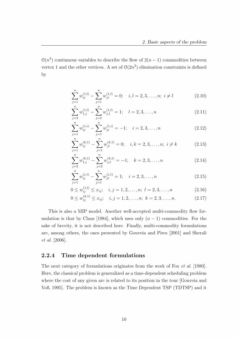
2. Basic aspects of the problem
O(n3) continuous variables to describe the flow of 2(n− 1) commodities between
vertex 1 and the other vertices. A set of O(2n3) elimination constraints is defined
by
n∑j=1
w(1,l)ij −
n∑j=1
w(1,l)ji = 0; i, l = 2, 3, . . . , n; i 6= l (2.10)
n∑j=2
w(1,l)1,j −
n∑j=2
w(1,l)j,1 = 1; l = 2, 3, . . . , n (2.11)
n∑j=1
w(1,i)ij −
n∑j=1
w(1,i)ji = −1; i = 2, 3, . . . , n (2.12)
n∑j=1
w(k,1)ij −
n∑j=1
w(k,1)ji = 0; i, k = 2, 3, . . . , n; i 6= k (2.13)
n∑j=2
w(k,1)1,j −
n∑j=2
w(k,1)j,1 = −1; k = 2, 3, . . . , n (2.14)
n∑j=1
w(i,1)ij −
n∑j=1
w(i,1)ji = 1; i = 2, 3, . . . , n (2.15)
0 ≤ w(1,l)ij ≤ xij; i, j = 1, 2, . . . , n; l = 2, 3, . . . , n (2.16)
0 ≤ w(k,1)ij ≤ xij; i, j = 1, 2, . . . , n; k = 2, 3, . . . , n. (2.17)
This is also a MIP model. Another well-accepted multi-commodity flow for-
mulation is that by Claus [1984], which uses only (n − 1) commodities. For the
sake of brevity, it is not described here. Finally, multi-commodity formulations
are, among others, the ones presented by Gouveia and Pires [2001] and Sherali
et al. [2006].
2.2.4 Time dependent formulations
The next category of formulations originates from the work of Fox et al. [1980].
Here, the classical problem is generalized as a time-dependent scheduling problem
where the cost of any given arc is related to its position in the tour [Gouveia and
Voß, 1995]. The problem is known as the Time Dependent TSP (TDTSP) and it
10

2. Basic aspects of the problem
is equivalent to the single machine scheduling problem.
A single machine is at the initial state, where job 1 is being processed. A
number of (n − 1) jobs must be performed before the machine returns to the
initial state. The cost of a task depends on its position in the sequence and the
preceding job. Thus, a cost cijk is incurred when job j is processed directly after
job i in the kth position and the corresponding binary variable rijk will be equal
to 1. The optimisation problem is stated as follows:
min.n∑i=1
n∑j=1
n∑k=1
cijkrijk (2.18)
s.t.n∑j=1
n∑k=1
rijk = 1; i = 1, 2, . . . , n (2.19)
n∑i=1
n∑k=1
rijk = 1; j = 1, 2, . . . , n (2.20)
n∑i=1
n∑j=1
rijk = 1; k = 1, 2, . . . , n (2.21)
n∑j=1
n∑k=2
krijk −n∑j=1
n∑k=1
krjik = 1; i = 2, 3, . . . , n (2.22)
rijk = {0, 1}; i, j, k = 1, 2, . . . , n (2.23)
This formulation requires O(n3) binary variables and O(4n) constraints and
it belongs to the IP class. Other TDTSP formulations can be found in the work
of Picard and Queyranne [1978] and Gouveia and Voß [1995].
2.2.5 Comparison of TSP formulations
Travelling Salesman Problem formulations are compared in terms of computa-
tional efficiency. The solution of TSP instances is computationally intense, es-
pecially as the number of cities increases. Therefore, it is beneficial to define
an efficiency scale where the formulations which require the least computational
effort are placed at the top, and those which force the solver into an endless run
at the bottom. The criterion for the classification is the LP-relaxation of each
11

2. Basic aspects of the problem
formulation [Gouveia and Voß, 1995; Langevin et al., 1990; Oncan et al., 2009].
The LP-relaxation of an IP (or MIP) model is simply the IP (or MIP) model
itself without the integrality conditions. Thus, the integer variables of IP (or
MIP) are now continuous (with lower and upper bounds) in the LP-relaxation.
Removing the integrality conditions means that the optimal solution of the LP-
relaxation, zrelLP, cannot exceed (since we are performing a minimisation) the opti-
mal solution of the IP model, zIP. Hence, the solution of the relaxation provides
a lower bound on the solution of the original model (zIP ≥ zrelLP). Moreover, an
LP-relaxation is said to be strong if the gap between zrelLP and zIP is relatively
small. A good IP (or MIP) formulation must have a strong LP-relaxation since
in general less computational effort will be required by the solver to reach the
optimal solution. For that to happen the LP-relaxation must be well-constrained.
The most recent comparative analysis of a number of well-known TSP for-
mulations is that by Oncan et al. [2009]. The authors have summarized results
obtained by previous researchers and they also established new relationships,
where non-existent, between the examined formulations. Herein, the interest
is focused on the models detailed above. Table 2.1 summarises the number of
binary variables, continuous variables and constraints for the described formula-
tions and Table 2.2 shows the relationships between these models [Oncan et al.,
2009]. Each model in the first column is classified as stronger, weaker or equiv-
alent with respect to the models in the first row. The word “Unknown” denotes
that a relationship is yet to be established between two formulations.
Table 2.1: Size of different ATSP formulations
Formulation Binary Variables Continuous Variables Constraints
DFJ O(n2) - O(2n)
MTZ O(n2) O(n) O(n2)
GG O(n2) O(n2) O(n2)
Wong O(n2) O(n3) O(2n3)
FGG O(n3) - O(4n)
On the efficiency scale, the DFJ and Wong formulations are placed at the top,
whereas the GG and MTZ formulations are located at the bottom. To date, the
12

2. Basic aspects of the problem
Table 2.2: Comparison of ATSP formulations
DFJ MTZ GG Wong FGG
DFJ - Stronger Stronger Equivalent Unknown
MTZ Weaker - Weaker Weaker Weaker
GG Weaker Stronger - Weaker Weaker
Wong Equivalent Stronger Stronger - Unknown
FGG Unknown Stronger Stronger Unknown -
relationship of the FGG formulation to the DFJ and Wong formulations has yet
to be established.
2.3 Searching for an optimal tour
The TSP has acted as an engine of discovery for many rigorous and heuristic
optimisation approaches. To date, these methods are used to solve many different
decision problems.
2.3.1 Exact methods
There are two rigorous methods for the exact solution of TSP instances, namely
the cutting-plane technique and the branch-and-bound technique. These tech-
niques are applicable to IP and MIP problems as well. The general framework
of the two methods is briefly described below. This is essential background for
understanding the computational studies presented in Chapter 3.
2.3.1.1 Cutting-plane method
The main idea of the cutting-plane approach was introduced by Dantzig et al.
[1954]: the LP-relaxation of the IP problem is solved iteratively while progres-
sively adding violated constraints, such as subtour elimination constraints, until
the solution produced is a closed tour. The name cutting-plane derives from
the fact that these added constraints act as cuts which progressively restrict the
feasible region containing the optimal solution.
13
2. Basic aspects of the problem
The cuts added at each step are relevant to the solution of the LP-relaxation
at that step. A valid cut must satisfy two criteria: (i) it excludes no feasible
integer solution and (ii) it is violated by the current solution. The difficulty of
applying this solution technique lies with the fact that the number of valid cuts
can be very large [Cook, 2011].
An extended catalogue of valid cuts, e.g. the constraints defined by (2.6),
exists for the travelling salesman problem. Nevertheless, using the library is not
an easy task. Sorting out the cuts that violate the solution of the LP problem at
each step is a great challenge. Correspondingly, much of the ongoing research on
the topic is focused on finding effective ways to identify possible cuts from the
catalogue.
Shortly after the fundamental work of Dantzig et al. [1954], the method was
generalised for the larger class of IP problems by Gomory [1958]. Gomory’s
algorithm gave birth to what we call today the general cutting-plane method. The
importance of his work is due to the fact that he described a routine for generating
the desired cuts automatically. Thus, the added constraints are named Gomory
cuts. The solution procedure can be summarized as follows: the LP-relaxation
of the IP problem is solved at each iteration while progressively adding Gomory
cuts until the optimal basic solution acquires integer values.
The cutting-plane method, general or TSP associated, has one drawback: the
number of added cuts can become very large. As a result, the solution of the
LP-relaxation at each step will become computationally expensive.
2.3.1.2 Branch-and-Bound method
The branch-and-bound method was first presented by Land and Doig [1960] and
was given its name by Little et al. [1963]. The method applies a “divide and
conquer” scheme which can be visualised using a binary tree structure. The use
of the method is illustrated using a small problem. The IP problem is:
min. z = 5x1 + 6x2 + 4x3 + 11x4 (2.24)
s.t. 5x1 + 8x2 + 6x3 + 4x4 ≥ 12 (2.25)
x1, x2, x3, x4 = {0, 1}. (2.26)
14

2. Basic aspects of the problem
The solution procedure is as follows.
1. Solve the LP-relaxation of the problem. This yields the solution:
(node 0) x1 = 0, x2 = 0.75, x3 = 1, x4 = 0, zrel = 8.5
which violates the integrality conditions. Variable x2 has a fractional value,
therefore it must be forced to take an integer value. Accordingly, the prob-
lem is divided into two sub-problems, one for x2 = 0 and one for x2 = 1.
The variable x2 is called the branching variable.
2. Apply integrality conditions on x2 at node 0. Enforcing x2 = 0 and solving
the corresponding LP-relaxation gives
(node 1) x1 = 1, x2 = 0, x3 = 1, x4 = 0.25, zrel = 11.75
which is not an integer solution. Enforcing x2 = 1 and solving the corre-
sponding LP-relaxation yields
(node 2) x1 = 0, x2 = 1, x3 = 0.67, x4 = 0, zrel = 8.67
which is also a fractional solution. As noticed, the objective value at nodes
1 and 2 is greater than the objective value at node 0. This was expected to
happen since more constraints were added. In general, as more constraints
are added, the objective value is expected to get worse (increase) or at
least remain unchanged. It can never be improved. The progress of the
branch-and-bound procedure is illustrated in Figure 2.1.
At this point there are two unacceptable solutions, each of which involves
a variable with fractional value. Obviously, a choice needs to be made:
which of the two will be the next branching variable? This is an important
decision since it can have a large effect on how quickly the problem is solved
[Williams, 1993]. A number of heuristic rules exist in the bibliography.
Here, after an arbitrary choice, branching is applied on variable x4. This
means that the tree is developed further past node 1.
15

2. Basic aspects of the problem
(node 0)zrel = 8.5fractional
(node 1)zrel = 11.75fractional
x2 = 0
(node 2)zrel = 8.67fractional
x2 = 1
Figure 2.1: Branch-and-bound example: solution tree after stage 2
3. Apply integrality conditions on x4 at node 1, recalling that x2 = 0. Setting
x4 = 0 and solving the corresponding LP-relaxation results in an infeasible
solution (node 3). Setting x4 = 1 and solving the LP-relaxation gives the
fractional solution:
(node 4) x1 = 0.4, x2 = 0, x3 = 1, x4 = 1, zrel = 17.
Figure 2.2 shows the updated solution tree.
(node 0)zrel = 8.5fractional
(node 1)zrel = 11.75fractional
(node 3)infeasible
x4 = 0
(node 4)zrel = 17fractional
x4 = 1
x2 = 0
(node 2)zrel = 8.67fractional
x2 = 1
Figure 2.2: Branch-and-bound example: solution tree after stage 3
Up to this point, an integer solution has yet to be obtained. Let us now
16
2. Basic aspects of the problem
return to node 2 and select x3 as the next branching variable.
4. Apply integrality conditions on x3 at node 2, with x2 = 1. Solving the LP
problem for x3 = 0 gives
(node 5) x1 = 0.8, x2 = 1, x3 = 0, x4 = 0, zrel = 10.
which again is a fractional solution. On the other hand, solving the LP-
relaxation for x3 results in
(node 6) x1 = 0, x2 = 1, x3 = 1, x4 = 0, zrel = 10
which is an integer solution. This is a significant step forward since the
integer solution identified provides an upper bound for the optimal objective
value of the IP problem. Any node that has an objective value greater or
equal to 10 can now be eliminated from the solution procedure. Further
development of such nodes will not provide any improvement. In branch-
and-bound jargon, it is said that these nodes can be fathomed. In this
fashion, the waiting nodes 4 and 5 are fathomed. Moreover, node 3 is
also fathomed since the associated LP-relaxation is found to be infeasible.
Therefore, it is now proven that the solution at node 6 is the optimal integer
solution. At this point, the search is terminated. The solution tree after
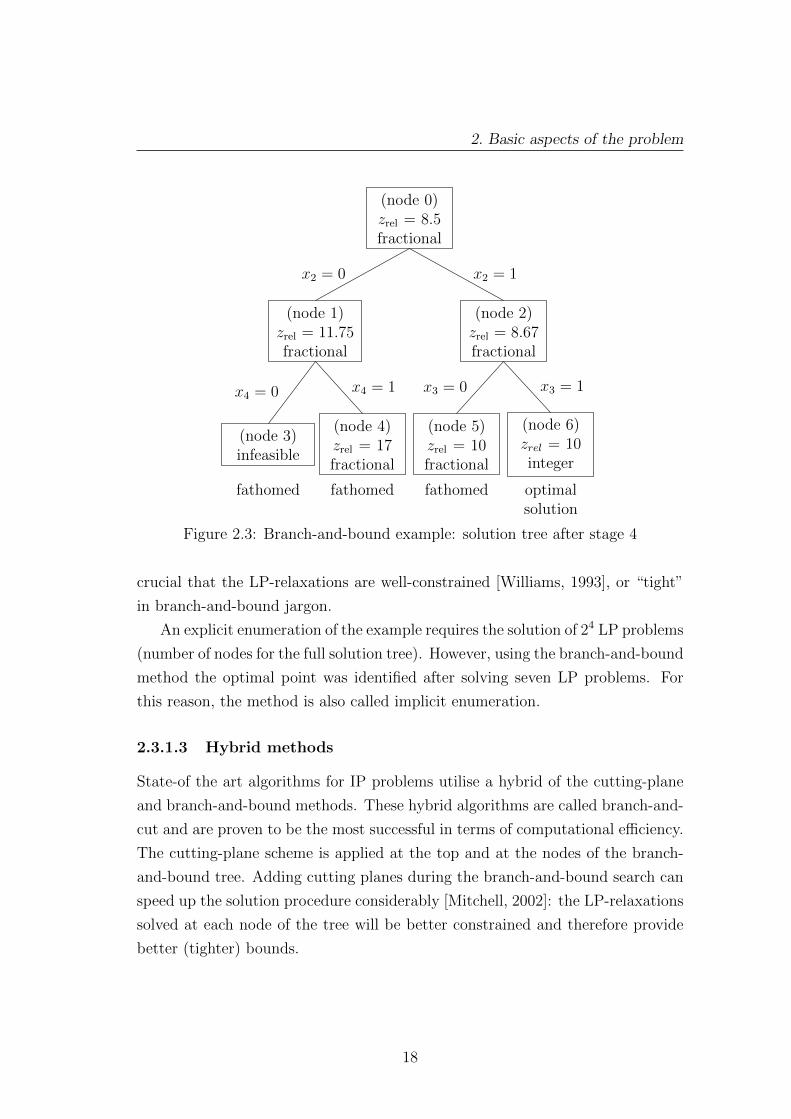
stage 4 is shown in Figure 2.3.
During the solution of this example, only the case where just one variable
took a fractional value at an examined node was encountered. Unfortunately
this is not the case in most real problems. Fortunately though, contemporary
branch-and-bound solvers include heuristic strategies for the selection of the next
branching variable and the selection of the next node to be developed.
One very important feature, which is also the main disadvantage of the branch-
and-bound method, is that it requires the solution of a series of LP-relaxations of
the initial IP problem. The LP-relaxation of a given node provides a lower bound
on the objective value of all subordinate nodes. If the LP-relaxations solved in
the course of the procedure are strong, then fewer nodes will be examined and
the optimal solution is obtained more quickly [Williams, 1990]. Therefore, it is
17
2. Basic aspects of the problem
(node 0)zrel = 8.5fractional
(node 1)zrel = 11.75fractional
(node 3)infeasible
fathomed
x4 = 0
(node 4)zrel = 17fractional
fathomed
x4 = 1
x2 = 0
(node 2)zrel = 8.67fractional
(node 5)zrel = 10fractional
fathomed
x3 = 0
(node 6)zrel = 10integer
optimalsolution
x3 = 1
x2 = 1
Figure 2.3: Branch-and-bound example: solution tree after stage 4
crucial that the LP-relaxations are well-constrained [Williams, 1993], or “tight”
in branch-and-bound jargon.
An explicit enumeration of the example requires the solution of 24 LP problems
(number of nodes for the full solution tree). However, using the branch-and-bound
method the optimal point was identified after solving seven LP problems. For
this reason, the method is also called implicit enumeration.
2.3.1.3 Hybrid methods
State-of the art algorithms for IP problems utilise a hybrid of the cutting-plane
and branch-and-bound methods. These hybrid algorithms are called branch-and-
cut and are proven to be the most successful in terms of computational efficiency.
The cutting-plane scheme is applied at the top and at the nodes of the branch-
and-bound tree. Adding cutting planes during the branch-and-bound search can
speed up the solution procedure considerably [Mitchell, 2002]: the LP-relaxations
solved at each node of the tree will be better constrained and therefore provide
better (tighter) bounds.
18

2. Basic aspects of the problem
2.3.2 Heuristic approaches
In the class of heuristic approaches the undisputed leader is a search technique
developed by Lin and Kernighan [1973]. This tour improvement method is known
as the Lin-Kernighan heuristic and it takes as an input a complete tour and tries
to modify it in order to produce an alternative solution of lower cost. The Lin-
Kernighan heuristic is widely used in conjunction with exact algorithms when
attacking large problems, because it can successfully provide initial tours which
are very close to the optimal solution. In fact, in many cases these initial tours are
proven to be the optimal solutions. A variant of the initial heuristic developed by
Helsgaun [2009] was the first to identify the optimal solution for the largest TSP
instance (85900 cities) solved to date, at the time of writing this dissertation.
Another popular heuristic that is used in computational studies of TSP is sim-
ulated annealing. A 400-city problem was solved by Kirkpatrick et al. [1983] as a
test problem in the paper that introduced the method to the scientific community.
Finally, another well-established heuristic which is widely used in optimisation,
the neural network technique reported by Hopfield and Tank [1985], was also
tested using two travelling salesman problems.
2.4 Travelling Salesman & Computational Com-
plexity Theory
One of the reasons the TSP has been studied so extensively is its relation to
Computational Complexity Theory. This area is common ground for theoretical
Computer Science and Mathematics and is concerned with the inherent difficulty
of computational problems.
Before moving on, let us introduce the notions of polynomial (P) and non-
deterministic polynomial (NP) problems. For the class P of computational prob-
lems there exist algorithms that solve them in polynomial time, whereas, roughly
speaking, for class NP problems no such algorithms are known (yet?). To formally
define the NP class one can say that it consists of all the decision problems (‘yes’
or ‘no’ problems) for which if the answer is positive, a certificate of correctness
can be issued in polynomial time. However, if the answer is negative it is not
19

2. Basic aspects of the problem
known whether the correctness can be checked in polynomial time.
Within the NP class there are the NP-complete problems. Now, an NP prob-
lem is NP-complete if every problem in NP can be reduced to it in polynomial
time. The travelling salesman problem is NP-complete. Proving that an NP-
complete problem can be solved in polynomial time, and therefore, P=NP, will
fetch an award of one million dollars from the Clay Institute of Mathematics. Ev-
ery year, tens of research articles appear in the bibliography claiming the award.
A large percentage of these, base their proof on the discovery of a polynomial-
time running algorithm that solves the TSP. None of them has survived close
examination. The search continues.
2.5 Applications in Chemical Engineering
The TSP is found in a large number of applications across many scientific areas
[Applegate et al., 2007; Gutin and Punnen, 2002]. Those related to Chemical
Engineering are the following:
a) Vehicle routing problem
TSP models are used to calculate optimal itineraries for vehicles that need
to travel between a number of destinations. These can be delivery or pick-
up trucks, laundry vans, school buses or a helicopter connecting the onshore
base of an oil company to the offshore platforms [Cook, 2011]. A taxonomic
review of the literature that refers to the problem can be found in [Eksioglu
et al., 2009].
b) Machine scheduling problem
The scheduling of repeated tasks to be carried out by industrial machines
is a common setting for TSP applications. The different versions of the
problem, along with other aspects, are described by Chen et al. [1998].
c) Genome mapping
An interesting application was reported by [Agarwala et al., 2000]. The
authors utilised TSP models to order chromosome markers while recon-
structing genome maps.
20
2. Basic aspects of the problem
d) X-ray diffractometer aiming in crystallography
A TSP model was used by Bland and Shallcross [1989] to determine se-
quences of X-ray diffraction measurements in crystallography. The travel
costs in this case refer to the time required to reposition the crystals and
to aim the X-ray instrument.
2.6 Conclusions
The Travelling Salesman Problem is a well-studied fundamental problem in the
area of Mathematical Programming. The study of the problem led to the devel-
opment of the disciplines of Integer and Mixed-Integer Programming. It has also
acted as an engine of discovery for some important optimisation methods.
Today the problem holds a central role in Computational Complexity theory.
Nevertheless, its importance is not only theoretical since it is found in numer-
ous practical applications such as vehicle routing, machine scheduling and data
organisation.
The development of a robust solution framework for attacking large travelling
salesman problems remains an open challenge. The two essential components of
a successful framework are: a tight mathematical formulation and an efficient
solution algorithm.
This work is not concerned with the discovery of a novel solution method but
rather with the development of a new modelling approach for the problem. A
number of different mathematical formulations have been proposed for the TSP,
some more well-accepted than others. None of the existing formulations includes
fewer binary degrees of freedom than O(n2). It is the primary aim of the current
work to develop a mathematical formulation which uses fewer than O(n2) binary
variables.
21

Chapter 3
Formulations & computational
studies
A general overview of the Travelling Salesman Problem was presented in Chap-
ter 2. Among the various relevant aspects, a number of different mathematical
programming formulations of the problem were presented. The choice of formu-
lation is critically essential since the TSP belongs to the NP-complete class and
the solution of large problems requires intense computational effort. Thus, it is
crucial to model the problem in a fashion that will ease the computational burden
on the solver.
Towards that end, a new family of formulations is presented in this chapter,
which attempts to reduce the complexity of the problem by reducing the number
of binary degrees of freedom. The computational efficiency of the proposed formu-
lations is then tested and the results of the computational studies are presented
at the end of the chapter.
3.1 Inspiration
The primary aim is to propose a mathematical description for the TSP that
involves fewer binary variables than O(n2). The approach taken is based on work
in Binary Arithmetic, and binary tree structures in particular.
Let us consider the binary tree in Figure 3.1. This is a directed graph where
22

3. Formulations & computational studies
the circles denote the vertices. The root vertex is at level 0 and the leaves of
the tree are the vertices at level 3. The vertices in levels 1 and 2 are called
intermediate vertices. An edge that connects the parent vertex with the left child
is assigned the value 0 and it is assigned the value 1 if it reaches the right child.
Thus, starting from the root, to get to leaf-1 one must follow the edge-sequence
000. Similarly, to reach leaf-6 the only way is to follow the path 101.
root
leaf-1
0
leaf-2
1
0
leaf-3
0
leaf-4
1
1
0
leaf-5
0
leaf-6
1
0
leaf-7
0
leaf-8 Level 3
Level 2
Level 1
Level 0
1
1
1
Figure 3.1: Binary tree with 8 leaves
The binary tree in Figure 3.1 is regular because each intermediate vertex has
two children, and it is full because all its leaves are at the same level. All binary
trees considered in this work are regular and full.
It is apparent that one can store up to 8 objects on the leaves of this tree to
create a binary data structure. The position of a certain object will be described
by a binary string. Can these objects be the cities of a travelling salesman
problem? Yes, the cities can be placed sequentially on the leaves according to
their position in the tour.
Let us explore the scheme where the set of cities is repeatedly partitioned into
left-right orientation from the root to the last level of a binary tree, where the
cities are allocated on the leaves according to their order in the optimal tour.
The proposed formulation is explained in detail in the following section.
23

3. Formulations & computational studies
3.2 Novel formulation
Let us consider the graph G = {V,A}, where V = {1, 2, . . . , n} is the set of ver-
tices (cities) and A = {(i, j) : i, j ∈ V } the set of arcs, on which the Hamiltonian
cycle of minimum cost has to be identified. The length of the arcs is given by
the cost matrix C = {cij : (i, j) ∈ A}. Also, consider the binary tree B = {L, P}where L = {1, 2, . . . , nl} is the set of levels and P = {1, 2, . . . , np} is the set of
leaves (available positions for the allocation of objects). It is a property of binary
trees that
np = 2nl. (3.1)
Now, for the binary tree structure to have enough positions to store the se-
quence of vertices for the optimal cycle, it is required that np ≥ n. If n is an
exact power of 2 then obviously np = n. For the rest of the analysis the general
case where n is not an exact power of 2 is considered. Thus, np > n and the
number of levels is equal to
nl = dlog2(n)e (3.2)
where the ceiling function d.e, applied on a real number, returns the smallest
integer number greater than the real number.
3.2.1 Basics
Here the basics of the proposed formulation are discussed. As already mentioned,
the position of a city on the tree will be coded by a binary string. For that purpose,
let us introduce the binary variables ril, for i ∈ V ; l ∈ L, such that:
ril =
0, if city i is directed left at level l
1, if city i is directed right at level l.(3.3)
At each level l of the tree, every city is allocated a left or right orientation.
Therefore, ndlog2(n)e of these binary variables are needed to describe the position
of all the cities. Decoding the binary string, the position of vertex i on the cycle
is given in decimal base by
24
3. Formulations & computational studies
posi = 1 +nl∑l=1
2nl−lril; i = 1, 2, . . . , n (3.4)
Assuming that the starting point of the tour is always vertex 1:
r1,l = 0; l = 1, 2, . . . , nl (3.5)
and, since there are more leaves than cities the position of the remaining vertices
on the optimal tour is restricted by
1 ≤nl∑l=1
2nl−lril ≤ n− 1; i = 2, 3, . . . , n (3.6)
To determine the partitioning of cities to left-right branching at each level,
the following set of constraints is necessary:
n∑i=1
ril =n∑k=1
tkl; l = 1, 2, . . . , nl (3.7)
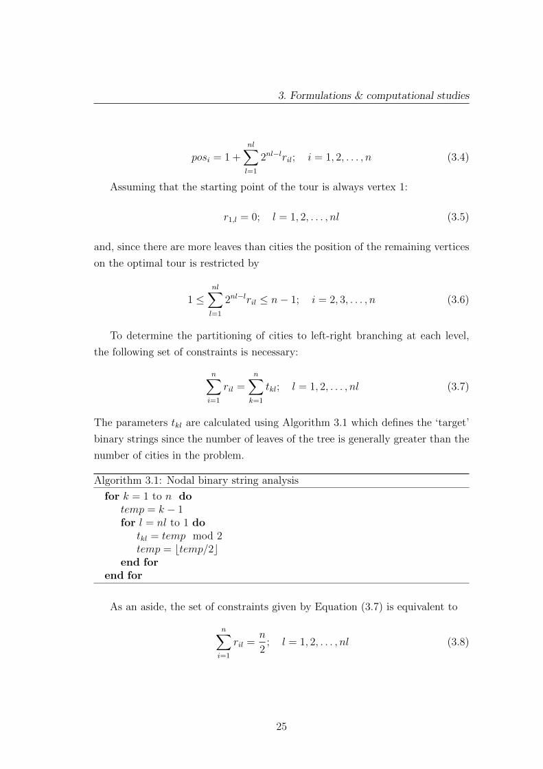
The parameters tkl are calculated using Algorithm 3.1 which defines the ‘target’
binary strings since the number of leaves of the tree is generally greater than the
number of cities in the problem.
Algorithm 3.1: Nodal binary string analysis
for k = 1 to n dotemp = k − 1for l = nl to 1 do
tkl = temp mod 2temp = btemp/2c
end forend for
As an aside, the set of constraints given by Equation (3.7) is equivalent to
n∑i=1
ril =n
2; l = 1, 2, . . . , nl (3.8)
25
3. Formulations & computational studies
when the cardinality of set V is an exact power of 2.
The constraints defined in equation (3.7) are not sufficient to allocate a unique
binary string to a city. For this reason, the variables zik, for i ∈ V ; k ∈ P , are
defined such that:
zik =
0, if city i is not allocated on leaf k
1, if city i is allocated on leaf k.(3.9)
The zik variables are continuous and constrained within [0, 1]. They will be forced
to take the value of 0 or 1 by the binary variables ril, viz.
zik ≤ α(tkl) + β(tkl)ril; i, k = 1, 2, . . . , n; l = 1, 2, ..., nl (3.10)
zik ≥ 1−nl∑l=1
[α(1− tkl) + β(1− tkl)ril]; i, k = 1, 2, . . . , n. (3.11)
where the functions α(v) and β(v) are defined as
α(v) =
1, if v = 0
0, if v = 1(3.12)
β(v) =
−1, if v = 0
1, if v = 1.(3.13)
Finally, it is necessary to use the variables xij, for i, j ∈ V , such that:
xij =
0, if arc (i, j) is not present in the optimal tour
1, if arc (i, j) is present in the optimal tour(3.14)
Unlike existing formulations, the variables xij are continuous and constrained
within [0, 1] in this work. These variables can be forced to take binary values
using the following constraints [Millar and Cyrus, 2000]:
zik + zj,k+1 − 1 ≤ xij; i, j = 1, 2, . . . n; k = 1, 2, . . . , n− 1 (3.15)
26
3. Formulations & computational studies
zi,n + zj,1 − 1 ≤ xij; i, j = 1, 2, . . . , n (3.16)
Constraints (3.15) – (3.16) force the variables xij to take the value of 1 if arc (i, j)
is included in the optimal tour. Otherwise, the lower bound is inactive. Due to
the fact that variables xij appear in the objective function multiplied by positive
coefficients, they will be driven to their lower bound, which is 0, if the constraints
do not enforce a value of 1.
Equations (3.15) – (3.16) define O(n3) constraints. The issue of reducing the
number of these adjacency constraints is examined next.
3.2.2 Adjacency of binary leaves
Consider two cities i and j, for i, j ∈ V , which occupy consecutive positions on the
leaves of a binary data structure. Assuming that city j is positioned immediately
after city i, it is true that:
posj − posi = 1 (3.17)
or using equation (3.4):nl∑l=1
2nl−l(rjl − ril) = 1 (3.18)
A link between equation (3.18) and the xij variables must be established, such
that:
xij = 1, ifnl∑l=1
2nl−l(rjl − ril) = 1 (3.19)
0 ≤ xij ≤ 1, ifnl∑l=1
2nl−l(rjl − ril) 6= 1 (3.20)
It is desired to reduce the order of adjacency constraints (3.15) – (3.16) to less
than O(n3). To achieve this, the constraints must be derived using the three
indices i, j ∈ V and l ∈ L. Recall that the cardinality of set V is n and that of
set L is nl = dlog2(n)e.
Theorem 3.1. Given two cities i and j and the binary representation of their
positions, posi and posj, in the tour by variable sets ril, rjl ∈ {0, 1} with l =
27

3. Formulations & computational studies
1, 2, . . . nl, then if and only if the cities are allocated adjacently such that the
position of city j is greater by 1 from the position of city i, posj = posi + 1, the
following properties hold:
Property A:
There exists exactly one and only one l′ ∈ L such that
ril′ = 0 and rjl′ = 1 (3.21)
Property B:
For 1 ≤ l < l′ (l = 1, 2, . . . , (l′ − 1))
ril = rjl (either both 0, or both 1) (3.22)
Property C:
For l′ < l ≤ nl (l = (l′ + 1), (l′ + 2), . . . , nl)
ril = 1 and rjl = 0 (3.23)
The converse is also true: if the three properties do not hold simultaneously
for a pair of cities i and j, then these are not placed on adjacent leaves of the
binary tree (i.e. the arc (i, j) is not present in the tour).
The following lemma:
Lemma 3.1. If and only if posj = posi then ril = rjl, ∀ l ∈ L.
Lemma 3.2. If and only if posj > posi then there exists an l′ = minl∈L
l for which
ril′ = 0, rjl′ = 1 and ril′′ = rjl′′, with l′′ = 1, 2, . . . , l′ − 1.
and the formulae given below are used to prove the theorem.
k∑i=1
2k−i = 2k − 1 (3.24)
m∑i=1
2k−i = 2k − 2k−m (3.25)
k∑i=m+1
2k−i =k∑i=1
2k−i −m∑i=1
2k−i = 2k−m − 1 (3.26)
28
3. Formulations & computational studies
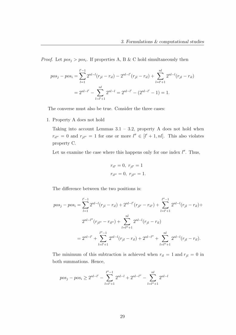
Proof. Let posj > posi. If properties A, B & C hold simultaneously then
posj − posi =l′−1∑l=1
2nl−l(rjl − ril)− 2nl−l′(rjl − ril) +
nl∑l=l′+1
2nl−l(rjl − ril)
= 2nl−l′ −
nl∑l=l′+1
2nl−l = 2nl−l′ − (2nl−l
′ − 1) = 1.
The converse must also be true. Consider the three cases:
1. Property A does not hold
Taking into account Lemmas 3.1 – 3.2, property A does not hold when
ril′′ = 0 and rjl′′ = 1 for one or more l′′ ∈ [l′ + 1, nl]. This also violates
property C.
Let us examine the case where this happens only for one index l′′. Thus,
ril′ = 0, rjl′ = 1
ril′′ = 0, rjl′′ = 1.
The difference between the two positions is:
posj − posi =l′−1∑l=1
2nl−l(rjl − ril) + 2nl−l′(rjl′ − ril′) +
l′′−1∑l=l′+1
2nl−l(rjl − ril)+
2nl−l′′(rjl′′ − ril′′) +
nl∑l=l′′+1
2nl−l(rjl − ril)
= 2nl−l′+
l′′−1∑l=l′+1
2nl−l(rjl − ril) + 2nl−l′′
+nl∑
l=l′′+1
2nl−l(rjl − ril).
The minimum of this subtraction is achieved when ril = 1 and rjl = 0 in
both summations. Hence,
posj − posi ≥ 2nl−l′ −
l′′−1∑l=l′+1
2nl−l + 2nl−l′′ −
nl∑l=l′′+1
2nl−l
29
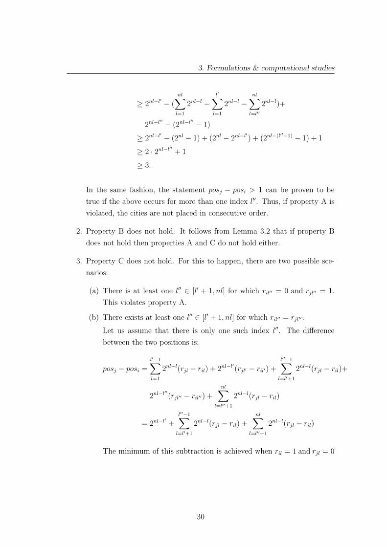
3. Formulations & computational studies
≥ 2nl−l′ − (
nl∑l=1
2nl−l −l′∑l=1
2nl−l −nl∑l=l′′
2nl−l)+
2nl−l′′ − (2nl−l
′′ − 1)
≥ 2nl−l′ − (2nl − 1) + (2nl − 2nl−l
′) + (2nl−(l
′′−1) − 1) + 1
≥ 2 · 2nl−l′′ + 1
≥ 3.
In the same fashion, the statement posj − posi > 1 can be proven to be
true if the above occurs for more than one index l′′. Thus, if property A is
violated, the cities are not placed in consecutive order.
2. Property B does not hold. It follows from Lemma 3.2 that if property B
does not hold then properties A and C do not hold either.
3. Property C does not hold. For this to happen, there are two possible sce-
narios:
(a) There is at least one l′′ ∈ [l′ + 1, nl] for which ril′′ = 0 and rjl′′ = 1.
This violates property A.
(b) There exists at least one l′′ ∈ [l′ + 1, nl] for which ril′′ = rjl′′ .
Let us assume that there is only one such index l′′. The difference
between the two positions is:
posj − posi =l′−1∑l=1
2nl−l(rjl − ril) + 2nl−l′(rjl′ − ril′) +
l′′−1∑l=l′+1
2nl−l(rjl − ril)+
2nl−l′′(rjl′′ − ril′′) +
nl∑l=l′′+1
2nl−l(rjl − ril)
= 2nl−l′+
l′′−1∑l=l′+1
2nl−l(rjl − ril) +nl∑
l=l′′+1
2nl−l(rjl − ril)
The minimum of this subtraction is achieved when ril = 1 and rjl = 0
30

3. Formulations & computational studies
in both summations. Thus,
posj − posi ≥ 2nl−l′ − (2nl − 1) + (2nl − 2nl−l
′)+
(2nl−(l′′−1) − 1)− (2nl−l
′′ − 1)
≥ 2 · 2nl−l′′ − 2nl−l′′
+ 1
≥ 2nl−l′′
+ 1
≥ 2.
Similarly, the statement posj−posi > 1 can be proven to be true if the
above occurs for more than one index l′′. It is obvious that if property
C does not hold then the cities are not allocated on adjacent leaves.
The challenge to face now is how to utilise the results of Theorem 3.1. At
first, it is essential to construct a test in order to check if two cities follow the
same branch of the tree at a given level. For this purpose, the variables eijl, for
i, j ∈ V ; l ∈ L \ {nl} are defined as follows:
eijl =
0, if cities i and j follow opposite branches at level l
1, if cities i and j follow the same branch at level l.(3.27)
The variables eijl are continuous and constrained within [0, 1], but can be
forced to take binary values by using the following set of constraints:
1− (ril + rjl) ≤ eijl; i, j = 1, 2, . . . , n; i 6= j; l = 1, 2, . . . , nl − 1 (3.28)
(ril + rjl)− 1 ≤ eijl; i, j = 1, 2, . . . , n; i 6= j; l = 1, 2, . . . , nl − 1. (3.29)
Constraints (3.28) – (3.29) will force the variable eijl to take the value of 1 if
the binary variables ril and rjl of the two cities i and j, respectively, are equal at
level l. If this is not the case, the variable is left loose within its bounds, and, due
to the fact that it is associated with variables xij (see equations (3.30) – (3.32)),
it will attain the value of its lower bound which is 0. The equality test is not
required for the last level, l = nl.
31

3. Formulations & computational studies
The ultimate goal is to impose lower bounds equal to 1 on the xij variables, if
the properties of Theorem 3.1 are met for each pair of cities i and j. To achieve
that, the following logical checks are employed:
xij ≥ [(1− ri,1) + rj,1 − 2]︸ ︷︷ ︸Property A
+
[nl∑l=2
[ril + (1− rjl)]− 2(nl − 1)
]︸ ︷︷ ︸
Property C
+1;
i, j = 1, 2, . . . , n (3.30)
xij ≥ [(1− ril′) + rjl′ − 2]︸ ︷︷ ︸Property A
+
[l′−1∑l=1
eijl − (l′ − 1)
]︸ ︷︷ ︸
Property B
+
[nl∑
l=l′+1
[ril + (1− rjl)]− 2(nl − (l′ + 1) + 1)
]︸ ︷︷ ︸
Property C
+1;
i, j = 1, 2, . . . , n; l′ = 2, 3, . . . , (nl − 1) (3.31)
xij ≥ [(1− ri,nl) + rj,nl − 2]︸ ︷︷ ︸Property A
+
[nl−1∑l=1
eijl − (nl − 1)
]︸ ︷︷ ︸
Property B
+1;
i, j = 1, 2, . . . , n (3.32)
Constraints (3.30) – (3.32) impose the adjacency properties and are used for
nl ≥ 3. For nl ≤ 2 only the set of constraints given by (3.30) is required.
32

3. Formulations & computational studies
3.2.3 Asymmetric Travelling Salesman model
It is now time to put the various components together and build the asymmetric
TSP model. Two new formulations are suggested. The only difference between
the two are the adjacency constraints. The basic formulation is as follows:
min.n∑i=1
n∑j=1
cijxij (3.33)
s.t.n∑i=1
xij = 1; j = 1, 2, ..., n (3.34)
n∑j=1
xij = 1; i = 1, 2, ..., n (3.35)
n∑i=1
zik = 1; k = 1, 2, ..., n (3.36)
n∑k=1
zik = 1; i = 1, 2, ..., n (3.37)
zik ≤ α(tkl) + β(tkl)ril; l = 1, 2, ..., nl; i, k = 1, 2, ..., n (3.38)
zik ≥ 1−nl∑l=1
[α(1− tkl) + β(1− tkl)ril]; i, k = 1, 2, ..., n (3.39)
xi,1 = zi,n; i = 1, 2, ..., n (3.40)n∑i=1
ril =n∑k=1
tkl; l = 1, 2, ..., nl (3.41)
r1,l = 0; l = 1, 2, . . . , nl (3.42)
1 ≤nl∑l=1
2nl−lril ≤ n− 1; i = 2, 3, ..., n (3.43)
0 ≤ xij ≤ 1; i, j = 1, 2, ..., n (3.44)
0 ≤ zik ≤ 1; i, k = 1, 2, ..., n (3.45)
ril = {0, 1}; i = 1, 2, ..., n; l = 1, 2, ..., nl (3.46)
+ adjacency constraints.
It is required that city i = 1 is the starting and finishing point of the tour.
33
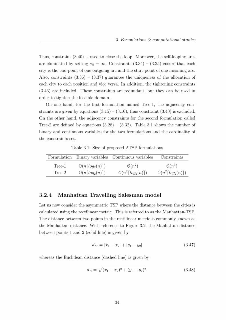
3. Formulations & computational studies
Thus, constraint (3.40) is used to close the loop. Moreover, the self-looping arcs
are eliminated by setting cii = ∞. Constraints (3.34) – (3.35) ensure that each
city is the end-point of one outgoing arc and the start-point of one incoming arc.
Also, constraints (3.36) – (3.37) guarantee the uniqueness of the allocation of
each city to each position and vice versa. In addition, the tightening constraints
(3.43) are included. These constraints are redundant, but they can be used in
order to tighten the feasible domain.
On one hand, for the first formulation named Tree-1, the adjacency con-
straints are given by equations (3.15) – (3.16), thus constraint (3.40) is excluded.
On the other hand, the adjacency constraints for the second formulation called
Tree-2 are defined by equations (3.28) – (3.32). Table 3.1 shows the number of
binary and continuous variables for the two formulations and the cardinality of
the constraints set.
Table 3.1: Size of proposed ATSP formulations
Formulation Binary variables Continuous variables Constraints
Tree-1 O(ndlog2(n)e) O(n2) O(n3)
Tree-2 O(ndlog2(n)e) O(n2dlog2(n)e) O(n2dlog2(n)e)
3.2.4 Manhattan Travelling Salesman model
Let us now consider the asymmetric TSP where the distance between the cities is
calculated using the rectilinear metric. This is referred to as the Manhattan-TSP.
The distance between two points in the rectilinear metric is commonly known as
the Manhattan distance. With reference to Figure 3.2, the Manhattan distance
between points 1 and 2 (solid line) is given by
dM = |x1 − x2|+ |y1 − y2| (3.47)
whereas the Euclidean distance (dashed line) is given by
dE =√
(x1 − x2)2 + (y1 − y2)2. (3.48)
34

3. Formulations & computational studies
y
x
(x1, y1)
(x2, y2)
Figure 3.2: Manhattan distance on a system of Cartesian coordinates
Let us assume that the pair of coordinates (x(0)i , y
(0)i ) for each city is available.
It is then easy to assign coordinates (x, y) to a leaf of the binary tree according
to which city is placed there:
xk =n∑i=1
x(0)i zik; k = 1, 2, . . . , n (3.49)
yk =n∑i=1
y(0)i zik; k = 1, 2, . . . , n. (3.50)
The pair of variables (xk, yk) represents the coordinates of posk. It follows
that the rectilinear distance between two adjacent leaves, k and k + 1, can be
calculated by
dMk= l
(x)k + l
(y)k ; k = 1, 2, . . . , n (3.51)
where
l(x)k ≡ |xk − xk+1|; k = 1, 2, . . . , n− 1 (3.52)
l(y)k ≡ |yk − yk+1|; k = 1, 2, . . . , n− 1. (3.53)
Equations (3.52) – (3.53) can be replaced by the following inequalities:
− l(x)k ≤ xk − xk+1 ≤ l(x)k ; k = 1, 2, . . . , n− 1 (3.54)
− l(y)k ≤ yk − yk+1 ≤ l(y)k ; k = 1, 2, . . . , n− 1. (3.55)
35
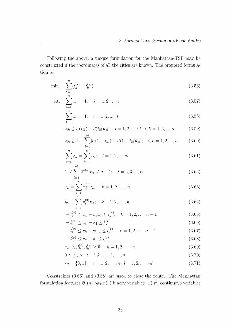
3. Formulations & computational studies
Following the above, a unique formulation for the Manhattan-TSP may be
constructed if the coordinates of all the cities are known. The proposed formula-
tion is:
min.n∑k=1
(l(x)k + l
(y)k ) (3.56)
s.t.n∑i=1
zik = 1; k = 1, 2, ..., n (3.57)
n∑k=1
zik = 1; i = 1, 2, ..., n (3.58)
zik ≤ α(tkl) + β(tkl)ril; l = 1, 2, ..., nl; i, k = 1, 2, ..., n (3.59)
zik ≥ 1−nl∑l=1
[α(1− tkl) + β(1− tkl)ril]; i, k = 1, 2, ..., n (3.60)
n∑i=1
ril =n∑k=1
tkl; l = 1, 2, ..., nl (3.61)
1 ≤nl∑l=1
2nl−lril ≤ n− 1; i = 2, 3, ..., n (3.62)
xk =n∑i=1
x(0)i zik; k = 1, 2, . . . , n (3.63)
yk =n∑i=1
y(0)i zik; k = 1, 2, . . . , n (3.64)
− l(x)k ≤ xk − xk+1 ≤ l(x)k ; k = 1, 2, . . . , n− 1 (3.65)
− l(x)n ≤ xn − x1 ≤ l(x)n (3.66)
− l(y)k ≤ yk − yk+1 ≤ l(y)k ; k = 1, 2, . . . , n− 1 (3.67)
− l(y)n ≤ yn − y1 ≤ l(y)n (3.68)
xk, yk, l(x)k , l
(y)k ≥ 0; k = 1, 2, . . . , n (3.69)
0 ≤ zik ≤ 1; i, k = 1, 2, . . . , n (3.70)
ril = {0, 1}; i = 1, 2, . . . , n; l = 1, 2, . . . , nl (3.71)
Constraints (3.66) and (3.68) are used to close the route. The Manhattan
formulation features O((ndlog2(n)e) binary variables, O(n2) continuous variables
36

3. Formulations & computational studies
and O(n2) constraints.
3.3 Computational studies
The computational performance of the proposed formulations is tested in prac-
tice using small instances of the problem. Furthermore, the efficiency of Tree-1
and Tree-2 formulations is compared against the efficiency of the MTZ formula-
tion [Miller et al., 1960] and the Wong formulation [Wong, 1980], on the basis
of the strength of their LP relaxation. For the computational studies, the prob-
lems are modelled in GAMSTM
[Brooke et al., 1992] and solved using CPLEX R©
10.1.1 [GAMS, 2010] on an ASUSTM
Chassis computer with 2.21 GHz CPU. The
CPLEX R© 10.1.1 solver employs a hybrid of the branch-and-bound and cutting
plane methods, i.e. a branch-and-cut algorithm.
3.3.1 ATSP case studies
The ATSP formulations, Tree-1 and Tree-2, are applied to three small problems:
(i) n = 8; (ii) n = 10 and (iii) n = 12. The asymmetric cost matrices for (i) and
(ii) are produced using a random-number generator. For the third problem the
cost matrix is symmetric and the data are part of the gr17 instance reported by
Reinelt [1991]. The cost matrices of all three problems are given in Appendix A.
Table 3.2 summarises the optimal solutions of the three instances. The number of
nodes refers to the nodes of the solution tree (branch-and-bound tree) examined.
The three problems are also modelled according to Miller et al. [1960]. The
tours reported in Table 3.2 are in agreement with the optimal tours obtained
when solving the MTZ models.
Let us now observe closely the results reported in Table 3.2. The Tree-1
formulation emerges as superior to the Tree-2 formulation in terms of computa-
tional performance. Firstly, the solver successfully produced a solution for the
largest instance tested, n = 12, when using the Tree-1 formulation, whereas for
the Tree-2 case it failed to converge after 1 day of execution time. Moreover,
the solver requires considerably less CPU time to converge for cases n = 8 and
n = 10 when implementing Tree-1. The large gap in performance becomes more
37

3. Formulations & computational studies
Table 3.2: Solution report for ATSP case studies
Formulation Optimal tour Nodes CPU time (s)n = 8
Tree-1 31 3 0.3Tree-2 31 78 1.8
n = 10
Tree-1 70 2 0.4Tree-2 70 602 33.7
n = 12
Tree-1 1799 3200 362.8Tree-2 not solved after 1 day of execution
apparent when comparing the nodes examined during the branch-and-cut scheme
for the two formulations. For n = 10 the solver visits 2 and 602 nodes for Tree-1
and Tree-2, respectively.
This difference arises due to one crucial factor on which the computational
performance of a branch-and-bound algorithm (and correspondingly of a branch-
and-cut algorithm) depends. This is the quality of the LP-relaxations solved
at each node of the solution tree. If these LP-relaxations are strong, then the
solver will examine fewer nodes and will converge to the optimal solution faster
[Williams, 1990].
Clearly, Tree-1 produces stronger LP-relaxations than the Tree-2 formulation.
This is due to the fact that the adjacency constraints (3.30) – (3.32) which are part
of Tree-2 formulation involve a large number of binary variables and continuous
variables in comparison to the adjacency constraints (3.15) – (3.16) which are
included in the Tree-1 formulation. Hence, the former constraints are not as
tight as the latter.
The formulations were also applied to larger instances (12 < n ≤ 20) without
any success. The solver failed to converge after one day of execution. For all
intents and purposes, the running time for small instances like the ones
38
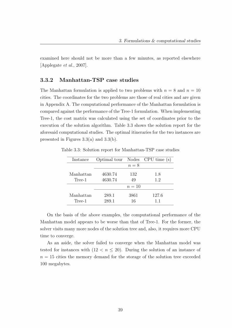
3. Formulations & computational studies
examined here should not be more than a few minutes, as reported elsewhere
[Applegate et al., 2007].
3.3.2 Manhattan-TSP case studies
The Manhattan formulation is applied to two problems with n = 8 and n = 10
cities. The coordinates for the two problems are those of real cities and are given
in Appendix A. The computational performance of the Manhattan formulation is
compared against the performance of the Tree-1 formulation. When implementing
Tree-1, the cost matrix was calculated using the set of coordinates prior to the
execution of the solution algorithm. Table 3.3 shows the solution report for the
aforesaid computational studies. The optimal itineraries for the two instances are
presented in Figures 3.3(a) and 3.3(b).
Table 3.3: Solution report for Manhattan-TSP case studies
Instance Optimal tour Nodes CPU time (s)n = 8
Manhattan 4630.74 132 1.8Tree-1 4630.74 49 1.2
n = 10
Manhattan 289.1 3861 127.6Tree-1 289.1 16 1.1
On the basis of the above examples, the computational performance of the
Manhattan model appears to be worse than that of Tree-1. For the former, the
solver visits many more nodes of the solution tree and, also, it requires more CPU
time to converge.
As an aside, the solver failed to converge when the Manhattan model was
tested for instances with (12 < n ≤ 20). During the solution of an instance of
n = 15 cities the memory demand for the storage of the solution tree exceeded
100 megabytes.
39

3. Formulations & computational studies
−1,000 −750 −500 −250 0
−800
−600
−400
−200
0
200
x-coordinate
y-coordinate
(a) n = 8
−80 −60 −40 −20 0
−40
−20
0
20
x-coordinate
y-coordinate
(b) n = 10
Figure 3.3: Optimal itinerary for Manhattan-TSP case studies
3.3.3 Comparison with existing formulations
The next step in the evaluation of the proposed formulations is to compare their
computational efficiency with those of existing formulations. Let us focus our
interest on the more general ATSP formulations, Tree-1 and Tree-2. The Man-
hattan formulation is not included in the analysis.
It is customary to conduct such a comparison by using the LP-relaxations of
40

3. Formulations & computational studies
the examined formulations. The Tree-1 and Tree-2 formulations are compared
against the MTZ formulation [Miller et al., 1960] and the Wong formulation
[Wong, 1980]. The MTZ formulation is proven to be one of the weakest among
the existing formulations, while the Wong formulation is proven to be one of the
strongest [Oncan et al., 2009]. Three TSP instances found in TSPLIB [Reinelt,
1991] are modelled with respect to the four formulations. The LP relaxation of
all four models is solved and the optimal value of the relaxed objective function,
zrelLP is reported in Table 3.4. The length of the optimal tour of each problem is
also given in Table 3.4.
Table 3.4: Comparison of LP-relaxations: optimal objective function value
Problem zrelLP Optimal tourTree-1 Tree-2 MTZ Wong
gr17 1652 1652 1656 2085 2085fri26 833 833 835.48 937 937dantzig42 533 532 535.65 697 699
It is helpful to recall our discussion in Section 2.2.5: for an efficient formula-
tion, the gap between the optimal objective value of the LP-relaxation, zrelLP, and
the optimal objective value of the original problem should be small. The results
of Table 3.4 confirm that Wong is more efficient than MTZ. It is notable that
for Wong the gap for gr17 and fri26 is 0% and it is only 2.8% for the dantzig42
problem.
As for the proposed formulations, they are ranked in the last two places. The
LP-relaxations of Tree-1 and Tree-2 are shown to be slightly weaker than those
of MTZ for all three instances. Hence, it is safe to place them at the bottom of
the computational efficiency scale of the existing TSP formulations. Tree-1 and
Tree-2 are proved to be poorly constrained.
The values of the LP-relaxations for the two smaller problems are equal for
Tree-1 and Tree-2. Nevertheless, as already seen in Section 3.3.1 the Tree-1
formulation is more computationally efficient than Tree-2.
41

3. Formulations & computational studies
3.4 Conclusions
A novel family of mathematical formulations, originating from work in Binary
Arithmetic and binary tree structures in particular, was developed for the Trav-
elling Salesman Problem. The proposed mathematical description succeeds in
decreasing the binary degrees of freedom for the problem to O(ndlog2(n)e).The three new formulations are named Tree-1, Tree-2 and Manhattan. The
first two apply to the general case of the asymmetric TSP while the third applies
only to the Manhattan-TSP case (the distance between two cities is calculated
on the basis of the rectilinear metric).
The results of test studies suggest that the computational performance of the
new formulations in practice is poor. Computational tests have shown that using
the three formulations to model problems with a number of cities 12 < n ≤ 20
leads to excessive computational effort.
In comparison to Tree-1, the Tree-2 formulation emerges as inferior in terms
of computational performance. When implementing Tree-2 the solver requires
notably more CPU time and it visits far more nodes of the solution tree than
when implementing Tree-1, on the same problems. Also, the results in Section
3.3.2 suggest that it is safe to discard the Manhattan formulation in favour of
Tree-1.
The computational efficiency of the Tree-1 and Tree-2 formulations was com-
pared to that of the Wong formulation [Wong, 1980] and to that of the MTZ for-
mulation [Miller et al., 1960]. The criterion for the comparison was the strength
of the LP-relaxation of the formulations. Both Tree-1 and Tree-2 are shown to
have weaker LP-relaxations than those of Wong and MTZ.
The comparison revealed a major disadvantage: the proposed formulations
are not tightly constrained. In turn, the larger feasible region forces the solver
to span a large portion of the solution tree before yielding the optimal tour.
This is the reason why the formulations can only be applied to very small TSP
instances. To overcome this drawback, additional constraints need to be added
to the formulations. Finding appropriate constraints is not a trivial task but it
is the only recourse for continuing this work.
42
Part II
Scheduling cleaning actions for
heat exchanger networks subject
to fouling

Chapter 4
Background
The first part of this dissertation was dedicated to a central problem of Mathe-
matical Programming, namely the Travelling Salesman Problem. The problem is
considered to be the cornerstone on which the areas of Integer Programming and
Mixed-Integer Programming developed.
Mixed-Integer Programming is used in the second part of this dissertation to
optimise the operation of heat transfer devices. The study of heat transfer and
the operation of heat transfer units is a matter of great industrial importance
and it lies at the core of Chemical Engineering.
This chapter introduces a major industrial problem: fouling of heat transfer
surfaces. The negative impact of fouling is described and the physical/chemical
mechanisms that lead to the formation of fouling layers are outlined briefly. One
of the main fouling mitigation methods for industrial heat transfer units is reg-
ular cleaning. Subsequent sections review the use of decision-making tools in
scheduling cleaning actions for process heat transfer devices subject to fouling.
4.1 Fouling & heat transfer processes
Fouling is a phenomenon prevalent in many industrial heat transfer processes: it
is the deposition of unwanted materials on heat transfer surfaces. The thermal
conductivity of such dirt-deposits is low [Muller-Steinhagen, 2000] and as a result,
fouling has a negative impact on the efficiency of heat transfer.
44

4. Background
To counter-balance the reduction in heat transfer efficiency the operator needs
to provide additional energy to the process by increasing the consumption of com-
bustible fuels or increasing the flow of utility, with associated financial penalties.
Adequate control measures must be taken to mitigate the negative effect of foul-
ing.
To avoid high operating cost the engineer must take precautionary measures
or apply effective mitigation strategies. For the former the heat transfer units
must be over-designed: the engineer takes into account the thermal inefficiencies
caused by fouling by assigning extra heat transfer surface to the device. This
strategy results in additional capital expenditure. Alternatively, the units might
be replaced with expensive non-fouling devices if these are available. The miti-
gation of fouling is achieved through the use of anti-fouling chemicals and/or the
regular on-line or off-line cleaning of the heat exchangers. These lead to high
maintenance costs as well as loss of production during the cleaning period.
The reduction of heat transfer efficiency is not the only result of fouling. The
presence of dirt layers in the channels of a heat transfer device causes a reduction
in the flow area, which leads to an increase in pressure drop. In turn this results
in reduced throughput and loss of production if the pumping power is limited.
To avoid such a scenario more pumping power and additional electricity costs are
required. Also, additional capital expenditure is required since the devices must
be designed to operate at high pressure.
Despite the fact that fouling is a well-established problem in many industries
it has only received detailed attention in the last forty years [Bott and Melo,
1997]. It is a problem that necessitates careful energy and financial management.
4.2 Fouling in heat exchangers
A heat exchanger is a device whose purpose is to transfer thermal energy from
a hot stream to a cold stream. Real-life processes sometimes involve networks of
heat exchangers in serial and/or parallel configurations. A simplified schematic
representation of such a device is shown in Figure 4.1.
Thermal energy is transferred from the hot stream to the cold stream through
the heat exchanger wall. The two streams can flow in co-current mode, as in
45

4. Background
heat transfer wall
cold stream
hot streamheat
Figure 4.1: Simplified representation of a heat exchanger, co-current flow
Figure 4.1, or in other configurations such as counter-current mode and cross-
flow. The amount of heat, Q, recovered from the hot stream for single phase heat
transfer (none of the streams changes phase) is given by
Q = FUA∆Tlm (4.1)
where F is the configuration correction factor, U is the overall heat transfer coef-
ficient, A is the heat transfer area and ∆Tlm is the logarithmic mean temperature
difference between the streams. The overall heat transfer coefficient for a clean
heat exchanger, assuming that the cold and hot side areas of the tubes are the
same, is given by1
U=
1
hhot+
1
hcold+Rw (4.2)
where hhot and hcold are the film heat transfer coefficients of the hot and cold
stream, respectively, and Rw is the thermal resistance of the wall. If, however,
the heat exchanger suffers from fouling, equation (4.2) is modified to include the
thermal resistance of the deposits on both sides of the wall, viz.
1
U=
1
hhot+
1
hcold+Rw +Rf,hot +Rf,cold (4.3)
The thermal fouling resistances Rf,hot and Rf,cold depend on the thickness and
the thermal conductivity of each layer. The overall thermal fouling resistance,
Rf,tot, is given by
Rf,tot = Rf,cold +Rf,hot. (4.4)
An accurate prediction of the fouling resistances is very difficult since reliable
estimation models are usually not available [Ishiyama et al., 2009].
46

4. Background
The main reason for the lack of robust estimation models is the number and
the complexity of different mechanisms responsible for the formation of the foul-
ing layers. Epstein [1983] identified five fouling types based on the key phys-
ical/chemical mechanism causing the formation of the deposit. In each case,
fouling involves five successive steps, any one of which (or combination thereof)
can be rate-determining.
4.2.1 Mechanisms of heat exchanger fouling
The taxonomy of fouling mechanisms into five major classes is accepted by many
researchers in the field. The classes are:
a) Crystallisation fouling
It is a broad class that can be divided into two categories. For the first cate-
gory, the formation of the fouling layer is caused by the growth of salt crys-
tals on the heat transfer surface. The salts (the term salts is also taken to
include non-mineral species such as fats and waxes) are originally dissolved
in the bulk fluid. Normal-solubility salts crystallise when cooled below their
solubility limit, while inverse-solubility salts crystallise when heated above
the limit. Furthermore, supersaturation may arise if an amount of solvent
evaporates or when two streams are mixed. For the second category, for-
mation of the fouling layer is caused by the cooling of a pure liquid or melt
below its freezing point: solid material is then generated at the cold wall.
This is often termed ‘freezing fouling’.
b) Particulate fouling
The process stream contains suspended particles which deposit on the heat
transfer surface. Fine particles may accumulate on surfaces of any orienta-
tion while relatively large particles settle on lower horizontal surfaces due
to gravity.
c) Chemical reaction fouling
Chemical reactions between some components of the stream generate fouling
precursors in the bulk fluid and/or on the heat transfer surface. The surface
material is not one of the reactants but may play a role as a catalyst. This
47

4. Background
type of fouling is common in petroleum refineries, polymer production and
food processing.
d) Corrosion fouling
The heat transfer wall is involved in a chemical reaction, often a corro-
sion mechanism, which generates a fouling layer. If the corrosion products
are removed from the surface fouling does not occur (but the mechanical
integrity is compromised).
e) Biological fouling (biofouling)
The fouling layer is caused by the attachment and growth of micro-organisms
(micro-biofouling) such as bacteria, fungi and algae or macro-organisms
(macro-biofouling) such as mussels and barnacles. In some cases, biofoul-
ing is a serious risk for human health. However, in other cases it can be
useful: it is a key feature of waste water treatment.
Many industrial fouling problems involve a combination of these mechanisms
[Bott, 1988]. Nonetheless, the classification scheme helps decompose this compli-
cated phenomenon into topics that can be studied separately in order to provide
fundamental understanding of the causes of the problem.
To assist the detailed study of each mechanism, Epstein [1983] also proposed
five sequential events that occur during the formation of a fouling layer. The
consecutive steps are:
1. Initiation
The formation of a fouling layer of appreciable thickness on a clean heat
transfer surface often occurs after a delay. A crucial factor for the occurrence
of this delay period is the cleanliness of the heat transfer surface [Epstein,
1988]. The length of the initiation period can vary from few seconds to
several days [Muller-Steinhagen, 2000] depending on the dominant fouling
mechanism. For crystallisation fouling the delay period is associated with
the crystal nucleation process. In cases of biological fouling it is linked with
the conditioning of the surface (colonisation) to favour micro-organism or
macro-organism attachment. Blochl and Muller-Steinhagen [1990] reported
that no initiation occurs for particulate fouling.
48

4. Background
2. Mass transport
At least one of the key components involved in the formation of the fouling
layer is transported from the fluid bulk to the heat transfer surface.
3. Attachment
After a key component is transported to the surface region to form fouling
precursors, these attach to the surface where the fouling layer is formed.
4. Growth retardation
The growth of the fouling layer can be decelerated by several mechanisms
such as increasing surface repulsion due to electrical interactions or decreas-
ing oxygen diffusion rate as the corrosion layer thickens [Epstein, 1983].
Furthermore, the growth of the layer can be hindered by the removal of
parts of the deposit.
5. Ageing
The physical/chemical properties of the fouling layer are altered due to
prolonged exposure to process conditions. Considering the effect of ageing
on fouling layers is an important aspect of this work, as explained below.
4.2.2 Ageing
Ageing has been for many years the least understood and the least investigated
step of fouling formation [Muller-Steinhagen, 2000]. Until recently, it was usually
ignored in modelling attempts and in the analysis of experimental data. It has
attracted the interest of fouling researchers in the last decade and the advances
in the subject have been reviewed by Wilson et al. [2009].
The effect of ageing on the physical/chemical properties of a deposit depends
on the formation mechanism. For most mechanisms the aged deposit is stronger
than the fresh deposit: it has a more cohesive structure. For crystallisation foul-
ing, it has been reported by Brahim et al. [2003] that the initial porous crystalline
matrix becomes denser over time to yield a more stable material. In chemical
reaction fouling, experimental studies conducted by Fan and Watkinson [2006]
showed the structural evolution of fluid-coker deposits from an amorphous con-
glomerate to a coherent graphitic arrangement. On the other hand, in some cases
49
4. Background
of biological fouling, ageing can weaken the initial fouling layer and cause deposit
sloughing [Muller-Steinhagen, 2000].
The structural properties of the fouling layer have a direct impact on the
choice of the appropriate cleaning method. The extent of ageing can determine
the ease with which a fouling layer can be removed: harder (stronger) deposits are
more difficult to remove from surfaces [Pogiatzis et al., 2012]. Also, an increase
in the deposit hardness is usually accompanied by an increase in the thermal
conductivity [Ishiyama et al., 2011a].
Experimental results reported by Er and Lee [2010] (reproduced with permis-
sion by Pogiatzis et al. [2012]), for fouling layer gums formed by auto-oxidation
of linseed oil, show such an increase in thermal conductivity as the initial deposit
ages. The change in thermal conductivity has significant consequences on the dy-
namics of fouling formation and the efficiency of the heat transfer process. The
increase in thermal conductivity with time changes the thermal resistance of the
deposit layer and thereby the temperature distribution across the layer [Pogiatzis
et al., 2012]. The deposit/bulk-fluid interface temperature is recognized to be a
key variable influencing fouling kinetics [Ishiyama et al., 2010a].
4.2.3 Fouling models
The purpose of a fouling model is to assist the designer or the operator of a heat
exchanger to make an assessment of the impact of fouling on the performance of
the unit [Bott, 1995]. In that respect, the two idealised curves shown in Figure 4.2
have been proposed for the prediction of the thermal fouling resistance, Rf , of a
fouling layer over time. These curves are often observed in practice on laboratory
units and on process units [Epstein, 1983].
The parameter tI represents the length of the initiation period. An initiation
period may not always occur or it may be so short as to be negligible. It is usually
ignored in modelling approaches as it is very difficult to predict [Bott, 1995].
Curve A on Figure 4.2 represents situations where the thickness of the de-
posit increases steadily with time. The evolution of the overall thermal fouling
resistance is given by
Rf = at (4.5)
50

4. Background
t
Rf
B
AA: linear rateB: asymptotic
tI
Figure 4.2: Idealised evolution of thermal fouling resistance
where t is time and a the slope of the line.
Curve B exemplifies the asymptotic fouling behaviour. The growth of the
layer is decelerated due to auto-retardation mechanisms [Epstein, 1988] which
cause a gradual decrease of the deposition rate, e.g. ever-reducing wall catalysis
of chemical reaction fouling as the deposit layer builds on the wall or because of
a decrease in the deposit/bulk-fluid interface temperature. Eventually a steady
state is reached when there is no net increase of the thickness of the fouling layer.
At that point the asymptotic value of the thermal fouling resistance, Rf∞ , is
attained. The model proposed by Kern and Seaton [1959] is commonly used to
describe the asymptotic fouling behaviour:
Rf = Rf∞(1− e−t/b) (4.6)
where b is a time constant and t is the time elapsed since fouling started.
The idealised curves shown in Figure 4.2 may fail to describe the fouling
process. In a real-life application, an ideal situation may not be achieved. Parts of
the deposit may be removed due to periodic weakening [Epstein, 1988]. Changes
in crystal structure, chemical degradation, the development of thermal stresses or
51

4. Background
the slow poisoning of micro-organisms can all be causes for weakening the deposit
[Epstein, 1988].
The fouling behaviour and kinetics depend on the following operating param-
eters [Muller-Steinhagen, 2000]: (i) foulant concentration in stream; (ii) surface
temperature; (iii) surface roughness and (iv) flow velocity.
4.2.4 Cleaning fouled heat exchangers
Fouling and cleaning are symbiotic processes, as outlined by Wilson [2005]. The
periodic cleaning of heat exchangers is essential in order to maintain the heat
recovery efficiency within desirable limits. The removal of unwanted deposits is
necessary even for well-designed devices because the operating conditions may
deviate considerably from the design conditions [Muller-Steinhagen, 2000].
Cleaning techniques can be categorized into chemical and mechanical meth-
ods. Chemical cleaning methods attempt to remove the fouling layer using chemi-
cal agents that react with the deposit layer causing it to dissolve, soften or detach
from the heat transfer surface, while mechanical methods remove the deposit by
applying shear forces (other mechanisms exist, e.g. ultrasound). The former have
certain advantages: chemical techniques are relatively quick, less costly, do not
damage the surfaces of the exchanger if the correct agent is chosen and can be
performed in situ. In contrast, mechanical methods are usually more effective in
removing resilient deposits and there is less need to handle dangerous chemicals
or dispose of chemical waste. Mechanical methods usually require direct access
to the fouled surface so the dirty heat exchanger must be disassembled. For the
recirculation of chemical agents there is no need to dismantle the unit if it has
been designed for cleaning-in-place.
An effective mitigation strategy may include a combination of both cleaning
types. The choice of the appropriate method relies on the physical/chemical
characteristics of the fouling layer and the costs associated with each cleaning
technique. For optimal energy and financial management the choice of method
and the timing of cleaning require the use of decision-making tools.
52
4. Background
4.3 Scheduling of cleaning actions
Let us firstly define the term heat exchanger cycle. The operation of a fouled
heat exchanger is succeeded by a maintenance period during which the unit is
cleaned in order to restore the heat recovery efficiency (partially or completely,
depending on the cleaning method). Hence, a heat exchanger cycle is divided in
two periods: the operating period and the cleaning period. The duration of the
cleaning period will depend on the severity of fouling and the type of cleaning.
Let us consider now the maintenance decisions the operator needs to make.
When the process involves only a single heat exchanger, then she needs to decide
the length of the operating period and the cleaning method (if more than one
are available). If, however, the process involves a network of interacting heat
exchangers, then she also needs to choose which units are to be cleaned at a
given time. There might be a restriction in the number of units that can be
cleaned at the same time. Other constraints, such as key target temperatures or
heat transfer duties, may also exist.
The optimal management of the heat transfer process is achieved through
the minimisation of energy losses and maintenance expenditure. It would be
beneficial for the minimisation to be performed over the life cycle of the process
or the time span between process shut-downs. Hence, the existence of a function
that captures the process and maintenance costs is essential. This cost function
is then minimized over the desired time horizon with respect to the decision
variables (cleaning and timing choices) to yield the optimal cleaning schedule.
The effect of fouling on the heat recovery process is quantified by the heat duty
which is related to the thermal fouling resistances. It has not yet been possible to
apportion a single measurement of the overall thermal fouling resistance, Rf,tot,
between the two sides of the wall. In all the studies presented below it is assumed
that fouling occurs only on one side of the heat transfer surface (i.e. that one
process stream is ‘clean’).
Let us assume that the duration of the cleaning period is fixed. The general
53

4. Background
form of the cost function is the following:
z =
∫ tf
0
p(t)dt + m(y) (4.7)
where function p(t) refers to process costs: energy losses due to fouling and lost-
production opportunity due to cleaning, integrated over a time horizon of length
tf . The energy losses due to fouling depend on the timing of cleaning actions
(timing decisions). Function m(y) refers to maintenance costs and y is the array
of cleaning decisions. The cleaning choices correspond to ‘yes’ or ‘no’ decisions
(should we clean exchanger i? / should we clean using a chemical method?)
which can be expressed by binary variables. Therefore, y is an array of binary
values.
The next section reviews the research already conducted on the subject. To
facilitate the discussion, the work on single units is presented first before moving
on to the more general case of heat exchanger networks. In all the approaches
described below two common assumptions are made: (i) there is only one avail-
able cleaning action and (ii) the properties of the fouling layer are uniform and
constant.
4.3.1 Single heat exchanger
Let us consider the case of a single heat exchanger and assume that a cleaning
action which removes the deposits completely is available. Since the cleaning
action restores the effectiveness of the unit, the minimisation needs only to be
performed over one heat exchanger cycle. This optimised cycle is then repeated
over again. The time horizon is given by
tf = top + tcl (4.8)
where top is the length of the operating period (decision variable) and tcl is the
duration of the cleaning period (fixed, only one cleaning action is available).
Hence, the operator needs only to calculate the optimal length of the operating
54

4. Background
period top. The simplified objective function is the following:
z =
∫ top+tcl
0
p(t)dt + c (4.9)
where c is the fixed maintenance cost.
The scheduling problem as described above was first considered by Epstein
[1979] who devised an analytical solution for determining the optimal heat ex-
changer cycle for an evaporator subject to fouling. The optimal duration of the
operating period can be calculated analytically using the first derivative, viz.
dz
dtop= 0 (4.10)
The solution of equation (4.10) provides an analytical result for the calculation of
the optimal operating period length, t∗op. Epstein [1979] assumed that the amount
of deposit at a given time t was proportional to the amount of heat transferred
up to that time.
Casado [1990] extended the analytical approach of Epstein [1979] to a single-
phase counter-current heat exchanger used in a crude oil preheat train. He pre-
sented a detailed economic model and explored the major operating trade-offs
that dictate the existence of a minimum cost. Casado [1990] also presented an
algorithm for computer implementation where the analytical formula was solved
using a trial-and-error procedure.
Zubair et al. [1992] argued that stochastic fouling models must be used to cap-
ture the true performance of a heat exchanger. In that vein, Sheikh et al. [1996]
introduced uncertainty in the linear fouling model and presented a reliability-
based cleaning strategy.
4.3.2 Heat exchanger networks
Scheduling the cleaning actions for heat exchanger networks subject to fouling is
the main topic of this work. The scheduling framework developed for a network
should be readily applicable to the special case of a single unit.
Let us assume that a cleaning action is available, which removes the deposits
55

4. Background
completely. The cost function is given by equation (4.7), where the binary array
y corresponds to unit choices. The cost function is non-differentiable and, hence,
an analytical formulae cannot be derived. The optimal cleaning schedule for the
network can only be obtained using numerical optimisation tools.
Let us now examine the scheduling problem with respect to mathematical
programming theory. The presence of the binary array y means the problem is
described by a Mixed-Integer Programming (MIP) formulation. It is desirable for
the MIP formulation to be convex as the identification of the global solution is
guaranteed for convex formulations. Nevertheless, identifying the global solution
for convex MIP problems can be very expensive computationally. For non-convex
formulations, it is not always possible to issue a certificate of global optimality.
4.3.2.1 Non-convex formulations
The scheduling problem is described by a non-convex Mixed-Integer Nonlinear
Programming (MINLP) formulation, primarily due to equation (4.1). The ther-
mal fouling resistance may also be nonlinearly related to some other variable
depending on the complexity of the fouling model. Smaıli et al. [1999] were the
first to formulate the problem as a non-convex MINLP while trying to optimise
the performance of a network of 11 units, representing a preheat train in a sugar
refinery, over a horizon of 120 days. Subsequently, Smaıli et al. [2001] presented
an improved MINLP formulation which was used to obtain cleaning schedules for
two oil refinery networks over a time-horizon of three years. Smaıli et al. [2001]
used two different models to estimate the thermal fouling resistance: the linear
and the asymptotic.
To calculate the process costs, p(t), the operation of the network must be
simulated in time. In that respect, Smaıli et al. [2001] discretised time: the
horizon was divided into periods of fixed and equal length. Each period was
further divided into an operating sub-period and a cleaning sub-period (both
of fixed length). If a cleaning action was selected, it was performed during the
cleaning sub-period while the other units continued to operate normally. In this
case, the binary array y corresponds to unit and timing decisions (e.g. the value
of yij denotes if unit i is cleaned at period j or not).
56

4. Background
The length of the operating sub-period can also be allowed to vary, e.g.
[Markowski and Urbaniec, 2005]. It will then be a decision variable for the MINLP
problem. Such an MINLP formulation is highly non-convex [Markowski and Ur-
baniec, 2005] and it may be impossible to solve (depending on how many variables
and constraints are involved).
Smaıli et al. [1999], Smaıli et al. [2001] and Markowski and Urbaniec [2005]
attempted to optimise the MINLP formulations they constructed using rigor-
ous optimisation methods developed for convex problems. Applying such exact
algorithms to non-convex programming problems is a heuristic approach. An
alternative path is to use heuristic solution techniques which usually require less
computational effort than exact algorithms to yield a sub-optimal solution.
In that fashion, Smaıli et al. [2001] proposed a simple greedy solution proce-
dure to act as a competitor to the rigorous optimisation algorithm. The greedy
solver considers cleaning actions in the current period and the effect of those
actions over a ‘sliding’ horizon (selected number of periods in the future). The
difference between the costs when the exchanger is cleaned and when no cleaning
occurs is calculated for each unit. The heat exchanger that exhibits the largest
return, given that it is greater than a predetermined threshold, is chosen to be
cleaned. The greedy solver was found to produce worse solutions than the exact
algorithm.
Calculating the return for each heat exchanger at each period requires the
simulation of the operation of the network several times. Ishiyama et al. [2009]
proposed the use of a ‘merit list’ to identify favourable candidates to be compared
in a full simulation in order to reduce the computational effort. Furthermore,
they included model-based representations of the fouling kinetics and considered
the impact of fouling on the hydraulic performance of crude oil preheat train
networks.
Ishiyama et al. [2010b] extended the above scheduling approach to deal with
the problem of controlling the inlet temperature of a de-salter. A de-salter is
an essential device on an oil refinery: it removes inorganic substances from the
crude oil to prevent damages such as the deactivation of catalysts used in the
process. The operation of the de-salter depends on the upstream temperature,
which varies due to deposits’ build-up in the exchangers. The inlet temperature
57
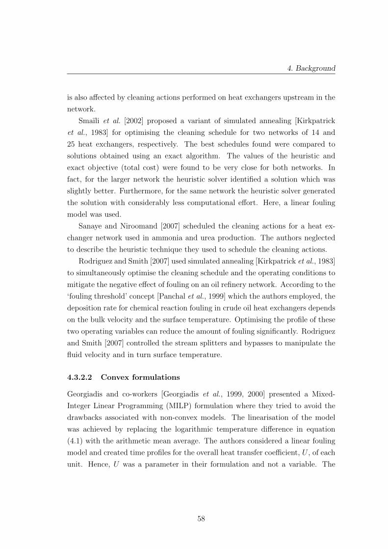
4. Background
is also affected by cleaning actions performed on heat exchangers upstream in the
network.
Smaıli et al. [2002] proposed a variant of simulated annealing [Kirkpatrick
et al., 1983] for optimising the cleaning schedule for two networks of 14 and
25 heat exchangers, respectively. The best schedules found were compared to
solutions obtained using an exact algorithm. The values of the heuristic and
exact objective (total cost) were found to be very close for both networks. In
fact, for the larger network the heuristic solver identified a solution which was
slightly better. Furthermore, for the same network the heuristic solver generated
the solution with considerably less computational effort. Here, a linear fouling
model was used.
Sanaye and Niroomand [2007] scheduled the cleaning actions for a heat ex-
changer network used in ammonia and urea production. The authors neglected
to describe the heuristic technique they used to schedule the cleaning actions.
Rodriguez and Smith [2007] used simulated annealing [Kirkpatrick et al., 1983]
to simultaneously optimise the cleaning schedule and the operating conditions to
mitigate the negative effect of fouling on an oil refinery network. According to the
‘fouling threshold’ concept [Panchal et al., 1999] which the authors employed, the
deposition rate for chemical reaction fouling in crude oil heat exchangers depends
on the bulk velocity and the surface temperature. Optimising the profile of these
two operating variables can reduce the amount of fouling significantly. Rodriguez
and Smith [2007] controlled the stream splitters and bypasses to manipulate the
fluid velocity and in turn surface temperature.
4.3.2.2 Convex formulations
Georgiadis and co-workers [Georgiadis et al., 1999, 2000] presented a Mixed-
Integer Linear Programming (MILP) formulation where they tried to avoid the
drawbacks associated with non-convex models. The linearisation of the model
was achieved by replacing the logarithmic temperature difference in equation
(4.1) with the arithmetic mean average. The authors considered a linear fouling
model and created time profiles for the overall heat transfer coefficient, U , of each
unit. Hence, U was a parameter in their formulation and not a variable. The
58

4. Background
MILP formulation was used to schedule the cleaning actions for heat exchanger
networks used for the sterilisation of milk.
Following the approach of Georgiadis et al. [2000], Lavaja and Bagajewicz
[2004] used the time profiles of the overall heat transfer coefficient, U , to devise an
MILP formulation for the problem without introducing any linear approximation
to the nonlinear heat duty equation (4.1). They considered only the linear fouling
model but stated that the approach is easily extended to the case of asymptotic
fouling. The MILP formulation of Lavaja and Bagajewicz [2004] is examined
more carefully in Chapter 5.
4.4 Motivating study
The scheduling studies reviewed in the previous section considered the physi-
cal/chemical properties of the fouling deposits to remain constant throughout
the operation of a heat exchanger. However, it is probable that the properties
of a foulant will change over time due to the prolonged exposure to process con-
ditions. The ageing of the deposit might result in structural changes as well as
changes in thermal conductivity (see Section 4.2.2). Furthermore, in all previ-
ous studies it was assumed that an available cleaning action restores the unit to
its original performance (completely clean state): the selection between different
cleaning methods was not considered.
Ishiyama et al. [2011a] were the first to introduce the economic competition
between two cleaning methods in a scheduling study. In their novel work, fouling
was defined as the combination of deposition and ageing phenomena and the
selection of the appropriate cleaning method relied on the extent of ageing.
The study focused on an isolated evaporator operating under chemical reac-
tion fouling and included the selection between solvent (chemical) cleaning and
mechanical cleaning. There, it was assumed that ageing converts the initial de-
posit into a harder and more conductive form which is not susceptible to removal
by the chemical cleaning method. A simple heuristic search that favoured the
selection of the method with the lowest daily average cost was used to obtain
mixed cleaning schedules.
In summary, Ishiyama et al. [2011b] investigated the benefits of applying
59

4. Background
mixed cleaning strategies rather than cleaning using only one technique. In ad-
dition, they incorporated, for the first time, the effects of ageing on fouling and
cleaning dynamics in a scheduling study. This work aims to extend their approach
to heat exchanger networks.
4.5 Conclusions
Fouling is identified as a major problem in industrial process heat transfer. It is
responsible for large energy and throughput losses resulting in financial penalties.
Fouling is a complicated phenomenon. Epstein [1983] presented a classifica-
tion scheme that describes the formation of a fouling layer as the result of five
different deposition mechanisms, acting separately or in synergy. Furthermore,
he suggested that the formation of a fouling layer can be decomposed to five
sequential steps: initiation, mass transport, attachment, growth retardation and
ageing.
One of the main mitigation strategies for industrial heat transfer devices sub-
ject to fouling is regular cleaning. The cleaning of fouled units involves the
formulation and optimisation of a scheduling problem. The goal is to minimise
the maintenance costs and the process losses, which include energy losses due to
fouling and lost-production opportunity during the cleaning intervals.
A number of scheduling studies have been presented for isolated heat ex-
changers or heat exchanger networks subject to fouling. Various mathematical
formulations have been proposed for the scheduling problem and different op-
timisation tools have been used to obtain cleaning programs. All studies that
preceded the work of Ishiyama et al. [2011b] considered the physical/chemical
properties of the fouling deposits to remain constant in time, and that a cleaning
action restores the heat exchanger to its original clean condition. None of these
studies has taken under consideration the effect of ageing on fouling and cleaning
dynamics or the competition between cleaning methods.
Motivated by the work of Ishiyama et al. [2011a], the current work focuses on
developing optimal mixed cleaning campaigns for heat exchanger networks. The
situation where more than one method is available, giving different degrees of
cleaning, is investigated. Two scenarios are studied: (i) heat exchanger networks
60

4. Background
subject to chemical reaction fouling and (ii) heat exchanger networks subject to
biofouling.
For the first scenario, the scheduling approach proposed by Ishiyama et al.
[2011b] for a single evaporator is extended to accommodate heat exchanger net-
works. Here, the extent of ageing has a direct impact on the selection between two
competing cleaning methods: the more conductive aged material can be removed
only by a mechanical action, while chemical actions are capable of removing only
the ‘softer’ fresh deposit.
The second scenario refers to the novel study of scheduling the cleaning ac-
tions for heat exchanger networks subject to biological fouling. The scheduling
problem features the selection between three cleaning methods: (i) a simple wa-
ter flush, which removes most of the biofilm but leaves the surface colonised and
ready to restart growth when process operation resumes; (ii) chemical cleaning,
which removes all biofilm and imposes a short initiation period and (iii) chemical
cleaning followed by disinfection, which resets the unit to its original clean state.
The scheduling formulation for the chemical reaction fouling scenario is de-
scribed in Chapter 5 along with the proposed solution methods. Chapter 7 in-
troduces two mathematical programming formulations for the biological fouling
scenario.
61

Chapter 5
Chemical reaction fouling:
formulation & solution methods
The previous chapter introduced the negative effect of fouling on industrial heat
transfer. It also established the importance of using optimisation tools to schedule
the cleaning actions for heat exchanger networks subject to fouling. Two scenar-
ios were identified, based on the fouling mechanism and the selection between
available cleaning techniques.
The current chapter describes the scheduling problem for the chemical reaction
fouling scenario. Firstly, after a brief heat transfer analysis, the two-layer fouling
model used to calculate the thermal resistance of the deposits is introduced. The
main part of the chapter is dedicated to the description of the mathematical
programming formulation. This includes the time representation, the constraints
and the objective function of the scheduling problem.
The last section discusses the suitability of an existing numerical solver for
the type of mathematical programming problem proposed. Subsequently, two
alternative solution procedures are suggested as more suitable. The first applies
Generalised Benders Decomposition while the second is inspired by Model Pre-
dictive Control.
62

5. Chemical reaction fouling: formulation & solution methods
5.1 Heat transfer analysis
The scheduling model is developed for networks of single-pass shell-and-tube heat
exchangers. Figure 5.1 shows the schematic representation of such a unit, operat-
ing in counter-current mode. The model can be easily modified to accommodate
different types of heat exchangers and other flow configurations.
tubeinlet
shelloutlet
tubeoutlet
shellinlet
Figure 5.1: Schematic representation of a shell-and-tube heat exchanger (counter-current mode)
For a unit in operation, the following assumptions are made:
a) it is in counter-current mode; consequently the configuration correction
factor, F , is equal to one;
b) the cold stream flows on the tube side and the hot stream on the shell side;
c) neither of the streams changes phase within the unit;
d) the specific heat capacities of the streams are constant;
e) the mass flow rate of both streams remains constant.
The rate of heat transfer of a shell-and-tube heat exchanger operating in
counter-current mode is given by equation (4.1). The logarithmic mean temper-
ature difference for the unit is calculated as follows:
∆Tlm =(Th,o − Tc,in)− (Th,in − Tc,o)
ln[(Th,o − Tc,in)/(Th,in − Tc,o)](5.1)
63

5. Chemical reaction fouling: formulation & solution methods
where T is the temperature with subscripts c, h, in and o referring to cold, hot,
inlet and outlet stream, respectively. Equation (4.1) can then be rewritten as
follows:
Q = UA(Th,o − Tc,in)− (Th,in − Tc,o)
ln[(Th,o − Tc,in)/(Th,in − Tc,o)]. (5.2)
The energy balance for the unit is
Q = mcCp,c(Tc,o − Tc,in) = mhCp,h(Th,in − Th,o) (5.3)
where m represents the mass flow rate and Cp is the specific heat capacity. Com-
bining equations (5.2) and (5.3) yields
Th,o = Tc,in + (Th,in − Tc,o) exp(UAC) (5.4)
with C given by
C =mhCp,h − mcCp,cmhCp,hmcCp,c
. (5.5)
The negative effect of fouling on the heat transfer process is quantified through
equation (5.4). Accumulation of deposits will cause a decrease of the overall heat
transfer coefficient U .
5.2 Fouling analysis
The key requirement is to be able to track the effect of fouling on heat recov-
ery and on cleaning effectiveness. A two-layer model is used to estimate the
thermal fouling resistance. The two layers are: the fresh deposit and the aged
material. The fresh deposit is susceptible to removal by both mechanical action
and chemical action. On the other hand, the more resilient aged material can
only be removed by mechanical cleaning. Hence, a mechanical action restores the
efficiency of a unit fully, while a chemical action does not.
The concept of a two-layer model was described by Atkins [1962] while con-
sidering fouling in crude oil preheat trains. Atkins [1962] proposed that there are
two discrete events taking place during the formation of fouling. At first, a layer
of soft material is deposited, which is then converted to a harder layer due to
64

5. Chemical reaction fouling: formulation & solution methods
ageing. The transition from soft to hard layer was modelled as a phase change so
that the growth of the aged layer followed a moving front.
Crittenden and Kolaczkowski [1979] extended the concept proposed by Atkins
[1962] and presented the first quantitative two-layer model. The conversion of
fresh deposit to hard material was assumed to be first order in foulant concen-
tration and to follow an Arrhenius-type temperature dependency.
The two-layer concept was used by Ishiyama et al. [2011a] for the investigation
of the thermal and hydraulic aspects of ageing on heat exchangers. The authors
used the terms ‘gel’ and ‘coke’, borrowed from the crude oil fouling literature, to
describe the fresh deposit and aged material, respectively. The same terminology
is used in the current study. Ishiyama et al. [2011a] compared the evolution of
the thermal fouling resistance over time for different ageing kinetic schemes under
constant heat flux operation and under constant wall temperature operation.
In their scheduling approach Ishiyama et al. [2011b] used the simplest possible
form of the two-layer model, where the rates of gel formation and coke formation
are constant. The same model is used here. Before introducing the model, the
following assumptions are made:
a) deposition occurs only on the tube side of the heat transfer wall (the shell
side is free of fouling). It is recognised that in practice both streams may
give rise to fouling but this scenario is not considered in this work.
b) The formation of foulant is entirely due to chemical reactions between the
components of the stream.
c) The duration of the initiation period is negligible.
d) The gel and coke formation rates are uniform at all locations along the
tubes of the heat exchanger.
e) The density of the two layers remains constant.
f) The coke layer is more thermally conductive than the gel layer.
The growth of the gel layer is expressed as the competition between gel for-
65

5. Chemical reaction fouling: formulation & solution methods
mation and coke formation, viz.
dδgdt
= kg − kc (5.6)
where δg the thickness of the gel layer, kg the gel formation rate and kc the coke
formation rate. The growth of the coke layer is given by
dδcdt
=
kc, if δg > 0
0, if δg = 0(5.7)
where δc is the thickness of the aged deposit. Figure 5.2 shows the growth of the
two layers as moving fronts in time.
heat transfer wall heat transfer wall
δc
δgcoke
gel
time
Figure 5.2: Growth of gel and coke layers in time
Recall that fouling occurs only on the cold side of the shell-and-tube heat
exchanger. Treating the two layers as a pair of thin insulating slabs, the thermal
fouling resistance, Rf , for the unit is as follows:
Rf =δgλg
+δcλc
(5.8)
where λg and λc are the thermal conductivities of the gel layer and coke layer,
respectively. The aged material is more conductive than the fresh deposit: λg <
λc.
Equation (4.3) can be rewritten as follows:
1
U=
1
U0
+Rf =1
U0
+δgλg
+δcλc
(5.9)
where U0 is the overall heat transfer coefficient for a foulant-free heat exchanger
66

5. Chemical reaction fouling: formulation & solution methods
given by1
U0
=1
hhot+
1
hcold+Rw. (5.10)
The growth of the two layers in the tubes of a heat exchanger will cause a
reduction in flow area and this will lead to an increase in pressure drop. If fouling
is severe, this will affect the pumping capacity as it is assumed that the mass flow
rate of the cold stream is maintained constant. The effects of fouling on pressure
drop are not considered in this work.
5.3 Time representation
The optimisation of the cleaning schedule for a heat exchanger network operating
under fouling requires the calculation of the process costs p(t) as noted in Section
4.3.2.1. To calculate the process costs the operation of the network must be
simulated.
The system to be simulated is dynamic due to equations (5.6) – (5.7). Hence,
an integration scheme is required to obtain numerical solutions for the differential
equations and to integrate the process costs p(t) over the examined time horizon.
For that purpose, orthogonal collocation is chosen for its precision and its need
for relatively few discretisation points [Biegler, 2010]. Among the different collo-
cation schemes, Radau collocation is chosen due to the fact that it allows large
time steps for systems with slow time scales [Biegler, 2010].
Let us assume that the cleaning actions are scheduled over a time horizon tf .
To achieve discretisation, the time horizon is divided into a finite number of
periods, np, of fixed length. In turn, each period is divided into three elements of
fixed length each of which contains four collocation nodes. Figure 5.3 shows the
graphic representation of a discrete period.
The first element considered to be the operating sub-period has length top,
which is assumed to be constant in this work. Elements 2 and 3 correspond
to the cleaning sub-periods and their added length corresponds to the duration
of a mechanical cleaning, tme. The length of the third element corresponds to
the duration of a chemical cleaning, tch. The duration of both cleaning actions
is assumed to be constant and independent of the thickness of the layers. The
67

5. Chemical reaction fouling: formulation & solution methods
element 1 element 2 element 3
operationtop
mechanicalcleaningtme
chemicalcleaningtch
Figure 5.3: Schematic representation of a discrete time period (filled circles: col-location nodes)
length of the time horizon is calculated as
tf = np(top + tme). (5.11)
where np is the number of periods. If a mechanical action is to be performed in
a given period, it will start at the beginning of element 2 and finish at the end of
element 3 (end of period). Similarly, a chemical action will be performed during
element 3. If no cleaning action is decided for a period the unit is considered to
operate without any disruptions through elements 2 and 3.
The solution of the differential equations and the integral in each element
are approximated by 3rd order polynomials. To facilitate discussion, the use of
orthogonal collocation is briefly reviewed.
Let us consider the following ordinary differential equation:
dv
dt= f(v(t), t), v(0) = v0. (5.12)
The time profile of variable v(t) is to be approximated using a 3rd order Lagrange
interpolation polynomial over the finite element shown in Figure 5.4, where τ0,
τ1, τ2 and τ3 are the collocation nodes and h the length of the element. Using
Radau collocation: τ0 = 0, τ1 = 0.155051, τ2 = 0.644949 and τ3 = 1. The first
collocation node at τ0 corresponds to the initial condition
v(t0) = v0. (5.13)
68

5. Chemical reaction fouling: formulation & solution methods
v0 v1 v2 v3
hτ0 hτ1 hτ2 hτ3t0 t1 t2 t3
h
Figure 5.4: Orthogonal (Radau) collocation over finite element
Also,
v(ti) = vi; i = 1, 2, 3 (5.14)
where
ti = t0 + hτi; i = 1, 2, 3. (5.15)
In Radau collocation the final element times are used as nodes, thus avoiding
the need for extrapolation. The variables vi for i = 1, 2, 3 are obtained by solving
the following system of algebraic equations:
3∑i=0
vidqi(τk)
dτ= hf(vk, tk); k = 1, 2, 3 (5.16)
where
qi(τ) =∏j=0j 6=i
τ − τjτi − τj
. (5.17)
anddqi(τ)
dτ=
3∑j=0
3∏m=0m 6=i,j
(τ − τm)/3∏
n=0n6=i
(τi − τn). (5.18)
The use of orthogonal collocation for the purposes of this work is described in
the section that follows. The next section introduces the proposed mathematical
programming formulation for the scheduling problem.
5.4 Mathematical programming formulation
The task is to identify the optimal cleaning schedule for a heat exchanger network
subject to chemical reaction fouling. Let us assume that U ′ = {1, 2, . . . , nu} is
69

5. Chemical reaction fouling: formulation & solution methods
the set of units, P = {1, 2, . . . , np} the set of discrete periods and M = {ch :
chemical, me : mechanical} the set of available cleaning modes.
The binary variables yijm, for i ∈ U ′; j ∈ P ; m ∈M , are such that:
yijm =
1, if cleaning mode m is chosen for unit i at period j
0, if cleaning mode m is not chosen for unit i at period j(5.19)
The following set of constraints:∑m∈M
yijm ≤ 1; i = 1, 2, . . . , nu; j = 1, 2, . . . , np (5.20)
is necessary to ensure that at most one cleaning mode is selected for unit i at
period j.
5.4.1 Constraints
The scheduling formulation includes two groups of constraints. The first group
corresponds to the simulation of the network’s operation, while the second group
refers to process constraints.
5.4.1.1 Simulation constraints
All simulation constraints are equality constraints. The efficiency of the heat
exchanger network decays in time due to the growth of gel layer and coke layer
on the heat transfer surface of the units. The thickness of gel and coke layers and
the temperature profile of each unit are calculated at the collocation nodes of the
time elements.
Let us define the set of time elements E = {1, 2, 3} and the set of collocation
nodes O = {0, 1, 2, 3}. Moreover, let us assume that:
a) the heat exchangers are completely clean (fouling-free) at the beginning of
the examined time horizon;
b) the gel formation rate is always greater than the ageing rate: kg > kc.
70
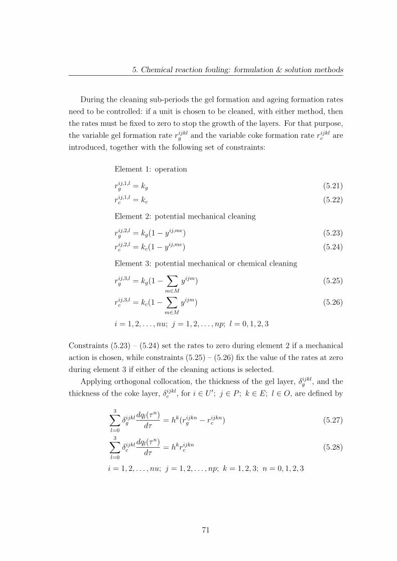
5. Chemical reaction fouling: formulation & solution methods
During the cleaning sub-periods the gel formation and ageing formation rates
need to be controlled: if a unit is chosen to be cleaned, with either method, then
the rates must be fixed to zero to stop the growth of the layers. For that purpose,
the variable gel formation rate rijklg and the variable coke formation rate rijklc are
introduced, together with the following set of constraints:
Element 1: operation
rij,1,lg = kg (5.21)
rij,1,lc = kc (5.22)
Element 2: potential mechanical cleaning
rij,2,lg = kg(1− yij,me) (5.23)
rij,2,lc = kc(1− yij,me) (5.24)
Element 3: potential mechanical or chemical cleaning
rij,3,lg = kg(1−∑m∈M
yijm) (5.25)
rij,3,lc = kc(1−∑m∈M
yijm) (5.26)
i = 1, 2, . . . , nu; j = 1, 2, . . . , np; l = 0, 1, 2, 3
Constraints (5.23) – (5.24) set the rates to zero during element 2 if a mechanical
action is chosen, while constraints (5.25) – (5.26) fix the value of the rates at zero
during element 3 if either of the cleaning actions is selected.
Applying orthogonal collocation, the thickness of the gel layer, δijklg , and the
thickness of the coke layer, δijklc , for i ∈ U ′; j ∈ P ; k ∈ E; l ∈ O, are defined by
3∑l=0
δijklg
dql(τn)
dτ= hk(rijkng − rijknc ) (5.27)
3∑l=0
δijklc
dql(τn)
dτ= hkrijknc (5.28)
i = 1, 2, . . . , nu; j = 1, 2, . . . , np; k = 1, 2, 3; n = 0, 1, 2, 3
71

5. Chemical reaction fouling: formulation & solution methods
where hn is the length of element n: h1 = top, h2 = tme− tch and h3 = tch. Recall,
the termdql(τ
n)
dτ, for n = 0, 1, 2, 3, is a constant.
The units are free of fouling at the beginning of the time horizon. The initial
condition for the thickness of each layer for the first element of the first period is:
δi,1,1,0g = 0 (5.29)
δi,1,1,0c = 0 (5.30)
i = 1, 2, . . . , nu.
The initial conditions for the first element of every other period must set the
thickness of the layers to be equal to that at the end of the previous period.
Hence:
δij,1,0g = δi,j−1,3,3g (5.31)
δij,1,0c = δi,j−1,3,3c (5.32)
i = 1, 2, . . . , nu; j = 2, 3, . . . , np.
For the second element of the periods, the initial conditions depend on whether
a mechanical action is performed or not, as follows:
δij,2,0g = δij,1,3g (1− yij,me) (5.33)
δij,2,0c = δij,1,3c (1− yij,me) (5.34)
i = 1, 2, . . . , nu; j = 1, 2, . . . , np.
If a mechanical action is performed, then the thickness of both layers, δg and δc,
is set to zero by constraints (5.33) – (5.34). Otherwise, it is forced to be equal to
the thickness of the layers at the end of element 1.
Finally, for the third element the initial conditions are crafted to account for
a mechanical or chemical action, viz.
δij,3,0g = δij,2,3g (1−∑m∈M
yijm) (5.35)
δij,3,0c = δij,2,3c (1− yij,me) (5.36)
72
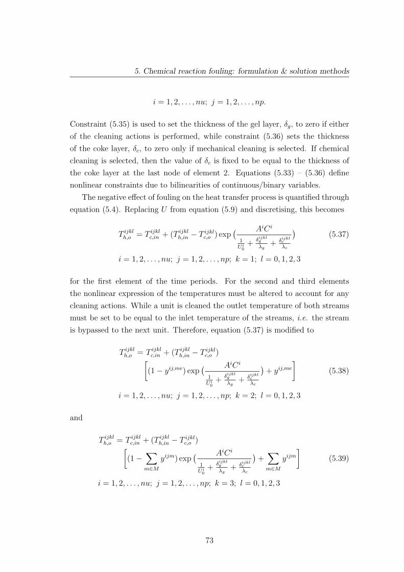
5. Chemical reaction fouling: formulation & solution methods
i = 1, 2, . . . , nu; j = 1, 2, . . . , np.
Constraint (5.35) is used to set the thickness of the gel layer, δg, to zero if either
of the cleaning actions is performed, while constraint (5.36) sets the thickness
of the coke layer, δc, to zero only if mechanical cleaning is selected. If chemical
cleaning is selected, then the value of δc is fixed to be equal to the thickness of
the coke layer at the last node of element 2. Equations (5.33) – (5.36) define
nonlinear constraints due to bilinearities of continuous/binary variables.
The negative effect of fouling on the heat transfer process is quantified through
equation (5.4). Replacing U from equation (5.9) and discretising, this becomes
T ijklh,o = T ijklc,in + (T ijklh,in − Tijklc,o ) exp
( AiCi
1U i0
+δijklg
λg+ δijklc
λc
)(5.37)
i = 1, 2, . . . , nu; j = 1, 2, . . . , np; k = 1; l = 0, 1, 2, 3
for the first element of the time periods. For the second and third elements
the nonlinear expression of the temperatures must be altered to account for any
cleaning actions. While a unit is cleaned the outlet temperature of both streams
must be set to be equal to the inlet temperature of the streams, i.e. the stream
is bypassed to the next unit. Therefore, equation (5.37) is modified to
T ijklh,o = T ijklc,in + (T ijklh,in − Tijklc,o )[
(1− yij,me) exp( AiCi
1U i0
+δijklg
λg+ δijklc
λc
)+ yij,me
](5.38)
i = 1, 2, . . . , nu; j = 1, 2, . . . , np; k = 2; l = 0, 1, 2, 3
and
T ijklh,o = T ijklc,in + (T ijklh,in − Tijklc,o )[
(1−∑m∈M
yijm) exp( AiCi
1U i0
+δijklg
λg+ δijklc
λc
)+∑m∈M
yijm]
(5.39)
i = 1, 2, . . . , nu; j = 1, 2, . . . , np; k = 3; l = 0, 1, 2, 3
73

5. Chemical reaction fouling: formulation & solution methods
for elements 2 and 3, respectively. Equations (5.37) – (5.39) define nonlinear
equality constraints.
The discrete energy balance for the units is given by
micC
ip,c(T
ijklc,o − T
ijklc,in ) = mi
hCip,h(T
ijklh,o − T
ijklh,in) (5.40)
i = 1, 2, . . . , nu; j = 1, 2, . . . , np; k = 1, 2, 3; l = 0, 1, 2, 3.
5.4.1.2 Process constraints
The process constraints are set by the configuration of the units of the network.
For heat exchangers in series such as the ones shown in Figure 5.5, the constraints
refer to the inlet and outlet temperatures of the connected devices as follows:
T ijklc,o = T i+1,jklc,in (5.41)
T ijklh,o = T i+1,jklh,in (5.42)
j = 1, 2, . . . , k = 1, 2, 3; l = 0, 1, 2, 3.
Constraint (5.41) corresponds to Figure 5.5(a) where the cold stream connects
units i and j, while constraint (5.42) refers to Figure 5.5(b) where the hot stream
connects the two exchangers.
i i+1
(a) cold stream connection
i
i+1
(b) hot stream connection
Figure 5.5: Units in serial configuration (solid line: cold stream; dashed line: hotstream)
For two heat exchangers in parallel configuration, as shown in Figure 5.6, the
74

5. Chemical reaction fouling: formulation & solution methods
following constraint∑m∈M
yijm +∑m∈M
yi+1,jm ≤ 1; j = 1, 2, . . . np (5.43)
ensures that only one of the units is selected for cleaning at a given period.
i
i+1
Figure 5.6: Units in parallel configuration (solid line: cold stream; dashed line:hot stream)
5.4.2 Objective function
The general form of the objective function of the scheduling problem is given by
equation (4.7) in Section 4.2.4 and it involves the process costs (energy losses due
to fouling and lost-production opportunity due to cleaning), p(t), integrated over
the examined time horizon, tf , plus the maintenance costs, m(y). Recall that:
z =
∫ tf
0
p(t)dt + m(y). (4.7)
The current work focuses on a class of heat exchanger networks called preheat
trains. A preheat train is used when a cold stream needs to be heated to a certain
temperature before entering some other process. Figure 5.7 shows such a heat
exchanger network.
The cold stream is required to be at a target temperature, Ttarget, before
entering the process following the preheat train. The initially fouling-free heat
exchanger network achieves the temperature target. However, the accumulation
of foulant in the units will cause the final temperature, Tf , of the cold stream to
75
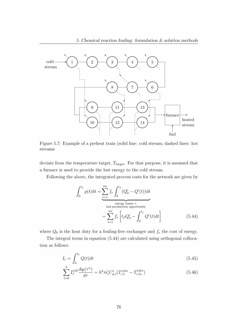
5. Chemical reaction fouling: formulation & solution methods
coldstream
1 2 3 4 5
678
9
10
11
12
13
14
furnace
fuel
heatedstream
Figure 5.7: Example of a preheat train (solid line: cold stream; dashed lines: hotstreams
deviate from the temperature target, Ttarget. For that purpose, it is assumed that
a furnace is used to provide the lost energy to the cold stream.
Following the above, the integrated process costs for the network are given by∫ tf
0
p(t)dt =nu∑i=1
fe
∫ tf
0
(Qi0 −Qi(t))dt︸ ︷︷ ︸
energy losses +lost-production opportunity
=nu∑i=1
fe
[tfQ
i0 −
∫ tf
0
Qi(t)dt
](5.44)
where Q0 is the heat duty for a fouling-free exchanger and fe the cost of energy.
The integral terms in equation (5.44) are calculated using orthogonal colloca-
tion as follows:
I1 =
∫ tf
0
Q(t)dt (5.45)
3∑l=0
I ijkl1
dql(τn)
dτ= hkmi
cCip,c(T
ijknc,o − T
ijknc,in ) (5.46)
76

5. Chemical reaction fouling: formulation & solution methods
i = 1, 2, . . . , nu; j = 1, 2, . . . , np; k = 1, 2, 3; n = 0, 1, 2, 3
The initial conditions are the following:
I ij,1,11 = 0; i = 1, 2, . . . , nu; j = 1, 2, . . . , np (5.47)
I ijk,01 = I ij,k−1,31 ; i = 1, 2, . . . , nu; j = 1, 2, . . . , np; k = 2, 3 (5.48)
Due to the discontinuities introduced to the model by the binary variables, the
process costs are estimated separately for each period. For that purpose the value
of the integrals is fixed to zero at the beginning of each period.
To facilitate understanding, the calculation of the energy losses plus the lost-
production opportunity for unit i in period j in which a mechanical cleaning
action is performed is illustrated. Figure 5.8 shows the time profile of the heat
duty for unit i at period j. Area 1 represents the heat exchanged, area 2 the energy
t
Qi
Qi0
1
2
. . . . . .
period j
tj−1 tj
3
Figure 5.8: Variation of heat duty with time for unit i in time period j (1: heatexchanged, 2: energy losses and 3: lost-production opportunity)
losses and area 3 the lost-production opportunity in period j, respectively. Area
1 is calculated by I ij,3,31 . The sum of areas 2 and 3 is given by
A2 + A3 = (tj − tj−1)Qi0 − I
ij,3,31 (5.49)
where tj−1 = (j − 1)3∑
k=1
hk and tj = j3∑
k=1
hk.
77

5. Chemical reaction fouling: formulation & solution methods
The maintenance costs depend only on the number of mechanical and chemical
actions performed as it is assumed that the duration of cleaning is independent
of the amount of foulant. The cost of each cleaning mode is fixed and it is given
by the cost vector C = {cm : m ∈M}.The objective function for the discrete scheduling model is given by
z =nu∑i=1
np∑j=1
fe(Qi
0
3∑k=1
hk − I ij,3,31
)+
nu∑i=1
np∑j=1
∑m∈M
yijmcm. (5.50)
5.4.3 Characteristics of the proposed scheduling formula-
tion
The mathematical programming formulation can be implemented for other types
of heat exchanger networks without modifying the set of constraints. Only the
objective function has to be altered since it refers to a class of heat exchanger
networks known as preheat trains.
The scheduling formulation detailed above is a non-convex MINLP problem
due to the nonlinear equality constraints defined by equations (5.37) – (5.39).
These constraints include products of continuous variables with nonlinear func-
tions of continuous variables. The equality constraints defined by equations (5.33)
– (5.36) are also nonlinear as they consist of bilinear products of binary and con-
tinuous variables. However, these can be replaced by linear constraints if nec-
essary by introducing additional variables. This is not required here since the
decomposition algorithm suggested for the solution of the problem (see Section
5.5.2) can treat such bilinear products explicitly [Floudas, 1995]. Due to the non-
convex nature of the scheduling formulation a number of sub-optimal points will
exist. The number of local optima is expected to increase as the number of units
and/or periods increases.
The non-convex MINLP scheduling problem includes O(120× nu× np) con-
tinuous variables and O(2 × nu × np) binary variables. Also, it is comprised of
O(72×nu×np) equality constraints and O(nu×np) inequality constraints which
involve only binary variables. The decision variables (degrees of freedom) for the
scheduling problem are the binary variables only.
78

5. Chemical reaction fouling: formulation & solution methods
5.4.4 The MILP formulation of Lavaja & Bagajewicz
For the scheduling problem with only one available cleaning method, a successful
linearisation framework was presented by Lavaja and Bagajewicz [2004] based on
the idea of parametrising the heat transfer coefficient of the units with the aid of
the binary variables of the formulation.
In the initial formulation of Lavaja and Bagajewicz [2004], the non-linearity
arose only by products of continuous variables with binary variables and products
of binary variables. The authors used standard transformations (see [Williams,
1990]) to rewrite the constraints including these products in exact equivalent lin-
ear form. The transformations require the use of additional continuous variables
and constraints. However, the number of variables and constraints to be added
grows rapidly as the number of periods and the number of units increases, making
the solution of the resulting MILP problems computationally unaffordable.
To overcome this drawback, Lavaja and Bagajewicz [2004] suggested a de-
composition method based on the assumption that the cleaning schedule of an
individual unit is not affected by the cleaning decisions for the rest of the units.
Using this decomposition technique the computational effort for obtaining a so-
lution is reduced significantly. Nonetheless, such an assumption is not valid for
large networks with strong couplings between heat exchangers arising from hot
streams passing through units in series.
To the author’s understanding, the linearisation framework proposed by Lavaja
and Bagajewicz [2004] is very difficult to adapt to the scheduling problem studied
in this work. The presence of two layers on the heat transfer surface renders the
parametrisation of the heat transfer coefficient to be extremely difficult. More-
over, even if one succeeds in adapting such a formulation to the case under study,
the resulting models will require a prohibitively large computational effort to
solve.
79

5. Chemical reaction fouling: formulation & solution methods
5.5 Solution methods
The non-convex MINLP scheduling problem is of the general form:
min.y
z = f(x, y)
s.t. g(x, y) = 0 (SP)
h(x) = 0
w(y) ≤ 0
x ∈ X ⊆ <nx
y ∈ Y = {0, 1}ny
where x is the vector of continuous variables, y is the vector of binary variables,
nx the dimension of vector x and ny the dimension of vector y.
The practical goal when dealing with non-convex problems is to obtain ‘good’
local optima. In that respect, solution algorithms addressing convex MINLP
problems can be used to solve the scheduling problem (SP) even if such an ap-
proach is considered to be heuristic, in the sense that there is no guarantee that
the global solution will be obtained. This line of approach is adopted in this
work.
A number of well-known solution algorithms for MINLP problems employ a
decomposition strategy. Such are the Generalised Benders Decomposition (GBD)
[Benders, 1962; Geoffrion, 1972] and the Outer Approximation (OA) [Duran and
Grossmann, 1986]/ Equality Relaxation (ER) [Kocis and Grossmann, 1987] algo-
rithms. The iterative structure of the decomposition algorithms is illustrated in
Figure 5.9. The MINLP problem is decomposed into a Nonlinear Programming
Primal: NLPproblem
Master: MIPproblem
Figure 5.9: Iterative structure of decomposition algorithms
(NLP) problem, the Primal problem, where the binary variables y are fixed and
one MIP problem, the Master problem. The Primal problem provides an upper
80

5. Chemical reaction fouling: formulation & solution methods
bound to the MINLP problem and the set of continuous variables to be used by
the Master problem. Conversely, the Master problem provides a lower bound for
the MINLP problem and the set of binary variables to be used by the Primal
problem.
If the MINLP problem is convex, then at some iteration the upper bound
provided by the Primal problem will become equal to the lower bound provided
by the Master problem and the algorithm terminates having produced the global
solution. For a non-convex MINLP problem the lower bound provided by the
Master problem is not always valid: there is the danger of cutting off parts of
the feasible region. Consequently, the global solution may be excluded from the
search at some iteration. In such an event, the lower bound will exceed the upper
bound at some iteration and the algorithm will terminate.
5.5.1 Outer approximation/Equality relaxation
One decomposition-based optimiser is DICOPT R© [Kocis and Grossmann, 1989],
included in the GAMSTM
[Brooke et al., 1992] modelling system. The DICOPT R©
solver is based on the OA/ER decomposition algorithm.
There are two drawbacks [Floudas, 1995] when applying the OA/ER algorithm
to the non-convex MINLP scheduling problem (SP). Briefly, these are:
a) the formulation of the master problem at each iteration involves the lineari-
sation of the objective function and the nonlinear constraints around the
primal solution. Linear approximations for non-convex functions are often
invalid.
b) A large number of constraints is added to the master problem at each it-
eration. Therefore, the computational effort for solving the corresponding
MIP Master problem increases significantly after a few iterations.
Thus, the OA/ER algorithm is not a suitable candidate for the solution of
large instances of the MINLP scheduling problem (SP), the main reason being
that the size of the Master problem will grow rapidly as the number of units
and the number of time periods increases. As a result, the algorithm will require
prohibitively long computational times to converge.
81

5. Chemical reaction fouling: formulation & solution methods
5.5.2 Generalised Benders Decomposition algorithm
A more appropriate solution algorithm for the problem of interest to this work
is Generalised Benders Decomposition [Benders, 1962; Geoffrion, 1972]. The key
feature of GBD, that is of interest to this work, is that only one constraint is added
to the Master problem at each iteration. As a result, the size of the corresponding
MIP Master problem remains small even after a large number of iterations. On the
other hand, one may argue that the Master problem in GBD provides looser lower
bounds than the Master problem in OA/ER [Grossmann and Kravanja, 1995] and
thus potentially requires many more iterations. However, for this application this
may work to our benefit since the MINLP problem is non-convex and the danger
of cutting off parts of the feasible region decreases.
There are three Nonlinear Programming (NLP) sub-problems to be derived
from problem (SP) with respect to GBD [Floudas, 1995]:
a) NLP relaxation: the binary requirements for variables y are lifted. Here,
variables y are continuous and constrained within the interval [0, 1]. The
NLP sub-problem is the following:
min.y
zR = f(x, y)
s.t. g(x, y) = 0 (NLP-R)
h(x) = 0
w(y) ≤ 0
x ∈ X ⊆ <nx
y ∈ Y = [0, 1]ny .
which yields a lower bound zR to problem (SP) if it has a feasible solution
[Grossmann and Kravanja, 1995].
b) NLP sub-problem for fixed binary variables yk: this is the Primal problem
and it is defined as follows:
min. zkPr = f(x, yk)
s.t. g(x, yk) = 0 (NLP-Pr)
82
5. Chemical reaction fouling: formulation & solution methods
h(x) = 0
x ∈ X ⊆ <nx .
The Primal problem yields an upper bound zkf to (SP) provided it has
a feasible solution [Grossmann and Kravanja, 1995]. The index k ∈ K
corresponds to the iteration counter for the decomposition algorithm (K is
the set of iterations).
In fact, there are no decision variables in the problem (NLP-Pr): once all the
binary variables are fixed the behaviour of the system is fully determined.
Thus, the solution of the Primal problem corresponds to the solution of a
square matrix of equations (simulation of the network’s operation). Hence,
it is guaranteed that it will always have a feasible solution. The set of con-
straints w(y) need not be included in the problem since the binary variables
y are fixed.
c) NLP feasibility sub-problem for fixed yk. The task here is to minimise
the infinity-norm, l∞, (among other appropriate norms) measuring the in-
feasibility of the corresponding (NLP-Pr) sub-problem. Since the Primal
problem is never infeasible, the NLP feasibility sub-problem can be omitted.
The Master problem corresponding to (SP) is the following MILP problem:
min.y,θ
θ
s.t. θ ≥ L(xk, y, λkg , λkh); k ∈ K (MILP-M)
w(y) ≤ 0∑i∈Bk
yi −∑l∈Ck
yl ≤ |Bk| − 1; k ∈ K
y ∈ Y = {0, 1}ny
Bk = {i : yki = 1}, Ck = {l : ykl = 0}; k ∈ K
where |Bk| is the cardinality of set Bk and
L(xk, y, λkg , λkh) = f(xk, y) + λk
T
g g(xk, y) + λkT
h h(xk); k ∈ K (5.51)
83
5. Chemical reaction fouling: formulation & solution methods
is the Lagrange function evaluated at the solution of the Primal problem at
each iteration. The parameters λkT
g and λkT
h are the Lagrange multipliers at the
solution of the k-th Primal problem. The set of integer cuts given by∑i∈Bk
yi −∑l∈Ck
yl ≤ |Bk| − 1; k ∈ K (5.52)
Bk = {i : yki = 1}, Ck = {l : ykl = 0}; k ∈ K
eliminates binary combinations already found at previous iterations.
The inequality constraints defined by
θk ≥ L(xk, y, λkg , λkh); k ∈ K (5.53)
are known as Benders cuts and they produce a non-decreasing sequence of lower
bounds [Floudas, 1995]. Benders cuts represent local underestimators of the
MINLP problem (SP). These underestimators are valid when the MINLP prob-
lem is convex and, particularly, when Slater’s condition for strong duality [Boyd
and Vandenberghe, 2004] holds. This is not true for problem (SP). As a result,
there exists the possibility that some Benders cuts will not be valid and the global
solution will be excluded from the search procedure. Figure 5.10 depicts the sit-
uation where an invalid underestimator cuts off a part of the feasible region that
includes the global solution (point A).
Sahinidis and Grossmann [1991] and Bagajewicz and Manousiouthakis [1991]
have shown that the GBD algorithm may terminate at a local optimum or even
worse at a non-stationary point for non-convex problems. Furthermore, they
have shown that if the starting point is a local minimum then the algorithm
will terminate at this point. This result can be used as a second termination
criterion for the GBD algorithm to guarantee that it will always converge at a
local minimum: the algorithm is restarted at the last solution point obtained
until it terminates at that same point. Algorithm 5.1 gives an overview of the
GBD algorithm implemented in this work.
84

5. Chemical reaction fouling: formulation & solution methods
x
z
A
Figure 5.10: Invalid Benders cut (underestimator)
5.5.3 Receding Horizon heuristic
A heuristic solution procedure inspired by Control Theory, due to the dynamic na-
ture of the scheduling problem, and particularly Model Predictive Control (MPC)
is also used to solve the MINLP problem (SP). The basic steps in the MPC
method [Camacho and Bordons, 2004] are the following:
a) calculate a control sequence after minimising an apt objective function over
a fixed time horizon;
b) recede the horizon and repeat minimisation after applying the first signal
of the control sequence.
The MPC approach can be adapted to attack the scheduling problem of clean-
ing heat exchanger networks subject to fouling. Here, the control sequence refers
to the cleaning schedule and the first signal corresponds to the cleaning deci-
sions for the first period of the examined number of periods, nRH (nRH < np).
Algorithm 5.2 describes the applied Receding Horizon (RH) heuristic solution
procedure.
Note that the number of periods nRH decreases as the iteration counter j
approaches the value of n′p. The solution procedure stops when j = np. Therefore,
85

5. Chemical reaction fouling: formulation & solution methods
Algorithm 5.1: Generalized Benders Decomposition
1: Begin2: Set number of periods nP3: Solve (NLP-R) ! obtain yR to use as starting point4: y1 = 1 ∀ yR > 0.5 ! R: Relaxed5: y1 = 0 ∀ yR ≤ 0.56: termination = False7: while (termination = False) do8: UB = +∞, LB = −∞ ! UB: upper bound, LB: lower bound9: criterion = True
10: k = 011: while (criterion = True) do12: k = k + 113: Solve (NLP-Pr) for given yk
14: Store xk = x, λk = λ, zkPr15: if (UB ≥ zkPr) then16: UB = zkPr17: x∗ = xk ! x∗: optimal x vector18: y∗ = yk ! y∗: optimal y vector19: end if20: Solve (MILP-M) for xk
21: Store yk+1 = y, LB = θk
22: if (LB ≥ UB) then23: criterion = False24: end if25: end while26: if (k = 1) then27: termination = True28: end if29: end while30: Solution: x∗, y∗, UB31: End
the obtained cleaning schedule is for np periods and it is comparable to the
cleaning schedules obtained using the GBD algorithm.
The merit of using the RH heuristic to solve the scheduling problem (SP) lies
in the size of the sub-problems solved at each iteration: the sub-problems are
relatively small and can be solved with relatively small computational effort. As
the number of units, nu, and/or the number of periods, np, increases it is ex-
86
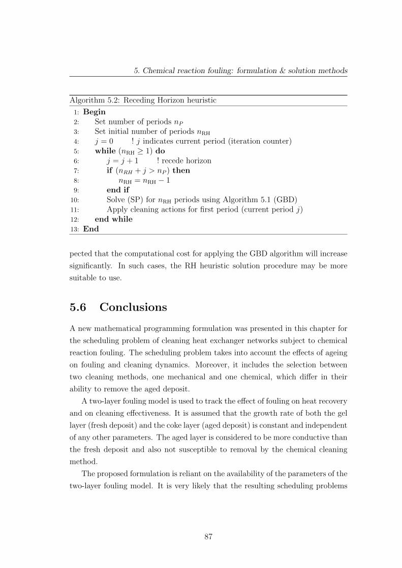
5. Chemical reaction fouling: formulation & solution methods
Algorithm 5.2: Receding Horizon heuristic
1: Begin2: Set number of periods nP3: Set initial number of periods nRH
4: j = 0 ! j indicates current period (iteration counter)5: while (nRH ≥ 1) do6: j = j + 1 ! recede horizon7: if (nRH + j > nP ) then8: nRH = nRH − 19: end if
10: Solve (SP) for nRH periods using Algorithm 5.1 (GBD)11: Apply cleaning actions for first period (current period j)12: end while13: End
pected that the computational cost for applying the GBD algorithm will increase
significantly. In such cases, the RH heuristic solution procedure may be more
suitable to use.
5.6 Conclusions
A new mathematical programming formulation was presented in this chapter for
the scheduling problem of cleaning heat exchanger networks subject to chemical
reaction fouling. The scheduling problem takes into account the effects of ageing
on fouling and cleaning dynamics. Moreover, it includes the selection between
two cleaning methods, one mechanical and one chemical, which differ in their
ability to remove the aged deposit.
A two-layer fouling model is used to track the effect of fouling on heat recovery
and on cleaning effectiveness. It is assumed that the growth rate of both the gel
layer (fresh deposit) and the coke layer (aged deposit) is constant and independent
of any other parameters. The aged layer is considered to be more conductive than
the fresh deposit and also not susceptible to removal by the chemical cleaning
method.
The proposed formulation is reliant on the availability of the parameters of the
two-layer fouling model. It is very likely that the resulting scheduling problems
87

5. Chemical reaction fouling: formulation & solution methods
will be highly sensitive to these parameters and reliable estimation of their values
is going to be crucial in the application of the described scheduling formulation.
The scheduling problem is formulated for networks of single pass shell-and-
tube exchangers operating in counter-current mode. It can be easily extended for
other types of heat exchangers and different flow configurations. It is assumed
that deposition of foulant occurs only in the tubes of the units where the cold
stream flows.
The need to simulate the operation of heat exchanger networks in order to
calculate the process costs due to fouling favours a discrete representation of time.
An orthogonal collocation scheme is included in the problem formulation and is
used to obtain numerical solutions for the differential equations, albeit these are
of zero order (the future direction of the work is to replace the simple two-layer
model with a more detailed one, e.g. the first order model described by Ishiyama
et al. [2011a]), and to estimate the integral of the process costs over the examined
time horizon.
The mathematical programming formulation of the scheduling task corre-
sponds to a non-convex MINLP problem. Due to the non-convex characteristics
of the problem it is very difficult to guarantee that a local solution is the globally
optimal point. The non-convexity of the problem arises from the sets of equality
constraints (5.37) – (5.39) and from the constraints defined by (5.23) – (5.26)
(can be replaced by linear constraints if required / can be treated explicitly by
Generalised Benders Decomposition).
The objective function of the scheduling problem is formulated for a special
class of heat exchanger networks called preheat trains. Nonetheless, the schedul-
ing problem may be extended to other types of heat exchanger networks after
minor modifications. A preheat train is used to raise the temperature of a cold
stream to a certain value before it enters some other process. Alas this target
temperature is not achieved due to fouling. The objective function includes the
energy losses due to fouling, the lost-production opportunity during the cleaning
intervals and the maintenance costs.
The standard Outer Approximation/Equality Relaxation decomposition algo-
rithm is deemed as unsuitable to attack large instances of the non-convex schedul-
ing problem. In that regard, two alternative solution methods are proposed.
88

5. Chemical reaction fouling: formulation & solution methods
The first algorithm applies Generalised Benders Decomposition, a well-known
exact solution method for convex MIP problems. For non-convex problems such
as the one studied here there is a high probability that the global solution will
be excluded by the search procedure at some iteration. Nonetheless, bearing in
mind the unavoidable difficulties associated with non-convex problems, the goal
here is to obtain ‘good’ local solutions with moderate computational cost. For
that purpose, the use of Generalised Benders Decomposition is favourable.
The second solution approach is inspired by Model Predictive Control. The
advantage of this heuristic solution procedure lies in the fact that the scheduling
problem is solved over a short time horizon (instead of the whole time horizon) at
each iteration. Thus, it is expected that a cleaning schedule can be obtained with
relatively small computational effort even for large instances of the scheduling
problem.
89
Chapter 6
Chemical reaction fouling:
computational studies
In Chapter 5, a new MINLP formulation was presented for the problem of schedul-
ing the cleaning actions for heat exchanger networks subject to chemical reaction
fouling and ageing. The proposed formulation is evaluated in the current chapter
through a series of computational studies. At first, the scheduling formulation
is implemented for an isolated heat exchanger and the resulting model is solved
using the Outer Approximation/Equality Relaxation algorithm. Subsequently,
cleaning schedules are obtained for two heat exchanger networks of different size
using the Generalized Benders Decomposition algorithm and the Receding Hori-
zon heuristic procedure. An assessment is presented at the end of the chapter
regarding the produced results and the computational performance of the differ-
ent solution procedures.
6.1 Introductory remarks
For the computational studies, the scheduling problems are modelled in GAMSTM
[Brooke et al., 1992] installed on an ASUSTM
Chassis computer with 2.21 GHz
CPU. The DICOPT R© solver (OA/ER algorithm) [Kocis and Grossmann, 1989],
the GBD algorithm and the RH heuristic require the use of an MILP solver and
an NLP solver. The MILP solver is CPLEX R© 10.1.1 [GAMS, 2010] which is a
90
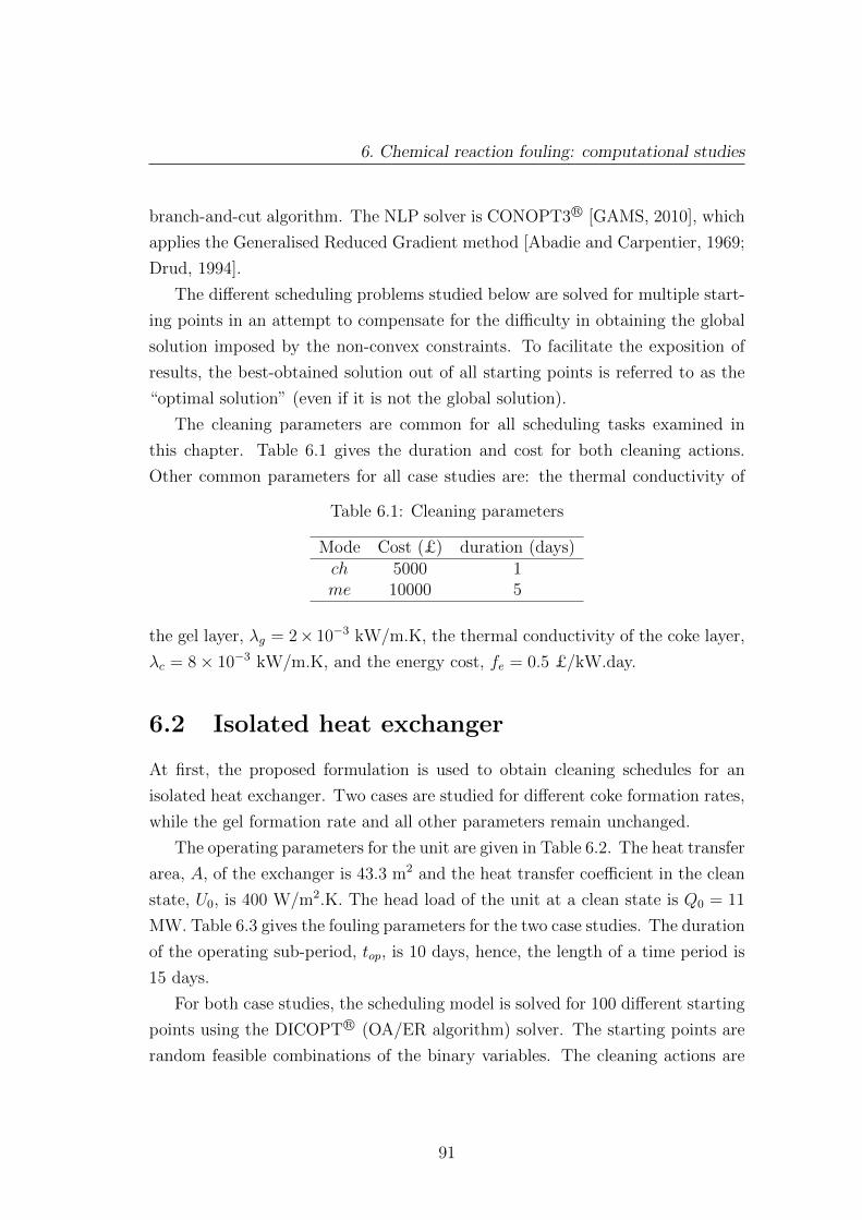
6. Chemical reaction fouling: computational studies
branch-and-cut algorithm. The NLP solver is CONOPT3 R© [GAMS, 2010], which
applies the Generalised Reduced Gradient method [Abadie and Carpentier, 1969;
Drud, 1994].
The different scheduling problems studied below are solved for multiple start-
ing points in an attempt to compensate for the difficulty in obtaining the global
solution imposed by the non-convex constraints. To facilitate the exposition of
results, the best-obtained solution out of all starting points is referred to as the
“optimal solution” (even if it is not the global solution).
The cleaning parameters are common for all scheduling tasks examined in
this chapter. Table 6.1 gives the duration and cost for both cleaning actions.
Other common parameters for all case studies are: the thermal conductivity of
Table 6.1: Cleaning parameters
Mode Cost (£) duration (days)ch 5000 1me 10000 5
the gel layer, λg = 2× 10⁻³ kW/m.K, the thermal conductivity of the coke layer,
λc = 8× 10⁻³ kW/m.K, and the energy cost, fe = 0.5 £/kW.day.
6.2 Isolated heat exchanger
At first, the proposed formulation is used to obtain cleaning schedules for an
isolated heat exchanger. Two cases are studied for different coke formation rates,
while the gel formation rate and all other parameters remain unchanged.
The operating parameters for the unit are given in Table 6.2. The heat transfer
area, A, of the exchanger is 43.3 m2 and the heat transfer coefficient in the clean
state, U0, is 400 W/m2.K. The head load of the unit at a clean state is Q0 = 11
MW. Table 6.3 gives the fouling parameters for the two case studies. The duration
of the operating sub-period, top, is 10 days, hence, the length of a time period is
15 days.
For both case studies, the scheduling model is solved for 100 different starting
points using the DICOPT R© (OA/ER algorithm) solver. The starting points are
random feasible combinations of the binary variables. The cleaning actions are
91

6. Chemical reaction fouling: computational studies
Table 6.2: Operating parameters: isolated heat exchanger
Tc,in (oC) Th,in (oC) mc (kg/s) mh (kg/s) Cp,c (kJ/kg.K) Cp,h (kJ/kg.K)27 227 135 128 3.1 2.2
Table 6.3: Fouling parameters: isolated heat exchanger
Case study kg (m/day) kc (m/day) kg/kc
A 1.6× 10⁻⁶ 8× 10⁻⁸ 20B 1.6× 10⁻⁶ 8× 10⁻⁷ 2
scheduled over 24 periods corresponding to a time horizon of one year. The
optimal schedule (best out of the 100) for both case studies is shown in Table 6.4.
Moreover, the optimal value of the cost function, z∗, for each case study, is given
in Table 6.5 and compared to the anticipated cost when no cleaning is performed,
zno.
Table 6.4: Optimal cleaning schedule: isolated heat exchanger (open circles:chemical actions; filled circles: mechanical action)
64 1
1 2 3 4 5 6 7 8 9 10 11 12 13 14 15 16 17 18 19 20 21 22 23 24PeriodCase
study
AB
Modech me
Table 6.5: Objective value for the optimal schedule and for the no-cleaning situ-ation: isolated heat exchanger
Case study zno×105 (£) z∗×105 (£) SavingsA 6.8 2.5 63 %B 5.1 2.6 49 %
The results presented in Tables 6.4 and 6.5 are in compliance with the assump-
tion that the aged material is more conductive than the gel layer. For case study
B, where the coke formation rate is ten times higher than that of case study A,
the objective function value for the no-cleaning situation is considerably smaller:
the objective value reflects the amount of heat losses due to fouling. Furthermore,
92

6. Chemical reaction fouling: computational studies
for case study A, where the coke formation rate is slow, the optimal schedule does
not include any mechanical cleaning. In contrast, for case study B, a mechanical
action is selected at period 12 as shown in Table 6.4.
The cleaning schedule for case study B suggests that an optimal mixed clean-
ing campaign can be identified, which can be repeated in time. This mixed
cleaning heat exchanger cycle is termed the cleaning super-cycle and it includes
a number of chemical actions to be followed by a mechanical cleaning, which will
reset the unit to the clean state. The advantage of such a mixed cleaning strat-
egy is that the operating time before lengthy cleaning shut-downs is extended by
performing short-length chemical actions.
For case study B the cleaning super-cycle has a length of 12 periods (120
days) as seen in Table 6.4 and it includes 2 chemical actions. The mechanical
cleaning performed at the end of period 12 restores fully the efficiency of the
unit. Subsequently, the same cleaning pattern is observed, albeit, no mechanical
action is performed at period 24 since there is no potential gain in cleaning the
unit at the end of the examined time horizon. For case study A, where the coke
formation rate is slower, a longer time horizon must be considered in order to
obtain a cleaning super-cycle.
Figures 6.1(a) and 6.1(b) show the variation of the gel and coke thickness in
time for case studies A and B, respectively. The timing of the cleaning actions is
60 120 180 240 300 3600
20
40
60
80
t (days)
δ(mm)
(a) Case study A
60 120 180 240 300 3600
50
100
150
t (days)
δgδc
(b) Case study B
Figure 6.1: Time profile of gel and coke thickness: isolated heat exchanger
93

6. Chemical reaction fouling: computational studies
apparent on both graphs. For case study B, Figure 6.1(b) shows the mechanical
cleaning occurring after 175 days, during which the thickness of both layers is set
to zero. The thickness of the coke layer in case study A increases throughout the
examined time horizon, as shown in Figure 6.1(a), since no mechanical action is
performed.
6.3 Heat exchanger networks
The MINLP scheduling formulation is applied to the two heat exchanger networks
reported by Smaıli et al. [2002]. The first network (referred to as heat exchanger
network I) involves 14 units and introduces some of the complexities found in
refinery networks caused by interconnecting hot streams [Smaıli et al., 2002].
The second network (referred to as heat exchanger network II) consists of 25
units and bears a resemblance to a real network where several units are used in
order to lessen the loss of production due to cleaning. Graphical representations
of the smaller network and the more realistic network are shown in Figures 6.2
and 6.4, respectively.
The two networks are altered in this work: the flash drum included by Smaıli
et al. [2002] is omitted. On the other hand, the desalter is included and therefore
an extra set of constraints needs to be incorporated in the scheduling formulation.
It is assumed that a drop of 10 oC occurs in the desalter. For heat exchanger
network I where unit 5 precedes and unit 6 follows the desalter, the following set
of constraints is added to the scheduling model:
T 6,jklc,in = T 5,jkl
c,o − 10; j = 1, 2, . . . , np; k = 1, 2, 3; l = 0, 1, 2, 3. (6.1)
For heat exchanger network II the constraints are the following:
T 8,jklc,in =
m6cT
6,jklc,o + m7
cT7,jklc,o
m6c + m7
c
− 10 (6.2)
T 9,jklc,in =
m6cT
6,jklc,o + m7
cT7,jklc,o
m6c + m7
c
− 10 (6.3)
j = 1, 2, . . . , np; k = 1, 2, 3; l = 0, 1, 2, 3.
94
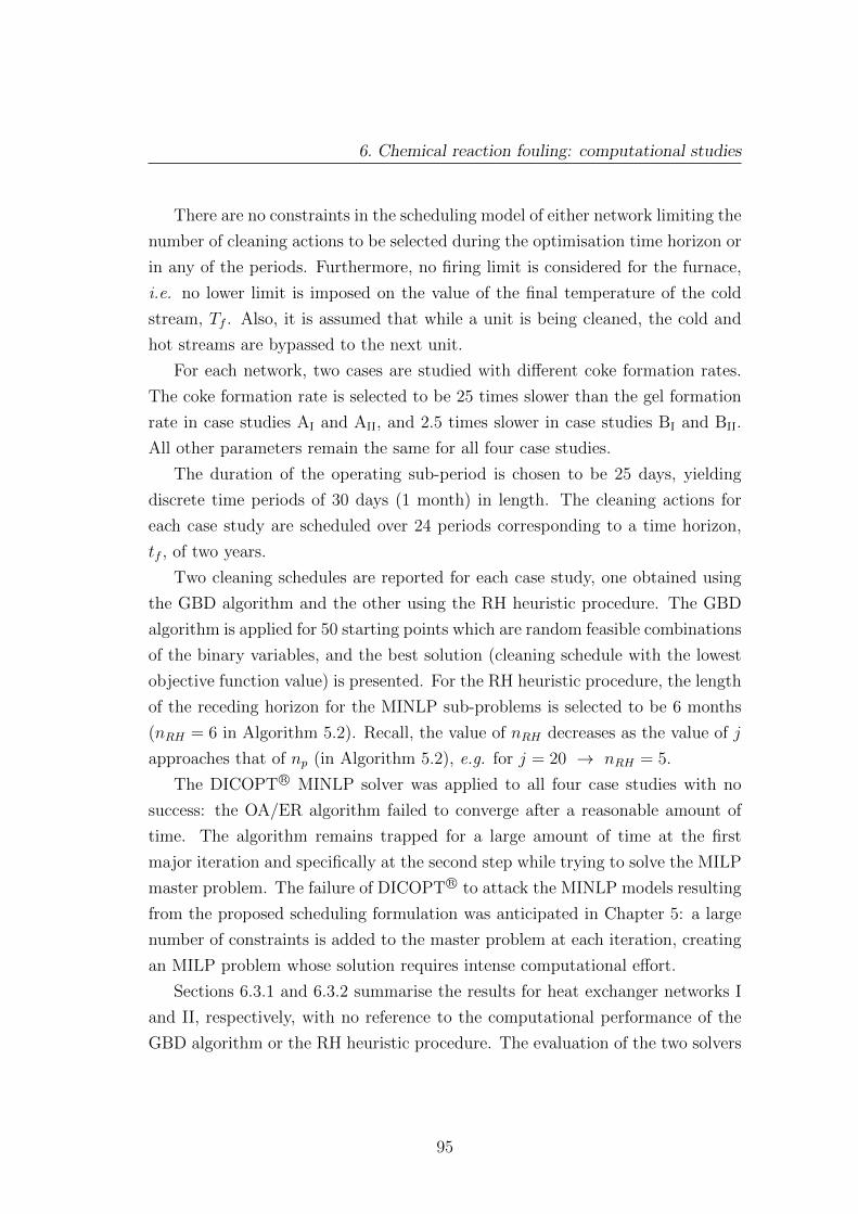
6. Chemical reaction fouling: computational studies
There are no constraints in the scheduling model of either network limiting the
number of cleaning actions to be selected during the optimisation time horizon or
in any of the periods. Furthermore, no firing limit is considered for the furnace,
i.e. no lower limit is imposed on the value of the final temperature of the cold
stream, Tf . Also, it is assumed that while a unit is being cleaned, the cold and
hot streams are bypassed to the next unit.
For each network, two cases are studied with different coke formation rates.
The coke formation rate is selected to be 25 times slower than the gel formation
rate in case studies AI and AII, and 2.5 times slower in case studies BI and BII.
All other parameters remain the same for all four case studies.
The duration of the operating sub-period is chosen to be 25 days, yielding
discrete time periods of 30 days (1 month) in length. The cleaning actions for
each case study are scheduled over 24 periods corresponding to a time horizon,
tf , of two years.
Two cleaning schedules are reported for each case study, one obtained using
the GBD algorithm and the other using the RH heuristic procedure. The GBD
algorithm is applied for 50 starting points which are random feasible combinations
of the binary variables, and the best solution (cleaning schedule with the lowest
objective function value) is presented. For the RH heuristic procedure, the length
of the receding horizon for the MINLP sub-problems is selected to be 6 months
(nRH = 6 in Algorithm 5.2). Recall, the value of nRH decreases as the value of j
approaches that of np (in Algorithm 5.2), e.g. for j = 20 → nRH = 5.
The DICOPT R© MINLP solver was applied to all four case studies with no
success: the OA/ER algorithm failed to converge after a reasonable amount of
time. The algorithm remains trapped for a large amount of time at the first
major iteration and specifically at the second step while trying to solve the MILP
master problem. The failure of DICOPT R© to attack the MINLP models resulting
from the proposed scheduling formulation was anticipated in Chapter 5: a large
number of constraints is added to the master problem at each iteration, creating
an MILP problem whose solution requires intense computational effort.
Sections 6.3.1 and 6.3.2 summarise the results for heat exchanger networks I
and II, respectively, with no reference to the computational performance of the
GBD algorithm or the RH heuristic procedure. The evaluation of the two solvers
95
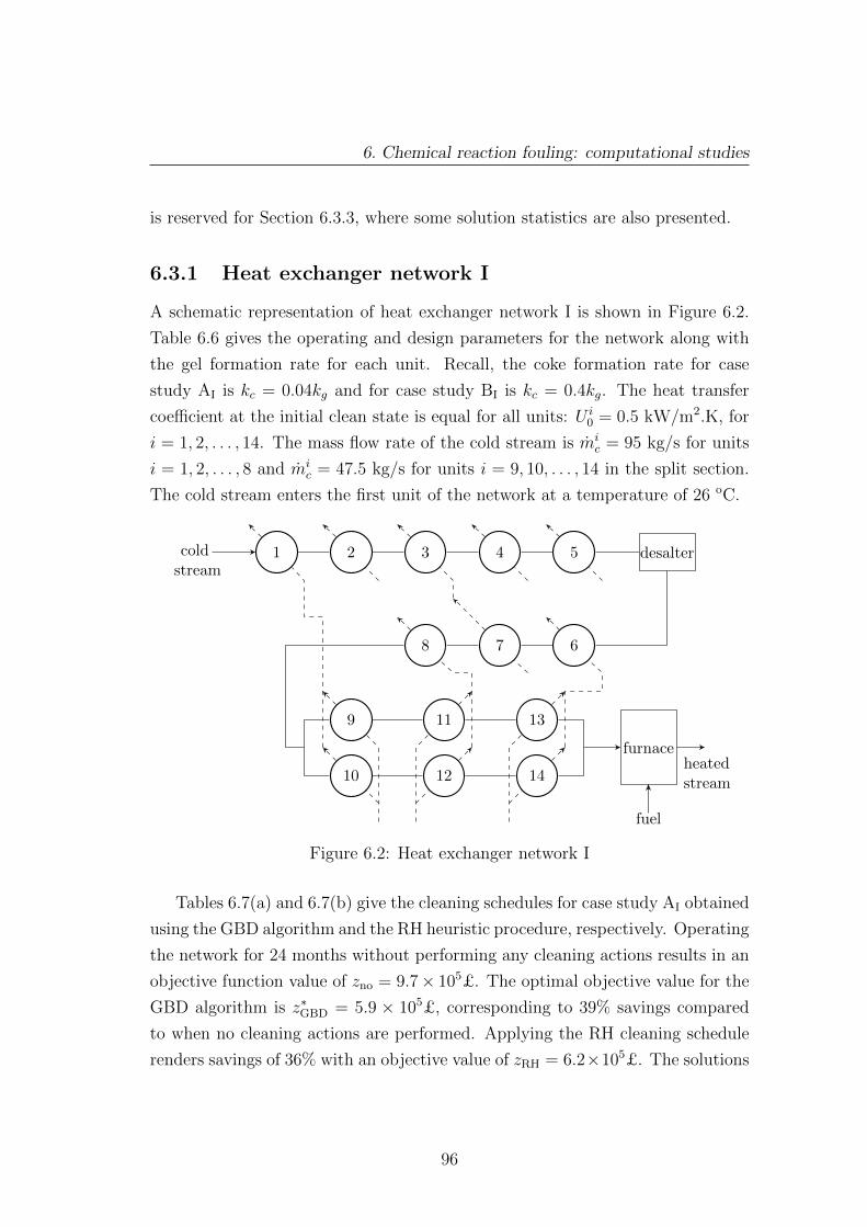
6. Chemical reaction fouling: computational studies
is reserved for Section 6.3.3, where some solution statistics are also presented.
6.3.1 Heat exchanger network I
A schematic representation of heat exchanger network I is shown in Figure 6.2.
Table 6.6 gives the operating and design parameters for the network along with
the gel formation rate for each unit. Recall, the coke formation rate for case
study AI is kc = 0.04kg and for case study BI is kc = 0.4kg. The heat transfer
coefficient at the initial clean state is equal for all units: U i0 = 0.5 kW/m2.K, for
i = 1, 2, . . . , 14. The mass flow rate of the cold stream is mic = 95 kg/s for units
i = 1, 2, . . . , 8 and mic = 47.5 kg/s for units i = 9, 10, . . . , 14 in the split section.
The cold stream enters the first unit of the network at a temperature of 26 oC.
coldstream
1 2 3 4 5 desalter
678
9
10
11
12
13
14
furnace
fuel
heatedstream
Figure 6.2: Heat exchanger network I
Tables 6.7(a) and 6.7(b) give the cleaning schedules for case study AI obtained
using the GBD algorithm and the RH heuristic procedure, respectively. Operating
the network for 24 months without performing any cleaning actions results in an
objective function value of zno = 9.7× 10⁵£. The optimal objective value for the
GBD algorithm is z∗GBD = 5.9 × 10⁵£, corresponding to 39% savings compared
to when no cleaning actions are performed. Applying the RH cleaning schedule
renders savings of 36% with an objective value of zRH = 6.2×10⁵£. The solutions
96
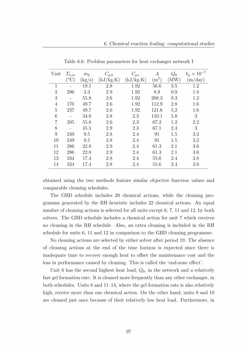
6. Chemical reaction fouling: computational studies
Table 6.6: Problem parameters for heat exchanger network I
Unit Th,in mh Cp,h Cp,c A Q0 kg × 10−7
(oC) (kg/s) (kJ/kg.K) (kJ/kg.K) (m2) (MW) (m/day)1 - 19.1 2.8 1.92 56.6 3.5 1.22 296 3.3 2.9 1.92 8.9 0.9 1.83 - 55.8 2.6 1.92 208.3 9.3 1.24 170 49.7 2.6 1.92 112.9 2.8 1.65 237 49.7 2.6 1.92 121.6 5.2 1.66 - 34.8 2.8 2.3 110.1 5.8 37 205 55.8 2.6 2.3 67.2 1.2 2.28 - 45.5 2.9 2.3 67.1 2.4 39 249 9.5 2.8 2.4 91 1.5 3.210 249 9.5 2.8 2.4 91 1.5 3.211 286 22.8 2.9 2.4 61.3 2.1 3.612 286 22.8 2.9 2.4 61.3 2.1 3.613 334 17.4 2.8 2.4 55.6 2.4 3.814 334 17.4 2.8 2.4 55.6 2.4 3.8
obtained using the two methods feature similar objective function values and
comparable cleaning schedules.
The GBD schedule includes 20 chemical actions, while the cleaning pro-
gramme generated by the RH heuristic includes 22 chemical actions. An equal
number of cleaning actions is selected for all units except 6, 7, 11 and 12, by both
solvers. The GBD schedule includes a chemical action for unit 7 which receives
no cleaning in the RH schedule. Also, an extra cleaning is included in the RH
schedule for units 6, 11 and 12 in comparison to the GBD cleaning programme.
No cleaning actions are selected by either solver after period 19. The absence
of cleaning actions at the end of the time horizon is expected since there is
inadequate time to recover enough heat to offset the maintenance cost and the
loss in performance caused by cleaning. This is called the ‘end-zone effect’.
Unit 6 has the second highest heat load, Q0, in the network and a relatively
fast gel formation rate. It is cleaned more frequently than any other exchanger, in
both schedules. Units 8 and 11–14, where the gel formation rate is also relatively
high, receive more than one chemical action. On the other hand, units 9 and 10
are cleaned just once because of their relatively low heat load. Furthermore, in
97

6. Chemical reaction fouling: computational studies
Table 6.7: Cleaning schedule for heat exchanger network I: case study AI (opencircles: chemical actions)
(a) GBD algorithm
1 2 3 4 5 6 7 8 9 10 11 12 13 14 15 16 17 18 19 20 21 22 23 24Period Mode
ch meUnits1234567891011121314
Total 20
1
1312112233
z∗GBD = 5.9× 10⁵£
(b) RH heuristic
1 2 3 4 5 6 7 8 9 10 11 12 13 14 15 16 17 18 19 20 21 22 23 24Period Mode
ch meUnits1234567891011121314
Total 22
1
14
2113333
zRH = 6.2× 10⁵£
98

6. Chemical reaction fouling: computational studies
both cleaning programmes, only one clean is performed on unit 3 even though it
has the largest heat load due to its relatively low gel formation rate.
The large number of chemical actions and the absence of mechanical actions
is a consequence of the slow coke formation rate. The thickness of the gel layer
which poses a high resistance to heat transfer is increasing relatively quickly and
as a response the solvers select frequent chemical actions in order to compensate
the energy losses.
The schedules generated by the two solvers exhibit similar selection patterns
but in the RH schedule the distribution of cleaning actions is more structured.
The RH cleaning programme displays periodicity: the chemical actions for units
which are cleaned more than once are selected after equal time intervals. Units
11–14 are cleaned thrice. The chemical actions for units 11 and 14 are performed
one period after units 12 and 13 are cleaned, respectively.
The cleaning schedules obtained for case study BI are given in Tables 6.8(a)
and 6.8(b). Operating the network without applying any cleaning actions renders
an objective value of zno = 7.2 × 10⁵£. The optimal objective value for the
GBD algorithm is z∗GBD = 6 × 10⁵£, while the objective function value for the
RH heuristic procedure is zRH = 5.9 × 10⁵£. The solution generated from the
RH heuristic in this case study is slightly better than the GBD solution. The
corresponding savings in comparison to zero cleaning actions are 18% for the RH
heuristic and 17% for the GBD algorithm.
A relatively small number of cleaning actions is selected by both solvers.
For this case study, the two schedules are very different. The GBD cleaning
programme includes four mechanical actions and two chemical actions, while
the RH schedule includes only one mechanical action and 6 chemical actions.
Furthermore, the cleaning actions are congested between periods 9 to 12 in the
GBD schedule, whereas the RH schedule is more sparse. There, four out of
the seven actions are performed after the fifteenth period. Nevertheless, both
schedules include the same intuitive choices: only units 6, 8 and 11–14 are cleaned,
where the gel and coke formation rates are relatively high.
For case study BI, fewer cleaning actions are selected by the solvers, including
some mechanical ones, compared to case study AI due to the increase of the coke
formation rate by a factor of 10. The aged material is four times more conductive
99

6. Chemical reaction fouling: computational studies
Table 6.8: Cleaning schedule for heat exchanger network I: case study BI (opencircles: chemical actions; filled circles: mechanical actions)
(a) GBD algorithm
1 2 3 4 5 6 7 8 9 10 11 12 13 14 15 16 17 18 19 20 21 22 23 24Period Mode
ch meUnits1234567891011121314
Total 2 4
1
1
11
11
z∗GBD = 6× 10⁵£
(b) RH heuristic
1 2 3 4 5 6 7 8 9 10 11 12 13 14 15 16 17 18 19 20 21 22 23 24Period Mode
ch meUnits1234567891011121314
Total 6 1
2
1
1111
zRH = 5.9× 10⁵£
100

6. Chemical reaction fouling: computational studies
than the fresh deposit. The objective value for the no-cleaning situation for
case study AI is zno = 9.7 × 10⁵£, whereas for case study BI is zno = 7.2 ×10⁵£. This corresponds to a decrease of 26%. The preceding facts show the
importance of the thermal conductivities of the two layers, which are parameters
in the fouling model. It should be noted that if the deposits are allowed to get
relatively thick this will affect the hydraulic performance of the network: this
aspect is not considered here.
The GBD and RH schedules include the same intuitive cleaning choices present
in those of case study AI: units 6, 8 and 11–14, which exhibit a high gel formation
rate, are cleaned more than once.
Figures 6.3(a) and 6.3(b) show the variation of the final temperature of the
cold stream, Tf , with time for case studies AI and BI, respectively. The three
profiles displayed on the graphs correspond to the GBD solution, the RH solution
and the zero cleaning actions situation.
For case study AI, the temperature profiles for the two solution methods are
very similar. At the end of the time horizon, both the GBD and RH cleaning
schedules achieve a final temperature, Tf , which is approximately 15 oC higher
than the case where no cleaning actions are performed.
The analogous temperature difference for case study BI is close to 7oC as seen
in Figure 6.3(b). The temperature profiles are very different for the two schedules.
The TGBDf is superior to TRH
f around the midpoint of the time horizon, but it
becomes inferior during the last periods.
The selection of multiple units to be cleaned in the same period has a com-
mensurate effect on the final temperature, Tf . Large spikes are observed in the
time profile of Tf for both case studies. These large drops in Tf can be avoided if
the permissible number of cleaning actions at each period is restricted. This can
be achieved by the following constraint:
nu∑i=1
∑m∈M
yijm ≤ nc; j = 1, 2, . . . , np (6.4)
where nc is the allowed number of cleaning actions for a period. The set of
constraints (6.4) will only participate in the Master problem (MILP-M).
101

6. Chemical reaction fouling: computational studies
0 120 240 360 480 600 720
200
205
210
215
220
225
230
t (days)
Tf(oC)
(a) Case study AI
0 120 240 360 480 600 720
205
210
215
220
225
230
t (days)
Tf(oC)
GBDRH
No cleaning
(b) Case study BI
Figure 6.3: Time profile of Tf : heat exchanger network I
102

6. Chemical reaction fouling: computational studies
For industrial networks, the firing limits of the furnace will impose a lower
bound on the value of Tf . In such a scenario, the following set of constraints
needs to be included in the MINLP formulation:
T jklf ≥ T limitf ; j = 1, 2, . . . , np; k = 1, 2, 3; l = 0, 1, 2, 3. (6.5)
If not absolutely necessary, the addition of inequality constraints involving
continuous variables to the formulation should be avoided. Constraints such as
the ones given by equation (6.5) will cause the Primal Problem (NLP-Pr) to be
infeasible for the given set of fixed binary values at some iterations of the GBD
algorithm. Thus, the feasibility test step (see [Floudas, 1995]) omitted here from
the algorithm will have to be included. In such a case, it is possible that the
computational cost for generating a solution will increase. Even worse, due to
the non-convex solution space of the problem the algorithm might terminate at
an infeasible point.
6.3.2 Heat exchanger network II
A graphical representation of heat exchanger network II is given in Figure 6.4.
The operating parameters, the area and the gel formation rate for each unit are
summarised in Table 6.9 . The overall heat transfer coefficient in the fouling-free
state is U i0 = 0.5 kW/m2.K for all units i = 1, 2, . . . , 25. The inlet temperature
of the cold stream at unit 1 is 26 oC. The inlet cold stream mass flow rate is
mic = 95 kg/s for units i = 1, 2, . . . , 5, mi
c = 47.5 kg/s for units i = 6, 7, . . . , 13
and mic = 23.75 kg/s for units i = 14, 15, . . . , 25. The coke formation rate for
case study AII is kc = 0.04kg and for case study BII is kc = 0.4kg.
The optimal cleaning schedule for case study AII, obtained using the GBD
algorithm, is given in Table 6.10. The solver selects 19 chemical actions to be
performed and the objective function value is z∗GBD = 6.7 × 10⁵£. Applying the
GBD schedule yields savings of 21%, with respect to the zero cleaning actions
situation (zno = 8.7× 10⁵£).
Only chemical actions are performed, because of the slow coke formation rate,
and only between periods 7 to 17. The absence of cleaning in the first six periods is
due to the fact that the units are fouling-free at the beginning of the time horizon:
103

6. Chemical reaction fouling: computational studies
coldstream
1 2 3 4 5
6
7
desalter
8
9
10
11
12
13
14
15
16
17
18
19
20
21
22
23
24
25
furnace
fuel
heatedstream
Figure 6.4: Heat exchanger network II
deposition has yet to cause significant loss of network performance. Moreover,
the lack of cleaning after period 17 is due to the ‘end-zone effect’. Out of the
25 units, eight (1, 3, 6-7, 14–19) do not receive any cleaning and 15 units are
cleaned once. Units 8 and 9, which have a moderate heat load and a moderate
gel formation rate compared to the other units, are cleaned twice.
At the hot end of the network, all heat exchangers of blocks 18-21 and 22-25
receive one cleaning. The units of block 14–17 have high gel formation rates
but are not cleaned. The reason for this is because the heat load, Q0, of these
exchangers is relatively low (0.3 MW) and part of the energy lost due to fouling
is recovered in the blocks downstream (18–21 and 22–25).
Table 6.11 shows the cleaning schedule produced by the RH heuristic proce-
104

6. Chemical reaction fouling: computational studies
Table 6.9: Problem parameters for heat exchanger network II
Unit Th,in mh Cp,h Cp,c A Q0 kg × 10−7
(oC) (kg/s) (kJ/kg.K) (kJ/kg.K) (m2) (MW) (m/day)1 - 19.2 2.8 1.92 56.6 4.1 1.22 - 55.8 2.6 1.92 96.6 6.5 1.83 296 3.3 2.9 1.92 8.5 0.7 1.24 - 55.8 2.6 1.92 109.6 7.7 1.85 - 49.6 2.6 1.92 129.2 3.4 1.66 - 50 2.6 1.92 80.3 2.1 1.67 237 50 2.6 1.92 60.8 2.1 1.68 - 34.8 2.6 2.3 79.1 3.3 2.29 - 34.8 2.9 2.3 79.1 3.3 2.210 293 56 2.9 2.3 29.2 1.2 311 293 56 2.8 2.3 29.2 1.2 312 - 45.6 2.8 2.3 35.4 0.8 3.213 - 45.6 2.6 2.3 35.4 0.8 3.214 249 19.2 2.8 2.4 31.4 0.3 3.215 249 19.2 2.8 2.4 31.4 0.3 3.216 249 19.2 2.8 2.4 31.4 0.3 3.217 249 19.2 2.8 2.4 41.4 0.3 3.218 286 45.6 2.9 2.4 29.7 0.7 3.619 286 45.6 2.9 2.4 29.7 0.7 3.620 286 45.6 2.9 2.4 29.7 0.7 3.621 286 45.6 2.9 2.4 29.7 0.7 3.622 334 34.8 2.8 2.4 21.3 0.8 3.823 334 34.8 2.8 2.4 21.3 0.8 3.824 334 34.8 2.8 2.4 21.3 0.8 3.825 334 34.8 2.8 2.4 21.3 0.8 3.8
dure. The corresponding objective function value is zRH = 7.7 × 10⁵£ and the
savings are 7% compared to the no-cleaning situation. The cleaning programme
includes 7 chemical actions, which is noticeably fewer than the GBD schedule
(19 chemical actions). No mechanical actions are selected. Out of the 25 units,
17 are not cleaned at all and among these are the units 14–25 at the hot end of
the network. As in the GBD schedule, units 8 and 9 are cleaned twice and units
2 and 4, which have the highest heat load of all exchangers in the network, are
cleaned once. Also, unit 12 receives a chemical action.
105

6. Chemical reaction fouling: computational studies
Table 6.10: Cleaning schedule for heat exchanger network II: GBD algorithm –case study AII (open circles: chemical actions)
1 2 3 4 5 6 7 8 9 10 11 12 13 14 15 16 17 18 19 20 21 22 23 24Period
Total 19
Modech meUnits
12345678910111213141516171819202122232425
1
11
221111
11111111
z∗GBD = 6.7× 10⁵£
106

6. Chemical reaction fouling: computational studies
Table 6.11: Cleaning schedule for heat exchanger network II: RH heuristic – casestudy AII (open circles: chemical actions)
1 2 3 4 5 6 7 8 9 10 11 12 13 14 15 16 17 18 19 20 21 22 23 24Period
Total 7
Modech meUnits
12345678910111213141516171819202122232425
1
1
22
1
zRH = 7.7× 10⁵£
107

6. Chemical reaction fouling: computational studies
For case study BII the optimal objective value for the GBD algorithm is
z∗GBD = 6× 10⁵£ and for the RH heuristic zRH = 6.2× 10⁵£, while the objective
value for the no-cleaning situation is zno = 6.3 × 10⁵. The resulting savings are
3% for the GBD solution and 2% for the RH solution.
The GBD and RH schedules include only two chemical actions. These are not
presented here. The GBD algorithm selects the two actions close to the midpoint
of the time horizon, with unit 8 being cleaned at period 14 and unit 9 being
cleaned at period 15. In the RH cleaning schedule, unit 8 is cleaned at period 19
and unit 9 is cleaned at period 20.
The small number of cleaning actions in contrast to case study AII is attributed
to the high coke formation rate. The objective value for the no-cleaning situation
is 26% less than that of case study AII, where the coke formation rate is ten
times lower. The decay in performance is relatively slow for the network and
longer time horizons must be considered for possibly more cleaning actions to be
selected.
The time profiles of the final temperature, Tf , for case studies AII and BII are
shown in Figures 6.5(a) and 6.5(b), respectively.
For case study AII, there is a 5 oC difference between the GBD and RH
profiles at some instants, with TGBDf being always higher than TRH
f after the
seventh period. At the end of the time horizon the GBD algorithm achieves a
final temperature which is 10 oC higher than that of the no-cleaning case. For
the RH heuristic the temperature difference is close to 6 oC.
For case study BII the temperature difference with respect to the no-cleaning
situation is close to 1 oC for both solvers. As observed in Figure 6.5(b) the solvers
allow a temperature drop of approximately 10 oC before selecting a cleaning
action.
108

6. Chemical reaction fouling: computational studies
0 120 240 360 480 600 720
220
225
230
235
240
245
t (days)
Tf(oC)
(a) Case study AII
0 120 240 360 480 600 720
225
230
235
240
245
t (days)
Tf(oC)
GBDRH
No cleaning
(b) Case study BII
Figure 6.5: Time profile of Tf : heat exchanger network II
109
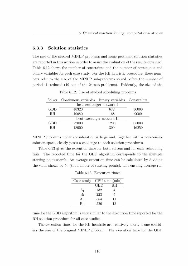
6. Chemical reaction fouling: computational studies
6.3.3 Solution statistics
The size of the studied MINLP problems and some pertinent solution statistics
are reported in this section in order to assist the evaluation of the results obtained.
Table 6.12 shows the number of constraints and the number of continuous and
binary variables for each case study. For the RH heuristic procedure, these num-
bers refer to the size of the MINLP sub-problems solved before the number of
periods is reduced (19 out of the 24 sub-problems). Evidently, the size of the
Table 6.12: Size of studied scheduling problems
Solver Continuous variables Binary variables Constraintsheat exchanger network I
GBD 40320 672 36000RH 10080 168 9000
heat exchanger network IIGBD 72000 1200 65000RH 18000 300 16250
MINLP problems under consideration is large and, together with a non-convex
solution space, clearly poses a challenge to both solution procedures.
Table 6.13 gives the execution time for both solvers and for each scheduling
task. The reported time for the GBD algorithm corresponds to the multiple
starting point search. An average execution time can be calculated by dividing
the value shown by 50 (the number of starting points). The ensuing average run
Table 6.13: Execution times
Case study CPU time (min)GBD RH
AI 132 4BI 223 5AII 554 11BII 526 13
time for the GBD algorithm is very similar to the execution time reported for the
RH solution procedure for all case studies.
The execution times for the RH heuristic are relatively short, if one consid-
ers the size of the original MINLP problem. The execution time for the GBD
110
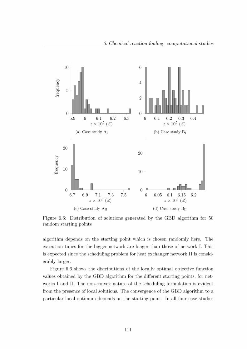
6. Chemical reaction fouling: computational studies
5.9 6 6.1 6.2 6.30
5
10
z × 105 (£)
frequen
cy
(a) Case study AI
6 6.1 6.2 6.3 6.40
2
4
6
z × 105 (£)
(b) Case study BI
6.7 6.9 7.1 7.3 7.50
10
20
z × 105 (£)
frequen
cy
(c) Case study AII
6 6.05 6.1 6.15 6.20
10
20
z × 105 (£)
(d) Case study BII
Figure 6.6: Distribution of solutions generated by the GBD algorithm for 50random starting points
algorithm depends on the starting point which is chosen randomly here. The
execution times for the bigger network are longer than those of network I. This
is expected since the scheduling problem for heat exchanger network II is consid-
erably larger.
Figure 6.6 shows the distributions of the locally optimal objective function
values obtained by the GBD algorithm for the different starting points, for net-
works I and II. The non-convex nature of the scheduling formulation is evident
from the presence of local solutions. The convergence of the GBD algorithm to a
particular local optimum depends on the starting point. In all four case studies
111

6. Chemical reaction fouling: computational studies
the GBD algorithm converged to the reported optimal solution only once. It
is, however, apparent from the dispersion of local solutions that a large number
of local optima lies within a short range (with respect to the magnitude of the
objective values reported). For case study AI, the local points generated lie in a
band of width 0.3× 10⁵ £, for case study BI in a band of width 0.4× 10⁵£ and
for case study BII in a band of width 0.2× 10⁵£. The band is slightly bigger for
case study AII: 0.7× 10⁵.
6.4 Conclusions
The scheduling framework presented in Chapter 5 was used to obtain cleaning
programmes for an isolated unit and two heat exchanger networks operating sub-
ject to chemical reaction fouling. Two cases were studied for each network and
the isolated unit, one with a higher coke formation rate than the other.
The results presented for the single unit exhibited the merits for optimising
the cleaning schedule: considerable savings are achieved compared to the no-
cleaning situation. Furthermore, the results suggest that for an isolated unit, it is
possible to identify an optimal mixed-cleaning campaign which can be repeated
over time. This optimal heat exchanger cycle, called the cleaning super-cycle,
includes a number of chemical actions before concluding with a mechanical action
which resets the unit to a completely clean state. The advantage of adapting
such a mixed-cleaning strategy is that the operating time before time-consuming
mechanical actions is prolonged by performing short-length chemical actions.
The Outer Approximation/Equality Relaxation (OA/ER) algorithm was suc-
cessfully used to obtain cleaning schedules for the isolated heat exchanger, but
failed to generate a solution for the case studies concerning the two heat ex-
changer networks. In all cases, the DICOPT R© solver remained trapped in the
first iteration for a relatively long period of time, as it was not able to solve the
first Master problem. The failure of the solver is due to the large size of the
MINLP scheduling models.
The Generalised Benders Decomposition (GBD) algorithm and the Receding
Horizon (RH) heuristic procedure described in Chapter 5 were used to optimise
the cleaning schedules for a network of 14 units and a network of 25 units. The
112

6. Chemical reaction fouling: computational studies
performance of the GBD algorithm and the RH heuristic procedure are found to
be satisfactory with respect to the computational effort required to generate a
solution.
A multiple starting point search was used in order to increase the possibility
of attaining a ‘good’ quality local solution: for each case study the scheduling
problem was solved by the GBD algorithm for 50 random starting points. These
starting points were feasible combinations of the binary variables. For the major-
ity of the starting points the algorithm converged to a different local optimum,
indicating the non-convex nature of the MINLP scheduling problem. The best
solution found was reported. No multiple starting point scheme was implemented
in conjunction with the RH heuristic.
The schedules generated by the two solution procedures are not always similar
in terms of objective function value or cleaning choices. Also, the schedules
obtained by the GBD algorithm are congested around the midpoint of the time
horizon, while the schedules generated by the RH heuristic are more sparse.
It emerges from the results that when deciding which units to clean the solvers
balance the choice between high heat load and high fouling rates. In that respect,
the units with moderate to relatively high heat load and moderate to relatively
fast fouling rates are selected for cleaning more frequently than units with just
high heat load or just high fouling rates.
The cleaning schedules generated suggest the importance of the thermal con-
ductivities of the two layers. The cleaning programmes for the cases with high
coke formation rate are found to be very different than those with slow coke
formation rate. The increase in the amount of aged material in the system and
the proportional decrease in the amount of fresh deposit lead to a significant
reduction of the energy losses.
113

Chapter 7
Biological fouling: formulations
& computational studies
Chapters 5 and 6 discussed the problem of scheduling the cleaning actions for
heat exchanger networks subject to chemical reaction fouling when two cleaning
methods are available. The current chapter studies the scheduling problem for
heat exchanger networks subject to biological fouling assuming that three cleaning
options are available.
The biological fouling model used to describe the progression of the thermal
fouling resistance is described first. Then, two mathematical programming for-
mulations are proposed for the scheduling problem under investigation. Section
7.4 presents and discusses the results obtained from implementing one of the
formulations for a small network of heat exchangers.
7.1 Introductory remarks
The problem of scheduling the cleaning actions for heat exchanger networks sub-
ject to biological fouling is formulated according to the methodology presented
in Chapter 5 for networks operating under chemical reaction fouling. The heat
transfer analysis, the time representation and the process constraints remain the
same. The set of assumptions regarding heat transfer analysis is restated for the
sake of lucidity. For a shell-and-tube unit in operation these are:
114
7. Biological fouling: formulations & computational studies
a) it is in counter-current mode. Therefore, the configuration correction factor,
F , is equal to one;
b) the cold stream flows on the tube side and the hot stream on the shell side;
c) none of the streams changes phase;
d) the specific heat capacities of the streams are constant;
e) the mass flow rate of both streams remains constant.
The fouling analysis differs since here the accumulation of deposits is due
to a different formation mechanism. Consequently this brings alterations to the
simulation constraints. Moreover, there are now three available cleaning actions.
7.2 Fouling analysis
The accumulation of foulant is entirely due to the attachment and growth of
micro-organisms on the heat transfer surface. It is assumed that a biofilm is
formed only on the tube side of the exchanger while the shell side remains clean.
The thermal fouling resistance, Rf , is considered to be zero for a period of
time known as the initiation period, during which the heat transfer surface is
colonised by micro-organisms [Bott, 2011]. After this induction period and the
pre-conditioning of the surface, the progression of Rf follows an asymptotic curve
such as the one shown in Figure 4.2.
The three cleaning methods available for the removal of the biofilm are the
following: (i) a water flush which removes most of the biofilm but leaves the
surface colonised and ready to restart growth when process operation resumes;
(ii) chemical cleaning, which removes all biofilm and imposes a short initiation
period; and (iii) chemical cleaning followed by disinfection (referred to as chemical
disinfection for simplicity), which restores the efficiency of the heat exchanger
back to its clean level and results in a longer induction period. The progression
of the thermal fouling resistance after each cleaning action is shown in Figure
7.1(a).
115

7. Biological fouling: formulations & computational studies
t
Rf
A B C
A: water flushB: chemical cleaning
C: chemical disinfection
tIbtI
(a) Initiation period and asymptotic model
t
Rf
tchle tflle
(b) Sigmoid model
Figure 7.1: Progression of thermal fouling resistance after cleaning
Curve A shows the evolution of Rf after a water flush cleaning is performed,
where the surface is receptive to immediate biofilm growth. Curves B and C give
the progression of Rf after a chemical cleaning, which imposes a short initiation
period of lengthtIb
(b > 1) and after a chemical disinfection, which results in a
longer induction time, tI , respectively.
Following a cleaning action, it must be determined if an initiation period will
occur and which of the three curves A, B and C will describe the progression
of Rf . The model proposed by Kern and Seaton [1959] can be used to describe
the asymptotic behaviour of Rf , but does not consider the initiation period. The
116

7. Biological fouling: formulations & computational studies
latter can be included explicitly in the scheduling formulation but this introduces
additional complexity. Modifications need to be made to the time discretisation
scheme presented in Section 5.3 since two extra elements must be added to each
discrete period (at the beginning of the period) to account for the shorter or longer
initiation time after a chemical action or a chemical disinfection, respectively.
Alternatively, the fouling model proposed by Nebot et al. [2007] can be used
to describe the progression of thermal fouling resistance in time. The evolution of
Rf follows a sigmoidal curve such as the one shown in Figure 7.1(b). The thermal
fouling resistance is modelled as to be negligible for a period of time (t ∈ [0, tflle ]
on the graph) termed as the delay period. Thereafter, the biofilm undergoes
an exponential growth before reaching a steady state, where the thermal fouling
resistance attains the asymptotic value Rf∞ . The delay period during which the
value of Rf is almost zero corresponds to the initiation period during which the
value of Rf is zero.
After a cleaning action is performed, the evolution of Rf will resume from a
different time point (starting time), t0, on the sigmoid curve:
t0 =
0, if chemical disinfection has occured
tchle , if chemical cleaning has occured
tflle , if water flush cleaning has occured
(7.1)
The parameters tflle and tchle are the ‘leap’ times after a water flush action and a
chemical action, respectively. The parameters derive their name from the fact
that the evolution of Rf does not resume from zero but from a point forward in
time (a jump in time takes place). Note that tflle = tI and tchle = tI/b.
The merit of using the model suggested by Nebot et al. [2007] is due to the
fact that it takes into account the existence of the induction period while still
being continuous. It is relatively straightforward to incorporate this fouling model
in the scheduling formulation since it does not require any changes in the time
representation scheme. Hence, the complexity of the scheduling problem does not
increase.
According to Nebot et al. [2007], the fouling rate is given by the following
117

7. Biological fouling: formulations & computational studies
second order kinetic expression:
dRf
dt= k(Rf∞ −Rf )Rf . (7.2)
where k is a constant representing the rate at which the asymptotic value Rf∞
is attained. In this work, the rate is considered to be uniform across the tubes
of the unit. By integration of equation (7.2) an algebraic expression is obtained
which relates the thermal fouling resistance to time as follows:
Rf =Rf∞
1 + (Rf∞Rf0− 1) exp(−kRf∞t)
(7.3)
where Rf0 represents the thermal fouling resistance during the delay period. Since
Rf is negligible during the early stages when the heat transfer surface is colonised,
the parameter Rf0 has a very small value.
Equation (7.2) is a modified version of the generalised expression for asymp-
totic fouling proposed by Konak [1973] for any deposition mechanism, viz.
dRf
dt= k(Rf∞ −Rf )
n (7.4)
The term (Rf∞ − Rf ) was postulated by Konak [1973] to be the driving force
for the accumulation of foulant. Integrating equation (7.4) for n = 1 yields the
following expression:
− ln(1− Rf
Rf∞
) = kt (7.5)
which is a form of equation (4.6) proposed by Kern and Seaton [1959].
The differential equation (7.2) used by Nebot et al. [2007] to describe the
growth of the biofouling layer is not a new one. It coincides in form with the
logistic function suggested by the French mathematician Pierre-Francois Verhulst
in 1838 to describe the self-limiting growth of a biological population.
118
7. Biological fouling: formulations & computational studies
7.3 Mathematical programming formulations
The task is to identify the optimal cleaning schedule for a heat exchanger net-
work subject to biological fouling. Let us assume that U ′ = {1, 2, . . . , nu} is
the set of units, P = {1, 2, . . . , np} the set of discrete periods and M = {fl :
water flush, ch : chemical, cd : chemical disinfection} the set of available clean-
ing modes. Two mathematical programming formulations are described below
for the studied problem: one MILP and one non-convex MINLP.
The binary variables yijm, for i ∈ U ′; j ∈ P ; m ∈M , are such that correspond
to ‘yes’ or ‘no’ decisions (cleaning choices and timings) as follows:
yijm =
1, if cleaning mode m is chosen for unit i at period j
0, if cleaning mode m is not chosen for unit i at period j(7.6)
Time is discretized as detailed in Section 5.3. Accordingly, orthogonal collo-
cation is used in order to acquire numerical estimations for the integrals involved
in the objective function of the scheduling problem. Furthermore, the duration
of a chemical disinfection is equal to the added length of elements 2 and 3 (see
Figure 5.3), while the duration of a chemical cleaning is equal to the length of
element 3 alone. The duration of a water flush cleaning is negligible compared
to the time scales involved in the problem and therefore it is assumed to be zero
days.
To facilitate the description of the proposed formulations the following func-
tion of v is defined:
rf (v) ≡ Rf∞
1 + (Rf∞Rf0− 1) exp(−kRf∞v)
. (7.7)
7.3.1 MINLP formulation
With the intention of avoiding confusion it is clarified that time, the dimension
with the aid of which events are ordered as past, present or future and which is
discretised here, does not coincide with the variable tijkl involved in some of the
constraints given below. Here, the variable tijkl is used in order to keep track of the
119

7. Biological fouling: formulations & computational studies
thermal fouling resistance, Rf , for a unit after a cleaning action is performed. It
is because of the discontinuities introduced in the system by the binary variables
that tijkl does not represent the dimension of time. For the remainder of this
chapter, the variable tijkl is referred to as sigmoid time.
Assume that all units are in a completely clean state at the beginning of the
time horizon. The sigmoid time for each unit for the first element of the first
period is given by
ti,1,1,l = τ lh1; i = 1, 2, . . . , nu; l = 0, 1, 2, 3 (7.8)
where, recall, τ l is the normalised position of the l-th Radau collocation node and
h1 the time-length of element 1. For any other period the sigmoid time during
element 1 has to account for any cleaning action as follows:
tij,1,l = τ lh1 + ti,j−1,3,3(1−∑m∈M
yi,j−1,m) + ti,chd yi,j−1,ch + ti,flle yi,j−1,f l (7.9)
i = 1, 2, . . . , nu; j = 2, 3, . . . , np; l = 0, 1, 2, 3.
To understand the set of constraints (7.9) better, suppose that a chemical action
is selected for unit i at period j−1, i.e. yi,j−1,ch = 1. In that case, equation (7.9)
yields the following set of equality constraints:
tij,1,l = τ lh1 + ti,chle ; l = 0, 1, 2, 3.
This correctly reflects the fact that the chemical cleaning action in period j − 1
has effectively reset time, as far as the fouling resistance is concerned, to tchle . The
set of equality constraints that involve the temperatures of the streams is given
by
T ijklh,o = T ijklc,in + (T ijklh,in − Tijklc,o ) exp
( AiCi
1U i0
+ rf (tijkl)
)(7.10)
i = 1, 2, . . . , nu; j = 1, 2, . . . , np; k = 1; l = 0, 1, 2, 3
for element 1.
120
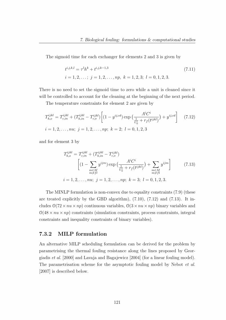
7. Biological fouling: formulations & computational studies
The sigmoid time for each exchanger for elements 2 and 3 is given by
ti,j,k,l = τ lhk + ti,j,k−1,3 (7.11)
i = 1, 2, . . . ; j = 1, 2, . . . , np, k = 1, 2, 3; l = 0, 1, 2, 3.
There is no need to set the sigmoid time to zero while a unit is cleaned since it
will be controlled to account for the cleaning at the beginning of the next period.
The temperature constraints for element 2 are given by
T ijklh,o = T ijklc,in + (T ijklh,in − Tijklc,o )
[(1− yij,cd) exp
( AiCi
1U i0
+ rf (tijkl)
)+ yij,cd
](7.12)
i = 1, 2, . . . , nu; j = 1, 2, . . . , np; k = 2; l = 0, 1, 2, 3
and for element 3 by
T ijklh,o = T ijklc,in + (T ijklh,in − Tijklc,o )[
(1−∑m∈Mm6=fl
yijm) exp( AiCi
1U i0
+ rf (tijkl)
)+∑m∈Mm 6=fl
yijm]
(7.13)
i = 1, 2, . . . , nu; j = 1, 2, . . . , np; k = 3; l = 0, 1, 2, 3.
The MINLP formulation is non-convex due to equality constraints (7.9) (these
are treated explicitly by the GBD algorithm), (7.10), (7.12) and (7.13). It in-
cludes O(72×nu×np) continuous variables, O(3×nu×np) binary variables and
O(48×nu×np) constraints (simulation constraints, process constraints, integral
constraints and inequality constraints of binary variables).
7.3.2 MILP formulation
An alternative MILP scheduling formulation can be derived for the problem by
parametrising the thermal fouling resistance along the lines proposed by Geor-
giadis et al. [2000] and Lavaja and Bagajewicz [2004] (for a linear fouling model).
The parametrisation scheme for the asymptotic fouling model by Nebot et al.
[2007] is described below.
121

7. Biological fouling: formulations & computational studies
Assume that the completely clean unit i will start operating at the beginning
of period 1. The thermal fouling resistance during the first period is given by
Ri,1,klf = rf (τ
lhk +k−1∑n=1
hn); k = 1, 2, 3; l = 0, 1, 2, 3. (7.14)
For the second period the thermal fouling resistance takes into account any pos-
sible cleaning action performed in period 1 as follows:
Ri,2,klf = rf (τ
lhk +k−1∑n=1
hn + ti,chle )yi,1,ch + rf (τlhk +
k−1∑n=1
hn + ti,flle )yi,1,f l (7.15)
rf (τlhk +
k−1∑n=1
hn)yi,1,cd + rf (tp + τ lhk +k−1∑n=1
hn)(1−∑m∈M
yi,1,m)
k = 1,2, 3; l = 0, 1, 2, 3.
where tp =3∑
k=1
hk is the time-length of a period. Accordingly, for the third period
the thermal fouling resistance is given by
Ri,3,klf =
[rf (τ
lhk +k−1∑n=1
hn + ti,chle + tp)yi,1,ch + rf (τ
lhk +k−1∑n=1
hn + ti,flle + tp)yi,1,f l
+ rf (τlhk +
k−1∑n=1
hn + tp)yi,1,cd
](1−
∑m∈M
yi,2,m) (7.16)
+ rf (τlhk +
k−1∑n=1
hn + ti,chle )yi,2,ch + rf (τlhk +
k−1∑n=1
hn + ti,flle )yi,2,f l
+ rf (τlhk +
k−1∑n=1
hn)yi,2,cd
+ rf (2tp + τ lhk +k−1∑n=1
hn)2∏p=1
(1−∑m∈M
yipm)
k = 1,2, 3; l = 0, 1, 2, 3.
If a water flush cleaning is performed at period 1 (yi,1,f l = 1) the above set of
122
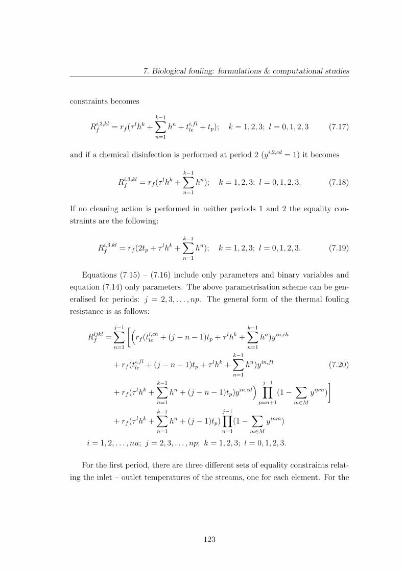
7. Biological fouling: formulations & computational studies
constraints becomes
Ri,3,klf = rf (τ
lhk +k−1∑n=1
hn + ti,flle + tp); k = 1, 2, 3; l = 0, 1, 2, 3 (7.17)
and if a chemical disinfection is performed at period 2 (yi,2,cd = 1) it becomes
Ri,3,klf = rf (τ
lhk +k−1∑n=1
hn); k = 1, 2, 3; l = 0, 1, 2, 3. (7.18)
If no cleaning action is performed in neither periods 1 and 2 the equality con-
straints are the following:
Ri,3,klf = rf (2tp + τ lhk +
k−1∑n=1
hn); k = 1, 2, 3; l = 0, 1, 2, 3. (7.19)
Equations (7.15) – (7.16) include only parameters and binary variables and
equation (7.14) only parameters. The above parametrisation scheme can be gen-
eralised for periods: j = 2, 3, . . . , np. The general form of the thermal fouling
resistance is as follows:
Rijklf =
j−1∑n=1
[(rf (t
i,chle + (j − n− 1)tp + τ lhk +
k−1∑n=1
hn)yin,ch
+ rf (ti,flle + (j − n− 1)tp + τ lhk +
k−1∑n=1
hn)yin,fl (7.20)
+ rf (τlhk +
k−1∑n=1
hn + (j − n− 1)tp)yin,cd) j−1∏p=n+1
(1−∑m∈M
yipm)
]
+ rf (τlhk +
k−1∑n=1
hn + (j − 1)tp)
j−1∏n=1
(1−∑m∈M
yinm)
i = 1, 2, . . . , nu; j = 2, 3, . . . , np; k = 1, 2, 3; l = 0, 1, 2, 3.
For the first period, there are three different sets of equality constraints relat-
ing the inlet – outlet temperatures of the streams, one for each element. For the
123

7. Biological fouling: formulations & computational studies
first element the set is as follows:
T ijklh,o = T ijklc,in + (T ijklh,in − Tijklc,o ) exp
( AiCi
1U i0
+ rf (τ lhk)
)(7.21)
i = 1, 2, . . . , nu; j = 1; k = 1; l = 0, 1, 2, 3.
For element 2 the constraints needs to account for a chemical disinfection, viz.
T ijklh,o = T ijklc,in + (T ijklh,in − Tijklc,o )[
(1− yij,cd) exp( AiCi
1U i0
+ rf (τ lhk +∑k−1
n=1 hn)
)+ yij,cd
](7.22)
i = 1, 2, . . . , nu; j = 1; k = 2; l = 0, 1, 2, 3.
Moreover for element 3 the equality constraints are modified to take into account
a chemical disinfection or chemical cleaning as follows:
T ijklh,o = T ijklc,in + (T ijklh,in − Tijklc,o )[
(1−∑m∈Mm6=fl
yijm)
exp( AiCi
1U i0
+ rf (τ lhk +∑k−1
n=1 hn)
) +∑m∈Mm 6=fl
yijm]
(7.23)
i = 1, 2, . . . , nu; j = 1; k = 3; l = 0, 1, 2, 3.
The constraints given by equation (7.21) are linear, while the constraints given by
equations (7.22) – (7.23) include only products of binary variables with continuous
variables which can be easily replaced by new linear constraints [Williams, 1990],
with the addition of new continuous variables, as shown next.
The term xy, where x is a continuous variable and y a binary variable, can
be replaced by a new continuous variable v by adding the following logical con-
straints:
v −By ≤ 0 (7.24)
v − x ≤ 0 (7.25)
x− v +By ≤ B (7.26)
124
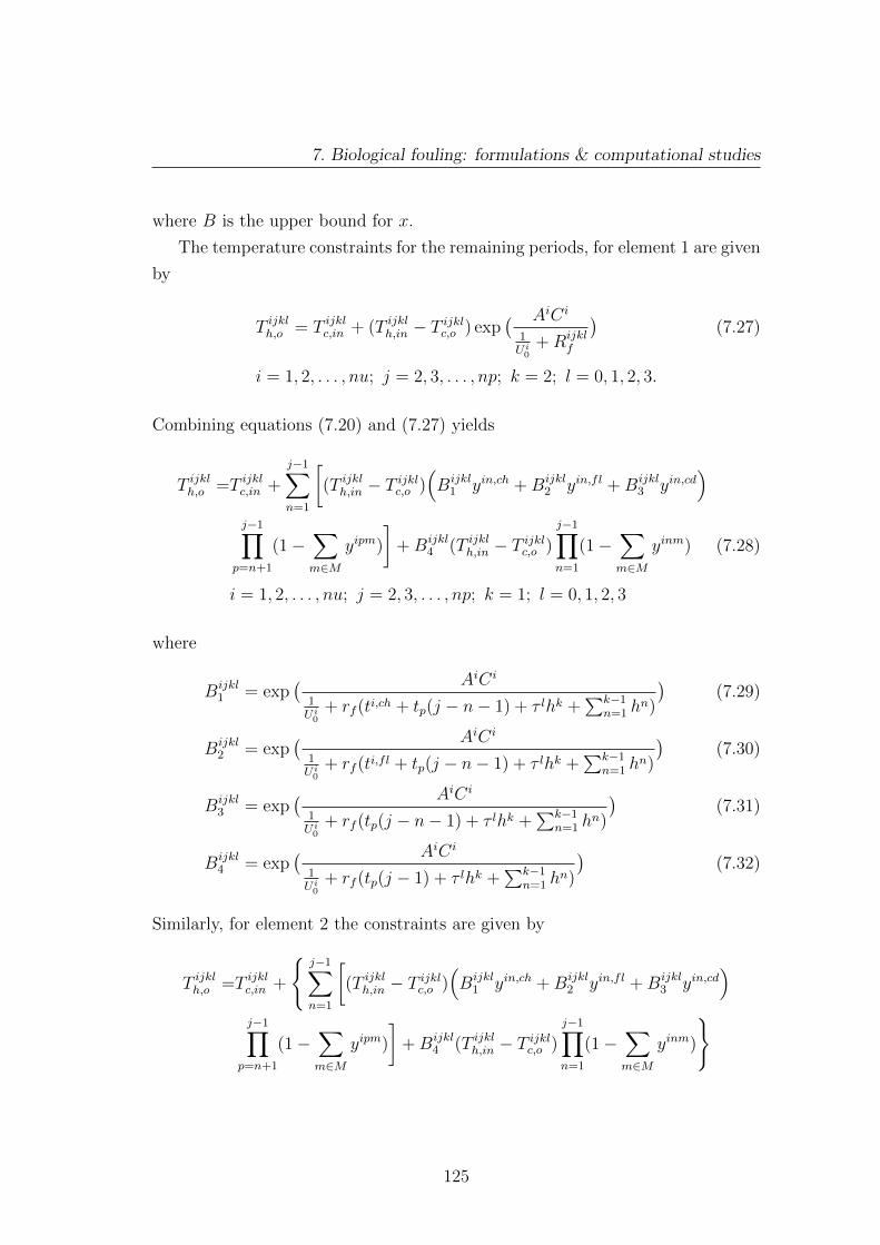
7. Biological fouling: formulations & computational studies
where B is the upper bound for x.
The temperature constraints for the remaining periods, for element 1 are given
by
T ijklh,o = T ijklc,in + (T ijklh,in − Tijklc,o ) exp
( AiCi
1U i0
+Rijklf
)(7.27)
i = 1, 2, . . . , nu; j = 2, 3, . . . , np; k = 2; l = 0, 1, 2, 3.
Combining equations (7.20) and (7.27) yields
T ijklh,o =T ijklc,in +
j−1∑n=1
[(T ijklh,in − T
ijklc,o )
(Bijkl
1 yin,ch +Bijkl2 yin,fl +Bijkl
3 yin,cd)
j−1∏p=n+1
(1−∑m∈M
yipm)
]+Bijkl
4 (T ijklh,in − Tijklc,o )
j−1∏n=1
(1−∑m∈M
yinm) (7.28)
i = 1, 2, . . . , nu; j = 2, 3, . . . , np; k = 1; l = 0, 1, 2, 3
where
Bijkl1 = exp
( AiCi
1U i0
+ rf (ti,ch + tp(j − n− 1) + τ lhk +∑k−1
n=1 hn)
)(7.29)
Bijkl2 = exp
( AiCi
1U i0
+ rf (ti,fl + tp(j − n− 1) + τ lhk +∑k−1
n=1 hn)
)(7.30)
Bijkl3 = exp
( AiCi
1U i0
+ rf (tp(j − n− 1) + τ lhk +∑k−1
n=1 hn)
)(7.31)
Bijkl4 = exp
( AiCi
1U i0
+ rf (tp(j − 1) + τ lhk +∑k−1
n=1 hn)
)(7.32)
Similarly, for element 2 the constraints are given by
T ijklh,o =T ijklc,in +
{j−1∑n=1
[(T ijklh,in − T
ijklc,o )
(Bijkl
1 yin,ch +Bijkl2 yin,fl +Bijkl
3 yin,cd)
j−1∏p=n+1
(1−∑m∈M
yipm)
]+Bijkl
4 (T ijklh,in − Tijklc,o )
j−1∏n=1
(1−∑m∈M
yinm)
}
125

7. Biological fouling: formulations & computational studies
(1− yij,cd) + (T ijklh,in − Tijklc,o )yij,cd (7.33)
i = 1, 2, . . . , nu; j = 2, 3, . . . , np; k = 2; l = 0, 1, 2, 3
and for element 3 by
T ijklh,o =T ijklc,in +
{j−1∑n=1
[(T ijklh,in − T
ijklc,o )
(Bijkl
1 yin,ch +Bijkl2 yin,fl +Bijkl
3 yin,cd)
j−1∏p=n+1
(1−∑m∈M
yipm)
]+Bijkl
4 (T ijklh,in − Tijklc,o )
j−1∏n=1
(1−∑m∈M
yinm)
}(1−
∑m∈Mm 6=fl
yijm) + (T ijklh,in − Tijklc,o )
∑m∈Mm 6=fl
yijm (7.34)
i = 1, 2, . . . , nu; j = 2, 3, . . . , np; k = 3; l = 0, 1, 2, 3.
In equations (7.28), (7.33), (7.34) the binary variables and the binary products
are moved out of the exponentials (terms Bijkl1 , Bijkl
2 , Bijkl3 and Bijkl
4 ). This is due
to the fact that one, and only one, of the corresponding terms can be different
from zero.
The nonlinearities in the aforementioned sets of constraints consist of products
of binary variables with continuous variables. These can be linearised by intro-
ducing new variables and additional constraints as shown above. However, by
doing so the size of the resulting MILP models will grow rapidly as the number of
periods and the number of units increases. Applying the MILP formulation for a
heat exchanger network is impractical (as Lavaja and Bagajewicz [2004] reported
for a similar formulation), even if the global minimum can be obtained, since the
solution of the corresponding model will be computationally unaffordable.
7.3.3 Objective function
The objective function depends on the type of network under consideration and
the performance targets imposed by the operator or other interacting processes.
Here, for the computational studies undertaken and presented in the next section,
the objective function needs to include only the energy losses due to fouling, the
lost-production opportunity during cleaning intervals and the cost of the cleaning
126

7. Biological fouling: formulations & computational studies
actions, as follows:
z =nu∑i=1
np∑j=1
fe(Qi
0
3∑k=1
hk − I ij,3,31
)+
nu∑i=1
np∑j=1
∑m∈M
yijmcm (7.35)
where C = {cm : m ∈ M} is the cost vector. The variable I ijkl1 (calculation of
integral for process costs) is involved in the equality constraints (5.46) – (5.48)
given in Chapter 5. These are re-introduced here:
3∑l=0
I ijkl1
dql(τn)
dτ= hnmn
cCnp,c(T
ijknc,o − T
ijknc,in ) (5.46)
i = 1, 2, . . . , nu; j = 1, 2, . . . , np; k = 1, 2, 3; n = 0, 1, 2, 3
I ij,1,11 = 0; i = 1, 2, . . . , nu; j = 1, 2, . . . , np (5.47)
I ijk,01 = I ij,k−1,31 ; i = 1, 2, . . . , nu; j = 1, 2, . . . , np; k = 2, 3. (5.48)
7.4 Computational studies
The MINLP formulation is implemented in the computational studies presented
next. The Generalised Bender’s Decomposition algorithm, described in Chapter
5, is utilised to solve the resulting scheduling models. Cleaning schedules are
obtained for the fictional heat exchanger network shown in Figure 7.2 for three
case studies with different fouling parameters.
1
2
3
coldstream
Figure 7.2: Heat exchanger network subject to biological fouling
Table 7.1 summarises the operating and design parameters for the three units
of the network. The energy cost is fe = 0.5 £/kW.day. Furthermore, the specific
heat capacity is Cp,h = 2.2 kJ/kg.K and Cp,c = 4.2 kJ/kg.K for the hot streams
127

7. Biological fouling: formulations & computational studies
and cold stream, respectively. The inlet temperature of the cold stream at the
first unit of the network is 25 oC.
Table 7.1: Operating and design parameters for heat exchanger network subjectto biological fouling
Unit Th,in mh mc U0 A Q0
(oC) (kg/s) (kg/s) (kW/m2.K) (m2) (MW)1 200 20.5 75 0.55 33 2.62 190 20 37.5 0.55 30 1.83 210 25.8 37.5 0.55 32.5 2.3
The parameters for the fouling model are given in Table 7.2. For case study
A, the thermal fouling resistance, Rf , in each unit, approaches the relatively
high asymptotic value, Rf∞ , with a relatively fast rate k. For case study B,
the asymptotic value is decreased by a factor of two, while the rate for each
exchanger remains the same compared to case study A. Finally, for case study C
the asymptotic value is equal to that of case study A but the rate, k, is decreased
by 33%. The changes in Rf∞ cause also the parameters tflle and tchle to take different
values.
Table 7.2: Parameters for biological fouling model
Unit Rf∞ Rf0 k tchle tflle(m2.K/kW) (m2.K/kW) (kW/m2.K.day) (days) (days)
case study A1 0.8 1×10⁻⁴ 0.18 19 382 0.8 1×10⁻⁴ 0.22 15 303 0.8 1×10⁻⁴ 0.25 13 26
case study B1 0.4 1×10⁻⁴ 0.18 31 622 0.4 1×10⁻⁴ 0.22 26 523 0.4 1×10⁻⁴ 0.25 23 46
case study C1 0.8 1×10⁻⁴ 0.12 24 482 0.8 1×10⁻⁴ 0.15 19 383 0.8 1×10⁻⁴ 0.17 17 34
If left unmitigated, the biofilm causes the overall heat transfer coefficient, U ,
128

7. Biological fouling: formulations & computational studies
to decrease from 0.55 kW/m2.K at the clean state to 0.38 kW/m2.K at the steady
state (31% drop), for case studies A and C. For case study B, U drops to 0.45
kW/m2.K, representing a 18% decrease compared to the fouling-free state.
The duration of the operating sub-period, top = h1, is chosen to be 10 days,
while the duration of a chemical disinfection, tcd = h2 + h3, is 5 days. Hence,
the length of a time period is 15 days. The duration of a chemical action is
tch = h3 = 1 day. Recall, the duration of a water flush cleaning is considered to
be negligible. The cleaning schedule is optimised over 24 periods (360 days).
Table 7.3 summarises the cleaning parameters used in the case studies.
Table 7.3: Cleaning parameters
Mode Cost (£) duration (days)fl 1000 0ch 2500 1cd 3500 5
A multiple starting point search is performed in order to increase the possi-
bility of finding a ‘good’ local solution. Therefore, the MINLP problem for each
case study is solved for 100 random starting points. These are feasible combina-
tions of the binary variables. Table 7.4 reports the best cleaning schedule and
the objective function value obtained for each of the case studies.
For case study A, operating the examined network without performing any
cleaning action for 360 days corresponds to an objective function value zno =
2.4 × 10⁵ £. Applying the best found cleaning schedule results in 46% savings.
The schedule includes cleaning by all three modes and the units are cleaned
frequently: nine cleaning actions are selected for units 1 and 3 and ten for unit
2. Unit 1 receives all the chemical actions and some water flush actions. Regular
water flush cleaning is performed on units 2 and 3, which also receive one and two
chemical disinfections, respectively. The cleaning actions span between periods 3
to 22.
For case study B, the savings for implementing the best schedule generated are
42% (zno = 1.2 × 10⁵£). Here, the cleaning actions are less frequent compared
to case study A, where fouling is more severe. One chemical disinfection, six
chemical actions and six water flushes are selected. Unit 1 receives only chemical
129
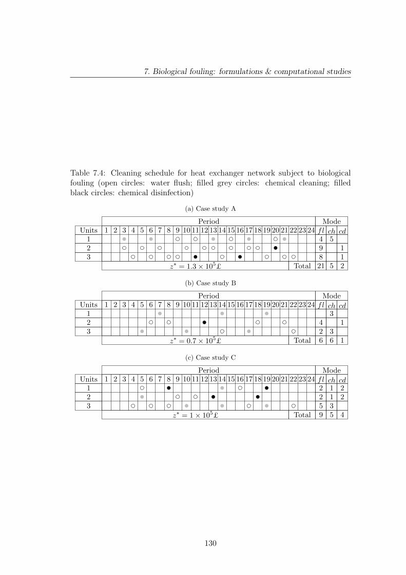
7. Biological fouling: formulations & computational studies
Table 7.4: Cleaning schedule for heat exchanger network subject to biologicalfouling (open circles: water flush; filled grey circles: chemical cleaning; filledblack circles: chemical disinfection)
(a) Case study A
1 2 3 4 5 6 7 8 9 10 11 12 13 14 15 16 17 18 19 20 21 22 23 24Period Mode
fl ch cdUnits123
Total 21 5 2
4 59 18 1
z∗ = 1.3× 10⁵£
(b) Case study B
1 2 3 4 5 6 7 8 9 10 11 12 13 14 15 16 17 18 19 20 21 22 23 24Period Mode
fl ch cdUnits123
Total 6 6 1
34 12 3
z∗ = 0.7× 10⁵£
(c) Case study C
1 2 3 4 5 6 7 8 9 10 11 12 13 14 15 16 17 18 19 20 21 22 23 24Period Mode
fl ch cdUnits123
Total 9 5 4
2 1 22 1 25 3
z∗ = 1× 10⁵£
130

7. Biological fouling: formulations & computational studies
actions, while unit 2 receives the chemical disinfection. All the cleaning actions
are performed between periods 5 to 22.
The optimal (best found) objective value for case study C is z∗ = 1×10⁵£ and
it yields savings of 54% compared to the no-cleaning situation, where the objective
value is zno = 2.2× 10⁵£. The best found cleaning programme includes cleaning
by all methods. A mixed cleaning campaign is performed on units 1 and 2, while
unit 3 receives only chemical and water flush cleaning.
Figures 7.3, 7.4 and 7.5 show the progression of the thermal fouling resistance,
Rf , in time for each unit, for case studies A, B and C, respectively. The time
profile of Rf for the no-cleaning situation is also displayed on the graphs.
As observed in Figure 7.3(a) the thermal fouling resistance for unit 1, which
has the highest heat load in the network, is maintained below 0.4 m2.K/kW during
the 360 days. For units 2 and 3, Rf reaches the asymptotic value, Rf∞ = 0.8
m2.K/kW, once. When no cleaning is performed, Rf attains the value of Rf∞ in
115 days, 96 days and 85 days in units 1, 2 and 3, respectively.
For case study B, the Rf < 0.3 m2.K/kW throughout the 24 periods for unit
2, while it exceeds this value only once for unit 1 and twice for unit 3. The
asymptotic value is attained after 209 days in unit 1 and after 171 days in units
2 and 3.
For case study C, the thermal fouling resistance of all three units is maintained
at a lower level than that for case study A. The value Rf∞ is reached after 171
days and 136 days for units 1 and 2, respectively. For unit 3, the growth reaches
the steady state after 121 days have elapsed.
For the three case studies, comparing the times in which the asymptotic value
is attained in each unit, it becomes apparent that the decay in network perfor-
mance is faster for case study A than for case studies B and C. Also, it is faster
for case study C than for case study B. This also becomes palpable when compar-
ing the objective values for the no-cleaning situation. The aforesaid explains the
relatively large number of cleaning actions selected for case study A (29 actions)
compared to case studies B (13 actions) and C (18 actions).
It emerges from the results that cleaning by water flush is favoured over the
other two methods when the thermal fouling resistance increases relatively quickly
for these cost parameters. Twenty-one water flush actions are selected for case
131

7. Biological fouling: formulations & computational studies
60 120 180 240 300 3600
0.2
0.4
0.6
0.8
t (days)
Rf(m
2.K/kW
)
No cleaningCleaning schedule
(a) unit 1
60 120 180 240 300 3600
0.2
0.4
0.6
0.8
t (days)
Rf(m
2.K/kW
)
(b) unit 2
60 120 180 240 300 3600
0.2
0.4
0.6
0.8
t (days)
Rf(m
2.K/kW
)
(c) unit 3
Figure 7.3: Time profile of Rf : case study A
132

7. Biological fouling: formulations & computational studies
60 120 180 240 300 3600
0.1
0.2
0.3
0.4
t (days)
Rf(m
2.K/kW
)No cleaning
Cleaning schedule
(a) unit 1
60 120 180 240 300 3600
0.1
0.2
0.3
0.4
t (days)
Rf(m
2.K/kW
)
(b) unit 2
60 120 180 240 300 3600
0.1
0.2
0.3
0.4
t (days)
Rf(m
2.K/kW
)
(c) unit 3
Figure 7.4: Time profile of Rf : case study B
133
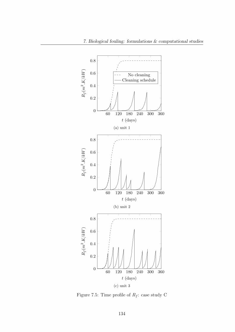
7. Biological fouling: formulations & computational studies
60 120 180 240 300 3600
0.2
0.4
0.6
0.8
t (days)
Rf(m
2.K/kW
)
No cleaningCleaning schedule
(a) unit 1
60 120 180 240 300 3600
0.2
0.4
0.6
0.8
t (days)
Rf(m
2.K/kW
)
(b) unit 2
60 120 180 240 300 3600
0.2
0.4
0.6
0.8
t (days)
Rf(m
2.K/kW
)
(c) unit 3
Figure 7.5: Time profile of Rf : case study C
134

7. Biological fouling: formulations & computational studies
study A, where the decay in heat transfer efficiency is faster than the other
two case studies. The solver prefers the cheapest, albeit less effective, water
flush cleaning which has negligible duration and therefore does not result in loss
of production, rather than the other two more time-consuming and expensive
methods. For case studies B and C, where the rate of decay is slower compared
to case study A, fewer water flush actions are selected.
7.4.1 Solution statistics
The MINLP problem solved for each case study involved 216 binary variables,
5100 continuous variables and 5400 constraints. The execution time for solving
the scheduling problem for 100 different random points was 50 minutes for case
study A and 38 minutes for cases B and C.
Figures 7.6(a) – 7.6(c) show the distribution of the local points obtained during
the multiple starting point search, for case studies A, B and C, respectively. The
local optima generated lie within a band of width 0.5×10⁵£ for case study A, of
width 0.2×10⁵£ for case study B and of width 0.6×10⁵£ for case study C.
7.5 Conclusions
A novel approach was presented in this chapter for the problem of scheduling
the cleaning actions for heat exchanger networks operating subject to biological
fouling. The proposed scheduling approach features the selection between three
cleaning techniques and it explores the concept of selection between cleaning
methods further.
The approach postulates that the receptiveness of the surface to immediate
biofilm growth differs after each cleaning action. The first cleaning method is
a simple water flush which removes most of the biofouling layer but leaves the
heat transfer surface colonised and ready to resume growth as soon as the unit
is back in operation. The second technique, a chemical cleaning, removes all the
biofoulant and imposes a short induction period. The third and most effective
cleaning option refers to chemical cleaning followed by disinfection, which resets
the surface to the clean, non-colonised, state and results in a longer induction
135
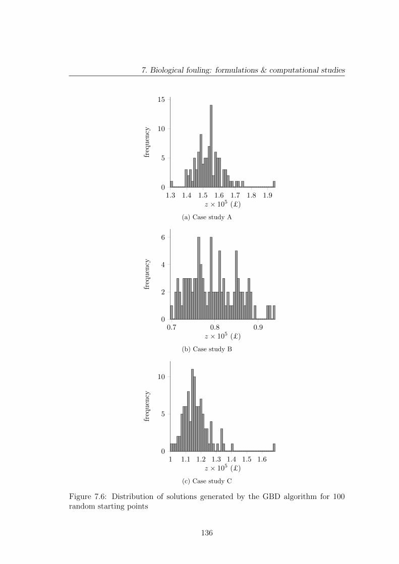
7. Biological fouling: formulations & computational studies
1.3 1.4 1.5 1.6 1.7 1.8 1.90
5
10
15
z × 105 (£)
frequen
cy
(a) Case study A
0.7 0.8 0.90
2
4
6
z × 105 (£)
frequen
cy
(b) Case study B
1 1.1 1.2 1.3 1.4 1.5 1.60
5
10
z × 105 (£)
frequen
cy
(c) Case study C
Figure 7.6: Distribution of solutions generated by the GBD algorithm for 100random starting points
136
7. Biological fouling: formulations & computational studies
period. This distinct conditioning of the heat transfer surface by each cleaning
method acts as the selection criterion.
The progression of the thermal fouling resistance in time is modelled according
to the logistic model proposed by Nebot et al. [2007]. The benefit of using this
fouling model arises from the fact that it takes into account the presence of the
induction period during which the growth of biofoulant is sluggish. The evolution
of thermal fouling resistance follows a sigmoidal curve. At first, the thermal
resistance of the biofilm remains negligible for a time interval termed as the “delay
period”, which corresponds to the induction period. Afterwards, the thermal
fouling resistance follows an exponential growth and asymptotic behaviour.
Two different mathematical programming formulations are introduced to de-
scribe the scheduling problem: a non-convex MINLP and an MILP. The former
corresponds to scheduling problems that cannot be solved to global optimality
but remain tractable as the number of units and time periods increases. On the
other hand, the MILP formulation produces problems which can, in principle,
be solved to attain the global optimum but are not tractable for heat exchanger
networks involving more than a few units.
A series of computational studies was presented, demonstrating the imple-
mentation of the non-convex MINLP formulation for a small network of heat ex-
changers. The Generalised Bender’s Decomposition (GBD) algorithm was used
to obtain cleaning schedules in conjunction with a multiple starting point search.
The best mixed cleaning campaigns generated resulted in significant savings com-
pared to the no-cleaning case.
The results of the computational studies are sensitive to the parameters of
the fouling model. Thus, reliable estimation of these parameters is crucial for the
application of the proposed scheduling approach.
137

Chapter 8
Conclusions & Recommendations
The theme of the first part of this thesis has been the Travelling Salesman Prob-
lem (TSP). A novel way of describing the problem mathematically has been pro-
posed, which resulted in reducing the binary degrees of freedom, for the first time,
to O(ndlog2(n)e). Three mathematical programming formulations have been in-
troduced and a series of computational studies has been conducted in order to
evaluate their computational performance in practice.
The second part of this dissertation reported the utilisation of Mixed-Integer
Programming (MIP) for scheduling the cleaning actions for heat exchanger net-
works subject to fouling. It described the extension of a novel work presented for
isolated units to networks of exchangers. The concept of choice between alterna-
tive cleaning methods was explored, with respect to the state of the deposit for
networks subject to chemical reaction fouling and the conditioning of the heat
transfer surface for networks subject to biological fouling.
8.1 Travelling Salesman Problem
The novel way of mathematically expressing the Travelling Salesman Problem
originates from work in Binary Arithmetic. The problem is described as the
repeated halving (partitioning) of the set of cities at each level of a regular and
full binary tree to left and right directions. Eventually, the cities are placed
sequentially on the leaves of the tree according to their position in the tour. In
138

8. Conclusions & Recommendations
that respect, the original problem can be viewed as a data storage problem on a
binary tree structure.
The new contribution of this work is that it reduces the binary degrees of
freedom for the Travelling Salesman Problem to O(ndlog2(n)e). To the author’s
knowledge, up to date, no other mathematical description of the problem, among
those found in the literature, succeeded in reducing the required number of bi-
nary variables below O(n2). The current work takes an incremental step towards
decreasing the formulation complexity of the Travelling Salesman Problem.
Two Mixed-Integer Linear Programming (MILP) formulations are developed
for the general case of the Asymmetric Travelling Salesman Problem (ATSP),
where the length of an arc connecting two cities depends on the direction in
which it is travelled. These are the Tree-1 and Tree-2 formulations. Another
MILP formulation is introduced for the special case where the distance between
two cities is calculated on the basis of the rectilinear metric. This special case is
referred to as the Manhattan Travelling Salesman Problem.
8.1.1 Asymmetric formulations
The two asymmetric formulations utilise a set of logical checks which force an arc
to be present in the optimal tour if two cities are placed on neighbouring leaves
of the binary tree. These adjacency constraints are the only difference between
formulations Tree-1 and Tree-2. The set of adjacency constraints proposed by
Millar and Cyrus [2000] is used in the Tree-1 formulation, while for Tree-2 the
logical checks are derived by Theorem 3.1. The Tree-1 and Tree-2 formulations
include O(n3) and O(n2dlog2(n)e) adjacency constraints, respectively.
The proposed formulations were implemented for small instances of the Trav-
elling Salesman Problem (n ≤ 12). It emerged from the results that the Tree-1
formulation is superior in computational performance to the Tree-2 formulation.
In particular, the branch-and-cut solver visits considerably fewer nodes of the
solution tree for Tree-1 than for Tree-2. In fact, the exact algorithm failed to
converge after one day of execution, when applying Tree-2 to a problem involving
12 cities. For the same problem, the optimal solution was obtained after 363 CPU
seconds when Tree-1 was applied. The dissimilar computational performance is
139

8. Conclusions & Recommendations
due to the different adjacency constraints included in each formulation.
Nevertheless, neither Tree-2 nor Tree-1 were successful when applied to prob-
lems involving 12 < n ≤ 20 cities. In all cases the branch-and-cut algorithm
failed to obtain the optimal solution after one day of execution. For all intents
and purposes, the solution of such small problems should be trivial.
The computational efficiency of the two formulations was found to be worse
than that of the well-known formulations proposed by Wong [1980] and Miller
et al. [1960]. The basis for the comparison was the strength of the Linear Pro-
gramming (LP) relaxation of each formulation. The formulation suggested by
Miller et al. [1960] is proven to be one of the weakest in comparison to others
existing in the literature [Oncan et al., 2009]. Therefore, the Tree-1 and Tree-2
are also placed among the weakest formulations.
The key finding that emerged from the computational studies is that the
Tree-1 and Tree-2 formulations are not tightly constrained, which means that
the resulting mixed-integer models have a large feasible region. It is due to this
that the proposed formulations can only be applied to very small instances of the
Travelling Salesman Problem.
8.1.2 Manhattan formulation
The computational performance of the Manhattan formulation in practice is
found to be worse that of Tree-1. For the solution of two small problems (n = 8
and n = 10), noticeably more computational effort is required when implement-
ing the former rather than the latter formulation. Therefore, it is concluded that
the Manhattan formulation is also loosely constrained.
8.1.3 Recommendations for future work
Future attempts for continuation of this work should focus on improving the Tree-
1 formulation. It is strongly recommended that additional constraints are added
to the formulation in order to reduce the size of the feasible region. Nonetheless,
the search for appropriate tightening constraints is not a trivial task and it might
not have fruitful results.
140

8. Conclusions & Recommendations
At the same time, future work should be directed towards developing pertinent
heuristic procedures in order to exploit the hierarchical structure of the asym-
metric formulations. Such a heuristic procedure might be successful in generating
initial tours that are close to the optimal solution.
8.2 Scheduling cleaning actions for heat exchanger
networks subject to fouling
In previous attempts to schedule the cleaning actions for heat exchangers sub-
ject to fouling it was postulated that the only form of cleaning available is one
that restores the performance of the unit back to its clean level. A recent study
presented by Ishiyama et al. [2011b] for an isolated evaporator included the eco-
nomic competition between two cleaning methods: one less time-consuming and
partially effective, the other requiring more resource but giving complete clean-
ing. The work reported in the second part of this thesis extends their approach
to accommodate heat exchanger networks and explores the concept of selection
of cleaning methods further.
The cleaning actions were scheduled for: (i) heat exchanger networks subject
to chemical reaction fouling and (ii) heat exchanger networks subject to biological
fouling. The goal was to minimise the process costs, including those associated
with the energy losses due to fouling and with the loss of production during
cleaning intervals, and the cleaning costs for an arbitrarily chosen time horizon.
8.2.1 Networks subject to chemical reaction fouling
The scheduling task for heat exchanger networks subject to chemical reaction
fouling, as per the work by Ishiyama et al. [2011b], featured the selection between
two methods that achieve a different degree of cleaning. Fouling was defined
as the combination of deposition and ageing phenomena. Ageing was assumed
to convert the initial fresh deposit into a harder and more conductive material
removable only by time and cost intensive mechanical cleaning. A less expensive
and faster chemical cleaning was assumed to remove only the soft deposit. A two
141

8. Conclusions & Recommendations
layer model was used to distinguish soft and aged deposits in order to track the
cleaning effectiveness and the decay in heat transfer efficiency.
A non-convex Mixed-Integer Nonlinear Programming (MINLP) formulation
was proposed to describe the scheduling problem. It was developed for networks
of single-pass shell-and-tube heat exchangers operating in counter-current mode.
The formulation can be altered to accommodate other types of units and flow
configurations without difficulty.
The scheduling formulation was applied to a heat exchanger operating in
isolation. A mixed cleaning cycle can be identified for a unit: a number of
chemical actions that partially restore the performance precede a mechanical
action that resets the exchanger to a clean state and restarts the cycle. This
mixed cleaning campaign was named a super-cycle and succeeds in extending the
operating time before lengthy mechanical cleaning by performing a number of
short-length chemical actions.
Cleaning schedules were also obtained for two preheat train networks of 14 and
25 units. The results suggest the importance of the fouling parameters, namely
the formation rates and the thermal conductivities of the two layers. The reliable
estimation of these parameters is imperative for the application of the proposed
scheduling formulation.
8.2.2 Networks subject to biological fouling
The new study of scheduling cleaning actions for heat exchanger networks sub-
ject to biological fouling involved the competition between three cleaning modes
differing in cost, duration and effectiveness. The evolution of the biofilm was
assumed to follow an exponential growth with asymptotic behaviour, after an
induction period during which the heat transfer surface is colonised. Thermal
fouling is modelled using the relation proposed by Nebot et al. [2007].
The three cleaning types considered are the following: (i) cheap water flush of
negligible duration which removes the bulk of the biofoulant but leaves the surface
colonised and ready to restart growth when process operation resumes; (ii) rela-
tively expensive but short-length chemical cleaning which removes all biofilm and
imposes a short induction period and (iii) expensive and time-consuming chem-
142

8. Conclusions & Recommendations
ical cleaning followed by disinfection, which resets the unit to its original clean
state.
A non-convex MINLP formulation was developed to describe the scheduling
problem. The formulation is applied to a small heat exchanger network in a
series of computational studies. Again, the results of the studies are found to be
sensitive to the parameters of the fouling model.
A MILP formulation can also be derived for the scheduling problem. For that
purpose, it was sufficient to express the thermal fouling resistance (of a unit) at
every node of a given time period as the function of the cleaning decisions of
all previous periods. The resulting constraints include only products of binary
variables with continuous variables, which can be replaced by linear terms using
standard transformations [Williams, 1990]. However, the transformations require
the addition of new continuous variables and extra constraints and cause the
MILP problem to be non-tractable for networks involving more than a few units.
8.2.3 Numerical methods
A direct transcription approach was adopted for the dynamic scheduling prob-
lems. The time horizon under consideration was discretised into a finite number
of periods, which in turn were represented by three elements in time. In each
element the variable profiles were approximated by polynomials, and orthogonal
collocation was used to calculate the values of the variables at selected points. In
particular, Radau collocation was chosen because it allows large time steps for
systems with slow time scales [Biegler, 2010].
The MINLP formulations presented for the two scenarios are non-convex.
Therefore, the resulting scheduling models cannot be solved to global optimality.
Despite the non-convex characteristics of the problems, it was decided to use a
rigorous solution method developed for convex problems, in a heuristic attempt
to obtain ‘good’ quality local optima.
The discretisation of time yielded relatively large scheduling problems. The
problems included a prohibitively large number of nonlinear equality constraints
with respect to the capabilities of the standard Outer Approximation/Equality
Relaxation (OA/ER) decomposition algorithm, which failed to converge to a
143
8. Conclusions & Recommendations
solution (after a considerable amount of time) when applied in practice.
Generalised Benders Decomposition (GBD) was selected as a suitable alter-
native algorithm to handle the relatively large Mixed-Integer Nonlinear Program-
ming problems. This algorithm was found to be superior to the OA/ER algorithm
in terms of computational performance, for this particular case. The reason for
this is that only one constraint is added to the Master Problem (see Section 5.5)
at each iteration of the GBD procedure, whereas the OA/ER algorithm demands
the addition of a relatively large number of constraints.
A heuristic solution procedure based on Model Predictive Control (MPC) was
also used to generate cleaning schedules for the two heat exchanger networks sub-
ject to chemical reaction fouling. At each iteration of the heuristic procedure the
GBD algorithm was utilised to solve the scheduling problem for a small number of
periods. In that respect, the scheduling problem is solved repeatedly over a short
time horizon rather than solved once for a long time horizon. The computational
cost for both approaches proved to be similar.
Inequality constraints involving continuous variables, e.g. performance targets
for a network, were not included in the scheduling formulation considered in this
work. The addition of such inequality constraints would presumably increase the
computational effort required by the GBD algorithm to obtain a local solution
or, in a more pessimistic scenario, cause the solver to terminate at an infeasible
point.
8.2.4 Recommendations for future work
The simple two-layer model included in the scheduling formulation proposed for
heat exchanger networks subject to chemical reaction fouling assumes that the
rates of gel and coke formation are constant throughout process operation. Future
continuation of this work can consider more detailed two layer models, such as
the ones presented by Ishiyama et al. [2011a], where the gel formation rate and
coke formation rate depend on the gel/bulk-fluid interface temperature and the
gel/coke interface temperature, respectively. A more detailed fouling analysis will
lead to more valid estimates of the decay in heat transfer efficiency. However,
these more realistic fouling models are highly nonlinear. As a result, the new
144

8. Conclusions & Recommendations
scheduling formulations might yield MINLP problems that are no longer tractable
by the GBD algorithm employed in the current work. In such an event, other apt
heuristic solution procedures will have to be considered.
Another direction for future study could be to consider the negative impact
of fouling on the hydraulic performance of the heat exchangers. The formation
of fouling in the channels of a unit causes a reduction in the flow area, with an
associated increase in pressure drop. This results in loss of throughput if the
pumping power is limited, and it affects the network profitability directly. This
was ignored in the current work. The increase in pressure drops might influence
the cleaning choices, especially for networks where the rate of formation of the
more conductive aged material is relatively high.
The computational studies conducted for the purposes of this work did not
consider any variations in the cost or the duration of the different cleaning meth-
ods. Future work can focus on analysing the sensitivity of the generated schedules
to different combinations of these parameters.
In addition to heat transfer systems, fouling is a major operational problem in
many mass transfer process [Tang et al., 2011; Wang and Tang, 2011]. Membrane
fouling results in loss of permeability and necessitates the cleaning or replacement
of the fouled units. The problem of scheduling the cleaning actions for networks
of membranes has been studied in the past [Lu et al., 2006; See et al., 1999]. It
would be very interesting to revisit the problem and add novelty to the area by
introducing the concept of choice of cleaning methods.
145

Appendix A
Table A.1: Cost matrix for ATSP case study: n = 8
1 2 3 4 5 6 7 81 ∞ 29 28 11 2 8 17 62 21 ∞ 2 13 12 9 5 233 27 24 ∞ 8 7 8 38 34 28 23 26 ∞ 1 13 28 255 21 2 23 15 ∞ 16 17 416 12 18 33 25 3 ∞ 15 27 3 13 9 27 24 25 ∞ 198 27 8 40 8 27 13 2 ∞
Table A.2: Cost matrix for ATSP case study: n = 10
1 2 3 4 5 6 7 8 9 101 ∞ 21 27 22 6 35 33 33 24 412 78 ∞ 34 23 46 48 4 2 13 223 32 7 ∞ 10 7 11 6 47 10 104 21 13 3 ∞ 47 40 48 21 45 175 13 27 12 8 ∞ 16 32 5 18 156 25 6 10 34 35 ∞ 21 49 4 227 25 7 22 25 39 27 ∞ 12 16 108 22 28 30 26 28 23 31 ∞ 45 339 24 5 39 5 21 5 32 26 ∞ 1610 29 3 7 31 21 4 26 35 30 ∞
146

Appendix A
Table A.3: Cost matrix for ATSP case study: n = 12
1 2 3 4 5 6 7 8 9 10 11 121 ∞ 633 257 91 412 150 80 134 259 505 353 3242 633 ∞ 390 661 227 488 572 530 555 289 282 6383 257 390 ∞ 228 169 112 196 154 372 262 110 4374 91 661 228 ∞ 383 120 77 105 175 476 324 2405 412 227 169 383 ∞ 267 351 309 338 196 61 4216 150 488 112 120 267 ∞ 63 34 264 360 208 3297 80 572 196 77 351 63 ∞ 29 232 444 292 2978 134 530 154 105 309 34 29 ∞ 249 402 250 3149 259 555 372 175 338 264 232 249 ∞ 495 352 9510 505 289 262 476 196 360 444 402 495 ∞ 154 57811 353 282 110 324 61 208 292 250 352 154 ∞ 43512 324 638 437 240 421 329 297 314 95 578 435 ∞
Table A.4: Coordinates for Manhattan-TSP case study: n = 8
x y-9.847410E+2 -8.154400E+2-6.160710E+2 -5.708020E+2-2.574970E+2 -5.779210E+2-2.191710E+2 -7.294700E+2-1.541140E+2 -2.258680E+289.83980000 -1.172060E+2
-9.062380E+2 160.76700000-8.003230E+2 -4.185860E+2-9.847410E+2 -8.154400E+2
147

Appendix A
Table A.5: Coordinates for Manhattan-TSP case study: n = 10
x y-79.29160000 -21.40330000-72.07850000 0.18158100-64.74730000 21.89820000-50.48080000 7.37447000-50.58590000 -21.58820000-36.03660000 -21.61350000-0.13581900 -28.72930000-14.65770000 -43.38960000-29.05850000 -43.21670000-65.08660000 -36.06250000-79.29160000 -21.40330000
148
References
J. Abadie and J. Carpentier. Generalization of the Wolfe reduced gradient method
to the case of nonlinear constraints. Optimization, pages 37–47, 1969. 91
R. Agarwala, D. L. Applegate, D. Maglott, G. D. Schuler, and A. A. Schffer. A
fast and scalable radiation hybrid map construction and integration strategy.
Genome Research, 10(3):350–364, 2000. 20
J. M. Aldous and R. J. Wilson. Graphs and Applications: An Introductory Ap-
proach. Springer, London, UK, 2000. 6
D. L. Applegate, R. E. Bixby, V. Chvatal, and W. J. Cook. The Traveling Sales-
man Problem: A Computational Study. Princeton University Press, Oxford,
UK, 2007. 20, 39
G. T. Atkins. What to do about high coking rates. Petro/Chemical Engineering,
(34):20–25, 1962. 64, 65
M. J. Bagajewicz and V. Manousiouthakis. On the Generalized Benders Decom-
position. Computers & Chemical Engineering, 15(10):691–700, 1991. 84
J. F. Benders. Partitioning procedures for solving mixed-variables programming
problems. Numerische Mathematik, 4(1):238–252, 1962. 80, 82
L. T. Biegler. Nonlinear Programming: Concepts, Algorithms, and Applications
to Chemical Processes. SIAM-Society for Industrial and Applied Mathematics,
Philadelphia, USA, 2010. 1, 67, 143
149

References
R. G. Bland and D. F. Shallcross. Large travelling salesman problems arising from
experiments in x-ray crystallography: a preliminary report on computation.
Operations Research Letters, 8(3):125–128, 1989. 21
R. Blochl and H. Muller-Steinhagen. Influence of particle size and particle/fluid
combination on particulate fouling in heat exchangers. The Canadian Journal
of Chemical Engineering, 68(4):585591, 1990. 48
T. R. Bott. General fouling problems. In L. F. Melo, T. R. Bott, and C. A.
Bernardo, editors, Fouling Science and Technology, NATO ASI series. Kluwer
Academic Publishers, Dordrecht, Netherlands, 1988. 48
T. R. Bott. Fouling of Heat Exchangers. Elsevier Science, Amsterdam, Nether-
lands, 1995. 50
T. R. Bott. Industrial Biofouling. Elsevier, Oxford, UK, 2011. 115
T. R. Bott and L. F. Melo. Fouling of heat exchangers. Experimental Thermal
and Fluid Science, 14(4):315, 1997. 45
S. Boyd and L. Vandenberghe. Convex Optimization. Cambridge University
Press, New York, USA, 2004. 84
F. Brahim, W. Augustin, and M. Bohnet. Numerical simulation of the fouling
process. International Journal of Thermal Sciences, 42(3):323–334, 2003. 49
A. Brooke, D. Kendrick, and A. Meeraus. GAMS: release 2.25 : A user’s guide.
GAMS Development Corporation, Washington, USA, 1992. 37, 81, 90
E. F. Camacho and C. Bordons. Model Predictive Control. Springer, Berlin,
Germany, 2004. 85
E. Casado. Model optimizes exchanger cleaning. Hydrocarbon Processing, 69(8):
71–76, 1990. 55
B. Chen, C. N. Potts, and G. J. Woeginger. Hanbook of Combinatorial Opti-
mization, volume 3, chapter A Review of Machine Scheduling: Complexity,
Algorithms and Approximability, pages 21–169. Kluwer Academic Publishers,
Dordrecht, The Netherlands, 1998. 20
150
References
A. Claus. A new formulation for the travelling salesman problem. SIAM Journal
on Algebraic and Discrete Methods, 5(1):21–25, 1984. 10
W. J. Cook. In Pursuit of the Traveling Salesman: Mathematics at the Limits of
Computation. Princeton University Press, New Jersey, USA, 2011. 5, 14, 20
B. D. Crittenden and S. T. Kolaczkowski. Energy savings through the accurate
prediction of heat transfer fouling resistances. Applied Scientific Research,
pages 257–266, 1979. 65
G. Dantzig, R. Fulkerson, and S. Johnson. Solution of a large-scale traveling-
salesman problem. Operations Research, 2(4):393–410, 1954. 6, 7, 8, 13, 14
M. Desrochers and G. Laporte. Improvements and extensions to the Miller-
Tucker-Zemlin subtour elimination constraints. Operations Research Letters,
10(1):27–36, 1991. 9
A. S. Drud. Conopt: a large scale GRG code. ORSA Journal on Computing, 6
(2):207–216, 1994. 91
M. A. Duran and I. E. Grossmann. An outer-approximation algorithm for a
class of mixed-integer nonlinear programs. Mathematical Programming, 36(3):
307–339, 1986. 80
B. Eksioglu, A. V. Vural, and A. Reisman. The vehicle routing problem: a tax-
onomic review. Computers & Industrial Engineering, 57(4):1472–1483, 2009.
20
N. Epstein. Optimum evaporator cycles with scale formation. Canadian Journal
of Chemical Engineering, 57:659–661, 1979. 55
N. Epstein. Thinking about heat transfer fouling: a 5 × 5 matrix. Heat Transfer
Engineering, 4(1):43–56, 1983. 47, 48, 49, 50, 60
N. Epstein. General thermal fouling models. In L. F. Melo, T. R. Bott, and C. A.
Bernardo, editors, Fouling Science and Technology, NATO ASI series. Kluwer
Academic Publishers, Dordrecht, Netherlands, 1988. 48, 51, 52
151

References
Y. L. Er and J. Lee. Fouling of food heat transfer surfaces. Part IIB Research
Project, 2010. 50
Z. Fan and A. P. Watkinson. Aging of carbonaceous deposits from heavy hy-
drocarbon vapors. Industrial & Engineering Chemistry Research, 45(18):6104–
6110, 2006. 49
G. Finke, A. Claus, and E. Gunn. A two commodity network flow approach to
the travelling salesman problem. Congressus Numerantium, 1:167–178, 1984.
9
C. A. Floudas. Nonlinear and Mixed-Integer Optimization: Fundamentals and
Applications. Oxford University Press, New York, USA, 1995. 1, 78, 81, 82,
84, 103
K. R. Fox, B. Gavish, and S. C. Graves. Technical note: An n-constraint formula-
tion of the (time-dependent) traveling salesman problem. Operations Research,
28(4):1018–1021, 1980. 10
GAMS. The Solver Manuals. GAMS Development Corporation, Washington,
USA, 2010. 37, 90, 91
B. Gavish and S. C. Graves. The travelling salesman problem and related prob-
lems. Working paper OR-078-78, 1978. Operation Research Center, MIT,
Cambridge, MA. 9
A. M. Geoffrion. Generalized Benders Decomposition. Journal of Optimization
Theory and Applications, 10(4):237–260, 1972. 80, 82
M. C. Georgiadis, L. G. Papageorgiou, and S. Macchietto. Optimal cyclic cleaning
scheduling in heat exchanger networks under fouling. Computers & Chemical
Engineering, 23(Supplement 1):203–206, 1999. 58
M. C. Georgiadis, L. G. Papageorgiou, and S. Macchietto. Optimal cleaning poli-
cies in heat exchanger networks under rapid fouling. Industrial & Engineering
Chemistry Research, 39(2):441–454, 2000. 58, 59, 121
152
References
R. Gomory. Outline for an algorithm for integer solutions to linear programs.
Bulletin of the American Mathematical Society, 64(5):275–278, 1958. 14
L. Gouveia and J. M. Pires. The asymmetric travelling salesman problem: On
generalizations of disaggregated Miller-Tucker-Zemlin constraints. Discrete Ap-
plied Mathematics, 112(1-3):129–145, 2001. 9, 10
L. Gouveia and S. Voß. A classification of formulations for the (time-dependent)
traveling salesman problem. European Journal of Operational Research, 83(1):
69–82, 1995. 10, 11, 12
I. E. Grossmann and Z. Kravanja. Mixed-integer nonlinear programming tech-
niques for process systems engineering. Computers & Chemical Engineering,
19, Supplement 1:189–204, 1995. 82, 83
M. Grotchel and M. Padberg. Polyhedral theory. In E. L. Lawler, J. K. Lenstra,
A. H. G. Rinnooy Kan, and D. B. Shymoys, editors, The Traveling Salesman
Problem: a guided tour of combinatorial optimization. Wiley, New York, USA,
1985. 8
G. Gutin and A. P. Punnen. The Traveling Salesman Problem and Its Variations.
Kluwer Academic Publishers, Dordrecht, Netherlands, 2002. 20
K. Helsgaun. General k -opt submoves for the Lin-Kernighan TSP heuristic. Math-
ematical Programming Computation, 1(2):119–163, 2009. 19
J. J. Hopfield and D. W. Tank. ‘Neural’ computation of decisions in optimization
problems. Biological Cybernetics, 52(3):141–152, 1985. 19
E. M. Ishiyama, W. R. Paterson, and D. I. Wilson. Platform for techno-economic
analysis of fouling mitigation options in refinery preheat trains. Energy and
Fuels, 23(3):1323–1337, 2009. 46, 57
E. M. Ishiyama, F. Coletti, S. Macchietto, W. R. Paterson, and D. I. Wilson.
Impact of deposit ageing on thermal fouling: Lumped parameter model. AIChE
Journal, 56(2):531–545, 2010a. 50
153

References
E. M. Ishiyama, A. V. Heins, W. R. Paterson, L. Spinelli, and D. I. Wilson.
Scheduling cleaning in a crude oil preheat train subject to fouling: Incorporat-
ing desalter control. Applied Thermal Engineering, 30(13):1852–1862, 2010b.
57
E. M. Ishiyama, W. R. Paterson, and D. I. Wilson. Exploration of alternative
models for the aging of fouling deposits. AIChE Journal, 57(11):3199–3209,
2011a. 50, 59, 60, 65, 88, 144
E. M. Ishiyama, W. R. Paterson, and D. I. Wilson. Optimum cleaning cycles for
heat transfer equipment undergoing fouling and ageing. Chemical Engineering
Science, 66(4):604–612, 2011b. v, 2, 59, 60, 61, 65, 141
D. Q. Kern and R. E. Seaton. A theoretical analysis of thermal surface fouling.
British Chemical Engineering, 4(5):258–262, 1959. 51, 116, 118
S. Kirkpatrick, C. D. Gelatt, and M. P. Vecchi. Optimization by simulated an-
nealing. Science, 220(4598):671–680, 1983. 19, 58
G. R. Kocis and I. E. Grossmann. Relaxation strategy for the structural optimiza-
tion of process flow sheets. Industrial and Engineering Chemistry Research, 26
(9):1869–1880, 1987. 80
G. R. Kocis and I. E. Grossmann. Computational experience with DICOPT solv-
ing MINLP problems in process systems engineering. Computers & Chemical
Engineering, 13(3):307–315, 1989. 81, 90
A. R. Konak. Prediction of fouling curves in heat transfer equipment. Transac-
tions of the Institution of Chemical Engineering, 51:377, 1973. 118
A. H. Land and A. G. Doig. An automatic method of solving discrete program-
ming problems. Econometrica, 28(3):497–520, 1960. 14
A. Langevin, F. Soumis, and J. Desrosiers. Classification of travelling salesman
problem formulations. Operations Research Letters, 9(2):127–132, 1990. 7, 9,
12
154

References
J. H. Lavaja and M. J. Bagajewicz. On a new MILP model for the planning of heat
exchanger network cleaning. Industrial & Engineering Chemistry Research, 43
(14):3924–3938, 2004. 59, 79, 121, 126
S. Lin and B. W. Kernighan. An effective heuristic algorithm for the traveling
salesman problem. Operations Research, 21(2):498–516, 1973. 19
J. D. C. Little, K. G. Murty, D. W. Sweeney, and C. Karel. An algorithm for the
traveling salesman problem. Operations Research, 11(6):972–989, 1963. 14
Y. Y. Lu, Y. D. Hu, D. M. Xu, and L. Y. Wu. Optimum design of reverse osmosis
seawater desalination system considering membrane cleaning and replacing.
Journal of Membrane Science, 282(12):7–13, 2006. 145
M. Markowski and K. Urbaniec. Optimal cleaning schedule for heat exchangers
in a heat exchanger network. Applied Thermal Engineering, 25(7):1019–1032,
2005. 57
H. Millar and P. Cyrus. An alternate formulation and Lagrangian heuristic for
the traveling salesman problem. In ASAC-IFSAM 2000 Conference, Montreal,
Quebec, Canada, 2000. 26, 139
C. E. Miller, A. W. Tucker, and R. A. Zemlin. Integer programming formulation
of traveling salesman problems. Journal of the Association for Computing
Machinery, 7(4):326–329, 1960. 8, 37, 41, 42, 140
J. E. Mitchell. Handbook of Applied Optimization, chapter Combinatorial Opti-
mization. Oxford University Press, New York, USA, 2002. 18
H. Muller-Steinhagen. Handbook of Heat Exchanger Fouling: Mitigation and
Cleaning Technologies. IChemE, Rugby, UK, 2000. 44, 48, 49, 50, 52
E. Nebot, J. F. Casanueva, T. Casanueva, and D. Sales. Model for fouling depo-
sition on power plant steam condensers cooled with seawater: Effect of water
velocity and tube material. International Journal of Heat and Mass Transfer,
50(17-18):3351–3358, 2007. 117, 118, 121, 137, 142
155

References
T. Oncan, I. K. Altinel, and G. Laporte. A comparative analysis of several
asymmetric traveling salesman problem formulations. Computers & Operations
Research, 36(3):637–654, 2009. 7, 12, 41, 140
A. Orman and H. P. Williams. Optimisation, Econometric and Financial Analy-
sis, volume 9, chapter A survey of different integer programming formulations
of the travelling salesman problem, pages 1–16. Springer-Verlag, Berlin, Ger-
many, 2007. 7
C. B. Panchal, W. C. Kuru, C. F. Liao, W. A. Ebert, and J. W. Palen. Threshold
conditions for crude oil fouling. In T. R. Bott, L. F. Melo, C. B. Panchal, and
E. F. C. Somerscales, editors, Understanding Heat Exchanger Fouling and Its
Mitigatio, pages 2273–2281, Castelvecchio Pascoli, Italy, 1999. Begell House
Inc. 58
J. C. Picard and M. Queyranne. Time-dependent traveling salesman problem and
its application to the tardiness problem in one-machine scheduling. Operations
Research, 26(1):86–110, 1978. 11
E. Pistikopoulos, M. Georgiadis, V. Dua, C. S. Adjiman, and G. Amparo, editors.
Process Systems Engineering: Molecular Systems Engineering, volume 6. John
Wiley & Sons, Weinheim, Germany, 2010. 1
T. Pogiatzis, E. M. Ishiyama, W. R. Paterson, V. S. Vassiliadis, and D. I. Wilson.
Identifying optimal cleaning cycles for heat exchangers subject to fouling and
ageing. Applied Energy, 89(1):60–66, 2012. 50
G. Reinelt. TSPLIB. a traveling salesman problem library. ORSA Journal on
Computing, 3(4):376–384, 1991. 37, 41
C. Rodriguez and R. Smith. Optimization of operating conditions for mitigat-
ing fouling in heat exchanger networks. Chemical Engineering Research and
Design, 85(6):839–851, 2007. 58
N. V. Sahinidis and I. E. Grossmann. Convergence properties of generalized
benders decomposition. Computers & Chemical Engineering, 15(7):481–491,
1991. 84
156

References
S. Sanaye and B. Niroomand. Simulation of heat exchanger network (HEN) and
planning the optimum cleaning schedule. Energy Conversion and Management,
48(5):1450–1461, 2007. 58
H. J. See, V. S. Vassiliadis, and D. I. Wilson. Optimisation of membrane re-
generation scheduling in reverse osmosis networks for seawater desalination.
Desalination, 125(1-3):37–54, 1999. 145
A. K. Sheikh, S. M. Zubair, M. U. Haq, and M. O. Budair. Reliability-based
maintenance strategies for heat exchangers subject to fouling. Journal of En-
ergy Resources Technology, Transactions of the ASME, 118(4):306–312, 1996.
55
H. D. Sherali and P. J. Driscoll. On tightening the relaxations of Miller-Tucker-
Zemlin formulations for asymmetric traveling salesman problems. Operations
Research, 50(4):656–669, 2002. 9
H. D. Sherali, S. C. Sarin, and P. F. Tsai. A class of lifted path and flow-based
formulations for the asymmetric traveling salesman problem with and without
precedence constraints. Discrete Optimization, 3(1):20–32, 2006. 10
F. Smaıli, D. K. Angadi, C. M. Hatch, O. Herbert, V. S. Vassiliadis, and D. I.
Wilson. Optimization of scheduling of cleaning in heat exchanger networks
subject to fouling: Sugar industry case study. Food and Bioproducts Processing,
77(2):159–164, 1999. 56, 57
F. Smaıli, V. S. Vassiliadis, and D. I. Wilson. Mitigation of fouling in refinery
heat exchanger networks by optimal management of cleaning. Energy & Fuels,
15(5):1038–1056, 2001. 56, 57
F. Smaıli, V. S. Vassiliadis, and D. I. Wilson. Long-term scheduling of cleaning
of heat exchanger networks: Comparison of Outer Approximation-based solu-
tions with a backtracking threshold accepting algorithm. Chemical Engineering
Research and Design, 80(6):561–578, 2002. 58, 94
157

References
C. Y. Tang, T. H. Chong, and A. G. Fane. Colloidal interactions and fouling of
NF and RO membranes: a review. Advances in Colloid and Interface Science,
164(1–2):126–143, 2011. 145
Y. N. Wang and C. Y. Tang. Nanofiltration membrane fouling by oppositely
charged macromolecules: Investigation on flux behavior, foulant mass deposi-
tion, and solute rejection. Environmental Science & Technology, 45(20):8941–
8947, 2011. 145
H. P. Williams. Model Building in Mathematical Programming. Wiley, Chichester,
UK, 3rd edition edition, 1990. 17, 38, 79, 124, 143
H. P. Williams. Model Solving in Mathematical Programming. Wiley, Chichester,
UK, 1993. 15, 18
D. I. Wilson. Challenges in cleaning: Recent developments and future prospects.
Heat Transfer Engineering, 26(1):51–59, 2005. 52
D. I. Wilson, E. M. Ishiyama, W. R. Paterson, and A. P. Watkinson. Ageing:
looking back and looking forward. In H. Muller-Steinhagen, M. R. Malayeri,
and A. P. Watkinson, editors, Proceedings of International Conference on Heat
Exchanger Fouling and Cleaning VIII, 2009. 49
R. T. Wong. Integer programming formulation for the traveling salesman prob-
lem. In Proceedings of the IEEE International Conference of Circuits and
Computers, pages 149–152, 1980. 9, 37, 41, 42, 140
S. M. Zubair, A. K. Sheikh, and M. N. Shaik. A probabilistic approach to the
maintenance of heat-transfer equipment subject to fouling. Energy, 17(8):769–
776, 1992. 55
158