application of pressure derivative in analysis of ... · application of pressure derivative in...

PROCLEDINGS INDONESIAN PETROLEUM ASSOCIATION Fifteenth Annual Convention, October 1986

APPLICATION OF PRESSURE DERIVATIVE IN ANALYSIS OF INDONESIA RESERVOIRS

N. Htein* D.H. Williams"

P.J. Cockcroft"

ABSTRACT This paper describes the use of pressure derivative in

the analysis and interpretation of pressure transient tests in oil and gas wells. This is accomplished by reviewing typical pressure responses covering various flow regimes and conibinations of different reservoir models; by discussing a series of case studies of Indonesian reservoirs and examples from published literature; and finally, by illustrating several possible pitfalls resulting from relying solely on the conventional semi-log analysis methods. The examples are selected in an effort to illustrate the advantages of the derivative approach, in obtaining a better solution to a problem, in comparison to the more traditional dimensionless pressure change type-curve and semi-log methods.

INTRODUCTION Log-log type-curves of dimensionless pressure change.

pD. versus a dimensionless time parameter, tD or tD/CD, [ 1, 2 , 31 have been used to analyse well test data for many years. However, this type-curve matching technique has not received complete acceptance by many practicing engineers. One of the problems in using these early type-curves is the difficulty in finding a unique match with field recorded data. This has resulted in the practicing engineer favoring the traditional semi-log analysis techniques, such as, the Horner [4] and the Miller, Dyes and Hutchinson (MDH) methods [ S ] , over type-curve matching technique.

However, the introduction and increased use of high resolution electronic pressure gauges, and the advent of the mici o-computer has significantly changed the trend in well test interpretation. The enhanced computing capabilities and the availability of accurate pressure and time data has put new, computation-intensive, interpretation techniques within the grasp of the practicing engineer. With the timely introduction of the concept of using pressure derivative in well test interpretation, type-curve matching technique has taken a new meaning and has become a very important and useful tool.

The objective of this paper is to illustrate the applications of the pressure derivative plot, a) as a powerful diagnostic tool for reservoir model identification; b) to perform type-curve analysis; and, c) as a stand alone specialised plot for evaluating basic reservoir parameters for single-well tests. This is accomplished by reviewing typical reservoir responses covering various flow regimes and reservoir models; by discussing a series of case studies of Indonesian * Corelab Indonesia

reservoirs and examples from published literature; and finally by illustrating several possible pitfalls resulting from relying solely on semi-log analysis. The examples are selected in an effort to illustrate the advantages of the derivative approach, in obtaining a better solution to a problem, in comparison to the more traditional dimensionless pressure change type-curve and semi-log approaches.

ANALYSIS PROCEDURE Pressure transient test data remain the primary source

of information available about the dynamic behavior of a reservoir. Interpretation of well test data involves performing the following sequence of operations

1 . System diagnosis 2. Analysis 3. Validity or consistency check Usually the first step undertaken is to identify the domi-

nating flow regimes and the well reservoir behavior. Prior to the introduction of the pressure derivative, system diagnosis was performed by generating a log-log plot of pressure change versus the test time, or by generating various plots of pressure drop or pressure recovery versus some function of time. For example, on a log-log plot of pressure change versus test time, wellbore storage is indicated by a unit slope, a high conductivity vertical fracture (linear flow) by a one half slope? and a finite conductivity vertical fracture (bilinear flow) by a one quarter slope straight lines. Tran- sient radial flow is characterised by a straight line when pressure or pressure change is plotted versus test time on a semi-log plot. Pseudo steady-state flow is indicated by a straight line when pressure or pressure change is piotted versus test time on a Cartesian grid. In practice, there are many instances where apparent straight lines may be present in more than one diagnostic plot, making system identification difficult [ 171 ;

Once the flow regimes and well/reservoir model has been identified, analysis of test data using appropriate nie- thods is performed. Two methods of analysis, namely, the type-curve matching technique and the so called "specialised" method are available. In the type-curve matching technique the appropriate type-curve for the well/reservoir model identified by system diagnosis is used to obtain a match with the entire test data. The most commonly used type-curves are log-log plots of dimensionless pressure, pD versus a diinensionless time group tD: tD/CD or tDf. These type-curves are usually graphed as a family of curves charac-

© IPA, 2006 - 15th Annual Convention Proceedings, 1986

98

terized by one or more dimensionless coefficients such as, CD, s, CDe2S, etc. Dimensionless terms are defined as, Dimensionless pressure

Dimensionless time 0.000264 k dt . . . . . . . . . . . . . . . 8 W h W 2

tD =

Dimensionless Wellbore Storage 0.8936 C . . . . . . . . . . . . . . . 8 cthrw2

CD =

Dimensionless time based on fracture half length

(3)

Y

0.000264 k dt tDf = . . . . . . . . . . 0 uctxf2 . . . . (4)

Specialised analyses are those methods that are specific for each flow regime and are used only for data identified to be representing that specific flow regime. These methods include the traditional semi-log methods, such as, Horner and MDH for radial flow; square root of time for linear flow, etc.

. Usually the analysis involve performing both the type- curve and specialised methods in an iterative manner until the results obtained are consistent between the two methods. When this is achieved a fairly good confidence in the validity of the results and interpretation of the reservoir model is obtained. Further consistency check may be made by simulating the theoretical pressure response for the selected reservoir model and comparing with the field data. A good match indicates the validity of computed reser- v ~ i r parameters and correct reservoir model.

Thus the analysis procedure is rather tedious andlengthy . ‘fie type-curve analysis alone is usually not enough to pro- vide a good solution, especially if the infinite-acting radial flow period has not been reached. The lack of resolution of the log-log pressure change curve in the middle and late time regions also causes difficulty in identifying reservoir heterogeneities.Another common difficulty is not being able to find a unique match between field data and the type-curves. This is usually encountered when skin factor representing wellbore damage is considerable.

THE APPLICATION OF PRESSURE DERIVATIVE The introduction of the concept of using pressure deri-

vative in single-well test analysis has significantly made well test interpretation easier to perform, essentially eliminating most of the difficulties mentioned earlier. There have been many papers published describing the theoretical basis of pressure derivatives and referring to their use in well test analysis [7-141. Since the emphasis of this paper is on the practical application of the pressure derivative for the field engineer, only the characteristic features relevant to practical well test analysis will be discussed here.

The pressure derivative typecurve is obtained by plotting the semi-log slope of the dimensionless pressure response versus the dimensionless time group, tD/CD on log- log grids [8]. The curve is generated by taking the derivative of the pressure with respect to the natural logarithm

of time. Calculating and plotting the derivative has the effect

of ”amplifying” subtle changes in the rate of pressure change that are either not distinguishable or not ordinarily treated as being significant. ‘As a result of this increase in character of the curve and the fact that the infinite-acting radial flow period plots as a horizontal straight line, it becomes much easier to distinguish between different flow regimes.

In addition, the enhanced geometric character allows a combined log-log representation of both pressure change and its derivative plotted versus time to be used to make an accurate qualitative assessment of the flow regimes encountered during a test.

Through familiarization with typical pressure derivative curve configurations, significant evaluations can be obtained via a qualitative approach.

The derivative plot can be used to clearly distinguish between periods of wellbore storage and skin, infinite acting radial flow, linear flow, bi-linear flow, boundary effects (both limited closed systems and constant pressure boundary), to identify reservoir heterogeneities, and to distinguish between various combinations of these types of flow and reservoir conditions.

In addition to its use as a powerful qualitative diagnostic tool the derivative plot can also be used in conjunction with the dimensionless pressure curve for type-curve analysis. This offers the advantage of a simultaneous match between the curves which increases the accuracy of type- curve analysis eliminating the need to perform complementary specialised analysis.

As a stand alone plot, match point parameters can be obtained from the pressure derivative curve without having to perform a typecurve match. This allows values of kh and C to be calculated from Equations 5 and 6 below. Values of pressure and time match are simply read from the inter- cept of the infinite-acting radial flow stabilisation line and the wellbore storage unit slope line of the data plot (see Figure 1).

kh = 141.2 qBu * , md-ft . . . . . . . 4 5 )

C = 0.000295 kh* , bbl/psi 46) [ g] match point

. . . . . [ &] match point

This technique is illustrated in Case 1 of example applications presented below.

Having reviewed the usefulness of the derivative approach several examples of the application of the pressure derivative will be discussed from both the qualitative and the quantitative aspects.

It is important to note that although the derivative approach provides a more accurate and less ambiguous method of test analysis, these interpretations should always be qualified by consideration of all available data. The following series of examples from Indonesian reservoirs and published literature are believed to be accurate in their representation. In all cases care was taken in select- ing examples with a large amount of corroborating evidence.

99

EXAMPLES OF PRESSURE DERIVATIVE APPLICA- TION

For the following cases, typical theoretical examples of the pressure derivative are presented and they are accompa- nied by examples from Indonesian reservoirs and published articles, when they are available.

Cases are presented for both drawdown and buildup data. It should be noted that the use of drawdown type- curves to analyze buildup data is reasonable as long as the producing time prior to shutin is long in comparison to the shutin time [15, 161. In the special case where producing time is shorter than or of the same magnitude as as the shutin time, pressure difference and its derivative can be plotted versus effective shutin time to eliminate the producing time effects. Drawdown type-curves can then be used for buildup analysis [15]. €n addition, the advent of the computer has allowed easy generation of multi-rate and buildup type-curves, making manual matching of buildup data much more practical.

CASE 1 HOMOGENEOUS INFINITE ACTING RESER- VOIR

Figure 1 shows the theoretical response for a well with wellbore storage and skin producing from an infinite- acting homogeneous reservoir. The plot initially depicts a unit slope for both the dimensionless pressure and its derivative curves indicating wellbore storage effect. The maximum in the derivative at early times indicates wellbore damage. The greater the maximum, the greater the amount of wellbore storage and damage to the wellbore. The value of the derivative then drops, and the curve levels off to give a horizontal straight line during the infinite-acting radial flow period. The horizontal straight line has a dimensionless value of 0.5, and is one of the most useful features of the derivative curve. The shape of the derivative is identical for both buildup and drawdown in the homogeneous reservoir case.

Figure 2 shows a typical infinite-acting homogeneous reservoir response for a well with wellbore storage and skin. The data, taken from Table 2-3 of reference 18, has been converted to dimensionless form and is plotted on log-log grids. The simulated theoretical response of dimensionless pressure change and its derivative is also drawn for comparison. The distinct flattening during infinite- acting radial flow is very clear from the pressure derivative curve and is level at a dimensionless value of 0.5

Figure 3 shows a combination pressure change and its derivative plot of data from an infiniteacting homogeneous Indonesian reservoir. The radial flow stabilization line is preceeded by a period of wellbore storage and skin. It shows the typical responses highlighted in Figures 1 and 2. The use of the pressure derivative curve as a stand alone plot for estimating the basic reservoir parameters is shown below and compared with the semi-log Horner analysis result. We utilize the fact that the infinite-acting radial flow period stabilizes at a value of (tD/CD) pD’= 0.5 and the value of tD/CD = 0.5 where the radial flow horizontal line intersects the wellbore storage unit slope line.

Reading the values dp = 33 psi and dte = 0.0045 hrs, from the unit slope line of Figure 3, and using correspond-

ing match poi& value of 0.5 for pD and tD/CD, we obtain from Equations 5 and 6:

kh= r633 md-ft and, C = 0.0052 bbls/psi,

where, q = 760BBL B = 1.21 RB/STB, and u = 0.83 cp

From the Horner plot (Figure 4) the semi-log straight line with a slope of 75 psi/cycle is obtained. Using Equa- tion 7 below,

162.6 qBu . . . . . . . . . . . 47) k h =

a value of kh = 165 5 md-ft is calculated. The two calculated values of kh, agree closely.

Thus a simple and accurate estimate of wellbore storage coefficient and permeability thickness product is possible without the need to construct any additional plots.

CASE 2 HETEROGENEOUS RESERVOIR Figure 5 depicts a typical response of a well with well-

bore storage and skin producing from a heterogeneous reservoir. Wellbore storage and skin is reflected by a hump with a maximum in the derivative curve. The derivative also depicts a minimum value. Usually the presence of a minimum value is indicative of reservoir heterogeneity, with the shape being indicative of the type of heterogeneous behavior. In this example the minimum corresponds to the radial flow line and therefore represents the infinite- acting radial flow period. Thereafter, there is an increase in the value of the derivative and a corresponding, but not so distinct, increase in the pressure difference curve which is followed by a stabilization period. This stabilization is a multiple of the level attained by the derivative curve during infinite acting radial flow period. If the heterogeneity was, for example, a single sealing fault, then the level of stabilization would be twice that of the radial flow line. The response of the dimensionless pressure and the derivative curves behaves in the same manner for both drawdown and buildup cases.

Figure 6 shows a late time doubling in stabilization level for a reservoir that was known to be faulted. The pressure derivative curve during infinite-acting radial flow that was initially at a value of 400, stabilizes at 800. The slope doubling, due to the presence of a sealing fault in the vici- nity of the well, is confirmed by the semi-log plot in Figure 7.

CASE 3 CLOSED BOUNDARY EFFECTS Figure 8 shows the typical response of a well located

within a closed bounded reservoir. An early time wellbore storage and skin dominated response and a period of infinite-acting radial flow are well defined. The late time closed boundary effects are also clearly defined. For the drawdown case, both the dimensionless pressure change and its derivative curves gradually rise and eventually becomes asymptotic to a unit slope. However, in the buildup case the dimensionless pressure change curve remained flat while the pressure derivative curve slopes down towards zero.

1

As can be seen from Figure 8, the responses for drawdown and buildup differ at late times. Figure 9 is derived from a reservoir limit test example given in reference 19. The data has been converted to dimensionless form and is plotted as dimensionless pressure change and its derivative on la log-log grid. The typical drawdown pressure derivative response of a closed boundary effect is observed. Note the greater sensitivity of the derivative in comparison to the pressure diffeience curve which improves the user's ability to perform accurate flow regime diagnostics.

Figure 10 is an Indonesian example of a well producing from a closed reservoir. It shows the derivative response for a test' in a reservoir that has displayed pressure deple- tion during previous testing, and is therefore known to be limited in its extent. No infinite-acting radial flow behavior is apparent as the derivative fails to level off and continues to decrease rapidly in value. Figure 11 is a field example for a buildup test. Once again the derivative falls below the infinite-acting radial flow line in a manner that would indicate either closed reservoir or pressure maintenance effects. Unfortunately, no corroborating evidence can be offered for this example to support one case or the other.

CASE 4 CBNS'rANT PRESSURE BOUNDARY Figure 12 illustrates the typical response of a well with

constant pressure boundary effect. Both drawdown and buildup behavior show the same responses. Beyond the infinite-acting flow period there is a rapid fall in the value of the derivative. The fact that during a test, both buildup and drawdown behavior show the same response and do not differ in behavior as in Figure 8, suggests a constant pressure boundary. For the Indonesian example presented in Figure 13 (data presented in dimensionless form) it was known that completion took place close to the oil water contact in a highly permeable reservoir. Therefore, an active water drive providing pressure maintenance would be sus- pected. This is confirmed by the shape of the pressure derivative curve which fails to level off and continues to fall below the infinite-acting radial flow stabilization line.

Once again it should be stressed that in the absence of supporting data, closed boundary and pressure maintenance can only be distinguished from each other by utilizing both buildup and drawdown data. For the former, behavior will be different at late times, but for the latter both drawdown and buildup behavior is the same.

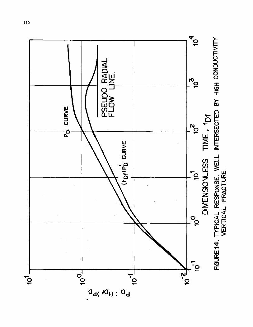
CASE 5 HIGH CONDUCTIVITY FRACTURE After a brief unit slope, Figure 14 shows a half slope in

both the dimensionless pressure difference and its derivative curves indicating a typical response of a well inter- sected by a high conductivity vertical fracture. Once again the differential stabilizes at a values of 0.5 depicting, in this case, pseudoradial flow. Both buildup and drawdown responses are the same.

Figure 15 depicts the same formation discussed in Case 1 (Figure 3). The retest was conducted after acid fracturing, and both the loglog of pressure derivative and pressure difference show a distinct half slope. In addition, Figure 16 displays a distinct straight line on the square root of effective shutin time plot. A high conductivity vertical fracture

is clearly present. It is interesting to compare the shapes of the pre-and post-acid fracturing profiles of the derivative curves. Note the greatet maximum in Figure 3 for the derivative measured from the infiniteacting radial flow line, in comparison to that measured in Figure 15 from the distinct pseudoradial flow line. This indicates that treatment was successful in removing near wellbore damage.

CASE6 DOUBLE POROSITY BEHAVIOR WITH R E S

Figure 17 shows the typical response of a well producing from a reservoir exhibiting double porosity behavior. It shows both a maximum and a minimum in the derivative curve. However, the minimum value occurs below the infinite-acting radial flow line. This is indicative of heterogeneous behavior, but in this case double porosity behavior. Figure 17 illustrates pseudo-steady state or restricted interporosity flow corresponding to a high skin between the highest (fracture) and lowest (matrix) flow capacity me- dia. Behavior for both buildup and drawdown is the same provided the flowing period prior to shutin is long enough to observe the total system behavior [6J ;

Figure 18, an example taken from reference 13, illustrates the double porosity behavior with the characteristic "trough" below the infinite-acting radial flow stabilization line. The storativity ratio (omega) and interporosity flow parameter (lamda) are both available by matching with the appropriate type-curves for a reservoir exhibiting double porosity behavior [9].

OTHER PRACTICAL APPLICATIONS In additional to their use as powerful qualitative diag-

nostic tools, and their quantitative applications, the pressure derivative has other practical applications. One major problem with a combination of traditional log-log and semilog analysis is that the incorrect Horner straight lines are often selected [17].

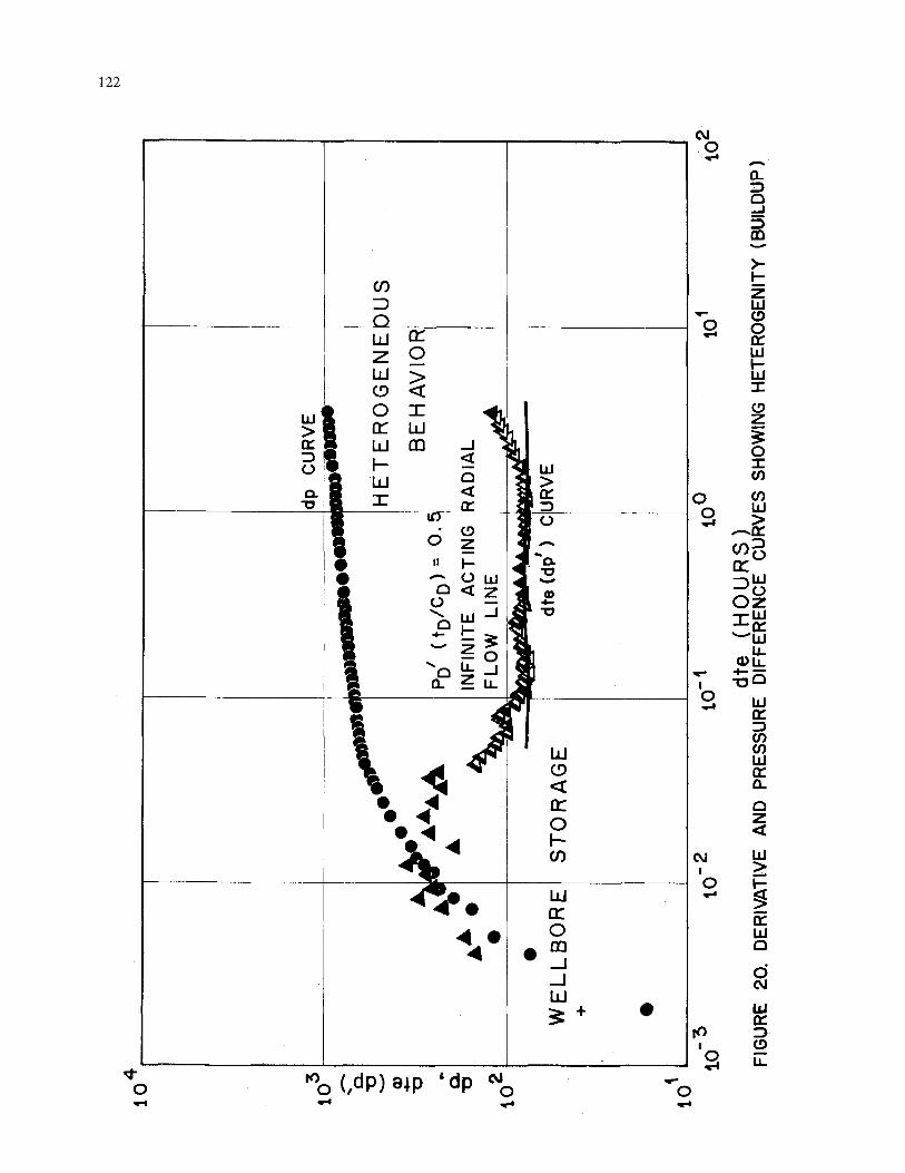
For example, Figure 19 is the Horner plot of a buildup test and shows the possibility of constructing two dis- tinctly separate straight h e s for semilog analysis. The log- log of pressure difference (Figure 20) shows deviation from unit slope early in the test, It would appear that all data from an effective time of dte = 0.1 hrs would be suitable for analysis. However, it is evident from an examination of the pressure derivative plot that shortly after dte = 1 .O hrs, a transition occurs and some form of reservoir heterogeneity is represented. It becomes clear from the extent of the infinite-actingradial flow line [(tD/CD)pD' = 0.51 where to precisely construct the Horner straight line to obtain kh, and the false pressure, p*.

Figure 21, an Indonesian example, shows 60 hour buildup data (presented in dimensionless form) that is still completely dominated by wellbore storage effects. The log- log plots of both the dimensionless pressure change and its derivative show that the buildup duration is not long enough to obtain the infinite-acting radial flow straight line and thus this well is still under the influence of wellbore storage.

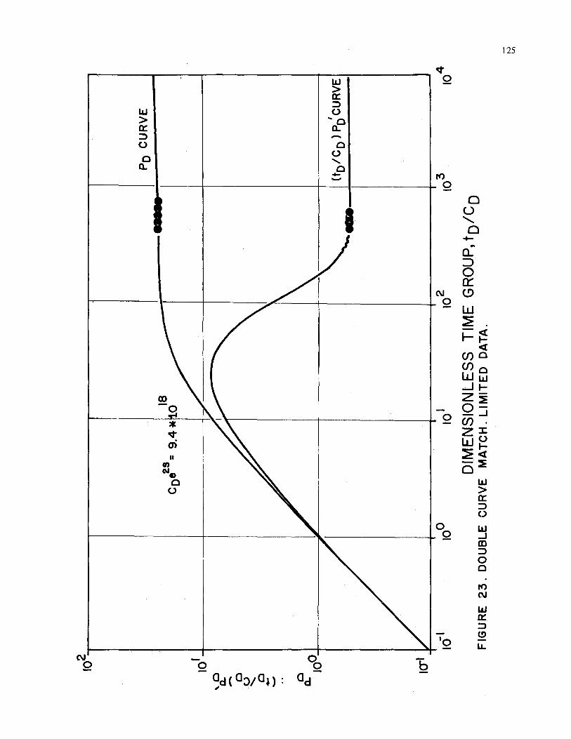
Figure 22 and 23, also an Indonesian example, show how the matching of two curves can reduce uncertainty

TRICTED INTERPOROSITY FLOW

101

when only a limited amount of data is available. Only a small portion of data could be plotted due to gauge failure. Although it is possible to draw a Horner straight line through these points in Figure 22, a difinitive answer is not possible. However, plotting the pressure difference and its derivative on a log-log grid and utilizing the separa- tion in the curves will indicate the validity of the Horner analysis. Figure 23 shows the double match of the data which is plotted in dimensionless form. In this example, the data is confirmed as being part of the homogeneous infinite-acting radial flow pericd, and not from some data possibly above, or below, the infinite-acting radial flow stabilization pressure derivative line (representing heterogeneous behavior), nor data still influenced by wellbore storage.

Figure 24 and 25 illustrate a similar situation. Again the combination of pressure derivative and pressure difference curve matching enhances the accuracy of the analysis.

CONCLUSION The pressure derivative has its primary use as a power-

ful diagnostic tool in identifying the interpretation model to be used in well test data analysis. Magnification of middle and late time pressure responses, and a clear dis- tinction between flow regimes allows the reservoir model to be identified with relative ease.

Validation of analysis can be achieved and performed by most practising engineers due to the increased use of computer-aided well test analysis software packages and high resolution pressure measurement equipment.

Flow regime diagnosis is now possible as an almost ”quick look” analysis as characteristic derivative shapes are easily recognized and identified.

The application of the pressure derivative has significantly made well test interpretation easier to perform.

In addition the pressure derivative allows greater accuracy in reservoir flow parameter determination eliminating the need to perform complementary specialised analysis.

The examples from Indonesian reservoirs as compared with theoretical and published examples highlight their practical application in this area. Features hitherto imper- ceptible on the pressure difference curve or formerly treated as not being meaningful will now often take on a new significance.

ACKNOWLEDGEMENTS

donesia for permission to publish this paper.

NOMENCLATURE B formation volume factor, RB/STB ct system total compressibility, psi-l C wellbore storage coefficient, BBL/psi. CD dimensionless wellbore storage. dt test time, hrs. dte tD dimensionless time tDf

We wish to thank the management of P.T. Corelab In-

effective time (Agarwal time), hrs.

dimensionless time based on fracture half length.

h k m P P” dP PD 9 rw S U xf 8

formation thickness, ft, permeability, md. slope of Horner straight line, psilcycle. subsurface pressure, psi. false pressure, psi. pressure difference, psi dimensionless pressure flow rate, STBOPD. wellbore radius, ft. skin factor viscosity, cp . fracture half length, ft. porosity, fraction

REFERENCES 1.

2.

3.

4.

5.

6.

7.

8 .

9.

10.

11.

12.

13.

Ramey, H.J., Jr.: ”Short-Time Well Test Data Inter- pretation in the Presence of Skin Effect and Well- bore Storage,” J.Pet.Tcch. (Jan 1970) 97.

Agarwa1,R.G.; Al-Hussainy , R.; and Ramey , H.J., Jr.: ”An Investigation of Wellbore Storage and Skin Effect in Unsteady Liquid Flow. I: Analytical Treatment,” SOC. Pet. Eng. J. (Sept 1970) 279.

Gringarten, A.C.; et.al: ”A Comparison Between Dif- ferent Skin and Wellbore Storage TypeCurves for Early-Time Transient Analysis,” paper SPE 8205, presented at the 54th SPE Annual Fall Meeting, LasVegas, Nevada, Sept 23-26,1979.

Horner, D.R.: ”Pressure Buildup in wells,” Proceed- ings, Third World Pet. Cong., Leiden (1951) 2, 503.

Miller, C.C., Dyes, A.B., and Hutchinson, C.A. Jr.: ”Estimation of Permeability and Reservoir Pres- sure From Bottomhole Pressure Buildup Charac- teristics,” Trans, AIME (1950) 189,91.

Gringarten, A.C.: ”Interpretation of Tests in Fissured and Multilayered Reservoirs with Double-Porosity Behavior: Theory and Practice,” J. Pet. Tech. (Apr 1984) 549-563.

Gringarten, A.C.: ”Computer-Aided Well Test Analy- sis,” paper SPE 14099, presented at the SPE Inter- national Meeting, Beijing, China, mar 1986).

Bourdet, D.; et.al.: ”A New Set of Type Curves Sim- plifies Well Test Analysis,” World Oil (May 1983), 95.

Bourdet, D.; et.al.: ”Interpreting Well Tests in Frac- tured Reservoirs,” World Oil (Oct 1983), 77.

Bourdet, D.; et. al.: ”New Type Curves Aid Analysis of Fissured Zone Well Tests,” World Oil (Apr 19841,111.

Alagoa, A.; Bourdet, D.; and Ayoub, J.A.: ”HOW to Simplify the Analysis of Fractured Well Tests,” World Oil (Oct 1985), 97.

Pirard, Y.M.; and Bocock, A.: ”Pressure Derivative Enhances Use of Type Curves for the Analysis of Well Tests,” paper SPE 14101, presefited lit the SPE International Meeting, kfjing, China, (Mar 1986).

Bourdet, D.; Ayoub, J.A.; and Pirard, Y.M.: ”Use of Pressure Derivative in Well Test Internretation.”

102

paper SPE 12777, presented at the SPE California Regional Meeting, Long Beach, Ca., (Apr 1984), 431.

Clark, D.G.; Van Golf-Racht, T.D.; "Pressure-Deriva- tive Approad to Transient Test Analysis: A High- Permeability North Sea Reservoir Examples," J.Pet.Tech. (Nov 1985) 2023.

15. Agarwal, R.G.: "A New Method To AccoClnt For Producing Time Effects when Drawdown Type Curves are Used to Analyse Pressure Buildup and Other Test Data, "paper SPE 9289, presented at the 55th SPE Annual Fall Meeting, Dallas, Tx.,

14.

Sep 21-24,1980. 16. Raghavan, R.: "The Effects of Producing Time on

Type Curve Analysis," J. Pet. Tech. (Jun 1980) 1053.

Ershaghi, I.; Woodbury, J. J.: "Examples of Pitfalls in Well Test Analysis, "J. Pet. Tech. (Feb 1985), 335.

Lee, J.: "Well Testing, " SF'E Textbook Series Vol. 1, (1982), 28-29.

Earlougher, R. C. Jr,: "Advances in Well Test Analy- sis,'' SPE of AIME Monograph Vol. 5 , (1977),

17.

18.

19.

29-30.

2 10

-

FLO

W

I 10

-

LIN

E

0

(3

(3

0

\

c

Y ..

0

11

10 - 10

''

/ 10 O

Pg

cu

I I 10 *

WE

CU

RVE

RAD

IAL

10

DIM

ENSI

ON

LESS

TIM

E G

ROUP

, tD

/CD

lo

4

FIG

UR

E 1.

TYP

ICA

L LO

G-L

OG

RES

PON

SE O

F D

IMEN

SIO

NLE

SS

PRES

SUR

E AN

D IT

S D

ERJV

ATI

VE. W

ELL

WIT

H S

TOR

AG

E A

ND

SK

IN. H

OM

OG

ENEO

US

c1

RES

E RV

OCR

. 8

I 10 loc

10-

I I

/--

I -

I

/, 10

10 '

lo2

3 10

SIO

NLE

SS T

I E

GRO

UP, t

D/c

Q

RES

ERVO

IR. W

ELL

WIT

H S

TOR

AG

E AN

D

SK

IN.

FIG

UR

E 2

. EX

AM

PLE

R

ESPO

NSE

FO

R

INFI

NIT

E

AC

TIN

G

HO

MO

GEN

EOU

S

4

10

3

0

P

lo4

- 103

Q

U

v

Q,

U t .. .- v

) 9.

Uni

t Sl

ope

4Mel

lbor

.e S

tora

ge A/

Li

+re

0

102

10’

.‘A

dp

CU

RVE

A A A A A

dte(

dp’

1 CU

RVE

Rad

ial F

low

Lin

e

Infin

ite A

ctin

g

10-3

10- *

16’

loo

10 ’

EFFE

CTI

VE S

HU

T IN

TIM

E,

dte,

hrs

FI

GU

RE 3.

INDO

NESI

AN E

XA

MP

LE. I

NFI

NIT

E A

CTI

NG

HO

MO

GEN

EOU

S R

ES

ER

VO

IR.

WE

LL

WIT

H S

TOR

AG

E A

ND

SK

IN

106

I- 0 I a. oz w 7 E 0 I

0 0

0

I

0 0

0 0

\ W Z

w I-* +P * kn .a U I- zz

.. a. lo

ot

Id ! 16

'

/ lo

o

MIN

VAL

UE

I

10'

lo2

to3

DIM

ENSI

ON

LESS

TIM

E G

ROUP

, tD

/CD

FI

GU

RE

5. T

YP

ICA

L R

ES

PO

NS

E. H

ETE

RO

GE

NE

OU

S R

ES

ER

VO

IR.

WE

LL W

ITH

ST

OR

AG

E A

ND

S

KIN

.

-- eL lo2

0

Q)

U

Y

t .. .- cn

Q.

U 10

”

loo

0‘

0 A’

A P

0

.lo-

I -*

dte

(d$)

CU

VE

t - 80

0

1

10 ’

loo

10’

lo2

EFFE

CTI

VE S

HU

T IN

TIM

E,

dte,

hrs

FI

GU

RE

6 .

IND

ON

ESIA

N E

XAM

PLE.

HET

ERO

GEN

EOU

S R

ESER

VOIR

(

SIN

GLE

SE

ALI

NG

FAU

LT I

N V

lGIN

ITY

0 F

W

ELL

.

560.

4 4

0-

260-

140-

I

loo

10

1 10

’@

10

HO

RN

ER T

IME

RAT

IO,

(T +

dt

) /

dt

FIG

UR

E7 H

ORN

ER P

LOT.

IN

DO

NES

IAN

EX

AM

PLE

. H

ETER

OG

ENEO

US

RE

SE

RV

OIR

. f S

ING

LE S

EA

LIN

G

FAU

LT

IN V

ICIN

ITY

OF

WE

LL

)

10 4

110

0 - OO _.

111

I

I 0 0 F

\

n

5 0 n 3 a n

& 0 > U w v, W U

W

Z 3 0

U

U v

n n

m

e W v, z 0 v, W U W -I n 2 a X w

0;

a

n

w 3 (3 LL -

112

n \

W n lo3 - Q)

U t

.. .- v) 9. a

U Q lo2

10’

0 &A& A

1 dp CURVE

‘E

I I lo-’ loo 10’ 1(

EFFECTIVE TIME dte hr FIGURE 10. INDONESIAN EXAMPLE FOR BOUNDED RESERVOIR

10' 2

n

'nio

U lo

o 1

@@

D-@- dp

C

UR

VE

10-

lo-*

10

- lo

o

TES

T T

IME

, hr

s FI

GU

RE

11.

IND

ON

ESIA

N E

XA

MP

LE F

OR

PO

SSIB

LE B

OU

ND

ED R

ESER

VOIR

( B

UIL

DU

P)

Y

L

w

lo2-

‘e 1

0’-

n

0

0

\ P

t

v ..

0

a

10

-

lo-!

I I

I I

16’

IbO

10’

1 lo2

I lo3

DIM

ENSI

ON

LESS

TI

ME

GRO

UP,

tD/C

D

FlG

UR

El2

. TY

PIC

AL

mS

E.

CO

NSTA

NT

PRES

SURE

B

OU

ND

AR

Y.

DIM

EN

SIO

NLE

SS

PR

ESSU

RE

GRO

UP

\

6

0

W

6 0

6 Iu

FIG

URE

13.

IND

ON

ES

IAN

EX

AMPL

E F

OR

BO

TTO

M W

ATER

D

RIV

E.

I-- - v,

\

Q

e

n rc

0

c

Y .. P

a.

10’ -

1 oo-

lo-’-

10-1

id1

I loo

I 10’

CURV

E I

lo2

‘3

10

lo4

DIM

ENSI

ON

LESS

TI

ME

tDf

FIG

URE

14. T

YPIC

AL

RES

PON

SE.

WEL

L IN

TER

SEC

TED

BY

HIG

H C

ON

WC

nVlT

Y

VER

TIC

AL

FRA

CTU

RE

.

-I

dp

10 'L

CU

RV

E

:a2

I 10 -'

10 O

'1

10

ib *

10

EF

FE

CT

IVE

SH

UT-

IN

TIM

E,

dte

, hrs

. FI

GUR

E 15

. IN

DO

NES

IAN

E

XA

MP

LE.

WEL

L IN

TER

SEC

TED

BY

HIG

H C

ON

DU

CTI

VITY

VER

TIC

AL

FRA

CTU

RE

I 2

3

4

5

SQU

ARE

RO

OT

of d

te.

FIG

URE

16. S

QU

ARE

RO

OT

OF

EFF

EC

TIV

E T

IME

PLO

T. IN

DO

NES

IAN

EX

AM

PLE

OF

LIN

EA

R

FLO

W. W

ELL

IN

TER

SEC

TED

BY

HIG

H C

APAC

ITY

VE

RTI

CA

L FR

AC

TUR

E.

\n

n

n

10’

*

0

\ (3

t

Y ..

0

n

10

*

Id’ I

t1

lo

o I

PD C

URVE

1 I

I

RAD

IAL

FLOW

LINE

I

10’

102

lo3

DIM

ENSI

ONL

ESS

TIM

E G

ROUF

to/co

FI

GU

RE

17. T

Y P

lCA

L R

ES

PO

NS

E. D

OUB

LE P

OR

OSI

TY B

EHAV

IOUR

4

10

FIG

URE

18. E

XA

MP

LE R

ESPO

NSE

. DO

UBL

E PO

RO

SITY

RES

ERVO

IR

121

I- C E a LL 2 Ly C I

a U I-

i 0‘

lo3

h

\ n

U

a

W

P

W

v

t c

lo2

10‘

A

AA

WE

LL

BO

R,

4-

ST

OR

AG

E

I /dp

CU

RV

E

INF

INIT

E

AC

TIN

G

IRA

DIA

L F

LO

W

LIN

E

dte

(dp’

1 C

UR

VE

>us

10- *

10‘’

loo

10’

102

dte

(HO

UR

S)

FIG

UR

E 2

0.

DE

RIV

ATI

VE

AND

P

RE

SS

UR

E D

IFFE

RE

NC

E C

UR

VES

SHO

WIN

G H

ETE

RO

GE

NIT

Y (

BU

ILD

UP

123

lo1 \

n!?

n

n

n

0 \

t Y .. n n 40° Y-

d

4 II I0

CURVE

0

) CURVE

4000-

3000-

P*=

3600 P

SlA

Of

SLO

PE

, m

= 1

10

psi/c

ycle

EAR

LY T

IME

DAT

A LO

ST

DU

E T

O P

RES

SUR

E G

AUG

E

MA

LFU

NC

TIO

N

IND

ON

EE

IAN

E

XA

MP

LE

moo

iOO

(T

+ d

Wd

t

FIG

UR

E 22.

HO

RN

ER

PLO

T. L

IMIT

ED

DA

TA.

lo’ c

h)

P

I

0

t

Y ..

! ia'

loo

lo2

I 10

DIM

EN

SIO

NLE

SS

TIM

E G

ROUP

, tD

/CD

C

IA

~

nc

n

-

nn

iI

n1

r

niin

\Ic

r

mb

nt ca. U

LJU

IXL

w

nv

c M

AT

CH

. LIM

ITE

D D

ATA

.

h

a

1000-,

- v> .m

oo-

n

1

v) 3

11 a

W

Qz:

3

cn

cn

W

E 2000-

a.

P*=

33

55

P

SlA

1

~ T

----

a 0 a

a a

-a

a

a 0

a a a

0

I

127

d

Q ‘p

J\

w -> 3 0

a

n \

CL 0 Y

w Z -I -

I

w 9 (3 .o + a

application of pressure derivative in analysis of ... · application of pressure derivative in...

Documents