1

[ua] [S][u

s] (1)

[fs] [S]T[f

a] . (2)

AIAA-2003-3514

Application of Spline Matrix for Mesh Deformation

with Dynamic Multi-Block Grids

K.L. Lai¶, H.M. Tsai‡

Temasek Laboratories, National University of Singapore

10 Kent Ridge Crescent, SINGAPORE 119260

F. Liu §

Department of Mechanical and Aerospace Engineering

University of California, Irvine, CA 92697-3975

ABSTRACT

The paper presents a three-dimensional mesh deformation algorithm for dynamic multiple-block

moving mesh configurations. The flow domain is modelled as an elastic solid body where the

Boundary Element Method (BEM) is applied to formulate a spline matrix that transforms the

displacement vectors at a solid boundary to the interior of the field grid. Using a similar approach,

a spline matrix for the interaction between the fluid grid and the structure grid of the flexible body

can be generated. The BEM-based approach provides an unified treatment for both the flow mesh

and the flexible body. For efficient implementation of deforming mesh, the BEM-based algorithm

is augmented with a conventional grid deformation method based on transfinite interpolation (TFI).

The BEM-based interpolation determines the boundary deformations of each block of the multiple-

block flow mesh, while an arclength based TFI deforms the grid within each flow-block.

1. INTRODUCTION

In calculations of the unsteady flow over flexible

structures in problems such as flutter analysis, mesh

deformation plays a vital part and has direct bearing on

the overall accuracy and efficiency of the numerical

scheme. As the fluid-structure system evolves, the

boundary between the fluid and structure may undergo

deformations. A deforming mesh algorithm is needed to

update the flow mesh in response to the boundary

deformation at each time step.

In the solution process where a coupled fluid and

structure model is involved, deforming the flow mesh is

effected in two steps. The first step is determination of

the boundary deformation for a specified deformation of

the structural model; this is accomplished by

interpolation between the structural grids and the

boundary grids. In the second step, the boundary

perturbations are propagated into the flow domain to

update the field mesh.

1.1 BEM-Based Interpolation

In general, the Computational Fluid Dynamics (CFD)

model and the Computational Structural Dynamics

(CSD) model are developed independently and will not

have common grid points. Interpolation or splining

methods are required to connect the displacements and

forces between the structural and aerodynamic grids. A

CFD-CSD interfacing algorithm, initially proposed by

Chen and Jadic2 based on the Boundary Element Method

for linear elasticity, has been developed in the present

work. A spline matrix [S] is generated to relate the

displacements [u] and forces [f] between the

aerodynamic grid (denoted with subscript a) and the

structural grid (subscript s) as

and

––––––––––––––––––––––––––––––––¶ Research Scientist, Temasek Laboratories, National University of

Singapore. Member AIAA.

‡ Principal Research Scientist, Temasek Laboratories, NationalUniversity of Singapore, Member AIAA.

§ Associate Professor, Department of Mechanical and AerospaceEngineering, University of California, Irvine. Senior MemberAIAA.

Copyright © 2003 by the authors. Published by the American Instituteof Aeronautics and Astronautics, Inc with permission

2

[uf] [B

f][u

a] . (3)

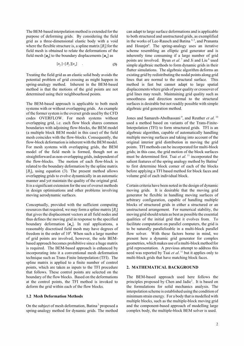
The BEM-based interpolation method is extended for the

purpose of deforming grids. By considering the field

grid as a three-dimensional elastic body with a void

where the flexible structure is, a spline matrix [Bf] for the

field mesh is obtained to relate the deformations of the

field mesh [uf] to the boundary displacements [ua] as

Treating the field grid as an elastic solid body avoids the

potential problem of grid crossing as might happen in

spring-analogy method. Inherent in the BEM-based

method is that the motions of the grid points are not

determined using their neighbourhood points.

The BEM-based approach is applicable to both mesh

systems with or without overlapping grids. An example

of the former system is the overset grids used by the CFD

codes OVERFLOW. For mesh systems without

overlapping grid, i.e. each flow block shares common

boundaries with adjoining flow-blocks, the BEM model

(a multiple block BEM model in this case) of the field

mesh coincides with the flow-blocks. Consequently, the

flow-block deformation is inherent with the BEM model.

For mesh systems with overlapping grids, the BEM

model of the field mesh is formed, though not as

straightforward as non-overlapping grids, independent of

the flow-blocks. The motion of each flow-block is

related to the boundary deformation by the spline matrix

[Bf], using equation (3). The present method allows

overlapping grids to evolve dynamically in an automatic

manner and yet maintain the quality of the original grid.

It is a significant extension for the use of overset methods

in design optimisations and other problems involving

moving aerodynamic surfaces.

Conceptually, provided with the sufficient computing

resources that required, we may form a spline matrix [Bf]

that gives the displacement vectors at all field nodes and

thus defines the moving grid in response to the specified

boundary deformation [ua]. In real applications, a

reasonably discretised field mesh may have degrees of

freedom in the order of 106. When such a large number

of grid points are involved, however, the sole BEM-

based approach becomes prohibitive since a huge matrix

is required. The BEM-based approach is enhanced by

incorporating into it a conventional mesh deformation

technique such as Trans-Finite Interpolation (TFI). The

spline matrix is applied to a finite number of control

points, which are taken as inputs to the TFI procedure

that follows. These control points are selected on the

boundary of the flow blocks. Based on the deformations

at the control points, the TFI method is invoked to

deform the grid within each of the flow blocks.

1.2 Mesh Deformation Methods

On the subject of mesh deformation, Batina 3 proposed a

spring-analogy method for dynamic grids. The method

can adapt to large surface deformations and is applicable

to both structured and unstructured grids, as exemplified

in the works of Lee-Rausch and Batina 4, 5, and Prananta

and Hounjet6. The spring-analogy uses an iterative

scheme resembling an elliptic grid generator and is

inherently time consuming if a large number of grid

points are involved. Byun et al. 7 and Ji and Liu 8 used

simple algebraic methods to form dynamic grids in their

flutter simulations. The algebraic algorithm deforms an

existing grid by redistributing the nodal points along grid

lines that are normal to the structural surface. This

method is fast but cannot adapt to large spatial

displacements where grids of poor quality or crossover of

grid lines may result. Maintaining grid quality such as

smoothness and direction normal to the structural

surfaces is desirable but not readily possible with simple

algebraic grid generation method.

Jones and Samareh-Abolhassani 9, and Reuther et al. 10

used a method based on variants of the Trans-Finite-

Interpolation (TFI) to form structured grids. TFI is an

algebraic algorithm, capable of automatically handling

multiple moving surfaces and taking into account of the

original interior grid distribution in moving the grid

points. TFI methods can be incorporated for multi-block

grids; in this case, the grid motion of the block surfaces

must be determined first. Tsai et al. 11 incorporated the

salient features of the spring analogy method by Batina3

to first determine block corner of each of the blocks

before applying a TFI based method for block faces and

volume grid of each individual block.

Certain criteria have been noted in the design of dynamic

moving grids. It is desirable that the moving grid

generator be flexible in handling moving surfaces of

arbitrary configuration, capable of handling multiple

blocks of structured grids in either a structured or an

unstructured arrangement. For numerical stability, the

moving grid should retain as best as possible the essential

qualities of the initial grid that it evolves from. To

facilitate computation on parallel computers, the grid is

to be naturally parallelizable in a multi-block parallel

flow solver. With these factors borne in mind, we

present here a dynamic grid generator for complex

geometries, which makes use of a multi-block method for

grid representation. A previous attempt to address this

need was reported by Tsai et al. 11 but it applies only to

multi-block grids that have matching block faces.

2. MATHEMATICAL BACKGROUND

The BEM-based approach used here follows the

principles proposed by Chen and Jadic2. It is based on

the formulations for solid mechanics analysis. The

interpolation scheme is established using the condition of

minimum strain energy. For a body that is modelled with

multiple blocks, such as the multiple-block moving grid

and the component-based approach of modelling large

complex body, the multiple-block BEM solver is used.

3

[ui] [H

bi][u

b] [G

bi][t

b] . (4)

[Hbb

][ub] [G

bb][t

b] . (5)

[K] [Gbb

] 1 [Hbb

] . (6)

[ui] [B][u

b] , (7)

[B] [Gbi

] 1[K] [Hbi

] . (8)

Figure 1 Schematic aeroelastic system where a

flexible body contains an internal loading carrying

structure.

Emphasis in this section is given to the underlying

principles of BEM and the development of the

interpolation scheme using the BEM approach. We will

also discuss the issues of corner and edge treatment in the

boundary element method and the assembly method for

multiple block BEM.

2.1 Boundary Element Methods

Interfacing between the structural grid and the

aerodynamic grid is treated here on the basis of

elastostatic problem. Consider an arbitrary three-

dimensional homogeneous body whose boundary is

defined by a closed surface , schematic shown in Figure

1. The CFD surface grid is defined on and the CSD

(internal) grid within . To arrive at the desired

interfacing algorithm, we make use of the BEM

formulation to relate the displacements and forces vectors

between and . The BEM formulations for elastostatic

problem (see, for example, Brebbia and Dominguez 1) are

based on the differential equations of displacement. The

Betti’s reciprocal work theorem and the Somigliana

identity for the displacements are used to derive an

integral equation for the displacements at an interior

point p due to tractions t(Q) and displacements u(Q) at a

point Q on the boundary . In numerical

implementation, the integral equations give a set of linear

algebraic equations which, in matrix form, is

The subscripts b and i signify boundary and interior

values respectively. By moving the load point p to the

boundary and taking care of the singularities that arise

when p coincides with Q, we establish a relationship for

the boundary variables only. The boundary integral

equations with boundary variables only take the form

The subscript bi refers to boundary-to-interior influence

where the subscript bb indicates boundary-to-boundary

influence. The matrices [H] and [G], termed as the

displacement matrix and the traction matrix, respectively,

contain the integrals of the kernels Tij and Uij,

respectively.

Note that equation (4) relating the displacements at

internal points to the variables at the boundary is

meaningful only for points that are within the volume of

. Therefore, those coefficients in [Hbi] and [Gbi] which

are associated with external points are nullified.

For three-dimensional problems, each element of [H] and

[G] is a 3×3 sub-matrix. From equation (5), the stiffness

matrix [K] that relates the boundary traction to boundary

displacement as [tb] = [K] [ub] is defined as

Substituting equation (6) and (5) into (4), we can relate

the displacements at internal points to those of the

boundary grids in the form of

in which, the influence matrix [B] is given by

Equations (6) and (8) are the basic equations for

establishing the spline matrix between boundary grids

and internal grids.

2.2 Constructing the Spline Matrix

The aim of this section is to develop the spline matrix

that relates the boundary displacement to the given

internal (structural) displacement.

Substituting equation (1) into (8), one may notice that the

spline matrix [S] may be interpreted as the ‘inverse’ of

[B] and that computing [S] may be regarded an inverse

BEM problem. To this connection, some considerations

of the characteristics of matrix [B] are in order.

In most practical applications, there is great disparity

between the number of internal grids and the number of

boundary grids, resulting in the formation of a non-

square and therefore non-invertible matrix [B].

Furthermore, by considering rigid body motion, for each

row of [B], the sum of all coefficients must equal the

identity matrix. However, exact satisfaction of the rigid-

body-motion condition leads to a singular matrix, [B].

Therefore, the [B] matrix is not invertible even if the

number of points defined in the interior is the same as

that of the boundary grids, i.e. [B] being a square matrix.

4

U u t d . (9)

UM

m 1

1

1

1

1

n

c 1

Nc(

1,

2)ue

c

n

c 1

Nc(

1,

2)te

c J(1,

2)d

1d

2

(10)

U [ub]T[R][u

b] (11)

[ub]T[R][u

b] T([B][u

b] [u

i]) (12)

ub

[R][ub] [R]T[u

b] [B]T

[ui] [B][u

b]

(13)

[S] [R R T ] 1B T [B [R R T ] 1B T] 1 . (14)

In all cases, inversion of matrix [B] is not possible.

Clearly, the spline matrix [S] cannot be obtained by direct

operation on [B] alone. An additional condition is

required to define [S].

The minimum strain energy requirement proposed by

Chen and Jadic2 is used in the present work as the

additional condition to determine the spline matrix. For

an elastic body acted upon by external forces only, the

strain energy stored in the deformed body equals the

work done by all external forces. A strain energy

function U is defined in terms of traction and

displacement as

Expressed in discretized form for numerical

implementation, equation (9) takes the form

where u e and t e denote, respectively, the displacements

and tractions at the nodal points of a boundary element,

and, Nc is the interpolation (shape) function and J the

Jacobian of transformation between global and local

coordinates. Rewriting (10) in matrix form, we have

where [R] = [N][K] and [N] contains the integrations of

the interpolation function N( 1, 2) indicated in (10).

Since the strain energy due to rigid body motion must be

zero, it follows that the sum of all coefficients in each

row of [R] must equal zero. This implies singularity of

the matrix [R].

For a given set of displacement vectors [ui] at internal

points, the strain energy function U is to be minimized so

as to avoid undue deformation of the structure. This is a

constrained quadratic minimization problem that can be

solved using the Lagrange multiplier technique. The

Lagrangian of the problem is given by

where is a vector containing the Lagrange multipliers.

Substituting equation (7) into (12) for [ui] and

differentiating the resulting equation with respect to ub

and separately, we have two differential equations:

Letting the derivatives in equation (13) be zero, and

rearranging, we arrive at an equation that relates [ub] and

[ui]. The spline matrix [S] is obtained as

A sufficient condition for equation (14) to be solvable is

that both matrices [R] and [B] have full rank. The

solution process for a spline matrix therefore requires the

singularity in these matrices to be eliminated. This is

accomplished by separating the displacements into rigid

body motion and elastic deformation, resulting in the

decomposition of [R] and [B] matrices. Based on the

decomposed matrices [R ] and [B ] for elastic motion,

which are non-singular, a spline matrix [S ] for elastic

deformation is obtained. The desired spline matrix [S]

for the free-free body is thus derived by recovering the

rigid body motion from [S ]. The correctness of [S] may

be verified by multiplying [S] with [B], the product

should approximate the identity matrix.

2.3 Treatment of Corners and Edges

As a prelude to the multiple block BEM presented in next

section, this section presents the solution procedures in

the boundary element method for modelling geometries

with corners where multiple traction values occur at a

node. The treatment of corners is of significant relevance

to multi-block BEM where the interfaces between blocks

always involve corners or edges.

The boundary integral equation (5) generates a system of

equations for solving one traction vector and one

displacement vector at a node. When corners are present,

tractions at corner points may take up multiple values.

As a result, the system of equations given by (5) will

have more unknowns than equations. Thus, auxiliary

equations are needed to close the system of equations.

Consider, for instance, a three-dimensional corner where

three surfaces meet, Figure 2, a total of twelve unknown

quantities exist at the corner node: nine traction

components and three displacement components. By

using equation (5) six linear equations can be established.

Therefore six auxiliary equations are needed to close the

equation set. Similarly, three auxiliary equations are

needed for three-dimensional edges where two surfaces

meet.

5

ti

1

1

0 ;t

i

2

2

0 for i 1,2,3. (15)

n p t q n q t p , (16)

[a] [A][t] , (17)

Hbb

0

0 I

u

a

Gbb

A

t

ta

, (18)

[Kl|K

r]

Gbb

A

1H

bb0

0 I(19)

Figure 2. 3D corner node and edge node, labelled

C and E, where tractions acquire discontinuous

values. Nodal positions are deliberately offset from

the corner point for clarity.

A number of schemes for obtaining the auxiliary

equations for the treatment of corners and edges have

been proposed for the boundary element method, for

example, Chaudonneret 12, Rudolphi 13 and Gao and

Davies 14. The scheme used in the present study is based

on the differential equations of equilibrium proposed by

Gao and Davies14. When the equilibrium equation is

applied to boundary stresses, it implies that the shear

stress approaches a constant value near the corner. On

the boundary the differential equation of equilibrium

can be written as

To obtain the derivatives in equation (15), a local

orthogonal coordinate system ( 1, 2) in the local

tangential directions at the corner is defined for each

boundary element. The components of the traction on

the surface of the boundary element i are differentiated

with respect to 1 and 2, yielding two linear equations for

each boundary element. Equation (15) can be rewritten

in terms of the local intrinsic coordinates ( 1, 2), the

interpolation function Nc ( 1, 2) and the global traction of

a boundary element. Application of equation (15) to the

three boundary elements connecting to the corner yields

six linear equations. There are now the same number of

equations as the number of unknown quantities. For

three-dimensional edge where three auxiliary equations

are needed, equation (15) provides four auxiliary

equations. In this case, the redundant equation may be

discarded.

In general, the auxiliary equations given by (15) are

linearly independent because they are derived from the

geometry of different boundary elements. The only

linkage between adjoining boundary elements is the

common nodes they share. In the cases where

neighbouring elements have corners along one common

axis (for example, one edge of a prism), the auxiliary

equations given by (15) for the nodes involved form a set

of linearly dependent equations, of degrees of freedom

(n 1) where n is the number of nodes involved. In this

situation, another additional equation is needed to close

the system of equation.

Another auxiliary equation can be generated on the

assumption that the stress tensor is unique at a point.

Making use the relationship between tractions t and

stresses (in tensor notations as ti = ij nj), we obtain

where p and q are the indices of the boundary elements

connected to the corner, and n is the local normal vector

at the corner node. Equations (15) and (16) may be used

in conjunction with each other to form a set of auxiliary

equations. Writing the auxiliary equations in matrix

form, we have

where [A] denotes the auxiliary matrix and [a] the

auxiliary array which generally contains zero’s .

When corners are present, the number of displacement

variables is greater than the number of traction variables,

resulting in [Hbb] and [Gbb] being non-square matrices.

Incorporating the boundary integral equation (5) and the

auxiliary equation (17), and partitioning the traction

vectors into [t] and [ta] where the latter accounts for the

additional traction variables at corners and edges, we

have the system of linear equations in the form

where [I] is an Identity matrix. Now that the system

matrices in equation (18) are square. The traction matrix

can be inverted. The stiffness matrix [K] is obtained by

eliminating the terms at the degrees of freedom

associated with [a]. That is, [K] is the left-hand side

partition [Kl] of the product of the following

multiplication

For the internal grids, the matrices [Hbi] and [Gbi] are

evaluated using equation (5). With the knowledge of

matrices [K], [Hbi] and [Gbi], the influence matrix [B] is

hence determined.

6

Hi

xx Hi

xc

Hi

cx Hi

cc

ui

x

ui

c

Gi

xx Gi

xc

Gi

cx Gi

cc

ti

x

ti

c

. (20)

[Hi

xx][ui

x ] [Hi

xc][ui

c ] [Gi

xx][ti

x ] [Gi

xc][ti

c ] , (21)

[Hi

cx][ui

x ] [Hi

cc][ui

c ] [Gi

cx][ti

x ] [Gi

cc][ti

c ] . (22)

[ti

c ] [Hi

cx][u

i

x ] [Hi

cc][u

i

c ] [Gi

cx][t

i

x ] , (23)

[Hcx

] [Gcc

] 1 [Hcx

]

[Hi

cc] [G

cc] 1 [H

i

cc]

[Gcx

] [Gcc

] 1 [Gcx

]

(24)

[Hi

xx][u

i

x ] [Hi

xc][u

i

c ] [Gi

xx][t

i

x ] . (25)

[Hi

xx] [H

i

xx] [Gi

xc][Gi

cc]1[H

i

cx]

[Hi

xc] [H

i

xc] [Gi

xc][Gi

cc]1[H

i

cc]

[Gi

xx] [G

i

xx] [Gi

xc][Gi

cc]1[G

i

cx] .

(26)

[Ai

x ][ti

x ] [Ai

c ][ti

c ] 0 ; (27)

[Ai

x] [t

i

x ] [Bi

x] [u

i

x ] [Bi

c] [u

i

c ] 0 (28)

[Ai

x] [A

i

x ] [Ai

c ][Gi

cx]

[Bi

x] [A

i

c ][Hi

cx]

[Bi

c] [A

i

c ][Hi

cc] .

(29)

m

i 1

[ti

c ] 0 . (30)

m

i 1

[Gi

cx][t

i

x ]m

i 1

[Hi

cx][u

i

x ]m

i 1

[Hi

cc][u

i

c ] 0 . (31)

2.4 Multiple Block BEM

The motivation of developing a multiple block BEM

solver in the present work is driven primarily by the need

to handle very large and complex structures, and to

reduce run time and disk space requirements.

Examining the solution process for the spline matrix, one

can note that it requires computations of matrix inverses.

These numerical operations require considerable

amounts of computing resources when large matrices are

involved. For very large and complex structures, the

computing resources needed may become prohibitive to

allow the structure to be treated in a single BEM model.

To avoid this problem, the complex structure is divided

into substructures (blocks) and the BEM model of each

block is considerably smaller and more manageable than

the model of the entire structure treated as a single block.

Using the condition of continuity and the condition of

equilibrium, the regional matrices are incorporated into

the global system matrices. The interactions between

regions are thus reflected in the global system matrices.

There are different methods of assembling the system

equations in a multiple block BEM. The method used

here is based on the sub-matrix approach. The aim is to

arrive at a matrix equation of the form [H][u] = [G] [t], in

which the global traction matrix [G] is a square matrix

while the global displacement matrix [H] is a general

rectangular matrix.

Consider the i-th region in a system consisting of m

regions, its BEM model is treated separately to obtain the

matrices of equation (6), or equation (18) when corner

treatment is implemented. The nodes for each region are

divided into two sets: external nodes [ux] that lie on the

external (wetted) face, and interface nodes [uc] that lie on

the interface between blocks. Note that a subset of [ux]

lies on the intersection between the external face and the

block-to-block interface. According to this classification,

the traction and displacement matrices can be partitioned

into sub-matrices that are associated with the external

grids and the interface grids of the i-th region:

The suffices x refers to the external grids while c

corresponds to the interface grids. From (20) we obtain

two sets of equations for the i-th block:

and

The tractions [tc] at interface nodes can be expressed as

where

Substituting (23) into (21), we have

where

When treatment of corner and edge is implemented, the

auxiliary equations (11) are also partitioned as

in which, we have made use of the fact that the elements

of array [a] are generally equal to zero. Using the

expression of [tc] in (23), equation (27) can be rewritten

as

where

To compile the global system equations, we make an

assumption that the blocks are in perfect contact and no

traction is applied at the interfaces. The equation of

equilibrium, in terms of traction, is

Using the expression of [tc] given in (23), equation (30)

becomes

7

m

i 1

[Fi

c ] 0 . (32)

[F] [C][t] (33)

F u t u( u) d , (34)

[F] [Cx] [t

x] [C

c] [t

c] (35)

[F] [Cx] [t

x] [K

x] [u

x] [K

c] [u

c] (36)

[Cx] [C

x] [C

c][G

cx]

[Kx] [C

c] [H

cx]

[Kc] [C

c] [H

cc]

(37)

m

i 1

[Ci

cx][t

i

x ]m

i 1

[Ki

cx][u

i

x]m

i 1

[Ki

cc][u

i

c] 0 . (38)

H1

xxN 12 N 1m

N 21 H2

xxN 2m

N 31

Hm

xx

K1

cxK

2

cxK

m

cx

u1

x

u2

x

um

x

G1

xxM 12 M 1m H

1

xc

M 21 G2

xxM 2m H

2

xc

M 31

Gm

xxH

m

xc

C1

cxC

2

cxC

m

cx

m

i 1

Ki

cc

t1

x

t2

x

tm

x

uc

,

(39)

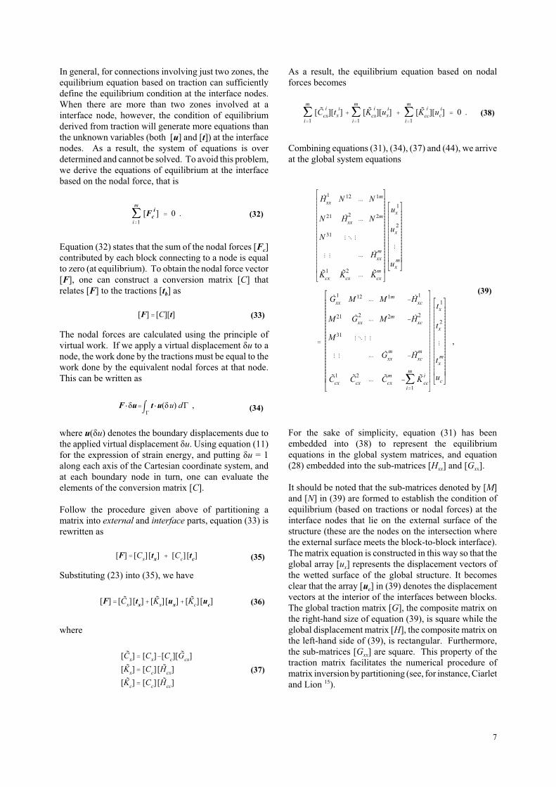
In general, for connections involving just two zones, the

equilibrium equation based on traction can sufficiently

define the equilibrium condition at the interface nodes.

When there are more than two zones involved at a

interface node, however, the condition of equilibrium

derived from traction will generate more equations than

the unknown variables (both [u] and [t]) at the interface

nodes. As a result, the system of equations is over

determined and cannot be solved. To avoid this problem,

we derive the equations of equilibrium at the interface

based on the nodal force, that is

Equation (32) states that the sum of the nodal forces [Fc]

contributed by each block connecting to a node is equal

to zero (at equilibrium). To obtain the nodal force vector

[F], one can construct a conversion matrix [C] that

relates [F] to the tractions [tb] as

The nodal forces are calculated using the principle of

virtual work. If we apply a virtual displacement u to a

node, the work done by the tractions must be equal to the

work done by the equivalent nodal forces at that node.

This can be written as

where u( u) denotes the boundary displacements due to

the applied virtual displacement u. Using equation (11)

for the expression of strain energy, and putting u = 1

along each axis of the Cartesian coordinate system, and

at each boundary node in turn, one can evaluate the

elements of the conversion matrix [C].

Follow the procedure given above of partitioning a

matrix into external and interface parts, equation (33) is

rewritten as

Substituting (23) into (35), we have

where

As a result, the equilibrium equation based on nodal

forces becomes

Combining equations (31), (34), (37) and (44), we arrive

at the global system equations

For the sake of simplicity, equation (31) has been

embedded into (38) to represent the equilibrium

equations in the global system matrices, and equation

(28) embedded into the sub-matrices [Hxx] and [Gxx].

It should be noted that the sub-matrices denoted by [M]

and [N] in (39) are formed to establish the condition of

equilibrium (based on tractions or nodal forces) at the

interface nodes that lie on the external surface of the

structure (these are the nodes on the intersection where

the external surface meets the block-to-block interface).

The matrix equation is constructed in this way so that the

global array [ux] represents the displacement vectors of

the wetted surface of the global structure. It becomes

clear that the array [uc] in (39) denotes the displacement

vectors at the interior of the interfaces between blocks.

The global traction matrix [G], the composite matrix on

the right-hand size of equation (39), is square while the

global displacement matrix [H], the composite matrix on

the left-hand side of (39), is rectangular. Furthermore,

the sub-matrices [Gxx] are square. This property of the

traction matrix facilitates the numerical procedure of

matrix inversion by partitioning (see, for instance, Ciarlet

and Lion 15).

8

[tx] [K ] [u

x] , (40)

[uc] [B

c] [u

x] , (41)

K

Bc

G 1 H . (42)

[ui

i ] [Hi

ix][ui

x ] [Hi

ic][ui

c ] [Gi

ix][ti

x ] [Gi

ic][ti

c ] (43)

[ui

i ] [Gi

ix][t

i

x ] [Hi

ix][u

i

x ] [Hi

ic][u

i

c ] , (44)

[Hi

ix] [H

i

ix] [Gi

ic][Gi

cc]1[H

i

cx]

[Hi

ic] [H

i

ic] [Gi

ic][Gi

cc]1[H

i

cc]

[Gi

ix] [G

i

ix] [Gi

ic][Gi

cc]1[G

i

cx] .

(45)

u1

i

u2

i

um

i

G1

ix0 0

0 G2

ix0

0

Gm

ix

t1

x

t2

x

tm

x

H1

ix0 0

0 H2

ix0

0

Hm

ix

u1

x

u2

x

um

x

H1

ic

H2

ic

Hm

ic

uc

.

(46)

B

G1

ix0 0

0 G2

ix0

0

Gm

ix

K

H1

ix0 0

0 H2

ix0

0

Hm

ix

H1

ic

H2

ic

Hm

ic

Bc

.

(47)

[uc] [B

c] [S] [u

i] . (48)

The global stiffness matrix [K], that relates the tractions

on wetted surface [tx] to the displacements on wetted

surface [ux] as

and the global influence matrix [Bc], that relates the

displacements at block-to-block interface [uc] to [ux] as

can be obtained, respectively, as the upper and lower

partitions of the matrix product

We now find the influence matrix that maps the

displacements at internal grid to the displacements at

boundary, i.e. [ui] = [B] [ux]. The partitions that divide

the structure into regions also distribute the internal grids

to their respective regions. Consider the portion of the

internal grid uii that is confined by the i-th region,

equation (4) is applied only to the i-th region as uii is

considered external points to other regions. Rewriting

the influence matrices into partitions associated with the

external grid and interface grid of the i-th region, we

have equation (4) in the following form

Substituting equation (29) into (49), we have

where

Incorporating the displacement vectors [ui] of each block

into a global array, we can write equation (44) in terms of

the global system matrices as

It follows that the global influence matrix [B] is given by

Considering the tractions and displacements on the

wetted surface only and using the expression of global

stiffness matrix [K] given by (42), one can establish an

expression for the strain energy of the global structure in

the form [ux]T [R] [ux], referring to the notations given in

(17). Substituting the global matrices of [B], and [R] into

the spline matrix formula, we obtain the spline matrix [S]

of the global structure.

For BEM models with multiple regions, the spline matrix

given by equation (14) maps the displacement vectors

[ux] at the external grids to the displacements of the

structural (internal) grids, i.e. [ux] = [S][ui]. Using the

expression for [Bc] given by (42), one can relate the

displacements at interface nodes [uc] to the displacements

of the structural grids as

With the spline matrices [S] and [Bc][S], we can define

the boundary deformation of the global body as well as

the boundary deformation of each block in association

with a given displacements of the structural grid.

2.5 Transfinite Interpolation

Deforming mesh within each flow block is executed

independently using the arclength-based TFI method

proposed by Jones and Samareh-Abolhassani9. In

summary, the solution process of the arclength-based TFI

method is implemented in the following steps:

1 Parameterize and normalise all grid points in the

mesh.

2 Compute deformations at corners and on edges.

3 Compute mesh deformation using TFI.

4 Generate new grid by adding to the original grid the

newly computed deformations.

9

si,j,k

i

i 2

|ri,j,k

ri 1,j,k

| (49)

Fi,j,k

si,j,k

sI,j,k

(50)

E1,1,k

(1 H1,1,k

) P1,1,1

H1,1,k

P1,1,K

, (51)

S1, j,k

A1, j,k

E1, j,1

B1, j,k

E1, j,K

C1, j,k

E1,1,k

D1, j,k

E1,J,k

A1, j,k

C1, j,k

P1,1,1

B1, j,k

C1, j,k

P1,1,K

A1, j,k

D1,j,k

P1,J,1

B1, j,k

D1, j,k

P1,J,K

(52)

Ai, j,k

1i, j,k

Bi, j,k i, j,k

Ci, j,k

1i, j,k

Di, j,k i, j,k

(53)

P1,j,k

1 G1,j,K

G1,j,1

H1,J,k

H1,1,k

G1,j,1

H1,1,k

G1,j,K

G1,j,1

P1,j,k

H1,1,k

G1,j,1

H1,J,k

H1,1,k

P1,j,k

(54)

Vi, j,k

V1 V2 V3 V12 V13 V23 V123 (55)

V1 (1 Fi, j,k

) S1, j,k

Fi, j,k

SI, j,k

V2 (1 Gi, j,k

) Si,1,k

Gi, j,k

Si,J,k

V3 (1 Hi, j,k

) Si, j,1

Hi, j,k

Si, j,K

V12 (1 Fi,j,k

) (1 Gi, j,k

) E1,1,k

(1 Fi, j,k

)Gi, j,k

E1,J,k

Fi, j,k

(1 Gi, j,k

) EI,1,k

Fi, j,k

Gi, j,k

EI,J,k

V13 (1 Fi,j,k

) (1 Hi, j,k

) E1, j,1

(1 Fi, j,k

)Hi, j,k

E1, j,K

Fi, j,k

(1 Hi, j,k

) EI, j,1

Fi, j,k

Hi, j,k

EI, j,K

V23 (1 Gi,j,k

) (1 Hi, j,k

) Ei,1,1

(1 Gi, j,k

)Hi, j,k

Ei,1,K

Gi, j,k

(1 Hi, j,k

) Ei,J,1

Gi, j,k

Hi, j,k

Ei,J,K

V123 (1 Fi, j,k

) (1 Gi, j,k

) (1 Hi, j,k

) P1,1,1

(1 Fi, j,k

) (1 Gi, j,k

)Hi, j,k

P1,1,K

(1 Fi, j,k

)Gi, j,k

(1 Hi, j,k

) P1,J,1

(1 Fi, j,k

)Gi, j,k

Hi, j,k

P1,J,K

Fi, j,k

(1 Gi, j,k

) (1 Hi, j,k

) PI,1,1

Fi, j,k

(1 Gi, j,k

)Hi, j,k

PI,1,K

Fi, j,k

Gi, j,k

(1 Hi, j,k

) PI,J,1

Fi, j,k

Gi, j,k

Hi, j,k

) PI,J,K

(56)

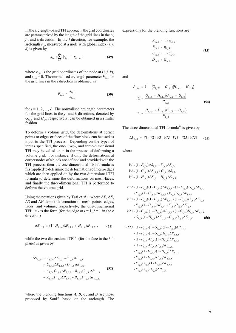
In the arclength-based TFI approach, the grid coordinates

are parameterized by the length of the grid lines in the i-,

j-, and k-direction. In the i direction, for example, the

arclength si,j,k measured at a node with global index (i, j,

k) is given by

where ri,j,k is the grid coordinates of the node at (i, j, k),

and s1,j,k = 0. The normalised arclength parameter Fi,j,k for

the grid lines in the i direction is obtained as

for i = 1, 2, ..., I. The normalised arclength parameters

for the grid lines in the j- and k-directions, denoted by

Gi,j,k and Hi,j,k respectively, can be obtained in a similar

fashion.

To deform a volume grid, the deformations at corner

points or edges or faces of the flow block can be used as

input to the TFI process. Depending on the types of

inputs specified, the one-, two-, and three-dimensional

TFI may be called upon in the process of deforming a

volume grid. For instance, if only the deformations at

corner nodes of a block are defined and provided with the

TFI process, then the one-dimensional TFI formula is

first applied to determine the deformations of mesh-edges

which are then applied on by the two-dimensional TFI

formula to determine the deformations on mesh-faces,

and finally the three-dimensional TFI is performed to

deform the volume grid.

Using the notations given by Tsai et al. 11 where P, E,

S and V denote deformation of mesh-points, edges,

faces, and volume, respectively, the one-dimensional

TFI11 takes the form (for the edge at i = 1, j = 1 in the k

direction)

while the two-dimensional TFI 11 (for the face in the i=1

plane) is given by

where the blending functions A, B, C, and D are those

proposed by Soni16 based on the arclength. The

expressions for the blending functions are

and

The three-dimensional TFI formula11 is given by

where

10

3. SOLUTION PROCEDURES

Specific to aeroelastic analysis using coupled structure

and aerodynamic models, the solution procedures of

deforming flow mesh are summarised as follows.

For the flexible body:

1 Build the BEM model of the flexible body and

compute the spline matrix [S] using equation (14).

2 For a specified deformation of the structure grid

[us], compute the boundary displacements [ua]

using equation [ua] = [S][us].

For the field mesh:

3 Build the BEM model of the field grid and compute

the spline matrix [Bf] using equation (47).

4 Compute flow-block motions [uf] using the

equation [uf] = [Bf] [ua].

5 Deform flow grid by performing TFI, equations

(51), (52) and (55), on each flow block.

Repeat steps (2), (4) and (5) in subsequent mesh

deformation processes.

4. RESULTS AND DISCUSSIONS

Numerical examples are given here to demonstrate the

capability of the BEM-based interpolation method in

deforming flow mesh. For the sake of clarity, two

dimensional problems are considered first to demonstrate

the solution procedures involved, followed by a three

dimensional problem with a wing section.

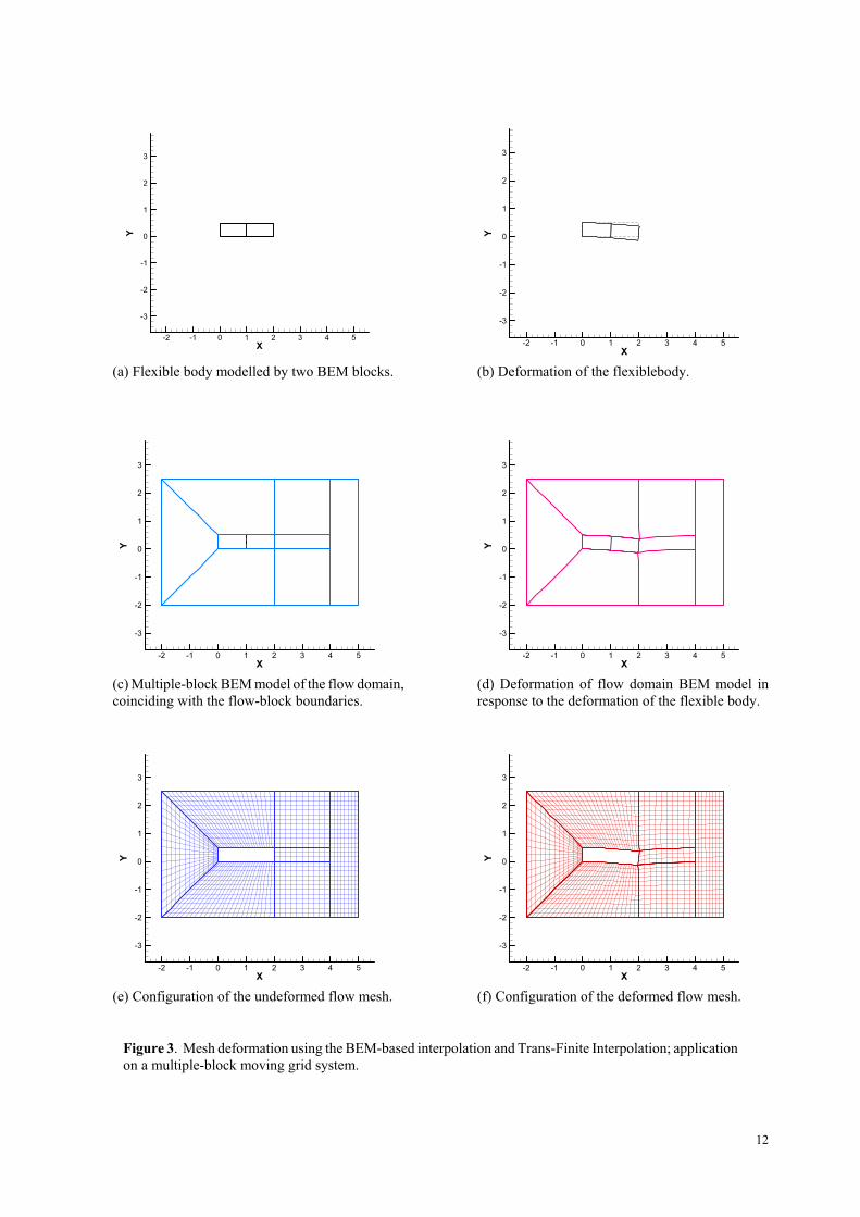
Consider a two-dimensional flexible body, Figure 3(a),

which is modelled by two BEM blocks. A multiple-

block flow grid configuration is used, as shown in Figure

3(c). The undeformed flow grids are shown in Figure

3(e). In order to perform flow-mesh deformation using

the BEM-based technique, the flow domain is considered

as an elastic body, and the multiple-block BEM is used

to represent it. Since the flow grids have matching

boundary, the BEM model of the flow domain is formed

by taking the flow blocks as the BEM blocks. The spline

matrix [Bf] is computed to relate the flow-block

deformation to the deflection of the solid body.

When the flexible body is deformed, the flow blocks are

deformed by using the spline matrix [Bf]. Deformations

of flow blocks associated with the deflection of the solid

body are shown in Figure 3(d). To deform the flow grid,

the TFI procedures are applied to each deformed flow

blocks. The deformed flow grids are computed as shown

in Figure 3(f).

In the second example, a system containing two flexible

bodies is considered, we demonstrate the usage of the

method for deforming overset grids. Figure 4(a) shows

the configuration of the undeformed bodies while Figure

4(c) depicts the BEM model of the undeformed flow

domain. For each body, a body-fitted grid is formed

independent of each other, Figure 4(e). The BEM

models of the body-fitted grids are also generated. (For

clarity, only the overset grids are shown in the figures

while the flow mesh covering the rest of the flow domain

is omitted.) The spline matrix [Bf] is computed for the

flow blocks to map the deformation of the flow-blocks to

the deflection of the flexible bodies. By considering the

body-fitted grid as internal nodes of the flow-block BEM

model, spline matrices [Bf1] and [Bf2] are computed to

relate the deformations of the body-fitted grids to the

deformation of the global flow domain.

In response to the deflections of the flexible bodies,

Figure 4(b), the flow blocks are deformed using spline

matrix [Bf]. Once the deformation of the global flow

domain has been computed, the motion of the body-fitted

grid around each body is computed using spline matrices

[Bf1] and [Bf2]. The deformed BEM models of the flow

blocks and the body-fitted grids are depicted in Figure

4(d). Applying the TFI procedures on the deformed

overset grids, we update the flow mesh within each body-

fitted grid, Figure 4(f). It is evident from the consistent

patterns of overlapping between the two body-fitted

grids, Figure 4(e) and Figure 4(f), that the BEM-based

mesh deformation method preserves the connectivity of

the original grids in the deformed grids.

Application of the BEM-based interpolation method for

deforming three-dimensional flow mesh is given in the

third example. In this example, the BEM-based mesh

deformation method is integrated with the CFD-CSD

interaction method to form an unified approach. For a

given deformation of the structure grid, the CFD-CSD

interaction method is applied to determine the motion of

the boundary grid. The boundary deformation is

subsequently propagated into the field mesh using the

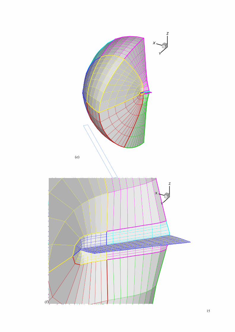
mesh deformation method. Consider an AGARD 445.6

wing section, the fluid model and the structure model of

which are shown in Figure 5(a) and Figure 5(c),

respectively. The flow domain is modelled with 32

multiple-grid flow blocks. Figure 5(e) shows one half of

the flow domain. The near-body flow blocks are shown

magnified in Figure 5(f). The spline matrix [S] for the

interaction between the CFD grid and the CSD grid is

formed using equation (14). As the structure grid is

deformed, the associated deformation of the boundary

grid is computed by the spline matrix [S]. Figures 5(d)

and 5(b) show the deformation of the structure grid and

the associated motion of the wing section.

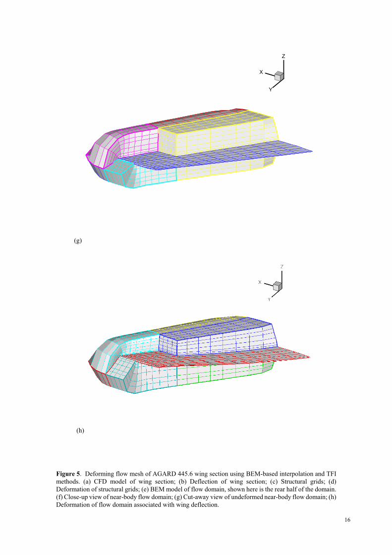
To propagate the boundary perturbation into the field

mesh, the BEM model of the flow domain is formed and

the spline matrix [Bf] computed to relate the flow-block

11

motions with the deformation of the boundary grid. This

is followed by deforming the field mesh within each flow

block using the TFI formulation according to equation

(55). For clear visualisation of the deforming flow

blocks, and without loss of generality of the method, the

BEM models of only the near-body flow blocks are

formed and a section of which is shown in the cut-away

view of Figure 5(g). The flow-block deformations

associated with the deflection of the structure grid are

shown in Figure 5(h).

5. CONCLUSIONS

The paper presented an interpolation method based on

the boundary element method and discussed its

applications in deforming flow mesh and in interaction

between fluid model and structure model in aeroelastic

simulations. In present approach with the BEM-based

interpolation method, the spline matrix [S] for CFD-CSD

interaction and the spline matrix [Bf] for deforming flow

mesh are computed at the onset of computation. They are

stored in disk and retrieved when they are needed in the

solution process. The spline matrix, based on linear

elasticity, is invariant with the deformed shape of the

flexible body and thus valid for any elastic deformation

that the flexible body may assume. The initial

investment in terms of computing resources required for

computing the BEM-based spline matrices may be higher

than conventional interpolation methods. The efficiency,

speed and robustness that the BEM-based interpolation

method offers make it a feasible approach for aeroelastic

simulation of large and complex configurations.

6. REFERENCES

[1] Brebbia, C.A. and Dominguez, J., Boundary

Elements: An Introductory Course, McGraw-Hill Book

Co, New York, 1992.

[2] Chen, P.C. and Jadic, I., “CFD/CSD Interfacing via

an Innovative Structural Boundary Element Approach,”

AIAA Paper 97-1088, 38th SDM Conference, April 7-10,

1997, Kissimmee, FL.

[3] Batina, J. T., “Unsteady Euler Airfoil Solutions Using

Unstructured Dynamic Meshes,” AIAA Journal, Vol. 28,

No. 8, August 1990, pp. 1381-1388.

[4] Lee-Rausch, E. M. and Batina, J. T., “Wing Flutter

Boundary Prediction Using Unsteady Euler Aerodynamic

Method,” Journal of Aircraft, Vol. 32, No. 2, March-

April 1995, pp. 416-422.

[5] Lee-Rausch, E. M. and Batina, J. T., “Wing Flutter

Configurations Using an Aerodynamic Model Based on

the Navier-Stokes Equations,” Journal of Aircraft, Vol.

33, No. 6, Nov.-Dec. 1996, pp. 1139-1147.

[6] Prananta, B. B. and Hounjet, M. H. L., “Large Time

Step Aero-Structural Coupling Procedures for

Aeroelastic Simulation,” In Proceedings of the

International forum on Aeroelasticity and Structural

Dynamics, Rome, Italy, Vol. 2, Confederation of

European Aerospace Societies, June 1997, pp. 63-70.

[7] Byun, C. and Guruswamy, G. P., “Aeroelastic

Computation on Wing-Body-Control Configurations on

Parallel Computers,” Journal of Aircraft, Vol. 35, No. 2,

March-April 1998, pp. 288-294.

[8] Ji, S. and Liu, F., “Flutter Computation of

Turbomachinery Cascades Using a Parallel Unsteady

Navier-Stokes Code,” AIAA Journal, Vol. 37, No. 3,

March 1999, pp. 320-327.

[9] Jones, W.T. and Samareh-Abolhassani, J., “A Grid

Generation System for Multi-Disciplinary Design

Optimization,” AIAA Paper 95-1689-CP, June 1995, 12th

AIAA Computational Fluid Dynamics Conference

Proceedings, Part I, pp. 74-482.

[10] Reuther, J., Alonso, J., Rimlinger, M.J., and

Jameson, A., “Aerodynamic Shape Optimization of

Supersonic Aircraft Configurations via an Adjoint

Formulation on Distributed Memory Parallel

Computers,” Computers and Fluids, Vol. 28, 1999, pp.

675-700.

[11] Tsai, H.M., Wong, A.S.W., Cai, J., Zhu, Y. and Liu,

F., “Unsteady Flow Calculation with a Parallel

Multiblock Moving Mesh Algorithm,” AIAA Journal,

Vol. 39, No. 6, June 2001, pp. 1021-1029.

[12] Chaudonneret, M., “On the Discontinuity of the

Stress Vector in the Boundary Integral Equation Method

for Elastic Analysis,” in Recent Advances in Boundary

Element Methods, ed. C.A. Brebbia, Pentech Press,

London, 1978.

[13] Rudolphi, T.J., “An Implementation of the

Boundary Element Method for Zoned Media with Stress

Discontinuities,” Int. J. Num. Meth. Engng., Vol. 19,

1983, pp. 1-15.

[14] Gao, X.W. and Davies, T.G. "3D Multi-Region

BEM with Corners and Edges," Int. Journal of Solids

and Structures, Vol. 37, 2000, pp. 1549-1560.

[15] P.G. Ciarlet, J. L. Lions. Handbook of numerical

analysis. Publisher Amsterdam; New York; Oxford,

England: North Holland, 1990-

[16] Soni, B. K. “Two- and Three-Dimensional Grid

Generation for Internal Flow Applications of

Computational Fluid Dynamics,” AIAA Paper 85-1526,

1985.

12

X

Y

-2 -1 0 1 2 3 4 5

-3

-2

-1

0

1

2

3

(e) Configuration of the undeformed flow mesh.

X

Y

-2 -1 0 1 2 3 4 5

-3

-2

-1

0

1

2

3

(a) Flexible body modelled by two BEM blocks.

X

Y

-2 -1 0 1 2 3 4 5

-3

-2

-1

0

1

2

3

(c) Multiple-block BEM model of the flow domain,

coinciding with the flow-block boundaries.

X

Y

-2 -1 0 1 2 3 4 5

-3

-2

-1

0

1

2

3

(b) Deformation of the flexiblebody.

X

Y

-2 -1 0 1 2 3 4 5

-3

-2

-1

0

1

2

3

(d) Deformation of flow domain BEM model in

response to the deformation of the flexible body.

X

Y

-2 -1 0 1 2 3 4 5

-3

-2

-1

0

1

2

3

(f) Configuration of the deformed flow mesh.

Figure 3. Mesh deformation using the BEM-based interpolation and Trans-Finite Interpolation; application

on a multiple-block moving grid system.

13

X

Y

-2 -1 0 1 2 3 4 5

-3

-2

-1

0

1

2

3

(e) Body-fitted overset grids of the flexible bodies.

X

Y

-2 -1 0 1 2 3 4 5

-3

-2

-1

0

1

2

3

(a) BEM models of the flexible bodies.

X

Y

-2 -1 0 1 2 3 4 5

-3

-2

-1

0

1

2

3

(c) Multiple-block BEM model of the flow domain.

X

Y

-2 -1 0 1 2 3 4 5

-3

-2

-1

0

1

2

3

(b) Deformation of the flexible bodies.

X

Y

-2 -1 0 1 2 3 4 5

-3

-2

-1

0

1

2

3

(d) Deformations of the flow domain and the

overset flow-blocks associated with the

deformation of the flexible bodies.

X

Y

-2 -1 0 1 2 3 4 5

-3

-2

-1

0

1

2

3

(f) Deformation of overset grids due to deflections

of the flexible bodies.

Figure 4. Application of the BEM-based mesh deformation method on overset grids.

14

(b)

(d)

(a)

(c)

15

(e)

X

Y

Z

(f)

16

(h)

X

Y

Z

(g)

Figure 5. Deforming flow mesh of AGARD 445.6 wing section using BEM-based interpolation and TFI

methods. (a) CFD model of wing section; (b) Deflection of wing section; (c) Structural grids; (d)

Deformation of structural grids; (e) BEM model of flow domain, shown here is the rear half of the domain.

(f) Close-up view of near-body flow domain; (g) Cut-away view of undeformed near-body flow domain; (h)

Deformation of flow domain associated with wing deflection.