application of vof and k-ε turbulence model in …application of vof and k-ε turbulence model in...

https://doi.org/10.4314/wsa.v45i2.15Available on website http://www.wrc.org.zaISSN 1816-7950 (Online) = Water SA Vol. 45 No. 2 April 2019Published under a Creative Commons Attribution Licence 278

Application of VOF and k-ε turbulence model in simulation of flow over a bottom aerated ramp and step structure

Talia Tokyay1* and Can Kurt1

1Department of Civil Engineering, Middle East Technical University, Ankara, 06800, Turkey

ABSTRACTA three-dimensional numerical model of ANSYS, Fluent (2011) was employed for studying mid to high discharge supercritical two-phase �ow over a single slope spillway with a single step for aeration of the �ow. In this study 18 simulations were conducted using the Volume of Fluid (VOF) method for air-water interface tracking and simple k-ε model for turbulence closure. Submerged circular shaped pipes located at the bottom of the step were utilized as aerators. Analyses concentrate on the air-entrainment phenomenon and jet-length of the �ow from the step to the re-attachment point. �e variables considered in the study are discharge, aerator size, di�erent aerator arrangements, Froude number of the �ow, presence of a ramp before the step and its angle. Observed jet-length values in this study were compared with two sets of empirical formulae from literature for code validation. Cross-sectional average of air concentration due to bottom aeration was determined in the streamwise direction downstream of the re-attachment of the jet. �e air concentration is observed to follow a logarithmic decay in the �ow direction within the de-aeration zone. Keywords: jet-length, aerator, VOF, air-entrainment, ramp, computational �uid dynamic

* To whom all correspondence should be addressed. e-mail: [email protected] 19 Feb 2018, accepted in revised form 4 April 2019.

INTRODUCTION

Dams have been constructed in di�erent ways and for di�erent purposes such as irrigation, power generation, water consumption, and �ood prevention, throughout the history of civilizations. Water demand, precipitation and �ow regime of the stream govern the capacity of the dams. Due to variability and instability of these factors, safety structures such as spillways are integral to dam wall structures. Since spillways are important key structures, their design life should be identical to that of the entire dam structure, and damage to spillways, such as due to cavitation, should be eliminated.

Pinto (1988) explained vaporous cavitation as the change of liquid phase to vapor phase resulting from decrease of pressure in �ow due to high speeds. During this pressure decrease vapour bubbles occur and at some point these bubbles encounter higher pressure zones, where they implode. �e imploding cavities in the high-pressure zones cause high pressure waves, which impact on �xed boundaries and could cause cavitation damage to the �xed boundaries. �e continuous impacting of these high-pressure waves could remove small particles from the surface of structures and could lead to signi�cant damage to the structure in time (Kells and Smith, 1991). Some of the real-life examples of cavitation damage to the structures are listed by Kramer (2004).

Estimating the cavitation potential can assist in prevention of cavitation damage to the structure. Most of the approaches in the literature for predicting cavitation potential of a �ow are based on velocity of the �ow. Cassidy and Elder (1984) stated that a �ow with 11 m∙s−1 velocity can damage a concrete channel bed with irregularities. Volkart and Rutschmann (1991) stated the limit for cavitation velocity for a completely smooth concrete surface between 22 m∙s−1 and 26 m∙s−1. Oskolkov and Semenkov (1979) stated a cavitation limit of operating heads exceeding 50–60 m. A more general approach

employs a cavitation number (index) which is a special form of Euler Number (Aydin, 2005) given in Eq. 1. Pinto (1988) states a cavitation risk for σ < 0.25.

𝜎𝜎 = (𝑃𝑃0 − 𝑃𝑃𝑣𝑣)𝜌𝜌𝑈𝑈0

2/2

1𝜌𝜌𝑞𝑞

[ 𝜕𝜕𝜕𝜕𝜕𝜕 (𝛼𝛼𝑞𝑞𝜌𝜌𝑞𝑞) + ∇. (𝛼𝛼𝑞𝑞𝜌𝜌𝑞𝑞𝑣𝑣𝑞𝑞⃗⃗⃗⃗ ) = 𝑆𝑆𝛼𝛼𝑞𝑞 + ∑(�̇�𝑚𝑝𝑝𝑞𝑞 − �̇�𝑚𝑞𝑞𝑝𝑝)

𝑛𝑛

𝑝𝑝=1]

𝐹𝐹𝐹𝐹 =𝑉𝑉𝑟𝑟𝑟𝑟𝑟𝑟𝑝𝑝

√𝑔𝑔ℎ𝑟𝑟𝑟𝑟𝑟𝑟𝑝𝑝

𝐿𝐿𝑗𝑗ℎ𝑟𝑟𝑟𝑟𝑟𝑟𝑝𝑝

= 0.28(1 + 𝛼𝛼)0.22𝐹𝐹𝐹𝐹1.75 (𝜕𝜕𝑟𝑟 + 𝐻𝐻𝑠𝑠ℎ𝑟𝑟𝑟𝑟𝑟𝑟𝑝𝑝

)0.44

[(1 + 𝜕𝜕𝑡𝑡𝑡𝑡𝑡𝑡) 𝐴𝐴𝑟𝑟𝐴𝐴𝑤𝑤

]−0.087

𝜕𝜕𝑗𝑗 =𝑉𝑉𝑟𝑟𝑟𝑟𝑟𝑟𝑝𝑝𝑠𝑠𝑠𝑠𝑡𝑡𝛼𝛼

𝑔𝑔(𝑐𝑐𝑐𝑐𝑠𝑠𝑡𝑡 + 𝑃𝑃𝑁𝑁) [1 + √1 + 2(𝜕𝜕𝑟𝑟 + 𝐻𝐻𝑠𝑠)𝑔𝑔(𝑐𝑐𝑐𝑐𝑠𝑠𝑡𝑡 + 𝑃𝑃𝑁𝑁)(𝑉𝑉𝑟𝑟𝑟𝑟𝑟𝑟𝑝𝑝𝑠𝑠𝑠𝑠𝑡𝑡𝛼𝛼)2]

𝜕𝜕𝑗𝑗 = √ 2𝐻𝐻𝑠𝑠𝑔𝑔(𝑐𝑐𝑐𝑐𝑠𝑠𝑡𝑡 + 𝑃𝑃𝑁𝑁)

𝑃𝑃𝑁𝑁 = ∆𝑃𝑃𝜌𝜌𝑤𝑤𝑔𝑔ℎ𝑟𝑟𝑟𝑟𝑟𝑟𝑝𝑝

𝐿𝐿𝑗𝑗 = 𝑔𝑔𝑠𝑠𝑠𝑠𝑡𝑡𝑡𝑡2 𝜕𝜕𝑗𝑗2 + 𝑉𝑉𝑟𝑟𝑟𝑟𝑟𝑟𝑝𝑝(𝑐𝑐𝑐𝑐𝑠𝑠𝛼𝛼)𝜕𝜕𝑗𝑗

𝑞𝑞𝑟𝑟 = 𝐾𝐾𝑉𝑉𝑟𝑟𝑟𝑟𝑟𝑟𝑝𝑝𝐿𝐿𝑗𝑗

(1)

where; σ is the cavitation number, Po is the local pressure including atmospheric pressure, Pv is the vapor pressure, ρ is the density of the �uid and Uo is the average �ow velocity.

Cavitation damage could be mitigated by aerating the �ow. Bottom aeration increases the air void ratio, which causes the water/air mixture to be more compressible. Higher compressibility lowers the pressure wave velocity and consequent impact of pressure waves. Aeration also increases the dissolved oxygen of the water and provides better dissolved oxygen values for the downstream natural life and �shery (Arantes et al., 2010). To this end, spillways designed to carry medium to high discharges, which are under a high risk of cavitation, o�en employ stepped structures to produce aeration zones for the �ow. �e aeration over the steps is o�en made possible by chimneys built on the side of the steps that allow air-entrainment from one side of the �ow. �e air-entrainment is further made possible by use of de�ecting chutes, which are also known as ramps, located just before the steps. In this study �ow over a ramp and step structure is simulated with a numerical model.

�e �ow over a ramp and step could be separated into three major zones. �e �rst zone is the approach zone. �is zone consists of the �ow upstream of the step over the spillway, and it ends just before the start of the ramp as shown in Fig. 1. �is region is immediately followed by a transition zone over the ramp where �ow gains upward momentum. Over the step, we can observe the aeration zone, where trajected nappe �ow entrains air both from the upper and the lower interface. �e aeration zone ends at the location where the �ow re-attaches to the spillway surface. In Fig. 1, the location of re-attachment is shown with xi. With the re-attachment of the �ow the de-aeration zone begins.

https://doi.org/10.4314/wsa.v45i2.15

http://www.wrc.org.za

https://creativecommons.org/licenses/by/4.0/

mailto:[email protected]


Generally, experimental models are used for design of hydraulic structures; however, in studies where two �uids with very di�erent properties are interacting, such as where �owing water entrains air, the scale e�ects become important. Most open-channel �ow physical model studies are based on Froude similarity. In the case of a physical model in which air-entrainment is studied, the Weber number becomes important as it represents the surface tension e�ects. However, it is o�en di�cult to achieve both Weber and Froude similarity in an experimental setting. In physical model studies it is commonly observed that larger scale models (smaller prototype/model scale ratios) give more realistic results. Due to small prototype/model scale ratios being needed for realistic results, the economy of the experiment is greatly compromised. Lee and Hoopes (1996) indicated scale e�ects and errors from physical model observations as one of the reasons for cavitation damage experienced in prototype spillways. Chanson (1990), who studied air demand of the Clyde Dam spillway with a 1:15 scale model, later stated that physical model studies and prototype results are far from being similar.

Air-entrainment ratio has been found to be related to some independent variables, such as slope of spillway and aerator, heights of the ramp and the offset, f low depth, Froude number and cavity sub-pressure (Rutschmann and Hager, 1990).

In literature, there are studies that employed the best of both experimental and numerical investigations of these �ows. In the study of Arantes et al. (2010), experimental and computational methods were employed concomitantly. As a result, it was found that calibrated numerical models can be used for determination of bottom inlet spillway aerators.

Jet-length is a common parameter used in air-entrainment of spillway �ow studies. Most of the empirical equations use jet-length for determining the air-entrainment ratio. �e �rst study that o�ered such an empirical equation for jet-length is

that of Schwartz and Nutt (1963). Likewise, Pan et al. (1980) and Pinto et al. (1982) showed a relation between geometry of jet-length and air-entrainment. In the study of Kokpinar and Gogus (2002), the major forces in an open channel �ow are listed as inertial, gravitational and pressure forces. In the study of Tan (1984), which is similar to the study of Rutschmann and Hager (1990), jet-length was based on sub-pressure number, PN, which is a function of atmospheric and lower nappe cavity pressure and gravitational forces.

Di�erent from air-entrainment ratio and jet-length studies, there are studies on aerator spacing on a spillway in order to maintain continuous aeration (Lesleighter and Chang, 1981; Pinto et al., 1982). Kells and Smith (1991) proposed limits for maximum air concentration of 45% and minimum of 8% for the proper protection of the spillway structure from cavitation.

In a recent numerical study of Aydin and Ozturk (2009), commercial CFD so�ware was used for numerical simulation of �ow over a stepped spillway with the Algebraic Slip Mixture (ASM) method and the k-ε model. �e geometry of the model was based on the prototype geometry of the study of Demiroz (1985).

METHODS

�e major advantage of numerical models over physical ones is their economy while eliminating scale e�ects. �e aim of the current study is to investigate the e�ect of ramp angle, �ow discharge, aerator size and arrangement over the jet-length, amount of air-entrainment, and general �ow structure. For this purpose, a three-dimensional model is developed using ANSYS Fluent. �e Volume of Fluid (VOF) method for air-water interface tracking and the simple k-ε model for turbulence closure were employed. Bottom aeration of �ow was made possible by using circular cross-sectioned bottom aerator pipes. �e diameter of the aerator pipe (Daerator) and the ramp height (tr), as shown in Fig. 2, were considered

Figure 1Sketch of the computational domain and definition of some parameters





as the variables in this study, together with the discharge of the �ow (qw), as given in Table 1, with the arrangement of the aerators on the step as presented in Fig. 4. �e air-entrainment quanti�ed in this study was solely due to the bottom aerators. �e additional air-entrainment through free-surface of the �ow was not considered separately in the results reported. �e numerical results of this study were compared to the results obtained from the empirical formulae of previous studies from literature.

Computational domain, boundary conditions, and numerical method

�e simulation domain is a long open-channel with bottom slope of θ = 16.70°. �e channel has a rectangular cross section. �e width of the channel is 5 m. In some of the simulations, a 1.5 m long ramp is attached to the domain just before the step in order to de�ect the �ow in the vertical direction. �e step height is 1 m and aerators with circular cross-sections are placed

on the horizontal surface of the step. �e length of the domain upstream of the step, Lus, is 5 m, and downstream of the step, Lds, is greater than 20 m in all the simulations. A sketch of the side view of the channel �oor with the step can be seen in Fig. 2.

�e computational grid is composed of hexahedral elements (Fig. 3b). �e grid sensitivity is tested for mesh sizes of 760 000, 1.2 million and 1.8 million for a single high-discharge value used in the simulations. �e tested mesh with highest number of cells is found to resolve the location of free surface and the position of the re-attachment clearer than the meshes with a lower number of cells, even though the results were comparable for 1.2 and 1.8 million meshes. �e mesh is kept denser in the region where water �ow is expected. Larger cell sizes and a lower number of cells are used in the region above the �ow for computational economy. �e average cell size in the domain is taken as (ΔX, ΔY, ΔZ) = (0.1, 0.05, 0.1) in meters. �is average cell size is found to be small enough for the accuracy of the k-ε turbulence model (ANSYS, 2011).

Figure 2Side view of the channel floor with the step (dimensions in mm)

Figure 3Simulation domain showing (a) boundary conditions and (b) computational grid. Computational grid is shown for the part of the domain isolated

with dashed blue rectangle in frame (a)





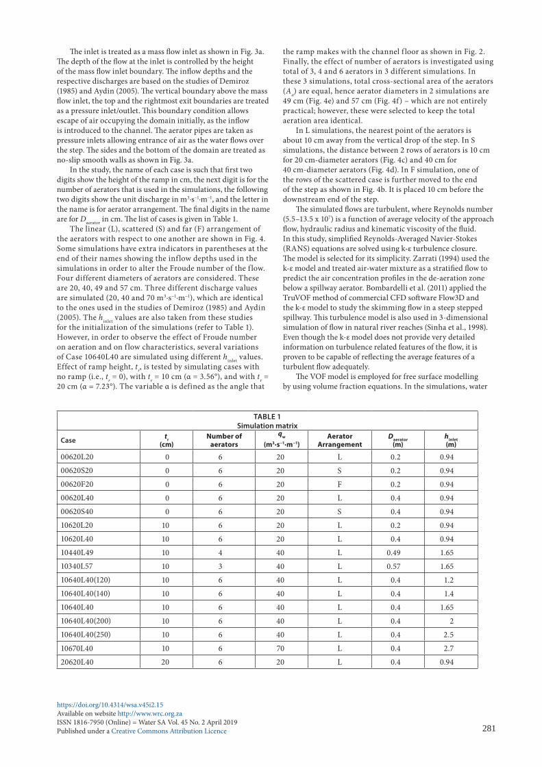
�e inlet is treated as a mass �ow inlet as shown in Fig. 3a. �e depth of the �ow at the inlet is controlled by the height of the mass �ow inlet boundary. �e in�ow depths and the respective discharges are based on the studies of Demiroz (1985) and Aydin (2005). �e vertical boundary above the mass �ow inlet, the top and the rightmost exit boundaries are treated as a pressure inlet/outlet. �is boundary condition allows escape of air occupying the domain initially, as the in�ow is introduced to the channel. �e aerator pipes are taken as pressure inlets allowing entrance of air as the water �ows over the step. �e sides and the bottom of the domain are treated as no-slip smooth walls as shown in Fig. 3a.

In the study, the name of each case is such that �rst two digits show the height of the ramp in cm, the next digit is for the number of aerators that is used in the simulations, the following two digits show the unit discharge in m3∙s−1∙m−1, and the letter in the name is for aerator arrangement. �e �nal digits in the name are for Daerator in cm. �e list of cases is given in Table 1.

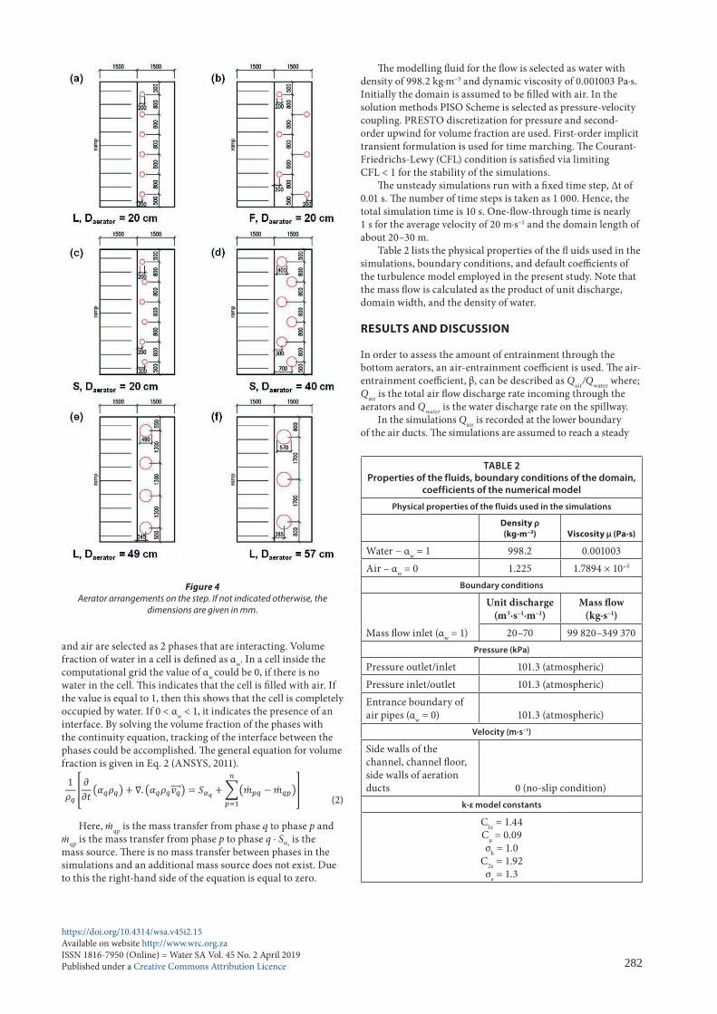
The linear (L), scattered (S) and far (F) arrangement of the aerators with respect to one another are shown in Fig. 4. Some simulations have extra indicators in parentheses at the end of their names showing the inf low depths used in the simulations in order to alter the Froude number of the f low. Four different diameters of aerators are considered. These are 20, 40, 49 and 57 cm. Three different discharge values are simulated (20, 40 and 70 m3∙s−1∙m−1), which are identical to the ones used in the studies of Demiroz (1985) and Aydin (2005). The hinlet values are also taken from these studies for the initialization of the simulations (refer to Table 1). However, in order to observe the effect of Froude number on aeration and on f low characteristics, several variations of Case 10640L40 are simulated using different hinlet values. Effect of ramp height, tr, is tested by simulating cases with no ramp (i.e., tr = 0), with tr = 10 cm (α = 3.56°), and with tr = 20 cm (α = 7.23°). The variable α is defined as the angle that

the ramp makes with the channel f loor as shown in Fig. 2. Finally, the effect of number of aerators is investigated using total of 3, 4 and 6 aerators in 3 different simulations. In these 3 simulations, total cross-sectional area of the aerators (Aa) are equal, hence aerator diameters in 2 simulations are 49 cm (Fig. 4e) and 57 cm (Fig. 4f) – which are not entirely practical; however, these were selected to keep the total aeration area identical.

In L simulations, the nearest point of the aerators is about 10 cm away from the vertical drop of the step. In S simulations, the distance between 2 rows of aerators is 10 cm for 20 cm-diameter aerators (Fig. 4c) and 40 cm for 40 cm-diameter aerators (Fig. 4d). In F simulation, one of the rows of the scattered case is further moved to the end of the step as shown in Fig. 4b. It is placed 10 cm before the downstream end of the step.

�e simulated �ows are turbulent, where Reynolds number (5.5–13.5 x 107) is a function of average velocity of the approach �ow, hydraulic radius and kinematic viscosity of the �uid. In this study, simpli�ed Reynolds-Averaged Navier-Stokes (RANS) equations are solved using k-ε turbulence closure. �e model is selected for its simplicity. Zarrati (1994) used the k-ε model and treated air-water mixture as a strati�ed �ow to predict the air concentration pro�les in the de-aeration zone below a spillway aerator. Bombardelli et al. (2011) applied the TruVOF method of commercial CFD so�ware Flow3D and the k-ε model to study the skimming �ow in a steep stepped spillway. �is turbulence model is also used in 3-dimensional simulation of �ow in natural river reaches (Sinha et al., 1998). Even though the k-ε model does not provide very detailed information on turbulence related features of the �ow, it is proven to be capable of re�ecting the average features of a turbulent �ow adequately.

�e VOF model is employed for free surface modelling by using volume fraction equations. In the simulations, water

TABLE 1Simulation matrix

Case tr (cm)

Number of aerators

qw (m3∙s−1∙m−1)

Aerator Arrangement

Daerator (m)

hinlet (m)

00620L20 0 6 20 L 0.2 0.94

00620S20 0 6 20 S 0.2 0.94

00620F20 0 6 20 F 0.2 0.94

00620L40 0 6 20 L 0.4 0.94

00620S40 0 6 20 S 0.4 0.94

10620L20 10 6 20 L 0.2 0.94

10620L40 10 6 20 L 0.4 0.94

10440L49 10 4 40 L 0.49 1.65

10340L57 10 3 40 L 0.57 1.65

10640L40(120) 10 6 40 L 0.4 1.2

10640L40(140) 10 6 40 L 0.4 1.4

10640L40 10 6 40 L 0.4 1.65

10640L40(200) 10 6 40 L 0.4 2

10640L40(250) 10 6 40 L 0.4 2.5

10670L40 10 6 70 L 0.4 2.7

20620L40 20 6 20 L 0.4 0.94





and air are selected as 2 phases that are interacting. Volume fraction of water in a cell is de�ned as αw. In a cell inside the computational grid the value of αw could be 0, if there is no water in the cell. �is indicates that the cell is �lled with air. If the value is equal to 1, then this shows that the cell is completely occupied by water. If 0 < αw < 1, it indicates the presence of an interface. By solving the volume fraction of the phases with the continuity equation, tracking of the interface between the phases could be accomplished. �e general equation for volume fraction is given in Eq. 2 (ANSYS, 2011).


2/2

1𝜌𝜌𝑞𝑞


𝑛𝑛

𝑝𝑝=1]





)0.44


]−0.087







(2)

Here, ṁqp is the mass transfer from phase q to phase p and ṁqp is the mass transfer from phase p to phase q ∙ Sαq

is the mass source. �ere is no mass transfer between phases in the simulations and an additional mass source does not exist. Due to this the right-hand side of the equation is equal to zero.

�e modelling �uid for the �ow is selected as water with density of 998.2 kg∙m−3 and dynamic viscosity of 0.001003 Pa∙s. Initially the domain is assumed to be �lled with air. In the solution methods PISO Scheme is selected as pressure-velocity coupling. PRESTO discretization for pressure and second-order upwind for volume fraction are used. First-order implicit transient formulation is used for time marching. �e Courant-Friedrichs-Lewy (CFL) condition is satis�ed via limiting CFL < 1 for the stability of the simulations.

�e unsteady simulations run with a �xed time step, Δt of 0.01 s. �e number of time steps is taken as 1 000. Hence, the total simulation time is 10 s. One-�ow-through time is nearly 1 s for the average velocity of 20 m∙s−1 and the domain length of about 20–30 m.

Table 2 lists the physical properties of the � uids used in the simulations, boundary conditions, and default coe�cients of the turbulence model employed in the present study. Note that the mass �ow is calculated as the product of unit discharge, domain width, and the density of water.

RESULTS AND DISCUSSION

In order to assess the amount of entrainment through the bottom aerators, an air-entrainment coe�cient is used. �e air-entrainment coe�cient, β, can be described as Qair/Qwater where; Qair is the total air �ow discharge rate incoming through the aerators and Qwater is the water discharge rate on the spillway.

In the simulations Qair is recorded at the lower boundary of the air ducts. �e simulations are assumed to reach a steady

Figure 4Aerator arrangements on the step. If not indicated otherwise, the

dimensions are given in mm.

TABLE 2Properties of the fluids, boundary conditions of the domain,

coefficients of the numerical model

Physical properties of the fluids used in the simulations

Density ρ (kg∙m−3) Viscosity μ (Pa∙s)

Water − αw = 1 998.2 0.001003Air – αw = 0 1.225 1.7894 × 10−5

Boundary conditions

Mass �ow inlet (αw = 1)

Unit discharge (m3∙s−1∙m−1)

Mass �ow (kg∙s−1)

20–70 99 820–349 370Pressure (kPa)

Pressure outlet/inlet 101.3 (atmospheric)Pressure inlet/outlet 101.3 (atmospheric)Entrance boundary of air pipes (αw = 0) 101.3 (atmospheric)

Velocity (m∙s−1)

Side walls of the channel, channel �oor, side walls of aeration ducts 0 (no-slip condition)

k-ε model constants

C1ε = 1.44Cμ = 0.09σk = 1.0

C2ε = 1.92σe = 1.3





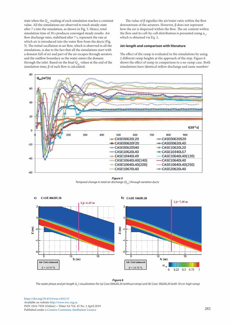
state when the Qair reading of each simulation reaches a constant value. All the simulations are observed to reach steady-state a�er 7 s into the simulation, as shown in Fig. 5. Hence, total simulation time of 10 s produces converged steady results. Air �ow discharge rates, stabilised a�er 7 s, represent the rate at which air is introduced into the water �ow from the ducts (Fig. 5). �e initial oscillation in air �ow, which is observed in all the simulations, is due to the fact that all the simulations start with a domain full of air and part of the air escapes through aerators and the out�ow boundary as the water enters the domain through the inlet. Based on the �nal Qair values at the end of the simulation time, β of each �ow is calculated.

�e value of β signi�es the air/water ratio within the �ow downstream of the aerators. However, β does not represent how the air is dispersed within the �ow. �e air content within the �ow and its cell-by-cell distribution is presented using αw, which is obtained via Eq. 2.

Jet-length and comparison with literature

�e e�ect of the ramp is evaluated in the simulations by using 2 di�erent ramp heights at the approach of the step. Figure 6 shows the e�ect of ramp in comparison to a no-ramp case. Both simulations have identical in�ow discharge and same number/

Figure 5Temporal change in total air discharge (Qair) through aeration ducts

Figure 6The water phase and jet-length (Lj ) visualization for (a) Case 00620L20 (without ramp) and (b) Case 10620L20 (with 10 cm-high ramp)





size of air ducts. However, Case 10620L20 has a 10 cm-high ramp at the approach of the step (Fig. 6b) as opposed to lack of a ramp in Case 00620L20 (Fig. 6a). �e ramp shows its e�ect in the upper air-water interface. �e jet li�s o� higher in the presence of a ramp as expected and this also a�ects the length of the jet which increases by almost a meter with the help of a 10 cm-high ramp. �e jet-length, Lj, is de�ned as the distance between the upstream end of the step and location of re-attachment, xi, as shown in Fig. 1. �e αw value of 0.5 is used in determination of the location of re-attachment. �e 10 cm-high ramp is observed to have no signi�cant e�ect on the air-entrainment coe�cient, β of the �ow, in the case of in�ow discharge of 20 m3∙s−1∙m−1.

However, the higher the ramp height, the greater the change observed in the jet-length and the air-entrainment. �e air-entrainment, β, increases from 30.6% to 47.6% when the ramp height increases from 0 to 20 cm for the simulations with 20 m3∙s−1∙m−1 in�ow and six 40-cm diameter air ducts. �e length of the jet increases about 4 m with the 20 cm-high ramp, which can be seen in Fig. 7. �e trajectory of the jet also changes quite dramatically allowing a much larger volume of the aeration zone over the step under the jet as seen in Fig. 7b. Depth of the �ow downstream of the re-attachment at x = 20 m is about 1.49 m for the case with no ramp, while with the ramp the depth increases to 1.83 m. �is is basically due to the entrained air, which increases the total volume (water and air mixture) of the �ow.

Identical in�ow discharge with various Froude numbers is possible, if one changes the average velocity (Vinlet) and �ow depth (hinlet) at the in�ow boundary (Fig. 1). �e Froude number, Fr, is calculated as the ratio between the inertia and the gravitational forces as given in Eq. 3.


2/2

1𝜌𝜌𝑞𝑞


𝑛𝑛

𝑝𝑝=1]





)0.44


]−0.087







(3)

In this equation, g represents the gravitational acceleration, Vramp represents the average cross-sectional velocity of the �ow at the downstream end of the ramp, and hramp represents the depth of the �ow at the downstream end of the ramp as shown in Fig. 1. In the absence of a ramp, Vramp and hramp values are

simply taken at a cross section right before the vertical drop of the step.

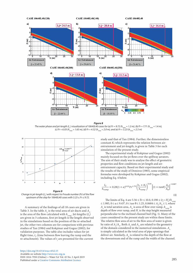
In the current study, all the simulations conducted are in the supercritical range; however, the ones that are discussed so far have a narrow range of Froude numbers between 5.04 and 6.03. Next, we present 5 simulations that have a constant in�ow discharge of 40 m3∙s−1∙m−1; adding on to the previous cases, these simulations have a Froude number range of 3.23–9.72. �e highest �ow velocity and hence the lowest �ow depth at the in�ow section is observed for Fr = 9.72. �e highest Froude number case has average �ow velocity of 33.33 m∙s−1 and the depth of the �ow is 1.2 m at the inlet. When Fr = 3.23, the average �ow velocity and the �ow depth at the inlet is 16 m∙s−1 and 2.5 m, respectively.

Lj is observed to increase quite signi�cantly as Fr increases (Fig. 8). Even though in all the simulations a ramp with height of 10 cm is used, the ramp is not observed to change the trajectory of the �ow signi�cantly in high Froude number simulations. In the high Froude number cases the inertia force dominates the �ow. �erefore, the e�ect of gravitational force is far less signi�cant in high Froude cases; this results in almost-straight water-air interfaces at the top of the jet parallel to the channel �oor. In smaller Froude number cases the e�ect of the ramp becomes noticeable at the top interface.

�e smallest Lj observed is about 11.2 m for the lowest Froude number case. �e largest Lj is about twice as large, at around 24.5 m, compared to the lowest Froude number case. �is jet-length is observed when the depth of the in�ow is almost half the one in the lowest Froude number simulation.

�e relation between Froude number and jet-length is shown in Fig. 9. �e jet-length increases with increasing Froude number. Following the empirical relation proposed by Kokpinar and Gogus (2002), the best-�t in Fig. 9 is selected as a function of Fr1.75. �e aeration index β is calculated as 33.45% at the highest Froude number simulation, while it drops down to 18.59% at the lowest Froude number simulation. Similar to our numerical results, Terrier (2016), who studied hydraulic performance of stepped spillway aerators with a physical model, recently observed that approach �ow Froude number increases the spread of the jet and value of β.

Figure 7The water phase and jet-length (Lj ) visualization for (a) Case 00620L40 (without ramp) and (b) Case 20620L40 (with 20 cm-high ramp)





A summary of the �ndings of all 18 cases are given in Table 3. In the table Aa is the total area of air ducts and Aw is the area of the �ow calculated with hramp. Jet-lengths (Lj) are given in 3 columns, �rst jet-length is the length observed in the simulations based on the position of the re-attached jet, the other two columns are for comparison with previous studies of Tan (1984) and Kokpinar and Gogus (2002), for validation purposes. �e table also includes values for jet �ight time, tj, (time between �ow leaving the ramp and the re-attachment). �e values of tj are presented for the current

study and that of Tan (1984). Further, the dimensionless constant K; which represents the relation between air-entrainment and jet-length, is given in Table 3 for each simulation of the present study.

�e experimental study of Kokpinar and Gogus (2002) mainly focused on the jet �ows over the spillway aerators. �e aim of their study was to analyse the e�ect of geometric properties and �ow conditions on jet-length and air-entrainment capacity. Based on their experimental study and the results of the study of Demiroz (1985), some empirical formulas were developed by Kokpinar and Gogus (2002), including Eq. 4 below.


2/2

1𝜌𝜌𝑞𝑞


𝑛𝑛

𝑝𝑝=1]





)0.44


]−0.087







(4)

�e limits of Eq. 4 are 5.56 ≤ Fr ≤ 10.0, 0.198 ≤ (tr+ Hs)/hramp ≤ 1.985, 0 ≤ α ≤ 9.45°, 0 ≤ tan θ ≤ 1.25, 0.0684 ≤ Aa/Aw ≤ 1, where Aa is total aeration area, Aw is area of �ow over ramp, hramp is depth of �ow over ramp, and Hs is the step height measured perpendicular to the inclined channel bed (Fig. 1). Many of the cases considered in the present study are within these limits. �e relative �ow area of air to the �ow area of water is given by ratio of Aa/Aw. Both Aa and Aw are related to the geometry of the domain considered in the numerical simulations. Aa is simply calculated as the total area of pipe openings that deliver air. Similarly, Aw is related to the depth of the �ow at the downstream end of the ramp and the width of the channel.

Figure 9Change in jet-length (Lj ) with respect to Froude number (Fr) of the flow

upstream of the step for 10640L40 cases with 3.23 ≤ Fr ≤ 9.72.

Figure 8The water phase and jet-length (Lj ) visualization of 10640L40 cases for (a) Fr = 9.72 (hinlet = 1.2 m), (b) Fr = 7.71 (hinlet = 1.4 m),

(c) Fr = 6.03 (hinlet = 1.65 m), (d) Fr = 4.52 (hinlet = 2.0 m), and (e) Fr = 3.23 (hinlet = 2.5 m)





�erefore, the ratio of Aa/Aw di�ers from β. �e β value includes the discharge rates of air and water.

Using the geometry of the simulation domain and simulation data from the present study (hramp and Fr), jet-lengths are calculated for each case based on Eq. 4. �is equation does not account for the location of the aerators. �erefore, Eq. 4 predicts identical jet-lengths for cases where aerator arrangement is the only variant. Jet-lengths obtained via Eq. 4 were plotted against �ndings of the numerical simulations in Fig. 10. �e dashed line shows a theoretical perfect agreement between numerical and experimental �ndings. �e linear regression �t (with R2 = 0.76) indicates that the physical model results are a regression factor of 1/1.4 times smaller than the numerical results.

Recording the re-attachment point in physical model studies could be di�cult due to accumulation of stagnant/circulating water upstream of the re-attachment point, xi. In the present numerical study, the re-attachment point is de�ned with a �xed value of αw = 0.5, as stated earlier. �is di�erence in recording of the re-attachment point in physical models and numerical simulations could be the main reason for the need of a regression factor. Furthermore, the scale e�ects could also play a role in the di�erence.

Tan’s (1984) study is selected for further validation of numerical results. Analytical recommendations of the study are based on geometric properties and a pressure term PN, which is the cavity sub-pressure number. PN is based on the pressure di�erence between atmospheric air pressure and lower nappe

air pressure, ∆P, density of water ρw, gravitational acceleration g, and depth of the �ow at the downstream end of the ramp, hramp. In the present study, the lower nappe air pressure value is obtained by reading pressure values using 100 numerical probes near the jet re-attachment. �ese values are averaged to obtain the cavity sub-pressure number. Inclusion of cavity sub-pressure number in the calculation of jet-length somehow accounts for the location of the aerators, hence jet-lengths calculated using Tan’s expression have varying values as the cavity sub-pressure

TABLE 3Summary of results and comparison with literature

Case hramp (m)

Vramp (m∙s−1) Aa/Aw Fr

Kokpinar and

Gogus (2002)

Tan (1984) Present study

Lj (m) Lj (m) tj (s) tj (s) Lj (m) β K

00620L20 1.10 18.2 0.03 5.53 5.00 5.61 0.30 0.35 6.45 16.95 0.029

00620S20 1.10 18.2 0.03 5.53 5.00 5.70 0.31 0.38 6.96 16.35 0.026

00620F20 1.10 18.2 0.03 5.53 5.00 5.65 0.30 0.37 6.65 16.50 0.027

00620L40 1.10 18.2 0.14 5.53 4.43 5.81 0.31 0.45 8.10 30.60 0.042

00620S40 1.10 18.2 0.14 5.53 4.43 5.76 0.31 0.40 7.27 27.99 0.042

10620L20 1.10 18.2 0.03 5.53 7.53 9.42 0.50 0.41 7.48 16.36 0.024

10620L40 1.10 18.2 0.14 5.53 6.68 9.43 0.50 0.56 10.10 48.37 0.053

10440L49 1.65 24.2 0.09 6.03 11.78 13.90 0.56 0.85 20.50 22.00 0.018

10340L57 1.65 24.2 0.09 6.03 11.78 13.90 0.56 0.89 21.55 21.60 0.017

10640L40(120) 1.20 33.3 0.13 9.72 22.12 22.00 0.64 0.73 24.20 33.45 0.017

10640L40(140) 1.40 28.6 0.11 7.71 16.31 17.58 0.60 0.70 20.00 29.60 0.021

10640L40 1.65 24.2 0.09 6.03 11.78 13.92 0.56 0.67 16.35 26.46 0.027

10640L40(200) 2.00 20.0 0.08 4.52 8.05 10.68 0.52 0.69 13.80 22.64 0.033

10640L40(250) 2.50 16.0 0.06 3.23 5.18 8.02 0.48 0.70 11.20 18.60 0.042

10670L40 2.70 25.9 0.06 5.04 11.84 15.19 0.57 0.69 17.90 17.25 0.026

20620L40 1.10 18.2 0.14 5.53 8.11 13.04 0.69 0.67 12.18 47.57 0.043

20620L20 1.10 18.2 0.03 5.53 9.15 13.30 0.70 0.56 10.10 20.50 0.043

00640L40 1.65 24.2 0.09 6.03 7.82 7.94 0.32 0.36 8.68 8.98 0.017

Figure 10Jet-lengths of present numerical study versus jet-lengths calculated

based on empirical formula of Kokpinar and Gogus (2002)





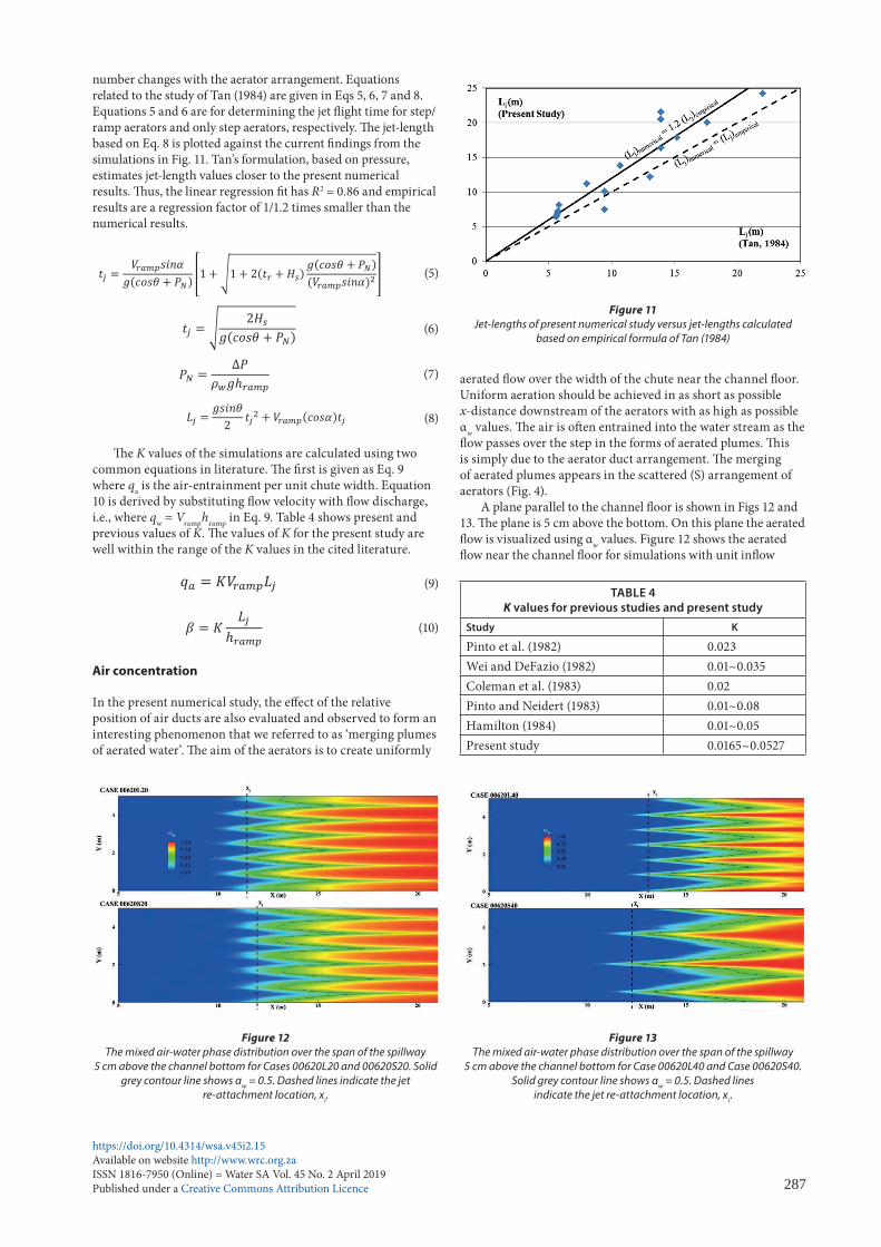
number changes with the aerator arrangement. Equations related to the study of Tan (1984) are given in Eqs 5, 6, 7 and 8. Equations 5 and 6 are for determining the jet �ight time for step/ramp aerators and only step aerators, respectively. �e jet-length based on Eq. 8 is plotted against the current �ndings from the simulations in Fig. 11. Tan’s formulation, based on pressure, estimates jet-length values closer to the present numerical results. �us, the linear regression �t has R2 = 0.86 and empirical results are a regression factor of 1/1.2 times smaller than the numerical results.


2/2

1𝜌𝜌𝑞𝑞


𝑛𝑛

𝑝𝑝=1]





)0.44


]−0.087







(5)


2/2

1𝜌𝜌𝑞𝑞


𝑛𝑛

𝑝𝑝=1]





)0.44


]−0.087







(6)


2/2

1𝜌𝜌𝑞𝑞


𝑛𝑛

𝑝𝑝=1]





)0.44


]−0.087







(7)


2/2

1𝜌𝜌𝑞𝑞


𝑛𝑛

𝑝𝑝=1]





)0.44


]−0.087







(8)

�e K values of the simulations are calculated using two common equations in literature. �e �rst is given as Eq. 9 where qa is the air-entrainment per unit chute width. Equation 10 is derived by substituting �ow velocity with �ow discharge, i.e., where qw = Vramphramp in Eq. 9. Table 4 shows present and previous values of K. �e values of K for the present study are well within the range of the K values in the cited literature.


2/2

1𝜌𝜌𝑞𝑞


𝑛𝑛

𝑝𝑝=1]





)0.44


]−0.087






𝑞𝑞𝑟𝑟 = 𝐾𝐾𝑉𝑉𝑟𝑟𝑟𝑟𝑟𝑟𝑝𝑝𝐿𝐿𝑗𝑗 (9)

𝛽𝛽 = 𝐾𝐾𝐿𝐿𝑗𝑗

ℎ𝑟𝑟𝑟𝑟𝑟𝑟𝑟𝑟

𝐶𝐶𝑟𝑟𝑎𝑎𝑟𝑟 = 1 − (∫𝛼𝛼𝑤𝑤𝑑𝑑𝑑𝑑) 𝑑𝑑⁄

(10)

Air concentration

In the present numerical study, the e�ect of the relative position of air ducts are also evaluated and observed to form an interesting phenomenon that we referred to as ‘merging plumes of aerated water’. �e aim of the aerators is to create uniformly

aerated �ow over the width of the chute near the channel �oor. Uniform aeration should be achieved in as short as possible x-distance downstream of the aerators with as high as possible αw values. �e air is o�en entrained into the water stream as the �ow passes over the step in the forms of aerated plumes. �is is simply due to the aerator duct arrangement. �e merging of aerated plumes appears in the scattered (S) arrangement of aerators (Fig. 4).

A plane parallel to the channel �oor is shown in Figs 12 and 13. �e plane is 5 cm above the bottom. On this plane the aerated �ow is visualized using αw values. Figure 12 shows the aerated �ow near the channel �oor for simulations with unit in�ow

TABLE 4K values for previous studies and present study

Study K

Pinto et al. (1982) 0.023Wei and DeFazio (1982) 0.01~0.035Coleman et al. (1983) 0.02Pinto and Neidert (1983) 0.01~0.08Hamilton (1984) 0.01~0.05Present study 0.0165~0.0527

Figure 12The mixed air-water phase distribution over the span of the spillway

5 cm above the channel bottom for Cases 00620L20 and 00620S20. Solid grey contour line shows αw = 0.5. Dashed lines indicate the jet

re-attachment location, xi.

Figure 11Jet-lengths of present numerical study versus jet-lengths calculated

based on empirical formula of Tan (1984)

Figure 13The mixed air-water phase distribution over the span of the spillway

5 cm above the channel bottom for Case 00620L40 and Case 00620S40. Solid grey contour line shows αw = 0.5. Dashed lines

indicate the jet re-attachment location, xi.





discharge of 20 m3∙s−1∙m−1 aerated using 20 cm-diameter aerators on the step. In both L20 and S20 cases, over the span one can observe formation of aerated plumes, where αw < 0.5. In case of S20, both the width and the length of these aerated plumes are observed to be longer than the ones observed in L20 case.

Figure 13 shows the aerated �ow near the channel �oor for simulations with unit in�ow discharge of 20 m3∙s−1∙m−1 aerated using 40 cm-diameter aerators on the step. In the L40 case presented in Fig. 13, one can still observe the formation of 6 well-de�ned aerated plumes (αw < 0.5) near the channel �oor. In the case of S40 however, only 3 separate aerated plumes are visible. �is shows how 2 neighbouring air ducts work as one big air duct and in a sense decrease the total number of air ducts used in the simulation in S40.

Using the data presented in Figs 12 and 13, αw values across the width of the chute are plotted 5 m downstream of the re-attachment point in Fig. 14. �e average αw values over the span for each case are indicated using dashed lines. �e lower the αw value, the higher the air content of the �ow is. Due to the arrangement and circular cross section of aerators, a continuously homogeneous aerated region 5 cm above the channel �oor 5 m downstream of the re-attachment point is not observed in any of the cases considered in the present study. �e αw values as shown in Fig. 14 follow an undulated pattern over the width of the chute. It is observed that average aeration over the span is higher via S-type aerator arrangement. �e regions where αw is less than 0.90 are assumed to be aerated as the cells in these regions have at least 10% air content in the �ow. Total length of at least 10% aerated regions in Case 00620L40, 5 m downstream of xi, is 3.74 m, while the total length of such regions is 4.28 m in Case 00620S40. It should be noted that the total width of the spillway is 5 m. Similarly, the lengths of aerated regions over the span of the spillway are 3.15 m for Case 00620L20, and 4.96 m for Case 00620S20.

Even though the size of the aerated regions is larger in S simulations, one can observe that the β values slightly decrease in these cases compared to the L arrangement of the aerators (Table 3). A similar reduction in air-entrainment is also noted in simulations 10440L49 and 10340L57 when β values are compared to the one obtained from Case 10640L40. All 3

simulations have identical total area for aeration, Aa. However, in Case 10440L49, 4 air ducts are used instead of 6 and in Case 10340L57, only 3 air ducts are used for aeration. In all 3 cases the unit water discharge is 40 m3∙s−1∙m−1. As given in Table 3, the value of β is around 22% for cases with fewer aerators, compared to 26% in Case 10640L40. �is might be due to a reduction in suctioning e�ect of �ow over larger diameter aerators compared to smaller diameter ones. In the S simulations, merging of air plumes creates a similar e�ect and in return causes reduction in values of β compared to the L simulations.

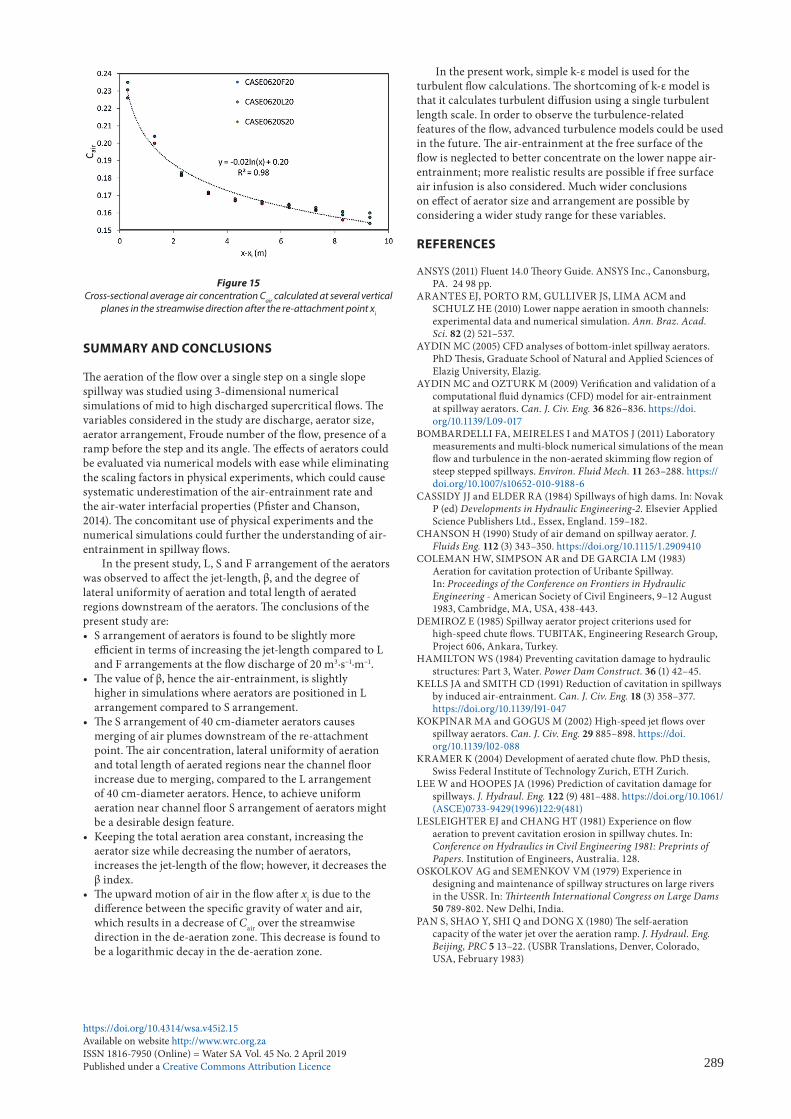
�e β index is based on the amount of total air discharge entrained from the aerators. However, a�er the re-attachment of jet at xi, the de-aeration zone begins as shown in Fig. 1. In this zone, the air content of the �ow starts decreasing as one goes away from the re-attachment point towards the exit boundary. Based on the amount of loss of the air content, better estimation of location of the next ramp/step and aerators is possible. �e cross-sectional average of air concentration (Cair) below the free surface of the �ow is calculated over many x-planes in the streamwise direction in the de-aeration zone. �e interface between the air and water at the free surface is omitted in the calculations as the results concentrate on air-entrainment through the air ducts over the step in the lower nappe. �e Cair depends on the cross-sectional average of αw values as given in Eq. 11. In this equation, A is the total area of the �ow below the free surface.

𝛽𝛽 = 𝐾𝐾𝐿𝐿𝑗𝑗

ℎ𝑟𝑟𝑟𝑟𝑟𝑟𝑟𝑟

𝐶𝐶𝑟𝑟𝑎𝑎𝑟𝑟 = 1 − (∫𝛼𝛼𝑤𝑤𝑑𝑑𝑑𝑑) 𝑑𝑑⁄ (11)

�e decrease in concentration in the x-direction a�er xi in the de-aeration zone could be expressed with a logarithmic decay as shown in Fig. 15 for Cases 00620L20, S20 and F20. �ese cases have the unit in�ow discharge of 20 m3∙s−1∙m−1, the �ow aeration is via six 20 cm-diameter aerators, and no ramp is used in the �ow domain. In Fig. 15, x − xi shows the distance from the re-attachment point. In these simulations, aerator arrangement is not observed to vary the average air concentration over the streamwise direction signi�cantly.

Figure 14The αw values across the width of the chute 5 m downstream of xi for simulations with unit discharge of 20 m3∙s−1∙m−1 aerated using (a) 20 cm-diameter

aerators, and (b) 40 cm-diameter aerators. Dashed lines indicate the average value of αw over the span





SUMMARY AND CONCLUSIONS

�e aeration of the �ow over a single step on a single slope spillway was studied using 3-dimensional numerical simulations of mid to high discharged supercritical �ows. �e variables considered in the study are discharge, aerator size, aerator arrangement, Froude number of the �ow, presence of a ramp before the step and its angle. �e e�ects of aerators could be evaluated via numerical models with ease while eliminating the scaling factors in physical experiments, which could cause systematic underestimation of the air-entrainment rate and the air-water interfacial properties (P�ster and Chanson, 2014). �e concomitant use of physical experiments and the numerical simulations could further the understanding of air-entrainment in spillway �ows.

In the present study, L, S and F arrangement of the aerators was observed to a�ect the jet-length, β, and the degree of lateral uniformity of aeration and total length of aerated regions downstream of the aerators. �e conclusions of the present study are:• S arrangement of aerators is found to be slightly more

e�cient in terms of increasing the jet-length compared to L and F arrangements at the �ow discharge of 20 m3∙s−1∙m−1.

• �e value of β, hence the air-entrainment, is slightly higher in simulations where aerators are positioned in L arrangement compared to S arrangement.

• �e S arrangement of 40 cm-diameter aerators causes merging of air plumes downstream of the re-attachment point. �e air concentration, lateral uniformity of aeration and total length of aerated regions near the channel �oor increase due to merging, compared to the L arrangement of 40 cm-diameter aerators. Hence, to achieve uniform aeration near channel �oor S arrangement of aerators might be a desirable design feature.

• Keeping the total aeration area constant, increasing the aerator size while decreasing the number of aerators, increases the jet-length of the �ow; however, it decreases the β index.

• �e upward motion of air in the �ow a�er xi is due to the di�erence between the speci�c gravity of water and air, which results in a decrease of Cair over the streamwise direction in the de-aeration zone. �is decrease is found to be a logarithmic decay in the de-aeration zone.

In the present work, simple k-ε model is used for the turbulent �ow calculations. �e shortcoming of k-ε model is that it calculates turbulent di�usion using a single turbulent length scale. In order to observe the turbulence-related features of the �ow, advanced turbulence models could be used in the future. �e air-entrainment at the free surface of the �ow is neglected to better concentrate on the lower nappe air-entrainment; more realistic results are possible if free surface air infusion is also considered. Much wider conclusions on e�ect of aerator size and arrangement are possible by considering a wider study range for these variables.

REFERENCES

ANSYS (2011) Fluent 14.0 �eory Guide. ANSYS Inc., Canonsburg, PA. 24 98 pp.

ARANTES EJ, PORTO RM, GULLIVER JS, LIMA ACM and SCHULZ HE (2010) Lower nappe aeration in smooth channels: experimental data and numerical simulation. Ann. Braz. Acad. Sci. 82 (2) 521–537.

AYDIN MC (2005) CFD analyses of bottom-inlet spillway aerators. PhD �esis, Graduate School of Natural and Applied Sciences of Elazig University, Elazig.

AYDIN MC and OZTURK M (2009) Veri�cation and validation of a computational �uid dynamics (CFD) model for air-entrainment at spillway aerators. Can. J. Civ. Eng. 36 826–836. https://doi.org/10.1139/L09-017

BOMBARDELLI FA, MEIRELES I and MATOS J (2011) Laboratory measurements and multi-block numerical simulations of the mean �ow and turbulence in the non-aerated skimming �ow region of steep stepped spillways. Environ. Fluid Mech. 11 263–288. https://doi.org/10.1007/s10652-010-9188-6

CASSIDY JJ and ELDER RA (1984) Spillways of high dams. In: Novak P (ed) Developments in Hydraulic Engineering-2. Elsevier Applied Science Publishers Ltd., Essex, England. 159–182.

CHANSON H (1990) Study of air demand on spillway aerator. J. Fluids Eng. 112 (3) 343–350. https://doi.org/10.1115/1.2909410

COLEMAN HW, SIMPSON AR and DE GARCIA LM (1983) Aeration for cavitation protection of Uribante Spillway. In: Proceedings of the Conference on Frontiers in Hydraulic Engineering - American Society of Civil Engineers, 9–12 August 1983, Cambridge, MA, USA, 438-443.

DEMIROZ E (1985) Spillway aerator project criterions used for high-speed chute �ows. TUBITAK, Engineering Research Group, Project 606, Ankara, Turkey.

HAMILTON WS (1984) Preventing cavitation damage to hydraulic structures: Part 3, Water. Power Dam Construct. 36 (1) 42–45.

KELLS JA and SMITH CD (1991) Reduction of cavitation in spillways by induced air-entrainment. Can. J. Civ. Eng. 18 (3) 358–377. https://doi.org/10.1139/l91-047

KOKPINAR MA and GOGUS M (2002) High-speed jet �ows over spillway aerators. Can. J. Civ. Eng. 29 885–898. https://doi.org/10.1139/l02-088

KRAMER K (2004) Development of aerated chute �ow. PhD thesis, Swiss Federal Institute of Technology Zurich, ETH Zurich.

LEE W and HOOPES JA (1996) Prediction of cavitation damage for spillways. J. Hydraul. Eng. 122 (9) 481–488. https://doi.org/10.1061/(ASCE)0733-9429(1996)122:9(481)

LESLEIGHTER EJ and CHANG HT (1981) Experience on �ow aeration to prevent cavitation erosion in spillway chutes. In: Conference on Hydraulics in Civil Engineering 1981: Preprints of Papers. Institution of Engineers, Australia. 128.

OSKOLKOV AG and SEMENKOV VM (1979) Experience in designing and maintenance of spillway structures on large rivers in the USSR. In: �irteenth International Congress on Large Dams 50 789-802. New Delhi, India.

PAN S, SHAO Y, SHI Q and DONG X (1980) �e self-aeration capacity of the water jet over the aeration ramp. J. Hydraul. Eng. Beijing, PRC 5 13–22. (USBR Translations, Denver, Colorado, USA, February 1983)

Figure 15Cross-sectional average air concentration Cair calculated at several vertical

planes in the streamwise direction after the re-attachment point xi




https://doi.org/10.1139/L09-017

https://doi.org/10.1139/L09-017

https://doi.org/10.1007/s10652-010-9188-6

https://doi.org/10.1007/s10652-010-9188-6

https://doi.org/10.1115/1.2909410

https://doi.org/10.1139/l91-047

https://doi.org/10.1139/l02-088

https://doi.org/10.1139/l02-088

https://doi.org/10.1061/(ASCE)0733-9429(1996)122:9(481)



PFISTER M and CHANSON H (2014) Two-phase air-water �ows: Scale e�ects in physical modelling. J. Hydrodyn. 26 (2) 291–298. https://doi.org/10.1016/S1001-6058(14)60032-9

PINTO NLS (1988) Cavitation and aeration. In: Jansen RB (ed) Advanced Dam Engineering for Design, Construction and Rehabilitation. Kluwer Academic Publishers, Dordrecht, �e Netherlands. 620–634.

PINTO NLS and NEIDERT SH (1983) Evaluating entrained air �ow through aerators. Water Power Dam Construct. 35 (8) 40–42.

PINTO NLS, NEIDERT S and OTA JJ (1982) Aeration at high velocity �ows. Water Power Dam Construct. 34 (2) 34–38.

RUTSCHMANN P and HAGER WH (1990) Air-entrainment by spillway aerators. ASCE J. Hydraul. Eng. 116 (6) 765–782. https://doi.org/10.1061/(ASCE)0733-9429(1990)116:6(765)

SCHWARTZ I and NUTT LP (1963) Projected nappes subjected to transverse pressure. ASCE J. Hydraul. Div. 89 (7) 97–104.

SINHA SK, SOTIROPOULOS F and ODGAARD AJ (1998) �ree-dimensional numerical model for �ow through natural rivers. J. Hydraul. Eng. 124 (1) 13–25. https://doi.org/10.1061/

(ASCE)0733-9429(1998)124:1(13)TAN P (1984) Model studies of aerators on spillways. Research Report

85-6, Department of Civil Engineering, University of Canterbury, Christchurch, New Zealand.

TERRIER SCO (2016) Hydraulic performance of stepped spillway aerators and related downstream �ow features. PhD thesis, Ecole Polytechnique Federale De Lausanne.

VOLKART P and RUTSCHMANN P (1991) Aerators on spillways. In: WOOD IR (ed) Air-Entrainment in Free-Surface Flows: IAHR Hydraulic Structures Design Manual 4. CRC Press, Rotterdam, �e Netherlands. 85–113.

WEI C and DEFAZIO F (1982) Simulation of free jet trajectories for the design of aeration devices on hydraulic structures. Proceedings of 4th International Conference on Finite Elements in Water Resources, June 1982. IAHR, ISCME, DFG, Hanover, Germany.

ZARRATI AR (1994) Mathematical modelling of air-water mixtures in open channels. J. Hydraul. Res. 32 (5) 707–720. https://doi.org/10.1080/00221689409498710




https://doi.org/10.1016/S1001-6058(14)60032-9

https://doi.org/10.1016/S1001-6058(14)60032-9





https://doi.org/10.1080/00221689409498710

https://doi.org/10.1080/00221689409498710

application of vof and k-ε turbulence model in …application of vof and k-ε turbulence model in...

Documents