applications and discretizations of the poisson-nernst ... · applications and discretizations of...

Overview Applications Discretization Solvers

Applications and Discretizations of thePoisson-Nernst-Planck Equations

Transport of Ionic Particles in Biological Environments

The Fields Institute, Toronto

Maximilian S. MettiCCMA, Department of Mathematics

The Pennsylvania State University

July 31, 2014

PSU Center for Computational Mathematics and Applications Slide 1/65, July 31, 2014


1 Background and Equations

2 Applications of PNP

3 Discretizations

4 Numerical Solvers



Charge Carrier Transport

Charge carrier transport refers to phenomena where chargedparticles interact with one another through an electric field.

These systems are often encountered in biological and engineeringsettings, and simulation can help improve understanding the role ofcharged particles in cellular nanochannels, microfluidic chips, solarcells, etc.



A brief history of time-dependent PNP

We are interested in charged particle transport in electrostaticsystems when magnetic forces are negligible.

Nernst and Planck modeled these phenomena using a continuummodel dating back to 1889, where the distribution of chargedparticles are distributed according to processes of drift anddiffusion.



Connection to the Maxwell’s equations

The PNP equations take root in the Maxwell equations:

ε0∇ · ~E = ρ, (Gauß’s Law)

∇ · ~B = 0, (Gauß’s Law for Magnetism)

∇× ~E =∂ ~B

∂t, (Faraday’s Law of Induction)

∇× ~B = µ0

(~j + ε0

∂ ~E

∂t

). (Ampere’s Circuital Law)



Connection to the Maxwell’s equations

In simple cases:

Magnetic field is absent: ~B = ~0

∇× ~E = ~0 =⇒ ~E = −εr∇φ

Ion flux driven by drift-diffusion

~ji = −Di∇ρi + µiρi ~E

Mass conservation∂ρi∂t

= −∇ · ~ji



What modifications are permitted?

The PNP equations are used to model many devices that producea wide variety of functionality

generating electrical energy in a solar cell

controlling fluid flow in microchannels

gating ionic particles from proteins

What are permissible (consistent with Maxwell’s equations)modifications that to generate this variety in functionality?



Multi-FunctionalityMaterial Parameters

A simple rescaling of the variables, in addition to the Einsteinrelation (κBT )µi = eDi , shows that all qualitative behavior of asimple PNP system can be reproduced by varying the electricpermitivitty and ionic diffusivities.

∂∂tp = ∇ · [Dp(∇p + p∇φ)] ,

∂∂tn = ∇ · [Dn(∇n − n∇φ)] ,

−∇ · (ε∇φ) = p − n.

A broad spectrum of qualitative behavior follows from relativescalings between coefficients and discontinuities of the coefficients,where we note ε = ε(L,T , ρref).

Analyses should be flexible with the values of these parameters inorder to be applicable to many devices.



Multi-FunctionalityIonic Flux

While the Nernst-Planck equations describe ion diffusivity andelectrostatic forces, additional physical forces can be taken intoaccount in the ion flux

~j = −D∇ρ+ µρ~E + ~F

These additional forces are often nonlinear expressions and maycouple to other PDEs.



Multi-FunctionalityMass Conservation

In the context of devices, we typically deal with finite domains.

Mass conservation then requires a prescribed boundary and a set ofboundary conditions, which indirectly influence the total ionic massin a device.

Additionally, we may add terms to specify ion sources and sinks:

∂ρ

∂t= −∇ · ~j + S



Multi-Functionality

Thus, a broad spectrum of qualitative behavior follows from:

scalings of coefficients and discontinuities of the coefficients

modification to the ionic fluxes

device-specific statement of mass conservation

domain geometry and boundary conditions



Multi-Functionality

We are primarily interested modeling devices using that PNPequations.

The takeaway: chairs are held together by nails and glue, a book isheld together by its binding, and devices in this talk are heldtogether by PNP.

The PNP equations serve as a platform to connect a prescribeddomain geometry, material parameters, and expressions for ionfluxes to create a device that subsequently yields somefunctionality, which depends on applied boundary conditions.



Applications and Collaborations

This work focuses on applications, discretizations, and numericalsolvers for PNP equations and is led by Prof. Jinchao Xu, withXiaozhe Hu and M. M.

Biology, Nanochannels (Profs Liu & Eisenberg, Penn State &Rush Medical)

Electrokinetics (Department of Energy, Collaboratory onMathematics for Mesoscopic Modeling of Materials)

Solar Cell (Prof. Fonash, Penn State)

LiPON Battery (Dr. G. Lin and Dr. B. Zheng, PNNL)

Ion Filtration using Poly-Membranes (Prof. Hickner and Dr.H. Xie, Penn State)

Semi-conductors (Prof. Bank, UCSD)



Semi-conductorsA prominent application of PNP in engineering applications is toexplore the efficiency and capability of various configurations ofsemi-conductor devices, such as transistors and diodes, numerically.

Figure: Semi-conductor

http://hyperphysics.phy-astr.gsu.edu/hbase/solids/intrin.html



Semi-conductors

By constructing a device using distinct semi-conductor materials,interactions between “electrons” and “holes” can modify currentthrough the device.

We require:

Discontinuous material parameters

Modifications to ion fluxes

Source terms added to mass conservation eqns



Semi-conductorsDoping

Combining several “doped” materials is modeled by using materialswith distinct diffusivities and electric permittivity

~jp = −Dp(∇p + p∇φ),

~jn = −Dn(∇n − n∇φ),

−∇ · (εrε0∇φ) = p + pf − (n + nf ),

and fixed charges

~jpf = ~0 and ~jnf = ~0.



Semi-conductorsRecombination

Furthermore, since holes model the lack of an electron, holes andelectrons are generated stochastically and can annihilate eachother by recombination.

This is modeled by generation and recombination terms

∂p

∂t= −∇ · ~jp + G (p, n)− R(p, n)

∂n

∂t= −∇ · ~jn + G (p, n)− R(p, n)



Semi-conductorsRecombination

In photovoltaic semi-conductors (aka solar cells), electron/holepairs are generated by an optical electric field

∇×∇× ~Eopt + κ2 ~Eopt = ~F ,

∂p

∂t= −∇ · ~jp + G (~Eopt)− R(p, n),

∂n

∂t= −∇ · ~jn + G (~Eopt)− R(p, n).



Semi-conductorsMaterials, Geometry, and BCs

A specific device is modeled by

material configuration

shape of the device

applied voltagesFigure: Diode

∂p

∂t= ∇ · [Dp(∇p + p∇φ)]− R(p, n),

∂n

∂t= ∇ · [Dn(∇n − n∇φ)]− R(p, n),

−∇ · (ε∇φ) = p + pf − n − nf .

http://hyperphysics.phy-astr.gsu.edu/hbase/solids/diod.html






shape of the device

applied voltagesFigure: Bipolar JunctionTransistor: forward and reversecurrent, saturation, cutoff

∂p

∂t= ∇ · [Dp(∇p + p∇φ)]− R(p, n),

∂n

∂t= ∇ · [Dn(∇n − n∇φ)]− R(p, n),

−∇ · (ε∇φ) = p + pf − n − nf .

http://en.wikipedia.org/wiki/Bipolar transistor



ElectrokineticsWe can enrich the functionality of a device by adding kinetic forcesin the ionic flux:

~j = −D∇ρ− µρ∇φ+ ρ~u.

This models electrokinetic systems where charged particles aresuspended in an electrolyte.

Some phenomena modeled by this system are electroosmosis,electrophoresis, and streaming potentials/currents.

Figure: Electroosmosis in a capillary tube

Wenxiao Pan, PNNL



Electrokinetics

Coupling the PNP equations with the incompressible Navier-Stokesequations expands the model to take into account the kineticeffects of charged particles suspended in an electrolyte.

pt = ∇ · [Dp(∇p + p∇φ)− p~u ] ,

nt = ∇ · [Dn(∇n − n∇φ)− n~u ] ,

−∇ · (ε∇φ) = p − n,

~ut + (~u ·∇)~u = ν∇2~u +∇π − (p − n)∇φ,∇ · ~u = 0.



ElectrokineticsElectroosmosis

Electroosmosis refers to the phenomenon where a fluid is driven byelectric forces.

This is an important model for engineering fluidic microchannels.

In these applications, controlling flows with small mechanicalpumps and valves is difficult to design and fabricate withoutdefects; electrokinetics can be used to remedy these issues.

Figure: Electroosmosis in a capillary tube

Wenxiao Pan, PNNL



ElectrokineticsElectroosmosis

For more complicated geometries, this can serve as a switch tocontrol where the fluid flows.

Figure: Controlled flow in T-juction

Dutta, Beskok, & Warburton, Num. Sim. of Mixed Electroosmotic/Pressure Driven Microflows (2002)



ElectrokineticsMicrofluidic Diode and Transistors

Diodes and Bipolar Transistors can be built from a nanochannelconnecting two salt baths.

Surface charges on a nannochannel can control the current in thechannel.

Figure: Nanofluidic Diode and Bipolar Transistor

Daiguji, Oka, & Shirono, Nanofluidic Diode and Bipolar Transistor



ElectrokineticsElectrophoresis

Another applications where the PNP equations are coupled withNavier-Stokes includes electrophoresis, where a solid chargedparticle is suspended in a charged fluid, and an applied electricfield moves the solid.

In this application, the “boundary” moves as the charged particleis driven through the device.

Figure: Electrophoresis

Zangle, Mani, & Santiago, Theory and experiments of concentration polarization and ion focusing atmicrochannel and nanochannel interfaces (2010)



Biological ApplicationsPassive transport through cell membrane

Modeling ions passing through the nanochannels of a cellular membraneis a well-studied example.

Passive transport through the nanochannel has been modeled using thePNP equations.

Ion diffusivity and electricpermittivity change from the bathto channel

Complicated mesh geometries areneeded to resolve proteins

Fixed charges generate surfacecharges on protein

Ionic fluxes must account forfixed charges and inter-ionicinteractions

Figure: Passive Transport

Horng, Lin, Liu, & Eisenberg, PNP Equations with Steric Effects: A Model of Ion Flow through Channels(2012)



Biological ApplicationsPassive transport: Geometry

The function of proteins are extremely sensitive to location of charges inproteins and protein shape.

Generating accurate, let alone adequate, protein meshes is a difficult task!

There exist software packages for mesh generation, such as TMSmesh,that are designed to produce high quality meshes for proteins.

Tu, Chen, Xie, Zhang, Eisenberg, & Lu, A Parallel Finite Element Simulator for Ion Transport throughThree-Dimensional Ion Channel Systems (2013)



Biological ApplicationsPassive Transport: Permanent Charges

Within each protein, there are many permanent charges, which aremodeled as point charges, to generate the surface charge on theprotein.The electric potential has a numerically stable decomposition intothree components:

Singular: −∇ · (εp∇φs(x)) =∑

i δ(|x − xi |)=⇒ φs =

∑Coloumb potentials

∣∣Ωp

Harmonic: −∇ · (εp∇φh) = 0, φh∣∣∂Ωp

= −φs∣∣∂Ωp

Regular: −∇ · (ε∇φr ) = p − n,εs∂φr∂n − εp

∂φr∂n = εp

∂∂n (φs + φh) on ∂Ωp

ε =

εp, in proteinεs , in solution



Biological ApplicationsPassive Transport: Steric Effects

Due to the small scale of this process, the size of ions becomesincreasingly important. This is especially true when studyingchannel selectivity.

Following Horng, Lin, Liu, Eisenberg, we can modify the ionic fluxto account for repulsive size effects between ions:

~jp = −Dp

(∇p + p∇φ+ p(εpp∇p + εpn∇n)

),

~jn = −Dn

(∇n − n∇φ+ n(εnp∇p + εnn∇n)

).

These modifications have recovered some selectivity behavior ofion nanochannels.

Further modifications employing relative drag have been analyzedto model ion crowding.



PNP Models and their Differences

While it has been emphasized that there are some standard classesof modifications to the PNP system, the effects of thesemodifications should not be downplayed.

The resulting behavior of a given device can change drastically, aswell as the analysis that is required to understand the modelmathematically.



Our Goal

Our focus is on designing and analyzing numerical discretizationsand solvers for the PNP equations.

We seek robust finite element discretizations for the PNPequations with solvers that have provable convergence and stabilityproperties to work for a wide variety of applications.



Formulating the PNP EquationsPrimitive Variables

For a system with a single cation and anion, the formulation usingprimitive variables is

∂

∂tp = ∇ · [Dp(∇p + p∇φ)] ,

∂

∂tn = ∇ · [Dn(∇n − n∇φ)] ,

−∇ · (ε∇φ) = p − n,

plus suitable boundary conditions that depend on the device in question.



Formulation Selectivity

In proving results for the discrete system, we must choose theappropriate variables to discretize a priori, as this determines therestricted class of discrete test functions.

We would like to prove:

An energy estimate for the discrete nonlinear solution

Convergence to the discrete nonlinear solution

Well-posedness of the linearized system



Energy Estimate for the Continuous Formulation

The solution of the simple PNP system satisfies the known energylaw

d

dt

∫Ω

ε

2|∇φ|2 + p log p + n log n dx

= −∫

ΩDpp|∇(log p + φ)|2 + Dnn|∇(log n − φ)|2 dx .

The energy norm used for this system is not typical of finiteelement discretizations where p, n, φ ∈ Vh = C0 ∩ pw linear



Formulating the PNP EquationsSlotboom Variables

An alternate formulation to the primitive variables involves theSlotboom variables,

p = eφp, Dp = Dpe−φ,

n = e−φn, Dn = Dneφ.

Then,

∂

∂te−φp = ∇ ·

(Dp∇p

),

∂

∂teφn = ∇ ·

(Dn∇n

),

−∇ · (ε∇φ) = e−φp − eφn.



Formulating the PNP EquationsSlotboom Variables

The Slotboom formulation is useful for proving analytical resultssuch as a maximum principle, since the Nernst-Planck equationsare symmetrized.

∂∂te−φp = ∇ ·

(Dp∇p

),

∂∂teφn = ∇ ·

(Dn∇n

).

Also, this formulation observes faster convergence numerically fornonlinear iterates.

One must be careful to account for the conditioning of the stiffnessmatrix, since the diffusion coefficient varies exponentially.

Dp = Dpe−φ, Dn = Dne

φ.



Formulating the PNP EquationsLog-Density Variables

Using a log transformation, we define

p = log p, n = log n.

Then,

∂

∂te p = ∇ ·

(Dpe

p∇(p + φ)),

∂

∂te n = ∇ ·

(Dne

n∇(n − φ)),

−∇ · (ε∇φ) = e p − e n.

This formulation displays nonlinear diffusion and guarantees positivityof the ionic densities.



Energy Estimate for Log-Density Weak Form

In order to prove the energy estimate, we assume a closed systemand p, n ∈ Vh ⊂ H1 and φ ∈ V ′h ⊆ Vh.Written in weak form:(

∂∂te p, χ

)+(Dpe

p∇(p + φ),∇χ)

= 0,(∂∂te n, λ

)+(Dne

n∇(n − φ),∇λ)

= 0,(ε∇φ,∇ψ

)−(e p − e n, ψ

)= 0.

Further, we assume the conservation of mass:

d

dt

∫Ωe p dx =

d

dt

∫Ωe n dx = 0.




Choosing χ = p + φ, λ = n − φ, and ψ = φ yields an energyestimate:(

∂∂te p, p

)+(∂∂te p, φ

)= −

(Dpe

p∇(p + φ),∇(p + φ)),(

∂∂te n, n

)−(∂∂te n, φ

)= −

(Dne

n∇(n − φ),∇(n − φ)),(

ε∇( ∂∂tφ),∇φ

)=(∂∂te p, φ

)−(∂∂te n, φ

),




Adding the PNP equations gives(ε∇( ∂∂tφ),∇φ

)+(∂∂te p, p

)+(∂∂te n, n

)= −

(Dpe

p∇(p + φ),∇(p + φ))−(Dne

n∇(n − φ),∇(n − φ))

and

ddt

(e p, 1

)=(e p,

∂∂tp)

= 0,

ddt

(e n, 1

)=(e n,

∂∂tn)

= 0.




Combining these equations, we recover an energy estimate:(ε∇( ∂∂tφ),∇φ

)+(∂∂te p, p

)+(∂∂te n, n

)+(e p,

∂∂tp)

+(e n,

∂∂tn)

=d

dt

∫Ω

ε

2|∇φ|2 + pe p + ne n dx

= −(Dpe

p∇(p + φ),∇(p + φ))−(Dne

n∇(n − φ),∇(n − φ)).



A Fully Discrete Energy Estimate

For the fully discrete system, we consider Backward Eulertime-stepping:(e pk − e pk−1

∆t, χ)

+(Dpe

pk∇(pk + φk),∇χ)

= 0,(e nk − e nk−1

∆t, λ)

+(Dne

nk∇(nk + φk),∇λ)

= 0,(ε∇φk ,∇ψ

)−(e pk − e nk , ψ

)= 0.

Subscripts denote the time-step.




To maintain an analogous energy estimate, there are twoalternative schemes for mass conservation:(e pk − e pk−1

∆t, 1)

= 0 and(e nk − e nk−1

∆t, 1)

= 0,

or (e pk−1 ,

pk − pk−1

∆t

)= 0 and

(e nk−1 ,

nk − nk−1

∆t

)= 0.




We first consider the conservation scheme(e pk − e pk−1

∆t, 1)

= 0 and(e nk − e nk−1

∆t, 1)

= 0.

For this discrete energy estimate, we must define an underlyingfinite element space.




Define e p(x ,t) =∑m

k=1 bk(t)e pk (x): then for tk−1 < t ≤ tk ,

∂e p(t)

∂t=

e pk − e pk−1

∆t

and

∂p(t)

∂t=

∂

∂tlog

( m∑k=1

bk(t)e pk (x)

)

=1∑m

k=1 bk(t)e pk (x)

∂

∂t

m∑k=1

bk(t)e pk (x) =1

e p(t)

e pk − e pk−1

∆t




Thus, the Nernst-Planck equation is(e pk − e pk−1

∆t, pk + φk

)=(∂∂te pk , pk

)+(e pk − e pk−1

∆t, φk

)= −

(Dpe

pk∇(pk + φk),∇(pk + φk))

and mass conservation is:(e pk − e pk−1

∆t, 1)

=(e pk ,

∂pk∂t

)= 0,

which combine into

∂∂t

(e pk , pk

)+(e pk − e pk−1

∆t, φk

)= −

(Dpe

pk∇(pk + φk),∇(pk + φk)).




We have

∂∂t

(e pk , pk

)+(e pk − e pk−1

∆t, φk

)= −

(Dpe


∂∂t

(e nk , nk

)−(e nk − e nk−1

∆t, φk

)= −

(Dne

nk∇(nk − φk),∇(nk − φk))

and(ε∇φk −∇φk−1

∆t,∇φk

)=(e pk − e pk−1

∆t, φk

)−(e nk − e nk−1

∆t, φk

).




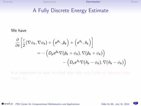
We have

∂

∂t

[ε

2

(∇φk ,∇φk) +

(e pk , pk

)+(e nk , nk

)]= −

(Dpe


−(Dne

nk∇(nk − φk),∇(nk − φk))

It is important to bear in mind that this only holds at discrete timesteps, tk .




This implies that mass is exactly conserved over time and

maxk

ε

2

∣∣φ(tk)|21 +(e p(tk ), p(tk)

)+(e n(tk ), n(tk)

)≤ ε

2

∣∣φ(0)|21 +(e p(0), p(0)

)+(e n(0), n(0)

)−∑k

∆t

[(Dpe


+(Dne

nk∇(nk − φk),∇(nk − φk))]

+ quadrature error




The alternate mass conservation scheme requires(e p,

∂∂tp)≈(e pk−1 ,

pk − pk−1

∆t

)= 0.

We note that this mass conservation constraints, together with abackward difference, yields an algebraic identity(e pk − e pk−1

∆t, pk

)+(e pk−1 ,

pk − pk−1

∆t

)=( pke pk − pk−1e

pk−1

∆t, 1).




The new identity along with same technique as the other(semi-)discrete energy estimates give

ε

2

|φk |21 − |φk−1|21∆t

+( pke pk − pk−1e

pk−1

∆t, 1)

+( nke nk − nk−1e

nk−1

∆t, 1)

≤ −(Dpe


−(Dne

nk∇(nk − φk),∇(nk − φk)).




Summing over k gives

maxk

ε

2|φk |21 +

(pke

pk , 1)

+(nke

nk , 1)

≤ ε

2|φ0|21 +

(p0e

p0 , 1)

+(n0e

n0 , 1)

−m∑

k=1

∆t

[(Dpe


+(Dne

nk∇(nk − φk),∇(nk − φk))].



Comparing the Estimates

The first scheme:(e pk−e pk−1

∆t , 1)

= 0 conserves mass exactly and

obeys an energy law at each time step, though the final estimatehas an additional quadrature error term.

The second scheme:(e p, ∂

∂t p)≈(e pk−1 ,

pk−pk−1

∆t

)= 0 has a

favorable energy estimate, though the mass is only approximatelyconserved.



Software Packages

We leverage the FEniCS and FASP software packages.

FEniCS Software Package:

Open source software, many collaborators

Translates weak form into linear systems

Interfaces with linear solvers

FASP Software Package:

Developed at Penn State

Fast solvers for linear systems



Robust DiscretizationNonlinear Problem

Our goal is to develop a software that can solve the PNP systemfor a wide variety range of parameters and applications withprovable stability and well-posedness properties.

The nonlinearity of the system is believed to provide stability; aNewton solver is used since the energy is convex.

Convergence is presumed once the relative residual is below apredefined threshold.




We take care to mention the case of modified ion fluxes or ionsources, as in the case of electrokinetics or ionic recombinations.

We take the Frechet derivative with respect to any additional termsalong with the rest of the system to take a monolithic approach.So,

~jp = −Dp

(∇p + p∇φ

)+ ~F (p, n, φ, u)

gives

δ~jp = −Dp

(∇δp + δp∇φ+ p∇δφ

)+

∂

∂ε

∣∣∣∣ε=0

~F (p + εδp, n + εδn, φ+ εδφ, u + εδu).



Robust DiscretizationLinear Problem

Currently, we employ a block G-S solver with a preconditioner onthe linearized system, which approximately solves PNP equationsgiven additional forces, updates the solution, then solves anyadditional equations with p, n, φ fixed, updates the solution, and socycles back and forth.

In this way, we can precondition the PNP system and the additionalequations separately, while maintaining a monolithic approach.




In both primitive and log-density variables, the Frechet derivativeyields linear convection-dominated problems:

1

∆t

(p, χ

)+(αp∇p + ~βpp,∇χ

)+(αp∇φ,∇χ

)= (Rp, χ),

1

∆t

(n, λ)

+(αn∇n + ~βnn,∇λ

)+(αn∇φ,∇λ

)= (Rn, λ),(

ε∇φ,∇ψ)−(γpp − γnn, ψ

)= (Rφ, ψ).

We use a quasi-Newton method, where an EAFE flux can be usedto approximate the flux terms on an element-by-element basis:

αp∇p + ~βpp ≈ Jp(p), αp∇p + ~βpp ≈ Jn(n).




Figure: The Jacobian matrix




Preconditioned Jacobi or Gauß-Seidel can be used to solve thelinear system, though convergence depends on the conditioning ofthe full linear system.

In addition to the off-diagonal blocks, another difficulty can arisefrom the ε-Poisson block:(

ε∇φ,∇ψ)−(γpp − γnn, ψ

)= (fφ, ψ).

Often, this is singularly perturbed: 0 < ε 1.

A posteriori error estimators and mesh adaptivity can be used toresolve φ.



Thank you for your attention


applications and discretizations of the poisson-nernst ... · applications and discretizations of...

Documents