applications of adaptive antennas in third-generation

i

Australian Telecommunications Research Institute

Applications of Adaptive Antennas in Third-Generation Mobile

Communications Systems

Buon Kiong Lau

This thesis is presented for the Degree of

Doctor of Philosophy

of

Curtin University of Technology

November 2002

i

5 Kingsway

Nedlands, WA 6009

6th Nov. 2002

The Director of Postgraduate Studies

Australian Telecommunications Research Institute

Curtin University of Technology

Bentley, WA 6102.

Dear Sir,

I have much pleasure in submitting this thesis entitled “Applications of Adaptive Antennas

in Third-Generation Mobile Communications Systems” as the requirement for the Degree

of Doctor of Philosophy.

I affirm that this thesis contains no material which has been accepted for the award of any

other degree or diploma in any university. And to the best of my knowledge and belief this

thesis contains no material previously published by any other person except where due

acknowledgment has been made.

Yours Sincerely,

______________

Buon Kiong Lau

ii

To God be the glory!

iii

Acknowledgments First of all, my Lord and Saviour Jesus Christ deserves all honour and praise for the

completion of this thesis. Through the course of my research study, I have come to

appreciate more of His love and grace that are always sufficient for me and my every need.

Secondly, I thank God for my parents who had inspired me to be my best by their own good

examples. I am deeply indebted by their ongoing love and support. I also thank my brother

and two sisters who have played a significant role in shaping me and preparing me for life’s

challenges.

I would also like to thank my supervisor, Dr. Yee Hong Leung, who, over the course of my

study, has become a good friend whom I treasure and respect. My heartfelt thanks extend

also to the staff and students of ATRI and the ATcrc. In particular, I thank ATRI director

Professor Sven Nordholm, for interesting discussions, valuable inputs to my thesis topic

and much practical assistance in other matters. I wish to thank Mr. Gregory J. Cook, a

Masters student, for his assistance and collaboration in some of the thesis work.

I am also indebted to Professor Doug Gray of Adelaide University for his exciting and

motivating short course on “Subspace Methods for Array Signal Processing” (in 1998) that

gave me an excellent overview of the area and helped define my research direction.

And how can I forget the wonderful year of work experience (April 2000-March 2001) with

Ericsson Research in Stockholm! I would like to thank my former bosses Dr. Sören

Andersson, Mr. Mikael Höök and Mr. Jan Färjh for the valuable work opportunity. I also

thank my former colleagues Dr. Andrew Logothetis, Mr. Magnus Berg, Dr. Bo Hagerman,

Dr. Hideshi Murai, Mr. Ming Chen, Dr. Bo Göransson and many others of the Access

Technologies and Signal Processing Department for their guidance and warm friendship. It

has also been a great privilege to receive significant in-kind contributions from the

department since I left Ericsson.

I am grateful towards the Australian Government for financial support through the

International Postgraduate Research Scholarship (formerly OPRS), and ATRI of Curtin

University and the Australian Telecommunications Cooperative Research Centre (ATcrc)

and its predecessor the CRC-BTN, for generous top-up scholarship awards.

iv

Friendship has always played an important role in my life. Here, I would like to thank

particularly my close friends, local and overseas, for their prayers, encouragement and fine

company. You have all been channels of God’s blessings to me. Gillian Goh and Annelise

Tan deserve a special mention for their important contribution in proofreading this thesis.

And lastly, my special thanks go to my lovely Duojia, whose love and constant

encouragement have been instrumental in making the journey of my research study that

much more pleasant and wonderful.

v

Abstract Adaptive antenna systems (AAS’s) are traditionally of interest only in radar and sonar

applications. However, since the onset of the explosive growth in demand for wireless

communications during the 1990’s, researchers are giving increasing attention to the use of

AAS technology to overcome practical challenges in providing the service. The main

benefit of the technology lies in its ability to exploit the spatial domain, on top of the

temporal and frequency domains, to improve on transceiver performance.

This thesis presents a unified study on two classes of preprocessing techniques for uniform

circular arrays (UCA’s). UCA’s are of interest because of their natural ability to provide a

full azimuth (i.e. 360°) coverage found in typical scenarios for sensor array applications,

such as radar, sonar and wireless communications. The two classes of preprocessing

techniques studied are the Davies transformation and the interpolated array transformations.

These techniques yield a mathematically more convenient form – the Vandermonde form –

for the array steering vector via a linear transformation. The Vandermonde form is useful

for different applications such as direction-of-arrival (DOA) estimation and optimum or

minimum variance distortionless response (MVDR) beamforming in correlated signal

environment, and beampattern synthesis. A novel interpolated array transformation is

proposed to overcome limitations in the existing interpolated array transformations.

A disadvantage of the two classes of preprocessing techniques for UCA’s with omni-

directional elements is the lack of robustness in the transformed array steering vector to

array imperfections under certain conditions. In order to mitigate the robustness problem,

optimisation problems are formulated to modify the transformation matrices. Suitable

optimisation techniques are then applied to obtain more robust transformations. The

improved transformations are shown to improve robustness but at the cost of larger

transformation errors. The benefits of the robustification procedure are most apparent in

DOA estimation.

In addition to the algorithm level studies, the thesis also investigates the use of AAS

technology with respect to two different third generation (3G) mobile communications

systems: Enhanced Data rates for Global Evolution (EDGE) and Wideband Code Division

Multiple Access (WCDMA). EDGE, or more generally GSM/EDGE Radio Access

Network (GERAN), is the evolution of the widely successful GSM system to provide 3G

vi

mobile services in the existing radio spectrum. It builds on the TDMA technology of GSM

and relies on improved coding and higher order modulation schemes to provide packet-

based services at high data rates. WCDMA, on the other hand, is based on CDMA

technology and is specially designed and streamlined for 3G mobile services.

For WCDMA, a single-user approach to DOA estimation which utilises the user spreading

code and the pulse-shaped chip waveform is proposed. It is shown that the proposed

approach produces promising performance improvements. The studies with EDGE are

concerned with the evaluation of a simple AAS at the system and link levels. Results from

the system and link level simulations are presented to demonstrate the effectiveness of AAS

technology in the new mobile communications system. Finally, it is noted that the

WCDMA and EDGE link level simulations employ the newly developed COST259

directional channel model, which is capable of producing accurate channel realisations of

macrocell environments for the evaluation of AAS’s.

vii

Table of Contents

Author’s publications 1

Chapter 1 Introduction.................................................................................................... 3

1.1 Introduction and Motivation .................................................................................... 3

1.2 Background and Contributions of the Thesis .......................................................... 7

1.3 Thesis Outline.........................................................................................................10

1.4 Mathematical Notations and Acronyms ................................................................11

Part I – AAS Algorithms......................................................................................................15

Chapter 2 UCA Preprocessing......................................................................................16

2.1 Introduction ............................................................................................................16

2.1.1 Davies Transformation ......................................................................................16

2.1.2 Interpolated Array Transformations .................................................................20

2.1.3 Discussions.........................................................................................................22

2.2 Signal and Array Models .......................................................................................23

2.3 Davies Transformation...........................................................................................26

2.3.1 Summary of the Method .....................................................................................26

2.3.2 Design Example .................................................................................................29

2.4 Interpolated Array Transformation of Bronez.......................................................31


2.4.2 Critique of the Method .......................................................................................34

2.5 Interpolated Array Transformation of Friedlander................................................39


2.5.2 Critique of the Method .......................................................................................41

2.6 Interpolated Array Transformation of Cook et al. ................................................47

2.6.1 Window Function ...............................................................................................49

2.6.2 Optimisation Sector versus Operational Sector................................................51

2.6.3 Virtual ULA Size.................................................................................................52

2.6.4 Orientation of the In-Sector and the Virtual ULA.............................................54

2.6.5 Design Examples................................................................................................58

2.7 Relationship between Davies and Interpolated Array Transformations...............62

2.8 Conclusions ............................................................................................................64

viii

Chapter 3 Robustness of UCA Preprocessing.............................................................65

3.1 Introduction ............................................................................................................65

3.1.1 The Robustness Problem and Proposed Solution .............................................66

3.1.2 Alternative Solutions ..........................................................................................67

3.2 Robustness Against Model Errors .........................................................................68


3.2.2 Interpolated Array Transformations .................................................................73

3.2.3 Discussions.........................................................................................................77

3.3 Problem Formulation .............................................................................................78

3.4 Quadratic Semi-Infinite Programming ..................................................................82

3.4.1 The Dual Parameterisation Method..................................................................82

3.4.2 The Algorithm.....................................................................................................84

3.4.3 Cook et al. Transformation................................................................................85

3.5 Numerical Examples ..............................................................................................86


3.5.2 Cook et al. Transformation................................................................................89

3.6 Comparisons between the SIP and CLS Formulations .........................................92

3.7 Directional Elements ..............................................................................................94

3.8 Additional Elements within Radius of UCA.........................................................99

3.9 Conclusions ..........................................................................................................101

Chapter 4 DOA Estimation .........................................................................................103

4.1 Introduction ..........................................................................................................103

4.2 Subspace Methods with Spatial Smoothing ........................................................106

4.2.1 Spatial Smoothing ............................................................................................106

4.2.2 MUSIC..............................................................................................................110

4.2.3 Root-MUSIC.....................................................................................................112

4.2.4 MUSIC and Root-MUSIC for Interpolated Arrays .........................................113

4.3 Root-WSF.............................................................................................................115

4.3.1 Background ......................................................................................................115

4.3.2 The Algorithm...................................................................................................116

4.3.3 Root-WSF for Interpolated Arrays ..................................................................121

4.4 Performance of MUSIC and Root-MUSIC with Spatial Smoothing .................123

4.4.1 Background ......................................................................................................123

ix

4.4.2 Cook et al. Transformation..............................................................................124

4.4.3 Summary of Analytical Expressions ................................................................126

4.5 Cramér-Rao Bound ..............................................................................................128

4.6 Numerical Examples for Ideal UCA’s.................................................................128

4.6.1 Davies Transformation ....................................................................................129

4.6.2 Interpolated Array Transformations ...............................................................134

4.7 Numerical Examples for Non-Ideal UCA’s ........................................................150



4.8 Conclusions ..........................................................................................................163

Chapter 5 Beampattern Synthesis..............................................................................165

5.1 Introduction ..........................................................................................................165

5.1.1 Davies transformation......................................................................................165

5.1.2 Interpolated Array Transformations ...............................................................167

5.2 Beamforming with Preprocessing Techniques....................................................168

5.3 Beampattern Synthesis with Davies Transformation..........................................170

5.3.1 Dolph-Chebyshev Formulation .......................................................................170

5.3.2 Rotational Invariance of the Dolph-Chebyshev Beampattern........................172

5.3.3 Implementation Considerations.......................................................................173

5.3.4 Numerical Examples for Ideal UCA’s.............................................................174

5.3.5 Numerical Examples for Non-Ideal UCA’s.....................................................178

5.4 Beampattern Synthesis with Cook et al. Transformation ...................................182

5.4.1 Dolph-Chebyshev Formulation .......................................................................182

5.4.2 Handovers Between In-Sectors........................................................................182

5.4.3 Numerical Examples for Ideal UCA’s.............................................................184

5.4.4 Numerical Examples for Non-Ideal UCA’s.....................................................187

5.5 Conclusions ..........................................................................................................190

Chapter 6 Optimum Beamforming............................................................................191

6.1 Introduction ..........................................................................................................191



6.2 Problem Statement ...............................................................................................192

x

6.3 Spatial Smoothing ................................................................................................193

6.4 Derivative Constraints..........................................................................................195

6.5 Weighted Averaging of Subarray Beamformer Outputs.....................................197

6.6 Implementation Considerations ...........................................................................199

6.7 Numerical Examples ............................................................................................199



6.8 Conclusions ..........................................................................................................205

Part II – 3G AAS Applications..........................................................................................206

Chapter 7 DOA Estimation in WCDMA...................................................................207

7.1 Introduction ..........................................................................................................207

7.2 WCDMA Uplink Signal Structure.......................................................................210

7.3 Proposed Approach ..............................................................................................214

7.3.1 Oversampling ...................................................................................................214

7.3.2 MAI Prewhitening ............................................................................................215

7.4 WCDMA Simulator .............................................................................................216

7.4.1 Simulator Structure ..........................................................................................216

7.5 Simulation Environment ......................................................................................216

7.5.1 COST259 Channel Model................................................................................217

7.6 Software Validation..............................................................................................219

7.7 Simulation Study ..................................................................................................219

7.8 Conclusions ..........................................................................................................223

Chapter 8 EDGE/EGPRS Downlink System Level Evaluations............................224

8.1 Background...........................................................................................................224

8.2 Introduction ..........................................................................................................225

8.3 Simulation Methodology......................................................................................228

8.3.1 Link Quality Control ........................................................................................228

8.3.2 System Setup for System Level Simulations.....................................................230

8.3.3 Adaptive Antenna System Configuration.........................................................231

8.3.4 Propagation Model ..........................................................................................232

8.3.5 Traffic Model....................................................................................................233

8.3.6 Simulation Assumptions ...................................................................................233

xi


8.5 Simulation Results................................................................................................234

8.6 Conclusions ..........................................................................................................238

Chapter 9 EDGE Uplink Link Level Evaluations....................................................239

9.1 Introduction ..........................................................................................................239

9.2 Simulation Methodology......................................................................................240

9.2.1 Simulation Scenario .........................................................................................240

9.2.2 Fixed Multibeam Configuration ......................................................................240

9.2.3 Multibeam Diversity Receiver .........................................................................241

9.2.4 COST259 Channel Model................................................................................242


9.4 Simulation Results................................................................................................243

9.5 Conclusions ..........................................................................................................249

Chapter 10 Conclusions and Suggestions for Future Work .....................................250

10.1 Conclusions ..........................................................................................................250

10.2 Suggestions for Future Work: Part I ....................................................................252

10.2.1 Derivation of Transformation Matrices by Weighted Optimisation ..........252

10.2.2 Alternative Approaches to the Robustness Problem...................................253

10.2.3 Directional Elements ...................................................................................253

10.2.4 Optimum Beamforming with Non-Ideal UCA’s in Correlated Signal

Environments ................................................................................................................254

10.3 Suggestions for Future Work: Part II...................................................................255

10.3.1 Link Level Evaluation of DOA Algorithms for WCDMA............................255

10.3.2 Array Calibration and Robustness Consideration in WCDMA .................255

10.3.3 Improving DOA Estimation in Challenging Mobile Environments ...........256

10.3.4 Feasibility Studies of AAS’s with UCA’s for Mobile Communications .....257

10.3.5 Link and System Level Interactions for AAS’s on the Uplink.....................257

Appendix A ..........................................................................................................................258

A.1 LS Solution for Interpolated Array Transformation of Cook et al. ....................258

A.1.1 Preliminaries................................................................................................258

A.1.2 Optimum Solution ........................................................................................259

A.2 Rotational Invariant Transformation Matrix .......................................................262

xii

A.3 Special Structure of the Transformation Matrix for the Symmetrical Case .......263

A.4 Closed Form LS Solution for Davies Array ........................................................267

Appendix B ..........................................................................................................................269

B.1 Special Structure of Robust Transformation Matrices........................................269

References ............................................................................................................................271

1

Author’s Publications [1] B. K. Lau, Y. H. Leung, K. L. Teo, and V. Sreeram, “Minimax filters for

microphone arrays,” IEEE Trans. Circuits and Systems II, vol. 46, no. 12, pp. 1522-

1525, Dec. 1999.1

[2] B. K. Lau and Y. H. Leung, “Dolph-Chebyshev approach to the synthesis of beam

patterns for uniform circular arrays,” in Proc. IEEE ISCAS’2000, vol. 1, pp. 124-

127, Geneva, Switzerland, May 28-31, 2000.

[3] B. K. Lau and Y. H. Leung, “Optimum beamformers for uniform circular arrays in

a correlated signal environment,” in Proc. IEEE ICASSP’2000, vol. 5, pp. 3093-

3096, Istanbul, Turkey, Jun. 5-9, 2000.

[4] B. K. Lau, M. Berg, S. Andersson, B. Hagerman, and M. Olsson, “System

performance of EGPRS with an adaptive antenna system,” in Proc. Nordic Radio

Symposium, Nynäshamn, Sweden, Apr. 3-5, 2001.

[5] B. K. Lau, M. Berg, S. Andersson, B. Hagerman, and M. Olsson, “Performance of

an adaptive antenna system in EGPRS networks,” in Proc. IEEE VTC Spring, vol.

4, pp. 2354-2358, Rhodes, Greece, May 6-9, 2001.

[6] B. K. Lau, M. Olsson, S. Andersson, and H. Asplund, “Link level performance of

EDGE with adaptive antenna systems,” in Proc. IEEE VTC Fall, vol. 4, pp. 2003-

2007, Atlantic City, NJ, Oct. 7-10, 2001.

[7] B. K. Lau, Y. H. Leung, Y. Liu, and K. L. Teo, “A robust approach to the synthesis

of Dolph-Chebyshev beampatterns for uniform circular arrays,” in Proc.

International Conference on Optimisation Techniques and Applications (ICOTA

2001), vol. 4, pp. 1464-1471, Hong Kong, China, Dec. 15-17, 2001.

[8] B. K. Lau. Y. H. Leung, Y. Liu, and K. L. Teo, “Direction-of-arrival estimation in

the presence of correlated signals and array imperfections with uniform circular

arrays,” in Proc. IEEE ICASSP'2002, vol. 3, pp. 3037-3040, Orlando, FL, May 13-

17, 2002.

[9] B. K. Lau. G. Cook, and Y. H. Leung, “Direction-of-arrival estimation in the

presence of correlated signals with non-ideal uniform circular arrays,” in Proc.

Konferensen RadioVetenskap och Kommunikation (RVK’2002), vol. 1, pp. 558-562,

Stockholm, Sweden, Jun. 10-13, 2002.

1 This work issues from the candidate’s honours project.

2

[10] B. K. Lau. Y. H. Leung, B. Hagerman, and S. Andersson, “A novel direction-of-

arrival estimation algorithm for WCDMA,” in Proc. Konferensen RadioVetenskap

och Kommunikation (RVK’2002), vol. 1, pp. 6-10, Stockholm, Sweden, Jun. 10-13,

2002.

[11] B. K. Lau, Y. H. Leung, Y. Liu, and K. L. Teo, “Direction-of-arrival estimation

with imperfect uniform circular arrays in correlated signal environments,” IEEE

Signal Processing Letters, submitted.

[12] G. J. Cook, B. K. Lau, and Y. H. Leung, “An alternative approach to interpolated

array processing for uniform circular arrays,” in Proc. IEEE Asia Pacific

Conference on Circuits and Systems (APCCAS’2002), vol. 1, pp. 411-414,

Singapore, Dec. 16-18, 2002.

3

Chapter 1 Introduction 1.1 Introduction and Motivation

In recent years, a phenomenal growth is being experienced by the number of worldwide

mobile subscribers, from 23 million in June 1992 to 781 million in June 2001 [1]. The huge

demand for mobile services, which include telephony, short message service (SMS), and

data (e.g. i-mode in Japan [2]), presents new technological challenges. The first commercial

launch of WCDMA [3], a major third generation (3G) mobile communication system, in

Japan in October 2001, heralds a new era in mobile communications. However, vastly

improved features and potentials, such as packet-switched services with data rates2 of up to

2Mbps (megabits per second), come at a cost of introducing even greater technological

problems. The mobile industry is thus a strong driving force for new and improved

technologies.

Today, array signal processing is a popular research area – due to its promising applications

in the booming mobile communications industry [4],[5]. Thanks to the ability of an

adaptive antenna3 system (AAS) to manipulate the spatial domain in addition to the

conventional time and frequency domains, it is able to provide significant improvement in

spectrum efficiency. The current interest has primarily been to incorporate AAS’s at the

base stations (BS’s) for several reasons: (i) BS equipment and sites are expensive; (ii)

proper use of AAS’s can significantly reduce the number of BS’s needed for a given

coverage area and system capacity [6],[7]. Furthermore, the popular trend of ever-smaller

mobile stations (MS’s), e.g. handsets, (iii) places a limitation on the practical array aperture

in MS’s as well as (iv) supports the concentration of hardware complexity and

corresponding power requirement at BS’s.

AAS’s can improve spectrum efficiency in several ways, including interference suppression

or cancellation [8], spatial division multiple access (SDMA) [9]-[12], and spatial diversity

(e.g. 2D rake) [13]-[16]. Moreover, where greater range of coverage is desired, an AAS is

able to spatially focus the radiating signal energy, i.e. beamform, on both the transmitting

2 IMT2000 requirements for 3G systems include support of data rates of up to 2Mbps in indoor or small-cell outdoor

environment, wide area coverage at rates of up to 384kbps (kilobits per second), and support for high-rate packet data and circuit-switched services.

3 Adaptive antennas [17] is also known as adaptive arrays [19],[155], adaptive array antennas [197], antenna arrays [2],[5], and smart antenna arrays [7].

4

and receiving4 modes [17]. However, the design of an AAS for mobile communications

should not be isolated from system design in order to realise its full potential. An integrated

design approach for the AAS should include many different system design considerations

such as power control algorithm (for CDMA systems), frequency hopping (e.g. in GSM),

resource management and allocation, channel assignment and network planning techniques

[18].

While the majority of research efforts in array processing for the mobile environment have

thus far been given to uniform linear arrays (ULA’s) [4],[5],[6],[19]-[22], attempts have

been made to apply other array geometries. In particular, uniform circular arrays (UCA’s)

have attracted growing research interests, e.g. in channel characterisation [23]-[25], GSM

[26], CDMA systems [27],[28], signal separation [29], coverage extension in cellular

networks [30], (single-cell) system level study [31], and FDD issues [32]. There are distinct

advantages in the use of UCA’s in comparison to ULA’s. Perhaps the most obvious is their

ability to provide a full azimuth coverage, which comes as a result of their two-dimensional

(2D) array structure. Furthermore, when called for, they are able to provide a 180° coverage

in elevation.

While one UCA is able to provide the full azimuth coverage, at least three separate ULA’s

are required for the same task. In this ULA configuration, each array covers a 120° sector

which accounts for the loss of spatial resolution5 near the endfires. The use of UCA’s can

thus lead to a reduction in hardware requirement at the BS’s. Aside from problems near the

endfires, ULA’s also suffer from decreasing spatial resolution (effective array aperture) as

the look direction shifts from broadside to endfires. For a UCA with a reasonable number of

elements, the spatial resolution is almost constant over any look direction in the azimuth.

Even though the majority of existing BS cells are of the sector configuration, this is merely

a crude approach to exploit the spatial domain (spatial division multiple access) on a cell

level, e.g. better reuse of frequency, rather than to anticipate the use of ULA’s in future

upgrades. Therefore, the combination of sector configuration and ULA’s, though may be

more convenient (where upgrades are possible), does not exploit the spatial domain as fully

4 This is when the uplink reception is limited by the transmitted power of MS’s. 5 Spatial resolution influences the performance of an antenna array. For instance, lower resolution leads to lower directivity

of main beam in beamforming applications and reduced ability to separate between two closely space signals in DOA estimation.

5

as a UCA. As an example, the use of only one UCA improves trunking efficiency as it

eliminates incidents of handover (or handoff) involving sectors (each equipped with a

ULA) handled by the same BS. In CDMA systems, this type of handover is known as the

softer handover [33]. In a well-designed radio network, 30-40% of the radio resources are

spent in either soft or softer handover [34]. Furthermore, the sectorisation approach suffers

from decreasing efficiency as the number of sectors increases, due to the necessity of an

overlapped region in the element patterns of antennas between any two adjacent sectors

[18].

Nevertheless, the advantages of UCA’s come at a cost. Many useful array processing

techniques that are derived for ULA’s do not extend to UCA’s due to their array steering

vector being non-Vandermonde. In particular, these include several ULA techniques

suitable for the challenging multipath (introducing highly correlated signal paths) and

multiple access interference (MAI) mobile environments. As a result, one would have to

resort to the use of more computationally intensive array processing techniques that are

suited for general 2D array geometries, such as maximum likelihood (ML) methods [35], to

deal with such environments.

In recent years, several telecommunications companies, including Ericsson [36] and

Arraycomm [37], have introduced commercially viable AAS’s for mobile communications.

One such system is Ericsson’s RBS2205, which is appropriately named “Capacity Booster”

[36]. This system employs a fixed multibeam AAS configuration on ULA [6] to ease

congestion (or increase system capacity) in conventional circuit-switched GSM networks

[17]. While AAS’s can play an important role in supporting the growth of second-

generation (2G) systems such Global Systems for Mobile Communications (GSM) and

TDMA IS-136 [17], they are also widely expected to take up a bigger role in 3G systems.

This is because AAS’s can assist the new systems to fulfil challenging 3G requirements

such as the support of high data rate packet-switched services and large numbers of

subscribers.

The two standards currently dominating the cellular market are GSM (68%) and TDMA IS-

136 (10%) [1],[38]. The total number of GSM subscribers reached 721 million by the end

of June 2002 and is expected to reach 834 million by this year’s end [1]. Both are based on

the time division multiple access (TDMA) technology.

6

For GSM, the first solution to provide packet-switched services is known as the General

Packet Radio Services (GPRS) [39]. GPRS had undergone global commercial deployment

since the beginning of 2001. A further step to improve packet-switched services in GSM

comes with the development of Enhanced Data Rates for Global Evolution (EDGE) [40]-

[42]. EDGE has recently been renamed GSM/EDGE Radio Access Network (GERAN) in

the standardisation process. EDGE uses 8-PSK modulation to further increase best effort

data rates and is able to provide 3G services with data rates up to 473.6kbps for wide area

coverage, which is well over the 384kbps benchmark set for 3G standards. Moreover, in

January 1998, EDGE was also accepted as the 3G evolutionary path for TDMA IS-136. At

present, exciting new developments and activities for EDGE are actively in progress

worldwide [38]. For instance, in July 2002, eight major mobile operators in the Americas

serving 74 million subscribers announced the deployment of EDGE [38].

While EDGE is designed as an evolutionary path for GSM and TDMA IS-136 in the

existing frequency spectra, new spectra (mostly) in the 2GHz band have been set aside for

3G systems. And among the new standards that have been decided upon for 3G systems are

WCDMA and CDMA2000, with each designed to migrate from existing TDMA- and

CDMA-based standards, respectively. While the 3G spectra differ slightly for different

parts of the world, they reside in the 2GHz range. Figure 1.1.1 summarises the evolution

from 2G to 3G systems6. A good summary of the ongoing evolutions of mobile

communications from its beginnings is given in [43].

For WCDMA, investigations into the use of AAS’s have begun [13],[14],[44]-[47]. Among

the options available for AAS’s are fixed multibeam and steerable beam systems. The use of

the latter involves a direction-of-arrival (DOA) estimation of MS’s for downlink

beamforming. This is a difficult task due to the large number of MS’s and the challenging

propagation environment expected for the system. Additionally, the Federal

Communications Commission (FCC) has been putting pressure on the mobile industry to

pinpoint emergency MS caller location with some degree of accuracy [48]. Phase one of the

1996 FCC ruling involved the identification of the location of the cell site where a MS is

connected. Phase two, to be completed by 1 October 2002, sets the target accuracy at 125m

6 The service framework of i-mode is overlaid on NTT DoCoMo’s PDC-P packet technology (a proprietary variant of

circuit-switched PDC). PDC-P is considered 2G due to its low data rate. However, GSM (2G) and GPRS (2.5G) are favoured as the transport technologies for the fresh adoption of i-mode in Europe and America in 2002.

7

in 67% of the cases for the MS location [49]. DOA estimation has been recognised as one

promising candidate to the localisation problem [50].

IS-136

GSM

PDC

cdmaONE

GPRS

EDGE

W CDM A

cdma2000 1×

cdma2000 3×, HDR

9.6-14.4 kbps 64-144 kbps 384 kbps -2 M bps

Figure 1.1.1. Evolution of mobile communication systems.

1.2 Background and Contributions of the Thesis

Two classes of UCA preprocessing techniques that take the form of linear transformations

of the UCA outputs are of interest to this work. The purpose of these transformations is to

adapt array processing techniques naturally suited for ULA’s to UCA’s.

For the first class, Davies [51] appears to be the first to recognise that a proper phasing

network7 transformation on the outputs of a UCA, henceforth called the Davies

transformation, allows continuous array pattern rotation using only phase change on the

array weights. This work was later followed up by numerous publications, e.g. [52]-[57]. In

particular, Wax and Sheinvald [54], Mathews and Zoltowski [55], and Eiges and Griffiths

[56] considered DOA estimation in correlated signal environment using subspace methods

based on the transformation.

The second class of techniques is known as the interpolated array transformations, first

proposed by Bronez [58]. Among others, Friedlander et al. [59]-[65] and Gershman et al.

7 When the Davies first proposed the transformation, it was achieved with a suitable analogue phasing network, such as the

Butler network [52],[54], on the radio frequency (RF) level. There was no digital/baseband technology at the time. The advent of digital technology means that a DFT operation may be used instead on the baseband level [54].

8

[66],[67] carried out further research in the area. The application has been in DOA

estimation for narrowband and wideband signals.

The problem of DOA estimation for WCDMA systems has been a subject of interest. While

the multiuser detection (MUD) approach has been given significant attention, it has thus far

involved many ideal assumptions, computationally intensive algorithms, and a priori

knowledge of all the MS’s in the environment (such as their signature waveforms and

timing information) [68],[69],[70]. The single user approach [68],[69], on the other hand,

though with poorer performance (given similar ideal assumptions), involves much fewer

computational complexities.

With the increasing complexity of mobile communications systems, system and link level

studies are becoming increasingly important for establishing the feasibility of the new

technology. With AAS’s, this work has previously been carried out for circuit-switched

systems such as GSM and TDMA IS-136 [17]. However, packet-switched services made

available by EDGE, have necessitated new feasibility studies.

In view of this, the author has investigated a number of problems within the broad and

existing framework of AAS’s for mobile communications and made the following

contributions:

I. On the algorithm level, a unified study of the two aforesaid classes of UCA

preprocessing techniques is carried out. Applications of the Davies transformation

in DOA estimation [71] and beamforming [72],[73] are proposed in this thesis to

complement some existing work.

II. Existing work on the interpolated array transformations has focused on a simple

least-squares (LS) formulation to obtain the required transformation matrix [60].

However, this formulation fails to perform well in some signal scenarios, as it

does not take into account the response of a UCA over the full azimuth. A novel

transformation based on a different formulation is proposed and is shown to

alleviate this problem [74]. This transformation also allows the analytical

expressions for the performance of Root-MUSIC with spatial smoothing, derived

in [122] under certain signal scenarios, to be applied to any signal scenarios. In

9

addition, Dolph-Chebyshev beampattern synthesis and optimum beamforming in

correlated signal environments with the transformation is proposed.

III. Aside from transformation error, both classes of preprocessing techniques can be

non-robust with respect to physical imperfections in the actual array (consisting of

omnidirectional elements). The idea of trading-off transformation error against

robustness to array imperfections is proposed [75]. With appropriate formulations

and solution methods, it is demonstrated that the use of slightly modified

transformations is vital for some applications [71],[75]-[77].

IV. Also on the algorithm level, the problem of DOA estimation in WCDMA is

investigated [78]. A simple single-user approach to the problem that makes use of

information available to a popular 2D rake receiver is proposed and is found to

work well in the propagation environments of the COST259 model [79]. The

COST259 model is a realistic spatial channel model made available by the

European COST259 project.

V. The feasibility studies on the use of AAS’s in EDGE at the system and link levels

are the firsts in the field [80]-[82]. They are performed in collaboration with

Ericsson Research and influence future adoption of the technology in EDGE

networks. The system level study [80],[81], which modelled EGPRS (packet-

switched component of EDGE) in a realistic fashion, shows that a simple

multibeam AAS can substantially improve the downlink system capacity and/or

quality of service (QOS). The link level study [82] investigates the uplink

performance of EDGE for the same multibeam AAS under the propagation

environments of the COST259 model [79]. The study shows that, in general, the

simple AAS is able to provide a large carrier-to-interference ratio (C/I) gain. The

results of the study are relevant in issues such as traffic distribution and link to

system interactions.

10

1.3 Thesis Outline

The unifying theme of this thesis is the application of AAS’s in 3G mobile

communications. This thesis is divided into two main parts.

Part I of the thesis, which spans from Chapters 2 to 6, deals with algorithmic design for

UCA’s, which is an attractive alternative to ULA’s. Chapter 2 focuses on the application of

two classes of preprocessing techniques that allow the UCA’s to take advantage of

techniques devised for ULA’s. However, when omnidirectional elements are used in the

UCA’s, both classes of preprocessing techniques are, in general, non-robust with respect to

array imperfections for certain array parameters8. Chapter 3 addresses this issue by

formulating problems that are solved by optimisation techniques. Some alternatives to

overcoming the robustness problem are also summarised. Chapters 4 to 6 examine the use

of these preprocessing techniques for DOA estimation, beampattern synthesis and optimum

beamforming, respectively.

Part II of this thesis (Chapters 7 to 9) deals with studies related to near future

implementations of AAS in two specific 3G systems, namely, WCDMA and EDGE. In

contrast to Part I, Part II considers only ULA's because they can be integrated easily into

the existing sector BS configurations. Chapter 7 looks into DOA estimation for the

WCDMA system. The DOA's estimated can then be used for downlink beamforming and

location-based services. Feasibility studies of a simple (fixed multibeam) AAS

configuration in EDGE are carried out on the link and system levels in EDGE networks in

Chapters 8 and 9, respectively. Simulation methodologies that are both realistic and

computationally modest for the specific purposes are described. Results indicate that the

simple AAS can give significant performance improvements for EDGE at both the link and

system levels.

Chapter 10 concludes the thesis and gives some suggestions for future work.

8 The only exception is the interpolated array transformation of Friedlander [60], which unfortunately does not work well in

some signal scenarios, e.g. correlated signal environment.

11

1.4 Mathematical Notations and Acronyms

Notation Description

AH

A*

AT

( )Tr A 1-A

†A

⊗

[ ]ix

[ ] ,i jA

[ ]iA T

iÈ ˘Î ˚A

Re{A}

Im{A}

[ ]{ }diag ix 2FA

I

+

N M¥ N M¥

Conjugate transpose or Hermitian of matrix A

Conjugate of matrix A

Transpose of matrix A

Trace of matrix A

Inverse of square matrix A

Moore-Penrose pseudo-inverse of matrix A

Convolution

Hadamard (or element by element) product

ith element of vector x

Element in the ith row and jth column of matrix A

ith row of matrix A

ith column of matrix A

Real part of matrix A

Imaginary part of matrix A

Diagonal matrix with elements of vector x

Frobenius norm of matrix A

Identity matrix

Set of complex scalars

Set of real scalars

Set of positive integers

Set of complex vectors of dimension N ¥ M

Set of real vectors of dimension N ¥ M

12

Acronyms Description 1D 2D 2G 3D 3G

AAS ALPINEX

ARQ BER BS BU C/I

CDMA CLS CRB DFT DOA

DPCCH DPDCH

DS-CDMA ECSD EDGE EGPRS ESPRIT

EVD FBI FDD

FDMA FF

FIFO FIR

GERAN

One-Dimensional Two-Dimensional Second-Generation Three-Dimensional Third-Generation

Adaptive Antenna System Aperture, Linear Prediction Interpolation and Extrapolation

Automatic Repeat Request Bit Error Rate Base Station Bad Urban

Carrier-to-Interference Ratio Code Division Multiple Access

Constrained LS Cramér-Rao Bound

Discrete Fourier Transform Direction of Arrival

Dedicated Physical Control Channel Dedicated Physical Data Channel

Direct Sequence CDMA Enhanced Circuit Switched Data

Enhanced Data Rates for Global Evolution Enhanced GPRS

Estimation of Signal Parameters via Rotational Invariance Techniques

Eigenvalue Decomposition Feedback Information

Frequency Division Duplex Frequency Division Multiple Access

Flat Fading First-In-First-Out

Finite Impulse Response GSM/EDGE Radio Access Network

13

Acronyms Description GMSK GPRS GSM HT I-

ICI IR

IRC ITS LA

LOS LQC LS

MAI MCS ML

MMS MODE MRC MS

MSE MVDR MUD

MUSIC NLOS OTH OVSF PSK Q-

QOS QPSK

RA RC

Gaussian Minimum Shift Keying General Packet Radio Services

Global Systems for Mobile Communications Hilly Terrain

In-Phase Interchip Interference

Incremental Redundancy Interference Rejection Combining Intelligent Transportation Systems

Link Adaptation Line of Sight

Link Quality Control Least-Squares

Multiple Access Interference Modulation and Coding Scheme

Maximum Likelihood Multimedia Messaging Service Method of Direction Estimation

Maximum Ratio Combining Mobile Station

Mean Square Error Minimum Variance Distortionless Response

Multiuser Detection Multiple Signal Classification

Non-LOS Over-the-Horizon

Orthogonal Variable Spreading Factor Phase Shift Keying Quadrature-Phase Quality of Service Quadrature PSK

Rural Area Raised Cosine

14

Acronyms Description RF

RLC RMSE RRC

SDMA SIP

SMS SNR SP SQ

TDMA TDOA TFCI TOA TPC TU

UCA ULA

WCDMA WSF

WWW

Radio Frequency Radio Link Control

Root MSE Root RC

Space Division Multiple Access Semi-Infinite Programming

Short Message Service Signal-to-Noise Ratio

Signal Power Signal Quality

Time Division Multiple Access Time Difference of Arrival

Transport Format Combination Indicator Time of Arrival

Transmit Power Control Typical Urban

Uniform Circular Array Uniform Linear Array

Wideband CDMA Weighted Subspace Fitting

Worldwide Web

15

Part I – AAS Algorithms

16

Chapter 2 UCA Preprocessing 2.1 Introduction

By virtue of their geometry, UCA’s are eminently suitable for applications such as radar,

sonar and wireless communications where one desires 360° coverage in the azimuth plane

[54],[83]. This built-in advantage of UCA’s is counterbalanced, however, by the awkward

mathematical structure of their steering vectors. In particular, many important techniques

that have been developed for ULA’s, such as (i) Dolph-Chebyshev beampattern design

[84], and (ii) spatial smoothing for DOA estimation [85]-[87] and adaptive and optimum

beamforming [88] in a correlated signal environment, cannot be applied to UCA’s directly.

In [72],[73], it is observed that the reason for this is that the aforesaid techniques exploit the

Vandermonde structure of a ULA’s steering vector while the steering vector of a UCA is

not Vandermonde. The ULA techniques are developed either purely from an array

processing perspective, or by noting the analogy between spectral and spatial filtering [89]

and estimation [90].

Currently, there are two classes of preprocessing techniques to achieving the desired

Vandermonde form for the steering vector of a UCA: Davies transformation9 and

interpolated array transformations. As will be demonstrated in this chapter, both methods

are closely related and can be understood under a unified framework.

2.1.1 Davies Transformation

The idea of the Davies transformation is closely related to the study of spatial harmonics

[83] (or phase mode excitations), which is essentially a Fourier analysis of the array

excitation functions for different array geometries (e.g. ULA and UCA) [55],[91]. The

pioneering works in this area focused on array pattern synthesis (or beamforming), where a

desired array pattern is obtained by designing a suitable set of array weights [83].

In [51], Davies made a breakthrough in proposing a method (the Davies transformation), in

the context of beamforming, to transform the sensor element outputs of an ideal UCA to

derive the so-called virtual array [54]. To avoid confusion with the virtual ULA to be

9 The Davies transformation is known by several other names: phasing network/system [51], phase mode excitations

[52],[55], array manifold interpolation [105],[107], and spatial discrete Fourier transform (DFT) [54].

17

discussed later, the virtual array will henceforth be referred to as the Davies array. The term

virtual array will instead be used more generally to represent a conceptual array, e.g. the

Davies array or the virtual ULA, which results from a linear transformation on actual array

outputs. The key feature of the Davies array is that its steering vector is Vandermonde, or

approximately so. Davies and his co-workers followed up this work in many subsequent

publications, including applications with directional array elements [52],[92], single sharp

null array response [93],[94], multiple null steering [95] for mobile communications [53],

and Adcock direction finder [96]. Davies later gave a comprehensive coverage of the

subject in a book chapter [91]. Another early work is that of Sheleg [97], who demonstrated

experimentally the successful application of the Davies transformation in beamforming on a

32-dipole UCA.

Maksym [98] drew on the idea of the Davies transformation to show that for small10 UCA’s

in sonar applications, optimum beamforming is an efficient DOA estimator. In fact, it

closely follows the performance of ML methods, which in turn, approach the Cramér-Rao

bound (CRB) for sufficiently large degrees of freedom.

Swingler and Davies [57] proposed the use of the transformation for DOA estimation using

their beamforming-based ALPINEX (Aperture, Linear-Prediction Interpolation, and

Extrapolation) method [99]. They referred to the Davies array as the Spatial Harmonics

pseudo-Array (SHA). In ALPINEX, resolution is enhanced through extrapolation while

failed sensors are compensated with interpolation. The method is especially effective when

the number of observations is small. In the case of UCA’s, the extrapolation is easily

performed on the Davies array and interpolation is used to compensate cases where some

Davies array elements have poor signal-to-noise ratios (which can be considered as failed

sensors) as a result of the transformation11.

Like Swingler and Davies, Rouphael and Cruz [28] also made use of the Davies

transformation, though formulated slightly differently, to obtain the Vandermonde form in

order to perform linear prediction via ALPINEX. However, their focus is on the use of the

linear prediction approach to generate virtual elements between real elements (i.e. up-

10 By small, Maksym implies the conditions in which the Davies array closely approximates the Vandermonde form and at

the same time maintains a comparable number of array elements relative to that of the UCA. 11 This phenomenon occurs for certain array parameters and is the subject of robustness study in the next chapter.

18

sampling) of an under-sampled UCA so that the spatial sampling condition12 is satisfied.

Their reasoning is that a larger array gives better fading diversity, reduces mutual coupling,

and enhances array resolution, features which are highly desirable for mobile

communications. Their results show that for high C/I’s, the beamforming performance of

the proposed UCA is superior to a UCA that has only real elements (smaller size due to

equivalent element spacing). Moreover, it is also comparable to having actual array

elements at the virtual element positions. However, the relative performances of the

proposed method degrade rapidly at low C/I’s.

Moreover, the Davies transformation has been extended to elevation coverage for

narrowband signals [55],[100]. Tewfik and Hong [100] applied the Davies transformation

to DOA estimation. However, the focus was on the Root-MUSIC technique with noise

whitening (given the noise covariance). They also considered elevation coverage along with

azimuth coverage, i.e. hemispherical (or 2D angle) coverage. They further investigated the

effect of the transformation on non-white noise, e.g. isotropic noise, in the UCA.

Unfortunately, Tewfik and Hong followed the spectral discrete Fourier Transform (DFT)

approach in fixing the Davies array size to the size of real array (i.e. the transformation

matrix is square) which can give rise to significant errors in the Vandermonde

approximation [55]. Mathews and Zoltowski [55],[101] later came up with improved

algorithms for 2D angle DOA estimation, namely beamspace Root-MUSIC (a

straightforward adaptation from ULA) [101], real beamspace Root-MUSIC (UCA-RB-

MUSIC) and closed form ESPRIT (UCA-ESPRIT) [55],[102]. It is interesting to note that

the Davies transformation can be seen as a type of beamspace transformation [35],[55],

which is a larger class of preprocessing techniques normally associated with reduced

computational load, improved performance in coloured noise and improved resolution in

DOA estimation [35],[103].

Moody [104] has also contributed to the area by solving the problem of DOA estimation for

perfectly coherent signals involving the Davies transformation and a polynomial rooting

procedure. However, Moody’s formulation neglects noise, and like Tewfik and Hong [100]

[100], he fixed the Davies array size to the size of real array.

12 To avoid confusion with the Nyquist sampling of continuous time signals, the sampling of wavefield in the spatial

domain shall be referred to as spatial sampling [108].

19

In [72], the Davies transformation was used to design Dolph-Chebyshev beampatterns for

UCA’s, while in [54],[55],[56] it is used with spatial smoothing [85]-[87] to enable DOA

estimation for UCA’s in a correlated signal environment. Eiges and Griffiths [56] also

proposed applying frequency domain smoothing on top of spatial smoothing in the case of

correlated wideband signals. Moreover, [73] shows that the spatially smoothed covariance

matrix for the Davies array also enables optimum beamforming in such an environment.

Derivative constraints have at the same time been successfully applied to optimum

beamforming in [73].

In a related development, Doron et al. [105] coined the term array manifold interpolation

(AMI) for a generalised Davies transformation13 for arrays of arbitrary geometry in

wideband signal environments. Specifically, they apply the transformation (or spatial DFT)

to different frequency bins of coherent wideband signals at the array outputs. The purpose

is to first transform the steering vector at different frequency bins to a common intermediate

form (of Davies array). An inverse Davies transformation then aligns them to a reference

frequency bin of the actual array. As a result, the transformed data from different frequency

bins now have the same transformed steering vector and can be averaged (analogous to

spatial smoothing) to reduce signal correlation and enable effective DOA estimation using

the MUSIC spectrum [106]. As might be expected, the transformation matrix reduces to a

simple form for a UCA [105]. The advantages of this approach are that it does not require

preliminary DOA estimates nor sector-by-sector processing, and offers modest

computational complexity [105]. Zeira et al. [107] later carried the same principle of AMI

to optimum beamforming in correlated wideband signal environments.

In three subsequent papers [108],[109],[110], Doron and Doron provided an interesting

theoretical development for the idea of AMI in the context of wavefield modelling. In the

first paper [108], they addressed the fundamental issue of spatial sampling in array

interpolation. Specifically, the extent to which the wavefield at a spatial location can be

accurately predicted by the samples obtained from a given array of sensors. They derived

the spatial sampling condition that quantifies when wavefield at any point in a continuous

spatial region can be predicted to a given accuracy. The second work [109] demonstrates

13 For the case of a UCA, even though AMI is also based on the study of spatial harmonics and involves the Davies array

(of a Vandermonde form), the formulation used to arrive at the Davies transformation differs slightly from that of Davies [51]. A brief description of the AMI approach will be given later in this chapter to highlight the difference.

20

how these results can be used to derive useful array processing algorithms applicable to

narrowband and/or wideband signals. These algorithms include some extensions on the

work of Doron et al. in [105] and a reduced rank processing technique (later expanded in

Doron and Doron [111]). The third paper [110] focuses on the use of the wavefield

modelling theory developed in [108] to derive the fundamental limitation of an array’s

resolution capacity and the impact this has on the performance of the array. Given that this

series of papers on wavefield modelling [108],[109],[110] is developed from fundamental

principles, it can be expected that their results will impact on some of the work in this

thesis. Consequently, the wavefield modelling work, especially that of [108], will be used

where appropriate to substantiate some of the results and observations in this thesis.

2.1.2 Interpolated Array Transformations

The second class of preprocessing techniques that synthesises a Vandermonde steering

vector is the interpolated array transformations, first proposed by Bronez [58], and later

extended by Friedlander [59],[60] and Cook et al. [74] using different formulations. For

convenience, the interpolated array transformations of Bronez, Friedlander and Cook et al.

will henceforth be called simply as the Bronez transformation, the Friedlander

transformation, and the Cook et al. transformation, respectively.

In the interpolated array transformations, the array outputs of a general planar array (e.g. a

UCA) are mapped to a virtual ULA, also called the interpolated array. However, due to the

large difference in form between the steering vector of a UCA and a ULA, the mapping is

obtained only for a sector of angles (henceforth called in-sector) to minimise transformation

errors. The preprocessing step could then be repeated to obtain the full azimuth coverage.

This means that, unlike the Davies transformation where one transformation matrix applies

for all angles, a different transformation matrix is used for each in-sector. As a result,

sector-by-sector array processing is required to perform a similar function and thus

typically involves a higher computational cost. Nevertheless, the method is more flexible

(more design parameters) and better performance can be expected via proper design. For

example, in the Friedlander transformation [60], one can vary the size of the in-sector to

control the transformation error.

In the pioneering work of Bronez [58], the transformation matrix is derived by minimising

the total response of the interpolated array under the constraint that the transformed array

response vector matches the ULA array response vector for a grid of angles within the

21

sector. Thus the out-of-sector response is reduced but not totally suppressed. All subsequent

works on the interpolated array transformations (e.g. [59]-[65]), except [74], are based on

the Friedlander transformation [59]. The Friedlander transformation matrix is found as the

LS solution which best maps a finite set of in-sector UCA steering vectors to a

corresponding set of ULA steering vectors. Even though this method is simple, it is

intuitively incomplete as it neglects the out-of-sector response. It has been shown in [74]

that the performance of DOA estimation with the Friedlander transformation can degrade

significantly when there are correlated signals in both the in-sector and out-of-sector

regions. In the Cook et al. transformation proposed in [74], an alternative formulation is

used to constrain the out-of-sector response in order to overcome the problem with out-of-

sector correlated signals. Although based on the same idea as the Bronez transformation,

the Cook et al. transformation more explicitly deals with the out-of-sector response by

setting a target response for this region in addition to the target response for the in-sector

region. A LS solution is then obtained over the continuum of azimuth angles of 360° (rather

than a finite set of points).

The interpolated array transformations have received significant attention in the area of

DOA estimation. In [58], Bronez applied a version of the high-resolution subspace method

that he proposed in [112] to perform DOA estimation. In the follow-up papers, different

DOA estimation algorithms were applied with the Friedlander transformation: Root-

MUSIC [59],[60], ESPRIT [113],[114], and a beamspace version of the pseudorandom

joint estimation strategy (PR-JES) [67]. And to deal with correlated signal environment, the

Friedlander transformation has been used with MUSIC with spatial smoothing for

correlated narrowband signals [63],[65], Root-MUSIC with frequency smoothing for

correlated wideband signals [61],[62], and MODE (or Root-WSF) [64],[115]. The

Friedlander transformation is further utilised in [66] to enable joint DOA and wave velocity

estimation using Root-MUSIC in seismic application, which typically involves wideband

signals and arbitrary planar arrays. This work [66] appears to be the first attempt to apply

the interpolated array technique to real applications. Joint azimuth and elevation estimation

for narrowband signals can be based on the same idea as [66] since elevation angle can be

included in the apparent wavenumber.

22

As will be shown in Chapters 5 and 6, the refined formulation of the Cook et al.

transformation [74] also enables it to be applied with ULA-based beamforming techniques,

e.g. Dolph-Chebyshev beamforming and optimum beamforming with spatial smoothing.

2.1.3 Discussions

The Davies Transformation can be seen as a special case of the interpolated array

transformations [55], although this is not immediately obvious in the existing context and

applications of these transformations. For instance, the interpolated array transformations,

due to the use of a ULA as the virtual array14, are unable to provide the full azimuth

coverage while using only one virtual ULA. Furthermore, it does not have a closed form.

The Davies transformation, on the other hand, is available in a closed form and the same

transformation is valid for the full azimuth coverage. In Section 2.7, this relationship is

examined. It is shown that when the Davies array has a small transformation error, the

corresponding Davies transformation can be obtained using the idea of interpolated array

transformations. In the next chapter, this relationship will be further demonstrated in terms

of the similarity between the robustness performance of the Davies transformation and that

of the Bronez and Cook et al. transformations [74].

Closely related to the interpolated array transformations is the work on DOA estimation for

correlated wideband signals that also uses the idea of transformation (or signal subspace

focusing [116]) matrices to obtain a common signal subspace for frequency averaging, e.g.

[116],[117]. However, the initial algorithms proposed in, e.g. [116],[117], require

preliminary DOA estimates prior to calculating the transformation matrices and thus is

iterative. The requirement for prior estimates was first relaxed for ULA’s [118], and shortly

after, for arbitrary arrays [119]. Nevertheless, with the removal of the requirement for

preliminary estimates, the proposed technique of Hong and Tewfik [119] shares striking

similarities with the Friedlander transformation for wideband signals [61],[62]. This is

because they now require large angular search intervals15 (which can be disjointed) in

which the focusing (or transformation) matrix matches the steering vector of a frequency

14 It is worth emphasising out that the virtual ULA does not behave like a normal ULA outside the angular sector (or in-

sector) that is optimised against UCA response (less than 180°). The Friedlander transformation treats the out-of-sector region as a “don’t care region”, while the Cook et al. transformation [74] specifically controls the response in this region. As such, it does not suffer (at least far less severely) from the ambiguity problem as a normal ULA for a signal coming from the opposite side (or the image) of its field of view.

15 This is in contrast to limiting (or “focusing”) the transformation to only small intervals around the preliminary DOA estimates [117],[116].

23

bin to that of a reference frequency bin in a LS sense. This is analogous to performing

sector-by-sector processing in the Friedlander transformation [61],[62], except that [119]

further restricts the focusing matrices to become unitary in order to avoid poorer

performance which is typical to non-unitary matrices [116].

Rendas and Moura [120] utilised the idea of signal subspace focusing in [116] to perform

high resolution DOA estimation for narrowband coherent signals. As such, it is also

iterative and requires preliminary DOA estimates [61]. Since narrowband signals preclude

the use of frequency averaging for wideband signals, they applied a transformation to

reconstruct the signals to the form as observed by a ULA so that spatial smoothing [85] can

be applied to decorrelate the coherent signals.

Although the focus of this chapter is on the use of the Davies transformation and the

interpolated array transformations on narrowband signals, nevertheless, the transformations

presented are equally applicable to wideband signals, subject to minor changes. For

instance, in DOA estimation for wideband signals, different transformation matrices are

required to obtain a reference array steering vector for the different frequency bands. The

reference array16 operates in either a sector (interpolated array transformations) or in the

entire azimuth (Davies transformation). As a result, the averaging of the transformed data

over these frequencies conveniently “compresses” the data into one reference form and

reduces the correlation of coherent signals, as opposed to using subarrays (and spatial

smoothing or averaging) to realise the same effect for the Davies array obtained from a

single frequency band in the narrowband case.

2.2 Signal and Array Models

Consider a UCA with N elements and radius r. The nth component of the N-dimensional

array response (or steering) vector ( ),q ja , 1, ,n N…= , to a narrowband signal of

wavelength l arriving from azimuth angle [ , ]q p pŒ - and elevation angle [0, 2]j pŒ is

given by ( ) ( ) ( )exp sin cos 2 ( 1)n na G jkr n Nq q j q pÈ ˘= - -Î ˚ (2.2.1)

16 For the interpolated array transformations, the reference array has a fixed element spacing-wavelength ratio, which

corresponds to physical arrays of different sizes (or element spacings), each “tuned” to a different frequency band. For the Davies transformation, the reference Davies array is independent of the element spacing-wavelength ratio, as it has been absorbed into the transformation matrix.

24

where 2k p l= is the wavenumber and ( )nG q is the complex gain pattern of the nth

element. Figure 2.2.1 gives the coordinates systems for a UCA. To circumvent spatial

aliasing in the UCA, it is necessary that the inter-element spacing17 2d l< [55],[108], or

equivalently 4N rp l> .

For the purpose of this thesis, only the plane containing the UCA elements is examined. An

extension to include j is straightforward. Thus,

( ) ( ) ( )exp cos 2 ( 1)nnG jkr n Nq q q pÈ ˘ È ˘= - -Î ˚ Î ˚a . (2.2.2)

q

j

y x

z ( )s t

Figure 2.2.1. Polar and rectangular coordinates for a UCA.

Suppose the UCA receives L narrowband signals, ( ) ( )1 , , Ls t s t… , each arriving from a

distinct (azimuth) direction 1, , Lq q… , the array output vector is given by

( ) ( ) ( )t t t= +x As n , (2.2.3)

where ( ) ( )1 , , Lq qÈ ˘= Î ˚A a a… , ( ) ( ) ( )1 , , TLt s t s tÈ ˘= Î ˚s … , ( ) ( ) ( )1 , , T

Nt n t n tÈ ˘= Î ˚n … ,

( )nn t is the noise output of the nth sensor, and ( )tn and ( )ts are assumed to be

stationary, zero mean, and uncorrelated with each other. The (exact) covariance matrix is

then given by

( ) ( ) 2H Hnt t sÈ ˘= = + SÎ ˚x s nR E x x AR A (2.2.4)

where ( ) ( )E Ht tÈ ˘= Î ˚sR s s is the signal covariance matrix, ( ) ( ) 2E Hnt t sÈ ˘S = Î ˚n n n is

the normalised noise covariance matrix, and ( ) ( )21 1En n t n ts *È ˘= Î ˚ is the noise power of the

17 For a UCA, the inter-element spacing ( )2 sind r Np= .

25

first (or reference) element. For DOA estimation with subspace methods, it is well known

that Sn must be strictly positive definite [60]. In practice, the (sample) covariance matrix is

usually estimated as the time average

( ) ( )1

1ˆK

Hi i

it t

K == ÂxR x x , (2.2.5)

where K is the number of samples or snapshots available. In the case of ergodicity in the

sample statistics, ˆ Æx xR R as K Æ • . It is possible that (2.2.5) is not strictly positive

definite, in which case the user can apply techniques such as diagonal loading. In all

subsequent developments, 2ns Sn is assumed known. Typically, and in the numerical

examples of Chapters 4 to 6, it is further assumed that the noise is white (complex Gaussian

distributed) and equal across the elements. In this case, S =n I , where I is the identity

matrix, and 2ns can be easily estimated through an eigenvalue decomposition (EVD).

In general, the scheme to apply a linear transformation T (either the Davies transformation

TDav or one of the interpolated array transformations TIA) to DOA estimation is shown in

Figure 2.2.2. The output of the transformation is given by

( ) ( )t t=y Tx , (2.2.6)

and the corresponding covariance matrix is given by

( ) ( ) 2H H H Hnt t sÈ ˘= = + S =Î ˚y s n xR E y y BR B T T TR T (2.2.7)

where =B TA . While Figure 2.2.2 is instructive of the impact a linear transformation T

has on the outputs of a UCA, often only the covariance matrix is required in array

processing. For instance, this is the case with optimum beamforming and DOA estimation

with high-resolution methods. In such cases, it is not required to explicitly obtain the

transformed (or virtual) array outputs and the transformation matrix can instead be applied

directly to the covariance matrix of (2.2.4), as shown in (2.2.7). This has both

computational and numerical advantages [59].

26

Virtual array

yM

. . .

y1

T. . .

x 2 x 1

x N Real array

DOA Estimation

or Beamforming

Figure 2.2.2. Linear transformation for a UCA.

The two aforementioned classes of preprocessing techniques that provide a Vandermonde

form in the steering vector via a transformation are given in the following sections. In each

case, the achieved (or approximate) Vandermonde steering vector after transformation and

the target Vandermonde steering vector are given by ( )qb and ( )qb , respectively. For the

particular case of the Cook et al. transformation [74], the use of a window function ( )w q

means that the target form of the steering vector is denoted by ( ) ( )w q qb .

2.3 Davies Transformation

2.3.1 Summary of the Method

Suppose the array elements are all identical and omnidirectional18 (or isotropic), such that

( ) 1nG q = , 1, ,n N…= . The case of directional elements is considered later in Chapter 3.

Suppose further the antenna element outputs are processed as shown in Figure 2.2.2 where

1, , Nx x… represent the baseband complex output signals of the actual array and y1, …, yM,

M N£ , represent the baseband complex output signals of the Davies array.

In [54], it is shown that if the transformation matrix T = TDav is defined by

Dav =T JF , (2.3.1)

where the matrices M MJ ¥Œ and M NF ¥Œ are given by

( ){ }111diag o

op M

p Mj N J kr-- -

- -È ˘= Î ˚J , ( )1 0op MJ kr- - π , (2.3.2)

and [ ] 2 ( 1 )( 1),

1oj p M n N

p n eN

p - - -=F , (2.3.3)

18 In this thesis, unless mentioned otherwise, array elements are assumed to be omnidirectional.

27

and where 1, ,p M…= , 1, ,n N…= , ( )nJ ◊ denotes a nth order Bessel function of the

first kind, and

( 1) 2oM M += - Œ , (2.3.4)

then the M-dimensional steering vector of the Davies array will take on, approximately, the

Vandermonde form

( ) ( ) ( )Dav 1o ojM j j jMe e e eq q q qq q q- - + +È ˘= ª Î ˚b T a b . (2.3.5)

Observe that the phase of ( )qb depends directly on q and consequently, unlike the steering

vector of a ULA, it is unambiguous for the full 360∞ coverage in the azimuth plane [121].

More specifically, the approximation above involves

[ ] ( ) ( )

( )

111( ) oo

o

j p M lNp M lNp M lNp

lm jm

m

N j J kr e

N j J kr e

q

q

q•

- - +- - +- - +

=-•=

ª

ÂFa, (2.3.6)

for N kr and where 1 om p M= − − represents the mth mode of the transformation. An

appropriate choice for oM is given by [54]

( )( )

1max and2

o

o

M No o

M

J krNM MJ kr

e-Ï ¸-Ô Ô£ <Ì ˝Ô ÔÓ ˛

, (2.3.7)

where the first inequality relates to the spatial sampling condition [55],[108], the second

determines the accuracy of the approximation. Discussions on the choice of oM are also

given in Longstaff et al. [92] and Mathews and Zoltowski [55]. An interesting fact is that

for a continuous UCA aperture, i.e. infinitely many elements distributed along its

circumference, the approximation in (2.3.6) becomes an equality [55]. This again indicates

the need to have “enough” UCA elements to ensure a good approximation for a given

Davies array size.

Note, in view of (2.3.4), M is odd. Further, apart from a scaling factor, F is essentially a

DFT matrix, i.e. for a length N input vector x, the DFT is a length M vector x defined by

28

[ ] [ ] ( )( )2 1 1

1

ˆ , 1, ,N

j p q Np q

q

e p Mp- - -

=

= =Âx x … , (2.3.8)

and where the DFT outputs are expressed in mth mode, ( )1m p= - - , , ,o om M M= - … ,

and M N£ .

Although the AMI approach of Doron et al. [105] was originally formulated for DOA

estimation of coherent wideband signals and may seem irrelevant to the present case of

Davies transformation for narrowband signals, the subsequent papers of Doron and Doron

[108],[109],[110] reveal that the idea of AMI is quite general. In particular, it may be

applied in order to interpolate up to, within a certain accuracy, the wavefield of an arbitrary

planar array to that of a given point in space. Here a summary is provided to demonstrate

how one part of the AMI is the Davies transformation for the special case of a UCA.

In AMI, the steering vector of a UCA is decomposed into spatial harmonics

( ) ( )q q=a Gb . (2.3.9)

The sampling matrix G [108] is an infinite dimensional matrix of the form

( ) 2 ( 1),

m j m n Nmn m

j J kr e p- -È ˘ =Î ˚G , (2.3.10)

where n = 1, …, N and , , 1,0,1,m = -• - •… … , and ( ) jmm

e qqÈ ˘ =Î ˚b is likewise infinite

dimensional.

For practical purposes, it is necessary to truncate the columns of G to a finite number

2 1oM M= + to obtain G and ( )qb . Thus (2.3.9) can be rewritten as

( ) ( )q qªa Gb , , ,o om M M= - … . (2.3.11)

Now, the form of G can be expressed in terms of J and F matrices in TDav

1H -=G F J . (2.3.12)

If F is square, then it is unitary and 1H -=F F ,

( ) ( )1 11 1 1 1Dav

H - -- - - -= = = =G F J F J JF T . (2.3.13)

29

However, in general F is not square, thus the Moore-Penrose pseudo-inverse may be used

( ) ( ) ( )

( ) ( )

11† 1 1 1

11 1 1

Dav

H HH H H H H

H H

-- - - -

-- - -

È ˘= = Í ˙Î ˚

È ˘= = =Í ˙Î ˚

G G G G F J F J F J

J J J F JF T

, (2.3.14)

where H =FF I . Here it is assumed that 2 oN M≥ in order for HG G to be full rank,

which coincides with the spatial sampling condition19 [55],[108]. It should be clear from

(2.3.6) and (2.3.10) that both the original Davies transformation and the Davies form in

AMI are derived by truncating the (infinitely many) higher order Bessel functions

corresponding to higher order modes. In essence, the condition 2 oN M≥ means that in

general one requires infinite array elements (or spatial samples) N Æ • in order to perfectly

reconstruct the wavefield G , i.e. M Æ •.

The full AMI procedure carries this further since the target or interpolated array is a

physical array with the steering vector

( ) ( )I Iq qªa G b , (2.3.15)

where IG is the sampling matrix of the interpolated array. Therefore, the transformation

matrix for AMI is

†AMI I=T G G . (2.3.16)

2.3.2 Design Example

For a 15-element UCA with d = 0.3λ (giving r = 0.721λ), the Davies transformation with

0.05e = in condition (2.3.7) gives a 13-element Davies array. The absolute value of the

transformation (or approximation) error for the elements of a 15-element Davies array (or

modes of the transformation) is shown in Figure 2.3.1. From the plot, the absolute value

error is observed to be almost constant over all angles (particularly for the higher order

modes). This can be understood from (2.3.6), which can be written to give the

Vandermonde term and the transformation error term as follows

19 This condition gives even N a lower bound compared to that in the first inequality of (2.3.7), i.e. 2 1oN M≥ + , where

2 1oM M= + in (2.3.7) is constrained to be odd. However, it is pointed out in [54] when N is even, choosing one of the modes om M= ± to give 2 oN M= will lead to unacceptably large transformation error in the Davies array.

30

( )

( )( ) ( )

( ) ( )

1

0

1 1

1o

o o

j m lNjm m lNm lNmm M

m ll

m M m M

e j J kr ej J kr

qqq

q q

•++

++ +=-•π

+ + + +

È ˘ = +Î ˚

È ˘ È ˘= +Î ˚ Î ˚

ÂJFa

b e

. (2.3.17)

Therefore, as long as there is only one dominant higher order term in the summation term

of (2.3.17) (corresponding to either l = 1 or l = -1), the error term ( ) 1om Mq

+ +È ˘Î ˚e is almost

constant in magnitude. Otherwise, its magnitude will vary significantly as the envelope of a

sum of sinusoids in q . Note that

( ) ( )1 1o om M m M

q q+ + - + +

È ˘ È ˘=Î ˚ Î ˚e e . (2.3.18)

−150 −100 −50 0 50 100 150

−70

−60

−50

−40

−30

−20

−10

0

Azimuth angle θ (°)

[ |e

( θ

)| ] m

(dB

)

m=−7,7m=−6,6m=−5,5m=−4,4m=−3,3m=−2,2m=−1,1m=0

Figure 2.3.1. Absolute-value transformation error of each Davies array element for

N= 15 and d = 0.3λ.

It is clear from the plot that the inclusion of the two highest order modes 7, 7m = -

introduces far larger errors to the Vandermonde form of (2.3.5) relative to the lower order

modes. However, the use of higher order modes gives the Davies array a larger aperture20

and this improves the resolution limit of the array.

20 Since the Davies array has no physical interpretation, the concept of “Davies array aperture” cannot be defined in the

same way as the aperture of a ULA. However, it should be clear by comparing the steering vector of a ULA (see (2.4.1)) with (2.3.5) that the effect of an increase in the number of Davies array elements (or modes) on the steering vector of the

31

The choice of larger values of d l , e.g. 0.4 and 0.5, while keeping the criterion at

0.05e = , will result in even smaller Davies arrays, i.e. M = 11 and M = 7 respectively.

Therefore, it appears that the Davies transformation will better preserve the degrees of

freedom of the original array in the Davies array for moderate values of d l .

The next three sections summarise the interpolated array transformations of Bronez [58],

Friedlander [60] and Cook et al. [74]. The focus is on UCA’s, though the techniques are

applicable to any planar array satisfying the spatial sampling condition [60],[108].

2.4 Interpolated Array Transformation of Bronez


In the Bronez transformation [58], the transformation problem is formulated as an

optimisation procedure that minimises the overall response of the transformed array

steering vector while trying to match the transformed in-sector steering vector to the

steering vector of a ULA. This has the resultant effect of minimising (or spatially filter) the

out-of-sector response while maintaining the target array steering vector over the in-sector.

The main idea behind the Bronez transformation is summarised as follows. The steering

vector of a M-element ULA is defined as

( ) ( )( )0exp sin 1 , 1, ,p

jk p d p Mb …q q dÈ ˘È ˘ = + - =Î ˚ Î ˚ , (2.4.1)

where k is defined as before, d is the inter-element spacing, and 0d is the x-axis position of

the first element as shown in Figure 2.4.1. In essence, Bronez recognised that the advantage

of a ULA over a planar array is due to the phase of the ULA steering vector (2.4.1) being

linear in sinq and p, which allows for computationally efficient, high resolution array

processing [58].

The proposed problem formulation is given by

Davies array is same as that of an increase in the number of ULA elements on the steering vector of the ULA (for a given inter-element spacing). Moreover, it is well known that an increase in the aperture of the ULA leads to an improved spatial resolution, e.g. the approximate mainlobe width of the ULA in conventional beamforming is given by l / dA, where dA is the aperture of the ULA [125].

32

( ) 2min

p

Hp d

p

p

q q-Út

t a (P2.1)

subject to Hp p=C t d ,

where ( ) ( ) ( )1 2| | | Sq q qÈ ˘= Î ˚C a a a… , ( )lqa is the steering vector of the planar array of

interest at the constraint angle lq , 1, ,l S= … , and the transformation matrix is given by

[ ]IA 1 2| | | HM=T t t t… , and

( ) ( )( )0exp sin 1p l ll pjk p dq q d* È ˘È ˘È ˘ = = - + -Î ˚ Î ˚ Î ˚d b . (2.4.2)

y

( )s t

0d

q

z

x

1 2

lN

. ..

Figure 2.4.1. Polar and rectangular coordinates for a ULA.

The cost function may be simplified as follows [58]

( ) ( ) ( )H H Hp p p p pf

p

p

q q-

È ˘= =Í ˙

Î ˚Út t a a t t Γ t , (2.4.3)

where [ ] ( )1 21 2 0 ,, 2 n nn n J krp=Γ , (2.4.4)

( ) ( )1 2 1 2 1 2

2 2

,n n n n n nr x x y y= - + - , 1 2, 1, ,n n N= … , and ( ),n nx y is the position of the nth

planar array element in rectangular coordinates.

The complete design procedure [58] involves the following steps:

1. The designer chooses a desired sector size defined by [ ]min max,q q qŒ (Bronez

suggested twice the 3dB mainlobe width of the UCA). A number of constraint

33

angles within the sector is set such that sin lq is linear in l, i.e. ( )0sin l l xq x= + D .

xD is thus known. The choice allows a linear phase representation of pd as follows

( ) ( )

( ) ( )0 0

0

exp ( 1)

exp exp

p l

p l l

jk l p d

j j l

x

x b

x d

x b b

È ˘È ˘ = - + D + -Î ˚ Î ˚È ˘= - D - = Î ˚

d

d, (2.4.5)

where ( )( )0 01p k p d px bb d b= D + - = + D (2.4.6)

is the phase slope.

2. The linear phase requirement of sin ql in l makes it easier to locate the entire range

of [ ],pb p pŒ - where (P2.1) will give good optimum solutions. This involves

rewriting (P2.1) as

( ) 2min p

pf

bb=

ττ τ (P2.2)

subject to ( )1p pb b

- =V C τ d ,

where 1p pb

-=τ V t and H=Γ VV . QR decomposition is used to solve the

problem, i.e. 1-=QR V C , where QHQ = I and R is upper triangular.

The optimum solution to (P2.2) is ( ) 1optpp

Hbb

-=τ Q R d and the optimum cost is

( ) ( ) ( ) 1opt opt optp pp p p

H H Hf b bb b b-

= =τ τ τ d R R d . This can be further simplified [58] to

( ) ( ) ( )opt

1exp

p

S

pl S

f j l g lb b= -

= -Âτ , (2.4.7)

where ( ),

1

,1

, 0

, 0

S lH

t t lt

SH

t t lt l

lg l

l

-

+=

+= -

Ï È ˘ ≥Ô Î ˚Ô= ÌÔ È ˘ <Î ˚ÔÓ

Â

Â

R R

R R. (2.4.8)

The range of acceptable pb ’s (that gives a good minimum cost) is decided by

observing a plot of the optimum cost (2.4.7) with respect to pb and then denoted by

[ ]min max,pb b bŒ , where max Mb b= and min 1 b b= .

34

For p = 1, (2.4.6) can be rewritten as 0 1 bb b= - D . bD is chosen so that the in-

sector of the virtual ULA satisfies the spatial sampling condition. This requires

( )max minsin sin 2kd q q p- £ . But

k db xD = D , (2.4.9)

which implies ( )max min2 sin sinb xp q qD £ D - . (2.4.10)

However, the in-sector limits for spatial aliasing calculation should be extended to

min max,q qÈ ˘Î ˚ in order to include some guardroom for rolloff, where

[ ]min max min max, ,q q q qÈ ˘Ã Î ˚ . The number of element in the virtual ULA M is then

found by solving

( ) max min1M b b b- D £ - . (2.4.11)

Finally, d and d0 are obtained by (2.4.9) and (2.4.6), respectively, and the

transformation matrix TIA may be formed upon solving for 1 optpp b

-=t V τ ,

1, ,p M= … .

2.4.2 Critique of the Method

The design procedure as outlined presents several difficulties. First, it appears to severely

limit M. And in many applications, such as DOA estimation, the degrees-of-freedom of the

virtual ULA as indicated by M is important. This problem can be illustrated using the only

example provided in Bronez’s paper [58].

Bronez applied the design procedure to a UCA of 48-elements with r = 2.75l (or d = 0.36l)

and obtained a virtual ULA of M = 4 elements. He used qmin= -7.5∞, qmax =7.5∞ (with S = 5

constraint angles ql = ±7.5∞, ±3.74∞ and 0∞), b min = -0.8, b max = 0.8, and minq = -22.5∞,

maxq = 22.5∞ (giving d = 1.31l for the virtual ULA). The power response of the

transformed steering vector ( ) 2Hpt a q is given in Figure 2.4.2. Note that the response is

symmetrical about q = 0∞, so for clarity of details only the responses for the positive

azimuth angles are shown. The phase response is also shown to be linear within the in-

sector region in [58]. The condition number of TIA is 6.4305.

35

0 20 40 60 80 100 120 140 160 180−40

−35

−30

−25

−20

−15

−10

−5

0

5


|t pH a

(θ)|

2 (dB

)

p=1,4p=2,3

Figure 2.4.2. Power response for each of the 4-element virtual ULA elements, p = 1,

…, 4. N = 48, r = 2.75l. The vertical dashed line marks the in-sector edge at 7.5∞.

Some adjustments as allowed in the intermediate design parameters [ ]min max,pb b bŒ and

bD can yield M = 12, albeit with larger ripples around the in-sector edges for some of the

elements near the ends of the ULA (see Figure 2.4.3). The parameters used are bmin =

-0.95, bmax = 0.95 and minq = -90∞, maxq = 90∞ (giving d = 0.5l). Unfortunately, the

resultant transformation matrix TIA for M = 12 is ill conditioned and has a very large

condition number ( 158.9 10¥ ). In fact, many design attempts appear to indicate that M

cannot be increased beyond 5 without significantly increasing the condition number of the

resultant transformation matrix. Well-conditioned transformation matrices are important to

many array processing algorithms [60]. For example, in DOA estimation with subspace

methods, an ill-conditioned transformation matrix means the covariance matrix of the data

outputs of the virtual ULA given by (2.2.7) is also ill conditioned. This causes numerical

problems in the generalised eigenvalue decomposition21 of the covariance matrix [60].

21 The generalised eigenvalue decomposition (EVD) is required to deal with non-whiteness in the noise covariance matrix

2ns Sn of the original array or the transformed noise covariance matrix 2 H

ns SnT T of the virtual ULA [59]. In the case of equal strength white noise across the array, the normal eigenvalue decomposition is used. In Chapter 4, instead of using the generalised EVD, the non-white noise is first prewhitened so that the normal EVD can be applied [60].

36

In addition, Step 1 of the design procedure prescribes the use of twice the 3dB mainlobe

width as the sector size without giving any reasons. For a UCA of a given d/l, an increase

in the number of elements translates to a smaller 3dB mainlobe width, which leads to a

smaller sector size. A smaller sector size implies a higher computational load, since more

sectors are needed to cover the full azimuth. On the other hand, the increase in the number

of UCA elements increases the degrees-of-freedom in the array, which can be used to

simultaneously create a larger sector size and maintaining a very good suppression in the

out-of-sector region. Therefore, his choice of sector size appears to be unsound.

Furthermore, the constrained minimisation procedure has (N - S) degrees-of-freedom,

where S is the number of constraint angles. Therefore, the trade-off of setting more

constraint angles that gives an exact fit between the transformed UCA (or virtual ULA) and

the ULA steering vectors at these angles is a degradation in the minimised cost. In the

extreme case where N = S, the minimisation procedure will be meaningless since the

solution only involves solving a set of N linear equations for N variables.

0 20 40 60 80 100 120 140 160 180−40

−35

−30

−25

−20

−15

−10

−5

0

5


|t pH a

(θ)|

2 (dB

)

Figure 2.4.3. Power response for each of the 12-element virtual ULA elements, p = 1,

…, 12 (6 pairs overlapping curves). N = 48, r = 2.75l. The vertical dashed line marks

the in-sector edge at 7.5∞.

37

Another criticism is whether the procedure is suited for different signal scenarios. In [58],

Bronez only tested the method for a scenario of uncorrelated signals. In Chapter 4, it will be

shown that even though the problem formulation attempts to control out-of-sector response,

the presence of out-of-sector signals that are correlated with in-sector signals can degrade

the performance of in-sector array processing. This is particularly the case for out-of-sector

correlated signals that are in the transition (or rolloff) regions. This indicates that the design

philosophy as given by the problem formulation of (P2.1) is flawed because it does not deal

with the transitions regions which can affect the in-sector results, as will be explained

below. Therefore, the design approach has failed to address adequately all practical

scenarios, such as those in mobile communications. This is perhaps the biggest limitation of

the Bronez transformation22.

To get a better appreciation of the problem, it is instructive to investigate the out-of-sector

response of the virtual ULA ( )IA qT a with respect to the target response ( )qb . The L2-

norm of the (local) transformation error normalised by the number of virtual ULA elements

is given by

( ) ( ) ( ) ( )IAe w Mq q q q= -T a b , (2.4.12)

where ( ) min max1 ,0 , elsewhere

wq q q

q£ £Ï

= ÌÓ

(2.4.13)

and the in-sector is defined by [ ]min max,q q qŒ . The use of ( )w q is not found in Bronez

[58]. It merely reflects an attempt to obtain a fair evaluation of the Bronez transformation,

and is based on the fact that the Bronez transformation equates the in-sector response of the

virtual ULA with the target ULA response while minimising the out-of-sector response,

which is ideally 0. Figure 2.4.4 shows the transformation error for the example given earlier

with N = 48, r = 2.75l, M = 4. Note that, as expected, the approximation is very good for

the in-sector region, particularly at the five constraint angles (where the transformation

22 It is noted that the design procedure given in [58] can be modified or expanded, such as introducing more rules in the

choice of design parameters, to overcome some of the above limitations. However, no modifications can change the characteristic behaviour of the optimum solution as determined by the problem formulation (e.g. the power response in Figure 2.4.2).

38

errors are zero). However, the transition region near the in-sectors edges has substantially

larger errors than those in the in-sector region due to the slow rolloff.

In Figure 2.4.2, it is clear that in the transition region the magnitude response of the virtual

ULA ( )IA qT a is significant. This magnitude gain can lead to problems in phase-dependent

array processing algorithms (e.g. DOA estimation in Chapter 4) if the phase relationship is

not maintained to that of the target ULA ( )qb . The phase response for the second element

(p = 2) of the virtual ULA is plotted against that of the target ULA response in Figure 2.4.5.

As can be seen, the two phase responses are significantly different. Similar behaviour has

also been observed for the other elements of the virtual ULA.

A similar analysis of the Friedlander transformation [59] of the next section reveals that it

too can suffer from the problem of out-of-sector distortion in the steering vector of the

virtual ULA, though in Friedlander’s case the out-of-sector distortion occurs further away

from the in-sector region.

Due to the aforesaid limitations to the Bronez transformation, the performance of the

Bronez transformation with respect to DOA estimation will only be briefly discussed in

Chapter 4.

−150 −100 −50 0 50 100 150−40

−35

−30

−25

−20

−15

−10

−5

0


e (

θ )

(dB

)

Figure 2.4.4. Normalised transformation error norm for N = 48, r = 2.75l, M = 4.

Vertical dashed lines mark the in-sector edges at -7.5∞ and 7.5∞.

39

−50 0 50

−3

−2

−1

0

1

2

3

Pha

se a

ngle

(ra

d)


TIA

a(θ)

b(θ)

Figure 2.4.5. Phase response for the second element of the virtual ULA and the

target ULA over the in-sector and transition regions for N = 48, r = 2.75l, M = 4.

Vertical dashed lines mark the in-sector edges at -7.5∞ and 7.5∞.

2.5 Interpolated Array Transformation of Friedlander


The Friedlander transformation [59] is based on matching the array response of a N-element

planar array with that of a M-element ULA at S discrete angles within the in-sector region

via a linear transformation [ ]IA 1 2| | | HM=T t t t… as follows

( ) ( )IAQ = QB T A , (2.5.1)

where TIA is a M × N matrix, ( ) ( ) ( )1 , , Sq qÈ ˘Q = Î ˚A a a… is a N × S matrix containing the

planar array steering vectors evaluated at S angles, and ( ) ( ) ( )1 , , Sq qÈ ˘Q = Î ˚B b b… is a M

× S matrix containing the target ULA23 steering vectors evaluated at the corresponding

angles. The ULA steering vector is defined in (2.4.1). In order to get a good match in the

responses of the virtual ULA and the target ULA over the constraint angles in the in-sector,

it is expedient to extend the number of constraint angles S to beyond N to ensure a

23 Even though the interpolated array is not confined to only ULA’s [59], they are used in almost all available examples in

the literature. They also appear to give the best performance with respect to DOA estimation in correlated signals [65]. Therefore, it seems reasonable to limit the discussions to the case where the interpolated array is a ULA.

40

sufficiently small spacing between them (some trial and error is involved). As such, only a

LS approximation can be obtained. The LS solution of (2.5.1) is then given by

( ) ( )†IA = Q QT B A , (2.5.2)

where † denotes the Moore-Penrose pseudo-inverse operation. Note that this is different to

the Bronez transformation where S £ N, and preferably S << N in order to achieve good

magnitude suppression of the out-of-sector response. Using the LS solution, the resultant

virtual ULA (transformed UCA) steering vector at these points is defined by

( ) ( ) ( )IAQ = Q ª QB T A B , (2.5.3)

where ( ) ( ) ( )1 , , Sq qÈ ˘Q = Î ˚B b b… . The grid of angles 1, , S…q q is typically chosen

uniformly between the extremities of the in-sector region [qmin , qmax ] = [ q1 , qS ], although

the Chebyshev distribution is also suggested [122] to achieve a minimax error performance

( ) ( ) ( )q q qD = -b b b over q Œ [qmin , qmax ].

The choice of the size of the in-sector and the corresponding number of in-sectors for full

coverage is based on the requirement of acceptable in-sector transformation error in the

steering vector of the virtual ULA with respect to a target ULA. A smaller in-sector

generally leads to a smaller transformation error. Some other design issues [60] include

1. the choice of number of virtual ULA elements, and

2. the alignment of the in-sector with respect to the virtual ULA.

These considerations help to ensure that (2.5.2) is well conditioned. As will be

demonstrated in the numerical examples, the requirement for a well-conditioned TIA

necessitates a significant reduction in the number of elements in the virtual ULA with

respect to the actual UCA, especially for a UCA with large number of elements. This

removes many of the elements that are almost linearly dependent on one another and are

thus redundant. The redundancy results from the virtual ULA interpolating spatial samples

that are more closely spaced than the actual UCA samples. The reduction in M allows

( )QA of rank M to be well conditioned, leading to a well-conditioned pseudo-inverse in

(2.5.2) and thus a well-conditioned transformation matrix.

41

Furthermore, it is also important to align the broadside of the virtual ULA so that it is at the

centre of the in-sector region. Friedlander [60] has found that by allowing the in-sector

region to tilt towards the endfire of the virtual ULA, the condition number of the

transformation matrix will degrade significantly. However, he did not appear to recognise

that this is simply due to the much smaller effective array aperture of a virtual ULA near

endfire, which means even fewer virtual elements are needed to ensure that they are linearly

independent. As a result, it is desirable to have a separate virtual ULA that is aligned

according to the orientation of each in-sector.

Another intuitive requirement given in [60] is that the interpolated array elements must not

be placed far away from the actual array elements for good interpolation to be obtained.

Friedlander [60] suggested a “rule of thumb” for the placement of the virtual elements. In

essence, he proposed that the virtual ULA elements should be positioned close to the actual

elements in some sense and the total aperture of the interpolated array should be adjusted to

be approximately that of the actual array. In the case of an actual UCA and its

corresponding virtual ULA, he restricted the placement of the virtual ULA elements to the

diameter or within the diameter of the UCA. Further discussions on the placement of virtual

elements are presented in Section 2.6.

Recall that the Bronez transformation allows spatial aliasing in the out-of-sector region that

lies beyond the in-sector and transition regions, where the array response of the virtual

ULA is significantly suppressed (see Section 2.4.1). This means that the well-known

condition 0.5d l£ that prevents spatial aliasing for a ULA over its entire field of view q Œ

[-90∞, 90∞] does not apply to the Bronez transformation in general. On the other hand, the

requirement on d is not discussed in papers on the Friedlander transformation, including

[59],[60],[61]-[67]. However, from Friedlander’s formulations and numerical examples, it

appears that he has assumed the condition 0.5d l£ . Therefore, it appears that he has

chosen to circumvent spatial aliasing for the ULA over the entire field of view, regardless

of possible good suppression in the out-of-sector region that justifies the use of a smaller

field of view and a larger d .

2.5.2 Critique of the Method

By treating the out-of-sector region as a “don't care region”, the Friedlander transformation

[59] is able to achieve very low in-sector transformation error. This is because the N-

42

element UCA has N degrees of freedom to give an exact N-point equivalence to a ULA

steering vector. Note that if the entire out-of-sector region is taken into account, such as the

Cook et al. transformation [74], then the overall approximation can worsen significantly.

However, by ignoring the out-of-sector response, one is unable to say exactly how the out-

of-sector signals are handled in the Friedlander transformation.

To get a feel for the error performance of the Friedlander transformation, consider a UCA

with N = 30, d = 0.4λ, in-sector size Dq = 90∞ and aperture ratio ra = 1. The aperture ratio ra

is defined as the ratio of the broadside aperture of the virtual ULA to the aperture of the

UCA. The choice of ra = 1 for the Friedlander transformation is recommended in [60].

Following Friedlander’s examples [60], the virtual ULA is placed along the diameter of the

actual UCA with the two virtual ULA elements at both ends placed on the circumference of

the UCA, i.e. ( )2 1d r M= - . This means that the condition 0.5d l£ requires that M ≥ 9.

Figure 2.5.1 shows the condition number for different numbers of virtual ULA elements.

The value of M = 13 is chosen to give reasonable and comparable condition numbers of TIA

for both the Friedlander transformation [60] and the Cook et al. transformation [74] of the

next section. The number of grid points S used is 2049, though the exact number is not

important as long as the grid spacing is sufficiently small [122].

10 15 20 25 300

20

40

60

80

100

120

140

160

180

Con

ditio

n nu

mbe

r of

TIA

(dB

)

Number of virtual ULA elements M

FriedlanderCook et al.(Gaussian)Cook et al.(raised cosine)

Figure 2.5.1. Condition number of T vs. number of elements in the virtual ULA for

the Cook et al. transformation with the Gaussian (a = 2) and raised cosine windows,

and the Friedlander transformation. In-sector size Dq = 90∞.

43

The power response plot of the elements of the virtual ULA steering vector is shown in

Figure 2.5.2. It is clear that with the Friedlander transformation the out-of-sector response

can behave very poorly. There is no apparent magnitude attenuation and most elements

would magnify the out-of-sector response, albeit with unequal magnifications across the

array elements. Though not shown here, the phase response of the transformed UCA also

experiences severe distortion relative to the desired phase response (of the target ULA) in

the out-of-sector region, as in the Bronez transformation.

−200 −150 −100 −50 0 50 100 150 200−30

−25

−20

−15

−10

−5

0

5

10

15

20

25


|t pH a

(θ)|

2 (dB

)

p=1,13p=2,12p=3,11p=4,10p=5,9p=6,8p=7

Figure 2.5.2. Power response of the virtual ULA elements (p=1, …, M) for the

Friedlander transformation. N = 30, d = 0.4λ, M = 13, sector size Dq = 90∞.

In Figure 2.5.3, the error performance, defined by (2.4.12), of the Friedlander

transformation is given. Here ( ) 1w q = is used (somewhat arbitrarily) since no target

response is defined for the out-of-sector region. It is obvious that the approximation

between the virtual ULA and target ULA is very good for the in-sector region. However,

since out-of-sector is a “don’t care region”, there is no resemblance between the steering

vectors of these two arrays in this region, except for small regions just beyond the in-sector

edges where the transformation error is still small. For a (small) UCA with few elements,

e.g. N = 8 in [60], these small regions do not appear. Moreover, note from Figure 2.5.3 that

smaller in-sector sizes do not necessarily lead to smaller transformation errors in the in-

sector region, as the examples involving small UCA’s in [60] may indicate. These

44

discrepancies result from the behaviour of the pseudo-inverse term †( )QA in (2.5.2) for

large UCA’s.

For small UCA’s, it is easy to calculate the pseudo-inverse with the well-known expression

1†( ) ( ) ( ) ( )H H -È ˘Q = Q Q QÎ ˚A A A A , (2.5.4)

since in such cases ( ) ( )HQ QA A has full rank. However, for large UCA’s, ( ) ( )HQ QA A

can become singular or near singular, and Matlab‚ performs the pseudo-inverse operation

as follows:

1. Singular value decomposition is performed on ( )QA , i.e. ( ) HQ =A USV .

2. The singular values ls ’s in the diagonal matrix S that are smaller than a preset or

supplied threshold ths are deleted along with the corresponding rows in U and V .

The reduced dimension matrices are denoted by a “r” subscript, i.e. rU , rS , and rV .

3. Each of the remaining singular values is then inverted (equivalent to 1r-S ), and

† 1( ) Hr r r

-Q ªA U S V . (2.5.5)

−200 −150 −100 −50 0 50 100 150 200−70

−60

−50

−40

−30

−20

−10

0

10

e( θ

) (

dB)


∆θ = 30°∆θ = 45°∆θ = 60°∆θ = 90°

Figure 2.5.3. Normalised transformation error norm of the Friedlander

transformation for different in-sector sizes.

45

The default threshold ths , used to obtain the results in Figure 2.5.1, Figure 2.5.2 and

Figure 2.5.3, is 115.6 10-¥ . The very small threshold means that when very small singular

value(s) exist, they appear in rS and the corresponding singular value(s) in 1r-S is very

large. Furthermore, when singular values are very small, numerical errors in estimating the

corresponding rows in U and V can be relatively large. These same rows are then related

to very large singular value(s) in the operation (2.5.5). Thus, retaining these very small

singular values can have a negative impact on the result. The effect of setting a larger

threshold, 5th 10s -= , is shown in Figure 2.5.4, Figure 2.5.5, and Figure 2.5.6.

10 15 20 25 300

20

40

60

80

100

120

140

160

180

Con

ditio

n nu

mbe

r of

TIA

(dB

)

Number of virtual ULA elements M

Friedlander σth

=10−5

Cook et al.(Gaussian)Cook et al.(raised cosine)

Figure 2.5.4. Condition number of T vs. number of elements in the virtual ULA for

the Cook et al. transformation with the Gaussian window (a = 2 and in-sector size

Dq = 90∞) and the raised cosine window (in-sector size Dq = 90∞) and the Friedlander

transformation. Pseudo-inverse threshold 5th 10s -= .

In Figure 2.5.4, it is noted that the condition number of the Friedlander transformation is

larger than that of Figure 2.5.1 for large M’s. However, large M’s yield very large condition

numbers and so are not of interest here. The power response of the virtual ULA for M = 13

is given in Figure 2.5.5. It is obvious that the out-of-sector responses of the virtual ULA

elements are better behaved. However, the out-of-sector suppression, where it occurs is still

only obtained to a certain extent (unlike those of the Bronez transformation in Figure 2.4.2

and Figure 2.4.3). Finally, Figure 2.5.6 also reveals that the modified pseudo-inverse

46

operation also gives a better error performance relative to that of Figure 2.5.3 for each in-

sector size. Nevertheless, a smaller in-sector again does not necessarily lead to better error

performance. A further distinction between Figure 2.5.6 and Figure 2.5.3 is that in the small

out-of-sector regions of good approximation just beyond the in-sector edges do not appear

in Figure 2.5.6. However, this is unimportant since the Friedlander transformation pays no

specific attention to the out-of-sector region. Therefore, it seems that by retaining only the

more significant singular values and their corresponding rows in U and V , the overall

behaviour of the virtual ULA can be improved.

Another interesting observation is that the transformation errors within the in-sector region

are very small in both Figure 2.5.3 and Figure 2.5.6. The question that arises naturally is

whether one requires the smallest error possible or whether it is good enough (for a given

application) that the errors are smaller than a threshold. This will be examined further in the

context of DOA estimation in Chapter 4.

−200 −150 −100 −50 0 50 100 150 200−30

−25

−20

−15

−10

−5

0

5


|t pH a

(θ)|

2 (dB

)

p=1,13p=2,12p=3,11p=4,10p=5,9p=6,8p=7

Figure 2.5.5. Power response of the virtual ULA elements (p=1, …, M) for the

Friedlander transformation. N = 30, d = 0.4λ, M = 13, sector size Dq = 90∞. Pseudo-

inverse threshold 5th 10s -= .

While Bronez [58] made an attempt to control the out-of-sector (magnitude) response, the

Friedlander transformation chose a simpler formulation that altogether ignored the out-of-

sector response. In a follow-up paper [60], Friedlander explained qualitatively that since in

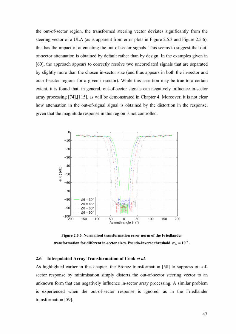
47

the out-of-sector region, the transformed steering vector deviates significantly from the

steering vector of a ULA (as is apparent from error plots in Figure 2.5.3 and Figure 2.5.6),

this has the impact of attenuating the out-of-sector signals. This seems to suggest that out-

of-sector attenuation is obtained by default rather than by design. In the examples given in

[60], the approach appears to correctly resolve two uncorrelated signals that are separated

by slightly more than the chosen in-sector size (and thus appears in both the in-sector and

out-of-sector regions for a given in-sector). While this assertion may be true to a certain

extent, it is found that, in general, out-of-sector signals can negatively influence in-sector

array processing [74],[115], as will be demonstrated in Chapter 4. Moreover, it is not clear

how attenuation in the out-of-signal signal is obtained by the distortion in the response,

given that the magnitude response in this region is not controlled.

−200 −150 −100 −50 0 50 100 150 200−100

−90

−80

−70

−60

−50

−40

−30

−20

−10

0

e( θ

) (

dB)


∆θ = 30°∆θ = 45°∆θ = 60°∆θ = 90°

Figure 2.5.6. Normalised transformation error norm of the Friedlander

transformation for different in-sector sizes. Pseudo-inverse threshold 5th 10s -= .

2.6 Interpolated Array Transformation of Cook et al.

As highlighted earlier in this chapter, the Bronez transformation [58] to suppress out-of-

sector response by minimisation simply distorts the out-of-sector steering vector to an

unknown form that can negatively influence in-sector array processing. A similar problem

is experienced when the out-of-sector response is ignored, as in the Friedlander

transformation [59].

48

The improved Cook et al. transformation [74] can successfully alleviate the above

problems. The principal idea is to use a LS formulation to approximate the steering vector

of a ULA for the in-sector region and concurrently suppress the out-of-sector response. The

LS fitting is carried out continuously, over the entire azimuth, as opposed to only for in-

sector or at discrete points as in the Friedlander transformation. A suitable problem

formulation is given by

( ) ( ) ( )IA

2IAmin w d

p

p

q q q q-

-ÚTT a b , (P2.3)

where TIA is the transformation matrix, ( )qa is the UCA steering vector, ( )qb is the target

ULA steering vector, and ( )w q is a window function which shapes the ULA response.

Therefore, as opposed to the Bronez transformation where the out-of-sector response is

suppressed as a best effort (with constraints defining the in-sector response), this approach

addresses the out-of-sector region more explicitly. The solution method to the LS problem

formulation of (P2.3) is outlined in Appendix A.1. If optIAT is the LS solution, then the

achieved target response is

( ) ( ) ( ) ( )optIA wq q q q= ªb T a b . (2.6.1)

where the accuracy of the approximation in (2.6.2) depends on the magnitude of the

transformation error.

However, it is noted that in the limit of an increasing number of grid points (or decreasing

grid spacing), the LS solution (2.5.2) for the Friedlander formulation will approach

( ) ( )IA

1

2IAmin

S

dq

q

q q q-ÚTT a b . (P2.4)

In [119], the integral form for a number of disjoint sectors (P2.4) is used to derive a

transformation matrix to perform frequency translation of the array steering vector for

wideband signals. In this case, the target steering vector is that of a reference array at a

given frequency bin. As such, a separate transformation matrix is needed to translate the

data of each frequency bin to that of the reference frequency bin. The method of [119] also

imposes the constraint IA IAH =T T I to ensure that the resulting IAT is unitary.

49

2.6.1 Window Function

The design of the window function ( )w q can be somewhat arbitrary, providing that these

requirements are met:

1. The ability to isolate the in-sector and out-of-sector response is important in order to

ensure that sector-by-sector processing can be performed satisfactorily.

2. The transformation error for different look direction, i.e. the Euclidean norm of (P2.3),

is kept low over the entire azimuth so that the steering vector of the virtual ULA closely

follows the target steering vector.

To satisfy the first prerequisite, a rectangular window function of the form (2.4.13) appears

to be the ideal choice. However, since the virtual ULA steering vector is continuous, the

sharp discontinuity at the edges of the in-sector can cause the transformation error to peak

at the sector boundaries (see case a Æ• in Figure 2.6.4). This is unsurprising as it is

analogous to a well-known problem in the design of brick-wall frequency response with

finite impulse response (FIR) filters.

The well-known solution for this problem in FIR filter design is to use a window function

that has a smooth rolloff in the transition region between the pass band and the stop band.

In view of this, Cook et al. [74] proposed a Gaussian window function with a smooth

rolloff so that a better LS solution of smaller transformation errors can be obtained, i.e.

( ) ( ){ }2exp ,

1 ,

b b

b

wa q q q q p

qq q

Ï - - < £Ô= Ì£ÔÓ

, (2.6.3)

where, with no loss of generality, the centre of the in-sector is aligned with the broadside of

the virtual ULA and the broadside is given by q = 0∞, [ ], , 0b b bq q q- > defines the in-

sector region, and a is a “rolloff factor” which defines the gradient of the Gaussian rolloff.

Moreover, while it is desirable to suppress the entire out-of-sector response, it is more

important to suppress the response in the sector of angles corresponding to the image of the

in-sector along the axis of the virtual ULA. The window function of (2.6.3) does not

explicitly define the “stop band” (the image sector). As such, the stop band response

50

depends on a. Some window functions are defined as follows where the rolloff occurs in

the “transition bands” between the in-sector and the image sector.

A piecewise linear window function (henceforth called the cropped triangular window

function) that satisfies the above specifications is given by

( ) ( )

( )

1 ,

,2

0 ,

b

ba b

b

b

w

q qq q p

q q q p qq p

p q q p

Ï £Ô

+ -Ô= < £ -Ì -ÔÔ - < £Ó

, (2.6.4)

where the in-sector, transition region and image sector are piecewise defined. The rolloff

for this function can be defined as the slope, i.e. ( )1 2 ba p q= - .

The well-known raised cosine function used in modem pulse-shaping filters appears to be

another good candidate for the window function

( ) ( ) ( )

( )

1 ,

1 1 cos ,2 2

0 ,

b

bb b

b

b

w

q q

p q qq q q p q

q p

p q q p

Ï £Ô

Ï ¸È ˘-Ô Ô Ô= + < £ -Í ˙Ì Ì ˝-Í ˙Ô ÔÔ Î ˚Ó ˛Ô - < £Ó

. (2.6.5)

In this case, the rolloff factor is 1 2 ba q p= - [123].

The error performance for different window functions over the parameters of interest is

shown for a specific example in Figure 2.6.4, Figure 2.6.6 and Figure 2.6.7, respectively.

For the Gaussian and cropped triangular window functions shown in Figure 2.6.4 and

Figure 2.6.6, respectively, the error performance varies significantly with the rolloff factor.

On the other hand, the raised cosine window function (see Figure 2.6.7), apart from giving

small transformation errors over the entire azimuth, is also found to give nearly identical

error performances for different rolloff factors (or in-sector sizes). This suggests that the

raised cosine window function may be close to being the “optimum” window function.

The impact of the window function on the received signals is somewhat intuitive. There are

3 regions of interest: For in-sector signals, they are received with approximately the same

51

gain as that received by an ideal ULA. For signals appearing in the transition region, they

will still have a Vandermonde steering vector but with attenuated envelope/amplitude

( )0 1lw q< < . And for signals appearing in the image sector ( ) 0lw q = (or ª 0 with the

Gaussian window), they are suppressed to a large extent. From a different perspective, the

latter two situations can be absorbed into the signal model. As far as the model is

concerned, the signals in the latter two cases are either weakened or suppressed. More

explicitly, recall from (2.2.7) the signal component of the covariance matrix is HsBR B .

Providing that the transformation error is small, it can be rewritten as follows

( ) ( ) ( ) ( )( ) ( )

( ) ( )

( ) ( )( )

( )

1 1

1 1

1

1

, ,

, ,

H

HL L

HL L

H

HL

HL

ww w

w

q qq q q q

q q

qq q

q

È ˘Í ˙

È ˘ª Í ˙Î ˚Í ˙Í ˙Î ˚

È ˘Í ˙

È ˘= =Í ˙Î ˚Í ˙Í ˙Î ˚

s s

s s

bBR B b b R

b

bb b R BR B

b

…

…

, (2.6.6)

where ( ) ( )[ ]1 2 1 21 2 ,, l l l ll lw wq qÈ ˘ =Î ˚s sR R , and [ ] 1 2 1 21 2, l l l ll l r s s=sR , l1, l2 = 1,…,L,

1 11l lr = ,

1 2 2 1l l l lr r*= , and ( ) ( )1 2 1 2 1 2E l l l l l ls t s t r s s*È ˘ =Î ˚ . Essentially, the signals in the new model

can be expressed as ( ) ( ) ( )l l ls t w s tq= . And if the number of signals in the image sector is

denoted by NI, then these NI signals will be suppressed in the virtual ULA, and HsBR B

will now in effect have a smaller rank of L – NI.

2.6.2 Optimisation Sector versus Operational Sector

The distinction between optimisation sector and operational sector should be made [74],

where the operational sector is a subset of the optimisation sector. For the Cook et al.

transformation, the optimisation sector is the region where ( ) 1w q = . The above distinction

is made because the error performance can be poor near the optimisation sector edges,

depending on the choice of the window function, sector size and rolloff factor. In addition,

the virtual ULA will have reduced ability to resolve closely spaced signals as they depart

from broadside. It is beneficial then to place a bound on the largest acceptable operational

sector size within which results from array processing applications such as DOA estimation

52

and beamforming are considered valid24. And in the special case of the Gaussian window

function, while a slower rolloff (i.e. a wider transition region) will generally reduce the

transformation error (see Figure 2.6.4), it is also necessary to sufficiently suppress signals

in the image of the operational sector. This places a further constraint on the operational

sector size [74].

Friedlander gave a similar proposal for his interpolated array transformation [60] since it is

observed that the transformation error peaks at the in-sector edges. By making the

optimisation sector slightly larger than the operational sector, one can avoid larger errors

for signals at the optimisation sector edges. However, this procedure involves sacrificing a

slight overall increase of transformation error over the in-sector region. In practice, this

procedure may not be important since the peak errors at the edges are still relatively small.

In the subsequent development, unless otherwise specified, “in-sector” is used

synonymously with optimisation sector. This is because the concept of operational sector is

of interest only with respect to a specific application such as DOA estimation.

2.6.3 Virtual ULA Size

As defined earlier, the aperture ratio ra is the ratio of the broadside aperture of the virtual

ULA to the aperture of the UCA. Thus, the virtual ULA is expected to have a better spatial

resolution capability (due to a larger aperture) than the actual UCA when ra > 1. However,

by intuition, such choices of ra’s will increase the transformation error rapidly, since

extrapolation is involved. A design example is given later in this section to illustrate the

problem of choosing ra > 1. In general, ra = 1 is found to be satisfactory.

As mentioned earlier, in the context of the Friedlander transformation, transforming from a

UCA to a ULA with equal apertures (ra = 1) and equal numbers of elements (M = N) may

introduce redundancy. As a guideline, the inter-element spacing in the virtual ULA should

be roughly similar to that of the UCA. For ra = 1, this implies a reduction in the number of

elements in the virtual ULA. This problem with redundancy is observed in Figure 2.5.1

where the condition number of the transformation matrix increases rapidly with the number

24 While this requirement means that the operational sector must be non-overlapping for DOA estimation (so that the DOA

estimates of the same signals from different sectors are not taken into account twice), the same cannot be said for beamforming. In beamforming, some overlapping between adjacent operational sectors is necessary to ensure that the mainlobe of the beampattern does not suffers from distortion in a “handover scenario” where the look direction moves continuously from one operational sector to an adjacent one. Detailed discussions are given in Chapters 5 and 6.

53

of virtual ULA elements. The requirement for a well-conditioned transformation matrix

thus places an upper limit on the number of virtual ULA elements.

At first glance, the above may suggest that interpolated array transformations have a serious

flaw in that the degree of freedom of the virtual ULA is less than that of the actual UCA.

Nonetheless, the following points should also be taken into account in a fair assessment:

1. The resolution capability of ULA’s and UCA’s for uncorrelated signals is based

primarily on the array aperture with respect to the azimuth plane, rather than the number

or distribution of the elements, provided the spatial sampling condition [108] is

satisfied. Therefore, if the aperture of the virtual ULA is the same as that of the UCA,

the resolution performance within the in-sector will be roughly equal.

2. In array processing algorithms such as the subspace methods for DOA estimation, fewer

elements in the virtual ULA, as compared to the original, means that they can handle

fewer signals. However, it is well known that the actual number of resolvable

uncorrelated signals in finite data (as indicated by the CRB) is limited severely by the

separation between signals with respect to the (conventional/Bartlett beamformer)

mainlobe width of the array [124],[125], which in turn is related to the array aperture.

This means that signals should be sufficiently separated for resolvability, and this can

easily overwrite the upper limit of resolvable signals based on the number of elements

especially for larger UCA’s. The same argument applies to optimum beamforming [35],

[126] where the number of elements determines the degrees of freedom for both

suppressing the overall response of the array pattern and maintaining some desired fixed

points (e.g. look direction(s) with magnitude 1).

3. UCA’s have very limited capability to handle highly correlated (or coherent) signal

environments when relatively simple algorithms such as MUSIC are used. As pointed

out by Mathews and Zoltowski [55] and confirmed by the general results for planar

arrays by Wang and Liu [127], forward-backward spatial smoothing (FBSS) can be

applied on the full UCA when the number of elements is even. However, this approach

limits the number of resolvable coherent signals to two. On the other hand, the virtual

ULA is well suited to the correlated signal environment due to the ease of forming

subarrays for FBSS. Moreover, correlated signals require larger angular separations

between the signals for resolvability as compared to the uncorrelated case [128].

54

4. Also, as a consequence of the severe suppression of response in the image sector (as

intended) for the Cook et al. transformation, any correlated signals in this region will be

suppressed significantly. Therefore, in such cases, subspace methods with spatial

smoothing will have an improved ability to resolve more correlated signals. However,

since in general there is no control over the DOA’s of the correlated signals, this

advantage cannot be guaranteed.

Therefore, in a proper design procedure, it would be advantageous to reduce the number of

virtual ULA elements M since this will lead to array processing in lower dimensions and

hence computational savings. And as noted earlier, as long as the aperture size of the virtual

ULA is maintained, the resolution performance is retained. However, a lower bound for M

exists in the Cook et al. transformation. In Section 2.5.1, it was stated that, in the

Friedlander transformation, the condition 0.5d £ prevents spatial aliasing and places a

lower bound on the number of virtual elements M. The same condition and hence the

corresponding lower bound applies also to the Cook et al. transformation since the steering

vector of the virtual ULA is only sufficiently suppressed within the image sector. The

transition region, though attenuated, is matched to the Vandermonde form of a ULA.

Therefore, spatial aliasing must be prevented in the virtual ULA over its entire field of

view.

2.6.4 Orientation of the In-Sector and the Virtual ULA

The orientation of the in-sector and the placement of the virtual ULA is somewhat arbitrary.

However, to take full advantage of the optimum spatial resolution of a ULA that occurs at

broadside, it is expedient to choose the broadside of the virtual ULA to correspond to the

mid-point of the in-sector region and the middle of the ULA to correspond to the centre of

the UCA, as shown in Figure 2.6.1.

In general, each in-sector requires a distinct transformation matrix [59], depending on the

actual array element positions and the alignment of the in-sector with respect to the

elements. However, this design approach would not present an additional computational

burden to online processing since these transformation matrices are computed only once

and are performed offline [59]. Nevertheless, since a UCA has rotational symmetry, it is

possible to exploit this property to simplify the interpolated array design by having one

transformation matrix that works equally well for all in-sectors. Bronez has earlier applied

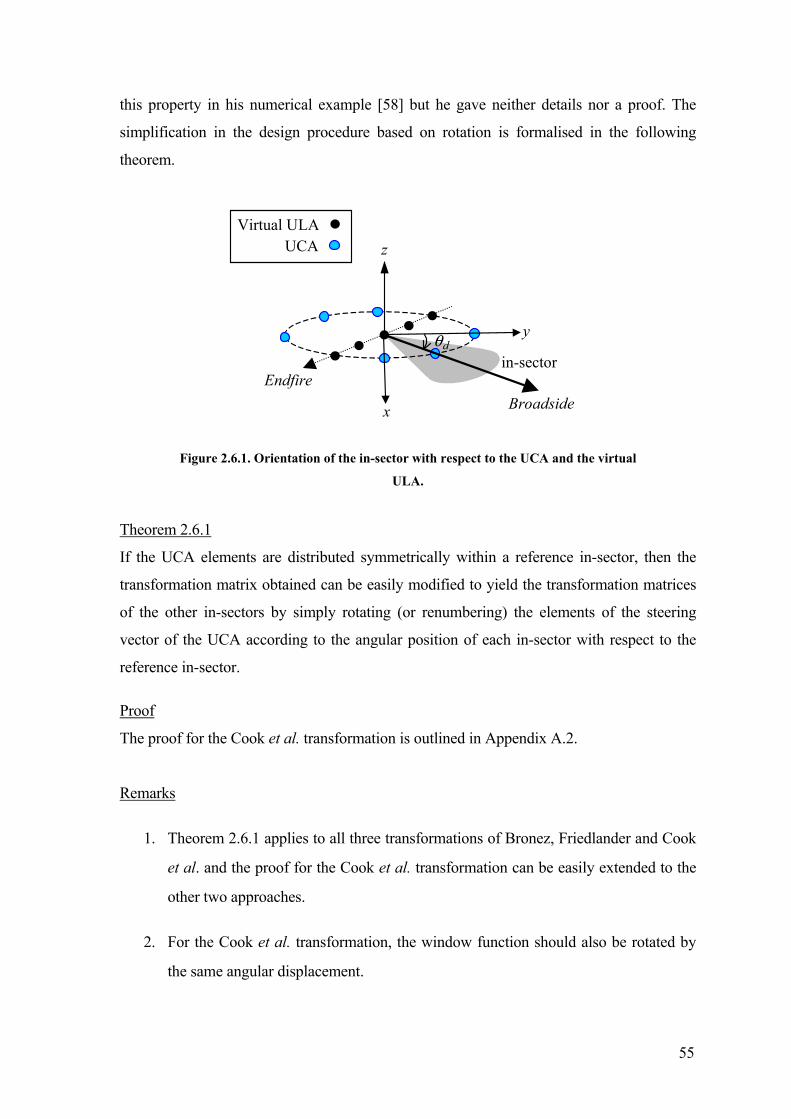
55

this property in his numerical example [58] but he gave neither details nor a proof. The

simplification in the design procedure based on rotation is formalised in the following

theorem.

x

z

in-sector

Broadside

Virtual ULA UCA

dq

Endfire

y

Figure 2.6.1. Orientation of the in-sector with respect to the UCA and the virtual

ULA.

Theorem 2.6.1

If the UCA elements are distributed symmetrically within a reference in-sector, then the

transformation matrix obtained can be easily modified to yield the transformation matrices

of the other in-sectors by simply rotating (or renumbering) the elements of the steering

vector of the UCA according to the angular position of each in-sector with respect to the

reference in-sector.

Proof

The proof for the Cook et al. transformation is outlined in Appendix A.2.

Remarks

1. Theorem 2.6.1 applies to all three transformations of Bronez, Friedlander and Cook

et al. and the proof for the Cook et al. transformation can be easily extended to the

other two approaches.

2. For the Cook et al. transformation, the window function should also be rotated by

the same angular displacement.

56

3. For DOA estimation, the selected operational sector size is such that any one

operational sector does not overlap with the two adjacent operational sectors.

4. The rows of TIA can be rotated (with the order of the UCA steering vector element

left unchanged) to produce the equivalent effect.

5. One restriction to the above procedure arises in the selection of the operational

sector size for DOA estimation25 when the number of UCA elements corresponds to

a large prime number. This is because for a large UCA with many elements, in-

sector size typically spans over several elements so as to limit the amount of

computation required26. But when the number of elements corresponds to a large

prime number, non-overlapping operational sectors (of one fixed size) spanning

several elements cannot be attained. For instance, while it is feasible to define 7 in-

sectors for a 7-element UCA (i.e. a small array), it is less convenient to choose 13

sectors for 13 elements (i.e. a larger array). 13 elements cannot be divided into a

round number of in-sectors. A related problem arises when the number of UCA

elements is a small integer multiple of a large prime number. In this case, even

though one can now have a number of non-overlapping operational sectors of a

fixed size, the number is restricted according to the small integer multiple (which

also means a large in-sector size). This can degrade the transformation error

performance of the virtual ULA.

However, the above restrictions can be relaxed by allowing for different operational

sector sizes. The reason being that such situations it is always possible to design all

operational sectors (each spanning the same number of elements) to be non-

overlapping except for two. The pair of overlapping operational sectors can then

have different operational sector sizes so that the overlapped region is taken into

account only once in the overall processing of the DOA estimation.

25 As mentioned earlier, the operational sector can be overlapping for beamforming applications so that the mainlobe does

not suffer from distortion as the look direction is moved continuously from one operational sector to another. However, since the operational sector size, and thus the overlapped region, is fixed, the same argument here applies to beamforming.

26 While it is always possible to have one in-sector spanning one element, this approach is undesirable for a UCA with many elements, since this means that a N-element UCA requires N times processing.

57

Theorem 2.6.2

If the UCA elements are distributed symmetrically about the broadside of the virtual ULA,

then TIA will exhibit a special structure of repeated matrix elements between each of

/ 2MÍ ˙Î ˚ pairs of rows, where Í ˙Î ˚i denotes the floor function. More specifically,

[ ] [ ] { }IA IA1, , ( 1)mod 1M p n p N n N- + - + +=T T , (2.6.7)

where p = 1, …, M and n = 1, …, N.

Proof

See Appendix A.3.

It is clear that Theorem 2.6.2 reduces the dimension of the problem. The dimension of the

problem formulation can be further reduced if the UCA elements are symmetrical about

both the broadside and endfire axes of the virtual ULA. This occurs when the number of

UCA elements is even. In this case, conjugate symmetry can be found for the elements

within each row of TIA.

Theorem 2.6.3

If the UCA elements are symmetrically distributed about the broadside of the virtual ULA,

then

[ ] { } [ ] ( ){ }*

IA IA, / 4 1 mod 1 , / 4 1 mod 1p n N N p N N n N- - + - - + +Í ˙ È ˘Î ˚ Í ˙=T T . (2.6.8)

Proof

See Appendix A.3

Two diagrams are given in Appendix A.3 to illustrate the symmetry in UCA elements that

will lead to the special structures within and among the rows of TIA.

Finally, it is worth nothing that the UCA steering vector ( )qa as defined in (2.2.2) sets the

first UCA element at the broadside of the virtual ULA. Nevertheless, it is easy to show that

when there is no physical UCA element at the broadside, the rotational properties as

outlined above will hold as long as the UCA elements are distributed symmetrically about

the in-sector.

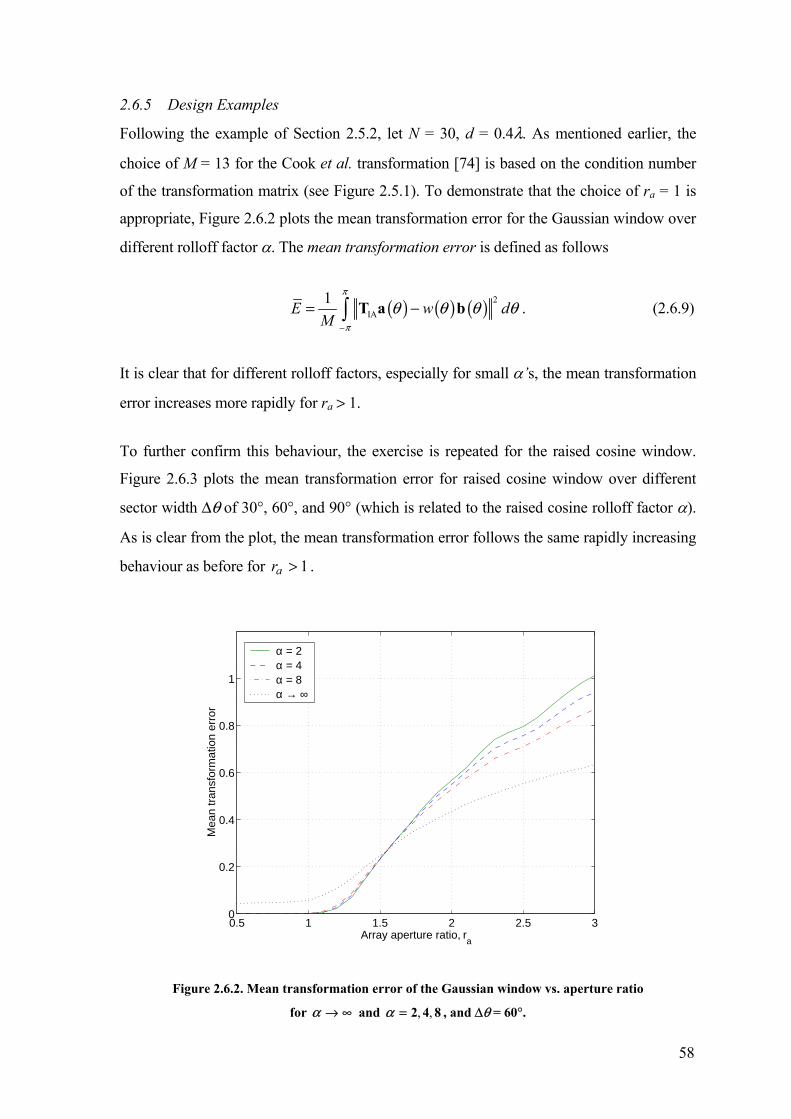
58

2.6.5 Design Examples

Following the example of Section 2.5.2, let N = 30, d = 0.4l. As mentioned earlier, the

choice of M = 13 for the Cook et al. transformation [74] is based on the condition number

of the transformation matrix (see Figure 2.5.1). To demonstrate that the choice of ra = 1 is

appropriate, Figure 2.6.2 plots the mean transformation error for the Gaussian window over

different rolloff factor α. The mean transformation error is defined as follows

( ) ( ) ( ) 2IA

1E w dM

p

p

q q q q-

= -Ú T a b . (2.6.9)

It is clear that for different rolloff factors, especially for small α’s, the mean transformation

error increases more rapidly for ra > 1.

To further confirm this behaviour, the exercise is repeated for the raised cosine window.

Figure 2.6.3 plots the mean transformation error for raised cosine window over different

sector width Dq of 30∞, 60∞, and 90∞ (which is related to the raised cosine rolloff factor α).

As is clear from the plot, the mean transformation error follows the same rapidly increasing

behaviour as before for 1ar > .

0.5 1 1.5 2 2.5 30

0.2

0.4

0.6

0.8

1

Mea

n tr

ansf

orm

atio

n er

ror

Array aperture ratio, ra

α = 2α = 4α = 8α → ∞

Figure 2.6.2. Mean transformation error of the Gaussian window vs. aperture ratio

for a Æ • and , ,2 4 8a = , and Dq = 60∞.

59

Next, the error performance of (2.4.12) is investigated for all the window functions ( )w q ’s

proposed in Section 2.6.1. For Gaussian window, Figure 2.6.4 shows how the error varies

with look direction θ for different values of α and an optimisation sector width of 90∞.

Ideally not only should the error be small, but also that it should be as flat as possible over

θ. Theoretically, a flatter error curve would translate to a smaller bias in the DOA estimates

for the entire azimuth. The error performance is very sensitive to α and it appears that a

small α translates to the best error performance. This is intuitively obvious, as a smaller

rolloff factor creates a larger transition region. However, careful design is needed to ensure

that the image sector region will get sufficient suppression. For α = 2, the window function

gives a target response of 0.0072 (0.7%) at the edges of the in-sectors image region while

for α = 1, this value goes up to 0.0848 (or 8.5%). Figure 2.6.5 shows the transformation

error for a fixed rolloff factor α = 2 and varying sector size. The best performance in this

case appears to be for a moderate sector size of around 45° or 60°.

0.5 1 1.5 2 2.5 30

0.2

0.4

0.6

0.8

1

Mea

n tr

ansf

orm

atio

n er

ror

Array aperture ratio, ra

∆θ = 30°∆θ = 60°∆θ = 90°

Figure 2.6.3. Mean transformation error of the raised cosine window vs. array

aperture ratio for different in-sector sizes.

In the case of the cropped triangular window (see Figure 2.6.6), the transformation error

suffers from peaks at both the in-sector edges and the image sector edges. This is due to the

60

piecewise linear window shape that inhibits a good fit at these points. Here, the error

performance is again dependent on the choice of in-sector size, which is related to rolloff.

−200 −150 −100 −50 0 50 100 150 200−35

−30

−25

−20

−15

−10

−5e(

θ )

(dB

)


α = 2α = 4α = 16α → ∞

Figure 2.6.4. Normalised transformation error norm of the Gaussian window

function for different rolloff factors and Dq = 90∞.

−200 −150 −100 −50 0 50 100 150 200−35

−30

−25

−20

e( θ

) (

dB)


∆θ = 30°∆θ = 45°∆θ = 60°∆θ = 90°

Figure 2.6.5. Normalised transformation error norm of the Gaussian window

function for different in-sector sizes and rolloff factor a = 2.

61

In contrast, the raised cosine window in Figure 2.6.7 appears to have the most consistent

error performance for different choice of in-sector sizes. All the curves shown have a

comparatively lower error performance than the other two above window functions. The

only exception is Gaussian windows with small rolloffs that give comparable performances.

This behaviour of raised cosine window shows that a larger in-sector size only involves a

small sacrifice in error performance. Therefore, it appears that a large operational (and

corresponding optimisation) sector size is desirable for the Cook et al. transformation when

the raised cosine window is used. A larger in-sector size implies that a smaller number of

in-sectors is needed and thus reduces the sector-by-sector computations.

In comparison to the Friedlander transformation (see Figure 2.5.3 and Figure 2.5.6), the in-

sector error performance of Cook et al. transformation [74] is far poorer. This, as discussed

earlier, is due to the Friedlander transformation ignoring the out-of-sector region, which

gives more degrees of freedom to obtain a better approximation in the in-sector. However,

this transformation is flawed since in general the out-of-sector signals can affect the in-

sector performance of the virtual ULA. The problem of ignoring the out-of-sector will be

discussed in the context of DOA estimation in Chapters 4.

−200 −150 −100 −50 0 50 100 150 200−34

−32

−30

−28

−26

−24

−22

−20

e( θ

) (

dB)


∆θ = 30°∆θ = 45°∆θ = 60°∆θ = 90°

Figure 2.6.6. Normalised transformation error norm of the cropped triangular

window function for different in-sector sizes.

62

Another interesting comparison is in the effect of varying in-sector size. For the Friedlander

transformation shown in Figure 2.5.3 and Figure 2.5.6, changing the in-sector size can

change the transformation error performance significantly (see also [60]). On the other

hand, changing the in-sector size does not appear to have a significant impact on the Cook

et al. transformation as seen in Figure 2.6.6 and Figure 2.6.7 (at least relative to the

Friedlander transformation). This is mainly because the Cook et al. transformation also

preserves the error performance of the out-of-sector region as opposed to the Friedlander

transformation of getting the best possible fit for the in-sector region regardless of the

behaviour of the “don’t care” out-of-sector region.

−200 −150 −100 −50 0 50 100 150 200−36

−34

−32

−30

−28

−26

−24

−22

e( θ

) (

dB)


∆θ = 30°∆θ = 45°∆θ = 60°∆θ = 90°

Figure 2.6.7. Normalised transformation error norm of the raised cosine window

function for different in-sector sizes.

2.7 Relationship between Davies and Interpolated Array Transformations

Applying the Davies transformation on the actual UCA results in a Davies array that has

Vandermonde form steering vector. On the other hand, the interpolated array

transformations give a virtual ULA that also has a Vandermonde form steering vector.

However, the two Vandermonde form steering vectors are different. While one Davies

array is sufficient to give the full azimuth coverage, one virtual ULA can only give a

limited sector coverage. Therefore, they appear to be two distinct and unrelated

transformations. However, the Davies transformation can be closely approximated as a

63

special case of the interpolated array transformation of Cook et al. The analysis is described

below.

First, let ( )qb of (P2.3) be the Davies array steering vector and the window function be

( ) 1w q = , [ ],q p pŒ - . From Appendix A.1, the LS solution of (P2.3) can be written in

closed form as follows.

( )opt 1IA 1 2j -= +T B B Γ , (2.7.1)

where B1, B2, and G are as defined.

Now it is shown in Appendix A.4 that

[ ] ( ) ( )

( ) ( ) ( )

1 2

1 1 (2 ( 1) / )12 o o

o

Hpq pq

p M j M p q Np M

j d

j J kr e

p

p

p

q q q

p-

- - - - + - -- -

È ˘+ = Î ˚

=

ÚB B b a. (2.7.2)

The optimum solution can then be written as

opt 1IA

-=T JFΓ , (2.7.3)

where ( )( 1 )1diag , 1, ,o

o

p Mp MN j J kr p M- - -- -

È ˘= =Î ˚J … (2.7.4)

and F is the spatial DFT as before. Numerical comparisons made between TDav and optIAT of

(2.7.3) reveal that as long as the design parameters are chosen such that the Vandermonde

approximation of the Davies array is good, then the two matrices are in close agreement

with each other in numerical values. This “equivalence” is helpful to give some insights to

some common properties between the Davies and the interpolated array transformations,

such as the robustness problem that will be introduced in the next chapter.

The only known reference where the interpolated array transformation is used with the

Davies array is [54]. The purpose of the interpolation is to incorporate array imperfections

into the Davies transformation. While it is similar to the interpolated array transformation

of Friedlander [59], when performed on a grid of azimuth angles (corresponding to

64

calibration positions) in a LS sense, the in-sector size for the Davies array can be extended

up to the full azimuth coverage of 360∞.

2.8 Conclusions

This chapter presents two classes of preprocessing techniques for a UCA to obtain the

desired Vandermonde form steering vector in the transformed domain. The Davies

transformation has the advantage of being in closed form and can maintain acceptable

transformation error for use over the entire azimuth (and elevation where necessary).

The interpolated array transformations, on the other hand, require processing in several

sectors for full azimuth coverage. While the Bronez and Friedlander transformations largely

focus on obtaining the Vandermonde form for the in-sector region, the Cook et al.

transformation [74] also aims to control the out-of-sector response. By controlling the out-

of-sector response to be either in Vandermonde form or severely suppressed, the Cook et al.

transformation demonstrates a significantly improved ability to cope with correlated signals

that occur in both in-sector and out-of-sector. For mobile communications, this is important

where there is a large spread of signals due to scattering and multipath, as is typical in

dense urban macrocell, microcell (outdoor environments with base stations lower than

average building heights) and picocell (indoor environments). Chapters 4 to 6 will examine

this aspect of the interpolated array transformations more explicitly with respect to DOA

estimation and beamforming.

65

Chapter 3 Robustness of UCA Preprocessing 3.1 Introduction

Though attractive, the original form of the Davies transformation does not address many

practical issues. Specifically, Davies [51] tacitly assumes that (i) all antenna elements are

omnidirectional, (ii) the elements all have the same element pattern, (iii) the electronics

associated with each antenna element are identical, (iv) the antenna elements are located at

their correct positions, and (v) there is no mutual coupling between the antenna elements.

Clearly, in a real system none of the above assumptions will hold, as will be discussed

further below.

Today, both omnidirectional and directional antenna elements are used for mobile

communications. Omnidirectional antennas are favoured for their uniform gain response in

the azimuth, while directional elements with a high gain in a given direction are suitable for

such systems as base stations in sector configuration. It is interesting to note that

assumption (i) can be relaxed. In particular, Longstaff et al. [92] showed the equivalence

between the effect of array element directional pattern and amplitude tapers (or amplitude

of the array weights) in phase mode excitations, suggesting that some element patterns may

conveniently eliminate (or complement) the need for amplitude tapers in beamforming.

Longstaff et al. [92] further suggested the use of directional elements to mitigate the

problem where for some array parameters some modes are unrealisable. Further works on

incorporating directional pattern into the Davies transformation are found in [52],[56], and

[121].

The requirement of identical antenna patterns (omnidirectional or directional) across the full

array in assumption (ii) is restricted by manufacturing technology and installation practice.

Thus, it can only be achieved to a given accuracy.

Also in [92],[96], and later in [54], the effect of mutual coupling was investigated. It was

shown that mutual coupling can be expressed in terms of spatial harmonics via DFT’s of

the (known) coupling coefficients. These are then readily incorporated into the Davies

transformation. Wax and Sheinvald [54] also suggested the direct measurement of array

imperfections using calibration sources and putting the measurements into a LS

approximation problem to derive a modified Davies transformation.

66

3.1.1 The Robustness Problem and Proposed Solution

Although the above works indicate that the real-world effects of array imperfections can be

ameliorated somewhat by appropriate theoretical formulation and array calibration, there

still remains the issues of calibration errors and the fact that the parameters of array

imperfections are time-varying. Eklöf [129] showed through numerical simulations that

when errors are introduced into the model of an ideal UCA with omnidirectional antennas,

as represented by a small perturbation of its steering vector, beampattern design on Davies

array can deform appreciably from the ideal.

The aim then is to find, through an appropriate optimisation problem formulation, an

alternative transformation that has the desirable property of the Davies transformation, i.e.,

transformation of the steering vector of a UCA to Vandermonde form, but which is more

robust with respect to perturbations to the steering vector of the ideal UCA. The main idea

is to trade off the Vandermonde approximation error of the Davies array steering vector for

robustness to imperfections. The optimisation formulation selected is quadratic semi-

infinite programming (SIP) [130],[131].

Interestingly, the robust formulation can also be expressed as a LS problem with a quadratic

constraint [132]. The standard Lagrange multiplier method can be applied to solve this

problem but it is known that the solution to this class of problems can suffer from numerical

problems. Nevertheless, the problem was successfully solved for the examples studied in

[132] in the context of Dolph-Chebyshev beamforming. The transformation error of the LS

solution exhibits a different behaviour to that of the SIP problem formulation.

In general, like the Davies transformation, known array imperfections (e.g. from calibration

data) can also be incorporated into the interpolated array transformations [60]. This applies

to all three different interpolated array transformations introduced in the previous chapter in

which the transformation matrix absorbs the imperfection and results in an ideal virtual

ULA (except for small transformation errors). However, no work has been done to deal

with unknown array imperfections or residual calibration error where calibration has been

performed.

Here the robustness of the interpolated array transformation of Cook et al. [74] against

array imperfection is examined. Not surprisingly, due to the similarity it has with the

67

Davies transformation (see Section 2.7), the proposed interpolated array formulation also

gives rise to a similar robustness problem, when omnidirectional elements are used. The

approach taken in the Davies transformation can be used to reduce the sensitivity to array

imperfections of the Cook et al. transformation. Apart from array imperfections, finite data

perturbations can also significantly degrade the performance of array processing algorithms

when the Davies transformation or the Cook et al. transformation [74] is used. This

problem is recognised by Doron and Doron [108] in their paper that focuses on the

generalised Davies transformation on the outputs of an arbitrary planar array. In general,

both array imperfections and finite data perturbations can be classified as model errors,

since they both introduce errors into the underlying signal model.

Interestingly, the Bronez transformation [58] will also be shown to have the aforesaid

robustness problem, even though it is less obvious from the formulation how it transpires.

The Friedlander transformation [59], on the other hand, while failing to adequately address

correlated signal environments with out-of-sector correlated signals, does not appear to

have this robustness problem with finite data and array perturbations. This will be

demonstrated later in this chapter.

3.1.2 Alternative Solutions

The proper use of directional elements in UCA, to mitigate the zero-crossings of the Bessel

functions of J in the Davies transformation [52], also renders the UCA robust against model

errors. It will be shown by numerical analysis that interpolated array transformation using

directional elements is also robust as in the omnidirectional element case. In [108], Doron

and Doron establish by wavefield theory that the proper addition of dipole elements on the

circumference of a UCA can overcome the robustness problem (in the context of finite data

perturbations) that exists for a generic linear transformation of the UCA steering vector to

that of an arbitrary interpolated array.

Another approach that is effective against the problem of robustness is with the use of

additional elements within the radius of a UCA. For Davies transformation, Swingler and

Davies [57] proposed an element at the centre of a UCA to overcome the problem of poor

SNR (which is directly related to the robustness problem) for the middle element of the

Davies array. In [108], Doron and Doron also carried this further by proposing the proper

68

addition of omnidirectional elements within the circumference of a UCA to overcome the

robustness problem for a generic linear transformation.

While directional elements and additional elements within the radius of the UCA present

alternatives to the use of the robustness formulation to effectively mitigate the robustness

problem related to omnidirectional elements, it should be noted that these involve changes

in the physical (or hardware) structure of the UCA. In contrast, the robustness formulation

is at the signal processing level and can be implemented in software.

In the following sections, the aforesaid robustness problem of the Davies and interpolated

array transformations to model errors is described in details. The SIP problem formulation

is then proposed to deal with the robustness problem of these preprocessing techniques for

UCA’s. This is followed by numerical examples which demonstrate its effectiveness to

mitigate the problem of robustness in UCA’s. Finally, two alternative solutions to the

robustness problem are also summarised in the context of existing work along with some

new insights.

3.2 Robustness Against Model Errors


The lack of robustness of the Davies transformation can be traced to the construction of J.

As can be seen from equation (2.3.2), for some choices of m, oM , and r/l, the magnitude

of one or more of the diagonal elements of J can approach infinity as the corresponding

value of ( )mJ kr approaches zero. Accordingly, the norm of TDav can become very large.

Now, the noise covariance matrix of the Davies array (in a simple case of white noise) is

Dav DavHT T . The large norm in some of the rows of TDav thus implies that the corresponding

Davies array elements will have very low SNR’s. This problem is reported in [57]. The

approach taken by Swingler and Davies [57] was to replace the data of these “failed” (low

SNR) virtual elements with that from linear predictions based on adjacent elements. The

problem with SNR can be shown as follows. In Figure 2.2.2, the output vector of the

Davies array is given by

( ) ( ) ( )Davt t t= =y T x JF x (3.2.1)

and the corresponding covariance matrix is given by

69

( ) ( ) 2H H H Hnt t sÈ ˘= = + SÎ ˚y s nR E y y BR B JF F J , (3.2.2)

where the steering matrix of the Davies array, =B JFA , is Vandermonde. As can be seen,

while the signal component in (3.2.2) undergoes only a change in its steering matrix from

the UCA form to that of the Davies array, the rows and columns of the noise component is

amplified by the respective diagonal elements of the J matrix. For the simple case of equal

Gaussian white noise27 across the UCA, n IS = . The noise component then becomes 2 Hn JJs , since FFH = I. This implies the noise power in the mth element of the Davies array

is amplified by a factor of

( ) 12diagHmN J kr

-È ˘= Î ˚JJ , , ,o om M M= - … . (3.2.3)

From another perspective, since large norms only occur for the rows or modes where the

Bessel functions approach zero-crossings, the J matrix becomes ill conditioned. This causes

TDav to be ill conditioned. Wax and Sheinvald [54] recognised this problem and proposed

that in addition to the condition ( ) 0mJ kr π in (2.3.2), the designer should also ensure that

J (and thus TDav) is well conditioned. However, this strategy merely avoids the problem and

can severely limit the designer’s choice of array parameters (especially for UCA with many

elements). Another serious consequence of a large norm is that the square of the norm of

TDav gives a measure of the amplification of model errors in the transformation matrix. To

see this, a deterministic but unknown array imperfection (or array perturbations) is defined

as ( )d qa . Then, the output of the UCA (2.2.3) can be rewritten as

( ) ( ) ( ) ( ) ( )1

L

l l ll

t s t tq d q=È ˘= + +Î ˚Âx a a n . (3.2.4)

The output of the Davies array is then

( ) ( ) ( ) ( ) ( )

( ) ( ) ( ) ( )

Dav Dav Dav1

Dav1

L

l l llL

l l ll

t s t t

s t t

q d q

q d q

=

=

È ˘= + +Î ˚

È ˘= + +Î ˚

Â

Â

y T a T a T n

b b T n

. (3.2.5)

27 An example of non-white noise is the ambient isotropic noise (that may dominate over thermal white noise) in

underwater sonar applications. Interestingly, it is shown to become spatially white after the Davies transformation [98].

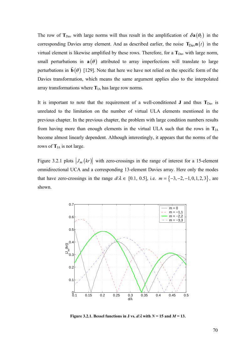
70

The row of TDav with large norms will thus result in the amplification of ( )ld qa in the

corresponding Davies array element. And as described earlier, the noise ( )Dav tT n in the

virtual element is likewise amplified by these rows. Therefore, for a TDav with large norm,

small perturbations in ( )qa attributed to array imperfections will translate to large

perturbations in ( )qb [129]. Note that here we have not relied on the specific form of the

Davies transformation, which means the same argument applies also to the interpolated

array transformations where TIA has large row norms.

It is important to note that the requirement of a well-conditioned J and thus TDav is

unrelated to the limitation on the number of virtual ULA elements mentioned in the

previous chapter. In the previous chapter, the problem with large condition numbers results

from having more than enough elements in the virtual ULA such that the rows in TIA

become almost linearly dependent. Although interestingly, it appears that the norms of the

rows of TIA is not large.

Figure 3.2.1 plots ( )mJ kr with zero-crossings in the range of interest for a 15-element

omnidirectional UCA and a corresponding 13-element Davies array. Here only the modes

that have zero-crossings in the range d/l Œ [0.1, 0.5], i.e. { }3, 2, 1, 0,1, 2,3m = - - - , are

shown.

0.1 0.15 0.2 0.25 0.3 0.35 0.4 0.45 0.50

0.1

0.2

0.3

0.4

0.5

0.6

0.7

|Jm

(kr)

|

d/λ

m = 0m = −1,1m = −2,2m = −3,3

Figure 3.2.1. Bessel functions in J vs. d/l with N = 15 and M = 13.

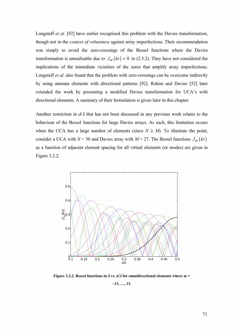
71

Longstaff et al. [92] have earlier recognised this problem with the Davies transformation,

though not in the context of robustness against array imperfections. Their recommendation

was simply to avoid the zero-crossings of the Bessel functions where the Davies

transformation is unrealisable due to ( ) 0mJ kr = in (2.3.2). They have not considered the

implications of the immediate vicinities of the zeros that amplify array imperfections.

Longstaff et al. also found that the problem with zero-crossings can be overcome indirectly

by using antenna elements with directional patterns [92]. Rahim and Davies [52] later

extended the work by presenting a modified Davies transformation for UCA’s with

directional elements. A summary of their formulation is given later in this chapter.

Another restriction in d/l that has not been discussed in any previous work relates to the

behaviour of the Bessel functions for large Davies arrays. As such, this limitation occurs

when the UCA has a large number of elements (since N ≥ M). To illustrate the point,

consider a UCA with N = 30 and Davies array with M = 27. The Bessel functions ( )mJ kr

as a function of adjacent element spacing for all virtual elements (or modes) are given in

Figure 3.2.2.

0.1 0.15 0.2 0.25 0.3 0.35 0.4 0.45 0.50

0.1

0.2

0.3

0.4

0.5

|Jm

(kr)

|

d/λ

Figure 3.2.2. Bessel functions in J vs. d/l for omnidirectional elements where m =

-13, …, 13.

72

It is observed that apart from the zero-crossings, the Bessel functions corresponding to

virtual elements of higher modes (i.e. larger m’s) increase slowly with /d l (prior to

reaching the respective maximum points). In this situation, one would not be able to both

choose / 0.3d l < and retain the virtual elements corresponding to highest order modes

(marked by thick solid line in Figure 3.2.2) as this will give rise to a large norm in the

transformation matrix and thus the robustness problem as discussed before. Therefore, the

range of /d l is limited. The squared norm of TDav for the scenario is given in Figure

3.2.3, together with M = 15. It is clear that when the higher modes are discarded (M = 15),

the corresponding problem of robustness for the entire range of small /d l ’s also

disappears. However, a smaller M also leads to a smaller aperture for the Davies array.

0.15 0.2 0.25 0.3 0.35 0.4 0.45 0.50

10

20

30

40

50

60

70

80

90

100

Squ

ared

nor

m o

f T

Dav

(dB

)

d/λ

M = 27M = 15

Figure 3.2.3. Squared norm of TDav vs. d/l for the Davies transformation with N = 30

(UCA with omnidirectional elements) and M = 15 and 27.

Furthermore, Figure 3.2.2 indicates that while the number of UCA elements can be

arbitrarily large, the number of Davies array elements (or spatial modes) is limited by the

slow increase in the Bessel function of the higher order modes in the operational range d/l

Œ [0.1, 0.5]. However, it should be noted that modes with order higher than a threshold

(e.g. the thick solid line in Figure 3.2.2) do not add any additional zero-crossings to this

range and thus do not worsen the large norm problem due to zero-crossings.

73


Like the Davies transformation, the issue of robustness has not been investigated for the

interpolated array transformations in previous works. It can be easily shown by examples

that the Cook et al. transformation [74] can be non-robust due to a large norm as with the

Davies transformation. However, it is more difficult to trace the cause of the problem as

compared to the Davies transformation due to the lack of an explicit closed form LS

solution in terms of the array parameters (refer to Appendix A.1). Figure 3.2.4 shows a

typical example of the squared norm of TIA obtained from the Cook et al. transformation.

0.15 0.2 0.25 0.3 0.35 0.4 0.45 0.50

10

20

30

40

50

60

70

Squ

ared

nor

m o

f T

IA (

dB)

d/λ

FriedlanderCook et al.(raised cosine)

Figure 3.2.4. Squared norm of TIA vs. d/l for the Cook et al. (raised cosine window)

and Friedlander transformations with N = 30 (UCA with omnidirectional elements),

M = 13 and in-sector size Dq = 90∞. For the Friedlander transformation, the pseudo-

inverse threshold 5th 10s -= .

In fact, on closer examination, it can be seen that all the peaks in Figure 3.2.3 except one28

occur at the same d/l’s as those in Figure 3.2.4, where in both cases the UCA has 30

28 The peak at d/l = 0.4815 in the Davies transformation does not appear in the Cook et al. transformation. On closer

examination, it is found that the transformation error of the Cook et al. transformation experiences a large peak at that point while it is relatively small for the rest of d/l Œ [0.1, 0.5]. As will be shown later in this chapter, robustness can be gained by sacrificing the transformation error. It appears that the LS formulation (P2.3) of the Cook et al. transformation at this point gives an optimum solution at a smaller norm for TIA and a larger transformation error. Furthermore, d/l = 0.4815 is in the vicinity of 0.5, which is the asymptotic limit (of infinite aperture) for a UCA to satisfy the spatial sampling condition [108]. Taking this into consideration, it is unsurprising to find an unexpected behaviour there.

74

elements. This suggests that the large norm problem is fundamental in nature rather than

specific to a particular preprocessing approach. This is reinforced by further numerical

studies on other window functions (including those suggested in Chapter 2 and ( ) 1w q = )

and other virtual planar arrays with elements located on and within the circumference of the

UCA.

Nevertheless, one marked difference observed in TIA of the Cook et al. transformation

compared to TDav of the Davies transformation is that the set of d/l’s where the large norms

occur in TIA is almost the same for all virtual ULA elements. Whereas as observed in

Figure 3.2.1, the large norms in TDav occur for different sets of d/l’s (with far fewer

overlaps) for different Davies array elements. The case of TDav can be easily understood

since its closed form is available in terms of Bessel functions of different orders. The reason

for the case of TIA is discussed qualitatively below.

The LS solution of the Cook et al. transformation, as derived in Appendix A.1, involves the

matrix Γ

( )opt 1IA 1 2j -= +T B B Γ , (3.2.6)

where ( ) ( )1 2Hj d

p

p

q q q-

+ = ÚB B b a , (3.2.7)

[ ] ( ) ( ) ( )1 21 2

1 2

0 ,,,

2Hn nn n

n n

d J krΓ a ap

p

q q q p-

È ˘= =Í ˙Î ˚Ú , (3.2.8)

and ( ) ( )1 2 1 2 1 2

2 2

,n n n n n nr x x y y= - + - , ( ),n nx y is the position of the nth planar array

element in rectangular coordinates.

For a UCA, Γ has a circulant form (a special case of Toeplitz form) and some interesting

properties of this matrix include:

1. The diagonal elements of Γ are 2p, with ( )0 0 1J = .

2. The off diagonal elements are less than 2p, since ( )1 20 , 1n nJ kr < for 1 2, 0n nr π and n1 π

n2.

75

A numerical analysis will reveal that some combinations of the parameters N, M and r/l

can result in a large norm in 1-Γ , and hence optIAT . The matrix Γ is both symmetric and

circulant. This implies 1-Γ is also symmetric and circulant [133]. For a symmetric circulant

matrix, the column or row norm is the same across the matrix. This means that any large

norm in 1-Γ is distributed uniformly across the rows and columns of the matrix. The

presence of the 1 2j+B B term “moderates” some of the large row norms in 1-Γ , such that

some row norms of optIAT become small. However, most row norms remain large, which

supports the observation that TIA and TDav have large norms at similar d/l’s.

It is also noted from numerical analysis that the large norm problem of the Cook et al.

transformation cannot be attributed to the zero-crossings of the zeroth order Bessel function

of the first kind in Γ (3.2.8), since they do not necessarily lead to an ill-conditioned Γ (and 1-Γ ) and a large norm in 1-Γ . This is contrary to the crucial role played by the zero-

crossings in the Bessel functions of the Davies transformation. Though outside the scope of

this thesis, it would be interesting to examine whether some closed form expressions can be

found for 1-Γ (as in matrix J in the Davies transformation) to indicate the exact conditions

that give rise to the large norm problem.

So far it has been established that the large norm problem of the Cook et al. transformation

comes from Γ and is inherent to a UCA, regardless of the form of the virtual array (and

whether or not it corresponds to the form of a physical array). However, it has been found

that the same conclusions do not extend to the interpolated array transformation of

Friedlander [59]. For instance, numerical analysis indicates that the Friedlander paradigm

does not suffer from robustness problems which is the case with the Cook et al.

transformation [74]. This could be attributed to the fact that [59] treats the out-of-sector

region as a “don’t care” region, thus allowing an easier interpolation that does not give rise

to a large norm transformation matrix. From another perspective, doing LS over a very

dense grid of points in (2.5.2) is equivalent to doing LS by integration. However, since

Friedlander “integrates” over only a sector rather than 2π, one fails to obtain a close form

involving Bessel functions which cause the large norm problem of the Cook et al.

transformation. Figure 3.2.4 gives an example of a well-behaved TIA for the Friedlander

transformation. It is obvious from the plot that in this case, the Friedlander transformation

has no large norm problems, unlike the Cook et al. transformation.

76

In the Bronez transformation, the cost function of the constrained minimisation problem

formulation (P2.1) of Bronez [58] is given by (2.4.3) and it also involves the matrix Γ. The

well-known solution of the constrained minimisation problem of (P2.1) is given by

[ ]IA 1 2| | | HM=T t t t… where

( ) 11 1Hp p

-- -=t Γ C C Γ C d . (3.2.9)

It is not easy to verify from (3.2.9) whether or not the Bronez transformation is robust. It is

observed that the row vectors of TIA involve both Γ and 1-Γ , which implies the possibility

that the ill-conditioning in Γ may be negated. However, some numerical analysis, including

that shown in Figure 3.2.5, contradicts this simplistic deduction. Figure 3.2.5 is based on

the example of Figure 2.4.2 with N = 48, sector size twice the 3dB mainlobe width, and 5

constraint angles, except that here the design of the transformation matrix is repeated over a

large range of d/l’s. The resultant number of virtual ULA elements M varies between three

and five inclusive. As can be seen, the Bronez transformation is also not robust due to the

possibility of TIA having large norms.

0.2 0.25 0.3 0.35 0.4 0.45 0.50

20

40

60

80

100

120

Squ

ared

nor

m o

f T

IA (

dB)

d/λ

BronezCook et al.(raised cosine)

Figure 3.2.5. Squared norm of TIA vs. d/l for the Bronez (N = 48 and different M’s)

and Cook et al. transformations (N = 48 and M = 12).

77

The case of the Cook et al. transformation for the same UCA of N = 48 with M fixed at 12

is also shown in Figure 3.2.5. As can be seen, the large norms occur at similar d/l’s for

both the Bronez and Cook et al. transformations. The squared norm of the Bronez

transformation appears to be much larger than that of the Cook et al. transformation for

small d/l’s and it dominates over the peaky response observed at higher d/l’s. However, its

large norm peaks (and troughs) at larger d/l’s are smaller than those of the Cook et al.

transformation. This is due to the use of less virtual ULA elements in the Bronez

transformation which corresponds to TIA of a smaller dimension.

3.2.3 Discussions

From the above development, it is clear that the source of the robustness problem in the

Davies transformation is the presence of zeros in the Bessel functions of J for certain spatial

modes. Similarly, the Bronez and Cook et al. transformations also suffer from the large

norm problem. This is not surprising given the equivalence between the Davies

transformation and a special case of the Cook et al. transformation (see Section 2.7). In fact,

they appear to substantiate some fundamental results in [108] where the large norm

problem is attributed to a phenomenon called “resonance”. In [108], Doron and Doron put

into context the large norm problem involved in the linear transformation of a planar array.

In particular, they recognised the implication this has on finite sampling, in that it amplifies

any difference in the estimated covariance matrix relative to the exact covariance matrix.

They showed that for a UCA, the transformation procedure involves Bessel functions29,

which cause the robustness problem by amplifying array imperfections in the virtual array.

However, as mentioned earlier, while for a given set of array parameters the large row

norms occur for only a few pairs of Davies array elements, they often occur for all pairs of

rows in the Bronez and Cook et al. transformations. This seeming “discrepancy” in

attributing the large norm problem to the same fundamental problem of resonance can be

explained by an analogy with time-frequency domain relationship in filter design. While the

Davies array is in the spatial-frequency domain (transformed with a DFT), the virtual ULA

is in the spatial domain. The large norm problem in the interpolated array indicates that

given a certain set of array parameters, the virtual ULA will experience the large norm

problem more or less uniformly across the array. On the other hand, the Davies

29 In Chapter 2, it was shown that †

Dav=G T for the case of a UCA, where G is the sampling matrix of AMI [105].

78

transformation “concentrates” the large norm problem in a few pairs of virtual array

elements, indicating that the problem of interpolation only exists in some spatial

frequencies.

3.3 Problem Formulation

Based on the above observation, the following semi-infinite optimisation problem is

formulated to find a more robust transformation matrix. The basic idea is to trade-off the

approximation error in the transformation of ( )qa to a vector with Vandermonde form, for

robustness.

Denote the robust transformation matrix by M NU ¥Œ . The matrix U is found as follows

2min FUU (P3.1)

subject to ( ) ( ) Aq q- £Ua b e , [ ],q p p" Œ - ,

where F◊ denotes Frobenius norm, and A◊ is the absolute value norm30 defined by

( ) ( )

( ) ( ){ } ( ) ( ){ }{ }

( ) ( ){ } ( ) ( ){ }{ }

1 1 1 1max Re , Im

max Re , Im

A

T T

T TM M M M

b b

b b

q q

q q q q

q q q q

- =

È ˘- -Í ˙Í ˙Í ˙Í ˙- -Í ˙Î ˚

Ua b

u a u a

u a u a

, (3.3.1)

[ ]1 2T

Me e e e= , (3.3.2)

pe +Œ , 1, ,p M= … , is the upper bound for the Vandermonde approximation error of

the pth virtual element, 1T Np

¥Œu is the pth row of U, ( )pb q is the pth element of ( )qb ,

and ◊ is the (scalar) absolute value operator.

Now, since the rows of U are not related in the above formulation, (P3.1) can be solved,

row-by-row, as follows:

30 The absolute value norm is a special norm that satisfies all the properties of a norm.

79

For 1, ,p M= … , 2

minp

p Fuu (P3.2)

subject to ( ) ( ){ }Re Tp p pbq q e- £u a ,

and ( ) ( ){ }Im Tp p pbq q e- £u a , [ ],q p p" Œ - .

The advantage of (P3.2) is that it allows the original problem (P3.1) to be solved

efficiently. The separate constraints on the real and imaginary parts of the transformation

error ensure that the phase error is controlled over the entire azimuth.

While the problem formulation (P3.2) solves the problem in the most direct way, Cook

[132] carried out a parallel study of the alternative problem formulation

( ) ( ) 2min dp

pq q q

-

-ÚUUa b (P3.3)

subject to 2

p pFe£u , 1, ,p M= … .

The formulation of (P3.3) shall be henceforth referred to as the Constrained LS (CLS)

formulation. As before, sub-problems can be devised to solve the problem. In [132], the

merit of the robustification procedure is evaluated by means of deviations from the ideal

Dolph-Chebyshev patterns.

The advantage of (P3.3) is that by some simple manipulation of the above formulation, the

Lagrange multiplier method may be applied to solve the problem [132]. However, (P3.3)

does not capture the problem as fully as the semi-infinite formulation. This is because:

1. The transformation error is solved in the LS sense over the full azimuth. Therefore

the performance at some angles could be sacrificed for better performance at other

angles.

80

2. The transformation error can occur in vastly uneven proportions in the real and

imaginary parts, as they are not separately constrained in the problem. This

produces large phase error in the Davies array steering vector.

Some comparisons of the results obtained by both the SIP and CLS formulations are given

later in this chapter to highlight the advantages of using the SIP formulation.

It is easy to note from the J and F matrices of the Davies transformation TDav that there is a

certain fixed structure between pairs of “conjugate rows”, i.e. 1, 2, , om M= ± ± ±… ,

1 om p M= - - . In particular, the elements of these pairs of rows are symmetrical either

about the real axis or the imaginary axis. This property, fortunately, also extends to the

robust transformation matrices (U’s) of the SIP formulation (P3.2) and the CLS

formulation (P3.3). Therefore, a substantial computational savings can be obtained by

solving only Mo + 1 sub-problems rather than for all the M = 2Mo + 1 rows of U. The

relationship between the elements in the conjugate rows is formalised in the following

theorem.

Theorem 3.3.1

The pairs of “conjugate rows” in the robust transformation matrix U of the SIP formulation

(P3.2) and the CLS formulation (P3.3) are related in the following manner

( ) ( )*opt opt 1 m

m m=- -u u , , ,o om M M= - … . (3.3.3)

Proof

See Appendix B.1.

Apart from the relationship between the conjugate pairs of rows, there also exists a

symmetry in the elements of a single row. This symmetry is however, more “complicated”

than that observed in TIA in the previous chapter. This is unsurprising since the Davies

array is unlike the virtual ULA in that it does not have a physical interpretation and has a

field of view of 360∞ (which is also the field of view of the UCA). It is observed that the

symmetry in U follows that in the Davies transformation matrix TDav = JF as discussed in

Chapter 2. In particular, for an odd number of UCA elements, the number of distinct row

81

elements (not related by simple reflections about the real or imaginary axis) is (N + 1) / 2;

for an even number of UCA elements not factorisable by four, the number of distinct row

elements is (N + 2) / 4; and for an even number of UCA elements that can be factorised by

four, the number of distinct row elements is N / 4. The proofs for these cases can be derived

following a similar procedure to that described for TIA in Appendix A.3.

Though outside the scope of this thesis, it is interesting to note that the case of a UCA

whose even number of elements is an integer multiple of four is unique in that the

symmetry of the array elements occurs for array elements within each of the four quadrants

over the 360∞ azimuth. As a result, symmetry occurs not only about the real (0∞) and

imaginary (90∞) axes, but also about the ±45∞ axes. This appears to further reduce the

number of distinct elements in the row elements to smaller than N / 4. The amount of

reduction depends on whether N can be factorised by 8. The symmetry that has been

described within each row of U gives further computational savings in solving the

optimisation problem (P3.2).

The following simpler LS problem formulation has also been investigated in [71].

However, the results are less satisfactory compared to both of the earlier formulations.

( ) ( ) ( )2 2min 1

p

Hp p p FF

b dp

pa q q q a-

Ï ¸Ô Ô- + -Ì ˝Ô ÔÓ ˛Úu

u a u (P3.4)

Remarks

1. The robustness of U depends on the choice of pe , 1, ,p M= … . One method is to

set pe to be some multiple of the corresponding value in TDav where the multiple is

greater than 1.

2. If, for a given p, 1pe ≥ , then for that p, (P3.2) has the trivial solution p =u 0 . This

follows since ( ) 1pb q = .

3. As a rough guide to robustness, the square of the norm of each row of U should not

greatly exceed N M . The reasoning is as follows. Suppose array imperfection can

be modelled as a (complex) noise output from the antenna elements. Suppose the

82

real and imaginary parts of these noise terms are independent with identical

variance 2xs , and the noise terms of all the antenna elements are mutually

independent. The total noise from the array of N elements is then given by 22 xNs .

Suppose the transformation matrix has Frobenius norm FU . The total noise at the

output of the Davies array is then given by 2 22 xF sU . If the transformation is

required to not increase noise, then we require 22 22 2x xFNs s≥ U , or 2F N£U .

Finally, suppose the noise gain is distributed uniformly over the elements of the

Davies array. This yields 2 2m FF M N M= £u U .

4. It is noted that the computational complexity involved in solving the SIP

formulation (P3.2) or the LS formulations (P3.3) and (P3.4) is not an important

issue since this is done offline and only once when designing the Davies array31.

Nevertheless, it is observed that in almost all cases except for UCA’s with a very

large number of elements or when there are a large number of constraint points in

(P3.2), the solution converges within a few minutes in Matlab“ on a 1GHz Pentium

IV PC.

3.4 Quadratic Semi-Infinite Programming

3.4.1 The Dual Parameterisation Method

Consider the pth sub-problem of (P3.2). Denote this sub-problem by ( pP ). Define the

vector of decision variables

{ } { } 2Re ImTT T N

p pÈ ˘= ŒÎ ˚x u u . (3.4.1)

( pP ) can be written as a standard quadratic SIP problem as follows

1min 2T

xx Qx ( p¢P )

subject to ( ) ( )q q- £A x c 0 , [ ],q p p" Œ -

31 Calibration data can be used to find a calibration matrix C (e.g. using simple least squares) which precedes the matrix U

in Figure 2.2.2, where T = U in the case of robust transformation. The robust matrix is then UC.

83

where 2 22 N NQ I ¥= , (3.4.2)

( )

( ){ } ( ){ }( ){ } ( ){ }( ){ } ( ){ }( ){ } ( ){ }

4 2

Re Im

Re Im

Im Re

Im Re

T T

T TN

T T

T T

q q

q qq

q q

q q

¥

È ˘-Í ˙Í ˙-Í ˙= ŒÍ ˙Í ˙Í ˙Í ˙-Î ˚

a a

a aA

a a

a a

, (3.4.3)

and

( ) ( ){ } ( ){ }

( ){ } ( ){ } 4

Re Re

Im Im .

p p p p

Tp p p p

b b

b b

q e q e q

e q e q

È= + -Î

˘+ - Œ˚

c (3.4.4)

The so-called dual parameterisation method of [130],[131] is employed to solve ( pP ). The

parameterised dual problem of ( pP ) with k parameters is defined as follows.

( ), , 1

1min 2k k

kT T

i ii

q=

+ Âx y z

x Qx c y ( ,p k¢P )

subject to ( )1

kT

i ii

q=

+ =ÂQx A y 0 , iy 0≥ ,

and 0 2iq p£ £ , 1, ,i k= … ,

where ,1 ,2 ,3 ,4T

i i i i iy y y yy È ˘= Î ˚ ,

1 2TT T T

k kÈ ˘= Î ˚y y y y ,

and 1 2T

k kq q qÈ ˘= Î ˚z .

The main result relating ( pP ) and ( ,p k¢P ) are stated in the following theorem.

84

Theorem 3.4.1

(i) There exists a k* satisfying 0 2k N*£ £ such that the optimal value sequence

( ){ } *

, 1k

p k kV =¢P is strictly decreasing, and for k k*> , ( ) ( )*, ,p k p kV V=¢ ¢P P .

(ii) The number k* in (i) is the smallest whole number such that for k k*≥ , the global

solution of ( ,p k¢P ) provides the solution of ( pP ) in the sense that, if * * *( , , )x y z is a

solution of ( ,p k¢P ), then *x is the solution of ( pP ).

Proof

See [130].

3.4.2 The Algorithm

Based on Theorem 3.4.1, the following adaptive algorithm is developed in [131]. Define

first the following problem

( ), 1

1min 2k

kT T

i ii

q=

+ Âx y

x Qx c y ( , kp¢ zP )

subject to ( )1

kT

i ii

q=

+ =ÂQx A y 0 and iy 0≥ , 1, ,i k= … ,

where 1 2T

k kq q qÈ ˘= Î ˚z is a fixed vector.

Step 1 Initialisation. Choose any 20

Nx Œ , a small number 0e > , an integer I, an

increasing sequence of integers { }ik , and a sequence of parameterisation sets

iQ = [ ]{ }, , 0, 2 , 1, , ii j i j j kq q pŒ = … such that

[ ]( )[ ] ,

10, 2, 0, 2 max min 0

ii i j

j kd

q pp q q

£ £ŒQ - Æ as i Æ • . (3.4.5)

Step 2 Let 0 = ∆E . Set 0i = .

Step 3 Set 1i i= + .

Find ( ) ( ){ }1 1i i i iq q q- -= ŒQ - ≥ »A x c 0G E .

85

Suppose { },1 ,2 ,, , ,ii i i i pq q q= …G .

Define ,1 ,2 ,i i

Tp i i i pq q qÈ ˘= Î ˚z .

Step 4 Solve problem ( , pip¢ zP ) to obtain an optimal solution ( ),i ix y .

Step 5 If i I£ or 1 11 12 2

T Ti i i i e- -- ≥x Qx x Qx ,

find ( ) ( ){ }i i iq q q= Œ - =A x c 0GE .

Go to Step 3.

Step 6 Solve problem ( , ip p¢P ) starting from ( ), ,ii i px y z . Denote the solution by

( )* * *, ,x y z . Take *x to be the solution of problem ( pP ).

Theorem 3.4.2

Suppose condition (3.4.5) is satisfied. Then, the sequence { }ix obtained from the

Algorithm will converge to the solution of problem ( pP ). Therefore, if e and I are suitably

chosen, the *x obtained in Step 6 is the optimal solution of ( pP ).

Proof

See [131].

It is expedient to point out here that, apart from dealing with amplification of array

perturbation, the robust transformation U, as a result of the reduced norm in the rows of

TDav, also reduces the corresponding low SNR problem pointed out by Swingler and Davies

[57]. The improved SNR (in the problematic virtual elements) will in itself also improve the

performance of array algorithms such as the subspace methods in DOA estimation [35].

3.4.3 Cook et al. Transformation

The robustness formulation above can be applied similarly to the Cook et al. transformation

[74], with the steering vector of the virtual ULA given by (2.6.1). As discussed, one marked

difference between the Cook et al. transformation and the Davies transformation is that

instead of having large norms in a few pairs of Davies array elements, large norms exist

86

across the virtual ULA. Consequently, the computational cost of the robustification

procedure is much higher for the Cook et al. transformation as compared to the Davies

transformation, provided that convergence times for solving for each row in the row-by-row

optimisation are comparable between the two approaches.

As in the Davies transformation, the robustification procedure also produces a special

structure for the interpolated array transformation. However, the structure, which depends

on both the UCA and the virtual ULA steering vectors, is similar to that of the interpolated

array transformation matrix described in Section 2.6.4. Moreover, it is easy to prove that the

same structure exists by following the same procedure as described in Appendix A.3. As a

result, computational saving can again be obtained by exploiting the structure to reduce the

dimension of the optimisation problem.

3.5 Numerical Examples


Consider a UCA with N = 15 and d = 0.34l (giving r = 0.818l). A criterion of e = 0.05 in

(2.3.7) gives M = 13. Table 3.1 summarises the squared-norm and the maximum error of

each row of the Davies transformation matrix for this UCA.

Davies Matrix Robust Matrix

Row # Squared-norm Max Error (¥10-2)

Squared-norm Max Error

1, 13 3.14200 4.66128

2, 12 0.85806 0.66800

3, 11 0.42321 0.11560

4, 10 0.57908 0.03028

5, 9 168062.188 3.35111 2.08681 0.86433

6, 8 0.57741 0.00121

7 3.84654 0.00011

Table 3.1. Characteristics of the Davies and robust transformation matrices for N =

15, M = 13 and r =0.818l.

Following the definition of the constraint cost of the SIP formulation in (3.3.1), the

maximum error for the pth virtual element is given by

87

( ) ( ){ } ( ) ( ){ }{ }max Re , ImT Tp p p pb b

qq q q q- -u a u a . (3.5.1)

As can be seen, the squared-norms of rows 5 and 9 greatly exceed 15 /13N M =

1.1538= . Indeed, it is the very presence of these rows that render the Davies matrix non-

robust.

−100 0 100−3

−2

−1

0

1

2

3


Re[

upH

a(θ)

−bp(θ

)]

p = 5upper boundlower bound

−100 0 100−3

−2

−1

0

1

2

3


Im[u

pHa(

θ)−b

p(θ)]


Figure 3.5.1. Solution for p = 5 of the SIP formulation (P3.2) with absolute value

constraints marked by upper and lower bounds. N = 15, M = 13 and r =0.818l.

For the robust transformation matrix, the strategy is to retain as many rows of the Davies

matrix as possible except for rows with large squared-norms. Accordingly, rows 5 and 9 are

replaced with rows found by solving (P3.2) with pe set to 0.86. Only the characteristics of

the robust transformation matrix that differ from the Davies matrix (rows 5 and 9) are also

summarised in Table 3.1. Note the increase in transformation error in rows 6 and 8 of the

robust transformation matrix. The target pe of 0.86 is nearly, but not exactly achieved (i.e.

0.86433) since a finite grid of points is used in the constraints. Furthermore, the numerical

example confirms that the resulting transformation vectors for rows 5 and 9 are related by a

phase rotation as given in Theorem 3.3.1. The relationship (3.3.3) also holds true if the

optimisation is carried out for any other “conjugate” pairs of rows in Table 3.1. Therefore,

(P3.2) is solved only once for each such pairs of rows. Figure 3.5.1 demonstrates that the

88

solution obtained for p = 5 satisfies the constraints of (P3.2) on the real and imaginary

parts. Recall that the solution of the related row (p = 9) is derived from row p = 5 and thus it

follows that the constraints are likewise satisfied.

In the second example, consider a larger UCA with N = 30 and d = 0.37l (giving r =

1.77l). A criterion of e = 0.05 in (2.3.7) gives M = 27. Table 3.2 summarises the squared-

norm and the maximum error (3.5.1) of each row of the Davies matrix for this UCA. As can

be seen, the squared-norms of two pairs of rows, i.e. 7 and 21, 10 and 18 greatly exceed the

maximum desirable squared-norm of 29 25 1.16N M = = .

Davies Matrix Robust Matrix


Squared-norm Max Error

1, 27 6.81492 3.06540

2, 26 1.97414 0.56573

3, 25 0.75223 0.11210

4, 24 0.40606 0.02487

5, 23 0.35881 0.00667

6, 22 0.77911 0.00266

7, 21 645.305313 0.01964 4.12994 0.92002

8, 20 0.71517 0.00016

9, 19 0.65389 0.00004

10, 18 201.70765 0.00014 3.65006 0.75345

11, 17 0.60344 0.00000

12, 16 2.56688 0.00000

13, 15 0.88532 0.00000

14 1.50438 0.00000

Table 3.2. Characteristics of the Davies and the robust transformation matrices for

N = 30, M = 27, and r = 1.77l.

Following the same strategy as in the previous example, rows 7 and 21, 10 and 18 are

replaced by rows found by solving (P3.2) with pe set to 0.92 and 0.75, respectively. The

characteristics of the robust transformation matrix are summarised also in Table 3.2. Note

89

again the increase in transformation error in rows 7 and 21, 10 and 18. Figure 3.5.2

demonstrates that the solution obtained for both p = 7 and p = 10 satisfy the constraints of

(P3.2) on the real and imaginary parts. Moreover, the solutions of the related rows (p = 21

and 18, respectively) are derived from rows 7 and 10, and thus it follows that the constraints

are also satisfied.

−100 0 100−3

−2

−1

0

1

2

3


Re[

upH

a(θ)

−bp(θ

)]


−100 0 100−3

−2

−1

0

1

2

3


Im[u

pHa(

θ)−b

p(θ)]


−100 0 100−3

−2

−1

0

1

2

3


Re[

upH

a(θ)

−bp(θ

)]


−100 0 100−3

−2

−1

0

1

2

3


Im[u

pHa(

θ)−b

p(θ)]


Figure 3.5.2. Solutions for p = 7 and 10 of the SIP formulation (P3.2) with absolute

value constraints marked by upper and lower bounds. N = 30, M = 27, and r = 1.77l.


For a UCA with N = 30 and M = 13, it is clear from Figure 3.2.4 that a peak in the norm

occurs for the Cook et al. transformation at around d = 0.37l. Here, the effectiveness of the

SIP robustness formulation for the Cook et al. transformation is demonstrated for d =

0.37l. The design procedure of the Cook et al. transformation matrix follows from Section

2.6. A raised cosine window with in-sector size Dq = 90∞ is used and the broadside of the

virtual ULA corresponds to the first element of the UCA.

90

In this case, the squared-norms of four pairs of rows, i.e. 2 and 12, 3 and 11, 4 and 10, 5 and

9 greatly exceed the maximum desirable squared-norm of 30 /13 2.31N M = = . Note that

in contrast to the examples for the Davies transformation shown in Table 3.1 and Table 3.2,

it has many more pairs of row with large norms (relative to the size of the virtual ULA). A

direct comparison with Table 3.2 can be made since N = 30 and d = 0.37l for both cases. In

particular, the large row norms in Table 3.3 are smaller in magnitude and appear to be

“distributed” over more pairs of rows when compared to those of Table 3.2. As discussed

earlier, this difference in behaviour can be attributed to the different domains in which the

Davies array (spatial-frequency domain) and the virtual ULA (actual spatial domain)

operate.

Cook et al. Matrix Robust Matrix

Row # Squared-norm

Max Error –Real

(¥10-2)

Max Error –Imaginary

(¥10-2)

Squared-norm

Max Error – Real

Max Error –Imaginary

1, 13 1.00162 1.58745 2.11333

2, 12 71.81239 0.28660 0.30034 2.23767 0.33872 0.33898

3, 11 54.10905 0.16650 0.20307 2.44468 0.24029 0.23767

4, 10 35.35054 0.08515 0.12625 2.43549 0.27370 0.27830

5, 9 15.00229 0.11891 0.08953 2.41704 0.15142 0.15202

6, 8 0.76569 0.02974 0.12867

7 0.55057 0.10992 0.00000

Table 3.3. Characteristics of the Cook et al. and the robust transformation matrices

for N = 29, M = 25, r = 1.77l, and in-sector size Dq = 90∞.

The four pairs of rows of the robust transformation matrix U are then found by solving

(P3.2) with pe set to 0.33, 0.23, 0.27 and 0.15, respectively. As mentioned before, the

structure of robust transformation matrix for the Cook et al. transformation follows that

obtained by the LS formulation (P2.3). Therefore, (P3.2) is solved for four rows and the

relationship between the rows given in Theorem 2.6.2 is used to find the four related rows.

The rows that do not have large norms are unchanged for the robust matrix.

91

−100 0 100−3

−2

−1

0

1

2

3


Re[

upH

a(θ)

−bp(θ

)]


−100 0 100−3

−2

−1

0

1

2

3


Im[u

pHa(

θ)−b

p(θ)]


−100 0 100−3

−2

−1

0

1

2

3


Re[

upH

a(θ)

−bp(θ

)]


−100 0 100−3

−2

−1

0

1

2

3


Im[u

pHa(

θ)−b

p(θ)]


−100 0 100−3

−2

−1

0

1

2

3


Re[

upH

a(θ)

−bp(θ

)]


−100 0 100−3

−2

−1

0

1

2

3


Im[u

pHa(

θ)−b

p(θ)]


−100 0 100−3

−2

−1

0

1

2

3


Re[

upH

a(θ)

−bp(θ

)]


−100 0 100−3

−2

−1

0

1

2

3


Im[u

pHa(

θ)−b

p(θ)]


Figure 3.5.3. Solutions for p = 2, 3, 4, and 5 of the SIP formulation (P3.2) with

absolute value constraints marked by upper and lower bounds. N = 30, M = 27, and r

= 1.77l.

92

Figure 3.5.3 demonstrates that the solutions obtained for p = 2, 3, 4, and 5 satisfy the

constraints of (P3.2) on the real and imaginary parts. Again, since the solutions of the

related rows (p = 12, 11, 10, and 9, respectively) are derived from rows 7 and 10, the

constraints are likewise satisfied. Note that the constraint envelopes in the out-of-sector

region are shaped according to the chosen raised cosine window function, in contrast to the

periodic behaviour over the entire azimuth as in the Davies transformation of Figure 3.5.1

and Figure 3.5.2.

It should be noted that the above examples of the robustification procedure only serve to

demonstrate its effectiveness to reduce the norms of some of the pairs of rows, at the cost of

larger transformation errors. It will be shown in the subsequent two chapters that the

optimum degree of trade-off, as determined by the parameter pe , depends on both the

algorithms and the applications involved. While the rough target squared row norm given

by N M is optimum for some algorithms and applications, significantly different target

values may be more appropriate in other cases.

3.6 Comparisons between the SIP and CLS Formulations

For the Davies transformation, a comparison between the SIP and CLS formulations is

made with respect to the maximum absolute real or imaginary error for a given squared row

norm of TDav. Figure 3.6.1 shows the max error of (3.5.1) for the SIP formulation and the

CLS formulation [132]. A UCA with N = 15 and M = 13 is utilised. The comparison is

made with respect to two different /d l ’s, where / 0.34d l = has a much larger norm

than / 0.345d l = for the pair of rows corresponding to virtual elements p = 5 and 9.

As expected, the SIP formulation (P3.2) outperforms the CLS formulation (P3.3) for this

error criterion. This is because the CLS formulation minimises the transformation error as

an absolute error and in a CLS sense over the entire azimuth, while the SIP formulation

forces the absolute error at all angles to be constrained to a given value, allowing a more

uniform array response (for the rows of interest) over the entire azimuth. Figure 3.6.3

compares the error performance of virtual elements p = 5 and 9 of the SIP formulation

against that of the CLS formulation. For both SIP and CLS formulations and /d l = 0.34

and 0.345, the row norms are fixed at 2.1p =u .

93

10−2

10−1

100

101

102

103

0

0.1

0.2

0.3

0.4

0.5

0.6

0.7

0.8

0.9

1

Max

abs

olut

e re

al o

r im

agin

ary

erro

r

Squared row norm

SIP, d/λ=0.34CLS, d/λ=0.34SIP, d/λ=0.345CLS, d/λ=0.345

Figure 3.6.1. Max absolute real or imaginary error vs. squared row norm of T for p

= 5 and 9 (or m = -2 and 2).

−200 −150 −100 −50 0 50 100 150 2000

0.1

0.2

0.3

0.4

0.5

0.6

0.7

0.8

0.9

1


Abs

olut

e re

al o

r im

agin

ary

erro

r

SIP, Absolute real errorSIP, Absolute imag errorCLS, Absolute real errorCLS, Absolute imag error

Figure 3.6.2. Absolute real or imaginary error of virtual elements p = 5 and 9 for N =

15, M = 13, and d/l = 0.345.

94

−200 −150 −100 −50 0 50 100 150 2000

0.1

0.2

0.3

0.4

0.5

0.6

0.7

0.8

0.9

1


Abs

olut

e re

al o

r im

agin

ary

erro

r

SIP, Absolute real errorSIP, Absolute imag errorCLS, Absolute real errorCLS, Absolute imag error

Figure 3.6.3. Absolute real or imaginary error of virtual elements p = 5 and 9 for N =

15, M = 13, and d/l = 0.34.

Similar results can also be shown for the interpolated array transformation of Cook et al. To

further substantiate the superiority of the SIP formulation over the CLS formulation, a

comparison between the two problem formulations in the context of DOA estimation will

be given in Chapter 4.

3.7 Directional Elements

Longstaff et al. [92] were the firsts to study the use of directional elements in a UCA and

recognised that they could overcome the problem with the J matrix as pointed out earlier.

Rahim and Davies [52] extended the work and gave an extensive coverage of this subject.

Many recent works, including that of Mathews and Zoltowski [55], Wax and Sheinvald

[54], Eiges and Griffiths [56] and Reddy and Reddy [121] have either acknowledged or

summarised the results of [52]. The main idea of this work is given as follows.

Suppose that a UCA is made up of directional elements, each with a response given by

( )nG q . As is apparent from the physical structure of an array element, ( )nG q is a periodic

function with period 2p and can be expressed as a Fourier series [121]

95

( ) ,

Qjl

n l nl Q

G c e qq=-

= Â , (3.7.1)

where Q is the number of significant terms in the series expansion. The orientation of each

element in the UCA is such that the main gain of each element’s pattern points outwards

along the radial axis. The nth element of the array steering vector is then

( ) ( ) ( )exp cos , 1, ,n n n na G j n Nq q g x q gÈ ˘= - - =Î ˚ … , (3.7.2)

where 2 rx p l= and ( )2 1n n Ng p= - . Suppose ( ) ( )nG Gq q= and ,l n lc c= , for n =

1, …, N. On applying the DFT matrix F of the Davies transformation, it can be shown that

[121]

( ) ( ) ( )

( )

( ) ( )

11

0

1 exp coso

N

n n nm Mn

Qm l jm

l m ll Q

Qj Nq mNq m l

l Nq m ll Q q

q

G jm jN

N c j J e

N c j J e

q

q

q q g g x q g

x

x

+ +=

--

=-

•++ -

+ -=- =-•

π

È ˘ È ˘= - + -Î ˚ Î ˚

Ï ¸Ô ÔÈ ˘= Ì ˝Î ˚Ô ÔÓ ˛

+

Â

Â

Â Â

Fa

. (3.7.3)

To obtain the Vandermonde Davies array as in (2.3.5), the dominant term (involving jme q )

in (3.7.3) is retained, while the second term (or residual term) is carefully designed to be

small. To complete the transformation, J is modified to retain only jme q for the principle

term

( )1

diag , , ,Q

m ll m l o o

l QN c j J m M Mx

--

-=-

Ï ¸Ô ÔÈ ˘= = -Ì ˝Î ˚Ô ÔÓ ˛ÂJ … . (3.7.4)

Note that (3.7.4) involves a weighted sum of Bessel functions where the weight is either

purely real or purely imaginary. While it is inconclusive from (3.7.4) whether the weighted

sum does not approach zero in the region of interest for d/l, it is clear from [134] that

directional patterns fulfilling certain criteria can be used to obtain this no-zero-crossing

property. This property is the underlying reason why certain directional elements can yield

a well-behaved J (and hence TDav).

96

A simple example [52] of a directional pattern that demonstrates the above property is

( ) 1 12 21 cos 1 j jG e eq qq q -= + = + + , where 0 1c = , 1

1 1 2c c- = = . Define

( ) ( )Q

l mm l l m

l Qf d c j Jl x-

-=-

È ˘= Î ˚Â . (3.7.5)

Figure 3.7.1 illustrates how the weighted sum of Bessel functions in (3.7.4) for each mode

modifies the omnidirectional case of Figure 3.2.1 (N = 15, M = 13). Note that, as in Figure

3.2.1, only selected modes are shown. It is easy to see that the curves for directional

elements are well behaved (reasonably flat and not significantly different for different

modes) and suffer from no zero crossing in the region of interest. This is also shown

analytically in [52]. This also implies that directional element can be used effectively with

the Davies transformation for applications with wideband signals without resorting to the

robustification procedure. In [134], Rahim showed that in order to obtain the well behaved

( )f d l , it is necessary for the directional pattern to have maximum gain in the outward

direction along the radial axis and almost null gain in the opposite (inward) direction.

Having maximum gains in both radial directions will result in an undesirable behaviour

with periodic zeros, similar to that of Figure 3.2.1. Rahim also presented some other

suitable directional patterns and suggested that endfire arrays may be used in place of

directional elements to synthesise such patterns.

Moreover, Eiges and Griffiths [56] showed that for the above choice of azimuth element

pattern, the weighted sum of Bessel functions is, for large x, asymptotically linear in phase

response with respect to angular frequency (though amplitude equalisation is required),

which is suitable for wideband applications. Rahim and Davies [52] further showed that

this result could be generalised for narrowband signals to elevation angle32 by having an

appropriate directional element pattern in the elevation, such as 1 sin cosj j+ .

While using directional elements instead of omnidirectional elements effectively remove

the zero-crossings of the Bessel functions in (2.3.2), it can still be restricted in the range of

operational /d l . To illustrate the point, consider the same example as before of Figure 32 Narrowband signals with DOA at different elevation angles j’s have a similar influence on the Bessel functions as

wideband signals, i.e. ( )2 sinmJ rp j l . They both require a region where the diagonal elements in J are well behaved.

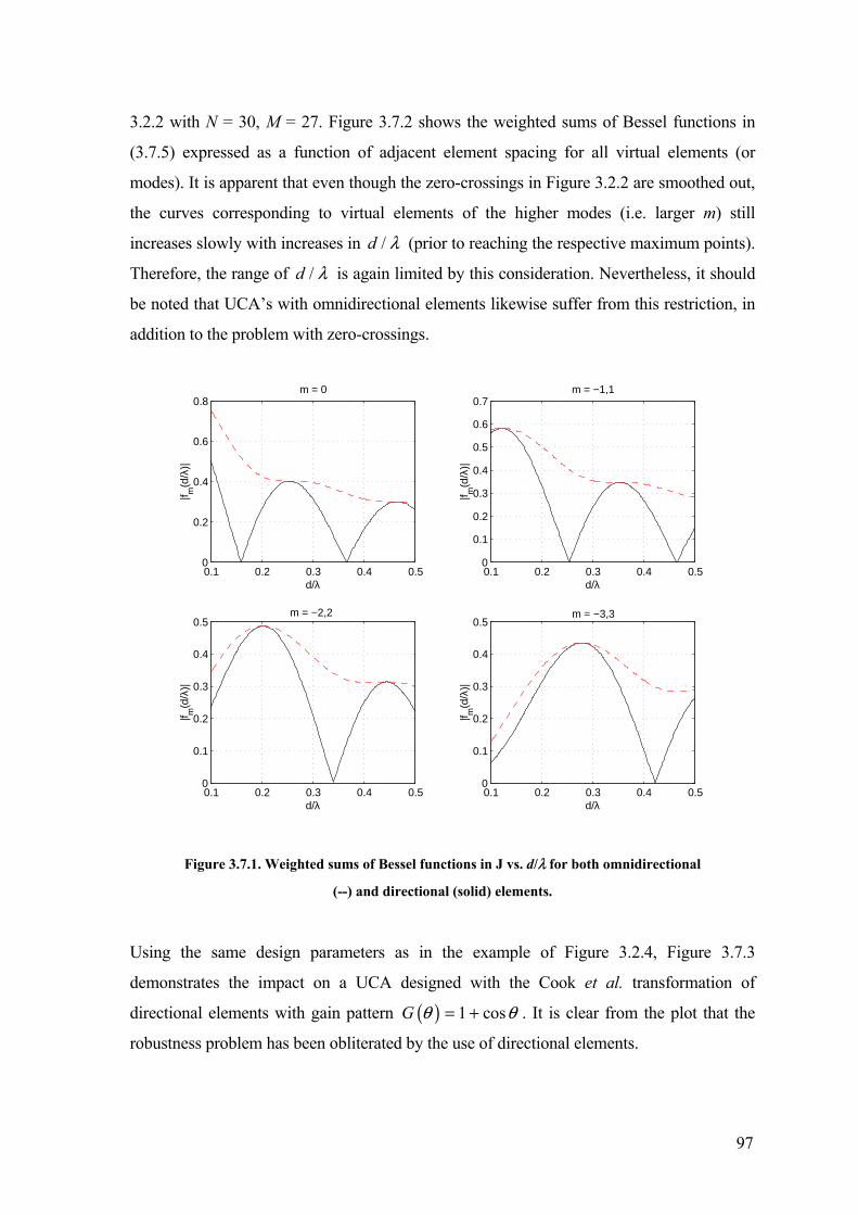
97

3.2.2 with N = 30, M = 27. Figure 3.7.2 shows the weighted sums of Bessel functions in

(3.7.5) expressed as a function of adjacent element spacing for all virtual elements (or

modes). It is apparent that even though the zero-crossings in Figure 3.2.2 are smoothed out,

the curves corresponding to virtual elements of the higher modes (i.e. larger m) still

increases slowly with increases in /d l (prior to reaching the respective maximum points).

Therefore, the range of /d l is again limited by this consideration. Nevertheless, it should

be noted that UCA’s with omnidirectional elements likewise suffer from this restriction, in

addition to the problem with zero-crossings.

0.1 0.2 0.3 0.4 0.50

0.2

0.4

0.6

0.8m = 0

|f m(d

/λ)|

d/λ0.1 0.2 0.3 0.4 0.50

0.1

0.2

0.3

0.4

0.5

0.6

0.7m = −1,1

|f m(d

/λ)|

d/λ

0.1 0.2 0.3 0.4 0.50

0.1

0.2

0.3

0.4

0.5m = −2,2

|f m(d

/λ)|

d/λ0.1 0.2 0.3 0.4 0.50

0.1

0.2

0.3

0.4

0.5

|f m(d

/λ)|

d/λ

m = −3,3

Figure 3.7.1. Weighted sums of Bessel functions in J vs. d/l for both omnidirectional

(--) and directional (solid) elements.

Using the same design parameters as in the example of Figure 3.2.4, Figure 3.7.3

demonstrates the impact on a UCA designed with the Cook et al. transformation of

directional elements with gain pattern ( ) 1 cosG q q= + . It is clear from the plot that the

robustness problem has been obliterated by the use of directional elements.

98

Though not explained in depth, Doron and Doron [108] suggested the addition of dipole

antenna elements (of directional characteristics) on the circumference of a UCA to

overcome the problem of resonance in array interpolation. Apparently, the presence of such

elements allows array interpolation to satisfy the alternative spatial sampling condition that

occurs for cases of resonance [108]. Once again, this can be understood from the positive

effect of directional elements on the Davies transformation, in which the zeros of the Bessel

functions are eliminated. In particular, Doron and Doron proposed the use of one additional

elements for the mode m = 0 and two additional elements for each of the other cases, since

they occur in pairs, i.e. m = ±1, ±2, …, ±Mo. Of course, the element(s) must be

appropriately placed [108].

0.1 0.15 0.2 0.25 0.3 0.35 0.4 0.45 0.50

0.1

0.2

0.3

0.4

0.5

|f m(d

/λ)|

d/λ

Figure 3.7.2. Weighted sums of Bessel functions in J vs. d/l for directional elements

where m = -13, …, 13.

However, the addition of one or two elements is not always adequate, since the zeros of

Bessel functions can be close to each other as seen in Figure 3.2.2, which can result in large

norms in more than one row or one pair of rows (also see Table 3.2). Furthermore, these

additional element(s) is designed to overcome the lack of robustness of a mode (or a pair of

modes) at a given d/l of a UCA. In contrast, the replacement of omnidirectional elements

by directional elements can solve the problem of robustness (due to zero-crossings) for all

modes over d/l Œ [0.1, 0.5], as shown in Figure 3.7.2. This suggests that for wideband

99

signals that spans over a considerable range of d/l, the Doron and Doron proposal may not

be sufficient. Additionally, mobile communications systems often require the same array to

operate over different frequency bands. For instance, the FDD mode of WCDMA systems

means that the uplink and downlink frequency bands are different and involves different

d/l.

0.15 0.2 0.25 0.3 0.35 0.4 0.45 0.50

10

20

30

40

50

60

70

80

90

Squ

ared

nor

m o

f T

(dB

)

d/λ

DirectionalOmnidirectional

Figure 3.7.3. Squared norm of TIA vs. d/l for the Cook et al. transformation (raised

cosine window): Omnidirectional and directional elements (of the pattern

( ) 1 cosG q q= + ) with N = 30, M = 13 and in-sector size Dq = 90∞.

3.8 Additional Elements within Radius of UCA

Interestingly, the use of additional omnidirectional element(s) within the radius of a UCA,

can also overcome the problem with the transformation matrix having a large norm and the

subsequent lack of robustness.

For the Davies transformation, Swingler and Davies [57] recognised that having an element

at the centre of a UCA can overcome the poor SNR problem for the middle element of the

Davies array. As mentioned, the SNR problem is another consequence of large row norms,

which can be contained if the magnitude row norm is reduced. The basis for the proposed

solution is described as follows.

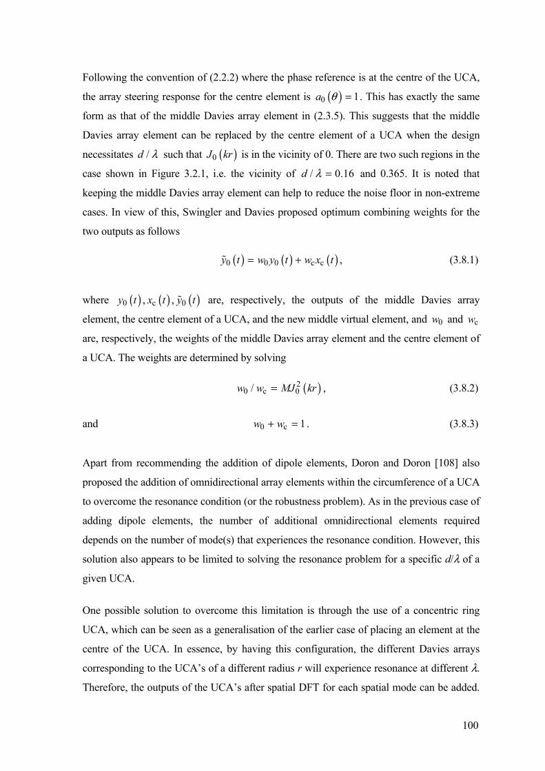
100

Following the convention of (2.2.2) where the phase reference is at the centre of the UCA,

the array steering response for the centre element is ( )0 1a q = . This has exactly the same

form as that of the middle Davies array element in (2.3.5). This suggests that the middle

Davies array element can be replaced by the centre element of a UCA when the design

necessitates /d l such that ( )0J kr is in the vicinity of 0. There are two such regions in the

case shown in Figure 3.2.1, i.e. the vicinity of / 0.16d l = and 0.365. It is noted that

keeping the middle Davies array element can help to reduce the noise floor in non-extreme

cases. In view of this, Swingler and Davies proposed optimum combining weights for the

two outputs as follows

( ) ( ) ( )0 0 0 c cy t w y t w x t= + , (3.8.1)

where ( ) ( ) ( )0 c 0, ,y t x t y t are, respectively, the outputs of the middle Davies array

element, the centre element of a UCA, and the new middle virtual element, and 0w and cw

are, respectively, the weights of the middle Davies array element and the centre element of

a UCA. The weights are determined by solving

( )20 c 0/w w MJ kr= , (3.8.2)

and 0 c 1w w+ = . (3.8.3)

Apart from recommending the addition of dipole elements, Doron and Doron [108] also

proposed the addition of omnidirectional array elements within the circumference of a UCA

to overcome the resonance condition (or the robustness problem). As in the previous case of

adding dipole elements, the number of additional omnidirectional elements required

depends on the number of mode(s) that experiences the resonance condition. However, this

solution also appears to be limited to solving the resonance problem for a specific d/l of a

given UCA.

One possible solution to overcome this limitation is through the use of a concentric ring

UCA, which can be seen as a generalisation of the earlier case of placing an element at the

centre of the UCA. In essence, by having this configuration, the different Davies arrays

corresponding to the UCA’s of a different radius r will experience resonance at different l.

Therefore, the outputs of the UCA’s after spatial DFT for each spatial mode can be added.

101

For example, if there are two UCA’s in the concentric ring configuration corresponding to

radius r1 and r2, and steering vectors ( )1 qa and ( )2 qa , then the output for the mth mode

after the spatial DFT is

( ) ( ) ( ) ( )1 2 1 21o

m jmm mm M

N j J kr J kr e qq q+ +

È ˘ È ˘+ ª +Î ˚ Î ˚Fa Fa , (3.8.4)

where , ,o om M M= - … and the condition for good approximation is assumed satisfied.

Since r1 π r2, the zero-crossings for the two Bessel functions in (3.8.4) do not occur at the

same d/l’s. The desired Vandermonde form can then be obtained from (3.8.4) using a new

J matrix

( ) ( ){ } 11 2diag m

m mN j J kr J kr-

È ˘= +Î ˚J . (3.8.5)

Consequently, as in the case of using directional elements for the UCA, the concentric ring

approach also enable the UCA to overcome the resonance problem. However, it should be

noted that in having a concentric ring configuration, the potential advantage of a UCA over

several ULA’s with respect to the total number of elements utilised for full azimuth

coverage [92] may be reduced due to the greater number of elements required than a single-

ring UCA.

3.9 Conclusions

This chapter addresses the important problem of finding a transformation matrix to

transform the steering vector of a UCA (with omnidirectional elements) to one with a

Vandermonde form, subject to a robustness requirement as demanded by practical

considerations. The robust transformation matrix is found by posing and solving a quadratic

semi-infinite optimisation problem. We showed that, by an appropriate formulation, the

problem can be decomposed into a set of much simpler optimisation problems which can

then be solved efficiently using the dual parameterisation method of [131]. Each sub-

problem yields a row of the robust transformation matrix. The robustness of the new

transformation matrix is demonstrated by a simulation example. The simulation example

also supports our hypothesis that robustness can be gained by sacrificing the approximation

accuracy of the steering vector of the virtual array from its target Vandermonde form.

102

It may be argued that the robustification procedure is unnecessary by designing an array

that avoids the array parameters that cause the transformation to be non-robust. This will

involve, among others, a stringent control33 on the frequency of operation of the

narrowband signals. However, such a design approach may not always be possible due to

other considerations such as the higher cost associated with more reliable components and

physical restrictions imposed to the array size. Also, when a large UCA with many

elements is called for, there are many more modes (virtual elements) and corresponding

nulls in the Bessel functions, such as those of Figure 3.2.2 as compared to those of Figure

3.2.1. Furthermore, for both Davies transformation and interpolated array transformation in

wideband (e.g. Multicarrier CDMA [135]) or 2D angle applications, it may be hard to avoid

the need to use the robustification procedure since it requires TDav and TIA to have

acceptable norm for a large range of d/l.

It has been shown that two other approaches, the proper use of directional elements and

additional elements in the UCA’s, where feasible, can effectively circumvent the problem

with the transformation matrix having a large norm. Nevertheless, it has been shown that

the addition of many higher order modes can result in a limitation in the range of

operational d/l that applies to all cases.

33 The need for a stringent control on the frequency of operation depends on its closeness to the resonance frequencies (and

the corresponding d/λ’s).

103

Chapter 4 DOA Estimation 4.1 Introduction

In this chapter, the focus is on DOA estimation for narrowband signals. It is well known

that many DOA estimators exist for arbitrary array geometry [35]. However, those

estimators that are suitable for correlated signal environment, such as deterministic

maximum likelihood (DML) and weighted subspace fitting (WSF) [35],[136], are often

complicated and involve a multidimensional parameter search. Moreover, their

convergence is generally not guaranteed [137]. And in the case of multidimensional

MUSIC [138], while the idea is simple, it too, involves multidimensional parameter

searching, as its name suggests. Correlated signal environments are common in mobile

communications, particularly in urban areas. A correlated signal environment is illustrated

in Figure 4.1.1 where there are remote scatterers, i.e. a building complex, and a significant

reflector, i.e. a hill, which produce correlated, multipath propagations.

BS with UCA MS

MS

Hill

Building complex

Figure 4.1.1. Multipath environment in mobile communications.

In a different perspective, computationally simple DOA estimators have also been devised

but they require special conditions such as ULA’s. The ULA-based estimators include

ESPRIT [139] or MUSIC [106] with spatial smoothing [85]-[87], and Root-WSF

[35],[137]. Specifically, these estimators take advantage of the Vandermonde form of the

steering vector of ULA’s (uniform spatial sampling) to reduce their computational

complexity. Examples include MUSIC with spatial smoothing requires eigenvalue

104

decomposition and 1D search, and Root-WSF involves eigenvalue decomposition, LS

solutions and polynomial rooting.

UCA is the most common array geometry apart from ULA [7]. And as pointed out in

earlier chapters, the techniques commonly employed for ULA’s can be readily applied to

UCA’s through a preprocessing step of either the Davies or the interpolated array

transformations.

Wax and Sheinvald [54] and Eiges and Griffiths [56] showed the use of Davies

transformation for coherent (or perfectly correlated) signals for Root-MUSIC and MUSIC

with spatial smoothing. Reddy and Reddy [121] followed up this work with a performance

analysis of Root-MUSIC with spatial smoothing as applied to the Davies array of a UCA.

They derived analytical expressions for the performance of Root-MUSIC with spatial

smoothing and investigated the impact of finite data perturbations, correlated signals,

directional elements and transformation error on the performance.

Mathews and Zoltowski [55] devised a computationally attractive version of Davies

transformation (in azimuth and elevation, or 2D angle) that gives a real-valued array

steering vector in the Davies array, which led to the novel UCA-RB-MUSIC DOA

estimation algorithm. They also proposed another slightly different form of Davies

transformation which facilitated the development of the UCA-ESPRIT algorithm [102] and

that enables real-valued, closed form 2D angle estimation on a UCA [55]. Unfortunately,

these algorithms, like the primitive forms of MUSIC and ESPRIT, demonstrate a limited

ability to cope with highly correlated signal environment. In UCA-RB-MUSIC, forward-

backward averaging can only be performed on the full Davies array, thus limiting its ability

to decorrelate two fully correlated signals only. Furthermore, Mathews and Zoltowski [55]

made an interesting observation that this limited form of forward-backward averaging can

also be applied in element space (i.e. without a transformation) on a UCA when the number

of element is even.

For interpolated array transformations, results are shown for different DOA estimators, i.e.

Root-MUSIC [59],[60], ESPRIT (or VIA34-ESPRIT) [113],[114], MUSIC with spatial

smoothing [65],[63] and Root-WSF [64],[115]. However, except for the pioneering work of

34 Virtual Interpolated Array.

105

Bronez [58], these results are based on the simple LS approach of the Friedlander

transformation [59].

It is worth pointing out that there have been other attempts to come up with simple DOA

estimation algorithms suited for correlated signal environment and UCA. One of these is

the circular spatial modulation averaging (CSMA) technique [140]. However, this

technique has only limited applications since it requires the UCA to be physically rotated

and allows only a small number of (sub)arrays which limits its ability to decorrelate the

coherent signals.

A computationally attractive DOA estimation technique35 that has recently received

significant attention in the literature is the Space-Alternating Generalized Expectation-

Maximisation (SAGE) algorithm proposed by Fessler et al. [141]. SAGE works well for an

arbitrary array geometry in a correlated signal environment and has maximum-likelihood

performance. It has been applied to offline channel parameter (including DOA) estimation

in mobile environments which is particularly useful for channel modelling [142]. As the

name suggests, SAGE is an extension of the iterative Expectation Maximisation (EM)

algorithm, and can have a much faster convergence than the EM algorithm. However,

despite the apparent success of SAGE, it has recently been discovered the faster

convergence can only be guaranteed only if the signal sources are sufficiently separated36

and have acceptable SNR’s [143]. Furthermore, EM and SAGE may converge to local

stationary points of the log-likelihood function and are not guaranteed to reach the global

maxima [143].

In this chapter, the application of MUSIC (and Root-MUSIC) with spatial smoothing on the

Davies array and the virtual ULA’s is shown [54],[61]. This is followed by the application

of Root-WSF on these virtual arrays [64],[71]. The analytical expressions of Root-MUSIC

with spatial smoothing for both the Davies transformation and the interpolated array

transformations [121],[122] are then summarised. The expressions are derived under the

assumption that all signals are in the in-sector region. However, for the Cook et al.

transformation, it will be argued that these expressions are equally applicable to cases

35 SAGE is a multi-parameter estimation algorithm. However, the focus here is on DOA estimation. 36 As Fleury et al. [142] suggest, this separation can be in relative time delay, Doppler frequency and/or DOA in the case of

multi-parameter estimation.

106

where there are out-of-sector signals. This conjecture appears to be supported by numerical

examples.

The numerical examples first examine the performances of MUSIC and Root-MUSIC with

spatial smoothing and Root-WSF for ideal UCA’s and the Davies transformation. A similar

numerical study is then carried out for the interpolated array transformations. In particular,

the focus is in comparing the different interpolated array transformations of Bronez,

Friedlander, and Cook et al. As was pointed out in Section 2.5.2, the out-of-sector response

of the Friedlander transformation can be significant and at the same time suffer from severe

distortion in magnitude and phase relative to the Vandermonde form of a ULA. This is

shown to effect a large performance degradation in the presence of out-of-sector signals

that are correlated with in-sector signals. Similar conclusions are drawn for the Bronez

transformation that also has a distorted out-of-sector response. On the other hand, the Cook

et al. transformation is shown to be far more reliable in such signal scenarios.

In addition, the impact of array imperfections on the Davies transformation and the Cook et

al. transformation for UCA’s with omnidirectional elements is demonstrated. The

robustification procedure proposed in the previous chapter is shown to be effective in

mitigating the performance degradation resulting from the problem of robustness.

4.2 Subspace Methods with Spatial Smoothing

4.2.1 Spatial Smoothing

Evans et al. [85] and Shan et al. [144] were the firsts to introduce spatial smoothing (or

more specifically, forward-only spatial smoothing (FOSS)). Its primary merit is in

countering the problem of rank deficiency in the signal covariance matrix sR of a coherent

signal environment. It is only applicable to arrays with a translational invariance property,

i.e. when divided into subarrays, the steering vectors of the subarrays are related to one

another by a pure phase shift. Both classes of UCA preprocessing techniques introduced in

this thesis yield a Vandermonde steering vector that satisfies this criterion. Here, an

improved version called forward-backward spatial smoothing (FBSS), developed separately

by Pillai and Kwon [86] and Williams et al. [87], is summarised. The following

development is generic for a linear transformation T and applies equally to the Davies

transformation and the interpolated array transformations. Figure 4.2.1 shows the block

diagram of a linear transformation of a UCA for DOA estimation.

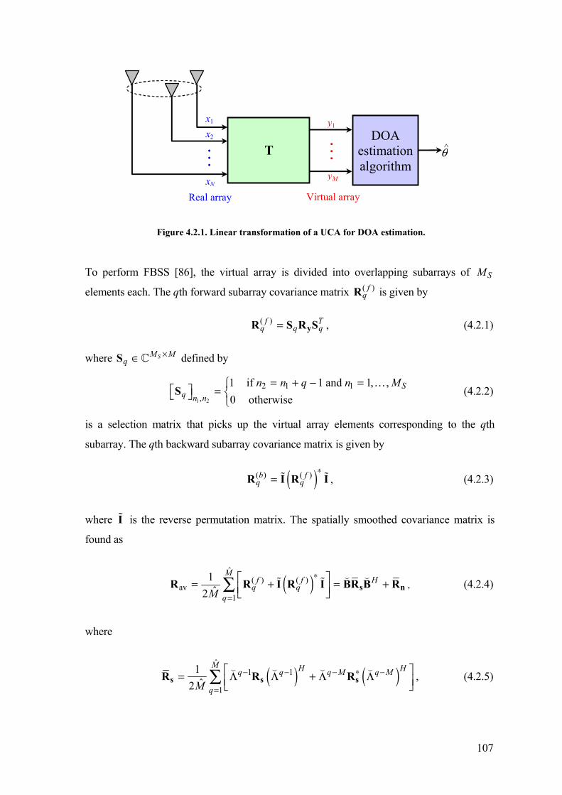
107

Virtual array

yM

. . .

y1

DOA estimation algorithm

q T. . .

x 2 x 1

x N Real array

Figure 4.2.1. Linear transformation of a UCA for DOA estimation.

To perform FBSS [86], the virtual array is divided into overlapping subarrays of SM

elements each. The qth forward subarray covariance matrix ( )fqR is given by

( )f Tq q q= yR S R S , (4.2.1)

where SM Mq

¥ŒS defined by

1 2

2 1 1,

1 if 1 and 1, ,0 otherwise

Sq n n

n n q n M= + - =ÏÈ ˘ = ÌÎ ˚ ÓS

… (4.2.2)

is a selection matrix that picks up the virtual array elements corresponding to the qth

subarray. The qth backward subarray covariance matrix is given by

( )( ) ( )b fq q

*=R I R I , (4.2.3)

where I is the reverse permutation matrix. The spatially smoothed covariance matrix is

found as

( )ˆ

( ) ( )av

1

1ˆ2

Mf f H

q qqM

*

=

È ˘= + = +Í ˙Î ˚Â s nR R I R I BR B R , (4.2.4)

where

( ) ( )ˆ

1 1

1

1ˆ2

M H Hq q q M q M

qM- - - * -

=

È ˘= L L + L LÍ ˙Î ˚Âs s sR R R , (4.2.5)

108

( )ˆ2 *

1ˆ2

Mn H T H T

q q q qqM

s

=

È ˘= S + SÍ ˙Î ˚Ân n nR S T T S IS T T S I , (4.2.6)

( ) ( ) ( )( )1 2diag , , , Lj j je e ew q w q w qL = … , (4.2.7)

( ) ( )1 , , Lq qÈ ˘= Î ˚B b b… , (4.2.8)

( ) ( )1q q=b S b , (4.2.9)

and ˆ 1SM M M= - + (4.2.10)

is the number of subarrays. For the Davies transformation, ( )l lw q q= , and for the

interpolated array transformations, ( ) sinl lkdw q q= . For the Davies transformation, Wax

and Sheinvald [54] refer to the noise covariance of the qth forward (or backward) subarray 2 H Tn q qs SnS T T S (or ( )*2 H T

n q qs SnIS T T S I ) as being spatially non-white, as it varies from

subarray to subarray. It is noted that for (4.2.4) to be valid, the transformation error is

assumed negligible, i.e. ( ) ( )q q=b b over the full azimuth for the Davies transformation

and over the in-sector region for the interpolated array transformations.

It is observed in (4.2.5) that spatial smoothing introduces a distinct phase term 1q-L (or q M-L ) to the signal covariance matrix for the qth forward (or backward) subarray prior to

averaging across the subarray. Under some mild conditions given in [85],[87],[145], the

phase modulation is able to restore the rank of sR for up to 2 3M coherent signals (in the

largest subgroup of coherent signals). Moreover, for finite data, spatial smoothing can yield

better statistical properties (due to the averaging effect) [35]. However, a careful design is

required since the gains can be offset by the reduced aperture size of the subarray

[121],[122]. Spatial smoothing is also known to be able to reduce the transformation error

in the steering vectors of the Davies array and the virtual ULA [121],[122].

It is important to note that while the steering vector of the Davies array retains the

approximate Vandermonde form over the full azimuth, in general, the steering vector of a

virtual ULA is only approximately Vandermonde for the in-sector region. Consequently,

the smoothing process described in (4.2.4) only applies to in-sector correlated signals. As

109

summarised in Chapter 2, the different formulations used to obtain the three interpolated

array transformations reflect very different strategies in addressing this problem. In essence,

Bronez [58] chose to minimise any impact of out-of-sector signals on the in-sector signals

by a best effort suppression of the out-of-sector response with no regard to the suppression

it actually attains. Friedlander hypothesised that the out-of-sector response is sufficiently

distorted relative to the Vandermonde form of the virtual ULA such that the suppression of

out-of-sector signals is obtained by default [60]. It is clear that these two transformations

make no effort to retain the (Vandermonde) form of ULA for the out-of-sector region.

Therefore, the effect of smoothing on out-of-sector correlated signals is unknown.

In [74], Cook et al. proposed a smooth rolloff of the steering vector that will allow the

Vandermonde form to be kept in the transition region together with a sufficient suppression

to be targeted in the image sector region. The Cook et al. transformation thus extends the

effect of spatial smoothing in (4.2.4) to the transition region with some degree of certainty

(providing transformation error is reasonable), albeit attenuating signals that fall within this

region. The image sector with a target response of 0 or close to 0 (depending on the window

used) is designed to give sufficient suppression for signals in this region such that they are

largely filtered out by the transformation from the covariance matrix representation of

(4.2.4) to prevent ambiguity in the virtual ULA.

An interesting result given in [121] is that due to the centro-Hermitian property of the

Davies array steering vector, i.e. ( ) ( )*q q=Ib b , FBSS on the Davies array reduces to

FOSS for the special case of real-valued correlation. But while FBSS in such cases reduces

to FOSS, it is still able to outperform the latter due to the further averaging of finite data

perturbations from the backward subarrays.

Prior to applying subspace methods, it is necessary to prewhiten the spatially smoothed

covariance matrix avR using the Hermitian square root of w wH=nR G G

( ) ( )1 1w 1 1av w av w w w

w w

H H H

H

- -- -= = +

= +

s

s

R G R G G BR B G I

B R B I, (4.2.11)

110

where 1w w

-=B G B is the prewhitened steering matrix. It is worth clarifying that the

prewhitening procedure merely changes the form of the noise covariance matrix to the

covariance matrix of white noise (diagonal matrix of equal elements) by “transferring” the

non-diagonal (or unequal diagonal) form into the signal part of the covariance matrix.

Prewhitening allows the normal eigenvalue decomposition, rather than the more involved

generalised version, to be used in DOA estimation with subspace methods. As such, it does

not fundamentally improve the performance of DOA algorithms. Similarly, it is unable to

mitigate the problem of robustness against unknown, deterministic array imperfections

when the transformation matrix has rows of large norms (see Chapter 3).

Another interesting aspect of the prewhitened form of (4.2.11) (be it for the subarray or the

full array MS = M) is that beamspace preprocessing can be applied to it so that the benefits

of beamspace processing can be realised [35],[103]. Sidorovich and Gershman [66] and

Gershman [67] employed beamspace preprocessing to improve the performance of

Friedlander’s interpolated array for wideband signals. It is also noted that the DFT matrix F

of the Davies transformation qualifies as a beamspace transformation [55],[101] for the full

Davies array.

As a proof of concept, the use of two subspace methods, MUSIC and Root-MUSIC on the

prewhitened, spatially smoothed covariance matrix is given as below.

4.2.2 MUSIC

Multiple Signal Classification (MUSIC), first proposed by Schmidt [106], is the most

popular high-resolution subspace methods. The main idea behind MUSIC is that

performing eigenvalue decomposition (EVD) on the covariance matrix separates it into two

orthogonal subspaces: a signal subspace and a noise subspace. And since the signal

subspace is spanned by the steering vectors of the received signals, a one-dimensional (1D)

search can be performed to find the steering vectors of the received signals by projecting

onto the noise subspace, the array steering vector over the field of view. This procedure will

work as long as no two signals are coherent. Here it is assumed that the spatial smoothing

procedure described previously has restored the rank of the signal covariance matrix to L.

However, it is well known that the statistical behaviour of MUSIC with spatial smoothing

differs from that with no spatial smoothing [145].

More explicitly, the MUSIC algorithm first involves an EVD

111

wav w w

H H= + = LsR B R B I E E , (4.2.12)

where ( )1 1diag , , , , ,SL L Ml l l l+È ˘L = Î ˚… … , 1 1, , , , ,

SL L M+È ˘= Î ˚E e e e e… … , ll ’s are

positive real eigenvalues in decreasing order of magnitude and le the corresponding

eigenvectors. Note that the ( )SM L- noise eigenvalues correspond to 1ll = ,

1, , Sl L M= + … and the signal eigenvalues are 1ll > , 1, ,l L= … . The EVD can also be

divided into mutually orthogonal signal and noise subspace components

H H HL = L + Ls s s n n nE E E E E E . (4.2.13)

where |È ˘= Î ˚s nE E E , ( )1diag , , Ll lÈ ˘L = ºÎ ˚s , ( )1diag , ,SL Ml l+È ˘L = ºÎ ˚n and

L =n I . Now if the eigenvalues of w w sH H= Ls sB R B E E are denoted by

0, 1, ,l l Ll > = … , and 0, 1, ,l Sl L Ml = = + … , then the signal eigenvalues can be

expressed as 1l ll l= + , 1, ,l L= … . This means that w wH

sB R B also spans the signal

subspace and is orthogonal to the noise subspace.

Denote the steering vector of the prewhitened subarray as ( ) ( )1w wq q-=b G b . Since the

noise subspace is orthogonal to ( )w qb at the DOA’s of the received signals, the MUSIC

algorithm exploits this property by performing a 1D search over q for these incidences of

orthogonality. The MUSIC power spectrum, in which these incidences occur in sharp

peaks, is defined by

( ) ( ) ( )( ) 1MUSIC w w

H HP q q q-

= n nb E E b . (4.2.14)

The DOA estimates are chosen at the L largest peaks of the power spectrum. While the

peaks are infinitely large theoretically, in practice, they are limited by machine accuracy

and finite data effect (i.e. , ,x y nR R E replaced by estimated quantities ˆˆ ˆ, ,x y nR R E ). It is

clear from the above discussion that the number of signals that MUSIC can handle is hard-

limited by the necessity of having a noise subspace with dimensions of at least 1, i.e. there

can be at most N -1 signals.

In addition, MUSIC requires knowledge of the number of signals L, which needs to be

estimated (correctly) by either examining the eigenvalues of wavR or using a model order

algorithm [145],[146]. Though unimportant for the present application, a favourable

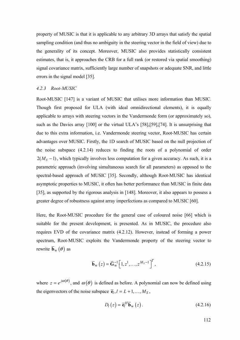
112

property of MUSIC is that it is applicable to any arbitrary 3D arrays that satisfy the spatial

sampling condition (and thus no ambiguity in the steering vector in the field of view) due to

the generality of its concept. Moreover, MUSIC also provides statistically consistent

estimates, that is, it approaches the CRB for a full rank (or restored via spatial smoothing)

signal covariance matrix, sufficiently large number of snapshots or adequate SNR, and little

errors in the signal model [35].

4.2.3 Root-MUSIC

Root-MUSIC [147] is a variant of MUSIC that utilises more information than MUSIC.

Though first proposed for ULA (with ideal omnidirectional elements), it is equally

applicable to arrays with steering vectors in the Vandermonde form (or approximately so),

such as the Davies array [100] or the virtual ULA’s [58],[59],[74]. It is unsurprising that

due to this extra information, i.e. Vandermonde steering vector, Root-MUSIC has certain

advantages over MUSIC. Firstly, the 1D search of MUSIC based on the null projection of

the noise subspace (4.2.14) reduces to finding the roots of a polynomial of order

2( 1)SM - , which typically involves less computation for a given accuracy. As such, it is a

parametric approach (involving simultaneous search for all parameters) as opposed to the

spectral-based approach of MUSIC [35]. Secondly, although Root-MUSIC has identical

asymptotic properties to MUSIC, it often has better performance than MUSIC in finite data

[35], as supported by the rigorous analysis in [148]. Moreover, it also appears to possess a

greater degree of robustness against array imperfections as compared to MUSIC [60].

Here, the Root-MUSIC procedure for the general case of coloured noise [66] which is

suitable for the present development, is presented. As in MUSIC, the procedure also

requires EVD of the covariance matrix (4.2.12). However, instead of forming a power

spectrum, Root-MUSIC exploits the Vandermonde property of the steering vector to

rewrite ( )w qb as

( ) 1 1 1w w 1, , , S

TMz z z- -È ˘= Î ˚b G … , (4.2.15)

where ( )jz e w q= , and ( )w q is defined as before. A polynomial can now be defined using

the eigenvectors of the noise subspace , 1, ,l Sl L M= +e … ,

( ) ( )wH

l lD z z= e b . (4.2.16)

113

The projection of the array steering vector onto the noise subspace (reciprocal of the power

spectrum) is given by

( ) ( ) ( ) ( ) ( ) ( ) 2w w w w

1 1

S SM MH H H H

l l ll L l L

D z z z z z D z= + = +

= = =Â Ân nb E E b b e e b . (4.2.17)

The above polynomial involves z*. In order to retain only z in the polynomial, it is noted

that ( ) 1* jz e zw q- -= = . Therefore, it is possible to write

( ) ( ) ( )1 1w w

SM T HD z z z z- -= n nb E E b , (4.2.18)

where ( )D z is a polynomial of degree 2( 1)SM - whose roots occur in mirrored pairs with

respect to the unit circle. Only the roots within the circle are examined, and the phases of

the L largest roots are denoted by 1 2ˆ ˆ ˆ, , , Lz z z… . The DOA estimates are obtained via

( )1ˆ ˆ , 1, ,l lz l Lq w -= = … . (4.2.19)

For the Davies transformation, this is simply ( )ˆ ˆargl lzq = , while for the interpolated array

transformation, it is ( )ˆ ˆarcsin argl lz kdq È ˘= Î ˚ .

4.2.4 MUSIC and Root-MUSIC for Interpolated Arrays

While the above-mentioned MUSIC and Root-MUSIC procedures work well for a normal

ULA and the Davies array, some modifications are necessary to adapt the procedure to the

virtual ULA of the interpolated array transformations. This is because multiple virtual

ULA’s are involved in performing DOA estimation. Friedlander [59] proposed the

following steps for Root-MUSIC (though it can be easily extended to MUSIC as follows by

considering magnitudes of peaks rather than roots):

1. For MUSIC (or Root-MUSIC), choose the DOA’s corresponding to the L largest

peaks (or roots within the circle) for each sector. If N is the number of in-sectors

for full coverage, the resulting number of DOA estimates is NL .

2. Eliminate out of the L DOA estimates of each in-sector those that fall outside the in-

sector region of interest.

114

3. Retain out of the remaining DOA’s those correspond to the L largest peaks (or

roots).

It is easy to see that step 2 can be omitted in MUSIC by only calculating the power

spectrum (4.2.14) for the operational sector region of each sector. It is noted that in rare

instances, the existence of in-sector spurious peaks (or roots) due to random distortion in

the out-of-sector steering vector can cause erroneous estimates for the Friedlander

transformation [60]. On the contrary, the Cook et al. transformation is expected to be

largely immune from this problem due to its attempt to control the out-of-sector response.

The above approach of choosing the final DOA’s will be subsequently used for the

interpolated array transformations of Bronez [58] and Cook et al. [74] as well.

Here, it is worth pointing out that the reliance of Root-MUSIC on the steering vector having

a Vandermonde form again raises the question of the influence of out-of-sector signals. As

mentioned, the Cook et al. transformation [74] gives more confidence as to the correctness

of the DOA estimates, as indicated by its reasonable error performance over the full

azimuth in the achieved steering vector relative to the target steering vector (see Figure

2.6.7).

One consequence of performing MUSIC and Root-MUSIC on an interpolated array is the

“overestimation” of the number of signals in the covariance matrix of the virtual ULA. This

occurs because the number of signals L is estimated by other methods that take into account

all signals present in the full azimuth rather than the number present in each in-sector. And

for each in-sector, while the out-of-sector signals are suppressed and/or distorted to some

extent, they are in general not completely removed.

In the case of very good out-of-sector suppression (especially in the image sector of the

Cook et al. transformation [74] where ( ) 0w q = ), some signals are in effect absent in the

virtual ULA, as indicated by (2.6.6). Choosing the full set of L signals for the in-sector of

interest will thus result in obtaining DOAs of “phantom signals”. In such cases,

overestimation of the number of signals is expected to marginally affect the performance of

MUSIC and Root-MUSIC. This is because the noise subspace, though present, is

incomplete and thus do not provide a full representation of the noise subspace. However, as

will be shown in the numerical examples, the negative impact seems limited.

115

In terms of computational load, the computational load of the interpolated array

transformations is generally higher than the Davies transformation, since DOA estimation

must be performed once for each in-sector. As noted earlier, at least three in-sectors are

needed for acceptable spatial resolution and full coverage. This is particularly so when the

Davies array has a comparable number of elements to the virtual ULA. However, providing

the number of in-sectors is not too large, the interpolated array transformations involve a

modest computational cost (multiple 1D searches or polynomial rootings) compared to

multidimensional search algorithms such as DML [35].

4.3 Root-WSF

4.3.1 Background

Stoica and Sharman proposed MODE (Method of Direction Estimation) [137] or Root-

WSF to fill the gap between the performance of MUSIC and ML methods. In particular,

they observed that the performance of MUSIC approaches that of the ML methods, such as

DML [35], for large sample sizes and uncorrelated signals. However, in the case of

correlated signals, MUSIC can no longer closely follow the ML performance [137]. Even

though spatial smoothing enables MUSIC to handle highly correlated and coherent signals,

it necessitates the reduction of array aperture in order to form subarrays for the smoothing

process. On the other hand, as mentioned earlier, ML methods are generally avoided in

practice because of the high computational complexity and occasional problems with

convergence. This raises interests for a method that performs well in correlated signals, and

is yet able to offer a computational complexity comparable to that of MUSIC and also

retain the full array aperture.

As pointed out in [137], Root-WSF fulfils above requirements for a ULA by exploiting the

Vandermonde structure of its steering vector and making large sample approximation in the

problem formulation. In essence, it is able to offer a computationally cost comparable to

that of MUSIC while attaining ML performance for correlated signals and reasonably large

sample sizes.

Weiss et al. proposed the use of Root-WSF with interpolated arrays in [64],[115]. The

beauty of the interpolation procedure is that it extends the advantages of Root-WSF to

arbitrary planar arrays, albeit with the need for sector-by-sector processing. And in the case

of the Davies transformation, only one Davies array is needed to estimate the DOA’s [71].

116

In the following, the Root-WSF procedure is summarised for a general transformation

matrix T that is applicable for both classes of preprocessing techniques.

Here, it is noted that Root-WSF [35] is perhaps a more appropriate name for the technique

since it can be derived from the WSF algorithm [136], and includes a polynomial rooting

procedure similar to that of Root-MUSIC. In this section, this perspective is taken to outline

the principal idea behind the technique [35].

4.3.2 The Algorithm

As in MUSIC with spatial smoothing, Root-WSF begins with an EVD of the covariance

matrix. However, instead of subarrays, Root-WSF operates on the covariance matrix of the

full transformed array Ry as in (2.2.7). To this end, Ry requires first a prewhitening

procedure, where the prewhitening matrix 1w-G is defined by the Hermitian square root of

2 Hns SnT T w w

H= G G

( ) 11w w w w

H H-- = +y sG R G B R B I , (4.3.1)

where 1w w

-=B G B . The EVD then gives

w wH H H+ = L + Ls s s s n n nB R B I E E E E , (4.3.2)

where [ ]|= s nE E E , ( )1diag , , zl lÈ ˘L = ºÎ ˚s , ( )1diag , , Mzl l+È ˘L = ºÎ ˚n ,L =n I , z is

the rank of the signal covariance matrix and the diagonal elements ll ’s of Ls and Ln are

positive real eigenvalues in decreasing order of magnitude. In the pioneering work [137],

Stoica and Sharman assumed that signals are highly correlated but not coherent, i.e. z = L.

However, in general, z ≤ L [35] since z π L where any two signals are coherent (recall that

no spatial smoothing is applied here).

As in MUSIC and Root-MUSIC, the number of signals L is assumed known. Also, z is

assumed known [64]. Given the properties of eigenvectors, it is easy to conclude that

H H+ =s s n nE E E E I . (4.3.3)

Combining (4.3.2) and (4.3.3) gives

117

( )w wH H= L -s s s sB R B E I E . (4.3.4)

Post-multiplying (4.3.4) by Es and rearranging, the basic form for a class of estimation

techniques called signal subspace fitting (SSF) is obtained

w=sE B Z , (4.3.5)

where ( ) 1wH -= L -s s sZ R B E I and H =s sE E I . The intention is to estimate the DOA’s

[ ]1, , Lq qQ = … embedded in Bw from actual data using ˆ sE . The approach taken is to

perform joint estimation of Q and Z using an error measure defined by

{ } 2w

,ˆ, arg min

FQQ = -s

ZZ E B Z . (4.3.6)

The minimisation problem is separable and the optimum Z is estimated by †wˆ ˆ= sZ B E and

( ) 1†w w w w

H H-=B B B B . This leads to

{ }{ }

w

w

w

2ˆ ârg min

ˆ ârg min Tr

ˆ ârg min Tr

F

H

H

^Q

^Q

^Q

Q = P

= P

= P

sB

s sB

s sB

E

E E

E E

, (4.3.7)

where w

†w w

^P = -B I B B . In [136], it is pointed out that the LS solution (4.3.7) can be

improved by an appropriate weighting of the form

{ }wˆ ˆ ârg min Tr H^

QQ = P s sB E WE , (4.3.8)

where W is the ζ × ζ weighting matrix. The form ˆ ˆ Hs sE WE is chosen because

w

^PB is the

projection onto the noise subspace, but ˆ ˆ Hs sE E gives the same weight (of 1) to all signals, as

opposed to the (estimated) signal subspace defined by ˆ ˆ ˆ HLs s sE E . Therefore, an appropriate

weighting is ˆ ˆ= LsW . Moreover, it has been shown that since w

ˆl^PB e ’s, 1, ,l z= … , are

asymptotically independent, the theory of weighted LS suggests that the optimal weighting

is [35]

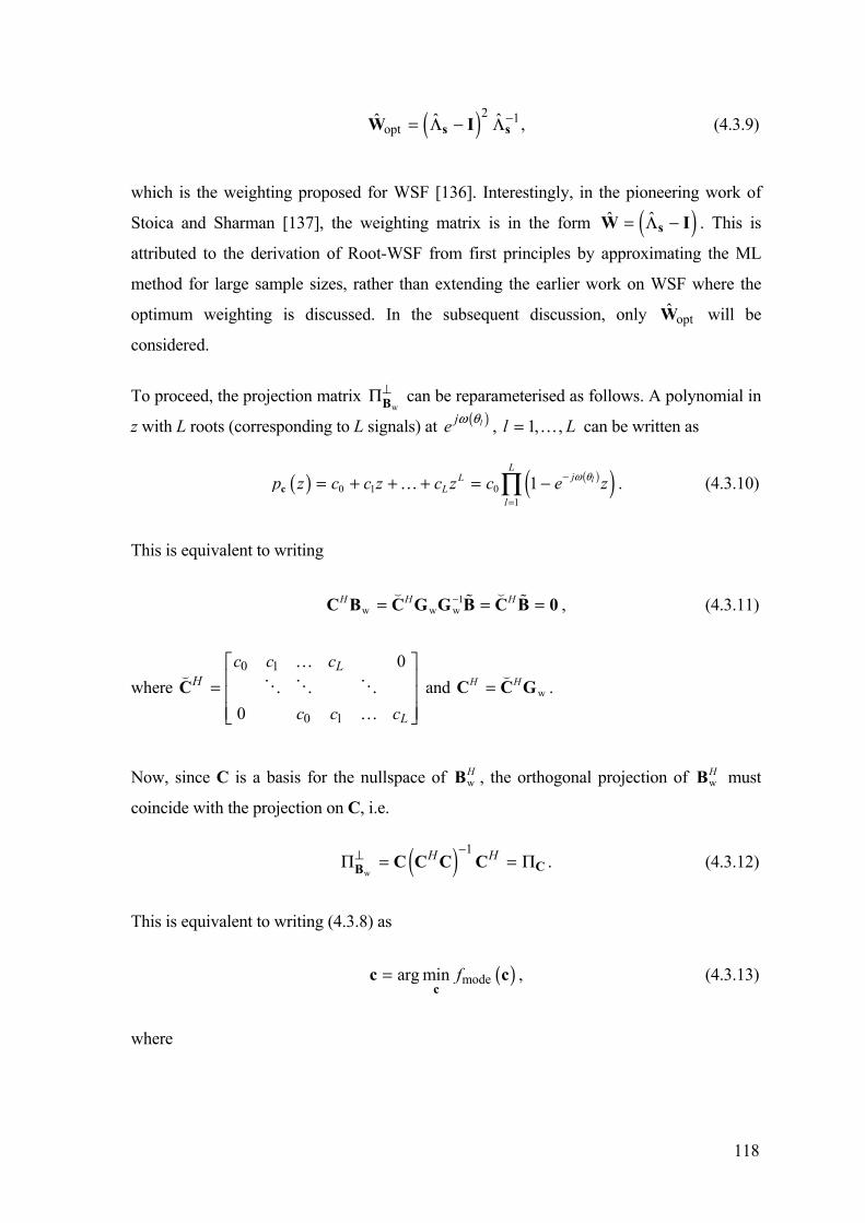
118

( )2 1optˆ ˆ ˆ -= L - Ls sW I , (4.3.9)

which is the weighting proposed for WSF [136]. Interestingly, in the pioneering work of

Stoica and Sharman [137], the weighting matrix is in the form ( )ˆ ˆ= L -sW I . This is

attributed to the derivation of Root-WSF from first principles by approximating the ML

method for large sample sizes, rather than extending the earlier work on WSF where the

optimum weighting is discussed. In the subsequent discussion, only optW will be

considered.

To proceed, the projection matrix w

^PB can be reparameterised as follows. A polynomial in

z with L roots (corresponding to L signals) at ( )lje w q , 1, ,l L= … can be written as

( ) ( )( )0 1 01

1 lL

jLL

lp z c c z c z c e zw q-

== + + + = -’c … . (4.3.10)

This is equivalent to writing

1w w w

H H H-= = =C B C G G B C B 0 , (4.3.11)

where 0 1

0 1

0

0

LH

L

c c c

c c c

È ˘Í ˙= Í ˙Í ˙Î ˚

C…

… and w

H H=C C G .

Now, since C is a basis for the nullspace of wHB , the orthogonal projection of w

HB must

coincide with the projection on C, i.e.

( )w

1H H-^P = = PCB C C C C . (4.3.12)

This is equivalent to writing (4.3.8) as

( )modearg min f=c

c c , (4.3.13)

where

119

( ) { } ( ){ }

( ){ }1

mode opt opt

1w w w w opt

ˆ ˆ ˆ ˆ ˆ ˆTr Tr

ˆ ˆ ˆTr

H H H H

H H H H H

f-

-

= P =

=

C s s s s

s s

c E W E C C C C E W E

G C C G G C C G E W E (4.3.14)

and [ ]0 1T

Lc c c=c , which is analogous to the form of the Iterative Quadratic

Maximum Likelihood (IQML) algorithm [35]. A similar iterative procedure can thus be

applied to solve the problem. To initialise the procedure, let =cW I , i = 1 and (0)ˆ 0l

È ˘Q =Î ˚ ,

1, ,l L= … .

1. Solve for { }optˆ ˆ ˆˆ arg min Tr H H= c s sc

c CW C E W E . (4.3.15)

2. Apply (4.2.19) to the roots of ( )p zc , i.e. ˆlz , 1, ,l L= … to obtain the DOA

estimates. If the DOA estimates ( )ˆ iQ are such that ( ) ( 1)ˆ ˆi il

e-È ˘Q - Q £Î ˚ , where e is

the convergence error tolerance, then end. Otherwise, form wˆˆ H=C G C using c , let

( ) 1ˆ ˆ H -=cW CC and i = i +1. Go to step 2.

The distinction between IQML and Root-WSF is that the latter converges rapidly. In fact,

numerical examples in [137] showed that provided the sample size is reasonably large, the

solution can converge very closely to the optimum upon the second iteration (i = 2) and

further iterations are unnecessary. As a result, Root-WSF becomes a non-iterative

procedure (involving as few as two or slightly more than two iterations) [137].

Remarks

1. While only about two iterations may be required in most cases, it was observed in

simulation studies that with an ideal ULA and white noise, the convergence can be

much slower in some scenarios, even with moderate to large sample sizes. The

difficult scenarios include low SNR’s, closely space correlated signals, and errors in

the underlying model (e.g. array imperfections). This suggests that while Root-WSF

is typically faster than IQML, its speed of convergence is unpredictable.

Furthermore, the use of Wc = I in the initialisation step for the transformed arrays

may also contribute to the slower convergence. This is because generally these

arrays involve coloured noise rather than white noise as assumed in [137]. Thus,

some other initialisations for the positive definite matrix Wc may bring the problem

(4.3.15) closer to the optimum solution.

120

2. It is non-trivial to solve the minimisation of (4.3.13) given the constraint in the form

{ } ( ){ }| 0 for 1lD c p z z= π πc , (4.3.16)

which forces the roots of the polynomial to be on the unit circle [137]. Therefore, it

is desirable to have a more tractable form for the constraint. A common practice is

to replace this constraint with a conjugate symmetry constraint on the vector c [137]

i L ic c*-= , 0, ,i L= … . (4.3.17)

In [137], it is shown how the constraint can be cleverly incorporated into the cost

function (4.3.13) to result in an unconstrained minimisation problem that can be

solved easily via QR decomposition. Note that the constraint (4.3.17) is a necessary

but not a sufficient condition for (4.3.16), which means that the solution found by

the constraint (4.3.17) may not satisfy (4.3.16). Nevertheless, Stoica and Sharman

[137] concluded from related work that the constraint (4.3.17) will typically only

result in a minor loss of performance. Stoica and Sharman [137] also proposed

some further conditions to circumvent certain situations in which the algorithm

under the constraint would fail.

In a follow-up paper on the IQML algorithm for frequency estimation (analogous to

DOA estimation in ULA), Nagesha and Kay [149] showed by counterexamples that

the conjugate symmetry constraint could still fail to converge to the correct result

even when all the conditions presented in [137] have been observed. However, this

problem only occurs for some very specific signal scenarios.

On the other hand, the quadratic (or norm) constraint on c as follows

1H= =c c c (4.3.18)

appears to be reliable and consistent [149]. The solution procedure with the norm

constraint is computationally modest and involves the EVD of a square matrix of

dimension L + 1 [64]. Weiss et al. [64] investigated both the conjugate symmetry

constraint and the norm constraint and showed, by a numerical example, that the

121

former has a performance advantage over the latter. This implies that to utilise the

reliable norm constraint, some sacrifice in performance is necessary.

In summary, though in general the convergence of Root-WSF can take far more than two

iterations, it is still very attractive since it is asymptotically (can handle coherent signals)

and computationally efficient (involving only EVD’s and polynomial rooting) and has a

faster convergence relative to close alternatives such as IQML [149].

From the above development, it is observed that like MUSIC, eigenvalue decomposition of

the sample covariance matrix (of dimension M ¥ M) forms the primary part of the

computational load in Root-WSF. The choice of conjugate constraint for c provides a

closed form to the minimisation procedure, while the norm constraint involves an

eigenvalue decomposition of a square matrix of dimension L ¥ L where L is typically much

smaller than M. On the other hand, polynomial rooting for Root-WSF involves only L roots

compared to 2(N – 1) roots of Root-MUSIC. Overall, the computational complexity of

Root-WSF is comparable, though usually slightly higher than MUSIC or Root-MUSIC.

4.3.3 Root-WSF for Interpolated Arrays

The relationship (4.3.11) will hold only approximately (due to transformation error) for the

Davies array and only where all signals lie in the in-sector for the interpolated array. In the

general case for interpolated arrays as discussed earlier, the steering vectors of the out-of-

sector signals will deviate from the Vandermonde form. This is especially so for the Bronez

[58] and Friedlander [60] transformations, though for the Cook et al. transformation [74],

the signals that fall in the image sector are suppressed, i.e. ( ) 0q ªb and the columns

corresponding to these signals will “disappear” from B (see also (2.6.6)).

As with Root-MUSIC, an important consideration for Root-WSF with the Cook et al.

paradigm is the issue of overestimating the number of signals when signals appear in the

image sector. As opposed to Root-MUSIC that uses an estimate of the noise subspace,

Root-WSF obtains DOA estimates through signal subspace fitting, as is clear from (4.3.8).

This suggests that its performance may be more sensitive to such signals. In the numerical

examples, it is found that the overestimation of signals does not appear to cause any

problems in the RMSE performance for uncorrelated signals. However, in the presence of

122

correlated signals, the performance of Root-WSF with the Cook et al. transformation can

degrade noticeably.

In [115], Weiss et al. showed that an out-of-sector (uncorrelated) signal could cause a

significant bias in the DOA estimate of an in-sector signal when Root-WSF is used with the

Friedlander transformation. The bias appears to grow as the out-of-sector signal is moved

further away from the in-sector region. This problem severely limits the usefulness of the

Friedlander transformation since in general it is impossible to confine all signals to the in-

sector region. For example, the 180∞ field of view of the virtual ULA will result in

ambiguity if all signals are contained in a sector width of over 180∞. Furthermore, a large

sector is undesirable for the Friedlander transformation as it increases the transformation

error [60]. It will be shown that the problem is even worse in the presence of correlated

signals in the out-of-sector region.

For the Friedlander transformation, while the method of combining DOA estimates from

the sector-by-sector processing is not given explicitly in Weiss et al. [64],[115], they

referred to the paper on Root-MUSIC [60] for details. Nevertheless, it is unclear how they

would decide on the final choice of DOA estimates, since the polynomial roots of Root-

MUSIC do not have the same interpretation as those of Root-WSF.

In the following, a rule for combining DOA estimates from different in-sectors based on the

corresponding rule of the Root-MUSIC procedure [60] is devised for Root-WSF with the

Cook et al. transformation. The rationale behind the rule is that the transformation error in

the steering vector with respect to the Vandermonde form is minimal over the entire

azimuth (except for the suppressed image sector). However, unlike Root-MUSIC, the

rooting procedure of Root-WSF directly produces the DOA estimates for L signals for a

given in-sector. Note the following:

1. If N is the number of in-sectors for full coverage, the resulting number of DOA

estimates is NL .

2. Eliminate out of the L DOA estimates of each in-sector those that fall outside of the

in-sector region of interest.

123

3. Retain out of the remaining DOA’s those that correspond to the L roots closest to

the unit circle.

It is found that Step 3 can be unreliable since unlike the Root-MUSIC procedure, closeness

to the unit circle is not a good measure of the goodness of the solution. As discussed, it is

unclear if Weiss et al. [64],[115] used Step 3 and encountered a similar problem. A simple

alternative that involves minimal computations and appears to be more reliable is to replace

Step 3 as follows

3. Find the conventional beamforming power ( )CONV lP q at each of the remaining

DOA’s where

( ) ( ) ( )CONVH

l l lP q q q= xa R a . (4.3.19)

Take the L DOA’s corresponding to the L largest powers.

4.4 Performance of MUSIC and Root-MUSIC with Spatial Smoothing

4.4.1 Background

Analytical expressions for the performance of MUSIC with spatial smoothing have been

derived with respect to the interpolated array transformation of Friedlander [63]. However,

the expression is only valid when

1. The bias due to the transformation (transformation error in the Vandermonde form)

is negligible compared to the variance. This bias cannot be removed even when the

sample size tends toward infinity.

2. All signals are confined to the in-sector region.

Reddy and Reddy [122] carried out an analytical study of Root-MUSIC based on Rao and

Hari [150] and they addressed the first restriction by also including in the formulation the

first order effect of the transformation error (which is sufficient for small errors). They

showed that FOSS and FBSS can effectively reduce the transformation error in the virtual

ULA. In a subsequent paper [121], Reddy and Reddy performed a similar analysis on the

Davies transformation and reached the similar conclusion that spatial smoothing can reduce

the transformation error of the Davies array in the smoothed covariance matrix. It is noted

that the Davies transformation does not suffer from the second restriction since it covers the

124

entire azimuth. Therefore, the analysis of [121] is satisfactory as long as the Davies array

size is chosen to give a small transformation error.

However, no attention has yet been given by Reddy and Reddy [122] to remove the second

restriction for the Friedlander transformation. This is unsurprising since the out-of-sector

power responses of the virtual ULA elements suffer from severe distortions (see Figure

2.5.2 and Figure 2.5.5) as compared to that of an ideal ULA with a constant power response

of 0dB for each element. Thus, popular perturbation analysis methods that rely on the

assumption of small errors, such as that of Reddy and Reddy [122], are rendered

ineffective.

As discussed, this restriction is unrealistic considering that many practical applications,

such as wireless communications, can involve uncorrelated or correlated signals spread

beyond a 180∞ sector. In fact, in the Friedlander transformation it is generally undesirable to

have a large in-sector size (maximum of 180∞) for the virtual ULA due to its larger

transformation error [60]. The Bronez transformation [58] experiences a similar problem

since even though the out-of-sector response is minimised, it remains unknown. This is

especially a problem in the rolloff region where the steering vector has a significant

magnitude gain, but does not have the Vandermonde form (see Section 2.4.2).


In the new interpolated array transformation of Cook et al. [74], the in-sector region

approximates the Vandermonde form of a ULA. This implies that the analysis of [122]

applies also for this transformation if all signals are in the in-sector region. Furthermore, it

was shown in (2.6.5) that out-of-sector signals can be represented in the signal covariance

matrix of the virtual ULA with scaling factors determined by the window function ( )w q

and their DOA’s. Thus, it seems that the same expressions can also be used to analyse the

impact of out-of-sector signals on the performance of DOA estimation of the in-sector

signals as well37.

37 While Reddy and Reddy [121] assumed no out-of-sector signals, here the argument is extended to include out-of-sector

signals for a given in-sector. It should be noted that the RMSE performance of a signal is only taken when it is in an in-sector. Each signal is an in-sector signal of one of the several in-sectors that cover the entire azimuth. When the operational sector size is smaller than the in-sector size, the non-overlapping operational sector is used instead to determine which in-sector the signal belongs to in order to obtain its RMSE performance.

125

However, a closer examination reveals that there are limitations to the use of these

expressions where out-of-sector signals are involved. This will be brought out in the

following that summarises the analytical expressions [121],[122] which are applicable to

both the Cook et al. and Davies transformations. Here the case of FBSS is shown and it

only differs slightly from that of FOSS by taking into account backward averaging

[121],[150]. In fact, as mentioned previously, for real-value signal correlation, FBSS

reduces to FOSS for both the Davies array and the virtual ULA.

First, it is noted that the scaling effect of the out-of-sector signals in (2.6.6) ignores the

transformation error in the virtual ULA. Here it is shown together with the transformation

error DB

( ) ( )HH

H H H H

= + D + D

= + D + D + D D

s s

s s s s

BR B BW B R BW B

BR B BWR B BR WB BR B, (4.4.1)

where =s sR WR W , ( ) ( )1diag , , Lw wq qÈ ˘= Î ˚W … , and H=W W . The first term H

sBR B belongs to the ideal virtual ULA. Note that the factorisation D = DB BW is only

possible when ( ) 0lw q π , 1, ,l L= … . Thus, sR cannot be incorporated into the other

terms in general.

The analytical expressions in [122] assume a small DB (and not DB ). While the Cook et

al. transformation maintains reasonably small absolute error DB over the entire azimuth

(see Figure 2.6.3), the relative error DB increases as the magnitude of the ideal (windowed)

Vandermonde steering vector decreases from the edges of the in-sector region towards the

image sector. In the image sector, the ideal steering vector is a zero vector due to the

window function ( ) 0lw q = . Therefore, while the signals in the rolloff region can be

represented as scaled versions in sR for every term in (4.4.1), DB becomes large for

signals close to the image sector and the corresponding signal power in sR is attenuated by

small ( )lw q ’s. Additionally, for signals appearing in the image sector, they are completely

cancelled in the ideal virtual ULA and the steering vector consists only of the error in DB .

On the other hand, the above limitations apply only to out-of-sector signals of a given in-

sector, especially those within and near the image sector. Given the attenuation or

cancellation of the signals in the out-of-sector region as shown by the inclusion of the

126

window function in sR , these out-of-sector signals are expected to have a limited influence

on the first order prediction of RMSE for the DOA estimates of the in-sector signals.

4.4.3 Summary of Analytical Expressions

Following the approach of [122] and [150], the transformation error DB is assumed small

(but not negligible as in Section 4.2) and the second order term is discarded HD DsBR B .

The mean square error (MSE) in the DOA estimation of the lth (in-sector) signal is given by

( ) ( )( ) ( ) ( )

2wav22

1 w 1w w

Re 2 ReE

2

H

lHH

q q

qq q- -

È ˘+ + DÎ ˚È ˘D =Î ˚ È ˘Í ˙Î ˚

ααββ αβαβ

n

Γ Γ α R β

b G P G b (rad2), (4.4.2)

where

( ) ( ) ( )

ˆ ˆ* *

21 1

1ˆ2

M M HH Hpq pq pq pq

p qK MααββΓ α R IR I αβ R IR I β

= == + +Â Â , (4.4.3)

( ) ( ) ( )

ˆ ˆ* *

21 1

1ˆ2

M M HH Hpq pq pq pq

p qK MαβαβΓ α R IR I βα R IR I β

= == + +Â Â (4.4.4)

( )w 1w lq q-= nα P G b , (4.4.5)

( ) ( )† 1

w w wH

lq-= sβ B R B G b , (4.4.6)

( )

( ) ( )

ˆw 1av w

1

* 1w

1ˆ2

MH H T

q qq

H H T Hq q

M-

=

-

ÈÍD = D + DÍÎ

˘+ D + D ˙

Â s s

s s

R G S BWR B BR WB S

IS BWR B BR WB S I G

, (4.4.7)

( )1 1w w

HTpq p q

- -= yR G S R S G , (4.4.8)

and w H=n n nP E E is the projection matrix onto the noise subspace of wavR , ( )q qb is the

first derivative of ( )qb with respect to q , ( )qb is the normalised Vandermonde steering

127

vector of the first virtual subarray for the in-sector region where ( ) 1w q = , i.e.

( ) ( )1 SMq q=b S b , the matrices 1w-G , wB , sR , w

avR , were defined as in Section 4.2

which assumed negligible transformation error, M is the number of subarrays and K is the

number of snapshots.

For the Davies transformation, the window function is set to =W I . And for the

interpolated array transformation of Friedlander, the expression (4.4.2) is only valid when

all signals are confined to the in-sector, which gives =W I .

The first two terms of (4.4.2) relates to error due to finite data effect, while the third gives

the deterministic DOA error (or bias) resulting from transformation error. Therefore, the

asymptotic performance of (4.4.2) is given by only the third term, i.e.

( )

( ) ( ) ( )

2wav2

21 w 1

w w

ReE

H

lHH

q q

qq q- -

È ˘DÎ ˚È ˘D =Î ˚ È ˘Í ˙Î ˚

n

α R β

b G P G b (rad2). (4.4.9)

On the other hand, if the transformation error is very small, such as for the in-sector of the

Friedlander transformation, then the first two terms dominate, i.e.

( )

( ) ( ) ( )2

21 w 1

w w

ReE

2l

HHq q

qq q- -

+È ˘D =Î ˚ È ˘

Í ˙Î ˚

ααββ αβαβ

n

Γ Γ

b G P G b (rad2). (4.4.10)

The above expressions hold when the SNR or K is relatively high [122]. As it will be

shown in the numerical examples, the above analytical expressions can be used to

characterise the merits of the preprocessing techniques with respect to several signal

scenarios. In particular, where signals appear in both in-sector and out-of-sector, the

expressions used for the Cook et al. transformation show good agreement with the Monte

Carlo simulation results, while significant differences are observed for the Friedlander

transformation38.

38 A similar discrepancy can be shown for the Bronez transformation.

128

Although the analytical performance with transformation is available thus far only for

MUSIC [63] and Root-MUSIC [122], similar analytical expressions can also be obtained

for the performance of Root-WSF as well [63]. While it is interesting to derive the

analytical performance of Root-WSF for a generic linear transformation, it is outside the

scope of this work. Therefore, only a numerical analysis based on Monte Carlos simulations

for Root-WSF is provided in the numerical examples.

4.5 Cramér-Rao Bound

In the numerical examples, the CRB will be used as a benchmark to assess the RMSE

performances of Root-MUSIC and Root-WSF. The unconditional CRB of any unbiased

estimator of DOA’s is given by [55],[128]

( ){ }2 1CRB Re

2n H TK

s -^È ˘= Î ˚D P D Σ , (4.5.1)

where ( ) ( )1

1, , L

L

q qq q

È ˘∂ ∂= Í ˙∂ ∂Î ˚

a aD … , 1H -= s x sΣ R A R AR , ( ) 1H H-^ = -P I A A A A is the

projection matrix onto the noise subspace, is the Hadamard (or element-by-element)

product, and the noise covariance matrix is assumed to be 2ns I .

The expression in (4.5.1) applies only to ideal arrays (including UCA’s). For non-ideal

arrays, the CRB is given, e.g. in [151],[153]. This CRB assumes however, knowledge of the

statistics of the model errors. Accordingly, since the Root-MUSIC and Root-WSF

algorithms given in the Sections 4.2 and 4.3, respectively, do not take into account these

statistics, they are unable to achieve the performance of the corresponding CRB in the

presence of model errors, even under favourable conditions such as signals with high SNR

[151]-[153].

4.6 Numerical Examples for Ideal UCA’s

The following study of DOA estimation with respect to ideal UCA’s is useful in

establishing the fundamental performance limits and the relative merits of Root-MUSIC

and Root-WSF for the Davies and interpolated array transformations. These results are also

indicative of that for well-calibrated UCA’s where small calibration errors do not

significantly alter the characteristics of the DOA estimators considered.

129


For ideal UCA’s, the performance of Root-MUSIC with spatial smoothing as applied to the

Davies array had been examined in [54],[100]. The performance of the popular MUSIC

algorithm can be similarly shown.

In this section, the UCA of Section 2.3.2 with N = 15, d/l = 0.3, and M = 13 (for e = 0.05)

is considered. The RMSE performances of Root-MUSIC39 with FBSS [85] and Root-WSF

are investigated with respect to:

• angular separation (Scenario 1),

• SNR (Scenario 2),

• number of snapshots (Scenario 3),

• correlation coefficient (Scenario 4), and

• number of subarrays (Scenario 5),

together with the unconditional CRB of (4.5.1). The RMSE performance from the Reddy

and Reddy (R&R) Root-MUSIC analytical expression (4.4.2) is also given to show that it

agrees with that obtained via Monte Carlos (MC) simulations. The number of Monte Carlo

trials is set at 200.

Scenario 1: RMSE Performance vs. Angular Separation

The first scenario consists of two signals with correlation coefficient of / 4je p , each with a

SNR of 10dB. The first signal is fixed at 0∞, while the second signal is varied from 10∞ to

40∞, in steps of 5∞. The number of snapshots K is fixed at 200. Two subarrays of 12

elements are used for FBSS in Root-MUSIC and the conjugate symmetry constraint

(4.3.17) is used in Root-WSF. The results are plotted in Figure 4.6.1.

For Root-MUSIC, it is observed that, albeit with some discrepancies, the RMSE

performances of MC and R&R closely agree with each other. The two main sources of 39 Since the performance of MUSIC with spatial smoothing is inferior to that of Root-MUSIC with spatial smoothing, it is

not shown here. Nevertheless, MUSIC will be used in some subsequent sections to illustrate the effectiveness of some proposed methods.

130

discrepancy are the finite number of Monte Carlo runs and the first order approximation

used in the R&R analytical expression (4.4.2). It is obvious that Root-WSF achieves a

better performance than Root-MUSIC, though both approach the CRB for large angular

separations, albeit with some difference due to a small estimation bias. For Root-MUSIC

with spatial smoothing, the (first order) bias is given by (4.4.9).

10 15 20 25 30 35 400

0.1

0.2

0.3

0.4

0.5

Signal at 0°

Angular separation (°)

RM

SE

(°)

Root−MUSIC(MC)Root−MUSIC(R&R)Root−WSFCRB

10 15 20 25 30 35 400

0.1

0.2

0.3

0.4

0.5

Second signal


RM

SE

(°)


Figure 4.6.1. RMSE performances of DOA estimators vs. angular separation.

Scenario 2: RMSE Performance vs. SNR

In the second scenario (see Figure 4.6.2), the two signals are fixed at 0∞ and 15∞ and the

SNR’s of both signals are simultaneously varied from 0dB to 20dB, in steps of 2dB. All

other parameters are kept the same as in Scenario 1.

As can be seen, the relative performances are as in Scenario 1. It is observed that for low

SNR’s, the discrepancies between the performances of MC and R&R Root-MUSIC are

larger. As noted in Section 4.4, this is because the R&R analytical expression (4.4.2)

assumes reasonably large SNR’s and number of snapshots. And as expected, the

performances of Root-MUSIC and Root-WSF are close to the CRB for large SNR’s.

Scenario 3: RMSE Performance vs. Number of Snapshots

In the third scenario (see Figure 4.6.3), the number of snapshots K is varied between 50 and

10000 and the two signals are fixed at 0∞ and 15∞, each with a SNR of 10dB. All other

parameters are kept the same as in Scenario 1.

131

As mentioned in a previous paragraph, the R&R Root-MUSIC analytical expression (4.4.2)

assumes a reasonably large number of snapshots, thus the discrepancies between the

performances of MC and R&R Root-MUSIC appear to be larger for a smaller number of

snapshots. As can be observed, the performances of Root-MUSIC and Root-WSF are both

close to the CRB for large sample sizes, which indicate that the two estimators are

statistically efficient.

0 5 10 15 200

0.2

0.4

0.6

0.8

1

1.2

Signal at 0°

SNR (dB)

RM

SE

(°)


0 5 10 15 200

0.2

0.4

0.6

0.8

1

1.2

Signal at 15°

SNR (dB)

RM

SE

(°)


Figure 4.6.2. RMSE performances of DOA estimators vs. SNR.

102

103

10450

0

0.1

0.2

0.3

0.4

0.5

0.6

Signal at 15°

Number of snapshots K

RM

SE

(°)


10

210

310

4500

0.1

0.2

0.3

0.4

0.5

0.6

Signal at 15°


RM

SE

(°)


Figure 4.6.3. RMSE performances of DOA estimators vs. number of snapshots.

Scenario 4: RMSE Performance vs. Correlation Coefficient

In the fourth scenario (see Figure 4.6.4), the correlation coefficient r for the two signals is

varied over r Œ [0, 1], where / 4je pr r= and r is varied in steps of 0.1. The signals

132

are fixed at 0∞ and 15∞, each with a SNR of 10dB. All other parameters are kept the same as

in Scenario 1.

The performances of the MC Root-MUSIC and the Root-WSF appear “noisy” as compared

to those of the R&R Root-MUSIC and the CRB. This is due to the use of a relatively

modest number of Monte Carlo trials (i.e. 200). Increasing the number of trials will

smoothen their RMSE performances.

0 0.2 0.4 0.6 0.8 10

0.05

0.1

0.15

0.2

0.25

0.3

0.35

Signal at 0°

|ρ|

RM

SE

(°)


0 0.2 0.4 0.6 0.8 10

0.05

0.1

0.15

0.2

0.25

0.3

0.35

Signal at 15°

|ρ|

RM

SE

(°)


Figure 4.6.4. RMSE performances of DOA estimators vs. correlation coefficient.

2 4 6 8 100

2

4

6

8

Signal at 0°

Number of subarrays

RM

SE

(°)


2 4 6 8 100

2

4

6

8

Signal at 15°

Number of subarrays

RM

SE

(°)


Figure 4.6.5. RMSE performances of DOA estimators vs. number of subarrays.

Scenario 5: RMSE Performance vs. Number of Subarrays

Finally, Figure 4.6.5 investigates the effect of changing the number of Davies subarrays M

on the performance of Root-MUSIC for M set between 1 (no smoothing) and 12

133

(maximum possible M for resolving 2 signals) inclusive. The performances of Root-WSF

and CRB are also given alongside that of Root-MUSIC of different M ’s for the full Davies

array (corresponding to ˆ 1M = ) and the UCA, respectively. As such, the performances of

Root-WSF and CRB are constant (or nearly constant for Root-WSF due to finite MC trials)

and are only shown to facilitate performance comparisons with Root-MUSIC. The signals

are fixed at 0∞ and 15∞, each with a SNR of 10dB. All other parameters are kept the same as

in Scenario 1.

Here it is observed that the MC and the R&R Root-MUSIC RMSE performances are in

very good agreement. And as expected, the performance of Root-WSF, as applied to the

full Davies array, is close to the CRB. It is clear from Figure 4.6.5 that for this scenario, the

range of M for optimum RMSE performance lies between 1 and 3. In this range of M , the

RMSE performance of Root-MUSIC is close to that of Root-WSF and the CRB. However,

it degrades rapidly for larger M ’s due to smaller subarrays apertures. Also note that since a

complex signal correlation coefficient / 4je pr = is considered, FBSS on the full Davies

array ( ˆ 1M = ) works well for Root-MUSIC. This is not the case for real-valued correlation

where FBSS reduces to FOSS [121].

The above plots (Figure 4.6.1 to Figure 4.6.5) demonstrate that the RMSE performances of

Root-MUSIC with spatial smoothing and Root-WSF, as applied to the Davies array, closely

follow that of the CRB. A key factors of the above results is that the Davies array chosen

for the given UCA has a small transformation error and at the same time retains a

reasonable aperture size (with M close to N). Moreover, the UCA examined does not suffer

from the robustness problem due to a large norm in the transformation matrix. As will be

shown in Section 4.7.1, finite data (i.e. a finite number of snapshots), like array

imperfections, can also effect a large performance degradation with respect to CRB if the

ideal UCA has a large norm in the transformation matrix. The R&R analytical expression

for Root-MUSIC (4.4.2) has also been found to be in good agreement with the MC Root-

MUSIC simulation results. As might be expected, Root-WSF consistently outperforms

Root-MUSIC with FBSS. This is because Root-MUSIC involves a reduced Davies array

134

aperture in order to form subarrays for FBSS40. In addition, Root-WSF can attain the ML

performance with highly correlated signals [137].


This section studies the absolute and relative performances of Root-MUSIC with spatial

smoothing and Root-WSF with respect to the interpolated array transformations of Bronez

[58], Friedlander [59] and Cook et al. [74]. The primary aim is to establish that the Cook et

al. transformation gives the best overall performance in a general signal scenario that may

involve both in-sector and out-of-sector signals.

First, the MUSIC spectrum is employed to illustrate the advantages of the Cook et al.

transformation over the Bronez and Friedlander transformations:

• Two fully correlated signals with the Bronez, Friedlander and Cook et al.

transformations (Scenario 1).

• Three fully correlated signals with the Friedlander and Cook et al. transformations

(Scenario 2).

This is followed by the use of Root-MUSIC with spatial smoothing and Root-WSF to

investigate more explicitly the relative merits of the Friedlander and Cook et al.

transformations:

• Two fully correlated signals vs. angular separation (Scenario 3).

• Three fully correlated signals with in-sector and out-of-sector signals (Scenario 4).

• As in Scenario 4 but with three uncorrelated signals (Scenario 5).

Having established that the Cook et al. transformation gives the best overall performance,

particularly for Root-MUSIC with spatial smoothing, the RMSE performance of Root-

MUSIC with spatial smoothing for the Cook et al. transformation is also investigated with

respect to:

40 Although FBSS can be performed on the full Davies array in the case of complex correlation between signals, the use of

subarrays ensures that the performance is maintained even when the signal correlation becomes real or close to real. As mentioned earlier, FBSS reduces to FOSS when the signal correlation is real [145].

135

• SNR (Scenario 6),

• number of snapshots (Scenario 7),

• number of subarrays (Scenario 8), and

• correlation coefficient (Scenario 9)

for a three-signal scenario. Finally, to complement an earlier discussion in Section 2.5.2,

Scenario 10 examines the effect of in-sector transformation error on the bias of DOA

estimation with Root-MUSIC and Root-WSF.

Scenario 1: Two Fully Correlated Signals with the Bronez, Friedlander and Cook et al.

Transformations

As described in Section 2.4.2, the Bronez transformation is restrictive in that for a given

UCA, the parameters of the resultant virtual ULA comes from a step-by-step design

procedure that gives little freedom to the designer. As such, it is non-trivial to reverse the

design procedure so that it yields a virtual ULA with a prescribed set of parameters to

facilitate a fair comparison with the Friedlander and Cook et al. transformations. Therefore,

the design example provided in Bronez’ paper [58] is used here to compare his approach

with those of Friedlander and Cook et al. In his example, Bronez considered a UCA with N

= 48, r/l = 2.75 (or d/l = 0.36), M = 4 and an in-sector size of 15∞. The resulting virtual

ULA has inter-element spacing 1.3066d l= .

A signal scenario consists of two fully correlated signals (with correlation coefficient of 1)

is considered. The two signals arrive from 5∞ and 15∞, each with a SNR of 10dB. For both

the Friedlander and Cook et al. transformations, M is set to 12 to circumvent spatial

aliasing. For the Friedlander transformation, the pseudo-inverse threshold sth is set to 710-

to ensure a well-conditioned TIA. For the Cook et al. transformation, the raised cosine

window is used. FBSS with two subarrays is applied in each case, which implies 3-element

subarrays for the Bronez transformation and 11-element subarrays for the Friedlander and

Cook et al. transformations. Also, exact covariance matrices are used since the finite data

effect is not of interest in this comparison.

136

In [65], Friedlander and Weiss pointed out that a sufficient condition for spatial smoothing

to restore the rank of the signal covariance matrix sR is for the number of subarrays M to

be larger than or equal to the number of fully correlated signals and the displacement

between adjacent subarrays to be less than or equal to 0.5l. For the overlapping subarrays

of the virtual ULA, this displacement corresponds to the inter-element spacing d . In the

present numerical example, the sufficient condition is not satisfied for the Bronez

transformation since his d is greater than 0.5l. Thus, to ensure a fair comparison, the

spatially smoothed signal covariance matrix sR of the Bronez transformation is checked

for singularity. It is found that the rank of sR had been restored through spatial smoothing

and was well conditioned.

The MUSIC spectrum is shown in Figure 4.6.6 for the first in-sector Ns = 1, where the

broadside of the virtual ULA coincides with the first element of the UCA of (2.2.2). The

operational region of the first in-sector region is Dq1 Œ [-7.5∞, 7.5∞] and the edges of this

region are marked by vertical dashed lines in Figure 4.6.6. In contrast, the DOA’s of the

signals are marked by vertical solid lines. Note that the first signal at 5∞ falls in the

operational sector, while the second at 15∞ is in the rolloff (or transition) region.

−30 −20 −10 0 10 20 30

0

10

20

30

40

50

60

70

PM

US

IC (

θ )

(dB

)


BronezFriedlanderCook et al.

Figure 4.6.6. MUSIC spectra for the first in-sector Dq Œ [-7.5∞, 7.5∞] with two fully

correlated signals at 5∞ and 15∞.

137

As can be seen, the Bronez transformation fails to resolve the in-sector signal while the

other two transformations are able to resolve both signals, even though the signal at 15∞ is

outside the in-sector region. This is not surprising since the Bronez virtual ULA has a

highly non-Vandermonde array response with substantial gain at 15∞ (see Figure 2.4.4 and

Figure 2.4.5) while the Friedlander transformation can still maintain an approximate

Vandermonde response there. Consequently, it appears that the FBSS technique that

assumes Vandermonde form to decorrelate signals will not work properly with the Bronez

transformation. On the other hand, it can be shown that the Bronez transformation can

successfully resolve the in-sector signal at 5∞, albeit with some bias error, if it is

uncorrelated with the out-of-sector signal at 15∞. This evidently shows that the Bronez

transformation can perform poorly in the presence of out-of-sector signal(s) that is highly

correlated with the in-sector signal and the following examples will focus on the

Friedlander and Cook et al. transformations only.

Scenario 2: Three Fully Correlated Signals with the Friedlander and Cook et al.

Transformations

In the second scenario, a UCA with N = 30, d/l = 0.4 is considered. The design procedure

outlined in Sections 2.5.1 and 2.6 is used and a virtual ULA size of M = 13 is chosen. The

widths of the operational sector and the optimisation sector are both41 set to 72∞. Note for

the given UCA with N = 30, the setting of the operational sector size at 72∞ conveniently

permits the use of the same transformation matrix for all five in sectors covering the

azimuth (5 ¥ 72∞ = 360∞). The squared norm of the Friedlander and Cook et al.

transformation matrices are 5.984 and 20.204, respectively. This implies that there is no

large norm problem in the transformations for the chosen parameters.

The signal scenario consists of three fully correlated signals (with correlation coefficient of

1). The three signals arrive from -160∞, 30∞, and 45∞, each with a SNR of 10dB. By the

choice of the first in-sector Dq Œ [-36∞, 36∞], the first signal falls in the image sector (out-

of-sector region), the second in the rolloff region and the third in the operational sector. The

41 Alternatively, one can use the in-sector (or optimisation sector) size of 90∞ for the same UCA as in Chapter 2 and make

the operational sector size smaller at 72∞. However, since in this case the error performances of these interpolated array transformations are reasonably uniform over the entire optimisation sector region, the operational sector can be set the same.

138

MUSIC spectrum for the first in-sector, together with its out-of-sector, is shown in Figure

4.6.7. It is noted that even though the peaks of the MUSIC spectrum that are located in the

out-of-sector region are not taken into account, it is nevertheless instructive to observe what

influence it has on the in-sector region.

−200 −150 −100 −50 0 50 100 150 200−5

0

5

10

15

20

25

30

35

40

45

PM

US

IC (

θ )

(dB

)


FriedlanderCook et al.

Figure 4.6.7. MUSIC spectra of the first in-sector Dq Œ [-36∞, 36∞] for look direction

over the entire azimuth. Fully correlated signals at -160∞, 30∞, and 45∞.

In Figure 4.6.7, it is observed that the MUSIC spectrum in the field of view of the ULA Dq

Œ [-90∞, 90∞] has an exact image in the region [90∞, 270∞ or -90∞]. This is because the

window function is omitted in the prewhitened virtual ULA steering vector ( )w qb used to

calculate the MUSIC spectrum using (4.2.14). The window function can be omitted in

( )w qb since it is implied in the transformation and can be viewed as a scale factor for

signals determined according to the angular location with respect to the window (see

Section 2.6.1). For the Friedlander transformation, MUSIC with spatial smoothing fails to

resolve the in-sector signal at 30∞. In contrast, for the Cook et al. transformation, not only is

the in-sector signal at 30∞ accurately resolved, the out-of-sector signal 45∞ is also accurately

resolved. Furthermore, as intended in the Cook et al. paradigm, the signal at 165∞ is

suppressed and does not appear in the MUSIC spectrum.

Next, the MUSIC spectrum is calculated over the in-sector region only for each of the five

in-sectors. Figure 4.6.8 shows the combined MUSIC spectrum from all five in-sectors. The

139

operational sector edges at q = -180∞ (or 180∞), -108∞, -36∞, 36∞, 108∞ are marked by

vertical dashed line. As can be seen, the combined MUSIC spectrum accurately resolves all

three signals for the Cook et al. transformation but fails to resolve any of the three fully

correlated signals for the Friedlander transformation. It is also observed that the spectrum

has a sharp discontinuity at the in-sector edge of 36∞ for the Cook et al. transformation.

However, this discontinuity will not result in a wrong estimate given the large magnitudes

of the peaks at the correct DOA’s and the combining procedure for DOA estimates outlined

Section 4.2.4.

−200 −150 −100 −50 0 50 100 150 200−5

0

5

10

15

20

25

30

35

40

45

PM

US

IC (

θ )

(dB

)



Figure 4.6.8. MUSIC spectra for all five in-sectors over the entire azimuth. Fully

correlated signals at -160∞, 30∞, and 45∞.

To show that the Friedlander transformation is also affected by uncorrelated signals in the

out-of-sector region, the cases in Figure 4.6.7 and Figure 4.6.8 are repeated, except that

now the signals at -160∞, 30∞, and 45∞ are uncorrelated. The results are shown in Figure

4.6.9 and Figure 4.6.10, respectively. As can be seen, while all three uncorrelated signals

can be resolved by the Friedlander transformation, the presence of out-of-sector signals

introduces biases to the DOA estimates of the in-sector signals. The Cook et al.

140

transformation, on the other hand, can resolve the DOA’s of all three signals with higher

MUSIC spectrum peaks and very small biases42.

−200 −150 −100 −50 0 50 100 150 200

0

10

20

30

40

50

60

PM

US

IC (

θ )

(dB

)



Figure 4.6.9. MUSIC spectra of the first in-sector Dq Œ [-36∞, 36∞] for look direction

over the entire azimuth. Uncorrelated signals at -160∞, 30∞, and 45∞.

−200 −150 −100 −50 0 50 100 150 200

0

10

20

30

40

50

60

PM

US

IC (

θ )

(dB

)



Figure 4.6.10. MUSIC spectra for all five in-sectors over the entire azimuth.

Uncorrelated signals at -160∞, 30∞, and 45∞.

42 While the superiority of the Cook et al. transformation over the Friedlander transformation is small and not statistically

significant here, further results in Figure 4.6.15 clearly highlight its superiority.

141

Scenario 3: RMSE Performance vs. Angular Separation (Two Fully Correlated Signals)

The third scenario studies the RMSE performances of Root-MUSIC and Root-WSF for the

Friedlander and Cook et al. transformations. In this and the following scenarios, it is found

that erroneous choices of DOA estimates are occasionally caused by cluster estimates,

which are two or more closely spaced estimates near the exact DOA of a signal. A simple

refinement is implemented to remove from the cluster all estimates that are within 1∞ of one

another, except the one giving the root closest to the unit circle for Root-MUSIC or the

largest ( )CONV lP q in (4.3.19) for Root-WSF. This is reasonable since for the scenarios

considered, these estimators (especially Root-MUSIC) have difficulties resolving signals as

closely spaced as 1∞ from each other.

The signal scenario consists of two fully correlated signals (with correlation coefficient of / 4je p ), each with SNR of 10dB. The first signal is at 0∞ and the second is varied from 10∞

to 180∞, in steps of 5∞, i.e. it is moved from the in-sector to the transition region and then to

the image sector. FBSS with two subarrays is used in Root-MUSIC and the conjugate

symmetry constraint (4.3.17) is used in Root-WSF. Both Root-MUSIC (MC) and Root-

WSF utilise 200 Monte Carlos trials with 200 snapshots each. As in Scenario 2, for the

Friedlander and Cook et al. transformations, M = 13, the widths of the operational and

optimisation sectors are set to 72∞, and five in-sectors are used for full azimuth coverage.

The RMSE performances of Root-MUSIC and Root-WSF for both the signal at 0∞ and the

second signal (at variable angular positions) are given in Figure 4.6.11. The analytical

performances for Root-MUSIC of Reddy and Reddy [122] and the CRB are also shown.

It is observed in Figure 4.6.11 that the RMSE performances of the Friedlander

transformation deteriorate significantly when the second signal leaves the first in-sector (i.e.

the in-sector of the first signal at 0∞). The degradation as it leaves the in-sector is not abrupt

since part of the transition region still has a small transformation error (e.g. see Figure

2.5.6). However, further into the transition region (of the first in-sector), the degradation for

Root-MUSIC can be so severe that it fails completely to resolve the two signals for many

angular separations beyond 95∞ due to insufficient in-sector signals to choose from in the

final combining of DOA estimates from the different in-sectors. These data points (15

points for the signal at 0∞ and 16 points for the second signal) are omitted from the plots.

142

10 50 100 1500

0.5

1

1.5

2

2.5

3Friedlander transformation: Signal at 0°


RM

SE

(°)


10 50 100 150

0

0.5

1

1.5

2

2.5

3Friedlander transformation: Second signal


RM

SE

(°)


10 50 100 1500

0.5

1

1.5

2

2.5

3Cook et al. transformation: Signal at 0°


RM

SE

(°)


10 50 100 150

0

0.5

1

1.5

2

2.5

3Cook et al. transformation: Second signal


RM

SE

(°)


Figure 4.6.11. RMSE performances vs. angular separation between two fully

correlated signals.

On the other hand, the RMSE performances of the Cook et al. transformation are far more

stable for different angular positions of the second signal, particularly for Root-MUSIC. For

Root-WSF, it is observed that there are two outlier points when the second signal is at 150∞

and 155∞. Each of these is caused by failures in one of the 200 Monte Carlo trials.

Additionally, it appears that the performance of Root-WSF is generally poorer when the

second signal enters the image sector of the first in-sector. This could be due to Root-WSF

being more sensitive to the overestimation of correlated signals (no such problem is

detected for uncorrelated signals) than Root-MUSIC. It can be shown that using the norm

constraint in Root-WSF, which is inherently more reliable, can reduce the sensitivity to this

problem when the second signal is in the image sector, but at a cost of performance

degradation outside this sector.

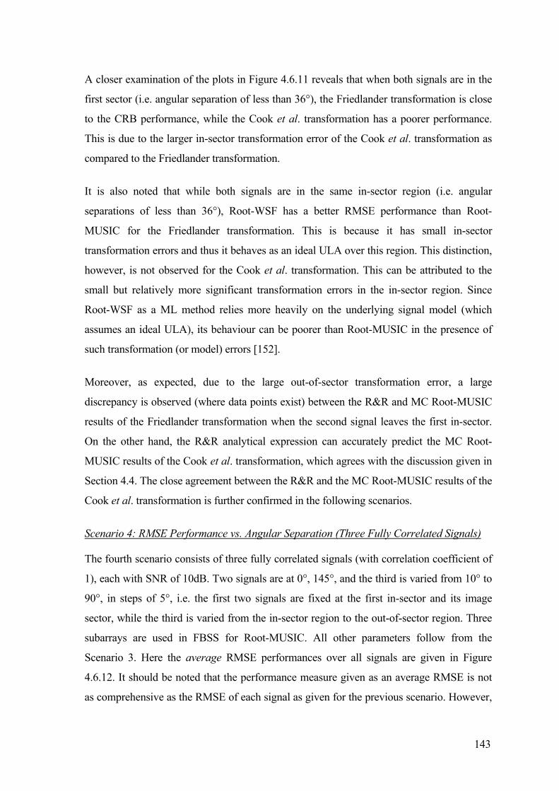
143

A closer examination of the plots in Figure 4.6.11 reveals that when both signals are in the

first sector (i.e. angular separation of less than 36∞), the Friedlander transformation is close

to the CRB performance, while the Cook et al. transformation has a poorer performance.

This is due to the larger in-sector transformation error of the Cook et al. transformation as

compared to the Friedlander transformation.

It is also noted that while both signals are in the same in-sector region (i.e. angular

separations of less than 36∞), Root-WSF has a better RMSE performance than Root-

MUSIC for the Friedlander transformation. This is because it has small in-sector

transformation errors and thus it behaves as an ideal ULA over this region. This distinction,

however, is not observed for the Cook et al. transformation. This can be attributed to the

small but relatively more significant transformation errors in the in-sector region. Since

Root-WSF as a ML method relies more heavily on the underlying signal model (which

assumes an ideal ULA), its behaviour can be poorer than Root-MUSIC in the presence of

such transformation (or model) errors [152].

Moreover, as expected, due to the large out-of-sector transformation error, a large

discrepancy is observed (where data points exist) between the R&R and MC Root-MUSIC

results of the Friedlander transformation when the second signal leaves the first in-sector.

On the other hand, the R&R analytical expression can accurately predict the MC Root-

MUSIC results of the Cook et al. transformation, which agrees with the discussion given in

Section 4.4. The close agreement between the R&R and the MC Root-MUSIC results of the

Cook et al. transformation is further confirmed in the following scenarios.

Scenario 4: RMSE Performance vs. Angular Separation (Three Fully Correlated Signals)

The fourth scenario consists of three fully correlated signals (with correlation coefficient of

1), each with SNR of 10dB. Two signals are at 0∞, 145∞, and the third is varied from 10∞ to

90∞, in steps of 5∞, i.e. the first two signals are fixed at the first in-sector and its image

sector, while the third is varied from the in-sector region to the out-of-sector region. Three

subarrays are used in FBSS for Root-MUSIC. All other parameters follow from the

Scenario 3. Here the average RMSE performances over all signals are given in Figure

4.6.12. It should be noted that the performance measure given as an average RMSE is not

as comprehensive as the RMSE of each signal as given for the previous scenario. However,

144

it is sufficient for the purpose of comparing between the Friedlander and Cook et al.

transformations. Presenting the RMSE separately for each signal is cumbersome for

scenarios with many signals. It is a common practice to show the RMSE of some signals

when all signals have similar RMSE characteristics. However, here the RMSE behaviour of

different signals can differ significantly.

While similar characteristics as in Scenario 3 (see Figure 4.6.11) are observed for Root-

MUSIC with the Cook et al. transformation, Root-WSF appears to experience significant

performance degradation with the introduction of the third signal in the image sector.

Interestingly, this degradation occurs only for correlated signals.

10 20 40 60 800

20

40

60

80

100

120

140

Friedlander transformation

Angular position of third signal (°)

Ave

rage

RM

SE

(°)


10 20 40 60 80

0

5

10

15

20

25

Cook et al. transformation


Ave

rage

RM

SE

(°)


Figure 4.6.12. Average RMSE performances vs. angular position of the third signal.

Case of three fully correlated signals.

As it turns out, for the Cook et al. transformation, the severe performance degradation in

Root-WSF results from occasional outliers in the estimates. This is different to the

Friedlander transformation where the poor performance in Root-MUSIC and Root-WSF in

the presence of out-of-sector signals in Figure 4.6.12 is mostly due to consistently large

estimation errors. To quantify the quality of the estimates, a Monte Carlo trial that has an

average DOA estimation error of over 10∞ is taken as a failure. Using this definition, Figure

4.6.13 plots the percentage of failures for the different estimators and the interpolated array

transformations of Friedlander and Cook et al. There was no failure for Root-MUSIC with

the Cook et al. transformation and is thus omitted from the plot.

145

10 20 40 60 800

20

40

60

80

100


Per

cent

age

of fa

ilure

s (%

)

Root−MUSIC(Friedlander)Root−WSF(Friedlander)Root−WSF(Cook et al.)

Figure 4.6.13. Failures as a percentage of 200 Monte Carlo trials.

To show that the removal of failures will drastically improve the performance of Root-WSF

for the Cook et al. transformation but not for the Friedlander transformation, Figure 4.6.14

repeats the plots of Figure 4.6.12, except with the failure points removed. It can be seen in

Figure 4.6.14 that the removal of 100% failures take away many of the data points of Root-

MUSIC for the Friedlander transformation, as it gives inherently wrong estimates for these

points (i.e. they are not outliers). Even though Root-WSF for the Friedlander transformation

has improved without the failures, the Cook et al. transformation clearly outperforms it by a

significant margin.

10 20 40 60 800

1

2

3

4

5Friedlander approach


Ave

rage

RM

SE

(°)


10 20 40 60 800

1

2

3

4

5Cook et al. transformation


Ave

rage

RM

SE

(°)



Case of three fully correlated signals.

146

It is clear from the above scenarios that the Friedlander transformation can give very good

performance (approach the CRB) when all signals are in the in-sector region and/or are

uncorrelated. The Cook et al. transformation, on the other hand, gives a better overall

performance under the different correlated signal environments examined. Therefore, it

appears that the Cook et al. paradigm is far more reliable in practice, especially when the

locations of signals are not estimated a priori and there is no guarantee that signals are

contained within moderate in-sector sizes (to give a small transformation error). Thus, the

Friedlander transformation will not be taken any further.

Moreover, some authors, e.g. Stoica and Sharman [137], also discount occasional outliers in

the DOA estimates in their numerical study in order to compare the performance among

different algorithms. However, for practical purposes, all DOA estimates should be taken

into account in the statistics to give a fair assessment of the DOA estimation algorithms.

Therefore, in view of the inconsistency of Root-WSF with the Cook et al. transformation,

Root-MUSIC appears to be the preferred choice of DOA estimator in correlated signal

environments.

10 20 40 60 800

0.2

0.4

0.6

0.8

1Friedlander transformation


Ave

rage

RM

SE

(°)


10 20 40 60 800

0.2

0.4

0.6

0.8

1Cook et al. transformation


Ave

rage

RM

SE

(°)



Case of three uncorrelated signals.

Scenario 5: RMSE Performance vs. Angular Separation (Three Uncorrelated Signals)

The RMSE performances of Scenario 4 but for three uncorrelated signals are shown in

Figure 4.6.15. Unlike Scenario 4, the RMSE results of both the Friedlander and Cook et al.

transformations do not suffer from any failures. However, it is noted that the Friedlander

transformation degrades significantly in performance in the in-sector region in the presence

147

of an uncorrelated signal at 145∞. In Figure 4.6.15, a large discrepancy is again observed

between the R&R and MC Root-MUSIC results for the Friedlander transformation, while

good agreement is obtained for the Cook et al. transformation.

Scenario 6: RMSE Performance vs. SNR

As mentioned in Scenario 4, Root-MUSIC appears to be the preferred DOA estimator in

correlated signal environments. Therefore, only the performance of Root-MUSIC will be

examined further in Scenarios 6 to 9.

The sixth scenario (see Figure 4.6.16) examines the RMSE performances of Root-MUSIC

with respect to different SNR’s. There are three fully correlated signals (with correlation

coefficient of 1) fixed at 0∞, 45∞, and 145∞, corresponding to one signal each in the in-

sector, transition region and the image sector of the first in-sector. All other simulation

parameters follow from the second scenario, except that the SNR’s of all signals are

simultaneously varied from 0dB to 20dB, in steps of 2dB.

Scenario 7: RMSE Performance vs. Number of Snapshots

The seventh scenario (see Figure 4.6.16) examines the finite data performance of Root-

MUSIC. The parameters similar to Scenario 6, except that the SNR of each signal is fixed

at 10dB. The number of snapshots is varied between 50 and 10000 inclusive.

Scenario 8: RMSE Performance vs. Number of Subarrays

The eighth scenario (see Figure 4.6.16) repeats Scenario 7, except that the number of

subarrays is varied between three and eight inclusive, and that the number of snapshots is

fixed at 200.

Scenario 9: RMSE Performance vs. Correlation Coefficient

The ninth scenario (see Figure 4.6.16) investigates the effect of different correlation among

the three signals. The two signals at 45∞ and 145∞ are fully correlated. However, the

correlation coefficient between these two signals and that at 0∞ is varied between 0 and 1.

Three subarrays are used and all other parameters follow those of Scenario 8.

In Figure 4.6.16, it is observed that for all four scenarios (i.e. Scenarios 6 to 9), the R&R

and MC performances of Root-MUSIC are in good agreement, except for isolated cases.

148

For instance, the use of 8 subarrays presents some difficulties to Root-MUSIC to resolve

the three signals. The RMSE performances are, however, considerably poorer than the CRB

performances even under favourable conditions, e.g. high SNR’s. One reason for this is the

use of subarrays reduces the aperture size of the array. Moreover, the transformation error

also introduces significant biases in the DOA estimates. It is also noted that the RMSE

performance is almost the same when the number of subarray is between three and seven

inclusive, suggesting that it is reasonably robust to different degrees of smoothing.

0 5 10 15 200

0.05

0.1

0.15

0.2

0.25

SNR (dB)

Ave

rage

RM

SE

(°)

Root−MUSIC(MC)Root−MUSIC(R&R)CRB

50 102

103

104

0

0.05

0.1

0.15

0.2

0.25


Ave

rage

RM

SE

(°)


3 4 5 6 7 80

0.5

1

1.5

2

2.5

3

Number of subarrays

Ave

rage

RM

SE

(°)


0 0.2 0.4 0.6 0.8 10

0.05

0.1

0.15

0.2

0.25

ρ

Ave

rage

RM

SE

(°)


Figure 4.6.16. Average RMSE performances for Root-MUSIC with the Cook et al.

transformation vs. SNR, number of snapshots, number of subarrays, and correlation

coefficient.

Scenario 10: Effect of In-Sector Transformation Error on Bias in DOA Estimation

The final example investigates the biases in DOA estimates which result from in-sector

transformation error. As noted in Section 2.5.2, the in-sector transformation error of the

149

Friedlander transformation is very small in both Figure 2.5.3 and Figure 2.5.6, which

applied the pseudo-inverse threshold sth of 510- and 115.6 10-¥ , respectively. Nonetheless,

Figure 2.5.6 has much smaller errors than Figure 2.5.3. Here two uncorrelated signals are

used to demonstrate that the effect transformation errors have on the estimation bias. An in-

sector size of 90∞ was used. One signal was at 0∞ and the second was varied from 5∞ to 30∞

in steps of at 5∞, and each signal had a SNR of 10dB. Both Root-MUSIC (with no spatial

smoothing) and Root-WSF were used to perform DOA estimation. Figure 4.6.17 shows the

estimation bias for Root-MUSIC and Root-WSF for sth = 510- and 115.6 10-¥ .

5 10 15 20 25 300

1

2

3

4

5

6

7

x 10−3 Signal at 0°, σ

th=5.6×10−11


Bia

s (°

)

Root−MUSICRoot−WSF

5 10 15 20 25 300

0.5

1

1.5

2

2.5

3

3.5

x 10−5 Signal at 0°, σ

th=10−5


Bia

s (°

)

Root−MUSICRoot−WSF

Figure 4.6.17. Bias errors in DOA estimates of signal at 5∞ using exact covariance

matrix for two uncorrelated signals at 5∞ and 10∞.

It is observed in Figure 4.6.17 that though the biases for both Root-MUSIC and Root-WSF

are much smaller for the case 5th 10s -= relatively to those of 115.6 10-¥ , both are

insignificant in absolute terms for practical purposes. Therefore, in such cases, it is perhaps

more important to opt for a well-behaved out-of-sector power response of the virtual ULA

to minimise the influence of out-of-sector signals. For instance, it appears that for this case, 5

th 10s -= is preferable since the out-of-sector power response of Figure 2.5.2 has worse

distortions than that of Figure 2.5.5.

150

4.7 Numerical Examples for Non-Ideal UCA’s

For the non-ideal UCA’s considered in this following sections, the gain and phase

responses and the location of each antenna element are perturbed, and mutual coupling

between the antenna elements is introduced. In the simulation studies, each realisation of

the perturbations is drawn from standard normal distributions with zero means, and the

perturbations are assumed constant over the number of finite snapshots K used to estimate

the covariance matrix. A different realisation is used for each Monte Carlos trial. The

standard deviation for both the real and imaginary parts of gain perturbations is 0.05

(relative to 1); for both x- and y-axes element position perturbation, 0.01l; and for both the

real and imaginary parts of mutual coupling, 0.01 (relative to 1). Mutual coupling is

assumed to be significant only for adjacent UCA elements. While the array perturbations

introduced here are fairly small, the point is made that the proposed procedure is able to

introduce robustness to the Davies and Cook et al. transformations which would otherwise

fail at even such small perturbations of the array parameters.


In this section, it will be demonstrated that (i) DOA estimators can suffer a great loss in

performance, even to the extent of failing, when a non-ideal UCA has the robustness

problem due to a large norm in TDav; (ii) the robustification procedure described in Chapter

3 can effectively mitigate the loss of performance in these estimators; and (iii) when the

norm in TDav is very large, then a simple alternative to the robustification procedure is to

use the trivial solutions.

To this end, the following scenarios for MUSIC with spatial smoothing with three fully

correlated signals are considered:

• The matrix TDav has a large norm (Scenario 1)

• The robustification procedure is applied onto the non-robust rows of TDav (Scenario

2).

• The non-robust rows in TDav are replaced with the trivial solutions (Scenario 3).

In the case of Root-MUSIC and Root-WSF, it will be established that (i) both estimators

can give good RMSE performances with the Davies array of a non-ideal UCA when TDav

151

does not have a large norm; (ii) severe degradation in performance will occur for these two

estimators due to a large norm in TDav. Indeed, the DOA estimators can even fail

completely. Furthermore, (iii) the robustification procedure introduced in Chapter 3 can

mitigate the above loss of performance and (iv) the SIP formulation will be shown to

outperform the CLS formulation in DOA estimation. Specifically, for scenarios of three

fully correlated signals, the average RMSE performances of Root-MUSIC with spatial

smoothing and Root-WSF are investigated and compared with respect to:

• angular separation without a large norm in TDav (Scenario 4),

• angular separation with a large norm in TDav (Scenario 5)

• angular separation for robust matrices (Scenario 6),

• SNR for robust matrices (Scenario 7),

• number of snapshots for robust matrices (Scenario 8),

• correlation coefficient for robust matrices (Scenario 9), and

• number of subarrays for robust matrices (Scenario 10).

The robust matrices for Scenarios 6 to 10 are obtained for the TDav with large norm of

Scenario 5 using the robustification procedure of the SIP and CLS formulations.

For the numerical examples of Sections 4.6 and 4.7.1, the RMSE performances of Root-

WSF with the norm constraint (4.3.18) have been found to be roughly similar, though

slightly poorer in general [64], to that with the conjugate symmetry constraint (4.3.17). In

this section, the norm constraint will be used exclusively since it is found that the conjugate

symmetry constraint can be unreliable in the presence of large transformation errors

introduced by the SIP robustification procedure. To ensure a fair assessment, for Scenario 5

where a large norm in the transformation matrix lead to the failure of Root-WSF with the

norm constraint to resolve the signals, the corresponding results are also obtained for the

conjugate symmetry constraint. It is found that Root-WSF with the conjugate symmetry

constraint also fails in this scenario.

152

Scenario 1: Robustness Problem of Large Norm in TDav

Consider a UCA with N = 15, d = 0.34l, M = 13, and FBSS [86] with five subarrays, each

of nine elements. In the signal scenario, there are three fully correlated signals (with

correlation coefficient of 1), each with SNR of 10 dB, arriving from -40°, 0°, and 55°. The

exact covariance matrix is used.

Figure 4.7.1 shows the MUSIC spectrum for the UCA with no array perturbations (ideal

UCA), and also that for five realisations of array perturbations on the UCA (non-ideal

UCA’s). Each of the five realisations is obtained under a different perturbation of the array

parameters. Recall from Section 3.5.1, the TDav of this UCA has a very large norm.

−150 −100 −50 0 50 100 150

0

10

20

30

40

50

60

70

80

PM

US

IC (

θ )

(dB

)


Ideal UCANon−ideal UCA’s

Figure 4.7.1. MUSIC spectra of an ideal and non-ideal UCA’s.

Scenario 2: Robustification Procedure for Robustness Problem

Following from Scenario 1, the corresponding MUSIC spectra obtained from the robust

transformation matrix given in Table 3.1 are shown in Figure 4.7.2.

It is clear from Figure 4.7.1 that while MUSIC with FBSS gives good performance with an

ideal UCA, the MUSIC spectra of the non-ideal UCA’s are unacceptable. On the other

hand, MUSIC with FBSS can correctly resolve all signals with the robust transformation,

albeit with some small biases in the estimates. The biases are primarily due to the increased

153

transformation error (or fixed modelling error) in the steering vector of the Davies array

which is necessary to obtain robustness (e.g. see Table 3.1 and Table 3.2).

−150 −100 −50 0 50 100 150−5

0

5

10

15

20

25

30

PM

US

IC (

θ )

(dB

)



Figure 4.7.2. MUSIC spectra of an ideal and non-ideal UCA’s with the robust

transformation matrix found by the SIP formulation.

Scenario 3: Trivial Solutions for Robustness Problem

As an alternative to using the robustification procedure as in Scenario 2, in this scenario, we

use the trivial solutions (setting the elements in these rows of large norms to zeros). The

trivial solution was suggested in [75] to synthesise Dolph-Chebyshev beampatterns with the

Davies transformation.

Figure 4.7.3 gives the corresponding MUSIC spectra when rows 5 and 9 of the robust

transformation matrix in Scenario 2 are replaced with zero rows. As can be seen, MUSIC

with FBSS can also correctly resolve all signals for this alternative robust transformation

matrix, although the estimates exhibit larger biases than those in Figure 4.7.2. Nonetheless,

as is confirmed by other numerical examples, the trivial solutions cannot be used in general,

especially when there is more than one pair of rows with large norms. This is because DOA

estimators can only tolerate to a certain extent the large transformation errors (of magnitude

1) in the Davies array, which are introduced by the trivial solutions, before they fail to work

completely.

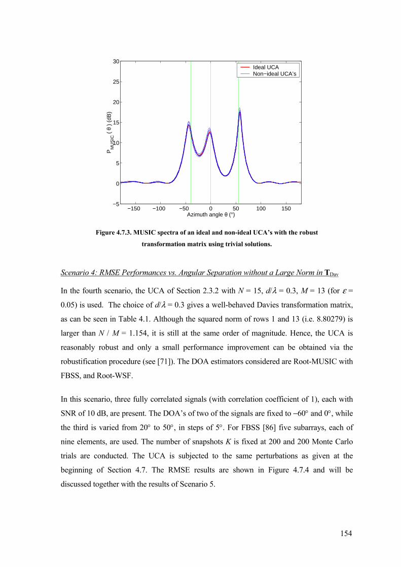
154

−150 −100 −50 0 50 100 150−5

0

5

10

15

20

25

30

PM

US

IC (

θ )

(dB

)




transformation matrix using trivial solutions.

Scenario 4: RMSE Performances vs. Angular Separation without a Large Norm in TDav

In the fourth scenario, the UCA of Section 2.3.2 with N = 15, d/l = 0.3, M = 13 (for e =

0.05) is used. The choice of d/l = 0.3 gives a well-behaved Davies transformation matrix,

as can be seen in Table 4.1. Although the squared norm of rows 1 and 13 (i.e. 8.80279) is

larger than N / M = 1.154, it is still at the same order of magnitude. Hence, the UCA is

reasonably robust and only a small performance improvement can be obtained via the

robustification procedure (see [71]). The DOA estimators considered are Root-MUSIC with

FBSS, and Root-WSF.

In this scenario, three fully correlated signals (with correlation coefficient of 1), each with

SNR of 10 dB, are present. The DOA’s of two of the signals are fixed to -60° and 0°, while

the third is varied from 20° to 50°, in steps of 5°. For FBSS [86] five subarrays, each of

nine elements, are used. The number of snapshots K is fixed at 200 and 200 Monte Carlo

trials are conducted. The UCA is subjected to the same perturbations as given at the

beginning of Section 4.7. The RMSE results are shown in Figure 4.7.4 and will be

discussed together with the results of Scenario 5.

155

Davies Matrix


1, 13 8.80279 2.95268

2, 12 1.68193 0.30749

3, 11 0.53753 0.03732

4, 10 0.37360 0.00608

5, 9 1.55657 0.00223

6, 8 1.15926 0.00033

7 0.68155 0.00008

Table 4.1. Characteristics of the Davies transformation matrices for N = 15, M = 13

and d =0.3l.

Scenario 5: RMSE Performances vs. Angular Separation with a Large Norm in TDav

Scenario 4 is repeated for d/l = 0.34 and the results shown in Figure 4.7.4. As observed in

Table 3.1, the squared norm for rows 5 and 9 of the new TDav is very large, i.e. 168062.188.

25 30 35 40 45 500

0.5

1

1.5

2

2.5

3


Ave

rage

RM

SE

(°)

d/λ=0.3

Root−MUSIC idealRoot−WSF idealRoot−MUSIC non−idealRoot−WSF non−ideal

25 30 35 40 45 50 55 600

10

20

30

40

50

60

70

80d/λ=0.34


Ave

rage

RM

SE

(°)

Root−MUSIC idealRoot−WSF idealRoot−MUSIC non−idealRoot−WSF non−ideal

Figure 4.7.4. Average RMSE performances of DOA estimation algorithms on the

Davies array vs. angular position of the third signal, for two different d/l’s.

It should be clear from Figure 4.7.4 (d/l = 0.3) that the introduction of array perturbations

significantly degrades the RMSE performances of both DOA estimators in Scenario 4.

Nonetheless, for both the ideal and non-ideal UCA’s, all three signals are successfully

resolved. On the other hand, the RMSE performances of Scenario 5 (see Figure 4.7.4 (d/l =

156

0.34)) reveal that the large norm problem can cause both Root-MUSIC and Root-WSF to

fail, regardless of whether array perturbations exist. The reason why the DOA estimation

fails with the ideal UCA is because the number of snapshots (200) used to estimate the

array covariance matrix xR is insufficient. As mentioned in Chapter 3, finite sample effect

introduces an error relative to the exact covariance matrix and this error is amplified by the

large row norm in TDav. In fact, it can be verified that when the exact covariance matrix is

used, the bias error of both Root-MUSIC and Root-WSF for the ideal UCA is very small –

in the order of 0.01∞ and 0.001∞, respectively.

Scenario 6: RMSE Performances vs. Angular Separation for Robust Matrices

Scenario 5 is repeated using the robust transformation matrix shown in Table 3.1. Recall

that the SIP formulation was used. To facilitate a comparison, the robust matrix with the

same squared norm (2.0868) for rows 5 and 9 is obtained from the CLS formulation of

Cook [132]. Robust matrices are also obtained from both formulations for a squared norm

of 19.462 (for rows 5 and 9) and the RMSE performances are calculated. The results for

both squared row norms are shown in Figure 4.7.5.

In Figure 4.7.5, it is clear that the robustification procedure is able to significantly improve

the RMSE performances of the DOA estimators. For Root-MUSIC with FBSS and Root-

WSF, both the SIP and CLS formulations are able to give an average RMSE of less than 5∞

when the angular position of the third signal is greater than 35∞. However, overall, the

RMSE performances of the SIP formulation are observed to be superior to those of the CLS

formulation. Moreover, Root-WSF is able to consistently outperform Root-MUSIC with

FBSS. Even though Root-WSF as a ML method is expected to perform better than Root-

MUSIC with FBSS for ideal arrays, this is not true in general with non-ideal arrays

[151],[152]. One possible explanation for Root-WSF giving a better performance is that the

smoothing process of FBSS for Root-MUSIC spreads the large transformation errors (see

Table 3.1) in the two Davies array elements (corresponding to rows 5 and 9 in TDav) to

other array elements. In contrast, no smoothing is performed on Root-WSF, and the large

transformation errors are confined to only two array elements.

Another observation is that Root-MUSIC gives an overall improvement in RMSE

performance at the smaller squared row norm of 2.0868. However, Root-WSF SIP appears

to give a better performance at in the range 25∞ to 35∞ for the smaller norm, while for the

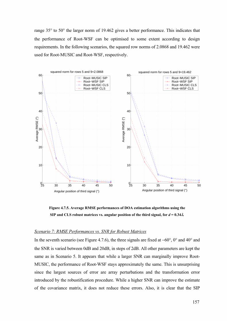
157

range 35∞ to 50∞ the larger norm of 19.462 gives a better performance. This indicates that

the performance of Root-WSF can be optimised to some extent according to design

requirements. In the following scenarios, the squared row norms of 2.0868 and 19.462 were

used for Root-MUSIC and Root-WSF, respectively.

25 30 35 40 45 500

10

20

30

40

50

60


Ave

rage

RM

SE

(°)

squared norm for rows 5 and 9=2.0868

Root−MUSIC SIPRoot−WSF SIPRoot−MUSIC CLSRoot−WSF CLS

25 30 35 40 45 500

10

20

30

40

50

60squared norm for rows 5 and 9=19.462


Ave

rage

RM

SE

(°)


Figure 4.7.5. Average RMSE performances of DOA estimation algorithms using the

SIP and CLS robust matrices vs. angular position of the third signal, for d = 0.34l.

Scenario 7: RMSE Performances vs. SNR for Robust Matrices

In the seventh scenario (see Figure 4.7.6), the three signals are fixed at -60∞, 0∞ and 40∞ and

the SNR is varied between 0dB and 20dB, in steps of 2dB. All other parameters are kept the

same as in Scenario 5. It appears that while a larger SNR can marginally improve Root-

MUSIC, the performance of Root-WSF stays approximately the same. This is unsurprising

since the largest sources of error are array perturbations and the transformation error

introduced by the robustification procedure. While a higher SNR can improve the estimate

of the covariance matrix, it does not reduce these errors. Also, it is clear that the SIP

158

formulation is significantly better than the CLS formulation for Root-MUSIC, while it is

only marginally better than CLS for Root-WSF.

0 5 10 15 200.5

1

1.5

2

2.5

SNR (dB)

Ave

rage

RM

SE

(°)


102

103

104

0

0.5

1

1.5

2

2.5

3


Ave

rage

RM

SE

(°)


0 0.2 0.4 0.6 0.8 10

0.5

1

1.5

2

2.5

|ρ|

Ave

rage

RM

SE

(°)


3 4 5 6 7 8 9 100

5

10

15

20

Number of subarrays

Ave

rage

RM

SE

(°)


Figure 4.7.6. Average RMSE performances of DOA estimation algorithms using the

SIP and CLS robust matrices vs. SNR, number of snapshots, correlation coefficient,

and number of subarrays.

Scenario 8: RMSE Performances vs. Number of Snapshots for Robust Matrices

The eighth scenario shown in Figure 4.7.6 follows from Scenario 7, except that the SNR’s

are fixed at 10dB, and the number of snapshots is varied from 50 to 10000. As in the case

of varying SNR’s, an increase in the number of snapshots does not have a significant

impact on the RMSE performance for the same underlying reason that the model errors are

fixed for a given Monte Carlo trial.

159

Scenario 9: RMSE Performances vs. Correlation Coefficient for Robust Matrices

The ninth scenario shown in Figure 4.7.6 sets the two signals at 0∞ and 40∞ to be fully

correlated (with correlation coefficient of 1), while the third signal at -60∞ has a different

correlation coefficient r with the pair of fully correlated signals where r Œ [0, 1] and r is

varied in steps of 0.1. All other parameters are kept the same as in Scenario 5. Here the

impact of correlation is clearly seen in Root-WSF where the performance degrades with an

increase in correlation. This can also be observed to some extent in Root-MUSIC SIP,

while Root-MUSIC CLS does not demonstrate such a trend.

Scenario 10: RMSE Performances vs. Number of Subarrays for Robust Matrices

Finally, the effect of changing the number of subarrays M on the performance of Root-

MUSIC is investigated for M set between three and ten (maximum possible M for

resolving 3 signals) inclusive. The three signals are fully correlated with a correlation

coefficient of 1. All other parameters are kept the same as in Scenario 5. The results are also

given in Figure 4.7.6. Here, the advantage of SIP over CLS is particularly apparent when ˆ 3M = . In general, both the performance of the SIP and CLS formulations are roughly

constant over the range between three and nine subarrays inclusive, which suggests that the

robust matrix is not very sensitive to the use of different numbers of subarrays. Moreover,

the reduction in array aperture due to the use of more subarrays can be offset by the benefit

of the spatial smoothing technique providing a greater reduction in error in the steering

vector of the Davies array [121]. The performances of Root-WSF are roughly constant

since it always operates on the full Davies array. It is only shown here as a reference for the

RMSE performances of Root-MUSIC.

Scenarios 5 to 10 above with d/l = 0.34 involve a pair of rows of very large norms. Thus,

the robustification procedure can mean the difference between failure and success in DOA

estimation. However, in a general situation when the row norms are of moderate values, the

performance improvement will not be as dramatic. Moreover, since the sacrifice in

transformation error can worsen the performance of DOA estimation with respect to certain

parameters such as signal separation, careful consideration is necessary when applying the

robustification procedure to obtain an overall improvement in performance (e.g. RMSE)

with respect to all parameters (or at least, to those of interest). As such, the rough guide for

the target row norms as described in Chapter 3, while instructive of the imperfection noise

160

amplification, is insufficient. Instead, an ad hoc trial and error procedure that checks the

performance (of DOA estimation) over a range of row norms is more appropriate to

optimise the robustness design.

The following section utilises MUSIC to illustrate the robustness problem due to large row

norms in the Cook et al. transformation and the successful use of the robustification

procedure to mitigate the lack of robustness.


In Section 3.2.2, it was shown that the Bronez and Cook et al. transformations can be non-

robust due to a large norm in the transformation, as in the Davies transformation, for some

combinations of array parameters N and d/l. In contrast, the Friedlander transformation

does not have the same robustness problem. However, in Section 4.6.2, it was found that

the Bronez and Friedlander transformations can cause Root-MUSIC with spatial smoothing

and Root-WSF to perform poorly in correlated signal scenario. Therefore, in this section,

the focus is on the Cook et al. transformation only.

Here, it will be demonstrated that (i) the loss of performance (or failure) in some DOA

estimators when a non-ideal UCA has the robustness problem due to a large norm in TIA;

(ii) the robustification procedure described in Chapter 3 can effectively mitigate the loss of

performance in these estimators.

To this end, the following scenarios for MUSIC with spatial smoothing with three fully

correlated signals are considered:

• The matrix TIA has a large norm (Scenario 1).

• The robustification procedure is applied on non-robust rows of TIA (Scenario 2).

In Section 3.5.2, it was shown that the large norm problem in the Cook et al. transformation

involves more pairs of rows of the transformation matrix compared to the Davies

transformation in Section 3.5.1. In addition, the squared norms for these pairs of rows are

generally smaller than those of the Davies transformation. The robustification procedure

can thus involve a smaller sacrifice in the transformation error in order to achieve

acceptable row norms. On the other hand, there are now more pairs of rows with larger

transformation errors. One consequence is that the trivial solution is ineffective since it

161

would require setting many pairs of rows to zero. This strategy will lead to very poor DOA

estimation performance for both Root-MUSIC and Root-WSF. Therefore, the

robustification procedure (with SIP or CLS formulations) is crucial for the Cook et al.

transformation.

A similar study of RMSE performances as in the previous section can be carried out for the

Cook et al. transformation. However, it should be clear from Scenarios 1 and 2 below that,

similar to the previous section, the robustification procedure is effective in improving the

performance of DOA algorithms in the presence of array imperfections and robustness

problem. Thus, the study of RMSE performance with Root-MUSIC and Root-WSF is

omitted.

Scenario 1: Robustness Problem of Large Norm in TIA

Consider a UCA, N = 30, d = 0.37l and M = 13. As can be seen in Table 3.3, the resulting

transformation matrix has large norms for four pairs of rows. The signal scenario consists

of three fully correlated signals (with correlation coefficient of 1), each with SNR of 10 dB,

and arriving from -170°, 30°, and 55°. Five subarrays, each of nine elements, are used in

FBSS. Since the finite data effect is not of interest here, exact covariance matrices are used.

Figure 4.7.7 shows the MUSIC spectrum for the UCA with no array perturbations (ideal

UCA), and also that for three realisations of array perturbations on the UCA (non-ideal

UCA’s). The perturbations include gain and phase errors, position errors and mutual

coupling, as given at the beginning of Section 4.7. Clearly, the MUSIC spectra of the non-

ideal UCA’s perform poorly.

Scenario 2: Robustification Procedure for Robustness Problem

Figure 4.7.8 demonstrates the effect of using the robust transformation matrix (with the

characteristics given in Table 3.3) on the non-ideal UCA’s of Scenario 1. As can be seen,

the robustification procedure greatly reduces the variability of the MUSIC spectra and

enables the DOA to be more accurately resolved. However, since the robustification

procedure involves a sacrifice in the transformation error in the virtual ULA, biases are

introduced into the DOA estimates. Note that the bias for the signal at -170° is particularly

obvious.

162

−200 −150 −100 −50 0 50 100 150 200

0

10

20

30

40

50

60

PM

US

IC (

θ )

(dB

)


Ideal UCANon−ideal UCA 1Non−ideal UCA 2Non−ideal UCA 3

Figure 4.7.7. MUSIC spectra of an ideal and non-ideal UCA’s.

−200 −150 −100 −50 0 50 100 150 200−5

0

5

10

15

20

25

30

PM

US

IC (

θ )

(dB

)


Ideal UCANon−ideal UCA 1Non−ideal UCA 2Non−ideal UCA 3


transformation matrix found by the SIP formulation.

163

4.8 Conclusions

This chapter presents a proof of concept for the application of the two classes of UCA

preprocessing techniques in DOA estimation. With the Davies transformation, it is clear

that the use of Root-WSF can be advantageous over MUSIC or Root-MUSIC with spatial

smoothing, especially in correlated signal environment. In the interpolated array

transformations, MUSIC or Root-MUSIC with spatial smoothing appears to have a better

overall performance than Root-WSF.

Although the focus of this chapter is on the use of the Davies and Cook et al.

transformations with MUSIC or Root-MUSIC with spatial smoothing and Root-WSF for

DOA estimation, it is clear that other DOA estimation techniques that exploits the

Vandermonde form such as ESPRIT [113],[114] (with or without spatial smoothing) can be

similarly applied to the Davies array and the virtual ULA, respectively.

The chapter also highlights the importance of an appropriate approach to the design of

interpolated arrays for a given application. While the Friedlander transformation is efficient

for specific circumstances or applications in which all signals are confined to a given sector

of up to 180∞43, its performance can degrade significantly when signals cannot be confined

to such a sector for the virtual ULA. This is because out-of-sector signals, both uncorrelated

and correlated with the in-sector signals, can interfere with DOA estimation of the in-sector

signals. Moreover, the single sector processing philosophy also runs contrary to the original

intention for the interpolated array transformations [58],[59] which circumvents the need to

perform prior (coarse) estimation.

The Cook et al. transformation, on the other hand, has a poorer performance than the

Friedlander transformation when all signals are confined to one in-sector. However, for

Root-MUSIC, it remains effective for a general environment where signals appear over the

entire azimuth. This also indicates that the Cook et al. transformation, unlike the

Friedlander transformation, does not require coarse DOA estimation to perform DOA

estimation reliably.

43 Typically a much smaller sector of up to 60∞ is used in the literatures to ensure acceptable transformation error and loss

of resolution towards endfire. [122] is perhaps the only reference where a 120∞-sector is used for the Friedlander transformation.

164

The robustification procedure outlined in Chapter 3 has also been shown to be effective in

mitigating the performance degradation of DOA estimation in the presence of array

imperfections and large norms in the Davies and Cook et al. transformation matrices for

UCA with omnidirectional elements. This is achieved with some sacrifice in the

Vandermonde approximation, which leads to biases in the DOA estimates. However, such a

sacrifice can result in a significant loss in performance with respect to the CRB for a non-

ideal UCA (e.g. [153]). Therefore, where feasible, it is prudent to avoid the robustness

problem through a proper design of the array parameters. Furthermore, as mentioned in

Chapter 3, the robustness problem can also be circumvented by the use of directional

elements or the use of additional elements in the UCA. Nevertheless, the choice of array

parameters and types are often restricted by practical considerations such as hardware cost

and the size and shape44 of the platform where the array is to be mounted [60],[122].

44 In the case of Cook et al. transformation, the original array can be an arbitrary planar array.

165

Chapter 5 Beampattern Synthesis 5.1 Introduction

The first application of the Davies transformation is in beamforming [51]. This is not

surprising since beamforming has traditionally been the focus of interest in the array signal

processing community.

While the beamforming techniques given in this and the next chapters may be used for

DOA estimation in correlated signal environment, it is well known that the high-resolution

DOA estimation techniques described in the previous chapter give superior performance

particularly for closely spaced signal sources [35]. However, beamforming finds important

application in spatially selective reception and transmission of signals. And in cases where

the performance is a lesser consideration than hardware and computationally cost, it may be

still be an attractive option for DOA estimation as well. This chapter focuses on the

application of the aforesaid UCA preprocessing techniques in beampattern synthesis [72],

while the next chapter examines their use in optimum beamforming [73].

In conventional beamforming, the steering vector (involving only phase shifts) of the look

direction forms the array weights. It is well-known for ULA, that the characteristics of the

conventional (or Bartlett) beampattern can be modified by using fixed amplitude tapers (or

shadings) on top of the phase shifts [89].

A popular approach to forming amplitude tapers is the Dolph-Chebyshev beampattern

synthesis technique, which gives a beampattern whose mainlobe is as narrow as possible

for a given guaranteed maximum sidelobe level [84],[154]. The Dolph-Chebyshev

technique has thus far been of interest to ULA’s only due to its requirement that the array

steering vector has a Vandermonde form [72]. Dolph-Chebyshev shading can have very

important implications in circular arrays where sidelobe levels are intrinsically higher than

for ULA’s [155].

5.1.1 Davies transformation

In this chapter, the Davies transformation is employed to facilitate the synthesis of minimax

patterns on UCA’s with the Dolph-Chebyshev technique [72]. This is possible since the

steering vector of the Davies array is Vandermonde, similar to that of a ULA. Since the

166

proposed approach is based on the Dolph-Chebyshev technique, it only requires linear

phase rotations of the steering vector to effect beam scanning. The linear phase rotations

can be implemented efficiently using a look up table or a CORDIC processor [160].

Currently, there are numerous other techniques available to produce the minimax response

on a UCA, including Jacobsen and Madsen [156], Olen and Compton [157], Tseng and

Griffith [158], and Zhou and Ingram [159]. Many of these techniques are quite general,

iterative45, and can be applied to arbitrary arrays with directional elements and unequal

characteristics. However, in contrast to the proposed Dolph-Chebyshev technique for

UCA’s, the array weights of the UCA as obtained from these techniques apply only for a

given look direction and need to be recalculated for another look direction. In the special

case of a N-element UCA, one can take advantage of both the reflection and the rotational

symmetries of the array to rotate the beampattern by up to 2N discrete steps by associating

the same array weights with different array outputs in each of these steps. Nevertheless,

even when the array weights are adapted in this manner, a continuous scan of the

beampattern is still not possible unless a look-up table containing many sets of array

weights corresponding to a grid of look directions in a 180∞/N angular sector is used. The

size of the table46 can be large for small N, apart from the additional complexity involved in

choosing and rearranging the correct set of weights for a given look direction. Moreover, an

interpolation procedure may also be needed to find the array weights for a look direction

that falls between the grid of look directions.

Specifically, the Tseng-Griffiths technique [158] will be used for comparison with the

proposed Dolph-Chebyshev technique for UCA’s, as it appears to be the most (or one of the

most) promising of recent methods in performance and computational complexity. It is

iterative and involves the solution of a sequence of linearly constrained least squares

problems. The underlying idea is to use constraints to control the sidelobe peaks at each

iteration to achieve a desired beampattern.

Summarising, the advantages of the Dolph-Chebyshev synthesis approach proposed in this

thesis are as follows: 45 This is only an issue if the techniques are used online. For offline calculations, a look-up table is used for online

operations and thus the size of the table (i.e. number of entries and quantisation level) is more important. 46 The larger the look-up table, the greater is the storage requirement.

167

1. No complex calculations or large look-up tables are necessary for different look

directions once the design weights are found. This translates to computational

savings when compared to other techniques such as that of Tseng and Griffiths

[158].

2. The new approach maintains the same beampattern for all look directions of the

mainlobe, demonstrating a rotational invariance property. This property will be

explained more explicitly in Section 5.3.2.

3. The Tseng-Griffiths approach [158] breaks down in cases where the constraint

matrices and/or the interference signal covariance matrices are ill conditioned (see

[158]). Even though remedial procedures are available, they require human

interventions. In contrast, the proposed approach does not suffer from these

problems.

4. While the synthesis of Dolph-Chebyshev beampatterns is originally applied to an

ideal ULA with omnidirectional element, the use of the Davies transformation

allows model errors (in calibration data) and directional element patterns to be

readily absorbed into the transformation so that they do not appear in the Davies

array [52],[54]. Consequently, the synthesis technique can be applied to non-ideal

UCA’s with directional elements.

5. The data at the Davies array outputs can be used for other applications, such as

direction finding of coherent signals with UCA’s as given in the previous chapter.

This suggests the sharing of computational load.

Recall that the Davies transformation is limited by the accuracy of the approximation

involved in the Davies array. This may necessitate some compromises in terms of the size

of the Davies array and thus may not yield the narrowest possible main lobe for a given

maximum sidelobe level.


In view of the distortion in the out-of-sector virtual ULA response (see Chapter 2), it is

unsurprising that, unlike the Davies transformation, thus far it has not been possible to use

the interpolated array transformations of Bronez [58] and Friedlander [59] for beampattern

168

synthesis. The Cook et al. paradigm [74], on the other hand, is not restricted in the same

manner due to the well-behaved (or controlled) out-of-sector response. Therefore, it is

possible to consider the Cook et al. transformation as a means to facilitating the synthesis of

beampatterns that have desirable characteristics, such as the aforementioned Dolph-

Chebyshev beampattern, on an arbitrary planar array. In fact, the advantages of using the

Cook et al. transformation for Dolph-Chebyshev beampattern synthesis follow those for the

Davies transformation, except that the virtual ULA requires sector by sector processing and

the nature of the steering vector means that, like a ULA, the mainlobe broadens and the

beampattern changes as the look direction moves away from the broadside of the virtual

ULA.

As shown in Chapter 3, the issue of robustness against model errors is important for both

the Davies transformation and the Cook et al. transformation. In particular, model errors are

amplified by the large norm of the transformation matrix at resonance. Numerical examples

will be presented to demonstrate the degradation in the Dolph-Chebyshev beampattern at

resonance and the effectiveness of the robustification procedure to mitigate this problem.

While the discussion on beampattern synthesis in this chapter is confined to Dolph-

Chebyshev beampatterns for UCA’s through two preprocessing techniques, it is easy to

show that these two techniques can be used to synthesise other ULA-based beampatterns.

Two such techniques are the Taylor beampattern synthesis [161],[162] and Butler

beamforming [163].

5.2 Beamforming with Preprocessing Techniques

In Chapter 4, the two classes of preprocessing techniques: the Davies transformation and

the interpolated array transformations are used in DOA estimation. As such, it only

involves the reception of signals. On the other hand, the beamforming applications

described in this and the next chapters entail both reception and transmission of signals.

The block diagrams for the beamformer structures for reception and transmission are given

in Figure 5.2.1 and Figure 5.2.2, respectively. Though instructive, the transformation

networks in Figure 5.2.1 and Figure 5.2.2 are not required in practice. This is explained as

follows. First, the beampattern of the array is given by

( ) 2H qw Ta , [ ],q p pŒ - , (5.2.1)

169

where [ ]1, , TMw w=w … is the array weight vector applied to the steering vector of the

Davies array (or virtual ULA) to get a look direction of lq .

. . .

w1

wM

+

¥

¥

Virtual array

yM

. . .

y1

T. . .

x 2 x 1

x N Real array

Figure 5.2.1. Linear transformation of a UCA for reception beamforming.

w 1

w M

¥

¥

Virtual array

y M

. . .

y 1

TH . . .

x2

x1

xN

Real array

s(t) . . .

Figure 5.2.2. Linear transformation of a UCA for transmission beamforming.

w1

wN

¥

¥

. . .

x2

x1

xN

s(t)¥

w2

Transmission Reception

w 1

w N

¥

¥ ¥

w 2

. . .

x 2 x 1

x N

. . . + . . .

Figure 5.2.3. Simplified block diagram for reception and transmission beamforming.

170

Thus

( ) ( ) ( ) ( )HH H Hq q q= =w Ta T w a w a , (5.2.2)

where [ ]1, , TNw w=w … is the equivalent array weight vector for the outputs of the UCA,

as shown in Figure 5.2.3.

5.3 Beampattern Synthesis with Davies Transformation

As mentioned, the focus of this chapter is on Dolph-Chebyshev beampattern synthesis. The

following introduces the Dolph-Chebyshev formulation as applied to the Davies arrays

[72].

5.3.1 Dolph-Chebyshev Formulation

Consider the output signals of the Davies array y1, …, yM, as shown in Figure 5.2.1. To

steer the look direction of the array to lq , one method is to set the weight vector of the

Davies array to the form

( )lw Db q= , (5.3.1)

where D is a diagonal matrix that specifies the shading to be applied to the array pattern.

Thus, the key design task is to find the matrix D.

Suppose D has the form

( )1 0 1diag , , , 2 , , ,o oM MI I I I I- -=D … … . (5.3.2)

The array response is given by

( ) ( ) ( )0

1 12

o ol l

M Mjm jmH

m mm m

I I e I eq q q qq - - --

= == + +Â Âw b . (5.3.3)

Hence, if the elements of D have mirror symmetry, i.e. m mI I- = , then

( ) ( )0

2 cos 2oM

Hm

mI muq q

=È ˘= Î ˚Âw b , (5.3.4)

171

where

( ) ( ) 2lu q q q= - . (5.3.5)

Now, ( )cos 2mu qÈ ˘Î ˚ can be written as a polynomial in ( )x q , as follows [84]

( ) ( )2 22

0cos 2

mm mq

qmu b xq q

=È ˘ =Î ˚ Â , (5.3.6)

where ( ) ( )cosx uq qÈ ˘= Î ˚ , (5.3.7)

and ( )22

21

2

mm qm

qs m q

s mb

s m q s-

= -

Ê ˆ Ê ˆ= - Á ˜ Á ˜- +Ë ¯ Ë ¯Â . (5.3.8)

Thus, substituting (5.3.6) into (5.3.4)

( ) ( )2 22

02

o oM MH m q

m qq m q

I b xq q= =

= Â Âw b . (5.3.9)

Equation (5.3.9) may be expressed as a Chebyshev polynomial with parameter β where β is

the ratio of the main lobe level to the sidelobe level of the Dolph-Chebyshev pattern. A

Chebyshev polynomial of degree 2Mo in z with all its roots in the range 1 1z- £ £ has the

following form

( ) 2 22 2

0

oo

o

MM q

M qq

T z b z=

= Â . (5.3.10)

Accordingly, defining

( )0 0 0,z z x z z zq= - £ £ , (5.3.11)

where z0 is defined by ( )2 0 1oMT z b= > and 0 0z > , we obtain, after substituting (5.3.11)

into (5.3.10) and then equating the resulting polynomial in ( )x q with (5.3.9)

172

2222 2 02

oo

MqMm

m q mm q

I b b z=

=Â . (5.3.12)

The coefficients Im’s (of matrix D) can now be found from (5.3.12) using one of the many

methods described in, for example, [84],[154],[164]. Note that as opposed to the iterative

procedure of [158], analytical expressions are available for Im’s.

Finally, it follows from (5.3.9) to (5.3.12) that

( ) ( )2 0oH

MT z xq qÈ ˘= Î ˚w b , (5.3.13)

and the beampattern is given by

( ) ( ) ( ) ( )2 2 22 0o

H Hl MT z xq q q qÈ ˘= = Î ˚w b b D b . (5.3.14)

Note that (5.3.14) has the same form as the Dolph-Chebyshev beampattern of a ULA

involving polynomials.

5.3.2 Rotational Invariance of the Dolph-Chebyshev Beampattern

Next, it is shown that as a result of the linear dependence of u(θ ) on lq in (5.3.5), the half

power main lobe width as defined in [84] is independent of lq .

The maximum amplitude of the main lobe is given by

( ) ( )12 0 0cosh 2 cosh

oM oT z M zb -È ˘= = Î ˚ (5.3.15)

or ( )10

1cosh cosh2 o

zM

b-È ˘= Í ˙

Î ˚. (5.3.16)

At the half power points,

( ) ( )12 1 1

1cosh cosh 222oM

oT z z

Mb b-È ˘

= fi = Í ˙Î ˚

. (5.3.17)

Now,

1 0 1cosz z u= (5.3.18)

173

and ( ) ( )1 1 1 2lu u q q q= = - . (5.3.19)

Thus

1 11

0cos l

zz

q q-= ± + . (5.3.20)

Denoting 1 1,a bq q as the half power points, it follows that the half power main lobe width is

given by

1 11 1

02 cosa b z

zq q -- = (5.3.21)

which does not depend on lq .

It is easy to extend the above result to show that the array pattern over the entire azimuth

also remains the same (albeit by a shift of lq and wrapping by 2π) regard-less of lq . This is

not surprising since the approximation involved in the modal transformation requires N >>

kr [54]. This translates to the need of having “enough” UCA elements so that the behaviour

between the elements closely approximates that of a continuous aperture circular array.

Finally, it is remarked that, even though the spatial response of a ULA is also

Vandermonde, its main lobe width and the array pattern change with different look

directions. This is because, for a ULA,

( ) ( )sin sinldu pq q ql

= - (5.3.22)

which is non-linear in lq [154].

5.3.3 Implementation Considerations

As pointed out in Chapter 3, model errors are amplified by the large norms in the

transformation matrix of a UCA with omnidirectional elements. While DOA estimation

with subspace methods in Chapter 4 uses prewhitening to deal with the problem of

amplified noise covariance matrix in the Davies array or virtual ULA (i.e. 2 HnTTs for

white noise), the same cannot be done for beampattern synthesis. This means that on top of

the amplified model errors, the amplified noise will also degrade the SNR performance of

174

the beamformer. In the case of reception or transmission of signals, the beamformer will

receive or transmit the desired signal together with a large amount of noise. Therefore,

careful considerations are required to ensure the row norms of the transformation matrix are

kept small. This is unlike the case in Chapter 4 where the trade off between robustness and

transformation does not have this restriction.

5.3.4 Numerical Examples for Ideal UCA’s

Consider the UCA in the design example of Section 2.3.2 where N = 15 and d/λ = 0.3. A

criterion of e = 0.05 gives M = 13. The peak sidelobe attenuation β is set to 40dB (i.e. 40 / 2010 100= ) and Stegen’s formula [154] is used to calculate the array weights. Figure

5.3.1 compares the beampattern obtained using the proposed Dolph-Chebyshev-Davies

technique against that obtained using the Tseng-Griffiths technique [158]. The look

direction lq is 55°. It is clear that the mainlobe of the proposed technique is slightly wider

than that of Tseng and Griffiths. This indicates the proposed technique is suboptimal but as

a compromise, it allows the mainlobe to be steered easily. It is also noted that the array

weight vector resulting from the Tseng-Griffiths technique typically has a larger squared

norm compared to the proposed technique. Since the squared norm of the weight vector

indicates noise gain, this means that the Tseng-Griffiths technique has a larger noise gain.

A larger N can reduce, however, the difference in the mainlobe widths as obtained by the

two techniques. This is shown in Figure 5.3.2 for N = 35 and d/λ = 0.3 (M = 33 with e =

0.05). The reduction in the difference between the two mainlobe widths can be understood

in terms of the smaller relative difference between N and M. Since the Tseng-Griffiths

technique is optimised with respect to the actual UCA, the UCA aperture places a limit on

the mainlobe width. Thus the smaller relative difference means that the Davies array

aperture is relatively “closer” to the aperture of the UCA for a larger N. In both cases, a

small d/λ of 0.3 allows the number of Davies array elements to be close to that of the UCA.

Next, the rotational invariance property of the beampatterns of the proposed technique is

illustrated. For N = 15, M = 13, and d/l = 0.3, Figure 5.3.3 shows the beampattern for four

different look directions. The angular positions of the UCA elements are superimposed on

the plot to demonstrate that the different look directions are not chosen with respect to the

symmetry in the element positions. Specifically, they are positioned at lq = 0°, 31.2° (1.3 ¥

175

360°/N), -108° (10.5 ¥ 360°/N), -52.8° (12.8 ¥ 360°/N). It is clear that these beampatterns

only differ from one another by a rotation. In each of the above examples, the Tseng-

Griffiths technique achieved convergence within 5 iterations.

−200 −150 −100 −50 0 50 100 150 200−70

−60

−50

−40

−30

−20

−10

0

Gai

n (d

B)


ProposedTseng−Griffiths

Figure 5.3.1. Dolph-Chebyshev beampatterns for N = 15, M = 13, and d/l = 0.3.

−200 −150 −100 −50 0 50 100 150 200−70

−60

−50

−40

−30

−20

−10

0

Gai

n (d

B)



Figure 5.3.2. Dolph-Chebyshev beampatterns for N = 35, M = 33, and d/l = 0.3.

176

In the final example, consider again the UCA with N = 35 but with d/λ increased to 0.6,

resulting in more peaks than those that can be directly controlled by the Tseng-Griffiths

technique [158]. As a result, the performance of the iterative Tseng-Griffiths technique

[158] and resulting beampattern is look-direction dependent and took much longer to

compute than the case of d/λ = 0.3. Also occasionally, human interventions are required to

deal with numerical difficulties. In this example, the ratio of maximum to minimum

diagonal values of R in the QR decomposition of the constraint matrix in [158] is set to

1000. For the Davies transformation, a good approximation in the Davies array necessitates

a significant reduction in the number of Davies array elements. The criterion e = 0.05 gives

M = 17.

−200 −100 0 100 200−70

−60

−50

−40

−30

−20

−10

0

Gai

n (d

B)

Azimuth angle θ (°)−200 −100 0 100 200

−70

−60

−50

−40

−30

−20

−10

0G

ain

(dB

)


−200 −100 0 100 200−70

−60

−50

−40

−30

−20

−10

0

Gai

n (d

B)

Azimuth angle θ (°)−200 −100 0 100 200

−70

−60

−50

−40

−30

−20

−10

0

Gai

n (d

B)


Figure 5.3.3. Dolph-Chebyshev beampatterns for look directions q l = 0°, 31.2°,

-108°, -52.8°. UCA element positions marked by ( ∑ ), N = 15, M = 13 and d/l = 0.3.

177

−200 −100 0 100 200−70

−60

−50

−40

−30

−20

−10

0G

ain

(dB

)



−200 −100 0 100 200−70

−60

−50

−40

−30

−20

−10

0

Gai

n (d

B)



−200 −100 0 100 200−70

−60

−50

−40

−30

−20

−10

0

Gai

n (d

B)



−200 −100 0 100 200−70

−60

−50

−40

−30

−20

−10

0

Gai

n (d

B)



Figure 5.3.4. Dolph-Chebyshev beampatterns for look directions q l = 30°, 108°,

-125°, -80°. UCA with N = 35, M = 33, and d/l = 0.6.

Figure 5.3.4 compares the beampatterns obtained from the proposed method against that

from the Tseng-Griffiths technique [158] for lq = 30°, 108°, -125°, -70°, and Table 5.1

summarises some characteristics of the solution from the two techniques. As can be seen,

the squared norm of the proposed technique is independent of look direction, as is clear

from (5.3.1). Also, as expected, the large reduction in the number of virtual elements (from

33 to 17) and thus the Davies array aperture of the proposed technique leads to a larger

mainlobe width. However, it may be surprising to observe that the mainlobe width for the

Tseng and Griffith technique also suffers a similar degradation. This reveals that both

methods are fundamentally limited by similar mechanisms. Specifically, the choice of d/λ =

0.6 means that the spatial sampling condition [108] is not satisfied for adjacent pairs of

UCA elements, which results in a smaller effective aperture for the UCA.

178

Tseng and Griffiths Proposed

q l Squared norm of

weight vector

Number of iterations

required

Squared norm of

weight vector

30° 2.64394 194 0.07686

108° 2.12498 84 0.07686

-125° 2.13090 81 0.07686

-80° 2.35992 27 0.07686

Table 5.1. Characteristics of the Tseng-Griffiths technique for the case of Figure 5.3.4.

5.3.5 Numerical Examples for Non-Ideal UCA’s

In this section, the impact of the robustness problem and the robustification procedure on

Dolph-Chebyshev beampatterns is demonstrated. Figure 5.3.5 shows the resultant Dolph-

Chebyshev beampatterns obtained from an ideal UCA and 10 perturbed UCA’s with N =

30, d = 0.4l, and a Davies array with M = 27. The mainlobe to sidelobe level is set to

-30dB and lq = 30°. The perturbed UCA’s are subject to perturbations in the gain and

phase responses of the antenna elements and their locations. Mutual coupling between the

antenna elements is also introduced. Ten realisations of the perturbations are drawn from

standard normal distributions with zero means.

As in Section 4.7, the standard deviation for both the real and imaginary parts of gain

perturbation is 0.05 (relative to 1); for both x- and y-axes element position perturbation,

0.01l; and for both the real and imaginary parts of mutual coupling, 0.01 (relative to 1).

Mutual coupling is assumed to be significant only for adjacent UCA elements. The same

above example is repeated for the Tseng-Griffiths technique. The resultant beampatterns are

shown in Figure 5.3.6. It is observed from both figures that there is some degradation in the

beampatterns of the perturbed UCA’s and that the amount of degradation appears to be

similar in these two cases.

In the numerical examples of Section 3.5.1, it was shown that one incident where the

Davies transformation is non-robust occurs when N = 30, M = 27, and d = 0.37l. Table 3.2

clearly shows large norms in the rows of the transformation matrix, i.e. 645.3 for rows 7

and 21 and 201.7 for rows 10 and 18. Figure 5.3.7 shows the resulting Dolph-Chebyshev

beampatterns obtained from an ideal UCA and 10 perturbed UCA’s for these parameters.

179

Clearly, the beampatterns of the perturbed UCA’s suffer severe distortion. The example is

then repeated for the Tseng-Griffiths technique. The resulting beampatterns are shown in

Figure 5.3.8. Interestingly, the beampatterns obtained by the Tseng-Griffiths technique also

appears to degrade significantly with array perturbations, indicating that likewise, it too is

limited by the resonance of the UCA [108].

−150 −100 −50 0 50 100 150−50

−45

−40

−35

−30

−25

−20

−15

−10

−5

0

5


Gai

n (d

B)

Ideal UCAPerturbed UCA’s

Figure 5.3.5. Dolph-Chebyshev beampatterns (b = 30dB) of an ideal and 10

perturbed UCA’s for the proposed technique. N = 30, d = 0.4l, and M = 27.

Next, the Davies transformation is replaced by the robust transformation matrix found by

the SIP formulation (with characteristics described in Table 3.2). The beampatterns

obtained using the robust transformation are shown in Figure 5.3.9. It is clear that

improvement is obtained in that the beampatterns of the perturbed UCA’s have lower

sidelobe levels and smaller variances in the mainlobe peaks from the desired look direction.

On the other hand, by sacrificing the transformation error for robustness, the beampattern of

the ideal UCA degrades considerably.

As suggested in [75], a simple approach to deal with very large row norms is to solve these

rows trivially, i.e. setting all elements in the rows to zeros. This approach appears to work

reasonably well in beampattern synthesis (e.g. for the case of N = 15, d = 0.34l, and M = 13

in Table 3.1) and one can bypass the robustification procedure. For the above example, the

180

row norms of rows 7, 10, 18, and 21 are also large (though much smaller than rows 5 and 9

for the case of Table 3.1). Consequently the solutions from the SIP formulation shown in

Figure 5.3.9 are only a slight improvement over the trivial solutions.

−150 −100 −50 0 50 100 150−50

−45

−40

−35

−30

−25

−20

−15

−10

−5

0

5


Gai

n (d

B)



perturbed UCA’s for the Tseng-Griffiths technique. N = 30, d = 0.4l, and M = 27.

−150 −100 −50 0 50 100 150−50

−45

−40

−35

−30

−25

−20

−15

−10

−5

0

5


Gai

n (d

B)



perturbed UCA’s for the proposed technique with N = 30, d = 0.37l, and M = 27.

181

−150 −100 −50 0 50 100 150−50

−45

−40

−35

−30

−25

−20

−15

−10

−5

0

5


Gai

n (d

B)



perturbed UCA’s for the Tseng-Griffiths technique. N = 30, d = 0.37l, and M = 27.

−150 −100 −50 0 50 100 150−50

−45

−40

−35

−30

−25

−20

−15

−10

−5

0

5


Gai

n (d

B)



perturbed UCA’s obtained by performing the robustification procedure on the

proposed technique. N = 30, d = 0.37l, and M = 27.

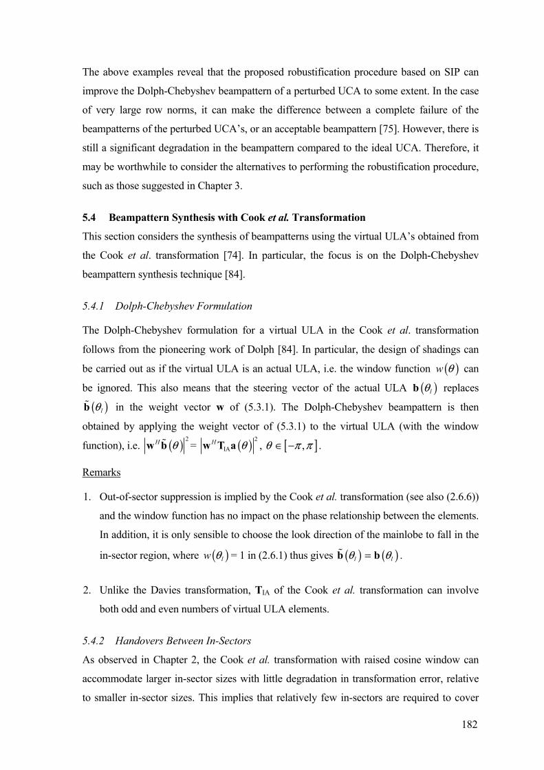
182

The above examples reveal that the proposed robustification procedure based on SIP can

improve the Dolph-Chebyshev beampattern of a perturbed UCA to some extent. In the case

of very large row norms, it can make the difference between a complete failure of the

beampatterns of the perturbed UCA’s, or an acceptable beampattern [75]. However, there is

still a significant degradation in the beampattern compared to the ideal UCA. Therefore, it

may be worthwhile to consider the alternatives to performing the robustification procedure,

such as those suggested in Chapter 3.

5.4 Beampattern Synthesis with Cook et al. Transformation

This section considers the synthesis of beampatterns using the virtual ULA’s obtained from

the Cook et al. transformation [74]. In particular, the focus is on the Dolph-Chebyshev

beampattern synthesis technique [84].

5.4.1 Dolph-Chebyshev Formulation

The Dolph-Chebyshev formulation for a virtual ULA in the Cook et al. transformation

follows from the pioneering work of Dolph [84]. In particular, the design of shadings can

be carried out as if the virtual ULA is an actual ULA, i.e. the window function ( )w q can

be ignored. This also means that the steering vector of the actual ULA ( )lqb replaces

( )lb q in the weight vector w of (5.3.1). The Dolph-Chebyshev beampattern is then

obtained by applying the weight vector of (5.3.1) to the virtual ULA (with the window

function), i.e. ( ) 2H qw b = ( ) 2IA

H qw T a , [ ],q p pŒ - .

Remarks

1. Out-of-sector suppression is implied by the Cook et al. transformation (see also (2.6.6))

and the window function has no impact on the phase relationship between the elements.

In addition, it is only sensible to choose the look direction of the mainlobe to fall in the

in-sector region, where ( )lw q = 1 in (2.6.1) thus gives ( ) ( )l lq q=b b .

2. Unlike the Davies transformation, TIA of the Cook et al. transformation can involve

both odd and even numbers of virtual ULA elements.

5.4.2 Handovers Between In-Sectors

As observed in Chapter 2, the Cook et al. transformation with raised cosine window can

accommodate larger in-sector sizes with little degradation in transformation error, relative

to smaller in-sector sizes. This implies that relatively few in-sectors are required to cover

183

the entire azimuth. As mentioned earlier, beampattern synthesis can be used for DOA

estimation and spatially sensitive reception and transmission of signals.

In contrast to the high-resolution DOA estimation techniques of Chapter 4, conventional

beamforming has a mainlobe with significant width. Therefore, it is important to ensure that

the choice of the operational sector is such that the beampattern suffers no significant

distortion for a continuously scanning operation over the full azimuth. This implies the need

for overlapping operational sectors where their overlapped region allows for a smooth

handover of the beampattern (especially the mainlobe) from one operational sector to an

adjacent one. Consequently, the overlap should not be smaller than the width of the

mainlobe. In the case of Dolph-Chebyshev beampattern, the width of the mainlobe can be

taken to be the width of the mainlobe at the sidelobe level. Figure 5.4.1 illustrates the

concept of handover of beampatterns between adjacent in-sectors.

∑ ∑ ∑ ∑ ∑ ∑

ql

(r + 1)th operational sector

rth operational sector

Handover point

Overlapped region

TIA(r)

TIA (r+1)

Azimuth angle q

Angular movement of beampattern

Gain (dB)

Figure 5.4.1. Overlapping of operational sectors and the handover of the mainlobe

between adjacent operational sectors in beampattern synthesis for the Cook et al.

transformation.

184

5.4.3 Numerical Examples for Ideal UCA’s

In the following examples, the focus is to demonstrate the synthesis of Dolph-Chebyshev

beampatterns with the Cook et al. transformation.

First, consider a UCA with N = 30, d/l = 0.4, a virtual ULA with ra = 1, M = 13, and b = 1.510 31.6ª (30dB). From the earlier discussion, it is clear that the mainlobe width at the

handover point (see Figure 5.4.1) should be considered in the selection of the in-sector size

Dq. The Dolph-Chebyshev beampattern of an actual ULA with the same element positions

as the virtual ULA can be used to get an indication of the mainlobe width at the sidelobe

level. Unlike the Davies array, the width of the mainlobe of the proposed technique

broadens in look directions away from broadside, as is characteristic of the Dolph-

Chebyshev technique on a ULA (see Section 5.3.2).

As pointed out in Chapter 2, the number of in-sectors chosen should correspond to a factor

of N = 30 (i.e. 2, 3, 5, 6, 10, 15) to allow for the same transformation matrix TIA to be used

for different sectors (except for a rotation of elements within the rows of TIA). It can be

shown that the mainlobe width at lq = 36∞ (for use with 5 in-sectors) is about 54∞, and at

lq = 60∞ (use with 3 in-sectors) is about 67∞. To limit the width of the mainlobe, the case of

5 in-sectors is used, each with the operational sector size Dqo = 360∞/5 + 54∞ = 126∞.

Similarly, for b = 1.510 3.16ª (10dB), it can shown that the width at lq = 36∞ is about

21.5∞. Thus, Dqo = 360∞/5 + 21.5∞ = 93.5∞. The raised cosine window is chosen for the

virtual ULA, since it gives more or less a uniform transformation error over the

optimisation sector region (see Figure 2.6.3), which means that the optimisation and

operational sector sizes (Dq and Dqo, respectively) can be set as equal.

In Figure 5.4.2, Dolph-Chebyshev beampatterns with b = 30dB with Dq = 126∞ (q Œ [-63∞,

63∞]) and b = 10dB with Dq = 93.5∞ (q Œ [-46.75∞, 46.75∞]), and the conventional

beampattern are shown for lq = 15∞. Note that the Dolph-Chebyshev beampattern for b =

10dB and the conventional beampattern have almost equal mainlobe width. As expected,

the first sidelobe of the Dolph beampattern is lower than that of the conventional

beampattern (by about 2dB). A typical minimax response is obtained over the in-sector

region, while the out-of-sector response is further suppressed due to the window function.

However, since the synthesised Dolph-Chebyshev beampattern on the virtual ULA does not

exhibit a minimax response over the entire azimuth, it may be technically incorrect to call

185

the beampattern “Dolph-Chebyshev”. Henceforth, the synthesis procedure for the virtual

ULA shall be known as the proposed technique. For the case of b = 30dB, it is clear that a

lower sidelobe level is obtained but at the cost of a wider mainlobe.

−150 −100 −50 0 50 100 150−70

−60

−50

−40

−30

−20

−10

0


Gai

n (d

B)

ConventionalDolph, β =10dBDolph, β =30dB

Figure 5.4.2. Dolph-Chebyshev beampatterns vs. conventional beampattern for q l =

15∞, N = 30, d/l = 0.4, M = 13, and raised cosine window.

It is clear that from Figure 5.4.2 that the window function has shaped the equiripple

sidelobes in the out-of-sector region, though the suppression in the image sector is bounded

by the transformation error. Nonetheless, as will be shown in the next section, practical

environment will introduce model errors. These will bring up the very low sidelobe levels

in the out-of-sector region and interestingly, give it a resulting “minimax-like response”.

A comparison between the proposed and the Tseng-Griffiths [158] techniques in Figure

5.4.3 reveals that the latter gives a narrower mainlobe. This results from the proposed

technique trading off the mainlobe width for scanning capability47 and a suppressed out-of-

sector response.

47 It is noted that the virtual ULA should be operated only within its operational sector. Also, within this sector, the

mainlobe of the virtual ULA will broaden as the look direction moves away from broadside. This is different from the Davies array where the mainlobe can be steered over the full azimuth with the shape of the beampattern kept the same.

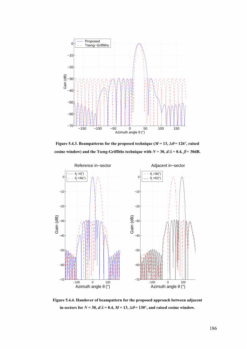
186

−150 −100 −50 0 50 100 150−70

−60

−50

−40

−30

−20

−10

0


Gai

n (d

B)


Figure 5.4.3. Beampatterns for the proposed technique (M = 13, Dq = 126∞, raised

cosine window) and the Tseng-Griffiths technique with N = 30, d/l = 0.4, b = 30dB.

−100 0 100−70

−60

−50

−40

−30

−20

−10

0

Reference in−sector


Ga

in (

dB

)

θl =0(°)

θl =36(°)

−100 0 100−70

−60

−50

−40

−30

−20

−10

0

Adjacent in−sector


Ga

in (

dB

)

θl =36(°)

θl =92(°)

Figure 5.4.4. Handover of beampattern for the proposed approach between adjacent

in-sectors for N = 30, d/l = 0.4, M = 13, Dq = 130∞, and raised cosine window.

187

The next example shows the mechanism of continuous scanning involving handovers from

one in-sector to an adjacent in-sector. Though the case of Dolph-Chebyshev beampattern

synthesis (with b = 30dB) is given, the handover procedure for virtual ULA is generic for

other ULA beampattern synthesis techniques. Figure 5.4.4 utilises two adjacent in-sectors

Dq1 and Dq2 defined by q Œ [-63∞, 63∞] and q Œ [9∞, 135∞], respectively. The beampatterns

for lq = 0∞, 36∞ of the reference in-sector Dq1, and those for lq = 36∞, 92∞ of the adjacent in-

sector Dq2 are shown. The handover point between the two adjacent in-sectors is lq = 36∞.

However, the beampatterns of the two sectors at lq = 36∞ do differ slightly.

5.4.4 Numerical Examples for Non-Ideal UCA’s

The implementation considerations of beampattern synthesis with the Cook et al.

transformation are similar to those of the Davies transformation given in Section 5.3.3. As

shown in Chapter 3, the robustification procedure devised originally for Davies

transformation [75] works equally well for the Cook et al. transformation at resonance.

First, the effect of model errors on the beampattern from the proposed technique is

demonstrated for a UCA with parameters48 N = 30, d/l = 0.4, M = 13, and Dq = 90∞. As can

be seen in Figure 3.2.4, these parameters (i.e. N and d/l) avoid the resonance condition and

thus the large norm problem as well. Figure 5.4.5 shows the resultant beampatterns for the

proposed technique when the UCA is subjected to ten realisations of the same model errors

(i.e. gain, phase, element position and mutual coupling) as those given in Section 5.3.5. The

beampattern for the proposed technique with the ideal UCA is also given for comparison.

Figure 5.4.5 shows a large overall degradation in the sidelobe suppression in the out-of-

sector region and a relatively smaller degradation in the in-sector region. However, the

difference in degradation is insignificant in practice. Interestingly, it appears that for UCA’s

with model errors, a form of “minimax-like response” is obtained in the beampatterns,

where the sidelobe peaks are confined to a narrower band than the case of the ideal UCA.

48 The example here with the in-sector size of Dq = 90∞ is used for demonstration purpose only. The exact Dq depends on

the scenario and design requirements. In the previous section, Dq was 93.5∞ and 126∞ for b = 10dB and 30dB, respectively. Furthermore, it should be clear from Chapter 3 that the robustness problem is fundamental for a given set of N, d/l, and other design parameters such as Dq has no influence on the positions of the large norm peaks.

188

−150 −100 −50 0 50 100 150−70

−60

−50

−40

−30

−20

−10

0


Gai

n (d

B)


Figure 5.4.5. Beampatterns of the proposed technique (M = 13, Dq = 90∞, raised

cosine window) an ideal and 10 perturbed UCA’s with N = 30, d/l = 0.4, and b =

30dB.

−150 −100 −50 0 50 100 150−70

−60

−50

−40

−30

−20

−10

0


Gai

n (d

B)




30dB.

189

Next, Figure 5.4.6 shows the respective beampatterns for the same example but with d/l =

0.37. The same perturbations as in the previous example are used. Note that as a result of

the large norm problem at d/l = 0.37, the beampatterns of the perturbed UCA’s experience

a much larger degradation than the previous example with d/l = 0.4.

Recall that the robustification procedure based on SIP formulation was applied on the same

UCA (with d/l = 0.37) and the corresponding virtual ULA in Section 3.5.2. Figure 5.4.7

shows the effect of the robust transformation matrix of Table 3.3 on the beampatterns of

both the ideal and the perturbed UCA’s. Again, the same perturbations as in the two

previous examples are used. As in the Davies transformation, the robustification procedure

causes significant degradation in the beampattern of the ideal UCA. However, the benefit of

the robustification procedure is clearly seen in the improved beampatterns of the perturbed

UCA’s, where the sidelobe peaks are generally lower than -15dB, as compared to those

around -10dB level in Figure 5.4.6. Furthermore, it is observed that the variance in the

positions of the mainlobe peak is smaller for the robust case.

−150 −100 −50 0 50 100 150−70

−60

−50

−40

−30

−20

−10

0


Gai

n (d

B)




30dB, using the robustification procedure.

190

In this case, although the row norms are large, they are nevertheless relatively small

compared to the cases shown in Table 3.1 and Table 3.2 for the Davies transformation.

Moreover, relatively many pairs of rows are involved. Therefore, one cannot make use of

the trivial solutions in the robustification procedure without suffering too much degradation

in the beampattern.

5.5 Conclusions

The use of Davies transformation in Dolph-Chebyshev beampattern synthesis of UCA has

distinct advantages over the existing method of [158]. Aside from its computational

efficiency when different look directions are desired (D is fixed, i.e. independent of lq ), it

represents a simple approach to designing minimax array patterns making use of the

Vandermonde structure and the Chebyshev polynomial. It is also shown that the

interpolated array transformation of Cook et al. [74] can be used to generate a Dolph

Chebyshev beampattern, although there are some restrictions due to the limited width of the

in-sector region.

One general observation is that clearly the robustness design does not work as well in

beampattern synthesis as it did with DOA estimation. The reason behind this can be

postulated in terms of degree of freedom. In beamforming, we are interested in constraining

the beam patterns to follow a particular behaviour, be it equiripple sidelobes, monotonically

decreasing sidelobe level, or pointing nulls at directions of interferers. In contrast, DOA

estimation only involves the estimation of a limited number of parameters (DOA of signal

sources). Therefore, the procedure is in itself more robust compared to beamforming.

191

Chapter 6 Optimum Beamforming 6.1 Introduction

In this chapter, the problem of designing beamformers for optimum signal reception for

UCA’s is considered. The classical approach to optimum beamformer49 design is to

minimise the beamformer output power subject to a constraint that enforces a fixed

response in the direction-of-arrival (DOA) of the desired signal (the look direction of the

beamformer) [126]. If none of the other received signals are correlated with the desired

signal, then, as expected, the optimum beamformer will exhibit the target response in the

look direction and nulls in the DOAs of the interfering signals. However, if one of the

interfering signals is highly correlated with the desired signal, such as that which may occur

in a multipath environment, the beamformer will make use of the correlated signal severely

attenuate the desired signal [5],[89].

Many approaches have been proposed to counteract the aforesaid signal cancellation

phenomenon [5],[88],[89],[165]. One general class is spatial smoothing [85],[87],[88]

which exploits the Vandermonde structure of the steering vector of a ULA to decorrelate

the correlated signals. Recall that spatial smoothing has been utilised in Chapter 4 to

perform DOA estimation in correlated signal environment.


As brought out in Chapter 2, optimum beamforming for wideband signals has been

demonstrated using the generalised Davies transformation that applies to planar (or 2D)

arrays of any arbitrary geometry [107]. This so-called array manifold interpolation (AMI)

method was used to perform optimum beamforming in the presence of correlated wideband

signals via frequency averaging. This chapter, though close in spirit to the work presented

in [107], is nevertheless distinct in that it considers narrowband signals and the averaging is

performed over a single Davies array. Derivative constraints [166],[167] are also introduced

to obtain robustness against directional mismatches. Furthermore, it is noted that the

conventional spatial smoothing technique only makes use of data from one subarray to

produce the array output. Here, a technique of averaging the beamformer outputs of the

subarrays [168] is utilised to lower the noise floor.

49 Numerous names have been given to this form of optimum beamformers that apply linear constraint(s) in the array

response, including Capon beamformers [35], adaptive beamformers [88],[173], and MVDR beamformers [35],[89].

192


As in beampattern synthesis of Chapter 5, the Cook et al. transformation can also be

applied in optimum beamforming. The advantage of this approach compared to performing

optimum beamforming on the actual planar array is that spatial smoothing may be applied

to the virtual ULA to deal with correlated signals. Also, the two techniques of derivative

constraints and subarray output averaging are also applicable to the virtual ULA. However,

as opposed to the Davies transformation, sector-by-sector processing is required for full

azimuth coverage in DOA estimation. However, if the DOA of the desired signal is known,

then only one in-sector containing the desired signal is sufficient for optimum reception and

transmission of signals.

This chapter only examines optimum beamforming in the context of an ideal UCA. Though

it would be interesting to analyse the performance of optimum beamforming on the Davies

array for a non-ideal UCA, and the corresponding robustness problem at resonance, it is

beyond the scope of this thesis. However, some remarks and comments relevant to such a

study will be made later in this chapter.

Although given in the context of the Davies transformation [73], the following development

applies equally to the Cook et al. transformation, apart from some obvious modifications

such as the need to perform sector-by-sector processing50. Also, the requirement of the

operational and optimisation sector sizes is similar to that discussed in Section 5.4.2, except

that the width of the mainlobe in optimum beamforming is generally far narrower than that

obtained from beampattern synthesis techniques that involve phase matching (e.g. the

Dolph-Chebyshev technique in Chapter 5).

6.2 Problem Statement

Let ( )1s t be the desired signal. If none of the other signals is correlated with ( )1s t , then

the optimum (or MVDR) beamformer for a UCA defined by the following problem

min Hx

ww R w subject to ( ) 1H

lq =w a , (P6.1)

50 This is only for DOA estimation in correlated signal environment. If the DOA is available, then only one in-sector

containing the desired signal is needed at any one time for the reception and transmission of the signal.

193

where lq is the look direction of the beamformer, will exhibit the expected characteristic of

unity gain in the desired signal direction if 1lq q= , and null in the other signal directions.

The solution to (P6.1) is given by

( ) ( ) ( ) 11 1opt = H

l l lq q q-- -È ˘

Î ˚x xw R a a R a . (6.2.1)

The beamformer as defined by (P6.1) shall be called the conventional optimum

beamformer.

The difficulty with the above design method is that if one of the interfering signals is highly

correlated with the desired (or look direction) signal, then the desired signal can be

cancelled [88]. A remedy is to perform spatial smoothing on xR but this requires the

steering vector to be in Vandermonde form which is not the case with UCA’s. In view of

our previous discussions, an obvious method to circumvent this is to use the Davies

transformation

The block diagram of the resulting beamformer will be very similar to that shown in Figure

5.2.1. The main difference between beampattern synthesis and optimum beamforming lies

in the calculation of the weights. While beampattern synthesis does not utilise the outputs

of the Davies array to form the weights, optimum beamforming make explicit use of them,

i.e. it is data dependent.

6.3 Spatial Smoothing

As pointed out in Chapter 4, spatial smoothing involves dividing the Davies array into a

number of equal size overlapping subarrays. The covariance matrix with a reduced

correlation in the signals is obtained by averaging the covariance matrices of the subarrays.

As long as the number of signals in the largest subgroup of highly correlated signals is not

more than 2 3M , the forward-backward procedure ensures that sR is well-conditioned

[85]. This means that the spatially smoothed sR has reduced signal correlations compared

to sR and optimum beamforming should now work [88],[169].

194

While spatial smoothing reduces the correlation of the signals, it does not reduce it to zero

in general51, especially when the number of subarrays and/or the angular separations

between correlated signals are small [165]. Therefore, different extents of magnitude

suppressions may be obtained (instead of deep nulls) in the optimum beampattern at the

DOA’s of the correlated interferers. The effectiveness of the optimum beamformer in

placing deep nulls at the DOA’s of correlated interferers has received significant attention

in the literature (see [5] and the references therein). One popular approach to address this

issue, e.g. Takao and Kikuma [165] and Reddy et al. [168], is by weighting the subarray

covariance matrix to approximate the resultant matrix in a Toeplitz form. However, in the

Davies array with non-equal diagonal values in the noise covariance matrix, the Toeplitz

form is not obtained even in the case of uncorrelated signals and thus this technique will not

work.

Summarising, the optimum beamformer for a UCA in a correlated signal environment is

found as follows

avmin Hw

w R w subject to ( ) 1Hlq =w b , (P6.2)

where vector w contains the first MS elements of w in Figure 5.2.1. Here vector ( )lqb

contains the first MS elements of the steering vector of the ideal Davies array ( )lqb 52. The

resulting optimal weight vector is given by

( ) ( ) ( ) 11 1opt av av= H

l l lq q q-- -È ˘

Î ˚w R b b R b . (6.3.1)

The beamformer as defined by (P6.2) shall be referred to as the spatially smoothed (SS)

optimum beamformer.

51 In DOA estimation, spatial smoothing is primarily used to restore the rank of the signal covariance and to reduce the

correlation amongst highly correlated signals. This is because high-resolution DOA estimation techniques such as MUSIC are able to perform sufficiently well at a reduced correlation, thus it is less important for these techniques to have zero or near-zero signal correlation as is with optimum beamforming.

52 For the Cook et al. transformation, the window function ( )lw q is omitted from the subarray steering vector ( )lqb (as with beampattern synthesis) to calculate the array weights and corresponding output power. This is because it is already implied in the transformed data embedded in avR and also the look direction lq is always in the operational sector where ( ) 1lw q = . Consequently, ( )lqb consists of the first MS elements of the steering vector of the ideal ULA ( )lqb .

195

Note that only one subarray of the Davies array is used in the SS optimum beamformer.

This suggests a compromise in the effective aperture of the beamformer when using this

approach to deal with highly correlated signals. Nevertheless, the subarray beamformer

output averaging technique, which will be described later, can make use of every output of

the Davies array to reduce the noise floor in the beamformer output.

Note also that for a signal ( )s t arriving from the look direction (assuming negligible noise

for now), the output of the Davies array is given by

( ) ( ) ( ) ( ) ( ) ( ) ( ) ( )Dav Dav l l lt t s t s t s tq q q= = = ªy T x T a b b . (6.3.2)

The output of the SS optimum beamformer (operating on one subarray) is given,

accordingly, by53

( ) ( ) ( )Hl s t s tq =w b , (6.3.3)

which follows from the look direction constraint in (P6.2). Thus, the beamformer is able to

receive the desired signal with no distortion, although strictly speaking there will be some

distortion due to the transformation error in the Davies array.

6.4 Derivative Constraints

In an uncorrelated signal environment, the conventional optimum beamformer is known to

be highly sensitive to mismatches between the beamformer's look direction lq and the

actual DOA of the desired signal 1q . In [167], it is shown that this sensitivity can be

reduced by appending derivative constraints to the optimisation problem (P6.1). For the SS

optimum beamformer, a similar problem is expected. Accordingly, derivative constraints

are derived for this beamformer.

Following [167], the derivative constraints are found by setting to zero the partial

derivatives (with respect to q ) of the power response of the Davies array, i.e.,

53 Here, and in the beampatterns expression ( ) [ ]2

, ,H q q p pŒ -w b , the subarray steering vector ( )qb is obtained via the linear transformation TDav or TIA. This steering vector is used because it reflects the actual (subarray) steering vector of the received signal.

196

( ) 20

l

nH

nq q

qq =

∂ =∂

w b , 1, 2,n = …. (6.4.1)

It can be shown, similarly to [167], that the first order ( 1n = ) derivative constraint is linear

in w where

{ } { }Re ImT TT È ˘= Î ˚w w w , (6.4.2)

whereas the higher order derivative constraints are quadratic in w . Therefore, only the first

order constraint is considered. The spatially smoothed robust (SSR) optimum beamformer is

defined, accordingly, by

min Hw

w Rw subject to ( )Tlq =C w f (P6.3)

where

{ } { }{ } { }

av av

av av

Re ImIm ReÈ ˘-

= Í ˙Î ˚

R RR

R R, (6.4.3)

( ) ( ) ( ) ( )1 2 3l l l lq q q qÈ ˘= Î ˚C c c c , (6.4.4)

[ ]1 0 0=f , (6.4.5)

( ) ( ){ } ( ){ }1 Re ImT TT

l l lq q qÈ ˘= Í ˙Î ˚c b b , (6.4.6)

( ) ( ){ } ( ){ }2 Im ReT TT

l l lq q qÈ ˘= -Í ˙Î ˚c b b , (6.4.7)

( ) ( ){ } ( ){ }3 Re ImT TT

l l lq qq q qÈ ˘= Í ˙Î ˚c b b , (6.4.8)

and where ( )lq qb is the first derivative of ( )qb with respect to q , evaluated at lq q= ,

( ) ( ) ( )11 o S lo lTj M MjM

l o o Sj M e M M e qqq q - - +-È ˘= - ◊ - +Í ˙Î ˚b . (6.4.9)

197

The solution to (P6.3) is given by

( ) ( ) ( )11 1

optT

l l lq q q-- -È ˘= Î ˚w R C C R C f . (6.4.10)

Note that if ( )lqC is not full rank, then the redundant constraint(s) will have to be located

and removed.

6.5 Weighted Averaging of Subarray Beamformer Outputs

The idea of averaging the subarray beamformer outputs was first proposed by Reddy et al.

[168] in the context of a ULA. Thus, it can be used directly on the virtual ULA of the Cook

et al. transformation. The following development continues from the previous section and

concerns the Davies array.

As noted, the design procedure so far uses only the first subarray of the Davies array to

obtain the array output. Likewise, the output can be obtained from any one of the other

subarrays. In particular, the steering vector of the qth subarray is given by

( ) ( ) ( )1 lj qq l l e qq q -=b b , q = 1, …, M , (6.5.1)

where ( )1 lj qe q- represents the phase of the qth subarray relative to the first subarray. It then

follows from (P6.2) that the optimum weight vector of the qth subarray is given by

( )1,opt optlj q

q e q-=w w , (6.5.2)

and the corresponding (subarray) beamformer output is given by

( )( )1opt( )q

lHj q

qz t e q-= w S y , (6.5.3)

where the selection matrix Sq was defined in (4.2.2).

Here it is noted that the beampatterns of the subarrays are identical, since from (6.5.1) and

(6.5.2)

( ) ( ),opt optH Hq q q q=w b w b . (6.5.4)

198

Hence, by averaging the subarray beamformer outputs, one can expect to reduce the noise

component in the array output

( ) ( )ˆ

1

1ˆ

M

qq

z t z tM =

= Â . (6.5.5)

As a refinement, observe that adjacent subarrays will have many antenna elements in

common. Their output noise will thus be highly correlated. The strategy in [168] is to

average the beamformer outputs of subarrays with non-overlapping elements. This strategy

is based on the assumption that the noise contributions from these subarrays are identical

and independent. However, this strategy is restrictive since typically a few overlapping

subarrays are sufficient to reduce the correlation among the signals. Alternatively, if non-

overlapping subarrays are required, then the subarrays will be smaller, leading to a smaller

subarray aperture. Smaller subarray apertures will lead to degradation in both the array

resolution and the noise floor of the beamformer. Moreover, no proof has been given to

substantiate the claimed in [168] that the use of non-overlapping subarrays is optimum.

This subarray beamformer structure (with derivative constraints) shall be subsequently

referred to as the spatially smoothed robust output averaged (SSROA) optimum

beamformer. Note that Reddy et al.’s original work does not include derivative constraints

but these constraints can be easily added, as in (P6.3).

Finally, it is noted that no additional computational cost is required to average the subarray

beamformer output as the averaging can be implemented by simply modifying the array

weights of the Davies array. Reddy et al. [168] did not appear to recognise this

simplification. Thus, for the beamformer of (6.5.5)

( )ˆ ˆ

1av ,opt opt

1 1

1 1ˆ ˆ

lM M

j qT Tq q q

q qe

M Mq-

= =

È ˘Í ˙= =Í ˙Î ˚

Â Âw S w S w , (6.5.6)

and the output of the beamformer is given by

( ) ( ) ( ) ( )av av Dav avH H Hz t t t t= = =w y w T x w x , (6.5.7)

where av Dav avH=w T w .

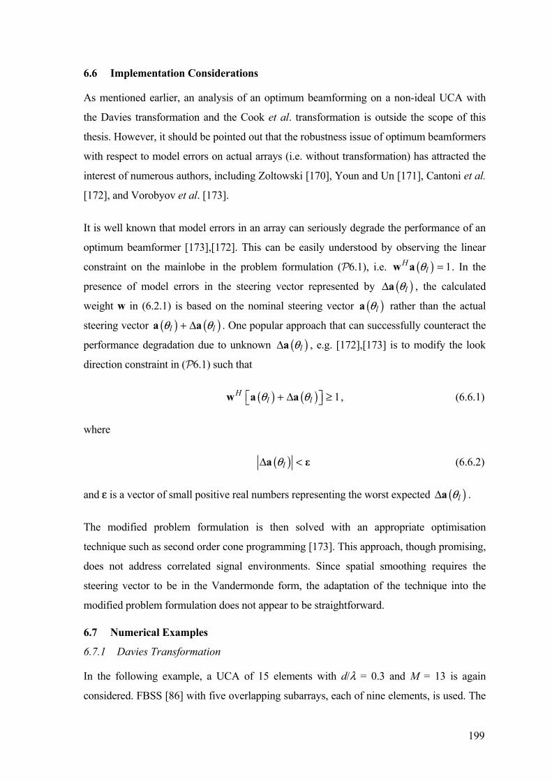
199

6.6 Implementation Considerations

As mentioned earlier, an analysis of an optimum beamforming on a non-ideal UCA with

the Davies transformation and the Cook et al. transformation is outside the scope of this

thesis. However, it should be pointed out that the robustness issue of optimum beamformers

with respect to model errors on actual arrays (i.e. without transformation) has attracted the

interest of numerous authors, including Zoltowski [170], Youn and Un [171], Cantoni et al.

[172], and Vorobyov et al. [173].

It is well known that model errors in an array can seriously degrade the performance of an

optimum beamformer [173],[172]. This can be easily understood by observing the linear

constraint on the mainlobe in the problem formulation (P6.1), i.e. ( ) 1Hlq =w a . In the

presence of model errors in the steering vector represented by ( )lqDa , the calculated

weight w in (6.2.1) is based on the nominal steering vector ( )lqa rather than the actual

steering vector ( ) ( )l lq q+ Da a . One popular approach that can successfully counteract the

performance degradation due to unknown ( )lqDa , e.g. [172],[173] is to modify the look

direction constraint in (P6.1) such that

( ) ( ) 1Hl lq qÈ ˘+ D ≥Î ˚w a a , (6.6.1)

where

( )lqD <a ε (6.6.2)

and e is a vector of small positive real numbers representing the worst expected ( )lqDa .

The modified problem formulation is then solved with an appropriate optimisation

technique such as second order cone programming [173]. This approach, though promising,

does not address correlated signal environments. Since spatial smoothing requires the

steering vector to be in the Vandermonde form, the adaptation of the technique into the

modified problem formulation does not appear to be straightforward.

6.7 Numerical Examples


In the following example, a UCA of 15 elements with d/l = 0.3 and M = 13 is again

considered. FBSS [86] with five overlapping subarrays, each of nine elements, is used. The

200

signal scenario consisted of uncorrelated sensor noise of 0 dB, and three equal power (10

dB) signals arriving from −90°, 0° and 60°. The signals arriving from −90° and 60° are

correlated with correlation coefficient / 4je p while the signal arriving from 0° is not

correlated with either of the other two signals. Here the exact covariance matrix is used,

since the interest is in the performance of the optimum beamformers. Studies into the effect

of finite data can be found in [174] and in the references therein.

Figure 6.7.1 shows the power responses of the conventional, spatially smoothed (SS),

spatially smoothed robust (SSR), and spatially smoothed robust output averaged (SSROA)

optimum beamformers, as the look direction is swept across the full azimuth. As can be

seen, in contrast to the SS, SSR, and SSROA optimum beamformers, the conventional

optimum beamformer is not able to receive the two correlated signals arriving from −90°

and 60°. The improvement in the latter three beamformers is, however, at the cost of a

reduced aperture in the subarrays. As can be observed, this resulted in an increase in the

noise floor.

The effect of implementing derivative constraints can be seen by observing that the peaks

of the SSR optimum beamformer are broader than the peaks of the SS optimum

beamformer. For the SSROA optimum beamformer, an improvement in the noise floor

(about 1.5 dB) together with the same broadening of peaks yet with a sharper rolloff is

obtained with respect to the SSR optimum beamformer. In this case, all 7 subarray

beamformers output are averaged together, as in (6.5.5). It is also confirmed through other

examples that the larger the number of subarrays, the larger the reduction in the noise floor.

To confirm that the averaging of (6.5.5) is reasonable, Figure 6.7.2 compares the output

averaging for all 7 subarrays with that of Reddy et al. [168]. But the strategy of Reddy et al.

requires non-overlapping subarrays, therefore, the first and last subarrays are used because

they have minimum overlap. It is observed that the noise floor is about the same in both

cases. However, the use of all subarrays gives the power response of the SSROA optimum

beamformer a sharper rolloff than that of Reddy et al. [168] while retaining the broader

peaks. Other test cases, including those with non-overlapping subarrays (not shown here)

show that while in general the Reddy et al. strategy can give a slightly lower noise floor

relative to that of (6.5.5), it is obtained at the price of sacrificing other desirable

beampattern characteristics such as lower received signal powers (at the peaks) and reduced

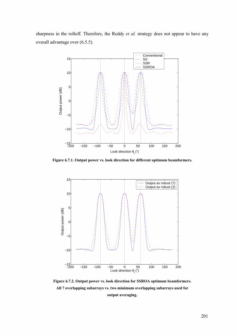
201

sharpness in the rolloff. Therefore, the Reddy et al. strategy does not appear to have any

overall advantage over (6.5.5).

−200 −150 −100 −50 0 50 100 150 200−15

−10

−5

0

5

10

15

Look direction θl (°)

Out

put p

ower

(dB

)

ConventionalSSSSRSSROA

Figure 6.7.1. Output power vs. look direction for different optimum beamformers.

−200 −150 −100 −50 0 50 100 150 200−15

−10

−5

0

5

10

15


Out

put p

ower

(dB

)

Output av robust (7)Output av robust (2)

Figure 6.7.2. Output power vs. look direction for SSROA optimum beamformers.

All 7 overlapping subarrays vs. two minimum overlapping subarrays used for

output averaging.

202

Figure 6.7.3 compares the beampatterns of the conventional, SS and SSROA optimum

beamformers to demonstrate the robustness of the SSROA optimum beamformer against

directional mismatches. A directional mismatch scenario is introduced where the

beamformers are steered towards the look direction at −85° while the signal of interest

arrived from −90°. As can be seen, they all achieve the target response (0 dB gain) in the

look direction, and place nulls in the DOA of the uncorrelated interferer at 0°. However,

only the SS and SSROA optimum beamformers are able to effectively suppress the

correlated interferer at 60°. The null at 60° can be made deeper by increasing the number of

subarrays used but this will reduce the subarray size and hence the number of degrees of

freedom [169].

It is also noted that the SSROA optimum beamformer is able to maintain an array response

close to 0 dB at the actual DOA of the desired signal, i.e. −90°, while the SS optimum

beamformer attenuates the desired signal by 12dB as a result of the directional mismatch.

−200 −150 −100 −50 0 50 100 150 200−60

−50

−40

−30

−20

−10

0

10

20


Gai

n (d

B)

ConventionalSSSSROA

Figure 6.7.3. Beampatterns for the look direction of −85° with different optimum

beamformers.


Consider a UCA of 30 elements with d/l = 0.4 and M = 13. For FBSS, five overlapping

subarrays, each of nine elements, are used. The output averaging technique of (6.5.5) is also

203

used. Here, optimum beamforming with the Cook et al. transformation is demonstrated

over the full azimuth. The design procedure for the in-sector size to allow for handovers

between in-sectors is as described in Section 5.4.2. The window function is the raised

cosine window and five in-sectors are defined. Allowing for the mainlobe width54, the

overlapped region between adjacent operational sectors is set to be 28∞, and thus the

operational (or optimisation) sector size Dqo = 360∞/5 + 28∞ = 100∞.

The signal scenario consists of uncorrelated sensor noise of 0 dB, and five equal power (10

dB) signals arriving from −160°, −115°, −36°, 10° and 108°. The signals arriving from

−160°, −36°, and 108° are fully correlated (with pairwise correlation coefficient of 1) while

the signals arriving from −115° and 10° are not correlated with any of the other three

signals and to each other. The handover points between the five in-sectors are at -180° (or

180°), -108°, -36°, 36°, and 108°. Note that two signals are deliberately placed at the

handover points of −36° and 108° so that the impact of handover on the output power may

be observed.

Figure 6.7.4 gives the power responses of the conventional, SS, SSR, and SSROA optimum

beamformers as the look direction is swept across the full azimuth. Vertical solid lines and

vertical dotted lines mark the DOA’s of the signals and handover points, respectively.

The characteristics of the beamformers are similar to that in Figure 6.7.1. Once again, only

the conventional optimum beamformer is not able to receive the three correlated signals

arriving from −160°, −36° and 108°. The broadening of the peaks due to the derivative

constraints can be seen in the SSR and SSROA optimum beamformers, in comparison to

the SS optimum beamformer. The improvement in the noise floor of the SSROA optimum

beamformer is only marginal (less than 1dB) relative to that of the SSR optimum

beamformer. However, the averaging technique appears to bring the output power closer

towards the 10dB signal power at the DOA’s of the signals. The output power appears to

undergo smooth handovers at the handover points. For instance, the maximum

discontinuity at the handover points in the SSROA optimum beamformer is only 0.2dB.

54 In contrast to the Dolph-Chebyshev beampattern, the mainlobe width of the scenario dependent optimum beampattern is

less well defined. A simple rule is to observe the gain suppression in the beampattern for two uncorrelated interferers, one on each side and equal distance from the look direction. The narrowest mainlobe width where a sufficient suppression can be obtained is taken to be the mainlobe width.

204

In Figure 6.7.5, the beampatterns of the conventional, SS and SSROA optimum

beamformers are compared to demonstrate the robustness of the SSROA optimum

beamformer against directional mismatches. A directional mismatch scenario where the

beamformers are steered towards the look direction at −33° while the signal of interest

arrives from −36° is given. Note that the look direction is located within the (first) in-sector

defined by q Œ [−50, 50∞]), thus only the transformation matrix of this in-sector is used.

Vertical solid lines and vertical dotted lines mark the DOA’s of the signals and the

handover points at ±36∞, respectively.

Again, the characteristics are similar to those obtained with the Davies transformation

shown in Figure 6.7.3, in that the target response (0 dB gain) at the look direction is

achieved and the gains at the DOA’s of the interferers are suppressed. One obvious

difference is that the beampattern of the Cook et al. transformation is shaped by the window

function and is suppressed accordingly within the image sector. The SSROA optimum

beamformer is able to maintain an array response close to 0 dB at the actual DOA of the

desired signal, i.e. −36°, while the SS optimum beamformer attenuates the desired signal by

12 dB as a result of the directional mismatch.

−200 −150 −100 −50 0 50 100 150 200−15

−10

−5

0

5

10

15


Out

put p

ower

(dB

)

ConventionalSSSSRSSROA

Figure 6.7.4. Output power vs. look direction. Vertical solid lines: DOA’s of signals.

Vertical dashed lines: handover points.

205

−200 −150 −100 −50 0 50 100 150 200−60

−50

−40

−30

−20

−10

0

10

20


Gai

n (d

B)

ConventionalSSSSROA

Figure 6.7.5. Beampattern for the look direction of −33°. Vertical solid lines: DOA’s

of signals. Vertical dashed lines: handover points at ±36∞.

6.8 Conclusions

This chapter demonstrates the use of two UCA preprocessing techniques for optimum

beamforming. The use of the preprocessing techniques provides a solution to the design of

optimum beamformers for UCA’s in the presence of highly correlated signals. However,

the approach is limited by the approximation involved in the transformation and the

problem with array imperfection. It is also shown that derivative constraints can be easily

incorporated into the design to effectively increase the robustness of the beamformer to

directional mismatches. The output averaging technique that utilises all virtual array

beamformer outputs rather than those of a single subarray has also been demonstrated to

give a noise reduction in the optimum beamformer output.

206

Part II – 3G AAS Applications

207

Chapter 7 DOA Estimation in WCDMA 7.1 Introduction

The long awaited rollout of wideband CDMA (WCDMA) services in Japan in October

2001 marked the beginning of 3G mobile telecommunications services. Even though the

initial consumer response did not match the industry’s optimism55, major

telecommunication companies around the world are going ahead with their plans to

introduce the new system. Aside from the pressure to recover the many billions of US

dollars already invested into research and the purchase of spectrum licenses and equipment,

the companies recognise the vast potential of the system in providing new revenue-

generating services. The search is currently on for killer application(s) to encourage quick

and widespread adoption of the technology.

One promising candidate for killer application is the multimedia messaging service (MMS)

[175], as indicated by the success of its predecessor, the SMS (see Figure 7.1.1). MMS, as

its name suggests, facilitates the transfer of messages comprising a combination of text,

sounds, images and video among MMS capable MS’s [175]. In contrast to the simple SMS,

the bandwidth-hungry MMS can benefit from the higher data rates afforded by 3G systems.

WCDMA is based on direct-sequence code division multiple access (DS-CDMA)

technology that has its roots in military applications [7]. The basic idea of DS-CDMA is to

create multiple access channels for mobile communications by using different codes to

spread the frequency spectrum of each channel’s information data bits. The spreading codes

can be orthogonal (zero cross correlation, e.g. downlink of IS-95) or quasi-orthogonal (non-

zero cross-correlation e.g. uplink of IS-95), depending on timing synchronisation. Due to

this “spread spectrum” property, it is resilient to hostile reception and jamming for military

applications, and can provide desirable features such as resilience to (unintentional)

interference, security, more accurate position location (using time-of-arrival (TOA)

methods) and soft limit on system capacity56 to mobile communications [7],[175]. In fact,

studies, e.g. [175], have shown that CDMA technology can achieve considerably higher

system capacity than conventional multiple access schemes such as frequency division

multiple access (FDMA) and TDMA. 55 By April 2002, the total number of WCDMA subscribers is estimated at 100,000 [1]. 56 Soft limit on system capacity can facilitate more efficient resource allocation and management.

208

Figure 7.1.1. Global SMS growth (Red line represents SMS messages per month) [1].

The development and rollout of WCDMA also pose a new set of difficult technical

challenges to engineers, as is clearly learnt from the recent Japanese experience. In

comparison with 2G systems that are only optimised for voice communications, WCDMA

is far more advance in technology, and therefore far more difficult to implement and

maintain. Issues such as system capacity and QOS will become increasingly important as

the systems grow. The maturing AAS technology is favoured57 to play an important role in

the future enhancement and development of WCDMA systems [46].

The main advantage of an AAS lies in its ability to exploit the spatial characteristics of the

mobile channel to improve the reception and/or transmission of mobile signals. WCDMA

systems, in particular, are inherently suitable for AAS’s because the capacity of CDMA

systems is soft-limited by interference level and any suppression of interference would

provide an instant capacity increase [18],[46].

Currently, there exist a few types of AAS architectures, ranging from the simple fixed

multibeam AAS’s for both uplink and downlink, to the fully steerable beam AAS’s for

57 Even though the AAS feature (network beamforming) is optional without any specific standardisation demands,

provisions are made in the standards for equipment suppliers to include this feature in future products.

209

downlink and combined spatial/temporal interference cancellation for uplink [17],[20]. For

steerable beam AAS’s, an explicit estimation of the DOA of the uplink signals of interest58

is required for downlink beamforming since the use of FDD mode in WCDMA renders the

use of estimated array weights based on uplink spatial signature ineffective for downlink

beamforming [6],[12],[21],[22],[24],[177]. Moreover, DOA is important for emergency

services and other radiolocation applications such as location sensitive billing, vehicle and

fleet management, fraud detection, Intelligent Transport Systems (ITS) [49],[50]. To

pinpoint a MS location, DOA estimates from at least two BS’s are required. However, due

to the challenging mobile environment (i.e. MAI, non-line of sight propagation, and

multipath), it is believed that a combination of different approaches, including DOA and

time difference of arrival (TDOA), are required to achieve the target accuracy for some

applications [50].

This chapter is concerned with the single-user approach to DOA estimation [68],[69] for

WCDMA using ULA’s59 in the AAS. In particular, the interest here is in techniques that

make use of information available to the AAS, e.g. [68],[69],[178]. A simple DOA

estimation approach is proposed with an aim to reuse as much as possible the decoupled 2D

rake receiver structure in [13]. The 2D (or space-time) rake receiver, first proposed in [15],

is an extension to the spatial domain of the conventional 1D (or temporal-only) rake

receiver [179]. In the proposed approach, the pilot sequence and the root raised cosine

(RRC) chip waveform in the Dedicated Physical Control Channel (DPCCH) [180] is

utilised on top of the known desired MS code in order to improve the estimate of the

desired signal covariance matrix. This involves oversampling of the received data. The

improvement results in smaller biases and standard deviations in the DOA estimates caused

by the non-whiteness of MAI. The proposed approach also employs an estimate of the

MAI-and-noise covariance matrix to prewhiten the signal-MAI-noise covariance matrix in

order to obtain a further improvement in performance. Among the benefits of the proposed

approach is the fact that the number of array elements no longer limits the number and

58 It should be noted that while the DOA approach effective for macrocell environment, which is the focus of this chapter,

the significant angular spread in indoor and microcell environment seriously degrades its performance [21]. Macrocell and microcell are BS sites where the BS antenna heights are respectively, higher and lower, than average building height.

59As explained in Section 1.3 Thesis Outline, Part II of this thesis (Chapters 7 to 9) will deal only with ULA's because they can be conveniently integrated into the existing sector BS configuration.

210

proximity of identifiable signal paths [68]. In fact, different MS’s with the same DOA can

be identified.

Here the received WCDMA signal is despread and Root-MUSIC [147] is applied on the

despreaded covariance matrix for DOA estimation. Root-MUSIC has better statistical

properties than MUSIC [106] for finite data, especially for small sample sizes. Many other

DOA estimation techniques may be similarly applied to the covariance matrix, e.g. Root-

WSF [137] and ESPRIT [5]. The simulation study demonstrates the performance of the

proposed approach in dynamic simulations (with MS mobility) by the use of the COST259

channel model [79]. It is shown that the proposed approach can significantly outperform the

conventional approach.

7.2 WCDMA Uplink Signal Structure

A summary of the WCDMA signal structure [13],[180],[181] is provided below. Figure

7.2.1 gives the block diagram for the uplink spreading of the DPCCH and the Dedicated

Physical Data Channels (DPDCH’s). The MS data is carried on the DPDCH’s. As shown,

up to three DPDCH’s may be multiplexed onto the in-phase (I-) and quadrature-phase (Q-)

channels. The DPDCH’s on each of the I- and Q-channels use orthogonal variable

spreading factor (OVSF) codes of a common spreading factor for channelisation. The

spreading factor is determined according to the desired data rate. Each MS also has a

DPCCH with a constant spreading factor of 256 that is mapped onto the Q-channel. The

binary DPCCH and DPDCH’s to be spread are represented by real-valued sequences, i.e.

the binary values “0” and “1” are mapped to the real values +1 and –1, respectively.

The amplitude gain factors are: βD for all six DPDCH’s, and βC for DPCCH. βD is assigned

according to the data rate: the higher the data rate (lower spreading factor), the higher the

βD. This chapter considers only one DPDCH on the I-channel and one DPCCH on the Q-

channel for demonstration purposes. Dropping the DPDCH channel reference in Figure

7.2.1, the data sequence and the chip sequence of the OVSF spreading code for the DPDCH

are denoted by { }( )D

kb and { }( )Dhc , respectively.

For the DPCCH, one radio frame contains 15 slots and each slot has 10 bits. Each slot

consists of a number of pilot bits, transmit power control (TPC) command bits, feedback

information (FBI) bits and an optional transport-format combination indicator (TFCI) bit.

211

Figure 7.2.2 shows the frame structure of the dedicated physical channels. The number of

pilot bits is [ ]3, ,8pN …∈ [180].

DPDCH data { }( )

D,1kb

OVSF code { }( )

D,1hc

+ ×

I

Complex scrambling code { }( )

Sqc

DPCCH data { }( )

Ckb

OVSF code { }( )

Chc

Q×

S{ }( )

D,3kb

{ }( )D,5

kb

S{ }( )

D,4kb

{ }( )D,6

kb

{ }( )D,2

kb

× ×

× ×

×

{ }( )D,3

hc

×

×

{ }( )D,5

hc

×

× ×

×

{ }( )D,4

hc

×

×

{ }( )D,6

hc

×

{ }( )D,2

hc

j

bD

bD

bD

bD

bD

bD

bC

I + jQ

Figure 7.2.1. Uplink spreading for DPCCH and DPDCH’s [181].

The baseband representation of DPDCH [13] is

( ) ( )( )D D D D

k

ks t b z t kT

∞

=−∞

= −∑ , (7.2.1)

where ( ) ( )D

( )D D c

1

Qh

hz t c p t hT

=

= −∑ , (7.2.2)

DT is the symbol period of the data, cT is the chip period corresponding to the WCDMA

chip rate of 63.84 10× chips/s, { }( )D 1hc ∈ ± is the hth chip of the OVSF spreading code,

212

{ }( )D 1kb ∈ ± is the kth data symbol and ( )p t is the impulse response of the RRC pulse

shaping filter for the chip waveform. The rolloff factor of ( )p t is 0.22a = .

Data, Ndata bits

Pilot, Np bits

TFCI, NTFCI bits

FBI, NFBI bits

TPC, NTPC bits

Slot 0 Slot 1 Slot i Slot 14

DPDCH

DPCCH

Tslot=2560 chips, Ndata=10 × 2k bits, k Œ{0,…,6}

Tslot=2560 chips, 10 bits

1 radio frame, Tf =10 ms

Figure 7.2.2. Frame structure for uplink DPDCH and DPCCH [180].

Similarly, the baseband representation of DPCCH is

( ) ( )( )C C C C

k

ks t b z t kT

∞

=−∞

= −∑ , (7.2.3)

where ( ) ( )C

( )C C c

1

Qh

hz t c p t hT

=

= −∑ , (7.2.4)

and ( )C

kb , ( )C

hc , CT and CQ are defined similarly. While different ( )D

hc ’s are assigned on the

I- or Q- channel for cases with multiple DPDCH’s, ( )C

hc always take the first OVSF code

(sequence 0) for a spreading factor of 256.

The DPDCH and DPCCH are appended onto the I- and Q-channels, respectively, of the

transmitted Quadrature Phase Shift Keying (QPSK) signal. A complex scrambling code of

length S 38400Q = chips (length of one radio frame) is also added. The scrambling code is

213

aligned with the start of each radio frame. The transmitted baseband signal of the ith MS60

is then

( ) ( ) ( ) ( )( )S D D C C

ii f

r

s t s t rT s t j s tβ β∞

=−∞

= − × + ∑ , (7.2.5)

where ( ) ( )S

c

( ) ( )S c

1

Qi q

S Tq

s t c p t qT=

= -Â , (7.2.6)

( )c

c1, 00, elsewhereT

t Tp t

£ <Ï= ÌÓ

, (7.2.7)

{ }( )S 1qc jŒ ± ± is the qth chip of the complex scrambling code, and fT is the period of one

radio frame, i.e. 10msf s cT Q T= = .

Since the uplink is asynchronous, the transmissions of the scrambled codes from different

MS’s are not time-aligned. Moreover, the codes are not strictly orthogonal even though

they have good autocorrelation and cross-correlation properties. This means that the

receiver for each MS will experience MAI from all other MS’s in the system. Hence the

number of MS’s that can be simultaneously accommodated in one cell is interference-

limited [7].

The AAS of interest is a N-element ULA with inter-element spacing d and operating

wavelength l . For Nu MS’s where 1i = is the desired MS, the continuous time signal at

the array output after the receiver RRC filter with impulse response ( )p t can be written as

follows:

( ) ( ) ( ) ( ) ( ) ( )1

1 1 1 11 2 1

( ) ( )u iN LL

i i i ii

t s t p t s t p t tr q t r q t= = =

= - ƒ + - ƒ +Â ÂÂx b b n (7.2.8)

where ƒ denotes the convolution operation, iq , ir , and it are respectively the DOA,

complex gain, and delay of the th path of the ith MS, iL is the number of signal paths of

60 User equipment (UE) is the designated name for MS in WCDMA standards. However, MS shall be used throughout this

thesis for the sake of consistency.

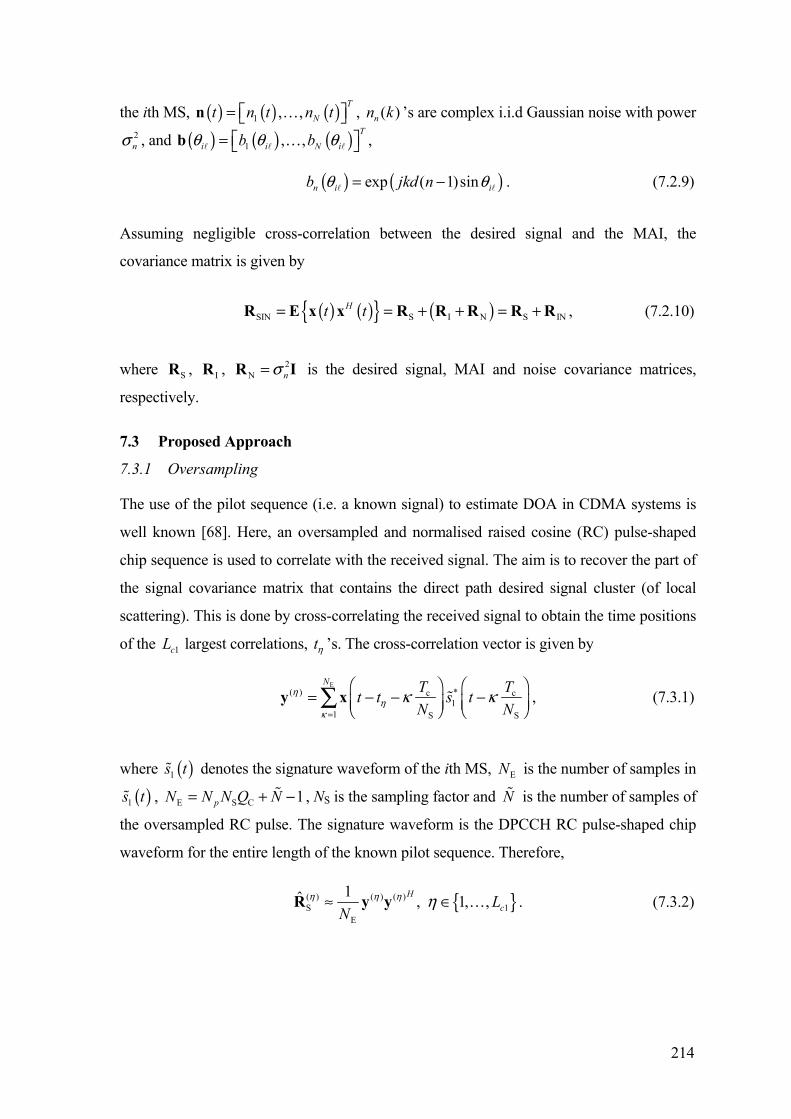
214

the ith MS, ( ) ( ) ( )1 , ,T

Nt n t n tÈ ˘= Î ˚n … , ( )nn k ’s are complex i.i.d Gaussian noise with power 2ns , and ( ) ( ) ( )1 , ,

T

i i N ib bq q qÈ ˘= Î ˚b … ,

( ) ( )exp ( 1)sinn i ib jkd nq q= - . (7.2.9)

Assuming negligible cross-correlation between the desired signal and the MAI, the

covariance matrix is given by

( ) ( ){ } ( )SIN S I N S INHt t= = + + = +R E x x R R R R R , (7.2.10)

where SR , IR , 2N ns=R I is the desired signal, MAI and noise covariance matrices,

respectively.

7.3 Proposed Approach

7.3.1 Oversampling

The use of the pilot sequence (i.e. a known signal) to estimate DOA in CDMA systems is

well known [68]. Here, an oversampled and normalised raised cosine (RC) pulse-shaped

chip sequence is used to correlate with the received signal. The aim is to recover the part of

the signal covariance matrix that contains the direct path desired signal cluster (of local

scattering). This is done by cross-correlating the received signal to obtain the time positions

of the 1cL largest correlations, th ’s. The cross-correlation vector is given by

E

( ) *c c1

1 S S

N T Tt t s tN N

hh

kk k

=

Ê ˆ Ê ˆ= - - -Á ˜ Á ˜Ë ¯ Ë ¯Ây x , (7.3.1)

where ( )1s t denotes the signature waveform of the ith MS, EN is the number of samples in

( )1s t , E S C 1pN N N Q N= + - , NS is the sampling factor and N is the number of samples of

the oversampled RC pulse. The signature waveform is the DPCCH RC pulse-shaped chip

waveform for the entire length of the known pilot sequence. Therefore,

{ }( ) ( ) ( )S 1

E

1ˆ , 1, ,HcL

Nh h h hª ŒR y y … . (7.3.2)

215

Apart from finite data effect, the estimate is limited by the amount of cross-correlation

among the signals from different MS’s and the autocorrelation of multipath signals from the

same (ith) MS.

7.3.2 MAI Prewhitening

To perform prewhitening for the nth rake finger, an estimate of INR , i.e. ( )IN

ˆ hR , is required

at that finger. The procedure to obtain an estimate of ( )SINhR begins with

E

( ) c cSIN

1E S S

1ˆN

HT Tt t t tN N N

hh h

kk k

=

Ê ˆ Ê ˆ= - - - -Á ˜ Á ˜Ë ¯ Ë ¯ÂR x x . (7.3.3)

When more than one slot is used for DOA estimation, the covariance matrices of all the

slots are averaged. From (7.2.8) and (7.2.10), the following expression can be formed

( ) ( ) ( )IN SIN S

ˆ ˆ ˆh h hª -R R R . (7.3.4)

Finally, ( )IN

ˆ hR is utilised to prewhiten the MAI in ( )SIN

ˆ hR . The resulting ( )SIN

ˆ hR is then used for

DOA estimation. Note that (7.3.4) has an exact form for chip rate sampling [13] (not

involving ( )p t ), though in [13] it is used for uplink beamforming on a 2D rake receiver.

Some recent work on CDMA systems may cast doubts on the merit of the prewhitening

procedure. For instance, according to [16] and [18], the interference can typically be

assumed to be statistically close to white Gaussian noise in an IS-95 system. While this may

be true for IS-95 where all MS’s have the same power at the AAS (with a single data rate

and good power control) and are roughly evenly distributed across the cell, the same

conclusion does not apply readily to 3G CDMA systems such as CDMA2000 and

WCDMA [18]. This is because WCDMA allows mixed services of different data rates [44],

which gives different received powers in the DPDCH’s even with perfect power control.

This mixed services scenario can colour the MAI, the extent of which depends on the

spatial distribution of the interfering MS’s and their respective data rates [18]. Indeed, the

simulation study reported in this chapter reveals that the MAI is coloured and that the

prewhitening procedure can result in significant performance improvements.

216

7.4 WCDMA Simulator

In this section, the WCDMA simulator developed for the evaluation of DOA estimation is

outlined.

7.4.1 Simulator Structure

In the simulator, all MS’s generate and transmit continuous data streams that follow the

WCDMA radio interface specifications [180],[181]. The long code is used for scrambling.

The signals are passed through a COST259 channel and received at a base station (BS)

equipped with an AAS. The AAS consists of a ULA where the array outputs are fed into a

decoupled 2D rake receiver [13].

The cross-correlation to search for the rake fingers is performed over NS = 2 oversampled

chip data. To model the asynchronous uplink, the samples of the desired MS are assumed to

be synchronised to the signature waveform in the receiver ( )1s t while the interfering MS’s

are not synchronised either with one another or with the desired MS. Figure 7.4.1 shows the

block diagram of the parts of the receiver that are relevant to DOA estimation. It is noted

that no additional information is required other than that available to the 2D rake receiver

with NS = 2.

DPCCH

correlator

N-element ULA

Baseband demodulator

ADC and Sampler

RRC filter

DOA estimation algorithm

DPCCH correlatorBaseband

demodulator ADC and Sampler

RRC filter

q ...

......

. . . . . .

. . .

Figure 7.4.1. Block diagram of simulator

7.5 Simulation Environment

In this study, a scenario with one desired MS and multiple interfering MS’s in the 2GHz

frequency band is investigated. The base station (BS) operates in a 120°-sector cell and

employs a 4-element ULA with d/λ = 0.5. The simulation scenario is given in Figure 7.5.1.

217

θ

Desired UE at 30°

Interfering UEs BS with AAS

COST259 channel

at varying θ

Figure 7.5.1. Simulation scenario: a BS, a desired MS and multiple interfering MS’s.

WCDMA utilises both open (slow) and closed loop (fast) power control for all active MS’s.

Therefore, the power discrepancies among the MS’s are expected to be small. Here perfect

power control is assumed such that the channel response of each MS in the system is

normalised with respect to the reference antenna (i.e. antenna 1).

7.5.1 COST259 Channel Model

Accurate channel models are important in order to study and validate the performance of

transceiver architectures prior to practical implementations. In the case of AAS’s in a

mobile environment, the channel model should include the multipath and channel fading

characteristics unique to multi-antenna systems. The so-called directional (or vector)

channel model for AAS’s is the subject of many recent publications, including [79],[182]-

[184].

The COST259 channel model [79] is a versatile directional channel model derived under

the COST259 project of the European Community. It has been validated using

measurements in the 1GHz to 2GHz range, but is expected to be applicable at least in the

range 450MHz to 5GHz. It is a wideband directional channel model capable of providing

channel impulse responses in both spatial (azimuth and elevation) and temporal domains.

Parameter

Channel

type Average number

of clusters

Typical azimuth

spread per cluster

(degrees)

LOS cut-off

distance (meters)

218

TU 1.17 10 500

BU 2.18 10 500

RA 1.06 5 5000

HT 2.00 5 5000

Table 7.1. Examples of COST259 channel parameters.

The COST259 channel model incorporates, inter alia, the effects of path loss, fast fading

and shadow fading61. The radio environment currently implemented is macrocell. The

channel types modelled are typical urban (TU), bad urban (BU), rural area (RA) and hilly

terrain (HT), which are generalisations of the GSM channel models with the same names.

Examples of the parameter settings are given in Table 7.1. An example of a BU channel

realisation with two clusters is shown in Figure 7.5.2.

0

5

10

0

50

100

150

0

10

20

30

40

50

Rel

ativ

e po

wer

(dB

)

Azimuth angle q (∞)

Time delay ( s) µ

Figure 7.5.2. Example of a BU channel realisation with two clusters in the

temporal/azimuth plane.

61 It should be noted that the shadow fading feature is not used in algorithm or link level evaluations such as those of this

chapter and Chapter 9.

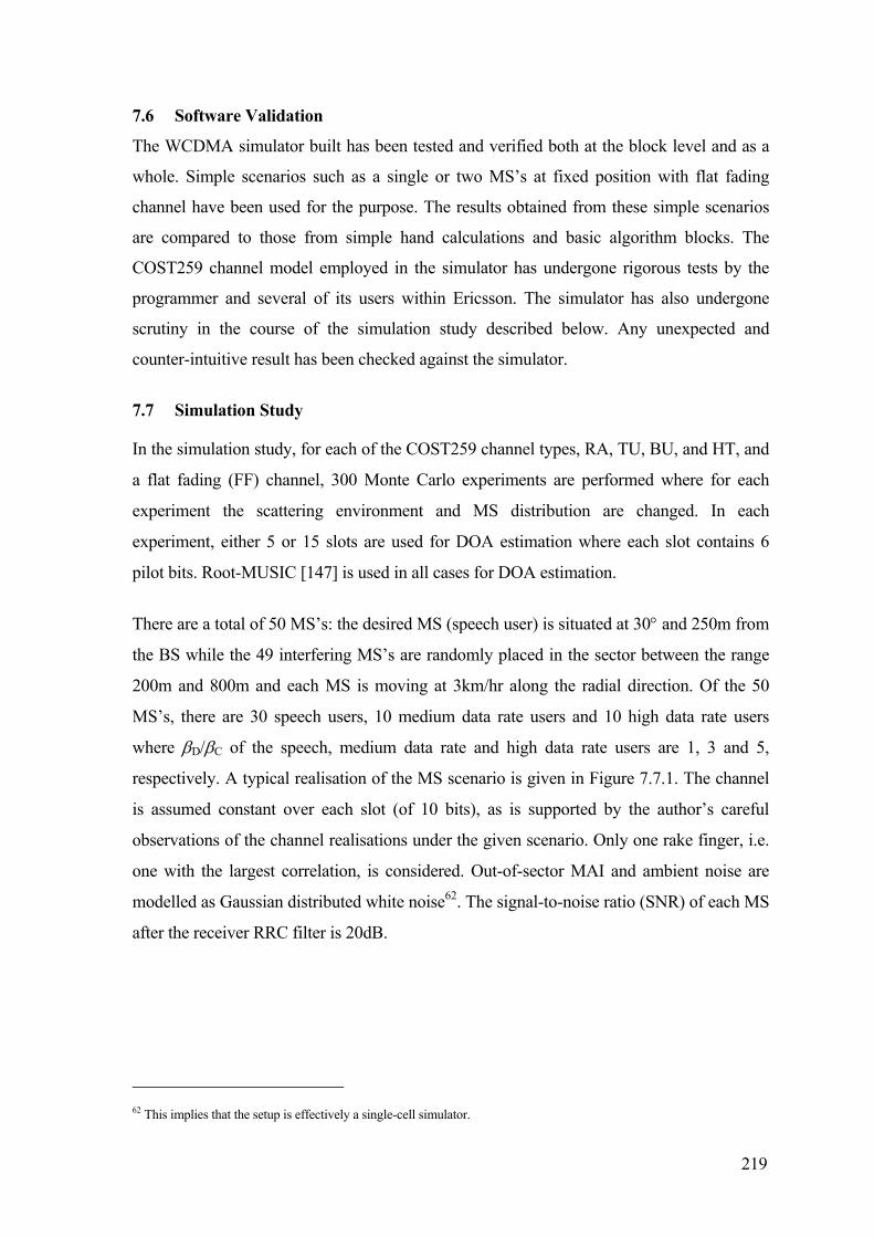
219

7.6 Software Validation

The WCDMA simulator built has been tested and verified both at the block level and as a

whole. Simple scenarios such as a single or two MS’s at fixed position with flat fading

channel have been used for the purpose. The results obtained from these simple scenarios

are compared to those from simple hand calculations and basic algorithm blocks. The

COST259 channel model employed in the simulator has undergone rigorous tests by the

programmer and several of its users within Ericsson. The simulator has also undergone

scrutiny in the course of the simulation study described below. Any unexpected and

counter-intuitive result has been checked against the simulator.

7.7 Simulation Study

In the simulation study, for each of the COST259 channel types, RA, TU, BU, and HT, and

a flat fading (FF) channel, 300 Monte Carlo experiments are performed where for each

experiment the scattering environment and MS distribution are changed. In each

experiment, either 5 or 15 slots are used for DOA estimation where each slot contains 6

pilot bits. Root-MUSIC [147] is used in all cases for DOA estimation.

There are a total of 50 MS’s: the desired MS (speech user) is situated at 30° and 250m from

the BS while the 49 interfering MS’s are randomly placed in the sector between the range

200m and 800m and each MS is moving at 3km/hr along the radial direction. Of the 50

MS’s, there are 30 speech users, 10 medium data rate users and 10 high data rate users

where βD/βC of the speech, medium data rate and high data rate users are 1, 3 and 5,

respectively. A typical realisation of the MS scenario is given in Figure 7.7.1. The channel

is assumed constant over each slot (of 10 bits), as is supported by the author’s careful

observations of the channel realisations under the given scenario. Only one rake finger, i.e.

one with the largest correlation, is considered. Out-of-sector MAI and ambient noise are

modelled as Gaussian distributed white noise62. The signal-to-noise ratio (SNR) of each MS

after the receiver RRC filter is 20dB.

62 This implies that the setup is effectively a single-cell simulator.

220

Figure 7.7.1. A typical traffic distribution scenario.

In the channel types considered, some experiments have completely failed to locate the

DOA of the desired MS. Therefore, statistical measures such as mean and standard

deviation are unsuitable for performance evaluation. Instead, the results are presented in

terms of the cumulative distribution functions (cdf’s) of the absolute DOA estimation

errors. Figure 7.7.2 shows the results for RA, TU and BU for 5 and 15 slots and Figure

7.7.3 shows the results for FF and HT. “conv” denotes the conventional approach of using

the desired MS chip waveform (over the pilot length) at chip rate to despread the received

signal, i.e. NS = 1 in (7.3.1)-(7.3.2) with E CpN N Q= , and ( )S

ˆ hR is used for DOA

estimation63. “new” denotes the proposed approach with oversampling (for cross-

correlation) and prewhitening, i.e. applying NS = 2 in (7.3.1) to (7.3.4).

63 The estimated signal covariance matrix ( )

Sˆ hR will have some residual noise due to imperfect decorrelation. Therefore, it

is full rank and Root-MUSIC that relies on the existence of noise subspace can be used. But if its condition number is very high, techniques like diagonal loading or appropriate alternatives such as conventional beamforming can be applied. In the simulations, there was no noticeable problem with the use of Root-MUSIC.

221

0 5 10 150

0.1

0.2

0.3

0.4

0.5

0.6

0.7

0.8

0.9

15 slots

absolute DOA error (degree)

cdf

RA convRA newTU convTU newBU convBU new

0 5 10 150

0.1

0.2

0.3

0.4

0.5

0.6

0.7

0.8

0.9

115 slots

absolute DOA errors (degree)

cdf

RA convRA newTU convTU newBU convBU new

Figure 7.7.2. Cdf’s of absolute DOA error for RA, TU and BU.

It is clear that in all cases, the use of more slots has improved the DOA estimation. This

gain is due to the slowly changing channel response for the MS speed of 3km/hr. In Figure

7.7.2 and Figure 7.7.3, note that the performance of the proposed approach is particularly

promising in FF and RA. If the performance benchmark is set at 5° absolute error (in view

of the mainlobe width of the 4-element ULA64), the correctly resolved DOA’s in both FF

and RA are improved by 12% for 5 slots, and 10% and 15% respectively for 15 slots. This

is unsurprising since FF only has one line-of-sight (LOS) direct path and the one rake finger

used is able to rake up all the desired signal power. The oversampling procedure provides

more samples (and information) to the cross-correlation of (7.3.1) and thus improves the

averaging process. This in turn reduces the level of MAI. Moreover, an accurate desired

signal estimate also enables an accurate estimate of the MAI for prewhitening. Therefore,

64 Since a 4-element ULA with half-wavelength spacing is used, the approximate mainlobe width is 38.2∞ [125]. The

mainlobe width limits the directivity of downlink beams and consequently for this application a larger absolute error benchmark can be tolerated. On the other hand, the performance requirement for positioning application can be higher, especially for emergency services, where it is important to obtain an accurate estimate of the MS position.

222

both oversampling and prewhitening procedures are effective. Likewise, RA has a high

probability of LOS in the given scenario. It also has small angular and temporal spreads

(see Table 7.1) that ensure a good estimate of the desired signal based on one rake finger.

0 5 10 150

0.1

0.2

0.3

0.4

0.5

0.6

0.7

0.8

0.9

15 slots

absolute DOA error (degree)

cdf

FF convFF newHT convHT new

0 5 10 150

0.1

0.2

0.3

0.4

0.5

0.6

0.7

0.8

0.9

115 slots

absolute DOA errors (degree)

cdf

FF convFF newHT convHT new

Figure 7.7.3. Cdf’s of absolute DOA error for FF and HT.

For TU, BU and HT, performance differences are less well defined within the range of

interest (at around absolute DOA error of 5°), with some cases giving only marginal

improvements (e.g. BU for 15 slots) while other cases giving only similar performances to

that of the conventional approach.

This is due to the significant angular and temporal spread for TU and BU and the high

probability of non-LOS (NLOS) (see Table 7.1 and Figure 7.5.2). In NLOS cases, even

though the signal cluster of the local scatterers are still contained in a region around the

nominal DOA, it has a smeared out energy spread in both the spatial and temporal domains.

The problem worsens when the desired MS has only NLOS while some of the interfering

MS’s have LOS. The temporal spread due to NLOS of the desired MS will cause

223

significant interchip interference (ICI). For the rake receiver, any signal path that is more

than a sampling period from the rake finger of interest produces a virtual interfering MS.

And since the channel resolution in this study is high (or the sampling period is small),

multipath signals of the desired MS result in such virtual interfering MS’s. Nevertheless,

high channel resolution circumvents the problem of having highly correlated signals that

fall within a chip period (where Root-MUSIC may fail to perform well).

Also, while HT has small angular and temporal spreads for each cluster and high LOS

probability, it has a high probability of having two or more signal clusters. Once again, this

smears out the energy and degrades the performance of one rake finger.

In view of the above discussions, some improvements are expected especially for complex

scattering environments (e.g. BU) if a few more rake fingers are taken into account.

Nevertheless, care is required in the choice of rake fingers due to the frequent occurrence of

more than one strong signal cluster in BU and HT where the DOA’s of these clusters are

significantly different from the nominal DOA’s of the desired MS.

7.8 Conclusions

The introduction of WCDMA presents many exciting technical challenges. Among them is

the application of AAS technology in which DOA estimation plays an integral part. Apart

from identifying the direction of the desired MS for downlink beamforming, it can also

provide important services on wireless communication networks. In this chapter, a novel

single-user approach to DOA estimation in WCDMA is proposed. In the simulation study,

it was shown that the proposed approach gives promising gains over a conventional

approach under favourable environments and that it experiences no noticeable degradation

in challenging environments.

224

Chapter 8 EDGE/EGPRS Downlink System Level Evaluations 8.1 Background

As communication systems become more and more complex, the importance of modelling

systems in software increases. The software models enable designs to be evaluated and

tradeoffs to be made before great expenses are spent to build the systems. Unfortunately,

the same complexity in real systems also compounds the complexity in the development of

software models.

The common approach in reducing the complexity of the simulation model is to separate

the full system model into different levels (or layers) so that the interactions can be

modelled by some simple functions of a set of input parameters. This simplification is

particularly useful in the study of a limited set of parameters on a given level, e.g. system

capacity on the system level. Naturally, careful consideration is necessary to minimise the

impact of the simplification on the integrity of the overall system model.

In this and the following chapters, software tools are developed to represent two different

levels of a 3G mobile communications system called EDGE. The system level study

presented in this chapter is concerned with the BS to MS (downlink) transmission where

the AAS’s (of fixed multibeam configuration) are at the BS’s. It makes use of summary

results from (radio) link level simulation for the downlink to obtain the bit error rates (BER)

for the MS of a particular receiver architecture, which first translates to link and

subsequently system throughput. The modelling of the downlink at the link level poses no

significant challenge as the radio interface behaviour of single-antenna receivers typical in a

MS can be well defined by numerical functions of few parameters, e.g. BER as a function

of link quality.

On the other hand, the link level study in the next chapter is concerned with the MS to BS

(uplink) transmission, where an accurate representation of the link level results for an AAS

in a system level study is still an open question. This is because the link level behaviour of a

particular AAS configuration for a given mobile traffic scenario65 involves many

65 A mobile traffic scenario is represented by a BS serving a number of MS’s that have a certain distribution across the cell.

225

parameters66. Moreover, the choice of AAS configuration involves a wide range of

parameters such as array geometry, number of antenna elements and type of algorithms.

The link level study in the following chapter is an attempt to address this issue by

characterising the performance of a simple fixed multibeam AAS configuration in the

spatial dimension. Nevertheless, it should be noted that the link to system level interaction

is not the sole purpose of the study, as will be brought out in the next chapter.

8.2 Introduction

The explosive growth of worldwide mobile subscribers as mentioned in Chapter 1 puts an

increasing demand on network capacity. Due to the capacity demand and the limited

amount of available spectrum, GSM and TDMA IS-136 operators are forced to tighten the

frequency reuse as much as possible resulting in interference-limited networks. This is

particularly a problem for the 800/900MHz band where the allocated bandwidth is limited

[185].

Adaptive antenna systems (AAS’s) have been demonstrated in field trials [17],[185],[186]

and simulations [17] to be an effective method for reducing downlink interference in GSM

systems67. Such reduction occurs even for AAS’s with limited complexity. These trials and

simulations have shown that the capacity can be increased by more than 100% in GSM

circuit-switched systems. Significant performance improvements have also been obtained

in research carried out on TDMA IS-136 systems [187],[188]. Studies have also revealed

that the deployment of AAS’s in GSM can follow a gradual, step-by-step manner in a given

system, with priorities given to “hotspot” cells that are congested and responsible for high

level of interference to adjacent cells. This strategy to adopt the AAS technology facilitates

lower initial costs for operators [189].

The development of GSM is currently focused on packet-switched services, which began

with GPRS and more recently extended with EDGE (or GERAN). Until recently, the

technology is optimised for circuit-switched voice rather than bandwidth hungry services.

The aim is to enable service providers to offer more wireless data applications for both

66 These include the angular positions of individual mobiles and relative angular separations. 67 In the 1800MHz band, where a larger bandwidth is available, AAS’s can have a more immediate application in coverage

extension (without increasing the transmitted power). This is because the path loss in the mobile environment is higher in the 1800MHz than in the 800/900MHz band due to use of higher frequencies [185].

226

consumers and business users, including wireless Internet, e-mail, web infotainment,

interactive services and multimedia applications.

Introducing EDGE will have limited technical impact on the existing infrastructure of GSM

and TDMA IS-136. This is particularly so for GSM, because EDGE is based fully on GSM

and will consequently require relatively small changes, or upgrades, to network hardware

and software. As a result, operators do not have to make large changes to the network

structure, or invest in new licenses. For example, EDGE uses the same frame structure,

logic channel and 200kHz carrier bandwidth as today’s GSM networks, which allows

existing cell plans to remain intact. This makes the technology particularly attractive to

existing operators seeking a way to roll out 3G services rapidly and cost-effectively across

large areas of existing networks.

As with the 2G systems, the capacity of EDGE is expected to be interference-limited,

particularly in urban areas. Since AAS’s are known to be effective in mitigating

interference in such scenarios [17] and thus allowing tighter frequency reuse and higher

network capacity, AAS’s can be expected to significantly improve the performance of

EDGE. However, the combination of packet-switched systems and AAS’s has so far

received relatively little attention and only a few studies on the system level performance is

available, e.g. [31],[190].

Stridh and Ottersten [31] considered the uplink performance of an AAS in a slotted

ALOHA scheme for a single-cell system, assuming negligible inter-cell interference. The

AAS utilises a UCA for diversity combining and interference rejection. The use of simple

and idealised models enabled the derivation of an analytical expression for the system

throughput. The expression is in agreement with simulation results, which shows that

AAS’s can offer substantial improvements in a system’s throughput while maintaining low

mean packet delay. Packet delay is a crucial parameter in determining the QOS.

In a more closely related work, Rehfuess and Ivanov [190] estimated the downlink gains of

AAS’s for GPRS and EDGE. Their focus was to present a simplified system level study in

which the system throughput is found by directly combining the relationship between C/I

and gross bit rate, as obtained from link level simulations, with the user C/I cumulative

distribution results from system level simulations. In this way, separate existing link and

system level simulation results are put together to give the system throughputs for GPRS

227

and EDGE with AAS’s without requiring further simulations. For instance, they showed

that for a 50% loaded 1/3 frequency reuse EGPRS system, the system throughput could be

increased by up to 282%. They also investigated the effect of power control on the system

throughput using the same methodology. While the simplification is useful to get a rough

estimate of the gains of using AAS’s in packet data systems, it is limited in scope and does

not preclude a more comprehensive study based on a more accurate modelling of the

systems. For instance, the system throughput in [190] is based solely on the gross bit rate

(over-the-air transmission) and it ignores the impact of packet queuing delay.

This chapter presents a simulation methodology to study the system level performance of

an AAS for EDGE. In particular, the focus is on the downlink system level performance of

the packet-switched component68 of EDGE called Enhanced GPRS (EGPRS). The

downlink traffic is examined since packet-switched mobile services are expected to be

downlink-limited. Several factors that can contribute to the downlink limitation are listed

below:

• The limited signal processing capability in the MS’s. The MS’s are constrained by

size and power consumption.

• The expected asymmetrical WWW traffic.

• The non-observability of the downlink channel spatial signature at the base station

[12] limits the effectiveness of AAS’s in the downlink. This is a problem inherent in

FDD systems, as mentioned in Chapter 7.

A homogenous system consisting three 120∞-sector BS’s is considered with different

frequency reuse schemes. Two different types of link quality control (LQC) within the

Standards, i.e. link adaptation (LA) and the more advanced incremental redundancy (IR)

[41],[191],[192], are considered. A fixed multibeam configuration is adopted for the AAS.

The traffic model mimics the behaviour of packet data traffic of the Worldwide Web

(WWW) [193] and the propagation model incorporates large-scale lognormal fading and

path loss.

68 There are two components within EDGE, the packet-switched EGPRS and the circuit-switched Enhanced Circuit Switched Data

(ECSD). ECSD also uses 8-PSK modulation to increase data rates, though it is not unlike GSM due to its circuit-switched operation.

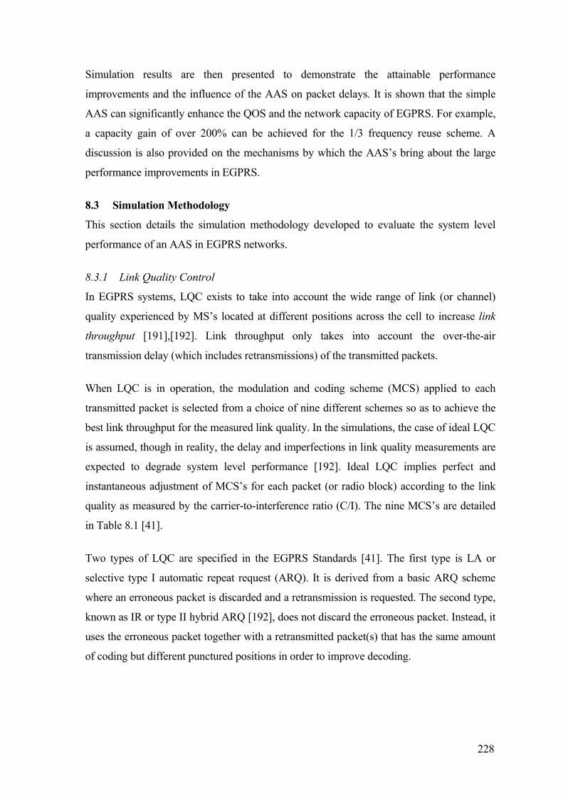
228

Simulation results are then presented to demonstrate the attainable performance

improvements and the influence of the AAS on packet delays. It is shown that the simple

AAS can significantly enhance the QOS and the network capacity of EGPRS. For example,

a capacity gain of over 200% can be achieved for the 1/3 frequency reuse scheme. A

discussion is also provided on the mechanisms by which the AAS’s bring about the large

performance improvements in EGPRS.

8.3 Simulation Methodology

This section details the simulation methodology developed to evaluate the system level

performance of an AAS in EGPRS networks.

8.3.1 Link Quality Control

In EGPRS systems, LQC exists to take into account the wide range of link (or channel)

quality experienced by MS’s located at different positions across the cell to increase link

throughput [191],[192]. Link throughput only takes into account the over-the-air

transmission delay (which includes retransmissions) of the transmitted packets.

When LQC is in operation, the modulation and coding scheme (MCS) applied to each

transmitted packet is selected from a choice of nine different schemes so as to achieve the

best link throughput for the measured link quality. In the simulations, the case of ideal LQC

is assumed, though in reality, the delay and imperfections in link quality measurements are

expected to degrade system level performance [192]. Ideal LQC implies perfect and

instantaneous adjustment of MCS’s for each packet (or radio block) according to the link

quality as measured by the carrier-to-interference ratio (C/I). The nine MCS’s are detailed

in Table 8.1 [41].

Two types of LQC are specified in the EGPRS Standards [41]. The first type is LA or

selective type I automatic repeat request (ARQ). It is derived from a basic ARQ scheme

where an erroneous packet is discarded and a retransmission is requested. The second type,

known as IR or type II hybrid ARQ [192], does not discard the erroneous packet. Instead, it

uses the erroneous packet together with a retransmitted packet(s) that has the same amount

of coding but different punctured positions in order to improve decoding.

229

Scheme Modulation Code rate Maximum data rate (kbps)

MCS9 8-PSK 1.0 59.2

MCS8 8-PSK 0.92 54.4

MCS7 8-PSK 0.76 44.8

MCS6 8-PSK 0.49 29.6

MCS5 8-PSK 0.37 22.4

MCS4 GMSK 1.0 17.6

MCS3 GMSK 0.85 14.8

MCS2 GMSK 0.66 11.2

MCS1 GMSK 0.53 8.8

Table 8.1. MCS’s for EGPRS.

0 5 10 15 20 25 30 35 40 45 500

10

20

30

40

50

60

Link

thro

ughp

ut (

kbps

)

C/I (dB)

MCS1MCS2MCS3MCS4MCS5MCS6MCS7MCS8MCS9

Figure 8.3.1. Link throughput vs. C/I curves for LA.

230

0 5 10 15 20 25 30 35 40 45 500

10

20

30

40

50

60

Link

thro

ughp

ut (

kbps

)

C/I (dB)

MCS1MCS2MCS3MCS4MCS5MCS6MCS7MCS8MCS9

Figure 8.3.2. Link throughput vs. C/I curves for IR.

In LA, the link quality performance curves for the nine MCS’s (see Figure 8.3.1) are

obtained from the link level simulations. These link simulations are carried out using the

Rayleigh fading ETSI typical urban channel for 3km/h (TU3) and ideal frequency hopping.

The performance curves are used in the system level simulations to map link quality (C/I)

to link throughput for each transmitted packet.

The link quality performance curves are also obtained for IR and these are shown in Figure

8.3.2. These are obtained under the same prerequisites as LA except that no frequency

hopping is used. However, despite this disadvantage (ideal frequency hopping outperforms

no frequency hopping due to diversity gain), IR is still several decibels better than LA for a

given link throughput.

8.3.2 System Setup for System Level Simulations

Homogeneous systems consisting of three-sector base station (BS) sites are studied. A

conventional sector configuration (100% sectorised antennas) is compared to an AAS

configuration (100% AAS). For both configurations, we examine the performance of

EGPRS for three different frequency reuse schemes: 4/12, 3/9, and 1/3. The three system

setups are shown in Table 8.2.

231

Cell plan 1 2 3

Frequency reuse 4/12 3/9 1/3

Number of clusters 9 9 16

Number of BS’s 36 27 16

Number of cells 108 81 48

Table 8.2. Parameters for the system cell plans.

All three systems have a cell radius of 1000 m and seven time slots per cell are used for

packet traffic. A wrap-around technique, which tiles copies of the network together with the

original, is used to counter border effects.

8.3.3 Adaptive Antenna System Configuration

The AAS investigated is based on a fixed multibeam configuration comprising of eight

interleaved beams from two Butler beamforming networks. These networks are fed from

two orthogonally polarised 4-element ULA’s with an inter-element distance of half a

wavelength [186]. The sectorised and the multibeam antenna patterns used in the

simulations were obtained from actual field measurements (see Figure 8.3.3).

The multibeam configuration is a simple but effective solution to perform spatial

processing. This is due to a system-integrated solution enabling the selection (on the radio

frequency level) of one of the pre-formed fixed narrow multibeams for downlink

transmission. This minimises the coherence requirements and removes the need for

calibration involved in baseband processing [17]. In the uplink, however, all beams are of

course available for diversity reception. Moreover, AAS’s are most probably first needed

and deployed in urban environments where the significant angular spread and the existence

of multipath mean that more sophisticated array configurations such as a steerable beam

solution (an AAS solution that requires baseband processing) could potentially offer only

small gains69 compared to the basic fixed multibeam configuration [185]. For such cellular

frequency reuse networks, higher complexity (more sophisticated) solutions may not be

economically viable for operators.

69 Nonetheless, it should be noted that the steerable beam solution has significant advantages over the fixed multibeam

solution in power-limited systems. This is because the typically large cell sizes of such systems means that the steerable beam could be more accurately directed towards the desired MS than any one of the fixed multibeams [18].

232

−200 −150 −100 −50 0 50 100 150 200−30

−25

−20

−15

−10

−5

0

5

10

15

20

Angles (degrees)

Gai

n (d

B)

Figure 8.3.3. The gains of a sectorised antenna (dashed line) and a fixed multibeam

AAS (solid line) as obtained from measurements.

8.3.4 Propagation Model

As is typical of propagation models for system level simulations, only large-scale

lognormal fading and distance attenuation (or path loss) are taken into account. In

particular, the propagation model uses the parameters in Table 8.3. Also note that only co-

channel interference is modelled in the simulations.

Parameters

System frequency 900 MHz

BS height 30 m

Thermal noise 1.58×10-15 W

Distance independent term in Okumara-Hata formula 21

Distance attenuation 3.5

Lognormal fading standard deviation 6

Correlation of lognormal fading between one MS and

different BS’s

0

Lognormal fading correlation distance 110 m

Table 8.3. Parameters for the propagation model.

233

8.3.5 Traffic Model

Since a packet network is expected to carry primarily WWW traffic, the corresponding

traffic model is setup to mimic this behaviour [193]. In essence, MS’s are introduced into

the system according to a Poisson process. The MS’s then receive downlink packets with

Pareto-distributed inter-arrival times. The packet sizes are drawn from a truncated

lognormal distribution. The parameters used are summarised in Table 8.4.

MS arrival

Distribution Poisson

Mean number of MS’s Variable

Packet arrival

Distribution Pareto

Packets/MS/second 0.1

Pareto shape, alpha 1.4

Mean number of packets per MS 10

Packet size

Distribution Lognormal

Mean 4,100 bytes

Max 100,000 bytes

Added TCP/IP header 50 bytes

Table 8.4. Parameters for the traffic model.

8.3.6 Simulation Assumptions

The system level simulations are performed under the following assumptions:

• Perfect beam selection based on gain and shadow fading. Shadow fading in the

beams are equal in the same cell.

• No admission control, i.e. all MS’s generating packets are either allocated resources

or put in the queue.

• First-in-first-out (FIFO) is used for scheduling.

234

• No angular spread over the channel.

• No multi-slot allocation.

• No transmission in idle slots.

• All BS’s are time-synchronised with one another.

• Perfect synchronisation between MS’s and BS’s.

• No receiver diversity in the MS’s.

• MS’s are placed in the systems according to a uniform area distribution.

• Same output power for Gaussian Minimum Shift Keying (GMSK) and 8-PSK

modulations.

• Only traffic channel carriers are considered.


The EGPRS simulator used in this study is built on an existing simulator which has been

tested and used extensively within Ericsson. However, the predecessor employs only

conventional sector antennas and basic ARQ scheme. The upgrade of the simulator to

employ AAS gives each BS a number of fixed beams for downlink transmission. As such,

the simulator now involves the BS dynamically choosing its downlink beam, where each

beam has a unique beampattern (see Figure 8.3.3). The upgrade further incorporates the link

results of the IR scheme. These upgrades have been tested against known results and also

with simple scenarios which are easily checked by hand calculations. In the case of IR with

conventional antennas, results obtained from the simulator are readily verified with those

from another purpose-built simulator within Ericsson. As mentioned in Section 7.6, the

software validation process is ongoing even during the simulation study.

8.5 Simulation Results

The simulation results show that the fixed multibeam AAS provides significant capacity

gains in all the systems examined. The gain is largest for the 1/3 reuse scheme, followed by

the 3/9 and the 4/12 reuse schemes. This implies that the tighter the reuse scheme, the

higher the resulting gain. This is because a tighter reuse scheme has higher inter-cell

235

interference. Since AAS’s can effectively reduce co-channel interference, a more marked

improvement is seen where the interference is higher.

Figure 8.5.1 shows system (or packet) throughput performance versus average capacity for

the three reuse schemes when LA is used. The throughput performance is measured by the

10% level or percentile of the cumulative distribution of all packet throughputs, which

means that 90% of all transmitted packets achieve this throughput. Note that as opposed to

the link throughput obtained from link simulations, system throughput takes into account

both the queuing delay and the transmission delay (which includes retransmissions) of the

transmitted packets. If the benchmark of acceptable quality for MS’s is that 90% of the

transmitted packets achieve 20kbps per time slot, the plot shows that the AAS will give a

capacity gain of 260% (a factor of 3.6) in the 1/3 reuse case, while the gains are 80% and

50% respectively for the 3/9 and 4/12 reuse schemes. On the other hand, if the average

number of MS’s is kept constant, for example, at 20, then the system throughput, i.e. QOS,

is increased from 8.4kbps to 25kbps for 1/3 reuse, a gain of 200% (a factor of 3).

0 10 20 30 40 50 60 70 80 900

5

10

15

20

25

30

35

Average number of MS’s per cell

10%

per

cent

ile o

f sys

tem

thro

ughp

ut (

kbps

)

4/12 reuse sect4/12 reuse AAS 3/9 reuse sect 3/9 reuse AAS 1/3 reuse sect 1/3 reuse AAS

Figure 8.5.1. Average system throughput vs. average number of MS’s for the

sectorised antennas (sect) and the AAS in 1/3, 3/9 and 4/12 reuse schemes for LA.

236

0 10 20 30 40 50 60 70 80 900

5

10

15

20

25

30

35


10%

per

cent

ile o

f sys

tem

thro

ughp

ut (

kbps

)

4/12 reuse sect4/12 reuse AAS 3/9 reuse sect 3/9 reuse AAS 1/3 reuse sect 1/3 reuse AAS

Figure 8.5.2. Average system throughput vs. average number of MS’s for the sect

and the AAS in 1/3, 3/9 and 4/12 reuse schemes for IR.

Using the above benchmark for the results when IR is applied (see Figure 8.5.2), the

capacity gains are 200%, 38% and 26% respectively for the 1/3, 3/9 and 4/12 reuse

schemes. Note also that in absolute terms the performance of IR is consistently better than

LA even though its relative capacity gains are lower.

As is apparent, all the systems investigated here are interference-limited, i.e. C/I determines

the system capacity. When the average number of MS’s per cell is high, the interference

experienced by the MS’s is also high. Therefore, even though the channel utilisation is

high, the poorer C/I performance reduces the link throughput, causing the number of

packets being queued to increase dramatically. This effect can be seen in the increasing

average of the transmission delay with the increasing average number of MS’s, as is

exemplified in Figure 8.5.3 for the 1/3 reuse scheme using LA. Note however that these

increases are small, especially in comparison to the increases in queuing delay, suggesting

that these systems are very sensitive towards changes in the link throughput. Simulations

have shown that further increases in traffic load would result in continuously growing

queues and therefore an unstable system. Of course, in a real system, admission control can

be implemented to circumvent this undesirable effect.

237

0 10 20 30 40 50 600

0.05

0.1

0.15

0.2

0.25

0.3

0.35

0.4

0.45

0.5


Ave

rage

nor

mal

ised

del

ay p

er p

acke

t (s/

kb)

sect tx sect queuesect total AAS tx AAS queue AAS total

Figure 8.5.3. Average normalised delays per packet, i.e. transmission delay (tx),

queuing delay (queue) and total delay (total) for the sect and the AAS in 1/3 reuse

for LA.

0 10 20 30 40 50 600

0.05

0.1

0.15

0.2

0.25

0.3

0.35

0.4

0.45

0.5


Ave

rage

nor

mal

ised

del

ay p

er p

acke

t (s/

kb)

sect tx sect queuesect total AAS tx AAS queue AAS total

Figure 8.5.4. Average normalised delays per packet, i.e. transmission delay (tx),

queuing delay (queue) and total delay (total) for the sect and the AAS in 1/3 reuse

for IR.

238

Figure 8.5.3 further shows that the use of the AAS is effective in reducing interference as

can be seen in the flatter slope in the corresponding transmission delay curves. For instance,

for the 1/3 reuse scheme and 25 MS’s, the use of the AAS reduces the transmission delay

from 0.053 s/kbyte to 0.025 s/kbyte. As a result, the system is able to accommodate many

more MS’s (giving large performance improvements) before this interference-queuing

limiting point is again reached. A similar behaviour has also been obtained for the 1/3 reuse

scheme using IR, as shown in Figure 8.5.4.

8.6 Conclusions

Even though GSM is the dominant player in today’s mobile market, the future of GSM

rests on its ability to provide 3G services. EDGE has been agreed upon as the evolution

path to achieve this goal. This chapter outlines the use of an AAS to enhance the ability of

EGPRS to provide 3G packet-switched mobile services. A simulation methodology to

evaluate and to compare the system level performance of a conventional sector

configuration with that of an AAS is described. It is shown that huge QOS and capacity

gains can be achieved through the use of the AAS employing a fixed multibeam

configuration. For the 1/3 reuse scheme, a capacity gain of over 200% has been realised for

the relatively low complexity AAS as compared to the conventional sector configuration.

239

Chapter 9 EDGE Uplink Link Level Evaluations 9.1 Introduction

The development of an uplink system model for EDGE is a challenging task. While the

downlink involves reception at the MS’s, as discussed in the previous chapter, the uplink

involves reception at the BS AAS’s. The modelling of the uplink transmission involving

AAS’s is an open issue at present. This chapter is one attempt to develop a methodology to

incorporate link level results of AAS’s into the system level model. In particular, link level

results with dependence on spatial information are obtained for a simple scenario involving

two MS’s: the desired MS and the interfering MS. Though limited, these results can be of

immediate interest to other aspects of AAS implementation such as the impact of the MS

traffic distribution in the spatial domain and the uplink link level performance requirement

given the achievable downlink performance. The latter requirement means that if the

performance is downlink-limited, then the performance requirement for the uplink AAS

algorithms can be less stringent (and vice-versa), or that the excess performance can be

utilised to give more flexibility to the system designers, such as reducing the MS transmit

power for a given coverage [18].

The (uplink) link performances of EDGE with single-antenna receivers [40] and two-

antenna diversity receivers [194] at the BS’s have been reported in previous studies.

However, to date, no work has been done on the link performance of EDGE with AAS’s at

the BS’s. Moreover, the channel models used in all previous simulation studies, including

those on GSM [17], do not incorporate a realistic spatial channel model such as that made

available by the COST259 Project [79].

This chapter presents a simulation methodology for evaluating the link level performance of

EDGE with a fixed multibeam AAS. The multibeam configuration is similar to that of the

previous chapter except that the interest here is on the link level results for uplink

transmission. Simulation results demonstrating the uplink performance of several fixed

multibeam AAS configurations in different channel types are then given. The aim is to

evaluate their relative merits and the conditions in which performance gains are achieved.

Moreover, qualitatively discussions and insights of the obtained performance with reference

to the different AAS receiver configurations and the characteristics of the propagation

channels are also presented.

240

9.2 Simulation Methodology

This section details the simulation methodology developed to evaluate the uplink link level

performance of an AAS in EDGE.

9.2.1 Simulation Scenario

In the simulator, all mobile stations (MS’s) generate and transmit continuous data streams

structured according to the EDGE radio interface specifications [41]. The signals are then

passed through the COST259 channel and received at a BS equipped with a fixed

multibeam AAS. The AAS consists of two Butler beamforming networks where a number

of the beam outputs are fed into a diversity receiver. In the receiver, the transmitted

symbols are recovered and checked for errors. A reference two-antenna sectorised system is

also implemented.

The simulation study investigates a scenario with one desired MS and one synchronised

interfering MS in the 900MHz frequency band. The objective is to determine the carrier-to-

interference ratio (C/I) that a given AAS receiver configuration requires to achieve a QOS

performance of 8% raw BER for a given angular separation between the two MS’s. The

desired MS is placed at a fixed position at 0° and the interfering MS is moved along radial

positions separated by an angle θ in order to locate the C/I of interest (see Figure 9.2.1).

The procedure is carried out for a set of angular separations θ’s between 0° and 30°.

q

Desired MS at 0°

Interfering MS

BS with AAS

COST259 channel

at varying q

Figure 9.2.1. Simulation scenario: a BS, a desired MS and an interfering MS.

9.2.2 Fixed Multibeam Configuration

The front-end of the simulated AAS is a fixed multibeam configuration comprising of eight

interleaved beams from two Butler beamforming networks, similar to that of the previous

chapter. These networks are fed from two orthogonally polarised four-element ULA’s with

241

an inter-element distance of half a wavelength [186]. All the antenna elements have a

sectorised gain pattern. This pattern is obtained from software calculations (see Figure

9.2.2), as opposed to that obtained from measurements in the previous chapter. The

multibeam patterns are also shown in Figure 9.2.2.

The multibeam configuration is a simple but effective solution to perform spatial

processing. This is because it not only allows the diversity receiver to operate on spatially

filtered outputs (a “beamspace”) in the uplink, but it can also form a system integrated

solution that enables the selection (on the radio frequency level) of one of the pre-formed

fixed narrow beams for downlink transmission, as discussed in the previous chapter.

Furthermore, the multibeam configuration is an effective way of exploiting angular

diversity, where in an urban environment it can give a diversity gain comparable to space

diversity [195].

−200 −150 −100 −50 0 50 100 150 200−40

−30

−20

−10

0

10

20


Gai

n (d

B)

Figure 9.2.2. Antenna gain patterns for the two sectorised antennas with ±45°

polarisation ( ) and the AAS: four fixed beams with +45° polarisation (––) and

four fixed beams with -45° polarisation (– –).

9.2.3 Multibeam Diversity Receiver

As part of the AAS, a multibeam (beamspace and polarisation) diversity receiver is devised

in the simulator. The receiver conforms fully to the EDGE Standards [41]. Receiver

filtering, channel estimation and symbol level synchronisation are performed on each of the

242

eight beam outputs. Then, M (M = 2, 4 or 8) of these beam outputs are selected based on

one of two different selection criteria: total received signal power (SP) or received signal

quality70 (SQ). These quantities are estimated based on the received signals. Next, the

selected beam outputs are passed through a single-tap pre-combiner [194] where either

maximum ratio combining (MRC) or interference rejection combining (IRC) [194] is

applied.

After combining, the signal is passed through an equaliser where the raw BER is

determined. Figure 9.2.3 shows a block diagram of the AAS receiver. In the reference two-

antenna sectorised system, the outputs of two orthogonally polarised sectorised antennas

(see Figure 9.2.2) are fed directly into the diversity receiver. Further, in this study we

consider only 8-PSK modulation. The simulation results are thus directly relevant to

modulation and coding schemes (MCS’s) 5 to 9.

Select M

beams

Weight generationMRC/IRC

Sync. & channel

estimation

2×4-element ULA

Butler Beam-

forming Equalisation

Sync. & channel

estimation

. . . . . .

...... +

¥

¥..... .

Figure 9.2.3. AAS – Butler beamforming networks and multibeam pre-combining

diversity receiver.

9.2.4 COST259 Channel Model

The COST259 model [79] has been briefly described in Chapter 7. However, it should be

noted that EDGE has a much larger symbol period (or time resolution) relative to that of

WCDMA. Consequently, for time-dispersive channels such as TU and BU, the same

COST259 wideband channel impulse response as seen by the data bits of EDGE and

WCDMA are very different.

70 The received signal quality is estimated from the 26-symbol training sequence of the time slot burst.

243

In addition, the antenna elements used in the link level simulation here are ±45° polarised

rather than exclusively vertically polarised as in Chapter 7. As such, COST259 is

configured to provide the channel impulse responses in vertical and horizontal polarisation

components. For the purpose of this study, the average channel vertical/horizontal

polarisation power ratio is set to 1. The model inputs include mobile and base station

heights, positions of the mobiles, and carrier frequency of interest (900MHz). Some input

parameters used in the link level simulations are summarised in Table 9.1.

Parameter Channel

type MS height

(m)

MS speed

(km/h)

BS height

(m)

TU 2 3 30

BU 2 3 50

RA 2 250 50

HT 2 100 50

Table 9.1. Examples of COST259 input parameters.


As in Chapters 7 and 8, the software simulator used in this chapter has also been validated.

In particular, simple scenarios which include where MS’s are deliberately fixed at locations

of beampattern nulls and maximum gains are used to verify that the simulator contains no

error or more obscure bug. Existing results from literature and internal reports have also

been used as a sanity check for the simulation results. And as before, the EDGE link

simulator has undergone scrutiny during the simulation study to ensure its integrity.

9.4 Simulation Results

As mentioned previously, the C/I required for 8% raw BER is set as the benchmark for

comparing the AAS receivers against one another and the sectorised system. The C/I used

here is defined as the ratio of the average power (over all transmitted time slot bursts) of the

desired MS signal to that of the interfering MS signal received at each of the two

orthogonally polarised sectorised antennas (of the reference sectorised system), i.e.

244

1 210

1 2

C CC/I=10log (dB)I I

+ +

(9.4.1)

where Cn and In are the average powers of the desired MS signal and the interfering MS

signal at the nth sectorised antenna (n = 1,2), respectively. In addition, for each spatial

(angular and radial) position, a fixed number of Radio Link Control (RLC) blocks are used

to obtain the raw BER. A RLC block consists of four bursts and each RLC block is

subjected to a different scattering and fast fading environment so that an average behaviour

is obtained.

First, the C/I curves of interest are obtained for the reference two-antenna sectorised

system. Figure 9.4.1 shows the normalised C/I for 8% raw BER of a two-antenna diversity

receiver that applies MRC and IRC for different propagation channels. A quick observation

of Figure 9.4.1 confirms that on average MRC and IRC are both independent of the angular

separation between the desired MS and the interfering MS [17]. Further, the sectorised

antenna pattern (see Figure 9.2.2) does not come into play here since both the desired MS

signal and the interfering MS signal are measured after the receiver filters. It is also

observed in Figure 9.4.1 that the MRC performance does not differ among the different

channels by more than 2 dB. This suggests that there is some degree of robustness in the

performance of MRC. The performance of MRC appears similar in TU and BU, while it is

slightly worse in RA and HT. This is postulated to be due mainly to delay diversity: MRC

yields more delay diversity gain in TU and BU than in RA and HT, due to the larger cluster

delay spread.

The performance of IRC (see Figure 9.4.1), on the other hand, is highly dependent on the

type of channel used. The difference is as large as 6 dB between TU and HT. The observed

behaviour can be explained in terms of the delay diversity gain and interference rejection

property of the IRC algorithm. First, it is noted that the optimal performance for this

channel/receiver setup is obtained when the desired MS signal has large temporal spread (or

dispersion, giving delay diversity gain) while the interfering MS signal is a single ray

(allowing optimal cancellation by the single-tap IRC [43]). For the COST259 model,

temporal spread is proportional to the square root of the distance. This means that the

movement of the interfering MS changes its temporal spread.

245

In TU, even though the interfering MS has significant temporal spread in comparison to the

RA case, the temporal spread decreases when it is moved closer to the BS to obtain the 8%

raw BER point. Therefore, TU presents the best condition for the IRC receiver and gives

the best performance. RA gives the same IRC gain but no delay diversity gain, since both

the desired MS and the interfering MS have small delay spreads.

In BU and HT, both the desired MS and the interfering MS have significant delay spreads.

In BU, the spread is attributed to the large temporal spread in both the first and the

additional clusters, while in HT, the delay spread is attributed to the occurrence of more

than one narrow cluster. In this case, the interference rejection property of IRC gives a

small gain in both BU and HT, while a high delay diversity gain is realised in BU.

0 5 10 15 20 25 30

0

2

4

6

8

10

12

14

16

18


Nor

mal

ised

C/I

for

8% r

aw B

ER

(dB

)

TU MRCBU MRCRA MRCHT MRCTU IRCBU IRCRA IRCHT IRC

Figure 9.4.1. Normalised angular performance of the two-antenna diversity receiver

using MRC and IRC for different channel types.

Next, results in terms of the C/I gains (at 8% raw BER) of AAS’s relative to the reference

two-antenna sectorised system are presented. Although the simulation study investigates all

possible AAS receiver configurations (pre-combining of all eight beams, or pre-combining

of four beams or two beams with selection based on SP or SQ) in the propagation channels

TU, BU, RA and HT, only the main findings are summarised here.

The performance gains of the different AAS receivers relative to the sectorised receiver (all

using MRC pre-combining) in the TU channel are shown in Figure 9.4.2. The different

246

receiver configurations are two-, four- or eight-beam pre-combining, where the beams are

selected based on SP or SQ. It is noted that the receivers that select beams based on signal

quality (four-beam SQ and two-beam SQ) give the best performance. The two-beam SQ

outperforms the four-beam SQ, which in turn outperforms the eight-beam case. This is

because most of the desired signal power is contained within the two beams. The selection

of more beams with poor signal quality only results in a higher level of noise in the pre-

combining process. On the other hand, the situation is reversed for the SP beam selection

cases. This is because beams with higher signal powers do not necessarily correspond to

those with higher signal quality. Thus, the selection of a greater number of beams in the SP

case boosts the reception of higher quality signals which leads to an improved performance.

0 5 10 15 20 25 30

0

2

4

6

8

10


C/I

gain

at 8

% r

aw B

ER

(dB

)

8−beam4−beam SQ2−beam SQ4−beam SP2−beam SP

Figure 9.4.2. Performance gain of AAS MRC receivers in the TU channel (SQ and

SP).

In this example, it is observed that the AAS not only outperforms the sectorised system, the

AAS can be optimised by careful consideration of the receiver configuration. Moreover, it

is observed that the AAS has positive C/I gain even at θ = 0°. This is due to the different

instantaneous angular (and temporal) spread of the desired MS signal and the interfering

MS signal. Figure 9.4.3 shows that in general the performance gains of the AAS receivers

increase with angular separation. This is due to the spatial filtering provided by the Butler

beamforming networks of the AAS. However, the pattern nulls at separation angles of 7.5°

and 22.5° (see Figure 9.2.2) are not reflected in the two-beam SP case. This follows from

247

the previous argument that beams of good signal quality (those giving high gain for the

desired MS and nulls or low gain for the interfering MS) may not correspond to beams with

high signal power. This can be illustrated with a simple example in Figure 9.4.3. The

desired MS is placed at 0° while the interfering MS is placed at 22.5°, i.e. at the pattern null

of beam 1. It is clear that beam 1 has a better signal quality than beam 2, while beam 2 has a

higher received power than beam 1. At the same time, it appears that the SP criterion has

failed to perform favourably compared to the SQ criterion in all cases investigated.

Therefore the focus is now on the SQ cases.

-10 0 10 20 30 40 50

-15

-10

-5

0

5

10

15

20

Angular separation (degrees)

Gai

n (d

B)

beam 1beam 2

Interfering MS Desired MS

Figure 9.4.3. Scenario for comparing SQ and SP.

For the case of IRC, Figure 9.4.4 shows the C/I gains of three AAS receiver configurations

(pre-combining of two, four or eight beams, selected based on SQ) relative to the two-

antenna IRC diversity receiver in TU and RA, respectively. Note that the performance gains

of these AAS IRC receivers are far larger if compared to the two-antenna MRC diversity

receiver (see Figure 9.4.1). Again, the performance gain with larger angular separations is

observed. As pointed out in the previous example, this is due to the spatial filtering effect of

the AAS.

It is interesting to note that the two-antenna diversity receiver outperforms the two-beam

AAS receiver for small angular separations. This can be accounted for by the different

angular distributions of the signals. The two-beam AAS receiver favours the two beams

with the best signal quality, of which one beam has far weaker signal strength than the other

beam. This deteriorates the interference rejection property of IRC in the two-beam AAS

receiver compared to the two-antenna diversity receiver. It is also shown that the

performance of the two-beam AAS receiver does not deteriorate as much in TU as in RA

248

for this scenario. This can be explained by the larger angular and delay spread of TU

compared to RA, which results in diversity gain. As can be observed, the larger angular

diversity of TU also reduces the effect of the pattern nulls of the AAS. Furthermore, on the

system level, an averaging of the angular link performance gain is expected due to aspects

such as frequency hopping, distribution of traffic, etc.

0 5 10 15 20 25 30

−4

−2

0

2

4

6

8

10

12

14

16

18


C/I

gain

at 8

% r

aw B

ER

(dB

)

TU 8−beamTU 4−beamTU 2−beamRA 8−beamRA 4−beamRA 2−beam

Figure 9.4.4. Performance gain of AAS IRC receivers in the TU and the RA channels

(SQ).

Figure 9.4.5 compares the performance of the AAS IRC receivers (utilizing SQ for beam

selection) relative to the two-antenna IRC diversity receiver in TU and BU, respectively. It

is observed that by going from the two-beam to the four-beam receiver configuration, the

receiver gains 2 dB more in terms of C/I in BU than in TU. This is due to the more frequent

occurrence of second clusters for both the desired MS and the interfering MS in BU. The

four-beam IRC receiver is able to cancel more interfering signal clusters than the two-beam

counterpart. On the other hand, the average number of clusters in TU is 1.17 (see Table

7.1). Hence, while the larger number of beams increases the ability of IRC to cancel more

than one interfering signal, there is a low probability of having more than one interfering

signal cluster to deal with in TU. As a result, the achieved gain is larger in BU than in TU.

In general, it is observed that that IRC receivers perform better by using more beams, as is

249

expected from the increasing degree of freedom the receivers gain for interference

cancellation.

0 5 10 15 20 25 30

−4

−2

0

2

4

6

8

10

12

14

16

18


C/I

gain

at 8

% r

aw B

ER

(dB

)

TU 8−beamTU 4−beamTU 2−beamBU 8−beamBU 4−beamBU 2−beam

Figure 9.4.5. Performance gain of AAS IRC receivers in the TU and the BU channels

(SQ).

9.5 Conclusions

This chapter investigates the uplink link performance of EDGE used in conjunction with

the promising AAS technology. The study shows that while, in general, a simple AAS is

able to provide a large C/I gain, the gain differs according to the receiver architecture and

the propagation environment. Finally, it is noted that the deployment of EDGE will focus

on urban areas, i.e. TU and BU channels, where an improvement in the link level

performance can be obtained with the AAS receivers investigated.

250

Chapter 10 Conclusions and Suggestions for Future Work 10.1 Conclusions

This thesis focused on AAS algorithms for UCA’s and possible near future applications of

AAS’s in WCDMA and EDGE.

In Part I, two classes of UCA preprocessing techniques that apply a linear transformation to

the UCA outputs were studied under a unified framework. These preprocessing techniques

are the Davies and interpolated array transformations and they allow array processing

techniques naturally suited for ULA’s to be adapted to UCA’s.

In Chapter 2, the Davies and interpolated array transformations were summarised. While

the Davies transformation is available in closed form and can maintain an acceptable

transformation error over the entire azimuth, the interpolated array transformations, though

they present a greater design flexibility, require processing in several sectors (or in-sectors)

for full azimuth coverage. The existing interpolated array transformations of Bronez and

Friedlander transformations largely focus on obtaining the Vandermonde form for the in-

sector region. As such, the out-of-sector response is largely unknown. As a result, the out-

of-sector response can harm the DOA estimation of signals in the in-sector region,

especially in correlated signal environments. This was highlighted in the simulation studies

of Chapter 4.

For this reason, the Cook et al. transformation [74] was proposed to improve the

performance of DOA estimation by controlling both the in-sector and out-of-sector

responses. Consequently, the Cook et al. transformation demonstrates a significantly

improved ability to cope with correlated signals in a general signal scenario. However, it is

noted that the well-behaved out-of-sector response is obtained at the cost of larger

transformation errors in the in-sector region. It was also found in the simulations of Chapter

4 that for the Cook et al. transformation, Root-MUSIC with spatial smoothing gives a better

performance than Root-WSF.

Chapter 3 investigated the robustness of the preprocessing techniques against model errors.

It was shown that, with the exception of the Friedlander transformation, the preprocessing

techniques are non-robust with respect to certain array parameters for UCA’s consisting of

omnidirectional elements. The cause of the robustness problem is a large norm in the

251

transformation matrix. A solution that utilises the SIP problem formulation was proposed.

In particular, it was demonstrated that robustness can be obtained at the cost of larger

transformation errors. It was also shown in both Chapters 3 and 4 that the SIP formulation

gives a better robust performance than the CLS formulation. For the sake of completeness,

some alternative solutions which require physical changes in the array were also

summarised.

In Chapters 5 and 6, applications of the Davies transformation on beamforming were

proposed. In particular, the synthesis of Dolph-Chebyshev beampatterns for a UCA with

the Davies paradigm was shown to be stable and gives advantages in terms of

implementation efficiency and in computational complexity over existing techniques that

obtain the desired minimax beampatterns. The idea of beamforming with the Cook et al.

transformation is also proposed with respect to the Dolph-Chebyshev technique and

optimum beamforming with spatial smoothing. This represents the first attempt to extend

the interpolated array transformations to beamforming applications in narrowband

applications and is made possible because the Cook et al. transformation takes into account

the out-of-sector response.

In Part II of the thesis, the problem of DOA estimation for WCDMA systems was

investigated firstly in Chapter 7. A simple single user approach that utilises the chip

waveform, on top of the known pilot bits, and a prewhitening procedure was proposed for

the popular 2D rake receiver. It was shown through simulations that the new approach can

give significant improvements in performance in the mobile environments of COST259

involving a large number of MS’s and mixed services.

With the increasing complexity of mobile communications systems, system and link level

studies are becoming increasingly important for establishing the feasibility of the new

technology. In particular, Chapters 8 and 9 studied the link and system level performance of

a simple multibeam AAS in EDGE. The system study showed that the AAS can

substantially improve the downlink system capacity and/or QOS. The link study

investigated the uplink performance of EDGE for the same AAS under the propagation

environments of the COST259 model. The study showed that while, in general, a simple

AAS is able to provide a large C/I gain, the gain differs according to the receiver

architecture and the propagation environment.

252

10.2 Suggestions for Future Work: Part I

10.2.1 Derivation of Transformation Matrices by Weighted Optimisation

The numerical examples in Chapter 4 indicate that as far as DOA estimation is concerned,

the Friedlander transformation outperforms the Cook et al. transformation when all signals

are in the in-sector region, and in some cases, when some of the signals are uncorrelated

and are out-of-sector. These results can be attributed to the fact that the Cook et al.

transformation has a much higher in-sector transformation error relative to the Friedlander

transformation for similar in-sector sizes (see Chapter 2). On the other hand, the Friedlander

transformation is undesirable for the general scenario when signal correlation and DOA’s

are arbitrary. Therefore, a possible compromise is to give more weight (and thus priority) to

the in-sector transformation error relative to the out-of-sector transformation error in the

optimisation problem formulation. For instance, it is worthwhile investigating a weighted

LS version of (P2.3) where the in-sector and out-of-sector regions are weighted differently,

i.e.

( ) ( ) ( ) ( )IA

2IAmin W w d

p

p

q q q q q-

-ÚTT a b , (P10.1)

where ( )W q is the weighting function. This consideration is especially important when the

number of elements (or the degree of freedom) in the actual UCA is small, e.g. N = 8, since

in such cases the in-sector error for the Cook et al. transformation can be quite large. In

general, it is important to ensure that the poorer Vandermonde approximation in the out-of-

sector response do not offset the improved performance due to better approximation of the

in-sector response.

An alternative to the LS formulation in designing the transformation matrix is the

(weighted) minimax formulation in the form

[ ]

( ) ( ) ( ) ( )IA

2IA,

min max W wq p p

q q q qŒ -

-T

T a b , (P10.2)

where the use of ( )W q allows for some flexibility to trade off the transformation error

between the in-sector and out-of-sector regions. The minimax formulation is an effective

way of ensuring that a more uniform (or minimax) error performance is obtained over the

253

entire azimuth, which is expected to improve DOA estimation for a general signal scenario.

An indication of this may be obtained in Chapter 3 from the comparison between the SIP

formulation (involving constraints that give a minimax behaviour) and the CLS formulation

for robustness design. The results show that the SIP formulation gives a better

transformation error performance.

10.2.2 Alternative Approaches to the Robustness Problem

Another interesting area for future work is to look at alternative ways71 of dealing with the

robustness problem inherent to a UCA72 with omnidirectional elements for the Davies

transformation and the Cook et al. transformation.

For DOA estimation, one possibility is to incorporate the amplification process of model

errors into an optimal weighting matrix in the algorithm formulation [151],[152]. The

drawback of this approach is that it assumes some a priori knowledge of the statistics of the

model errors in the real array in order to determine the weighting matrix.

It may also be worthwhile to examine the proposal of Swingler and Davies [57] to mitigate

the robustness problem. Recall that they proposed the beamforming based ALPINEX

(Aperture, Linear-Prediction Interpolation, and Extrapolation) method for DOA estimation

[99]. In ALPINEX, the “failed” array elements (those with low SNR) are replaced by a

“virtual” element whose data is obtained from linear prediction based on adjacent elements.

While Swingler and Davies [57] used the idea to overcome amplified noise ( )qTn in some

virtual elements (due to large row norms), it is fair to expect that the model error

component in the linearly predicted samples (based on array elements with no large norm

problems) to be small as well.

10.2.3 Directional Elements

Even though the benefits of using directional elements with Davies transformation has been

examined [52],[91],[134], many practical issues remain that have to be addressed. In

particular, these include the real world effects of misalignment and deviation of the element

pattern from the nominal pattern. For the interpolated array transformations of Bronez [58] 71 The main idea of chapter 3 is to trade-off approximation accuracy with robustness against array imperfections (or model

errors in general). 72 or a planar array in general for the Cook et al. transformation.

254

and Friedlander [59], although they can accommodate the use of directional elements, the

impact of these elements on performance has not been considered. Doron and Doron [108]

suggested from wavefield modelling that the use of a directional element has performance

benefits for the interpolated array. However, it appears that their idea of interpolation does

not apply to the two aforesaid approaches. The approach of Cook et al. [74], on the other

hand, fits into the framework. Recall from Chapter 3 that it is the integration of a UCA’s

(with omnidirectional elements) steering vector power response (that produces the Bessel

function dependence) that is responsible for the large norm in the resulting transformation

matrix. Although this can be addressed with the robustification procedure, the use of

directional element appears to also alleviate this problem. Moreover, an investigation into

real world effects of directional elements for the Cook et al. transformation [74] for UCA’s

(and for that matter, any arbitrary planar arrays) would be appropriate for practical

implementations.

10.2.4 Optimum Beamforming with Non-Ideal UCA’s in Correlated Signal Environments

As mentioned in Section 6.6, though the approach proposed in [172] and [173] to overcome

the problem of optimum beamforming with non-ideal UCA’s is promising, it does not

address correlated signal environments.

For non-ideal UCA’s with the Davies and Friedlander transformations, spatial smoothing

has been shown to reduce the error of the Vandermonde steering vector in both the Davies

array and the virtual ULA [121],[122]. Thus, it is possible that the equivalent steering

vector error ( )lqDa of the desired signal after spatial smoothing may satisfy (6.6.2) and

thus the constraint (6.6.1) is appropriate. Consequently, a more thorough investigation may

be warranted.

In the case of resonance occuring in the pth row of the transformation matrix T, the large

norm of that row will amplify ( )lqDa in the Davies array or the virtual ULA, i.e.

( )Hp lqDt a . The optimum beamformer can thus suffer far greater performance degradation

as compared to the case of a well-conditioned T. The direct application of the SIP

robustification procedure in Section 3.4 may not be sufficient to bring the performance to

an acceptable level since a smaller ( )Hp lqDt a can only be obtained by tolerating a larger

error in the response of the corresponding virtual element ( )p lb q . It is believed, however,

that the approach of designing a robust beamformer in [172] and [173] can be combined

255

with the SIP formulation to address the problem of large row norms in optimum

beamforming with correlated signals. In particular, the larger error in ( )p lb q that results

from the robustification procedure can be incorporated into (6.6.2).

10.3 Suggestions for Future Work: Part II

10.3.1 Link Level Evaluation of DOA Algorithms for WCDMA

A straightforward extension to the work on WCDMA in Chapter 7 is to evaluate the link

level performance (in terms of bit/block error rates) at the desired MS on the downlink by

the use of the uplink DOA estimates. This is possible with the COST259 channel model

since it has the capability to produce simultaneously uplink and downlink channels for the

FDD mode (of WCDMA). This is arguably a better measure of the usefulness of the

proposed DOA algorithms because it indicates the actual improvement experienced at the

desired MS. Furthermore, the assumption of perfect power control may be relaxed in order

to study the impact of power imbalance on the non-whiteness of the MAI and the resulting

performance of the proposed DOA estimators.

10.3.2 Array Calibration and Robustness Consideration in WCDMA

It is also important to consider the issue of antenna array calibration for WCDMA systems.

Almost all AAS algorithms that have been developed subsume perfect knowledge of the

characteristics of the antenna array. Research has shown that the performance of AAS’s can

degrade significantly in real environment where the antenna characteristics are not fully

known or accounted for [35],[196]. Offline and online calibration procedures are required

respectively prior to installation and to deal with time-varying characteristics of the AAS’s.

Many of the recent papers in the area of AAS calibration for CDMA systems, e.g.

[197],[198], focus only on compensation schemes for the gain and phase drifts in the RF

receiver chains. In [199], Solomon proposed a promising calibration scheme for over-the-

horizon (OTH) radar that could be used for the simultaneous calibration of different array

imperfections including mutual coupling and element position errors. In this scheme, the

initial DOA estimates for the sources of opportunities73 in the uncalibrated AAS is used to

calibrate the AAS. A similar scheme can be envisaged for AAS in mobile communications

since signals from MS’s are freely available to be the sources of opportunities. Of course, in

contrast with the OTH application where there are very few signals at a given time, mobile 73 In the case of OTH radar, these are scattered echoes from meteor trails.

256

communications typically involve signals from many MS’s. Therefore, some modifications

such as limiting the calibration to favourable time intervals where there are few users may

be necessary. This scheme also suggests that apart from applications in downlink

beamforming and position location, DOA estimates can also be used in array calibration. Of

course, such a scheme is unnecessary when calibration sources, i.e. beacons of known

locations and signals [54], are available.

Apart from calibrating for mutual coupling and other model errors in the AAS, there is also

a need for some robustness in the design of AAS against model errors since electronic

components (on the RF level) with very low parameter variations (in time) can be very

expensive. In addition, there is also the issue of residual calibration errors. Time varying

parameters can include array imperfections such as gain and phase errors of antenna

elements and relative phase drift among the RF receiver chains for different array elements.

10.3.3 Improving DOA Estimation in Challenging Mobile Environments

In Chapter 7, it is pointed out that mobile environments can involve time-varying

asymmetrical angular spread in the (multipath) signals about the nominal DOA’s. DOA

estimation of scattered sources is currently a popular research topic, e.g. [200]-[202]. Even

though significant progress has been made in this area, many existing work rely on certain

restrictions in the underlying model such as:

• The scattered source(s) is symmetrically distributed [201],[202] and

• Some a priori knowledge of the angular distribution [200]-[202].

As such, it is desirable to devise a robust DOA estimator that does not rely too much on

such restrictions to work properly. This can involve some form of tracking algorithm that

can exploit previous data and estimates intelligently to give an averaged behaviour. As an

example, Andersson et al. [17] proposed a simple algorithm which can be used for a fixed

multibeam or a steerable beam AAS configuration in GSM or TDMA IS-136. In their

proposal, the downlink beam selection (one of out of a set of fixed beams) or steering is

based on both the present and the past estimates of the signal quality and/or signal strength

of the desired signal in the fixed beams or the spatial power spectra. In addition, the

adaptive nature of real time implementations means that for subspace-based algorithms,

257

efficient updates of the estimated signal or noise subspace are desirable to prevent

bottleneck resulting from computational intensive EVD of the data covariance matrix [35].

10.3.4 Feasibility Studies of AAS’s with UCA’s for Mobile Communications

As pointed out in the introduction, while the current interest is in ULA’s for near future

AAS implementations, there are additional benefits for using UCA’s as the array

configuration, such as the complete removal of softer handovers for WCDMA. As such,

studies similar to that of ULA’s can be extended to the case of UCA’s in anticipation of

future adoption of UCA’s in wireless communications that would realise even greater

advantages of the AAS technology. The algorithms introduced in Part I of the thesis can

play an important role in this development.

10.3.5 Link and System Level Interactions for AAS’s on the Uplink

The link level study in Chapter 9 investigated the link level performance of a simple AAS

for a given angular separation of the desired and interfering MS’s. The results from the

study can be used either independently or as part of a larger effort. One example of the

latter is the need to have an accurate representation of the system and link level interactions

for uplink system simulation of AAS’s, where much research remains to be done.

258

Appendix A A.1 LS Solution for Interpolated Array Transformation of Cook et al.

A.1.1 Preliminaries

To find the optimum result, the derivative for each function is required. Integration and

differentiation can be interchanged in order of operation, which means the integrand of the

unconstrained minimisation problem (P2.3) can be examined first. For notational

simplicity, the q index is omitted temporarily

( ) ( )( )( )

2 H

H H H

H H H H H H

- = - -

= - -

= - - +

Ta b Ta b Ta b

a T b Ta b

a T Ta a T b b Ta b b

, (A.1.1)

where ( ) ( )w q q=b b to take into account the window function.

The derivative with respect to T of this function cannot be taken directly as it contains

complex conjugates which do not satisfy the Cauchy-Riemann equations and hence are not

analytical. Thus, the derivative is taken separately with respect to the real and imaginary

parts of T. Define

R I

R I

R I

jjj

= += += +

T T Ta a ab b b

. (A.1.2)

It follows that the term H Ha T Ta can be expressed as

( ) ( ) { } { } { } { }Re Re Im ImH T T= +Ta Ta Ta Ta Ta Ta , (A.1.3)

where ( )( )

( )R I R I

R R I I R I I R

j j

j

= + +

= - + +

Ta T T a a

T a T a T a T a. (A.1.4)

Substituting (A.1.4) into (A.1.3) gives

( ) ( ) ( ) ( )T TH HR R I I R R I I R I I R R I I R

T T T T T T T TR R R R I I I I R R I I I I R RT T T T T T T TI R R I R I I R I R I R R I R I

= - - + + +

= + - -

+ + + +

a T Ta T a T a T a T a T a T a T a T a

a T T a a T T a a T T a a T T aa T T a a T T a a T T a a T T a

. (A.1.5)

259

Each of the terms in (A.1.5) is a scalar, which implies T T T TR R I I I I R R=a T T a a T T a and

T T T TI R I R R I R I=a T T a a T T a . Thus, (A.1.6) can be rewritten to give

2 2

H H T T T T T TR R R R I I I I I R R I

T T T T T TR I I R R R I I I R I R

= + +

+ - +

a T Ta a T T a a T T a a T T a

a T T a a T T a a T T a. (A.1.7)

The H H H- -a T b b Ta term is the sum of a complex scalar and its complex conjugate

transpose, i.e.

{ } { }2Re 2ReH H H H H H- - = - = -a T b b Ta b Ta a T b . (A.1.8)

This can be expanded as

{ } ( )( )( ){ }( ) [ ]( ){ }

( )

2 Re 2 Re

2 Re

2

2 2 2 22 2 2 2

H T TR I R I R I

T TR I R R I I R I I R

T T T TR R R R I I I I R I R I

T T T TR I I I I R I R I R R RT T T T T T T TI I R R I I I R I R R R

j j j

j j

- = - - + +

= - - - + +

= - - + +

= - - -

= - - -

b Ta b b T T a a

b b T a T a T a T a

b T a b T a b T a b T a

b T a b T a b T a b T aa T b a T b a T b a T b

. (A.1.9)

A.1.2 Optimum Solution

Substituting (A.1.7) and (A.1.9) back into (A.1.1) gives

2

2 2 2 2

2 2

T T T T T T T TR R R R I I I I I R R I R I I R

T T T T T TR R I I I R I R R I I I I R

T T T TI R I R R R R R I I

- = + + +

- + + -

- - + +

Ta b a T T a a T T a a T T a a T T a

a T T a a T T a b T a b T a

b T a b T a b b b b

. (A.1.10)

The derivatives with respect to TR and TI can now be found using the following identities

2

T T T T

T T T

d dd d

dd

= =

=

a Xb b X a abX X

a X Xa XaaX

, (A.1.11)

260

( ) ( ) ( )

2 2 2 2 2 2 2

2 2 2

T T T TR R R R I I I I R I R I

R

T T T TR R R I I I I R R I

T TR R I I

T TR R I I

dd

- = + - + - -

= + - - - +

Ta b T a a T a a T a a T a aT

T a a a a T a a a a

b a b a

b a b a, (A.1.12)

( ) ( ) ( )

2 2 2 2 2 2 2

2 2 2

T T T TI I I I R R R I R R R I

I

T T T TI R R I I R I R R I

T TI R R I

T TI R R I

dd

- = + + - - +

= + + - - -

Ta b T a a T a a T a a T a aT

T a a a a T a a a a

b a b a

b a b a.

(A.1.13)

The dependence on q will now be shown for (A.1.12) and (A.1.13). Also note that there is

a clear symmetry between these two equations. By observing

( ) ( ) ( ) ( ) ( ) ( ) ( ) ( ) ( ) ( )T T T T HR R I I I R R Ijq q q q q q q q q qÈ ˘ È ˘+ + - =Î ˚ Î ˚a a a a a a a a a a , (A.1.14)

and ( ) ( ) ( ) ( ) ( ) ( ) ( ) ( ) ( ) ( )HT T T TR R I I I R R Ijq q q q q q q q q qÈ ˘ È ˘+ + - =Î ˚ Î ˚ b ab a b a b a b a ,

(A.1.15)

equations (A.1.12) and (A.1.13) can be rewritten as

( ) ( ) 21 2 12 2 2R I

R

d dd

p

p

q q q-

- = + -Ú Ta b T A T A BT

, (A.1.16)

( ) ( ) 21 2 22 2 2I R

I

d dd

p

p

q q q-

- = - -Ú Ta b T A T A BT

, (A.1.17)

where ( ) ( ){ }1 Re H dp

p

q q q-

= ÚA a a , (A.1.18)

( ) ( ){ }2 Im H dp

p

q q q-

= ÚA a a , (A.1.19)

( ) ( ){ }1 Re H dp

p

q q q-

= ÚB b a , (A.1.20)

261

and ( ) ( ){ }2 Im H dp

p

q q q-

= ÚB b a . (A.1.21)

The stationary point with respect to TR is where (A.1.16) equates to zero, i.e.

( )

1 2 1

1 1 21

1 2 1

2 2 2 0R I

R I

R I-

+ - == -

= -

T A T A BT A B T A

T B T A A

. (A.1.22)

Substituting this optimum TR into equation (A.1.17), a single expression for the optimum TI

can be found

( )( )

( )( )

1 2 21

1 1 2 1 2 2

1 11 2 1 2 2 1 1 2

11 12 1 1 2 1 2 1 2

2 2 2 0I R

I I

I

I

-

- -

-- -

- - =

- - =

- = +

= + -

T A T A B

T A B T A A A B

T A A A A B B A A

T B B A A A A A A

. (A.1.23)

This TI can then be used to evaluate TR using equation (A.1.22). Now, it can be easily

verified that [58]

[ ] ( ) ( )1 21 2

1 2

0 ,,,

2Hn nn n

n n

d J krp

p

q q q p-

È ˘È ˘= =Í ˙ Î ˚

Î ˚ÚΓ a a , (A.1.24)

where ( ) ( )1 2 1 2 1 2

2 2

,n n n n n nr x x y y= - + - is the distance between the rectangular coordinates

positions of the n1th element and the n2th element of the UCA74, { }1 2, 1, ,n n NŒ … . This

implies that 1 =A Γ , 2 0=A in (A.1.22) and (A.1.23). Therefore, the optimum solution is

given by ( )opt 1

IA 1 2j -= +T B B Γ , (A.1.25)

where ( ) ( ){ }1 Re H dp

p

q q q-

= ÚB b a , (A.1.26)

and ( ) ( ){ }2 Im H dp

p

q q q-

= ÚB b a . (A.1.27)

74 This result applies in general to a planar array.

262

A.2 Rotational Invariant Transformation Matrix

Establishing the rotational property of UCA’s allows for one transformation matrix to be

used for all sectors. Here, an example proof is given for the problem formulation of Cook et

al., i.e. (P2.3). The steering vector of the virtual ULA is defined by (see Figure 2.6.1)

( ) exp 2 sind ppdq q p q lÈ ˘È ˘+ =Î ˚ Î ˚b , 1, ,p M= … , (A.2.1)

where ( ) ( )2 1 1p a ad r r p M r= È - - - ˘Î ˚ and qd is the angular displacement of the

broadside of the virtual ULA with respect to the y-axis. In the case of Figure 2.6.1, qd = 45∞,

the in-sector size is 45∞, the end elements of virtual ULA correspond to two UCA elements

and 1ar = .

The transformation matrix for the shaded in-sector for 0dq = is found by solving

( ) ( ) ( )IA

2optIA IAarg min w d

p

p

q q q q-

= -ÚTT T a b . (A.2.2)

Now, for a different sector displaced by 2d n Nq p= radians with respect to the sector

where 0dq = , the target response for this new sector is ( ) ( )2 2w n N n Nq p q p+ +b . The

UCA remains as ( )qa (for the same reference axes). In which case we have

( ) ( ) ( )IA

2IAmin 2 2w n N n N d

p

p

q q p q p q-

- + +ÚTT a b . (A.2.3)

To proceed, a new angular reference 2 n Nq q p= + is defined, such that

( ) ( ) ( )IA

22

IA2

min 2n N

n N

n N w dp p

p p

q p q q q-

- -

- -ÚTT a b . (A.2.4)

Since the integration is carried out over one cycle of sinusoid for the UCA and the shaped

response ULA, a linear shift of the integration boundary has no effect on the cost function.

Note that for the UCA, 2 n Nq p- merely rotates the array steering vector such that the

first element, now the original n th element, has realigned itself with the broadside of the

new virtual ULA, i.e.

263

( ) ( ) ( )mod2

n n n Nn Nq p q

+È ˘ È ˘- =Î ˚ Î ˚a a , (A.2.5)

where 1,n N= … . Therefore, solving for the above LS formulation for the new in-sector

also gives optIAT , which is equivalent to solving for that of the original in-sector upon

rotating the UCA outputs appropriately before feeding them into the transformation matrix.

A.3 Special Structure of the Transformation Matrix for the Symmetrical Case

Defining the cost function of LS problem (P2.3) as ( )IAf T which can be rewritten as

( ) ( ) ( ) ( )

[ ] ( ) ( ) ( ) [ ] ( ) ( ) ( ){[ ] ( ) ( ) ( ) }

2IA IA

22

IA IA1 21 2

2

IA M M

f w d

w w

w d

p

p

p

p

q q q q

q q q q q q

q q q q

-

-

= -

È ˘ È ˘= - + - +Î ˚ Î ˚

È ˘+ - Î ˚

Ú

Ú

T T a b

T a b T a b

T a b

… (A.3.1)

where [ ]IA pT denotes the pth row of IAT . It is clear from (A.3.1) that the problem

formulation (P2.3) can be decoupled and solved row by row, i.e.

( )IA

IAmin , 1, ,pf p M=T

T … , (A.3.2)

where ( ) [ ] ( ) ( ) ( )2

IA IAp p pf w d

p

p

q q q q-

È ˘= - Î ˚ÚT T a b . The remaining task is to show that

there is a symmetrical relationship between pairs of rows, except for the stand-alone middle

row in the case of a virtual ULA with an odd number of elements. Now, part of the pth sub-

problem can be rewritten as follows

[ ] ( ) ( ) ( )

[ ] ( ) ( ) ( )IA

IA ,1

exp cos exp sin

p p

N

n pp nn

w

kr w kd

q q q

q g q q=

È ˘- Î ˚

Ï ¸È ˘= - -Ì ˝Î ˚Ó ˛Â

T a b

T, (A.3.3)

where ( )2 1n n Ng p= - . Let q q= - , the RHS becomes

[ ] ( ) ( ) ( )IA ,1

exp cos exp sinN

n pp nn

kr w kdq g q q=

Ï ¸È ˘- - - - -Ì ˝Î ˚Ó ˛Â T . (A.3.4)

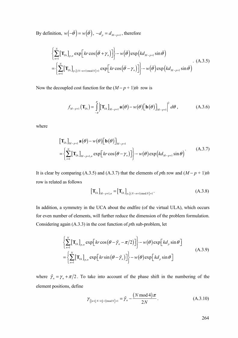
264

By definition, ( ) ( )w wq q- = , 1p M pd d - +- = , therefore

[ ] ( ) ( ) ( )

[ ] { } ( ) ( ) ( )

IA 1,1

IA 1, ( 1)mod 11

exp cos exp sin

exp cos exp sin

N

n M pp nn

N

n M pp N n Nn

kr w kd

kr w kd

q g q q

q g q q

- +=

- +- + +=

Ï ¸È ˘+ -Ì ˝Î ˚Ó ˛Ï ¸È ˘= - -Ì ˝Î ˚Ó ˛

Â

Â

T

T. (A.3.5)

Now the decoupled cost function for the (M - p + 1)th row is

( ) [ ] ( ) ( ) ( )2

1 IA IA 1 1M p M p M pf w d

p

p

q q q q- + - + - +-

È ˘= - Î ˚ÚT T a b , (A.3.6)

where

[ ] ( ) ( ) ( )

[ ] ( ) ( ) ( )IA 1 1

IA 11,1

exp cos exp sin

M p M p

N

n M pM p ni

w

kr w kd

q q q

q g q q

- + - +

- +- +=

È ˘- Î ˚

Ï ¸È ˘= - -Ì ˝Î ˚Ó ˛Â

T a b

T. (A.3.7)

It is clear by comparing (A.3.5) and (A.3.7) that the elements of pth row and (M - p + 1)th

row is related as follows

[ ] [ ] { }IA IA1, , ( 1)mod 1M p n p N n N- + - + +=T T . (A.3.8)

In addition, a symmetry in the UCA about the endfire (of the virtual ULA), which occurs

for even number of elements, will further reduce the dimension of the problem formulation.

Considering again (A.3.3) in the cost function of pth sub-problem, let

[ ] ( ) ( )

[ ] ( ) ( )

IA ,1

IA ,1

exp cos 2 exp sin

exp sin exp sin

N

n pp nn

N

n pp nn

kr w kd

kr w kd

q g p q q

q g q q

=

=

Ï ¸ È ˘È ˘- - -Ì ˝Î ˚ Î ˚Ó ˛Ï ¸ È ˘È ˘= - -Ì ˝Î ˚ Î ˚Ó ˛

Â

Â

T

T (A.3.9)

where 2n ng g p= + . To take into account of the phase shift in the numbering of the

element positions, define

( ){ }( )

/ 4 1 mod 1

mod 42nn N N

NN

pg g

+ - +Í ˙Î ˚= - . (A.3.10)

265

Using this in the summation term of (A.3.9)

[ ] ( ){ }( ) ( )

[ ] { }( ) ( )

IA , / 4 1 mod 11

IA , / 4 1 mod 11

mod 4exp sin exp sin

2


2

N

pp n n N Nn

N

n pp n N Nn

Nkr w kd

N

Nkr w kd

N

pq g q q

pq g q q

+ - +Í ˙Î ˚=

- - +Í ˙Î ˚=

Ï ¸È ˘Ê ˆÔ Ô È ˘- - -Í ˙Ì ˝ Î ˚Á ˜Ë ¯Ô ÔÎ ˚Ó ˛Ï ¸È ˘Ê ˆÔ Ô È ˘= - - -Í ˙Ì ˝ Î ˚Á ˜Ë ¯Ô ÔÎ ˚Ó ˛

Â

Â

T

T

.

(A.3.11)

Alternatively, from (A.3.9) and let u q= - , thus

[ ] ( ) ( )IA ,1

exp sin exp sinN

n pp nn

kr w kdu g u u=

Ï ¸ È ˘È ˘- + - -Ì ˝Î ˚ Î ˚Ó ˛Â T . (A.3.12)

Now, note that the cost function involves the absolute value of (A.3.12). Therefore, the cost

function is unchanged by taking the complex conjugate of (A.3.12)

[ ] ( ) ( )*IA ,

1

exp sin exp sinN

n pp nn

kr w kdu g u u=

Ï ¸ È ˘È ˘+ -Ì ˝Î ˚ Î ˚Ó ˛Â T , (A.3.13)

where the window function ( )w u is real-valued. Applying (A.3.10) to (A.3.13)

[ ] ( ){ }( ) ( )

[ ] ( ){ }( ) ( )

[ ] ( ){ }

*IA , / 4 1 mod 1

1

*IA , / 4 1 mod 1

1

IA , / 4 1 mod


2


2

N

pp n n N Nn

N

pp n n N Nn

p N n N N

Nkr w kd

N

Nkr w kd

N

pu g u u

pu g u u

+ - +Í ˙Î ˚=

+ - +È ˘Í ˙=

- - +È ˘Í ˙

Ï ¸È ˘Ê ˆÔ Ô È ˘+ + -Í ˙Ì ˝ Î ˚Á ˜Ë ¯Ô ÔÎ ˚Ó ˛Ï ¸È ˘Ê ˆÔ Ô È ˘= + - -Í ˙Ì ˝ Î ˚Á ˜Ë ¯Ô ÔÎ ˚Ó ˛

=

Â

Â

T

T

T ( ) ( )*

11


2

N

n pn

Nkr w kd

Np

u g u u+=

Ï ¸È ˘Ê ˆÔ Ô È ˘- - -Í ˙Ì ˝ Î ˚Á ˜Ë ¯Ô ÔÎ ˚Ó ˛Â

,

(A.3.14)

where ( ){ } ( ){ }( )

/ 4 1 mod 1 / 4 1 mod 1

mod 42n N N n N N

NN

pg g

+ - + + - +È ˘ Í ˙Í ˙ Î ˚= + .

Comparing (A.3.11) and (A.3.14), the elements in the pth row of TIA are related by

[ ] { } [ ] ( ){ }*

IA IA, / 4 1 mod 1 , / 4 1 mod 1p n N N p N N n N- - + - - + +Í ˙ È ˘Î ˚ Í ˙=T T , n = 1,…, N. (A.3.15)

266

Simple diagrams are also helpful to illustrate the relationships among the elements within

the matrix TIA which result from symmetry in the spatial distribution of the UCA elements.

The case of symmetry about broadside only is shown in Figure A.3.1. The relationship

between the elements in each row of TIA in the case of double symmetry (about both

broadside and endfire) is shown in Figure A.3.2.

Broadside Virtual ULA UCA

Endfire

q -q

Figure A.3.1. Mirror symmetry about broadside, N = 5, M = 3.

Broadside Virtual ULA UCA

Endfire b

-b l

l

Figure A.3.2. Mirror symmetrical about broadside and endfire, N = 8, M = 5.

It is interesting to note that for an even number of UCA elements in the case of double

symmetry, if four is not a factor of that number, the double symmetry about the endfire axis

occurs for all elements. Otherwise, when four is a factor of N, such as shown in Figure

A.3.2, the double symmetry occurs for all elements except the two UCA elements that fall

on the endfire axis. As a result, the elements of the transformation corresponding to these

267

two UCA elements do not appear in related pairs. This means that there is slightly less

reduction in the dimension of the problem, as compared to case where the number of

elements cannot be factorised by four. More explicitly, the number of distinct elements is

/ 2 1, mod 4 0/ 2, mod 4 2

N NN N

- =ÏÌ =Ó

. (A.3.16)

A.4 Closed Form LS Solution for Davies Array

From [203],

( ) ( )0

1 cos sinnJ t n t dp

j j jp

= -Ú . (A.4.1)

Note that ( )cos sinn tj j- is even since

( ) ( ) ( ) ( )cos sin cos sinf n t n t fj j j j j j- = - + = - = . (A.4.2)

Therefore,

( ) ( )cos sin 2 nn t d J tp

pj j j p

=

- = È ˘Î ˚Ú . (A.4.3)

Let ( )qb be the steering vector of the Davies array and ( )qa is the steering vector of a

UCA in polar form,

( ) ( ) [ ] ( ){ }[ ] [ ]{ }

( ){ }( ) ( )

exp ( 1 ) exp cos 2 1 /

exp exp sin 2 ( 1) / / 2

exp sin

cos sin sin sin

Hpq

j H p jkr q N

j jkr q N

j kr

kr j kr

q q q q p

hq q p p

hq q c

hq q c hq q c

È ˘ = - + - - È - - ˘Î ˚Î ˚

= - - - - +

= - È + + ˘Î ˚= È + + ˘ - È + + ˘Î ˚ Î ˚

b a

,

(A.4.4)

where 2 ( 1) / / 2q Nc p p= - - + , ( )1oM ph = + - , , , 0, , , 1, ,o op M M q N= - =… … … .

Let , 1ddqj q cq

= + = , The two terms of (A.4.4) becomes

268

( )

( ) ( ) ( ) ( )

( ) ( )

cos sin

cos cos sin sin sin sin

cos 2 0

n t d

kr d kr d

J kr

p a

p ap c p c

p c p c

h

j j ha j

hc hj j j hc hj j j

hc p

+

- +

+ +

- + - +

+ -

= - + - - +

= - +

Ú

Ú Ú , (A.4.5)

and

( ) ( ) ( ) ( )

( ) ( )

sin sin

sin cos sin cos sin sin

sin 2 0

kr d

kr d kr d

n J kr

p c

p c

p c p c

p c p c

h

hq hc j j

hc hj j j hc hj j j

c p

+

- +

+ +

- + - +

È ˘- +Î ˚

= - + + - +

= - - +

Ú

Ú Ú . (A.4.6)

Therefore,

( ) ( ) ( )

( ) ( )( )

( )( ) ( ) ( )( )

1 2 ( 1) / / 21

1 / 2 1 2 ( 1) /1

2

2

2

oo

o oo

H jpq

j M p q NM p

j M p j M p q NM p

d J kr e

J kr e

e J kr e

phc

hp

p p

p p

q q q p

p

p

-+ - - - +

+ -

+ - - + - -- + -

È ˘ = -Î ˚

= -

=

Ú b a

, (A.4.7)

since

( ) ( ) ( ) ( )1 nn n nJ t J t J t-- = - = . (A.4.8)

269

Appendix B B.1 Special Structure of Robust Transformation Matrices

In this section, the special structure of the robust transformation matrices for the SIP and LS

problem formulations is investigated. First, the relationship between pairs of conjugate

rows is derived. To this end, the error function that forms part of the constraint of ( 3.2P ) is

defined as

( ) { }( ) ( ) , 1, ,Tp p pe b p Mq q q= - =u a … . (B.1.1)

If the minimiser of ( 3.2P ) is given by opt , 1, ,p p M=u … , then the task is to explicitly

show the relationship of optpu between pairs of conjugate rows, i.e. 1, 2, , om M= ± ± ±… ,

where 1om p M= - - . Using the earlier definitions for UCA and Davies array steering

vectors, (B.1.1) can be expressed as

( ) ( ) ( )opt

1exp cos exp , , ,

N

m m i o oiie jkr jm m M Mq q g q

=

È ˘ È ˘= - - = -Î ˚Î ˚Â u … . (B.1.2)

It is easy to see that a conjugate operation on (B.1.2) does not affect the constraints of

( 3.2P ), i.e.

{ }Re ( ) ( )Tm m mbq q e- £u a and { }Im ( ) ( )T

m m mbq q e- £u a . (B.1.3)

Therefore, as far as the problem formulation is concerned, the conjugated error function

also satisfies the constraints

( ) ( ) ( )** opt

1exp cos exp

N

m m iiie jkr jmq q g q

=

È ˘ È ˘= - - - -Î ˚Î ˚Â u . (B.1.4)

Now, since ( )cos cosq p q+ = - ,

( ) ( ) ( )

( ) ( )

** opt

1

*opt

1

exp cos exp

exp cos exp

N

m m iiiN

m iii

e jkr jm

jkr jm

q q g p q

q g q p

=

=

È ˘ È ˘= - + - -Î ˚Î ˚

È ˘ È ˘ È ˘= - - - -Î ˚ Î ˚Î ˚

Â

Â

u

u

, (B.1.5)

270

where q q p= + . Multiplying (B.1.5) by ( ) ( )exp 1 mjmp- = - again will not affect the

constraints of (B.1.3)

( ) ( ){ } ( ) ( )** opt

11 exp cos exp

Nm

m m iiie jkr jmq q g q

=

È ˘ È ˘= - - - -Î ˚Î ˚Â u . (B.1.6)

Now the error function for the -mth sub-problem can be written as

( ) ( ) ( )opt

1exp cos exp

N

m p iiie jkr jmq q g q-

=

È ˘ È ˘= - - -Î ˚Î ˚Â u . (B.1.7)

Comparing (B.1.6) and (B.1.7), the following relationship between the conjugate rows of

mth and thm- , is established

( ) ( )*opt opt 1 m

m m=- -u u . (B.1.8)

Note that this is related to the Bessel function property of ( ) ( ) ( )1 mm mJ t J t- = - reflected

in the conjugate rows (diagonal elements) of the J matrix of the Davies transformation. In

essence, the special structure in the Davies transformation is similar to that obtained via the

robustification procedure.

It should be noted that while applying property (B.1.8) for a conjugate row saves

computation, the optm-u as obtained is not necessarily the solution of the conjugate row opt

mu

if the dual parameterisation approach is performed directly on that row. This is because

dual parameterisation does not guarantee the global solution. Therefore, optm-u is only one

local minimum satisfying the constraints. Other local solutions may be found by direct

computation.

271

References [1] http://www.gsmworld.com, Oct. 2002.

[2] G. Vincent, “Learning from i-mode,” IEE Review, vol. 47, no. 6, pp. 13-18, Nov.

2001.

[3] E. Dahlman, P. Beming, J. Knutsson, F. Ovesjö, M. Persson, and C. Roobol,

“WCDMA-the radio interface for future mobile multimedia communications,”

IEEE Trans Vehic. Technol., vol. 47, no. 4, pp. 1105-1118, Nov. 1998.

[4] L. C. Godara, “Application of antenna arrays to mobile communications, Part I:

Performance improvement, feasibility, and system considerations,” Proc. IEEE, vol.

85, No. 7, pp. 1029-1060, Jul. 1997.

[5] L. C. Godara, “Application of antenna arrays to mobile communications, Part II:

Beamforming and direction-of-arrival considerations,” Proc. IEEE, vol. 85, No. 8,

pp. 1193-1245, Aug. 1997.

[6] S. Swales, M. Beach, D. Edwards, and J. McGeehan, “The performance

enhancement of multibeam adaptive base-station antennas for cellular land mobile

radio systems,” IEEE Trans. Vehic. Technol., vol. 39, pp. 56-67, Feb. 1990.

[7] J. S. Thompson, P. M. Grant, and B. Mulgrew, “Smart antenna arrays for CDMA

systems,” IEEE Personal Commun., vol. 3, no. 5, pp. 16-25, Oct. 1996.

[8] G. E. Bottomley and K. J. Molnar, “Interference cancellation for improved channel

estimation in array processing MLSE receivers,” in Proc. IEEE 47th VTC, vol.1, pp.

140-144, Phoenix, Arizona, May 4-7, 1997.

[9] H. P. Lin, S. S. Jeng, I. Parra, G. Xu, W. J. Vogel, and G. W. Torrence,

“Experimental studies of SDMA schemes for wireless communications,” in Proc.

IEEE ICASSP’95, vol. 3, pp. 1760-1763, Detroit, MI, May 1995.

[10] G. Tsoulos, J. McGeehan, M. Beach, “Space Division Multiple Access (SDMA)

field trials. Part 1: Tracking and BER performance,” IEE Proc.- Radar, Sonar, and

Navig., vol. 145, no. 1, pp. 73-78, Feb. 1998.

[11] G. Tsoulos, J. McGeehan, M. Beach, “SDMA field trials. Part 2: Calibration and

linearity issues,” IEE Proc.- Radar, Sonar, and Navig., vol. 145, no. 1, pp. 79-84,

Feb. 1998.

[12] B. Ottersten, “Array processing for wireless communications,” in Proc 8th IEEE

Signal Processing Workshop on Statistical Signal and Array Processing, pp. 466-

473, Corfu, Greece, Jun. 1996.

272

[13] C. Brunner, M. Haardt, and J. A. Nossek, “On space-time RAKE receiver structures

for WCDMA,” in Proc. 33th Asilomar Conf. Signals, Syst., Comput., vol. 2, pp.

1546-1551, Pacific Grove, CA, Oct. 1999.

[14] C. Brunner, M. Haardt, and J. A. Nossek, “Adaptive space-frequency rake receivers

for WCDMA,” in Proc. IEEE ICASSP’99, vol. 4, pp. 2383-2386, Phoenix, Arizona,

USA, Mar. 1999.

[15] A. Naguib and A. Paulraj, “Performance of CDMA cellular networks with base-

station antenna arrays,” in Proc. International Zurich Seminar on Digital

Communications 1994, pp. 87-100, Zurich, Switzerland, Mar. 1994.

[16] A. F. Naguib, “Adaptive Antennas for CDMA wireless networks,” PhD Thesis,

Department of Electrical Engineering, Stanford University, Aug. 1996.

[17] S. Andersson, B. Hagerman, H. Dam, U. Forssén, J. Karlsson, F. Kronestedt, S.

Mazur, and K. J. Molnar, “Adaptive Antennas for GSM and TDMA Systems,”

IEEE Personal Commun., vol. 6., no. 3, pp. 74-86, Jun. 1999.

[18] A. E. Zooghby, “Potentials of smart antennas in CDMA systems and uplink

improvements,” IEEE Antennas Propagat. Mag., vol. 43, pp. 172-177, Oct. 2001.

[19] S. Anderson, M. Millnert, M. Viberg, and B. Wahlberg, “An adaptive array for

mobile communication systems,” IEEE Trans. Vehic. Technol., vol. 40, pp. 230-

236, Feb. 1991.

[20] S. Choi, D. Shim, and T. K. Sarkar, “A comparison of tracking-beam arrays and

switching-beam arrays operating in a CDMA mobile communication channel,”

IEEE Antennas and Propagation Magazine, vol. 41, no. 6, pp. 10-22, Dec. 1999.

[21] S. S. Jeng, G. Xu, H. P. Lin, and W. J. Vogel, “Experimental studies of spatial

signature variation at 900MHz for smart antenna systems,” IEEE Trans. Antennas

Propagat., vol. 46, pp. 953-962, Jul. 1998.

[22] G. Xu and H. Liu, “An effective transmission beamforming scheme for frequency-

duplex digital wireless communication systems,” in Proc. IEEE ICASSP’95, vol.3,

pp.1729-1731, Detroit, MI, May 1995.

[23] W. Yang, A. Kavak, and G. Xu, “On the multichannel characteristics of a 1.8GHz

smart antenna system using a circular array in realistic non-stationary wireless

scenarios,” in Proc. IEEE ICASSP’99, vol. 5, pp. 2607-2610, Phoenix, Arizona,

USA, Mar. 1999.

[24] A. Kavak, M. Torlak, W. J. Vogel, and G. Xu, “Vector channels for smart antennas.

Measurements, statistical modeling, and directional properties in outdoor

273

environments,” IEEE Transactions on Microwave Theory and Techniques, pp. 930-

937, Jun. 2000

[25] J. P. Rossi, J. P. Barbot, A. J. Levy, “Theory and measurement of the angle of

arrival and time delay of UHF radiowaves using a ring array,” IEEE Trans.

Antennas Propagat., vol. 45, pp. 876-884, May 1997.

[26] P. Chevalier, F. Pipon, J. J. Monot, and C. Demeure, “Smart antennas for the GSM

system: experimental results for a mobile reception,” in Proc. IEEE 47th VTC, vol.

3, pp.1572-1576, Phoenix, Arizona, May 1997.

[27] J. A. Tsai and B. D. Woerner, “Adaptive beamforming of uniform circular arrays

(UCA) for wireless CDMA system,” in Proc. 35th Asilomar Conf. Signals, Syst.,

Comput., vol. 1, pp. 399-403, Pacific Grove, CA, 4-7 Nov. 2001.

[28] T. Rouphael and J. R. Cruz, “Enhanced CDMA cellular system using interpolated

circular arrays,” in Proc. IEEE 46th VTC, vol. 2, pp. 1071-1075, Atlanta, Georgia,

Apr. 1996.

[29] I. Jouny, “Signal separation using circular arrays,” in Proc. IEEE MILCOM, vol. 1,

pp. 666-670, Atlantic City, NJ, Oct. 1999.

[30] J. W. Liang and A. Paulraj, “On optimizing base station antenna array topology for

coverage extension in cellular radio networks,” in Proc. IEEE 47th VTC, vol. 1, pp.

866-870, Phoenix, Arizona, May 1997.

[31] R. Stridh and B. Ottersten, “Packet data throughput for wireless systems with smart

antennas,” Proc. IEEE 50th VTC Fall, vol. 1, pp. 32-36, Amsterdam, Netherlands,

Sep. 1999.

[32] H. Asakura and T. Matsumoto, “Cooperative signal reception and down-link beam

forming in cellular mobile communications,” IEEE Trans Vehic. Technol., vol. 48,

no. 2, pp. 333-341, Mar. 1999.

[33] D. Wong and T. J. Lim, “Soft handoffs in CDMA mobile systems,” IEEE Personal

Commun., vol. 4, pp. 6-17, Dec. 1997.

[34] Basic concepts of WCDMA Radio Access Networks. Ericsson White Paper.

http://www.ericsson.com/products/white_papers_pdf/, Oct. 2002.

[35] H. Krim and M. Viberg, “Two decades of array signal processing research: The

parametric approach,” IEEE Signal Processing Magazine, vol. 13, pp. 67-94, Jul.

1996.

[36] http://www.ericsson.com, Oct. 2002.

[37] http://www.arraycomm.com, Oct. 2002.

274

[38] http://www.3gamericas.org, Oct. 2002.

[39] J. Cai and D. J. Goodman, “General Packet Radio Service in GSM,” IEEE

Commun. Mag., vol. 35, no. 10, pp. 122-131, Oct. 1997.

[40] A. Furuskär, S. Mazur, F. Müller, and H. Olofsson, “EDGE: Enhanced data rates

for GSM and TDMA/136 evolution,” IEEE Personal Commun., vol. 6, no. 3, pp.

56-66, Jun. 1999.

[41] ETSI. 3GPP. TS 03.64, “Digital cellular telecommunications system (Phase 2+);

Overall description of the GPRS radio interface; Stage 2,” version 8.9.0, Jan. 2002.

[42] P. Schramm, H. Andreasson, C. Edholm, N. Edvardsson, M. Höök, S. Jäverbring, F.

Müller, and J. Sköld, “Radio interface performance of EDGE, a proposal for

enhanced data rates in existing digital cellular systems,” in Proc. IEEE 48th VTC,

vol. 2, pp. 1064-1068, Ottawa, Canada, May 1998.

[43] J. Uddenfeldt, “Digital cellular – its roots and its future,” Proc. IEEE, vol. 86, pp.

1319-1324, Jul. 1998.

[44] B. Göransson, B. Hagerman, and J. Barta, “Adaptive Antennas in WCDMA

Systems – Link Level Simulation Results Based on Typical User Scenarios,” in

Proc. IEEE 52nd VTC Fall, vol. 1, pp. 157-164, Boston, MA, Sep. 2000

[45] F. Petré, G. Leus, L. Deneire, M. Engels, M. Moonen, H. D. Man, “Space-time chip

equalizer receivers for WCDMA forward link with time-multiplexed pilot,” in Proc.

IEEE 54th VTC Fall, vol. 2, pp. 1058-1062, Atlantic City, NJ, Oct. 2001.

[46] Y. J. Guo, S. Vadgama, and Y. Tanaka, “Advanced base station technologies for

UTRAN,” IEE Electron. Commun. Eng. J., pp. 123-132, Jun. 2000.

[47] I. Sawahashi, K. Higuchi, S. Tanaka, F. Adachi, “Enhanced wireless access

technologies and experiments for W-CDMA communications,” IEEE Personal

Commun., vol. 7., no. 6, pp. 6-16, Dec. 2000.

[48] “FCC - Enhance 911 (E-911) Homepage”, http://www.fcc.gov/911/enhanced/

[49] J. J. Caffery, Jr. and G. L. Stüber, “Overview of radiolocation in CDMA cellular

systems,” IEEE Commun. Mag., vol. 36, no. 4, pp. 38-45, Apr. 1998.

[50] T. S. Rappaport, J. H. Reed, and B. D. Woerner, “Position location using wireless

communications on highways of the future,” IEEE Commun. Mag., vol. 34, pp. 33-

41, Oct. 1996.

[51] D. E. N. Davies, “A transformation between the phasing techniques required for

linear and circular aerial arrays,” Proc. IEE, vol. 112, pp. 2041-2045, Nov. 1965.

275

[52] T. Rahim and D. E. N. Davies, “Effect of directional elements on the directional

response of circular antenna arrays,” IEE Proc., vol. 129, pt. H, pp. 18-22, Feb.

1982.

[53] D. E. N. Davies and M. S. A. S. Rizk, “A broadband experimental null-steering

antenna system for mobile communications,” Radio & Electron. Eng., vol. 48, pp.

509-517, Oct. 1978.

[54] M. Wax and J. Sheinvald, “Direction finding of coherent signals via spatial

smoothing for uniform circular arrays,” IEEE Trans. Antennas Propagat., vol. 42,

pp. 613-620, May 1994.

[55] C. P. Mathews, M. D. Zoltowski, “Eigenstructure techniques for 2-D angle

estimation with uniform circular arrays,” IEEE Trans. Signal Processing, vol. 42,

pp. 2395-2407, Sep. 1994.

[56] R. Eiges and H. D. Griffiths, “Mode-space spatial spectral estimation for circular

arrays,” IEE Proc. – Radar, Sonar Navig., vol. 141, pp. 300-306, Dec. 1994.

[57] D. N. Swingler and S. Davies, “Spatial harmonic interpolation and extrapolation for

use with circular arrays,” in Proc. IEEE Pacific Rim Conference on

Communications, Computers and Signal Processing, Victoria, Canada, vol. 1,

pp.138-141, May 1991.

[58] T. P. Bronez, “Sector interpolation of nonuniform arrays for efficient high

resolution bearing estimation,” in Proc. IEEE ICASSP’88, vol. 5, pp. 2885-2888,

New York, NY, Apr. 1988.

[59] B. Friedlander, “Direction finding with an interpolated array,” in Proc. ICASSP’90,

vol. 5, pp. 2951-2954, Albuquerque, NM, USA, Apr. 1990.

[60] B. Friedlander, “The Root-MUSIC algorithm for direction finding with interpolated

arrays,” Signal Processing, vol. 30, pp. 15-29, Jan. 1993.

[61] B. Friedlander and A. J. Weiss, “Direction finding for wide-band signals using an

interpolated array,” IEEE Trans. Signal Processing, vol. 41, pp. 1618-1634, Apr.

1993.

[62] B. Friedlander, A. J. Weiss, “Performance analysis of wideband direction finding

using interpolated arrays,” in Proc. IEEE ICASSP’92, vol. 4, pp. 457-460, San

Francisco, CA, Apr. 1992.

276

[63] A. J. Weiss and B. Friedlander, “Performance analysis of spatial smoothing with

interpolated array,” IEEE Trans. Signal Processing, vol. 41, pp. 1881-1892, May

1993.

[64] A. J. Weiss, B. Friedlander, and P. Stoica, “Direction-of-arrival estimation using

MODE with interpolated arrays,” IEEE Trans. Signal Processing, vol. 43, pp. 296-

300, Jan. 1995.

[65] B. Friedlander and A. J. Weiss, “Direction finding using spatial smoothing with

interpolated arrays,” IEEE Trans. Aerosp. Electron. Syst., vol. 28, pp. 574-587, Apr.

1992.

[66] D. V. Sidorovich and A. B. Gershman, “Two-dimensional wideband interpolated

Root-MUSIC applied to measured seismic data,” IEEE Trans. Signal Processing,

vol.46, pp.2263-2267, Aug. 1998.

[67] A. B. Gershman, “Direction finding using beamspace root estimator banks,” IEEE

Trans. Signal Processing, vol. 46, pp. 3131-3135, Nov. 1998.

[68] T. E. Biedka, J. H. Reed, and B. D. Woerner, “Direction finding methods for

CDMA systems,” in Proc. 30th Asilomar Conf. Signals, Syst., Comput., vol. 1, pp.

637-641, Pacific Grove, CA, Nov. 1996.

[69] T. E. Biedka, “Direction finding methods for CDMA mobile wireless systems,”

Class Project MPRG-TR-96-20, Department of Electrical Engineering, Virginia

Tech, Blacksburg, VA, May 1996.

[70] Z. Lei and T. J. Lim, “Estimation of directions of arrival of multipath signals in

CDMA systems,” IEEE Trans. Commun., vol. 48, pp. 1022-1028, Jun. 2000.

[71] B. K. Lau, G. Cook, and Y. H. Leung, “Direction-of-arrival estimation in the

presence of correlated signals with non-ideal uniform circular arrays,” in Proc.

Konferensen RadioVetenskap och Kommunikation (RVK’2002), vol. 1, pp. 558-562,

Stockholm, Sweden, Jun. 2002.

[72] B. K. Lau and Y. H. Leung, “Dolph-Chebyshev Approach to the Synthesis of Beam

Patterns for Uniform Circular Arrays,” in Proc. IEEE ISCAS’2000, vol. 1, pp. 124-

127, Geneva, Switzerland, May 2000.

[73] B. K. Lau and Y. H. Leung, “Optimum Beamformers for Uniform Circular Arrays

in a Correlated Signal Environment,” in Proc. IEEE ICASSP’2000, vol. 5, pp. 3093-

3096, Istanbul, Turkey, Jun. 2000.

277

[74] G. J. Cook, B. K. Lau, and Y. H. Leung, “An alternative approach to interpolated

array processing for uniform circular arrays,” IEEE Asia Pacific Conference on

Circuits and Systems (APCCAS’2002), accepted.

[75] B. K. Lau, Y. H. Leung, Y. Liu, and K. L. Teo, “A robust approach to the synthesis

of Dolph-Chebyshev beampatterns for uniform circular arrays,” in Proc.

International Conference on Optimisation Techniques and Applications, vol. 4, pp.

1464-1471, Hong Kong, China, Dec. 2001.

[76] B. K. Lau. Y. H. Leung, Y. Liu, and K. L. Teo, "Direction-of-arrival estimation in

the presence of correlated signals and array imperfections with uniform circular

arrays," in Proc. IEEE ICASSP'2002, vol. 3, pp. 3037-3040, Orlando, FL, May

2002.

[77] B. K. Lau, Y. H. Leung, Y. Liu, and K. L. Teo, “Direction-of-arrival estimation

with imperfect uniform circular arrays in correlated signal environments,” IEEE

Signal Processing Letters, submitted.

[78] B. K. Lau. Y. H. Leung, B. Hagerman, and S. Andersson, “A novel direction-of-

arrival estimation algorithm for WCDMA,” in Proc. Konferensen RadioVetenskap

och Kommunikation (RVK’2002), vol. 1, pp. 6-10, Stockholm, Sweden, Jun. 2002.

[79] L. M. Correia, ed., Wireless flexible personalized communications - COST 259:

European co-operation in mobile radio research, John Wiley & Sons, 2001.

[80] B. K. Lau, M. Berg, S. Andersson, B. Hagerman, and M. Olsson, “System

Performance of EGPRS with an Adaptive Antenna System,” in Proc. Nordic Radio

Symposium, Nynäshamn, Sweden, Apr. 2001.

[81] B. K. Lau, M. Berg, S. Andersson, B. Hagerman, and M. Olsson, “Performance of

an Adaptive Antenna System in EGPRS Networks,” in Proc. IEEE VTC Spring,

vol. 4, pp. 2354-2358, Rhodes, Greece, May 2001.

[82] B. K. Lau, M. Olsson, S. Andersson, and H. Asplund, “Link Level Performance of

EDGE with Adaptive Antenna Systems,” in Proc. VTC Fall, vol. 4, pp. 2003-2007

Atlantic City, NJ, Oct. 2001.

[83] G. Ziehm, “Optimum directional pattern synthesis of circular arrays,” Radio &

Electron. Eng., vol. 28, pp. 341-355, Nov. 1964.

[84] C. L. Dolph, “A current distribution for broadside arrays which optimizes the

relationship between beam width and side-lobe level,” Proc. IRE, vol. 34, pp. 335-

348, Jun. 1946.

278

[85] J. E. Evans, J. R. Johnson, and D. F. Sun, “Application of advanced signal

processing angle-of-arrival estimation in ATC navigation and surveillance

systems,” MIT Lincoln Lab., Lexington, MA, Rep. 582, 1982.

[86] S. U. Pillai and B. H. Kwon, “Forward-backward spatial smoothing techniques for

coherent signal identification,” IEEE Trans. Acoust., Speech, Signal Processing,

vol. 37, no. 1, pp. 8-15, Jan. 1989.

[87] R. T. Williams, S. Prasad, A. K. Mahalanabis, and L. H. Sibul, “An improved

spatial smoothing technique for bearing estimation in a multipath environment,”

IEEE Trans. Acoust., Speech and Signal Processing, vol. ASSP-36, pp. 425-432,

Apr. 1988.

[88] T. J. Shan and T. Kailath, “Adaptive beamforming for coherent signals and

interference,” IEEE Trans. Acoust., Speech, Signal Processing, vol. 33, no. 3, pp.

527-536, Mar. 1985.

[89] B. D. van Veen and K. M. Buckley, “Beamforming: a versatile approach to spatial

filtering,” IEEE ASSP Magazine, vol. 5, no. 2, pp. 4-24, Apr. 1988.

[90] C. W. Therrien, Discrete random signals and statistical signal processing, Prentice

Hall, 1992.

[91] D. E. N. Davies, “Circular arrays,” in The handbook of antenna design (A. W.

Rudge et al., eds.), Peter Peregrinus, Stevenage, vol. 2, chap. 12, 1983.

[92] I. D. Longstaff, P. E. K. Chow, and D. E. N. Davies, “Directional properties of

circular arrays,” Proc. IEE, vol. 114, pp. 713-718, Jun. 1967.

[93] J. C. Lim and D. E. N. Davies, “Synthesis of a single null response in an otherwise

omnidirectional pattern using a circular array,” Proc. IEE, vol. 122, pp. 349-352,

Apr. 1975.

[94] J. R. F. Guy and D. E. N. Davies, “UHF circular arrays incorporating open-loop null

steering for communications,” IEE Proc., vol. 130, pt. F and H, pp. 67-77, Feb.

1983.

[95] D. E. N. Davies and M. Rizk, “Electronic steering of multiple nulls for circular

arrays,” Electron. Lett., vol. 13, pp. 669-670, 27th Oct. 1977.

[96] J. R. F. Guy and D. E. N. Davies, “Studies of the Adcock direction finder in terms

of phase-mode excitations around circular arrays,” Radio & Electron. Eng., vol. 53,

pp. 33-38, Jan. 1983.

279

[97] B. Sheleg, “A matrix-fed circular array for continuous scanning,” Proc. IEEE, vol.

56, no. 11, pp. 2016-2027, Nov. 1968.

[98] J. N. Maksym, “Directional accuracy of small ring arrays,” J. Acoust. Soc. Amer.,

vol. 61, no. 1, pp. 105-109, Jan. 1977.

[99] D. N. Swingler and R. S. Walker, “Line-array beamforming using linear prediction

for aperture interpolation and extrapolation,” IEEE Trans. Acoust., Speech and

Signal Processing, vol. 37, pp. 16-30, Jan. 1989.

[100] A. H. Tewfik and W. Hong, “On the application of uniform linear array bearing

estimation techniques to uniform circular array,” IEEE Trans. Signal Processing,

vol. 40, pp. 1008-1011, Apr. 1992.

[101] M. D. Zoltowski and C. P. Mathews, “Direction finding with uniform circular

arrays via phase mode excitation and beamspace Root-MUSIC,” in Proc. IEEE

ICASSP’92, vol. 5, pp. 245-248, San Francisco, CA, Mar. 1992.

[102] C. P. Mathews and M. D. Zoltowski, “Performance analysis of the UCA-ESPRIT

algorithm for circular ring arrays,” IEEE Trans. Signal Processing, vol. 42, pp.

2535-2539, Sep. 1994.

[103] A. J. Weiss and B. Friedlander, “Preprocessing for direction finding with minimal

variance degradation,” IEEE Trans. Signal Processing, vol. 42, pp. 1478-1485, Jun.

1994.

[104] M. P. Moody, “Resolution of coherent sources incident on a circular antenna array,”

Proc. IEEE, vol. 68, no. 2, pp. 276-277, Feb. 1980.

[105] M. A. Doron, E. Doron, and A. J. Weiss, “Coherent wide-band processing for

arbitrary array geometry,” IEEE Trans. Signal Processing, vol. 41, pp. 414-415,

Jan. 1993.

[106] R. O. Schmidt, “Multiple emitter location and signal parameter estimation,” IEEE

Trans. Antennas Propagat., vol. AP-34, pp. 276-280, Mar. 1986.

[107] A. Zeira and B. Friedlander, “Interpolated array minimum variance beamforming

for correlated interference rejection,” in Proc. IEEE ICASSP’96, vol. 6, pp. 3165-

3168, Atlanta, Georgia, USA, May 1996.

[108] M. A. Doron and E. Doron, “Wavefield modelling and array processing, part I –

spatial sampling”, IEEE Trans. Signal Processing, vol. 42, pp. 2549-2559, Oct.

1994.

[109] M. A. Doron and E. Doron, “Wavefield modeling and array processing, part II –

algorithms”, IEEE Trans. Signal Processing, vol. 42, pp. 2560-2570, Oct. 1994.

280

[110] M. A. Doron and E. Doron, “Wavefield modeling and array processing, part III –

resolution capacity”, IEEE Trans. Signal Processing, vol. 42, pp. 2571-2580, Oct.

1994.

[111] M. A. Doron and E. Doron, “Reduced rank processing for oversampled arrays,”

IEEE Trans. Signal Processing, vol. 44, pp. 900-911, Apr. 1996.

[112] T. P. Bronez and J. A. Cadzow, “An algebraic approach to superresolution array

processing,” IEEE Trans. Aerosp. Electron. Syst., vol. AES-19, pp. 123-133, Jan.

1983.

[113] A. J. Weiss and M. Gavish, “Direction finding using ESPRIT with interpolated

arrays,” IEEE Trans. Signal Processing, vol. 39, pp. 1473-1478, Jun. 1991.

[114] M. Gavish, A. J. Weiss, "Performance analysis of the VIA-ESPRIT algorithm", IEE

Proc. - Radar and Signal Processing, vol. 140, pt. F, pp. 123-128, Apr. 1993.

[115] A. J. Weiss, B. Friedlander, and P. Stoica, “Direction finding with interpolated

MODE,” in Proc. IEEE 27th Asilomar Conf. Signals, Syst., Comput., vol. 2, pp.

1376-1380, Pacific Grove, CA, Nov. 1993.

[116] H. Hung and M. Kaveh, “Focussing matrices for coherent signal-subspace

processing,” IEEE Trans. Acoust., Speech and Signal Processing, vol. 36, pp. 1272-

1281, Aug. 1988.

[117] H. Wang and M. Kaveh, “Coherent signal-subspace processing for the detection and

estimation of angles of arrival of multiple wide-band sources,” IEEE Trans. Acoust.,

Speech and Signal Processing, vol. ASSP-33, pp. 823-831, Aug. 1985.

[118] J. Krolik and D. Swingler, “Focused wide-band array processing by spatial

resampling,” IEEE Trans. Signal Processing, vol. 38, pp. 356-360, Feb. 1990.

[119] W. Hong and A. H. Tewfik, “Focusing matrices for wideband array processing with

no a priori angle estimates,” in Proc. IEEE ICASSP’92, vol. 2, pp. 493-496, San

Francisco, CA, Mar. 1992.

[120] M. J. D. Rendas and J. M. F. Moura, “Resolving narrowband coherent paths with

non-uniform arrays,” in Proc. IEEE ICASSP’89, vol. 4, pp. 2625-2628, Glasgow,

Scotland, UK, May 1989.

[121] K. M. Reddy and V. U. Reddy, “Analysis of spatial smoothing with uniform

circular arrays,” IEEE Trans. Signal Processing, vol. 47, pp. 1726-1730, Jun. 1999.

[122] K. M. Reddy and V. U. Reddy, “Analysis of interpolated arrays with spatial

smoothing,” Signal Processing, vol. 54, no. 3, pp. 261-272, Nov. 1996.

[123] S. Haykin, Communication systems, 4th Edition, John Wiley & Sons, 2001.

281

[124] Y. Bresler and A. Macovski, “On the number of signals resolvable by a uniform

linear array,” IEEE Trans. Acoust., Speech and Signal Processing, vol. ASSP-34,

pp. 1361-1375, Dec. 1986.

[125] B. Friedlander and A. J. Weiss, “On the number of signals whose directions can be

estimated by an array,” IEEE Trans. Signal Processing, vol. 39, pp. 1686-1689, Jul.

1991.

[126] J. Capon, “High-resolution frequency-wavenumber spectrum analysis,” Proc. IEEE,

vol. 57, pp. 1408-1418, Aug. 1969.

[127] H. Wang, K. J. R. Liu, “2-D spatial smoothing for multipath coherent signal

separation,” IEEE Trans. Aerosp. Electron. Syst., vol. 34, pp. 391-405, Apr. 1998.

[128] A. J. Weiss and B. Friedlander, “On the Cramér-Rao bound for direction finding of

correlated signals,” IEEE Trans. Signal Processing, vol. 41, pp. 495-499, Jan. 1993.

[129] R. Eklöf, “Dolph-Chebyshev shading for non-ideal uniform linear arrays and non-

ideal uniform circular arrays,” MSc Thesis, ATRI, Curtin University of

Technology, Australia, and Blekinge Institute of Technology, Sweden, Dec. 2000.

[130] Y. Liu, K. L. Teo, and S. Ito, “Global optimisation in quadratic semi-infinite

programming,” Computing, Supplement 15, pp. 119-132, 2001.

[131] Y. Liu and K. L. Teo, “Adaptive dual parameterization algorithm for quadratic

semi-infinite programming problems,” J. of Global Optimization, vol. 24, pp. 205-

217, Oct. 2002.

[132] G. Cook, “A robust mode space transform for uniform circular arrays,” Final Year

Engineering Project Thesis, Department of Electrical and Electronic Engineering,

University of Western Australia, Australia, Nov. 2001.

[133] R. Bronson, Schaum's Outline of Theory and Problems of Matrix Operations,

McGraw-Hill, New York, 1989.

[134] T. Rahim, “Analysis of the element pattern shape for circular arrays,” Electron.

Lett., vol. 19, no. 20 , pp. 838-840, 29th Sep. 1983.

[135] A. C. McCormick and E. A. Al-Susa, “Multicarrier CDMA for future generation

mobile communication,” IEE Electron. Commun. Eng. J., vol. 14, no. 2, pp. 52-60,

Apr. 2002.

[136] M. Viberg, B. Ottersten, and T. Kailath, “Detection and estimation in sensor arrays

using weighted subspace fitting,” IEEE Trans. Signal Processing, vol. 39, pp. 2436-

2449, Nov. 1991.

282

[137] P. Stoica and K. Sharman, “Novel eigenanalysis method for direction estimation,”

IEE Proc., vol. 137, pt. F, pp. 19-26, Feb. 1990.

[138] M. Zoltowski and F. Haber, “A vector space approach to direction finding in a

coherent multipath environment,” IEEE Trans. Antennas Propagat., vol. AP-34, pp.

1069-1079, Sep. 1986.

[139] R. Roy and T. Kailath, “ESPRIT - Estimation of Signal Parameters Via Rotational

Invariance Techniques,” IEEE Trans. Acoust., Speech and Signal Processing, vol.

37, pp. 984-995, Jul. 1989.

[140] B. L. Lim, S. K. Hui, and Y. C. Lim, “Bearing estimation of coherent sources by

circular spatial modulation averaging (CSMA) technique,” Electronic Lett., vol. 26,

no. 5, pp. 343-345, 1st Mar. 1990.

[141] J. A. Fessler and A. O. Hero, “Space-alternating generalized expectation-

maximization algorithm,” IEEE Trans. Signal Processing, vol. 42, no. 10, pp. 2664-

2677, Oct. 1994.

[142] B. H. Fleury, M. Tschudin, R. Heddergott, D. Dahlhaus, and K. I. Pedersen,

“Channel parameter estimation in mobile radio environments using the SAGE

algorithm,” IEEE J. Select. Areas Commun., vol. 17, no. 3, pp. 434-450, Mar. 1999.

[143] P. J. Chung and J. F. Böhme, “Comparative convergence analysis of EM and SAGE

algorithms in DOA estimation,” IEEE Trans. Signal Processing, vol. 49, pp. 2940-

2949, Dec. 2001.

[144] T. J. Shan, M. Wax, and T. Kailath, “On spatial smoothing for direction-of-arrival

estimation of coherent signals,” IEEE Trans. Acoust., Speech and Signal

Processing, vol. ASSP-33, pp. 806-811, Aug. 1985.

[145] J. S. Thompson, P. M. Grant, and B. Mulgrew, “Performance of spatial smoothing

algorithms for correlated sources,” IEEE Trans. Signal Processing, vol. 44, pp.

1040-1046, Apr. 1996.

[146] M. Wax and T. Kailath, “Determining the number of sources by information

theoretic criteria,” IEEE Trans. Acoust., Speech and Signal Processing, vol. ASSP-

33, pp. 387-392, Apr. 1985.

[147] A. J. Barabell, “Improving the resolution performance of eigenstructure-based

direction-finding algorithms,” Proc. IEEE ICASSP, Boston, MA, pp. 336-339.

1983.

[148] B. D. Rao and K. V. S. Hari, “Performance analysis of Root-MUSIC,” IEEE Trans.

Acoust., Speech and Signal Processing, vol. 37, pp. 1939-1949, Dec. 1989.

283

[149] V. Nagesha and S. Kay, “On frequency estimation with the IQML algorithm,” IEEE

Trans. Signal Processing, vol. 42, pp. 2509-2513, Sep. 1994.

[150] B. D. Rao and K. V. S. Hari, “Effect of spatial smoothing on the performance of

MUSIC and the minimum-norm method,” IEE Proc., vol. 137, pt. F, pp. 449-458,

Dec. 1990.

[151] A. L. Swindlehurst and T. Kailath, “A performance analysis of subspace-based

methods in the presence of model errors, part 1: The MUSIC algorithm,” IEEE

Trans. Signal Processing, vol. 40, pp. 1758-1774, Jul. 1992.

[152] A. L. Swindlehurst and T. Kailath, “A performance analysis of subspace-based

methods in the presence of model errors: part II – multidimensional algorithms,”

IEEE Trans. Signal Processing, vol. 41, pp. 2882-2890, Sep. 1993.

[153] B. Wahlberg, B. Ottersten, and M. Viberg, “Robust signal parameter estimation in

the presence of array perturbations,” in Proc. IEEE ICASSP’91, vol. 5, pp. 3277-

3280, Toronto, Canada, May 1991.

[154] R. J. Stegen, “Excitation coefficients and beam-widths of Tschebyscheff Arrays,”

Proc. IRE, vol. 40, no. 11, pp. 1671-1674, 1953.

[155] J. E. Hudson, Adaptive Array Principles (Revised Ed.) – IEE electromagnetic

waves series v. 28, Peregrinus (London), 1989.

[156] H. Schjær-Jacobsen and K. Madsen, “Synthesis of nonuniformly-spaced arrays

using a general nonlinear minimax optimization method,” IEEE Trans. Antennas

Propagat., vol. AP-24, pp. 501-506, Jul. 1976.

[157] C. A. Olen and R. T. Compton, Jr., “A numerical pattern synthesis algorithm for

arrays,” IEEE Trans. Antennas Propagat., vol. 38, pp. 1666-1676, Oct. 1990.

[158] C. Y. Tseng and L. J. Griffiths, “A simple algorithm to achieve desired patterns for

arbitrary arrays,” IEEE Trans. Signal Processing, vol. 40, pp. 2737-2746, Nov.

1992.

[159] P. Y. Zhou and M. A. Ingram, “Pattern synthesis for arbitrary arrays using an

adaptive array method,” IEEE Trans. Antennas Propagat., vol. 47, pp. 862-869,

May 1999.

[160] Y. H. Hu, “CORDIC-based VLSI architectures for digital signal processing,” IEEE

Signal Processing Magazine, vol. 9, pp. 16-35, Jul. 1992.

[161] T. T. Taylor, “Design of line source antennas for narrow beamwidth and low

sidelobes,” IRE Trans. Antennas Propagat., vol. AP-3, pp. 16-28, Jan. 1955.

284

[162] A. T. Villeneuve, “Taylor patterns for discrete arrays,” IEEE Trans. Antennas

Propagat., vol. AP-32, pp. 1089-1093, Oct. 1984.

[163] J. Butler and R. Lowe, “Beam forming matrix simplifies design of electronically

scanned antennas,” Electron. Des., vol. 9 pp. 120-133, Apr. 1961.

[164] A. Safaai-Jazi, “A new formulation for the design of Chebyshev arrays,” IEEE

Trans. Antennas Propagat., vol. 42, pp. 439-443, Mar. 1994.

[165] K. Takao and N. Kikuma, “An adaptive array utilizing an adaptive spatial averaging

technique for multipath environments,” IEEE Trans. Antennas Propagat., vol. AP-

35, pp. 1389-1396, Dec. 1987.

[166] S. P. Applebaum and D. J. Chapman, “Adaptive arrays with main beam

constraints,” IEEE Trans. Antennas Propagat., vol. 24, pp. 650-662, Sep. 1976.

[167] C. Y. Tseng, “Minimum variance beamforming with phase-independent derivative

constraints,” IEEE Trans. Antennas Propagat., vol. 40, pp. 285-294, Mar. 1992.

[168] V. U. Reddy, T. J. Shan, T. Kailath, “Modified Capon beamformer for coherent

interference,” in Proc. 20th Asilomar Conf. on Signals, Syst. and Computers,

Monterey, CA, pp. 110-114, Nov. 1986.

[169] V. U. Reddy, A. Paulraj, and T. Kailath, “Performance analysis of the optimum

beamformer in the presence of correlated sources and its behavior under spatial

smoothing,” IEEE Trans. Acoust., Speech and Signal Processing, vol. ASSP-35, pp.

927-936, Jul. 1987.

[170] M. D. Zoltowski, “On the performance analysis of the MVDR beamformer in the

presence of correlated interference,” IEEE Trans. Acoust., Speech and Signal

Processing, vol. 36, pp. 945-947, Jun. 1988.

[171] W. S. Youn and C. K. Un, “A linearly constrained beamforming robust to array

imperfections,” IEEE Trans. Signal Processing, vol. 41, pp. 1425-1428, Mar. 1993.

[172] A. Cantoni, X. G. Lin, and K. L. Teo, “A new approach to the optimisation of

robust antenna array processors,” IEEE Trans. Antennas Propagat., vol. 41, pp.

403-411, Apr. 1993.

[173] S. A. Vorobyov, A. B. Gershman, and Z. Q. Luo, “Robust adaptive beamforming

using worst-case performance optimization via second-order cone programming,”

in Proc. IEEE ICASSP’02, vol. 3, pp. 2901-2904, Orlando, FL, May. 2002.

[174] M. Wax and Y. Anu, “Performance analysis of the minimum variance

beamformer,” IEEE Trans. Signal Processing, vol. 44, pp. 928-937, Apr. 1996.

[175] http://www.mobilemms.com/, Oct. 2002.

285

[176] A. J. Viterbi, CDMA – Principles of spread spectrum communication, Addison-

Wesley Wireless Communications Series, 1995.

[177] L. Bigler, H. P. Lin, S. S. Jeng, and G. Xu, “Experimental direction-of-arrival and

spatial signature measurements at 900 MHz for smart antenna systems,” in Proc.

IEEE 45th VTC, vol. 1, pp. 55-58, Chicago, Illinois, Jul. 1995.

[178] H. Park and H. Kim, “A new direction finding scheme for DS/CDMA systems with

array antenna,” in Proc. IEEE MILCOM, vol. 2, pp. 836-840, Los Angeles, CA,

Oct. 2000.

[179] R. Price and P. E. Green, Jr., “A communication technique for multipath channels,”

Proc. IRE, vol. 46, pp. 555-570, 1958.

[180] ETSI. 3GPP. TS 25.211. Universal Mobile Telecommunications System (UMTS);

Physical channel and mapping of transport channels onto physical channels (FDD).

version 4.1.0, Jun. 2001.

[181] ETSI. 3GPP. TS 25.213. Universal Mobile Telecommunications System (UMTS);

Spreading and modulation (FDD). version 4.1.0, Jun. 2001.

[182] R. B. Ertel, P. Cardieri, K. W. Sowerby, T. S. Rappaport, and J. H. Reed,

“Overview of spatial channel models for antenna array communication systems,”

IEEE Personal Commun., pp. 10-22, Feb. 1998.

[183] G. Raleigh, S. Diggavi, A. F. Naguib, and A. Paulraj, “Characterization of fast

fading vector channels for multi-antenna communication systems,” in Proc. 28th

Asilomar Conference on Signals, Systems, and Computers, vol. 2, pp. 853-857,

Pacific Grove, CA, Nov. 1994.

[184] R. J. Piechocki, J. P. McGeehan, G. V. Tsoulos, “A new stochastic spatio-temporal

propagation model (SSTPM) for mobile communications with antenna arrays,”

IEEE Trans. Commun., vol. 49, pp. 855-862, May 2001.

[185] S. Andersson, U. Forssén, and J. Karlsson, “Ericsson/Mannesmann GSM field trials

with adaptive antennas,” Proc. IEEE 47th VTC, vol. 3, pp. 1587-1591, Phoenix,

Arizona, May 1997.

[186] H. Dam, M. Berg, S. Andersson, R. Bormann, M. Frerich, F. Ahrens, and T. Henβ,

“Performance evaluation of smart antenna base stations in a commercial GSM

network,” in Proc. 50th IEEE VTC Fall, vol. 1, pp. 47-51, Amsterdam, Netherlands,

Sep. 1999.

286

[187] B. Hagerman and S. Mazur, “Adaptive antennas in IS-136 systems,” in Proc. IEEE

48th VTC, vol. 3, pp. 2282-2286, Ottawa, Canada, May 1998.

[188] B. Hagerman, T. Östman, M. Desgagné, T. Mcgann, P. Minichiello, L. L. Loyet, J.

Swant, G. Monell, A. Forde, B. Johannisson, and K. J. Molnar, “Ericsson-AT&T

wireless services joint adaptive antenna multi-site field-trial for TDMA (IS-136)

systems,” in Proc. Sixth Workshop on Smart Antennas in Wireless Mobile

Communications (SAW’99), Stanford, California, Jul. 1999.

[189] F. Kronestedt and S. Andersson, “Migration of adaptive antennas into existing

networks,” in Proc. IEEE 48th VTC, vol. 3, pp. 1670-1674, Ottawa, Canada, May

1998.

[190] U. Rehfuess and K. Ivanov, “Estimating the gains of adaptive antenna systems for

GPRS and EDGE data services in GSM networks,” in Proc. IEEE 52nd VTC Fall,

vol. 6, pp. 3026-3032, Boston, MA, Sep. 2000.

[191] S. Eriksson, A. Furuskär, M. Höök, S. Jäverbring, H. Olofsson, and J. Sköld,

“Comparison of link quality control strategies for packet data services in EDGE,” in

Proc. IEEE 49th VTC Spring, pp. 938-942, Houston, Texas, May 1999.

[192] R. van Nobelen, N. Seshadri, J. Whitehead, and S. Timiri, “An adaptive radio link

protocol with enhanced data rates for GSM evolution,” IEEE Personal Commun.,

vol. 6, no. 1, pp. 54-64, Feb. 1999.

[193] K. Blomqvist and J-Å. Kjellberg, “A study of self-similar data traffic and

development of a WWW traffic model,” Technical Report LiTH-ISY-EX-1996,

Linköping University, Sweden.

[194] D. Bladsjö, A. Furuskär, S. Jäverbring and E. Larsson, “Interference Cancellation

using Antenna Diversity for EDGE - Enhanced Data Rates in GSM and

TDMA/136,” Proc. IEEE VTC-Fall, pp. 1956-1960, Amsterdam, The Netherlands,

Sep. 1999.

[195] P. L. Perini and C. L. Holloway, “Angle and space diversity comparisons in

different mobile radio environments,” IEEE Trans. Antennas Propagat., vol. 46, pp.

764-775, Jun. 1998.

[196] K. R. Dandekar, H. Ling, and G. Xu, “Effect of mutual coupling on direction

finding in smart antenna applications,” Electron. Lett., vol. 36, pp. 1889-1891, 26

Oct. 2000.

287

[197] S. Kobayakawa, M. Tsutsui, and Y. Tanaka, “A blind calibration method for an

adaptive array antenna in DS-CDMA systems using an MMSE algorithm,” in Proc.

IEEE 51st VTC Spring, vol. 1, pp. 21-25, Tokyo, Japan, May 2000.

[198] C. H. Lee, S. H. Kim, J. H. Chun, and J. H. Lee, “An online calibration algorithm

for the CDMA-based adaptive antenna array,” in Proc. 34th Asilomar Conf. Signals,

Syst., Comput., vol. 2, pp. 1586-1590, Pacific Grove, CA, Oct. 2000.

[199] I. S. D. Solomon, “Over-the-horizon radar array calibration,” PhD Thesis,

Department of Electrical and Electronic Engineering, The University of Adelaide,

SA, Australia, Apr. 1998.

[200] S. Valaee, B. Champagne, and P. Kabal, “Parametric localization of distributed

sources,” IEEE Trans. Signal Processing, vol. 43, pp. 2144-2153, Sep. 1995.

[201] O. Besson, F. Vincent, P. Stoica, and A. B. Gershman, “Approximate maximum

likelihood estimators for array processing in multiplicative noise environments,”

IEEE Trans. Signal Processing, vol. 48, pp. 2506-2518, Sep. 2000.

[202] M. Bengtsson and B. Ottersten, “Low-complexity estimators for distributed

sources,” IEEE Trans. Signal Processing, vol. 48, pp. 2185-2194, Aug. 2000.

[203] M. Abramowitz and I. A. Stegun, ed., Handbook of mathematical functions with

formula’s, graphs, and mathematical tables, Dover Publications, New York, 1970.

applications of adaptive antennas in third-generation

Documents