Page 1 of 13

Applications of Bayesian Networks

Ron S. Kenett KPA Ltd., Raanana, Israel and Inatas, Uppsala, Sweden

University of Turin, Turin, Italy and Center for Risk Engineering, NYU Poly, New York, USA

ron@kpa-group.com

Abstract

Modelling cause and effect relationships has been a major challenge for statisticians in a wide

range of application areas. Bayesian Networks (BN) combine graphical analysis with

Bayesian analysis to represent causality maps linking measured and target variables. Such

maps can be used for diagnostics and predictive analytics. The paper presents an introduction

to Bayesian Networks and various applications such as the impact of management style on

statistical efficiency (Kenett1), studies of web site usability (Kenett

2), operational risks

(Kenett3), biotechnology (Peterson

4), customer satisfaction surveys (Kenett

5), healthcare

systems (Kenett6) and the testing of web services (Bai

7). Following the presentation of these

case studies, a general section discusses various properties of Bayesian Networks. Some

references to software programs used to construct BNs are also provided. A concluding

section lists some possible directions for future research.

1. Introduction to Bayesian Networks

Bayesian Networks (BN) implement a graphical model structure known as a directed acyclic

graph (DAG) that is popular in Statistics, Machine Learning and Artificial Intelligence. BN

are both mathematically rigorous and intuitively understandable. They enable an effective

representation and computation of the joint probability distribution over a set of random

variables (Pearl8). The structure of a DAG is defined by two sets: the set of nodes and the set

of directed edges. The nodes represent random variables and are drawn as circles labelled by

the variables names. The edges represent direct dependencies among the variables and are

represented by arrows between nodes. In particular, an edge from node Xi to node Xj

represents a statistical dependence between the corresponding variables. Thus, an arrow

indicates that a value taken by variable Xj depends on the value taken by variable Xi. A BN

reflects a simple conditional independence statement, namely that each variable is

independent of its non-descendants in the graph given the state of its parents. This property is

used to reduce, sometimes significantly, the number of parameters that are required to

characterize the joint probability distribution (JPD) of the variables. This reduction provides

an efficient way to compute the posterior probabilities given the evidence present in the data

(Pearl8, Jensen

9, Ben Gal

10, Koski

11, Kenett

12,6). In addition to the DAG structure, which is

often considered as the "qualitative" part of the model, one needs to specify the "quantitative"

parameters of the model. These parameters are described by applying the Markov property,

where the conditional probability distribution (CPD) at each node depends only on its

parents. For discrete random variables, this conditional probability is often represented by a

table, listing the local probability that a child node takes on each of the feasible values – for

each combination of values of its parents. The joint distribution of a collection of variables

can be determined uniquely by these local conditional probability tables (CPT). In learning

the network structure, one can include white lists of forced causality links imposed by expert

opinion and black lists of links that are not to be included in the network, again using inputs

from content experts. Examples of Bayesian Networks are provided next.

Page 2 of 13

2. The Case Studies

This section presents applications of Bayesian Networks to: 1) management efficiency

(Kenett1), 2) web site usability (Kenett

2), 3) operational risks (Kenett

3), 4) biotechnology

(Peterson4), 5) customer satisfaction surveys (Kenett

5), 6) healthcare systems (Kenett

6) and 7)

testing of web services (Bai7). The range of applications is designed to demonstrate the wide

applicability of Bayesian Networks and their central role in statistical inference and

modelling. The examples will focus on the diagnostic and predictive properties. Section 3

presents various methodological and theoretical aspects of Bayesian Networks.

2.1 Management: The Statistical Efficiency Conjecture

This case study is focused on demonstrating the impact of statistical methods on process and

product improvements and therefore on the competitive position of organizations. It describes a

systematic approach to the evaluation of benefits from process improvement and quality by

design that can be implemented within and across organizations. The different approaches to

the management of industrial organizations can be summarized and classified using a four steps

Quality Ladder (Kenett1). The four approaches are 1) Fire Fighting, 2) Inspection, 3) Process

Control and 4) Quality by Design and Strategic management. To each management approach

corresponds a particular set of statistical methods and the quality ladder maps management

approach with corresponding statistical methods. Managers involved in reactive fire fighting

need to be exposed to basic statistical thinking. Managers attempting to contain quality and

inefficiency problems through inspection and 100% control can have their tasks alleviated by

implementing sampling techniques. More proactive managers investing in process control and

process improvement are well aware of the advantages of control chart and process control

procedures. At the top of the quality ladder is the quality by design approach where up front

investments are secured in order to run experiments designed to impact product and process

specifications. At that level, reliability engineering is performed routinely and reliability

estimates are compared to field returns data in order to monitor the actual performance of

products and improve the organizations’ predictive capability.

Efficient implementation of statistical methods requires a proper match between management

approach and statistical tools. This case study demonstrates, with 19 examples, the benefits

achieved by organizations from process and quality improvements. The underlying theory

behind the approach is that organizations that increase the maturity of their management

system, moving from fire fighting to quality by design, are experiencing increased benefits and

significant improvements in their competitive position. Kenett1 derive a measure of practical

statistical efficiency (PSE) to assess the impact of problem solving initiatives.

As organizations move up the Quality Ladder, more useful data is collected, more significant

projects get solved and solutions developed locally get replicated throughout the organization.

We show, with data, that increasing an organization’s maturity by going up the Quality Ladder

results in higher PSE and increased benefits are experienced. The data consists of 21 projects

conducted in companies of various size and type of activity. Figure 1a presents a Bayesian

Network of the collected data. From this figure we note that, overall in the sample, 11%

experienced very high PSE and 54% very low and low PSE. Figure 1b presents the fitted data,

conditioned on a company being located at the highest Quality by Design maturity level. In this

group, 50% have very low or low PSE and 17% very high PSE. In the companies at the

Inspection maturity level, only 8% experienced very high PSE. These are only initial

indications of such possible relationships and more data, under better control, needs to be

collected to validate such patterns. We labeled this finding “The Statistical Efficiency

Page 3 of 13

Conjecture”, i.e. companies higher up on the Quality Ladder experience higher efficiencies in

problem solving with statistical and anaytical methods.

Figure 1: Left side (1a) presents Bayesian Network of 21 companies in case study, right side

(1b) presents Bayesian Network conditioned on Quality by Design (QbD) maturity level.

2.2 Web Usability: Handling Big Data

The goal of web usability diagnostics is to identify, for each site page, design deficiencies

that hamper a positive navigation experience. To understand the user experience we need to

compare the user activity to the user expectation. Both are not available from the server log

file, but can be estimated by appropriate processing. A system flagging possible usability

design deficiencies requires a statistical model of server log data. How can we tell whether

visitors encounter difficulty in exploring a particular page, and if so, what are the causes for

this experience? We assume that the site visitors are task driven, but we do not know if the

visitors’ goals are related to a specific website. It may be that the visitors are simply

exploring the site, or that they follow a procedure to accomplish a task. Yet, their behaviours

reflect their perceptions of the site contents, and estimates of their effort in subsequent site

investigation. Server logs provide time stamps for all hits, including those of page html text

files, but also of image files and scripts used for the page display.

The time stamps of the additional files enable us to estimate three important time intervals:

1. The time the visitors wait until the beginning of the file download, is used as a measure of

page responsiveness

2. The download time, is used as a measure of page performance

3. The time from download completion to the visitor's request for the next page, in which

the visitor reads the page content, but also does other things, some of them unrelated to

the page content.

The challenge is to decide, based on statistics of these time intervals, whether the visitors feel

comfortable during the site navigation; when do they feel that they wait too long for the page

download, and how do they feel about what they see on screen. To enable statistical analysis,

we need to consider how the download time depends on the exit behavior. More generally

we construct a Bayesian Network derived from analysis of web log analyzers (see Figure 2).

The network variables include page size, seeking time, download time and other statistics

Page 4 of 13

characterizing the web surfer’s experience. We can use the network for predicting posterior

probabilities after conditioning on variables affecting others or, in a diagnostic capacity, by

conditioning on end result variables.

Figure 2: Bayesian Network of weblog data

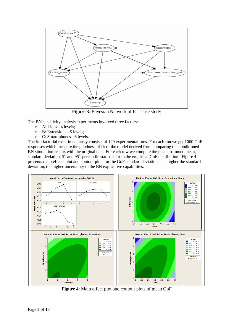
2.3 ICT Operational Risks: Sensitivity Analysis of a Bayesian Network

In information and communication technology (ICT) operational risk analysis, different data sets are

typically merged. Examples of such data sources include CRM call centre data, financial data from

companies and log data utilized to monitor the provisioning of IT services (Kenett3). This case study

is based on a firm marketing and operating telecommunication equipment in small, medium and large

enterprises. The company records data such as “Last Boot and Cause”, “Alarms”, “System and

Restarts”, and “Problem description”. The data we analyse consists of 4703 problems that occurred to

a client. The ordinal target variables is the “Severity” of loss due to the reported problem. In this case

study we use of prior knowledge to set some constraints over the causal variables and new arcs are

learned by E-M algorithm (Heckerman13

). Figure 3 presents the Bayesian Network (BN) for this case

study. On the basis of this BN, a sensitivity analysis was performed using statistically designed

experiments (Cornalba14

). Basically, we set up a variety of conditioning scenarios (i=1,…,120) using

a full factorial experimental array. From a given BN one can generate simulated outcomes (we used

1000 runs). Empirical goodness of fit (GoF) of a BN model is computed using a distance measure

between the simulated data and the real data. Among the various possible distance measures, we use a

classification error defined as:

)(1

)( xIruns

i

ss ii

where I is the indicator function of the subset of severities, s, of the set X and is

defined as:

}:{ if 0

}:{ if 1

ii

ii

sssx

sssxI

and is is the i-th simulated values of severity and is the i-

th real data. As a response, we measure the GoF distribution, for a specific scenario.

Page 5 of 13

Figure 3: Bayesian Network of ICT case study

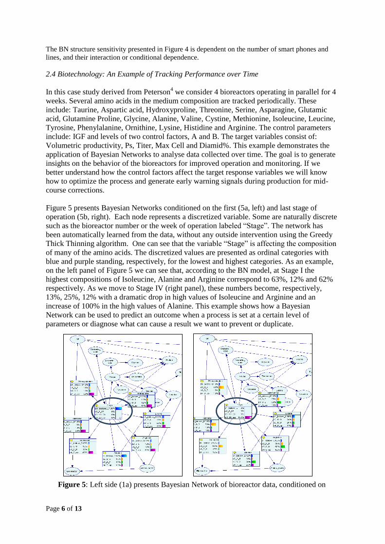
The BN sensitivity analysis experiments involved three factors:

o A: Lines - 4 levels;

o B: Extensions - 5 levels;

o C: Smart phones - 6 levels.

The full factorial experiment array consists of 120 experimental runs. For each run we get 1000 GoF

responses which measure the goodness of fit of the model derived from comparing the conditioned

BN simulation results with the original data. For each row we compute the mean, trimmed mean,

standard deviation, 5th and 95

th percentile statistics from the empirical GoF distribution. Figure 4

presents main effects plot and contour plots for the GoF standard deviation. The higher the standard

deviation, the higher uncertainty in the BN explicative capabilities.

Figure 4: Main effect plot and contour plots of mean GoF

Page 6 of 13

The BN structure sensitivity presented in Figure 4 is dependent on the number of smart phones and

lines, and their interaction or conditional dependence.

2.4 Biotechnology: An Example of Tracking Performance over Time

In this case study derived from Peterson4 we consider 4 bioreactors operating in parallel for 4

weeks. Several amino acids in the medium composition are tracked periodically. These

include: Taurine, Aspartic acid, Hydroxyproline, Threonine, Serine, Asparagine, Glutamic

acid, Glutamine Proline, Glycine, Alanine, Valine, Cystine, Methionine, Isoleucine, Leucine,

Tyrosine, Phenylalanine, Ornithine, Lysine, Histidine and Arginine. The control parameters

include: IGF and levels of two control factors, A and B. The target variables consist of:

Volumetric productivity, Ps, Titer, Max Cell and Diamid%. This example demonstrates the

application of Bayesian Networks to analyse data collected over time. The goal is to generate

insights on the behavior of the bioreactors for improved operation and monitoring. If we

better understand how the control factors affect the target response variables we will know

how to optimize the process and generate early warning signals during production for mid-

course corrections.

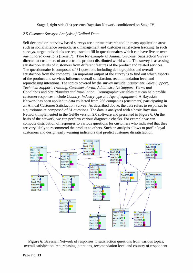
Figure 5 presents Bayesian Networks conditioned on the first (5a, left) and last stage of

operation (5b, right). Each node represents a discretized variable. Some are naturally discrete

such as the bioreactor number or the week of operation labeled “Stage”. The network has

been automatically learned from the data, without any outside intervention using the Greedy

Thick Thinning algorithm. One can see that the variable “Stage” is affecting the composition

of many of the amino acids. The discretized values are presented as ordinal categories with

blue and purple standing, respectively, for the lowest and highest categories. As an example,

on the left panel of Figure 5 we can see that, according to the BN model, at Stage I the

highest compositions of Isoleucine, Alanine and Arginine correspond to 63%, 12% and 62%

respectively. As we move to Stage IV (right panel), these numbers become, respectively,

13%, 25%, 12% with a dramatic drop in high values of Isoleucine and Arginine and an

increase of 100% in the high values of Alanine. This example shows how a Bayesian

Network can be used to predict an outcome when a process is set at a certain level of

parameters or diagnose what can cause a result we want to prevent or duplicate.

Figure 5: Left side (1a) presents Bayesian Network of bioreactor data, conditioned on

Page 7 of 13

Stage I, right side (1b) presents Bayesian Network conditioned on Stage IV.

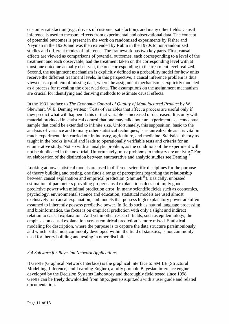
2.5 Customer Surveys: Analysis of Ordinal Data

Self declared or interview based surveys are a prime research tool in many application areas

such as social science research, risk management and customer satisfaction tracking. In such

surveys, target individuals are requested to fill in questionnaires which can have five or over

one hundred questions (Kenett5). Take for example an Annual Customer Satisfaction Survey

directed at customers of an electronic product distributed world wide. The survey is assessing

satisfaction levels of customers from different features of the product and related services.

The questionnaire is composed of 81 questions including demographics and overall

satisfaction from the company. An important output of the survey is to find out which aspects

of the product and services influence overall satisfaction, recommendation level and

repurchasing intentions. The topics covered by the survey include: Equipment, Sales Support,

Technical Support, Training, Customer Portal, Administrative Support, Terms and

Conditions and Site Planning and Installation. Demographic variables that can help profile

customer responses include Country, Industry type and Age of equipment. A Bayesian

Network has been applied to data collected from 266 companies (customers) participating in

an Annual Customer Satisfaction Survey. As described above, the data refers to responses to

a questionnaire composed of 81 questions. The data is analyzed with a basic Bayesian

Network implemented in the GeNIe version 2.0 software and presented in Figure 6. On the

basis of the network, we can perform various diagnostic checks. For example we can

compute distribution of responses to various questions for customers who indicated that they

are very likely to recommend the product to others. Such an analysis allows to profile loyal

customers and design early warning indicators that predict customer dissatisfaction.

Figure 6: Bayesian Network of responses to satisfaction questions from various topics,

overall satisfaction, repurchasing intentions, recomendation level and country of respondent.

Page 8 of 13

2.6 Healthcare Systems: A Decision Support System Case Study

Health care organizations understand the importance of risk management as a key element to

improve service deliveries and patient outcomes. This however requires that clinical and

operational risks are quantified and managed. A risk assessment involves two elements that

are a probability or frequency with which an event might take place and an assessment of

impact severity or consequences from such events. Physicians usually want to evaluate and to

forecast adverse events that may provoke morbidity, mortality or a longer hospital stay for a

patient; moreover, they want to quantify patient’s risk profile. The latter is the assessment of

patient’s medical parameters by using probability distributions, given patient’s status and

prior domain knowledge. Physicians typically summarize risk probability distributions

through a percentile and decide acceptability of risks. Detection of unacceptable risks and the

resulting risk mitigation analysis completes the risk management process. At an upper level

of a health care organization economic losses and costs due to adverse events are evaluated,

mainly to choose convenient forms of insurance; furthermore, for better governance it is

useful to understand risk levels and how each risk contributes to economic losses.

When data is scarce, the experience of physicians often offers a good source of information.

Bayesian methodology can be used for the estimation of operational and clinical risk profiles.

The approach that is described in this section includes an example involving health care of

End Stage Renal Disease (ESRD). The main goal is to support nephrologist and risk

managers who have to manage operational and clinical risk in health care (Kenett6). Many

statistical models applied to risk management estimate only risks without consideration for

decision making. Decisions models have to be considered in order to realize a fully integrated

risk management process. The integration between risk estimations and decision making can

be achieved with Bayesian Networks.

Given medical parameters, X1, . . . , Xn, physicians want to estimate both mortality and

hospitalization risk of a patient and the failure risks of a device. In the ESRD case, more than

one target variable is analyzed under the hypothesis that X1, . . . , Xj (j ≤ n) are positive

dependent, with targets, and the combinations (Xi, Xk), where X1, . . . , Xq q ≤ j ≤ n, i k, are

either positive dependent or independent. Dependencies and independence between variables

are typically determined in medicine through scientific studies and clinical research. In

general, unknown dependency can be extracted from data using data mining techniques and

statistical models. Different sources of knowledge such as subjective information (e.g. expert

opinions of nephrologists, knowledge from literature) and data can be integrated with a

Bayesian Network (BN). In our case, a BN offers several advantages: 1) the method allows to

easily combine prior probability distributions, 2) the complexity of the ESRD domain and the

relationships among medical parameters can be intuitively represented with graphs and, 3)

utility or loss functions can be included in the model. The complex domain of ESRD is

represented by a BN with 34 variables used to describe dialysis. Each variable beeing

classified into one group of causes, such as Dialysis Quality Indexes = {Dialysis adequacy

(Kt/V), PTH pg/ml, Serum albumin g/dl} and HD Department Performances = {Serum

phosphorus PO4 mg/dl, Potassium mEq/l, Serum calcium mg/dl}.

From the BN one can derive that the most important adverse event is due to an incorrect dose

of erythropoietin administered to the j-th patient. Moreover, it is possible to explore also

marginal posterior probability distributions of the target variables. For example, during the

first update both of therapeutic protocol and data collection, the mortality risk of the j-th

Page 9 of 13

patients increases (the probability distribution shifts to right). To restore the correct risk

profile, the nephrologist can add a dose of erytropoietin. To complete the risk management

process, physicians have to make decision either on patient’s treatment or device’s

substitution. This decision problem can be represented by an influence diagram (ID). The set

of decision D and the corresponding set of actions A for each decision are the following:

o “Time”: keep or add 30 minutes to dialysis session.

o “Ca-based therapy”: treat hypercalcemia; continue current therapy; decrease vitamin D

dose to achieve ideal Ca; decrease Ca-based phosphate binders; decrease or discontinue

vitamin D dose/Ca-based phosphate binders; decrease Ca dialysate if still needed; assess

trend in serum PTH as there may be low turnover.

o “Phosphate binder”: assess nutrition, discontinue phosphate binder if being used; being

dietary counseling and restrict dietary phosphate; start or increase phosphate binder

therapy; being short-term Al-based phosphate binder use, then increase non-Al based

phosphate binder; begin dietary counseling and restrict dietary phosphate increase

dialysis frequency.

o “Diet?”: apply an “hypo” diet or keep his/her diet.

o “QB”: increase, keep or decrease QB.

o “Erythropoietin”: keep, decrease or increase (1 EPO) the current dose.

o “Iron management”: keep the treatment; iron prescription.

Nephrologists provided an ordering of the decision nodes (d1, . . . , d7). The shape of the loss

function, L(d, θ), depends on how individual views of risk; the risk attitude of nephrologists

(or clinical governance) can be assumed as neutral and a linear loss function is chosen. The

Quality indicator node summarizes L(d, θ) within the influence diagram. Mortality Ratio,

Hospitalization Ratio, and Adherence to treatment represent the weighted contribution to the

loss function, defined on D and θ. Analyzing the most important causes and the consequence

of each action, it is possible to assess each scenario and prioritize actions that should be taken

for the j-th patient. With the approach presented in this section the physician can recommend

the best treatment (for more on this topic see Kenett6 and references therein).

2.7 System Testing: Risk Based Group Testing

Testing is necessary to ensure the quality of web services that are loosely coupled, dynamic

bound and integrated through standard protocols. Exhaustive testing of web services is

usually impossible due to the unavailable source code, diversified user requirements and the

large number of service combinations delivered by the open platform. The case study outlines

a risk-based approach for selecting and prioritizing test cases to test service-based systems.

We specially address the problem in the context of semantic web services. Semantic web

services introduce semantics to service integration and interoperation, using ontology models

and specifications like OWL-S. In this example we analyze the semantic structure from

various perspectives such as ontology dependency, ontology usage and service workflow to

identify the factors that contribute to the risks of the services. Risks are assessed for

ontologies from two aspects: ontology failure probability and importance. These are

measured and predicted using Bayesian Network analysis techniques that are based on the

semantic models. With this approach, test cases are associated to the semantic features and

scheduled based on the risks of their target features. As a statistical testing technique, the

proposed approach aims to detect, as early as possible, the problems with highest impact on

the users. For more details on this application of Bayesian Networks see Kenett3 and Bai

7.

Page 10 of 13

3. Properties of Bayesian Networks

3.1 Parameter Learning

In order to fully specify the Bayesian Network (BN) and thus fully represent the joint

probability distribution, it is necessary to specify for each node X the probability distribution

for X conditional upon X's parents. The distribution of X conditional upon its parents may

have any form. Sometimes only constraints on a distribution are known; one can then use the

principle of maximum entropy to determine a single distribution, the one with the greatest

entropy given the constraints (Ben Gal10

). Often these conditional distributions include

parameters which are unknown and must be estimated from data, sometimes using the

maximum likelihood approach. Direct maximization of the likelihood (or of the posterior

probability) is often complex when there are unobserved variables. A classical approach to

this problem is the expectation-maximization (E-M) algorithm which alternates computing

expected values of the unobserved variables conditional on observed data, with maximizing

the complete likelihood (or posterior) assuming that previously computed expected values are

correct. Under mild regularity conditions this process converges on maximum likelihood (or

maximum posterior) values for parameters (Heckerman13

). A more fully Bayesian approach

to parameters is to treat parameters as additional unobserved variables and to compute a full

posterior distribution over all nodes conditional upon observed data, then to integrate out the

parameters. This approach can be expensive and lead to large dimension models, so in

practice classical parameter-setting approaches are more common.

The general problem of computing posterior probabilities in Bayesian networks is

NP-hard (Cooper15

). However, efficient algorithms are often possible for particular

applications by exploiting problem structures. It is well understood that the key to the

materialization of such a possibility is to make use of conditional independence and work

with factorizations of joint probabilities rather than joint probabilities themselves. Different

exact approaches can be characterized in terms of their choices of factorizations.

3.2 Structure Learning

Bayesian Network (BN) can be specified by expert knowledge (white lists and black lists) or

network structure and the parameters of the local distributions must be learned from data, or

both. Learning the graph structure of a BN is based on the distinction between the three

possible types of adjacent triplets allowed in a directed acyclic graph (DAG). An alternative

method of structural learning uses optimization based search. It requires a scoring function

and a search strategy. A common scoring function is posterior probability of the structure

given the training data. The time requirement of an exhaustive search returning back a

structure that maximizes the score is superexponential in the number of variables. A local

search strategy makes incremental changes aimed at improving the score of the structure. A

global search algorithm like Markov chain Monte Carlo can avoid getting trapped in local

minima. The R bnlearn application invokes several possible algorithms for learning the

network structure. For more on BN structure learning see Gruber16

.

3.3 Causality and Bayesian Networks

Research questions motivating many scientific studies are causal in nature. Causal questions

arise in medicine (e.g., treatment of diseases), management (e.g., the effects of management

style on problem solving efficiencies), risk management (e.g., causes of risk events),

Page 11 of 13

customer satisfaction (e.g., drivers of customer satisfaction), and many other fields. Causal

inference is used to measure effects from experimental and observational data. The concept

of potential outcomes is present in the work on randomized experiments by Fisher and

Neyman in the 1920s and was then extended by Rubin in the 1970s to non-randomized

studies and different modes of inference. The framework has two key parts. First, causal

effects are viewed as comparisons of potential outcomes, each corresponding to a level of the

treatment and each observable, had the treatment taken on the corresponding level with at

most one outcome actually observed, the one corresponding to the treatment level realized.

Second, the assignment mechanism is explicitly defined as a probability model for how units

receive the different treatment levels. In this perspective, a causal inference problem is thus

viewed as a problem of missing data, where the assignment mechanism is explicitly modeled

as a process for revealing the observed data. The assumptions on the assignment mechanism

are crucial for identifying and deriving methods to estimate causal effects.

In the 1931 preface to The Economic Control of Quality of Manufactured Product by W.

Shewhart, W.E. Deming writes: “Tests of variables that affect a process are useful only if

they predict what will happen if this or that variable is increased or decreased. It is only with

material produced in statistical control that one may talk about an experiment as a conceptual

sample that could be extended to infinite size. Unfortunately, this supposition, basic to the

analysis of variance and to many other statistical techniques, is as unrealizable as it is vital in

much experimentation carried out in industry, agriculture, and medicine. Statistical theory as

taught in the books is valid and leads to operationally verifiable tests and criteria for an

enumerative study. Not so with an analytic problem, as the conditions of the experiment will

not be duplicated in the next trial. Unfortunately, most problems in industry are analytic.” For

an elaboration of the distinction between enumerative and analytic studies see Deming17

.

Looking at how statistical models are used in different scientific disciplines for the purpose

of theory building and testing, one finds a range of perceptions regarding the relationship

between causal explanation and empirical prediction (Shmueli18

). Basically, unbiased

estimation of parameters providing proper causal explanations does not imply good

predictive power with minimal prediction error. In many scientific fields such as economics,

psychology, environmental science and education, statistical models are used almost

exclusively for causal explanation, and models that possess high explanatory power are often

assumed to inherently possess predictive power. In fields such as natural language processing

and bioinformatics, the focus is on empirical prediction with only a slight and indirect

relation to causal explanation. And yet in other research fields, such as epidemiology, the

emphasis on causal explanation versus empirical prediction is more mixed. Statistical

modeling for description, where the purpose is to capture the data structure parsimoniously,

and which is the most commonly developed within the field of statistics, is not commonly

used for theory building and testing in other disciplines.

3.4 Software for Bayesian Network Applications

i) GeNIe (Graphical Network Interface) is the graphical interface to SMILE (Structural

Modelling, Inference, and Learning Engine), a fully portable Bayesian inference engine

developed by the Decision Systems Laboratory and thoroughly field tested since 1998.

GeNIe can be freely downloaded from http://genie.sis.pitt.edu with a user guide and related

documentation.

Page 12 of 13

ii) Hugin (http://www.hugin.com/index.php) is a commercial software which provides a

variety of products for both research and non-academic use. The Hugin GUI (Graphical User

Interface) allows building BN, learning diagrams, etc.

iii) IBM SPSS Modeller (http://www.spss.com/) includes several tools which enable the user

to deal with a list of features and statistical methods such as BN. IBM SPSS is not free

software.

iv) The R bnlearn package is powerful and free. Compared with other available BN software

programs, it is able to perform both constrained-based and score-based methods. It

implements five constraint based learning algorithms (Grow-Shrink, Incremental

Association, Fast Incremental Association, Interleaved Incremental association, Max-min

Parents and Children), two scored based learning algorithms (Hill-Climbing, TABU) and two

hybrid algorithms (MMHC, Phase Restricted Maximization).

v) Inatas (www.inatas.com) provides the Inatas System Modeler software package for both

research and commercial use. The software permits the generation of networks from data

and/or expert knowledge. It also permits the generation of ensemble models and the

introduction of decision theoretic elements for decision support or, through the use of a real

time data feed API, system automation. A cloud based service with GUI is in development.

The main disadvantage in most available BN programs is that they do not allow the mixing of

continuous and categorical variables. Some experimental libraries handle networks with

mixed variables; however their learning procedures are not yet applicable to complex models

and large datasets.

4. Summary and Conclusions

This paper presents various examples of Bayesian Networks designed to illustrate their wide

range of application. They are used to evaluate the impact of management maturity level

using 21 case studies and assess the usability web sites using web logs which represent big

data analytics. BN are very effective in combining various data sources such as in operational

risk analysis and in tracking a very large number of variables like in monitoring bioreactors.

We also show how BN can be used to analyse customer survey data, an application they are

very well adapted to perform given the natural discretization of responses to a survey

questionnaire. Other applications we covered include a decision support system to help

manage patients undergoing dialysis and a risk based approach to test web services.

In section 3 we discuss various technical aspects of BN, including estimation of distributions

and algorithms for learning the BN structure. In learning the network structure, one can

include white lists of forced causality links imposed by expert opinion and black lists of links

that are not to be included in the network, again using inputs from content experts. This

essential feature permits an effective dialogue with content experts who can impact the model

used for data analysis. We also briefly discuss statistical inference of causality links. In

general, BN provide a very effective descriptive causality analysis, with a natural graphical

display that enhances the quality of the information derived from such an analysis. For more

on how to generate information quality see Kenett19

and Kenett and Salini20

.

Page 13 of 13

Future research will provide good solutions to the generation of BN using continuous data.

Moreover, the proper scaling up of BN to big data still requires investigation, including the

possible combination of Hadoop and R (Kenett21

). In conclusion, we suggest that Bayesian

Networks offer unique opportunities for statisticians to work collaboratively with content

experts in a wide range of application domains.

References 1. Kenett RS, De Frenne A, Tort-Martorell X and McCollin C. The Statistical Efficiency Conjecture, in

Applying Statistical Methods in Business and Industry – the state of the art, Greenfield, T. , Coleman and

Montgomery, R. (editors), John Wiley and Sons, Chichester: UK, 2008.

2. Kenett RS., Harel A and Ruggeri F. Controlling the Usability of Web Services. International Journal of

Software Engineering and Knowledge Engineering 2009; 19 (5): 627-651.

3. Kenett RS. and Raanan Y. Operational Risk Management: a practical approach to intelligent data analysis,

John Wiley and Sons, Chichester: UK, 2010.

4. Peterson J. and Kenett RS. Modelling Opportunities for Statisticians Supporting Quality by Design Efforts

for Pharmaceutical Development and Manufacturing. Biopharmaceutical Report, ASA Publications 2011;

18 (2): 6-16.

5. Kenett RS and Salini S. Modern Analysis of Customer Satisfaction Surveys: with applications using R, John

Wiley and Sons, Chichester: UK, 2011.

6. Kenett RS. Risk Analysis in Drug Manufacturing and Healthcare, in Statistical Methods in Healthcare,

Faltin, F., Kenett, R.S. and Ruggeri, F. (editors in chief), John Wiley and Sons. Chichester: UK, 2012.

7. Bai X, Kenett RS. and Yu W. Risk Assessment and Adaptive Group Testing of Semantic Web Services.

International Journal of Software Engineering and Knowledge Engineering, 2012; in press.

8. Pearl J. Causality: Models, Reasoning, and Inference, 2nd

ed., Cambridge University Press, UK, 2009.

9. Jensen FV. Bayesian Networks and Decision Graphs, Springer, 2001.

10. Ben Gal I. Bayesian Networks, in Encyclopaedia of Statistics in Quality and Reliability, Ruggeri, F.,

Kenett RS. and Faltin, F. (editors in chief), John Wiley and Sons, Chichester: UK, 2007.

11. Koski T. and Noble J. Bayesian Networks – An Introduction, John Wiley and Sons, Chichester: UK, 2009.

12. Kenett RS. Cause and Effect Diagrams, in Encyclopedia of Statistics in Quality and Reliability, Ruggeri, F.,

Kenett, R.S. and Faltin, F. (editors in chief), John Wiley and Sons, Chichester: UK, 2007.

13. Heckerman D. A tutorial on learning with Bayesian networks. Microsoft Research tech. report

MSR-TR-95-06. 1995, http://research.microsoft.com, downloaded 20/10/2012. 14. Cornalba C, Kenett RS and Giudici P. Sensitivity Analysis of Bayesian Networks with Stochastic

Emulators. 2007 ENBIS-DEINDE proceedings, University of Torino, Turin, Italy.

15. Cooper GF. The computational complexity of probabilistic inference using Bayesian belief networks

Artificial Intelligence 1990; 42,393-405.

16. Gruber A. and Ben Gal I. Efficient Bayesian Network Learning for System Optimization in Reliability

Engineering," Quality Technology & Quantitative Management, 2012; 9 (1), 97-114.

17. Deming WE. On the Distinction Between Enumerative and Analytic Surveys. Journal of the American

Statistical Association, 1953;48 (262),244-255.

18. Shmueli G. To Explain or To Predict?, Statistical Science, 2010; 25(3) 289-310.

19. Kenett RS. and Shmueli, G. On Information Quality, http://ssrn.com/abstract=1464444, Journal of the

Royal Statistical Society (Series A), 2012, in press

20. Kenett RS. and Salini, S. Modern Analysis of Customer Surveys: comparison of models and integrated

analysis, with discussion, Applied Stochastic Models in Business and Industry 2011; 2, 465–475.

21. Kenett RS, Gruber A. and Ben Gal I. Applications of Bayesian Networks to Small, Mid-size and Massive

Data, The 6th

Inter. Workshop on Applied Probability – IWAP, 2012, Jerusalem, June 11-14th

.

================================================================== Ron Kenett, Chairman and CEO of the KPA Group (www.kpa-group.com), Research Professor, University of

Torino, Turin, Italy, International Professor Associate, Center for Risk Engineering, NYU-Poly, NY, USA.

Member of the Board of Inatas (www.inatas.com), a startup developing advanced stochastic modeling and data

analysis technologies and President of the Israel Statistical Association (ISA). Ron is Past President (2006-

2007) of the European Network for Business and Industrial Statistics (ENBIS). He published over 160

publications and 9 books are on topics in industrial statistics, multivariate statistics, risk management,

biostatistics and quality management and served as Editor in Chief for Europe of Quality Technology and

Quantitative Management and as Associate Editor of the Journal of the Royal Statistical Society, Series A and

Applied Stochastic Models in Business and Industry. His PhD is in Mathematics from the Weizmann Institute of

Science, Rehovot, Israel, and BSc in Mathematics, with first class honors, from Imperial College, London

University.