applications of computer modelling to behavioural coordination · applications of computer...
TRANSCRIPT
Applications of computer modelling to
behavioural coordination
A thesis submitted for the degree of Doctor of Philosophy in the University of
London.
ANTHONY RICHARD LUDLOW. B.Sc. (London)
Department of Pure and Applied Biology,Imperial College of Science and Technology
December 1983

2
To R.F.L. and E.M.L.
Acknowledgements
I am most grateful to Professor John Kennedy who has been my mentor andfriend in the best traditions of scientific apprenticeships. The work reported herestarted during a conversation with him and he encouraged me to develop it longbefore the direction or relevance could be discerned. In the years that followedhe has been generous in allowing me to spend time working on the “modelanimal” when I might have been doing work closer to his personal interests.I am grateful, too, for his penetrating questions and constructive comments;without his support, permission and guidance the work simply could not havebeen done.
I have been supported throughout by the Agricultural Research Council,while employed as a member of their Insect Physiology Group, and I am grate-ful to the current head of the group, Dr. John Moorhouse, whose data on locustbehaviour raised many of the questions discussed in Ludlow (1976). His com-ments on numerous occasions since then have been invaluable. More recentlyhe was determined that I should complete the thesis when other challenges haveoften been distracting. I am particularly grateful for that determination.
Especial thanks are due to Dr. David Marsh whose work on moth orientationwas the trigger for the second study. No one, with whom I have worked, is moreable to keep in mind all of the complexities of a difficult subject; collaborationwith him has always been a pleasure. I thank, too, my colleagues Ian Fosbrooke,Drs. Charles David, John Brady, and Tim Seller for valuable conversations.
I thank Professors T R. E. Southwood, M. J. Way and R K. S. Wood forspace and facilities within the department.
Finally, I thank my wife Liz, for help in preparation of drawings and text ofthis volume, and much more for her understanding when I have been preoccupiedwith the minutiae of some problem in moth orienlaton or decision making.
3

4
Abstract
The physiological basis of behaviour is so complex that few hypotheses can betested adequately without resort to a precise mathematical model. But the aimof modelling is not simply to calculate the predictions of hypotheses. Beforethat final stage is reached the act of modelling tests hypotheses in three ways:
1. it may reveal contradictions in the hypothesis,
2. it may demonstrate that the hypothesis is no more than a circular argu-ment, and
3. it makes it possible to compare the simplicity of competing hypotheses
If a working model is not built, necessary but unacceptable assumptions areeasily overlooked so that complex theories appear simple. All the assumptionshave to be spelt out before a working model works.
A rich byproduct of modelling is that it generates numerous searching ques-tions, both theoretical and experimental.
The present volume combines two studies which illustrate different aspectsof modelling praxis. The first (Chapters 2-4) is based on a simple switch mech-anism which would prevent an animal from performing inappropriate combi-nations of activity at the same time. Added to that is the postulate that allactivities are subject to a central nervous decay process (fatigue) which leads tospontaneous alternation of behaviour. When built into a working model thesetwo ideas have far-reaching implications and the model displays paradoxicalfeatures of behaviour often observed in real animals. A frequent result of thesesimulations is that arguments widely accepted in the literature are exposed asnot necessarily true or definitely false.
The second study (Chapter 5) is a survey of theoretical problems in insectorientation. The achievements of insects are well known, but it is difficult in-deed to find hypotheses which remain plausible when analysed in depth. Untilthey are so analysed, all half-baked hypotheses seem to work, and the oftencontradictory assumptions are easily overlooked.
5

6
Contents
1 Introduction 9
1.1 Hypotheses and models . . . . . . . . . . . . . . . . . . . . . . . 91.2 Reasons for modelling . . . . . . . . . . . . . . . . . . . . . . . . 101.3 Summary . . . . . . . . . . . . . . . . . . . . . . . . . . . . . . . 13
2 An introduction to the model animal 15
2.1 Questions behind the model . . . . . . . . . . . . . . . . . . . . . 152.2 Changing stimuli . . . . . . . . . . . . . . . . . . . . . . . . . . . 162.3 The long-term satiation loop . . . . . . . . . . . . . . . . . . . . 192.4 Inhibitory connections . . . . . . . . . . . . . . . . . . . . . . . . 202.5 The short-term fatigue loop . . . . . . . . . . . . . . . . . . . . . 212.6 Summary of calculations during each step . . . . . . . . . . . . . 252.7 A complication in calculating the inhibition . . . . . . . . . . . . 282.8 Summary . . . . . . . . . . . . . . . . . . . . . . . . . . . . . . . 29
3 Consequences of mutual inhibition 31
3.1 Properties or the switch mechanism . . . . . . . . . . . . . . . . 313.2 Hysteresis in the switch mechanism . . . . . . . . . . . . . . . . . 343.3 The control of sequences in a model with many subsystems . . . 363.4 Learning and the model animal . . . . . . . . . . . . . . . . . . . 383.5 Alternative arrangements of the inhibitory connections . . . . . . 403.6 Mutual inhibition in more complex networks - a model brain . . 403.7 Summary . . . . . . . . . . . . . . . . . . . . . . . . . . . . . . . 52
4 Consequences of fatigue 55
4.1 Differences between satiation and fatigue — reward and effort . . 554.2 Interactions between feeding and drinking . . . . . . . . . . . . . 614.3 Discussion and Summary . . . . . . . . . . . . . . . . . . . . . . 64
5 Mechanisms of Moth Orientation 69
5.1 How does a male moth find a female emitting sex-pheromone—current views . . . . . . . . . . . . . . . . . . . . . . . . . . . . . 69
5.2 How does a moth turn upwind? . . . . . . . . . . . . . . . . . . . 765.3 The problem of maintaining cross-wind tracks . . . . . . . . . . . 85
7

8 CONTENTS
5.4 Course control by counting the angle turned . . . . . . . . . . . . 1135.5 Windspeed Compensation . . . . . . . . . . . . . . . . . . . . . . 1145.6 Towards a model of moth orientation . . . . . . . . . . . . . . . . 1195.7 Tests of the model . . . . . . . . . . . . . . . . . . . . . . . . . . 1285.8 Summary . . . . . . . . . . . . . . . . . . . . . . . . . . . . . . . 140
6 Postscript 143
Chapter 1
Introduction
The application of control theory to biological systems is seen bysome as being quite essential to their understanding, in somethinglike the way that the ability to count is necessary for knowing whetherone’s change is correct. By others it is seen as yet one more fadwhereby those with some faintly exotic expertise can rephrase whatis known already in terms that serve to obscure it.K. Oatley. Book review in Quarterly Journal of Experimental Psy-chology, 1972
1.1 Hypotheses and models
I shall use the word model to mean a working version of an hypothesis. It maybe a special case of the hypothesis, but the model is completely defined so thatanyone building the same model will get the same results. Hypotheses on theotherhand are often stated verbally in terms which mean different things todifferent people. Moreover, verbally stated hypotheses are often incomplete, sothat one does not realise all of the assumptions they imply. A working modelhas to be complete; if not it does not work. Some of the most famous modelsin the behavioural literature have been qualitative, such as the hydraulic modeldescribed by Lorenz and discussed in numerous text-books (e.g. Manning, 1972).I shall not be discussing such qualitative models, except as stepping stones toquantitative models. The latter, quantitative, models are more satisfactorybecause they make exact predictions.
Quantitative or mathematical models can be represented as systems of equa-tions and if the equations can be solved the model’s behaviour can often be de-duced by inspecting or manipulating the equations. In the study of behaviourhowever, one frequently has to build models which arc not mathematicallytractable and then one has to resort to computer simulation. Computer modelsare always special cases, which raises problems but has advantages too. Boththe modeller, and anyone with access to the model immediately start to twiddle
9
10 CHAPTER 1. INTRODUCTION
knobs. What happens if you change this value or that? Such knob twiddlingcan be surprisingly fruitful, raising new questions and providing unexpected ex-planations. The mathematician does the same thing mentally when gazing atequations, but one can play with a computer model with less training. For non-mathematicians, like the author, that is important.
1.2 Reasons for modelling
The main aim of this volume is to convince readers of the usefulness of be-havioural modelling and to illustrate ways in which it has been done. Many ofthe illustrations are from my own work because the literature contains few ac-counts of how models were developed, and my main concern is with behaviouralmodelling rather than behavioural models. Many authors have discussed thephilosophy of modelling, and particularly how we should choose between dif-ferent models (e.g. Popper, 1972; Dawkins and Dawkins, 1974; McCleery, 1977;Sibly, 1980). Here I want to begin by considering the usefulness of modellingrather than the evaluation of models, because the usefulness begins long beforeany testable predictions can be derived. As Popper points out (pp. 32-33) thereare four lines along which an hypothesis may be tested.
First there is the logical comparison of the conclusions among them-selves, by which the internal consistency of the system is tested.
Secondly there is the investigation of the logical form of the theory,with the object of determining whether it has the character of anempirical or scientific theory, or whether it is. for example, tauto-logical.
Thirdly, there is the comparison with other theories, chiefly with theaim of determining whether the theory would constitute a scientificadvance should it survive our various tests.
And finally, there is the testing of the theory by way of empiricalapplications of the conclusions which can be derived from it.
Only in the last phase are the predictions put to the test. The first three phasesform the stuff of theoretical analysis.
Put quite simply, stage one involves asking the question: does the hypothesisexplain anything at all? Can a working model be built? I have argued elsewhere(Ludlow, 1980, and below) that van Iersel and Bol (1958) disinhibition hypoth-esis, although widely credited, never did explain displacement activities. Theirproposed explanation was incomplete, so that no working model is specified bytheir description, and I do not believe that a working model can be built with-out making special ad hoc and unnattractive assumptions. One wonders howmany other hypotheses, widely propogated in the literature, would fail the firstelementary test of building a working model?
The problem of tautologies, exposing circular arguments, is particularlydeep, and building a working model is not a sufficient test. Nevertheless, a
1.2. REASONS FOR MODELLING 11
working model is usually easier to analyse than the original verbal hypothesis.Bits of the model may be left out or altered to see how the explanation rests onthe assumptions.
The third stage, of comparing theories, is only possible when both theo-ries are known to be complete, because concealed assumptions invalidate thecomparison of theories. For example, the disinhibition hypothesis appeareddisarmingly simple, but until a working model is built we have no means ofsaying how simple it is. Hence, we cannot compare its simplicity with any othertheories.
The fourth stage, of testing the predictions of an hypothesis, has probablyreceived more philosophical attention than the other three, although many hy-potheses never reach that stage, or if they do their original elegance is oftenbadly tarnished.
Thus, modelling is a necessary part of testing hypotheses, and as Poppersees it this is the essence of science. Indeed, he states (p.59) that the empiricalsciences are systems of theories. The logic of science can therefore be describedas a theory of theories. However, Popper was concerned with the logic of science,the limits of knowledge. He deliberately excluded the invention of theories fromhis analysis (p. 31). To the practicing scientist, however, that is a vital question,and for the student of behaviour it is also a question of academic interest. Indiscussing the usefulness of modelling, therefore, we must go beyond Popper’slimited analysis of the progress of science.
I personally see the growth of knowledge as the accumulation of answeredquestions. That is not the same as the accumulation of random observationsbecause the questions give the observations significance. In the case of universalquestions we must always be content with a provisional answer, or theory. AsPopper has argued, such theories can be rejected but never verified, because itis impossible to examine all the past and future events which might disprovethe theory. Nevertheless, there are many significant empirical questions whichare not universal, and which can be answered directly. For example, Popper (p.68) excludes statements of the type: Of all human beings now living on earthit is true that their height never exceeds a certain amount (say 8 ft). In biol-ogy there are numerous significant questions which should be answered in thatform. Indeed, it is the business of biology to define the populations and groupsfor which certain statements are true. In addition to empirical questions of fi-nite range, there are theoretical questions which can be answered unequivocally.One such appears to have prompted Newton’s theory of universal gravity (seean excellent account of these developments by Cohen (1981)). Robert Hookeasked Newton, in a letter dated January 17th 1680, what path a planet wouldtake (other than a concentric circle) if it were attracted to the sun with a forceinversely proportional to the square of its distance from the sun. When Halleyrepeated the question, in August 1684, Newton replied “an ellipse” and within afew months had published an outline of his work. That seminal question led to aturning point in the history of science, and illustrates the enormous importanceof starting with the right question, Hooke’s question undoubtedly arose fromhis own theoretical work, when he realised that the old idea of centrifugal force
12 CHAPTER 1. INTRODUCTION
acting on the planets could be replaced by resolving the forces into two compo-nents: a tendency to travel in straight lines (due to inertia) and an attractiontowards the centre which prevented the inertial forces from carrying the planetsoff into space.
Not all questions arise from earlier theories, however. Questions have beenraised by the pressure of the market place, the need to care for the sick, or thedemands of space travel. The early development of statistics, for example, wasstimulated by questions from gamblers, questions based more on dreams thantheories. Thus, the reiterative process of theory, prediction (=question), experi-ment, questions, improved theory is not the only way in which knowledge grows,although it may be the most elegant. In addition there are questions which canbe answered directly by experiment or theoretical analysis, and questions whichdo not owe their birth to previous theories.
My emphasis on the importance of questions is borne of experience. I am fre-quently consulted by students seeking statistical advice, when what they reallyhave is a set of observations looking for the right questions. Finding answersis often a technical problem, but finding the right question requires luck ordeep insight, as innumerable examples from the history of science show. BeforeFleming. for example, bacteriologists used to curse Penicillium because it sofrequently ruined their cultures. Fleming, however, had been studying the anti-bacterial effects of natural substances such as lysozymes, hence he approachedthe observation with the right question. Similarly, Jenner wanted to know whymilkmaids were less affected than others by smallpox, and he discovered theprinciples of immunization. (For an outstanding description of both Flemingsand Jenner’s work see Beveridge (1970)).
New questions may sometimes be raised by colleagues with many years ofdeep insight in a subject, or by non-scientists asking for clarification at a party.Often they are raised by scientists who move into a new subject after workingin other disciplines. But one of the most fertile sources of questions is theprocess of model building. Indeed, it is almost impossible to build only onemodel. At each step one is faced with choices and alternative models, untilthe process becomes a veritable flowering of questions. Nor does it stop whenthe model is built, for models instantly attract criticism. A working model isoutrageously precise, it does not embody vague plausible assumptions but statesunambigously that the value of that particular signal is now 42. No-one believesit; it is a special case and people start suggesting changes to this or that feature.Perhaps this is the most valuable aspect of model building; it leads to a profoundscepticism and, faced with many choices, even the modeller becomes impartial.By concentrating on one hypothesis, on the otherhand, one may become a littlebiased (see Platt, 1964; Chamberlain, 1897, for discussions).
How should one judge the usefulness of a model then? Assuming that itis bound to be superseded in the long run, a long life is not a useful feature.On the contrary, we may hope that its faults will be quickly revealed. Thebest measure of usefulness seems to me to be some estimate of the number ofquestions it answers and the number of answerable questions it generates. Itmight be thought that a doomed model cannot answer questions, but that is not

1.3. SUMMARY 13
true. Newton answered Hooke’s question by assuming that the sun was fixed.It was only later that he asked how this model was unrealistic, and realised thatthe earth must attract the sun just as the sun attracts the earth. Hence, theyboth orbit round their combined centre of gravity. Then he asked what effectthe planets would have on each other and realised that they must perturb eachother’s orbits. This he confirmed by observation (with John Flamstead) andformulated his law of universal gravity: All objects attract each other with aforce proportional to the product of their masses and inversely proportional tothe square of their separations. The preceding, oversimple, models answeredthe questions for which they were intended, and their limitations led to furtherquestions. His final model failed after two centuries, but in failing it raised thequestions that stimulated Einstein. Without Newton’s doomed model, Einsteinwould not have realised there was a problem.
Thus, precise and careful modelling can answer some questions and raiseothers. The answers may later prove irrelevant to the real world, but even thatis hard-won knowledge. Such modelling is not the same as speculation. I amconcerned here with the patient testing of hypotheses by analysis, and that,in my view, is as important as testing hypotheses by experiment because I donot believe that the human brain can cope unaided with the complexities ofbehaviour. As Toates (1975) wrote
The human brain is often quite incapable of appreciating the conse-quences of the theories that it is able to propose. It is all too easyto make mistakes in logic when proposing an explanation in words,and to pass over the mistake repeatedly. A computer model that em-bodies our assumptions will ruthlessly expose any weaknesses thatare inherent in our theorising. . . on the otherhand it will also revealunexpected explanations. The computer will present us with an un-biased account of our assumptions, something we might be quiteincapable of doing even with the most honest intentions.
1.3 Summary
A model is a working version of a theory or hypothesis, and the excercise ofbuilding a model is an important part of testing theories. For the model to workit must be complete, hence a working model proves that the theory containsno internal contradictions. In addition, its construction will reveal all of theassumptions implied by the theory, which is essential if the simplicity of anyhypothesis is to be compared with the simplicity of others. Studying the model’sbehaviour will show whether the theory really does explain the phenomena forwhich it was proposed, and will confirm that testable predictions really do followfrom the theory. Simulations are also useful when checking to see if a theoryis tautological, or whether parts of the hypothesis are redundant and can beeliminated to produce a simpler theory.
The excercise of building the model involves making decisions which raisequestions one might otherwise overlook. The simulations may also provide un-

14 CHAPTER 1. INTRODUCTION
expected explanations, or new hypotheses, and modelling frequently revealsnon-sequiturs or fallacies which have become widely propogated in the litera-ture.
Chapter 2
An introduction to the
model animal
In the Art of reasoning upon Things by Figures, ’tis some Praise, atfirst, to give an imperfect and rough Draft and Model, which, uponmore Experience, and better Information, may be corrected.
Charles Davenant, Discourses on the Public Revenues and on theTrade of England, 1698
2.1 Questions behind the model
I begin by describing the model which has taught me more than any other.Its principles, which are not original, were put forward while discussing aphidbehaviour with Professor J. S. Kennedy. The two questions before the housewere: how do aphids avoid performing inappropriate pairs of activities at thesame time: and why do their activities alternate in an apparently constantenvironment? To answer the first question we postulated inhibition between thesubsystems controlling each activity. To answer the second we suggested thatthe suppressed subsystems adapted to inhibition received from the dominantactivity, until its dominance was usurped. An alternative suggestion was thatthe dominant subsystem fatigued until it was no longer able to suppress one ofthe other subsystems. For some reason the fatigue idea stuck and has been partof all the working models since.
The inhibitory connections we postulated provide a switch mechanism thatprevents more than one subsystem being active at a time. However, I will explainthe principle of the switch mechanism in the next chapter. In the present chapterI want to describe the current version of the model animal, so that the readercan see the ideas it embodies before considering its behaviour; basically there areonly four ideas. In addition to the idea of inhibition between subsystems, and theidea that the subsystems fatigue when active, I have used the idea that feeding
15
16 CHAPTER 2. AN INTRODUCTION TO THE MODEL ANIMAL
reduces hunger, drinking reduces thirst and so on. Finally, I have used the ideathat particular internal and external factors affect different activities, and thatthese factors may change with time. These four ideas are hardly original, butthey seem to me to form the minimum kit for explaining behaviour. Notice thatI have not included learning. The model animal does not learn. As the nextchapter shows, it does many things which look like learning, and which havebeen attributed to learning when observed in animals, but the model animaldoes them passively.
As I have said, these ideas were not original. In fact the ideas of inhibitionand fatigue were first combined, in essentially the same model, by McDougall(1903). McDougall, in turn was inspired by Sherrington’s work on the interac-tions of reflexes (see Sherrington, 1906). They were employed again by Reiss(1962). Both of these authors were concerned with the alternate contractionsof muscles, rather than whole-animal behaviour, but they began with the samequestions. Why do both muscles not contract at the same time, and why dotheir contractions alternate? More recently, Joseph et al. (1979) have proposedessentially the same model in a discussion of schizophrenia.
In the context of whole-animal behaviour one is dealing with more than twoactivities, and the activities are more complex than individual muscle contrac-tions. Nevertheless, we begin by assuming that the subsystems controlling eachactivity can be treated as if they were discrete. Thus, we postulate a subsys-tem controlling feeding, another controlling drinking and so on. Although themodel was proposed in the context of aphid behaviour, I have so far simulatedmore vertebrate than insect behaviour because the vertebrate literature is fullof experiments which test different parts of the model. Let us suppose then,that the model has been set up to simulate four activities often performed bybirds: feeding, drinking, preening and song. Each activity will be controlled bya subsystem which embodies the ideas of:
1. changing stimuli,
2. satiation (at least in the feeding and drinking subsystems),
3. inhibitory connections to and from other subsystems, and
4. fatigue when the activity is performed.
We discuss below how each of these ideas is built into the model.
2.2 Changing stimuli
The early attempts to describe behaviour in terms of reflexes are well known,and although we now regard them as naive, there is still much to learn fromstudying stimulus-response combinations in behaviour. As Hinde (1970) text-book shows, the more complex features in the control of behaviour becameapparent when it was found that responsiveness to the same stimulus changedwith time. For each new species we must still define the significant stimuli
2.2. CHANGING STIMULI 17
and responses before making much progress on more complex features of be-haviour. Moreover, the stimulus-response combinations contribute hugely tothose features of behaviour which make species distinct; key stimuli and ap-propriate responses lead to successful mating and reduce inappropriate pairingswith individuals of another species. The selection of specific habitats or diets,the defence of territory and the complexities of social behaviour all depend onspecific stimulus-response combinations. Within an individual too, the mostcost-effective allocation of time, choice of diet, foraging strategies and so ondepend on appropriate stimulus-response combinations as do mechanisms oforientation and migration.
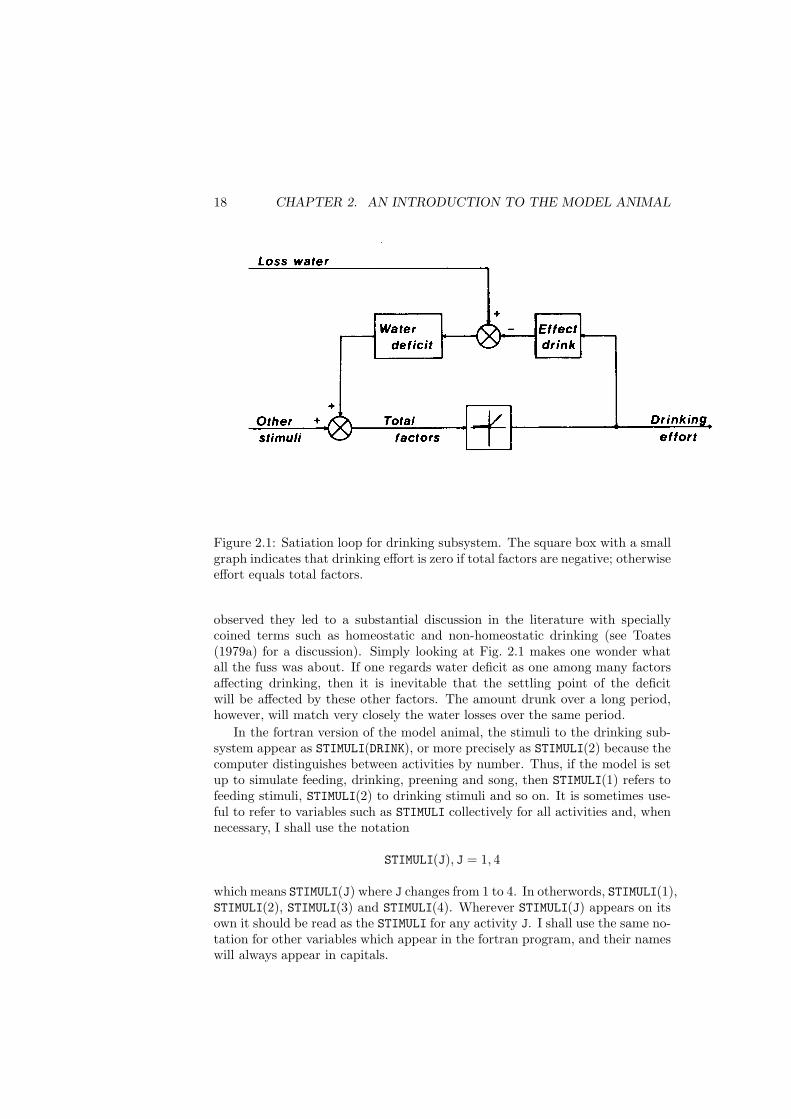
Without doubt then, stimulus-response combinations are still at the heartof behavioural studies. Some of the experimental work has achieved great el-egance, for example, Tinbergen’s field work on gulls (Tinbergen, 1951), andmuch has been learned of the way in which information is filtered, so that onlycertain features of a complex stimulus are selected. We also know a great dealabout sensory physiology, the processing of visual stimuli, encoding of soundfrequencies and so on. But it comes as rather a shock to discover that thetrail stops there. We know virtually nothing of the way stimuli are weighedin the decisions which comprise animal behaviour. For example, a bright lightpromotes take-off in aphids and reduces probing. Does the light inhibit prob-ing directly, or is the effect indirect so that probing is inhibited by the flightsubsystem when the latter is excited by bright light? Perhaps the probing andflight subsystems do not exist separately. It may be that the aphid’s nervoussystem is one vast telephone exchange with light receptors connected directlyto the muscles which withdraw the stylets, as well as to those which flap thewings. I hope not, because it would make the analysis of behaviour hopelesslydifficult. In the context of all that is known about stimuli and responses, themodel animal is extraordinarily primitive. It has no eyes or ears, it has no meansof analysing patterns or extracting information from complex stimuli. Insteadit deals with the sums of certain groups of factors. For example, Fig. 2.1 showsa simplified version of the model’s drinking subsystem and, in this simplifiedversion, drinking depends on two factors: the water deficit and other stimuli.The other stimuli include both internal and external factors and these may beeither excitatory or inhibitory. Moreover, a given stimulus may affect more thanone subsystem, perhaps exciting one and inhibiting another.
It would be more realistic to specify all of the stimuli affecting each activity,and build them into the model for a given species. Indeed, that must be theultimate aim. However, I believe we must learn to walk before we can run, and Ihave argued elsewhere (Ludlow, 1976) that the identification of individual stim-uli with particular subsystems can only be done, if at all, after we understandhow subsystems interact. In the meantime, even this simple model allows oneto see the complex consequences of changing stimuli to various activities. Forexample, I have used the model to simulate the effects on drinking of a moretasty diet (Ludlow, 1982).
Another point which will be made later is that the strength of other stimulimust affect the settling point of the water deficit. When these effects were first
18 CHAPTER 2. AN INTRODUCTION TO THE MODEL ANIMAL
Figure 2.1: Satiation loop for drinking subsystem. The square box with a smallgraph indicates that drinking effort is zero if total factors are negative; otherwiseeffort equals total factors.
observed they led to a substantial discussion in the literature with speciallycoined terms such as homeostatic and non-homeostatic drinking (see Toates(1979a) for a discussion). Simply looking at Fig. 2.1 makes one wonder whatall the fuss was about. If one regards water deficit as one among many factorsaffecting drinking, then it is inevitable that the settling point of the deficitwill be affected by these other factors. The amount drunk over a long period,however, will match very closely the water losses over the same period.
In the fortran version of the model animal, the stimuli to the drinking sub-system appear as STIMULI(DRINK), or more precisely as STIMULI(2) because thecomputer distinguishes between activities by number. Thus, if the model is setup to simulate feeding, drinking, preening and song, then STIMULI(1) refers tofeeding stimuli, STIMULI(2) to drinking stimuli and so on. It is sometimes use-ful to refer to variables such as STIMULI collectively for all activities and, whennecessary, I shall use the notation
STIMULI(J), J = 1, 4
which means STIMULI(J) where J changes from 1 to 4. In otherwords, STIMULI(1),STIMULI(2), STIMULI(3) and STIMULI(4). Wherever STIMULI(J) appears on itsown it should be read as the STIMULI for any activity J. I shall use the same no-tation for other variables which appear in the fortran program, and their nameswill always appear in capitals.
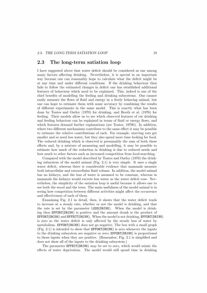
2.3. THE LONG-TERM SATIATION LOOP 19
2.3 The long-term satiation loop
I have suggested above that water deficit should be considered as one amongmany factors affecting drinking. Nevertheless, it is special in an importantway because one can reasonably hope to calculate what the deficit might beat any time and under different conditions. If the drinking behaviour thenfails to follow the estimated changes in deficit one has established additionalfeatures of behaviour which need to be explained. This, indeed is one of thechief benefits of modelling the feeding and drinking subsystems. One cannoteasily measure the flows of fluid and energy in a freely behaving animal, butone can hope to estimate them with some accuracy by combining the resultsof different experiments in the same model. This is exactly what has beendone by Toates and Oatley (1970) for drinking, and Booth et al. (1976) forfeeding. Their models allow us to see which observed features of rat drinkingand feeding behaviour can be explained in terms of fluid or energy flows, andwhich features demand further explanations (see Toates, 1979b). In addition,where two different mechanisms contribute to the same effect it may be possibleto estimate the relative contributions of each. For example, starving rats getsmaller and so need less water, but they also spend more time looking for food.The reduced drinking which is observed is presumably the sum of both theseeffects and, by a mixture of measuring and modelling, it may be possible toestimate how much of the reduction in drinking is due to reduced needs andhow much to other factors such as increased competition from food-searching.
Compared with the model described by Toates and Oatley (1970) the drink-ing subsystem of the model animal (Fig. 2.1) is very simple. It uses a singlewater deficit, whereas there is considerable evidence that mammals measureboth intracellular and extracellular fluid volume. In addition, the model animalhas no kidneys, and the loss of water is assumed to be constant, whereas inmammals the kidneys would excrete less water as the water deficit rose. Nev-ertheless, the simplicity of the satiation loop is useful because it allows one tosee both the wood and the trees. The main usefulness of the model animal is inseeing how competition between different activities might affect the occurrenceand effectiveness of each of them.
Examining Fig. 2.1 in detail, then, it shows that the water deficit tendsto increase at a steady rate, whether or not the model is drinking, and thatthe rate is set by the parameter LOSS(DRINK). When the model is drink-ing then EFFORT(DRINK) is positive and the amount drunk is the product ofEFFORT(DRINK) and EFFECT(DRINK). When the model is not drinking, EFFORT(DRINK)is zero so the water deficit is only affected by the steady loss of water bymetabolism. EFFORT(DRINK) does not go negative. The box with a small graph(Fig. 2.1) is intended to show that EFFORT(DRINK) is zero whenever the inputsto the drinking subsystem are negative or zero; EFFORT(DRINK) is proportionalto those inputs when they are positive. (Remember, Fig. 2.1 is simplified anddoes not show all of the inputs to the drinking subsystem.)
The parameter EFFECT(DRINK) may be set to zero, which would mimic theeffects of water deprivation. The model would still spend time in drinking
20 CHAPTER 2. AN INTRODUCTION TO THE MODEL ANIMAL
activities, i.e. searching for water or pressing the appropriate bar, but the effortwould be unrewarded and the water deficit would rise unchecked. One mightalso set the parameter LOSS(DRINK) to zero and, with EFFECT(DRINK) also atzero the satiation loop would be completely disabled, having no effect. Forthe drinking subsystem that might be nonsense, but one may wish to eliminatethe satiation loop from subsystems controlling other activities. For example, Ihave simulated preening without a satiation loop by setting LOSS(PREEN) andEFFECT(PREEN) to zero.
The behaviour of the drinking subsystem may be summarised by the equa-tion
dDEFICIT(DRINK)/dt = LOSS(DRINK)
−EFFORT(DRINK) ∗ EFFECT(DRINK)
which states simply that the rate at which deficit changes in a very short time,dt, is equal to the rate of water-loss minus the drinking rate over that timeperiod. As we shall see below, the computer calculates in steps of length DTand what it actually does is calculate
DEFICIT(J) = DEFICIT(J) + LOSS(J) ∗ DT
−EFFORT(J) ∗ EFFECT(J) ∗ DT
To readers unfamiliar with fortran this looks odd because DEFICIT(J) appearson both sides of the equation. The reason is that the line is not an equationbut a statement, or instruction. It tells the computer to replace the old valueof DEFICIT(J) by the new value. In otherwords the ‘=’ sign in the statementshould be read as is replaced by. Other languages such as Algol or Pascal usea special symbol ‘:=’ to mean replace, but fortran is confusing in this respect.The computer performs calculations of the same form for all subsystems, andif a satiation loop is not required in a subsystem it must be disabled by settingthe appropriate LOSS and EFFECT parameters to zero.
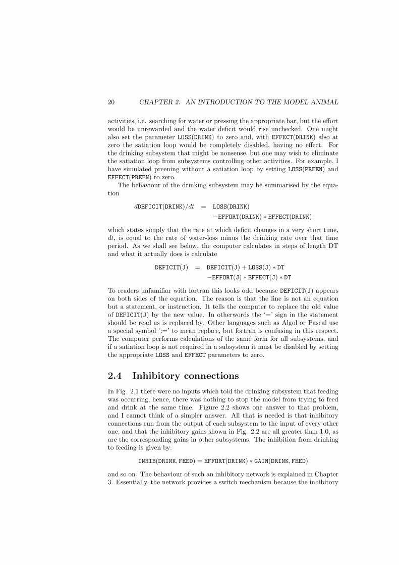
2.4 Inhibitory connections
In Fig. 2.1 there were no inputs which told the drinking subsystem that feedingwas occurring, hence, there was nothing to stop the model from trying to feedand drink at the same time. Figure 2.2 shows one answer to that problem,and I cannot think of a simpler answer. All that is needed is that inhibitoryconnections run from the output of each subsystem to the input of every otherone, and that the inhibitory gains shown in Fig. 2.2 are all greater than 1.0, asare the corresponding gains in other subsystems. The inhibition from drinkingto feeding is given by:
INHIB(DRINK, FEED) = EFFORT(DRINK) ∗ GAIN(DRINK, FEED)
and so on. The behaviour of such an inhibitory network is explained in Chapter3. Essentially, the network provides a switch mechanism because the inhibitory
2.5. THE SHORT-TERM FATIGUE LOOP 21
connections form a series of flip-flops which prevent two or more activities fromoccurring at the same time.
There is nothing in the model to prevent certain stimuli from exciting one ac-tivity and inhibiting another. For example, a hawk overhead may excite escapeand inhibit chirping. But in the model animal there is an important distinctionbetween inhibitory signals which act directly on a given subsystem, and thosewhich act indirectly, through an inhibitory pathway from another subsystem.We may not know at the outset which route is involved, for example, does theaction of escape inhibit chirping, or is chirping inhibited directly by the hawk?However, direct and indirect inhibition have different consequences in the modelanimal, and it may be possible to separate them in real animals. For the mo-ment, however, I make it clear that where direct inhibition is thought to occur,the inhibitory signal should be incorporated among STIMULI(J). STIMULI(J)and DEFICIT(J) are then said to contribute to the direct factors for drinking.The inhibitory signals from the other activities, feeding, preening and song, areadded to form SUMIN(DRINK) and these are said to be indirect factors becausethey depend on the direct factors for other activities. The indirect factors alsodepend on whether, or not, any other activity is occurring. If EFFORT(FEED)is zero, then the inhibition from feeding to drinking will also be zero and thedrinking subsystem will receive no inhibition from the feeding subsystem.
2.5 The short-term fatigue loop
The short-term loop was part of the model from the start, and was proposedto explain the alternation of activities in a constant environment. The environ-ment concerned was a perspex sphere in which aphids could obtain no nutrient,so attempts at feeding were not ended by satiation. Why then did the aphidsalternate between activities? The first suggestion was that suppressed subsys-tems might adapt to the inhibition suppressing them. The first subsystem toescape from suppression would then inhibit all the others. A second possibilitywas that the active subsystem fatigued and as its output declined one of theother subsystems would be released. Many such decay processes are known toaffect transmission within and between neurons (see Sinclair, 1978, for a review).Their timescales vary from milleseconds to days.
In the original simulations (Ludlow, 1976) I used the idea of neurons usingup transmitter to provide a short-term fatigue loop. Whenever a given activitywas performed its subsystem would use up transmitter. If the release rate wasfaster than the rate at which it arrived at the terminal the reserve declinedand the subsystem would inhibit others less strongly. The higher the input tothe subsystem the more rapidly the transmitter was released. Furthermore thetransmitter carried the signal, so using up transmitter reduced the gain of thepathway. This idea has several merits. It is easy to visualise; it is known tooccur in some neurons (Sinclair, 1978) and it would be easily invented in thecourse of evolution. Indeed, it would be hard to design a neuron which did notsuffer this kind of decay.
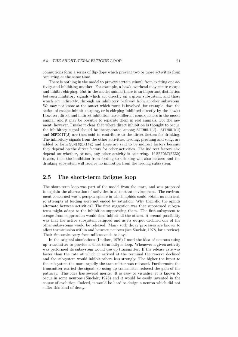
22 CHAPTER 2. AN INTRODUCTION TO THE MODEL ANIMAL
Figure 2.2: Satiation loop for the drinking subsystem together with inhibitoryconnections which form the switch mechanim. The inhibition to other subsys-tems depends on effort and the gain in the specific pathways (From Ludlow,1980).
2.5. THE SHORT-TERM FATIGUE LOOP 23
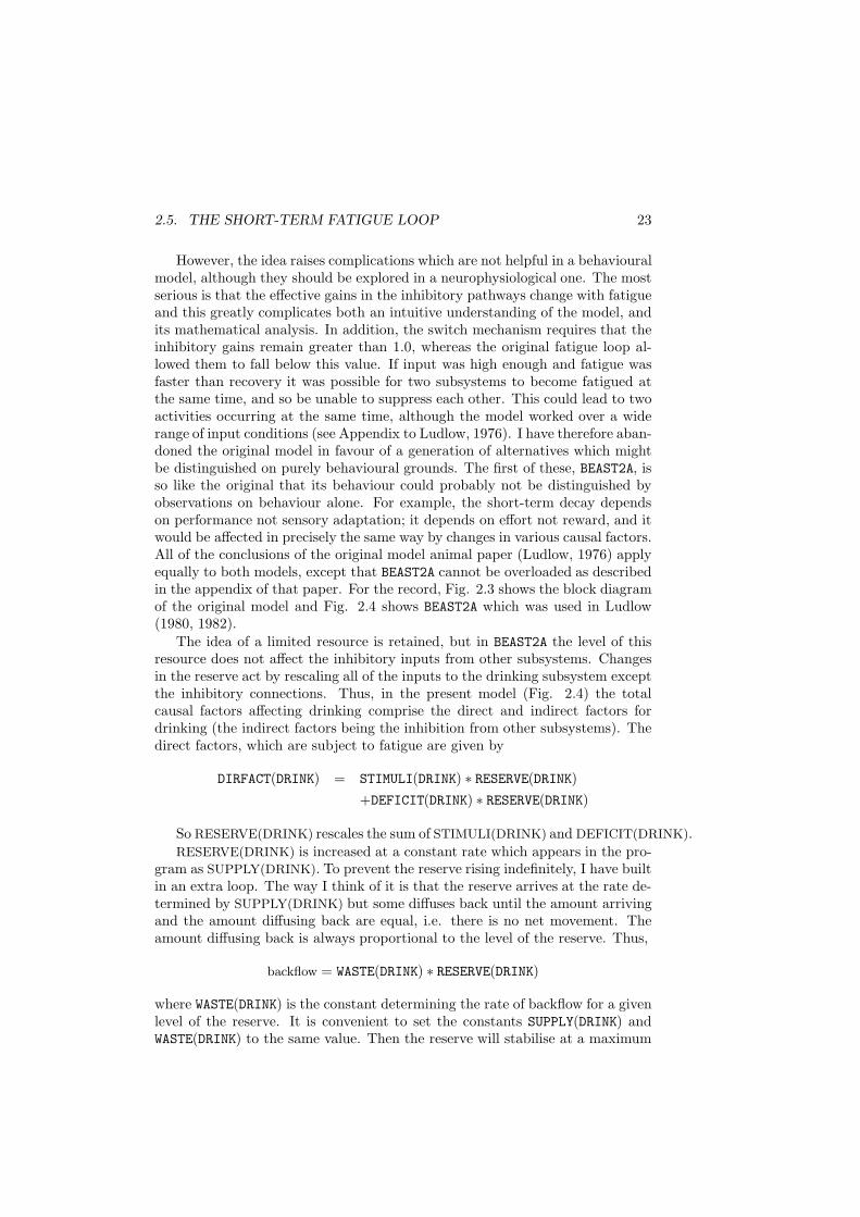
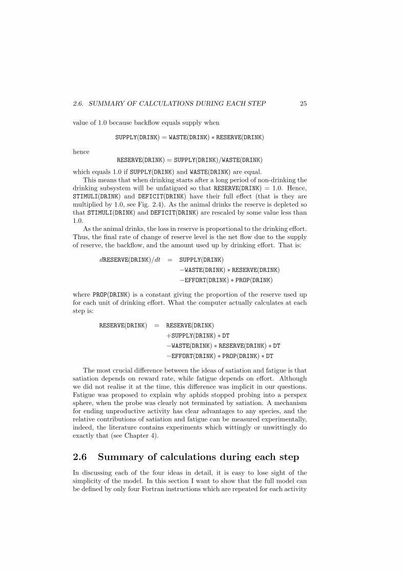
However, the idea raises complications which are not helpful in a behaviouralmodel, although they should be explored in a neurophysiological one. The mostserious is that the effective gains in the inhibitory pathways change with fatigueand this greatly complicates both an intuitive understanding of the model, andits mathematical analysis. In addition, the switch mechanism requires that theinhibitory gains remain greater than 1.0, whereas the original fatigue loop al-lowed them to fall below this value. If input was high enough and fatigue wasfaster than recovery it was possible for two subsystems to become fatigued atthe same time, and so be unable to suppress each other. This could lead to twoactivities occurring at the same time, although the model worked over a widerange of input conditions (see Appendix to Ludlow, 1976). I have therefore aban-doned the original model in favour of a generation of alternatives which mightbe distinguished on purely behavioural grounds. The first of these, BEAST2A, isso like the original that its behaviour could probably not be distinguished byobservations on behaviour alone. For example, the short-term decay dependson performance not sensory adaptation; it depends on effort not reward, and itwould be affected in precisely the same way by changes in various causal factors.All of the conclusions of the original model animal paper (Ludlow, 1976) applyequally to both models, except that BEAST2A cannot be overloaded as describedin the appendix of that paper. For the record, Fig. 2.3 shows the block diagramof the original model and Fig. 2.4 shows BEAST2A which was used in Ludlow(1980, 1982).
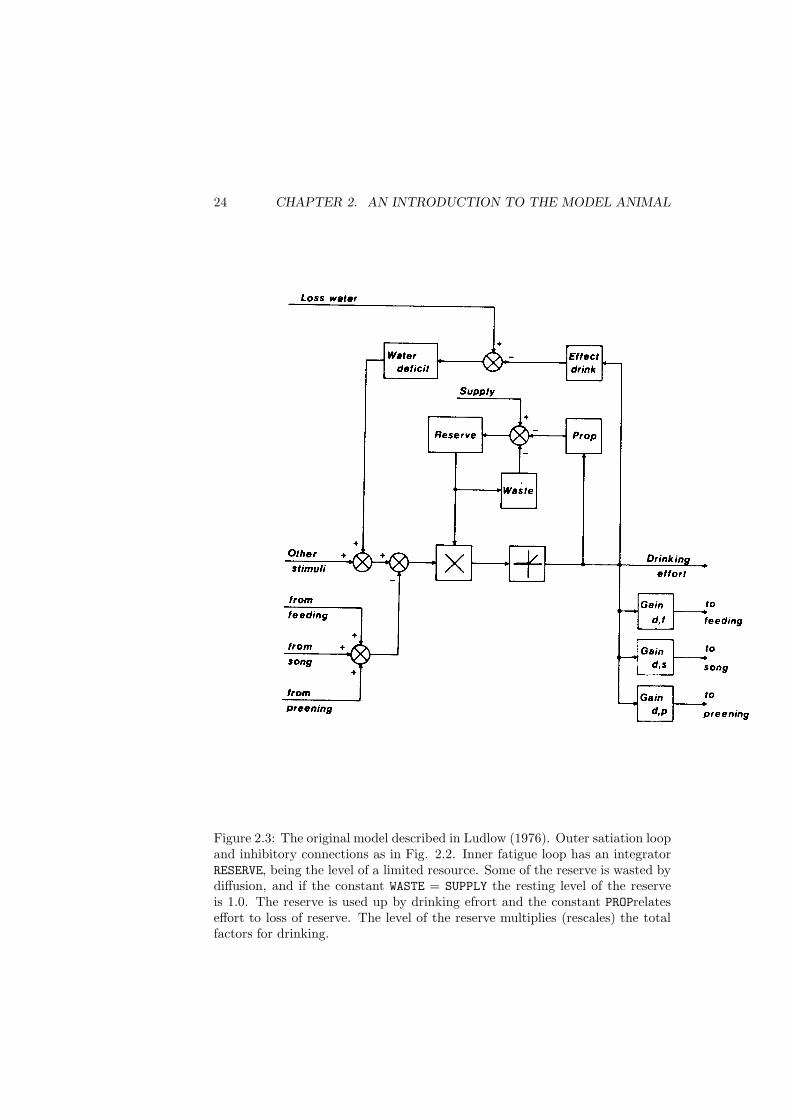
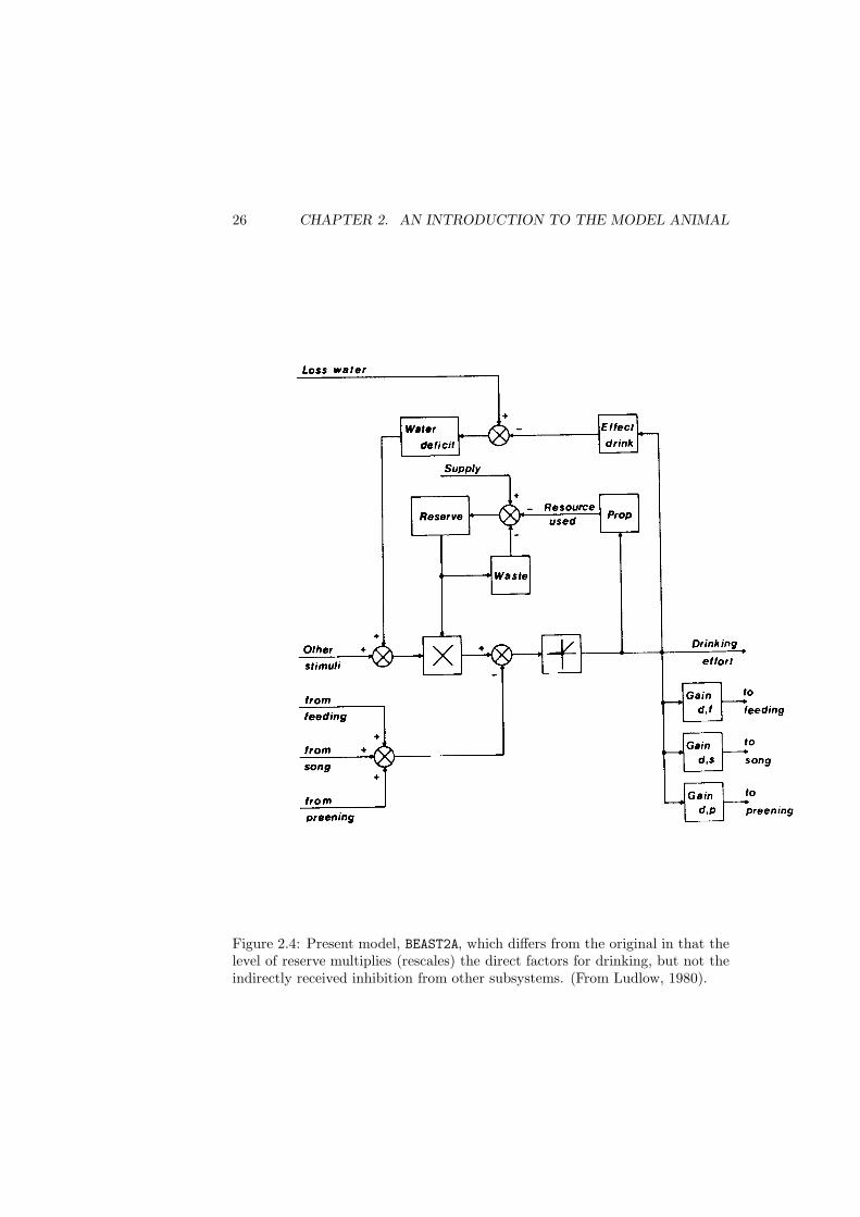
The idea of a limited resource is retained, but in BEAST2A the level of thisresource does not affect the inhibitory inputs from other subsystems. Changesin the reserve act by rescaling all of the inputs to the drinking subsystem exceptthe inhibitory connections. Thus, in the present model (Fig. 2.4) the totalcausal factors affecting drinking comprise the direct and indirect factors fordrinking (the indirect factors being the inhibition from other subsystems). Thedirect factors, which are subject to fatigue are given by
DIRFACT(DRINK) = STIMULI(DRINK) ∗ RESERVE(DRINK)
+DEFICIT(DRINK) ∗ RESERVE(DRINK)
So RESERVE(DRINK) rescales the sum of STIMULI(DRINK) and DEFICIT(DRINK).
RESERVE(DRINK) is increased at a constant rate which appears in the pro-gram as SUPPLY(DRINK). To prevent the reserve rising indefinitely, I have builtin an extra loop. The way I think of it is that the reserve arrives at the rate de-termined by SUPPLY(DRINK) but some diffuses back until the amount arrivingand the amount diffusing back are equal, i.e. there is no net movement. Theamount diffusing back is always proportional to the level of the reserve. Thus,
backflow = WASTE(DRINK) ∗ RESERVE(DRINK)
where WASTE(DRINK) is the constant determining the rate of backflow for a givenlevel of the reserve. It is convenient to set the constants SUPPLY(DRINK) andWASTE(DRINK) to the same value. Then the reserve will stabilise at a maximum
24 CHAPTER 2. AN INTRODUCTION TO THE MODEL ANIMAL
Figure 2.3: The original model described in Ludlow (1976). Outer satiation loopand inhibitory connections as in Fig. 2.2. Inner fatigue loop has an integratorRESERVE, being the level of a limited resource. Some of the reserve is wasted bydiffusion, and if the constant WASTE = SUPPLY the resting level of the reserveis 1.0. The reserve is used up by drinking efrort and the constant PROPrelateseffort to loss of reserve. The level of the reserve multiplies (rescales) the totalfactors for drinking.
2.6. SUMMARY OF CALCULATIONS DURING EACH STEP 25
value of 1.0 because backflow equals supply when
SUPPLY(DRINK) = WASTE(DRINK) ∗ RESERVE(DRINK)
henceRESERVE(DRINK) = SUPPLY(DRINK)/WASTE(DRINK)
which equals 1.0 if SUPPLY(DRINK) and WASTE(DRINK) are equal.This means that when drinking starts after a long period of non-drinking the
drinking subsystem will be unfatigued so that RESERVE(DRINK) = 1.0. Hence,STIMULI(DRINK) and DEFICIT(DRINK) have their full effect (that is they aremultiplied by 1.0, see Fig. 2.4). As the animal drinks the reserve is depleted sothat STIMULI(DRINK) and DEFICIT(DRINK) are rescaled by some value less than1.0.
As the animal drinks, the loss in reserve is proportional to the drinking effort.Thus, the final rate of change of reserve level is the net flow due to the supplyof reserve, the backflow, and the amount used up by drinking effort. That is:
dRESERVE(DRINK)/dt = SUPPLY(DRINK)
−WASTE(DRINK) ∗ RESERVE(DRINK)
−EFFORT(DRINK) ∗ PROP(DRINK)
where PROP(DRINK) is a constant giving the proportion of the reserve used upfor each unit of drinking effort. What the computer actually calculates at eachstep is:
RESERVE(DRINK) = RESERVE(DRINK)
+SUPPLY(DRINK) ∗ DT
−WASTE(DRINK) ∗ RESERVE(DRINK) ∗ DT
−EFFORT(DRINK) ∗ PROP(DRINK) ∗ DT
The most crucial difference between the ideas of satiation and fatigue is thatsatiation depends on reward rate, while fatigue depends on effort. Althoughwe did not realise it at the time, this difference was implicit in our questions.Fatigue was proposed to explain why aphids stopped probing into a perspexsphere, when the probe was clearly not terminated by satiation. A mechanismfor ending unproductive activity has clear advantages to any species, and therelative contributions of satiation and fatigue can be measured experimentally,indeed, the literature contains experiments which wittingly or unwittingly doexactly that (see Chapter 4).
2.6 Summary of calculations during each step
In discussing each of the four ideas in detail, it is easy to lose sight of thesimplicity of the model. In this section I want to show that the full model canbe defined by only four Fortran instructions which are repeated for each activity
26 CHAPTER 2. AN INTRODUCTION TO THE MODEL ANIMAL
Figure 2.4: Present model, BEAST2A, which differs from the original in that thelevel of reserve multiplies (rescales) the direct factors for drinking, but not theindirectly received inhibition from other subsystems. (From Ludlow, 1980).
2.6. SUMMARY OF CALCULATIONS DURING EACH STEP 27
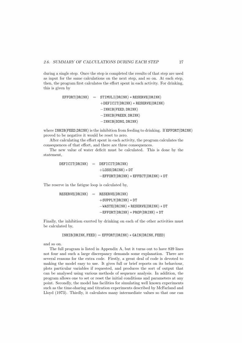
during a single step. Once the step is completed the results of that step are usedas input for the same calculations on the next step, and so on. At each step,then, the program first calculates the effort spent in each activity. For drinking,this is given by
EFFORT(DRINK) = STIMULI(DRINK) ∗ RESERVE(DRINK)
+DEFICIT(DRINK) ∗ RESERVE(DRINK)
−INHIB(FEED, DRINK)
−INHIB(PREEN, DRINK)
−INHIB(SONG, DRINK)
where INHIB(FEED,DRINK) is the inhibition from feeding to drinking. If EFFORT(DRINK)proved to be negative it would be reset to zero.
After calculating the effort spent in each activity, the program calculates theconsequences of that effort, and there are three consequences.
The new value of water deficit must be calculated. This is done by thestatement,
DEFICIT(DRINK) = DEFICIT(DRINK)
+LOSS(DRINK) ∗ DT
−EFFORT(DRINK) ∗ EFFECT(DRINK) ∗ DT
The reserve in the fatigue loop is calculated by,
RESERVE(DRINK) = RESERVE(DRINK)
+SUPPLY(DRINK) ∗ DT
−WASTE(DRINK) ∗ RESERVE(DRINK) ∗ DT
−EFFORT(DRINK) ∗ PROP(DRINK) ∗ DT
Finally, the inhibition exerted by drinking on each of the other activities mustbe calculated by,
INHIB(DRINK, FEED) = EFFORT(DRINK) ∗ GAIN(DRINK, FEED)
and so on.The full program is listed in Appendix A, but it turns out to have 839 lines
not four and such a large discrepancy demands some explanation. There areseveral reasons for the extra code. Firstly, a great deal of code is devoted tomaking the model easy to use. It gives full or brief reports on its behaviour,plots particular variables if requested, and produces the sort of output thatcan be analysed using various methods of sequence analysis. In addition, theprogram allows one to set or reset the initial conditions and parameters at anypoint. Secondly, the model has facilities for simulating well known experimentssuch as the time-sharing and titration experiments described by McFarland andLloyd (1973). Thirdly, it calculates many intermediate values so that one can
28 CHAPTER 2. AN INTRODUCTION TO THE MODEL ANIMAL
measure direct factors, or total factors as well as ettort spent in each activity.Finally, there is a complication which arises from trying to simulate a continuousprocess like behaviour on a digital computer which can calculate only in steps.The last point needs to be discussed here, and is covered in the next section.
2.7 A complication in calculating the inhibition
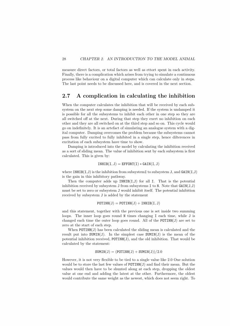
When the computer calculates the inhibition that will be received by each sub-system on the next step some damping is needed. If the system is undamped itis possible for all the subsystems to inhibit each other in one step so they areall switched off at the next. During that step they exert no inhibition on eachother and they are all switched on at the third step and so on. This cycle wouldgo on indefinitely. It is an artefact of simulating an analogue system with a dig-ital computer. Damping overcomes the problem because the subsystems cannotpass from fully excited to fully inhibited in a single step, hence dilterences inexcitation of each subsystem have time to show.
Damping is introduced into the model by calculating the inhibition receivedas a sort of sliding mean. The value of inhibition sent by each subsystem is firstcalculated. This is given by:
INHIB(I, J) = EFFORT(I) ∗ GAIN(I, J)
where INHIB(I,J) is the inhibition from subsystemI to subsystem J, and GAIN(I,J)is the gain in this inhibitory pathway.
Then the computer adds up INHIB(I,J) for all I. That is the potentialinhibition received by subsystem J from subsystems I to N. Note that GAIN(J,J)must be set to zero or subsystem J would inhibit itself. The potential inhibitionreceived by subsystem J is added by the statement
POTINH(J) = POTINH(J) + INHIB(I, J)
and this statement, together with the previous one is set inside two summingloops. The inner loop goes round N times changing I each time, while J ischanged each time the outer loop goes round. All of the POTINH(J) are set tozero at the start of each step.
When POTINH(J) has been calculated the sliding mean is calculated and theresult put into SUMIN(J). In the simplest case SUMIN(J) is the mean of thepotential inhibition received, POTINH(J), and the old inhibition. That would becalculated by the statement:
SUMIN(J) = (POTINH(J) + SUMIN(J))/2.0
However, it is not very flexible to be tied to a single value like 2.0 One solutionwould be to store the last few values of POTINH(J) and find their mean. But thevalues would then have to be shunted along at each step, dropping the oldestvalue at one end and adding the latest at the other. Furthermore, the oldestwould contribute the same weight as the newest, which does not seem right. To
2.8. SUMMARY 29
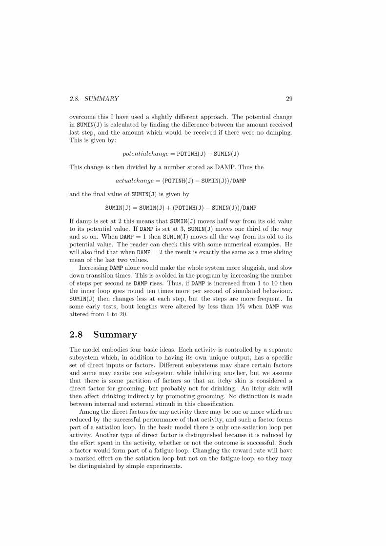
overcome this I have used a slightly different approach. The potential changein SUMIN(J) is calculated by finding the difference between the amount receivedlast step, and the amount which would be received if there were no damping.This is given by:
potentialchange = POTINH(J) − SUMIN(J)
This change is then divided by a number stored as DAMP. Thus the
actualchange = (POTINH(J) − SUMIN(J))/DAMP
and the final value of SUMIN(J) is given by
SUMIN(J) = SUMIN(J) + (POTINH(J) − SUMIN(J))/DAMP
If damp is set at 2 this means that SUMIN(J) moves half way from its old valueto its potential value. If DAMP is set at 3, SUMIN(J) moves one third of the wayand so on. When DAMP = 1 then SUMIN(J) moves all the way from its old to itspotential value. The reader can check this with some numerical examples. Hewill also find that when DAMP = 2 the result is exactly the same as a true slidingmean of the last two values.
Increasing DAMP alone would make the whole system more sluggish, and slowdown transition times. This is avoided in the program by increasing the numberof steps per second as DAMP rises. Thus, if DAMP is increased from 1 to 10 thenthe inner loop goes round ten times more per second of simulated behaviour.SUMIN(J) then changes less at each step, but the steps are more frequent. Insome early tests, bout lengths were altered by less than 1% when DAMP wasaltered from 1 to 20.
2.8 Summary
The model embodies four basic ideas. Each activity is controlled by a separatesubsystem which, in addition to having its own unique output, has a specificset of direct inputs or factors. Different subsystems may share certain factorsand some may excite one subsystem while inhibiting another, but we assumethat there is some partition of factors so that an itchy skin is considered adirect factor for grooming, but probably not for drinking. An itchy skin willthen affect drinking indirectly by promoting grooming. No distinction is madebetween internal and external stimuli in this classification.
Among the direct factors for any activity there may be one or more which arereduced by the successful performance of that activity, and such a factor formspart of a satiation loop. In the basic model there is only one satiation loop peractivity. Another type of direct factor is distinguished because it is reduced bythe effort spent in the activity, whether or not the outcome is successful. Sucha factor would form part of a fatigue loop. Changing the reward rate will havea marked effect on the satiation loop but not on the fatigue loop, so they maybe distinguished by simple experiments.
30 CHAPTER 2. AN INTRODUCTION TO THE MODEL ANIMAL
Finally, activities which should not occur together do not because their sub-systems inhibit each other. The inhibition runs from the output of one sub-system to the input of every other, and the gain in the inhibitory pathways isgreater than 1.0.
The total factors affecting any subsystem are divided into two groups: thedirect factors which comprise the satiation factor, the fatigue factor and otherstimuli, and the indirect factors which act directly on some other subsystem,but affect drinking through the inhibitory pathways from other subsystems. Anitchy skin which acted directly on the grooming subsystem would be just suchan indirect factor for drinking because it would influence any inhibition fromthe grooming to the drinking subsystem.
A computer simulation involves calculating the model’s state in a series ofsteps. First the effort spent in each activity is calculated. This should be zerofor all but one activity (apart from the brief transition between activities). Thenthe consequences of that effort are calculated for: (a) the satiation loop, (b) thefatigue loop and (c) the inhibition which will act on other subsystems duringthe next step.
There are one or two practical complications in running the computer model.Of these the most important is that the inhibition between subsystems has tohave some damping in order to smooth the jerky effects of calculating continuouschanges as a series of steps.
An annotated copy of the fortran program is given in Appendix A.
Chapter 3
Consequences of mutual
inhibition
We may fairly lament that intuitive probability is insufficient for sci-entific purposes, but it is a historical fact. W. Feller, An introductionto probability theory and its applications. 1968
I hope, in the next two chapters, to show how the model animal has beenuseful in raising questions I should not otherwise have asked and in answeringother questions, sometimes in unexpected ways. At several points it has becomeclear that arguments widely propogated in the literature are incomplete and lesscompelling than they have usually appeared.
3.1 Properties or the switch mechanism
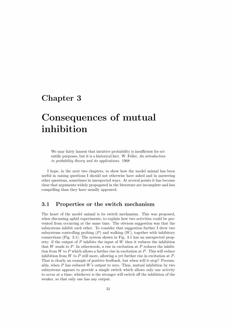
The heart of the model animal is its switch mechanism. This was proposed,when discussing aphid experiments, to explain how two activities could be pre-vented from occurring at the same time. The obvious suggestion was that thesubsystems inhibit each other. To consider that suggestion further I drew twosubsystems controlling probing (P ) and walking (W ), together with inhibitoryconnections (Fig. 3.1). The system shown in Fig. 3.1 has an unexpected prop-erty: if the output of P inhibits the input of W then it reduces the inhibitionthat W sends to P . In otherwords, a rise in excitation at P reduces the inhibi-tion from W to P which allows a further rise in excitation at P . This will reduceinhibition from W to P still more, allowing a yet further rise in excitation at P .That is clearly an example of positive feedback, but when will it stop? Presum-ably, when P has reduced W ’s output to zero. Thus, mutual inhibition by twosubsystems appears to provide a simple switch which allows only one activityto occur at a time; whichever is the stronger will switch off the inhibition of theweaker, so that only one has any output.
31
32 CHAPTER 3. CONSEQUENCES OF MUTUAL INHIBITION
Figure 3.1: Two subsystems connected by mutual inhibition
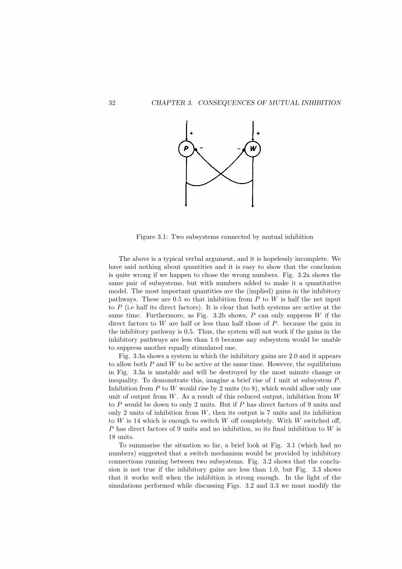
The above is a typical verbal argument, and it is hopelessly incomplete. Wehave said nothing about quantities and it is easy to show that the conclusionis quite wrong if we happen to chose the wrong numbers. Fig. 3.2a shows thesame pair of subsystems, but with numbers added to make it a quantitativemodel. The most important quantities are the (implied) gains in the inhibitorypathways. These are 0.5 so that inhibition from P to W is half the net inputto P (i.e half its direct factors). It is clear that both systems are active at thesame time. Furthermore, as Fig. 3.2b shows, P can only suppress W if thedirect factors to W are half or less than half those of P . because the gain inthe inhibitory pathway is 0.5. Thus, the system will not work if the gains in theinhibitory pathways are less than 1.0 because any subsystem would be unableto suppress another equally stimulated one.
Fig. 3.3a shows a system in which the inhibitory gains are 2.0 and it appearsto allow both P and W to be active at the same time. However, thc equilibriumin Fig. 3.3a is unstable and will be destroyed by the most minute change orinequality. To demonstrate this, imagine a brief rise of 1 unit at subsystem P .Inhibition from P to W would rise by 2 units (to 8), which would allow only oneunit of output from W . As a result of this reduced output, inhibition from Wto P would be down to only 2 units. But if P has direct factors of 9 units andonly 2 units of inhibition from W , then its output is 7 units and its inhibitionto W is 14 which is enough to switch W off completely. With W switched off,P has direct factors of 9 units and no inhibition, so its final inhibition to W is18 units.
To summarise the situation so far, a brief look at Fig. 3.1 (which had nonumbers) suggested that a switch mechanism would be provided by inhibitoryconnections running between two subsystems. Fig. 3.2 shows that the conclu-sion is not true if the inhibitory gains are less than 1.0, but Fig. 3.3 showsthat it works well when the inhibition is strong enough. In the light of thesimulations performed while discussing Figs. 3.2 and 3.3 we must modify the
3.1. PROPERTIES OR THE SWITCH MECHANISM 33
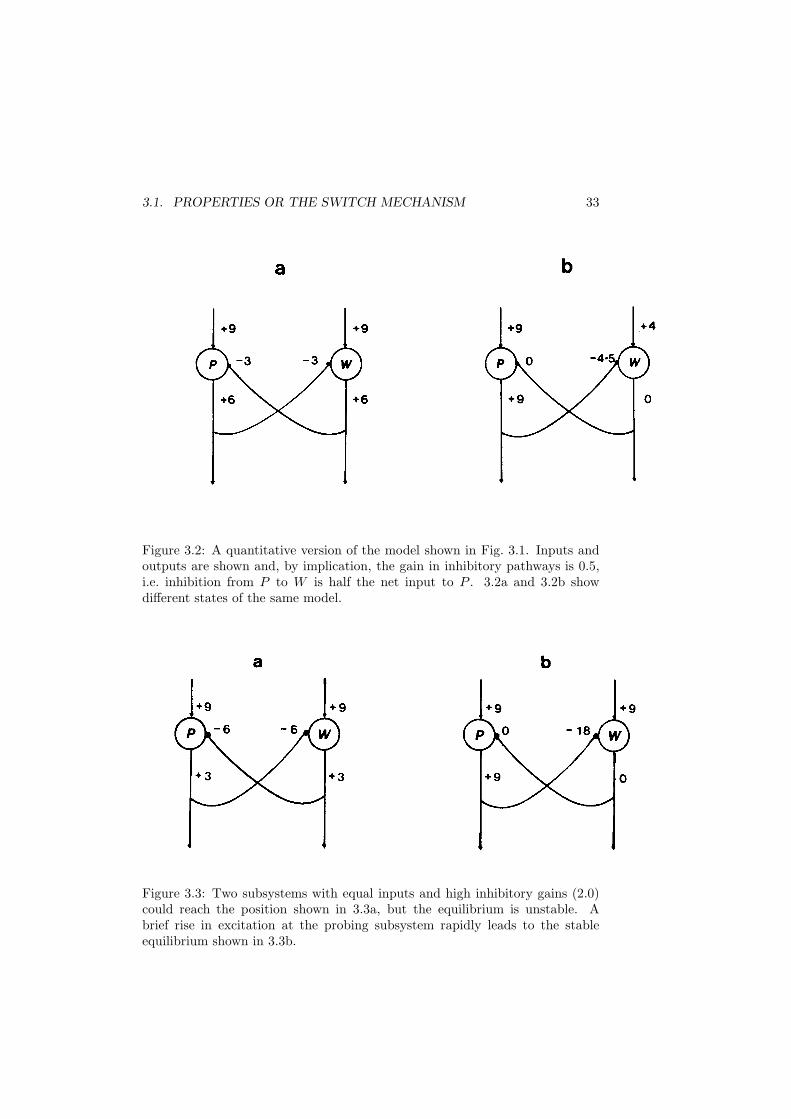
Figure 3.2: A quantitative version of the model shown in Fig. 3.1. Inputs andoutputs are shown and, by implication, the gain in inhibitory pathways is 0.5,i.e. inhibition from P to W is half the net input to P . 3.2a and 3.2b showdifferent states of the same model.
Figure 3.3: Two subsystems with equal inputs and high inhibitory gains (2.0)could reach the position shown in 3.3a, but the equilibrium is unstable. Abrief rise in excitation at the probing subsystem rapidly leads to the stableequilibrium shown in 3.3b.
34 CHAPTER 3. CONSEQUENCES OF MUTUAL INHIBITION
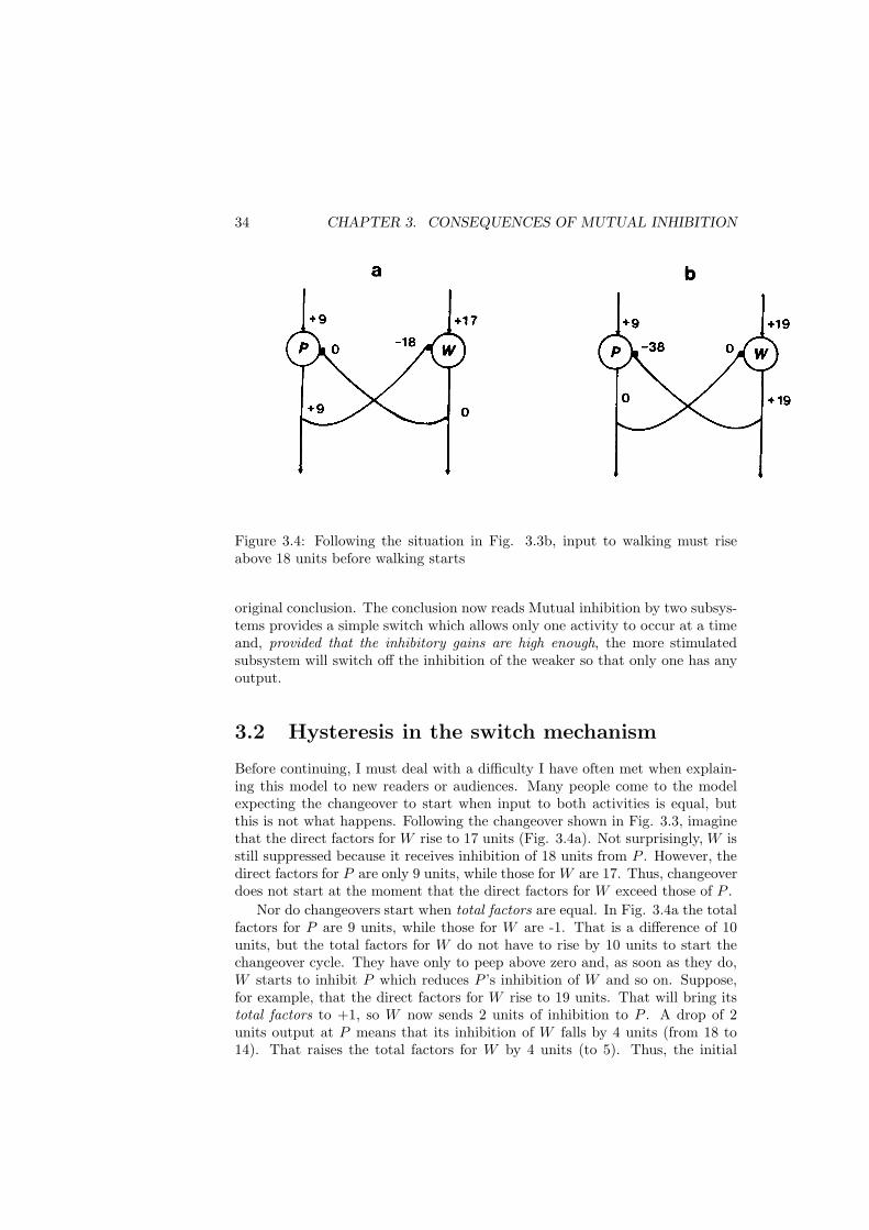
Figure 3.4: Following the situation in Fig. 3.3b, input to walking must riseabove 18 units before walking starts
original conclusion. The conclusion now reads Mutual inhibition by two subsys-tems provides a simple switch which allows only one activity to occur at a timeand, provided that the inhibitory gains are high enough, the more stimulatedsubsystem will switch off the inhibition of the weaker so that only one has anyoutput.
3.2 Hysteresis in the switch mechanism
Before continuing, I must deal with a difficulty I have often met when explain-ing this model to new readers or audiences. Many people come to the modelexpecting the changeover to start when input to both activities is equal, butthis is not what happens. Following the changeover shown in Fig. 3.3, imaginethat the direct factors for W rise to 17 units (Fig. 3.4a). Not surprisingly, W isstill suppressed because it receives inhibition of 18 units from P . However, thedirect factors for P are only 9 units, while those for W are 17. Thus, changeoverdoes not start at the moment that the direct factors for W exceed those of P .
Nor do changeovers start when total factors are equal. In Fig. 3.4a the totalfactors for P are 9 units, while those for W are -1. That is a difference of 10units, but the total factors for W do not have to rise by 10 units to start thechangeover cycle. They have only to peep above zero and, as soon as they do,W starts to inhibit P which reduces P ’s inhibition of W and so on. Suppose,for example, that the direct factors for W rise to 19 units. That will bring itstotal factors to +1, so W now sends 2 units of inhibition to P . A drop of 2units output at P means that its inhibition of W falls by 4 units (from 18 to14). That raises the total factors for W by 4 units (to 5). Thus, the initial

3.2. HYSTERESIS IN THE SWITCH MECHANISM 35
rise of 1 unit in total factors for W goes round the loop and removes 4 unitsof inhibition from W . The four unit rise at W means that its output goes upfrom 1 to 5, and its inhibition of P from 2 to 10, which is enough to suppressP completely. Now, unsuppressed, the total factors for W become equal to itsdirect factors (19 units) as shown in Fig. 3.4b.
With inhibitory gains of 2.0 the changes accelerate (a 1 unit rise leads to a4 unit rise which leads to total liberation) but the point I want to emphasiseis that neither direct factors nor total factors were equal when the changeoverstarted. On the contrary, the changeover started as soon as direct factors forW rose above 18 units (while those for P were 9) and when total factors for Wrose above 0 (while those for P were 9).
I labour this point because it appears to conflict with a fundamental assump-tion which most people make implicitly, and some authors have made explicitly(e.g. Atkinson and Birch, 1970). The assumption is that the activity being per-formed at any instant is always that which is most strongly stimulated and thechangeover point must therefore be the point at which stimulation was equal.In otherwords it is a landmark which can be used in the analysis of behaviour.The model animal does not contradict the premise but it shows the conclusionto be oversimple. The activity being performed at any instant is always the onewith the highest total factors. Indeed, it is the only one with total factors abovezero, because the fundamental assumption behind the model animal is that anyactivity with positive total factors at any instant will be performed. The in-hibitory connections were proposed to ensure that only one activity ever hadpositive total factors at any one time (apart from the brief changeover cycle).
Thus, there is no conflict between the model animal and Atkinsons andBirchs assumption, but their conclusion that the changeover point marks thepoint of equal causal factors does not apply to the model animal. What hap-pens is that the changeover starts well before the total factors are equal and, amoment later, when the changeover has finished their positions are completelyreversed. The changeover rushes past the point of equality somewhere betweenthese two extremes. I find that hard to visualise exactly, so I never think interms of total factors. Instead I work with direct factors which do not dependon each other as total factors do. But if we work with direct factors we mustnever try and apply Atkinsons and Birchs assumption. The assumption is truefor total factors, but definitely not true for direct factors. The activity beingperformed at any instant is not always the one with the highest direct factors.Figure 3.4a shows that quite clearly. Direct factors for P are less than those forW , but it is P which is occurring. There is nothing contradictory about thisbecause direct factors are a subset of the total factors. The confusion arises ifwe blur the distinction between total and direct factors. Inhibition is necessaryto prevent two activities from occurring at the same time, and the inhibitionmust be strong enough to hold down a rival with equal direct factors (or theywould both occur at once). If the inhibition has strength to spare it can holddown a rival whose direct factors have become greater than its own since the lastchangeover. However, it is very important to remember the distinction betweendirect and total factors. I shall always work with direct factors because we can
36 CHAPTER 3. CONSEQUENCES OF MUTUAL INHIBITION
then regard the inhibitory network as a black box giving well-defined start andstop thresholds for each activity.
The start threshold is still a useful landmark and, if we work with directfactors, the start threshold for W is the level of direct factors for W which mustbe exceeded before changeover starts. When the direct factors for P were 9units, and P was occurring, the start threshold for W was 18. In a two unitsystem, the start threshold for W is equal to the inhibition from P to W . That isequal to the direct factors for P multiplied by the gain in the inhibitory pathwayfrom P to W . Once W has started, however, its stop threshold is much lower.In Fig. 3.4b, for example, the direct factors for W would have to fall to 4.5before P was disinhibited. This is because the gain in the inhibitory pathwayfrom W to P is 2.0, and even if direct factors for W fell to 4.5 it would still send9 units of inhibition to P , which is enough to keep P suppressed. Thus, withtwo subsystems, the stop threshold for W is equal to the direct factors for Pdivided by the gain in the inhibitory pathway from W to P . The stop thresholdhas no physiological counterpart, in the way that the start threshold equals theinhibition received from the ongoing activity. Nevertheless, the stop threshold isparticularly helpful in understanding the sequence of activities. Ludlow (1982)gives a full discussion of start and stop thresholds.
A large gap between start and stop thresholds is known as hysteresis. In themodel animal it is due to the two things which happen when W ousts P . Wnot only throws off the inhibition it previously received from P , it also starts tosend inhibition to P . Removing former inhibition is equivalent to receiving anadded positive signal, or to positive feedback. Imposing inhibition of its own isan increase relative to P , even if it is not an increase in absolute terms. Someweeks after dicovering these properties of the switch mechanism I attended ameeting of the Association for the Study of Animal Behaviour where Dr. IDuncan delivered a paper on meal size in chickens. The question he posed was:why does a chicken go on eating after the first mouthful? If it has only justbecome hungry enough to start feeding, then the first mouthful might reduceits hunger enough to stop it eating. In fact it eats so much thai it does not thenfeed again for some time. Duncan proposed that delays in food absorption wereresponsible, and other authors (eg. McFarland and Sibly, 1975) have argued thatthe sensation of food in the mouth excites feeding so that it continues beyondthe point at which it was started. This is another example of positive feedback.As shown above, however, an additional possibility is that the mechanism bywhich animals switch between activities might show hysteresis. It seems verylikely that all three of these mechanisms are involved.
3.3 The control of sequences in a model with
many subsystems
Up to now we have considered only two activities, do the conclusions still applyif there are more than two? To test this, an electrical model was built with
THE CONTROL OF SEQUENCES 37
four subsystems. It confirmed that the network would allow only one activityto occur at a time, even when all activities had the same excitatory inputs. Themodel also confirmed that high gains in the pathways caused rapid transitions,and it had the hysteresis properties described above. However, one could noteasily follow the inputs, outputs and inhibitory connections of the 4 electricalsubsystems simultaneously, so further work proceeded by calculating the changesstep by step, culminating in the present computer programs. During many hoursof simulation, with ten activities and many thousands of changeovers, there havebeen no cases where the switch mechanism has broken down, providing thatreasonable damping was used (see Chapter 2).
The only significant difference between a two and a multi-subsystem modelis that the stop thresholds are calculated differently. The stop threshold forW , at any instant, depends on the strongest rival at that instant, and the othersuppressed activities can be ignored when calculating stop thresholds. However,the strongest rival is not necessarily the one with the highest direct factors. Ifind it best to think of the suppressed activities bidding to succeed the ongoingone, and the bid each one offers to W is equal to its own direct factors dividedby the the gain in inhibition from W to it. Thus, BID(P |W ) is the bid offeredby P when W is occurring, and is given by
BID(P |W ) = D(P )/GAIN(W, P )
where D(P ) is the sum of direct factors for activity P . The vertical line in theequation should be read as “given”. The highest bid provides the stop thresholdfor W because W will be replaced as soon as its direct factors fall below that bid.The start thresholds in the multi-subsystem model are calculated just as in thetwo-subsystem model because the start threshold for any suppressed activityis equal to the inhibition it receives from the ongoing activity. When W isoccurring, the inhibition to P equals D(W ) ∗ GAIN(W, P ) so the start thresholdis given by:
START(P |W ) = D(W ) ∗ GAIN(W, P )
If the gains in the inhibitory pathways determine the start thresholds for thesuppressed activities, then it follows that differences in these gains would allowlower start thresholds for one activity than another. For example, one activity,say P , might inhibit X more weakly than it inhibits W . In that case thestart threshold for X would be lower than that for W . All other things beingequal, X would be more likely than W to follow P . Simulations immediatelyconfirmed that differences in gains would indeed affect transition probabilitiesand that, if the gains were sufficiently different, the sequence of activities couldbe completely determined. If the sequence of activities could be influenced, oreven determined, by the gains in the inhibitory pathways, then perhaps learnedchanges in sequences of behaviour might be due to changes in inhibitory gains.
For example, in some simulations of rat behaviour (Ludlow, 1982, and below)it was important to arrange that drinking tended to follow feeding. This wasdone very simply by setting a relatively low value for the gain in inhibition fromfeeding to drinking. As a result, the model showed several peculiar properties
38 CHAPTER 3. CONSEQUENCES OF MUTUAL INHIBITION
of rat behaviour. One of these was that it tended to drink more in the earlydays of starvation because food searching was more frequent and led to morefrequent drinking. Milgram et al. (1974) reared one group of rats on chowand lettuce so that they had no prior experience of drinking water with meals.The control group was reared on chow and water. When both groups weregiven chow and water there was no difference in the amount drunk, but whenboth groups were starved, those with experience of water drank more than thechow and lettuce reared rats. These differences were successfully simulated byadjusting the inhibitory gain between feeding and drinking, a relatively weakgain gave normal rat behaviour; a slightly higher gain gave the behaviour foundin lettuce-reared rats (Ludlow, 1979, 1982).
3.4 Learning and the model animal
The current version of the model animal is incapable of learning but the controlof sequences is so simple that one can easily see what would have to change for aparticular sequence of activities to become a habit. From the Milgram, Kramesand Thompson experiment, it looks as if the normal coupling of feeding anddrinking requires learning, and from the simulations it is clear that the processof learning could involve a resetting of the relevant inhibitory gain.
To explain learning in this way one must suggest a mechanism whereby thegain between feeding and drinking is reduced whenever the sequence feedingto drinking occurs. The simplest learning rule which might be postulated isthat specific inhibitory receptors in the drinking subsystem become less sen-sitive whenever drinking occurs immediately after feeding. Immediately aftersuch a transition the neurons on the drinking subsystem will become activewhile inhibitory transmitter from the feeding subsystem still occupies their re-ceptors. Hence, learning could occur by knocking out any inhibitory receptorswhich were caught with transmitter still on them at the moment of membranedepolarisation. This would reduce the gain in the inhibitory pathway from thefeeding to the drinking subsystems whenever feeding was followed by drinking.The gain in other inhibitors pathways would not be affected.
As Sinclair (1978) has pointed out there are numerous processes which causea decrease in gain as pathways are used, while there is no good evidence of aprocess which causes a long-term increase in gain with use. Hence, to decreasethe gain in an inhibitory pathway may be more in keeping with known physiologythan to increase the gain in an excitatory pathway as many other learningtheories require. However, it is essential that the gain is reduced only in thepathway from feeding to drinking. It is known that absence of transmitterincreases the number of receptors and that the number is reduced by persistantoccupancy (see Sinclair, 1978, for a review), but the mechanism proposed hererequires, in addition, that the reduction in sites is greatest if the membranedepolarises during site occupancy. That additional mechanism would allow thetwo events, feeding and drinking, to become coupled at a single synapse withoutneeding auxilliary neurones to register the coincidence of the activities as other
ALTERNATIVE INHIBITORY CONNECTIONS 39
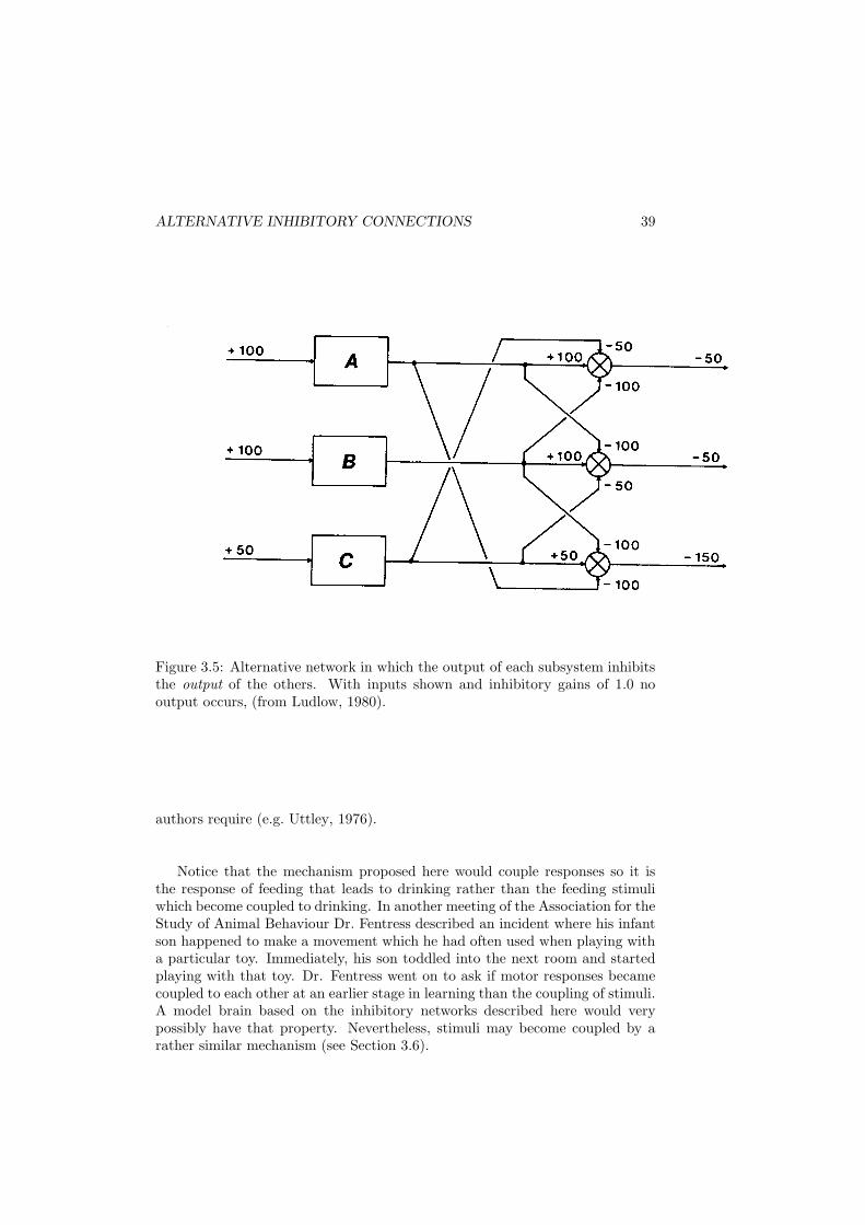
Figure 3.5: Alternative network in which the output of each subsystem inhibitsthe output of the others. With inputs shown and inhibitory gains of 1.0 nooutput occurs, (from Ludlow, 1980).
authors require (e.g. Uttley, 1976).
Notice that the mechanism proposed here would couple responses so it isthe response of feeding that leads to drinking rather than the feeding stimuliwhich become coupled to drinking. In another meeting of the Association for theStudy of Animal Behaviour Dr. Fentress described an incident where his infantson happened to make a movement which he had often used when playing witha particular toy. Immediately, his son toddled into the next room and startedplaying with that toy. Dr. Fentress went on to ask if motor responses becamecoupled to each other at an earlier stage in learning than the coupling of stimuli.A model brain based on the inhibitory networks described here would verypossibly have that property. Nevertheless, stimuli may become coupled by arather similar mechanism (see Section 3.6).
40 CHAPTER 3. CONSEQUENCES OF MUTUAL INHIBITION
3.5 Alternative arrangements of the inhibitory
connections
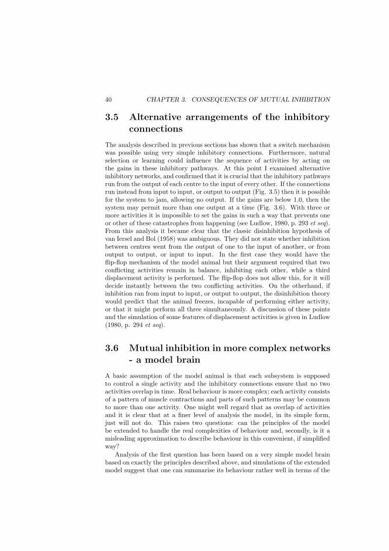
The analysis described in previous sections has shown that a switch mechanismwas possible using very simple inhibitory connections. Furthermore, naturalselection or learning could influence the sequence of activities by acting onthe gains in these inhibitory pathways. At this point I examined alternativeinhibitory networks, and confirmed that it is crucial that the inhibitory pathwaysrun from the output of each centre to the input of every other. If the connectionsrun instead from input to input, or output to output (Fig. 3.5) then it is possiblefor the system to jam, allowing no output. If the gains are below 1.0, then thesystem may permit more than one output at a time (Fig. 3.6). With three ormore activities it is impossible to set the gains in such a way that prevents oneor other of these catastrophes from happening (see Ludlow, 1980, p. 293 et seq).From this analysis it became clear that the classic disinhibition hypothesis ofvan Iersel and Bol (1958) was ambiguous. They did not state whether inhibitionbetween centres went from the output of one to the input of another, or fromoutput to output, or input to input. In the first case they would have theflip-flop mechanism of the model animal but their argument required that twoconflicting activities remain in balance, inhibiting each other, while a thirddisplacement activity is performed. The flip-flop does not allow this, for it willdecide instantly between the two conflicting activities. On the otherhand, ifinhibition ran from input to input, or output to output, the disinhibition theorywould predict that the animal freezes, incapable of performing either activity,or that it might perform all three simultaneously. A discussion of these pointsand the simulation of some features of displacement activities is given in Ludlow(1980, p. 294 et seq).
3.6 Mutual inhibition in more complex networks
- a model brain
A basic assumption of the model animal is that each subsystem is supposedto control a single activity and the inhibitory connections ensure that no twoactivities overlap in time. Real behaviour is more complex; each activity consistsof a pattern of muscle contractions and parts of such patterns may be commonto more than one activity. One might well regard that as overlap of activitiesand it is clear that at a finer level of analysis the model, in its simple form,just will not do. This raises two questions: can the principles of the modelbe extended to handle the real complexities of behaviour and, secondly, is it amisleading approximation to describe behaviour in this convenient, if simplifiedway?
Analysis of the first question has been based on a very simple model brainbased on exactly the principles described above, and simulations of the extendedmodel suggest that one can summarise its behaviour rather well in terms of the
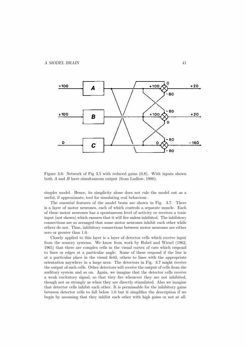
A MODEL BRAIN 41
Figure 3.6: Network of Fig 3.5 with reduced gains (0.8). With inputs shownboth A and B have simultaneous output (from Ludlow, 1980).
simpler model. Hence, its simplicity alone does not rule the model out as auseful, if approximate, tool for simulating real behaviour.
The essential features of the model brain are shown in Fig. 3.7. Thereis a layer of motor neurones, each of which controls a separate muscle. Eachof these motor neurones has a spontaneous level of activity or receives a tonicinput (not shown) which ensures that it will fire unless inhibited. The inhibitoryconnections are so arranged that some motor neurones inhibit each other whileothers do not. Thus, inhibitory connections between motor neurones are eitherzero or greater than 1.0.
Closely applied to this layer is a layer of detector cells which receive inputfrom the sensory systems. We know from work by Hubel and Wiesel (1962,1965) that there are complex cells in the visual cortex of cats which respondto lines or edges at a particular angle. Some of these respond if the line isat a particular place in the visual field, others to lines with the appropriateorientation anywhere in a large area. The detectors in Fig. 3.7 might receivethe output of such cells. Other detectors will receive the output of cells from theauditory system and so on. Again, we imagine that the detector cells receivea weak excitatory signal, so that they fire whenever they are not inhibited,though not as strongly as when they are directly stimulated. Also we imaginethat detector cells inhibit each other. It is permissable for the inhibitory gainsbetween detector cells to fall below 1.0 but it simplifies the description if webegin by assuming that they inhibit each other with high gains or not at all.
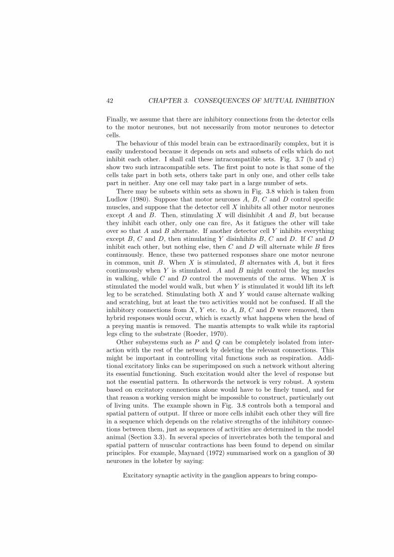
42 CHAPTER 3. CONSEQUENCES OF MUTUAL INHIBITION
Finally, we assume that there are inhibitory connections from the detector cellsto the motor neurones, but not necessarily from motor neurones to detectorcells.
The behaviour of this model brain can be extraordinarily complex, but it iseasily understood because it depends on sets and subsets of cells which do notinhibit each other. I shall call these intracompatible sets. Fig. 3.7 (b and c)show two such intracompatible sets. The first point to note is that some of thecells take part in both sets, others take part in only one, and other cells takepart in neither. Any one cell may take part in a large number of sets.
There may be subsets within sets as shown in Fig. 3.8 which is taken fromLudlow (1980). Suppose that motor neurones A, B, C and D control specificmuscles, and suppose that the detector cell X inhibits all other motor neuronesexcept A and B. Then, stimulating X will disinhibit A and B, but becausethey inhibit each other, only one can fire, As it fatigues the other will takeover so that A and B alternate. If another detector cell Y inhibits everythingexcept B, C and D, then stimulating Y disinhihits B, C and D. If C and Dinhibit each other, but nothing else, then C and D will alternate while B firescontinuously. Hence, these two patterned responses share one motor neuronein common, unit B. When X is stimulated, B alternates with A, but it firescontinuously when Y is stimulated. A and B might control the leg musclesin walking, while C and D control the movements of the arms. When X isstimulated the model would walk, but when Y is stimulated it would lift its leftleg to be scratched. Stimulating both X and Y would cause alternate walkingand scratching, but at least the two activities would not be confused. If all theinhibitory connections from X , Y etc. to A, B, C and D were removed, thenhybrid responses would occur, which is exactly what happens when the head ofa preying mantis is removed. The mantis attempts to walk while its raptoriallegs cling to the substrate (Roeder, 1970).
Other subsystems such as P and Q can be completely isolated from inter-action with the rest of the network by deleting the relevant connections. Thismight be important in controlling vital functions such as respiration. Addi-tional excitatory links can be superimposed on such a network without alteringits essential functioning. Such excitation would alter the level of response butnot the essential pattern. In otherwords the network is very robust. A systembased on excitatory connections alone would have to be finely tuned, and forthat reason a working version might be impossible to construct, particularly outof living units. The example shown in Fig. 3.8 controls both a temporal andspatial pattern of output. If three or more cells inhibit each other they will firein a sequence which depends on the relative strengths of the inhibitory connec-tions between them, just as sequences of activities are determined in the modelanimal (Section 3.3). In several species of invertebrates both the temporal andspatial pattern of muscular contractions has been found to depend on similarprinciples. For example, Maynard (1972) summarised work on a ganglion of 30neurones in the lobster by saying:
Excitatory synaptic activity in the ganglion appears to bring compo-
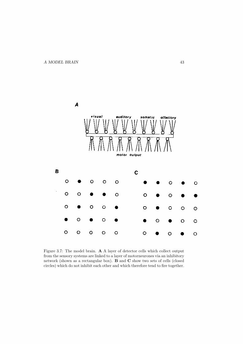
A MODEL BRAIN 43
Figure 3.7: The model brain. A A layer of detector cells which collect outputfrom the sensory systems are linked to a layer of motorneurones via an inhibitorynetwork (shown as a rectangular box). B and C show two sets of cells (closedcircles) which do not inhibit each other and which therefore tend to fire together.
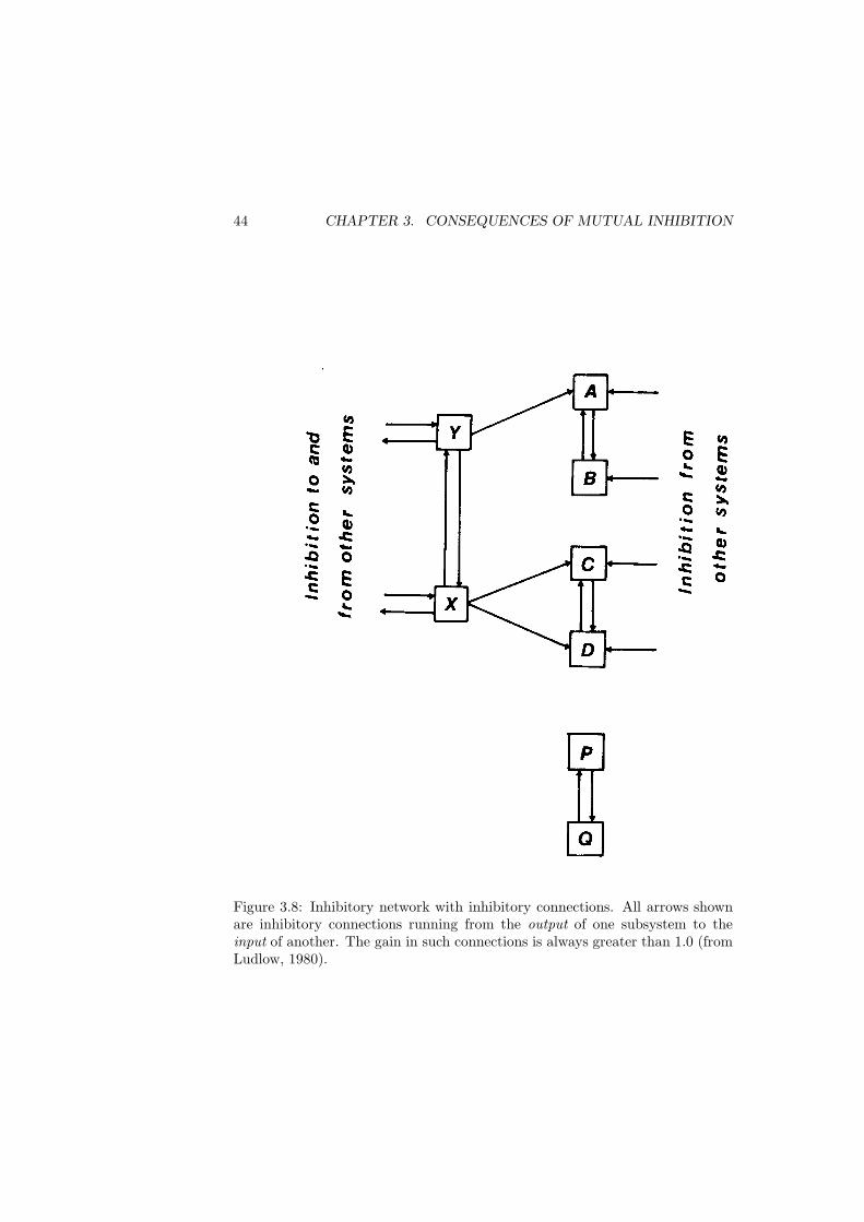
44 CHAPTER 3. CONSEQUENCES OF MUTUAL INHIBITION
Figure 3.8: Inhibitory network with inhibitory connections. All arrows shownare inhibitory connections running from the output of one subsystem to theinput of another. The gain in such connections is always greater than 1.0 (fromLudlow, 1980).
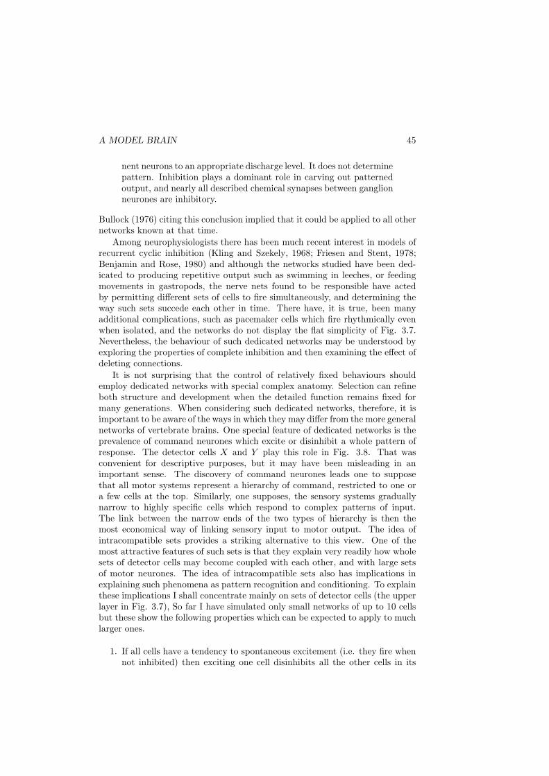
A MODEL BRAIN 45
nent neurons to an appropriate discharge level. It does not determinepattern. Inhibition plays a dominant role in carving out patternedoutput, and nearly all described chemical synapses between ganglionneurones are inhibitory.
Bullock (1976) citing this conclusion implied that it could be applied to all othernetworks known at that time.
Among neurophysiologists there has been much recent interest in models ofrecurrent cyclic inhibition (Kling and Szekely, 1968; Friesen and Stent, 1978;Benjamin and Rose, 1980) and although the networks studied have been ded-icated to producing repetitive output such as swimming in leeches, or feedingmovements in gastropods, the nerve nets found to be responsible have actedby permitting different sets of cells to fire simultaneously, and determining theway such sets succede each other in time. There have, it is true, been manyadditional complications, such as pacemaker cells which fire rhythmically evenwhen isolated, and the networks do not display the flat simplicity of Fig. 3.7.Nevertheless, the behaviour of such dedicated networks may be understood byexploring the properties of complete inhibition and then examining the effect ofdeleting connections.
It is not surprising that the control of relatively fixed behaviours shouldemploy dedicated networks with special complex anatomy. Selection can refineboth structure and development when the detailed function remains fixed formany generations. When considering such dedicated networks, therefore, it isimportant to be aware of the ways in which they may differ from the more generalnetworks of vertebrate brains. One special feature of dedicated networks is theprevalence of command neurones which excite or disinhibit a whole pattern ofresponse. The detector cells X and Y play this role in Fig. 3.8. That wasconvenient for descriptive purposes, but it may have been misleading in animportant sense. The discovery of command neurones leads one to supposethat all motor systems represent a hierarchy of command, restricted to one ora few cells at the top. Similarly, one supposes, the sensory systems graduallynarrow to highly specific cells which respond to complex patterns of input.The link between the narrow ends of the two types of hierarchy is then themost economical way of linking sensory input to motor output. The idea ofintracompatible sets provides a striking alternative to this view. One of themost attractive features of such sets is that they explain very readily how wholesets of detector cells may become coupled with each other, and with large setsof motor neurones. The idea of intracompatible sets also has implications inexplaining such phenomena as pattern recognition and conditioning. To explainthese implications I shall concentrate mainly on sets of detector cells (the upperlayer in Fig. 3.7), So far I have simulated only small networks of up to 10 cellsbut these show the following properties which can be expected to apply to muchlarger ones.
1. If all cells have a tendency to spontaneous excitement (i.e. they fire whennot inhibited) then exciting one cell disinhibits all the other cells in its
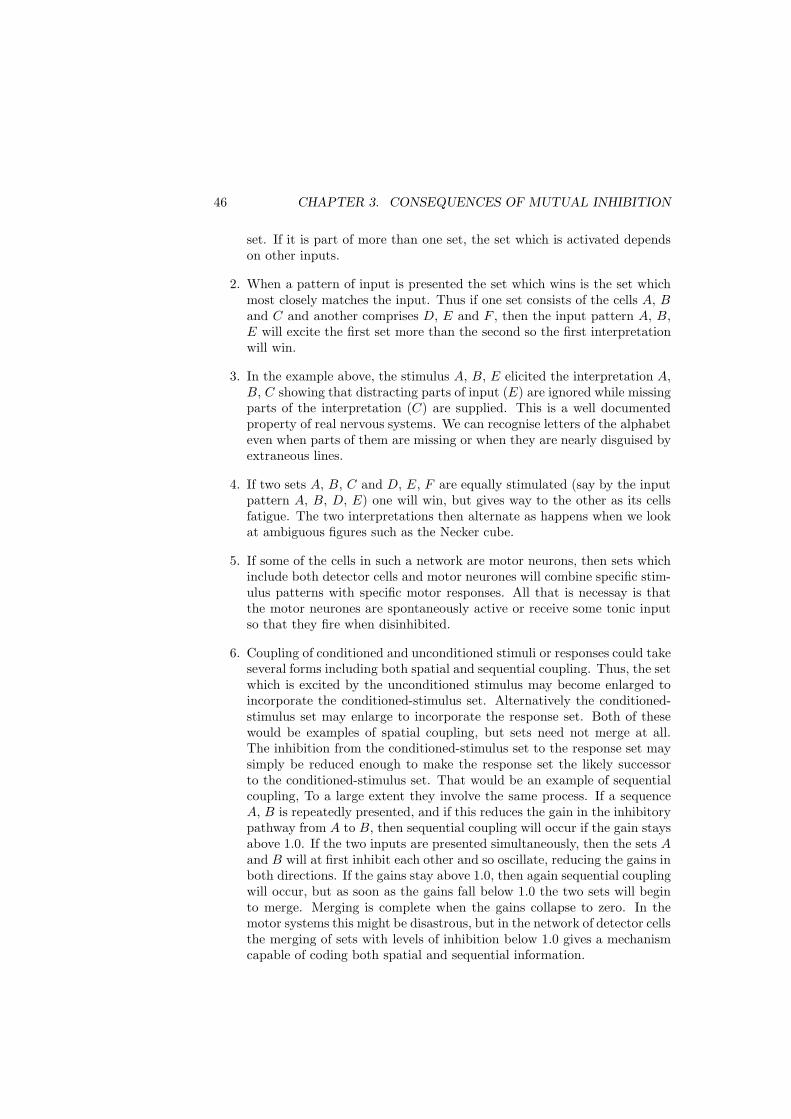
46 CHAPTER 3. CONSEQUENCES OF MUTUAL INHIBITION
set. If it is part of more than one set, the set which is activated dependson other inputs.
2. When a pattern of input is presented the set which wins is the set whichmost closely matches the input. Thus if one set consists of the cells A, Band C and another comprises D, E and F , then the input pattern A, B,E will excite the first set more than the second so the first interpretationwill win.
3. In the example above, the stimulus A, B, E elicited the interpretation A,B, C showing that distracting parts of input (E) are ignored while missingparts of the interpretation (C) are supplied. This is a well documentedproperty of real nervous systems. We can recognise letters of the alphabeteven when parts of them are missing or when they are nearly disguised byextraneous lines.
4. If two sets A, B, C and D, E, F are equally stimulated (say by the inputpattern A, B, D, E) one will win, but gives way to the other as its cellsfatigue. The two interpretations then alternate as happens when we lookat ambiguous figures such as the Necker cube.
5. If some of the cells in such a network are motor neurons, then sets whichinclude both detector cells and motor neurones will combine specific stim-ulus patterns with specific motor responses. All that is necessay is thatthe motor neurones are spontaneously active or receive some tonic inputso that they fire when disinhibited.
6. Coupling of conditioned and unconditioned stimuli or responses could takeseveral forms including both spatial and sequential coupling. Thus, the setwhich is excited by the unconditioned stimulus may become enlarged toincorporate the conditioned-stimulus set. Alternatively the conditioned-stimulus set may enlarge to incorporate the response set. Both of thesewould be examples of spatial coupling, but sets need not merge at all.The inhibition from the conditioned-stimulus set to the response set maysimply be reduced enough to make the response set the likely successorto the conditioned-stimulus set. That would be an example of sequentialcoupling, To a large extent they involve the same process. If a sequenceA, B is repeatedly presented, and if this reduces the gain in the inhibitorypathway from A to B, then sequential coupling will occur if the gain staysabove 1.0. If the two inputs are presented simultaneously, then the sets Aand B will at first inhibit each other and so oscillate, reducing the gains inboth directions. If the gains stay above 1.0, then again sequential couplingwill occur, but as soon as the gains fall below 1.0 the two sets will beginto merge. Merging is complete when the gains collapse to zero. In themotor systems this might be disastrous, but in the network of detector cellsthe merging of sets with levels of inhibition below 1.0 gives a mechanismcapable of coding both spatial and sequential information.
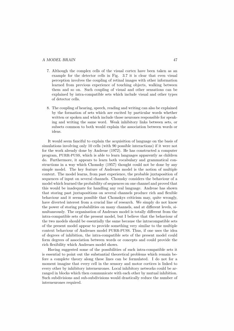
A MODEL BRAIN 47
7. Although the complex cells of the visual cortex have been taken as anexample for the detector cells in Fig. 3.7 it is clear that even visualperception involves the coupling of retinal images with other informationlearned from previous experience of touching objects, walking betweenthem and so on. Such coupling of visual and other sensations can beexplained by intra-compatible sets which include visual and other typesof detector cells.
8. The coupling of hearing, speech, reading and writing can also be explainedby the formation of sets which are excited by particular words whetherwritten or spoken and which include those neurones responsible for speak-ing and writing the same word. Weak inhibitory links between sets, orsubsets common to both would explain the association between words orideas.
It would seem fanciful to explain the acquisition of language on the basis ofsimulations involving only 10 cells (with 90 possible interactions) if it were notfor the work already done by Andreae (1972). He has constructed a computerprogram, PURR-PUSS, which is able to learn languages apparently as childrendo. Furthermore, it appears to learn both vocabulary and grammatical con-structions in a way which Chomsky (1957) thought could not be done by anysimple model. The key feature of Andreaes model is the notion of multiplecontext. The model learns, from past experience, the probable juxtaposition ofsequences of input on several channels. Chomsky considers the behaviour of amodel which learned the probability of sequences on one channel and proved thatthis would be inadequate for handling any real language. Andreae has shownthat storing past juxtapositions on several channels produce rich and flexiblebehaviour and it seems possible that Chomskys criticism may, quite wrongly,have diverted interest from a crucial line of research. We simply do not knowthe power of storing probabilities on many channels, and at different levels, si-multaneously. The organisation of Andreaes model is totally different from theintra-compatible sets of the present model, but I believe that the behaviour ofthe two models should be essentially the same because the intracompatible setsof the present model appear to provide something very similar to the multiplecontext behaviour of Andreaes model PURR-PUSS. Thus, if one uses the ideaof degrees of inhibition, the intra-compatible sets of the present model couldform degrees of association between words or concepts and could provide therich flexibility which Andreaes model shows.
Having suggested some of the possibilities of such intra-compatible sets itis essential to point out the substantial theoretical problems which remain be-fore a complete theory along these lines can be formulated. I do not for amoment imagine that every cell in the sensory and motor cortices is linked toevery other by inhibitory interneurones. Local inhibitory networks could be ar-ranged in blocks which then communicate with each other by mutual inhibition.Such subdivisions and sub-subdivisions would drastically reduce the number ofinterneurones required.
48 CHAPTER 3. CONSEQUENCES OF MUTUAL INHIBITION
Another possibility has been suggested by Joseph et al. (1979). They in-dependently proposed the sort of reciprocal inhibition being considered here,but went on to develop a model which required fewer inhibitory connections.Each cell is supposed when active to excite a general inhibitory system which,in turn, inhibits all cells. Self-suppression is prevented because each cell excitesitself with as much inhibition as it would receive back from its own contributionto the general inhibitory system. Such self-excitation must compensate exactlyfor the extra inhibition the cell receives as a result of its own output. This ismathematically equivalent to the present model when all the inhibitory gainsare equal. I suspect that there may be problems with their model if inequalitiesin gains are allowed, and it is exactly the development of such inequalities whichwould be required for learning to take place in the way I have suggested. Nev-ertheless, their extension of the ideas of reciprocal inhibition is an importantcontribution because it is very likely that some hybrid version, in which gen-eral inhibition occurs at some levels and one-to-one inhibition at others, wouldprovide an economical model with high learning and coordinating power.
One should not expect to find individual cells in the cortex correspondingto those in Fig. 3,7. Any corresponding units in the cortex would have evolvedadditional specialised functions and anatomical features, and would almost cer-tainly consist of several different cell-types. Secondly, the layout of Fig. 3.7contains enormous and wasteful redundancy. While it might be embryologicallysimple to grow all possible connections and then delete the irrelevant ones, itis far more efficient not to grow some of them at all. For example, there is nopossible reason for antagonism between the muscles of the foot and those ofthe larynx, so it would be wasteful to grow and delete inhibition between suchmotor neurones. By grouping together those groups which must or might haveto inhibit each other, and not growing irrelevant connections the total numberof neurones can be enormously reduced. Specialised regions which obscure thesimplicity of Fig. 3.7 would be expected if such a system had passed throughmillions of years of evolution.
Nor is it necessary for learning to take place at inhibitory synapses. Thecrucial thing is that gains in inhibitory pathways should be reduced. This canbe done by reducing the excitation of an inhibitory neurone, or by reducing theamount or effect of transmitter released by the inhibitory neurone.
It might be thought that a model based on deleting inhibitory connections issimply the mirror image of the more usual models in which learning occurs byforming excitatory connections (e.g. Sutton and Barto, 1981). However, thereare unique features of inhibition. In the first place excess inhibition does notover-inhibit, it simply switches off, and once that has happened it does notmatter if the inhibition is too strong. Thus, two inhibited cells have the sameoutput if they are both switched off, whereas they would have to be excitedto exactly the same extent if they were to have the same positive output inan excitatory network. Furthermore, it is clear that inhibition is necessary intheories of selective attention or singleness of action.
In this context, the two functions of learning and coordination may conflictwith each other to some extent because it is essential, if inappropriate pairs
A MODEL BRAIN 49
of activities or movements are to be prevented, that inhibitory gains are keptgreater than 1.0. The flexible learning networks on the otherhand must havegains which are modified by experience and which can go below 1.0. Thus, thelearning mechanism suggested here must be prevented or restricted in some partsof the nervous system and allowed in others. As mentioned above, alterations inthe control of sequences in time are possible with gains greater than 1.0, providedthat relative differences in the gains can he changed. But the developmentof simultaneous activity within a set of cells requires that the gains go below1.0. In both types of learning, however, it is essential that gains are restoredif the occurrence of a pattern or a repeated sequence does not occur. Moreprecisely, the inhibition from A to B must be reduced by the sequence A, B,but strengthened by the sequence A, X . Similarly it must be reduced by thesimultaneous presentation of A and B but strengthened by the simultaneouspresentation of A and X . This requirement would be fulfilled if inhibitoryreceptors tended to proliferate unless the cell membrane becomes excited whilethe receptors still have inhibitory transmitter on their receptors.
One way in which the separation of high and low gain networks might beachieved is to ensure that all inhibition between motor neurones is much greaterthan 1.0 (but variable above a high value) while detector cells are able to elim-inate any particular inhibitory input completely. The ability of motor neuronesto throw off inhibitory connections might be high in early development but belost later. In that way the learning mechanism suggested here might also be im-portant in setting up the known inhibitory connections between motor neuronesin the spinal cord. Inappropriate connections made by random growth could beeliminated by the coincidence of adjacent cells firing, and so being excited whileinhibitory transmitter is still on them.
Another problem faced by the theory is that, in many known nervous net-works, the inhibitory connections from one cell all appear to diminish with dis-tance from the cell. In the retina, for example, cells exert inhibition on nearby,but not distant, cells and this is important in sharpening the response to edges.In other networks too, the inhibitory field of a given cell appears limited, butthis may be the anatomical equivalent of small local telephone exchanges con-nected to each other by larger trunk routes. Certainly some cells receive upto 10,000 connections which is enough to take part in many large and flexibleintra-compatible sets.
We are quite obviously a long way from any formal model embodying thesehypotheses, but they have already generated many questions about the wayparts of the nervous system might work, and there is enough circumstantialevidence in support of these ideas to make them worth serious study.
In the first place, it is clear that inhibition plays a major part in the controlof patterns of motor activity, as already described.
Secondly, there has been a great deal of work on attention and perceptionwhich has led writers to propose similar ideas, For example, Konorski (1967)concentrated much on the role of inhibition in the nervous system. He furtherproposed that gnostic units responding to significant features of the environmentwere formed, and that these inhibited each other, although sets of them would be
50 CHAPTER 3. CONSEQUENCES OF MUTUAL INHIBITION
mutually compatible. He did not specify exactly how the inhibitory connectionswere linked, or their gains, but he was clearly thinking along similar lines.However, my detector cells are not equivalent to Konorsis gnostic units. Thelatter are formed by the growth of excitatory connections during learning andrepresent the highest level of a hierarchical analysis system. Perhaps his gnosticunits correspond roughly to subsets within my intracompatible sets, althougheven there there are differences. The elements of gnostic units are linked byexcitation, my subsets by lack of inhibition.
It would certainly be a fruitful task to attempt to simulate the many ob-servations in Konorski’s volume, but it is important to point out that the ex-planations based on the model brain would be quite different from those givenby Konorski. Many differences arise because he was not aware of all the pos-sibilities of inhibitory networks, nor of the crucial differences between differenttypes of network (compare Figs. 3.2, 3.3, 3.5 and 3.6). So neither the similari-ties nor the differences between Konorskis ideas and the present model shouldbe exaggerated. Although his contribution was immense, his models were notcompletely defined.
The papers of Shallice (1972), Walley and Weiden (1973) and Joseph et al.(1979) form a series which explores the consequences of mutual inhibition inincreasing depth. Shallice proposed that only one action system can be stronglyactivated at a time, but that others remain weakly activated. This implies in-hibitory gains of less than 1.0, but one cannot be sure whether the connectionswould be as in Fig. 3.2 or Fig. 3.6. Walley and Weiden (1973) used an unam-biguous computer model to study the behaviour of low-gain networks as shownin Fig. 3.2. They were interested in the way sets of gnostic units would inhibiteach other, assuming no inhibition within sets, and they simulated the dynamicchanges as two sets of equal, or unequal size were excited. They also simulatedthe case where only one set was strongly excited (the other had a spontaneouslow level of excitation) and their most important result was that a set which hadpreviously been excited remained excitable for several seconds after the stimuluswas withdrawn.
These results suggest that activity in a set of gnostic units producesafter effects which can persist for a time which is comparable tothe duration of short-term memory. As long as this after-effect per-sists Set A would be more easily re-excited than Set B. It appearsthat explanations of short-term memory need not rely solely on themechanism of reverberating circuits.
Walley and Weiden simulated only two sets inhibiting each other and they sim-plified their calculations by assuming that all of the inhibitory gains in any onesimulation were equal (0.2 in some simulations up to 0.45 in others). As a resultthey overlooked the fact that variable gains between cells could determine bothtemporal and spatial patterns, and that modifying the gains could produce ameans of learning temporal and spatial probabilities.
The evidence reviewed by Walley and Weiden is concerned mainly with thephenomena of selective attention and cognitive masking. The latter being the
A MODEL BRAIN 51
way the performance of one task interferes to a greater or lesser extent withthe simultaneous performance of another. They review, in particular, the effectof arousal on masking and point out that this could involve changes in theinhibitory gains.
Joseph et al. (1979) took the theory a step further by showing that onecan postulate a general inhibitory system instead of the one-to-one connec-tions I have discussed. As mentioned above, this appears to involve assumingthat all inhibitory gains are equal and their model does not therefore have arich capacity for storing temporal and spatial information. However, they wereprincipally concerned with the mechanism of selective attention, and also withthe observation that schizophrenia appears to involve the breakdown of exactlythat mechanism. If selective attention is due to inhibitory networks of the typediscussed here, then the breakdown could be due to the overstimulation of thosenetworks, so that the inhibitory gains fall too low to maintain unique interpre-tations characteristic of normal attention.
As a result the patient becomes aware of multiple interpretations ofstimuli and has difficulty in carrying out any activity since manypossible actions are equally potent. This deficit can account formany of the symptoms of schizophrenia. For example, hallucinationswould be a consequence of becoming aware of possible, but unlikelyinterpretations of real sounds. Such interpretations are made byeveryone but are normally inhibited from reaching awareness.
Agents stimulating dopamine release (e.g. increased arousal or amphetamine)will increase the activity in the inhibitory networks, thus leading to their break-down. Agents which block dopamine will allow recovery, but this will be slow inspite of the fact that the sedative effect of the drug is immediate, because the re-covery rate depends on the recovery of the inhibitory system. This accords wellwith clinical observation, and the model links aspects of the chemical pathologyand the behavioural disorders which had previously been hard to explain.
Taken together, these examples do not establish that the mammalian brainoperates in the same way as the model brain portrayed in Fig. 3.7, but I claimwithout reservation that understanding the behaviour of models like that shownin Fig. 3.7 is an essential stage in understanding the organisation of real brains.Among the many theoretical questions that we need to answer are the following.
1. How large can sets be, and how does size effect speed of response?
2. What arrangements are the most economical in number of connections?
3. Can the model proposed by Joseph et al. work with unequal gains?
4. What hybrid systems would work?
5. How much of the work described by Konorski can be simulated?
6. What happens if one tries to teach a model brain to use a language?
52 CHAPTER 3. CONSEQUENCES OF MUTUAL INHIBITION
7. Does the model brain really behave like Andreae’s PURR-PUSS.
8. Do Chomskys criticisms of Markov models of language apply to multiplecontext models and intracompatible sets?
9. What other types of inhibitory network would work?
10. Is inhibition really better than excitation in such a model?
None of these questions are yet answerable, and they represent many man-yearsof work, but they seem crucial to me. Notice, I have not included such questionsas, Does learning really modify inhibitory synapses? or Is the mechanism ofreceptor-loss proposed here the most plausible suggestion? These are importantquestions but answering them would not help us understand the workings of themodel brain, and I do not believe that they provide the key to understandingmammalian brains. What we need to know is how information in the brain isorganised. As Oatley (1978) wrote
The problems of memory thus cease to be How does storage of infor-mation take place? but 1. How is knowledge of the world organised?2. How does the knowledge inform the reconstructive processes, andgenerate behaviour? 3. How is new knowledge incorporated into themental schemata? and 4. How do these structures themselves changewith the passage of time or the growth of understanding?
The speculation here began with a consideration of how responses are coordi-nated, which lead directly to an idea of how information might be organisedand recalled. In turn this lead to a view of the changes in the network whichwould affect the output, and thence to an idea of how these changes might beinduced by repeated patterns of input. I can see no other way of approachingthe problem of learning. I cannot imagine how information is stored unless Ican imagine how it can be used, and I cannot imagine how it can be used by anexcitatory network but I can imagine how it might be done by disinhibition ofintracompatible sets.
3.7 Summary
The original model animal provides an explanation of singleness of action. Twoor more activities are prevented from occuring at the same time because in-hibitory pathways run between the subsystems controlling each activity. Theinhibitory connections must run from the output of each subsystem to the inputof every other, and the gain in each pathway must be greater than 1.0. If theseconditions are not met then singleness of action is not guaranteed and in somecases all outputs will be blocked simultaneously. Given these two conditions,however, only one activity can occur at a time and transitions between activitiesare fast.
3.7. SUMMARY 53
The switch mechanism shows hysteresis, in other words, the causal factorsrequired to maintain an activity, once started, are lower than those required tostart it.
Relative differences in the gains in inhibitory pathways affect the transitionprobabilities and hence the sequence of activities. If the gains could be alteredby experience the sequence of activities would become modified by learning.
Complex activities are controlled, in the original model, by rather simple sub-systems but simulations indicate that a much more sophisticated model couldbe built on the same principles. Such a model brain could coordinate complexpatterns of muscular output, and might explain many features of pattern reco-nition and learning, possibly even the ability to learn languages. Since it workson the same principles as the model animal, the model brains ability to couplecomplex outputs with specific patterns of input suggests that the simplifyingassumptions behind the original model are not seriously misleading and thatit provides a useful if approximate way of simulating the interactions betweendifferent activities. Such simulations are described in the next chapter.

54 CHAPTER 3. CONSEQUENCES OF MUTUAL INHIBITION
Chapter 4
Consequences of fatigue
Our idealised model can be extremely useful even if it never appliesexactly. . . It is more important that the idealised scheme, when itdoes not apply, permits the discovery of assignable causes for thediscrepancies.
W. Feller, An introduction to probability theory and its applications.1968.
4.1 Differences between satiation and fatigue —
reward and effort
Apart from the switch-mechanism, the most unusual feature of the model animalis that each subsystem has a fatigue loop. Hence, all activities tend to beself-terminating and an alternation of activities will occur even when none isrewarded. The idea of fatigue was part of the model from the start and was notnew even then. McDougall (1903) and Reiss (1962) had proposed essentially thesame model to explain oscillations at the neurophysiological level. But fatiguehad unforseen implications in the context of animal behaviour.
Fatigue and satiation are very different processes. Among the most impor-tant differences is that satiation depends on reward rate, but fatigue dependson effort. Hence, they can be separated experimentally.
A number of examples in the literature suggest that both types of loop areoften needed to explain observed behaviour. For example, McFarland and Lloyd(1973) found that Barbary Doves switched from feeding to drinking and vice-versa, and that the bout-length of each did not depend on the reward rate.Doves ate more in a single bout when reward rate was high and less when itwas low. If the bout had been ended by a satiation loop they would have fedfor longest when reward rate was lowest. Ludlow (1980) showed that theseobservations could be simulated by the present model because its fatigue loopterminated feeding after a given effort, not a given reward.
55
56 CHAPTER 4. CONSEQUENCES OF FATIGUE
When simulating experiments on rat feeding and drinking, by Fitzsimons andLeMagnen (1969), the model animal ate the same volume of food in a meal onboth rich and standard diets. Thus, it was not measuring calory content of themeal (satiation) although the calory content affected the interval between meals(Ludlow, 1982). The simulations agreed with rat behaviour astonishingly wellThis is by no means conclusive evidence of a fatigue loop because it is possiblethat the rats measured the volume directly. The model animal had no stretchreceptors signalling meal size. Instead it measured the effort spent in each mealand, under ad lib feeding conditions, effort and volume were equivalent. Thisis one of many cases where quite different mechanisms can produce the sameobserved behaviour, and in such cases we need to perform specific experiments todistinguish between and measure the relative contributions of each mechanism.I suspect that the vast amount of work on reinforcement schedules may provide arich ground for simulations which will test the model’s fatigue loop and, perhaps,challenge current explanations.
Very many animals show brief interruptions of an activity which, one imag-ines, still has a high priority. For example, a hungry rat does not eat uninter-ruptedly for the whole meal. Instead, it stops briefly and cleans its whiskers orengages in some other activity. This type of alternation, between apparentlyhigh and low priority activities, has been studied in great detail and in variousspecies by McFarland and his colleagues (McFarland and Lloyd, 1973; McFar-land, 1974; Sibly and McCleery, 1976; Larkin and D., 1978; Cohen and McFar-land, 1979). They have used the term time-sharing to describe the alternationbetween a high priority (dominant) activity which appears to permit a low pri-ority (subdominant) activity to occur, but only for a brief time. For example,an individual which is known to be hungry may interrupt feeding and performsome lower priority activity, say drinking. But the interruptions are brief andfeeding is always resumed after such natural interruptions. If both activitieswere prevented for a time as soon as the individual stopped feeding, however,it might subsequently resume either feeding or the low-priority drinking. Thechoice depended on the length of the forced interruption. If both activities wereprevented for a short time (shorter than the natural drinking bout) then theindividual would usually resume drinking, but if the interruptions were longerthan the normal drinking bout, then the animal would always resume feeding.The opportunity for drinking had passed, and feeding had now withdrawn itspermission of drinking. Thus, it appeared that the dominant activity was per-mitting the subdominant to occur during a brief window. Such sophisticatedallocation of time seemed quite beyond the model animals simple mechanism,hence the attempt to simulate time-sharing looked like a severe test of themodel. When put to the test, however, it passed. It interrupted feeding whenhungry, but drinking was permitted for only a short time, and it showed otherdiagnostic features of time-sharing. The explanation turned out to be simple(Fig 4.1). The feeding fatigue-loop caused feeding to give way to drinking, butduring an uninterrupted drinking bout the feeding fatigue-loop recovered andfeeding was resumed (Fig 4.1 a). If both activities were prevented, however, assoon as feeding gave way to drinking, then a long interruption would allow time
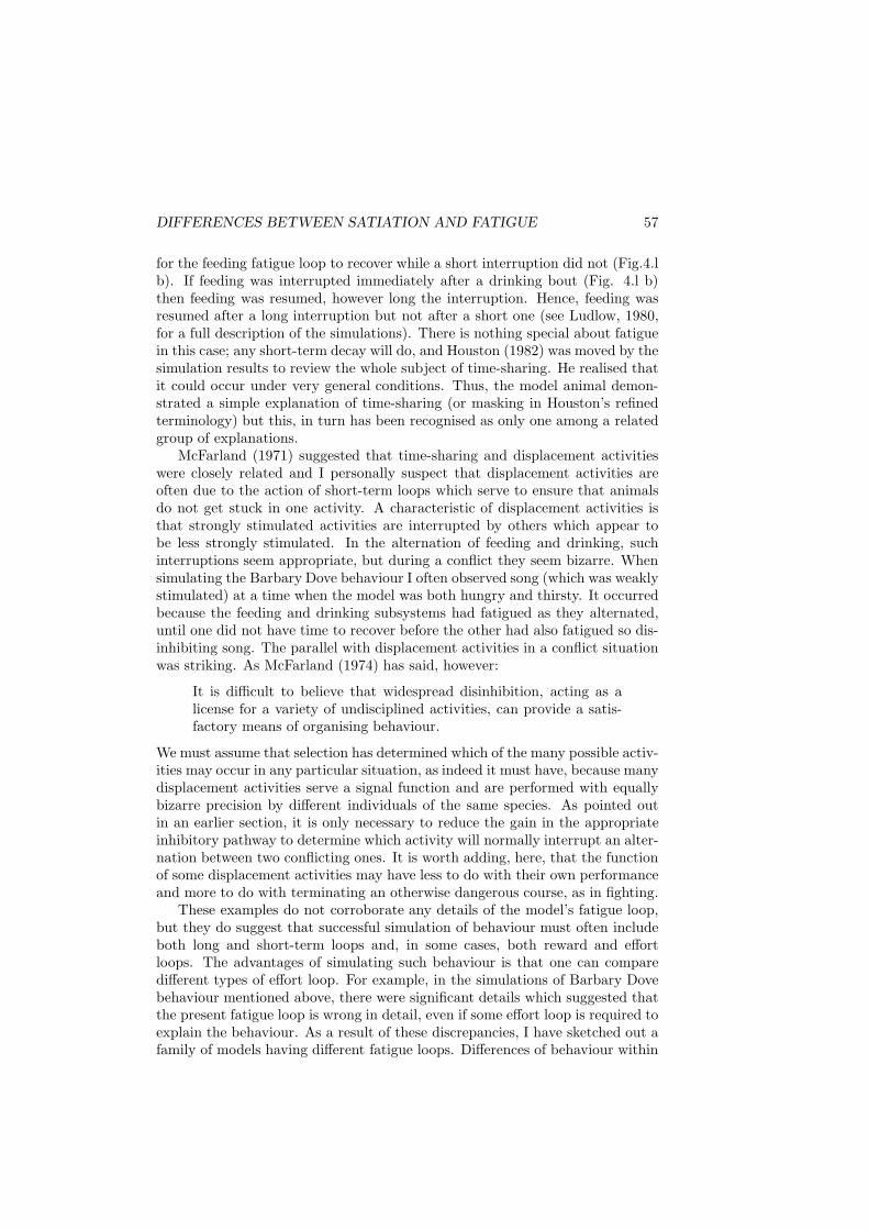
DIFFERENCES BETWEEN SATIATION AND FATIGUE 57
for the feeding fatigue loop to recover while a short interruption did not (Fig.4.lb). If feeding was interrupted immediately after a drinking bout (Fig. 4.l b)then feeding was resumed, however long the interruption. Hence, feeding wasresumed after a long interruption but not after a short one (see Ludlow, 1980,for a full description of the simulations). There is nothing special about fatiguein this case; any short-term decay will do, and Houston (1982) was moved by thesimulation results to review the whole subject of time-sharing. He realised thatit could occur under very general conditions. Thus, the model animal demon-strated a simple explanation of time-sharing (or masking in Houston’s refinedterminology) but this, in turn has been recognised as only one among a relatedgroup of explanations.
McFarland (1971) suggested that time-sharing and displacement activitieswere closely related and I personally suspect that displacement activities areoften due to the action of short-term loops which serve to ensure that animalsdo not get stuck in one activity. A characteristic of displacement activities isthat strongly stimulated activities are interrupted by others which appear tobe less strongly stimulated. In the alternation of feeding and drinking, suchinterruptions seem appropriate, but during a conflict they seem bizarre. Whensimulating the Barbary Dove behaviour I often observed song (which was weaklystimulated) at a time when the model was both hungry and thirsty. It occurredbecause the feeding and drinking subsystems had fatigued as they alternated,until one did not have time to recover before the other had also fatigued so dis-inhibiting song. The parallel with displacement activities in a conflict situationwas striking. As McFarland (1974) has said, however:
It is difficult to believe that widespread disinhibition, acting as alicense for a variety of undisciplined activities, can provide a satis-factory means of organising behaviour.
We must assume that selection has determined which of the many possible activ-ities may occur in any particular situation, as indeed it must have, because manydisplacement activities serve a signal function and are performed with equallybizarre precision by different individuals of the same species. As pointed outin an earlier section, it is only necessary to reduce the gain in the appropriateinhibitory pathway to determine which activity will normally interrupt an alter-nation between two conflicting ones. It is worth adding, here, that the functionof some displacement activities may have less to do with their own performanceand more to do with terminating an otherwise dangerous course, as in fighting.
These examples do not corroborate any details of the model’s fatigue loop,but they do suggest that successful simulation of behaviour must often includeboth long and short-term loops and, in some cases, both reward and effortloops. The advantages of simulating such behaviour is that one can comparedifferent types of effort loop. For example, in the simulations of Barbary Dovebehaviour mentioned above, there were significant details which suggested thatthe present fatigue loop is wrong in detail, even if some effort loop is required toexplain the behaviour. As a result of these discrepancies, I have sketched out afamily of models having different fatigue loops. Differences of behaviour within
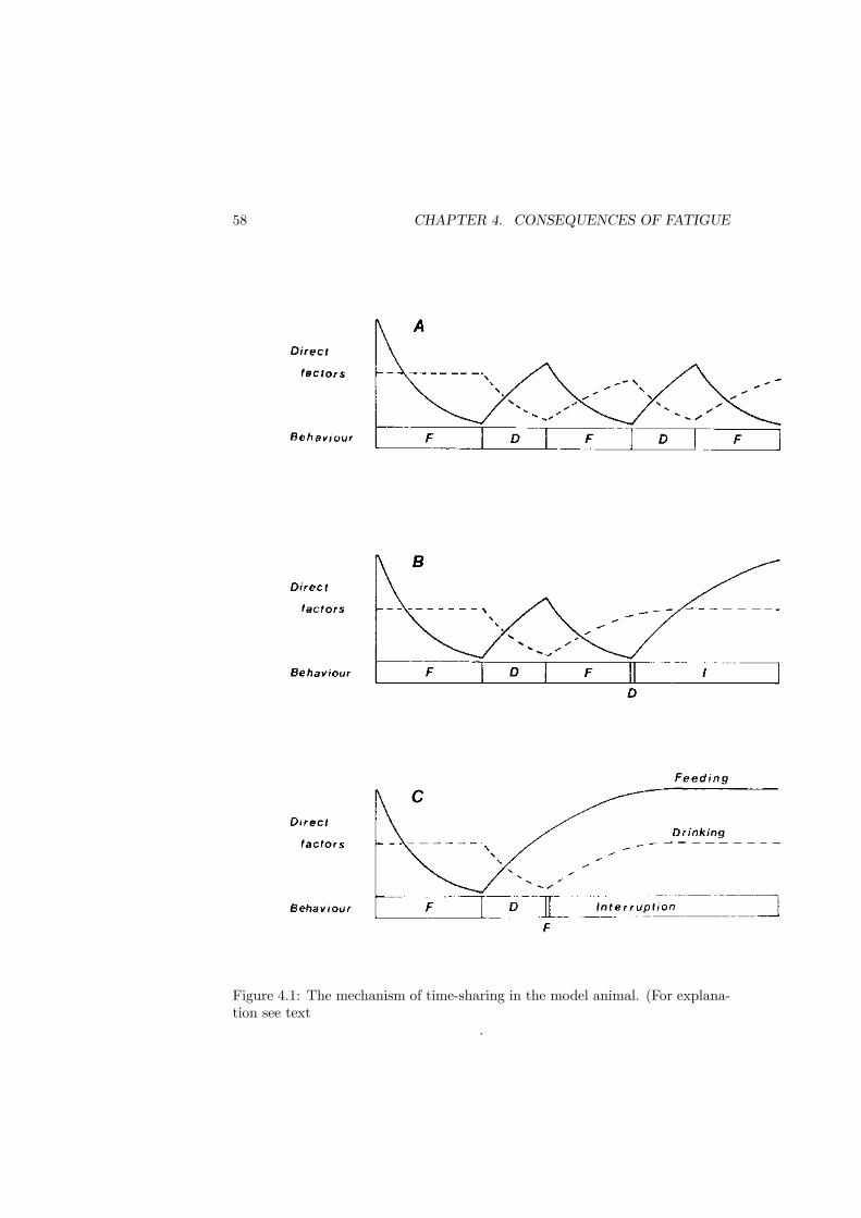
58 CHAPTER 4. CONSEQUENCES OF FATIGUE
Figure 4.1: The mechanism of time-sharing in the model animal. (For explana-tion see text
.
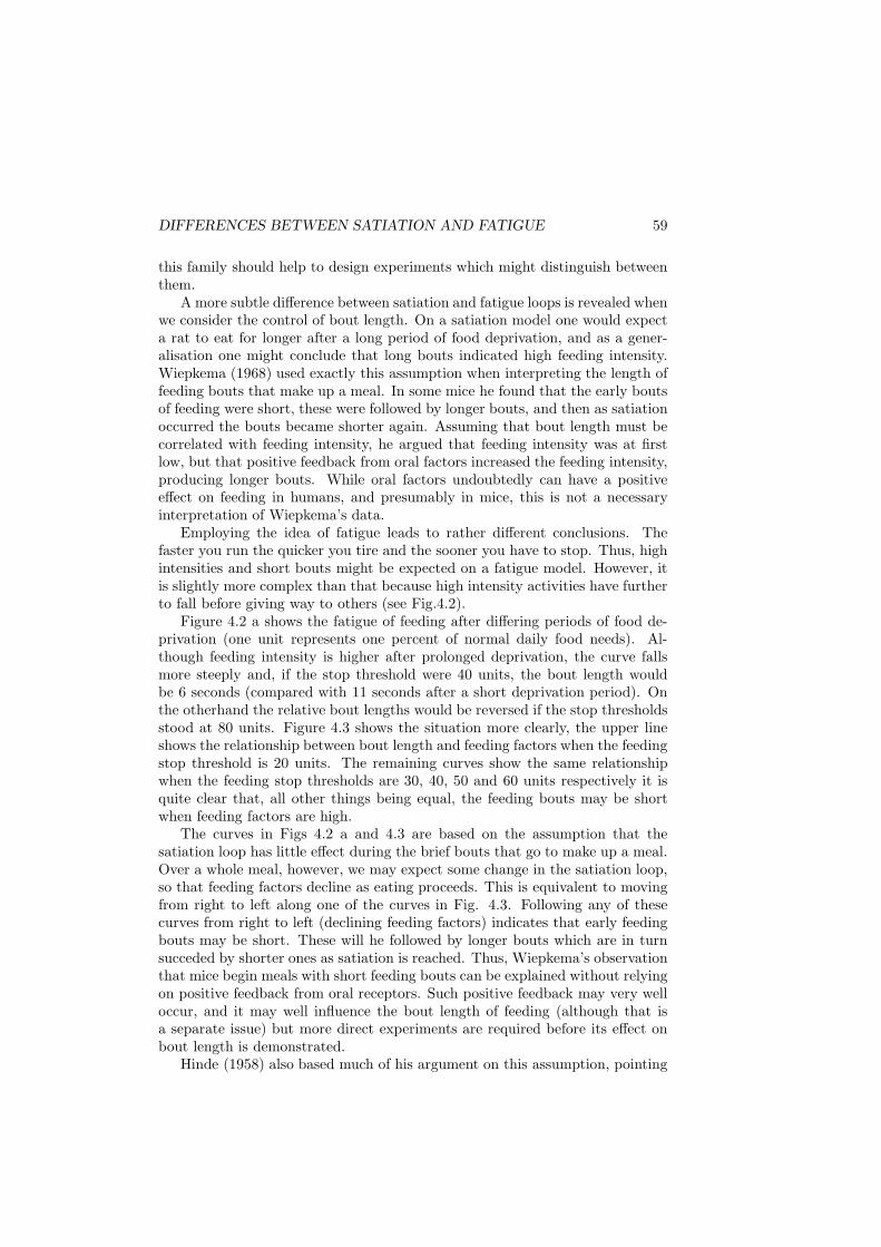
DIFFERENCES BETWEEN SATIATION AND FATIGUE 59
this family should help to design experiments which might distinguish betweenthem.
A more subtle difference between satiation and fatigue loops is revealed whenwe consider the control of bout length. On a satiation model one would expecta rat to eat for longer after a long period of food deprivation, and as a gener-alisation one might conclude that long bouts indicated high feeding intensity.Wiepkema (1968) used exactly this assumption when interpreting the length offeeding bouts that make up a meal. In some mice he found that the early boutsof feeding were short, these were followed by longer bouts, and then as satiationoccurred the bouts became shorter again. Assuming that bout length must becorrelated with feeding intensity, he argued that feeding intensity was at firstlow, but that positive feedback from oral factors increased the feeding intensity,producing longer bouts. While oral factors undoubtedly can have a positiveeffect on feeding in humans, and presumably in mice, this is not a necessaryinterpretation of Wiepkema’s data.
Employing the idea of fatigue leads to rather different conclusions. Thefaster you run the quicker you tire and the sooner you have to stop. Thus, highintensities and short bouts might be expected on a fatigue model. However, itis slightly more complex than that because high intensity activities have furtherto fall before giving way to others (see Fig.4.2).
Figure 4.2 a shows the fatigue of feeding after differing periods of food de-privation (one unit represents one percent of normal daily food needs). Al-though feeding intensity is higher after prolonged deprivation, the curve fallsmore steeply and, if the stop threshold were 40 units, the bout length wouldbe 6 seconds (compared with 11 seconds after a short deprivation period). Onthe otherhand the relative bout lengths would be reversed if the stop thresholdsstood at 80 units. Figure 4.3 shows the situation more clearly, the upper lineshows the relationship between bout length and feeding factors when the feedingstop threshold is 20 units. The remaining curves show the same relationshipwhen the feeding stop thresholds are 30, 40, 50 and 60 units respectively it isquite clear that, all other things being equal, the feeding bouts may be shortwhen feeding factors are high.
The curves in Figs 4.2 a and 4.3 are based on the assumption that thesatiation loop has little effect during the brief bouts that go to make up a meal.Over a whole meal, however, we may expect some change in the satiation loop,so that feeding factors decline as eating proceeds. This is equivalent to movingfrom right to left along one of the curves in Fig. 4.3. Following any of thesecurves from right to left (declining feeding factors) indicates that early feedingbouts may be short. These will he followed by longer bouts which are in turnsucceded by shorter ones as satiation is reached. Thus, Wiepkema’s observationthat mice begin meals with short feeding bouts can be explained without relyingon positive feedback from oral receptors. Such positive feedback may very welloccur, and it may well influence the bout length of feeding (although that isa separate issue) but more direct experiments are required before its effect onbout length is demonstrated.
Hinde (1958) also based much of his argument on this assumption, pointing
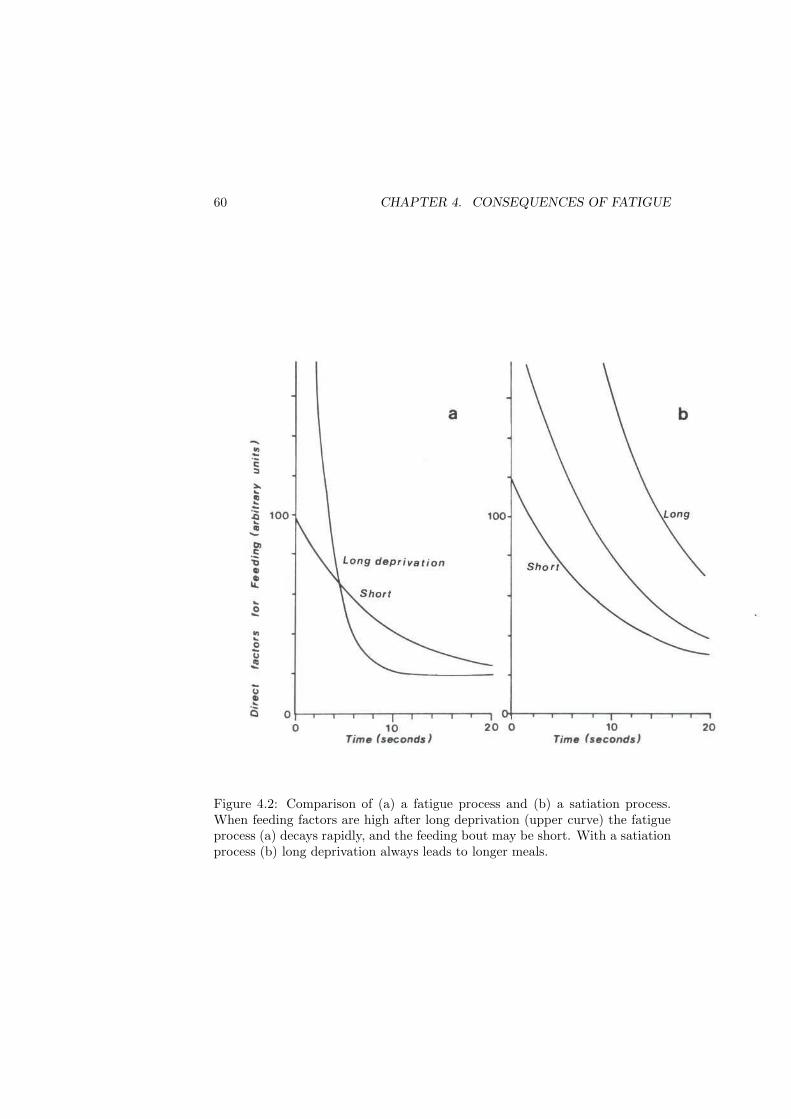
60 CHAPTER 4. CONSEQUENCES OF FATIGUE
Figure 4.2: Comparison of (a) a fatigue process and (b) a satiation process.When feeding factors are high after long deprivation (upper curve) the fatigueprocess (a) decays rapidly, and the feeding bout may be short. With a satiationprocess (b) long deprivation always leads to longer meals.
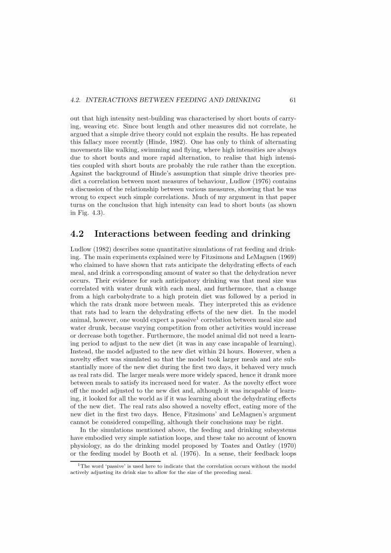
4.2. INTERACTIONS BETWEEN FEEDING AND DRINKING 61
out that high intensity nest-building was characterised by short bouts of carry-ing, weaving etc. Since bout length and other measures did not correlate, heargued that a simple drive theory could not explain the results. He has repeatedthis fallacy more recently (Hinde, 1982). One has only to think of alternatingmovements like walking, swimming and flying, where high intensities are alwaysdue to short bouts and more rapid alternation, to realise that high intensi-ties coupled with short bouts are probably the rule rather than the exception.Against the background of Hinde’s assumption that simple drive theories pre-dict a correlation between most measures of behaviour, Ludlow (1976) containsa discussion of the relationship between various measures, showing that he waswrong to expect such simple correlations. Much of my argument in that paperturns on the conclusion that high intensity can lead to short bouts (as shownin Fig. 4.3).
4.2 Interactions between feeding and drinking
Ludlow (1982) describes some quantitative simulations of rat feeding and drink-ing. The main experiments explained were by Fitzsimons and LeMagnen (1969)who claimed to have shown that rats anticipate the dehydrating effects of eachmeal, and drink a corresponding amount of water so that the dehydration neveroccurs. Their evidence for such anticipatory drinking was that meal size wascorrelated with water drunk with each meal, and furthermore, that a changefrom a high carbohydrate to a high protein diet was followed by a period inwhich the rats drank more between meals. They interpreted this as evidencethat rats had to learn the dehydrating effects of the new diet. In the modelanimal, however, one would expect a passive1 correlation between meal size andwater drunk, because varying competition from other activities would increaseor decrease both together. Furthermore, the model animal did not need a learn-ing period to adjust to the new diet (it was in any case incapable of learning).Instead, the model adjusted to the new diet within 24 hours. However, when anovelty effect was simulated so that the model took larger meals and ate sub-stantially more of the new diet during the first two days, it behaved very muchas real rats did. The larger meals were more widely spaced, hence it drank morebetween meals to satisfy its increased need for water. As the novelty effect woreoff the model adjusted to the new diet and, although it was incapable of learn-ing, it looked for all the world as if it was learning about the dehydrating effectsof the new diet. The real rats also showed a novelty effect, eating more of thenew diet in the first two days. Hence, Fitzsimons’ and LeMagnen’s argumentcannot be considered compelling, although their conclusions may be right.
In the simulations mentioned above, the feeding and drinking subsystemshave embodied very simple satiation loops, and these take no account of knownphysiology, as do the drinking model proposed by Toates and Oatley (1970)or the feeding model by Booth et al. (1976). In a sense, their feedback loops
1The word ‘passive’ is used here to indicate that the correlation occurs without the model
actively adjusting its drink size to allow for the size of the preceding meal.
62 CHAPTER 4. CONSEQUENCES OF FATIGUE
Figure 4.3: Relationship between feeding bout length and direct factors forfeeding. Stop threshold for feeding varies from 20 units (upper curve) to 60units (lowest curve). Strong competition (high stop threshold) shortens feedingbouts, but high direct factors for feeding can also shorten feeding bout length.
4.2. INTERACTIONS BETWEEN FEEDING AND DRINKING 63
are all outside the nervous system; they assume that rats measure intra- andextracellular fluid volume, or energy flow rate, and drink or eat accordingly.The models explain how fluid volumes or energy flow rates change with timeunder different experimental conditions. Discrepancies between the model andreal rats can then be due to two causes. Either the model makes the wrongpredictions ahout fluid volume or energy flow, or real rats are measuring andresponding to other factors. Since the physiology of fluid volume and energy floware fairly well understood, the observed discrepancies between rat and modelcan usually be pinned on the behaviour, or more precisely, on the very simplebehavioural assumptions built into the two models. In discussing the drinkingmodel, Toates (1979a) suggested that many discrepancies between his modeland real rats were due to the rats learning about the availability of water.However, both drinking and feeding models make the oversimple behaviouralassumption that there are static start and stop thresholds for each activity. Ibelieve that many of the discrepancies between real rats and the feeding anddrinking models are due to the fixed thresholds of the two models. In bothmodels the fixed threshold mechanisms were built in, as ad hoc assumptions, toexplain experimental observations of hysteresis in feeding and drinking.
The model animal differs in several respects. Its thresholds are dynamic, andwhat is more, the start threshold for each activity depends on which activityis being performed. For example, the success of the simulations of rat feedingand drinking behaviour (Ludlow, 1982) was due partly to the fact that feedingin the model animal tended to lead to drinking. During starvation, however,food searching behaviour reduced drinking by fierce competition. This paradox-ical effect was because the inhibitory gains were set so that the drinking startthreshold was relatively low when the model was feeding, hence drinking wasmore likely than other activities to follow feeding or food-searching. But, asstarvation progressed, the mean start threshold for drinking became progres-sively higher because food-searching behaviour became more intensely excited.To simulate the known link between feeding and drinking with either of the twospecialist models one might postulate a cue in the feeding situation which stim-ulated drinking. Or, as Fitzsimons and LeMagnen argued, the rat may measureand learn the dehydrating effects of each diet. In the model animal, however,an appropriate setting of one parameter, the gain in the inhibitory pathwayfrom feeding to drinking, caused the model to compensate in advance for thedehydrating effects of its meals and exhibit the behaviour shown by starvingrats.
Thus, the model animal is weak on fluid and energy physiology, while thespecialist feeding and drinking models are weak on behavioural assumptions.As a result of these differences they must be extended in quite different ways inthe face of new behavioural problems, such as anticipatory drinking. Such com-parisons are illuminating because one sees how much an apparently compellingextension of each model depends on the preconceptions already built into it. Inaddition, the two types of model, together, generate alternative explanationswhereas alone they would each advance a single candidate which might be ac-cepted uncritically. For example, Toates (1979b) has argued that reduced water
64 CHAPTER 4. CONSEQUENCES OF FATIGUE
intake during starvation is due to reduced water needs, as tissues are brokendown: the rat gets smaller and small rats need less water. Such an explanationwould never have been suggested by examination of the model animal. A sim-ilar case was provided by the idea that bout lengths must be correlated withintensity, which follows naturally from ideas about satiation. It was accepteduncritically because there seemed to be no alternative, although it is now clearthat fatigue provides one.
In the long run we must combine the dynamic thresholds of the model an-imal with the specialist feeding and drinking models. It would be particularlyinstructive to see which bits of one are made redundant by properties of theother. However, I personally find it illuminating to compare many simple mod-els which fail for different reasons. There is a danger that any grand model wouldhave too many ways of explaining the same problem and be too complicatedfor any of us to understand. I therefore make no apology for the oversimplefeedback loops in the model animal, nor would I ask Toates, Oatley, Booth andPlatt to change their threshold mechanisms. An unbiased comparison of modelsseems to be the most fruitful way ahead, and when different explanations of thesame phenomenon are found they will often be compatible, not mutually exclu-sive. Hence, our experiments will have to measure the relative contribution ofeach mechanism or effect.
4.3 Discussion and Summary
The model animal has generated numerous questions and I hope that the ac-count given above shows that the exercise of modelling has borne fruits whichwill last long after the original model is superseded. In otherwords, the hypothe-ses may prove wrong but the working version has produced lessons and raisedquestions which might otherwise have been overlooked. The principal lesson isthat arguments must be made quantitative at an early stage. For example, thefirst version of the model animal was a drawing without numbers (Fig. 3.1).The drawing turned out to be incomplete precisely because the numbers weremissing. I had drawn the diagram to explain how aphids avoided probing andwalking at the same time, when factors exciting both were present. As Fig. 3.2shows, the original incomplete hypothesis did not explain the observations be-cause the two activities can occur at the same time if the gains in the inhibitorypathways are less than 1.0. van Iersel and Bol (1958) published an even lesscomplete diagram when explaining displacement activities. They not only leftout the numbers, but they did not specify whether the inhibitory connectionsare supposed to run from the output of one centre to the input of another (likeFig.3.3) or from output to output (like Fig.3.5). Since this is undefined, theirhypothesis is undefined, hence no predictions can be made from it, not even thetarget prediction that displacement activities will occur in conflict situations.
Quite apart from the specific questions about the disinhibition hypothesis,one of the most important questions raised by this example is: how many otherwell known hypotheses are undefined? It may be unfair to pick on van lersel
4.3. DISCUSSION AND SUMMARY 65
and Bol in this way because they wrote at a time when the dangers of verbalargument were not fully appreciated, and when simulation techniques were notavailable. But that is all the more reason to suppose that the literature containsa legacy of undefined hypotheses which may or may not explain the observationsfor which they were proposed.
Undefined hypotheses are untested in two senses. Firstly, they have not beentested to see whether they actually explain the observations for which theywere proposed, and even when they do they may imply special assumptions,or assumptions which conflict with each other. For example, the disinhihitionhypothesis appeared disarmingly simple, but it turns out that a working ver-sion may be unattractively complex because it involves conflicting assumptions.Thus, if we regard hypothesis testing as the essence of the scientific method, itseems to me that modelling is an obligation which we can only avoid by leavingour hypotheses inadequately tested. In the early days, proponents of modellingwere perhaps wrong-footed because they appeared to be defending particularmodels. The conventional wisdom was that a model was just another hypothesisor, worse, a misleadingly oversimple hypothesis. While models often have to beoversimple (we cannot run before we can walk) it is now clear that behaviouris far too complicated to be thought about without the help of models. This isillustrated by Fig. 4.4 which is intended to summarise the logical connectionsbetween the assumptions and properties of the model animal. As explained inChapter 2, the model employs four ideas:
1. Each activity is influenced by a number of causal factors,
2. Some of these factors are reduced by the effectiveness of the activity (feed-ing, reduces hunger),
3. Other factors are reduced by the effort spent in each activity,
4. The activities are prevented from occurring at the same time by a switchmechanism which involves competition between activities.
This seems to me to be the minimum kit for explaining behaviour, but the fullimplications of even these minimal ideas is not clear at first sight (Fig. 4.4).
Thus, the model has been useful as a thought tool, and in challenging ideasand assumptions, but the credibility of the underlying hypotheses must be ex-amined. It is quite obvious that the inhibitors connections postulated are a mereshadow of those known to take part in the organisation of individual activities,such as feeding in gastropods (Benjamin and Rose, 1980). Even if the principlesturn out to be similar, the details are so different that there is little point indoing a neurophysiological test of the model animal’s switch mechanism. Onthe other hand, at the behavioural level of analysis, the switch mechanism is anadvance on the fixed thresholds of some models. The latter would not predicta passive correlation between meal size and water drunk, as the model animaldoes.
The model animal is also astonishingly simple. Figure 4.4 is an attemptto show this simplicity by showing the logical connections between the basic
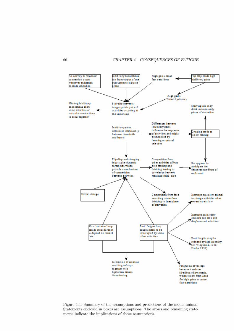
66 CHAPTER 4. CONSEQUENCES OF FATIGUE
Figure 4.4: Summary of the assumptions and predictions of the model animal.Statements enclosed in boxes are assumptions. The arows and remaining state-ments indicate the implications of those assumptions.
4.3. DISCUSSION AND SUMMARY 67
assumptions and the models explanations/predictions. Thus, the fixed startand stop thresholds in the model of Toates and Oatley (1970) were proposed toexplain hysteresis, whereas that falls out of the model animal as a consequenceof the inhibition required to prevent activities from occurring at the same time.
It is robust, the gains in the inhibitory pathways must be greater than 1.0.but the precise value is not critical. This makes the model more plausible be-cause the values of the gains would not have to be specified with great accuracyin the course of development, nor would they have to he maintained with greataccuracy.
The switch mechanism appears, for the moment, to be unique in that I havecome across no other model which explains how incompatible activities are pre-vented from occurring at the same time, and I can see no way of solving thisproblem without inhibition. Joseph et al. (1979) have suggested that the nu-merous inhibitory pathways running from each subsystem to every other couldbe replaced by a system of general inhibition to which each subsystem con-tributes, and from which each receives inhibition. While reducing the numberof connections, this also reduces the flexibility of the system. In particular itwould be harder to arrange that drinking follows feeding in their model. Theirsimplified model might also be much less robust, as the transactions with a gen-eral inhibitory system would have to he very precise to avoid two subsystemsbeing permitted at the same time. Nevertheless, I personally suspect that realnervous systems may employ a hybrid network including general inhibition aswell as some one-to-one links.
The fatigue loop is far from unique because there are numerous processeswhich would substitute for it, although some effort-loop is necessary to simulatethe behaviour of Barbary Doves which switch from feeding to another activityafter a given effort rather than a given reward (McFarland and Lloyd, 1973).The Fitzsimons and LeMagnen (1969) data on rats are less conclusive; mealsize on different diets did not depend on calories consumed, but volume eaten.Their rats could have been measuring volume per se or effort. It is likely thatdifferent species have a number of different long- and short-term loops, and themodel’s usefulness in this area is confined to showing the interactions of twoloops with substantially different time-constants.
When one tries to assess the model’s predictive value it is impossible toderive one prediction which tests the whole model. The simulation of time-sharing looked to be such a general test because it depended on hysteresis andboth long- and short-term loops, but it is now clear that other models willexplain time-sharing at least as simply. One can derive predictions which testdifferent parts of the model separately. For example, it is in principle possible tomeasure the inhibitory gains. Moreover, every simulation is a test of the modeland the literature on animal behaviour is so vast that many of the most testingexperiments have already been done. Thus, there are numerous ways of testingthe model animal and these are being pursued.
In conclusion, the model animal provides a convenient way of calculatingthe effects of competition between activities, given very simple assumptions.It has already demonstrated that these interactions are more complex than

68 CHAPTER 4. CONSEQUENCES OF FATIGUE
earlier authors have sometimes appreciated, and it has challenged the rigour ofsome widely propogated arguments. It has raised numerous questions and byits existence has made alternative possibilities clearer. Competition betweenthese alternative hypotheses should provide further insights into the control ofbehaviour, and we may reasonably hope that the model animal will lead usnearer to the truth, or at the very least, keep us from some serious errors.
Chapter 5
Mechanisms of Moth
Orientation
Why, sometimes I’ve believed as many as six impossible things beforebreakfast.
Lewis Carroll, Through the Looking Glass
The subject matter of this chapter is very different from the material in the restof the volume, and it illustrates a different aspect of modelling. The previouschapters have described the rich consequences of a simple theory (Fig. 4.4).The present chapter is largely a survey of impossibilities, many of which appearplausible until closely examined. Moth orientation is a subject where pitfalls aremore extensive than safe ground, and where each new worker seems to propose,with confidence, the same series of impossible solutions. There can be no fieldof biology where modelling is more necessary and few where it is more difficult.
Before discussing the physiological mechanisms underlying moth orientationI shall review the curent ideas of the strategy that male moths employ whenlocating a pheromone-emitting female.
5.1 How does a male moth find a female emit-
ting sex-pheromone—current views
For over a century it has been known that males of some moth species willassemble around an empty box which had previously contained a female of thesame species. The obvious conclusion was drawn that the males were attractedto scent left by the female. But understanding progressed little over the sub-sequent decades. Now, at last, we have a theory which is essentially complete,and has been extensively tested in both wind tunnels and the field. As humanswho rely so little on a sense of smell, we seem to be congenitally ignorant ofthe movement of odours in a wind and hence blind to the simplicity, accuracy
69

70 CHAPTER 5. MECHANISMS OF MOTH ORIENTATION
Figure 5.1: Segments of tracks of smoke puffs recorded within a 10-min period.Grid markers 5 m apart. (From David et al., 1982)
and efficiency of the mechanisms. I shall therefore review the findings with thebenefit of hindsight, beginning with information which would have changed ourapproach if we had gleaned it earlier. Information which is rapidly learned byevery hunting dog but which humans have only recently discovered.
The key to it all is that air-borne scents travel in straight lines and thatany animal which fixes the wind direction at the instant it detects an odourwill very probahly have fixed the direction of the odour source. This result,first communicated to biologists by a meteorologist (Dr. F.B. Smith) and tous by Dr. Clive Wall, seemed quite unbelievable but was rapidly confirmed byexperiment (David et al., 1982). Figure 5.1 (taken from that paper) shows thetracks of individual parcels of smoke moving over open ground. Over the firstfifteen metres, at least, the wind direction at any point where smoke was presentwas highly correlated with the source direction. Thus a moth (or any animal)has only to locate the wind direction at the moment it detects an odour tofix the direction of the odour source. The wind direction at that moment willoccasionally be misleading, but errors of more than a few degrees should be veryrare.
Fixing the source direction, however, is not enough to fix the position of anunseen source because the distance remains unknown. If the odour formed acontinuous field there would be little problem. The moth could simply fly upthe appropriate direction until it passed the source, at which point it wouldsuddenly cease detecting odour. A few moments observation of the smoke from
HOW DOES A MALE MOTH FIND A FEMALE? 71
a cigarette or bonfire will show that, in practice, odours are carried in discon-tinuous parcels and whisps, so the moth (or any other animal) would detect aseries of discrete bursts of odour and there is probably no way of telling whethera gap in stimulation is an interruption of the plume or whether the moth hasflown past the source. It should come as no surprise, therefore, to find thatthe moth’s response to odour loss is well adapted to both contingencies. Whatmoths, of several species, do when odour is removed or lost is to cast from sideto side across the wind with increasing amplitude, often losing a little groundagainst the wind (Marsh et al., 1978, 1981). This is obviously a good strategy ifthe moth has overshot the female because it will bring the male back downwinda little, and in casting he covers a wide area.
It is also a good strategy if the gap is an interruption in the plume, becausethe cross-wind casting prevents upwind movements which lead the moth to over-shoot. Furthermore, many interruptions to the moth’s pheromone stimulationwill be due to a change in wind direction, which means that the pheromoneoften can be found again if the moth searches across wind in both directions.Until recently we thought that these were the only advantages, but David et al.(1983) have found that long casts often bring the moth back into the odourcloser to the source than when the pheromone was lost. In a field study, wereleased pheromone and bubbles together, and filmed male gypsy moths (Ly-mantria dispar, L.) approaching the source. Fig. 5.2 (taken from that paper)shows a number of tracks. Sections drawn with thick lines show when the mothwas among bubbles and probably receiving pheromone. The remaining sectionswere filmed when the moth was away from bubbles and almost certainly with-out pheromone. One sees at once how accurately the moths moved towards thesource when they were among bubbles. When the moth lost contact with thebubbles (and pheromone) this was usually due to a change in wind direction. Bycasting across the new wind direction, the moth was casting alternately nearerand further from the source. But because of simple geometry it was the castsin the direction of the plume which brought these moths closer to the source,Thus, the plume was always found on those casts which were nearer to thesource, and a substantial proportion of the progress made towards the sourceby some moths was made when they were casting.
At the very closest range, visual cues will also play a part but Figs. 5.1 and5.2 show how effective is the combined strategy of flying upwind when stimulatedby odour and casting across wind on losing it. However, we need to considertwo complications. What happens during a lull in the wind, and what happenswhen there are thousands of females so that the whole air is full of their scent?
Recently Baker and Kuenen (1982) showed that when they stopped the windin a wind tunnel, their oriental fruit moths (Grapholitha molesta) continued upthe plume. However if they removed the odour first, the moths started castingacross the wind and continued casting in the same way when the wind wasstopped. Finally, when Baker and Kuenen withdrew the odour source justbefore stopping the wind, they created a hanging plume which did not reach allthe way up the tunnel. In such cases, the moths continued up the plume untilthey passed out of the end of the plume and started to cast from side to side
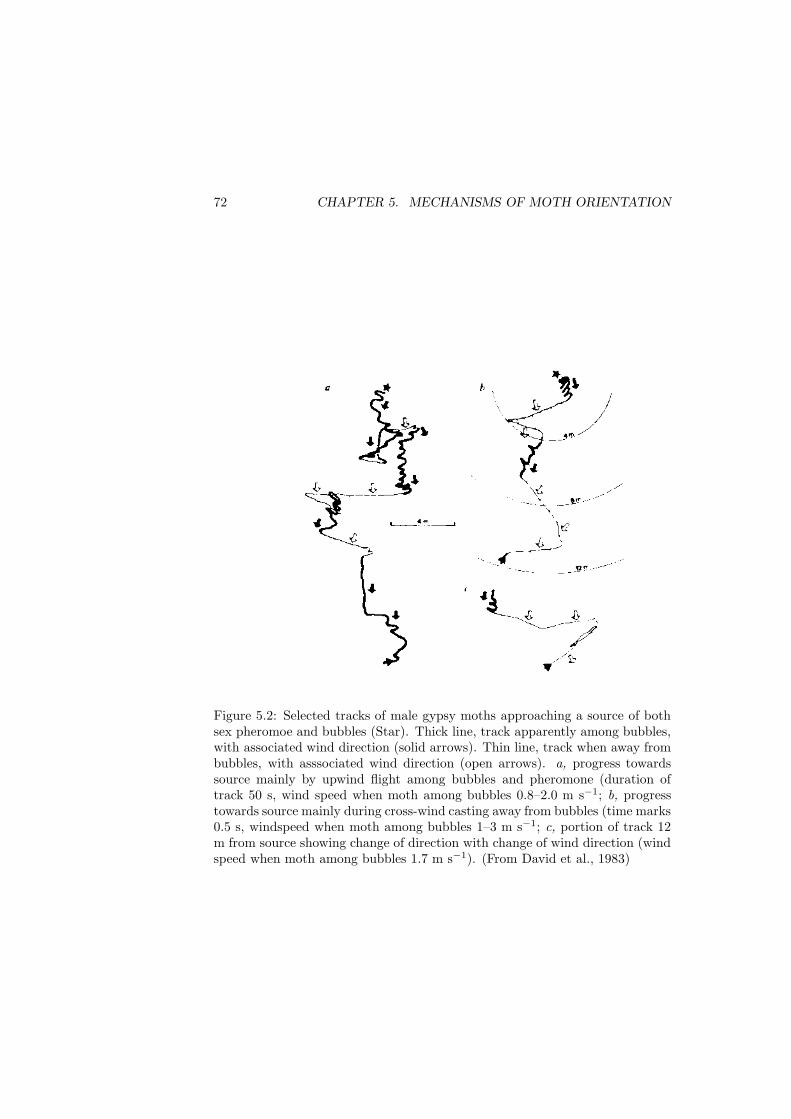
72 CHAPTER 5. MECHANISMS OF MOTH ORIENTATION
Figure 5.2: Selected tracks of male gypsy moths approaching a source of bothsex pheromoe and bubbles (Star). Thick line, track apparently among bubbles,with associated wind direction (solid arrows). Thin line, track when away frombubbles, with asssociated wind direction (open arrows). a, progress towardssource mainly by upwind flight among bubbles and pheromone (duration oftrack 50 s, wind speed when moth among bubbles 0.8–2.0 m s−1; b, progresstowards source mainly during cross-wind casting away from bubbles (time marks0.5 s, windspeed when moth among bubbles 1–3 m s−1; c, portion of track 12m from source showing change of direction with change of wind direction (windspeed when moth among bubbles 1.7 m s−1). (From David et al., 1983)
HOW DOES A MALE MOTH FIND A FEMALE? 73
across the former wind direction. These results have since been confirmed byDavid and Kennedy (pers. comm.) using gypsy moths. If the same behaviouroccurs in the field, then we may expect moths to continue in the former directionduring a lull provided there is pheromone all the way. As soon as they pass outof pheromone they will cast from side to side. This again makes excellent sensebecause, as Fig. 5.1 shows, the former upwind direction is a good indicator ofthe source direction, but flying on without pheromone would incurr the risk ofovershooting the source.
Now suppose that there are thousands of females upwind. The air will befull of pheromone, and males which flew upwind would fly on and on, passinghundreds of calling females, and wasting both time and effort. But that is notwhat happens. In a wind tunnel study we (Kennedy et al., 1980, 1981) showedwith Adoxophyes orana that a moth which was casting after losing a pheromoneplume did not fly continuously upwind when enveloped in a cloud of uniformlydistributed pheromone. It might make a brief surge in the first three seconds ofstimulation, but the main effect of the uniform cloud was to narrow the ampli-tude of the casts dramatically, the moth oscillated from side to side making noheadway. However, if a single source was added to create a plume, superimposedon the pheromone background, then the moths could find it. The single sourcecaused fluctuations in pheromone concentration (though these never fell to zerobecause of the pheromone background) and the sudden increases in pheromoneseemed to be needed to stimulate upwind flight. The uniform pheromone-clouddid not stimulate upwind flight, even when the concentration was higher thanthe average in a typical plume.
If we can apply this result to the field, it probably means that a male haslittle difficulty finding a nearby female among thousands, because it is onlystimulated to fly upwind by the sudden rises in pheromone concentration whichare caused by the nearby female. Hence it will waste little time on more distantones whose pheromone has been mixed into a uniform cloud. This finding hasimplications for the way we attempt to control moth pests using pheromone.Blanketting the whole area with uniform pheromone has not been particularlyeffective (R.J., 1982) presumably because it is a situation the moths are adaptedto overcome. Discrete, well scattered sources, would seem to offer more chanceof success. These observations on Adoxophyes orana have since been confirmedby Kennedy and David (pers comm.) with gypsy moths.
Up to now we have been discussing what moths do and how that helps themto get to a source. Later we shall he looking in more detail at the underly-ing mechanisms but while still on this level of analysis, let me summarise theabove remarks and consider alternative theories. Figures 5.1 and 5.2 show thatflying upwind when a moth detects pheromone, and casting across wind whenpheromone is lost, is a good strategy. If there is a lull in the wind, the samestrategy can be employed provided that the former wind direction can be re-membered. Finally, the strategy is well adapted to large populations if it is onlyan increase in pheromone concentration which stimulates upwind flight. Thisbody of ideas has become known as the theory of odour-modulated anemotaxisbecause the odour concentration modulates the response to the wind direction
74 CHAPTER 5. MECHANISMS OF MOTH ORIENTATION
(or the former wind direction during a lull). The experimental basis of the the-ory is due in very large part to J. S. Kennedy and his co-workers and a historicalperspective can be gained by reading the following papers: Wright (1958); Kel-logg et al. (1962); Kennedy and Marsh (1974); Marsh et al. (1978, 1981); Cardeand Hagaman (1979); Kennedy et al. (1980, 1981); Baker and Kuenen (1982);David et al. (1982, 1983). Although the theory is now well established, thereare and have been alternatives which must be considered.
Laithwaite (1960) and Callahan (1977) have proposed that pheromone moleculesradiate in the far infra-red and that the antennae of some moth species areadapted to detect such wavelengths. As a result, the moths can see the plumeand perhaps the emitting source. However, in a wind tunnel it is possible tomove the floor pattern downwind faster than the windspeed. If that is done thewind should appear to a moth to be blowing up instead of down the tunnel. Ifmoths were able to see the plume and its source they should not be confused,but they are. Kennedy and Marsh (1974, footnote 5) did exactly this and foundthat Plodia interpunctella males flew down the tunnel away from the female.This was also the first direct proof that moths were responding to apparentwind-direction, as the anemotactic theory demands; Kellogg et al. (1962) hadpreviously demonstrated anemotaxis in Drosophila flying in a wind tunnel.
By far the strongest alternative is the theory that moths turn towards highpheromone concentration and away from low concentrations, that is, simplechemotaxis. I suspect that this idea has so much appeal because it is the way inwhich humans trace an odour source and therefore the only way they can imagineanything else doing it. Indeed. Laithwaite (1960) argues that this is how dogsrespond to odours, but the Setters and Pointers refute him at once. They havebeen bred for over 250 years precisely because they are able to indicate thedirection of game at a distance. Moreover, there are serious objections to thechemotactic theory. Plumes are discontinuous (just look at the way smoke leavesa cigarette). Any moth which turned towards the highest concentration wouldsoon become trapped in an isolated cloud of pheromone drifting downwind awayfrom the female. In otherwords, the chemotactic gradients simply do not leadto the female.
Nevertheless, there is a feature of moth behaviour which looks very likechemotaxis. Many species move up a plume in zigzags, as if they were turningback into the plume at its edges. i.e. turning back to the highest concentration.However, this interpretation does not bear with the facts. Carde and Hagaman(1979) showed that increasing the concentration at the source reduced the am-plitude of zigzags. On the chemotactic theory, the high concentration shouldhave led to a wider plume and wider zigzags. Later we showed that uniformpheromone reduced the amplitude of cross-wind movements (Kennedy et al.,1980, 1981). In our case the moths could not have been turning back at theedges because there were no edges. The uniform pheromone-cloud filled thetunnel, and the presence of pheromone caused more frequent turns than oc-curred when it was withdrawn. When we did introduce a clearly defined edge,we found that the probability of turning was reduced when the moth flew outof the pheromone. On the chemotactic theory the probability of turning should
HOW DOES A MALE MOTH FIND A FEMALE? 75
have increased when the moths flew out of the pheromone.The simplest explanation of our data is that the side to side movements,
common to casting and zigzagging, form a continuum, There seems to be anoscillator which commands left and right turns at somewhat irregular intervals.When pheromone is present, the period of the oscillator is reduced and narrowzigzagging or narrow cross-wind movements occur. When the pheromone stim-ulus is lost, the period rises leading to long casts to one side and the other. As aresult the moth searches widely when pheromone is lost and moves across windvery little when it is present.
Thus, the strategy of turning towards the highest concentration would notwork in an interrupted plume because the gradients lead nowhere. Moreover,the wind tunnel experiments suggest that the moths do the opposite, having anoscillator which causes fewer turns on leaving the pheromone. This strategy willtend to keep them within a plume when pheromone is present (because largesideways movements are inhibited) but will allow them to scan widely whenpheromone is lost. The opposite strategy, of turning back into the plume, wouldwork if plumes were well behaved and remained in one place for long periods,but they do not. We tend to assume that moths loose pheromone because theyfly out of plumes which remain where they are. In that case turning back intothe plume would pay, but most losses of plume are probably due to the plumemoving more than the moth, and turning back to where the plume was wouldbe, quite simply, irrelevant. Long casting (i.e. fewer turns when pheromonehas been lost) would appear to be adapted to the real problem, rather thanthe problem we have imagined for the moths. Chemotaxis is a solution to theimaginary problem. Of course, the best strategy will depend on the insect’sspeed. Fast flight makes fast searching and sudden arrestment a viable strategy.Walking insects, on the otherhand, may do better by averaging odours over timeand using a slow form of chemotaxis together with anemotaxis.
Why moths should zigzag, rather than fly straight upwind in a plume isnot, however, clear. We argued (Marsh et al., 1978) that even in a plume themoths were alternatively receiving and losing pheromone. Hence, the zigzagsrepresented alternate upwind and casting movements. However, with Adoxo-phyes orana, small amplitude cross-wind movements occurred, when we knowthat they were receiving pheromone all the time (Kennedy et al., 1980, 1981).Baker (pers. comm.) has suggested that some cross-wind movement is necessaryto confirm the upwind direction. It is interesting to note that Drosophila donot zigzag when flying upwind to banana odour (David, pers. comm.). Perhapszigzagging behaviour is adapted to the size of the target. Drosophila, trying tofind a banana tree, and a moth, trying to find the closest female among thou-sands, have very different problems. Differences in their behaviour, doubtless,reflect the situations to which they are adapted.
For the remainder of the chapter we shall consider how moths identify theupwind direction, and how they maintain an angle of about 90◦ to the windwhen casting in different windspeeds. We shall also keep in mind that Bakerand Kuenen (1982) have shown that moths can persist up, or cast across, theformer wind direction after the wind has stopped. However, gypsy moths cannot
76 CHAPTER 5. MECHANISMS OF MOTH ORIENTATION
fly up, or cast across, a plume unless they have previously experienced wind andpheromone together (David and Kennedy, pers. comm.).
5.2 How does a moth turn upwind?
For an animal on the ground, the problem of locating the upwind directionis simple. Humans use a wet finger and I suspect, as Schwinck (1958) sug-gested, that dogs and wild beasts use their wet noses. Wet noses are commonthroughout the mammalia, occurring among marsupials, the insectivora, roden-tia, ungulata, carnivora and fruit bats. No really satisfactory explanation forthem has been given. whiskers too will indicate wind direction and, whatevertheir original function, it seems inevitable that mammals will have learned touse whiskers and wet noses to fix the direction of odour sources. Sight and smelland wind direction must often be coupled, allowing numerous opportunities forassociation. In this context, it is worth noting that young pointers begin bypointing novel visual objects, but may take over a year before they point gameby scent alone. While experiments are needed to confirm these suggestions, itseems likely that we have grossly underestimated the information available tomost mammals through their noses and their unappreciated abilities may haveprejudiced some experimental designs.
For an insect on the ground, the antennae and numerous hairs can provideinformation about wind direction (Linsenmair, 1972). In the air the same recep-tors provide information about airspeed (Weiss-Fogh, 1949, 1950; Camhi, 1969;Gewecke, 1974) but such hairs would indicate the airflow over the insects body(which results exclusively from its own efforts) not the movement of the air overthe ground. In very gusty winds the insect’s body would be buffetted morefiercely in one direction than another. Inertial receptors or hairs might be usedto detect the wind direction from such violent movements of the air, but thiswould not work in the smooth conditions of a wind tunnel, or in light winds inthe field.
This problem was recognised by Fraenkel (1931, 1932); Schulz (1931); Lyon(1904) who, in various contexts, proposed that air- or water-borne animalsturn upcurrent in response to the apparent movement of visible fixed objects.Kennedy (1940), studying mosquitoes, went further. He showed that mosquitoesflying in still air, over moving stripes, tended to fly in the same direction asthe stripes. A few flew waveringly against the stripes, but as stripe speed in-creased they soon turned and flew with them. The effect of stripe movementin still air is similar to the effect of a wind blowing in the opposite direction.Thus, mosquitoes facing against the stripes were in an apparent tailwind and,as stripe speed increased, they turned round to face into the apparent winddirection. What Kennedy noticed was that the tendency to turn was low whenthey were facing downwind, but increased rapidly as they turned across wind.Or as he put it, the turning tendency depends on both speed and obliquity ofimage movement.
Kennedy (1951) reviewed the mosquito work saying:
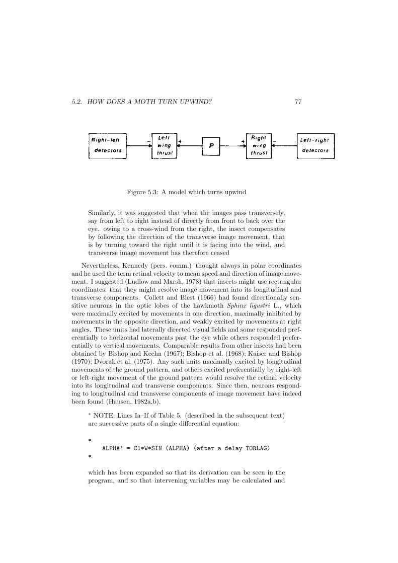
5.2. HOW DOES A MOTH TURN UPWIND? 77
Figure 5.3: A model which turns upwind
Similarly, it was suggested that when the images pass transversely,say from left to right instead of directly from front to back over theeye. owing to a cross-wind from the right, the insect compensatesby following the direction of the transverse image movement, thatis by turning toward the right until it is facing into the wind, andtransverse image movement has therefore ceased
Nevertheless, Kennedy (pers. comm.) thought always in polar coordinatesand he used the term retinal velocity to mean speed and direction of image move-ment. I suggested (Ludlow and Marsh, 1978) that insects might use rectangularcoordinates: that they might resolve image movement into its longitudinal andtransverse components. Collett and Blest (1966) had found directionally sen-sitive neurons in the optic lobes of the hawkmoth Sphinx ligustri L., whichwere maximally excited by movements in one direction, maximally inhibited bymovements in the opposite direction, and weakly excited by movements at rightangles. These units had laterally directed visual fields and some responded pref-erentially to horizontal movements past the eye while others responded prefer-entially to vertical movements. Comparable results from other insects had beenobtained by Bishop and Keehn (1967); Bishop et al. (1968); Kaiser and Bishop(1970); Dvorak et al. (1975). Any such units maximally excited by longitudinalmovements of the ground pattern, and others excited preferentially by right-leftor left-right movement of the ground pattern would resolve the retinal velocityinto its longitudinal and transverse components. Since then, neurons respond-ing to longitudinal and transverse components of image movement have indeedbeen found (Hausen, 1982a,b).
∗ NOTE: Lines Ia–If of Table 5. (described in the subsequent text)are successive parts of a single differential equation:
*
ALPHA’ = C1*W*SIN (ALPHA) (after a delay TORLAG)
*
which has been expanded so that its derivation can be seen in theprogram, and so that intervening variables may be calculated and
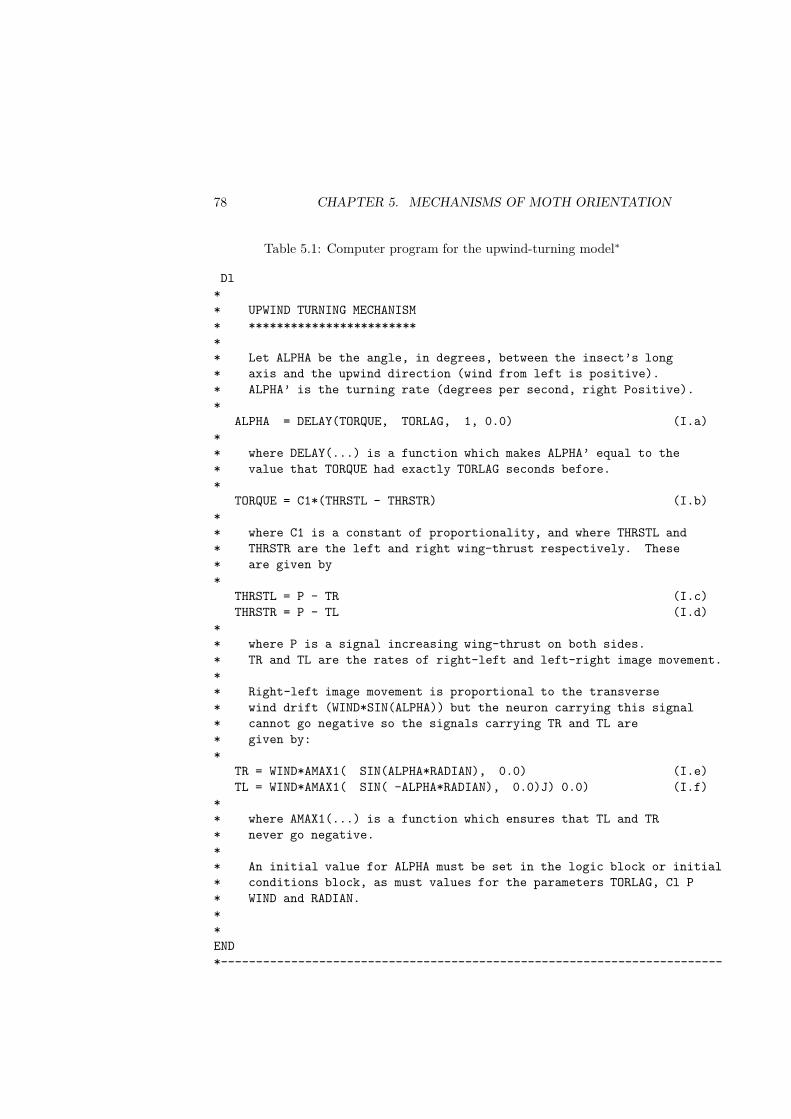
78 CHAPTER 5. MECHANISMS OF MOTH ORIENTATION
Table 5.1: Computer program for the upwind-turning model∗
Dl
*
* UPWIND TURNING MECHANISM
* ************************
*
* Let ALPHA be the angle, in degrees, between the insect’s long
* axis and the upwind direction (wind from left is positive).
* ALPHA’ is the turning rate (degrees per second, right Positive).
*
ALPHA = DELAY(TORQUE, TORLAG, 1, 0.0) (I.a)
*
* where DELAY(...) is a function which makes ALPHA’ equal to the
* value that TORQUE had exactly TORLAG seconds before.
*
TORQUE = C1*(THRSTL - THRSTR) (I.b)
*
* where C1 is a constant of proportionality, and where THRSTL and
* THRSTR are the left and right wing-thrust respectively. These
* are given by
*
THRSTL = P - TR (I.c)
THRSTR = P - TL (I.d)
*
* where P is a signal increasing wing-thrust on both sides.
* TR and TL are the rates of right-left and left-right image movement.
*
* Right-left image movement is proportional to the transverse
* wind drift (WIND*SIN(ALPHA)) but the neuron carrying this signal
* cannot go negative so the signals carrying TR and TL are
* given by:
*
TR = WIND*AMAX1( SIN(ALPHA*RADIAN), 0.0) (I.e)
TL = WIND*AMAX1( SIN( -ALPHA*RADIAN), 0.0)J) 0.0) (I.f)
*
* where AMAX1(...) is a function which ensures that TL and TR
* never go negative.
*
* An initial value for ALPHA must be set in the logic block or initial
* conditions block, as must values for the parameters TORLAG, Cl P
* WIND and RADIAN.
*
*
END
*------------------------------------------------------------------------
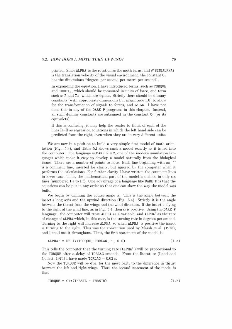
5.2. HOW DOES A MOTH TURN UPWIND? 79
printed. Since ALPHA’ is the rotation as the moth turns, and W*SIN(ALPHA)is the translation velocity of the visual environment, the constant C1
has the dimensions “degrees per second per metre per second”.
In expanding the equation, I have introduced terms, such as TORQUEand THRSTL, which should be measured in units of force, and termsuch as P and TR, which are signals. Strictly there should be dummyconstants (with appropriate dimensions but magnitude 1.0) to allowfor the transformanon of signals to forces, and so on. I have notdone this in any of the DARE P programs in this chapter. Instead,all such dummy constants are subsumed in the constant C1 (or itsequivalets).
If this is confusing, it may help the reader to think of each of thelines Ia–If as regression equations in which the left hand side can bepredicted from the right, even when they are in very different units.
We are now in a position to build a very simple first model of moth orien-tation (Fig. 5.3), and Table 5.l shows such a model exactly as it is fed intothe computer. The language is DARE P 4.2, one of the modern simulation lan-guages which make it easy to develop a model naturally from the biologicalissues. There are a number of points to note. Each line beginning with an ‘*’is a comment line, inserted for clarity, but ignored by the computer when itperforms the calculations. For further clarity I have written the comment linesin lower case. Thus, the mathematical part of the model is defined in only sixlines (numbered I.a to I.f). One advantage of a language like DARE P is that theequations can be put in any order so that one can show the way the model wasbuilt.
We begin by defining the course angle α. This is the angle between theinsect’s long axis and the upwind direction (Fig. 5.4). Strictly it is the anglebetween the thrust from the wings and the wind direction. If the insect is flyingto the right of the wind line, as in Fig. 5.4, then α is positive. Using the DARE P
language. the computer will treat ALPHA as a variable, and ALPHA’ as the rateof change of ALPHA which, in this case, is the turning rate in degrees per second.Turning to the right will increase ALPHA, so when ALPHA’ is positive the insectis turning to the right. This was the convention used by Marsh et al. (1978),and I shall use it throughout. Thus, the first statement of the model is
ALPHA’ = DELAY(TORQUE, TORLAG, 1, 0.0) (I.a)
This tells the computer that the turning rate (ALPHA’ ) will be proportional tothe TORQUE after a delay of TORLAG seconds. From the literature (Land andCollett, 1974) I have made TORLAG = 0.02 s.
Now the TORQUE will be due, for the most part, to the difference in thrustbetween the left and right wings. Thus, the second statement of the model isthat
TORQUE = Cl*(THRSTL - THRSTR) (I.b)
80 CHAPTER 5. MECHANISMS OF MOTH ORIENTATION
Figure 5.4: Triangle of velocities for an insect flying to the right of the wind-line,showing the notation used throughout. The sides of the triangle are proportionalto the moth’s airspeed (A), the windspeed (W ) and the resultant groundspeed(G). α is the angle between the insect’s long axis and the wind; θ is the anglebetween ground track and wind, while δ is the angle between the insect’s longaxis and the direction of ground track. L and TL are the longitudinal andtransverse components of the insect’s groundspeed. For further explanation seetext.
5.2. HOW DOES A MOTH TURN UPWIND? 81
where: THRSTL is the thrust from the left wings and THRSTR the thrust from theright wings, C1 is a constant of proportionality. A moment’s thought confirmsthat we have statement I.b the right way round. If the left wing-thrust isgreater than the right wing-thrust the insect will turn to the right, and ALPHA
will increase so TORQUE will be positive. Increased right wing-thrust will makeit turn left and TORQUE will then go negative.
So far so good, but what determines the left and right wing-thrust? Figure5.3 illustrates the hypothesis that the left wing-thrust is increased by a signal,P and reduced by right-to-left image movement, TR, so we can translate thatdirectly into the statement
THRSTL = P - TR (I.c)
Similarly,
THRSTR = P - TL (I.d)
These two statements form the heart of the model. Few readers would quar-rel with statements l.a and I.b which are essentially physics, but I.e and I.drepresent the biological ideas discussed above.
Calculating the values of TL and TR at any instant is an elementary problemin trigonometry, but first we must define some terms. As the insect in Fig. 5.4flies on a course of α degrees to the wind, and with an airspeed, (Ams−1). Thewind (Wms−1) reduces its headway and causes some lateral drift, TR. Theresulting track over the ground will be at a groundspeed G and a track angleθ to the wind, but for the moment we are interested in calculating the amountof lateral drift, which the insect sees as transverse image movement, TR. FromFig. 5.4, this is given by
TR = W*SIN(ALPHA)
If the insect flies to the right of the wind line, as in Fig. 4. it will be drifted tothe right. The ground pattern will, of course, appear to move in the oppositedirection, from right to left, so the signal, TR from the right -left detectors willbe positive, To avoid confusion, I shall always draw the insects movement overthe ground, and one can simply forget that image movement is actually in theopposite direction. Thus, the transverse image movement TR is proportional tothe transverse drift caused by the wind. The perceived signal, TR may well beaffected by height, but for the moment we ignore that complication and assumethat
TR = W*SIN(ALPHA)
There is another complication we cannot ignore, and that is that the neuronscarrying the signal TR cannot go negative. They can fire at 10 or 100 spikes persecond, but they cannot fire at -10 spikes per second. Thus, if TR is positive(i.e. image movement is from right to left) then TR will have a positive value,but if image movement is from left to right TR will be zero, not negative. Tobuild this into the model I have used the function AMAX1 which ensures that TR
82 CHAPTER 5. MECHANISMS OF MOTH ORIENTATION
= W*SIN(ALPHA) when that is positive, but that TR = 0 when W*SIN(ALPHA) isnegative. The statements (I.e and I.f) are therefore
TR = W*AMAX1( SIN(ALPHA*RADIAN, 0.0) (I.e)
TL = W*AMAX1( -SIN(ALPHA*RADIAN, 0.0) (I.f)
and these complete the model. Together the statements form a single differentialequation because ALPHA’ , the rate of change of ALPHA, is defined in terms ofALPHA, itself. The computer will reorder these statements and write a Fortransubroutine which is called at frequent small time steps, dt. Using DARE P it isprogrammed to choose appropriate values of dt to calculate the turning rate,and total angle turned, to a given level of accuracy.
Notice that constructing the model raised a number of questions. Whatwould be a suitable value for TORLAG, the delay in the loop? Furthermore, wesee that the signals, TR and TL are assumed to reduce total wing thrust. If so,they will surely interfere with flight speed control, because total thrust mustaffect speed. Can we test that? Would it have been better to write
THRSTL = P + TL
instead of
THRSTL = P - TR
I shall later describe an experiment on Plodia interpunctella which indicatesthat, for that species at least, the formulation in the model is best. The pointhere is that the consequences of either assumption are clearly defined and leadus to the question: should it be this way or that? Without drawing Fig. 5.3 andcalculating its consequences we might have overlooked that question. Anotherpoint is that both formulations lead to the same values of TORQUE, so measuringthe turning tendency is not the way to distingish between them. By substitutingalternative equations in the full model one can see which experiments test whichparts of the model, although this becomes less easy with more complex models.
Finally, we have assumed that the right-left detectors give zero signal whenimage movement is from left to right. Is that true, and does it affect the ar-gument? The answer to both questions is probably no. The detectors whichhave been observed, to date, give a resting signal when there is no movement,are excited by movement in one direction and inhibited by movement in theopposite direction (Collett and Blest, 1966; Hausen, 1982a,b). Thus, TR and TL
might be more accurately written as
TR = C0 + W*SIN(ALPHA)
TL = C0 - W*SIN(ALPHA)
Although, this would give the same value of TORQUE, the effects on groundspeedwould be different so the choice is not arbitrary. Thus, the model summarisesthe biological hypothesis clearly and unambiguously, and because it can be
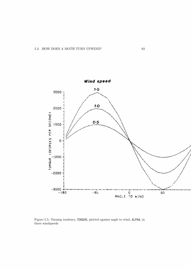
5.2. HOW DOES A MOTH TURN UPWIND? 83
Figure 5.5: Turning tendency, TORQUE, plotted against angle to wind, ALPHA, inthree windspeeds
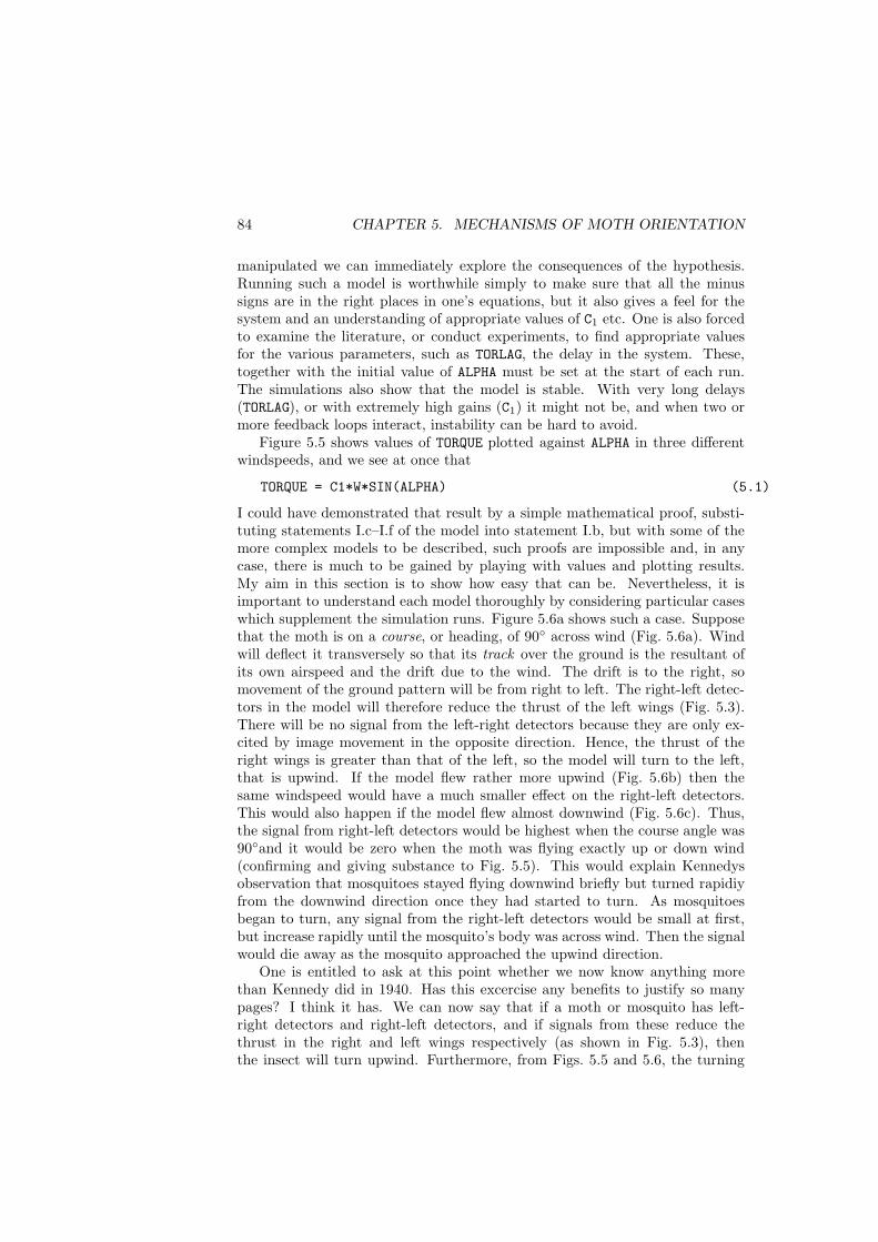
84 CHAPTER 5. MECHANISMS OF MOTH ORIENTATION
manipulated we can immediately explore the consequences of the hypothesis.Running such a model is worthwhile simply to make sure that all the minussigns are in the right places in one’s equations, but it also gives a feel for thesystem and an understanding of appropriate values of C1 etc. One is also forcedto examine the literature, or conduct experiments, to find appropriate valuesfor the various parameters, such as TORLAG, the delay in the system. These,together with the initial value of ALPHA must be set at the start of each run.The simulations also show that the model is stable. With very long delays(TORLAG), or with extremely high gains (C1) it might not be, and when two ormore feedback loops interact, instability can be hard to avoid.
Figure 5.5 shows values of TORQUE plotted against ALPHA in three differentwindspeeds, and we see at once that
TORQUE = C1*W*SIN(ALPHA) (5.1)
I could have demonstrated that result by a simple mathematical proof, substi-tuting statements I.c–I.f of the model into statement I.b, but with some of themore complex models to be described, such proofs are impossible and, in anycase, there is much to be gained by playing with values and plotting results.My aim in this section is to show how easy that can be. Nevertheless, it isimportant to understand each model thoroughly by considering particular caseswhich supplement the simulation runs. Figure 5.6a shows such a case. Supposethat the moth is on a course, or heading, of 90◦ across wind (Fig. 5.6a). Windwill deflect it transversely so that its track over the ground is the resultant ofits own airspeed and the drift due to the wind. The drift is to the right, somovement of the ground pattern will be from right to left. The right-left detec-tors in the model will therefore reduce the thrust of the left wings (Fig. 5.3).There will be no signal from the left-right detectors because they are only ex-cited by image movement in the opposite direction. Hence, the thrust of theright wings is greater than that of the left, so the model will turn to the left,that is upwind. If the model flew rather more upwind (Fig. 5.6b) then thesame windspeed would have a much smaller effect on the right-left detectors.This would also happen if the model flew almost downwind (Fig. 5.6c). Thus,the signal from right-left detectors would be highest when the course angle was90◦and it would be zero when the moth was flying exactly up or down wind(confirming and giving substance to Fig. 5.5). This would explain Kennedysobservation that mosquitoes stayed flying downwind briefly but turned rapidiyfrom the downwind direction once they had started to turn. As mosquitoesbegan to turn, any signal from the right-left detectors would be small at first,but increase rapidly until the mosquito’s body was across wind. Then the signalwould die away as the mosquito approached the upwind direction.
One is entitled to ask at this point whether we now know anything morethan Kennedy did in 1940. Has this excercise any benefits to justify so manypages? I think it has. We can now say that if a moth or mosquito has left-right detectors and right-left detectors, and if signals from these reduce thethrust in the right and left wings respectively (as shown in Fig. 5.3), thenthe insect will turn upwind. Furthermore, from Figs. 5.5 and 5.6, the turning

5.3. THE PROBLEM OF MAINTAINING CROSS-WIND TRACKS 85
tendency will be zero if the insect is flying exactly downwind, but as soon as itdeparts from this angle it will turn rapidly upwind, just as Kennedy observed. Inotherwords, both upwind and downwind directions have zero turning tendency,but the downwind direction is unstable. The text of Kennedy (1940) is certainlynot as clear as that, and later authors made mistakes which he did not. Forexample, Kellogg et al. (1962) and Bell and Tobin (1982) did not realise thatturning in response to transverse image movement was sufficient to distinguishup and downwind directions. They thought that an insect must also compareairspeed and groundspeed (if the insect is flying downwind its groundspeedwill be higher than its airspeed, if it is flying upwind its groundspeed will beless). Figures 5.5 and 5.6 show that there is no need for the moth to make thiscomparison.
Before concluding this section I should point out that one could base a modelon COS(ALPHA). That would represent the loss of headway due to the wind,instead of the lateral drift. In Fig. 5.4 COS(ALPHA) = (A - L)/W and that revealsseveral problems. A is airspeed and L is longitudinal movement. If the insectmeasures L in terms of angular velocity of the ground pattern, then the apparentvalue of L will be affected by height above ground. The higher the insect, themore slowly the ground will appear to move. Perception of airspeed, on the otherhand, will not be affected by height. Thus, a theory based on A - L concealsan additional assumption: that the insect can compensate for the effects ofheight on its perception of groundspeed. Even if it does compensate, however,the upwind direction would not be stable. The stable course angle would be90◦. An angle of 0◦ could be commanded if the system had an appropriate setpoint, but this would have to be adjusted according to windspeed, and if theadjustment were not absolutely perfect the moth might turn endlessly.
Another type of theory would postulate that the moth minimised L. Inotherwords it turned (with constant airspeed) until L reached a minimum. Howone predicts turning tendency from such a theory is not clear, but we shouldbear in mind that insects may respond to the rate of change of signals such asL and TR rather than their instantaneous values.
5.3 The problem of maintaining cross-wind tracks
Figure 5.2c shows a moth casting at about 90◦ to the wind. The broad arrowsshow that the wind direction changed in mid-cast, and yet the moth was ableto adjust its track to about 90◦ to the new wind direction. The windspeedtoo may have varied during that cast, although we cannot tell because therewere no bubbles nearby from which to calculate windspeed. Certainly, mothsdo maintain the same track angles in different windspeeds, as was first shownby Marsh et al. (1978)). There was, unfortunately, an intermittent fault inreplaying the original video tapes in that study and the time base used in theoriginal analysis was incorrect (as already reported in a brief note (Marsh et al.,1981). However, the track angles were not affected and Fig. 5.7 shows the tracksof the same moth in three different windspeeds, with corrected time marks one
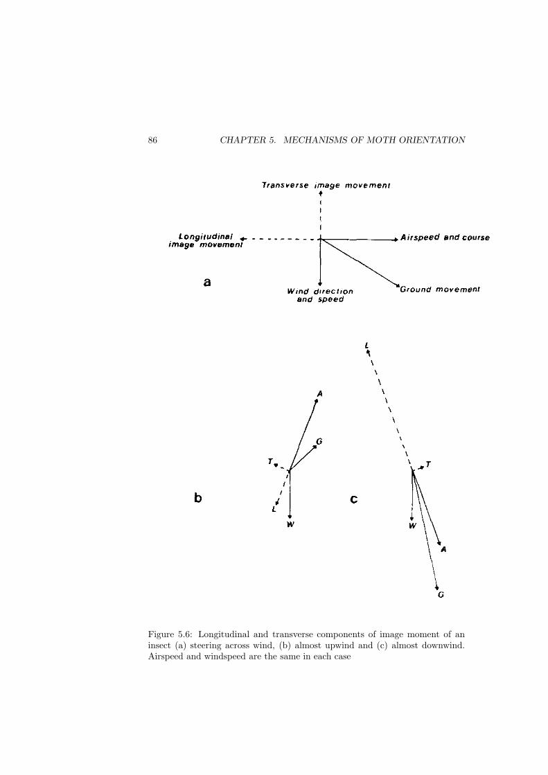
86 CHAPTER 5. MECHANISMS OF MOTH ORIENTATION
Figure 5.6: Longitudinal and transverse components of image moment of aninsect (a) steering across wind, (b) almost upwind and (c) almost downwind.Airspeed and windspeed are the same in each case
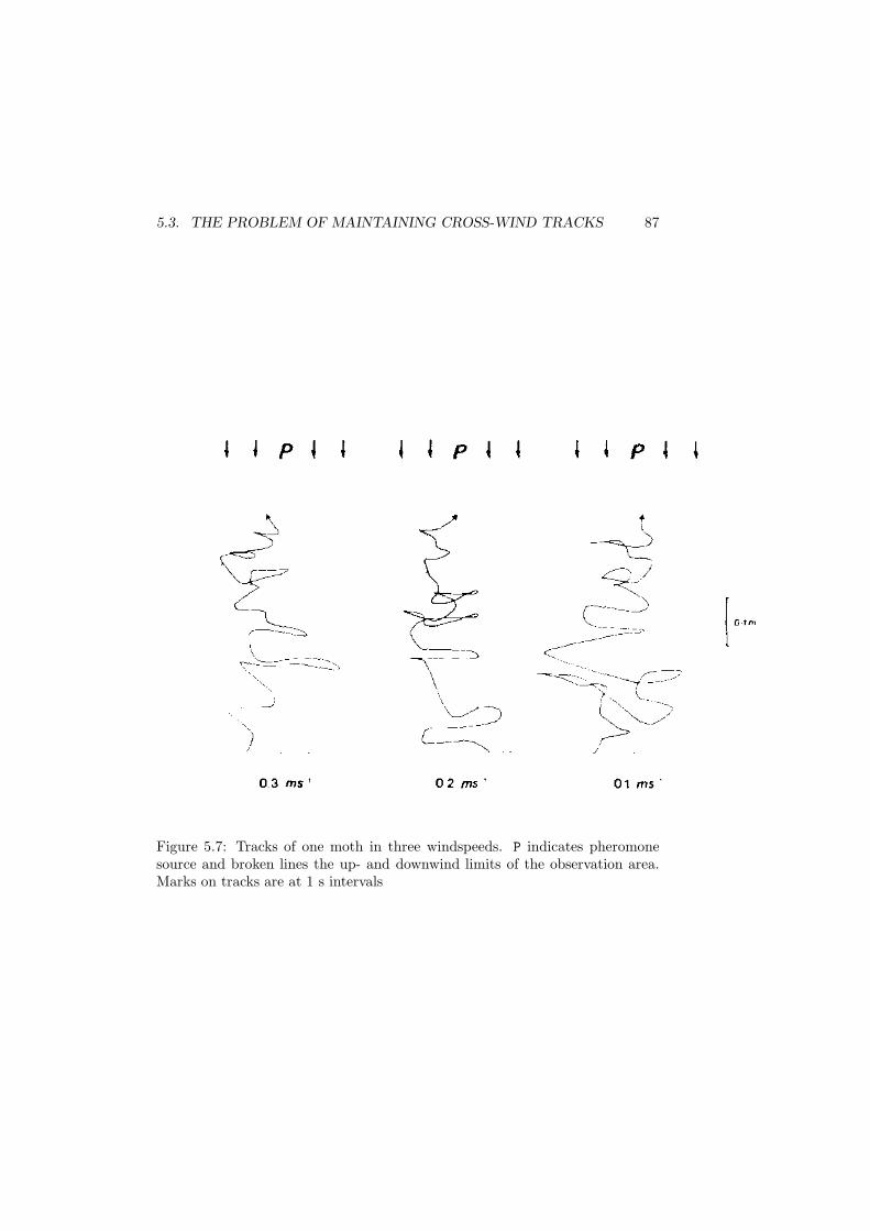
5.3. THE PROBLEM OF MAINTAINING CROSS-WIND TRACKS 87
Figure 5.7: Tracks of one moth in three windspeeds. P indicates pheromonesource and broken lines the up- and downwind limits of the observation area.Marks on tracks are at 1 s intervals
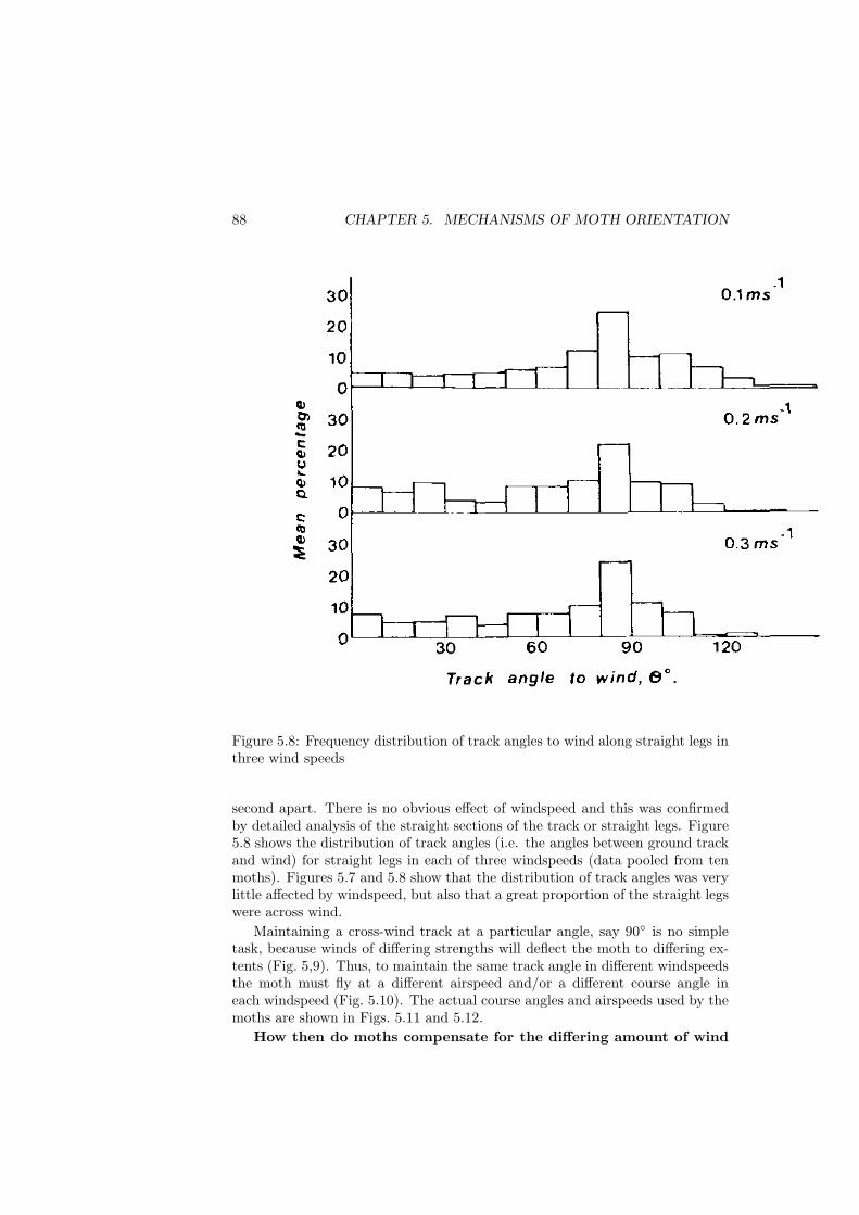
88 CHAPTER 5. MECHANISMS OF MOTH ORIENTATION
Figure 5.8: Frequency distribution of track angles to wind along straight legs inthree wind speeds
second apart. There is no obvious effect of windspeed and this was confirmedby detailed analysis of the straight sections of the track or straight legs. Figure5.8 shows the distribution of track angles (i.e. the angles between ground trackand wind) for straight legs in each of three windspeeds (data pooled from tenmoths). Figures 5.7 and 5.8 show that the distribution of track angles was verylittle affected by windspeed, but also that a great proportion of the straight legswere across wind.
Maintaining a cross-wind track at a particular angle, say 90◦ is no simpletask, because winds of differing strengths will deflect the moth to differing ex-tents (Fig. 5,9). Thus, to maintain the same track angle in different windspeedsthe moth must fly at a different airspeed and/or a different course angle ineach windspeed (Fig. 5.10). The actual course angles and airspeeds used by themoths are shown in Figs. 5.11 and 5.12.
How then do moths compensate for the differing amount of wind
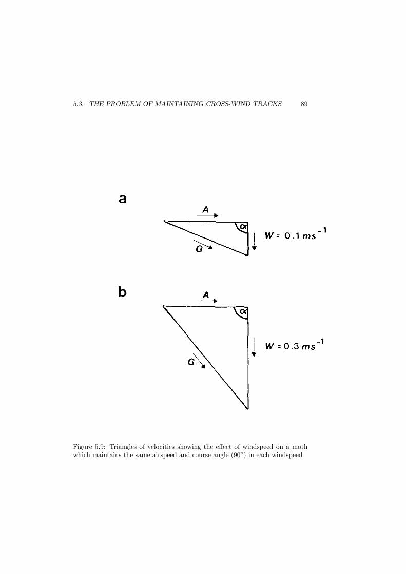
5.3. THE PROBLEM OF MAINTAINING CROSS-WIND TRACKS 89
Figure 5.9: Triangles of velocities showing the effect of windspeed on a mothwhich maintains the same airspeed and course angle (90◦) in each windspeed
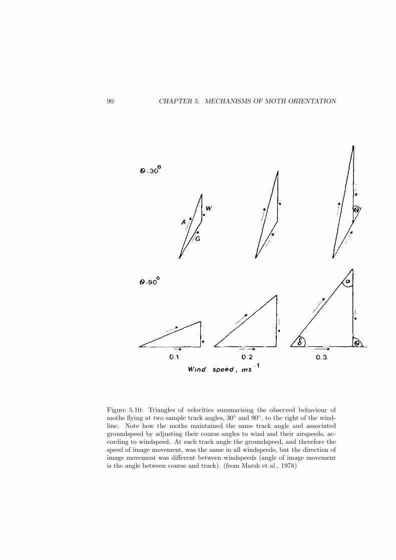
90 CHAPTER 5. MECHANISMS OF MOTH ORIENTATION
Figure 5.10: Triangles of velocities summarising the observed behaviour ofmoths flying at two sample track angles, 30◦ and 90◦, to the right of the wind-line. Note how the moths maintained the same track angle and associatedgroundspeed by adjusting their course angles to wind and their airspeeds, ac-cording to windspeed. At each track angle the groundspeed, and therefore thespeed of image movement, was the same in all windspeeds, but the direction ofimage movement was different between windspeeds (angle of image movementis the angle between course and track). (from Marsh et al., 1978)
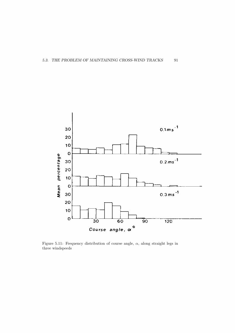
5.3. THE PROBLEM OF MAINTAINING CROSS-WIND TRACKS 91
Figure 5.11: Frequency distribution of course angle, α, along straight legs inthree windspeeds
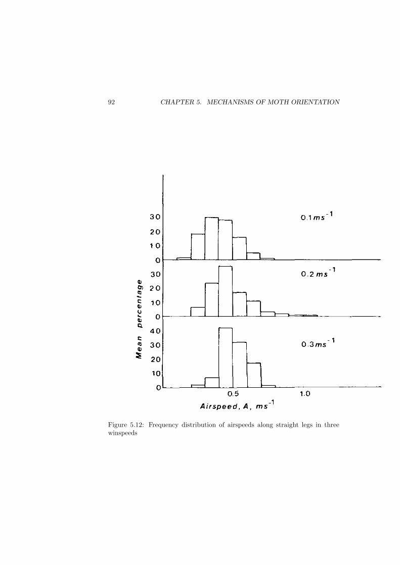
92 CHAPTER 5. MECHANISMS OF MOTH ORIENTATION
Figure 5.12: Frequency distribution of airspeeds along straight legs in threewinspeeds
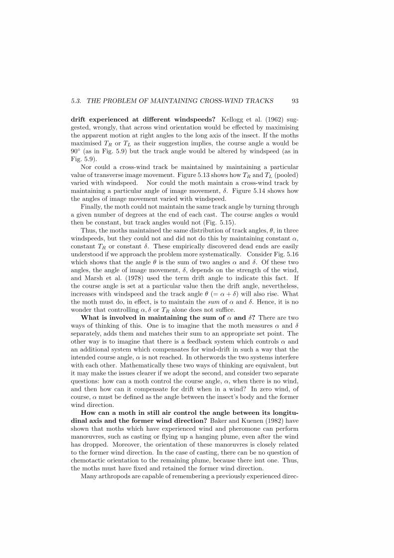
5.3. THE PROBLEM OF MAINTAINING CROSS-WIND TRACKS 93
drift experienced at different windspeeds? Kellogg et al. (1962) sug-gested, wrongly, that across wind orientation would be effected by maximisingthe apparent motion at right angles to the long axis of the insect. If the mothsmaximised TR or TL as their suggestion implies, the course angle a would be90◦ (as in Fig. 5.9) but the track angle would be altered by windspeed (as inFig. 5.9).
Nor could a cross-wind track be maintained by maintaining a particularvalue of transverse image movement. Figure 5.13 shows how TR and TL (pooled)varied with windspeed. Nor could the moth maintain a cross-wind track bymaintaining a particular angle of image movement, δ. Figure 5.14 shows howthe angles of image movement varied with windspeed.
Finally, the moth could not maintain the same track angle by turning througha given number of degrees at the end of each cast. The course angles α wouldthen be constant, but track angles would not (Fig. 5.15).
Thus, the moths maintained the same distribution of track angles, θ, in threewindspeeds, but they could not and did not do this by maintaining constant α,constant TR or constant δ. These empirically discovered dead ends are easilyunderstood if we approach the problem more systematically. Consider Fig. 5.16which shows that the angle θ is the sum of two angles α and δ. Of these twoangles, the angle of image movement, δ, depends on the strength of the wind,and Marsh et al. (1978) used the term drift angle to indicate this fact. Ifthe course angle is set at a particular value then the drift angle, nevertheless,increases with windspeed and the track angle θ (= α + δ) will also rise. Whatthe moth must do, in effect, is to maintain the sum of α and δ. Hence, it is nowonder that controlling α, δ or TR alone does not suffice.
What is involved in maintaining the sum of α and δ? There are twoways of thinking of this. One is to imagine that the moth measures α and δseparately, adds them and matches their sum to an appropriate set point. Theother way is to imagine that there is a feedback system which controls α andan additional system which compensates for wind-drift in such a way that theintended course angle, α is not reached. In otherwords the two systems interferewith each other. Mathematically these two ways of thinking are equivalent, butit may make the issues clearer if we adopt the second, and consider two separatequestions: how can a moth control the course angle, α, when there is no wind,and then how can it compensate for drift when in a wind? In zero wind, ofcourse, α must be defined as the angle between the insect’s body and the formerwind direction.
How can a moth in still air control the angle between its longitu-
dinal axis and the former wind direction? Baker and Kuenen (1982) haveshown that moths which have experienced wind and pheromone can performmanœuvres, such as casting or flying up a hanging plume, even after the windhas dropped. Moreover, the orientation of these manœuvres is closely relatedto the former wind direction. In the case of casting, there can be no question ofchemotactic orientation to the remaining plume, because there isnt one. Thus,the moths must have fixed and retained the former wind direction.
Many arthropods are capable of remembering a previously experienced direc-
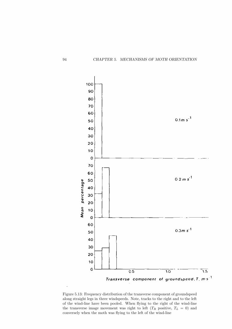
94 CHAPTER 5. MECHANISMS OF MOTH ORIENTATION
Figure 5.13: Frequency distribution of the transverse component of groundspeedalong straight legs in three windspeeds. Note, tracks to the right and to the leftof the wind-line have been pooled. When flying to the right of the wind-linethe transverse image movement was right to left (TR positive, TL = 0) andconversely when the moth was flying to the left of the wind-line
5.3. THE PROBLEM OF MAINTAINING CROSS-WIND TRACKS 95
Figure 5.14: Frequency distributions of angle of image movement, δ, alongstraight legs in three windspeeds
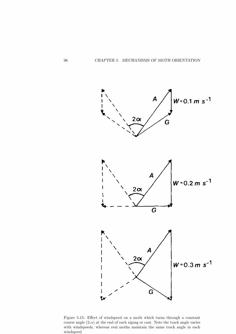
96 CHAPTER 5. MECHANISMS OF MOTH ORIENTATION
Figure 5.15: Effect of windspeed on a moth which turns through a constantcourse angle (2.α) at the end of each zigzag or cast. Note the track angle varieswith windspeeds, whereas real moths maintain the same track angle in eachwindspeed
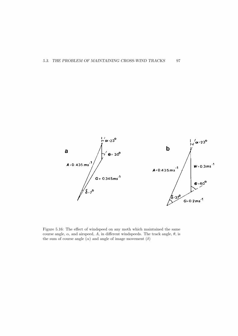
5.3. THE PROBLEM OF MAINTAINING CROSS-WIND TRACKS 97
Figure 5.16: The effect of windspeed on any moth which maintained the samecourse angle, α, and airspeed, A, in different windspeeds. The track angle, θ, isthe sum of course angle (α) and angle of image movement (δ)
98 CHAPTER 5. MECHANISMS OF MOTH ORIENTATION
tion, and there is an extensive literature on the subject of correcting behaviour,whereby an insect returns to its former direction after an enforced turn (see ref-erences in Barnwell, 1965; Jander, 1963; Mittelstaedt et al., 1979; Mittelstaedtand Mittelstaedt, 1973) found it useful to distinguish between allothetic orien-tation, which relies on external cues, and idiothetic or self-steered orientation.The latter may depend on internal cues such as signals from proprioceptors (ki-naesthesis), or on summing the signals which command a turn. Both allotheticand idiothetic orientation have been clearly demonstrated in insects. Among theallothetic cues are light direction, plane of polarisation, gravity and magnetism.Usually, an insect will respond to several cues at once, as can be demonstratedwhen they are pitted against each other (e.g. M-L., 1972). For example, themigratory large yellow underwing moth (Noctua pronuba) uses the moon, starsand magnetism (Baker and Mather, 1982).
Because magnetism was not recognised as a potential cue until recently, itseffects were not sufficiently controlled in the earlier studies, and some examplesof idiothetic or self-steered orientation may turn out to depend on magneticcues instead. However, magnetism was ruled out by Beale and Webster (1971)who showed that a passive rotation of 90◦ did not affect the frequency withwhich woodlice (Porcello scaber) compensated for a forced turn. Moreover,when the woodlice were allowed to walk on a split track which could be movedso that the right legs walked further than the left, the woodlice compensatedfor this apparent left hand turn by turning right as soon as they were allowed.Millipedes, too, have been shown to compensate accurately for forced turns evenwhen visual, mechanical and magnetic cues were eliminated (M-L., 1972). Theyalso appear to integrate walking effort on each side, and the stable positionwould be facing directly toward the light source, in the second, directly away.
Jander proposed that, superimposed on these basic responses, was a com-mand signal so that an insect deviated from the switched on positive or negativephototaxis by a given amount. In that way it would maintain a given angle tothe light. The simplest implementation of this idea is to suppose that there isa difference between the excitatory commands PL and PR in Fig. 5.17. Thecommand is then proportional to that difference.
Table 5.2 shows a computer model of Jander’s theory. The angle BETA isthat between the insects long axis and the stimulus, say a bright light. Apartfrom that, the first two statements (II.a and b) are the same as those in theupwind turning model. Once again, I am using the convention that turning tothe right increases BETA, so BETA is positive when the stimulus is to the insect’sleft (Fig. 5.18).
The next two statements are a simple translation of Fig. 5.17. We assumethat the right wing-thrust is reduced by a bright light on the right hand side(STIMR is high), and this will obviously cause the insect to turn to the right(towards the light).
In a complete, working, model we must define STIMR and STIML, and thisraises two questions, What is the actual light distribution, and how much ofthe world does each receptor see? The actual light distribution depends on theexperiment, and we may wish to simulate a variety of experiments, so the model
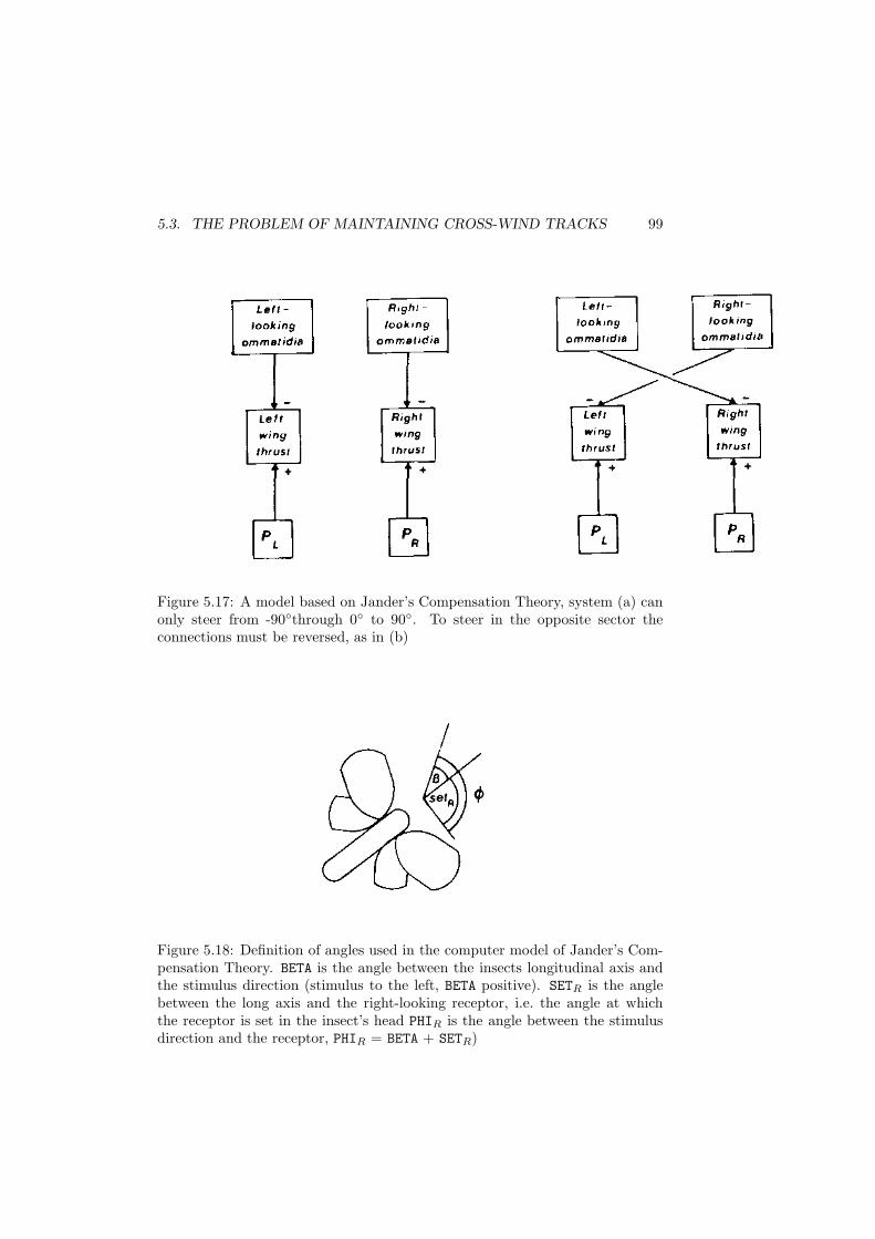
5.3. THE PROBLEM OF MAINTAINING CROSS-WIND TRACKS 99
Figure 5.17: A model based on Jander’s Compensation Theory, system (a) canonly steer from -90◦through 0◦ to 90◦. To steer in the opposite sector theconnections must be reversed, as in (b)
Figure 5.18: Definition of angles used in the computer model of Jander’s Com-pensation Theory. BETA is the angle between the insects longitudinal axis andthe stimulus direction (stimulus to the left, BETA positive). SETR is the anglebetween the long axis and the right-looking receptor, i.e. the angle at whichthe receptor is set in the insect’s head PHIR is the angle between the stimulusdirection and the receptor, PHIR = BETA + SETR)
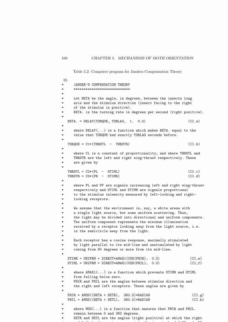
100 CHAPTER 5. MECHANISMS OF MOTH ORIENTATION
Table 5.2: Computer program for Janders Compensation Theory
Dl
* JANDER’S COMPENSATION THEORY
* ****************************
*
* Let BETA be the angle, in degrees, between the insects long
* axis and the stimulus direction (insect facing to the right
* of the stimulus is positive).
* BETA. is the turning rate in degrees per second (right positive).
*
BETA. = DELAY(TORQUE, TORLAG, 1. 0.0) (II.a)
*
* where DELAY(...) is a function which makes BETA. equal to the
* value that TORQUE had exactly TORLAG seconds before.
*
TORQUE = C1*(THRSTL - THRSTR) (II.b)
*
* where Cl is a constant of proportionality, and where THRSTL and
* THRSTR are the left and right wing-thrust respectively. These
* are given by
*
THRSTL = C2*(PL - STIML) (II.c)
THRSTR = C3*(PR - STIMR) (II.d)
*
* where PL and PP are signals increasing left and right wing-thrust
* respectively and STIML and STIMR are signals proportional
* to the stimulus inlensity measured by left-looking and right-
* looking receptors.
*
* We assume that the environment is, say, a white arena with
* a single light source, but some uniform scattering. Thus,
* the light may be divided into directional and uniform components.
* The uniform component represents the minimum illumination
* received by a receptor looking away from the light source, i.e.
* in the semicircle away from the light.
*
* Each receptor has a cosine response, maximally stimulated
* by light parallel to its mid-line and unstimulated by light
* coming from 90 degrees or more from its mid-line.
*
STIMR = UNIFRM + DIRECT*AMAX1(COS(PHIR), 0.0) (II,e)
STIML = UNIFRM + DIRECT*AMAX1(COS(PHIL), 0.0) (II,f)
*
* where AMAX1(...) is a function which prevents STIMR and STIML
* from falling below zero.
* PHIR and PHIL are the angles between stimulus direction and
* the right and left receptors. These angles are given by
*
PHIR = AMOD((BETA + SETR), 360.0)*RADIAN (II.g)
PHIL = AMOD((BETA + SETL), 360.0)*RADIAN (II.h)
*
* where MOD(...) is a function that ensures that PHIR and PHIL.
* remain between 0 and 360 degrees.
* SETR and SETL are the angles (right positive) at which the right
* and left hand receptors are set in the insects head (+90 and -90
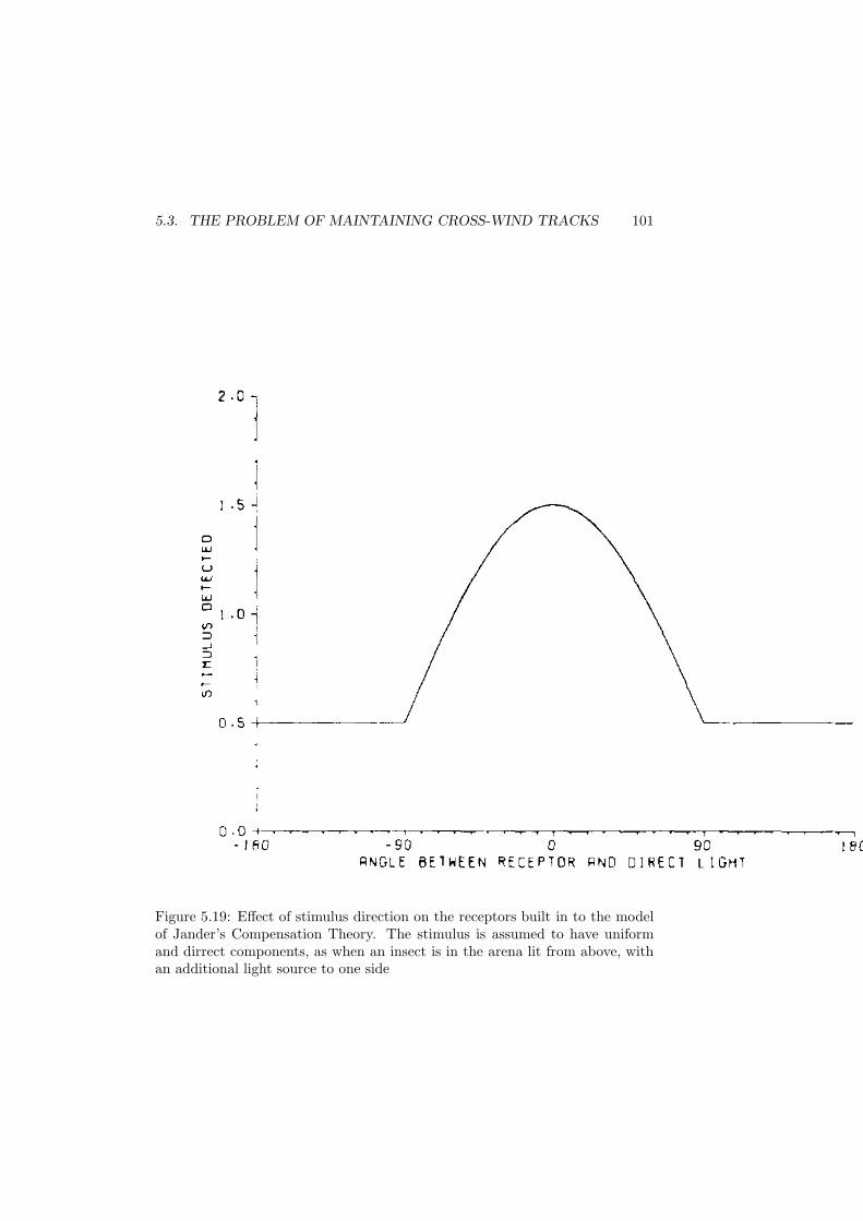
5.3. THE PROBLEM OF MAINTAINING CROSS-WIND TRACKS 101
Figure 5.19: Effect of stimulus direction on the receptors built in to the modelof Jander’s Compensation Theory. The stimulus is assumed to have uniformand dirrect components, as when an insect is in the arena lit from above, withan additional light source to one side
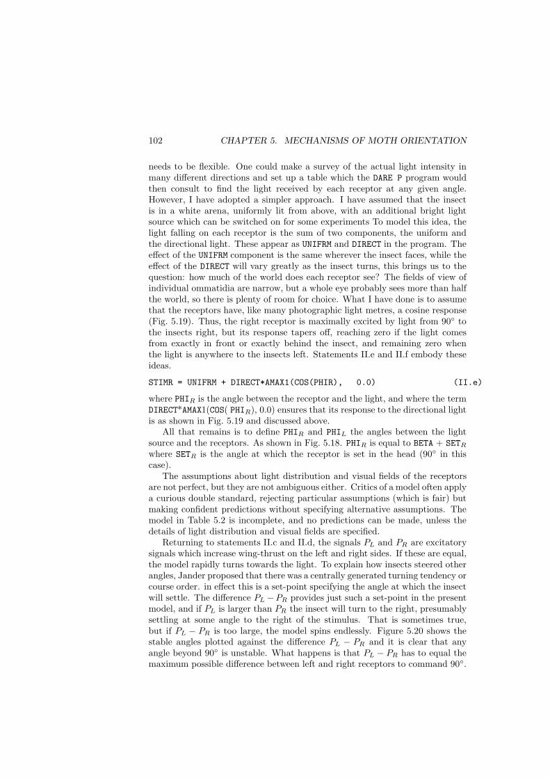
102 CHAPTER 5. MECHANISMS OF MOTH ORIENTATION
needs to be flexible. One could make a survey of the actual light intensity inmany different directions and set up a table which the DARE P program wouldthen consult to find the light received by each receptor at any given angle.However, I have adopted a simpler approach. I have assumed that the insectis in a white arena, uniformly lit from above, with an additional bright lightsource which can be switched on for some experiments To model this idea, thelight falling on each receptor is the sum of two components, the uniform andthe directional light. These appear as UNIFRM and DIRECT in the program. Theeffect of the UNIFRM component is the same wherever the insect faces, while theeffect of the DIRECT will vary greatly as the insect turns, this brings us to thequestion: how much of the world does each receptor see? The fields of view ofindividual ommatidia are narrow, but a whole eye probably sees more than halfthe world, so there is plenty of room for choice. What I have done is to assumethat the receptors have, like many photographic light metres, a cosine response(Fig. 5.19). Thus, the right receptor is maximally excited by light from 90◦ tothe insects right, but its response tapers off, reaching zero if the light comesfrom exactly in front or exactly behind the insect, and remaining zero whenthe light is anywhere to the insects left. Statements II.e and II.f embody theseideas.
STIMR = UNIFRM + DIRECT*AMAX1(COS(PHIR), 0.0) (II.e)
where PHIR is the angle between the receptor and the light, and where the termDIRECT*AMAX1(COS( PHIR), 0.0) ensures that its response to the directional lightis as shown in Fig. 5.19 and discussed above.
All that remains is to define PHIR and PHIL the angles between the lightsource and the receptors. As shown in Fig. 5.18. PHIR is equal to BETA + SETR
where SETR is the angle at which the receptor is set in the head (90◦ in thiscase).
The assumptions about light distribution and visual fields of the receptorsare not perfect, but they are not ambiguous either. Critics of a model often applya curious double standard, rejecting particular assumptions (which is fair) butmaking confident predictions without specifying alternative assumptions. Themodel in Table 5.2 is incomplete, and no predictions can be made, unless thedetails of light distribution and visual fields are specified.
Returning to statements II.c and II.d, the signals PL and PR are excitatorysignals which increase wing-thrust on the left and right sides. If these are equal,the model rapidly turns towards the light. To explain how insects steered otherangles, Jander proposed that there was a centrally generated turning tendency orcourse order. in effect this is a set-point specifying the angle at which the insectwill settle. The difference PL −PR provides just such a set-point in the presentmodel, and if PL is larger than PR the insect will turn to the right, presumablysettling at some angle to the right of the stimulus. That is sometimes true,but if PL − PR is too large, the model spins endlessly. Figure 5.20 shows thestable angles plotted against the difference PL − PR and it is clear that anyangle beyond 90◦ is unstable. What happens is that PL − PR has to equal themaximum possible difference between left and right receptors to command 90◦.

5.3. THE PROBLEM OF MAINTAINING CROSS-WIND TRACKS 103
If it rises above this value, then there is no way in which the opposing torque(tending to cause the insect to face the light) can ever match the command sothe model spins endlessly. Thus, the system cannot reach angles of say, 95◦ atall, unless the turning tendency is reversed, i.e. the model switches from positiveto negative phototaxis. Jander’s solution to this problem was to postulate justsuch reversals of response and Fig. 5.17 shows how they might be done. Anotherproblem with the theory is that the model does not always turn through thesmallest angle to reach its stable state. Thus, if it is stable at 85◦ and thestimulus is suddenly moved to the left by 10◦ (to 95◦, the model would not turnleft by 10◦. Instead it would turn right for 350◦. Real insects would turn left.
Mittelstaedt (1961, 1962) was the first to recognise the various problems oftheories based on the sine component: that they could not explain how insectssteered at exactly 90◦ to a stimulus, and that their explanation of how insectssteered angles of greater than 90◦ was cumbersome. He therefore proposed analternative: his theory of the reciprocal modulation of bicomponents, now knownas the Bicomponent Theory. In doing so, Mittelstaedt brought two importantideas into the discussion.
1. that two components of the stimulus direction might be measured, and
2. that the weight accorded by the insect to each component would determinethe angle reached.
Mittelstaedt did not derive his theory ‘in print’ but, since the main aim ofmodelling is to make the biological issues clearer, I will derive the theory bytwo different routes. By analogy with the upwind model sinβ is the transversecomponent of the stimulus direction and is measured by comparing intensity onthe right and left sides of the insect. In the same way, cosβ is the longitudinalcomponent and may be measured by comparing intensities in front of, andbehind the insect. Suppose that the insect receives signals from receptors lookingforwards STIMF and backwards STIMB, and that it turned left whenever STIMF
exceeded STIMB. Then it would face across the stimulus direction, with thesource to its right. In that position STIMF and STIMB would be equal.
Thus, a transverse comparison is ideal for facing toward or away from astimulus, while a longitudinal comparison is ideal for steering at 90◦ to it.Mittelstaedt proposed that insects measure both components, but ignore thelongitudinal in order to face towards the stimulus and ignore the transversecomponent in order to steer across the stimulus direction. The intermediateangles are steered by responding in different degree to both components, andthe mechanism commanding a particular angle does so by adjusting the weightaccorded to each of the observed components. That is the essence of his Bicom-ponent Theory.
We may approach the theory by another route. Jander’s compensation the-ory implied, as we have seen, that the insect measured the sine of the stimulusdirection and compared that sine with a set point or command value (PL−PR).Mittelstaedt’s theory, instead, implies that the insect controls the sum of twoangles, the observed and the preferred, so that their sum is zero. Thus, if the
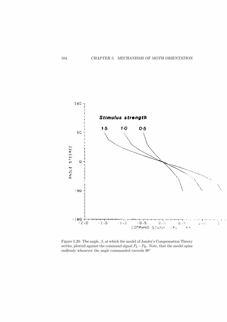
104 CHAPTER 5. MECHANISMS OF MOTH ORIENTATION
Figure 5.20: The angle, β, at which the model of Jander’s Compensation Theorysettles, plotted against the command signal PL−PR. Note, that the model spinsendlessly whenever the angle commanded exceeds 90◦
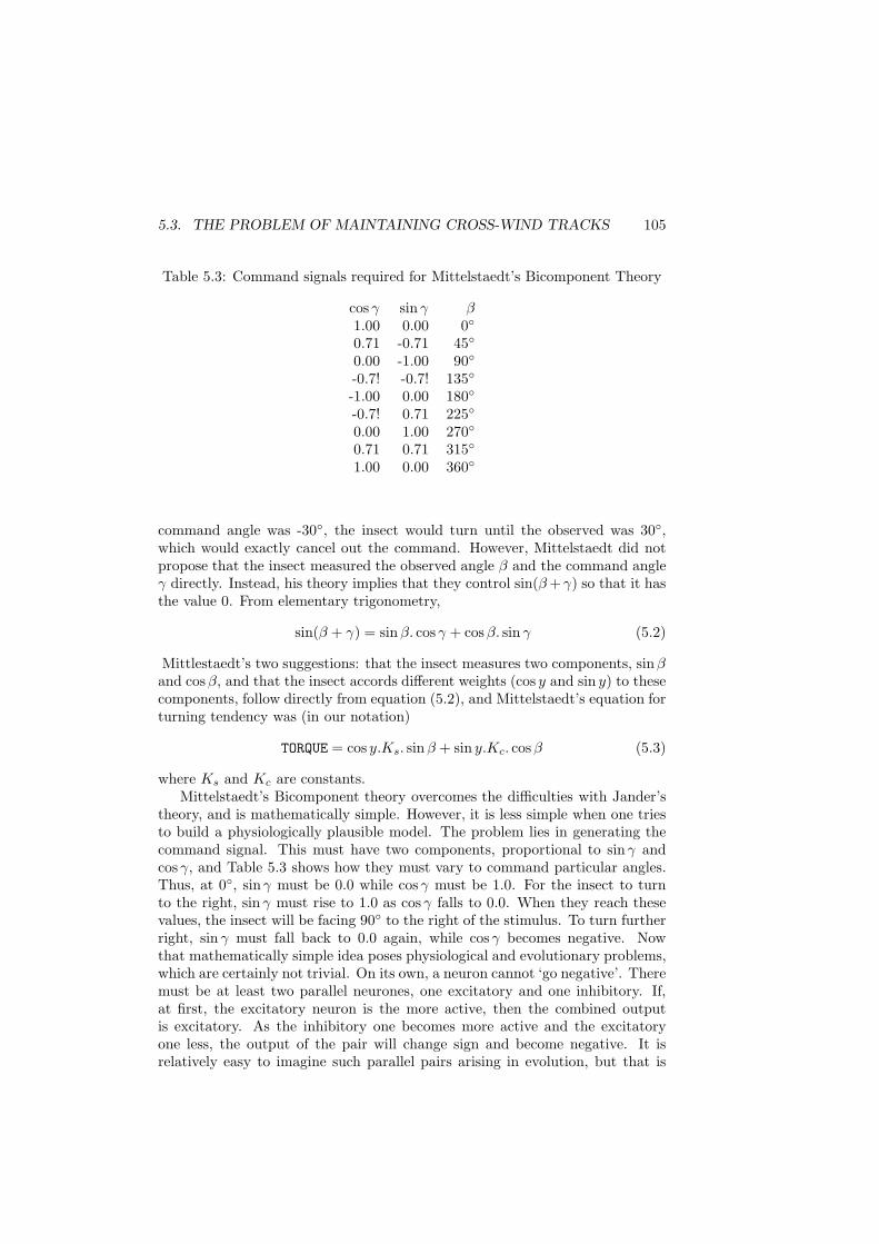
5.3. THE PROBLEM OF MAINTAINING CROSS-WIND TRACKS 105
Table 5.3: Command signals required for Mittelstaedt’s Bicomponent Theory
cos γ sin γ β1.00 0.00 0◦
0.71 -0.71 45◦
0.00 -1.00 90◦
-0.7! -0.7! 135◦
-1.00 0.00 180◦
-0.7! 0.71 225◦
0.00 1.00 270◦
0.71 0.71 315◦
1.00 0.00 360◦
command angle was -30◦, the insect would turn until the observed was 30◦,which would exactly cancel out the command. However, Mittelstaedt did notpropose that the insect measured the observed angle β and the command angleγ directly. Instead, his theory implies that they control sin(β +γ) so that it hasthe value 0. From elementary trigonometry,
sin(β + γ) = sin β. cos γ + cosβ. sin γ (5.2)
Mittlestaedt’s two suggestions: that the insect measures two components, sinβand cosβ, and that the insect accords different weights (cos y and sin y) to thesecomponents, follow directly from equation (5.2), and Mittelstaedt’s equation forturning tendency was (in our notation)
TORQUE = cos y.Ks. sin β + sin y.Kc. cosβ (5.3)
where Ks and Kc are constants.Mittelstaedt’s Bicomponent theory overcomes the difficulties with Jander’s
theory, and is mathematically simple. However, it is less simple when one triesto build a physiologically plausible model. The problem lies in generating thecommand signal. This must have two components, proportional to sinγ andcos γ, and Table 5.3 shows how they must vary to command particular angles.Thus, at 0◦, sinγ must be 0.0 while cos γ must be 1.0. For the insect to turnto the right, sin γ must rise to 1.0 as cos γ falls to 0.0. When they reach thesevalues, the insect will be facing 90◦ to the right of the stimulus. To turn furtherright, sin γ must fall back to 0.0 again, while cos γ becomes negative. Nowthat mathematically simple idea poses physiological and evolutionary problems,which are certainly not trivial. On its own, a neuron cannot ‘go negative’. Theremust be at least two parallel neurones, one excitatory and one inhibitory. If,at first, the excitatory neuron is the more active, then the combined outputis excitatory. As the inhibitory one becomes more active and the excitatoryone less, the output of the pair will change sign and become negative. It isrelatively easy to imagine such parallel pairs arising in evolution, but that is
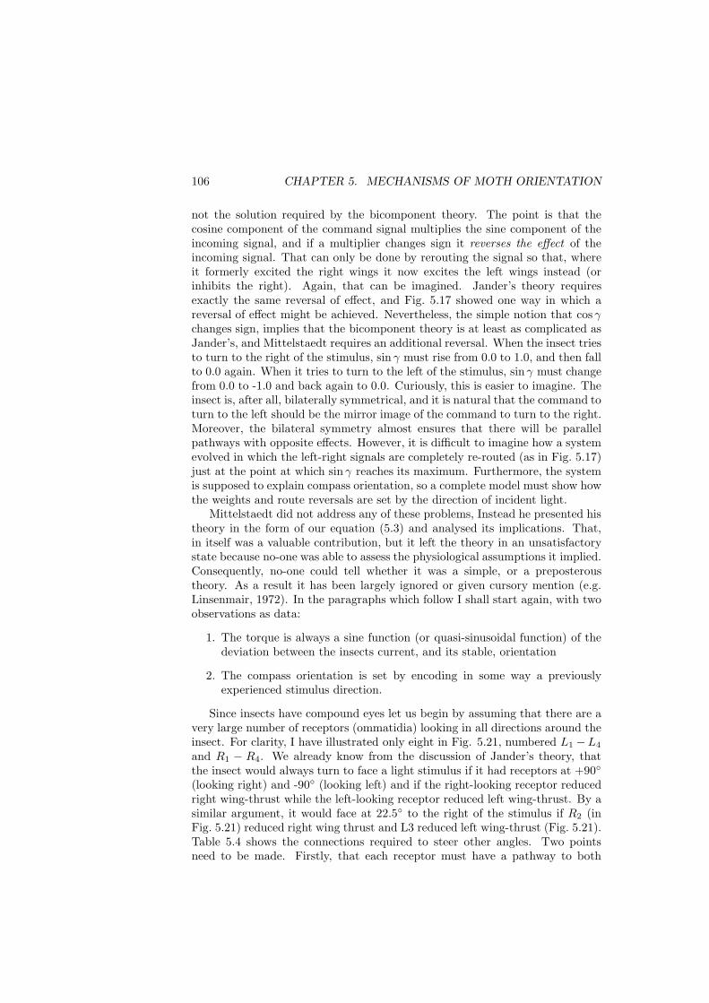
106 CHAPTER 5. MECHANISMS OF MOTH ORIENTATION
not the solution required by the bicomponent theory. The point is that thecosine component of the command signal multiplies the sine component of theincoming signal, and if a multiplier changes sign it reverses the effect of theincoming signal. That can only be done by rerouting the signal so that, whereit formerly excited the right wings it now excites the left wings instead (orinhibits the right). Again, that can be imagined. Jander’s theory requiresexactly the same reversal of effect, and Fig. 5.17 showed one way in which areversal of effect might be achieved. Nevertheless, the simple notion that cos γchanges sign, implies that the bicomponent theory is at least as complicated asJander’s, and Mittelstaedt requires an additional reversal. When the insect triesto turn to the right of the stimulus, sin γ must rise from 0.0 to 1.0, and then fallto 0.0 again. When it tries to turn to the left of the stimulus, sinγ must changefrom 0.0 to -1.0 and back again to 0.0. Curiously, this is easier to imagine. Theinsect is, after all, bilaterally symmetrical, and it is natural that the command toturn to the left should be the mirror image of the command to turn to the right.Moreover, the bilateral symmetry almost ensures that there will be parallelpathways with opposite effects. However, it is difficult to imagine how a systemevolved in which the left-right signals are completely re-routed (as in Fig. 5.17)just at the point at which sin γ reaches its maximum. Furthermore, the systemis supposed to explain compass orientation, so a complete model must show howthe weights and route reversals are set by the direction of incident light.
Mittelstaedt did not address any of these problems, Instead he presented histheory in the form of our equation (5.3) and analysed its implications. That,in itself was a valuable contribution, but it left the theory in an unsatisfactorystate because no-one was able to assess the physiological assumptions it implied.Consequently, no-one could tell whether it was a simple, or a preposteroustheory. As a result it has been largely ignored or given cursory mention (e.g.Linsenmair, 1972). In the paragraphs which follow I shall start again, with twoobservations as data:
1. The torque is always a sine function (or quasi-sinusoidal function) of thedeviation between the insects current, and its stable, orientation
2. The compass orientation is set by encoding in some way a previouslyexperienced stimulus direction.
Since insects have compound eyes let us begin by assuming that there are avery large number of receptors (ommatidia) looking in all directions around theinsect. For clarity, I have illustrated only eight in Fig. 5.21, numbered L1 −L4
and R1 − R4. We already know from the discussion of Jander’s theory, thatthe insect would always turn to face a light stimulus if it had receptors at +90◦
(looking right) and -90◦ (looking left) and if the right-looking receptor reducedright wing-thrust while the left-looking receptor reduced left wing-thrust. By asimilar argument, it would face at 22.5◦ to the right of the stimulus if R2 (inFig. 5.21) reduced right wing thrust and L3 reduced left wing-thrust (Fig. 5.21).Table 5.4 shows the connections required to steer other angles. Two pointsneed to be made. Firstly, that each receptor must have a pathway to both

5.3. THE PROBLEM OF MAINTAINING CROSS-WIND TRACKS 107
Figure 5.21: The radial theory of compass orientation. (For explanation seetext)
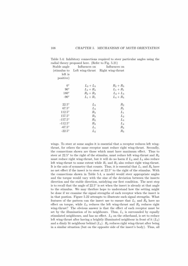
108 CHAPTER 5. MECHANISMS OF MOTH ORIENTATION
Table 5.4: Inhibitory connections required to steer particular angles using theradial theory proposed here. (Refer to Fig. 5.21)Stable angle Influences on Influences on(stimulus to Left wing-thrust Right wing-thrust
left ispositive)
0◦ L2 + L3 R2 + R3
90◦ L4 + R4 L1 + R1
180◦ R2 + R3 L2 + L3
-90◦ L1 + R1 L4 + R4
22.5◦ L3 R2
67.5◦ L4 R1
112.5◦ R4 L1
157.5◦ R3 L2
-157.5◦ R2 L3
-112.5◦ R3 L4
-67.5◦ L1 R4
-22.5◦ L2 R3
wings. To steer at some angles it is essential that a receptor reduces left wing-thrust, for others the same receptor must reduce right wing-thrust. Secondly,the connections shown are those which must have maximum effect. Thus tosteer at 22.5◦ to the right of the stimulus, must reduce left wing-thrust and R2
must reduce right wing-thrust, but it will do no harm if L2 and L4 also reduceleft wing-thrust to some extent while R1 and R3 also reduce right wing-thrust.It is the axis of symmetry that counts. Thus, it is essential that L1 and R4 haveno net effect if the insect is to steer at 22.5◦ to the right of the stimulus. Withthe connections shown in Table 5.4, a model would steer appropriate anglesand the torque would vary with the sine of the deviation between the insectsdirection and the stable direction, satisfying our first condition. The next stepis to recall that the angle of 22.5◦ is set when the insect is already at that angleto the stimulus. We may therfore hope to understand how the setting mightbe done if we examine the signal strengths of each receptor when the insect isin that postion. Figure 5.22 attempts to illustrate such signal strengths. Whatfeatures of the pattern can the insect use to ensure that L1 and R4 have noeffect on torque, while L3 reduces the left wing-thrust and R2 reduces rightwing-thrust? The obvious answer is that the effect of each receptor must beset by the illumination of its neighbours. Thus, L1 is surrounded by equallystimulated neighbours, and has no effect. L3 on the otherhand, is set to reduceleft wing-thrust after having a brightly illuminated neighbour in front of it (L2)and a dimly lit neighbour behind (L4). R2 reduces right wing-thrust after beingin a similar situation (but on the opposite side of the insect’s body). Thus, all
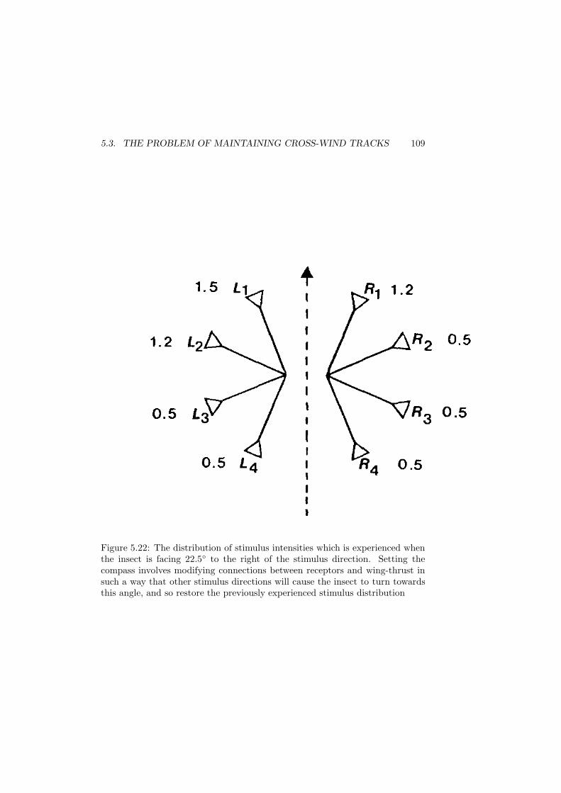
5.3. THE PROBLEM OF MAINTAINING CROSS-WIND TRACKS 109
Figure 5.22: The distribution of stimulus intensities which is experienced whenthe insect is facing 22.5◦ to the right of the stimulus direction. Setting thecompass involves modifying connections between receptors and wing-thrust insuch a way that other stimulus directions will cause the insect to turn towardsthis angle, and so restore the previously experienced stimulus distribution
110 CHAPTER 5. MECHANISMS OF MOTH ORIENTATION
we need to postulate is a special form of lateral inhibition, and lateral inhibitionis well known in arthropod and vertebrate visual systems. In this case, we needto postulate that each receptor reduces both left and right wing-thrust, but thatif the receptor in front was brightly illuminated, then the contralateral effectis reduced. The ipsilateral effect is reduced if the receptor behind was brightlyilluminated. Notice the tenses in the previous two sentences. The effect of thereceptors is set by previous, not current stimulation, of their neighbours.
What about the front-most (or back-most) receptors? They will have noth-ing behind them (or in front). Fortunately, it does not matter if the front-lookingreceptors on both sides look in exactly the same direction. Although there isnothing to reduce the contralateral effect of the front-looking receptor on theleft hand side, there is equally nothing to reduce the contralateral effect of thefront-looking receptor on the right hand side, and these two omissions cancelout. The same argument applies to the back-most receptors.
How is the setting achieved? It might involve no more than adaptation inappropriate pathways. Furthermore, the system should work when there is morethan one bright spot in the environment, as when an insect uses landmarks tofix its course. Again, it should enable an insect to follow the rotation of a stripeddrum, as many insects are known to do, Hence, the compass orientation andoptomotor turning responses of insects may be very closely linked. If the settingmechanism does indeed involve adaptation, and the adaptation is fast enough,then the network necessary to set a compass direction might also be capable ofrecording velocity information, although separate networks with differing time-constants might be more appropriate. These questions deserve exploration, buttwo further points must be addressed immediately. How might an insect reverseits course through 180◦ as when a Honey Bee returns to its hive? And whathappens if there are very few receptors?
The reversal through 180◦ is a relatively simple matter because all thatis necessary is that receptors which previously reduced right wing-thrust nowreduce left wing-thrust, and vice versa. This could be done downstream ofthe compass-setting network, and involves the sort of switching illustrated inFig. 5.17.
The theory does not depend on a large number of receptors, Table 5.4 showedthat any number of angles could be set even when there were only eight recep-tors. If the number of receptors is reduced still further, to the six shown in Fig.5.23 it is still possible to set any angle.
Thus, a simple rule will allow the insect to set the effect of each receptorso that it will later turn with a sinusoidal torque until the stimulus is onceagain in the same direction. It would, doubtless, be rewarding to pursue thefull implications of this idea. The fact that a small number of receptors can stillprovide a compass mechanism is important when considering sensory modalitiesother than vision. Gravity, for example, or magnetism may be sensed in a limitednumber of directions, and the properties of the system shown in Fig. 5.23 arethen relevant.
In a sense, Fig. 5.23 illustrates a version of Mittelstaedt’s Bicomponent The-ory. The receptors certainly measure the transverse (sine) and longitudinal

5.3. THE PROBLEM OF MAINTAINING CROSS-WIND TRACKS 111
Figure 5.23: A version of the radial theory with only six receptors
112 CHAPTER 5. MECHANISMS OF MOTH ORIENTATION
(cosine) components of the stimulus. Furthermore, the setting rules explainedabove would provide a mechanism of implementing Mittelstaedt’s equation. Thesignals from the six receptors are rerouted, just as the multiplications in equa-tion (5.3) imply. However, the system has limitations which Mittelstaedt didnot discuss and it is unlikely that he envisaged a system like the one shown inFig. 5.23.
Throughout his discussions, Mittelstaedt (1962, 1964) appears to have con-sidered the command signal as a continuously variable signal split by some net-work into its sine and cosine components. Thus, one would expect the insect,not only to be able to steer any previously experienced angle, but to be ableto deviate from that angle by any given amount, as moths do when casting. Inotherwords, if the sun had previously been at 22.5◦ when the insect was facingupwind, then it should be able to cast at 90◦ on either side of this directionsimply by adding or subtracting 90◦ to the signal for 22.5◦. There is no obviousway in which that could be done in the systems in Figs. 5.21 or 5.23.
Mittelstaedt (1964) showed that it was mathematically simple to extend theBicomponent Theory to explain how honey bees compensate for the sun’s hourlymovement, the time of year and the insect’s lattitude, All that is necessary is tohave appropriate signals, split into sine and cosine components, which modifythe sine and cosine components of the command signal. Something similarwould be needed to explain how moths cast to left and right of a compassdirection previously set upwind. However, the mathematical solution once againrequires multipliers which change sign. As we have seen, that means reroutingsignals through different pathways. The mind boggles at the complexity of suchrerouting, and I cannot imagine how it might have evolved in real animals.Thus, one can see how a compass might be set (Fig. 5.22) and how it mightwork with very few receptors (Fig. 5.23) but not how the set-point could bemoved through 90◦, as required in casting.
Another way of extending the compass theory is to postulate that it is setwhen the moth is facing upwind, and remains set in that direction, If a commandsignal then causes the moth to turn to the right, the output of the compass mech-anism will rise as the moth turns. It will stop turning when the feedback fromthe compass mechanism matches the strength of the command signal. Unfortu-nately, that idea runs straight into the difficulties met by Jander’s compensationtheory. The output from every known compass mechanism is quasi-sinusoidal,and it would be impossible to command a turn of 91◦, which is what moths dofrequently when casting.
Moths may use a compass mechanism to guide them through long lulls inthe wind, but no postulated mechanism is sufficient to explain how they couldcast using a compass. As I shall show in the next section, a compass mechanismis not necesary either. So if they do use one it is presumably as an adjunct toa counting mechanism.
5.4. COURSE CONTROL BY COUNTING THE ANGLE TURNED 113
5.4 Course control by counting the angle turned
The compass mechanism shown in Figs. 5.21 and 5.23 would provide a meanswhereby an insect could steer a previously experienced angle to the sun, but itis not sufficient to explain the casting behaviour of moths because the compasscannot be used to steer angles at 90◦ to the original compass direction, If wepostulate that an additional signal causes the moth to deviate from the compassdirection set when the moth last faced upwind, then we run into exactly theproblems which beset Jander’s Compensation Theory which was at its worsttrying to steer an angle of 90◦ from the basic direction.
It seems necessary to postulate an alternative mechanism: that the mothcounts the angle through which it has turned. It could do this in at leasttwo ways. The moth could count the effort spent turning, that is, it couldmeasure the difference between left and right wing-thrust, and integrate thisdifference over time. Walking arthropods are known to measure the angle turnedin this way (Beale and Webster, 1971; Mittelstaedt et al., 1979; Gorner, 1972).Equally, however, insects are known to measure the angular velocity of imagemovement. As the insect moves, the angular velocity will be the same on bothsides unless it turns. If it turns to the right, however, the image movementsensed by the left eye will be faster than that sensed by the right, and thedifference between these two signals is a direct measure of the speed at whichthe insect is turning. It need only integrate this difference over time to havea signal which will increase monotonically with the angle turned. Thus, thereis no need to postulate a compass sense to explain the casting behaviour ofmoths after the wind has stopped. Moreover, it is hard to see how a compassmechanism would help, because the signal from a compass mechanism would bea sine function and would start to decline as soon as the insect turned throughmore than 90◦. Counting the angle turned, however, would work well becausethe signal would go on increasing even when the insect turned through morethan 90◦ from the basic direction. The command signal would be a simpleincreasing function which could command a turn of any size from the directionwhich the insect last faced upwind. Furthermore, the measurement of angularvelocity, or turning-effort would not be affected, within reasonable limits, bylight intensity or other extraneous factors. Any compass mechanism wouldhave a signal strength proportional to the overall stimulus intensity unless aspecific compensation mechanism exists. It is only at the previously experienceddirection that a compass mechanism gives zero signal, zero torque, and so isunaffected by stimulus intensity.
In the next section, therefore, which deals with the mechanism of wind com-pensation, I shall assume that the insect detects the upwind direction when thewind is blowing and ‘sets’ a counter so that all subsequent turns are integrated.Whether this is done by visual or kinesthetic means, one should expect theaccuracy to deteriorate with time after the wind has stopped. Baker and Kue-nen (1982, Fig 1B) show 4.4 seconds of track after the wind had stopped, andin that time the moth made 16 reversals of direction. The accumulated errorappears to be about 15◦. Gypsy moths, observed for many seconds after the
114 CHAPTER 5. MECHANISMS OF MOTH ORIENTATION
wind has been stopped appear to accumulate errors at least as fast (Kennedyand David, pers. comm.), If the two moth species are indeed counting turns, assuggested here, it should be possible to demonstrate the relative importance ofvisual cues by comparing the variance of tracks in a visually rich and a visuallypoor environment. If errors accumulate more rapidly in the latter case, thenvisual cues are implicated. A similar test should make it possible to compare therelative importance of a compass mechanism and an angle-counting mechanism.If a unidirectional visual field reduces the variance more than one with uniformstripes all round, then a compass component is contributing to the control ofcasting. These tests would seem to be more reliable than actually moving com-ponents of the visual field, because it is probable that moths use a variety ofloops to control their course. Hence, it is not possible to predict the effects ofinterfering with one among several such systems (except that removal of thatcue should increase the variance of track-angles). In otherwords, measuring thevariance measures the simultaneous effects of all control systems. Moving avisual system involves pitting one against an unknown number of alternatives.
5.5 Windspeed Compensation
The work described here grew out of an experiment by Dr D. Marsh whichshowed that Plodia interpunctella compensate for windspeed (Marsh et al.,1978). As mentioned above, the original description of that experiment waspublished before an error in the playback of the video tapes was discovered.The tracks have now been re-analysed and all of the Figures in this chapterare based on the corrected data. Figure 5.8, showed that the angles betweenground track and wind direction were very similar in the three windspeeds of0.1, 0.2 and 0.3m s−1. However, the study also revealed that the moths flew atthe same groundspeed in the three windspeeds (Fig. 5.24) and that there was asimilar relationship between groundspeed and track angle in each of the threewindspeeds (Fig. 5.25).
In this section I shall consider how moths might modify their course angles,α, so that the tracks angles, θ are the same in each windspeed. As we shall see,the simplest explanation requires that the moths control their groundspeed, butit is important to make clear that that is not strictly a prediction; I knew atthe start of the analysis that groundspeed was indeed controlled.
Figure 5.13 shows that the transverse image movement TR or TL increasedwith windspeed. Consequently it is logical to suggest that the moths used anangle-counting mechanism to try and turn through 90◦ from the upwind direc-tion, but that, as they turned, the transverse image movement, TR, increased.If they simply left the upwind turning tendency switched on, then a compromisecourse angle would be reached between the command to turn through 90◦ fromthe wind line, and the tendency to turn upwind. Because the transverse im-age movement increases with windspeed, then the upwind turning tendency willincrease with windspeed and the compromise course angle will be more upwind.
In zero wind, there would be no wind drift, and hence the upwind turning
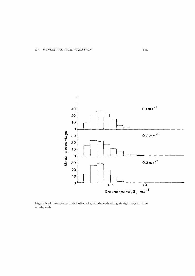
5.5. WINDSPEED COMPENSATION 115
Figure 5.24: Frequency distribution of groundspeeds along straight legs in threewindspeeds
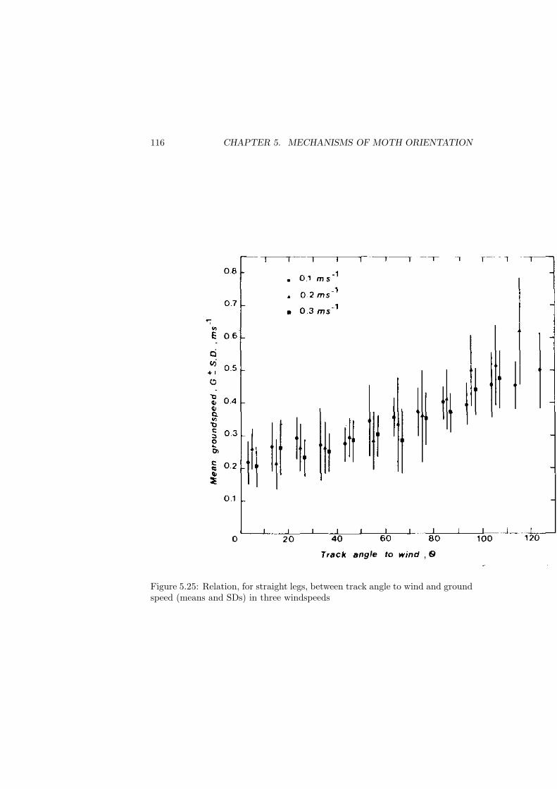
116 CHAPTER 5. MECHANISMS OF MOTH ORIENTATION
Figure 5.25: Relation, for straight legs, between track angle to wind and groundspeed (means and SDs) in three windspeeds
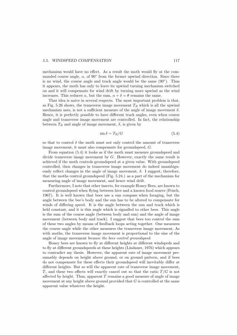
5.5. WINDSPEED COMPENSATION 117
mechanism would have no effect. As a result the moth would fly at the com-manded course angle, α, of 90◦ from the former upwind direction. Since thereis no wind, the course angle and track angle would be the same (90◦). Thusit appears, the moth has only to leave its upwind turning mechanism switchedon and it will compensate for wind drift by turning more upwind as the windincreases. This reduces α, but the sum, α + δ = θ remains the same.
That idea is naive in several respects. The most important problem is that,as Fig. 5.26 shows, the transverse image movement TR which is all the upwindmechanism uses, is not a sufficient measure of the angle of image movement δ.Hence, it is perfectly possible to have different track angles, even when courseangle and transverse image movement are controlled. In fact, the relationshipbetween TR and angle of image movement, δ, is given by
sin δ = TR/G (5.4)
so that to control δ the moth must not only control the amount of transverseimage movement, it must also compensate for groundspeed, G.
From equation (5.4) it looks as if the moth must measure groundspeed anddivide transverse image movement by G. However, exactly the same result isachieved if the moth controls groundspeed at a given value. With groundspeedcontrolled, then changes in transverse image movement do indeed unambigu-ously reflect changes in the angle of image movement, δ. I suggest, therefore,that the moths control groundspeed (Fig. 5.24.) as a part of the mechanism formeasuring angle of image movement, and hence wind drift.
Furthermore, I note that other insects, for example Honey Bees, are known tocontrol groundspeed when flying between hive and a known food source (Frisch,1967). It is well known that bees use a sun compass when foraging, but theangle between the bee’s body and the sun has to be altered to compensate forwinds of differing speed. It is the angle between the sun and track which isheld constant, and it is this angle which is signalled to other bees. This angleis the sum of the course angle (between body and sun) and the angle of imagemovement (between body and track). I suggest that bees too control the sumof these two angles by means of feedback loops acting together. One measuresthe course angle while the other measures the transverse image movement, Aswith moths, the transverse image movement is proportional to the sine of theangle of image movement because the bees control groundspeed.
Honey bees are known to fly at different heights at different windspeds andto fly at different groundspeeds at these heights (Lindauer, 1976) which appearsto contradict my thesis. However, the apparent rate of image movement pre-sumably depends on height above ground, or on ground pattern, and if beesdo not compensate for these effects their groundspeed will inevitably differ atdifferent heights. But so will the apparent rate of transverse image movement,T , and these two effects will exactly cancel out so that the ratio T/G is notaffected by height. Thus, apparent T remains a good measure of angle of imagemovement at any height above ground provided that G is controlled at the sameapparent value whatever the height.
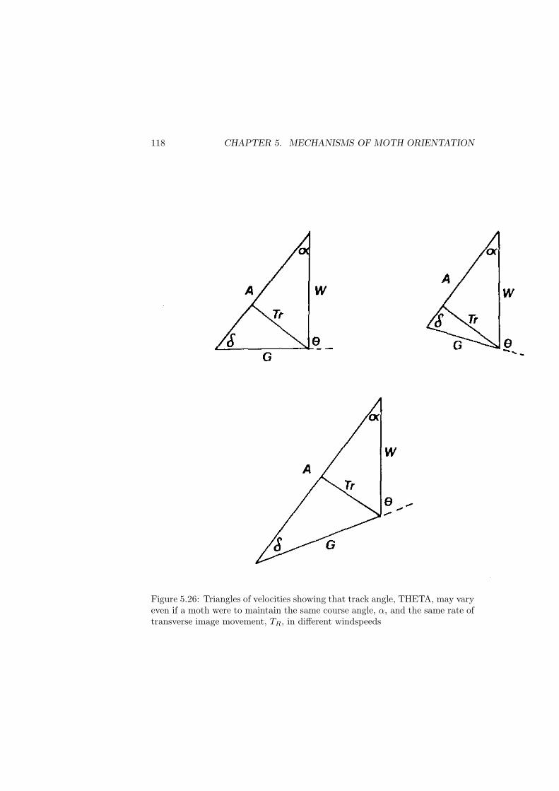
118 CHAPTER 5. MECHANISMS OF MOTH ORIENTATION
Figure 5.26: Triangles of velocities showing that track angle, THETA, may varyeven if a moth were to maintain the same course angle, α, and the same rate oftransverse image movement, TR, in different windspeeds
5.6. TOWARDS A MODEL OF MOTH ORIENTATION 119
If groundspeed control is indeed part of the mechanism of track-angle control,then one can see that groundspeed must be controlled at a speed which the insectcan maintain in the highest windspeeds it is likely to encounter. If the systemwere calibrated at too high a groundspeed, then moths could not cast accuratelyin high winds because they could not reach the calibrated groundspeed. Thus,a system which will work accurately over a large range of windspeeds must becalibrated for a low groundspeed. Honey bees may have overcome this problemneatly. Their system is calibrated at a high groundspeed, but when the wind istoo high for them to reach it, they fly lower, This not only brings them into aregion where the wind is slower, but it increases their apparent groundspeed sothat the system may be calibrated at a higher speed than they could actuallyreach in high winds. Conversely, they fly higher and faster in low winds, buttheir apparent groundspeed is the same. On grounds of efficiency alone onewould expect them to fly as low as possible in all windspeeds. This trick ofvarying height is not available to male moths which must remain at the heightof the pheromone plume, and hence must fly slowly, even in low windspeeds.
In summary, then, I propose that the moths turn upwind in the presenceof pheromone, using the upwind turning mechanism described in Table 5.1.Having identified the upwind direction they count the angle through which theyhave turned, either visually or kinaesthetically, and so maintain their orientationeven when the wind has dropped. A flier, however, has to contend with winddrift, and this is done by leaving the upwind turning mechanism switched onso that right to left image movement causes them to turn left (towards theupwind direction). They will not turn completely upwind, because the actualcourse angle is a compromise between the effects of the upwind mechanism andthe signal commanding a given course angle. Even that, apparently complexsystem is not enough to ensure that the track angle remains the same in differentwindspeeds. To ensure that, they must also maintain groundspeed at the valuefor which the system has been calibrated.
While that seems to be a complex and demanding hypothesis, it turns out,when one constructs a model, that a very simple system will suffice. What ismore, the simple system. although approximate, fits the data rather well. In thenext two sections I shall first construct a model, and then show how it explainsthe results obtained by Marsh, Kennedy and Ludlow.
5.6 Towards a model of moth orientation
As explained in the previous section, it is necessary to include groundspeed con-trol in a model of moth orientation because the moths appear to use groundspeedcontrol as part of their wind-compensating system. Even if they did not con-trol groundspeed, however, it would be necessary to include groundspeed in themodel because changes in groundspeed will inevitably affect the track angle,and similarly, the groundspeed will be altered as the insect turns more, or less,into the wind, making more, or less, headway against it. Such interactions area product of simple geometry; they result from the fact that groundspeed is one

120 CHAPTER 5. MECHANISMS OF MOTH ORIENTATION
of the sides in the triangle of velocities shown in Fig. 5.4. It is impossible for themoth to turn, altering the angle α, without disturbing the rest of the triangle.Either airspeed, or groundspeed, or track angle is bound to alter as the mothturns. However, there is a further way in which turning affects groundspeed.The moth uses the same effectors (its wings) to turn and to generate its thrust.It turns by making the output of the wings on either side unequal. It would takea sophisticated system to ensure that the sum of the thrusts remained the samewhatever their difference. For example, when discussing the upwind turningmechanism I postulated that right to left image movement reduced the thrustof the left wings. If we now propose (as in the last section) that the upwindturning mechanism is left on as part of the wind compensating system. then weshould predict that total wing-thrust will be reduced by this mechanism.
It is quite impossible to follow all of these interactions intuitively. Someform of computer simulation is essential to calculate predictions, or even to seeif the system works at all: does it actually maintain the same track angles ateach windspeed? The computer model is inevitably detailed, and all the author,or any reader, can do is to examine each bit of the program in turn and checkthat it embodies the theory correctly. It is impossible to keep all the issues inmind at once, but it is possible to check them one at a time. Once this has beendone, one relies on the computer to ensure that the interaction of these ideas isaccurately calculated.
In order to calculate groundspeed and track angle, which were the observeddata, the computer needs to know the moth’s airspeed and its course angle,together with the windspeed and direction. For present purposes the windspeedis held constant and the wind direction always comes from 0◦, so it is only theairspeed and course angle which change. These are the state variables and allother variables are calculated from the current airspeed and course, togetherwith numerous constants (the parameters).
To calculate the value of airspeed and course angle at any instant, the com-puter has to be supplied with the initial value of each measure, and equationsdefining the way airspeed and course angle change. The model of upwind turn-ing mechanism (Table 5.1) has already illustrated the way in which changes incourse angle, α can be defined. In that case, and again here, we shall beginby assuming that ALPHA’, the rate of change of ALPHA, is proportional to theTORQUE, after a definite delay, TORLAG. The TORQUE in turn, is proportional tothe difference between left and right wing-thrust. The task at present is to listthe factors that contribute to that difference. From the preceding discussion wepostulate that the difference between left and right wing-thrusts is due to threeterms:
1. the signal commanding a given course angle,
2. a feedback signal proportional to angle turned, and
3. a feedback signal proportional to transverse image movement
Combining the ideas in the upwind turning model (Table 5.1) with those in the
5.6. TOWARDS A MODEL OF MOTH ORIENTATION 121
model of Jander’s Compensation Theory (Table 5.2) we may quickly write aprovisional definition of left and right wing thrusts, Thus:
THRSTL = PL - ALPHAL - TR
THRSTR = PR - ALPHAr - TL
where PL and PR arc excitatory signals increasing wing-thrust. Their impor-tance, as in the Jander model (Table 5.2, lines II.c and II.d) is that the differencebetween them is, in effect, a command to turn. Thus if PL exceeds PR then themoth will tend to turn to the right. As it does so the signal ALPHAL will riseand ALPHAR will fall, because these are signals proportional to the angle turnedsince the moth last faced upwind. The important difference between ALPHAL
and the corresponding STIML (in Table 5.2) is that the latter varied with thesine of the angle turned, while ALPHAL goes on increasing even when the insectturns through more than 90◦, Thus if there is no wind, a difference between PL
and PR will cause the moth to turn. As it does so, ALPHAL and ALPHAR willchange, and the moth will stop turning when the differences exactly cancel out,i.e. PL - PR = ALPHAL - ALPHAR.
If there is a wind, the third terms, TR or TL. also operate. Only one willhave a positive value at any time because TR is positive when the insect is flyingto the
right of the upwind direction, while TL is zero. When the insect flies to theleft of the upwind direction, then TL is positive, while TR is zero. In either casethe signal will tend to oppose the command signal PL - PR so that the insectwill stop turning sooner than it would if only ALPHAL and ALPHAR had beenoperating.
Thus, if the moth is turning right because PL exceeds PR, then ALPHAL willrise (because both effort and angular velocity are greater on the left than theright sides when the insect is turning right). In addition, the transverse imagemovement will be from right to left (because the insect will be drifted to theright) hence TR will be positive. The insect will stop turning when these effectsmatch the difference between PL and PR. The reader is advised to check eachstatement in this paragraph against lines III.c and III.d of Table 5, because thatis the only way in which the computer model can be checked. Provided thereare no errors, then the above discussion can be forgotten; the computer will notforget.
The next step in checking the program (Table 5.5) is to ensure that TR andare properly calculated. This is simple trigonometry, and the justification oflines III.e and III.f is the same as that given above for lines I.e and I.f, exceptthat, here, I have introduced a term for the insects height above ground. Thatis necessary because the receptors measuring TR and TL may measure angularvelocity of image movement. If so, the values of TR and TL would be inverselyproportional to the insects height above ground.
Finally, lines III.g and III.h simply state that ALPHAL is proportional toALPHA’ Thus, ALPHAL rises when ALPHA rises and, by definition, that happenswhen the insect turns to the right. ALPHAR, on the otherhand, falls when ALPHA
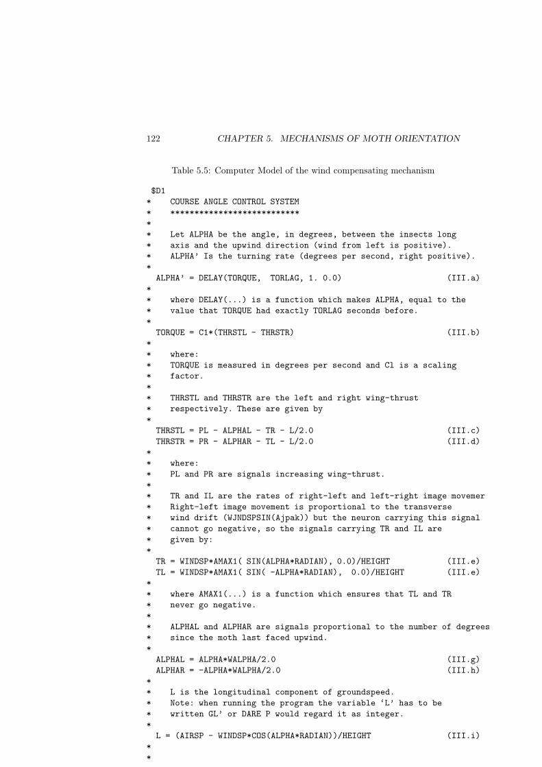
122 CHAPTER 5. MECHANISMS OF MOTH ORIENTATION
Table 5.5: Computer Model of the wind compensating mechanism
$D1
* COURSE ANGLE CONTROL SYSTEM
* ***************************
*
* Let ALPHA be the angle, in degrees, between the insects long
* axis and the upwind direction (wind from left is positive).
* ALPHA’ Is the turning rate (degrees per second, right positive).
*
ALPHA’ = DELAY(TORQUE, TORLAG, 1. 0.0) (III.a)
*
* where DELAY(...) is a function which makes ALPHA, equal to the
* value that TORQUE had exactly TORLAG seconds before.
*
TORQUE = C1*(THRSTL - THRSTR) (III.b)
*
* where:
* TORQUE is measured in degrees per second and Cl is a scaling
* factor.
*
* THRSTL and THRSTR are the left and right wing-thrust
* respectively. These are given by
*
THRSTL = PL - ALPHAL - TR - L/2.0 (III.c)
THRSTR = PR - ALPHAR - TL - L/2.0 (III.d)
*
* where:
* PL and PR are signals increasing wing-thrust.
*
* TR and IL are the rates of right-left and left-right image movemer
* Right-left image movement is proportional to the transverse
* wind drift (WJNDSPSIN(Ajpak)) but the neuron carrying this signal
* cannot go negative, so the signals carrying TR and IL are
* given by:
*
TR = WINDSP*AMAX1( SIN(ALPHA*RADIAN), 0.0)/HEIGHT (III.e)
TL = WINDSP*AMAX1( SIN( -ALPHA*RADIAN), 0.0)/HEIGHT (III.e)
*
* where AMAX1(...) is a function which ensures that TL and TR
* never go negative.
*
* ALPHAL and ALPHAR are signals proportional to the number of degrees
* since the moth last faced upwind.
*
ALPHAL = ALPHA*WALPHA/2.0 (III.g)
ALPHAR = -ALPHA*WALPHA/2.0 (III.h)
*
* L is the longitudinal component of groundspeed.
* Note: when running the program the variable ‘L’ has to be
* written GL’ or DARE P would regard it as integer.
*
L = (AIRSP - WINDSP*COS(ALPHA*RADIAN))/HEIGHT (III.i)
*
*
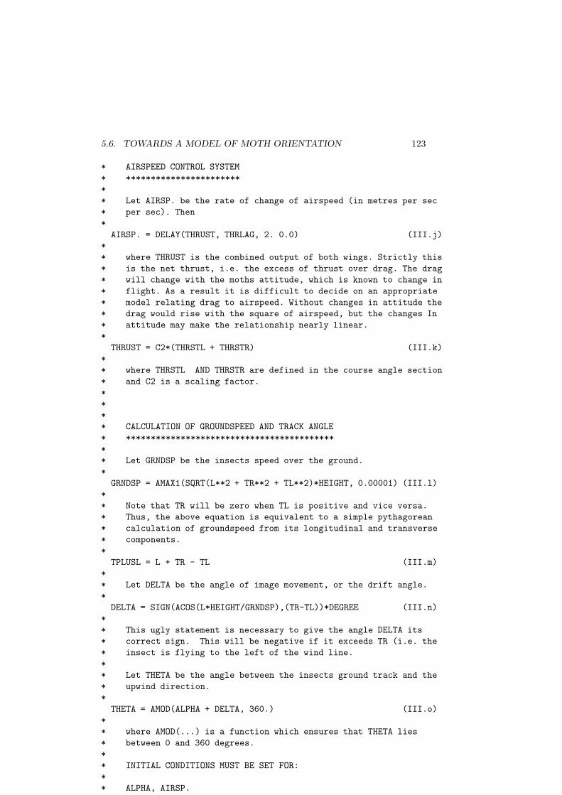
5.6. TOWARDS A MODEL OF MOTH ORIENTATION 123
* AIRSPEED CONTROL SYSTEM
* ***********************
*
* Let AIRSP. be the rate of change of airspeed (in metres per sec
* per sec). Then
*
AIRSP. = DELAY(THRUST, THRLAG, 2. 0.0) (III.j)
*
* where THRUST is the combined output of both wings. Strictly this
* is the net thrust, i.e. the excess of thrust over drag. The drag
* will change with the moths attitude, which is known to change in
* flight. As a result it is difficult to decide on an appropriate
* model relating drag to airspeed. Without changes in attitude the
* drag would rise with the square of airspeed, but the changes In
* attitude may make the relationship nearly linear.
*
THRUST = C2*(THRSTL + THRSTR) (III.k)
*
* where THRSTL AND THRSTR are defined in the course angle section
* and C2 is a scaling factor.
*
*
*
* CALCULATION OF GROUNDSPEED AND TRACK ANGLE
* ******************************************
*
* Let GRNDSP be the insects speed over the ground.
*
GRNDSP = AMAX1(SQRT(L**2 + TR**2 + TL**2)*HEIGHT, 0.00001) (III.l)
*
* Note that TR will be zero when TL is positive and vice versa.
* Thus, the above equation is equivalent to a simple pythagorean
* calculation of groundspeed from its longitudinal and transverse
* components.
*
TPLUSL = L + TR - TL (III.m)
*
* Let DELTA be the angle of image movement, or the drift angle.
*
DELTA = SIGN(ACOS(L*HEIGHT/GRNDSP),(TR-TL))*DEGREE (III.n)
*
* This ugly statement is necessary to give the angle DELTA its
* correct sign. This will be negative if it exceeds TR (i.e. the
* insect is flying to the left of the wind line.
*
* Let THETA be the angle between the insects ground track and the
* upwind direction.
*
THETA = AMOD(ALPHA + DELTA, 360.) (III.o)
*
* where AMOD(...) is a function which ensures that THETA lies
* between 0 and 360 degrees.
*
* INITIAL CONDITIONS MUST BE SET FOR:
*
* ALPHA, AIRSP.
*
124 CHAPTER 5. MECHANISMS OF MOTH ORIENTATION
rises, so the difference, ALPHAL - ALPHAR is proportional to ALPHA. To commanda given course angle, the difference PL - PR must be set at an appropriate value,and the insect will turn until ALPHAL - ALPHAR = PL - PR However, the termsPL and PR are also important in setting groundspeed (see below) so we are notat liberty to choose arbitrary values of PL - PR to specify a given angle. Thevalues of ALPHAL and ALPHAR must be appropriately weighted if they are not toconflict with the control of groundspeed, hence, the weighting constant WALPHAin lines III.g and III.h. Appropriate values for these weights will be discussedlater.
In discussing lines III.e and III.d, I have not mentioned the term L/2.0 whichappears in both lines. This term is part of the groundspeed control system and,because it affects both THRSTL and THRSTR equally, it has no effect on thedifference between them, and hence no effect on TORQUE.
Thus, the terms discussed above are the only ones to affect the moths courseangle, ALPHA, and together they comprise a differential equation for ALPHA’, therate of change of ALPHA.
The corresponding equation defining rate of change of airspeed is derived asfollows. Let AIRSP stand for airspeed, and let AIRSP’ stand for the rate of changeof airspeed. I begin by assuming that the rate of change of airspeed dependson total wing-thrust. The aerodynamics of flight are complicated and littleunderstood, Essentially, there are two forces controlling the insects airspeed:thrust and drag. If thrust exceeds drag, the insect will accelerate. If drag exceedsthrust, it will slow down. The complications arise because drag changes withthe insects airspeed. Hence, there is already a sort of feedback loop controllingairspeed: additional thrust brings diminishing returns. If the insect did not alterits flight attitude the drag would rise approximately with the square of airspeed.But insects do alter flight attitude (see David, 1978, for a discussion) and dragmay increase linearly with airspeed. Another complication is that extra thrustwould cause the insect to climb, unless it changed the direction of that thrust,Since Plodia fly at an even height when following a plume they must redirecttheir changing thrust.
In short, we are not even at first base in modelling the relationship betweenwing-thrust and airspeed, except to say that increasing thrust increases airspeed.There is no option, therefore, but to make a simple working assumption thatacceleration is proportional to total wing-thrust. There will be non-linearitiesin the actual relationship which we do not simulate, and there are further non-linearities in the neuronal signals which we suppose underlie this behaviour. Itis quite impossible to build them into the model at this stage. but the errors arenot likely to be serious, Nevertheless, the reader should be suitably sceptical.If moved to consider the matter further he is referred to David (1978) andto Thomas et al. (1977) to which I contributed a discussion of drag forces oninsects, and which contains references to the literature of drag coefficients.
Thus we begin with the naive assumption that acceleration, AIRSP’ , is pro-portional to total wing-thrust, THRUST, after a finite delay, THRLAG, (line III.j,Table 5). Used in that sense, THRUST is effectively the net thrust, in otherwords, the thrust less the drag. Thus, if net THRUST is positive, the insect will
5.6. TOWARDS A MODEL OF MOTH ORIENTATION 125
accelerate: if negative it will slow down. Obviously, the total THRUST = THRSTL
+ THRSTR (Line III.k, Table 5). Figure 5.24 shows that Plodia controlled theirgroundspeed, and I have argued above that this is part of their track-angle con-trol mechanism. What factors then, must affect total wing-thrust if the modelis to fly at a preset groundspeed? Clearly there must be:
1. an excitatory signal increasing wing-thrust and
2. a feedback signal proportional to groundspeed.
Examining lines III.c and III.d in Table 5 shows that there is already anexcitatory signal on each side, PL and PR respectively. As I have argued, thedifference between them is a command which determines the course angle, butthat in no way prevents their sum being the command that controls ground-speed. On the contrary, any excitatory signal is bound to increase wing thrust,and that is bound to cause some acceleration, so influencing airspeed and ulti-mately groundspeed.
Thus, all we need to do to complete the model is to specify the feedback fromgroundspeed. I have suggested earlier (Ludlow and Marsh, 1978) that insectsresolve movements of the ground pattern into longitudinal and transverse com-ponents, and the discussion of upwind turning (above) cites evidence supportingthat suggestion. If moths do indeed measure longitudinal and transverse com-ponents of groundspeed then, by Pythagoras, groundspeed may be calculatedfrom
G2 = L2 + T 2 (5.5)
where L is the longitudinal and T the transverse component of groundspeed G(seeFig 5.4). From this it appears that the moth would have to extract a squareroot to control groundspeed, but that is not necessary. It could control G2 or itcould even use an approximate mechanism and control the sum L + T. In thenext section I shall show that a model based on the approximate method, L +T, fits the data best, so the present model includes that idea, and the feedbacksignal is made equal to L + T. The point to emphasise here is that addingthis approximate mechanism to the model, as discussed so far, is astonishinglysimple. The turning mechanism already requires that the signals TR + TL affectwing thrust. Thus, if we wish to modify the model so that the feedback equals L+ T, all we have to do is subtract the term L from total wing-thrust. The exactimplementation of this idea has to be done carefully. The acceleration, or rateof change of airspeed is proportional to total THRUST, and that, in turn is equalto THRSTL + THRSTR. What we must now do is define THRSTL and THRSTR insuch a way that the acceleration is given by:
AIRSP′ = (PL + PR) − (TR + TL) − L (5.6)
The term (TR + TL) in equation (5.6) represents total transverse imagemovement (because TL will be zero when the insect is being drifted to the rightand TR is zero when it is being drifted to the left). Thus, (TR + TL) is equivalentto T, and we are trying to make the feedback equal to L + T. Since, TR and TL
126 CHAPTER 5. MECHANISMS OF MOTH ORIENTATION
are already built into the model, the only remaining problem is to distribute L
between the two wings so that L does not influence TORQUE. That, clearly meansthat we have to add L/2 to each side.
To summarise: The groundspeed control mechanism requires the followingdefinitions of wing thrust:
THRSTL = PL - TR - L/2.0
THRSTR = PR - TL - L/2.0
while, as stated above, the turning mechanism requires the definitions:
THRSTL = PL - ALPHAL - TR
THRSTR = PR - ALPHAR - TL
Combining these two requirements in the same model we get:
THRSTL = PL - ALPHAL - TR - L/2.0 (III.c)
THRSTR = PR - ALPHAR - TL - L/2.0 (III.d)
This combination poses no conflicts because L/2.0 affects both equally so doesnot affect TORQUE, while ALPHAL and ALPHAR have opposite signs and their sumis always zero. Hence ALPHAL + ALPHAR does not affect total wing-thrust.
The calculation of L (III.i, Table 5) is straightforward trigonometry, from thetriangle of velocities (Fig 5.4), except that I have included a term for HEIGHT
as with the calculation of TL and TR. These three terms (L, TL and TR) aretherefore represented in the model as apparent velocities. The true groundspeedis calculated from the apparent velocities (III,l, Table 5) using Pythagoras andthe insect’s height above ground.
The drift angle, DELTA, is also calculated using simple trigonometry (III.n)and true velocities.
Finally, the track angle, THETA, is calculated as the sum of ALPHA and DELTA
(III.o).The various issues discussed in constructing this model are each relatively
simple. Matters of elementary trigonometry, or simple ideas of the way theinsect combines internal and external signals. Taken together, however, theyseem to indicate a system of daunting complexity. One, perhaps, which couldnot possibly have evolved in real animals. Figure 5.27 is intended to showthat it is, on the contrary, an astonishingly simple system and that each of thecomponents postulated is already known to operate in other arthropod species.Figure 5.27 shows four movement detectors, front-back, back-front, right-left,and left-right. Receptors of these types have been found in Drosophila (Hausen,1982a,b), and similar receptors in the Hawk moth, Sphinx ligustri by Collettand Blest (1966). The difference between front-back and back-front detectors
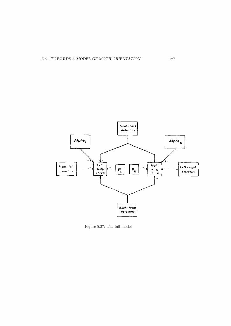
5.6. TOWARDS A MODEL OF MOTH ORIENTATION 127
Figure 5.27: The full model
128 CHAPTER 5. MECHANISMS OF MOTH ORIENTATION
provides a signal proportional to longitudinal image movement L, hence thefront-back detectors are shown inhibiting wing-thrust on each side, while theback-front ones are shown increasing it. Such connections are likely to haveevolved early in flight because controlled landing speeds are possible only if theinsect’s forward movement can be controlled.
The transverse detectors, responding to right-left and left-right image move-ment, are shown reducing wing-thrust on one side only (as in Fig. 5.3) and thusproviding a system which tends to make the insect turn upwind. Again, landingis simplified if the insect turns upwind, and such connections would have hadadvantages early in the evolution of flight.
Receptors signalling ALPHAL and ALPHAR could respond either to effort in-volved in turning, or to the velocity of image movement on the left and rightsides respectively. Both types of response are known in insects (Mittelstaedtet al., 1979; Wehner, 1981), The only special feature is that the effort (or front-back image movement) on either side must be integrated, so that the signalsrepresent the cumulative turns since last upwind, rather than the instantaneousvalues of effort or image movement. Such integration is known in other arthro-pods (op. cit.).
Finally the signals commanding increased thrust to each wing form, simul-taneously, the command for a given angle and the command for a given ground-speed. The difference in stimulation of the two sides determines the angle, thesum of stimulation determines the groundspeed.
One way of describing the system shown in Fig. 5.27 and Table 5.5, is to saythat it comprises not two, but three feedback systems which interfere with oneanother. One adjusts front-back image movement (the moths forward progressor headway). One responds to the degree of rotation, and tends to reducethat rotation (the ALPHAL, ALPHAR loop). Finally, one responds to sidewaystranslation (the transverse image movement loop). None of these alone, nor anypair, could steer the same track-angle in different windspeeds. Only when allthree are left switched on is the insect able to compensate accurately for winddrift.
Simulations of the model developed here will be described in the next sectionafter I have presented a re-analysis of the data collected by Marsh, Kennedyand Ludlow.
5.7 Tests of the model
Figure 5.24 shows that Plodia controlled groundspeed rather accurately in spiteof a threefold increase in windspeed. But in the model just described I have sug-gested that they control L + T, the sum of longitudinal and transverse ground-speed. To test this idea I have plotted L + T in Fig. 5.28, L alone in Fig 5.29and finally, L2 + T2 = G2 in Fig 5.30, On inspection, L shows some systematicchanges, but the others are very little affected by windspeed I therefore com-pared the distributions of L, L + T, G and G2 in the three windspeeds in thefollowing way. The mean value of each function was calculated for each moth

5.7. TESTS OF THE MODEL 129
Figure 5.28: Frequency distribution of the sum, L + T of longitudinal andtransverse cormponents of groundspeed (image movement) along straight legsin three windspeeds
at each windspeed. The means were then compared using a Friedman two-wayanalysis of variance. Since the Friedman test is not sensitive to the order ofthe three windspeeds. the highest and the lowest were also compared using aWilcoxon signed-ranks test. Probabilities are given in Table 5.6; L varies slightlyand the difference between L in the highest and lowest windspeed is significant,although the overall difference is not. Neither L + T, G nor G2 was significantlyaffected.
Whichever variable the moths were controlling should be the least affectedby windspeed. thus, it should have the smallest value of χ2
r. The smallest value
is 1.4, for L+T , and that is extremely close to the value of 1.39 which would beexpected if there was no effect of windspeed on L+T . The remaining functionsdo not fit as well, but none can be ruled out conclusively because they do notdiffer significantly in the three windspeeds. However, L + T gives a fairly goodapproximation to groundspeed, and if the moths were controlling this function
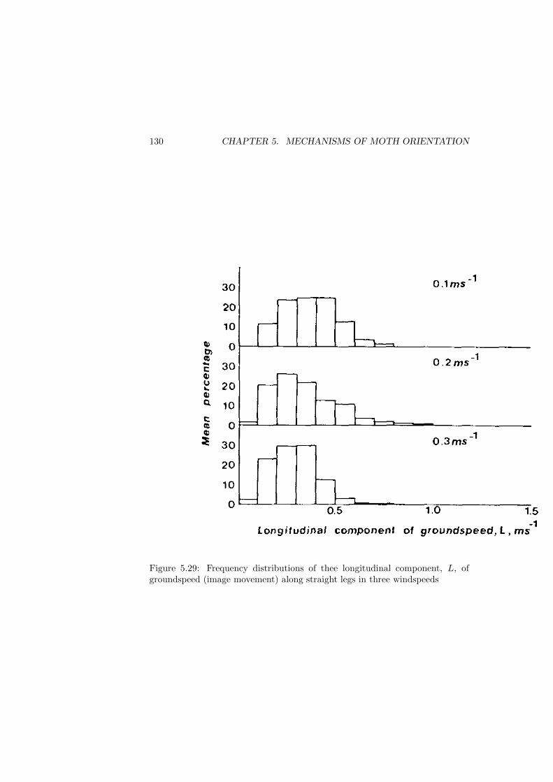
130 CHAPTER 5. MECHANISMS OF MOTH ORIENTATION
Figure 5.29: Frequency distributions of thee longitudinal component, L, ofgroundspeed (image movement) along straight legs in three windspeeds
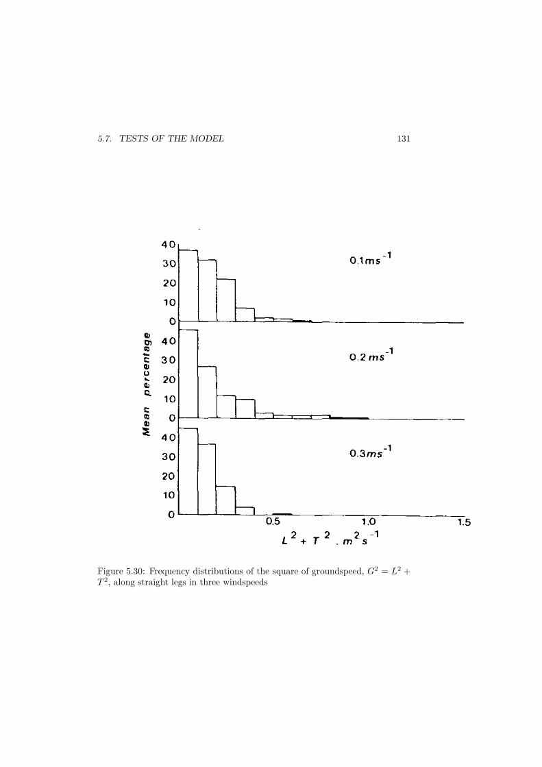
5.7. TESTS OF THE MODEL 131
Figure 5.30: Frequency distributions of the square of groundspeed, G2 = L2 +T 2, along straight legs in three windspeeds
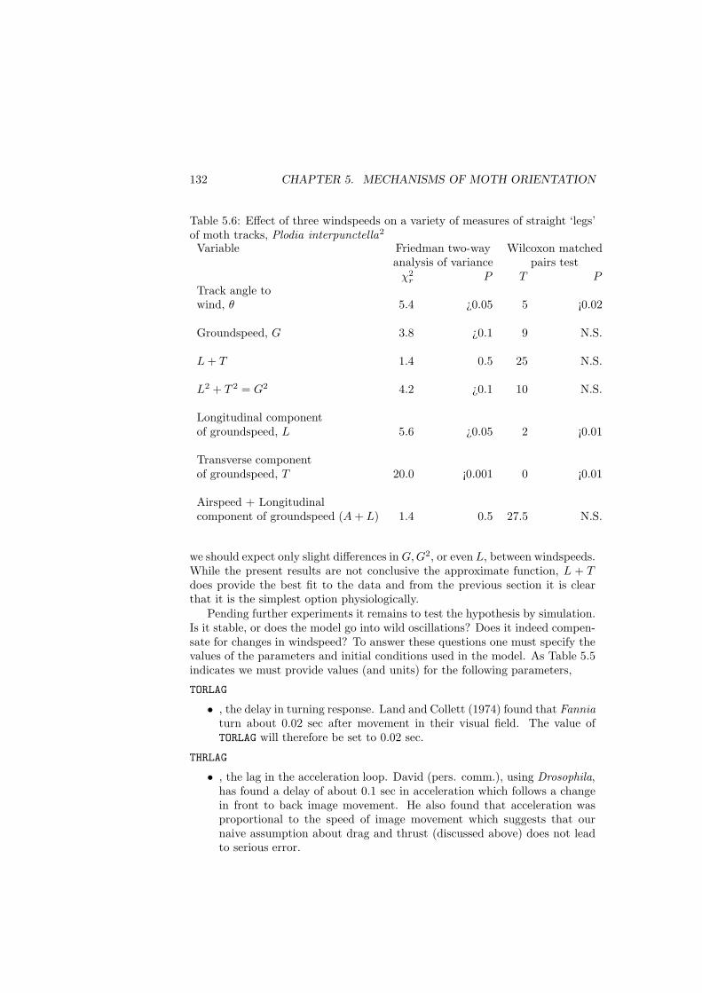
132 CHAPTER 5. MECHANISMS OF MOTH ORIENTATION
Table 5.6: Effect of three windspeeds on a variety of measures of straight ‘legs’of moth tracks, Plodia interpunctella2
Variable Friedman two-way Wilcoxon matchedanalysis of variance pairs test
χ2
rP T P
Track angle towind, θ 5.4 ¿0.05 5 ¡0.02
Groundspeed, G 3.8 ¿0.1 9 N.S.
L + T 1.4 0.5 25 N.S.
L2 + T 2 = G2 4.2 ¿0.1 10 N.S.
Longitudinal componentof groundspeed, L 5.6 ¿0.05 2 ¡0.01
Transverse componentof groundspeed, T 20.0 ¡0.001 0 ¡0.01
Airspeed + Longitudinalcomponent of groundspeed (A + L) 1.4 0.5 27.5 N.S.
we should expect only slight differences in G, G2, or even L, between windspeeds.While the present results are not conclusive the approximate function, L + Tdoes provide the best fit to the data and from the previous section it is clearthat it is the simplest option physiologically.
Pending further experiments it remains to test the hypothesis by simulation.Is it stable, or does the model go into wild oscillations? Does it indeed compen-sate for changes in windspeed? To answer these questions one must specify thevalues of the parameters and initial conditions used in the model. As Table 5.5indicates we must provide values (and units) for the following parameters,
TORLAG
• , the delay in turning response. Land and Collett (1974) found that Fanniaturn about 0.02 sec after movement in their visual field. The value ofTORLAG will therefore be set to 0.02 sec.
THRLAG
• , the lag in the acceleration loop. David (pers. comm.), using Drosophila,has found a delay of about 0.1 sec in acceleration which follows a changein front to back image movement. He also found that acceleration wasproportional to the speed of image movement which suggests that ournaive assumption about drag and thrust (discussed above) does not leadto serious error.
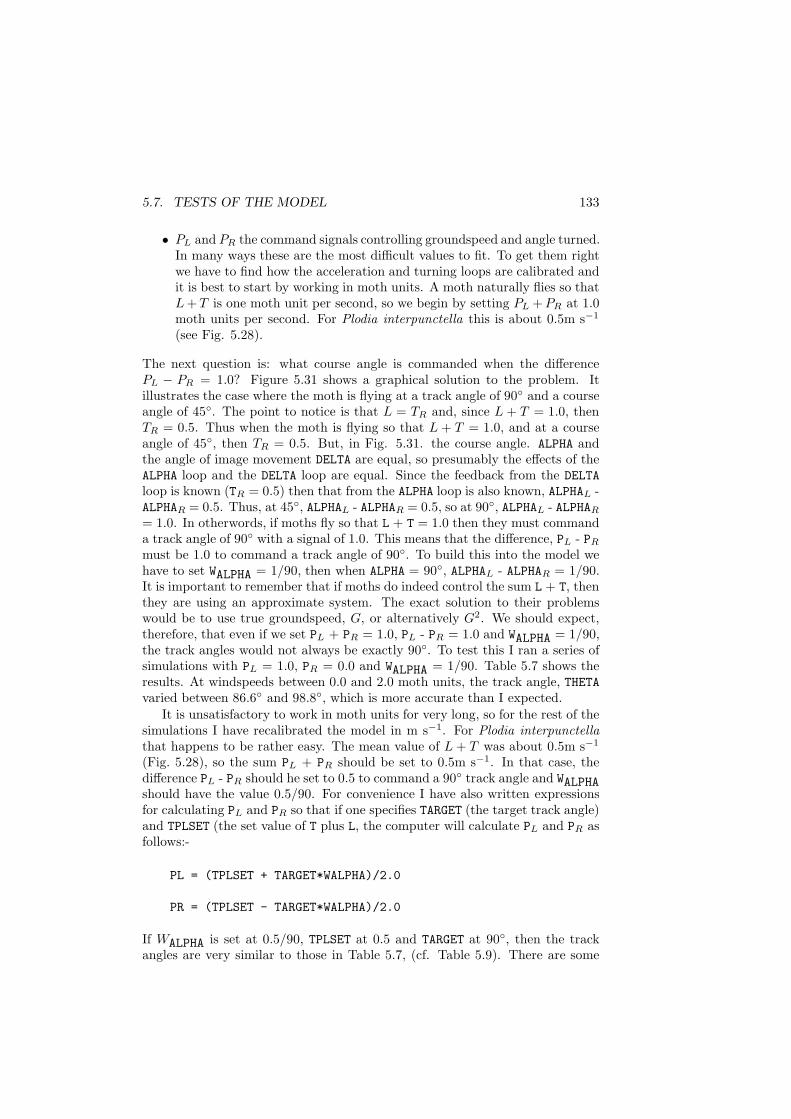
5.7. TESTS OF THE MODEL 133
• PL and PR the command signals controlling groundspeed and angle turned.In many ways these are the most difficult values to fit. To get them rightwe have to find how the acceleration and turning loops are calibrated andit is best to start by working in moth units. A moth naturally flies so thatL + T is one moth unit per second, so we begin by setting PL + PR at 1.0moth units per second. For Plodia interpunctella this is about 0.5m s−1
(see Fig. 5.28).
The next question is: what course angle is commanded when the differencePL − PR = 1.0? Figure 5.31 shows a graphical solution to the problem. Itillustrates the case where the moth is flying at a track angle of 90◦ and a courseangle of 45◦. The point to notice is that L = TR and, since L + T = 1.0, thenTR = 0.5. Thus when the moth is flying so that L + T = 1.0, and at a courseangle of 45◦, then TR = 0.5. But, in Fig. 5.31. the course angle. ALPHA andthe angle of image movement DELTA are equal, so presumably the effects of theALPHA loop and the DELTA loop are equal. Since the feedback from the DELTA
loop is known (TR = 0.5) then that from the ALPHA loop is also known, ALPHAL -ALPHAR = 0.5. Thus, at 45◦, ALPHAL - ALPHAR = 0.5, so at 90◦, ALPHAL - ALPHAR
= 1.0. In otherwords, if moths fly so that L + T = 1.0 then they must commanda track angle of 90◦ with a signal of 1.0. This means that the difference, PL - PR
must be 1.0 to command a track angle of 90◦. To build this into the model wehave to set WALPHA = 1/90, then when ALPHA = 90◦, ALPHAL - ALPHAR = 1/90.It is important to remember that if moths do indeed control the sum L + T, thenthey are using an approximate system. The exact solution to their problemswould be to use true groundspeed, G, or alternatively G2. We should expect,therefore, that even if we set PL + PR = 1.0, PL - PR = 1.0 and WALPHA = 1/90,the track angles would not always be exactly 90◦. To test this I ran a series ofsimulations with PL = 1.0, PR = 0.0 and WALPHA = 1/90. Table 5.7 shows theresults. At windspeeds between 0.0 and 2.0 moth units, the track angle, THETAvaried between 86.6◦ and 98.8◦, which is more accurate than I expected.
It is unsatisfactory to work in moth units for very long, so for the rest of thesimulations I have recalibrated the model in m s−1. For Plodia interpunctellathat happens to be rather easy. The mean value of L + T was about 0.5m s−1
(Fig. 5.28), so the sum PL + PR should be set to 0.5m s−1. In that case, thedifference PL - PR should he set to 0.5 to command a 90◦ track angle and WALPHAshould have the value 0.5/90. For convenience I have also written expressionsfor calculating PL and PR so that if one specifies TARGET (the target track angle)and TPLSET (the set value of T plus L, the computer will calculate PL and PR asfollows:-
PL = (TPLSET + TARGET*WALPHA)/2.0
PR = (TPLSET - TARGET*WALPHA)/2.0
If WALPHA is set at 0.5/90, TPLSET at 0.5 and TARGET at 90◦, then the trackangles are very similar to those in Table 5.7, (cf. Table 5.9). There are some
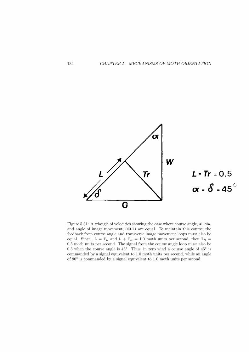
134 CHAPTER 5. MECHANISMS OF MOTH ORIENTATION
Figure 5.31: A triangle of velocities showing the case where course angle, ALPHA,and angle of image movement, DELTA are equal. To maintain this course, thefeedback from course angle and transverse image movement loops must also beequal. Since. L = TR and L + TR = 1.0 moth units per second, then TR =0.5 moth units per second. The signal from the course angle loop must also be0.5 when the course angle is 45◦. Thus, in zero wind a course angle of 45◦ iscommanded by a signal equivalent to 1.0 moth units per second, while an angleof 90◦ is commanded by a signal equivalent to 1.0 moth units per second
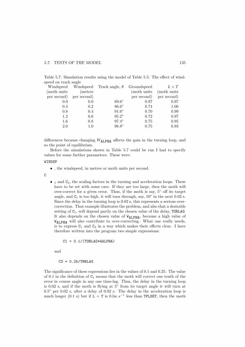
5.7. TESTS OF THE MODEL 135
Table 5.7: Simulation results using the model of Table 5.5: The effect of wind-speed on track angle
Windspeed Windspeed Track angle, θ Groundspeed L + T(moth units (metres (moth units (moth unitsper second) per second) per second) per second)
0.0 0.0 89.6◦ 0.97 0.970.4 0.2 86.6◦ 0.74 1.000.8 0.4 91.6◦ 0.70 0.991.2 0.6 95.2◦ 0.72 0.971.6 0.8 97.4◦ 0.75 0.952.0 1.0 98.8◦ 0.75 0.93
differences because changing WALPHA affects the gain in the turning loop, andso the point of equilibrium.
Before the simulations shown in Table 5.7 could be run I had to specifyvalues for some further parameters. These were:
WINDSP
• , the windspeed, in metres or moth units per second.
C
• 1 and C2, the scaling factors in the turning and acceleration loops. Thesehave to be set with some care. If they are too large, then the moth willover-correct for a given error. Thus, if the moth is say, 5◦ off its targetangle, and C1 is too high, it will turn through, say, 10◦ in the next 0.02 s.Since the delay in the turning loop is 0.02 s, this represents a serious over-correction. That example illustrates the problem, and also that a desirablesetting of C1, will depend partly on the chosen value of the delay, TORLAG.It also depends on the chosen value of WALPHA, because a high value ofWALPHA will also contribute to over-correcting. What one really needs,is to express C1 and C2 in a way which makes their effects clear. I havetherefore written into the program two simple expressions:
Cl = 0.1/(TORLAG*WALPHA)
and
C2 = 0.25/THRLAG
The significance of these expressions lies in the values of 0.1 and 0.25. The valueof 0.1 in the definition of C1 means that the moth will correct one tenth of theerror in course angle in any one time-lag. Thus, the delay in the turning loopis 0.02 s, and if the moth is flying at 5◦ from its target angle it will turn at0.5◦ per 0.02 s, after a delay of 0.02 s. The delay in the acceleration loop ismuch longer (0.1 s) but if L + T is 0.lm s−1 less than TPLSET, then the moth
136 CHAPTER 5. MECHANISMS OF MOTH ORIENTATION
will accelerate by 0.025m s−1 per 0.1 s, after a delay of 0.1 s. If, instead of0.1 and 0.25, I had written 1.0, in specifying C1 and C2, then each of the loopswould have over corrected. From this, one might imagine that the ideal valuewas close to 1.0, but it has to be much less than that because the two loopsinteract. As the model turns into the wind, L + T changes because the mothmakes less headway. The extent of such disturbances depends on windspeed,and in higher windspeeds they can be very destabilising. Thus, the gain in theL + T loop must be much less than 1.0 to ensure that ii is not too sensitive tothese disturbances as the model turns,
Until doing the simulations I had overlooked another factor affecting thegain. That is height. As the model gets close to the ground a small change inairspeed leads to a large change in the apparent values of L + T, and this toocan be destabilisingHEIGHT
, the insect’s height above ground. If the insect responds to the angular ve-locity of image movement, its estimate of L and T will be inversely proportionalto height. As it gets closer to the ground the ground pattern will appear tomove faster. If, on the otherhand, the insect measures the flicker frequency asit passes over a mottled ground pattern, or if it compensates in some way forheight, then its estimate of L and T will not be affected by changing height.The parameter HEIGHT is provided to simulate the effects of height changes onangular velocity.
Finally, one needs to define initial conditions for ALPHA and AIRSP. Table 5.8shows the parameters and initial conditions used to obtain the results shownin Table 5.7. The results of Table 5.7 demonstrate that the model proposedcan compensate for differences in windspeed over a wide range, and can modifyits course angle so that its track angle, THETA is close to 90◦, just as moths dowhen casting. However, it also suggests that the compensation is less accurate inwindspeeds of 1.0m s−1 (much higher than those used in the experiment). Table5.7 also demonstrates that the model controlled L + T , not true groundspeed,which leads to testable predictions of the model. Additional simulations wererun to answer the following questions.
I have argued above that the moth has to control groundspeed in order tocompensate for wind drift, and that the system has to be calibrated at oneparticular groundspeed. If that is so, then one must ask whether the model’sability to compensate for wind-drift is spoiled by changing the set value of L +T? Table 5.9 shows that it is. When the set value of L + T was doubled, to l.0ms−1 , the model over compensated for windspeed and flew at less than 90◦ inhigh windspeeds. Halving the value of L + T had the opposite effect, causing themodel to under-compensate for windspeed, so that it was drifted more downwindin high windspeeds. It flew at exactly 90◦ in zero wind, whatever the value of L+ T, because the drift angle, DELTA was zero in zero wind, and it is to measuresin(δ) that the groundspeed (or L + T ) must be controlled.
Given that L + T is maintained at the calibrated value, is the wind- compen-sation still accurate at target angles other than 90◦? To test this I set TARGET
to 30◦, 60◦and 120◦. The results are shown in Table 5.10, There was a slight
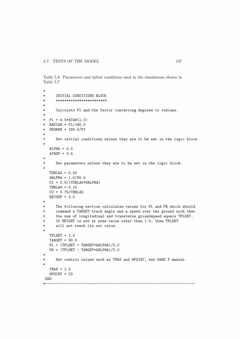
5.7. TESTS OF THE MODEL 137
Table 5.8: Parameters and initial conditions used in the simulations shown inTable 5.7
*
* INITIAL CONDITIONS BLOCK
* ************************
*
* Calculate PI and the factor converting degrees to radians.
*
* P1 = 4.0*ATAN(l.0)
* RADIAN = P1/180.0
* DEGREE = 180.0/PI
*
* Set initial conditions unless they are to be set in the logic block.
*
ALPHA = 0.0
AIRSP = 0.4
*
* Set parameters unless they are to be set in the logic block.
*
TORLAG = 0.02
WALPHA = 1.0/90.0
Cl = 0.5/(TORLAG*WALPHA)
THRLAG = 0.10
C2 = 0.75/THRLAG
HEIGHT = 3.0
*
* The following section calculates values for PL and PR which should
* command a TARGET track angle and a speed over the ground such that
* the sum of longitudinal and transverse groundspeed equals TPLSET.
* If HEIGHT is set at some value other than 1.0, then TPLSET
* will not reach its set value.
*
TPLSET = 1.0
TARGET = 90.0
PL = (TPLSET + TARGET*WALPHA)/2.0
PR = (TPLSET - TARGET*WALPHA)/2.0
*
* Set control values such as TMAX and NPOINT, see DARE P manual.
*
TMAX = 1.0
NPOINT = 23
END
*-----------------------------------------------------------------------
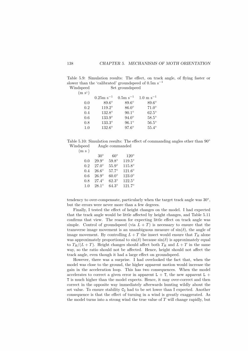
138 CHAPTER 5. MECHANISMS OF MOTH ORIENTATION
Table 5.9: Simulation results: The effect, on track angle, of flying faster orslower than the ‘calibrated’ groundspeed of 0.5m s−1
Windspeed Set groundspeed(m s1)
0.25m s−1 0.5m s−1 1.0 m s−1
0.0 89.6◦ 89.6◦ 89.6◦
0.2 119.2◦ 86.0◦ 71.0◦
0.4 132.8◦ 90.1◦ 62.5◦
0.6 133.9◦ 94.0◦ 58.5◦
0.8 133.3◦ 96.1◦ 56.5◦
1.0 132.6◦ 97.6◦ 55.4◦
Table 5.10: Simulation results: The effect of commanding angles other than 90◦
Windspeed Angle commanded(m s )
30◦ 60◦ 120◦
0.0 29.9◦ 59.8◦ 119.5◦
0.2 27.0◦ 55.9◦ 115.8◦
0.4 26.6◦ 57.7◦ 121.6◦
0.6 26.9◦ 60.0◦ 123.0◦
0.8 27.4◦ 62.3◦ 122.5◦
1.0 28.1◦ 64.3◦ 121.7◦
tendency to over-compensate, particularly when the target track angle was 30◦,but the errors were never more than a few degrees.
Finally, I tested the effect of height changes on the model. I had expectedthat the track angle would be little affected by height changes, and Table 5.11confirms that view. The reason for expecting little effect on track angle wassimple. Control of groundspeed (via L + T ) is necessary to ensure that thetransverse image movement is an unambiguous measure of sin(δ), the angle ofimage movement. By controlling L + T the insect would ensure that TR alonewas approximately proportional to sin(δ) because sin(δ) is approximately equalto TR/(L + T ). Height changes should affect both TR and L + T in the sameway, so the ratio should not be affected. Hence, height should not affect thetrack angle, even though it had a large effect on groundspeed.
However, there was a surprise. I had overlooked the fact that, when themodel was close to the ground, the higher apparent motion would increase thegain in the acceleration loop. This has two consequences. When the modelaccelerates to correct a given error in apparent L + T, the new apparent L +T is much higher than the model expects. Hence, it may over-correct and thencorrect in the opposite way immediately afterwards hunting wildly about theset value. To ensure stability C2 had to be set lower than I expected. Anotherconsequence is that the effect of turning in a wind is greatly exaggerated. Asthe model turns into a strong wind the true value of T will change rapidly, but
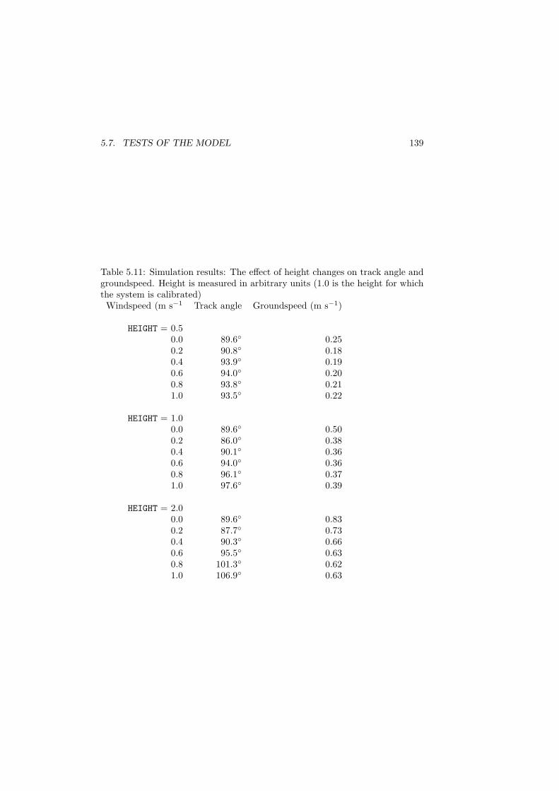
5.7. TESTS OF THE MODEL 139
Table 5.11: Simulation results: The effect of height changes on track angle andgroundspeed. Height is measured in arbitrary units (1.0 is the height for whichthe system is calibrated)Windspeed (m s−1 Track angle Groundspeed (m s−1)
HEIGHT = 0.50.0 89.6◦ 0.250.2 90.8◦ 0.180.4 93.9◦ 0.190.6 94.0◦ 0.200.8 93.8◦ 0.211.0 93.5◦ 0.22
HEIGHT = 1.00.0 89.6◦ 0.500.2 86.0◦ 0.380.4 90.1◦ 0.360.6 94.0◦ 0.360.8 96.1◦ 0.371.0 97.6◦ 0.39
HEIGHT = 2.00.0 89.6◦ 0.830.2 87.7◦ 0.730.4 90.3◦ 0.660.6 95.5◦ 0.630.8 101.3◦ 0.621.0 106.9◦ 0.63

140 CHAPTER 5. MECHANISMS OF MOTH ORIENTATION
if it is close to the ground the change in apparent T will be even more dramaticand can lead to wild instability, so that C1 had to be set low. It may be someconsolation to moths that windspeeds are at their lowest close to the ground.
In conclusion: the model provides an unambiguous theory of wind com-pensation in moths. It explains satisfactorily how they might command theobserved track-angles, ranging from 0◦ to rather over 90◦ from the upwind di-rection. Moreover, it suggests that groundspeed control is a necessary part ofthe mechanism of track angle control. Since the value of groundspeed for whichthe system is calibrated, must be one which the insect can reach in high winds,the theory explains the enigma that moths fly rather slowly in a race to thefemale. The widespread occurence of groundspeed control in other insects sug-gests that they may use similar means of wind compen5ation. However, themodel is not perfect. It could be made more realistic in a number of ways. Asingle delay parameter has been used in the turning loop, whereas there areprobably several, There is a delay due to the moths inertia, so that it actuallyturns some time after the change in thrust. Before that, however, there aredelays in the various neural pathways, and these delays may differ in differentpathways. In particular, the measurement of rotation of the visual field maybe much faster than the measurement of transverse image movement. The gainin the loops (C1 and C2) have been chosen arbitrarily, these could be estimatedmore reliably. A further area for improvement is in the aerodynamics of dragand thrust. But most important of all, the model does not explain the observedrelationship between groundspeed and track angle shown in Fig. 5.25. It wouldnot be difficult to explain this relationship. It can be simulated readily by in-creasing the sum of PL + PR whenever the difference between them is increasedto command a higher track angle. However, that is an ad hoc explanation and,as Popper has argued, we should make ad hoc assumptions with caution.
5.8 Summary
Even in turbulent conditions, individual parcels of air travel in straight lines forquite long distances. Thus, the wind direction at the time an animal detectsan odour gives a much more accurate estimate of the source direction thanpreviously realised. Animals of many species may have evolved strategies takingadvantage of this fact; for example, the wet noses of numerous mammal speciesmay allow them to fix the direction of prey or predators at a distance.
Some male moths fly upwind on detecting the sex pheromone emitted by a fe-male. However this is not the only component of their strategy—their crosswindmovement is also modulated by pheromone. It is best to think of pheromoneas arresting crosswind movement, so that the males make narrow side to sidemovements in the presence of pheromone, but cast widely across wind when theylose it. On finding it again their crosswind movement is once again arrested sothat they are unlikely to lose the plume until the wind direction changes. Thisarresting affect of pheromone appears to be incompatible with the old idea ofchemotaxis because, on that hypothesis, one would expect a moth to turn sooner
5.8. SUMMARY 141
on losing pheromone; in fact they turn later, so making long casts across wind.Baker and Kuenen (1982) have demonstrated a third component of the
moths strategy: that moth’s can orient to the former wind direction duringlulls. Finally, we have demonstrated that increases of pheromone concentrationare needed to promote upwind flight, which requirement probably prevents amale from flying past nearby females in pursuit of the large numbers furtherupwind.
These four components of the moths strategy provide an exceptionally effi-cient guidance system, but the mechanisms by which an insect can fly up, oracross wind, pose questions at a different level of study, and the bulk of thechapter has been adressed to theoretical aspects of these questions. The prob-lem of flying upwind is relatively trivial and can be solved by turning to theright if transverse image movement is from left to right, and vice versa, Thisworks in winds of any strength.
Steering across winds of differing strength, on the otherhand. is an achieve-ment of awesome complexity. The upwind turning system would turn harderupwind in high windspeeds, and so provide an element of compensation forwindspeed, but that alone is not enough. Transverse image movement is not asufficient measure of drift angle (the angular deviation due to wind drift). Tomeasure drift angle completely, and so to compensate for wind drift, the mothmust measure some well defined function of drift angle, such as its sine (trans-verse image movement/groundspeed). One solution would be for the moth tomeasure, or better still control, its groundspeed so that transverse image move-ment alone is always proportional to the sine of the drift angle. It is extremelyinteresting to note, therefore, that moths, and indeed many other insects doindeed control groundspeed. Indeed, it is something of an enigma that malemoths racing to a female should race so slowly. The model proposed here wouldresolve that enigma because it assumes that a moth casting across wind con-tinues to respond to transverse image movement, as when turning upwind, butthat it also controls groundspeed at some precalibrated value. Since the systemmust be calibrated so that it operates in high winds, the calibrated ground-speed cannot be too high, and so the moth flies more slowly than it could inlow windspeeds.
Even that is not enough to steer at 90◦ to the wind, as moths do whencasting. In addition they must measure the course angle. the angle betweentheir long axis and the wind direction. To compensate for wind drift the mothmust reduce the course angle by just the amount that the wind increases thedrift angle. One way of doing this is to control the sum of the two angles. Inzero wind the drift angle will be zero, so the sum will be entirely due to thecourse angle. As the wind increases, the sum remains the same, but the courseangle is reduced as the drift angle rises.
Measuring the course angle raises all sorts of problems. Perhaps the simplestmethod would be for the moth to fix the wind direction as it turns upwind.The upwind direction can be judged because there will be no transverse imagemovement when the moth is facing upwind. Following this the moth could countthe angle through which it has turned since last upwind. Many arthropods are
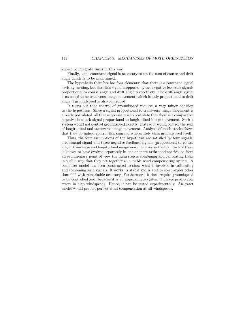
142 CHAPTER 5. MECHANISMS OF MOTH ORIENTATION
known to integrate turns in this way.Finally, some command signal is necessary to set the sum of course and drift
angle which is to be maintained.The hypothesis therefore has four elements: that there is a command signal
exciting turning, but that this signal is opposed by two negative feedback signalsproportional to course angle and drift angle respectively. The drift angle signalis assumed to be transverse image movement, which is only proportional to driftangle if groundspeed is also controlled.
It turns out that control of groundspeed requires a very minor additionto the hypothesis. Since a signal proportional to transverse image movement isalready postulated, all that is necessary is to postulate that there is a comparablenegative feedback signal proportional to longitudinal image movement. Such asystem would not control groundspeed exactly. Instead it would control the sumof longitudinal and transverse image movement. Analysis of moth tracks showsthat they do indeed control this sum more accurately than groundspeed itself.
Thus, the four assumptions of the hypothesis are satisfied by four signals:a command signal and three negative feedback signals (proportional to courseangle. transverse and longitudinal image movement respectively). Each of theseis known to have evolved separately in one or more arthropod species, so froman evolutionary point of view the main step is combining and calibrating themin such a way that they act together as a stable wind compensating system. Acomputer model has been constructed to show what is involved in calibratingand combining such signals. It works, is stable and is able to steer angles otherthan 90◦ with remarkable accuracy. Furthermore, it does require groundspeedto be controlled and, because it is an approximate system it makes predictableerrors in high windspeeds. Hence, it can be tested experimentally. An exactmodel would predict perfect wind compensation at all windspeeds.
Chapter 6
Postscript
These two studies have raised inumerable questions far more in fact than Ihave had space to discuss. Most of the questions omitted concern models orideas rejected at an early stage. Perhaps these silent witnesses are the bestjustification for the work, because they would, if listed, demonstrate how manypossibilities can be rejected on theoretical grounds alone, thus saving time inexpensive experiments. They could not have been rejected unless they hadpreviously been defined in quantitative terms. Such a list would be unreadable.but I hope that enough cases remain, for example, the disinhibition hypothesis ofvan Iersel and Bol (1958) contains inconsistencies which had not been recognisedbefore. Similarly, the problems of compass theories were not appreciated.
These and other examples have convinced me that the chief benefits of mod-elling occur long before any predictions can be tested experimentally. Indeed,the result of a modelling exercise is often to say “it ain’t necessarily so” to somewidely propogated theory. This may be a passing phase. For the moment stu-dents of behaviour work with a legacy of loosely defined hypotheses and until weinsist that all our ideas go through consistency testing this legacy will remainunchecked,
Thus, there is a very great deal of theoretical analysis to be done, and I hopeI have demonstrated that it is a discipline in its own right, demanding as muchpatience and care as experimental hypothesis testing. Demanding too, perhaps,a particular sort of mind. There is a danger, however, that students of behaviourwill divide into ‘modellers’ and ‘non-modellers’. Modelling must therefore bepresented in a way that is intelligible to workers of all levels of mathematicalability. Up to now that has not happened. One way in which a bridge might bebuilt is by using programming languages that are easily understood. The DARE P
programs in Tables 5.1. 5.2 and 5.5 represent first attempts in this directionand, while they may not be completely successful, they contrast favourably withthe long FORTRAN program of the model animal (see Appendix A). The next stepin this direction would seem to be to develop a way of combining large amountsof experimental information and a number of alternative models in some sortof computer based library. Work on this is already proceeding. particularly in
143

144 CHAPTER 6. POSTSCRIPT
Holland and although it is at an early stage, it would seem to be a particularlywelcome development.
Bibliography
J.H. Andreae. Thinking with a teachable machine. Academic Press, London,1972. 3.6
J.W. Atkinson and D. Birch. The dynamics of action. John Wiley, New York,1970. 3.2
R.R. Baker and J.G. Mather. Magnetic compass sense in the large yellow un-derwing moth, noctua pronuba l. Animal Behaviour, 30:543–548, 1982. 5.3
T.C. Baker and L.P.S. Kuenen. Pheromone source location by flyin moths: asupplementary non-anemotactic mechanism. Science, 216:424–427, 1982. 5.1,5.3, 5.4, 5.8
F.H. Barnwell. An angle sense in the orientation of a millipede. BiologicalBulletin, 128:33–50, 1965. 5.3
I.L. Beale and D.M. Webster. The relevance of leg-movement cues to turnalternation in woodlice (porcellio scaber). Animal Behaviour, 19:353–356,1971. 5.3, 5.4
W.J. Bell and T.R. Tobin. Chemo-orientation. Biological Review, 57:219–260,1982. 5.2
P. Benjamin and R.M. Rose. Interneuronal circuitry underlying cyclical feedingin gastropod molluscs. TINS, 3:272–274, 1980. 3.6, 4.3
W.I.B. Beveridge. The art of scientific investigation. Heinemann EducationalBooks, London, 1970. 1.2
L.G. Bishop and D.G. Keehn. Neural correlates of the optomotor response inthe fly. Kybernetik, 3:288–295, 1967. 5.2
L.G. Bishop, D.G. Keehn, and D.G. McCann. Motion detection by interneuronsof optic lobes and brain of the flies calliphora phoenicia and musca domestica.Journal of Neurophysiol, 3:509–525, 1968. 5.2
D.A. Booth, F.M. Toates, and S.V. Platt. Control system for hunger and itsimplications in animals and man. In D. Novin, W. Wyrwicka, and G.A. Bray,editors, Hunger, pages 127–142. Raven, New York, 1976. 2.3, 1
145
146 BIBLIOGRAPHY
T.H. Bullock. In search of principles in neural integration. In J.C. Fentress,editor, Simpler networks and behaviour, pages 52–60. Sinauer Associates Inc.,Sunderland, Massachusetts, 1976. 3.6
P.S. Callahan. Tuning into Nature, Solar Energy, Infra-red radiation and theinsect communication system. Routledge and Kegen Paul, London and Henley,1977. 5.1
J.M. Camhi. Locust wind receptors. i. transducer mechanics and sensory re-sponses. Journal of Experimental Biology, 50:335–348, 1969. 5.2
R.T. Carde and T.E. Hagaman. Behavioural responses of the gypsy moth in awind tunnel to air-borne emanations of dispalure. Environmental Entomology,8:475–484, 1979. 5.1
T.C. Chamberlain. The method of multiple working hypotheses. Journal ofGeology, 5:837–848, 1897. 1.2
N. Chomsky. Syntactic Structures. Mouton, The Hague, 1957. 3.6
I.B. Cohen. Newton’s discovery of gravity. Scientific American, 244:167–179,1981. 1.2
S. Cohen and D.J. McFarland. Time-sharing as a mechanism for the controlof behaviour sequences during the courtship of the three-spined stickleback(gasterosteus aculeatus). Animal Behaviour, 27:270–283, 1979. 4.1
T.S. Collett and A.D. Blest. Binocular, directionally selective neurones, possiblyinvolved in the optomotor response of insects. Nature (London), 212:1330–1333, 1966. 5.2, 5.2, 5.6
C.T. David. The relationship between body angle and flight speed in free-flyingdrosophila. Physiological Entomology, 3:191–195, 1978. 5.6
C.T. David, J.S. Kennedy, and A.R. Ludlow. Finding of a sex pheromone sourceby gypsy moths released in the field. Nature, Lond., 303:804–806, 1983. 5.1,5.2, 5.1
C.T. David, J.S. Kennedy, A.R. Ludlow, J.N. Perry, and C. Wall. A reappraisalof insect flight towards a distant point source of wind-borne odor. Journal ofChemical Ecology, 8:1207–1215, 1982. 5.1, 5.1, 5.1
M. Dawkins and R. Dawkins. Some descriptive and explanatory stochasticmodels of decision-making. In D.J. McFarland, editor, Motivational controlsystems analysis, pages 119–168. Academic Press, London, 1974. 1.2
D.R. Dvorak, L.G. Bishop, and H.E. Eckert. On the identification of movementdetectors in the fly optic lobe. Journal of Comparative Physiology, 100:5–24,1975. 5.2
BIBLIOGRAPHY 147
J.T. Fitzsimons and J. LeMagnen. Eating as a regulatory control of drinkingin the rat. Journal of Comparative and Physiological Psychology, 67:273–283,1969. 4.1, 4.2, 4.3
G. Fraenkel. Die mechanik der orientierung der tiere im raum. Biological Review,6:36–87, 1931. 5.2
G. Fraenkel. Die wanderungen der insekten. Ergebn. Biol., 9:1–238, 1932. 5.2
W.O. Friesen and G.S. Stent. Neural circuits for generating rhythmic move-ments. Annual Review of Biophysics and Bioengineering, 7:37–61, 1978. 3.6
K. von. Frisch. The Dance language and Orientation of Bees. Oxford UniversityPress, London, 1967. 5.5
M. Gewecke. The antennae of insects as air-current sense organs and theirrelationship to the control of flight. In L. Burton-Browne, editor, Experimentalanalysis of insect behaviour, pages 100–113. Springer-Verlag, Berlin, 1974. 5.2
P. Gorner. Resultant positioning between optical and kinesthetic orientationin the spider agelena labyrinthica (clerk). In R. Wehner, editor, Informationprocessing in the visual system of the arthropods, pages 269–274. Springer-Verlag, Berlin, 1972. 5.4
K. Hausen. Motion sensitive interneurones in the optomotor system of the flyI. The horizontal cells: structure and signals. Biological Cybernetics, 45:143–156, 1982a. 5.2, 5.2, 5.6
K. Hausen. Motion sensitive interneurons in the optomotor system of the fly. II.The horizontal cells: receptive field organisation and response characteristics.Biological Cybernetics, 46:67–79, 1982b. 5.2, 5.2, 5.6
R.A. Hinde. The nest-building behaviour of domesticated canaries. Proceedingsof the Zoological Society of London, 131:1–48, 1958. 4.1
R.A. Hinde. Animal Behaviour. A synthesis of Ethology and Comparative Psy-chology. McGraw Hill, New York, 2nd edn. edition, 1970. 2.2
R.A. Hinde. Ethology. Oxford University Press/Fontatana Paperback, London,1982. 4.1
A Houston. Time sharing. Animal Behaviour, 30:???, 1982. 4.1
D.H. Hubel and T.N. Wiesel. Receptive fields, binocular interaction and func-tional architecture in the cats visual cortex. Journal of Physiology, (London),160:106–154, 1962. 3.6
D.H. Hubel and T.N. Wiesel. Receptive fields and functional architecture in thenon-striate visual areas (18 and 19) of the cat. Journal of Neurophysiology,18:229–289, 1965. 3.6
148 BIBLIOGRAPHY
R. Jander. Insect orientation. Annual Review of Entomology, 8:95–114, 1963.5.3
M.H. Joseph, C.D. Frith, and J.L. Waddington. Dopaminergic mechanisms andcognitive deficit in schizophrenia. Psychopharmacology, 63:273–280, 1979.2.1, 3.6, 4.3
W. Kaiser and L.G. Bishop. Directionally selective motion detecting units inthe optic lobes of the honeybee. Z. vergl. Physiol., 67:403–413, 1970. 5.2
F.E. Kellogg, D.E. Frizel, and R.H. Wright. The olfactory guidance of flyinginsects. Canadian Entomoloy, 94:884–888, 1962. 5.1, 5.2, 5.3
J.S. Kennedy. The visual responses of flying mosquitoes. Proceedings of theZoological Society of London, 109:221–242, 1940. 5.2, 5.2
J.S. Kennedy. The migraion of the desert locust (schistocerca gregaria forsk.).Philosophical Transactions of the Royal Society, 235:163–290, 1951. 5.2
J.S. Kennedy, A.R. Ludlow, and C.J. Sanders. Guidance system used in mothsex attraction. Nature, Lond., 288:475–477, 1980. 5.1
J.S. Kennedy, A.R. Ludlow, and C.J. Sanders. Guidance of flying male mothsby wind-borne sex pheromone. Physiological Entomology, 6:395–412, 1981.5.1
J.S. Kennedy and D. Marsh. Pheromone-regulated anemotaxis in flying moths.Science, 184:999–1001, 1974. 5.1
U. Kling and G. Szekely. Simulation of rhythmic nervous activities. i. functionof networks with cyclic inhibitions. Kybernetik, 5:89–103, 1968. 3.6
J. Konorski. Integrative Activity of the brain. University of Chicago Press,Chicago, 1967. 3.6
E.R. Laithwaite. A radiation theory of the assembling of moths. Entomologist,93:113–117; 133–137, 1960. 5.1
M.F. Land and T.S. Collett. Chasing behaviour of house flies, (fannia canicu-laris). Journal of Comparative Physiology, 89:331–357, 1974. 5.2, 5.7
S. Larkin and McFarland. D. The cost of changing from one activity to another.Animal Behaviour, 26:1237–1246, 1978. 4.1
M. Lindauer. Foraging and homing flight of the honey-bee: some general prob-lems of orientation. In R.C. Rainey, editor, Insect Flight, pages 199–216.Blackwell, Oxford, 1976. 5.5
K.E. Linsenmair. Anemotactic orientation in beetles and scorpions. In S.R.Galler, K. Schimdt-Koenig, G.K. Jacobs, and R.E. Belleville, editors, Ani-mal Orientation and Navigation. NASA Scientific and Technical Informationoffice, Washington, D.C., 1972. 5.2, 5.3
BIBLIOGRAPHY 149
A.R. Ludlow. The behaviour of a model animal. Behaviour, 58:131–172, 1976.2.2, 2.5, 2.3, 4.1
A.R. Ludlow. The importance of temporal coupling between feeding and drink-ing — simulations prompted by Toates’paper. Behavioural and Brain Sci-ences, 2:110–111, 1979. 3.3
A.R. Ludlow. The evolution and simulation of a decision maker. In F.M. Toatesand T.R. Halliday, editors, Analysis of motivational processes, pages 273–296.Academic Press, 1980. 1.2, 2.2, 2.5, 2.4, 3.5, 3.6, 3.6, 3.8, 4.1
A.R. Ludlow. Towards a theory of thresholds. Animal Behaviour, 30:253–267,1982. 2.2, 2.5, 3.2, 3.3, 4.1, 4.2, 1
A.R. Ludlow and D. Marsh. Mechanisms of moth orientation. Presentation atSEB meeting, Reading University, 1978. 5.2, 5.6
E.P. Lyon. On rheotropism: I. rheotropism in fishes. American Journal ofPhysiology, 12:49–16, 1904. 5.2
Mittelstaedt-Burger M-L. Idiothetic course control and visual orientation. InR. Wehner, editor, Information processing in the visual system of arthropods,pages 275–279. Springer, Berlin, 1972. 5.3
A. Manning. An introduction to animal behaviour. Edward Arnold, London,2nd edition, 1972. 1.1
D.M. Marsh, J.S. Kennedy, and A.R. Ludlow. Anemotactic zigzagging flight inmale moths stimulated by pheromone. Physiological Entomology, 3:221–240,1978. 5.1, 5.1, 5.2, 5.3, 5.10, 5.3, 5.5
D.M. Marsh, J.S. Kennedy, and A.R. Ludlow. Analysis of zigzagging flight inmoths: a correction. Physiological Entomology, 6:225, 1981. 5.1, 5.1, 5.3
D. Maynard. Simpler networks. Annals of New York Academy of Sciences, 193:59–72, 1972. 3.6
R.H. McCleery. On satiation curves. Animal Behaviour, 25:1005–1015, 1977.1.2
W. McDougall. The nature of inhibitory processes within the nervous system.Brain, 26:153–191, 1903. 2.1, 4.1
D.J. McFarland. Feedback mechanisms in animal behaviour. Academic Press,London, 1971. 4.1
D.J. McFarland. Experimental investigation of motivational state. In D.J. Mc-Farland, editor, Motivational control systems analysis, pages 251–282. Aca-demic Press, London, 1974. 4.1, 4.1

150 BIBLIOGRAPHY
D.J. McFarland and I.H. Lloyd. Time-shared feeding and drinking. QuarterlyJournal of Experimental Psychology, 25:48–61, 1973. 2.6, 4.1, 4.3
D.J. McFarland and R.M. Sibly. The behavioural final common path. Philo-sophical Transactions of Royal Society, 270:265–293, 1975. 3.2
N.W. Milgram, L. Krames, and R. Thompson. Influence of drinking history onfood deprived drinking in the rat. Journal of Comparative and PhyiologicalPsychology, 87:126–133, 1974. 3.3
H. Mittelstaedt. Probleme der kursregelung bei freibeweglichen tieren. In Auf-nahme und Verarbetung von Nachrichten durch Organismen, pages 138–148.Hirzel-Verlag, Stuttgart, 1961. 5.3
H. Mittelstaedt. Control systems of orientation in insects. Annual Review ofEntomology, 7:177–198, 1962. 5.3, 5.3
H. Mittelstaedt. Basic solutions to a problem of angular orientation. In R.F.Reiss, editor, Neural Theory and Modelling, pages 259–272. University Press,Stanford, 1964. 5.3
H. Mittelstaedt and M-L. Mittelstaedt. Mechanisms der orientierung ohne rich-tende aussenreize. Forstschr. Zool., 21:46–58, 1973. 5.3
M-L. Mittelstaedt, H. Mittelstaedt, and W. Mohren. Interaction of gravity andidiothetic course control in millipedes. Journal of Comparative Physiology,133:267–281, 1979. 5.3, 5.4, 5.6
K. Oatley. Perceptions and Representations. Methuen, London, 1978. 3.6
J.R. Platt. Strong inference. Science, 146:347–353, 1964. 1.2
K.. Popper. The logic of scientific discovery. Hutchinson, London, 1972. 1.2
R.F. Reiss. A theory and simulation of rhythmic behaviour due to recipro-cal inhibitions in small nerve nets. In Proceedings Spring Joint ComputerConference 21, pages 171–194, 1962. 2.1, 4.1
Bartell. R.J. Mechanisms of communication disruption by pheromone in thecontrol of lepidoptera: a review. Physiological Entomology, 7:353–364, 1982.5.1
K.D. Roeder. Episodes in insect brains. Am. Scient., 58:378–389, 1970. 3.6
W. Schulz. Die orientierung des ruckenschwimmers zum licht und zur stromung.Z. vergl. Physiol., 14:392–404, 1931. 5.2
I. Schwinck. A study of olfactory stimuli in the orientation of moths. In Proceed-ings of 10th International Congress of Entomology, Montreal 1956, volume 2,pages 577–582, 1958. 5.2
BIBLIOGRAPHY 151
T. Shallice. Dual functions of consciousness. Psychol. Rev., 79:383–393, 1972.3.6
C. Sherrington. The Integrative Action of the Nervous System. Charles Scrib-ner’s Sons, New York, 1906. 2.1
R.M. Sibly. The use of mathematical models to describe behavioural sequencesand to study their physiology and survival value. In F.M. Toates and T.R.Haliday, editors, Analysis of motivational processes, pages 245–271. AcademicPress, 1980. 1.2
R.M. Sibly and R.H. McCleery. The dominance boundary method of determin-ing motivational state. Animal Behaviour, 24:108–124, 1976. 4.1
J.D. Sinclair. A theory of behaviour, based on “rest principle” control of thestrength of neural connections. Neurosci. Biobehav., 2:357–366, 1978. 2.5,3.4
R.S. Sutton and A.G. Barto. Towards a modern theory of adaptive networks:expectation and prediction. Psychol. Rev., 88:135–170, 1981. 3.6
A.A.G. Thomas, A.R. Ludlow, and J.S. Kennedy. Sinking speeds of falling andflying aphis fabae Scopoli. Ecological Entomology, 2:315–326, 1977. 5.6
N. Tinbergen. The Study of Instinct. Clarendon Press, Oxford, 1951. 2.2
F.M. Toates. Control theory in biology and experimental psychology. Hutchinson,London, 1975. 1.2
F.M. Toates. Homeostasis and drinking. Behav. brain, Sci., 2:95–102, 1979a.2.2, 1
F.M. Toates. Water and energy in the interaction of thirst and hunger. InK. Brown and S.J. Cooper, editors, Chemical Influences on Behaviour, pages135–200. Academic Press, London, 1979b. 2.3, 1
F.M. Toates and K. Oatley. Computer simulation of thirst and water balance.Med. biol. Engng., 8:71–87, 1970. 2.3, 1, 4.3
A.M. Uttley. A two-pathway informon theory of conditioning and adaptivepattern recognition. Brain Res, 102:23–35, 1976. 3.4
J.J. van Iersel and A.C.A. Bol. Preening of two tern species. a study of dis-placement activities. Behaviour, 13:1–88, 1958. 1.2, 3.5, 4.3, 6
R.E. Walley and T.D. Weiden. Lateral inhibition and cognitive masking: a neu-rophysiological theory of attention. Psychological Review, 80:284–302, 1973.3.6
R. Wehner. Spatial vision in arthropods. In H. Autrum, editor, Handbookof sensory physiology, Vol. VII/6C, pages 287–616. Springer-Verlag, Berlin,1981. 5.6
152 BIBLIOGRAPHY
T. Weiss-Fogh. An aerodynamic sense organ stimulating and regulating flightin locusts. Nature (London), 164:873–874, 1949. 5.2
T. Weiss-Fogh. An aerodynamic sense organ in locusts. In Proc. 8th Int. Cong.Ent. (Stockholm, 1948), pages 584–588. 1950. 5.2
P. Wiepkema. Behaviour changes in cba mice as a result of one goldthioglucoseinjection. Behaviour, 32:179–210, 1968. 4.1
R.H. Wright. The olfactory guidance of flying insects. Canadian Entomology,90:81–89, 1958. 5.1