Applications of coupled mode theory to microcavities with

Kerr nonlinearities

Roman Shugayev

April 30, 2014

1 Introduction

Optical frequency comb formation is a very powerful technology, in which optical signals are gen-erated at pre-determined frequency intervals with precisely controlled amplitudes and phases [1].Optical frequency combs have a number of important current and potential applications, includ-ing precision metrology for improved GPS [2, 3], pulse shaping [4], terahertz spectroscopy andsensing, RF modulation [4], quantum photonics [5] and high-harmonic generation for extendedUV (XUV) sources for lithography. Typically, optical combs are generated by using a pulsedfemtosecond laser. However, such a solution tends to be relatively bulky and expensive. Withadvances in fabrication techniques, optical frequency combs have been recently fabricated on-chip- a milestone in ultrafast optics, allowing integration and size reduction of the overall system.With a bandwidth of at least an octave (frequencies from ω to 2ω), coherent combs can be inter-locked to span a very broad spectrum, enabling the full range of applications mentioned above.However, experimental microresonator combs typically experience too much incoherence for fullspectral control at this time. Several theories have been proposed to explain the generation ofcoherent and incoherent combs, including multilevel comb growth [6] , modulation instability [7],and deterministic chaos [8, 9].

Photonic microresonator frequency combs amenable to on-chip fabrication at small scaleshave recently attracted significant attention; they enable novel features, including in particularvery large (hundreds of GHz or above) free spectral range, increased flexibility in dispersionmatching, and especially very high field intensities compared to macroscopic resonators [10,11].For four-wave mixing processes, a 1000-fold increase in intensity associated with photonic modeconfinement can increase signal and idler generation by a factor of 1,000,000 or more [11].

There have been several theoretical microresonator frequency comb studies performed re-cently using various approaches such as Lugiato-Lefever (L-L) equation [12, 13] and nonlinearSchrodinger equation [7]. These methods can provide excellent agreement with the experi-ment [18] on structures that can be approximated as stright waveguides. However they maylead to inaccuracies for small-scale devices such as small radius microresonators and photoniccrystals. Additionaly the use of these methods will not be appropriate for multimode-familyananlysis where sub-FSR mode spacing is required. Alternatively, coupled mode theory (CMT)[14–17] circumvents described obstacles and has been extensively used to model nonlinear pro-cesses in microcavities. However a one-to-one match between realistic microring comb formationprocesses and coupled mode theory parameters has not yet been directly demonstrated. In orderto study the comb formation in the regime approaching experimental systems we implemented ahybrid CMT / FDTD method. In this approach the key degrees of freedom are modeled through

1

coupled mode theory with parameters such as mode profiles, mode frequencies and quality factorscalculated in finite-difference time-domain (FDTD) simulations.

2 Theory

We can derive the equations of motion for Kerr nonlinear coupled mode theory as follows. Webegin with the well-known electromagnetic field Hamiltonian:

H =1

2

∫dr

[εE(r)2 +

1

µB(r)2

](1)

In the presence of a Kerr medium, we can generally write the refractive index as follows:

ε(r) = εo(r) + ε2|E(r)|2 (2)

Substituting this expression in yields:

H =1

2

∫dr[εo(r) + ε2|E(r)|2

] [E(r)2 +

1

µεB(r)2

](3)

We can assume that we can represent electric field in the single mode k in terms of quadratureoperators

Ek(r) = Ck · gk(r)(ak + a†k) (4)

where ak is the annihilation operator, a†k is the creation operator and gk(r) is the normalizedamplitude function. Ck is normalization constant.

By normalizing Equation 3 to h̄ωk it can be shown that

Ck =

√h̄ωk

2∫ε0(r)gk(r)

2dr

(5)

By substituting Equation 4 into Equation 1 we can obtain corresponding coupled mode theoryequations:

H =∑k

h̄ωk(a†kak +1

2)+h̄2ε2

8

∑i,j,k,l

√ωiωjωkωlMijkla

†ia†jakale

i(ωk+ωl−ωi−ωj)t (6)

where

Mijkl =

∫gi(r)gj(r)gk(r)gl(r)dr[∫

ε0(r)gi(r)2dr]1/2[∫

ε0(r)gj(r)2dr]1/2[∫

ε0(r)gk(r)2dr]1/2[∫

ε0(r)gl(r)2dr]1/2 (7)

3 Numerical Methods

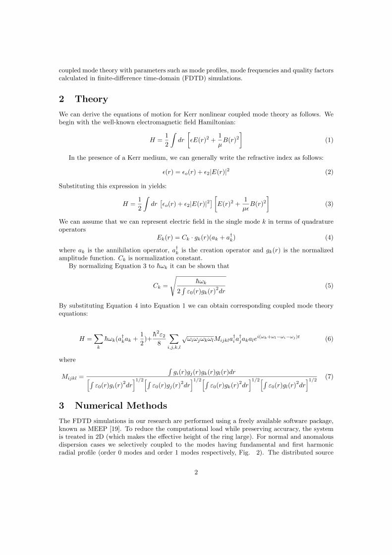
The FDTD simulations in our research are performed using a freely available software package,known as MEEP [19]. To reduce the computational load while preserving accuracy, the systemis treated in 2D (which makes the effective height of the ring large). For normal and anomalousdispersion cases we selectively coupled to the modes having fundamental and first harmonicradial profile (order 0 modes and order 1 modes respectively, Fig. 2). The distributed source

2

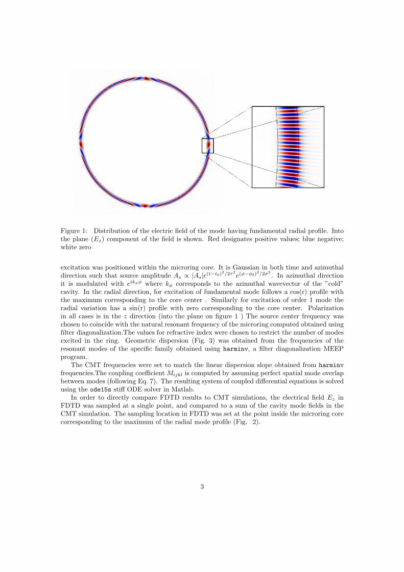
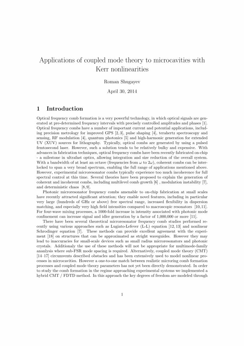
Figure 1: Distribution of the electric field of the mode having fundamental radial profile. Intothe plane (Ez) component of the field is shown. Red designates positive values; blue negative;white zero

excitation was positioned within the microring core. It is Gaussian in both time and azimuthaldirection such that source amplitude As ∝ |As|e(t−t0)

2/2τ2

e(φ−φ0)2/2σ2

. In azimuthal directionit is modulated with eikφφ where kφ corresponds to the azimuthal wavevector of the ”cold”cavity. In the radial direction, for excitation of fundamental mode follows a cos(r) profile withthe maximum corresponding to the core center . Similarly for excitation of order 1 mode theradial variation has a sin(r) profile with zero corresponding to the core center. Polarizationin all cases is in the z direction (into the plane on figure 1 ) The source center frequency waschosen to coincide with the natural resonant frequency of the microring computed obtained usingfilter diagonalization.The values for refractive index were chosen to restrict the number of modesexcited in the ring. Geometric dispersion (Fig. 3) was obtained from the frequencies of theresonant modes of the specific family obtained using harminv, a filter diagonalization MEEPprogram.

The CMT frequencies were set to match the linear dispersion slope obtained from harminv

frequencies.The coupling coefficient Mijkl is computed by assuming perfect spatial mode overlapbetween modes (following Eq. 7). The resulting system of coupled differential equations is solvedusing the ode15s stiff ODE solver in Matlab.

In order to directly compare FDTD results to CMT simulations, the electrical field Ez inFDTD was sampled at a single point, and compared to a sum of the cavity mode fields in theCMT simulation. The sampling location in FDTD was set at the point inside the microring corecorresponding to the maximum of the radial mode profile (Fig. 2).

3

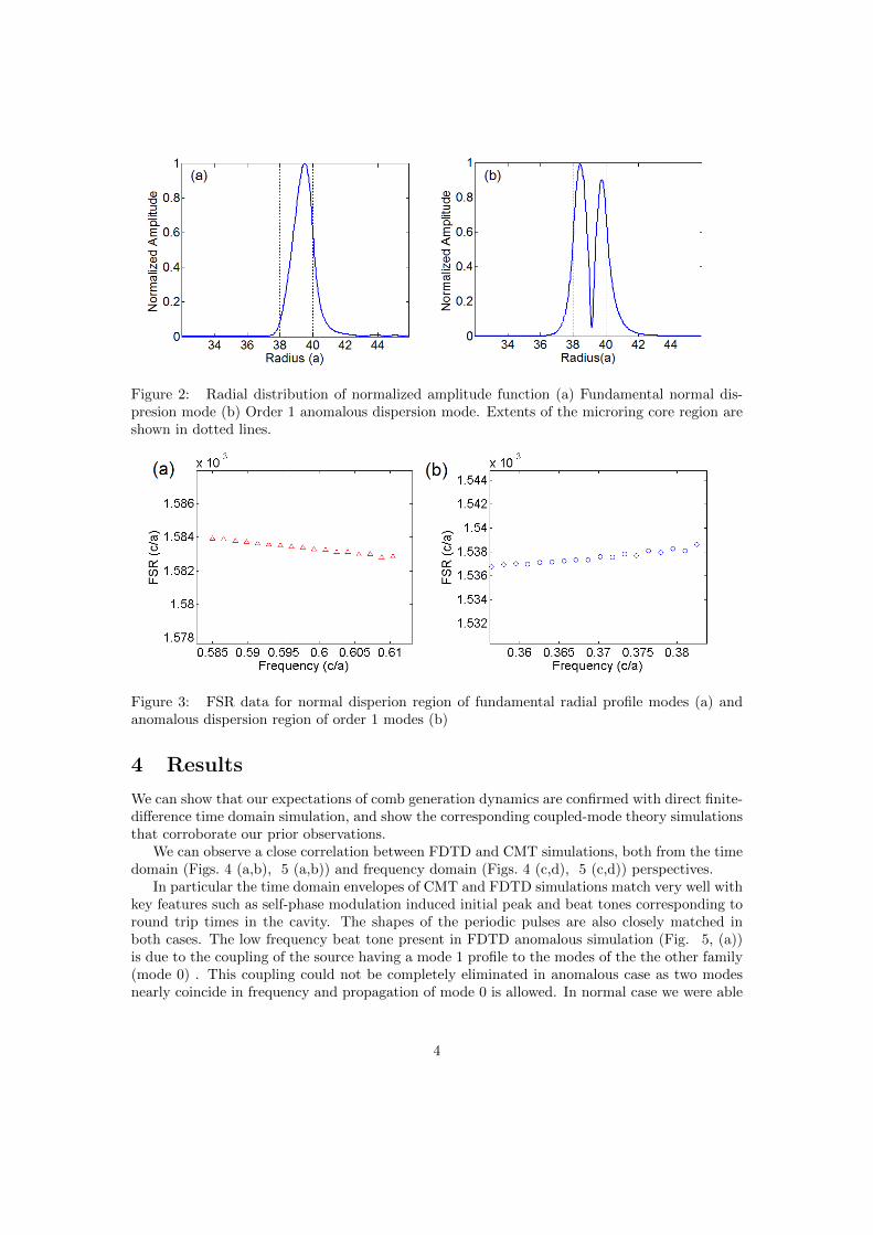
Figure 2: Radial distribution of normalized amplitude function (a) Fundamental normal dis-presion mode (b) Order 1 anomalous dispersion mode. Extents of the microring core region areshown in dotted lines.

Figure 3: FSR data for normal disperion region of fundamental radial profile modes (a) andanomalous dispersion region of order 1 modes (b)

4 Results

We can show that our expectations of comb generation dynamics are confirmed with direct finite-difference time domain simulation, and show the corresponding coupled-mode theory simulationsthat corroborate our prior observations.

We can observe a close correlation between FDTD and CMT simulations, both from the timedomain (Figs. 4 (a,b), 5 (a,b)) and frequency domain (Figs. 4 (c,d), 5 (c,d)) perspectives.

In particular the time domain envelopes of CMT and FDTD simulations match very well withkey features such as self-phase modulation induced initial peak and beat tones corresponding toround trip times in the cavity. The shapes of the periodic pulses are also closely matched inboth cases. The low frequency beat tone present in FDTD anomalous simulation (Fig. 5, (a))is due to the coupling of the source having a mode 1 profile to the modes of the the other family(mode 0) . This coupling could not be completely eliminated in anomalous case as two modesnearly coincide in frequency and propagation of mode 0 is allowed. In normal case we were able

4

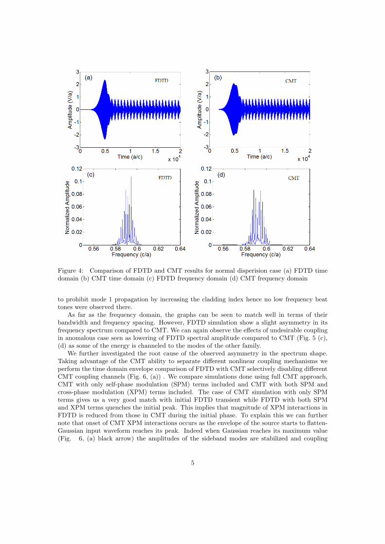
Figure 4: Comparison of FDTD and CMT results for normal disperision case (a) FDTD timedomain (b) CMT time domain (c) FDTD frequency domain (d) CMT frequency domain

to prohibit mode 1 propagation by increasing the cladding index hence no low frequency beattones were observed there.

As far as the frequency domain, the graphs can be seen to match well in terms of theirbandwidth and frequency spacing. However, FDTD simulation show a slight asymmetry in itsfrequency spectrum compared to CMT. We can again observe the effects of undesirable couplingin anomalous case seen as lowering of FDTD spectral amplitude compared to CMT (Fig. 5 (c),(d) as some of the energy is channeled to the modes of the other family.

We further investigated the root cause of the observed asymmetry in the spectrum shape.Taking advantage of the CMT ability to separate different nonlinear coupling mechanisms weperform the time domain envelope comparison of FDTD with CMT selectively disabling differentCMT coupling channels (Fig. 6, (a)) . We compare simulations done using full CMT approach,CMT with only self-phase modulation (SPM) terms included and CMT with both SPM andcross-phase modulation (XPM) terms included. The case of CMT simulation with only SPMterms gives us a very good match with initial FDTD transient while FDTD with both SPMand XPM terms quenches the initial peak. This implies that magnitude of XPM interactions inFDTD is reduced from those in CMT during the initial phase. To explain this we can furthernote that onset of CMT XPM interactions occurs as the envelope of the source starts to flatten-Gaussian input waveform reaches its peak. Indeed when Gaussian reaches its maximum value(Fig. 6, (a) black arrow) the amplitudes of the sideband modes are stabilized and coupling

5

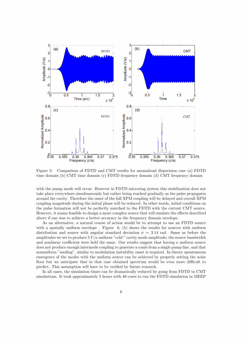
Figure 5: Comparison of FDTD and CMT results for anomalousl disperision case (a) FDTDtime domain (b) CMT time domain (c) FDTD frequency domain (d) CMT frequency domain

with the pump mode will occur. However in FDTD microring system this stabilization does nottake place everywhere simultaneously but rather being reached gradually as the pulse propagatesaround the cavity. Therefore the onset of the full XPM coupling will be delayed and overall XPMcoupling magnitude during the initial phase will be reduced. In other words, initial conditions onthe pulse formation will not be perfectly matched to the FDTD with the current CMT source.However, it seams feasible to design a more complex source that will emulate the effects describedabove if one was to achieve a better accuracy in the frequency domain envelope.

As an alternative, a natural course of action would be to attempt to use an FDTD sourcewith a spatially uniform envelope . Figure 6, (b) shows the results for sources with uniformdistribution and source with angular standard deviation σ = 3.14 rad. Same as before theamplitudes we set to produce 5 V/a uniform ”cold ” cavity mode amplitude; the source bandwidthand nonlinear coefficient were held the same. Our results suggest that having a uniform sourcedoes not produce enough intermode coupling to generate a comb from a single pump line, and thatnonuniform ”seeding”, similar to modulation instability onset is required. In theory spontaneousemergence of the modes with the uniform source can be achieved by properly setting the noisefloor but we anticipate that in that case obtained spectrum would be even more difficult topredict. This assumption will have to be verified by future research.

In all cases, the simulation times can be dramatically reduced by going from FDTD to CMTsimulations. It took approximately 5 hours with 48 cores to run the FDTD simulation in MEEP

6

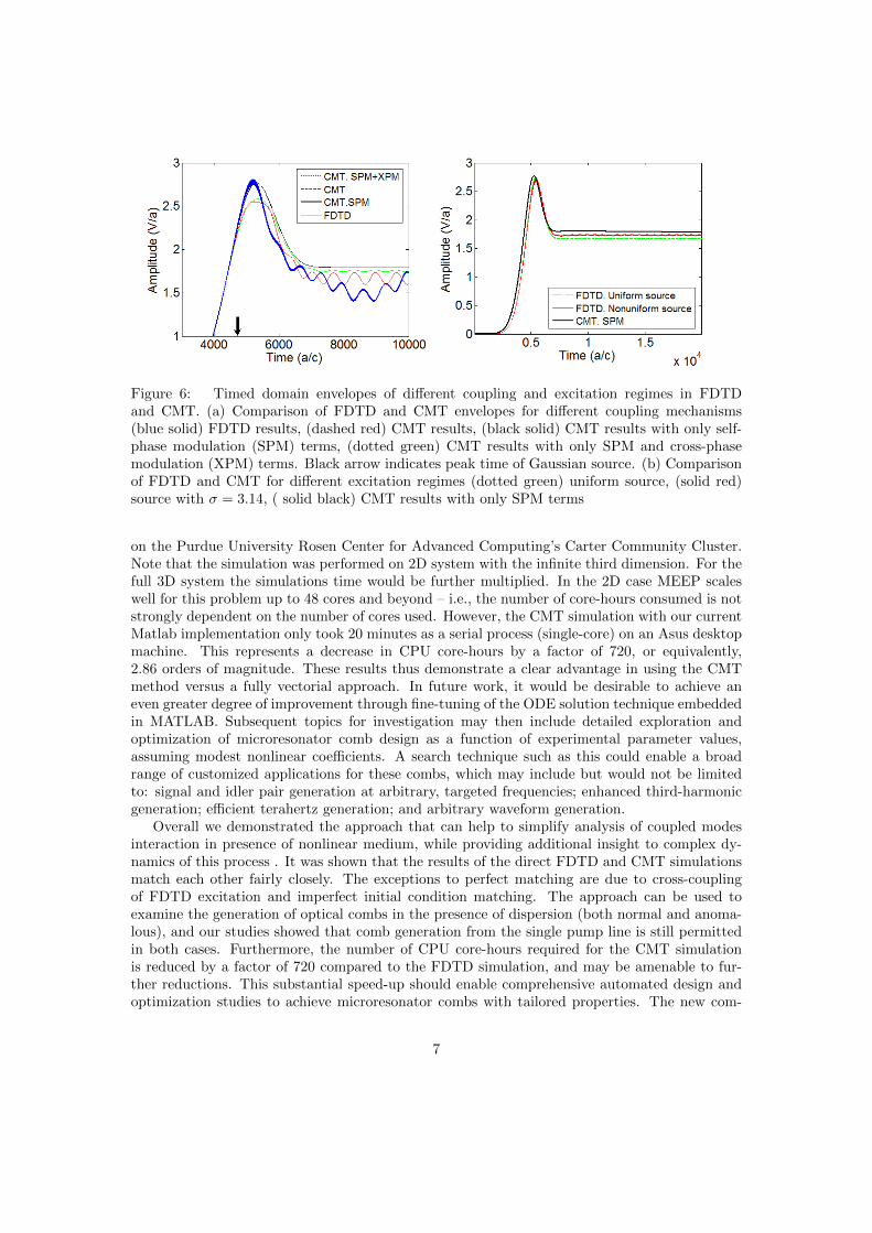
Figure 6: Timed domain envelopes of different coupling and excitation regimes in FDTDand CMT. (a) Comparison of FDTD and CMT envelopes for different coupling mechanisms(blue solid) FDTD results, (dashed red) CMT results, (black solid) CMT results with only self-phase modulation (SPM) terms, (dotted green) CMT results with only SPM and cross-phasemodulation (XPM) terms. Black arrow indicates peak time of Gaussian source. (b) Comparisonof FDTD and CMT for different excitation regimes (dotted green) uniform source, (solid red)source with σ = 3.14, ( solid black) CMT results with only SPM terms

on the Purdue University Rosen Center for Advanced Computing’s Carter Community Cluster.Note that the simulation was performed on 2D system with the infinite third dimension. For thefull 3D system the simulations time would be further multiplied. In the 2D case MEEP scaleswell for this problem up to 48 cores and beyond – i.e., the number of core-hours consumed is notstrongly dependent on the number of cores used. However, the CMT simulation with our currentMatlab implementation only took 20 minutes as a serial process (single-core) on an Asus desktopmachine. This represents a decrease in CPU core-hours by a factor of 720, or equivalently,2.86 orders of magnitude. These results thus demonstrate a clear advantage in using the CMTmethod versus a fully vectorial approach. In future work, it would be desirable to achieve aneven greater degree of improvement through fine-tuning of the ODE solution technique embeddedin MATLAB. Subsequent topics for investigation may then include detailed exploration andoptimization of microresonator comb design as a function of experimental parameter values,assuming modest nonlinear coefficients. A search technique such as this could enable a broadrange of customized applications for these combs, which may include but would not be limitedto: signal and idler pair generation at arbitrary, targeted frequencies; enhanced third-harmonicgeneration; efficient terahertz generation; and arbitrary waveform generation.

Overall we demonstrated the approach that can help to simplify analysis of coupled modesinteraction in presence of nonlinear medium, while providing additional insight to complex dy-namics of this process . It was shown that the results of the direct FDTD and CMT simulationsmatch each other fairly closely. The exceptions to perfect matching are due to cross-couplingof FDTD excitation and imperfect initial condition matching. The approach can be used toexamine the generation of optical combs in the presence of dispersion (both normal and anoma-lous), and our studies showed that comb generation from the single pump line is still permittedin both cases. Furthermore, the number of CPU core-hours required for the CMT simulationis reduced by a factor of 720 compared to the FDTD simulation, and may be amenable to fur-ther reductions. This substantial speed-up should enable comprehensive automated design andoptimization studies to achieve microresonator combs with tailored properties. The new com-

7

putational framework can be leveraged for analyzing important optical applications of nonlinearphenomena in photonic crystals, plasmonics and metamaterials. The approach can be readilytransfered to the analysis of weakly coupled system having nontrivial mode distribution andcoupling such as random lasers, laser focusing on nanoscale, high harmonic generation, pulseshaping and quantum photonics.

References

[1] P. Del’Haye, A. Schliesser, O. Arcizet, T. Wilken, R. Holzwarth, and T. J. Kippenberg,”Optical frequency comb generation from a monolithic microresonator,” Nature 450, 1214(2007).

[2] J. Ye and S.T. Cundiff,Femtosecond Optical Frequency Comb: Principle, Operation, andApplications (Kluwer, Norwell, MA, 2005)

[3] P. Del’Haye, S.B. Papp, S.A. Diddams,” Hybrid Electro-Optically Modulated Microcombs”, Phys. Rev. Lett. 109, 263901 (2012)

[4] I. S. Grudinin, N. Yu, and L. Maleki, ”Generation of optical frequency combs with a CaF2

resonator,” Opt. Lett. 34, 878-880 (2009).

[5] W. C Jiang, X. Lu, J. Zhang, O. Painter, Q. Lin, ”A silicon-chip source ofbright photon-paircomb,” Preprint at http://arxiv.org/abs/1210.4455v1 (2012).

[6] T. Herr , K. Hartinger, J. Riemensberger,, C.Y. Wang, E. Gavartin, R. Holzwarth, M.L.Gorodetsky, T.J. Kippenberg, Universal formation dynamics and noise of Kerr-frequencycombs in microresonators Nature Photon. 6, 480-7 (2012).

[7] A. B. Matsko, A. A. Savchenkov, W. Liang, V. S. Ilchenko, D. Seidel, and L. Maleki, ”Mode-locked Kerr frequency combs,” Opt. Lett. 36, 2845 (2011).

[8] Y.K. Chembo and N. Yu, ”Modal expansion approach to optical-frequency-comb generationwith monolithic whispering-gallery-mode resonators,” Phys Rev. A 82, 033801 (2010).

[9] E. Granados ,D.W. Coutts, D.J. Spence,”Mode-locked deep ultraviolet Ce:LiCAF laser,” Opt.Lett. 34, 1660-1662 (2009).

[10] M. Popovic, Theory and design of High-Index-Contrast microphotonic circuits, MIT librariesthesis collection (2008).

[11] J.D. Joannopoulos, S.G.Johnson, J.N. Winn and R.D. Meade, et al., Photonic Crystals:Molding the Flow of Light, Second Edition (Princeton University Press, Princeton, 2007).

[12] L.A. Lugiato, R. Lefever,”Spatial dissipative structures in passive optical systems,” Phys.Rev. Lett. 58 2209 -2211 (1987)

[13] S. Coen, H.G. Randle, T. Sylvestre, M. Erkintalo,”Modeling of octave-spanning Kerr fre-quency combs using a generalized mean-field Lugiato-Lefever model”, Opt. Lett. 38, 37-39(2013)

[14] A. Yariv, P. Yeh Photonics: optical electronics in modern communications, Oxford Univer-sity Press (2007)

8

[15] A. B. Matsko, W. Liang, A. A. Savchenkov, L. Maleki ”Chaotic dynamics of frequencycombs generated with continuously pumped nonlinear microresonators”, Opt. Lett. 38,, 525-527 (2013)

[16] T. Hansson, D. Modotto, S. Wabnitz ”On the numerical simulation of Kerr frequency combsusing coupled mode equations” Opt. Comm., 312, 134 (2014)

[17] M. Peccianti, A. Pasquazi, Y. Park, B.E. Little, S.T. Chu, D.J. Moss and R. Morandotti”Demonstration of a stable ultrafast laser based on a nonlinear microcavity” Nature Comm.,3,765 (2012)

[18] M.R. Lamont, Y. Okawachi,A.L. Gaeta,”Route to stabilized ultrabroadband microresonator-based frequency combs,” Opt. Lett. 38 3478-3481 (2013)

[19] A. F. Oskooi, D. Roundy, M. Ibanescu, P. Bermel, J. D. Joannopoulos, and S. G. Johnson,”MEEP A flexible free software package for electromagnetic simulations by the FDTD method,Comp. Phys. Commun. 181, 687702 (2010).

9