Applications of Data Mining Techniques for Churn

Prediction and Cross-selling in the

Telecommunications Industry

Dissertation submitted in part fulfilment of the requirements

for the degree of

[MSc Data Analytics]

at Dublin Business School

Emad Hanif

10374354

DECLARATION

I, Emad Hanif, declare that this research is my original work

and that it has never been presented to any institution or university for the award of

Degree or Diploma. In addition, I have referenced correctly all literature and sources used

in this work and this work is fully compliant with the Dublin Business School’s

academic honesty policy.

Signed: Emad Hanif

Date: 07-01-2019

ACKNOWLEDGEMENTS

I would like to express deepest gratitude to my supervisor Dr. Shahram Azizi Sazi who built

the foundations of my work through his “Research Methods” modules, for his guidance,

encouragement, and gracious support throughout the course of my work and for his expertise

in the field that motivated me to work in this area.

I would like to thank Terri Hoare, instructor for “Data Mining” and John O’Sullivan, instructor

for “Programming for Data Analysis, Processing and Visualization”, who both taught me

several important concepts.

I would also like to thank Anita Dwyer, Postgraduate Program Coordinator who was always

helpful and super-fast to clarify and resolve any query.

Finally, I dedicate my work to my mother who motivated me to pursue Master’s degree and

who always supported me through prays, financial and moral support, especially during my

illness and difficulties.

ABSTRACT

Customer Churn is a critical point of concern for organizations in the telecommunications

industry. It is estimated that this industry has an approximate annual churn rate of 30% leading

to a huge loss of revenue for organizations every year. Even though the telecom industry was

one of the first adopters of data mining and machine learning techniques to gain meaningful

insights from large sets of data, the issue of customer churn is still at large in this industry. This

thesis presents a predictive analytics approach to improve customer churn in the telecom

industry as well as the application of a technique typically used in retail contexts known as

“cross-selling” or “market basket analysis”.

A publicly available telecom dataset was used for the analysis. K-Nearest Neighbor, Decision

Tree, Naïve Bayes and Random Forest were the four classification algorithms that were used

to predict customer churn in RapidMiner and R. Apriori and FP-Growth were implemented in

RapidMiner to understand the associtations between the attributes in the dataset. The results

show that Decision Tree and Random Forest are the two most accurate algorithms in predicting

customer churn. The “cross-selling” results show that association algorithms are a practical

solution to discover associations between these items and services in this industry. The

discovery of patterns and frequent item sets can be used by telecom companies to engage

customers and offer services in a unique manner that is beneficial to their operation.

Overall, the key drivers of churn are identified in this study and useful associations between

products are established. This information can be used by companies to create personalised

offers and campaigns for customers who are at risk of churning. The study also shows that

association rules can help in identifying usage patterns, buying preferences, socio-economic

influences of customers.

Keywords: Data Mining, Machine Learning, Classification, Association, Churn, Cross-selling,

Telecom

TABLE OF CONTENTS

DECLARATION .................................................................................................. 2

ACKNOWLEDGEMENTS .................................................................................. 3

ABSTRACT .......................................................................................................... 4

TABLE OF FIGURES .......................................................................................... 8

LIST OF TABLES .............................................................................................. 10

CHAPTER 1 - INTRODUCTION ...................................................................... 11

1.1 Introduction and Background ...................................................................................................... 11

1.1.1 Introduction to Data Mining ................................................................................................ 11

1.1.2 Source of Data in the Telecom Industry .............................................................................. 11

1.1.3 Customer Churn in the Telecom Industry ............................................................................ 11

1.1.4 Types of Data Generated in the Telecom Industry .............................................................. 13

1.1.5 Data Mining Challenges in Telecom Industry ..................................................................... 14

1.2 Market Basket Analysis for Marketing in Telecom .................................................................... 15

1.3 Research Problem Definition & Research Purpose .................................................................... 16

1.4 Research Questions & Research Objectives ............................................................................... 16

1.5 Thesis Roadmap/Structure .......................................................................................................... 17

CHAPTER TWO - LITERATURE REVIEW .................................................... 18

2.1 Literature Review - Introduction ................................................................................................. 18

2.2 Research Model of Churn Prediction Based on Customer Segmentation and Misclassification

Cost in the Context of Big Data (Yong Liu and Yongrui Zhuang, 2015) ......................................... 18

2.3 Analysis and Application of Data Mining Methods used for Customer Churn in Telecom

Industry (Saurabh Jain, 2016) ........................................................................................................... 19

2.4 A Survey on Data Mining Techniques in Customer Churn Analysis for Telecom Industry (Amal

M. Almana, Mehmet Sabih Aksoy, Rasheed Alzahrani, 2014) ........................................................ 20

2.5 Mining Big Data in Telecommunications Industry: Challenges, Techniques, and Revenue

Opportunity (Hoda A. Abdel Hafez, 2016) ....................................................................................... 21

2.6 Improved Churn Prediction in Telecommunication Industry Using Data Mining Techniques (A.

Keramati, R. Jafari-Marandi, M. Aliannejadi, I. Ahmadian, M. Mozzafari, U. Abbasi, 2014) ........ 23

2.7 Predict the Rotation of Customers in the Mobile Sector Using Probabilistic Classifiers in Data

Mining (Clement Kirui, Li Hong, Wilson Cheruiyot and Hillary Kirui, 2013) ................................ 24

2.8 A Proposed Model of Prediction of Abandonment (Essam Shaaban, Yehia Helmy, Ayman

Khedr, Mona Nasr, 2012) ................................................................................................................. 25

2.9 Telecommunication Subscribers' Churn Prediction Model Using Machine Learning (Saad

Ahmed Qureshi, Ammar Saleem Rehman, Ali Mustafa Qamar, Aatif Kamal, Ahsan Rehman, 2013)

.......................................................................................................................................................... 26

2.10 Cross-Selling Models for Telecommunication Services (Szymon Jaroszewicz) ...................... 26

2.11 Crunch Time: Using Big Data to Boost Telco Marketing Capabilities (Holger Hurtgen, Samba

Natarajan, Steven Spittaels, Ole Jorgen Vetvik, Shaowei Ying, 2012) ............................................ 27

2.2 Literature Review of Machine Learning Algorithms .................................................................. 28

2.2.1 Classification Algorithms .................................................................................................... 28

2.2.2 Association Rules Algorithms ............................................................................................. 34

CHAPTER 3 – RESEARCH METHODOLOGY .............................................. 38

3.1 Research Process and Methodology ........................................................................................... 38

3.2 Research Strategy ........................................................................................................................ 39

3.3 Data Collection ........................................................................................................................... 39

3.3.1 Dataset Information ............................................................................................................. 39

3.3.2 Data Preprocessing ............................................................................................................... 40

3.4 Exploratory Data Analysis of the Dataset in Tableau ................................................................. 41

3.5 Data Mining and Machine Learning Tools ................................................................................. 43

3.5.1 RapidMiner .......................................................................................................................... 43

3.5.2 R ........................................................................................................................................... 44

CHAPTER 4 – IMPLEMENTATION, ANALYSIS AND RESULTS ............. 45

4.1 Introduction ................................................................................................................................. 45

4.2 Building Predictive Models in RapidMiner ................................................................................ 45

4.3 k-Nearest Neighbor: How to Implement in RapidMiner ............................................................ 49

4.3.1 k-Nearest Neighbor: How to Implement in RapidMiner with Cross-validation .................. 53

4.3.2 k-Nearest Neighbor: Interpreting the Results ...................................................................... 55

4.4 Decision Tree: How to Implement in RapidMiner ..................................................................... 56

4.4.1 Decision Tree: Interpreting the Results................................................................................ 59

4.5 Decision Tree: How to Implement in R ...................................................................................... 61

4.5.1 Decision Tree in R: Interpreting the Results ........................................................................ 63

4.6 Naïve Bayes: How to Implement in RapidMiner ........................................................................ 64

4.6.1 Naïve Bayes: Interpreting the Results .................................................................................. 65

4.7 Naïve Bayes: How to Implement in R ........................................................................................ 67

4.7.1 Naïve Bayes in R: Interpreting the Results .......................................................................... 69

4.8 Random Forest: How to Implement in RapidMiner ................................................................... 71

4.8.1 Random Forest: Interpreting the Results.............................................................................. 72

4.9 Random Forest: How to Implement in R .................................................................................... 74

4.9.1 Random Forest in R: Interpreting the Results ...................................................................... 76

4.10 ROC Curve of the Classification Models in R .......................................................................... 76

4.11 FP-Growth: How to Implement in RapidMiner ........................................................................ 78

4.11.1 FP-Growth: Interpreting the Results .................................................................................. 79

4.12 Apriori: How to Implement in RapidMiner .............................................................................. 82

4.12.1: Apriori: Interpreting the Results ....................................................................................... 83

CHAPTER 5 – CONCLUSION .......................................................................... 84

5.1 Introduction ................................................................................................................................. 84

5.2 Summary of Performance of Classification Models in RapidMiner ........................................... 84

5.3 Summary of Results and Conclusion .......................................................................................... 85

5.4 Future Work ................................................................................................................................ 86

REFERENCES .................................................................................................... 87

APPENDIX ......................................................................................................... 92

TABLE OF FIGURES

Figure 1: Types of Churners. (Source: Saraswat and Tiwari, 2018). .................................................... 12

Figure 2: Data Mining Process (Han et al, 2011). ................................................................................ 15

Figure 3: Hybrid Methodology (Source: Keramati et. al, 2014). .......................................................... 24

Figure 4: NPTB Recommendation Engine (Source: Hurtgen et. al (2012). ......................................... 28

Figure 5: k-nearest neighbour algorithm (Bronshtein, 2017). ............................................................... 29

Figure 6: Decision tree showing survival probability of passengers on the Titanic ship (Source:

Milborrow, 2011). ................................................................................................................................. 30

Figure 7: Artificial Neural Networks example. Source (McDonald, 2017). ......................................... 33

Figure 8: FP-Tree of the example (Source: Kotu and Deshpande, 2014). ............................................ 36

Figure 9: Customer Churn by Gender and Type of Contract ................................................................ 41

Figure 10: Treemap of Customer Churn, Tenure and Monthly Charges .............................................. 42

Figure 11: Customer Churn by Gender and Payment Method .............................................................. 42

Figure 12: Customer Churn by Tenure ................................................................................................. 43

Figure 13: Auto Model Overview ......................................................................................................... 45

Figure 14: Auto Model Select Inputs .................................................................................................... 46

Figure 15: Model Types in Auto Model ............................................................................................... 47

Figure 16: Auto Model Results Screen ................................................................................................. 47

Figure 17: Auto Model Simulator ......................................................................................................... 48

Figure 18: Auto Model Simulator ......................................................................................................... 49

Figure 19: k-Nearest Neighbor: How to Implement in RapidMiner with Split Validation .................. 49

Figure 20: k-Nearest Neighbor: How to Implement in RapidMiner with Split Validation .................. 51

Figure 21: K-Nearest Neighbor: Performance Vector .......................................................................... 52

Figure 22: K-Nearest Neighbor: How to Implement in RapidMiner with Split Data ........................... 52

Figure 23: K-Nearest Neighbor: Performance Vector .......................................................................... 53

Figure 24: K-Nearest Neighbor: How to Implement in RapidMiner with Cross-validation ................. 53

Figure 25: k-nearest neighbor: Performance Vector ............................................................................. 54

Figure 26: K-Nearest Neighbor: Interpreting the Results ..................................................................... 55

Figure 27: Decision Tree: How to Implement in RapidMiner with Cross-validation........................... 56

Figure 28: Decision Tree: Interpreting the Results ............................................................................... 59

Figure 29: Decision Tree: Interpreting the Results ............................................................................... 59

Figure 30: Decision Tree: Interpreting the Results ............................................................................... 60

Figure 31: Decision Tree in R: Interpreting the Results ....................................................................... 63

Figure 32: Decision Tree in R: Interpreting the Results ....................................................................... 63

Figure 33: Naïve Bayes: How to Implement in RapidMiner ................................................................ 64

Figure 34: Naïve Bayes: Performance Vector ...................................................................................... 65

Figure 35: Naïve Bayes: Interpreting the Results – Distribution Table Output (Class Conditional

Probability Table) ................................................................................................................................. 65

Figure 36: Naïve Bayes: Interpreting the Results – Distribution Table Output (Class Conditional

Probability Table) ................................................................................................................................. 65

Figure 37: Naïve Bayes: Interpreting the Results – Probability Distribution Function for “Tenure”. .. 66

Figure 38: Naïve Bayes: Interpreting the Results – Bar Chart for Contract (Yes or No) ..................... 66

Figure 39: Naïve Bayes: Interpreting the Results – Probability Distribution Function for “Monthly

Charges”. ............................................................................................................................................... 67

Figure 40: Naïve Bayes in R: Class Conditional Probability for Attributes ......................................... 69

Figure 41: Naïve Bayes in R: Class Conditional Probability for Attributes ......................................... 70

Figure 42: Random Forest: How to Implement in RapidMiner ............................................................ 71

Figure 43: Random Forest: Performance Vector .................................................................................. 72

Figure 44: Random Forest: Interpreting the Results ............................................................................. 72

Figure 45: Random Forest: Interpreting the Results – Random Forest Tree ........................................ 73

Figure 46: Random Forest Model in R ................................................................................................. 74

Figure 47: Random Forest Model in R ................................................................................................. 74

Figure 48: Random Forest: Plotting Important Variables ..................................................................... 76

Figure 49: ROC Curve of the Three Classification Models .................................................................. 77

Figure 50: FP-Growth: How to Implement in RapidMiner .................................................................. 78

Figure 51: FP-Growth: Interpreting the Results – Frequent Item Sets ................................................. 79

Figure 52: FP-Growth: Interpreting the Results – Frequent Item Sets ................................................. 79

Figure 53: FP-Growth: Interpreting the Results – Association Rules ................................................... 80

Figure 54: FP-Growth: Interpreting the Results – Association Rules ................................................... 80

Figure 55: FP-Growth: Interpreting the Results – Association Rules ................................................... 81

Figure 56: FP-Growth: Interpreting the Results – Association Rules ................................................... 81

Figure 57: Apriori: How to Implement in RapidMiner ......................................................................... 82

Figure 58: Apriori: Interpreting the Results .......................................................................................... 83

LIST OF TABLES

Table 1: Example of list of transactions .................................................................................. 36

Table 2: Optimizing Decision Tree Parameters ....................................................................... 57

Table 3: Summary of Performance of Classification Algorithms ........................................... 84

CHAPTER 1 - INTRODUCTION

1.1 Introduction and Background

Chapter 1 covers the contextual background for the topic at hand. This section also addresses

what the study will entail, the problem statement and the research objectives, why the research

is necessary and the overall structure of this thesis.

1.1.1 Introduction to Data Mining

Data mining is the process of examining data in order to extract interesting information like

patterns, anomalies and correlations from large pre-existing datasets. This information is

extracted using a broad range of techniques and can then be used by organization to increase

revenue, reduce costs, improve customer relationships, reduce risks etc. (SAS, no date). The

telecom industry was one of the first industries to adopt data mining techniques in order to

extract useful information from the enormous data that is generated in this industry.

1.1.2 Source of Data in the Telecom Industry

The digital explosion that has been happened in the last 10 years or so has led to an exponential

increase in the data that is generated in the telecom industry. Advances in computing and

communication technologies has led to a massive increase in the number of applications

accessible through mobile phones. This has led to creation of highly diverse sources of data

available in many different forms including tabular, objects, log records and free text (Chen,

2016, p. 3). Telecom data has also grown enormously since the influx of 3G and Broadband,

and it will continue to grow exponentially as technology continues to evolve. According to

Marr (2015), data generated in the last 4 years has been more than the entire data generated

previously in the history of the human race. According to an IBM report (2017) around 2.5

quintillion bytes of data was generated daily in the year 2017. This figure is likely to be even

more in 2018.

1.1.3 Customer Churn in the Telecom Industry

The issue of customer churn or customer attrition is not unique to the telecom industry. Almost

every company in every industry at some point in time faces the problem of losing their

customer to a competitor. This is usually a source of huge financial loss for companies as it is

considered easier and much cheaper to retain existing customer than to attract new ones. A

number of studies and surveys back up this fact. Van den Poel and Larivière (2004) validate

this in their study on the importance of the economic value of customer retention in the context

of a European Financial Services company.

Customers in the telecom industry, especially pre-paid customers are usually not under any

contract by a telecom operator and are thus always at risk of churning. This means that

customers could change their telecom operator without notice at their own convenience. Hence,

it is important to manage and identify customers that are likely to churn, especially in an

industry such as the telecom industry which is often characterized by strong competition and

volatile markets. Proper management of customers that are likely to churn can minimize the

probability of churn, while maximizing the profit of a company. Data mining plays a very

important role in telecommunications companies and their effort to reduce overall churn by

developing better marketing strategies, identifying fraudulent activities and customers and

better managing their network. Hence, one of the first and most important steps in managing

and improving churn is identifying customers that are likely to churn.

There are two main categories of churners - voluntary or involuntary.

Involuntary Churners

Some customers are deliberately withheld service due to reasons which may include fraud,

failure to pay bills and sometimes even non-utilization or insufficient utilization of the service.

Figure 1: Types of Churners. (Source: Saraswat and Tiwari, 2018).

It can also be due to a customer’s relocation to a “long-term care facility, death, or the

relocation to a distant location”. These customers are generally removed by the phone company

from their service and are referred to as involuntary churners (Saraswat and Tiwari, 2018).

Voluntary Churners

Voluntary churner occurs when a customer decides to terminate his/her service with the

provider and switch to another company or provider. Telecom churn is usually of the voluntary

kind. It can also be further divided into two sub-categories – deliberate and incidental (Saraswat

and Tiwari, 2018).

Incidental churn can happen when something significant changes in a customer’s personal lives

which forces a customer to churn whereas deliberate churn can happen for reasons of

technology, with customers always wanting newer or better technology, better service quality

factors, social or psychological factors, and convenience reasons. According to Shaaban et. al

this churn issue is the one that management in telecom companies are always looking to solve

(Shaaban et. al, 2014).

1.1.4 Types of Data Generated in the Telecom Industry

Data in the telecom industry can be classified into three groups:

1. Call Detail Data: This relates to information about the call, which is stored as a call detail

record. For every call placed on a network, a call detail record is generated to store information

about the call. Call detail data essentially relates to the average call duration, average call

originated, call period and call to/from different area code.

2. Network Data: Network data includes information about error generation and status

messages, which need to be generated in real time. The volume of network messages generated

is huge and data mining techniques and technologies are used to identify network faults by

extracting knowledge from network data (Joseph, 2013, p. 526). The network data also includes

information about the complex configuration of equipment data, data about error generation

and data that is essential for network management configuration.

3. Customer Data: The customer data includes information about the customer which includes

their name, age, address, telephone type, type of subscription plan, payment history and so on.

1.1.5 Data Mining Challenges in Telecom Industry

Data mining in the telecommunications industry faces a number of challenges. Advances in

technology has led to a monumental increase in the amount of data in the last decade or so. The

advent of mobile phones has led to the creation of highly diverse sources of data, which are

available in many different forms including tabular, objects, log records and free text (Chen,

2016, p. 3). Data in this industry has also grown exponentially since the growth of 3G and

Broadband, and it will continue to grow as technology is evolving constantly and at a rapid

pace.

According to Weiss (2010, p. 194), “telecom companies generate a tremendous amount of data,

the sequential and temporal aspects of their data, and the need to predict very rare events—

such as customer fraud and network failures—in real-time”. According to Joseph (2013),

another challenge in mining big data in the telecom industry is in the form of transactions,

which is not at the proper level for semantic data mining.

The biggest telecom companies have data which is usually in petabytes and often exceeds

manageable levels. Hence the scalability of data mining can also be a concern. Another concern

with telecommunication data and its associated applications includes the problem of rarity.

This is because telecom fraud and network failure are both rare events. According to Weiss,

(2004) “predicting and identifying rare events has been shown to be quite difficult for many

data mining algorithms” and this issue must be approached carefully to ensure good results.

These challenges can be overcome by the application of appropriate data mining techniques ,

and useful insights from data can be gained from the data that is available in this industry.

1.2 Market Basket Analysis for Marketing in Telecom

Market Basket Analysis is a technique used by retailers to discover association between items.

It allows companies to identify relationship between items that people buy. It is not a widely

used technique in the telecom industry, but telecom companies can benefit if market basket

analysis is applied appropriately.

The telecom industry has mainly 3 services – phone service, internet service and TV cable

service. Association rules can be used to identify customer paths. For example, a customer may

be interested in beginning with a single phone line and then moving to more phone lines plus

internet connection and TV cable service. This can be used for identification of customers who

are interested in purchasing new services (Jaroszewicz, 2008). This is also described as the

process of cross-selling. Association rules algorithms like Apriori, FP-Growth will be used to

analyze data for frequent if/then patterns. Support and Confidence thresholds will be calculated

to quantify the frequency of items appearing in different transactions. Similar to cross-selling

is the recommendation system which offers recommendations to customers based on their

purchase history. This has been used with great success in e-commerce but its implementation

in the telecom industry can be challenging due to the small number of services that are

available.

For data mining, CRISP-DM will be followed. This methodology provides a complete

blueprint for tackling data mining projects in 6 stages. These 6 stages are business

understanding, data understanding, data preparation, modelling, evaluation and deployment.

Figure 2: Data Mining Process (Han et al, 2011).

1.3 Research Problem Definition & Research Purpose

Customer churn is a focus of any services & customer centric industry. Among them is the

telecom industry which suffers greatly from customer churn every year. It is estimated that this

industry has an approximate annual churn rate of 30%.

The telecom industry was one of the first adopters of data mining techniques to gain meaningful

insights from large sets of data. In order to tackle the issue of customer churn, data mining and

machine learning can be applied to predict customers who are likely to churn. These customers

can then be approached with appropriate sales and marketing strategies in order to retain their

services. Mining of big data in the telecom industry also offers organizations a real opportunity

to gain a comprehensive view of their business operations.

Cross-selling or market basket analysis is a technique that is usually applied in retail contexts

to discover associations between frequently purchased items. The telecom industry has become

an industry where customers usually buy or subscribe to multiple services from one company.

These include phone service, internet service, TV packages, streaming TV, online security etc.

Finding associations between these items can lead to the discovery of patterns that can be used

by telecom companies to engage customers and offer services that are beneficial to their

operation.

Hence, the purpose of this is to not only develop effective and efficient models to recognize

customer before they churn, but also to apply cross-selling techniques in a telecom context to

find useful patterns and associations that can be used effectively by telecom companies.

1.4 Research Questions & Research Objectives

Based on section 1.4, the research questions are defined as:

How can data mining and machine learning techniques be effectively applied to predict

customer churn in the telecom industry?

Does cross-selling or market basket analysis offer a viable solution to gain valuable

insights in the telecom industry?

What are the opportunities and challenges in the application of data mining and machine

learning techniques in the telecom industry?

The research objectives are therefore defined as:

To use a large and diverse telecom dataset and apply machine learning algorithms to

identify customers that are likely to churn from this dataset.

Identify the best performing machine learning techniques and algorithms.

Apply association algorithms such as Apriori and FP-Growth to find interesting

patterns between various telecom services.

To establish the opportunities and challenges that are present in the application of data

mining in the telecom industry.

1.5 Thesis Roadmap/Structure

This section defines the roadmap/structure of the thesis. The different chapters along with a

brief explanation of the content of these chapters are illustrated in the figure shown below:

Chapter 5 - This chapter concludes the thesis with a conclusion of the results and the insights gained from the study.

Chapter 4 - This chapter includes the process of creating classification and association models in RapidMiner as well as an analysis of their performance, results and the insights gained

from applying these models. These classification algorithms are also applied in R.

Chapter 3 -This chapter defines the research methodology and the information about the dataset used for the research.

Chapter 2 - This chapter includes a review of relevant literature, summary and findings from the reviewed research papers as well as a review of classification and association machine

learning algorithms.

Chapter 1 - This chapter includes the Introduction and background of the topic as well as the research problem & purpose, research question and objectives.

CHAPTER TWO - LITERATURE REVIEW

2.1 Literature Review - Introduction

An essential part of any research is reviewing relevant literature. Literature review can be

defined as an objective and critical summary of published literature within a particular area of

research. It covers the research that has been done in the relevant field and provides the

researcher with knowledge that can used to additional research and/or identify a research gap.

The literature review for this thesis summarizes the research from a list of papers related to

churn modeling, prediction as well as cross-selling products in telecom. The algorithms and

the methodologies used by the researchers has also been detailed.

2.2 Research Model of Churn Prediction Based on

Customer Segmentation and Misclassification Cost in the

Context of Big Data (Yong Liu and Yongrui Zhuang, 2015)

According to research done by Liu and Zhuang (2015, pp. 88-90), a model for

predicting customer churn and analysing customer behaviour is by combining a

Decision Tree algorithm (C5.0) with misclassification cost factor to predict customer

loyalty status.

In their research they got data of more than a million customers and then used K-means

method to cluster the data into three groups of high, medium and low.

They used C5.0 with misclassification cost & segmentation and C5.0 without

misclassification cost and segmentation to predict customer churn.

Their research showed that model accuracy was much higher when C5.0 was used with

misclassification cost and segmentation.

Their results show that this model is better than those models without customer

segmentation and misclassification cost in terms of the performance, accuracy and

coverage of model.

Summary and Findings from this Research Paper

This research paper helped in addressing some of the commonly used machine learning

algorithms to develop a research model on churn prediction. The research showed that a

decision tree algorithm C5.0 with misclassification cost & segmentation was much more

accurate than without misclassification cost & segmentation. To summarize, they established

a research model of customer churn based on customer segmentation and misclassification cost

and utilized this model to analyze customer behavior data of a Chinese telecom company.

2.3 Analysis and Application of Data Mining Methods used

for Customer Churn in Telecom Industry (Saurabh Jain,

2016)

Jain (2016) used statistical based techniques such as Linear Regression, Logistic

Regression, Bayes Naïve Classifier and K-nearest neighbour and suggested that they

can be applied to predict churn with varying degrees of success. Jain’s research showed

that logistic regression was successful in correctly predicting only 45% of the churners,

whereas Bayes Naïve Classifier was successful in predicting around 68% of the

churners.

He also evaluated the use of Decision Trees and Artificial Neural Networks to predict

customer churn and found that when Decision trees and ANNs are used they outperform

neural networks in terms of accuracy.

In his research he also used, many covering algorithms like AQ, CN2 and RULES

family. In these algorithms’ rules are extracted from a given set of training examples.

He stated that there has been very little work done on these algorithms and their

applications in predicting customer churn in the telecom industry.

But he stated that these algorithms, especially RULES3 is an excellent choice for data

mining in this industry as it can handle large datasets without having to break them up

into smaller sub sets. This also allows for a degree of control over the number of rules

to be extracted.

Summary and Findings from this Research Paper

This paper based used a number of statistical techniques to analyze customer churn in the

telecom industry. It essentially analyzed the performance and accuracy of different algorithms

and how they can be applied to a large telecom dataset. The researcher concluded that decision

tree-based techniques especially C5.0 and CART (Classification and Regression Trees)

outperformed widely used techniques such as regression in terms of accuracy. He also stated

that the selection the correct combination of attributes and fixing proper threshold values may

produce much more accurate results. It was also established that RULES3 is a great choice for

handling large datasets.

2.4 A Survey on Data Mining Techniques in Customer

Churn Analysis for Telecom Industry (Amal M. Almana,

Mehmet Sabih Aksoy, Rasheed Alzahrani, 2014)

A research paper by Almana, Aksoy and Alzahrani (2014), surveys the most frequently

used methods to identify customer churn in the telecommunications industry.

The researchers follow the CRISP-DM methodology for this study and apply a number

of supervised learning algorithms on a telecom dataset.

Based on their study, they concluded that neural networks and a number of statistical

based methods work extremely well for predicting telecom churn.

Linear and Logistic Regression, Naïve Bayes and K Nearest Neighbor and their usage

and viability in the context of customer churn analysis was established during this

study.

Covering algorithms families like AQ, CN2, RIPPER, and RULES family in which

rules are extracted from a set of training examples.

Their research concluded that Decision Trees, Regression Techniques and Neural

Networks can be successfully applied to predict customer churn in the telecom industry.

They also found that decision tree based techniques like C5.0 and CART outperformed

some existing data techniques like regression in terms of accuracy.

Summary and Findings from this Research Paper

Another research paper that focuses on the use of different algorithms in the context of a

customer churn analysis problem for the telecom industry. This paper helped in establishing

the usefulness of neural networks and statistical based methods for predicting telecom churn.

Like the previous research paper, it also validated the use of C5.0 for churn prediction.

2.5 Mining Big Data in Telecommunications Industry:

Challenges, Techniques, and Revenue Opportunity (Hoda

A. Abdel Hafez, 2016)

This research paper focuses on the challenges present by the mining of big data in the

telecom industry as well as some of the more commonly used techniques and data

mining tools to solve these challenges.

The paper goes into detail about some of the major challenges presented by mining of

big data in the telecom industry.

Massive volume of data in this industry is represented by heterogenous and diverse

dimensionalities. Also, “the autonomous data sources with distributed and

decentralized controls as well as the complexity and evolving relationships among data

are the characteristics of big data applications” (Abdel Hafez, 2016). These

characteristics present an enormous challenge for the mining of big data in this industry.

Apart from this, the data that is generated from different sources also possesses different

types and representation forms that can lead to a great variety or heterogeneity of big

data and mining from a massive heterogeneous dataset can be a big challenge.

Heterogeneity in big data deals with structured, semi-structured, and unstructured data

simultaneously and unstructured data may not always fit with traditional database

systems.

There is also the issue of privacy, accuracy, trust and provenance. Personal data is

usually contained within the high volume of big data in the telecom industry. According

to the researcher, for this issue, it would useful to develop a model where a balance is

reached with the benefits of mining this data for business and research purposes against

individual privacy rights.

The issue of accuracy and trust arises because these data sources have different origins,

all of which are not known and verifiable. According to the researcher, to solve this

problem, data validation and provenance tracing is a necessary step in the data mining.

For this, unsupervised learning methods have been used to the trust measures of

suspected data sources using other data sources as testimony.

The paper also goes into detail about the machine learning techniques that can be used

to mine big data in the telecom industry. Both, classification and clustering techniques

are discussed in this paper.

Classification algorithms like decision trees (BOAT - optimistic decision tree

construction, ICE - implication counter examples and VFDT - very fast decision tree)

and artificial neural networks.

Clustering algorithms for handling large datasets mentioned in this paper include

hierarchical clustering, k-means clustering and density based clustering.

Both k-means and hierarchical clustering are used for high dimensional datasets and

improving data streams processing. Whereas, density based clustering which is another

method for identifying clusters in large high dimensional datasets with varying sizes

and shapes is a better option for inferring the noise in a dataset. DBSCAN and

DENCLUE are two common examples of density based clustering.

The paper also goes into detail about some of the tools that can be used for performing

data mining tasks including R, WEKA, KNIME, RapidMiner, Orange, MOA etc.

The paper mentions that WEKA is useful for classification and regression problems but

not recommended for descriptive statistics and clustering methods. The software works

well on large datasets according to the developers of WEKA, but the author of this

research paper mentions that there is limited support for big data, text mining and semi-

supervised learning. It is also mentioned that WEKA is weaker in classical testing than

R but stronger in a machine learning. It supports many model evaluation procedures

and metrics but lacks many data survey and visualization methods despite some recent

improvements.

KNIME is also mentioned as a useful for performing data mining tasks on large

datasets. One of the biggest advantages of KNIME is that it can be easily integrated

with WEKA and R, which allows for use of almost all of the functionality of WEKA

and R in KNIME. The tool has been used primarily in pharmaceutical research, business

intelligence and financial data analysis but is also often used in areas like customer data

analysis and can be a great tool for extracting information from customer data in the

telecom industry.

Orange is a python based data mining tool which can be used either through Python

scripting as a Python plug-in, or through visual programming. It offers a visual

programming front-end for exploratory data analysis and data visualisation. It consists

of a canvas in which users can place different processors to create a data analysis

workflow. Its components are called widgets and they can be used for combining

methods from the core library and associated modules to create custom algorithms. An

advantage of this tool is that the algorithms are organized in hierarchical toolboxes,

making them easy to implement.

RapidMiner is another excellent data mining tool and is generally considered one of the

most useful data mining tools in the market today. It offers an environment for for data

preparation, machine learning, deep learning, text mining, predictive analytics and

statistical modelling. According to the official RapidMiner website, this tool unifies the

entire data science lifecycle from data preparation to machine learning and predictive

modelling to deployment (RapidMiner, no date). It is an excellent tool that can be used

resourcefully in the telecom industry to gain useful insights using data mining

techniques like classification, clustering, support vector machines etc.

Summary and Findings from this Research Paper

This paper went into great detail in covering the challenges, techniques, tools and

advantages/revenue opportunity from mining big data in the telecom industry. Starting with

the challenges presented by mining big data, covering issues like the diversity of data sources,

with the issues of data privacy, customer trust, the paper also addressed how these challenges

can be tackled by using data validation and provenance tracing. A number of supervised and

unsupervised algorithms and their usefulness was also explored. K-means and DBSCAN are

mentioned as two important clustering-based algorithms.

This paper also covered the practicality of different data mining tools. R, WEKA and

RapidMiner are mentioned as some of the best tools for the purpose of data mining and it

helped in finalizing RapidMiner as the primary data mining tool for this thesis.

2.6 Improved Churn Prediction in Telecommunication

Industry Using Data Mining Techniques (A. Keramati, R.

Jafari-Marandi, M. Aliannejadi, I. Ahmadian, M.

Mozzafari, U. Abbasi, 2014)

In this paper, the data of an Iranian mobile company was used for the research, and

algorithms like Decision Tree, Artificial Neural Networks, K-Nearest Neighbours, and

Support Vector Machine were employed to improve churn prediction. Artificial Neural

Network (ANN) significantly outperformed the other three algorithms.

Keramati et. al proposed a hybrid methodology to improve churn prediction, which

made several improvements to value of evaluation metrics. This proposed methodology

is essentially based on the idea of using all of 4 experienced classifiers to make a better

and more accurate hybrid classifier.

The results showed that this proposed methodology gave an accuracy of 95% for both

precision and recall measures.

They also presented a new dimensionality reduction methodology to extract the most

influential set of features from their dataset. Frequency of use, total number of

complaints, and seconds of use were shown to be the most influential features.

2.7 Predict the Rotation of Customers in the Mobile Sector

Using Probabilistic Classifiers in Data Mining (Clement

Kirui, Li Hong, Wilson Cheruiyot and Hillary Kirui, 2013)

In this paper, Kirui et al. address the issue of customer churn and state that telecom

companies “must develop precise and reliable predictive models to identify the possible

churners beforehand and then enlist them to intervention programs in a bid to retain as

many customers as possible”.

Kirui et. al in their research proposed a new set of features with the objective of

improving the recognition rates of likely churners.

Figure 3: Hybrid Methodology (Source: Keramati et. al, 2014).

These features which include contract related features, call description features as well

as call pattern changes description features which resulted from traffic figures and

customer profile data.

These features were evaluated using Naïve Bayes and Bayesian Network and the results

achieved were compared to the results achieved using a C4.5 decision tree.

To further assess the impact of the proposed features, the researchers ranked the feature

sets of both the original and the modified datasets using information gain feature

selection technique.

Their results showed improved prediction rates for all the used models. The

probabilistic classifiers showed higher true positive rate than the decision tree but the

decision tree performed better in overall accuracy.

2.8 A Proposed Model of Prediction of Abandonment

(Essam Shaaban, Yehia Helmy, Ayman Khedr, Mona Nasr,

2012)

Shaaban et. al introduced a model based on data mining to track customers and their

behaviour against churn.

Their dataset consisted of 5000 rows of 23 different attributes and 1000 instances were

used to test the model and the rest (4000) were used to train the model using 4 different

algorithms.

Decision trees, Support Vector Machines and Neural Networks were used for

classification and k-means was used for clustering using the software WEKA.

Using k-means, the predicted churners are clustered into 3 categories in case of using

in a retention strategy.

Their results showed that Support Vector Machines to be the best algorithm for

predicting churn in telecom.

2.9 Telecommunication Subscribers' Churn Prediction

Model Using Machine Learning (Saad Ahmed Qureshi,

Ammar Saleem Rehman, Ali Mustafa Qamar, Aatif Kamal,

Ahsan Rehman, 2013)

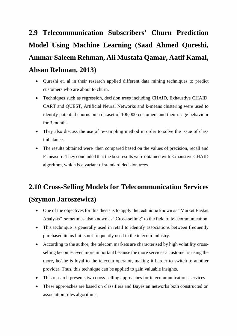
Qureshi et. al in their research applied different data mining techniques to predict

customers who are about to churn.

Techniques such as regression, decision trees including CHAID, Exhaustive CHAID,

CART and QUEST, Artificial Neural Networks and k-means clustering were used to

identify potential churns on a dataset of 106,000 customers and their usage behaviour

for 3 months.

They also discuss the use of re-sampling method in order to solve the issue of class

imbalance.

The results obtained were then compared based on the values of precision, recall and

F-measure. They concluded that the best results were obtained with Exhaustive CHAID

algorithm, which is a variant of standard decision trees.

2.10 Cross-Selling Models for Telecommunication Services

(Szymon Jaroszewicz)

One of the objectives for this thesis is to apply the technique known as “Market Basket

Analysis” sometimes also known as “Cross-selling” to the field of telecommunication.

This technique is generally used in retail to identify associations between frequently

purchased items but is not frequently used in the telecom industry.

According to the author, the telecom markets are characterised by high volatility cross-

selling becomes even more important because the more services a customer is using the

more, he/she is loyal to the telecom operator, making it harder to switch to another

provider. Thus, this technique can be applied to gain valuable insights.

This research presents two cross-selling approaches for telecommunications services.

These approaches are based on classifiers and Bayesian networks both constructed on

association rules algorithms.

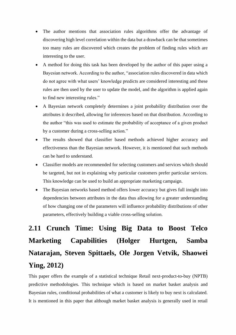
The author mentions that association rules algorithms offer the advantage of

discovering high level correlation within the data but a drawback can be that sometimes

too many rules are discovered which creates the problem of finding rules which are

interesting to the user.

A method for doing this task has been developed by the author of this paper using a

Bayesian network. According to the author, “association rules discovered in data which

do not agree with what users’ knowledge predicts are considered interesting and these

rules are then used by the user to update the model, and the algorithm is applied again

to find new interesting rules.”

A Bayesian network completely determines a joint probability distribution over the

attributes it described, allowing for inferences based on that distribution. According to

the author “this was used to estimate the probability of acceptance of a given product

by a customer during a cross-selling action.”

The results showed that classifier based methods achieved higher accuracy and

effectiveness than the Bayesian network. However, it is mentioned that such methods

can be hard to understand.

Classifier models are recommended for selecting customers and services which should

be targeted, but not in explaining why particular customers prefer particular services.

This knowledge can be used to build an appropriate marketing campaign.

The Bayesian networks based method offers lower accuracy but gives full insight into

dependencies between attributes in the data thus allowing for a greater understanding

of how changing one of the parameters will influence probability distributions of other

parameters, effectively building a viable cross-selling solution.

2.11 Crunch Time: Using Big Data to Boost Telco

Marketing Capabilities (Holger Hurtgen, Samba

Natarajan, Steven Spittaels, Ole Jorgen Vetvik, Shaowei

Ying, 2012)

This paper offers the example of a statistical technique Retail next-product-to-buy (NPTB)

predictive methodologies. This technique which is based on market basket analysis and

Bayesian rules, conditional probabilities of what a customer is likely to buy next is calculated.

It is mentioned in this paper that although market basket analysis is generally used in retail

contexts, telecom companies can adopt NPTB algorithms specific to the telecom industry. For

this, the definition or function of market basket has to be altered slightly from a singular visit

to a collection of data specific to the customer attained over a long period of time (Hurtgen et.

al, 2012)

The data about the customer can include sociodemographic as well as purchase history, contact

data etc. and an example of how it was done in this paper is shown below. The NPTB engine

is able to identify the top 3-5 services that a customer is likely to purchase, thus informing the

sales agents of what products to up-sell or cross-sell when a customer steps into a store or

reaches out to a call center. It is also able to inform marketing agents of specific products

customers are likely to buy. This information can be used by marketers to tailor specific

marketing campaigns for different customers.

2.2 Literature Review of Machine Learning Algorithms

2.2.1 Classification Algorithms

In data mining and machine learning, classification can be defined as the task of identifying a

model or function that describes data classes for the purpose of being able to use this model to

predict where a set of new observations belongs to. This is achieved using training data where

the class label is known.

Figure 4: NPTB Recommendation Engine (Source: Hurtgen et. al (2012).

Berry and Linoff (2004) define classification in machine learning as the process of examining

the features of a new object and assigning to a set of predefined set of classes. Classification

can be summarized as an instance of supervised learning where models learn from historical

data and predict/classify future outcomes. Some of the most commonly used classification

algorithms include:

1. K-nearest Neighbor: This classification algorithm is an instance of lazy learning, an

area of machine learning in which generalisation of the training data is withheld until a

query is made to the system (Webb, 2011). The algorithms works by classifying a

majority vote of its neighbors based on a minimum distance from the query to the

training data. The training data is set in multidimensional feature space with a class

label where k is a user defined arbitrary constant. An object is classified by a majority

vote of its neighbors. Euclidean distance is generally used as a distance metric.

One of the challenges of this algorithm is the selection of the parameter k. In research

studies, it has been mentioned that the selection of k should be done on the basis of data

and large value of k reduces the effect of noise on the data according to research done

by Everitt et. al in 2011. K-nearest neighor is an easy to understand and a good choice

for an algorithm where there is little or no prior information about the distribution data

(Bronshtein, 2017). However, it is also computationally expensive & requires high

memory requirement.

2. Decision Tree: Decision tree is one of the most popular classification algorithms used

in data mining and machine learning. As the name suggests, in this algorithm a tree-

shaped structure is used to represent set of related decisions or choices. Berry and Linoff

Figure 5: k-nearest neighbor algorithm (Bronshtein, 2017).

(2004) perhaps offer the easiest understanding of a decision tree by explaining that a

large collection of data is divided into smaller sets of data by applying a set of decision

rules. They can be either classification trees where the target variable contains a set of

discrete values or a regression tree where the target variable comprises of a set of

continuous values. A decision tree comprises of leaves, branches and nodes where the

leaf is the output variable and lies at the base of the decision tree.

A decision tree shown below representing the survival probability of passengers on the

ship Titanic can be used to understand the process of a decision tree and also help solve

a series of questions.

In the figure below, the percentage represents the percentage of observations in the leaf

and the number for example 0.73 represents the probability of survival of a passenger.

It can be summarized that if the passenger was not a male, then there was a probability

of 0.73 or a 73% chance of survival. A male passenger greater than 9.5 years old only

had a 17% chance of survival however a male passenger greater than 9.5 years old with

less than 2.5 (2, 1 or 0) siblings had an 89% chance of survival.

This was a simple example of a how a decision tree works and how it can be used to

answer a series of questions about a particular problem. There are a few decision tree

specific algorithms, some of which have been discussed in the previous section of this

chapter. These include ID3 (Iterative Dichotomiser 3), C4.5 (a successor of ID3),

Figure 6: Decision tree showing survival probability of

passengers on the Titanic ship (Source: Milborrow,

2011).

CHAID (chi-squared automatic interaction detector) and CART (Classification and

Regression Tree).

An important metric in decision trees is the split criteria. For this, Information Gain,

Gain Ratio, Gini impurity and Variance reduction are often used but only the first two

are recommended as the best methods in relevant literature.

Information Gain uses Entropy and Information content from Information Theory and

is calculated as the information before the split minus the information after the split.

According to Witten, Frank and Hall (2011), for each node of the tree, the information

value “represents the expected amount of information that would be needed to specify

whether a new instance should be classified yes or no, given that the example reached

that node”.

Gain Ratio is the ratio of information gain to the intrinsic information. It typically

reduces the bias that information gain has towards multi-valued attributes by taking the

number of branches into account when choosing an attribute according to Witten, Frank

and Hall (2011).

One of the biggest advantages that a decision tree has is that it can easily understood

and interpreted by non-experts in the area of data mining and machine learning. It can

also does not require any normalization of data and can handle both numerical and

categorical attributes with ease. It also performs well with large datasets and unlike k-

nearest neighbor, it is computationally efficient.

3. Naïve Bayes: This algorithm is based on Bayes’ theorem but is called “naïve” because

of the strong assumption of independence between the features. Bayes’ theorem given

a class variable y and dependent feature 𝑥1 through 𝑥𝑛, states that:

𝑷( 𝒚 ∣∣ 𝒙𝟏, … , 𝒙𝒏 ) =𝑷(𝒚)𝑷( 𝒙𝟏, … 𝒙𝒏 ∣∣ 𝒚 )

𝑷(𝒙𝟏,   … ,  𝒙𝒏)

Using the Naïve condition of independence:

𝑷(𝒙𝒊|𝒚, 𝒙𝟏, … , 𝒙𝒊−𝟏, 𝒙𝒊+𝟏, … , 𝒙𝒏) = 𝑷(𝒙𝒊|𝒚),

Since 𝑷(𝒙𝟏, … , 𝒙𝒏) is constant because of the assumption of independence, we can use

the classification rule:

𝑷( 𝒚 ∣∣ 𝒙𝟏, … , 𝒙𝒏 ) ∝ 𝑷(𝒚) ∏ 𝑷( 𝒙𝒊 ∣∣ 𝒚 )

𝒏

𝒊=𝟏

⇓

�̂� = 𝐚𝐫𝐠 𝐦𝐚𝐱𝐲

𝐏 (𝐲) ∏ 𝐏( 𝐱𝐢 ∣∣ 𝐲 )

𝐧

𝐢=𝟏

Despite this assumption of independence, the Naïve Bayes classifier still works well,

and its use cases include the likes of spam filtering and document classification. The

algorithm can input both numerical and categorical attributes and is robust to outliers

and missing data.

4. Neural Networks: Neural networks also known as artificial neural networks are

inspired by the biological neural networks that constitute the brain. Neural networks

cannot be defined as an algorithm in itself, but rather a framework for many different

machine learning algorithms to work together and process data inputs (Deep AI, 2018).

This works by learning and processing examples with input, learning the characteristics

of the input and using this information to correctly construct the output. Once the

algorithm has processed a sufficient number of examples, the neural network can start

processing unseen inputs and successfully return the correct results (Deep AI, 2018).

An example of how the process of identifying an image by neural networks works can

help in better understanding neural networks. According to Deep AI (2018), the image

is decomposed into data points and information that a computer can use using layers of

function. Once this happens, “the neural network can start to identify trends that exist

across the many, many examples that it processes and classify images by their

similarities”. After studying and many examples of this image, the algorithm has an

idea of what data points and elements to look for when classifying this particular image

again. Hence it is often said for neural networks that, the more examples the algorithm

sees, the more accurate the results become as it learns from experience.

Berry and Linoff (2004) share a similar opinion about neural networks and mention that

neural networks have the ability to learn by example much the same way humans have

the ability to learn from experience.

The input layer is the layer of the model that depicts the data in its raw form according

to McDonald (2017). An Artificial Neural Network is typically used for modelling non-

linear, complex relationships between input and output variables. A hidden layer acts

as the activation function. The activation function used in the output function allows

for a linear transformation for a particular range of values and a non-linear

transformation for the rest of the values according to Kotu and Deshpande (2014).

5. Support Vector Machines: This algorithm works on the principle of assigning a

boundary to a set of training examples that belong to one of two categories. There are

a number of hyperplanes and the objective of the algorithm is to find a hyperplane in

n-dimensional space that distinctly classifies the data points. These hyperplanes act as

decision boundaries that help classify the data points to one category or the other. The

model in SVM is usually robust meaning small changes do not lead to expensive

remodeling and is fairly resistant to overfitting. It does however require fully labelled

data and has high computational costs. Its applications range from text categorization

to image classification.

6. Logistic Regression: Logistic Regression is a type of statistical analytical method used

for predictive analytics. It is a type of regression method, but technically it is classified

as a classification algorithm closer in application to decision trees or Bayesian methods

(Kotu and Deshpande, 2014). It is an appropriate algorithm to implement when the

Figure 7: Artificial Neural Networks example.

Source (McDonald, 2017).

dependent variable is dichotomous (binary). Logistic Regression has become

increasingly important in a variety of scientific and business applications over the last

few decades.

The working of Logistic Regression can best be described as a modeling approach in

which a best fitting, yet a least restrictive model is selected to describe the relationship

between several independent variables and a dependent binary response variable (Kotu

and Deshpande, 2014). According to Statistic Solutions, the algorithm estimates the log

odds of an event. Mathematically it estimates a multiple linear regression function

defined as:

𝒍𝒐𝒈𝒊𝒕(𝒑) = (𝒍𝒐𝒈𝒑)/(𝟏 − 𝒑) = 𝜷𝟎 + 𝜷𝟏𝒙𝟏 + ⋯ . . +𝜷𝒏𝒙𝒏

2.2.2 Association Rules Algorithms

Association rule learning is a rule-based machine learning technique to discover the co-

occurrence of one item to another in a dataset. The concept is based on the proposal of

association rules for discovering relationships between items bought by a customer in a

supermarket.

Introduced by Rakesh Agarwal, Arun Swani and Tomasz Imielinski in 1993, it is a concept

that is now widely used across retail sectors, recommendation engines in e-commerce and

social media websites and online clickstream analysis across pages. One of the most popular

applications of this concept is “Market Basket Analysis” which finds the co-occurrence of one

retail item with another. For example, {milk, bread → eggs). In simpler terms, if a customer

bought product milk and bread, then there is an increased likelihood that the customer will buy

product eggs as well (Agarwal et. al, 1993). Such information is used by retailers to create

bundle pricing, shelf optimization and product placement. This is also implemented in e-

commerce through cross-selling and upselling to increase the average value of an order.

This thesis will aim to explore the concept of “Market Basket Analysis” and whether it can be

implemented in a telecom context. The two main algorithms used in association rules are

discussed below:

1. Apriori Algorithm: The principle of apriori algorithm defines that if an item set is

frequent, then all its subsets will be frequent and conversely if an item set is infrequent

then all its subsets will be infrequent as long as these items sets appear sufficiently in

the database. The algorithm uses a “bottom up” approach, meaning that frequent subsets

are extended one at a time till no further extensions are found, upon which the algorithm

is terminated.

A support threshold is used to measure how popular an item set is, measured by the

proportion of transactions in which an item set appears. Another measure is Confidence,

which is used to measure the likelihood of the purchase of item Y when item X is

purchased. Confidence of (X → Y) is calculated by:

Confidence (X → Y) = 𝑺𝒖𝒑𝒑𝒐𝒓𝒕 (𝑿∪𝒀)

𝑺𝒖𝒑𝒑𝒐𝒓𝒕 (𝑿)

A drawback of the Confidence measure is it only accounts for how popular item X is,

and does not consider the popularity of item Y, thus misrepresenting the importance of

an association. If item Y is popular in general then there is a higher chance that a

transaction containing item X will also contain item Y, thus inflating the value of the

Confidence measure.

A third measure known as Lift is used to account for the popularity of both items. Lift

is the ratio of observed support with what is expected if X and Y were completely

independent. It can be measured by

Lift (X → Y) = 𝑺𝒖𝒑𝒑𝒐𝒓𝒕 (𝑿∪𝒀)

𝑺𝒖𝒑𝒑𝒐𝒓𝒕 (𝑿)×𝑺𝒖𝒑𝒑𝒐𝒓𝒕 (𝒀)

A lift value of greater than 1 suggests that item Y is likely to be bought if item X is

bought, while a lift value of less than 1 suggests that is not likely to be bought if item

X is bought.

The algorithm still has some drawbacks mainly due to its requirement of a large number

of subsets. It also scans the database too many times which leads to huge memory

consumption and performance issues.

2. FP-Growth: This algorithm known as the Frequent Pattern-Growth algorithm uses a

graph data structure called the FP-Tree. The FP-Tree can be considered a

transformation of a dataset into a graph format. It is considered an improvement over

Apriori and is designed to reduce some of the bottlenecks of Apriori by first generating

the FP-Tree rather than the generate and test approach used in Apriori. It then uses this

compressed tree to generate the frequent item sets. In the tree each node represents an

item and it’s count, and each branch shows a different association.

The steps in generating an FP-Tree are described below using an example of list of

media categories accessed by an online user.

Table 1: Example of list of transactions

Items are sorted in descending order of frequency in each transaction.

Starting with a null node, map the transactions to the FP-Tree.

In this case, the tree follows the same path since the second transaction is

identical to the first transaction.

The third transaction contains the category Sports in addition to News and

Finance, so the tree is extended with the category Sports and its count is

incremented.

A new path from the null point is created for the fourth transaction. This

transaction only contains the Sports category and is not preceded by News,

Finance.

The process is continued until all the items are scanned and the resulting FP-

Tree is shown in the figure below.

Session Items

1. {News, Finance}

2. {News, Finance}

3. {News, Finance, Sports}

4. {Sports}

5. {News, Finance, Sports}

6. {News, Entertainment}

Figure 8: FP-Tree of the example (Source: Kotu

and Deshpande, 2014).

The completed FP-Tree can be used effectively to generate the most frequent item set.

Like Apriori, this algorithm also adopts a bottom up approach to generating all the item

sets, starting with the least frequent items.

To summarize, both association algorithms have their own pros and cons. An FP-Growth is

considered by many to be the better option due to its due to ability to compress the data, which

means that it requires less time and memory usage than Apriori. FP-Growth is however more

expensive to build and may not fit in memory. Both algorithms offer the advantage of offering

easy to understand rules.

This concludes the review of the different types of classification and association algorithms

that will be implemented in the design phase.

CHAPTER 3 – RESEARCH METHODOLOGY

3.1 Research Process and Methodology

As detailed in chapter 1, CRISP-DM, which provides a complete blueprint for tackling data

mining is the methodology that is followed for this research. The steps of CRISP are detailed

below:

Business Understanding

• A project always starts off with understanding the business context. Thisstep invovles setting project objectives, setting up a project plan, definingbusiness sucess criteria and determining data mining goals.

Data Understanding

• The second phase involves acquiring the data that will be used in theproject, understanding of this data. It also involves describing the data thathas been acquired and assessing the quality of this data.

Data Preparation

• Once the data has been collected, it is time for cleaning the data,identifying any missing values, errors and making sure the data is ready forthe modeling phase.

Modeling

• This phase involves selecting the modeling technique(s) and tool(s) that will be used in the project. Generating a test design, using the modeling tool(s) on the prepared dataset and assessing the performance and quality of the model is also part of this phase.

Evaluation

• This step involves evaluating the results of the modeling phase, assessing to what degree the models meet the business objectives. The entire process is reviewed to make the results satisy the business needs. The review also covers quality assurance questions and the next steps are also determined.

Deployment

• The deployment is mostly important for industrial contexts, where adeployment plan determines the post project steps. This includes plannedmonitoring and maintenance. A final report is also produced whichincludes all the deliverables with a summary of the results.

3.2 Research Strategy

The research strategy defines the objectives and states a clear strategy of how the researcher

will plan to answer the research question/objectives.

Generally, there are two categories of data in a research project – Primary and Secondary.

Primary data refers to data this is collected by the researcher him/herself for a specific purpose.

Secondary data refers to data collected by someone other than the researcher for some other

purpose, but data that is utilized by the researcher for another purpose. This can be classified

as a fusion of primary and secondary data since this data was collected by someone other than

this researcher, but the purpose of this research remains similar to what it was originally

collected for – data mining and data analytics.

3.3 Data Collection

The dataset is a part of IBM’s sample datasets for analytics. The dataset includes total of 7043

rows with 21 attributes of various customer related information. The dataset will be used for

predicting customer behavior by using predictive analytics and market basket analysis

techniques.

3.3.1 Dataset Information

The columns of the dataset are detailed below:

Customer ID – A unique ID that identifies every customer.

Gender – Binary attribute. Male or Female.

Senior Citizen – Binary attribute. Defines whether the customer is a senior citizen or

not (0 or 1. 0 means that the customer is not a senior citizen, while 1 means that the

customer is a senior citizen).

Partner – Binary attribute. Defines whether the customer has a partner or not (yes or

no).

Dependents – Binary attribute. Defines whether the customer has any dependents (yes

or no).

Tenure – Numeric attribute. Number of months the customer has been a subscriber of

the telecom company’s services.

Phone Service – Binary attribute. Defines whether the customer has a phone service or

not (yes or no).

Multiple Lines – Categorical attribute. Defines whether the customer has multiple

phone lines or not (yes, no, no phone service).

Internet Service – Categorical attribute. Defines whether and the type of internet

service the customer (Fiber Optic, DSL, no).

Online Security – Categorical attribute. Defines whether the customer has online

internet security or not (yes, no, no internet service).

Online Backup – Categorical attribute. Whether the customer has online backup or not

(yes, no, no internet service).

Device Protection – Categorical attribute. Defines whether the customer has device

protection or not (yes, no, no internet service).

Tech Support – Categorical attribute. Whether the customer has technical support or

not. (yes, no, no internet service).

Streaming TV – Categorical attribute. Whether the customer has streaming TV or not.

(yes, no, no internet service).

Streaming Movies – Categorical attribute. Whether the customer has streaming movies

or not (yes, no, no internet service).

Contract – Categorical attribute. Defines the type of contract the customer has with the

telecom company (month-to-month, one year, two year).

Paperless Billing – Binary attribute. Checks whether the customer has paperless billing

or not (yes or no).

Payment Method – Categorical attribute. Defines the method of payment by the

customer. This can be Electronic check, mailed check, bank transfer (automatic), credit

card (automatic).

Monthly Charges – Numeric attribute. The monthly charges accrued by the customer.

Total Charges – Numeric attribute. Total charges accumulated by the customer.

Churn – Binary attribute. Defines whether the customer churned or not (yes or no).

3.3.2 Data Preprocessing

Data pre-processing is an important part of data mining. It can be defined as the task of

transforming raw data into a format that is readable and easily understandable. This can involve

data integration if the data is not in the right format for analysis, data cleansing if there are

inaccurate records. It also includes the task of checking for any significant outlier or missing

data.

For the dataset being used for this research, the data was already in a readable and

understandable format and hence there was no need for data integration. There were however,

11 missing values in the attribute “TotalCharges” which were corrected by using the “Replace

Missing Values” operator in RapidMiner. The application of this operator in discussed in detail

in chapter 4. The values in the “Senior Citizen” attribute where changed from 0 and 1 to No

and Yes respectively using the “Turbo Prep” feature in RapidMiner. Meanwhile in R, this

attribute was removed from the dataset.

3.4 Exploratory Data Analysis of the Dataset in Tableau

This section presents an exploratory analysis of the dataset through data visualization in

Tableau.

The visualization in figure 9 is that of a bar showing customer churn by gender and the type of

contract. The binary attribute churn is shown by color. The bar chart illustrates that the

distribution of churn by the type of contract is relatively the same for both genders.

Figure 9: Customer Churn by Gender and Type of Contract

Figure 10 is a visualization of a tree map showing customer churn, tenure and monthly charges.

Tree map is a data visualization technique that is used to illustrate hierarchical data using nested

rectangles. The rectangles are separated based on the tenure attributes (One year, two years

etc.), the size of the rectangles illustrates the amount of monthly charges. Similar to figure 9,

figure 11 is bar chart of customer churn by gender and the type of payment method. Again, the

distribution of churn is relatively the same across the attributes.

Figure 10: Tree map of Customer Churn, Tenure and Monthly Charges

Figure 11: Customer Churn by Gender and Payment Method

In Tableau, the tenure attribute was converted from months to year thereby creating 6 groups

in this attribute. The final visualization shown in figure 12, illustrates the distribution of

customer churn by tenure. The size of the circle represents the number of customers in a tenure

group. From this visualization, it can be noticed that the distribution of churn favors “NO” as

the tenure increases.

3.5 Data Mining and Machine Learning Tools

This section covers the choice and application of tools that were used for performing the data

mining tasks for this thesis.

3.5.1 RapidMiner

RapidMiner is a leading data science tool that offers an all in 1 package for data preparation,

data mining, machine learning, text mining amongst a plethora of other useful features. It offers

a user-friendly environment for data preparation, data modelling and evaluation. It allows users

to create workflows that can be basic or highly advanced to deliver almost instantaneous

results. RapidMiner offers a simplified and unified approach to data mining and machine

learning resulting to greatly enhanced productivity and efficiency. It also features scripting

support in several languages and offers a number of data mining tool sets including:

Data Importing and Exporting Tools

Data Visualization Tools

Figure 12: Customer Churn by Tenure

Data Transformation Tools

Sampling and Missing Value Tools

Optimization Tools

It offers a free license for students and researchers, with its educational license offering

unlimited data rows and premium features like Turbo Prep and Auto Model. Another excellent

feature of this tool is the “Wisdom of Crowds” feature, which works as a sort of

recommendation system for the operator and parameters that can be used in a data mining

process. These recommendations are derived from the activities of more than 250,000

RapidMiner users worldwide. According to RapidMiner “This data is anonymously gathered

and stored in a best-practice knowledge base” (RapidMiner, no date). All these features

combine to make RapidMiner one of the best data science platforms in the market, which is

validated by its place as one of the leaders in the 2018 Gartner Magic Quadrant for Data Science

and Machine Learning platforms.

3.5.2 R

R is an open source programming language which offers fast implementations of various

machine learning algorithms. Jovic, Brkic and Bogunovic (2014, p.1112) mention that R has

specific data types for big data, web mining, data streams, graph mining and spatial mining and

that it can be easily implemented for use in the telecom industry. R can be easily extended with

more than 13,000 packages available on CRAN (The Comprehensive R Archive Network) as

of November 2018.

RStudio is an IDE (Integrated Development Environment) for R. It is a powerful tool for R

programming and RStudio will be used for the purpose of this project.

CHAPTER 4 – IMPLEMENTATION, ANALYSIS

AND RESULTS

4.1 Introduction

This chapter details the process of building and implementation of the machine learning models

in RapidMiner and R. The quality of the models will be assessed based on measures such as

accuracy, AUC, precision and recall.

4.2 Building Predictive Models in RapidMiner

The following section covers the process of building a machine learning process in

RapidMiner. The first step is using the Auto Model feature of RapidMiner, which essentially

accelerates the process of building and validating predictive models. It can be used for

clustering, classification and also for detecting outliers.

After selecting Auto Model in RapidMiner studio, the first step is to load the dataset from the

repository. Once the dataset is selected, the type of task needs to be selected (Predict, Clusters

Figure 13: Auto Model Overview

or Outliers). Since we want to predict customer churn, predict is selected and Churn is

selected as the attribute that we want to predict.

At this stage, the inputs are selected. Not all attributes are useful when making a prediction and

removing the unneeded attributes can help speed up the model and improve its performance.

Attributes with a high degree of correlation or attributes where all values are different or

identical (Customer ID in this case) should be removed. Auto Model helps in this task by

marking the attributes that should be removed as red.

The next step is selecting the models that are relevant to the problem. Auto Model provides a

default list of classification models. Some models like Deep Learning and Random Forest

take longer than others to run. If there is no time constraint, it makes sense to run all the models

and compare their performance and fit with the dataset. The following models were run for the

Telecom Churn dataset:

Naïve Bayes

Generalized Linear Model (GLM)

Logistic Regression

Deep Learning

Decision Tree

Figure 14: Auto Model Select Inputs

Random Forest

Figure 15: Model Types in Auto Model

Figure 16: Auto Model Results Screen

The screenshot above shows the results screen of Auto Model with a summary of each model’s

accuracy and runtime for the dataset being used.

Random Forest takes the longest time to run and Naïve Bayes was the least accurate model

with an accuracy of 72.7%.

The next two screenshots show the Auto Model simulator. This interactive simulator consists

of sliders and dropdowns and the user has the ability to change the values for different attributes

to see how the predicted variable is impacted.

For example, by changing the contract from “Two year” to “Month-to-month” changes the

probability of customer not churning significantly from 58% to 83% which tells us that the

length of the contract is an important factor in deciding whether a customer will churn or not.

It also has an “Important Factors for No” section which shows how the different attributes

affect the possibility of a customer not churning.

Overall, Auto Model serves as a great feature for quickly creating automated predictive models.

It highlights the features which have the greatest impact on the business objective and also

offers built in visualizations and an interactive model simulator to see how the model performs

under a variety of conditions.

Figure 17: Auto Model Simulator

4.3 k-Nearest Neighbor: How to Implement in RapidMiner The following section covers the method in manually building a RapidMiner process. The

screenshot below shows one way to build a k-nearest neighbor process in RapidMiner.

Figure 18: Auto Model Simulator

Figure 19: k-Nearest Neighbor: How to Implement in RapidMiner with Split Validation

The steps in building a k-nearest neighbor classification process in RapidMiner are detailed

below:

Load the dataset from the repository.

The out port of the dataset is connected to the Set Role operator. This operator performs

the function of defining a “label”, which in this case is the “Churn” attribute.

The k-nearest neighbor model requires normalized attributes and the “Normalize”

operator performs the function of normalizing attributes. The type of normalization

method is chosen as “z-transformation”.

One of the attributes called “TotalCharges” had 11 missing values. This was corrected

using the “Replace Missing Values” operator. The missing values were replaced by

using the average value of that attribute.

The next step involves removing any redundant attributes by calculating pair

correlations and producing a weight vector based on these correlations. This is achieved

by using the “Correlation Matrix” operator in conjunction with the “Select by Weights”

operator which also performs the task of selecting the top-5 attributes based on the

weight vector.

The dataset is trained and tested using Split Validation. The “Validation” operator

performs this role. The data is shuffled into two subsets with a ratio of 0.8 to 0.2 for

training and testing the model respectively. The sampling type is set to Stratified

Sampling so that random subsets are built.

Split Validation is a compound process with an inner process inside, which can be

opened by double clicking the validation operator. The training and testing process is

built as shown in the next screenshot.

The k-nearest neighbor model is built in the training phase using the “k-NN” operator

in RapidMiner.

The model is then connected to the testing phase, where the “Apply Model” operator

runs the model on the test data and predicts the churn for each example in the test set.

The Apply Model operator is then fed into the lab port of the “Performance” operator,

which delivers a list of performance criteria including accuracy, AUC, precision and

recall.

An operator called “Write as Text” exports the results to a text file.

This completes the process of building a k-nearest neighbor model in RapidMiner. The

performance of the model is shown in a screenshot on the next page.

The list of port names in RapidMiner are as follows:

out: Output port

exa: Example set

ori: Original dataset

pre: Pre-processing model

mat: Matrix

wei: Weight

tra: Training set

inp: Input port

tra: Training set

mod: Model

ave: Averaged result

per: Performance of the Model

lab: Labelled data

Figure 20: k-Nearest Neighbor: How to Implement in RapidMiner with Split Validation

The screenshot on the next page shows the performance of the k-nearest neighbor model with

split validation. As the screenshot shows, the model does not perform well and only has an

accuracy of 51.38%, with an AUC of 0.520. Using this model to predict churn would not be of

much and thus for this reason, the k-nearest neighbor model was also built using a simple split

data operator and also a k-fold cross validation. It was also found that the correlation matrix

removed too many attributes from the dataset, leading to the model performing poorly. This

operator was not used again, and the performance of the model improved significantly

thereafter.

Figure 21: K-Nearest Neighbor: Performance Vector

Figure 22: K-Nearest Neighbor: How to Implement in RapidMiner with Split Data

4.3.1 k-Nearest Neighbor: How to Implement in RapidMiner with Cross-

validation

Cross Validation can be described as a technique to evaluate predictive models by dividing

the original dataset into a training set to train the model, and a test set to test the model. In k-

fold cross validation, the example set is divided into random k equal sized sub samples. The

value of k is entered by the user. Out of the k sub samples, 1 sub sample is withheld for testing,

Figure 23: K-Nearest Neighbor: Performance Vector

Figure 24: K-Nearest Neighbor: How to Implement in RapidMiner with Cross-validation

and the remaining k-1 samples are used for training the model. The cross-validation process is

then repeated k times and each of the k sub samples are used exactly once as the test data. Cross

validation offers a certain advantage over other evaluation methods. All observations are used

exactly once for training and testing.

The Cross-Validation operator in RapidMiner offers users to input the value of k, which

determines the number of sub samples the example set should be divided into. The value of k

was set to 10, and the sampling type can be selected as either shuffled or stratified sampling so

that random sub samples are created.

One of the reasons for the large variance seen in the performance when using cross-validation

and split validation is due to the difference in the number of iterations that take place when

using the two validation processes. In split validation, the model is learned on a training set

and then applied on a test set in a single iteration, whereas in cross-validation, as explained

above, the number of iterations are k, and k in this case is 10, leading to a more accurate k-

nearest neighbor model.

As can be seen from the three performance vector screenshots, using cross-validation for the

Naïve Bayes delivered the most accurate results. The model achieves an accuracy of 76.36%

with an AUC of 0.785.

Figure 25: k-nearest neighbor: Performance Vector

4.3.2 k-Nearest Neighbor: Interpreting the Results

The screenshot above, shows the output of the k-nearest neighbor algorithm. The

prediction(churn) variable shows if there are any customers who are likely to turn from no to

yes. These customers are ones identified to be the most likely churners. The confidence interval

for both yes and no is also shown. The customers who are likely to churn can then be

approached with appropriate marketing strategies.

Figure 26: K-Nearest Neighbor: Interpreting the Results

4.4 Decision Tree: How to Implement in RapidMiner

The screenshot below shows the process of creating a classification decision tree in RapidMiner

with cross-validation. The classification decision tree operator in RapidMiner is a collection of

nodes intended to create decisions on values belong to a class or the estimate of a numerical

target value. The nodes represent a splitting rule for a specific attribute and a classification

decision tree uses these rules to separate values belonging to different classes (RapidMiner).

One of the benefits of a decision tree is its relative ease in interpreting the results for both

technical and non-technical users. However, a large number of attributes can lead to a decision

tree becoming cluttered and hard to understand, hence eliminating one of its biggest benefits.

Another advantage of a decision tree is that it requires very little data preparation.

Normalization is not necessary and the tree is not sensitive to missing values.

Here, the select attributes operator is used to select the attributes that are important for

the data mining process. The rest of the attributes are not used and this makes the

resulting tree easier to interpret.

Cross validation is used for training and testing.

Figure 27: Decision Tree: How to Implement in RapidMiner with Cross-validation

The model does require some fine tuning to get the most accurate results. The decision

tree operator has a number of parameters that can be optimized and experimented with

in order to improve precision, accuracy and recall.

Feature selection is implicitly performed using Information Gain. The partitioning

criteria is set to information gain and the maximal depth of tree = 5.

The minimal gain, according to RapidMiner is “The gain of a node calculated before

splitting it and the node is split if its gain is greater than the minimal gain. A higher

value of minimal gain results in fewer splits and thus a smaller tree. A value that is too

high will completely prevent splitting and a tree with a single node is generated”

(RapidMiner). The minimal gain was kept to its default value of 0.01. Other larger

values were also tested but this led to a decrease in accuracy, precision and AUC.

The values for minimal size for split, minimal leaf size, maximal depth were kept to

their default values. These are auto determined by size of the dataset.

Apply Model and the Performance operator are then applied to assess the quality of

the model.

The table below shows the task of optimizing decision tree parameters to get the best

possible value for accuracy, precision and AUC.

Table 2: Optimizing Decision Tree Parameters

Splitting

Criteria

Minimal

Gain

Maximal

Depth

Accuracy Precision AUC

Information

Gain

0.01 5 78.79% +/-

1.27%

64.13% +/-

3.08%

0.822 +/-

0.015

Information

Gain

0.1 6 73.46% +/-

0.09%

57.56%+/-

0.87%

0.739 +/-

0.014

Information

Gain

0.01 10 76.90% +/-

1.46%

56.94% +/-

2.96%

0.783 +/-

0.020

Information

Gain

0.01 20 75.00% +/-

1.78%

53.10% +/-

3.67%

0.731 +/-

0.023

Gain Ratio 0.01 5 75.99% +/-

1.50%

54.07% +/-

2.43%

0.797 +/-

0.020

Gain Ratio 0.01 6 76.00% +/-

1.35%

54.36% +/-

2.59%

0.800 +/-

0.021

Gain Ratio 0.01 7 76.30% +/-

1.50%

55.19% +/-

3.29%

55.19%

+/-

3.29%

Gain Ratio 0.01 10 76.66% +/-

1.75%

56.50% +/-

4.06%

0.803 +/-

0.022

Gain Ratio 0.01 15 76.67% +/-

1.75%

56.06% +/-

3.65%

0.787 +/-

0.018

Gain Ratio 0.01 20 76.18% +/-

1.42%

55.08% +/-

2.90%

0.776 +/-

0.013

Gini Index 0.01 5 78.59% +/-

1.44%

63.54% +/-

4.03%

0.825 +/-

0.017

Gini Index 0.01 6 78.53% +/-

1.53%

60.42% +/-

3.08%

0.828 +/-

0.015

Gini Index 0.01 7 78.35% +/-

1.13%

60.68% +/-

2.32%

0.825 +/-

0.014

Gini Index 0.01 10 75.92% +/-

1.06%

54.99% +/-

2.47%

0.780 +/-

0.012

Gini Index 0.01 20 74.71% +/-

1.38%

52.71% +/-

3.10%

0.730 +/-

0.015

4.4.1 Decision Tree: Interpreting the Results

The two figures on this page show the results of the decision tree algorithm in RapidMiner.

Analyzing the results of the decision tree can inform us of how the attributes affect the output

variable “Churn”.

In figure 28:

The “Contract” attribute manages to classify 100% of the rows in the dataset.

Contract = Two-year, manages to classify a total of 1695 customers. The output variable

distribution is “NO” for 1647 customers and “YES” for 48 customers. We can conclude

that when the contract of a customer two years, it is unlikely that the customer will

churn.

Figure 28: Decision Tree: Interpreting the Results

Figure 29: Decision Tree: Interpreting the Results

Contract = One-year, manages to classify a total of 1473 customers. The output variable

distribution is “NO” for 1307 customers and “YES” for 166 customers. Again, we can

conclude that customer with a one-year contract are unlikely, though their probability

of churning is slightly more when compared to customers with a two-year contract.

The contract variable is highly significant in predicting whether a customer will churn

or not.

Contract = month-to-month manages to classify 3875 customers. When contract =

month-to-month, Internet Service = DSL, total charges > 310.9, the output variable

distribution is “NO” for 583 customers and “YES” for 142 customers.

When contract = month-to-month and Internet Service = Fiber Optic and tenure > 15.5,

the output variable distribution is “NO” for 647 customers and “YES” for 445

customers. When tenure <= 15.5, output variable distribution is “YES” for 717

customers and “NO” for 319 customers.

We can conclude that, the tenure – which means the number of months the customer

has been a subscriber of the telecom company’s services –is also an important variable

for predicting whether a customer will churn or not.

Using this information, the telecom company can identify the customers with a high

probability of churning. They can focus their marketing efforts on customers with

shorter contract lengths and customers who are relatively new to the telecom company’s

services.

Figure 30: Decision Tree: Interpreting the Results

4.5 Decision Tree: How to Implement in R

The R code used to create the decision tree model in R is given below.

# Decision Tree

# For easier interpretation, we can convert the tenure attribute from months to year for

the decision tree.

NewTelecomChurn <- mutate (NewTelecomChurn, TenureYear = tenure)

NewTelecomChurn$TenureYear[NewTelecomChurn$TenureYear >=0 &

NewTelecomChurn$TenureYear <= 12] <- '0-1 Year'

NewTelecomChurn$TenureYear[NewTelecomChurn$TenureYear > 12 &

NewTelecomChurn$TenureYear <= 24] <- '1-2 Years'

NewTelecomChurn$TenureYear[NewTelecomChurn$TenureYear > 24 &

NewTelecomChurn$TenureYear <= 36] <- '2-3 Years'

NewTelecomChurn$TenureYear[NewTelecomChurn$TenureYear > 36 &

NewTelecomChurn$TenureYear <= 48] <- '3-4 Years'

NewTelecomChurn$TenureYear[NewTelecomChurn$TenureYear > 48 &

NewTelecomChurn$TenureYear <= 60] <- '4-5 Years'

NewTelecomChurn$TenureYear[NewTelecomChurn$TenureYear > 60 &

NewTelecomChurn$TenureYear <= 72] <- '5-6 Years'

NewTelecomChurn$TenureYear <- as.factor(NewTelecomChurn$TenureYear)

# Split data into training and test sets

n = nrow (NewTelecomChurn)

indexes = sample (n , n * (80/100))

Trainset = NewTelecomChurn[indexes,]

Testset = NewTelecomChurn[-indexes,]

# Using the attributes "contract", "TenureYear", “TotalCharges” and

"PaperlessBilling" to create the plot the decision tree

CustomerChurn_ctree <- ctree (Churn ~ Contract + TenureYear + PaperlessBilling +

TotalCharges , data = Trainset)

Print (CustomerChurn_ctree)

# Plotting decision tree

plot(CustomerChurn_ctree)

plot(CustomerChurn_ctree, type="simple")

# Testset Predictions

Pred_test_Dtree <- predict (CustomerChurn_ctree, Testset)

confusionMatrix_Dtree = table (pred = Pred_test_Dtree, true = Testset$Churn)

pred_dtree = mean (Pred_test_Dtree == Testset$Churn)

print (paste('Decision Tree Accuracy',mean (Pred_test_Dtree == Testset$Churn)))

“Decision Tree Accuracy 0. 761194029850746”

4.5.1 Decision Tree in R: Interpreting the Results

Similar to the decision tree in RapidMiner, the decision tree in R can be analyzed to find out

how the selected attributes affect the outcome of Churn:

Again, the contract variable is very important in predicting whether a customer will

churn or not.

Figure 31: Decision Tree in R: Interpreting the Results

Figure 32: Decision Tree in R: Interpreting the Results

Customers with one-year or two-year contracts, with or without paperless billing are

not going to churn.

Customers on a month-to-month contract, with tenure of 0-1 year, with paperless billing

are much more likely to churn.

4.6 Naïve Bayes: How to Implement in RapidMiner

The screenshot shows the process of creating a Naïve Bayes process in RapidMiner with cross-

validation.

The Naïve Bayesian model accepts both numeric and categorical variables.

Cross-validation is used for training and testing the model. Random subsets can be built

using stratified sampling and this is important as the training set needs to be

representative and proportional to the underlying dataset.

The Naïve Bayes operator in RapidMiner has one parameter – Laplace Correction. If

within a training set a given value never occurs within the context of a given class, then

the class conditional probability is set to 0. Using Laplace Correction adds 1 to the

count of each attribute to avoid the occurrence of zero values. This is recommended for

smaller data sets.

Figure 33: Naïve Bayes: How to Implement in RapidMiner

Apply Model and the Performance operator are then applied to assess the quality of

the model.

4.6.1 Naïve Bayes: Interpreting the Results

Figure 34: Naïve Bayes: Performance Vector

Figure 35: Naïve Bayes: Interpreting the Results – Distribution Table Output (Class

Conditional Probability Table)

Figure 36: Naïve Bayes: Interpreting the Results – Distribution Table Output (Class

Conditional Probability Table)

Figure 35 and 36 show the Naïve Bayes Distribution Table Output (Class Conditional

Probability Table) for the attributes in the dataset.

The probability distribution function for tenure as shown in figure 37, illustrates that the

likelihood of “Yes” and “No” for the output variable churn.

When tenure exceeds 36 months, the likelihood of churn = no also increases.

Figure 37: Naïve Bayes: Interpreting the Results – Probability Distribution Function for

“Tenure”.

Figure 38: Naïve Bayes: Interpreting the Results – Bar Chart for Contract (Yes or No)

Figure 38 is a bar chart showing the results of whether a customer will churn or not based on

their contract with the telecom company. The bar chart proves that the length of the contract is

a vital factor in determining whether a customer will churn or not. If a customer is on a short-

term contract (month-to-month), it increases the probability of a customer churning. However,

customers on one-year and two-year contracts are more likely to retain the telecom company’s

services.

Figure 39 is chart for the probability distribution function for the attribute “Monthly Charges”.

This attribute denotes the monthly charges accrued by the customer. The probability

distribution function shows the effect of this attribute on whether a customer will churn or not.

When monthly charges exceed 60, the likelihood of churn = no increases.

4.7 Naïve Bayes: How to Implement in R

# Naive Bayes in R

n2 = nrow (NewTelecomChurn)

indexes2 = sample (n , n * (80/100))

Trainset2 = NewTelecomChurn[indexes,]

Testset2 = NewTelecomChurn[-indexes,]

Figure 39: Naïve Bayes: Interpreting the Results – Probability Distribution Function for

“Monthly Charges”.

NaiveBayes <- naiveBayes(Churn ~ ., data = Testset2)

NaiveBayes

predNaiveBayes = predict(NaiveBayes, Testset2)

# Confusion Matrix

tab = table(predNaiveBayes, Testset2$Churn)

sum (tab[row(tab)==col(tab)])/sum(tab)

# accuracy = 0.7342222

# Using Laplace Smoothing:

model <- naiveBayes(Churn ~ ., data = NewTelecomChurn, laplace = 1)

pred1 <- predict(model, NewTelecomChurn)

tab1 <- table(pred1, NewTelecomChurn$Churn)

sum(tab[row(tab)==col(tab)])/sum(tab)

The code above was used to implement Naïve Bayes in R for the dataset.

The accuracy (73.42) for the model was slightly more than the Naïve Bayes model in

RapidMiner. The same accuracy was achieved using Laplace smoothing.

4.7.1 Naïve Bayes in R: Interpreting the Results

Figure 40: Naïve Bayes in R: Class Conditional Probability for

Attributes

Figures 40 and 41, show the class conditional probabilities for the Naïve Bayes model

implemented in R.

The priori are calculated from the proporition of the training data. The Y values are the means

and standard deviations of the predictors from each class.

Figure 41: Naïve Bayes in R: Class Conditional Probability for Attributes

4.8 Random Forest: How to Implement in RapidMiner

Random Forest also known as Random Decision Forests does random selection of attributes

and training records. It is a type of ensemble model where, for each base ensemble decision

tree model, a random sample is selected with replacement and a random subset of all the

attributes in the training set is considered when deciding how to split each node of the tree.

Once all trees are built, for each new record, all the trees predict a class and vote with equal

weight (Kotu and Deshpande, 2014).

The steps in implementing Random Forest in RapidMiner are as follows:

“Churn” is set as the label using the set role operator.

Missing values are replaced using “Replace Missing Values” operator.

The “Split Data” operator is used to split the data into training and testing subsets. The

ratio is 80% for training and 20% for testing.

Random Forest operator has a number of parameter that have to be fine-tuned in order

to get the best performing model.

The number of trees is set to 20 and the split criteria is selected as “Information Gain”

and the maximal depth is kept to 5. Pruning and pre-pruning are both applied.

Selecting the above parameters resulted in the highest accuracy for the model.

Figure 42: Random Forest: How to Implement in RapidMiner

4.8.1 Random Forest: Interpreting the Results

The results of the Random Forest model are shown in the screenshot below. The

prediction(churn) variable shows the customers that are likely to churn. These customers are

ones identified to be the most likely churners in the future. The confidence level for both yes

and no is also shown. The attributes can for the customers who are likely to churn can be

examined and they can then be approached with appropriate marketing strategies.

Figure 43: Random Forest: Performance Vector

Figure 44: Random Forest: Interpreting the Results

As mentioned above, Random Forest is also known as Random Decision Forests. It operates

by constructing a multitude of decision trees at training time. For this model, a total of 20 trees

were constructed and one of the Random Forest decision trees is shown in figure 41. Analyzing

the results of the Random Forest decision tree can let us know of how the attributes affect the

output variable “Churn”.

In figure 45:

The “Paperless Billing” attribute manages to classify 1409 records in the dataset.

The decision tree is then split into customers with paperless billing and customers

without paperless billing.

For customers without paperless billing, the attribute “Tech Support” is checked next.

For this attribute, customers with “no internet service” are highly likely to not churn.

With a distribution of 179 for “No” and 14 for “Yes”.

For customers with paperless billing and tech support, the “Total Charges” is the next

node to be checked. Customers with total charges of <= 332.95 are likely to churn,

whereas customer with total charges of >332.95 are highly unlikely to churn with a

distribution of 135 for “No” and 20 for “Yes”.

Similarly other nodes and their distribution of “No” and “Yes” can be examined.

Understanding how these attributes effect customer churn can help the telecom

company in prioritizing their marketing efforts on specific aspects.

Figure 45: Random Forest: Interpreting the Results – Random Forest Tree

4.9 Random Forest: How to Implement in R

# Random Forest in R

n1 = nrow (NewTelecomChurn)

indexes1 = sample (n , n * (80/100))

Trainset1 = NewTelecomChurn[indexes,]

Testset1 = NewTelecomChurn[-indexes,]

# Creating Random Forest model with default parameters

RandomForestModel <- randomForest(Churn ~ ., data = Trainset1, importance = TRUE)

RandomForestModel

# Fine tuning parameters of Random Forest model

RandomForestModel2 <- randomForest(Churn ~ ., data = Trainset1, ntree = 500, mtry = 3,

importance = TRUE)

RandomForestModel2

Figure 46: Random Forest Model in R

Figure 47: Random Forest Model in R

# Predicting on Training Set

predTrainRandomForest <- predict(RandomForestModel2, Trainset1, type = "class")

# Checking classification accuracy

table(predTrainRandomForest, Trainset1$Churn)

# Predicting on Test set

predTestRandomForest <- predict(RandomForestModel2, Testset1, type = "class")

# Checking classification accuracy

mean(predTestRandomForest == Testset1$Churn)

# 0.7896233

# Checking Important Variables

importance(RandomForestModel2)

# Plotting Important Variables

varImpPlot(RandomForestModel2)

RandomForest gives out-of-bag (OOB) error estimates, which is the mean prediction error on

a training sample. The OOB error estimate using the default parameters for Random Forest is

19.82% as shown in figure 46. The parameters that can be changed are the number of trees and

the No. of variables tried at each split. After changing the latter parameter from 4 to 3, the OOB

error estimate achieved is slightly less for the model as shown in figure 47. The number of trees

parameter was also experimented with, but this always increased the OOB error estimate and

hence it was kept to its default value of 500. The accuracy for the Random Forest model after

some fine tuning was 78.96%.

4.9.1 Random Forest in R: Interpreting the Results

The variable importance plot shows the most significant attributes in decreasing order by mean

decrease in accuracy and mean decrease in Gini.

According to Metagenomics Statistics “The more the accuracy of the random forest decreases

due to the exclusion of a single variable, the more important that variable is deemed, and

therefore variables with a large mean decrease in accuracy are more important for classification

of the data.”

The mean decrease in Gini are a measure of the pureness of the nodes at the end of the tree and

hence a higher Gini Index correlates with higher homogeneity (Rahman, 2018).

The plot reaffirms the fact the attributes “Total Charges”, “Tenure”, “Monthly Charges” and

“Contract” are the 4 most important variables in determining customer churn.

4.10 ROC Curve of the Classification Models in R

A ROC (Receiver Operating Characteristic) curve shows the performance of a classification

model at all classification thresholds. It plots the true positive against the false positive at

different threshold settings. An AUC value of 1 represents a perfect model whereas anything

below 0.5 means that the model is worthless.

Figure 48: Random Forest: Plotting Important Variables

# AUC for the three models

DecisionTreeROC <- roc (response = Testset$Churn, predictor = as.numeric

(Pred_test_Dtree))

RandomForestROC <- roc (response = Testset1$Churn, predictor = as.numeric

(predTestRandomForest))

NaiveBayesROC <- roc (response = Testset2$Churn, predictor = as.numeric

(predNaiveBayes))

# Plotting ROC curves for the three models

plot (DecisionTreeROC,legacy.axes = TRUE, col = "blue", print.auc.y = 0.4, print.auc =

TRUE)

plot (RandomForestROC, col = "red", add = TRUE, print.auc.y = 0.5, print.auc = TRUE)

plot (NaiveBayesROC, col = "green" , add = TRUE, print.auc.y = 0.6, print.auc = TRUE)

legend(0.1,0.3, c("Naive Bayes", "Random Forest", "Decision Tree"), lty = c(1,1), lwd = c(2,

2), col = c("green", "red", "blue"), cex = 0.8)

Naïve Bayes has the highest AUC value, followed by Random Forest and Decision Tree.

Figure 49: ROC Curve of the Three Classification Models

4.11 FP-Growth: How to Implement in RapidMiner

The screenshot above shows the process of creating a FP-Growth process in RapidMiner. For

the association algorithms, the categorical attributes were converted into binomial attributes in

excel.

Missing values are replaced using “Replace Missing Values” operator.

The FP-Growth algorithm should have binomial data with items in the columns and

each transaction as a row. The numerical attributes can be converted to binomial using

the “Numerical to Binomial” operator.

The “Create Association Rules” operator is used to generate a set of association rules.

In this operator, the criterion for creating association rules is set to “confidence” and

the min confidence is set to 0.5. Rest are kept to their default values.

The FP-Growth operator has a set of parameters that have to set. The min support can

be set between 0-1. This defines the number of occurrences of an itemset. Lower the

value, more are the number of itemsets in the result. The Min support was set to 0.25.

Figure 50: FP-Growth: How to Implement in RapidMiner

4.11.1 FP-Growth: Interpreting the Results

Support quantifies the strength of an association rule and works well as a measure of how all

the items in a rule are represented. In figures 51 and 52 the frequent item sets created by the

FP-Growth algorithm along with their support value can be seen. Streaming Movies and

Streaming TV as well as Phone Service and Multiple Lines appear in various frequent item

sets. This shows a high degree of association between these items and candidates who buy

Figure 51: FP-Growth: Interpreting the Results – Frequent Item Sets

Figure 52: FP-Growth: Interpreting the Results – Frequent Item Sets

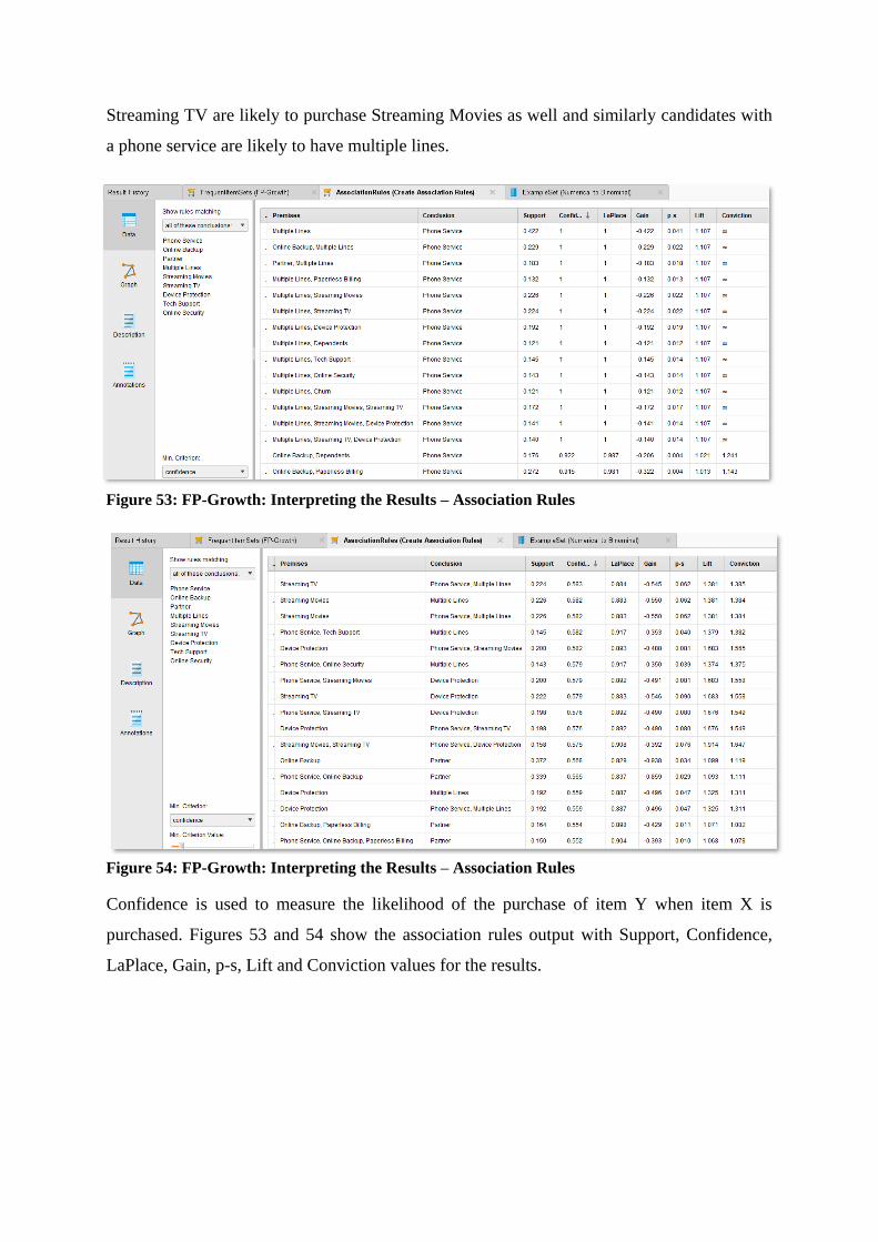
Streaming TV are likely to purchase Streaming Movies as well and similarly candidates with

a phone service are likely to have multiple lines.

Confidence is used to measure the likelihood of the purchase of item Y when item X is

purchased. Figures 53 and 54 show the association rules output with Support, Confidence,

LaPlace, Gain, p-s, Lift and Conviction values for the results.

Figure 53: FP-Growth: Interpreting the Results – Association Rules

Figure 54: FP-Growth: Interpreting the Results – Association Rules

Figures 55 and 56 show easy to understand rules of the FP-Growth algorithm. For example,

[Multiple Lines, Streaming TV] [Device Protection] (confidence: 0.627) can be interpreted

Figure 55: FP-Growth: Interpreting the Results – Association Rules

Figure 56: FP-Growth: Interpreting the Results – Association Rules

as a customer with multiple lines and streaming TV is likely to purchase device protection with

a confidence of 0.627. Similarly, other rules and their confidence values are in the two

aforementioned figures. These rules and the frequent item sets can be used to generate an

effective cross-selling model for telecom services and products.

4.12 Apriori: How to Implement in RapidMiner

Missing values are replaced using “Replace Missing Values” operator.

The “Select Attributes” operator is used to remove certain attributes like Monthly

Charges, Total Charges, Contract, Tenure from the process.

The Apriori algorithm should have binomial data with items in the columns and each

transaction as a row. The numerical attributes can be converted to binomial using the

“Numerical to Binomial” operator.

RapidMiner by default does not have the Apriori algorithm. The “W-Apriori” operator

is an extension of WEKA that can be used in RapidMiner. This operator implements

the apriori algorithm. It iteratively reduces the minimum support until it finds the

required number of rules with the given minimum confidence.

The “Create Association Rules” operator is not to used for implementing Apriori in

RapidMiner.

Figure 57: Apriori: How to Implement in RapidMiner

4.12.1: Apriori: Interpreting the Results

Similar to the FP-Growth results, the results of Apriori can be interpreted to understand the

rules found by Apriori. For example, result 4 – Multiple Lines = Yes, Device Protection = Yes,

Streaming Movies = Yes Streaming TV = Yes with confidence of 0.83 can be interpreted

as customers with the services of multiple lines, device protection and streaming movies are

very likely to subscribe to streaming TV as well.

Figure 58: Apriori: Interpreting the Results

CHAPTER 5 – CONCLUSION

5.1 Introduction

This chapter concludes the thesis with a review of the overall research performed as the well

the results and the insights gained from performing the research. The ways in which the telecom

industry can benefit from using data mining and machine learning are also discussed.

Suggestions for future research are also presented. The performance of the classification

algorithms implemented in RapidMiner are shown in the table below.

5.2 Summary of Performance of Classification Models in

RapidMiner

Table 3: Summary of Performance of Classification Algorithms

Algorithm Training

and Testing

Technique

Accuracy Precision Recall AUC

K-NN Split-

validation

51.38% 28.07% 53.21% 0.769

K-NN Split Data

(0.8:0.2 ratio

for training

and testing

respectively)

75.02% 52.91% 53.48% 0.794

K-NN Cross-

validation

76.36 +/-

1.40%

55.85 +/-

3.21%

53.35 +/-

3.67%

0.810

Overall, Random Forest with splitting data in to the ratio of 80% for training and 20%

for testing was the best performing classification model with an accuracy of 79.39%. It

also had the highest AUC value with 0.829.

Naïve Bayes with a recall of 83.21 +/- 2.73% had the highest recall value.

Meanwhile, k-nearest neighbor with split-validation was the worst performing model.

5.3 Summary of Results and Conclusion

As defined in section 1.4, this purpose of this research was to “to not only develop effective

and efficient models to recognize customer before they churn, but also to apply cross-selling

techniques in a telecom context to find useful patterns and associations that can be used

effectively by telecom companies”.

To successfully achieve the objectives of this research, as defined in section 1.5, a publicly

available telecom dataset consisting of a total of 7043 rows with 21 attributes of customers was

used. The data was already in a clean and readable format and hence significant data pre-

processing was not necessary. RapidMiner and R were used for implementing the machine

learning models. The results were similar in both the tools. K-Nearest Neighbor, Decision Tree,

Naïve Bayes and Random Forest were the four classification algorithms that were used to

predict customer churn and understand which of the attributes in the dataset were most

significant in determining whether a customer will churn or not. The results show that these

algorithms are successful in predicting customer churn. The attributes that were found to be

most significant in predicting customer churn are Contract, Tenure, Monthly Charges and

Decision

Tree

Cross-

validation

78.79 +/-

1.27%

64.13 +/-

3.08%

61.17 +/-

3.46%

0.822

Naïve Bayes Cross-

validation

70.08 +/-

0.80 %

46.45 +/-

0.84%

83.21 +/-

2.73%

0.820

Random

Forest

Split Data

(0.8:0.2 ratio

for training

and testing

respectively)

79.39% 69.42% 39.93% 0.829

Total Charges. It was found that customers with longer contracts (one year and two year) are

less likely to churn as opposed to customers with a month-to-month contract. The tenure

attribute is also highly influential in determining customer churn. Longer tenure customers are

less likely to churn. Loyal customers are also more likely to have high total and monthly

charges. The large number of telecom services related attributes this dataset also allowed for a

successful implementation of “Cross-selling” techniques in a telecom context. FP-Growth and

Apriori were implemented in RapidMiner to discover frequent item sets and associations

between attributes such as “Streaming Movies”, “Streaming TV”, “Device Protection”, “Tech

Support”, “Online Backup”, “Multiple Lines” etc.

To summarize, the key drivers of churn are identified in this study and relevant and useful

associations between products are established. Using this information telecom companies can

successfully work on improving customer churn by performing targeted marketing.

Companies can create personalized offers and campaigns customers who are at risk of

churning. Association rules can also help in identifying usage patterns, buying preferences,

socio-economic influences of customers.

5.4 Future Work

While the current research explores the implementation of classification and association

algorithms in great detail, ideas for future work can include the implementation of clustering

algorithms as well as classification algorithms such as Support Vector Machines and Neural

Networks. RapidMiner and R were used for this thesis and in the future studies can also

incorporate other data mining and machine learning platforms. Apart from churn prediction

and cross-selling, data mining in the telecom industry offers some other benefits as well. Some

of these are:

Fraud Detection: Fraud detection is a major source of revenue loss for organisations

every year can also be improved by mining of data in the telecom industry.

Network Optimisation and Expansion: Correlating network usage and subscriber

density with traffic and location data can help telecom providers in accurately managing

network capacity and forecasting & planning for any potential network outages. Data

mining techniques can also be used while planning for network expansions by

identifying areas where network usage is nearing its capacity.

Future studies can focus on this aspect of data mining in the telecom industry. Overall, machine

learning and data mining can help telecom companies to make much better decisions regarding

their own business, marketing, service offerings etc. in order to get the most out of their

business.

REFERENCES

Agrawal, R., Imieliński, T. & Swami, A. (1993). ‘Mining association rules

between sets of items in large databases’. Proceedings of the 1993 ACM

SIGMOD international conference on Management of data - SIGMOD '93.

p. 207.

Almana, A.M., Aksoy, M.S. & Alzahrani, R. (2014), ‘A Survey On Data

Mining Techniques In Customer Churn Analysis For Telecom Industry’,

Int. Journal of Engineering Research and Applications, Vol. 4(5), pp. 165-

171.

Berry, M. & Linoff, G. (2014), ‘Data Mining Techniques for Marketing,

Sales and Customer Relationship Management (2nd edition)’. Indianapolis:

Wiley.

Bronhstein, A. (2017), ‘A Quick Introduction to K-Nearest Neighbors

Algorithm’, Medium. Http: https://medium.com/@adi.bronshtein/a-

quick-introduction-to-k-nearest-neighbors-algorithm-62214cea29c7

(Last Accessed: 25/10/2018).

Chaurasia, K. (No Date), ‘DBSCAN Clustering Algorithm’, Practice 2

Code. Http: https://practice2code.blogspot.com/2017/07/dbscan-

clustering-algorithm.html (Last Accessed: 1/11/2018).

Chen, C. (2016), ‘Use Cases and Challenges in Telecom Big Data

Analytics’, Asia Pacific Signal and Information Processing Association ,

Vol. 5(19), pp. 1-7.

Deep AI (2018), ‘Neural Network: What is a Neural Network?’. Http:

https://deepai.org/machine-learning-glossary-and-terms/neural-

network (Last Accessed: 29/10/2018).

Deshpande, B. & Kotu, V. (2014), ‘Predictive Analytics and Data Mining:

Concepts and Practice with RapidMiner’. London: Elsevier

Gruber, C. (2016), ‘Using Customer Behavior Data to Improve Customer

Retention’, IBM. Http:

https://www.ibm.com/communities/analytics/watson-analytics-

blog/using-customer-behavior-data-to-improve-customer-retention/.

(Last Accessed: 15/10/2018).

Hafez, H.A.A (2016), ‘Mining Big Data in Telecommunications Industry:

Challenges, Techniques, and Revenue Opportunity’, Dubai UAE Jan 28-

29, 18 (1), pp. 4297-4304. Academia [Online].

Han, J., Pei, J., & Kamber, M. (2011), Data mining: concepts and

techniques. Elsevier.

Hurtgen, H., Natarajan, S., Spittaels, S., Vetvik, O.J. & Ying, S. (2012),

‘Crunch Time: Using Big Data to Boost Telco Marketing Capabilities’,

McKinsey. Http:

https://www.mckinsey.com/~/media/mckinsey/dotcom/client_service/T

elecoms/PDFs/RecallNo21_Big_Data_2012-07.ashx (Last Accessed:

17/11/2018).

Jain, S. (2016) ‘Analysis and Application of Data Mining Methods used

for Customer Churn in Telecom Industry’, LinkedIn. Http:

https://www.linkedin.com/pulse/analysis-application-data-

miningmethods-used-customer-saurabh-jain/ (Accessed: 4 September

2018).

Jaroszewicz, S. (2008), ‘Cross-Selling Models for Telecommunication

Services’, Journal of Telecommunications and Information Technology,

Vol. 3. pp. 52-59.

Jin, X. & Han, J. (2011), ‘K-Medoids Clustering. In: Sammut C., Webb

G.I. (eds) Encyclopedia of Machine Learning’. Boston, MA: Springer.

Joseph, M. (2013), ‘Data Mining and Business Intelligence Applications

in Telecommunication Industry’, International Journal of Engineering and

Advanced Technology, Vol. 2(3), pp. 525-528.

Jovic, A., Brkic, K. & Bogunovic, N. (2014), “An Overview of Free

Software Tools for General Data Mining”, 37th International Convention

on Information & Communication Technology Electronics &

Microelectronics, pp. 1112-1117.

Keramati, A., Jafari-Marandi, R., Aliannejadi, M, Ahmadian, I.,

Mozzafari, M. & Abbasi, U. (2014), ‘Improved churn prediction in

telecommunication industry using data mining techniques’, Applied Soft

Computing, Vol. 24, pp. 994-1012.

Kirui, C., Hong, L., Cheruiyot, W. & Kirui, H. (2013), ‘Predicting

Customer Churn in Mobile Telephony Industry Using Probabilistic

Classifiers in Data Mining’, International Journal of Computer Science

Issues, Vol. 10(2), pp. 165-172.

Liu, Y. & Zhuang, Y. (2015), ‘Research Model of Churn Prediction Based

on Customer Segmentation and Misclassification Cost in the Context of

Big Data’, Journal of Computer and Communications, Vol. 3, pp. 87- 93.

McDonald, C. (2017), ‘Machine learning fundamentals (II): Neural

networks’, Towards Data Science. Http:

https://towardsdatascience.com/machine-learning-fundamentals-ii-

neural-networks-f1e7b2cb3eef (Last Accessed: 29/10/2018).

Qureshi, S.A., Rehman, A.S., Qamar, A.M., Kamal, A. & Rehman, A.

(2013), ‘Telecommunication Subscribers' Churn Prediction Model Using

Machine Learning’, Conference: IEEE International Conference on Digital

Information Management (ICDIM)At: Islamabad, Pakistan.

RapidMiner (No Date), ‘RapidMiner Documentation (Auto Model)’, Http:

https://docs.rapidminer.com/latest/studio/auto-model/ (Last Accessed:

21/11/2018).

RapidMiner (No Date), ‘RapidMiner Documentation: Cross Validation

(Concurrency)’, Http:

https://docs.rapidminer.com/latest/studio/operators/validation/cross_v

alidation.html (Last Accessed: 27/11/2018).

Saraswat, S. & Tiwari, A. (2018), ‘A New Approach for Customer Churn

Prediction in Telecom Industry’, International Journal of Computer

Applications, Vol. 181(11), pp. 40-46.

SAS (No Date), ‘What is Data Mining?’. Http:

https://www.sas.com/en_ie/insights/analytics/data-mining.html (Last

Accessed: 4/9/2018).

Scheffer, T. (2001) ‘Finding Association Rules That Trade Support

Optimally against Confidence. In: 5th European Conference on Principles

of Data Mining and Knowledge Discovery’, pp. 424-435.

Shaaban, E., Helmy, Y., Khedr, A. & Nasr, M. (2012), ‘A Proposed Churn

Prediction Model’, International Journal of Engineering Research and

Applications, Vol. 2(4), pp. 693-697.

Tsiptsis, K. and Chorianopoulos, A. (2009), ‘Data Mining Techniques in

CRM: Inside Customer Segmentation’. Chichester: Wiley.

Van den Poel, D. & Lariviere, B. (2004), ‘Customer Attrition Analysis for

Financial Services Using Proportional Hazard Models’, European Journal

of Operational Research, Vol. 157(1), pp. 196-217.

Webb, G.I. (2011) Lazy Learning. In: Sammut, C., Webb, G.I. (eds)

Encyclopedia of Machine Learning. Boston, MA: Springer.

Weiss, G. (2010), ‘Data Mining in the Telecommunications Industry’,

Networking and Telecommunications: Concepts, Methodologies, Tools,

and Applications, pp. 194-201.

Witten, I., Frank, E. & Hall, M. (2011), ‘Data Mining’. Burlington, MA:

Morgan Kaufmann.

APPENDIX

# Installing relevant packages

# install.packages("ggplot2")

# install.packages("caret")

# install.packages("class)

# install.packages("rpart")

# install.packages("arules")

# Load libraries

library(MASS)

library(randomForest)

library(party)

library(e1071)

library(caret)

library(caTools)

library(dplyr)

library(rpart)

library(arules)

library(randomForest)

library(pROC)

# Load the dataset

TelecomChurn <- read.csv(file.choose(), header = T)

summary(TelecomChurn)

str(TelecomChurn)

# Check if the dataset has missing values

sum(is.na(TelecomChurn)

# There are a total of 11 missing values in the dataset

# Checking the attribute(s) with the missing values

sapply(TelecomChurn, function(x) sum(is.na(x)))

# The attribute TotalCharges has 11 missing values

# create new dataset without missing data

NewTelecomChurn <- na.omit(TelecomChurn)

# Checking if the missing values attribute was removed successfully

sum(is.na(NewTelecomChurn))

# There are no missing values now

# More data cleansing

# Removing Customer ID attribute since it is of no use for the analysis

NewTelecomChurn$customerID <- NULL

str(NewTelecomChurn)

# Changing the values for the Senior Citizen attribute from 0 and 1 to No and Yes

respectively

NewTelecomChurn$SeniorCitizen <- as.factor(ifelse(NewTelecomChurn$SeniorCitizen ==

0, "No", "Yes"))

str(NewTelecomChurn)

# Decision Tree

# For easier interpretation, we can convert the tenure attribute from months to year for

the decision tree.

NewTelecomChurn <- mutate(NewTelecomChurn, TenureYear = tenure)

NewTelecomChurn$TenureYear[NewTelecomChurn$TenureYear >=0 &

NewTelecomChurn$TenureYear <= 12] <- '0-1 Year'

NewTelecomChurn$TenureYear[NewTelecomChurn$TenureYear > 12 &

NewTelecomChurn$TenureYear <= 24] <- '1-2 Years'

NewTelecomChurn$TenureYear[NewTelecomChurn$TenureYear > 24 &

NewTelecomChurn$TenureYear <= 36] <- '2-3 Years'

NewTelecomChurn$TenureYear[NewTelecomChurn$TenureYear > 36 &

NewTelecomChurn$TenureYear <= 48] <- '3-4 Years'

NewTelecomChurn$TenureYear[NewTelecomChurn$TenureYear > 48 &

NewTelecomChurn$TenureYear <= 60] <- '4-5 Years'

NewTelecomChurn$TenureYear[NewTelecomChurn$TenureYear > 60 &

NewTelecomChurn$TenureYear <= 72] <- '5-6 Years'

NewTelecomChurn$TenureYear <- as.factor(NewTelecomChurn$TenureYear)

# Split data into training and test sets

n = nrow (NewTelecomChurn)

indexes = sample (n , n * (80/100))

Trainset = NewTelecomChurn[indexes,]

Testset = NewTelecomChurn[-indexes,]

# Using the attributes "contract", "TenureYear" and "PaperlessBilling" to create the

plot the decision tree

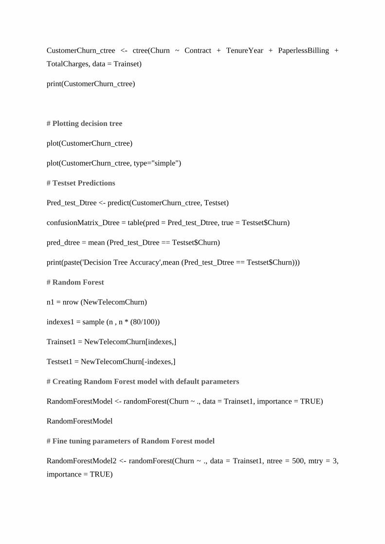
CustomerChurn_ctree <- ctree(Churn ~ Contract + TenureYear + PaperlessBilling +

TotalCharges, data = Trainset)

print(CustomerChurn_ctree)

# Plotting decision tree

plot(CustomerChurn_ctree)

plot(CustomerChurn_ctree, type="simple")

# Testset Predictions

Pred_test_Dtree <- predict(CustomerChurn_ctree, Testset)

confusionMatrix_Dtree = table(pred = Pred_test_Dtree, true = Testset$Churn)

pred_dtree = mean (Pred_test_Dtree == Testset$Churn)

print(paste('Decision Tree Accuracy',mean (Pred_test_Dtree == Testset$Churn)))

# Random Forest

n1 = nrow (NewTelecomChurn)

indexes1 = sample (n , n * (80/100))

Trainset1 = NewTelecomChurn[indexes,]

Testset1 = NewTelecomChurn[-indexes,]

# Creating Random Forest model with default parameters

RandomForestModel <- randomForest(Churn ~ ., data = Trainset1, importance = TRUE)

RandomForestModel

# Fine tuning parameters of Random Forest model

RandomForestModel2 <- randomForest(Churn ~ ., data = Trainset1, ntree = 500, mtry = 3,

importance = TRUE)

RandomForestModel2

# Predicting on Training Set

predTrainRandomForest <- predict(RandomForestModel2, Trainset1, type = "class")

# Checking classification accuracy

table(predTrainRandomForest, Trainset1$Churn)

# Predicting on Test set

predTestRandomForest <- predict(RandomForestModel2, Testset1, type = "class")

# Checking classification accuracy

mean(predTestRandomForest == Testset1$Churn)

# 0.7896233

# Checking Important Variables

importance(RandomForestModel2)

# Plotting Important Variables

varImpPlot(RandomForestModel2)

# Naive Bayes

n2 = nrow (NewTelecomChurn)

indexes2 = sample (n , n * (80/100))

Trainset2 = NewTelecomChurn[indexes,]

Testset2 = NewTelecomChurn[-indexes,]

NaiveBayes <- naiveBayes(Churn ~ ., data = Testset2)

NaiveBayes

predNaiveBayes = predict(NaiveBayes, Testset2)

# Confusion Matrix

tab = table(predNaiveBayes,Testset2$Churn)

sum (tab[row(tab)==col(tab)])/sum(tab)

# Using Laplace Smoothing:

model <- naiveBayes(Churn ~ ., data = NewTelecomChurn, laplace = 1)

pred1 <- predict(model, NewTelecomChurn)

tab1 <- table(pred1, NewTelecomChurn$Churn)

sum(tab[row(tab)==col(tab)])/sum(tab)

# AUC for the three models

DecisionTreeROC <- roc (response = Testset$Churn, predictor = as.numeric(Pred_test_Dtree))

RandomForestROC <- roc (response = Testset1$Churn, predictor =

as.numeric(predTestRandomForest))

NaiveBayesROC <- roc (response = Testset2$Churn, predictor =

as.numeric(predNaiveBayes))

# Plotting ROC curves for the three models

plot (DecisionTreeROC,legacy.axes = TRUE, col = "blue", print.auc.y = 0.4, print.auc =

TRUE)

plot (RandomForestROC, col = "red", add = TRUE, print.auc.y = 0.5, print.auc = TRUE)

plot (NaiveBayesROC, col = "green" , add = TRUE, print.auc.y = 0.6, print.auc = TRUE)

legend(0.1,0.3, c("Naive Bayes", "Random Forest", "Decision Tree"), lty = c(1,1), lwd = c(2,

2), col = c("green", "red", "blue"), cex = 0.8)