applications of network science to criminal networks...
TRANSCRIPT

University of California
Los Angeles
Applications of Network Science to Criminal
Networks, University Education, and Ecology
A dissertation submitted in partial satisfaction
of the requirements for the degree
Doctor of Philosophy in Mathematics
by
Charles Zachary Marshak
2016


Abstract of the Dissertation
Applications of Network Science to Criminal
Networks, University Education, and Ecology
by
Charles Zachary Marshak
Doctor of Philosophy in Mathematics
University of California, Los Angeles, 2016
Professor Andrea L. Bertozzi, Co-chair
Professor Mason A. Porter, Co-chair
Networks are a powerful tool to investigate complex systems. In this work, we apply
network–theoretic tools to study criminal, educational, and ecological systems.
First, we propose two generative network models for recruitment and disruption in a
hierarchal organized crime network. Our network models alternate between recruitment and
disruption phases. In our first model, we simulate recruitment as Galton–Watson branching.
We simulate disruption with an agent that moves towards the root and arrests nodes in ac-
cordance with a stochastic process. We prove a lower bound on the probability that the agent
reaches the kingpin and verify this numerically. In our second model, we propose a network
attachment mechanism to simulate recruitment. We define an attachment probability based
on an existing node’s distance to the leaf set (terminal nodes), where this distance is a proxy
for how close a criminal is to visible illicit activity. Using numerical simulation, we study the
network structures such as the degree distribution and total attachment weight associated
with large networks that evolve according to this recruitment process. We then introduce a
disruptive agent that moves through the network according to a self-avoiding random walk
and can remove nodes (and an associated subtree) according to different disruption strate-
gies. We quantify basic law enforcement incentives with these different disruption strategies
and study costs and eradication probability within this model.
ii

In our next chapter, we adapt rank aggregation methods to study how Mathematics
students navigate their coursework. We first translate 15 years of grade data from the
UCLA Department of Mathematics into a network whose nodes are the various Mathematics
courses and whose edges encode the flow of students between these courses. Applying rank
aggregation on such networks, we extract a linear sequence of courses that reflects the order
students select courses. Using this methodology, we identify possible trends and hidden
course dependencies without investigating the entire space of possible schedules. Specifically,
we identify Mathematics courses that high–performing students take significantly earlier than
low–performing students in various Mathematics majors. We also compare the extracted
sequence of several rank aggregation methods on this data set and demonstrate that many
methods produce similar sequences.
In our last chapter, we review core–periphery structure and analyze this structure in mu-
tualistic (bipartite) fruigivore–seed networks. We first relate classical graph cut problems to
previous work on core–periphery structure to provide a general mathematical framework. We
also review how core–periphery structure is traditionally identified in mutualistic networks.
Next, using a method from Rombach et al., we analyze the core–periphery structure of 10
mutualistic fruigivore–seed networks that encode the interaction patterns between birds and
fruit–bearing plants. Our collaborators use our network analysis with other ecological data
to identify important species in the observed habitats. In particular, they identify certain
types of birds (mashers) that play crucial roles at a variety of sites, which are though to be
less important due to their feeding behaviors.
iii

The dissertation of Charles Zachary Marshak is approved.
P. Jeffrey Brantingham
Joseph Teran
Wotao Yin
Mason A. Porter, Committee Co-chair
Andrea L. Bertozzi, Committee Co-chair
University of California, Los Angeles
2016
iv

To Nade
v

Table of Contents
1 Introduction . . . . . . . . . . . . . . . . . . . . . . . . . . . . . . . . . . . . . . 1
2 Growth and Disruption of a Hierarchical Criminal Network . . . . . . . . 5
2.1 Related Models for Criminal Organization and Behavior . . . . . . . . . . . 6
2.2 Criminal Recruitment and Disruption Model I . . . . . . . . . . . . . . . . . 10
2.2.1 Recruitment Mechanism . . . . . . . . . . . . . . . . . . . . . . . . . 10
2.2.2 Pursuit Mechanism . . . . . . . . . . . . . . . . . . . . . . . . . . . 15
2.2.3 Conclusions from Model . . . . . . . . . . . . . . . . . . . . . . . . . 21
2.3 Criminal Recruitment and Disruption Model II . . . . . . . . . . . . . . . . 22
2.3.1 Model Overview and Related Network Processes . . . . . . . . . . . . 23
2.3.2 Recruitment Mechanism . . . . . . . . . . . . . . . . . . . . . . . . . 30
2.3.3 Pursuit Mechanism . . . . . . . . . . . . . . . . . . . . . . . . . . . . 39
2.3.4 Conclusions from Model . . . . . . . . . . . . . . . . . . . . . . . . . 53
2.4 Conclusions and Future Work . . . . . . . . . . . . . . . . . . . . . . . . . . 55
3 Rank Aggregation for Course Sequence Discovery . . . . . . . . . . . . . . 58
3.1 Introduction . . . . . . . . . . . . . . . . . . . . . . . . . . . . . . . . . . . . 59
3.2 Related Work . . . . . . . . . . . . . . . . . . . . . . . . . . . . . . . . . . . 61
3.3 Student Data . . . . . . . . . . . . . . . . . . . . . . . . . . . . . . . . . . . 64
3.4 Models and Methods for Rank Aggregation . . . . . . . . . . . . . . . . . . . 69
3.5 Matrix Methods for Rank Aggregation . . . . . . . . . . . . . . . . . . . . . 74
3.5.1 Preliminary Networks . . . . . . . . . . . . . . . . . . . . . . . . . . . 75
3.5.2 PageRank . . . . . . . . . . . . . . . . . . . . . . . . . . . . . . . . . 77
3.5.3 Rank Centrality . . . . . . . . . . . . . . . . . . . . . . . . . . . . . . 79
vi

3.5.4 SerialRank . . . . . . . . . . . . . . . . . . . . . . . . . . . . . . . . . 80
3.5.5 SyncRank . . . . . . . . . . . . . . . . . . . . . . . . . . . . . . . . . 82
3.5.6 Least Squares . . . . . . . . . . . . . . . . . . . . . . . . . . . . . . . 84
3.5.7 Ranking via Singular Value Decomposition . . . . . . . . . . . . . . . 84
3.5.8 Evaluating a Course Sequence . . . . . . . . . . . . . . . . . . . . . . 85
3.6 Course-Sequence Discovery . . . . . . . . . . . . . . . . . . . . . . . . . . . . 87
3.6.1 Evaluating the Matrix Methods . . . . . . . . . . . . . . . . . . . . . 87
3.6.2 Identifying Hidden Course Dependencies . . . . . . . . . . . . . . . . 95
3.7 Conclusions and Future Work . . . . . . . . . . . . . . . . . . . . . . . . . . 97
4 Core–Periphery Structure in Frugivore–Seed Networks . . . . . . . . . . . 103
4.1 Notations and Related Graph Calculus . . . . . . . . . . . . . . . . . . . . . 104
4.2 Core–Periphery Structure . . . . . . . . . . . . . . . . . . . . . . . . . . . . 110
4.2.1 Combinatorial Quantities Related to Core–Periphery Structure . . . . 113
4.2.2 Models for Core–Periphery Structure . . . . . . . . . . . . . . . . . . 118
4.3 Core–Periphery Structure in Frugivore–Seed Networks . . . . . . . . . . . . . 135
4.4 Conclusions and Future Work . . . . . . . . . . . . . . . . . . . . . . . . . . 140
A Rank Aggregation for Course–Sequence Discovery . . . . . . . . . . . . . . 143
A.1 Course Numbers . . . . . . . . . . . . . . . . . . . . . . . . . . . . . . . . . 143
B Core-Periphery Structure in Fruigivore–Seed Networks . . . . . . . . . . 145
B.1 Simulated Annealing . . . . . . . . . . . . . . . . . . . . . . . . . . . . . . . 145
References . . . . . . . . . . . . . . . . . . . . . . . . . . . . . . . . . . . . . . . . . 148
vii

List of Figures
2.1 The recruitment process at t = 3 with ξ ∼ Pois(1.3). The darkest node at
the top is the kingpin. The yellow nodes at the bottom are those recruited
at t = 3. These yellow nodes are the only nodes eligible to recruit during
t = 4. The variable ξti indicates the number of criminals recruited at time
t by the ith criminal previously added during t − 1. We have enumerated
criminals recruited at time t from left to right. The variable Ct indicates the
total number of criminals added at time t. . . . . . . . . . . . . . . . . . . . 12
2.2 We estimate the expected height E(H) in two different ways for varying λ
for R(ξ) and ξ Poisson-distributed with mean λ. First, we estimate E(H)
using the experimental mean H over 10,000 simulations. We set the height
threshold m = 250 and stop the recruitment process when this height is
reached. Alternatively, we inspect m(1 − r), numerically solving for r using
Eq. (2.2) with ϕ(s) = eλ(s−1). . . . . . . . . . . . . . . . . . . . . . . . . . . 16
2.3 An example of a P(ξ,N0, z) during the first time step. Let N0 be the network
found in Figure 2.1. Let z ∈ [0, 1] and ξ ∼ Pois(1.3). The agent uniformly at
random selects a node eligible to recruit; these are the yellow nodes in Figure
2.1. The agent begins their investigation at v1, moves to v2, and then ends at
v3. At v3, the agent is unable to move upwards once more and removes the
subtree below their current position. The arrested criminals are in blue with
thick boundary. The yellow node at the bottom right, labeled with an l, is
still able to recruit, and the network has not been terminated. . . . . . . . . 18
2.4 The experimental mean H and the upper bound from Eq. (2.5) for various
z. We use 10,000 simulations to compute H and initialize a network to be a
perfect binary tree of height 2. We set the height threshold m to be 250. . . 20
viii

2.5 A simulated recruitment process for t = 0, 1, 2, 3. The network starts with
a single criminal (the kingpin) and then evolves according to the proposed
attachment mechanism. Here the number of new criminals introduced into
the network is given by the recruitment index k = 5. The leaf nodes (light
yellow) represent criminals without underlings. In our model, these leaf nodes
are called street criminals. Of these, the nodes with the darker boundary are
those freshly recruited at a given time step. For example, the number of street
criminals when t = 3 is 8, of which 5 are new recruits. . . . . . . . . . . . . . 29
2.6 The criminal network at t = 3 with the values of w(j; t) shown. Here, the
recruitment index k = 5 and the initial configuration consists of a single
kingpin. All criminals j in S(t) have attachment weight w(j; t) = 1. . . . . . 31
2.7 The out-degree distribution P∞(d) of nodes on a criminal network determined
from numerical simulations for t → ∞. The three curves correspond to re-
cruitment indices k = 1, 10, 20. We terminate a simulation when the total
number of criminals reaches or exceeds 5 × 10³. Each curve for P∞(d) rep-
resents 100 simulations. The tail of the degree distribution is noisier as high
degree nodes are rarer than low degree nodes. As discussed in the text, we fit
the distribution to a decaying exponential distribution. The numerics indicate
that P∞(d = 0) ≈ 0.39 for all the values of k we considered. . . . . . . . . . . 32
2.8 We show the distribution of distances from the kingpin. These distributions
are the average over 100 runs, stopping each simulation at t = 100, 200, or 300.
We set the recruitment index k = 10 and the initial configuration to be the
kingpin alone. We then fit the measured distributions using a shifted gamma
density ρα,β,s(y) (Eq. (2.12)). We label this fit γ-distribution as γ(α, β, s). . 35
ix

2.9 (Top) The number s(t) of street criminals as a function of time t for recruit-
ment rates k = 10, 50, 100. In each simulation, we terminate the recruitment
process when the total number of criminals exceeded 5×10³. Each data point
is the average of 250 simulations. We fit the data to s(t) = rst+ 1 and expect
rs ≈ P∞(d = 0)k, where P∞(d = 0) ≈ 0.39. This scaling is confirmed with the
fit values of rs in the legend. (Bottom) The slope values rs as a function of
k with the rs values from the top display shown in dark symbols with corre-
sponding shapes. We then fit the data with a line as indicated in the bottom
legend, providing evidence of our conjecture rs ≈ P∞(d = 0)k. . . . . . . . . 36
2.10 Schematic of the addition of new nodes from time t to time t + 1. Here, the
recruitment index k is 3. We depict the leaf nodes in yellow and those nodes
added from t to t + 1 with thick boundary. We indicate the attachment of a
new leaf node to an internal node with a solid gray halo seen on the lower left
hand side of the image. We also indicate the attachment of new leaf nodes to
previously leaf nodes with a the dashed ring. In this recruitment phase, the
total number of street criminals at time t + 1 increase by 1 from time t. In
other words, this recruitment phase dictates s(t+ 1) = s(t) + 1. . . . . . . . 37
2.11 Total attachment weight∑
j∈C(t) w(j; t) of the network as a function of time
averaged over 100 runs for k = 10, 20, 30, 40. We initialized the network as the
kingpin alone. We terminate each simulation when the number of criminals
reaches 5 × 10³. We fit the data to a linear form Wt + w0 and find that the
extrapolated values of W in the figure legend are in excellent agreement with
the ones predicted from Eq. (2.18), given by W = 6.39, 12.79, 19.18, 25.57 for
k = 10, 20, 30, 40, respectively. . . . . . . . . . . . . . . . . . . . . . . . . . . 40
x

2.12 The pursuit phase as we describe in Section 2.3.3. We initialize the network
as a perfect ternary tree of height three. The network consists of the light
and dark colored nodes. The light nodes are those nodes invisible to our
agent during the pursuit phase. The dark nodes are those nodes that have
been investigated or arrested. (Left) At time t = 1 the agent begins their
pursuit from the yellow criminal and without having perfect knowledge of the
network. He investigates three other nodes, highlighted in red marked by a
solid dark line. The last node, surrounded by a dark ring, is the criminal that is
currently under investigation. (Right) The criminal that is under investigation
is arrested. Once a criminal is arrested, they are removed from the network
along with all of their direct underlings, their direct underlings, and so on.
The arrested nodes are depicted in blue and have a darker boundary. Note
that not all criminals arrested are investigated and vice versa. . . . . . . . . 43
2.13 Network eradication probability as a function of the recruitment index k,
obtained by averaging over 10,000 simulations for different strategies. We
consider a total population of n∗ = 500, 1000, 2000 individuals and halt our
simulations when the criminal network reaches this size. For each strategy,
the Beat(Q) denotes the maximum recruitment index k for which the network
is eradicated with probability 1, over all simulations. . . . . . . . . . . . . . 45
xi

2.14 Varying initial conditions prior to law enforcement intervention. (Left) Erad-
ication probabilities on a complete initial tree with b branches and forty crim-
inals for k = 30 and law enforcement strategy QD(q = 3). When a graph
consists of a single path (b = 1), the eradication probability is 1, because dead
ends cannot be reached. Increasing b allows more dead ends to be encoun-
tered, so that the eradication probability decreases until b = 3 and plateaus
until b = 6. After b = 6, the height of the network becomes small enough to
allow for easier access to the kingpin. (Center and Right) Eradication proba-
bilities using perfect initial trees with branching factor b and height h as initial
conditions and using strategy QD(q = 3). The initial number of criminals is
(bh+1 − 1)/(b− 1). . . . . . . . . . . . . . . . . . . . . . . . . . . . . . . . . 46
2.15 (Top) Costs incurred by law enforcement conditioned on kingpin capture as
a function of the recruitment index k. Shades in the data points represent
the probabilities of network eradication. We consider 10000 simulations and
allow the network to grow to n∗ = 1000. There is the emergence of maxima
for certain curves because we condition on the eradication of the network.
As k increases initially for such curves, the network grows more rapidly and
so too does the number of investigations necessary for eradication. Upon
reaching a threshold in k (maxima), the number of possible pursuit phases
greatly decreases. In particular, for large k, a network must be eradicated
within fewer pursuit phases and thereby reducing cost. (Bottom) The mean
eradication time as a function of k for various strategies. Similarly as in the
above panel, there is an emergence of maxima only now for all curves. Note
that cost and time curves for QA(p = 1) and QD(q = 1) are identical and that
QI = QA(p→∞) = QD(q →∞). . . . . . . . . . . . . . . . . . . . . . . . . 57
xii

3.1 A subgraph corresponding to the proportion matrix P defined Eq. (3.9) for
Applied Mathematics majors. Each node represents a course; for this sub-
graph, we selected Linear Algebra I (Math 115A), Real Analysis I (Math
131A), and Discrete Structures (Math 61). The edge weight Pij from course i
to j indicates the proportion of students that took i in an earlier quarter than
j out of all those students that took the pair of courses in different quarters. 79
3.2 The proportion matrix P for Pure Mathematics students with A-range GPA.
We order courses with PageRank. . . . . . . . . . . . . . . . . . . . . . . . . 94
4.1 Two examples weight matrices for networks with characteristic mesoscale
structures: community structure (a) and core–periphery structure (b). We
illustrate strong, intermediate, and weak edge weight. In Figure 4.1a, C1 and
C2 are two disjoint communities with strong edge weight within a community
and weak edge weight between communities. In Figure 4.1b, C1 is the core
and C2 the periphery such that the core is strongly connected to itself, the core
is connected to the periphery with intermediate weight, and the periphery is
connected weakly to itself. . . . . . . . . . . . . . . . . . . . . . . . . . . . 110
4.2 The barbell graph in which there are two complete graphs on 10 vertices
connected by a single edge. The shaded regions indicate the disconnected
subgraphs when a single edge connecting these two subgraphs is removed. . . 113
4.3 The k-cores for k = 1, 2, 3 enclosed in increasingly dark concentric ellipses,
respectively. Note that the largest degree node is not considered part of the
core for k > 1 as it is connected to several degree one nodes. Using the
k-core requires a core structure to be well connected with itself, though not
necessarily with the periphery. . . . . . . . . . . . . . . . . . . . . . . . . . . 115
4.4 (a) A realization of a network from the stochastic block model from Eq.
(4.23)–(4.24) with parameters nc = np = 50, pcc = .8, and pcp = ppp = .5
specified. (b) A histogram of degrees in the same network. . . . . . . . . . . 120
xiii

4.5 (a) A rank-2 adjacency matrix of a core–periphery structure. (b) An adjacency
matrix that we generate from a stochastic block model with parameters pcc =
pcp = .8 and ppp = .5. (c) A rank-2 approximation of the adjacency matrix
with entrywise thresholding such that each entry wij in rank-2 matrix is set
to 0 if wij < .5 else we set wij to 1. . . . . . . . . . . . . . . . . . . . . . . . 122
4.6 S(α, β, n) where α = .7, β = .5, and n = 30. We consider fα,β with range
S(α, β, n). . . . . . . . . . . . . . . . . . . . . . . . . . . . . . . . . . . . . . 131
4.7 Core matrices for an instance of a stochastic block model using three different
centralities. The network was generated using tje stochastic block model
specified with Eq. (4.23)–(4.24) and parameters nc = np = 50, pcc = .8,
pcp = ppp = .5. We set t in Eq. (4.55) to be the median of nonzero entries. . 134
4.8 The weight matrix associated to Pozo Verde, one of the 10 sites. Each fru-
givore is labeled with an ‘(F)’. The weight between frugivores and plants is
determined from the number of recorded interactions. A related network vi-
sualization is in Figure 4.9. . . . . . . . . . . . . . . . . . . . . . . . . . . . . 136
4.9 The network from Pozo Verde with weight matrix shown in Figure 4.8. The
nodes’s sizes are proportional to their aggregate core score (Eq. (4.51)). The
edges are proportional to the weight. The two darker nodes are core-nodes.
These nodes define a cut that maximizes CP-Cut from (Eq. (4.52)). . . . . 137
4.10 The matrix of Rα,β from Eq. (4.50). . . . . . . . . . . . . . . . . . . . . . . . 141
4.11 The profile of CP-Cut(Ck, Pn−k) as a function of k, where we scaled each
entry of W dividing by the maximum entry. . . . . . . . . . . . . . . . . . . 142
4.12 A scatter plot for degree versus core scores for two sites. We compute the
correlation coefficient ρ. . . . . . . . . . . . . . . . . . . . . . . . . . . . . . 142
xiv

List of Tables
2.1 A table comparing the terminology used for our recruitment and disruption
model and that of standard network theory. . . . . . . . . . . . . . . . . . . 10
2.2 A table comparing the terminology used in this paper and that of standard
network theory. . . . . . . . . . . . . . . . . . . . . . . . . . . . . . . . . . . 28
2.3 The parameters of the recruitment mechanism. . . . . . . . . . . . . . . . . . 33
3.1 Sample of data provided by department of mathematics. . . . . . . . . . . . 65
3.2 Course Sequences for Applied Mathematics Majors obtained by three of the
six methods discussed in this chapter. . . . . . . . . . . . . . . . . . . . . . . 88
3.3 Course Sequences for Applied Mathematics Majors obtained by the three of
the six methods discussed in this chapter. . . . . . . . . . . . . . . . . . . . 89
3.4 K(q) coefficients for Applied Mathematics, Applied Science, and Pure Math-
ematics. Each major has ns total students. We subdivide each majors into
GPA categories: All ([0, 4.3]), A-range ([3.7, 4.3]), B-range ([2.7, 3.7)), and
C-range ([1.7, 2.7)). . . . . . . . . . . . . . . . . . . . . . . . . . . . . . . . . 93
3.5 First 11 courses for A students in five different majors using SerialRank. . . 98
3.6 Comparing the A and C students in three majors using SyncRank. . . . . . . 99
A.1 Course names and numbers. . . . . . . . . . . . . . . . . . . . . . . . . . . . 144
xv

Acknowledgments
This thesis is the culmination of several years of study, research, and collaboration. It is
an honor and a privilege to move through the doctoral process at UCLA. I am appreciative
of the exceptional academic guidance of my supervisors: Professor Andrea Bertozzi and
Professor Mason Porter. It was a joy to work under Professor Bertozzi. She gave me
interesting applied problems to study, freely shared her mathematical insights, provided
fascinating datasets for me and colleagues to explore, and connected me with the talented
students, postdocs, and professors in her group. Professor Porter generously shared his
time, energy, expertise, and humor in my final quarter and pushed me to be a better applied
mathematician and analytic thinker. His passion and integrity has been inspiring even before
he became an official supervisor. I also want to acknowledge the mentorship of Professor
Puck Rombach, who was my guide through the wonderful world of networks since she first
introduced me to Galton-Watson branching in the Fall of 2013. I am appreciative of my
fruitful collaborations with Professor Mihai Cucuringu, Professor Maria D’Orsogna, and
Dillon Montag. Professor Cucuringu, in particular, helped me to ask great questions of large
data sets. I am also grateful to my committee: Professor Brantingham, Professor Teran, and
Professor Yin. Each were available for discussions and guidance during this research.
I feel fortunate to have been apart of an amazing community at UCLA. I am grateful to
Ryan Compton for sparking my interest in applied mathematics. He pointed me toward im-
portant computational tools, inspired me with his knack for data-centric problems, provided
endless encouragement and shared a love for international cuisine. I am very grateful to the
numerous classes that I took at UCLA in mathematics, each building confidence and skills
that made this research tenable. Specifically, I am particularly grateful for Professor Teran’s
great courses on computational linear algebra; Professor Yin’s insights into the field of nu-
merical optimization, in which he plays a pivotal role; and Professor Petersen’s perspective of
differential geometry. It’s hard to quantify all the mathematics I learned in informal conver-
sations with colleagues, but these have been truly the most integral to my development as a
xvi

mathematician. Gergley Klar shared his multilingual computational expertise; Andre Prad-
hana elucidated several numerical methods; and Joseph Woodworth intuitively explained
many machine learning models. I am also grateful to Juan Carlos Apitz, Zach Boyd, Charles
Chen, Brent Edmunds, Miguel Hidalgo, Ritvik Kharkar, Eric Larson, Stephen Lu, Xiyang
Luo, Zhaoyi Meng, Cassidy Mentus, Travis Meyer, Shoo Seto, and Jessica Tran.
I also feel it is important to thank excellent instructors and teachers that challenged and
nurtured my early mathematical interests. In that regard, I want to thank Cheryl Katz, Ira
Moscow, Leigh Morris, Professor Arthur Ogus, Professor Ming Gu, Professor Joshua Sussan,
Professor Fraydoun Rezakhanlou, and Professor John Kreuger. I also want especially thank
Patrick Barrow for being the first to formally introduce me to a mathematical proof and for
his friendship.
The UCLA staff Maida Bassili, Maggie Albert, Martha Contreras, Leticia Domingues,
Jacquie Bauwens, and Babbette Dalton each helped me navigate the day-to-day logistics
of the doctoral program and provided me the resources I needed to succeed as a graduate
student.
I am also indebted to the support I received from my large extended family. Most im-
portantly, I am forever grateful to my fiancee, Nadine Levyfield, who is a constant source
of inspiration. She has constantly pushed me to always be my best self. I am grateful to
my mom, Susan Zachary, for providing me with numerous educational opportunities and
experiences (e.g. QED). I am extraordinary thankful to those who patiently supported me
through life challenges: Thomas Kielty, Clare Sassoon, and Mona Field. This process was
a little bit easier thanks to the regular hot food and good conversation of Ali Lake, Claude
Zachary, Gregg Montefierre, Martin Goldstein, Ken Levy, Karen Hilfman, Ben Goldstein,
Tania Verafield, Max Goldstein, Lois Levy, Jose Vera, Maggie Hasse, and Johanna Zetter-
burg.
All the research (models, methods, code, and analysis) is the shared work of several
people, which I now discuss. Chapter 2 is a collaboration between myself, Andrea Bertozzi,
xvii

Maria D’Orsogna, and Puck Rombach. We introduce a model that we proposed and pub-
lished in [127]. Puck Rombach supervised the design of the generative network mechanism.
James von Brecht was also involved in the preliminary stages of this project. I had helpful
discussions on programming related to this project with Ryan Compton, Gergely Klar, and
the Stackoverflow Community. The work was supported by ARO MURI grant W911NF-
11-1-0332, AFOSR MURI grant FA9550-10-1-0569, NSF grant DMS-0968309, ONR grant
N000141210838. We simulated the criminal networks and collected statistics using Net-
workX, NumPy, and SciPy. The library d3.js was used for the network diagrams. All the
code can be found at the site https://github.com/cmarshak/GameOfPablos.
In Chapter 3, we present an ongoing collaboration between Mihai Cucuringu, Puck Rom-
bach and Dillon Montag. There is a preprint posted on the arXiv [139]. We thank Dimitri
Shlyakhtenko and Andrea Bertozzi for acquiring the data from the UCLA Department of
Mathematics and help with related administrative issues related to doing research on this
data set. Mihai Cucuringu originally proposed the project, who initially explored a vari-
ety of approaches based on his recent work [53]. Dillon Montag provided crucial numerical
investigation and analysis during the 2015 Research Experience for Undergraduates (REU)
at UCLA. Afterwards, we supplemented his initial investigation with additional rank ag-
gregation methodologies. We would like to acknowledge the invaluable conversations with
Juan Carlos Apitz, Jessica Tran, Ritvik Kharkar, and Milicia Hadzi-Tanovic, with whom
we worked extensively on processing and understanding this academic data set. This work
will be the basis for a journal submission after this thesis is formally reviewed. This work
was supported by NSF grant DMS-1045536, UC Lab Fees Research Grant 12-LR-236660,
ARO MURI grant W911NF-11-1-0332, AFOSR MURI grant FA9550-10-1-0569, NSF grant
DMS-1417674, and ONR grant N-0001-4121-0838.
In Chapter 4, we present two projects. The first is an ongoing work on core-periphery
structure and a collaboration between Puck Rombach and Andrea Bertozzi. We present an
exposition on core–periphery structure with an eye toward adapting an MBO-scheme [138].
The second is a brief description of our contribution to core–periphery network analysis
appearing in [179]. This is joint work with Roman A. Ruggera, Pedro G. Blendinger, and
xviii

M. Daniela Gomez, I am grateful for Puck Rombach’s introduction to the team of ecologists
and her permission to use her Matlab code, which was used for the network analysis.
xix

Vita
2006 – 2010 B.A. Mathematics, University of California, Berkeley
2010 Dorothy Klumpke Award for Scholarship in Mathematics, University of
California, Berkeley.
2010 Phi Beta Kappa
2010 – 2015 Teaching Assistant, University of California, Los Angeles
Summer 2014 M.S. Applied Mathematics, University of California, Los Angeles
Summer 2014 Graduate Student Asst. Mentor for Applied Mathematics REU at Univer-
sity of California, Los Angeles (Project: Criminal Networks)
Fall 2014 Research Assistant (Project: Criminal Networks)
Summer 2015 Graduate Student Mentor for the Applied Mathematics REU at University
of California, Los Angeles (Project: Educational Data Mining)
Fall 2015 Research Assistant (Project: Core Periphery Structures)
2016 Graduate Student Instructor, University of California, Los Angeles
Summer 2016 Graduate Student Intern at Jet Propulsion Laboratory (Project: Two-layer
Separation Problem)
Publications
Ritvik Y. Kharkar, Jessica Tran, and Charles Z. Marshak. Core Course Analysis for Under-
xx

graduate Students in Mathematics. (Submitted)
Charles Z. Marshak, Mihai Cucuringu, Dillon V. P. Montag, and Puck Rombach. Rank
Aggregation for Course Sequence Discovery. (In Preparation)
Charles Z. Marshak, Puck Rombach, Andrea L. Bertozzi, and Maria R. D’Orsogna. Pursuit
on an Organized Crime Network. Physical Review E 93.2 (2016): 022308.
Roman A. Ruggera, Pedro G. Blendinger, M. Daniela Gomez, and Charles Z. Marshak.
Linking Structure and Functionality in Mutualistic Networks: Do Core Frugivores Disperse
More Seeds than Peripheral Species? Oikos 2015.
xxi

CHAPTER 1
Introduction
Networks are a powerful mathematical object to help understand data in our digital age.
Networks represent a group of entities (humans, animals, servers, subway stops, politicians,
college courses, films, websites, etc.) and the connections between them. They can model air-
plane flyways [38,111], political collaboration [149,176], pixels in an image [22,138], neuronal
pathways [17], online social communities [132, 198], plant-animal interaction [136, 137, 167],
and the authority of webpages [89, 166] to name but a few. Network science has matured
in recent decades because of its varied contributions from mathematics [27], physics [154],
social statistics [203], and computer science [72]. Generally, networks are a set of nodes
and edges. Each node represents an entity and each edge a pairwise connections (e.g. a
friendship in a social network or a hyperlink on the WWW). Many networks are described
using the terminology of graph theory [27]. In addition to nodes and edges, networks often
encode heterogeneous edge traits to study varied, nuanced relationships between nodes in
empirical data sets. For example, not all connections are symmetric and one employs di-
rected edges to encode such connections, as in a citation network [58]. In addition, an edge
weight can quantify the strength of a particular connection, such as the distance between
two airports [38,111] or the frequency two politicians vote on the same bill [154,176]. More
recently, multilayer networks model relationships across networks [111], where nodes or edges
between different networks can also be connected (though with a different edge type). Mul-
tilayer networks can model the evolution of political bodies over time [149] or the different
types of interactions (trophic, mutualistic, or parasitic) in ecological systems [169]. This dis-
sertation discusses the application of network science to model recruitment and disruption
in organized crime networks (Chapter 2), to study course selection at the university level
1

(Chapter 3), and to investigate core–periphery structure in ecological networks (Chapter 4).
We have organized this dissertation so that each of the chapters can be read independently.
Each chapter develops its own mathematical machinery and discusses the pertinent related
work.
In Chapter 2, we model the evolution and disruption of a hierarchal organized crime
network. We propose two models to analyze recruitment and disruption in a hierarchal
organized crime network. For both models, we represent an evolving hierarchal structure
using a rooted tree, in which the root node represents the kingpin. We alternate between
a recruitment phase, in which new criminals are added, and a disruption phase, in which
a single disruptor moves through the network stochastically towards the kingpin. In our
first model, we study a recruitment phase simulated using a dynamical process from pop-
ulation biology (Galton–Watson braching [85]). We then introduce a disruptive agent that
climbs the network and arrests nodes according to a stochastic process. We prove a lower
bound on the probability that the network is eradicated depending on the initial conditions
of the model. In our second model, we propose a general attachment mechanism to simulate
recruitment. Our attachment model adds new nodes at a constant rate. Each new node
has a single edge and attaches to an existing node in the network according to an evolving
probability distribution. For this recruitment process, we assume that nodes without any
criminal underlings (terminal nodes) are those most involved in visible illicit activity. We
then define the attachment probability in terms of a criminal’s distance to these nodes with-
out underlings. Specifically, those that are closer to visible illicit activity are more likely to
recruit. We then study statistics associated to large networks generated from this recruit-
ment mechanism. We then introduce a single disruptor that moves through the network
according to a self-avoiding random walk. This agent may select nodes to arrest according
to certain disruption strategies. We numerically analyze the eradication probability and
costs related to these disruption strategies. Although these models are far from explaining
empirical criminal behavior, they introduce a template to quantify basic criminal and law
enforcement incentives for future study.
In Chapter 3, we study how Mathematics students at University California–Los Angeles
2

(UCLA) navigate their coursework. We build several weighted, directed networks to model
the varied way that hundreds of students select their Mathematics courses. We weight each
directed edge according to the frequency one course was taken in an earlier term. We use
these networks to aggregate course selection habits, rather than focusing on numerous pos-
sible schedules and orderings. We apply rank aggregation methods [53,71] to uncover course
sequences and investigate possible trends in course selection and hidden dependencies be-
tween courses. Rank aggregation has been used to rank athletes [37], sports teams [53],
movies [71], or webpages [166]. This application applies the same techniques to extract a
sequence of courses. Using this methodology, we explore how different Mathematics ma-
jors (there are seven different Mathematics majors in total at UCLA) navigate their courses
and compare differences in the course selection of high– and low–performing students. Our
preliminary research suggest that certain classes taken early in a student’s schedule are in-
dicative of strong performance, and in future work, we plan to investigate causal relationships
between our extracted sequence and performance.
In Chapter 4, we review core–periphery structure in networks and discuss an application
to ecological networks. Core–periphery structure represents a fundamental mesoscale struc-
ture. Core nodes are those well-connected to an entire network and periphery nodes are
those connected to a network’s core, but not with each other. However, this is not a mathe-
matically precise definition and there has been a great deal of work to identify this structure
in networks [54, 120, 167, 176, 216]. We originally became interested in quantifying core–
periphery structure with total variation minimization, which enjoys great computational
efficiency [34,99,138]. In the first part of this chapter, we relate core–periphery structure to
several classical combinatorial optimization problems as a first step towards this end. Then,
we analyze core–periphery in an empirical ecological network. Typically, ecologists study
core structure using nestedness [16, 167]. Due to the recent advances in core–periphery de-
tection [176], there is great interest understanding the relationship between nestedness and
other core–periphery methods [119]. We briefly discuss the relationship between these two
notions and related open questions. Then, we analyze the structure in an ecological data
set collected from 10 sites in northeastern Argentina that encodes birds (fruigivores) and
3

seed interactions using a particular method from [176]. Using our network analysis, our
collaborators identify several species that are core within the context of the interactions of
each site. They discover that certain types of birds (mashers) typically ignored in ecological
analysis play crucial roles in these ecological networks.
4

CHAPTER 2
Growth and Disruption of a Hierarchical Criminal
Network
This chapter explores two new models for the growth and disruption of hierarchal organized
crime networks. In this work, a hierarchal crime network is modeled with a rooted tree. Each
criminal is represented by a node, their criminal connections by edges, and the network’s
kingpin by the root. Both models follow the same general organization. We first introduce
a recruitment mechanism to add nodes to the criminal network. We then measure certain
network structures such as the height or degree distribution when a network grows under
this recruitment. After studying this growth, we introduce a disruptive agent and a pursuit
mechanism specifying how this agent can remove nodes. We then allow networks to evolve
alternating between recruitment and pursuit phases. We perform a sensitivity analysis on
parameters associated to this network process.
The rest of the chapter is organized as follows. In Section 2.1, we discuss related work
on criminal organization and behavior. In Section 2.2, we propose a model for recruitment
and disruption in a criminal network based on a classical generative processes. We provide
a bound on the probability of the network’s eradication for a certain class of examples.
In Section 2.3, we introduce another model for recruitment and disruption and study the
process numerically. For the recruitment, we propose a new attachment mechanism using
graph distance. This discussion elaborates on our work in [127].
5

2.1 Related Models for Criminal Organization and Behavior
In recent years, researchers have applied statistical mechanics, network science, partial dif-
ferential equations, and game theory to model criminal organization and behavior [39,42,65].
This interdisciplinary effort has shed light onto crime hotspots [43,185,186], community polic-
ing [19,64], gang rivalries [192] and recidivism [20]. In this work, we propose two models for
the recruitment and disruption on hierarchal criminal networks.
Large organized crime networks are successful illicit business operations. To avoid gov-
ernment detection, these networks are extremely secretive about their operations and mem-
bership. Crime researchers refer to such secretive criminal networks as dark networks [209].
Dark networks are those with nodes and the edges hidden, or at least partially so, from
possible disruptors [209]. Criminals balance the threat of arrest with the profits of greater
criminal collaboration. In addition to organized crime networks, dark networks encompass
a wide range of criminal networks including terrorist networks [209], drug trafficking net-
works [67], and gang networks [145]. Each class of dark network has a different power and
organizational structure. For this work, we concentrate on hierarchal organized crime net-
works such that nodes represent criminals and edges represent their professional connections
within the criminal organization.
Broadly speaking, network disruption may represent the destabilization of communica-
tion, operations, or decision processes in a network [67]. In our models and those we review
below, disruption is the permanent removal of nodes and edges. There are other mechanisms
to simulate network disruption that we do not consider. For example, network disruption
may be modeled as the temporary removal of nodes and edges [147, 148]. In other models,
disruption is the weakening of edges of a network to minize the flow of illicit goods such as
drugs [94,207].
There are three important parts of the disruption models we consider. First, a model
must specify the information available to this disruptive agent. For clarity of our discussion,
we assume that a single disruptive agent orchestrates all disruption. This information must
specify which nodes and edges the agent is allowed to remove. We refer to this as the
6

disruption mechanism. Second, the model specifies one or more disruption strategies that
a disruptive agent follows in removing nodes and edges. Third, a model must specify a
disruption measure to evaluate the impact of a given disruptive act. In some models, the
agent uses this numerical quantity to inform their disruption strategy. Each of the models
we review and the new models that we propose in Section 2.2 and Section 2.3 specify these
three parts.
In [29], the authors proposed a disruption model in which the disruptor has complete
information of a network’s structure. The agent selects a node to remove according to
the measure of network fragmentation. Suppose a network has n nodes and k connected
components each of size si for i = 1, . . . , k. The fragmentation f of a network is
f = 1−∑k
i=1 si(si − 1)
n(n− 1).
The fragmentation varies on a scale from 0 to 1, in which a network without any edges
has f = 1 and a connected network has f = 0. Using this measure, the agent selects a
node along with its incident edges to remove to maximize f for the resulting network. To
effectively compute f in these different scenarios, the disruptor must have full information
about a network’s structure. To address this shortcoming, the models of McBride et al.
studied disruption when only a portion of a network’s structure is known to the disruptive
agent [133, 134]. In their work, a disruptive agent can see all the nodes but only a portion
of the edges. This agent then removes a node and its incident edges using this limited
information. The agent’s goal is to minimize a measure of criminal activity that is determined
using the entire criminal network. The criminal activity of a network is given by
A =n∑
j=1
cjdj,
where dj is the degree of each node j and cj are fixed positive scalars associated to each node
j. The degree of a node is the number of edges connected to this node. If the full network
structure is known and cj = 1 for all j, then removing the node with the largest degree
maximizes the decrease in A. However, the disruptor has only partial information about
a network’s edges–this information is determined as follows. The disruptor chooses some
7

subset of nodes uniformly at random to monitor. The edges that are visible to the disruptor
are those incident to at least one monitored criminal. In [134], the authors showed for this
model that, when cj = 1 for all j, a disruptor removing a node with highest monitored
degree maximizes the expected decrease in A for Erdos-Renyi random graphs [75]. Erdos-
Renyi graphs are a class of artificial networks that consider n nodes such that an edge
between any pair of nodes occurs with probability p ∈ (0, 1).
The above two models do not directly employ any criminal data. In [67], however, the
authors reconstructed a drug trafficking network using several years of Dutch police data
and designed a disruption model on top of this network. Their disruption model considers
an additional categorical variable called the role of a criminal–a role determines a criminal’s
contribution to drug production and distribution. These roles include the sale of drugs at
local coffee shops or the disposal of wastes during the care of illicit crops. Using these roles,
Duijn et al. defined a new network in which each node represents a different role. This
network is called the value-chain network. Edges between distinct roles in the value-chain
network are weighted by the number of times an edge connects two criminals with the same
roles in the original drug trafficking network. Duijn et al. studied several disruption mech-
anisms including the random removal of nodes or removal of all nodes whose role had the
highest degree in the value-chain network. Their model also considered several different
recovery mechanisms, in which, once nodes and edges are removed due to disruption, new
edges are created according to these mechanisms. Duijn et al. evaluated the disruption
mechanisms according to measures of efficiency and density. These measures were defined
using the structures associated to the drug trafficking network and the value-chain network.
For the several disruption strategies and recovery mechanisms they investigated, they con-
cluded that disruption become less effective over time as each recovery resulted in greater
decentralization (low density) and efficiency. In [209], Xu and Chen investigated a disruption
model both on artificial networks and several well-known terrorist networks. The agent’s dis-
ruption strategy is to first order the nodes from highest to lowest according to a particular
node centrality and then remove some proportion of nodes with highest centrality. Xu and
Chen investigated two centralities: degree and betweenness. Roughly speaking, the between-
8

ness measures the proportion of shortest paths that a particular node i lies on between all
nodes. We define the betweenness gi as
gi =∑
j 6=kj 6=i;k 6=i
σjk(i)
σjk
where σjk(i) are the total number of shortest paths between j and k that pass through i, while
σjk are the total number of shortest paths from j to k. The model assumes that a disruptive
agent knows the full network structure and can thus compute these node centralities to
select those nodes to remove. They compared the efficacy of these two disruptions according
to the size decrease of the largest connected component. Measuring this size decrease, the
authors found that removing nodes with high betweenness was more effective than removing
nodes with high degree on the several terrorist networks they investigated. However, the two
strategies were comparable for a class of artificial networks similar to the Barabasi–Albert
model [14]. The model we propose will simultaneously introduce new nodes (recruitment)
while a disruptive agent removes nodes and edges in search of a kingpin (pursuit). To our
knowledge, this alternation between two competing processes is a new way to organize and
understand criminal network disruption.
In the remainder of the chapter, we describe two growth disruption models. We focus
on hierarchal crime networks, commonly present in vertically-organized criminal networks
such as the Central and South American drug cartels [12, 13, 121, 131]. Both models are
organized so that they alternate between a recruitment phase and disruption phase. In the
recruitment phase, a recruitment mechanism specifies how new nodes enter a network. In the
disruption phase, a disruption mechanism specifies how a disruptive agent moves through
a network, remove nodes and can capture the kingpin. We henceforth label the disruption
mechanism as the pursuit mechanism as the disruptors primary objective is to capture the
kingpin. The two mechanisms lead to interesting dynamics and implications for criminal
network eradication.
9

This model Network theory
Criminal network Rooted directed tree
Kingpin Root
Criminal j Node j
Direct underlings of criminal j Children of node j
Underlings of criminal j Subtree under node j
Criminal superior of node j Parent of node j
Table 2.1: A table comparing the terminology used for our recruitment and disruption
model and that of standard network theory.
2.2 Criminal Recruitment and Disruption Model I
In this section, we propose our first model for criminal recruitment and disruption. This
section is organized as follows. In Section 2.2.1, we discuss the recruitment mechanism,
which is the Galton–Watson process. We provide numerical experiments to approximate
the height of such networks when the process terminates. In Section 2.2.2, we introduce the
pursuit mechanism. We specify how the agent investigates criminals and pursues the kingpin.
We provide a lower bound on the probability the kingpin is removed by the disruptive agent.
2.2.1 Recruitment Mechanism
Since its 1874 publication [85], the Galton–Watson process has become a powerful appara-
tus in population biology [62, 100] and random graph theory [7, 26, 125]. There are many
important variations of this process that model social phenomena [36,106]. In this work, we
use the Galton–Watson process to model criminal recruitment.
We now discuss the classical Galton–Watson setup, though we use the terminology of
criminal recruitment. All the material here is well-known and a rigorous treatment can be
found in [68]. Our discussion is heuristic.
The recruitment process is a generative network model. A network evolves according to
10

this process. Networks we consider are rooted trees, in which the root represents a network’s
kingpin. Nodes represent criminals and edges are the professional ties between them. We
view such a network as representing a criminal hierarchy in which the orientation of edges
away from the kingpin determines relative seniority. We also refer to the node’s children as
the criminal’s direct underlings. We say the node’s underlings are the subtree consisting of
the node itself, the node’s children, their children, and so on. We also call a node’s parent
their superior. We summarize this terminology and relate it to standard network theory
in Table 2.1. In our model, only those recruited in the previous time step are eligible to
recruit. For clarity, we often assume that leaf nodes are initially the only nodes eligible to
recruit unless we state otherwise. Let the number of new criminals recruited by each eligible
criminal be independent and identically distributed as a nonnegative random variable ξ. Let
N0 be the initial network. We denote the recruitment process as R(ξ,N0). We write R(ξ)
when the initial network is the kingpin alone. In Figure 2.1, a network evolves according
to R(ξ) with ξ ∼ Pois(1.3). Each level indicates the order the nodes were added with the
kingpin at the top. The yellow nodes at the bottom of the figure are those who can recruit
during the next time step. Let the random variable Ct be the number of new criminals
recruited at time step t. For R(ξ), there is only one new criminal, the kingpin, and C0 = 1.
Additionally, for t > 0, we have
Ct =
ξt1 + ξt2 + . . .+ ξtCt−1
if Ct−1 > 0
0 if Ct−1 = 0,
(2.1)
where ξti for 1 ≤ i ≤ Ct−1 denotes the number of criminals recruited by the ith criminal at the
bottom of the network hierarchy during the time step t. All ξti are independent and identically
distributed with ξti ∼ ξ. Figure 2.1 shows the values of these random variables for the
particular example. At t = 1, the kingpin recruits two new criminals, so ξ11 = 2 and C1 = 2.
At t = 2, the left criminal recruits 1 new criminal into the network and the right criminal
recruits 2. Therefore, ξ21 = 1, ξ2
2 = 2, and C2 = 3. We say that criminal network process
terminates if Ct = 0 for some t > 0. Let pk := P (ξ = k) and ϕ(s) := E(sξ) =∑∞
k=0 pksk be
the probability generating function.
11

Kingpin ξ11 = 2 C0 = 1
ξ21 = 1
ξ31 = 1
ξ22 = 2 C1 = 2
ξ32 = 0 ξ3
3 = 1 C2 = 3
C3 = 3
Figure 2.1: The recruitment process at t = 3 with ξ ∼ Pois(1.3). The darkest node
at the top is the kingpin. The yellow nodes at the bottom are those recruited at t = 3.
These yellow nodes are the only nodes eligible to recruit during t = 4. The variable ξti
indicates the number of criminals recruited at time t by the ith criminal previously added
during t − 1. We have enumerated criminals recruited at time t from left to right. The
variable Ct indicates the total number of criminals added at time t.
12

Proposition 2.2.1. [107]. Consider a recruitment process R(ξ). Let r be the probability
the process terminates. The termination probability r is the smallest nonnegative solution to
the fixed-point equation
s = ϕ(s). (2.2)
We verify that r solves the fixed-point equation (Eq. (2.2)). If the kingpin recruits k
criminals, then the probability that a network terminates is rk. From this and the law of
total probability, we see that
r =∞∑
k=0
P (ξ = k)rk =∞∑
k=0
pkrk = ϕ(r). (2.3)
The next proposition shows that such networks grow rapidly or terminate quickly.
Proposition 2.2.2. [68] Consider the recruitment process R(ξ) and let Ct be be the number
of new criminals recruited at time t. If λ = E(ξ), then E(Ct) = λt.
A proof is found in [68]. In summary, when λ > 1, the expected growth of a network is
exponential in time t. Moreover, the rate is E(ξ), the expected number of criminals recruited
per eligible criminal. When λ < 1, the expected number of criminals decreases exponentially,
implying that termination occurs quickly.
We now use these propositions to approximate expected height of a network. The height
of our network, a rooted tree, is the maximum distance from the root to another node in the
network. Let ht denote the height of a network at time t. For R(ξ), ht is equal to t as long
as a network has not terminated.
For the remainder of this section, consider R(ξ) with Poisson distributed ξ and E(ξ) = λ.
The probability generating function of the Poisson distribution is ϕ(s) = eλ(s−1) [68]. From
Proposotion 2.2.1, the smallest nonnegative solution to the equation s = eλ(s−1) determines
termination probability r. We know that s = 1 is a solution to the fixed-point equation Eq.
(2.2) for all possible λ. When λ ≤ 1, this is the only solution by the intermediate value
theorem. When λ > 1 there is a unique solution in (0, 1).
13

For the remainder of Section 2.2.1, we consider processes of the form R(ξ) with ξ ∼Pois(λ). We make the following assumptions to relate the expected height at which the
recruitment process terminates and the termination probability r.
Assumption 1. If a network reaches a large enough height m, then the recruitment process
does not terminate.
We give a heuristic justification of this assumption. By Proposition 2.2.2, the expected
number Ct of recruits at time t is λt. Because ht = t for R(ξ), it follows that E(Ct) = λht .
Moreover, the probability of termination becomes negligible as the number of criminals
eligible to recruit increases because the probability that the process terminates at t+ 1 is
P (ξt+11 = 0) · · ·P (ξt+1
Ct= 0) = P (ξ = 0)Ct .
We see that P (ξ = 0)Ct → 0 as Ct →∞. We assume a stronger version of the contrapositive
of Assumption 1. Specifically, termination is completely characterized by the recruitment of
the kingpin.
Assumption 2. If a network terminates, the height is 0.
In the case when λ� 1, the above assumption can be justified similarly to Assumption
1. Specifically, P (ξ = 0) → 0 as λ → ∞. However, when λ ≈ 1, the assumption becomes
poorer as termination becomes more likely, so termination may occur at nontrivial heights.
Indeed our numerics confirm this. When λ→ 1− (λ approaches 1 from the left), the height
at termination is as large as 42, though averages never exceeded 8 when m = 100 for 10,000
simulations. For λ between 4 and 6, any terminating tree never grew past height 3.
We can now use these assumptions to investigate the mean height of these networks. Let
m be the height for which Assumption 1 holds. Let H be the random variable denoting the
height of R(ξ) after it terminates or reaches height m. Let the termination probability r
be as in Proposition 2.2.1. If Assumptions 1 and 2 hold, then the following approximation
holds
E(H) ≈ m(1− r). (2.4)
14

We can also average the heights of several networks that follow R(ξ) to approximate E(H).
We call this average the experimental mean H. In Figure 2.2, we show the expected height
E(H) approximated as H and m(1 − r). Again, we note that the height for the process
R(ξ) with λ ≤ 1 may terminate with height larger than 0, contrary to Assumption 2. For
λ ≤ 1, the approximation m(1− r) is strictly smaller than E(H). In our numerics of Figure
2.2, the difference was no more than 8 in the regime λ ≤ 1. The approximation gets better
as λ increases past 1 as apparent from Figure 2.2. In particular, the experimental mean is
within one decimal place of the approximation m(1− r) for 10,000 simulations for λ ∈ [5, 6]
(not shown). We note that the approximation in Eq. (2.4) (when viewed as a function of λ)
has a discontinuous derivative with respect to λ at λ = 1 (confirmed in Figure 2.2), which
contrasts with the experimental mean H over 10,000 simulations. We expect that E(H) is
smooth with respect to λ as this is approximately a mean over several simulations and a
small change in λ should not impact the terminating height. However, the approximation
m(1− r) is proportional to the probability of the process not terminating. This must have
a derivative change change at λ = 1 between those process with r = 1 for λ < 1 and those
with r < 1 for λ > 1. This change in qualitative behavior at λ = 1 is referred to as a
phase-transition or critical-branching process [68]. In Section 2.2.2, we introduce the pursuit
mechanism. We then study the termination probability of this new process using the same
assumptions we discussed in this section.
2.2.2 Pursuit Mechanism
In this section, we introduce the pursuit mechanism of this model. The agent has an op-
portunity between each recruitment to investigate and arrest criminals in a network. The
agent’s primary objective is to reach the kingpin during one of these pursuit phases. The
recruitment here is identical to the mechanism associated to R(ξ,N0) discussed in Section
2.2.1. We assume that ξ is Poisson-distributed or constant. The initial rooted tree N0 must
have nonzero height otherwise the disruptor always captures the kingpin. The agent selects,
uniformly at random, one of the nodes eligible to recruit and then investigates this node.
The agent then moves up a network by one edge to the node’s superior with some probabil-
15

0.0 0.5 1.0 1.5 2.0λ
0
20
40
60
80
100
E(H
)
H
m(1− r)
Figure 2.2: We estimate the expected height E(H) in two different ways for varying
λ for R(ξ) and ξ Poisson-distributed with mean λ. First, we estimate E(H) using the
experimental mean H over 10,000 simulations. We set the height threshold m = 250
and stop the recruitment process when this height is reached. Alternatively, we inspect
m(1− r), numerically solving for r using Eq. (2.2) with ϕ(s) = eλ(s−1).
16

ity z. Each upward movement indicates a successful investigation by the agent. This might
reflect successful surveillance or a criminal informing on their superior. A successful inves-
tigation permits the agent to continue their pursuit of the kingpin. When the agent reaches
the kingpin, the agent captures the kingpin, and eradicates the criminal network. Once the
agent fails to move upward in a network, the agent arrests the criminal under investigation
and all of their underlings. The probability of a failed investigation is 1 − z. Removal of
the subtree of a network slows the growth of a network because it removes several nodes
eligible to recruit. After making an arrest, the agent has to wait until the next time step,
after another recruitment occurs. To reach and capture the kingpin, the agent must make
consecutive investigation successfully. In certain instances, the agent effectively eradicates a
network even when this agent does not reach the kingpin. This occurs when the subtree that
the agent removes includes all nodes eligible to recruit. In this situation, the recruitment
process does not move forward. The agent is then able to eradicate a network in some finite
time. The longer the kingpin is not captured and a network grows, the harder for the agent
to reach the kingpin. A network terminates when either the agent reaches the kingpin or
removes all nodes that are eligible to recruit. We use the notation P(ξ,N0, z) to refer to
the alternating recruitment process with the parameters ξ, N0, and z. In Figure 2.3, we
illustrate the first pursuit process of P(ξ,N0, z) with ξ ∼ Pois(1.3), z ∈ [0, 1] and N0 as in
Figure 2.1. The agent begins their pursuit at v1, moves to v2 and ends at v3. Two successful
investigations up the network occur with probability z2. Their failure to move up once more
results in an arrest of the node v3 and all of their underlings. The arrested criminals are
indicated in blue with a thick boundary. The network is not eradicated because there is still
a yellow node eligible to recruit at the bottom right labeled l.
For the process P(ξ,N0, z) with ξ = c and c > 0, we can bound the probability of
termination r from below. For clarity, we will consider initial networks that are perfect trees.
A perfect b-ary tree of height h is a tree such that all internal nodes have exactly b children
and leaf nodes have distance h from the root. We call b the branching factor of such a
network.
Proposition 2.2.3. Let P(ξ,N0, z) be an alternating recruitment and pursuit process with
17

Kingpin
v3
v2
v1 l
Figure 2.3: An example of a P(ξ,N0, z) during the first time step. Let N0 be the
network found in Figure 2.1. Let z ∈ [0, 1] and ξ ∼ Pois(1.3). The agent uniformly at
random selects a node eligible to recruit; these are the yellow nodes in Figure 2.1. The
agent begins their investigation at v1, moves to v2, and then ends at v3. At v3, the agent is
unable to move upwards once more and removes the subtree below their current position.
The arrested criminals are in blue with thick boundary. The yellow node at the bottom
right, labeled with an l, is still able to recruit, and the network has not been terminated.
18

ξ = c > 0 and c ∈ Z. Let the probability of a successful investigation be z. Let N0 be a perfect
tree of height 2 in which only leaves are eligible to recruit . If rk denotes the probability the
agent reaches the kingpin while there are still nodes eligible to recruit, then:
rk =z2
1 + (z2 − 1)z.
In particular, the termination probability r is bounded below by rk, that is r ≥ rk.
For the proof, see Section 2.2.2.1. We note that the argument in the proof can be adapted
for an initial perfect tree of any height and any branching factor as long as only leaf nodes
are eligible to recruit. The proof assumes the agent does not remove all criminals who are
eligible to recruit, a valid method for terminating the process P(ξ,N0, z). When ξ = 1, a
single arrest guarantees all criminals eligible to recruit have been removed and termination
probability r is 1. However, for ξ = c > 1, a more rigorous treatment of this stochastic
network process would be required and is beyond the scope of this work.
Proposition 2.2.2 also provides an upper bound for the expected height of a network.
We use Assumptions 1 and 2 again for the process P(ξ,N0). Assumption 2 now holds
because the termination of a network occurs precisely when the agent reaches the kingpin
and then arrests all criminals. In other words, the height is 0. However, Assumption 1 may
not lead to appropriate approximations of E(H). As z increases, the agent has a higher
probability of reaching the kingpin even for networks with large height. In particular, as the
height reaches m, there is a nontrivial chance of termination. In our numerics, we observed
that the maximum height over terminating networks did not reach a height of m = 100
for z ∈ [.9, 1]. In other words, as z gets very close to 1, networks terminate quickly, so
Assumption 1 is acceptable in this regime. For z ≤ .9, we observed in our numerics (not
shown) an increase in m from 100 to 200 also increased the probability of termination, though
the probabilities of termination only changed in their second decimal. We conjecture that
the probabilities of termination converge for large enough m and that indeed Assumption 1
is acceptable. Precisely, if rm is the approximation of the termination probability r when we
stop a network once it reaches height m (Assumption 1), then we conjecture that rm → r as
19

0.0 0.2 0.4 0.6 0.8 1.0z
0
20
40
60
80
100
E(H
)
H
(m− 2)(1− rk) + 2
Figure 2.4: The experimental mean H and the upper bound from Eq. (2.5) for various
z. We use 10,000 simulations to compute H and initialize a network to be a perfect binary
tree of height 2. We set the height threshold m to be 250.
m→∞. We approximate the mean height and determine an upper bound:
E(H) ≈ (1− r)(m− 2) + 2 ≤ (1− rk)(m− 2) (2.5)
where we have assumed the height of N0 is 2. In Figure 2.4, we compare the bound of Eq.
(2.5) to H. Observe that the discrepancy between our bound and H grows as z increases
away from 0 and then decreases for z close to 1. We expect that as z increases there are
more instances in which a network is eradicated due to the removal of all nodes eligible to
recruit. However, as z approaches 1, we expect the agent to reach the kingpin while the
network is still growing and rk ≈ r.
2.2.2.1 Proof of Proposition 2.2.2
In this section, we prove Proposition 2.2.2.
Proof of Proposition 2.2.2. Let rk be the probability the agent reaches the kingpin while a
20

network has criminals eligible to recruit. There are two cases to consider. The first case is
when the agent reaches the kingpin at t = 0. This requires two successful investigations and
has probability z2. The second case is when t > 1. Because we assume a network still has
criminals eligible to recruit, the height of this network increases by 1. Reaching the kingpin
now requires an extra successful investigation and the probability is zrk. By the law of total
probability, rk = z2 + (1 − z2)zrk. Solving this equation for rk determines the bound. As
noted in the hypothesis regarding the existence of criminals eligible to recruit, rk does not
consider termination when the agent’s arrests removes all criminals eligible to recruit.
2.2.3 Conclusions from Model
In this section, we introduced a model for the recruitment and disruption of a hierarchal
organized crime network. The recruitment mechanism adapts a well-known tree model from
population biology known as the Galton–Watson process [85]. The disruption mechanism
introduces an agent that removes nodes from a network after each recruitment. The agent
moves up through a network beginning at those nodes eligible to recruit. Each movement
upwards is a successful investigation. When the investigations fail and the agent does not
move upwards, the agent arrests the criminal under investigation and all of their underlings.
If the agent reaches the kingpin, the entire process terminates. The model alternates between
these recruitment and pursuit phases.
We briefly explored the disruption process numerically and theoretically. We measured
the likelihood an agent terminates the network process (i.e. reaches the kingpin) and the
expected height of such networks. We also related these quantities to model’s parameters
and initial conditions. To do so, we recalled a fixed-point equation (Eq. (2.2)) to determine
the termination probability for the Galton–Watson process. Using this formula, we approx-
imate the expected height of networks that grow according to ξ ∼ Pois(λ) and do not grow
past some fixed height m. In Figure 2.2, we showed numerically that our approximation is
reasonable comparing this approximation to the experimental mean H. We observed some
discrepancies in our approximation, particularly for λ near 1. In this regime, the expected
21

height E(H) has smooth derivative, whereas our approximation does not. However, the
method for obtaining the approximation exploits the recursive nature of the recruitment
process and can be adapted for the full disruption model. Using the same setup, we inves-
tigate the termination probability and expected height of networks for the full disruption
model. We provide a lower bound on the probability of termination for a special class of
networks in Proposition 2.2.2. We again numerically approximate the expected height of
networks using this proposition and investigate the bound for various z ∈ [0, 1]. We did not
give precise analytic formulas for the termination probabilities nor the heights of terminating
networks, even in the special case ξ = c > 0. These questions we hope to answer in future
work, though we will require a more rigorous framework.
Unfortunately, this model in its current form is far from explaining the complex formation
and disruption of real-world criminal networks. Ultimately, we hope this work provides
researchers with new tools for modeling the recruitment and disruption on a criminal network.
2.3 Criminal Recruitment and Disruption Model II
In this section, we describe a different model for recruitment and disruption on an organized
crime network [127]. Our recruitment mechanism introduces a model for attachment. We
then propose a disruptive mechanism and examine various disruption strategies for a disrup-
tive agent. The rest of the section is outlined as follows. We first provide a general overview
in Section 2.3.1 of the recruitment and pursuit model. We then elaborate on the specific
construction of the recruitment mechanism and its numerics in Section 2.3.2. In Section
2.3.3, we propose a disruptive mechanism and various disruption strategies for the agent
to follow. We propose measures to study the effectiveness of these disruption and briefly
explore them numerically. Finally, in Section 2.3.4, we evaluate the disruption strategies and
discuss future work.
22

2.3.1 Model Overview and Related Network Processes
In this section, we overview the recruitment and pursuit mechanisms of this model. Our
model alternates between two phases: the recruitment of criminals into the network and
the subsequent disruption by law enforcement. We define the processes precisely in Section
2.3.2 after providing this high level overview of our model and review of related processes
on networks.
To recruit new criminals into a network, we propose a new attachment mechanism, a
schematic of which we show in Figure 2.5. An attachment model refers to a diverse class
of generative network models in which nodes are added to a network and attach to existing
nodes according to an evolving probability distribution [154]. An attachment model begins
as an initial network at t = 0 and then new nodes are added during each subsequent discrete
time step t (t = 1, 2, . . .). Each incoming node has a positive number of edges and each edge
attaches to an existing node according to a probability distribution that evolves with t. The
number of incoming nodes and the number of edges per incoming node can change from time
step to time step [58, 154]. Such attachment models considers either directed networks [58]
or undirected networks [14]. The evolving probability distribution is determined according
to a non-negative quantity called the attachment weight w(j; t) that depends on the existing
node j and the time step t. These attachment weights are often a function of node centrality
(e.g. degree). If an incoming node i has m edges and each edge attaches to the network
independently, then each edge attaches to an existing node j at time t with probability:
p(i, j; t) =w(j; t)∑
i′∈V(t) w(i′; t),
where V(t) are the nodes in the network at time t. Certain models specify that edges from
an incoming node are not permitted to the same node in the network [154]. For such models,
each edge’s probability of attachment is no longer independent and the probability p(i, j; t)
that an incoming node i attaches to node j for a particular edge changes as each of i’s
edges attach to the network. Some attachment models also introduce mechanisms for the
stochastic removal and addition of nodes and edges [47, 50, 142]. In [47, 50], nodes follow
a normal attachment mechanism with probability α1, delete nodes uniformly at random
23

with probability α2, delete edges uniformly at random with probability α3, and add edges
between existing nodes are added with probability α4. In addition to the constraint that
α1+α2+α3+α4 = 1, the parameters α1, α2, α3, and α4 are chosen to ensure that the expected
number of nodes and edges in a network at time t are both monotonically increasing (i.e.
the expected size of the network grows over time, which is normally the case for attachment
models).
We presented a definition of attachment weight is non-standard, and we now relate our
notion of attachment weight to standard attachment model constructions. The most studied
attachment models are those in which the degree determines the attachment weight w(j; t).
That is,
w(j; t) = ηjf(dtj),
where f : R≥0 → R≥0, ηj is a non-negative parameter depending on the node j, and dtj is
the degree of node j at time t. When ηj = 1, f is known as the attachment kernel [101,113].
When f(dtj) = dtj and ηj is some positive parameter depending on each j, then ηj is known
as the fitness of a node [24]. When f is monotonically increasing, such models are known
as preferential attachment models [14, 21, 58]. Preferential attachment models capture the
heuristic that the “rich get richer” [14] or “cumulative advantage” [187] with respect to
degree, meaning that nodes with the greatest degree are the most likely to increase their
degree in future time steps. Udny Yule used a stochastic mechanism, which has since been
shown to be equivalent to a particular preferential attachment model [21], to describe the
distribution of species in genera over time [215]. Herbert Simon generalized this model
to discuss the distribution of words in prose and the distribution of wealth [187]. More
generally, the stochastic process known as the Polya urn model is equivalent to a large class
of preferential attachment models [21, 46]. Although the preferential attachment models
of Yule, Simon, and Polya do not explicitly consider networks, the analysis has proven
crucial for the mathematical investigation of preferential attachment [21,68]. Derek de Solla
Price used a preferential attachment model to describe the directed network of academic
citations [58]. Barabasi and Albert proposed an undirected preferential attachment model
24

to study the growth of the World Wide Web (WWW) [14, 102]. Although the Barabasi–
Albert model renewed interest in the preferential attachment models, there is significant
doubt as to their claim that preferential attachment describes the creation of webpages and
links on the WWW [2,205].
An important feature of networks that grow according to preferential attachment is their
degree distributions. Let P (d; t) be the probability a node chosen uniformly at random on a
network has degree d. We refer to P (d; t) as the degree distribution at time t. Because we
are interested in the degree distribution for large t, we consider the formal distribution as
t→∞. Assuming this distribution is well defined [68], we denote this limiting distribution
as P (d; t→∞) or P∞(d). To investigate this limiting distribution, one usually measures the
degree distribution for sufficiently large t. For a wide class of attachment models, Chayes
et al. showed that as t → ∞, the degree distribution P∞(d) ≈ Cd−α for suitable positive
constants C and α. The degree distributions of the form Cd−α obey a power law. More
generally, the degree distributions of attachment models are heavy-tailed if
limd→∞
e−d
P∞(d)= 0.
In [14], a large subset of the WWW was measured to have degree distribution approximately
Cd−3. Measuring a heavy tail distribution on a network does not imply that a preferential
attachment mechanism accurately describes the method of attachment [2, 205]. For exam-
ple, for certain large subsets of the WWW, there was no correlation between the number of
links on a webpage and the time it was created as the Barabasi–Albert preferential attach-
ment model suggests [2]. Additionally, measuring the link structure of webpages is quite
complicated, and can erroneously detect high degree nodes [205]. There are several more
statistical challenges to validating a power-law distribution on real-world degree distribu-
tions [88, 122, 194] In light of these challenges, it has been reported that scientific citation
networks is governed by some preferential attachment mechanism [153]. Generally speaking,
validating any attachment mechanism (preferential or otherwise) requires careful statistical
analysis beyond the simple measurement of a network’s degree distribution.
There are some attachment models that consider quantities other than degree. For ex-
25

ample, in [25, 40], each node has an associated feature vector xi of dimension N encoding
some node metadata. In [25], the attachment weight depends only on these feature vectors
and is independent of the time step t. The attachment weight was defined as
w(i, j) =N∑
k=1
ωk1 + νk · dk(xki ,xkj )ζk
, (2.6)
where ωk, νk and ζk are positive constants; xki aren xkj are the kth feature of xi and xj
respectively; dk(·, ·) is a distance function in which two nodes with relatively high similarity
with respect to their features xki and xkj have relatively small distance with respect to dk.
The authors claimed that their generative model shared similar statistics with the Pretty
Good Privacy (PGP) network such as the distribution of the local clustering coefficient. The
local clustering coefficient of a node j is the proportion of pairs of nodes adjacent to j that
are themselves connected. If a node j has nj neighbors, then the local clustering coefficient
cj of a node j is
cj =|{est | s and t are adjacent to j}|(
nj2
) ,
where est denotes the edge between nodes s and t. The authors then studied the mean
of the local clustering coefficient of nodes with degree k both in their attachment model
as well as the PGP network. Because the similarity considered in [25] is transitive (two
nodes that are similar to a third node are similar to each other), the attachment model
produces networks with high local clustering coefficient relative to those generative models
in which edges are assigned uniformly at random such as the Erdos-Renyi model [75,154]. In
particular, the local clustering coefficient can be used to differentiate this generative process
from the Erdos-Renyi model [154]. However, the several parameters and inputs such as
xi, dk, ωk, ζk, and νk makes validating this generative mechanism in real-world networks
extraordinarily challenging.
We now propose a new attachment mechanism for our recruitment phase. In our model,
incoming nodes have attachment weight negatively correlated with the distance from the leaf
set. This distance between a criminal and the leaf set represents the criminals distance to
visible illicit activity. We refer to this visible illicit activity as street activity. Therefore, our
26

model specifies that leaf nodes are the closest to street activity with distance 0. We refer
to leaf nodes as street criminals. The closer a criminal is to visible street activity the more
vulnerable they are to detection and arrest [1]. Indeed, in organized crime networks, senior
criminals maintain a buffer between themselves and any direct illicit activity [51, 109, 143].
Our model introduces new nodes at constant rate and they attach to one existing node of
the network preserving the hierarchal structure. The attachment weights reflect that street
criminals have the greatest visibility to new recruits due to their visible street activity [61].
The constant rate mechanism assumes that a criminal network can continue to recruit from a
large pool of criminals. For large Central and South American drug cartels, this is often the
case as their substantial revenue streams provide incentive to poor populations to join their
ranks [66, 121]. In fact, such cartels can even lure middle-class, highly-trained soldiers and
military personal away from their government jobs due to the promise of higher pay and a
more lavish lifestyle [66]. We provide a precise mathematical formulation of this recruitment
in Section 2.3.2.
Now we turn to the pursuit phase of the model. Our pursuit mechanism simulates an
agent’s whose primary target is the kingpin of a criminal network. When a criminal enter-
prise is large, arresting low-level criminals may not be effective as such criminals are usually
the most easily replaced [1, 12]. Law enforcement thus pursue the so-called “kingpin strat-
egy” targeting the highest ranking criminals for arrest [108]. For instance, the Colombian
government in collaboration with the Drug Enforcement Administration (DEA) successfully
employed this strategy against the Medellın cartel targeting Pablo Escobar and his inner
circle [108]. The Mexican government is pursuing the same strategy in its current war on
drugs [165], although with mixed results.
In a pursuit phase, the agent begins their pursuit from visible street criminals, pro-
gressively moving to more nested criminals. Each node encountered by law enforcement
represents an investigation, and their path is determined using a self-avoiding random walk.
Because the agent’s information about the criminal network is incomplete or inaccurate,
their movements may appear random to a neutral observer with perfect information. At any
point during the pursuit, the criminal under investigation can be arrested with all of the
27

This model Network theory
C(t): Criminals (including kingpin) at time
t
Nodes (including root) at time t
S(t): Set of criminals without underlings
(street criminals) at time t
Set of leaves at time t, (nodes of out-degree
0)
C(t)\S(t): Set of criminals with at least one
underling at time t
Internal nodes (nodes with out-degree at
least 1) at time t
Table 2.2: A table comparing the terminology used in this paper and that of standard
network theory.
node’s associated underlings. Although we refer to node removal as “arrest”, the removal
can also represent exile, extradition, or assassination [31,196]. Because the overall structure
of a network is unknown to the agent, the random walk may also lead to another street
criminal with no further investigation possible. In this case, the pursuit is terminated and
deemed unsuccessful. If instead the kingpin is reached, the kingpin is captured and the crim-
inal network is eradicated. We remark this fundamental assumption that kingpin capture is
equivalent to the network’s eradication underlying this disruption mechanism is invalid for
decentralized networks such as terrorist networks and gang networks [114,144].
We employ the same criminal terminology for network structures as in Section 2.2. A
summary of this terminology is found in Table 2.1. In Table 2.2, we list additional terminol-
ogy we require along with the corresponding network theory terms. As mentioned before,
our criminal network is a tree with criminals as nodes and the kingpin as the root. The edges
are directed away from the kingpin, from superior to underling in the power structure. The
street criminals are leaf nodes while the nodes above the leaves are internal nodes. Internal
nodes are those nodes that are not leaf nodes, or equivalently, those nodes that have out-
degree at least 1. We use the criminal terminology interchangeably with those from network
science.
28

Recruitment Process
1/14/2016 Growth of Organized Crime Network
file:///Users/HiPi/Google%20Drive/GameOfPablos/d3/evolutionHashing.html 1/1
THE GROWTH OF AN ORGANIZED CRIME NETWORK
Restart Simulation Recruitment Rate: k=5k=5 Criminals in Network: N=20N=20 Traits:
Recruitment Weight Heirarchal Arrows
KingpinKingpin
t = 0
1/14/2016 Growth of Organized Crime Network
file:///Users/HiPi/Google%20Drive/GameOfPablos/d3/evolutionHashing.html 1/1
THE GROWTH OF AN ORGANIZED CRIME NETWORK
Restart Simulation Recruitment Rate: k=5k=5 Criminals in Network: N=20N=20 Traits:
Recruitment Weight Heirarchal Arrows
KingpinKingpin
t = 1
1/14/2016 Growth of Organized Crime Network
file:///Users/HiPi/Google%20Drive/GameOfPablos/d3/evolutionHashing.html 1/1
THE GROWTH OF AN ORGANIZED CRIME NETWORK
Restart Simulation Recruitment Rate: k=5k=5 Criminals in Network: N=20N=20 Traits:
Recruitment Weight Heirarchal Arrows
KingpinKingpin
t = 2
1/14/2016 Growth of Organized Crime Network
file:///Users/HiPi/Google%20Drive/GameOfPablos/d3/evolutionHashing.html 1/1
THE GROWTH OF AN ORGANIZED CRIME NETWORK
Restart Simulation Recruitment Rate: k=5k=5 Criminals in Network: N=20N=20 Traits:
Recruitment Weight Heirarchal Arrows
KingpinKingpin
t = 3
1
1/14/2016 Growth of Organized Crime Network
file:///Users/HiPi/Google%20Drive/GameOfPablos/d3/evolutionHashing.html 1/1
THE GROWTH OF AN ORGANIZED CRIME NETWORK
Restart Simulation Recruitment Rate: k=5k=5 Criminals in Network: N=20N=20 Traits:
Recruitment Weight Heirarchal Arrows
KingpinKingpin
t = 0
1/14/2016 Growth of Organized Crime Network
file:///Users/HiPi/Google%20Drive/GameOfPablos/d3/evolutionHashing.html 1/1
THE GROWTH OF AN ORGANIZED CRIME NETWORK
Restart Simulation Recruitment Rate: k=5k=5 Criminals in Network: N=20N=20 Traits:
Recruitment Weight Heirarchal Arrows
KingpinKingpin
t = 1
1/14/2016 Growth of Organized Crime Network
file:///Users/HiPi/Google%20Drive/GameOfPablos/d3/evolutionHashing.html 1/1
THE GROWTH OF AN ORGANIZED CRIME NETWORK
Restart Simulation Recruitment Rate: k=5k=5 Criminals in Network: N=20N=20 Traits:
Recruitment Weight Heirarchal Arrows
KingpinKingpin
t = 2
1/14/2016 Growth of Organized Crime Network
file:///Users/HiPi/Google%20Drive/GameOfPablos/d3/evolutionHashing.html 1/1
THE GROWTH OF AN ORGANIZED CRIME NETWORK
Restart Simulation Recruitment Rate: k=5k=5 Criminals in Network: N=20N=20 Traits:
Recruitment Weight Heirarchal Arrows
KingpinKingpin
t = 3
1
Figure 2.5: A simulated recruitment process for t = 0, 1, 2, 3. The network starts with
a single criminal (the kingpin) and then evolves according to the proposed attachment
mechanism. Here the number of new criminals introduced into the network is given by
the recruitment index k = 5. The leaf nodes (light yellow) represent criminals without
underlings. In our model, these leaf nodes are called street criminals. Of these, the nodes
with the darker boundary are those freshly recruited at a given time step. For example,
the number of street criminals when t = 3 is 8, of which 5 are new recruits.
29

2.3.2 Recruitment Mechanism
We now precisely define the recruitment process. We start with an initial tree. We often
assume the network begins as a the kingpin alone for clarity. The network recursively evolves
so that with each new time step, new criminals and edges are added to the existing network.
Let C(t) denote the set of criminals at time t. Let S(t) be the set of leaf nodes, also referred
to as the set of street criminals. Let dist(j; t) denote the graph distance separating node j
from S(t) at time t. Recall the distance between a node j and a leaf node is the shortest
path between them. The distance from a node j to the set S(t) is the minimum of all such
distances. From t to t+ 1, we add k new recruits to the network according to an attachment
mechanism. Every node j is assigned a attachment weights w(j; t). We define w(j; t) to be
w(j; t) =1
dist(j; t) + a, (2.7)
where a is a positive parameter. Roughly speaking, w(j; t) determines the proximity of
criminal j to visible street activity on a scale from 0 to 1. If node j is a street criminal and
a = 1, then dist(j; t) = 0 and w(j; t) = 1/a = 1, the maximum possible value. However,
as the network keeps growing, internal nodes j that have been in the network for large t
can become progressively more detached from street activity with d(j; t) becoming large for
such nodes j. Before adding criminals, we first evaluate w(j; t) for all existing nodes in the
network. We then introduce k new criminals and link them to a single existing criminals with
probability proportional to w(j; t). Specifically, this probability p(i, j; t) that an incoming
node i attaches to node j is
p(i, j; t) =w(j; t)∑
i′∈C(t) w(i′; t). (2.8)
Note that each existing node can recruit multiple nodes within a single time step, though
each new recruit is connected to a single node. We call k the recruitment index. In Figure 2.6
we show a particular network configuration, including the explicit weights w(j; t) assigned to
each criminal j. Note that as the weight parameter a approaches ∞, the attachment weight
w(j; t) becomes identical for all nodes j. In this instance, the recruitment process reduces
to the recursive tree model [126, 189]. If the parameter approaches 0, then recruitment is
30

1/14/2016 Growth of Organized Crime Network
file:///Users/HiPi/Google%20Drive/GameOfPablos/d3/recruitmentweight3.html 1/1
THE GROWTH OF AN ORGANIZED CRIME NETWORK
Restart Simulation Recruitment Rate: k=5k=5 Criminals in Network: N=20N=20 Traits:
None Heirarchal Arrows
0.50.5KingpinKingpin
11
0.50.5
0.50.5
0.50.5
0.50.5
0.50.5
11
11
0.50.5 11
1111
11
1111
1
Figure 2.6: The criminal network at t = 3 with the values of w(j; t) shown. Here, the
recruitment index k = 5 and the initial configuration consists of a single kingpin. All
criminals j in S(t) have attachment weight w(j; t) = 1.
limited to street criminals and the model reduces to the model from Section 2.2 with ξ = k.
We set a = 1 so that the model balances the two different attachment weights that govern
these other models.
2.3.2.1 Out-degree Distribution
We numerically examine the statistics associated network properties associated with the
recruitment process. We first study the degree distribution (specifically, the out-degree). The
out-degree represents number of direct underlings of a criminal. For example, in Figure 2.6
the out-degree of the kingpin is 5. Of these five, the upper left two have out-degree 1
and the other three have out-degree 2. Let P (d; t) equal the probability a node selected
uniformly at random has out-degree d at time t. At the beginning of network growth, when
the only criminal present is the kingpin, P (0; 0) = 1. As the number n of nodes increases,
we conjecture that for d ≥ 1, P (d; t→∞) can be approximated as
P∞(d) ≡ P (d; t→∞) = c1e−c2d, (2.9)
31

0 2 4 6 8 10 12 14 16Out-degree d
10−6
10−5
10−4
10−3
10−2
10−1
100
P∞
(d)
Out-degree Distribution
k = 1
(c1, c2) ≈ (0.82, 0.89)
k = 10
(c1, c2) ≈ (0.92, 0.92)
k = 20
(c1, c2) ≈ (0.86, 0.90)
Figure 2.7: The out-degree distribution P∞(d) of nodes on a criminal network deter-
mined from numerical simulations for t → ∞. The three curves correspond to recruit-
ment indices k = 1, 10, 20. We terminate a simulation when the total number of criminals
reaches or exceeds 5× 10³. Each curve for P∞(d) represents 100 simulations. The tail of
the degree distribution is noisier as high degree nodes are rarer than low degree nodes.
As discussed in the text, we fit the distribution to a decaying exponential distribution.
The numerics indicate that P∞(d = 0) ≈ 0.39 for all the values of k we considered.
32

Parameter Description
t Time
kRecruitment index: number of new criminals added to the net-
work at each time step
a attachment weight parameter in w(j; t); often set to 1
nNumber of criminals on network at time t; when network begins
as kingpin alone obeys n = kt+ 1
Table 2.3: The parameters of the recruitment mechanism.
for constants c1, c2. In Figure 2.7, we plot the conjectured distribution of Eq. (2.9) versus the
degree distribution averaged over 100 different network realizations. In these computations,
we grow a network until there are 5 × 10³ total criminals. We expect that as t→∞ most of
the new criminals connect to existing street criminals, resulting in P∞(d = 0) ≈ P∞(d = 1).
Using this approximation and Eq. (2.9) for d ≥ 1, we expect c1, c2, P∞(d = 0) to be related
by
c1 ≈ [1− P∞(d = 0)](ec2 − 1). (2.10)
We observe that when c1 and c2 are numerically fit with Eq. (2.9), then the relationship
between c1 and c2 specified with Eq. (2.10) is valid to 1 decimal place. In Figure 2.7, we
vary the recruitment index k between 1 and 20 and do not notice substantial variations in
c1 and c2. We also examine networks with 500 criminals (not shown) and find that their
degree distributions are well approximated with the exponential form of Eq. (2.9). These
results suggest that, as t→∞, the degree distributions converge P (d; t)→ P∞(d) and this
distribution P∞(d) is independent of k. In Section 2.3.2.3, we give further evidence that
P∞(d = 0) is independent of k. Using this degree distribution, we see that the expected
out-degree d is given by
〈d〉 ≈ c1
∞∑
d=1
de−c2d =1− P∞(d = 0)
1− e−c2 ≈ 1. (2.11)
33

For any large rooted tree, the mean out-degree approaches 1 because
〈d〉 =|E||V | =
n− 1
n→ 1
as n → ∞, where n is the number of nodes and we recall that a tree has precisely n − 1
edges. As in other attachment models in which all incoming nodes have the same number
of edges [68], we expect as t→∞ that the mean out-degree 〈d〉 to approach the number of
new edges per incoming node, which in our model is 1.
2.3.2.2 Criminal Density and Position
We now focus on the distribution of distances from the kingpin–the distances from the
root node. In Figure 2.8, we stop the process at a fixed time t, and then we measure the
distribution ρ(y), which is the fraction of criminals at a distance y from the kingpin. We fit
ρ(y) to a shifted gamma probability density [21]
ρα,β,s(y) =βα
Γ(α)(y − s)α−1e−β(y−s) (2.12)
for y > s and α > 1. Our choice is motivated by the fact that this distribution is supported
on the positive y-axis. Using the fitted values of ρα,β,s(y) the probability that a criminal is
a distance y from the kingpin can be estimated by
∫ y
s
ρα,β,s(y′) dy′. (2.13)
Figure 2.8 shows that as t increases, the expected distance from the kingpin increases. Ad-
ditionally, examining different initial conditions, we see that the shifted gamma probability
density appears to be a good approximation for ρ(y). We expect the parameters associated
to the distribution to depend on k, the initial configuration of the network, and the time t
which ρ(y) is measured.
2.3.2.3 Street Criminals
We now study the population of street criminals over time. Recall the street criminals are
the leaf nodes of a network. By our construction of the recruitment process, street criminals
34

0 5 10 15 20 25Distance y to Kingpin
0.00
0.05
0.10
0.15
0.20
ρ(y
)
Distance to Kingpin
Model (100 runs; t = 100.0)
γ(25.4, 0.5,−5.8)
Model (100 runs; t = 200.0)
γ(26.9, 0.5,−6.5)
Model (100 runs; t = 300.0)
γ(30.6, 0.5,−7.6)
Figure 2.8: We show the distribution of distances from the kingpin. These distributions
are the average over 100 runs, stopping each simulation at t = 100, 200, or 300. We set
the recruitment index k = 10 and the initial configuration to be the kingpin alone. We
then fit the measured distributions using a shifted gamma density ρα,β,s(y) (Eq. (2.12)).
We label this fit γ-distribution as γ(α, β, s).
35

0 200 400 600 800 1000Time Step t
0
500
1000
1500
2000
s(t)
Number of Street Criminals
k = 1rs = 0.39
k = 10rs = 3.90
k = 50rs = 19.47
k = 100rs = 39.00
0 50 100 150Recruitment Index k
0
20
40
60
80
r s
rs = 0.39k
Figure 2.9: (Top) The number s(t) of street criminals as a function of time t for
recruitment rates k = 10, 50, 100. In each simulation, we terminate the recruitment
process when the total number of criminals exceeded 5 × 10³. Each data point is the
average of 250 simulations. We fit the data to s(t) = rst+1 and expect rs ≈ P∞(d = 0)k,
where P∞(d = 0) ≈ 0.39. This scaling is confirmed with the fit values of rs in the legend.
(Bottom) The slope values rs as a function of k with the rs values from the top display
shown in dark symbols with corresponding shapes. We then fit the data with a line as
indicated in the bottom legend, providing evidence of our conjecture rs ≈ P∞(d = 0)k.
36

1/14/2016 Growth of Organized Crime Network
file:///Users/HiPi/Google%20Drive/GameOfPablos/d3/evolutionHashing.html 1/1
THE GROWTH OF AN ORGANIZED CRIME NETWORK
Restart Simulation Recruitment Rate: k=3k=3 Criminals in Network: N=20N=20 Traits:
Recruitment Weight Heirarchal Arrows
KingpinKingpin
1
Figure 2.10: Schematic of the addition of new nodes from time t to time t+ 1. Here,
the recruitment index k is 3. We depict the leaf nodes in yellow and those nodes added
from t to t + 1 with thick boundary. We indicate the attachment of a new leaf node to
an internal node with a solid gray halo seen on the lower left hand side of the image. We
also indicate the attachment of new leaf nodes to previously leaf nodes with a the dashed
ring. In this recruitment phase, the total number of street criminals at time t+1 increase
by 1 from time t. In other words, this recruitment phase dictates s(t+ 1) = s(t) + 1.
are those most likely to recruit new members into an organization. Let s(t) be the number
of street criminals in a network at time t. Because a network grows linearly in time t, we
might expect s(t) to increase linearly as well. Recall from our numerics in Section 2.3.2.1,
we found that P∞(d = 0) ≈ 0.39 for large t. This also implies that leaves grow linearly in t
because for fixed k we have
s(t) ≈ P∞(d = 0)n = P∞(d = 0)(kt+ 1),
when the initial configuration of the network is the kingpin alone. In Figure 2.9, we plot
s(t) and fit the data to a linear form s(t) = rst + 1. Note we enforce s(0) = 1 as all of
our simulations start as a single node (i.e. the kingpin). Indeed, the fit slope rs satisfies
rs ≈ P∞(d = 0)k as verified in the lower panel of Figure 2.9.
Recall the attachment weight that we define in Eq. (2.7). We now relate the total
attachment weight for all nodes in a network at time t to s(t). We first write an iterative
equation for s(t) [68, 154]. At time t, the likelihood of increasing the total number of street
37

criminals to the network is approximately the probability that an internal node recruits.
We observe that the number of leaf nodes does not change if a leaf node recruits a single
new node. However, if a leaf node recruits multiple new nodes into the network, then the
total number of leaf nodes increases. We assume for large networks that each street criminal
recruits at most one new criminal. We justify this assumption as follows. If we assume that
each of the k incoming nodes attach to one of the n existing nodes uniformly at random and
k � n, then the probability that no two nodes attach to the same existing node approaches
1 because
limn→∞
n!
(n− k)!· 1
nk= 1.
If we condition that the k new nodes each connect to leaf nodes, the same argument implies
that, as long as k � s(t), the probability that no two new nodes attach the same leaf
node approaches 1 as well. Indeed, we have found the leaf nodes grows linearly in time,
and therefore, for large enough t, we must have k � s(t) and the assumption should be
reasonable. With this assumption, we conclude the only observed increase to s(t) occurs
when internal nodes recruit. We illustrate how s(t) increases for k = 3 in Figure 2.10. First,
we compute the total attachment weight of internal nodes as the difference between the total
attachment weight and the attachment weight of leaf nodes; explicitly, this is
∑
j∈C(t)\S(t)
w(j; t) =∑
j∈C(t)
w(j; t)− s(t). (2.14)
In Eq. (2.14) above, we use that the attachment weight of leaf nodes are 1 implying that
the total attachment weight of all leaf nodes is s(t). The probability of adding a criminal
to an internal node can be found with Eq. (2.14) after it is normalized with respect to the
total attachment weight∑
j∈C(t) w(j; t). We now write our iterative equation for s(t) as
s(t+ 1) ≈ s(t) +
∑j∈C(t) w(j; t)− s(t)∑
j∈C(t) w(j; t)k. (2.15)
We use the approximation in Eq. (2.15) to determine the attachment weight of the entire
tree∑
j∈C(t) w(j; t) in terms of the constant P∞(d = 0). To do so, we assume that the
total attachment weight scales linearly when t is large which is confirmed by the numerics
38

displayed in Figure 2.11. Let W be the constant such that∑
j∈C(t) w(j; t) ≈ Wt for large t.
We now substitute that s(t) ≈ rst into Eq. (2.15) and obtain
rs ≈W − rsW k. (2.16)
Now, Eq. (2.16) yeilds
W ≈ krsk − rs
(2.17)
≈ kP∞(d = 0)
1− P∞(d = 0), (2.18)
where the the approximation in Eq. (2.18) follows from rs ≈ kP∞(d = 0). In Figure 2.11 we
plot the total attachment weight of the network as a function of time for k = 10, 20, 30, 40
and find that it scales linearly, as we had assumed. We also find that the corresponding
numerical estimation of W agrees with the estimates from Eq. (2.18) within two decimal
places.
2.3.3 Pursuit Mechanism
In this section, we introduce the mechanism for pursuit and subsequent disruption by law
enforcement. For this model, the primary objective of law enforcement is to find and arrest
the kingpin. We represent law enforcement as a single disruptive agent. We equate the
dismantling of the network with this agent’s capture of the kingpin. With this pursuit
mechanism, we then define a network evolving in time t, in which a single time step consists
of a recruitment phase and a pursuit phase. The recruitment phase is described in Section
2.3.2. We now define the pursuit mechanism for the pursuit phase.
During the pursuit phase, the agent moves through the network according to a self-
avoiding random walk. A self-avoiding walk ensures that each new investigation leads to
a criminal that has not previously been investigated. This self-avoiding mechanism may
reflect a negative cost associated to the agent’s reinvestigation of a criminal within a pursuit
phase. However, we select this mechanism primarily for its simplicity and computational
considerations. Indeed, a random walk with repetitions or a biased random walk are viable
alternatives to a self-avoiding walk. In the case of a random walk with repetitions, the pursuit
39

0 100 200 300 400 500Time Step t
0
1000
2000
3000T
otal
Wei
ght
InN
etw
ork
Total Weight
(W = 6.36, w0 = 5.31)
k = 10
(W = 12.72, w0 = 14.86)
k = 20
(W = 19.08, w0 = 20.63)
k = 30
(W = 25.49, w0 = 21.23)
k = 40
Figure 2.11: Total attachment weight∑
j∈C(t)w(j; t) of the network as a function
of time averaged over 100 runs for k = 10, 20, 30, 40. We initialized the network as
the kingpin alone. We terminate each simulation when the number of criminals reaches
5× 10³. We fit the data to a linear form Wt+ w0 and find that the extrapolated values
of W in the figure legend are in excellent agreement with the ones predicted from Eq.
(2.18), given by W = 6.39, 12.79, 19.18, 25.57 for k = 10, 20, 30, 40, respectively.
phases may become arbitrarily long and make our simulations significantly slower. This is
an important consideration because our numerical experiments require a large number of
simulations and each test an array of parameters and initial conditions. We note that since
the average degree in a criminal network is 1 (Section 2.3.2.1), the self-avoiding random walk
exhibits qualitatively different behavior than a random walk with repetitions. As a result,
this selection impacts our numerical experiments. We did not select the biased random walk
in order to avoid the introduction of a new parameter. The self-avoiding mechanism implies
that if the agent does not reach the kingpin, then the agent eventually ends the pursuit
40

phase at a different leaf node. We refer to the latter situation as the agent reaching a dead
end. The agent’s current position in a network indicates the criminal under investigation.
We allow the agent to investigate only one criminal at a time. This agent begins their
investigations with a street criminal (leaf node) as these criminals are assumed to be the
most visible in the network. Before moving to an adjacent node, the agent is given the
opportunity to make an arrest. When the agent arrests a criminal under investigation, the
agent also arrests all of this criminal’s underlings. Because a node at which the arrest takes
place can be a few edges removed from the original leaf node, an arrest does not necessarily
imply that the first criminal investigated is removed. The removal of criminals may decrease
the the distance between the kingpin and street criminals, therefore increasing the likelihood
the agent reaches the kingpin in subsequent pursuit phases. In Section 2.3.3.1, we propose
some arrest criteria for the agent and study their efficacies. The arrest criteria represent
high-level strategies of law enforcement. The pursuit phase stops when the agent reaches the
kingpin, makes an arrest, or reaches a dead end. If the agent reaches the kingpin during a
pursuit phase, then the entire network process ends because the agent effectively dismantles
the network. In this case, we say the network is eradicated. In the second scenario, the agent
arrests the criminal and their underlings, and resumes their investigations during the next
time step. Once the pursuit phase at time t is completed and assuming the kingpin has not
been reached, we proceed to the next time step. During the next time step, the criminal
network grows according to the recruitment process discussed in Section 2.3.2 followed by
another pursuit phase. This proceeds until the network reaches or exceeds a given size n∗,
with the network evolving dynamically in time. We note this pursuit mechanism implicitly
assumes the agent does not retain information from previous pursuit phases. This assumption
is for simplicity. Precisely defining how information is transmitted from pursuit phase to
pursuit phase and specifying how the agent processes this information is beyond the scope
of this work. To ensure that the kingpin is not inevitably captured, we assume there is
some nontrivial number of edges between the kingpin and the street criminals. Many of our
simulations initialize our network as in Figure 2.12 with a perfect ternary tree of height three
with forty criminals. In some instances, we initialize networks as complete b-ary trees of
41

height h. These are trees such that all leaf nodes have distance h or h− 1 from the root and
all nodes have b children except for nodes a distance h and possibly those h − 1 from the
root. Again, we call b the branching factor of the network just as we did for perfect trees.
All perfect trees are complete trees, but not conversely. In the next section, we describe
three arrest criteria for the pursuit process we have defined.
2.3.3.1 Disruption Strategies
We now consider some disruption strategies for arrest that the agent may employ within a
pursuit phase. As discussed at the beginning of Section 2.3.3, we assume the agent only
has knowledge of the criminals that they investigate during the current time step. From
the agent’s viewpoint, the decision to continue investigating could lead to a dead end or the
kingpin.
The first arrest criterion we consider is the fixed-investigation-number strategy. For this
strategy, the disruptor investigates p successive nodes before making an arrest, assuming
they have not reached a dead end in that time. As usual, reaching a dead end halts the
process for a given time step. We denote this strategy by QA(p). In Figure 2.12, we show a
disruptor pursuing strategy QA(q = 3) on an initial perfect ternary tree of height three.
The second arrest criterion is the degree strategy, where the agent arrests a node if the
out-degree is at least q. Again, if the agent does not reach a node of out-degree q before
a dead end, the pursuit stops for a given time step. In this case, the agent uses degree
as a proxy for a criminal’s influence in the network and this strategy selects criminals to
arrest that possess a certain amount of influence. The agent may make a different number
investigations within each pursuit phase, but the agent arrests a criminal with at least q
direct underlings and likely many more total underlings. We denote this strategy by QD(q).
Finally, we consider the persistent-investigative strategy, where the pursuit is stopped
only upon reaching the kingpin or a dead end. We denote this strategy by QI .
The above pursuit strategies are meant to reflect real-world objectives of law enforcement.
StrategyQA(p) represents those law enforcement agencies that must regularly make arrests to
42

1/14/2016 Growth of Organized Crime Network
file:///Users/HiPi/Google%20Drive/GameOfPablos/d3/pursuit3.html 1/1
THE GROWTH OF AN ORGANIZED CRIME NETWORK
Restart Simulation Recruitment Rate: k=1k=1 Criminals in Network: N=20N=20 Traits:
None Heirarchal Arrows
KingpinKingpin
Investigation
1/14/2016 Growth of Organized Crime Network
file:///Users/HiPi/Google%20Drive/GameOfPablos/d3/pursuit3.html 1/1
THE GROWTH OF AN ORGANIZED CRIME NETWORK
Restart Simulation Recruitment Rate: k=1k=1 Criminals in Network: N=20N=20 Traits:
None Heirarchal Arrows
KingpinKingpin
Arrest
1
Figure 2.12: The pursuit phase as we describe in Section 2.3.3. We initialize the
network as a perfect ternary tree of height three. The network consists of the light and
dark colored nodes. The light nodes are those nodes invisible to our agent during the
pursuit phase. The dark nodes are those nodes that have been investigated or arrested.
(Left) At time t = 1 the agent begins their pursuit from the yellow criminal and without
having perfect knowledge of the network. He investigates three other nodes, highlighted in
red marked by a solid dark line. The last node, surrounded by a dark ring, is the criminal
that is currently under investigation. (Right) The criminal that is under investigation
is arrested. Once a criminal is arrested, they are removed from the network along with
all of their direct underlings, their direct underlings, and so on. The arrested nodes are
depicted in blue and have a darker boundary. Note that not all criminals arrested are
investigated and vice versa.
43

demonstrate incremental success to the government or other regulating bodies [10]. One may
also view this arrest criterion as the analogy of a so-called “broken windows policy” [78],
in which regular arrests are a proxy for securing public confidence and deterring future
offenses. Strategy QD(q) reflects a disruption strategy that undermines the operations of
a network’s hierarchy removing nodes with many professional connections [1, 206]. Lastly,
strategy QI represents law enforcement’s choice to minimize violence and act covertly only
arresting when the kingpin is reached [1]. In some cases, an arrest at any level may lead to
deadly confrontation or violent reorganization. Keeping the pursuit covert until the kingpin
is reached may generate less violence [13, 196]. We say two strategies are equal when the
agent adhering to the two strategies is indistinguishable to an outside observer. The above
strategies are related by the following equalities
limp→∞
QA(p) = limq→∞
QD(q) = QI , (2.19)
QA(1) = QD(1). (2.20)
Note that as the parameters p or q increase, the movements of agents adhering to QA(p)
or QD(q) become indistinguishable from the agent adhering to QI . Additionally, note that
under strategy QA(1) law enforcement removes the node directly above the street criminal
initially investigated. This is the same result that would arise from strategy QD(1), because
all nodes above street criminals have at least one direct underling.
We evaluate each strategy’s performance versus the recruitment index k using numerical
simulations. We continue simulations until either the kingpin is arrested or the network
reaches or exceeds a population size n∗. In the former case, the network is eradicated. The
latter case represents a failure of the agent to disrupt the network. We can thus compute the
the eradication probability as the total number of successful runs divided by the total number
of simulations run. In Figure 2.13 we plot the eradication probability forQA(p), QD(q) andQI
as a function of the recruitment index k for various choices of p, q and n∗. For all strategies,
as can be expected, the probability of eradication decreases with k. In other words, the
faster criminals are added to a network, the less likely the agent reaches the kingpin. We
also define Beat(Q), the beat number of strategy Q, as the maximum recruitment index k
44

0.0 0.2 0.4 0.6 0.8 1.0
Recruitment Index k
0.0
0.2
0.4
0.6
0.8
1.0
Era
dic
atio
nP
rob
abili
ty
0.0
0.2
0.4
0.6
0.8
1.0
Beat(QA(p = 2)) = 8
QA(p)
p = 1
p = 2
p = 4
p = 6
p = 8
0.0
0.2
0.4
0.6
0.8
1.0
Beat(QA(p = 2)) = 9
p = 1
p = 2
p = 4
p = 6
p = 8
0 10 20 30 40 50 60 70 80
0.0
0.2
0.4
0.6
0.8
1.0
Beat(QA(p = 2)) = 11
p = 1
p = 2
p = 4
p = 6
p = 8
Beat(QI) = 2
QI
Beat(QI) = 2
0 10 20 30 40 50 60 70 80
Beat(QI) = 3
n∗
=50
0
Beat(QD(q = 3)) = 12
QD(q)
q = 1
q = 2
q = 3
q = 4
q = 8
q = 16
n∗
=10
00
Beat(QD(q = 3)) = 16
q = 1
q = 2
q = 3
q = 4
q = 8
q = 16
0 10 20 30 40 50 60 70 80n∗
=20
00
Beat(QD(q = 3)) = 20
q = 1
q = 2
q = 3
q = 4
q = 8
q = 16
Figure 2.13: Network eradication probability as a function of the recruitment index
k, obtained by averaging over 10,000 simulations for different strategies. We consider a
total population of n∗ = 500, 1000, 2000 individuals and halt our simulations when the
criminal network reaches this size. For each strategy, the Beat(Q) denotes the maximum
recruitment index k for which the network is eradicated with probability 1, over all
simulations.
45

0.0 0.2 0.4 0.6 0.8 1.00.0
0.2
0.4
0.6
0.8
1.0
Era
dic
atio
nP
rob
abili
ty
QD(3)
0 5 10 15 20 25 30 35 40Branching Factor b
0.0
0.2
0.4
0.6
0.8
1.0
0 10 20 30 40 50 60 70Recruitment Index k
(h = 4, b = 1)
(h = 4, b = 2)
(h = 4, b = 4)
0 10 20 30 40 50 60 70Recruitment Index k
(h = 2, b = 2)
(h = 4, b = 2)
(h = 6, b = 2)
Figure 2.14: Varying initial conditions prior to law enforcement intervention. (Left)
Eradication probabilities on a complete initial tree with b branches and forty criminals
for k = 30 and law enforcement strategy QD(q = 3). When a graph consists of a single
path (b = 1), the eradication probability is 1, because dead ends cannot be reached.
Increasing b allows more dead ends to be encountered, so that the eradication probability
decreases until b = 3 and plateaus until b = 6. After b = 6, the height of the network
becomes small enough to allow for easier access to the kingpin. (Center and Right)
Eradication probabilities using perfect initial trees with branching factor b and height h
as initial conditions and using strategy QD(q = 3). The initial number of criminals is
(bh+1 − 1)/(b− 1).
46

of the network such that the agent reaches the kingpin with probability 1. The eradication
probabilities and Beat(Q) depend on the total size n∗ of the network. For instance, from
the rightmost column of Figure 2.13, the beat number Beat(QD(q = 3)) of strategy QD(q)
increases with n∗ = 500, 1000, 2000 as 12, 16, 20, respectively. This comes as no surprise
as larger values for n∗ imply that there are more opportunities for the agent to capture the
kingpin.
Fixing n∗, we can compare different strategies using the curves in Figure 2.13. The left-
most column of panels of Figure 2.13 illustrates results for strategy QA(p). The simulations
in Figure 2.13 are initialized as perfect ternary trees of height 3 (40 initial criminals). When
k ≥ 30 and n∗ = 2000 are fixed, the eradication probability increases with the parameter p.
In other words, for recruitment index k in this regime, increasing p provides more opportunity
to reach the kingpin. For these recruitment indices, the growth is so rapid that arresting
a smaller number of criminals than the number of new criminals added in the next time
step is not advantageous for eradication. For fixed k < 30 and n∗ = 2000, strategy QA(p)
requires different considerations. Specifically, the growth of a network is now slow enough
that the arrest of a small number of criminals during a pursuit phase can compete with the
addition of newly recruited criminals and improve the likelihood of eradication. Smaller p
(for p = 1, 2, 3, 4) implies that the agent is more likely to arrest criminals during a pursuit
phase, reduce the number of total nodes in a network, and eventually capture the kingpin.
For example, QA(p = 6) and QA(p = 8) have smaller eradication probability than QA(p = 1)
and QA(p = 2) in this regime of k. Similar analysis is true for lower values of total network
size n∗. We also analyze QD(q), whose eradication probabilities are shown in the rightmost
column of Figure 2.13. For fixed n∗ = 2000 and k > 50, a large degree threshold q increases
the eradication probability. Therefore, for k in this regime, it is advantageous to allow the
agent more investigations to reach the kingpin just as with QA(p). However, for fixed k ≤ 50
and n∗ = 2000, a moderate degree threshold q (q = 2, 3, 4) has the highest eradication prob-
ability. Here, regular arrests of nodes with sufficiently high out-degree is more valuable for
eradication than just searching for the kingpin. For k ≤ 50, we see that q = 4 eradicates
the network with highest probability of those considered. Again, similar analysis can be
47

made for n∗ = 500 or 1000. Lastly, the middle column of panels in Figure 2.13 shows results
stemming from the persistent-investigative strategy QI . Comparing the the many panels of
Figure 2.13 shows that the selection of an optimal disruption strategy depends on k. We see
as p or q increase in the leftmost column or rightmost column of Figure 2.13 respectively,
the eradication probabilities resemble those of QI due to Eqn. 2.19. Often, regular arrests
must be balanced with supplying sufficient investigations to reach the kingpin. The local
arrest criterion of QD(q = 3, 4) is particularly effective for k ≤ 50 as indicated in Figure
2.13.
Now we turn to the effect of the initial configurations on the eradication probability.
Let an initial network be perfect or complete b-ary trees. If k and n∗ are fixed, we expect
that, as the number of initial nodes increases, so too does the eradication probability. The
symmetry of perfect networks implies that the success of the agent’s first pursuit does not
depend on which leaf node the agent selects to investigate first. In other words, the agent
is equally likely to reach the kingpin from any street criminal when the initial network is a
perfect tree. With these initial configurations in mind, we examine the effect of the number
b of branches and the height h on the eradication probability. Note that perfect trees have
a total of (bh+1 − 1)/(b− 1) criminals.
We first investigate the eradication probability as b and h vary for complete trees of fixed
size. We note that as b increases, h decreases and vice versa. In particular, if we fix the
number of criminals and maximize b, then h = 1 and the agent always reaches the kingpin.
However, the choice of b = 1 turns the network into a line graph and the agent always
reaches the kingpin given enough investigations. We now examine all possible b which the
eradication probabilities are smallest. In the left hand panel of Figure 2.14, we show the
eradication probability for QD(q = 3) on an initial network of 40 criminals with varying b
and a fixed value of k = 30. We see from this panel that the smallest eradication probabilities
occur when b for an initial network is lies in the range 3 to 6. Similar trends related to the b
of initial complete trees also arise for strategy QA(p) and QI (not shown) although the sharp
decrease for small b is less pronounced.
We next consider initial networks made of perfect trees with fixed b and variable h and
48

vice versa without limits on a network’s size (middle and right panels of Figure 2.14). We
expect increases in b or h to lead to lower eradication probabilities, because the number of
initial criminals is larger and there are more chances the investigation leads to a dead end.
In the middle panel of Figure 2.14 we examined an initial network of height h = 4 for various
b. In this panel, we see that when b = 1, the agent always reaches the kingpin for QD(3).
When b increases to 2 and then 4, the eradication probability decreases as we expect. In
the right panel of Figure 2.14 we find similar results for an initial perfect binary tree with
b = 2 and heights h = 2, 4, 6. Qualitatively similar results arise for other strategies QD(q)
and QA(p) as those results as those in Figure 2.14.
2.3.3.2 Strategic Costs and Time to Eradication
In this section, we introduce two measures for costs associated to a pursuit, and we evaluate
each strategy according to these measures. First, we associate a cost to investigations and
arrests during a pursuit. We assume that the public and the government are the primary
levers for replenishing law enforcement resources. For example, in the United States, each
fiscal year Congressional representatives must negotiate and approve a detailed budget for all
law enforcement agencies [158]. When the government assesses the cost of law enforcement
actions, certain actions such as investigations are difficult to quantify while others such as
arrest and seizures are more easily quantifiable and can help ensure future funding [140,174].
Moreover, arrests visibly reduce criminal activity, while investigations do not [174]. Addi-
tionally, the United States Justice Department program of asset forfeiture–the confiscation
of criminal assets after an arrest–fund future criminal investigations [140]. We now define
the cost associated to the pursuit mechanism of Section 2.3.3. We define the cost during a
single pursuit phase as the number of investigations minus the number of criminals removed,
if this difference is positive. In the event that the kingpin is reached, the cost is the number
of investigations made minus the criminals in the network. In both cases, if this difference
is negative, the cost is set to 0. The higher the numerical cost of a pursuit, the harder
for law enforcement to replenish their resources. Our definition of cost implies that pursuit
phases that reach a dead end occur at high cost. However, a pursuit phase that ends with
49

an arrest may occur at low cost depending on the number of investigations and total number
of investigations. We compute the cost of the pursuit phase shown in Figure 2.12. In the
left diagram, four nodes are investigated: the street criminal (depicted in yellow) and three
other criminals (depicted in green connected by a dark line). During the arrest phase, in the
right panel of Figure 2.12, four criminals (depicted in red) are eliminated. Thus, the costs
associated with this iteration is 0. We calculate the total cost as the cumulative cost over
all time steps.
We study the costs associated to each strategy. There are two cases: when the network
is eradicated and when it is not. We study the cost versus the recruitment index k for each
case. We initialize the network as a perfect tree with b = h = 3. We first discuss the
cost when the network is eradicated. The top row of Figure 2.15 shows the total cost of
eradication with n∗ = 1000. We average the total cost over 10000 simulations. We inspect
strategies QA(p) and QD(q) starting on an initial perfect ternary tree. We also depict the
probability of kingpin capture and criminal network eradication as shades in the data points.
Costs are identically 0 for QA(p = 1) and QD(q = 1) because, in these cases, there are two
investigations and at least two criminals removed at every time step. Similarly, costs stay
relatively low for p = 2, 3 and q = 2, 3. For example, the total cost of eradication for QD(q =
3) is nearly 0, indicating that the number of investigations is comparable to the number of
arrests on average. For sufficiently large k, the cost of eradication decreases monotonically
in k for QA(p = 2, 3, 4, 5) and QA(p = 3, 4, 5, 6) because we stop network growth at n∗. As
k increases, the network reaches n∗ more quickly and the agent must eradicate a network in
less time with fewer investigations. In fact, strategies QA(p = 3), QA(p = 4) and QD(q = 4),
the cost curves are monotonically decreasing for all k . As p and q increase further for
strategies QA(p) and QD(q), the agent arrests less frequently and reaches more dead ends,
increasing the costs particularly for fixed k < 10 (Figure 2.15). Moreover, the equivalence
of strategies QA(p→∞) = QD(p→∞) = QI is apparent in cost curves as the parameters
p and q increase.
We now transition to the costs associated to networks that are not eradicated. For
networks not eradicated, our numerics (not shown) indicate that cost monotonically decreases
50

with k for all strategies. In this case, the cost of a strategy can only be studied for k that
exceed this strategy’s beat number Beat(Q). Moreover, if we wish to compare two strategies,
then we can only compare them for k that exceed both their beat numbers (otherwise,
one strategy will not have a well-defined cost because all of the networks simulated were
eradicated). As k increases past the beat number of a strategy, the number of pursuit phases
decreases and so too does the cost. For networks that are not eradicated, arrests actually
increase costs because arresting criminals increases the number of pursuit phases before the
network reaches a size n∗. Our numerics (not shown) show that QI is the least expensive
strategy. Strategy QI ensures that the network grows without arrests, and thus requires the
least number of pursuit phases until n∗ is reached.
We now examine the time until a network is eradicated or reaches total size n∗. We
record the number T of time steps required for each case. For the former case, the lower
panel of Figure 2.15 shows time versus recruitment index k. Unlike cost, the time of first
eradication is always nonmonotonic: it increases in k before decreasing again. Here, as k
increases initially, the network grows more rapidly requiring more time on average to reach
the kingpin. However, for sufficiently large k, we see that T decreases in k. We can explain
T ’s decrease as follows. Because the maximum network size n∗ is fixed, if the network is
eradicated, T must decrease in k. In particular, the larger k becomes, the fewer pursuit
phases are possible. Additionally, peaks in the curves in Figure 2.15 are close to the beat
numbers and correspond to drops in the eradication probability. For networks that are not
eradicated, the time T is monotonically decreasing in k (not shown), identical to the cost
scenario discussed in the previous paragraph. Moreover, the total time T is smallest for QI
just as was the case with cost.
It is important to note that the exact cost curves depend significantly on the initial
network configuration: different initial conditions yield different eradication probabilities,
costs and eradication times. However, our comparison of strategies made in this section
remain valid for many different initializations that are perfect tree. For networks that were
initialized as perfect trees (all possible initializations with b = 2, 3, 4 and h = 2, 3, 4; numerics
not shown), the cost comparisons we made remain valid. For instance, although the exact
51

cost curve changes for an initial perfect tree with b = 2 and h = 4, strategy QI still has
the lowest cost when compared to other strategies for networks not eradicated. We expect
the cost comparisons to be valid for complete tree initializations, though future work will
consider the precise dependence of eradication probability and costs associated to different
initial conditions.
2.3.3.3 Evaluation of Disruption Strategies
In this section, we evaluate each disruption strategy with respect to the associated eradica-
tion probability (Section 2.3.3.1), pursuit cost (Section 2.3.3.2), and the total pursuit time
(Section 2.3.3.2). For each measure of disruption, we studied the measure versus the recruit-
ment index k. For this numerical analysis, we assume that an agent cannot influence the
recruitment index k and we view this rate k as an intrinsic property of the network. This
assumption is done for simplicity because we do not wish to introduce a new mechanism
that influences k, though this is certainly an avenue for future research. We also assume
the agent selects the parameter p or q associated to the appropriate strategy and never
changes them during the process. Again, this assumption is made for simplicity and may
be altered in future work. We use the numerical experiments performed in the previous
sections. Figure 2.13 shows that for small values of k eradication probabilities were all 1 or
close to it. As k increases and we move past the beat number of a strategy, we see some
strategies (QA(p = 2) and QD(q = 2)) have sharp decrease whereas others decrease more
gradually (QA(p = 6) and QD(q = 8)). For intermediate values of k (10 ≤ k ≤ 30), the
degree strategy QD(q) is associated with the highest eradication probabilities particularly
when q = 3 compared to any QD(q) or QA(p). We also note that Beat(QD(p = 3, 4)) >
Beat(QA(q = 3, 4)) for all values of n∗. However, as k increases past these intermediate
values, QI becomes the most effective. Moreover, as the parameters p and q increase, QA(p)
and QD(q) become indistinguishable to QI .
In our model, the agent’s optimal strategy–in the sense of ensuring the highest likelihood
of eradication–is to employ QD(q) and select q based on an estimation of k. If the agent is
52

interested in lowering costs–for instance, when the criminal organization is not engaged in
activities that are deemed to be especially dangerous for the community–that agent should
lower the parameter q to ensure regular arrests. From Figure 2.15, we see that QD(q) costs are
lower than those for QA(p) costs for comparable eradication probabilities when the network
is eradicated. Similarly, if the agent is concerned in reducing eradication time, the degree
strategy also QD(q) usually yields better results than QA(p). Moreover, selecting q large
enough makes the strategy indistinguishable from QI , which is best for large k.
2.3.4 Conclusions from Model
The recruitment and disruption model introduced in Section 2.3 provides a template for
the formation and disruption of growing criminal networks. Although this model is far from
providing an explanation of criminal network data, this generative network process may help
future research into criminal organizations and their disruption. We focused on organized,
hierarchical networks motivated by the vertical structure of the Medellın and Sinaloa drug
cartels [1,4,12,13,79,121,131,196]. There are other smaller hierarchal criminal organizations
for which this work may be applicable such as the American and Sicilian Cosa Nostra mafia
networks [57,128,129] and the Hells Angels biker gang [145].
In this model, we first proposed new attachment model for criminal recruitment. We
first studied how a network evolved with respect to this mechanism. There is an important
distinction between this model and preferential attachment, including the model of Barabasi–
Albert. The resulting degree distribution is not heavy tailed [15, 193]. Additionally, we
examined the statistics of several network structures for large networks. We found the
distribution of criminal position relative to the kingpin to be well approximated by a shifted
gamma distribution. Our model also yields a linear relationship between the number of street
criminals and the recruitment rate k. Moreover, we found the total attachment weight of
the network scaled linearly in t for large t. We also conjecture the degree distribution to be
independent of the recruitment index k. All these claims are supported by careful numerical
simulations although rigorous analysis is still required.
53

We then introduced a pursuit mechanism into our model. The pursuit mechanism de-
termines the movement and arrest patterns of a disruptive agent. During a time step of an
evolving network process, a recruitment phase is followed by a pursuit phase. The network
then evolves according this alternation between these recruitment and pursuit phases. We
then analyzed the efficacy of three disruption strategies: QD(p) with a preset number of
investigations p before an arrest is made; QA(q) in which the agent arrests only when a crim-
inal with at least q underlings; and QI in which no arrests are made save for the kingpin. We
used numerical simulation to examine the strategies in terms of their eradication probability,
measured costs, and total time. We found QD(q) to be effective from all these standpoints
though selecting q depends on the recruitment index k. For example, from Figure 2.13 it
appears that QD(q = 8) is more effective than QD(q = 4) only when k ≥ 40 for all values
of n∗. However, for k ≤ 50, QD(q = 4) has the highest probability of eradication for all
strategies and all n∗. We remark that the removal of nodes with high degree has also been
seen as effective in dark network models of [133,134,209] (see Section 2.1 for more discussion
of this model). Our model also echoed the common sense strategy that the faster a network
grows, the more quickly it needs to be eradicated if it is to be at all.
Finally, we briefly explored the effect initial configuration of the network played on dis-
ruption. We studied complete trees and varied their height and branching factor fixing the
number of criminals available for each configuration. As we expect, networks with small or
large branching factor b (large or small height respectively) are the easiest to eradicate. We
found a range b for which the eradication probability is significantly lower particularly than
other configurations.
In future work, we will further quantify the resilience of this network model. Specifically,
we plan to quantify the flow of illicit goods or criminal information through a criminal
networks in future work. For instance, we can simulate the flow of illicit goods stochastically
and examine disruption as not only the removal of criminals but also the removal of goods. To
do so, we may wish to adapt network interdiction for our generative network process [94,207].
In this work, we have only modeled a hierarchal network of criminals. However, we
plan to generalize this model in future work to acyclic directed networks. We consider an
54

initial acyclic directed network and consider the following attachment mechanism. There are
k incoming nodes as usual, now each with m in-edges (in the current model each incoming
node has 1 in-edge). We then set the attachment weight of an existing node j on the network
to be:
w(j; t) =1
1 + dist(j; t),
where dist(j; t) is the distance of node j to nodes of out-degree 0. The disruption strategies
that we presented could be modified for this acyclic model. Another possible relaxation on
the structure is to remove a single root node, and replace it with a larger set of criminal nodes
that all equally oversee the organization. We also may want to consider different distances
for the attachment weights to simulate other criminal considerations. For example, we may
wish to instead to investigate the distance to a fixed set of nodes of high rank and set
the attachment weight to be positively correlated with this distance. This model is in its
current form is theoretical and quite simplistic. In future work, we plan to carefully motivate
new generative network models (or adapt existing attachment models) to agree with the data
found in such studies as [67,144]. We proposed a generative network model for the formation
and disruption of criminal networks. This network process, although far from explaining real-
world criminal networks, introduces new mechanisms that can be adapted for the dynamics
of criminal recruitment and disruption.
2.4 Conclusions and Future Work
The network models we presented in Section 2.2 and Section 2.3 describe mechanisms for
recruitment and disruption on a hierarchal criminal network. Both models will require sig-
nificant modifications and improvement to resemble real-world dark networks. Nonetheless,
this work proposes a new framework to model these complex criminal organizations and
law-enforcement interactions. In Section 2.2, we presented our first model for recruitment
and disruption. We adapted the Galton–Watson branching process to simulate recruitment
into a hierarchal criminal network. We then introduced a disruptive agent who moves up the
network and arrests according to a stochastic process. In Section 2.3, we presented our sec-
55

ond model. We proposed a new attachment model to simulate recruitment based on certain
criminal incentives. We then introduced a disruptive agent that followed a self-avoiding ran-
dom walk through the network and arrested nodes according to certain disruption strategies.
We designed each model so that they alternate between a recruitment phase and a disruption
phase. Moreover, we equated the capture of the kingpin (the root) with the dismantling of
the network. These simplifying assumptions, though unrealistic, allowed us to simulate the
resulting network dynamics and discuss criminal disruption. In particular, for each model,
we measured the probability a network was terminated (Section 2.2) or eradicated (Section
2.3). In Proposition 2.2.2, we proved a bound on this probability in Section 2.2. Using the
model in Section 2.3, we compared several simplified disruption strategies for law enforce-
ment. This attachment model (Section 2.3.2) may be adapted for more general network
science applications. For example, our process resembles the online referral networks dis-
cussed in [8] because incoming nodes are most likely to attach to those most recently added
to the network.
For this work, rather than using specific criminal network data, we designed our model
considering high-level criminal incentives and law-enforcement goals. In future work, we plan
to carefully integrate criminal network data into these models as in [67, 144, 209]. However,
there are many challenges associated with the reconstruction of criminal network data [67,
144, 209]. For example, criminals must remain secretive about their connections to avoid
government detection, and thus the reconstruction of a criminal network may be incomplete
or inaccurate. Moreover, there are wide variety of incentive structures in various types
of criminal networks such as terrorist networks [114, 209], gang networks [144], and drug
trafficking networks [67, 144]. Additionally, to our knowledge, there is no real-world data
relating the disruption and recovery of criminal networks [67]. As a result, we expect the
validation of all aspects of a criminal disruption model to be largely untenable. However,
using suitable criminal data, we plan to adapt the generative processes studied here to study
real-world criminal organizations and support law enforcement objectives.
56

0.0 0.2 0.4 0.6 0.8 1.0
Recruitment Index k
0.0
0.2
0.4
0.6
0.8
1.0
0
50
Cos
tQA(p)
p = 1
p = 2
p = 3
p = 4
p = 5QI
5 10 15 20 25 30 35 40 450
50
100
150
Era
dic
atio
nT
imeT
QD(q)
q = 1
q = 3
q = 4
q = 5
q = 6
5 10 15 20 25 30 35 40 45
01 Eradication Probability
Figure 2.15: (Top) Costs incurred by law enforcement conditioned on kingpin capture
as a function of the recruitment index k. Shades in the data points represent the prob-
abilities of network eradication. We consider 10000 simulations and allow the network
to grow to n∗ = 1000. There is the emergence of maxima for certain curves because we
condition on the eradication of the network. As k increases initially for such curves, the
network grows more rapidly and so too does the number of investigations necessary for
eradication. Upon reaching a threshold in k (maxima), the number of possible pursuit
phases greatly decreases. In particular, for large k, a network must be eradicated within
fewer pursuit phases and thereby reducing cost. (Bottom) The mean eradication time as
a function of k for various strategies. Similarly as in the above panel, there is an emer-
gence of maxima only now for all curves. Note that cost and time curves for QA(p = 1)
and QD(q = 1) are identical and that QI = QA(p→∞) = QD(q →∞).
57

CHAPTER 3
Rank Aggregation for Course Sequence Discovery
In this chapter, we adapt rank-aggregation for university-level course-sequence discovery
of mathematics, we consider a large pool of undergraduate students and the sequence of
mathematics courses they take. Our methodology aggregates the course sequences of these
students and outputs a single linear ordering of courses. We refer to this methodology as
course-sequence discovery. Although students rarely take courses in a strictly sequential
fashion, our method’s extraction of a course sequence can assist students in their selection
of courses and determine hidden dependencies between courses.
For this chapter, we apply rank aggregation methods to 15 years of student data (2000–
2015) from the UCLA department of mathematics. We obtained the data from the depart-
ment and discuss it at length in Section 3.3. A student profile determines a partial pairwise
ranking of courses, and a course is ranked higher than another if the course was taken in
an earlier academic term than the other. These individual pairwise rankings are partial
because a student only enrolls in a subset of all the courses offered in the mathematics de-
partment. Moreover, a mathematics student often takes several courses within the same
academic term, in which no pairwise comparison can be made. Using these pairwise ranking
of courses from each student profile, we construct network models, in which nodes represent
courses and edges quantify the flow of students between courses from term to term. With
these network models, we apply several rank aggregation methods and extract a single course
sequence. Using this methodology, we explore the course sequences for different subsets of
students. For instance, we compare the course sequences of high and low performing Pure
Mathematics majors. We are able to identify a course (Discrete Mathematics/Math 61) that
high-performing Pure Mathematics majors take earlier than low performing math majors.
58

Although we do not verify there is no causal relationship between a student’s performance
and the course sequence they take, identifying possible trends can assist students in their
course selection and provide administrators information regarding how students are moving
through the coursework of their major.
The rest of the chapter is organized as follows. In Section 3.1, we discuss how our work
fits into larger university-level education and a literature review. In Section 3.2, we review
machine learning and data mining techniques for course-sequence discovery and related tasks.
In Section 3.3, we discuss the student data that we analyzed; specifically the data from the
UCLA Department of Mathematics between 2000–2015. In Section 3.4, we review various
methods and models for rank aggregation. In Section 3.5, we outline the methods we use for
rank aggregation in this chapter. In Section 3.6, we apply these methods to analyze sequences
of mathematics courses at UCLA. We use our findings to infer course sequences from these
records and hidden dependencies between them. We also compare the performance of each
rank aggregation method to demonstrate the many different approaches are fairly consistent
for this data set. In our final Section 3.7, we review our findings and explore future directions.
3.1 Introduction
Many statistics suggest that a college education has become an increasingly important hurdle
in securing one’s financial future [56, 156]. In November 2016, the unemployment rate for
college educated adults was 2.3%, which is less than half of the unemployment rate of adults
with only a high school diploma (4.9%) and almost a quarter of the unemployment rate
for adults who did not graduate high school (7.9%) [156]. Moreover, for 15–32 year olds
in 2013, the median annual income for a college educated person was $45,500, whereas it
was $30,000 for those with only a high school diploma-a more than 50% increase in median
salary. Additionally, college enrollment has grown in recent decades. From 2003–2013,
the proportion of 18–24 year olds in the United States enrolling in colleges has risen by
20% in addition to the population growth of this same segment (18–24 year old adults
rose by 9% in the same period) [56]. To meet this increasing demand, universities must
59

create systems to efficiently guide their undergraduate students towards the completion
of their degrees. In this chapter, we focus on a specific aspect of the education process:
how students navigate through their coursework required by their major. The expected
sequence a student navigates through his/her educational coursework informs each course’s
sophistication, the instructor’s expectations, a student’s performance in the course, and the
content covered [96,182]. We apply rank aggregation to analyze temporal patterns of course
sequences in the UCLA department of mathematics.
To earn a college degree, a student must pass a certain number of required classes. A
department often encourages students to take required courses in a particular order, so
that students are best prepared for each subsequent course. For example, departments of
science, technology engineering, and mathematics (STEM) fields frequently have a list of
required course work to provide foundational knowledge for advanced topics and research
[96]. For example, in Department of Mathematics at UCLA, there are six introductory
courses (Math 31AB, Math 32AB, Math 33AB) that every math major must complete in
sequence at the beginning of his/her undergraduate study [161], although some students may
fulfill this requirement in high school or community college. Moreover, the more advanced
introductory courses that introduce linear algebra and differential equations (Math 33AB)
do not formally require all the introductory calculus courses [161], but as we discuss in
Section 3.3, a majority of students take Math 33AB after the calculus sequence is complete.
Generally, the recommended ordering of courses is the product of practical considerations
within a department and broader curriculum goals set by professors and educators to ensure
students are building a core competency in their major [48,96]. A university can ensure that
courses are taken in a specific order by restricting enrollment to those who have fulfilled the
specified prerequisites. For UCLA mathematics courses, course prerequisites are not enforced
due to the changing availability of courses and the diverse needs of a large student population.
Moreover, a popular professor or an early-morning lecture may also influence how a student
selects his/her courses regardless of what a department recommends. Additionally, there
large number of possible student schedules–too many to investigate separately. To do these
considerations, it is important to have tools to identify trends in the order students select
60

courses.
We apply rank aggregation to analyze the order students take courses within the UCLA
Department of Mathematics. We obtain a single course sequence that aggregates the several
different ways students navigate their coursework. From this sequence, we can infer and
compare trends in course selection between different student populations. The ability to
determine trends in student course selection is a challenge because of the number of possible
schedules. We assume that an underlying sequence determines the distribution of how courses
are arranged in a students schedule. With this assumption, we obtain the underlying ranking
via rank aggregation and can more easily identify possible trends. For instance, comparing
the course sequences of high- and low-performing Pure Mathematics students, we identify
a course (Discrete Mathematics/Math 61) that high-performing students take significantly
earlier than low-performing students.
To our knowledge, the application of rank aggregation methods to order temporal data
and uncover patterns has not been thoroughly explored in the literature [95, 202]. We hope
that this work can help provide a proof-of-concept and be adapted for other pattern-mining
applications for the temporal ordering of events [73, 74, 112, 177]. In the next section, we
discuss machine learning and data mining approaches for assisting students in their course
scheduling, course-sequence discovery and related tasks.
3.2 Related Work
The mining and analysis of educational data allows universities to build effective systems
to serve their diverse and intelligent undergraduate population. In recent years, researchers
have applied machine learning techniques to model course selection, automate curriculum
design, forecast educational consumption, and understand related student behaviors. For
example, in [210], van der Schaar et al. propose a system to help UCLA engineering students
select courses, term by term. Their model first considers two inputs: the prerequisites of
each STEM course required to graduate and the availability of courses in past years (e.g.
some engineering classes may be offered in a particular term). The system then selects
61

candidate schedules for students that minimize a student’s expected time to graduation,
while ensuring a student only takes courses for which he/she has the official prerequisites.
The system then groups students according to their past performance in university courses,
Scholastic Aptitude Test (SAT) scores, and their high school ranking to select those schedules
that maximize their expected grade point average (GPA) at UCLA based on students with
similar profiles. As another example of the application of machine learning to educational
systems, the authors in [213] applied natural language processing to extract a directed graph
model called a concept graph that describes how physics and mathematics concepts depend
on one another. The authors used materials from massive open online courses (MOOCs)
and Wikipedia corpus to infer dependencies between concepts. This approach provides
a system for automating curriculum design. However, it ignores that each university often
customizes courses and particular curriculum to meet departmental goals. In [84], researchers
constructed a correlation network to identify key STEM courses at Warsaw University of
Technology. More specifically, for every pair of courses, they considered the students that
took both and analyzed their grades in each. Suppose there n such students that take both
course i and course j. Let gi and gj be n × 1 vectors such that the kth student’s grades
in course i and course j are the kth component of gi and gj, respectively. The covariance
matrix Σ between any two courses has entries
Σij = (gi − µi1n)T (gj − µj1n)
where µi is the mean of the entries of vector gi and 1n is the n× 1 vector consisting entirely
of 1’s. They defined the correlation network be the weighted, undirected network in which
nodes are the courses and edges between course i and j are weighted according to their
correlation coefficient. The correlation coefficent ρij between two courses is
ρij =Σij
σiσj. (3.1)
In Eq. (3.1) above, σi and σj denote the standard deviation of grades in course i and j,
respectively. Specifically, the standard deviation in course i is defined as
σi =√
(gi − µi1n)T (gi − µi1n) .
62

Using this framework, the authors of [84] performed elementary network analysis to identify
key courses. Specifically, they calculated the degree of nodes in the correlation network
to determine which courses had the highest aggregate correlation coefficient among those
courses considered. They also explored maximum spanning trees to investigate how courses
could potentially built on one another. Recall that a spanning tree is a sub-tree that contains
all the nodes of a network. The maximum spanning tree has the additional property that
the total edge weight is greater than or equal to any other spanning tree. Focusing only on
student grades, their analysis suggested that courses such as “Introduction to Programming”
and “Fundamentals of Physics” are key courses, which were both introductory STEM courses
at Warsaw University of Technology.
Researchers have also used MOOC data to analyze how students move through course-
work. On MOOC platforms, students watch lectures from a computer, submit problem
sets electronically, and complete exams online. Even though many elite universities rarely
grant undergraduate degrees strictly with online courses, many university professors have de-
signed university-level courses for MOOC platforms [33,105]. For example, many researchers
adapted internet recommendation systems for MOOC platforms to analyze course naviga-
tion and material consumption [195, 204]. A recommendation system first clusters similar
student profiles using personal data, previous course grades/scores, and usage patterns. The
system then forecasts how students will perform in future courses analyzing the profiles of
students with similar profiles. With the tools to forecast course grades/scores, educators
can better recommend courses for students and identify features that correlate with course
grades. For example, in [204], the authors deployed a recommendation system for six online
business courses at the University of Taiwan. The system collected each students’ gender,
course grade and the order courses were taken (only one course was taken per term); the sys-
tem also surveyed each student at the end of a course about the perceived level of difficulty.
The students were then clustered according to the data allowing the administrators to help
guide students through their coursework. After the system was deployed, 850 students were
required to follow the recommended coursework and provide their feedback at the end of the
online coursework. Over 80% of the students participating in the pilot program thought the
63

recommendations were appropriate, although the work did not survey any online learners
that were not confined to the recommendation system. Overall, MOOCs are very different
than typical university classes: only 5–10% of students that sign up for a course complete
it [33, 105]. Although MOOCs rarely provide the same level of accreditation that univer-
sities do (Georgia Institute of Technology is offering an online masters through a MOOC
platform [135] with additional university support), they offer a glimpse into how students
consume educational content and navigate through courses.
For this work, rather than using existing prerequisite structures or course content, we
focus on the flow of students from course to course. We assume an underlying sequence
determines the distribution of course selections and then use student data to infer this
sequence. Our approach applies well-known rank aggregation techniques to infer this global
sequence of courses. We also use this information to identify possible hidden dependencies
between courses whose dependency is not listed in the course catalog.
Rank aggregation is widely applied and studied; it is a powerful tool in Web search
[71, 166], sport rankings [37, 53], recommendation systms [44, 71], and other applications.
In Section 3.5, we adapt it to extract course sequence from student schedules. In the next
section (Section 3.3), we discuss the data set that we use for this application.
3.3 Student Data
We use student data from the UCLA Department of Mathematics between Fall 2000 and
Spring 2015. We provide a snapshot of this data in Table 3.1. This table shows five courses
taken by a student. Each row corresponds to a course taken by this student. Additionally,
each row contains identification information and this student’s grade.
This data set contains only a subset of courses taken by students. Specifically, it only
reveals courses that a student was enrolled in the same term as a mathematics course.
Although all science and engineering majors require completion of particular mathematics
courses, we can only inspect those the terms that such students were enrolled in math courses.
In this data set, there are 66,881 unique students, but many students have only a few terms
64

Tab
le3.1
:S
amp
leof
dat
ap
rovid
edby
dep
artm
ent
ofm
ath
emat
ics.
Hash
ed
IDT
erm
Majo
rC
lass
Sta
ndin
g
Adm
it
Cla
ssE
thnic
ity
CA
Res-
ident
U.S
.
Resi
dent
Sub
ject
Cours
eG
rade
0x00
09...
Fal
l20
10P
ure
Mat
hJunio
rF
resh
man
Chin
ese-
Am
eric
an
No
No
Mat
h11
5A2.
7
0x00
09...
Win
ter
2011
Pure
Mat
hJunio
rF
resh
man
Chin
ese-
Am
eric
an
No
No
Mat
h13
1A4.
0
0x00
09...
Win
ter
2011
Pure
Mat
hSen
ior
Fre
shm
anC
hin
ese-
Am
eric
an
No
No
Mat
h17
0A4.
0
0x00
09...
Spri
ng
2011
Pure
Mat
hSen
ior
Fre
shm
anC
hin
ese-
Am
eric
an
No
No
Mat
h17
2A4.
0
0x00
09...
Fal
l20
11P
ure
Mat
hSen
ior
Fre
shm
anC
hin
ese-
Am
eric
an
Yes
Yes
Mat
h17
2B3.
0
65

visible for inspection. Each mathematics major (there are seven) has relatively few students.
For example, this data set contains only 346 students declared as a Pure Mathematics Majors
(Bachelor of Science Degree) during 2000–2015 that earned average passing grades in their
mathematics courses.
We now discuss each field listed in Table 3.1. We also point out how certain information
within a field that may be ambiguous or incomplete. The ID field is a student’s unique
identification number. To protect each student’s privacy, the ID number has been encrypted
using a Hash function from a Microsoft SQL database product. The Term field refers to the
academic term from Fall 2000 to Spring 2015.
UCLA is on a quarter system and there are four academic terms each year: (in order)
fall, winter, spring, and summer. Summer term is over 3 months long, while the other terms
are approximately 10 weeks. Moreover, summer quarter is organized differently than the
other quarters. There are three different summer sessions within a single summer quarter
and Math courses are typically offered in two minimally overlapping sessions (the overlap is
1 week) [184]. Each of the two sessions that math is offered lasts 8 weeks. This means that
an individual course is faster paced; however, instructors meet with students more frequently
and generally students do not take as many courses during a single summer quarter (90%
of students take no more than two Math courses). However, we only have records from the
summer quarter from 2010–2014. We are also not able to differentiate between the different
summer sessions; namely, if a student was able to take two math courses in different summer
sessions then this appears the same in the data set as a student that completed two courses
in a single summer session (the latter being much more demanding of a student’s time).
Additionally, summer courses may be taught by external faculty; and enrollment is open to
international students, professionals, and students from other universities. If we consider all
students that took at least five courses and at least one upper-division math course (a course
beyond the six introductory courses required for all math majors), there are 5,327 students.
Of these students, 1,384 students at least one summer course; 599 took multiple courses in a
single summer quarter; and 119 students took courses in multiple summer quarters. These
small percentages of students are not a reflection of the popularity in summer courses, but
66

rather a reflection that we only have summer quarters beginning in 2010. Although summer
quarter is a markedly different experience for students, we do not differentiate summer
quarter from Fall, Winter, and Spring quarters.
The Major field indicates one of the several majors offered at UCLA [3]. The seven Math-
ematics majors are Pure Mathematics, Applied Mathematics, Mathematics & Economics,
Financial and Actuarial Mathematics, Mathematics for Teaching, Mathematics for Applied
Science, and Mathematics of Computation [157]. Since a student can change his/her major
from quarter to quarter, we assume a student’s major is the major he or she declared in their
last quarter. Due to the current data pipeline in place, the department only records stu-
dent’s first major field in his/her student record. Although a student can major in multiple
disciplines, this data set does not reveal those students who obtained multiple degrees. For
this work, we do not ever consider students in the Mathematics for Teaching or the Financial
and Actuarial Mathematics major because there so few students in each. In the entire data
set, there are only 84 students who declare as a Mathematics for Teaching major and only
73 for Financial and Actuarial Mathematics. The Financial and Actuarial Mathematics is a
new major and has only been able since Fall 2014. However, the Mathematics for Teaching
has been available to students since Winter 2007.
The Class Standing deals with what academic rank a particular student has due to their
completed units [159]. There are four possible choices “Freshman”, “Sophmore”, “Junior”,
or “Senior”. Class standing does not refer to the number of years a student has completed.
The Admit Class field refers to the class standing given to an incoming student due to
his/her prior college-approved course credits. There are two types of incoming undergraduate
students: freshman admits and transfer admits. Each of these incoming students can have
two different admit classes. A freshman admit can have either a “Freshman” or “Sophmore”
admit class, but not higher because there are caps on the total number of outside credits
that such students can use toward their degree. Transfer admits can have either “Junior”
or “Senior” admit class. These two types of incoming student navigate their coursework
differently: transfer students have 2 years at UCLA, while freshman students have a full 4
years.
67

The Subject field indicates the department of the course from a particular row. The
Course field is the numerical value of a class found in the course catalog [161]. Although we
often include the full course names in our discussion, there are some instances where we refer
to a course in number only. For convenience, we have Appendix A.1 that includes a table
with course name and number. Although there are honor track courses, we ignored honors
labeling. For example there is both an honors Real Analysis I and a non-honors Real Analysis
I, and for this work, we consider them the same. In the UCLA Mathematics Department,
courses numbered from 0–99 are lower-division courses [157]. These courses are viewed
as foundational and can frequently fulfill requirements for other STEM majors. Courses
numbered from 100–199 are upper-division courses and cover more advanced material [157].
Typically, students enrolling in these courses are mostly Mathematics majors.
The Grade field is a numerical score from 0.0 to 4.3 corresponding to letter grades [160].
We note that A-range grades occur in the interval [3.7, 4.3], B-range grades occur in the
interval [2.7, 3.7); and C-range grades occur in the interval [1.7, 2.7). We frequently refer
to such students as A, B, and C students, respectively. We do not further subdivide GPA
categories in this work because in certain instances further subdivision can lead to inference
on very small populations. For example, for students that average an A- (GPAs that lie in
[3.7, 3.85)) there are only 20 such Pure Mathematics students. The population of A-range
Pure Mathematics students is still relatively small with only 87 students in our data set.
We do not specifically consider D-range or F-range students because the GPA requirements
to complete any of the seven math majors pose a significant obstacle. Specifically, for each
major anywhere for 12-15 courses beyond the six introductory courses are submitted to fulfill
major requirements. For each of these submitted courses, a student must at least C grade.
If there are courses that a student receives a C- or worse, these cannot be counted towards
his/her degree. For simplicity, we assume that students with at least a 1.7 major GPA are
those that will be able to eventually earn his/her degree.
The CA Resident and U.S. Resident fields refer to residency status in California and the
U.S., respectively. A student’s tuition is determined using his/her residency status.
We also discuss an important aspect of the mathematics curriculum–namely the set of
68

required calculus and related introductory courses [157]. There are six introductory math
courses that all students must take: Calculus I (Math 31A), Calculus II (Math 31B), Mul-
tivariable Calculus I (Math 32A), Multivariable Calculus II (Math 32B), Linear Algebra for
Applications (Math 33A), and Differential Equation (Math 33B). A majority of students
take these courses in this order. However, because many STEM departments only require a
strict subset of these six courses, the math department has made it easier for students take
the sequence in different orders [161]. For example, chemistry students are required to take
all these courses except for Math 33A [155]. As a result, Math 33B does not require Math
33A even though the course numbers may suggest that it does [161]. Twenty-six percent of
students that have taken at least 5 math courses that includes an upper-division math course
(6,250 students total) took the introductory courses in a way that violated the sequence in
the listed order at the beginning of this paragraph. We do not view courses taken concur-
rently as inconsistent with this order. While this is a sizable population that did not follow
the standard order of introductory math courses, our rank aggregation methods should order
courses to reflect how the majority of students select their coursework.
In the following section (Section 3.4), we review matrix techniques for rank aggregation
and discuss their applicability for extracting global course sequences that are most consistent
with the given data. Rank aggregation has been a powerful tool in Web search [71], sport
rankings [37, 53], and more recently, grading schemes [172]. To our knowledge, it has not
been used to infer trends in ordering temporal data [202,211,212].
3.4 Models and Methods for Rank Aggregation
Rank aggregation is the process of obtaining a single ranking from incomplete and noisy
comparisons [71, 80]. In this section, we review a few different methods and models to rank
aggregation. When possible, we connect the methods to our particular application: ordering
courses from student schedules.
Rank aggregation considers n items to rank using the information from a set of compar-
isons. There are numerous applications of rank aggregation methods spanning from informa-
69

tion technology to social choice. Some of the earliest applications were to model the perceived
degree of various criminal offenses from vagrancy to murder [197]. Rank aggregation has also
been used to construct voting systems in which voters rank candidates [151,214], and it can
also be used to crowd-source comparisons of movies, video games skill levels, online seller
ratings, etc. [44,70,163]. It is also used to rank professional teams and athletes [37,53,163].
Moreover, the internet company Google uses rank aggregation methods to help infer the
authority of websites and search the WWW [35,89,166].
The manner items are compared and the number of items compared in a single compar-
ison may vary in different data sets. We assume all comparisons are pairwise, but for many
practical applications, comparisons can consider comparisons that are made on a larger sub-
set of items [71, 80]. Aggregating rankings from pairwise comparisons is rather common in
professional sports. For example, National Collegiate Athletic Association (NCAA) ranks
each team according to how well it performs in its regular season games (a pairwise compar-
isons of two teams) [37,163]. We remark that comparisons of multiple items arise frequently
in recommendation systems [70,71]. For instance, MovieLens aggregates user film ratings to
determine a list of best films: each user rates a subset of films and thus ranks these films [70].
Two types of pairwise comparison data can arise. There are ordinal comparisons in which
the data ranks two items relative to each other. For example, in a sports league, an ordinal
comparison of two teams is the identification of the winner in a head-to-head match up as
the better team. There are also cardinal comparisons in items are scored individually or
relatively. Again, using the sports league, a cardinal comparison between two teams may
be the point totals in a head-to-head matchup or the difference of such totals. A cardinal
comparison not only ranks two items, but also provides data about how much better one
item is relative to another.
For our data set, we break up a student’s schedule into several pairwise ordinal compar-
isons. Specifically, we rank course i lower than course j if course i came before course j in
a student’s schedule. We do not make cardinal comparisons between courses, as we do not
consider the number of terms between courses. Such comparisons invariably require more
careful constructions and are beyond the scope of this work. Our simplifying construction
70

allows us to ignore complications associated to the varying speeds a student moves through
his/her coursework. We also avoid complications from our data associated to summer quarter
such as several missing summer quarters and the different way summer courses are organized
(see Section 3.3).
There are many challenges extracting a single ranking from pairwise comparisons. First,
many pairs of items are never compared. Second, the comparisons between items may not be
evenly distributed with respect to all possible pairs. For example, the distribution of head-to-
head matchups in a sports league may not be evenly distributed because teams located in the
same geographic region may play each other more frequently than teams that are not. For our
application, because different math majors have different course requirements, certain pairs
of courses may rarely be taken by a students, and thus we are not able to compare the order
of these courses. However, certain courses may be taken frequently in sequence providing
multiple comparisons reinforcing the order such courses. Third, some of the comparisons
may be “noisy.” For example, a hidden variable can influence how comparisons are being
made. A sports team may win all of its head-to-head matchups except one because its star
player was ill. For course-sequence discovery, a “noisy” comparison may be the result of
course availabilities, early-morning lectures, or a popular professor that influenced a student
to not take courses in the recommended order.
For many of our methods, we translate the pairwise comparison data to a directed net-
work. Let G = (V,E) be a network, in which V are the n items to be ranked and E encode
the pairwise comparisons. There are various ways to model the edges to represent pairwise
comparisons. For example, if the pairwise comparisons are ordinal comparisons, the direction
indicates which item is ranked higher: if i is ranked higher than j, then the edge is directed
from i to j. We often describe these networks using a weight matrix W. We also define the
measurement graph GM = (VM , EM) as the graph whose nodes are the n items and edges
between items i and j whenever these items are compared at least once.
We now discuss some of the generative models associated with rank aggregation. These
models describe how rankings (and associated parameters) generate a set of pairwise com-
parisons. These models also provide synthetic benchmarks to evaluate a rank aggregation
71

methods. We first discuss the Bradley–Terry–Luce (BTL) model [32, 124]. The BTL model
takes a vector x ∈ Rn as input, where n denotes the number of items compared and xi
represents the skill parameter associated to the ith item. We assume all the components xi
are nonnegative. The BTL model produces a set of pairwise ordinal comparisons of the n
items. Let i and j be two items and consider the lth comparison between them. Let Y lij be
a random variable that takes values in {0, 1} such that Y lij = 1 if i is ranked higher than j
in the lth comparison and 0 otherwise. Note that Y lij = 1 − Y l
ji. This construction assumes
there are no ties when items are compared. The BTL model specifies that
P (Y lij = 1) =
xixi + xj
. (3.2)
To obtain a more general form, we select vi such that xi = evi for all i = 1, . . . , n and write
P (Y lij = 1) =
1
1 + e−(vi−vj). (3.3)
We can rewrite Eq. (3.3) as
P (Y lij = 1) = F (vi − vj) , (3.4)
where F (x) = 1/(1 + e−x). The form of Eq. (3.4) can be generalized to other ordinal
comparison models as long as F is the cumulative distribution function of a random variable
symmetric about the origin [41, 81]. When F is the cumulative distribution function for a
normal distribution with mean 0 and fixed variance, Eq. (3.4) is an example of the Thurston
model [41,197]. These generative models can be used to provide synthetic data sets for rank
aggregation [53, 81,152] in addition to describing simple mechanisms to relate rankings and
comparisons [197].
However, rankings alone often do not adequately describe cardinal comparisons. For
example, models that forecast professional sport scores in head-to-head matchups consider
weather, player profiles, coaching strategies, and other inputs [86, 91]. Because of this com-
plexity, generative models that produce cardinal comparison data often make simplifying
assumptions. In [53], Cucuringu proposed a generative model for cardinal ranking called the
Erdos–Renyi–Outlier (ERO) model with parameters v, p, and r. Here, v is a vector of skill
72

parameters for each of the n items, similar to the BTL model. The vector v is a permutation
on {1, . . . , n}. In other words, the map i 7→ vi is a bijective function. To reduce complexity,
the model considers the rank offsets Rij defined to be
Rij = vi − vj . (3.5)
The ERO Model then outputs a network G = (V,E) with weight matrix W with entries
Wij =
Rij with probability (1− r)p
URij with probability rp
0 with probability 1− p
(3.6)
when i < j where URij is a uniform, integer-valued random variable on [−Rij, Rij]. When
i > j, we define Wij = −Wji; when i = j, Wii = 0. This model specified in Eq. (3.6)
can be generalized replacing Rij with Rij + εij, where εij is a Gaussian random variable
with 0 mean and represents noise in the measurements. Unfortunately, even with these
generative models, estimating parameters of a model with maximum likelihood estimation
is problematic because comparisons may be incomplete or unevenly distributed among pairs
[55]. In [44], Chen et al. applied expectation maximization on a related graphical model
to approximate the parameters of the BTL model in the presence of incomplete and noisy
comparisons.
To circumvent the challenge associated to noisy and incomplete comparison data, rank
aggregation can be posed as a combinatorial problem on a network whose edges encode
pairwise comparison data [90, 104, 163, 164]. This approach requires two steps. First, the
pairwise comparisons are translated into a network model. We assume the weight matrix
W is skew-symmetric. The entry Wij > 0 implies that i is ranked higher than j; Wji < 0
implies that j is ranked higher than i; and Wij = 0 means i and j were never compared.
Next, one extracts the rankings from the structure of the network. There are numerous
network constructions that are possible. Often, several different network constructions are
used for rank aggregation and then compared [81, 90, 104, 163]. We describe a particular
model explored in [90,104,163] to elucidate how such a combinatorial problem can be posed.
73

Let’s assume that for each pair i and j, there are Lij cardinal pairwise comparisons. We also
associate a score Rli with i and a score Rl
j with j with the lth comparison. We construct a
weight matrix W with entries that are the mean of the rank offsets for these comparison.
Specifically,
Wij =
1Lij
Lij∑
l=1
(Rli −Rl
j) Lij > 0
0 Lij = 0 .
(3.7)
In [104, 163], Jiang et al. and Osting et al. ranked items according to the vector x that
solves
x = arg minx : 1Tnx=1
∑
(i,j)∈EM
|xi − xj −Wij|p (3.8)
where p = 1 or 2; the vector 1n of length n all of whose entries are 1; and EM are the
edges in the measurement graph defined earlier in this section. There is the constraint
1Tnx = 0 because the addition of any constant to x does not alter the objective Eq. (3.8).
The minimization in Eq. (3.8) is a continuous, convex optimization problem and an optimal
solution can be found using a linear program as in [104]. When p = 2, the above problem can
be well-approximated using low-rank matrix approximations [53, 89]. We refer to the later
approach as a matrix method because it is reduced to a well-known numerical matrix routine
such as the computation of eigenvalues/eigenvectors [60]. In the following section (Section
3.5), we discuss the matrix methods for rank aggregation that we apply for course-sequence
discovery.
3.5 Matrix Methods for Rank Aggregation
We now discuss the methods for rank aggregation that we use for course-sequence discovery.
These methods reduce rank aggregation to a numerical matrix computation. For clarity, we
first discuss some preliminary network constructions in Section 3.5.1 to more easily describe
ordinal course comparisons data. We then describe the different matrix methods in Sections
3.5.2–3.5.6 for rank aggregation and course-sequence discovery.
74

3.5.1 Preliminary Networks
In this section, we introduce some preliminary networks and notation to help describe this
pairwise ordinal comparison data. Each method either uses or modifies the networks de-
scribed here. Each network has nodes that represent courses. We consider directed edges to
encode the frequency a course i was taken before course j.
The first model we consider defines directed edge weights to be the ratio of students
that took courses in a particular order out of all the total students that took the courses
in different quarters. Let l = 1, . . . , ns be an enumeration of students. Let i and j be an
enumeration of courses with i, j = 1, . . . , nc. We first define the indicator variable I lij if
student l took course i before course j
I lij =
1 if student l took course i before j
0 otherwise .
Let the count matrix C be an nc × nc matrix such that
Cij =ns∑
l=1
I lij when i 6= j,
and Cij = 0 when i = j. Let the proportion matrix P be
Pij =Cij
Cij + Cji, (3.9)
whenever Cij + Cji > 0. If Cij = Cji = 0, then we define Pij = Pji = 0. By construction,
Pij + Pji = 1 when course i and course j have been taken in different quarters at least
once. The proportion matrix P defines a directed multigraph in which an edge weight
Pij approximates the flow of students moving from course i to course j. In Figure 3.1, we
illustrate a portion of the network model using three courses: Discrete Structures (Math 61),
Linear Algebra I (Math 115A), and Real Analysis I (Math 131A). We have only considered
Applied Mathematics students to construct the edge weights of the network; there were 672
students total. Of these students, there were 437 Applied Mathematics Students that took
Real Analysis I (Math 131A) and Linear Algebra I (Math 115A) in different quarters. Only
24 students of the 437 took real analysis first. The appropriate proportion is applied in the
edge weight (0.056) from Real Analysis I to Linear Algebra I.
75

We now define the flow matrix F. Let F be a skew-symmetric matrix of size nc×nc with
|Fij| ∈ [0.5, 1]. Using Pij (Eq. (3.9)), define Fij as
Fij =
Pij if Pij ≥ 0.5
Pij − 1 if Pij < 0.5 .(3.10)
For example, if 70% of the students (who took both courses i and j) attended course i before
j, then we set Fij = 0.7 and Fji = −0.7. The matrix F defines a multigraph such that edge
weights encodes the flow of the majority of students between two courses. Many of the rank
aggregation methods require a skew-symmetric matrices as in Eq. 3.8. Several other choices
for candidate skew-symmetric matrices are explored in [90] such as Fp = P− PT , where P
is the proportion matrix defined in Eq. (3.9).
We also briefly review the terminology of a (discrete time) Markov chain in the context
of a student moving through coursework. A complete treatment can be found in [69]. We
assume a student is enrolled in precisely one of the nc courses at time discrete time steps
t = 1, 2, . . .. The model assumes that, with each subsequent time step, the student can move
to a new course repeating courses as needed. We define the probability that a student enrolls
in course j is taken after course i as the the transition probability Tij and Tij does not depend
on t (time homogeneity). We also assume that the probability that course j is taken after
i is independent of the courses taken prior to i (Markov property). The transition matrix
T associated with this Markov chain has entries given as Tij. We can associate a directed
network structure with T if we view T as a weight matrix.
For Markov chains, we investigate systems as t→∞. Let qt be the nc × 1 vector whose
ith entry denotes the probability that a student is at course i in the tth time step. For
normalization,∑nc
i=1(qt)i = 1. From our construction above, the following equation holds for
all t
qTt = qTt−1T . (3.11)
We define the stationary distribution q∞ associated to Markov chain as the vector that
satisfies
qT∞ = qT∞T .
76

This defines a linear system of equations. In certain cases, we can compute the stationary
distribution as
qT∞ = limt→∞
qT0 Tt , (3.12)
independent of an initial condition q0 as is common for several rank aggregation methods [89].
In [69,123], there are conditions that guarantee the limit in Eq. (3.12) exists and equals the
stationary distribution. As another example, if we assume that a Markov chain denotes the
movement of a walker along an undirected graph, then Eq. (3.12) holds as long as the graph
is not bipartite [123]. We use Eq. (3.12) to approximate a stationary distribution via power
iteration (a spectral method discussed [60]).
3.5.2 PageRank
PageRank (“bringing order to the Web” [166]) ranks the authority of websites by computing
the stationary distribution of a random web surfer who either moves to an adjacent website
via a hyperlink or moves uniformly at random anywhere in the network [35,89,166]. In [37],
the authors adapted a similar framework to model voters in the NCAA poll and extract
football rankings based on regular season matchups.
We use PageRank to determine a course sequence. Recall our construction of the pro-
portion matrix P from Eq. (3.9). We define a transition Sα to describes the motion of a
student. This transition matrix Sα is
Sprα = (1− α)D−1P + α
(1
nc1nc×nc
), (3.13)
where α ∈ (0, 1), 1nc×nc is the nc × nc matrix of all 1s, and D is the diagonal matrix of out
degrees related to P (i.e. dii =∑
j Pij). The first term (1 − α)D−1P indicates that with
probability (1 − α) a student at course i travels to an adjacent node j in the network with
probability pij/∑
j′ pij′ . The second term α(
1nc
1nc×nc
)determines with probability α that
the student moves to any other course uniformly at random. One observes that
1
nc1nc×nc = 1nc ·
(1
nc1Tnc
),
77

and the latter vector 1nc
1Tnc is the uniform distribution on the nc courses. One can generalize
Eq. (3.13) replacing 1nc
1Tnc with an arbitrary distribution v ∈ Rnc on the nc courses with∑
i vi = 1 from normalization. Specifically,
Sprα = (1− α)D−1P + α
(1ncv
T). (3.14)
The movement determined in the second term of Eq. (3.14) is called teleportation and v
as the vector of teleportation probabilities. One associates a Markov chain with states qt at
time t with Sprα and the transition rule:
(qt+1)T = (qt)TSpr
α . (3.15)
The PageRank vector q∞ is defined to be the stationary distribution associated to the Markov
chain in Eq. (3.15) and computed as a limit, limt→∞ qt. In our case, the ith component
of q∞ gives the ranking of course i. The smaller (q∞)i for a course i, the more likely a
student is to take course i early in his/her sequence. From this ordering, we extract a
global ranking for ordering courses. We use power iteration to obtain q∞ and find that 200
iterations are sufficient to ensure a relative error ||qk+1 − qk||1 < 10−10. We remark that
PageRank is guaranteed to converge to the stationary distribution via power iteration as
noted in Theorem 2.2 of [89].
Teleportation is required to ensure that all courses have nonzero stationary probability.
When the stationary distribution is determined entirely by P (α = 0), many entries in q∞
are 0 as t→∞. For example, if a student takes Calculus I (Math 31A), this is his/her first
math course. We exclude Precalculus in our network construction because fewer than 1%
of math majors take this course. As a result, there are no in-edges for Calculus I in our
network when α = 0 and the stationary probability associated to Calculus I is 0. Similarly,
when a student takes Calculus II (Math 31B), it is either the first math course taken or
taken after Math 31A. As a result, the stationary probability of Calculus II is 0 as its only
in edge is 0. Therefore, we cannot differentiate the order of Calculus I and Calculus II when
α = 0. Similar problems exist for the six lower-division calculus courses: Math 31AB, 32AB,
and 33AB. In our applications, we select α = .15 as in the original work [166]. We make
78

Linear
Algebra I
Real
Analysis I
Discrete
Structures
.944
.588
.260
.056 .740
.412
Figure 3.1: A subgraph corresponding to the proportion matrix P defined Eq. (3.9)
for Applied Mathematics majors. Each node represents a course; for this subgraph,
we selected Linear Algebra I (Math 115A), Real Analysis I (Math 131A), and Discrete
Structures (Math 61). The edge weight Pij from course i to j indicates the proportion of
students that took i in an earlier quarter than j out of all those students that took the
pair of courses in different quarters.
this selection not to align with prior applications of PageRank, but to ensure that the the
six introductory courses are ordered as Math 31A, Math 31B, Math 32A, Math 32B, 33A,
and Math 33B (see Section 3.3 for a discussion). In our experiments, these introductory
math courses were correctly ordered for α between .13 and .17. We examine a type of
personalized PageRank [89] to further differentiate early and late coursework. Specifically,
we first compute q∞ using Eq. (3.13) and then set v = 1n − q∞ when we apply Eq. (3.14)
again.
3.5.3 Rank Centrality
In [152], the method of Rank Centrality was proposed to recover the parameters associated
to the BTL model from a set of pairwise comparisons (Section 3.4). Let x be the vector of
parameters associated to the BTL model. The goal of the network construction is to produce
a Markov chain with transition probability Tij proportional to xixi+xj
. Rank Centrality defines
79

a Markov chain on the nc courses with the following transition matrix
Src =1
dmax
P +
(Inc −
1
dmax
D
), (3.16)
where D is the diagonal matrix of out-degrees given as dii =∑
j Pij, dmax is the maximum
out-degree of all course nodes in the network, and Inc is the nc×nc identity matrix. To obtain
the rankings from the Markov chain of Eq. (3.16), we determine the stationary distribution
q∞ by computing the top eigenvector of (Src)T . This is the numerical method prescribed
in [152], which is guaranteed to be the stationary distribution because Src has both row and
column sums 1 [152]. Again, the smaller (q∞)i, the more likely a student takes course i early
in his/her sequence. Rank Centrality recovers x as long as the pairwise comparison data is
distributed uniformly among pairs (see Theorem 2 of [152]). In our numerics in Section 3.6,
Rank Centrality does poorly in certain cases. Specifically, Rank Centrality poorly orders
advanced classes that are offered infrequently. We conjecture that such classes are highly
correlated with a particular sequence within a major and are not compared to the full range
of classes that are taken. One possible way to explore this poor performance would be to
extract sequences of students that took these poorly ordered courses and compare them to
the larger population. Because the other five rank aggregation methods produced sequences
that were in relative agreement (see Table 3.2 and Table 3.2), we did not examine this aspect
of Rank Centrality further.
3.5.4 SerialRank
SerialRank [81] adapts the seriation problem proposed in [11] to determine a global ranking
of items, which we now detail. The seriation problem is the problem of determining an
ordering of n items given a real-valued similarity function f so that items closer together in
the ordering are more similar than items farther apart [11]. Precisely, if π(i) < π(j) < π(k)
is an ordering of the three elements i, j, and k, then f(i, j) ≥ f(i, k) and f(j, k) ≥ f(i, k).
For SerialRank, one defines a similarity function that counts how frequently two courses are
ordered similarly relative to other courses. To construct the similarity matrix, we first define
80

the comparison matrix Ak for course k as
(Ak)ij = 1− |Pik − Pjk|2
whenever Pik 6= 0 and Pjk 6= 0
where Pij is the proportion matrix (Eq. (3.9)). If either course i or course j has not been
taken in sequence with k, we define (Ak)ij = 12. The comparison matrix Ak counts how
frequently course i and course j are ordered similarly relative to k. The similarity matrix
Ssr is then determined by summing over all possible comparison matrices
Ssr =nc∑
k=1
Ak.
We can then subtract the minimum value of Ssr from all the entries of Ssr so that those
courses with minimum similarity now have similarity of 0. To determine a ranking from Ssr,
we form the (combinatorial) graph laplacian L and rank the courses using the components
of the Fiedler vector [81]. The graph laplacian L is defined as
L = D− Ssr .
The Fiedler vector is the eigenvector associated to the smallest nonzero eigenvalue of L. Our
rankings can are extracted from q. We interpret q as approximation to a NP-hard ranking
problem described in [11]:
q = arg minp∈Snc
∑
i,j
ssrij(pi − pj)2 , (3.17)
where Snc is the subset of vectors with integer entries representing permutations on the set
{1, 2, . . . , nc} such that i 7→ pi. First, we observe that∑
i,j ssrij(pi− pj)2 = (p)TLp. Then, we
allow p ∈ Rnc and relax Eq. (3.17) into a minimization that is solved by the the eigenvector
associated to the smallest nonzero eigenvalue of L:
q = arg minp∈Rnc : ||p||=1
(p)TLp .
After ordering the nc courses using the components of q, we obtain a course sequence. In [81]
(Proposition 2.4), the authors provide guarantees on recovery of the ranking if the pairwise
comparisons are drawn from a BTL model and sufficiently many comparisons from each
possible pair are obtained. In [81], the authors rank teams in the English Premier Soccer
League and competitors on TopCoder.com and both compare favorably to the true rankings
of each data set.
81

3.5.5 SyncRank
In [53], Cucuringu formulated rank aggregation as an instance of angular synchronization,
which we now discuss. Group synchronization reconstructs a finite subset S ⊂ G of a group
G given a set M of measurements of the form
M ={mij | mij = g1g
−12 , g1, g2 ∈ S
}.
In [188], Singer studied the angular synchronization problem, a special case of the above
where G = SO(2) = {S | S ∈ R2×2, det(S) = 1}. Elements of SO(2) can be identified with
z ∈ C with |z| = 1, where | · | is the norm of a complex number. If we write z = eiθ, the group
operation is given as complex multiplication: eiθ1eiθ2 = ei(θ1+θ2) whenever eiθ1 , eiθ2 ∈ SO(2).
We can also identify each element eiθ ∈ C with θ ∈ [0, 2π) so that the complex multiplication
becomes addition modulo 2π. The angular synchronization problem can be stated as a set
of measurements M with elements
Θij = θi − θj (mod 2π). (3.18)
Singer assumed that each Θij of M is corrupted with additive zero-mean Gaussian noise
and that |M | �(|S|
2
). Singer introduced a spectral method for approximating the set
S = {θ1, . . . , θn} from Θij [188]. We observe that, for any ω ∈ [0, 2π), the set S + ω =
{θ + ω (mod 2π) | θ ∈ S} produces the same set of Θij. Accordingly, once we recover
θ1, . . . , θn, we must use some additional information to determine a suitable phase ω to add
to each angle.
We now relate the angular synchronization problem to rank aggregation. As in [53], we
refer to this method as SyncRank. Suppose we have cardinal comparisons Θij that determine
a skew-symmetric matrix as in Eq. (3.18). The spectral method of [188] guarantees we can
recover real numbers θi ∈ [0, 2π) such that θi − θj ≈ Θij as long as there are sufficiently
many measurements Θij and the pairs are uniformly distributed among possible pairs. After
suitable rotation, we can then rank courses according to the recovered θi. To obtain a
suitable skew symmetric Θij for this method, we define Θij = πFij (Eq. (3.10) in Section
3.5.1). Note that there are several other methods to construct a skew-symmetric matrices
82

from ordinal (or cardinal) comparisons as in [90]. With this skew-symmetric πF, SyncRank
correctly orders the six introductory math courses (Math 31AB, Math 32AB, Math 33AB)
for all seven math majors. W use this ordering of courses to tune α in our application of
PageRank in Section 3.5.2 and noted in that section that a majority of students do not
violate this sequence. As a result, we did not explore other skew-symmetric matrices.
We now discuss the matrix formulation of angular synchronization and its spectral relax-
ation [188]. We first build a nc × nc Hermitian matrix H with
Hij =
eiΘij , if Cij + Cji > 0
0 otherwise
.
where i =√−1. First, we note that
∣∣e−iθjHijeiθi∣∣2 =
∣∣e−iθjeiΘijeiθi∣∣2 ≤ 1 . (3.19)
Suppose that Θij = θi− θj (mod 2π) for angles θ1, . . . , θnc . Then, for each i = 1, . . . , nc, Eq.
(3.19) obtains its maximum value of 1. We thus write the angular synchronization problem
as
z = arg maxw∈Cnc : |wi|=1
||wTHw||2 . (3.20)
Note the constraint on w in Eq. (3.20) is non-convex. We solve the angular synchronization
problem via its spectral relaxation
v = arg maxw∈Cnc : ||w||2=nc
||wTHw||2 . (3.21)
Note that the constraint that |wi| = 1 is stronger than ||w||2 = nc. We solve Eq. (3.21)
finding the largest eigenvector of H. We approximate z from Eq. (3.20) as
zi = eiθi =vi|vi|
for i = 1, 2, . . . , nc. We extract the corresponding angles θ1, . . . , θnc . These angles are
correct up to a circular permutation because, for any ω ∈ [0, 2π), the vector eiωv is also an
eigenvector of H. To determine the correct ranking, we use the consistency coefficient that
we introduce in Section 3.5.8 (Eq. (3.26)).
83

3.5.6 Least Squares
We now discuss the method of [97] for course-sequences discovery. This method uses the
framework introduced in Eq. (3.8) in Section 3.4. Assume we are given a network with a
skew symmetric weight matrix W. Let k = 1, . . . , |EM | be enumeration of edges ek ∈ EM of
the measurement graph GM . Define the gradient operator associated to this enumeration as
Bik =
1 if ek = (i, j) and i > j
−1 if ek = (i, j) and i < j .(3.22)
Observe that B ∈ R|EM |×nc . Let w be a vector of size |EM | × 1 that includes only the
nonzero entries of W. We assume that Wij = Wji = 0 precisely when i and j have not been
compared and so there is no edge in the measurement graph GM . The enumeration of edges
to construct B should agree with w. Then Eq. (3.8) can be rewritten as
minimizex∈Rnc : 1Tnx=0
||Bx−w||22. (3.23)
We assume that nc < |EM |; this is always the case in our data set as the number of courses is
much less than the pairs of courses that co-occurr in a student’s schedule. This assumption
means that Eq. (3.23) is an over-determined system. We apply least-squares [60] to deter-
mine x. In our applications, we use the skew-symmetric F (Eq. (3.10)) as a weight matrix
W.
3.5.7 Ranking via Singular Value Decomposition
We now discuss a rank aggregation method that assumes a skew-symmetric weight matrix
W has a low-rank approximation. These methods were introduced in [53,90]. We follow [53]
and apply the Singular Value Decomposition (SVD) to obtain a low-rank approximation.
Recall a special case of the Singular Value Decomposition of a real nc × nc matrix W is
W = UΣVT ,
where U = [u1u2 . . .unc ] and V = [v1 . . .vnc ] are unitary matrices such that each ui, vi are
unit-length column vectors and Σ is a diagonal matrix of singular values given by σ1, . . . , σn
84

[60]. Each ui is a left singular vector and each vi is the right singular vector. If all but the
top two singular values are negligible in size relative to σ1 and σ2, then we can approximate
W as a rank-2 matrix. Specifically,
W ≈ σ1u1vT1 + σ2u2v
T2 . (3.24)
We observe that the rank of W’s approximation is determined entirely by v1 and v2 and
we refer to these as the top (right) singular vectors. In [90], Gleich applied techniques from
compressive sensing to determine a low-rank approximation of W.
For our application, we assume that v is an nc×1 vector such that vi provides a numerical
score associated to the rank of a course. Let R be the matrix of rank offsets associated to
this vector v given as Rij = vi − vj (see Eq. (3.5)). We observe that R has rank 2 because
R = v1Tnc − 1ncvT , (3.25)
where 1nc denotes the all-ones column vector of size nc × 1. We assume that a skew-
symmetric weight matrix W can be approximated by R. To obtain a decomposition as in
Eq. (3.25) of W, we assume v is approximately a scalar multiple of one of the top two
singular vectors v1 or v2 given in Eq. (3.24). As in Section 3.5.6, we set W = F (Eq.
(3.10)). Because we obtain singular vectors v1 and v2 up to sign, we must also compare (the
reversed) rankings associated to −v1 and −v2. We choose the ranking that has the highest
consistency coefficient that we introduce in Section 3.5.8 (Eq. (3.26)).
3.5.8 Evaluating a Course Sequence
To compare extracted course sequences from each of the methods above, we need a measure
that demonstrates how well a particular sequence agrees with our student data. We assume
that a hidden course sequence determines the order in which courses are taken. However,
there is no underlying ground truth course sequence that we can use to measure the accuracy
of an extracted sequence. Moreover, rank aggregation should not be viewed as a model for
forecasting course orders, but rather a tool to better analyze high-dimensional space of
course schedules. Also, we do not expect exact agreement of course orders from the different
85

rank aggregation methods we apply. For example, in [53, 81], English Premier soccer teams
were ranked using several different methods according to the head-to-head matchups played
during the regular season. Of the eight methods applied, there was no consensus on the top
ranked team.
There are several different methods for evaluating rankings when ground truth is known
and when it is not [44, 53, 71, 152]. We define a measure similar to a measure that can be
found in [53, 152]. Let q be the score vector of our courses such that qi < qj implies that
course i comes before course j in the sequence. If two courses i and j can be taken in any
order and are offered with similar frequency, our null hypothesis is that Pij = Pji. Because
Pij + Pji = 1, we also have that Pij = Pji = .5. However, if two courses are offered with
similar frequency and course i depends on course j or course j depends on course i, then the
alternate hypothesis is Pij 6= .5. We define the consistency coefficient K(q) to measure the
refutation of our null hypothesis over every possible pair in our ordered sequence. Specifically,
the formula is
K(q) =4
n2 − n∑
qi<qj
(Pij − .5) =2
n2 − n∑
qi<qj
(Pij − Pji) . (3.26)
The coefficient in front of the sum ensures that K(q) ∈ [−1, 1]. When the courses are taken
in random order by students, we expect K(q) ≈ 0 for any ranking q. On one hand, if all
students take their courses in a single linear order determined by q, then K(q) = 1. On the
other hand, if the courses were all taken the reverse order determined by q, then K(q) = −1.
We can use the consistency coefficient to compare a pair of courses. If we consider two vectors
q1 and q2 from different rank aggregation methods, with K(q1) ≥ K(q2), we conclude that
for any course i coming before course j in the extracted sequence of q1 the mean difference
Pij − Pji over all such pairs is greater than or equal to the same mean for q2. Additionally,
using K(q), we can measure how consistently a particular population takes courses in the
same order as q. No population we consider is aligned perfectly with the extracted course
sequence so K(q) < 1 . The closer K(q) is to 1, the closer the mean Pij −Pji is to 1 for each
course i coming before course j in the extracted sequence.
There are several ways to refine the consistency coefficient K(q), which we will explore
86

in future work. First, it would be helpful to incorporate the number of terms between
course i and course j in a meaningful way. However, as noted in Section 3.4, students go
through course offerings at different speeds and spend different amounts of time completing
their required coursework (e.g. incoming transfers versus freshman). Moreover, the distance
between each term is not uniform (e.g. summer break discussed in Section 3.3 breaks up
spring and fall terms). Second, comparing the numerical scores associated to qi and qj may
be interesting as we expect from most methods qi � qj means not only that course i comes
after j, but more frequently. A natural avenue for exploration would be the modification
K(q) =4
n2 − n∑
qi<qj
(qj − qi)(Pij − .5),
where we have normalized ||q||2 = 1. Third, the measure we define in Eq. (3.26) views each
course comparison as equally important, but the number of students taking a pair of courses
is ignored. For instance, a ranking that correctly orders a pair of required courses both with
high enrollment should be more valuable than a ranking that orders a pair of specialized
courses with relatively low enrollment. These improvements will be explored in future work.
3.6 Course-Sequence Discovery
We now apply the six methods discussed in Section 3.5 to the student data described in
Section 3.3. This section is organized as follows. We compare each of the course sequences
obtained by the six matrix methods. We also discuss how the extracted course sequence
compares to the prerequisites in the UCLA general catalog [161] and the recommendations
provided by the UCLA department of mathematics [157]. In Section 3.6.2, we then com-
pare the course sequences of high and low performing students and identify possible hidden
dependencies between courses.
3.6.1 Evaluating the Matrix Methods
In this section, we discuss some of the results when we apply rank aggregation to various
segments of the student population (see Section 3.3). When applying a method, we construct
87

Table 3.2: Course Sequences for Applied Mathematics Majors obtained by three of the
six methods discussed in this chapter.
PageRank Rank Centrality SerialRank
Linear Algebra I Linear Algebra I Linear Algebra I
Discrete Structures Discrete Structures Discrete Structures
Real Analysis I Applied Algebra Real Analysis I
Probability I Partial Diff. Equations Probability I
Numerical Analysis I Mathematical Modeling Numerical Analysis I
Nonlinear Systems Real Analysis I Nonlinear Systems
Complex Analysis Abstract Algebra I Abstract Algebra I
Abstract Algebra I Game Theory Complex Analysis
Real Analysis II Complex Analysis Real Analysis II
Graph Theory Numerical Analysis II Graph Theory
Mathematical Modeling Numerical Analysis I Mathematical Modeling
Actuarial Mathematics Graph Theory Actuarial Mathematics
Ordinary Diff. Equations Probability I Ordinary Diff. Equations
Applied Algebra Nonlinear Systems Applied Algebra
Optimization History of Mathematics History of Mathematics
History of Mathematics Probability II Probability II
Probability II Actuarial Mathematics Optimization
Numerical Analysis II Real Analysis II Game Theory
Game Theory Ordinary Diff. Equations Numerical Analysis II
Partial Diff. Equations Optimization Partial Diff. Equations
88

Table 3.3: Course Sequences for Applied Mathematics Majors obtained by the three
of the six methods discussed in this chapter.
SVD Least Squares SyncRank
Linear Algebra I Linear Algebra I Linear Algebra I
Discrete Structures Discrete Structures Discrete Structures
Real Analysis I Real Analysis I Real Analysis I
Probability I Probability I Probability I
Nonlinear Systems Numerical Analysis I Numerical Analysis I
Numerical Analysis I Nonlinear Systems Nonlinear Systems
Complex Analysis Complex Analysis Complex Analysis
Abstract Algebra I Abstract Algebra I Abstract Algebra I
Real Analysis II Real Analysis II Actuarial Mathematics
Graph Theory Graph Theory Graph Theory
Actuarial Mathematics Mathematical Modeling Real Analysis II
Mathematical Modeling Actuarial Mathematics Applied Algebra
Applied Algebra Applied Algebra Mathematical Modeling
Ordinary Diff. Equations Ordinary Diff. Equations Ordinary Diff. Equations
History of Mathematics History of Mathematics History of Mathematics
Probability II Optimization Probability II
Optimization Probability II Optimization
Numerical Analysis II Numerical Analysis II Numerical Analysis II
Game Theory Game Theory Game Theory
Partial Diff. Equations Partial Diff. Equations Partial Diff. Equations
89

the relevant matrix (e.g. the flow matrix F) using only students from this population.
In all of our applications, we remove courses in which fewer than 10% of a population
enrolled in order to more easily identify trends. We did not observe relative changes in an
extracted sequence when we lowered the enrollment threshold from 5–15% in our numerical
experiments. Specifically, when we compared a sequence in which we excluded courses with
fewer than 5% enrollment to a sequence with fewer than 10%, the relative positions of
individual courses in both sequences was unchanged except for Rank Centrality, which we
detail below.
We first discuss how the extracted course sequence matched the prerequisites in the course
catalog [161] and capture trends in student course selection we discussed in Section 3.3. First,
all the methods ordered the six introductory math courses (Section 3.3) as Calculus I (Math
31A), Calculus II (Math 31B), Multivariable Calculus I (Math 32A), Multivariable Calculus
II (Math 32B), Linear Algebra for Applications (Math 33A), and Differential Equation (Math
33B), for each math major. This provides some indication that all the methods correctly
identify that a majority of students take introductory courses in this order (see Section 3.3).
In Table 3.2 and Table 3.3, we compare the output sequences beyond these introductory
courses for all six methods on Applied Mathematics majors with A-range GPAs. We inspect
Applied Math majors because they are the largest of the seven possible math majors. We
focus A students because we expect this smaller population (ns = 140) to select similar
coursework. When we further subdivided students between A-, A, and A+ GPAs, we did
not notice variation in the extracted course sequence. In Table 3.2 and Table 3.3, all meth-
ods place Linear Algebra I and Real Analysis I early in the sequence as these are courses
required for all math majors. In fact, the department explicitly encourages students to take
Linear Algebra I as their first proof course [157]. All the methods consistently placed Real
Analysis I before Real Analysis II and III and similarly for other courses that span a single
topic over many quarters (e.g. Numerical Methods I, II). Although no two methods were
in total agreement, we observed that Rank Centrality produced results that were largely
different than the others for this particular population. Specifically, Rank Centrality placed
Applied Algebra and Partial Differential Equations much earlier than the other methods.
90

Approximately 10% of students in the Applied Mathematics major took these classes, which
was the minimum for a class to be considered in our course sequence. When Rank Centrality
was applied to all Applied Math majors (not shown), Real Analysis II, which is only taken by
10% of the population, was placed before Real Analysis I in the sequence. When we consider
courses with at least 5% (as opposed to 10%), courses with low enrollment frequently are
moved up and even the introductory courses (see Section 3.3 are not ordered correctly). We
conjecture that this method does poorly when a class is infrequently taken.
After we extract a sequence, we can inspect the heat map of the weight matrix according
to the extracted sequence to obtain a granulated view of the data. For example, in Figure
3.2, we construct P of Pure Mathematics students with A-range GPAs. See Appendix A.1
for a reference of course name of each course number in the axes. Again, we can see from
the same Figure 3.2 that the introductory course sequence (31A, 31B, 32A, 32B, 33A, 33B)
is taken earliest in the sequence and a majority of students take this sequence in this order.
We observe Pij + Pji = 1 when both i and j have been taken by at least one in different
quarters. There are some pairs of classes for which Pij + Pji = 0, which occurs when either
no student takes both course i and j or there are no students that take these courses in
different quarters. For instance, we can see from Figure 3.2 that this is the case for Math 61
(Discrete Structures) and Math 133 (Fourier Series).
We also evaluate each course sequence using the consistency coefficient introduced in
Section 3.5.8. In Table 3.4, we provide values of K(q) for all six methods and their corre-
sponding rankings q for three different majors across four different performance categories.
The majors shown are Applied Mathematics, Applied Science and Pure Mathematics; we
computed similar consistency coefficients for the other four majors not shown. The first
two majors are the largest mathematics majors of those seven in the mathematics depart-
ment. These majors often allow students to allow requirements outside of the mathematics
department (e.g. Statistics) [157]. Because we only have a student’s record when they are
enrolled in a Mathematics course, we expect some “noise” in the pairwise comparison data
as students fulfill similar requirements with courses from different departments. Within each
major, we also illustrate three GPA categories (see Section 3.3). Using the numerics listed
91

in the table, we compare different populations as follows. We see that in general, K(q) is
maximal for A range students and minimized when we consider the entire major population.
The large value of K(q) for A students indicate their navigation through coursework is more
homogeneous in terms of the ordering in which classes are taken (see Section 3.5.8). We also
note that Rank Centrality has low consistency coefficient relative to the other methods for
Applied Mathematics majors, reinforcing similar observations we made earlier in this section
that several courses with low enrollment were placed early in an extracted sequence even
though students did not generally follow this ordering. The low consistency coefficient means
relative to the other methods that the extracted course sequence from Rank Centrality has
Outside of Rank Centrality (specifically for Applied Mathematics majors), the coefficients
for K(q) are all within .015 of each other. Again, we are not using the course sequence to
forecast the order of students but rather identify possible trends in a very high dimensional
space of students schedules. Specifically, we can extract a single linear sequence that re-
flects how students fulfill math major requirements to better identify courses that may be
important for students to take early in their mathematics education or hidden dependencies
between courses. We explore such dependencies in Section 3.6.2.
We can also apply rank aggregations to compare how different majors navigate their
coursework. In Table 3.6, we apply SerialRank to students with A-range GPAs from five
different math majors. We exclude Financial and Actuarial Mathematics and Mathematics
for Teaching because these majors are much smaller than the other mathematics majors as
discussed in Section 3.3 (there are only 6 students with A-range GPAs in the Mathematics
for Teaching Major). We observe that the Applied Math disciplines (Applied Science, Math-
ematics & Economics, Mathematics for Computation, and Applied Mathematics) all take
Probability I early, while Pure Mathematics students generally do not. In the next section,
we identify possible hidden dependencies between courses.
92

Table 3.4: K(q) coefficients for Applied Mathematics, Applied Science, and Pure Math-
ematics. Each major has ns total students. We subdivide each majors into GPA cate-
gories: All ([0, 4.3]), A-range ([3.7, 4.3]), B-range ([2.7, 3.7)), and C-range ([1.7, 2.7)).
Method Applied Mathematics (ns = 672)
All GPAs A-range B-range C-range
PageRank (α = .15) 0.652 0.691 0.669 0.674
Rank Centrality 0.531 0.671 0.546 0.670
SerialRank 0.657 0.696 0.674 0.678
SyncRank 0.657 0.696 0.669 0.679
Least Squares 0.654 0.697 0.676 0.679
SVD 0.657 0.701 0.674 0.678
Applied Science (ns = 499)
All GPAs A-range B-range C-range
PageRank (α = .15) 0.707 0.772 0.722 0.757
Rank Centrality 0.727 0.743 0.740 0.757
SerialRank 0.725 0.768 0.737 0.767
SyncRank 0.725 0.763 0.737 0.768
Least Squares 0.725 0.760 0.727 0.771
SVD 0.715 0.746 0.735 0.766
Pure Mathematics (ns = 346)
All GPAs A-range B-range C-range
PageRank (α = .15) 0.618 0.706 0.634 0.645
Rank Centrality 0.606 0.708 0.622 0.685
SerialRank 0.617 0.713 0.631 0.692
SyncRank 0.617 0.721 0.632 0.694
Least Squares 0.619 0.718 0.634 0.707
SVD 0.618 0.714 0.632 0.69293

31A
31B
32A
32B
33A
33B 61
115A
131A
115B
131B
110A13
513
217
0A11
4L 180
110B
151A
170B14
212
0B167
120A
131C13
312
113
417
111
0C15
1B111
191
Math Courses
31A31B32A32B33A33B
61115A131A115B131B110A
135132
170A114L
180110B151A170B
142120B
167120A131C
133121134171
110C151B
111191
Mat
hC
ours
es
P
0.0
0.1
0.2
0.3
0.4
0.5
0.6
0.7
0.8
0.9
1.0
Figure 3.2: The proportion matrix P for Pure Mathematics students with A-range
GPA. We order courses with PageRank.
94

3.6.2 Identifying Hidden Course Dependencies
One of the motivations for examining the manner students navigate through coursework is
to be able to identify possible hidden course dependencies. Specifically, we want to iden-
tify courses, when taken earlier in a sequence, that may improve a student’s performance
overall and in a specific later course. Indeed, there are a number of factors that influence
a student’s performance (financial responsibilities, prior training, work ethic), and in this
work, we do not demonstrate causal relationship between the order students take courses
and their performance. In future work, we plan to design hypothesis tests on the possible
hidden dependencies we identify. Our focus in this work is to introduce a tool to reduce the
dimensionality of possible course schedules and more easily identify possible hidden course
dependencies.
We first compare course sequences from two GPA categories: A and C students. In doing
so, we attempt to identify possible hidden dependencies assuming in aggregate A students
more successfully navigate their coursework than C students. This assumption should be
viewed with caution. We expect that a stronger student is able to earn an A GPA taking
courses in a variety of orders assuming he or she has a reasonable amount of prerequisites
for each subsequent course in the sequence. In contrast, we expect weaker students to select
fewer, less-challenging classes to fulfill the basic requirements and regardless of the order
they take courses they will do poorly. Another flaw in this setup is that we completely omit
B students. We chose to omit this population because the extracted course sequence of A
and B students are similar with various methods (not shown). Specifically, the extracted
sequences from A and B students had roughly 5 to 6 courses in identical order following there
introductory lower-division coursework, which too were in the same order. We are uncertain
if B students represent a population similar to A or C students, a mixture of A students
and C students, or a wholly different population. Moreover, we expect that permutation
of course orders should not drastically change a students GPA, and so B students offer
insights into how possible permutations of course orders to impact a student’s performance.
Even with these flaws, the comparison of the extracted sequences from these vastly different
95

performance categories have noticeable differences in the ordering of courses, and we can
identify possible hidden course dependencies.
In Table 3.6, we use SyncRank (Section 3.5.5) to extract the course sequences within
these two GPA categories from three different majors. We compare the first 11 courses for
A-range students and C-range students (excluding the required the six introductory courses
discussed in Section 3.3). A-range students have Discrete Structures (Math 61) earlier in
their sequence than do C-range students. Discrete structures is not a required course and
it’s only prerequisite is Calculus I (Math 31A). The course introduces proof techniques
and basic combinatorics. However, there are several challenges associated to validating that
Discrete Structures may improve overall GPA or performance in a specific course when taken
earlier. First, the number of Pure Mathematics students constitutes a fairly small population
(ns = 346) and the number of A-range Pure Mathematics students is even smaller (ns = 86).
Second, only 20% of mathematics students in our sample take Discrete Structure. This
implies that our conclusions are based on a relatively small population and careful statistical
hypothesis tests are needed. Nonetheless, the ability to identify possible hidden dependencies
between courses from a large set of possibilities is valuable for guiding statistical analysis.
In a similar fashion, we observe that Probability I is taken early by A students who
major in Mathematics of Computation (Table 3.5). Probability I is not required, although
this course can serve as an upper-division elective course requirement (an upper-division
mathematics course is numbered 100-199) [157]. Mathematics of Computation majors are
required to take six upper division elective courses in addition to a list of required courses.
Numerical Analysis I is on the list of required courses that all Math of Computation ma-
jors must take. However, the extracted course sequence indicates Numerical Analysis I is
taken significantly later than Probability I. Numerical Analysis I requires Linear Algebra
I, usually the first proof-based course, whereas Probability I does not. However, if Prob-
ability I is taken much earlier, certain unique skills and knowledge acquired in this course
may help a student in future Mathematics courses. We inspect all the 203 students that
were Mathematics of Computation majors and we find that their sequence extracted from
SerialRank is Linear Algebra I (Math 115A), Discrete Structures (Math 61), Real Analysis
96

I (Math 131A), Numerical Analysis I (Math 151A), and then Probability I (Math 170A).
Because there are only 20 students in Mathematics of Computation with A-range GPAs, this
observation regarding course ordering must be viewed with a healthy level of skepticism. It
is beyond the scope of this work to provide detailed statistical evidence that Probability I
influences mathematics performance in this major. However, rank aggregation is a tool to
uncover possible trends in student schedules.
We mention a few more observations that we draw from the extracted sequences in Table
3.6. First, A-range Pure Mathematics students tend to take Real Analysis I and Real Analy-
sis II within two courses of each other whereas C students tend to take Real Analysis II much
later (not in the 11 courses shown). Real Analysis I and II are both required—approximately
90% of the Pure Mathematics students in this data set took both. The department recom-
mends enrolling in Real Analysis after Linear Algebra I [157]. This recommendation suggests
that sufficient experience with proof-based mathematics is important for a students taking
Real Analysis I [157]. Strong mathematics students may continue through the sequence
faster, whereas poor-performing students may postpone the completion the completion of
this course. Similarly, for Applied Science students, we can see from Table 3.6 that a major-
ity of A students take Actuarial Math I much earlier than a majority of C students. Rank
aggregation identifies these possible trends easily and can guide future analysis (statistical
or otherwise) to better quantify these differences in student behaviors.
3.7 Conclusions and Future Work
In this chapter, we applied rank aggregation methods to examine how UCLA mathematics
students navigate their coursework. We used rank aggregation to identify possible hidden
course dependencies and investigate patterns in the order students select courses. The space
of possible course schedules is large and studying all related order statistics is infeasible.
However, if we assume that the order that courses are selected is the result of an underlying
course sequence, we can extract a sequence with rank aggregation and investigate patterns
associated with this sequence. For example, in our application of rank aggregation, we were
97

Table
3.5
:F
irst
11co
urs
esfo
rA
stu
den
tsin
five
diff
eren
tm
ajo
rsu
sin
gS
eria
lRan
k.
Ap
plied
Math
em
ati
cs
Pure
Math
em
ati
cs
Appli
ed
Sci
ence
s
Math
em
ati
cs&
Eco
nom
ics
Math
em
ati
csfo
r
Com
puta
tion
ns
=14
0ns
=86
ns
=75
ns
=10
1ns
=20
Lin
ear
Alg
ebra
ID
iscr
.S
tru
ct.
Lin
ear
Alg
ebra
IL
inea
rA
lgeb
raI
Lin
ear
Alg
ebra
I
Dis
cr.
Str
uct
.L
inea
rA
lgeb
raI
Pro
bab
ilit
yI
Dis
cr.
Str
uct
.P
rob
abil
ity
I
Rea
lA
naly
sis
IR
eal
An
aly
sis
ID
iscr
.S
tru
ct.
Pro
bab
ilit
yI
Rea
lA
nal
ysi
sI
Pro
bab
ilit
yI
Lin
ear
Alg
ebra
IIA
ct.
Mat
hR
eal
An
alysi
sI
Dis
cr.
Str
uct
.
Non
lin
ear
Syst
ems
Rea
lA
naly
sis
IIP
rob
abil
ity
IIA
pp
lied
Alg
ebra
Pro
bab
ilit
yII
Nu
m.
An
alysi
sI
Alg
ebra
IR
eal
An
alysi
sI
Op
tim
izat
ion
Act
.M
ath
Gra
ph
Th
eory
Ord
.D
iff.
Eqn
s.N
um
.A
nal
ysi
sI
Pro
bab
ilit
yII
Mat
hM
od
elin
g
Com
ple
xA
naly
sis
Com
ple
xA
naly
sis
Act
.M
od
els
IIN
um
.A
nal
ysi
sI
Mat
hE
con
.
Rea
lA
naly
sis
IIP
rob
abil
ity
IG
rap
hT
heo
ryR
eal
An
alysi
sII
Act
.M
od
els
II
Mat
hM
od
elin
gA
lgeb
raII
Op
tim
izat
ion
Gam
eT
heo
ryN
um
.A
nal
ysi
sI
Alg
ebra
IG
rap
hT
heo
ryA
ct.
Mod
els
IIM
ath
Eco
n.
Los
sM
od
els
I
98

Tab
le3.6
:C
omp
arin
gth
eA
and
Cst
ud
ents
inth
ree
majo
rsusi
ng
Syn
cRan
k.
Ap
plied
Math
em
ati
csA
ppli
ed
Sci
ence
sP
ure
Math
em
ati
cs
A(n
s=
140)
C(n
s=
198)
A(n
s=
75)
C(n
s=
162)
A(n
s=
86)
C(n
s=
95)
Lin
ear
Alg
ebra
IL
inea
rA
lgeb
raI
Lin
ear
Alg
ebra
IL
inea
rA
lgeb
raI
Dis
cr.
Str
uct
.L
inea
rA
lgeb
raI
Dis
cr.
Str
uct
.D
iscr
.S
tru
ct.
Pro
bab
ilit
yI
Dis
cr.
Str
uct
.L
inea
rA
lgeb
raI
His
tory
ofM
ath
Rea
lA
naly
sis
IP
rob
abil
ity
ID
iscr
.S
tru
ct.
Pro
bab
ilit
yI
Rea
lA
nal
ysi
sI
Rea
lA
nal
ysi
sI
Pro
bab
ilit
yI
Rea
lA
naly
sis
IR
eal
An
alysi
sI
Rea
lA
nal
ysi
sI
Lin
ear
Alg
ebra
IID
iscr
.S
tru
ct.
Com
ple
xA
naly
sis
Alg
ebra
IA
ct.
Mat
hN
onli
nea
rS
yst
ems
Alg
ebra
IA
lgeb
raI
Non
lin
ear
Syst
ems
Nu
m.
An
alysi
sI
Nu
m.
An
alysi
sI
Mat
hM
od
elin
gR
eal
An
alysi
sII
Ord
.D
iff.
Eqn
s.
Nu
m.
An
alysi
sI
Gra
ph
Th
eory
Pro
bab
ilit
yII
Gra
ph
Th
eory
Ord
.D
iff.
Eqn
s.C
omp
lex
An
alysi
s
Mat
hM
od
elin
gR
eal
An
alysi
sII
Gra
ph
Th
eory
Gam
eT
heo
ryC
omp
lex
An
alysi
sG
ame
Th
eory
Rea
lA
naly
sis
IIA
ct.
Mat
hA
ct.
Mod
els
IIN
um
.A
nal
ysi
sI
Pro
bab
ilit
yI
Pro
bab
ilit
yI
Alg
ebra
IN
on
lin
ear
Syst
ems
Act
.M
od
els
IIO
pti
miz
atio
nA
lgeb
raII
Gra
ph
Th
eory
Gra
ph
Th
eory
Mat
hM
od
elin
gO
rd.
Diff
.E
qn
s.O
rd.
Diff
.E
qn
s.G
rap
hT
heo
ryN
um
.A
nal
ysi
sI
Ord
.D
iff.
Eqn
s.H
isto
ryof
Math
Nu
m.
An
alysi
sII
Act
.M
ath
Rea
lA
nal
ysi
sII
IO
pti
miz
atio
n
Gam
eT
heo
ryC
omp
lex
An
aly
sis
Op
tim
izat
ion
Pro
bab
ilit
yII
Nu
m.
An
alysi
sI
Nu
mb
erT
heo
ry
Res
earc
hS
emin
arP
rob
abil
ity
IIM
ath
Eco
n.
Act
.M
od
els
IIL
ogic
Alg
ebra
II
99

investigated how five of the different mathematics majors at UCLA navigate their course-
work. The extracted sequence of all the methods that we investigated when applied to an
entire major population ordered the introductory Mathematics courses that a majority of
students follow (3.3). Now, the teleportation probability α was selected so that PageRank
ordered these introductory Mathematics courses correctly. However, the other five methods
that we investigated did not require a parameter. The other methods depend on the partic-
ular weight matrix that encodes student data between courses. The matrices we investigated
all crucially relied on the proportion matrix. Moreover, when we inspected the entire major
population, each method also placed Linear Algebra I (Math 115A) directly after this intro-
ductory sequence, consistent with the recommended selection of courses at the departmental
website [157].
We were also able to identify possible hidden course dependencies by comparing high-
performing (A-range GPA) students to low-performing (C-range GPA) students. This ap-
proach compares two populations with vastly different grades. We selected this methodology
because our setup was able to distinguish differences in the extracted sequence between these
GPA categories. We omitted B students because their extracted course sequence was similar
to the extracted sequences of A students and identifying possible hidden course dependen-
cies would be more tenuous. Nonetheless, our work provides an important first step to more
easily identify possible course orders that may impact an overall students performance.
Using our comparison of A and C students, we observed that high-performing Pure
Mathematics students tend to take Discrete Mathematics earlier than low-performing math-
ematics. Another observation was that A students in the Mathematics of Computation
majors [157] tend to take Probability I relatively early in the course sequence even though it
is not required. Unfortunately, although our data set spans 15 years of grade data, there is
not enough data to avoid examining small, specialized populations. For example, there are
only 86 A students that major in Pure Mathematics and 20 A students in the Mathematics
of Computation major. As a result, statistical analysis to validate our findings is hardly pos-
sible without further assumptions. We hope that this preliminary work will prompt future
investigations as the UCLA Department of Mathematics collects more data and larger data
100

sets in different academic departments are made available.
To validate the application of rank aggregation in this context of extracting course se-
quences, we compared six different matrix methods: PageRank, Rank Centrality, SerialRank,
SyncRank, Least Squares, and SVD ranking. To compare these methods, we examine a con-
sistency coefficient K(q) in Section 3.5.8. The consistency coefficient measures the mean
proportion of students who move between ordered pairs of courses that are drawn from the
extracted sequence. We observed that the output of all the ranking methods have compara-
ble consistency coefficients (Section 3.6.1). Rank Centrality, however, produced output very
different than the other methods on certain populations. In particular, it incorrectly ranked
courses with low enrollment. Although we removed courses in which fewer than 10% of a
population enrolled, Rank Centrality incorrectly placed courses with low enrollment early
in a course sequence—including placing Real Analysis II before Real Analysis I for Applied
Mathematics majors. Despite the failure of Rank Centrality in certain instances, the compa-
rability of the consistency coefficient among methods suggests that these methods perform
similarly for course sequence discovery.
In future work, we plan to examine the differences among ranking methods more care-
fully particularly on synthetic generative models that include parameters and systems for
the uneven comparison of courses and noise within comparison data. Specifically, we plan
to generate proportion matrices P (Eq. (3.9)) from comparison data generated from ap-
propriate synthetic models. The addition of noise into generative comparison models was
numerically explored in [53] and more theoretically in [171]. Moreover, the original works
of Rank Centrality [152] and Serial Rank [81] provide theoretical investigations about miss-
ing comparisons for particular generative models. The analysis require an assumption that
there are enough comparisons to ensure the proportion matrix of Eq. (3.9) converges to the
probability dictated by the particular generative process producing comparison data (e.g.
the BTL model from Eq. (3.2)). There is no explicit discussion as to how many compar-
isons are required to ensure exact recovery of rankings from a particular generative pairwise
comparison model, nor is there indication of the effect when these comparisons are unevenly
distributed. Such exploration will help us better understand the effect on extracted course
101

sequences of low enrollment courses—particularly those that are more advanced, infrequently
offered, or not required. For example, if only two students take course i in a population,
then Pij ∈ {0, .5, 1} for all courses j and our rank aggregation method can incorrectly place
course i in a particular sequence due to the selection of these two students. To more directly
account for such courses, we also plan to integrate the number of times a course was offered
and the number of students enrolled in a particular course (or pair of courses) into the edge
weights of our various network model. Additionally, we plan to build models that integrate
the time between them (cardinal comparisons) in order to more effectively describe course
dependencies. We also plan to build upon our consistency coefficient to reflect more complex
network models (see our discussion in Section 3.5.8).
Ultimately, we want to use this methodology to understand optimal course sequences
that provide the greatest (in a measurable sense) opportunity for students to succeed in
their coursework. This will likely require the integration of grade data directly into network
models to better capture a student’s navigation patterns and the direct impact on his/her
performance. More specifically, we plan to explore the impact of only comparing courses for
a particular student when the grade in both courses are within 1 standard deviation of a
student’s overall GPA and then appropriately encode this data into the matrix P. We also
wish to explore network models that only compare courses when there is an improvement
in course grade and exclude any comparison of courses when a course grade declined. Our
ability to identify possible trends using ordinal comparison data can serve as a foundation
for future, more detailed investigations into course navigation and optimal course selection.
102

CHAPTER 4
Core–Periphery Structure in Frugivore–Seed Networks
Local, intermediate (mesoscale), and global structures each help describe the function and
organization of a network. Local structures are structures at the level of nodes and edges.
For example, local structures may be an edge weight or a node degree. Global structures
are those that aggregate various local structures throughout a network. For example, a
global structure is the average node degree or the total number of edges in a network.
Mesoscale structures lie between local and global scales and help to capture intermediate
modes of organization and function. Core–periphery structure is a mesoscale structure that
has attracted attention [176,216] due to varied application in fields such as in economics [115],
sociology [117], and political science [190]. For simplicity, we first describe a core–periphery
structure on an undirected, unweighted network. A core–periphery structure for such a
network is a structure that describes a core that is well connected to the network and a
periphery that is poorly connected to itself. In this case, there has been several methods for
quantifying well-connected and poorly-connected nodes to describe core–periphery structure
[98,120,176,216]. This suggests that formalizing this intuitive definition (even in the simple
case of an undirected, unweighted networks) must be done with some care. When more
general network structures are considered, core–periphery structure must be extended to
account for heterogeneous edge traits. For example, when edges are directed, each pairwise
connection is asymmetric, and therefore, the notion of a well-connected core must be adapted
appropriately [52]. Additionally, when edges are weighted, there are additional considerations
that must be made because a well-connected node may be stipulated as one with large total
edge weight, total number of neighbors, a combination of the previous two, or an entirely
different measure altogether [52]. Due to the varied structure of networks, core–periphery
103

structure frequently must be adapted for each particular application [52,176].
Once a specific core–periphery structure is identified, then one can either look to parti-
tion the set of network nodes into core and periphery; score nodes based on their core (or
peripheral) position within a network; or perform some combination of these two approaches.
In the seminal work of Borgatti and Everett in [30], they explored core–periphery structure
both as a partition of nodes into core and periphery in addition to measuring core in terms
of a node centrality. Methods for examining core–periphery structure have been applied to
political networks [176], transportation networks [98, 176], internet networks [98, 216], and
others. In this chapter, we apply a method of core–periphery structure proposed in Rombach
et al. [176] to frugivore–seed dispersal networks.
This chapter consists of three parts. The first part (Section 4.1) reviews graph calculus,
which we use for our discussion of core–periphery structure for undirected networks (weighted
and unweighted). The second part (Section 4.2) is an overview of models of core–periphery
structure in networks. The third and final part (Section 4.3) is an application of the core–
periphery framework described in [176] to describe core–periphery structure in an frugivore–
seed dispersal network.
4.1 Notations and Related Graph Calculus
We review the graph calculus useful for graph cuts and network analysis [99,138,199]. This
framework allows us to discuss core–periphery structure in a unified framework. Let G =
(V,E) be a network, where V is the node set and E the edge set. For simplicity, we identify
V with {1, 2, . . . , n} and edges E as pairs {ij | i, j ∈ V } of vertices. Although we assume all
networks are undirected, we associate two orientations with each edge. Specifically we write
ij for the orientation of edge ij beginning at i and ending at j and ji for the reverse. We
also use an n× n weight matrix W that indicates the edge weight between node i and node
j. In many cases, we identify the weight matrix with the adjacency matrix for which wij = 1
if i is adjacent to j and 0 otherwise. Because we assume that our networks we consider are
undirected, we assume that wij = wji.
104

We define the set of real-valued functions on the node set as
FV := {f : V → R} . (4.1)
We write f = (f1, . . . , fn) for f ∈ FV , identifying the function with a vector in Rn. In
particular, we write fi to mean the output of f at node i, or in functional notation f(i).
Because FV is the set of real-valued functions, we also define the product fg, the sum f + g,
and the absolute value |f | for any f ,g ∈ FV .
Using this functional notation, we specify node centrality measures as real-valued func-
tions on V . For instance, the degree of node i in an undirected network is defined to be
di :=∑
j∈V wij. When W is the adjacency matrix, di is the number of neighbors of node i.
We then define d ∈ FV as d(i) = di.
We also study partitions using this functional notation. Specifically, consider a charac-
teristic function χA of a fixed subset of nodes A contained in V . The characteristic function
χA has range {0, 1} such that χA(i) = 1 if i ∈ A and 0 otherwise.
We define the set of skew-symmetric functions on the edge set E as
FE := {a : E → R, a(ij) = −a(ji)} . (4.2)
Often such functions are construed as flows from one node to another so skew symmetry is a
natural property [199]. Because we view each edge ij as also carrying two orientations, each
a ∈ FE can be interpreted as measuring the flow with respect to one of two orientations.
We define ab, a + b, and |a| for a,b ∈ FE, though to do so, we first must fix an orientation
for every edge first. After an orientation on each edge is fixed, we define the operation on
functions for each edge as (ab)ij = aij ·aij for the appropriate orientation of ij. One possible
way to fix an orientation on a network is to orient edges so that an edge ij is oriented from i
to j such that i < j. For clarity, we orient networks in this fashion for the remainder of our
discussion. We equip FV and FE with inner products and these become finite-dimensional
105

Hilbert Spaces [199]. Specifically,
〈f ,g〉 :=∑
i∈V
figi , f ,g ∈ FV , (4.3)
〈a,b〉 :=∑
ij∈E:i<j
aijbij , a,b ∈ FE . (4.4)
Observe that the inner product over edges is depends on how we fix our orientation. In Eq.
(4.4), we assume that each edge ij is oriented from i to j such that i < j. We also define
the gradient operator ∇ : FV → FE as follows:
(∇f)ij =√wij(fj − fi) . (4.5)
In other words, gradient operator of a function f in Eq. (4.5) takes as input an oriented edge
and outputs the difference in f along this edge with respect to the reverse orientation. The
normalized gradient operator ∇nor : FV → FE is defined as
(∇nor f)ij =√wij
(fj√di− fi√
dj
), (4.6)
where again di is the degree of node i.
The divergence operator div : FE → FV is the adjoint of the gradient. The divergence
(written as div) is characterized by the relation
〈∇f , a〉FE = 〈f , div a〉FV , f ∈ FV , a ∈ FE. (4.7)
From the metrics on FV and FE given in Eq. (4.3) and Eq. (4.4) respectively, we obtain the
explicit formula for the divergence and normalized divergence as
(div a)i =∑
j∈V
√wij(aij − aji). (4.8)
(divnor a)i =∑
j∈V
√wij
(aij√di− aji√
dj
). (4.9)
The divergence of an a ∈ FE at node i (Eq. (4.8)) can be interpreted as the net change of a
moving outward from all edges incident to node i. Now, we can define the the (combinatorial)
106

Laplacian and normalized Laplacian as
∆ := div ◦ ∇ , (4.10)
∆nor := divnor ◦ ∇nor , (4.11)
respectively. The quantity (∆f)i measures the total flow associated to ∇f that leaves node
i. A computation shows that the definitions of Laplacians given above agree with the com-
binatorial and normalized Laplacian given in [201] as
∆ = D−W , (4.12)
∆nor = I−D−1/2WD−1/2 , (4.13)
where W is the weight matrix and D is the diagonal matrix in which the ith diagonal element
is the degree of ith node. Clustering nodes using the eigenvectors associate to the Laplacians
defined in Eq. (4.12) and Eq. (4.13) has been applied to problems in image-segmentation
and data science [22].
We now define the integration of functions in FV and FE as∫
V
f :=∑
i∈V
fi = 〈f ,1V 〉 , f ∈ FV ,∫
E
a :=∑
ij∈E:i<j
aij = 〈a,1E〉 , a ∈ FE ,
where 1V : V → R is the constant function with 1(i) = 1 and 1E is defined similarly for a
fixed orientation on E. Note that the integral over E depends on how edges are oriented;
for simplicity, we select edges to be oriented as i < j. We can now write our inner products
as the integrals
〈f ,g〉 =
∫fg , f ,g ∈ FV ,
〈a,b〉 =
∫
E
ab , a,b ∈ FE .
Using this notation, we have the following divergence theorems [199]:∫
V
∆f = 0 , f ∈ FV ,∫
E
div a = 0 , a ∈ FE .
107

We define harmonic functions as those functions that satisfy ∆f = 0. As in a continuous
setting, harmonic functions are constant on each connected component as shown in [201].
Recall a connected component on a graph is a set of nodes such that each pair can be joined
with a path. The eigenvectors of higher eigenvalues are also important for determining
subgraphs with high edge density relative to the rest of the graph [45,191].
Finally, we define Lp
norms for functions on nodes and edges for p ∈ N such that p ≥ 1.
Let f ∈ FV and
||f ||p := p
√∫
V
|f |p = p
√∑
i∈V
|fi|p ,
where |f | = (|f1|, . . . , |fn|). For a ∈ FE, we define two different Lp
norms. One is a local norm
relative to a node i and the other is a quantity associated to the whole network [138, 178].
They are respectively
||a||p(i) := p
√∑
j∈V
|aij|p ,
||a||p := p
√∫
E
|a|p = p
√∑
ij∈E
|aij|p .
Using the Lp
norms, we define the total-variation (TV) norms of a function f ∈ FV as
in [34,178]. The anisotropic total-variation norm is given as
||∇f ||1 :=
∫
E
|∇f | =∑
ij∈E
√wij|fi − fj| .
The isotropic total-variation is given as
||∇f ||iso1 :=
∫
Vi
||∇f ||1(i) =∑
i∈V
√∑
j∈V
wij(fi − fj)2 .
These TV norms are important tools for image denoising, inpainting, and segmentation
[93, 178], to name a few. This framework and its techniques have also used successfully for
graph clustering and machine learning [22,34,138]. For example, let A be a subset of nodes
V . Define Cut(A,Ac) from A to Ac as
Cut(A,Ac) =∑
i∈A,j∈Acwij .
108

We can write the cut in terms of the anisotropic total-variation norm associated to the
characteristic function on A. Specifically,
Cut(A,Ac) =∑
i∈A,j∈Ac
√wij =
∑
i∈A,j∈Ac
wij =∑
ij∈E
wij|(χA)i − (χA)j| = ||∇χA||1 .
In fact, this this relationship between graph cuts and TV norms fashions a variational frame-
work for many important graph cut problems that are NP-hard. For example, in [34], the
authors demonstrated the Cheeger cut C(G) of a graph admits a continuous relaxation that
can be solved efficiently. The Cheeger cut is
C(G) := minA⊂V
Cut(A,Ac)
min(|A|, |Ac|) ,
and can write the Cheeger cut as
C(G) = minf∈FV :f=χA
||∇f ||1||f −med(f)||2
. (4.14)
where med(f) is the median of all the values in the range of f . If one removes the restriction
that f = χA, Eq. (4.14) is solved efficiently in [34]. The graph calculus discussed in this
section connects the methods of image processing [178] to those of classical graph cuts [201].
We also define some foundational graph-cut quantities for subsets S, S1, S2 of nodes as in [45].
Let the volume vol(S), the boundary |∂S|, total edge weight E(S1, S2) from S1 to S2, and
total edge weight |ES| in S be defined (respectively) as
vol(S) :=∑
i∈S
di , (4.15)
|∂S| :=∑
i∈S,j∈V \S
wij , (4.16)
E(S1, S2) :=∑
i∈S1,j∈S2
wij , (4.17)
|ES| :=∑
i∈S1,i<j
wij . (4.18)
This implies that |∂S| = Cut(S, Sc) and that
vol(S) = 2|ES|+ |∂S| . (4.19)
109

C1
C2
(a) Community Structure
C1
C2
Weak
Inter.
Strong
(b) Core–Periphery Structure
Figure 4.1: Two examples weight matrices for networks with characteristic mesoscale
structures: community structure (a) and core–periphery structure (b). We illustrate
strong, intermediate, and weak edge weight. In Figure 4.1a, C1 and C2 are two disjoint
communities with strong edge weight within a community and weak edge weight between
communities. In Figure 4.1b, C1 is the core and C2 the periphery such that the core
is strongly connected to itself, the core is connected to the periphery with intermediate
weight, and the periphery is connected weakly to itself.
We also define the edge expansion eS of a set of nodes S contained in a network (as in [9])
to be
eE(S) :=|∂S|
min(|S|, |V \S|) . (4.20)
These quantities arise often in spectral graph theory [45,191].
4.2 Core–Periphery Structure
Core–periphery structure is a mesoscale structure that describes a network’s so-called core
and periphery [52, 176]. For simplicity, we first discuss the undirected, unweighted case,
although our focus will return to the weighted case shortly as this latter structure is what
concerns us for ecological applications. A core structure is interpreted as a set of nodes that
is well connected a network, whereas a periphery structure is poorly connected to itself. This
110

definition is not mathematically precise (even in this limited context), and core–periphery
structures continue to be actively developed and explored [52, 98, 176, 216]. Specifically, the
notions of “well connected” and “poorly connected” must be properly specified to describe
this structure. For example, we can quantify a nodes connections via adjacency. In other
situations, a courser resolution of connections (or proximity) may be quantified using shortest
path lengths or the distribution of a walkers starting at a particular node [54,120,130]. Once
a suitable definition for core–periphery structure is selected, one can score nodes according
to a related measure [120,176], partition a network into core and periphery [216], or provide
combination of both scoring and partitioning [54,176].
Core–periphery structure for undirected, unweighted networks can be transferred to
weighted networks, but notions of “well connected” and “poorly connected” must be ap-
propriately specified. In this chapter, we quantify how “well connected” two nodes are
relative to the weight of an edge connecting them. More generally, we quantify how well
connected a particular node v is to a fixed set S of nodes using the total weight of edges
from v to S. Even though this definition appears reasonable, we remark that there are still
caveats that may produce unintended consequences in certain applications. For example, let
v be a node and S a fixed set of nodes in a network. Let’s assume that S � 1. According
to our definition, a node v can be measureably well connected to S even if it has but one
neighbor in S if its edge weight connecting it to a node in S is high enough relative to
other edge weights in the network. We note that the edge density (counting the number of
edges per node) is a wholly separate measure than the edge weight and the total edge weight
associated to a node. We attempt to highlight this distinction for core–periphery structures
in weighted networks. We will not consider directed networks in this chapter.
Core–periphery structure contrasts another mesoscale structure known as community
structure. Just as with core–periphery structure, we begin our discussion our discussion
in an undirected, unweighted network. Intuitively, a community structure may be thought
of as a division (or sometimes a set of partitions at different resolutions) of nodes into
communities, in which nodes within a community are well connected to each other but not
to the rest of the network. However, this intuitive explanation is imprecise and runs into
111

several complications when applied to empirical networks. For example, communities can
overlap and each node may have mixed membership; a node’s community membership can
be determined as a probability distribution (not a partition); there can be several different
community structures valid within a network (and possibly organized hierarchically); or
nodes may be sorted into communities based on similarities of local or global structures
rather than adjacency. Reviews of community detection methods and analyses can be found
in [82,170]. When extending our preliminary notion to weighted networks, we quantify how
well two nodes are connected via the weight of an edge connecting them. We again remark
that this particular generalization is not suitable for all applications due to the distinction
between edge density and weight.
To compare community and core–periphery structures, we illustrate two weight matrices
that represent particular forms of community and core–periphery structures. For this brief
discussion that occupies the remainder of the section, we assume that the blocks (either
core and periphery or two communities) can be partitioned into separate sets of nodes. In
Figure 4.1a, we illustrate a weight matrix and a division into two communities, C1 and
C2. In this representation, each node within a community is strongly connected with one
another but connections between each community is weak. This representation focuses on
edge weight and ignores edge density. We can also interpret Fig 4.1a as probabilities that an
edges connects two nodes with the assumption that all nodes are equally weighted. In this
interpretation, we ignore edge weights and focus on the edge density. In either interpretation
of Figure 4.1a, a form of community structure in a weighted network is highlighted. In Figure
4.1b, we illustrate a weight matrix of a core–periphery structure in a network. We have a
core C1 that is strongly connected to every core other node in the network and connected
with intermediate strength to each peripheral node C2. We also see that peripheral nodes are
weakly connected to each other. We can also interpret this as probabilities that two nodes
connected assuming edge weights are again uniform throughout a network. Again, each
different interpretation highlights a different aspect of core–periphery structure in weighted
networks, namely edge density and edge weights. Even in the scenario that a core and
peripheral nodes can be divided, a network can have multiple cores or can be separated into
112

Figure 4.2: The barbell graph in which there are two complete graphs on 10 vertices
connected by a single edge. The shaded regions indicate the disconnected subgraphs when
a single edge connecting these two subgraphs is removed.
communities each with their own core–periphery structure as discussed in [176]. In practice,
one must carefully select and possibly adapt a particular core–periphery structure for an
application.
4.2.1 Combinatorial Quantities Related to Core–Periphery Structure
In this section, we discuss some combinatorial quantities and graph structures related to
core–periphery structure. Because we consider graphs, such discussions center on unweighted
networks. Although these methods have frequently been applied to empirical networks, many
of the methods and models were described within graph theory or theoretical computer
science. We indicate whenever possible which structures can be extended to the weighted
case. We also provide examples of how a combinatorial quantity or structure may differ from
a particular core–periphery heuristic.
Let G = (V,E) be an unweighted network (or a graph). We write H ⊂ G to denote a
subnetwork (or subgraph) if H = (VH , EH) when VH ⊂ V and i, j ∈ VH and ij ∈ E for every
ij ∈ EH . Therefore, one may wish to phrase core–periphery structure as finding a particular
subgraph with a certain graph-theoretic property. This particular choice would correspond
to determining core–periphery structure as a partition, though this may not be suitable for
all applications.
One may define a core structure as a maximal clique [28]. To define a maximal clique,
113

we first define a complete graph, which is a graph in such that every node is adjacent to all
others. A maximal clique is is the maximal subgraph that is complete subgraph. In general,
a maximal subgraph with respect to a property is a subgraph with the greatest number of
nodes that still possesses this property. A maximal subgraph is not unique. For example,
there are two maximal cliques in Figure 4.2. When a small fraction of edges are removed
from a clique, the clique structure is destroyed and this combinatorial definition may be too
restrictive for analyzing possible core–periphery structure [176]. Also, this combinatorial
structure ignores the notion of periphery. To our knowledge, there is not a generalization of
this structure to weighted networks.
Another possible way to analyze core structure in unweighted, undirected networks is a
k-core for fixed k ∈ N with k > 0 [63,98]. A k-core is the maximal subgraph such that every
node is connected to at least k other nodes in the subgraph. For social network analysis,
the k-core can model social cohesion [18]. A interesting feature of the k-core is that it
decomposes a network into nested core structures as if Gk is a k-core of a network G, then
Gk ⊃ Gk+1. In Figure 4.3, we illustrate a sequence of k-cores for k = 1, 2, 3. We note that
the largest degree node is not included in the top most k-core as it is connected to many
degree one nodes in Figure 4.3. Finding a k-core has time complexity O(|E|) = O(|V |2) [18],
so it can be found in large empirical networks. Recently, the notion of a k-core has been
studied in weighted networks [87] by defining the notion of a weighted degree dwi of node i.
In [87], they defined the weighted degree dwi of node i with d incident edges and w as the
total edge weight of incident edges as
diw = (dαi wβi )
1α+β ,
for α, β ≥ 0. W remark that there are other combinatorial notions for unweighted networks
that identify core structures using shortest path distance. For example, a k-clan is a maximal
subgraph with diameter exactly k [141]. The diameter of a subgraph is the maximal edge
distance between any two nodes. See [141] for a survey of combinatorial core quantities
related to k-core and k-clan in unweighted networks.
Core structures can also be examined in terms of the connectivity of a network. The edge
114

Figure 4.3: The k-cores for k = 1, 2, 3 enclosed in increasingly dark concentric ellipses,
respectively. Note that the largest degree node is not considered part of the core for k > 1
as it is connected to several degree one nodes. Using the k-core requires a core structure
to be well connected with itself, though not necessarily with the periphery.
connectivity is defined to be the minimal number of edges that disconnects a graph when
they are removed [76]. Similarly, the node connectivity is the minimal number of nodes
when removed that disconnects a graph when they are removed [76]. For edge connectivity,
we can associate a subgraph to the network structure after edges are removed. One may
elect to view the remaining edge set as representing a peripheral structure. However, the
resulting connected components may be well connected unto themselves and not reflect that
a periphery structure is poorly connected onto itself. For example, in Figure 4.2, we see that
once a single edge is removed, we have two complete subgraphs. We can similarly examine
peripheral structures when we remove nodes and incident edges. Node connectivity can be
examined for weighted networks as in [173]. Specifically, they examine those nodes and edges
when removed have minimal total edge weight.
Some core-structures are also related to the combinatorial optimization problem of dense
subgraphs in unweighted networks. There are several nonequivalent ways to define a maximal
dense subgraphs, each depending on how we define subgraph density. Ultimately, finding a
dense subgraph is finding a subgraph with maximum density.
We first discuss edge–edge density related to a subgraph. LetH = (VH , EH) be a subgraph
115

of G = (V,E). We define the edge–edge density of H as
dE(H) :=|EH |
|VH |2
∈ [0, 1] . (4.21)
We see that dE is maximum on any complete subgraph H and minimum on a subgraph
H with EH = ∅. Many subgraphs of very different sizes within the same graph may have
maximum edge–edge density. For instance, every subgraph in the complete graph with at
least 2 vertices has maximal edge–edge density 1. In particular, the subgraph of two nodes
connected by a single edge has maximum edge–edge density. As a result, one must specify a
range of acceptable sizes for possible. An algorithmic framework for studying the edge–edge
density is still nascent [23], and to our knowledge, has not been directly applied to core–
periphery detection. Moreover, we are not aware of extensions of the edge–edge density to
weighted networks. The challenge of this extension comes in part because the denominator
of Eq. (4.21) may have several different extensions for a weighted network.
The edge–node density [92] of a subgraph H is defined as
dV (H) :=|EH ||VH |
. (4.22)
Finding a maximal edge–node density subgraph can be translated into a Min-Cut problem
[23, 92]. The Min-Cut problem is the task on a weighted undirected graph that partitions
the network into two subsets S and Sc such that |∂S| is minimized. Note that 2dV (H) is
the average degree of the subgraph H. One can rephrase the maximal edge–node dense
subgraph problem as finding a subgraph with maximal degree (here, degree is the degree
in H rather than in G). Let S ⊂ V be a subset of nodes. We define dV (S) and dE(S) to
be dV (HS) and dE(HS), where HS is the induced subgraph on the nodes of S. When we
think of core–periphery structure as a partition, it is useful to have notation for this induced
subgraph density. The notion of a dense subgraph can be generalized to weighted networks
using total edge weight and enjoys the same computational efficiency [92].
Although a maximal edge–node density can be extracted in O(|V |)-time when G =
(V,E) is unweighted or weighted [23], edge–node density may not be desirable to examine
116

core–periphery structure. We illustrate this with a family of synthetic unweighted networks
Gn = (V,E) indexed by a size parameter n > 1 with a core C and periphery P such that
|C| = |P | = n. Let Gn = (V,E) such that C and P partition V and both C and P each have
n nodes. Let C be a complete subgraph. Let each node of P be connected to each node of
C. Further assume no pair of nodes in P are connected to each other. We show that any
maximal edge–node density subgraph of Gn that contains C must also include all nodes of
Gn. In general, if we consider a subgraph H ⊂ Gn and add a node v in V \VH such that
v is adjacent to more nodes in H than dV (H), then the edge–node density increases. This
follows from the fact that
dV (H ∪ {v}) > |EH |+ dV (H)
|VH |+ 1
=|EH |+ |EH |
|VH |
|VH |+ 1
=|EH ||VH |
×1 +
1
|VH |1 +
1
|VH |= dV (H) ,
where H∪{v} is the subgraph adding v to H and all incident edges of v that connect to nodes
in H. For any proper subgraph H of Gn that contains C, dV (H) is bounded from above by
12(2n− 1) because the maximum degree in Gn is 2n− 1. However, whenever a new node of
P is added, we introduce n new edges since we assume C ⊂ H. Therefore, the number of
incident edges to a new node from C is larger than dV (H) because n > 12(2n− 1). From our
heuristic, we expect that for Gn, the node sets C and P provide a partition that describes
a core–periphery structure. Specifically, core nodes are connected to the entire network and
peripheral nodes are not well connected to each other (there are no edges connecting any
pair of peripheral nodes). Unfortunately, the subgraph with largest edge–node density does
not partition Gn as we expect.
In general, one must be careful when adapting combinatorial quantities or methods to
examine core–periphery structure. First, many quantities and methods are defined for un-
weighted networks and may not suitable for weighted networks. Additionally, some networks
117

may admit a particular core–periphery description that is incompatible with a combinatorial
quantity or method. For example, when we describe core–periphery structure as a partition
of a Gn into C and P above, this was not compatible with the notion of a dense subgraph
with respect to edge–node density.
4.2.2 Models for Core–Periphery Structure
As we discussed at the beginning of Section 4.2, core–periphery structure can be described
with the heuristic that core nodes are well connected to the entire network, while peripheral
nodes are poorly connected to each other. We introduced this heuristic specifically for the
unweighted case and discussed it appropriate adaption to the weighted case. In this section,
we overview models for core–periphery and their related models that arise outside of graph-
theoretic setting. Although many of the methods that we introduce in Section 4.2.1 have
been explored in empirical settings, many of the models for core–periphery structure that
we discuss now frequently require numerical simulations and consider more general network
structures. We will focus on weighted and unweighted networks, and will make sure the
particular structure is apparent. As usual, we assume our networks are undirected, unless
otherwise specified.
We first discuss stochastic block models that describe core–periphery structure in un-
weighted networks. It is convenient to consider generative network models that specify blocks
of nodes and the inter– and intra–connection probabilities of connections as in [168]. We
investigate stochastic block models that represent a particular form core–periphery struc-
ture. In this case, we assume that core and periphery are blocks of nodes and hence are
described with a partition of our network. Although these models are not historically the
first to describe core–periphery structure in networks, they have been used to explore core–
periphery structure in synthetic networks [54, 176, 216]. For stochastic block models with
core–periphery structure, we consider two blocks, C and P . Set |C| = nc and |P | = np. One
defines the the stochastic symmetric matrix S as in [168,216] to specify the edge probability
118

across and within core/periphery blocs as
S =
C P( )
C pcc pcp
P pcp ppp
. (4.23)
For instance, we place an edge between two nodes in C with probability pcc. One additionally
stipulates that
pcc ≥ pcp ≥ ppp , (4.24)
with at least one strict inequality so that we do not have the Erdos-Renyi model [75].
Assuming we measure how well connected a node according to which nodes and how many
a particular node is adjacent to, this block model (Eq. (4.23)–(4.24)) satisfies the heuristic
that a core node is well-connected to a network and periphery connected is poorly connected
to itself. Moreover, the constraints in Eq. (4.24) imply that a core has highest expected
degree and periphery has the lowest expected degree. Frequently, a coarse measure for
core–periphery structure is to group nodes according to their degree. For stochastic block
models described according to Eq. (4.23)–(4.24), degree can in fact be used to partition
nodes and extract the desired structure. In general, we cannot expect that core–periphery
structure to be entirely determined from the distribution of degrees and even in the case of
the stochastic block model we consider, more advanced methods can be used to partition
nodes with greater accuracy. In Figure 4.4, we illustrate the adjacency matrix of a stochastic
block model with np = nc = 50 and its distribution of degrees as in [216]. We set pcc = .8 and
pcp = ppp = .5. In Figure 4.4b, we see the degree distribution of core nodes minimally overlaps
from the degree distribution of peripheral nodes. In [216], the parameters of the stochastic
block models were inferred using an iterative statistical inference algorithm. Specifically,
they applied belief propagation [146,150] to infer which nodes are members of the core and
periphery blocks. A powerful feature of the approach is that all the parameters (nc, np,
pcc, pcp, and ppp) of the stochastic block model are approximately recovered. Unfortunately,
general convergence of belief propagation requires either sparse [5] or “locally tree-like”
networks [216]. Clauset et al. proposed stochastic block models for weighted networks
119

Cor
eP
erip
her
y
(a)
40 45 50 55 60 65 70 75 80Degree
0123456789
Fre
quen
cy
Core Periphery
(b)
Figure 4.4: (a) A realization of a network from the stochastic block model from Eq.
(4.23)–(4.24) with parameters nc = np = 50, pcc = .8, and pcp = ppp = .5 specified. (b) A
histogram of degrees in the same network.
in [5] and discuss possible core–periphery structures on such networks. To our knowledge,
the methods in [216] do not provide a measure to compare the strength of core–periphery
structures in networks. Specifically, given a particular network, it is useful to have a measure
to numerically compare a networks mesoscale structure to synthetic networks (e.g. networks
with identical degree distributions) or other empirical networks with similar functions. For
example, we do not expect a block structure in a complete graph; in particular, we do
not expect a core–periphery structure for such a graph when core–periphery structure is
stipulated as a connection patterns of blocks as in Eq. (4.23)–(4.24). We remark that
the work of Jeub et al. [103] provided a general discussion regarding a class of unweighted
networks (expander graphs) that have poor block structure with respect to edge expansion
(Eq. 4.20).
Continuing with unweighted networks, core–periphery structure can also be described in
terms of low-rank matrix models [30,54]. These models assume that the observed network’s
adjacency matrix is a perturbation of a low-rank matrix. In [54], Cucuringu et al. assumed
that a weight matrix W is a perturbation of a rank-2 matrix when core–periphery structure is
present. For example, Figure 4.5a shows a rank-2 matrix with self-loops at each core node. To
120

find a rank two-approximation of an adjacency matrix W, one computes the diagonalization
W = QΛQT , where Q is an orthonormal matrix whose columns are eigenvectors of W and
Λ is a diagonal matrix of eigenvalues. The rank-2 approximation is
W ≈ QΛQT , (4.25)
where Λ is the diagonal matrix with all but the top two eigenvalues of W set to 0. When
W is an adjacency matrix, they also thresholded each entry of QΛQT to 0 or 1 such that
each entry greater than or equal to .5 is set to 1 and those less than .5 set to 0. In Figure
4.5, we apply this method on a stochastic block model with parameters nc = np = 50
and pcc = pcp = .8 and ppp = .5. One can inspect the degree distribution of the low-rank
approximation of W and then extract a possible core–periphery division. This degree of
each node associated to the low-rank approximation can also be seen as numerical scoring
of core position [54]. This low-rank model can in practice be applied to weighted networks
without modification. However, given possible distribution of edge weights, this approach
requires careful consideration when using this model to examine core–periphery structure in
weighted networks.
In [30], Everett and Borgatti provided another low-rank model to examine possible core–
periphery structure for unweighted networks. They assumed that the adjacency matrix W of
a network with core–periphery structure is rank-1. The rank is then determined according
to a single vector ccp, which approximates off-diagonal elements. (They only considered
networks without self-loops). Specifically, they defined ccp ∈ FV as
ccp := arg minc∈Rn
∑
i 6=j
(wij − cicj)2 = arg minc∈Rn
||PO(W − cTc)||22 , (4.26)
where PO : Rn2 → Rn2−n is the projection onto the off-diagonal of a matrix. Eq. (4.26)
can be solved iteratively as in [49]. As with rank-2 approximation, this rank-1 model can be
applied to weighted networks without any modification. However, the interpretation given
in [30] is only for unweighted networks and must be cautiously applied to weighted networks.
Core structures can also be characterized in terms of shortest paths. In [54, 120], core
nodes are characterized as those frequently occurring in short paths, while peripheral nodes
121

Cor
eP
erip
her
y
(a) Rank-2 Adjacency Matrix
(b) Adjacency matrix (c) Rank-2 Approximation
Figure 4.5: (a) A rank-2 adjacency matrix of a core–periphery structure. (b) An
adjacency matrix that we generate from a stochastic block model with parameters pcc =
pcp = .8 and ppp = .5. (c) A rank-2 approximation of the adjacency matrix with entrywise
thresholding such that each entry wij in rank-2 matrix is set to 0 if wij < .5 else we set
wij to 1.
122

are rarely occurring. In [120], they similarly describe core edges as those that are frequently
occurring in short paths, while periphery edges are rarely occurring. In many networks,
short paths between nodes represent the pathway that information is transmitted [154]. A
well-known way of quantifying this heuristic for nodes is betweenness centrality [154, 176].
Let σst be the number of shortest paths between s, t ∈ V . Let σst(i) be the number of
shortest paths between s, t ∈ V that pass through i. In either case, if no such path exists,
we define this quantity to be 0. The betweenness centrality bi of a node i is defined as
bi =∑
s,t∈V \i :s<t
σst(i)
σst. (4.27)
For simplicity, we assume that the network is connected so there is no division by 0. For fixed
s, t ∈ V , if the ratio of shortest paths(σst(i)σst
)between s and t that pass through i is large
relative to other nodes, then node i has a core position relative to nodes s and t. Summing
this ratio for all possible pairs is what determines betweenness centrality and can be used to
assess core position in a network. In [176], a family of stochastic block models (specifically,
Eq. (4.23)–(4.24) with pcc = k2/4 and pcp = ppp = k/4 for k ∈ [1, 2] and nc = np = 50) had
nodes from the specified core block with much smaller betweenness centrality than nodes
from the periphery block. In [54, 120], Cucuringu et al. improve betweenness centrality for
core–periphery detection making the observation that in the rare case two peripheral nodes
are adjacent, any shortest path that avoids this edge should pass through the core. Let
E\i := {st ∈ E|s, t 6= i}. Let G\st to be the graph omitting st ∈ E. The path score pi of a
node i is defined as
pi :=∑
st∈E\i
σst(i)|G\stσst|G\st
. (4.28)
When there are not paths in G\st, the ratio in Eq. (4.28) is set to 1. The removal of st
of the graph differentiates Eq. (4.28) from betweenness Eq. (4.27) [175]. Cucuringu et
al. expected that many short paths should pass through the core: the removal of any edge
between core nodes should not impact the betweenness centrality. However, if two peripheral
nodes are connected by an edge, the removal of this edge should force shortest paths to travel
through the core. An analogous measure for edges is defined in [120]. The time complexity
123

of computing the vector p of path scores is O(|E|2) [54], which is prohibitive for large dense
graphs.
One can also measure for core–periphery structure is using the stationary distribution
of a random walker in a network. We employ the terminology of a discrete-time random
walk described in Section 3.5.1. Such measures are easily adapted to weighted networks if
one assumes that a random walker travels to an adjacent node with probability proportional
to the weight of the incident edge connecting the edges. We assume that the walker has
probability 0 of remaining at the same node. Consider a random walker that begins a
discrete time random walk at node i with probability (q0)i. The n× 1 column vector of all
such probabilities is q0. Let qt be the vector of probabilities associated that a random walker
is at node i at time t ∈ N. We specify the time-homogeneous transition between discrete
times as
qTt = qTt T , (4.29)
where T is the transition matrix. In this discussion, we set T = D−1W, where D is the
diagonal matrix of degrees and W is the weight matrix. Each entry of T has the form
Tij =wijdi
. (4.30)
The stationary distribution q∞ is the solution to the linear system qT∞ = qT∞TT . As in [130],
we note that
(q∞)i =di∑
i′,j′∈V wi′j′=
di∑j′∈V dj
(4.31)
for undirected weighted networks. In [59], core structure of a set S was measured in terms of
the probability that a random walker stays in S after a single time step and its initial state
is q∞. This is
αS =
∑i,j∈S(q∞)iTij∑i∈S(q∞)i
. (4.32)
Substituting Eq. (4.30) and Eq. (4.31) into Eq. (4.32), we obtain
αS =
∑i,j∈S wij∑i∈S di
. (4.33)
124

We expect a set S of peripheral nodes to have αS ≈ 0. In [59, 130], a randomized greedy
algorithm was employed to incrementally add nodes from a network to build a periphery set
S with low αS. Nodes of a network can also be ranked in the order they are added to a
periphery set S using this greedy algorithm. Let Sk be the set S after k nodes have been
added. Let ik be the kth node added to S. The node ik may be different with different
runs of the randomized algorithm in [59]. The authors in [59] measured the core quality of
a node as αik = αSk − αSk−1. Using this ranking of nodes, they profiled a core–periphery
structure by incrementally adding nodes to S and inspecting the curve αik versus k =
1, . . . , n. Their null model for assessing the presence of core-periphery in unweighted networks
is the complete graph, where αik increases linearly as αik = k/n. Networks with more core–
periphery structure have αik-curves below this curve and candidate periphery sets P are
those with αP ≈ 0. The authors suggested with various numerical experiments that these
curves can be used to compare the presence of core–periphery structure in networks. We
remark that, in the recent work of Jeub et al. [103], the authors suggested that expander
graphs do not have identifiable block structure. It seems a natural question to ask if αSk
has a similar contour as a complete graph. We do not agree with the authors of [59] that
complete graphs are an appropriate null model. A large sparse unweighted network has
such different global structure than a complete graph of the same size that it doesn’t seem
appropriate to compare these two networks. However, expander graphs may serve as a more
appropriate null model assuming they have similar αik-curves.
In the early pioneering work on core–periphery structure [98], Holme provided another
distance-based measure to assess core–periphery structure in unweighted networks. Recall
that the closeness centrality CC(i) of a node is
CC(i) =∑
j∈V
1
d(i, j),
where d(i, j) denotes the shortest path distance from node i to j [154]. The closeness cen-
trality of a node i measures when the shortest path length between i and other nodes is
small. In [98], Holme defined the closeness centrality of a subset U of nodes V as
CC(U) = 〈CC(i)〉i∈U (4.34)
125

Holme defined the core vertices Vcore(G) of a network G as the k-core (see Section 4.2.1) that
maximizes the closeness centrality in Eq. (4.34). He also defined the core coefficient cc for
evaluating if a network possessed core–periphery structure as
cc(G) =CC(Vcore(G))
CC(V )−⟨CC(Vcore(G
′))
CC(V ′)
⟩
G′∈G(G)
, (4.35)
where G(G) is the set of networks with the same degree distribution as G generated using
a configuration model (self-loops permitted) [83]. In this case, the null model is taken to
be a configuration model and the core–periphery structure in a given network is compared
to networks generated from this null model. We observe that the null model selected (a
configuration model) is highly constrained when dealing with unweighted networks with a
core that is well connected to the entire network such as Gn from Section 4.2.1. Specifically,
if we consider a network with the same degree distribution as Gn, there are no other possible
networks if we forbid self-loops. Additionally, because degree can serve as a preliminary way
to classify core and peripheral nodes for certain core and periphery structures, we expect that
certain degree distributions may be much more likely to exhibit particular core–periphery
structures. As a result, the configuration model may not serve as null model that effectively
differentiates networks with high core–periphery structure and those that do not.
Ecologists have also developed their own notions of core–periphery structure to study
animal–plant interactions. The so-called mutualistic frugivore–seed networks are networks
that encode the interactions between fruit-eating species (frugivores) and the seeds they
spread [136, 137, 183]. These networks are bipartite networks. A bipartite network is a
network with two independent sets S1 and S2 of nodes. Subsets S1 and S2 of nodes are
said to be independent if no edges have both endpoints in the same set. An important core
quantity associated to such mutualistic networks is nestedness. There is a lot of debate
among ecologists and network scientists as to the appropriate definition of nestedness in
mutualistic networks [52]. We discuss a few notions of nestedness in this chapter. According
to [52], a heuristic that frequently guides the notion of a perfectly nested mutualistic network
is a network with the following property: if the degrees di and dj of nodes i and j respectively
obey di < dj, then all of the adjacent nodes of i are also adjacent to j. To measure nestedness
126

in unweighted bipartite networks, the authors in [167] proposed a nestedness coefficient Nc.
They labeled nodes by degree so that i < j implies that di < dj. They first defined the
matching coefficient
Nij =|Ni ∩Nj||Ni|
=|Ni ∩Nj|
dj,
where Ni is the set of adjacent nodes of i. The nestedness coefficient is then
Nc =
∑
i,j∈S1,i<j
Nij +∑
i,j∈S2,i<j
Nij
(|S1|2
)+
(|S2|2
) . (4.36)
The authors in [6] extended nestedness to weighted networks. First, they defined the weighted
matching coefficient
Nwij =
∑
l∈V :l∈Ni∩Nj
min(wil, wjl) . (4.37)
This weighted matching coefficient is then substituted into Eq. (4.36). In [120], Nwij is
defined as∑
l∈V :l∈Ni∩Nj
1wil<wjl , where 1wil<wjl = 1 if wil < wjl and 0 otherwise. In [120],
Lee explores particular core–periphery structures and nestedness on synthetic and ecological
networks and found high correlation between the measures he investigated. He suggests that
core–periphery and nestedness are related, and are “two sides of the same coin.” There are
several other related definitions of nestedness on bipartite networks [52, 208]. Nestedness
can also be extended to general non-bipartite networks in [118]. We remark that for many
notions of nestedness including the unweighted coefficient Nc in Eq. (4.36) assumes that
degree determines how nested a node is in a network. While nestedness does not explicitly
score nodes according to its core position or partition nodes into different blocks, the basic
assumption that a nested core are those with highest degree contrasts many models of core–
periphery structure such as k-core used by Holme [98].
In the seminal work of [30], Everett and Borgatti first to formalized the study of core-
periphery structure in networks. We discuss a model they proposed using the graph calculus
that we discussed in Section 4.1. Let us first consider G = (V,E) to be a weighted network.
127

In this model, Everett and Borgatti viewed core–periphery structure as a partition of nodes
into a core C with |C| = nc and periphery P with |P | = np. Let BV (nc) be the set of
binary-valued functions on V that map nc vertices to 1. Specifically,
BV (nc) = {f ∈ FV | ran(f) = {0, 1}, 1Tn f = nc} , (4.38)
where 1n is the n × 1 vector of 1s. The set BV (nc) specifies candidate core sets of size nc.
Let Fa : R2 → R for a ∈ [0, 1] be the function
Fa(x, y) =
1 if x = y = 1
0 if x = y = 0
a otherwise .
We define a core–periphery structure as a maximization of a functional Ea : BV (nc) → R.
Let Ea : FV → R be the functional
Ea(f) =∑
i,j∈V
wijFa(fi, fj) . (4.39)
One then determines
χC = arg maxf∈BV (nc)
Ea(f) . (4.40)
In this model, it is crucial to specify nc (the size of the core) otherwise the functional is
trivially maximized when f = 1n. The maximization in Eq. (4.39) can be expressed as
C = arg maxS⊆V ; |S|=nc
vol(S) + (2a− 1)|∂S| , (4.41)
where vol(S) and ∂S were defined in Eq. (4.15) and Eq. (4.16), respectively. This follows
128

from the following computation for f = χS:
∑
i,j∈V
wijFa(fi, fj) =∑
i,j∈S
wijFa(fi, fj) + 2∑
i∈S,j∈V \S
wijFa(fi, fj) +∑
i,j∈V \S
wijFa(fi, fj)
=∑
i,j∈S
wij + 2a∑
i∈S,j∈V \S
wij
=∑
i,j∈S
wij +∑
i∈S,j∈V \S
1−∑
i∈S,j∈V \S
1 + 2a∑
i∈S,j∈V \S
wij
= 2|ES|+ |∂S| − |∂S|+ 2a|∂S|
= vol(S) + (2a− 1)|∂S| .
We now investigate the parameter a using Eq. (4.41). When a = 1/2, the solution to the
cut problem is precisely the set of nc nodes with highest degree in G as vol(S) is the sum of
degrees of nodes in S. When a = 0, the cut problem of Eq. (4.41) is equivalent to finding the
maximum edge–node density subgraph of fixed size [77] because we are maximizing |ES| (Eq.
(4.19)). Recall the extraction of subgraph with maximum edge–node density is equivalent
to a minimum cut, where there is no restriction on the possible size of a subgraph [92].
However, if we restrict our search to only those subgraphs of fixed size, the problem becomes
NP-hard [77]. When a = 1, Eq. (4.41) becomes 2|ES| + 2|∂S|. In other words, the number
of edges contained entirely in S and the number of edges from S to Sc are weighted equally.
We are not aware of related combinatorial quantities.
We can relate Eq. (4.41) to the edge–node densest subgraph problem (see Section 4.2.1)
for all a ∈ [0, 1]. Let nc ≤ |V |/2. We can divide both sides of Eq. (4.41) by |S| without
affecting the maximum S since nc is fixed. The cut energy is given by
vol(S)
|S| +(2a− 1)|∂S|
|S| = 2dV (GS) + 2a · eE(GS), (4.42)
where eE is the edge expansion (Eq. (4.20)). We assumed that |S| ≤ |V |/2 to ensure the
equality of Eq. (4.42) holds.
We now relate Eq. (4.39) to eigenvector centrality e as in [30]. Borgatti and Everette
viewed eigenvector centrality as a numerical score to measure each node’s core position in
129

the network. We note this is a different approach from their model that assumed there
was an underlying partition of core and periphery nodes. Eigenvector centrality e ∈ FVis defined to be a unit-length n × 1 eigenvector associated to the largest eigenvalue of the
weight matrix W [175]. Because wij ≥ 0, the Perron–Frobenius theorem guarantees that
there is a unit-length e with ei ≥ 0 for all i = 1, . . . , n [191] . If we set a = 0 in Eq. (4.39),
then
E0(f) =∑
i,j∈V
wijF0(fi, fj)
=∑
i,j∈V
wijfifj
= fTWf ,
for binary f ∈ FV . Let the quadratic form QW for f ∈ FV be
QW(f) := fTWf . (4.43)
The largest eigenvector of W maximizes QW over the set of unit vectors [191]. Thus, if
change the constraint on f in Eq. (4.39) to those with ||f || = 1 and set a = 0, we recover
eigenvector centrality. We can view this eigenvector as a ranking of a each node’s “coreness”,
which we refer to as a nodes core score. A node’s core score is a numerical score assigned to
each node according to a particular core–periphery model. We specify a core score using an
f ∈ FV .
In [176], the core–periphery models from Eq. (4.39) and Eq. (4.40) were generalized so
that the constraint on f is relaxed to a broader classes of functions to obtain core scores.
We focus on a particular case discussed in which the functions were piecewise-linear. First,
they defined the sets
S1(α, β, n) :=
{k(1− α)
2bβnc
∣∣∣∣ k = 1, . . . , bβnc}, (4.44)
S2(α, β, n) :=
{(k − bβnc))(1− α)
2(n− bβnc
∣∣∣∣ k = bβnc+ 1, ..., n
}, (4.45)
S(α, β, n) := S1(α, β, n) ∪ S2(α, β, n) , (4.46)
130

k0.0
0.2
0.4
0.6
0.8
1.0
ran
ge(f
)
Periphery Core
Figure 4.6: S(α, β, n) where α = .7, β = .5, and n = 30. We consider fα,β with range
S(α, β, n).
where n ∈ N, α ∈ [0, 1], and β ∈ (0, 1). For this discussion, let n = |V |. In Figure 4.6, we
show S(α, β, n) with α = .7, β = .5, and n = 30. Rombach et al. then replace BV (nc) of
candidate binary functions (Eq. 4.38) with the set
PV (α, β) = {fα,β ∈ FV | ran(fα,β) = S(α, β, n)} . (4.47)
Note that |S(α, β)| = n so fα,β hits precisely each element of S(α, β, n) exactly once. The
function fα,β maps peripheral nodes to S1(α, β, n) and core nodes to S2(α, β, n). The pa-
rameter β specifies the fraction of nodes to include into the periphery (|P | = bβnc), and the
parameter α represents the discontinuity of f between peripheral node scores and core node
scores.
In [176], the authors also considered more general F in the functional Ea (Eq. (4.39)).
This function F : R2 → R in [176] is called a transition function. In [176], the authors
considered nonnegative functions that are monotonic in each component, that is for every
fixed x0, the function F (x0, y) is monotonic in y. For example, they considered the Lp
norm
on Rn to be a transition function Fp(x, y) = ||xp + yp||p and multiplication F (x, y) = xy.
With these constructions, Rombach et al. defined the functional
E(f) =∑
i,j∈V
wijF (fi, fj) . (4.48)
131

We often consider F (x, y) = xy because the functional E in Eq. (4.48) resembles the
quadratic form in Eq. (4.43) discussed in [30]. A core score fα,β is obtained through the
maximization procedure
fα,β = arg maxfα,β∈P(α,β)
E(fα,β) . (4.49)
Numerically, the function fα,β is obtained through a stochastic optimization technique known
as simulated annealing. We briefly discuss simulated annealing for this application in Ap-
pendix B.1. To assess the validity of a particular core score fα,β, the authors of [176] defined
the core quality Rα,β as
Rα,β = E(fα,β) =∑
i,j∈V
wij fα,β(i)fα,β(j) . (4.50)
To obtain a core score independent of the parameters α and β, Rombach et al. defined the
aggregate core score as the weighted mean with respect to the core quality of a core score
for fixed α and β. Specifically,
fcp(i) =1
Z
∑
α,β
fα,β(i)Rα,β , (4.51)
where Z is a normalizing constant so that fcp(i) ∈ [0, 1] for all i ∈ V . The aggregate core
score fcp is quite computationally expensive to compute because to obtain this vector, the
maximization problem Eq. (4.49) must be solved for each (α, β) on a mesh of [0, 1]× (0, 1)
(these restrictions on α and β are required by Eq. (4.46)).
Although core scores provide extra information about a core–periphery structure, there
is not a standard way of obtaining a partition. In [54], Cucuringu et al. defined the following
core–periphery cut CP-Cut(C,P ) for a given partition C and P in V :
CP-Cut(C,F ) =1
n
(|EC |(|C|
2
) +E(C,P )
|C||P | −|EP |(|P |
2
)). (4.52)
This is related to the densities discussed in Section 4.2.1, as one can write
CP-Cut(C,P ) =1
n
(dE(C) +
E(C,P )
|C||P | − dE(P )
). (4.53)
132

Cucuringu et al. [54] also discussed an optional term to control the core-size in Eq. (4.52).
To determine a cut from a general core score f , Cucuringu et al. outlined the following
process in [54]. First, one orders f as fi1 ≤ fi2 ≤ . . . ≤ fin or as fi1 ≥ fi2 ≥ . . . ≥ fin so that
i1 is the most core-like node and in is the most periphery-like node with respect to f . One
then computes the cut in Eq. (4.52) for Ck of the form {i1, . . . , ik} and Pn−k = V \C. The
final C and P are those sets with maximum CP-Cut(Ck, Pn−k) such that k, n − k > τ for
some fixed τ ∈ N. Although the cut from Eq. (4.52) captures the heuristic associated with
core–periphery structure, there are some challenges. Define the function L : {1, . . . , n} → R
as L(k) = CP-Cut(Ck, Pn−k). In general, because we expect the landscape of Eq. (4.52)
to be nonconvex with many local maxima according to all possible partitions C and P , the
1-dimensional view of this cut (i.e. L) can still be nonconvex, too [54]. Moreover, the core
score f that we select may be measuring a different core–periphery structure and it is not
clear the relative size of L’s maximum relative to the absolute maximum of the cut for all
possible partitions.
Lastly, there are some exploratory methods for core–periphery detection related to Eq.
(4.39) and Eq. (4.48) [30]. Given a centrality c or a vector of core scores f , one defines a
core matrix K as
Kij = wijF (fi, fj) . (4.54)
As in [30], we consider F (x, y) = xy. One can rescale K to ensure that Kij ∈ [0, 1] by
dividing entrywise by the maximum value in K. One can explore the core matrix directly
or further threshold low-weight edges to 0. Specifically,
Kij =
Kij if Kij > t,
0 otherwise,
(4.55)
with t ∈ R a thresholding constant. In this discussion, we have thresholded K using the
median of K’s nonzero entries. In Figure 4.7, we provide some examples of core matrices.
We use degree centrality, eigenvector centrality, and Pagerank with α = .15.
133
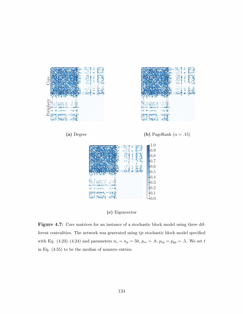
Cor
eP
erip
her
y
(a) Degree (b) PageRank (α = .15)
0.00.10.20.30.40.50.60.70.80.91.0
(c) Eigenvector
Figure 4.7: Core matrices for an instance of a stochastic block model using three dif-
ferent centralities. The network was generated using tje stochastic block model specified
with Eq. (4.23)–(4.24) and parameters nc = np = 50, pcc = .8, pcp = ppp = .5. We set t
in Eq. (4.55) to be the median of nonzero entries.
134

4.3 Core–Periphery Structure in Frugivore–Seed Networks
Ecological systems are not easily transferred into a network structure. The interaction pat-
terns of two species are much more nuanced than simply counting the number of times two
species interact. For example, within a particular ecological system, there are varying inter-
action types (e.g. avian–seed versus. predator–prey), time dependencies, and environmental
factors (e.g. seasons or weather) [169]. Nonetheless, networks can provide a simplified struc-
ture to measure biological systems and quantify certain ecological phenomena [136,137,181].
For example, the community structure of seed dispersion provides insights into the precise or-
ganization of particular mutualistic networks [137,162]. In this section, we briefly discuss our
joint investigation of core–periphery structure in frugivore–seed dispersion networks [179].
The focus in this section is the examination of core–periphery structure.
We model each mutualistic networks as a weighted bipartite network. We consider data
collected from ecologists’ observations of fruit-eating bird (frugivorous birds) and seed dis-
persion at 10 sites in northwestern Argentina [179, 180]. A node represents an animal or
plant species. We weight each edge by the number of interactions between a bird species and
a seed species during observation. This construction was also used in [6, 137]. A discussion
on how this data was collected can be found in [179, 180]. Although this simple network
construction is common for ecological applications, there are many potential problems with
this approach [169]. In this data set, we only consider 3–4 days during the rainy season. The
types of interaction patterns frequently change in different seasons [169]. In our network, the
various seed types of fruits often lead to different types of dispersal by the birds. Nonetheless,
we stick with this relatively simple construction because forms of core–periphery structures
other than nestedness have been less studied in ecological systems. To illustrate the network
structure, we show the weighted adjacency matrix and related network at Pozo Verde in
Figure 4.8 and Figure 4.9, respectively.
We apply a core–periphery methods introduced in [54, 176] and that we discussed in
Section 4.2.2. Specifically, we first obtain core–scores fα,β using Eq. (4.49) for (α, β) ∈[0, 1] × (0, 1) using a multiplicative transition function. We then compute aggregate core
135

A.ed
ulis
T.sa
yaca
(F)
B.sa
lici
folius
E.st
reper
a(F
)
T.nig
rice
ps
(F)
V.bre
vifl
ora
C.ust
ula
tus
(F)
C.st
riat
a
S.nig
ra
C.op
hth
alm
icus
(F)
P.m
elan
onot
a(F
)
T.so
rdid
a(F
)
S.buxifol
ia
P.tu
cum
anen
sis
E.unifl
ora
P.er
yth
rophry
s(F
)
M.co
riac
ea
T.ru
five
ntr
is(F
)
A.to
rquat
us
(F)
E.cy
anoce
phal
a(F
)
V.ol
ivac
eus
(F)
P.ob
scura
(F)
R.im
per
ialis
A.ci
trin
ellu
s(F
)
E.ob
scura
(F)
D.in
dic
a
Sol
anum
3
A. edulis
T. sayaca (F)
B. salicifolius
E. strepera (F)
T. nigriceps (F)
V. breviflora
C. ustulatus (F)
C. striata
S. nigra
C. ophthalmicus (F)
P. melanonota (F)
T. sordida (F)
S. buxifolia
P. tucumanensis
E. uniflora
P. erythrophrys (F)
M. coriacea
T. rufiventris (F)
A. torquatus (F)
E. cyanocephala (F)
V. olivaceus (F)
P. obscura (F)
R. imperialis
A. citrinellus (F)
E. obscura (F)
D. indica
Solanum 3
Pozo Verde
0
52
wij
Figure 4.8: The weight matrix associated to Pozo Verde, one of the 10 sites. Each
frugivore is labeled with an ‘(F)’. The weight between frugivores and plants is determined
from the number of recorded interactions. A related network visualization is in Figure
4.9.
136

file:///Users/HiPi/Google Drive/Core Periphery Write Ups/AVI...
1 of 1 1/2/17, 12:15 PM
Figure 4.9: The network from Pozo Verde with weight matrix shown in Figure 4.8.
The nodes’s sizes are proportional to their aggregate core score (Eq. (4.51)). The edges
are proportional to the weight. The two darker nodes are core-nodes. These nodes define
a cut that maximizes CP-Cut from (Eq. (4.52)).
137

scores using Eq. (4.51). We finally propose a core–periphery partition according to the
CP-Cut proposed in [54]. To obtain a partition, we order the aggregate core scores (fcp)i1 ≥(fcp)i2 ≥ . . . ≥ (fcp)in and check each possible core and periphery partition of the form
Ck = {(fcp)i1 , . . . , (fcp)ik} (4.56)
Pn−k = {(fcp)k+1, . . . , (fcp)in} , for k = 0, . . . , n+ 1, (4.57)
such that CP-Cut(Ck, Pn−k) from Eq. (4.52) is maximized. We note that when k = 0, C
is empty and the cut takes a negative value. The definition of the cut CP-Cut(Ck, Pn−k)
assumed an unweighted network, as two of the terms can be interpreted as an edge–edge
density (Eq. (4.21)). To modify this cut for our weighted network by scaling each entry wij
so that wij ∈ [0, 1]. Specifically, we divide each entry wij by the maximum over all possible
entries in W. We explore two other methods to rescale W as well. First, we set each nonzero
to 1 and examine the underlying connections ignoring weights. Second, we divide each entry
by the average of non-zero entries of W. However, we find that these two alternative scalings
of W produced identical cuts C and P at all 10 sites.
We select these particular core–periphery methodologies from [54,176] because this model
numerically assigns a core score to each node (Eq. (4.51)) in addition to providing a partition.
Moreover, the aggregate core scores from Eq. (4.51) have been applied to small (less than
100 nodes), weighted empirical networks and we believe it would be beneficial to investigate
such structures in ecological networks [17, 176]. Additionally, we wanted to provide some
more empirical comparisons of nestedness to core–periphery structure as in [120]. We remark
that scoring nodes with Eq. (4.51) is computationally expensive. The greatest bottleneck is
the computation of Rα,β (Eq. (4.50)) and fα,β (Eq. (4.49)). Although each site has at most
50 nodes, the computation of the Rα,β and fα,β on a 100× 100 grid required approximately
2 hours per site on a quad 2.6 GHz Intel Core i7. In Figure 4.10, we display the grid of
core-qualities Rα,β for the 100× 100 grid. We note that the maximum values of Rα,β occur
for β ∈ (.92, .96). To obtain a partition from Rα,β, we compute the aggregate core score fcp
(Eq. (4.51)) and then maximize the cut CP-Cut (Eq. (4.52)) using the ordering induced
from the core scores. For all 10 sites, we find that |C| = 2. In Figure 4.11, we show the
138

contour of the function k 7→ CP-Cut(Ck, Pn−k). All the sites have a similar contour with
maximum at k = 2.
We briefly verify that the core scores differ from degree. In Figure 4.12, we show a scatter
plot for the degree and the core scores. We can see that for both sites, the two nodes with
highest degree are the core-nodes (this was always the case). However, as we examine the
group of seven nodes with highest degree, we see that there aggregate core score and degree
are not perfectly correlated as in Figure 4.12b. We also compute the correlation coefficient
for the entire network and find ρ ≥ .9 at all sites.
Our colleagues used our core–periphery analysis along with additional ecological tools to
identify those bird species that played a crucial role in seed dispersion [179]. We do our best
to briefly discuss some of their findings. Because the cores we obtain from our methodology
were rather small (precisely 2 core nodes), our collaborators used core scores to evaluate the
core position of different species in a network. Our colleagues found that the bird species
Austral Yungas had high core score at several sites (frequently ranked among the top five
in aggregate core score). This bird species is a masher and often discards large seeds near
the plant. As a result, many ecologists classify mashers as poor seed dispersers as opposed
to gulpers that swallow fruit whole including the seeds [179]. However, the watery fruit
that mashers in the ecological system ate have seeds are embedded inside the fruit and thus
these seeds are more easily dispersed by mashers. Our collaborators also used our analysis
to indicate that the core plant species across 10 sites were more heterogeneous than the bird
species with respect to ecological metrics. Specifically, the fruits of each plant identified
as core varied in shape, color, seed number, pulp mass, etc. across the 10 sites, whereas
the birds had similar assemblage (bill morphology and size) across these sites. Our brief
exploration of core–periphery structure in ecological networks can provide a template for
more advanced core–periphery analysis in future ecological analysis. More often, nestedness
is used as a measure for core structure in ecological networks. Here, we introduce a new tool
for assessing core–periphery structure. Although we did not explore nestedness here, Lee
in [119] explored the relationship between a particular definition of nestedness and a core–
periphery model proposed in Rombac et al [176]. Lee found that the nestedness coefficient
139

Nc (Eq. (4.36)) was correlated with a aggregate core-quality (Eq. (4.50)) defined as:
Rcp =
∑i,j∈V wij fcp(i)fcp(j)
∑i,j∈V wij
∑i,j∈V fcp(i)fcp(j)
.
in synthetic and empirical networks. We hope to more carefully examine differences between
possible core–periphery structure and nestedness for future ecological analysis.
4.4 Conclusions and Future Work
Core–periphery structure is a fundamental mesoscale structure. One can describe this struc-
ture as a core that is well connected to a network and a periphery that is poorly connected
to itself. Even with this seemingly simple definition, there are many varied interpretations
into how to quantify this structure in weighted and unweighted networks.
In Section 4.1, we reviewed graph calculus and then then used this framework to provide
a mathematical overview of some of the models for core–periphery structure in 4.2. In partic-
ular, we related various combinatorial quantities in unweighted networks such as subgraph
densities to the core–periphery structure, specifically to the seminal work of Everett and
Borgatti [30]. We highlight those quantities that are easily generalized to the weighted case
as this is our focus in our ecological application. Our original motivation for this research was
to find methods to improve the computational overhead associated with methods introduced
in [176] and to scale faster methods to larger networks. Although we did not accomplish this,
we plan to use the research here to further explore methods for core–periphery structure and
help illustrate the broad landscape of such models for related endeavors in the future.
In Section 4.3, we briefly discussed our joint work analyzing core–periphery structure
in mutualistic frugivore–seed networks [179]. We identify core and periphery structures in
these networks using methods from Rombach et al. [176] and discuss the interpretations of
this analysis made our ecologist colleagues. For example, our colleagues found that birds
classified as mashers were characterized as core at a variety of the 10 sites investigated. Our
colleagues suggest that certain mashers are good dispersers at these sites because they feed
on watery fruit with seeds embedded in the fruit’s flesh. Typically, mashers are seen as poor
140

0.0 0.1 0.2 0.3 0.4 0.5 0.6 0.7 0.8 0.9 1.0↵
0.0
0.1
0.2
0.3
0.4
0.5
0.6
0.7
0.8
0.9
1.0
�
Pozo Verde
0 26R↵,�
Figure 4.10: The matrix of Rα,β from Eq. (4.50).
dispersers because they use their beak as a sieve to sort out hard seeds when eating fruit.
Admittedly, this exploration of core–periphery structure was brief, and in future work, we
plan to more fully explore the bipartite nature of core–periphery structure as Larremore did
for community structure [116] and Lee began to using a core–periphery structure proposed
in [120]. We also hope to provide a more detailed analysis of the relationship between
nestedness and core–periphery structure.
141

0 5 10 15 20 25 30k
−0.05
0.00
0.05
0.10
0.15
0.20
0.25
0.30
0.35
CP
-Cut
(Ck,P
n−k)
Pozo Verde
Figure 4.11: The profile of CP-Cut(Ck, Pn−k) as a function of k, where we scaled
each entry of W dividing by the maximum entry.
−0.2 0.0 0.2 0.4 0.6 0.8 1.0 1.2Aggregate Core Score
−20
0
20
40
60
80
100
120
140
Deg
ree
Pozo Verde, ρ ≈ 0.99
(a)
−0.2 0.0 0.2 0.4 0.6 0.8 1.0 1.2Aggregate Core Score
−20
0
20
40
60
80
100
120
140
160
Deg
ree
Sevenguillar, ρ ≈ 0.95
(b)
Figure 4.12: A scatter plot for degree versus core scores for two sites. We compute
the correlation coefficient ρ.
142

APPENDIX A
Rank Aggregation for Course–Sequence Discovery
A.1 Course Numbers
Table A.1 shows the official course numbers and the associated course names used throughout
the paper. We shortened the official course names wherever possible, to make the tables
more visually appealing. For example, “Introduction to Fourier Analysis” is simply labelled
“Fourier Analysis”. Also, A, B, C are substituted with I, II, and III respectively. A short
description of each course in addition to the courses prerequisites is available in the UCLA
general catalog [161].
143

Table
A.1
:C
ours
en
ames
and
nu
mb
ers.
#CourseName
#CourseName
#CourseName
31A
Calc
ulu
sI
120A
Diff
eren
tial
Geo
met
ryI
164
Op
tim
izat
ion
31B
Calc
ulu
sII
120B
Diff
eren
tial
Geo
met
ryII
167
Gam
eT
heo
ry
32A
Mu
lti.
Cal
culu
sI
121
Top
olog
y17
0AP
rob
abil
ity
I
32B
Mu
lti.
Cal
culu
sII
123
Axio
mat
icG
eom
etry
170B
Pro
bab
ilit
yII
33A
Ap
pli
edL
inea
rA
lgeb
ra13
1AR
eal
An
alysi
sI
172A
Act
uar
ial
Mat
hem
atic
s
33B
Ap
pli
edO
DE
’s13
1BR
eal
An
alysi
sII
172B
Act
uar
ial
Mod
els
II
61D
iscr
ete
Str
uct
ure
s13
1CR
eal
An
alysi
sII
I17
2CA
ctu
aria
lM
od
els
II
106
His
tory
ofM
ath
emat
ics
132
Com
ple
xA
nal
ysi
s17
3AC
asu
alty
Los
sM
od
els
I
110A
Ab
stra
ctA
lgeb
raI
133
Fou
rier
An
alysi
s17
3BC
asu
alty
Los
sM
od
els
II
110B
Ab
stra
ctA
lgeb
raII
134
Non
lin
ear
Syst
ems
174
Mat
hem
atic
alE
con
omic
s
110C
Ab
stra
ctA
lgeb
raII
I13
5O
DE
’s18
0G
rap
hT
heo
ry
111
Nu
mb
erT
heo
ry13
6P
DE
’s18
2A
lgor
ith
ms
115A
Lin
ear
Alg
ebra
I14
2M
ath
emat
ical
Mod
elin
g18
4C
omb
inat
oric
s
115B
Lin
ear
Alg
ebra
II15
1AN
um
eric
alA
nal
ysi
sI
191
Res
earc
hS
emin
ar
117
Ap
pli
edA
lgeb
ra15
1BN
um
eric
alA
nal
ysi
sII
199
Ind
ivid
ual
Res
earc
h
144

APPENDIX B
Core-Periphery Structure in Fruigivore–Seed Networks
B.1 Simulated Annealing
Kirkpatrick et al. in [110] proposed simulated annealing as a stochastic minimization algo-
rithm for combinatorial problems. We present pseudocode in Alg. 1 to represent the main
idea of the minimization algorithm. Roughly speaking, Alg. 1 performs a local search, but
rather than rejecting all states with higher cost J , we accept new states with a diminishing
probability that depends on the difference in costs between the current state and possible
new state.
Algorithm 1 Simmulated Annealing for Minimization
1: Inputs: Finite set of states S, cost function J : S → R, cooling schedule C : R →(0,∞) such that limnC(n) = 0, randomized neighbor function N : S → S; minimum
temperature Tmin
2: Select s ∈ S; select T .
3: while T > Tmin do
4: s′ ← N(s)
5: if J(s) < J(s′) then
6: s← s′
7: else
8: s← s′ with probability exp(−(J(s′)− J(s))/T )
9: T ← C(T ) (cooling)
We use the Matlab code in [200]. The full pseudocode of this algorithm is given in
Algorithm 2. We do not experiment with local search heuristics, neighboring functions and
145

different cooling schedules, in part because we select parameters are designed to survey a
large portion of the possible states [176]. We specify the inputs here. The set S of states
from Line 1 of Alg. 2 is precisely the set PV (α, β) from Eq. (1). Recall that P(α, β) is
the set of all possible bijections of nodes V to S(α, β, n) (see Eq. (4.46)), where n = |V |.The cost function J is E from Eq. (4.48). Given an assignment fα,β, we define the set of
neighbors of fα,β as gα,β such that if i1, . . . , in is an enumeration of the nodes V , then
1. fα,β = gα,β on nodes i1, . . . , in−2,
2. fα,β(in−1) = gα,β(in), and
3. fα,β(in) = gα,β(in−1).
In other words, the set of neighbors of fα,β are those functions in PV (α, β) whose assignment
on two nodes are swapped. The randomized neighboring function N from Line 1 of Alg.
2 is a random selection of one of the possible neighbors. We used the cooling schedule
C(T ) = .8T given as default in [200]. We also set attmax = 5000 and succmax = 1000 using
the code from [17].
146

Algorithm 2 Simmulated Annealing for Minimization from [200]
1: Inputs: Finite set of states S; cost function J : S → R; randomized neighbor function
N : S → S; minimum temperature Tmin; maximum consecutive rejections R; maximum
number of attempts attmax; maximum number of successes succmax; cooling schedule
C : R→ (0,∞) such that limy→∞C(y) = 0.
2: Select state s ∈ S uniformly at random (or using a heuristic).
3: Current consecutive rejections r (r ← 0); current number of attempts att (att ← 0);
current number of successful attempts succ (succ← 0).
4: Temperature T (T ← 1).
5: while T > Tmin and r < R do
6: if att > attmax or succ > succmax then
7: T ← C(T )
8: succ← 0
9: att← 0
10: s′ ← N(s).
11: att← att + 1
12: if J(s′) < J(s) then
13: s← s′
14: r ← 0
15: succ← succ + 1
16: else
17: x← Rand(0, 1)
18: if x < exp(J(s′)− J(s)/T ) then
19: s← s′
20: r ← 0
21: succ← succ + 1
22: else
23: r ← r + 1
147

References
[1] Howard Abadinsky. Organized Crime. Cengage Learning, 2012.
[2] Lada A. Adamic and Bernardo A. Huberman. Power-law Distribution of the WorldWide Web. Science, 287(5461):2115–2115, 2000.
[3] UCLA Undergraduate Admissions. Majors and Minors, December 2016. https:
//www.admission.ucla.edu/prospect/coll_sch.htm (Accessed: December 26th,2016).
[4] Azam Ahmed and Randal Archibold. Mexican Drug Kingpin, El Chapo, EscapesPrison Through Tunnel, 2015. http://nyti.ms/1K2b6em (Accessed: January 6th,2017).
[5] Christopher Aicher, Abigail Z. Jacobs, and Aaron Clauset. Learning Latent BlockStructure in Weighted Networks. Journal of Complex Networks, 3(2):221–248, 2015.
[6] Mario Almeida-Neto and Werner Ulrich. A Straightforward Computational Approachfor Measuring Nestedness using Quantitative Matrices. Environmental Modelling &Software, 26(2):173–178, 2011.
[7] Noga Alon and Joel H. Spencer. The Probabilistic Method. John Wiley & Sons, 2004.
[8] Ashton Anderson, Daniel Huttenlocher, Jon Kleinberg, Jure Leskovec, and Mitul Ti-wari. Global Diffusion via Cascading Invitations: Structure, Growth, and Homophily.In Proceedings of the 24th International Conference on World Wide Web, pages 66–76.ACM, 2015.
[9] Sanjeev Arora, Satish Rao, and Umesh Vazirani. Expander Flows, Geometric Embed-dings and Graph Partitioning. Journal of the ACM, 56(2):5, 2009.
[10] Luis Astorga and David A. Shirk. Drug Trafficking Organizations and Counter-DrugStrategies in the U.S.–Mexican Context. Center for U.S.-Mexican Studies, 2010.
[11] Jonathan E. Atkins, Erik G. Boman, and Bruce Hendrickson. A Spectral Algorithm forSeriation and the Consecutive Ones Problem. SIAM Journal on Computing, 28(1):297–310, 1998.
[12] Bruce Bagley. Drug Trafficking and Organized Crime in the Americas. WoodrowWilson Center: Update of the Americas, 2012.
[13] John Bailey and Matthew M. Taylor. Evade, Corrupt, or Confront? Organized Crimeand the State in Brazil and Mexico. Journal of Politics in Latin America, 1(2):3–29,2009.
[14] Albert-Laszlo Barabasi and Reka Albert. Emergence of Scaling in Random Networks.Science, 286(5439):509–512, 1999.
148

[15] Alain Barrat, Marc Barthelemy, Romualdo Pastor-Satorras, and Alessandro Vespig-nani. The Architecture of Complex Weighted Networks. Proceedings of the NationalAcademy of Sciences, 101(11):3747–3752, 2004.
[16] Jordi Bascompte, Pedro Jordano, Carlos J Melian, and Jens M. Olesen. The NestedAssembly of Plant–Animal Mutualistic Networks. Proceedings of the National Academyof Sciences, 100(16):9383–9387, 2003.
[17] Danielle S. Bassett, Nicholas F. Wymbs, Puck Rombach, Mason A. Porter, and Scott T.Mucha, Peter J .and Grafton. Task-based Core-Periphery Organization of HumanBrain Dynamics. PLoS Computational Biology, 9(9):e1003171, 2013.
[18] Vladimir Batagelj and Matjaz Zaversnik. An O(m) Algorithm for Cores Decompositionof Networks. arXiv preprint cs/0310049, 2003.
[19] Nicola Bellomo, Francesca Colasuonno, Damian Knopoff, and Juan Soler. From aSystems Theory of Sociology to Modeling the Onset and Evolution of Criminality.Networks and Heterogeneous Media, 10(3):421–441, 2015.
[20] Bijan Berenji, Tom Chou, and Maria R. D’Orsogna. Recidivism and Rehabilitationof Criminal Offenders: a Carrot and Stick Evolutionary Game. PLoS One, 9:e85531,2014.
[21] Noam Berger, Christian Borgs, Jennifer T. Chayes, and Amin Saberi. AsymptoticBehavior and Distributional Limits of Preferential Attachment Graphs. The Annalsof Probability, 42(1):1–40, 2014.
[22] Andrea L. Bertozzi and Arjuna Flenner. Diffuse Interface Models on Graphs for Clas-sification of High Dimensional Data. Multiscale Modeling & Simulation, 10(3):1090–1118, 2012.
[23] Aditya Bhaskara, Moses Charikar, Eden Chlamtac, Uriel Feige, and Aravindan Vi-jayaraghavan. Detecting High Log-Densities: an O(1/4) Approximation for Densestk-Subgraph. In Proceedings of the 42nd ACM symposium on Theory of Computing,pages 201–210. ACM, 2010.
[24] Ginestra Bianconi and Albert-Laszlo Barabasi. Bose-Einstein Condensation in Com-plex Networks. Physical Review Letters, 86(24):5632, 2001.
[25] Marian Boguna, Romualdo Pastor-Satorras, Albert Dıaz-Guilera, and Alex Arenas.Models of Social Networks Based on Social Distance Attachment. Physical Review E,70:056122, 2004.
[26] Bela Bollobas. The Evolution of Random Graphs. Transactions of the AmericanMathematical Society, 286(1):257–274, 1984.
[27] Bela Bollobas. Modern Graph Theory, volume 184. Springer, 2013.
149

[28] Immanuel M. Bomze, Marco Budinich, Panos M. Pardalos, and Marcello Pelillo. Themaximum clique problem. In Handbook of Combinatorial Optimization, pages 1–74.Springer, 1999.
[29] Stephen P. Borgatti. Identifying Sets of Key Players in a Social Network. Computa-tional & Mathematical Organization Theory, 12(1):21–34, 2006.
[30] Stephen P. Borgatti and Martin G. Everett. Models of Core-Periphery Structures.Social Networks, 21(4):375–395, 2000.
[31] Mark Bowden. Killing Pablo: The Inside Story of the Manhunt to Bring Down theMost Powerful Criminal in History. Atlantic Books, 2012.
[32] Ralph A. Bradley and Milton E. Terry. Rank Analysis of Incomplete Block Designs:I. The Method of Paired Comparisons. Biometrika, 39(3):324–345, 1952.
[33] Lori Breslow, David E. Pritchard, Jennifer DeBoer, Glenda S. Stump, Andrew D. Ho,and Daniel T. Seaton. Studying Learning in the Worldwide Classroom: Research intoedX’s First MOOC. Research & Practice in Assessment, 8:13–25, 2013.
[34] Xavier Bresson and Arthur D. Szlam. Total variation and cheeger cuts. In Proceedingsof the 27th International Conference on Machine Learning, pages 1039–1046, 2010.
[35] Sergey Brin and Lawrence Page. The Anatomy of a Large-scale Hypertextual WebSearch Engine. Computational Networks and ISDN Systems, 30(1-7):107–117, April1998.
[36] F. Thomas Bruss. A Note on Extinction Criteria for Bisexual Galton–Watson Pro-cesses. Journal of Applied Probability, 21(4):915–919, 1984.
[37] Thomas Callaghan, Peter J. Mucha, and Mason A. Porter. Random Walker Rankingfor NCAA Division IA Football. American Mathematical Monthly, 114(9):761–777,2007.
[38] Alessio Cardillo, Jesus Gomez-Gardenes, Massimiliano Zanin, Miguel Romance, DavidPapo, Francisco del Pozo, and Stefano Boccaletti. Emergence of Network Featuresfrom Multiplexity. Scientific Reports, 3:1344 EP–, 02 2013.
[39] Claudio Castellano, Santo Fortunato, and Vittorio Loreto. Statistical Physics of SocialDynamics. Reviews of Modern Physics, 81:591–646, 2009.
[40] Michele Catanzaro, Marian Boguna, and Romualdo Pastor-Satorras. Generation ofUncorrelated Random Scale-Free Networks. Physical Review E, 71(2):027103, 2005.
[41] Manuela Cattelan. Models for Paired Comparison Data: A Review with Emphasis onDependent Data. Statistical Science, pages 412–433, 2012.
[42] Bikas K. Chakrabarti, Anirban Chakraborti, and Arnab Chatterjee. Econophysics andSociophysics: Trends and Perspectives. John Wiley & Sons, 2007.
150

[43] Sorathan Chaturapruek, Jonah Breslau, Daniel Yazdi, Theodore Kolokolnikov, andScott G. McCalla. Crime Modeling with Levy flights. SIAM Journal on AppliedMathematics, 73(4):1703–1720, 2013.
[44] Xi Chen, Paul N. Bennett, Kevyn Collins Thompson, and Eric Horvitz. PairwiseRanking Aggregation in a Crowdsourced Setting. In Proceedings of the Sixth ACMInternational Conference on Web Search and Data Mining, pages 193–202, New York,NY, 2013. ACM.
[45] Fan Chung. Spectral Graph Theory, volume 92. American Mathematical Society, 1997.
[46] Fan Chung, Shirin Handjani, and Doug Jungreis. Generalizations of Polya’s Urn Prob-lem. Annals of Combinatorics, 7(2):141–153, 2003.
[47] Fan Chung and Linyuan Lu. Coupling Online and Offline analyses for Random PowerLaw Graphs. Internet Mathematics, 1(4):409–461, 2004.
[48] Douglas H. Clements and Julie Sarama. Learning Trajectories in Mathematics Edu-cation. Mathematical Thinking and Learning, 6(2):81–89, 2004.
[49] Andrew Comrey. The Minimum Residual Method of Factor Analysis. PsychologicalReports, 11(1):15–18, 1962.
[50] Colin Cooper, Alan Frieze, and Juan Vera. Random Deletion in a Scale-Free RandomGraph Process. Internet Mathematics, 1(4):463–483, 2004.
[51] Donald R. Cressey. Theft of the Nation: The Structure and Operations of OrganizedCrime in America. Harper & Row, 1969.
[52] Peter Csermely, Andrs London, Ling-Yun Wu, and Brian Uzzi. Structure and Dynam-ics of Core/Periphery Networks. Journal of Complex Networks, 1(2):93–123, 2013.
[53] Mihai Cucuringu. Sync-Rank: Robust Ranking, Constrained Ranking and Rank Ag-gregation via Eigenvector and SDP Synchronization. IEEE Transactions on NetworkScience and Engineering, 3(1):58–79, 2016.
[54] Mihai Cucuringu, Puck Rombach, Sang Hoon Lee, and Mason A. Porter. Detectionof Core-Periphery Structure in Networks using Spectral Methods and Geodesic Paths.European Journal of Applied Mathematics, 27(6):846–887, 12 2016.
[55] H. A. David and D. M. Andrews. Nonparametric Methods of Ranking from PairedComparisons. In Probability Models and Statistical Analyses for Ranking Data, pages20–36. Springer, 1993.
[56] Cristobal de Brey, Thomas D. Snyder, and Sally A. Dillow. Mobile Digest of EducationStatistics, 2014. National Center for Education Statistics, 2016.
[57] Pierre de Champlain. Mobsters, Gangsters and Men of Honour: Cracking the MafiaCode. Harper Collins (Canada), 2005.
151

[58] Derek J. de Solla Price. Networks of Scientific Papers. Science, 149(3683):510–515,1965.
[59] Fabio Della Rossa, Fabio Dercole, and Carlo Piccardi. Profiling Core-Periphery Net-work Structure by Random Walkers. Scientific Reports, 3, 2013.
[60] James W. Demmel. Applied Numerical Linear Algebra. SIAM, 1997.
[61] James A. Densley. Street Gang Recruitment: Signaling, Screening, and Selection.Social Problems, 59(3):301–321, 2012.
[62] Jean-Pierre Dion. Estimation of the Mean and the Initial Probabilities of a BranchingProcess. Journal of Applied Probability, 11(4):687–694, 1974.
[63] Sergey N. Dorogovtsev, Alexander V. Goltsev, and Jose Ferreira F. Mendes. k-coreOrganization of Complex Networks. Physical Review Letters, 96(4):040601, 2006.
[64] Maria R. D’Orsogna, Michael McBride, Ryan Kendall, and Martin B. Short. CriminalDefectors Lead to the Emergence of Cooperation in an Experimental, AdversarialGame. PloS One, 8:e61458, 2013.
[65] Maria R D’Orsogna and Matjaz Perc. Statistical Physics of Crime. Physics of LifeReviews, 12:1–21, 2014.
[66] Steven S. Dudley. Drug Trafficking Organizations in Central America: Transportistas,Mexican Cartels and Maras, pages 63–93. Woodrow Wilson International Center forScholars, 2010.
[67] Paul A. C. Duijn, Victor Kashirin, and Peter M. A. Sloot. The Relative Ineffectivenessof Criminal Network Disruption. Scientific Reports, 4(4238), 2014.
[68] Richard Durrett. Random Graph Dynamics. Cambridge University Press, 2007.
[69] Richard Durrett. Essentials of Stochastic Processes. Springer, 2012.
[70] Cynthia Dwork, Ravi Kumar, Moni Naor, and D. Sivakumar. Rank AggregationRevisited, 2001. http://www.eecs.harvard.edu/~michaelm/CS222/rank2.pdf (Ac-cessed: January 15th, 2017).
[71] Cynthia Dwork, Ravi Kumar, Moni Naor, and Dandapani Sivakumar. Rank Aggre-gation Methods for the Web. In Proceedings of the 10th international conference onWorld Wide Web, pages 613–622. ACM, 2001.
[72] David Easley and Jon Kleinberg. Networks, Crowds, and Markets: Reasoning about aHighly Connected World. Cambridge University Press, 2010.
[73] John Eid, Adrian Fehr, Jeremy Gray, Khai Luong, John Lyle, Otto, et al. Real-timeDNA Sequencing from Single Polymerase Molecules. Science, 323(5910):133–138, 2009.
152

[74] Magdalini Eirinaki and Michalis Vazirgiannis. Web Mining for Web Personalization.ACM Transactions on Internet Technology, 3(1):1–27, 2003.
[75] Paul Erdos and Alfred Renyi. On the Strength of Connectedness of a Random Graph.Acta Mathematica Hungarica, 12(1):261–267, 1961.
[76] Shimon Even and R. Endre Tarjan. Network Flow and Testing Graph Connectivity.SIAM Journal on Computing, 4(4):507–518, 1975.
[77] Uriel Feige, David Peleg, and Guy Kortsarz. The Dense k-Subgraph Problem. Algo-rithmica, 29(3):410–421, 2001.
[78] Marcus Felson. The Ecosystem for Organized Crime. European Institute for CrimePrevention and Control, 2006.
[79] Robert Filippone. The Medellin Cartel: Why We Can’t Win The Drug War. Studiesin Conflict & Terrorism, 17(4):323–344, 1994.
[80] Michael A. Fligner and Joseph S. Verducci. Probability Models and Statistical Analysesfor Ranking Data, volume 80. Springer, 1993.
[81] Fajwel Fogel, Alexandre d’Aspremont, and Milan Vojnovic. SerialRank: SpectralRanking using Seriation. In Advances in Neural Information Processing Systems, pages900–908, 2014.
[82] Santo Fortunato. Community Detection in Graphs. Physics Reports, 486(3):75–174,2010.
[83] Bailey K. Fosdick, Daniel B. Larremore, Joel Nishimura, and Johan Ugander.Configuring Random graph Models with Fixed Degree Sequences. arXiv preprintarXiv:1608.00607, 2016.
[84] Lukasz Gajewski, Jan Cho loniewski, and Janusz Ho lyst. Key Courses of the Aca-demic Curriculum Uncovered by Data Mining of Students’ Grades. arXiv preprintarXiv:1604.07074, 2016.
[85] Francis Galton and Henry W. Watson. On the Probability of Extinction of Families,volume 4, pages 138–144. Wiley, 1875.
[86] John Gandar, Richard Zuber, Thomas O’Brien, and Ben Russo. Testing Rationalityin the Point Spread Betting Market. The Journal of Finance, 43(4):995–1008, 1988.
[87] Antonios Garas, Frank Schweitzer, and Shlomo Havlin. A k-shell DecompositionMethod for Weighted Networks. New Journal of Physics, 14(8):083030, 2012.
[88] James P. Gleeson, Davide Cellai, Jukka-Pekka Onnela, Mason A. Porter, and FelixReed-Tsochas. A Simple Generative Model of Collective Online Behavior. Proceedingsof the National Academy of Sciences, 111(29):10411–10415, 2014.
[89] David F. Gleich. PageRank Beyond the Web. SIAM Review, 57(3):321–363, 2015.
153

[90] David F. Gleich and Lek-Heng Lim. Rank Aggregation via Nuclear Norm Minimiza-tion. In Proceedings of the 17th ACM SIGKDD International Conference on KnowledgeDiscovery and Data Mining, pages 60–68, New York, NY, 2011. ACM.
[91] John Goddard and Ioannis Asimakopoulos. Forecasting Football Results and the Ef-ficiency of Fixed-Odds Betting. Journal of Forecasting, 23(1):51–66, 2004.
[92] Andrew Goldberg. Finding a Maximum Density Subgraph. University of CaliforniaBerkeley, CA, 1984.
[93] Tom Goldstein and Stanley Osher. The Split Bregman Method for `1-RegularizedProblems. SIAM Journal on Imaging Sciences, 2(2):323–343, 2009.
[94] Alexander Gutfraind, Aric Hagberg, and Feng Pan. Optimal Interdiction of UnreactiveMarkovian Evaders. In Integration of AI and OR Techniques in Constraint Program-ming for Combinatorial Optimization Problems: 6th International Conference, pages102–116. Springer Berlin, 2009.
[95] Jiawei Han, Hong Cheng, Dong Xin, and Xifeng Yan. Frequent Pattern Mining: Cur-rent Status and Future Directions. Data Mining and Knowledge Discovery, 15(1):55–86, 2007.
[96] William J. Hardin. Mathematics, Prerequisites, and Student Success in IntroductoryCourses, pages 352–360. Josey–Bass, 3 edition, 2008.
[97] Anil N. Hirani, Kaushik Kalyanaraman, and Seth Watts. Least Squares Rankingon Graphs, November 2011. http://arxiv.org/abs/1011.1716 (Accessed: January15th, 2017).
[98] Petter Holme. Core–Periphery Organization of Complex Networks. Physical ReviewE, 72(4):046111, 2005.
[99] Huiyi Hu, Thomas Laurent, Mason A. Porter, and Andrea L. Bertozzi. A MethodBased on Total Variation for Network Modularity Optimization using the MBO-Scheme. SIAM Journal on Applied Mathematics, 73(6):2224–2246, 2013.
[100] David M. Hull. A Reconsideration of Galton’s Problem (Using a Two-Sex Population).Theoretical Population Biology, 54(2):105–116, 1998.
[101] Hawoong Jeong, Zoltan Neda, and Albert-Laszlo Barabasi. Measuring PreferentialAttachment in Evolving Networks. Europhysics Letters, 61(4):567, 2003.
[102] Hawoong Jeong, Zoltan Neda, and Albert-Laszlo Barabasi. Measuring PreferentialAttachment in Evolving Networks. Europhysics Letters, 61(4):567, 2003.
[103] Lucas G. S. Jeub, Prakash Balachandran, Mason A. Porter, Peter J. Mucha, andMichael W. Mahoney. Think Locally, Act Locally: Detection of Small, Medium-Sized,and Large Communities in Large Networks. Physical Review E, 91:012821, 2015.
154

[104] Xiaoye Jiang, Lek-Heng Lim, Yuan Yao, and Yinyu Ye. Statistical Ranking and Com-binatorial Hodge Theory. Mathematical Programming, 127(1):203–244, 2011.
[105] Katy Jordan. Initial Trends in Enrollment and Completion of Massive Open OnlineCourses. The International Review of Research in Open and Distributed Learning,15(1):133–160, 2014.
[106] Norman Kaplan. The Multitype Galton–Watson Process with Immigration. Annalsof Probability, 1(6):947–953, 1973.
[107] David G. Kendall. Branching Processes since 1873. Journal of the London Mathemat-ical Society, 1(1):385–406, 1966.
[108] Michael Kenney. From Pablo to Osama: Counter–Terrorism Lessons from the War onDrugs. Survival, 45(3):187–206, 2003.
[109] Michael Kenney. The Architecture of Drug Trafficking: Network Forms of Organizationin the Colombian Cocaine Trade. Global Crime, 8(3):233–259, 2007.
[110] Scott Kirkpatrick, C. Daniel Gelatt, and Mario P. Vecchi. Optimization by SimmulatedAnnealing. Science, 220(4598):671–680, 1983.
[111] Mikko Kivela, Alex Arenas, Marc Barthelemy, James P. Gleeson, Yamir Moreno, andMason A. Porter. Multilayer Networks. Journal of Complex Networks, 2(3):203–271,2014.
[112] Krzysztof Koperski and Jiawei Han. Discovery of Spatial Association Rules in Geo-graphic Information Databases. In Proceedings of the 4th International Symposium onAdvances in Spatial Databases, pages 47–66, London, UK, 1995. Springer.
[113] Paul L. Krapivsky and Sidney Redner. Organization of Growing Random Networks.Physical Review E, 63(6):066123, 2001.
[114] Valdis Krebs. Mapping Networks of Terrorist Cells. Connections, 24(3):43–52, 2002.
[115] Paul R. Krugman. Geography and Trade. MIT press, 1991.
[116] Daniel B. Larremore, Aaron Clauset, and Abigail Z. Jacobs. Efficiently Inferring Com-munity Structure in Bipartite Networks. Physical Review E, 90(1):012805, 2014.
[117] Edward O. Laumann and Franz Urban Pappi. New Directions in the Study of Com-munity Elites. American Sociological Review, pages 212–230, 1973.
[118] Deok-Sun Lee, Seong Eun Maeng, and Jae Woo Lee. Scaling of Nestedness in ComplexNetworks. Journal of the Korean Physical Society, 60(4):648–656, 2012.
[119] Sang Hoon Lee. Network Nestedness as Generalized Core–Periphery Structures. Phys-ical Review E, 93(2):022306, 2016.
155

[120] Sang Hoon Lee, Mihai Cucuringu, and Mason A. Porter. Density-Based and Transport-Based Core–Periphery Structures in Networks. Physical Review E, 89:032810, Mar2014.
[121] Robert S. Leiken. Mexico’s Drug War. Center for the National Inter-est, 2012. http://www.cpimexico.org.mx/portal/wp-content/uploads/2014/01/
Mexicos-drug-war.pdf.
[122] Lun Li, David Alderson, John C. Doyle, and Walter Willinger. Towards a Theory ofScale–Free Graphs: Definition, Properties, and Implications. Internet Mathematics,2(4):431–523, 2005.
[123] Laszlo Lovasz. Random Walks on Graphs. Combinatorics, Paul Erdos is Eighty,2:1–46, 1993.
[124] Robert D. Luce and Patrick Suppes. Preference, Utility, and Subjective Probability.Wiley, 1965.
[125] Tomasz Luczak. Component Behavior Near the Critical Point of the Random GraphProcess. Random Structures & Algorithms, 1(3):287–310, 1990.
[126] Hosam M. Mahmoud. Distances in Random Plane-Oriented Recursive Trees. Journalof Computational and Applied Mathematics, 41(1):237–245, 1992.
[127] Charles Z. Marshak, M. Puck Rombach, Andrea L. Bertozzi, and Maria R. D’Orsogna.Growth and Containment of a Hierarchical Criminal Network. Physical Review E,93:022308, Feb 2016.
[128] Giovanni Mastrobuoni and Eleonora Patacchini. Understanding Organized Crime Net-works: Evidence based on Federal Bureau of Narcotics Secret Files on American Mafia.Carlo Alberto Notebooks, 152:1–58, 2010.
[129] Giovanni Mastrobuoni and Eleonora Patacchini. Organized Crime Networks: An Ap-plication of Network Analysis Techniques to the American Mafia. Review of NetworkEconomics, 11(3):1–43, 2012.
[130] Naoki Masuda, Mason A. Porter, and Renaud Lambiotte. Random Walks and Diffu-sion on Networks. arXiv preprint arXiv:1612.03281, 2016.
[131] Antonio L. Mazzitelli. Mexican Cartel Influence in Central America. Western Hemi-sphere Security Analysis Center, 2011.
[132] Julian J. McAuley and Jure Leskovec. Learning to Discover Social Circles in EgoNetworks. In Advances in Neural Information Processing, volume 2012, pages 548–56,2012.
[133] Michael McBride and Michael Caldara. The Efficacy of Tables versus Graphs in Dis-rupting Dark Networks: An Experimental Study. Social Networks, 35(3):406–422,2013.
156

[134] Michael McBride and David Hewitt. The Enemy You Cannot See: An Investigationof the Disruption of Dark Networks. Journal of Economic Behavior & Organization,93:32–50, 2013.
[135] Rachel McCulloch and Linda P. Rothschild. MOOCs: An Inside View. Notices of theAmerican Mathematical Society, 61(8):866–872, 2014.
[136] Marco Aurelio Ribeiro Mello, Flavia Maria Darcie Marquitti, Paulo RobertoGuimaraes, Jr., et al. The Missing Part of Seed Dispersal Networks: Structure andRobustness of Bat–Fruit Interactions. PLoS One, 6(2):1–10, 2011.
[137] Marco Aurelio Ribeiro Mello, Flavia Maria Darcie Marquitti, Paulo R. Guimaraes Jr.,et al. The Modularity of Seed Dispersal: Differences in Structure and Robustnessbetween Bat– and Bird–Fruit Networks. Oecologia, 167(1):131–140, 2011.
[138] Ekaterina Merkurjev, Tijana Kostic, and Andrea L. Bertozzi. An MBO Scheme onGraphs for Classification and Image Processing. SIAM Journal on Imaging Sciences,6(4):1903–1930, 2013.
[139] Dillon V. P. Montag Mihai Cucuringu, Charlie Marshak and Puck Rombach. RankAggregation for Course Sequence Discovery, March 2016. https://arxiv.org/abs/
1603.02695 (In preparation).
[140] J. Mitchell Miller and Lance H. Selva. Drug Enforcement’s Double-Edged Sword: AnAssessment of Asset Forfeiture Programs. Justice Quarterly, 11(2):313–335, 1994.
[141] Robert J. Mokken. Cliques, Clubs and Clans. Quality & Quantity, 13(2):161–173,1979.
[142] Cristopher Moore, Gourab Ghoshal, and Mark E. J. Newman. Exact Solutions forModels of Evolving Networks with Addition and Deletion of Nodes. Physical ReviewE, 74(3):036121, 2006.
[143] Carlo Morselli. Contacts, Opportunities, and Criminal Enterprise. University ofToronto Press, 2005.
[144] Carlo Morselli. Inside Criminal Networks, volume 8. Springer, 2008.
[145] Carlo Morselli. Assessing Vulnerable and Strategic Positions in a Criminal Network.Journal of Contemporary Criminal Justice, 26(4):382–392, 2010.
[146] Elchanan Mossel, Joe Neeman, and Allan Sly. Stochastic block models and reconstruc-tion. arXiv preprint arXiv:1202.1499, 2012.
[147] Adilson E. Motter. Cascade Control and Defense in Complex Networks. PhysicalReview Letters, 93(9):098701, 2004.
[148] Adilson E. Motter and Ying-Cheng Lai. Cascade-Based Attacks on Complex Networks.Physical Review E, 66(6):065102, 2002.
157

[149] Peter J. Mucha, Thomas Richardson, Kevin Macon, Mason A. Porter, and Jukka-Pekka Onnela. Community Structure in Time-Dependent, Multiscale, and MultiplexNetworks. Science, 328(5980):876–878, 2010.
[150] Kevin P. Murphy, Yair Weiss, and Michael I. Jordan. Loopy Belief Propagation for Ap-proximate Inference: An Empirical Study. In Proceedings of the Fifteenth Conferenceon Uncertainty in Artificial Intelligence, pages 467–475, 1999.
[151] Roger B. Myerson. Analysis of Democratic Institutions: Structure, Conduct and Per-formance. The Journal of Economic Perspectives, 9(1):77–89, 1995.
[152] Sahand Negahban, Sewoong Oh, and Devavrat Shah. Iterative Ranking from Pair-wiseComparisons. In Advances in Neural Information Processing Systems, pages 2474–2482, 2012.
[153] Mark E. J. Newman. Clustering and Preferential Attachment in Growing Networks.Physical review E, 64(2):025102, 2001.
[154] Mark E. J. Newman. Networks: An Introduction. Oxford University Press, 2010.
[155] UCLA Department of Chemistry. The UCLA Chemistry Major, 2016. http:
//www.chem.ucla.edu/dept/ugrad/majors/chemistry.htm (Accessed: December26th, 2016).
[156] Bureau of Labor Statistics. Economics News Release, 2016. http://www.bls.gov/
news.release/empsit.t04.htm (Accessed: December 26th, 2016).
[157] UCLA Department of Mathematics. Majors, Minors & Specializations, Decem-ber 2016. https://www.math.ucla.edu/ugrad/majors (Accessed: December 26th,2016).
[158] Congressional Budget Office. National Defense Authorization Act for Fiscal Year 2017,2016. https://www.cbo.gov/publication/51570 (Accessed: January 6th, 2017).
[159] UCLA Registrar’s Office. Class Levels, 2016. hhttp://www.registrar.ucla.edu/
Registration-Classes/Enrollment-Policies/Class-Levels (Accessed: Decem-ber 26th, 2016).
[160] UCLA Registrar’s Office. Grades, 2016. http://catalog.registrar.ucla.edu/
ucla-cat2016-58.html (Accessed: December 26th, 2016).
[161] UCLA Registrar’s Office. UCLA General Catalog, 2016. http://catalog.
registrar.ucla.edu/ (Accessed: December 26th, 2016).
[162] Jens M. Olesen, Jordi Bascompte, Yoko L. Dupont, and Pedro Jordano. The Mod-ularity of Pollination Networks. Proceedings of the National Academy of Sciences,104(50):19891–19896, 2007.
158

[163] Braxton Osting, Christoph Brune, and Stanley Osher. Enhanced Statistical Rankingsvia Targeted Data Collection. In International Conference on Machine Learning, pages489–497, 2013.
[164] Braxton Osting, Jerome Darbon, and Stanley Osher. Statistical Ranking Using the`1-norm on Graphs. AIMS Journal on Inverse Problems and Imaging, 7(3):907–926,2013.
[165] Elyssa Pachico. Mexico Defense of Kingpin Strategy Falls Short. Insight Crime, 2011.
[166] Lawrence Page, Sergey Brin, Rajeev Motwani, and Terry Winograd. The PageRankCitation Ranking: Bringing Order to the Web. Technical Report 1999-66, StanfordInfoLab, 1999. http://ilpubs.stanford.edu:8090/422/1/1999-66.pdf (Accessed:January 15th, 2017).
[167] Bruce D. Patterson and Wirt Atmar. Nested Subsets and the Structure of InsularMammalian Faunas and Archipelagos. Biological Journal of the Linnean Society, 28(1-2):65–82, 1986.
[168] Tiago P. Peixoto. Hierarchical Block Structures and High-Resolution Model Selectionin Large Networks. Phys. Rev. X, 4:011047, Mar 2014.
[169] Shai Pilosof, Mason A. Porter, Mercedes Pascual, and Sonia Kefi. The MultilayerNature of Ecological Networks. arXiv preprint arXiv:1511.04453, 2015.
[170] Mason A. Porter, Jukka-Pekka Onnela, and Peter J. Mucha. Communities in Networks.Notices of the American Mathematical Society, 56(9):1082–1097, 2009.
[171] Arun Rajkumar and Shivani Agarwal. A Statistical Convergence Perspective of Al-gorithms for Rank Aggregation from Pairwise Data. In International Conference onMachine Learning, pages 118–126, 2014.
[172] Karthik Raman and Thorsten Joachims. Methods for Ordinal Peer Grading. In Pro-ceedings of the 20th ACM SIGKDD International Conference on Knowledge Discoveryand Data Mining, pages 1037–1046. ACM, 2014.
[173] R. Ravi and D. P. Williamson. An Approximation Algorithm for Minimum–CostVertex–Connectivity Problems. Algorithmica, 18(1):21–43, 1997.
[174] Peter Reuter and Mark A. R. Kleiman. Risks and Prices: An Economic Analysis ofDrug Enforcement. Crime and Justice, pages 289–340, 1986.
[175] Puck Rombach and Mason A. Porter. Discriminating Power of Centrality Measures.arXiv preprint arXiv:1305.3146, 2013.
[176] Puck Rombach, Mason A. Porter, James H. Fowler, and Peter J. Mucha. Core-periphery structure in networks. SIAM Journal on Applied Mathematics, 74(1):167–190, 2014.
159

[177] Jonathan B. Rothbard and William R. Taylor. A Sequence Pattern Common to T-cellEpitopes. The EMBO Journal, 7(1):93–100, 1988.
[178] Leonid Rudin, Stanley Osher, and Emad Fatemi. Nonlinear Total Variation basedNoise Removal Algorithms. Physica D: Nonlinear Phenomena, 60(1):259–268, 1992.
[179] Roman A. Ruggera, Pedro G. Blendinger, M. Daniela Gomez, and Charlie Marshak.Linking Structure and Functionality in Mutualistic Networks: Do Core FrugivoresDisperse More Seeds than Peripheral Species? Oikos, August 2015.
[180] Roman A. Ruggera, M. Daniela Gomez, and Pedro G. Blendinger. Frugivory and SeedDispersal Role of the Yellow–Striped Brush–Finch (Atlapetes citrinellus), an EndemicEmberizid of Argentina. EMU, 114(4):343–351, 2014.
[181] Matthias Schleuning, Lili Ingmann, Rouven Strauss, Susanne A. Fritz, Bo Dalsgaard,D. Matthias Dehling, et al. Ecological, Historical and Evolutionary Determinantsof Modularity in Weighted Seed–Dispersal Networks. Ecology letters, 17(4):454–463,2014.
[182] Barbara Schneider, Christopher B. Swanson, and Catherine Riegle-Crumb. Opportu-nities for Learning: Course Sequences and Positional Advantages. Social Psychologyof Education, 2(1):25–53, 1997.
[183] Eugene W. Schupp, Pedro Jordano, and Jose Marıa Gomez. Seed Dispersal Effective-ness Revisited: a Conceptual Review. New Phytologist, 188(2):333–353, 2010.
[184] UCLA Summer Session. UCLA Summer Session, December 2016. http://www.
summer.ucla.edu/ (Accessed: December 26th, 2016).
[185] Martin B. Short, Andrea L. Bertozzi, and P. Jeffrey Brantingham. Nonlinear Patternsin Urban Crime: Hotspots, Bifurcations, and Suppression. SIAM Journal on AppliedDynamical Systems, 9(2):462–483, 2010.
[186] Martin B. Short, Maria R. D’Orsogna, Virginia B. Pasour, George E. Tita, P. JeffreyBrantingham, Andrea L. Bertozzi, and Lincoln Chayes. A Statistical Model of CriminalBehavior. Mathematical Models and Methods in Applied Science, 18:1249–67, 2008.
[187] Herbert A. Simon. On a Class of Skew Distribution Functions. Biometrika, 42(3):425–440, 1955.
[188] Amit Singer. Angular Synchronization by Eigenvectors and Semidefinite Program-ming. Applied Computational Harmonic Analysis, 30(1):20–36, 2011.
[189] Robert T. Smythe and Hosam M. Mahmoud. A Survey of Recursive Trees. Theory ofProbability and Mathematical Statistics, 51:1–28, 1995.
[190] David Snyder and Edward L. Kick. Structural Position in the World System and Eco-nomic Growth, 1955-1970: A Multiple-Network Analysis of Transnational Interactions.American Journal of Sociology, pages 1096–1126, 1979.
160

[191] Daniel A. Spielman. Spectral Graph Theory and Its Applications. In IEEE 54thAnnual Symposium on Foundations of Computer Science, pages 29–38. IEEE, 2007.
[192] Alexey Stomakhin, Martin B. Short, and Andrea L. Bertozzi. Reconstruction of Miss-ing Data in Social Networks based on Temporal Patterns of Interactions. InverseProblems, 27(11):115013, 2011.
[193] Steven H. Strogatz. Exploring Complex Networks. Nature, 410(6825):268–276, 2001.
[194] Michael P. H. Stumpf and Mason A. Porter. Critical Truths about Power Laws. Sci-ence, 335(6069):665–666, 2012.
[195] Nguyen Thai-Nghe, Lucas Drumond, Artus Krohn-Grimberghe, and Lars Schmidt-Thieme. Recommender System for Predicting Student Performance. Procedia Com-puter Science, 1(2):2811–2819, 2010.
[196] David P. Thompson. Pablo Escobar, Drug Baron: His Surrender, Imprisonment, andEscape. Studies in Conflict & Terrorism, 19(1):55–91, 1996.
[197] L. L. Thurstone. The Method of Paired Comparisons for Social Values. The Journalof Abnormal and Social Psychology, 21(4):384–400, 1927.
[198] Amanda L. Traud, Peter J. Mucha, and Mason A. Porter. Social Structure of FacebookNetworks. Physica A: Statistical Mechanics and its Applications, 391(16):4165–4180,2012.
[199] Yves van Gennip, Nestor Guillen, Braxton Osting, and Andrea L. Bertozzi. MeanCurvature, Threshold Dynamics, and Phase field theory on Finite Graphs. MilanJournal of Mathematics, 82(1):3–65, 2014.
[200] Joachim Vandekerckhove. General Simulated Annealing Algorithm, 2006. https:
//is.gd/fXikwf (Accessed: January 3rd).
[201] Ulrike Von Luxburg. A Tutorial on Spectral Clustering. Statistics and Computing,17(4):395–416, 2007.
[202] Haixun Wang, Wei Wang, Jiong Yang, and Philip S. Yu. Clustering by Pattern Sim-ilarity in Large Data Sets. In Proceedings of the 2002 ACM SIGMOD InternationalConference on Management of Data, SIGMOD, pages 394–405. ACM, 2002.
[203] Stanley Wasserman and Katherine Faust. Social Network Analysis: Methods and Ap-plications, volume 8. Cambridge University Press, 1994.
[204] David Wen-Shung Tai, Hui-Ju Wu, and Pi-Hsiang Li. Effective e-Learning Recommen-dation System based on Self-Organizing Maps and Association Mining. The ElectronicLibrary, 26(3):329–344, 2008.
[205] Walter Willinger, David Alderson, and John C. Doyle. Mathematics and the Internet:A Source of Enormous Confusion and Great Potential. Notices of the AMS, 56(5):586–599, 2009.
161

[206] James Q. Wilson. The Investigators: Managing FBI and Narcotics Agents. BasicBooks, 1978.
[207] R. Kevin Wood. Deterministic Network Interdiction. Mathematical and ComputerModelling, 17(2):1–18, 1993.
[208] David H. Wright, Bruce D. Patterson, Greg M. Mikkelson, Alan Cutler, and WirtAtmar. A Comparative Analysis of Nested subset Patterns of Species Composition.Oecologia, 113(1):1–20, 1997.
[209] Jennifer Xu and Hsinchun Chen. The Topology of Dark Networks. Communicationsof the ACM, 51(10):58–65, 2008.
[210] Jie Xu, Tianwei Xing, and Mihaela van der Schaar. Personalized Course SequenceRecommendations. IEEE Transactions on Signal Processing, 64(20):5340–5352, 2016.
[211] Jiong Yang, Wei Wang, and Philip S. Yu. Mining Asynchronous Periodic Patterns inTime Series Data. IEEE Transactions on Knowledge and Data Engineering, 15(3):613–628, 2003.
[212] Jiong Yang, Wei Wang, Philip S. Yu, and Jiawei Han. Mining Long Sequential Patternsin a Noisy Environment. In Proceedings of the 2002 ACM SIGMOD InternationalConference on Management of Data, pages 406–417. ACM, 2002.
[213] Yiming Yang, Hanxiao Liu, Jaime Carbonell, and Wanli Ma. Concept Graph Learningfrom Educational Data. In Proceedings of the Eighth ACM International Conferenceon Web Search and Data Mining, pages 159–168, New York, NY, 2015. ACM.
[214] H. P. Young. Condorcet’s Theory of Voting. The American Political Science Review,82(4):1231–1244, 1988.
[215] G. Udny Yule. A Mathematical Theory of Evolution. Philosophical Transactions ofthe Royal Society of London, 213(402-410):21–87, 1925.
[216] Xiao Zhang, Travis Martin, and Mark Newman. Identification of Core-Periphery Struc-ture in Networks. Physical Review E, 91(3):032803, 2015.
162