applications of smart materials in · pdf filex-ışınlı görüntüleme eğitimi...
TRANSCRIPT

X-RAY PHYSICS AND COMPUTERIZED TOMOGRAPHY SIMULATION USING JAVA AND FLASH
A THESIS SUBMITTED TO
THE GRADUATE SCHOOL OF NATURAL AND APPLIED SCIENCES OF
THE MIDDLE EAST TECHNICAL UNIVERSITY
BY
AYHAN SERKAN ŞIK
IN PARTIAL FULFILMENT OF THE REQUIREMENTS FOR THE DEGREE OF
MASTER OF SCIENCE
IN
THE DEPARTMENT OF ELECTRICAL AND ELECTRONICS BIOMEDICAL ENGINEERING
DECEMBER 2003
Approval of the Graduate School of Natural and Applied Sciences
______________________________
Prof. Dr. Canan Özgen
Director
I certify that this thesis satifies all the requirements as a thesis for the degree of
Master of Science
______________________________
Prof. Dr. Mübeccel Demirekler
Head of the Department
This is to certify that we have read this thesis and that in our opinion it is fully adequate, in scope and quality, as a thesis for the degree of Master of Science
______________________________
Prof. Dr. Nevzat Güneri Gençer
Supervisor
Examining Commitee Members
Prof. Dr. Murat Eyüboğlu ______________________________
Prof. Dr. Nevzat Güneri Gençer ______________________________
Prof. Dr. Mete Severcan ______________________________
Assoc. Prof. Dr. Temel Engin Tuncer ______________________________
Assist. Prof. Dr. Erkan Mumcuoğlu ______________________________
ABSTRACT
X-RAY PHYSICS AND COMPUTERIZED TOMOGRAPHY SIMULATION USING JAVA AND FLASH
Şık, Ayhan Serkan
M. Sc., Department of Electrical and Electronics Engineering
Biomedical Engineering
Supervisor: Prof. Dr. Nevzat Güneri Gençer
December 2003
For the education of X-ray imaging, having a detailed knowledge on the interaction
of radiation with matter is very important. Also the generation and detection
concepts of the X-ray have to be grasped well. Sometimes it is not easy to visualize
the interactions and assess the scheme in quantum physics level for the medical
doctors and the engineers who have not studied on the modern physics in an
appropriate level. This thesis aims to visualize these interactions, X-ray generation
and detection, and computerized tomographic imaging. With these simulations, the
user can 1) observe and analyze which type of interaction occurs under which
condition, 2) understand the interaction cross sections and interaction results, 3)
visualise X-ray generation and detection features, 4) clarify the method of image
reconstruction, and the features affecting the image quality in computerized
tomography system. This is accomplished by changing the controllable variables of
the radiation and the systems with the provided interfaces.
iii

In this thesis, JAVA/FLASH based simulation interfaces are designed to easily
assess the subject. The benefits of these software are their ability to execute the
programs prepared on the World Wide Web media. The interfaces are accessible
from anywhere, at any time.
Keywords: Radiation interaction with matter, cross section of interaction, radiation
generation and detection, computerized tomographic imaging, Java/Flash
simulations.
iv
ÖZ
JAVA VE FLASH KULLANARAK X-IŞINI FİZİĞİ VE BİLGİSAYARLI TOMOGRAFİ SİMULATÖRÜ
Şık, Ayhan Serkan
Yüksek Lisans, Elektrik Elektronik Biyomedikal Mühendisliği Bölümü
Tez Yöneticisi: Prof. Dr. Nevzat Güneri Gençer
Aralık 2003
X-ışınlı görüntüleme eğitimi için ışımanın madde ile etkileşimini bilmek çok
önemlidir. Aynı zamanda X-ışınının nasıl oluştuğunu ve ışımanın belirlenme
yollarını da bilmek gereklidir. Bu etkileşimlerin oluşum şekillerini ve sonuçlarını,
tıp doktorları ve yeterli seviyede modern fizikle uğraşmamış mühendislerin
kafalarında canlandırmaları kolay olmayabilir. Bu tez, X-ışını etkileşimlerini, X-
ışını oluşumu ve belirlenmesini ve bilgisayarlı tomografik görüntüleme işlemlerinde
canlandırmayı kolay ve anlaşılabilir hale getirmeyi amaçlamaktadır. Oluşturulan
arayüzler ile kullanıcı 1) hangi koşullar altında ne tip etkileşimin oluştuğunu,
2) etkileşimin oluşma yatkınlığını (kesit alanlarını) ve sonuçlarını, 3) X-ışını
oluşturma ve belirleme özelliklerini anlamayı, 4) görüntü oluşturma ve bilgisayarlı
tomografi sistemlerindeki görüntü kalitesini etkileyen faktörleri analiz edip
kavrayabilecektir.
Bu tezde konuların daha iyi kavranabilmesi için JAVA/FLASH tabanlı benzetim
arabirimi programları hazırlanmıştır. Bu yazılımların faydası, oluşturulan
v

programların internet üzerinden rahatlıkla yürütülebilmesidir. Arabirimlere her
zaman her yerden ulaşılabilir.
Anahtar sözcükler: Işımanın madde ile etkileşimi, etkileşim oluşma kesit alanı,
ışıma oluşumu ve belirlenmesi, bilgisayarlı tomografik görüntüleme, JAVA/FLASH
benzetimleri.
vi

ACKNOWLEDGMENTS
I would like to acknowledge my indebtedness to my supervisor, Prof. Dr. Nevzat
Güneri GENÇER for the guidance, supervision, encouragement and patience given
during this long process.
I also wish to express my gratitude to my parents Nuriye and Halil ŞIK and my
sisters Seda and Seray ŞIK, for their patience, unlimited support and understanding
throughout my long-term studies.
I also express my sincere appreciation to my colleagues at METU Informatics
Institute Department, Cemile Hoşver Serçe, Nigar Şen Köktaş, Bülent Öztürk,
Murat Kurt, and Umut Hüseyinoğlu, and my friend Fatih Nar for their support and
advices.
vii

This work is dedicated to my mother Nuriye Şık, and my father Halil Şık, who have
sacrificed everthing in their life for me.
Bu çalışma, hayatlarındaki herşeyi benim için feda eden annem Nuriye Şık ve
babam Halil Şık’a ithaf edilmiştir.
viii

TABLE OF CONTENTS
ABSTRACT................................................................................................. iii
ÖZ................................................................................................................. v
ACKNOWLEDGEMENTS.......................................................................... vii
TABLE OF CONTENTS............................................................................. ix
LIST OF FIGURES...................................................................................... xiii
LIST OF SYMBOLS.................................................................................... xv
CHAPTER
1 INTRODUCTION............................................................................... 1
1.1 Background to the Study........................................................... 1
1.2 Contents ans Scope of this Study............................................... 3
1.3 The Limitations of the Study...................................................... 5
2 STRUCTURE OF MATTER.............................................................. 6
2.1 Introduction................................................................................ 6
2.2 Thomson’s Model of the Atom.................................................. 6
2.3 Rutherford’s Model of the Atom................................................ 7
2.4 Bohr’s Model of the Atom......................................................... 8
2.4.1 Bohr’s Postulates............................................................ 8
2.5 Features of the Atom used in Medical Imaging Studies............ 9
2.5.1 Names of the Quantum Numbers................................... 12
2.5.2 Energy Units of the Atom............................................... 13
3. PARTICLE PROPERTIES OF RADIATION AND IT’S
INTERACTION WITH MATTER………………………………….. 14
3.1 Introduction…………………………………………………… 14
ix

3.2 Wave-Particle Duality...………………………………….…… 15
3.3 Particle Properties of Radiation……………………………….. 16
3.3.1 Photon............................................................................ 16
3.4 Definition of Cross Section …………………………………... 17
3.5 Interaction of radiation with matter via its particle
properties.................................................................................... 17
3.5.1 Photoelectric Effect........................................................ 17
3.5.2 Compton Effect.............................................................. 22
3.5.3 Pair Production............................................................... 29
3.5.4 Attenuation of the Radiation…...................................... 31
4 GENERATION AND DETECTION OF X-RAYS ………………... 34
4.1 Introduction…………………………………………………… 34
4.2 Production of X-Rays.………………………………………… 35
4.2.1 Characteristic Emission………………………………. 35
4.2.2 Bremsstrahlung..……………………………………… 36
4.3 X-Ray Tube …………………………………………………... 37
4.3.1 Currents Flowing in the X-Ray Tube…...…………….. 38
4.3.2 X-Ray Emission Spectra in the X-Ray Tube ………… 39
4.3.3 X-Ray Tube Ratings….………………………………. 39
4.4 Photomultiplier Tube……………..…………………………… 40
4.4.1 Parts of the Photomultiplier Tube….…...…………….. 40
5 JAVA SIMULATIONS OF COMPUTERIZED TOMOGRAPHIC
IMAGING............................................................................................
42
5.1 Introduction................................................................................ 42
5.2 Theory and Mathematical Background.………………………. 43
5.2.1 Introduction…...………………………………………. 43
5.2.2 Basic Image Reconstruction Algorithms...…………… 45
5.3 Implementation of the Code………………………….……….. 47
5.4 JAVA Simulation of Single Energy CT System........................ 49
5.5 JAVA Simulation of Energy Dependent Attenuation
Coefficient CT System……………………...………………… 52
x
6 ANIMATION AND SIMULATION INTERFACES….…………… 63
6.1 Introduction…………………………………………………… 63
6.2 Photoelectric Effect…...………………………………………. 67
6.2.1 Photoelectric Effect Flash Animation ………………... 67
6.2.2 Photoelectric Effect Flash Simulation………………… 68
6.2.3 Photoelectric Effect Cross Section Java Simulations…. 71
6.2.4 Angular Distribution of Photoelectrons Java
Simulation…………………………………………….. 74
6.3 Compton Effect Animation and Simulations….……………… 76
6.3.1 Compton Effect Flash Animation.……………………. 76
6.3.2 Compton Effect Flash Simulation…..………………… 77
6.3.3 Compton Effect Cross Section Java Simulations……... 80
6.4 Pair Production…………………...…………………………… 83
6.4.1 Pair Production Flash Simulation……………...……… 83
6.4.2 Pair Production Cross Section JAVA Simulation..…… 85
6.5 Attenuation of X-rays Flash…...……………………………… 86
6.5.1 Attenuation of X-rays Flash Simulation..……………... 86
6.6 Bremsstrahlung Animation and Simulations..………………… 88
6.6.1 Bremsstrahlung Flash Animation..…………….……… 88
6.6.2 Bremsstrahlung JAVA Simulations..…………….…… 90
6.7 X-ray Generation..…………………………………………….. 96
6.7.1 X-ray Tube Flash Simulation..…………….………….. 96
6.8 Photomultiplier Tubes..……………………………………….. 98
6.8.1 Photomultiplier Tube Flash Simulation..……………... 98
7 CONCLUSION AND DISCUSSION ……………………………… 100
REFERENCES…………………………………………………………… 103
APPENDICES
A.1. COMPTON EFFECT AND CROSS SECTION
FORMULATIONS............................................................................ 106
A.2. PHOTOELECTRIC EFFECT CROSS SECTION AND
ANGULAR DISTRIBUTION FORMULATIONS..……………… 110
xi

A.3. PAIR PRODUCTION CROSS SECTION FORMULATIONS…... 115
A.4. BREMSSTRAHLUNG ENERGY CALCULATIONS AND
CROSS SECTION FORMULATIONS.…………………………... 116
xii
LIST OF FIGURES
FIGURES
2.1. Thomson’s Atom Model ……………………………………………… 7
2.2. Rutherford’s Atom Model……………………………………………... 7
2.3. Bohr’s Atom Model.………………………………………………….. 8
2.4. The Quantum States for the Hydrogen Atom. ………………………….. 10
2.5. Free electron After a Collision by a Photon……………………………….. 12
2.6. Quantum State Numbers and Barkla’s Nomenclature.…………………….. 13
3.1. Radiation composed of Massless Particle Photon ………………………… 16
3.2. Photoelectric Experiment Design.…………………………………………. 18
3.3. Photoelectric Effect.……………………………………………………….. 19
3.4. Compton Effect.……………………………………………………………. 24
3.5. Compton’s Experimental Set-Up to Determine the Scattering Angle……... 25
3.6. Single Photon Single Electron Collision.………………………………….. 27
3.7. Compton Formulation.…………………………….……………………….. 28
4.1. X-Ray Tube.…………………………….…………………………………. 37
5.1. Line integral projection of object distribution �� (x, y) at view angle �.….. 44
5.2. Implementation of the Code.…………………………….………………… 48
5.3. Single Energy CT (1) Effect of Angle and Projection Number.…………... 50
5.4. Single Energy CT (2) Effect of Angle and Projection Number.…………... 51
5.5. Variable Energy CT (1) Effect of Angle and Projection Number.………… 55
5.6. Variable Energy CT (2) Effect of Angle and Projection Number.………… 56
5.7. Foreground, different material object distribution, on a fat background at
an X-ray energy of 5 keV………………………………………………….. 57
5.8. Same object at different X-ray energy of 8.5 keV…………………………. 58
5.9. Effect of background on blurring. Background material is water imaged at
X-ray energy of 5 keV……………………………………………………... 59
xiii

5.10. Effect of background on blurring. Background material is water imaged at X-ray energy of 30 keV…………………………………………………….
60
5.11. Circular Phantom Image………………………………………………. 61
5.12. Strip Phantom Image.…………………………………………………. 62
6.1. The road map for the animation and simulations.……………………….. 65
6.2. Photoelectric Animation Interface…………………………………………. 68
6.3. Photoelectric Effect Flash Simulation Graphic User Interface ……... 70
6.4. Photoelectric Cross Section vs. Atomic Number Z……………………… 72
6.5. Photoelectric Cross Section vs. electron rest mass photon energy ratio, n... 73
6.6. Angular Distribution of Photoelectrons……………………………………. 75
6.7. Compton Animation.………………………………………………….. 76
6.8. Compton Flash Simulation Interface (1)………………………………... 78
6.9. Compton Flash Simulation Interface (2)..………………………………. 78
6.10. Compton Flash Simulation Interface (3)..………………………………. 79
6.11. Compton cross-section for the number of photons scattered.……………. 81
6.12. Compton cross-section for the energy of photons scattered……………….. 82
6.13. Flash Simulation Interface for Pair Production……………………………. 84
6.14. Pair Production Java User Interface……………………………………….. 86
6.15. Flash Simulation for X-Ray Attenuation…………………………………... 88
6.16. Bremsstrahlung Animation………………………………………….. 89
6.17. Bremsstrahlung Cross-Section.………………………………………… 92
6.18. Bremsstrahlung Spectrum Relative Intensity……………………………… 94
6.19. Angular Dependence of Bremsstrahlung Cross-Section …………… 95
6.20 X-Ray Tube Flash User Interface………………………………………….. 97
6.21. Photomultiplier Tube Flash Interface.………………………………….. 99
A.1. Single Photon and Single Electron Collision.…………………………... 107
xiv

LIST OF SYMBOLS
h Planck’s constant
� �2h
L Orbital angular momentum
E Energy
n Quantum state number
Z Atomic number
m, me Electron mass
�� Radiation frequency
P Photon momentum
�� Photon wavelength
c Speed of light
�� Photon scattering angle, Ct view angle
�� Electron scattering angle
�� Ratio of electron speed to the speed of light
pp� Pair production cross section
�� Attenuation coefficient
I Light intensity
��
Photoelectric effect cross section
Compton effect cross section
�
�
�
�
�
xv

Pr Radiated power
Pd Power deposition
n Ratio of electron rest mass energy to the energy of the incoming photon
ratio of the incoming photon energy to the electron rest mass energy
Other parameters are clearly defined wherever applicable.
xvi
CHAPTER 1
INTRODUCTION
1.1 Background to the study
Medical imaging tools utilize the interaction of radiation with matter. Interaction
can be assessed either via electromagnetic properties (classical physics) or via
particular properties (quantum physics) of radiation. Both properties can be used in
medical imaging depending on the intend of the physician. To handle these events,
one must know the structure of matter and the properties of radiation. Structure of
matter can be studied in the atomic level. Thus, structure and properties of the atom
that are important for medical imaging are reviewed in this study. Thereafter tools
developed to analyze the interaction properties are introduced.
Several animations and simulations on this topic are supplied in the World Wide
Web media. However, these studies are in the introductory level. Most of them
provide the mechanism behind these subjects without any simulations. The
following links are useful for this purpose:
1. http://www.colorado.edu/physics/2000/index.pl, a page provided by
University of Colorado,
2. http://www.usd.edu/phys/courses/phys431/notes/notes5g/photoelectric.html,
a page provided by University of South Dakota,
1

3. http://www.ndt-ed.org/EducationResources/CommunityCollege/
Radiography/Physics/ applet_2_6/applet_2_6.htm, a page provided by NDT
Resource Center,
4. http://www.med.siemens.com/med/rv/spektrum/radIn.asp, a page provided
by Siemens Medical Branch.
5. http://quarknet.fnal.gov/projects/pmt/student/dynodes.shtml,
a page provided by QuarkNet.
In the first link, interactions and radiation detection and measurement methods are
studied in question and answer form. Answers are supplied with animations, which
were done either with Flash or JAVA. These visual supplies are just animations;
they do not provide a numeric example or simulation to any kind of mechanisms
taught.
In the second link, a Flash simulation interface is supplied showing the
experimental setup. In this simulation, user has an ability to observe the results
according to the changes made on the controllable variables of the experiment.
In the third one, a JAVA simulation applet is supplied about Compton Effect. User
can observe the change in the intensity ratio of the scattered photon with respect to
the incident, according to the change in the scattering angle of photon or the
electron recoiling angle. This simulation uses Klein-Nishina formulation that is
described in Chapter 3.
In the fourth link provided by Siemens, X-ray spectrum graphics is supplied
according to the variables user enters. In this animation, results are kept in a
database, and they are called by a function according to the values entered.
In the last one, a detailed knowledge on the photomultiplier tube is given. This page
teaches the parts of the tube, the facts affecting the output current together with
2
animations step by step. And at the last an animation is given for the overall scheme
and mechanism of the photomultiplier tube.
These studies motivated this thesis to supply an education tool that can be reached
via World Wide Web, and to give both animations and simulations about the
subjects studied.
Supplying animations and simulations together makes user to understand the
mechanisms and the physical rules of the subjects researched. On the other hand,
one may just want to observe and clarify the mechanism with the animation and the
other may want to observe the fact affecting the subject with the simulation
supplied.
To visualize and observe the results of the interactions Flash 5.0/MX and JAVA
software are used. The main reason is their ability to run in the World Wide Web.
To develop a dynamic learning tool, to reach the people at distant locations this is a
must for this study. Besides these, users can detect the changes and learn more with
the components supplied, like scrollbar, and combo box, rather than giving random
numbers to a text box.
1.2. Contents and Scope of this Study
In Chapter 2, the structure of the atom and its properties useful for medical imaging
are introduced.
Chapter 3 reviews the particle properties of radiation. The particles constituting the
radiation interact with atoms. According to the energy content of the radiation and
the atomic number of the interacted matter, different kinds of interactions and
accordingly different results take place. As a result of these interactions, the
intensity of the initial beam decreases. This process is called attenuation and will be
introduced in Chapter 3.
3
X-ray radiation can be produced in various ways, either using naturally radioactive
materials or using items that could be made to radiate X-ray radiation after some
processes. Characteristic radiation occurs when an electron in a higher shell of an
atom fills the vacancy in a lower shell. Bremsstrahlung occurs due to the
deceleration of the electron while passing the nucleus field of the target material.
These two main generation styles are introduced in Chapter 4. The intensity of the
radiation decreases due to different interaction mechanisms. The low intensity
radiation can be detected by a photomultiplier tube, which will also be introduced in
Chapter 4.
Chapter 5 introduces computerized tomographic imaging (CT). CT system enables
the physician to obtain slice images of a portion of the body. A CT system relies
upon the attenuation coefficient, � of the imaged organ. Each organ of the body has
different attenuation coefficients and hence attenuates the incident radiation on it in
different ratios. Attenuation is energy dependent entity. Its value changes under
different energies according to the atomic number and the density of the material
imaged [1]. In this chapter, image formation and reconstruction algorithm is also
introduced. A JAVA simulation interface is given both for dual and constant energy
imaging methods.
In Chapter 6, the aims and results of the animations and simulations prepared are
itemized, together with the interfaces separately.
This thesis first introduces the key concepts of matter and X-ray radiation used for
medical imaging without entering into the physical depths. It provides a means to
visualize the fundamental concepts for X-ray imaging. Later, CT system basics and
its simulation are given, using the fundamentals mentioned in the first part. These
visualizations are done with the software, which runs in the World Wide Web
media. World Wide Web users can reach these programs without requiring extra
programs to execute them. The thesis provides a useful tool for web-based
education.
4
The capabilities and the features of a medical imaging modality are shaped in
accordance with intends of the medical doctors. So the medical doctors must know
the underlying physics of the imaging method and the limits of their intend. For
medical doctors, who have limited background in physics, this thesis will provide
the fundamental concepts.
1.3 The Limitations of the Study
The main difficulty in this study is the limits of physics. Deeper physical knowledge
stands for quantum physics that is out of the scope of this thesis. Deciding where to
cut the formulas depends on the amount of knowledge one wants to provide.
The other difficulty is deciding on a scenario for the programs. As mentioned
above, the scenarios for the interactions must reflect the knowledge to be provided.
They must neither be so complex nor so simple.
5

CHAPTER 2
STRUCTURE OF MATTER
2.1 Introduction
Matter is composed of atoms, owing all the chemical properties of it. A sample of a
pure element is composed of a single type of an atom. X-ray radiation incident on a
matter make interactions in the atomic size. Results of these interactions show the
properties of the matter.
X-ray interactions types are scattering, absorption and emission, and the results are
photoelectron, photon, electron, positron and ionized atoms; all depending on the
energy content of the incident radiation and the atomic number of the interacting
matter. Understanding the structure of atom helps us to understand the types and
results of the interactions more neatly. This chapter introduces the three different
models of the atom.
2.2 Thomson’s Model of the Atom
The first model of the atom was given by J.J. Thomson in 1897 [3]. He established
this model after discovering the electrons. He was also able to show that electrons
are the constituents of all atoms [3]. His tentative model proposed that negatively
charged electrons were located within a continuous distribution of positive charge.
This model is also called a plum pudding model and illustrated in the Figure 2.1
below.
6

Figure 2.1 Thomson’s Atom Model: A sphere of positive charge and embedded electrons.
The qualitative description for the radiation emission depending on this model using
classical theory of radiation is obvious; however the quantitative evaluation with
experimentally observed spectrum was lacking [5].
2.3 Rutherford’s Model of the Atom
The better model of the atom was first given by Ernest Rutherford in 1911 [3]. He
showed experimentally that the atom has a nucleus, by scattering � rays from the
atom. In this model, the region of positive charges in the center is called the atomic
nucleus as shown in Figure 2.2. The scattering is due to the repulsive Coulomb
force acting between positively charged nucleus and positively charged � particles.
Figure 2.2 Rutherford’s Atom Model: All positive charges of the atom are concentrated in a
small region called nucleus.
7
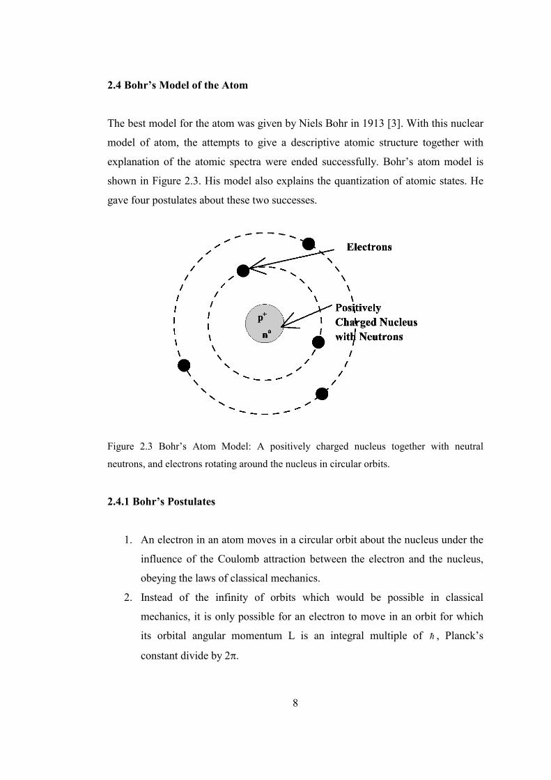
2.4 Bohr’s Model of the Atom
The best model for the atom was given by Niels Bohr in 1913 [3]. With this nuclear
model of atom, the attempts to give a descriptive atomic structure together with
explanation of the atomic spectra were ended successfully. Bohr’s atom model is
shown in Figure 2.3. His model also explains the quantization of atomic states. He
gave four postulates about these two successes.
Figure 2.3 Bohr’s Atom Model: A positively charged nucleus together with neutral
neutrons, and electrons rotating around the nucleus in circular orbits.
2.4.1 Bohr’s Postulates
1. An electron in an atom moves in a circular orbit about the nucleus under the
influence of the Coulomb attraction between the electron and the nucleus,
obeying the laws of classical mechanics.
2. Instead of the infinity of orbits which would be possible in classical
mechanics, it is only possible for an electron to move in an orbit for which
its orbital angular momentum L is an integral multiple of � , Planck’s
constant divide by 2��
8

3. Despite the fact that it is constantly accelerating, an electron moving in such
an allowed orbit does not radiate electromagnetic energy. Thus its total
energy E remains constant.
4. Electromagnetic radiation is emitted if an electron, initially moving in an
orbit of total energy Ei, discontinuously changes its motion so that it moves
in an orbit of total energy Ef. The frequency of the emitted radiation � is
equal to the quantity (Ef-Ei) divided by Planck’s constant h.
First postulate explains the existence of the atomic nucleus and the motion of the
electrons around the nucleus in a circular orbit, and the second introduces the
quantization. His third postulate states that the concept of radiation emission due to
the motion of charged particles in classical physics does not hold in the case of an
atomic electron. And for the last, fourth postulate explains the spectrum observed
belonging to an atom excited by an incident radiation [5].
2.5 Features of the Atom used in Medical Imaging Studies
In this section, the formation of the interaction products i.e., photoelectron and
photon of the matter is explained.
The quantization of the orbital angular momentum of the electron in the third
postulate leads to the quantization of its energy. This means any electron moving in
a certain orbit has certain energy. The total energy of the electron in the n-th
quantum state is given by equation below.
� �,..3,2,1n ,
24emZ
n1E 22
42
2 ����
��
��
(2.1)
As can easily be observed from (2.1), the lowest (the most negative) total energy of
the electron is for the smallest orbital quantum number n=1. As n increases, the total
9

energy of the quantum state decreases, and approaches to zero as n approaches to
infinity [5]. The most stable state of every particle is its lowest energy state. For
one electron atom, hydrogen, it is obvious that the most stable state of the electron
is the n=1 state. This state is called the ground state1 [5]. Quantum state diagram
according to (2.1) for hydrogen atom is depicted in Figure 2.4.
Figure 2.4 The Quantum States for the Hydrogen Atom: As n reaches infinity, binding
energy of the electron goes to zero.
1 Ground state means fundamental state, the term originates from the German word “grund”
meaning the fundamental.
10
The energy equation (2.1) is also called the binding energy of the electron to the
atom in a particular quantum state. This energy defines how strong the electron is
connected to the atom. If an electron is to be removed from its quantum state, a
specific amount of energy equal or greater than its peculiar binding energy must be
applied to the atom.
In an interaction process with matter, the atom receives energy. This energy is
absorbed by the electron and as a result of the received energy, electron makes
transitions to higher orbital quantum states n, greater than its original quantum state
having higher energy. Since the electron in the higher energy state will return to its
most stable, lower energy state, the energy difference between these states
encountered by the electron will be emitted as an electromagnetic radiation. This
transition is the reason of photon production of an atom. Bohr’s fourth postulate
gives that reason and the frequency of this electromagnetic radiation.
When the energy content of the incoming photon is high, an electron gets free rather
than being excited to higher quantum states as shown in Figure 2.5. This electron is
named as photoelectron. From the theory of classical physics, the moving charged
particle radiates electromagnetic energy.
11
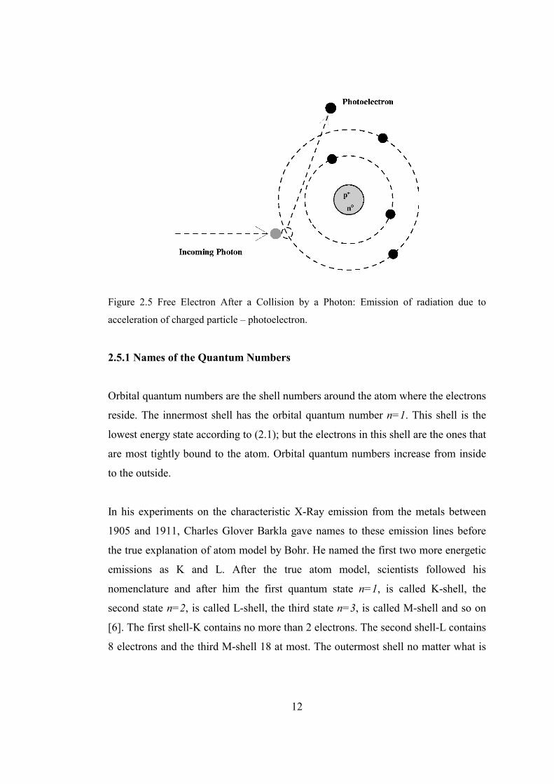
Figure 2.5 Free Electron After a Collision by a Photon: Emission of radiation due to
acceleration of charged particle – photoelectron.
2.5.1 Names of the Quantum Numbers
Orbital quantum numbers are the shell numbers around the atom where the electrons
reside. The innermost shell has the orbital quantum number n=1. This shell is the
lowest energy state according to (2.1); but the electrons in this shell are the ones that
are most tightly bound to the atom. Orbital quantum numbers increase from inside
to the outside.
In his experiments on the characteristic X-Ray emission from the metals between
1905 and 1911, Charles Glover Barkla gave names to these emission lines before
the true explanation of atom model by Bohr. He named the first two more energetic
emissions as K and L. After the true atom model, scientists followed his
nomenclature and after him the first quantum state n=1, is called K-shell, the
second state n=2, is called L-shell, the third state n=3, is called M-shell and so on
[6]. The first shell-K contains no more than 2 electrons. The second shell-L contains
8 electrons and the third M-shell 18 at most. The outermost shell no matter what is
12
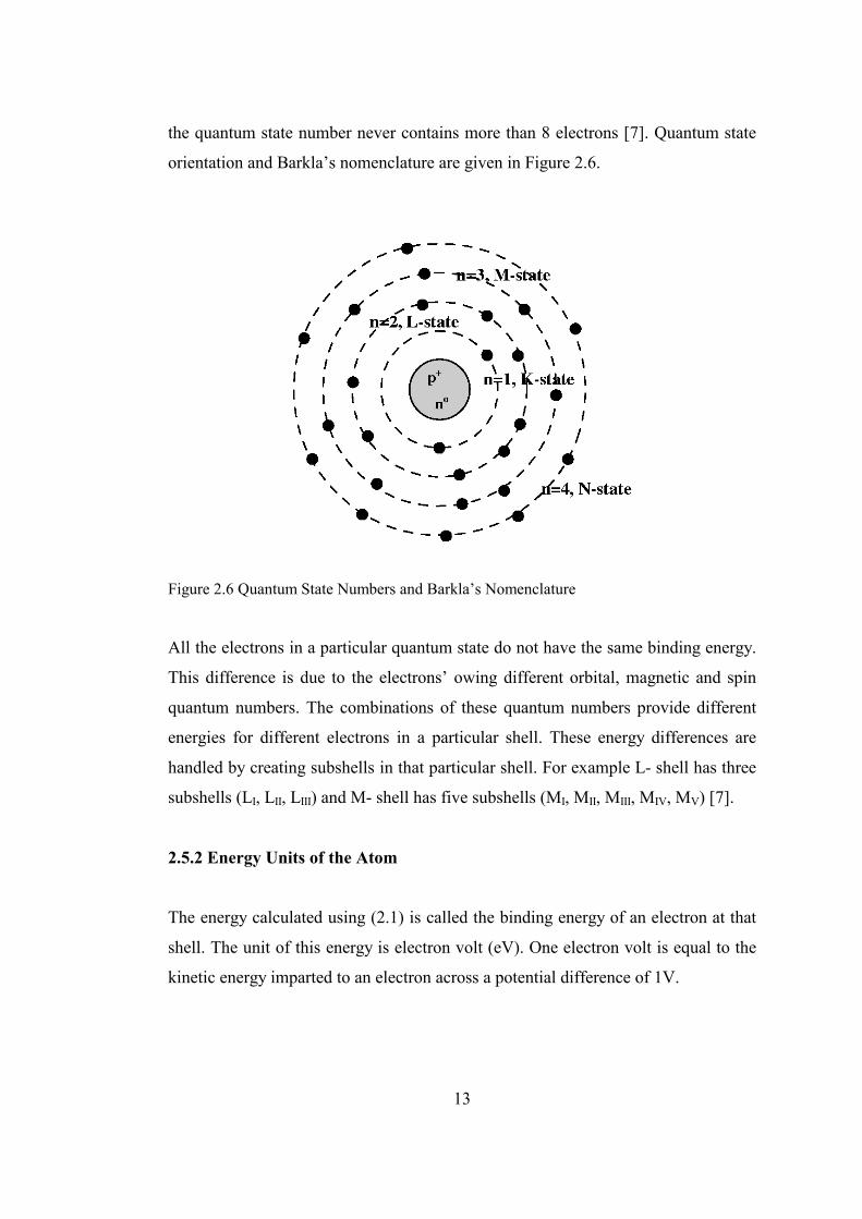
the quantum state number never contains more than 8 electrons [7]. Quantum state
orientation and Barkla’s nomenclature are given in Figure 2.6.
Figure 2.6 Quantum State Numbers and Barkla’s Nomenclature
All the electrons in a particular quantum state do not have the same binding energy.
This difference is due to the electrons’ owing different orbital, magnetic and spin
quantum numbers. The combinations of these quantum numbers provide different
energies for different electrons in a particular shell. These energy differences are
handled by creating subshells in that particular shell. For example L- shell has three
subshells (LI, LII, LIII) and M- shell has five subshells (MI, MII, MIII, MIV, MV) [7].
2.5.2 Energy Units of the Atom
The energy calculated using (2.1) is called the binding energy of an electron at that
shell. The unit of this energy is electron volt (eV). One electron volt is equal to the
kinetic energy imparted to an electron across a potential difference of 1V.
13
CHAPTER 3
PARTICLE PROPERTIES OF RADIATION
AND IT’S INTERACTION WITH MATTER
3.1 Introduction
Until the corpuscular (particle like) definition of radiation named photons, all the
physical relations were defined on the theory of wave. It is hard to accept two
different definitions for a single quantity. Sometimes radiation interacts with matter,
as it is a particle, i.e. Compton Effect that will be described later in this chapter, and
sometimes, as it is a wave, i.e. diffraction. So the radiation has a dual nature, and
this phenomenon is called the wave-particle duality [3]. Duality will be explained
briefly in this chapter.
Particles constituting the radiation interact with the matter according to the energy
content of the radiation, through the processes namely
1. Photoelectric Effect,
2. Compton Effect,
3. Pair Production.
Each of the interactions occurs in different mechanisms, has different formation
conditions and has different end products.
14
This chapter provides the basic knowledge to the animations and simulations
prepared and presented in Chapter6.
3.2 Wave-Particle Duality
After the experimental verification of the corpuscular nature of radiation by
photoelectric effect and Compton scattering, Louis de Broglie stated that the
radiation has dual nature and the particle constituting the radiation, called photon,
has a wave associated with its motion [3]. According to his theory, the total energy
of the photon is related to its frequency of wave associated with its motion as given
by (3.1),
�hE � (3.1)
and its momentum P is related to the wavelength of � of the associated wave by,
�
hP � . (3.2)
As observed from above equations, particle properties energy E and momentum P
are related with the wave concepts frequency � and wavelength � through universal
Planck’s constant h. The wavelength of the particle associated with its motion is
called de Broglie wavelength [3].
The duality exists as; in any event a measurement can be described using only one
model; both models –wave and particle– cannot be used to explain the event under
the same conditions. The summary of this duality was given by Niels Bohr in his
principle of complementarity [3]. This principle states that the wave and particle
models are complementary; if a measurement proves the particle character of
radiation then it is impossible to prove the wave character in the same measurement,
and conversely.
15
3.3 Particle Properties of Radiation
As explained above, sometimes radiation has particle-like properties and energy is
imparted to the matter interacted by particles, rather than waves. These particles are
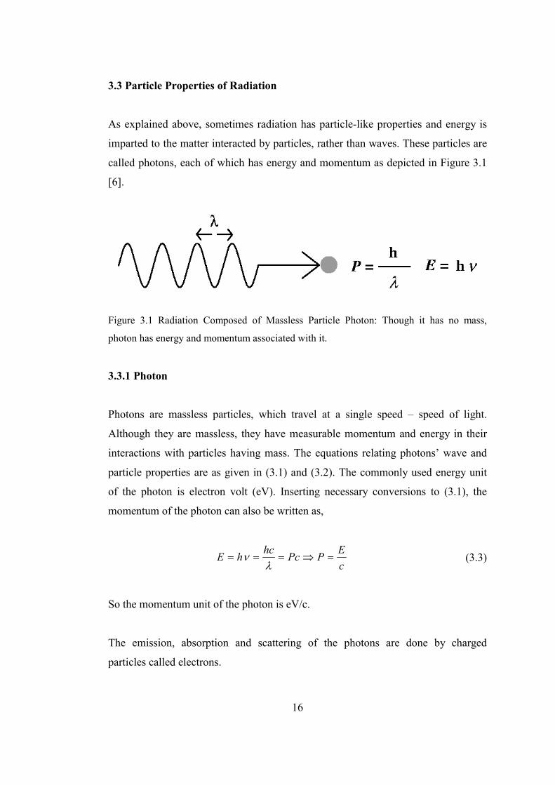
called photons, each of which has energy and momentum as depicted in Figure 3.1
[6].
Figure 3.1 Radiation Composed of Massless Particle Photon: Though it has no mass,
photon has energy and momentum associated with it.
3.3.1 Photon
Photons are massless particles, which travel at a single speed – speed of light.
Although they are massless, they have measurable momentum and energy in their
interactions with particles having mass. The equations relating photons’ wave and
particle properties are as given in (3.1) and (3.2). The commonly used energy unit
of the photon is electron volt (eV). Inserting necessary conversions to (3.1), the
momentum of the photon can also be written as,
cEPPchchE �����
�� (3.3)
So the momentum unit of the photon is eV/c.
The emission, absorption and scattering of the photons are done by charged
particles called electrons.
16

3.4 Definition of Cross Section
One of the important terms in the interaction of radiation with matter is the cross
section term. A cross section is an expression of probability that an interaction will
occur between particles. The bigger the cross section, the higher the probability an
interaction will occur. The atomic cross section unit is the barn. One barn is equal
to 10-28 cm2 [5]. Although not an official SI unit, it is widely used by nuclear
physicists in cross section calculations.
3.5 Interaction of radiation with matter via its particle properties
Introduction
Massless corpuscles constituting the radiation interact with matter via three
processes. These are the 1) photoelectric effect, 2) the Compton Effect, 3) pair
production and 4) bremsstrahlung. First three processes involve the scattering or
absorption and the last involves the production of radiation [3].
3.5.1 Photoelectric Effect
In 1886 and 1887, Heinrich Hertz noted the photoelectric effect. In his experiment,
he shone the electrodes in the glass cathode ray tube with ultraviolet light while
there is an electric discharge between the electrodes. He observed an increase in the
intensity of the discharge. This foundation implies that the number of electrons
freed from the electrodes to jump across the gap is increased [7].
It is the first evidence on wave particle duality. Hertz observed the corpuscular
property of light while he was working on the wave properties of it, to confirm the
existence of electromagnetic waves and Maxwell’s electromagnetic theory of light.
17
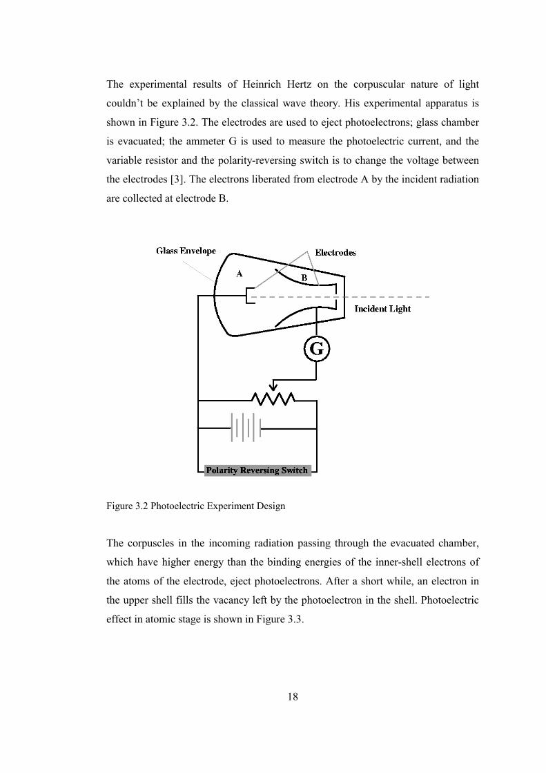
The experimental results of Heinrich Hertz on the corpuscular nature of light
couldn’t be explained by the classical wave theory. His experimental apparatus is
shown in Figure 3.2. The electrodes are used to eject photoelectrons; glass chamber
is evacuated; the ammeter G is used to measure the photoelectric current, and the
variable resistor and the polarity-reversing switch is to change the voltage between
the electrodes [3]. The electrons liberated from electrode A by the incident radiation
are collected at electrode B.
Figure 3.2 Photoelectric Experiment Design
The corpuscles in the incoming radiation passing through the evacuated chamber,
which have higher energy than the binding energies of the inner-shell electrons of
the atoms of the electrode, eject photoelectrons. After a short while, an electron in
the upper shell fills the vacancy left by the photoelectron in the shell. Photoelectric
effect in atomic stage is shown in Figure 3.3.
18

Figure 3.3 Photoelectric Effect: Incoming photon ejects an electron from the inner shell of
the atom. The vacancy left by the photoelectron is filled by the electron in the upper shell
resulting characteristic radiation.
This passage results a radiation whose frequency is the energy difference between
the two states of the electron divided by the Planck’s constant as given by Bohr’s
fourth postulate.
The kinetic energy of the ejected electron is equal to the difference between the
energy of the incoming photon and the binding energy of the ejected electron as
given by Einstein’s equation (3.4) [3].
bphK EEE �� (3.4)
As in all interactions, the incoming photon wants to conserve the momentum, and
that’s why it will try to interact with the nucleus of the atom. But its energy is
insufficient to interact with the nucleus and as a result interacts with orbital
electrons. This orbit is with 80% probability the K-shell orbital electrons as
explained in Appendix 2. In photoelectric effect, momentum is conserved with the
19

recoil of the whole atom, since the incoming photon vanishes at the end of the
interaction.
The results obtained from the experiments can be listed as follows.
�� As the voltage supplied between the electrodes increases, the photoelectric
current increases up to a certain saturation limit at which all electrons
ejected from the electrode A, which the light hits.
�� As the polarity of the applied voltage is reversed, the photoelectric current
does not immediately drop to zero, there are still some energetic electrons
ejected from electrode A, reaching the electrode B despite the opposing
electric field. But there is a certain voltage level Vo where the current
becomes zero. This stopping potential times the electron charge e is equal to
the kinetic energy of the fastest ejected photoelectron, which is given below.
�eVKmax � (3.5)
�� The photoelectric effect is not observed below a certain frequency, �,
specific to the electrode used and this frequency is called cut-off frequency
�o.
A Flash animation of photoelectric effect and a simulation interface of photoelectric
experiment are given in Chapter 6, together with the aims and results of the
programs.
20

Photoelectric Effect Cross Section
Theoretical analyses of photoelectric effect in the energy region of 0.35 MeV to 2
MeV has been obtained by Hulme, McDougall, Buckingham, and Fowler [8]; but
no simple formula was given in this energy region. In the other energy regions,
solutions can be obtained by approximations. These solutions can be divided into
three energy regions: 1) energies greater than 2 MeV, 2) energies from 0.35 MeV to
2 MeV, 3) energies below 0.35 MeV.
Theoretical explanations and the mathematical formulas for the photoelectric cross
section calculations are given in Appendix 2.
Angular Distribution of Photoelectrons
Photoelectrons produced as a result of interaction of the photons with the atom are
not all emitted in the same direction nor their directional distribution is isotropic [8].
As can be understood easily, photons with higher energy will produce more
photoelectrons than the lower energy ones. Also, high energy photons will forward
scatter photons, and the lower energy ones will backscatter them.
The angular distribution formulas of the photoelectrons, applicable to the cloud
chamber measurements for relativistic and nonrelativistic photon energies are given
in Appendix 2. Photon energies greater than 0.511 MeV are called relativistic and
the ones having energy below this value are called nonrelativistic.
The JAVA simulation interfaces of photoelectric effect cross-section and angular
distribution of photoelectrons are supplied in Chapter 6. The aims and results of the
simulation are also given.
21
3.5.2 Compton Effect
Introduction
The hypothesis of quantum theory of the scattering of X-rays by light – low atomic
number, Z – elements suggests that when an X-ray quantum is scattered it spends all
of its energy and momentum upon some particular electron.
In 1923, when Arthur Holly Compton performed his experiment, it had already been
known that a material shone by X-rays give of secondary rays that have different
wavelength than the incident rays [9]. He proved that these secondary rays were
primarily the result of scattering of the incident X-rays from the electrons in the
metal. At this year, he discovered that when a beam of X-rays of well-defined
wavelength �o is scattered through an angle � by sending the radiation through a
metallic foil, the scattered radiation contains a component of a well-defined
wavelength �1, which is longer than �o [10].
This event occurs in a corpuscular manner. Incoming photon is scattered by the free
electron in the target foil. The change in the wavelength that corresponds to a
change in momentum is given by de Broglie (3.2). This change is due to the change
in the direction of the incoming photon.
The change in the momentum of the X-ray quantum due to the change in its
direction of propagation results in a recoil of the scattering electron. The decrease in
the energy of the scattered quantum (secondary radiation) is equal to the kinetic
energy of recoil of the scattering electron.
So using the above changes in momentum and energy, Compton verified that the
corresponding increase (��) in the wavelength of the scattered beam is,
22
)21(sin2)cos1( 2
00
���cm
hcm
h���� (3.6)
In (3.6), h is the Planck’s constant, mo is the rest mass of the electron, c is the speed
of light in vacuum, and � is the scattering angle of the photon in the collision with
respect to its incoming direction.
Before Compton, Thomson stated a classical physics approach to the change in the
wavelength observed. Thomson’s theory is based on the usual electromagnetics
since the incoming radiation is regarded as a wave not bundles of quanta.
Thomson regarded X-ray as a beam of electromagnetic waves whose oscillating
field interacts with every electron in the matter traversed. This interaction produces
forces on the electrons, which cause oscillating accelerations, with the same
frequency as the electromagnetic wave has [3]. According to the classical
electromagnetic theory, any oscillating charged particle radiates electromagnetic
waves. Thus the atomic electrons absorb energy from the incident beam of X-rays
and scatter it in all directions, without modifying the wavelength.
According to the experiments done by Compton on the scattering of X-rays by light
elements, the theory given by Thomson is correct when X-rays of moderate
hardness are employed, but when very hard X-rays interact with atom, the scattered
energy is found to be less than Thomson’s theoretical value [11]. Also secondary X-
rays are softer –longer wavelength, shorter frequency – than the primary rays which
excite them. After the spectroscopic examination of the secondary X-rays Compton
observed that only a small part of the secondary X-radiation is of the same
wavelength as the primary.
Compton stated a theory that exactly explains the scattering of radiation from the
atom using quantum theory of physics. He assumed that X-rays with a wavelength
23

of �o consists of a stream of corpuscles or quantum of energy E as given below by
Max Planck [3]:
�
�
��
hchE �� (3.7)
In his theory, he stated that when one of these quanta hit any free or loosely bound
electron in the scatterer, the electron, which is a quite light particle, would recoil.
The scheme of the effect is shown in Figure 3.4. Its recoiling kinetic energy has to
overcome from the energy of the incident quantum. As a result, that quantum will
be left with energy E1<Eo. Smaller energy of the scattered photon denotes longer
wavelength. This should satisfy the wavelength shift after the collision.
Figure 3.4 Compton Effect: Incoming photon recoils a free bound electron of the atom and
the photon scatters together with it.
To sum up, in the classical theory, each X-ray affects every electron in the atoms of
the matter traversed and the scattering is due to the combined effects of all
electrons. However in the quantum theoretical view X-radiation is composed of
particles and each X-ray quanta is scattered by a particular electron spending its
energy upon it, not by any random electron in the radiator. This particular electron
24
in turn scatters the ray in some definite direction, at an angle with the incident
beam. This bending of the path of the quantum of radiation results in a change in its
momentum.
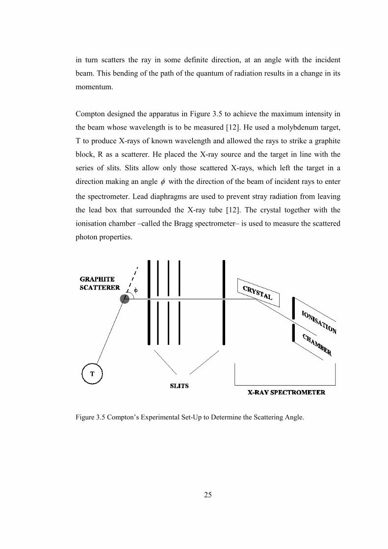
Compton designed the apparatus in Figure 3.5 to achieve the maximum intensity in
the beam whose wavelength is to be measured [12]. He used a molybdenum target,
T to produce X-rays of known wavelength and allowed the rays to strike a graphite
block, R as a scatterer. He placed the X-ray source and the target in line with the
series of slits. Slits allow only those scattered X-rays, which left the target in a
direction making an angle � with the direction of the beam of incident rays to enter
the spectrometer. Lead diaphragms are used to prevent stray radiation from leaving
the lead box that surrounded the X-ray tube [12]. The crystal together with the
ionisation chamber –called the Bragg spectrometer– is used to measure the scattered
photon properties.
Figure 3.5 Compton’s Experimental Set-Up to Determine the Scattering Angle.
25
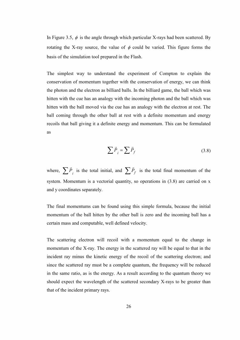
In Figure 3.5 �� is the angle through which particular X-rays had been scattered. By
rotating the X-ray source, the value of � �could be varied. This figure forms the
basis of the simulation tool prepared in the Flash.
The simplest way to understand the experiment of Compton to explain the
conservation of momentum together with the conservation of energy, we can think
the photon and the electron as billiard balls. In the billiard game, the ball which was
hitten with the cue has an analogy with the incoming photon and the ball which was
hitten with the ball moved via the cue has an analogy with the electron at rest. The
ball coming through the other ball at rest with a definite momentum and energy
recoils that ball giving it a definite energy and momentum. This can be formulated
as
�� � fiPP��
(3.8)
where, is the total initial, and i
P��
� fP�
is the total final momentum of the
system. Momentum is a vectorial quantity, so operations in (3.8) are carried on x
and y coordinates separately.
The final momentums can be found using this simple formula, because the initial
momentum of the ball hitten by the other ball is zero and the incoming ball has a
certain mass and computable, well defined velocity.
The scattering electron will recoil with a momentum equal to the change in
momentum of the X-ray. The energy in the scattered ray will be equal to that in the
incident ray minus the kinetic energy of the recoil of the scattering electron; and
since the scattered ray must be a complete quantum, the frequency will be reduced
in the same ratio, as is the energy. As a result according to the quantum theory we
should expect the wavelength of the scattered secondary X-rays to be greater than
that of the incident primary rays.
26
Compton Equations
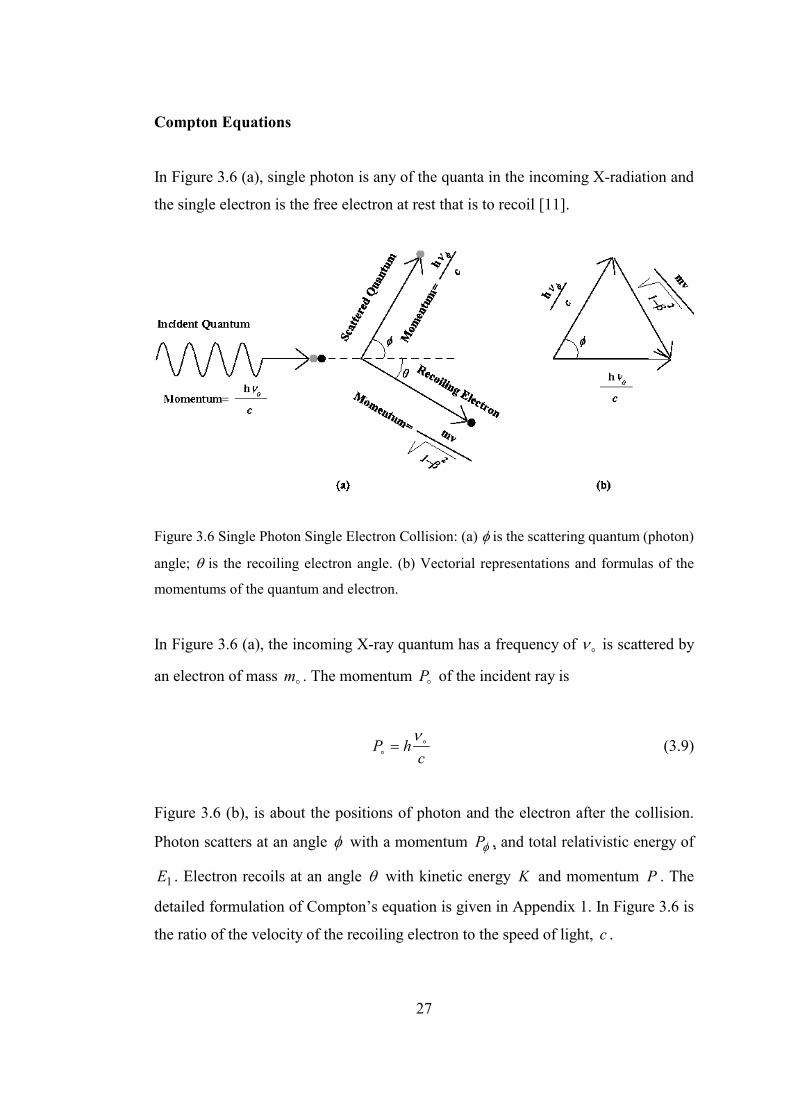
In Figure 3.6 (a), single photon is any of the quanta in the incoming X-radiation and
the single electron is the free electron at rest that is to recoil [11].
Figure 3.6 Single Photon Single Electron Collision: (a) � is the scattering quantum (photon)
angle; � is the recoiling electron angle. (b) Vectorial representations and formulas of the
momentums of the quantum and electron.
In Figure 3.6 (a), the incoming X-ray quantum has a frequency of � is scattered by
an electron of mass . The momentum of the incident ray is
�
�m
�P
chP �
�
�
� (3.9)
Figure 3.6 (b), is about the positions of photon and the electron after the collision.
Photon scatters at an angle � with a momentum , and total relativistic energy of
. Electron recoils at an angle � with kinetic energy
�P
1E K and momentum P . The
detailed formulation of Compton’s equation is given in Appendix 1. In Figure 3.6 is
the ratio of the velocity of the recoiling electron to the speed of light, c .
27

To have the form of Compton’s relation that is mostly encountered, and the
formulas used in the simulation tool, we apply the conservation of momentum and
energy according to the Figure 3.7. The primed quantities are the values of the
momentum and energy after the collision.
Figure 3.7 Compton Formulation: (a) Single photon and electron before the collision and
their initial energy and momentum values are given. (b) Single photon and electron after the
collision and their final energy and momentum values.
Compton Scattering Cross Sections
The cross section equations were obtained by Klein and Nishina [13] and given in
(A.6) and (A.7) in Appendix 1. Simulation interfaces prepared in JAVA are given in
Chapter 6.
28

3.5.3 Pair Production
Introduction
In this type of interaction, photon in the beam produces an electron - positron pair,
whose total kinetic energy is equal to the energy of the photon minus the rest mass
energy of the two created particles.
Theory
Principles of conservation of total relativistic energy, conservation of charge and
conservation of momentum are not violated even in the case of pair production.
Photon does not disappear; it creates two pairs and then vanishes. The conservations
of energy and momentum are satisfied with the presence of the massive nucleus.
Conservation of charge is also obvious; since the photon, which has no charge,
produces an electron and a positron whose total charge yields zero.
The materialisation of photon energy occurs only in the presence of a nucleus or an
electron. The threshold energy for pair production in the field of a nucleus is about
two rest mass energy of an electron while in the field of an electron, double the
energy of the nucleus field energy – that is four rest mass energy of an electron – is
required to conserve the momentum [14]. The energy of the incoming photon is
dissipated as in (3.10) in the case of nucleus field pair production, and as in (3.11)
in the case of electron field pair production [5].
h� (MeV) = 1.02 + (Ek) e- + (Ek) e+ (3.10)
h� (MeV) = 2.04 + (Ek) e- + (Ek) e+ (3.11)
Positron (e+) is a particle which is identical to an electron (e-) with all of its
properties, except that the sign of its charge. It has an opposite charge that of an
29
electron; simply positron is a positively charged electron. It is apparent that the
kinetic energy of the positron produced is slightly larger than that of the electron,
because the Coulomb interaction of the pair with the positively charged nucleus
results to an acceleration of the positron and a deceleration of the electron [3].
Pair production occur in the presence of a nucleus or an electron. The threshold for
pair production in the field of a nucleus is about two electron masses while, in the
event of pair production in the field of an electron, double the energy is required to
conserve momentum [14].
The ratio of probability for the occurrence of pair production due to the electron
field over nucleus field nucleuspp
electronpp
:
:
�
�
is given in Appendix 3, (A.18).
Pair Production Cross Section
The differential cross section equation � for the creation of an electron
positron pair at photon energy k is given in Appendix 3, (A.19). Differential cross
section is the unit change in the cross section for the pair production to occur with
respect to the unit change in the photon energy.
�ppk dkd�
A Java simulation applet is supplied to the user to observe the change in the pair
production cross-section with respect to the photon energy and the atomic number Z
of the interacting material. The cross section for the pair production is zero at 1.02
MeV, rises and at higher energies, i.e. greater than 1000 MeV, a plateau is observed
in the graph. That plateau depends on the material and exists for photon energy
k >> mec2 [15].
30

3.5.4 Attenuation of the Radiation
Introduction
All three interactions of radiation with matter introduced above causes a decrease in
the intensity of the incoming radiation. Each type of radiation takes a certain portion
of the incoming radiation.
There are more interactions that the radiation encounters with regard to its energy
content, namely, coherent scattering, and photodisintegration; however these types
of interactions are not important in the energy range used for medical imaging
purposes. Thus, they are not introduced in this section [5].
X-Ray Attenuation Theory
When a radiation passes through a material with a certain thickness, it is attenuated.
This attenuation effect results a decrease of the intensity of the incoming radiation
due to absorption of photons. Intensity is a measure of field strength of the energy
transmitted by radiation. It is proportional to the product of the photon energy and
the number per unit time [16]. Energy is carried by the photons and the number of
photons defines the intensity strength of the radiation.
The change �I in the intensity of the initial radiation passing through a small
distance �x of a material is proportional to the thickness and the incident intensity I
as given in (3.12).
xII ��� �� ��� (3.12)
� is the proportionality constant, and is the total absorption coefficients or cross
sections of the interactions of radiation with matter. All interaction processes act
independently. Consequently, one can separate the absorption coefficients into five
31
parts: � for coherent scattering, ���for photoelectric effect, � for Compton Effect, �
for pair production, and � for photodisintegration. For each interaction, equations
similar to 3.12 can be written [8]:
� �
� �
� �
� �
� � xII
xII
xII
xII
xII
tegrationsinPhotodi
Production Pair
Effect Compton
Effect ricPhotoelect
Scattering Coherent
���
���
���
���
���
��
��
��
��
��
(3.13)
Total intensity change is obtained by adding the five equations in (3.13) yielding
������ ����� ��� (3.14)
For the X-ray energies used for imaging purposes, absorption coefficients for
coherent scattering, pair production, and photodisintegration are not applicable [5].
Thus, the total attenuation coefficient � can be approximated as:
��� �� ��� (3.15)
If the incident radiation is homogeneous (single wavelength) and the absorption
coefficient is constant (pure matter), integration of (3.12) gives
xeII ��
��
(3.16)
32
The physical meaning of (3.16) is that when a beam with initial intensity
traverses a matter of thickness x, due to absorption of photons in the matter has a
final intensity of
�I
I .
Intensity I can be expressed as
BhI �� (3.17)
where, B is the number of photons crossing unit area in unit time, and h� is the
energy per photon. Thus (3.16) can also be written as
xeBB ��
��
(3.18)
A Flash simulation interface is given in Chapter 6 for the attenuation of X-rays
through various materials.
33
CHAPTER 4
GENERATION AND DETECTION OF X-RAYS
4.1 Introduction
X-rays can be produced in various ways, either by using radioactive materials or by
the methods explained later in this chapter, namely characteristic radiation and
bremsstrahlung processes. To take the benefits of X-ray, in any X-ray examination,
the source of the X-ray must provide sufficient amount of X-ray energy in a certain
time. Also its energy must be variable according to the intend of the physician.
There are two types of X-ray detection methods:
1. X-ray Film.
2. Radiation Detectors.
Radiation detectors are divided into two types namely,
a) Scintillation detectors (Photomultiplier Tubes).
b) Ionisation chamber detectors.
34

In this thesis, no animation or a simulation tool is prepared for X-ray film and
ionisation chamber detectors. No enough knowledge could be obtained for these
types of detectors, to simulate or animate them.
Photomultiplier tube is selected for simulation of X-ray detection. After the
interactions of radiation with matter, the intensity of the radiation is too low to
process and to detect, as a result of the attenuation faced. To enhance and to have a
sufficient amount of knowledge from that signal, photomultiplier tubes are used.
In this chapter, methods to generate X-rays and its detection will be presented.
4.2 Production of X-Rays
4.2.1 Characteristic Emission
When an atom is excited by an incident radiation, an electron in the lower shell of
an atom is ejected and the atoms in the upper states fill the vacancy [5]. As stated
before during this transition, photons will be produced. The emitted photons are in
the range of X-ray. For the characteristic radiation to occur, incoming photon must
interact with the bound electron. Incoming photon disappears; it imparts all its
energy remained to the photoelectron after breaking the binding energy of the
electron to the atom. Too many kinds of characteristic radiation can be observed
depending on the orbit of the removed electron and the number of orbits containing
electrons beyond the stimulated electrons orbit.
Intensity of this type of production is very precise at certain energy. However
continuously achieving that single intensity at that energy is very hard. As time
precedes the electron population in the higher energy shell producing that intended
X-ray intensity decreases. Also the intensity cannot be varied according to the
intend, it is not economic. The concept of intensity variation also determines the
quality of the radiographic image produced because, during the exam, voluntary or
35
involuntary motions of the patient decreases the clarity of the image produced. This
is overcome by using X-ray exposures of high intensity and short duration.
Together with these reasons, characteristic X-ray emission is not a desired
generation method for imaging purposes.
4.2.2 Bremsstrahlung
Introduction
The continuous X-ray radiation due to the deceleration of the electron from passing
the nucleus field is called bremsstrahlung [3]. Concept is obvious using the classical
theory of the electromagnetic radiation – any decelerating charged particle, brought
into rest in the target material, results in the emission of a continuous spectrum of
electromagnetic radiation.
The word bremsstrahlung comes from the German brems – braking + strahlung –
radiation [3].
Bremsstrahlung Cross Section
The bremsstrahlung cross section d for single photon emission is given by the
transition probability per atom per electron divided by the incoming electron
velocity [16].
�
The units used in the calculations for the energies and momenta are in moc2 and moc
units respectively [16]. So the energies and momenta given in MeV and MeV/c
units must be converted to the units appropriately as given in Appendix 4.
The formulas used in the cross section simulations are given in Appendix 4.
36

4.3 X-Ray Tube
To obtain efficient variable energy and safer X-rays, X-ray tubes are designed. The
scheme of the commercial tubes widely used today is shown in Figure 4.1.
Figure 4.1 X-Ray Tube: The electrons freed from the filament by applying a voltage Vin, hit
the target material and produces photons. The magnets are used to rotate the target material
to prevent heating of it.
To get X-rays, the target material is bombarded via the electrons produced by the
filament through the current passing through it. Filament must have a very high
melting point to sustain the overheating during current passage to produce electrons.
More current produces more desirable electrons resulting higher temperature. The
glass envelope is evacuated to prevent the interaction of electrons with gas
molecules. The electrons produced by the filament are called the tube current [5].
Electrons produced bombard the target to produce X-ray. Continuous bombarding
heats the target material and this heat make it work improperly. To prevent
overheating of the target it must be rotated. By rotation not only a single portion of
the target is affected by the electrons; all parts of it are bombarded properly.
37
Rotation is satisfied by the stator magnets [5]. Target materials that are widely used
are tungsten, rhodium and molybdenum, since they overwhelm the heat produced
better than the other materials.
The voltage between the target and the electron-producing filament must be kept
positive – target anode, filament cathode. The electrons produced by the filament is
repelled from negative anode and attracted through the positive cathode. To satisfy
this condition, the input AC voltage is rectified to have a DC input. When polarity is
reversed, current cannot be produced in the tube; since target material does not
produce electrons via heating at such tube operating voltages. If the tube voltage
increases, target becomes to produce electrons and these electrons flow from
negative target, to positive filament across the X-ray tube. This reverse flow of
electrons damages the X-ray tube [5], because the tube was designed for X-ray
production, not electron production.
4.3.1 Currents Flowing in the X-Ray Tube
Two electrical currents flow in the X-ray tube. First type is to heat the filament for
the release of the electrons. The flow of electrons for this purpose is called the
filament current. Second type is the flow of released electrons from the filament to
the anode to produce X-ray photons [5].
These currents are different but they affect themselves mutually. If the tube voltage
is low, electron release rate from the filament is more rapidly than the rate of
electron flow acceleration towards the target anode. So after a while a cloud of
electrons occurs around the filament preventing the release of additional electrons
from the filament. This cloud of electrons is termed – space charge [5].
To obtain X-ray in the medical diagnosis range and high tube currents to prevent
space charge effect decreasing the X-ray emission rate, high filament currents and
voltages between 40 and 140 kV must be used [5].
38

4.3.2 X-Ray Emission Spectra in the X-Ray Tube
Even single energy electrons bombards the target, X-rays are produced in a range of
energies. Characteristic radiation is released independent of the energy of the
bombarding electron, as long as the energy of the bombarding electrons exceeds the
binding energy for characteristic emission [3].
4.3.3 X-Ray Tube Ratings
Tube Voltage
As mentioned in bremsstrahlung process, the highest energy of the X-ray is equal to
the energy of the bombarding electron. So as the energy of the electrons
bombarding the target in the tube increases with the increase of tube voltage, the
high-energy limit of the X-ray spectrum increases. Also, the efficiency of the
bremsstrahlung production increases with the electron energy yielding more X-ray
photons [5].
Tube Current and Time
Charge, in unit of Coulomb, is equal to the product of current and time. The total
number of electrons hitting the target is calculated by multiplying the tube current
and the exposure time.
To get a figure, the number of electrons hitting the target for 1 mA tube current for
1 second exposure time is
� �� � .1025.6106.1
sec sec/10 1519
3
electronselectroncoulomb
coulomb��
��
�
(4.1)
39

Target Material
Atomic number of the material used for X-ray production affects the efficiency.
Target material with a higher atomic number produces more X-ray photons.
The efficiency of X-ray production is defined as the ratio of energy emerging as X-
ray radiation from the target – radiated power (Pr), divided by the energy deposited
by electrons hitting on the target [5] – power deposition (Pd):
ZV109.0VI
IZV109.0PP
Efficiency 929
d
r �
�
��
�
�� (4.2)
where, V is the tube voltage.
4.4 Photomultiplier Tube
Introduction
As a result of the interactions of radiation with matter, extremely weak light signals
occur. To get a usable amount of knowledge from this signal, containing no more
than a few hundred photons, photomultiplier tubes are used. These tubes are very
advantageous because they do not add random noise to the signal. The main parts of
the photo-multiplier tubes are the photocathode, anode and dynodes.
In this section the features of the photomultiplier tubes are introduced.
4.4.1 Parts of the Photomultiplier Tube
In the photomultiplier tube, photocathode is coupled to the electron multiplier
structure. The incident radiation ejects photoelectrons through the photocathode.
These photoelectrons are directed to the electron multiplier structure by the focusing
40
electrodes. In this structure the number of electrons are increased and converted into
a useful electrical signal [17].
The electron number is increased in the electrodes called dynode. The number of the
dynodes used in the photomultiplier tube is one of the things that determine the
number of electrons produced.
The dynodes are kept at a potential relative to the other. This potential difference
between each dynode determines the kinetic energy of the incident electron by
accelerating it to the next dynode. Incident electrons with higher kinetic energies
tend to emit more secondary electrons from the next dynode they will go. The
variation between the potential difference and the number of electrons produced in
the dynodes is exponential. For example for a tube design with 3 dynodes, first
dynode producing 2 electrons as a gain will produce 4 electron if the potential
difference is increased twice. In the first scheme, each electron will produce 2 more
electrons in each dynode yielding 8 electrons in the third, but in the second scheme
each electron will produce 4 more electrons in each dynode yielding 64 electrons in
the third [18].
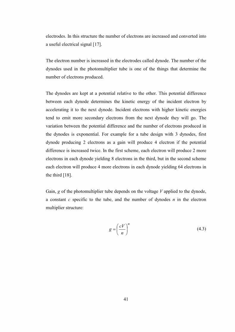
Gain, g of the photomultiplier tube depends on the voltage V applied to the dynode,
a constant c specific to the tube, and the number of dynodes n in the electron
multiplier structure:
n
ncVg �
�
���
�� (4.3)
41
CHAPTER 5
JAVA SIMULATIONS OF COMPUTERIZED TOMOGRAPHIC IMAGING
5.1 Introduction
Every tissue has a unique attenuation coefficient under the influence of certain X-
ray energy [1]. This property of the tissues makes it possible to use X-rays for
imaging the attenuation coefficient distribution and differentiating tissues having
attenuation coefficients close to each other.
The projection of the attenuation distribution is obtained mathematically by taking
the line integrals of the object along the ray path. This method is carried over all
view angles by a method called Radon Transform. Projection data obtained with
this method is used to reconstruct the image. Various methods can be used to
reconstruct the attenuation distribution [18] [1].
Computerized tomography (CT) system produces slice images of the object. In a CT
setup, a rotating X-ray source together with a detector just ahead it rotates together
around the object to obtain projection data [18].
In this study, first the theory related to CT data collection and image reconstruction
will be presented. Next, two CT simulators will be introduced.
42

5.2 Theory and Mathematical Background
5.2.1 Introduction
X-ray radiation of intensity I passing through a material of thickness dx and
attenuation coefficient � satisfies the following equation:
IdxdI ��� (5.1)
where dI is the part of energy removed in a distance dx. If the medium is not
homogeneous, then � in two dimensions can be expressed as . The
attenuation of the incident beam along y=y
� yx,�� � �
1 can be written as,
� �IdxyxdI 1,��� (5.2)
If we take the integral of the attenuation distribution along y=y1 line, one may
obtain the line integral of the attenuation function at y=y1, as
� � � ���� dxyxIIyp 11 ,ln �
�
(5.3)
where p (y1) is named as the projection function.
Projection function is also a function of angle of view (Figure 5.1). At each view,
a set of line integral data is obtained giving the projection of the distribution.
Complete projection data is obtained by calculating the projection functions with a
specified angle step covering 180° [18]. In a parallel projection system, parallel ray
integrals are obtained for each angle of view. In this study, this method is utilized to
obtain projections in the simulation program.
43

The projection of the object distribution , at a view angle is shown in
Figure 5.1 [18]. is also known as the Radon transform of the object along � �
direction ����.
� yx,� �
� �tp�
For a general view angle � , can be expressed as [19]. � �tp�
� � � � � �� ��
��
��� dxdytyxyxtp sincos, ����� (5.4)
Figure 5.1 Line integral projection of object distribution at view angle � . � yx,� �
44
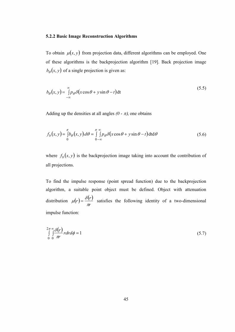
5.2.2 Basic Image Reconstruction Algorithms
To obtain from projection data, different algorithms can be employed. One
of these algorithms is the backprojection algorithm [19]. Back projection image
of a single projection is given as:
� yx,� �
�
�
� yxb ,�
� � � ���
��
��� dt sincos, tyxpyxb ����� (5.5)
Adding up the densities at all angles (0 - �, one obtains
� � � � � �� � ��
��
����
� �
�� �����0 0
dtd sincos ,, tyxpdyxbyxfb (5.6)
where is the backprojection image taking into account the contribution of
all projections.
� yxfb ,
To find the impulse response (point spread function) due to the backprojection
algorithm, a suitable point object must be defined. Object with attenuation
distribution � �� �rrr
�
�� � satisfies the following identity of a two-dimensional
impulse function:
� � 1 2
0 0�� �
�
��
��
rdrdrr (5.7)
45

The impulse response h of the back projection algorithm can be obtained as
[19]
� �rb
� � .1r
rhh bb �� (5.8)
Thus, the reconstructed image using the backprojection algorithm can be expressed
as:
� � � �r
yxfyxfb1,, ��� (5.9)
To avoid blurring, one way is to use two-dimensional filters. This method is
computationally inefficient. Another method, namely the convolution
backprojection algorithm employs one-dimensional operations. In this approach, the
projection function is convolved with a function c(t), and then the filtered
projections are backprojected. In space domain backprojected function can written
as
� �� �� � � � � ��� ��
111
11
��
�� FtPtPFF (5.10)
where � � � �tcF �
�
�1
1 .
The image reconstructed using this approach can be expressed as:
� � � � � �� � � �� ��
��
����
�
� ����
0dtd sincos,ˆ tyxtctpyxf (5.11)
46
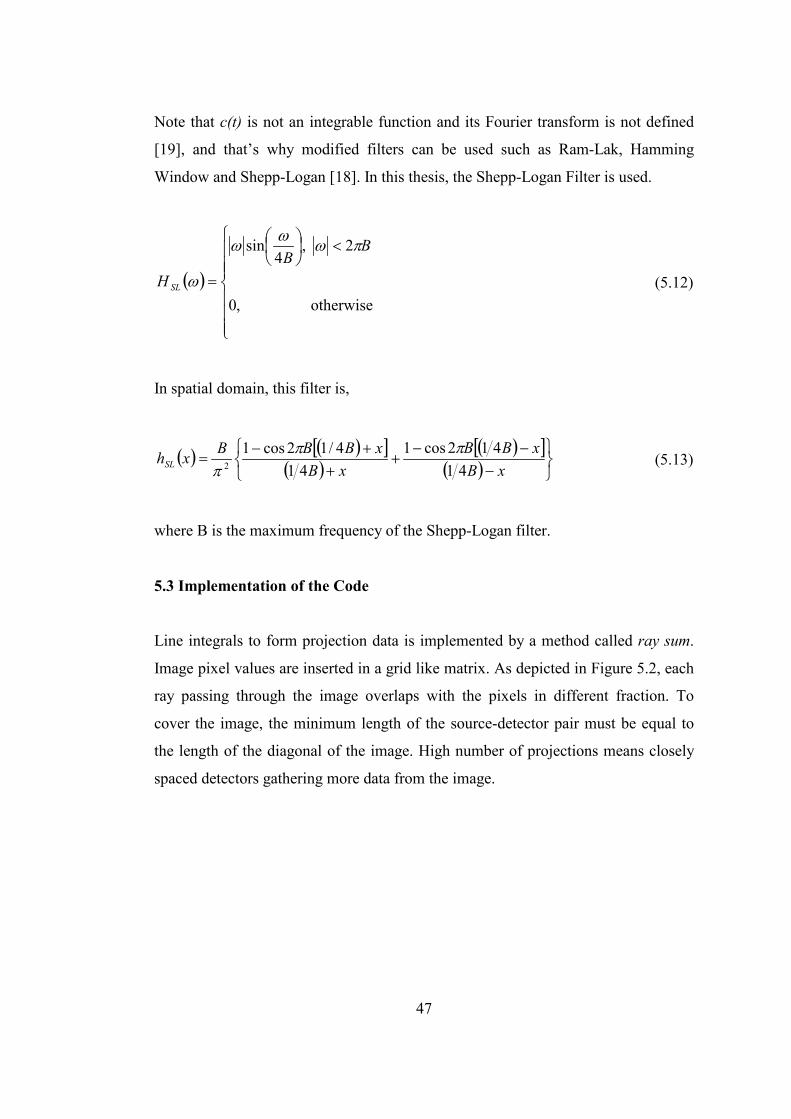
Note that c(t) is not an integrable function and its Fourier transform is not defined
[19], and that’s why modified filters can be used such as Ram-Lak, Hamming
Window and Shepp-Logan [18]. In this thesis, the Shepp-Logan Filter is used.
� �
���
�
���
�
���
�
�
�
�
otherwise ,0
2 ,4
sin BB
H SL
��
�
�
� (5.12)
In spatial domain, this filter is,
� �� �� �
� �� �� �
� � ���
���
�
���
�
��
xBxBB
xBxBBBxhSL 41
412cos141
4/12cos12
��
�
(5.13)
where B is the maximum frequency of the Shepp-Logan filter.
5.3 Implementation of the Code
Line integrals to form projection data is implemented by a method called ray sum.
Image pixel values are inserted in a grid like matrix. As depicted in Figure 5.2, each
ray passing through the image overlaps with the pixels in different fraction. To
cover the image, the minimum length of the source-detector pair must be equal to
the length of the diagonal of the image. High number of projections means closely
spaced detectors gathering more data from the image.
47
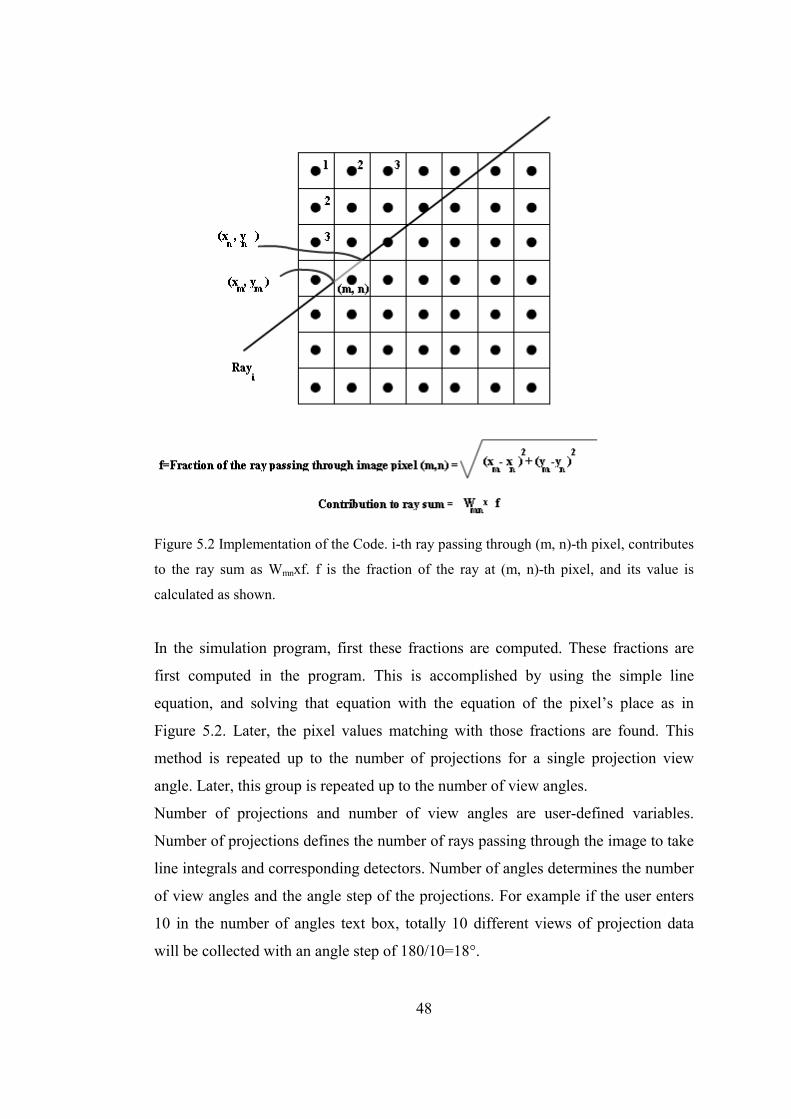
Figure 5.2 Implementation of the Code. i-th ray passing through (m, n)-th pixel, contributes
to the ray sum as Wmnxf. f is the fraction of the ray at (m, n)-th pixel, and its value is
calculated as shown.
In the simulation program, first these fractions are computed. These fractions are
first computed in the program. This is accomplished by using the simple line
equation, and solving that equation with the equation of the pixel’s place as in
Figure 5.2. Later, the pixel values matching with those fractions are found. This
method is repeated up to the number of projections for a single projection view
angle. Later, this group is repeated up to the number of view angles.
Number of projections and number of view angles are user-defined variables.
Number of projections defines the number of rays passing through the image to take
line integrals and corresponding detectors. Number of angles determines the number
of view angles and the angle step of the projections. For example if the user enters
10 in the number of angles text box, totally 10 different views of projection data
will be collected with an angle step of 180/10=18°.
48
After forming the projection data matrix, it is convolved with the Shepp-Logan
filter. Convolving operation is carried over the rows of the projection matrix one by
one.
5.4 JAVA Simulation of Single Energy CT System
Presentation of the Simulation Interface
In the first JAVA simulation supplied, user can define the object shape from the
radio buttons, its size and weights from their respective scrollbars supplied. These
weights represent different attenuation coefficients of the objects imaged using X-
rays. They are not a function of some variable; these are just showing a distribution
mimicking the different attenuation coefficients in the image to be reconstructed.
Attenuation coefficient scroll-bar value is between 1 and 17. These values are
multiplied with 15 to form the images yielding color values between 15 and 255.
Higher color values yields whiter images meaning a higher attenuation value.
User can also define the number of projections and the number of angles in the
simulation in their appropriate places. When necessary, user can reset the image
formed by pressing the reset button, and start to make a new image configuration.
After completing the image configuration and entering the number of angles and
number of projections, user can start the projection and filtered backprojection
algorithm by pressing the start button.
Aim
In this simulation we aim to obtain projection and filtered backprojection images of
the distribution that the user defined. A sample scheme is shown in Figure 5.3 and
Figure 5.4. The image distribution having different weights implements a slice of
the body containing different organs having different attenuation coefficients,
imaged under computerized tomography system having single energy. Circle in the
49

left side has a size 20 pixels, and attenuation mimicking gray level of 1x15=15. The
size of the square in the middle is 23 with a gray level 7x15=105 and the oval has a
size 34 and a gray level of 16x15=240.
Simulation User Interface
Figure 5.3 Single Energy CT (1) Effect of Angle and Projection Number: Object
distribution, size, shape and attenuation coefficients are determined by the user and the
backprojected and filtered backprojected images are formed for angle number of 180 and
projection number of 200.
50

Figure 5.4 Single Energy CT (2) Effect of Angle and Projection Number: Same object but;
backprojected and filtered backprojected images are formed for angle number of 35 and
projection number of 165.
Results
1. Backprojected image and filtered backprojected image is obtained at the end
of the simulation.
2. As the number of angles or the number of projections is increased, better
image reconstructions are obtained. With an increase in these numbers, more
knowledge is obtained from the processed image.
3. Objects having same weights – same attenuation coefficients, that were put
so close to each other cannot be differentiated from each other, but objects
with different weights that were close to each can be differentiated easily.
51
5.5 JAVA Simulation of Energy Dependent Attenuation Coefficient CT System
In the second JAVA simulation supplied, user again can define the object shape
from the radio buttons, its size and weights from the scrollbars supplied. This time
these weights are a function of energy showing a distribution in the image to be
reconstructed. As noted in Chapter 3.5.4, attenuation coefficient of materials
changes with a change in the X-radiation energy it interacts. User can also define
the number of projections, the number of angles, can reset the image s/he formed by
pressing the reset button to start to make a new image configuration and can start
the algorithm by pressing the start button in the simulation again.
Different than the first one, user can determine and change the background of the
image and observe the change in the attenuation of the image with a change in the
energy of the X-ray beam using the energy scrollbar supplied. User does not define
the image weight, s/he only defines the material and the simulation calculates the
weight according to the energy with the formulation in (5.14) [1].
� ���
���
��
���
� n
m
pgZCfN�
��� (5.14)
In (5.14), ��is the bulk density of the material, � is the energy of the incoming X-
radiation; Ng is the electron mass density, which is2
AAg A
ZNN ��
N
f
where NA is
the Avogadro number, portion of the attenuation coefficient from the
Compton Effect, given by Klein and Nishina as given in (A.8). C
� ��
p is the coefficient
for the photoelectric dependent portion of the attenuation coefficient, and m and n
are the powers for the atomic number of the material and the energy of the radiation
respectively, that are m = 3.8, and n = 3.2.
52
Energy of the incoming X-ray beam is between 5 and 30 keV. This range is the
initial portion of the currently used medical imaging X-ray devices energy range.
This range is between 10 and 300 keV. The reason of this choice is that the
materials supplied as background or foreground begins to have approximately the
same attenuation coefficients after 30 keV, except for bone and cortical bone. This
equalizing causes confusion in the images formed and reconstructed.
The background and foreground materials that can be selected are blood, water,
bone, cortical bone, adipose tissue, muscle, brain white matter/ grey matter, breast
tissue, lung tissue, ovary, testis, eye lens, radiographic dye film and alanine. These
materials were chosen for the simulation because they are the tissues and materials
that come first to mind in imaging studies. The atomic numbers and densities of
these materials are taken from [20] and [21]. Their Z/A ratio are taken as 0.5,
because except for hydrogen, all the elements have Z/A ratio approximately 0.5.
In the simulation, the attenuation values of these 14 materials at different energies
are scaled between 0 and 255. These numbers are the color value ranges used by the
computers. The highest value of attenuation belongs to the bone at 5 keV and the
lowest value belongs to fat at 30 keV X-Ray energy, which are, 642.539 cm2/g and
0.206 cm2/g respectively. 642.539 is scaled to 255, whose color is white, and 0.206
is scaled to 0, whose color is black. The remaining materials in different energy
values are set to gray levels.
53

Aim
In the following simulations we want to observe,
1. The change in the attenuation coefficient of the materials with respect to the
X-ray energy.
2. The contrast between background and foreground with respect to X-ray
energy.
3. Effect of background material attenuation coefficient value on the 1/r
blurring.
4. Investigate the resolution by forming a phantom image.
Simulation A
A sample scheme for the same image distribution under 10.5 keV X-ray energy at
different angle and projection numbers is shown in Figure 5.5 and Figure 5.6. In
Figure 5.5, number of angles is 180 and the number of projections is 200, but in
Figure 5.6, number of angles is 35 and the number of projections is 130. The circle
of size 23 in the left is fat and has an attenuation value 1.406 cm2/g, the square in
the middle is muscle whose size and attenuation values are 45 and 3.392 cm2/g
respectively, and the oval is bone of size 18, and attenuation coefficient value
60.118 cm2/g. The background material is selected as water whose attenuation
coefficient is 13.403 cm2/g at 10.5 keV X-ray energy.
54
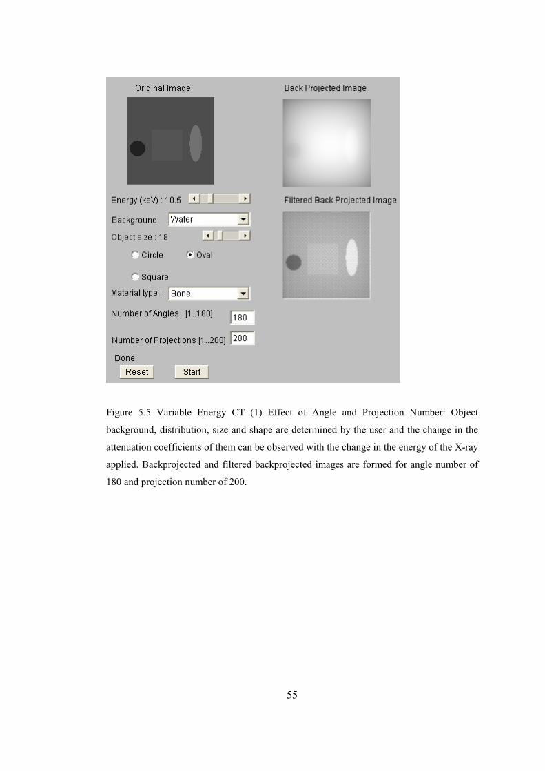
Figure 5.5 Variable Energy CT (1) Effect of Angle and Projection Number: Object
background, distribution, size and shape are determined by the user and the change in the
attenuation coefficients of them can be observed with the change in the energy of the X-ray
applied. Backprojected and filtered backprojected images are formed for angle number of
180 and projection number of 200.
55
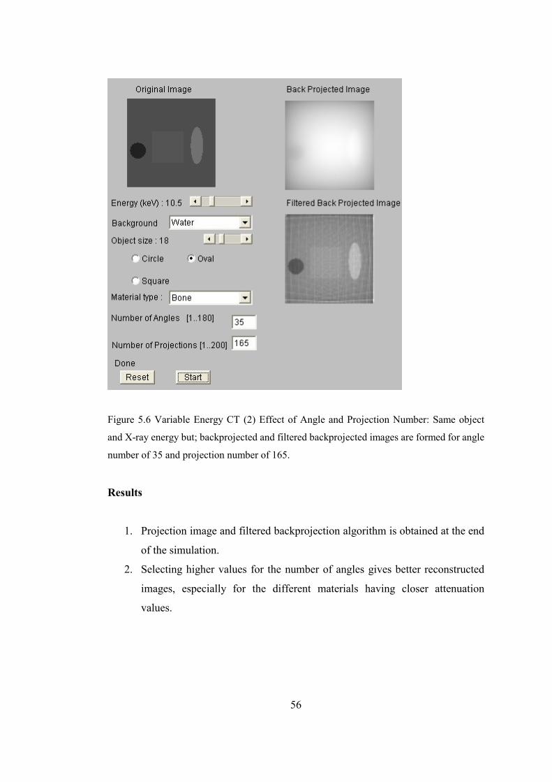
Figure 5.6 Variable Energy CT (2) Effect of Angle and Projection Number: Same object
and X-ray energy but; backprojected and filtered backprojected images are formed for angle
number of 35 and projection number of 165.
Results
1. Projection image and filtered backprojection algorithm is obtained at the end
of the simulation.
2. Selecting higher values for the number of angles gives better reconstructed
images, especially for the different materials having closer attenuation
values.
56
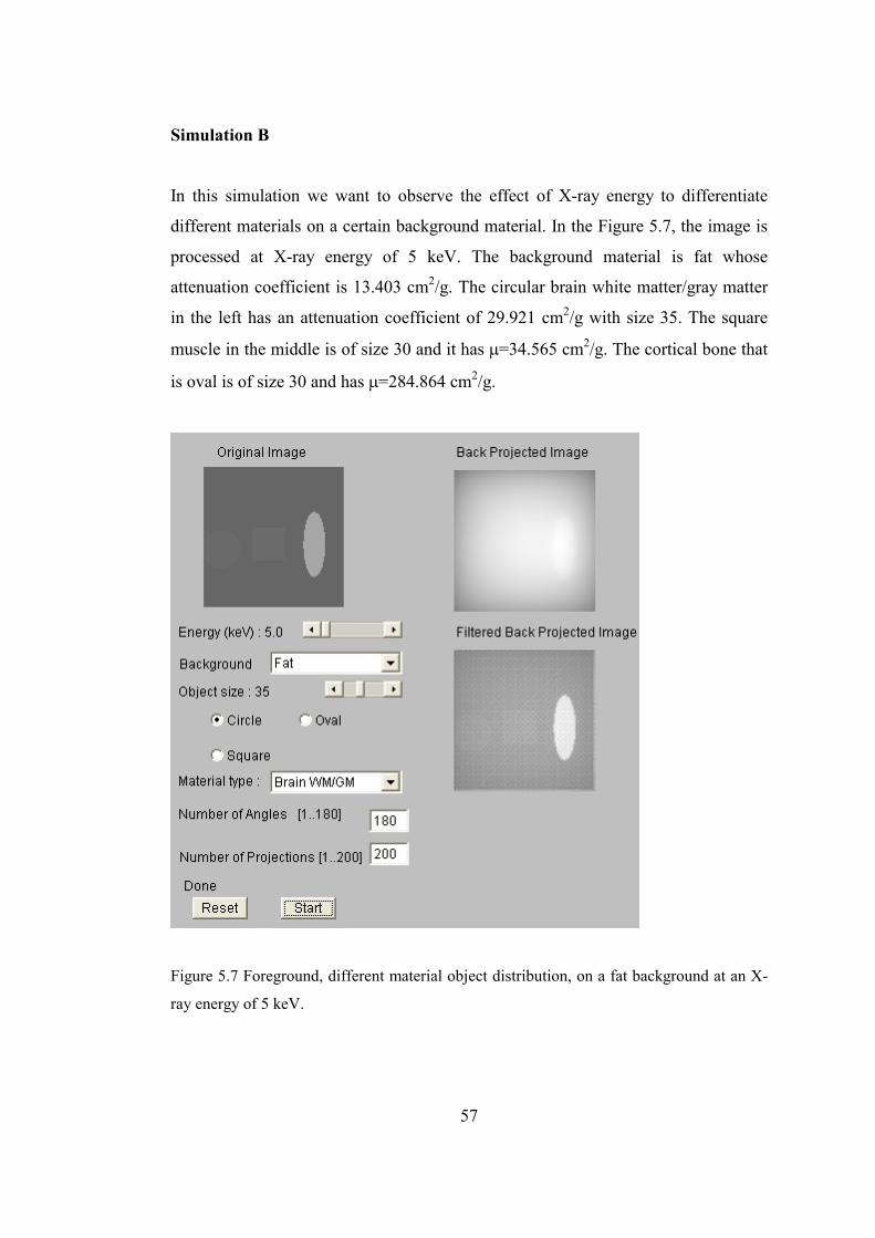
Simulation B
In this simulation we want to observe the effect of X-ray energy to differentiate
different materials on a certain background material. In the Figure 5.7, the image is
processed at X-ray energy of 5 keV. The background material is fat whose
attenuation coefficient is 13.403 cm2/g. The circular brain white matter/gray matter
in the left has an attenuation coefficient of 29.921 cm2/g with size 35. The square
muscle in the middle is of size 30 and it has �=34.565 cm2/g. The cortical bone that
is oval is of size 30 and has �=284.864 cm2/g.
Figure 5.7 Foreground, different material object distribution, on a fat background at an X-
ray energy of 5 keV.
57
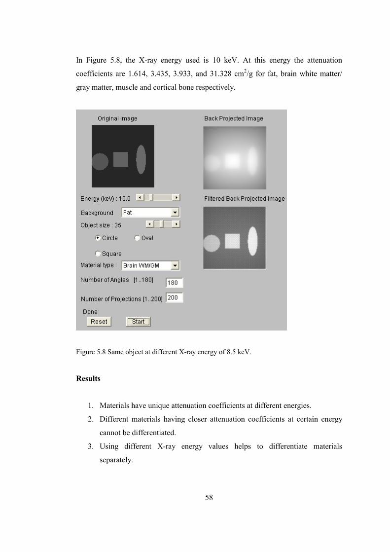
In Figure 5.8, the X-ray energy used is 10 keV. At this energy the attenuation
coefficients are 1.614, 3.435, 3.933, and 31.328 cm2/g for fat, brain white matter/
gray matter, muscle and cortical bone respectively.
Figure 5.8 Same object at different X-ray energy of 8.5 keV.
Results
1. Materials have unique attenuation coefficients at different energies.
2. Different materials having closer attenuation coefficients at certain energy
cannot be differentiated.
3. Using different X-ray energy values helps to differentiate materials
separately.
58

Simulation C
In this simulation we want to observe the effect of background material on 1/r
blurring, together with the foreground images. In Figure 5.9, water background
under 5 keV has an attenuation coefficient value of 31.942 cm2/g, and in Figure
5.10, attenuation coefficient of water is 0.281 cm2/g under 30 keV X-ray energy.
Figure 5.9 Effect of background on blurring. Background material is water imaged at X-ray
energy of 5 keV.
59
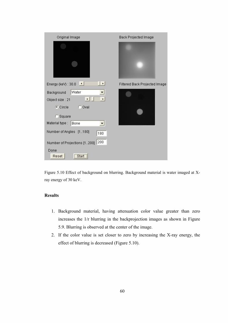
Figure 5.10 Effect of background on blurring. Background material is water imaged at X-
ray energy of 30 keV.
Results
1. Background material, having attenuation color value greater than zero
increases the 1/r blurring in the backprojection images as shown in Figure
5.9. Blurring is observed at the center of the image.
2. If the color value is set closer to zero by increasing the X-ray energy, the
effect of blurring is decreased (Figure 5.10).
60
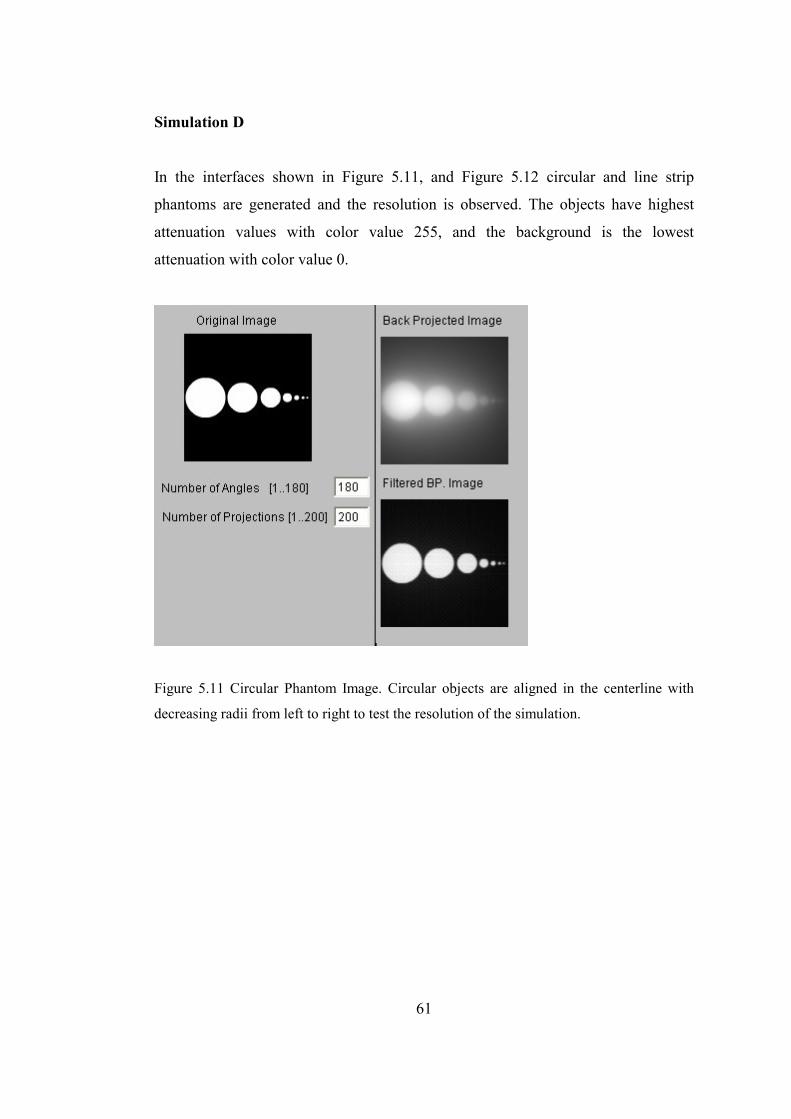
Simulation D
In the interfaces shown in Figure 5.11, and Figure 5.12 circular and line strip
phantoms are generated and the resolution is observed. The objects have highest
attenuation values with color value 255, and the background is the lowest
attenuation with color value 0.
Figure 5.11 Circular Phantom Image. Circular objects are aligned in the centerline with
decreasing radii from left to right to test the resolution of the simulation.
61
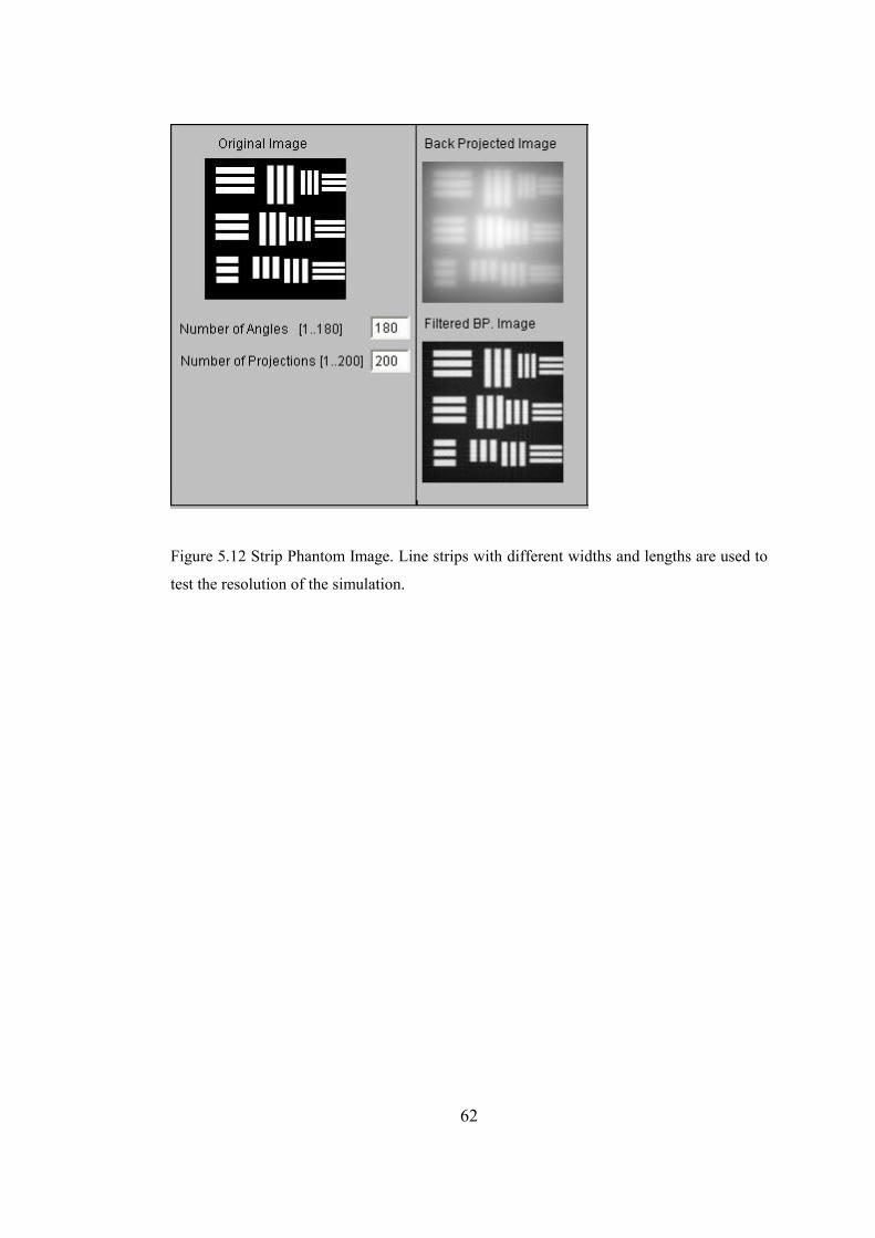
Figure 5.12 Strip Phantom Image. Line strips with different widths and lengths are used to
test the resolution of the simulation.
62
CHAPTER 6
ANIMATION AND SIMULATION INTERFACES
6.1 Introduction
In this Chapter, the simulation and animation interfaces prepared for X-ray
interactions with matter, X-ray generation and X-ray detection methods are
presented. For each simulation/animation, the aims and the results are shown
explicitly. The formulations used in the simulations are given in the Appendix. The
aim of the animations is to give brief information about the mechanism of the
subject.
In an education tool, animation is as necessary as simulation for the users. It
enhances the visualization capability of the user, and performs the first step of
education tools.
Simulations reflect the physical basis of the subjects. They include formulations,
and take into consideration all the variables affecting the event. With the
simulations, one can observe the changes in the event by changing the controllable
variables. For some topics, animation is not supplied, because simulation is also
enough for visualization of the event.
Our basic aim in this study is to prepare a web-based education tool. So the
simulations and animations prepared must be reachable from the Internet, with no
63
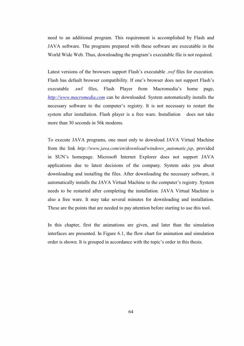
need to an additional program. This requirement is accomplished by Flash and
JAVA software. The programs prepared with these software are executable in the
World Wide Web. Thus, downloading the program’s executable file is not required.
Latest versions of the browsers support Flash’s executable .swf files for execution.
Flash has default browser compatibility. If one’s browser does not support Flash’s
executable .swf files, Flash Player from Macromedia’s home page,
http://www.macromedia.com can be downloaded. System automatically installs the
necessary software to the computer’s registry. It is not necessary to restart the
system after installation. Flash player is a free ware. Installation does not take
more than 30 seconds in 56k modems.
To execute JAVA programs, one must only to download JAVA Virtual Machine
from the link http://www.java.com/en/download/windows_automatic.jsp, provided
in SUN’s homepage. Microsoft Internet Explorer does not support JAVA
applications due to latest decisions of the company. System asks you about
downloading and installing the files. After downloading the necessary software, it
automatically installs the JAVA Virtual Machine to the computer’s registry. System
needs to be restarted after completing the installation. JAVA Virtual Machine is
also a free ware. It may take several minutes for downloading and installation.
These are the points that are needed to pay attention before starting to use this tool.
In this chapter, first the animations are given, and later than the simulation
interfaces are presented. In Figure 6.1, the flow chart for animation and simulation
order is shown. It is grouped in accordance with the topic’s order in this thesis.
64
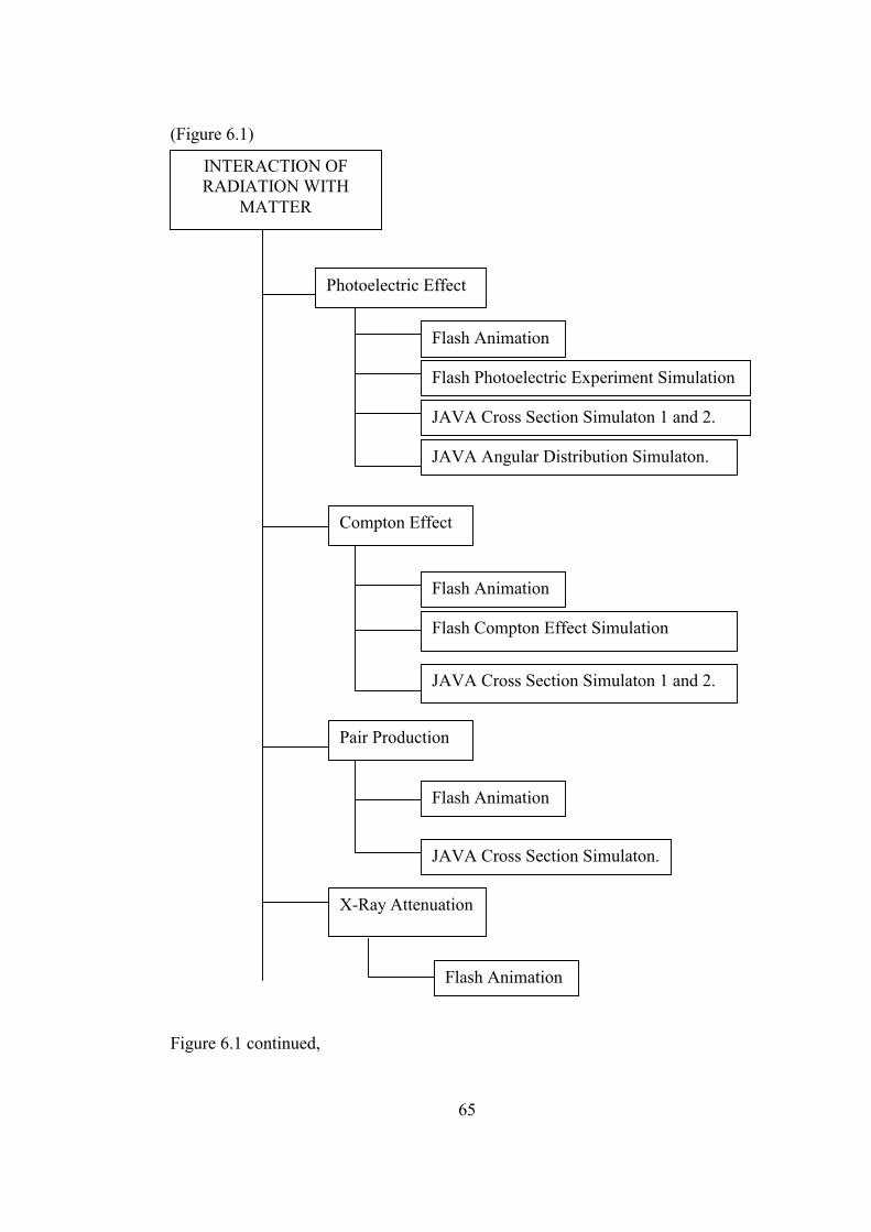
(Figure 6.1)
Photoelectric Effect
Flash Animation
Flash Photoelectric Experiment Simulation
JAVA Cross Section Simulaton 1 and 2.
Compton Effect
Flash Animation
Flash Compton Effect Simulation
JAVA Cross Section Simulaton 1 and 2.
JAVA Angular Distribution Simulaton.
Pair Production
Flash Animation
JAVA Cross Section Simulaton.
Flash Animation
X-Ray Attenuation
INTERACTION OF RADIATION WITH
MATTER
Figure 6.1 continued,
65
Flash Simulation
Flash Simulation
Photomultiplier Tube
X-Ray Tube
JAVA Cross Section Simulaton 1, 2 and 3.
Flash Animation
Bremsstrahlung
Flash Animation
Characteristic Radiation
GENERATION AND DETECTION OF X-RAYS
66

Figure 6.1 continued
JAVA Simulation 1 and 2
COMPUTERIZED TOMOGRAPHY SIMULATOR
Figure 6.1 The road map for the animation and simulations.
6.2 Photoelectric Effect
6.2.1 Photoelectric Effect Flash Animation
All the facts and theories explained in 3.5.1 about the mechanism of photoelectric
effect in atomic scale are animated in the prepared Flash program. Interaction
mechanism, its end products, and conservation of momentum are animated in the
programs. These interfaces are depicted in Figure 6.2.
Aims of the Animations
1. To observe the main scheme of the photoelectric effect in atomic scale,
2. to observe the recoil of the whole atom to conserve momentum in the
photoelectric effect,
3. to observe end products of the photoelectric effect,
4. to observe possible electron shell transitions.
67

Fig. 6.2. Photoelectric Animation Interface
Results of the Animations
1. The phenomenon is due to the interaction of photons with the bound
electrons.
2. Photoelectric effect results with a characteristic radiation whose frequency
depends on the energy difference of the two orbits (i.e., energies
corresponding to the orbits of the photoelectron and the electron which fills
the vacancy).
3. The incoming photon vanishes after the interaction with an orbital electron.
4. To conserve the momentum, the whole atom recoils after the collision.
6.2.2 Photoelectric Effect Flash Simulation
The simulation graphical user interface is given in Figure 6.3. In the simulation
supplied the user can select the electrode material in the combo-box supplied. After
determining the material the user can observe the binding energies of the electrons
in their respective shells namely, K, LI, LII, and LIII shells. With this knowledge, the
user then selects the shell to be excited. From the scrollbar in the right bottom user
68
can select the energy of the incoming radiation. In this part user can also observe
the relation between the wavelength and frequency of the radiation together with its
energy. Kinetic Energy vs. Frequency graph gives the relation between the
maximum energy and frequency of the released photoelectrons, and the cut-off
frequency of the material. Current vs. Voltage graph gives the relation between
photoelectric current and applied voltage. Gathering these data one can observe the
facts explained in Chapter 3.5.1, by changing the voltage supplied between the
electrodes and the intensity of the incident radiation via their respective scrollbars
supplied.
Aims of the Simulation
In the following simulation, the purpose is to observe;
1. the main parts of the photoelectric experiment,
2. the dependence of the photoelectric effect on the incoming photon energy
and material type,
3. the kinetic energy of the photoelectron,
4. the current versus voltage graphics of the photoelectric effect,
5. the kinetic energy of the photoelectron versus the frequency of the
incoming photon.
69

Figure 6.3 Photoelectric Effect Flash Simulation Graphic User Interface: The experimental
set-up is as given in Figure 3.2.
Results of the Simulation
1. Photoelectric effect is not observed if the incoming photon energy does not
exceed the binding energy of the orbital electron it interacts with, even the
intensity of the radiation is increased.
2. If energy of the photon is more than the threshold energy, the remaining
energy of the photon is imparted to the photoelectron as the kinetic energy
and this energy does not increase with an increase in the intensity, i.e., the
number of photons of the incoming radiation.
3. If the photons have sufficient energy, current can be observed even the
voltage applied between the electrodes is zero, showing that there exists a
flow of electrons between the electrodes.
4. Current versus voltage graphics show a sudden increase and a plateau after
some voltage value. This plateau is due to space charge neutrality. The
70
charges accumulated in electrode B in Figure 3.2 starts to repel new
photoelectrons, resulting a saturation value of current.
5. From the kinetic energy versus frequency graph, it is observed that energy
of the photoelectron is zero below a certain frequency. This is due to the
inadequacy of the energy of the photon to eject the orbital electron. This
threshold frequency depends on the material and the orbital number of the
ejected electron and is called the binding frequency.
6.2.3 Photoelectric Effect Cross Section Java Simulations
Photoelectric effect cross section calculations are divided into three different photon
energy regions: 1) energies greater than 2 MeV, 2) energies from 0.35 MeV to 2
MeV, 3) energies below 0.35 MeV. The calculations for each region are given in
Appendix 2. The simulations are based on the formulations given there. Cross
section calculations were done according to the energy considerations given above.
n, used in figures is the ratio of electron rest mass energy mc2 to the energy h� of
the incoming photon, where mc2 is equal to 0.511 MeV.
Two simulations were supplied for the photoelectric cross section.
A. First one simulates the change in the cross section values with respect to
atomic number Z of the interacted material for the user defined n via the
scrollbar. In this simulation n is between 0.5 and 2, and Z is from 1 to 100.
(A.11) in Appendix 2 is used in the first simulation. Simulation result for
n=2 and Z=92 is depicted in Figure 6.4. In the figure apses is the atomic
number of the interacted material and ordinate is nZ 5
a� , so note that a
decrease in the graphics means an increase in the atomic number of the
interacted material.
71

Aims of the Simulation A
1. To observe the dependence of photoelectric effect cross section on the
wavelength and energy of the incoming photon,
2. to observe the dependence on the atomic number of interacted material
using the atomic number scrollbar supplied,
3. to observe the dependence of photoelectric cross section on n.
Figure 6.4 Photoelectric Cross Section vs. Atomic Number Z: Cross section graphs for
electron rest mass photon energy ratio, n between 0.1 and 2. In this figure, n=2 and Z=92.
Results of the Simulation A
1. As the photon energy is increased -n decreases-, photoelectric effect cross
section is decreased.
2. As the atomic number of the interacted material increases, photoelectric
cross section increases.
72
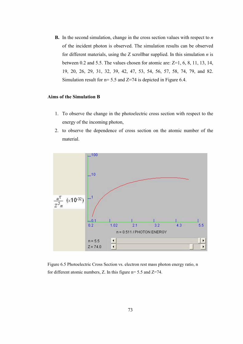
B. In the second simulation, change in the cross section values with respect to n
of the incident photon is observed. The simulation results can be observed
for different materials, using the Z scrollbar supplied. In this simulation n is
between 0.2 and 5.5. The values chosen for atomic are: Z=1, 6, 8, 11, 13, 14,
19, 20, 26, 29, 31, 32, 39, 42, 47, 53, 54, 56, 57, 58, 74, 79, and 82.
Simulation result for n= 5.5 and Z=74 is depicted in Figure 6.4.
Aims of the Simulation B
1. To observe the change in the photoelectric cross section with respect to the
energy of the incoming photon,
2. to observe the dependence of cross section on the atomic number of the
material.
Figure 6.5 Photoelectric Cross Section vs. electron rest mass photon energy ratio, n
for different atomic numbers, Z. In this figure n= 5.5 and Z=74.
73
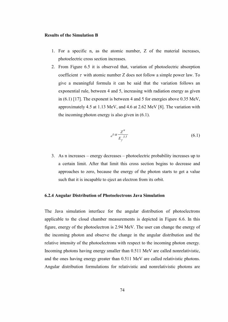
Results of the Simulation B
1. For a specific n, as the atomic number, Z of the material increases,
photoelectric cross section increases.
2. From Figure 6.5 it is observed that, variation of photoelectric absorption
coefficient �� with atomic number Z does not follow a simple power law. To
give a meaningful formula it can be said that the variation follows an
exponential rule, between 4 and 5, increasing with radiation energy as given
in (6.1) [17]. The exponent is between 4 and 5 for energies above 0.35 MeV,
approximately 4.5 at 1.13 MeV, and 4.6 at 2.62 MeV [8]. The variation with
the incoming photon energy is also given in (6.1).
5.3
n
aE
Z
�
�� (6.1)
3. As n increases – energy decreases – photoelectric probability increases up to
a certain limit. After that limit this cross section begins to decrease and
approaches to zero, because the energy of the photon starts to get a value
such that it is incapable to eject an electron from its orbit.
6.2.4 Angular Distribution of Photoelectrons Java Simulation
The Java simulation interface for the angular distribution of photoelectrons
applicable to the cloud chamber measurements is depicted in Figure 6.6. In this
figure, energy of the photoelectron is 2.94 MeV. The user can change the energy of
the incoming photon and observe the change in the angular distribution and the
relative intensity of the photoelectrons with respect to the incoming photon energy.
Incoming photons having energy smaller than 0.511 MeV are called nonrelativistic,
and the ones having energy greater than 0.511 MeV are called relativistic photons.
Angular distribution formulations for relativistic and nonrelativistic photons are
74
given in Appendix 2, in (A.15) and (A.16) respectively, and velocity calculation for
the photoelectrons is given in (A.17).
Aim of the Simulation
1. To observe the angular distribution of the photoelectron and its dependence
on the incoming photon energy.
Figure 6.6 Angular Distribution of Photoelectrons: Angular Distribution of relativistic
(energy>0.511 MeV) and nonrelativistic (energy<0.511 MeV) photon energies. In this
figure, energy of the photoelectron is 2.94 MeV (relativistic).
Result of the Simulation
1. As the energy of the incoming photon increases photoelectrons scatters at
small angles.
75

6.3 Compton Effect Animation and Simulations
6.3.1 Compton Effect Flash Animation
All the facts and theories explained in 3.5.2 about the mechanism of Compton
Effect in atomic scale are animated in the Flash program prepared. In the program
interaction mechanism and its end products are animated. The interface is given in
Figure 6.7.
Aims of the Compton Effect Animation
1. To understand the mechanism of Compton Effect,
2. to observe the recoiling of the electron and the scattering of the incoming
photon to conserve the momentum, rather than the recoiling of whole atom
as in the photoelectric effect.
3. to observe end products of the Compton Effect.
Fig. 6.7 Compton Animation
76
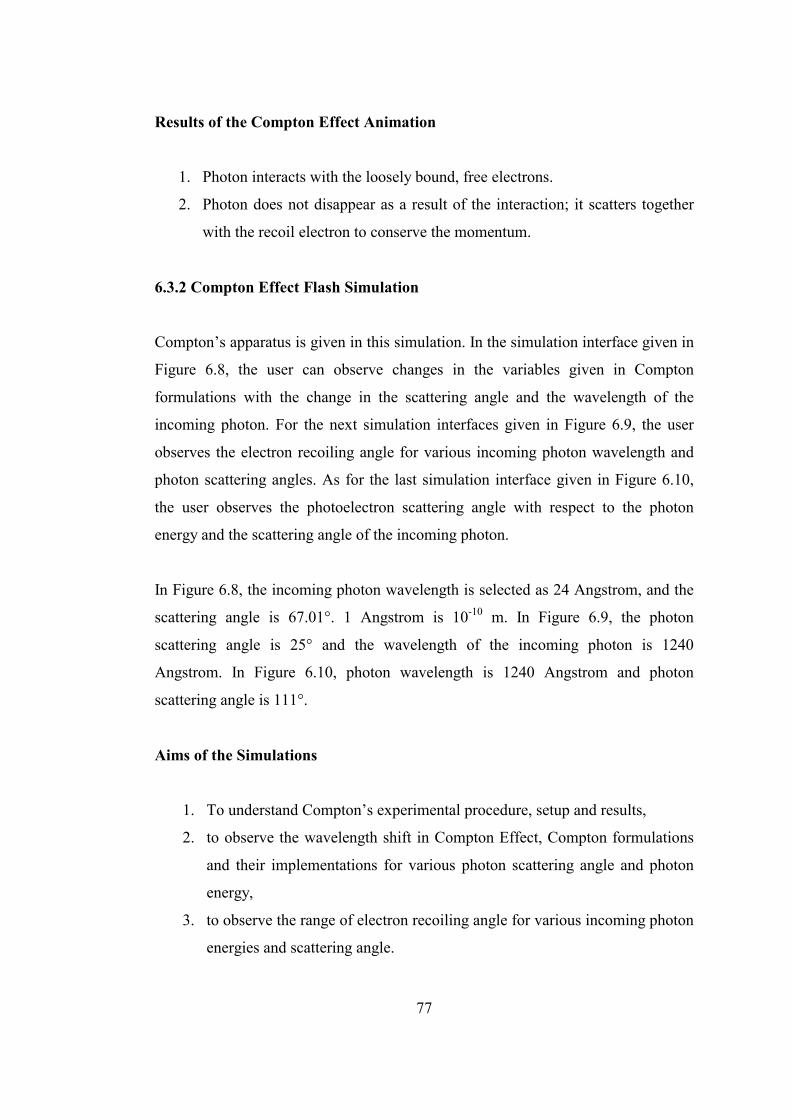
Results of the Compton Effect Animation
1. Photon interacts with the loosely bound, free electrons.
2. Photon does not disappear as a result of the interaction; it scatters together
with the recoil electron to conserve the momentum.
6.3.2 Compton Effect Flash Simulation
Compton’s apparatus is given in this simulation. In the simulation interface given in
Figure 6.8, the user can observe changes in the variables given in Compton
formulations with the change in the scattering angle and the wavelength of the
incoming photon. For the next simulation interfaces given in Figure 6.9, the user
observes the electron recoiling angle for various incoming photon wavelength and
photon scattering angles. As for the last simulation interface given in Figure 6.10,
the user observes the photoelectron scattering angle with respect to the photon
energy and the scattering angle of the incoming photon.
In Figure 6.8, the incoming photon wavelength is selected as 24 Angstrom, and the
scattering angle is 67.01°. 1 Angstrom is 10-10 m. In Figure 6.9, the photon
scattering angle is 25° and the wavelength of the incoming photon is 1240
Angstrom. In Figure 6.10, photon wavelength is 1240 Angstrom and photon
scattering angle is 111°.
Aims of the Simulations
1. To understand Compton’s experimental procedure, setup and results,
2. to observe the wavelength shift in Compton Effect, Compton formulations
and their implementations for various photon scattering angle and photon
energy,
3. to observe the range of electron recoiling angle for various incoming photon
energies and scattering angle.
77

Figure 6.8 Compton Flash Simulation Interface (1): User enters the wavelength of the
incoming photon and observes the variables given in the boxes by changing the scattering
angle dynamically.
Figure 6.9 Compton Flash Simulation Interface (2): User enters the photon scattering angle
and the wavelength of the incoming photon and observes the recoiling angle of the electron.
78

Figure 6.10 Compton Flash Simulation Interface (3): User enters the wavelength of the
incoming photon and selects the photon scattering angle from the scroll bar and observes
that the recoiling angle of the electron is between 0� and 90�.
Results of the Simulations
1. The wavelength shift between the incoming and the scattered photon
changes with the change in the scattering angle of the photon.
2. The change in the photon’s wavelength, it’s final wavelength, it’s initial
and final energy, change in it’s energy, final electron momentum, and the
velocity of the electron according to the initial wavelength of the incoming
photon with respect to different photon scattering angles is observed.
3. Electron recoiling angle depends on the photon scattering angle and
incoming photon wavelength.
79
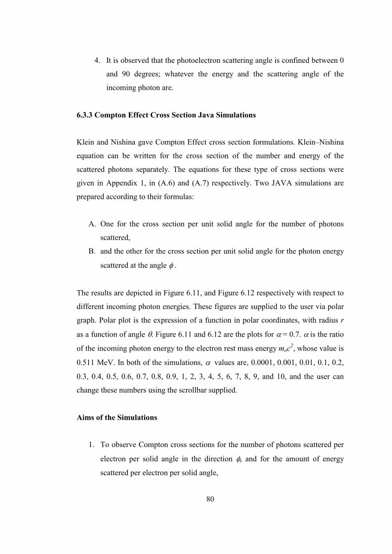
4. It is observed that the photoelectron scattering angle is confined between 0
and 90 degrees; whatever the energy and the scattering angle of the
incoming photon are.
6.3.3 Compton Effect Cross Section Java Simulations
Klein and Nishina gave Compton Effect cross section formulations. Klein–Nishina
equation can be written for the cross section of the number and energy of the
scattered photons separately. The equations for these type of cross sections were
given in Appendix 1, in (A.6) and (A.7) respectively. Two JAVA simulations are
prepared according to their formulas:
A. One for the cross section per unit solid angle for the number of photons
scattered,
B. and the other for the cross section per unit solid angle for the photon energy
scattered at the angle ��.
The results are depicted in Figure 6.11, and Figure 6.12 respectively with respect to
different incoming photon energies. These figures are supplied to the user via polar
graph. Polar plot is the expression of a function in polar coordinates, with radius r
as a function of angle �. Figure 6.11 and 6.12 are the plots for ��= 0.7. ��is the ratio
of the incoming photon energy to the electron rest mass energy moc2, whose value is
0.511 MeV. In both of the simulations, �� values are, 0.0001, 0.001, 0.01, 0.1, 0.2,
0.3, 0.4, 0.5, 0.6, 0.7, 0.8, 0.9, 1, 2, 3, 4, 5, 6, 7, 8, 9, and 10, and the user can
change these numbers using the scrollbar supplied.
Aims of the Simulations
1. To observe Compton cross sections for the number of photons scattered per
electron per solid angle in the direction �� and for the amount of energy
scattered per electron per solid angle,
80
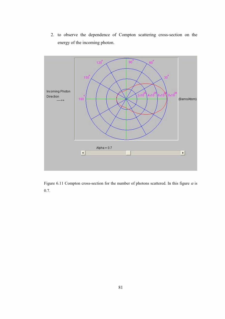
2. to observe the dependence of Compton scattering cross-section on the
energy of the incoming photon.
Figure 6.11 Compton cross-section for the number of photons scattered. In this figure � is
0.7.
81
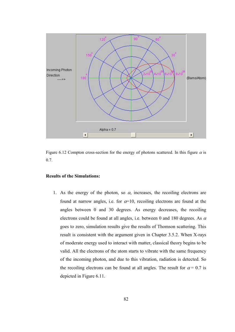
Figure 6.12 Compton cross-section for the energy of photons scattered. In this figure � is
0.7.
Results of the Simulations:
1. As the energy of the photon, so �, increases, the recoiling electrons are
found at narrow angles, i.e. for �=10, recoiling electrons are found at the
angles between 0 and 30 degrees. As energy decreases, the recoiling
electrons could be found at all angles, i.e. between 0 and 180 degrees. As �
goes to zero, simulation results give the results of Thomson scattering. This
result is consistent with the argument given in Chapter 3.5.2. When X-rays
of moderate energy used to interact with matter, classical theory begins to be
valid. All the electrons of the atom starts to vibrate with the same frequency
of the incoming photon, and due to this vibration, radiation is detected. So
the recoiling electrons can be found at all angles. The result for ��= 0.7 is
depicted in Figure 6.11.
82
2. For the simulation of cross section calculations of Compton scattering for
the energy of photons scattered as energy increases, more energetic
electrons are found at narrow degrees. As the energy of the incoming photon
decreases, energetic electrons are found at higher angles. The result for ��=
0.7 is depicted in figure 6.12.
6.4 Pair Production
6.4.1 Pair Production Flash Simulation
A Flash simulation is prepared to visualize the pair production formulations and
mechanisms explained in Chapter 3.5.3. Two types of pair production can occur:
A. Nucleus field pair production.
B. Electron field pair production.
Energy of the incoming photon must be higher than 1.02 MeV for nucleus field and
two times this value is needed for the electron field pair production to conserve the
momentum. At the end of the pair production positron e+ and an electron e- pair is
formed. The simulation prepared in Flash is depicted in Figure 6.13. The
mechanism and end products of this type of interaction can also be observed in this
simulation. User can change the energy of the incoming photon and see whether the
electron field or nucleus field pair production occurs for that particular energy. User
can also observe the kinetic energy of the positron and electrons produced at the end
of the interaction. The simulation is prepared based on the knowledge given in
Chapter 3.5.3.
One can also observe the ratio of probability for the occurrence of pair production
due to the electron field over nucleus field nucleuspp
electronpp
:
:
�
�
. The formulation is given in
Appendix 3, in (A.18).
83

Aims of the Simulation
1. To observe the two types of pair production and their dependencies on
incoming photon energy,
2. to see pair production end products,
3. to observe the kinetic energies of the electron and positron produced for the
two types of pair production cases,
4. to understand the threshold energy value for the photon for two types of pair
production interactions,
5. to observe the cross section ratios of the nucleus and electron field pair
production.
Figure 6.13 Flash Simulation Interface for Pair Production: In the Flash simulation
prepared, user can change the energy of the incoming photon and observe the nucleus and
electron pair production. The energy of the positron and electron can also be observed.
84

Results of the Flash Simulation
1. Energy considerations for nucleus field and electron field pair production
are observed. To conserve the momentum, energy of the photon must be
greater than 1.02 MeV for nucleus field and greater than 2.04 MeV for
electron field pair production.
2. If the photon energy is greater than the threshold energy values of pair
production, the remaining energy of the photon is imparted to the positron
and electron as kinetic energy equally.
3. nucleuspp
electronpp
:
:
�
�
is detected and it is observed that pair production near an electron
is less important than near nucleus except for materials of low atomic
number.
6.4.2 Pair Production Cross Section JAVA Simulation
JAVA simulation interface is prepared for the pair production cross section versus
photon energies between 1.02 and 50 MeV for interacted material atomic numbers
between 1 and 100. In the Figure 6.14, the result is given for photon energy of 31
MeV and material atomic number Z = 60. The formula used in this simulation is
explained and given in (A.19) in Appendix 3.
Aims of the Simulation
1. To observe the pair production cross section due to nucleus field,
2. to observe dependence of pair production cross section on incoming photon
energy and the atomic number of the material interacted,
3. to observe dependence of pair production cross section on the energy of one
of the produced electrons or positrons.
85

Figure 6.14 Pair Production Java User Interface: User can change the energy of the
incoming photon and the atomic number, Z of the target material.
Results of the Simulation
1. Pair production cross section increases with the increase in the atomic
number of the material interacted. The proportionality is about Z2.
2. Probability for the pair production to occur increases slowly with incoming
photon energy.
3. Pair production cross section increases together with the increase in the
energy of one of the produced electrons or positrons.
6.5 Attenuation of X-rays Flash
6.5.1 Attenuation of X-rays Flash Simulation
In this simulation, photoelectric effect, Compton Effect, and pair production cross
sections are added to obtain the total attenuation coefficient at a specific energy. As
86
explained in Chapter 3.5.4, each interaction mechanism attenuates radiation
independently and their total effect is calculated by simply adding them.
Attenuation coefficient is energy dependent. As the energy of the incident X-ray
increases, the attenuation it is faced by the material it traverses decreases.
A Flash simulation is prepared for the user. The interface is as given in Figure 6.15.
From the combo box, user selects the material to test its attenuation coefficient
change with respect to the energy of the incident radiation, using the energy scroll
bar. At the same time, type of interactions existing at that energy can be observed.
After selecting the energy and the matter, in the intensity versus distance graph,
user observes the exponential decrease in the intensity of the incoming radiation.
Also a simulation for the change in the intensity change when the radiation enters
and exits the material is given.
Aims of the Simulation
1. To observe the dependence of attenuation coefficient on the type of the
material and the energy content of the radiation,
2. to observe the exponential change in the intensity as a function of distance,
3. to observe the types of interaction for a specific material at a specific
energy.
87

Figure 6.15 Flash Simulation for X-Ray Attenuation: User can observe the dependence of
the attenuation to the energy of the radiation, material type and thickness of the material
traversed.
Results of the Simulation
1. The simulation shows the dependency of the output intensity on the
thickness and the attenuation coefficient of the material.
2. The exponential decrease in the intensity is observed.
3. As the energy of the incoming radiation changes, the attenuation coefficient
of the material also changes. Attenuation coefficient for different energies is
also observed in this simulation. As the attenuation coefficient decreases,
attenuation is smaller for the same thickness of material.
6.6 Bremsstrahlung Animation and Simulations
6.6.1 Bremsstrahlung Flash Animation
A Flash animation is prepared to observe and understand the mechanism of
bremsstrahlung process. In the following animation shown in Figure 6.16, we aim
to visualize how bremsstrahlung occurs. The incoming electron passes close enough
to a nucleus. The attraction of the positive electric field of nucleus makes electron
88

to orbit partially around it. This orbiting causes a sudden deceleration and hence a
decrease in energy of the electron. This rapid deceleration results as a
bremsstrahlung radiation. If the electron stops, maximum bremsstrahlung radiation
is achieved that is equal to the incoming energy of the electron. If it continues to
motion, bremsstrahlung energy is between 0 and Emax.
Aims of the Animation
1. To observe the bremsstrahlung mechanism,
2. to observe the end products of bremsstrahlung.
Fig 6.16 Bremsstrahlung Animation: Bremsstrahlung radiation occurs from the
deceleration of charged particle named electron.
89

Results of the Animation
1. Bremsstrahlung occurs due to sudden deceleration of the electron in the filed
of an atom.
2. Maximum X-ray energy is achieved if the electron completely stops, if it
decelerates and continues to motion, X-ray energy between 0 and Emax is
obtained.
6.6.2 Bremsstrahlung JAVA Simulations
In the following section, the dependence of bremsstrahlung spectrum to the atomic
number of the material the electron interacts; energy of the incoming electron and
photon angle will be introduced. The cross section formulations are given for an
electron decelerated in the field of an atomic nucleus [16]. The formulas used in
these simulations are given in Appendix 4.
Java Simulation Graphics User Interface Results
JAVA Applets are supplied for the user to investigate the dependencies given
below. User can observe the changes in the spectrum and relative radiation intensity
with respect to the variables satisfied by the scrollbars in the simulation interfaces.
Three Applets are prepared, namely for:
A. Bremsstrahlung cross section,
B. Bremsstrahlung spectrum relative intensity,
C. Angular dependence of bremsstrahlung cross section.
Bremsstrahlung cross section is depicted in Figure 6.17. The dependence of the
spectrum on electron energy and the atomic number of the matter are observed. One
can observe the changes by using the scrollbars supplied. In this figure, the cross
section graphics is given for electron energy of 40 MeV and the atomic number of
90
the material Z=72. Electron energy values used in this simulation are 0.05, 0.1, 0.2,
0.3, 0.4, 0.5, 0.6, 0.7, 0.8, 0.9, 1, 2, 3, 4, 5, 6, 7, 8, 9, 10, 20, 30, 40, 50, 60, 70, 80,
90, 100, 200, 300, 400, and 500 MeV. For the electron energies smaller than 0.5
MeV, equation (A.24) is used and for the energies greater than 0.5 MeV, equation
(A.25) is used. The ordinate of the graph isdk
dk k�
� �k
, where k is the emitted photon
energy, and the apses of the graph is . Spectrum given is differential in
photon energy k, that is
10log
dkd k�
. The cross section is integrated over all photon
directions.
Bremsstrahlung spectrum relative intensity is depicted in Figure 6.18. Dependence
of the bremsstrahlung spectrum shape on the electron kinetic energy is observed. In
this figure, atomic number of the target material is 82 (Lead), and the kinetic energy
of the electron is 259 MeV. (A.25) is used for the spectrum. Spectrum shapes for
electron energies, To = 10, 20, 40, 90, 150, and 300 MeV are observed and
compared for target material atomic number between 41 and 100. The ordinate of
this applet is dk
d k�
, the apses is oT
k , that is the ratio of photon energy to electron
kinetic energy.
Angular dependence of bremsstrahlung cross section for various photon energies
over initial electron kinetic energy is depicted in Figure 6.19. (A.26) is used to
calculate the spectrum. The simulation graphics is given differential in photon
energy and angle; � �
��
��
�
��
Edkdd k . The apses of the plot is Eo�o, that is the initial total
energy of the electron in a collision times the angle between initial momentum of
the electron and the momentum of the emitted photon. This multiplication is
between 0 and 4. The graphics is drawn for emitted photon energy over initial
electron kinetic energy values of k/To = 0, 0.1, 0.2, 0.3, 0.4, 0.5, 0.6, 0.7, 0.8, 0.9, 1.
91
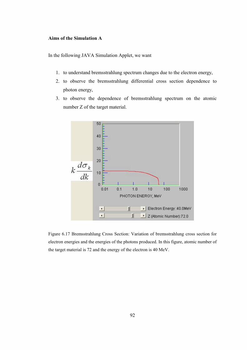
Aims of the Simulation A
In the following JAVA Simulation Applet, we want
1. to understand bremsstrahlung spectrum changes due to the electron energy,
2. to observe the bremsstrahlung differential cross section dependence to
photon energy,
3. to observe the dependence of bremsstrahlung spectrum on the atomic
number Z of the target material.
Figure 6.17 Bremsstrahlung Cross Section: Variation of bremsstrahlung cross section for
electron energies and the energies of the photons produced. In this figure, atomic number of
the target material is 72 and the energy of the electron is 40 MeV.
92
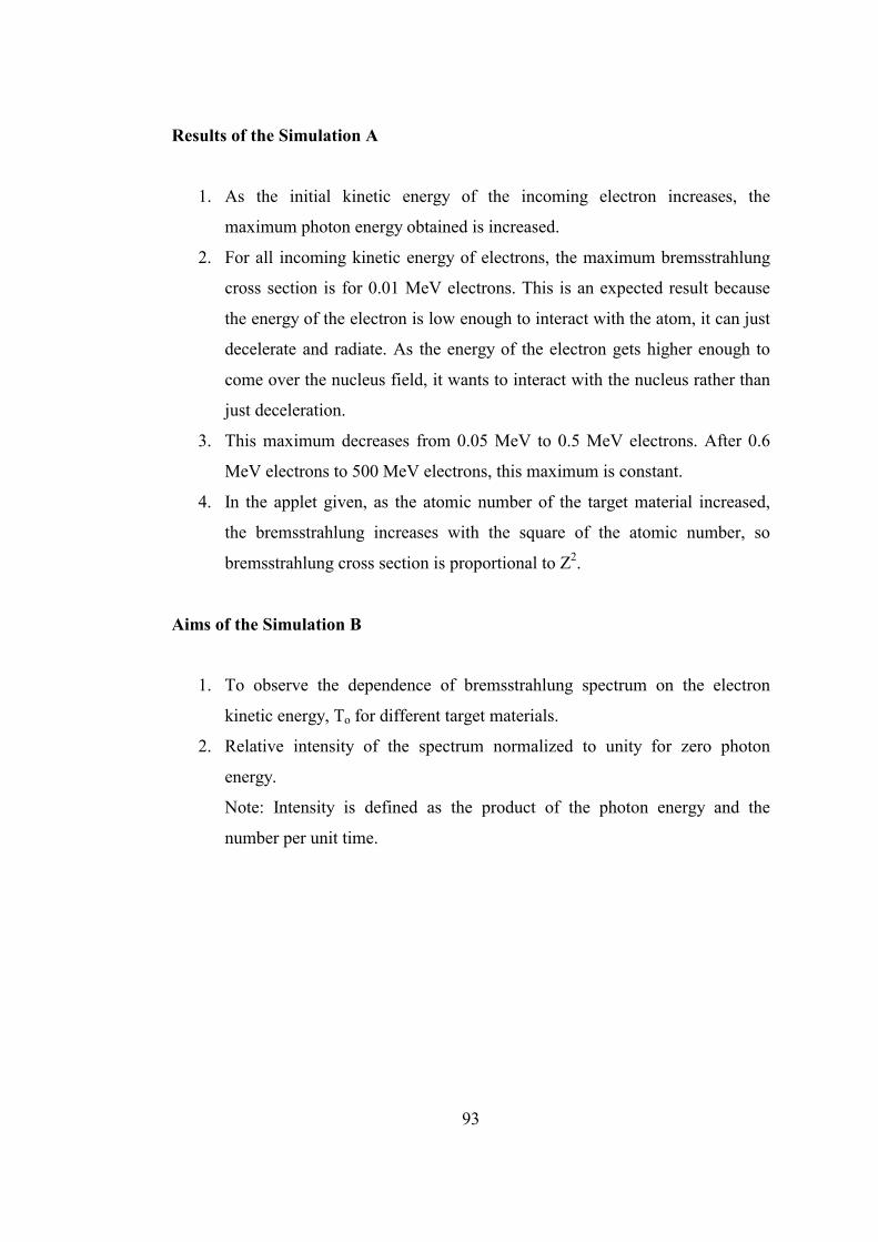
Results of the Simulation A
1. As the initial kinetic energy of the incoming electron increases, the
maximum photon energy obtained is increased.
2. For all incoming kinetic energy of electrons, the maximum bremsstrahlung
cross section is for 0.01 MeV electrons. This is an expected result because
the energy of the electron is low enough to interact with the atom, it can just
decelerate and radiate. As the energy of the electron gets higher enough to
come over the nucleus field, it wants to interact with the nucleus rather than
just deceleration.
3. This maximum decreases from 0.05 MeV to 0.5 MeV electrons. After 0.6
MeV electrons to 500 MeV electrons, this maximum is constant.
4. In the applet given, as the atomic number of the target material increased,
the bremsstrahlung increases with the square of the atomic number, so
bremsstrahlung cross section is proportional to Z2.
Aims of the Simulation B
1. To observe the dependence of bremsstrahlung spectrum on the electron
kinetic energy, To for different target materials.
2. Relative intensity of the spectrum normalized to unity for zero photon
energy.
Note: Intensity is defined as the product of the photon energy and the
number per unit time.
93
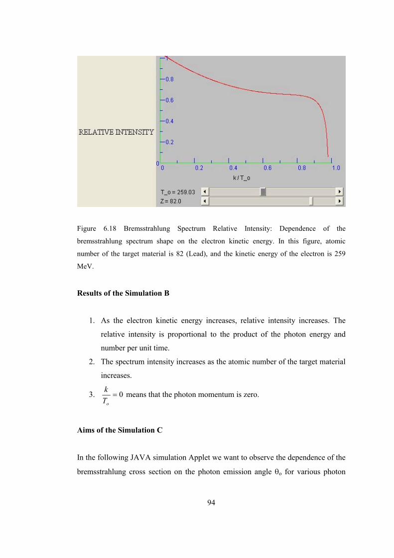
Figure 6.18 Bremsstrahlung Spectrum Relative Intensity: Dependence of the
bremsstrahlung spectrum shape on the electron kinetic energy. In this figure, atomic
number of the target material is 82 (Lead), and the kinetic energy of the electron is 259
MeV.
Results of the Simulation B
1. As the electron kinetic energy increases, relative intensity increases. The
relative intensity is proportional to the product of the photon energy and
number per unit time.
2. The spectrum intensity increases as the atomic number of the target material
increases.
3. 0�
oTk means that the photon momentum is zero.
Aims of the Simulation C
In the following JAVA simulation Applet we want to observe the dependence of the
bremsstrahlung cross section on the photon emission angle �o for various photon
94
and electron energies. �o is the angle between the initial momentum of electron, po
and the momentum of the emitted photon.
Figure 6.19 Angular Dependence of Bremsstrahlung Cross-Section: Angular dependence of
bremsstrahlung cross-section for various photon energy over initial electron kinetic energy.
Results of the Simulation C
1. The probability of bremsstrahlung is highest when the ratio of momentum of
the emitted photon to initial kinetic energy of the electron is zero and
decreases as this ratio goes to 1 for a definite Eo�o.
2. As the atomic number of the target material increases, the probability for
bremsstrahlung to occur increases.
3. Increase in the total energy of the electron increases the cross section of
bremsstrahlung effect for k/To <1.
95
6.7 X-ray Generation
6.7.1 X-ray Tube Flash Simulation
A Flash simulation is supplied for the user to observe the features of the X-ray tube
and their effects on X-ray production as shown in Figure 6.20. X-ray tubes are the
commercially used X-ray generation devices. User can change the tube operation
voltage, tube current, operation time – exposure time, and the target material. Three
target materials are supplied to the user namely, tungsten, rhodium and
molybdenum. The features that can be observed in the simulation are the number of
electrons hitting the target, maximum energy of the emitted photons, energy
released as X-radiation, and the efficiency of X-ray production. At the same time,
user observes the rotating anode to prevent overheating and the DC supply voltage
during the simulation.
Aims of the Simulation
To observe
1. the effects of operation voltage, operation duration, tube current and target
material on the number of electrons hitting the target,
2. maximum energy of emitted photons,
3. energy released as X-radiation,
4. efficiency of X-ray production.
96

Figure 6.20 X-Ray Tube Flash User Interface: User can observe the features of the tube by
changing the target material, operation voltage, operation duration and tube current.
97
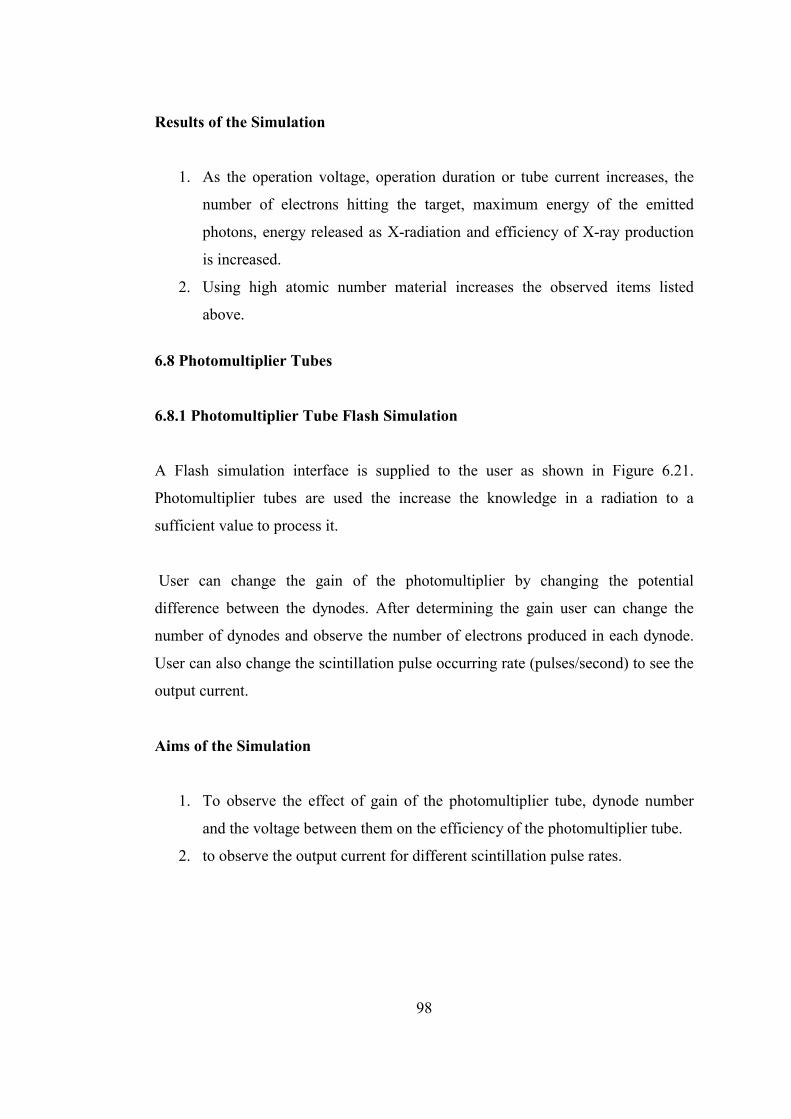
Results of the Simulation
1. As the operation voltage, operation duration or tube current increases, the
number of electrons hitting the target, maximum energy of the emitted
photons, energy released as X-radiation and efficiency of X-ray production
is increased.
2. Using high atomic number material increases the observed items listed
above.
6.8 Photomultiplier Tubes
6.8.1 Photomultiplier Tube Flash Simulation
A Flash simulation interface is supplied to the user as shown in Figure 6.21.
Photomultiplier tubes are used the increase the knowledge in a radiation to a
sufficient value to process it.
User can change the gain of the photomultiplier by changing the potential
difference between the dynodes. After determining the gain user can change the
number of dynodes and observe the number of electrons produced in each dynode.
User can also change the scintillation pulse occurring rate (pulses/second) to see the
output current.
Aims of the Simulation
1. To observe the effect of gain of the photomultiplier tube, dynode number
and the voltage between them on the efficiency of the photomultiplier tube.
2. to observe the output current for different scintillation pulse rates.
98
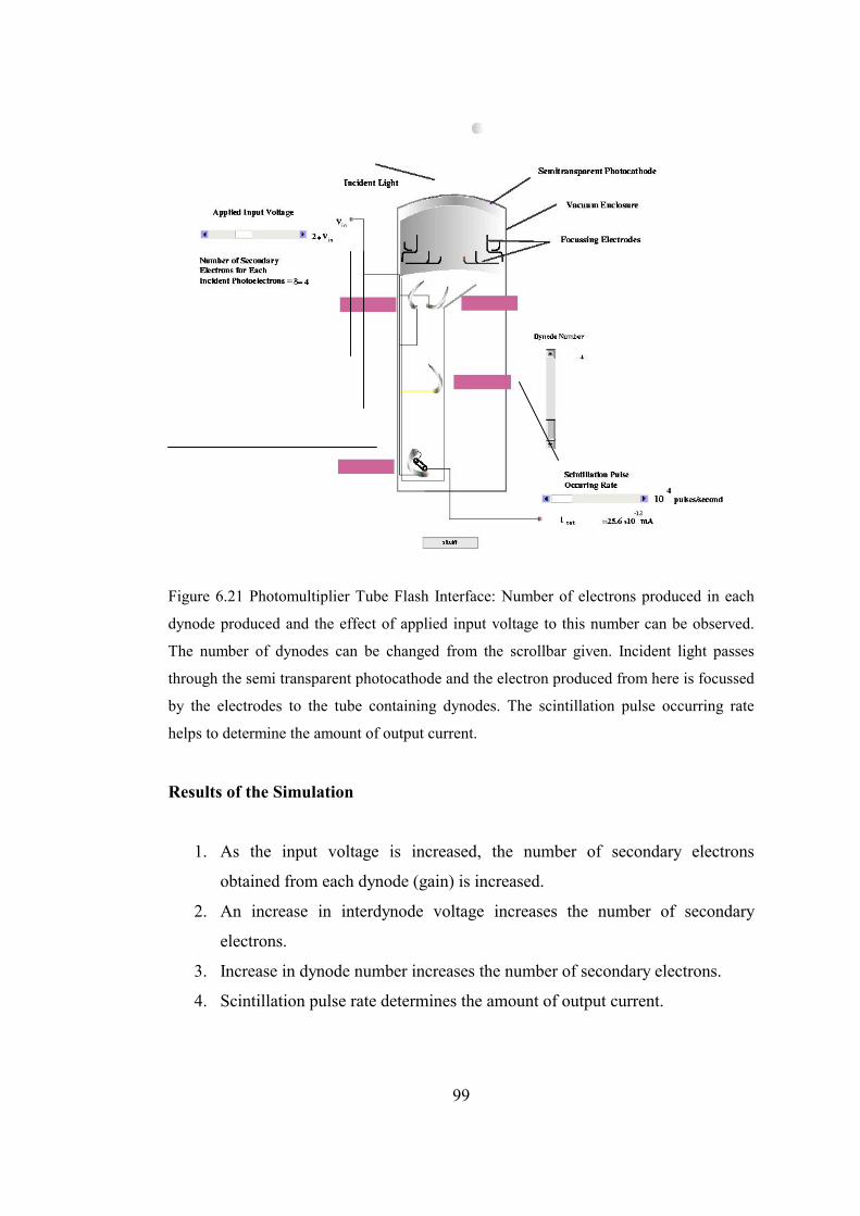
Figure 6.21 Photomultiplier Tube Flash Interface: Number of electrons produced in each
dynode produced and the effect of applied input voltage to this number can be observed.
The number of dynodes can be changed from the scrollbar given. Incident light passes
through the semi transparent photocathode and the electron produced from here is focussed
by the electrodes to the tube containing dynodes. The scintillation pulse occurring rate
helps to determine the amount of output current.
Results of the Simulation
1. As the input voltage is increased, the number of secondary electrons
obtained from each dynode (gain) is increased.
2. An increase in interdynode voltage increases the number of secondary
electrons.
3. Increase in dynode number increases the number of secondary electrons.
4. Scintillation pulse rate determines the amount of output current.
99

CHAPTER 7
CONCLUSION AND DISCUSSION
In this thesis, web-based education tools are generated for the topics related to X-
ray imaging. The generated simulation and animation tools are in the following
major fields:
1. Interaction of radiation with matter.
2. Generation and detection of X-rays.
3. Computerized Tomographic (CT) image reconstruction.
The main contributions of this study are listed below:
1. Animation and simulation programs for the study of X-ray physics in
medical imaging are provided to improve understanding of the topics via
visual aids.
2. A CT simulator is prepared that allows the use of energy-dependent
attenuation coefficients of several tissues. The user can define the
background and the foreground organs and observe the relative changes in
the attenuation coefficients with the change in the X-ray energy. The
simulator can be used to design experiments to distinguish selected organs
from the background or selected tissues.
Tools generated are executable in the World Wide Web media, because the main
purpose of this study is to satisfy animation and simulation programs for the people
100

who want to learn subject material without requiring additional software. This
requirement is satisfied by using JAVA and Flash software for the programs
prepared.
Animations and simulations are complementary to each other in an education tool
because animations give a flash knowledge of the mechanism and simulations give
in depth physical knowledge of the subject observed. Animations prepared removed
the visualization problems faced in the medical imaging education. Animation tools
attract the attention of the user to the point one wants to give.
Simulations are prepared using the mathematical formulations and the physical
rules. Simulations prepared made the user to learn physical properties of the subject
studied. User investigates changes in the subjects studied with respect to the
controllable variables of the system. Simulations prepared uses computer graphics
and animation tools. They dynamically show the behaviour and relationship of all
the simulated system components. JAVA software is used for graphic and Flash
software is used for numerical simulations. So no computational inefficiency is
observed in the programs prepared except for the Flash animation of X-ray
attenuation. Flash does not have graphical drawing property. One of my aims in this
simulation is to test this property. During the execution of the program, no
computational inefficiency is observed, but when user wants to reset the system, the
response of the program to this request is slow. It takes time for the program to
clear the graphics.
There are three types of interaction of radiation with matter: 1) Photoelectric effect,
2) Compton Effect, 3) Pair Production. In the animations, the mechanisms of these
interaction types are presented. In the simulations, their dependencies on the energy
and wavelength of the incident radiation, and the atomic number of the material that
the radiation interacts is presented.
101

The two types of X-ray generation are: 1) Characteristic radiation, 2)
Bremsstrahlung. In the animations, this thesis showed the mechanisms behind these
X-ray generation types. The simulations mimicked the bremsstrahlung, and showed
its dependency on the electron energy, the initial momentums of the electron and
the emitted photon and the angle between them, and the atomic number of the target
material interacted. The results obtained from these simulations are also presented
in this thesis.
For commercial use, X-ray tubes are utilized for the generation of X-rays. A
simulation tool about it’s operation principles and the variables affecting its
efficiency are also given in this thesis. Generation of X-rays in the X-ray tubes
relies upon the bremsstrahlung process, not on characteristic radiation. The reason
of the inadequacy of characteristic radiation in commercial X-ray generation is also
mentioned in this thesis.
For the detection of radiation, photomultiplier tube is selected, and a simulation of it
is presented. The responses of the photomultiplier tube to the controllable variables
are observed.
Image reconstruction is explained in this thesis for the computerized tomography
imaging. Two simulators are presented to the user. One of them is for single and the
other is for variable X-ray energy CT system. In the interfaces, user is able to 1)
form the image 2) select background material 3) observe the changes in the
attenuation coefficients of the tissues and materials formed by changing the energy
of the X-ray radiation used for the imaging.
As compared to the other investigated five web pages noted in Chapter 1, this thesis
satisfies large number of animations and simulations together. The subjects are
explained in a more detailed manner including deeper physics. So it is directly
applicable for class presentations.
102
REFERENCES
[1] Albert Macowski, “Medical Imaging Systems”, Prentice-Hall Inc., 1983
[2] R. D. Evans, “The Atomic Nucleus”, McGraw-Hill, Inc. Twelveth Print,
1969
[3] R. Eisberg, R. Resnick, “Quantum Physics of Atoms, Molecules, Solids,
Nuclei, and Particles”, John Wiley & Sons, Inc. , 1974
[4] L. Pauling, “General Chemistry”, Dover Publications, New York, 1988
[5] W. R. Hendee, E. R. Ritenour, “Medical Imaging Physics”, John Wiley &
Sons, Inc.Fourth Edition , 2002
[6] P. Signell and K. Gilbert, “Characteristics of Photons”, Physnet, MISN-0-
212, http://35.8.247.219/home/modules/pdf_modules/m212.pdf
[7] M. Brandl, “The Photoelectric Effect”, Physnet, MISN-0-213,
http://35.8.247.219/home/modules/pdf_modules/m213.pdf
[8] C. M. Davisson, R. D. Evans, “Gamma Ray Absorption Coefficients”,
pp.79-107, Rev. Of Mod. Phys., Vol. 24, No. 2, April 1952
[9] M. Brandl, “The Compton Effect”, Physnet, MISN-0-219,
http://35.8.247.219/home/modules/pdf_modules/m219.pdf
103
[10] R. M. Eisberg, “Fundamental of Modern Physics”, John Wiley & Sons, Inc.,
1967
[11] A. H. Compton, “A Quantum theory of the Scattering of X-rays by Light
Elements”, pp.483-502, Phys. Rev., Vol. 21, No. 5, May 1923
[12]
A. H. Compton, “The spectrum of Scattered X-rays”, pp.409-413, Phys.Rev.
[13] O. Klein, Y. Nishina, 853, Z. Physik, Vol. 52, 1929
[14] A. Fasso, K. Göbel, M. Höfert, et. al., , “Landolt-Börnstein - Group I
Elementary Particles, Nuclei and Atoms”, pp. 1-349, Springer-Verlag
Heidelberg, Vol. 11, 1990
[15] W. S. C. Williams, “Nuclear and Particle Physics”, Oxford University
Clarendon Press, Oxford, 1992
[16] H. W. Koch, J. W. Motz, “Bremsstrahlung Cross-Section Formulas and
Related Data ”, pp.920-956, Rev.Mod. Phys., Vol. 31, No. 4, Oct 1959
[17] G. F. Knoll, “Radiation Detection and Measurement”, John Wiley & Sons,
Inc.Second Edition , 1987
[18] Z. H. Cho, Joie P. Jones, Manbir Singh, “Foundations of Medical Imaging”,
John Wiley & sons Inc., 1993
[19] Prof. Dr. Murat Eyüpoğlu, “EE 415 Lecture Notes”
[20] http://www.rgi.tut.fi/kurssit/71304/ex1.pdf
[21] http://physics.nist.gov/PhysRefData/XrayMassCoef/tab2.html
[22] H. Hall, p.620, Phys. Rev., Vol. 45, 1934
104
[23] M. Stobbe, p. 661, Ann. Physik, Vol. 7, 1930
[24] H. Hall, W. Rarita, p143, Phys. Rev., Vol. 46, 1934
[25] Rutherford, Chadwick, and Ellis, “Radiation From Radiactive Substances”,
Cambridge University Press, 1930
[26] Z. S. Davidson, G. D. Latyshev, p. 15, J. Phys. (U.S.S.R.), Vol. 6, 1942
Heitler, W, “The Quantum Theory of Radiation”, Oxford University Press,
3rd ed, 1954.
[27] Claus Grupen, e-mail:[email protected]
[28] Hulme, Mc Dougall, Buckingham, and Fowler, p. 131, Proc. Roy. Soc.
(London), Vol. 149A, 1935
[29] F. Sauter, p. 454, Ann. Physik, Vol. 11, 1931
[30] W. Heitler, “The Theory of Quantum Radiation”, Oxford University Press,
New York, 1936
[31] M. Stobbe, p. 661, Ann. Physik, Vol. 7, 1930
[32] J. Fischer p. 821, Ann. Physik, Vol. 8, 1931
[33] R. S. Shankland, “Atomic and Nuclear Physics”, The MacMillan Company, New York, , 1955
105

APPENDIX 1 COMPTON EFFECT AND CROSS SECTION
FORMULATIONS
Figure A.1 Single Photon and Single Electron Collision: In Figure A.1-a, single photon and electron before the collision and their initial energy and momentum values are given. In Figure A.1-b, single photon and electron after the collision and their final energy and momentum values are given.
In Figure A.1 primed quantities are the values of the momentum and energy after the
collision.
Shift in the wavelength of incident and scattered photon is,
� � cos10
���� ������
cmh (A.1)
106

The shift in the energy between the primary and the secondary rays is
� �
� � 200
20
0cos1
1cos
cmE
EEEE
��
�����
�
� (A.2)
The velocity, final momentum and recoil angle of the recoil electron is given in
(A.3), (A.4), and (A.5) respectively.
� �
� � ���
���
��
21sin21
21sin21
21sin2cv
22
22
��
��
�� (A.3)
2
2phfphph
2ph
ec
EcosEE2EP fii
f
�����
�
�
(A.4)
cP
sinEarcsin
f
f
e
ph �
�
�
� (A.5)
Compton Scattering Cross-Sections
The cross section equations were obtained by Klein and Nishina [13]. The cross
section or in other words the probability of the occurrence of Compton scattering
for the number of photons scattered per electron and per unit solid angle in the
direction � is as given in (A.6).
107
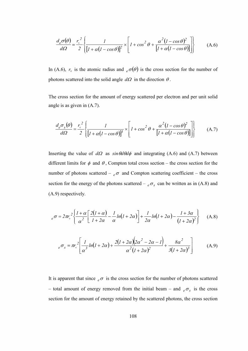
� �
� �� �
� �� �� � ��
���
��
���
��
���
��
����
���
��
���
���
��
cos11cos1cos1
cos111
2r
dd 22
22
2e � (A.6)
In (A.6), is the atomic radius and e�r � ���
�d
is the cross section for the number of
photons scattered into the solid angle in the direction � .
The cross section for the amount of energy scattered per electron and per unit solid
angle is as given in (A.7).
� �
� �� �
� �� �� � ��
���
��
���
��
���
��
����
���
��
���
���
��
cos11cos1cos1
cos111
2r
dd 22
23
2se � (A.7)
Inserting the value of as and integrating (A.6) and (A.7) between
different limits for � and � , Compton total cross section – the cross section for the
number of photons scattered – e and Compton scattering coefficient – the cross
section for the energy of the photons scattered – e can be written as in (A.8) and
(A.9) respectively.��
�d ��� ddsin
�
s�
� �� � � �
� � ��
���
��
���
�
���
�
� �
��
�
��� 22
2e 21
3121ln2121ln1
21121r2
�
�
�
�
�
��
�
�
�
���
(A.8)
� �� �� �
� � � � ���
�
���
�
��
�
����� 3
2
22
2
32
se 2138
21
12221221ln1r�
�
��
���
�
�
���
(A.9)
It is apparent that since is the cross section for the number of photons scattered
– total amount of energy removed from the initial beam – and is the cross
section for the amount of energy retained by the scattered photons, the cross section
�e
se�
108

for the amount of energy absorbed by the electrons, is obtained by subtracting
from �as in (A.10).
ae�
se� �e
aesee ��� �� (A.10)
109

APPENDIX 2 PHOTOELECTRIC EFFECT CROSS SECTION AND
ANGULAR DISTRIBUTION FORMULATIONS
1) Photon Energies Greater than 2 MeV
In this energy region as an approximation, Hall [22] has expanded the wave
function of the radiation in powers of the wavelength of the photon. Since the
photon energies in this region are greater than , considering only the first term
of the expansion is adequate for this approximation. With this formulation Hall
obtained the photoelectric cross section (absorption coefficient) , due to
absorption by the two electrons in the K shell only is given in (A.11).
2cm�
Ka�
� � � �� � ��
��
�
��
��
�
��
��
�
��
�
�
��
�
�
�
���
�
���
�
'o
'o
'o
43'o22
4o
5Ka
k
kln
k211
12
34nk
e
137123
nZ2
�
�
��
�
��
�
��
����
(A.11)
In (A.11), Z is the atomic number, n is �hmc2������is� 22 ehc � � � is o 3r8 2
�� ,
is � 137Z , is � � � � �21n1 ���
� �
– the total energy of the photoelectron in units of
, and is 2mc 'ok
212 1�� . This approximation in the theory gives successful
results for 1.13 MeV photons, so at higher energies the results are even better.
Hall gave the cross section in (A.11) due to absorption by two electrons in the K-
shell. But the atomic cross section is defined as the total absorption due to all
atomic electrons in the atom. The atomic cross-section is 5/4 times the cross
section , due to the K-shell electrons. This ratio has been verified both
theoretically [23, 24] and experimentally [25, 26]. Physically it means that, as long
�a
Ka�
110

as the energy of the incoming photon is enough, the probability of its interaction
and absorption by K-shell electrons is 80% more than the probability of interaction
and absorption by other shell electrons L, M … even their lower binding energies.
The quantitative description for this result depends on the conservation of
momentum. To conserve the momentum in the interaction, photon wants to interact
with the whole atom including the nucleus. However, the energy of the photon is
too low to interact with the nucleus, even to scatter together with the electron to
conserve the momentum as in the case of Compton Effect that will be described
later. With these reasons the photon is immediately absorbed completely by an
orbital electron. But due to aforementioned reasons, as long as the energy of the
photon is enough, it interacts with the electrons that are most tightly bound to the
atom, i.e. K-shell electrons. On the other hand, for the photon energies greater than
the rest mass energy of the electron, there is infinite number of wave functions
corresponding to that energy, and each of these wave functions corresponds to
different orbital angular momentum quantum number, l. The matching of K-shell
electrons (l =1) wave functions is highest with the wave functions of the atom [27].
Since the energy of the photon is not enough to interact with the atom, it will
interact with the K-shell electrons. With those reasons, the photoelectric effect will
happen with K-shell electrons with 80% probability.
The conservation of momentum in the photoelectric effect is satisfied with the
recoil of the entire atom, as a result of complete absorption of the photon.
2) Photon Energies from 0.35 MeV to 2 MeV
Hulme, McDougall, Buckingham, and Fowler [28] made experiments and
theoretical calculations in this energy region. Their calculations based on the single
electron thought in the K-shell. To find the cross section for the K-shell they
multiplied their results with two. From their results, they obtained curves yielding
the cross section for different values of Z.
111

3) Photon Energies from 0.1 MeV to 0.35 MeV
In this energy region relativistic and non-relativistic calculations were done.
3-a) Relativistic Calculations
Sauter [29] obtained an equation given below as a result of his works in this energy
region.
� �� �
� �
� �� �� � �
�����
�
�
������
�
�
���
�
�
�
�
��
�
�
212
212
212
23254
5
oKa
1
1ln12
11...
...12
34
1n137Z
23
��
��
��
�
��
��� (A.12)
In (A.12), � is equal to,
� � energy mass electronenergy electron total
mc
mcEh
1
12
2B
212�
��
�
�
�
�
�
�
where EB is the binding energy of a K electron, so since EB is different for different
atoms, it is possible to have a cross section curve for different values of Z.
3-b) Nonrelativistic Calculations
Heitler [30] obtained the results for nonrelativistic energies by neglecting the
binding energies of the K-shell electrons. The formulation he obtained is given in
(A.13) below.
� � � � 2745 241371 nZoKa �� � (A.13)
112
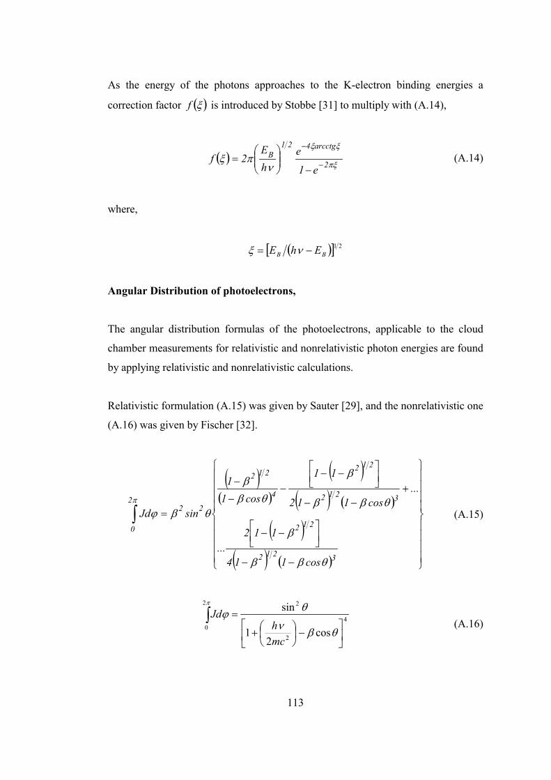
As the energy of the photons approaches to the K-electron binding energies a
correction factor is introduced by Stobbe [31] to multiply with (A.14), � ��f
� ���
��
��� 2
arcctg421B
e1
ehE
2f�
�
����
����
�� (A.14)
where,
� �� � 21BB EhE �� ��
Angular Distribution of photoelectrons,
The angular distribution formulas of the photoelectrons, applicable to the cloud
chamber measurements for relativistic and nonrelativistic photon energies are found
by applying relativistic and nonrelativistic calculations.
Relativistic formulation (A.15) was given by Sauter [29], and the nonrelativistic one
(A.16) was given by Fischer [32].
� �� �
� �
� � � �
� �
� � � �
�
����
�
����
�
�
����
�
����
�
�
��
��
���
�
��
��
���
��
�
�
�
���
�
���
�
��
�
���
2
0
3212
212
3212
212
4
212
22
cos114
112...
...cos112
11
cos11
sinJd (A.15)
���
���
���
��
�
��
���
��
2
04
2
2
cos2
1
sin
mch
Jd (A.16)
113
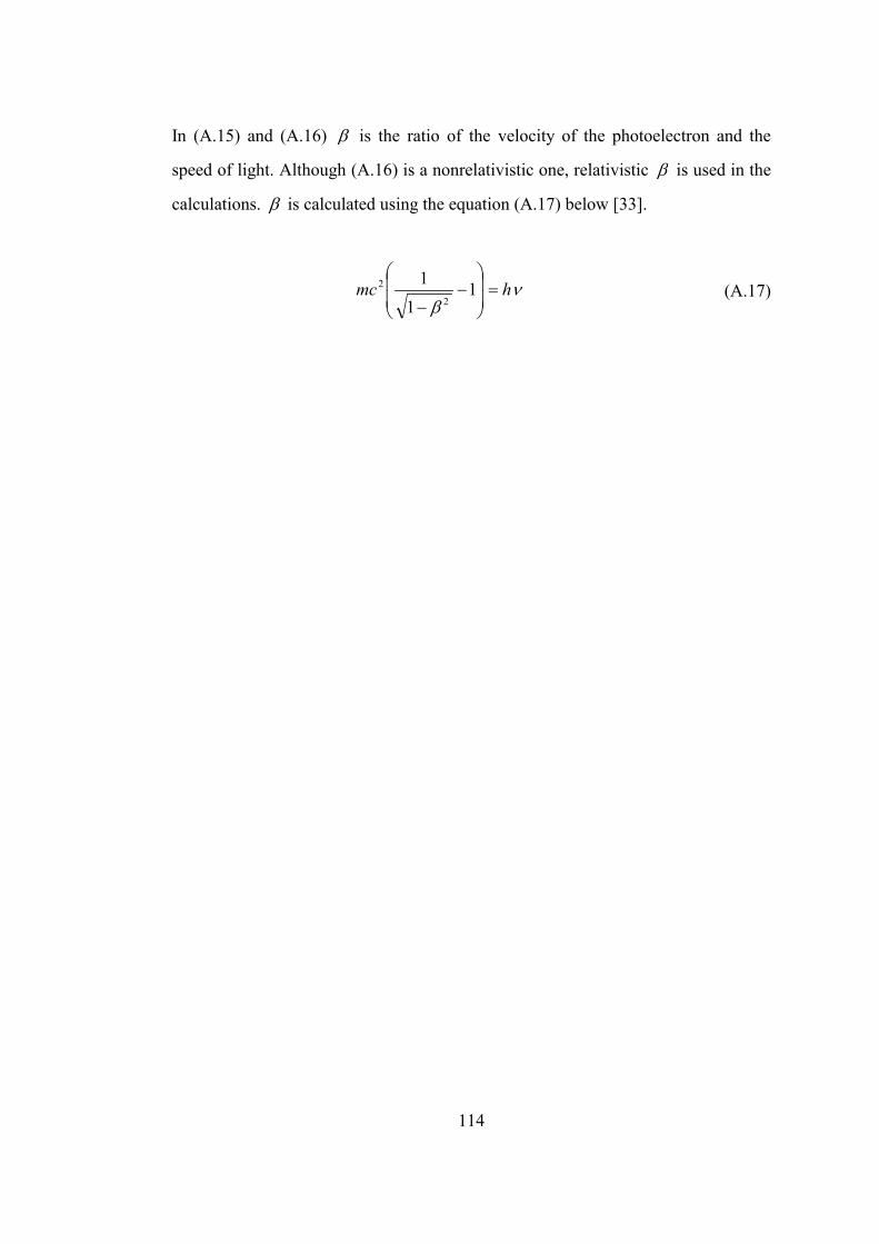
In (A.15) and (A.16) � is the ratio of the velocity of the photoelectron and the
speed of light. Although (A.16) is a nonrelativistic one, relativistic � is used in the
calculations. � is calculated using the equation (A.17) below [33].
��
hmc ���
�
�
��
�
��
�1
11
2
2 (A.17)
114

APPENDIX 3 PAIR PRODUCTION CROSS SECTION FORMULATIONS
Pair Production Cross Section Ratio for Electron and Nucleus Field The ratio of probability for the occurrence of pair production due to the electron field
over nucleus field nucleuspp
electronpp
:
:
�
�
is given in (A.18) [14].
��
�
�
��
�
���
���
���
cnucleus:pp
electron:pp
m2kln
3Z1
31 �
�
�
(A.18)
Pair Production Cross Section [32]
� � � � � ����
���
���
��
�������
�
���
�������
�� 191
Z
183ln1321
krZ4
dkd
3122
2e
2
pp (A.19)
115

APPENDIX 4 BREMSSTRAHLUNG ENERGY CALCULATIONS AND CROSS
SECTION FORMULATIONS
In bremsstrahlung calculations, momentum is given in m and energy is given in
units.
c�
2cm�
The symbols and energy momentum relations are;
E ,E�
Initial and final total energy of the electron in a collision.
pp ,�
Initial and final momentum of the electron in a collision.
T ,T�
Initial and final kinetic energy of the electron in a collision.
k ,k Energy and momentum of the emitted photon.
�� ,� Angles of and �p p with respect to k
� �� � � �� � 2121
2222
2TTp ,2TTp
EkE
1TE ,1TE
1pE ,1pE
����
��
����
����
���
�
��
��
116

To convert the energy values to m unit from MeV units we divide the MeV unit by
0.51. To have a figure, initial total and kinetic energy, and momentum of the electron is
calculated the for electron kinetic energy of 0.5 MeV in (A.20).
2c�
� �� � 73.12TTp
21TE
151.05.0T
T 0.51 MeV5.0
21���
���
��
�
���
��
�
�
(A.20)
At any instant of the collision the energy of the electron is equal to the initial energy of
the electron minus the energy transferred to the photon given as in (A.21). The final
kinetic energy of the electron is given as (A.22), and the final momentum of the
electron is as in (A.23).
kEE ���
(A.21)
1kE1ET
1TE
�����
��
�
(A.22)
� � � �� � � � 1kE1kE1kE2TTp 2����������
��� (A.23)
Dependence of the Bremsstrahlung Spectrum on Atomic Number
The formulas given in (A.24), (A.25), and (A.26) shows the dependence of the
spectrum on atomic number of the material that the photon interacts.
117
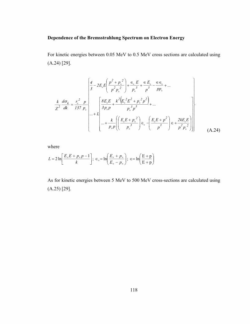
Dependence of the Bremsstrahlung Spectrum on Electron Energy
For kinetic energies between 0.05 MeV to 0.5 MeV cross sections are calculated using
(A.24) [29].
� �
�����
�
�����
�
�
�����
�
�����
�
�
�������
�������
�
��
�
�
��
�
���
��
�
�
��
�
� ���
��
�
�
��
�
� ��
��
�
�
���
��
��
���
�
�
��
�
� ��
�
223
2
3
2
33
22222
3322
22
2k
2
pp
EkE2
p
pEE
p
pEEpp
k...
...pp
ppEEkpp3EE8
L...
...ppp
E
p
E
pp
ppEE2
34
pp
137r
dkd
Zk
�
��
�
�
��
�
�
��
�
�
�
��
�
�
�
�
�
�
��
where
���
����
�
�
����
�
����
�
���
�
��
� �
pEpEln ; ln ;
1ln2
��
��
�
��
pEpE
kppEE
L
(A.24)
As for kinetic energies between 5 MeV to 500 MeV cross-sections are calculated using
(A.25) [29].
118
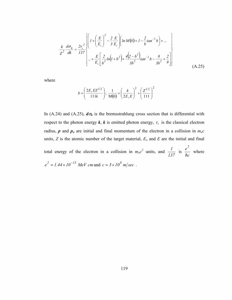
� �
� � � ����
�
���
�
�
���
�
���
�
�
��
���
��
����
���
���
���
���
�
�
���
�
��
��
�
�
��
�
��
�
�
�
92
b38btan
b3b24b1ln
b2
EE...
...btanb210Mln
EE
32
EE1
137r2
dkd
Zk
21
2
22
2
12
2k
2
�
��
��
where
� �
221221
11120M1 ;
1112
��
�
�
��
�
����
�
����
��
��
�
�
��
�
��
ZEE
kk
EZEb
�
�
(A.25)
In (A.24) and (A.25), d�k is the bremsstrahlung cross section that is differential with
respect to the photon energy k, k is emitted photon energy, is the classical electron
radius, p and p�
r
o are initial and final momentum of the electron in a collision in moc
units, Z is the atomic number of the target material, Eo and E are the initial and final
total energy of the electron in a collision in moc2 units, and 137
1 is c
e2
� where
and cm MeV1044.1e 132 �
�� secm103c 8�� .
119
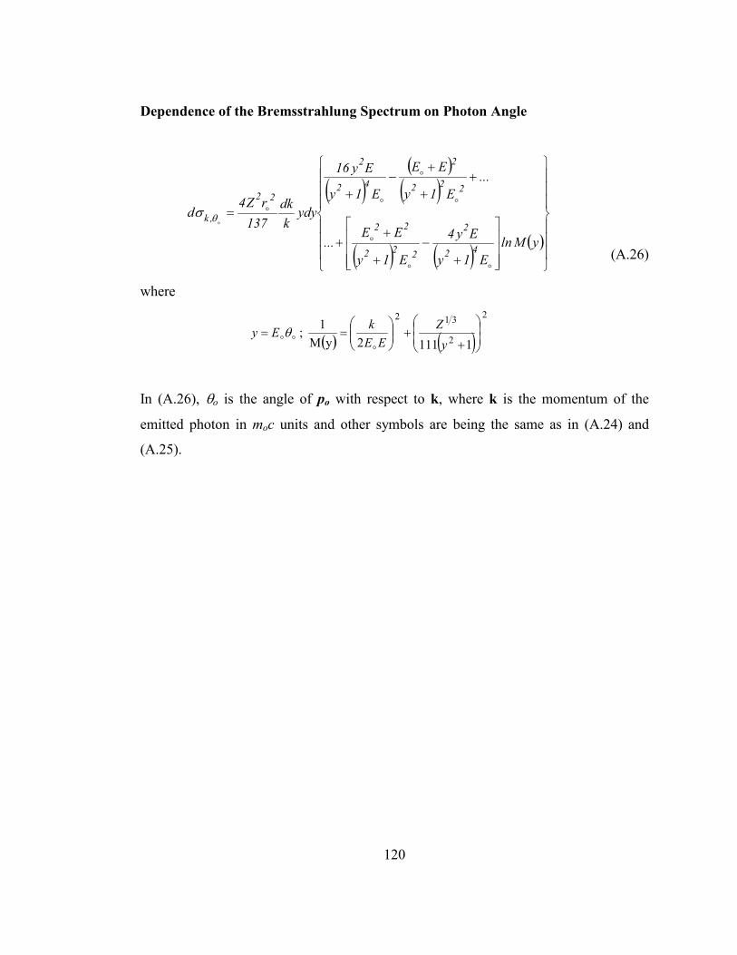
Dependence of the Bremsstrahlung Spectrum on Photon Angle
� �� �
� �
� � � �� �
���
�
���
�
�
���
�
���
�
�
���
���
�
�
�
�
��
�
�
��
�
�
yMlnE1y
Ey4
E1y
EE...
...E1y
EE
E1y
Ey16
ydykdk
137rZ4
d
42
2
222
22
222
2
42
2
22
,k
��
�
�
�
�
�
��
�
where
� � � �
2
2
312
11112yM1 ;
��
�
�
��
�
�
����
�
����
���
yZ
EEkEy�
���
(A.26)
In (A.26), �o is the angle of po with respect to k, where k is the momentum of the
emitted photon in moc units and other symbols are being the same as in (A.24) and
(A.25).
120