Till Anna

List of Papers

This thesis is based on the following papers, which are referred to in the text by their Roman numerals.

I Influence of the Radiative Decay on the Cross Section for Double Excitations in Helium, J.-E. Rubensson, C. Såthe, S.Cramm, B. Kessler, S. Stranges, R. Richter, M. Alagia and M. Coreno, Phys. Rev. Lett. 83, 947, (1999)

II Radiative and Relativistic Effects in the Decay of Highly Excited States in Helium, T.W. Gorczyca, J.-E. Rubensson, C. Såthe, M. Ström, M. Agåker, D. Ding, S. Stranges, R. Richter and M. Alagia, Phys Rev. Lett. 85, 1202, (2000)

III Double Excitations of Helium in Weak Static Electric Fields, C Såthe, M. Ström, M. Agåker, J. Söderström, J.-E. Rubensson, R. Richter, M. Alagia, S. Stranges, T.W. Gor-czyca and F. Robicheaux, Phys. Rev. Lett. 96, 043002 (2006)

IV Magnetic-Field Induced Enhancment in the Flourescence Yield Spectrum of Doubly Excited States in Helium, M. Ström, C. Såthe, M. Agåker, J. Söderström, J.-E. Rubensson, S. Stranges, R. Richter, M. Alagia, T.W. Gorczyca and F. Ro-bicheaux, Phys. Rev. Lett. 97, 253002, (2006)

V Quenching of Symmetry Breaking in Resonant Inelastic X-Ray Scattering by Detuned Excitation, P. Skytt, P. Glans, J.-H. Guo, K. Gunnelin, C. Såthe, J. Nordgren, F. Kh. Gel’mukhanov, A.Cesar and H. Ågren, Phys Rev. Lett. 77, 5035, (1996)

VI Bond-Length-Dependent Core Hole Localization Observed in Simple Hydrocarbon, K. Gunnelin, P. Glans, J.-E. Ru-bensson, C. Såthe, J. Nordgren,Y. Li, F. Gel’mukhanov and H. Ågren, Phys. Rev. Lett. 83, 1315, (1999)

VII Competition between decay and dissociation of core-excited carbonyl sulfide studied by x-ray scattering, M. Magnusson, J. Guo, C. Såthe, J.-E. Rubensson, J. Nordgren, P. Glans, L. Yang, P. Salak and H. Ågren, Phys. Rev. A 59, 4281, (1999)

VIII Resonant LII,III x-ray Raman scattering from HCl, C. Såthe, F. F. Guimarães, J.-E. Rubensson, J. Nordgren, A. Agui, J. Guo, U. Ekström, P.Norman, F. Gel’mukhanov and H. Ågren, Phys. Rev. A 74,062512, (2006)

IX X-Ray Emission Spectroscopy of Hydrogen Bonding and Electronic Structure of Liquid Water, J.-H. Guo, Y. Luo, A. Augustsson, J.-E. Rubensson, C. Såthe, H. Ågren, H. Sieg-bahn and J. Nordgren, Phys. Rev. Lett. 89, 137402, (2002)

X Local structures of liquid water studied by x-ray emission spectroscopy, S. Kashtanov, A. Augustsson, Y. Luo, J.-H. Luo, C. Såthe, J.-E. Rubensson, H. Siegbahn, J. Nordgren and H. Ågren, Phys, Rev, B 69, 024201 (2004)

XI Direct observation of interface effects of thin AlAs(100) layers buried in GaAs, A. Agui, C. Såthe, J.-H. Guo, J. Nordgren, S. Mankefors, P.O. Nilsson, J.Kanski, T.G. An-dersson, K. Karlsson, Applied Surface Science 166, 309, (2000)

XII Theoretical investigation of the thickness dependence of soft-x-ray emission from thin AlAs(100) layers buried in GaAs, S. Mankefors, P.O. Nilsson, J. Kanski, T. Andersson, K. Karlsson, A. Agui C. Såthe, J.-H. Guo and J. Nordgren, Phys. Rev. B 61, 5540, (2000)

XIII Hydrogen-induced changes of the electronic states in ul-trathin single-crystal vanadium layers, L.-C. Duda, P. Is-berg, P.H. Andersson, P. Skytt, B. Hjörvarsson, J.-H. Guo, C. Såthe and J. Nordgren, Phys. Rev. B 55, 12914, (1997)

XIV Probing the local electronic structure in the H induced metal-insulator transition of Y, B. Hjlrvarsson, J.-H. Guo, R. Ahuja, R.C.C. Ward, G. Andersson, O. Eriksson, M.R. Wells, C. Såthe, A. Agui, S.M. Butorin and J. Nordgren, J. Phys.: Condens. Matter 11, L119, (1999)

XV Resonant X-Ray Raman Spectra of Cu dd Excitations in Sr2CuO2Cl2, P. Kuiper, J.-H. Guo, C. Såthe, L.-C. Duda, J. Nordgren, J.J.M. Puthuizen, F.M.F. de Groot and G.A. Sawatzky, Phys. Rev. Lett. 80, 5204, (1998)

Reprints were made with permission from the respective publishers.

The following papers have been omitted from the thesis due to the character of the material, or due to the limited extent of my contribution.

Resonant X-ray emission from gas-phase TiCl4, Hague, C.F.;

Tronc, M.; Yanagida, Y.; Kotani, A.; Guo, J.H.; Sathe, C., Physical Review A (Atomic, Molecular, and Optical Physics) 63 (2001)

Resonant soft X-ray fluorescence spectra of molecules, Nordgren, J.; Glans, P.; Gunnelin, K.; Guo, J.; Skytt, P.; Sathe, C.; Wassdahl, N. , Applied Physics A (Materials Science Pro-cessing), 65,(1997)

Core electron spectroscopy of chromium hexacarbonyl. A comparative theoretical and experimental study, Yang, L.; Agren, H.; Pettersson, L.G.M.; Guo, J.; Sathe, C.; Fohlisch, A.; Nilsson, A.; Nordgren, J., Physica Scripta 59, (1999)

Study of oxygen-C60 compound formation by NEXAFS and RIXS, ): Kaambre, T.; Qian, L.; Rubensson, J.-E.; Guo, J.-H.; Sathe, C.; Nordgren, J.; Palmqvist, J.-P.; Jansson, U., European Physical Journal D 16, (2001)

Bond formation in titanium fulleride compounds studied through X-ray emission spectroscopy, Nyberg, M.; Yi Luo; Qian, L.; Rubensson, J.-E.; Sathe, C.; Ding, D.; Guo, J.-H.; Kaambre, T.; Nordgren, J. Physical Review B (Condensed Mat-ter and Materials Physics 63, (2001)

Bonding mechanism in the transition-metal fullerides stud-ied by symmetry-selective resonant X-ray inelastic scatter-ing, Qian, L.; Nyberg, M.; Luo, Y.; Rubensson, J.-E.; Talyzine, A.V.; Sathe, C.; Ding, D.; Guo, J.-H.; Hogberg, H.; Kambre, T.; Jansson, U.; Nordgren, J ,Physical Review B (Condensed Mat-ter) 63, (2001)

The electronic structure of polyaniline and doped phases studied by soft X-ray absorption and emission spectrosco-pies, Magnuson, M.; Guo, J.-H.; Butorin, S.M.; Agui, A.; Sathe, C.; Nordgren, J.; Monkman, A.P., Journal of Chemical Physics 111, (1999)

Formation of titanium fulleride studied by X-ray spectros-copies, Qian, L.; Norin, L.; Guo, J.-H.; Sathe, C.; Agui, A.; Jansson, U.; Nordgren, J., Physical Review B (Condensed Mat-ter) 59, (1999)

The electronic structure of poly(pyridine-2,5-diyl) investi-gated by soft X-ray absorption and emission spectroscopies, Magnuson, M.; Yang, L.; Guo, J.-H.; Sathe, C.; Agui, A.; Nordgren, J.; Luo, Y.; Agren, H.; Johansson, N.; Salaneck, W.R.; Horsburgh, L.E.; Monkman, A.P. Chemical Physics 237, (1998)

Resonant and nonresonant X-ray scattering spectra of some poly(phenylenevinylene)s, Guo, J.-H.; Magnuson, M.; Sathe, C.; Nordgren, J.; Yang, L.; Luo, Y.; Agren, H.; Xing, K.Z.; Jo-hansson, N.; Salaneck, W.R.; Daik, R.; Feast, W.J., Journal of Chemical Physics108 , (1998)

Electronic structure of single-wall carbon nanotubes studied by resonant inelastic X-ray scattering, Eisebitt, S.; Karl, A.; Eberhardt, W.; Fischer, J.E.; Sathe, C.; Agui, A.; Nordgren, J., Applied Physics A (Materials Science Processing) 67, (1998)

Resonant Cu L , emission spectra of CuGeO3 single crys-tal, Agui, A. ; Guo, J.-H.; Sathe, C.; Nordgren, J.; Hidaka, M.; Yamada, I. Physica Status Solidi C 8, (2006)

Resonant Mn L emission spectra of layered manganite La1.2Sr1.8Mn2O7, Agui, A.; Butorin, S.M.; Kaambre, T.; Sathe, C.; Saitoh, T.; Moritomo, Y.; Nordgren, J. ,Journal of the Physical Society of Japan, v 74, n 6, (2005)

Intra- versus inter-site electronic excitations in NdNiO3 by resonant inelastic ultra-soft X-ray scattering at Ni 3p edge, Butorin, S.M.; Sathe, C.; Agui, A.; Saalem, F.; Alonso, J.A.; Nordgren, J. Solid State Communications, v 135, n 11-12,(2005)

Resonant O K emission spectroscopy of layered manganate La1.2Sr1.8Mn2O7, Agui, A.; Kaambre, T.; Sathe, C.; Nordgren, J.; Usuda, M.; Saitoh, T.; Moritomo, Y. , Journal of Electron Spectroscopy and Related Phenomena, v 144-147, (2005)

Electronic structure of carbon nitride thin films studied by X-ray spectroscopy techniques, Hellgren, N.; Jinghua Guo; Yi Luo; Sathe, C.; Agui, A.; Kashtanov, S.; Nordgren, J.; Agren, H.; Sundgren, J., Thin Solid Films, v 471, n 1-2,(2005)

Spin transition in LaCoO3 investigated by resonant soft X-ray emission spectroscopy, Magnuson, M.; Butorin, S.M.; Sathe, C.; Nordgren, J.; Ravindran, P. ,Europhysics Letters, v 68, n 2, (2004)

Probing the Mn3+ sublattice in La0.5Ca0.5MnO3 by reso-nant inelastic soft X-ray scattering at the Mn L2,3 edge, Bu-torin, S.M. (Dept. of Phys., Uppsala Univ., Sweden); Sathe, C.; Saalem, F.; Nordgren, J.; Zhu, X.-M. , Surface Review and Let-ters, v 9, n 2,(2002)

Magnetic circular dichroism in X-ray fluorescence of Heu-sler alloys at threshold excitation, Yablonskikh, M.V.; Grebennikov, V.I.; Yarmoshenko, Yu.M.; Kurmaev, E.Z.; Bu-torin, S.M.; Duda, L.-C.; Sathe, C.; Kaambre, T.; Magnuson, M.; Nordgren, J.; Plogmann, S.; Neumann, M., Solid State Communications 117, (2001)

Resonant OK alpha emission spectra of CuGeO3 single-crystal, Agui, A.; Guo, J.-H.; Sathe, C.; Nordgren, J.; Hidaka, M.; Yamada, I, Solid State Communications 118, (2001)

Nitrogen bonding structure in carbon nitride thin films studied by soft X-ray spectroscopy, Hellgren, N.; Jinghua Guo; Sathe, C.; Agui, A.; Nordgren, J.; Yi Luo; Agren, H.; Sundgren, J.-E., Applied Physics Letters 79, (2001

Structural and electronic properties of low dielectric con-stant fluorinated amorphous carbon films, Ma, Y.; Yang, H.; Guo, J.; Sathe, C.; Agui, A.; Nordgren, J., Applied Physics Let-ters 72, (1998)

The characterization of undulator radiation at MAXII using a soft X-ray fluorescence spectrometer Guo, J.-H.; Butorin, S.M.; Sathe, C.; Nordgren, J.; Bassler, M.; Feifel, R.; Werin, S.; Georgsson, M.; Andersson, A.; Jurvansuu, M.; Nyholm, R.; Eriksson, M., Nuclear Instruments & Methods in Physics Re-search, Section A (Accelerators, Spectrometers, Detectors and Associated Equipment) 431, (1999)

Comments on my participation

Experimental studies performed at synchrotron facilities are often the effort of many people, as reflected by the author lists. My involvement has for the most part been on the experimental side. Most of my effort has gone into constructing, preparing and conducting the experiments. I have also been involved in the analysis of the data and the subsequent discussions and au-thoring process. The theoretical calculations presented in the papers were for the most part done by collaborating authors. Samples in papers XI-XV were prepared and provided by co-authors. The beautiful drawings in this thesis were made by Marcus Agåker.

Contents

Introduction ................................................................................................... 13

Matter ............................................................................................................ 14 Bohr's Model of the Atom ........................................................................ 15 Quantum Mechanics ................................................................................. 17

Wave-Particle Duality ......................................................................... 18 The Schrödinger Equation ................................................................... 18 Heisenberg's description, Matrix mechanics ....................................... 19 Splitting the Energy Levels, quantum numbers and the exclusion principle ............................................................................................... 19 Atoms in external fields ....................................................................... 22

Scattering ...................................................................................................... 23 Fermi’s Golden Rule ................................................................................ 23 Dipole approximation and selection rules ................................................ 24 X-ray absorption ....................................................................................... 24 X-ray emission ......................................................................................... 25 Competing channels ................................................................................. 26 Resonant Inelastic X-ray Scattering ......................................................... 27

Experiment .................................................................................................... 29 Synchrotron Radiation .............................................................................. 29 Monochromator ........................................................................................ 32 Gratings .................................................................................................... 32 The Helium Experiments (Papers I-IV) ................................................... 36

Double excitations in helium ............................................................... 37 Applied external fields ......................................................................... 39

Spectrometer ............................................................................................. 40 Resolution ............................................................................................ 43 Slit-Limited Resolution ....................................................................... 43 Detector-Limited Resolution ............................................................... 45 Grating-Limited Resolution ................................................................. 45

Gas-phase experiments ............................................................................. 46 Paper V and VI .................................................................................... 46 Paper VII and VIII ............................................................................... 47

Liquids ...................................................................................................... 49 Buried Layers ........................................................................................... 51

Hydrides ................................................................................................... 52 Correlated materials and dd- excitations .................................................. 53 Conclusions and outlook .......................................................................... 54

Acknowledgements ....................................................................................... 56

Summary in Swedish .................................................................................... 57

Bibliography ................................................................................................. 60

13

Introduction

A driving interest in physics is the understanding of the structure and behav-ior of matter. What makes a metal a metal? Why are silicates in glass form transparent to visible light but not other forms of silicates? What makes iron a magnetic material? Why is diamond hard but a lump of coal fairly soft? They are both made of the same atoms after all. The list can be made long and it is easy to see that this is a both fascinating and in the end potentially rewarding endeavor. In order to understand the nature of matter we need to turn to its building blocks, the atoms.

My goal here is not to dive down all the way to elementary particle level but rather to explore matter on an atomic, molecular and condensed matter scale. The borderlands of physics and chemistry will be our main domain and interaction between matter and radiation will be our tool of investiga-tion. The focus will be on the electrons and how they bind the atomic nuclei together, i.e., the electronic structure of matter.

14

Matter

As so often in physics it begins with Newton. In 1666 he used a lens, a prism and a simple screen to show that what was perceived as “white” light from the sun was in fact made up of a continuum of all colors in the rainbow. This led him to coin the phrase “spectrum”. Later in 1802 William Hyde Wollas-ton refined Newtons observations and found dark lines in this continuum. These lines were systematically investigated by Joseph von Fraunhofer in Munich 1814 and they are named after him – the Fraunhofer lines.

In 1752 the Scotsman Thomas Melvill showed that a mixture of alcohol and salt water would burn with a yellow flame. When the salt was removed this distinctive yellow flame disappeared. Melvill is regarded as the founder of the technique of flame spectroscopy. Further studies by Talbot lead him to show in 1826 that different salts would produce different colors when put in a flame. The groundwork was now laid and in 1860 Gustav Kirchhoff and Robert Bunsen, using proper spectroscopes, found that the observed spectral lines were unique to each element. They could then put their new tool to work and in the coming few years they and others discovered the elements cesium, rubidium, thallium and indium. Maybe the crowning achievement of these early years of spectral analysis was the discovery of what turned out to be the second most abundant element in the universe, helium, in 1868, a discovery made independently by the two astronomers Pierre Janssen and sir Joseph Norman Lockyer.

The next step in the development was to turn spectroscopy into spectrom-etry, actually measuring the wavelengths of the recorded spectral lines. In 1868, the same year that helium was discovered, the Swedish physicist An-ders Jonas Ångström published his study of the solar spectrum, giving the wavelengths of the most important lines in the unit of 10-10 m. This unit was later named 1 Ångström (Å) in his honor. Ångström later made the first re-flection grating, for which the author of this thesis is indebted to him.

Finding patterns in the known spectral lines was the next level of devel-opment. A big step in this direction was taken in 1885 when Johann Jakob Balmer found that the wavelengths of the visible spectral lines of the hydro-gen atom followed a simple mathematical formula. This series was later named after him – the Balmer series. Balmer’s findings were later general-ized in 1888 by Johannes Rydberg in Lund into

15

where RH is now called the Rydberg constant, n and m are integers where n < m. In the particular case of the Balmer series n =2 and m 3. The validity of Rydberg’s discovery was strengthened in 1906 when Theodore Lyman dis-covered a series of spectral lines in the ultraviolet wavelength region of hy-drogen corresponding to n = 1 and m 2 in Rydberg’s formula.

Outside the developing field of spectroscopy Heinrich Hertz found in 1887 that materials could emit electrons if illuminated with light of suffi-ciently high frequency, and this frequency depends on the material. It was also later found that the energy of the emitted electron depends on the fre-quency of the impinging light. Having this knowledge as well as Max Planck's explanation of the black-body radiation at hand, Albert Einstein formulated in 1905 what is known as the photoelectric law. He proposed that light was in fact made up of discrete quanta, which were later on called pho-tons by Gilbert Newton Lewis. Einstein further proposed that the energy of each of these quanta was determined by their frequency , which is related to the energy E by

where h is the so-called Planck's constant.

Bohr's Model of the Atom The Danish physicist Niels Bohr now tasked himself with solving the riddle set forth by the Rydberg formula. Taking a lead from Rutherford's scattering experiments, which showed that the atom consists of a heavy positively charged nucleus surrounded by a cloud of negative charges, he proposed a new descriptive model based on classical motions augmented by three postu-lates.

1. The electrons can only travel in certain stationary orbits; at a certain

discrete set of distances from the nucleus with specific energies. 2. The electrons do not lose energy as they travel. They can only gain and

lose energy by undergoing a transition from one allowed orbit to another, absorbing or emitting electromagnetic radiation with a frequency deter-mined by the energy difference of the levels according to the relation

16

3. The frequency of the radiation is as it would be in classical mechanics

the reciprocal of the classical orbit period T:

In his study, Bohr introduced a quantization of the angular momentum, L, of the electrons in the atom according to

where n = 1, 2, 3,… suggesting an atomic model akin to that of the planetary system with the electrons orbiting the nucleus much like the planets orbit the sun.

Figure 1. The Bohr atom

17

This simple model was a big step forward in the understanding of the at-om and probably its biggest achievement was that it could accurately give the value of the Rydberg constant, RH. Using the classical formulas for the kinetic energy and Coulomb interaction of an electron orbiting the nucleus along with its quantized angular momentum, gives the following expression for the energy of an electron in the n-th level of a hydrogen atom

where

Here ke is the Coulomb constant, e is the charge of the electron and me is the mass of the electron. A transition from level m to lower level n realizes an energy that fits well to the Rydberg formula.

This first atomic model had some serious shortcomings. In particular, it cannot properly predict energies of multi-electron atoms, it cannot predict relative intensities of emission lines and it cannot provide an explanation for the fine structure or splitting of atomic lines as observed by Johannes Stark and Pieter Zeeman in external electric and magnetic fields, respectively. Another difficulty is that it provides no real explanation as to why the elec-tron does not loose energy as it undergoes centripetal acceleration while orbiting the nucleus as predicted by classical theory. Already Bohr himself was aware of these shortcomings.

Quantum Mechanics In the 1920's there were several important developments and breakthroughs in the theoretical treatment of the atom. Based on the work of, in particular, Louis de Broglie, Werner Heisenberg and Erwin Schrödinger, another step was taken from the semi-classical quantized description into the realm of quantum mechanics, culminating in the Copenhagen interpretation of quan-tum mechanics in 1927. In order to understand quantum mechanics it is good to consider a few of its fundamental ideas.

18

Wave-Particle Duality As first demonstrated by Einstein, light cannot be described as either wave or particle but rather exhibits behaviors of both aspects. This idea was ex-tended to electrons as well as all matter by de Broglie in 1923. It was previ-ously known from Thomson’s cathode ray experiments in 1897 that the elec-tron is indeed particle-like. In light of all these findings, de Broglie proposed that all matter has an associated wavelength , known as the de Broglie wavelength, which is related to its momentum p by the formula

Since Planck's constant is very small (6.626 × 10 34 Js) compared to the momentum of macroscopic objects the wave nature of matter is effectively hidden to us. However, on an atomic scale it becomes the dominating fea-ture. De Broglie’s idea was confirmed in 1927 through electron diffraction measurements independently by two different laboratories. The fact that the electrons could be described as waves pointed towards a description of the discrete energy levels in atoms as a standing wave phenomenon rather than particles orbiting a nucleus. This leads to the formulation of a wave-mechanical description of quantum mechanics.

The Schrödinger Equation In 1926 Erwin Schrödinger presented an equation reminiscent to the Hamil-tonian version of Lagrangian classical mechanics. He basically formulated a wave-mechanical description that in its most general form looks like

where denotes the wave function. The operator on the left hand side of the equation is called the energy operator and H is the Hamiltonian operator corresponding to the total energy of the system. As in classical mechanics, the Hamiltonian can be broken down to

where T is the kinetic energy and V is the potential energy. Using

19

where V(r) is the potential from the nucleus seen by the electron. Schröding-er was able to reproduce Bohr's results for the hydrogen atom. The square of the wave function, , was later interpreted by Max Born as the probability amplitude of the particle. The wave function itself lacks concrete physical meaning; it is only when it is operated on that it gives rise to a measurable physical quantity.

Heisenberg's description, Matrix mechanics One very important discovery that came out of Heisenberg's work was the realization that an attempt to measure two observables simultaneously can become troublesome. Effectively, such an attempt is equivalent to a collapse of the system into two solutions at the same time, and more often do these not commute. This happens when the following holds true for two matrices A and H

In particular this is true for the position and momentum operators as well as for energy and time. In the case of energy and time we get the relation

This gives rise to a well-known spectroscopic phenomenon, the natural life-time broadening. The uncertainty principle is often misunderstood as an effect of the measurement, but is really an intrinsic property of the quantum mechanical description of nature.

Splitting the Energy Levels, quantum numbers and the exclusion principle So far we have not gone beyond Bohr and his explanation of the Rydberg series as far as describing emission lines in atomic spectra. However, already in 1887 Albert Michelson and Edward Morley noted a splitting in the princi-pal emission line of hydrogen which was so apparent that some more physics needed to be understood. The explanation of their observation relates to the fact that the electron is a charged particle and is associated with it two types of magnetic moment as it is bound in the atom. One is associated with the orbital angular momentum expressed by the quantum number l. The binding energy of an electron will depend on how far away from the nucleic charge its orbital is and how many electrons shield it. This will lead to different binding energies for different l even though their value of n is the same. Tra-

20

ditionally these lines were named sharp, principal, diffuse and fundamental giving rise to the nomenclature s, p, d and f corresponding to l = 0, 1, 2, 3… The other magnetic moment associated with the electron is that of its spin, an intrinsic property of the electron always with the value ½.

The concept of quantum numbers is, as we shall see later on in this thesis, very useful when studying quantum mechanical systems such as atoms, mol-ecules and condensed systems. A quantum number describes values of con-served physical quantities in the dynamics of a quantum system. They must also either correspond to the Hamiltonian, or an operator that commutes with it. In the case of solving the Schrödinger equation for an atom one ends up with four quantum numbers which completely define the state of an electron. The most common set of quantum numbers comprises the principal quantum number n, which is associated with the energy level or the main shell the electron belongs to, and which can take values equal to or larger than 1. Fur-thermore, within this set of quantum numbers, l denotes the angular momen-tum with values ranging from 0 l n – 1. The third quantum number of relevance is the magnetic quantum number ml which denotes the projection of l onto a defined axis of the coordinate system used. Values for ml range from -l l. The fourth quantum number, s, represents the spin of the elec-tron, and as the electron is a fermion s=1/2. Akin to ml the projection of the intrinsic spin of the electron on a defined axis gives rise to a new quantum number, ms, which can take the values -1/2 and +1/2.

An important fact regarding the angular momentum in quantum mechan-ics is that for three spatial dimensions the operators lx ,ly and lz do not com-mute. This implies that if one component is measured the others can never be fully determined. This leads to a precession of the angular momentum. Most often the angular momentum ml is used for the projection of the orbital angular momentum onto an arbitrary axis z. Associated with an electron is also an intrinsic magnetic moment, which is ascribed to a spin with the quan-tum number s=1/2 as mentioned above. The projection onto the z-axis can take the value ms = ½ relative to ml, so coupling of the angular momenta, spin-orbit coupling, causes further splitting of the energy levels. The result-ing levels are defined by the quantum number j which can take values be-tween l – s and l+s in integer steps.

In systems with more than one electron the spin and orbital angular mo-menta couple in a highly non-trivial way. The phenomenology is determined by the interaction strength, so that if the spin-orbit interaction is small the angular and spin momenta for all the electrons couple to a total L and S for the whole system, and these couple to a final total angular momentum J. This coupling scheme is called LS, or Russel-Saunders coupling, and the state of the system is defined by the term symbol

21

along with the electron occupancy of the nl orbitals.

.

Figure 2. The splitting of the energy levels using quantum numbers n, l, and ml,

When the spin-orbit interaction is strong the spin and orbital angular mo-menta of each electron first couple to a total angular momentum j. The angu-lar momenta, j, of all the electrons then add up to a total J for the system; this is scheme is called jj coupling. It is often stated that LS coupling should

22

be used for light atoms whereas jj coupling is appropriate for heavy atoms. Note, however, that these coupling schemes are the limits of the general intermediate coupling. The coupling scheme to be used depends on the state under study, and also other schemes can be envisioned. The strategy is al-ways to take the strongest interaction into account first, and add the weaker interaction as a perturbation

In 1925 Wolfgang Pauli introduced his exclusion principle which states that no two electrons (later generalized into fermions in general, i.e. particles with s = 1/2) could have the same set of quantum numbers. Based on this Friedrich Hund could then propose a set of rules for how to determine the term symbol corresponding to the ground state for a multi-electron atom in the LS-coupling regime. In another, subsequent step, the concept of sym-metry was introduced and in this description the exclusion principle requires that the total wave function of two electrons must be anti-symmetric with respect to exchange of the electrons.

Atoms in external fields Observations of splitting and shifts of spectral lines due to static external magnetic (Zeeman (1896)) and electric fields (Stark (1913)) were made early on. As the electrons are electrically charged and have magnetic properties associated with the angular momentum it is easy to understand that external fields must have an influence. The external fields produced under laboratory conditions are generally very small compared to the internal fields due to the nucleus and the other electrons in the system. Thus, the influence of the ex-ternal fields is mostly successfully treated as a small perturbation of the orig-inal system. The shifts are so small that they are difficult to observe directly in VUV and X-ray spectroscopy. However, when electrons are excited to levels of high principal quantum numbers, their interaction with the rest of the electron system and the nucleus becomes so small that large effects can be observed already at minute external fields.

23

Scattering

We now have a working theory on matter but we need some way verifying and exploring how it corresponds to reality. One cannot gain knowledge by only contemplating our model, science needs experiments and observations. If you want to know which of two eggs is boiled, what do you do? If you just observe the eggs they seem identical but if you interact with them something else may be revealed. Spinning the two eggs will reveal that since the boiled egg has a solid content it will spin much faster than the raw egg with its liq-uid content. We have revealed something previously hidden by a perturba-tion.

In learning about the nature of matter we need ways to interact with it, perturbing it and observing the results. There are many ways to do this, but our way in this thesis is to study how matter interacts with radiation and what we can learn from it. We need to describe the process by which radia-tion scatters from matter. Since my region of interest is the ultra soft x-ray energy region the descriptions below will always center on the particulars of that energy region. This means that we will typically always talk about core electron transitions for the lighter elements and outer core/inner valence transitions for the heavier elements. This also means we can make certain assumptions about the processes.

Fermi’s Golden Rule Derived by Dirac and named by Fermi, we have an expression for the transi-tion rate T from one electronic state into a continuum of eigenstates. Expressed using the bra-ket notation [1] we get

where is the density of final states and is the operator describing the interaction between photons and electrons. The values of the matrix ele-ments will depend on the electronic system and if the interaction is absorp-tion, spontaneous emission or stimulated emission. They can be calculated

24

using the Einstein coefficients [2]. Discrete electronic states are described using the Dirac function, in place of .

Dipole approximation and selection rules If we assume that the wavelength of the radiation is longer than the atomic dimension (~1 Å), which is certainly true in the soft x-ray region, the inter-action operator becomes

where is the polarization of the radiation. This assumption is called the dipole approximation.

This gives certain selection rules that will limit the states allowed to par-ticipate in the transitions. For transitions in an atom governed by LS cou-pling this implies that the angular momentum quantum number has to change by one i.e. l = ±1, the z-projection ml has to change by ml = ±1 or 0 and the spin will be conserved, S = 0. In molecular systems the rules will be slightly different depending on the symmetry of the molecule and less stringent since we have to account for vibronic-coupling.

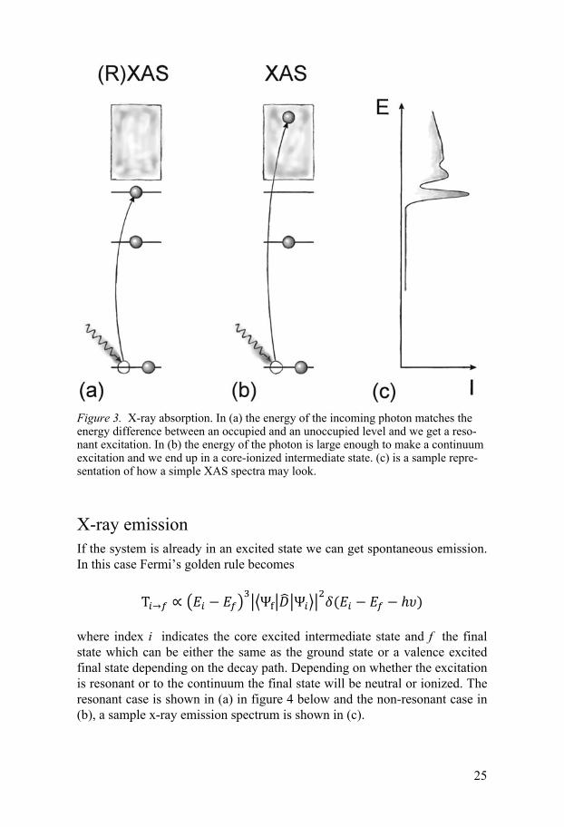
X-ray absorption The electronic structure of a material will consist of occupied orbitals popu-lated by the available electrons according to Hund’s rules. There will also be available empty bound orbitals of lower binding energy and a continuum of unbound orbitals. Each orbital will have associated with it an ionization en-ergy, the energy necessary to eject the electron from that orbital into the continuum. Illustrated in figure 3 below we can see the two possible pro-cesses of absorption, (a) a photon of energy is absorbed leaving the system in a core excited state and (b) where the energy of the photon is large enough to leave the system in a core ionized state. This gives us access to an experimental technique called x-ray absorption spectroscopy (XAS), the process described by (a) is called a resonance. A sample absorp-tion spectrum can be seen imaged in (c).

25

Figure 3. X-ray absorption. In (a) the energy of the incoming photon matches the energy difference between an occupied and an unoccupied level and we get a reso-nant excitation. In (b) the energy of the photon is large enough to make a continuum excitation and we end up in a core-ionized intermediate state. (c) is a sample repre-sentation of how a simple XAS spectra may look.

X-ray emission If the system is already in an excited state we can get spontaneous emission. In this case Fermi’s golden rule becomes

where index i indicates the core excited intermediate state and f the final state which can be either the same as the ground state or a valence excited final state depending on the decay path. Depending on whether the excitation is resonant or to the continuum the final state will be neutral or ionized. The resonant case is shown in (a) in figure 4 below and the non-resonant case in (b), a sample x-ray emission spectrum is shown in (c).

26

Figure 4. The process of X-ray emission. In (a) a core excited state decays into a valence excited state and the emitted photon has an energy corresponding to the energy difference between them. (b) shows the decay of a core-ionized state into a valence-ionized one. This corresponds to the classical X-ray emission spectroscopy. In (c) we see representations of how the two cases would look recorded in a spec-trum.

This technique goes under the name x-ray emission spectroscopy (XES), nowadays this name is however only used for the non-resonant case since the resonant case should be viewed as a one-step scattering process rather than a two-step one like i f . One should note that the core decay is a very fast process. The timescale involved is typically of the order 10-15 s, a femto-second timescale. This is manifested in a significant life-time broad-ening due to the Heisenberg uncertainty principle. It should also be noted that since we are looking at decays of core hole excited states we get highly element specific information since the core hole is largely localized.

Competing channels The radiative process is not the only way a core excited state can decay. There is a competing channel where an ejected electron carries away the energy while a second electron fills the core hole. This leaves the system ionized and possibly in a valence excited state. This decay is called Auger

27

decay and in the soft X-ray region it is in fact the dominating channel ac-counting for > 99.9% of the transitions. It is also prudent to point out that in the case of the absorption process described above one can detect the energy of the ejected electron, thereby measuring the binding energy of the electron. This technique is called photoemission spectroscopy (PES) and is the basis for the very successful Electron Spectroscopy for Chemical Analysis (ES-CA) technique pioneered by Kai Siegbahn in Uppsala. There are many sub-techniques of PES and it is at the moment probably the most prevalent ex-perimental method for determination of the electronic structure of a material.

Resonant Inelastic X-ray Scattering As experimentalists gained access to better and more well defined light sources it became clear that a simple two-step model of resonant X-ray emission was insufficient to describe the experimental results. In some cases it turned out to be essential to view the process as a one-step scattering pro-cess. Experimentally, it was for instance shown by Eisenberger, Platzman and Winick in 1976 [3] that by tuning the energy of the incoming photon around Cu K-edge one could obtain sub-lifetime linewidths of the emitted emission lines. Clearly the dynamics of the scattering process needed to be addressed. Here we can fall back to a formula first derived by Hendrik Kra-mers and Werner Heisenberg in 1925 [4].

where i is the intrinsic linewidth of the intermediate state. We need to take the interference between the channels into account summing up the ampli-tudes rather than just adding the channel intensities like in a two-step model.

Combining state of the art light sources like modern third generation syn-chrotrons and well constructed spectrometers we can now study Resonant Inelastic X-ray Spectroscopy (RIXS), a powerful technique gaining in im-portance as it becomes more available. In figure 5 below a schematic repre-sentation of RIXS can be seen in (a) and in (b) an example of how a RIXS measurement can be presented.

28

Figure 5. The one-step process of Resonant Inelastic X-ray Scattering (RIXS). In (a) we see an incoming photon scatter, producing a valence excited state. The energy of the scattered photon will be h -(Ei - Ef). In (b) we see a sample representation of how spectra taken at different excitation energies may look.

This thesis covers a few examples of RIXS applications, where the unique features of the process are exploited. Before describing these examples we briefly describe some technical aspect of the experiments. If you are further interested in the theory of quantum mechanics and scattering I recommend Advanced Quantum Mechanics by J.J Sakurai [5].

29

Experiment

Synchrotron Radiation The research covered in this thesis was conducted primarily at various syn-chrotron radiation sources around the world, in combination with extensive preparation in our home laboratory. Synchrotron radiation (SR) is generated when a relativistic charged particle undergoes acceleration in a magnetic field [6,7]. The wavelength of the radiation typically ranges from the infra-red to the X-ray region well covering our region of interest from VUV to soft X-rays. The synchrotron consists of an injection device and a storage ring. The injection device is typically a linear accelerator that operates to ensure that the current in the storage ring is maintained at sufficiently high level and is injected at the appropriate energy. A matrix of magnets makes up the storage ring where a beam of charged particles is kept at constant kinetic energy by means of radio frequency cavities. The magnets are needed in order for the beam to be maintained in the desired orbit and to focus the beam. The details of how this is done is beyond the scope of this summary. Figure 6 is a schematic view of a typical storage ring.

30

Figure 6. A schematic representation of a storage ring

The means of producing SR vary from letting the beam of charged particles pass through a single dipole magnet (called bending magnet), to a series of magnets designed to make the particles undergo small oscillations . The pe-riod and field strength from the magnets in the device can be tuned in such a way that the intensity of the emitted radiation is greatly pronounced for the desired wavelength. The latter design is called an undulator and is employed at all state-of-the-art third generation synchrotron facilities.

31

Figure 7. Electrons making their way through the changing magnetic field of an undulator.

As can be seen in figure 7 above the oscillations of the charged particles will be in one plane giving rise to highly plane polarized radiation in the forward direction. It is however possible to obtain radiation with circular or elliptical polarization by using two crossed undulators or new novel design undulators like the Apple II undulator [8]. In the papers presented in this thesis all radia-tion has been plane polarized. An in depth description of undulators and undulator radiation can be found in [7]. If you consider the low fluorescence yield for the scattering processes that are of interest to us (typically < 0.1) [9], the use of an undulator as a high spectral brightness source is vital to the success of our experiments. Spectral brightness is defined as the brightness per unit relative spectral bandwidth , with brightness being radiated pow-er ( ) from an area A into a solid angle [7].

BP

A· ·

We now have a high brightness source of synchrotron radiation in the de-sired wavelength region, but the spectral range of the radiation is still far too wide for our purpose, and the beam too unfocused. The solution to this prob-lem is an optical array called a monochromator.

32

Monochromator The monochromator consists of a series of optical elements designed to nar-row the wavelength bandwidth of the radiation. The word is derived from Greek and a free translation would be a verb form of one color. In order to monochromatize the radiation wavelength dispersive elements, either crys-tals or gratings, are used. The choice depends on the wavelength of the in-coming radiation. Crystals are used for shorter wavelengths (<1Å) while a grating is more suitable for longer X-ray wavelengths. In the soft X-ray and VUV wavelength regions of interest here we exclusively use gratings so I will not discuss crystals and their wavelength dispersive properties, but refer to [10] for more information. Gratings, however, are of central importance in this work so I will make a more in-depth description of them.

Gratings A diffraction grating is an optical element with periodically modulated opti-cal properties. Most commonly this is realized as a set of parallel grooves in a material. Diffraction and interference have played a great role in the devel-opment of our understanding of the nature of waves and wave mechanics, and the realization that light is in fact a wave phenomenon. When radiation is scattered against a periodic structure interference between the different scattered wave fronts leads to a complicated angular dependence. Depending on the wavelength of the scattered waves, the periodicity of the grating struc-ture and the incidence angle of the incoming radiation in relation to the structure. In order for us to understand why this happens we can look at a simple system where we only have two sources. This famous two-slit exper-iment is illustrated in figure 8 below.

33

Figure 8. Diffraction from a double slit with m denoting different orders of diffrac-tion.

Here we can see that the impinging plane wave gives rise to two sources of radiation. These will send out wave fronts that at certain conditions will give rise to constructive interference, increasing the amplitude of the waves by adding them together for certain angles. This will happen periodically giv-ing rise to what is referred to as orders of diffraction, noted as m=0, 1, 2... in the image. There will also be conditions where the waves will cancel each other out, destructive interference. Diffraction and interference effects are

34

often seen in nature and everyday life. Examples include the iridescent col-ors of peacock feathers, mother-of-pearl and even such commonplace ob-jects as DVDs. For those wanting to further familiarize themselves with the concepts of diffraction and interference I recommend the Feynman Lectures of Physics [11].

We can now turn our attention to the gratings used in our experiments. They are reflection diffraction gratings consisting of a surface with a known groove density measured in lines per millimeter. The surface is covered with a reflective material (gold, silicon carbide and platinum to name a few ex-amples used depending on the wavelength region). If we assume that the incoming rays of radiation are parallel i.e. constituting a plane wave front, we can derive a simple equation for the diffraction from the grating [11]. We let the incoming radiation hit the grating at an angle i and the scattered radi-ation exit at the angle r with respect to the grating normal, as seen in figure 9. If the groove distance is d, we get the grating equation

where m is the order of diffraction, is the wavelength of the radiation.

Figure 9. Diffraction from a grazing incidence reflective grating. The groves are blazed in a saw tooth shape to enhance efficiency for the wavelengths of interest.

As seen in the grating equation above the same wavelength will be diffracted to many different angles, one for each diffraction order. The value of m is always an integer but can be positive or negative. If m=0 then we see from the grating equation that i = r , and we have pure reflection. The order m

35

will have impact on the dispersion and we can use this to get higher wave-length resolution from our grating, usually at the cost of intensity. In order to maximize grating efficiency for certain wavelengths one can tune the groove profile in different ways, this is called blazing the grating. Usually we use saw-toothed groove profiles with the angle of incidence on the individual grooves such that the exit angle for the efficiency is enhanced in regions where incidence and exit angles on the individual groove are similar. There are other ways of blazing gratings with other groove profiles where you can tune depth and width of the grooves/ridges, for instance laminar blazing that will give stronger diffraction from odd orders at the price of suppressing even orders.

An important note to make here is that in the wavelength region of inter-est to us, most materials are very absorptive to electromagnetic radiation. However, the refractive index n is close to but slightly less than that in vacu-um (nV=1) for almost all materials. This will give us a way to enhance the reflectivity by choosing the incidence angle, otherwise the reflectivity would be close to zero at these wavelengths. Snell’s law [12] of refraction tells us that the impinging electromagnetic radiation will refract according to

It follows that if n1=1 and n2<1 we will get a r that is larger than i. This gives us a way to greatly enhance the efficiency of our optical elements by use of total external reflection. For this to occur we need to use a grazing incidence angle of the radiation onto our grating, eliminating the transmis-sion through the grating. The phenomenon is analogous to a phenomenon that most people have encountered when diving under water. Water has a higher refractive index than air, hence if you look up through the surface at an angle it will act as a mirror. Total external reflection will also be used for all mirrors involved in any optics for the VUV and X-ray region. This is of course only part of the truth, for a more in depth explanation on reflection one has to go into the Fresnel equations, more about that can be found in [11].

We now have our wavelength dispersive element ready for use in our monochromator. As we can see from the grating equation it is very important to have a well defined angle of incidence onto the grating. To ensure this either an entrance slit or some form of aperture and collimating mirror is used. The uncertainty of the incidence angle will be one of the determining factors of the wavelength resolution of the monochromator. We also need to be able to choose which wavelength that is transmitted to our experiment. This is commonly done by positioning an exit slit in focus of any optics and at the angle of diffraction for the wanted wavelength. A monochromator together with all necessary optical elements are usually called a beamline. A

36

schematic view of a typical beamline is shown in figure 10 below. Besides the grating (G1) and the exit slit, this beamline has a three mirrors (M1),(M2) and (M3) which collect the undulator radiation and focus it onto the exit slit. It also has a set of refocusing mirrors, a so called Kirkpatrick-Baez pair [13] (M4 and M5) focusing the image of the exit slit onto the sam-ple ensuring a high brightness source for our spectrometer. .

Figure 10. The optical elements of a sample beamline. The details will vary be-tween different designs.

There are many different ways to construct monochromators, some use spherical gratings (SGM), others use plain gratings and mirrors and others use varied line space gratings, but they all do essentially the same job. They provide us with a spot of highly monochromatic SR with a wavelength of our choosing, and with high photon flux.

The Helium Experiments (Papers I-IV) We are now at a point where we can describe the simplest of the experiments in this thesis. By varying the wavelength of the radiation and letting it im-pinge onto the sample under study we have the opportunity to study how the material interacts with radiation at these wavelengths. All measurements for papers I-IV were conducted at beamline 6.2L at Elettra, Trieste Italy [14]. In paper I we let the radiation pass through a jet of helium gas from a hypoder-mic needle inside a differentially pumped vacuum chamber. We measured the fluorescence yield perpendicular to the plane of polarization by use of a multi-sphere plate protected by a thin polyimide window to ensure that we only measured photons. Otherwise we would run the risk of polluting the measurements with excited metastable atoms or ions. After this first simple experiment we returned with an improved experimental set-up to first refine our original experiment including a more quantified theoretical interpretation published in paper II and later with the added complexity of an external elec-tric (paper III) and magnetic (paper IV) field. This time we used a sealed

37

gas cell with thin carbon coated Aluminum (1000 Å) windows to ensure a clean photonic signal. Aluminum has the advantage of being very transpar-ent to radiation below 72 eV while the carbon coating helps us to get rid of the signal from singly excited helium at ~21 eV. By increasing the pressure to 10-3 Torr, using more efficient multi channel plate (MCP) detectors with simple copper anodes and mounting two detectors closer to the source thus increasing the measured solid angle, we also increased the signal strength in our experiment. Schematics of the different iterations of this setup can be seen in figure 11 below.

Figure 11. Three generations of experimental setups used for our helium experi-ments at Elettra.

Double excitations in helium The scattering process under study in papers I-IV was a double excitation of the two 1s electrons in helium. The fluorescence yield spectrum was record-ed as described above and the results presented as a function of excitation energy. This series has been well studied in the auto-ionization channel after the pioneering study of Madden and Codling [15] and are fundamental to our understanding of electron correlation. In the theoretical description the fluo-rescence channel had been ignored since auto-ionization was thought to be by far the dominating channel, especially far below the threshold. The fluo-rescence yield intensity Sn for the state n in a Rydberg series is given by

Where n is the excitation cross section, f,n the fluorescence rate and a,n the auto-ionization rate. If a,n >> f,n the fluorescence yield will be very low. We do however know that after ionization above the N = 2 threshold a,n = 0

38

since there is only one electron left in the system so our original idea was to map the transition from a fluorescence that according to theory could be neglected to where it was the only allowed transition.

The classification of the doubly excited states put forth by Lin [16] is based on a description of the electron correlation in hyperspherical coordi-nates, leading to a set of correlation quantum numbers K and T, associated with angular correlation, and A, associated with radial correlation. This sets up a description with three dipole allowed Rydberg series leading up to the N = 2 ionization threshold.

We found two fluorescence yield maxima at 20 and 35 meV below threshold that could not be explained in this model. The models used so far in describing the double excitations of helium did not aim to describe states of high quantum numbers. Note that there are three N = 2 thresholds, due to the splitting between j =1/2 and j = 3/2 which is about 700 meV, and the smaller splitting between the 2s1/2 and the 2p1/2 states, due to the Lamb shift. Disregarding correlation, there are therefore at least three Rydberg series converging to these three thresholds. Here, the LS coupling scheme breaks down and the 1P states are split over an intermediate coupling regime just below the three thresholds.

In paper II we refined our measurements by making sure we only see the photons from the double core hole excited state to the single core hole state transition. This paired with a collaboration with Tom Gorczyca led to a more quantized interpretation of our results. We see that we do in fact have to go to a JK-coupling picture, with as many as seven JK-allowed members in our Rydberg series. The theoretical calculations yielded a quite impressive agreement with experiment even across the threshold as seen in figure 12.

39

Figure 12. Helium fluorescence cross sections: The solid line is the experimental results and the two dotted lines are the theoretical results convoluted with a Voigt profile. We can see a good agreement between experiment and the JK-theory.

Applied external fields In papers III and IV we took our experiment one step further by applying external electric and magnetic fields at the point of excitation. We saw dra-matic effects in the fluorescence yield spectrum already at moderate fields of a few V/cm. At such small fields the Stark shifts are not directly measure-able, but instead the electric field has a strong influence on the balance be-tween the two decay mechanisms, auto-ionization and fluorescence. The main effect is the mixing of the weak n+ series with other states increasing its fluorescence yield while the n- and n0 series goes the other way due to mix-ing with states with lower fluorescence branching ratio. Once again the ex-perimental results are in good agreement with theoretical calculations as can be seen in figure 13.

40

Figure 13. Experimental and theoretical fluorescence yield spectra at various exter-nal electric fields. Experimental data is shown as a solid line and theoretical results as a dotted line. The field-modified N = 2 ionization threshold is indicated by ar-rows.

Note that all results in papers I-IV were obtained without measuring the wavelength of the radiation resulting from the scattering of the incoming light. It could consist of both elastically and in-elastically scattered light of a broad spectrum. Other information about the studied material can be extract-ed if we could also obtain this information. In order to do this we need an instrument called a spectrometer.

Spectrometer Gratings are not only used in the monochromator for our experiments. They are a central part of our soft x-ray spectrometer, Grace [17]. The difference between a monochromator and a spectrometer is that in a spectrometer we measure the relative intensities of the various wavelengths from the diffrac-tion pattern instead of just picking out a narrow bandwidth of radiation for transmission. Grace consists of three grazing incidence spherical gratings, an entrance slit and a 2-D imaging detector operation at grazing incidence. It also has baffles to ensure that we only illuminate one grating at a time and to control how much of the grating is illuminated to optimize performance. A

41

sketch to illustrate the principle of the instrument is shown below in figure 14.

Figure 14. A sketch of Grace, our soft X-ray spectrometer. From right to left we see the slit, the grating selectors which give us control over which and how much of the grating we illuminate. The three gratings and finally our detector mounted on a X-Y table allowing us always to position it in the wanted focal position and the correct Rowland circle. The detector can be tilted to always stay tangential to the Rowland circle. Note that the slit is mounted at the intersection for all three Rowland circles so it can act as a source for all three gratings. The slit width can be adjusted.

By using a spherical grating we can combine the focusing properties of a concave spherical mirror with the diffractive properties of a grating. This was first suggested by Rowland in 1882 when he found that if a source and the grating center are placed on a circle with half the radius R of the grating radius 2R, all wavelengths will with good approximation be focused onto the same circle, the Rowland circle.

42

Figure 15. The Rowland circle. The radius of the curvature of the grating is 2R. The source is positioned at S and the focus positions of different wavelengths are indi-cated by in the figure.

Assuming a small grating we can derive an expression for calculating the distance S from the source to the grating center

and the distance to the focus position of any given wavelength and order with the diffraction angle given by the grating equation will become

The fact that the gratings are spherical will produce an image that will be a slightly bent line, looking like a smile for positive orders. This means we will have to use a detector system with 2-D imaging qualities. The detector of choice for us has been a Multi-channel plate (MCP) array for amplifica-tion of the signal with either a position sensitive resistive anode or a fluo-rescence screen combined with a CCD based camera system. The top MCP is coated with cesium iodide to increase its efficiency in the wavelength re-gion of interest to us. The detector has to be operated in grazing incidence due to the geometrical constraints of the instrument which means that most of the events will actually come from between the pores in the MCPs. We therefore have to introduce an electric field that will “push” the produced

43

electrons down into the MCP pores. This is done by having a plate above the top MCP at a higher negative bias voltage than the MCP itself.

The detector image is then recorded by data acquisition software and the image can be analyzed to produce the resulting spectra. The Grace spec-trometer has been used at various beamlines in papers V through XV

Resolution The ultimate resolving power of a grating, P, is given by Fourier analysis:

Where N is the number of grooves which are coherently illuminated, and

E and are the smallest possible resolvable energy difference and wave-length difference, respectively.

Slit-Limited Resolution If everything else is perfect, this number is determined by the slit width, w. This is because the radiation is diffracted in the slit so that the first intensity maximum falls within the angle ±

In Rowland geometry light from the slit falls on the grating as seen in figure 16.

44

Figure 16. Light illuminating a grating through a slit with width w, the incidence angle on the grating is i the number of illuminated grooves is N and the grating constant is d.

The cosine from the projection of the grating cancels the cosine in the dis-tance to the grating.

Together they become

finally we arrive at

In a more stringent derivation the correct expression for the slit limited reso-lution is in fact:

45

Note that is independent of . This means that the absolute energy reso-lution becomes worse with energy, in convenient units we get:

)(

)()(11

12400

)()(

12400

)()(

22

mmR

mmdmweVEÅ

eVEEeVE

Detector-Limited Resolution The resolution of the position sensitive detector will also limit the resolution of our instrument. It can easily be shown geometrically how a small distance

z along the detector relates to a small variation in wavelength.

Usually the detector resolution is something that you cannot change since it is set by hardware and/or software parameters by its design and function. Assuming a detector resolution of z the smallest useful slit will be deter-mined by

Grating-Limited Resolution Aberration destroys the energy resolution when the gratings become too big (remember that we used the small-grating approximation to get the Rowland criterion). Therefore the illumination of the gratings can be changed by the baffles/grating selectors in front of the gratings. For the typical gratings used by us grating illumination lengths larger than 20-30 mm means that the aber-ration becomes important enough to become an issue if high resolution is to be attained. Optimizing for high throughput of course means opening the input slit and using the whole grating.

46

Gas-phase experiments In order to study molecules in gas-phase we need to consider how to main-tain the vacuum conditions dictated by the wavelength region of interest. In order to get high enough yields from our experiment we need to run with a pressure in the order of 0.1-10 mbar. This makes it very hard to keep the rest of the experiment in the needed ~10-7 mbar or less region unless we use a sealed gas cell to contain the sample. We used a setup where we were able to carefully control the pressure in our cell by a valve-manifold. Light from the synchrotron was admitted into the gas cell through a thin (1000 Å) Si3N4 window. The scattered photons exited the system at 90 degrees to incoming light through a thin polyimide film mounted on an aluminium support mesh. The setup could be run with the exit angle either perpendicular or parallel to the polarization of the incoming photons. All gas-phase experiments were performed at beamline 7.0 at the Advanced Light Source, Lawrence Berke-ley National Laboratory using Grace, our spectrometer. The beamline was protected by the insertion of a small pinhole between the beamline and our experiment, in case one of our windows broke.

Paper V and VI For inversion symmetrical molecules we get strict selection rules governing dipole transitions. The total scattering process should always be a gerade gerade transition. In a two step process this would mean that the excitation would be a g u and the emission would be a u g transition.

However, when measuring the O 1s u* resonance in CO2 forbidden

transitions appear in the recorded spectrum. This can be explained in terms of dynamic symmetry breaking due to vibronic coupling. We found that this symmetry breaking could be quenched by detuning the excitation energy from the resonance, as demonstrated in figure 17. A hand-waving explana-tion of this observation is that by detuning the energy Heisenberg’s uncer-tainty principle gives the vibronic coupling less time to break the symmetry, leading to a restoration of the stricter selection rules. A more rigorous de-scription of the phenomenon and an elaboration of the scattering duration time concept can be found in [18]. The observations again demonstrate the need to view the scattering in the one-step RIXS picture.

47

Figure 17. Oxygen K 2 u resonant x-ray emission spectra of CO2 with different detuning energies below the 2 u resonance seen on the left. On the right we see a principal description of the dipole-allowed and forbidden transitions.

In paper VII we further investigated the observation of symmetry breaking transitions. This time for three simple hydrocarbons: acetylene, ethylene and ethane. We found that shorter bond lengths give smaller symmetry-breaking contributions in the spectra. This could indicate that the asymmetric modes are more important than previously thought due to core hole localization.

Paper VII and VIII In some cases the core excited intermediate state will be strongly anti-bonding. One such example was explored in the OCS molecule when the sulphur 2p electron is excited to the anti- * and * orbitals we clearly see atomic lines appearing for the resonant excitation which are absent for con-tinuum excitation or the other resonances. Atomic lines are absent also in RIXS spectra excited at corresponding O-K and C-K resonances. Only at the specific sulphur resonances we have a competition between the de-excitation and the dissociation channels, indicating a fast dissociation process.

48

Figure 18. On the left we see a series of x-ray emission spectra of the S L2,3 excita-tions of OCS. On the right we have the experimental and calculated resonant x-ray emission spectra of oxygen, carbon and sulfur for the * resonance.

In paper VIII we studied the Cl L2,3 RIXS from HCl. Here we also found emission lines from dissociative core-excited states, specifically the 2p-16 state. They appear as non-dispersive lines in the spectra also prior to full dissociation due to the fact that the dissociative potentials of the core-excited and the final states are almost parallel to each other along the pathway of the nuclear wave packet. Note that both in the case of both Cl-L and S-L emis-sion we see transitions from the inner valence as seen on the right in figure 19.

49

Figure 19. Experimental and theoretical RIXS spectra of HCl for different excitation energies. As seen on the right hand side of the figure we see inner valence transi-tions from the 5 and 4 band.

Liquids The next step is to study liquids. Here we can use the large photon attenua-tion length to our advantage and yet again go for a sealed cell setup. This is an advantage of our photon-in-photon-out technique over competing tech-niques like photoemission where you would have to use solutions based on differential pumping. We opted to enclose a small amount of liquid in a small cell and glue a 1000 Å thick Si3N4 window in front of it. Using this window as both entrance and exit window we were able to record X-ray emission spectra of water molecules in the liquid state. We could then com-

50

pare these with gas-phase results obtained from our set up described in the previous section. The results, presented in papers IX and X, sparked a lively debate regarding the nature of hydrogen bonding in liquid water. The oppor-tunity to obtain RIXS spectra from liquids and wet systems in general prom-ises applications in a wide range of fields. These opportunities are presently being explored by several groups.

Figure 20. X-ray emission spectra of water molecules in gas-phase and liquid water, formed as electrons from the three outermost occupied molecular orbitals, schemati-cally depicted in the right panel, fill a vacancy in the 1a1 core-level. The excitation energy is 543 eV, well above the ionization limit.

51

Buried Layers The large probing depth together with the inherent element specificity of the technique makes soft X-ray spectroscopy a good choice if you want to study buried layers. We did this by looking at the Al L2,3 emission from AlAs lay-ers buried in GaAs(100). We chose AlAs layers of four different thicknesses , 20 monolayers (ML), 5 ML, 2 ML, and 1 ML. The results are presented in papers XI and XII as well as in fig 21 below.

Figure 21. Al L2,3 soft x-ray emission spectra from AlAs films buried under 100 Å GaAs(100). Theoretical spectra shown as dashed lines.

A distinct thickness dependent behaviour can be seen and it corresponds well with calculations. This shows that the technique can be used to study the electronic structure of buried interfaces.

52

Hydrides Hydrogen storage in multilayer and superlattices has gained increasing inter-est. Not only as containers of hydrogen but also due to the fact that one can tune a material’s optical and magnetic properties by introducing hydrogen into it. One good example of this is yttrium (Y). Application of a hydrogen partial pressure the material can be transformed from a conducting, opaque metal into a transparent insulator alloy (YH3), a process which is reversible. By mounting an yttrium sample inside our gas cell and varying the hydrogen pressure we studied this process in-situ. In figure 22 we show that a band gap opens up when you transition from Y, YH2 to YH3.

Figure 22. Emission (dotted) and absorption (solid) spectra mapping out occupied and unoccupied states close to the Fermi level.

We also used an experimental setup where we had pre-prepared samples with a capping layer to keep the hydrogen in the sample. This gave us better con-

53

trol over the exact hydrogen content of our samples. Once again this is possi-ble due to the high penetration depth and element specificity of the technique. The results from these studies are covered in papers XIII and XIV.

Correlated materials and dd- excitations In paper XV we turned our technique to Sr2CuO2Cl2, an insulating model compound for high-Tc superconductors. In order for us to be able to reach the Cu-M edge at beamline 7.0, ALS [19] we performed the experiments while the machine was operated at 1.5 GeV energy, which is lower than the energy normally used. The sample was mounted on a manipulator so we could adjust the incidence angle of the incoming radiation. The spectrometer was mounted at 90 degrees to the incoming light

Probing a transition like Cu 3p63d9 3p53d10 3p63d9 in a correlated ma-terial you can see a strong participator decay where the energy of the emitted photon is the same as that of the impinging one. We also observed dd-excitations accompanied by a local spin flip excitation manifested as a loss feature in our spectrum.

Figure 23. On the left polarization-dependent x-ray resonant Raman spectra at the Cu M3 resonance (74 eV). The angle between the emission direction and the sample normal is 30, 40 and 60 degrees from top to bottom. On the right, the x-ray resonant Raman spectra at the Cu M3 (solid line) and Cu M2 (dotted line) ,74 and 76,3 eV respectively.

By tuning the incidence angle and record the intensity distribution of the emission lines we could identify the different d states involved. This tech-nique of looking at loss like Raman features in the soft x-ray regime has since taken off in a big way due to availability of new and better synchrotron

54

facilities and refined instruments like the ADRESS beamline at the Swiss Light Source [20].

Conclusions and outlook In summary I have demonstrated how the unique features of the RIXS pro-cess can be used in several applications. These range from gaining funda-mental insights regarding electronic structure and ultrafast dynamics in at-oms and simple molecules, over addressing the weak interaction between molecules in the liquid phase, in-situ monitoring of modifications of materi-als properties with reduced dimensions, and as a function of hydrogen pres-sure, and determining the fundamental excitations of correlated materials such as high-Tc superconductors.

I have been deeply involved in the technical achievements which have been essential to facilitate such measurements, and it is very rewarding to see how several research groups all over the world continue to develop the RIXS technique for these and similar applications. While still rapidly evolv-ing, RIXS is now also becoming a “standard” technique which is regularly used as an analysis tool.

Especially, the brilliance of new synchrotron radiation and free-electron-laser facilities open new fascinating perspectives. This is because RIXS is a photon-hungry technique which directly benefits from the increased bril-liance. For the measurements presented in this thesis the spectral resolution has been compromised to get a reasonable signal, and inevitably a lot of intrinsic fine structure is smeared out. At today’s state-of-the-art beamlines it is possible to measure RIXS spectra with a resolution that allows for studies of fine details, via spectral features that are much narrower than the lifetime width of the intermediate state. New ambitious projects are pursued, e.g. at SOLEIL and SPring-8, and large scale instruments are being planned at ESRF, NSLS-II and MAX-IV. For the latter facility the first beamlines re-cently received funding, with the RIXS-dedicated VERITAS beamline given highest priority.

This development promises a significantly increased spectral quality, and one can foresee that a lot of information about local electronic structure and ultrafast dynamics will be gained

I am convinced that RIXS studies of molecules in solution have an enor-mous potential, once it is recognized as a new tool for biochemistry and pharmacy. The ability to probe the local structure in complex molecules, together with the feasibility to measure in-situ in the liquid phase makes the method totally unique. First, together with quantum chemical calculations RIXS will be instrumental in developing a firm physics base for interactions and processes in complex liquids, and second it may develop into a diagnos-tics tool, providing spectral fingerprints for crucial interactions.

55

At LCLS, the free-electron-laser facility in Stanford, the first pump-probe RIXS experiments have recently been performed. RIXS, being entirely pho-ton based, is an ideal method at these new facilities where large plasma po-tentials distort the signals from charged particles measured with alternative techniques. As these new sources become more available RIXS experiments will most likely use a large share of the beamtime, especially when we learn to use non-linear effects in the soft X-ray region.

Throughout this development the experimental challenge continues to be the exploitation of the improved brilliance to optimize the quality of RIXS spectra. My intention is to continue to make significant contributions to this quest.

56

Acknowledgements

Even though our experiments are conducted under vacuum conditions, rarely will you see scientific progress in a social vacuum. Science and especially experimental physics is a joint venture with an array of collaborators. In order to build, set up, run and analyze experiments at synchrotrons you need a number of people, usually with different specialties. In my case, since my work spans a considerable time the list of people to thank runs long. I will surely unintentionally miss a few but I have to try so here goes.

To start I have to thank professors Joseph Nordgren and Jan-Erik Ru-bensson without whom any of this would have been impossible. Working with and alongside you really puts one in awe of the depth and width of your understanding and overview of the field.

Early on I learnt the ropes from co-workers Jinghua Guo and Akane Agui. We spent many weeks playing backbone to a multitude of collaborations in Berkeley, Grenoble and Hamburg. They also helped fireproof my stomach while introducing me to the world of asian cooking. Really Jinghua, 6 jala-penos per serving?

A freezing Trieste in late November was made warmer by co-workers like Magnus, Marcus and Johan. This time around the culinary excursions cen-tered around a selection of primi piatti, secondi piatti and an assortment of Italian pizza. But the long night-shifts and discussions, scientific and other, continued in new constellations.

Special thanks goes out to Marcus Agåker and Raimund Feifel for kicking me back on track after I strayed off the path and into darkness.

Our efforts would all have been in vain without our stainless steel wizard Calle and his magic CAD wand. Your designs are much appreciated and the fact that you picked up the phone and called leaves me forever in your debt. A big thanks to Anne for smoothing out the paper-trail.

There are many, many more so to all my co-workers. Thank You! Finally on a private note I have to thank my parents Gunnar and Lisbeth,

without you nothing of this would possible, literally. Thanks little brother Roger for being you, hug that lovely family of yours for me.

I have lots of friends who have helped me along the way but I would like to especially mention Jerker and Arne for keeping me sane and in a generally good mood. Thanks to my in-law family Georgios, Sofia, Peppi and Ulla.

Last and most, thank you Anna- for making it all worthwhile!

57

Summary in Swedish

En av drivkrafterna bakom fysiken är strävan att förstå hur vår omvärld är uppbyggd. Ofta när frågan kommer på tal så går tankarna till elementarpar-tiklar och strängteori men faktum är att det finns många fascinerande myste-rier redan på atomär och molekylär nivå. De flesta egenskaper som vi till-skriver material har sitt ursprung i hur atomerna binds samman till moleky-ler, vätskor och fasta material. Varför är diamant hårt men grafit relativt mjukt? De består ju bägge endast av kolatomer. Magnetiska, optiska och elektriska egenskaper bestäms av hur de ingående atomerna delar på elektro-ner för att binda sig samman. Vi talar om materials elektronstruktur men hur kan vi utforska denna domän? Det går ju inte att med blotta ögat eller ens genom mikroskop se dessa elektroner, vi behöver en annan teknik.

Ett sätt att få reda på något som ligger fördolt kan vara att helt enkelt störa objektet och se hur det beter sig. Om vi tar ett vardagligt exempel som de flesta känner igen: jag har lagt in ett kokt ägg i kylen tillsammans med alla de okokta. Hur kan jag ta reda på vilket av äggen som är det kokta? Genom lägga äggen på bordet och sätta fart på dem så kommer det kokta ägget bete sig helt annorlunda än de okokta eftersom det är helt igenom fast medans de okokta äggen har ett flytande innehåll . Vi har fått fram ny information som var till synes osynlig genom en störning. På liknande sätt kan vi få fram in-formation om ett materials elektronstruktur genom att utsätta det för en stör-ning och se vad som händer. I vårt fall består störningen av strålning i ett våglängdsområde mellan ultraviolett och vanlig röntgenstrålning som kallas mjukröntgenområdet. Vi skickar in strålningen mot ett system och studerar sedan den mjukröntgenstrålning som kommer ut, framför allt mäter vi dess våglängd och jämför med våglängden på den inskickade strålningen. Vi försöker sen jämföra resultaten med de teorier vi har för hur materien är uppbyggd och hur den växelverkar med strålningen.

Vi vet att materien består av atomer som har en massiv kärna med en po-sitiv laddning i mitten och ett antal elektroner som är bundna till systemet. För en neutral atom är antalet elektroner lika med antalet positivt laddade protoner i kärnan. Ju större kärnladdning desto hårdare bundna kan elektro-nerna vara. De lösast bundna elektronerna är de som är inblandade i kemiska bindningar. Det är de som delas mellan flera atomer när de sätter ihop sig till molekyler, vätskor och fasta material. För att en foton skall kunna absorberas av ett material måste dess våglängd matcha energiskillnaden mellan två elektrontillstånd i ett material. Det måste dessutom finnas plats för fler

58

elektroner i det exciterade tillståndet. Fotonen kan även absorberas om våg-längden är så kort att dess energi räcker till för att kasta ut en elektron ur systemet, så kallad joniserande strålning. Gränsen för joniserande strålning går i det ultravioletta våglängdsområdet. Mjukröntgenområdet omfattar strålning som motsvarar bindningsenergin hos de hårdast bundna elektroner i lättare grundämnena som kol, syre och kväve för att nämna några av de van-ligaste. Mjukröngenstrålning kan endast färdas en mycket kort sträcka i luft innan den absorberas, det är alltså nödvändigt att sätta de material vi vill undersöka i ett vakuum annars kommer vi inte kunna se något.

En typisk spridningsprocess som vi studerar är att skicka in en stråle med mycket välbestämd energi mot ett prov. Vi vet på förhand vilka atomslag som ingår i ett material och kan därför välja en energi som är precis lagom för att flytta upp en av de hårdast bundna elektronerna till antingen ett tomt elektrontillstånd eller slunga ut den. Systemet har nu hamnat i ett mycket stört och instabilt tillstånd och sannolikheten är stor att det mycket snart kommer göra sig av med sin förhöjda energi genom att låta en av de lösare bundna elektronerna fylla det tomrum i elektronstrukturen som den tidigare hårt bundna elektronen lämnat efter sig. I den processen kommer en foton att skickas ut med en våglängd som motsvarar energiskillnaden mellan de två elektrontillstånden och vi får alltså en möjlighet att mäta bindningse-nergin hos den lösare bundna elektronen. De hårdast bundna elektronerna i en molekyl eller kemisk förening sitter dessutom fast mer på sin moder-atomkärna. Detta gör att vi genom välja på vilken atom vi ska skapa elektronhålet kan studera just denna atoms bidrag till den elektroniska struk-turen hos materialet, vi är elementspecifika.

För att kunna göra dessa mätningar behöver vi fotoner, massor med foto-ner och dessutom med välbestämd våglängd. Dessa produceras av en sorts partikelacceleratorer som kallas synkrotroner där laddade partiklar under acceleration ger ifrån sig elektromagnetisk strålning av en välbestämd våg-längd. Vi förfinar vidare urvalet av fotoner genom att kasta bort de som av-viker från det vi vill ha i en konstruktion som vi kallar monokromator. Vi låter sen denna stråle träffa det prov vi vill studera. För att sen kunna mäta den strålning som kommer från experimentet så använder vi en spektrome-ter, en våglängdsmätare. I vårt fall använder vi ett gitter, som likt ett prisma delar upp strålningen så att olika våglängder kommer ut i olika riktningar. Vi mäter sedan fördelningen av fotoner på en detektor som likt en gammeldags fotofilm sparar ner bilden av våglängdsfördelningen i ett spektrum. Allt detta måste ske i vakuum.

I den här avhandlingen presenterar jag resultaten från mätningar på flera olika material. Jag har vid Elettra i Trieste, Italien studerat grundläggande växelverkan mellan elektroner i högt exciterade heliumatomer. Vi har sett hur man genom att samtidigt utsätta atomerna för relativt svaga elektriska eller magnetiska fält kan påverka hur atomerna sprider ljus. Jag har vid the Advanced Light Source i Berkley, USA i gasfas-mätningar studerat urvals-

59

regler i koldioxid och några olika kolväten samt dissociationsdynamik hos molekyler som karbonylsulfid (OCS) och väteklorid (HCl). Jag har deltagit i studier av vatten i såväl gas som vätskeform, där en livlig debatt om hur vätebindningarna i vätskefasen fungerar satts igång mellan flera forsknings-grupper runt om i världen. Tekniken har använts för att titta på begravda tunna lager av aluminiumarsenid (AlAs) under ett lager av galliumarsenid (GaAs) där vi kunnat utnyttja det faktum att fotonerna trots allt kan ta sig hundratals atomlager ner. Vi kan därigenom studera dolda strukturer bara man kan särskilja materialets innersta elektroners bindningsenergi från de som ligger ovanpå. Jag har tittat på hur elektronstrukturen ändras om man pumpar in vätgas i ett material. Yttrium förändras från att vara en ogenom-skinlig och ledande metall till att vara ett genomskinlig och isolerande material när väte introduceras i det. Vi kunde se hur den elektroniska struk-turen ändrades på motsvarande sätt. Vi har även tittat på system som liknar de högtemperatursupraledare som så mycken forskning fokuserats på.

Mjukröntgenspektroskopin är fortsatt under stark utveckling och runt om i världen byggs såväl spektrometrar som synkrotroner av allt bättre kvalitet. Framtiden ser ljus ut för mjukröntgenspektroskopin och jag hoppas kunna vara en del av dess framtid.

60

Bibliography

[1] Paul A. M. Dirac, The Principles of Quantum Mechanics, Oxford University Press © 1958, ISBN 0198520115

[2] B.H. Bransden and C.J. Jochain, Introduction to Quantum Mechanics, Long-

man Scientific & Technical © 1989, ISBN 0582444985 [3] P. Eisenberger, P. M. Platzman, and H. Winich, Phys. Rev. Lett. 36, 623

(1976). [4] Kramers, H. A.; Heisenberg, W. (Feb 1925). "Über die Streuung von Strah-

lung durch Atome". Z. Phys. 31 (1): 681–708 [5] J. J. Sakurai, Advanced Quantum Mechanics , Addison – Wesley Publishing

Company Inc © 1994, ISBN 0201539292 [6] J Schwinger. Phys. Rev., 75 (1949), p. 1912 [7] David Attwood, Soft X-rays and Extreme Ultraviolet Radiation, Cambridge

University Press © 1999, ISBN 0521652146 [8] J. Bahrdt, Proceedings of the FEL-conference, Berlin, Germany, 2006, pp 521-

528. [9] M. O. Krause, “Atomic Radiative and Radiationless Yields for K and L

Shells,” J. Phys. Chem. Ref. Data 8, 307 (1979) [10] B.K. Agarwal , X-Ray Spectroscopy , Springer-Verlag Berlin Hedelberg ©

1979,1991 , ISBN 3540507191 (1979) [11] Eugene Hecht, Optics, Addison Wesley © 2002, ISBN 0321188780 [12] C. Nordling, J. Österman, Physics Handbook,, Studentlitteratur © 1982, 1987,

ISBN 9144165749 [13] P. Kirkpatrick and A. Baez, Formation of Optical Images by X-Rays, J. Opt.

Soc. Am. 38, 766 (1948)

[14] K. C. Prince et al., J. Synchrotron Radiat. 5, 565 (1998)

[15] R. P. Madden and K. Codling, Phys. Rev. Lett. 10, 516 (1963).

61

[16] C. D. Lin, Phys. Rev. A 29, 1019 (1984) [17] J. Nordgren, G. Bray, S. Cramm, R. Nyholm, J.E. Rubensson, and N. Was-

sdahl, Rev. Sci. Instrum. 60, 1690 (1989)

[18] F. Gel’mukhanov and H. Ågren, Phys. Rev. A 49, 4378 (1994) [19] T. Warwick, P. Heimann, D. Mossessian, W. McKinney, and H. Padmore,

Rev. Sci. Instrum. 66, 2037 (1995) [20] V. N. Strocov, T. Schmitt, U. Flechsig, T. Schmidt, A. Imhof, Q. Chen, J.

Raabe, R. Betemps, D. Zimoch, J. Krempasky, X. Wang, M. Grioni, A. Piaz-zalunga and L. Patthey, J. Synchrotron Rad. 17 (2010) 631