Louisiana State UniversityLSU Digital Commons

LSU Historical Dissertations and Theses Graduate School

1972

Applications of the Polarized-Orbital Method: I.Slow Electron-Scattering From Neon and Agron. II.Photoionization Cross-Sections of Sodium andPotassium.Edward Andrew GarbatyLouisiana State University and Agricultural & Mechanical College

Follow this and additional works at: https://digitalcommons.lsu.edu/gradschool_disstheses

This Dissertation is brought to you for free and open access by the Graduate School at LSU Digital Commons. It has been accepted for inclusion inLSU Historical Dissertations and Theses by an authorized administrator of LSU Digital Commons. For more information, please contactgradetd@lsu.edu.

Recommended CitationGarbaty, Edward Andrew, "Applications of the Polarized-Orbital Method: I. Slow Electron-Scattering From Neon and Agron. II.Photoionization Cross-Sections of Sodium and Potassium." (1972). LSU Historical Dissertations and Theses. 2339.https://digitalcommons.lsu.edu/gradschool_disstheses/2339

INFORMATION TO USERS

This dissertation was produced fro m a m icrofilm copy o f the original document. While the most advanced technological means to photograph and reproduce this document have been used, the quality is heavily dependent upon the quality of the original submitted.

The fo llow ing explanation of techniques is provided to help you understand markings or patterns which may appear on this reproduction.

1. The sign o r "target” fo r pages apparently lacking from the document photographed is "Missing Page(s)” . If it was possible to obtain the missing page(s) or section, they are spliced into the film along with adjacent pages. This may have necessitated cutting thru an image and duplicating adjacent pages to insure you complete continuity.

2. When an image on the film is obliterated w ith a large round black mark, it is an indication that the photographer suspected that the copy may have moved during exposure and thus cause a blurred image. Y ou will find a good image o f the page in the adjacent frame.

3. When a map, drawing or chart, etc., was part of the material being p h o to g rap h ed the photographer followed a definite method in "sectioning” the material. It is customary to begin photoing at the upper le ft hand corner o f a large sheet and to continue photoing from le ft to right in equal sections w ith a small overlap. If necessary, sectioning is continued again — beginning below the first row and continuing on until complete.

4. The m ajority of users indicate that the textual content is o f greatest value, however, a somewhat higher quality reproduction could be made from "photographs" if essential to the understanding o f the dissertation. Silver prints o f "photographs" may be ordered at additional charge by w riting the O rder Department, giving the catalog number, title , author and specific pages you wish reproduced.

University Microfilms300 North Zeeb RoadAnn Arbor. Michigan 48106

A Xerox Education Company

73-13,663GARBATY, Edward Andrew, 1930- APPLICATIONS OF THE POLARIZED-ORBITAL METHOD:I. SLOW ELECTRON SCATTERING FRCM NEON AND AGRON. II. PHOTOIONIZATION CROSS SECTIONS OF SODIUM AND POTASSIUM.The Louisiana State University and Agricultural and Mechanical College, Ph.D., 1972 Physics, atonic

University Microfilms, A XEROX Company, Ann Arbor, Michigan

APPLICATIONS OF THE POLARIZED-ORBITAL METHOD:I. SLOW ELECTRON SCATTERING FROM NEON AND AGRONII. PHOTOIONIZATION CROSS SECTIONS OF SODIUM AND POTASSIUM

A DissertationSubmitted to the Graduate Faculty of the

Louisiana State University and Agricultural and Mechanical College

in partial fulfillment of the requirements for the degree of

Doctor of Philosophyin

The Department of Physics and Astronomy

byEdward Garbaty A.B., Rutgers University, 1953 M.S., Iowa State University, 1959

December, 1972

PLEASE NOTE:

Some pages may have

i n d i s t i n c t p r i n t .

F i l me d as r e c e i v e d .

U n i v e r s i t y M i c r o f i l m s , A X erox E d u c a t i o n Company

ACKNOWLEDGEMENTS

The author wishes to express his deepest appreciation to Dr. R. W. LaBahn for his supervision of my graduate research.

The author is indebted to the L.S.U. Computer Research Center for making available the needed computational facilities.

Financial assistance received from the "Dr. Charles E. Coates Memorial Fund of the LSU Foundation" for the publi­cation of this work is gratefully acknowledged.

Finally, I would like to dedicate this dissertation to my wife and parents in gratitude for their encouragement.

TABLE OF CONTENTSPage

ACKNOWLEDGEMENTS ...................................... iiLIST OF T A B L E S ............................... ivLIST OF F I G U R E S ...................................... vA B S T R A C T ......................................... . viPART I: SLOW ELECTRON SCATTERING FROM NEON AND ARGON 1

1-1, INTRODUCTION ................................ 21-2. PERTURBATION THEORY FORMALISM..... .......... 51-3. STERNHEIMER AND SLATER APPROXIMATIONS . . 91-4. RESULTS AND DISCUSSIONS................ 15

PART II: PHOTOIONIZATION CROSS SECTIONS OF SODIUM ANDPOTASSIUM................................ 28

II-l. INTRODUCTION............................. 29II-2. REPRESENTATION OF INITIAL AND FINAL STATES . 3111-3. MATRIX ELEMENTS.......................... 36II-4. R E S U L T S ................................ 41II-5. CONCLUSIONS............................. 44

REFERENCES............................................ 5 5V I T A ................................................... 57

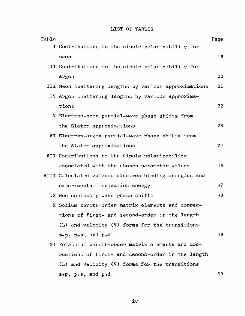
LIST or TABLESTable Page

I Contributions to the dipole, polarizabilitv forneon 19

II Contributions to the dipole polarizability forargon 20

III Neon scattering lengths by various approximations 21IV Argon scattering lengths by various approxima­

tions 22V Electron-neon partial-wave phase shifts from

the Slater approximations 23VI Electron-argon partial-wave phase shifts from

the Slater approximations 24VII Contributions to the dipole polarizability

associated with the chosen parameter values 46VIII Calculated valence-electron binding energies and

experimental ionization energy 47IX Non-coulomb p-wave phase shifts 48X Sodium zeroth-order matrix elements and correc­

tions of first- and second-order in the length (L) and velocity (V) forms for the transitions s-»-p} p-*s, and p-*.d 49

XI Potassium zeroth-order matrix elements and cor­rections of first- and second-order in the length (L) and velocity (V) forms for the transitions s-*-p, p->s, and p-*d 5 0

iv

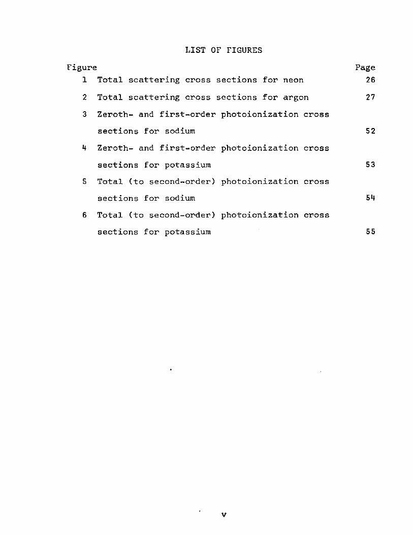
LIST OF FIGURESFigure Page

1 Total scattering cross sections for neon 262 Total scattering cross sections for argon 273 Zeroth- and first-order photoionization cross

sections for sodium 524 Zeroth- and first-order photoionization cross

sections for potassium 535 Total (to second-order) photoionization cross

sections for sodium 546 Total (to second-order) photoionization cross

sections for potassium 55

v

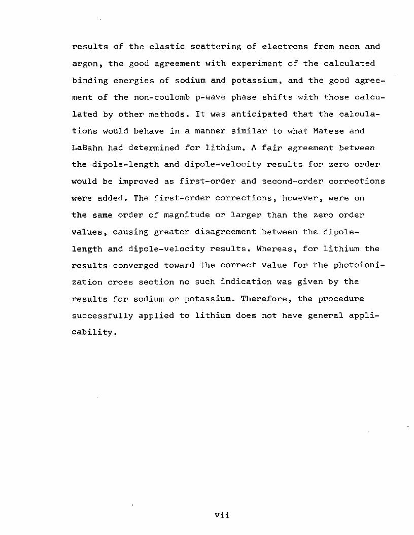
results of the elastic scattering of electrons from neon and argon, the good agreement with experiment of the calculated binding energies of sodium and potassium, and the good agree­ment of the non-coulomb p-wave phase shifts with those calcu­lated by other methods. It was anticipated that the calcula­tions would behave in a manner similar to what Matese and LaBahn had determined for lithium. A fair agreement between the dipole-length and dipole-velocity results for zero order would be improved as first-order and second-order corrections were added. The first-order corrections, however, were on the same order of magnitude or larger than the zero order values, causing greater disagreement between the dipole- length and dipole-velocity results. Whereas, for lithium the results converged toward the correct value for the photoioni­zation cross section no such indication was given by the results for sodium or potassium. Therefore, the procedure successfully applied to lithium does not have general appli­cability .

vii

PART I SLOW ELECTRON SCATTERING FROM NEON AND ARGON

1-1. INTRODUCTION

Recently Matese and LaBahn^ calculated the photoioniza­tion cross section for lithium, wherein they successfully applied the method of polarized orbitals to account for corepolarization effects. Their approach was a logical extension

2 3of the application by LaBahn and Callaway * of the polarized orbital method to the analysis of elastic scattering of electrons from helium. A similar approach suggested itself for the case of the heavier alkali metals, the next two being sodium and potassium. The complementary problem which will give some indication of the validity of a polarized orbital calculation on equivalent electronic core configurations, is the analysis of elastic scattering of electrons by neon and argon. The purpose of this part is to present the results of calculations on the elastic scattering of electrons by neon and argon by the polarized-orbital method.

It has been understood for about 40 years that the problem of slow electron scattering by rare gas atoms re­quires consideration of both exchange and polarization ef­fects. Exchange effects have generally been accounted for by assuming the wave function for the system to be of a properly antisymmetrized form. Polarization effects avoided a simple analysis until about 15 years ago, when the method of pola- rized orbital was developed. This method, which is applied in this work, determines a polarization potential that ac­counts for the polarization of the atom by the scattering electron.

2

5In 1966, Thompson analyzed the elastic scattering of electrons by neon and argon, incorporating both exchange and polarization effects. He used a variant of the polarized or­bital method known as the adiabatic-exchange approximation. His results were in good agreement with experiment near zero energy and maintained relatively good agreement to an energy of one rydberg. Whereas he considered only the np-*d transi­tion, we have examined all the excitations from the outermost orbital for which A£=±l. Calculations were made in both an unnormalized or normalized manner, depending on whether or not the calculated polarizability was close to the experi­mental value.

Thompson obtained his polarization potential by deter­mining the polarized orbitals using the Sternheimer approxi­mation. In this calculation the Sternheimer procedure was also utilized and in addition, an alternate one was developed based upon the Slater-averaged-exchange approximation. A com­parison of our total cross section results from both proce­dures is made with those of Thompson and some recent experi­ments .

The derivation of the pertinent equations, up to the point of applying either the Sternheimer or Slater approxima­tion is given in Section 1-2. The formalism of the Sternheim­er and Slater approximations appears in Section 1-3. Section I_i| contains the results and discussions.

1-2. PERTURBATION THEORY FORMALISM6

In the method of polarized orbitals one seeks to find the first-order correction to the atomic orbitals arising from the perturbation by the electric field of the scatter­ing electron. The only orbitals considered to be perturbed are the outer ones which correspond to the least tightly bound electrons. The extension of the Hartree-Fock (HF) for­malism for an unperturbed atom or ion to first-order pertur­bation theory yields for the form of the one-electron HF equation

U *0 )t X f i ' - i j J X A 1) ~ 0 ; i = 1,2,...,N, 1.1

where the spin orbitals X-X are orthonormal; that is,

i,j = 1,2,...,N. 1.2

In Eq. 1.1, h(l) is the one-electron HF operator which for an atom of charge Z takes the form

- V ,1- < 0 - / > , , ) ! XJ> J 1-3

h represents the perturbation ( 2 j / \ - * in our case, withre as the coordinate of the perturbing charge), and A serves as the usual perturbation theory expansion parameter which is later set equal to 1. The operator in the summation in Eq. 1.3 signifies

< Xj K(l-Pn)IXj) (to = (0)Jxj(t) XTi 1*4- )

4

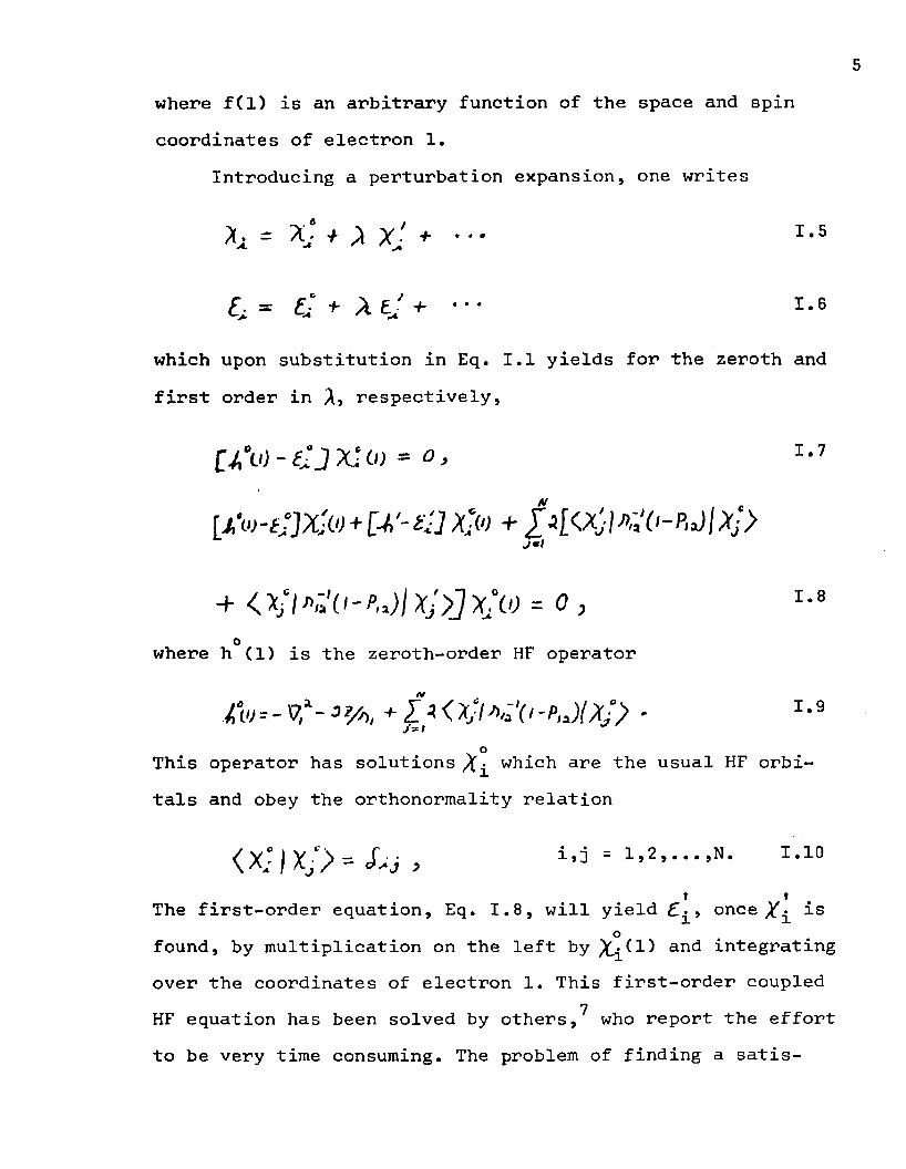
where f(l) is an arbitrary function of the space and spin coordinates of electron 1.

Introducing a perturbation expansion, one writes

* > xj + T - s

i - = e ; 1- x t j + ••• 1.6

which upon substitution in Eq. 1.1 yields for the zeroth and first order in respectively,

[ A o - £ 3 xl 0) = o,

li,'o)-£]X-w + [3'-£] X-C) + p ^ l ^ O - P J l X j }

1.7

1.8+ <£lK'tj-p,3lxJ)JxJ\o = 0 ,owhere h (1) is the zeroth-order HF operator

A o = - V , 1 - + £ h < X - I A * X i - P J I X J ) ■ I-9. oThis operator has solutions which are the usual HF orbi­

tals and obey the orthonormality relation

i,j = 1,2,...,N. I.10« *The first-order equation, Eq. 1.8, will yield £\, once i-s

ofound, by multiplication on the left by ^ ( 1 ) and integratingover the coordinates of electron 1. This first-order coupled

7HF equation has been solved by others, who report the effort to be very time consuming. The problem of finding a satis-

factory approximation to the solution can be expedited byneglecting all of the terms which represent essentially smalleffects but add considerable complication.

One of the simplest uncoupling procedures, first sug- 8gested by Dalgarno, is to neglect in Eq. 1.8 all terms in

the sum over j. This results in the equation

U"(0-i:]xU'J + O ' - f / J X / c y = o. x.iiAnother uncoupling procedure which is equally convenient

7was suggested by Langhoff, Karplus, and Hurst. We first rearrange Eq. 1.8 and write it in the form

u ’ o)

+■ < x ; k ' o - p M / } ] x ' c j = 0 ,o twhere the operator h^(l) acting on is

j~ >

One should note that Eqs. 1.8 and 1.12 are equivalent, since in Eq. 1.8 the term (j=i) in the explicit sum over j cancels

othe self-potential term (j=i) in h (1). The terms with i in Eq. 1.12, known as the first-order self-consistency cor­rection, are now dropped to simplify the equation. This will

ieliminate all the terms involving first-order functions other than the one being calculated (X^)» thus uncoupling the equation and leaving the expression

7

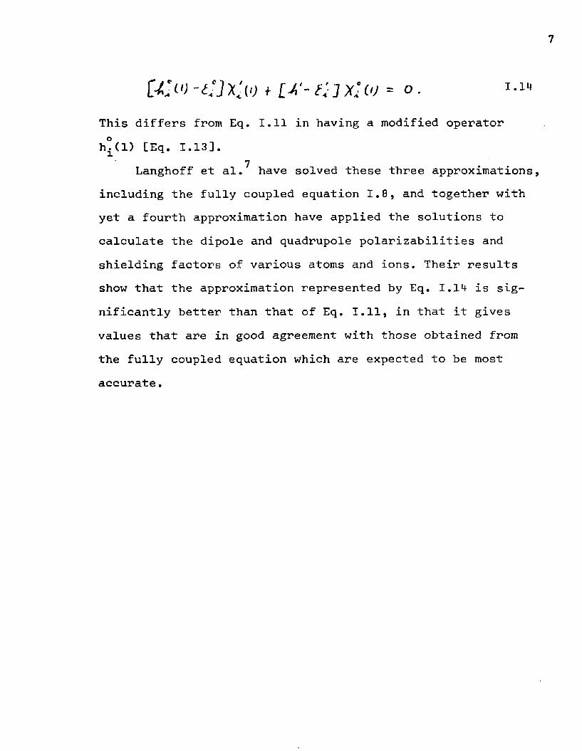
£ & » - t ' J x l i o * [ ■ * ' - t y j x U o = o . i . »

This differs from Eq. I.11 in having a modified operator h!(l) [Eq. 1.13].

7Langhoff et al. have solved these three approximations, including the fully coupled equation 1.8, and together with yet a fourth approximation have applied the solutions to calculate the dipole and quadrupole polarizabilities and shielding factors of various atoms and ions. Their results show that the approximation represented by Eq. 1.14 is sig­nificantly better than that of Eq. I.11, in that it gives values that are in good agreement with those obtained from the fully coupled equation which are expected to be most accurate.

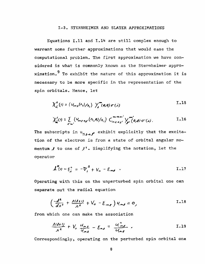
1-3. STERNHEIMER AND SLATER APPROXIMATIONS

Equations I.11 and 1.14 are still complex enough to warrant some further approximations that would ease the computational problem. The first approximation we have con­sidered is what is commonly known as the Sternheimer appro-

9ximation. To exhibit the nature of this approximation it is necessary to be more specific in the representation of the spin orbitals. Hence, let

if) = ( ^jrKV/iJ yj C0;<P) <r(J) 1.15

- L i/* * ,* ) /* ,) C ^ , )/, ( w ) c r ( A ) . I*16

The subscripts in exhibit explicitly that the excita­tion of the electron is from a state of orbital angular mo­mentum Jt to one of J ' . Simplifying the notation, let the operator

J ’ o - e j = - v , * + v 0

Operating with this on the unperturbed spin orbital one can separate out the radial equation

- J L 4- J. \/ « 1.18A('7P =

from which one can make the association

f- \ / _ c - , 1.19

Correspondingly, operating on the perturbed spin orbital one

8

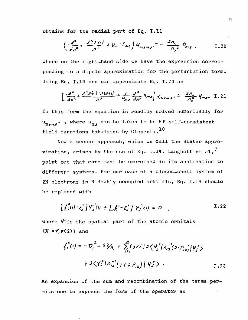
obtains for the radial part of Eq, I.11

/ . J'fJ'-fO . 1/ - f ) // - _ t,C V * ’ 1,20

where on the right-hand side we have the expression corres­ponding to a dipole approximation for the perturbation term. Using Eq. 1.19 one can approximate Eq. 1.20 as

r_^4 , j ' ( n o - J ( s + t } _j_ ef i u 1 „ T on1-J1

In this form the equation is readily solved numerically for.» » where u „ can be taken to be HF self-consistentnjt-* j ' 9 n j

field functions tabulated by Clementi.^Now a second approach, which we call the Slater appro-

7ximation, arises by the use of Eq. 1.14. Langhoff et al.point out that care must be exercised in its application todifferent systems. For our case of a closed-shell system of 2N electrons in N doubly occupied orbitals, Eq. 1.14 should be replaced with

+ L - A ' - t J ] ¥■■<.<) -- 0 , 1-22

where is the spatial part of the atomic orbitals (Xi=^i«r(i)) and

fiO) = -v,2-2 54, t 2 (^7Aa'(3-P,

+ I * , , (/f a fa > • i.23

An expansion of the sum and recombination of the terms per­mits one to express the form of the operator as

10

/JO, - -v7,a - “ /A t Z' jIfivj2 ^

/V1.24

A/

Adding and subtracting ^ f >puts the operator in the form

/ ; « = 'V,J - + i ' j I i i % „ - * r xJ i

f j

+ Z * I 0 ’ J W f K fia /tf*;/.1-

Employing Slater's approximation of the exchange operator

term, 3 {_<% • V m V , 1| » bV ‘ ^XjO^jCj] %and labeling it Ag; one can then write

25

I 26M ^ IV T W ” s ~ 7 i* \s J ~ J

where

v' = - ; * A + | ' , *•”

and ^ is a parameter, the value of which will be discussed later. The single prime implies that one excludes from the sum the electron that is in the orbital being perturbed.The double prime implies that two electrons in the orbital being perturbed are excluded from the sum. A is the well

b

known Slater-averaged-exchange potential originally computed11as the exchange correction in a free-electron gas model.

The particular combination that arises in the operator Eq. 1.26 stems from the need to preserve spherical symmetry.

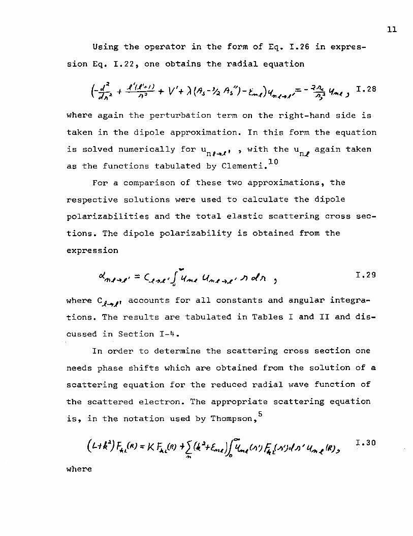
Using the operator in the form of Eq. 1.26 in expres­sion Eq. 1.22, one obtains the radial equation

+ ^ + I - 2 8

where again the perturbation term on the right-hand side is taken in the dipole approximation. In this form the equation is solved numerically for un^^» > with the u again takenas the functions tabulated by Clementi.^

For a comparison of these two approximations, therespective solutions were used to calculate the dipolepolarizabilities and the total elastic scattering cross sec­tions. The dipole polarizability is obtained from the expression

J) o(J\ 1.29

where accounts for all constants and angular integra­tions. The results are tabulated in Tables I and II and dis­cussed in Section 1-4.

In order to determine the scattering cross section one needs phase shifts which are obtained from the solution of a scattering equation for the reduced radial wave function of the scattered electron. The appropriate scattering equation is, in the notation used by Thompson,^

30(Lit1) - K +l(i*+ent)pL40>V%{4'J‘(j>'IU.< (*), 1•Ak *0where

12

The polarization potential V is given by

1.32

The other terms and symbols in Eqs. 1.31 and 1.3 2 are defined as

with representing the Legendre polynomial of order J ,

In the numerical solution of Eqs. 1.22, 1.28, and 1.30,all iterations were performed using Numerov1s method. Allintegrals were evaluated by means of the trapezoidal rule.The starting values required were obtained by appropriatepower-series expansion of the functions. In the iterationsa variable mesh size was used that began with Ar=0.0025aQ atthe origin and doubled periodically to Ar=0.16aQ at r=25.0ao ,remaining at this value for all larger r. The phase shifts

12were determined by employing a procedure due to Burgess,with the iteration extended until the value converged to

-5within 5 x 10 rad. This occured usually in the neighborhood of r=35aQ. Having determined the phase shifts, the total elastic scattering cross section is calculated from the

O'* A

1.34

1.33

J t P j t U ) P l ^ p ^ ) f t r 1.35

13expression

~ ( V h 3‘) 2 ^ ( * l +0 ^ A' I l • 1.36

The range of the partial-wave sum for neon was L=0,l,2 and for argon L=0,l,2,3. Some of the partial-wave shifts and scattering cross section results are presented in the fol­lowing section.

1-4. RESULTS AND DISCUSSIONS

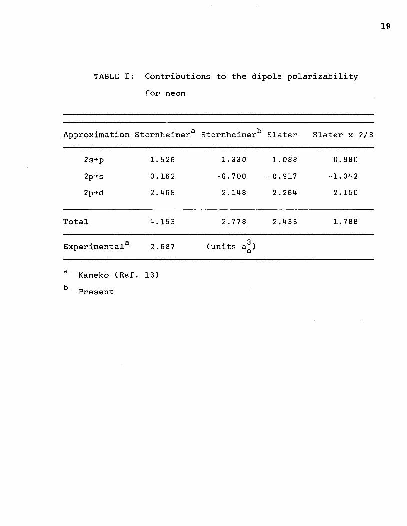
Contributions to the dipole polarizability from theoutermost occupied level are listed for neon in Table I andfor argon in Table II. They are compared with earlier calcu-

13lations by Kaneko, who used the Sternheimer approximation, and experiment. Our Sternheimer results for neon are in bet­ter agreement with experiment than Kaneko’s. In addition, the Sternheimer components calculated by Montgomery and LaBahn^ in an independent calculation agree with the present calculations.

Results for argon were not as satisfying in that no significant change in the values of the polarizabilities inSternheimer approximation were obtained from those of

13 14Kaneko or Montgomery and LaBahn. The change in the totalpolarizability through use of the Slater approximation also went the wrong way and did not yield the desirable reduction that occurred for neon.

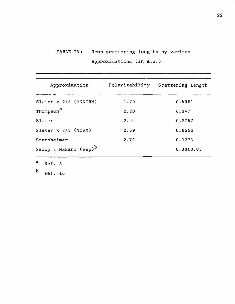
The additional sets of values listed correspond to some of the modifications made to the Slater approximation. The nature of these modifications will be described later. The seven modifications being reported for which the total scat­tering cross sections were calculated are listed in Table III, This table gives a comparison of the total polarizabili­ty with the zero-energy scattering length for argon. The analogous results for neon are exhibited in Table IV. The scattering lengths were observed to be quite sensitive to the value of the total polarizability, in a given approxima-

14

tion.The total scattering cross sections were generally cal­

culated at energies in the range 0.00 to 1.00 rydbergs at increments of 0.10 rydbergs. A few additional values were calculated in the neighborhood of the maximum and minimum for the Slater x 0.594 modification. As was mentioned earlier, all calculations included the three transitions ns+p, np->s, and np->-d, where n has the value corresponding to the outer­most occupied level. The partial phase shifts are listed for only a few modifications, viz., those for neon in Table V and argon in Table VI.

Let us now consider the nature of the modifications used. If the calculated value of the polarizability was sig­nificantly different from the experimental one, a second solution of the scattering equation was made using a polari­zation potential normalized to the experimental value of the polarizability. The normalizing factors were just the ratio of the experimental to calculated values of the polarizabili­ty. The results are labeled appropriately as unnormalized and normalized.

Another modification was made to the Slater approxima­tion of the exchange term in the potential. Slater"^ derivedhis averaged-exchange potential on the basis of a free-

15electron-gas model. More recently Kohn and Sham in their consideration of the problem of a homogeneous gas of inter­acting electrons have obtained the same functional form ex­cept reduced by a factor of 1/3. Slater has found a conve-

nient approximation for the exchange interaction which may be successfully applied to different systems, with more than just a few electrons, by suitably choosing a multiplicative strength parameter. Calculations were made with the factor taken as both six and four, and the corresponding results labeled as Slater and Slater x 2/3. One would have hoped that the better agreement with the experimental results would have decided which factor was more correct.

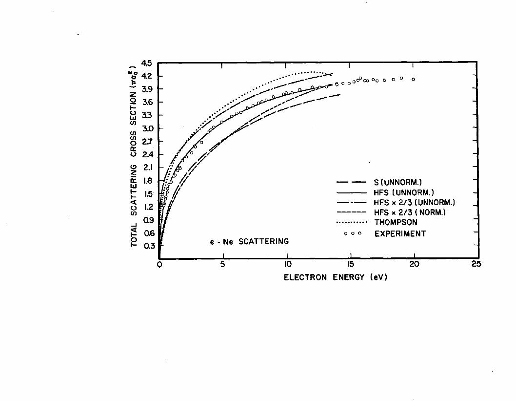
The good agreement of the Slater cross sections for neon16with the recent experimental results of Salop and Nakano

shown in Fig. 1 would indicate the factor of six as being better. Although no improvement was expected, the modifica­tions Slater x 2/3 (UNNORM) and Slater x 2/3 (NORM) were cal­culated for neon to observe the relative behavior when they are applied to argon.

The argon results shown in Fig. 2 imply in contradiction that the factor of four will yield results in better agree­ment with experiment. Argon results for Slater x 2/3 are not plotted because they are almost identical with Thompson’s above 5 eV and our Sternheimer (NORM) below 5 eV. Since the Slater x 2/3 modification did not yield the experimental pol- larizability it was used in a normalized calculation as des­cribed above.

The polarizability obtained from the Slater x 2/3 appro­ximation was considerably improved over the value arising from the Slater approximation. This suggested an alternative normalization procedure, that of multiplying the Slater-

averaged-exchange potential by an appropriate factor which would yield a polarizability equal to the experimental value.A justification for this procedure stems from the fact that the multiplicative factor is dependent on the type of system that is being described. The factors of six or four arise from consideration of systems of a free-electron gas or a homogeneous gas of interacting electrons and should not be ex­pected to be correct in describing the electron distribution in an isolated atom. The results of this calculation, labeled Slater x 0.594, are in best agreement with experiment, which is represented in Fig. 2 by the open circles. No further im­provement on the agreement however was attempted by an arbi­trary manipulation of the factor. Thompson's argon results, obtained through a normalized Sternheimer approximation in­cluding only the 3p+d transition, was in excellent agreement with the Slater x 0.594 below 2 eV.

A single curve represents the normalized results of the two approximations (Sternheimer and Slater) since they are in essential agreement. There was a slight deviation in the range of 6-10 eV. The normalized Slater x 2/3 curve for argon was not shown since it essentially paralleled the Slater x0.594 curve, lying above it except for the range between 1 and 5 eV where it dips slightly below.

The behavior of the argon results leads one to conclude that the two different approximations in the normalized modi­fication account for those aspects of the scattering process known as adiabatic-exchange effects. The nature of the dis-

18agreement with experiment indicates that some nonadiabaticeffects are making an appreciable contribution. The formalismfor accounting the nonadiabatic effects has been established

3and successfully applied to helium . The procedure is known as the extended polarization approximation.

An analysis of the extended polarization approximation has established that the nonadiabatic effects add a repulsive contribution via a distortion potential. This has been shown to be less significant at larger distances than the polariza­tion potential but comparable in the vicinity of the core*Hence, only those scattered electrons that penetrate the core, which are those of the higher energies, will be appre­ciably affected. The agreement of the results at the lower energies and the appreciable deviation at the higher energies suggests that argon would be an ideal system for testing the extended polarization approximation. Its application would however be difficult and for our ultimate application of this formalism to photoionization of Na and K, the adiabatic-di- pole approximation is believed to be sufficiently accurate.

19

TABLE I : Contributions to the dipole polarizabilityfor neon

Approximation Sternheimera Sternheimer*5 Slater Slater x 2/3

2s+p2p-*s2p-*d

1.526 0.162 2 . 465

1.330-0.7002.148

1. 088 -0.917 2.264

0.980-1.3422.150

Total 4.153 2.778 2.435 1.788

d.Experimental 2 .687 (units a^) o

a Kaneko (Ref. 13) k Present

TABLE II: Contributions to the dipole polarizability for argon

Approximation Sternhe imera Sternheimer^ Slater Slater x 2/3 Slater x 0.594

3s-»-p 5.598 5.888 5.070 4.224 4.0763p-*-s -3. 282 -3.374 -3.467 -6.255 -7.0753p-*-d 13.883 13.998 16.875 14.435 14.000

Total 16.199 16.512 18.478 12.404 11.001

Experimental 11.000 (units a3) o

a Kaneko (Ref. 13)Present

21

TABLE III: Argon scattering lengths by various approximations (in a .u.)

Approximation Polarizability Scattering Length

Slater (UNNORM) QO3-00 1—I -8.062Sternheimer (UNNORM) 16. 51 -5.819Slater x 2/3 (UNNORM) 12.40 -2 .327Sternheimer (NORM) 11.00 -1.946Slater (NORM) 11.00 -1.898Slater x 2/3 (NORM) 11. 00 -1.689Slater x 0.594 11.00 -1.608Thompson3 11.00 -1.60Golden £ Bandel (exp)b -1.647

a Ref. 5 b Ref. 17

22

TABLE IV: Neon scattering lengths by variousapproximations (in a.u.)

Approximation Polarizability Scattering Length

Slater x 2/3 (UNNORM) 1.79 0.4351Thompson3 2. 20 0.347Slater 2.44 0.2757Slater x 2/3 (NORM) 2.69 0.0556Sternheimer 2.78 0.0276Salop 6 Nakano (exp)b 0.30±0.03

a Ref. 5b Ref. 16

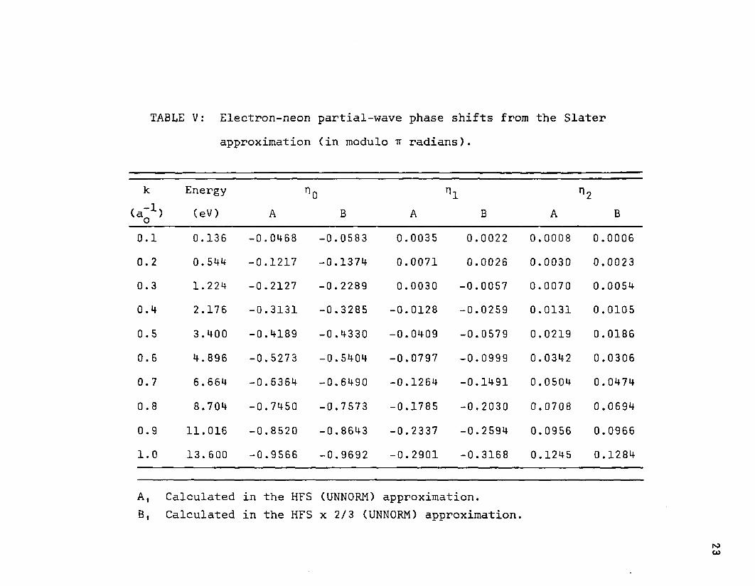
TABLE V: Electron-neon partial-wave phase shifts from the Slaterapproximation (in modulo tt radians).

k Energy rig n1 n2(a-1) (eV) A B A B A Bo

1—1 «o 0.136 -0.0468 -0.0583 0.0035 0.0022 0.0008 0.0006

0.2 0.544 -0.1217 -0.1374 0.0071 0.0026 0.0030 0.00230.3 1.224 -0.2127 -0.2289 0.0030 -0.0057 0.0070 0.00540.4 2.176 -0.3131 -0.3285 -0.0128 -0.0259 0.0131 0.01050.5 3.400 -0.4189 -0.4330 -0.0409 -0.0579 0.0219 0.01860.6 4.896 -0.5273 -0.5404 -0.0797 -0.0999 0.0342 0.03060.7 6.664 -0.6364 -0.6490 -0.1264 -0.1491 0.0504 0.0474

00•o 8.704 -0.745Q -0.7573 -0.1785 -0.2030 0.0708 0.0694

0.9 11.016 -0.8520 -0.8643 -0.2337 -0.2594 0.0956 0.09661.0 13.600 -0.9566 -0.9692 -0.2901 -0.3168 0.1245 0.1284

A, Calculated in the HFS (UNNORM) approximation.B, Calculated in the HFS x 2/3 (UNNORM) approximation.

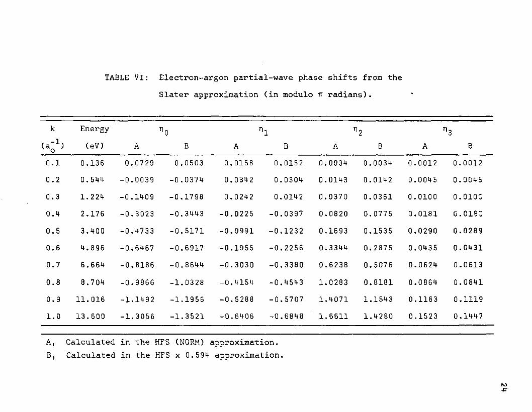
TABLE VI: Electron-argon partial-wave phase shifts from theSlater approximation (in modulo tt radians). •

k Energy no n1 n2 n3(eV) A B A B A B A B

0.1 0.136 0.0729 0.0503 0.0158 0.0152 0.0034 0.0034 0.0012 0.00120.2 0.544 -0.0039 -0 .0374 0.0342 0.0304 0.0143 0.0142 0.0045 0*90450.3 1. 224 -0.1409 -0.1798 0.0242 0.0142 0.0370 0.0361 0.0100 0.010C0.4 2.176 -0.3023 -0.3443 -0.0225 -0.0397 0.0820 0.0775 0.0181 o.ois:0.5 3.400 -0.4733 -0.5171 -0.0991 -0.1232 0.1693 0.1535 0.0290 0.02890.6 4. 896 -0.6467 -0.6917 -0.1955 -0. 2256 0.3344 0.2875 0.0435 0.04310.7 6.664 -0.8186 -0.8644 -0.3030 -0.3380 0.6238 0.5076 0.0624 0.06130.8 8.704 -0.9866 -1.0328 -0.4154 -0.4543 1.0283 0.8181 0.0864 0.08410.9 11.016 -1.1492 -1.1956 -0.5288 -0.5707 1.4071 1.1543 0.1163 0.11191.0 13.600 -1.3056 -1.3521 -0.6406 -0.6848 1.6611 1.4280 0.1523 0.1447

A, Calculated in the HFS (NORM) approximation.B, Calculated in the HFS x 0.594 approximation.

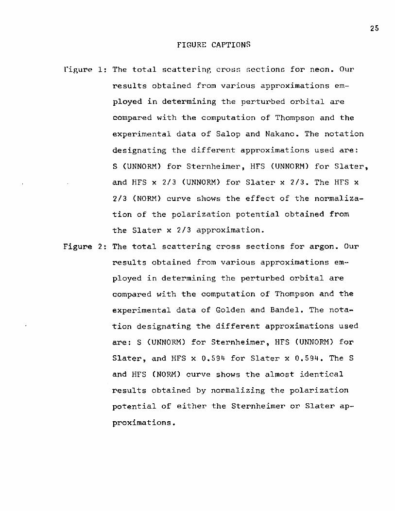
FIGURE CAPTIONS

Figure 1: The total scattering cross sections for neon. Our results obtained from various approximations em­ployed in determining the perturbed orbital are compared with the computation of Thompson and the experimental data of Salop and Nakano. The notation designating the different approximations used are:S (UNNORM) for Sternheimer, HFS (UNNORM) for Slater, and HFS x 2/3 (UNNORM) for Slater x 2/3. The HFS x 2/3 (NORM) curve shows the effect of the normaliza­tion of the polarization potential obtained from the Slater x 2/3 approximation.

Figure 2: The total scattering cross sections for argon. Our results obtained from various approximations em­ployed in determining the perturbed orbital are compared with the computation of Thompson and the experimental data of Golden and Bandel. The nota­tion designating the different approximations used are: S (UNNORM) for Sternheimer, HFS (UNNORM) for Slater, and HFS x 0.594 for Slater x 0.594. The S and HFS (NORM) curve shows the almost identical results obtained by normalizing the polarization potential of either the Sternheimer or Slater ap­proximations .

4.5N o O 4 2

'—’ 3.9Zo £ <nhOUJ 3.3CO

3.0COCOo 2.7cro 2.4o 2.1zQT 1.8UJ1-1- 1.5<o 1.2CO

0 9

2 0 6oJ- 0.3

S( UNNORM.)HFS (UNNORM.)HFS x 2 /3 (UNNORM.) HFS x 2 /3 ( NORM.) THOMPSON EXPERIMENT

e - Ne SCATTERING

0 5 10 15 20

ELECTRON ENERGY (eV )

25

TOTA

L SC

ATTE

RING

CR

OSS

SECT

ION

(*a,

• - A r SCATTERING

S (UNNORM.)HFS (UNNORM.)S 8 HFS (NORM.) HFS * 0 .5 9 4 THOMPSON EXPERIMENT

4 6 8 10 12 14 16 18ELECTRON ENERGY (eV)

PART II PHOTOIONIZATION CROSS SECTIONS OF SODIUM AND POTASSIUM

28

II-l. INTRODUCTION

The success of the analysis by Matese and LaBahn^ of the photoionization cross section for the lithium atom has sug­gested this application to the alkali metals, sodium and po­tassium. This calculation of the photoionization cross sec­tion by the polarized orbital method will explicitly account for the effect of individual orders of correction, to second order.

The well known formalism for calculating photoionization 1 8cross sections requires the evaluation of matrix elements

between the initial and final states. Representing thesestates with exact wave functions permits defining the dipole

19photoionization cross section in three equivalent ways, known as the dipole-length, dipole-velocity and dipole-acce- leration formulae. Calculations have generally been carried out only in the dipole-length and dipole-velocity approxima­tions. The degree of agreement between the results is used as a measure of the exactness of the state wave functions.

Good representation of the state wave functions has been achieved by considering them to be determinantal wave func­tions, with those elements representing the bound states being taken as fixed-core Hartree-Fock or variationally determined one-electron wave functions. Polarization of the core electrons exists and this has been accounted for by the method of polarized orbitals, primarily by its effect on the continuum wave function. Matese and LaBahn^ in addition have

29

30incorporated perturbed orbitals for some core states in their representation of the initial and final states. They point out that failing to so so would include some second-order effects in the analysis while neglecting first-order correc­tions.

20Chang and McDowell in their many-body perturbation theory analysis of the photoionization of lithium have deter­mined the relative sizes of various initial and final state corrections. Their results indicate that the second-order final-state correction is dominant in the dipole-length approximation; whereas in the dipole-velocity approximation, it is comparable in magnitude to first-order initial state and first-order final-state corrections. Their results imply that the discrepancies that have existed between calculated photoionization cross sections using the length and velocity approximations may be attributed to the neglect of first- order effects.

In Section II-2 we discuss the representation for the initial and final states. The formalism for computing photo­ionization cross sections in the dipole-length and dipole- velocity is given in Section II-3. The results are discussed in Section II-4, and the conclusions in Section II-5.

II-2. REPRESENTATION OF INITIAL AND FINAL STATES

In the car.p of alkali metals which possess only a single electron over a closed shell core, the total wave function can be represented by a single determinant

f - A t I x j ' ) X , • II. 1

The X p» •••» Xjr are one-electron spin orbitals represent­ing the unperturbed and perturbed bound states or a continuum state. Taking the bound state functions representing the core as the corresponding ionic functions tabulated by dementi"^ will not include any polarization effects.

Designate the spin orbitals that are unperturbed by ao ° tzero superscript, X > an< those perturbed by X + X , where

X are the first-order perturbation corrections of the unper­turbed orbitals, determined by the polarized orbital proce­dure discussed in Section 1-3. Expressing the wave function [11.13 in this new notation and then expanding into a linear combination of determinantal functions, we represent the ini­tial and final state wave functions for N electrons as

' I I , II. 2

where the first sum is over a cyclical permutation of the indices and the second over the perturbed orbital components. The ^ £ is the wave function for the valence electron in the initial s t a t e , = ^ns> or continuum electron in the final state, ^ ^ and Z = N-l. Four types of wave functions arerepresented by with

31

32

¥ - U * f lX ,V > ' = ¥ ( • , " ; * > IT.3

containing only unperturbed core wave functions. The

f • ' - X m >SAf J)x> *•'///¥? ^ 11 •4

contains the perturbed orbitals for the nfs-*-p transition, and andjf^^, respectively, those from the n fp-*-s and n’p+d

transitions (n1 = n-1).The perturbed orbitals are determined by the procedure

described in Section 1-3. For this analysis only the ordinary Slater-averaged-exchange approximation was used. Thus, the radial equation [1.28] was slightly modified to the form

^ • TI-5

The reason for this modification will be explained shortly. All the symbols retain their earlier definition. The X’s are parameters which are adjusted to yield perturbed orbitals satisfying certain conditions.

In order for the total wave function [Eq. II.2] to be normalized correctly to first-order, the constituent single­electron orbitals must satisfy the following orthogonality conditions^

< x ;i x p =cf., , < x j i x i > - ° ,

•*- - °> i,j = II.6

The first condition is satisfied by using the Hartree-Fock orbitals for the unperturbed states. The second condition is satisfied automatically by angular symmetries since we are only considering dipole perturbations. The last condition was satisfied approximately for all positions of the perturb­ing charge by adjusting A i n the s+p and p-t-s equations. The remaining Ain the p->d equation was then adjusted such that the partial dipole polarizabilities CEq. 1.29], summed to the experimental value.

These conditions were observed to restrict the values of X for each of the three transitions to a relatively unique triplet. Those chosen for this calculation are listed in Table VII. As may be observed from the values chosen, there is some arbitrariness in their choice. Although negative values would permit satisfying the conditions, they were not considered. Choosing two of the triplet values to be the same of course made satisfying the imposed conditions more diffi­cult. The conditions also justified our approximating theexchange integral by A , as above, rather than the more com-splex combination (A - 3/2 A”) used for the electron scatter-s sing calculation in Part I. The perturbed orbitals, determined by using both forms for the approximation and satisfying the conditions discussed above with appropriate triplets, were then used to calculate a polarization potential given by Eq. 1.32. The two potentials were found to be almost identical, hence the simpler approach was adopted.

We now conclude this discussion of the representation

of the initial and final stator, with a few comments regard­ing the bound valence and continuum states. Their determina­tion reduces to a solution of an appropriate radial equation, which can be written as, using the notation defined in Eqs. 1.31 through 1.35,

(L + jtyF ju to )= M J ^ iew V p w f t, • II. 7

This equation serves to determine both the bound and conti­nuum state reduced radial wave function. The continuum func-

otion, is determined if k is taken as the kineticenergy of the scattered electron; or the bound state, =

2u* , if k is taken as the binding energy. These are the per-I I S

turbed functions, as is implied by the primes. The solution of the equation, with = 0, are the unperturbed fixed-core Hartree-Fock (FCHF) functions and designated by the absence of the prime. The last term, which is summed over all occu­pied states, imposes the constraint that the continuum and bound state functions shall be orthogonal to the core states.

The calculated binding energies are tabulated and com-2 2pared with experiment in Table VIII. The non-coulomb phase

shifts of the continuum wave functions are compared with those of o t h e r s 9^ ^ in Table IX.

In the succeeding discussions, we refer to calculations using only FCHF wave functions and restricting the sum over p in Eq. II.2 to just the zero value, as the zeroth-order calculation. Matrix elements constructed with initial and final states of the form of Eq. II.2 are referred to as

first-order corrections, if the valence and continuum wavefunctions are taken as the solutions of Eq. II.7 with V = 0.PThe second-order corrections are those when the valence and continuum states are taken as the solutions of the full Eq,

IT-3. MATRIX ELEMENTS

In the dipole approximation, the valence electron eject­ed from the ground state of the sodium or potassium atom is in a p-wave state, and the expressions for the photoioniza­tion cross sections in the length and velocity forms are

i. 18given by

<rt = % r*. (x n ) 2_ jFll;*f\ ii.s

<rv = % r«. I I P l'J 'j ‘ II-9

where I is the first ionization potential , £ is the energy of the ejected electron, «_is the fine structure constant,

* T ‘ J W " n < » ■ ,

and 0L = r, 0^ = V . The summation is over final state orbital- projection quantum numbers.

The matrix elements are evaluated after inserting (jJng into Eq. II. 2 for and into Eq. II. 2 forThe bound state function was normalized to one and the conti­nuum to

Lit*fa) A *-***> + + A A/>) ii.ii2 —19 2The constant 4/3 Ila aQ = 8.56 x 10 cm and the remaining

2quantities are taken in the system of atomic units ft = 1, e = 1/m = 2. The non-coulomb phase shift is and = argT(2-i/k), whereris the gamma function.

36

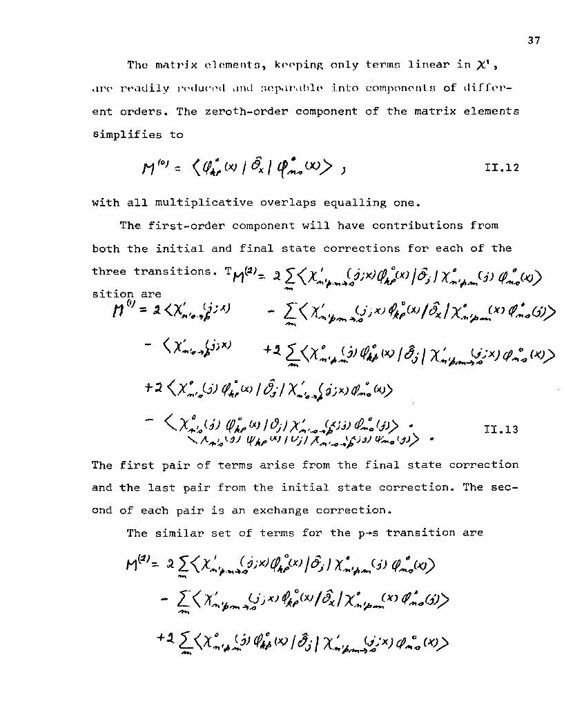
The matrix elements, keeping only terms linear in X ’ » are readily redured and separable into components of differ­ent orders. The zeroth-order component of the matrix elements simplifies to

with all multiplicative overlaps equalling one.The first-order component will have contributions from

both the initial and final state corrections for each of the three transitions. The terms that remain from the s-*-p tran­sition are

The first pair of terms arise from the final state correction and the last pair from the initial state correction. The sec­ond of each pair is an exchange correction.

The similar set of terms for the p+s transition are

11.12

nt,=iZiK'jjj- < j j>

" I # j ) & ' . ' # >11.13

aI<?J I'•n r

4 4 1

38

~ l o * > / % € : « > > ■

II. 14

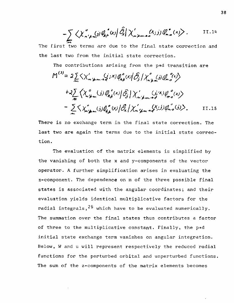
The first two terms are due to the final state correction and the last two from the initial state correction.

The contributions arising from the p-»d transition are

$ K>t »

" I S W / 4 ixi 0'J>. 11.15

There is no exchange term in the final state correction. The last two are again the terms due to the initial state correc­tion.

The evaluation of the matrix elements is simplified by the vanishing of both the x and y-components of the vector operator. A further simplification arises in evaluating the z-component. The dependence on m of the three possible final states is associated with the angular coordinates; and their evaluation yields identical multiplicative factors for the radial integrals, which have to be evaluated numerically.The summation over the final states thus contributes a factor of three to the multiplicative constant. Finally, the p+d initial state exchange term vanishes on angular integration. Below, W and u will represent respectively the reduced radial functions for the perturbed orbital and unperturbed functions. The sum of the z-components of the matrix elements becomes

39

- l ( ® u 11.16 A

^ j j W * ?)(tf (v Y'*' (,))<Ya, Hti 11.16 B

11.16 c

V(%*(o W & f* 11.16 D

- j U W^ +■* { ° 'i0) o {0 Y*r 11.16 E

~ r J J K ' * * 4 ^ q{ K ' 0 ) '/iJJ J m' t* - (i)^ (sJ 11. ib f

n '16 G

-j-JJ\'O U;V(&A0^0)jA,^^(v«A^^ 11,16 H^ 1 1 ,1 6 1

" j ' ' J) ^ W cJa*

+ t y < * + * ^ (v (V

44

11.16 J

11.16 K

The operators in the integrals will be dependent on whether the dipole-length or dipole-velocity approximation is being considered. Their form is determined by the notation

length: ~ C j ~ SX jt f * + ')

velocity: & ' * — -~Y~ + *j('J „ 11.17t w ? y j

The choice of J or /f+1 is associated respectively with the upper + or lower - sign.

One last consideration is the second-order corrections. These are obtained from the zeroth-order integrals by re­placement of the unperturbed reduced radial functions for the valence and continuum states by the corresponding perturbed functions. The subscripts on the reduced radial function representing the perturbed orbital indicates the transition being considered. The five integrals after the first corres­pond to the final state correction and the last five to the initial state correction.

II-4. RESULTS

The contributions from the integrals are combined and listed in Table X for sodium and Table XI for potassium. The columns labeled L or V respectively signify that their values were obtained by using the length or velocity operators in the integrals. When the velocity operator is used some of the integrals will cancel; for example, the sum of the integrals11.16 B, C, Gand H give the values listed in LI , but only7 7 O S~*-pthe integrals 11.16 C and H will sum to the values listed in

'*'s->-p. Similarly the sum of the integrals 11.16 D, E, I andJ appears in the column Ll^ s, while just the integrals 11.16E and J sum to the value in column VI . . The values in co-p-*slumns LO and VO are those of the integral 11.16 A and those in Llp_^ are the sum of the integrals 11.16 F and K.

The second-order corrections listed in columns L2 and V2 are obtained by taking the difference between

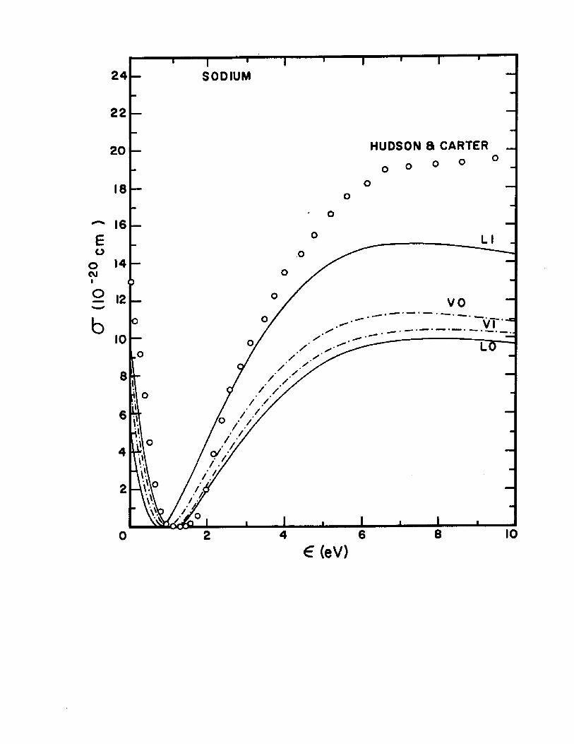
The most prominent aspect of the values of the first- order correction is that they exceed those of the zeroth- order near threshold. The first-order contributions from the

values. There is no p*>d contribution in the velocity case, and the cancellation between the s->-p and p+s is less satis-

11.18 Aand

J ( ( * ) ) W ^ • 11.18 B

LI comnensate those of the LI as is exDected. but thet' ^

values remain to overwhelm the zeroth-order

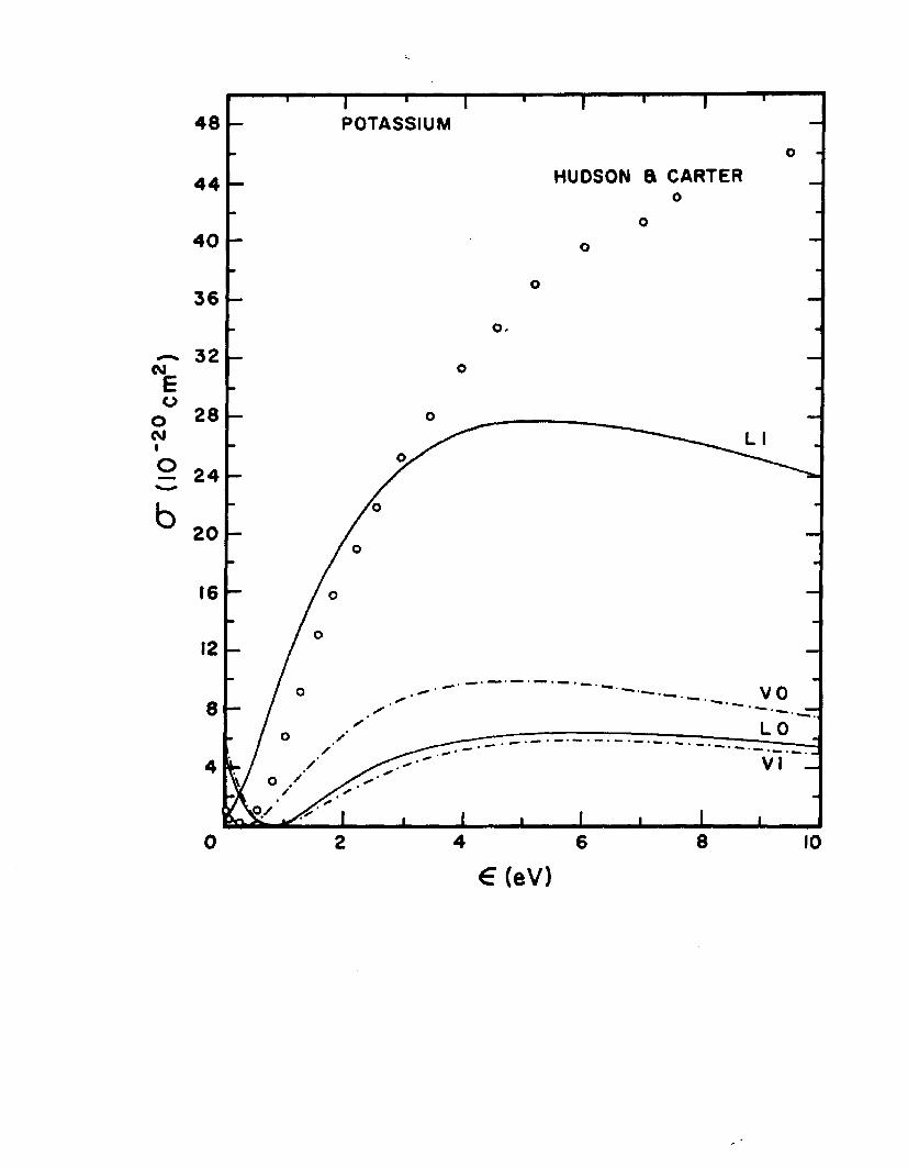
factory.The plot of the photoionization cross section of zero-

order and first-order are given in Fig. 3 for sodium and Fig. 4 for potassium. The agreement between the zero-order length and velocity curves are good except for the relative dis­placement of their minima. The disruptive effect of the first order correction destroys the approximate agreement of the length and velocity curves that existed in zero-order.

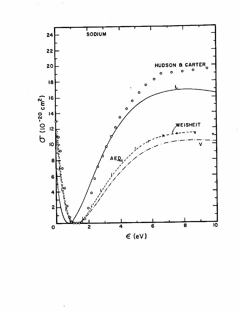
The dipole-length and dipole-velocity curves for the total photoionization cross section correct to second order are shown in Fig. 5 for sodium and Fig. 6 for potassium. Inthese figures are included for comparison the experimental

2 6points of Hudson and Carter and the recent calculations of 27Weisheit. Also shown in Figures 5 and 6 are the adiabatic-

exchange-dipole (AED) approximation results given by Eq.11.18 A. The AED results for sodium are in agreement with

2 gthose of Boyd who used the AED approach for her analysis. Only a slight improvement in the agreement of the length and velocity curves is seen for the potassium AED results. The vertical bars represent the deviations between the length and velocity calculations.

The good agreement of the AED results for sodium but not for potassium was considered to be due to the failure to sa­tisfy the orthogonality condition to as high a degree as was done for sodium. An additional calculation for potassium was performed and the orthogonality condition was best satisfied by choosing the same value (0.44413 9) in both the s-*p and p-*s

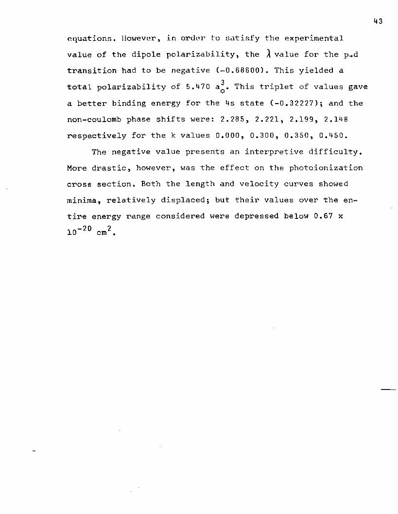
equations. However, in order l:o satisfy the experimentalvalue of the dipole polarizability, the \ value for the p+dtransition had to be negative (-0.68600). This yielded a

3total polarizability of 5.470 aQ. This triplet of values gave a better binding energy for the 4s state (-0.32227); and the non-coulomb phase shifts were: 2.285, 2.221, 2.199, 2.148 respectively for the k values 0.000, 0.300, 0.350, 0.450.

The negative value presents an interpretive difficulty. More drastic, however, was the effect on the photoionization cross section. Both the length and velocity curves showed minima, relatively displaced; but their values over the en­tire energy range considered were depressed below 0.67 x

TI-5. CONCLUSIONS

In their analysis of the lithium atom, Matese and LaBahn1 were successful in calculating photoionization cross sections to different orders, up to the second. Using the polarized orbital method they were able to improve on their initial and final state representation and obtained better agreement between the dipole-length and dipole-velocity curves and also with experiment.

The application of their analysis here to sodium and potassium failed because of the large value of the first- order corrections. The first-order correction is on the order of and larger than the zero-order value whereas for lithium it was lower by an order of magnitude. The non-cancellation of the p-*-d first-order contribution may indicate that this method is applicable only to atomic systems containing s-type electrons.

Their was no attempt made to fit the experimental curve by varying the adjustable parameter. This would be contrary to the nature of the procedure, i.e., to predict the shape of the curve. Weisheit using a different approach was able to reproduce a portion of the photoionization curve with an effective dipole operator containing a cut-off parameter, provided he had knowledge of the location of the minimum or the value at threshold.

The fortuitous agreement of the AED curves, with those of Weisheit does not justify the conclusion that the final and initial states are correctly represented in the AED

44

approximation.Sufficient agreement of specific results of this calcu­

lation with those of others confirms our faith in the absence ol any significant errors in the computer programs. With the failure of the cross sections to behave in the same manner as illustrated by lithium, we have to conclude that the proce­dure cannot be relied upon to predict the interaction of com­plex atoms with radiation.

46

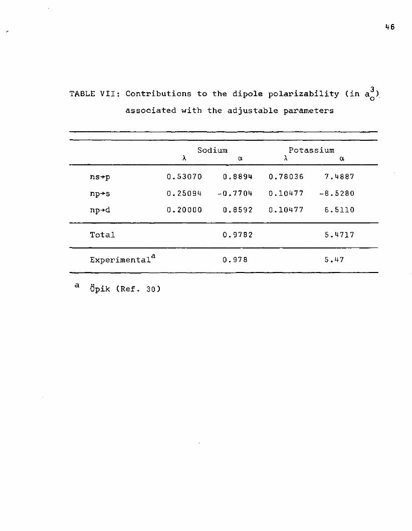
TABLE VII: Contributions to the dipole polarizability (in a^) associated with the adjustable parameters

Sodium A aPotassium

A ans-*-p 0.53070 0.8894 0.78036 7 .4887np+s 0.25094 -0.7704 0.10477 -8 . 5280np-*-d 0.20000 0.8592 0.10477 6.5110

Total 0.9782 5.4717

Experimental3 0 . 978 5.47

a Opik (Ref. 30)

47

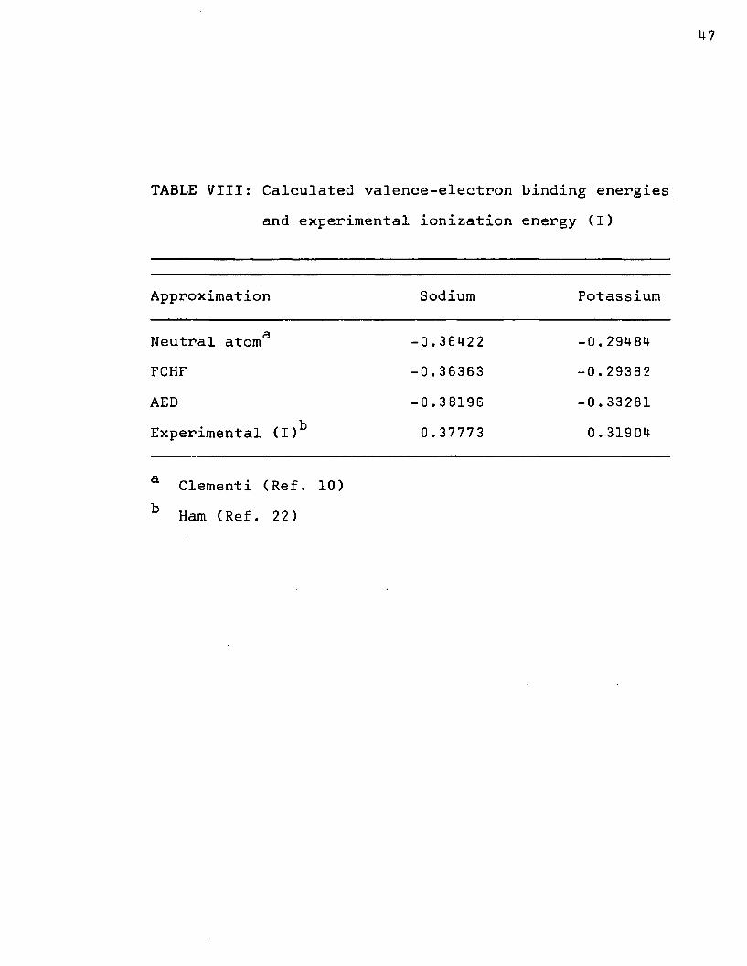
TABLE VIII: Calculated valence-electron binding energies and experimental ionization energy (I)

Approximation Sodium Potassium

Neutral atoma -0.36422 -0,29484FCHF -0.36363 -0.29382AED -0.38196 -0.33281Experimental (I)b 0.37773 0.31904

a Clementi (Ref. 10) b Ham (Ref. 22)

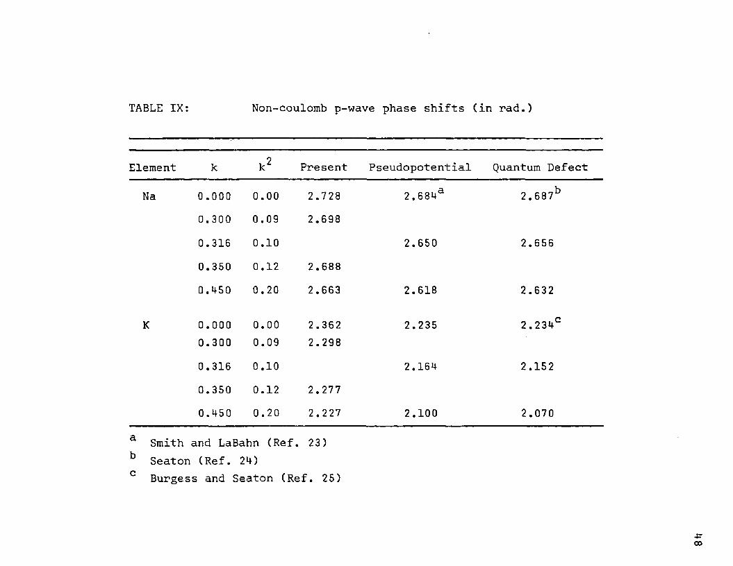
TABLE IX: Non-coulomb p-wave phase shifts (in rad.)

Element k k2 Present Pseudopotential Quantum Defect

Na 0.000 0.00 2.728 2.684a 2.687b0.300 0.09 2.6980.316 0.10 2.650 2.6560.350 0.12 2.688

0.450 0.20 2.663 2.618 2.632

K 0.000 0.00 2.362 2.235 2.234C0.300 0.09 2.2980.316 0.10 2.164 2.1520.350 0.12 2.2770.450 0.20 2.227 2.100 2.070

a Smith and LaBahn (Ref. 23) b Seaton (Ref. 24) c Burgess and Seaton (Ref. 25)

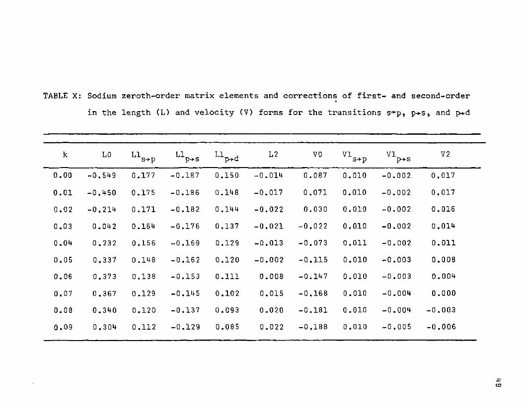
TABLE X: Sodium zeroth-order matrix elements and corrections of first- and second-orderin the length (L) and velocity (V) forms

•for the transitions s-*-p, p+s , and p-*-d

k L0 LIs-*p LIp-*s LI ,p-t-d L2 VO VIs+p VIp+s V2

0.00 -0.549 0.177 -0.187 0.150 -0.014 0.087 0.010 -0.002 0.0170.01 -0.450 0.175 -0.186 0.148 -0.017 0.071 0.010 -0.002 0.0170.02 -0.214 0.171 -0.182 0 .144 -0.022 0.030 0.010 -0.002 0.0160.03 0.042 0.164 -0.176 0.137 -0.021 -0.022 0.010 -0.002 0.0140.04 0 .232 0.156 -0.169 0.129 -0.013 -0.073 0.011 -0.002 0.011

0.05 0.337 0.148 -0.162 0.120 -0.002 -0.115 0.010 -0.003 0.0080.06 0.373 0.138 -0.153 0.111 0.008 -0.147 0.010 -0.003 0.0040.07 0.367 0 .129 -0.145 0.102 0.015 -0.168 0.010 -0.004 0.000

0.08 0.340 0.120 -0.137 0 .093 0.020 -0.181 0 .010 -0.004 -0.0030.09 0.304 0.112 -0.129 0.085 0.022 -0.188 0.010 -0.005 -0.006

•p<o

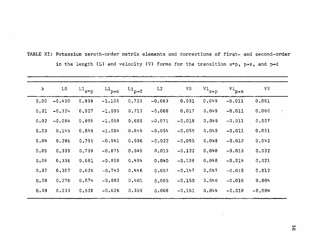
TABLE XI: Potassium zeroth-order matrix elements and corrections of first- and second-order in the length (L) and velocity (V) forms for the transition s-*-p, p-»-s, and p-*d

k LO LI ^ s-*p LIp-vS LlP.d L2 VO VIS-vp VIp-*-s V 2

0.00 -0.430 0.938 -1.106 0.723 -0.063 0.031 0 .049 -0.011 0.0610.01 -0.324 0.927 -1.093 0.713 -0.068 0.017 0.049 -0.011 0.0600.02 -0.084 0.895 -1.058 0.686 -0.071 -0.018 0.049 -0.011 0.0570.03 0.145 0.849 -1.004 0.645 -0.054 -0.059 0.049 -0.011 0.0510.04 0.286 0.795 -0.941 0.596 -0.022 -0.095 0.048 -0.012 0.0420.05 0.339 0.738 -0.875 0.545 0.013 -0.122 0.048 -0.013 0.0320.06 0.336 0.681 -0.808 0.494 0.040 -0.138 0.048 -0.014 0.0210.07 0.307 0.626 -0.743 0.446 0.057 -0.147 0.047 -0.015 0.012

0.08 0.270 0.574 -0.683 0.401 0.065 -0.150 0.046 -0.016 0.0040.09 0.233 0.526 -0.626 0.359 0.068 -0.151 0.044 -0.018 -0.004

C/1o

FIGURi: CAFTIONS

figure 3

Figure 4

Figure 5

Figure 6

: Photoionization cross sections for sodium. LO and VO are Hartree-Fock calculations in the length and velocity forms, respectively. LI and VI included first-order corrections as explained in the text.

: Photoionization cross sections for potassium. LO and VO are Hartree-Fock calculations in the length and velocity forms, respectively, LI and VI in­cluded first-order corrections as explained in the text.

: Photoionization cross sections for sodium. L and V indicate respectively the final length and velocity calculations of this work. The circles are the experimental data (Ref. 27) and dashed curve are recent calculations by Weisheit (Ref. 28).

: Photoionization cross sections for potassium. L and V indicate respectively the final length and velo­city calculations of this work. The circles are the experimental data (Ref. 27) and dashed curve are recent calculations by Weisheit (Ref. 28).

2 4 SODIUM

22

HUDSON a CARTER20

Eo0OJ1O

V O

b

€ (eV)

4 8 POTASSIUM

HUDSON 8 CARTER4 4

4 0

3 6

— 3 2CMEo

o 2 8CM

§ 24 ^ 2 0

VO

L O

p/80 42 106

€ (eV)

SODIUM24

22

HUDSON ft CARTER20

W£o0CJ1O ,W EISHEIT

-

bt rVo

A E D , / /

/•

€ (eV)

POTASSIUM4 8

4 4 HUDSON B CARTER

4 0

3 6

32

2 8CVJ

O 2 4

20

WEISHEIT

AED

0 2 6 84

€ (eV)

REFERENCES

1. J. J. Matese and R. W. LaBahn, Phys. Rev. 188, 17 (1969).2. R. W. LaBahn and J. Callaway, Phys. Rev. 135, A15 39

(1964) .3. R. W. LaBahn and J. Callaway, Phys. Rev. 147, 2 8 (1966).4. A. Temkin. Phys. Rev. 107, 1004 (1957).5. D. G. Thompson, Proc. Roy. Soc. A, 294, 160 (1966).6. The notation used in this section is that of Langhoff,

7Karplus, and Hurst with minor modifications. One modifi­cation corresponds to the use of the set of atomic units

owhere fi=l, and e =l/m=2 (energies in rydbergs).7. Langhoff, Karplus, and Hurst, J. Chem. Phys. 4_4, 505

(1966) .8. A. Dalgarno, Advan. Phys. 11, 281 (1962).9. R. M. Sternheimer, Phys. Rev. 9_6, 951 (19 54).

10. E. Clementi, IBM Journal 9_, 2 (1965).11. J. C. Slater. "Quantum Theory of Atomic Structure",

(McGraw-Hill, New York, 1960), Vol. II, p. 14.12 A. Burgess, Proc. Phys. Soc. 8JL, 442 (1962).13. S, Kaneko, J. Phys. Soc. Japan 14.» 1600 (1959).14. R. E. Montgomery and R. W. LaBahn, Can. J. Phys. 48,

1287 (1970).15. W. Kohn and L. J. Sham, Phys. Rev. 140, A1133 (1965).16 A. Salop and H. H. Nakano, Phys. Rev. A2^ 127 (1970).17. D. E. Golden and H. W. Bandel, Phys. Rev. 149, 58 (1966).18. H. A. Bethe and E. F. Salpeter, "Quantum Mechanics of

One- and Two-Electron Atoms" (Academic Press Inc., New

56

57York, 1957) pgs. 248 and 295.

19. S. Chandrasekhar, Astrophys. J. 102, 223 (1945).20. E. S. Chang and M. R. C. McDowell, Phys. Rev. 176, 126

(1968).21. L. C. Allen, Phys. Rev. 118 , 167 (1960).22. F. S. Ham, ''Solid State Physics", edited by F. Seitz and

D. Turnbull (Academic Press, New York, 19 55), Vol. 1,p. 127.

23. R. L. Smith and R. W. LaBahn, Phys. Rev. A2_, 2317 (1970).24. M. J. Seaton, Proc. Phys. Soc. (London) A70, 620 (1957).25. A. Burgess and M. J. Seaton, Mon. Not. Roy. Astr. Soc.

120, 121 (1960).26. M. Mizushima, "Quantum Mechanics of Atomic Spectra and

Atomic Structure" (W. A. Benjamin, New York, 1970) p.119.27. R. D. Hudson and V. L. Carter, J. Opt. Soc. Amer. 57,

651 and 1471 (1967).28. J. C. Weisheit, Phys. Rev. A5 , 1621 (1972).29. A. H. Boyd, Planet Space Sci. 729 (1964),30. U. Opik, Proc. Phys. Soc. (London) 9_2, 566 (1967).

VITA

Edward Andrew Garbaty, son of Anthony and Nellie Garbaty was born in Jersey City, New Jersey on November 30, 1930. He graduated from North Arlington High School in New Jersey in 1948. He studied physics at the Newark Colleges of Rutgers University, and received an A. B. degree in 1953. He then served two years with the U. S. Army Signal Corp. After Ser­vice he entered the Graduate School of Iowa State University and in 1959 received a M. S. degree in physics. In succession he held posts as instructor for two years at Loras College, Dubuque, Iowa; a year appointment at Tri-State College, Angola, Indiana; and after four years held the rank of associate pro­fessor at the State University of New York at Geneseo. Before taking the position at Geneseo, he married Caroline Becker of Dayton, Ohio; who while at Geneseo gave birth to a daughter, a son, and twin daughters. He brought them to Baton Rouge in the Fall of 1966, to earn a Ph. D. degree at Louisiana State University. He left LSU in August, 1971 without the degree to take a position at Saint Johnfs University, Collegeville, Minnesota. Caroline did not leave empty-handed, with two sons born to her while in Baton Rouge. Currently Edward A. Garbaty ia a candidate for the degree of Doctor of Philosophy in the Department of Physics and Astronomy at the 197 2 Fall Commen­cement .

58