MPM-DREDGEPIAP-GA-2012-324522

Applications of the two-phase MPM

Francesca Ceccato

DICEA – University of Padua

francesca.ceccato@dicea.unipd.it

MPM-DREDGE

PIAP-GA-2012-324522

Contents

Applications of the one-layer, two-phase formulation:

1. Collapse of a submerged slope

1. Motivations

2. Numerical model

3. Results

2. Simulation of cone penetration testing

1. Introduction

2. The soil-structure interaction (contact algorithm)

3. Numerical model

4. Results

2

MPM-DREDGE

PIAP-GA-2012-324522

Two-phase formulation: discretized equations

ext int

w w w M w Q w v F F momentum of fluid

pn

int T

p p p

p=1

p dV p Vw T

F B I B I

pn pp Tw wf p p pp

p=1

n γ n γdV m V

k k

TQ N N N N

pn

T p T

p p

p=1

dV mw w w M N N N N

ext int

s w M v M w F F momentum of mixture

mass balance

stress-strain equation

pn

int T

p ppp=1

p dV p V TF B σ I B σ I

pn

T p T

s s s p p

p=1

(1-n)ρ dV (1-n )mp M N N N N

n

p 1-n nKw

v w

σ D:ε σ ω ω σ Ι :ε σ

for nodes:

for material points:

T

1 1 1 0 0 0I

pn

T p T

p p

p=1

dV n mw w p wn M N N N N

3

MPM-DREDGE

PIAP-GA-2012-324522

Collapse of a submerged slope

4

MPM-DREDGE

PIAP-GA-2012-324522

• Erosion process.

• Natural and man-induced

slope liquefaction

De Jager (2008)

Concern for the stability of

the dams!

Schelda

barrier

Motivations

5

MPM-DREDGE

PIAP-GA-2012-324522

Laboratory test: initial configuration

6

MPM-DREDGE

PIAP-GA-2012-324522

Laboratory test: final configuration

7

MPM-DREDGE

PIAP-GA-2012-324522

2202 elements, 4545 nodes, 1567 active elements, 6252material points

Geometry and discretization

Numerical model

8

MPM-DREDGE

PIAP-GA-2012-324522

Mohr-Coulomb material model is used.

Local damping factor = 0,05

Parameter Symbol Value Unit of measure

Saturated unit weigth gsat 18.71 kN/m3

Water unit weigth gw 9.81 kN/m3

Submerged unit weigth g’ 8.90 kN/m3

Young’s modulus E 5000 kPa

Effective Poisson’s ratio n’ 0.2 -

Bulk modulus of water Kw 45310 kPa

Porosity n 0.45 -

Darcy’s permeability k 10-4 m/s

Cohesion c’ 0 kPa

Friction angle j 32 deg

Dilatancy angle y 0 deg

Numerical model

9

MPM-DREDGE

PIAP-GA-2012-324522

Numerical model

The computation steps are:

1. Generate initial stresses via gravity loading ($$APPLY_QUASI_STATIC/$$APPLY_IMPLICIT_QUASI_STATIC)

0kPa

12kPa

𝐹𝑒𝑥𝑡 − 𝐹𝑖𝑛𝑡𝐹𝑒𝑥𝑡

< 𝑡𝑜𝑙

𝐹𝑒𝑥𝑡 − 𝐹𝑖𝑛𝑡 = 0 static equilibrium

𝐾𝐸

𝑊𝑒𝑥𝑡< 𝑡𝑜𝑙and

Convergence

condition

10

MPM-DREDGE

PIAP-GA-2012-324522

Numerical model

2. Apply excess pore pressure: the pressure increases linearly in the time tloading and then goes to zero (=experiment)

pw

11

MPM-DREDGE

PIAP-GA-2012-324522

Results

Excess pore pressure at material points

12

MPM-DREDGE

PIAP-GA-2012-324522

Results

Vertical effective stress at material points

13

MPM-DREDGE

PIAP-GA-2012-324522

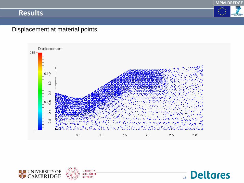
Results

Displacement at material points

14

MPM-DREDGE

PIAP-GA-2012-324522

Numerical vs experimental reults

Final configuration predicted by MPM and comparison with the experiment.

15

MPM-DREDGE

PIAP-GA-2012-324522

Cone penetration testing

16

MPM-DREDGE

PIAP-GA-2012-324522

Measurement of:

• tip resistance qc

• sleeve friction fs

• pore water pressure u

qcfsu

The Cone Penetration Test (CPT) is an in situ test, widely used to characterize the soil profile.The device has a conical tip that penetrates the soil with a velocity of 2cm/s.

Introduction

17

MPM-DREDGE

PIAP-GA-2012-324522

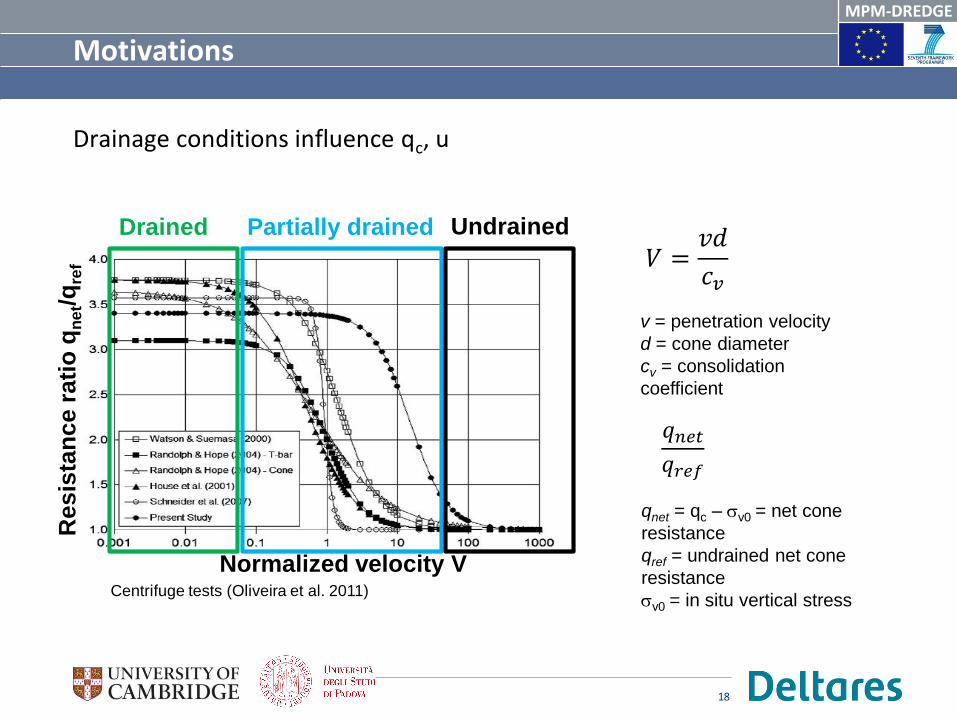
Motivations

Drainage conditions influence qc, u

Drained Partially drained Undrained

Centrifuge tests (Oliveira et al. 2011)

Normalized velocity V

Res

ista

nc

era

tio

qn

et/q

ref 𝑉 =

𝑣𝑑

𝑐𝑣

𝑞𝑛𝑒𝑡𝑞𝑟𝑒𝑓

v = penetration velocity

d = cone diameter

cv = consolidation

coefficient

qnet = qc – sv0 = net cone

resistance

qref = undrained net cone

resistance

sv0 = in situ vertical stress

18

MPM-DREDGE

PIAP-GA-2012-324522

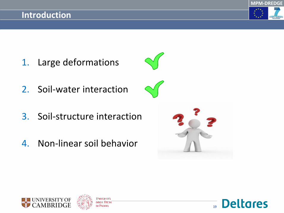
Introduction

1. Large deformations

2. Soil-water interaction

3. Soil-structure interaction

4. Non-linear soil behavior

19

MPM-DREDGE

PIAP-GA-2012-324522

Soil structure interaction

Consider a single phase material.

Lagrangian phase:

• Initialize momentum equation (nodes)

• Find nodal acceleration

• …

Convective phase:

• Map momentum to MPs

• Find incremental strains

• Find stresses

• Update MP position

• …

Contact algorithm

20

MPM-DREDGE

PIAP-GA-2012-324522

not contact node

predict velocities for

Contact algorithm

t+Δt

detect contact nodes for t+Δt

no correction

contact node

no correction

tangential component

normal component

separatingapproaching

no correction

Bardenhagen et al. (2000, 2001)

sliding no sliding

corr

ection to ensure no penetration

to satisfy the contact law

𝒗 = 𝒗 − [ 𝒗 − 𝒗𝒔𝒚𝒔 ∙ 𝒏] 𝒏 + 𝜇𝒕 − 𝛼𝒕

Correction for tangential component.

𝜇 = friction coefficient, 𝛼 = adhesion factor

body A

body B

node

𝒏 : unit normal vector

𝒕: unit tangential vector

21

MPM-DREDGE

PIAP-GA-2012-324522

Predict velocity

solution for body A only:

solution for body B only:

solution for coupled bodies:

body A

body B

node

𝑴𝑨𝒕 𝒗𝑨

𝒕 = 𝑭𝑨𝒕

𝒗𝑨𝒕+∆𝒕 = 𝒗𝑨

𝒕 + ∆𝒕 𝒗𝑨𝒕

𝑴𝑩𝒕 𝒗𝑩

𝒕 = 𝑭𝑩𝒕

𝒗𝑩𝒕+∆𝒕 = 𝒗𝑩

𝒕 + ∆𝒕 𝒗𝑩𝒕

𝑴𝑨𝒕 +𝑴𝑩

𝒕 𝒗𝒔𝒚𝒔𝒕 = 𝑭𝑨

𝒕 + 𝑭𝑩𝒕

𝒗𝒔𝒚𝒔𝒕+∆𝒕 = 𝒗𝒔𝒚𝒔

𝒕 + ∆𝒕 𝒗𝒔𝒚𝒔𝒕

22

MPM-DREDGE

PIAP-GA-2012-324522

node a

Detect contact nodes

a is not a contact node.

node b

b is a contact node

a

b

𝒗𝑨𝒕+∆𝒕 = 𝒗𝒔𝒚𝒔

𝒕+∆𝒕

𝒗𝑨𝒕+∆𝒕 ≠ 𝒗𝒔𝒚𝒔

𝒕+∆𝒕

23

MPM-DREDGE

PIAP-GA-2012-324522

node b

separating

approachingn

A

A

n

b

b

correction is required

Detect approaching/separating bodies

𝒗𝑨𝒕+∆𝒕 ≠ 𝒗𝒔𝒚𝒔

𝒕+∆𝒕

𝒗𝑨𝒕+∆𝒕 − 𝒗𝒔𝒚𝒔

𝒕+∆𝒕 ∙ 𝒏 < 𝟎

𝒗𝑨𝒕+∆𝒕 − 𝒗𝒔𝒚𝒔

𝒕+∆𝒕 ∙ 𝒏 > 𝟎

𝒗𝑨𝒕+∆𝒕 − 𝒗𝒔𝒚𝒔

𝒕+∆𝒕

𝒗𝑨𝒕+∆𝒕 − 𝒗𝒔𝒚𝒔

𝒕+∆𝒕

24

MPM-DREDGE

PIAP-GA-2012-324522

correction of the normal and

tangential components

Correction for

adhesion

Correction for

friction

Correct velocity

The expression for the corrected nodal velocity is derived imposing:

1. The normal component of body velocity has to be equal to the normal component of the system velocity to avoid interpenetration

2. The maximum tangential force has to respect the contact law.

𝒗 = 𝒗 − [ 𝒗 − 𝒗𝒔𝒚𝒔 ∙ 𝒏] 𝒏 + 𝜇𝒕 − 𝛼𝒕

n: unit vector normal to

the contact surface

t: unit vector tangent to

the surface

𝒗 = 𝒗𝒕+∆𝒕 − 𝒗𝒕

∆𝒕The corrected nodal acceleration is computed:

25

MPM-DREDGE

PIAP-GA-2012-324522

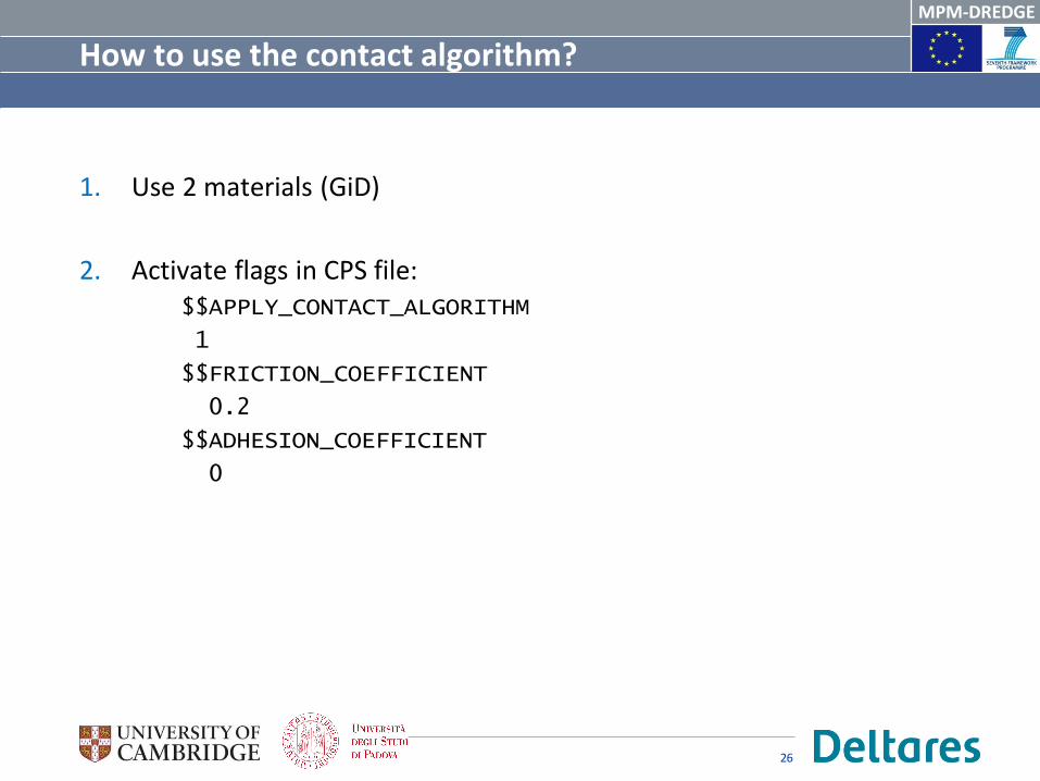
How to use the contact algorithm?

1. Use 2 materials (GiD)

2. Activate flags in CPS file:$$APPLY_CONTACT_ALGORITHM

1

$$FRICTION_COEFFICIENT

0.2

$$ADHESION_COEFFICIENT

0

26

MPM-DREDGE

PIAP-GA-2012-324522

Upper block is pushed by an increasing horizontal load

m=0.25

a=5kPa

W=40kN

A=2m2 Tmax = 40*0.25 + 2*5 = 20kN

T < 20kN

Very small displacements !

Bodies are stick!

Validation of contact algorithm

27

MPM-DREDGE

PIAP-GA-2012-324522

T > 20kNVery large displacements!

Bodies are sliding!

A B C D

A

D

Validation of contact algorithm

KE

28

MPM-DREDGE

PIAP-GA-2012-324522

Two-phase contact algorithm

not contact node

predict velocities for

detect contact nodes for t+Δt

no correction

contact node

no correction

Correction of the

normal component

separatingapproaching

no correction

sliding no sliding

𝒘 = 𝒘 − 𝒘− 𝒗𝒄𝒐𝒏𝒆 ∙ 𝒏 𝒏

Impermeable structure

t+Δt

29

MPM-DREDGE

PIAP-GA-2012-324522

Contact algorithm

𝒘 𝒘

𝒘 𝒘 = 𝒘𝒕+∆𝒕 − 𝒘𝒕

∆𝒕

𝑴𝒘 𝒘 + 𝑸 𝒘− 𝒗 = 𝑭𝒘𝒆𝒙𝒕 − 𝑭𝒘

𝒊𝒏𝒕

𝒗 𝒗

𝑴𝒔 𝒗 + 𝑴𝒘 𝒘 = 𝑭𝒆𝒙𝒕 − 𝑭𝒊𝒏𝒕

𝒗 𝒗 = 𝒗𝒕+∆𝒕 − 𝒗𝒕

∆𝒕

30

MPM-DREDGE

PIAP-GA-2012-324522

The Modified Cam Clay model is implemented in the MPM

MCC takes into account:

• stress-path dependency of the shear strength

• hardening behavior

• non linear soil compressibility

• shear and volumetric plastic deformations during yielding

Five parameters: l, k, n, M, e0

The initial stress state must be specified, together with pc or OCR.

l 0.205

k 0.044

M 0.92

e0 1.41

n' 0.25

Kaolin (Silva et al. 2006)

The constitutive model

31

MPM-DREDGE

PIAP-GA-2012-324522

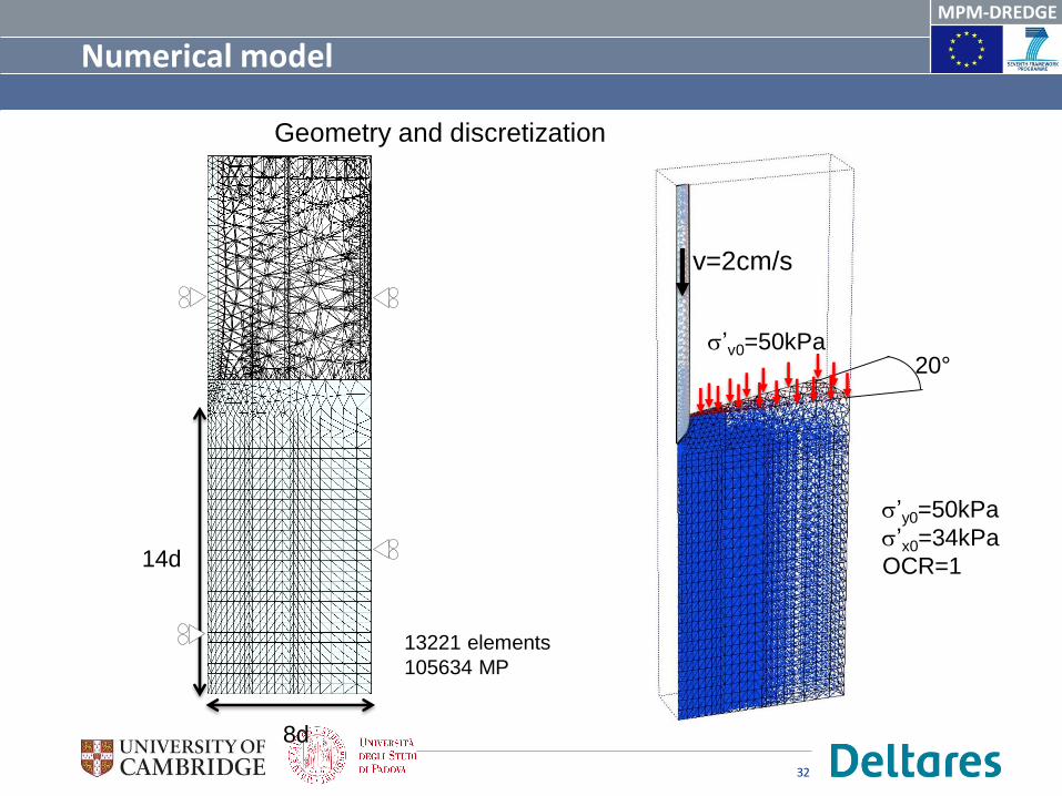
8d

14d

13221 elements

105634 MP

Geometry and discretization

20°s’v0=50kPa

s’y0=50kPa

s’x0=34kPa

OCR=1

Numerical model

v=2cm/s

32

MPM-DREDGE

PIAP-GA-2012-324522

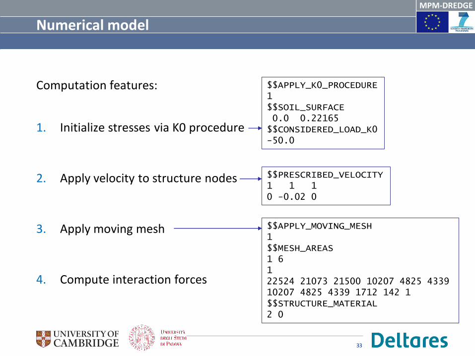
Numerical model

Computation features:

1. Initialize stresses via K0 procedure

2. Apply velocity to structure nodes

3. Apply moving mesh

4. Compute interaction forces

$$APPLY_K0_PROCEDURE1$$SOIL_SURFACE0.0 0.22165 $$CONSIDERED_LOAD_K0-50.0

$$PRESCRIBED_VELOCITY1 1 10 -0.02 0

$$APPLY_MOVING_MESH1$$MESH_AREAS1 6122524 21073 21500 10207 4825 433910207 4825 4339 1712 142 1$$STRUCTURE_MATERIAL2 0

33

MPM-DREDGE

PIAP-GA-2012-324522

• The moving mesh zone is attached to the cone and moves down with the same velocity.

• A fine mesh is kept around the cone and the contact is solved accurately.

The moving mesh approach (Beuth 2012) is adopted

Moving mesh approach

34

MPM-DREDGE

PIAP-GA-2012-324522

𝑞𝑐 = 𝐹𝑖,𝑦

𝐴=Sum vertical reaction forces at the cone face

Cone area

𝐹𝑖,𝑦𝑖

The tip resistance is calculated as:

A

Compute interaction forces

35

MPM-DREDGE

PIAP-GA-2012-324522

MCC: Nc=9.6

Tresca (su =12kPa,

G=1300, Ir=108):

Nc=9.5

Reference: Nc=9.55

(Lu et al. 2004)

Smooth contact

qc

𝑁𝑐 =𝑞𝑐−𝜎𝑣0

𝑠𝑢

Cone factor:Penetration in undrained conditions pexcess [kPa]

Results

36

MPM-DREDGE

PIAP-GA-2012-324522

The variation of V is obtained by changing the permeability k of the soil.

The penetration velocity is constant v = 2 cm/s

Smooth contact

𝑉 =𝑣𝑑

𝑐𝑣

𝑐𝑣 =𝑘(1 + 𝑒0)𝜎′𝑣0

𝜆𝛾𝑤V=12 (k=10-6m/s)

V=1.2 (k=10-5m/s)

undrained

drained

k V

The tip stress increases with the

consolidation coefficient

because the soil ahead of the

advancing cone consolidates

developing larger shear strength

and stiffness.

Results: tip stress

37

MPM-DREDGE

PIAP-GA-2012-324522

Results: deviatoric stress

38

MPM-DREDGE

PIAP-GA-2012-324522

Partially drained (V=1.2) Partially drained (V=12) Undrained

Excess pore pressure around the cone for different drainage conditions.

The pore pressure decreases with the normalized velocity.

Results: excess pore pressure

39

MPM-DREDGE

PIAP-GA-2012-324522

Effect of normalized penetration velocity V on the resistance ratio and

normalized pore pressure.

∆𝑢𝑟𝑒𝑓 = excess pore pressure in undrained conditions

Resis

tan

ce

ratio

No

rma

lize

dp

ore

pre

ssu

re

Results: normalized velocity

40

MPM-DREDGE

PIAP-GA-2012-324522

• Linear increase of qc in

drained and nearly-

drained conditions.

• Non-linear increase of qc

in undrained and nearly-

undrained conditions.

Effect of friction coefficient on the tip resistance

Results: friction coefficient

41

MPM-DREDGE

PIAP-GA-2012-324522

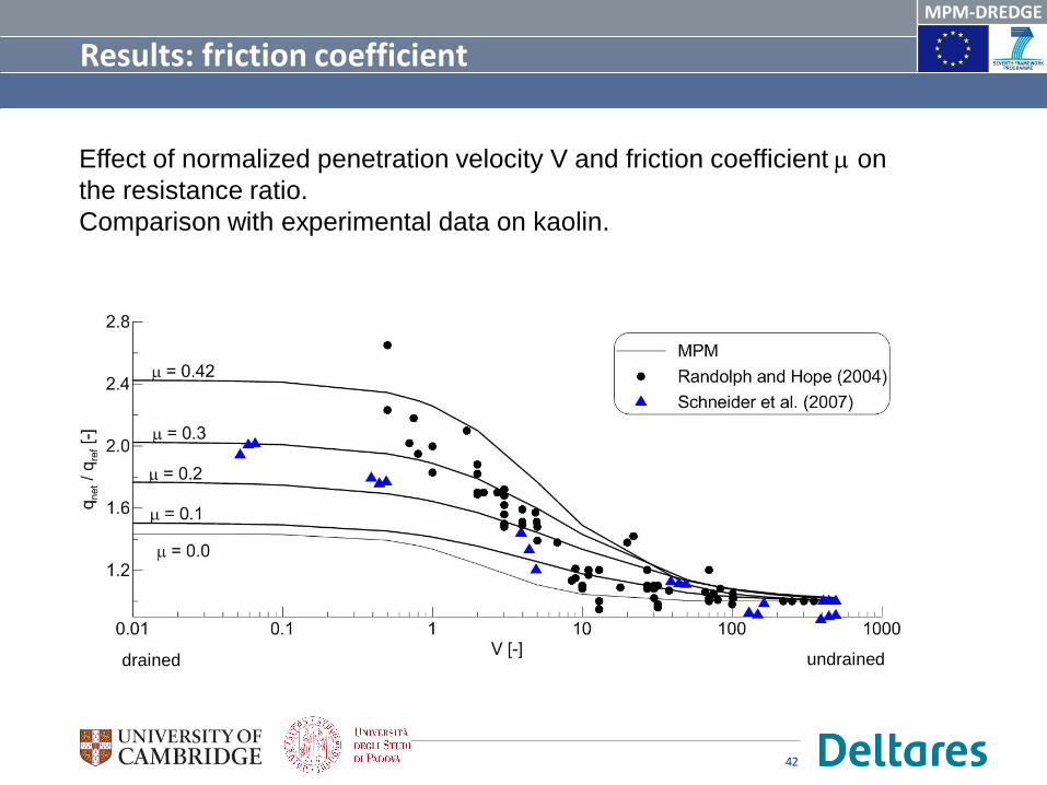
Effect of normalized penetration velocity V and friction coefficient m on

the resistance ratio.

Comparison with experimental data on kaolin.

undraineddrained

Results: friction coefficient

42

MPM-DREDGE

PIAP-GA-2012-324522

Conclusions

• Many geotechnical problems involve soil-structure and soil-water

interaction.

• Two examples have been shown (slope collapse, CPT), for which good

agreement between numerical and experimental results is obtained.

• The soil-structure interaction is simulated with the algorithm proposed

by Bardenhagen et al. (2001), which is extended for two-phase problems

• Stresses (gravity load) can be initialized running a quasi static load step

(implicit/explicit) or via K0 procedure

• Features like prescribed velocity and moving mesh are available

43

MPM-DREDGE

PIAP-GA-2012-324522

References

Ceccato F., Beuth L, Vermeer P.A., Simonini P. (2016). Two-phase material point method applied to the study of cone penetration. Computers and Geotechnics (published online). DOI: 10.1016/j.compgeo.2016.03.003

Ceccato F., Simonini P. (2016). Numerical study of partially drained penetration and pore pressure dissipation in piezocone test. ActaGeotechnica DOI:10.1007/s11440-016-0448-6

Ceccato, F. (2015). Study of large deformation geomechanical problems with the material point method. Ph.D thesis University of Padua. Available at: http://paduaresearch.cab.unipd.it/7478/

Ceccato F., Beuth L., Simonini P. (2015). Study of the effect of drainage conditions on cone penetration with the Material Point Method. In: Proceedings XV Pan-American Conference on Soil Mechanics and Geotechnical Engineering. Buenos Aires, Argentina.

44