Applied and Numerical Harmonic Analysis

Series Editor

John J. BenedettoUniversity of Maryland

Editorial Advisory Board

Akram Aldroubi Douglas CochranVanderbilt University Arizona State University

Ingrid Daubechies Hans G. FeichtingerPrinceton University University of Vienna

Christopher Heil Murat KuntGeorgia Institute of Technology Swiss Federal Institute of Technology, Lausanne

James McClellan Wim SweldensGeorgia Institute of Technology Lucent Technologies, Bell Laboratories

Michael Unser Martin VetterliSwiss Federal Institute Swiss Federal Instituteof Technology, Lausanne of Technology, Lausanne

M. Victor WickerhauserWashington University

Advances inMathematical Finance

Michael C. FuRobert A. Jarrow

Ju-Yi J. YenRobert J. Elliott

Editors

BirkhauserBoston • Basel • Berlin

Michael C. FuRobert H. Smith School of BusinessVan Munching HallUniversity of MarylandCollege Park, MD 20742USA

Robert A. JarrowJohnson Graduate School of Management451 Sage HallCornell UniversityIthaca, NY 14853USA

Ju-Yi J. YenDepartment of Mathematics1326 Stevenson CenterVanderbilt UniversityNashville, TN 37240USA

Robert J. ElliottHaskayne School of BusinessScurfield HallUniversity of CalgaryCalgary, AB T2N 1N4Canada

Cover design by Joseph Sherman.

Mathematics Subject Classification (2000): 91B28

Library of Congress Control Number: 2007924837

ISBN-13: 978-0-8176-4544-1 e-ISBN-13: 978-0-8176-4545-8

Printed on acid-free paper.

c©2007 Birkhauser BostonAll rights reserved. This work may not be translated or copied in whole or in part without the writtenpermission of the publisher (Birkhauser Boston, c/o Springer Science+Business Media LLC, 233Spring Street, New York, NY 10013, USA) and the author, except for brief excerpts in connection withreviews or scholarly analysis. Use in connection with any form of information storage and retrieval,electronic adaptation, computer software, or by similar or dissimilar methodology now known orhereafter developed is forbidden.The use in this publication of trade names, trademarks, service marks and similar terms, even if theyare not identified as such, is not to be taken as an expression of opinion as to whether or not they aresubject to proprietary rights.

9 8 7 6 5 4 3 2 1

www.birkhauser.com (KeS/EB)

In honor of Dilip B. Madan on the occasion of his 60th birthday

ANHA Series Preface

The Applied and Numerical Harmonic Analysis (ANHA) book series aims toprovide the engineering, mathematical, and scientific communities with sig-nificant developments in harmonic analysis, ranging from abstract harmonicanalysis to basic applications. The title of the series reflects the importanceof applications and numerical implementation, but richness and relevance ofapplications and implementation depend fundamentally on the structure anddepth of theoretical underpinnings. Thus, from our point of view, the inter-leaving of theory and applications and their creative symbiotic evolution isaxiomatic.

Harmonic analysis is a wellspring of ideas and applicability that has flour-ished, developed, and deepened over time within many disciplines and bymeans of creative cross-fertilization with diverse areas. The intricate and fun-damental relationship between harmonic analysis and fields such as signalprocessing, partial differential equations (PDEs), and image processing is re-flected in our state-of-the-art ANHA series.

Our vision of modern harmonic analysis includes mathematical areas suchas wavelet theory, Banach algebras, classical Fourier analysis, time-frequencyanalysis, and fractal geometry, as well as the diverse topics that impinge onthem.

For example, wavelet theory can be considered an appropriate tool todeal with some basic problems in digital signal processing, speech and imageprocessing, geophysics, pattern recognition, biomedical engineering, and tur-bulence. These areas implement the latest technology from sampling methodson surfaces to fast algorithms and computer vision methods. The underlyingmathematics of wavelet theory depends not only on classical Fourier analysis,but also on ideas from abstract harmonic analysis, including von Neumannalgebras and the affine group. This leads to a study of the Heisenberg groupand its relationship to Gabor systems, and of the metaplectic group for ameaningful interaction of signal decomposition methods. The unifying influ-ence of wavelet theory in the aforementioned topics illustrates the justification

viii ANHA Series Preface

for providing a means for centralizing and disseminating information from thebroader, but still focused, area of harmonic analysis. This will be a key roleof ANHA. We intend to publish with the scope and interaction that such ahost of issues demands.

Along with our commitment to publish mathematically significant works atthe frontiers of harmonic analysis, we have a comparably strong commitmentto publish major advances in the following applicable topics in which harmonicanalysis plays a substantial role:

Antenna theory Prediction theoryBiomedical signal processing Radar applicationsDigital signal processing Sampling theory

Fast algorithms Spectral estimationGabor theory and applications Speech processing

Image processing Time-frequency andNumerical partial differential equations time-scale analysis

Wavelet theory

The above point of view for the ANHA book series is inspired by thehistory of Fourier analysis itself, whose tentacles reach into so many fields.

In the last two centuries Fourier analysis has had a major impact on thedevelopment of mathematics, on the understanding of many engineering andscientific phenomena, and on the solution of some of the most important prob-lems in mathematics and the sciences. Historically, Fourier series were devel-oped in the analysis of some of the classical PDEs of mathematical physics;these series were used to solve such equations. In order to understand Fourierseries and the kinds of solutions they could represent, some of the most basicnotions of analysis were defined, e.g., the concept of “function.” Since thecoefficients of Fourier series are integrals, it is no surprise that Riemann inte-grals were conceived to deal with uniqueness properties of trigonometric series.Cantor’s set theory was also developed because of such uniqueness questions.

A basic problem in Fourier analysis is to show how complicated phenom-ena, such as sound waves, can be described in terms of elementary harmonics.There are two aspects of this problem: first, to find, or even define properly,the harmonics or spectrum of a given phenomenon, e.g., the spectroscopyproblem in optics; second, to determine which phenomena can be constructedfrom given classes of harmonics, as done, for example, by the mechanical syn-thesizers in tidal analysis.

Fourier analysis is also the natural setting for many other problems inengineering, mathematics, and the sciences. For example, Wiener’s Tauberiantheorem in Fourier analysis not only characterizes the behavior of the primenumbers, but also provides the proper notion of spectrum for phenomena suchas white light; this latter process leads to the Fourier analysis associated withcorrelation functions in filtering and prediction problems, and these problems,in turn, deal naturally with Hardy spaces in the theory of complex variables.

ANHA Series Preface ix

Nowadays, some of the theory of PDEs has given way to the study ofFourier integral operators. Problems in antenna theory are studied in termsof unimodular trigonometric polynomials. Applications of Fourier analysisabound in signal processing, whether with the fast Fourier transform (FFT),or filter design, or the adaptive modeling inherent in time-frequency-scalemethods such as wavelet theory. The coherent states of mathematical physicsare translated and modulated Fourier transforms, and these are used, in con-junction with the uncertainty principle, for dealing with signal reconstructionin communications theory. We are back to the raison d’etre of the ANHAseries!

John J. BenedettoSeries Editor

University of MarylandCollege Park

Preface

The “Mathematical Finance Conference in Honor of the 60th Birthday ofDilip B. Madan” was held at the Norbert Wiener Center of the Universityof Maryland, College Park, from September 29 – October 1, 2006, and thisvolume is a Festschrift in honor of Dilip that includes articles from most of theconference’s speakers. Among his former students contributing to this volumeare Ju-Yi Yen as one of the co-editors, along with Ali Hirsa and Xing Jin asco-authors of three of the articles.

Dilip Balkrishna Madan was born on December 12, 1946, in Washington,DC, but was raised in Bombay, India, and received his bachelor’s degree inCommerce at the University of Bombay. He received two Ph.D.s at the Uni-versity of Maryland, one in economics and the other in pure mathematics.What is all the more amazing is that prior to entering graduate school he hadnever had a formal university-level mathematics course! The first section ofthe book summarizes Dilip’s career highlights, including distinguished awardsand editorial appointments, followed by his list of publications.

The technical contributions in the book are divided into three parts. Thefirst part deals with stochastic processes used in mathematical finance, pri-marily the Levy processes most associated with Dilip, who has been a ferventadvocate of this class of processes for addressing the well-known flaws of geo-metric Brownian motion for asset price modeling. The primary focus is on theVariance-Gamma (VG) process that Dilip and Eugene Seneta introduced tothe finance community, and the lead article provides an historical review fromthe unique vantage point of Dilip’s co-author, starting from the initiation ofthe collaboration at the University of Sydney. Techniques for simulating theVariance-Gamma process are surveyed in the article by Michael Fu, Dilip’slongtime colleague at Maryland, moving from a review of basic Monte Carlosimulation for the VG process to more advanced topics in variation reductionand efficient estimation of the “Greeks” such as the option delta. The nexttwo pieces by Marc Yor, a longtime close collaborator and the keynote speakerat the birthday conference, provide some mathematical properties and iden-tities for gamma processes and beta and gamma random variables. The finalarticle in the first part of the volume, written by frequent collaborator RobertElliott and his co-author John van der Hoek, reviews the theory of fractionalBrownian motion in the white noise framework and provides a new approachfor deriving the associated Ito-type stochastic calculus formulas.

xii Preface

The second part of the volume treats various aspects of mathematical fi-nance related to asset pricing and the valuation and hedging of derivatives.The article by Bob Jarrow, a longtime collaborator and colleague of Dilip inthe mathematical finance community, provides a tutorial on zero volatilityspreads and option adjusted spreads for fixed income securities – specificallybonds with embedded options – using the framework of the Heath-Jarrow-Morton model for the term structure of interest rates, and highlights thecharacteristics of zero volatility spreads capturing both embedded options andmispricings due to model or market errors, whereas option adjusted spreadsmeasure only the mispricings. The phenomenon of market bubbles is addressedin the piece by Bob Jarrow, Phillip Protter, and Kazuhiro Shimbo, who pro-vide new results on characterizing asset price bubbles in terms of their martin-gale properties under the standard no-arbitrage complete market framework.General equilibrium asset pricing models in incomplete markets that resultfrom taxation and transaction costs are treated in the article by Xing Jin –who received his Ph.D. from Maryland’s Business School co-supervised byDilip – and Frank Milne – one of Dilip’s early collaborators on the VG model.Recent work on applying Levy processes to interest rate modeling, with afocus on real-world calibration issues, is reviewed in the article by WolfgangKluge and Ernst Eberlein, who nominated Dilip for the prestigious HumboldtResearch Award in Mathematics. The next two articles, both co-authored byAli Hirsa, who received his Ph.D. from the math department at Maryland co-supervised by Dilip, focus on derivatives pricing; the sole article in the volumeon which Dilip is a co-author, with Massoud Heidari as the other co-author,prices swaptions using the fast Fourier transform under an affine term struc-ture of interest rates incorporating stochastic volatility, whereas the articleco-authored by Peter Carr – another of Dilip’s most frequent collaborators –derives forward partial integro-differential equations for pricing knock-out calloptions when the underlying asset price follows a jump-diffusion model. Thefinal article in the second part of the volume is by Helyette Geman, Dilip’slongtime collaborator from France who was responsible for introducing himto Marc Yor, and she treats energy commodity price modeling using real his-torical data, testing the hypothesis of mean reversion for oil and natural gasprices.

The third part of the volume includes several contributions in one of themost rapidly growing fields in mathematical finance and financial engineering:credit risk. A new class of reduced-form credit risk models that associatesdefault events directly with market information processes driving cash flows isintroduced in the piece by Dorje Brody, Lane Hughston, and Andrea Macrina.A generic one-factor Levy model for pricing collateralized debt obligationsthat unifies a number of recently proposed one-factor models is presented inthe article by Hansjorg Albrecher, Sophie Ladoucette, and Wim Schoutens.An intensity-based default model that prices credit derivatives using utilityfunctions rather than arbitrage-free measures is proposed in the article byRonnie Sircar and Thaleia Zariphopoulou. Also using the utility-based pricing

Preface xiii

approach is the final article in the volume by Marek Musiela and ThaleiaZariphopoulou, and they address the integrated portfolio management optimalinvestment problem in incomplete markets stemming from stochastic factorsin the underlying risky securities.

Besides being a distinguished researcher, Dilip is a dear friend, an esteemedcolleague, and a caring mentor and teacher. During his professional career,Dilip was one of the early pioneers in mathematical finance, so it is onlyfitting that the title of this Festschrift documents his past and continuing lovefor the field that he helped develop.

Michael FuBob JarrowJu-Yi Yen

Robert ElliottDecember 2006

xiv Preface

Conference poster (designed by Jonathan Sears).

Preface xv

Photo Highlights (September 29, 2006)

Dilip delivering his lecture.

Dilip with many of his Ph.D. students.

xvi Preface

Norbert Wiener Center director John Benedetto and Robert Elliott.

Left to right: CGMY (Carr, Geman, Madan, Yor).

Preface xvii

VG inventors (Dilip and Eugene Seneta) with the Madan family.

Dilip’s wife Vimla cutting the birthday cake.

Career Highlights and List of Publications

Dilip B. Madan

Robert H. Smith School of BusinessDepartment of FinanceUniversity of MarylandCollege Park, MD 20742, USAdmadan@rhsmith.umd.edu

Career Highlights

1971 Ph.D. Economics, University of Maryland1975 Ph.D. Mathematics, University of Maryland

2006 recipient of Humboldt Research Award in MathematicsPresident of Bachelier Finance Society 2002–2003Managing Editor of Mathematic Finance, Review of Derivatives ResearchSeries Editor on Financial Mathematics for CRC, Chapman and HallAssociate Editor for Quantitative Finance, Journal of Credit Risk

1971–1975: Assistant Professor of Economics, University of Maryland1976–1979: Lecturer in Economic Statistics, University of Sydney1980–1988: Senior Lecturer in Econometrics, University of Sydney1981–1982: Acting Head, Department of Econometrics, Sydney1989–1992: Assistant Professor of Finance, University of Maryland1992–1997: Associate Professor of Finance, University of Maryland1997–present: Professor of Finance, University of Maryland

Visiting Positions:La Trobe University, Cambridge University (Isaac Newton Institute),Cornell University, University Paris,VI, University of Paris IX at Dauphine

Consulting:Morgan Stanley, Bloomberg, Wachovia Securities, Caspian Capital, FDIC

xx Dilip B. Madan

Publications (as of December 2006 (60th birthday))

1. The relevance of a probabilistic form of invertibility. Biometrika, 67(3):704–5, 1980 (with G. Babich).

2. Monotone and 1-1 sets. Journal of the Australian Mathematical Society,Series A, 33:62–75, 1982 (with R.W. Robinson).

3. Resurrecting the discounted cash equivalent flow. Abacus, 18-1:83–90,1982.

4. Differentiating a determinant. The American Statistician, 36(3):178–179,1982.

5. Measures of risk aversion with many commodities. Economics Letters,11:93–100, 1983.

6. Inconsistent theories as scientific objectives. Journal of the Philosophy ofScience, 50(3):453–470, 1983.

7. Testing for random pairing. Journal of the American Statistical Associa-tion, 78(382):332–336, 1983 (with Piet de Jong and Malcolm Greig).

8. Compound Poisson models for economic variable movements. SankhyaSeries B, 46(2):174–187, 1984 (with E. Seneta).

9. The measurement of capital utilization rates. Communications in Statis-tics: Theory and Methods, A14(6):1301–1314, 1985.

10. Project evaluations and accounting income forecasts. Abacus, 21(2):197–202, 1985.

11. Utility correlations in probabilistic choice modeling. Economics Letters,20:241–245, 1986.

12. Mode choice for urban travelers in Sydney. Proceedings of the 13th ARRBand 5th REAAA Conference, 13(8):52–62, 1986 (with R. Groenhout andM. Ranjbar).

13. Simulation of estimates using the empirical characteristic function. Inter-national Statistical Review, 55(2):153–161, 1987 (with E. Seneta).

14. Chebyshev polynomial approximations for characteristic function estima-tion. Journal of the Royal Statistical Society, Series B, 49(2):163–169,1987 (with E. Seneta).

15. Modeling Sydney work trip travel mode choices. Journal of TransportationEconomics and Policy, XXI(2):135–150, 1987 (with R. Groenhout).

16. Optimal duration and speed in the long run. Review of Economic Studies,54a(4a):695–700, 1987.

17. Decision theory with complex uncertainties. Synthese, 75:25–44, 1988(with J.C. Owings).

18. Risk measurement in semimartingale models with multiple consumptiongoods. Journal of Economic Theory, 44(2):398–412, 1988.

19. Stochastic stability in a rational expectations model of a small open econ-omy. Economica, 56(221):97–108, 1989 (with E. Kiernan).

20. Dynamic factor demands with some immediately productive quasi fixedfactors. Journal of Econometrics, 42:275–283, 1989 (with I. Prucha).

Career Highlights and List of Publications xxi

21. Characteristic function estimation using maximum likelihood on trans-formed variables. Journal of the Royal Statistical Society, Series B,51(2):281–285, 1989 (with E. Seneta).

22. The multinomial option pricing model and its Brownian and Poisson lim-its. Review of Financial Studies, 2(2):251–265, 1989 (with F. Milne andH. Shefrin).

23. On the monotonicity of the labour-capital ratio in Sraffa’s model. Journalof Economics, 51(1):101–107, 1989 (with E. Seneta).

24. The Variance-Gamma (V.G.) model for share market returns. Journal ofBusiness, 63(4):511–52,1990 (with E. Seneta).

25. Design and marketing of financial products. Review of Financial Studies,4(2):361–384, 1991 (with B. Soubra).

26. A characterization of complete security markets on a Brownian filtration.Mathematical Finance, 1(3):31–43, 1991 (with R.A. Jarrow).

27. Option pricing with VG Martingale components. Mathematical Finance,1(4):39–56, 1991 (with F. Milne).

28. Informational content in interest rate term structures. Review of Eco-nomics and Statistics, 75(4):695–699, 1993 (with R.O. Edmister).

29. Diffusion coefficient estimation and asset pricing when risk premia andsensitivities are time varying. Mathematical Finance, 3(2):85–99, 1993(with M. Chesney, R.J. Elliott, and H. Yang).

30. Contingent claims valued and hedged by pricing and investing in a basis.Mathematical Finance, 4(3):223–245, 1994 (with F. Milne).

31. Option pricing using the term structure of interest rates to hedge system-atic discontinuities in asset returns. Mathematical Finance, 5(4):311–336,1995 (with R.A. Jarrow).

32. Approaches to the solution of stochastic intertemporal consumption mod-els. Australian Economic Papers, 34:86–103, 1995 (with R.J. Cooper andK. McLaren).

33. Pricing via multiplicative price decomposition. Journal of Financial Engi-neering, 4:247–262, 1995 (with R.J. Elliott, W. Hunter, and P. EkkehardKopp).

34. Filtering derivative security valuations from market prices. Mathematics ofDerivative Securities, eds. M.A.H. Dempster and S.R. Pliska, CambridgeUniversity Press, 1997 (with R.J. Elliott and C. Lahaie)

35. Is mean-variance theory vacuous: Or was beta stillborn. European FinanceReview, 1:15–30, 1997 (with R.A. Jarrow).

36. Default risk. Statistics in Finance, eds. D. Hand and S.D. Jacka, ArnoldApplications in Statistics, 239–260, 1998.

37. Pricing the risks of default. Review of Derivatives Research, 2:121–160,1998 (with H. Unal).

38. The discrete time equivalent martingale measure. Mathematical Finance,8(2):127–152, 1998 (with R.J. Elliott).

39. The variance gamma process and option pricing. European Finance Re-view, 2:79–105, 1998 (with P. Carr and E. Chang).

xxii Dilip B. Madan

40. Towards a theory of volatility trading. Volatility, ed. R.A. Jarrow, RiskBooks, 417–427, 1998 (with P. Carr).

41. Valuing and hedging contingent claims on semimartingales. Finance andStochastics, 3:111–134, 1999 (with R.A. Jarrow).

42. The second fundamental theorem of asset pricing theory. MathematicalFinance, 9(3):255–273, 1999 (with R.A. Jarrow and X. Jin).

43. Pricing continuous time Asian options: A comparison of Monte Carlo andLaplace transform inversion methods. Journal of Computational Finance,2:49–74, 1999 (with M.C. Fu and T. Wang).

44. Introducing the covariance swap. Risk, 47–51, February 1999 (with P.Carr).

45. Option valuation using the fast Fourier transform. Journal of Computa-tional Finance, 2:61–73, 1999.

46. Spanning and derivative security valuation. Journal of Financial Eco-nomics, 55:205–238, 2000 (with G. Bakshi).

47. A two factor hazard rate model for pricing risky debt and the term struc-ture of credit spreads. Journal of Financial and Quantitative Analysis,35:43–65, 2000 (with H. Unal).

48. Arbitrage, martingales and private monetary value. Journal of Risk,3(1):73–90, 2000 (with R.A. Jarrow).

49. Investing in skews. Journal of Risk Finance, 2(1):10–18, 2000 (with G.McPhail).

50. Going with the flow. Risk, 85–89, August 2000 (with P. Carr and A.Lipton).

51. Optimal investment in derivative securities. Finance and Stochastics,5(1):33–59, 2001 (with P. Carr and X. Jin).

52. Time changes for Levy processes. Mathematical Finance, 11(1):79–96,2001 (with H. Geman and M. Yor).

53. Optimal positioning in derivatives. Quantitative Finance, 1(1):19–37, 2001(with P. Carr).

54. Pricing and hedging in incomplete markets. Journal of Financial Eco-nomics, 62:131–167, 2001 (with P. Carr and H. Geman).

55. Pricing the risks of default. Mastering Risk Volume 2: Applications, ed.C. Alexander, Financial Times Press, Chapter 9, 2001.

56. Purely discontinuous asset price processes. Handbooks in MathematicalFinance: Option Pricing, Interest Rates and Risk Management, eds. J.Cvitanic, E. Jouini, and M. Musiela, Cambridge University Press, 105–153, 2001.

57. Asset prices are Brownian motion: Only in business time. QuantitativeAnalysis of Financial Markets, vol. 2, ed. M. Avellanada, World ScientificPress, 103–146, 2001 (with H. Geman and M. Yor).

58. Determining volatility surfaces and option values from an implied volatil-ity smile. Quantitative Analysis of Financial Markets, vol. 2. ed. M. Avel-lanada, World Scientific Press, 163–191, 2001 (with P. Carr).

Career Highlights and List of Publications xxiii

59. Towards a theory of volatility trading. Handbooks in Mathematical Fi-nance: Option Pricing, Interest Rates and Risk Management, eds. J. Cvi-tanic, E. Jouini and M. Musiela, Cambridge University Press, 458–476,2001 (with P. Carr).

60. Pricing American options: A comparison of Monte Carlo simulation ap-proaches. Journal of Computational Finance, 2:61–73, 2001 (with M.C.Fu, S.B. Laprise, Y. Su, and R. Wu).

61. Stochastic volatility, jumps and hidden time changes. Finance and Stochas-tics, 6(1):63–90, 2002 (with H. Geman and M. Yor).

62. The fine structure of asset returns: An empirical investigation. Journal ofBusiness, 75:305–332, 2002 (with P. Carr, H. Geman, and M. Yor).

63. Pricing average rate contingent claims. Journal of Financial and Quanti-tative Analysis, 37(1):93–115, 2002 (with G. Bakshi).

64. Option pricing using variance gamma Markov chains. Review of Deriva-tives Research, 5:81–115, 2002 (with M. Konikov).

65. Pricing the risk of recovery in default with APR violation. Journal ofBanking and Finance, 27(6):1001–1025, June 2003 (with H. Unal and L.Guntay).

66. Incomplete diversification and asset pricing. Advances in Finance andStochastics: Essays in Honor of Dieter Sondermann, eds. K. Sandmannand P. Schonbucher, Springer-Verlag, 101–124, 2002 (with F. Milne andR. Elliott).

67. Making Markov martingales meet marginals: With explicit constructions.Bernoulli, 8:509–536, 2002 (with M. Yor).

68. Stock return characteristics, skew laws, and the differential pricing of indi-vidual stock options. Review of Financial Studies, 16:101–143, 2003 (withG. Bakshi and N. Kapadia).

69. The effect of model risk on the valuation of barrier options. Journal ofRisk Finance, 4:47–55, 2003 (with G. Courtadon and A. Hirsa).

70. Stochastic volatility for Levy processes. Mathematical Finance, 13(3):345–382, 2003 (with P. Carr, H. Geman, and M. Yor).

71. Pricing American options under variance gamma. Journal of Computa-tional Finance, 7(2):63–80, 2003 (with A. Hirsa).

72. Monitored financial equilibria. Journal of Banking and Finance, 28:2213–2235, 2004.

73. Understanding option prices. Quantitative Finance, 4:55–63, 2004 (withA. Khanna).

74. Risks in returns: A pure jump perspective. Exotic Options and AdvancedLevy Models, eds. A. Kyprianou, W. Schoutens, and P. Willmott, Wiley,51–66, 2005 (with H. Geman).

75. From local volatility to local Levy models. Quantitative Finance, 4:581–588, 2005 (with P. Carr, H. Geman and M. Yor).

76. Empirical examination of the variance gamma model for foreign exchangecurrency options. Journal of Business, 75:2121–2152, 2005 (with E. Daal).

xxiv Dilip B. Madan

77. Pricing options on realized variance. Finance and Stochastics, 9:453–475,2005 (with P. Carr, H. Geman, and M. Yor).

78. A note on sufficient conditions for no arbitrage. Finance Research Letters,2:125–130, 2005 (with P. Carr).

79. Investigating the role of systematic and firm-specific factors in defaultrisk: Lessons from empirically evaluating credit risk models. Journal ofBusiness, 79(4):1955–1988, July 2006 (with G. Bakshi and F. Zhang).

80. Credit default and basket default swaps. Journal of Credit Risk, 2:67–87,2006 (with M. Konikov).

81. Ito’s integrated formula for strict local martingales. In Memoriam Paul-Andre Meyer – Seminaire de Probabilites XXXIX, eds. M. Emery and M.Yor, Lecture Notes in Mathematics 1874, Springer, 2006 (with M. Yor).

82. Equilibrium asset pricing with non-Gaussian returns and exponential util-ity. Quantitative Finance, 6(6):455–463, 2006.

83. A theory of volatility spreads. Management Science, 52(12):1945–56, 2006(with G. Bakshi).

84. Asset allocation for CARA utility with multivariate Levy returns. forth-coming in Handbook of Financial Engineering (with J.-Y. Yen).

85. Self-decomposability and option pricing. Mathematical Finance, 17(1):31–57, 2007 (with P. Carr, H. Geman, and M. Yor).

86. Probing options markets for information. Methodology and Computing inApplied Probability, 9:115–131, 2007 (with H. Geman and M. Yor).

87. Correlation and the pricing of risks. forthcoming in Annals of Finance(with M. Atlan, H. Geman, and M. Yor).

Completed Papers

88. Asset pricing in an incomplete market with a locally risky discount factor,1995 (with S. Acharya).

89. Estimation of statistical and risk-neutral densities by hermite polynomialapproximation: With an application to Eurodollar Futures options, 1996(with P. Abken and S. Ramamurtie).

90. Crash discovery in options markets, 1999 (with G. Bakshi).91. Risk aversion, physical skew and kurtosis, and the dichotomy between

risk-neutral and physical index volatility, 2001 (with G. Bakshi and I.Kirgiz).

92. Factor models for option pricing, 2001 (with P. Carr).93. On the nature of options, 2001 (with P. Carr).94. Recovery in default risk modeling: Theoretical foundations and empirical

applications, 2001 (with G. Bakshi and F. Zhang).95. Reduction method for valuing derivative securities, 2001 (with P. Carr

and A. Lipton).96. Option pricing and heat transfer, 2002 (with P. Carr and A. Lipton).97. Multiple prior asset pricing models, 2003 (with R.J. Elliott).

Career Highlights and List of Publications xxv

98. Absence of arbitrage and local Levy models, 2003 (with P. Carr, H. Gemanand M. Yor).

99. Bell shaped returns, 2003 (with A. Khanna, H. Geman and M. Yor).100. Pricing the risks of deposit insurance, 2004 (with H. Unal).101. Representing the CGMY and Meixner processes as time changed Brown-

ian motions, 2006 (with M. Yor).102. Pricing equity default swaps under the CGMY Levy model, 2005 (with S.

Asmussen and M. Pistorious).103. Coherent measurement of factor risks, 2005 (with A. Cherny).104. Pricing and hedging in incomplete markets with coherent risk, 2005 (with

A. Cherny).105. CAPM, rewards and empirical asset pricing with coherent risk, 2005 (with

A. Cherny).106. The distribution of risk aversion, 2006 (with G. Bakshi).107. Designing countercyclical and risk based aggregate deposit insurance pre-

mia, 2006 (with H. Unal).108. Sato processes and the valuation of structured products, 2006 (with

E. Eberlein).109. Measuring the degree of market efficiency, 2006 (with A. Cherny).

Contents

ANHA Series Preface . . . . . . . . . . . . . . . . . . . . . . . . . . . . . . . . . . . . . . . . . . vii

Preface . . . . . . . . . . . . . . . . . . . . . . . . . . . . . . . . . . . . . . . . . . . . . . . . . . . . . . . . xi

Career Highlights and List of PublicationsDilip B. Madan . . . . . . . . . . . . . . . . . . . . . . . . . . . . . . . . . . . . . . . . . . . . . . . . . . xix

Part I Variance-Gamma and Related Stochastic Processes

The Early Years of the Variance-Gamma ProcessEugene Seneta . . . . . . . . . . . . . . . . . . . . . . . . . . . . . . . . . . . . . . . . . . . . . . . . . . . 3

Variance-Gamma and Monte CarloMichael C. Fu . . . . . . . . . . . . . . . . . . . . . . . . . . . . . . . . . . . . . . . . . . . . . . . . . . . 21

Some Remarkable Properties of Gamma ProcessesMarc Yor . . . . . . . . . . . . . . . . . . . . . . . . . . . . . . . . . . . . . . . . . . . . . . . . . . . . . . . 37

A Note About Selberg’s Integrals in Relation with theBeta-Gamma AlgebraMarc Yor . . . . . . . . . . . . . . . . . . . . . . . . . . . . . . . . . . . . . . . . . . . . . . . . . . . . . . . 49

Ito Formulas for Fractional Brownian MotionRobert J. Elliott and John van der Hoek . . . . . . . . . . . . . . . . . . . . . . . . . . . . 59

Part II Asset and Option Pricing

A Tutorial on Zero Volatility and Option Adjusted SpreadsRobert Jarrow . . . . . . . . . . . . . . . . . . . . . . . . . . . . . . . . . . . . . . . . . . . . . . . . . . . 85

xxviii Contents

Asset Price Bubbles in Complete MarketsRobert A. Jarrow, Philip Protter, and Kazuhiro Shimbo . . . . . . . . . . . . . . . 97

Taxation and Transaction Costs in a General EquilibriumAsset EconomyXing Jin and Frank Milne . . . . . . . . . . . . . . . . . . . . . . . . . . . . . . . . . . . . . . . . . 123

Calibration of Levy Term Structure ModelsErnst Eberlein and Wolfgang Kluge . . . . . . . . . . . . . . . . . . . . . . . . . . . . . . . . 147

Pricing of Swaptions in Affine Term Structures withStochastic VolatilityMassoud Heidari, Ali Hirsa, and Dilip B. Madan . . . . . . . . . . . . . . . . . . . . 173

Forward Evolution Equations for Knock-Out OptionsPeter Carr and Ali Hirsa . . . . . . . . . . . . . . . . . . . . . . . . . . . . . . . . . . . . . . . . . 195

Mean Reversion Versus Random Walk in Oil and NaturalGas PricesHelyette Geman . . . . . . . . . . . . . . . . . . . . . . . . . . . . . . . . . . . . . . . . . . . . . . . . . 219

Part III Credit Risk and Investments

Beyond Hazard Rates: A New Framework for Credit-RiskModellingDorje C. Brody, Lane P. Hughston, and Andrea Macrina . . . . . . . . . . . . . . 231

A Generic One-Factor Levy Model for Pricing SyntheticCDOsHansjorg Albrecher, Sophie A. Ladoucette, and Wim Schoutens . . . . . . . . 259

Utility Valuation of Credit Derivatives: Single and Two-NameCasesRonnie Sircar and Thaleia Zariphopoulou . . . . . . . . . . . . . . . . . . . . . . . . . . . 279

Investment and Valuation Under Backward and ForwardDynamic Exponential Utilities in a Stochastic Factor ModelMarek Musiela and Thaleia Zariphopoulou . . . . . . . . . . . . . . . . . . . . . . . . . . 303

Part I

Variance-Gamma and Related

Stochastic Processes

The Early Years of the Variance-GammaProcess

Eugene Seneta

School of Mathematics and Statistics FO7University of SydneySydney, New South Wales 2006, Australiaeseneta@maths.usyd.edu.au

Summary. Dilip Madan and I worked on stochastic process models with stationaryindependent increments for the movement of log-prices at the University of Sydneyin the period 1980–1990, and completed the 1990 paper [21] while respectively at theUniversity of Maryland and the University of Virginia. The (symmetric) Variance-Gamma (VG) distribution for log-price increments and the VG stochastic processfirst appear in an Econometrics Discussion Paper in 1985 and two journal papersof 1987. The theme of the pre-1990 papers is estimation of parameters of log-priceincrement distributions that have real simple closed-form characteristic function,using this characteristic function directly on simulated data and Sydney Stock Ex-change data. The present paper reviews the evolution of this theme, leading to thedefinitive theoretical study of the symmetric VG process in the 1990 paper.

Key words: Log-price increments; independent stationary increments; Brownianmotion; characteristic function estimation; normal law; symmetric stable law; com-pound Poisson; Variance-Gamma; Praetz t .

1 Qualitative History of the Collaboration

Our collaboration began shortly after my arrival at the University of Sydney inJune 1979, after a long spell (from 1965) at the Australian National University,Canberra. After arrival I was in the Department of Mathematical Statistics,and Dilip a young lecturer in the Department of Economic Statistics (laterrenamed the Department of Econometrics). These two sister departments,neither of which now exists as a distinct entity, were in different Faculties(Colleges) and in buildings separated by City Road, which divides the maincampus.

Having heard that I was an applied probabilist with focus on stochasticprocesses, and wanting someone to talk with on such topics, he simply walkedinto my office one day, and our collaboration began. We used to meet aboutonce a week in my office in the Carslaw Building at around midday, and our

4 Eugene Seneta

meetings were accompanied by lunch and a long walk around the campus.This routine at Sydney continued until he left the University in 1988 for theUniversity of Maryland at College Park, his alma mater. I remember tellinghim on several of these walks that Sydney was too small a pond for his talents.

I was to be on study leave and teaching stochastic processes and timeseries analysis at the Mathematics Department of the University of Virginia,Charlottesville, during the 1988–1989 academic year. This came about throughthe efforts of Steve Evans, whom Dilip and I had taught in a joint course,partly on the Poisson process and its variants, at the University of Sydney.The collaboration on what became the foundation paper on the Variance-Gamma (VG) process (sometimes now called the Madan–Seneta process) anddistribution [21] was thus able to continue, through several of my visits to hisnew home. The VG process had appeared in minor roles in two earlier jointpapers [16] and [18].

There was a last-to-be published joint paper from the 1988 and 1989 years,[22], which, however, did not have the same econometric theme as all theothers, being related to my interest in the theory of nonnegative matrices.

After 1989 there was sporadic contact, mainly by e-mail, between Dilipand myself, some of which is mentioned in the sequel, until I became aware ofwork by another long-term friend and colleague, Chris Heyde, who divides histime between the Australian National University and Columbia University.His seminal paper [8] was about to appear when he presented his work at aseminar at Sydney University in March 1999. Among his various themes, headvocates the t distribution for returns (increments in log-price) for financialasset movements. This idea, as shown in the sequel, had been one of themotivations for the work on the VG by Dilip and myself, on account of a 1972paper of Praetz [25].

I was to spend the fall semester of the 1999–2000 academic year again atthe University of Virginia, where Wake (T.W.) Epps asked me to be presentat the thesis defence of one of his students, and surprised me by saying toone of the other committee members that as one of the creators of the VGprocess, I “was there to defend my turf.” Wake had learned about the VGprocess during my 1988–1989 sojourn, and a footnote in [21] acknowledges hishelp, and that of Steve Evans amongst others. Wake’s book [2] was the firstto give prominence to VG structure. More recently, the books of Schoutens[27] and Applebaum [1] give it exposure.

At about this time I had also had several e-mail inquiries from outsideAustralia about the fitting of the VG model from financial data, and therewas demand for supervision of mathematical statistics students at SydneyUniversity on financial topics. I was supervising one student by early 2002, soI asked Dilip for some offprints of his VG work since our collaboration, andthen turned to him by e-mail about the problem of statistical estimation ofparameters of the VG. I still have his response of May 20, 2002, generouslytelling me something of what he had been doing on this.

The Early Years of the Variance-Gamma Process 5

My personal VG story restarts with the paper [28], produced for aFestschrift to celebrate Chris Heyde’s 65th birthday. In this I tried to syn-thesize the various ideas of Dilip and his colleagues on the VG process withthose of Chris and his students on the t process. The themes are: subordinatedBrownian motion, skewness of the distribution of returns, returns over unittime forming a strictly stationary time series, statistical estimation, long-rangedependence and self-similarity, and duality between the VG and t processes.Some of the joint work with M.Sc. dissertation graduate students [30; 5; 6]stemming from that paper has been, or is about to be, published.

I now pass on to the history of the technical development of my collabo-ration with Dilip.

2 The First Discussion Paper

The classical model (Bachelier) in continuous time t ≥ 0 for movement ofprices {P (t)}, modified to allow for drift, is

Z(t) = log{P (t)/P (0)} = μt+ θ1/2b(t), (1)

where {b(t)} is standard Brownian motion (the Wiener process); μ is a realnumber, the drift parameter; and θ is a positive scale constant, the diffusionparameter. Thus the process {Z(t)} has stationary independent incrementsin continuous time, which over unit time are:

X(t) = log{P (t)/P (t− 1)} ∼ N (μ, θ), (2)

where N (μ, θ) represents the normal (Gaussian) distribution with mean μ andvariance θ. When we began our collaboration, it had been observed for sometime that although the assumed common distribution of the {X(t)} given bythe left-hand side of (2) for historical data indeed seemed symmetric aboutsome mean μ, the tails of the distribution were heavier than the normal. Theassumption of independently and identically distributed (i.i.d.) incrementswas pervasive, making the process {Z(t), t = 1, 2, . . .} a random walk.

Having made these points, our first working paper [12], which has neverbeen published, retained all the assumptions of the classical Bachelier model,with drift parameter given by μ = r − θ/2. This arose out of a model in con-tinuous time, in which the instantaneous rate of return on a stock is assumednormally distributed, with mean r and variance θ. Consequently, {e−rtP (t)} isseen to be a martingale, consistent with option pricing measure for Europeanoptions under the Merton–Black–Scholes assumptions, where r is the interestrate. The abstract to [12] reads:

Formulae are developed for computing the expected profitability ofmarket strategies that involve the purchase or sale of a stock on thesame day, with the transaction to be reversed when the price reacheseither of two prespecified limits or a fixed time has elapsed.

6 Eugene Seneta

This paper already displayed Dilip’s computational skills (not to mentionhis analytical skills) by including many tables with the headings: Probabilitiesof hitting the upper [resp., lower] barrier. The profit rate r is characteristicallytaken as 0.002.

Dilip had had a number of items presented in the Economic StatisticsPapers series before number 45 appeared in February 1981. These were ofboth individual and joint authorship. Several, from their titles, seem of aphilosophical nature, for example:

• No. 34. D. Madan. Economics: Its Questions and Answers• No. 37. D. Madan. A New View of Science or at Least Social Science• No. 38. D. Madan. An Alternative to Econometrics in Economic Data

Analyses

There were also technical papers foreshadowing things to come on his returnto the University of Maryland, for example:

• No. 23. P. de Jong and D. Madan. The Fast Fourier Transform in AppliedSpectral Inference

Dilip was clearly interested in, and very capable in, an extraordinarily widerange of topics. Our collaboration seems to have marked a narrowing of focus,and continued production on more specific themes. The incoming Head of theDepartment of Econometrics, Professor Alan Woodland, also encouraged himin this.

3 The Normal Compound Poisson (NCP) Process

Our first published paper [14], based on the the Economics Discussion Paper[13] dated February 1982, focuses on modelling the second differences in log-price: log{P (t)/P (0)} by the first difference of the continuous-time stochasticprocess {Z(t), t ≥ 0}, where

Z(t) = μt +N(t)∑

i=1

ξi + θ1/2b(t). (3)

Here {N(t)} is the ordinary Poisson process with arrival rate λ, and {b(t)}is standard Brownian motion (the Wiener process), μ is a real constant, andθ > 0 is a scale parameter. The ξi, i = 1, 2, . . . , form a sequence of i.i.d.N (0, σ2) rv’s, probabilistically independent of the process {b(t)}. The process{Z(t), t ≥ 0}, called in [14] the Normal Compound Poisson (NCP) process,is therefore a process with independent stationary increments, whose distri-bution (the NCP distribution) over unit time interval, is given by:

X |V ∼ N (μ, θ + σ2V ),whereV ∼ Poisson(λ). (4)

The Early Years of the Variance-Gamma Process 7

Hence the cumulative distribution function (c.d.f.) and the characteristic func-tion (c.f.) of X are given by

F (x) =∞∑

n=0

λne−λ

n!Φ

(x− μ

θ + σ2n

), (5)

φX(u) = exp(iμu− u2θ/2 + λ(e−u

2σ2/2 − 1)). (6)

Here Φ(·) is the c.d.f. of a standard normal distribution.The distribution of X is thus a normal with mixing on the variance, is

symmetric about μ, and has the same form irrespective of the size of timeincrement t. It is long-tailed relative to the normal in the sense that its kurtosisvalue

3 +3λσ4

(θ + σ2λ)2

exceeds that of the normal (whose kurtosis value is 3). When the NCP distri-bution is symmetrized about the origin by putting μ = 0, it has a simple realcharacteristic function of closed form.

The NCP process from the structure (3) clearly has jump components(the ξis are regarded as “shocks” arriving at Poisson rate), and through theBrownian process add-on θ1/2b(t) in (3), has obviously a Gaussian component.The NCP distribution and NCP process, and the above formulae, are due toPress [26]; in fact, our NCP structure is a simplification of his model (whereξi ∼ N (ν, σ2)) to symmetry by taking ν = 0. Note that the nonsimplifiedmodel of Press is normal with mixing on both the mean and variance:

X |V ∼ N (μ + νV, θ + σ2V ),

where as before V ∼ Poisson(λ). Normal variance–mean mixture models havebeen studied more recently; see [30] for some cases and earlier references.

The c.f.s of the symmetric stable laws,

eiuμ−γ|u|β

, γ > 0, 0 < β < 2, (7)

where γ is a scale parameter, were also fitted in this way, as was the c.f. ofthe normal (the case β = 2). The distributions fitted were thus symmetricabout a central point μ, and the c.f.s, apart from allowing for the shift toμ, were consequently real-valued, and of simple closed form. Like the NCP,the process of independent stable increments has both continuous and jumpcomponents.

The continuous-time strictly stationary process of i.i.d. increments withstable law also has the advantage of having laws of the same form for anincrement over a time interval of any length, and heavy tails, but such lawshave infinite variance.

The data for the statistical analysis consisted of five series of share pricesand six series on economic variables. The share prices taken were daily lastprices on the Sydney Stock Exchange.

8 Eugene Seneta

Estimation in [14] was undertaken by Press’s minimum distance method,which amounts to minimizing the L1-norm of the difference of the empiricaland actual log c.f. evaluated at a set of arguments u1, u2, . . . , un. Each fittedc.f. was then inverted using the fast Fourier transform, and comparison madebetween the fitted and empirical c.f.s, using Kolmogorov’s test. A variant ofthis estimation procedure was to be investigated in the next two papers [16],[18]. This is anticipated in [14] by mentioning the paper [4].

It was remarked that the estimate of θ for the NCP was generally small,thus arguing for a purely compound Poisson process, and against the stablelaws.

The VG distribution and process were yet to make their appearance. TheVG was to share equal standing with the NCP in the next two papers [16] and[18]. An important difference between the VG and NCP models, however, isthat the VG turns out to be a pure jump process, and the limit of compoundPoisson processes.

The paper [14] displays to a remarkable degree Dilip’s knowledge andproficiency in statistical computing methodology, and his to-be-ongoing focuson the c.f.

4 The Praetz t and VG Distributions

The symmetric VG distribution (and corresponding VG process) first occurin our writings in [15] as the fourth of five parametric classes of distribu-tion with real c.f. of simple closed form. The first three of these, including theorigin-centered NCP, had been considered in [14]. The fifth parametric class isrelated to the NCP but was constructed to generate continuous sample paths.A revised version of [15] was eventually published, two years later, in the Inter-national Statistical Review [ISR] [16] after trials and tribulations with anotherjournal. It was received by ISR in May 1986 and revised November 1986.

Because a random variable X with real c.f. is symmetrically distributedabout zero, c.f. E[eiuX ] = E[cosuX ], so for a set of i.i.d. observationsX1, X2, . . . , Xn, with characteristic function φ(u;α), where α denotes an m-dimensional vector of parameters, the empirical c.f. is

φ(u) =∑ni=1cos(uXi)

n.

Selecting a set of p values u1, u2, . . . , up of u for p ≥ m, construct the p-dimensional vector z(α) = {zj(α)} where zj(α) =

√n(φ(uj) − φ(uj ;α)). The

vector z(α) is asymptotically normally distributed with covariance matrixΣ(α) = {σjk(α)}, where the individual covariances may be expressed explic-itly in terms of φ(·;α) evaluated at various combinations of the uj , uk. Inthe simulation study, specific true values α∗ in the five distributions studiedwere used to construct Σ(α∗), and then estimates of α were obtained by min-imizing zT (α)Σ+z(α), where Σ+ is a certain generalized inverse of Σ(α∗).

The Early Years of the Variance-Gamma Process 9

There is obviously some motivation from the estimation procedure of Press[26], inasmuch as what is being minimized is a generalized distance, but themain motivation was the work of Feuerverger and McDunnough [4]. The es-timation was successful for just the first two classes, the normal (m = 1), thesymmetric stable (m = 2), and the fourth class, the VG (with m = 2). Theremaining classes, including the NCP, each had three parameters.

On the whole, the paper motivated further consideration of more effectivec.f. estimation methods.

But the main feature of this paper, as regards history, was the appearanceof the c.f. of the symmetric VG and the associated stochastic process. Thisintroduction of the VG material is expressed, verbatim, as follows in both [15]and [16]:

The fourth parametric class is motivated by the derivation of thet distribution proposed by Praetz (1972). Praetz took the variance ofthe normal to be uncertain with reciprocal of the variance distributedas a gamma variable. The characteristic function of this distributionis not known in closed form, nor is it known what continuous timestochastic process gives rise to such a period-one distribution. Wewill, in contrast, take the variance itself to be distributed as a gammavariable. Letting Y (t) be the continuous time process of independentgamma increments with mean mτ and variance vτ over nonoverlap-ping increments of length τ and X(t) = b(Y (t)), where b is againstandard Brownian motion, yields a continuous time stochastic pro-cess X(t) with X(1) being a normal variable with a gamma variance.Furthermore, the characteristic function of X(1) is easily evaluatedby conditioning on Y (1) as

φ4(u;m, v) = [(m/v)/(m/v + u2/2)]m2/v.

Thus the distribution of an increment over unit time is specified by mixinga normal variable on the variance:

X |V ∼ N (0, V ), (8)

where V ∼ Γ (γ, c). By this notation we mean that the probability densityfunction (p.d.f.) of V is

gV (w) = cγwγ−1e−cw/Γ (γ), w > 0; 0 otherwise. (9)

Praetz’s paper [25], published in 1972 and in the Journal of Business as wasthat of Press [26], had come to our attention sometime after February 1982, thedate of [13]. He focuses on the issue that although evidence of independence ofreturns (log-price increments of shares) had been widely accepted, the actualdistribution of returns seemed to be highly nonnormal.

He describes this distribution as typically symmetric, with fat tails, a highpeaked center, and hollow in between, and proposes a general mixing distri-bution on the variance of the normal.

10 Eugene Seneta

Then he settles on the inverse gamma distribution for the variance V ,described by the p.d.f.:

gI(w) = σ2m0 (m− 1)mw−(m+1)e(m−1)σ2

0/w/Γ (m), w > 0; 0 otherwise, (10)

so thatE[V ] = σ2

0 , Var V = σ40/(m− 2).

The reason for the choice is doubtless because this p.d.f. for V produces forthe p.d.f. of X :

fT (x; ν, δ) =Γ (ν+1

2 )δ√πΓ (ν2 )

· 1(1 + (xδ )

2)(ν+1)/2, (11)

where −∞ < x < ∞, ν = 2m, δ = σ0(ν − 2)1/2. This expression (11) corre-sponds to (6) in [25], which is misprinted there. Equation (11) is the p.d.f. ofa t distribution with scaling parameter δ. The classical form Student-t distri-bution with n degrees of freedom has δ =

√n, with n a positive integer.

An appealing feature of the t p.d.f. is that it has at least fatter tails thanthe normal, actually of Pareto (power-law) type, and that it has a well-knownclosed form. Whether it is sufficiently peaked at the origin and hollow in theintermediate range, however, is still a matter of debate [6].

The simple form of the p.d.f. (11) makes estimation from i.i.d. readingsstraightforward. Praetz notes that there had been difficulties in estimating theparameters of the symmetric stable laws (for which the p.d.f. was not known,although the form of c.f. is simple, (7)), and the parameters of the compoundevents distribution of Press [26].

In his Section 4, Praetz fits the scaled t, the normal, the compound eventsdistribution, and the symmetric stable laws (he calls these stable Paretian) to17 share-price index series from weekly observations from the Sydney StockExchange for the nine years 1958–1966: a total of 462 observations. He says ofan earlier paper of his [24] that none of the series gave normally distributedincrements.

Using a χ2 statistic for goodness of fit, he concludes that the scaled tdistribution gives superior fit in all cases. The compound events model causeslarger χ2 values through inability as in the past to provide suitable estimatesof the parameters.

He also makes the interesting comparison that the symmetric stable laws(c.f.s given by (7) with 1 < β < 2) used by Mandelbrot to represent shareprice changes are intermediate between a Cauchy and a normal distribution(the respective cases with β = 1, 2), and that the scaled t distribution alsolies between these two extremes (resp., ν = 1, ν → ∞).

These various issues served as stimulus for the creation of the VG distri-bution and empirical characteristic function estimation methods in [15] and[16]. Praetz [25] had shifted the argument into p.d.f. domain, whereas in [14]we had stayed with simple closed-form c.f.s, and persisted with this.

The Early Years of the Variance-Gamma Process 11

My recollection is that Dilip began by attempting to find the c.f. for mix-ing on the variance V as in (8), and thus integrating out the conditionalexpectation expression:

E[E[eiXu|V ]

], (12)

taking V to have the p.d.f. of an inverse gamma distribution, and trying tofind the c.f. corresponding to t. I think that when I looked at the calculation,he had in fact calculated the c.f. of X , where

X |V ∼ N (0, 1/V ),

so that in effectX |V ∼ N (0, V ),

where V has an ordinary gamma distribution. There was in any case someinteraction at this point, and the result was the beautifully simple c.f. of theVG distribution.

At the time, the corresponding c.f. of the t distribution was not known.It may be interesting to Dilip and other readers if I break in the technical

history of our collaboration to reflect on background concerning Praetz andmyself.

5 The Praetz Confluence

The VG distribution is a direct competitor to the Praetz t, and is in fact dualto it [28, Section 6]; [7]. Our paper [21] was deliberately published in the samejournal.

Praetz was an Australian econometrician, and focused on Sydney StockExchange data, as did all our collaborative papers on the VG before [21].

Peter David Praetz was born February 7, 1940. His university trainingwas B.A. (Hons) 1961, M.A. 1963, both at University of Melbourne. His Ph.Dfrom the University of Adelaide, South Australia, in 1971, was titled A Sta-tistical Study of Australian Share Prices. From 1966 to 1970 he was Lecturerthen Senior Lecturer in the Faculty of Commerce, University of Adelaide.For 1971–1975 he was Senior Lecturer, Faculty of Economics and Politics atMonash University in Melbourne, and in 1975–1989 Associate Professor (thiswas equivalent to full Professor in the U.S. system) jointly in the Departmentof Econometrics and Operations Research and in the Department of Account-ing and Finance, Monash University. He took early retirement in 1989 onaccount of his health, and died October 6, 1997.

As a young academic at the Australian National University, Canberra,from the beginning of 1965, and interested primarily in stochastic processes, Ihad noticed in the Australian Journal of Statistics the well-documented paperof Praetz [24] investigating thoroughly the adequacy of various properties ofthe simple Brownian model for returns (Bachelier), in particular independence

12 Eugene Seneta

of nonoverlapping increments and the tail weight of the common distribution.Praetz’s address is given as the University of Adelaide. The paper was receivedAugust 20, 1968 and revised December 11, 1968. There are no earlier papersof Praetz cited in it, although he did have several papers published earlier inTransactions of the Institute of Actuaries of Australia, so it is likely associatedwith work for his Ph.D. dissertation in a somewhat new direction.

In the paper [25] there is a footnote which reads:

Department of Economics, University of Adelaide, Adelaide, SouthAustralia. I am grateful to Professor J. N. Darroch, who suggestedthe possibility of this approach to me.

John N. Darroch is a mathematical statistician who was a Senior Lecturer atthe University of Adelaide’s then-Department of Mathematics, from about Au-gust 1962 to August 1964. In 1963 I took his courses in Mathematical Statistics(with Hogg and Craig’s first edition as back-up text), and in Markov chains(with Kemeny and Snell’s 1960 edition of Finite Markov Chains as back-uptext). These courses largely determined my future research and teaching di-rections. In 1964 until his departure he supervised my work on absorbingMarkov chains and nonnegative matrices for my M.Sc. dissertation. After hisdeparture from Adelaide, he spent two years at the University of Michigan,Ann Arbor, and then returned to Adelaide as Professor and Head of Statisticsat the newly created Flinders University of South Australia. One of his pre-vailing interests was in contingency tables, and he was on friendly terms withProfessor H. O. Lancaster, another leader in that area who was at the Univer-sity of Sydney, and at the time editor of the Australian Journal of Statistics,which Lancaster had founded. It is possible Darroch refereed [24]. In any case,the contact mentioned by Praetz in 1972 took place on Darroch’s return toAdelaide. Regrettably in retrospect, I never had any contact with Praetz.

The step in Praetz’s paper for computing the p.d.f. of X , where

X |V ∼ N (μ, V ),

where V has inverse gamma distribution described by (10), with its Bayesianand decision-theoretic interpretation, leading to a t distribution, which is offundamental importance in elementary statistical inference theory and prac-tice, has strong resonance with my memory of John Darroch’s teaching, andHogg and Craig’s book.

John Darroch is now happily retired in Adelaide, still in very good health,and pursuing interests largely other than in mathematical statistics, not theleast of which are the works of Shakespeare, and just a little in option pricing.We have kept in touch over the years, and last met in Adelaide in Januaryof this year (2006). I wrote to him a few weeks later relating to the Praetzfootnote, but his memory of the contact is very vague. But, albeit in anindirect way through Praetz, he nevertheless influenced the genesis of the VGdistribution.

The Early Years of the Variance-Gamma Process 13

6 Chebyshev Polynomial Approximations andCharacteristic Function Estimation

6.1 The Theme

The work leading to [18] (in its first incarnation [17]) overlapped with thatleading to [16]. The paper [18] was received August 1986 and revised December1986. It had very similar motivation, and very similar introduction, and waspartly a result of our dissatisfaction with the effectiveness of empirical charac-teristic estimation procedures in [16], and the delays in getting that materialpublished. The paper [18] cites only [15] as motivation, and focuses again onthe simple c.f. structure of the symmetric stable laws, the VG and NCP, usingthe same parametrization for the VG as in [15] and [16]. Much is made of thepoint that the VG and NCP distributions for i.i.d. returns are consistent withan underlying continuous-time stochastic process for log-prices, in contrast tothe Praetz t distribution.

The essential idea is that if one has a random variable with real c.f. φX(u)of simple closed form, it is possible to express the p.d.f. of a transformedvariable T in terms of φX(u). The transforming function ψ(·) is taken asa simple bounded periodic function of period 2π, which maps the interval[−π, π) onto the interval [−b, b), for fixed b. The transformation of the wholesample space of X to that of T is in general not one-to-one, thus involvingsome loss of information. A sample X1, X2, . . . , Xn of i.i.d. random variablesis transformed via

Ti = ψ(ωXi), i = 1, 2, . . . , n,

where ω > 0 is a parameter chosen at will to control the loss of information ingoing to the transformed sample. The random variable T = ψ(ωX) is boundedon the interval (−b/ω, b/ω], and because the original random variable is sym-metrically distributed about 0 (it has real c.f.), if the function ψ is an even(or odd) function, the random variable T will be symmetrically distributedon (−b/ω, b/ω].

Because the random variable T is bounded and its p.d.f. depends on thesame parameters as the distribution of X , if it is explicitly available, theseparameters may be estimated by maximum likelihood procedures from thetransformed observations T1, T2, . . . , Tn.

In Madan and Seneta [18] the choice ψ(v) = cos v, −∞ < v < ∞ ismade, so Ti = cosωXi, i = 1, . . . , n. There is an intimate relation betweentrigonometric functions and Chebyshev polynomials, and in fact the p.d.f. ofT is given by

g(t) =∞∑

n=0

2nφX(nω)qn(t)(π(1 − t2)1/2)−1, (13)

where q0(y) = 1 and qn(y), n ≥ 1, is the nth Chebyshev polynomial. Here(π(1 − y2)1/2)−1 is the weight function with respect to which the Chebyshev

14 Eugene Seneta

polynomials form an orthogonal family. There is a simple recurrence relationbetween Chebyshev polynomials by which the successive polynomials may becalculated. The value ω = 1 was used in [18]. After some simulation investi-gation, parameters were estimated for daily returns from 19 large companystocks on the Sydney Stock Exchange, after standardizing the returns to unitsample mean and unit sample variance, using the symmetric stable law (twoparameters, γ, β); the VG (two parameters, m, v); the NCP (three parame-ters θ, λ, σ2); and the normal (one parameter, σ2). The χ2 goodness-of-fit testindicated that the VG and NCP models for returns were superior to the sym-metric stable law model. The following passage from [17; 18, p.167] verbatim,indicates that the deeper quantitative structure of the VG stochastic processin continuous time had already been explored in preparation for [21]:

We observe . . . that the shares with low β’s . . . also have largeestimates for v and this is consistent as high v’s and low β’s generatelong tailedness, the Kurtosis of the v.g. being 3+(3v/m2), . . .. The lowvalues of θ in the n.c.p. model are suggestive of the most appropriatemodel being a pure jump process. The v.g. model can be shown to be apure jump process while the process of independent stable incrementshas both continuous and jump components. Judging on the basis of thechi-squared statistics, it would appear that the stable model generallyoverstates the longtailedness.

6.2 Variations on the Theme

There was one last Econometric Discussion Paper [19] in our collaboration.The paper following on from it, [20], was received December 1987, and revisedOctober 1988. It was thus completed in revised form in the Fall of 1988, whenDilip was already at Maryland and I at Virginia. It addresses a number ofpractical numerical issues relating to the implementation of the procedure of[18], including the truncation point of the expansion (13) of the p.d.f., andthe choice of ω.

The paper also addresses the possibility of using the simpler transforma-tion ψ(v) = v, mod 2π; and also problems of parameter estimation by thismethod for a nonsymmetrically distributed random variable. Section 4 of [19]on simulation results was never published. It relates to applying the estimationprocedure to an asymmetric stable law with c.f. of general form; and conse-quently there are still occasional requests for the Discussion Paper, becausethe p.d.f. for the stable case is unavailable.

However, inasmuch as the p.d.f. of the symmetric VG distribution wasexplicitly stated in [21], there was no need for estimation methodology usingthe c.f. as soon as MATLAB became available because that could handle thespecial function that the p.d.f. involves; and likewise for the asymmetric VGdistribution, given later in [10].

The Early Years of the Variance-Gamma Process 15

7 The VG paper of 1990

The Journal of Business does not show received/revised dates for [21], but theoriginal submission, printed on a dot-matrix printer, carries the date February1988, and I have handwritten notes dated 23 March 1988 relating to thingsthat need to be addressed in a possible revision.

To give an idea of the evolution to [21], the following presents some of theflow of the original submission, which begins by taking the distribution of thereturn R to be given by

R|V ∼ N (μ, σ2V ),

where V ∼ Γ (γ, c). Taking X = R− μ for the centered return, the c.f. is

φX(u) = [1 + (σ2v/m)(u2/2)]−m2/v, (14)

where m = γ/c is the mean of the gamma distribution and v = γ/c2 isits variance. Taking m = E[V ] = 1 to correspond to unit time change inthe gamma process {Y (t)}, t ≥ 0, by which the Brownian motion process issubordinated to give the VG process {Z(t)}, where

Z(t) = μt+ b(Y (t)), (15)

the c.f. (14) becomes

φX(u) = [1 + (σ2vu2/2)]−1/v. (16)

From the c.f. (13), it is observed that X may be written as

X = Y − Z, (17)

where Y, Z are i.i.d. gamma random variables because (1 + a2u2) = (1 −iau)(1 + iau). Kullback [9] had investigated the p.d.f. of such an X, and thisgives the p.d.f. symmetric about the origin corresponding to (16) for x > 0 as

f(x) =

√2/vσ

(x√

2/v/σ)(2/v−1)/2

2(2/v−1)/2Γ (1/v)√πK(2/v−1)/2(x

√2/v/σ), (18)

where Kη(x) is a Bessel function of the second kind of order η and of imaginaryargument. At the time it was thought of as a power series.

Usage of (17) leads to the process {X(t)}, t ≥ 0, where

X(t) = Z(t) − μt = b(Y (t)), (19)

to be written in terms of

X(t) = U(t) −W (t), (20)

where {U(t), t ≥ 0} and {W (t), t ≥ 0} are i.i.d. gamma processes.

16 Eugene Seneta

The preceding more or less persists in the published version [21], alongwith the possibility of estimation by using the p.d.f. of Θ = ωX, mod 2π, thesubmission citing [19]. The published paper replaces this with the by-thenpublished [20]. (See our Section 6.2.)

In the original submission, the fact that {Z(t), t ≥ 0} is a pure-jumpprocess is argued in a similar way to how Dilip had first obtained the result inearly 1986 ([17], in which the fact is first mentioned, actually carries the dateJuly 1986). I still see him walking into my office one day and saying, “TheVG process is pure-jump!”

I still think that this is one of the most striking features arguing for useof the VG as a feasible financial model. Another is that the VG distributionof an increment over a time interval of any length is still VG, so the formpersists over any time interval. This is a feature in common with the NCPand stable forms, is aesthetically pleasing, and not shared by the t process.Other positive attributes are examined in [6].

Here, verbatim, is the leadin to Dilip’s argument in the original submission:

We now show that the process of i.i.d. gamma increments is purelydiscontinuous and so X(t) is a pure jump process. Let Y (t) be theprocess with i.i.d. gamma increments. Consider any interval of time,[t, t + h], and define ΔY to be Y (t + h) − Y (t). Also define yk to bethe k-th largest jump of process Y (t) in the time interval [t, t+h]. Weshall derive the exact density of yk and show that

E[ΔY ] = E[Σ∞k=1y

k]. (3.3)

Equation 3.3 then implies that

H = ΔY −Σ∞k=1y

k

has zero expectation.

The derivation (over pp. 7–10) of the p.d.f. of the size of the kth jumpin a gamma process {Y (t)}, which allows E[yk] to be calculated, is followedon pp. 11–13 by an argument which shows that the gamma process can beapproximated by a nondecreasing compound Poisson process {Y n(t)} withmean Poisson arrival rate of jumps βn/ν and density of jumps given by

β−1n [e−x/ν/x]1{x>1/n}, x > 0,

where the normalization constant is given by

βn =∫ ∞

0

[e−x/ν/x]1{x>1/n}dx.

Because in this approach nonnegative random variables are being considered,it is possible to work with Laplace transforms of real nonnegative arguments rather than c.f.s; this is done using a spectral approach extracted from

The Early Years of the Variance-Gamma Process 17

[29], Theorem A, which gives the representation of a Laplace transform of anonnegative random variable as

Ψ(s) = exp{−∫ ∞

0−

1 − e−sx

1 − e−xμ(dx)}, s > 0,

for a measure μ(·) on the positive half line.Thus the VG process as the difference of two i.i.d. gamma processes can be

approximated by the difference of two i.i.d. nondecreasing compound Poissonprocesses. This conclusion is obtained more compactly in the published version[21].

That the subordinated process is a pure jump process is argued theredirectly from the Levy representation of the log-c.f. of Z(t), which shows thatthere is no Gaussian component. This argument is in a short Appendix in linewith the editor’s instruction to compress and then move any mathematicalproofs to the back of the paper, to accord with the requirement that papersin the Journal of Business should be accessible to a wide audience. In thediscussion of the Levy representation, it is shown that the process {Z(t)} canbe viewed as the limit of compound Poisson processes.

A direct approach through the c.f. of this kind is obviously more appro-priate when considering the VG process allowing for skewness, as is done inwhat in my perception is the next major breakthrough paper for VG theory[10], where a commensurate form of the VG p.d.f. generalizing (18) is alsogiven.

However, the fact that the skewed VG process is a difference of two inde-pendent gamma processes is still a key player in that exposition, even thoughthe processes are no longer identically distributed.

I remember an e-mail from Dilip, telling me he had achieved such moregeneral results during a conference at the Newton Institute, Cambridge, U.K.I believe [10] also took much too long to find a publisher. It now enjoys awell-deserved status.

The photograph shown in Figure 1 taken in my Sydney office shows Dilipand me finalizing a first revision of what became [21] just before he left Sydneyfor the University of Maryland, and so dates to about July 1988. There wereto be several further revisions during the 1988–1989 U.S. academic year, andI recall last touches on a brief conference visit which I made to the UnitedStates in January 1990.

Acknowledgments

I am indebted to Keith McLaren, Professor of Econometrics at Monash Uni-versity, and Emeritus Professor Helen Praetz, Peter Praetz’s widow, for bio-graphical and academic information about him.

18 Eugene Seneta

Fig. 1. Dilip Madan (left) in my Sydney office circa July 1988, finalizing a firstrevision of what became the original VG paper [21].

References

1. D. Applebaum. Levy Processes and Stochastic Calculus. Cambridge UniversityPress, 2003.

2. T.W. Epps. Pricing Derivative Securities. World Scientific, 2000.3. E.F. Fama. The behaviour of stock-market prices. J. Business, 38:34–105,1965.4. A. Feuerverger and P. McDunnough. On the efficiency of empirical characteristic

function procedures. J. R. Statist. Soc., Ser. B, 43:20–27, 1981.5. R. Finlay and E. Seneta. Stationary-increment Student and Variance-Gamma

processes. J. Appl. Prob., 43:441–453, 2006.6. T. Fung and E. Seneta. Tailweight, quantiles and kurtosis: A study of competing

distributions.Operations Research Letters, in press, 2006.7. S.W. Harrar, E. Seneta, and A.K. Gupta. Duality between matrix variate t and

matrix variate V.G. distributions. J. Multivariate Analysis, 97:1467–1475,2006.8. C.C. Heyde. A risky asset model with strong dependence through fractal activity

time. J. Appl. Prob., 36: 1234–1239, 1999.9. S. Kullback. The distribution laws of the difference and quotient of variables

independently distributed in Pearson type III laws. Ann. Math. Statist., 7:51–53,1936.

10. D.B. Madan, P. Carr, and E.C. Chang. The variance gamma process and optionpricing. European Finance Review, 2:79–105, 1998.

The Early Years of the Variance-Gamma Process 19

11. D.B. Madan and F. Milne. Option pricing with VG martingale components.Mathematical Finance, 1(4): 19–55,1991.

12. D.B. Madan and E. Seneta. The profitability of barrier strategies for the stockmarket. Economic Statistics Papers, No.45, 39 pp, University of Sydney, 1981.

13. D.B. Madan and E. Seneta. Residuals and the compound Poisson process. Eco-nomic Statistics Papers, No. 48, 17 pp, University of Sydney, 1982.

14. D.B. Madan and E. Seneta. Compound Poisson models for economic variablemovements. Sankhya, Ser.B, 46:174–187, 1984.

15. D.B. Madan and E. Seneta. Simulation of estimates using the empirical charac-teristic function. Econometric Discussion Papers, No. 85-02, 18 pp, Universityof Sydney, 1985.

16. D.B. Madan and E. Seneta. Simulation of estimates using the empirical charac-teristic function. International Statistical Review, 55:153–161, 1987.

17. D.B. Madan and E. Seneta. Chebyshev polynomial approximations and charac-teristic function estimation. Econometric Discussion Papers, No. 87-04, 13 pp,University of Sydney, 1987.

18. D.B. Madan and E. Seneta. Chebyshev polynomial approximations and charac-teristic function estimation. J.R. Statist. Soc., Ser. B, 49:163–169, 1987.

19. D.B. Madan and E. Seneta. Characteristic function estimation using maximumlikelihood on transformed variables. Econometric Discussion Papers, No. 87-08,9 pp, University of Sydney, 1987.

20. D.B. Madan and E. Seneta. Chebyshev polynomial approximations for charac-teristic function estimation: Some theoretical supplements. J.R. Statist. Soc.,Ser. B, 51:281–285, 1989.

21. D.B. Madan and E. Seneta. The Variance-Gamma (V.G.) model for share mar-ket returns. J. Business, 63: 511–524, 1990.

22. D.B. Madan and E. Seneta. On the monotonicity of the labour-capital ratioin Sraffa’s model. Journal of Economics [Zeitschrift fur Nationalokonomie], 51:101–107, 1990.

23. B.B. Mandelbrot. New methods in statistical economics. J. Political Economy,71:421–440, 1963.

24. P.D. Praetz. Australian share prices and the random walk hypothesis. Austral.J. Statist., 11:123–139, 1969.

25. P.D. Praetz. The distribution of share price changes. J. Business, 45:49–55,1972.26. S.J. Press. A compound events model for security prices. J. Business, 40:317–

335, 1967.27. W. Schoutens. Levy Processes in Finance: Pricing Financial Derivatives. Wiley,

2003.28. E. Seneta. Fitting the Variance-Gamma model to financial data. Stochastic

Methods and Their Applications (C.C. Heyde Festschrift), eds. J. Gani and E.Seneta, J. Appl. Prob., 41A:177–187, 2004.

29. E. Seneta and D. Vere-Jones. On the asymptotic behaviour of subcritical branch-ing processes with continuous state-space. Z. Wahrscheinlichkeutstheorie verw.Geb, 10:212–225,1968.

30. A. Tjetjep and E. Seneta. Skewed normal variance-mean models for asset pricingand the method of moments. International Statistical Review, 74: 109–126, 2006.

Variance-Gamma and Monte Carlo

Michael C. Fu

Robert H. Smith School of BusinessDepartment of Decision & Information TechnologiesUniversity of MarylandCollege Park, MD 20742, USAmfu@rhsmith.umd.edu

Summary. The Variance-Gamma (VG) process was introduced by Dilip B. Madanand Eugene Seneta as a model for asset returns in a paper that appeared in 1990,and subsequently used for option pricing in a 1991 paper by Dilip and Frank Milne.This paper serves as a tutorial overview of VG and Monte Carlo, including threemethods for sequential simulation of the process, two bridge sampling methods,variance reduction via importance sampling, and estimation of the Greeks.

Key words: Variance-Gamma process; Levy processes; Monte Carlo simulation;bridge sampling; variance reduction; importance sampling; Greeks; perturbationanalysis; gradient estimation.

1 Introduction

1.1 Reflections on Dilip

Dilip and I have been colleagues since 1989, when I joined the faculty ofthe Business School at the University of Maryland, and just one year afterDilip himself had returned to his (Ph.D.) alma mater after twelve years on thefaculty at the University of Sydney, Australia, following the earning of his twoPh.D.s in pure math (1975) and economics (1971). However, because we werein different departments—he in the Finance Department and I in what wasthen called the Management Science & Statistics Department—we did not re-ally start collaborating until the mid-1990s when I first became interested in fi-nancial applications. Since then, Dilip and I have co-chaired five Ph.D. studentdissertations (Tong Wang, Rongwen Wu, Xing Jin, Yi Su, Sunhee Kim), andeach of us serves regularly on dissertation committees of the other’s Ph.D. stu-dents. We team-taught a course on computational finance twice (1997, 1999).We have led a research group on computational/mathematical finance sincethe late 1990s, which became known as the Mathematical Finance ResearchInteractions Team (RIT) under the interdisciplinary Applied Mathematics and

22 Michael C. Fu

Scientific Computing program at the University of Maryland. From this grouphave graduated scores of Ph.D. students (mostly supervised by Dilip; see thephoto in the preface) who have almost all gone on to high-octane “quant”positions at financial institutions on Wall Street and in the Washington, D.C.area. Dilip has always been an inspiration to us all and an ideal academiccolleague, always energetic and enthusiastic and full of ideas, whether it beat the research meetings with students or during our regular lunch strolls todowntown College Park.

As Dilip has told me numerous times in our discussions, on Wall Streetthere are really two main numerical models/techniques employed for pricingderivative securities: Monte Carlo simulation or numerical solution of partialdifferential equations. The former depends on the first fundamental theoremof asset pricing: the existence of a martingale measure so that the price canbe expressed as the expectation of an appropriately discounted payoff func-tion. For exotic, hybrid, and complicated path-dependent derivatives, how-ever, simulation is often the only method available. Of course, Dilip’s mainresearch interests do not lie in simulation, but he is a regular consumer of themethod, and as a result, we collaborated on two papers in the area, on controlvariates for pricing continuous arithmetic Asian options [12] and on pricingAmerican-style options [11]. Furthermore, many of his recent papers addresssimulation of processes, for example, [21]. This brief tutorial is intended tobe my small tribute to Dilip and also to provide a bridge or segue betweenthe historical perspective on the VG process provided in the opening articleby Eugene Seneta [27] and the remarkable properties of the gamma processdescribed in the subsequent piece by Marc Yor [28], who provides a far moreadvanced and sophisticated view of gamma processes than the rudimentarypresentation here.

1.2 The Variance-Gamma Process

The Variance-Gamma (VG) process was introduced to the finance commu-nity as a model for asset returns (log-price increments) and options pricingin Madan and Seneta [20], with further significant developments in Madanand Milne [19] and Madan et al. [18]. More recently, it has been applied toAmerican-style options pricing in [15] and [17], the latter using the fast Fouriertransform introduced in [6]. For more history on the earlier pioneering years,see the paper in this volume by Eugene Seneta [27], which also discusses distri-butions similar to VG proposed earlier as a possible alternative to the normaldistribution (see also [22], [23, p. 166]).

The VG process is a Levy process, that is, it is a process of independent andstationary increments (see the appendix for a review of basic definitions). ALevy process can be represented as the sum of three independent components(cf. [26]): a deterministic drift, a continuous Wiener process, and a pure-jump process. Brownian motion is a special case where the latter is zero,and the Poisson process is a special case on the other end where the first

Variance-Gamma and Monte Carlo 23

two components are zero. Like the Poisson process, the VG process is purejump; that is, there is no continuous (Brownian motion and deterministic)component, and thus it can be expressed in terms of its Levy density, thesimplest version with no parameters being

k(x) =1|x|e

−√

2|x|.

For the VG process with the usual (θ, σ, ν) parameterization, the Levy densityis given by

k(x) =1

ν|x| exp

(θ

σ2x− 1

σ

√2ν

+θ2

σ2|x|), (1)

where ν, σ > 0.The VG is a special case of the CGMY model of [4, 5], whose Levy density

is given by

k(x) =

{C exp(−G|x|)/|x|1+Y x < 0,

C exp(−M |x|)/|x|1+Y x > 0,

where VG is obtained by taking Y = 0, C = 1/ν,G = 2μ+/σ2, and

M = 2μ−/σ2, where μ± are defined below in (4). Unlike the Poisson pro-

cess, the VG process may have an infinite number of (infinitesimally small)jumps in any interval, making it a process of infinite activity. Unlike Brownianmotion, the VG process has finite variation, so it is in some sense less erraticin its behavior.

The representation of the VG process presented above hides its roots,which come from the following well-known alternative representations:

1. Time-changed (subordinated) Brownian motion, where the subordinatoris a gamma process.

2. Difference of two gamma processes.

As described in detail in [27], these are the original ways in which the processwas introduced and proposed as a model for asset returns. The CGMY processcan also be expressed as time-changed Brownian motion (see Madan and Yor[21]), but it seems that there is no simple representation as the differenceof two increasing processes, although in principle such a representation doesexist, because all processes with finite variation can be so expressed.

To express the process in terms of the two representations above, let {Wt}denote standard Brownian motion (Wiener process), B(μ,σ)

t ≡ μt+σWt denoteBrownian motion with constant drift rate μ and volatility σ, γ(μ,ν)

t the gammaprocess with drift parameter μ and variance parameter ν, and γ

(ν)t the gamma

process with unit drift (μ = 1) and variance parameter ν. Letting φX(u) =E[eiuX ] denote the characteristic function (c.f.) of random variable X , the c.f.for the VG process is given simply by

φXt(u) = (1 − iuθν + σ2u2ν/2)−t/ν ,

24 Michael C. Fu

which can be expressed in two forms

φXt(u) = [(1 − iuνμ+)(1 + iuνμ−)]−t/ν ,φXt(u) = [1 − iν(uθ + iσ2u2/2)]−t/ν ,

reflecting the two representations above. In particular, using the notation in-troduced above, the representation of the VG process as time-changed Brow-nian motion is given by

Xt = B(θ,σ)

γ(ν)t

= θγ(ν)t + σW

γ(ν)t, (2)

whereas the difference-of-gammas representation is given by

Xt = γ(μ+,ν+)t − γ

(μ−,ν−)t , (3)

where the two gamma processes are independent (but defined on a commonprobability space) with parameters

μ± = (√θ2 + 2σ2/ν ± θ)/2, (4)

ν± = μ2±ν.

In general, there is no unique martingale measure for a Levy process,due to the jumps, and thus this is the case for the (pure jump) VG process.Assume the asset price dynamics for a Levy process {Xt} (with no dividendsand constant risk-free interest rate) are given by

St = S0exp((r + ω)t+Xt) , (5)

where the constant ω is such that the discounted asset price is a martingale;that is, it must satisfy

E[e−rtSt] = S0,

which leads to the condition

e−ω = φ(−i),

where φ denotes the characteristic function of the Levy process. In the caseof VG, we have

ω = ln(1 − θν − σ2ν/2)/ν. (6)

2 Monte Carlo Simulation

General books on Monte Carlo (MC) simulation for financial applicationsinclude [16], [14] and [23]; see also [2]. Monte Carlo simulation is most fruit-ful for “high-dimensional” problems, which in finance are prevalent in path-dependent options, such as Asian, lookback, and barrier options, all of which

Variance-Gamma and Monte Carlo 25

are considered in [1], from which most of our discussion on bridge sampling forsimulating VG is taken. The importance sampling discussion following that isbased on [29]. Efficiently estimating the Greeks from simulation is included in[10], [16], [14], and [23]. Although extensions such as the CGMY process [4]are not treated explicitly here, comments are occasionally made on how themethods extend to that more general setting.

We begin by presenting sequential sampling and bridge sampling tech-niques for constructing sample paths of a VG process. Sequential samplingis called incremental path construction in [16], which also includes anothertechnique for the Wiener process based on a spectral decomposition using anorthogonal Hilbert basis.

2.1 Sequential Sampling

There are three main methods to simulate VG (cf. [1, 29]). The first two arebased on the two representations presented in the previous section and are“exact” in the sense of having the correct distribution. The third method forsimulating VG is to approximate it by a compound Poisson process. The mainadvantage of the third method is its generality, in that it can be used for anyLevy process, in particular in those settings where a representation as sub-ordinated Brownian motion or as the difference of two other easily simulatedprocesses is not readily available. Representation of the CGMY process astime-changed Brownian motion is treated in [21], which also includes proce-dures for simulating using that representation; see also [29].

Figure 1 presents the three different algorithms for sequentially generatingVG sample paths on [0, T ] at time points 0 = t0 < t1 < · · · < tN−1 < tN = T ,where the time spacings Δti, i = 1, . . . , N are given as inputs, along with VGparameters. In the compound Poisson process approximation, the positive andnegative jumps are separated, and there is a cutoff of ε for the magnitude ofthe jumps. The Poisson rates are calculated by integrating the Levy densityover the appropriate range, and the jump sizes are then sampled from the cor-responding renormalized Levy density. Smaller jumps (which occur infinitelyoften) are incorporated into a diffusion process with zero drift and volatilityestimated by the second moment of the Levy density integrated over the range[−ε,+ε].

2.2 Bridge Sampling

In [25], bridge sampling for the time-changed Brownian motion representationis introduced, along with stratified sampling and quasi-Monte Carlo to furtherreduce variance. In [1], bridge sampling for the difference-of-gammas represen-tation is introduced and combined with randomized quasi-Monte Carlo, andbounds (upper and lower) on the discretization error for pricing certain formsof path-dependent options are derived. Here, we present these two bridge sam-pling approaches, but without the additional variance reduction techniques,to make the exposition easy to follow.

26 Michael C. Fu

Simulating VG as Gamma Time-Changed Brownian Motion

Input: VG parameters θ, σ, ν; time spacing Δt1, ..., ΔtN s.t.∑N

i=1 Δti = T .

Initialization: Set X0 = 0.

Loop from i = 1 to N :1. Generate ΔGi ∼ Γ (Δti/ν, ν), Zi ∼ N (0, 1)

independently and independent of past r.v.s.2. Return Xti = Xti−1 + θΔGi + σ

√ΔGiZi.

Simulating VG as Difference of Gammas

Input: VG parameters θ, σ, ν; time spacing Δt1, ..., ΔtN s.t.∑N

i=1 Δti = T .

Initialization: Set X0 = 0.

Loop from i = 1 to N :1. Generate Δγ−

i ∼ Γ (Δti/ν, νμ−), Δγ+i ∼ Γ (Δti/ν, νμ+)

independently and independent of past r.v.s.2. Return Xti = Xti−1 + Δγ+

i −Δγ−i .

Simulating VG as (Approximate) Compound Poisson Process

Input: VG parameters θ, σ, ν; time spacing Δt1, ..., ΔtN s.t.∑N

i=1 Δti = T .

Initialization: Set X0 = 0;

σ2ε =

∫ +ε

−ε

x2k(x)dx, λ+ε =

∫ ∞

+ε

k(x)dx, λ−ε =

∫ −ε

−∞k(x)dx,

k+ε (x) = k(x)1{x≥ε}/λ+

ε , k−ε (x) = k(x)1{x≤−ε}/λ−

ε .

Loop from i = 1 to N :1. Generate number of positive and negative jumps in Δti (N+

i and N−i ,

respectively) and corresponding size of jumps using Levy density(everything independent of each other and of past generated samples):

N+i ∼ Poisson(λ+

ε Δti), N−i ∼ Poisson(λ−

ε Δti),

X+i,j ∼ {k+

ε }, j = 1, ..., N+i , X−

i,j ∼ {k−ε }, j = 1, ..., N−

i ,

Zi ∼ N (0, 1).

2. Return Xti = Xti−1 + Ziσε

√Δti +

∑N+i

j=1 X+i,j +∑N−

ij=1 X−

i,j .

Fig. 1. Algorithms for sequentially simulating VG process on [0, T ].

Variance-Gamma and Monte Carlo 27

Instead of sequential sampling, which progresses chronologically forwardin time, an alternative method for simulating asset price paths is to use bridgesampling, which samples the end of the path first, and then “fills in” the restof the path as needed. This can lead to a more efficient simulation. In bridgesampling, fixed times are chosen, and the value of the process at such an arbi-trary fixed time is a random variable with known (conditional) distribution.It is particularly effective in combination with quasi-Monte Carlo methods,because the sampling sequence usually means that the first samples are morecritical than the latter ones, leading to a lower “effective dimension” thanin the usual sequential sampling. It is in this setting that quasi-Monte Carlomethods show the greatest improvement over traditional MC methods, andgamma bridge sampling coupled with quasi-Monte Carlo is treated in [25]and [1].

The main idea of bridge sampling is that the conditional distribution of astochastic process Xt at time t ∈ (T1, T2), given XT1 and XT2 can be easilyobtained; that is, for T1 ≤ t ≤ T2, one can apply Bayes’ rule to get thenecessary conditional distribution:

P (Xt|XT1 , XT2) =P (XT2 |XT1 , Xt)P (Xt|XT1)

P (XT2 |XT1).

The following are the most well-known examples.

Poisson process {Nt}: Conditional on NT1 and NT2 ,

Nt ∼ NT1 + bin(NT2 −NT1 , (t− T1)/(T2 − T1)),

where bin(n, p) denotes the binomial distribution with parameters n and p(mean np and variance np(1− p)). Note that the conditional distribution hasno dependence on the arrival rate.

Brownian motion {B(μ,σ)t }: Conditional on BT1 and BT2 ,

Bt ∼ N (αBT1 + (1 − α)BT2 , α(t− T1)σ2),

where α = (T2 − t)/(T2 − T1), and there is dependence on σ, but not on thedrift μ.

Gamma process {γ(μ,ν)t }: Conditional on γT1 and γT2 ,

γt ∼ γT1 + (γT2 − γT1)Y,

where Y ∼ β((t−T1)/ν, (T2 − t)/ν), which only depends on the parameter ν,where β(α1, α2) denotes the beta distribution with mean α1/(α1 + α2), vari-ance α1α2/[(α1 +α2)2(α1 +α2 +1)], and density xα1−1(1−x)α2−1/B(α1, α2)on [0, 1], where

B(x, y) =∫ 1

0

tx−1(1 − t)y−1dt =Γ (x)Γ (y)Γ (x+ y)

, Γ (x) =∫ ∞

0

tx−1e−tdt.

28 Michael C. Fu

Simulating VG via Brownian (Gamma Time-Changed) Bridge

Input: VG parameters θ, σ, ν; number of bridges N = 2M (T = tN).

Initialization: Set X0 = 0, γ0 = 0.Generate γtN ∼ Γ (tN/ν, ν),XtN ∼ N (θγtN , σ2γtN ) independently.

Loop from k = 1 to M : n← 2M−k;Loop from j = 1 to 2k−1:1. i← (2j − 1)n;2. Generate Yi ∼ β((ti − ti−n)/ν, (ti+n − ti)/ν) independent of past r.v.s;3. γti = γti−n + [γti+n − γti−n ]Yi;4. Generate Zi ∼ N (0, [γti+n − γti ]σ

2Yi) independent of past r.v.s;5. Return Xti = YiXti+n + (1− Yi)Xti−n + Zi.

Simulating VG via Difference-of-Gammas Bridge

Input: VG parameters θ, σ, ν; number of bridges N = 2M (T = tN).

Initialization: Set γ+0 = γ−

0 = 0.Generate γ+

tN∼ Γ (tN/ν, νμ+), γ−

tN∼ Γ (tN/ν, νμ−) independently.

Loop from k = 1 to M : n← 2M−k;Loop from j = 1 to 2k−1:1. i← (2j − 1)n;2. Generate Y +

i , Y −i ∼ β((ti − ti−n)/ν, (ti+n − ti)/ν) independently;

3. γ+ti

= γ+ti−n

+ [γ+ti+n− γ+

ti−n]Y +

i , γ−ti

= γ−ti−n

+ [γ−ti+n− γ+

ti−n]Y −

i ;

4. Return Xti = γ+ti− γ−

ti.

Fig. 2. Algorithms for simulating VG process on [0, T ] via bridge sampling.

As with the gamma distribution, there is no analytical closed form for thec.d.f.; also β(1, 1) = U(0, 1). If either of the parameters is equal to 1, then theinverse transform method can be easily applied. Otherwise, the main methodsto generate variates are acceptance–rejection, numerical inversion, or a specialalgorithm using the following known relationship with the gamma distribu-tion: if Yi ∼ Γ (αi, ψ) independently generated, then Y1/(Y1+Y2) ∼ β(α1, α2).For more information on efficiently generating samples from the gamma andbeta distributions, see [7]. MATLAB and other commercial software generallyhave built-in functions/subroutines to handle these distributions.

The two algorithms given in Figure 2, adapted from [1] and correspondingto the time-changed Brownian motion representation of (2) and the difference-of-gammas representation of (3), respectively, generate VG sample paths ofprogressively finer resolution by adding bisecting bridge points, so the number

Variance-Gamma and Monte Carlo 29

of simulated points on the path should be a power of 2, called the dyadicpartition in [1], where it is noted this allows the simulation efficiency to befurther improved by using “a fast beta random-variate generator that exploitsthe symmetry.” This partition also makes the methods easier to present inalgorithmic form; however, the method is clearly just as easily applicable togeneral time steps as in the previous sequential versions.

For pricing path-dependent options that depend on the entire continuoussample path—such as continuous Asian, barrier, and lookback options—theadvantage of the bridge sampling is that the first samples often capture mostof the contribution to the expected payoff that is being estimated. In eithercase, Richardson extrapolation is one method that can be used to go fromthe discrete to the continuous case. This is discussed for the difference-of-gammas bridge sampling in [1]; it was also used in [12] in sequential MonteCarlo simulation.

2.3 Variance Reduction

Variance reduction techniques can lead to orders of magnitude of improve-ment in simulation efficiency, and thus are of practical importance. A simpleexample where it would be critical is a deep out-of-the-money barrier option,in which the payoff on most sample paths generated by simulation would bezero, so being in the money is essentially a “rare event” in simulation lingo. Inthis section, we briefly discuss the variance reduction technique of importancesampling, whereby simulation is carried out under a different measure thanthe one of interest, and then an adjustment is made to the payoff functionby way of the Radon–Nikodym derivative (change of measure). In the barrieroption example, the resulting measure change would lead to a great increasein the number of generated paths that are in the money. Other useful variancereduction techniques not discussed here that are effective in financial simu-lations include common random numbers (called “variate recycling” in [16]),conditional Monte Carlo, stratified sampling, and control variates; see [14] formore details. As mentioned earlier, quasi-Monte Carlo combined with gammabridge sampling for the VG process is described in [25] and [1].

The general form for the Radon–Nikodym derivative of a Levy processcan be found in [26]; see also [28] for gamma processes. For pure-jump Levyprocesses, it turns out that sufficient conditions for ensuring equivalence inthe measure change are that the corresponding Levy measures be equivalentplus a constraint relating the drifts and corresponding Levy measures. Forthe VG process, under the difference-of-gammas representation, it turns outthat the measure change in which the ν parameter is kept the same can becomputed based on just the terminal values; that is, the intermediate valueson the path are not needed (cf. [29, Propositions 2 and 3 in Chapter 2]).The Radon–Nikodym derivative needed to adjust for going from VG withparameters (θ, σ, ν) to the measure change of VG with parameters (θ

′, σ

′, ν)

is given by the following exponential twisting:

30 Michael C. Fu

exp(−t∫ +∞

−∞(k(x) − k′(x))dx)φ+(γ+

t )φ−(−γ−t ),

φ±(x) = e2(μ′∓/(σ

′)2−μ∓/σ2|x|),

where γ±t are the independent processes generated in the difference-of-gammasrepresentation of VG with (VG) parameters (θ

′, σ

′, ν), and μ± is given by (4).

2.4 The Greeks

In many cases, it is possible to estimate sensitivities of derivatives prices withrespect to various parameters directly using the same sample path that wasused to estimate the price itself, that is, without resorting to resimulation.This was first demonstrated in [9] and [3]. In this section, we discuss onlyinfinitesimal perturbation analysis (IPA), or what is called pathwise differ-entiation in [16] and [14]. We do not treat the likelihood ratio method (alsoknown as the score function method or measure-valued differentiation); seethe previous two referenced books [16, 14], or [8] for further discussion ofthis approach, which is also related to the Malliavin calculus approach pro-posed by some researchers (see [14]). An extension of IPA based on conditionalMonte Carlo, which can handle discontinuous payoff functions, is treated in[10]. None of the previous references treat the estimation of Greeks explicitlyin the VG (or general Levy process) context.

The basis of IPA is quite simple: one differentiates the sample quantities ofinterest with respect to the parameter of interest. Specifically, one is usuallyinterested in some payoff function h that may depend on the entire path of{St}. For simplicity of illustration here, we assume the payoff depends onlyon a single point in time, such as a call option with h(x) = (x−K)+, whereK is the strike price. Then, the price to be estimated by simulation is givenby

E[e−rTh(ST )],

for maturity T (European option), whereas the sensitivity to be estimated isgiven by

dE[e−rTh(ST )]dχ

,

where χ is the parameter of interest. The IPA estimator is given by

d(e−rTh(ST ))dχ

= h(ST )d(e−rT )dχ

+ e−rT(∂h

∂χ+ h′(ST )

dSTdχ

),

so the applicability of the IPA estimator comes down to a question of whetherexchanging the operations of expectation (integration) and differentiation(limit) is justified (according to the dominated convergence theorem); thatis, whether

Variance-Gamma and Monte Carlo 31

E

[d(e−rTh(ST ))

dχ

]=

dE[e−rTh(ST )]dχ

,

which clearly depends both on the payoff function h and the representationof the VG process {Xt}, which enters {St} through (5).

As an example, it can be easily seen from (5) that the current asset priceis a scale parameter for a future stock price, so that we have

dStdS0

=StS0

.

Thus, for example, a call option with the usual payoff (ST −K)+, which wouldbe estimated in simulation by

e−rT (ST −K)+,

would have its delta estimated by

e−rTSTS0

1{ST>K},

because h′(x) = 1{x>K}. However, a digital option with payoff 1{ST>K} wouldlead to a biased estimator (identically zero). Thus, the IPA estimator for thegamma would be biased. Roughly speaking, if h is almost surely continuouswith respect to the parameter of interest, then the IPA estimator will beunbiased. The call payoff function is continuous, with a “kink” at K, whichleads to a discontinuity in its first derivative at K, just as for the digitaloption.

The example above was in some sense the simplest, because S0 doesn’tappear anywhere else in the expression for St given by (5) except as a scalefactor. Other parameters of interest include time t, the interest rate r, and theVG parameters (θ, σ, ν), and these all make more complicated appearances inSt, both directly through (5) and indirectly through Xt, where in the lattercase the chain rule would be applied. The resulting quantity dXt/dχ maydepend on the representation of {Xt}, that is, in how the stochastic process{Xt} is constructed, and we saw there are at least three different ways aVG process can be generated. Thus, for the simple call option, we have thefollowing IPA estimators (for any exercise point t).

dStdr

= tSt,

dStdt

= St

(r + ω +

dXt

dt

),

dStdθ

= St

(tdω

dθ+dXt

dθ

),

dStdσ

= St

(tdω

dσ+dXt

dσ

),

dStdν

= St

(tdω

dν+dXt

dν

),

32 Michael C. Fu

with (from differentiating (6))

dω

dθ= −1/(1 − θν − σ2ν/2),

dω

dσ= −σ/(1 − θν − σ2ν/2),

dω

dν= −[(θ + σ2/2)/(1 − θν − σ2ν/2) + ω]/ν,

but the dXt/dχ term in the IPA estimators for dSt/dχ above undeterminedwithout specifying a particular representation of {Xt}. For example, if wechose the parameter of interest χ to be the θ parameter defining the VGprocess, then using the time-changed Brownian motion representation givenby (2) leads to a very simple

dXt

dθ= γ

(ν)t ,

whereas for the difference-of-gammas representation given by (3),

dXt

dθ=

dγ(μ+,ν+)t

dθ− dγ

(μ−,ν−)t

dθ,

which is more complicated to compute. In this case, it is likely that both leadto unbiased IPA estimators, but the resulting estimators would have verydifferent variance properties.

3 Conclusions

In the context of Monte Carlo simulation, there is a large body of work onvariance reduction techniques and gradient estimation techniques for the usualGaussian/diffusion setting in finance, but with the exception of a few recentresults such as [25] and [1], the more general Levy process setting is relativelyuntouched. After reviewing the three main methods for simulating a VG pro-cess and presenting two recently developed bridge sampling approaches, wejust scratched the surface here in presenting the importance sampling changeof measure and introducing IPA sensitivity estimators for the Greeks in theVG setting. In the latter case, the choice of representation plays a key role indetermining the applicability of IPA; see [13] and [10] for more on this theme.

Acknowledgments

This work was supported in part by the National Science Foundation underGrant DMI-0323220, and by the Air Force Office of Scientific Research underGrant FA95500410210. I thank Eugene Seneta, Philip Protter, Andy Hall,Scott Nestler, Qing Xia, and Huiju Zhang for their comments and corrections.

Variance-Gamma and Monte Carlo 33

References

1. A.N. Avramidis and P. L’Ecuyer. Efficient Monte Carlo and quasi-MonteCarlo option pricing under the Variance-Gamma model. Management Science,52:1930–1944, 2006.

2. P. Boyle, M. Broadie, and P. Glasserman. Monte Carlo methods for securitypricing. Journal of Economic Dynamics and Control, 21:1267–1321, 1997.

3. M. Broadie and P. Glasserman. Estimating security price derivatives using sim-ulation. Management Science, 42:269–285, 1996.

4. P. Carr, H. Geman, D.B. Madan, and M. Yor. The fine structure of asset returns:An empirical investigation. Journal of Business, 75:305–332, 2002.

5. P. Carr, H. Geman, D.B. Madan, and M. Yor. Stochastic volatility for Levyprocesses. Mathematical Finance, 2:87–106, 2003.

6. P. Carr and D. Madan. Option valuation using the fast Fourier transform. Jour-nal of Computational Finance, 2:61–73, 1999.

7. G.S. Fishman. Monte Carlo Methods: Concepts, Algorithms, and Applications.Springer, 1996.

8. M.C. Fu. Stochastic gradient estimation. Chapter 19 in Handbooks in Opera-tions Research and Management Science: Simulation, eds. S.G. Henderson andB.L. Nelson, Elsevier, 2006.

9. M.C. Fu and J.Q. Hu, Sensitivity analysis for Monte Carlo simulation of optionpricing. Probability in the Engineering and Informational Sciences, 9:417–446,1995.

10. M.C. Fu and J.Q. Hu. Conditional Monte Carlo: Gradient Estimation and Op-timization Applications. Kluwer Academic, 1997.

11. M.C. Fu, S.B. Laprise, D.B. Madan, Y. Su, and R. Wu. Pricing American op-tions: A comparison of Monte Carlo simulation approaches. Journal of Compu-tational Finance, 4:39–88, 2001.

12. M.C. Fu, D.B. Madan and T. Wang. Pricing continuous Asian options: A com-parison of Monte Carlo and Laplace transform inversion methods. Journal ofComputational Finance, 2:49–74, 1999.

13. P. Glasserman. Gradient Estimation Via Perturbation Analysis. Kluwer Aca-demic, 1991.

14. P. Glasserman. Monte Carlo Methods in Financial Engineering. Springer, 2003.15. A. Hirsa and D.B. Madan. Pricing American options under variance gamma.

Journal of Computational Finance, 7:63–80, 2004.16. P. Jackel. Monte Carlo Methods in Finance. Wiley, 2002.17. S. Laprise. Stochastic Dynamic Programming: Monte Carlo Simulation and Ap-

plications to Finance. Ph.D. dissertation, Department of Mathematics, Univer-sity of Maryland, 2002.

18. D.B. Madan, P. Carr, and E.C. Chang. The variance gamma process and optionpricing. European Finance Review, 2:79–105, 1998.

19. D.B. Madan and F. Milne. Option pricing with V.G. martingale components.Mathematical Finance, 1:39–55, 1991.

20. D.B. Madan and E. Seneta. The Variance-Gamma (V.G.) model for share mar-ket returns. Journal of Business, 63:511–524, 1990.

21. D.B. Madan and M. Yor. Representing the CGMY and Meixner processes astime changed Brownian motions. manuscript, 2006.

22. D.L. McLeish. A robust alternative to the normal distribution. Canadian Jour-nal of Statistics, 10:89–102, 1982.

34 Michael C. Fu

23. D.L. McLeish, Monte Carlo Simulation and Finance. Wiley, 2005.24. P. Protter. Stochastic Integration and Differential Equations, 2nd edition.

Springer-Verlag, 2005.25. C. Ribeiro, and N. Webber. Valuing path-dependent options in the Variance-

Gamma model by Monte Carlo with a gamma bridge. Journal of ComputationalFinance, 7:81–100, 2004.

26. K. Sato. Levy Processes and Infinitely Divisible Distributions. Cambridge Uni-versity Press, 1999.

27. E. Seneta. The early years of the Variance-Gamma process. In this volume,2007.

28. M. Yor. Some remarkable properties of gamma processes. In this volume, 2007.29. B. Zhang. A New Levy Based Short-Rate Model for the Fixed Income Market

and Its Estimation with Particle Filter. Ph.D. dissertation (directed by Dilip B.Madan), Department of Mathematics, University of Maryland, 2006.

Appendix: Review of Basic Definitions

Here we provide the elementary characterizations of the Wiener, Poisson,and gamma processes. (For further properties on the gamma process, seeMarc Yor’s contribution [28] in this volume.) Each of these is a Levy process,that is, a process of independent and stationary increments. We consider onlyhomogeneous Levy processes, in which case the increments are i.i.d. Thus,one way to differentiate among them is to specify the distribution of theincrements. For standard Brownian motion {Wt}, also known as the Wienerprocess, the increments are normally distributed with zero mean and varianceequal to the size of the increment; that is, for any t,

Wt+δ −Wt ∼ N (0, δ),

where N (μ, σ2) denotes the normal (Gaussian) distribution with mean μ andvariance σ2. Similarly, the gamma process {γt} has gamma distributed in-crements; that is, for any t, γt+δ − γt ∼ Γ (δ, 1), where Γ (α, β) denotes thegamma distribution with mean αβ and variance αβ2. Unlike the Wiener pro-cess, the gamma process is discontinuous, and like the Poisson process, it isnondecreasing (since the gamma distribution has support on the positive realline). For the two-parameter gamma process {γ(μ,ν)

t }, increments are gammadistributed with the mean μ and variance ν both multiplied by the size of theincrement; that is, for any t,

γ(μ,ν)t+δ − γ

(μ,ν)t ∼ Γ (δμ2/ν, ν/μ).

The nondecreasing property makes the gamma distribution suitable as a sub-ordinator (time change). Although the difference-of-gammas representation ofVG uses the two-parameter gamma distribution, the time-changed representa-tion of VG uses the one-parameter version (taking μ = 1 in the two-parameterversion), denoted here {γ(ν)

t }, where for any t,

γ(ν)t+δ − γ

(ν)t ∼ Γ (δ/ν, ν),

Variance-Gamma and Monte Carlo 35

with a mean equal to the size of the increment, making it most suitable fora time change. This is also the version of the gamma process that is used inthe following paper by Marc Yor [28] in this volume.

By the Levy–Khintchine theorem (cf. [24, 26]), a Levy process {Xt}, withfinite-variation jump component can be specified by its unique characteristicfunction

φXt(u) = E[eiuXt ] = exp(iuat− u2b2t/2 + t

∫ +∞

−∞(eiux − 1)k(x)dx

),

where k(x) is the Levy density, a is the drift rate, and b is the diffusion coeffi-cient. The three components correspond to a deterministic drift, a continuousWiener process, and a pure-jump process, where intuitively the Levy densityis a measure on the arrival rate of different jump sizes. Note that because aLevy process is infinitely divisible, a single time point (e.g., t = 1) suffices tocharacterize the process, in terms of its marginal distribution at any time. Inthe VG process, the drift rate (a) and diffusion coefficient (b) are both zero,and the process is characterized by three parameters (θ, σ, ν) that appear inthe Levy density according to (1). The symmetric version of the VG processgiven by (θ = 0),

Xt = σWγ(ν)t,

has mean 0, variance σ2t, skewness 0, and kurtosis 3(1+ν), so the parameter νgives the excess kurtosis over Brownian motion (which has a kurtosis of 3). Inthe symmetric version, the difference-of-gammas representation involves two(independent) gamma processes with the same distribution. In the asymmetricVG process, the parameter θ controls skewness, with a negative value giving afatter (heavier) left tail. Brownian motion can be obtained as a limiting caseof the VG process, because limν→0 γ

(ν)t = t.

Some Remarkable Properties of GammaProcesses

Marc Yor

Laboratoire de Probabilites et Modeles AleatoiresUniversite Paris VI, 175 rue du Chevaleret - Boıte courrier 18875013 Paris, France& Institut Universitaire de Francedeaproba@proba.jussieu.fr

Summary. A number of remarkable properties of gamma processes are gathered inthis paper, including realisation of their bridges, absolute continuity relationships,realisation of a gamma process as an inverse local time, and the effect of a gammaprocess as a time change. Some of them are put in perspective with their Browniancounterparts.

Key words: Gamma process; bridges; absolute continuity; inverse local time; timechanges.

1 Acknowledging a Debt

1.1 A Good Fairy

Helyette Geman played the role of a ‘good fairy’ in two instances of my re-search activities:

• The first instance was when Helyette kept asking me, at the end of 1988,about the price of Asian options, that is, finding a closed-form formula for

E

⎡

⎣(∫ T

0

ds exp(Bs + νs) −K

)+⎤

⎦ , (1)

where (Bs, s ≥ 0) is a Brownian motion, ν ∈ R, T > 0 is the maturityof the option, and K its strike. It took us some time to introduce whatnow seem to be the ‘right’ tools to deal with this question, namely the useof Lamperti’s representation of {exp(Bs + νs), s ≥ 0} as a time-changedBessel process, together with the Laplace transform in T . See [21] for acompendium of a number of papers on this subject.

38 Marc Yor

• The second instance was when Helyette introduced me to Dilip Madan,around January 1996, when Dilip was visiting Helyette at the Universityof Dauphine. This was the beginning of multiple collaborations amongthe three of us, and sometimes other coauthors; these joint works mostlyoriginated from a constant stream of questions by Dilip, formulated whiledrinking coffees on rue Soufflot, or at the Hotel Senlis nearby, or . . . .

I have been deeply impressed with the ease with which Dilip, starting froma finance question that arises as he is trying to develop a new model, isable to raise quite challenging related mathematical questions, involving Levyprocesses, semimartingales, and so on.

1.2 Propaganda for Gamma Processes

As is well known, Dilip has been an ardent propagandist, over the years,of the gamma processes, that is, the one-parameter family of subordinators(γ(m)t , t ≥ 0), with Levy measure

dx

xexp(−mx), x > 0,

whose Levy–Khintchine representation is given by

E[exp(−λγ(m)t )] =

(1 +

λ

m

)−t(2)

= exp(−t∫ ∞

0

dx

xe−mx(1 − e−λx)

). (3)

Clearly, from Equation (2), we obtain

(γ(m)t , t ≥ 0)

(law)=(

1m

γt, t ≥ 0),

with γt = γ(1)t ; hence, there is no loss of generality in assuming m = 1,

although it may be convenient sometimes to avail oneself of the parameter m.In fact, Dilip even prefers the Variance-Gamma (VG) processes [11] and

[12], which may be presented either as

(γ(m)t − γ

(m)t , t ≥ 0),

or as(βγ(m)t

, t ≥ 0),

where (βu, u ≥ 0) is a Brownian motion independent of (γ(m)t , t ≥ 0) and

(γ(m)t , t ≥ 0) is an independent copy of (γ(m)

t , t ≥ 0).This festschrift for Dilip’s 60th birthday seems to be a good opportunity

to gather a few remarkable properties of the gamma processes, which makethem worthy companions of Brownian motion.

Some Remarkable Properties of Gamma Processes 39

2 Brownian Bridges and Gamma Bridges

I begin with a somewhat informal statement. Among Levy processes, I onlyknow of two processes for which one can present an explicit construction oftheir bridges in terms of the original Levy process: Brownian motions (withor without drift) and gamma processes.

2.1 Brownian Bridges

Letting (Bu, u ≥ 0) denote a standard Brownian motion, then the process(Bu − (u/t)Bt, u ≤ t) is independent of Bt, hence of (Bv, v ≥ t). Conse-quently, as is well known, a Brownian bridge of length t, starting at 0, andending at y at time t, may be obtained:

b(t)y (u) =(Bu −

u

tBt

)+u

ty , u ≤ t.

2.2 Gamma Bridges

It follows from the beta-gamma algebra (see, e.g., Dufresne [6] and Chaumontand Yor [3]) that if (γ(m)

t , t ≥ 0) denotes a gamma process with parameterm, then (γ(m)

u /γ(m)t , u ≤ t) is independent of γ(m)

t , hence of (γ(m)v , v ≥ t).

Moreover, it is obvious that the law of (γ(m)u /γ

(m)t , u ≤ t) does not depend on

m. Hence, a gamma bridge of length t, starting at 0, and ending at a > 0,may be obtained by taking (a γu/γt, u ≤ t). The process D(t)

udef= γu/γt, u ≤ t,

is often called the Dirichlet process with parameter t, and a number of studieshave been devoted to the laws of means of Dirichlet processes; that is, the

laws of∫ t

0

h(u)dD(t)u , for deterministic functions h (see, e.g., [1] and [2]).

2.3 The Filtration of Brownian Bridges

Denote by (Bt, t ≥ 0) the natural filtration of (Bt, t ≥ 0), and let

Gt = σ{b(t)y (u), u ≤ t} ≡ σ{b(t)o (u), u ≤ t} .

It is easily shown that (Gt, t ≥ 0) is an increasing family of σ-fields, whichdeserves to be called the filtration of Brownian bridges. It has been proven(Jeulin and Yor [8], Yor [20] Chapter 1) that its natural filtration is that ofa Brownian motion; more precisely, the process (Bt −

∫ t0(ds/s)Bs, t ≥ 0) is a

Brownian motion, whose natural filtration is {Gt}.

40 Marc Yor

2.4 The Filtration of Gamma Bridges

Inspired by the result just recalled for the filtration of Brownian bridges {Gt},it is natural to ask whether the filtration

Ht = σ

{γuγt, u ≤ t

}, t ≥ 0 ,

of gamma bridges is also the natural filtration of a gamma process. Thisquestion has been solved by Emery and Yor [7].

Theorem 1. For each s > 0, the formula∫ ∞

us(x)

e−zdz

z=∫ ∞

x

dy

y(1 + y)s(< +∞, for x > 0),

defines a bijection us : R+ → R

+. The sum γ∗t =∑s≤t us (Δγs/γs−), t ≥ 0 is

a.s. convergent and defines a gamma process γ∗ which generates the filtration(Ht, t ≥ 0).

2.5 Absolute Continuity Relationships

Closely related to the bridges constructions recalled in Sections 2.3 and 2.4are the following absolute continuity relationships.

Proposition 1. (i) For every measurable functional F , and every a > 0,

E[F (aγu, u ≤ t)] = E

[F (γu, u ≤ t)

exp(−(

1a − 1)γt)

at

].

(ii) For every measurable functional F , for every ν ∈ R,

E[F (Bu + uν;u ≤ t)] = E

[F (Bu, u ≤ t) exp

(νBt −

ν2t

2

)].

Proof. We only give it for the gamma process, as the proof for Brownianmotion is well known.

E[F (aγu, u ≤ t)] = E

[F

(aγuγt

γt;u ≤ t

)]

=1

Γ (t)

∫ ∞

0

dxxt−1e−xE

[F

(aγuγt

x;u ≤ t

)]

=1

Γ (t)

∫ ∞

0

dy yt−1

ate−y/aE

[F

(γuγty;u ≤ t

)]

=1

Γ (t)

∫ ∞

0

dy yt−1 e−y(e−y(1/a−1)

at

)E

[F

(γuγty;u ≤ t

)]

= E

[F (γu;u ≤ t)

e−γt(1/a−1)

at

].

�

Some Remarkable Properties of Gamma Processes 41

2.6 Brownian Motion and the Gamma Process as SpecialHarnesses

Let X = (Xt, t ≥ 0) be a Levy process such that E(|Xt|) < ∞ for every t ≥ 0.It is known that the following conditional expectation result holds,

E

[Xc −Xb

c− b

∣∣∣∣FXa,d

]=

Xd −Xa

d− a, a < b < c < d, (4)

where FXa,d denotes the σ-field generated by (Xu, u ≤ a) and (Xv, v ≥ d).

A process that satisfies the property (4) is called a harness, following Ham-mersley’s terminology (see e.g., [3] and [13]). The Brownian motion B = (Bt)and the gamma process γ = (γt) are special harnesses in the following sense.

(i) For X = B ,Xc −Xb

c− b− Xd −Xa

d− ais independent of FX

a,d,

(ii) For X = γ ,Xc −Xb

Xd −Xais independent of FX

a,d.

It is quite plausible that these properties characterize, respectively, Brown-ian motion and the gamma process, say, for example, among Levy processes.Indeed, in the same spirit, we may recall D. Williams ([19] and unpublishedmanuscript), who asserts that the only continuous harnesses are (essentially)Brownian motion with drift.

3 Space–Time Harmonic Functions for Brownian Motionand the Gamma Process

If X = (Xt, t ≥ 0) is a real-valued stochastic process, we say that f : R × R+

is a space–time harmonic function if

{f(Xt, t), t ≥ 0}

is a martingale (with respect to the filtration of X). For now, let X denoteeither Brownian motion or the gamma process (or the VG process). In thissection, we describe the following.

1. Polynomials P (x, t) in both variables x and t, which are space–time har-monic functions of X

2. All positive space–time harmonic functions for X , a Brownian motion, ora gamma process

3.1 Polynomial Space–Time Harmonic Functions

We start, for Brownian motion (Bt) and the gamma process (γt), with theexponential martingales

42 Marc Yor

exp(λβt −

λ2t

2

)and (1 + λ)texp(−λγt),

which have appeared naturally in the expressions of the Radon–Nikodym den-sities in Proposition 1. From the classical series expansions

exp(λx− λ2t

2

)=

∞∑

n=0

λn

n!Hn(x, t),

(1 + λ)uexp(−λg) =∞∑

n=0

λn

n!Cn(u, g),

where

Hn(x, t) = tn/2hn

(x√t

),

with (hn) the classical Hermite polynomials, and where Cn(u, g) are the so-called monic Charlier polynomials (see, e.g., Schoutens [15, p. 66]), we obtainthe following martingales,

(Hn(Bt, t), t ≥ 0) and (Cn(u, γu), u ≥ 0).

It is noteworthy that the latter gamma martingales admit counterparts forthe standard Poisson process (Nt, t ≥ 0), with the roles of time and spaceinterchanged. Thus, ((1 + λ)Ntexp(−λt), t ≥ 0) and (Cn(Nt, t), t ≥ 0) arePoisson martingales. That this results from the corresponding ones for thegamma process may be (partly) understood from the fact that the sequenceTn ≡ inf{t : Nt = n}, n = 1, 2, . . . , is the trace of a gamma process (γu, u ≥ 0)on the integers; that is, the sequences (Tn)n≥1 and (γn)n≥1 are identical inlaw.

3.2 On Positive Space–Time Harmonic Functions

We now show the following.

Theorem 2. (i) Every R+-valued space–time harmonic function of (Bt, t ≥ 0)

such that f(0, 0) = 1, may be written as

f(x, t) =∫ ∞

−∞dμ(λ) exp

(λx− λ2t

2

), (5)

for some probability measure dμ(λ) on R.(ii) Every R

+-valued space–time harmonic function of (γt, t ≥ 0) may be writ-ten as

f(g, t) =∫ ∞

0

dν(a)1at

exp(−(

1a− 1)g

), (6)

for some probability measure dν(a) on R+.

Some Remarkable Properties of Gamma Processes 43

Proof. We consider the new probabilities induced by the Radon–Nikodymdensities f(Xt, t), with respect to the law of Brownian motion (respectively,gamma process), which we denote P 0. Thus, we have

E[F (Xs, s ≤ t)] = E(0)[F (Xs, s ≤ t)f(Xt, t)]. (7)

To prove the desired result, we show that under P , (Xs, s ≥ 0) may be writtenas

(i) Xs = sΛ+Bs , s ≥ 0 ,where Λ is a real-valued r.v. independent of the Brownian motion (Bt, t ≥ 0);(ii) Xs = Aγs , s ≥ 0 ,where A is a R

+-valued r.v. independent of the gamma process (γs, s ≥ 0).

Then, denoting μ (respectively, ν) the law of Λ (respectively, A), we deducefrom Proposition 1 in the Brownian case that

E[F (Xs, s ≤ t)] =∫

dμ(λ)E[F (Bs, s ≤ t) exp

(λBt −

λ2t

2

)]. (8)

It now remains to use Fubini’s theorem on the RHS, and to compare theexpression thus obtained with the RHS of (7). A similar argument holds inthe gamma case.

It now remains to prove (i) and (ii). This follows easily enough from thefacts that

• In the Brownian case, the two-parameter process(Xu

u− Xv

v; 0 < u < v ≤ t

)

is distributed under P as under P 0, and is independent of Xt,• In the gamma case, the two-parameter process

(Xu

Xv; 0 < u < v ≤ t

)

is distributed under P as under P 0, and is independent of Xt. �

4 The Gamma Process as Inverse Local Time of aDiffusion

Roughly, it is a consequence of Krein’s theory of strings that any subordinatorwithout drift, and whose Levy measure ν(dx) is of the form

ν(dx) = dx

(∫μ(dy) exp(−yx)

), (9)

44 Marc Yor

for μ(dy) a suitable Radon measure on R+, may be obtained as the inverse

local time of a diffusion (see, e.g., Kotani–Watanabe [10] and Knight [9] forprecise statements). The Levy measure (dx/x) exp(−mx) of the gamma pro-cess with parameter m is a particular instance of (9), with

μ(dy) = dy 1{y≥m}.

Hence, it is natural to ask for the description of a diffusion whose inverselocal time at zero is the gamma process γ(m). This question was solved byDonati-Martin and Yor [4]; see also [5] for further examples.

Theorem 3. Let m > 0. The diffusion on [0,∞), with 0 instantaneously re-flecting, and infinitesimal generator

Lm↓ =12

d2

dx2+(

12x

+√

2mK ′

0

K0

(√2mx)) d

dx,

where K0 denotes the Bessel–McDonald function with index 0, admits (γ(m)t , t ≥

0) as inverse local time at 0.

5 The Gamma Process Time Changes Many ‘Erratic’Processes into Processes with Bounded Variation

5.1 Why Does the VG Process Have Bounded Variation?

The following statement gives a partial answer to a more general question ofD. Madan.

Proposition 2. Consider a process (Xu, u ≥ 0) such that there exist twoconstants C and α > 0 for which

E[|Xu −Xv|] ≤ C|u− v|α for all u, v ≥ 0. (10)

Then the process (Yt = Xγt , t ≥ 0), where (γt, t ≥ 0) is a gamma processindependent of (Xu, u ≥ 0), has bounded variation on any finite interval [0, T ].More precisely,

E

[∫ T

0

|dYs|]≤ CΓ (α)T < ∞.

Proof. It follows from our hypothesis (10) that for any pair (s, t), with s < t,

E[|Yt − Ys|] ≤ CE[(γt − γs)α].

Now, the gamma process satisfies

E[(γt − γs)α] = E[(γt−s)α] =Γ (α+ t− s)Γ (t− s)

.

Some Remarkable Properties of Gamma Processes 45

Thus,

E[(γs+h − γs)α] =Γ (α+ h)hΓ (1 + h)

∼(h→0)

Γ (α)h.

As a consequence of these estimates, if (τn)n∈N is a refining sequence of sub-divisions of [0, T ], then the increasing sequence

E

[∑

τn

∣∣∣Ytk+1 − Ytk

∣∣∣

], n ≥ 1,

is majorized by CΓ (α)T , which implies the desired result. �

In fact, the property that was crucial in the proof of Proposition 2 is thatfor every α > 0, the gamma process is of α-bounded variation on compactsets (in time).

The statement of Proposition 2 deserves a number of further comments.

(i) The condition (10) is not sufficient to yield the existence of a continuousversion of (Xt), unless α > 1, in which case Kolmogorov’s continuity crite-rion applies. However, if (Xt) is a centred Gaussian process, then for anyp > 1, there exist universal constants 0 < cp < Cp < ∞ such that

cp(E[|Xu −Xv|p])1/p ≤ E[|Xu −Xv|] ≤ CpE[|Xu −Xv|p]1/p.

Thus, if α > 0 is given such that (10) is satisfied, then there exists p > 1sufficiently large such that pα > 1; hence,

E[|Xu −Xv|p] ≤ Kp|u− v|pα,

and (Xu) admits a continuous version, which is locally Holder with expo-nent β, for any β < α.

(ii) In the same vein as in (i), note that if (BHu , u ≥ 0) is a fractional Brownian

motion with Hurst index H , that is,

E[(BHu −BH

v )2] = C(u− v)2H ,

then Proposition 2 applies, and (BHγt, t ≥ 0) has bounded variation.

(iii)In the particular case when H = 1/2, then {B1/2 ≡ (Bu, u ≥ 0)} is aBrownian motion, and there is the identity in law

(γt − γ′t; t ≥ 0)(law)= (

√2Bγ′

t; t ≥ 0),

where γ and γ′ are two independent copies, and B is independent of γ′.(iv)Another interesting question is whether for any H ∈ (0, 1), there exist two

independent copies (γHt ) and (γHt ) such that

(BHγt, t ≥ 0)

(law)= (γHt − γHt , t ≥ 0) ?

46 Marc Yor

5.2 Some Occurrences of Gamma Time Changes with BrownianMotion and Markov Processes

Here we consider (Xt, t ≥ 0) a real-valued diffusion such that 0 is regular foritself; we denote (Lt, t ≥ 0) a choice of the local time at 0, and τ� = inf{t ≥ 0 :Lt > �} the inverse local time. We assume that L∞ = ∞ a.s. It is well known

that if At =∫ t

0

ds f(Xs), for f ≥ 0, Borel, then (Aτ�, � ≥ 0) is a subordinator.

We note here, following Salminen et al. [14], that if (ψ(θ), θ ≥ 0) denotes theBernstein function associated with (τ�, � ≥ 0), then for eθ an exponentialvariable with parameter θ independent of (Xt, t ≥ 0), the following hold,

(i) Leθ

(law)= eψ(θ);

(ii) P (Ageθ∈ du|Leθ

= �) = P (Aτ�∈ du; exp(−θτ� + ψ(θ)�)),

where gt = sup{s < t : Xs = 0}. As a consequence, if (γt, t ≥ 0) denotes agamma process independent of (Xu, u ≥ 0), then (Agγt

, t ≥ 0) is a subordi-nator time changed by an independent gamma process.

6 Conclusion

Although I have tried hard to present the main remarkable properties ofgamma processes, I still feel that – due perhaps to the richness of the subject –I have not quite succeeded, and would like to refer the reader to the papers byN. Tsilevich and A. Vershik ([16–18]) which may complete the picture some-what. In one sentence, these papers interpret gamma processes as ‘0-stable’processes, which may be obtained as the limit, when α → 0, of tilted α-stablesubordinators; links with Poisson-Dirichlet measures are also established.

References

1. D.M. Cifarelli and E. Melilli. Some new results for Dirichlet priors. Ann. Stat.,28:1390–1413, 2000.

2. D.M. Cifarelli and E. Regazzini. Distribution functions of means of a Dirichletprocess. Ann. Stat., 18:429–442, 1990.

3. L. Chaumont and M. Yor. Exercises in Probability. Cambridge University Press,2003.

4. C. Donati-Martin and M. Yor. Some explicit Krein representations of certainsubordinators, including the gamma process. Publ. RIMS, Kyoto, 42(4):879–895,2006.

5. C. Donati-Martin and M. Yor. Further examples of explicit Krein representa-tions of certain subordinators. Publ. RIMS, Kyoto, 43(4), 2007.

6. D. Dufresne. Algebraic properties of beta and gamma distributions, and appli-cations. Adv. in App. Math., 20(3):285–299, 1998.

Some Remarkable Properties of Gamma Processes 47

7. M. Emery and M. Yor. A parallel between Brownian bridges and gamma bridges.Publ. RIMS, Kyoto Univ., 40(3):669–688, 2004.

8. T. Jeulin and M. Yor. Filtration des ponts Browniens et equations differentiellesstochastiques lineaires. Seminaire de Probabilites XXIV, Springer LNM 1426,227–265, 1990.

9. F. Knight. Characterization of the Levy measure of inverse local times of gapdiffusion. Seminar on Stochastic Processes, eds. E. Cinlar, K. Chung, and R.Getoor, Birkhauser, 53–78, 1981.

10. S. Kotani and S. Watanabe. Krein’s spectral theory of strings and general-ized diffusion process. Functional Analysis in Markov Processes (Katata/Kyoto1981), Springer LNM 923, 235–259, 1982.

11. D.B. Madan, P. Carr, and E.C. Chang. The variance gamma process and optionpricing. European Finance Review, 2:79–105, 1998.

12. D. Madan and E. Seneta. The variance gamma (V.G.) model for share marketreturns. J. of Business, 63(4):511–524, 1990.

13. R. Mansuy and M.Yor. Harnesses, Levy bridges and Monsieur Jourdain. Stoch.Proc. and Applications, 115(2):329–338, February 2005.

14. P. Salminen, P. Vallois, and M. Yor. On the excursion theory for linear diffusions.Jap. J. Maths, in honor of K. Ito, 2(1)97–127, 2007.

15. W. Schoutens. Stochastic Processes and Orthogonal Polynomials. LNS 146,Springer, 2000.

16. N. Tsilevich and A. Vershik. Quasi-invariance of the gamma process and multi-plicative properties of the Poisson-Dirichlet measures. C. R. Acad. Sci., Paris,Ser. I, 329:163–168, 1999.

17. N. Tsilevich, A. Vershik, and M. Yor. An infinite-dimensional analogue of theLebesgue measure and distinguished properties of the gamma process. J. Funct.Anal., 185:274–296, 2001.

18. A. Vershik and M. Yor. Multiplicativite du processus gamma et etude asymp-totique des lois stables d’indice α, lorsque α tend vers 0. Prepublication 289,Laboratoire de Probabilites, Paris, 1995.

19. D. Williams. Some basic theorems on harnesses. Stochastic Analysis (A Tributeto the Memory of Rollo Davidson), eds. D. Kendall and H. Harding, Wiley, 1973.

20. M. Yor. Some Aspects of Brownian Motion, Part I: Some Special Functionals.ETH Zurich, Birkhauser, 1992.

21. M. Yor. On Exponential Functionals of Brownian Motion and Related Processes.Springer, 2001.

A Note About Selberg’s Integrals in Relationwith the Beta-Gamma Algebra

Marc Yor

Laboratoire de Probabilites et Modeles AleatoiresUniversite Paris VI, 175 rue du Chevaleret - Boıte courrier 18875013 Paris, France& Institut Universitaire de Francedeaproba@proba.jussieu.fr

Summary. To prove their formulae for the moments of the characteristic polyno-mial of the generic matrix of U(N), Keating and Snaith [8] (see also Keating [7]) useSelberg’s integrals as a ‘black box.’ In this note, we point out some identities in lawwhich are equivalent to the expressions of Selberg’s integrals and which involve beta,gamma, and normal variables. However, this is a mere probabilistic translation ofSelberg’s results, and does not provide an independent proof of them. An outcomeof some of these translations is that certain logarithms of (Vandermonde) randomdiscriminants are self-decomposable, which hinges on the self-decomposability of thelogarithms of the beta (a, b) (2a + b ≥ 1) and gamma (a > 0) variables. Such self-decomposability properties have been of interest in some joint papers with D. Madan.

Key words: Selberg’s integrals; beta-gamma algebra; self-decomposable distribu-tions; Vandermonde determinant; characteristic polynomial.

1 Introduction and Statement of Results

Recall that for a, b > 0, a beta random variable βa,b with parameters a and bis distributed as

P (βa,b ∈ dx) =dxxa−1(1 − x)b−1

B(a, b), 0 < x < 1, (1)

whereas a gamma random variable γa with parameter a > 0 is distributed as

P (γa ∈ dt) =dt

Γ (a)ta−1exp(−t), t > 0. (2)

The beta-gamma algebra mentioned in the title of this paper may be sum-marized as follows. If γa and γb are two independent gamma variables, thenthere is the identity in law:

(γa, γb)(law)= (βa,b, (1 − βa,b))γa+b, (3)

50 Marc Yor

where on the RHS, the variables βa,b and γa+b are independent. For variousextensions of this fact, see Dufresne [4].

In the following, we also need to use the Mellin transforms of the laws ofβa,b and γa, which are given by, for any m ≥ 0:

E[(γa)m] =Γ (a +m)Γ (a)

,

E[(βa,b)m] =Γ (a +m)Γ (a)

/Γ (a+ b+m)Γ (a+ b)

.

The second identity follows from the first one, together with (3).The celebrated Selberg integrals (see, e.g., [1, Theorem 8.1.1]) may be

expressed partly in probabilistic terms as follows. For any integer n ≥ 2 andany γ > 0,

E[(Δ(β(i)a,b; 1 ≤ i ≤ n))2γ ]

n∏

j=1

(Γ (a+ b+ (n + j − 2)γ)Γ (1 + γ)

Γ (a+ b)

)

=n∏

j=1

(Γ (a+ (j − 1)γ)

Γ (a)Γ (b+ (j − 1)γ)

Γ (b)

)Γ (1 + jγ), (4)

where Δ(x(i); 1 ≤ i ≤ n) =∏i<j(x

(i) − x(j)) is the value of the Vandermondedeterminant associated with the x(i)s.

In order to present below an identity in law involving (and characterizingthe law of) (Δ(β(i)

a,b; 1 ≤ i ≤ n))2, we need the following.

Lemma 1. Let e be a standard exponential variable (with expectation 1), so

that e(law)= γ1. Then, for any μ ∈ (0, 1),

e1/μ (law)=

eTμ

, (5)

where Tμ denotes the one-sided stable variable with index μ, whose law ischaracterized by

E[exp(−λTμ)] = exp(−λμ), λ ≥ 0.

Moreover, in (5), Tμ is assumed to be independent of e.

A proof and extensions of this lemma are presented in Chaumont and Yor[3, Exercise 4.19]. The identity in law (5) goes back at least to Shanbhag andSreehari [10].

Comment about notation for identities in law. Throughout this note,it should be understood that when an identity in law such as

Φ(X,Y )(law)= Ψ(Z, T )

Selberg’s Integrals and the Beta-Gamma Algebra 51

is presented, with Φ and Ψ two functions, then the r.v.’s X and Y on onehand, and Z and T , are assumed to be independent. Moreover, these vari-ables are often multidimensional; then their components are assumed to beindependent.

We now present three identities in law, which involve, respectively,

Δ(β(i)a,b; 1 ≤ i ≤ n), Δ(γ(i)

a ; 1 ≤ i ≤ n), Δ(N (i); 1 ≤ i ≤ n),

where N (i), i = 1, . . . , n, are independent standard Gaussian variables.

Proposition 1. The following identity in law holds,

(Δ(β(i)a,b; 1 ≤ i ≤ n))2

n∏

j=1

(γ(j)a+b)

n+j−2

(law)=

n∏

j=2

{(β(j)a,b(1 − β

(j)a,b))

j−1(γ(j)a+b)

2(j−1) 1T1/j

}. (6)

Proposition 2. The following identity in law holds,

(Δ(γ(i)a ; 1 ≤ i ≤ n))2

(law)=

n∏

j=2

(γ(j)a )j−1 1

T1/j. (7)

Proposition 3. The following identity in law holds,

(Δ(N (i); 1 ≤ i ≤ n))2(law)=

n∏

j=2

(1

T1/j

). (8)

Consequently,

E[(Δ(N (i); 1 ≤ i ≤ n))2] =n∏

j=2

(j!). (9)

The two following identities in law are immediate consequences of (7) and (8).

Corollary 1. For any a, b > 0,

(Δ(γ(i)a ; 1 ≤ i ≤ n))2

(law)=

⎛

⎝n∏

j=2

(β(j)a,b)

j−1

⎞

⎠ (Δ(γ(i)a+b; 1 ≤ i ≤ n))2, (10)

(Δ(γ(i)a ; 1 ≤ i ≤ n))2

(law)=

⎛

⎝n∏

j=2

(γ(j)a )j−1

⎞

⎠ (Δ(N (i); 1 ≤ i ≤ n))2. (11)

One may note the parenthood between (10) and the identity in law,

γa(law)= βa,bγa+b,

which is the main ingredient of the beta-gamma algebra, already presented ina slightly different manner in (3).

52 Marc Yor

2 Proofs of the Three Propositions

Proof (of Proposition 1). In order to prove the identity in law (6), we firstshow the following,

(Δ(β(i)a,b; 1 ≤ i ≤ n))2

n∏

j=1

(γ(j)a+b)

n+j−2e(j)

(law)=

n∏

j=1

{(β(j)a,b(1 − β

(j)a,b))

j−1(γ(j)a+b)

2(j−1)(e(j))j}. (12)

Indeed, assuming that (12) holds, we then use the identity (5) to write

(e(j))j(law)=

e(j)

T1/j,

and we then proceed to the simplification on both sides of (12) of all thevariables e(j). Thus, it now remains to prove (12), or the equivalent identityin law (i.e., (12)) with its RHS written as

n∏

j=1

{(γ(j)a γ

(j)b )j−1(e(j))j}. (13)

Now, in order to prove the identity in law between the LHS of (12) and (13),it suffices to show the equality of the Mellin transforms of both sides, whichboils down to (4). �

We now indicate that Proposition 2 may be deduced from Proposition 1,thanks to an application of the law of large numbers, whereas Proposition3 follows from Proposition 2, thanks to an application of the central limittheorem.

Proof (of Proposition 2). On the LHS of (6), we multiply every β(i)a,b by b, and

divide every γ(j)a+b by b (or a+b). Then, letting b → ∞, we obtain that the LHS

of (6) converges in law towards the LHS of (7). The operation we have justeffected on the LHS of (6) translates, on the RHS of (6), into the replacementof β(j)

a,b(1 − β(j)a,b) by bβ

(j)a,b(1 − β

(j)a,b) and of γ(j)

a+b by (γ(j)a+b)/b. Letting b → ∞,

this RHS of (6), so modified, converges in law towards the RHS of (7). �

Proof (of Proposition 3). We start from (7), where, on the LHS, we replaceγ

(i)a by (γ(i)

a − a)/√a, whereas on the right-hand side, we may replace γ(i)

a by(γ(i)a )/a. Then, letting a → ∞, and applying the central limit theorem on the

LHS, and the law of large numbers on the RHS, we obtain (8). The identityin law (9) follows from (8) and (5). (I only added it here because it is easy tomemorize, and it has been given a combinatorial proof in [5].) �

Selberg’s Integrals and the Beta-Gamma Algebra 53

3 Comments and Further References

Some of the results reported above are closely related with those of Lu andRichards [9], as already mentioned in the Comments about Exercise 4.19 inChaumont and Yor [3].

If we compare the identities in law (6), (7), and (8), we find that in thefirst case of (6), the term (Δ(β(i)

a,b; 1 ≤ i ≤ n))2 needs to be multiplied by

a certain independent r.v., say X(n)a,b , to obtain an identity in law with the

RHS of (6), which we denote Y(n)a,b , whereas for the two other cases (7) and

(8), the square of the Vandermonde determinant stands alone on the RHS ofthese identities in law. Thus, coming back to (6), it seems reasonable to askwhether one might find Z

(n)a,b such that

Y(n)a,b

(law)= X

(n)a,b Z

(n)a,b ,

in which case we could conclude with the identity in law between (Δ(β(i)a,b; i ≤

n))2 and Z(n)a,b . I have not been able to solve this question so far, but it is

clearly closely related to the self-decomposability of the variables log(γa) andlog(1/βa,b), which we discuss below, before attempting to simplify the identityin law (6).

As a consequence of Propositions 2 and 3, it may be pointed out that thevariables

log |Δ(γ(i)a ; 1 ≤ i ≤ n)|, log |Δ(N (i); 1 ≤ i ≤ n)|, (14)

are infinitely divisible, and even self-decomposable, which follows from thewell-known results.

Proposition 4. (a) For any a > 0, the characteristic function of (− log γa)admits the Levy–Khintchine representation:

E[exp iv(− log γa)] = exp{iv(−ψ(a)) +

∫ ∞

0

ds e−as

s(1 − e−s)(eivs − 1 − ivs)

},

v ∈ R, where ψ(a) = Γ ′(a)/Γ (a).(b) For any a, b > 0, the Laplace transform of log(1/βa,b) admits the Levy–Khintchine representation:

E[exp(−λ log(1/βa,b))] = exp{−∫ ∞

0

dse−as(1 − e−bs)s(1 − e−s)

(1 − e−λs)}.

Proof (of Proposition 4).(a) is a well-known result; see, for example, Carmona et al. [2] and Gordon[6].(b) follows from (a), thanks to the identity

− log(γa)(law)= log(1/βa,b) − log(γa+b). �

54 Marc Yor

Corollary 2. (a) For any a > 0, log γa is self-decomposable.(b) For any a, b > 0, log(1/βa,b) is self-decomposable if and only if 2a+ b ≥ 1.

Proof. In both cases, the self-decomposability property boils down to theproperty that, if (h(s))/s denotes the Levy density of the variable in question,then h is decreasing on R+. Now, with obvious notation, we have

ha(s) =e−as

1 − e−s≡ ka(e−s),

ha,b(s) =e−as(1 − e−bs)

1 − e−s≡ ka,b(e−s).

Thus, the result follows from the elementary facts that ka is increasing,whereas ka,b is increasing if and only if 2a+ b ≥ 1. �Comment and reference. The results for Corollary 2 may be found, forexample, in Steutel and van Harn’s book [11], respectively, in Example 9.18,p. 322 and Example 12.21, p. 422.

To prove the result concerning (14), we also need the self-decomposabilityproperty of log(1/Tμ) (see, e.g., (5)).

Proposition 5. Let 0 < μ < 1. The Levy–Khintchine representation oflog(Tμ) is given by

E

((1Tμ

)k)≡ E[e−k log Tμ ]

= exp{k

μ(1 − μ)ψ(1) +

∫ ∞

0

du

u(ϕ(μu) − ϕ(u))(e−ku − 1 + ku)

},

where ϕ(u) = 1/(eu − 1), and ψ(1) = Γ ′(1) is Euler’s constant. Consequently,log(Tμ) is self-decomposable.

Proof. The Levy–Khintchine representation is easily deduced from that of(log e), thanks to (5). �Comment and reference. As for Corollary 2, the results of Proposition 5may be found in [11, p. 321, Example 9.17].

Corollary 3. log |Δ(γ(i)a ; 1 ≤ i ≤ n)| and log |Δ(N (i); 1 ≤ i ≤ n)| are self-

decomposable.

4 On the Joint Distribution of the VandermondeDeterminant and the Characteristic PolynomialAssociated to a Uniform Unitary Matrix

My starting point here is formula (110) in [8]. If θN = (θ1, . . . , θN ) denotesthe random vector consisting of N independent, uniform variables on [0, 2π],then

Selberg’s Integrals and the Beta-Gamma Algebra 55

E[|Δ(eiθN )|2β |ZN (eiθN )|s] =

⎧⎨

⎩

N−1∏

j=0

Γ (1 + jβ)Γ (1 + s+ jβ)(Γ (1 + s

2 + jβ))2

⎫⎬

⎭Γ (1 +Nβ)(Γ (1 + β))N

,

(15)where we assume that β, s ≥ 0 (for simplicity). On the LHS of (15), I haveadopted the shorthand notation Δ(xN) and ZN (xN ) for, respectively, theVandermonde determinant

∏

i<j≤N(xi − xj),

and the ‘characteristic polynomial’∏

j≤N(1 − xj)

associated with the vector xN = (xj)1≤j≤N .In this section, I provide some probabilistic interpretations – in the form

of identities in law – of the general formula (15). To give some flavor of theseinterpretations, let us consider the case s = 0 in (15); in this case, (15) reducesto

Γ (1 +Nβ) = E[|Δ(eiθN )|2β ](Γ (1 + β))N , (16)

which, by injectivity of the Mellin transform, may be written as

eN(law)= |Δ(eiθN )|2e1...eN , (17)

where e on the LHS, and e1, . . . , eN on the RHS denote standard exponentialvariables (with mean 1), with Δ(eiθN ) and (e1, . . . , eN) independent on theRHS of (17). Also, note that on the RHS of (17), it is the ordinary productof the variables e1, . . . , eN which occurs. In the sequel, without mentioning itanymore, we always understand that, in identities in law such as (17) algebraicquantities f(X1, . . . , XN) concern independent random variables.

Taking logarithms on both sides of (17), we obtain

log e(law)=

1N

(N∑

i=1

log ei

)+

2N

log|Δ(eiθN )|. (18)

The identity (18) suggests introducing the notion of an arithmetically de-composable random variable (AD for short), that is, a r.v. X such that for anyinteger N ,

X(law)=

1N

(N∑

i=1

Xi

)+ YN ,

where on the RHS the Xi’s are independent copies of X , and YN is indepen-dent from the Xi’s. Note the parenthood between an AD random variable andthe notion of a self-decomposable random variable, which satisfies

56 Marc Yor

X(law)= cX +X(c),

for every c ∈ (0, 1), with X(c) independent of X . Thus, from (18), log e is ADand, in Section 4.1, we discuss further the notion of AD variables, and exploitformula (15) to provide other examples.

In random matrix theory, it is not so much random vectors such as θN ,with uniform components, which are of interest, but rather the probabilities

P(β)N (dθN ) ≡

{|Δ(eiθN )|2β

Cβ

}• P

(o)N (dθN ),

where Cβ = (Γ (1 +Nβ))/((Γ (1 + β))N ) and under P (o)N the θis are indepen-

dent and uniform. In fact, it is the particular cases β = 1, 2, 4, which arerelevant (see [8]). It is, of course, immediate to rewrite formula (15) so as togive the joint Mellin transform of |Δ(eiθN )|2 and |ZN(eiθN )| under P (β)

N . Asan example, we write

E(β)N (|ZN (eiθN )|s) =

N−1∏

j=0

Γ (1 + jβ)Γ (1 + s + jβ)(Γ (1 + s

2 + jβ))2,

which, when written in the equivalent form

N−1∏

j=0

Γ (1 + jβ + s)Γ (1 + jβ)

= E(β)N (|ZN (eiθN )|s)

N−1∏

j=0

(Γ (1 + s

2 + jβ)Γ (1 + jβ)

)2

,

may be translated as

N−1∏

j=0

γ(1+jβ)(law)= |Z(β)

N (eiθN )|

√√√√N−1∏

j=0

γ(1+jβ)γ′(1+jβ), (19)

where Z(β)N (eiθN ) denotes ZN (eiθN ) under P (β)

N . Clearly, the identities in law(18) and (19) are two instances of consequences of the general formula (15),which we exploit more systematically later on. In the case β = 1, formula (19)has been the starting point of the discussion in [12] of the understanding ofthe factor ((G(1 + λ))2)/(G(1 + 2λ)) in the expression of the Keating–Snaithconjecture for the asymptotics of the moments of |ζ (1/2 + it) |; see [12] fordetails.

The remainder of this section consists of a discussion of the arithmeticdecomposability of log(γa), for any a ≥ 1, in the light of, for example, formula(16). This is done below in Section 4.1. In Section 4.2, an identity in lawequivalent to the general formula (15) is presented and briefly discussed.

Notation. Unfortunately, I use the Greek letters beta and gamma for twoaltogether different items: the beta and gamma random variables; and, on theother hand, the parameters in the usual random matrix models. Nevertheless,this should not lead to any confusion.

Selberg’s Integrals and the Beta-Gamma Algebra 57

4.1 The Arithmetic Decomposability of log(γa), a ≥ 1, and theDistribution of |Δ(β)(eiθN )|The aim of this section is to understand better the identities in law (17)and (18), where exponential random variables are featured; moreover, someadequate extensions to gamma variables are proposed.

We first discuss the arithmetic decomposability of log(γa), a ≥ 1. It hasbeen shown in [12], as a consequence of the beta-gamma algebra, that

γa(law)= (γ(1)

a . . . γ(N)a )1/N N

(N−1∏

k=0

β((a+k)/N,a−((a+k)/N))

)1/N

, (20)

which clearly implies the AD property of log(γa). Comparing formulae (20)and (17), we obtain

|Δ(eiθN )|2 (law)= (NN )

N∏

k=1

β(k/N,1−(k/N)).

In order to obtain an adequate extension of this formula, we consider formula(16), in which we change β in (β + γ); thus, we obtain

Γ (1 +Nβ +Nγ)Γ (1 +Nβ)

= E[|Δ(β)(eiθN )|2γ ](Γ (1 + β + γ)Γ (1 + β)

)N,

which translates as

(γ1+Nβ)N(law)= |Δ(β)(eiθN )|2 γ(1)

1+β ...γ(N)1+β . (21)

From the beta-gamma algebra, we can write

γ(i)1+β

(law)= β

(i)1+β,(N−1)β γ

(i)1+Nβ .

We first plug these in (21), and then compare (21), thus modified, with (20).We then obtain, with a = 1 +Nβ:

NNN−1∏

k=0

β(((a+k)/N),a−((a+k)/N))(law)= |Δ(β)(eiθN )|2

{N∏

i=1

β(i)1+β,(N−1)β

}.

Note in particular how this formula simplifies for β = 0:

|Δ(0)(eiθN )|2 (law)= NN

N∏

j=1

β(j/N,1−(j/N)),

as discussed earlier.

58 Marc Yor

4.2 An Interpretation of Formula (15)

As we did in (16) and (17), bringing the denominator in (15) on the LHS, itis not difficult to see that this identity may be interpreted as the following(complicated!) identity in law between two 2-dimensional random variables.⎛

⎝N−1∏

j=0

(eje′j)jeN ,N−1∏

j=0

e′j

⎞

⎠

(law)=

⎧⎨

⎩

N−1∏

j=0

(eje′j)j |Δ(eiθN )|2N−1∏

j=0

e′′j ; |ZN(eiθN )|N−1∏

j=0

√eje′j

⎫⎬

⎭ . (22)

We note in particular that the identity in law between the two first componentsof (22) reduces to the identity (17), whereas the identity in law between thetwo second components of (22) is the particular case β = 0 of (19).

Finally, we leave to the interested reader the task of interpreting the lawof {|Δ(eiθN )|2, |ZN (eiθN )|} under the probability

P(β,s)N =

|Δ(eiθN )|2β |ZN (eiθN )|sCN (β, s)

• P.

References

1. G.E. Andrews, R.A. Askey, and R. Roy. Special functions. Encyclopedia of Math-ematics and its Applications, 71. Cambridge Univ. Press, 1999.

2. P. Carmona, F. Petit, and M. Yor. On the distribution and asymptotic re-sults for exponential functionals of Levy processes. Exponential Functionals andPrincipal Values Related to Brownian Motion. A Collection of Research Papers.Biblioteca de la Revista Matematica Ibero-Americana, ed. M. Yor, 73–126, 1997.

3. L. Chaumont and M. Yor. Exercises in Probability: A Guided Tour from MeasureTheory to Random Processes, via Conditioning. Cambridge Univ. Press, 2003.

4. D. Dufresne. Algebraic properties of beta and gamma distributions, and appli-cations. Adv. in App. Math., 20(3):385–399, 1998.

5. R. Ehrenborg. A bijective answer to a question of Zvonkin. Ann. Comb., 4:195–197, 2000.

6. L. Gordon. A stochastic approach to the gamma function. Amer. Math. Monthly,101:858–865, 1994.

7. J. Keating. L-functions and the characteristic polynomials of random matrices.Recent Perspectives in Random Matrix Theory and Number Theory, eds. F.Mezzadri, N. Snaith, London Mathematical Society LN 322, 2004.

8. J. Keating and N. Snaith. Random matrix theory and ζ( 12

+ it). Comm. Math.Physics, 214:57–89, 2000.

9. I.L. Lu and R. Richards. Random discriminants. Ann. Stat, 21:1982–2000, 1993.10. D.N. Shanbhag and M. Sreehari. On certain self-decomposable distributions.

Zeit fur Wahr., 38:217–222, 1977.11. F.W. Steutel and K. van Harn. Infinite Divisibility of Probability Distributions

on the Real Line. M. Dekker, 2003.12. M. Yor. Reading Notes from [7]. Preprint 2006.

Ito Formulas for Fractional Brownian Motion

Robert J. Elliott1 and John van der Hoek2

1 Haskayne School of BusinessScurfield HallUniversity of Calgary2500 University Drive NWCalgary, Alberta T2N 1N4, Canadarelliott@ucalgary.ca

2 Discipline of Applied MathematicsUniversity of AdelaideAdelaide, South Australia 5005, Australiajohn.vanderhoek@adelaide.edu.au

Summary. This article reviews the theory of fractional Brownian motion (fBm) inthe white noise framework, and we present a new approach to the proof of Ito-typeformulas for the stochastic calculus of fractional Brownian motion.

Key words: Ito formulas; fractional Brownian motion; white noise analysis.

1 Introduction

There are various approaches to this topic. We adopt the white noise analysis(WNA) approach, whose origins go back to the work of Hida [8]. Literatureclosest to this approach includes Holden, et al. [11], Hu and Øksendal [12],Huang and Yan [13], Hida et al. [9], Kuo [17], and papers of Lee [19–21].The Malliavin-style approach is represented by Nualart [23; 24]. The WNAapproach was used by Elliott and van der Hoek [6].

We present an introduction to white noise analysis in Section 2, a con-struction of fractional Brownian motion in Sections 3 through 5, and a newapproach to the study of Ito-type formulas in Section 6. Only the outlines ofproofs have been provided.

2 White Noise Analysis

We first want to construct a probability space (Ω,F , P ) with Ω = S′(R) suchthat for all f ∈ S(R), we have

60 Robert J. Elliott and John van der Hoek

E[e〈f,·〉]

= e1/2‖f‖2, (1)

where S(R) is the usual space of rapidly decreasing C∞ functions on R andS′(R) its dual space of tempered distributions. It is important to note thatS(R) is what is called a nuclear space. The pairing 〈f, g〉 represents a dualpairing, with f ∈ S(R) and g ∈ S′(R). The basic theory of these objects canbe found in Gel’fand and Vilenkin [7] and in Reed and Simon [26]. We cannotreplace S′(R) by a separable Hilbert space H , say. Let {en} be a completeorthonormal system for H . Then we would have

E[e〈en,·〉]

= e1/2 �= 1,

but the left-hand side converges to 1 as n → ∞, giving a contradiction. Thisshould suggest that the construction of such a probability space is nontrivial.The existence of such a probability is due to the Bochner–Minlos theorem.For the basic ideas, see Kuo [17] and Holden et al. [11].

We have the Gel’fand triple:

S(R) ⊂ L2(R) ⊂ S′(R).

Here ‖f‖2 =∫R|f(t)|2dt and 〈f, 〉 : S′(R) → R with 〈f, ω〉 ∈ R for all ω ∈ Ω.

It is called a Gaussian space, because the random variable 〈f, 〉 is N (0, ‖f‖2)for any f ∈ S(R). Indeed, later 〈f, 〉 is defined for all f ∈ L2(R).

We can also consider 〈f, 〉 : S′(R) → Rm when f ∈ S(R)m and ‖f‖2 =∑mi=1 ‖fi‖2, where f = (f1, f2, . . . , fm). We concentrate in this paper on the

case m = 1. For any real t, we have

E[e〈tf,·〉]

= e1/2t2‖f‖2

,

or∞∑

n=0

tn

n!E [〈f, ·〉n] =

∞∑

k=0

t2k

2kk!‖f‖2k, (2)

and we can obtain various identities by comparing powers in t on the left- andright-hand sides of Equation (2). So

E [〈f, ·〉] = 0,

E[〈f, ·〉2]

= ‖f‖2,

E[〈f, ·〉2k

]= (2k − 1)!!‖f‖2k,

where (2k − 1)!! = 1.3.5...(2k − 1). Likewise, we can show

E [〈f1, ·〉〈f2, ·〉] = 〈f1, f2〉,E [〈f1, ·〉〈f2, ·〉〈f3, ·〉〈f4, ·〉] = 〈f1, f2〉〈f3, f4〉 + 〈f1, f3〉〈f2, f4〉 + 〈f2, f3〉〈f1, f4〉,

Ito Formulas for Fractional Brownian Motion 61

by taking f = t1f1 + t2f2 + t3f3 + t4f4 in Equation (1). Clearly,

E[(〈f, ·〉 − 〈g, ·〉)2

]= ‖f − g‖2, (3)

for f, g ∈ S(R). We can now extend the definition of 〈f, ·〉 from f ∈ S(R) tof ∈ L2(R), for if f ∈ L2(R), there exists a sequence {fn} ⊂ S(R) such that‖fn − f‖ → 0 as n → ∞. Then by (3), 〈fn, ·〉 converges in mean-square. Wedefine (using this meaning of limit)

〈f, ·〉 = limn→∞

〈fn, ·〉,

and, of course, by standard theorems, 〈f, ·〉 is also Gaussian for f ∈ L2(R),with

E [〈f, ·〉] = 0,

E[〈f, ·〉2]

= ‖f‖2.

We write L2 for the space of square integrable random variables on Ω. Thus〈f, ·〉 ∈ L2 for each f ∈ L2(R). These results are classical and are discussedby various authors, for example, in Janson [15], Neveu [22], and Kuo [16].

2.1 Brownian Motion

We can now give the WNA definition of Brownian motion. Let 1(0, t](x) = 1if x ∈ (0, t] and 1(0, t](x) = 0 if x �∈ (0, t]. Then Brownian motion B can bedefined by

B(t)(ω) = 〈1(0, t], ω〉.

Technically speaking, we can consider a continuous (in t) version of this defi-nition. We then have the standard properties:

B(0)(ω) = 0,E [B(t)B(s)] = E [〈1(0, t], ·〉〈1(0, s], ·〉] = min{t, s},B(t) −B(s) = 〈1(s, t], ·〉 ∼ N (0, t− s) for t > s.

Remark. If we wish to construct m-dimensional Brownian motion, we pro-ceed in a similar way, but with S(R) replaced by S(R)m and S′(R) by S′(R)m,and we require a probability measure space (Ω,F , P ) satisfying Equation (1),where 〈f, ω〉 = 〈f1, ω1〉 + · · · + 〈fm, ωm〉, and ‖f‖2 = ‖f1‖2 + · · · + ‖fm‖2.Then

B(t)(ω) = (B1(t)(ω), . . . , Bm(t)(ω)) = (〈1(0, t], ω1〉, . . . , 〈1(0, t], ωm〉).

See Holden et al. [11] for more discussion.

62 Robert J. Elliott and John van der Hoek

2.2 Hermite Polynomials and Functions

We define Hermite polynomials {hn} on R by

hn(x) = (−1)nex2/2 dn

dxne−(x2/2),

for n = 0, 1, 2, . . . . The first few are

h0(x) = 1,h1(x) = x,

h2(x) = x21,

h3(x) = x3 − 3x,

and so on. In fact, we can establish the following useful properties:

hn+1(x) = xhn(x) − nhn−1(x),

and we have the generating function

ext−(1/2)t2 =∞∑

n=0

tn

n!hn(x). (4)

Expanding the left-hand side of (4) in powers of t

hn(x) =[n/2]∑

l=0

(−1)ln!

2ll!(n− 2l)!xn−2l =

[n/2]∑

l=0

(−1)l(n

2l

)(2l − 1)!! xn−2l,

where [y] is the integer part of y, and starting with

ext = e(1/2)t2

∞∑

n=0

tn

n!hn(x),

we obtain

xn =[n/2]∑

l=0

(n

2l

)(2l − 1)!! hn−2l(x).

Also

hn(x) =∫

R

(x± iy)n1√2π

e−(1/2)y2dy,

and

xn =∫

R

hn(x+ y)1√2π

e−(1/2)y2dy.

Ito Formulas for Fractional Brownian Motion 63

We also use

hn(x)hm(x) =m∧n∑

p=0

p!(n

p

) (m

p

)hn+m−2p(x) (5)

and many other nice identities. An important orthogonality identity is thefollowing,

∫

R

hn(x)hm(x) e−(x2/2)dx =√

2π n! δn,m.

The Hermite functions {ξn|n = 1, 2, 3, . . .} are defined by

ξn(x) = π−(1/4) [(n− 1)!]−(1/2)hn−1(

√2 x)e−(x2/2),

and constitute a complete orthonormal sequence for L2(R). These propertiesare discussed in various places, for example, in Lebedev [18]. The completenessis established in Hille and Phillips [10].

2.3 Chaos Expansions in L2

We also talk about the Wiener–Ito chaos expansion. Any Φ ∈ L2 has theunique representation:

Φ(ω) =∑

α∈IcαHα(ω),

where I is the collection of all multi-indices α = (α1, α2, . . .), where αi ∈{0, 1, 2, 3, . . .} and only a finite number of these indices are nonzero. We writefor |α| = α1 + α2 + · · · < ∞,

Hα(ω) =∞∏

i=1

hαi(〈ξi, ω〉).

For each α, Hα ∈ L2 and for α, β ∈ 1,

E [HαHβ ] = α! δα,β ,

where

α! =∞∏

i=1

αi!,

δα,β =∞∏

i=1

δαi,βi .

64 Robert J. Elliott and John van der Hoek

In fact,

E [HαHβ ] =∞∏

i=1

E [hαi(〈ξi, ·〉)hβi(〈ξi, ·〉)]

=∞∏

i=1

∫

R

hαi(z)hβi(z)1√2π

e−(z2/2)dz

=∞∏

i=1

αi! δαi,βi = α! δα,β.

We also have

cα =1α!E [ΦHα] ,

E[Φ2]

=∑

α

α! c2α < ∞.

Before concluding this section, we also mention that an alternative chaosexpansion can be given in terms of multiple integrals with respect to Brownianmotion. We do not use this form of the chaos expansion in this paper, butrefer readers to the beautiful paper of Ito [14] or to Holden et al. [11].

2.4 Hida Test Functions and Distributions

If f ∈ L2(R), then f =∑n cnξn, where cn =

∫R f(x)ξn(x)dx and

∑n c

2n =

‖f‖2 < ∞. It can be shown (see Reed and Simon [26]) that f ∈ S(R) ifff =∑

n cnξn and for all integers p ≥ 0, |f |2p ≡∑

n n2pc2n < ∞. In a similar

way, we can express f ∈ S′(R) in the form f =∑

n cnξn, where |f |2−q ≡∑n n

−2qc2n < ∞ for some q ≥ 0. To illustrate this latter representation, iff ∈ S′(R), then cn = 〈ξn, f〉. For the Dirac-delta function δ, we write

δ =∑

n

ξn(0) ξn.

By the estimate

supx

| ξn(x)| ≤ Cn−(1/4), (6)

then∑

n

n−2qξn(0)2 ≤ C2∑

n

n−2qn−(1/2) < ∞,

for q > 14 . If f =

∑n cnξn ∈ S(R) and g =

∑n dnξn ∈ S′(R), then

〈f, g〉 =∑

n

cndn (7)

Ito Formulas for Fractional Brownian Motion 65

is always a finite sum. These ideas are now generalized to the Hida test func-tions (S) and distributions (S)∗. Just as

S(R) ⊂ L2(R) ⊂ S′(R),

so we have

(S) ⊂ L2 ⊂ (S)∗.

In fact, Φ ∈ (S) iff Φ =∑α cαHα and

‖Φ‖2p =∑

α∈Iα! c2α(2N)pα < ∞,

for all p ∈ {0, 1, 2, . . .}, where

(2N)pα =∞∏

i=1

(2i)pαi .

Likewise, we can represent Ψ ∈ (S)∗ as Ψ =∑α dαHα, and for some integer

q ≥ 0,

‖Ψ‖2−q =∑

α∈Iα! c2α(2N)−qα < ∞,

and then

〈〈Φ, Ψ〉〉 =∑

α

α! cαdα.

We show that (S)∗ is a very large class of objects that is closed under manydifferent operations. One of these is the Wick product. If Φ =

∑cαHα and

Ψ =∑

dαHα are elements of (S)∗, then their Wick product Φ � Ψ ∈ (S)∗ isdefined by

Φ � Ψ =∑

α,β

cαdβHα+β .

A useful operator is the S-transform. If Φ ∈ (S)∗, then the S-transform SΦ isdefined for h ∈ S(R) by

(SΦ) (h) = 〈〈Φ, Eh〉〉 =∑

α

cα〈ξ, h〉α,

where

Eh(ω) = exp�(〈h, ω〉) = exp(〈h, ω〉 − 12‖h‖2) ∈ (S),

〈ξ, h〉α =∞∏

i=1

〈ξi, h〉αi .

66 Robert J. Elliott and John van der Hoek

The characterization of T such that T = SΨ for some Ψ ∈ (S)∗ is givenin Chapter 8 of Kuo [17]. We can define the Wick product of Ψ, Φ ∈ (S)∗ asthe unique Hida distribution T ∈ (S)∗ such that ST = SΨSΦ. In WNA, theS-transform plays a role analogous to a Fourier transform. Other transformsare also used (see Kuo [17] and Holden et al. [11]).

We now give some examples.

(1) Brownian motion

B(t)(ω) =∞∑

i=1

〈1(0, t], ξi〉〈ξi, ω〉 =∞∑

i=1

[∫ t

0

ξi(u)du]Hεi(ω),

and

∞∑

i=1

[∫ t

0

ξi(u)du]2

= t < ∞.

(2) Brownian white noise

W (t)(ω) =∞∑

i=1

ξi(t)Hεi(ω),

which is the “derivative” of B with respect to t, and we have (using (6))

‖W (t)‖2−q =

∞∑

i=1

(ξi(t))2(2i)−q ≤ C2∞∑

i=1

i−(1/2)(2i)−q < ∞,

for q > 12 , and so W (t) ∈ (S)∗ for all t ≥ 0. Of course W (t) �∈ L2.

In both examples we usedHεi(ω) = 〈ξi, ω〉, where εi = (0, 0, . . . , 0, 1, 0, . . .),with the 1 in the ith place.

(3) A Wick product

B(t) �W (t) =∞∑

i,j=1

[ξi(t)∫ t

0

ξj(u)du]Hεi+εj

= B(t)W (t) −∞∑

i=1

ξi(t)∫ t

0

ξi(u)du, (8)

because

Hεi+εj =

{HεiHεj if i �= j,

H2εi− 1 if i = j.

Ito Formulas for Fractional Brownian Motion 67

So by (8),∫ T

0

B(t) �W (t) dt =∞∑

i,j=1

[∫ T

0

ξi(t)∫ t

0

ξj(u)dudt

]Hεi+εj

=12

∞∑

i,j=1

[∫ T

0

ξi(u)du∫ T

0

ξj(u)du

]Hεi+εj

=12

[ ∞∑

i=1

(∫ T

0

ξi(u)du

)Hεi

]2− 1

2

∞∑

i=1

[∫ T

0

ξi(u)du

]2

=12B(T )2 − 1

2T.

So (as we show),∫ T

0

B(t)dB(t) =∫ T

0

B(t) �W (t) dt =12B(T )2 − 1

2T.

(4) Wick exponential

We define X�n = X �X � · · · �X (n times) and

exp�(X) =∞∑

n=0

1n!X�n.

Then we have

exp�(〈f, ω〉) = exp(〈f, ω〉 − 1

2‖f‖2

).

2.5 Wiener Integrals

When f ∈ L2(R), we can define∫

R

f(t)dB(t)(ω) = 〈f, ω〉.

We now exploit this observation to define fractional Brownian motion (fBm).We also note that the chaos expansion of

∫Rf(t)dB(t) is

∫

R

f(t)dB(t) =∞∑

i=1

[∫

R

f(u)ξi(u)du]Hεi .

We make a comment about the important role played by the Wick product.For f, g ∈ L2(R), we define

I2(f ⊗ g) =∫

R2f(s)g(t)dB(s)dB(t) = 2

∫

R

g(t)[∫ t

−∞f(s)dB(s)

]dB(t).

68 Robert J. Elliott and John van der Hoek

The left-hand side is not equal to(∫

R

f(s)dB(s))(∫

R

g(t)dB(t)),

but rather to (∫

R

f(s)dB(s))�(∫

R

g(t)dB(t)).

Likewise, it can be shown for any multi-index α with |α| = n, we have theformula for the multiple Wiener integral

∫

Rn

ξ⊗αdB⊗n = Hα,

where we have used tensor product and symmetric tensor product notation.If we consider symmetric functions fn =

∑|α|=n cαξ

⊗α, then

Φ =∑

α

cαHα =∞∑

n=0

∑

|α|=ncαHα =

∞∑

n=0

In(fn)

gives the alternate chaos expansion of Φ in terms of multiple Wiener integrals.This is another classical starting point for WNA when Φ ∈ L2. The mappingΦ → (f0, f1, f2, . . .) establishes

L2 �∞⊕

n=0

L2(Rn).

2.6 Convergence of Distributions

Many of the results that we discuss below can be proved by approximationand taking limits in (S) or (S)∗.

We can let (S)p = {Φ ∈ L2 | ||Φ||p < ∞} and then (S) =⋂p>0(S)p, and

Φn → Φ in (S) as n → ∞ if for all p > 0, {Φ,Φn n = 1, 2, 3, . . .} ⊆ (Sp) and||Φn − Φ||p → 0 as n → ∞.

In a similar way, we define (S)∗−q = {Φ ∈ (S)∗ | ||Φ||−q < ∞} and then(S)∗ =

⋃q≥0(S)∗−q, and Φn → Φ in (S)∗ as n → ∞ if for some q ≥ 0,

{Φ,Φn n = 1, 2, 3, . . .} ⊆ (S)∗−q and ||Φn − Φ||−q → 0 as n → ∞.Convergence is often demonstrated using S-transforms (see Kuo [17]). The

following two results from this reference are used.Let Φ ∈ (S)∗. Then the S-transform F = SΦ satisfies:

(a) For any ξ, η ∈ Sc(R) (the complexification of S(R)), F (zξ+η) is an entirefunction of complex variable z,

(b) There exist nonnegative K, a, and p such that for all ξ ∈ Sc(R),

|F (ξ)| ≤ K exp(a|ξ|2p).

Ito Formulas for Fractional Brownian Motion 69

Conversely, if F is defined on Sc(R) and satisfies (a) and (b) above, thenthere is a unique Φ ∈ (S)∗ with F = SΦ. This is one of the characterizationtheorems for (S)∗.

Now for n = 1, 2, 3, . . . , let Φn ∈ (S)∗ and Fn = SΦn. Then {Φn} convergesin (S)∗ if and only if the following conditions are satisfied.

(a) limn→∞ Fn(ξ) exists for each ξ ∈ S(R),(b) There exist nonnegative K, a, and p independent of n such that for all

n = 1, 2, 3, . . . , and ξ ∈ S(R),

|Fn(ξ)| ≤ K exp(a|ξ|2p).

3 Fractional Brownian Motion

There are several constructions of fractional Brownian motion. See Samorod-nitsky and Taqqu [27] (Chapter 7), for several approaches. In [6], we intro-duced an alternative approach for all Hurst indices 0 < H < 1, and this is theapproach that is reviewed here.

A fBm with Hurst parameter H (0 < H < 1) is a zero mean Gaussianprocess BH = {BH(t) | t ∈ R} with covariance

E[BH(t)BH(s)

]=

12{| t|2H + | s|2H − | t− s|2H

}.

We take BH(0) = 0. For H = 12 , B1/2 is standard Brownian motion.

We define the operator MH on S(R) by

(MHf) (x) = − d

dxCH

∫

R

(t− x)| t− x|H−(3/2)f(t)dt,

for each 0 < H < 1. We should remark that M1−H is the inverse operator toMH (up to a constant multiple); see [6]. This operator also makes sense whenf = 1(0, t], and then we write MH(0, t) for the resultant function which liesin L2(R). In fact,

MH(0, t)(x) = CH

[(t− x)| t− x|H−(3/2) + x| x|H−(3/2)

].

The constant CH is chosen such that∫

R

[MH(0, t)(x)]2dx = t2H , (9)

because it is easy to show that the right-hand side of (9) is a multiple of t2H .We can then define BH by

BH(t)(ω) = 〈MH(0, t), ω〉. (10)

70 Robert J. Elliott and John van der Hoek

Technically, we take the continuous version of the process defined in (10). Itis a technical exercise to show that this definition does verify the conditionsfor the definition of fBm with Hurst index H .

We can define multiple fBms in various ways, either in the way we havejust described based on a number of independent standard Brownian mo-tions, or we can define various fBms with different Hurst parameters basedon a common standard Brownian motion, or we can adopt a combination ofboth approaches. For this paper we focus on a single fBm process with Hurstparameter 0 < H < 1.

A second-order stationary process X = {X(t), t ≥ 0} has Hurst indexdefined by

H = inf{h : lim supt→∞

t−2h var (X(t) −X(0)) < ∞} .

BH has Hurst index H, but so does BH+BK when H > K. This indicatesthat using fBm to model long-range dependence is not a trivial issue. We donot digress into this area, except to say that our machinery can deal withmultiple fBm models. However, as we said before, we focus on the stochasticcalculus with a simple fBm with a fixed Hurst parameter 0 < H < 1.

The chaos expansion for BH is

BH(t)(ω) =∞∑

i=1

[∫ t

0

(MHξi) (u)du]Hεi(ω),

and leads to a definition of fractional white noise WH : R → (S)∗ by

WH(t)(ω) =∞∑

i=1

[(MHξi) (t)]Hεi(ω).

In fact, because

supt

|MHξn(t)| ≤ C n(2/3)−(H/2),

so

‖WH(t)‖2−q =

∞∑

i=1

|MHξi(t)|2 (2i)−q ≤ C22−q∞∑

i=1

i(2/3)−(H/2)−q < ∞,

for q > (5/3)− (H/2).With these definitions, we can now generalize the Wiener integral. For

f ∈ S(R) we can define∫

R

f(t)dBH(t)(ω) = 〈MHf, ω〉,

for ω ∈ Ω. This definition can readily be extended to functions f for which∫R

[(MHf)(x)]2 dx < ∞.

Ito Formulas for Fractional Brownian Motion 71

4 Integrals with Respect to fBm

If Z : R → (S)∗ is such that⟨〈Z(t), F 〉

⟩∈ L1(R) for all F ∈ (S), then∫

R Z(t)dt is defined to be that unique element of (S)∗ such that

⟨〈∫

R

Z(t)dt, F 〉⟩

=∫

R

⟨〈Z(t), F 〉

⟩dt for all F ∈ (S).

We then say that Z(t) is integrable in (S)∗.If Y : R → (S)∗ is such that Y (t)�WH(t) is integrable in (S)∗, then define

∫

R

Y (t)dBH(t) �∫

R

Y (t) �WH(t)dt.

We note that (with limits in (S)∗),

∫ t

0

Y (s)dBH(s) = limn→∞

n−1∑

i=0

Y (ti) �(BH(ti+1) −BH(ti)

),

using suitable partitions. Furthermore,

E[Y (ti) �

(BH(ti+1) − BH(ti)

)]= 0,

because

E [Hα � 〈MH(ti, ti+1), ·〉] = E

[ ∞∑

i=1

(∫ ti+1

ti

(MHξi)(u)du)Hα �Hεi

]

=∞∑

i=1

(∫ ti+1

ti

(MHξi)(u)du)E [Hα �Hεi ]

=∞∑

i=1

(∫ ti+1

ti

(MHξi)(u)du)E [Hα+εi ]

=∞∑

i=1

(∫ ti+1

ti

(MHξi)(u)du)E [Hα+εiH0] = 0,

and so having displayed the crucial steps,

E

[∫ t

0

Y (s)dBH(s)]

= 0.

From now on, we write this Hitsuda–Skorohod integral as∫

R

Y (t) � dBH(t),

to distinguish it from some other stochastic integrals. When H = 12 , this

integral is more general than the Ito integral, because we did not require that

72 Robert J. Elliott and John van der Hoek

Y be adapted. However, in this case when Y is adapted to Brownian motion,the Hitsuda–Skorohod integral is the same as the classical Ito integral.

Path integrals are based on approximations

n−1∑

i=0

Y (ti)(BH(ti+1) −BH(ti)

),

and a satisfactory theory exists for H > 12 . We refer readers to Chapter 5 of

the forthcoming book by Biagini et al. [4] for details and references. However,in this case

E

[∫

R

Y (t)dBH(t)]�= 0.

In fact, if Y (t) = BH(t), then

E[BH(ti)

(BH(ti+1) −BH(ti)

)]�= 0,

by a direct computation. For H > 12 , using these path integrals

∫ t

0

BH(s)dBH(s) =12[BH(t)

]2,

and so

E

[∫ t

0

BH(s)dBH(s)]

=12t2H �= 0.

When H = 12 , the path integral and the Ito integral agree for suitably adapted

integrands.To show how this all works we provide the following example,

∫ t

0

BH(s) � dBH(s) =12[BH(t)

]2 − 12t2H .

To show this, recall the chaos expansions for BH and WH :

BH(s)(ω) =∞∑

i=1

(∫ s

0

MHξi(u)du)Hεi(ω),

WH(s)(ω) =∞∑

j=1

MHξj(s)Hεj (ω).

Ito Formulas for Fractional Brownian Motion 73

Then∫ t

0

BH(s) � dBH(s) =∞∑

i,j

∫ t

0

(∫ s

0

MHξi(u)du)MHξj(s)dsHεi+εj (ω)

=12

∞∑

i,j

∫ t

0

MHξi(u)du∫ t

0

MHξj(s)dsHεi+εj (ω)

=12

∞∑

i,j

∫ t

0

MHξi(u)du∫ t

0

MHξj(s)ds[Hεi(ω)Hεj (ω) − δi,j

]

=12[BH(t)

]2 − 12

∞∑

i=1

(∫ t

0

MHξi(u)du)2

=12[BH(t)

]2 − 12t2H .

The same proof works with H = 12 . �

Under weak conditions,∫RY (t) � dBH(t) ∈ (S)∗, and under stronger con-

ditions, it is in L2.

5 Hida Derivatives

A good reference for this topic is Kuo [17]. For Φ ∈ (S)∗ and y ∈ S′(R), define

(DyΦ) (ω) = limε→0

Φ(ω + εy) − Φ(ω)ε

.

This can be computed in terms of the chaos expansion of Φ:

Φ(ω) =∑

α

cαHα(ω),

for which we have

(DyΦ) (ω) =∞∑

i=1

∑

α

cααiHα−εi(ω)〈ξi, y〉.

For y = δt, we then write Dy = ∂t:

(∂tΦ) (ω) =∞∑

i=1

∑

α

cααiHα−εi(ω)ξi(t).

We always apply the Hida derivative to the chaos expansion. Kuo [17] pointsout the following example where the left-hand sides are formally different, butthe right-hand sides are equal,

〈1(0, t], ω〉 =∞∑

i=1

(∫ t

0

ξi(u)du)Hεi(ω)

74 Robert J. Elliott and John van der Hoek

and

〈1(0, t), ω〉 =∞∑

i=1

(∫ t

0

ξi(u)du)Hεi(ω).

Using the left-hand sides,

∂t〈1(0, t], ω〉 = 1,∂t〈1(0, t), ω〉 = 0,

but using the right-hand sides,

∂tB(t)(ω) =∞∑

i=1

(∫ t

0

ξi(u)du)ξi(t).

A basic identity is the following,

Φ(ω) [Ψ(ω) � 〈h, ω〉] = (Φ(ω)Ψ(ω)) � 〈h, ω〉 + Ψ(ω)DhΦ(ω), (11)

which is proved first by taking Φ = Hα, Ψ = Hβ , and h = ξi and then usinglinearity and limits in (S)∗. We also use

Hα(ω)Hβ(ω) =∑

γ≤α∧βγ!(α

γ

)(β

γ

)Hα+β−2γ(ω),

which generalizes (5).We now define the generalized Hida derivatives. It is easy to check that

〈MHφ, ψ〉 = 〈φ,MHψ〉,

for all φ, ψ ∈ S(R). By analogy to what was done above, we define

(DHy Φ)(ω) = lim

ε→0

Φ(ω + εMHy) − Φ(ω)ε

.

Define for each φ ∈ S(R),

〈MHy, φ〉 � 〈y,MHφ〉 = 〈y,∞∑

i=1

〈MHφ, ξi〉ξi〉

=∞∑

i=1

〈MHφ, ξi〉〈y, ξi〉 =∞∑

i=1

〈φ,MHξi〉〈y, ξi〉.

This all makes sense when y has compact support. We write ∂Ht for DHy when

y = δt, and if Φ =∑α cαHα, then

Ito Formulas for Fractional Brownian Motion 75

(∂Ht Φ)(ω) =

∞∑

i=1

∑

α

cααiHα−εi(ω)MHξi(t).

Here are some examples:

(1) We have (for H > 12 )

∂Ht BH(u) =

{H ·(t2H−1 − (t− u)2H−1

)if t ≥ u,

H ·(t2H−1 + (u− t)2H−1

)if t ≤ u.

(12)

This follows from two observations,

∂Ht BH(u) = M2

H(0, u)(t),∫ s

0

M2H(0, t)(x)dx =

∫

R

MH(0, t)(x)MH(0, s)(x)dx

=12[|t|2H + |s|2H − |s− t|2H

],

and from differentiating both sides of this identity with respect to s.

(2) (MHδt) (x) ≡ γHt (x) = CH ·(H − 1

2

)|t−x|H−(2/3) ∈ S′(R) for all 0 < H <

1. For H > 12 , γHt ∈ L1

loc(R) ⊂ S′(R), and for H < 12 , it is the distributional

derivative of such a function.

(3) Let X(t) =∫ t0 v(s)dB

H(s) for some deterministic function v. Then

∂Ht X(t) = H(2H − 1)∫ t

0

v(z)(t− z)2H−2dz,

for H > 12 . In fact, for such H ,

(M2Hf)(x) = H(2H − 2)

∫

R

|x− z|2H−2f(z)dz, (13)

which follows from∫

R

(MHf)(x)(MHg)(x)dx = H(2H − 2)∫ ∞

−∞

∫ ∞

−∞|x− z|2H−2f(x)g(z)dxdz.

So

∂Ht X(t) = 〈MH(1(0, t)v),MHδt〉 = 〈1(0, t)v,M2Hδt〉

=∫ t

0

v(z)(M2Hδt)(z)dz

= H(2H − 1)∫ t

0

v(z)(t− z)2H−2dz.

On the other hand, when H < 12 , we first write

76 Robert J. Elliott and John van der Hoek

X(t) = v(t)BH(t) −∫ t

0

v′(s)BH(s)ds,

so

∂Ht X(t) = Hv(t)t2H−1 −∫ t

0

v′(s)∂Ht BH(s)ds,

and by (12),

∂Ht X(t) = Hv(t)t2H−1 −H

∫ t

0

v′(s)[t2H−1 − (t− s)2H−1

]ds.

We formally define the adjoint of ∂Ht , written (∂Ht )∗, by⟨〈(∂Ht )∗Ψ, Φ〉

⟩=⟨〈Ψ, ∂Ht Φ〉

⟩.

By (7) we can find a formula for the (∂Ht )∗Ψ ,

(∂Ht )∗Ψ =∑

α,i

cαMHξi(t)Hα+εi = Ψ �WH(t).

We obtain the generalization∫

R

Y (t) � dBH(t) =∫

R

Y (t) �WH(t)dt =∫

R

(∂Ht )∗Y (t)dt,

which is known as a representation of the Hitsuda–Skorohod integral whenH = 1

2 ; see Kuo [17].

(4) If S(t) = S(0)exp[BH(t) − 1

2 t2H], then ∂Ht S(t) = H · t2H−1S(t), which

follows from an obvious chain rule.

(5) ∂Ht WH(r) = H(2H − 1)|t− r|2H−2 ∈ S′(R) for t �= r.

(6) By the identity (11) with h = δt, we can deduce the following two identities.

Ψ(ω)[Φ(ω) �WH

t (ω)]

= [Ψ(ω)Φ(ω)] �WHt (ω) + Ψ(ω)∂Ht Φ(ω),

Ψ

∫

R

Φ(t) � dBHt =∫

R

[ΨΦ(t)] � dBHt +∫

R

Φ(t)∂Ht Ψdt, (14)

so∫

R

Y (t)dBH(t) =∫

R

Y (t) � dBH(t) +∫

R

∂Ht Y (t)dt, (15)

where Equation (14) leads to (15) as follows. If Ψ = Y (ti) and Φ = 1(ti, ti+1]in (14), then

Y (ti)[BH(ti+1) −BH(ti)

]=∫ ti+1

ti

Y (ti) � dBH(t) +∫ ti+1

ti

∂Ht Y (ti)dt.

Ito Formulas for Fractional Brownian Motion 77

One then does some approximations and limits in (S)∗. Equation (15) canbe regarded as an alternative formulation of the path integral, which mayexist as an object in (S)∗ for all 0 < H < 1. Sottinen and Valkeila [28] andØksendal [25] give alternative equivalent formulations of (14), but we thinkthe one presented here is more transparent.

We note that our generalized Hida derivative is the compositionM2H◦D(H)

t ,where D(H)

t is a Malliavin derivative (see Biagini and Øksendal [3]), and thiscan be compressed by writing Γ = M2

H in (13), an operator used by severalauthors for H > 1

2 .

6 Ito-Type Formulas

We now present some new ideas on how to prove Ito-type formulas based onthe identity (14). If

X(t) = X(0) +∫ t

0

a(u)du+∫ t

0

b(u) � dBH(u),

and F ≡ F (t, x) is sufficiently smooth, then we wish to obtain an expressionfor F (t,X(t)). For simplicity of presentation, we set a(u) ≡ 0 and F ≡ F (x).To adapt this to the more general case is not difficult.

The idea is as follows. Let 0 = t0 < t1 < · · · < tn = t. Then

F (X(t)) − F (X(0)) =n−1∑

j=0

F (X(tj+1)) − F (X(tj))

=n−1∑

j=0

∫ 1

0

d

dθF (X(tj) + θ(X(tj+1) −X(tj)))dθ

=n−1∑

j=0

Φj [X(tj+1) −X(tj)]

=n−1∑

j=0

Φj

∫ tj+1

tj

b(u) � dBH(u)

=n−1∑

j=0

∫ tj+1

tj

[Φjb(u)] � dBH(u) +n−1∑

j=0

∫ tj+1

tj

b(u)∂Hu Φjdu

= T1 + T2,

where

Φj =∫ 1

0

F ′(X(tj) + θ(X(tj+1) −X(tj)))dθ.

78 Robert J. Elliott and John van der Hoek

Now,

T1 →∫ t

0

[b(u)F ′(X(u))] � dBH(u),

where the convergence is in (S)∗ as the mesh{tj} → 0. We now consider T2.

∂Hu Φj =∫ 1

0

F ′′(X(tj) + θ(X(tj+1)−X(tj)))[(1 − θ)∂Hu X(tj) + θ∂Hu X(tj+1)

]dθ.

Now,

X(t) = X(0) +∫ t

0

b(u) � dBH(u),

and for H > 12 and b deterministic,

∂Hu X(t) = H(2H − 1)∫ t

0

b(r)|u − r|2H−2dr,

and so

∂Hu Φj = H(2H − 1)∫ 1

0

F ′′(X(tj) + θ(X(tj+1) −X(tj)))·[(1 − θ)

∫ tj

0

b(r)|u − r|2H−2dr + θ

∫ tj+1

0

b(r)|u − r|2H−2dr

]dθ

→ H(2H − 1)b(u)F ′′(X(u))[∫ u

0

b(r)|u − r|2H−2dr

],

so

F (X(t)) = F (X(0)) +∫ t

0

[b(u)F ′(X(u))] � dBH(u)

+H(2H − 1)∫ t

0

b(u)F ′′(X(u))[∫ u

0

b(r)|u − r|2H−2dr

]du. (16)

This agrees with the results of Sottinen and Valkeila [28] and Øksendal [25].Sottinen and Valkeila also write the Ito-type formula when b is not determin-istic, but by different methods. Writing X(t) as a chaos expansion, we areable to compute ∂Ht X(t) and compare the resulting Ito-type formula with theone obtained by Sottinen and Valkeila; see also the paper by Bender [2].

We could also note that

F (X(t)) = F (X(0)) +∫ t

0

[b(u)F ′(X(u))] � dBH(u)

+∫ t

0

b(u)F ′′(X(u))∂Hu X(u) du,

Ito Formulas for Fractional Brownian Motion 79

and if H > 12 , then

X(t) =∫ t

0

b(r) � dBH(r) =∫ t

0

b(r) �WH(r) dr

implies

∂Ht X(t) =∫ t

0

∂Ht b(r) �WH(r) dr +∫ t

0

b(r) � ∂Ht WH(r) dr

=∫ t

0

∂Ht b(r) � dBH(r) +H(2H − 1)∫ t

0

b(r)(t− r)2H−2dr.

This leads to a result that agrees with the results of Alos and Nualart [1,(Theorem 8)].

For H < 12 , and b deterministic, we could proceed as follows. From

X(t) = b(t)BH(t) −∫ t

0

b′(u)BH(u)du,

we have

∂Ht X(t) = b(t)∂Ht BH(t) −

∫ t

0

b′(u)∂Ht BH(u)du

= Hb(t)t2H−1 −H

∫ t

0

b′(u)[t2H−1 − (t− u)2H−1

]du,

so

F (X(t)) = F (X(0)) +∫ t

0

[F ′(X(u))b(u)] � dBH(u)

+∫ t

0

b(u)F ′′(X(u))∂Hu X(u)du

= F (X(0)) +∫ t

0

[F ′(X(u))b(u)] � dBH(u)

+H

∫ t

0

b(u)2F ′′(X(u))u2H−1du

−H

∫ t

0

b(u)F ′′(X(u))∫ u

0

b′(r)[u2H−1 − (u− r)2H−1

]drdu,

(17)

which is the usual Ito formula when H = 12 , where we used Equation (12)

for t ≥ u. Note that the case H = 12 follows from taking limit at H → 1

2−in (17) but not from taking limits as H → 1

2+ in (16). This makes intuitivesense, because Brownian motion can be obtained (in some sense) from BH byfractional integration if H < 1

2 , but by fractional differentiation if H > 12 .

80 Robert J. Elliott and John van der Hoek

The case when b is not deterministic is not treated here but will be dis-cussed along with other details in a future paper.

Various Ito-type formulas are presented in Biagini et al. [4], where anextensive bibliography is provided, and we mention also a paper of Decreuse-fond [5], which used the Malliavin calculus approach to obtain Ito-type for-mulas for 0 < H < 1.

References

1. E. Alos and D. Nualart. Stochastic integration with respect to the fractionalBrownian motion, Stochastics, 75:129–152, 2003.

2. C. Bender. An Ito formula for generalized functionals of fractional Brownianmotion with arbitrary Hurst parameter. Working Paper, University of Konstanz,2002.

3. F. Biagini and B. Øksendal. Forward integrals and an Ito formula for fractionalBrownian motion. Preprint, University of Oslo, 2005.

4. F. Biagini, Y. Hu, B. Øksendal, and T. Zhang. Fractional Brownian Motion andApplications. Springer Verlag, forthcoming.

5. L. Decreusefond. Stochastic integration with respect to Volterra processes. Ann.Inst. H. Poincar Probab. Statist., 41:123–149, 2005.

6. R.J. Elliott and J. van der Hoek. A general fractional white noise theory andapplications to finance. Mathematical Finance, 13:301–330, 2003.

7. I.M. Gel’fand and N.Y. Vilenkin. Generalized Functions, vol.4, Academic Press,1964.

8. T. Hida, Brownian Motion. Springer-Verlag, 1983.9. T. Hida, H.-H. Kuo, J. Pothoff, and L. Streit. White Noise - An Infinite Dimen-

sional Analysis. Kluwer Academic, 1993.10. E. Hille and R.S. Phillips. Functional Analysis and Semigroups. American Math-

ematical Society, 1957.11. H. Holden, B. Øksendal, J. Ubøe, and T. Zhang. Stochastic Partial Differential

Equations. Birkhauser, 1996.12. Y. Hu and B. Øksendal. Fractional white noise calculus and applications to fi-

nance. Infinite Dimensional Analysis, Quantum Probability and Related Topics,6:1–32, 2003.

13. Z.-Y. Huang and J.-A. Yan. Introduction to Infinite Dimensional StochasticAnalysis. Kluwer Academic, 2000.

14. K. Ito. Multiple Wiener integral. J. Math. Soc. Japan, 3:157–169, 1951.15. S. Janson. Gaussian Hilbert Spaces. Cambridge University Press, 1997.16. H.-H. Kuo. Gaussian Measures in Banach Spaces. LNM, 463. Springer-Verlag,

1975.17. H.-H. Kuo. White Noise Distribution Theory. CRC Press, 1996.18. N.N. Lebedev. Special Functions and their Applications. Prentice-Hall, 1965.19. Y.J. Lee. Generalized functions on infinite dimensional spaces and its applica-

tions to white noise calculus. J. Funct. Anal., 82:429–464, 1989.20. Y.J. Lee. A characterization of generalized functions on infinite dimensional

spaces and Bargman-Segal analytic functions. Gaussian Random Fields, eds. K.Ito and T. Hida, World Scientific, 272–284, 1991.

Ito Formulas for Fractional Brownian Motion 81

21. Y.J. Lee. Analytic version of test functionals - Fourier transform and a char-acterization of measures in white noise calculus. J. Funct. Anal., 100:359–380,1991.

22. J. Neveu. Processus Aleatoires Gaussiens. Montreal, Presses de l’Universite deMontreal, 1968.

23. D. Nualart. The Malliavin Calculus and Related Topics. Springer-Verlag, 1995.24. D. Nualart. Stochastic integration with respect to fractional Brownian motion

and applications. Stochastic Models (Mexico City, 2002), Contemp. Math. 336,American Math. Soc., Providence, RI, 3–39, 2003.

25. B. Øksendal. Fractional Brownian motion in finance. Stochastic Economic Dy-namics, eds. B.S. Jensen and T. Palokangas, Cambridge Univ. Press (to appear).

26. M. Reed and B. Simon. Functional Analysis, Vol. 1, Academic Press, 1980.27. G. Samorodnitsky and M.S. Taqqu. Stable Non-Gaussian Random Processes.

Chapman and Hall, 1994.28. A. Sottinen and B. Valkeila. On arbitrage and replication in the fractional Black-

Scholes pricing model. Working Paper, University of Helsinki, 2003.

Part II

Asset and Option Pricing

A Tutorial on Zero Volatility and OptionAdjusted Spreads

Robert Jarrow

Johnson Graduate School of ManagementCornell UniversityIthaca, NY 14853, USAraj15@cornell.edu

Summary. This paper provides a brief tutorial on the notions of a zero volatility(ZV) spread and an option adjusted spread (OAS), as applied to fixed income se-curities. Using the standard definitions, it is shown that the zero volatility spreadmeasures the percentage of a security’s spread due to any embedded options andany mispricings. The mispricings could be due to either market or model error. Incontrast, the OAS only measures the percentage of the security’s spread due to mis-pricings. Refinements and alternative measures of a bond’s embedded optionalityand mispricings are also provided.

Key words: Option adjusted spreads; zero volatility spreads; HJM model; arbitrageopportunities.

1 Introduction

Zero volatility (ZV) and option adjusted spreads (OAS) apply to bonds withembedded options. The embedded options could be call provisions, prepay-ment provisions, or even credit risk (viewed as the option to default). ZVspreads and OAS were first used in the residential mortgage-backed securitiesmarket to adjust for prepayment risk.

The purpose of this paper is to provide a brief tutorial on the notions ofa ZV spread and OAS, using as a frame of reference the HJM [4] arbitrage-free term structure models. The HJM model, as applied to bonds, providesan objective method for valuing embedded options and determining marketmispricings. Using these objective measures, we can more easily define andcharacterize both ZV spreads and OAS. We show that ZV spreads measurethe excess spread on a bond due to both the embedded options and anymispricings. The mispricings could be due to either model or market errors.A market error represents an arbitrage opportunity. A model error representsa misspecified model perhaps due to the selection of an incorrect stochasticprocess, omitted risk premia, omitted risks (e.g., liquidity risk), or market

86 Robert Jarrow

imperfections (e.g., transaction costs). In contrast, we show that OAS is ameasure of the residual spread in a bond due to only mispricings (after theremoval of all embedded options and interest rate risk); see [2; 3], and [8]for background material. Refinements and alternative measures of a bond’sembedded optionality and mispricings are provided.

An outline for this paper is as follows. Section 2 presents the theory, Sec-tion 3 discusses ZV spreads, and Section 4 studies OAS. Section 5 provides anumerical example to illustrate the previous concepts. Section 6 concludes.

2 The Theory

Assume a typical Heath–Jarrow–Morton (HJM [4]) economy. Given is a fil-tered probability space (Ω, Fτ , P, (Ft)t∈[0,τ ]) satisfying the usual conditions(see [7]), where Ω is the state space with generic element ω, Fτ is a set ofevents, P the statistical probability measure, and (Ft)t∈[0,τ ] is the filtration.The state ω can be thought of as a possible interest rate scenario. Traded area collection of default-free zero coupon bonds and various other (as needed)fixed income securities with embedded options. The spot rate of interest isdenoted by rs(ω), time 0 forward rates of maturity T by f(0, T ), and time 0default-free zero coupon bond prices of maturity T by p(0, T ).

We assume that the market for interest rate risk is arbitrage-free andcomplete; hence, this implies the existence and uniqueness of an equivalentmartingale probability Q, with expectation denoted by E[·], that can be usedfor valuation. This is the standard model used for valuing interest rate risk.For simplicity, we only investigate securities that reflect interest rate risk. Theanalysis, however, readily extends for the inclusion of credit risk; see [1] for agood review of this extension.

Let us consider a traded fixed income security, called a bond, that has anembedded option(s). The bond is, otherwise, default-free. For concreteness,we can think of the embedded option as a prepayment provision (the bondis short this option), although as evidenced below, the analysis applies incomplete generality.

Let the bond have a maturity T , with discrete cash flows given by(Ct)t=1,2,...,T if no embedded options are exercised. For these bonds, we imposethe condition that Ct ≥ 0 for all t and Ct > 0 for some t. Let (ct(ω))t=1,2,...,T

be the bond’s cash flows in state ω given embedded options are possibly ex-ercised where ct(ω) ≥ 0 with probability one for all t and for some t thereis a set of positive probability where ct(ω) > 0. This excludes interest rateswaps from consideration. (In fact, we argue below that the notion of an OASis not useful for comparing fixed income securities that violate this nonnega-tive cash flow condition due to nonuniqueness of computed OAS.) The cashflows with embedded options (ct(ω))t=1,2,...,T will differ from the cash flowswithout (Ct)t=1,2,...,T . For example, for a bond with a prepayment provision,the two cash flows are the same except if prepayment occurs, and afterwards.

Zero Volatility and Option Adjusted Spreads 87

On the prepayment date (assuming it occurs on a coupon payment date), thecash flow with embedded options includes the coupon and remaining principal(the prepayment). There are no further cash flows if prepayment occurs. Incontrast, on the prepayment date, the cash flow without embedded optionsis just the coupon payment. The remaining cash flows without the embeddedoption consist of the coupons on the coupon payment dates and the principalon the maturity date.

Given this structure, the time 0 price of the bond with embedded options,denoted V0, is given by

V0 = E

[T∑

t=1

ct(ω)e−∫ t0 rs(ω)ds

]> 0. (1)

This represents the present value of the discounted cash flows from holdingthe bond. The expectation is taken under the martingale measure Q, whichimplies that the formula adjusts for interest rate risk premia. An intuitive wayto understand this is to note that instead of increasing the discount rate incomputing the present value, the probabilities are adjusted to reflect interestrate risk. Note that the price of the bond is positive due to the nonnegativ-ity conditions imposed on the bond’s cash flows. This is called the fair orarbitrage-free price of the bond.

It is convenient to consider an otherwise identical bond that has no em-bedded options. This bond also has a maturity T , and its cash flows (acrossall states) are given by (Ct)t=1,2,...,T . Its time 0 value, denoted B0, is givenby

B0 = E

[T∑

t=1

Cte−∫

t0 rs(ω)ds

]> 0. (2)

Again, this value is strictly positive. Using the properties of the martingalemeasure, some algebra yields the following equivalent expressions for B0,

T∑

t=1

CtE[e−∫

t0 rs(ω)ds

]=

T∑

t=1

Ctp(0, t) =T∑

t=1

Cte−∫

t0 f(0,s)ds. (3)

These alternative expressions prove useful below.Given expressions (1)–(3), the dollar value of the bond’s embedded options

can be computed asV0 −B0.

If the bond holder is long an embedded option, then V0 −B0 ≥ 0. Conversely,as in the case of a prepayment provision, if the bondholder is short an em-bedded option, then V0 −B0 ≤ 0.

In the above structure, both V0 and B0 represent the fair or arbitrage-freevalue of the bonds given a particular cash flow pattern. These are the bondprices in markets with no mispricings. To complete the setup for the discussion

88 Robert Jarrow

of ZV spreads and OAS, we need to introduce some notation for the marketprice of the bonds, denoted V mkt

0 and Bmkt0 , respectively. These prices could

differ from the fair values.From the interest rate derivatives literature, standard measures of mispric-

ings are readily available including the dollar mispricing, represented by

V mkt0 − V0 = V mkt

0 − E

[T∑

t=1

ct(ω)e−∫

t0 rs(ω)ds

],

and the percentage dollar mispricing, represented by

V mkt0 − V0

V mkt0

=Vmkt0 − E

[∑Tt=1 ct(ω)e−

∫t0 rs(ω)ds

]

V mkt0

.

The mispricings characterized by these measures could be due to either modelor market errors. A market error represents an arbitrage opportunity. A modelerror represents a misspecified model perhaps due to the selection of an incor-rect stochastic process, omitted risk premia, omitted risks (e.g., liquidity risk),or market imperfections (e.g., transaction costs). To obtain a spread mispric-ing measure, we next discuss zero volatility and option-adjusted spreads.

3 ZV Spread

This section defines a ZV spread (sometimes called a static spread); see [3,p. 340]. Here, we show that the ZV spread captures both mispricings and thevalue of any embedded options.

Definition 1 (ZV spread). The static or ZV spread zv(mkt) is the solutionto the following expression,

V mkt0 =

T∑

t=1

Cte−∫ t0 [f(0,s)+zv(mkt)]ds

=T∑

t=1

e−zv(mkt)·tCtp(0, t). (4)

zv(mkt) is that spread such that the discounted cash flows to the bond Ct(excluding any embedded options) equal the market price. Note that becausethe market price (the left side) includes both the value of the embedded op-tions and any possible mispricings, zv(mkt) is a joint measure of the excessspread in the bond due to both the embedded options and mispricings.

The first question to ask with respect to ZV spreads concerns their ex-istence and uniqueness. Using Sturm’s Theorem [5, p. 298], it can be easilyshown that there is always one relevant real root to this equation (the proof

Zero Volatility and Option Adjusted Spreads 89

is in the appendix). This is due to the fact that both the bond’s cash flowsand market price are nonnegative.

To obtain a spread measure of the bond’s mispricing alone, using ZVspreads, we need to define another quantity, zv(fair), as the solution to thefollowing expression,

V0 =T∑

t=1

Cte−∫

t0 [f(0,s)+zv(fair)]ds.

Note that the computation of zv(fair) uses the bond’s fair price V0, and notthe market price on the left side of the expression. (This zv(fair) exists and isunique by the same argument used previously.) This computation, therefore,requires the use of a model for the evolution of the term structure of interestrates.

Then, a spread mispricing measure is defined by

spread mispricing = zv(market) − zv(fair).

If this quantity is positive, then the bond is earning too large a spread and it isundervalued. If it is negative, the converse is true. As a spread, this mispricingmeasure can be compared across bonds with different maturities, coupons, orembedded options. This spread measure of mispricing is an alternative to anOAS, discussed in the next section.

4 OAS

This section defines OAS and explains its meaning. We show that OAS is aspread measure of mispricing. OAS is defined in the literature in the followingfashion (cf. [2, p. 2; 3, p. 359], and [8, p. 253]).

Definition 2 (OAS). OAS, ϕ, is the solution to the following expression,

V mkt0 = E

[T∑

t=1

ct(ω)e−∫ t0 [rs(ω)+ϕ]ds

]

=T∑

t=1

e−ϕtE[ct(ω)e−

∫ t0 rs(ω)ds

]. (5)

OAS is that spread ϕ that equates the expected value of the bond’s cashflows (including any embedded options) to the market price. The probabilitiesare computed under the martingale measure so that they are adjusted toreflect any relevant risk premia. As before, it can be shown that there isalways one relevant real root to this equation (the proof is in the appendix).This is due to the fact that both the bond’s cash flows and market price arenonnegative.

90 Robert Jarrow

As defined, OAS is a measure of mispricings. This can be easily proven byreferring back to expression (1). If the bond is properly priced (i.e., V mkt

0 = V0)then we get

V mkt0 =

T∑

t=1

E[ct(ω)e−

∫ t0 rs(ω)ds

]. (6)

This is similar in appearance to expression (5) in the definition of an OAS. Inexpression (6), a zero spread equates the expected discounted cash flows to themarket price. Hence, any nonzero spread added to expression (6) representsa mispricing. As before, the mispricing reflects both market error and modelerror. Market errors represent arbitrage opportunities, whereas model errorsrepresent a misspecified model.

The notion of an OAS cannot be extended to swaps or futures. The reasonis that if the cash flows ct(ω) can be nonpositive, then multiple relevant realroots are possible to expression (6). For this more general situation, OAS isno longer a useful measure of the security’s mispricing. Indeed, given multipleroots, which one to use for relative comparisons is indeterminate. This problemis similar to the well-known difficulties with using the internal rate of returnfor comparing different (capital budgeting) investment projects.

5 An Example

This section presents a numerical example to illustrate the previous pointswith respect to ZV spreads and OAS. The example represents a discrete timeversion of an HJM model. For a complete discussion of these discrete timemodels see [6]. Because the example is in discrete time, we use discrete insteadon continuously compounded interest rates. Otherwise, the notation followsthe theory section above.

5.1 The Economy

Consider a three-period economy with time periods 0,1,2. Trading are zero-coupon bonds that mature at times 1 and 2. The bond prices are given in thefollowing tree.

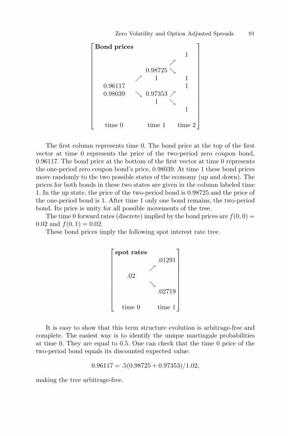
Zero Volatility and Option Adjusted Spreads 91

⎡

⎢⎢⎢⎢⎢⎢⎢⎢⎢⎢⎢⎢⎢⎢⎢⎢⎣

Bond prices1

↗0.98725 ↘

↗ 1 10.96117 10.98039 ↘ 0.97353 ↗

1 ↘1

time 0 time 1 time 2

⎤

⎥⎥⎥⎥⎥⎥⎥⎥⎥⎥⎥⎥⎥⎥⎥⎥⎦

The first column represents time 0. The bond price at the top of the firstvector at time 0 represents the price of the two-period zero coupon bond,0.96117. The bond price at the bottom of the first vector at time 0 representsthe one-period zero coupon bond’s price, 0.98039. At time 1 these bond pricesmove randomly to the two possible states of the economy (up and down). Theprices for both bonds in these two states are given in the column labeled time1. In the up state, the price of the two-period bond is 0.98725 and the price ofthe one-period bond is 1. After time 1 only one bond remains, the two-periodbond. Its price is unity for all possible movements of the tree.

The time 0 forward rates (discrete) implied by the bond prices are f(0, 0) =0.02 and f(0, 1) = 0.02.

These bond prices imply the following spot interest rate tree.

⎡

⎢⎢⎢⎢⎢⎢⎢⎢⎢⎢⎣

spot rates.01291

↗.02

↘.02719

time 0 time 1

⎤

⎥⎥⎥⎥⎥⎥⎥⎥⎥⎥⎦

It is easy to show that this term structure evolution is arbitrage-free andcomplete. The easiest way is to identify the unique martingale probabilitiesat time 0. They are equal to 0.5. One can check that the time 0 price of thetwo-period bond equals its discounted expected value:

0.96117 = .5(0.98725 + 0.97353)/1.02,

making the tree arbitrage-free.

92 Robert Jarrow

5.2 The Bonds and the Prepayment Option

Next, consider a coupon bond with coupon rate 0.015, principal 100, maturitytime 2. Its value plus cash flow tree is:

⎡

⎢⎢⎢⎢⎢⎢⎢⎢⎢⎢⎢⎢⎢⎢⎢⎢⎢⎢⎢⎢⎣

Coupon Bondcash flow 101.5

↗cash flow 1.5

value 100.2064 ↘

↗ cash flow 101.5B0 = 99.0292 cash flow 101.5

↘ ↗cash flow 1.5value 98.8132 ↘

cash flow 101.5

time 0 time 1 time 2

⎤

⎥⎥⎥⎥⎥⎥⎥⎥⎥⎥⎥⎥⎥⎥⎥⎥⎥⎥⎥⎥⎦

Consider a prepayment option with maturity time 1 and strike price K =100. Its value tree is:

⎡

⎢⎢⎢⎢⎢⎢⎢⎢⎢⎢⎣

optionmax(100.2064−K, 0) = 0.2064

↗C0 = 0.101105

↘max(98.8132−K, 0) = 0

time 0 time 1

⎤

⎥⎥⎥⎥⎥⎥⎥⎥⎥⎥⎦

where C0 = .5(max(100.2064−K, 0)+max(98.8132−K, 0))/1.02 = 0.101105.Next, consider a bond with an embedded prepayment option. Its value is

V0 = B0 − C0 = 98.928074. One subtracts the prepayment option, becauseit is exercised by the issuer of the bond. The cash flow to the bond with theprepayment option is:

Zero Volatility and Option Adjusted Spreads 93

⎡

⎢⎢⎢⎢⎢⎢⎢⎢⎢⎢⎢⎢⎢⎢⎢⎢⎢⎢⎢⎢⎣

Bond withembedded cash flow 0

option ↗

cash flow101.5

prepaid ↘↗ value 0 cash flow 0

V0

= 98.928074 cash flow 101.5

↘ ↗cash flow 1.5 ↘value 98.8132 cash flow 101.5

time 0 time 1 time 2

⎤

⎥⎥⎥⎥⎥⎥⎥⎥⎥⎥⎥⎥⎥⎥⎥⎥⎥⎥⎥⎥⎦

This cash flow tree is needed for the computation of OAS below.

5.3 The ZV Spread Computation

Using the arbitrage-free price for the bond 98.928074, the zv(fair) is obtainedby solving the following equation,

98.928074 =1

(1 + zv(fair))(1.5)(.98039) +

1(1 + zv(fair))2

(101.5)(.96117).

There are two solutions to this expression: zv(fair) = 0.0005155,−1.9856503.There is only one root that keeps the discount factor nonnegative. This is therelevant root (0.0005155).

Supposing the market value of the bond is 99, we can compute the zv(mkt)by solving a similar equation,

99.00 =1

(1 + zv(mkt))(1.5)(.98039) +

1(1 + zv(mkt))2

(101.5)(.96117).

There are two solutions to this expression: zv(mkt) = 0.0001493,−1.9852949.There is only one root that keeps the discount factor nonnegative. This is therelevant root (0.0001493).

The mispricing measure based on ZV spreads is zv(market) − zv(fair)= 0.0001493− 0.0005155 = −.0003662. The bond is overvalued by −3.7 basispoints.

5.4 The OAS Computation

Using the arbitrage-free price for the bond, 98.928074, the OAS is obtainedby solving the following equation,

94 Robert Jarrow

98.928074 =.5

(1 + ϕ)

[1.5

1 + .02+

101.51 + .02

]

+.5

(1 + ϕ)2

[101.5

(1 + .02)(1 + .02719)

]1

(1 + ϕ)2.

There are two solutions to this expression: ϕ = 0 and −1.48963. There is onlyone root that keeps the discount factor nonnegative. This is the proper root(ϕ = 0). This example shows that OAS reflects the fact that there are nomispricings in this economy.

Next, let us suppose that the bond trades for 99.00 dollars; that is, it isovervalued. OAS is then the solution to:

99.00 =.5

(1 + ϕ)

[1.5

1 + .02+

101.51 + .02

]

+.5

(1 + ϕ)2

[101.5

(1 + .02)(1 + .02719)

]1

(1 + ϕ)2.

The solutions are −.0004878 and −1.48951. Ignoring the second root again,the OAS of −4.9 basis points shows the bond is overvalued.

Note that the mispricing measure based on ZV spreads versus OAS differs,although both show an overvaluation.

6 Conclusion

This paper provides a tutorial on two commonly used measures: a zero volatil-ity spread and an option adjusted spread. The Heath–Jarrow–Morton modelis used as a frame of reference for understanding these two quantities. We showthat the ZV spread is a measure of the excess spread due to both a bond’sembedded options and any mispricings, whereas the OAS provides only a validmeasure of a bond’s mispricings.

If mispricings exist, they are due to either market error or model error. If itis market error, then it represents an arbitrage opportunity. If it is model error,then it represents either an incorrect stochastic process, omitted risk premia,omitted risks (e.g., liquidity risk), or market imperfections (e.g., transactioncosts). To distinguish between these two alternatives, one can backtest themodel with the arbitrage trading strategies implied by the mispricing (nec-essarily including all market imperfections). If it is market error, then thetrading strategy will earn abnormal returns. If not, then it is model error.

Zero Volatility and Option Adjusted Spreads 95

References

1. T. Bielecki and M. Rutkowski. Credit Risk: Modeling, Valuation, and Hedging.Springer, 2002.

2. J. Cilia. Product summary: Advanced CMO analytics for bank examiners: Prac-tical applications using Bloomberg. Federal Reserve Bank of Chicago, May 1995.

3. F. Fabozzi. Bond Markets, Analysis and Strategies, 4th edition. Prentice-Hall,2000.

4. D. Heath, R. Jarrow, and A. Morton. Bond pricing and the term structure ofinterest rates: A new methodology for contingent claims valuation. Econometrica,60:77–105, 1992.

5. N. Jacobson. Basic Algebra I. W. H. Freeman, 1974.6. R. Jarrow. Modeling Fixed Income Securities and Interest Rate Options, 2nd

edition. Stanford University Press, 2002.7. P. Protter. Stochastic Integration and Differential Equations, 2nd edition.

Springer, 2005.8. B. Tuckman. Fixed Income Securities. John Wiley and Sons, 1996.

Appendix: Real Root Solution to Equations (4) and (5)

Both Equations (4) and (5) take the form

T∑

t=1

e−β·tαt − α0 = 0, (7)

where αt ≥ 0 for all t and α0 > 0. Let us write x = e−β. Then the relevantrange for x is (0,∞). We seek a real root of the polynomial equation

f(x) =T∑

t=1

xtαt − α0

on [0,M ] for M chosen large enough so that f(M) > 0. Using Sturm’s theorem(see [5, p. 298]), we note that because f(0) = −α0 < 0, f(M) > 0, and allderivatives of f(x) up to degree T are nonnegative for all x, we get thatthe number of variations in the sign of {f(0), f ′(0), . . . , fT (0)} is 1, wherefT (0) denotes the T th derivative, and the number of variations in the sign of{f(M), f ′(M), . . . , fT (M)} is 0. Sturm’s theorem then tells us the number ofdistinct real roots of f(x) in (0,M) is 1.

Inasmuch as this is true for all x > M , we see that there is one distinctreal root of f(x) for x ∈ (0,∞).

Finally, because x = e−β, this gives us one real root β of (7).

Asset Price Bubbles in Complete Markets

Robert A. Jarrow,1 Philip Protter,2 and Kazuhiro Shimbo2

1 Johnson Graduate School of ManagementCornell UniversityIthaca, NY 14850, USAraj15@cornell.edu

2 School of Operations Research and Industrial EngineeringCollege of EngineeringCornell UniversityIthaca, NY, 14850, USApep4@cornell.edu, ks266@cornell.edu

Summary. This paper reviews and extends the mathematical finance literature onbubbles in complete markets. We provide a new characterization theorem for bub-bles under the standard no-arbitrage framework, showing that bubbles can be ofthree types. Type 1 bubbles are uniformly integrable martingales, and these can ex-ist with an infinite lifetime. Type 2 bubbles are nonuniformly integrable martingales,and these can exist for a finite, but unbounded, lifetime. Last, Type 3 bubbles arestrict local martingales, and these can exist for a finite lifetime only. When one addsa no-dominance assumption (from Merton [24]), only Type 1 bubbles remain. Inaddition, under Merton’s no-dominance hypothesis, put–call parity holds and thereare no bubbles in standard call and put options. Our analysis implies that if onebelieves asset price bubbles exist and are an important economic phenomena, thenasset markets must be incomplete.

Key words: Bubbles; no free lunch with vanishing risk (NFLVR); complete markets;local martingale; put–call parity; derivative pricing.

1 Introduction

Although asset price bubbles, their existence and characterization, have en-thralled the imagination of economists for many years, only recently has thistopic been studied using the tools of mathematical finance; see in particularLoewenstein and Willard [22], Cox and Hobson [7], Jarrow and Madan [20],Gilles [15], Gilles and Leroy [16], and Huang and Werner [17]. The purposeof this paper is to review and to extend this mathematical finance literaturein order to increase our understanding of asset price bubbles. In this paper,

98 Robert A. Jarrow, Philip Protter, and Kazuhiro Shimbo

we restrict our attention to arbitrage-free economies that satisfy both the no-free-lunch-with-vanishing-risk (NFLVR) and complete markets hypotheses, inorder that both the first and second fundamental theorems of asset pricingapply. Equivalently, there exists a unique equivalent local martingale measure.We exclude the study of incomplete markets. (We study incomplete marketasset price bubbles in a companion paper, see Jarrow et al. [21].) We alsoexclude the study of charges, because charges require a stronger notion of no-arbitrage (see Jarrow and Madan [20], Gilles [15], and Gilles and Leroy [16]).

We make two contributions to the bubbles literature. First, we provide anew characterization theorem for asset price bubbles. Second, we study theeffect of additionally imposing Merton’s [24] no-dominance assumption on theexistence of bubbles in an economy. Our new results in this regard are:

(i) Bubbles can be of three types: an asset price process that is (1) auniformly integrable martingale, (2) a martingale that is not a uniformlyintegrable martingale, or (3) a strict local martingale that is not a martingale.Bubbles of Type 1 can be viewed as the asset price process containing acomponent analogous to fiat money (see Example 2). Type 2 bubbles aregenerated by the fact that all trading strategies must terminate in finite time,and Type 3 bubbles are caused by the standard admissibility condition usedto exclude doubling strategies.

(ii) Bubbles cannot be started—“born”—in a complete market. (In con-trast, they can be born in incomplete markets.) They either exist at the startor not, and if they do exist, they may disappear as the economy evolves.

(iii) Bubbles in standard European call and put options can only be ofType 3, because standard options have finite maturities. Under NFLVR, anyassets and contingent claims can have bubbles and put–call parity does nothold in general.

(iv) Under NFLVR and no-dominance, in complete markets, there can beno Type 2 or Type 3 asset price bubbles. Consequently, standard options haveno bubbles and put–call parity holds.

The economic conclusions from this paper are threefold. First, bubbles ofType 1 are uninteresting from an economic perspective because they representa permanent but stochastic wedge between an asset’s fundamental value andits market price, generated by a perceived residual value at time infinity.

Second, Type 2 bubbles are the result of trading strategies being of finitetime duration, although possibly unbounded. To try to profit from a bubbleof Type 2 or Type 3, one would short the asset in anticipation of the bubblebursting. Because a Type 2 bubble can exist, with positive probability, be-yond any trading strategy, these bubbles can persist as they do not violatethe NFLVR assumption. Type 3 bubbles occur in assets with finite maturities.For these asset price bubbles, unprotected shorting is not feasible, because dueto the admissibility condition, if the short’s value gets low enough, the trad-ing strategy must be terminated with positive probability before the bubblebursts. This admissibility condition removes downward selling pressure on theasset’s price, and hence enables these bubbles to exist.

Asset Price Bubbles in Complete Markets 99

Third, modulo Type 1 bubbles, under both the NFLVR and no-dominancehypotheses, there can be no asset pricing bubbles in complete markets. Thisimplies that if one believes asset pricing bubbles exist and are an importanteconomic phenomenon, and if one accepts Merton’s “no-dominance” assump-tion, then asset markets must be incomplete.

An outline of this paper is as follows. Section 2 presents our model struc-ture and defines an asset price bubble. Section 3 characterizes the properties ofasset price bubbles. Section 4 provides the economic intuition underlying themathematics, and Section 5 extends the analysis to contingent claims bubbles.Finally, Section 6 concludes.

2 Model Description

This section presents the details of our economic model.

2.1 No Free Lunch with Vanishing Risk (NFLVR)

Traded in our economy is a risky asset and a money market account. Forsimplicity, and without loss of generality, we assume that the spot interestrate is 0 in our economy, so that the money market account has constantunit value. Let τ be a maturity (life) of the risky asset. Let (Dt)0≤t<τ bea cadlag semimartingale representing the cumulative dividend process of therisky asset, with Xτ its terminal payoff or liquidation value at time τ . Weassume that Xτ , Dt ≥ 0 for each t ∈ (0, τ). The market price of the riskyasset is given by a nonnegative cadlag semimartingale S = (St)t≥0 definedon a filtered complete probability space (Ω,F ,F, P ) where F = (Ft)t≥0. Weassume that the filtration F satisfies the usual hypotheses (cf. [25]). Note thatfor t such that �Dt > 0, St denotes a price ex-dividend, because S is cadlag.Let W = (Wt)t≥0 be a wealth process from owning the asset, given by

Wt = St +∫ t∧τ

0

dDu +Xτ1{τ≤t}.

A key notion in our economy is an equivalent local martingale measure.

Definition 1 (Equivalent Local Martingale Measure). Let Q be a prob-ability measure equivalent to P such that the wealth process W is a Q-localmartingale. We call Q an Equivalent Local Martingale Measure (ELMM). Wedenote the set of ELMMs by Me

loc(W ).

A trading strategy is defined to be a pair of processes (π, η) = (πt, ηt)t≥0

representing the number of units of the risky asset and money market accountheld at time t with π ∈ L(W ) (see [25] for the definition of the space ofintegrable processes L(W )). The wealth process of the trading strategy (π, η)

100 Robert A. Jarrow, Philip Protter, and Kazuhiro Shimbo

is given by V π,η = (V π,ηt )t≥0, where V π,η

t = πtSt + ηt. Assume temporarilythat π is a semimartingale. Then a self-financing trading strategy with V π,η

0 =0 is a trading strategy (π, η) such that the associated wealth process V π,η isgiven by

V π,ηt =

∫ t

0

πudWu =∫ t

0

πudSu +∫ t∧τ

0

πudDu + πτXτ1{τ≤t}

=(πtSt −

∫ t

0

Su−dπu − [πc, Sc]t

)+∫ t∧τ

0

πudDu + πτXτ1{τ≤t}

= πtSt + ηt, (1)

where we have used integration by parts, and where

ηt =∫ t∧τ

0

πudDu + πτXτ1{τ≤t} −∫ t

0

Su−dπu − [πc, Sc]t. (2)

If we now discard the temporary assumption that π is a semimartingale, wesimply define a self-financing trading strategy (π, η) to be a pair of processes,with π predictable and η optional and such that:

V π,ηt = πtSt + ηt =

∫ t

0

πudWu.

As noted, a self-financing trading strategy starts with zero units of the moneymarket account η0 = 0, and it reflects proceeds from purchases/sales of a riskyasset that accumulate holdings in the money market account as the cash flowsfrom the risky asset are deposited. In particular, Equation (2) shows that ηis uniquely determined by π if a trading strategy is self-financing. Thereforewithout loss of generality, we represent (π, η) by π.

To avoid doubling strategies, we further restrict the class of self-financingtrading strategies.

Definition 2 (Admissibility). Let V π,η be the wealth process given by (1).We say that the trading strategy π is a−admissible if it is self-financing andV π,ηt ≥ −a a.s. for all t ≥ 0. We say a trading strategy is admissible if it is

self-financing and V π,ηt ≥ −a for all t ≥ 0 for some a ∈ R

+.

The notion of admissibility corresponds to a lower bound on the wealthprocess, an implicit inability to borrow if one’s debt becomes too large. (Forexample, see Loewenstein and Willard [22, Equation (5), p. 23].) There areseveral alternative definitions of admissibility that could be employed andthese are discussed in Section 4.3. However, all of our results are robust tothese alternative formulations.

We want to explore the existence of bubbles in arbitrage-free markets,hence, we need to define the NFLVR hypothesis. Let

K = {Wπ∞ = (π ·W )∞ : π is admissible},

C = (K − L0+) ∩ L∞.

Asset Price Bubbles in Complete Markets 101

Definition 3 (NFLVR). We say that a semimartingale S satisfies the nofree lunch with vanishing risk (NFLVR) condition with respect to admissibleintegrands, if

C ∩ L∞+ = {0},

where C denotes the closure of C in the sup-norm topology of L∞.

Given NFLVR, we impose the following assumption.

Assumption 1 The market satisfies NFLVR hypothesis.

By the first fundamental theorem of asset pricing [9], this implies that themarket admits an equivalent σ-martingale measure. By Proposition 3.3 andCorollary 3.5 [1, pp. 307, 309], a σ-martingale bounded from below is a localmartingale. (For the definition and properties of σ-martingales, see [25; 14; 9;19, Section III.6e].) Thus we have the following theorem.

Theorem 1 (First Fundamental Theorem). A market satisfies the NFLVRcondition if and only if there exists an ELMM.

Theorem 1 holds even if the price process is not locally bounded, due tothe assumption that W is nonnegative. (In [9], the driving semimartingale(price process) takes values in R

d and is not locally bounded from below.)We are interested in studying the existence and characterization of bubbles

in complete markets. A market is complete if for all X∞ ∈ L2(Ω,F∞, P ), thereexists a self-financing trading strategy (π, η) and c ∈ R such that

X∞ = c+∫ ∞

0

πudWu.

For the subsequent analysis, we also assume that the market is complete,hence by the second fundamental theorem of asset pricing (cf. [18]), the ELMMis unique.

Assumption 2 Given the market satisfies NFLVR, the ELMM is unique.

This assumption is key to a number of the subsequent results. For theremainder of the paper we assume that both Assumptions 1 and 2 hold, thatis, that the markets are arbitrage-free and complete.

2.2 No-Dominance

In addition to Assumption 1, we also study the imposition of Merton’s [24] no-dominance assumption. To state this assumption in our setting, assume thatthere are two assets or contingent claims characterized by the pair of cashflows ({D1

t }t≥0, X1τ ), ({D2

t }t≥0, X2τ ). Let V 1

t , V2t denote their market prices at

time t.

102 Robert A. Jarrow, Philip Protter, and Kazuhiro Shimbo

Assumption 3 (No-Dominance) For any stopping time τ0 ≤ τ a.s., if

D2τ0+u−D

2τ0 ≥ D1

τ0+u−D1τ0 and X2

τ1{τ>τ0} ≥ X1τ1{τ>τ0} for u > 0, (3)

then V 2τ0 ≥ V 1

τ0 . Furthermore, if for some stopping time τ0,

E[1({D2∞−D2

τ0>D1∞−D1

τ0}∪{X2

τ1{τ>τ0}>X1τ1{τ>τ0}})

∣∣∣Fτ0]> 0

with positive probability, then V 2τ0 > V 1

τ0 .

Note that (3) implies that X2τ1{τ>τ0} ≥ X1

τ1{τ>τ0} for any stopping time τ0such that τ0 ≤ τ .

This assumption rephrases Assumption 1 of [24] in modern mathematicalterms, we believe for the first time. In essence, it codifies the intuitively ob-vious idea that, all things being equal, financial agents prefer more to less.Assumption 3 is violated only if there is an agent who is willing to buy adominated security at the higher price.

Assumption 3 is related to Assumption 1, but they are not equivalent.

Lemma 1. Assumption 3 implies Assumption 1. However, the converse is nottrue.

Proof. Assume that W allows for a free lunch with vanishing risk. There isf ∈ L∞

+ (P )\{0} and sequence {fn}∞n=0 = {(Hn · W )∞}∞n=0 where Hn is asequence of admissible integrands and {gn} satisfying gn ≤ fn such that

limn

‖f − gn‖∞ = 0.

In particular, the negative part {(fn)−} tends to zero uniformly. (See [10,p. 131]). Applying Assumption 3 to two terminal payoffs f and 0, we have0 = V0(f) > 0, a contradiction. Therefore Assumption 3 implies Assumption1. For the converse, see Example 1. �

The domain of Assumption 3 contains a domain of Assumption 3, C∩L∞+ (P ).

This explains why Assumption 3 implies Assumption 1.The following is an example consistent with Assumption 1 but excluded

by Assumption 3.

Example 1. Consider two assets maturing at τ with payoffs Xτ and Yτ , re-spectively. Suppose that Xτ ≥ Yτ a.s. Then,

X∗t = EQ[Xτ |Ft]1{t<τ} ≥ EQ[Yτ |Ft]1{t<τ} = Y ∗

t .

Let β be a nonnegative local martingale such that βτ = 0 and βt > X∗t − Y ∗

t

for some t ∈ (0, τ). (The existence of such a process follows, for example,from Example 3.) Suppose further that the prices of asset Xt = X∗

t andYt = βt + Y ∗

t . Then, Assumption 3 is violated because Yt > Xt.

Asset Price Bubbles in Complete Markets 103

To see that this is not an NFLVR, consider a strategy that would attemptto take advantage of this mispricing. One would want to sell Y and to buyX , say at time t. Then, if held until maturity, this would generate a cashflow equal to βt − (X∗

t − Y ∗t ) > 0 at time t and Xτ − Yτ ≥ 0 at time τ .

However, for any u with t < u ≤ τ , the market value of this trading strategyis −Yu + Xu = −βu + (X∗

u − Y ∗u ). Because −β is negative and unbounded,

this strategy is inadmissible and not a FLVR. We discuss issues related toadmissibility further in Section 4.3.

One situation Assumption 3 is meant to exclude is often called a suicidestrategy (see Harrison and Pliska [18] for the notion of a suicide strategy).An alternative approach for dealing with suicide strategies is to restrict theanalysis to the set of maximal assets. An outcome (π · S)∞ of an admissiblestrategy π is called maximal if for any admissible strategy π′ such that (π′ ·S)∞ ≥ (π · S)∞, then π′ = π.

2.3 Bubbles

This section provides the definition of an asset pricing bubble in our economy.To do this, we must first define the asset’s fundamental price.

The Fundamental Price

We define the fundamental price as the expected value of the asset’s futurepayoffs with respect to the ELMM Q ∈ Me

loc(W ). (Recall that we assumethat the market is complete, Assumption 2.)

Definition 4 (Fundamental Price). The fundamental price S∗t of an asset

with market price St is defined by

S∗t = EQ

[∫ τ

t

dDu +Xτ1{τ<∞}|Ft]1{t<τ}. (4)

Note that the fundamental price is just the conditional expected value ofthe asset’s cash flows, under the valuation measure Q. (Note that becausethe random variable is positive, the conditional expectation is always defined;however, in Lemma 2 that follows, we show that it is actually in L1 and thusis classically defined.) Also, note that if the asset has a payoff at τ = ∞, thenthis payoff Xτ1{τ=∞} does not contribute to the fundamental price S∗

t . We dothis because an agent cannot consume the payoff Xτ1{τ=∞} by employing anadmissible trading strategy. Indeed, although unbounded in time, for a givenω ∈ Ω, all such admissible trading strategies must terminate in finite time.

Lemma 2. The fundamental price in (4) is well defined. Furthermore, (St)t≥0

converges to S∞ ∈ L1(Q) a.s. and (S∗t )t≥0 converges to 0 a.s.

104 Robert A. Jarrow, Philip Protter, and Kazuhiro Shimbo

Proof. Fix Q ∈ Meloc(W ). To show that S∗

t is well defined, it suffices to showthat∫ τ0 dDu +Xτ1{τ<∞} ∈ L1(Q) because for all t,

0 ≤∫ τ

t

dDu +Xτ1{t<τ} ≤∫ τ

0

dDu +Xτ1{t<τ}.

By hypothesis, W is a nonnegative supermartingale. By the martingale con-vergence theorem (see [11, VI.6, p. 72]), there exists W∞ ∈ L1(Q) such thatW converges to W∞ a.s. To show the convergence of S, observe that

W∞ = limt→∞

Wt = limt→∞

(St +∫ t∧τ

0

dDu +Xτ1{τ≤t}

)

= limt→∞

St +∫ τ

0

dDu +Xτ1{τ<∞} a.s.

It follows that there exist S∞ ∈ L1(Q) and∫ τ0 dDu + Xτ1{τ<∞} ∈ L1(Q)

because S ≥ 0. Therefore S∗t is well defined for all t ≥ 0. Observe that

EQ

[∫ τ

t

dDu +Xτ1{τ<∞}|Ft]

= −∫ t

0

dDu + EQ

[(∫ τ

0

dDu +Xτ1{τ<∞}

)|Ft] (5)

and

EQ

[(∫ τ

0

dDu +Xτ1{τ<∞}

)|Ft]1{t<τ}

=(EQ

[(∫ τ

0

dDu +Xτ

)1{τ<∞}|Ft

]+ EQ

[1{τ=∞}

∫ ∞

0

dDu|Ft])

1{t<τ}.

(6)

Substituting (6) into (5) and then into (4),

limt→∞

S∗t = −

∫ ∞

0

dDu1{τ=∞} + 1{τ=∞}EQ

[∫ τ

0

dDu +Xτ1{τ<∞}|F∞

]

= −∫ ∞

0

dDu1{τ=∞} + 1{τ=∞}EQ{∫ ∞

0

dDu|F∞} = 0.

�Note that, in general,

∫∞0 dDu + Xτ1{τ<∞} need not be P -integrable. In

this regard, Lemma 2 shows that the existence of Q implies that∫∞0 dDu +

Xτ1{τ<∞} is Q-integrable.

Lemma 3. The fundamental wealth process W ∗ = (Wt)t≥0 given by W ∗t =

S∗t +∫ τ∧t0 dDu + Xτ1{τ≤t} is a uniformly integrable martingale under Q ∈

Meloc(W ) closed by

W ∗∞ =∫ τ

0

dDu +Xτ1{τ<∞}.

Asset Price Bubbles in Complete Markets 105

Proof. By Lemma 2,

W ∗∞ := lim

t→∞W ∗t = lim

t→∞

(S∗t +∫ t∧τ

0

dDu +Xτ1{τ≤t}

)

=∫ τ

0

dDu +Xτ1{τ<∞} a.s.

W ∗∞ is in L1(Q) because S∞ ≥ 0, W∞ ∈ L1, and W ∗

∞ + S∞ = W∞. Observethat

EQ [W ∗∞|Ft] = EQ

[(∫ τ

t

dDu +Xτ

)|Ft]1{t<τ}

+(−∫ t

τ

dDu +Xτ

)1{τ≤t} +

(∫ t

0

dDu

)1{t<τ}

= S∗t +∫ t∧τ

0

dDu +Xτ1{τ≤t} = W ∗t .

It follows that W ∗ is a closable and hence uniformly integrable martingale. �

The Asset Price Bubble

Definition 5 (Bubble). The asset price bubble βt for St is given by

βt = St − S∗t .

As indicated, the asset price bubble is the asset’s market price less theasset’s fundamental price.

3 Properties of Bubbles

In this section, we analyze the properties of asset price bubbles, applyingsemimartingale theory and potential theory. We begin with a nonstandarddefinition.

Definition 6 (Strict Local Martingale). A strict local martingale is alocal martingale that is not a martingale.

The term “strict local martingale” is not common in the literature, but itcan be found in the recent book of Delbaen and Schachermayer [10], who inturn refer to a paper of Elworthy et al. [13]. We hasten to remark that theirdefinition of a strict local martingale is different from our definition. Indeed,Delbaen and Schachermayer refer to a strict local martingale as being a localmartingale that is not a uniformly integrable martingale. They allow a strictlocal martingale to be actually a martingale, as long as the martingale itselfis not uniformly integrable. Our definition is more appropriate for the studyof bubbles, as is made clear shortly.

106 Robert A. Jarrow, Philip Protter, and Kazuhiro Shimbo

3.1 Characterization of Bubbles

Theorem 2. If there exists a nontrivial bubble β := (β)t≥0 �≡ 0 in an asset’sprice, then we have three and only three possibilities:

1. β is a local martingale (which could be a uniformly integrable martingale)if P (τ = ∞) > 0.

2. β is a local martingale but not a uniformly integrable martingale if it isunbounded, but with P (τ < ∞) = 1.

3. β is a strict Q-local martingale, if τ is a bounded stopping time.

Proof. Fix Q ∈ Meloc(W ). Because W is a closable supermartingale (see proof

of Lemma 2), there exists W∞ ∈ L1(Q) such that W converges to W∞ a.s.Let

β′t = Wt − EQ[W∞|Ft]. (7)

Then (β′t)t≥0 is a (nonnegative) local martingale, because it is a difference of

a local martingale and a uniformly integrable martingale. By Lemma 3,

EQ[W∞|Ft] = EQ[W ∗∞|Ft] + EQ[S∞|Ft] = W ∗

t + EQ[S∞|Ft]. (8)

By the definition of wealth processes, and applying Equations (7) and (8),

βt = St − S∗t = Wt −W ∗

t

=(EQ[W∞|Ft] + β1

t

)− (EQ[W∞|Ft] − EQ[S∞|Ft]) = β′

t + EQ[S∞|Ft].

If τ < T for T ∈ R+, then S∞ = 0. A bubble βt = β′

t = 0 for t ≥ τ and inparticular βT = 0. If βt is a martingale,

βt = EQ[βT |Ft] = 0 ∀t ≤ T.

It follows that β is a strict local martingale. This proves Part 1. For Part 2,assume that β is a uniformly integrable martingale. Then by Doob’s optionalsampling theorem, for any stopping time τ0 ≤ τ ,

βτ0 = EQ[βτ |Fτ0 ] = 0, (9)

and because β is optional, it follows from (for example) the section theoremsof P.A. Meyer that β = 0 on [0, τ ]. Therefore the bubble does not exist. ForPart 3, (EQ[S∞|Ft])t≥0 is a uniformly integrable martingale. �

As indicated, there are three types of bubbles that can be present in anasset’s price. Type 1 bubbles occur when the asset has infinite life with apayoff at {τ = ∞}. Type 2 bubbles occur when the asset’s life is finite,but unbounded. Type 3 bubbles are for assets whose lives are bounded. Ina subsequent section, we provide an intuitive economic explanation for whythese bubbles exist. Before that, however, we provide some examples.

Asset Price Bubbles in Complete Markets 107

3.2 Examples

This section presents simple examples of bubbles of Types 1, 2, and 3.

A Uniformly Integrable Martingale Bubble: Fiat Money (Type 1)

Example 2. Let S be fiat money given by St = 1 for all t ≥ 0. Fiat moneyis money that the government declares to be legal tender, although it cannotbe converted into standard specie. Because money never matures, τ = ∞ andX∞ = 1. Money pays no dividend and hence D ≡ 0. Therefore S∗ ≡ 0 and

βt = St − S∗t = 1 ∀t ≥ 0.

The entire value of money comes from the bubble, its payoff X∞ = 1, andit is a trivial uniformly integrable martingale. Note that in our setting, fiatmoney is equivalent to our money market account (paying zero interest for alltime).

A Martingale Bubble (Type 2)

Example 3. Let the asset’s maturity τ be a positive random time with P (τ >t) > 0 for all t ≥ 0. Let the fundamental price process be (S∗

t )t≥0 =(1{t<τ})t≥0, with payoff 1 at time τ . Set a process β by

βt =1 − 1{τ≤t}Q(τ > t)

.

Lemma 4 shows that β is a martingale that is not a uniformly integrablemartingale, with β∞ = 0. Then

S = S∗ + β

is a price process with a nonuniformly integrable bubble.

Lemma 4. Let τ0 be a positive finite random variable such that P (τ0 > t) > 0for all t ≥ 0. Let D = (Dt)t≥0 = (1{τ0≤t})t≥0 and D = (Dt)t≥0 be a naturalfiltration generated by D. Then a process N defined by

Nt =1 −Dt

P (τ0 > t)

is a martingale that is not a uniformly integrable martingale, and N∞ = 0.

Proof. By the structure of D (e.g., see Protter [25, Lemma on p. 121]) fors < t,

P (τ0 > t|Ds) = 1{τ0>t}P (τ0 > t|τ0 > s) = 1{τ0>s}P (τ0 > t)P (τ0 > s)

.

108 Robert A. Jarrow, Philip Protter, and Kazuhiro Shimbo

Therefore,

E [1 −Dt|Ds] = (1 −Ds)P (τ0 > t)P (τ0 > s)

.

This shows that N is a martingale. Observe that Nt = 0 on {t > τ0} andhence N converges to 0 a.s., because τ0 < ∞ a.s. If N is a uniformly integrablemartingale, then N is closable by N∞ and Nt = E[N∞|Dt] ≡ 0, which is nottrue. Therefore N is not uniformly integrable. �

This example has the asset’s maturity τ having a positive probability ofcontinuing past any given future time t. Although finite with probability one,the asset’s life is unbounded.

A Strict Local Martingale Bubble (Type 3)

The following example is essentially that contained in Cox and Hobson [7,Example 3.5, p. 9 and 2.2.1, p. 4]. In this example, although the asset hasfinite maturity T , a bubble still exists, as the following lemma shows.

Example 4. Let D = (Dt)t≥0 ≡ 0 τ = T and Xτ = XT = 1. Then thefundamental price at t ≥ 0 is S∗

t = 1{t<T}. Define a process β by

βt = 1 +∫ t

0

βu√T − u

dBu, (10)

where B = (Bt)t≥0 is a standard Q-Brownian motion. Lemma 5 shows thatβ is a strict local martingale with βT = 0. Then

S = S∗ + β

is a price process with a strict local martingale bubble.

Lemma 5. A process β defined by Equation (10) is a continuous local mar-tingale on [0, T ].

Proof. The stochastic integral (∫ t0dBs/

√T − s)t≥0 is a local martingale but

not a martingale on [0, T ) (because it is a stochastic integral of a predictableintegrand w.r.t Brownian motion), such that

[∫ ·

0

dBs/√T − s,

∫ ·

0

dBs/√T − s

]

u

= − ln[1 − u− t

T

]:= Au

and continuous on [0, T ). By the Dubins–Schwartz theorem, there exists aBrownian motion B such that

dβu = βudBAu

and

βu = β0E(B)

Au

= β0exp(BAu − 1

2Au

)

Asset Price Bubbles in Complete Markets 109

for all u < T . By the law of the iterated logarithm, we can show thatlimt→∞ E(B)t = 0. Inasmuch as Au is monotonic and limu→∞ Au = ∞,

limu→T

βu = 0 a.s.

Because we set βT = 0, βT− = ST and β is continuous on [0, T ], EQ[βT ] =0 < EQ[β0] implies that β is not a martingale. �

3.3 A Bubble Decomposition

In this section, we refine Theorem 2 to obtain a unique decomposition of anasset price bubble that yields some additional insights. The key tool is thedecomposition of a positive supermartingale.

Theorem 3 (Riesz Decomposition I). Let X be a right-continuous su-permartingale such that E[X−

t ] = limt→∞E[X−t ] < ∞. Then the limit

X∞ = limt→∞Xt a.s. exists and E [|X∞|] < ∞. X has the decompositionX = U +V , where U is a right-continuous version of the uniformly integrablemartingale E[X∞|Ft] and V is a right-continuous supermartingale that is zeroa.s. at infinity. V is positive if (X−)t≥0 are uniformly integrable.

Proof. See Dellacherie and Meyer [11, V.34, 35 and VI.8, p. 73]. �

Definition 7 (Potential). A positive right-continuous supermartingale suchthat limt→∞ E[Zt] = 0 is called a potential.

Theorem 4 (Riesz Decomposition II). Every right-continuous positivesupermartingale X can be decomposed as a sum of X = Y + Z, where Yis a right-continuous martingale and Z is a potential. This decomposition isunique, except on an evanescent set, and Y is the greatest right-continuousmartingale bounded above by X.

Proof. See Dellacherie and Meyer [11, VI.9, p. 73]. �

Theorem 5. S admits a unique (up to an evanescent set) decomposition

S = S∗ + β = S∗ + (β1 + β2 + β3), (11)

where β = (βt)t≥0 is a cadlag local martingale and

• β1 is a cadlag nonnegative uniformly integrable martingale with β1t → X∞

a.s.• β2 is a cadlag nonnegative nonuniformly integrable martingale with β2

t → 0a.s.

• β3 is a cadlag nonnegative supermartingale (and strict local martingale)such that E[β3

t ] → 0 and β3t → 0 a.s. That is, β3

t is a potential.

110 Robert A. Jarrow, Philip Protter, and Kazuhiro Shimbo

Furthermore, (S∗ + β1 + β2) is the greatest submartingale bounded above byW .

Proof. Let β be a cadlag process defined by β1t = EQ[S∞|Ft]. Define

Kt = Wt − (W ∗t + β1

t ) = Wt − EQ[Wt|Ft].

By Theorem 3, K = (Kt)t≥0 is a nonnegative supermartingale and K con-verges to 0 a.s. Let M be a uniformly integrable martingale such that

0 ≤ Mt ≤ Wt −Kt ∀t ≥ 0.

Because W − K converges to 0 a.s., M converges to 0 a.s. Then M ≡ 0.Therefore K is unique up to an evanescent set. By Theorem 4, K has aunique decomposition:

K = β2 + β3,

where β2 is a martingale, β3 is a nonnegative supermartingale such thatE[β3

t ] → 0, which implies β3 converges to 0 a.s. Because K converges to0 a.s., β2 = K − β3 converges to 0 a.s. Because β2 is a cadlag process definedas

β2t = lim

u→∞EQ[Kt+u|Ft],

and Ks ≥ 0 for all s ∈ [0,∞), β2 ≥ 0. This completes the proof. �

As in the previous Theorem 2, β1, β2, β3 give the Type 1, 2, and 3 bubbles,respectively. First, for Type 1 bubbles with infinite maturity, we see that theType 1 bubble component converges to the asset’s value at time ∞, X∞. Thistime ∞ value X∞ can be thought of as analogous to fiat money, embeddedas part of the asset’s price process. Indeed, it is a residual value that payszero dividends for all finite times. Second, this decomposition also shows thatfor finite maturity assets τ < ∞, the critical threshold is that of uniformintegrability. This is due to the fact that when τ < ∞, the Type 2 and 3bubble components of β = (βt)t≥0 have to converge to 0 a.s., whereas theyneed not converge in L1.

As a direct consequence of this theorem, we obtain the following corollary.

Corollary 1. Any asset price bubble β has the following properties.

1. β ≥ 0.2. βτ1{τ<∞} = 0.3. If βt = 0 then βu = 0 for all u ≥ t.

Proof. Parts 1 and 2 hold by Theorem 5. A nonnegative supermartingale staysat 0 once it hits 0, which implies Part 3. �

Asset Price Bubbles in Complete Markets 111

This is a key result. Condition 1 states that bubbles are always nonnega-tive; that is, the market price can never be less than the fundamental value.Condition 2 states that if the bubble’s maturity is finite τ < ∞, then the bub-ble must burst on or before τ . Finally, Condition 3 states that if the bubbleever bursts before the asset’s maturity, then it can never start again. Alter-natively stated, Condition 3 states that in the context of our model, bubblesmust either exist at the start of the model, or they never will exist. And, ifthey exist and burst, then they cannot start again. The fact that this modeldoes not include bubble birth is a weakness of the theory, due in part to thefact that the markets are complete and there is a unique martingale measure.

3.4 No-Dominance

In this section, we add Assumption 3 (the assumption of no-dominance) tothe previous structure to see what additional insights can be obtained. Weonly consider assets whose maturities are finite (i.e., τ < ∞ a.s). This meansthat we only consider bubbles of Types 2 and 3.

Let W be the wealth process generated by the asset with price S. Now, byour complete markets Assumption 2, we know that there exist π1, π2 ∈ L(W )such that

W ∗t = W ∗

0 +∫ t

0

π1udWu, βt = β0 +

∫ t

0

π2udWu,

where W ∗ is the fundamental wealth process and β is the asset price bubble.Let ηi = (ηit)t≥0 be holdings in the money market account given by Equation(2) so that the trading strategies (πi, ηi) are self-financing. Because β∞ = 0,two portfolios represented by W and W ∗ have the same cash flows. BecauseW ∗

∞ ≥ 0, πi represents an admissible trading strategy. This observation im-plies that there are two alternative ways of obtaining the asset’s cash flows.The first is to buy and hold the asset, obtaining the wealth process W. Thesecond is to hold the admissible trading strategy π1, obtaining the wealthprocess W ∗ instead. The cost of obtaining the first position is W0 ≥ W ∗

0 ,with strict inequality if a bubble exists. This implies that if there is a bubble,then the second method for buying the asset dominates the first, yielding thefollowing proposition.

Proposition 1. Under Assumption 3, Type 2 and Type 3 bubbles do not exist.

Proof. For any admissible payoff function, there is an admissible trading strat-egy to replicate S∗. Under Assumption 3, V0(S∗

0 ) ≥ V0(S0) and V0(S0) ≥V0(S∗

0 ). Hence V0(S0) = V0(S∗0 ), because the cash flow of a synthetic asset S∗

and an asset St are the same. It follows that β ≡ 0 and Type 2 or Type 3bubbles do not exist. �

This proposition implies that given both the NFLVR assumption 1 and theno-dominance assumption 3, the only possible asset price bubbles are those

112 Robert A. Jarrow, Philip Protter, and Kazuhiro Shimbo

of Type 1. Essentially, under these two weak no-arbitrage assumptions, onlyinfinite horizon assets can have bubbles in complete markets.

4 The Economic Intuition

This section provides the economic intuition underlying the existence of assetprice bubbles of Types 1, 2, and 3.

4.1 Type 1 Bubbles

Type 1 bubbles are for assets with infinite lives, with positive probability.As argued after Theorem 5, Type 1 bubbles are due to a component of anasset’s price process X∞ that is obtained at time ∞. This component of theasset’s price is analogous to fiat money, a residual value received at time ∞.As such, bubbles of Type 1 are uninteresting from an economic perspectivebecause they represent a permanent (but stochastic) wedge between an asset’sfundamental value and its market price, generated by an exogenously givenvalue at time ∞.

4.2 Type 2 Bubbles

Type 2 bubbles are for assets with finite, but unbounded, lives. In a Type 2bubble, the market price of the asset exceeds its fundamental value. To takeadvantage of this discrepancy, one would form a trading strategy that is longthe fundamental value, and short the asset’s price. This is possible because themarket is complete. If held until the asset’s maturity, when β2

τ1{τ<∞} = 0, thiswould (if possible) create an arbitrage opportunity (FLVR). Unfortunately, forany sample path of the asset price process, the trading strategy must terminateat some finite time. And, there is a positive probability that the bubble exceedsthis termination time, ruining the trading strategy, and making it “risky” andnot an arbitrage. This situation enables asset price bubbles of Type 2 to existin our economy.

4.3 Type 3 Bubbles

Type 3 bubbles are for assets with finite and bounded lives. In a Type 3bubble, the market price of the asset exceeds its fundamental value. Justas for a Type 2 bubble, to take advantage of this discrepancy, one wouldform a trading strategy that is long the fundamental value, and short theasset’s price. This is possible because the market is complete. If held untilthe asset’s maturity, when β3

τ1{τ<∞} = 0, this would (if possible) create anarbitrage opportunity (FLVR). Unfortunately, to be a FLVR trading strategy,the trading strategy must be admissible. Shorting the asset is an inadmissible

Asset Price Bubbles in Complete Markets 113

trading strategy, because if the price of the asset becomes large enough, thevalue of the trading strategy will fall below any given lower bound. Hence,there are NFLVR with Type 3 bubbles.

Alternatively stated, the first fundamental theorem of asset pricing is for-mulated for admissible trading strategies. And, admissible trading strategiesare used to exclude doubling strategies, which would be possible otherwise.Restricting the class of trading strategies to be admissible (to exclude dou-bling strategies) implies that it also excludes shorting the asset for a fixedtime horizon (short and hold) as an admissible trading strategy. This removesdownward selling pressure on the asset price process, allowing bubbles to existin an arbitrage-free setting.

The question naturally arises, therefore, whether the class of admissibletrading strategies can be relaxed further, to exclude both doubling strategies,but still allow shorting the stock over a fixed investment horizon. Unfortu-nately, the answer is no. To justify this statement, we briefly explore theconcept of admissibility. The standard definition of admissibility, the one weadopted, yields the following set of possible trading strategy values,

W =⋃

a

{Wu : Wu ≥ −a, ∀u ∈ [0, T ]} .

As usual, W is the wealth process generated by a risky asset with price processS. The weakest notion of admissibility consistent with NFLVR (see Strasser[29]) yields the following set of trading strategy values,

W∗ ={X = H ·W : H ∈ L(W ) ∧ lim

n→∞EQ[(H ·W )−σn

1{σn<∞}] = 0}, (12)

where the notation Z− for a random variable Z means Z− = −(Z ∧ 0), and

σn = inf{t ∈ [0, T ] : Xt ≤ −n}.

Clearly W ⊂ W∗. Replacing our definition by this weaker notion of admissi-bility does not affect our analysis for Type 3 bubbles. Short-selling an assetwith a Type 3 bubble is not admissible even in the sense of (12) as followsfrom Lemma 6.

Lemma 6. Assume that S has a Type 3 bubble β. Then a trading strategyH = (Ht)t≥0 = (−1{t≤T})t≥0 is not an admissible strategy, and W0 −WT /∈W∗.

Proof. It suffices to show that if W0 −WT ∈ W∗ then a Type 3 bubble doesnot exist. Observe that

(H ·W )−σn= (W0 −Wσn∧T )− = (Wσn∧T −W0)+ ≥ Wσn∧T −W0. (13)

By definition, σn takes a value in [0, T ] ∪ {∞} and (σn ∧ T )1{σn<∞} = σn.By (13) and hypothesis,

114 Robert A. Jarrow, Philip Protter, and Kazuhiro Shimbo

limn→∞

EQ[Wσn1{σn<∞}] = limn→∞

EQ[(Wσn −W0)1{σn<∞}]

≤ limn→∞

EQ[(H ·W )−σn1{σn<∞}] = 0.

Because W ≥ 0, limn→∞ EQ[Wσn1{σn<∞}] = 0. Because W is a supermartin-gale and W0 ≥ 0,

EQ[(H ·W )−T ] = EQ[(WT −W0)+] ≤ EQ[WT ] ≤ EQ[W0] < ∞.

By [29, Theorem 1.4], {(H · W )t}t≥0 = (W0 − Wt)t≥0 is a supermartin-gale. Then by [1, Theorem 3.3], there exists a martingale M such that(W0 −Wt)− ≤ Mt for 0 ≤ t ≤ T . Then Wt ≤ Mt + W0 for 0 ≤ t ≤ T .Because W is a local martingale and (Mt + W0)t≥0 is a martingale, W is amartingale. Because 0 ≤ β ≤ W , β is also a martingale and a Type 3 bubbledoes not exist. �

This motivation for the existence of stock price bubbles is consistent withthe rich literature on the question, “If stocks are overpriced, why aren’t pricescorrected by short sales?” To answer this question, two types of short-salesconstraints were used. The first constraint is a structural limitation in theeconomy caused by a limited ability and/or costs to borrow an asset for ashortsale (see, e.g., [23; 12; 6; 8]). The second constraint is indirect and iscaused by the risk associated with short sales (see, e.g., [3; 28]). Using Internetstock data from the alleged bubble period (1999 to 2000), Battalio and Schultz[2] argue that put–call parity holds and the constraint on shortsales was notthe reason for the alleged Internet stock bubble.

5 Bubbles and Contingent Claims Pricing

This section studies the pricing of contingent claims in markets where theunderlying asset price process has a bubble. Bubbles can have two impactson a contingent claim’s value. The first is that a bubble in the underlyingasset price process influences the contingent claim’s price. The second is thatthe contingent claim itself can have a bubble. This section explores thesepossibilities in our market setting. For the remainder of this section we assumethat the risky asset S does not pay dividends, so that Wt = St. We restrictour attention to European contingent claims in this paper because under theNFLVR and no-dominance assumptions, American contingent claims provideno additional insights. However, this is not true for the incomplete marketsetting (cf. [21]). Following our analysis for the underlying asset price process,the first topic to discuss is the fundamental price for a contingent claim.

5.1 The Fundamental Price of a Contingent Claim

Definition 8. The fundamental price V (H)t of a European contingent claimwith payoff function H at maturity T is given by

Asset Price Bubbles in Complete Markets 115

V ∗t (H) = EQ[H(S)T |Ft],

where H(S)T denotes a functional of the path of S on the time interval [0, T ].That is, H(S)T = H(Sr; 0 ≤ r ≤ T ).

Note that in this definition, the market price of the asset S = (St)0≤t≤T ,and not its fundamental value, is used in the payoff function. This makessense because the contingent claim is written on the market price of the asset,and not its fundamental value. As seen in Theorem 6 below, this definitionis equivalent to the fair price as defined by Cox and Hobson [7]. We believeDefinition 8 is more natural inasmuch as it is valid in an incomplete marketsetting as well.

Theorem 6 (Cox and Hobson Theorem 3.3). If the market is complete,the fundamental price is equivalent to the smallest initial cost to finance areplicating portfolio of a contingent claim.

Proof. Let θ = (θu)0≤u≤T be an admissible trading strategy and v = (vt)t≥0

be a wealth process associated with θ with initial value v0:

vt = v0 +∫ t

0

θudSu. (14)

Let V be a subcollection of wealth processes defined by (14) such that

V = {v : vT ≥ H(S)T , admissible, self-financing} .

Fix v ∈ V . By the definition of risk-neutral measure, v is a local martingale.Because H(S)T ≥ 0, v is nonnegative and hence v is a supermartingale. Thenthere exists a decomposition on [0, T ]:

v = M + C,

where M is a uniformly integrable martingale and C is a potential (a nonnega-tive supermartingale converging to 0). This decomposition is unique (up to anevanescent set). In addition, M is the greatest martingale dominated by v (see[11, V.34, 35 and VI.8, 9 on page 73] for a discussion of this decomposition).At option maturity date T ,

vT = H(S)T = MT + CT ,

and vt = Mt = Ct = 0 on t > T , CT = 0 and hence MT = H(S)T . Recallthat M is a uniformly integrable martingale, whence:

Mt = EQ[H(S)T |Ft] a.s.

Because we assume a complete market, there exists a predictable process θsuch that

Mt = M0 +∫ T

0

θudSu.

116 Robert A. Jarrow, Philip Protter, and Kazuhiro Shimbo

Because H is positive, M ≥ 0 and hence this strategy is admissible. Thereforefor any potential C, v = M + C is a superreplicating portfolio. (M is areplicating portfolio. Adding C makes it superreplicating except for the caseC ≡ 0). The fair price is the infimum of such vts:

V ∗t (H) = inf

v∈Vvt = Mt + inf

Ct:potential with CT =0Ct = Mt + 0 = EQ[H(S)T |Ft],

which completes the proof. �

Because contingent claims discussed here have a fixed maturity T , by The-orem 2, contingent claims cannot have Type 1 or Type 2 bubbles. The onlypossible bubbles in the contingent claim’s price are of Type 3. We explorethese bubbles below. However, this does not imply that the existence of Type1 or 2 bubbles in the underlying asset’s price does not affect the price ofthe contingent claim. Indeed, it appears within the payoff function H as acomponent of the asset price ST .

5.2 A Contingent Claim’s Price Bubble

Analogous to the underlying asset, a contingent claim’s price bubble is definedby

δt = Vt(H) − V ∗t (H),

where Vt(H) is the market price of the contingent claim at time t.

5.3 Bubbles Under NFLVR

This section studies a contingent claim’s price bubble under NFLVR. Assumethat St is a nondividend-paying asset with τ > T a.s. for some T ∈ R

+.Let Ct(K)∗, Pt(K)∗, Ft(K)∗ be the fundamental prices of a call option, putoption, and forward contract on S.

Lemma 7 (Put–Call Parity for Fundamental Prices). The fundamentalprices satisfy put–call parity:

C∗(K) − P ∗(K) = F ∗(K).

Proof. At maturity of an option with terminal time T ,

(ST −K)+ − (K − ST )+ = ST −K ∀K ≥ 0.

Because a fundamental price of a contingent claim with payoff function H isEQ[H(S)T |Ft],

C∗t (K) − P ∗

t (K) = EQ[(ST −K)+|Ft] − EQ[(K − ST )+|Ft]= EQ[ST −K|Ft] = F ∗

t (K).

�

Asset Price Bubbles in Complete Markets 117

However, the market prices of the call, put, and forward need not satisfyput–call parity.

Example 5. LetBi, i = {1, 2, 3, 4, 5} be independent Brownian motions. Defineprocesses M i by

M1t = exp

(B1t −

t

2

), M i

t = 1 +∫ t

0

M is√

T − sdBi

s, 2 ≤ i ≤ 5.

Consider a market with a finite time horizon [0, T ]. The market is completewith respect to the filtration generated by {(M i

t )t≥ 0}5i=1. M

1 is a uniformlyintegrable martingale on [0, T ]. By Lemma 5, (M i

t )5i=2 are nonnegative strictlocal martingales that converge to 0 a.s. as t → T . Let S∗

t = sups≤tM1s .

Suppose the market prices in this model are given by

• S = S∗ +M2.• C(K) = C∗(K) + M3.• P (K) = P ∗(K) +M4.• F (K) = F ∗(K) +M5.

All of the traded securities in this example have bubbles. To take advantageof any of these bubbles {M i}4

i=2 based on the time T convergence, an agentmust short-sell at least one asset. However, as shown in Lemma 6, shorting anasset with a Type 3 bubble is not admissible. Therefore, such strategies arenot a free lunch with vanishing risk.

In summary, this example shows that Assumption 1 is not strong enoughto exclude bubbles in contingent claims. And, given the existence of bubblesin calls and puts, we get various possibilities for put–call parity in marketprices.

• Ct(K) − Pt(K) = Ft(K) if and only if δFt = δct − δpt .• Ct(K) − Pt(K) = St −K if and only if δSt = δct − δpt .

This example validates the following important observation. In the well-studied Black–Scholes economy (a complete market under the standard NFLVRstructure), contrary to common belief, the Black–Scholes formula need nothold! Indeed, if there is a bubble in the market price of the option M3, thenthe market price C(K) can differ from the option’s fundamental price C∗(K),the Black–Scholes formula. This insight has numerous ramifications; for ex-ample, it implies that the implied volatility (from the Black–Scholes formula)does not have to equal the historical volatility. In fact, if there is a bubble,then the implied volatility should exceed the historical volatility, and thereexist no arbitrage opportunities! (Note that this is with the market still beingcomplete.) This possibility, at present, is not commonly understood. However,all is not lost. One additional assumption returns the Black–Scholes economyto normalcy, but an additional assumption is required. This is the assumptionof no-dominance, which we discuss in the next section.

118 Robert A. Jarrow, Philip Protter, and Kazuhiro Shimbo

5.4 Bubbles Under No-Dominance

This section analyzes the behavior of the market prices of call and put optionsunder Assumption 3. We start with a useful lemma.

Lemma 8. Let H ′ be a payoff function of a contingent claim such thatVt(H ′) = V ∗

t (H ′). Then for every contingent claim with payoff H such thatH(S)T ≤ H ′(ST ), Vt(H) = V ∗

t (H).

Proof. Because contingent claims have bounded maturity, we only need toconsider Type 3 bubbles. Let L be a collection of stopping times on [0, T ].Then for all L ∈ L, VL(H) ≤ VL(H ′) by Assumption 3. Because V (H ′) isa martingale on [0, T ] it is a uniformly integrable martingale and in class(D) on [0, T ]. Then V (H) is also in class (D) and it is a uniformly integrablemartingale on [0, T ]. (See Jacod and Shiryaev [19, Definition 1.46, Proposition1.47, p. 11]). Therefore Type 3 bubbles do not exist for this contingent claim.

�

This lemma states that if we have a contingent claim with no bubbles, andthis contingent claim dominates another contingent claim’s payoff, then thedominated contingent claim will not have a bubble as well. Immediately, weget the following corollary.

Corollary 2. If H(S)T is bounded, then V (H) ≡ V (H∗). In particular, a putoption does not have a bubble.

Proof. Assume that H(S)T < α for some α ∈ R+. Then applying Lemma 8

for H(x) = α, we have the desired result. �

Theorem 7. Ct(K) − C∗t (K) = St − EQ[ST |Ft] for all K ≥ 0. This implies

calls and forwards (with K = 0) can only have Type 3 bubbles and that theymust be equal to the asset price Type 3 bubble.

Proof. Let Ct(K), Pt, and Ft(K) denote market prices of call, put optionswith strike K and a forward contract with delivery price K. Then

F ∗t (K) = EQ[ST |Ft] −K ≤ St −K.

By Assumption 3, the price of two admissible portfolios with the same cashflow are the same. Thus,

Ft = St −K = F ∗t (K) + (St − EQ[ST |Ft]), (15)

implying a forward contract has a Type 3 bubble of size β3t = St−EQ[ST |Ft].

To investigate put–call parity, take the conditional expectation on the identity:(ST −K)+ − (K − ST )+ = ST −K.

C∗t (K) − P ∗

t (K) = F ∗t (K) ≤ St −K. (16)

Asset Price Bubbles in Complete Markets 119

By Assumption 3 and Equation (15),

Ct(K) − Pt(K) = Ft(K) = St −K.

By subtracting Equation (16) from Equation (15),

[Ct(K) − C∗t (K)] − [Pt(K) − Pt(K)∗] = β3

t .

By Corollary 2, Pt(K) − Pt(K)∗ = 0, so Ct(K) − C∗t (K) = β3

t . �

This theorem states that a call option’s bubble, if it exists, must equal thestock price’s Type 3 bubble. But, we know from Proposition 1 that under theno-dominance assumption, asset prices have no Type 3 bubbles. Thus, calloptions have no bubbles under the no-dominance assumption, as well.

Inasmuch as both European calls and puts have no bubbles under the no-dominance assumption, put–call parity (as in [24]) holds, as well.

6 Conclusion

This paper reviews and extends the mathematical finance literature on bub-bles in complete markets. We provide a new characterization theorem forbubbles under the standard no-arbitrage (NFLVR) framework, showing thatbubbles can be of three types. Type 1 bubbles are uniformly integrable mar-tingales, and these can exist for assets with infinite lifetimes. Type 2 bubblesare nonuniformly integrable martingales, and these can exist for assets withfinite, but unbounded, lives. Last, Type 3 bubbles are strict local martingales,and these can exist for assets with finite lives. In addition, we show that bub-bles can only be nonnegative, and must exist at the start of the model. Bubblebirth cannot occur in the standard NFLVR, complete markets structure.

When one adds a no-dominance assumption (from [24]), we show thatonly Type 1 bubbles are possible. In addition, under Merton’s no-dominancehypothesis, put–call parity holds and there are no bubbles in standard calland put options. Our analysis implies that if one believes asset price bubblesexist and are an important economic phenomenon, then asset markets mustbe incomplete. Incomplete market bubbles are studied in a companion paper,which is in preparation.

Acknowledgments

It is a privilege to be included in this volume honoring Dilip Madan on his60th birthday. Dilip is one of those pioneers who carried the torch through thedark years when only a few people in the United States—and for that matter,the world—considered mathematical finance a subject worthy of study. Nowthat he is 60, and a leader in the field, he can look back with satisfaction

120 Robert A. Jarrow, Philip Protter, and Kazuhiro Shimbo

on a job well done. More than just an academic researcher, Dilip is also anentertaining communicator. His presentations are always lucid, often sarcastic,and humorous. He is also one of the few prominent researchers with intimateties to industry. He is loved by his students and his colleagues. We are proudto be considered his friends.

The authors wish to thank Nicolas Diener and Alexandre Roch for helpfuldiscussions concerning this paper, and financial bubbles in general. PhilipProtter gratefully acknowledges support from an NSF grant DMS-0604020and an NSA grant H98230-06-1-0079.

References

1. J.P. Ansel and C. Stricker. Couverture des actifs contingents et prix maximum.Ann. Inst. H. Poincare Probab. Statist., 30:303–315, 1994.

2. R. Battalio and P. Schultz. Options and bubble. Journal of Finance, 59(5),2017–2102, 2006.

3. J.B. DeLong, A. Shleifer, L.H. Summers, and R.J. Waldmann.Noise trader riskin financial markets. Journal of Political Economy, 98:703–738, 1990.

4. P. Bremaud and M. Yor. Changes of filtrations and of probability measures.Z.Wahrsch. Verw. Gebiete, 45:269–295, 1978.

5. G. Cassese. A note on asset bubbles in continuous time. International Journalof Theoretical and Applied Finance, 8:523–536, 2005.

6. J. Chen, H. Hong, and S.C. Jeremy. Breadth of ownership and stock returns.Journal of Financial Economics, 66:171–205, 2002.

7. A.M. Cox and D.G. Hobson. Local martingales, bubbles and option prices.Finance and Stochastics, 9:477–492, 2005.

8. G. D’Avolio. The market for borrowing stock. Journal of Financial Economics,66:271–306, 2002.

9. F. Delbaen and W. Schachermayer. The fundamental theorem of asset pricingfor unbounded stochastic processes. Math. Ann., 312:215–250, 1998.

10. F. Delbaen and W. Schachermayer. The Mathematics of Arbitrage. Springer-Verlag, 2006.

11. C. Dellacherie and P.A. Meyer. Probabilities and Potential B. North-Holland,1982.

12. D. Duffie, N. Garleanu, and L. Pedersen. Securities lending, shorting and pricing.Journal of Financial Economics, 66:307-339, 2002.

13. D. Elworthy, X-M. Li, and M. Yor. The importance of strictly local martingales:Applications to redial Ornstein-Uhlenback processes. Probability Theory andRelated Fields, 115:325–255, 1999.

14. M. Emery. Compensation de processus a variation finie nonlocalementintegrables. Seminare de probabilites, XIV:152–160, 1980.

15. C. Gilles. Charges as equilibrium prices and asset bubbles. Journal of Mathe-matical Economics, 18:155–167, 1988.

16. C. Gilles and S.F. LeRoy. Bubbles and charges. International Economic Review,33:323–339, 1992.

17. K.X. Huang and J. Werner. Asset price bubbles in Arrow-Debreu and sequentialequilibrium. Economic Theory, 15:253–278, March 2000.

Asset Price Bubbles in Complete Markets 121

18. J.M. Harrison and S. Pliska. Martingales and stochastic integrals in the theoryof continuous trading. Stochastic Processes and Their Applications, 11:215–260,1981.

19. J. Jacod and A.N. Shiryaev. Limit Theorems for Stochastic Processes, 2ndedition. Springer-Verlag, 2003.

20. R.A. Jarrow and D.B. Madan. Arbitrage, martingales, and private monetaryvalue. Journal of Risk, 3:73–90, 2000.

21. R.A. Jarrow, P. Protter, and K. Shimbo. Bubbles in incomplete markets. Inpreparation, Cornell University, 2006.

22. M. Loewenstein and G.A. Willard. Rational equilibrium asset-pricing bubblesin continuous trading models. Journal of Economic Theory, 91:17–58, 2000.

23. E. Oftek and M. Richardson. Dotcom mania: The rise and fall of Internet stockprices. Journal of Finance, 58:1113-1137, 2003

24. R.C. Merton. Theory of rational option pricing. Bell Journal of Economics,4:141–183, 1973.

25. P. Protter. Stochastic Integration and Differential Equations, 2nd edition.Springer-Verlag, 2005.

26. M. Schweizer. Martingale densities for general asset prices. Journal of Mathe-matical Economics, 21:363–378, 1992.

27. M. Schweizer. On the minimal martingale measure and the Follmer-Schweizerdecomposition. Stochastic Anal. Appl., 13:573–599, 1995.

28. A. Shleifer and R.W. Vishny. The limit of arbitrage. Journal of Finance, 52:35–55, 1997.

29. E. Strasser. Necessary and sufficient conditions for the supermartingale propertyof a stochastic integral with respect to a local martingale. Seminare de Prob-abilites XXXVII, eds. J. Azema, M. Emery, M. Ledoux, and M. Yor, LectureNotes in Mathematics, 1832, Springer, 2004.

Taxation and Transaction Costs in a GeneralEquilibrium Asset Economy

Xing Jin1 and Frank Milne2

1 Warwick Business SchoolUniversity of WarwickCoventry CV4 7AL, United KingdomXing.Jin@wbs.ac.uk

2 Department of EconomicsQueen’s UniversityKingston, Ontario K7L 3N2, Canadamilnef@econ.queensu.ca

Summary. Most financial asset-pricing models assume frictionless competitivemarkets that imply the absence of arbitrage opportunities. Given the absence of ar-bitrage opportunities and complete asset markets, there exists a unique martingalemeasure that implies martingale pricing formulae and replicating asset portfolios.In incomplete markets, or markets with transaction costs, these results must bemodified to admit nonunique measures and the possibility of imperfectly replicat-ing portfolios. Similar difficulties arise in markets with taxation. Some theoreticalresearch has argued that some taxation functions will imply arbitrage opportunitiesand the nonexistence of a competitive asset economy. In this paper we constructa multiperiod, discrete time/state general equilibrium model of asset markets withtransaction costs and taxes. The transaction cost technology and the tax system arequite general, so that we can include most discrete time/state models with transac-tion costs and taxation. We show that a competitive equilibrium exists. Our resultsrequire careful modeling of the government budget constraints to rule out tax arbi-trage possibilities.

Key words: Taxation; transaction costs; general equilibrium; asset economy.

1 Introduction

There is an extensive literature addressing the role of taxation and transactioncosts in competitive financial markets. In an earlier paper [15], we proposed ageneral competitive asset economy with very general transaction technologiesand provided sufficient conditions for the existence of a competitive equilib-rium. This model allowed us to consider economies with brokers, dealers, anda wide range of market constraints on trade (e.g., short-sale constraints). We

124 Xing Jin and Frank Milne

considered economies with convex and nonconvex transaction technologies. Ina complementary paper, Milne and Neave [18] provide characterizations ofagent and competitive equilibria in such an economy and demonstrate thatmost known discrete time/state models can be accommodated as special cases.

In this paper we address another major imperfection in asset markets: tax-ation. As pointed out by Schaefer [20] and Dammon and Green [6], there aredifficulties in dealing with taxes in a general equilibrium one-period setting.To clear markets, when there are no restrictions on asset trading, relativeprices must reflect the after-tax marginal rates of substitution of all agentssimultaneously. When tax rates differ across investors, however, this condi-tion can be impossible to achieve. Schaefer [20] and Dammon and Green [6]give examples showing that when tax rates between investors are sufficientlydifferent, there may exist arbitrage opportunities for at least one investor:this is inconsistent with the existence of general competitive equilibrium. Themain reason that investors can exploit tax arbitrage opportunities is that theycan infinitely short sell assets, and exploit unlimited tax rebates on capitallosses. An alternative and more realistic view, which can accommodate as-set short selling and individuals in different tax brackets, is where potentialtax arbitrage opportunities exist, but there are realistic restrictions on theirexploitation.

Unlike Schaefer [20] and Dammon and Green [6], we investigate a closedmodel where the government is modeled explicitly, and tax rebates are limited(ultimately) by the government budget constraint. Long before governmentrevenues and wealth are exhausted, sections of the tax code limit the abilityof private agents or organizations to exploit unbounded loopholes in the taxlaw. For example, our modeling captures the essential features of the currentU.S. tax code. The Tax Reform Act of 1986 has eliminated the net capitalgains deduction. Prior to this date, individuals could deduct 60 percent of netlong-term capital gains from income. A $3000 loss limitation was applied tonet long-term capital losses. Under the new rules, the capital gains deductionis eliminated, but the $3000 loss limitation is retained. More generally, thegovernment can always make contingent provisions in the application of taxlaws to avoid large revenue losses from implausible (unbounded) claims. Morerealistically, its revenues from wages and salaries dwarf any revenue or drainsfrom financial taxes: in other words, the government cannot, and will not,promise infeasible tax rebates to consumers and firms. We call this a No PonziGame (NPG) condition. We stress that this constraint is a weak bound andthat more restrictive conditions could be introduced by appealing to detailedtax laws or financial regulations. These tighter constraints would not destroyour equilibrium existence result.

Conceptually, the forms of tax on capital gains and losses are very com-plicated to analyze because the investment strategies depend on the wholehistory of the investment (e.g., see Dammon and Spatt [7] and Dammon et al.[8]). Instead of giving concrete examples of capital gains and tax rebate rules,we impose an upper bound on rebates for each investor. The bound can be

Taxation and Transaction Costs in a General Equilibrium Asset Economy 125

regarded as being exogenously determined by government and legal consider-ations. Realistically, it is far less than the bound that would exhaust govern-ment resources.

Rather than considering bounds on short positions, the upper bound onrebates is the first friction in the present paper and is an asymmetric treat-ment of taxes on long and short positions. If the asymmetry is sufficientlypronounced to eliminate arbitrage opportunities, the only motivation for in-dividuals to take short positions is to construct a profile of portfolio cash flowsthat is not feasible with entirely nonnegative portfolio weights. However, whenthere are a large number of securities, and tax asymmetries have eliminatedarbitrage opportunities, individuals may have little motivation to take shortpositions. Consequently, prices may be similar to those that would result ifshort-sales were explicitly disallowed.

The second friction considered in this paper is transaction costs. Effec-tively, we have extended our earlier paper [15] on transaction costs to includetaxation. This means short sales have additional costs over and above taxationasymmetries, and are consistent with the discussion of Allen and Gale [1]. Inthis paper, we do not impose any constraints on short selling, and short-salesare determined endogenously. Limited tax rebates on capital losses and trans-action costs are suggested as possible explanations for the lack of apparentarbitrage and why a general competitive equilibrium can exist.

Another difficult issue is to construct a model that is sufficiently generalto deal with the complexities of the tax law and yet remain tractable. Thereare many papers that consider the implications for asset prices or asset al-locations in specialized models (for a small sample, see Constantinides [4],Dammon and Green [6], Dammon and Spatt [7], Dammon et al. [8], Dybvigand Ross [12], Ross [19], Green [14], and Zechner [22]). Before discussing theproperties of an equilibrium, it is important to note that there are sufficientrestrictions imposed on the economy to imply the existence of an equilibrium.As we indicated above, if agents face agent-specific tax functions that allowtax arbitrage possibilities, then an equilibrium may not exist. This issue hasbeen addressed in a two-period exchange economy by Dammon and Green [6]and Jones and Milne [16]. Dammon and Green [6] consider restrictions on taxfunctions to eliminate arbitrage and define a set of arbitrage-free asset prices.Their paper considered tax functions of considerable generality and exploitedthe theory of recession (asymptotic) cones to determine arbitrage-free prices.Jones and Milne [16] argued that Dammon and Green [6] did not includethe government sector explicitly, ignoring the feasibility constraints implicitin the government budget constraint. Once these constraints were introducedand recognized by the agents, there were natural bounds on the possible assettrades consistent with tax arbitrage. These restrictions allowed more generaland complex tax functions to be consistent with equilibrium. Of course thedifferences in the two models could be resolved by assuming that Dammon andGreen’s tax functions included the implicit tax rules that come into play as

126 Xing Jin and Frank Milne

soon as large tax arbitrages were claimed from the government by consumers.In that sense the two models could be made consistent.

The models in Dammon and Green [6] and Jones and Milne [16] were two-period exchange economies. In this paper, we extend the two-period modelto a more general multiperiod economy with an explicit government sector,productive firms, brokers/dealers who operate the costly transaction technol-ogy, and spot commodity markets. The aim of the paper is to show how theideas of earlier simpler models can be extended in a number of realistic di-rections. In particular, the introduction of firms allows us to accommodatemodels (see Zechner [22], Swoboda and Zechner [21], and Graham [13] for asample) that discuss the interaction of personal and corporate taxation, thetrade-off between corporate equity and debt taxation, and their impact oncorporate financial structure. The introduction of government is more generalthan the modeling in Jones and Milne [16], in that we allow the governmentto choose commodity trades optimally, given its net tax revenues. We showthat the introduction of spot commodity markets is easily accommodated,although we exclude commodity and wage income taxation for simplicity. Weallow general tax functions on asset capital gains and dividends that can ac-commodate most properties of tax codes on financial assets. For example, thetax functions can be nonlinear, convex, or piecewise linear; they can dependupon dynamic asset strategies, so that capital gains or other complex tax sys-tems can be incorporated; the tax functions can include financial subsidies aswell as taxes; and the state contingent taxation functions can be interpreted toinclude (random) legal interpretations of the tax code where a dynamic assetposition is deemed to violate the code and subsequent income or capital gainsare taxed at a higher rate with possible penalties. In the body of the paper,we rule out nonconvex tax functions due to subsidy/tax thresholds. Later inthe paper, we discuss how this (and other extensions) could be incorporatedin a more extensive model.

The model can be used as a basic structure to discuss incomplete assetmarkets and government policies to use the tax code and subsidies to completeasset markets, or at least improve the welfare of some agents.

The remainder of the paper is organized as follows. In Section 2 we set outthe model and present fundamental assumptions. Section 3 is devoted to theproof of the main theorem. In Section 4 we discuss extensions or variationsof the model and how they could be incorporated in an extended or modifiedversion of the model. Also we discuss equilibrium efficiency properties and thecomplexity of general characterizations of an equilibrium.

2 The Economic Setting

Consider an economy with uncertainty characterized by a event tree such asthat depicted in Figure 1 of Duffie [11]. This tree consists of a finite set ofnodes E and directed arcs A ⊂ E × E such that (E,A) forms a tree with

Taxation and Transaction Costs in a General Equilibrium Asset Economy 127

a distinguished root e0. The number of immediate successor nodes of anye ∈ E is denoted #e. A node e ∈ E is terminal if it has no successor node.Let T denote the set of all terminal nodes. The immediate successor nodesof any nonterminal node e ∈ E are labeled e+1, . . . , e+K , where K = #e.The subtree with root e is denoted E(e). In particular, E = E(e0). Supposethere are N securities and M commodities at any node e ∈ E′ = E−T. Thisassumption can be relaxed by assuming that the numbers of securities canvary across nodes, because we do not require every asset to be held by agentsat node e0. This relaxation covers the case where some securities are issuedand some mature in interim periods. For the sake of simplicity, we assumethat there is only one commodity at each terminal node (this is largely forexpositional convenience and avoids some minor technical issues). At eachnode, all securities first distribute dividends, and then are available for trading;that is, all security prices are ex-dividend.

Let pC(e) = (pC1 (e), . . . , pCM (e)) denote the spot price of commodities atnode e ∈ E′. At each node e ∈ E′, asset n (n = 1, . . . , N) has a buying pricepBn (e) and a selling price pSn(e) and a dividend pC1 (e)Dn(e), where we take thefirst commodity as numeraire. Moreover, let Dn(e) be the dividend of asset nat the terminal node e′ ∈ T. We denote pB(e) = (pB1 (e), . . . , pBN (e)), pS(e) =(pS1 (e), . . . , pSN (e)) and p(e) = (pB(e), pS(e)) and D(e) = (D1(e), . . . , DN (e)).And it is assumed that dividends are always nonnegative.

2.1 Intermediaries

Suppose that there are H brokers or intermediaries (indexed by h) with anobjective (utility) function UBh (·) defined over the nonnegative orthant, andcommodity endowment vector ωBh (e) at each node e. They are intermediariesspecializing in the transaction technology that transforms bought and soldassets. Let φBh,n(e)(φ

Sh,n(e)) be the number of bought (sold) asset n supplied

by intermediary h at node e ∈ E′ (denote φBh (e) = (φBh,1(e), . . . , φBh,N (e))T

and φSh (e) = (φSh,1(e), . . . , φSh,N (e))T , where T is the transpose transforma-

tion) and zh(e) = (zh,1(e), . . . , zh,M (e))T be the vector of contingent com-modities used up in the activity of intermediation at node e ∈ E′. Thenthe broker pays tax on capital gains via a general tax function TBCh (e) =TBCh (e)((pB(e′), pS(e′), φh(e′))e′∈PA(e)), where PA(e) is a path from e0 to e;and pays tax on dividends via a general tax function

TBDh (e) = TBDh (e)(D(e)[ ∑

e′∈PA(e)−{e}

(φBh (e′) − φSh(e′)

) ]).

At any terminal node e ∈ T, the broker receives dividends

D(e)[ ∑

e′∈PA(e)−{e}

(φBh (e′) − φSh (e′)

) ]

128 Xing Jin and Frank Milne

and pays tax via a general tax function

TBDh (e) = TBDh (e)(D(e)[ ∑

e′∈PA(e)−{e}

(φBh (e′) − φSh(e′)

) ]).

Denote zh = (. . . , zh(e), . . . )e∈E′ ∈ R|E′|×M+ , where |E′| denotes the number

of nodes in the set E′, and the portfolio plan by

φh = (φh(e))e∈E′ = (φBh (e), φSh (e))e∈E′ ∈ R2(|E′|×N)+ .

And set

γh =(pB(e0)φSh (e0) − pS(e0)φBh (e0) − TBCh (e0)

+ p(e0)(ωBh (e0) − zh(e0)

),(pB(e)φSh(e) − pS(e)φBh (e)

+ pC1 (e)D(e)[ ∑

e′∈PA(e)−{e}

(φBh (e′) − φSh(e′)

) ]

− TBCh (e) − TBDh (e) + p(e)(ωBh (e) − zh(e)

) )

e∈E′−{e0},

(D(e)[ ∑

e′∈PA(e)−{e}

(φBh (e′) − φSh(e′)

)]− TBDh (e)

)

e∈T

).

For intermediary h, let T(h, e) ⊆ RN+ ×RN+ ×RM denote his or her technologyat node e.

The maximization problem of broker h can be stated as

sup(φh,zh)∈ΓB

h (p)

UBh (γh),

where ΓBh (p) is the space of feasible trade-production plans (φh, zh) =(φBh , φ

Sh , zh) given p = (pB, pS , pC), which satisfies:

(2.1)(φBh (e), φSh (e), zh(e)

)∈ T(h, e) and zh(e) ≥ 0,

(2.2) pB(e0)φSh (e0)− pS(e0)φBh (e0) + p(e0)(ωBh (e0) − zh(e0)

)− TBCh (e0) ≥ 0,

and pBφSh(e) − pS(e)φBh (e) + pC(e)(ωBh (e) − zh(e)

)+

pC1 (e)D(e)[∑

e′∈PA(e)−{e}(φBh (e′) − φSh (e′)

)]− TBCh (e) − TBDh (e) ≥ 0,

∀e ∈ E′ − {e0},(2.3) D(e)

[∑e′∈PA(e)−{e}

(φBh (e′) − φSh (e′)

)]− TBDh (e) ≥ 0, ∀e ∈ T,

(2.4) γh ≥ 0.

Remark 1. The intermediary formulation allows the agent to trade on his ownaccount; or by interpreting the transaction technology more narrowly, it canbe restricted to a pure broker with direct pass-through of assets bought andsold (see Milne and Neave [18] for further discussion). Note: our tax functionsare sufficiently general in formulation that our capital gains tax function couldincorporate dividend taxes as well (apart from the final date).

Taxation and Transaction Costs in a General Equilibrium Asset Economy 129

2.2 Firms

Suppose there are J firms. At node e0, the firm j ∈ J = {1, . . . , J} hasan initial endowment ωFj (e0), which gives the firm a positive cash flow. Thefirm chooses an input plan y−j (e0) ∈ RM+ and a trading strategy βj(e0) =(βBj (e0), βSj (e0))T = (βBj,1(e0), . . . , β

Bj,N (e0), βSj,1(e0), . . . , β

Sj,N (e0))T ∈ R2N

+ ,where βBj,n(e0)(β

Sj,n(e0)) represents the purchase (sale) of asset n by firm j

at node e0. Then, the firm pays tax according to the tax function TFj (e0).At every node e(∈ E′) other than node e0, the firm produces an outputy+j (e) ∈ RM+ and receives a net dividend

pC1 (e)D(e)[ ∑

e′∈PA(e)−{e}

(βBj (e′) − βSj (e′)

) ],

then chooses an input plan y−j (e) ∈ RM+ and a trading strategy βj(e) =(βBj (e), βSj (e))T = (βBj,1(e), . . . , β

Bj,N (e), βSj,1(e), . . . , β

Sj,N (e))T ∈ R2N

+ and paystax TFCj (e) and TFDj (e) on capital gains and ordinary income. It is assumed(y+j (e) − yj(e)) ∈ Yj(e) ⊆ RM , where Yj(e) is a production set. At each

terminal node e, the firm j produces y+j (e) ∈ RM+ , gets its dividend, and then

pays tax TFDj (e). Set

δ(e0) = pC(e0)(ωFj (e0) − y−j (e0)

)+ pS(e0)βSj (e0) − pB(e0)βBj (e0) − TFCj (e0),

δ(e) = pC(e)(y+j (e) − y−j (e)

)+ pS(e)βSj (e) − pB(e)βBj (e)

+ pC1 (e)D(e)[ ∑

e′∈PA(e)−{e}

(βBi (e′) − βSi (e′)

) ]− TFDj (e) − TFCj (e),

e ∈ E′ − {e0},

δ(e) = pC(e)y+j (e) + pC1 (e)D(e)

[ ∑

e′∈PA(e)−{e}

(βBi (e′) − βSi (e′)

) ]− TFDj (e),

e ∈ T.

Therefore, the problem of the firm j can be stated as

max(yj,βj)∈ΓF

j (p)Uj

((δj(e))e∈E

),

where ΓFj (p) is the feasible set of production-portfolio plans of firm j givenp, which satisfies:

δj(e) ≥ 0, e ∈ E.

Remark 2. The modeling of the objective of the firm avoids the failure ofprofit to be well defined, and the nonapplicability of the Fisher separation

130 Xing Jin and Frank Milne

theorem. We can think of the firm being either a sole proprietorship or thatthe utility function is derived from some group preference arrangement (fora more detailed discussion of these issues see Kelsey and Milne [17]). Theutility function can incorporate a number of interpretations (e.g., it could in-clude job perquisite consumption by a manager, where her optimal perquisiteconsumption is endogenously determined in equilibrium).

2.3 Consumers

In addition to brokers/intermediaries and firms, there are I consumers, in-dexed by i ∈ I = {1, . . . , I}. The consumer i has endowment ωCi (e) of com-modity at any node e ∈ E. At any node e ∈ E′, the consumer i has a con-sumption xi(e) = (xi,1(e), . . . , xi,M (e))T ∈ RM+ and chooses an asset portfolioαi(e) = (αBi (e), αSi (e))T = (αBi,1(e), . . . , α

Bi,N (e), αSi,1(e), . . . , α

Si,N (e))T ∈ R2N

+ ,where αBi,n(e)(αSi,n(e)) represents the purchase (sale) of asset n by consumeri at node e. The consumer pays capital gains tax via a tax function

TCCi (e)((pB(e′), pS(e′), αi(e′)

)e′∈PA(e)

)

and dividend taxes via a function defined similarly to the broker tax function,TCDi (e). At any terminal node e ∈ T, the consumer receives dividends

D(e)[ ∑

e′∈PA(e)−{e}

(αBi (e′) − αSi (e′)

) ]

and pays tax via a general tax function TCDi (e), and then consumes. Wedenote the consumption plan xi = (. . . , xi(e), . . . )e∈E′ ∈ R

|E′|×M+ , and the

portfolio plan αi = (αi(e))e∈E′ = (αBi (e), αSi (e))e∈E′ ∈ R2(|E′|×N)+ .

The consumer i has a consumption set Xi ⊆ RE′×M+ and a utility function

UCi (·) over the consumption plan xi and the consumption

D(e)[ ∑

e′∈PA(e)−{e}

(αBi (e′) − αSi (e′)

) ]− TCDi (e)

at terminal nodes. Denote

xi =

(xi,

(D(e)[ ∑

e′∈PA(e)

(αBi (e′) − αSi (e′)

) ]− TCDi (e)

)

e∈T

).

So the problem of consumer i can be expressed as

max(xi,αi)∈ΓC

i (p,γ,δ)UCi (xi),

where ΓCi (p, γ, δ) is the feasible set of portfolio consumption plans of consumeri, given (p, γ, δ), which satisfies

Taxation and Transaction Costs in a General Equilibrium Asset Economy 131

pC(e)xi(e) + pB(e)αBi (e) − pS(e)αSi (e) + TCCi (e) + TCDi (e)

≤ pC(e)ωi(e) + pC1 (e)D(e)[ ∑

e′∈PA(e)−{e}

(αBi (e′) − αSi (e′)

) ]

+∑

j

ηi,jδj(e) +∑

h

θi,hγh(e) ∀e ∈ E′,

D(e)[ ∑

e′∈pa(e)

(αBi (e′) − αSi (e′)

) ]− TCDi (e) ≥ 0 ∀e ∈ T,

where ηi,j is the share of the profit of the jth producer owned by the ithconsumer. The numbers ηi,j are positive or zero, and for every j,

∑Ii=1 ηi,j = 1.

The numbers θi,h have the same explanation.

2.4 Government

The government is also included as part of the economy. Rather than provid-ing a detailed analysis of the operations of the government, we place weakrestrictions on government activity. For simplicity, assume that the govern-ment has net resources ωG(e) ∈ RM+ at node e, sets tax rates ex ante, and thenconsumes xG(e) at node e. The government can always propose precommit-ted tax laws that avoid government bankruptcy due to errors or subtle legalinterpretations; and its revenues from taxes on wages and salaries dwarf anyrevenue or drains from financial taxes. In other words, the government can-not promise infeasible tax rebates to consumers and firms. We call this a NoPonzi Game (NPG) condition, which has been introduced in macroeconomicmodels to eliminate unbounded borrowing positions by consumers and/or gov-ernments (cf. [3]). We stress that this constraint is a weak bound, and thatmore restrictive conditions could be introduced by appealing to detailed taxlaws or financial regulations.

Suppose that the government has preferences over its consumption setXG = R

|E′|×M+ , represented by a utility function UG (this is simplistic but

avoids more complex issues of government decision making). At node e ∈ E′,it spends its income, which comes from its endowment ωG(e) and tax revenue

T (e) =∑

h

(TBCh (e) + TBDh (e)

)+∑

j

(TFCj (e) + TFDj (e)

)

+∑

i

(TCCi (e) + TCDi (e)

).

The government’s problem can be stated as

maxxG∈ΓG

UG(xG),

where ΓG denote the set of government’s consumption xG, which satisfies

pC(e)xG(e) ≤ pC(e)ωG(e) + T (e).

132 Xing Jin and Frank Milne

2.5 Competitive Equilibrium and Assumptions

To conclude the section, we give the definition of a competitive equilibriumand assumptions made throughout the remainder of this paper.

Definition 1. A competitive equilibrium with asset taxation and transactioncosts is a nonnegative vector of prices p∗ = (p∗C , p∗B, p∗S) and allocations(x∗i , α

∗i ) for all i ∈ I; (z∗h, φ

∗h) for all h ∈ H; (y∗j , β

∗j ), for all j ∈ J;x∗G such

that:

(i) (z∗h, φ∗h) solves the broker problem for each h ∈ H,

(ii) (y∗j , β∗j ) solves the firm’s problem for each j ∈ J,

(iii) (x∗i , α∗i ) solves the consumer problem for each i ∈ J,

(iv) x∗G solves government’s problem,(v)∑

i x∗i +∑h z

∗h+∑j y

∗−j +x∗G = ωG+

∑j y

∗+j +∑i ω

Ci +∑j ω

Fj +∑h ω

Bh ;

(vi)∑

i α∗Bi,n +∑

j β∗Bj,n =∑

h φ∗Sh,n and

∑i α

∗Si,n +∑j β

∗Sj,n =∑

h φ∗Bh,n if

p∗Bn > p∗Sn ;∑

i α∗Bi,n +∑

j β∗Bj,n +∑

h φ∗Bh,n =

∑h φ

∗Sh,n +∑

i α∗Si,n +∑

j β∗Sj,n

if p∗Bn = p∗Sn .

Notice that condition (vi) allows for the extreme case where the transactiontechnology is costless.

The following assumptions are made in the remainder of this paper.For consumer i:

(A1) Xi = R|E′|×M+ ,

(A2) UCi is a continuous, concave, and strictly increasing function,(A3) TCCi and TCDi are continuous convex functions, and there exist posi-

tive constants cCCi (e) < 1, cCDi (e) < 1 such that TCCi (e)[x] ≤ cCCi (e)x,TCDi (e)[x] ≤ cCDi (e)x, for any x ≥ 0; that is, the taxes can never be largerthan revenues,

(A4) We assume that the tax rebates on capital losses and ordinary incomeon long and short positions have lower bounds; that is, TCCi (e)+TCDi (e) >αCi (e), where αCi is determined by the government,

(A5) ωCi (e) > 0 ∀e ∈ E′, where for x = (x1, . . . , xn) ∈ Rn, x � 0 meansxi > 0, i = 1, . . . , n; x > 0 means xi ≥ 0, i = 1, . . . , n but xi0 > 0 for atleast one i0.

For broker h:

(A6) For each e, T(h, e) is a closed and convex set with 0 ∈ T(h, e),(A7) For any e and given x = (x1, . . . , x2N , z1, . . . , zM ) ∈ T(h, e), if y =∑2N

n=1 xn −→ ∞, then |(z1, . . . , zM )| =∑M

m=1 zm −→ ∞,(A8) For each e, if (ψ, z) ∈ T(h, e) and z′ ≥ z, then (ψ, z′) ∈ T(h, e) (free

disposal),(A9) UBh (·) is a continuous, concave, and strictly increasing function,(A10) ωBh (e) > 0, ∀e ∈ E′,

Taxation and Transaction Costs in a General Equilibrium Asset Economy 133

(A11) TBCh and TBDh satisfy Assumptions (A3) and (A4) for some cBCh (e),cBDh (e), and αBh (e).

For firm j:

(A12) For each e ∈ E′, Yj(e) is a closed and convex set ,(A13) For each e ∈ E′, Yj(e) ∩ R 2M

+ = {0},(A14) For each e ∈ E′, (

∑j Yj(e)) ∩ (−

∑j Yj(e)) = {0},

(A15) UFj (·) is a continuous, concave, and strictly increasing function,(A16) ωFj (e0) > 0,(A17) TFCj and TFDj satisfies Assumptions (A3) and (A4) for some cFCj (e),

cFDj (e), and αFj (e).

For government:

(A18) UG is a continuous, concave, and strictly increasing function,(A19) ωG(e) > 0,(A20) For each security and any e ∈ E′ there exists a terminal node e′ ∈ E(e)

such that the dividend of this security is positive at this node,(A21)

∑i α

Ci (e) +

∑j α

Fj (e) +

∑h α

Bh (e) ≥ 0, ∀e ∈ E′.

All assumptions except (A7), (A15), (A4), (A11), (A17), and (A21) arestandard. (A7) says that transactions must consume resources. Assumptions(A4), (A11), (A17), and (A21) say that the government has designed into thetax code, and in the application of tax laws, measures that avoid large revenuelosses from implausible (unbounded) claims. In other words, the governmentcannot/will not promise infeasible tax rebates to consumers and firms, pre-venting consumers from exploiting unlimited arbitrage opportunities throughtax rebates on capital losses. According to the Federal Tax Code, the govern-ment often recognizes realized capital gains and does not recognize realizedcapital losses. Observe that the tax functions and trading restrictions aresufficiently general to allow the government to levy taxes on capital gains,interest, and dividends, and delay paying tax rebates on capital losses. Alsothe tax functions are state contingent allowing for random audits or (randomfrom the point of view of agents and the government) legal interpretations.Strictly speaking, a fully rational system would model the intricacies of thelegal tax system; here we simply assume that is an exogenous mechanism thatis precommitted by the government.

3 The Competitive Equilibrium Existence Theorem

The main theorem of this paper is the following.

Theorem 1. Suppose that Assumptions (A1)–(A21) hold. Then there existsan equilibrium (ξ∗, p∗); that is, (ξ∗, p∗) satisfies (i)–(vi) of Definition 1, whereξ∗ = ((x∗i , α

∗i )i∈I, (z∗h, φ

∗h)h∈H, (y∗j , β

∗j )j∈J, x

∗G).

134 Xing Jin and Frank Milne

3.1 The Modified Economy

To show the existence of equilibrium, as in Arrow and Debreu [2], or De-breu [9], we construct a bounded commodity spot market. Unfortunately, thismethod does not apply directly because of the possible emptiness of the bud-get correspondence of agents in a multiperiod assets market. To overcomethis problem, we approximate the original economy with a sequence of neweconomies with positive commodity prices, which has the property that thelimit of the equilibria of the new economies is an equilibrium of the originaleconomy. In the following, we first truncate the commodity spot market as inArrow and Debreu [2] and then truncate the asset space.

First of all, we truncate the commodity space. For broker h, define

Zh = {zh : there exists (φBh , φSh ) � 0 such that (φBh (e), φSh (e), zh(e)) ∈

T(h, e), ∀e ∈ E′};Zh = {zh ∈ Zh : there exist xi ∈ Xi, i = 1, . . . , I, yj ∈ Yj , j = 1, . . . , J,

zh′ ∈ Zh′ , h′ �=h, and xG ∈ XG such that∑i xi(e)+

∑j y

−j (e)+

∑h zh(e)+

xG(e) − ωG(e) −∑

j y+j (e) −

∑i ω

Ci (e) −

∑j ω

Fj (e) −

∑h ω

Bh (e) � 0,

∀e ∈ E′}.For consumer i, define

Xi = {xi ∈ Xi : there exist xi′ ∈ Xi′ , i′ �= i, yj ∈ Yj , j = 1, . . . , J,

zh ∈ Zh, h = 1, . . . , H, and xG ∈ XG such that∑

i xi(e) +∑

j y−j (e) +∑

h zh(e)+xG(e)−ωG(e)−∑

j y+j (e)−

∑i ω

Ci (e)−

∑j ω

Fj (e)−

∑h ω

Bh (e)

� 0, ∀e ∈ E′}.For firm j, set

Yj = {yj ∈ Yj : there exist xi ∈ Xi, i = 1, . . . , I, yj′ ∈ Yj′ , j′ �= j,

zh ∈ Zh, h = 1, . . . , H, and xG ∈ XG such that∑

i xi(e) +∑

j y−j (e) +∑

h zh(e)+xG(e)−ωG(e)−∑

j y+j (e)−

∑i ω

Ci (e)−

∑j ω

Fj (e)−

∑h ω

Bh (e)

� 0, ∀e ∈ E′}.For the government, set

XG = {xG ∈ XG : there exist xi ∈ Xi, i = 1, . . . , I, yj ∈ Yj , j = 1, . . . , J,zh ∈ Zh, h = 1, . . . , H, such that

∑i xi(e)+

∑j y

−j (e)+

∑h zh(e)+xG(e)−

ωG(e) −∑

j y+j (e) −

∑i ω

Ci (e) −

∑j ω

Fj (e) −

∑h ω

Bh (e) � 0, ∀e ∈ E′}.

As in Arrow and Debreu [2], we have the boundedness of sets Xi, Yj ,Zh, andXG, which is stated in the following lemma. The proof is omitted, because itis standard.

Lemma 1. The sets Xi, Yj,Zh, and XG are all convex and compact.

Now we turn to truncating trading sets of asset. For broker h, define Φh ={φh = (φBh , φ

Sh) : there exists zh ∈ Zh such that (φh(e), zh(e)) ∈ T(h, e), ∀e ∈

E′}.

Taxation and Transaction Costs in a General Equilibrium Asset Economy 135

In the following lemma, Φh is shown to be bounded, which plays an im-portant role in proving the existence of the general equilibrium.

Lemma 2. The set Φh is a compact and convex subset of R|E′|×N , h =1, . . . , H.

Proof. If Assumption (A6) holds, then the set Φh is a closed convex set. Theconvexity of Φh is obvious. It remains to show its closedness. To this end, sup-pose that for each k, there exist φ(k)

h ∈ Φh and zkh ∈ Zh such that (φ(k)h , zkh) ∈

T(h, e), ∀e ∈ E′, and, in particular, by (A8), (φ(k)h , zkh) ∈ T(h, e), ∀e ∈ E′,

where zkh = (maxk zkh,1, . . . ,maxk zkh,M ). If {φ(k)h } is unbounded, we may sup-

pose (φ(k))Bh,1 −→ ∞ without loss of generality. But by Assumption (A7),

limk−→∞

|z|kh = ∞,

which provides a contradiction, because Zh is bounded by Lemma 1, andproves the boundedness of {φ(k)

h }. Hence, we can choose a subsequence {φ(kn)h }

from {φ(k)h } such that

limn−→∞

φ(kn)h = φh;

this implies, inasmuch as T(h, e) is closed, that Φh is compact. �

By Lemma 2, there exists a positive constant M0 such that for any(φBh , φ

Sh) ∈ Φh, φBh,n(e) ≤ M0 and φSh,n(e) ≤ M0, n = 1, . . . , N, h = 1, . . . , H,

∀e ∈ E′. For consumer i, define

Ψi ={αi = (αBi , α

Si ) : αBi,n(e) ≤ HM0, n = 1, . . . , N, ∀e ∈ E′

}.

For firm j, define

Θj ={βj = (βBj , β

Sj ) : βBj,n(e) ≤ HM0, n = 1, . . . , N, ∀e ∈ E′

}.

Define

C1 ={(c1, . . . , c2(|E′|×N)

): |ci| ≤ M1, i = 1, . . . , 2

(|E′| ×N

)}(⊆ R

2(|E′|×N)+

),

where M1 > HM0. Let X′i be the set of xi ∈ Xi with property that

∑

i

xi(e) +∑

j

y−j (e) +∑

h

zh(e) + xG(e)

− ωG(e) −∑

j

y+j (e) −

∑

i

ωCi (e) −∑

j

ωFj (e) −∑

h

ωBh (e)

� D(e)[ ∑

e′∈PA(e)−{e}M1(e′)

], ∀e ∈ E′,

136 Xing Jin and Frank Milne

for some xi′ ∈ Xi′ , i′ �= i, yj ∈ Yj , j = 1, . . . , J, zh ∈ Zh, h = 1, . . . , H, and

xG ∈ XG. Here

M1(e′) = (3M1, . . . , 3M1).

Likewise, we can define Y′j , Z′

h, and X′G. As in Lemma 1, it can be shown

that X′i, Y′

j , Z′h, and X′

G are compact and convex, and therefore, there existsa cube C2 = {(c1, . . . , c|E′|×M ) : |ci| ≤ M2, i = 1, . . . , |E′| ×M} (⊆ R|E′|×M )such that C2 contains in its interior for all sets X′

i, Y′j , Z′

h, and X′G. Define

Xi = C2 ∩ Xi, XG = C2 ∩ XG, Yj = C2 ∩ Yj , Zh = C2 ∩ Zh, and Φh =Ψi = Θj = C1. And let ΓCi (p, γ, δ), ΓFj (p), ΓBh (p), and ΓG be the resultantmodification of ΓCi (p, γ, δ), ΓFj (p), ΓBh (p), and ΓG, respectively. Define

� ={p =(pC , pB, pS

):N∑

n=1

(pBn (e) + pSn(e)

)+

M∑

m=1

pCm(e) = 1,

pBn (e) ≥ pSn(e) ≥ 0, pCm(e) ≥ 0,m = 1, . . . ,M, n = 1, . . . , N, ∀e ∈ E′},

�k ={p =(pC , pB, pS

)∈ � : pCm(e) ≥ 1/k,

m = 1, . . . ,M,∀e ∈ E′},

where k ≥ M. In this model, excess demand is not necessarily homogeneousof degree zero in prices; thus the equilibrium prices may depend on the nor-malization chosen. For example, this will be the case for specific taxes.

In the next section, we prove the existence of the modified economy, andthen prove the existence of equilibrium of the original economy.

3.2 The Proof of Existence of General Equilibrium

We adopt the Arrow–Debreu technique to prove existence in the modifiedeconomy. Given p ∈ �k, let

μCi = μCi (p, γ, δ) ={

(ψi, xi) : UCi (xi) = sup(ψi,xi)∈ΓC

i (p,γ,δ)

UCi (xi)}.

μFj = μFj (p) ={

(βj , yj) : UFj (δj) = sup(β′

j ,y′j)∈ΓF

i (τ)

UFj (δ′j)}.

μBh = μBh (p) ={

(φh, zh) : UBh (γh) = sup(φh,zh)∈ΓB

h (γh)

UBh (γh)}.

υG = υG(p) ={xG : UG(xG) = sup

xG∈ΓG

UG(xG)}.

Taxation and Transaction Costs in a General Equilibrium Asset Economy 137

μM (e) ={p ∈ �k|pB(e)

(∑

i

αBi (e) +∑

j

βBj (e) −∑

h

φSh (e))

− pS(e)(∑

i

αSi (e) +∑

j

βSj (e) −∑

h

φBh (e))

+M∑

m=2

pCm(e)[∑

i

xi,m(e) +∑

j

y−j,m(e) +∑

h

zh,m(e) + xG,m(e)

−(ωG,m(e) +

∑

j

y+j,m(e) +

∑

i

ωCi,m(e)

+∑

j

ωFj,m(e) +∑

h

ωBh,m(e))]

+ pC1 (e){D(e)[ ∑

e′∈PA(e)−{e}

(αBi (e′) − αSi (e′)

) ]

+ D(e)[ ∑

e′∈PA(e)−{e}

(βBi (e′) − βSi (e′)

) ]

+ D(e)[ ∑

e′∈PA(e)−{e}

(φBh (e′) − φSh(e′)

) ]}is maximum

}.

Now we make the last assumption, the boundary condition for government.

(A22) If p(k) = (pC(k), pB(k), pS(k)), pCm(k) → 0 as k goes to infinity, thenxG,m(p(k)) → ∞, where xG,m(p(k)) is the government’s optimal consump-tion of commodity m corresponding to price p(k).

This assumption makes the plausible condition that the government can in-crease its consumption of a commodity to infinity when the price of thatcommodity declines to zero. A sufficient condition to imply this would beto assume that the government utility function has the property that themarginal utility of its consumption goes to infinity as consumption goes tozero. Here we merely assume the condition directly.

Now we turn to the proof of the lower hemi-continuity of ΓCi (p, γ, δ),ΓFj (p), ΓBh (γh), and ΓG .

Lemma 3. ΓCi (p, γ, δ), ΓFj (p), ΓBh (γh), and ΓG are lower hemi-continuous on�k for each k, and therefore, μCi (p, γ, δ), μFj (p), μBh (p), and υG(p) are upperhemi-continuous on �k for each k.

Proof. It suffices to show that the correspondences ΓCi (p, γ, δ), ΓFj (p), ΓBh (γh),and ΓG(τ) all have interior points for the given price p ∈ �k. From (A5),ΓCi (p, γ, δ) has an interior point; from (A10), ΓBh (γh) has an interior point;from (A16), ΓFj (p) has an interior point, because the firm can buy some se-curity at the initial node and sell it gradually afterwards; and from (A19)and (A20), ΓG(τ) has an interior point. By Berge’s maximum theorem and

138 Xing Jin and Frank Milne

standard methods, we can prove that the correspondences μCi , μFj , μBh , andυG are upper hemi-continuous and convex-valued. �

Define

Ψ(ξ, p) =I∏

i=1

μCi⊗ J∏

j=1

μFj⊗ H∏

h=1

μBh⊗

υG⊗∏

e∈E′μM .

Ψ is also upper hemi-continuous and convex-valued. Under these conditions,Ψ satisfies all the conditions of the Kakutani fixed point theorem. Thus thereexist (x∗i (k), α

∗i (k)) for all i ∈ I; (z∗h(k), φ

∗h(k)) for all h ∈ H; (y∗j (k), β

∗j (k)) for

all j ∈ J; x∗G(k) and p∗(k) such that (ξ∗(k), p∗(k)) ∈ Ψ(ξ∗(k), p∗(k)), whereξ∗(k) = ((x∗i (k), α

∗i (k))i∈I, (z∗h(k), φ

∗h(k))h∈H,(y∗j (k), β

∗j (k))j∈J, x∗G(k)). In

particular, for all p ∈ �k

pB(e)(∑

i

αB∗i (k, e) +

∑

j

βB∗j (k, e) −

∑

h

φS∗h (k, e))

− pS(e)(∑

i

αS∗i (k, e) +∑

j

βS∗j (k, e) −∑

h

φB∗h (k, e)

)

+M∑

m=2

pCm(e)[∑

i

x∗i,m(k, e) +∑

j

y−∗j,m(k, e) +

∑

h

z∗h,m(k, e) + x∗G,m(k, e)

−(ωG,m(e) +

∑

j

y+∗j,m(k, e) +

∑

i

ωCi,m(e) +∑

j

ωFj,m(e) +∑

h

ωBh,m(e))]

+ pC1 (e){D(e)[ ∑

e′∈PA(e)−{e}

(αB∗i (k, e′) − αS∗i (k, e′)

) ]

+ D(e)[ ∑

e′∈PA(e)−{e}

(βB∗i (k, e′) − βS∗i (k, e′)

) ]

+ D(e)[ ∑

e′∈PA(e)−{e}

(φB∗h (k, e′) − φS∗h (k, e′)

) ]}

≤ 0, e ∈ E′, (1)

where (αB∗i (k, e))e∈E′ = αB∗

i (k), and the other variables are defined in exactlythe same manner.

Because (ξ∗(k), p∗(k)) are bounded, we may assume that the sequence(ξ∗(k), p∗(k)) converges, say to (ξ∗, p∗). By Lemma 3, in order to prove that(ξ∗, p∗) is an equilibrium of the modified economy, we should show thatpC∗m (e) > 0,m = 1, . . . ,M, e ∈ E′, and ξ∗ satisfies market clearance.

Lemma 4. pC∗(e) � 0, pB∗(e) � 0, e ∈ E′.

Proof. First of all, we prove that pC∗ � 0. It is obvious that for all p ∈ �,ξ∗ satisfies (1), and in particular,

Taxation and Transaction Costs in a General Equilibrium Asset Economy 139

∑

i

αB∗i (e) +

∑

j

βB∗j (e) −

∑

h

φS∗h (e)

−(∑

i

αS∗i (e) +∑

j

βS∗j (e) −∑

h

φB∗h (e))� 0; (2)

∑

i

αB∗i (e) +

∑

j

βB∗j (e) −

∑

h

φS∗h (e) � 0; (3)

∑

i

x∗i,m(e) +∑

j

y−∗j,m(e) +

∑

h

z∗h,m(e) + x∗G,m(e)

−(ωG,m(e) +

∑

j

y+∗j,m(e) +

∑

i

ωCi,m(e)

+∑

j

ωFj,m(e) +∑

h

ωBh,m(e))

≤ 0, m = 2, . . . ,M, (4)∑

i

x∗i,1(e) +∑

j

y−∗j,1 (e) +

∑

h

z∗h,1(e) + x∗G,1(e)

−(ωG,1(e) +

∑

j

y+∗j,1 (e) +

∑

i

ωCi,1(e)

+∑

j

ωFj,1(e) +∑

h

ωBh,1(e))

≤ D(e)[ ∑

e′∈PA(e)−{e}

(αB∗i (e′) − αS∗i (e′)

) ]

+ D(e)[ ∑

e′∈PA(e)−{e}

(βB∗i (e′) − βS∗i (e′)

) ]

+ D(e)[ ∑

e′∈PA(e)−{e}

(φB∗h (e′) − φS∗h (e′)

) ]≤ 0, (5)

where the last inequality follows from (2). This means that x∗i ∈ Xi, y∗j ∈Yj , z∗h ∈ Zh, and x∗G ∈ XG and therefore, (φBh , φ

Sh ) ∈ Φh, h = 1, . . . , H,

(αB∗i , αS∗i ) ∈ Ψi, and (βB∗

i , βS∗i ) ∈ Θj . Thus, by Assumption (A22), pC∗m (e) >

0,m = 1, . . . ,M,∀e ∈ E′, otherwise, x∗G /∈ XG.Now we turn to proving pB∗(e) � 0, ∀e ∈ E′. To the contrary, suppose

pB∗n (e0) = 0 for some n and some e ∈ E′. By considering the consumer i and

noticing that pC∗(e) � 0, ∀e ∈ E′, (αB∗i , αS∗i ) �= Ψi, because, by Assumption

(A20), the consumer can unlimitedly increase his wealth at one of the terminalnodes by buying asset n at the node e. Consequently, pB∗(e) � 0, ∀e ∈ E′. �

Lemma 5. ξ∗ satisfies market clearance.

Proof. Note that from the proof of Lemma 4, x∗i ∈ Xi, y∗j ∈ Yj , z∗h ∈ Zh, andx∗G ∈ XG. Hence,

140 Xing Jin and Frank Milne

pB∗(e)(∑

i

αB∗i (e) +

∑

j

βB∗j (e) −

∑

h

φS∗h (e))

− pS∗(e)(∑

i

αS∗i (e) +∑

j

βS∗j (e) −∑

h

φB∗h (e))

+M∑

m=2

pC∗m (e)[∑

i

x∗i,m(e) +∑

j

y−∗j,m(e) +

∑

h

z∗h,m(e) + x∗G,m(e)

−(ωG,m(e) +

∑

j

y+∗j,m(e) +

∑

i

ωCi,m(e) +∑

j

ωFj,m(e) +∑

h

ωBh,m(e))]

+ pC∗1 (e){D(e)[ ∑

e′∈PA(e)−{e}

(αB∗i (e′) − αS∗i (e′)

) ]

+ D(e)[ ∑

e′∈PA(e)−{e}

(βB∗i (e′) − βS∗i (e′)

) ]

+ D(e)[ ∑

e′∈PA(e)−{e}

(φB∗h (e′) − φS∗h (e′)

) ]}= 0, e ∈ E′.

Suppose pB∗n (e) > pS∗n (e). Define pSn(e) = pS∗n (e) + ε, pCM (e) = pC∗

M (e) − εfor ε sufficiently small, pSl (e) = pS∗l (e), l �= n, pBl (e) = pB∗

l (e), l = 1, . . . , N ,pCm(e) = pC∗

m (e), m = 1, . . . ,M − 1. Plugging this price into (1) and by theabove equality and (5),

ε(∑

h

φB∗h,n(e) −

∑

i

αS∗i,n(e) −∑

j

βS∗j,n(e))

≤ ε[∑

i

x∗i,M (e) +∑

j

y−∗j,M (e) +

∑

h

z∗h,M (e) + x∗G,M (e)

−(ωG,M (e) +

∑

j

y+∗j,M (e) +

∑

i

ωCi,M (e) +∑

j

ωFj,M (e) +∑

h

ωBh,M (e))]

≤ 0, e ∈ E′,

implying∑

h

φB∗h,n(e) −

∑

i

αS∗i,n(e) −∑

j

βS∗j,n(e) ≤ 0, e ∈ E′. (6)

On the other hand, as in the proof of pB∗(e) � 0, we can show thatif pS∗m (e0) = 0 for some m and some e0 ∈ E′, then, by Assumption (A20),αS∗i,n(e0) = βS∗j,n(e

0) = 0, ∀i, j, and therefore, by (6), φB∗h,n(e

0) = 0. Conse-quently, by noticing that pC∗(e) � 0, pB∗(e) � 0, e ∈ E′, and combining (2),(3), (4), (5), and (6),

Taxation and Transaction Costs in a General Equilibrium Asset Economy 141

∑

i

x∗i (e) +∑

j

y−∗j (e) +

∑

h

z∗h(e) + x∗G(e)

−(ωG(e) +

∑

j

y+∗j (e) +

∑

i

ωCi (e) +∑

j

ωFj (e) +∑

h

ωBh (e))

= 0;

∑

i

αB∗i,n(e) +

∑

j

βB∗j,n(e) −

∑

h

φS∗h,n(e)

−(∑

i

αS∗i,n(e) +∑

j

βS∗j,n(e) −∑

h

φB∗h,n(e))

= 0

if pB∗n (e) = pS∗n (e); if pB∗

n (e) > pS∗n (e),∑

i

αB∗i,n(e) +

∑

j

βB∗j,n(e) −

∑

h

φS∗h,n(e) = 0

and ∑

i

αS∗i,n(e) +∑

j

βS∗j,n(e) −∑

h

φB∗h,n(e) = 0

finishing the proof of Lemma 5. �

Combining the above three lemmas, we have proved the existence of gen-eral equilibrium in the modified economy. Consequently, in exactly the samemanner as in Arrow and Debreu [2], it can be shown that (ξ∗, p∗) is an equi-librium of the original economy, completing the proof of Theorem 1. �

4 Discussion

We have provided sufficient conditions for the existence of a competitive equi-librium for a multiperiod asset economy with taxes and transaction costs.The point of the paper is to show how common assumptions on taxes andtransaction costs can be incorporated into a competitive asset economy in aconsistent manner. For expositional reasons, we have introduced a number ofassumptions to simplify the analysis and proofs. Below we sketch how onecould relax these assumptions in a more general model and how one couldmodify the strategy of proof to deal with this added complexity.

Having proved the existence of a competitive equilibrium in this model, weshould be interested in the efficiency properties of the equilibrium, uniquenessof the equilibria, and characterizations of the equilibrium. We argue that ef-ficiency and uniqueness are problematic except under very strong conditions.The characterization of the asset prices and portfolios can be very complex;simple arbitrage pricing relations will occur under certain restrictive condi-tions, but one must be careful to check that the taxation functions and trans-action costs are consistent with the standard results. Dynamic portfolios withtransaction costs, trading constraints, and taxes will be highly sensitive to

142 Xing Jin and Frank Milne

the specification of those functions. There are numerous simple models in theliterature, but most rely on strong assumptions to obtain analytic results, orrequire numerical simulation.

4.1 Extensions and Generalizations of the Model

First, one could introduce multiple physical commodities in the final period.We assumed a single commodity in the last period to simplify the technicalanalysis. Apart from some additional technical restrictions, the addition ofmultiple commodities in the last period is a straightforward generalization.

Second, the brokers and firms have utility functions. We assumed this typeof objective because profit maximization is no longer the unanimous objectivefor shareholders with incomplete markets or transaction costs. Similar prob-lems arise with differing taxation across firms and shareholders in multiperiodeconomies. Rather than attempt to address this difficult issue here, we haveavoided it by assuming utility functions for brokers and firms. There havebeen attempts to discuss more abstract firm objectives (see Kelsey and Milne[17] and their references), but we do not pursue that line of argument here.Similar arguments can be applied to the government utility function. Clearly,assuming a utility function is a gross simplification of government decisionmaking, but it suffices to provide sufficiently regular responses in the govern-ment demands for goods and services for our existence proof, and it closesour economy. It would be possible to introduce less regular preferences forgovernment; see the techniques on voting outcomes for firm decision makingin Kelsey and Milne [17] for some possible ideas that could apply to firms andgovernments. If the economy has a single physical commodity and the gov-ernment cannot trade securities, then government consumption is specifiedby the budget constraint, and we can dispense with the government utilityfunction.

Third, we have assumed that the transaction technology is convex. It iswell known that transactions involve setup costs, or nonconvex technologies. In[15], we address that issue by considering approximate equilibria in economieswith nonconvex transaction technologies. Clearly, these ideas could be in-troduced here for our transaction technologies. Similar arguments could beapplied to nonconvex tax functions that arise from tax/subsidy thresholdsthat induce sharp nonconvexities in tax schedules. As long as the nonconvex-ities in these functions are not large in comparison to the overall economy, anapproximate equilibrium could be obtained.

Fourth, we assumed that taxation over dividends and capital gains areadditively separable. This is assumed for expositional convenience. We couldhave assumed that the capital gains tax function included dividend taxationand suppressed the dividend tax function. Notice that agent’s asset demandsand supplies will depend upon buying and selling prices, their utility functions,endowments, technology, and their tax functions. This allows considerablegenerality in taxation law. For example, our model allows for tax timing in

Taxation and Transaction Costs in a General Equilibrium Asset Economy 143

buying or selling assets (for more discussion and examples of this type ofbehavior, see Dammon et al. [8]).

Fifth, although we consider the simple case of brokers/intermediaries, themodel can be adapted quite easily to accommodate restrictions on consumerand/or firm asset positions that are imposed by regulation (see Milne andNeave [18] for either a reinterpretation of our model, or a more straightforwardmodification of the consumer model). Thus our model could be adapted toinclude discrete versions of Detemple and Murthy [10] and Cuoco and Liu [5]on trading restrictions.

Sixth, one can consider the government precommitting to a general tax-ation system of laws that specify contingent rates and rules depending uponthe behavior of the agents. Given that the government could compute theequilibrium given the competitive actions of all other agents, then the gov-ernment could simulate different tax codes and choose among the equilibria.The equilibria we have discussed here is merely one of that set.

Seventh, we have omitted taxation on commodities and services at eachevent. It is not difficult to add those taxation functions to accommodate theinteraction of financial and income taxation and subsidies. This modificationwould be necessary to include standard economic discussions of the interactionof the taxation and social security systems.

4.2 Efficiency and Uniqueness

It is well known in the economics and finance literature that an equilibriumin incomplete asset markets is generically inefficient. This result carries overto the economy with transaction costs, because the incomplete market modelis simply an economy with zero or infinite transaction costs on disjoint sets ofassets. There are special cases where the economy is efficient; the representa-tive agent model is a standard example. Another case is where the agents haveidentical hyperbolic absolute risk averse (HARA) von Neumann–Morgensternpreferences. Related to the efficiency property is the derivation of an objec-tive function for the firm. With transaction costs and taxation, there are manycases where the objective function cannot be obtained by the Fisher separa-tion theorem. We have assumed the existence of a firm utility function, buta more serious construction would introduce a welfare function that weightedthe utility of the controlling agents. Or more abstractly, we could allow foran efficient outcome where a social-welfare function does not exist (see Kelseyand Milne [17]).

One strand of literature in public economics discusses incomplete marketsand taxation with respect to the social security system. It suggests that thetaxation system can help overcome asset market incompleteness. As the tax-ation and asset return functions enter in the budget constraints, it is possibleto construct tax functions that would mimic the missing asset returns andprices. It is clear that altering the taxation system will also alter the actionsof agents in equilibrium and the relative prices of assets, so that the design of

144 Xing Jin and Frank Milne

the taxation system would require very detailed information about economicagents.

In general, the equilibria for the economy will not be unique. This is wellknown in the general equilibrium literature. Often in simple models withtransaction costs and taxes, the modeler assumes HARA utilities (or identicalrisk-neutral preferences) to avoid the difficulties of nonuniqueness of equilib-ria. These restrictive assumptions greatly simplify the model, and in extremecases imply a representative agent.

4.3 Characterizations of Equilibria

Our model includes the well-studied case where there are no transaction costsand taxes. This model implies martingale pricing results and the generalizedModigliani–Miller theorems for derivative or redundant assets. With completemarkets, any equilibrium is efficient.

With transaction costs, or incomplete markets, it is well known that onecan still derive martingale pricing results, but the martingale measure maynot be unique. This type of model is consistent with a subcase of our model.Similar characterizations with bounds on martingale measures can be derivedwith the version of the model with different buying and selling prices for assets.A number of papers use this characterization to bound derivative prices in anequilibrium (see Milne and Neave [18] for a synthesis and discussion of theliterature).

A more difficult issue arises with the introduction of a new derivative secu-rity that cannot be priced by arbitrage, and the derivation of pricing bounds.In a two-period setting, this model is identical to an industrial organizationmodel with the introduction of a new commodity. The pricing of the com-modity, and related commodities, will be very sensitive to the structure of themodel and assumptions on strategic behavior by the agents. Clearly this typeof model is not nested in our model, as we are restricted to an equilibriummodel and do not consider comparative equilibria or strategic behavior.

Turning to the economy with taxation, there are a number of results thatcan be nested in our model. First, the introduction of taxation introducesdistortions that destroy efficiency. But the purpose of government taxationis to raise revenue to provide public goods and redistribute wealth (we couldhave modified our model to allow for this extension). Second, the existence oftransaction costs, or incomplete asset markets, raises the possibility of gov-ernment taxation acting as a proxy for the missing or inactive asset markets.This type of argument is often used to justify social security systems to redis-tribute wealth and to act as an implied insurance market for the poor. Third,restricting our attention to asset pricing, it is easy to show that if taxationdoes not discriminate across assets and falls only on net income after assettrading, then the standard arbitrage pricing results continue to hold. As theseresults rely on zero arbitrage profits, and there is no profit in trading dy-namic portfolios, the martingale pricing results follow. Fourth, when taxation

Taxation and Transaction Costs in a General Equilibrium Asset Economy 145

discriminates across assets or dynamic asset portfolios, then arbitrage assetpricing must include taxes in the marginal conditions. These results are wellknown in corporate finance when dealing with corporate leverage, or dividendpolicy. In the case of capital gains taxation, characterizations will involve op-timal stopping rules that will be very sensitive to the specification of the taxrules, asset price movements, and the preferences and income of the agent (foran example, see Dammon et al. [8]). Fifth, although we have only one govern-ment, it is easy to introduce other governments and their taxation systems.This modification would allow the model to deal with international taxationand tax arbitrage through financial markets.

5 Conclusion

We have constructed a model that is sufficiently general to include most knownmodels of competitive asset economies with “frictions” in asset markets. Wehave omitted two important classes of frictions. The first is price-making be-havior where agents’ asset trades have an impact on prices. Clearly, this wouldviolate our competitive assumption. The second friction involves asymmetricinformation between agents. Nearly all of the latter literature is restricted topartial equilibrium frameworks with strategic behavior, and is not consistentwith our competitive assumptions.

References

1. F. Allen and D. Gale Financial Innovation and Risk Sharing. MIT Press, 1994.2. K.J. Arrow and G. Debreu. Existence of an equilibrium for a competitive econ-

omy. Econometrica, 22:265–290, 1954.3. O. Blanchard and S. Fischer. Lectures in Macroeconomics. MIT Press, 1989.4. G. Constantinides. Capital market equilibrium with personal tax. Econometrica,

51:611–636, 1983.5. D. Cuoco and H. Liu. A martingale characterization of consumption choices

and hedging costs with margin requirements. Mathematical Finance, 10:355–385, 2000.

6. R.M. Dammon and R.C. Green. Tax arbitrage and the existence of equilibriumprices for financial assets. Journal of Finance, 42:1143–1166, 1987.

7. R. Dammon and C. Spatt. The optimal trading and pricing of securities withasymmetric capital gains taxes and transaction costs. Review of Financial Stud-ies, 9:921–952, 1996.

8. R. Dammon, C. Spatt, and H. Zhang. Optimal asset allocation with taxable andtax-deferred investing. Journal of Finance, 59:999–1037, 2004.

9. G. Debreu. Existence of competitive equilibrium. Handbook of MathematicalEconomics, Vol. II, eds. K. Arrow and M. Intriligator, North Holland, 1982.

10. J. Detemple and S. Murthy. Equilibrium asset prices and no-arbitrage withportfolio constraints. Review of Financial Studies, 10(4):1133–1174, 1997.

146 Xing Jin and Frank Milne

11. D. Duffie. Stochastic equilibria with incomplete financial markets. Journal ofEconomic Theory, 41:405–416, 1987.

12. P.H. Dybvig and S.A. Ross. Tax clienteles and asset pricing. Journal of Finance,39:751–762, 1986.

13. J.R. Graham. Taxes and corporate finance: A review. Review of Financial Stud-ies, 16, 4:1075–1130, 2003.

14. R.C. Green. A simple model of the taxable and tax-exempt yield curves. Reviewof Financial Studies, 6:233–264, 1993.

15. X. Jin and F. Milne. The existence of equilibrium in a financial market withtransaction costs. Quantitative Analysis in Financial Markets, ed. M. Avel-laneda, 1:323–343, 1999.

16. C. Jones and F. Milne. Tax arbitrage, existence of equilibrium, and boundedtax rebates. Mathematical Finance, 2:189–196, 1992.

17. D. Kelsey and F.Milne. The existence of equilibrium in incomplete markets andthe objective function of the firm. Journal of Mathematical Economics, 25:229–245, 1996.

18. F. Milne and E. Neave. A general equilibrium financial asset economy withtransaction costs and trading constraints. WP. 1082, Economics Dept., Queen’sUniversity, 2003.

19. S. Ross. Arbitrage and martingales with taxation. Journal of Political Economy,95:371–393, 1987.

20. S. Schaefer. Taxes and security market equilibrium. Financial Economics: Es-says in Honor of Paul Cootner, eds. W. Sharpe and C. Cootner, Prentice-Hall,1982.

21. P. Swoboda and J. Zechner. Financial structure the tax system. Chapter 24 inFinance: Handbooks in Operations Research and Management Science, eds. R.Jarrow, V. Maksimovic, and W.T. Ziemba, North-Holland, 1995.

22. J. Zechner. Tax clienteles and optimal capital structure under uncertainty. Jour-nal of Business, 63:465–491, 1990.

Calibration of Levy Term Structure Models

Ernst Eberlein1 and Wolfgang Kluge2

1 Department of Mathematical StochasticsUniversity of Freiburg79104 Freiburg, Germanyeberlein@stochastik.uni-freiburg.de

2 BNP Paribas London BranchLondon, NW1 6AA, United Kingdomwolfgang.kluge@uk.bnpparibas.com

Summary. We review the Levy-driven interest rate theory that has been devel-oped in recent years. The intimate relations between the various approaches, as wellas the differences, are outlined. The main purpose of this paper is to elaborate oncalibration in the real world as well as in the risk-neutral setting.

Key words: Levy processes; market models; forward rate model; calibration.

1 Introduction

Although the mathematical theory of Levy processes in general originated inthe first half of the last century, its use in finance started only in the lastdecade of that century. Because Brownian motion, itself a Levy process, is sowell understood, and also because a broad community is familiar with diffu-sion techniques, it is not surprising that this technology became the basis forthe classical models in finance. On the other hand, it has been known for along time that the normal distribution, which generates the Brownian motionand which is reproduced on any time horizon by this process, is only a poorapproximation of the empirical return distributions observed in financial data.Of course, diffusion processes with random coefficients produce distributionsdifferent from the normal one; however, the resulting distribution on a giventime horizon is not even known in general, and can only be determined ap-proximately and visualized by Monte Carlo simulation. This remark holds formost of the extensions of the classical geometric Brownian motion model suchas models with stochastic volatility or stochastic interest rates.

In [21] and [20], a genuine Levy model for the pricing of derivatives wasintroduced by Madan and Seneta and Madan and Milne. Based on a three-parameter Variance-Gamma (VG) process as the driving process, they derived

148 Ernst Eberlein and Wolfgang Kluge

a pricing formula for standard call options. This approach was extended andrefined in a series of papers by Madan and coauthors. We only mention theextension to the four-parameter CGMY-model in [4], which added more flexi-bility to the initial VG model. Based on an extensive empirical study of stockprice data, in an independent line of research Eberlein and Keller introducedthe hyperbolic Levy model in [7]. Both processes, the VG as well as the hyper-bolic Levy process, are purely discontinuous and, therefore, in a sense oppositeto the Brownian motion. Starting from empirical results, the basic concern in[7] was to develop a model which produces distributions that fit the observedempirical return distributions as closely as possible. This led to exponentialLevy models

St = S0exp(Lt), t ≥ 0, (1)

to describe stock prices or indices. The log returns logSt − logSt−1 derivedfrom model (1) are the increments of length 1 of the driving Levy processL. Therefore, by feeding in the Levy process L which is generated by an(infinitely divisible) empirical return distribution, at least on the time horizon1, this model reproduces exactly the distribution that one sees in the data.This is not the case if one starts with a model for prices given by the stochasticdifferential equation

dSt = St−dLt, (2)

or equivalently by the stochastic exponential

St = E(L)t (3)

of a Levy process L = (Lt)t≥0.A model based on normal inverse Gaussian (NIG) distributions was added

by Barndorff-Nielsen in [2]. Normal inverse Gaussian Levy processes have niceanalytic properties. As the class of hyperbolic distributions, NIG distributionsconstitute a subclass of the class of generalized hyperbolic distributions. Thestock price model based on this five-parameter class was developed in [13] and[5]. VG distributions turned out to be another subclass. A further interestingclass of Levy models based on Meixner processes was introduced by Schoutens(see [23; 24]).

Calibration of the exponential Levy model (1), at least with respect to thereal-world (or historical) measure, is conceptually straightforward, because—as pointed out above—the return distribution is the one that generates thedriving Levy process. See [7] for calibration results in the case of the hyperbolicmodel. In this paper we study calibration of Levy interest rate models. Thecorresponding theory has been developed in a series of papers starting with[14] and continuing with [11; 6; 12; 8; 18; 10]. During the extensions of theinitial model, it turned out that the natural driving processes for interestrate models are time-inhomogeneous Levy processes. They are described inthe next section. Section 3 is a brief review of the three basic approaches: theLevy forward rate model (HJM-type model), the Levy forward process model,and the Levy LIBOR (London Interbank Offered Rate) model.

Calibration of Levy Term Structure Models 149

In each of these approaches, a different quantity is modeled: the instan-taneous forward rate f(t, T ), the forward process F (t, T, U) corresponding totime points T and U , and the δ-(forward) LIBOR rate L(t, T ). The relationbetween the latter quantities is obvious, because 1+ δL(t, T ) = F (t, T, T + δ).Although L(t, T ) and F (t, T, T + δ) differ only by an additive and multiplica-tive constant, the two specifications lead to models that behave quite differ-ently. The reason is that the changes of the driving process have a differentimpact on the forward LIBOR rates. In the Levy LIBOR model, forward LI-BOR rates change by an amount that is relative to their current level whereasthe change in the Levy forward process model does not depend on the actuallevel. Let us note that by construction the forward process model is easier tohandle and implement. On the other hand, this model—as does the classi-cal HJM and therefore also the Levy forward rate model—produces negativerates with some (small) probability. Negative rates are excluded in the LevyLIBOR model.

It is shown in Section 4 that there is also a close relation to the forwardrate model. We prove that the forward process model can be seen as a specialcase of the forward rate model. In Section 5 we describe how the Levy forwardrate model can be calibrated with respect to the real-world measure as well aswith respect to the risk-neutral martingale measure. Some explicit calibrationresults for driving generalized hyperbolic Levy processes are given.

In Section 6 calibration of the Levy forward process and the Levy LIBORmodel is discussed. Again, generalized hyperbolic Levy processes, in particularNIG processes, are considered in the explicit results.

2 The Driving Process

Let (Ω,F ,F, P ) be a complete stochastic basis, where F = (Ft)t∈[0,T∗], thefiltration, satisfies the usual conditions, T ∗ ∈ R

+ is a finite time horizon,and F = FT∗ . The driving process L = (Lt)t∈[0,T∗] is a time-inhomogeneousLevy process, that is, an adapted process with independent increments andabsolutely continuous characteristics, which is abbreviated by PIIAC in [16].We can assume that the paths of the process are right-continuous with left-hand limits. We also assume that the process starts in 0. The law of Lt isgiven by its characteristic function

E[ei〈u,Lt〉] = exp∫ t

0

[i〈u, bs〉 −

12〈u, csu〉

+∫

Rd

(ei〈u,x〉 − 1 − i〈u, x〉1{|x|≤1}

)Fs(dx)

]ds. (4)

Here, bs ∈ Rd, cs is a symmetric nonnegative-definite d× d-matrix, and Fs is

a Levy measure, that is, a measure on Rd that integrates (|x|2∧1) and satisfies

150 Ernst Eberlein and Wolfgang Kluge

Fs({0}) = 0. By 〈·, ·〉, we denote the Euclidean scalar product on Rd, and | · |

is the corresponding norm. We assume that∫ T∗

0

(|bs| + ‖cs‖ +

∫

Rd

(|x|2 ∧ 1)Fs(dx))ds < ∞, (5)

where ‖ · ‖ denotes any norm on the d× d-matrices. The triplet (b, c, F ) =(bs, cs, Fs)s∈[0,T∗] represents the local characteristics of the process L. Weimpose a further moment assumption.

Assumption EM: There are constants M , ε > 0, such that for every u ∈[−(1 + ε)M, (1 + ε)M ]d,

∫ T∗

0

∫

{|x|>1}exp〈u, x〉Fs(dx)ds < ∞. (6)

EM is a very natural assumption. It is equivalent to E[exp〈u, Lt〉] < ∞for all t ∈ [0, T ∗] and all u as above. In the interest rate models that we con-sider, the underlying processes are always exponentials of stochastic integralswith respect to the driving processes L. In order to allow pricing of derivatives,these underlying processes have to be martingales under the risk-neutral mea-sure and, therefore, a priori have to have finite expectations, which is exactlyassumption EM.

In particular, under EM the random variable Lt itself has finite expecta-tion, and consequently we do not need a truncation function. The represen-tation (4) simplifies to

E[ei〈u,Lt〉] = exp∫ t

0

[i〈u, bs〉 −

12〈u, csu〉

+∫

Rd

(ei〈u,x〉 − 1 − i〈u, x〉

)Fs(dx)

]ds, (4′)

where the characteristic bs is now different from the one in (4). We always usethe local characteristics (b, c, F ) derived from (4′).

Another consequence of assumption EM is that L is a special semimartin-gale, and thus its canonical representation has the simple form

Lt =∫ t

0

bsds +∫ t

0

√csdWs +

∫ t

0

∫

Rd

x(μL − ν)(ds, dx), (7)

where W = (Ws)s≥0 is a standard d-dimensional Brownian motion,√cs is a

measurable version of the square root of cs, and μL is the random measure ofjumps of L with compensator ν(ds, dx) = Fs(dx)ds.

Assumption EM, which is assumed throughout the following sections,holds for all processes we are interested in, in particular for processes gen-erated by generalized hyperbolic distributions. It excludes processes gener-ated by stable distributions in general, but these processes are a priori notappropriate for developing a martingale theory to price derivative products.

Calibration of Levy Term Structure Models 151

We denote θs the cumulant associated with a process L as given in (7)with local characteristics (bs, cs, Fs); that is,

θs(z) = 〈z, bs〉 +12〈z, csz〉 +

∫

Rd

(e〈z,x〉 − 1 − 〈z, x〉)Fs(dx). (8)

3 Levy Term Structure Models

We give a short review of the three basic interest rate models that are drivenby time-inhomogeneous Levy processes. Although the focus is on differentrates in these three approaches, the models are closely related. All three ofthem are appropriate for pricing standard interest rate derivatives.

3.1 The Levy Forward Rate Model

Modeling the dynamics of instantaneous forward rates is the starting pointin the Heath–Jarrow–Morton approach ([15]). The forward rate model drivenby Levy processes was introduced in [14] and developed further in [11], wherein particular a risk-neutral version was identified. The model was extendedto driving time-inhomogeneous Levy processes in [6] and [8]. In the formerreference, a complete classification of all equivalent martingale measures wasachieved. As an unexpected consequence of this analysis, it turned out that un-der the standard assumption of deterministic coefficients for one-dimensionaldriving processes there is a single martingale measure, and thus—as in theBlack–Scholes option pricing theory—there is a unique way to price inter-est rate derivatives. Explicit pricing formulae for caps, floors, swaptions, andother derivatives, as well as efficient algorithms to evaluate these formulae,are given in [8] and [9].

Denote B(t, T ) the price at time t of a zero coupon bond with maturityT . Obviously B(T, T ) = 1 for any maturity date T ∈ [0, T ∗]. Because zerocoupon bond prices can be deduced from instantaneous forward rates f(t, T )via B(t, T ) = exp

(−∫ Ttf(t, u)du

)and vice versa, the term structure can be

modeled by specifying either of them. Here we specify the forward rates. Itsdynamics is given for any T ∈ [0, T ∗] by

f(t, T ) = f(0, T ) +∫ t

0

α(s, T )ds−∫ t

0

σ(s, T )dLs, (9)

where L = (Lt)t∈[0,T∗] is a PIIAC with local characteristics (b, c, F ). For de-tails concerning assumptions on the coefficients α(t, T ) and σ(s, T ), we refer to[6] and [8]. The simplest case and at the same time the most important one forthe implementation of the model is the case where α and σ are deterministicfunctions. Defining

A(s, T ) :=∫ T

s∧Tα(s, u)du and Σ(s, T ) =

∫ T

s∧Tσ(s, u)du, (10)

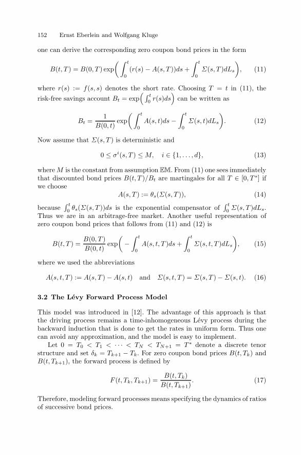
152 Ernst Eberlein and Wolfgang Kluge

one can derive the corresponding zero coupon bond prices in the form

B(t, T ) = B(0, T ) exp(∫ t

0

(r(s) −A(s, T ))ds +∫ t

0

Σ(s, T )dLs

), (11)

where r(s) := f(s, s) denotes the short rate. Choosing T = t in (11), therisk-free savings account Bt = exp

( ∫ t0 r(s)ds

)can be written as

Bt =1

B(0, t)exp(∫ t

0

A(s, t)ds −∫ t

0

Σ(s, t)dLs

). (12)

Now assume that Σ(s, T ) is deterministic and

0 ≤ σi(s, T ) ≤ M, i ∈ {1, . . . , d}, (13)

whereM is the constant from assumption EM. From (11) one sees immediatelythat discounted bond prices B(t, T )/Bt are martingales for all T ∈ [0, T ∗] ifwe choose

A(s, T ) := θs(Σ(s, T )), (14)

because∫ t0θs(Σ(s, T ))ds is the exponential compensator of

∫ t0Σ(s, T )dLs.

Thus we are in an arbitrage-free market. Another useful representation ofzero coupon bond prices that follows from (11) and (12) is

B(t, T ) =B(0, T )B(0, t)

exp(−∫ t

0

A(s, t, T )ds+∫ t

0

Σ(s, t, T )dLs

), (15)

where we used the abbreviations

A(s, t, T ) := A(s, T ) −A(s, t) and Σ(s, t, T ) = Σ(s, T )−Σ(s, t). (16)

3.2 The Levy Forward Process Model

This model was introduced in [12]. The advantage of this approach is thatthe driving process remains a time-inhomogeneous Levy process during thebackward induction that is done to get the rates in uniform form. Thus onecan avoid any approximation, and the model is easy to implement.

Let 0 = T0 < T1 < · · · < TN < TN+1 = T ∗ denote a discrete tenorstructure and set δk = Tk+1 − Tk. For zero coupon bond prices B(t, Tk) andB(t, Tk+1), the forward process is defined by

F (t, Tk, Tk+1) =B(t, Tk)B(t, Tk+1)

. (17)

Therefore, modeling forward processes means specifying the dynamics of ratiosof successive bond prices.

Calibration of Levy Term Structure Models 153

Let LT∗

be a time-inhomogeneous Levy process on a complete stochasticbasis (Ω,FT∗ ,F, PT∗). The probability measure PT∗ can be interpreted as theforward measure associated with the settlement date T ∗. The moment con-dition EM is assumed as before. The local characteristics of LT

∗are denoted

(bT∗, c, FT

∗). Two parameters, c and FT

∗, are free parameters, whereas the

drift characteristic bT∗

is chosen to guarantee that the forward process is amartingale. Because we proceed by backward induction, let us use the nota-tion T ∗

i := TN+1−i and δ∗i = δN+1−i for i ∈ {0, . . . , N + 1}. The followingingredients are needed.

(FP.1) For any maturity Ti there is a bounded, continuous, deterministicfunction λ(·, Ti) : [0, T ∗] → R

d that represents the volatility of theforward process F (·, Ti, Ti+1). We require for all k ∈ {1, . . . , N},

∣∣∣k∑

i=1

λj(s, Ti)∣∣∣ ≤ M (s ∈ [0, T ∗], j ∈ {1, . . . , d}), (18)

where M is the constant in assumption EM and λ(s, Ti) = 0 fors > Ti.

(FP.2) The initial term structure of zero coupon bond prices B(0, Ti), 1 ≤i ≤ N + 1, is strictly positive. Consequently, the initial values of theforward processes are given by

F (0, Ti, Ti+1) =B(0, Ti)B(0, Ti+1)

. (19)

We begin to construct the forward process with the longest maturity andpostulate

F (t, T ∗1 , T

∗) = F (0, T ∗1 , T

∗) exp(∫ t

0

λ(s, T ∗1 )dLT

∗s

). (20)

Now we choose bT∗

such that F (·, T ∗1 , T

∗) becomes a PT∗ -martingale. This isachieved via the following equation,∫ t

0

〈λ(s, T ∗1 ), bT

∗s 〉ds = −1

2

∫ t

0

〈λ(s, T ∗1 ), csλ(s, T ∗

1 )〉ds (21)

−∫ t

0

∫

Rd

(e〈λ(s,T∗

1 ),x〉 − 1 − 〈λ(s, T ∗1 ), x〉)νT

∗(ds, dx),

where νT∗(ds, dx) = FT

∗s (dx)ds is the PT∗ -compensator of the random mea-

sure of jumps μL given by the process LT∗. Using Lemma 2.6 in [17], one can

express the ordinary exponential (20) as a stochastic exponential, namely,

F (t, T ∗1 , T

∗) = F (0, T ∗1 , T

∗)Et(H(·, T ∗1 )),

154 Ernst Eberlein and Wolfgang Kluge

where

H(t, T ∗1 ) =∫ t

0

√csλ(s, T ∗

1 )dWT∗s

+∫ t

0

∫

Rd

(e〈λ(s,T∗

1 ),x〉 − 1)(μL − νT

∗)(ds, dx). (22)

Because F (·, T ∗1 , T

∗) is a martingale, we can define the forward martingalemeasure associated with the date T ∗

1 by setting

dPT∗1

dPT∗=

F (T ∗1 , T

∗1 , T

∗)F (0, T ∗

1 , T∗)

= ET∗1(H(·, T ∗

1 )). (23)

Using Girsanov’s theorem for semimartingales (see [16, Theorem III.3.24]),we can identify from (22) the predictable processes β and Y that describe themeasure change, namely,

β(s) = λ(s, T ∗1 ) and Y (s, x) = exp〈λ(s, T ∗

1 ), x〉.

Consequently WT∗1

t := WT∗t −∫ t0

√csλ(s, T ∗

1 )ds is a standard Brownian mo-tion under PT∗

1, and νT

∗1 (dt, dx) := exp〈λ(s, T ∗

1 ), x〉νT∗(dt, dx) is the PT∗

1-

compensator of μL.Now we construct the forward process F (·, T ∗

2 , T∗1 ) by postulating

F (t, T ∗2 , T

∗1 ) = F (0, T ∗

2 , T∗1 ) exp

(∫ t

0

λ(s, T ∗2 )dLT

∗1s

),

where

LT∗1t =∫ t

0

bT∗1s ds+

∫ t

0

√csdW

T∗1

s +∫ t

0

∫

Rd

x(μL − νT∗1 )(ds, dx).

The drift characteristic bT∗1 can be chosen in an analogous way as in (21), and

we define the next measure change from the resulting equation. Proceedingthis way, we get all forward processes in the form

F (t, T ∗i , T

∗i−1) = F (0, T ∗

i , T∗i−1) exp

(∫ t

0

λ(s, T ∗i )dL

T∗i−1s

), (24)

with

LT∗

i−1t =

∫ t

0

bT∗

i−1s ds +

∫ t

0

√csdW

T∗i−1

s +∫ t

0

∫

Rd

x(μL − νT∗i−1)(ds, dx). (25)

WT∗i−1 is here a PT∗

i−1-standard Brownian motion, and νT

∗i−1 is the PT∗

i−1-com-

pensator of μL given by

νT∗i−1(dt, dx) = exp

( i−1∑

j=1

〈λ(t, T ∗j ), x〉)FT

∗t (dx)dt. (26)

Calibration of Levy Term Structure Models 155

The drift characteristic bT∗i−1 satisfies

∫ t

0

〈λ(s, T ∗i ), b

T∗i−1s 〉ds = −1

2

∫ t

0

〈λ(s, T ∗i ), csλ(s, T ∗

i )〉ds (27)

−∫ t

0

∫

Rd

(e〈λ(s,T∗

i ),x〉 − 1 − 〈λ(s, T ∗i ), x〉)νT

∗i−1(ds, dx).

All driving processes LT∗i remain time-inhomogeneous Levy processes under

the corresponding forward measures, because they differ only by deterministicdrift terms.

3.3 The Levy LIBOR Model

This approach has been described in full detail in [12]; therefore, we justlist some of the properties. As in Section 3.2 the model is constructed bybackward induction along the discrete tenor structure and is driven by a time-inhomogeneous Levy process LT

∗, which is given on a complete stochastic

basis (Ω,FT∗ ,F, PT∗). As in the Levy forward process model, PT∗ should beregarded as the forward measure associated with the settlement day T ∗. LT

∗

is required to satisfy assumption EM and can be written in the form

LT∗

t =∫ t

0

bT∗

s ds +∫ t

0

√csdW

T∗s +∫ t

0

∫

Rd

x(μL − νT∗)(ds, dx), (28)

where νT∗(dt, dx) = FT

∗s (dx)dt is the compensator of μL. The ingredients

needed for the model are as follows.

(LR.1) For any maturity Ti, there is a bounded, continuous, deterministicfunction λ(·, Ti) : [0, T ∗] → R

d that represents the volatility of theforward LIBOR rate process L(·, Ti). In addition,

N∑

i=1

|λj(s, Ti)| ≤ M, s ∈ [0, T ∗], j ∈ {1, . . . , d},

where M is the constant from assumption EM and λ(s, Ti) = 0 fors > Ti.

(LR.2) The initial term structure B(0, Ti), 1 ≤ i ≤ N + 1, is strictly positiveand strictly decreasing (in i). Consequently, the initial term structureL(0, Ti) of forward LIBOR rates is given by

L(0, Ti) =1δi

(B(0, Ti)B(0, Ti+1)

− 1)> 0.

Now we can start the induction by postulating that

L(t, T ∗1 ) = L(0, T ∗

1 ) exp(∫ t

0

λ(s, T ∗1 )dLT

∗s

). (29)

156 Ernst Eberlein and Wolfgang Kluge

The drift characteristic bT∗

is chosen as in (21) to make this process a mar-tingale. Writing (29) as a stochastic exponential and exploiting the relationF (t, T ∗

1 , T∗) = 1 + δ∗1L(t, T ∗

1 ), one gets the dynamics in terms of the forwardprocess F (·, T ∗

1 , T∗). From this, the measure change can be done as in Section

3.2. As a result of the backward induction, one gets for each tenor time pointthe forward LIBOR rates in the form

L(t, T ∗j ) = L(0, T ∗

j ) exp(∫ t

0

λ(s, T ∗j )dL

T∗j−1s

)(30)

under the corresponding forward martingale measure PT∗j−1

. The successiveforward measures are related by the following equation,

dPT∗j

dPT∗j−1

=1 + δjL(T ∗

j , T∗j )

1 + δjL(0, T ∗j )

. (31)

The driving process LT∗j−1 in (30) has the canonical representation

LT∗

j−1t =

∫ t

0

bT∗

j−1s ds +

∫ t

0

√csdW

T∗j−1

s +∫ t

0

∫

Rd

x(μL − νT∗j−1)(ds, dx). (32)

WT∗j−1 is a PT∗

j−1-Brownian motion via

WT∗

j−1t = W

T∗j−2

t −∫ t

0

√csα(s, T ∗

j−1, T∗j−2)ds,

where

α(t, T ∗k , T

∗k−1) =

δ∗kL(t−, T ∗k )

1 + δ∗kL(t−, T ∗k )λ(t, T ∗

k ). (33)

Similarly νT∗j−1 is the PT∗

j−1-compensator of μL which is related to the PT∗

j−2-

compensator via

νT∗j−1 (ds, dx) = β(s, x, T ∗

j−1, T∗j−2)ν

T∗j−2 (ds, dx),

where

β(t, x, T ∗k , T

∗k−1) =

δ∗kL(t−, T ∗k )

1 + δ∗kL(t−, T ∗k )

(e〈λ(t,T∗

k ),x〉 − 1)

+ 1. (34)

The backward induction guarantees that zero coupon bond prices B(·, Tj)discounted by B(·, Tk) (i.e., ratios B(·, Tj)/B(·, Tk)) are PTk

-martingales forall j, k ∈ {1, . . . , N + 1}, and thus we have an arbitrage-free market. This fol-lows directly for successive tenor time points from the relation 1+ δL(t, Tj) =B(t, Tj)/B(t, Tj+1), because L(t, Tj) is by construction a PTj+1 -martingale.Expanding ratios with arbitrary tenor time points Tj and Tk into productsof ratios with successive time points, one gets the result from this specialcase. To see this, one has to use Proposition 3.8 in [16, p. 168], which is a

Calibration of Levy Term Structure Models 157

fundamental result for the analysis of all interest rate models where forwardmartingale measures are used.

Note that the driving processes LT∗

j−1t that are derived during the backward

induction are no longer time-inhomogeneous Levy processes. This is clear from(34), because due to the random term β(s, x, T ∗

j−1, T∗j−2), the compensator

νT∗j−1 is no longer deterministic. One can force the process β(·, x, T ∗

j−1, T∗j−2) to

become deterministic by replacing L(t−, T ∗k )/(1+δ∗kL(t−, T ∗

k )) by its startingvalue L(0, T ∗

k )/(1 + δ∗kL(0, T ∗k )) in (34). This approximation is convenient for

the implementation of the model, because then all driving processes are time-inhomogeneous Levy processes. Because the process Y (·, x), which is used inthe change from one compensator to the next in the forward process approach,is nonrandom, one can implement the model from Section 3.2 without anyapproximation.

4 Embedding of the Forward Process Model

In this section we show that the Levy forward process model can be seen as aspecial case of the Levy forward rate model. We choose the parameters of thelatter in such a way that we get the forward process specification as shown in(24)–(27). In the martingale case, which is defined by (14), according to (15),zero coupon bond prices can be represented in the form

B(t, T ) =B(0, T )B(0, t)

exp(∫ t

0

(θs(Σ(s, t)) − θs(Σ(s, T ))

)ds+∫ t

0

Σ(s, t, T )dLs

),

(35)where L is a time-inhomogeneous Levy process with characteristics (b, c, F )under the (spot martingale) measure P . L satisfies assumption EM andθs denotes the cumulant associated with the triplet (bs, cs, Fs). Recall thatΣ(s, T ) =

∫ Ts∧T σ(s, u)du.

The forward martingale measure PT∗i

associated with the settlement dateT ∗i is related to the spot martingale measure P via the Radon–Nikodym

derivativedPT∗

i

dP=

1BT∗

iB(0, T ∗

i )P -a.s.

Choosing T = t = T ∗i in (11), one gets immediately the representation

dPT∗i

dP= exp

(−∫ T∗

i

0

θs(Σ(s, T ∗i ))ds +

∫ T∗i

0

Σ(s, T ∗i )dLs

). (36)

Because σ and, therefore, Σ are deterministic functions, L is also a time-inhomogeneous Levy process with respect to PT∗

i, and its PT∗

i-characteristics

(bT∗i , cT

∗i , FT

∗i ) are given by

158 Ernst Eberlein and Wolfgang Kluge

bT∗

is = bs + csΣ(s, T ∗

i ) +∫

Rd

(e〈Σ(s,T∗

i ),x〉 − 1)x Fs(dx),

cT∗

is = cs, (37)

FT∗

is (dx) = e〈Σ(s,T∗

i ),x〉Fs(dx).

Because L is also a PT∗i-special semimartingale, it can be written in its PT∗

i-

canonical representation as

Lt =∫ t

0

bT∗

is ds +

∫ t

0

√csdW

T∗i

s +∫ t

0

∫

Rd

x(μL − ν T∗i )(ds, dx), (38)

where WT∗i is a PT∗

i-standard Brownian motion and where ν T

∗i (ds, dx) :=

FT∗

is (dx)ds is the PT∗

i-compensator of μL, the random measure associated

with the jumps of the process L.Using this representation in (35), we derive the forward process

F (t, T ∗i+1, T

∗i ) =

B(t, T ∗i+1)

B(t, T ∗i )

=B(0, T ∗

i+1)B(0, T ∗

i )exp(∫ t

0

(θs(Σ(s, T ∗

i )) − θs(Σ(s, T ∗i+1)))ds

+∫ t

0

Σ(s, T ∗i , T

∗i+1)dLs

)

= F (0, T ∗i+1, T

∗i ) exp

(I1t + I2

t +∫ t

0

√csΣ(s, T ∗

i , T∗i+1)dW

T∗i

s

+∫ t

0

∫

Rd

〈Σ(s, T ∗i , T

∗i+1), x〉

(μL − ν T

∗i)(ds, dx)

).

Here

I1t :=∫ t

0

(θs(Σ(s, T ∗

i )) − θs(Σ(s, T ∗i+1)))ds

=∫ t

0

[− 〈Σ(s, T ∗

i , T∗i+1), bs〉

+12〈Σ(s, T ∗

i ), csΣ(s, T ∗i )〉 − 1

2〈Σ(s, T ∗

i+1), csΣ(s, T ∗i+1)〉

+∫

Rd

(e〈Σ(s,T∗

i ),x〉− e〈Σ(s,T∗i+1),x〉+〈Σ(s, T ∗

i , T∗i+1), x〉

)Fs(dx)

]ds,

and making use of the first equation in (37),

Calibration of Levy Term Structure Models 159

I2t :=∫ t

0

〈Σ(s, T ∗i , T

∗i+1), b

T∗i

s 〉ds

=∫ t

0

[〈Σ(s, T ∗

i , T∗i+1), bs〉 + 〈Σ(s, T ∗

i , T∗i+1), csΣ(s, T ∗

i )〉

+∫

Rd

〈Σ(s, T ∗i , T

∗i+1), x〉

(e〈Σ(s,T∗

i ),x〉 − 1)Fs(dx)

]ds.

Summing up I1 and I2 yields

I1t + I2

t = −12

∫ t

0

〈Σ(s, T ∗i , T

∗i+1), csΣ(s, T ∗

i , T∗i+1)〉ds

−∫ t

0

∫

Rd

(e〈Σ(s,T∗

i ,T∗i+1),x〉 − 1 − 〈Σ(s, T ∗

i , T∗i+1), x〉

)FT∗

is (dx)ds.

Hence, the forward process is given by

F (t, T ∗i+1, T

∗i )

= F (0, T ∗i+1, T

∗i ) exp

(− 1

2

∫ t

0

〈Σ(s, T ∗i , T

∗i+1), csΣ(s, T ∗

i , T∗i+1)〉ds

−∫ t

0

∫

Rd

(e〈Σ(s,T∗

i ,T∗i+1),x〉 − 1 − 〈Σ(s, T ∗

i , T∗i+1), x〉

)FT∗

is (dx)ds

+∫ t

0

√csΣ(s, T ∗

i , T∗i+1)dW

T∗i

s

+∫ t

0

∫

Rd

〈Σ(s, T ∗i , T

∗i+1), x〉

(μL − ν T

∗i)(ds, dx)

).

Now we shall specify the model parameters, that is, the volatility σ and thecharacteristics (b, c, F ) of L, in such a way that the forward process dynamicsmatch the dynamics given in (24)–(27). First, we choose

Σ(s, T ∗i , T

∗i+1) = λ(s, T ∗

i+1).

This can be reached by setting

σ(s, u) := −N∑

i=0

1δ∗i+1

λ(s, T ∗i+1)1[T∗

i+1,T∗i )(u),

because

Σ(s, T ∗i , T

∗i+1) = −

∫ T∗i

T∗i+1

σ(s, u)du = λ(s, T ∗i+1).

Of course there are many other possibilities to specify σ. It could also bechosen to be continuous or smooth in the second variable.

Next, we specify the triplet (b, c, F ). bs can be chosen arbitrary. We setcs = cs and

160 Ernst Eberlein and Wolfgang Kluge

Fs(dx) = exp〈−Σ(s, T ∗), x〉FT∗s (dx), (39)

where FT∗

is the third characteristic of the driving process LT∗

in the Levyforward process model. Then using the third equation in (37),

FT∗

is (dx) = exp〈Σ(s, T ∗

i ) −Σ(s, T ∗), x〉FT∗s (dx)

= exp( i∑

j=1

〈Σ(s, T ∗j ) −Σ(s, T ∗

j−1), x〉)FT

∗s (dx)

= exp( i∑

j=1

〈λ(s, T ∗j ), x〉)FT

∗s (dx),

and we arrive at the forward process

F (t, T ∗i+1, T

∗i ) = F (0, T ∗

i+1, T∗i ) exp

(∫ t

0

λ(s, T ∗i+1)dL

T∗i

s

),

where

LT∗

it =∫ t

0

bT∗

is ds+

∫ t

0

√csdW

T∗i

s +∫ t

0

∫

Rd

x(μL − ν T∗i )(ds, dx).

The PT∗i-compensator ν T

∗i of μL is given by

ν T∗i (dt, dx) = exp

( i∑

j=1

〈λ(t, T ∗j ), x〉)FT

∗t (dx)dt,

and finally (bT∗is ) satisfies

∫ t

0

〈λ(s, T ∗i+1), b

T∗is 〉ds

= −12

∫ t

0

〈λ(s, T ∗i+1), csλ(s, T ∗

i+1)〉ds

−∫ t

0

∫

Rd

(e〈λ(s,T∗

i+1),x〉 − 1 − 〈λ(s, T ∗i+1), x〉

)ν T

∗i (ds, dx).

Remark 1. This embedding works only for driving processes that are time-inhomogeneous Levy processes. If both models are driven by a process withstationary increments (i.e., FT

∗s and Fs do not depend on s), in general we

cannot embed the forward process model in the forward rate model.

5 Calibration of the Levy Forward Rate Model

5.1 The Real-World Measure

In this section we consider the Levy forward rate model with a time-homogeneous driving process L; that is, L has stationary increments. The

Calibration of Levy Term Structure Models 161

goal is to estimate the parameters of the driving process under the real-worldmeasure. For this purpose, we use market data of discount factors (zero couponbond prices) for one year up to ten years, quoted between September 17, 1999,and September 17, 2001 (i.e., for 522 trading days).

The parameter estimation in the forward rate model is substantially moredifficult than in a stock price model. The reason is that we have a numberof different assets, namely ten bonds in the case of our data set (in theory ofcourse an infinite number), but only one driving process. Therefore, we haveto find a way to extract the parameters of the driving process from the logreturns of all ten bond prices.

Let us start by considering the logarithm of the ratio between the bondprice and its forward price on the day before; that is,

LR(t, T ) := logB(t + 1, t+ T )B(t, t + 1, t+ T )

.

Here, B(t, t+1, t+T ) is the forward price of B(t+1, t+T ) at time t; that is,

B(t, t + 1, t+ T ) :=B(t, t + T )B(t, t + 1)

.

We call LR the daily log return. Using (15), we get

LR(t, T ) = logB(t + 1, t+ T ) − logB(t, t+ T ) + logB(t, t + 1)

= −∫ t+1

t

A(s, t + 1, t+ T )ds+∫ t+1

t

Σ(s, t+ 1, t+ T )dLs. (40)

In what follows, we consider for simplicity the Ho–Lee volatility structure,that is, Σ(s, T ) = σ(T−s) for a constant σ, which we set equal to one withoutloss of generality. Similar arguments can be carried out for other stationaryvolatility structures, such as the Vasicek volatility function. By stationary, wemean that Σ(s, T ) depends only on (T −s). We assume that the drift termalso satisfies some stationarity condition, namely,

A(s, T ) = A(0, T−s) for s ≤ t.

In the risk-neutral case given by (14), this stationarity follows from the sta-tionarity of the volatility function Σ(s, T ). We get

−∫ t+1

t

A(s, t + 1, t+ T )ds = −∫ 1

0

A(s, 1, T )ds =: d(T ), (41)

independent of t and∫ t+1

t

Σ(s, t+ 1, t+ T )dLs = (T−1)(Lt+1 − Lt).

162 Ernst Eberlein and Wolfgang Kluge

Fig. 1. Negative logarithms of bond prices on September 17, 1999 and interpolatingcubic spline.

Consequently,LR(t, T ) = d(T ) + c(T )Yt+1, (42)

where c(T ) := (T−1) is deterministic and

Yt+1 := Lt+1 − Lt ∼ L1

is Ft+1-measurable and does not depend on T .To estimate the parameters of the driving process, we first determine the

daily log returns; that is, for k ∈ {0, 1, . . . , 520}, n ∈ {1, . . . , 10},

LR(k, k + (n years)) = logB(k + 1, k + (n years)) + logB(k, k + 1)

B(k, k + (n years)).

Unfortunately, we can only get B(k, k+(n years)) directly from our data set.To determine B(k+1, k+(n years)) and B(k, k+1), we use an idea developedin [22, Section 5.3] and interpolate the negative of the logarithm of the bondprices with a cubic spline. We do this procedure separately for each day of thedata set. Figure 1 shows the interpolation for the first day (even for maturitiesup to 30 years).

Calibration of Levy Term Structure Models 163

Table 1. Estimated parameters of the distribution L1 under the measure P .

α β δ μ λ Method

1474224 -34659 1.1892e-12 7.5642e-08 2.37028 Max-Likelihood (GH)

590033 -14 1.3783e-06 3.2426e-11 -0.5 Max-Likelihood (NIG)

1195475 -114855 2.5614e-06 2.4723e-07 -0.5 Moments (NIG)

Because E[L1] = 0, we know that

LR(t, T ) − E[LR(t, T )] = (T−1)Yt+1; (43)

that is, the centered log returns are affine linear in T . Moreover, Y1, Y2,. . . , Y521 are independent and equal to L1 in distribution. The correspondingsamples y1, y2, . . . , y521 could be calculated for a fixed n ∈ {1, 2, . . . , 10} via

yk+1 :=LR(k, k + (n years)) − xn

(n years) − 1, with (44)

xn :=1

521

520∑

k=0

LR(k, k + (n years)). (45)

However, inasmuch as the centered empirical log returns LR(k, k+(n years))−xn are not exactly affine linear in n (compare Figure 2), the yk+1 in (44) wouldthen depend on n. Remember that the distribution of L1 in the Levy forwardrate model does not depend on the time to maturity of the bonds. Therefore,we take a different approach and use the points

((1 year)−1, LR(k, k+(1 year))−x1), . . . , ((10 years)−1, LR(k, k+(10 years))−x10)

for a linear regression through the origin. The gradient of the straight lineyields the value for yk+1. Figure 2 shows the centered empirical log returns andthe regression line for the first day of the data set. Repeating this procedure foreach day provides us with the samples y1, y2, . . . , y521, which can now be usedto estimate the parameters of L1 by using maximum likelihood estimation.

The parametric class of distributions we use here are generalized hyper-bolic distributions (see, e.g., [5]) or subclasses such as hyperbolic [7] or normalinverse Gaussian (NIG) distributions [2]. The resulting densities for our dataset are shown in Figure 3. Figure 4 shows the same densities on a log-scale,which allows us to see the fit in the tails. The estimated distribution param-eters corresponding to the densities in Figure 3 are given in Table 1.

One of the densities in Figures 3 and 4 was estimated using the methodof moments. This is a somewhat simpler approach where one exploits therelation between moments of order i and the ith cumulant (see [1, 26.1.13 and26.1.14]). Because for generalized hyperbolic distributions the cumulants areexplicitly known, one can express the moments (up to order 4) as functions ofthe distribution parameters λ, α, β, δ, and μ. Applying the usual estimatorsfor moments, one obtains the parameters.

164 Ernst Eberlein and Wolfgang Kluge

Fig. 2. Centered empirical log returns and regression line for the first day of thedata set.

5.2 The Risk-Neutral Measure

There are very liquid markets for the basic interest rate derivatives such ascaps, floors, and swaptions. Therefore, market prices for these instruments—typically quoted in terms of their (implied) volatilities with respect to thestandard Gaussian model—contain a maximum of information. A cap is aseries of call options on subsequent variable interest rates, namely LIBORrates. Each option is called a caplet. It is easy to see that the payoff of acaplet can be expressed as the payoff of a put option on a zero coupon bond.In the same way a floor is a series of floorlets, and each floorlet is equivalentto a call option on a bond. Thus to price a floorlet one has to price a callon a bond. According to the general no-arbitrage valuation theory, the time-0-value of a call with strike K and maturity t on a bond with maturity Tis

C0(t, T,K) := E

[1Bt

(B(t, T ) −K)+], (46)

where the expectation is taken with respect to the risk-neutral measure (spotmartingale measure). Because one would need the joint distribution of Bt

Calibration of Levy Term Structure Models 165

Fig. 3. Densities of empirical and estimated distributions.

and B(t, T ) to evaluate this expectation, it is more efficient to express thisexpectation with respect to the forward measure associated with time t. Onethen gets

C0(t, T,K) = B(0, t)EPt [(B(t, T ) −K)+]. (47)

Once one has numerically efficient algorithms to compute these expectations,one can calibrate the model by minimizing the differences between modelprices and market quotes simultaneously across all available option maturitiesand strikes. This has been described in detail in [8].

Let us mention that in the stationary case, one can derive risk-neutralparameters from the real-world parameters, which we estimated in Section5.1. Because of the martingale drift condition (14), we get from (41)

d(T ) =∫ 1

0

(A(s, 1) −A(s, T ))ds =∫ 1

0

(θ(Σ(σ, 1)) − θ(Σ(s, T )))ds, (48)

where θ is the logarithm of the moment generating function of L(L1) underthe risk-neutral measure. By stationarity L(Yn+1) = L(L1) and E[L1] = 0,therefore, (42) implies

E[LR(t, T )] = d(T ). (49)

The arithmetic mean of the empirical log returns (45) is an estimator for theexpectation on the left side. By a minimization procedure, one can now extract

166 Ernst Eberlein and Wolfgang Kluge

Fig. 4. Log-densities of empirical and estimated distributions.

the distribution parameters of L(L1), which are implicit on the right-hand sideof (48) from this equation.

In the case of generalized hyperbolic Levy processes as driving processes,it is known from [22] that the parameters μ and δ do not change when oneswitches from the real-world to the risk-neutral distribution. Therefore, onehas only to extract the remaining parameters λ, α, β via minimization of thedistance between average log returns and the integral on the right side in (48).

It is clear that due to the highly liquid market in interest rate derivatives,the direct fit to market quotes as described at the beginning of this sectionprovides more reliable calibration results than the derivation from real-worldparameters. It will, therefore, be preferred by practitioners.

6 Calibration of Forward Process and LIBOR Models

Recall that a cap is a sequence of call options on subsequent LIBOR rates.Each single option is called a caplet. Let a discrete tenor structure 0 = T0 <T1 < · · · < Tn+1 = T ∗ be given as before. The time-Tj payoff of a caplet thatis settled in arrears is

Nδj−1(L(Tj−1, Tj−1) −K)+, (50)

Calibration of Levy Term Structure Models 167

where K is the strike and N the notional amount, which we assume to be 1.The corresponding payoff of a floorlet settled in arrears is

Nδj−1(K − L(Tj−1, Tj−1))+. (51)

The time-t price of the cap is then

Ct(K) =N+1∑

j=1

B(t, Tj)EPTj

[δj−1(L(Tj−1, Tj−1) −K)+|Ft

]. (52)

Given this formula, the LIBOR model is the natural approach to price caps,because then the LIBOR rates L(Tj−1, Tj−1) are given in the simple form (30)with respect to the forward martingale measure PTj .

Numerically efficient ways based on bilateral Laplace transforms to eval-uate the expectations in (52) are described in [12]. For numerical purposes,the nondeterministic compensators that arise during the backward inductionin the Levy LIBOR model can be approximated by deterministic ones. Con-cretely, the stochastic ratios δjL(s−, Tj)/(1 + δjL(s−, Tj)) are replaced bytheir deterministic initial values δjL(0, Tj)/(1 + δjL(0, Tj)). An alternativeapproximation method, which is numerically much faster, is described in [18,Section 3.2.1].

Instead of basing the pricing on the LIBOR model, one can use the forwardprocess approach outlined in Section 3.2. It is then more natural to write thecaplet payoff (50) in the form

(1 + δj−1L(Tj−1, Tj−1) − Kj−1

)+, (53)

where Kj−1 = 1+δj−1K. Because 1+δj−1L(Tj−1, Tj−1) = F (Tj−1, Tj−1, Tj),the pricing formula is then instead of (52)

Ct(K) =N+1∑

j=1

B(t, Tj)EPTj

[(F (Tj−1, Tj−1, Tj) − Kj−1)+|Ft

]. (54)

The implementation of this approach leads to a much faster algorithm,inasmuch as the backward induction is more direct in the case of the forwardprocess model. Also, any approximation can be avoided here.

In the implementations, we use mildly time-inhomogeneous Levy pro-cesses, namely those that are piecewise homogeneous Levy processes. In orderto catch the term structure of smiles, which one sees in implied volatilitysurfaces (see [8, Figure 1]), with sufficient accuracy, typically three Levy pa-rameter sets are needed: one Levy process corresponding to short maturitiesup to one year roughly, a second one for maturities between one and five years,and a third Levy process corresponding to long maturities from five to tenyears. Instead of predetermining the breakpoints where the Levy parameterschange, one can actually include the choice of the breakpoints in the estimationprocedure. These random breakpoints improve the calibration results further.

168 Ernst Eberlein and Wolfgang Kluge

0.1

1.1

2.1 0 1 2 3 4 5 6 7 8 9 10

0

1

2

3

4

Time to Maturity (years)

Parameter b

Fig. 5. A variety of shapes for the instantaneous volatility curve produced by (55)with a = 1, b ∈ [0.1, 2.1], c = 0.1 (source: [19]).

According to (FP.1) and (LR.1), a volatility structure has to be chosenin both models. In [3], a broad spectrum of suitable volatility structures isdiscussed, which can be used in the forward process or the LIBOR model.A sufficiently flexible structure is given by

λ(t, Tj) = a(Tj − t) exp(−b(Tj − t)) + c, (55)

with three parameters a, b, c. Note that we consider one-dimensional processesand consequently also scalar volatility functions in all calibrations. Figure 5shows a variety of shapes produced by formula (55).

Without loss of generality one can set a = 1, because this parametercan be included in the specification of the Levy process. To see this, takefor example a Levy process L generated by a normal inverse Gaussian dis-tribution; that is, L(L1) = NIG(α, β, δ, μ) and a �= 1. Define L = aL andλ(t, T ) = λ(t, T )/a; then (cf., e.g., [5]) L(L1) = NIG(α/|a|, β/|a|, |a|δ, aμ) and∫ t0λ(s, T )dLs =

∫ t0λ(s, T )dLs. Thus, the model (λ, L) is exactly of the same

type with parameter a = 1.For the driving process L, we consider one-dimensional processes generated

by generalized hyperbolic distributions GH(λ, α, β, δ, μ), or subclasses such asthe hyperbolic, where λ = 1, or normal inverse Gaussian distributions, whereλ = − 1

2 . The generalized hyperbolic distribution is given by its characteristicfunction

Calibration of Levy Term Structure Models 169

2.5% 3.5% 4.5% 5.5% 7.0% 9.0%

1 2

34

5 6

78

910

0.0%

2.0%

4.0%

6.0%

8.0%

10.0%

12.0%

14.0%

16.0%

Strike Rate

Maturity (years)

Fig. 6. Data set I. Absolute errors of EUR caplet calibration: forward process model(source: [19]).

ΦGH(u) = eiμu(

α2 − β2

α2 − (β + iu)2

)λ/2Kλ(δ√α2 − (β + iu)2)

Kλ(δ√α2 − β2)

, (56)

where Kλ denotes the modified Bessel function of the third kind with indexλ. For normal inverse Gaussian distributions, this simplifies to

ΦNIG(μ) = eiμuexp(δ√α2 − β2)

exp(δ√α2 − (β + iu)2)

. (57)

The class of generalized hyperbolic distributions is so flexible that onedoes not have to consider higher-dimensional driving processes. Note that itwould not be appropriate to classify a model driven by a one-dimensional Levyprocess as a one-factor model, because the driving Levy process itself is alreadya high-dimensional object. The notion of an x-factor model (x = 1, 2, . . . , n)should be reserved for the world of classical Gaussian models.

To extract the model parameters from market quotes, one considers foreach caplet the (possibly squared) difference between the market and modelprice. The objective function to be minimized is then the weighted sum overall strikes and over all caplets along the tenor structure. A possible choice ofweights would be the at-the-money prices for the respective maturity. Figure6 shows how close one gets to the empirical volatility surface on the basis ofthe forward process model. The figure shows the absolute difference betweenmodel and market prices expressed in volatilities. For the relevant part of the

170 Ernst Eberlein and Wolfgang Kluge

2.5% 3.5% 4.5% 5.5% 7.0% 9.0%

12

34

56

78

910

0.0%

1.0%

2.0%

3.0%

4.0%

5.0%

6.0%

7.0%

Strike Rate

Maturity (years)

Fig. 7. Data set I. Absolute errors of EUR caplet calibration: LIBOR rate model(source: [19]).

moneyness–maturity plane the differences are below 1%. The large deviationsat the short end are of no importance, because the one-year caplet prices are ofthe order of magnitude 10−9 for the strike rates 8, 9, and 10%. The underlyingdata set consists of cap prices in the Euro market on February 19, 2002. Thedifferences one gets for the same data set on the basis of the Levy LIBORmodel are shown in Figure 7.

Comparing the two calibration results, one sees that the forward processapproach yields a more accurate fit than the LIBOR approach. In [10], boththe Levy LIBOR as well as the Levy forward process approach have beenextended to a multicurrency setting, which takes the interplay between inter-est rates and foreign exchange rates into account. This model is also drivenby a single time-inhomogeneous Levy process, namely the process that drivesthe most distant forward LIBOR rate (or forward process) in the domesticmarket. Implementation of this sophisticated model was tested for up to threecurrencies (EUR, USD, and GBP).

Acknowledgments

Wolfgang Kluge has been partially supported by a grant from the DeutscheForschungsgemeinschaft (DFG). We would like to thank N. Koval for provid-ing some of the figures in Section 6.

Calibration of Levy Term Structure Models 171

References

1. M. Abramowitz and I.A. Stegun. Handbook of Mathematical Functions. Dover,1968.

2. O.E. Barndorff-Nielsen (1998). Processes of normal inverse Gaussian type. Fi-nance and Stochastics, 2:41–68, 1998.

3. D. Brigo and F. Mercurio. Interest Rate Models: Theory and Practice. Springer,2001.

4. P. Carr, H. Geman, D. Madan, and M. Yor. The fine structure of asset returns:An empirical investigation. Journal of Business, 75:305–332, 2002.

5. E. Eberlein. Application of generalized hyperbolic Levy motions to finance. LevyProcesses: Theory and Applications, eds. O.E. Barndorff-Nielsen, T. Mikosch,and S. Resnick, Birkhauser Verlag, 319–337, 2001.

6. E. Eberlein, J. Jacod, and S. Raible. Levy term structure models: No-arbitrageand completeness. Finance and Stochastics, 9:67–88, 2005.

7. E. Eberlein and U. Keller (1995). Hyperbolic distributions in finance. Bernoulli,1:281–299, 1995.

8. E. Eberlein and W. Kluge. Exact pricing formulae for caps and swaptions ina Levy term structure model. Journal of Computational Finance, 9(2):99–125,2006.

9. E. Eberlein and W. Kluge. Valuation of floating range notes in Levy term struc-ture models. Mathematical Finance, 16:237–254, 2006.

10. E. Eberlein and N. Koval. A cross-currency Levy market model. QuantitativeFinance, 6(6):465–480, 2006.

11. E. Eberlein and F. Ozkan. The defaultable Levy term structure: Ratings andrestructuring. Mathematical Finance, 13:277–300, 2003.

12. E. Eberlein and F. Ozkan. The Levy LIBOR model. Finance and Stochastics,9:327–348, 2005.

13. E. Eberlein and K. Prause. The generalized hyperbolic model: Financial deriva-tives and risk measures. Mathematical Finance – Bachelier Congress 2000, eds.H. Geman, D. Madan, S. Pliska, and T. Vorst, Springer, 2002.

14. E. Eberlein and S. Raible. Term structure models driven by general Levy pro-cesses. Mathematical Finance, 9:31–53, 1999.

15. E. Heath, R.A. Jarrow, and A. Morton. Bond pricing and the term structure ofinterest rates: A new methodology for contingent claims valuation. Economet-rica, 60:77–105, 1992.

16. J. Jacod and A.N. Shiryaev. Limit Theorems for Stochastic Processes, 2nd edi-tion, Springer, 2003.

17. J. Kallsen and A.N. Shiryaev. The cumulant process and Esscher’s change ofmeasure. Finance and Stochastics, 6:397–428, 2002.

18. W. Kluge. Time-Inhomogeneous Levy Processes in Interest Rate and Credit RiskModels. Ph.D. thesis, University of Freiburg, Germany, 2005.

19. N. Koval. Time-Inhomogeneous Levy processes in Cross-currency Market Mod-els. Ph.D. thesis, University of Freiburg, Germany, 2005.

20. D.B. Madan and F. Milne. Option pricing with VG martingale components.Mathematical Finance, 1(4):39–55, 1991.

21. D.B. Madan and E. Seneta. The variance gamma (V.G.) model for share marketreturns. Journal of Business, 63:511–524, 1990.

22. S. Raible. Levy Processes in Finance: Theory, Numerics, and Empirical Facts.Ph.D. thesis, University of Freiburg, Germany, 2000.

172 Ernst Eberlein and Wolfgang Kluge

23. W. Schoutens. Meixner processes in finance. Report 2001-002, EURANDOM,Eindhoven, 2001.

24. W. Schoutens. Levy Processes in Finance: Pricing Financial Derivatives. Wiley,2003.

Pricing of Swaptions in Affine Term Structureswith Stochastic Volatility

Massoud Heidari,1 Ali Hirsa,1 and Dilip B. Madan2

1 Caspian Capital Management, LLC745 Fifth AvenueNew York, NY 10151, USAmassoud.heidari@ixis-ccm.com; ali.hirsa@ixis-ccm.com

2 Robert H. Smith School of BusinessDepartment of FinanceUniversity of MarylandCollege Park, MD 20742, USAdbm@rhsmith.umd.edu

Summary. In an affine term structure framework with stochastic volatility, wederive the characteristic function of the log swap rate. Having the characteristicfunction, we employ the fast Fourier transform (FFT) to price swaptions. Using tenyears of swap rates and swaption premiums, model parameters are estimated us-ing a square-root unscented Kalman filter. We investigate the relationship betweenmodel premiums and interest rate factors, as well as between market premiums andinterest factors, to conclude that long-dated swaptions are highly correlated to theshape of the curve.

Key words: Affine term structure models; characteristic function; fast Fouriertransform (FFT); swaptions; straddles.

1 Introduction

Although there exist closed-form and/or efficient approximate solutions forpricing swaptions in Heath–Jarrow–Morton (HJM [8]) and market (e.g., BGM[2]) models, these models have the following shortcomings: (a) the yield curveis exogenous to the model and the volatility structure constrains the shape ofthe yield curve, and (b) they are generally overparameterized. These classesof models are typically used for marking and risk management, and are greattools for interpolation–extrapolation purposes. In current application, thesemodels are calibrated on a daily or a weekly basis.

In contrast to HJM or BGM models, affine term structure models (ATSMs)[6] are parsimonious, and the yield curve is endogenous to the model. Affine

174 Massoud Heidari, Ali Hirsa, and Dilip B. Madan

parameters can be estimated via filtering methods, and the need for updatingis infrequent. This makes ATSMs ideal for analyzing the cross-properties ofswap rates and swaptions.

Pricing swaptions in an affine framework with constant volatility datesback to the work by Munk [9], based on the assumption that the price of aEuropean option on a coupon bond (European swaption) is approximatelyproportional to the price of a European option on a zero coupon bond withmaturity equal to the stochastic duration of the coupon bond. In [5], theauthors perform an approximation based on an Edgeworth expansion of thedensity of the coupon bond price. This requires the calculation of the momentsof the coupon bond through the joint moments of the individual zero couponbonds. Singleton and Umanstev [11] price swaptions based on approximationof the exercise region in the space of the underlying factors by line segments.Finally, Schrager and Pelsser’s approximation [10] is based on the derivationof approximate dynamics in which the volatility of the forward swap rate isitself an affine function of the factors.

To check the approximation method for swaption premiums in [10] forconstant volatility, we implemented the methodology and compared the ap-proximate premiums against simulated ones for 12 different swaptions (1× 2,1× 5, 1× 10, 2× 2, 2× 5, 2× 10, 5× 2, 5× 5, 5× 10, 10× 2, 10× 5, 10× 10).For 1,000,000 simulated paths, the absolute value of the largest relative errorwas less than 0.35%.

Our focus in this paper is on pricing swaptions in an affine term structuresetting with stochastic volatility. Using the Schrager and Pelsser approxima-tion [10], we derive the characteristic function of the log swap rate under theswap measure, and then employ the fast Fourier transform (FFT) to priceswaptions. This efficient method enables us to price ATSM swaps and swap-tions simultaneously and consistently. We use ten years of swap rates andswaption premiums to estimate model parameters via a square-root unscentedKalman filter. Time series of the interest rate factors are a byproduct of theestimation procedure. We then look more closely at the relationship betweenmodel premiums and interest rate factors, as well as between market premi-ums and interest factors, to conclude that long-dated swaptions are highlycorrelated with the slope of the yield curve.

2 Affine Term Structure Models with StochasticVolatility

We are interested in a stochastic interest rate model with stochastic volatility.Using an affine structure for interest rates, the short rate is specified as

rt = ar + b�r xt,

where rt and xt are n-dimensional vectors, with n the number of factors inthe model, and xt follows the matrix Ornstein–Uhlenbeck equation driven by

Pricing of Swaptions in Affine Term Structures 175

Brownian noise, that is,

dxt = (−bγ −Bxt)dt +ΣdWt,

where {Wt} is an n-dimensional vector of independent standard Brownianmotion and Σ is the (constant) n× n volatility matrix. In general, the n× nmatrix B may be full, with all eigenvalues having positive real part.

To incorporate stochastic volatility, we introduce the square root equationfor (scalar) variance vt, and write

dvt = κ(θ − vt)dt + λ√vtdZt,

where {Zt} is a standard Brownian motion, with the correlation between {Wt}and {Zt} denoted by the vector ρ. We now reformulate the equation for xt as

dxt = (−bγ −Bxt)dt +Σ√vtdWt.

3 Swaption Problem Formulation

Let S denote the start time of the interest rate swap, T the end time of theswap, and t denote a time between the present time 0 and S, so t < S < T.Suppose fixed payments occur at times Tj, n < j ≤ N, where TN = T . DefineTn = S, and let Δj = Tj − Tj−1 be the interval between swap times. Forsimplicity, assume that the Δs are constant; that is, Δj = Δ for all j.

The forward swap rate at time t is

kS,Tt =P (t, S) − P (t, T )

Δ∑N

j=n+1 P (t, Tj). (1)

The present value of a swaption struck at the rate K is

V (K) =

⎛

⎝ΔN∑

j=n+1

P (0, Tj)

⎞

⎠E[(kS,TS −K)+],

under the swap measure. The swaption pricing problem is to evaluate theexpectation under the given interest rate model.

4 The Characteristic Function Pricing Method

The characteristic function pricing method values options using the charac-teristic function of the underlying process. For ease of notation, define theconstant c = Δ

∑Nj=n+1 P (0, Tj), let X denote the random variable ln kS,TS ,

let f be the probability density function of X under the swap measure, andk = lnK. With this new notation,

176 Massoud Heidari, Ali Hirsa, and Dilip B. Madan

V (k) = cE[(eX − ek)+].

Denote the Fourier transform of eαkV (k) by Ψ(·), where the term α > 0 is adamping factor, which is included so that the Fourier integral is well defined.Thus,

Ψ(ν) =∫ ∞

−∞V (k)e(α+iν)kdk

= c

∫ ∞

−∞

∫ ∞

k

(ex − ek)e(α+iν)kf(x)dxdk

= c

∫ ∞

−∞

∫ x

−∞(ex − ek)e(α+iν)kdkf(x)dx

=c

(α + iν)(α + 1 + iν)

∫ ∞

−∞ei(ν−i(α+1))xf(x)dx.

Let c2 = c/[(α+ iν)(α + 1 + iν)] and u = ν − i(α + 1) to get

Ψ(ν) = c2E[eiuX ] = c2E[eiu ln kS,T

S

],

where E[eiu ln kS,TS ] is the characteristic function of ln kS,TS . If the characteristic

function is known, then so is Ψ(ν), and the price of the swaption can beobtained by taking the inverse Fourier transform

V (K) = e−α lnK 12π

∫ ∞

−∞Ψ(ν)e−iν lnKdν.

(Note that we have interchangeably denoted the argument of V as k and K.)

4.1 Fast Fourier Transform

The inverse transform can be evaluated numerically using the FFT, where theresulting integral can be discretized using Simpson’s rule. Choose B >> 1, fixthe number of time steps m, and let h = B/m. Then

ψ(t) ≡ 12π

∫ ∞

−∞Ψ(ν)e−iνkdν ≈ Re

{1π

∫ B

0

Ψ(ν)e−iνkdν

}

≈ Re

{h

3π

m∑

l=1

Ψ((l − 1)h)e−i(l−1)hk(3 + (−1)l − δl−1)

}.

Next, consider the discrete times tj , 0 ≤ j ≤ m− 1, where

tj = (j − 1)λ+A.

The parameter λ is chosen so that λh = 2π/m, and A is chosen so thattm−1 = t = lnK, namely A = lnK − (m− 1)λ. Then

Pricing of Swaptions in Affine Term Structures 177

ψ(tj) = Re

{m∑

k=1

e−i(2π/m)(j−1)(k−1)X(k)

},

where we have let

X(k) =h

3πΨ((k − 1)h)e−i(k−1)hA(3 + (−1)k − δk−1).

Thus, {ψ(tj)} (which includes ψ(t)) can be obtained by taking the real partof the FFT of {X(k)}.

5 Computing the Characteristic Function

One of the main contributions of this paper is the derivation of the character-istic function E[eiu ln kS,T

S ] under the swap measure. The paper proceeds in twomajor steps. First, the bond prices {P (t, Tj)} are derived. This is necessarybecause kS,Tt is a function of the bond prices. Then the main task of findingthe characteristic function is undertaken.

5.1 Bond Prices

First, define two new variables, yt and wt, in terms of xt and vt:

yt =∫ t

0

xsds,

wt =∫ t

0

vsds.

Next, define the joint characteristic function of (x, v, y, w) at time 0 for fixedtime T as

φ(0, ξ, ζ, ω, ϕ) = E[exp(iξ�xT + iζ�yT + iωvT + iϕwT

) ∣∣ x0 = x, v0 = v],

where (ξ, ζ, ω, ϕ) are the transform variables. More generally, define the char-acteristic function at time t, 0 < t < T , as

φ(t, ξ, ζ, ω, ϕ) = E

[exp

(iξ�xt + iζ�

∫ T

t

xsds+ iωvt + iϕ

∫ T

t

vsds

)

∣∣∣∣∣ xt = x, vt = v

]. (2)

It is conjectured that the characteristic function at time 0 has a solution ofthe form

φ(0, ξ, ζ, ω, ϕ) = exp(−a(T )− b(T )�x− c(T )v

).

178 Massoud Heidari, Ali Hirsa, and Dilip B. Madan

Therefore, by the Markov property, it must be the case that

φ(t, ξ, ζ, ω, ϕ) = exp(−a(T − t) − b(T − t)�x− c(T − t)v

). (3)

In the next subsection, it is shown how to compute this characteristic function,or a(·), b(·), and c(·).

To compute bond prices, note that the bond price P (t, T ) is

P (t, T ) = E

[exp

(−∫ T

t

rsds

)]= E

[exp

(−ar(T − t) − bTr

∫ T

t

xsds

)]

= e−ar(T−t)E

[exp

(−bTr∫ T

t

xsds

)]= e−ar(T−t)φ(t, 0, ibr, 0, 0).

This corresponds to Equation (2) with (ξ, ζ, ω, ϕ) = (0, ibr, 0, 0). Thus,

P (t, T ) = e−ar(T−t) exp(− a(T − t, 0, ibr, 0, 0) − b(T − t, 0, ibr, 0, 0)�x

− c(T − t, 0, ibr, 0, 0)v). (4)

Here we are explicitly showing the dependence of a(·), b(·), and c(·) on(ξ, ζ, ω, ϕ); that is, a(t) = a(t, ξ, ζ, ω, ϕ) and so on.

Computing a(·), b(·), and c(·)The first thing to note is that evaluating Equation (3) at t = T gives thefollowing boundary conditions,

a(0) = 0,

b(0) = −iξ,c(0) = −iω.

The second is that the function G(t) defined as

G(t) = exp(iζT∫ t

0

xsds + iϕ

∫ t

0

vsds

)φ(t, ξ, ζ, ω, ϕ),

is equal toE[H(T )|Ft],

with

H(T ) = exp

(iξTxt + iζT

∫ T

0

xsds + iωvt + iϕ

∫ T

0

wsds

).

Pricing of Swaptions in Affine Term Structures 179

Thus, for any t1 < t2,

E [G(t2)|Ft1 ] = E [E(H(T )|Ft2)|Ft1 ] = E [H(T )|Ft1 ] = G(t1);

that is, G(t) is a martingale.Because G(t) is a martingale, its derivative with respect to time (the dt

term) must be identically 0. This leads to the expression

0 = (iζTx+ iϕv)φ + φt + φx(−bγ −Bx) + φv(κ(θ − v))

+12Trace(φxxΣΣT v) +

12φvvλ

2v + λρTΣTφvxv.

We can use Equation (2) to solve for the derivatives of φ to get

0 = φ{iζTx+ iϕv + a′(T − t) + b′(T − t)Tx+ c′(T − t)v

− bT (T − t)(−bγ −Bx) − (κ(θ − v))c(T − t)

+12bT (T − t)ΣΣT b(T − t)v +

12λ2vc(T − t)2 + λρTΣT b(T − t)c(T − t)v

}.

Because this equation must hold for all (x, v), we get three simpler equationsby grouping the x terms, the v terms, and the remaining terms:

a′(τ) = −bT (τ)bγ + κθc(τ), (5)b′(τ) = −iζ −BT b(τ), (6)

c′(τ) = −iϕ− (κ+ λρTΣT b(τ))c(τ) − 12bT (τ)ΣΣT b(τ) − λ2

2c2(τ), (7)

where τ = T − t.We now have a set of equations, which are satisfied by a(·), b(·), and

c(·). These ordinary differential equations (ODEs) are referred to as Riccatiequations. The Riccati equations together with the boundary conditions com-pletely characterize a(·), b(·), and c(·). Note that the ODE for b(·) is linearand has a known analytical solution. In stock models, b′ = 0 and b is a con-stant, as there is no dependence of log stock on the state variable of log stock.Here we have a dependence of state variable drifts on the state variables, andthis introduces −BT b and the associated additional structure to the equation.Also in stock, we have integrated vol but no interest in integrated log stock,but now we are interested in the integral of xt, and this introduces iζ.

b(τ) = − exp(−BT τ)iξ − (BT )−1(I − exp(−BT τ))iζ,

where we employ a matrix exponential of the full matrix BT .We next have to solve the following ODEs for c and a.

c′(τ) = −iϕ−(κ + λρ�Σ�b(τ)

)c(τ) − 1

2b�(τ)ΣΣ�b(τ) − λ2

2c2(τ),

a′(τ) = −b�(τ)bγ + κθc(τ).

The two ODEs can be solved numerically.

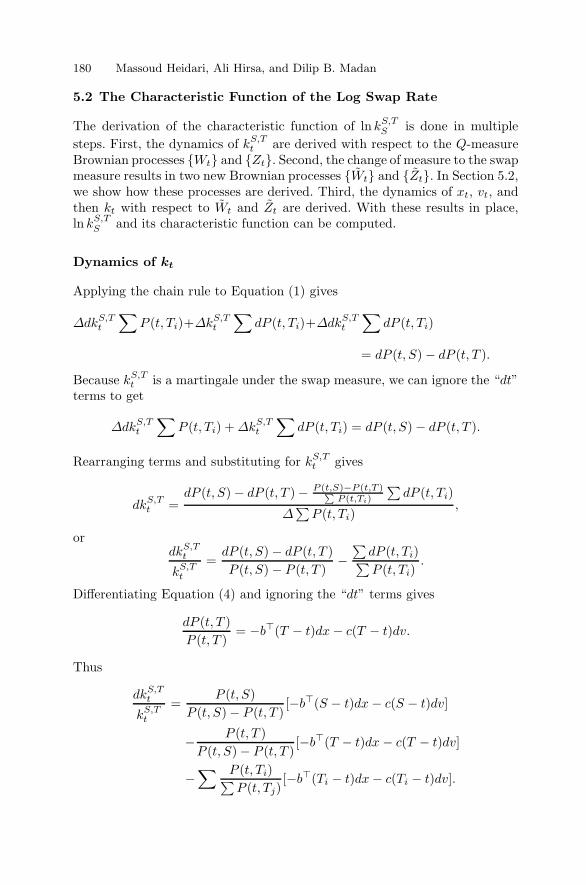
180 Massoud Heidari, Ali Hirsa, and Dilip B. Madan

5.2 The Characteristic Function of the Log Swap Rate

The derivation of the characteristic function of ln kS,TS is done in multiplesteps. First, the dynamics of kS,Tt are derived with respect to the Q-measureBrownian processes {Wt} and {Zt}. Second, the change of measure to the swapmeasure results in two new Brownian processes {Wt} and {Zt}. In Section 5.2,we show how these processes are derived. Third, the dynamics of xt, vt, andthen kt with respect to Wt and Zt are derived. With these results in place,ln kS,TS and its characteristic function can be computed.

Dynamics of kt

Applying the chain rule to Equation (1) gives

ΔdkS,Tt∑

P (t, Ti)+ΔkS,Tt∑

dP (t, Ti)+ΔdkS,Tt∑

dP (t, Ti)

= dP (t, S) − dP (t, T ).

Because kS,Tt is a martingale under the swap measure, we can ignore the “dt”terms to get

ΔdkS,Tt∑

P (t, Ti) +ΔkS,Tt∑

dP (t, Ti) = dP (t, S) − dP (t, T ).

Rearranging terms and substituting for kS,Tt gives

dkS,Tt =dP (t, S) − dP (t, T ) − P (t,S)−P (t,T )∑

P (t,Ti)

∑dP (t, Ti)

Δ∑

P (t, Ti),

ordkS,Tt

kS,Tt=

dP (t, S) − dP (t, T )P (t, S) − P (t, T )

−∑

dP (t, Ti)∑P (t, Ti)

.

Differentiating Equation (4) and ignoring the “dt” terms gives

dP (t, T )P (t, T )

= −b�(T − t)dx− c(T − t)dv.

Thus

dkS,Tt

kS,Tt=

P (t, S)P (t, S) − P (t, T )

[−b�(S − t)dx− c(S − t)dv]

− P (t, T )P (t, S) − P (t, T )

[−b�(T − t)dx − c(T − t)dv]

−∑ P (t, Ti)∑

P (t, Tj)[−b�(Ti − t)dx− c(Ti − t)dv].

Pricing of Swaptions in Affine Term Structures 181

At this point, we make use of an approximation. It is argued in [1], thatthe (P (t, Tj))/(

∑P (t, Tj)) terms are low-variance martingales in the context

of the market models (e.g., BGM). In [10], it is conjectured that this is alsotrue in ATSMs.

As mentioned earlier, to check the approximation in [10], for the constantvolatility case, we implemented the methodology and compared the approx-imated premiums against simulated ones for 12 different swaptions (1 × 2,1× 5, 1× 10, 2× 2, 2× 5, 2× 10, 5× 2, 5× 5, 5× 10, 10× 2, 10× 5, 10× 10).For 1,000,000 simulated paths, the absolute value of the largest relative errorwas less than 0.35%.

Making use of the same approximation in the stochastic volatility case, wereplace the (P (t, Tj))/(

∑P (t, Tj)) terms by their conditional expected values,

under the swap measure (P (0, Tj))/(∑

P (0, Tj)). This approximation yieldsthe following.

dkS,Tt

kS,Tt≈ P (0, S)

P (0, S)− P (0, T )[−bT (S − t)dx − c(S − t)dv]

− P (0, T )P (0, S) − P (0, T )

[−bT (T − t)dx− c(T − t)dv]

−∑ P (0, Ti)∑

P (0, Tj)[−bT (Ti − t)dx− c(Ti − t)dv].

Letting

ηt = −P (0, S)b(S − t) − P (0, T )b(T − t)P (0, S) − P (0, T )

+∑ P (0, Ti)∑

P (0, Tj)b(Ti − t),

δt = −P (0, S)c(S − t) − P (0, T )c(T − t)P (0, S) − P (0, T )

+∑ P (0, Ti)∑

P (0, Tj)c(Ti − t),

we havedkS,Tt

kS,Tt= ηTt dx+ δtdv.

Change of Measure

The random variable, which changes the Q measure to the swap measure isz = zT , where zt = Λt/Λ0 and

Λt = e−∫

t0 rsdsΔ

∑P (t, Ti). (8)

The process Λt is a martingale under the Q measure, thus

dΛtΛt

= ΦT1,tdW + Φ2,tdZ, (9)

= (ΦT1,t + Φ2,tρT )dW +

√1 − ‖ρ‖2

2Φ2,tdY,

182 Massoud Heidari, Ali Hirsa, and Dilip B. Madan

for some Φ1,t, Φ2,t, and univariate Brownian process Y that is independent ofW . Letting

Φ1,t = Φ1,t + Φ2,tρ,

Φ2,t =√

1 − ‖ρ‖22Φ2,t,

givesdΛtΛt

= ΦT1,tdW + Φ2,tdY. (10)

Solving this SDE gives

ΛtΛ0

= exp(∫ t

0

ΦT1,tdW + Φ2,tdY − 12

∫ t

0

‖Φ1,t‖22 + Φ2

2,tdt

).

Thus the processes W and Y , which are given by

dW = −Φ1,t + dW,

dY = −Φ2,t + dY,

are independent univariate Brownian processes under the swap measure. De-fine the Brownian process Z by

dZ = ρTdW +√

1 − ‖ρ‖22dY

= −(ΦT1,tρ+√

1 − ‖ρ‖22Φ2,t) + dZ

= −(ΦT1,tρ+ Φ2,t) + dZ.

Note that the correlation between W and Z is the vector ρ. Furthermore, itfollows from Equations (9) and (10) that

dW = dW+ < dW,dΛtΛt

>,

dZ = dZ+ < dZ,dΛtΛt

> .

Dynamics of x and v Under the Swap Measure

From Equation (8)

dΛtΛt

= (· · · )dt +∑ P (t, Ti)∑

P (t, Tj)[−b�(T − t)dx − c(T − t)dv]

≈ (· · · )dt +∑ P (0, Ti)∑

P (0, Tj)[−b�(T − t)dx− c(T − t)dv]

= (· · · )dt +∑ P (0, Ti)∑

P (0, Tj)(−b�(Ti − t)Σ

√vdW − c(Ti − t)λ

√vdZ),

Pricing of Swaptions in Affine Term Structures 183

so

< dW,dΛtΛt

> = −∑ P (0, Ti)∑

P (0, Tj)[Σ�b(Ti − t)

√v + c(Ti − t)λ

√vρ]dt,

< dZ,dΛtΛt

> = −∑ P (0, Ti)∑

P (0, Tj)[√vb�(Ti − t)Σρ+ c(Ti − t)λ

√v]dt.

So now we have

dx = (−bγ −Bx+ μtv)dt +Σ√vdW ,

dv = κt(θt − v)dt + λ√vdZ,

where

μt = −∑ P (0, Ti)∑

P (0, Tj)[ΣΣ�b(Ti − t) + c(Ti − t)λΣρ],

πt = −∑ P (0, Ti)∑

P (0, Tj)[λb�(Ti − t)Σρ+ c(Ti − t)λ2],

κt = κ− πt,

θt =κθ

κt.

Dynamics of kS,Tt Revisited

Plugging into the expression for dkt using the latest expressions for dx and dvand noting that kt is a martingale under the swap measure and eliminatingthe “dt” terms gives

dktkt

= ηTt Σ√vdW + δtλ

√vdZ.

Solving for ln kS,TS

We have that

d ln kS,Tt =dkS,Tt

kS,Tt− 1

2

(dkS,Tt

kS,Tt

)2

= ηTt Σ√vdW + δtλ

√vdZ − 1

2(ηTt ΣΣ

T ηt + δ2t λ

2 + 2δtληTt Σρ)vdt

= ηTt (dx+ (bγ +Bx− μtv)dt) + δt(dv + (−κθ + κtv)dt)

− 12(ηTt ΣΣ

Tηt + δ2t λ

2 + 2δtληTt Σρ)vdt.

184 Massoud Heidari, Ali Hirsa, and Dilip B. Madan

Integrating and collecting terms gives

ln kS,TS = ln kS,T0 +∫ S

0

ηTt bγdt−∫ S

0

δtκθdt

+∫ S

0

ηTt dxt +∫ S

0

δtdvt +∫ S

0

ηTt Bxtdt

+∫ S

0

(−ηTt μt + δtκt −

12(ηTt ΣΣ

T ηt + δ2t λ

2 + 2δtληTt Σρ))

vtdt.

Noting that∫ S

0

ηTt dxt = ηTS xS − ηT0 x0 −∫ S

0

∂ηTt∂t

xtdt,

∫ S

0

δtdvt = δSvS − δ0v0 −∫ S

0

∂δt∂t

vtdt,

we have

ln kS,TS = ln kS,T0 − η�0 x0 − δ0v0 +∫ S

0

η�t bγdt−∫ S

0

δtκθdt

+ ηTSxS + δSvS +∫ S

0

(η�t B − ∂η�t∂t

)xtdt

+∫ S

0

(−η�t μt + δtκt −

12(ηTt ΣΣ

�ηt + δ2t λ

2 + 2δtλη�t Σρ)− ∂δt

∂t

)vtdt.

Letting

pt = BT ηt −∂ηt∂t

,

qt = −η�t μt + δtκt −12(η�t ΣΣ

�ηt + δ2t λ

2 + 2δtλη�t Σρ)− ∂δt

∂t,

gives

ln kS,TS = ln kS,T0 − η�0 x0 − δ0v0 +∫ S

0

η�t bγdt−∫ S

0

δtκθdt

+ η�S xS +∫ S

0

p�t xtdt+ δSvS +∫ S

0

qtvtdt.

Note that pt = 0. We can see this as follows. From Equation (6) (and the factthat ζ = ibr),

B�b(τ) − ∂b(τ)∂t

= BT b(τ) + b′(τ) = br,

where τ = S − t, τ = T − t, or τ = Ti − t. It now follows from the definitionof ηt that

pt = −P (0, S)− P (0, T )P (0, S)− P (0, T )

br +∑ P (0, Ti)∑

P (0, Tj)br = 0.

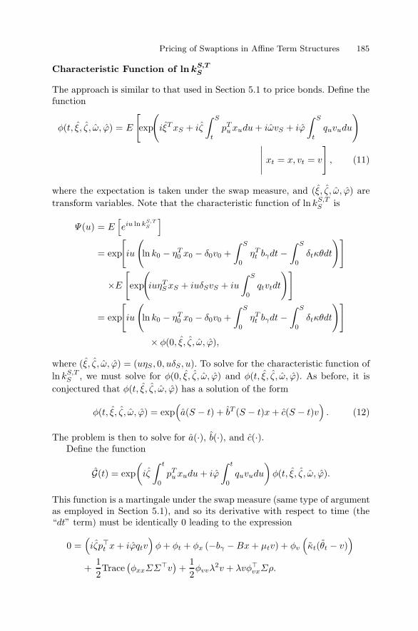
Pricing of Swaptions in Affine Term Structures 185

Characteristic Function of lnkS,TS

The approach is similar to that used in Section 5.1 to price bonds. Define thefunction

φ(t, ξ, ζ , ω, ϕ) = E

[exp

(iξTxS + iζ

∫ S

t

pTuxudu+ iωvS + iϕ

∫ S

t

quvudu

)

∣∣∣∣∣ xt = x, vt = v

], (11)

where the expectation is taken under the swap measure, and (ξ, ζ, ω, ϕ) aretransform variables. Note that the characteristic function of ln kS,TS is

Ψ(u) = E[eiu ln kS,T

S

]

= exp

[iu

(ln k0 − ηT0 x0 − δ0v0 +

∫ S

0

ηTt bγdt−∫ S

0

δtκθdt

)]

×E[exp

(iuηTSxS + iuδSvS + iu

∫ S

0

qtvtdt

)]

= exp

[iu

(ln k0 − ηT0 x0 − δ0v0 +

∫ S

0

ηTt bγdt−∫ S

0

δtκθdt

)]

× φ(0, ξ, ζ, ω, ϕ),

where (ξ, ζ , ω, ϕ) = (uηS , 0, uδS, u). To solve for the characteristic function ofln kS,TS , we must solve for φ(0, ξ, ζ, ω, ϕ) and φ(t, ξ, ζ, ω, ϕ). As before, it isconjectured that φ(t, ξ, ζ, ω, ϕ) has a solution of the form

φ(t, ξ, ζ, ω, ϕ) = exp(a(S − t) + bT (S − t)x+ c(S − t)v

). (12)

The problem is then to solve for a(·), b(·), and c(·).Define the function

G(t) = exp(iζ

∫ t

0

pTuxudu+ iϕ

∫ t

0

quvudu

)φ(t, ξ, ζ, ω, ϕ).

This function is a martingale under the swap measure (same type of argumentas employed in Section 5.1), and so its derivative with respect to time (the“dt” term) must be identically 0 leading to the expression

0 =(iζp�t x+ iϕqtv

)φ+ φt + φx (−bγ −Bx+ μtv) + φv

(κt(θt − v)

)

+12Trace

(φxxΣΣ

�v)

+12φvvλ

2v + λvφ�vxΣρ.

186 Massoud Heidari, Ali Hirsa, and Dilip B. Madan

We can use Equation (12) to solve for the derivatives of φ to get

0 = φ{(

iζp�t x+ iϕqtv)−(a′(S − t) + b′(S − t)�x+ c′(S − t)v

)}

+ b�(S − t)(−bγ −Bx+ μtv) + c(S − t)κt(θt − v)

+12b�(S − t)ΣΣ�b(S − t)v +

12c(S − t)2λ2v + λc(S − t)vb(S − t)�Σρ.

Because this has to hold for all (x, v), we get the following three equations bygrouping the x terms, v terms, and the remaining terms.

a′(τ) = −b�(τ)bγ + c(τ)κθ,

b′(τ) = −B�b(τ),

c′(τ) = iϕqt + b�(τ)μt +12b�(τ)ΣΣ�b(τ) −

[κt − λb�(τ)Σρ

]c(τ) +

λ2

2c2(τ),

where τ = S − t. The boundary conditions follow from Equations (11) and(12) at t = S, and are given by

a(0) = 0,

b(0) = iξ,

c(0) = iω.

As before, the above ODEs are Riccati equations, and there is an explicitsolution for b(τ) given by

b(τ) = exp(−B�τ)iξ.

The remaining two ODEs must be solved numerically, as before.

6 Data and Estimation

Having the characteristic function of the log swap rate, we can employ thetechniques in [3] or [4] to price swaptions. The data consist of (i) constantmaturity forward 6 months/12 months, (ii) swap rates at maturities 2, 3, 5, 10,15, and 30 years, and (iii) at-the-money swaption premiums with maturitiesof 1, 2, 5, and 10 years. At each option maturity, we have three contracts withdifferent underlying swap maturities: 2, 5, and 10 years. All interest rates andinterest rate options are on U.S. dollars. The data are daily closing mid-quotesfrom March 7, 1997, through October 16, 2006 (2399 observations).

For parameter and state estimation of our two-factor ATSM, we employa square-root unscented Kalman filter [7]. Figure 1 illustrates the estimatedfactors for both constant volatility and stochastic volatility. Figures 2 through4 display market premiums versus model premiums for both constant volatilityand stochastic volatility models for at-the-money straddles 2 × 5, 5 × 5, and10×5. The figures clearly indicate that the stochastic volatility model providesa superior match to market premiums; however, the longer the maturity, thecloser the constant volatility model comes to the stochastic volatility model.

Pricing of Swaptions in Affine Term Structures 187

Jan00 Jan05

0

0.5

1F

acto

rs

Constant Volatility Model

Jan00 Jan05−5

0

5

Fac

tors

Stochastic Volatility Model

Fig. 1. Top: time series of the factors estimated for the constant volatility case.Bottom: time series of the factors estimated for the stochastic volatility case.

Jan00 Jan05

350

400

450

500

550

600

650

700

Mar

ket v

s. M

odel

Straddle 2Y−5Y from 07−Mar−1997 to 16−Oct−2006

MarketSVCV

Fig. 2. Market premiums versus model premiums for both constant volatility andstochastic volatility; at-the-money straddle 2× 5.

188 Massoud Heidari, Ali Hirsa, and Dilip B. Madan

Jan00 Jan05

450

500

550

600

650

700

750

800

850M

arke

t vs.

Mod

el

Straddle 5Y−5Y from 07−Mar−1997 to 16−Oct−2006

MarketSVCV

Fig. 3. Market premiums versus model premiums for both constant volatility andstochastic volatility: at-the-money straddle 5× 5.

Jan00 Jan05350

400

450

500

550

600

650

700

750

800

Mar

ket v

s. M

odel

Straddle 10Y−5Y from 07−Mar−1997 to 16−Oct−2006

MarketSVCV

Fig. 4. Market premiums versus model premiums for both constant volatility andstochastic volatility; at-the-money straddle 10× 5.

Pricing of Swaptions in Affine Term Structures 189

7 Findings and Observations

Having model premiums and time series of the factors, we regress the log ofmodel premiums against the factors as follows,

Regressed Premiumst = exp(α + β�xt),

where α and β are obtained from regression, and xt is the time series of thefactors from estimation. For the same three at-the-money straddles—2 × 5,5 × 5, and 10 × 5—we plot model premiums versus regressed premiums forboth constant volatility and stochastic volatility models, as shown in Figures5, 6, and 7, respectively. In the constant volatility model, model premiumsare log-linear with respect to interest rate factors, but in stochastic volatilitythat is not the case.

We repeat the same procedure, but this time we regress the log of marketpremiums against the factors. The results are shown in Figures 8 through 10.

To establish a relationship between market premiums and the curve, weregress the difference of the ten-year swap rate and the five-year swap rateagainst the at-the-money straddle 5×5, and as before construct the regressedpremiums. Figure 11 gives plots of regressed premiums versus market premi-ums and the z-score of the residual.

Our conclusions from the regressions are as follows. (a) Volatility is ap-proximately log-linear in the factors, and (b) long-dated swaptions (straddles)are highly correlated to the slope of the yield curve. This makes logical sense,inasmuch swaption premiums are related to risk premiums, and the risk pre-mium is approximated by the slope of the yield curve.

Acknowledgments

Ali Hirsa would like to thank Ashok Tikku for his comments and suggestions.We also thank participants of the Bachelier Finance Society Conference 2006in Tokyo and participants of the Madan 60th Birthday Mathematical FinanceConference in College Park, Maryland for their comments and discussions.Errors are our own responsibility.

190 Massoud Heidari, Ali Hirsa, and Dilip B. Madan

440 460 480 500 520

440

460

480

500

520m

odel

pre

miu

ms

Straddle 2Y−5Y R−Squared 100.00 (Constant Vol)

400 450 500 550 600 650 700400

500

600

700

regressed premiums

mod

el p

rem

ium

s

Straddle 2Y−5Y R−Squared 85.88 (Stochastic Vol)

Fig. 5. Regressed premiums versus model premiums for at-the-money straddle 2×5:Constant volatility model at the top, and stochastic volatility model at the bottom.

550 600 650 700

550

600

650

700

mod

el p

rem

ium

s

Straddle 5Y−5Y R−Squared 100.00 (Constant Vol)

500 550 600 650 700 750 800 850

500

600

700

800

regressed premiums

mod

el p

rem

ium

s

Straddle 5Y−5Y R−Squared 87.39 (Stochastic Vol)

Fig. 6. Regressed premiums versus model premiums for at-the-money straddle 5×5:Constant volatility model at the top, and stochastic volatility model at the bottom.

Pricing of Swaptions in Affine Term Structures 191

450 500 550 600 650450

500

550

600

650m

odel

pre

miu

ms

Straddle 10Y−5Y R−Squared 100.00 (Constant Vol)

400 450 500 550 600 650 700 750 800400

500

600

700

800

regressed premiums

mod

el p

rem

ium

s

Straddle 10Y−5Y R−Squared 88.51 (Stochastic Vol)

Fig. 7. Regressed premiums versus model premiums for at-the-money straddle10 × 5: Constant volatility model at the top, and stochastic volatility model atthe bottom.

350 400 450 500 550 600 650 700

400

500

600

700

mar

ket p

rem

ium

s

Straddle 2Y−5Y R−Squared 87.84 (Constant Vol)

350 400 450 500 550 600 650 700

400

500

600

700

regressed premiums

mar

ket p

rem

ium

s

Straddle 2Y−5Y R−Squared 88.53 (Stochastic Vol)

Fig. 8. Regressed premiums versus market premiums for at-the-money straddle2 × 5: Constant volatility model at the top, and stochastic volatility model at thebottom.

192 Massoud Heidari, Ali Hirsa, and Dilip B. Madan

450 500 550 600 650 700 750 800 850

500

600

700

800m

arke

t pre

miu

ms

Straddle 5Y−5Y R−Squared 83.15 (Constant Vol)

450 500 550 600 650 700 750 800 850

500

600

700

800

regressed premiums

mar

ket p

rem

ium

s

Straddle 5Y−5Y R−Squared 83.95 (Stochastic Vol)

Fig. 9. Regressed premiums versus market premiums for at-the-money straddle5 × 5: Constant volatility model at the top, and stochastic volatility model at thebottom.

350 400 450 500 550 600 650 700 750

400

500

600

700

mar

ket p

rem

ium

s

Straddle 10Y−5Y R−Squared 75.82 (Constant Vol)

350 400 450 500 550 600 650 700 750

400

500

600

700

regressed premiums

mar

ket p

rem

ium

s

Straddle 10Y−5Y R−Squared 75.50 (Stochastic Vol)

Fig. 10. Regressed premiums versus market premiums for at-the-money straddle10× 5: Constant volatility model at the top, and stochastic volatility model at thebottom.

Pricing of Swaptions in Affine Term Structures 193

450 500 550 600 650 700 750 800 850

500

600

700

800

mar

ket p

rem

ium

s

Straddle 5Y−5Y R−Squared 84.69

Jan98 Jan00 Jan02 Jan04 Jan06

−2

0

2

ZS

Cor

e

Fig. 11. Market premiums versus regressed premiums against the curve, and thez-score of the regression residuals.

References

1. A. Brace, T. Dunn, and G. Barton. Towards a central interest rate model.Option Pricing, Interest Rates and Risk Management: Handbooks in Mathemat-ical Finance, eds. E. Jouini, J. Cvitanic, and M. Musiela, Cambridge UniversityPress, 278–313, 2001.

2. A. Brace, D. Gatarek, and M. Musiela. The market model of interest ratedynamics. Mathematical Finance, 7:127–155, 1997.

3. P. Carr and D. B. Madan. Option valuation using the fast Fourier transform.The Journal of Computational Finance, 2(4):61–73, 1999.

4. K. Chourdakis. Option valuation using the fast Fourier transform. Journal ofComputational Finance, 8(2):1–18, Winter 2004.

5. P. Collin-Dufresne and R. Goldstein. Pricing swaptions in affine models. Journalof Derivatives, 10(1):9-26, Fall 2002.

6. Q. Dai and K. Singleton. Specification analysis of affine term structure models.Journal of Finance, 55:1943–1978, 2000.

7. R. Van der Merwe and E.A. Wan. The square-root unscented Kalman filter forstate and parameter estimation. IEEE International Conference on Acoustics,Speech, and Signal Processing, 6:3461–3464, 2001.

8. D. Heath, R. Jarrow, and A. Morton. Bond pricing and the term structure ofinterest rates: A discrete time approximation. Journal of Financial and Quan-titative Analysis, 25:419–440, 1990.

9. C. Munk. Stochastic duration and fast coupon bond option pricing in multi-factor models. Review of Derivative Research, 3:157–181, 1999.

10. D.F. Schrager and A.J. Pelsser. Pricing swaptions and coupon bond options inaffine term structure models. Mathematical Finance, 16(4):673–694, 2006.

11. K. Singleton and L. Umanstev. Pricing coupon bond and swaptions in affineterm structure models. Mathematical Finance, 12:427–446, 2002.

Forward Evolution Equations for Knock-OutOptions

Peter Carr1 and Ali Hirsa2

1 Bloomberg731 Lexington AvenueNew York, NY 10022, USApcarr4@bloomberg.net

2 Caspian Capital Management, LLC745 Fifth AvenueNew York, NY 10151, USAali.hirsa@ixis-ccm.com

Summary. We derive forward partial integrodifferential equations (PIDEs) forpricing up-and-out and down-and-out call options when the underlying is a jumpdiffusion. We assume that the jump part of the returns process is an additive pro-cess. This framework includes the Variance-Gamma, finite moment logstable, Mertonjump diffusion, Kou jump diffusion, Dupire, CEV, arcsinh normal, displaced diffu-sion, and Black–Scholes models as special cases.

Key words: Partial integrodifferential equation (PIDE); forward equations; knock-out options; jump diffusion; Levy processes.

1 Introduction

Pricing and hedging derivatives consistent with the volatility smile has been amajor research focus for over a decade. A breakthrough occurred in the mid-nineties with the recognition that in certain models, European option pricessatisfied forward evolution equations in which the independent variables arethe option’s strike and maturity. More specifically, [12] showed that underdeterministic carrying costs and a diffusion process for the underlying assetprice, no-arbitrage implies that European option prices satisfy a certain par-tial differential equation (PDE), now called the Dupire equation. Assumingthat one could observe European option prices of all strikes and maturities,then this forward PDE can be used to explicitly determine the underlier’s in-stantaneous volatility as a function of the underlier’s price and time. Once thisvolatility function is known, the value function for European, American, andmany exotic options can be determined by a wide array of standard methods.

196 Peter Carr and Ali Hirsa

As this value function relates theoretical prices of these instruments to theunderlier’s price and time, it can also be used to determine many Greeks ofinterest as well.

Aside from their use in determining the volatility function, forward equa-tions also serve a second useful purpose. Once one knows the volatility functioneither by an explicit specification or by a prior calibration, the forward PDEcan be solved via finite differences to efficiently price a collection of Europeanoptions of different strikes and maturities all written on the same underlyingasset. Furthermore, as pointed out in [4], all the Greeks of interest satisfy thesame forward PDE and hence can also be efficiently determined in the sameway.

Since the original development of forward equations for European optionsin continuous models, several extensions have been proposed. For example,Esser and Schlag [14] developed forward equations for European options writ-ten on the forward price rather than the spot price. Forward equations forEuropean options in jump diffusion models were developed in Andersen andAndreasen [1] and extended by Andreasen and Carr [3]. It is straightforwardto develop the relevant forward equations for European binary options or forEuropean power options by differentiating or integrating the forward equa-tion for standard European options. Buraschi and Dumas [6] develop forwardequations for compound options. In contrast to the PDEs determined by oth-ers, their evolution equation is an ordinary differential equation whose soleindependent variable is the intermediate maturity date.

Given the close relationship between compound options and American op-tions, it seems plausible that there might be a forward equation for Americanoptions. The development of such an equation has important practical impli-cations, because all listed options on individual stocks are American-style. TheDupire equation cannot be used to infer the volatility function from marketprices of American options, nor can it be used to efficiently value a collectionof American options of differing strikes and maturities.

This problem is addressed for American calls on stocks paying discretedividends in Buraschi and Dumas [6], and it is also considered in a latticesetting in Chriss [10]. In [8], we address the more difficult problem of pricingcontinuously exercisable American puts in continuous-time models. To do so,we depart from the diffusive models that characterize most of the previousresearch on forward equations in continuous time. To capture the smile, weassume that prices jump rather than assuming that the instantaneous volatil-ity is a function of stock price and time. Dumas et al. [11] find little empiricalsupport for the Dupire model, whereas there is a long history of empiricalsupport for jump-diffusion models; three recent papers documenting supportfor such models are [2; 7; 9]. In particular, we assume that the returns on theunderlying asset have stationary independent increments, or in other wordsthat the log price is a Levy process. Besides the [5] model, our frameworkincludes as special cases the Variance-Gamma (VG) model of Madan et al.[18], the CGMY model of Carr et al. [7], the finite moment logstable model of

Forward Evolution Equations for Knock-Out Options 197

Carr and Wu [9], the Merton [19] and Kou [17] jump diffusion models, and thehyperbolic models of Eberlein et al. [13]. In all of these models except Black–Scholes, the existence of a jump component implies that the backward andforward equations contain an integral in addition to the usual partial deriva-tives. Despite the computational complications introduced by this term, weuse finite differences to solve both of these fundamental partial integrodif-ferential equations (PIDEs). To illustrate that our forward PIDE is a viablealternative to the traditional backward approach, we calculate American op-tion values in the diffusion-extended VG option pricing model and find veryclose agreement. For details on the application of finite differences to valuingAmerican options in the VG model, see [16].

The approach to determining the forward equation for American optionsin [8] is to start with the well-known backward equation and then exploit thesymmetries that essentially define Levy processes. In the process of developingthe forward equation, we also determine two hybrid equations of independentinterest. The advantage of these hybrid equations over the forward equationis that they hold in greater generality. Depending on the problem at hand,these hybrid equations can also have large computational advantages over thebackward or forward equations when the model has already been calibrated.In particular, the advantage of these hybrid equations over the backwardequation is that they are more computationally efficient when one is interestedin the variation of prices or Greeks across strike or maturity at a fixed time,for example, market close.

The first of these hybrid equations has the stock price and maturity asindependent variables. The numerical solution of this hybrid equation is analternative to the backward equation in producing a spot slide, which showshow American option prices vary with the initial spot price of the underlier.If one is interested in understanding how this spot slide varies with maturity,then our hybrid equation is much more efficient than the backward equation.This hybrid equation also has important implications for path-dependent op-tions such as cliquets whose payoff directly depends on the particular levelreached by an intermediate stock price.

Their second hybrid equation has the strike price and calendar time asindependent variables. The numerical solution of this hybrid equation is analternative to the forward equation in producing an implied volatility smileat a fixed maturity. If one is interested in understanding how the model pre-dicts that this smile will change over time, then our hybrid equation is muchmore computationally efficient than the forward equation. This second hybridequation also allows parameters to have a term structure, whereas our forwardequation does not. Note, however, that implied volatility can have a term orstrike structure in our Levy setting. Hence, if one needs to efficiently valuea collection of American options of different strikes in the time-dependentBlack–Scholes model, then it is far more efficient to solve our hybrid equationthan to use the standard backward equation.

198 Peter Carr and Ali Hirsa

In this paper, we focus on forward evolution equations for knock-out op-tions. We derive forward partial integrodifferential equations for up-and-outand down-and-out call options when the model dynamics are jump diffusion,where jumps are additive in the log of the price. This framework includes VG,finite moment logstable, Merton and Kou jump diffusions, Dupire, CEV, arc-sinh normal, displaced diffusion, and Black–Scholes models as special cases.The remainder of this paper is structured as follows. The next section in-troduces our assumptions for down-and-out calls and derives the forwardPIDE for down-and-out calls. The following section introduces our settingand reviews the backward PIDE that governs up-and-out call values in thissetting and then develops the forward equation for up-and-out call options.We present some numerical results afterwards, and the final section suggestsfurther research.

2 Down-and-Out Calls

2.1 Assumptions and Notations

Throughout this paper, we assume the standard model of perfect capital mar-kets, continuous trading, and no-arbitrage opportunities.

When a pure discount bond is used as numeraire, then it is well knownthat no-arbitrage implies that there exists a probability measure Q underwhich all nondividend-paying asset prices are martingales. Under this measurewe assume that a stock price St obeys the following stochastic differentialequation,

dSt = [r(t)−q(t)]St−dt+a(St−, t)dWt+∫ ∞

−∞St−(ex−1)[μ(dx, dt)−ν(x, t)dxdt],

(1)for all t ∈ [0, T ], where the initial stock price S0 > 0 is known, and T is somearbitrarily distant horizon. The process is Markov in itself because the coef-ficients of the stock price process at time t depend on the path only throughSt−, which is the prejump price at t. Thus, the dynamics are fully deter-mined by the drift function b(S, t) ≡ [r(t) − q(t)]S, the (normal) volatilityfunction a(S, t), and the jump compensation function ν(x, t). The term dWt

denotes increments of a standard Brownian motion Wt defined on the timeset [0, T ] and on a complete probability space (Ω,F , Q). The random measureμ(dx, dt) counts the number of jumps of size x in the log price at time t. Thefunction {ν(x, t), x ∈ R, t ∈ [0, T ]} is used to compensate the jump processJt ≡

∫ t0

∫∞−∞ St−(ex − 1)μ(dx, ds), so that the last term in Equation (1) is

the increment of a Q jump martingale. The function ν(x, t) must have thefollowing properties.

1. ν(0, t) = 0.2.∫∞−∞(x2 ∧ 1)ν(x, t)dx < ∞, t ∈ [0, T ].

Forward Evolution Equations for Knock-Out Options 199

Thus, each price change is the sum of the increment in a general diffusionprocess with proportional drift and the increment in a pure jump martingale,where the latter is an additive process in the log price. We restrict the functiona(S, t) so that the spot price is always nonnegative and absorbing at the origin.A sufficient condition for keeping the stock price away from the origin is tobound the lognormal volatility. In particular, we set

a(0, t) = 0. (2)

Hence, Equation (1) describes a continuous-time Markov model for the spotprice dynamics, which is both arbitrage-free and consistent with limited liabil-ity. Aside from the Markov property, the main restrictions inherent in Equa-tion (1) are the standard assumptions that interest rates, dividend yields, andthe compensator do not depend on the spot price.

2.2 Analysis

Let time t = 0 denote the valuation date for a European down-and-out calloption with strike price K, barrier L ≤ K, initial spot S0 > L, and maturityT ≥ 0. Let Dc

0(K,T ) denote an initial price of the down-and-out call which isimplied by the absence of arbitrage. Consider the product e

∫ Ttr(u)du(St−K)+.

By the Tanaka–Meyer formula,

(ST −K)+ = e∫ T0 r(u)du(S0 −K)+ +

∫ T

0

e∫ T

tr(u)du1{St−>K}dSt

+∫ T

0

e∫ T

tr(u)du

{a2(St−, t)

2δ(St− −K) − r(t)(St− −K)+

}dt

+∫ T

0

e∫ T

tr(u)du

∫ ∞

−∞

[(St−ex −K)+ − (St− −K)+

− 1{St−>K}St−(ex − 1)]μ(dx, dt),

where μ(·, ·) denotes the integer-valued counting measure and δ(·) denotes theDirac delta function, a generalized function characterized by two properties:

1. δ(x) ={

0 if x �= 0,∞ if x = 0;

2.∫∞−∞ δ(x)dx = 1.

Multiplying by e−∫

T0 r(u)du1{τL>T} and taking expectations on both sides un-

der an equivalent martingale measure Q, we have

200 Peter Carr and Ali Hirsa

Dc0(K,T ) = (S0 −K)+EQ0 [1{τL>T}]

+∫ T

0

e−∫

t0 r(u)duEQ0

[1{τL>T}1{St−>K}[r(t) − q(t)]St−

]dt

+∫ T

0

e−∫

t0 r(u)du

{a2(K, t)2

EQ0 [1{τL>T}δ(St− −K)]

− r(t)EQ0 [1{τL>T}(St− −K)+]}dt

+

T∫

0

e−

t∫0r(u)du

EQ0 [1{τL>T}]

∞∫

−∞

[(St−ex −K)+ − (St− −K)+

− 1{St−>K}St−(ex − 1)]ν(x, t)dxdt.

Differentiating w.r.t. T implies

∂

∂TDc

0(K,T ) = −e−∫ T0 r(u)duEQ0

[δ(τL − T )(ST −K)+

]

+ e−∫ T0 r(u)duEQ0

[1{τL>T}1{ST−>K}[r(T ) − q(T )]ST−

]

+a2(K,T )

2e−∫

T0 r(u)duEQ0 [1{τL>T}δ(ST− −K)]

− r(T )e−∫

T0 r(u)duEQ0 [1{τL>T}(ST− −K)+]

+ e−

T∫0r(u)du

EQ0

[1{τL>T}

∞∫

−∞

((ST−e

x −K)+ − (ST− −K)+

− 1{ST−>K}ST−(ex − 1))ν(x, T )dx

].

The payoff in the first term vanishes. Subtracting and adding

e−∫ T0 r(u)duEQ0

[1{τL>T}[r(T ) − q(T )]K1{ST−>K}

]

to the second term on the right-hand side (RHS) gives

∂

∂TDc

0(K,T ) = e−∫

T0 r(u)duEQQ

0

[1{τL>T}1{ST−>K}[r(T ) − q(T )](ST− −K)

]

+ e−∫ T0 r(u)duEQ0

[1{τL>T}[r(T ) − q(T )]K1{ST−>K}

]

+a2(K,T )

2∂2

∂K2Dc

0(K,T ) − r(T )Dc0(K,T ) + e

−T∫0r(u)du

EQ0

[1{τL>T}

∞∫

−∞

(ex(ST− −Ke−x)+− 1{ST−>K}(ST− −K + ST−e

x − ST−))ν(x, T )dx

]

Forward Evolution Equations for Knock-Out Options 201

= [r(T ) − q(T )]Dc0(K,T ) − [r(T ) − q(T )]K

∂

∂KDc

0(K,T )

+a2(K,T )

2∂2

∂K2Dc

0(K,T )− r(T )Dc0(K,T ) + e−

∫ T0 r(u)duEQ0

[1{τL>T}

∫ ∞

−∞ex((ST− −Ke−x)+ − 1{ST−>K}(ST− −Ke−x +K −K)

)ν(x, T )dx

]

= −q(T )Dc0(K,T )− [r(T )−q(T )]K

∂

∂KDc

0(K,T ) +a2(K,T )

2∂2

∂K2Dc

0(K,T )

+ e−∫

T0 r(u)duEQ0

[1{τL>T}

∞∫

−∞

((ST− −Ke−x)+ − (ST− −K)+

− ∂

∂K(ST− −K)+K(e−x − 1)

)exν(x, T )dx

]

= −q(T )Dc0(K,T )− [r(T ) − q(T )]K

∂

∂KDc

0(K,T ) +a2(K,T )

2∂2

∂K2Dc

0(K,T )

+∫ ∞

−∞

[Dc

0(Ke−x, T ) −Dc0(K,T )− ∂

∂KDc

0(K,T )K(e−x− 1)]exν(x, T )dx.

(3)

This PIDE holds on the domain K ≥ L, T ∈ [0, T ].For a down-and-out call, the initial condition is

Dc0(K, 0) = (S0 −K)+, K ≥ L.

Because a down-and-out call behaves as a standard call as its strike approachesinfinity, we have

limK↑∞

Dc0(K,T ) = lim

K↑∞

∂

∂KDc

0(K,T ) = limK↑∞

∂2

∂K2Dc

0(K,T ) = 0, T ∈ [0, T ].

For a lower boundary condition, we note that a down-and-out call on a stockwith the dynamics in Equation (1) has the same value prior to knocking outas a down-and-out call on a stock that absorbs at L. The second derivativeof this latter call gives the r-discounted risk-neutral probability density forthe event that the stock price has survived to at least T and is in the interval(K,K + dK). Now it is well known that the appropriate boundary conditionfor an absorbing process is that this PDF vanishes on the boundary. Hence,

limK↓L

∂2

∂K2Dc

0(K,T ) = 0, T ∈ [0, T ]. (4)

Evaluating Equation (3) at K = L and substituting in (4) implies

∂Dc0(L, T )∂T

=∫ ∞

−∞

[Dc

0(Le−x, T ) −Dc

0(L, T )− ∂

∂KDc

0(L, T )L(e−x − 1)]

exν(x, T )dx− [r(T ) − q(T )]L∂

∂KDc

0(L, T ) − q(T )Dc0(K,T ), T ∈ [0, T ].

202 Peter Carr and Ali Hirsa

This is a Robin condition, as it involves the value and both its first partialderivatives along the boundary.

3 Up-and-Out Calls

3.1 The Backward Boundary Value Problem

Consider an up-and-out European call on a stock with a fixed maturity dateT ∈ [0, T ]. At the first time that the stock price crosses an upper barrier H ,the call knocks out. If the upper barrier is not touched prior to T , the callmatures and pays (ST −K)+ at T , where K ∈ [0, H) is the strike price.

We let τH denote the first passage time to H . We adopt the usual con-vention of setting this first passage time to infinity if the barrier is neverhit. For t ≥ τ , the call has knocked out and is defined to be worthlessat t. If t < τ , then the stock price St must be in the continuation regionC ≡ (S, t) ∈ (0, H) × [0, T ). While the call is alive, its value is given by afunction, denoted U(S, t), mapping C into the real line. In the interior of thecontinuation region, the partial derivatives, ∂U/∂t, ∂U/∂S, and ∂2U/∂S2 allexist as classical functions. No-arbitrage implies that the up-and-out call valuefunction U(S, t) satisfies the following deterministic PIDE in the continuationregion C; that is,

∞∫

−∞

[U(Sex, t) − U(S, t) − ∂

∂SU(S, t)S(ex − 1)

]ν(x, t)dx +

a2(S, t)2

∂2U(S, t)∂S2

+ [r(t) − q(t)]S∂U(S, t)

∂S− r(t)U(S, t) +

∂U(S, t)∂t

= 0, for (S, t) ∈ C. (5)

A fortiori, the up-and-out call value function U(S, t) solves a backward bound-ary value problem (BVP), consisting of the backward PIDE given by Equation(5) subject to the following boundary conditions.

U(S, T ) = (S −K)+, S ∈ [0, H ], (6)limS↓0

U(S, t) = 0, t ∈ [0, T ], (7)

limS↑H

U(S, t) = 0, t ∈ [0, T ]. (8)

Equation (6) states that the up-and-out call is worth its intrinsic value atexpiration. The value matching conditions given by Equations (7) and (8)show that at each t ∈ [0, T ), the up-and-out call’s value tends to zero as thestock price approaches the origin or the barrier. For each t, the up-and-outcall value is not in general differentiable in S at H .

Partial derivatives or integrals of the up-and-out call value with respectto K or T also satisfy a backward BVP. In particular, the second partial

Forward Evolution Equations for Knock-Out Options 203

derivative of the up-and-out call value with respect to K, denoted Ukk(S, t),solves the same PIDE as U(S, t) in the continuation region C; that is,∫ ∞

−∞

[Ukk(Sex, t) − Ukk(S, t) −

∂

∂SUkk(S, t)S(ex − 1)

]ν(x, t)dx

+a2(S, t)

2∂2Ukk(S, t)

∂S2+ [r(t) − q(t)]S

∂Ukk(S, t)∂S

− r(t)Ukk(S, t)

+∂Ukk(S, t)

∂t= 0, for (S, t) ∈ C. (9)

The partial derivative Ukk(S, t) is subject to the following boundary condi-tions.

Ukk(S, T ) = δ(S −K), S ∈ [0, H ],limS↓0

Ukk(S, t) = 0, t ∈ [0, T ],

limS↑H

Ukk(S, t) = 0, t ∈ [0, T ].

3.2 Forward Propagation of Up-and-Out Call Values

Until now, we have been thinking of K and T as constants. In this section, wevary K and T , which will induce variation in the up-and-out call value. Wealso hold S and t constant at S0 ∈ (0, H) and 0, respectively. We let u(K,T )denote the function relating the up-and-out call value to the strike price Kand the maturity T when (S, t) = (S0, 0). Although we are interested in u forall T ∈ [0, T ], we are only interested in u for all real K ∈ [0, H ].

Let ukk(K,T ) ≡ Ukk(S0, 0) be the function emphasizing the dependenceof the second strike derivative of the up-and-out call value on K and T . Theappendix shows that the adjoint of the backward PIDE given by Equation (9)governing ukk is∫ ∞

−∞

[e−xukk(Ke−x, T ) + (ex−2)ukk(K,T ) +

∂

∂Kukk(K,T )K(ex−1)

]ν(x, T )dx

+∂2

∂K2

[a2(K,T )

2ukk(K,T )

]− ∂

∂K{[r(T ) − q(T )]Kukk(K,T )}

− r(T )ukk(K,T )− ∂ukk(K,T )∂T

= 0, (10)

for K ∈ [0, H ], T ∈ [0, T ]. Note that

∂2

∂K2{−[r(T ) − q(T )]Kvk(K,T ) − q(T )v(K,T )}

=∂

∂K{−[r(T ) − q(T )]vk(K,T ) − [r(T ) − q(T )]Kvkk(K,T ) − q(T )vk(K,T )}

= − ∂

∂K{[r(T ) − q(T )]Kvkk(K,T )} − r(T )vkk(K,T ). (11)

204 Peter Carr and Ali Hirsa

Also note that

ex∂2

∂K2

{u(Ke−x, T )− u(K,T ) − uk(K,T )K(e−x − 1)

}

= ex∂

∂K

{e−xuk(Ke−x, T ) − uk(K,T ) − ukk(K,T )K(e−x − 1)

− uk(K,T )(e−x − 1)}

=∂

∂K

{uk(Ke−x, T ) − uk(K,T ) − ukk(K,T )K(1 − ex)

}

= e−xukk(Ke−x, T )− ukk(K,T )− ukkk(K,T )K(1− ex) − ukk(K,T )(1− ex)= e−xukk(Ke−x, T ) + (ex − 2)ukk(K,T ) + ukkk(K,T )K(ex − 1). (12)

Substituting Equations (11) and (12) into (10) implies

∂2

∂K2

{∫ ∞

−∞[u(Ke−x, T ) − u(K,T )− uk(K,T )K(e−x − 1)]exν(x, T )dx

+a2(K,T )

2ukk(K,T )−[r(T )− q(T )]Kuk(K,T )−q(T )u(K,T )−∂u(K,T )

∂T

}

= 0, K ∈ [0, H ], T ∈ [0, T ].

Integrating on K twice implies∫ ∞

−∞[u(Ke−x, T )− u(K,T ) − uk(K,T )K(e−x − 1)]exν(x, T )dx

+a2(K,T )

2ukk(K,T ) − [r(T ) − q(T )]Kuk(K,T ) − q(T )u(K,T )− ∂u(K,T )

∂T= A(T )K +B(T ), (13)

for K ∈ [0, H ], T ∈ [0, T ], and where A(T ) and B(T ) are independent of K.The forward PIDE is solved subject to an initial condition:

u(K, 0) = (S0 −K)+. (14)

Suppose we regard the Levy density ν(x, T ) and volatility function a(S, t) asgiven, and use Equation (13) subject to the initial condition given by Equation(14) to determine u(K,T ). Then the solution of the inhomogeneous PIDEgiven by Equation (13) subject to the initial condition given by (14) is notunique. As we don’t know A(T ) and B(T ), we need two conditions just todetermine the operator. For uniqueness, we may need two more independentboundary conditions as well. If both the origin and the upper barrier areaccessible, then we will definitely need two additional independent boundaryconditions to obtain uniqueness. However, if the origin is inaccessible (e.g.,for geometric Brownian motion), then we can uniquely determine up-and-outcall values without specifying a lower boundary condition.

Forward Evolution Equations for Knock-Out Options 205

We may alternatively suppose that all up-and-out call values are alreadyknown from the marketplace, and that the objective is to uniquely determinethe Levy density ν(x, t) and the volatility function a(S, t). Under this perspec-tive, one needs to supplement (13) subject to (14) with only two boundaryconditions in order to determine A(T ) and B(T ). If one somehow knows theLevy density, then it is straightforward to solve the algebraic equation (13)for a(S, t).

We now assume that the objective is to determine u(K,T ) given ν(x, t)and a(S, t). Differentiating Equation (13) with respect to K implies

A(T ) =∫ ∞

−∞

[e−xuk(Ke−x, T )−uk(K,T )− ∂uk

∂K(K,T )K(e−x−1)

− uk(K,T )(e−x−1)]exν(x, T )dx+

∂

∂K

{a2(K,T )2

ukk(K,T )

− [r(T ) − q(T )]Kuk(K,T )− q(T )u(K,T )− ∂u(K,T )∂T

}

=∫ ∞

−∞[uk(Ke−x, T )− uk(K,T )− ∂uk

∂K(K,T )K(1 − e−x)]ν(x, T )dx

+a2(K,T )

2∂2

∂K2uk(K,T )

−{

[r(T ) − q(T )]K − a(K,T )∂a

∂S(K,T )

}∂

∂Kuk(K,T )

− r(T )uk(K,T ) − ∂uk(K,T )∂T

. (15)

As the left-hand side (LHS) is invariant to K, the RHS is as well, and sowe are free to determine A(T ) by evaluating the RHS at either K = 0 or atK = H .

Once A(T ) is known, then from Equation (13),

B(T ) =∫ ∞

−∞[u(Ke−x, T )− u(K,T ) − uk(K,T )K(e−x − 1)]exν(x, T )dx

+a2(K,T )

2ukk(K,T )− [r(T ) − q(T )]Kuk(K,T ) − q(T )u(K,T )

−∂u(K,T )∂T

−A(T )K. (16)

Once again, the LHS is invariant to K, and so we are free to determine B(T )by evaluating the RHS at either K = 0 or at K = H .

Appealing to the Feynman–Kac theorem, the solution to the backwardBVP given by Equations (5) to (8) can be represented as

u(K,T ) = e−∫ T0 r(u)duEQ[1{τH>T}(ST −K)+], (17)

where the expectation is conditional on the known initial stock price S0. Thestock price process used to calculate these so-called risk-neutral expectations

206 Peter Carr and Ali Hirsa

is the one solving the SDE given by Equation (1). At K = H , the function ugives the value of a call whose underlying must cross a knock-out barrier tofinish above the strike:

u(H,T ) = 0. (18)

Differentiating Equation (17) w.r.t. K implies that

uk(K,T ) = −e−∫

T0 r(u)duEQ[1{τH>T}1{ST>K}]. (19)

At K = H , the function uk gives the value of a short binary call whoseunderlying must cross a knock-out barrier to finish above the strike:

uk(H,T ) = 0. (20)

Differentiating Equation (19) w.r.t. K implies that

ukk(K,T ) = e−∫ T0 r(u)duEQ[1{τH>T}δ(ST −K)],

where δ(·) denotes the Dirac delta function. Hence, the function ukk(K,T )gives the r-discounted risk-neutral probability density for the event that thestock price process survives to T and that the time T stock price is in (K,K+dK):

ukk(K,T ) = e−∫ T0 r(u)duQ(τH > T, ST ∈ (K,K + dK))

dK. (21)

Hence, as the strike price K approaches the knock-out barrier H , the proba-bility of surviving beyond T goes to zero:

limK↑H

ukk(K,T ) = 0. (22)

Differentiating Equation (21) w.r.t. K implies that the slope of the discountedsurvival probability in K is given by

ukkk(K,T ) = e−∫

T0 r(u)duEQ[1{τH>T}δ

(1)(ST −K)],

where δ(1)(·) denotes the first derivative of a delta function. When evaluatedat K = H , ukkk does not appear to simplify. We later show how the infor-mation at K = 0 allows us to relate ukkk to the PDF for the first passagetime τH .

Differentiating Equation (17) w.r.t. T implies that

∂

∂Tu(K,T ) = −r(T )u(K,T ) + e−

∫ T0 r(u)duEQ[δ(τH − T )(ST −K)+]. (23)

One may interpret the second term as the value of a call whose notional iscontingent on the first passage time to H being the call’s maturity T . Forany H ≤ K, this term vanishes. Hence, evaluating Equation (23) at K = Himplies

Forward Evolution Equations for Knock-Out Options 207

∂

∂Tu(H,T ) = 0, (24)

applying Equation (18). Differentiating Equation (19) w.r.t. T implies that

∂

∂Tuk(K,T ) = −r(T )uk(K,T ) + e−

∫T0 r(u)duEQ[δ(τH − T )1{ST>K}]. (25)

The only difference between Equations (23) and (25) is that the second termnow represents the value of a binary call with contingent notional. Hence,

∂2

∂T∂Ku(H,T ) = 0, (26)

applying Equation (20).We have less in the way of additional boundary conditions as K ↓ 0.

Because an up-and-out call has less value than a standard call, we have anupper bound on the value at K = 0:

u(0, T ) ≤ S0e−∫

T0 q(u)du.

Similarly, because an up-and-out binary call has less value than a standardbinary, we have a lower bound on the absolute slope in K at K = 0:

uk(0, T ) ≥ −e−∫ T0 r(u)du.

As an up-and-out butterfly spread has the same or lower value than a standardbutterfly spread, we have

ukk(0, T ) = 0. (27)

Similarly, as an up-and-out vertical spread of butterfly spreads has the sameor lower value than a vertical spread of butterfly spreads, we have

ukkk(0, T ) = 0. (28)

Evaluating Equation (23) at K = 0 implies

∂

∂Tu(0, T ) = −r(T )u(0, T ) + e−

∫ T0 r(u)duEQ[δ(τH − T )ST ]. (29)

As the stock price must be worth H in order for the call holder to receiveanything, Equation (29) yields a simple expression for the discounted firstpassage time density:

φ(H,T ) ≡ e−∫ T0 r(u)duQ(τH ∈ (T, T + dT ))

dT=

1H

[r(T )u(0, T ) +

∂

∂Tu(0, T )

].

When ν(x, t) and a(S, t) are known and u(K,T ) is to be determined, theRHS is not known exante. However, when ν(x, t) and a(S, t) are not knownand when one can observe market prices of up-and-out calls with zero strikes

208 Peter Carr and Ali Hirsa

(which are up-and-out shares with no dividends received prior to T ), then theRHS is observable. Evaluating Equation (25) at K = 0 implies

∂

∂Tuk(0, T ) = −r(T )uk(0, T ) + e−

∫T0 r(u)duEQ[δ(τH − T )].

Hence, we have another simple expression for the discounted first passage timedensity:

φ(H,T ) = r(T )uk(0, T ) +∂

∂Tuk(0, T ). (30)

Evaluating Equation (15) at K = H and substituting in Equations (20),(22), and (26) implies that for an up-and-out call,

A(T ) =∫ ∞

0

uk(He−x, T )ν(x, T )dx+a2(H,T )

2∂2

∂K2uk(H,T ). (31)

Evaluating Equation (16) at K = H and substituting in Equations (18), (20),(22), (24), and (31) implies that for an up-and-out call,

B(T ) =∫ ∞

0

u(He−x, T )exν(x, T )dx

−[∫ ∞

0

uk(He−x, T )ν(x, T )dx+a2(H,T )

2∂2

∂K2uk(H,T )

]H. (32)

We can alternatively try to determine A(T ) and B(T ) using boundaryconditions for K = 0. Evaluating Equation (15) at K = 0 and substituting inEquations (2), (27), and (28) implies that for an up-and-out call,

A(T ) = −r(T )uk(0, T )− ∂uk(0, T )∂T

= −φ(H,T ), (33)

applying Equation (30). Evaluating Equation (16) at K = 0 and substitutingin Equations (2), (27), (28), and (33) implies that for an up-and-out call,

B(T ) = −q(T )u(0, T )− ∂u(0, T )∂T

. (34)

Using A(T ) and B(T ) determined by Equations (31) and (32), respectively,(13) becomes∫ ∞

−∞[u(Ke−x, T ) − u(K,T )− uk(K,T )K(e−x − 1)]exν(x, T )dx

+a2(K,T )

2ukk(K,T ) − [r(T )−q(T )]Kuk(K,T ) − q(T )u(K,T )− ∂u(K,T )

∂T

=[∫ ∞

0

uk(He−x, T )ν(x, T )dx+a2(H,T )

2ukkk(H,T )

](K −H)

+∫ ∞

0

u(He−x, T )exν(x, T )dx, (35)

Forward Evolution Equations for Knock-Out Options 209

for K ∈ (0, H), T ∈ [0, T ] and for H > S0. Recall that for an up-and-out call,the initial condition is

u(K, 0) = (S0 −K)+, K ∈ [0, H), (36)

and for H > S0. For boundary conditions, Equations (18), (20), (22), (27),and (28) are all available. As a result, we have more than enough independentboundary conditions to uniquely determine u(K,T ). Note that the forwardoperator is not local as it acts on the function u(K,T ) and its derivatives atboth K < H and at K = H .

As Equations (31) and (33) both yield expressions for A(T ), it follows that∫ ∞

0

uk(He−x, T )ν(x, T )dx+a2(H,T )

2∂2

∂K2uk(H,T ) = −φ(H,T ). (37)

Substituting Equation (37) in (35) implies that the forward PIDE for an up-and-out call can also be written as

∂u(K,T )∂T

=∫ ∞

−∞[u(Ke−x, T ) − u(K,T )− uk(K,T )K(e−x − 1)]exν(x, T )dx

+a2(K,T )

2ukk(K,T ) − [r(T ) − q(T )]Kuk(K,T ) − q(T )u(K,T )

−φ(H,T )(H −K) −∫ ∞

0

u(He−x, T )exν(x, T )dx. (38)

To interpret this PIDE financially, first note that if an investor buys a calendarspread of up-and-out calls, then the initial cost is given by the LHS. The firstterm on the RHS arises only from paths that survive to T and cross K then.It can be shown that this first term is the initial value of a path-dependentclaim that pays the overshoots of the strike at T . The second term on the RHSarises only from paths that survive to T and finish at K. Consider the infiniteposition in the later maturing call at time t = T if the option survives untilthen. This position will have infinite time value when ST = K and zero valueotherwise. The greater is the local variance rate at ST = K, the greater is thisconditional time value and the more valuable is this position initially. The nexttwo terms arise only from paths that survive to T and finish above K. Theycapture the additional carrying costs of stock and bond that are embedded inthe time value of the later maturing call. The operator given by the first fourterms on the RHS also represents the present value of benefits obtained at Twhen an investor buys a calendar spread of standard or down-and-out calls. Incontrast, the last two terms in Equation (38) have no counterpart for calendarspreads in standard or down-and-out calls. To interpret them financially, notethat

210 Peter Carr and Ali Hirsa

φ(H,T )(H −K) +∫ ∞

0

u(He−x, T )exν(x, T )dx

= e−∫

T0 r(u)duEQ0 [δ(τH − T )(H −K)]

+ e−∫

T0 r(u)duEQ0

[ ∫ ∞

0

(ST− −He−x)+exν(x, T )dx]

= e−∫

T0 r(u)duEQ0 [δ(τH − T )1{ST≥H}(H −K)]

+ e−∫

T0 r(u)duEQ0

[ ∫ ∞

0

(ST−ex −H)+1{τH≥T}e

xν(x, T )dx]

= e−∫ T0 r(u)duEQ0

[δ(τH − T )(ST −H)+

].

Thus, the last two terms in Equation (38) represent the discounted expectedvalue of the payoff from a call struck at H if the first passage time to H is T .Note that the possibility of this loss can cause the calendar spread value tobe negative.

If we take the up-and-out call prices as given by the market, and evensupposing that we know the Levy density ν(x, t), then solving Equation (13) or(38) for the local volatility function a(S, t) is problematic, unless we somehowknow a(H,T ) or φ(H,T ) ex ante. Fortunately, this problem is solved by usingA(T ) and B(T ) determined by Equations (33) and (34), respectively, instead.In this case, Equation (13) becomes:∫ ∞

−∞[u(Ke−x, T ) − u(K,T )− uk(K,T )K(e−x − 1)]exν(x, T )dx

+a2(K,T )

2ukk(K,T )− [r(T )−q(T )]Kuk(K,T ) − q(T )u(K,T )− ∂u(K,T )

∂T

=[−r(T )uk(0, T )− ∂uk(0, T )

∂T

]K − q(T )u(0, T )− ∂u(0, T )

∂T. (39)

When the up-and-out call prices are given by the market and the Levy densityν(x, t) is known, then solving Equation (39) for the local volatility functiona(S, t) is straightforward. Note that our assumption that the origin is inac-cessible was crucial for achieving this result.

If the Levy density ν(x, t) and volatility function a(S, t) are instead given,then one must try to solve Equation (39) for the up-and-out call value func-tion u(K,T ) on the domain K ∈ (0, H), T ∈ [0, T ]. Once again, this forwardoperator is not local. The PIDE (39) is also solved subject to the initialcondition given by Equation (36). Once again, we have the five boundaryconditions (18), (20), (22), (27), and (28) available. As usual, we need atleast one boundary condition to uniquely determine u(K,T ) once the oper-ator is determined. In this specification, we also need to solve for the fourfunctions u(0, T ), uk(0, T ), (∂uk(0, T ))/∂T , and (∂u(0, T ))/∂T to determinethe operator. Hence, it appears that u(K,T ) is not determined uniquely bythe forward BVP involving (39). Fortunately, it is determined by the forward

Forward Evolution Equations for Knock-Out Options 211

BVP involving (35), and so we are able to solve for either a(S, t) or u(K,T )through use of the appropriate forward BVP.

4 Numerical Examples

We employ the same methodology used in [8] and [16] to numerically solvethe backward and forward PIDEs for both down-and-out and up-and-out calls.For our numerical examples, we take ν(x)dx to be the Levy density for theVG process in the following form.

ν(x) =e−λpx

νxfor x > 0 and ν(x) =

e−λn|x|

ν|x| for x < 0

and

λp =(θ2

σ4+

2σ2ν

)1/2

− θ

σ2λn =(θ2

σ4+

2σ2ν

)1/2

+θ

σ2,

where σ, ν, and θ are VG parameters.We consider the following local volatility surface,

σ(K,T ) = 0.3e−T (100/K)0.2 ,

which is plotted in Figure 1. Other parameter values for our numerical ex-periments are as follows: spot S0 = 100, risk-free rate r = 6%, dividend rateq = 2, and VG parameters σ = 0.3, ν = 0.25, θ = −0.3.

Numerical Results on Up-and-Out Calls

In the case of up-and-out calls, the up-barrier is taken to be H = 140. Inthe backward case, for each maturity and each strike, we solve the backwardPIDE and extract the value for time 0 and spot 100 as shown in Figures 2through 4. In Figure 2, the left graph illustrates the value for up-and-outcalls for 3-month maturity and strike 90, and the right graph displays thevalue for up-and-out calls for 3-month maturity and strike 110. In Figure 3,the left graph illustrates the value for up-and-out calls for 6-month maturityand strike 90, and the right graph displays the value for up-and-out calls for6-month maturity and strike 110. In Figure 4, the left graph illustrates thevalue for up-and-out calls for 12-month maturity and strike 90, and the rightgraph displays the value for up-and-out calls for 12-month maturity and strike110. In the forward case, however, we just solve the forward PIDE once andextract the values at these maturities and strikes as shown in Figure 5. Table 1summarizes the results for up-and-out calls from both backward and forwardPIDEs, where as expected, the two prices match pretty closely.

212 Peter Carr and Ali Hirsa

Fig. 1. Local volatility surface.

Fig. 2. On the left, up-and-out call prices for 3-month maturity and strike 90; onthe right, up-and-out call prices for 3-month maturity and strike 110.

Numerical Results on Down-and-Out Calls

Table 2 illustrates the numerical results for down-and-out calls for both back-ward and forward PIDEs for maturities: 3, 6, and 12 months, strikes: 90 and110. For down-and-out calls, the down-barrier is assumed to be L = 60. Asbefore, in the backward case, for each maturity and each strike, we solve the

Forward Evolution Equations for Knock-Out Options 213

Fig. 3. On the left, up-and-out call prices for 6-month maturity and strike 90; onthe right, up-and-out call prices for 6-month maturity and strike 110.

Fig. 4. On the left, up-and-out call prices for 12-month maturity and strike 90; onthe right, up-and-out call prices for 12-month maturity and strike 110.

Table 1. Up-and-out call prices for three maturities and two strikes (up-barrierH = 140).

Maturity T1 = 0.25 T2 = 0.5 T3 = 1.0

Barrier Strike Bwd Fwd Bwd Fwd Bwd Fwd

140 90 11.9869 11.98901 9.56714 9.56918 5.33683 5.33786110 2.38287 2.38951 2.32168 2.32895 1.28613 1.28012

backward PIDE and extract the value for time 0 and spot at 100. In the for-ward case, we solve it once and extract the values at (Ki, Tj). As we expected,the prices are nearly identical.

214 Peter Carr and Ali Hirsa

Fig. 5. Up-and-out call prices for maturities 3, 6, and 12 months and strikes 90 and110.

Table 2. Down-and-out call prices for three maturities and and two strikes (down-barrier L = 60).

Maturity T1 = 0.25 T2 = 0.5 T3 = 1.0

Barrier Strike Bwd Fwd Bwd Fwd Bwd Fwd

60 90 13.8837 13.8798 16.8732 16.8801 21.3305 21.3345110 3.57784 3.57891 6.99384 6.98564 12.1307 12.1295

5 Future Research

We would like to extend this work to other kind of barrier options suchas no-touches and double-barrier options. One can also attempt to extendthe dynamics assumption to stochastic volatility and stock jump arrivalrates.

Forward Evolution Equations for Knock-Out Options 215

Acknowledgments

We would like to thank participants of the ICBI Global Derivatives Conference2003 in Barcelona, participants of Risk Europe 2003 in Paris, participants ofthe Control and Dynamical Systems Lecture Series at the Institute for SystemsResearch at the University of Maryland at College Park, and students atthe Mathematics of Finance Programs at Courant Institute and ColumbiaUniversity for their comments and discussions. We would also like to thankRobert Kohn and Pedro Judice of Courant Institute for their comments andsuggestions. Errors are our own responsibility.

References

1. L. Andersen and J. Andreasen. Jumping smiles. Risk, 12:65–68, November 1999.2. T. Andersen, L Benzoni, and J. Lund. An empirical investigation of continu-

oustime equity return models. Journal of Finance, 57:1239–1284, June 2002.3. J. Andreasen and P. Carr. Put-call reversal. Manuscript, University of Aarhus.4. J. Anreasen. Implied modelling, stable implementation, hedging, and duality.

Manuscript, University of Aarhus, 1998.5. F. Black and M. Scholes. The pricing of options and corporate liabilities. Journal

of Political Economy, 81:637–654, 1973.6. A. Buraschi and B. Dumas. The forward valuation of compound options. Journal

of Derivatives, 9:8–17, Fall 2001.7. P. Carr, H. Geman, D.B. Madan, and M. Yor. The fine structure of asset returns:

An empirical investigation. Journal of Business, 75(2):305–332, April 2002.8. P. Carr and A. Hirsa. Why be backward? Risk, 16(1):103–107, January 2003.9. P. Carr and L. Wu. The finite moment logstable process and option pricing.

Journal of Finance, 58(2):753–770, April 2003.10. N. Chriss. Transatlantic trees. Risk, 9(7):45–48, July 1996.11. B. Dumas, J. Fleming, and R. Whaley. Implied volatilities: Empirical tests.

Journal of Finance, (53):2059–2106, 1998.12. B. Dupire. Pricing with a smile. Risk, 7(1):18–20, January 1994.13. E. Eberlein, U. Keller, and K. Prause. New insights into smile, mispricing, and

value at risk: The hyperbolic model. Journal of Business, 71:371–406, 1998.14. A. Esser and C. Schlag. A note on forward and backward partial differen-

tial equations for derivative contracts with forwards as underlyings in foreignexchange risk. Edited by Jurgen Hakala and Uwe Wystup, Chapter 12, RiskBooks, 2002.

15. I.I. Gihman and A.V. Skorohod. Stochastic Differential Equations. Springer-Verlag, 1972.

16. A. Hirsa and D.B. Madan. Pricing American options under variance gamma.Journal of Computational Finance, 7(2):63–80, Winter 2003.

17. S.G. Kou. A jump-diffusion model for option pricing. Management Science,48:1086–1101, 2002.

18. D.B. Madan, P. Carr, and E.C. Chang. The variance gamma process and optionpricing. European Finance Review, 2:79–105, 1998.

19. R. Merton. Option pricing when underlying stock. Journal of Financial Eco-nomics, 3:125–144, 1976.

216 Peter Carr and Ali Hirsa

Appendix: Adjoint of Backward PIDE

From Gihman and Skorohod [15, p. 297],

∂

∂Te−∫ T

tr(u)duEtf(ST ) =

−r(T )Ete−∫

Ttr(u)duf(ST ) + e−

∫Ttr(u)duEt[(LT f)(ST )], (40)

where

LT f(S) ≡∞∫

−∞

[f(Sex) − f(S) − f ′(S)S(ex − 1)] ν(x, T )dx

+a2(S, T )

2f ′′(S) + [r(T ) − q(T )]Sf ′(S).

Taking f(S) = δ(S −K), Equation (40) becomes

∂

∂Te−∫ T

tr(u)duEtδ(ST −K) + r(T )e−

∫ Ttr(u)duEtδ(ST −K)

= e−∫ T

tr(u)duEt[(LT δ(S −K))(ST )]. (41)

The LHS of Equation (41) equals

∂

∂Tukk(K,T ) + r(T )ukk(K,T ),

whereas the RHS of Equation (41) equals

∫ ∞

0

ukk(L, T ){ ∞∫

−∞

[δ(Lex −K) − δ(L−K) − δ(1)(L −K)L(ex − 1)

]ν(x, T )dx

+a2(L, T )

2δ(2)(L−K)+[r(T )−q(T )]Lδ(1)(L−K)

}dL

=

∞∫

−∞

[e−xukk(Ke−x, T )− ukk(K,T ) +

[∂ukk∂K

(K,T )K + ukk(K,T )]

(ex − 1)]ν(x, T )dx

+∂2

∂K2

[a2(K,T )

2ukk(K,T )

]− ∂

∂K{[r(T ) − q(T )]Kukk(K,T )}

=

∞∫

−∞

[e−xukk(Ke−x, T )+(ex− 2)ukk(K,T )+

∂ukk∂K

(K,T )K(ex− 1)]ν(x, T )dx

+∂2

∂K2

[a2(K,T )

2ukk(K,T )

]− ∂

∂K{[r(T ) − q(T )]Kukk(K,T )} .

Forward Evolution Equations for Knock-Out Options 217

Thus, the adjoint is

∂

∂Tukk(K,T ) (42)

=

∞∫

−∞

[e−xukk(Ke−x, T )+(ex− 2)ukk(K,T )+

∂ukk∂K

(K,T )K(ex− 1)]ν(x, T )dx

+∂2

∂K2

[a2(K,T )

2ukk(K,T )

]

− ∂

∂K{[r(T ) − q(T )]Kukk(K,T )} − r(T )ukk(K,T ).

Mean Reversion Versus Random Walk inOil and Natural Gas Prices

Helyette Geman

Birkbeck, University of London, United Kingdom& ESSEC Business School, Cergy-Pontoise, Francehgeman@ems.bbk.ac.uk

Summary. The goals of the paper are as follows: (i) review some qualitative prop-erties of oil and gas prices in the last 15 years; (ii) propose some mathematicalelements towards a definition of mean reversion that would not be reduced to theform of the drift in a stochastic differential equation; (iii) conduct econometric testsin order to conclude whether mean reversion still exists in the energy commodityprice behavior. Regarding the third point, a clear “break” in the properties of oiland natural gas prices and volatility can be exhibited in the period 2000–2001.

Key words: Oil and gas markets; mean reversion; invariant measure.

1 Introduction

Energy commodity prices have been rising at an unprecedented pace overthe last five years. As depicted in Figure 1, an investment of $100 made inJanuary 2002 in the global Dow Jones–AIG Commodity Index had more thandoubled by July 2006, whereas Figure 2 indicates that an investment of $100in the Dow Jones–AIG Energy subindex had turned into $500 in July 2005.Among the numerous explanations for this phenomenon, we may identify thesevere tensions on oil and their implications for other fossil fuels that may besubstitutes. The increase of oil prices is driven by demand growth, particularlyin Asia where Chinese consumption rose by 900,000 barrels per day, mostlyaccounted for by imports.

At the world level, the issue of “peak oil”—the date at which half ofthe reserves existing at the beginning of time are (will be) consumed—is thesubject of intense debates. Matthew Simmons asks in his book, Twilight inthe Desert, whether there is a significant amount of oil left in the soil of SaudiArabia. The concern of depleting reserves in the context of an exhaustivecommodity such as oil is certainly present on market participants’ minds, andin turn, on the trajectory depicted in Figure 2.

220 Helyette Geman

Fig. 1. Dow Jones–AIG Total Return Index over the period January 2002–July2006.

Fig. 2. Dow Jones–AIG Energy Sub-Index over the period January 2000–July 2005.

Mean Reversion Versus Random Walk 221

Fig. 3. Goldman Sachs Commodity Index Total Return and Dow Jones–AIG Com-modity Index total return over the period February 1991–December 1999.

The financial literature on commodity price modeling started with the pi-oneering paper by Gibson and Schwartz [7]. In the spirit of the Black–Scholes–Merton [2] formula, they use a geometric Brownian motion for oil spot prices.Given the behavior of commodity prices during the 1990s depicted in Figure 3by the two major commodity indexes, [10] introduces a mean-reverting drift inthe stochastic differential equation driving oil price dynamics; [14; 4; 12] keepthis mean-reversion representation for oil, electricity, and bituminous coal.

The goal of this paper is to revisit the modeling of oil and natural gas pricesin the light of the trajectories observed in the recent past (see Figure 2), as wellas the definition of mean reversion from a general mathematical perspective.Note that this issue matters also for key quantities in finance such as stochasticvolatility. Fouque et al. [5] are interested in the property of clustering exhibitedby the volatility of asset prices. Their view is that volatility is “bursty” innature, and burstiness is closely related to mean reversion, because a burstyprocess is returning to its mean (at a speed that depends on the length of theburst period).

222 Helyette Geman

2 Some Elements on Mean Reversion in Diffusion from aMathematical Perspective

The long-term behavior of continuous-time Markov processes has been thesubject of much attention, starting with the work of Has’minskii [8]. Accord-ingly, the long-term evolution of the price of an exhaustible commodity, suchas oil or copper, is a topic of major concern in finance, given the world geopolit-ical and economic consequences of this issue. In what follows, (Xt) essentiallyhas the economic interpretation of a log-price. We start with a process (Xt)defined as the solution of a stochastic differential equation

dXt = b (Xt) dt + σ (Xt) dWt,

where (Wt) is a standard Brownian motion on a probability space (Ω,F ,P)describing the randomness of the economy. We know from Ito that if b andσ are Lipschitz, there exists a unique solution to the equation. If only b isLipschitz and σ Holder of coefficient 1

2 , we still have existence and uniquenessof the solution. In both cases, the process (Xt) will be Markov and the driftb (Xt) will contain the representation of the trend perceived at date t for futurespot prices.

Given a process (Xt), we are in finance particularly interested in the pos-sible existence of a distribution for X0 such that, for any positive t, Xt hasthe same distribution. This distribution, if it exists, may be viewed as anequilibrium state for the process. We now recall the definition of an invari-ant probability measure for a Markov process (Xt)t≥0, whose semi-group isdenoted (Pt)t≥0 and satisfies the property that, for any bounded measurablefunction, Ptf (x) = E [f (Xt)].

Definition 1. (i) A measure μ is said to be invariant for the process (Xt) ifand only if ∫

μ (dx)Ptf (x) =∫

μ (dx) f (x) ,

for any bounded function f . (ii) μ is invariant for (Xt) if and only if μPt = μ.Equivalently, the law of (Xt+u)u≥0 is independent of t if we start at date 0with the measure μ.

Proposition 1. The existence of an invariant measure implies that the pro-cess (Xt) is stationary. If (Xt) admits a limit law independent of its initialstate, then this limit law is an invariant measure.

Proof. The first part of the proposition is nothing but one of the two formsof the definition above. Now suppose E [f (Xt)] →t→∞

∫μ (dy) f (y), for any

bounded function f . Then

EX [f (Xt+s)] = EX [PSf (Xt)] →t→∞

∫μ (dy) f (y) .

Hence, μPS = μ, and μ is invariant. �

Mean Reversion Versus Random Walk 223

Proposition 2. 1. The Ornstein–Uhlenbeck process admits a finite invariantmeasure, and this measure is Gaussian.

2. The Cox–Ingersoll–Ross (or square-root) process also has a finite invariantmeasure.

3. The arithmetic Brownian motion (as do all Levy processes) admits theLebesgue measure as an invariant measure, hence, not finite.

4. A (squared) Bessel process exhibits the same property, namely an infiniteinvariant measure.

Proof. 1. For φ : R → R in C2, consider the Smoluchowski equation

dXt = φ′ (Xt) dt+ dWt,

where Wt is a standard Brownian motion. Then the measure μ (dx) =e2φ(x)dx is invariant for the process (Xt). If we consider now an Ornstein–Uhlenbeck process (with a standard deviation equal to 1 for implicity),then dXt = (a− bXt) dt+dWt, a, b > 0, φ′ (x) = a−bx, φ (x) = c+ax−bx2/2, and μ (dx) = e−bx

2+2ax+cdx is an invariant measure (normalizedto 1 through c), and we recognize the Gaussian density. In the generalcase of an Ornstein–Uhlenbeck process reverting to the mean m, and witha standard deviation equal to σ, the invariant measure will be N

(m,σ2).

2. We recall the definition of the squared-root (or CIR) process introducedin finance by Cox et al. [3]:

dXt = (δ − bXt) dt + σ√XtdWt.

We remember that a CIR process is the square of the norm of a δ-dimensional Ornstein–Uhlenbeck process, where δ is the drift of the CIRprocess at 0. The semi-group of a CIR process is the radial projection ofthe semi-group of an Ornstein–Uhlenbeck. If we note v, the image of μ,by the radial projection∫v (dr)φ (r)=

∫μ (dx)Pt (φ |·|) (x)=

∫μ (dx)Ptφ (|x|)=

∫v (dr)Ptφ (r) .

Hence v, the image of μ by the norm application, is invariant for Pt.3. Consider a Levy process (Lt) and Pt its semi-group. Then

Pt (x, f) = E0 [f (x+ Lt)] ,∫

dxPt (x, f) =Fubini E0

[∫f (x+ Lt) dx

]=∫

f (y) dy.

Consequently, the Lebesque measure is invariant for the process (Lt).4. We use the well-known relationship between a Bessel process and the

norm of Brownian motion and also obtain an infinite invariant measurefor Bessel processes. �

224 Helyette Geman

Having covered the fundamental types of Markovian diffusions used infinance, we are led to propose the following definition.

Definition 2. Given a Markov diffusion (Xt), we say that the process (Xt)exhibits mean reversion if and only if it admits a finite invariant measure.

Remarks.

1. The definition does not necessarily involve the drift of a stochastic differ-ential equation satisfied by (Xt), as also suggested in [11].

2. It allows inclusion of high-dimensional non-Markovian processes drivingenergy commodity prices or volatility levels.

3. Following [13], we can define the set

TP ={probability measure μ such that μPt = μ ∀t ≥ 0}.Then the set TP is convex and closed for the tight convergence topology(through Feller’s property) and possibly empty. If TP is not the empty setand compact (for the tight convergence topology), there is at least oneextremal probability μ∗ in TP . Then the process (Xt) is ergodic for thismeasure μ∗: for any set A ∈ FX

∞ that is invariant by the time translators(θt)t≥0, then Pμ∗ (A) = 0 or 1, where we classically denote FX

∞ the naturalfiltration of the process (Xt). The time-translation operator θt is definedon the space Ω by (θt (X))s = Xt+s. It follows by Birkhoff’s theorem that,for any function F ∈ L1 (Pμ∗),

1t

∫ t

0

F (Xs) ds → EPμ∗ [F (X)] Pμ∗ − a.s.

when t → ∞. The interpretation of this result is the following: the long-run time average of a bounded function of the ergodic process (Xt) isclose to its statistical average with respect to its invariant distribution.This property is crucial in finance, as the former quantity is the only onewe can hope to compute using an historical database of the process (Xt).

3 An Econometric Approach to Mean Reversion inEnergy Commodity Prices

We recall the classical steps in testing mean reversion in a series of prices(Xt). The objective is to check whether in the representation

Xt+1 = ρXt + εt,

the coefficient ρ is significantly different from 1. The H0 hypothesis is theexistence of a unit root (i.e., ρ = 1). A p-value smaller than 0.05 allows one toreject the H0 hypothesis with a confidence level higher than 0.95, in which casethe process is of the mean-reverting type. Otherwise, a unit root is uncovered,and the process is of the “random walk” type. The higher the p-value, themore the random walk model is validated.

Mean Reversion Versus Random Walk 225

3.1 Mean-Reversion Tests

They are fundamentally of two types:

(i) The Augmented Dickey–Fuller (ADF) consists in estimating the regressioncoefficient of p (t) on p (t− 1). If this coefficient is significantly below 1, itmeans that the process is mean reverting; if it is close to 1, the process isa random walk.

(ii) The Phillips–Perron test consists in searching for a unit root in the equa-tion linking Xt and Xt+1. Again, a high p-value reinforces the hypothesisof a unit root.

3.2 Statistical Properties Observed on Oil and Natural Gas Prices

For crude oil,

• A mean-reversion pattern prevails over the period 1994–2000,• It changes into a random walk (arithmetic Brownian motion) as of 2000.

Whereas for natural gas,

• There is a mean-reversion pattern until 1999,• Since 2000, a change into a random walk occurs, but with a lag compared

to oil prices,• During both periods, seasonality of gas prices tends to blur the signals.

For U.S. natural gas prices over the period January 1994–October 2004,spot prices are proxied by the New York Mercantile Exchange (NYMEX) one-month futures contract. Over the entire period January 1994–October 2004,the ADF p-value is 0.712 and the Phillips–Perron p-value is 0.1402, whereasover the period January 1999–October 2004, the ADF p-value is 0.3567 andthe Phillips–Perron p-value is 0.3899. Taking instead log-prices, the numbersbecome

Jan 94–Oct 04 Jan 99–Oct 04ADF p-value = 0.0863 ADF p-value = 0.4452Phillips–Perron p-value = 0.0888 Phillips–Perron p-value = 0.4498

Over the last five years of the period, the arithmetic Brownian motion as-sumption clearly prevails and mean reversion seems to have receded.

For West Texas Intermediate (WTI) oil spot prices over the same periodJanuary 1994–October 2004, again spot prices are proxied by NYMEX one-month futures prices, and the tests are conducted for log-prices.

1994–2004 Jan 1999–Oct 2004ADF p-value 0.651 ADF p-value 0.7196Phillips–Perron 0.5048 Phillips–Perron 0.5641

The mean-reversion assumption is strongly rejected over the whole periodand even more so over the recent one. Because of absence of seasonality, thebehavior of a random walk is more pronounced in the case of oil log-pricesthan in the case of natural gas.

226 Helyette Geman

4 The Economic Literature on Mean Reversion inCommodity Prices

In [1], the term structure of futures prices is tested over the period January1982 to December 1991, for which mean reversion is found in the 11 marketsexamined, and it is also concluded that the magnitude of mean reversion islarge for agricultural commodities and crude oil, and substantially less formetals. Rather than examining evidence of ex-post reversion using time seriesof asset prices, [1] uses price data from futures contracts with various hori-zons to test whether investors expect prices to revert. The “price discovery”element in forward and futures prices is related to the famous “rational expec-tations hypothesis” long tested by economics, for interest rates in particular(cf. [9]), and stating that forward rates are unbiased predictors of future spotrates. The paper [1] analyzes the relation between price levels and the slope ofthe futures term structure defined by the difference between a long maturityfuture contract and the first nearby. Assuming that futures prices are unbiasedexpectations (under the real probability measure) of future spot prices, an in-verse relation between prices and this slope constitutes evidence that investorsexpect mean reversion in spot prices, as it implies a lower expected future spotwhen prices rise. The authors conclude the existence of mean reversion for oilprices over the period 1982–1999; however, the same computations conductedover the period 2000–2005 lead to inconclusive results.

Pindyck [12] analyzes 127 years (1870–1996) of data on crude oil andbituminous coal, obtained from the U.S. Department of Commerce. Using aunit root test, he shows that prices mean revert to stochastically fluctuatingtrend lines that represent long-run total marginal costs but are themselvesunobservable. He also finds that during the time period of analysis, the randomwalk distribution for log-prices (i.e., the geometric Brownian motion for spotprices) is a much better approximation for coal and gas than oil. As suggestedby Figure 4, the recent period (2000–2006) has been quite different.

One way to reconcile the findings in [12] and the properties we observedin the recent period described in this paper, is to “mix” mean reversion forthe spot price towards a long-term value of oil prices driven by a geometricBrownian motion. The following three-state variable model also incorporatesstochastic volatility.

dSt = a (Lt − St)St dt+ σt St dW1t ,

dyt = α (b− yt) dt+ η√yt d W

2t , where yt = σ2

t ,

dLt = μLt dt+ ξLt dW3t ,

where the Brownian motions are positively correlated. The positive correlationbetween W 1and W 2 accounts for the “inverse leverage” effect that prevails forcommodity prices (in contrast to the “leverage effect” observed in the equitymarkets), whereas the positive correlation between W 1 and W 3 translatesthe fact that news of depleted reserves will generate a rise in both spot andlong-term oil prices.

Mean Reversion Versus Random Walk 227

Fig. 4. NYMEX Crude Oil Front: month daily prices over the period January 2003–August 2005.

5 Conclusion

From the methodological standpoint, more work remains to be done in orderto analyze in a unified setting (i) the mathematical properties of existence ofan invariant measure and ergodicity for a stochastic process, and (ii) the mean-reversion behavior as it is intuitively perceived in the field of finance. Froman economic standpoint, the modeling of oil and natural gas prices shouldincorporate the recent perception by market participants of the importanceof reserves uncertainty and exhaustion of these reserves.

References

1. H. Bessembinder, J. Coughenour, P. Seguin, and M. Smoller. Mean reversion inequilibrium asset prices: Evidence from the futures term structure. Journal ofFinance, 50:361–375, 1995.

2. F. Black and M. Scholes. The pricing of options and corporate liabilities. Journalof Political Economy, 81:637–659, 1973.

3. J.C. Cox, J.E. Ingersoll, and S.A. Ross. A theory of the term structure of interestrates. Econometrica, 53:385–408, 1985.

4. A. Eydeland and H. Geman. Pricing power derivatives. Risk, 71–73, September1998.

5. J.P. Fouque, G. Papanicoleou, and K.R. Sircar. Derivatives in Financial Marketswith Stochastic Volatility. Cambridge University Press, 2000.

228 Helyette Geman

6. H. Geman. Commodities and Commodity Derivatives: Modeling and Pricing forAgriculturals, Metals and Energy. Wiley, 2005.

7. R. Gibson and E.S. Schwartz. Stochastic convenience yield and the pricing ofoil contingent claims. Journal of Finance, 45:959–976, 1990.

8. R.Z. Has’minskii. Stochastic Stability of Differential Equations. Sitjthoff & No-ordhoff, 1980.

9. J.M. Keynes. The Applied Theory of Money. Macmillan, 1930.10. R.H. Litzenberger and N. Rabinowitz. Backwardation in oil futures markets:

Theory and empirical evidence. Journal of Finance, 50(5):1517–1545, 1995.11. M. Musiela. Some issues on asset price modeling. Isaac Newton Institute Work-

shop on Mathematical Finance, 2005.12. R. Pindyck. The dynamics of commodity spot and futures markets: A primer.

Energy Journal, 22(3):1–29, 2001.13. G. Pages. Sur quelques algorithmes recursifs pour les probabilites numeriques.

ESAIM, Probability and Statistics, 5:141–170, 2001.14. E.S. Schwartz. The stochastic behavior of commodity prices: Implications for

valuation and hedging. Journal of Finance, 52(3):923–973, 1997.15. Simmons, M.R. Twilight in the Desert: The Coming Saudi Shock and the World

Economy. John Wiley & Sons, 1995.

Part III

Credit Risk and Investments

Beyond Hazard Rates: A New Framework forCredit-Risk Modelling

Dorje C. Brody,1 Lane P. Hughston,2 and Andrea Macrina2

1 Department of MathematicsImperial CollegeLondon SW7 2BZ, United Kingdomdorje@imperial.ac.uk

2 Department of MathematicsKing’s College LondonThe Strand, London WC2R 2LS, United Kingdomlane.hughston@kcl.ac.uk, andrea.macrina@kcl.ac.uk

Summary. A new approach to credit risk modelling is introduced that avoids theuse of inaccessible stopping times. Default events are associated directly with thefailure of obligors to make contractually agreed payments. Noisy information aboutimpending cash flows is available to market participants. In this framework, themarket filtration is modelled explicitly, and is assumed to be generated by one ormore independent market information processes. Each such information process car-ries partial information about the values of the market factors that determine futurecash flows. For each market factor, the rate at which true information is provided tomarket participants concerning the eventual value of the factor is a parameter of themodel. Analytical expressions that can be readily used for simulation are presentedfor the price processes of defaultable bonds with stochastic recovery. Similar expres-sions can be formulated for other debt instruments, including multi-name products.An explicit formula is derived for the value of an option on a defaultable discountbond. It is shown that the value of such an option is an increasing function of therate at which true information is provided about the terminal payoff of the bond.One notable feature of the framework is that it satisfies an overall dynamic consis-tency condition that makes it suitable as a basis for practical modelling situationswhere frequent recalibration may be necessary.

Key words: Credit risk; credit derivatives; incomplete information; information-based asset pricing; market filtration; Bayesian inference; Brownian bridge process.

1 Introduction and Summary

Models for credit risk management and, in particular, for the pricing of creditderivatives are usually classified into two types: structural and reduced-form.

232 Dorje C. Brody, Lane P. Hughston, and Andrea Macrina

For general overviews of these approaches, see, for example, Jeanblanc andRutkowski [25], Hughston and Turnbull [18], Bielecki and Rutkowski [4],Duffie and Singleton [12], Schonbucher [35], Bielecki et al. [3], Lando [29],and Elizalde [13].

There is a divergence of opinion in the literature as to the relative mer-its of the structural and reduced-form methodologies. Both approaches havestrengths, but there are also shortcomings. Structural models attempt to ac-count at some level of detail for the events leading to default (see, e.g., Merton[33], Black and Cox [5], Leland and Toft [30], Hilberink and Rogers [17], Jarrowet al. [23], and Hull and White [19]). One general problem of the structuralapproach is that it is difficult in a structural model to deal systematically withthe multiplicity of situations that can lead to default. For this reason, struc-tural models are sometimes viewed as unsatisfactory as a basis for a practicalmodelling framework, particularly when multi-name products such as nth-to-default swaps and collateralised debt obligations (CDOs) are involved.

Reduced-form models are more commonly used in practice, on accountof their tractability and because fewer assumptions are required about thenature of the debt obligations involved and the circumstances that might leadto default (see, e.g., Flesaker et al. [14], Jarrow and Turnbull [22], Duffie etal. [10], Jarrow et al. [20], Lando [28], Madan and Unal [31], [32], Duffie andSingleton [11], and Jarrow and Yu [24]). Most reduced-form models are basedon the introduction of a random time of default, modelled as the time at whichthe integral of a random intensity process first hits a certain critical level, thislevel itself being an independent random variable. An unsatisfactory featureof such intensity models is that they do not adequately take into account thefact that defaults are typically associated directly with a failure in the deliveryof a contractually agreed cash flow—for example, a missed coupon payment.Another drawback of the intensity approach is that it is not well adapted to thesituation where one wants to model the rise and fall of credit spreads, whichcan in reality be due in part to changes in the level of investor confidence.

The purpose of this paper is to introduce a new class of reduced-form creditmodels in which these problems are addressed. The modelling framework thatwe develop is broadly in the spirit of the incomplete-information approachesof Kusuoka [27], Duffie and Lando [9], Cetin et al. [6], Gieseke [15], Giesekeand Goldberg [16], Jarrow and Protter [21], and others. In our approach,no attempt is made as such to bridge the gap between the structural andthe intensity-based models; rather, by abandoning the need for the intensity-based approach, we are able to formulate a class of reduced-form models thatexhibit a high degree of intuitively natural behaviour and analytic tractability.Our approach is to build an economic model for the information that marketparticipants have about future cash flows.

For simplicity, we assume that the underlying default-free interest ratesystem is deterministic. The cash flows of the debt obligation—in the caseof a coupon bond, the coupon payments and the principal repayment—aremodelled by a collection of random variables, and default is identified as the

A New Framework for Credit-Risk Modelling 233

event of the first such payment that fails to achieve the terms specified in thecontract. We assume that partial information about each such cash flow isavailable at earlier times to market participants; however, the information ofthe actual value of the payout is obscured by a Gaussian noise process that isconditioned to vanish once the time of the required cash flow is reached. Weproceed under these assumptions to derive an exact expression for the bondprice process.

In the case of a defaultable discount bond admitting two possible payouts(either the full principal, or some partial recovery payment), we derive anexact expression for the value of an option on the bond. Remarkably, thisturns out to be a formula of the Black–Scholes–Merton type. In particular,the parameter σ that governs the rate at which the true value of the impendingcash flow is revealed to market participants, against the background of theobscuring noise process, turns out to play the role of a volatility parameter inthe associated option pricing formula; this interpretation is reinforced with theobservation that the option price is an increasing function of this parameter.

The structure of the paper is as follows. In Section 2, we introduce thenotion of an ‘information process’ as a mechanism for modelling the marketfiltration. In the case of a credit-risky discount bond, the information processcarries partial information about the terminal payoff, and it is assumed thatthe market filtration is generated by this process. The price process of thebond is obtained by taking the conditional expectation of the payout, andthe properties of the resulting formula are analysed in the case of a binarypayout. In Section 3, these results are extended to the situation of a defaultablediscount bond with stochastic recovery, and a proof is given for the Markovproperty of the information process. In Section 4, we work out the dynamicsof the price of a defaultable bond, and we show that the bond price processsatisfies a diffusion equation. An explicit construction is presented for theBrownian motion that drives this process. This is given in Equation (20).We also work out an expression for the volatility of the bond price, given inEquation (28). In Section 5, we simulate the resulting price processes and showthat for suitable values of the information flow-rate parameter introduced inEquation (4) the default of a credit-risky discount bond occurs in effect as a‘surprise.’ In Section 6, we establish a decomposition formula similar to thatobtained by Lando [28] in the case of a bond with partial recovery. In Section 7,we show that the framework has a general ‘dynamical consistency’ property.This has important implications for applications of the resulting models. Inderiving these results we make use of special orthogonality properties of theBrownian bridge process (see, e.g., Yor [36; 37]). In Sections 8 and 9, weconsider options on defaultable bonds and work out explicit formulae for theprice processes of such options. In doing so, we introduce a novel change-of-measure technique that enables us to calculate explicitly various expectationsinvolving Brownian bridge processes. This technique is of some interest in itsown right. One of the consequences of the fact that the bond price process is adiffusion in this framework is that explicit formulae can be worked out for the

234 Dorje C. Brody, Lane P. Hughston, and Andrea Macrina

delta-hedging of option positions. In Section 10, we extend the general theoryto the situation where there are multiple cash flows. We look in particularat the case of a coupon bond and derive an explicit formula for the priceprocess of such a bond. In Sections 11, 12 and 13, we consider complex debtinstruments, and construct appropriate information-based valuation formulaefor credit default swaps (CDSs) and portfolios of credit-risky instruments.

2 The Information-Based Approach

The object of this paper is to build an elementary modelling framework inwhich matters related to credit are brought to the forefront. Accordingly, weassume that the background default-free interest-rate system is deterministic:this assumption allows us to focus attention on credit-related issues; it alsopermits us to derive explicit expressions for certain types of credit derivativeprices. The general philosophy is that we should try to sort out credit-relatedmatters first, before attempting to incorporate a stochastic default-free systemof interest rates.

As a further simplifying feature we take the view that default events aredirectly linked with anomalous cash flows. Thus default is not something thathappens ‘in the abstract,’ but rather is associated with the failure of an agreedcash flow to materialise at the required time. In this way we improve the theoryby eradicating the superfluous use of inaccessible stopping times.

Our theory is based on modelling the flow of partial information to marketparticipants about impending debt payments. As usual, we model the financialmarkets with the specification of a probability space (Ω,F , Q) with filtration{Ft}0≤t<∞. The probability measure Q is understood to be the risk-neutralmeasure, and {Ft} is understood to be the market filtration. All asset-priceprocesses and other information-providing processes accessible to market par-ticipants are adapted to {Ft}. Contrary to the usual practice, we shall model{Ft} explicitly, rather than simply regarding it as being given.

The real probability measure does not enter into the present investigation.We assume the absence of arbitrage and the existence of a pricing kernel(cf. Cochrane [8], and references cited therein). With these conditions theexistence of a unique risk-neutral measure is ensured, even though the marketmay be incomplete. We assume further that the default-free discount-bondsystem, denoted {PtT }0≤t≤T<∞, can be written in the form PtT = P0T /P0t,where the function {P0t}0≤t<∞ is differentiable and strictly decreasing, andsatisfies 0 < P0t ≤ 1 and limt→∞ P0t = 0. Under these assumptions it followsthat if the integrable random variable HT represents a cash flow occurring atT , then its value Ht at any earlier time t is given by

Ht = PtTE [HT |Ft] . (1)

Now let us consider, as a first example, the case of a simple credit-riskydiscount bond that matures at time T to pay a principal of h1 dollars, if there

A New Framework for Credit-Risk Modelling 235

is no default. In the event of default, the bond pays h0 dollars, where h0 < h1.When two such payoffs are possible we call the resulting structure a ‘binary’discount bond. In the case given by h1 = 1 and h0 = 0 we call the resultingdefaultable debt obligation a ‘digital’ bond.

Let us write p0 for the probability that the bond will pay h0, and p1 forthe probability that the bond will pay h1. The probabilities are risk-neutral,and hence build in any risk adjustments required in expectations needed inorder to deduce prices. Thus if we write B0T for the price at time 0 of thecredit-risky discount bond we have

B0T = P0T (p0h0 + p1h1). (2)

It follows that, providing we know the market data B0T and P0T , we can inferthe a priori probabilities p0 and p1:

p0 =1

h1 − h0

(h1 −

B0T

P0T

), p1 =

1h1 − h0

(B0T

P0T− h0

). (3)

Given this setup we proceed to model the bond-price process {BtT }0≤t≤T .We suppose that the true value of HT is not fully accessible until time T ;that is, we assume HT is FT -measurable, but not Ft-measurable for t < T .We assume, nevertheless, that partial information regarding the value of theprincipal repayment HT is available at earlier times. This information willin general be imperfect; one is looking into a crystal ball, so to speak, butthe image is cloudy. Our model for such cloudy information is of a simpletype that allows for analytic tractability. More precisely, we assume that thefollowing {Ft}-adapted process is accessible to market participants:

ξt = σHT t + βtT . (4)

We call {ξt} a market information process. The process {βtT }0≤t≤T appearinghere is a standard Brownian bridge on the time interval [0, T ]. Thus {βtT } isa Gaussian process satisfying β0T = 0 and βTT = 0, such that E[βtT ] = 0 andE [βsTβtT ] = s(T − t)/T for all s, t satisfying 0 ≤ s ≤ t ≤ T . We assume that{βtT } is independent of HT , and thus represents pure noise. Market partici-pants do not have direct access to {βtT }; that is to say, {βtT } is not assumedto be adapted to {Ft}. We can think of {βtT } as representing the rumour,speculation, misrepresentation, overreaction, and general disinformation oftenoccurring, in one form or another, in connection with financial activity.

Clearly the choice (4) can be generalised to include a wider class of modelsenjoying similar qualitative features. The present analysis sticks with (4) forthe sake of definiteness and tractability. Indeed, the choice of {ξt} defined by(4) has many attractive features, and can be regarded as a convenient ‘stan-dard’ model for an information process. The motivation for the use of a bridgeprocess to represent the noise is intuitively as follows. We assume that initiallyall available market information is taken into account in the determination ofthe price; in the case of a credit-risky discount bond, the relevant information

236 Dorje C. Brody, Lane P. Hughston, and Andrea Macrina

is embodied in the a priori probabilities. After the passage of time, new ru-mours and stories start circulating, and we model this by taking into accountthat the variance of the Brownian bridge steadily increases for the first half ofits trajectory. Eventually, however, the variance falls to zero at the maturityof the bond, when the ‘moment of truth’ arrives.

The parameter σ in this model represents the rate at which the true valueof HT is ‘revealed’ as time progresses. Thus, if σ is low, then the value of HT

is effectively hidden until very near the maturity date of the bond; on theother hand, if σ is high, then we can think of HT as being revealed quickly.The parameter σ has the units σ ∼ [time]−1/2[price]−1. A rough measure forthe timescale τD over which information is revealed is τD = 1/σ2(h1 − h0)2.In particular, if τD � T , then the value of HT will be revealed rather early inthe history of the bond, for example, after the passage of a few multiples ofτD. In this situation, if default is ‘destined’ to occur, even though the initialvalue of the bond is high, then this will be signalled by a rapid decline in thebond price. On the other hand, if τD � T , then HT will only be revealed atthe last minute, so to speak, and the default will come as a surprise. It is byvirtue of this feature of the framework that the use of inaccessible stoppingtimes can be avoided.

To make a closer inspection of the default timescale, we proceed as follows.For simplicity, we assume that the only market information available aboutHT at times earlier than T comes from observations of {ξt}. Specifically, if wedenote Fξ

t the subalgebra of Ft generated by {ξs}0≤s≤t, then our simplifyingassumption is that {Ft} = {Fξ

t }. That is to say, we assume that the marketfiltration is generated by the information process.

Now we are in a position to determine the price-process {BtT }0≤t≤T for acredit-risky bond with payout HT . In particular, the bond price is given by

BtT = PtTHtT , (5)

where HtT denotes the conditional expectation of the bond payout:

HtT = E[HT

∣∣∣Fξt

]. (6)

It turns out that this conditional expectation can be worked out explicitly.The result is given by the following expression:

HtT =p0h0exp

[TT−t(σh0ξt− 1

2σ2h2

0t)]

+ p1h1exp[

TT−t(σh1ξt− 1

2σ2h2

1t)]

p0exp[

TT−t(σh0ξt− 1

2σ2h2

0t)]

+ p1exp[

TT−t(σh1ξt− 1

2σ2h2

1t)] . (7)

Thus we see that there exists a function H(x, y) of two variables such thatHtT = H(ξt, t), and as a consequence that the bond price can be expressedas a function of the market information.

Because {ξt} is given by a combination of the random bond payout andan independent Brownian bridge, it is straightforward to simulate trajectories

A New Framework for Credit-Risk Modelling 237

for {BtT}. The bond price trajectories rise and fall randomly in line withthe fluctuating information about the likely final payoff: in this respect, theresulting model is more satisfactory than an intensity-based model, wherethe only basis for shifts in credit spreads is through a random change in thedefault intensity.

The details of the derivation of the formula presented above are givenin the next section. First, however, let us verify that the expression in (7)converges, as t approaches T , to the ‘actual’ value of HT . The proof is asfollows. Suppose that the actual value of the payout is HT = h0. In that casethe information process takes the form

ξt = σh0t+ βtT (8)

Inserting this expression into (7), we divide the numerator and the denomi-nator by the coefficient of p0h0. As a consequence we obtain

HtT =p0h0 + p1h1exp

[− TT−t(

12σ

2(h1 − h0)2t− σ(h1 − h0)βtT)]

p0 + p1exp[− TT−t(

12σ

2(h1 − h0)2t− σ(h1 − h0)βtT)] . (9)

We observe that as t approaches T the bond price converges to h0, as required.A similar argument shows that if HT = h1, then the bond price converges toh1. We note, in line with our heuristic arguments concerning the characteristictimescale τD, that the parameter σ2(h1−h0)2 governs the speed at which HtT

converges to its terminal value. In particular, if the a priori probability of nodefault is high (say, p1 ≈ 1), and if σ is very small, and if in fact HT = h0,then it will only be when t is near T that serious decay in the bond price willset in.

3 Defaultable Discount Bond Price Processes

Let us now consider the more general situation where the discount bond paysthe value HT = hi (i = 0, 1, . . . , n) with a priori probability Q(HT = hi) = pi.For convenience we assume hn > hn−1 > · · · > h1 > h0. The case n =1 corresponds to the binary bond we have just considered. In the generalsituation we think of HT = hn as the case of no default, and the other casesas various possible degrees of recovery.

Although for simplicity we work with a discrete payout spectrum for HT ,the continuous case can be formulated analogously. In that situation we assigna fixed a priori probability p1 to the case of no default, and a continuousprobability distribution function p0(x) = Q(HT < x) for values of x less thanor equal to h, satisfying p1 + p0(h) = 1.

Now defining the information process {ξt} as before, we want to find theconditional expectation (6). It follows from the Markovian property of {ξt},

238 Dorje C. Brody, Lane P. Hughston, and Andrea Macrina

which is established below, that to compute (6), it suffices to take the con-ditional expectation of HT with respect to the subalgebra generated by therandom variable ξt alone. Therefore, writing HtT = E[HT |ξt] we have

HtT =∑

i

hiπit, (10)

where πit = Q(HT = hi|ξt) is the conditional probability that the credit-riskybond pays out hi. That is to say, πit = E[1{HT =hi}|ξt].

To show that the information process satisfies the Markov property, weneed to verify that

Q(ξt ≤ x|Fξs ) = Q(ξt ≤ x|ξs) (11)

for all x ∈ R and all s, t such that 0 ≤ s ≤ t ≤ T . It suffices to show that

Q (ξt ≤ x|ξs, ξs1 , ξs2 , . . . , ξsk) = Q (ξt ≤ x|ξs) (12)

for any collection of times t, s, s1, s2, . . . , sk such that T ≥ t > s > s1 > s2 >· · · > sk > 0. First, we remark that for any times t, s, s1 satisfying t > s >s1 the Gaussian random variables βtT and βsT /s − βs1T /s1 have vanishingcovariance, and thus are independent. More generally, for s > s1 > s2 > s3the random variables βsT /s−βs1T /s1 and βs2T /s2−βs3T /s3 are independent.Next, we note that ξs/s− ξs1/s1 = βsT /s− βs1T /s1. It follows that

Q (ξt ≤ x|ξs, ξs1 , ξs2 , . . . , ξsk)

= Q

(ξt ≤ x

∣∣∣ξs,ξss

− ξs1s1

,ξs1s1

− ξs2s2

, . . . ,ξsk−1

sk−1− ξsk

sk

)

= Q

(ξt ≤ x

∣∣∣ξs,βsTs

− βs1Ts1

,βs1Ts1

− βs2Ts2

, . . . ,βsk−1T

sk−1− βskT

sk

). (13)

However, because ξs and ξt are independent of the remaining random variablesβsT /s− βs1T /s1, βs1T /s1 − βs2T /s2, . . . , βsk−1T /sk−1 − βskT /sk, the desiredMarkov property follows immediately.

Next we observe that the a priori probability pi and the a posteriori prob-ability πit are related by the following version of the Bayes formula:

Q(HT = hi|ξt) =piρ(ξt|HT = hi)∑i piρ(ξt|HT = hi)

. (14)

Here the conditional density function ρ(ξ|HT = hi), ξ ∈ R, for the randomvariable ξt is defined by the relation

Q (ξt ≤ x|HT = hi) =∫ x

−∞ρ(ξ|HT = hi) dξ, (15)

A New Framework for Credit-Risk Modelling 239

and is given explicitly by

ρ(ξ|HT = hi) =1√

2πt(T − t)/Texp(− 1

2

(ξ − σhit)2

t(T − t)/T

). (16)

This expression can be deduced from the fact that conditional on HT = hithe random variable ξt is normally distributed with mean σhit and variancet(T − t)/T . As a consequence of (14) and (16), we see that

πit =piexp[TT−t (σhiξt −

12σ

2h2i t)]

∑i piexp

[TT−t (σhiξt −

12σ

2h2i t)] . (17)

It follows then, on account of (10), that

HtT =

∑i pihiexp

[TT−t(σhiξt − 1

2σ2h2i t)]

∑i piexp

[TT−t(σhiξt − 1

2σ2h2i t)] . (18)

This is the desired expression for the conditional expectation of the bondpayoff. In particular, for the binary case i = 0, 1 we recover formula (7). Thediscount-bond price BtT is then given by (5), with HtT defined as in (18).

4 Defaultable Discount Bond Dynamics

In this section we analyse the dynamics of the defaultable bond price process{BtT } determined in Section 3. The key relation we need for working out thedynamics of the bond price is that the conditional probability {πit} satisfiesa diffusion equation of the form

dπit =σT

T − t(hi −HtT )πit dWt. (19)

In particular, we can show that the process {Wt}0≤t<T arising here, definedby the expression

Wt = ξt +∫ t

0

1T − s

ξs ds− σT

∫ t

0

1T − s

HsT ds, (20)

is an {Ft}-Brownian motion. The fact that {πit} satisfies (19) with {Wt}defined as in (20) can be obtained directly from (17) by an application ofIto’s lemma. We need to use the relation (dξt)2 = dt, which follows fromthe relation (dβtT )2 = dt. The fact that {Wt} is an {Ft}-Brownian motioncan then be verified by showing that {Wt} is an {Ft}-martingale and that(dWt)2 = dt. We proceed as follows.

To prove that {Wt} is an {Ft}-martingale, we need to show that E[Wu|Ft] =Wt for 0 ≤ t ≤ u < T . First we note that it follows from (20) and the Markovproperty of {ξt} that

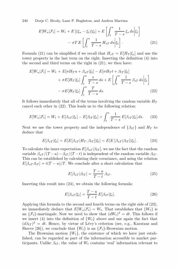
240 Dorje C. Brody, Lane P. Hughston, and Andrea Macrina

E[Wu|Ft] = Wt + E [(ξu − ξt)|ξt] + E

[∫ u

t

1T − s

ξs ds

∣∣∣∣ξt]

− σT E

[∫ u

t

1T − s

HsT ds

∣∣∣∣ξt]. (21)

Formula (21) can be simplified if we recall that HsT = E[HT |ξs] and use thetower property in the last term on the right. Inserting the definition (4) intothe second and third terms on the right in (21), we then have:

E[Wu|Ft] = Wt + E[σHTu+ βuT |ξt] − E[σHT t+ βtT |ξt]

+ σE[HT |ξt]∫ u

t

s

T − sds + E

[∫ u

t

1T − s

βsT ds

∣∣∣∣ξt]

− σE[HT |ξt]∫ u

t

T

T − sds. (22)

It follows immediately that all of the terms involving the random variable HT

cancel each other in (22). This leads us to the following relation:

E[Wu|Ft] = Wt + E[βuT |ξt] − E[βtT |ξt] +∫ u

t

1T − s

E[βsT |ξt] ds. (23)

Next we use the tower property and the independence of {βtT } and HT todeduce that

E[βuT |ξt] = E[E[βuT |HT , βtT ]|ξt] = E[E [βuT |βtT ]|ξt] . (24)

To calculate the inner expectation E[βuT |βtT ], we use the fact that the randomvariable βuT /(T −u)−βtT /(T − t) is independent of the random variable βtT .This can be established by calculating their covariance, and using the relationE[βuTβtT ] = t(T − u)/T . We conclude after a short calculation that

E[βuT |βtT ] =T − u

T − tβtT . (25)

Inserting this result into (24), we obtain the following formula:

E[βuT |ξt] =T − u

T − tE[βtT |ξt]. (26)

Applying this formula to the second and fourth terms on the right side of (23),we immediately deduce that E[Wu|Ft] = Wt. That establishes that {Wt} isan {Ft}-martingale. Now we need to show that (dWt)2 = dt. This follows ifwe insert (4) into the definition of {Wt} above and use again the fact that(dβtT )2 = dt. Hence, by virtue of Levy’s criterion (see, e.g., Karatzas andShreve [26]), we conclude that {Wt} is an {Ft}-Brownian motion.

The Brownian motion {Wt}, the existence of which we have just estab-lished, can be regarded as part of the information accessible to market par-ticipants. Unlike βtT , the value of Wt contains ‘real’ information relevant to

A New Framework for Credit-Risk Modelling 241

the bond payoff. It follows from (10) and (19) that for the discount bonddynamics, we have

dBtT = rtBtT dt +ΣtT dWt. (27)

Here rt = −∂ lnP0t/∂t is the short rate, and the absolute bond volatility ΣtTis given by

ΣtT =σT

T − tPtTVtT , (28)

where VtT is the conditional variance of the terminal payoff HT , defined by

VtT =∑

i

(hi −HtT )2πit. (29)

We observe that as the maturity date is approached the absolute discountbond volatility will be high unless the conditional probability has most of itsmass concentrated around the ‘true’ outcome; this ensures that the correctlevel can be eventually reached.

It follows as a consequence of (20) that {ξt} satisfies the following stochas-tic differential equation:

dξt =1

T − t

(σTH(ξt, t) − ξt

)dt + dWt. (30)

We see that {ξt} is a diffusion process; and because H(ξt, t) is monotonic inits dependence on ξt, we deduce that {BtT } is also a diffusion process. Toestablish that BtT is increasing in ξt, we note that PtTH ′(ξt, t) = ΣtT , whereH ′(ξ, t) = ∂H(ξ, t)/∂ξ. It is interesting to observe that, in principle, insteadof ‘deducing’ the dynamics of {BtT} from the information-based arguments ofthe previous sections, we might have simply ‘proposed’ on an ad hoc basis theone-factor diffusion process (30), noting that it leads to the correct defaultdynamics. This reasoning shows that our framework can be viewed, if desired,as leading to purely ‘classical’ financial models, based on observable priceprocesses.

5 Simulation of Bond Price Processes

The present framework allows for a highly efficient simulation methodologyfor the dynamics of defaultable bonds. In the case of a defaultable discountbond, all we need to do is to simulate the dynamics of {ξt}. For each run ofthe simulation, we choose at random a value for HT (in accordance with thea priori probabilities), and a sample path for the Brownian bridge. That isto say, each simulation corresponds to a choice of ω ∈ Ω, and for each suchchoice we simulate the path ξt(ω) = σtHT (ω)+βtT (ω) for t ∈ [0, T ]. One way

242 Dorje C. Brody, Lane P. Hughston, and Andrea Macrina

to simulate a Brownian bridge is to write βtT = Bt − (t/T )BT , where {Bt}is a standard Brownian motion. It is straightforward to verify that if {βtT } isdefined in this way then it has the correct mean and covariance. Because thebond price at t is expressed directly as a function of the random variable ξt,this means that pathwise simulation of the bond price trajectory is feasiblefor any number of recovery levels.

In Figure 1 we present some sample trajectories of the defaultable bondprice process for various values of σ. These illustrations are fascinating inas-much as they show that for small values of σ the default comes almost as a‘surprise’ near the maturity date of the bond; whereas for large values of σthe default, if it occurs, effectively takes place early in the life of bond.

6 Digital Bonds and Binary Bonds with Partial Recovery

It is interesting to ask whether in the case of a binary bond with partialrecovery, with possible payoffs {h0, h1}, the bond-price process admits therepresentation

BtT = PtTh0 +DtT (h1 − h0). (31)

Here DtT denotes the value of a digital credit-risky bond that at maturity paysa unit of currency with probability p1 and zero with probability p0 = 1 − p1.Thus h0 is the amount that is guaranteed, whereas h1 − h0 is the part thatis ‘at risk.’ It is well known that such a relation can be deduced in intensity-based models. The problem now is to find a process {DtT} consistent withour scheme such that (31) holds. It turns out that this can be achieved.

Suppose we consider a digital payoff structure DT ∈ {0, 1} for which theinformation-flow parameter σ is replaced by σ = σ(h1 − h0). In other words,in establishing the appropriate dynamics for {DtT } we ‘renormalise’ σ byreplacing it with σ. The information available to market participants in thecase of the digital bond is represented by the process {ξt} defined by

ξt = σDT t + βtT . (32)

It follows from (18) that the corresponding digital bond price is given by

DtT = PtTp1exp[

TT−t(σξt − 1

2 σ2t)]

p0 + p1exp[TT−t(σξt − 1

2 σ2t)] . (33)

A calculation making use of (7) then allows us to confirm that (31) holds,where DtT is given by (33). Thus even though prima facie the general bi-nary bond process (7) does not appear to admit a decomposition of the form(31), we see that it does, once a suitably renormalised value for the marketinformation flow-rate parameter has been introduced.

A New Framework for Credit-Risk Modelling 243

1 2 3 4 5T

0.2

0.4

0.6

0.8

1BtT

1 2 3 4 5T

0.2

0.4

0.6

0.8

1BtT

1 2 3 4 5T

0.2

0.4

0.6

0.8

1BtT

1 2 3 4 5T

0.2

0.4

0.6

0.8

1BtT

Fig. 1. Bond price processes for various information flow rates. The parameter σgoverns the rate at which information is released to market participants concerningthe payout of a defaultable discount bond. Four values of σ are illustrated, given by.04, .2, 1, and 5. The bond has a maturity of five years, and the default-free interest-rate system has a constant short rate given by r = 5%. The a priori probabilityof default is taken to be 20%. For low values of σ, collapse of the bond price, if itoccurs, takes place only ‘at the last minute.’

More generally, if the bond has a number of recovery levels, so the randomvariable HT can take the values {h0, h1, . . . , hn}, then h0 can be regardedas the ‘risk-free’ component of the bond. The bond price process admits anadditive decomposition into two parts, namely, a default-free discount bondthat pays h0, and a credit-risky discount bond that pays hi = hi − h0 with apriori probability pi. This decomposition is given by

BtT = PtTh0 + PtT

n∑i=1

pihiexp[

TT−t(σhiξt − 1

2σ2h2i t)]

p0 +n∑i=1

piexp[

TT−t(σhiξt − 1

2σ2h2i t)] , (34)

where ξt = σ(HT − h0)t + βtT is the resulting price-shifted informationprocess. Note that h0 = 0, which makes the summation in the numeratorbegin from i = 1; thus the second term in the right-hand side of (34) is themultiple-recovery-level analogue of formula (33) above.

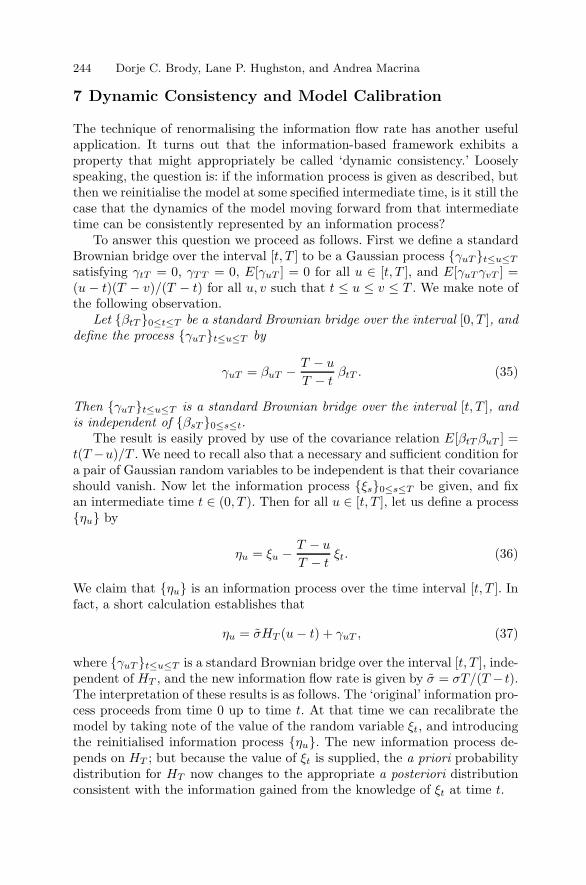
244 Dorje C. Brody, Lane P. Hughston, and Andrea Macrina

7 Dynamic Consistency and Model Calibration

The technique of renormalising the information flow rate has another usefulapplication. It turns out that the information-based framework exhibits aproperty that might appropriately be called ‘dynamic consistency.’ Looselyspeaking, the question is: if the information process is given as described, butthen we reinitialise the model at some specified intermediate time, is it still thecase that the dynamics of the model moving forward from that intermediatetime can be consistently represented by an information process?

To answer this question we proceed as follows. First we define a standardBrownian bridge over the interval [t, T ] to be a Gaussian process {γuT }t≤u≤Tsatisfying γtT = 0, γTT = 0, E[γuT ] = 0 for all u ∈ [t, T ], and E[γuTγvT ] =(u − t)(T − v)/(T − t) for all u, v such that t ≤ u ≤ v ≤ T . We make note ofthe following observation.

Let {βtT }0≤t≤T be a standard Brownian bridge over the interval [0, T ], anddefine the process {γuT }t≤u≤T by

γuT = βuT − T − u

T − tβtT . (35)

Then {γuT }t≤u≤T is a standard Brownian bridge over the interval [t, T ], andis independent of {βsT }0≤s≤t.

The result is easily proved by use of the covariance relation E[βtTβuT ] =t(T −u)/T . We need to recall also that a necessary and sufficient condition fora pair of Gaussian random variables to be independent is that their covarianceshould vanish. Now let the information process {ξs}0≤s≤T be given, and fixan intermediate time t ∈ (0, T ). Then for all u ∈ [t, T ], let us define a process{ηu} by

ηu = ξu −T − u

T − tξt. (36)

We claim that {ηu} is an information process over the time interval [t, T ]. Infact, a short calculation establishes that

ηu = σHT (u− t) + γuT , (37)

where {γuT }t≤u≤T is a standard Brownian bridge over the interval [t, T ], inde-pendent of HT , and the new information flow rate is given by σ = σT/(T − t).The interpretation of these results is as follows. The ‘original’ information pro-cess proceeds from time 0 up to time t. At that time we can recalibrate themodel by taking note of the value of the random variable ξt, and introducingthe reinitialised information process {ηu}. The new information process de-pends on HT ; but because the value of ξt is supplied, the a priori probabilitydistribution for HT now changes to the appropriate a posteriori distributionconsistent with the information gained from the knowledge of ξt at time t.

A New Framework for Credit-Risk Modelling 245

These interpretive remarks can be put into a more precise form as follows.Let 0 ≤ t ≤ u < T . What we want is a formula for the conditional probabilityπiu expressed in terms of the information ηu and the ‘new’ a priori probabilityπit. Such a formula exists, and is given as follows:

πiu =πitexp

[T−tT−u(σhiηu − 1

2 σ2h2i (u− t)

)]

∑i πitexp

[T−tT−u(σhiηu − 1

2 σ2h2i (u − t)

)] . (38)

This remarkable relation can be verified by substituting the given expressionsfor πit, ηu, and σ into the right-hand side of (38). But (38) has the samestructure as the original formula (17) for πit, and thus we see that the modelexhibits manifest dynamic consistency.

8 Options on Credit-Risky Bonds

We now turn to consider the pricing of options on credit-risky bonds. As wedemonstrate shortly, in the case of a binary bond there is an exact solutionfor the valuation of European-style vanilla options. The resulting expressionfor the option price exhibits a structure that is strikingly analogous to thatof the Black–Scholes–Merton option pricing formula.

We consider the value at time 0 of an option that is exercisable at a fixedtime t > 0 on a credit-risky discount bond that matures at time T > t. Thevalue C0 of a call option is

C0 = P0tE[(BtT −K)+

], (39)

where K is the strike price. Inserting formula (5) for BtT into the valuationformula (39) for the option, we obtain

C0 = P0tE[(PtTHtT −K)+

]

= P0tE

⎡

⎣(

n∑

i=0

PtTπithi −K

)+⎤

⎦

= P0tE

⎡

⎣(

1Φt

n∑

i=0

PtT pithi −K

)+⎤

⎦

= P0tE

⎡

⎣ 1Φt

(n∑

i=0

(PtThi −K

)pit

)+⎤

⎦ . (40)

Here the random variables pit, i = 0, 1, . . . , n, are the ‘unnormalised’ condi-tional probabilities, defined by

pit = piexp[

T

T − t

(σhiξt − 1

2σ2h2i t)]

. (41)

246 Dorje C. Brody, Lane P. Hughston, and Andrea Macrina

Then πit = pit/Φt where Φt =∑

i pit, or, more explicitly,

Φt =n∑

i=0

piexp[

T

T − t

(σhiξt − 1

2σ2h2i t)]

. (42)

Our plan now is to use the factor 1/Φt appearing in (40) to make a changeof probability measure on (Ω,Ft). To this end, we fix a time horizon u at orbeyond the option expiration but before the bond maturity, so t ≤ u < T . Wedefine a process {Φt}0≤t≤u by use of the expression (42), where now we let tvary in the range [0, u]. It is a straightforward exercise in Ito calculus, makinguse of (30), to verify that

dΦt = σ2

(T

T − t

)2

H2tTΦt dt + σ

T

T − tHtTΦt dWt. (43)

It follows then that

dΦ−1t = −σ T

T − tHtTΦ

−1t dWt, (44)

and hence that

Φ−1t = exp

(−σ∫ t

0

T

T − sHsT dWs − 1

2σ2

∫ t

0

T 2

(T − s)2H2sT ds

). (45)

Because {HsT } is bounded, and s ≤ u < T , we see that the process{Φ−1

s }0≤s≤u is a martingale. In particular, because Φ0 = 1, we deduce thatEQ[Φ−1

t ] = 1, where t is the option maturity date, and hence that the factor1/Φt in (40) can be used to effect a change of measure on (Ω,Ft). Writing Bfor the new probability measure thus defined, we have

C0 = P0t EB

⎡

⎣(

n∑

i=0

(PtThi −K

)pit

)+⎤

⎦ . (46)

We call B the ‘bridge’ measure because it has the special property thatit makes {ξs}0≤s≤t a B-Gaussian process with mean zero and covarianceEB[ξrξs] = r(T − s)/T for 0 ≤ r ≤ s ≤ t. In other words, with respectto the measure B, and over the interval [0, t], the information process has thelaw of a standard Brownian bridge over the interval [0, T ]. Armed with thisfact, we proceed to calculate the expectation in (46).

The proof that {ξs}0≤s≤t has the claimed properties under the measureB is as follows. For convenience we introduce a process {W ∗

t }0≤t≤u which wedefine as the following Brownian motion with drift in the Q-measure:

W ∗t = Wt + σ

∫ t

0

T

T − sHsT ds. (47)

A New Framework for Credit-Risk Modelling 247

It is straightforward to check that on (Ω,Ft) the process {W ∗t }0≤t≤u is a

Brownian motion with respect to the measure defined by use of the densitymartingale {Φ−1

t }0≤t≤u given by (45). It then follows from the definition of{Wt}, given in (20), that

W ∗t = ξt +

∫ t

0

1T − s

ξs ds. (48)

Taking the stochastic differential of each side of this relation, we deduce that

dξt = − 1T − t

ξt dt+ dW ∗t . (49)

We note, however, that (49) is the stochastic differential equation satisfied bya Brownian bridge (see, e.g., Karatzas and Shreve [26], Yor [37], and Protter[34]) over the interval [0, T ]. Thus we see that in the measure B defined on(Ω,Ft), the process {ξs}0≤s≤t has the properties of a standard Brownianbridge over [0, T ], albeit restricted to the interval [0, t].

For the transformation back from B to Q on (Ω,Ft), the appropriatedensity martingale {Φt}0≤t≤u with respect to B is given by

Φt = exp(σ

∫ t

0

T

T − sHsT dW

∗s − 1

2σ2

∫ t

0

T 2

(T − s)2H2sT ds

). (50)

The crucial point that follows from this analysis is that the random variableξt is B-Gaussian. In the case of a binary discount bond, therefore, the relevantexpectation for determining the option price can be carried out by standardtechniques, and we are led to a formula of the Black–Scholes–Merton type. Inparticular, for a binary bond, (46) reads

C0 = P0tEB

[((PtTh1 −K)p1t + (PtTh0 −K)p0t

)+], (51)

where p0t and p1t are given by

p0t = p0exp[

TT−t(σh0ξt − 1

2σ2h2

0t)],

p1t = p1exp[

TT−t(σh1ξt − 1

2σ2h2

1t)].

(52)

To compute the value of (51), there are essentially three different cases thathave to be considered: (i) PtTh1 > PtTh0 > K, (ii) K > PtTh1 > PtTh0, and(iii) PtTh1 > K > PtTh0. In case (i) the option is certain to expire in themoney. Thus, making use of the fact that ξt is B-Gaussian with mean zeroand variance t(T − t)/T , we see that EB[pit] = pi; hence in case (i) we haveC0 = B0T − P0tK. In case (ii) the option expires out of the money, and thusC0 = 0. In case (iii) the option can expire in or out of the money, and there

248 Dorje C. Brody, Lane P. Hughston, and Andrea Macrina

is a ‘critical’ value of ξt above which the argument of (51) is positive. This isobtained by setting the argument of (51) to zero and solving for ξt. Writingξt for the critical value, we find that ξt is determined by the relation

T

T − tσ(h1 − h0)ξt = ln

[p0(PtTh0 −K)p1(K − PtTh1)

]+ 1

2σ2(h2

1 − h20)τ, (53)

where τ = tT/(T − t). Next we note that inasmuch as ξt is B-Gaussianwith mean zero and variance t(T − t)/T , for the purpose of computing theexpectation in (51) we can set ξt = Z

√t(T − t)/T , where Z is B-Gaussian

with zero mean and unit variance. Then writing Z for the correspondingcritical value of Z, we obtain

Z =ln[p0(PtTh0−K)p1(K−PtTh1)

]+ 1

2σ2(h2

1 − h20)τ

σ√τ (h1 − h0)

. (54)

With this expression at hand, we can work out the expectation in (51). Weare thus led to the following option pricing formula:

C0 = P0t

[p1(PtTh1 −K)N(d+) − p0(K − PtTh0)N(d−)

]. (55)

Here d+ and d− are defined by

d± =ln[p1(PtT h1−K)p0(K−PtT h0)

]± 1

2σ2(h1 − h0)2τ

σ√τ (h1 − h0)

. (56)

A short calculation shows that the corresponding option delta, defined byΔ = ∂C0/∂B0T , is given by

Δ =(PtTh1 −K)N(d+) + (K − PtTh0)N(d−)

PtT (h1 − h0). (57)

This can be verified by using (3) to determine the dependency of the optionprice C0 on the initial bond price B0T .

It is interesting to note that the parameter σ plays a role like that of thevolatility parameter in the Black–Scholes–Merton model. The more rapidlyinformation is ‘leaked out’ about the true value of the bond repayment, thehigher the volatility. It is straightforward to verify that the option price hasa positive vega, that is, C0 is an increasing function of σ. This means that wecan use bond option prices (or, equivalently, caps and floors) to back out animplied value for σ, and hence to calibrate the model. Writing V = ∂C0/∂σfor the corresponding option vega, we obtain the following positive expression:

V =1√2π

e−rt−(1/2)A(h1 − h0)√τp0p1(PtTh1 −K)(K − PtTh0), (58)

A New Framework for Credit-Risk Modelling 249

where

A =1

σ2τ(h1 − h0)2

(ln[p1(PtTh1 −K)p0(K − PtTh0)

])2

+ 14σ

2τ(h1 − h0)2. (59)

We remark that in the more general case of a stochastic recovery, a semi-analytic option pricing formula can be obtained that, for practical purposes,can be regarded as fully tractable. In particular, starting from (46), we con-sider the case where the strike price K lies in the range PtThk+1 > K > PtThkfor some value of k ∈ {0, 1, . . . , n}. It is an exercise to verify that there exists aunique critical value of ξt such that the summation appearing in the argumentof the max(x, 0) function in (46) vanishes. Writing ξt for the critical value,which can be obtained by numerical methods, we define the scaled criticalvalue Z as before, by setting ξt = Z

√t(T − t)/T . A calculation then shows

that the option price is given by the following expression:

C0 = P0t

n∑

i=0

pi (PtThi −K) N(σhi√τ − Z). (60)

9 Bond Option Price Processes

In the previous section we obtained the initial value C0 of an option on abinary credit-risky bond. In the present section we determine the price process{Cs}0≤s≤t of such an option. We fix the bond maturity T and the optionmaturity t. Then the price Cs of a call option at time s ≤ t is given by

Cs = Pst E[(BtT −K)+|Fs

]

=PstΦs

EB[Φt(BtT −K)+|Fs

]

=PstΦs

EB

⎡

⎣(

n∑

i=0

(PtThi −K

)pit

)+∣∣∣∣∣∣Fs

⎤

⎦ . (61)

We recall that pit, defined in (41), is a function of ξt. The calculation can thusbe simplified by use of the fact that {ξt} is a B-Brownian bridge. To determinethe conditional expectation (61) we note that the B-Gaussian random variableZst defined by

Zst =ξt

T − t− ξsT − s

(62)

is independent of {ξu}0≤u≤s. We can then express {pit} in terms of ξs andZst by writing

pit = piexp[

T

T − sσhiTξs − 1

2

T

T − tσ2h2

i t + σhiZstT

]. (63)

250 Dorje C. Brody, Lane P. Hughston, and Andrea Macrina

Substituting (63) into (61), we find that Cs can be calculated by taking anexpectation involving the random variable Zst, which has mean zero and vari-ance v2

st, given by

v2st =

t− s

(T − t)(T − s). (64)

In the case of a call option on a binary discount bond that pays h0 or h1,we can obtain a closed-form expression for (61). In that case the option priceis given as follows:

Cs =PstΦs

EB[(

(PtTh0 −K)p0t + (PtTh1 −K)p1t

)+∣∣∣∣Ft]. (65)

Substituting (63) in (65) we find that the expression in the expectation ispositive only if the inequality Zst > Z is satisfied, where

Z =ln[π0s(K−PtT h0)π1s(PtT h1−K)

]+ 1

2σ2(h2

1 − h20)v2

stT

σvstT (h1 − h0). (66)

It is convenient to set Zst = vstZ, where Z is a B-Gaussian random variablewith zero mean and unit variance. The computation of the expectation in (65)then reduces to a pair of Gaussian integrals, and we obtain

Cs = Pst

[π1s (PtTh1 −K)N(d+

s ) − π0s (K − PtTh0)N(d−s )], (67)

where the conditional probabilities {πis} are as defined in (17), and

d±s =ln[π1s(PtT h1−K)π0s(K−PtT h0)

]± 1

2σ2v2stT

2(h1 − h0)2

σvstT (h1 − h0). (68)

We note that d+s = d−s + σvstT (h1 − h0), and that d±0 = d±.

One important feature of the model worth pointing out in the presentcontext is that a position in a bond option can be hedged with a positionin the underlying bond. This is because the option price process and theunderlying bond price process are one-dimensional diffusions driven by thesame Brownian motion. Because Ct and BtT are both monotonic in theirdependence on ξt, it follows that Ct can be expressed as a function of BtT ;the delta of the option can then be obtained in the conventional way as thederivative of the option price with respect to the underlying. In the case of abinary bond, the resulting hedge ratio process {Δs}0≤s≤t is given by

Δs =(PtTh1 −K)N(d+

s ) + (K − PtTh0)N(d−s )PtT (h1 − h0)

. (69)

This brings us to another interesting point. For certain types of instru-ments, it may be desirable to model the occurrence of credit events (e.g.,

A New Framework for Credit-Risk Modelling 251

credit-rating downgrades) taking place at some time preceding a cash-flowdate. In particular, we may wish to consider contingent claims based on suchevents. In the present framework we can regard such contingent claims asderivative structures for which the payoff is triggered by the level of {ξt}.For example, it may be that a credit event is established if BtT drops belowsome specific level, or if the credit spread widens beyond some threshold. Asa consequence, a number of different types of contingent claims can be valuedby use of barrier option methods in this framework (cf. Albanese et al. [1],Chen and Filipovic [7], and Albanese and Chen [2]).

10 Coupon Bonds: The X-Factor Approach

The discussion so far has focused on simple structures, such as discount bondsand options on discount bonds. One of the advantages of the present approach,however, is that its tractability extends to situations of a more complex nature.In this section we consider the case of a credit-risky coupon bond. One shouldregard a coupon bond as being a rather complicated instrument from thepoint of view of credit risk management, because default can occur at anyof the coupon dates. The market will in general possess partial informationconcerning all of the future coupon payments, as well as the principal payment.

As an illustration, we consider a bond with two payments remaining: acoupon HT1 at time T1, and a coupon plus the principal totalling HT2 at timeT2. We assume that if default occurs at T1, then no further payment is madeat T2. On the other hand, if the T1-coupon is paid, default may still occur atT2. We model this by setting

HT1 = cXT1 and HT2 = (c + p)XT1XT2 , (70)

where XT1 and XT2 are independent random variables each taking the values{0, 1}, and the constants c and p denote the coupon and principal. Let us write{p(1)

0 , p(1)1 } for the a priori probabilities that XT1 = {0, 1}, and {p(2)

0 , p(2)1 } for

the a priori probabilities that XT2 = {0, 1}. We introduce a pair of informationprocesses

ξ(1)t = σ1XT1t + β

(1)tT1

and ξ(2)t = σ2XT2t + β

(2)tT2

, (71)

where {β(1)tT1

} and {β(2)tT2

} are independent Brownian bridges, and σ1 and σ2

are parameters. Then for the credit-risky coupon-bond price process we have

St = cPtT1E[XT1

∣∣ξ(1)t

]+ (c + p)PtT2E

[XT1

∣∣ξ(1)t

]E[XT2

∣∣ξ(2)t

]. (72)

The two conditional expectations appearing in this formula can be workedout explicitly using the techniques already described. The result is

252 Dorje C. Brody, Lane P. Hughston, and Andrea Macrina

E[XTi

∣∣ξ(i)t

]=

p(i)1 exp[Ti

Ti−t

(σiξ

(i)t − 1

2σ2i t)]

p(i)0 + p

(i)1 exp[

Ti

Ti−t

(σiξ

(i)t − 1

2σ2i t)] , (73)

for i = 1, 2. It should be evident that in the case of a bond with two paymentsremaining we obtain a natural ‘two-factor’ model, the factors being the twoindependent Brownian motions arising in connection with the information pro-cesses {ξ(i)

t }i=1,2. Similarly, if there are n outstanding coupons, we model thepayments by HTk

= cXT1 · · ·XTkfor k ≤ n−1 and HTn = (c+p)XT1 · · ·XTn ,

and introduce the information processes

ξ(i)t = σiXTit+ β

(i)tTi

(i = 1, 2, . . . , n). (74)

The case of n outstanding payments leads to an n-factor model. The inde-pendence of the random variables {XTi}i=1,2,...,n implies that the price of acredit-risky coupon bond admits a closed-form expression analogous to (72).

With a slight modification of these expressions, we can consider the casewhen there is partial recovery in the event of default. In the two-couponexample discussed above, for instance, we can extend the model by sayingthat in the event of default on the first coupon the effective recovery rate (asa percentage of coupon plus principal) is R1, whereas in the case of default onthe final payment, the recovery rate is R2. Then HT1 = cXT1 +R1(c+p)(1−XT1) and HT2 = c+ pXT1XT2 +R2(c +p)XT1(1−XT2). A further extensionof this reasoning allows for the introduction of a stochastic recovery rate.

11 Credit Default Swaps

Swap-like structures can also be readily treated. For example, in the case of abasic credit default swap (CDS), we have a series of premium payments, eachof the amount g, made to the seller of protection. The payments continueuntil the failure of a coupon payment in the reference bond, at which point apayment n is made to the buyer of protection.

As an illustration, we consider two reference coupons, letting XT1 and XT2

be the associated independent market factors, following the pattern of theprevious example. We assume for simplicity that the default-swap premiumpayments are made immediately after the coupon dates. Then the value ofthe default swap, from the point of view of the seller of protection, is

Vt = gPtT1E[XT1

∣∣ξ(1)t

]− nPtT1E

[1 −XT1

∣∣ξ(1)t

]

+ gPtT2E[XT1

∣∣ξ(1)t

]E[XT2

∣∣ξ(2)t

]

−nPtT2E[XT1

∣∣ξ(1)t

]E[1 −XT2

∣∣ξ(2)t

]. (75)

After some rearrangement of terms, this can be expressed more compactly asfollows:

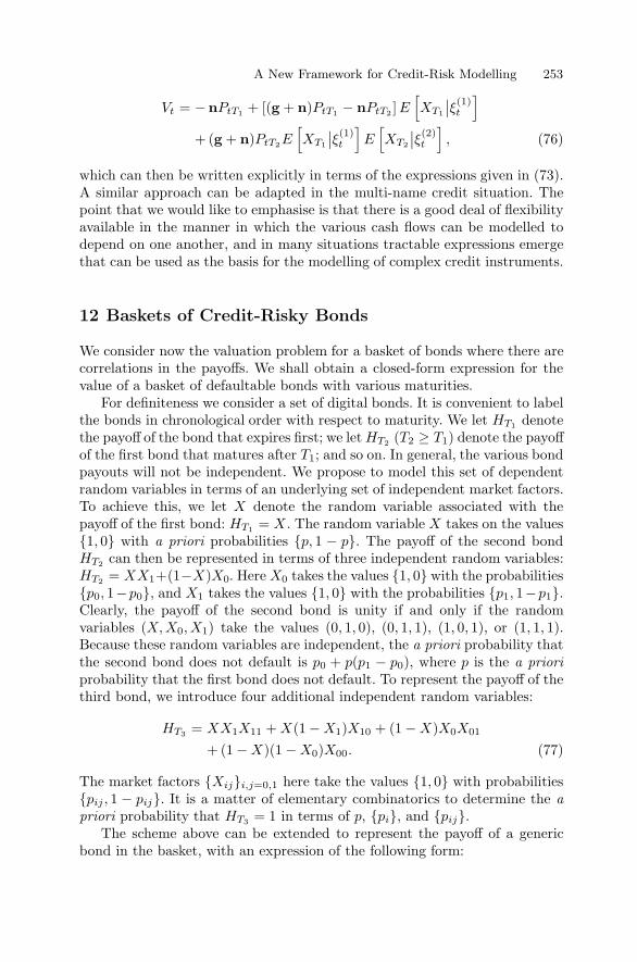
A New Framework for Credit-Risk Modelling 253

Vt = −nPtT1 + [(g + n)PtT1 − nPtT2 ]E[XT1

∣∣ξ(1)t

]

+ (g + n)PtT2E[XT1

∣∣ξ(1)t

]E[XT2

∣∣ξ(2)t

], (76)

which can then be written explicitly in terms of the expressions given in (73).A similar approach can be adapted in the multi-name credit situation. Thepoint that we would like to emphasise is that there is a good deal of flexibilityavailable in the manner in which the various cash flows can be modelled todepend on one another, and in many situations tractable expressions emergethat can be used as the basis for the modelling of complex credit instruments.

12 Baskets of Credit-Risky Bonds

We consider now the valuation problem for a basket of bonds where there arecorrelations in the payoffs. We shall obtain a closed-form expression for thevalue of a basket of defaultable bonds with various maturities.

For definiteness we consider a set of digital bonds. It is convenient to labelthe bonds in chronological order with respect to maturity. We let HT1 denotethe payoff of the bond that expires first; we letHT2 (T2 ≥ T1) denote the payoffof the first bond that matures after T1; and so on. In general, the various bondpayouts will not be independent. We propose to model this set of dependentrandom variables in terms of an underlying set of independent market factors.To achieve this, we let X denote the random variable associated with thepayoff of the first bond: HT1 = X . The random variable X takes on the values{1, 0} with a priori probabilities {p, 1 − p}. The payoff of the second bondHT2 can then be represented in terms of three independent random variables:HT2 = XX1+(1−X)X0. Here X0 takes the values {1, 0} with the probabilities{p0, 1−p0}, and X1 takes the values {1, 0} with the probabilities {p1, 1−p1}.Clearly, the payoff of the second bond is unity if and only if the randomvariables (X,X0, X1) take the values (0, 1, 0), (0, 1, 1), (1, 0, 1), or (1, 1, 1).Because these random variables are independent, the a priori probability thatthe second bond does not default is p0 + p(p1 − p0), where p is the a prioriprobability that the first bond does not default. To represent the payoff of thethird bond, we introduce four additional independent random variables:

HT3 = XX1X11 +X(1 −X1)X10 + (1 −X)X0X01

+ (1 −X)(1 −X0)X00. (77)

The market factors {Xij}i,j=0,1 here take the values {1, 0} with probabilities{pij , 1 − pij}. It is a matter of elementary combinatorics to determine the apriori probability that HT3 = 1 in terms of p, {pi}, and {pij}.

The scheme above can be extended to represent the payoff of a genericbond in the basket, with an expression of the following form:

254 Dorje C. Brody, Lane P. Hughston, and Andrea Macrina

HTn+1 =∑

{kj}=1,0

Xω(k1)Xω(k2)k1

Xω(k3)k1k2

· · ·Xω(kn)k1k2···kn−1

Xk1k2···kn−1kn . (78)

Here, for any random variableX we define Xω(0) = 1−X and Xω(1) = X . Thepoint to observe is that if we have a basket of N digital bonds with arbitrarya priori default probabilities and correlations, then we can introduce 2N − 1independent digital random variables to represent the N correlated randomvariables associated with the bond payoffs.

One advantage of the decomposition into independent market factors isthat we retain analytical tractability for the pricing of the basket. In partic-ular, because the random variables {Xk1k2···kn} are independent, it is naturalto introduce 2N −1 independent Brownian bridges to represent the noise thatveils the values of the independent market factors:

ξk1k2···knt = σk1k2···knXk1k2···knt + βk1k2···kn

tTn+1. (79)

The number of independent factors grows rapidly with the number of bonds inthe portfolio. As a consequence, a market that consists of correlated bonds is ingeneral highly incomplete. This fact provides an economic justification for thecreation of products such as CDSs and CDOs that enhance the ‘hedgeability’of such portfolios.

13 Homogeneous Baskets

In the case of a ‘homogeneous’ basket, the number of independent factorsdetermining the payoff of the portfolio can be reduced. We assume now thatthe basket contains n defaultable discount bonds, each maturing at time T ,and each paying 0 or 1, with the same a priori probability of default. Thissituation is of interest as a first step in the analysis of the more general setup.Our goal is to model default correlations in the portfolio, and in particular tomodel the flow of market information concerning default correlation. Let uswrite HT for the payoff at time T of the homogeneous portfolio, and set

HT = n−X1 −X1X2 −X1X2X3 − · · · −X1X2 . . . Xn, (80)

where the random variables {Xj}j=1,2,...,n, each taking the values {0, 1}, areassumed to be independent. Thus if X1 = 0, then HT = n; if X1 = 1 andX2 = 0, then HT = n − 1; if X1 = 1, X2 = 1, and X3 = 0, then HT = n − 2;and so on. Now suppose we write pj = Q(Xj = 1) and qj = Q(Xj = 0) forj = 1, 2, . . . , n. Then Q(HT = n) = q1, Q(HT = n − 1) = p1q2, Q(HT =n − 2) = p1p2q3, and so on. More generally, we have Q(HT = n − k) =p1p2 . . . pkqk+1. Thus, for example, if p1 � 1 but p2, p3, . . . , pk are large, thenwe are in a situation of low default probability and high default correlation;that is to say, the probability of a default occurring in the portfolio is small,

A New Framework for Credit-Risk Modelling 255

but conditional on at least one default occurring, the probability of severaldefaults is high.

The market will take a view on the likelihood of various numbers of defaultsoccurring in the portfolio. We model this by introducing a set of independentinformation processes {ηjt } defined by

ηjt = σjXjt+ βjtT , (81)

where {σj}j=1,2,...,n are parameters, and {βjtT }j=1,2,...,n are independentBrownian bridges. The market filtration {Ft} is generated collectively by{ηjt }j=1,2,...,n, and for the portfolio value Ht = PtTE [HT |Ft], we have

Ht = PtT

[n− Et[X1] − Et[X1]Et[X2] − · · · −Et[X1]Et[X2] . . . Et[Xn]

]. (82)

The conditional expectations appearing here can be calculated by means offormulae established earlier in the paper. The resulting dynamics for {Ht}can then be used to describe the evolution of correlations in the portfolio. Forexample, if Et[X1] is low and Et[X2] is high, then the conditional probabilityat time t of a default at time T is small, whereas if Et[X1] were to increasesuddenly, then the conditional probability of two or more defaults at T wouldrise as a consequence. Thus, the model is sufficiently rich to admit a detailedaccount of the correlation dynamics of the portfolio. The losses associatedwith individual tranches can be identified, and derivative structures associ-ated with such tranches can be defined. For example, a digital option thatpays out in the event that there are three or more defaults has the payoffstructure H

(3)T = X1X2X3. The homogeneous portfolio model has the prop-

erty that the dynamics of equity-level and mezzanine-level tranches involve arelatively small number of factors. The market prices of tranches can be usedto determine the a priori probabilities, and the market prices of options ontranches can be used to fix the information-flow parameters.

Acknowledgments

The authors are grateful to T. Bielecki, I. Buckley, T. Dean, G. Di Graziano,A. Elizalde, B. Flesaker, T. Hurd, M. Jeanblanc, B. Meister, C. Rogers,M. Rutkowski, and M. Zervos, for helpful comments.

We are grateful to seminar participants at the Isaac Newton Institute,Cambridge, 3 May, 19 June, and 8 July 2005; at the Mathematics in FinanceConference, Kruger Park, RSA, 9 August 2005; at the Imperial College Work-shop on Mathematical Finance and Stochastic Analysis, 23 August 2005; atCEMFI (Centro de Estudios Monetarios y Financieros), Madrid, 3 October2005; at the Winter School in Financial Mathematics, Lunteren, the Nether-lands, 24 January 2006; at the First Conference on Advanced MathematicalMethods for Finance, Side, Antalya, Turkey, 26–29 April 2006; and at the

256 Dorje C. Brody, Lane P. Hughston, and Andrea Macrina

Bachelier Finance Society Fourth World Congress, Tokyo, Japan, 17–19 Au-gust 2006, where drafts of this paper have been presented, for their comments.

This work was carried out in part while Lane Hughston and Andrea Mac-rina were participants in the Isaac Newton Institute’s Developments in Quan-titative Finance programme (April–July 2005). We thank I. Buckley for assis-tance with the figures. Dorje Brody and Lane Hughston acknowledge supportfrom The Royal Society; Lane Hughston and Andrea Macrina acknowledgesupport from EPSRC grant number GR/S22998/01; Andrea Macrina thanksthe Public Education Authority of the Canton of Bern, Switzerland, and theUK Universities ORS scheme.

Finally, it is our pleasure to dedicate this paper to Dilip Madan on the oc-casion of his sixtieth birthday, in acknowledgment of his numerous significantcontributions to mathematical finance and in recognition of the inspirationand encouragement he has so often and so generously given to others workingin the subject.

References

1. C. Albanese, J. Campolieti, O. Chen, and A. Zavidonov. Credit barrier models.Risk, 16:109–113, 2003.

2. C. Albanese and O. Chen. Implied migration rates from credit barrier models.J. Banking and Finance, 30:607–626, 2006.

3. T.R. Bielecki, M. Jeanblanc, and M. Rutkowski. Modelling and valuation ofcredit risk. In Stochastic Methods in Finance, Bressanone Lectures 2003, eds.M. Fritelli and W. Runggaldier, LNM 1856, Springer, 2004.

4. T.R. Bielecki and M. Rutkowski. Credit Risk: Modelling, Valuation and Hedging.Springer, 2002.

5. F. Black and J.C. Cox. Valuing corporate securities: Some effects of bond in-denture provisions. J. Finance, 31:351–367, 1976.

6. U. Cetin, R. Jarrow, P. Protter, and Y. Yildrim. Modelling credit risk withpartial information. Ann. Appl. Prob., 14:1167–1172, 2004.

7. L. Chen and D. Filipovic. A simple model for credit migration and spread curves.Finance and Stochastics, 9:211–231, 2005.

8. J.H. Cochrane. Asset Pricing. Princeton University Press, 2005.9. D. Duffie and D. Lando. Term structure of credit spreads with incomplete ac-

counting information. Econometrica, 69:633–664, 2001.10. D. Duffie, M. Schroder, and C. Skiadas. Recursive valuation of defaultable secu-

rities and the timing of resolution of uncertainty. Ann. Appl. Prob., 6:1075–1090,1996.

11. D. Duffie and K.J. Singleton. Modelling term structures of defaultable bonds.Rev. Financial Studies, 12:687–720, 1999.

12. D. Duffie and K.J. Singleton. Credit Risk: Pricing, Measurement and Manage-ment. Princeton University Press, 2003.

13. A. Elizalde. Credit risk models: I Default correlation in intensity models, IIStructural models, III Reconciliation structural-reduced models, IV Understand-ing and pricing CDOs. www.abelelizalde.com, 2005.

A New Framework for Credit-Risk Modelling 257

14. B. Flesaker, L.P. Hughston, L. Schreiber, and L. Sprung. Taking all the credit.Risk, 7:104–108, 1994.

15. K. Giesecke. Correlated default with incomplete information. J. Banking andFinance, 28:1521–1545, 2004.

16. K. Giesecke and L.R. Goldberg. Sequential default and incomplete information.J. Risk, 7:1–26, 2004.

17. B. Hilberink and L.C.G. Rogers. Optimal capital structure and endogenousdefault. Finance and Stochastics, 6:237–263, 2002.

18. L.P. Hughston and S. Turnbull. Credit risk: Constructing the basic buildingblocks. Economic Notes, 30:281–292, 2001.

19. J. Hull and A. White. Merton’s model, credit risk and volatility skews. J. CreditRisk, 1:1–27, 2004.

20. R.A. Jarrow, D. Lando, and S.M. Turnbull. A Markov model for the term struc-ture of credit risk spreads. Rev. Financial Stud., 10:481–528, 1997.

21. R.A. Jarrow and P. Protter. Structural versus reduced form models: A newinformation based perspective. J. Invest. Management, 2:1–10, 2004.

22. R.A. Jarrow and S.M. Turnbull. Pricing derivatives on financial securities sub-ject to credit risk. J. Finance, 50:53–85, 1995.

23. R.A. Jarrow, D. van Deventer, and X. Wang. A robust test of Merton’s structuralmodel for credit risk. J. Risk, 6:39–58, 2003.

24. R.A. Jarrow and F. Yu. Counterparty risk and the pricing of defaultable secu-rities. J. Finance, 56:1765–1799, 2001.

25. M. Jeanblanc and M. Rutkowski. Modelling of default risk: An overview. InMathematical Finance: Theory and Practice, Higher Education Press, 2000.

26. I. Karatzas and S. Shreve. Brownian Motion and Stochastic Calculus, 2nd edi-tion. Springer, 1991.

27. S. Kusuoka. A remark on default risk models. Advances Math. Economics, 1:69-82, 1999.

28. D. Lando. On Cox processes and credit risky securities. Rev. Derivatives Re-search, 2:99-120, 1998.

29. D. Lando. Credit Risk Modelling. Princeton University Press, 2004.30. H.E. Leland and K.B. Toft. Optimal capital structure, endogenous bankruptcy

and the term structure of credit spreads. J. Finance, 50:789–819, 1996.31. D. Madan and H. Unal. Pricing the risks of default. Rev. Derivatives Research,

2:121–160, 1998.32. D. Madan and H. Unal. A two-factor hazard-rate model for pricing risky debt

and the term structure of credit spreads. J. Financial and Quantitative Analysis,35:43–65, 2000.

33. R. Merton. On the pricing of corporate debt: The risk structure of interest rates.J. Finance, 29:449–470, 1974.

34. P.E. Protter. Stochastic Integration and Differential Equations. Springer, 2004.35. P.J. Schonbucher. Credit Derivatives Pricing Models. John Wiley & Sons, 2003.36. M. Yor. Some Aspects of Brownian Motion, Part I: Some Special Functionals.

Birkhauser Verlag, 1992.37. M. Yor. Some Aspects of Brownian Motion, Part II: Some Recent Martingale

Problems. Birkhauser Verlag, 1996.

A Generic One-Factor Levy Model for PricingSynthetic CDOs

Hansjorg Albrecher,1,2 Sophie A. Ladoucette,3 and Wim Schoutens3

1 Johann Radon InstituteAustrian Academy of SciencesAltenbergerstrasse 69A-4040 Linz, Austria

2 Graz University of TechnologyDepartment of MathematicsSteyrergasse 30A-8010 Graz, Austriaalbrecher@tugraz.at

3 Katholieke Universiteit LeuvenDepartment of MathematicsW. de Croylaan 54B-3001 Leuven, Belgiumsophie.ladoucette@wis.kuleuven.be, wim@schoutens.be

Summary. The one-factor Gaussian model is well known not to fit the prices of thedifferent tranches of a collateralized debt obligation (CDO) simultaneously, leadingto the implied correlation smile. Recently, other one-factor models based on differ-ent distributions have been proposed. Moosbrucker [12] used a one-factor Variance-Gamma (VG) model, Kalemanova et al. [7] and Guegan and Houdain [6] workedwith a normal inverse Gaussian (NIG) factor model, and Baxter [3] introduced theBrownian Variance-Gamma (BVG) model. These models bring more flexibility intothe dependence structure and allow tail dependence. We unify these approaches,describe a generic one-factor Levy model, and work out the large homogeneousportfolio (LHP) approximation. Then we discuss several examples and calibrate abattery of models to market data.

Key words: Levy processes; collateralized debt obligation (CDO); credit risk; creditdefault; large homogeneous portfolio approximation.

1 Introduction

A collateralized debt obligation (CDO) can be defined as a transaction thattransfers the credit risk on a reference portfolio of assets. A standard feature

260 Hansjorg Albrecher, Sophie A. Ladoucette, and Wim Schoutens

of a CDO structure is the tranching of credit risk. Credit tranching refers tocreating multiple tranches of securities that have varying degrees of seniorityand risk exposure. The risk of loss on the reference portfolio is then dividedinto tranches of increasing seniority in the following way. The equity trancheis the first to be affected by losses in the event of one or more defaults inthe portfolio. If losses exceed the value of this tranche, they are absorbed bythe mezzanine tranche(s). Losses that have not been absorbed by the othertranches are sustained by the senior tranche and finally by the super-seniortranche. Each tranche then protects the ones senior to it from the risk of losson the underlying portfolio. When tranches are issued, they usually receivea rating by rating agencies. The CDO issuer typically determines the size ofthe senior tranche so that it is AAA-rated. Likewise, the CDO issuer gener-ally designs the other tranches so that they achieve successively lower ratings.The CDO investors take on exposure to a particular tranche, effectively sell-ing credit protection to the CDO issuer, and in turn collecting premiums(spreads).

We are interested in pricing tranches of synthetic CDOs. A synthetic CDOis a CDO backed by credit default swaps (CDSs) rather than bonds or loans;that is, the reference portfolio is composed of CDSs. Recall that a CDS offersprotection against default of an underlying entity over some time horizon. Theterm synthetic is used because CDSs permit synthetic exposure to credit risk.By contrast, a CDO backed by ordinary bonds or loans is called a cash CDO.Synthetic CDOs recently have become very popular.

It turns out that the pricing of synthetic CDO tranches only involves lossdistributions over different time horizons (see Section 4). Then, we may thinkof using the large homogeneous portfolio (LHP) approximation to computethe premiums of these tranches. This convenient method is well known inthe credit portfolio field and permits us to approximate the loss distributionwhich is computationally intensive.

Assuming a one-factor model approach for modeling correlated defaultsof the different names in the reference portfolio together with the condi-tional independence of these defaults on a common market factor leads toa simplification of the calculation of the loss distribution (see Section 2). Theone-factor Gaussian model is well known not to fit the prices of the differenttranches of a CDO simultaneously, leading to the implied correlation smile.Recently, other one-factor models based on different distributions have beenproposed. Moosbrucker [12] used a one-factor Variance-Gamma (VG) model,Kalemanova et al. [7] and Guegan and Houdain [6] worked with a normal in-verse Gaussian (NIG) factor model, and Baxter [3] introduced the BrownianVariance-Gamma (BVG) model. These models bring more flexibility into thedependence structure and allow tail dependence. We unify these approachesin Section 2, describe a generic one-factor Levy model, and work out the LHPapproximation. With such a model, the distribution function of any name’s as-set value is analytically known, bringing significant improvement with respectto computation times. In Section 3, we discuss several examples, including the

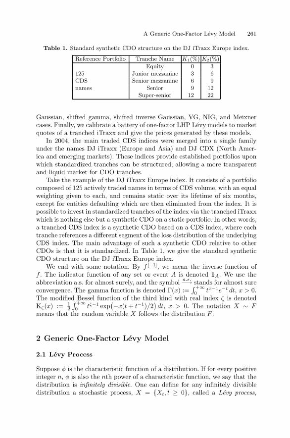
A Generic One-Factor Levy Model 261

Table 1. Standard synthetic CDO structure on the DJ iTraxx Europe index.

Reference Portfolio Tranche Name K1(%) K2(%)

Equity 0 3125 Junior mezzanine 3 6CDS Senior mezzanine 6 9names Senior 9 12

Super-senior 12 22

Gaussian, shifted gamma, shifted inverse Gaussian, VG, NIG, and Meixnercases. Finally, we calibrate a battery of one-factor LHP Levy models to marketquotes of a tranched iTraxx and give the prices generated by these models.

In 2004, the main traded CDS indices were merged into a single familyunder the names DJ iTraxx (Europe and Asia) and DJ CDX (North Amer-ica and emerging markets). These indices provide established portfolios uponwhich standardized tranches can be structured, allowing a more transparentand liquid market for CDO tranches.

Take the example of the DJ iTraxx Europe index. It consists of a portfoliocomposed of 125 actively traded names in terms of CDS volume, with an equalweighting given to each, and remains static over its lifetime of six months,except for entities defaulting which are then eliminated from the index. It ispossible to invest in standardized tranches of the index via the tranched iTraxxwhich is nothing else but a synthetic CDO on a static portfolio. In other words,a tranched CDS index is a synthetic CDO based on a CDS index, where eachtranche references a different segment of the loss distribution of the underlyingCDS index. The main advantage of such a synthetic CDO relative to otherCDOs is that it is standardized. In Table 1, we give the standard syntheticCDO structure on the DJ iTraxx Europe index.

We end with some notation. By f [−1], we mean the inverse function off . The indicator function of any set or event A is denoted 1A. We use theabbreviation a.s. for almost surely, and the symbol a.s.−→ stands for almost sureconvergence. The gamma function is denoted Γ(x) :=

∫ +∞0 tx−1e−t dt, x > 0.

The modified Bessel function of the third kind with real index ζ is denotedKζ(x) := 1

2

∫ +∞0 tζ−1 exp

(−x(t + t−1)/2

)dt, x > 0. The notation X ∼ F

means that the random variable X follows the distribution F .

2 Generic One-Factor Levy Model

2.1 Levy Process

Suppose φ is the characteristic function of a distribution. If for every positiveinteger n, φ is also the nth power of a characteristic function, we say that thedistribution is infinitely divisible. One can define for any infinitely divisibledistribution a stochastic process, X = {Xt, t ≥ 0}, called a Levy process,

262 Hansjorg Albrecher, Sophie A. Ladoucette, and Wim Schoutens

which starts at zero, has stationary independent increments, and such thatthe distribution of an increment over [s, s + t], s, t ≥ 0 (i.e., Xt+s −Xs) hasφt as characteristic function.

The function ψ := logφ is called the characteristic exponent, and it satisfiesthe following Levy–Khintchine formula (see Bertoin [4]),

ψ(z) = iγz − ς2

2z2 +∫ +∞

−∞

(exp(izx) − 1 − izx1{|x|<1}

)ν(dx), z ∈ R,

where γ ∈ R, ς2 ≥ 0, and ν is a measure on R\{0}with∫ +∞−∞ min

(1, x2)ν(dx) <

∞. From the Levy–Khintchine formula, one sees that, in general, a Levy pro-cess consists of three independent parts: a linear deterministic part, a Brown-ian part, and a pure jump part. We say that our infinitely divisible distributionhas a triplet of Levy characteristics [γ, ς2, ν(dx)]. The measure ν(dx) is calledthe Levy measure of X , and it dictates how the jumps occur. Jumps of sizesin the set A occur according to a Poisson process with parameter

∫Aν(dx). If

ς2 = 0 and∫ +1

−1 |x| ν(dx) < ∞, it follows from standard Levy process theory(e.g., Bertoin [4] and Sato [16]) that the process is of finite variation. Formore details about the applications of Levy processes in finance, we refer toSchoutens [20].

2.2 Generic One-Factor Levy Model

Next, we model a portfolio of n obligors; each obligor has the same weightin the portfolio. Later on we focus on a homogeneous portfolio, but we startwith the general situation where each obligor has some recovery value Ri incase of default and some individual default probability term structure pi(t),t ≥ 0, which is the probability that obligor i will default before time t.

Fix a time horizon T . For the modeling, let us start with a mother infinitelydivisible distribution L. Let X = {Xt, t ∈ [0, 1]} be a Levy process based onthat infinitely divisible distribution, such that X1 follows the law L. Note thatwe only work with Levy processes with time running over the unit interval.Denote the distribution function of Xt by Ht, t ∈ [0, 1], and assume it iscontinuous. Assume further that the distribution is standardized in the sensethat E[X1] = 0 and Var[X1] = 1. In terms of ψ, this means that ψ′(0) = 0and ψ′′(0) = −1. Then, it is not that hard to prove that Var[Xt] = t.

Let X = {Xt, t ∈ [0, 1]} and X(i) = {X(i)t , t ∈ [0, 1]}, i = 1, . . . , n be

independent and identically distributed Levy processes (so all processes areindependent of each other and are based on the same mother infinitely divisibledistribution L).

Next, we propose the generic one-factor Levy model. Let ρ ∈ (0, 1). Weassume that the asset value of obligor i = 1, . . . , n at time T is of the form:

Ai(T ) = Xρ +X(i)1−ρ. (1)

A Generic One-Factor Levy Model 263

Each Ai(T ) has by the stationary and independent increments property thesame distribution as the mother distribution L with distribution function H1.Indeed, the sum of an increment of the process over a time interval of length ρand an independent increment over a time interval of length 1− ρ follows thedistribution of an increment over an interval of unit length, that is, followsthe law L. As a consequence, E[Ai(T )] = 0 and Var[Ai(T )] = 1. Furthermore,the asset values of any two obligors i and j (i �= j) are correlated with linearcorrelation coefficient ρ. Indeed, one readily computes

Corr[Ai(T ), Aj(T )] =E[Ai(T )Aj(T )] − E[Ai(T )]E[Aj(T )]√

Var[Ai(T )]√

Var[Aj(T )]

= E[Ai(T )Aj(T )] = E[X2ρ ] = ρ.

So, starting from any mother standardized infinitely divisible law, we can setup a one-factor model with the required correlation.

We say that the ith obligor defaults at time T if its firm value Ai(T ) fallsbelow some preset barrier Ki(T ), that is, if Ai(T ) ≤ Ki(T ). In order to matchdefault probabilities under this model with default probabilities pi(T ) ob-served in the market, we have to set Ki(T ) = H

[−1]1 (pi(T )). Indeed, it follows

that P (Ai(T ) ≤ Ki(T )) = P (Ai(T ) ≤ H[−1]1 (pi(T ))) = H1(H

[−1]1 (pi(T ))) =

pi(T ).Notice that conditional on the common factor Xρ, the firm values and the

defaults are independent.From now on, we assume that the portfolio is homogeneous ; that is,

• All obligors have the same default barrier (Ki(T ) = K(T ), i = 1, . . . , n),and hence the same marginal default distribution (pi(T ) = p(T )).

• All obligors have the same recovery rate (Ri = R, i = 1, . . . , n).• All obligors have the same notional amount: denoting the total portfolio

notional by N , we then set Ni = N/n for all i = 1, . . . , n.

Let us denote the number of defaults in the portfolio until time T by DT,n.The probability of having exactly k defaults equals

P (DT,n = k) =∫ +∞

−∞P (DT,n = k|Xρ = y) dHρ(y), k = 0, . . . , n.

Conditional on Xρ = y, the probability of having k defaults is (because ofindependence)

P (DT,n = k|Xρ = y) =(n

k

)p(y;T )k (1 − p(y;T ))n−k,

where p(y;T ) denotes the probability that the firm’s value Ai(T ) is below thebarrier K(T ), given that the systematic factor Xρ takes the value y; that is,

264 Hansjorg Albrecher, Sophie A. Ladoucette, and Wim Schoutens

p(y;T ) := P (Ai(T ) ≤ K(T )|Xρ = y)

= P (Xρ +X(i)1−ρ ≤ K(T )|Xρ = y)

= P (X(i)1−ρ ≤ K(T )− y)

= H1−ρ(K(T ) − y).

Substituting then yields

P (DT,n = k) =(n

k

)∫ +∞

−∞(H1−ρ(K(T ) − y))k

(1 −H1−ρ(K(T ) − y))n−k dHρ(y).

The loss fraction on the portfolio notional at time T given by

LHPT,n :=

1 −R

n

n∑

i=1

1{Ai(T )≤K(T )} (2)

is clearly one-to-one related with the number of defaults. We then obtain thefollowing distribution function for the portfolio loss fraction,

P

(LHPT,n ≤ k(1 −R)

n

)=

k∑

i=0

P (DT,n = i), k = 0, . . . , n.

In the next subsection, we consider a method to approximate the latter dis-tribution that turns out to be of prime interest in the CDO pricing (see Sec-tion 4).

Now, denote for small x by λij(x) := P (Aj(T ) ≤ x|Ai(T ) ≤ x), i �= j,a measure for the dependence in the tail. Using (conditional) independencearguments yields

λij(x) =P (Xρ +X

(j)1−ρ ≤ x, Xρ +X

(i)1−ρ ≤ x)

P (Xρ +X(i)1−ρ ≤ x)

=E[P(Xρ +X

(j)1−ρ ≤ x, Xρ +X

(i)1−ρ ≤ x

∣∣∣Xρ

)]

H1(x)

=∫ +∞

−∞

P (X(j)1−ρ ≤ x− y, X

(i)1−ρ ≤ x− y)

H1(x)dHρ(y)

=∫ +∞

−∞

H21−ρ(x− y)H1(x)

dHρ(y).

The limit λij := limx→−∞ λij(x) is then the well-known lower tail dependencecoefficient of Ai(T ) and Aj(T ). Lower tail dependence exactly captures theprobability of concordant down movements of the underlying asset values. Theformula being stated in terms of the distribution Ht, the quantity λij(x) andits limit can be evaluated for any one-factor Levy model.

A Generic One-Factor Levy Model 265

2.3 The Large Homogeneous Portfolio Approximation

We are interested in approximating the distribution function of the portfolioloss fraction LHP

T,n. This proves to be possible if the homogeneous portfolio getsvery large (i.e., n → ∞).

When conditioned on the systematic factor Xρ, the default variables1{Ai(T )≤K(T )}, i = 1, . . . , n become independent. Hence, by the strong lawof large numbers, we obtain

P(

limn→∞

LHPT,n = (1 −R) p(Xρ;T )

∣∣∣Xρ

)= 1 a.s.,

and taking expectations on both sides gives

LHPT,n

a.s.−→ (1 −R) p(Xρ;T ) as n→ ∞.

For large homogeneous portfolios, we then make the approximation

FHPT,n(x) := P (LHP

T,n ≤ x) = FHPT

(x

1 −R

), x ∈ [0, 1 −R], (3)

where FHPT denotes the distribution function of p(Xρ;T ), that turns out to

be the loss fraction with a zero recovery rate (or equivalently the fraction ofdefaults) on the limiting portfolio at time T . We easily compute

FHPT (x) = P (H1−ρ(K(T )−Xρ) ≤ x)

= P (Xρ ≥ K(T ) −H[−1]1−ρ (x))

= 1 −Hρ

(H

[−1]1 (p(T )) −H

[−1]1−ρ (x)

), x ∈ [0, 1], (4)

so that we obtain an explicit handy expression for the distribution FHPT,n of the

portfolio fractional loss.Note that if the portfolio contains a moderately large number of credits,

the approximation (3) turns out to be remarkably good.

3 Examples of One-Factor Levy Models for CorrelatedDefaults

3.1 Based on the Normal Distribution—Brownian Motion

The Vasicek [22] one-factor model assumes the following dynamics.

• Ai(T ) =√ρ Y +

√1 − ρXi, i = 1, . . . , n,

• Y , Xi, i = 1, . . . , n are i.i.d. standard normal random variables with com-mon distribution function Φ.

266 Hansjorg Albrecher, Sophie A. Ladoucette, and Wim Schoutens

Table 2. Mean, variance, skewness, and kurtosis of the Gamma(a, b) distribution.

Gamma(a, b)

Mean a/bVariance a/b2

Skewness 2/√

aKurtosis 3(1 + 2/a)

This model can be cast in the above general Levy framework. The motherinfinitely divisible distribution is here the standard normal distribution andthe associated Levy process is the standard Brownian motion W = {Wt, t ∈[0, 1]}. Indeed, note that Wρ follows an N (0, ρ) distribution as does

√ρ Y ;

similarly W(i)1−ρ follows an N (0, 1− ρ) distribution as does

√1 − ρXi. Adding

these independent random variables leads to a standard normally distributedrandom variable.

Using the classical properties of normal random variables, the distributionfunction (4) of the fraction of defaulted securities in the limiting portfolio attime T transforms into

FHPT (x) = 1 − Φ

(Φ[−1](p(T )) −

√1 − ρΦ[−1](x)

√ρ

)

= Φ(√

1 − ρΦ[−1](x) − Φ[−1](p(T ))√ρ

), x ∈ [0, 1].

3.2 Based on the Shifted Gamma Process

The density function of the gamma distribution Gamma(a, b) with parametersa > 0 and b > 0 is given by

fGamma(x; a, b) =ba

Γ(a)xa−1 e−xb, x > 0.

The distribution function of the Gamma(a, b) distribution is denoted HG(x; a, b)and has the following characteristic function,

φGamma(u; a, b) = (1 − iu/b)−a, u ∈ R.

Clearly, this characteristic function is infinitely divisible. The gamma processX(G) = {X(G)

t , t ≥ 0} with parameters a, b > 0 is defined as the stochasticprocess that starts at zero and has stationary independent gamma-distributedincrements such that X(G)

t follows a Gamma(at, b) distribution.The properties of the Gamma(a, b) distribution given in Table 2 can be

easily derived from its characteristic function. Now, if X is Gamma(a, b)-distributed and c > 0, then cX is Gamma(a, b/c)-distributed. Furthermore,if X ∼ Gamma(a1, b) is independent of Y ∼ Gamma(a2, b), then X + Y ∼Gamma(a1 + a2, b).

A Generic One-Factor Levy Model 267

Let us start with a gamma process G = {Gt, t ∈ [0, 1]} with parametersa > 0 and b =

√a, so that E[G1] =

√a and Var[G1] = 1. As driving Levy

process, we take the shifted gamma process X = {Xt, t ∈ [0, 1]} defined as

Xt =√at−Gt, t ∈ [0, 1].

The interpretation in terms of firm value is that there is a deterministic uptrend (

√at) with random downward shocks (Gt).

The one-factor shifted gamma–Levy model is then in the form of (1),

Ai(T ) = Xρ +X(i)1−ρ, i = 1, . . . , n,

where Xρ, X(i)1−ρ, i = 1, . . . , n are independent shifted gamma random vari-

ables defined as Xρ =√aρ−Gρ and X

(i)1−ρ =

√a(1− ρ)−G1−ρ. By construc-

tion, each Ai(T ) follows the same distribution as X1 and as such has zeromean and unit variance.

As derived in general, we have that the distribution of the limiting portfoliofractional loss with a zero recovery rate at time T is as in (4). The distributionfunction Ht(x; a) of Xt, t ∈ [0, 1], can be easily obtained from the gammadistribution function. Indeed,

Ht(x; a) = P (√at−Gt ≤ x)

= 1 − P (Gt <√at− x)

= 1 −HG(√at− x; at,

√a), x ∈ (−∞,

√at).

For the inverse function, we have the following relation for each t ∈ [0, 1]:

H[−1]t (y; a) =

√at−H[−1]

G (1 − y; at,√a), y ∈ [0, 1].

3.3 Based on the Shifted IG Process

The inverse Gaussian IG(a, b) law with parameters a > 0 and b > 0 hascharacteristic function

φIG(u; a, b) = exp(−a(√−2iu+ b2 − b)

), u ∈ R.

The IG distribution is infinitely divisible and we define the IG processX(IG) ={X(IG)

t , t ≥ 0} with parameters a, b > 0 as the process that starts at zero andhas stationary independent IG-distributed increments such that

E[exp(iuX(IG)t )] = φIG(u; at, b) = exp

(−at(√−2iu+ b2 − b)

), u ∈ R

meaning that X(IG)t follows an IG(at, b) distribution.

268 Hansjorg Albrecher, Sophie A. Ladoucette, and Wim Schoutens

Table 3. Mean, variance, skewness, and kurtosis of the IG(a, b) distribution.

IG(a, b)

Mean a/bVariance a/b3

Skewness 3/√

abKurtosis 3(1 + 5(ab)−1)

The density function of the IG(a, b) law is given by

fIG(x; a, b) =a eab√

2πx−3/2exp

(−(a2x−1 + b2x)/2

), x > 0,

and we denote its distribution function HIG(x; a, b). The characteristics ofthe IG distribution given in Table 3 can be easily obtained. Now, if X isIG(a, b)-distributed, then cX is IG(a

√c, b/

√c)-distributed for any positive c.

Furthermore, if X ∼ IG(a1, b) is independent of Y ∼ IG(a2, b), then X +Y ∼IG(a1 + a2, b).

Let us start with an IG process I = {It, t ∈ [0, 1]} with parameters a > 0and b = a1/3, so that E[I1] = a2/3 and Var[I1] = 1. As driving Levy process,we take the shifted IG process X = {Xt, t ∈ [0, 1]} defined as

Xt = a2/3t− It, t ∈ [0, 1].

The interpretation in terms of firm value is that there is a deterministic uptrend (a2/3t) with random downward shocks (It).

The one-factor shifted IG-Levy model is then

Ai(T ) = Xρ +X(i)1−ρ, i = 1, . . . , n,

where Xρ, X(i)1−ρ, i = 1, . . . , n are independent shifted IG random variables

defined as Xρ = a2/3ρ−Iρ and X(i)1−ρ = a2/3(1−ρ)−I1−ρ. Each Ai(T ) follows

the same distribution as X1 and as such has zero mean and unit variance.The distribution of the fraction of defaulted securities in the limiting port-

folio at time T is therefore as in (4). The distribution function Ht(x; a) of Xt,t ∈ [0, 1], can be easily obtained from the IG distribution function as follows.

Ht(x; a) = P (a2/3t− It ≤ x)= 1 − P (It < a2/3t− x)= 1 −HIG(a2/3t− x; at, a1/3), x ∈ (−∞, a2/3t).

For the inverse function, we have the following relation for each t ∈ [0, 1],

H[−1]t (y; a) = a2/3t−H[−1]

IG (1 − y; at, a1/3), y ∈ [0, 1].

A Generic One-Factor Levy Model 269

Table 4. Mean, variance, skewness, and kurtosis of the VG(σ, ν, θ, μ) distribution.

VG(σ, ν, θ, μ) VG(σ, ν, 0, μ)

Mean θ + μ μVariance σ2 + νθ2 σ2

Skewness θν(3σ2 + 2νθ2)/(σ2 + νθ2)3/2 0Kurtosis 3(1 + 2ν − νσ4(σ2 + νθ2)−2) 3(1 + ν)

3.4 Based on the VG Process

The Variance-Gamma (VG) distribution with parameters σ > 0, ν > 0, θ ∈ R,and μ ∈ R, denoted VG(σ, ν, θ, μ), is infinitely divisible with characteristicfunction

φV G(u;σ, ν, θ, μ) = eiuμ(1 − iuθν + u2σ2ν/2

)−1/ν, u ∈ R.

We can then define the VG process X(VG) = {X(VG)t , t ≥ 0} with param-

eters σ, ν > 0 and θ, μ ∈ R as the process that starts at zero and has sta-tionary independent VG-distributed increments such that X

(V G)t follows a

VG(σ√t, ν/t, θt, μt) distribution. Note that a VG process may also be defined

as a Brownian motion with drift time-changed by a gamma process (e.g.,Schoutens [20]).

The density function of the VG(σ, ν, θ, μ) distribution is given by

fV G(x;σ, ν, θ, μ) =(GM)C√π Γ(C)

exp(

(G−M)(x− μ)2

)

×(|x− μ|G+M

)C−1/2

KC−1/2 ((G+M) |x− μ|/2) , x ∈ R,

where C, G, M are positive constants given by

C = 1/ν,

G =

(√θ2ν2

4+σ2ν

2− θν

2

)−1

,

M =

(√θ2ν2

4+σ2ν

2+θν

2

)−1

.

In Table 4, we give the values of the mean, variance, skewness, and kurtosisof the VG(σ, ν, θ, μ) distribution (the case θ = 0 is also included). This distri-bution is symmetric around μ if θ = 0, whereas negative values of θ result innegative skewness. Also, the parameter ν primarily controls the kurtosis.

The VG(σ, ν, θ, μ) distribution satisfies the following scaling property. IfX ∼ VG(σ, ν, θ, μ), then cX ∼ VG(cσ, ν, cθ, cμ) for all c > 0. Also, we have thefollowing convolution property. If X ∼ VG(σ

√ρ, ν/ρ, θρ, μρ) is independent

270 Hansjorg Albrecher, Sophie A. Ladoucette, and Wim Schoutens

of Y ∼ VG(σ√

1 − ρ, ν/(1−ρ), θ(1−ρ), μ(1−ρ)), then X+Y ∼ VG(σ, ν, θ, μ)under the constraint ρ ∈ (0, 1).

The class of VG distributions was introduced by Madan and Seneta [9].A number of papers have developed the VG model for asset returns and itsimplications for option pricing. In Madan and Seneta [9; 10] and Madan andMilne [8], the symmetric case (θ = 0) is considered. In Madan et al. [11], thegeneral case with skewness is treated. In equity and interest rate modeling,the VG process has already proven its capabilities (see, e.g., Schoutens [20]).

Moosbrucker assumes in [12] a one-factor VG model where the asset valueof obligor i = 1, . . . , n is of the form

Ai(T ) = c Y +√

1 − c2 Xi,

where Y , Xi, i = 1, . . . , n are independently VG-distributed random vari-ables with Xi ∼ VG(

√1 − νθ2, ν/(1 − c2), θ

√1 − c2,−θ

√1 − c2) for all i and

Y ∼ VG(√

1 − νθ2, ν/c2, θc,−θc). In this setting, the random variable Ai(T )

is VG(√

1 − νθ2, ν, θ,−θ)-distributed. All these random variables have indeedzero mean and unit variance but there is a constraint on the parameters,namely νθ2 < 1. Furthermore, we point out that the fractional loss distri-bution obtained by Moosbrucker [12, p. 19, Eq.(13)] with the LHP methodunder the above one-factor model approach is not correct. It should be in hisnotation:

Fportfolio loss(x) = 1 − FM

(C −

√1 − c2F−1

Zi(x)

c

),

because the VG distribution function is not an even function if (θ, μ) �= (0, 0).For a variant of the VG model, extended with an additional normal factor,

we refer to Baxter [3].Many variations are possible. For example, one could start with a zero

mean VG(κσ, ν, κθ,−κθ) distribution for Ai(T ), with κ = 1/√σ2 + νθ2 in

order to force unit variance. The one-factor VG-Levy model is then in theform of (1)

Ai(T ) = Xρ +X(i)1−ρ, i = 1, . . . , n,

where Xρ, X(i)1−ρ, i = 1, . . . , n are independent VG random variables with the

following parameters. The common factor Xρ follows a distribution VG(κ√ρσ,

ν/ρ, κρθ,−κρθ) and the idiosyncratic risks X(i)1−ρ all follow a distribution

VG(κ√

1 − ρσ, ν/(1 − ρ), κ(1 − ρ)θ,−κ(1 − ρ)θ).

3.5 Based on the NIG Process

The normal inverse Gaussian (NIG) distribution with parameters α > 0,β ∈ (−α, α), δ > 0, and μ ∈ R, denoted NIG(α, β, δ, μ), has a characteristicfunction given by

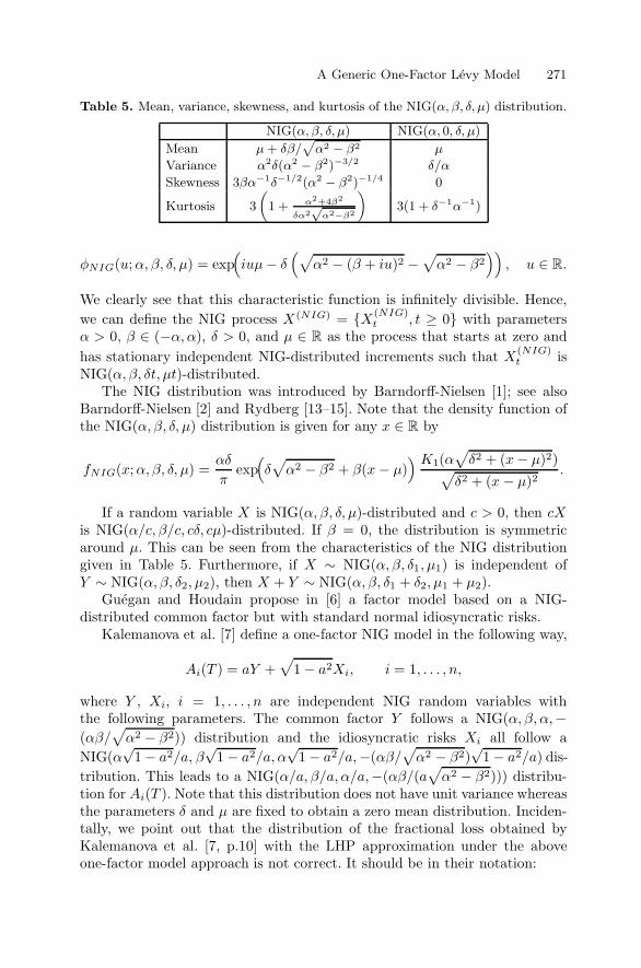
A Generic One-Factor Levy Model 271

Table 5. Mean, variance, skewness, and kurtosis of the NIG(α, β, δ, μ) distribution.

NIG(α,β, δ, μ) NIG(α, 0, δ, μ)

Mean μ + δβ/√

α2 − β2 μ

Variance α2δ(α2 − β2)−3/2 δ/α

Skewness 3βα−1δ−1/2(α2 − β2)−1/4 0

Kurtosis 3

(1 + α2+4β2

δα2√

α2−β2

)3(1 + δ−1α−1)

φNIG(u;α, β, δ, μ) = exp(iuμ− δ

(√α2 − (β + iu)2 −

√α2 − β2

)), u ∈ R.

We clearly see that this characteristic function is infinitely divisible. Hence,we can define the NIG process X(NIG) = {X(NIG)

t , t ≥ 0} with parametersα > 0, β ∈ (−α, α), δ > 0, and μ ∈ R as the process that starts at zero andhas stationary independent NIG-distributed increments such that X(NIG)

t isNIG(α, β, δt, μt)-distributed.

The NIG distribution was introduced by Barndorff-Nielsen [1]; see alsoBarndorff-Nielsen [2] and Rydberg [13–15]. Note that the density function ofthe NIG(α, β, δ, μ) distribution is given for any x ∈ R by

fNIG(x;α, β, δ, μ) =αδ

πexp(δ√α2 − β2 + β(x − μ)

) K1(α√δ2 + (x− μ)2)√

δ2 + (x − μ)2.

If a random variable X is NIG(α, β, δ, μ)-distributed and c > 0, then cXis NIG(α/c, β/c, cδ, cμ)-distributed. If β = 0, the distribution is symmetricaround μ. This can be seen from the characteristics of the NIG distributiongiven in Table 5. Furthermore, if X ∼ NIG(α, β, δ1, μ1) is independent ofY ∼ NIG(α, β, δ2, μ2), then X + Y ∼ NIG(α, β, δ1 + δ2, μ1 + μ2).

Guegan and Houdain propose in [6] a factor model based on a NIG-distributed common factor but with standard normal idiosyncratic risks.

Kalemanova et al. [7] define a one-factor NIG model in the following way,

Ai(T ) = aY +√

1 − a2Xi, i = 1, . . . , n,

where Y , Xi, i = 1, . . . , n are independent NIG random variables withthe following parameters. The common factor Y follows a NIG(α, β, α,−(αβ/√α2 − β2)) distribution and the idiosyncratic risks Xi all follow a

NIG(α√

1 − a2/a, β√

1 − a2/a, α√

1 − a2/a,−(αβ/√α2 − β2)

√1 − a2/a) dis-

tribution. This leads to a NIG(α/a, β/a, α/a,−(αβ/(a√α2 − β2))) distribu-

tion for Ai(T ). Note that this distribution does not have unit variance whereasthe parameters δ and μ are fixed to obtain a zero mean distribution. Inciden-tally, we point out that the distribution of the fractional loss obtained byKalemanova et al. [7, p.10] with the LHP approximation under the aboveone-factor model approach is not correct. It should be in their notation:

272 Hansjorg Albrecher, Sophie A. Ladoucette, and Wim Schoutens

F∞(x) = 1 − FNIG(1)

⎛

⎝C −

√1 − a2F−1

NIG√

1−a2/a(x)

a

⎞

⎠ ,

because the NIG distribution function is not an even function if (β, μ) �= (0, 0).Using our methodology, one can set up similar NIG models. For example,

let X = {Xt, t ∈ [0, 1]} be a NIG process, where X1 follows a distributionNIG(α, β, (α2 − β2)3/2/α2,−(α2 − β2)β/α2). Note that the parameters δ andμ are chosen such that X1 has zero mean and unit variance. The one-factorNIG–Levy model is then

Ai(T ) = Xρ +X(i)1−ρ, i = 1, . . . , n,

where Xρ, X(i)1−ρ, i = 1, . . . , n are independently NIG-distributed random vari-

ables with X(i)1−ρ ∼ NIG(α, β, (1− ρ)(α2 − β2)3/2/α2,−(1− ρ)(α2 − β2)β/α2)

for all i and Xρ ∼ NIG(α, β, ρ(α2 − β2)3/2/α2,−ρ(α2 − β2)β/α2). By con-struction, each Ai(T ) follows the same distribution as X1.

3.6 Based on the Meixner Process

The density function of the Meixner distribution (Meixner(α, β, δ, μ)) is givenfor any x ∈ R by

fMeixner(x;α, β, δ, μ) =(2 cos(β/2))2δ

2απ Γ(2δ)exp(β(x − μ)

α

) ∣∣∣∣Γ(δ +

i(x− μ)α

)∣∣∣∣2

,

where α > 0, β ∈ (−π, π), δ > 0, and μ ∈ R.The characteristic function of the Meixner(α, β, δ, μ) distribution is

φMeixner(u;α, β, δ, μ) = eiuμ(

cos(β/2)cosh((αu − iβ)/2)

)2δ

, u ∈ R.

The Meixner(α, β, δ, μ) distribution being infinitely divisible, we can then as-sociate with it a Levy process which we call the Meixner process. More pre-cisely, a Meixner process X(Meixner) = {X(Meixner)

t , t ≥ 0} with parametersα > 0, β ∈ (−π, π), δ > 0, and μ ∈ R is a stochastic process that startsat zero and has stationary independent Meixner-distributed increments suchthat X(Meixner)

t is Meixner(α, β, δt, μt)-distributed.The Meixner process was introduced in Schoutens and Teugels [21]; see also

Schoutens [17]. It was suggested to serve for fitting stock returns in Grigelio-nis [5]. This application in finance was worked out in Schoutens [18; 19].

In Table 6, we give some relevant quantities for the general case and thesymmetric case around μ, that is, with β = 0. Note that the kurtosis of anyMeixner distribution is greater than that of the normal distribution. Now, if X

A Generic One-Factor Levy Model 273

Table 6. Mean, variance, skewness, and kurtosis of the Meixner(α, β, δ, μ) distribu-tion.

Meixner(α, β, δ, μ) Meixner(α, 0, δ, μ)

Mean μ + αδ tan(β/2) μVariance (cos−2(β/2))α2δ/2 α2δ/2

Skewness sin(β/2)√

2/δ 0Kurtosis 3 + (2− cos(β))/δ 3 + 1/δ

is Meixner(α, β, δ, μ)-distributed and c > 0, then cX is Meixner(cα, β, δ, cμ)-distributed. Furthermore, if X ∼ Meixner(α, β, δ1, μ1) is independent of Y ∼Meixner(α, β, δ2, μ2), then X + Y ∼ Meixner(α, β, δ1 + δ2, μ1 + μ2).

Using our methodology, one can easily set up a Meixner model. For ex-ample, let X = {Xt, t ∈ [0, 1]} be a Meixner process, where X1 follows adistribution Meixner(α, β, 2 cos2(β/2)/α2,− sin(β)/α). Note that again theparameters δ and μ are chosen such that X1 has zero mean and unit variance.The one-factor Meixner–Levy model is then

Ai(T ) = Xρ +X(i)1−ρ, i = 1, . . . , n,

where Xρ, X(i)1−ρ, i = 1, . . . , n are independent Meixner random variables

with the following parameters. The common factor Xρ follows a Meixner(α, β,2ρ cos2(β/2)/α2,−ρ sin(β)/α) distribution and the idiosyncratic risksX(i)

1−ρ allfollow a Meixner(α, β, 2(1 − ρ) cos2(β/2)/α2,−(1 − ρ)sin(β)/α) distribution.By construction, each Ai(T ) follows the same distribution as X1.

3.7 Other Candidate Models

We hope the idea is clear and invite the reader to set up the CGMY, Gener-alized Hyperbolic (GH), Generalized z (GZ), and other Levy-based models ina similar way. For definitions, we refer to Schoutens [20].

4 Fair Pricing of a Synthetic CDO Tranche

In this section, we explain the procedure for valuing the tranches of syntheticCDOs. Consider a synthetic CDO tranche on a given reference portfolio of nnames defined by an interval [K1,K2] of loss fractions on the total portfolionotionalN for which the tranche investor is responsible. The endpointsK1 andK2 of the interval are called attachment and detachment points, respectively.The tranche investor receives periodic spread payments from the CDO issuer(the premium leg) and makes payments to the CDO issuer when defaults affectthe tranche (the protection leg). Note that for a synthetic CDO, any defaultcorresponds to a credit event under a CDS in the reference portfolio. It turnsout that the fair price of the tranche [K1,K2] can be calculated using the

274 Hansjorg Albrecher, Sophie A. Ladoucette, and Wim Schoutens

same idea as for the pricing of a CDS, that is, by setting the fair premium ssuch that the expected present values of the premium leg and the protectionleg are equal.

The loss fraction on the portfolio notional at time t is given by

Lt,n :=1N

n∑

i=1

1{τi≤t}(1 −Ri)Ni,

where τi, Ri, and Ni denote the default time, the recovery rate, and the no-tional amount of name i, respectively, i = 1, . . . , n. Under the factor model (1),we have {τi ≤ t} = {Ai(t) ≤ Ki(t)} with Ki(t) = H

[−1]1 (pi(t)), i = 1, . . . , n.

The loss fraction on the CDO tranche [K1,K2] at time t is simply expressedby means of Lt,n as

Lt,n(K1,K2) :=max{min(Lt,n,K2) −K1, 0}

K2 −K1.

We assume that the payments (premium and protection legs) occur on pe-riodic payment dates t1, . . . , tm. Furthermore, we assume that the CDO issuerreceives compensation at the next scheduled payment date after a default hasoccurred. Note that payments are only made as long as the effective notionalof the tranche at time ti is positive. Denote τ(1), . . . , τ(n) the order statistics,arranged in increasing order, of the random sample τ1, . . . , τn of default times.Put t0 := 0, τ(0) := 0, and L0,n := 0. In what follows, expectations are takenunder a risk-neutral measure, that is, risk-adjusted expectations.

The expected present value of the premium leg of the tranche is the presentvalue of all spread payments the tranche investor expects to receive

PL(s) = sE

⎡

⎣m∑

j=1

{(tj − tj−1)D(0, tj)

(1 − Ltj ,n(K1,K2)

)

+n∑

i=1

1{tj−1<τ(i)<tj}(τ(i) − tj−1

)D(0, τ(i))

×(Lτ(i),n(K1,K2) − Lτ(i−1),n(K1,K2)

)}]

,

where D(0, tj) is the risk-free discount factor for payment date tj and s is thespread per annum paid to the tranche investor. The term 1 − Ltj ,n(K1,K2)is the fraction of the tranche notional outstanding on payment date tj andreflects the decline in notional as defaults affect the tranche. The second termin the sum over j corresponds to the discounted sum of accrual payments thetranche investor receives when defaults occur between payment dates. Theyare paid at the next payment date and are based on the previous effectivetranche notional.

A Generic One-Factor Levy Model 275

The expected present value of the protection leg of the tranche is thediscounted sum of the expected payments the tranche investor must makewhen defaults affect the tranche:

LL = E

⎡

⎣m∑

j=1

D(0, tj)n∑

i=1

1{tj−1<τ(i)<tj}(Lτ(i),n(K1,K2) − Lτ(i−1),n(K1,K2)

)⎤

⎦.

The fair tranche premium spar is then the spread s solving PL(s) = LL. As aconsequence, the periodic payment received by the tranche investor from theCDO issuer in return for bearing the risk of losses is equal to spar times theeffective outstanding notional of the tranche.

Now, assume a homogeneous portfolio. Recall that all obligors have thesame default barrier Ki(t) = K(t), the same recovery rate Ri = R, and thesame notional amount Ni = N/n. Each of the n obligors either takes noloss or a loss of (1 − R)(N/n) so that multiplying the number of defaultsby (1 − R)(N/n) gives losses. Clearly, Lt,n reduces to the loss fraction LHP

t,n

defined in (2). It follows that the expected loss fraction on the portfolio attime t is

E[LHPt,n ] =

1 −R

n

n∑

k=0

k P

(LHPt,n =

k(1 −R)n

),

and, denoting LHPt,n (K1,K2) := Lt,n(K1,K2), that the expected loss fraction

on the CDO tranche [K1,K2] at time t is

E[LHPt,n (K1,K2)]

=1

K2 −K1

n∑

k=0

P

(LHPt,n =

k(1 −R)n

)max{

min(k(1 −R)

n,K2

)−K1, 0

},

where P(LHPt,n = (k(1 −R))/n

)is the probability that exactly k defaults occur

by time t, k = 0, . . . , n.As soon as the expected loss fraction on the tranche is calculated, the com-

putation of the tranche premium becomes easy. Unfortunately, the derivationof the fractional loss distribution on the reference portfolio is not trivial. How-ever, under the above homogeneity assumptions, we know from Subsection 2.3that this distribution can be approximated using the LHP approximationmethod. As a consequence, this method provides an easy tool to computeboth the fractional loss distribution and the expected loss fraction on thetranche over different time horizons.

With the LHP approximation given in (3), that is, FHPt,n (x) = FHP

t (x/(1−R)) for x ∈ [0, 1 − R], we compute the expected loss fraction on the CDOtranche [K1,K2] at time t as

E[LHPt,n (K1,K2)]

= E

[max{min(LHPt,n ,K2

)−K1, 0

}

K2 −K1

]

276 Hansjorg Albrecher, Sophie A. Ladoucette, and Wim Schoutens

Table 7. Pricing of iTraxx tranches of May 4, 2006 with LHP Levy models.

0–3% 3–6% 6–9% 9–12% 12–22% AbsoluteModel/Quotes (bp) (bp) (bp) (bp) (bp) Error (bp)

Market 17 44.0 12.8 6.0 2.0Gaussian 17 105.7 22.4 5.7 0.7 73.7Shifted Gamma 17 44.0 19.7 11.9 6.0 16.8Shifted IG 17 44.0 19.8 12.2 6.5 17.7VG 17 43.9 21.8 14.1 7.8 23.0NIG 17 44.0 24.1 17.1 11.7 32.1

= E

[max(LHPt,n −K1, 0

)− max

(LHPt,n −K2, 0

)

K2 −K1

]

=1

K2 −K1

(∫ 1−R

K1

(x−K1) dFHPt,n (x) −

∫ 1−R

K2

(x−K2) dFHPt,n (x)

)

=1 −R

K2 −K1

(∫ 1

K1/(1−R)

(x− K1

1 −R

)dFHP

t (x)

−∫ 1

K2/(1−R)

(x− K2

1 −R

)dFHP

t (x)

).

Similarly, the expected loss fraction on the last tranche [K, 1] at time t isgiven by

E[LHPt,n (K, 1)] = E

[max(LHPt,n −K, 0

)

1 −K

]

=1

1 −K

∫ 1−R

K

(x−K)dFHPt,n (x)

=1 −R

1 −K

∫ 1

K/(1−R)

(x− K

1 −R

)dFHP

t (x).

Finally, we report on a small calibration exercise of the Gaussian, shiftedgamma, shifted IG, VG, and NIG cases. We calibrate the model to the iTraxxof the 4th of May 2006. In Table 7, one finds the market quotes together withthe calibrated model quotes for the different tranches. Note that for the 0–3%tranche, the upfront is quoted with a 500 bp running.

Acknowledgments

The authors thank Nomura and ING for providing the data. Special thanksgo to Martin Baxter and Jurgen Tistaert. Hansjorg Albrecher is supported bythe Austrian Science Fund Project P18392. Sophie A. Ladoucette is supportedby the grant BDB-B/04/03 from the Catholic University of Leuven.

A Generic One-Factor Levy Model 277

References

1. O.E. Barndorff-Nielsen. Normal inverse Gaussian distributions and the mod-elling of stock returns. Research Report No. 300, Department of TheoreticalStatistics, Aarhus University, 1995.

2. O.E. Barndorff-Nielsen. Normal inverse Gaussian distributions and stochasticvolatility modelling. Scandinavian Journal of Statistics, 24(1):1–13, 1997.

3. M. Baxter. Dynamic modelling of single-name credits and CDO tranches. Work-ing Paper - Nomura Fixed Income Quant Group, 2006.

4. J. Bertoin. Levy Processes. Cambridge Tracts in Mathematics 121. CambridgeUniversity Press, 1996.

5. B. Grigelionis. Processes of Meixner type. Lithuanian Mathematical Journal,39(1):33–41, 1999.

6. D. Guegan and J. Houdain. Collateralized debt obligations pricing and factormodels: A new methodology using normal inverse Gaussian distributions. Re-search Report IDHE-MORA No. 07-2005, ENS Cachan, 2005.

7. A. Kalemanova, B. Schmid, and R. Werner. The normal inverse Gaussian dis-tribution for synthetic CDO pricing. Technical Report, 2005.

8. D.B. Madan and F. Milne. Option pricing with VG martingale components.Mathematical Finance, 1(4):39–55, 1991.

9. D.B. Madan and E. Seneta. Chebyshev polynomial approximations and charac-teristic function estimation. Journal of the Royal Statistical Society, Series B,49(2):163–169, 1987.

10. D.B. Madan and E. Seneta. The Variance-Gamma (V.G.) model for share mar-ket returns. Journal of Business, 63(4):511–524, 1990.

11. D.B. Madan, P.P. Carr, and E.C. Chang. The variance gamma process andoption pricing. European Finance Review, 2:79–105, 1998.

12. T. Moosbrucker. Pricing CDOs with correlated variance gamma distributions.Research Report, Department of Banking, University of Cologne, 2006.

13. T. Rydberg. Generalized hyperbolic diffusions with applications towards finance.Research Report No. 342, Department of Theoretical Statistics, Aarhus Univer-sity, 1996.

14. T. Rydberg. The normal inverse Gaussian Levy process: Simulations and ap-proximation. Research Report No. 344, Department of Theoretical Statistics,Aarhus University, 1996.

15. T. Rydberg. A note on the existence of unique equivalent martingale measuresin a Markovian setting. Finance and Stochastics, 1:251–257, 1997.

16. K. Sato. Levy Processes and Infinitely Divisible Distributions. Cambridge Stud-ies in Advanced Mathematics 68. Cambridge University Press, 2000.

17. W. Schoutens. Stochastic Processes and Orthogonal Polynomials. Lecture Notesin Statistics 146. Springer-Verlag, 2000.

18. W. Schoutens. The Meixner process in finance. EURANDOM Report 2001-002,EURANDOM, Eindhoven, 2001.

19. W. Schoutens. Meixner processes: Theory and applications in finance. EURAN-DOM Report 2002-004, EURANDOM, Eindhoven, 2002.

20. W. Schoutens. Levy Processes in Finance - Pricing Financial Derivatives. JohnWiley & Sons, 2003.

21. W. Schoutens and J.L. Teugels. Levy processes, polynomials and martingales.Communications in Statistics - Stochastic Models, 14(1–2):335–349, 1998.

22. O. Vasicek. Probability of loss on loan portfolio. Technical Report, KMV Cor-poration, 1987.

Utility Valuation of Credit Derivatives: Singleand Two-Name Cases

Ronnie Sircar1 and Thaleia Zariphopoulou2

1 ORFE DepartmentPrinceton UniversityE-QuadPrinceton, NJ 08544, USAsircar@princeton.edu

2 Department of Mathematics and InformationDepartment of Risk and Operations ManagementThe University of Texas at AustinAustin, TX 78712, USAzariphop@math.utexas.edu

Summary. We study the effect of risk aversion on the valuation of credit deriva-tives. Using the technology of utility-indifference valuation in intensity-based modelsof default risk, we analyze resulting yield spreads for single-name defaultable bondsand a simple representative two-name credit derivative. The impact of risk aversevaluation on prices and yield spreads is expressed in terms of “effective correlation.”

Key words: Credit derivatives; indifference pricing; reaction–diffusion equations.

1 Introduction

In this article, we analyze the impact of risk aversion on the valuation of de-faultable bonds and a simple multiname credit derivative. Our approach is towork within intensity-based models, as initiated by, among others, Artznerand Delbaen [1], Madan and Unal [26], Lando [23], and Jarrow and Turnbull[19]. In these models, a firm’s default time is modeled directly by a totallyinaccessible stopping time, typically the first jump of a Cox process. However,rather than pricing using no-arbitrage arguments, we apply the utility-basedvaluation methodology, which entails analysis of portfolio optimization prob-lems under default risk.

A major limitation of many traditional approaches is the inability to cap-ture and explain high premiums observed in credit derivatives markets forunlikely events, for example, the spreads quoted for senior tranches of col-laterized debt obligations (CDOs) written on investment grade firms. The

280 Ronnie Sircar and Thaleia Zariphopoulou

approach explored here, and in our related work [29], aims to explain suchphenomena as a consequence of tranche holders’ risk aversion, and to quan-tify this through the mechanism of utility-indifference valuation. For a gen-eral introduction to credit risk, including other approaches to default, such asstructural models, we refer, for example, to the books [5; 13; 24; 27].

1.1 Valuation Mechanisms

In complete financial market environments, such as in the classical Black–Scholes model, the payoffs of derivative securities can be replicated by tradingstrategies in the underlying securities, and their prices are naturally deducedfrom the value of these associated portfolios. However, once nontraded risks,such as unpredictable defaults, are considered, the possibility of replicationand, therefore, risk elimination breaks down and alternative ways are neededfor the quantification of risk and assignation of price. One approach is touse market derivatives data, when available, to identify which of the manyfeasible arbitrage-free pricing measures is consistent with market prices. Ina different direction, valuation of claims involving nontradable risks can bebased on optimality of decisions once this claim is incorporated in the in-vestor’s portfolio. Naturally, the risk attitude of the individual needs to betaken into account, and this is typically modeled by a concave and increasingutility function U . In a static framework, prices are determined through thecertainty equivalent, otherwise known as the principle of equivalent utility [6;17]. The utility-based value of the claim, written on the risk Y and yieldingpayoff C (Y ), is ν (C) = U−1 {EP [U (C(Y ))]}. Note that the arbitrage-freeprice and the certainty-equivalent price are very different. The first is linearand uses the risk-neutral measure. The certainty-equivalent price is nonlinearand uses the historical assessment of risks.

Prompted by the ever-increasing number of applications (event risk-sensitive claims, insurance plans, mortgages, weather derivatives, etc.), con-siderable effort has been put into analyzing the utility-based valuation mech-anism. Due to the prevalence of instruments dependent on nonmarket risks(such as default), there is a great need for building new dynamic pricing rules.These rules should identify and price unhedgeable risks and, at the same time,build optimal risk-monitoring policies. In this direction, a dynamic utility-based pricing theory has been developed producing the so-called indifferenceprices. The approach is based on finding the amount at which the buyer of theclaim is indifferent, in terms of maximum expected utility, between holdingor not holding the derivative. Specification of the indifference price requiresunderstanding how investors act optimally with or without the derivative athand. These issues are naturally addressed through stochastic optimizationproblems of expected utility maximization. We refer to [21; 22] and [8] asclassical references in this area. The indifference approach was initiated forEuropean claims by Hodges and Neuberger [18] and further extended by Daviset al. [10].

Utility Valuation of Credit Derivatives 281

1.2 Credit Derivatives

As well as single-name securities, such as credit default swaps (CDSs), inwhich there is a relatively liquid market, basket, or multiname, products havegenerated considerable over-the-counter activity. Popular cases are collateral-ized debt obligations, whose payoffs depend on the default events of a basketportfolio of up to 300 firms, over a five-year period. As long as there are nodefaults, investors in CDO tranches enjoy high yields, but, as defaults startoccurring, they affect first the high-yield equity tranche, then the mezzaninetranches, and, perhaps, the senior and super-senior tranches. See Davis andLo [9] or Elizalde [15] for a concise introduction to these products.

The focus of modeling in the credit derivatives industry has been on cor-relation between default times. Partly, this is due to the adoption of the one-factor Gaussian copula model as industry standard and the practice (up untilrecently) of analyzing tranche prices through implied correlation. This re-vealed that traded prices of senior tranches could only be realized throughthese models with an implausibly high correlation parameter, the so-calledcorrelation smile.

Rather than focusing on models with “enough correlation” to reproducemarket observations via traditional no-arbitrage pricing, our goal is to under-stand the effects of risk aversion on valuation of single- and two-name creditderivatives. Questions of interest are (i) how does risk aversion affect the valueof portfolios that are sensitive to the potential default of a number of firms,and so to correlation between these events, and (ii) does the nonlinearityof the indifference pricing mechanism enhance the impact of correlation. Itseems natural that some of the prices, or spreads, seen in credit markets aredue mainly to “crash-o-phobia” in a relatively illiquid market, with the effectenhanced nonlinearly in baskets. When super-senior tranches offer nontriv-ial spreads (albeit a few basis points) for protection against the default riskof 15–30% of investment grade U.S. firms over the next five years, they areascribing a seemingly large probability to “the end of the world as we knowit.” We seek to capture this directly as an effect of risk aversion leading toeffective or perceived correlation, in contrast to a mechanism of high directcorrelation.

Taking the opposite angle, the method of indifference valuation should beattractive to participants in this still quite illiquid over-the-counter (OTC)market. It is a direct way for them to quantify the default risks they face ina portfolio of complex instruments, when calibration data are scarce. Unlikewell-developed equity and fixed-income derivatives markets, where the casefor traditional arbitrage-free valuation is more compelling, the potential forutility valuation to account for high dimensionality in a way that is consistentwith investors’ fears of a cascade of defaults is a case for its application here.

For applications of indifference valuation to credit risk, see also Collin-Dufresne and Hugonnier [7], Bielecki et al. [4; 3], and Shouda [28].

282 Ronnie Sircar and Thaleia Zariphopoulou

1.3 Outline

In Section 2, we introduce the model used to value a single-name defaultablebond. We study there the two utility optimization problems that lead to theindifference price. The first is the usual Merton optimal investment problem,and the second is the portfolio problem where the investor also holds thecorporate bond. We present the analysis under stochastic default intensity,and give bounds on the indifference value. In the case of constant intensity,we give the explicit formula and study the implied term structure of yieldspreads.

In Section 3, we take a first step towards extending the analysis to multi-name credit derivatives, by looking at a simple two-name example. This high-lights the key role of a diversity coefficient in indifference valuation. In the caseof constant intensities, we study the indifference value as a function of the ma-turity, and describe the correlating effect of the utility valuation mechanism.We conclude in Section 4.

2 Indifference Valuation: Single Name

We start with single-name defaultable bonds to illustrate the approach. Wework within models incorporating information from the firm’s stock price S,but unlike in a traditional structural approach, default occurs at a nonpre-dictable stopping time τ with stochastic intensity process λ, which is corre-lated with the firm’s stock price. These are sometimes called hybrid models(see, e.g., [25]). The process S could alternatively be taken as the price ofanother firm or index used to hedge the default risk. Of course, the choice ofthe investment opportunity set affects the ensuing indifference price.

The stock price S is taken to be a geometric Brownian motion. The inten-sity process is λ(Yt), where λ(·) is a nonnegative, locally Lipschitz, smooth,and bounded function, and Y is a correlated diffusion. The dynamics of S andY are

dSt = μSt dt + σSt dW(1)t , S0 = S > 0,

dYt = b(Yt) dt+ a(Yt)(ρ dW

(1)t +√

1 − ρ2 dW(2)t

), Y0 = y ∈ R.

The coefficients a and b are taken to be Lipschitz functions with sublineargrowth. The processes W 1 = (W (1)

t ) and W 2 = (W (2)t ) are independent stan-

dard Brownian motions defined on a probability space (Ω,F , P ), and we de-note Ft the augmented σ-algebra generated by ((W (1)

u ,W(2)u ); 0 ≤ u ≤ t). The

parameter ρ ∈ (−1, 1) measures the instantaneous correlation between shocksto the stock price S and shocks to the intensity-driving process Y . In applica-tions, it is natural to expect that λ(·) and ρ are specified in a way such thatthe intensity tends to rise when the stock price falls. Random fluctuationsin the default intensity may be due to economywide factors, as well as firm-

Utility Valuation of Credit Derivatives 283

or industry-specific issues that cause yield spreads to change. They may alsoincorporate the effects of ratings changes. We refer to [13, Chapter 3] for adetailed discussion.

The default time τ of the firm is defined by

τ = inf{t ≥ 0 :

∫ t

0

λ(Ys) ds = ξ

},

the first time the cumulated intensity reaches the standard exponentially dis-tributed random variable ξ, which is independent of the Brownian motions.

2.1 Maximal Expected Utility Problem

Let T < ∞ denote our finite fixed horizon, chosen later to coincide with theexpiration date of the derivative contract of interest. We consider the portfolioproblem of an investor who can trade the stock S and has access to a risklessmoney market account that pays interest at rate r. The investor’s controlprocess is πt, representing the dollar amount held in the stock at time t, untilτ ∧ T . For t < τ ∧ T , her wealth process X = (Xt) follows

dXt = πtdStSt

+ r(Xt − πt) dt

= (rXt + πt(μ− r)) dt + σπt dW(1)t .

The control π = (πt) is called admissible if it is Ft-measurable and satisfiesthe integrability constraint E[

∫ T0 π2

s ds] < ∞. The set of admissible policies isdenoted A.

If the default event occurs before T , the investor can no longer trade thefirm’s stock. She has to liquidate holdings in the stock and deposit in thebank account, so the effect is to reduce her investment opportunities. Forsimplicity, we assume she receives full predefault market value on her stockholdings on liquidation, although one might extend to consider some loss, orjump downwards in the stock price at the default time (see, e.g., [25] for sucha model). Therefore, given that τ < T , for τ ≤ t ≤ T , we have

Xt = Xτer(t−τ),

as the bank account is the only remaining investment.We work with exponential utility of discounted (to time zero) wealth. We

are first interested in the optimal investment problem up to time T of theinvestor who does not hold any derivative security. At time zero, the maximumexpected utility payoff then takes the form

supπ∈A

E[−e−γ(e−rTXT )1{τ>T} + (−e−γ(e−rτXτ ))1{τ≤T}

].

284 Ronnie Sircar and Thaleia Zariphopoulou

We switch to the discounted variable Xt → e−rtXt and excess growth rateμ → μ− r; with a slight abuse, we use the same notation.

Next, we consider the stochastic control problem initiated at time t ≤ T ,and define the default time τt by

τt = inf{s ≥ t :

∫ s

t

λ(Yu) du = ξ

},

where ξ is an independent standard exponential random variable.In the absence of the defaultable claim, the investor’s value function is

given by

M(t, x, y) = supπ∈A

Et,x,y[−e−γXT 1{τt>T} + (−e−γXτt )1{τt≤T}

], (1)

where Et,x,y[·] = E[· | Xt = x, Yt = y].

Proposition 1. The value function M : [0, T ] × R × R → R− is the unique

viscosity solution in the class of functions that are concave and increasing in x,and uniformly bounded in y of the Hamilton–Jacobi–Bellman (HJB) equation

Mt + LyM + maxπ

{12σ2π2Mxx + π(ρσa(y)Mxy + μMx)

}

+ λ(y)(−e−γx −M) = 0, (2)

with M(T, x, y) = −e−γx and

Ly =12a(y)2

∂2

∂y2+ b(y)

∂

∂y.

Proof. The proof follows by extension of the arguments used in Theorem 4.1of Duffie and Zariphopoulou [14] and is omitted. �

2.2 Bondholder’s Problem and Indifference Price

We now consider the same problem from the point of view of an investor whoowns a defaultable bond of the firm. The bond pays $1 on date T if the firmhas survived until then. Defining c = e−rT , we have the bondholder’s valuefunction

H(t, x, y) = supπ∈A

Et,x,y

[−e−γ(XT +c)1{τt>T} + (−e−γXτt )1{τt≤T}

]. (3)

As in Proposition 1 for the plain investor’s value function M , we have thefollowing HJB characterization.

Utility Valuation of Credit Derivatives 285

Proposition 2. The value function H : [0, T ] × R × R → R− is the unique

viscosity solution in the class of functions that are concave and increasing inx, and uniformly bounded in y of the HJB equation

Ht+LyH+maxπ

{12σ2π2Hxx + π(ρσa(y)Hxy + μHx)

}+λ(y)(−e−γx−H) = 0,

(4)with H(T, x, y) = −e−γ(x+c).

The indifference value of the defaultable bond, from the point of view of thebondholder, is the reduction in his initial wealth level such that his maximumexpected utility H is the same as the plain investor’s value function M .

Definition 1. The buyer’s indifference price p0(T ) (at time zero) of a de-faultable bond with expiration date T is defined by

M(0, x, y) = H(0, x− p0, y). (5)

The indifference price at times 0 < t < T can be defined similarly, withminor modifications to the previous calculations (in particular, with quantitiesdiscounted to time t dollars.)

2.3 Variational Results

In this section, we present some simple bounds for the value functions andthe indifference price introduced above.

Proposition 3. The value functions M and H satisfy, respectively,

−e−γx ≤ M(t, x, y) ≤ −e−γx−(μ2/2σ2)(T−t), (6)

and

−e−γx + (e−γx − e−γ(x+c))P (τt > T | Yt = y) ≤ H(t, x, y)

≤ −e−γ(x+c)−(μ2/2σ2)(T−t).(7)

Proof. We start with establishing (6). We first observe that the functionM(t, x, y) = −e−γx is a subsolution of the HJB equation (2). Moreover,M(T, x, y) = M(T, x, y). The lower bound then follows from the compari-son principle. �

Similarly, testing the function

M(t, x, y) = −e−γx−(μ2/2σ2)(T−t)

286 Ronnie Sircar and Thaleia Zariphopoulou

yields

Mt +LyM + maxπ

{12σ2π2Mxx + π(ρσa(y)Mxy + μMx)

}

+ λ(y)(−e−γx + e−γx−(μ2/2σ2)(T−t)

)

= λ(y)e−γx(e−(μ2/2σ2)(T−t) − 1

)≤ 0.

Therefore, M is a supersolution, with M(T, x, y) = M(T, x, y), and the upperbound follows.

Next, we establish (7). To obtain the lower bound, we follow the sub-optimal policy of investing exclusively in the default-free bank account (i.e.,taking π ≡ 0). Then

H(t, x, y) ≥ Et,x,y

[−e−γ(x+c)1{τt>T} + (−e−γx)1{τt≤T}

]

= −e−γ(x+c)P (τt > T | Yt = y) + (−e−γx)P (τt ≤ T | Yt = y)= −e−γx + (e−γx − e−γ(x+c))P (τt > T | Yt = y),

and the lower bound follows. The upper bound is established by testing thefunction

H(t, x, y) = −e−γ(x+c)−(μ2/2σ2)(T−t)

in the HJB equation (4) for H , and showing that H is a supersolution. �

Remark 1. The bounds given above reflect that, in the presence of default, thevalue functions are bounded between the solutions of two extreme cases. Forexample, the lower bounds correspond to a degenerate market (only the bankaccount available for trading in [0, T ]), and the upper bounds correspond tothe standard Merton case with no default risk.

2.4 Reduction to Reaction–Diffusion Equations

The HJB equation (2) can be simplified by the familiar distortion scaling

M(t, x, y) = −e−γxu(t, y)1/(1−ρ2), (8)

with u : [0, T ]× R → R+ solving the reaction–diffusion equation

ut + Lyu− (1 − ρ2)(μ2

2σ2+ λ(y)

)u+ (1 − ρ2)λ(y)u−θ = 0, (9)

u(T, y) = 1,

where

θ =ρ2

1 − ρ2,

Utility Valuation of Credit Derivatives 287

andLy = Ly −

ρμ

σa(y)

∂

∂y. (10)

Similar equations arise in other utility problems in incomplete markets, forexample, in portfolio choice with recursive utility [30], valuation of mortgage-backed securities [31], and life-insurance problems [2]. One might work firstwith (9) and then provide the verification results for the HJB equation (2),because the solutions of (2) and (9) are related through (8). It is worth noting,however, that the reaction–diffusion equation (9) does not belong to the classof such equations with Lipschitz reaction term. Therefore, more detailed anal-ysis is needed for directly establishing existence, uniqueness, and regularityresults. In the context of a portfolio choice problem with stochastic differentialutilities, the analysis can be found in [30]. The equation at hand is slightlymore complicated than the one analyzed there, in that the reaction term hasthe multiplicative intensity factor. Because λ(·) is taken to be bounded andLipschitz, an adaptation of the arguments in [30] can be used to show thatthe reaction–diffusion problem (9) has a unique bounded and smooth solution.Furthermore, using (8) and the bounds obtained for M in Proposition 3, wehave

e−(1−ρ2)(μ2/2σ2)(T−t) ≤ u(t, y) ≤ 1.

For the bondholder’s value function, the transformation

H(t, x, y) = −e−γ(x+c)w(t, y)1/(1−ρ2)

reduces to

wt + Lyw − (1 − ρ2)(μ2

2σ2+ λ(y)

)w + (1 − ρ2)eγcλ(y)w−θ = 0, (11)

w(T, y) = 1,

which is a similar reaction–diffusion equation as (9). The only difference is thecoefficient eγc > 1 in front of the reaction term. Existence of a unique smoothand bounded solution follows similarly.

The following lemma gives a relationship between u and w.

Lemma 1. Let u and w be solutions of the reaction–diffusion problems (9)and (11). Then

u(t, y) ≤ w(t, y) for (t, y) ∈ [0, T ]× R.

Proof. We have u(T, y) = w(T, y) = 1. Moreover, because eγc > 1 and λ > 0,

(1 − ρ2)eγcλ(y)w−θ > (1 − ρ2)λ(y)w−θ ,

which yields

wt + Lyw − (1 − ρ2)(μ2

2σ2+ λ(y)

)w + (1 − ρ2)λ(y)w−θ < 0.

Therefore, w is a supersolution of (9), and the result follows. �

288 Ronnie Sircar and Thaleia Zariphopoulou

From this, we easily obtain the following sensible bounds on the indiffer-ence value of the defaultable bond, and the yield spread.

Proposition 4. The indifference bond price p0 in (5) is given by

p0(T ) = e−rT − 1γ(1 − ρ2)

log(w(0, y)u(0, y)

), (12)

and satisfies p0(T ) ≤ e−rT . The yield spread defined by

Y0(T ) = − 1T

log(p0(T )) − r

is nonnegative for all T > 0.

Remark 2. We denote the seller’s indifference price by p0(T ). In order to con-struct it, we replace c by −c in the definition (3) of the value function H andin the ensuing transformations. If w is the solution of

wt + Lyw − (1 − ρ2)(μ2

2σ2+ λ(y)

)w + (1 − ρ2)e−γcλ(y)w−θ = 0, (13)

with w(T, y) = 1, then

p0(T ) = e−rT − 1γ(1 − ρ2)

log( uw

).

Using comparison results, we obtain u > w as e−γc < 1. Therefore p0(T ) ≤e−rT , and the seller’s yield spread is nonnegative for all T > 0.

2.5 Connection with Relative Entropy Minimization

For completeness, we connect the HJB equations characterizing the primaloptimal investment problem that we study with the dual problem of relativeentropy minimization. The reader can skip this section without affecting theunderstanding of the rest of the paper.

Let G be the bounded FT -measurable payoff of a credit derivative, and letP denote the primal problem’s value (for simplicity, at time zero):

P = supπ∈A

E[−e−γ(Xτ∧T +G1{τ>T})

].

In our problem (3), we have G = c.As is well known, under quite general conditions, we have the duality

relationP = −e−γx−γD,

where x is the initial wealth and D is the value of the dual optimizationproblem:

Utility Valuation of Credit Derivatives 289

D = infQ∈Pf

(EQ[G] +

1γH(Q|P )

). (14)

Here H(Q|P ) is the relative entropy between Q and P , namely,

H(Q|P ) =

{E[dQdP log

(dQdP

)], Q� P ,

∞, otherwise.(15)

In (14), Pf denotes the set of absolutely continuous local martingale measureswith finite relative entropy with respect to P . We refer the reader to [11; 20]for full details.

We now derive the related HJB equation for the dual problem. This ap-proach is taken in [3]. Under Q ∈ Pf , the stock price S is a local martingale,but the intensity-driving process Y need not be. Under mild regularity condi-tions, the measure change from P to Q is parameterized by a pair of adaptedprocesses, ψt and φt ≥ 0, with

EQ

[∫ T

0

ψ2t dt

]< ∞, and

∫ T

0

φtλ(Yt) dt < ∞ a.s.,

such that

dSt = σSt dWQ(1)t ,

dYt =(b(Yt) −

ρμ

σa(Yt) − ψtρ

′a(Yt))dt+ a(Yt)

(ρ dW

Q(1)t + ρ′ dW

Q(2)t

),

and the intensity isλQt = φtλ(Yt).

Here, WQ(1) and WQ(2) are independent Q-Brownian motions, and ρ′ =√1 − ρ2. The control ψ can be interpreted as a risk premium for the non-

traded component of Y , whereas φ directly affects the stochastic intensity.The Radon–Nikodym derivative is given by (cf., e.g., [12, Appendix E])

logdQ

dP= 1{τ<T}logφτ −

12

∫ τ∧T

0

(μ2

σ2+ ψ2

t

)dt−∫ τ∧T

0

μ

σdW

(1)t

−∫ τ∧T

0

ψt dW(2)t +∫ τ∧T

0

(1 − φt)λ(Yt) dt.

Therefore, we have the expression

H(Q|P ) = EQ[1{τ<T}logφτ

]+∫ τ∧T

0

(μ2

2σ2+

12ψ2t + (1 − φt)λ(Yt)

)dt.

In passing to the associated HJB equation, we use the fact that if φ isbounded and adapted to the filtration generated by the two Brownian motions,then τ retains the so-called “doubly stochastic” property under Q. This meansthat, conditioned on the path of Y , the distribution of τ under Q is given by

290 Ronnie Sircar and Thaleia Zariphopoulou

PQ (τ > t | (Ys)0≤s≤t) = e−∫

t0 φsλ(Ys) ds.

We henceforth assume G is bounded and of European-type, in the sense thatG = G(YT ) (note that the payoff does not depend on the stock). In thedefaultable bond case of interest, G is a constant.

We are thus led to define the stochastic optimization problem

J(t, y) = infψ;φ≥0

EQt,y

[γEt,TG

+∫ T

t

(μ2

2σ2+

12ψ2s + (1 − φs)λ(Ys) + φsλ(Ys) logφs

)Et,s ds

],

whereEt,s = e−

∫ stφuλ(Yu) du.

The associated HJB equation is

Jt + LyJ +μ2

2σ2+ λ(y) + inf

ψ

(12ψ2 − ψρ′a(y)Jy

)

+ infφ≥0

(φλ(y) log φ− (J + 1)φλ(y)

)= 0,

with J(T, y) = γG(y), and L as in (10). In turn, the optimizing φ is given byφ∗ = eJ , so we have

Jt + LyJ +μ2

2σ2− 1

2(1 − ρ2)a(y)2J2

y + λ(y)(1 − eJ) = 0.

Finally, setting G = c = e−rT and making the transformation

J = γc− 1(1 − ρ2)

logw

recovers the reaction–diffusion equation (11).

2.6 Intensity Bounds

We next investigate the behavior of the prices with respect to the intensityprocess. Specifically, we assume that, for y ∈ R,

0 < λ ≤ λ(y) ≤ λ < ∞. (16)

Proposition 5. Let

α =μ2

2σ2+ λ, and α =

μ2

2σ2+ λ.

Then, under assumption (16), the value functions M and H satisfy for x, y ∈R,

Utility Valuation of Credit Derivatives 291

−[(

1 − λ

α

)e−α(T−t) +

λ

α

]≤ eγxM(t, x, y) ≤ −

[(1 − λ

α

)e−α(T−t) +

λ

α

],

(17)and

−[(

1 − λeγc

α

)e−α(T−t) +

λeγc

α

]≤ eγ(x+c)H(t, x, y)

≤ −[(

1 − λeγc

α

)e−α(T−t) +

λeγc

α

].

(18)

Proof. To show (17), we introduce the function

M(t, x, y) = −e−γx[(

1 − λ

α

)e−α(T−t) +

λ

α

].

Direct calculations show that, for x ∈ R, t ∈ [0, T ],

M(t, x, y) ≥ −e−γx,

and that

Mt+LyM+maxπ

{12σ2π2Mxx+π(ρσa(y)Mxy+μMx)

}+λ(y)(−e−γx−M) ≥ 0.

Mt + LyM + maxπ

{12σ2π2Mxx + π(ρσa(y)Mxy + μMx)

}

+ λ(y)(−e−γx − M) ≥ 0.

Moreover, M(T, x, y) = −e−γx. We easily conclude using the comparison prin-ciple. The other bounds are obtained similarly. �

Proposition 6. The indifference price satisfies

− 1γ

log

⎛

⎝

(1 − λeγc

α

)e−α(T−t) + λeγc

α(1 − λ

α

)e−α(T−t) + λ

α

⎞

⎠ ≤ (p0 − e−rT )

≤ − 1γ

log

⎛

⎝

(1 − λeγc

α

)e−α(T−t) + λeγc

α(1 − λ

α

)e−α(T−t) + λ

α

⎞

⎠ .

Proof. The assertion follows from the definition of the indifference price andthe inequalities (17) and (18). �

292 Ronnie Sircar and Thaleia Zariphopoulou

2.7 Constant Intensity Case

We study explicitly the case of constant intensity, when the default time τ isindependent of the level of the firm’s stock price S, and is simply an exponen-tial random variable with parameter λ. This simplified structure is employedin the multiname models that we analyze for CDO valuation in [29].

Proposition 7. When λ is constant, the indifference price p0(T ) (at timezero) of the defaultable bond expiring on date T is given by

p0(T ) = e−rT − 1γ

log

(e−αT + λ

αeγc(1 − e−αT

)

e−αT + λα (1 − e−αT )

), (19)

where

α =μ2

2σ2+ λ.

Proof. We construct the explicit solutions of the HJB equations solved by thetwo value functions M and H . When λ is constant, the value functions Mand H do not depend on y, and the HJB equation (2) reduces to

Mt −μ2

2σ2

M2x

Mxx+ λ(−e−γx −M) = 0, (20)

with M(T, x) = −e−γx. Substituting M(t, x) = −e−γxm(t), we obtain

m′ − αm + λ = 0,

with m(T ) = 1, and α as above. The unique solution is

m(t) = e−α(T−t) +λ

α

(1 − e−α(T−t)

).

Similarly, the defaultable bondholder’s value function H(t, x) satisfies thesame equation as M , but with terminal condition H(T, x) = −e−γ(x+c). Sub-stituting H(t, x) = −e−γ(x+c)h(t), we obtain h′−αh+λeγc = 0,with h(T ) = 1.The unique solution is

h(t) = e−α(T−t) +λeγc

α

(1 − e−α(T−t)

).

We easily deduce that the indifference price of the defaultable bond attime zero is given by

p0(T ) = e−rT − 1γ

log(h(0)m(0)

),

leading to formula (19). �

Utility Valuation of Credit Derivatives 293

0 1 2 3 4 5 6 7 8 9 100.1

0.12

0.14

0.16

0.18Single−Name Yield Spreads

0 1 2 3 4 5 6 7 8 9 100.06

0.08

0.1

0.12

0.14

0.16

Maturity T

BUYER

SELLER

Fig. 1. Single-name buyer’s and seller’s indifference yield spreads. The parametersare λ = 0.1, along with μ = 0.09, r = 0.03, and σ = 0.15. The curves correspond todifferent risk aversion parameters γ and the arrows show the direction of increasingγ over the values (0.01, 0.1, 0.25, 0.5, 0.75, 1).

Remark 3. The seller’s indifference price is given by

p0(T ) = e−rT +1γ

log

(e−αT + λ

αe−γc (1 − e−αT

)

e−αT + λα (1 − e−αT )

).

A plot of the yield spreads Y0(T ) = −(1/T ) log(p0(T )/e−rT ) for the buyer,and similarly Y0(T ) for the seller, for various risk aversion coefficients, isshown in Figure 1. Observe that both spread curves are, in general, sloping,so the spreads are not flat even though we started with a constant intensitymodel. Although the seller’s curve is upward sloping, the buyer’s may becomedownward sloping when the risk aversion is large enough. Upward slopingyield spreads are commonly observed in market data; see, for example, [13,Figure 6.8] and [16, Figures 7, 8]. The short-term limit of the yield spread isnonzero, as we would expect in the presence of nonpredictable defaults. Forthe buyer’s yield spread, we have

limT↓0

Y0(T ) =(eγ − 1)

γλ,

294 Ronnie Sircar and Thaleia Zariphopoulou

which is larger than λ because γ > 0. This is amplified as γ becomes larger.In other words, the buyer values the claim as though the intensity were largerthan the historically estimated value λ. The seller, on the other hand, valuesshort-term claims as though the intensity were lower, because

limT↓0

Y0(T ) =(1 − e−γ)

γλ ≤ λ.

The long-term limit for both buyer’s and seller’s spread is simply α,

limT→∞

Y0(T ) = limT→∞

Y0(T ) =μ2

2σ2+ λ,

which is always larger than λ. Both long-term yield spreads converge to theintensity plus a term proportional to the square of the Sharpe ratio of thefirm’s stock.

3 A Two-Name Credit Derivative

To illustrate how the nonlinearity of the utility indifference valuation mecha-nism affects basket or multiname claims, we look at the case of two (N = 2)firms. The more realistic application to CDOs, where N might be on the orderof a hundred, is studied in [29]. As with other approaches to these problems,particularly copula models, it becomes necessary to make substantial simplifi-cations, typically involving some sort of symmetry assumption, in order to beable to handle the high-dimensional computational challenge. For example, inthe one-factor copula model, the default times have the same pairwise correla-tion. Often, the single-name default probabilities and the losses-given-defaultare assumed to be identical, so the basket is homogeneous, or exchangeable:it does not specify which names default, just how many of them.

We assume throughout this section that intensities are constant or, equiv-alently, that the default times of the firms are independent.

The firms’ stock prices processes (S(i)) follow geometric Brownian motions:

dS(i)t

S(i)t

= (r + μi) dt+ σi dW(i)t , i = 1, 2,

where (W (i)) are Brownian motions with instantaneous correlation coefficientρ ∈ (−1, 1) and volatilities σi > 0. The two firms have independent exponen-tially distributed default times τ1 and τ2, with intensities λ1 and λ2, respec-tively. We let τ = min(τ1, τ2), and value a claim that pays $1 if both firmssurvive until time T , and zero otherwise.

While both firms are alive, investors can trade the two stocks and therisk-free money market. When one defaults, its stock can no longer be traded,and if the second also subsequently defaults, the portfolio is invested entirely

Utility Valuation of Credit Derivatives 295

in the bank account. As in the single-name case, we work with discountedwealth X , and μi denotes the excess growth rate of the ith stock. The controlprocesses π(i) are the dollar amount held in each stock, and the discountedwealth process X evolves according to

dXt =2∑

i=1

π(i)t 1{τi>t}μi dt+

2∑

i=1

π(i)t 1{τi>t}σi dW

(i)t .

When both firms are alive, the investor’s objective is to maximize her expectedutility from terminal wealth,

supπ(1), π(2)

E[−e−γXT

].

To solve the problem, we need to recursively deal with the cases whenthere are no firms left, when there is one firm left, and, finally, when bothfirms are present. Let M (j)(t, x) denote the value function of the investor whostarts at time t ≤ T , with wealth x, when there are j ∈ {0, 1, 2} firms availableto invest in. In the case j = 1, we denote by M

(j)i (t, x) the subcases when it

is the firm i ∈ {1, 2} that is alive.When there are no firms left, we have the value function

M (0)(t, x) = −e−γx. (21)

When only firm i is alive, we have the single-name value functions computedin the proof of Proposition 7, namely,

M(1)i (t, x) = −e−γxv(1)

i (t),

wherev(1)i (t) = e−αi(T−t) +

λiαi

(1 − e−αi(T−t)

), (22)

and

αi =μ2i

2σ2i

+ λi.

When both firms are alive, the value function M (2)(t, x) solves

M(2)t − 1

2D2

(M (2)x )2

M(2)xx

+2∑

i=1

λi(M(1)i −M (2)) = 0, (23)

with M (2)(T, x) = −e−γx. Here, the diversity coefficient D2 is given by

D2 = μTA−1μ,

where

μ =(μ1

μ2

)and A =

(σ2

1 ρσ1σ2

ρσ1σ2 σ22

).

296 Ronnie Sircar and Thaleia Zariphopoulou

Evaluating D2 yields

D2 =μ2

1

σ21

+1

(1 − ρ2)

(ρμ1

σ1+μ2

σ2

)2

. (24)

Remark 4. In the single-name case (with constant intensity), the analogue of(23) is (20). It is clear that the analogue of D2 would be D1 = μ2

1/σ21 (if

it is firm 1, e.g., in question), the square of the Sharpe ratio of the stockS(1). The formula (24) implies D2 ≥ μ2

1/σ21 , and, by interchanging subscripts,

D2 ≥ μ22/σ

22 . Therefore, it is natural to think of D2 as a measure of the

improved investment opportunity set offered by the diversity of having twostocks in which to invest. This idea may be naturally extended to N > 2dimensions (see [29]).

Proposition 8. The value function M (2)(t, x), solving (23), is given by

M (2)(t, x) = −e−γxv(2)(t), (25)

where

v(2)(t) = e−α1,2(T−t) +2∑

i=1

λi

[(1 − λ1

α1

)1

(α1,2 − αi)(e−αi(T−t) − e−α1,2(T−t)

)+

λiαiα1,2

(1 − e−α1,2(T−t)

)], (26)

and α1,2 = D2 + λ1 + λ2.

Proof. Inserting (25) into (23) gives the following ODE for v(2)(t),

d

dtv(2) − α1,2v +

2∑

i=1

λiv(1)i (t) = 0,

with v(2)(T ) = 1. Using the formula (22) for v(1)i and solving the ODE leads

to (26). �We next consider the investment problem for the holder of the basket claim

that pays $1 if both firms survive up to time T . With c = e−rT as before, thevalue function H(2)(t, x) for the claimholder, starting with wealth x at timet ≤ T when both firms are still alive, solves

H(2)t − 1

2D2

(H(2)x )2

H(2)xx

+2∑

i=1

λi(M(1)i −H(2)) = 0, (27)

with H(2)(T, x) = −e−γ(x+c). Notice that in the case of this simple claim, wedo not have to consider separately the case of one or no firm left because theclaim pays nothing in these cases. Once one firm defaults, the bond holder’sproblem reduces to the previous case of no claim. In general, however, for amore complicated claim, there will be a chain of value functions H(j).

Working as above, we can show the following.

Utility Valuation of Credit Derivatives 297

Proposition 9. The value function H(2)(t, x), solution of (27), is given by

H(2)(t, x) = −e−γ(x+c)w(2)(t), (28)

where

w(2)(t) = e−α1,2(T−t) +2∑

i=1

λieγc

[(1 − λ1

α1

)1

(α1,2 − αi)(29)

(e−αi(T−t) − e−α1,2(T−t)

)+

λiαiα1,2

(1 − e−α1,2(T−t)

)].

Finally, the buyer’s indifference price at time zero of the claim with ma-turity T is given by

p0(T ) = c+1γ

log(v(2)(0)w(2)(0)

).

Next, we collect the analogous formulas for the seller of the claim, whichare found by straightforward calculations, in the following proposition.

Proposition 10. The value function of the seller is given by

H(2)(t, x) = −e−γ(x−c)w(2)(t),

where

w(2)(t) = e−α1,2(T−t) +2∑

i=1

λie−γc[(

1 − λ1

α1

)1

(α1,2 − αi)(e−αi(T−t) − e−α1,2(T−t)

)+

λiαiα1,2

(1 − e−α1,2(T−t)

)].

The seller’s indifference price of the claim with maturity T at time zero isgiven by

p0(T ) = c− 1γ

log(v(2)(0)w(2)(0)

).

A plot of the yield spreads,

Y0(T ) = − 1T

log(p0(T )/e−rT )

for the buyer, and similarly for the seller, for various risk aversion coefficients,is shown in Figure 2. As in the single-name case, both spread curves are, ingeneral, sloping, so the spreads are not flat even though we started with aconstant intensity model. Although the seller’s curve is upward sloping, thebuyer’s may become downward sloping when the risk aversion is large enough.The long-term limit of both buyer’s and seller’s yield spread is simply α1,2:

298 Ronnie Sircar and Thaleia Zariphopoulou

0 1 2 3 4 5 6 7 8 9 10

0.16

0.18

0.2

0.22

0.24

0.26Yield Spread

0 1 2 3 4 5 6 7 8 9 100.08

0.1

0.12

0.14

0.16

0.18

Maturity T

BUYER

SELLER

Fig. 2. Buyer’s and seller’s indifference yield spreads for two-name survival claim.The curves correspond to different risk aversion parameters γ and the arrows showthe direction of increasing γ over the values (0.01, 0.1, 0.25, 0.5, 0.75, 1). The otherparameters are: excess growth rates (0.04, 0.06), volatilities (0.2, 0.15), correlationρ = 0.2, and intensities (0.05, 0.1).

limT→∞

Y0(T ) = D2 + λ1 + λ2,

which dominates the actual joint survival probability’s hazard rate λ1 + λ2.Another way to express the correlating effect of utility indifference valua-

tion is through the linear correlation coefficient. Let p1(T ) and p2(T ) denotethe indifference prices of the (single-name) defaultable bonds for firms 1 and2, respectively, computed as in Section 2.7. Let p12(T ) denote the value ofthe two-name survival claim, as in Proposition 9. Then we define the linearcorrelation coefficient (see [27, Section 10.1]):

#(T ) =p12(T ) − p1(T )p2(T )√

p1(T )(1 − p1(T ))p2(T )(1 − p2(T )).

This is plotted for different maturities, risk aversions, and for buyer and sellerin Figure 3. We observe that the correlating effect is enhanced by the morerisk averse buyer, and reduced by the risk averse seller. For both, the effectincreases over short to medium maturities, before plateauing, or dropping offslightly.

Utility Valuation of Credit Derivatives 299

0 1 2 3 4 5 6 7 8 9 100

0.05

0.1

0.15

0.2Linear Correlation Coefficient

0 1 2 3 4 5 6 7 8 9 100

0.02

0.04

0.06

0.08

0.1

0.12

Maturity T

BUYER

SELLER

Fig. 3. Linear correlation coefficient �(T ) from buyer’s and seller’s indifference val-ues for single-name and two-name survival claims. The curves correspond to differentrisk aversion parameters γ and the arrows show the direction of increasing γ overthe values (0.01, 0.1, 0.25, 0.5, 0.75, 1). The other parameters are as in Figure 2.

4 Conclusions

The preceding analysis demonstrates that utility valuation produces nontrivialyield spreads and “effective correlations” within even the simplest of intensity-based models of default. They are able to incorporate equity market informa-tion (growth rates, volatilities of the nondefaulted firms) as well as investorrisk aversion to provide a relative value mechanism for credit derivatives.

Here we have studied single-name defaultable bonds, whose valuation un-der a stochastic (diffusion) intensity process leads naturally to the study ofreaction–diffusion equations. However, even with constant intensity, the yieldspreads due to risk aversion are striking. The subsequent analysis of the sim-ple two-name claim demonstrates how nonlinear pricing can be interpreted ashigh “effective correlation.” The impact on more realistic multiname basketderivatives, such as CDOs, is investigated in detail in [29].

300 Ronnie Sircar and Thaleia Zariphopoulou

Acknowledgments

Ronnie Sircar’s work is partially supported by NSF grant DMS-0456195.Thaleia Zariphopoulou’s work is partially supported by NSF grants DMS-0456118 and DMS-0091946. This work was presented at conferences at theCRM Montreal, Newton Institute Cambridge, SAMSI North Carolina, theSIAM Annual Meeting in New Orleans, the INFORMS Annual Meeting inSan Francisco, and at a seminar at UC Santa Barbara. We are grateful to theparticipants for fruitful comments.

References

1. P. Artzner and F. Delbaen. Default risk insurance and incomplete markets.Mathematical Finance, 5:187–195, 1995.

2. D. Becherer. Rational hedging and valuation of integrated risks under con-stant absolute risk aversion. Insurance: Mathematics and Economics, 33(1):1–28, 2003.

3. T. Bielecki and M. Jeanblanc. Indifference pricing of defaultable claims. InR. Carmona, editor, Indifference Pricing. Princeton University Press, 2006.

4. T. Bielecki, M. Jeanblanc, and M. Rutkowski. Hedging of defaultable claims.Paris-Princeton Lectures on Mathematical Finance, ed. R. Carmona, Springer,2004.

5. T. Bielecki and M. Rutkowski. Credit Risk. Springer-Verlag, 2001.6. H. Buhlmann. Mathematical Methods in Risk Theory. Springer-Verlag, 1970.7. P. Collin-Dufresne and J. Hugonnier. Event risk, contingent claims and the

temporal resolution of uncertainty. Carnegie Mellon University Working Paper,2001.

8. J. Cvitanic, W. Schachermayer, and H. Wang. Utility maximization in incom-plete markets with random endowment. Finance and Stochastics, 5(2):259–272,2001.

9. M. Davis and V. Lo. Infectious defaults. Quantitative Finance, 1(4):382-387,2001.

10. M.H.A. Davis, V. Panas, and T. Zariphopoulou. European option pricing withtransaction costs. SIAM J. Control and Optimization, 31:470–93, 1993.

11. F. Delbaen, P. Grandits, T. Rheinlander, D. Samperi, M. Schweizer, andC. Stricker. Exponential hedging and entropic penalties. Mathematical Finance,12(2):99–123, 2002.

12. D. Duffie. Credit risk modeling with affine processes. J. Banking and Finance,29:2751–2802, 2005.

13. D. Duffie and K. Singleton. Credit Risk. Princeton University Press, 2003.14. D. Duffie and T. Zariphopoulou. Optimal investment with undiversifiable in-

come risk. Mathematical Finance, 3(2):135–148, 1993.15. A. Elizalde. Credit risk models IV: Understanding and pricing CDOs.

www.abelelizalde.com, 2005.16. J.P. Fouque, R. Sircar, and K. Sølna. Stochastic volatility effects on defaultable

bonds. Applied Finance, 13(3), 215–244, 2006.

Utility Valuation of Credit Derivatives 301

17. H. Gerber. An Introduction to Mathematical Risk Theory. Huebner Foundationfor Insurance Education, Wharton School, University of Pennsylvania, 1979.

18. S.D. Hodges and A. Neuberger. Optimal replication of contingent claims undertransaction costs. Review of Futures Markets, 8:222–239, 1989.

19. R. Jarrow and S. Turnbull. Pricing options on financial securities subject tocredit risk. J. Finance, 50:53–85, 1995.

20. Y. M. Kabanov and C. Stricker. On the optimal portfolio for the exponentialutility maximization: Remarks to the six-author paper. Mathematical Finance,12(2):125–34, 2002.

21. I. Karatzas and S. Shreve. Methods of Mathematical Finance. Springer-Verlag,1998.

22. D. Kramkov and W. Schachermayer. The asymptotic elasticity of utility func-tions and optimal investment in incomplete markets. Annals of Applied Proba-bility, 9(3):904–950, 1999.

23. D. Lando. On Cox processes and credit risky securities. Review of DerivativesResearch, 2:99–120, 1998.

24. D. Lando. Credit Risk Modeling: Theory and Applications. Princeton Series inFinance. Princeton University Press, 2004.

25. V. Linetsky. Pricing equity derivatives subject to bankruptcy. MathematicalFinance, 16(2):255–282, 2006.

26. D. Madan and H. Unal. Pricing the risks of default. Review of DerivativesResearch, 2:121–160, 1998.

27. P. Schonbucher. Credit Derivatives Pricing Models. Wiley, 2003.28. T. Shouda. The indifference price of defaultable bonds with unpredictable re-

covery and their risk premiums. Preprint, Hitosubashi University, Tokyo, 2005.29. R. Sircar and T. Zariphopoulou. Utility valuation of credit derivatives and

application to CDOs. Submitted, 2006.30. C. Tiu. On the Merton Problem in Incomplete Markets. Ph.D. thesis, The

University of Texas at Austin, 2002.31. T. Zhou. Indifference valuation of mortgage-backed securities in the presence of

payment risk. Preprint, The University of Texas at Austin, 2006.

Investment and Valuation Under Backwardand Forward Dynamic Exponential Utilities in

a Stochastic Factor Model

Marek Musiela1 and Thaleia Zariphopoulou2

1 BNP ParibasLondon, United Kingdommarek.musiela@bnpparibas.com

2 Department of Mathematics and InformationDepartment of Risk and Operations ManagementThe University of Texas at AustinAustin, TX 78712, USAzariphop@math.utexas.edu

Summary. We introduce a new class of dynamic utilities that are generated for-ward in time. We discuss the associated value functions, optimal investments, andindifference prices and we compare them with their traditional counterparts, impliedby backward dynamic utilities.

Key words: Forward dynamic utilities; time invariance; indifference valuation; min-imal martingale measure; minimal entropy measure; incomplete markets.

1 Introduction

This paper is a contribution to integrated portfolio management in incompletemarkets. Incompleteness stems from a correlated stochastic factor affecting thedynamics of the traded risky security (stock). The investor trades betweena riskless bond and the stock, and may incorporate in his or her portfolioderivatives and liabilities. The optimal investment problem is embedded intoa partial equilibrium one that can be solved by the so-called utility-basedpricing approach. The optimal portfolios can be, in turn, constructed as thesum of the policy of the plain investment problem and the indifference hedgingstrategy of the associated claim.

In a variety of applications, the investment horizon and the maturitiesof the claims do not coincide. This misalignment might cause price discrep-ancies if the current optimal expected utility is not correctly specified. Thefocus herein is in exploring which classes of utilities preclude such pathologicalsituations.

304 Marek Musiela and Thaleia Zariphopoulou

In the traditional framework of expected utility from terminal wealth, thecorrect dynamic utility is easily identified, namely, it is given by the impliedvalue function. Such a utility is, then, called self-generating in that it is indis-tinguishable from the value function it produces. This is an intuitively clearconsequence of the dynamic programming principle. There are, however, twoimportant underlying ingredients. Firstly, the risk preferences are a priorispecified at a future time, say T, and, secondly, the utility, denoted UBt (x;T ),is generated at previous times (0 ≤ t ≤ T ). Herein, T denotes the end of theinvestment horizon and x represents the wealth argument. Due to the back-ward in time generation, T is called the backward normalization point andUBt (x;T ) the backward dynamic utility.

Despite their popularity, the traditional backward dynamic utilities con-siderably constrain the set of claims that can be priced to the ones that expirebefore the normalization point T . Moreover, even in the absence of payoffs andliabilities, utilities of terminal wealth do not seem to capture very accuratelychanges in the risk attitude as the market environment evolves. In many as-pects, in the familiar utility framework utilities “move” backwards in timeand market shocks are revealed forward in time.

Motivated by such considerations, the authors recently introduced the no-tion of forward dynamic utilities (see Musiela and Zariphopoulou [23; 24]) ina simple multiperiod incomplete binomial model. These utilities, as with theirbackward counterparts, are created via an expected criterion, but in contrast,they evolve forward in time. Specifically, they are determined today, say ats, and they are generated for future times, via a self-generating criterion. Inother words, the forward dynamic utility UFt (x; s) is normalized at the presenttime and not at the end of the generic investment horizon.

In this paper, we extend the notion of forward dynamic utilities in a dif-fusion model with a correlated stochastic factor. For simplicity, we assumethat the utility data, at both backward and forward normalization points, aretaken to be of exponential type with constant risk aversion. This assumptioncan be relaxed without losing the fundamental properties of the dynamic util-ities. We also concentrate our analysis on European-type liabilities so thatclosed-form variational results can be obtained.

The two classes of dynamic utilities, as well as the emerging prices andinvestment strategies, have similarities but also striking differences. As men-tioned above, both utilities are self-generating and, therefore, price discrepan-cies are precluded in the associated backward and forward indifference pricingsystems. A consequence of self-generation is that an investor endowed withbackward and forward utilities receives the same dynamic utility across dif-ferent investment horizons. It is worth noting that although the backwarddynamic utility is unique, the forward one might not be.

The associated indifference prices have very distinct characteristics. Back-ward indifference prices depend on the backward normalization point (and,thus, implicitly on the trading horizon) even if the claim matures beforeT . However, forward indifference prices are not affected by the choice of

Backward and Forward Utilities 305

the forward normalization point. For the class of European claims exam-ined herein, backward prices are represented as nonlinear expectations as-sociated with the minimal relative entropy measure. On the other hand, for-ward prices are also represented as nonlinear expectations but with respectto the minimal martingale measure. The two prices coincide when the marketis complete. This is a direct consequence of the fact that the internal mar-ket incompleteness—coming from the stochastic factor—is processed by thebackward and forward dynamic utilities in a very distinct manner.

The portfolio strategies related to the backward and forward utilities alsohave very different characteristics. The optimal backward investments consistof the myopic portfolio, the backward indifference deltas, and the excess riskydemand. The latter policy reflects, in contrast to the myopic portfolio, theincremental changes in the optimal behavior due to the movement of thestochastic factor. The forward optimal investments have the same structureas their backward counterparts but do not include the excess risky demand.

The paper is organized as follows. In Section 2, we introduce the invest-ment model and its dynamic utilities. In Section 3, we provide some auxil-iary technical results related to the minimal martingale and minimal entropymeasures. In Sections 4 and 5, respectively, we construct the backward andforward dynamic utilities, the associated prices, and the optimal investments.We conclude in Section 6, where we provide a comparative study for integratedportfolio problems under the two classes of dynamic risk preferences.

2 The Model and Its Dynamic Utilities

Two securities are available for trading, a riskless bond and a risky stockwhose price solves

dSs = μ (Ys)Ssds + σ (Ys)SsdW 1s , (1)

for s ≥ 0 and S0 = S > 0. The bond offers zero interest rate. The caseof (deterministic) nonzero interest rate may be handled by straightforwardscaling arguments and is not discussed.

The process Y, referred to as the stochastic factor, is assumed to satisfy

dYs = b (Ys) ds+ a (Ys) dWs, (2)

for s ≥ 0 and Y0 = y ∈ R.The processes W 1 and W are standard Brownian motions defined on a

probability space (Ω,F , (Fs) , P ) with Fs being the augmented σ-algebra. Weassume that the correlation coefficient ρ ∈ (−1, 1) and, thus, we may write

dWs = ρdW 1s +√

1 − ρ2dW 1,⊥s , (3)

with W 1,⊥ being a standard Brownian motion on (Ω,F , (Fs) , P ) orthogo-nal to W 1. For simplicity, we assume that the dynamics in (1) and (2) areautonomous. We denote the stock’s Sharpe ratio process by

306 Marek Musiela and Thaleia Zariphopoulou

λs = λ (Ys) =μ (Ys)σ (Ys)

. (4)

The following assumption is assumed to hold throughout.

Assumption 4 The market coefficients μ, σ, a, and b are assumed to beC2 (R) functions that satisfy |f (y)| ≤ C (1 + |y|) for y ∈ R and f = μ, σ, aand b, and are such that (1) and (2) have a unique strong solution satisfyingSs > 0 a.e. for s ≥ 0. There also exists ε > 0 such that g(y) > ε, for y ∈ Rand g = σ and a.

Next, we consider an arbitrary trading horizon [0, T ], and an investor whostarts, at time t0 ∈ [0, T ] , with initial wealth x ∈ R and trades betweenthe two securities. His or her current wealth Xs, t0 ≤ s ≤ T , satisfies thebudget constraint Xs = π0

s + πs where π0s and πs are self-financing strategies

representing the amounts invested in the bond and the stock accounts. Directcalculations, in the absence of intermediate consumption, yield the evolutionof the wealth process

dXs = μ (Ys)πsds+ σ (Ys)πsdWs, (5)

with Xt0 = x ∈ R. The set A of admissible strategies is defined asA ={π : π is Fs-measurable, self-financing, and EP

[∫ T0 σ2 (Ys)π2

sds]< ∞}

.

Further constraints might be binding due to the specific application and/orthe form of the involved utility payoffs. In order, however, to keep the expo-sition simple and to concentrate on the new notions and insights, we chooseto abstract from such constraints. We denote D the generic spatial solvencydomain for (x, y) .

We start with an informal motivational discussion for the upcoming no-tions of backward and forward dynamic utilities. In the traditional economicmodel of expected utility from terminal wealth, a utility datum is assigned ata given time, representing the end of the investment horizon. We denote theutility datum u (x) and the time at which it is assigned T . At t0 ≥ 0, the in-vestor starts trading between the available securities until T . At intermediatetimes t ∈ [t0, T ], the associated value function v : D × [0, T ] → R is definedas the maximal expected (conditional on Ft) utility that the agent achievesfrom investment. For the model at hand, v takes the form

v (x, y, t) = supA

EP [u (XT )|Xt = x, Yt = y] , t ∈ [t0, T ] , (6)

with the wealth and stochastic factor processes X , Y solving (5) and (2).The scope is to specify v and to construct the optimal control policies. The

duality approach can be applied to general market models and provides char-acterization results for the value function, but limited results for the optimalportfolios. The latter can be constructed via variational methods for certain

Backward and Forward Utilities 307

classes of diffusion models. To date, although there is a rich body of work forthe value function, very little is understood about how investors adjust theirportfolios in terms of their risk preferences, trading horizon, and the marketenvironment.

2.1 Integrated Models of Portfolio Choice

In a more realistic setting, the investor might be interested in incorporating inhis or her portfolio derivative securities, liabilities, proceeds from additionalassets, labor income, and so on. Given that such situations arise frequently inpractice, it is important to develop an approach that accommodates integratedinvestment problems and yields quantitative and qualitative results for theoptimal portfolios. This is the aim of the study below.

To simplify the presentation, we assume, for the moment, that the investorfaces a liability at T , represented by a random variable CT ∈ FT . We recallthat FT is generated by both the traded stock and the stochastic factor, andthat the investor uses only self-financing strategies.

In a complete market setup (e.g., when the processes S and Y are perfectlycorrelated) the optimal strategy for this generalized portfolio choice model isas follows. At initiation t0, the investor splits the initial wealth, say x, intothe amounts EQ [CT | Ft0 ] and x = x−EQ [CT | Ft0 ], with EQ [CT | Ft0 ] beingthe arbitrage-free price of CT . The residual amount x is used for investmentas if there were no liability. The dynamic optimal strategy is, then, the sum ofthe optimal portfolio, corresponding to initial endowment x and the hedgingstrategy, denoted δs (CT ) , of a European-type contingent claim written onthe traded stock, maturing at T and yielding CT . Using ∗ to denote optimalpolicies, we may write

πx,∗s = πx,∗s + δs (CT ) with x = x− EQ [CT | Ft0 ] . (7)

This can be established either by variational methods or duality. This re-markable additive structure, arising in the highly nonlinear utility setting, isa direct consequence of the ability to replicate the liability. Note that for afixed choice of wealth units, the second portfolio component is not affected bythe risk preferences.

When the market is incomplete, similar argumentation can be developedby formulating the problem as a partial equilibrium one and, in turn, usingresults from the utility-based valuation approach. The liability may be, then,viewed as a derivative security and the optimal portfolio choice problem is em-bedded into an indifference valuation one. Using payoff decomposition results(see, e.g., Musiela and Zariphopoulou [20] and [21], Stoikov and Zariphopoulou[32], and Monoyios [19]), we associate to the liability an indifference hedg-ing strategy, say Δs (CT ) , that is the incomplete market counterpart of itsarbitrage-free replicating portfolio. Denoting the relevant indifference price byνt (CT ), we obtain an analogous to (7) decomposition of the optimal invest-ment strategy in the stock account, namely,

308 Marek Musiela and Thaleia Zariphopoulou

πx,∗s = πx,∗s +Δs (CT ) with x = x− νt0 (CT ) . (8)

Because the indifference valuation approach incorporates the investor’s riskpreferences, the choice of utility will influence—in contrast to the completemarket case—both components of the emerging optimal investment strategy.Note, however, that due to the dynamic nature of the problem, utility effectsevolve both with time and market information. In order to correctly quantifythese effects, it is imperative to be able to specify the dynamic value of ourinvestment strategies across horizons, maturities, and units. As the analysisbelow indicates, the cornerstone of this endeavor is the specification of a dy-namic utility structure that yields consistent valuation results and investmentbehavior across optimally chosen self-financing strategies.

Before we introduce the dynamic utilities, we first recall the auxiliaryconcept of indifference value. To preserve simplicity, we consider the afore-mentioned single liability CT . To calculate its indifference price νt (CT ) fort ∈ [0, T ] , we look at the investor’s modified utility,

vCT (x, y, t) = supA

EP [u (XT − CT )|Xt = x, Yt = y] , (9)

and, subsequently, impose the equilibrium condition

v (x− νt (CT ) , y, t) = vCT (x, y, t) . (10)

The optimal policy is given by (8) and can be retrieved in closed formfor special cases. For example, when the utility is exponential, u (x) = −e−γxwith γ > 0, the stock’s Sharpe ratio is constant and CT = G (YT ) , for somebounded function G, variational arguments yield the optimal investment rep-resentation

πx,∗s = πx,∗s + ρa (Ys)σ (Ys)

(∂g (y, t)∂y

∣∣∣∣y=Ys,t=s

),

with x = x − g (y, t0) , and g : R × [0, T ] → R solving a quasilinear PDE, ofquadratic gradient nonlinearities, with terminal condition g (y, T ) = G (y) .

2.2 Liabilities and Payoffs of Shorter Maturities

Consider a liability to be paid before the fixed horizon T , say at T0 < T . Thereare two ways to proceed. The first alternative is to work with portfolio choicein the initial investment horizon [t0, T ]. In this case, the utility (9) becomes

vCT0 (x, y, t) = supA

EP [u (XT − CT0)|Xt = x, Yt = y] , (11)

where we took into consideration that the riskless interest rate is zero. Theindifference value is, then, calculated by the pricing condition (10), for t ∈[t0, T0]. However, such arguments might not be easily implemented, if at all,

Backward and Forward Utilities 309

as it is the case of liabilities and payoffs of random maturity and/or variousexotic characteristics.

The second alternative is to derive the indifference value by consideringthe investment opportunities, with and without the liability, up to the claim’smaturity T0. For this, we first need to correctly specify the value functions,denoted, respectively, v and vCT0 , that correspond to optimality of invest-ments in the shorter investment horizon [t0, T0]. Working along the lines thattheir long-horizon counterparts v and vCT were defined, let us, hypothetically,assume that we are given a utility datum for the point T0. We denote thisdatum u (x, y, T0). We henceforth use the − notation for all quantities, thatis, utilities, investments, and indifference values, associated with the shorterhorizon. For t ∈ [t0, T0],

v (x, y, t) = supA

EP [ u (XT0 , YT0 , T0)|Xt = x, Yt = y] ,

and

vCT0 (x, y, t) = supA

EP [ u (XT0 − CT0 , YT0 , T0)|Xt = x, Yt = y] .

The associated indifference value νt (CT0) is then, given by

v (x− νt (CT0) , y, t) = vCT0 (x, y, t) .

Clearly, in order to have a well-specified valuation system, we must have, forall CT0 ∈ FT0 and t ∈ [t0, T0] ,

νt (CT0) = νt (CT0) ,

which strongly suggests that the utility datum u (x, y, T0) cannot be exoge-nously assigned in an arbitrary manner.

Such issues, related to the correct specification and alignment of interme-diate utilities, and their value functions, with the claims’ possibly differentand/or random maturities, were first discussed in Davis and Zariphopoulou[7] in the context of utility-based valuation of American claims in marketswith transaction costs. Recall that when early exercise is allowed, the firstalternative computational step (cf. (11)) cannot be implemented because T0

is not a priori known. For the same class of early exercise claims, but when in-completeness comes exclusively from a nontraded asset (which does not affectthe dynamics of the stock), and the claim is written on both the traded andnontraded assets, further analysis on the specification of preferences acrossexercise times, was provided in Kallsen and Kuehn [15], Oberman and Za-riphopoulou [25], and Musiela and Zariphopoulou [22]. In the latter papers,the related intermediate utilities and valuation condition took, respectively,the forms

u (x, S, t) = v (x, S, t) and v (x, S, t) = u (x, S, t) ,

310 Marek Musiela and Thaleia Zariphopoulou

vCτ (x, S, z, t) = supA×T

EP [v (Xτ − C (Sτ , Zτ ) , Sτ , τ)|Xt = x, St = S,Zt = z] ,

where T is the set of stopping times in [t0, T ] . The processes S and Z rep-resent the traded and nontraded assets and X the wealth process. The earlyexercise indifference price of Cτ is, then, given by

v (x, S, t) = vCτ (x+ νt (C (Sτ , Zτ )) , S, z, t) .

Although the above calculations might look pedantic when a single exoge-nous cash flow (liability or payoff) is incorporated, the arguments get muchmore involved when a family of claims is considered and arbitrary, or stochas-tic, maturities are allowed. Naturally, the related difficulties disappear whenthe market is complete. However, when perfect replication is not viable anda utility-based approach is implemented for valuation, discrepancies leadingto arbitrage might arise if we fail to properly incorporate in our model dy-namic risk preferences that process and price the market incompleteness ina consistent manner. This issue was exposed by the authors in Musiela andZariphopoulou [23] and [24], who initiated the construction of indifferencepricing systems based on the so-called backward and forward dynamic ex-ponential utilities. In these papers, indifference valuation of arbitrary claimsand specification of integrated optimal policies were studied in an incompletebinomial case. Even though this model setup was rather simple, it offered astarting point in exploring the effects of the evolution of risk preferences toprices and investments. What follows is, to a great extent, a generalization ofthe theory developed therein.

2.3 Utility Measurement Across Investment Times

Let us now see how a dynamic utility can be introduced and incorporatedin the stochastic factor model in which we are interested. We recall that thestanding assumptions are: (i) the trading horizon [0, T ] is preassigned, (ii) autility datum is given for T , and (iii) T dominates the maturities of all claimsand liabilities in consideration.

We next assume that instead of having the single static measurementof utility u at expiration, the investor is endowed with a dynamic utilityut (x, y;T ) , t ∈ [0, T ]. Being vague, for the moment, we view this utility as afunctional, at each intermediate time t, of his current wealth and the level ofthe stochastic factor. Obviously, we must have

uT (x, y;T ) = u (x) ,

in which case, we say that ut (x, y;T ) is normalized at T . As a consequence,we refer to T as the normalization point. For reasons that are apparent in thesequel, we choose to carry T in our notation.

If a maximal expected criterion is involved, the associated value function,denoted with a slight abuse of notation by vt, will naturally take the form

Backward and Forward Utilities 311

vt(x, y, T

)= sup

AEP [uT (XT , YT ;T )|Xt = x, Yt = y] ,

in an arbitrary subhorizon[t, T]∈ [t0, T ] and with X , Y solving (5) and (2).

Let us now see how the generic liability CT0 ∈ FT0 would be valued un-der such a utility structure. For t ∈ [t0, T0], the relevant maximal expecteddynamic utility will be

vCT0t (x, y, T0) = sup

AEP [uT0 (XT0 − CT0 , YT0 ;T )|Xt = x, Yt = y] .

Respectively, the indifference value νt (CT0 ;T ) must satisfy, for t ∈ [t0, T0],

vt (x− νt (CT0 ;T ) , y, T0) = vCT0t (x, y, T0) .

Observe that because ut is normalized at T , the associated value functions willdepend on the normalization point. The latter will also affect the indifferenceprice νt (CT0 ;T ), even though the claim matures at an earlier time.

So far, the above formulation seems convenient and flexible enough for thevaluation of claims with arbitrary maturities, as long as these maturities areshorter than the time at which risk preferences are normalized. However, asthe next two examples show, it is wrong to assume that a dynamic utility canbe introduced in an ad hoc way.

In both examples, it is assumed that the terminal utility datum is of ex-ponential type, and independent of the level of the stochastic factor,

uT (x, y;T ) = −e−γx (12)

with (x, y) ∈ D and γ being a given positive constant. It is also assumedthat there is a single claim to be priced. Its payoff is taken to be of the formCT0 = G (YT0) , for some bounded function G : R → R+. Albeit the fact thatin the model considered herein such a payoff is, to a certain extent, artificial,we, nevertheless, choose to work with it because explicit formulae can beobtained and the exposition is, thus, considerably facilitated.

Example 1. Consider a dynamic utility of the form

ut (x, y;T ) =

⎧⎨

⎩

−e−γx, T < t ≤ T,

−e−γx, 0 < t ≤ T ,

with T > T0, γ as in (12) and γ �= γ.

Let us now see how CT0 will be valued under the above choice of dynamicutility. If the investor chooses to trade in the original horizon [t0, T ] , theassociated intermediate utilities are

v0,CT0t (x, y, T ) = sup

AEP [uT (XT − CT0 , YT ;T )|Xt = x, Yt = y]

312 Marek Musiela and Thaleia Zariphopoulou

= supA

EP

[−e−γ(XT −CT0)

∣∣∣Xt = x, Yt = y].

Obviously, the discontinuity, with regard to the risk aversion coefficient of utwill not alter the above value functions. Following the results of Sircar andZariphopoulou [31] yields

νt (CT0) =1

γ (1 − ρ2)lnEQme

[eγ(1−ρ

2)G(YT0)∣∣∣Yt = y

], (13)

with Qme being the minimal relative entropy martingale measure (see thenext section for the relevant technical arguments).

If, however, the investor chooses to trade solely in the shorter horizon[t0, T], analogous argumentation yields

v0,CT0t

(x, y, T

)= sup

AEP

[−e−γ(XT −G(YT0))

∣∣∣Xt = x, Yt = y],

where we used the − notation to denote the shorter horizon choice. The as-sociated indifference price is

νt (CT0) =1

γ (1 − ρ2)lnEQme

[eγ(1−ρ

2)G(YT0)∣∣∣Yt = y

],

and we easily deduce that, in general,

νt (CT0) �= νt (CT0) ,

an obviously wrong result.Note that even if we, naively, allow γ = γ price discrepancies will still

emerge.

Example 2. Consider the dynamic utility

ut (x, y;T ) = −e−γx−F (y,t;T ),

with γ as in (12) and

F (y, t;T ) = EP

[∫ T

t

12λ2 (Ys) ds

∣∣∣∣∣Yt = y

],

where P is the historical measure. If the agent chooses to invest in the longerhorizon [t0, T ], the indifference value remains the same as in (13). How-ever, if she chooses to invest exclusively till the liability is met, we have, fort ∈ [t0, T0],

v0,CT0t (x, y, T0) = sup

AEP [uT0 (XT0 −G (YT0) , YT0 ;T )|Xt = x, Yt = y]

= supA

EP

[−e−γ(XT0−G(YT0))−F(YT0 ,T0;T)

∣∣∣Xt = x, Yt = y].

Backward and Forward Utilities 313

Setting

ZT0 =1γF (YT0 , T0;T ) ,

we deduce that, in the absence of the liability, the current utility is

v0t (x, y, T0) = sup

AEP

[−e−γ(XT0+ZT0)

∣∣∣Xt = x, Yt = y].

Note that, by definition, ZT0 ∈ FT0 . Therefore, we may interpret v0t as a

buyer’s value function for the claim ZT0 , in a traditional (nondynamic) ex-ponential utility setting of constant risk aversion γ and investment horizon[0, T0]. Then,

v0t (x, y, T0) = −e−γ(x+μt(ZT0))−H(y,t;T0),

with H being the aggregate entropy function (see Equation (24) in the nextsection) and

μt (ZT0) = − 1γ (1 − ρ2)

lnEQme

[e−γ(1−ρ

2)ZT0

∣∣∣Yt = y].

Proceeding similarly, we deduce

vCT0t (x, y, T0) = sup

AEP

[−e−γ(XT0+(ZT0−G(YT0)))

∣∣∣Xt = x, Yt = y]

= −e−γ(x+μt(ZT0−G(YT0)))−H(y,t;T0),

with

μt (ZT0 −G (YT0)) = − 1γ (1 − ρ2)

lnEQme

[e−γ(1−ρ

2)(ZT0−G(YT0))∣∣∣Yt = y

].

Applying the definition of the indifference value, we deduce that, with regardto the shorter horizon,

νt (G (YT0)) = μt (ZT0) − μt (ZT0 −G (YT0))

=1

γ (1 − ρ2)lnEQme

[e−γ(1−ρ

2)(ZT0−G(YT0))∣∣∣Yt = y

]

EQme

[e−γ(1−ρ2)(ZT0)

∣∣∣Yt = y] ,

which, in general, does not coincide with νt (G (YT0)), given in (13).

314 Marek Musiela and Thaleia Zariphopoulou

2.4 Backward and Forward Dynamic Exponential Utilities

The above examples expose that an ad hoc choice of dynamic utility mightlead to price discrepancies. This, in view of the structural form of the optimalpolicy for the integrated model (cf. (8)) would, in turn, yield wrongly speci-fied investment policies. It is, thus, important to investigate which classes ofdynamic utilities preclude such pathological situations.

For the simple examples above, the correct choice of the dynamic utilityis essentially obvious, namely,

ut (x, y;T ) =

⎧⎨

⎩

u (x) , t = T,

v (x, y, t) , t ∈ [t0, T ] ,

with v as in (6).This simple observation indicates the following. First, observe that if ut is

the candidate dynamic utility, then, in all trading subhorizons, say[t, t], the

associated dynamic value function vt will be

vt (x, y;T ) = supA

EP [ut (Xt, Yt;T )|Xt = x, Yt = y] .

Discrepancies in prices will be, then, precluded if at all intermediate times thedynamic utility coincides with the dynamic value function it generates,

ut (x, y;T ) = vt (x, y;T ) .

We then say that the dynamic utility is self-generating.Building on this concept, we are led to two classes of dynamic utilities,

the backward and forward ones. Their definitions are given below. Becausethe applications herein are concentrated on exponential preferences, we workwith such utility data. Throughout, we take the risk aversion coefficient to bea positive constant γ.

Although the backward dynamic utility is essentially the traditional valuefunction, the concept of forward utility is, to the best of our knowledge, new.As mentioned earlier, it was recently introduced by the authors in an incom-plete binomial setting (see Musiela and Zariphopoulou [23] and [24]) and it isextended herein to the diffusion case.

We continue with the definition of the backward dynamic utility. This util-ity takes the name backward because it is first specified at the normalizationpoint T and is then generated at previous times.

Definition 1. Let T > 0. An Ft-measurable stochastic process UBt (x;T ) iscalled a backward dynamic utility (BDU), normalized at T , if for all t, T itsatisfies the stochastic optimality criterion

UBt (x;T ) =

⎧⎨

⎩

−e−γx, t = T,

supA EP[UBT

(XT ;T )∣∣Ft], 0 ≤ t ≤ T ≤ T,

(14)

with X given by (5) and Xt = x ∈ R.

Backward and Forward Utilities 315

The above equation provides the dynamic law for the backward dynamicutility. Note that even though this dynamic utility coincides with the fa-miliar value function, its notion was created from a very different point ofview and scope. Under mild regularity assumptions on the coefficients of thestate processes, it is easy to deduce that the above problem has a solutionthat is unique. There is ample literature on the value function and, thus, onthe backward dynamic utility (see, e.g., Kramkov and Schachermayer [17],Rouge and El Karoui [28], Delbaen et al. [8], and Kabanov and Stricker[14]).

The fact that UBt is self-generating is immediate. Indeed, in an arbitrarysubhorizon

[t, T], the associated value function V B

t , given by

V Bt

(x, T ;T

)= sup

AEP[UBT (XT ;T )

∣∣Ft],

coincides with its associated dynamic utility

UBt (x;T ) = V Bt

(x, T ;T

)

by Definition 1.A consequence of self-generation is that the investor receives the same

dynamic utility across different investment horizons. This is seen by the factthat, for T ≤ T

′, self-generation yields

V Bt(x, T ;T

)= UBt (x;T ) ,

andV Bt

(x, T

′;T)

= UBt (x;T ) ,

and the horizon invariance

V Bt

(x, T ;T

)= V B

t

(x, T

′;T)

follows.In most of the existing utility models, the dynamic utility (or, equivalently,

its associated value function) is generated backwards in time. The form ofthe utility might be more complex, as it is in the case of recursive utilitieswhere dynamic risk preferences are generated by an aggregator. Nevertheless,the features of utility prespecification at a future fixed point in time andgeneration at previous times are still prevailing.

One might argue that an ad hoc specification of utility at a future timeis, to a certain extent, nonintuitive, given that our risk attitude might changewith the way the market environment enfolds from one time period to thenext. Note that changes in the investment opportunities and losses/gains arerevealed forward in time and the traditional value function appears to pro-cess this information backwards in time. Such issues have been considered inprospect theory where, however, utility normalization at a given future pointis still present.

316 Marek Musiela and Thaleia Zariphopoulou

From the valuation perspective, working with utilities normalized in thefuture severely constrains the class of claims that can be priced. Indeed, theirmaturities must be always dominated by the time at which the backwardutility is normalized. This precludes opportunities related to claims arrivingat a later time and/or maturing beyond the normalization point.

In order to be able to accommodate claims of arbitrary maturities, onemight propose to work in an infinite horizon framework and to employ eitherdiscounted at optimal growth utility functionals or utilities allowing for in-termediate consumption. The perpetual nature of these problems, however,might not be appropriate for a variety of applications in which the agentfaces defaults, constraints due to reporting periods, and other “real-time”issues.

Motivated by these considerations, the authors recently introduced theconcept of forward dynamic utilities. Their main characteristic is that theyare determined at present time and, as their name indicates, are generated,via their constitutive equation, forward in time.

Definition 2. Let s ≥ 0. An Ft-measurable stochastic process UFt (x; s) iscalled a forward dynamic exponential utility (FDU), normalized at s, if, forall t, T, with s ≤ t ≤ T , it satisfies the stochastic optimization criterion

UFt (x; s) =

⎧⎨

⎩

−e−γx, t = s,

supAEP[UFT (XT ; s)

∣∣Ft], t ≥ s.

(15)

Observe that by construction, there is no constraint on the length of thetrading horizon.

As with its backward dynamic counterpart, the forward dynamic utility isself-generating and makes the investor indifferent across distinct investmenthorizons. Indeed, self-generation, that is,

V Ft (x, T ; s) = UFt (x; s) ,

withV Ft (x, T ; s) = sup

AEP[UFT (XT ; s)

∣∣Ft],

is an immediate consequence of the above definition. For the horizon invari-ance, it is enough to observe that in distinct investment subhorizons, say [t, T ]and[t, T],

V Ft (x, T ; s) = sup

AEP[UFT (XT ; s)

∣∣Ft],

andV Ft

(x, T ; s

)= sup

AEP[UFT (XT ; s)

∣∣Ft],

Backward and Forward Utilities 317

and, therefore,V Ft (x, T ; s) = V F

t

(x, T ; s

).

We stress that, in contrast to their backward dynamic counterparts, for-ward dynamic utilities might not be unique. In general, the problem of ex-istence and uniqueness is an open one. This issue is discussed in Section 5.Determining a natural class of forward utilities in which uniqueness is estab-lished is a challenging and, in our view, interesting question.

3 Auxiliary Technical Results

In the upcoming sections, two equivalent martingale measures are used,namely, the minimal martingale and the minimal entropy ones. They are de-noted, respectively, Qmm and Qme and are defined as the minimizers of theentropic functionals

H0 (Qmm|P ) = minQ∈Qe

EP

[− ln

dQ

dP

],

and

H (Qme|P ) = minQ∈Qe

EP

[dQ

dPlndQ

dP

],

where Qe stands for the set of equivalent martingale measures. There is ampleliterature on these measures and on their role in valuation and optimal portfo-lio choice in the traditional framework of exponential utility; see, respectively,Foellmer and Schweizer [10], Schweizer [29] and [30], Bellini and Frittelli [2]and Frittelli [11], Rouge and El Karoui [28], Arai [1], Delbaen et al. [8], andKabanov and Stricker [14].

For arbitrary T > 0, the restrictions of Qmm and Qme on the σ-algebraFT = σ

{(W 1u ,Wu

): 0 ≤ u ≤ T

}, can be explicitly constructed as discussed

next. We remark that, with a slight abuse of notation, the restrictions of thetwo measures are denoted as their original counterparts.

The density of the minimal martingale measure is given by

dQmm

dP= exp

(−∫ T

0

λsdW1s −∫ T

0

12λ2sds

), (16)

with λ being the Sharpe ratio process (4).Calculating the density of the minimal relative entropy measure is more

involved and we refer the reader to Rheinlander [27] (see, also, Grandits andRheinlander [12]) for a concise treatment. For the diffusion case consideredherein, the density can be found through variational arguments and is repre-sented by

dQme

dP= exp

(−∫ T

0

λsdW1s −∫ T

0

λsdW1,⊥s −

∫ T

0

12

(λ2s + λ2

s

)ds

), (17)

318 Marek Musiela and Thaleia Zariphopoulou

with W 1,⊥ as in (3). The process λ is given by

λs = λ (Ys, s;T ) , (18)

with Y solving (2) and λ : R× [0, T ] → R+ defined as

λ (y, t;T ) = − 1√1 − ρ2

a (y)fy (y, t;T )f (y, t;T )

, (19)

where f : R × [0, T ] → R+ is the unique C1,2 (R× [0, T ]) solution of theterminal value problem⎧⎨

⎩

ft + 12a

2 (y) fyy + (b (y) − ρλ (y)a (y)) fy = 12

(1 − ρ2

)λ2 (y) f,

f(y, T ) = 1.(20)

The proof can be found in Benth and Karslen [3] (see, also, Stoikov andZariphopoulou [32] and Monoyios [19]).

The dependence of f and λ on the end of the horizon T is highlighted dueto the role that it will play in the upcoming dynamic utilities.

It easily follows that the aggregate, relative to the historical measure,entropies of Qmm and Qme are, respectively,

H (Qmm|P ) = EP

[dQmm

dPlndQmm

dP

]= EQmm

[∫ T

0

12λ2sds

],

and

H (Qme|P ) = EP

[dQme

dPlndQme

dP

]= EQme

[∫ T

0

12

(λ2s + λ2

s

)ds

].

When the market becomes complete, the two measures Qmm and Qme coin-cide with the unique risk neutral measure. In general, they differ and theirrespective relative entropies are related in a nonlinear manner. This was ex-plored in Stoikov and Zariphopoulou [32, Corollary 3.1], where it was shownthat

H (Qme|P ) = EQmm

[∫ T

0

12λ2sds |F0

]. (21)

The conditional nonlinear expectation EQ of a generic random variable Z ∈ FTand measure Q on (Ω,FT ) is defined, for t ∈ [0, T ] and γ ∈ R+, by

EQ [Z| Ft; γ] = − 1γ (1 − ρ2)

lnEQ[e−γ(1−ρ

2)Z |Ft]. (22)

The aggregate entropy H (Qme|P ) is then the nonlinear expectation of therandom variable ZT =

∫ T0

12λ

2sds, for Q = Qme and γ = 1.

Backward and Forward Utilities 319

Next, we introduce two quantities that facilitate our analysis. Namely, for0 ≤ t ≤ T ≤ T , we define the aggregate relative entropy process

H(t, T)

= EQme

[∫ T

t

12

(λ2 (Ys) + λ2 (Ys, s;T )

)ds

∣∣∣∣∣Ft

], (23)

and the function H : R×[0, T]→ R+,

H(y, t; T)

= EQme

[∫ T

t

12

(λ2 (Ys) + λ2 (Ys, s;T )

)ds

∣∣∣∣∣Yt = y

], (24)

for λ, λ defined in (4) and (18). We also introduce the linear operators

LY =12a2 (y)

∂2

∂y2+ b (y)

∂

∂y, (25)

LY,mm =12a2 (y)

∂2

∂y2+ (b (y) − ρλ (y)a (y))

∂

∂y, (26)

and

LY,me =12a2 (y)

∂2

∂y2+ (b (y) − ρλ (y) a (y))

∂

∂y(27)

+ a2 (y)fy (y, t;T )f (y, t;T )

∂

∂y,

with f solving (20).The following results follow directly from the definition of H, and (19) and

(20).

Lemma 1. For T ≤ T , the function H : R× [0, T ] → R+ solves the quasilin-ear equation

Ht + LY,mmH − 12(1 − ρ2)a (y)2 H2

y +λ2(y)

2= 0,

or, equivalently, the linear equation

Ht + LY,meH +λ2(y) + λ2 (y, t;T )

2= 0,

with H(y, T ;T

)= 0, and LY,mm, LY,me as in (26) and (27).

320 Marek Musiela and Thaleia Zariphopoulou

4 Investment and Valuation Under Backward DynamicExponential Utilities

In this section, we provide an analytic representation of the backward dy-namic exponential utility (cf. Definition 1) and construct the agent’s optimalinvestment in an integrated portfolio choice problem. We recall that the in-vestment horizon is fixed, the utility is normalized at this horizon’s end, andthat no liabilities, or cash flows, are allowed beyond the normalization point.For convenience, we occasionally rewrite some of the quantities introduced inearlier sections.

Proposition 1. Let Qme be the minimal relative entropy martingale measureand H (t, T ) the aggregate relative entropy process (cf. (23)),

H(t, T)

= EQme

[∫ T

t

12

(λ2 (Ys) + λ2 (Ys, s;T )

)ds

∣∣∣∣∣Ft

],

with λ and λ as in (4) and (18). Then, for x ∈ R, t ∈ [0, T ] , the processUBt ∈ Ft, given by

UBt (x;T ) = −e−γx−H(t,T ), (28)

is the backward dynamic exponential utility.

The proof is, essentially, a direct consequence of the dynamic programmingprinciple and the results of Rouge and El Karoui [28]. For the specific technicalarguments, related to the stochastic factor model we examine herein, we referthe reader to Stoikov and Zariphopoulou [32]. We easily deduce the followingresult.

Corollary 1. The backward dynamic utility is given by

UBt (x;T ) = u (x, Yt, t;T ) ,

with u : R×R+ × [0, T ] → R− defined as

u (x, y, t;T ) = −e−γx−H(y,t;T ),

with

H(y, t; T)

= EQme

[∫ T

t

12

(λ2 (Ys) + λ2 (Ys, s;T )

)ds

∣∣∣∣∣Yt = y

].

4.1 Backward Indifference Values

Next, we revisit the classical definition of indifference values but in the frame-work of backward dynamic utility. This framework allows for a concise val-uation of claims and liabilities of arbitrary maturities, provided that these

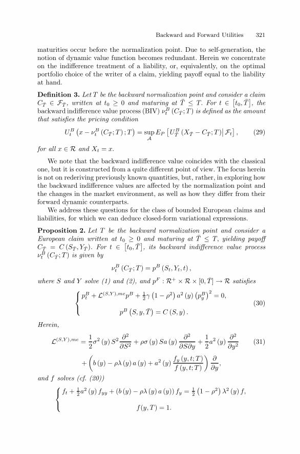
Backward and Forward Utilities 321

maturities occur before the normalization point. Due to self-generation, thenotion of dynamic value function becomes redundant. Herein we concentrateon the indifference treatment of a liability, or, equivalently, on the optimalportfolio choice of the writer of a claim, yielding payoff equal to the liabilityat hand.

Definition 3. Let T be the backward normalization point and consider a claimCT ∈ FT , written at t0 ≥ 0 and maturing at T ≤ T. For t ∈

[t0, T], the

backward indifference value process (BIV) νBt (CT ;T ) is defined as the amountthat satisfies the pricing condition

UBt(x− νBt (CT ;T ) ;T

)= sup

AEP[UBT (XT − CT ;T )

∣∣Ft], (29)

for all x ∈ R and Xt = x.

We note that the backward indifference value coincides with the classicalone, but it is constructed from a quite different point of view. The focus hereinis not on rederiving previously known quantities, but, rather, in exploring howthe backward indifference values are affected by the normalization point andthe changes in the market environment, as well as how they differ from theirforward dynamic counterparts.

We address these questions for the class of bounded European claims andliabilities, for which we can deduce closed-form variational expressions.

Proposition 2. Let T be the backward normalization point and consider aEuropean claim written at t0 ≥ 0 and maturing at T ≤ T, yielding payoffCT = C (ST , YT ). For t ∈

[t0, T], its backward indifference value process

νBt (CT ;T ) is given by

νBt (CT ;T ) = pB (St, Yt, t) ,

where S and Y solve (1) and (2), and pF : R+ ×R× [0, T ] → R satisfies⎧⎨

⎩

pBt + L(S,Y ),mepB + 12γ(1 − ρ2

)a2 (y)

(pBy)2 = 0,

pB(S, y, T

)= C (S, y) .

(30)

Herein,

L(S,Y ),me =12σ2 (y)S2 ∂2

∂S2+ ρσ (y)Sa (y)

∂2

∂S∂y+

12a2 (y)

∂2

∂y2(31)

+(b (y) − ρλ (y) a (y) + a2 (y)

fy (y, t;T )f (y, t;T )

)∂

∂y,

and f solves (cf. (20))⎧⎨

⎩

ft + 12a

2 (y) fyy + (b (y) − ρλ (y) a (y)) fy = 12

(1 − ρ2

)λ2 (y) f,

f(y, T ) = 1.

322 Marek Musiela and Thaleia Zariphopoulou

Proof. For convenience, we recall the entropic quantities

H(t, t

′)= EQme

[∫ t′

t

12

(λ2 (Ys) + λ2 (Ys, s;T )

)ds

∣∣∣∣∣Ft

],

and

H(y, t; t

′)= EQme

[∫ t′

t

12

(λ2 (Yu) + λ2 (Yu, u;T )

)du

∣∣∣∣∣Yt = y

],

for 0 ≤ t ≤ t′ ≤ T ≤ T . We first calculate the right-hand side of (29), which,

in view of Proposition 1, becomes

supA

EP

[−e−γ(XT −CT )−H(T ;T)

∣∣∣Ft]

= supA

EP

[−e−γ(XT −GT )

∣∣∣Ft],

withGT = C (ST , YT ) − 1

γH(T ;T).

One may, then, view this problem as a traditional indifference valuation one inwhich the trading horizon is

[t, T]

and the utility is the exponential functionat T . For the stochastic factor model we consider herein, we obtain (see Sircarand Zariphopoulou [31] and Grasselli and Hurd [13])

supA

EP

[−e−γ(XT −GT )

∣∣∣Ft]

= −e−γ(x−h(St,Yt,t))−H(t;T),

with h : R+ ×R× [0, T ] → R solving⎧⎨

⎩

ht + L(S,Y ),meh+ 12γ(1 − ρ2

)a2 (y)h2

y = 0,

h(S, y, T

)= C (S, y) − 1

γ H(y, T ;T

).

Next, we introduce the function pB : R+ ×R× [0, T ] → R,

pB (S, y, t) = h (S, y, t) +1γ

(H (y, t;T )− H

(y, t; T))

.

Using the equation satisfied by h, we deduce that pB solves (30). On the otherhand, Corollary 1 and the above equalities yield

supA

EP

[−e−γ(XT −GT )

∣∣∣Xt = x, St = S, Yt = y]

= −e−γ(x−pB(S,y,t))−(H(y,t;T)+H(y,T ;T)) = −e−γ(x−p

B(S,y,t))−H(y,t;T ),

and the assertion follows from Definition 3 and Proposition 1. �

Backward and Forward Utilities 323

4.2 Optimal Portfolios Under Backward Dynamic Utility

Next, we construct the optimal portfolio strategies in the integrated portfolioproblem. We start with the agent’s optimal behavior in the absence of theliability/payoff. We concentrate our attention on optimal behavior in a shorterhorizon. For simplicity, its end is taken to coincide with T , the point at whichthe liability is met.

Proposition 3. Let T be the backward normalization point and [t, T ] ∈ [t, T ]be the trading horizon of an investor endowed with the backward exponentialdynamic utility UB. The processes πB,∗s and πB,0,∗s , representing the optimalinvestments in the risky and riskless asset, are given, for s ∈ [t, T ], by

πB,∗s = πB,∗(XB,∗s , Ys, s

)=

μ (Ys)γσ2 (Ys)

− ρa (Ys)σ (Ys)

Hy (Ys, s;T ) (32)

andπB,0,∗s = πB,0,∗ (X∗

s , Ys, s) = XB,∗s − πB,∗s .

Herein, XB,∗s solves (5) with πB,∗s being used, and H : R × [0, T ] → R+

satisfies

Ht + LY,meH +λ2(y) + λ2 (y, t;T )

2= 0,

with terminal condition

H(y, T ;T

)= EQme

[∫ T

T

12

(λ (Ys)

2 + λ (Ys, s;T )2)ds

∣∣∣∣∣YT = y

]. (33)

Given the diffusion nature of the model, the form of the utility data andthe regularity assumptions on the market coefficients, optimality follows fromclassical verification results (see, among others, Duffie and Zariphopoulou [9],Zariphopoulou [35], Pham [26], and Touzi [33]).

Due to the stochasticity of the investment opportunity set, the optimalinvestment strategy in the stock account consists of two components, namely,the myopic portfolio and the so-called excess risky demand, given, respec-tively, by μ (Ys)/γσ2 (Ys) and −ρ((a (Ys))/(σ (Ys)))Hy (Ys, s;T ). The myopiccomponent is what the investor would follow if the coefficients of the riskysecurity remained constant across trading periods. The excess risky demandis the required investment that emerges from the local in time changes inthe Sharpe ratio (see, among others, Kim and Omberg [16], Liu [18], Camp-bell and Viceira [4], Chacko and Viceira [6], Wachter [34], and Campellet al. [5]).

Note that even though the trading horizon [t, T ] is shorter than the origi-nal one [t, T ], the optimal policies depend on the longer horizon because thedynamic risk preferences are normalized at T and not at T .

324 Marek Musiela and Thaleia Zariphopoulou

Remark 1. The reader familiar with the representation of indifference pricesmight try to interpret the excess risky demand as the indifference hedgingstrategy of an appropriately chosen claim. Such questions were studied inStoikov and Zariphopoulou [32] where the relevant claim was identified andpriced.

We continue with the optimal strategies in the presence of a European-typeliability CT , which, we recall, is taken to be bounded.

Proposition 4. Let T be the backward normalization point and consider aninvestor endowed with the backward dynamic exponential utility UB and facinga liability CT = C (ST , YT ). The processes πB,∗s and πB,0,∗s , representing theoptimal investments in the risky and riskless asset, are given, for s ∈ [t, T ],by

πB,∗s = πB,∗(XB,∗s , Ss, Ys, s

)=

μ (Ys)γσ2 (Ys)

− ρa (Ys)σ (Ys)

Hy (Ys, s;T ) (34)

+ SspBS (Ss, Ys, s) + ρ

a (Ys)σ (Ys)

pBy (Ss, Ys, s)

andπB,0,∗s = πB,0,∗ (X∗

s , Ss, Ys, s) = XB,∗s − πB,∗s .

Herein, XB,∗s solves (5) with πB,∗s being used, H as in Proposition 1, and pB

solves (30).

Proof. In the presence of the liability, we observe

supA

EP[UBT (XT − CT ;T )

∣∣Ft]

= uC (x, St, Yt, t) ,

where uC : R×R+ ×R×[0, T]→ R− solves the Hamilton–Jacobi–Bellman

equation

uCt + maxπ

{12σ2 (y)π2uCxx + π

(σ2 (y)SuCxS + ρa(y)σ (y)uCxy + μ (y)uCx

)}

+ L(S,Y )uC = 0,

withuC(x, S, y, T

)= −e−γ(x−C(S,y))−H(y,T ;T)

and

L(S,Y ) =12σ2 (y)S2 ∂2

∂S2+ ρσ (y)Sa (y)

∂2

∂S∂y+

12a2 (y)

∂2

∂y2(35)

+ μ (y)∂

∂S+ b (y)

∂

∂y.

Backward and Forward Utilities 325

Verification results yield that the optimal policy πB,∗s is given in the feedbackform

πB,∗s = πB,∗(XB,∗s , Ss, Ys, s

),

with

πB,∗ (x, S, y, t) = −σ2 (y)SuCxS + ρa(y)σ (y)uCxy + μ (y)uCx

σ2 (y)uCxx.

On the other hand, from Proposition 1,

uC (x, S, y, t) = −e−γ(x−pB(S,y,t))−H(y,t;T ).

Combining the above and the feedback form of πB,∗ (x, S, y, t) we conclude.�

5 Investment and Valuation Under Forward DynamicExponential Utilities

We now revert our attention to portfolio choice and pricing under the newlyintroduced class of forward dynamic utilities. We start with the analytic con-struction of such a utility. As mentioned in Section 2, general existence anduniqueness results for forward dynamic utilities are lacking. As a matter offact, an alternative solution to (15) is presented in Example 3.

Proposition 5. Let s ≥ 0 be the forward normalization point. Define, fort ≥ s, the process

h (s, t) =∫ t

s

12λ2udu, (36)

with λ being the Sharpe ratio (4). Then, the process UFt (x; s) given, for x ∈ Rand t ≥ s, by

UFt (x; s) = −e−γx+h(s,t), (37)

is a forward dynamic exponential utility, normalized at s.

Proof. The fact that UFt (x; s) is Ft-measurable and normalized at s is imme-diate. It remains to show (15), namely, that for arbitrary T ≥ t,

−e−γx+h(s,t) = supA

EP

[−e−γXT +h(s,T )

∣∣∣Ft].

Using (36), the above reduces to

−e−γx = supA

EP

[−e−γXT +h(t,T )

∣∣∣Ft]. (38)

326 Marek Musiela and Thaleia Zariphopoulou

Next, we introduce the function u : R×R×[0, T ] → R−,

u (x, y, t) = supA

EP

[−e−γXT +

∫ Tt

(1/2)λ2(Ys)ds∣∣∣Xt = x, Yt = y

].

Classical arguments imply that u solves the Hamilton–Jacobi–Bellman equa-tion

ut + LY u+λ2 (y)

2u

+ maxπ

{12σ2 (y)π2uxx + π (ρa(y)σ (y)uxy + μ (y)ux)

}= 0,

withu (x, y, T ) = −e−γx,

and LY as in (15). We deduce (see, e.g., Duffie and Zariphopoulou [9] andPham [26]) that the above equation has a unique solution in the class offunctions that are concave and increasing in x, and are uniformly bounded iny. We, then, see that the function u (x, y, t) = −e−γx is such a solution and,by uniqueness, it coincides with u. The rest of the proof follows easily. �

We next present an alternative forward dynamic utility.

Example 3. Consider, for x ∈ R and t ≥ s, the process

UFt (x; s) = −e−γx−Z(s,t),

with

Z (s, t) =∫ t

s

12λ2sds+

∫ t

s

λsdW1s . (39)

Observe that, for Xt = x, the forward stochastic criterion (cf. (15)),

−e−γx−Z(s,t) = supA

EP

[−e−γXT−Z(s,T )

∣∣∣Ft],

will hold if we establish

−e−γx = supA

EP

[−e−γXT−Z(t,T )

∣∣∣Ft],

or, equivalently,

−e−γx = supA

EP

[−e−γXT−Z(t,T )

∣∣∣Xt = x, Yt = y, Zt = 0],

with Zt′ = z + Z(t, t′). Defining v : R×R×R× [0, T ] → R− by

v (x, y, z, t) = supA

EP

[−e−γXT−ZT

∣∣∣Xt = x, Yt = y, Zt = z],

Backward and Forward Utilities 327

we see that it solves the Hamilton–Jacobi–Bellman equation

vt + maxπ

{12σ2 (y)π2uxx + π (λ (y)σ (y)uxz + ρa(y)σ (y)uxy + μ (y)ux)

}

+12λ2 (y) vzz + ρλ (y) a (y) vzy +

12a2 (y) vyy + b (y) vy +

12λ2 (y) vz,

withv (x, y, z, T ) = −e−γx−z.

Substituting above the function v (x, y, z, t) = −e−γx−z, and after some cal-culations, yields

− (λ (y)σ (y) vxz + μ (y) vx)2

2σ2 (y) vxx+

12λ2 (y) (vzz + vz) = 0.

We easily conclude that v ≡ v, and the assertion follows.

5.1 Forward Indifference Values

Next, we introduce the concept of forward indifference value. As is its back-ward counterpart, it is defined as the amount that generates the same level of(forward) dynamic utility with and without incorporating the liability. Note,also, that in the definition below, it is only the forward dynamic utility that en-ters, eliminating the need to incorporate in the definition the forward dynamicvalue function. This allows for a concise treatment of payoffs and liabilitiesof arbitrary maturities. Finally, we remark, that the nomenclature “forward”does not refer to the terminology used in derivative valuation pertinent towealth expressed in forward units. Rather, it refers to the forward in timemanner that the dynamic utility evolves.

Although the concept of forward indifference value appears to be astraightforward extension of the backward one, it is important to observethat the maturities of the claims in consideration need not be bounded byany prespecified horizon. This is one of the striking differences between theclasses of claims that can be priced by the two distinct dynamic utilities weconsider herein.

Definition 4. Let s ≥ 0 be the forward normalization point and consider aclaim CT ∈ FT , written at t0 ≥ s and maturing at T. For t ∈ [t0, T ], theforward indifference value process (FIP) νFt (CT ; s) is defined as the amountthat satisfies the pricing condition

UFt(x− νFt (CT ; s) ; s

)= sup

AEP[UFT (XT − CT ; s)

∣∣Ft], (40)

for all x ∈ R and Xt = x.

328 Marek Musiela and Thaleia Zariphopoulou

We continue with the valuation of a bounded European-type liability andwe examine how its forward indifference value is affected by the choice of thenormalization point. We show that even though both forward dynamic utili-ties, entering in (40) above, depend on the normalization point, the emergingforward price does not. This is another important difference between the back-ward and the forward indifference values.

Proposition 6. Let s ≥ 0 be the forward normalization point and considera European claim written at t0 ≥ s and maturing at T yielding payoff CT =C (ST , YT ). For t ∈ [t0, T ], its forward indifference value νFt (CT ; s) is givenby

νFt (CT ; s) = pF (St, Yt, t) ,

where S and Y solve (1) and (2), and pF : R+ ×R× [0, T ] → R satisfies⎧⎨

⎩

pFt + L(S,Y ),mmpF + 12γ(1 − ρ2

)a2 (y)

(pFy)2 = 0,

pF (S, y, T ) = C (S, y) ,(41)

with

L(S,Y ),mm =12σ2 (y)S2 ∂2

∂S2+ ρσ (y)Sa (y)

∂2

∂S∂y+

12a2 (y)

∂2

∂y2

+ (b (y) − ρλ (y) a (y))∂

∂y.

Proof. We first note that

supA

EP[UFT (XT − CT ; s)

∣∣Ft]

= supA

EP

[−e−γ(XT −CT )+

∫Ts

(1/2)λ2(Yu)du∣∣∣Ft]

= e∫

ts(1/2)λ2(Yu)du sup

AEP

[−e−γ(XT −CT )+

∫Tt

(1/2)λ2(Yu)du∣∣∣Ft],

where we used Proposition 5 and the measurability of the process h (cf. (36)).Define uC : R×R+ ×R× [0, T ]→ R−,

uC (x, S, y, t) = supA

EP

[−e−γ(XT −CT )+

∫ Tt

(1/2)λ2(Yu)du∣∣∣Xt=x, St=S, Yt=y

],

and observe that it solves the Hamilton–Jacobi–Bellman equation

uCt + maxπ

{12σ2 (y)π2uCyy + π

(σ2 (y)SuCxS + ρa(y)σ (y)uCxy + μ (y)uCx

)}

+ L(S,Y )uC +λ2 (y)

2uC = 0,

withuC (x, S, y, T ) = −e−γ(x−C(S,y)),

Backward and Forward Utilities 329

and L(S,Y ) as in (35). Using the transformationuC (x, S, y, t) = −e−γ(x−p

F (S,y,t)),

we deduce, after tedious but straightforward calculations, that the termpF (S, y, t) solves (41). We, then, easily, see that

supA

EP[UFT (XT − CT ; s)

∣∣Ft]

= −e∫ t

s(1/2)λ2(Yu)duuC (x, St, Yt, t) ,

and applying Proposition 5 and Definition 4 completes the proof. �

5.2 Optimal Portfolios Under Forward Dynamic Utilities

We continue with the optimal investment policies under the forward dynamicrisk preferences.

Proposition 7. Let s ≥ 0 be the forward normalization point and [t, T ] thetrading horizon, with s ≤ t. The processes πF,∗ and πF,0,∗, representing theoptimal investments in the risky and riskless asset, are given, respectively, foru ∈ [t, T ], by

πF,∗u = πF,∗(XF,∗u , Yu, u

)=

μ (Yu)γσ2 (Yu)

(42)

andπF,0,∗u = πF,0,∗ (X∗

u, Yu, u) = XF,∗u − πF,∗u ,

with XF,∗u solving (5) with πF,∗u being used.

Two important facts emerge. Firstly, both optimal investment policies πF,∗

and πF,0,∗ are independent of the spot normalization point. Secondly, the in-vestment in the risky asset consists entirely of the myopic component. Indeed,the excess hedging demand, which emerges due to the presence of the stochas-tic factor, has vanished. The investor has processed the stochasticity of the(incomplete) market environment into her preferences, that are dynamicallyupdated, following, forward in time, the market movements.

Proposition 8. Let s ≥ 0 be the forward normalization point and consider aninvestor endowed with the forward exponential dynamic utility UF and facinga liability CT = C (ST , YT ). The processes πF,∗s and πF,0,∗s , representing theoptimal investments in the risky and riskless asset in the integrated portfoliochoice problem, are given, for u ∈ [t, T ], by

πF,∗u = πF,∗(XF,∗u , Su, Yu, u

)=

μ (Yu)γσ2 (Yu)

+SupFS (Su, Yu, u) + ρa (Yu)σ (Yu)

pFy (Su, Yu, u) (43)

330 Marek Musiela and Thaleia Zariphopoulou

andπF,0,∗u = πF,0,∗ (X∗

u, Su, Yu, u) = XF,∗u − πF,∗u .

Herein, XF,∗s solves (5) with πF,∗s being used, and pF satisfies (41).

6 Concluding Remarks: Forward Versus BackwardUtilities and Their Associated Indifference Prices

In the previous two sections, we analyzed the investment and pricing problemsof investors endowed with backward (BDU) and forward (FDU) dynamic ex-ponential utilities. These utilities have similarities but also striking differences.These features are, in turn, inherited by the associated optimal policies, indif-ference prices, and risk monitoring strategies. Below, we provide a discussionon these issues.

We first observe that the backward and forward utilities are producedvia a conditional expected criterion. They are both self-generating, in thatthey coincide with their implied value functions. Moreover, in the absence ofexogenous cash flows, investors endowed with such utilities are indifferent tothe investment horizons.

Backward and forward dynamic utilities are constructed in entirely differ-ent ways. Backward utilities are first specified at a given future time T and,they are, subsequently, generated at previous to T times. Forward utilities aredefined at present s and are, in turn, generated forward in time. The timesT and s, at which the backward and forward utility data are determined, arethe backward and forward normalization points. We recall, from Equations(28) and (37), that the BDU and FDU processes UBt and UFt are Ft-adaptedand given, respectively, by

UBt (x;T ) = −e−γx−H(t,T )

andUFt (x; s) = −e−γx−h(s,t),

with

H (t, T ) = EQme

[∫ T

t

12

(λ2u + λ2

u

)du

∣∣∣∣∣Ft

]

and

h(s, t) =∫ t

s

12λ2udu.

Herein, λ and λ are given in (4) and (18), and Qme is the minimal relativeentropy measure.

Both BDU and FDU have an exponential, affine in wealth, structure. How-ever, the backward utility compiles changes in the market environment in anaggregate manner, whereas the forward utility does so in a much finer way.

Backward and Forward Utilities 331

This is seen by the nature of the processes H (t, T ) and h (s, t) . It is worthobserving that

H (t, T ) �= EQme [h (t, T )| Ft] ,

and that UFt is not affected by λ (cf. (18) and (19)) that represent the “or-thogonal” component of the market price of risk.

Backward and forward utilities generate different optimal investmentstrategies (see, respectively, Propositions 3 and 7). Under backward dynamicpreferences, the investor invests in the risky asset an amount equal to the sumof the myopic portfolio and the excess risky demand. The former investmentstrategy depends on the risk aversion coefficient γ, but not on the backwardnormalization point T . The excess risky demand, however, is not affected byγ but depends on the choice of the normalization point, even if investmenttakes place in a shorter horizons.

Under forward preferences, the investor invests in the risk asset solelywithin the myopic portfolio. The myopic strategy does not depend on theforward normalization point or the investment horizon.

As a consequence of the above differences, the emerging backward (BIV)and forward (FIV) indifference values νBt (CT ;T ) and νFt (CT ; s) , 0 ≤ s ≤t ≤ T ≤ T have very distinct characteristics. Concentrating on the class ofbounded European claims, we see that νBt (CT ;T ) and νFt (CT ; s) are con-structed via solutions of similar quasilinear PDEs. The nonlinearities in thepricing PDEs are of the same type, however, the associated linear operatorsL(S,y),me and L(S,y),mm differ (see, respectively, (30) and (41)). The former,appearing in the BIV equation, corresponds to the minimal relative entropymeasure and the latter, appearing in the FIV equation, to the minimal martin-gale measure. Denoting the solutions of these PDEs as nonlinear expectations,we may formally represent (with a slight abuse of notation) the two indiffer-ence values as

νBt (CT ;T ) = EQme [CT ;T ]

andνFt (CT ; s) = EQmm [CT ; s] .

The FIV is independent on the forward normalization point. The BIVdepends, however, on the backward normalization point, even if the claimmatures in a shorter horizon.

As the investor becomes risk neutral, γ → 0, we obtain

limγ→0

νBt (CT ;T ) = EQme [CT |Ft ]

andlimγ→0

νFt (CT ; s) = EQmm [CT |Ft ] .

However, as the investor becomes infinitely risk averse, γ → ∞, both BIV andFIV converge to the same limit given by the super replication value,

332 Marek Musiela and Thaleia Zariphopoulou

limγ→∞

νBt (CT ;T ) = limγ→∞

νFt (CT ; s) = ‖CT ‖L∞{ .|Ft} .

In the presence of the liability and under backward dynamic utility, theinvestment in the risky asset consists of the myopic portfolio, the excess riskydemand, and the backward indifference risk monitoring strategies (see Propo-sition 4). With the exception of the myopic portfolio, all other three portfoliocomponents depend on the normalization point T . When, however, the in-vestor uses forward dynamic utility, his optimal integrated policy does notinclude the excess risky demand (see Proposition 8). The entire policy is in-dependent of the forward normalization point s, and depends exclusively onthe maturity of the claim and the changes in the market environment.

When the market becomes complete, the backward and forward pricingmeasures Qme and Qmm coincide with the unique risk-neutral measure Q∗,and (BIV) and (FIV) reduce to the arbitrage free price.

In general, the backward and forward indifference values do not coincide.The underlying reason is that they are defined via the backward and forwarddynamic utilities that process the internal model incompleteness, generatedby the stochastic factor Y , in a very different manner. Characterizing themarket environments as well as the claims for which the two prices coincideis an open question.

Acknowledgments

Thaleia Zariphopoulou’s work is partially supported by NSF grants DMS-0456118 and DMS-0091946. This work was presented at the Workshop inSemimartingale Theory and Practice in Finance, Banff (June 2004), Impe-rial College (June 2004), Cornell University (November 2004), the Workshopin Mathematical Finance at Carnegie Mellon University (January 2005), theSecond Bachelier Colloquium, Metabief (January 2005), London School ofEconomics (April 2005), the Conference on Stochastic Processes and TheirApplications, Ascona (June 2005), the SIAM Conference on Control and Op-timization, New Orleans (July 2005), the Stochastic Modeling Workshop onPDEs and their applications to Mathematical Finance at KTH, Stockholm(August 2005), the Bachelier Seminar (May 2006), and the Conference inHonor of S. Sethi at the University of Texas at Dallas (May 2006). The authorswould like to thank the participants for fruitful comments and suggestions.

References

1. T. Arai. The relation between the minimal martingale measure and the mini-mal entropy martingale measure. Asia-Pacific Financial Markets, 8(2):167–177,2001.

Backward and Forward Utilities 333

2. F. Bellini and M. Frittelli. On the existence of the minmax martingale measures.Mathematical Finance, 12:1–21, 2002.

3. F.E. Benth and K.H. Karlsen. A PDE representation of the density of theminimal martingale measure in stochastic volatility markets. Stochastics andStochastics Reports, 77:109–137, 2005.

4. J.Y. Campbell and L.M. Viceira. Consumption and portfolio decisions whenexpected returns are time-varying. Quarterly Journal of Economics, 114:433–495, 1999.

5. J.Y. Campell, J. Cocco, F. Gomes, P.J. Maenhout, and L.M. Viceira. Stockmarket mean reversion and the optimal equity allocation of a long-lived investor.European Finance Review, 5:269–292, 2001.

6. G. Chacko and L. Viceira. Dynamic consumption and portfolio choice withstochastic volatility in incomplete markets. NBER Working papers, No.7377,1999.

7. M.H.A. Davis and T. Zariphopoulou. American options and transaction fees.Mathematical Finance, IMA Volumes in Mathematics and its Application,65:47–61, Springer-Verlag, 1995.

8. F. Delbaen, P. Grandits, T. Rheinlander, D. Samperi, M. Schweizer, and C.Stricker. Exponential hedging and entropic penalties. Mathematical Finance,12:99–123, 2002.

9. D. Duffie and T. Zariphopoulou. Optimal investment with undiversifiable in-come risk. Mathematical Finance, 3(2):135–148, 1993.

10. H. Foellmer and M. Schweizer. Hedging of contingent claims under incompleteinformation. Applied Stochastic Analysis, Stochastic Monographs, Vol. 5, eds.M.H.A. Davis and R.J. Elliott, Gordon and Breach, 389–414, 1991.

11. M. Frittelli. The minimal entropy martingale measure and the valuation problemin incomplete markets. Mathematical Finance, 10:39–52, 2000.

12. P. Grandits and T. Rheinlander. On the minimal entropy measure. Annals ofProbability, 30(3):1003–1038, 2002.

13. M.R. Grasselli and T. Hurd. Indifference pricing and hedging in stochasticvolatility models. preprint, 2004.

14. Y. Kabanov and C. Stricker. On the optimal portfolio for the exponential util-ity maximization: Remarks to the six-author paper “Exponential hedging andentropic penalties.” Mathematical Finance, 12(2):125–134, 2002.

15. J. Kallsen and C. Kuehn. Pricing derivatives of American and game type inincomplete markets. Finance and Stochastics, 8(2):261–284, 2004.

16. T.S. Kim and E. Omberg. Dynamic nonmyopic portfolio behavior. Review ofFinancial Studies, 9:141–161, 1996.

17. D. Kramkov and W. Schachermayer. The asymptotic elasticity of utility func-tions and optimal investments in incomplete markets. Annals of Applied Prob-ability, 9:904–950, 1999.

18. J. Liu. Portfolio selection in stochastic environments. Working paper, StanfordUniversity, 1999.

19. M. Monoyios. Characterization of optimal dual measures via distortion. Deci-sions in Economics and Finance, 29:95–119, 2006.

20. M. Musiela and T. Zariphopoulou. Indifference prices and related mea-sures. Technical report, The University of Texas at Austin, 2001.http://www.ma.utexas.edu/users/zariphop/.

21. M. Musiela and T. Zariphopoulou. An example of indifference prices under ex-ponential preferences. Finance and Stochastics, 8:229–239, 2004.

334 Marek Musiela and Thaleia Zariphopoulou

22. M. Musiela and T. Zariphopoulou. Indifference prices of early exercise claims.Proceedings of AMS-IMS-SIAM Joint Summer Conference on Mathematical Fi-nance, eds. G. Yin and Q. Zhang, Contemporary Mathematics, AMS, 351:259–272, 2004.

23. M. Musiela and T. Zariphopoulou. The backward and forward dynamic utilitiesand their associated pricing systems: The case study of the binomial model.Indifference Pricing, ed. R. Carmona, Princeton University Press, 2005.

24. M. Musiela and T. Zariphopoulou. Forward dynamic utilities and indifferencevaluation in incomplete binomial models. Preprint, 2005.

25. A. Oberman and T. Zariphopoulou. Pricing early exercise contracts in incom-plete markets. Computational Management Science, 1:75–107, 2003.

26. H. Pham. Smooth solutions to optimal investment models with stochasticvolatilities and portfolio constraints. Applied Mathematics and Optimization,46:55–78, 2002.

27. T. Rheinlander. An entropy approach to the Stein/Stein model with correlation.Finance and Stochastics, 9:399–413, 2003.

28. R. Rouge and N. El Karoui. Pricing via utility maximization and entropy. Math-ematical Finance, 10:259–276, 2000.

29. M. Schweizer. On the minimal martingale measure and the Foellmer-Schweizerdecomposition. Stochastic Processes and Applications, 13:573–599, 1995.

30. M. Schweizer. A minimality property of the minimal martingale measure. Statis-tics and Probability Letters, 42:27–31, 1999.

31. R. Sircar and T. Zariphopoulou. Bounds and asymptotic approximations forutility prices when volatility is random. SIAM Journal on Control and Opti-mization, 43(4):1328–1353, 2005.

32. S. Stoikov and T. Zariphopoulou. Optimal investments in the presence of un-hedgeable risks and under CARA preferences. IMA Volumes in Mathematicsand its Application, in print, 2004.

33. N. Touzi. Stochastic control problems, viscosity solutions and application tofinance. Technical report, Special research semester on Financial Markets, Pisa,2002.

34. J. Wachter. Portfolio consumption decisions under mean-reverting returns: Anexact solution for complete markets. Journal of Financial and QuantitativeAnalysis, 37(1):63–91, 2002.

35. T. Zariphopoulou. Stochastic control methods in asset pricing. Handbook ofStochastic Analysis and Applications, eds. D. Kannan and V. Lakshmikanthan,Statistics, Textbooks, Monographs, 163, Dekker, 679–753, 2002.