applied functional analysis - 2nd edition - j. tinsley oden
DESCRIPTION
funtional analysisTRANSCRIPT


C1956_FM.indd 1 1/29/10 11:44:14 AM

C1956_FM.indd 2 1/29/10 11:44:14 AM

C1956_FM.indd 3 1/29/10 11:44:14 AM

Chapman & Hall/CRCTaylor & Francis Group6000 Broken Sound Parkway NW, Suite 300Boca Raton, FL 33487-2742
© 2010 by Taylor and Francis Group, LLCChapman & Hall/CRC is an imprint of Taylor & Francis Group, an Informa business
No claim to original U.S. Government works
Printed in the United States of America on acid-free paper10 9 8 7 6 5 4 3 2 1
International Standard Book Number-13: 978-1-4200-9196-0 (Ebook-PDF)
This book contains information obtained from authentic and highly regarded sources. Reasonable efforts have been made to publish reliable data and information, but the author and publisher cannot assume responsibility for the valid-ity of all materials or the consequences of their use. The authors and publishers have attempted to trace the copyright holders of all material reproduced in this publication and apologize to copyright holders if permission to publish in this form has not been obtained. If any copyright material has not been acknowledged please write and let us know so we may rectify in any future reprint.
Except as permitted under U.S. Copyright Law, no part of this book may be reprinted, reproduced, transmitted, or uti-lized in any form by any electronic, mechanical, or other means, now known or hereafter invented, including photocopy-ing, microfilming, and recording, or in any information storage or retrieval system, without written permission from the publishers.
For permission to photocopy or use material electronically from this work, please access www.copyright.com (http://www.copyright.com/) or contact the Copyright Clearance Center, Inc. (CCC), 222 Rosewood Drive, Danvers, MA 01923, 978-750-8400. CCC is a not-for-profit organization that provides licenses and registration for a variety of users. For organizations that have been granted a photocopy license by the CCC, a separate system of payment has been arranged.
Trademark Notice: Product or corporate names may be trademarks or registered trademarks, and are used only for identification and explanation without intent to infringe.
Visit the Taylor & Francis Web site athttp://www.taylorandfrancis.com
and the CRC Press Web site athttp://www.crcpress.com

To
John James and Sara Elizabeth Oden
and
Wiesława and Kazimierz Demkowicz


Preface to the Second Edition
The rapid development of information and computer technologies and of the computational sciences has cre-
ated an environment in which it is critically important to teach applicable mathematics in an interdisciplinary
setting. The trend is best illustrated with the emergence of multiple graduate programs in applied and com-
putational mathematics, and computational science and engineering across the nation and worldwide. With a
finite number of curriculum hours and a multitude of new subjects, we are constantly faced with the dilemma
of how to teach mathematics and which subjects to choose.
The main purpose of Applied Functional Analysis for Science and Engineering has been to provide a
crash course for beginning graduate students with non-math majors, on mathematical foundations leading to
classical results in Functional Analysis. Indeed, it has served its purpose over the last decade of the graduate
program on Computational and Applied Mathematics at The University of Texas. A more particular goal
of the text has been to prepare the students to learn the variational theory of partial differential equations,
distributions and Sobolev spaces and numerical analysis with an emphasis on finite element methods.
This second edition continues to serve both of these goals. We have kept the original structure of the book,
resisting temptation of adding too many new topics. Instead, we have revised many of the original examples
and added new ones, reflecting very often our own research experience and perspectives. In this revised
edition, we start each chapter with an extensive introduction and conclude it with a summary and historical
comments referring frequently to other sources. The number of exercises has been significantly increased and
we are pleased to provide a solution manual. Problems provided in the text may be solved in many different
ways, but the solutions presented are consistent with the style and philosophy of the presentation.
Main revisions of the material include the following changes:
Chapter 1: The order of presentations of elementary logic and elementary set theory has been reversed.
The section on lim sup and lim inf has been completely revised with functions taking values in the
extended set of real numbers in mind. We have complemented the exposition on elementary topology
with a discussion on connected sets.
Chapter 2: A new section on elements of multilinear algebra and determinants and a presentation on the
Singular Value Decomposition Theorem have been added.
Chapter 3: We have added an example of a Lebesgue non-measurable set, a short discussion on proba-
bility and Bayesian Statistical Inference, and a short presentation on the Cauchy Principal Value and
Hadamard Finite Part integrals.
vii

viii
Chapter 4: We have added a discussion on connected sets.
Chapter 5: The discussion on representation theorems for duals of Lp-spaces has been complemented with
the Generalized (Integral) Minkowski Inequality.
The book attempts to teach the rigor of logic and systematical, mathematical thinking. What makes it dif-
ferent from other mathematical texts is the large number of illustrative examples and comments. Engineering
and science students come with a very practical attitude, and have to be constantly motivated and guided into
appreciating the value and importance of mathematical rigor and the precision of thought that it provides.
Nevertheless, the class in which the book has been used focuses on teaching how to prove theorems and pre-
pares the students for further study of more advanced mathematical topics. The acquired ability to formulate
research questions in a mathematically rigorous way has had a tremendous impact on our graduates and, we
believe, it has been the best measure of the success of the text.
The book has been used as a text for a rather intensive two-semester course. The first semester focuses on
real analysis with attention to infinite-dimensional settings, and it covers the first four chapters, culminating
with the Banach Fixed Point Theorem. The second semester covers the actual Functional Analysis topics
presented in Chapters 5 and 6.
We wish to thank a number of students and colleagues who made useful suggestions and read parts of the
text during the preparation of the second edition: Tan Bui, Jessie Chan, Paolo Gatto, Antti Niemi, Frederick
Qiu, Nathan Roberts, Jamie Wright and Jeff Zitelli.
We thank James Goertz for helping with typing of the text.
J. Tinsley Oden and Leszek F. Demkowicz
Austin, September 2009
Preface to the First Edition
Worldwide, in many institutions of higher learning, there has emerged in recent years a variety of new aca-
demic programs designed to promote interdisciplinary education and research in applied and computational
mathematics. These programs, advanced under various labels such as computational and applied mathemat-
ics, mathematical sciences, applied mathematics, and the like, are created to pull together several areas of
mathematics, computer science, and engineering and science which underpin the broad subjects of mathe-
matical modeling and computer simulation. In all such programs, it is necessary to bring students of science
and engineering quickly to within reach of modern mathematical tools, to provide them with the precision
and organization of thought intrinsic to mathematics, and to acquaint them with the fundamental concepts
and theorems which form the foundation of mathematical analysis and mathematical modeling. These are
among the goals of the present text.
This book, which is the outgrowth of notes used by the authors for over a decade, is designed for a course
for beginning graduate students in computational and applied mathematics who enter the subject with back-
grounds in engineering and science. The course purports to cover in a connected and unified manner an in-
troduction to the topics in functional analysis important in mathematical modeling and computer simulation;
particularly, the course lays the foundation for futher work in partial differential equations, approximation
theory, numerical mathematics, control theory, mathematical physics, and related subjects.
Prerequisites for the course for which this book is written are not extensive. The student with the usual
background in calculus, ordinary differential equations, introductory matrix theory, and, perhaps, some back-
ground in applied advanced calculus typical of courses in engineering mathematics or introductory mathe-
matical physics, should find much of the book a logical and, we hope, exciting extension and abstraction of
his knowledge of these subjects.
It is characteristic of such courses that they be paradoxical, in a sense, because on the one hand they
presume to develop the foundations of algebra and analysis from the first principles, without appeal to any
previous prejudices toward mathematical methods; but at the same time, they call upon undergraduate mathe-
matical ideas repeatedly as examples or as illustrations of purpose of the abstractions and extensions afforded
by the abstract theory. The present treatment is no exception.
We begin with an introduction to elementary set theoretics, logic, and general abstract algebra, and with
an introduction to real analysis in Chapter 1. Chapter 2 is devoted to linear algebra in both finite and infinite
dimensions. These two chapters could be skipped by many readers who have an undergraduate background
in mathematics. For engineering graduate students, the material is often new and should be covered. We have
provided numereous examples throughout the book to illustrate concepts, and many of these, again, draw
ix

x
from undergraduate calculus, matrix theory, and ordinary differential equations.
Chapter 3 is devoted to measure theory and integration and Chapter 4 covers topological and metric spaces.
In these chapters, the reader encounters the fundamentals of Lebesgue integration, Lp spaces, the Lebesgue
Dominated Convergence Theorem, Fubini’s Theorem, the notion of topologies, filters, open and closed sets,
continuity, convergence, Baire categories, the contraction mapping principle, and various notions of com-
pactness.
In Chapter 5, all of the topological and algebraic notions covered in Chapters 1–4 are brought together to
study topological vector spaces and, particularly, Banach spaces. This chapter contains introductions to many
fundamental concepts, including the theory of distributions, the Hahn-Banach Theorem and its corollaries,
open mappings, closed operators, the Closed Graph Theorem, Banach Theorem, and the Closed Range The-
orem. The main focus is on properties of linear operators on Banach spaces and, finally, the solution of linear
equations.
Chapter 6 is devoted to Hilbert spaces and to an introduction to the spectral theory of linear operators. There
some applications to boundary-value problems of partial differential equations of mathematical physics are
discussed in the context of the theory of linear operators on Hilbert spaces.
Depending upon the background of the entering students, the book may be used as a text for as many as
three courses: Chapters 1 and 2 provide a course on real analysis and linear algebra; Chapters 3 and 4, a
text on integration theory and metric spaces, and Chapters 5 and 6 an introductory course on linear operators
and Banach spaces. We have frequently taught all six chapters in a single semester course, but then we have
been very selective of what topics were or were not taught. The material can be covered comfortably in
two semesters, Chapters 1–3 and, perhaps, part of 4 dealt with in the first semester and the remainder in the
second.
As with all books, these volumes reflect the interests, prejudices, and experience of its authors. Our main
interests lie in the theory and numerical analysis of boundary- and initial-value problems in engineering
science and physics, and this is reflected in our choice of topics and in the organization of this work. We
are fully aware, however, that the text also provides a foundation for a much broader range of studies and
applications.
The book is very much based on the text with the same title by the first author and, indeed, can be consid-
ered as a new, extended, and revised version of it. It draws heavily from other monographs on the subject,
listed in the References, as well as from various old personal lecture notes taken by the authors when they
themselves were students. The second author would like especially to acknowledge the privilege of listening
to unforgettable lectures of Prof. Stanisław Łojasiewicz at the Jagiellonian University in Cracow, from which
much of the text on integration theory has been borrowed.
We wish to thank a number of students and colleagues who made useful suggestions and read parts of
the text during the preparation of this work: Waldek Rachowicz, Andrzej Karafiat, Krzysztof Banas, Tarek

xi
Zohdi, and others. We thank Ms. Judith Caldwell for typing a majority of the text.
J. Tinsley Oden and Leszek F. Demkowicz
Austin, September 1995


Contents
1 Preliminaries 1
Elementary Logic and Set Theory
1.1 Sets and Preliminary Notations, Number Sets . . . . . . . . . . . . . . . . . . . . . . . . 1
1.2 Level One Logic . . . . . . . . . . . . . . . . . . . . . . . . . . . . . . . . . . . . . . . . 3
1.3 Algebra of Sets . . . . . . . . . . . . . . . . . . . . . . . . . . . . . . . . . . . . . . . . 9
1.4 Level Two Logic . . . . . . . . . . . . . . . . . . . . . . . . . . . . . . . . . . . . . . . 16
1.5 Infinite Unions and Intersections . . . . . . . . . . . . . . . . . . . . . . . . . . . . . . . 18
Relations
1.6 Cartesian Products, Relations . . . . . . . . . . . . . . . . . . . . . . . . . . . . . . . . . 21
1.7 Partial Orderings . . . . . . . . . . . . . . . . . . . . . . . . . . . . . . . . . . . . . . . 26
1.8 Equivalence Relations, Equivalence Classes, Partitions . . . . . . . . . . . . . . . . . . . 31
Functions
1.9 Fundamental Definitions . . . . . . . . . . . . . . . . . . . . . . . . . . . . . . . . . . . 36
1.10 Compositions, Inverse Functions . . . . . . . . . . . . . . . . . . . . . . . . . . . . . . . 43
Cardinality of Sets
1.11 Fundamental Notions . . . . . . . . . . . . . . . . . . . . . . . . . . . . . . . . . . . . . 52
1.12 Ordering of Cardinal Numbers . . . . . . . . . . . . . . . . . . . . . . . . . . . . . . . . 54
Foundations of Abstract Algebra
1.13 Operations, Abstract Systems, Isomorphisms . . . . . . . . . . . . . . . . . . . . . . . . . 58
1.14 Examples of Abstract Systems . . . . . . . . . . . . . . . . . . . . . . . . . . . . . . . . 63
Elementary Topology in IRn
1.15 The Real Number System . . . . . . . . . . . . . . . . . . . . . . . . . . . . . . . . . . . 73
1.16 Open and Closed Sets . . . . . . . . . . . . . . . . . . . . . . . . . . . . . . . . . . . . 78
1.17 Sequences . . . . . . . . . . . . . . . . . . . . . . . . . . . . . . . . . . . . . . . . . . . 85
1.18 Limits and Continuity . . . . . . . . . . . . . . . . . . . . . . . . . . . . . . . . . . . . . 92
xiii

xiv
Elements of Differential and Integral Calculus
1.19 Derivatives and Integrals of Functions of One Variable . . . . . . . . . . . . . . . . . . . 97
1.20 Multidimensional Calculus . . . . . . . . . . . . . . . . . . . . . . . . . . . . . . . . . . 104
2 Linear Algebra 111
Vector Spaces—The Basic Concepts
2.1 Concept of a Vector Space . . . . . . . . . . . . . . . . . . . . . . . . . . . . . . . . . . 111
2.2 Subspaces . . . . . . . . . . . . . . . . . . . . . . . . . . . . . . . . . . . . . . . . . . . 118
2.3 Equivalence Relations and Quotient Spaces . . . . . . . . . . . . . . . . . . . . . . . . . 123
2.4 Linear Dependence and Independence, Hamel Basis, Dimension . . . . . . . . . . . . . . 129
Linear Transformations
2.5 Linear Transformations—The Fundamental Facts . . . . . . . . . . . . . . . . . . . . . . 139
2.6 Isomorphic Vector Spaces . . . . . . . . . . . . . . . . . . . . . . . . . . . . . . . . . . . 146
2.7 More About Linear Transformations . . . . . . . . . . . . . . . . . . . . . . . . . . . . . 150
2.8 Linear Transformations and Matrices . . . . . . . . . . . . . . . . . . . . . . . . . . . . . 156
2.9 Solvability of Linear Equations . . . . . . . . . . . . . . . . . . . . . . . . . . . . . . . . 159
Algebraic Duals
2.10 The Algebraic Dual Space, Dual Basis . . . . . . . . . . . . . . . . . . . . . . . . . . . . 162
2.11 Transpose of a Linear Transformation . . . . . . . . . . . . . . . . . . . . . . . . . . . . 170
2.12 Tensor Products, Covariant and Contravariant Tensors . . . . . . . . . . . . . . . . . . . . 176
2.13 Elements of Multilinear Algebra . . . . . . . . . . . . . . . . . . . . . . . . . . . . . . . 181
Euclidean Spaces
2.14 Scalar (Inner) Product, Representation Theorem in Finite-Dimensional Spaces . . . . . . . 188
2.15 Basis and Cobasis, Adjoint of a Transformation, Contra- and Covariant Components of Ten-
sors . . . . . . . . . . . . . . . . . . . . . . . . . . . . . . . . . . . . . . . . . . . . . . 192
3 Lebesgue Measure and Integration 201
Lebesgue Measure
3.1 Elementary Abstract Measure Theory . . . . . . . . . . . . . . . . . . . . . . . . . . . . 201
3.2 Construction of Lebesgue Measure in IRn . . . . . . . . . . . . . . . . . . . . . . . . . . . 210
3.3 The Fundamental Characterization of Lebesgue Measure . . . . . . . . . . . . . . . . . . 221
Lebesgue Integration Theory
xv
3.4 Measurable and Borel Functions . . . . . . . . . . . . . . . . . . . . . . . . . . . . . . . 230
3.5 Lebesgue Integral of Nonnegative Functions . . . . . . . . . . . . . . . . . . . . . . . . . 233
3.6 Fubini’s Theorem for Nonnegative Functions . . . . . . . . . . . . . . . . . . . . . . . . 238
3.7 Lebesgue Integral of Arbitrary Functions . . . . . . . . . . . . . . . . . . . . . . . . . . . 245
3.8 Lebesgue Approximation Sums, Riemann Integrals . . . . . . . . . . . . . . . . . . . . . 254
Lp Spaces
3.9 Holder and Minkowski Inequalities . . . . . . . . . . . . . . . . . . . . . . . . . . . . . . 260
4 Topological and Metric Spaces 269
Elementary Topology
4.1 Topological Structure—Basic Notions . . . . . . . . . . . . . . . . . . . . . . . . . . . . 269
4.2 Topological Subspaces and Product Topologies . . . . . . . . . . . . . . . . . . . . . . . 287
4.3 Continuity and Compactness . . . . . . . . . . . . . . . . . . . . . . . . . . . . . . . . . 291
4.4 Sequences . . . . . . . . . . . . . . . . . . . . . . . . . . . . . . . . . . . . . . . . . . . 301
4.5 Topological Equivalence. Homeomorphism . . . . . . . . . . . . . . . . . . . . . . . . . 306
Theory of Metric Spaces
4.6 Metric and Normed Spaces, Examples . . . . . . . . . . . . . . . . . . . . . . . . . . . . 308
4.7 Topological Properties of Metric Spaces . . . . . . . . . . . . . . . . . . . . . . . . . . . 316
4.8 Completeness and Completion of Metric Spaces . . . . . . . . . . . . . . . . . . . . . . 321
4.9 Compactness in Metric Spaces . . . . . . . . . . . . . . . . . . . . . . . . . . . . . . . . 333
4.10 Contraction Mappings and Fixed Points . . . . . . . . . . . . . . . . . . . . . . . . . . . 346
5 Banach Spaces 355
Topological Vector Spaces
5.1 Topological Vector Spaces—An Introduction . . . . . . . . . . . . . . . . . . . . . . . . 355
5.2 Locally Convex Topological Vector Spaces . . . . . . . . . . . . . . . . . . . . . . . . . . 357
5.3 Space of Test Functions . . . . . . . . . . . . . . . . . . . . . . . . . . . . . . . . . . . 364
Hahn–Banach Extension Theorem
5.4 The Hahn–Banach Theorem . . . . . . . . . . . . . . . . . . . . . . . . . . . . . . . . . 368
5.5 Extensions and Corollaries . . . . . . . . . . . . . . . . . . . . . . . . . . . . . . . . . . 371
Bounded (Continuous) Linear Operators on Normed Spaces
5.6 Fundamental Properties of Linear Bounded Operators . . . . . . . . . . . . . . . . . . . . 374
xvi
5.7 The Space of Continuous Linear Operators . . . . . . . . . . . . . . . . . . . . . . . . . 382
5.8 Uniform Boundedness and Banach–Steinhaus Theorems . . . . . . . . . . . . . . . . . . 387
5.9 The Open Mapping Theorem . . . . . . . . . . . . . . . . . . . . . . . . . . . . . . . . . 389
Closed Operators
5.10 Closed Operators, Closed Graph Theorem . . . . . . . . . . . . . . . . . . . . . . . . . . 392
5.11 Example of a Closed Operator . . . . . . . . . . . . . . . . . . . . . . . . . . . . . . . . 398
Topological Duals. Weak Compactness
5.12 Examples of Dual Spaces, Representation Theorem for Topological Duals of Lp Spaces . . 401
5.13 Bidual, Reflexive Spaces . . . . . . . . . . . . . . . . . . . . . . . . . . . . . . . . . . . 412
5.14 Weak Topologies, Weak Sequential Compactness . . . . . . . . . . . . . . . . . . . . . . 417
5.15 Compact (Completely Continuous) Operators . . . . . . . . . . . . . . . . . . . . . . . . 425
Closed Range Theorem. Solvability of Linear Equations
5.16 Topological Transpose Operators, Orthogonal Complements . . . . . . . . . . . . . . . . 430
5.17 Solvability of Linear Equations in Banach Spaces, The Closed Range Theorem . . . . . . 434
5.18 Generalization for Closed Operators . . . . . . . . . . . . . . . . . . . . . . . . . . . . . 439
5.19 Examples . . . . . . . . . . . . . . . . . . . . . . . . . . . . . . . . . . . . . . . . . . . 443
5.20 Equations with Completely Continuous Kernels. Fredholm Alternative . . . . . . . . . . . 449
6 Hilbert Spaces 463
Basic Theory
6.1 Inner Product and Hilbert Spaces . . . . . . . . . . . . . . . . . . . . . . . . . . . . . . . 463
6.2 Orthogonality and Orthogonal Projections . . . . . . . . . . . . . . . . . . . . . . . . . . 480
6.3 Orthonormal Bases and Fourier Series . . . . . . . . . . . . . . . . . . . . . . . . . . . . 487
Duality in Hilbert Spaces
6.4 Riesz Representation Theorem . . . . . . . . . . . . . . . . . . . . . . . . . . . . . . . . 498
6.5 The Adjoint of a Linear Operator . . . . . . . . . . . . . . . . . . . . . . . . . . . . . . . 506
6.6 Variational Boundary-Value Problems . . . . . . . . . . . . . . . . . . . . . . . . . . . . 516
6.7 Generalized Green’s Formulas for Operators on Hilbert Spaces . . . . . . . . . . . . . . . 530
Elements of Spectral Theory
6.8 Resolvent Set and Spectrum . . . . . . . . . . . . . . . . . . . . . . . . . . . . . . . . . . 540
6.9 Spectra of Continuous Operators. Fundamental Properties . . . . . . . . . . . . . . . . . . 545

xvii
6.10 Spectral Theory for Compact Operators . . . . . . . . . . . . . . . . . . . . . . . . . . . 550
6.11 Spectral Theory for Self-Adjoint Operators . . . . . . . . . . . . . . . . . . . . . . . . . . 560
7 References 569
Index 570


1
Preliminaries
Elementary Logic and Set Theory
1.1 Sets and Preliminary Notations, Number Sets
An axiomatic treatment of algebra, as with all mathematics, must begin with certain primitive concepts that
are intuitively very simple but that may be impossible to define very precisely. Once these concepts have been
agreed upon, true mathematics can begin—structure can be added, and a logical pattern of ideas, theorems,
and consequences can be unraveled. Our aim here is to present a brief look at certain elementary, but essential,
features of mathematics, and this must begin with an intuitive understanding of the concept of a set.
The term set is used to denote a collection, assemblage, or aggregate of objects. More precisely, a set is a
plurality of objects that we treat as a single object. The objects that constitute a set are called the members
or elements of the set. If a set contains a finite number of elements, we call it a finite set; if a set contains an
infinity of elements, we call it an infinite set. A set that contains no elements at all is called an empty, void,
or null set and is generally denoted ∅.
For convenience and conciseness in writing, we should also agree here on certain standard assumptions
and notations. For example, any collection of sets we consider will be regarded as a collection of subsets of
some mathematically well-defined set in order to avoid notorious paradoxes concerned with the “set of all
sets,” etc. The sets to be introduced here will always be well-defined in the sense that it will be possible to
determine if a given element is or is not a member of a given set. We will denote sets by uppercase Latin
letters such as A, B, C, . . . and elements of sets by lowercase Latin letters such as a, b, c, . . . . The symbol ∈
will be used to denote membership of a set. For example, a ∈ A means “the element a belongs to the set A”
or “a is a member of A.” Similarly, a stroke through ∈ negates membership; that is, a ∈ A means “a does
not belong to A.”
Usually various objects of one kind or another are collected to form a set because they share some common
property. Indeed, the commonality or the characteristic of its elements serves to define the set itself. If set
A has a small finite number of elements, the set can be defined simply by displaying all of its elements. For
example, the set of natural (whole) numbers greater than 2 but less than 8 is written
A = 3, 4, 5, 6, 7
1

2 APPLIED FUNCTIONAL ANALYSIS
However, if a set contains an infinity of elements, it is obvious that a more general method must be used to
define the set. We shall adopt a rather widely used method: Suppose that every element of a set A has a
certain property P ; then A is defined using the notation
A = a : a has property P
Here a is understood to represent a typical member of A. For example, the finite set of whole numbers
mentioned previously can be written
A = a : a is a natural number; 2 < a < 8
Again, when confusion is likely, we shall simply write out in full the defining properties of certain sets.
Sets of primary importance in calculus are the number sets. These include:
• the set of natural (whole) numbers
IN = 1, 2, 3, 4, . . .
• the set of integers (this notation honors Zermelo, a famous Italian mathematician who worked on
number theory)
IZ = . . . ,−3,−2,−1, 0, 1, 2, 3, . . .
• the set of rational numbers (fractions)
IQ =
p
q: p ∈ IZ, q ∈ IN
• the set of real numbers IR
• the set of complex numbers IC
We do not attempt here to give either axiomatic or constructive definitions of these sets. Intuitively, once the
notion of a natural number is adopted, IZ may be constructed by adding zero and negative numbers, and IQ is
the set of fractions with integer numerators and natural (in particular different from zero) denominators. The
real numbers may be identified with their decimal representations, and complex numbers may be viewed as
pairs of real numbers with a specially defined multiplication.
The block symbols introduced above will be used hereafter to denote the number sets.
Subsets and Equality of Sets. If A and B are two sets, A is said to be a subset of B if and only if every
element of A is also an element of B. The subset property is indicated by the symbolism
A ⊂ B
which is read “A is a subset ofB” or, more frequently, “A is contained inB.” Alternately, the notationB ⊃ A
is sometimes used to indicate that “B contains A” or “B is a ‘superset’ of A.”

Preliminaries 3
It is clear from this definition that every set A is a subset of itself. To describe subsets of a given set B that
do not coincide with B, we use the idea of proper subsets; a set A is a proper subset of B if and only if A is
a subset of B and B contains one or more elements that do not belong to A. Occasionally, to emphasize that
A is a subset of B but possibly not a proper subset, we may write A ⊆ B or B ⊇ A.
We are now ready to describe what is meant by equality of two sets. It is tempting to say that two sets
are “equal” if they simply contain the same elements, but this is a little too imprecise to be of much value in
proofs of certain set relations to be described subsequently. Rather, we use the equivalent idea that equal sets
must contain each other; two sets A and B are said to be equal if and only if A ⊂ B and B ⊂ A. If A is
equal to B, we write
A = B
In general, to prove equality of two sets A and B, we first select a typical member of A and show that it
belongs to the set B. Then, by definition, A ⊂ B. We then select a typical member of B and show that it also
belongs to A, so that B ⊂ A. The equality of A and B then follows from the definition.
Exercises
Exercise 1.1.1 If IZ = . . . ,−2,−1, 0, 1, 2, . . . denotes the set of all integers and IN = 1, 2, 3, . . . the set
of all natural numbers, exhibit the following sets in the form A = a, b, c, . . .:
(i) x ∈ IZ : x2 − 2x+ 1 = 0
(ii) x ∈ IZ : 4 ≤ x ≤ 10
(iii) x ∈ IN : x2 < 10
1.2 Level One Logic
Statements. Before we turn to more complicated notions like relations or functions, we would do well to
examine briefly some elementary concepts in logic so that we may have some idea about the meaning of a
proof. We are not interested here in examining the foundations of mathematics, but in formalizing certain
types of thinking people have used for centuries to derive meaningful conclusions from certain premises.
Millenia ago, the ancient Greeks learned that a deductive argument must start somewhere. In other words,
certain statements, called axioms, are assumed to be true and then, by reasonable arguments, new “true”
statements are derived. The notion of “truth” in mathematics may thus have nothing to do with concepts
of “truth” (whatever the term may mean) discussed by philosophers. It is merely the starting point of an
exercise in which new true statements are derived from old ones by certain fixed rules of logic. We expect

4 APPLIED FUNCTIONAL ANALYSIS
that there is general agreement among knowledgeable specialists that this starting point is acceptable and that
the consequences of the choices of truth agree with our experiences.
Typically, a branch of mathematics is constructed in the following way. A small number of statements
called axioms is assumed to be true. To signify this, we may assign the letter “t” (true) to them. Then there
are various ways to construct new statements, and some specific rules are prescribed to assign the value “t” or
“f” (false) to them. Each of the new statements must be assigned only one of the two values. In other words,
no situation can be accepted in which a statement could be simultaneously true and false. If this happens, it
will mean that the set of axioms is inconsistent and the whole theory should be abandoned (at least from the
mathematical point of view; there are many inconsistent theories in engineering practice and they are still in
operation).
For a consistent set of axioms, the statements bearing the “t” value are called theorems, lemmas, corollaries,
and propositions. Thoughmany inconsistencies in using these words are encountered, the following rules may
be suggested:
• a theorem is an important true statement;
• a lemma is a true statement, serving, however, as an auxiliary tool to prove a certain theorem or theo-
rems;
• a proposition is (in fact) a theorem which is not important enough to be called a theorem. This suggests
that the name theorem be used rather rarely to emphasize especially important key results;
• finally, a corollary is a true statement, derived as an immediate consequence of a theorem or proposition
with little extra effort.
Lowercase letters will be used to denote statements. Typically, letters p, q, r, and s are preferred. Recall
once again that a statement p is a sentence for which only one of the two values “true” or “false” can be
assigned.
Statement Operations, Truth Tables. In the following, we shall list the fundamental operations on state-
ments that allow us to construct new statements, and we shall specify precisely the way to assign the “true”
and “false” values to those new statements.
Negation: ∼ q, to be read: not q
If p =∼ q then p and q always bear opposite values; p is false when q is true and, conversely, if q is false
then p is true. Assigning value 1 for “true” and 0 for “false,” we may illustrate this rule using the so-called
truth table:
q ∼ q1 0
0 1

Preliminaries 5
Alternative: p ∨ q, to be read: p or q
The alternative r = p ∨ q is true whenever at least one of the two component statements p or q is true. In
other words, r is false only when both p and q are false. Again we can use the truth table to illustrate the
definition:
p q p ∨ q1 1 11 0 10 1 10 0 0
Note in particular the non-exclusive character of the alternative. The fact that p ∨ q is true does not indicate
that only one of the two statements p or q is true; they both may be true. This is somewhat in conflict with
the everyday use of the word “or.”
Conjunction: p ∧ q, to be read: p and q
The conjunction p ∧ q is true only if both p and q are true. We have the following truth table:
p q p ∧ q1 1 11 0 00 1 00 0 0
Implication: p⇒ q, to be read in one of the following ways:
• p implies q
• q if p
• q follows from p
• if p then q
• p is a sufficient condition for q
• q is a necessary condition for p
It is somewhat confusing, but all these sentences mean exactly the same thing. The truth table for implica-
tion is as follows:
p q p⇒ q1 1 11 0 00 1 10 0 1

6 APPLIED FUNCTIONAL ANALYSIS
Thus, the implication p ⇒ q is false only when “true” implies “false.” Surprisingly, a false statement may
imply a true one and the implication is still considered to be true.
Equivalence: p⇔ q, to be read: p is equivalent to q.
The truth table is as follows:
p q p⇔ q1 1 11 0 00 1 00 0 1
Thus the equivalence p⇔ q is true (as expected) when both p and q are simultaneously true or false.
All theorems, propositions, etc., are formulated in the form of an implication or an equivalence. Notice
that in proving a theorem in the form of implication p⇒ q, we typically assume that p is true and attempt to
show that q must be true. We do not need to check what will happen if p is false. No matter which value q
takes on, the whole implication will be true.
Tautologies. Using the five operations on statements, we may build new combined operations and new
statements. Some of them always turn out to be true no matter which values are taken on by the initial
statements. Such a statement is called in logic a tautology.
As an example, let us study the fundamental statement known as one of De Morgan’s Laws showing the
relation between the negation, alternative, and conjuction.
∼ (p ∨ q)⇔ (∼ p) ∧ (∼ q)
One of the very convenient ways to prove that this statement is a tautology is to use truth tables.
We begin by noticing that the tautology involves two elementary statements p and q. As both p and q
can take two logical values, 0 (false) or 1 (true), we have to consider a total of 22 = 4 cases. We begin by
organizing these cases using the lexicographic ordering (same as in a car’s odometer):
p q0 0
0 1
1 0
1 1
It is convenient to write down these logical values directly underneath symbols p and q in the statement:
∼ (p ∨ q) ⇔ (∼ p) ∧ (∼ q)0 0 0 00 1 0 11 0 1 01 1 1 1

Preliminaries 7
The first logical operations made are the negations on the right-hand side and the alternative on the left-hand
side. We use the truth table for the negation and the alternative to fill in the proper values:
∼ (p ∨ q) ⇔ (∼ p) ∧ (∼ q)0 0 0 1 0 1 00 1 1 1 0 0 11 1 0 0 1 1 01 1 1 0 1 0 1
The next logical operations are the negation on the left-hand side and the conjuction on the right-hand side.
We use the truth tables for the negation and conjuction to fill in the corresponding values:
∼ (p ∨ q) ⇔ (∼ p) ∧ (∼ q)1 0 0 0 1 0 1 1 00 0 1 1 1 0 0 0 10 1 1 0 0 1 0 1 00 1 1 1 0 1 0 0 1
Finally, we use the truth table for the equivalence to find out the ultimate logical values for the statement:
∼ (p ∨ q) ⇔ (∼ p) ∧ (∼ q)1 0 0 0 1 1 0 1 1 00 0 1 1 1 1 0 0 0 10 1 1 0 1 0 1 0 1 00 1 1 1 1 0 1 0 0 1
The column underneath the equivalence symbol⇔ contains only the truth values (1’s), which prove that the
statement is a tautology. Obviously, it is much easier to do this on a blackboard.
In textbooks, we usually present only the final step of the procedure. Our second example involves the
fundamental statement showing the relation between the implication and equivalence operations:
(p⇔ q)⇔ ((p⇒ q) ∧ (q ⇒ p))
The corresponding truth table looks as follows:
((p⇔ q) ⇐⇒ ((p⇒ q) ∧ (q ⇒ p))0 1 0 1 0 1 0 1 0 1 00 0 1 1 0 1 1 0 1 0 01 0 0 1 1 0 0 0 0 1 11 1 1 1 1 1 1 1 1 1 1
The law just proven is very important in proving theorems. It says that whenever we have to prove a theorem
in the form of the equivalence p ⇔ q, we need to show that both p ⇒ q and q ⇒ p. The fact is commonly
expressed by replacing the phrase “p is equivalent to q” with “p is a necessary and sufficient condition for q.”
Another very important law, fundamental for the methodology of proving theorems, is as follows:
(p⇒ q)⇔ (∼ q ⇒∼ p)
Again, the truth table method can be used to prove that this statement is always true (see Exercise 1.2.2). This
law lays down the foundation for the so-called proof by contradiction. In order to prove that p implies q, we
negate q and show that this implies ∼ p.

8 APPLIED FUNCTIONAL ANALYSIS
Example 1.2.1
As an example of the proof by contradiction, we shall prove the following simple proposition:
If n = k2 + 1, and k is natural number, then n cannot be a square of a natural number.
Assume, contrary to the hypothesis, that n = 2. Thus k2 + 1 = 2 and, consequently,
1 = 2 − k2 = (− k)(+ k)
a contradiction, since − k = + k and 1 is divisible only by itself.
In practice, there is more than one assumption in a theorem; this means that statement p in the theorem
p⇒ q is not a simple statement but rather a collection of many statements. Those include all of the theorems
(true statements) of the theory being developed which are not necessarily listed as explicit assumptions.
Consider for example the proposition:
√2 is not a rational number
It is somewhat confusing that this proposition is not in the form of an implication (nor equivalence). It looks
to be just a single (negated) statement. In fact the proposition should be read as follows:
If all the results concerning the integers and the definition of rational numbers hold, then√2 is
not a rational number.
We may proceed now with the proof as follows. Assume, to the contrary, that√2 is a rational number. Thus
√2 = p
q , where p and q are integers and may be assumed, without loss of generality (why?), to have no
common divisor. Then 2 = p2
q2 , or p2 = 2q2. Thus p must be even. Then p2 is divisible by 4, and hence q
is even. But this means that 2 is a common divisor of p and q, a contradiction of the definition of rational
numbers and the assumption that p and q have no common divisor.
Exercises
Exercise 1.2.1 Construct the truth table for De Morgan’s Law:
∼ (p ∧ q)⇔ ((∼ p) ∨ (∼ q))
Exercise 1.2.2 Construct truth tables to prove the following tautologies:
(p⇒ q) ⇔ (∼ q ⇒∼ p)
∼ (p⇒ q) ⇔ p ∧ ∼ q

Preliminaries 9
Exercise 1.2.3 Construct truth tables to prove the associative laws in logic:
p ∨ (q ∨ r) ⇔ (p ∨ q) ∨ r
p ∧ (q ∧ r) ⇔ (p ∧ q) ∧ r
1.3 Algebra of Sets
Set Operations. Some structure can be added to the rather loose idea of a set by defining a number of
so-called set operations. We shall list several of these here. As a convenient conceptual aid, we also illustrate
these operations by means of Venn diagrams in Fig. 1.1; there an abstract set is represented graphically by
a closed region in the plane. In this figure, and in all of the definitions listed below, sets A, B, etc., are
considered to be subsets of some fixed master set U called the universal set; the universal set contains all
elements of a type under investigation.
Union. The union of two sets A and B is the set of all elements x that belong to A or B. The union of A
and B is denoted by A ∪B and, using the notation introduced previously,
A ∪Bdef= x : x ∈ A or x ∈ B
Thus an element in A ∪B may belong to either A or B or to both A and B. The equality holds by definition
which is emphasized by using the symboldef= . Frequently, we replace symbol
def= with a more compact
and explicit notation “:=.” The colon on the left side of the equality sign indicates additionally that we are
defining the quantity on the left.
Notice also that the definition of the union involves the logical operation of alternative. We can rewrite the
definition using the symbol for alternative:
A ∪Bdef= x : x ∈ A ∨ x ∈ B
Equivalently, we can use the notion of logical equivalence to write:
x ∈ A ∪Bdef⇔ x ∈ A ∨ x ∈ B
Again, the equivalence holds by definition. In practice, we limit the use of logical symbols and use verbal
statements instead.
Intersection. The intersection of two sets A and B is the set of elements x that belong to both A and B.
The symbolism A ∩B is used to denote the intersection of A and B:
A ∩Bdef= x : x ∈ A and x ∈ B

10 APPLIED FUNCTIONAL ANALYSIS
Figure 1.1
Venn diagrams illustrating set relations and operations; a: A ⊂ B, b: A ∪ B, c: A ∩ B, d: A ∩ B = ∅, e:A−B, f: A.
Equivalently,
x ∈ A ∩Bdef⇔ x ∈ A and x ∈ B
Disjoint Sets. Two sets A and B are disjoint if and only if they have no elements in common. Then their
intersection is the empty set ∅ described earlier:
A ∩B = ∅
Difference. The difference of two sets A and B, denoted A−B, is the set of all elements that belong to A
but not to B.
A−Bdef= x : x ∈ A and x /∈ B
Equivalently,
x ∈ A−Bdef⇔ x ∈ A and x /∈ B

Preliminaries 11
Complement. The complement of a set A (with respect to some universal set U ), denoted by A, is the set
of elements which do not belong to A:
A = x : x ∈ U and x /∈ A
In other words, A = U −A and A ∪A = U . In particular, U = ∅ and ∅ = U .
Example 1.3.1
Suppose U is the set of all lowercase Latin letters in the alphabet, A is the set of vowels (A = a, e, i, o, u),
B = c, d, e, i, r, C = x, y, z. Then the following hold:
A = b, c, d, f, g, h, j, k, l,m, n, p, q, r, s, t, v, w, x, y, z
A ∪B = a, c, d, e, i, o, r, u
(A ∪B) ∪ C = a, c, d, e, i, o, r, u, x, y, z
= A ∪ (B ∪ C)
A−B = a, o, u
B −A = c, d, r
A ∩B = e, i = B ∩A
A ∩ C = x, y, z = C ∩A
U − ((A ∪B) ∪ C) = b, f, g, h, j, k, l,m, n, p, q, s, t, v, w
Classes. We refer to sets whose elements are themselves sets as classes. Classes will be denoted by script
letters A,B, C, . . ., etc. For example, if A, B, and C are the sets
A = 0, 1 , B = a, b, c , C = 4
the collection
A = 0, 1 , a, b, c , 4
is a class with elements A, B, and C.
Of particular interest is the power set or power class of a set A, denoted P(A). Based on the fact that a
finite set with n elements has 2n subsets, including ∅ and the set itself (see Exercise 1.4.2), P(A) is defined as
the class of all subsets of A. Since there are 2n sets in P(A), when A is finite we sometimes use the notation:
P(A) = 2A

12 APPLIED FUNCTIONAL ANALYSIS
Example 1.3.2
Suppose A = 1, 2, 3. Then the power class P(A) contains 23 = 8 sets:
P(A) = ∅, 1, 2, 3, 1, 2, 1, 3, 2, 3, 1, 2, 3
It is necessary to distinguish between, e.g., element 1 and the single-element set 1 (sometimes
called singleton). Likewise, ∅ is the null set, but ∅ is a nonempty set with one element, that element
being ∅.
Set Relations—Algebra of Sets The set operations described in the previous paragraph can be used to
construct a sort of algebra of sets that is governed by a number of basic laws. We list several of these as
follows:
Idempotent Laws
A ∪A = A; A ∩A = A
Commutative Laws
A ∪B = B ∪A; A ∩B = B ∩A
Associative LawsA ∪ (B ∪ C) = (A ∪B) ∪ C
A ∩ (B ∩ C) = (A ∩B) ∩ C
Distributive LawsA ∪ (B ∩ C) = (A ∪B) ∩ (A ∪ C)
A ∩ (B ∪ C) = (A ∩B) ∪ (A ∩ C)
Identity Laws
A ∪ ∅ = A; A ∩ U = A
A ∪ U = U ; A ∩ ∅ = ∅
Complement Laws
A ∪A = U ; A ∩A = ∅
(A) = A; U = ∅, ∅ = U
There are also a number of special identities that often prove to be important. For example:
De Morgan’s Laws
A− (B ∪ C) = (A−B) ∩ (A− C)
A− (B ∩ C) = (A−B) ∪ (A− C)

Preliminaries 13
All of these so-called laws are merely theorems that can be proved by direct use of the definitions given in
the preceding section and level-one logic tautologies.
Example 1.3.3
(Proof of Associative Laws)
We begin with the first law for the union of sets,
A ∪ (B ∪ C) = (A ∪B) ∪ C
The law states the equality of two sets. We proceed in two steps. First, we will show that the
left-hand side is contained in the right-hand side, and then that the right-hand side is also contained
in the left-hand side. To show the first inclusion, we pick an arbitrary element x ∈ A∪ (B ∪C). By
definition of the union of two sets, this implies that
x ∈ A or x ∈ (B ∪ C)
By the same definition, this in turn implies
x ∈ A or (x ∈ B or x ∈ C)
If we identify now three logical statements,
x ∈ A p
, x ∈ B q
, x ∈ C r
the logical structure of the condition obtained so far is
p ∨ (q ∨ r)
It turns out that we have a corresponding Associative Law for Alternative:
p ∨ (q ∨ r)⇔ (p ∨ q) ∨ r
The law can be easily proved by using truth tables. By means of this law, we can replace our
statement with an equivalent statement:
(x ∈ A or x ∈ B) or x ∈ C
Finally, recalling the definition of the union, we arrive at:
x ∈ (A ∪B) ∪ C

14 APPLIED FUNCTIONAL ANALYSIS
We shall abbreviate the formalism by writing down all implications in a table, with the logical
arguments listed on the right.
x ∈ A ∪ (B ∪ C)⇓ definition of union
x ∈ A or (x ∈ B or x ∈ C)⇓ tautology: p ∨ (q ∨ r)⇔ (p ∨ q) ∨ r
(x ∈ A or x ∈ B) or x ∈ C)⇓ definition of union
x ∈ (A ∪B) ∪ C
Finally, we notice that all of the implications can be reversed, i.e., in fact all statements are equivalent
to each other:
x ∈ A ∪ (B ∪ C) definition of union
x ∈ A or (x ∈ B or x ∈ C) tautology: p ∨ (q ∨ r)⇔ (p ∨ q) ∨ r
(x ∈ A or x ∈ B) or x ∈ C) definition of union
x ∈ (A ∪B) ∪ C
We have thus demonstrated that, conversely, each element from the right-hand side is also an element
of the left-hand side. The two sets are therefore equal to each other. The second law is proved in a
similar manner.
Example 1.3.4
(Proof of De Morgan’s Laws)
We follow the same technique to obtain the following sequence of equivalent statements:
x ∈ A− (B ∪ C) definition of difference of sets
x ∈ A and x /∈ (B ∪ C) x /∈ D ⇔∼ (x ∈ D)
x ∈ A and ∼ (x ∈ B ∪ C) definition of union
x ∈ A and ∼ (x ∈ B ∨ x ∈ C) tautology: p∧ ∼ (q ∨ r) ⇔ (p∧ ∼ q) ∧ (p∧ ∼ r)
(x ∈ A and x /∈ B) and (x ∈ A and x /∈ C) definition of difference of sets
x ∈ (A−B) and x ∈ (A− C) definition of intersection
x ∈ (A−B) ∩ (A− C)
Notice that in the case of set A coinciding with the universal set U , the laws reduce to a simpler
form expressed in terms of complements:
(B ∪ C) = B ∩ C
(B ∩ C) = B ∪ C
Preliminaries 15
The second De Morgan’s Law is proved in an analogous manner; see Exercise 1.3.7.
The presented examples illustrate an intrinsic relation between the level-one logic tautologies and the
algebra of sets. First of all, let us notice that we have implicitly used the operations on statements when
defining the set operations. We have, for instance:
x ∈ A ∪B ⇔ (x ∈ A ∨ x ∈ B)
x ∈ A ∩B ⇔ (x ∈ A ∧ x ∈ B)
x ∈ A ⇔ ∼ (x ∈ A)
Thus the notions like union, intersection, and complement of sets correspond to the notions of alternative,
conjunction, and negation in logic. The situation became more evident when we used the laws of logic
(tautologies) to prove the laws of algebra of sets. In fact, there is a one-to-one correspondence between laws
of algebra of sets and laws of logic. The two theories express essentially the same algebraic facts. We will
continue to illuminate this correspondence between sets and logic in subsequent sections.
Exercises
Exercise 1.3.1 Of 100 students polled at a certain university, 40 were enrolled in an engineering course,
50 in a mathematics course, and 64 in a physics course. Of these, only 3 were enrolled in all three
subjects, 10 were enrolled only in mathematics and engineering, 35 were enrolled only in physics and
mathematics, and 18 were enrolled only in engineering and physics.
(i) How many students were enrolled only in mathematics?
(ii) How many of the students were not enrolled in any of these three subjects?
Exercise 1.3.2 List all of the subsets of A = 1, 2, 3, 4. Note: A and ∅ are considered to be subsets of A.
Exercise 1.3.3 Construct Venn diagrams to illustrate the idempotent, commutative, associative, distributive,
and identity laws. Note: some of these are trivially illustrated.
Exercise 1.3.4 Construct Venn diagrams to illustrate De Morgan’s Laws.
Exercise 1.3.5 Prove the distributive laws.
Exercise 1.3.6 Prove the identity laws.
Exercise 1.3.7 Prove the second of De Morgan’s Laws.
Exercise 1.3.8 Prove that (A−B) ∩B = ∅.
Exercise 1.3.9 Prove that B −A = B ∩A.

16 APPLIED FUNCTIONAL ANALYSIS
1.4 Level Two Logic
Open Statements, Quantifiers. Suppose that S(x) is an expression which depends upon a variable x. One
may think of variable x as the name of an unspecified object from a certain given set X . In general it is
impossible to assign the “true” or “false” value to such an expression unless a specific value is substituted for
x. If after such a substitution S(x) becomes a statement, then S(x) is called an open statement.
Example 1.4.1
Consider the expression:
x2 > 3 with x ∈ IN
Then “x2 > 3” is an open statement which becomes true for x bigger than 1 and false for x = 1.
Thus, having an open statement S(x) we may obtain a statement by substituting a specific variable from
its domainX . We say that the open statement has been closed by substitution. Another way to close an open
statement is to add to S(x) one of the two so-called quantifiers:
∀x ∈ X , to be read: for all x belonging to X , for every x in X , etc.
∃x ∈ X , to be read: for some x belonging to X , there exists x in X such that, etc.
The first one is called the universal quantifier and the second the existential quantifier. Certainly by adding
the universal quantifier to the open statement from Example 1.4.1, we get the false statement:
∀x ∈ IN x2 > 3
(every natural number, when squared is greater than 3), while by adding the existential qualifier we get the
true statement:
∃x ∈ IN x2 > 3
(there exists a natural number whose square is greater than 3).
Naturally, the quantifiers may be understood as generalizations of the alternative and conjunction. First of
all, due to the associative law in logic (recall Exercise 1.2.3):
p ∨ (q ∨ r) ⇔ (p ∨ q) ∨ r
we may agree to define the alternative of these statements:
p ∨ q ∨ r

Preliminaries 17
by either of the two statements above. Next, this can be generalized to the case of the alternative of the finite
class of statements:
p1 ∨ p2 ∨ p3 ∨ . . . ∨ pN
Note that this statement is true whenever there exists a statement pi, for some i, that is true. Thus, for finite
sets X = x1, . . . , xN, the statement
∃x ∈ X S(x)
is equivalent to the alternative
S(x1) ∨ S(x2) ∨ . . . ∨ S(xN )
Similarly, the statement
∀x ∈ X S(x)
is equivalent to
S(x1) ∧ S(x2) ∧ . . . ∧ S(xN )
Negation Rules for Quantifiers. We shall adopt the following negation rule for the universal quantifier:
∼ (∀x ∈ X, S(x)) ⇔ ∃x ∈ X ∼ S(x)
Observe that this rule is consistent with De Morgan’s Law:
∼ (p1 ∧ p2 ∧ . . . ∧ pN ) ⇔ (∼ p1∨ ∼ p2 ∨ . . .∨ ∼ pN )
Substituting ∼ S(x) for S(x) and negating both sides, we get the negation rule for the existential quantifier:
∼ (∃x ∈ X, S(x)) ⇔ ∀x ∈ X ∼ S(x)
which again corresponds to the second De Morgan’s Law:
∼ (p1 ∨ p2 ∨ . . . ∨ pN ) ⇔ (∼ p1∧ ∼ p2 ∧ . . .∧ ∼ pN )
Principle of Mathematical Induction. Using the proof-by-contradiction concept and the negation rules
for quantifiers, we can easily prove the Principle of Mathematical Induction. Let T (n) be an open statement
for n ∈ IN . Suppose that:1. T (1) (is true)
2. T (k)⇒ T (k + 1) ∀k ∈ IN
Then,
T (n) ∀n (is true)
PROOF Assume, to the contrary, that the statement T (n) ∀n is not true. Then, by the negation
rule, there exists a natural number, say k, such that T (k) is false. This implies that the set
A = k ∈ IN : T (k) is false

18 APPLIED FUNCTIONAL ANALYSIS
is not empty. Let l be the minimal element of A. Then l = 1 since, according to the assumption,
T (1) is true. Thus l must have a predecessor l − 1 for which T (l − 1) holds. However, according to
the second assumption, this implies that T (l) is true as well: a contradiction.
It is easy to generalize the notion of open statements to more than one variable; for example:
S(x, y) x ∈ X, y ∈ Y
Then the two negation rules may be used to construct more complicated negation rules for many variables,
e.g.,
∼ (∀x ∈ X ∃y ∈ Y S(x, y)) ⇔ ∃x ∈ X ∀y ∈ Y ∼ S(x, y)
This is done by negating one quantifier at a time:
∼ (∀x ∈ X ∃y ∈ Y S(x, y)) ⇔ ∼ (∀x ∈ X (∃y ∈ Y S(x, y)))
⇔ ∃x ∈ X ∼ (∃y ∈ Y S(x, y))
⇔ ∃x ∈ X ∀y ∈ Y ∼ S(x, y)
We shall frequently use this type of technique throughout this book.
Exercises
Exercise 1.4.1 Use Mathematical Induction to derive and prove a formula for the sum of squares of the first
n positive integers:n
i=1
i2 = 1 + 22 + . . .+ n2
Exercise 1.4.2 Use mathematical induction to prove that the power set of a set U with n elements has 2n
elements:
#U = n ⇒ #P(U) = 2n
The hash symbol # replaces the phrase “number of elements of.”
1.5 Infinite Unions and Intersections
Unions and Intersections of Arbitrary Families of Sets. Notions of union and intersection of sets can be
generalized to the case of arbitrary, possibly infinite families of sets. Let A be a class of sets A (possibly
infinite). The union of sets from A is the set of all elements x that belong to some set from A:
A∈A
Adef= x : ∃A ∈ A : x ∈ A

Preliminaries 19
Notice that in the notation above we have used the very elements of the family to “enumerate” or “label”
themselves. This is a very convenient (and logically precise) notation and we will use it from time to time.
Another possibility is to introduce an explicit index ι ∈ I to identify the family members:
A = Aι : ι ∈ I
We can use then an alternative notation to define the notion of the union:
ι∈I
Aιdef= x : ∃ι ∈ I : x ∈ Aι
The ι indices on both sides are “dummy (summation) indices” and can be replaced with any other letter. By
using the Greek letter ι in place of an integer index i, we emphasize that we are dealing with an arbitrary
family.
In the same way we define the intersection of an arbitrary family of sets:
A∈A
Adef= x : ∀A ∈ A x ∈ A
Traditionally, the universal quantifier is appended to the end of the statement:
A∈A
Adef= x : x ∈ A ∀A ∈ A
Again, the same definition can be written out using explicit indexing:
ι∈I
Aιdef= x : x ∈ Aι ∀ι ∈ I
As in the case of finite unions and intersections, we can also write these definitions in the following way:
x ∈
ι∈I
Aιdef⇔ ∃ι ∈ I x ∈ Aι
x ∈
ι∈I
Aιdef⇔ x ∈ Aι ∀ι ∈ I
Example 1.5.1
Suppose IR denotes the set of all real numbers and IR2 the set of ordered pairs (x, y) of real numbers
(we make these terms precise subsequently). Then the set Ab =(x, y) ∈ IR2 : y = bx
is equivalent
to the set of points on the straight line y = bx in the Euclidean plane. The set of all such lines is
the class
A = Ab : b ∈ IR
In this case,
b∈IR
Ab = (0, 0)
b∈IR
Ab = IR2 − (0, y) : |y| > 0

20 APPLIED FUNCTIONAL ANALYSIS
That is, the only point common to all members of the class is the origin (0, 0), and the union of all
such lines is the entire plane IR2, excluding the y-axis, except the origin, since b =∞ /∈ IR.
De Morgan’s Laws can be generalized to the case of unions and intersections of arbitrary (in particular
infinite) classes of sets:
A−
B∈B
B =
B∈B
(A−B)
A−
B∈B
B =
B∈B
(A−B)
When the universal set U is taken for A, we may use the notion of the complement of a set and write De
Morgan’s Laws in the more concise form
B∈B
B
=
B∈B
B
B∈B
B
=
B∈B
B
De Morgan’s Laws express a duality effect between the notions of union and intersection of sets, and some-
times they are called the duality laws. They are a very effective tool in proving theorems.
The negation rules for quantifiers must be used when proving De Morgan’s Laws for infinite unions and
intersections. Indeed, the equality of sets
B∈B
B
=
B∈B
B
is equivalent to the statement
∼ (∀B ∈ B, x ∈ B) ⇔ ∃B ∈ B ∼ (x ∈ B)
and, similarly, the second law
B∈B
B
=
B∈B
B
corresponds to the second negation rule
∼ (∃B ∈ B x ∈ B) ⇔ ∀B ∈ B ∼ (x ∈ B)

Preliminaries 21
Exercises
Exercise 1.5.1 Let B(a, r) denote an open ball centered at a with radius r:
B(a, r) = x : d(x, a) < r
Here a, x are points in the Euclidean space and d(x, a) denotes the (Euclidean) distance between the
points. Similarly, let B(a, r) denote a closed ball centered at a with radius r:
B(a, r) = x : d(x, a) ≤ r
Notice that the open ball does not include the points on the sphere with radius r, whereas the closed
ball does.
Determine the following infinite unions and intersections:
r<1
B(a, r),
r<1
B(a, r),
r<1
B(a, r),
r<1
B(a, r),
1≤r≤2
B(a, r),
1≤r≤2
B(a, r),
1≤r≤2
B(a, r),
1≤r≤2
B(a, r)
Relations
1.6 Cartesian Products, Relations
We are accustomed to the use of the term “relation” from elementary algebra. Intuitively, a relation must
represent some sort of rule of correspondence between two or more objects; for example, “Bob is related to
his brother Joe” or “real numbers are related to a scale on the x-axis.” One of the ways to make this concept
more precise is to recall the notion of the open statement from the preceding section.
Suppose we are given an open statement of two variables:
R(x, y), x ∈ A, y ∈ B
We shall say that “a is related to b” and we write a R b whenever R(a, b) is true, i.e., upon the substitution
x = a and y = b, we get the true statement.
There is another equivalent way to introduce the notion of the relation by means of the set theory. First, we
must introduce the idea of ordered pairs of mathematical objects and then the concept of the product set, or
the Cartesian product of two sets.

22 APPLIED FUNCTIONAL ANALYSIS
Ordered Pairs. By an ordered pair (a, b) we shall mean the set (a, b) = a, a, b. Here a is called the
first member of the pair and b the second member.
Cartesian Product. The Cartesian product of two sets A and B, denoted A × B, is the set of all ordered
pairs (a, b), where a ∈ A and b ∈ B:
A×B = (a, b) : a ∈ A and b ∈ B
We refer to the elements a and b as components of the pair (a, b).
Two ordered pairs are equal if their respective components are equal, i.e.,
(x, y) = (a, b) ⇔ x = a and y = b
Note that, in general,
A×B = B ×A
More generally, if A1, A2, . . . , Ak are k sets, we define the Cartesian product A1 × A2 × . . . × Ak to be
the set of all ordered k-tuples (a1, a2, . . . , ak), where ai ∈ Ai, i = 1, 2, . . . , k.
Example 1.6.1
Let A = 1, 2, 3 and B = x, y. Then
A×B = (1, x), (1, y), (2, x), (2, y), (3, x), (3, y)
B ×A = (x, 1), (x, 2), (x, 3), (y, 1), (y, 2), (y, 3)
Suppose now that we are given an open statement R(x, y), x ∈ A, y ∈ B and the corresponding relation
R. With each such open statement R(x, y) we may associate a subset of A× B, denoted by R again, of the
form:
R = (a, b) ∈ A×B : a R b = (a, b) ∈ A×B : R(a, b) holds
In other words, with every relation R we may identify a subset of the Cartesian product A × B of all the
pairs in which the first element is related to the second by R. Conversely, if we are given an arbitrary subset
R ⊂ A×B, then we may define the corresponding open statement as
R(x, y) = (x, y) ∈ R
which in turn implies that
a R b⇔ (a, b) ∈ R
Thus there is the one-to-one correspondence between the two notions of relations which let us identify rela-
tions with subsets of the Cartesian products. We shall prefer this approach through most of this book.

Preliminaries 23
More specifically, the relation R ⊆ A × B is called a binary relation since two sets A and B appear in
the Cartesian product of which R is a subset. In general, we may define a “k-ary” relation as a subset of
A1 ×A2 × . . .×Ak.
The domain of a relation R is the set of all elements of A that are related by R to at least one element in B.
We use the notation “dom R” to denote the domain of a relation. Likewise, the range of R, denoted “range
R,” is the set of all elements of B to which at least one element of A is related by R. Thus:
dom R = a : a ∈ A and a R b for some b ∈ B
range R = b : b ∈ B and a R b for some a ∈ A
We see that a relation, in much the same way as the common understanding of the word, is a rule that
establishes an association of elements of a set A with those of another set B. Each element in the subset of
A that is from R is associated by R with one or more elements in range R. The significance of particular
relations can be quite varied; for example, the statement “Bob Smith is the father of John Smith” indicates a
relation of “Bob Smith” to “John Smith,” the relation being “is the father of.” Other examples are cited below.
Figure 1.2
Graphical representation of a relation R from a set A to a set B.
Example 1.6.2
Let A = 1, 2, 3 and B = α, β, γ, δ, and let R be the subset of A × B that consists of the pairs
24 APPLIED FUNCTIONAL ANALYSIS
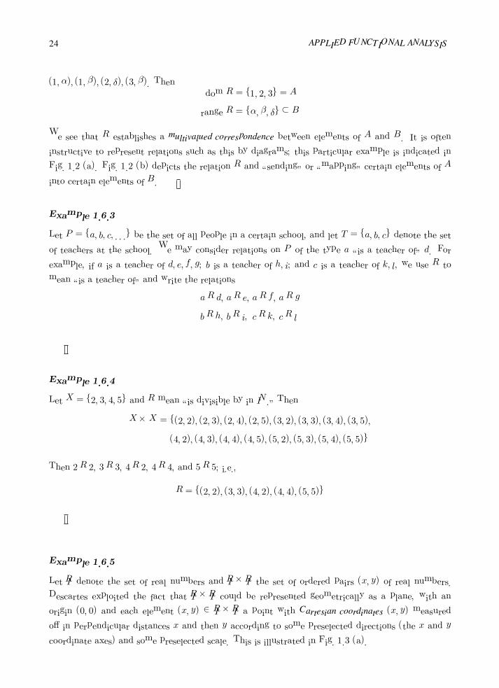
(1, α), (1, β), (2, δ), (3, β). Then
dom R = 1, 2, 3 = A
range R = α, β, δ ⊂ B
We see that R establishes a multivalued correspondence between elements of A and B. It is often
instructive to represent relations such as this by diagrams; this particular example is indicated in
Fig. 1.2 (a). Fig. 1.2 (b) depicts the relation R and “sending” or “mapping” certain elements of A
into certain elements of B.
Example 1.6.3
Let P = a, b, c, . . . be the set of all people in a certain school, and let T = a, b, c denote the set
of teachers at the school. We may consider relations on P of the type a “is a teacher of” d. For
example, if a is a teacher of d, e, f, g; b is a teacher of h, i; and c is a teacher of k, l, we use R to
mean “is a teacher of” and write the relations
a R d, a R e, a R f, a R g
b R h, b R i, c R k, c R l
Example 1.6.4
Let X = 2, 3, 4, 5 and R mean “is divisible by in IN .” Then
X ×X = (2, 2), (2, 3), (2, 4), (2, 5), (3, 2), (3, 3), (3, 4), (3, 5),
(4, 2), (4, 3), (4, 4), (4, 5), (5, 2), (5, 3), (5, 4), (5, 5)
Then 2R 2, 3R 3, 4R 2, 4R 4, and 5R 5; i.e.,
R = (2, 2), (3, 3), (4, 2), (4, 4), (5, 5)
Example 1.6.5
Let IR denote the set of real numbers and IR × IR the set of ordered pairs (x, y) of real numbers.
Descartes exploited the fact that IR × IR could be represented geometrically as a plane, with an
origin (0, 0) and each element (x, y) ∈ IR × IR a point with Cartesian coordinates (x, y) measured
off in perpendicular distances x and then y according to some preselected directions (the x and y
coordinate axes) and some preselected scale. This is illustrated in Fig. 1.3 (a).

Preliminaries 25
Figure 1.3
Cartesian coordinates and the relation y = x2 from IR into IR.
Now consider the relation
R = (x, y) : x, y ∈ IR, y = x2
that is, R is the set of ordered pairs such that the second member of the pair is the square of the
first. This relation, of course, corresponds to the sets of all points on the parabola. The rule y = x2
simply identifies a special subset of the Cartesian product (the plane) IR× IR, see Fig. 1.3 (b).
We now list several types of relations that are of special importance. Suppose R is a relation on a set A,
i.e., R ⊆ A×A; then R may fall into one of the following categories:
1. Reflexive. A relation R is reflexive if and only if for every a ∈ A, (a, a) ∈ R; that is, a R a, for every
a ∈ A.
2. Symmetric. A relation R is symmetric if and only if (a, b) ∈ R =⇒ (b, a) ∈ R; that is, if a R b, then
also b R a.
3. Transitive. A relation R is transitive if and only if (a, b) ∈ R and (b, c) ∈ R =⇒ (a, c) ∈ R; that is, if
a R b and if b R c, then a R c.
4. Antisymmetric. A relationR is antisymmetric if and only if for every (a, b) ∈ R, (b, a) ∈ R =⇒ a = b;
that is, if a R b and b R a, then a = b.
The next two sections are devoted to a discussion of two fundamental classes of relations satisfying some
of these properties.
Exercises
Exercise 1.6.1 Let A = α, β, B = a, b, and C = c, d. Determine

26 APPLIED FUNCTIONAL ANALYSIS
(i) (A×B) ∪ (A× C)
(ii) A× (B ∪ C)
(iii) A× (B ∩ C)
Exercise 1.6.2 Let R be the relation < from the set A = 1, 2, 3, 4, 5, 6 to the set B = 1, 4, 6.
(i) Write out R as a set of ordered pairs.
(ii) Represent R graphically as a collection of points in the xy-plane IR× IR.
Exercise 1.6.3 Let R denote the relation R = (a, b), (b, c), (c, b) on the set R = a, b, c. Determine
whether or not R is (a) reflexive, (b) symmetric, or (c) transitive.
Exercise 1.6.4 Let R1 and R2 denote two nonempty relations on set A. Prove or disprove the following:
(i) If R1 and R2 are transitive, so is R1 ∪R2.
(ii) If R1 and R2 are transitive, so is R1 ∩R2.
(iii) If R1 and R2 are symmetric, so is R1 ∪R2.
(iv) If R1 and R2 are symmetric, so is R1 ∩R2.
1.7 Partial Orderings
Partial Ordering. One of the most important kinds of relations is that of partial ordering. If R ⊂ A × A
is a relation, then R is said to be a partial ordering of A iff R is:
(i) transitive
(ii) reflexive
(iii) antisymmetric
We also may say that A is partially ordered by the relation R. If, additionally, every two elements are
comparable by R, i.e., for any a, b ∈ A, (a, b) ∈ R or (b, a) ∈ R, then the partial ordering R is called the
linear ordering (or total ordering) of set A and A is said to be linearly (totally) ordered by R.
Example 1.7.1
The simplest possible example of partial ordering is furnished by any subset A of the real line IR
and the usual ≤ (less than or equal) inequality relation. In fact, since every two real numbers are
comparable, A is totally ordered by ≤.

Preliminaries 27
Example 1.7.2
A nontrivial example of partial ordering may be constructed in IR2 = IR × IR. Let x = (x1, x2) and
y = (y1, y2) be two points of IR2. We shall say that
x ≤ y iff x1 ≤ y1 and x2 ≤ y2
Note that we have used the same symbol ≤ to define the new relation as well as to denote the
usual “greater or equal” correspondence for the numbers (coordinates of x and y). The reader will
easily verify that the relation is transitive, reflexive, and antisymmetric, and therefore it is a partial
ordering of IR2. It is not, however, a total ordering of IR2. To visualize this let us pick a point x in IR2
and try to specify points y which are “greater or equal” (i.e., x ≤ y) than x and those which are
“smaller or equal” (i.e., y ≤ x) than x.
Drawing horizontal and vertical lines through x we subdivide the whole IR2 into four quadrants
(see Fig. 1.4). It is easy to see that the upper-right quadrant (including its boundary) corresponds
to the points y such that x ≤ y, while the lower-left quadrant contains all y such that y ≤ x.
In particular, all the points which do not belong to the two quadrants are neither “greater” nor
“smaller” than x. Thus ≤ is not a total ordering of IR2.
Figure 1.4
Illustration of a partial ordering in IR.
Example 1.7.3
Another common example of a partial ordering is furnished by the inclusion relation for sets. Let
P(A) = 2A denote the power class of the set A and define a relation R on P(A) such that (C,B) ∈ R
iff C ⊂ B, where C, B ∈ P(A). Then R is a partial ordering. R is transitive; if C ⊂ B and B ⊂ D,
then C ⊂ D. R is reflexive, since C ⊂ C. Finally, R is antisymmetric, for if C ⊂ B and B ⊂ C,
then B = C.

28 APPLIED FUNCTIONAL ANALYSIS
The notion of a partial ordering makes it possible to give a precise definition to the idea of the greatest and
least elements of a set.
(i) An element a ∈ A is called a least element of A iff a R x for every x ∈ A.
(ii) An element a ∈ A is called a greatest element of A iff x R a for every x ∈ A.
(iii) An element a ∈ A is called a minimal element of A iff x R a⇒ x = a for every x ∈ A.
(iv) An element a ∈ A is called a maximal element of A iff a R x⇒ x = a for every x ∈ A.
While we used the term “a is a least element,” it is easy to show that when a exists, it is unique. Indeed, if
a1 and a2 are two least elements of A, then in particular a1 R a2 and a2 R a1 and therefore a1 = a2.
Similarly, if the greatest element exists, then it is unique. Note also, that in the case of a totally ordered set,
every two elements are comparable and therefore the notions of the greatest and maximal as well as the least
and minimal elements coincide with each other (a maximal element is the greatest element of all elements
comparable with it). In the general case, of a set only partially ordered, if the greatest element exists, then
it is also the unique maximal element of A (the same holds for the least and minimal elements). The notion
of maximal (minimal) elements is more general in the sense that there may not be a greatest (least) element,
but still maximal (minimal) elements, in general not unique, may exist. Examples 1.7.4–1.7.6 illustrate the
difference.
The notion of a partial ordering makes it also possible to define precisely the idea of bounds on elements
of sets. Suppose R is a partial ordering on a set B and A ⊂ B. Then, continuing our list of properties, we
have:
(v) An element b ∈ B is an upper bound of A iff x R b for every x ∈ A.
(vi) An element b ∈ B is a lower bound of A iff b R x for every x ∈ A.
(vii) The least upper bound of A (i.e., the least element of the set of all upper bounds of A), denoted supA,
is called the supremum of A.
(viii) The greatest lower bound of A, denoted inf A, is called the infimum of A.
Note that if A has the greatest element, say a, then a = supA. Similarly, the smallest element of a set
coincides with its infimum.
Example 1.7.4
The set IR of real numbers is totally ordered in the classical sense of real numbers. Let A = [0, 1) =
x ∈ IR : 0 ≤ x < 1 ⊂ IR be the interval “closed on its left end and open on the right.” Then:
• A is bounded from above by every y ∈ IR, y ≥ 1.

Preliminaries 29
• supA = 1.
• There is neither a greatest nor a maximal element of A.
• A is bounded from below by every y ∈ IR, y ≤ 0.
• inf A = the least element of A = the minimal element of A = 0.
Example 1.7.5
Let IQ denote the set of all rational numbers and A be a subset of IQ such that for every a ∈ A,
a2 < 2. Then:
• A is bounded from above by every y ∈ IQ, y > 0, y2 > 2.
• There is not a least upper bound of A (supA) and therefore there is neither a greatest nor a
maximal element of A.
• Similarly, no inf A exists.
We remark that set A is referred to as order complete relative to a linear ordering R if and only if every
nonempty subset of A that has an upper bound also has a least upper bound. This idea makes it possible
to distinguish between real numbers (which are order complete) and rational numbers (which are not order
complete).
Example 1.7.6
Let A ⊂ IR2 be the set represented by the shaded lower-left area in Fig. 1.5, including its boundary,
and consider the partial ordering of IR2 discussed in Example 1.7.2. Then:
• The first (upper-right) quadrant of IR2, denoted B, (including its boundary) consists of all
upper bounds of A.
• The origin (0, 0) is the least element of B and therefore is the supremum of A.
• All the points belonging to the “outer” corner (see Fig. 1.5) are maximal elements of A.
• There is not a greatest element of A.

30 APPLIED FUNCTIONAL ANALYSIS
Figure 1.5
Illustration of the notion of upper bound, supremum, maximal, and greatest elements of a set.
The Kuratowski–Zorn Lemma and the Axiom of Choice. The notion of maximal elements leads to a
fundamental mathematical axiom known as the Kuratowski-Zorn Lemma:
The Kuratowski–Zorn Lemma. Let A be a nonempty, partially ordered set. If every linearly ordered subset
of A has an upper bound, then A contains at least one maximal element.
Kuratowski–Zorn’s Lemma asserts the existence of certain maximal elements without indicating a con-
structive process for finding them. It can be shown that Kuratowski-Zorn’s Lemma is equivalent to the axiom
of choice:
Axiom of Choice. Let A be a collection of disjoint sets. Then there exists a set B such that B ⊂ ∪A,
A ∈ A and, for every A ∈ A, B ∩A has exactly one element.
The Kuratowski–Zorn Lemma is an essential tool in many existence theorems covering infinite-dimensional
vector spaces (e.g., the existence of Hamel basis , proof of the Hahn–Banach theorem, etc.).
Exercises
Exercise 1.7.1 Consider the partial ordering of IR2 from Examples 1.7.2 and 1.7.6. Construct an example of
a set A that has many minimal elements. Can such a set have the least element?
Exercise 1.7.2 Consider the following relation in IR2:
xR y iff (x1 < y1 or (x1 = y1 and x2 ≤ y2))
(i) Show that R is a linear (total) ordering of IR2.
(ii) For a given point x ∈ IR2 construct the set of all points y “greater than or equal to” x, i.e., xR y.
(iii) Does the setA from Example 1.7.6 have the greatest element with respect to this partial ordering?

Preliminaries 31
Exercise 1.7.3 Consider a contact problem for the simply supported beam shown in Fig. 1.6. The set K of
Figure 1.6
A contact problem for a beam.
all kinematically admissible deflections w(x) is defined as follows:
K = w(x) : w(0) = w(l) = 0 and w(x) ≤ g(x), x ∈ (0, l)
where g(x) is an initial gap function specifying the distance between the beam and the obstacle. Let V
be a class of functions defined on (0, l) including the gap function g(x). For elements w ∈ V define
the relation
w R v(w ≤ v) iff w(x) ≤ v(x) for every x ∈ (0, l)
(i) Show that R is a partial ordering of V .
(ii) Show that R is not a linear ordering of V .
(iii) Show that the setK can be rewritten in the form:
K = w(x) : w(0) = w(l) = 0 and w ≤ g
Exercise 1.7.4 Let P(A) denote the power class of a set A; then P(A) is partially ordered by the inclusion
relation (see Example 1.7.3). Does P(A) have the smallest and greatest elements?
1.8 Equivalence Relations, Equivalence Classes, Partitions
Equivalence Relations. A relation R ⊂ A×A is called an equivalence relation on A iff it is:
(i) reflexive
(ii) transitive

32 APPLIED FUNCTIONAL ANALYSIS
(iii) symmetric
Such relations may serve to generalize the familiar notion of equality (=) in the set of real numbers. Numer-
ous other examples can be cited.
Example 1.8.1
Let C denote the set of male children living in a certain residential area. We may introduce a
relation “is a brother of” on C × C. If we accept that a given male child can be the brother of
himself, then this relation on C is reflexive. Also, if a is the brother of b, then, of course, b is the
brother of a. Moreover, if b is also the brother of c, then so is a. It follows that “is the brother of”
is an equivalence relation on C.
Example 1.8.2
Let L denote the set of all straight lines in the Euclidean plane. The rule “is parallel to” defines a
relation R on L; indeed, R is an equivalence relation. R is transitive, since if line a is parallel to line
b and b is parallel to c, then a is parallel to c (aR b and bR c =⇒ aR c). R is symmetric, since aR b
and b R a, and R is reflexive if we admit that every line is parallel to itself.
Example 1.8.3
Let IZ+ = 0, 1, 2, . . . denote the nonnegative integers and R be a relation on IZ+ such that (a, b) ∈ R
if a − b is divisible by 3 on IZ. Then R is an equivalence relation. It is reflexive, since a − a = 0 is
divisible by 3; it is transitive, for if a− b = 3r and b− c = 3s, where r, s ∈ IZ, then a− c = 3(r+ s).
Finally, R is symmetric because b− a is divisible by 3 if a− b is divisible by 3.
Equivalence Classes. Let A be a set and R be an equivalence relation defined on A. If a ∈ A, the elements
x ∈ A satisfying x R a constitute a subset of A, denoted R[a], called an equivalence class of a. That is,
R[a] = x : x ∈ A, x R a
Example 1.8.4
Let IZ+ be the set of nonnegative integers and define a relation R on IZ+ such that (a, b) ∈ R iff a− b
is divisible by 3 on IZ. Consider the equivalence class R[1]. By definition, R[1] is the set of elements
x in IZ+ such that x R 1; i.e., x− 1 is divisible by 3. Hence,
R[1] = 1, 4, 7, 10, . . .
Similarly,

Preliminaries 33
R[2] = 2, 5, 8, 11, . . .
R[3] = 0, 3, 6, 9, 12, . . .
R[4] = 1, 4, 7, 10, . . .
and so forth. Notice that 4 ∈ R[1] and, as a consequence, R[4] = R[1].
Example 1.8.5
The rational numbers IQ are equivalence classes on pairs of integers. Consider the relation R on
IZ × (IZ − 0) defined by (p, q), (r, s) ∈ R iff ps = qr. Then R[(p, q)] is a set of pairs (r, s) ∈ IZ × IZ
such that (r, s)R(p, q); i.e., r/s = p/q. Of course, instead of always writing out this elaborate
equivalence class notation, we prefer to simply denote
R[(p, q)] =p
q
Partition of a Set. A class B ⊂ C(A) of nonempty subsets of a set A is called a partition of A iff:
(i) ∪B : B ∈ B = A
(ii) every pair of distinct subsets of B is disjoint; i.e., if B, C ∈ B, B = C then B ∩ C = ∅
We are approaching the important idea of an equivalence relation R partitioning a set into equivalence
classes. For example, if A is the set of all triangles, the relations “is congruent to” or “has the same area as”
are equivalence relations that segregate triangles into certain equivalence classes in A. To make this assertion
precise, we first need:
LEMMA 1.8.1
Let R denote an equivalence relation on a set A and R[a] an equivalence class for a ∈ A. If b ∈ R[a],
then R[b] = R[a].
PROOF By definition, b ∈ R[a] = x : x ∈ A, xR a ⇒ bR a; similarly, x ∈ R[b]⇒ xR b. Since
R is transitive, x R a, and therefore, R[b] ⊆ R[a]. A repetition of the argument assuming x ∈ R[a]
yields R[a] ⊆ R[b], which means that R[a] = R[b] and completes the proof.
Example 1.8.6
Recall Example 1.8.4 in which R was a relation on IZ+ such that (a, b) ∈ R⇒ a− b was divisible by
3. Observe that R[1] = R[4].

34 APPLIED FUNCTIONAL ANALYSIS
LEMMA 1.8.2
If R[a] ∩R[b] = ∅, then R[a] = R[b].
PROOF Suppose that R[a] ∩ R[b] = α, β, . . . = ∅. Then α ∈ R[a] and α ∈ R[b]. By
Lemma 1.8.1, this means that R[a] = R[b].
LEMMA 1.8.3
If R is an equivalence relation on A and R[a] an equivalence class for a ∈ A, then
R[x] : x ∈ A = A
PROOF Let Y = ∪R[x] : x ∈ A. Then each y ∈ Y belongs to an R[x] for some x ∈ A, which
means that Y ⊆ A. Consequently, ∪R[x] : x ∈ A ⊂ A. Now take z ∈ A. Since R is reflexive,
z R z and z ∈ R[z]. Therefore A ⊆ ∪R[x] : x ∈ A. This completes the proof.
Finally, we have:
PROPOSITION 1.8.1
An equivalence relation R on a set A effects a partitioning of A into equivalence classes. Conversely,
a partitioning of A defines an equivalence relation on A.
PROOF LetR[a], R[b], R[c], . . . denote equivalence classes induced onA byR, with a, b, c, . . . ∈ A.
By Lemma 1.8.3, R[a]∪R[b]∪R[c]∪ . . . = A, so that property (i) of a partitioning of A is satisfied.
Also (ii) is satisfied, because if R[a] and R[b] are distinct equivalence classes, they are disjoint by
Lemma 1.8.2.
To prove the converse, let B be any partition of A and define a relation R on A such that aR b iff
there exists a set B in the partition such that a, b ∈ B. Clearly, such a relation is both reflexive and
symmetric; for every a ∈ A there is a set B in the partition such that a ∈ B. Formally, a, a ∈ B,
also a, b ∈ B implies that b, a ∈ B.
Now suppose a R b and b R c. This implies that a, b ∈ B for some B and b, c ∈ C for some C.
Consequently, b ∈ B ∩ C, which, according to the definition of partition, implies that B = C. Thus
both a and c belong to the same set B = C and therefore a R c, which means that R is transitive.
This completes the proof that R is an equivalence relation.
Quotient Sets. The collection of equivalence classes of A is a class, denoted by A/R, called the quotient
of A by R : A/R = R[a] : a ∈ A. According to Proposition 1.8.1, the quotient set A/R is, in fact, a

Preliminaries 35
partition of A.
Example 1.8.7
Let S be a collection of circles in IR2, centered at the origin:
S(0, r) = x ∈ IR2 : distance from 0 to x = r
Let us identify the origin 0 with the circle of zero radius. Obviously,
S = S(0, r), r ≥ 0
is a partition of IR2. Defining an equivalence relation R by x R y iff the distance from x to 0 =
distance from y to 0, we may identify the circles with equivalence classes of points in IR2 and the
partition with the quotient set IR2/R.
We shall return to the important issue of equivalence classes and quotient sets in the context of vector
spaces in Chapter 2.
Exercises
Exercise 1.8.1 (i) Let T be the set of all triangles in the plane IR2. Show that “is similar to” is an equiva-
lence relation on T .
(ii) Let P be the set of all polygons in the plane IR2. Show that “has the same number of vertices” is
an equivalence relation on P .
(iii) For part (i) describe the equivalence class [T0], where T0 is a (unit) right, isosceles triangle with
unit sides parallel to the x- and y-axes.
(iv) For part (ii) describe the equivalence class [P0], where P0 is the unit square
(x, y) : 0 ≤ x ≤ 1, 0 ≤ y ≤ 1
(v) Specify quotient sets corresponding to the relations in (i) and (ii).
Exercise 1.8.2 Let A = IN × IN , where IN is the set of natural numbers. The relation
(x, y)R (u, v)def⇔ x+ v = u+ y
is an equivalence relation on A. Determine the equivalence classes [(1, 1)], [(2, 4)], [(3, 6)].
Exercise 1.8.3 Let Xι, ι ∈ I , be a partition of a set X . Show that the relation
x ∼ ydef⇔ ∃ι ∈ I : x ∈ Xι and y ∈ Xι
is an equivalence relation on X .

36 APPLIED FUNCTIONAL ANALYSIS
Exercise 1.8.4 Let ∼ be an equivalence relation on a set X . Consider the corresponding quotient set X|∼,
i.e., the partition ofX into equivalence classes [x]∼ corresponding to relation∼. Let≈ be a (potentially
new, different) relation corresponding to the partition discussed in Exercise 1.8.3. Demonstrate that the
two equivalence relations are identical, i.e.,
x ∼ y ⇔ x ≈ y
Exercise 1.8.5 Let Xι, ι ∈ I be a partition of a set X . Let ∼ be the corresponding induced equivalence
relation defined in Exercise 1.8.3. Consider the corresponding (potentially different) partition of X
into equivalence classes with respect to the relation ∼. Prove that the two partitions are identical.
Functions
1.9 Fundamental Definitions
Functions. A function from a set A into a set B, denoted f : A→ B, is a relation f ⊂ A×B such that:
(i) for every x ∈ A there exists a y ∈ B such that x f y
(ii) for every x ∈ A and y1, y2 ∈ B, if x f y1 and x f y2, then y1 = y2
In other words, for every x ∈ A there exists a unique y ∈ B such that x f y. We write:
y = f(x)
If f : A → B, A is called the domain of f , denoted dom f , and B is called the codomain of f . Clearly,
a function f from A into B is a relation R ⊂ A × B such that for every (a, b) ∈ R, each first component
a appears only once. Thus a function may be thought of as a “single-valued relation” since each element in
dom f occurs only once in f . We also note that dom f = ∅. The element y ∈ B in f(x) = y is called the
image of x ∈ A, or the value of the function at x.
The range of a function f : A→ B, denotedR(f), is the set of elements inB that are images of elements
in A; i.e.,R(f) is the set of all images of f :
R(f) = f(a) : a ∈ A
R(f) is also sometimes called the image set.

Preliminaries 37
Once the relations are identified with subsets of the appropriate Cartesian products, functions are identified
with their graphs. The graph of function f : A→ B is the set
graph f = (x, f(x)) : x ∈ A
It is customary to use the terms function, mapping, transformation, and operator synonymously. Thus, if
f : A → B, we say that “f maps A into B” or “f is a transformation from A into B” or “f is an operator
from A into B” (in some works the term “operator” is reserved for functions whose domains are subsets of
spaces; we consider these in Chapter 5).
Clearly, this generalization of the elementary idea of a function is in complete accord with our first notions
of functions; each pair (a, b) ∈ f associates an a ∈ A with an element b ∈ B. The function thereby
establishes a correspondence between elements of A and those of B that appear in f .
For example, we have often encountered expressions of the form
y = f(x) = x2
which we read as “y is a function of x.” Technically, we consider a set of (say) real numbers IR to which there
belong the elements x, and another set IR+ of nonnegative numbers y ∈ IR+. The particular subset of IR× IR+,
which is the function f under consideration, is identified by the rule y = x2. We may define the function f
by:
f = (x, y) : x ∈ IR, y ∈ IR+, y = x2
Example 1.9.1
Let IR be the real numbers and consider the relation
R = (x, y) : x, y ∈ IR, x2 +y
2
2
= 1
Obviously, R defines the points on the ellipse shown in Fig. 1.7 (a). Notably, R is not a function,
since elements x ∈ IR are associated with pairs of elements in IR. For example, both (0,+2) and
(0,−2) ∈ R.
Example 1.9.2
The relation R = (x, y) : x, y ∈ IR, y = sinx is shown in Fig. 1.7 (b). This relation is a function.
Its domain is IR, the entire x-axis, −∞ < x <∞. Its codomain is also IR, i.e., the y-axis. Its range is
the set y : y ∈ IR, −1 ≤ y ≤ 1. Notice that specific values of y ∈ R(R) are the images of infinitely
many points in the domain of R. Indeed, y = 1 is the image of π/2, 5π/2, 9π/2, . . ..
An arbitrary function f : A → B is said to map A into B and this terminology suggests nothing special
about the range of f or the nature of its values in B. To identify special properties of f , we use the special
nomenclature listed below:

38 APPLIED FUNCTIONAL ANALYSIS
Figure 1.7
Examples of two relations on IR of which one (a) is not a function and one (b) is a function.
1. Surjective (Onto) Functions. A function f : A→ B is surjective, or from A onto B, if every b ∈ B is
the image of some element of A.
2. Injective (One-to-One) Functions. A function f : A→ B is said to be injective or one-to-one (denoted
1:1) from A into B iff, for every b ∈ R(f), there is exactly one a ∈ A such that b = f(a).
3. Bijective (One-to-One and Onto) Functions. A function f : A → B is bijective, or one-to-one and
onto, iff it is both injective and surjective, i.e., iff every b ∈ B is the unique image of some a ∈ A.
Figure 1.8 illustrates geometrically the general types of functions. The correspondence indicated in Fig. 1.8 (a)
is a relation, but is not a function, because elements ofA do not have distinct images inB. That in Fig. 1.8 (d)
is one-to-one, but not onto, because the element b3 is not an image of an element of A.

Preliminaries 39
Figure 1.8
Classification of functions f : A→ B.

40 APPLIED FUNCTIONAL ANALYSIS
Example 1.9.3
Let IR denote the set of real numbers and IR+ the set of nonnegative real numbers. Let f denote the
rule f(x) = x2. Then consider the following functions:
1. f1 : IR→ IR. This function is not one-to-one, since both −x and +x are mapped into x2. It is
not onto, since the negative real numbers are in the codomain IR, but are not images.
2. f2 : IR→ IR+. This function is not one-to-one, but it is onto.
3. f3 : IR+ → IR. This function is one-to-one, but it is not onto.
4. f4 : IR+ → IR+. This function is bijective; it is both one-to-one and onto.
Note that although the rule f(x) = x2 defining each function f1, f2, f3, and f4 is the same, the four
are quite different functions.
Direct and Inverse Images. The set
f(C) = f(a) : a ∈ C ⊆ A
is called the direct image of C. Obviously,
f(C) ⊂ R(f)
Likewise, suppose f : A→ B and D is a subset of B. Then the set
f−1(D) = a : f(a) ∈ D
is called the inverse image of D under f . Clearly,
f−1(D) ⊂ A
i.e., f−1(D) is a subset of the domain of f .
These ideas are illustrated symbolically in Fig. 1.9, where the set G denotes the intersection of R(f) and
a subset D ⊂ B. It is clear that f−1(D) consists of those elements in A that have images in G ⊂ D; in
other words, not all of D need consist of images of elements of A. We now list several properties involving
functions. Let f : X → Y , A ⊂ X , B ⊂ X , D ⊂ Y , and F ⊂ Y . Then the following hold:
1. f(A ∪B) = f(A) ∪ f(B)
2. f(A ∩B) ⊂ f(A) ∩ f(B)
3. f−1(D ∪ F ) = f−1(D) ∪ f−1(F )
4. f−1(D ∩ F ) = f−1(D) ∩ f−1(F )

Preliminaries 41
Figure 1.9
Illustration of f(C),R(f), and f−1(D) for f : A→ B.
Example 1.9.4
Let A = −1,−2, B = 1, 2, f(x) = x2. Then:
A ∩B = ∅
f(A ∩B) = ∅
However,
f(A) = 1, 4, f(B) = 1, 4
Consequently,f(A) ∩ f(B) = 1, 4 = ∅
= f(A ∩B)
However, f(A ∪B) = f(A) ∪ f(B) always.
Example 1.9.5
(Proof of f(A ∪B) = f(A) ∪ f(B))
Let y ∈ f(A ∪ B). Then there exists an x ∈ A or B such that y = f(x). If x ∈ A, then
y = f(x) ∈ f(A); if x ∈ B, then y = f(x) ∈ f(B). Consequently, y ∈ f(A) ∪ f(B), which proves
that f(A∪B) ⊆ f(A)∪ f(B). Conversely, let w ∈ f(A)∪ f(B). Then w is the image of an x ∈ A or
an x ∈ B; i.e., w = f(x), x ∈ A ∪B. Hence w ∈ f(A ∪B) and, therefore, f(A) ∪ f(B) ⊆ f(A ∪B).
Example 1.9.6
(Proof of f−1(D ∪ F ) = f−1(D) ∪ f−1(F ))
Suppose that x ∈ f−1(D ∪ F ). Then there exists a y ∈ D or F such that y = f(x); i.e.,
f(x) ∈ D ∪ F . If f(x) ∈ D, x ∈ f−1(D) and if f(x) ∈ F , x ∈ f−1(F ), so that x ∈ f−1(D)∪ f−1(F )
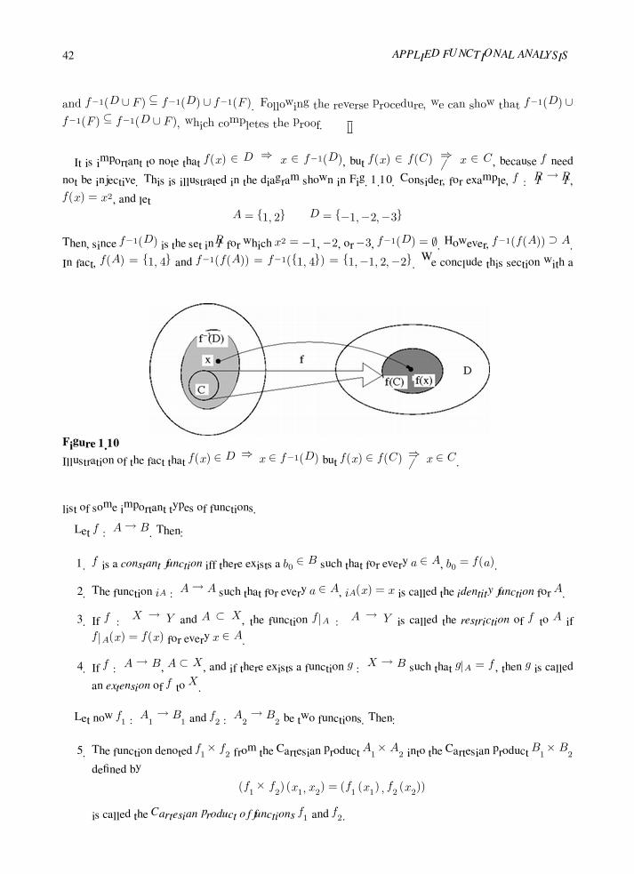
42 APPLIED FUNCTIONAL ANALYSIS
and f−1(D ∪ F ) ⊆ f−1(D) ∪ f−1(F ). Following the reverse procedure, we can show that f−1(D) ∪
f−1(F ) ⊆ f−1(D ∪ F ), which completes the proof.
It is important to note that f(x) ∈ D ⇒ x ∈ f−1(D), but f(x) ∈ f(C) ⇒ x ∈ C, because f need
not be injective. This is illustrated in the diagram shown in Fig. 1.10. Consider, for example, f : IR → IR,
f(x) = x2, and let
A = 1, 2 D = −1,−2,−3
Then, since f−1(D) is the set in IR for which x2 = −1, −2, or −3, f−1(D) = ∅. However, f−1(f(A)) ⊃ A.
In fact, f(A) = 1, 4 and f−1(f(A)) = f−1(1, 4) = 1,−1, 2,−2. We conclude this section with a
Figure 1.10
Illustration of the fact that f(x) ∈ D ⇒ x ∈ f−1(D) but f(x) ∈ f(C) ⇒ x ∈ C.
list of some important types of functions.
Let f : A→ B. Then:
1. f is a constant function iff there exists a b0 ∈ B such that for every a ∈ A, b0 = f(a).
2. The function iA : A→ A such that for every a ∈ A, iA(x) = x is called the identity function for A.
3. If f : X → Y and A ⊂ X , the function f |A : A → Y is called the restriction of f to A if
f |A(x) = f(x) for every x ∈ A.
4. If f : A → B, A ⊂ X , and if there exists a function g : X → B such that g|A = f , then g is called
an extension of f to X .
Let now f1 : A1 → B1 and f2 : A2 → B2 be two functions. Then:
5. The function denoted f1× f2 from the Cartesian product A1×A2 into the Cartesian product B1×B2
defined by
(f1 × f2) (x1, x2) = (f1 (x1) , f2 (x2))
is called the Cartesian product of functions f1 and f2.

Preliminaries 43
Similarly, if f1 : A → B1 and f2 : A → B2 are defined on the same set A, we define the composite
function of functions f1 and f2, denoted (f1, f2) : A→ B1 ×B2, as
(f1, f2) (x) = (f1(x), f2(x))
Exercises
Exercise 1.9.1 Let f : X → Y be an arbitrary function. Let A,B ⊂ Y . Prove that f−1(A − B) =
f−1(A) − f−1(B). In particular, taking A = Y , we get f−1(B) = f−1(Y − B) = f−1(Y ) −
f−1(B) = X − f−1(B) = (f−1(B)).
Exercise 1.9.2 Let f : X → Y be an arbitrary function. Let A,B ⊂ X . Prove that f(A) − f(B) ⊂
f(A−B). Is the inverse inclusion true (in general)?
Exercise 1.9.3 Let f : X → Y be an arbitrary function. Let Bι ⊂ Y, ι ∈ I be an arbitrary family. Prove
that
f−1
ι∈I
Bι
=
ι∈I
f−1(Bι) and f−1
ι∈I
Bι
=
ι∈I
f−1(Bι)
Exercise 1.9.4 Prove that f−1(D ∩H) = f−1(D) ∩ f−1(H).
Exercise 1.9.5 Let f : X → Y be a function. Prove that, for an arbitrary set C ⊂ Y ,
f−1(R(f) ∩ C) = f−1(C)
1.10 Compositions, Inverse Functions
Compositions or Product Functions. Let f : X → Y and g : Y → Z. Then f and g define a product
function, or composition, denoted g f (or sometimes simply gf ), from X into Z, g f : X → Z. We
define g f by saying that for every x ∈ X ,
(g f)(x) = g(f(x))
Example 1.10.1
Consider functions f : IR→ IR, f(x) = x2 and g : IR→ IR, g(x) = 1 + x. Then:
(gf)(x) = 1 + x2 (fg)(x) = (1 + x)2
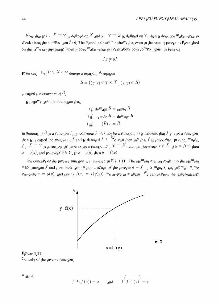
44 APPLIED FUNCTIONAL ANALYSIS
Note that if f : X → Y is defined on X and g : Y → Z is defined on Y , then it does not make sense to
speak about the composition f g. The preceding example shows that even in the case of functions prescribed
on the same set into itself, when it does make sense to speak about both compositions, in general
fg = gf
Inverses. Let R ⊂ X × Y denote a relation. A relation
R = (y, x) ∈ Y ×X : (x, y) ∈ R
is called the converse of R.
It follows from the definition that:
(i) domain R = range R
(ii) range R = domain R
(iii) (R) ˇ = R
In general, if R is a function f , its converse f may not be a function. If it happens that f is also a function,
then it is called the inverse of f and is denoted f−1. We also then say that f is invertible. In other words,
f : X → Y is invertible iff there exists a function g : Y → X such that for every x ∈ X , if y = f(x) then
x = g(y), and for every y ∈ Y , if x = g(y) then y = f(x).
The concept of the inverse function is illustrated in Fig. 1.11. The element x is set forth into the element
y by function f and then back from y into x again by the inverse g = f−1. Similarly, starting with y, we
prescribe x = g(y), and taking f(x) = f(g(y)), we arrive at x again. We can express this algebraically
Figure 1.11
Concept of the inverse function.
writing:
f−1 (f (x)) = x and ff−1 (y)
= y

Preliminaries 45
or, equivalently,
f−1 f = iX and f f−1 = iY
where iX and iY are the identity functions on X and Y , respectively. In other words,
a function f : X → Y is invertible iff there exists a function g : Y → X such that
g f = iX and g f = iY
Note that g = f−1 as the converse of f is unique.
This suggests the following definitions:
A function f : X → Y is said to be left-invertible if there exists a function g : Y → X such that
g f = iX
The function g is called a left inverse of f .
A function f : X → Y is said to be right-invertible iff there exists a function g : Y → X such that
f g = iY
The function g is called a right inverse of f .
Thus if function f is invertible, then it is both left- and right-invertible and its inverse is a left and a right
inverse as well. It turns out that the converse is also true. We need the following:
LEMMA 1.10.1
Let f : X → Y and g : Y → X be two functions such that
g f = iX
Then f is injective and g is surjective.
PROOF Pick an arbitrary x ∈ X and set y = f(x). We have
g(y) = g(f(x)) = x
which proves that g is surjective.
Also, if f(x1) = f(x2) for some x1, x2 then
x1 = g(f(x1)) = g(f(x2)) = x2

46 APPLIED FUNCTIONAL ANALYSIS
which implies that f is injective.
We have the immediate corollaries:
COROLLARY 1.10.1
(i) Every left-invertible function is injective.
(ii) Every right-invertible function is surjective.
(iii) Every left- and right-invertible function is bijective .
Finally, we arrive at the following important result:
PROPOSITION 1.10.1
Let f : X → Y be a function. The following conditions are equivalent to each other:
(i) f is invertible.
(ii) f is both left- and right-invertible.
(iii) f is bijective.
PROOF (ii) follows from (i) by definition. We have just shown in Corollary 1.10.1(iii) that
(ii) implies (iii). Thus it remains to prove that every bijective function f is invertible. But this is
trivial because bijective maps establish a one-to-one correspondence between all elements of X and
all elements of Y . In other words, for every y ∈ Y (f is surjective) there exists a unique x ∈ X (f
is injective) such that y = f(x). Set by definition,
g(y) = x
Thus g is a function and g(f(x)) = x as well as f(g(y)) = y, which ends the proof.
The notion of the inverse f−1 of a function f : X → Y should not be confused with the inverse image
set f−1(B), for some B ⊂ Y . The latter is a set which exists for every function f and the prior is a function
which exists only when f is bijective. Note, however, that the direct image of the inverse function f is equal
to the inverse image of f and therefore it is not necessary to distinguish between the symbols (f−1)(B) and
f−1(B) (comp. Exercise 1.10.7).

Preliminaries 47
Example 1.10.2
Let f : IR → IR+, IR = dom f = the set of real numbers, and IR+ = range f = y : y ∈ IR, y ≥ 0.
Suppose f is defined by the rule f(x) = x2, i.e., f = (x, y) : x, y ∈ IR, y = x2. Then f does not
have an inverse since it is clearly not one-to-one.
Example 1.10.3
Let dom f = x : x ∈ IR, x ≥ 0 and range f = y : y ∈ IR, y = x2. That is, f = (x, y) : x, y ∈
IR, x ≥ 0, y = x2. Clearly, f is one-to-one and onto. Also, f has an inverse f−1 and y = f(x) = x2
if and only if x = f−1(y). The inverse function f−1, in this case, is called the positive square root
function and we use the notation f−1(y) =√y. (Likewise, if f1 = (x, x2) : x ∈ IR, x ≤ 0,
f−11 (y) = −
√y is the inverse of f1 and is called the negative square root function, etc.)
Example 1.10.4
The sine function, f(x) = sinx, is, of course, not one-to-one (sin 0 = sinπ = sin 2π = · · · = 0).
However, if IRπ/2 = x : x ∈ IR, −π/2 ≤ x ≤ π/2, the restriction f |IRπ/2 is one-to-one and onto and
has an inverse function, called the inverse sine function, denoted by f−1(y) = arcsin(y) or sin−1(y).
When a function f : X → Y is not invertible, it may still have a left- or right inverse. We have already
learned from Lemma 1.10.1 that injectivity and surjectivity are the necessary conditions for left- and right-
invertibility, respectively. It turns out that they are also sufficient.
PROPOSITION 1.10.2
Let f : X → Y be a function. Then:
(i) f is left-invertible iff f is injective.
(ii) f is right-invertible iff f is surjective.
PROOF
(i) Let f be an injective map. Restricting its codomain to its range R(f), we get a bijective
function (it becomes surjective by definition) that, according to Proposition 1.10.1, is invertible
with an inverse g defined on R(f). Let G be any extension of g to Y . Then for every x ∈ X,
G(f(x)) = g(f(x)) = x
and therefore f is left-invertible.

48 APPLIED FUNCTIONAL ANALYSIS
(ii) Let f be surjective. For every y ∈ Y , consider the inverse image set
f−1(y)
Since f is a function, f−1(y1) ∩ f−1(y2) = ∅, for different y1 and y2.
Thus
f−1(y), y ∈ Y
is a partition of X and, by the Axiom of Choice, for every y ∈ Y one can choose a corresponding
representative xy ∈ f−1(y). Consider the relation g ⊂ Y ×X, ygx⇔ x = xy, i.e., (y, xy) ∈ g. It
is clear that g is a function from Y to X with the property that
g(y) = xy
But then
f(g(y)) = y
which means that g is a right inverse of f . The fact that a right-invertible f is surjective was
established in Corollary 1.10.1.
Example 1.10.5
Let A = 1, 2, 3 and B = x, y. Consider the correspondence:
f :
1→ x
2→ y
3→ x
Clearly, f is onto. Hence it should have a right inverse. Indeed, consider the functions g1 and g2
from B to A:
g1 :x→ 1
y → 2g2 :
x→ 3
y → 2
We see that
f g1 :x→ 1→ x
y → 2→ yf g2 :
x→ 3→ x
y → 2→ y
Hence both g1 and g2 are right inverses of f .
This example shows that when f is onto but not one-to-one, it can have more than one right inverse. If
f is neither onto nor one-to-one, no inverses of any kind exist. The invertibility properties of a function
f : A→ B can be summarized in the network diagram shown in Fig. 1.12.

Preliminaries 49
Figure 1.12
A diagram illustrating the invertibility properties of functions.
Example 1.10.6
(The Motion of a Continuous Medium)
One bijective map that is fundamental to physics is the primitive notion of motion that can be
defined for general continua in terms of an invertible map of points in one region of Euclidean space
into points in another. Since we may wish to use some concepts of continuum mechanics as examples
of various mathematical ideas, we shall describe motion as a special invertible function.
Consider a material body B in motion under the action of external forces. The body B may be
considered to be a set consisting of material points P . Such a body is also endowed with additional
structures; for example, every physical body has mass, and, mathematically, this is manifested as a
measure m on B (see Chapter 3). Conceptually, B is viewed as an actual piece of physical material
set in motion by certain prescribed forces.
To describe this motion, we establish a fixed (inertial) frame of reference described by the Cartesian
coordinates xi, which are called spatial coordinates because they identify points in space as opposed to
particles of material. We observe the motion of B by watching it assume various places in Euclidean
space IR3 at each time t. These places that the body occupies are called its configurations. Thus, if P
denotes a material particle in B and x =3
k=1 xkik is the spatial position vector, then the relation
x = κ(P )
defines a configuration κ of B. We refer to the functions κ of B into IR3 as configuration maps, or also
simply configurations. The motion of the body is observed relative to some fixed configuration κ0,
known as the reference configuration. Generally, the reference configuration is chosen as the location
of B at some convenient time when its geometrical features are known, and the deformation of B
relative to this natural state is to be determined. The images X of material points P ∈ B under κ0

50 APPLIED FUNCTIONAL ANALYSIS
are called material coordinates, and we use the notation
Z = κ0(P )
where κ0 : B → E0 ⊂ IR3. Then the composition
x = κ(P ) = κ(κ−10 (Z)) ≡ χ(Z)
is called a deformation of E0 into IR3, and the one-parameter family of deformations,
x = χ(Z, t), t ≥ 0
is called the motion of the body B relative to the reference configuration. In essence, the motion of
the body defines a one-parameter family of deformations.
Example 1.10.7
The reader familiar with matrices will appreciate the following example of left and right inverses
(we discuss matrices and linear equations in Chapter 2). Suppose IR is the set of real numbers. Let
A = IR3 = IR × IR × IR denote the set of ordered triples A = (a1, a2, a3) : a1, a2, a3 ∈ IR and let
B = IR2 = IR × IR = (b1, b2) : b1, b2 ∈ IR denote the set of ordered pairs of real numbers. Consider
the mapping f : A→ B defined by the matrix equation:
b1
b2
=
1 1 2
−1 1 0
a1
a2
a3
Clearly, R(f) = B; i.e., f is onto. Therefore, f has a right inverse. Indeed, the mapping g : B → A
defined by
a1
a2
a3
=
2 −9
2
2 −7
2
−3
24
b1
b2
is a right inverse of f . In fact, the identity mapping for B is obtained by the composition
1 1 2
−1 1 0
2 −9
2
2 −7
2
−3
24
=
1 0
0 1
since
b1
b2
=
1 0
0 1
b1
b2

Preliminaries 51
Note that this right inverse is not unique; indeed, the matrix
0 −1
0 0
1
2
1
2
is also a right inverse.
Exercises
Exercise 1.10.1 If F is the mapping defined on the set IR of real numbers by the rule: y = F (x) = 1 + x2,
find F (1), F (−1), and F ( 12 ).
Exercise 1.10.2 Let IN be the set of all natural numbers. Show that the mapping F : n → 3 + n2 is an
injective mapping of IN into itself, but it is not surjective.
Exercise 1.10.3 Consider the mappings F : n→ n+ 1, G : n→ n2 of IN into IN . Describe the product
mappings FF , FG, GF , and GG.
Exercise 1.10.4 Show that if f : IN → IN and f(x) = x+ 2, then f is one-to-one but not onto.
Exercise 1.10.5 If f is one-to-one from A onto B and g is one-to-one from B onto A, show that (fg)−1 =
g−1 f−1.
Exercise 1.10.6 Let A = 1, 2, 3, 4 and consider the sets
f = (1, 3), (3, 3), (4, 1), (2, 2)
g = (1, 4), (2, 1), (3, 1), (4, 2)
(i) Are f and g functions?
(ii) Determine the range of f and g.
(iii) Determine f g and g f .
Exercise 1.10.7 Let f : X → Y be a bijection and f−1 its inverse. Show that:
(f−1)(B) = f−1(B)
(direct image of B through inverse f−1) = (inverse image of B through f )
Exercise 1.10.8 Let A = [0, 1] ⊂ IR, and let fi : A→ A be defined by:
(i) f1(x) = sinx

52 APPLIED FUNCTIONAL ANALYSIS
(ii) f2(x) = sinπx
(iii) f3(x) = sin(π2x)
Classify each fi as to whether or not it is surjective, injective, or bijective.
Cardinality of Sets
1.11 Fundamental Notions
The natural idea of counting that lets us compare finite sets (two sets are “equivalent” if they have the same
number of elements) may be generalized to the case of infinite sets. Every set may be assigned a symbol,
called its “cardinal number,” which describes its “number of elements” in the sense that, indeed, in the case
of a finite set, its cardinal number is equal to its number of elements.
To make this idea precise, we introduce the following relation for sets: two sets A and B are said to be
equivalent, denoted A ∼ B, if there exists a bijective map which maps A onto B. In other words, there
is a one-to-one correspondence between all elements of A and all elements of B. It is easy to prove that,
given a universal set U and its power set P(U) consisting of all subsets of U , the relation ∼ on P(U) is an
equivalence relation. As a consequence, P(U) may be partitioned into equivalence classes and every such
class may be assigned a symbol, called its cardinal number; that is, cardinality is a property that all sets
equivalent to each other have in common.
To see that the notion of equivalent sets generalizes the idea of counting, let us notice that two finite sets
have the same number of elements if and only if they are equivalent to each other. More precisely, a set A is
finite iff there exists an n ∈ IN such that A ∼ 1, 2, . . . , n. If A ∼ B then also B ∼ 1, 2, . . . , n and the
class of sets equivalent to A is assigned the cardinal number n equal to the number of elements of A.
We say that a set A is infinite if it is not finite; i.e., no natural number n exists such that A ∼ 1, . . . , n.
It is obvious that the theory of cardinal numbers is mainly concerned with infinite sets. The simplest infinite
sets are those which can be enumerated with natural numbers; that is, we can represent them in a sequential
form.
We say that a setA is denumerable iffA ∼ IN . The symbol ℵ0 (aleph-naught) is used to denote the cardinal
number of denumerable sets, ℵ being the Hebrew letter aleph. Sets which are either finite or denumerable
bear a common name of countable sets; i.e., a set A is countable iff it is finite or denumerable.
There are numerous properties of countable sets. Some of them are listed below:
(i) A ⊂ B, B countable implies that A is countable; i.e., every subset of a countable set is countable.

Preliminaries 53
(ii) If A1, . . . , An are countable then A1 × . . .×An is countable.
(iii) If Ai, i ∈ IN are countable then ∪Ai is countable.
Example 1.11.1
To prove property (ii) of countable sets it is sufficient to prove that IN×IN is denumerable. Indeed,
if A and B are countable then A × B is equivalent to a subset of IN × IN , then by property (i),
A × B is countable. Since A1 × . . . × An−1 × An ∼ (A1 × . . . × An−1) × An, the property may be
generalized to any finite family of sets.
To see that IN × IN is denumerable, consider the diagram shown in Fig. 1.13. By letting 1
Figure 1.13
A diagram showing the equivalence of sets IN and IN × IN .
correspond to the pair (1,1), 2 correspond to (2,1), 3 to (1,2), and continuing to follow the path
indicated by the arrows, it is easily seen that the elements of IN×IN are in one-to-one correspondence
with those of IN itself.
Example 1.11.2
As an example of application of properties (i)–(iii), we may prove that the set IQ of rational numbers
is denumerable. To see this, recall that a rational number is identified with an equivalence class of
all fractions of the form p/q where p ∈ IZ, q ∈ IN and two fractions p1/q1 and p2/q2 are equivalent
to each other iff p1q2 = q1p2.
Since the set of all integers is countable (explain, why?), the rationals may be identified with a
subset of the Cartesian product IZ × IN and therefore, by properties (i) and (ii), are denumerable.
54 APPLIED FUNCTIONAL ANALYSIS
At this moment we might ask a natural question: are all infinite sets denumerable? In other
words, do infinite sets exist which could not be represented in a sequential form? The famous
Cantor theorem brings an answer.
THEOREM 1.11.1
(Cantor)
The power set P(A) of a set A is not equivalent to A.
In other words, the sets A and P(A) have different cardinal numbers. In particular, the power set P(IN) is
not equivalent to IN and therefore is not denumerable.
At this point it is very important to realize that we have to deal in mathematics with infinite sets which
cannot be represented in the sequential form. In particular, it can be proved that the set of real numbers IR is
equivalent to the power set of the set of natural numbers, i.e., IR ∼ P(IN). The small Gothic letter “c” is used
to denote the cardinal number assigned to IR.
Exercises
Exercise 1.11.1 Show that if U is a universal set, the relation ∼ is an equivalence relation on P(U).
Exercise 1.11.2 Prove the following properties of countable sets:
(i) B countable, A ⊂ B implies A countable.
(ii) A1, . . . , An countable implies A1 × . . .×An countable.
(iii) An countable, n ∈ IN implies ∪∞n=1An countable.
1.12 Ordering of Cardinal Numbers
If the cardinal numbers are supposed to be a generalization of the natural numbers, then the next natural
thing to do will be to establish an ordering allowing one to compare cardinal numbers. The ordering should
generalize the usual “greater than or equal to” relation for numbers.
Let A and B be two subsets of a universal set U and #A and #B denote their corresponding cardinal
numbers. We say that the cardinal number #B is greater than or equal to the cardinal number #A, denoted
#A ≤ #B, if and only if there exists a one-to-one map TAB from A into B. In other words, every element
Preliminaries 55
in A has its counterpart in B but not necessarily conversely; there may be some elements in B that have not
been assigned to elements of A. This intuitively corresponds to the fact that B has “more” elements than A.
Obviously, if A1 ∼ A, B1 ∼ B, and A ≤ B, then also A1 ≤ B1. Thus ≤ is a well-defined∗ relation on
the quotient set P(U)/∼.
To prove that the relation≤ between the cardinal numbers is indeed a linear ordering on P(U)/∼, we have
to show that it is reflexive, transitive, antisymmetric, and that every two equivalence classes from P(U)/∼
are comparable to each other. Two of the four properties listed above can be easily shown. Using the identity
map from a set A onto itself, we easily show that
#A ≤ #A
Also, to prove that the relation is transitive, i.e., that#A ≤ #B,#B ≤ #C implies#A ≤ #C, it is enough
to define the mapping TAC as
TAC = TBC TAB
where TAB and TBC are the two mappings corresponding to pairs (A,B) and (B,C), respectively. As a
composition of two injective mappings, TAC is injective, too. It is also defined on the whole set A, which
altogether proves that #A ≤ #C.
The third condition is much more difficult. It is the famous Cantor-Bernstein theorem.
THEOREM 1.12.1
(Cantor–Bernstein)
The cardinal numbers relation is antisymmetric; i.e., if #A ≤ #B and #B ≤ #A then #A =
#B(A ∼ B).
The proof of this theorem considerably exceeds the scope of this book. We shall show, however, as an
example of application of the Kuratowski–Zorn Lemma , the proof of the last property.
PROPOSITION 1.12.1
Let U be a universal set and A, B ∈ P(U). Then either #A ≤ #B or #B ≤ #A.
PROOF Consider a family F consisting of the following triples:
(X,Y, TXY )
∗Elements of P(U)/∼ can in fact be identified as the cardinal numbers themselves in the same way that natural numbers n ∈ IN can
be identified with finite sets consisting of precisely n elements. The relation ≤ is defined for equivalence classes [A]∼ and [B]∼ from
P(U)/∼ through their representatives A andB. By saying that the relation is well-defined we mean that it is independent of the choice
of the representatives.

56 APPLIED FUNCTIONAL ANALYSIS
where X is a subset of A, Y is a subset of B, and TXY : X → Y is a one-to-one mapping from X
onto Y . The family F is certainly not empty (explain, why?). Next we introduce a relation ≤ in F
by setting
(X1, Y1, TX1Y1) ≤ (X2, Y2, TX2Y2
)
iff X1 ⊂ X2, Y1 ⊂ Y2 and restriction of TX2Y2 to the set X1 coincides with TX1Y1 . It can be easily
shown (see Exercise 1.12.1) that the relation is a partial ordering of F . We shall prove now that F
with this partial ordering satisfies the assumptions of the Kuratowski–Zorn Lemma. To do so, we
have to show that every linearly ordered subset L of F has an upper bound in F .
Assuming that L consists of triples (X,Y, TXY ), define:
W = ∪X
Z = ∪Y
TWZ(x) = TXY (x) for some X such that x ∈ X
The (infinite) unions above are taken over all triples from L. From the fact that L is linearly ordered
in the sense of the relation ≤, it follows that:
1. TWZ is well-defined; i.e., its value TWZ(x) is independent of the choice of X such that x ∈ X.
2. TWZ is a bijection.
Therefore, as a result of our construction,
(X,Y, TXY ) ≤ (W,Z, TWZ)
for every triple (X,Y, TXY ) from L, which proves that the just-constructed triple is an upper bound
for L.
Thus, by the Kuratowski–Zorn Lemma, there exists a maximal element in F , say a triple (X,Y, TXY ).
We claim that either X = A or Y = B, which proves that either A ≤ B or B ≤ A. Indeed, if both X
and Y were different from A and B respectively, i.e., there existed an a ∈ A−X and b ∈ B−Y , then
by adding element a to X, element b to Y , and extending TXY to X ∪ a by setting T (a) = b, we
would obtain a new triple in F greater than (X,Y, TXY ). This contradicts the fact that (X,Y, TXY )
is a maximal element in F .
Using the linear ordering ≤ of cardinal numbers we can state now the Cantor Theorem more precisely.
THEOREM 1.12.2
(Cantor Theorem Reformulated)
#A < #P(A), i.e., #A ≤ #P(A) and #A is different from #P(A).

Preliminaries 57
Proof of this theorem is left as an exercise (see Exercise 1.12.2).
We have, in particular,
ℵ0 < c
The question arises as to whether or not there exist infinite sets with cardinal numbers greater than ℵ0 and
smaller than c. In other words, are there any cardinal numbers between ℵ0 and c?
It is somewhat confusing, but this question has no answer. The problem is much more general and deals
with the idea of completeness of the axiomatic number theories (and, therefore, the foundations of mathe-
matics as well) and it is connected with the famous result of Godel, who showed that there may be some
statements in classical number theories which cannot be assigned either “true” or “false” values. These in-
clude the problem stated above.
The continuum hypothesis conjectures that there does not exist a set with a cardinal number between ℵ0
and c. This has led to an occasional use of the notation c = ℵ1.
Exercises
Exercise 1.12.1 Complete the proof of Proposition 1.12.1 by showing that ≤ is a partial ordering of family
F .
Exercise 1.12.2 Prove Theorem 1.12.2.
Hint: Establish a one-to-one mapping showing that #A ≤ #P(A) for every set A and use next
Theorem 1.12.1.
Exercise 1.12.3 Prove that if A is infinite, A×A ∼ A.
Hint: Use the following steps:
(i) Recall that IN × IN ∼ IN (recall Example 1.11.1).
(ii) Define a family F of couples (X,TX) where X is a subset of A and TX : X → X × X is a
bijection. Introduce a relation ≤ in F defined as
(X1, TX1) ≤ (X2, TX2
)
iff X1 ⊂ X2 and TX2 is an extension of TX1 .
(iii) Prove that ≤ is a partial ordering of F .
(iv) Show that family F with its partial ordering ≤ satisfies the assumptions of the Kuratowski–Zorn
lemma (recall the proof of Proposition 1.12.1).
(v) Using the Kuratowski–Zorn Lemma, show that X ∼ X ×X .
Question: Why do we need the first step?
58 APPLIED FUNCTIONAL ANALYSIS
Exercise 1.12.4 Prove that if A is infinite, and B is finite, then A ∪B ∼ A.
Hint: Use the following steps:
(i) Prove that the assertion is true for a denumerable set.
(ii) Define a family F of couples (X,TX) where X is a subset of A and TX : X → X ∪ B is a
bijection. Introduce a relation ≤ in F defined as
(X1, TX1) ≤ (X2, TX2
)
iff X1 ⊂ X2 and TX2is an extension of TX1
.
(iii) Prove that ≤ is a partial ordering of F .
(iv) Show that family F with its partial ordering ≤ satisfies the assumptions of the Kuratowski–Zorn
Lemma.
(v) Using the Kuratowski–Zorn Lemma, show that A ∪B ∼ A.
Question: Why do we need the first step?
Foundations of Abstract Algebra
1.13 Operations, Abstract Systems, Isomorphisms
Consider the set IN of all natural numbers IN = 1, 2, 3, 4, . . .. If a and b are two typical elements of IN ,
it is clear that a × b ∈ IN , b × a ∈ IN , a + b ∈ IN , and b + a ∈ IN , where × and + denote the familiar
operations of multiplication and addition. Technically, the symbols× and+ describe relations between pairs
of elements of IN and another element of IN . We refer to such relations as “operations on IN” or, more
specifically, as binary operations on IN since pairs of elements of IN are involved. A generalization of this
property is embodied in the general concept of binary operations.
Binary Operation. A binary operation on a set A is a function f from a set A× A into A. Thus, a binary
operation can be indicated by the usual function notation as f : A×A→ A, but it is customary to use special
symbols. Thus, if b ∈ A and b is the image of (a1, a2) ∈ A × A under some binary operation, we may
introduce some symbol, e.g., , such that a1 a2 denotes the image b. In other words, if f : A × A → A
and if (a1, a2) ∈ A×A, b ∈ A, and b is the image of (a1, a2) under the mapping f , then we write
a1 a2 = f ((a1, a2)) = b

Preliminaries 59
For obvious reasons, we say that the symbol describes the binary operation defined by f . The familiar
symbols +, −, ÷, × are examples of binary operations on pairs of real numbers (IR× IR→ IR).
A binary operation is said to be closed on E ⊂ A iff it takes elements from E × E into E; i.e., if a,
b ∈ E then a b ∈ E.
The idea of binary operations on a set A can be easily generalized to k-ary operations on A. Indeed, a
k-ary operation on A is a mapping from A× A× · · · ×A (k times) into A; it is a function whose domain is
the set of ordered k-tuples of elements of A and whose range is a subset of A.
Classification of Operations. We now cite several types of binary operations and properties of sets per-
taining to binary operations of particular importance:
(i) Commutative Operation. A binary operation ∗ on a set is said to be commutative whenever
a ∗ b = b ∗ a
for all a, b ∈ A.
(ii) Associative Operation. A binary operation ∗ on a set A is said to be associative whenever
(a ∗ b) ∗ c = a ∗ (b ∗ c)
for all a, b, c ∈ A.
(iii) Distributive operations. Let ∗ and denote two binary operations defined on a set A. The operation ∗
is said to be left-distributive with respect to iff
a ∗ (b c) = (a ∗ b) (a ∗ c)
for all a, b, c ∈ A. The operation ∗ is said to be right-distributive with respect to if
(b c) ∗ a = (b ∗ a) (c ∗ a)
for all a, b, c ∈ A. An operation ∗ that is both left- and right-distributive with respect to an operation
is said to be simply distributive with respect to .
(iv) Identity Element. A set A is said to have an identity element with respect to a binary operation ∗ on A
iff there exists an element e ∈ A with the property
e ∗ a = a ∗ e = a
for every a ∈ A.
(v) Inverse Element. Consider a set A in which an identity element e relative to a binary operation ∗ on A
has been defined, and let a be an arbitrary element of A. An element b ∈ A is called an inverse element
of a relative to ∗ if and only if
a ∗ b = e = b ∗ a
Ordinarily we write a−1 for the inverse element of a.

60 APPLIED FUNCTIONAL ANALYSIS
(vi) Idempotent Operation. An operation ∗ on a set A is said to be idempotent whenever, for every a ∈ A,
a ∗ a = a.
Still other classifications of operations could be cited.
Example 1.13.1
Consider the set A = a1, a2, a3 and suppose that on A we have a binary operation such that
a1 ∗ a1 = a1, a1 ∗ a2 = a2, a1 ∗ a3 = a3
a2 ∗ a1 = a2, a2 ∗ a2 = a3, a2 ∗ a3 = a1
a3 ∗ a1 = a3, a3 ∗ a2 = a1, a3 ∗ a3 = a2
We can visualize the properties of this operation more easily with the aid of the following tabular
form:
∗ a1 a2 a3
a1 a1 a2 a3
a2 a2 a3 a1
a3 a3 a1 a2
Tabular forms such as this are sometimes called “Cayley squares.” Clearly, the operation ∗ is
commutative on A, for a1 ∗ a2 = a2 ∗ a1, a1 ∗ a3 = a3 ∗ a1, and a2 ∗ a3 = a3 ∗ a2. Finally, note that
A has an identity element: namely, a1 (since a1 ∗ a1 = a1, a1 ∗ a2 = a2, and a1 ∗ a3 = a3).
Example 1.13.2
On the set of integers IZ, consider an operation ∗ such that
a ∗ b = a2b2, a, b ∈ IZ
Clearly, a2b2 ∈ Z, so that ∗ is defined on IZ. We have the ordinary operation of addition (+) of
integers defined on IZ also. Note that
a ∗ (b+ c) = a2b2 + 2a2bc+ a2c2
and
(a ∗ b) + (a ∗ c) = a2b2 + a2c2
Thus ∗ is not left-distributive with respect to +.
Abstract Systems. The term “system” is another primitive concept – like “set” – which is easy to grasp
intuitively, but somewhat difficult to define with absolute precision. According to Webster, a system is “a
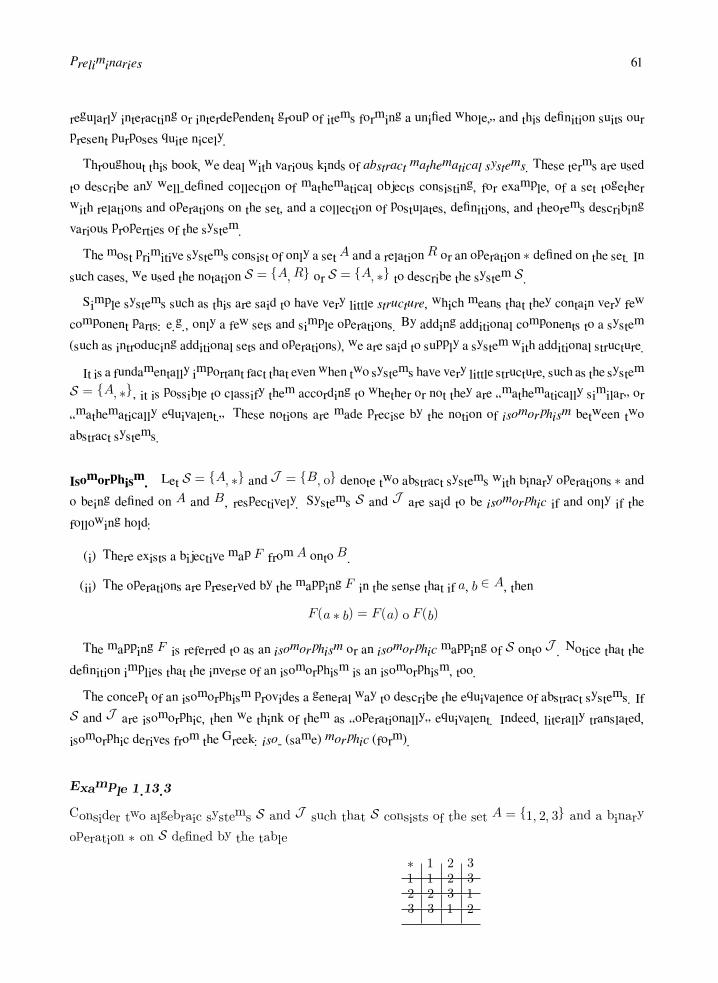
Preliminaries 61
regularly interacting or interdependent group of items forming a unified whole,” and this definition suits our
present purposes quite nicely.
Throughout this book, we deal with various kinds of abstract mathematical systems. These terms are used
to describe any well-defined collection of mathematical objects consisting, for example, of a set together
with relations and operations on the set, and a collection of postulates, definitions, and theorems describing
various properties of the system.
The most primitive systems consist of only a set A and a relation R or an operation ∗ defined on the set. In
such cases, we used the notation S = A,R or S = A, ∗ to describe the system S .
Simple systems such as this are said to have very little structure, which means that they contain very few
component parts: e.g., only a few sets and simple operations. By adding additional components to a system
(such as introducing additional sets and operations), we are said to supply a system with additional structure.
It is a fundamentally important fact that even when two systems have very little structure, such as the system
S = A, ∗, it is possible to classify them according to whether or not they are “mathematically similar” or
“mathematically equivalent.” These notions are made precise by the notion of isomorphism between two
abstract systems.
Isomorphism. Let S = A, ∗ and J = B, o denote two abstract systems with binary operations ∗ and
o being defined on A and B, respectively. Systems S and J are said to be isomorphic if and only if the
following hold:
(i) There exists a bijective map F from A onto B.
(ii) The operations are preserved by the mapping F in the sense that if a, b ∈ A, then
F (a ∗ b) = F (a) o F (b)
The mapping F is referred to as an isomorphism or an isomorphic mapping of S onto J . Notice that the
definition implies that the inverse of an isomorphism is an isomorphism, too.
The concept of an isomorphism provides a general way to describe the equivalence of abstract systems. If
S and J are isomorphic, then we think of them as “operationally” equivalent. Indeed, literally translated,
isomorphic derives from the Greek: iso- (same) morphic (form).
Example 1.13.3
Consider two algebraic systems S and J such that S consists of the set A = 1, 2, 3 and a binary
operation ∗ on S defined by the table
∗ 1 2 31 1 2 32 2 3 13 3 1 2

62 APPLIED FUNCTIONAL ANALYSIS
For example, 1 ∗ 2 = 2, 3 ∗ 2 = 1, etc. Next, suppose that J consists of a set B = x, y, z and a
binary operation o on J defined by the table
o x y zx x y zy y z xz z x y
The mapping
f : 1→ x, 2→ y, 3→ z
is an isomorphism of S onto J , because it is one-to-one and for any a, b ∈ A and a1, b1 ∈ B, if
a1 = F (a) and b1 = F (b), it is clear that F (a ∗ b) = F (a) o F (b) = a1 o b1.
Example 1.13.4
As another example of an isomorphism, consider the system S consisting of the setA = a1, a2, a3, a4,
where a1 = 1, a2 = i =√−1, a3 = −1, and a4 = −i, and the operation of ordinary multiplication
of complex numbers. Here a1 is an identity element since a1ai = ai(i = 1, 2, 3, 4). Note also that
a2a2 = a3, a4a3 = a3a4 = a2, a4a4 = a3, etc., and a−13 = a3, a
−14 = a2, . . . and so forth. Now
consider the system J consisting of the set B = b1, b2, b3, b4, where bi are 2× 2 matrices:
b1 =
1 00 1
, b2 =
0 1
−1 0
, b3 =
−1 00 −1
, b4 =
0 −11 0
Using ordinary matrix multiplication as the defining operation of J , note that b1 is an identity
element since b1bi = bi (i = 1, 2, 3, 4). We observe that b2b2 = b3, b4b3 = b3b4 = b2, b4b4 = b3,
etc., and that b−13 = b3, b
−14 = b2, and so forth. Using the symbol ∼ to indicate correspondence, we
can see that a1 ∼ b1, a2 ∼ b2, a3 ∼ b3, and a4 ∼ b4. This correspondence is clearly an isomorphism;
it is bijective and operations in A are mapped into corresponding operations on B.
It is clear from these examples that knowledge of an isomorphism between two systems can be very useful
information. Indeed, for algebraic purposes, we can always replace a given system with any system isomor-
phic to it. Moreover, if we can identify the properties of any abstract system, we can immediately restate
them as properties of any other system isomorphic to it.
We remark that an isomorphism of a system S onto itself is called an automorphism. We can generally
interpret an automorphism as simply a rearrangement of the elements of the system.
Subsystem. Let S be any abstract mathematical system consisting of a setA and various operations ∗, , . . .
defined on A. Suppose there exists a subset B of A such that all operations ∗, , . . . defined on A are closed
on B. Then the system U consisting of set B and the operations induced from A is called a subsystem of S .

Preliminaries 63
Exercises
Exercise 1.13.1 Determine the properties of the binary operations ∗ and % defined on a set A = x, y, z by
the tables below:
∗ x y zx x y zy y y xz z x x
% x y zx x y zy y z xz z x y
Exercise 1.13.2 Let ∗ be a binary operation defined on the set of integers IZ such that a ∗ b = a2b, where
a, b ∈ IZ. Discuss the distributive properties of ∗ with respect to addition + on IZ.
Exercise 1.13.3 If ∗ is a binary operation on IZ defined by a ∗ b = ab for a, b ∈ IZ, is ∗ commutative? Is it
associative? Is it distributive with respect to −?
Exercise 1.13.4 Let S and J denote two systems with binary operations ∗ and , respectively. If S and J
are isomorphic, i.e., there exists an isomorphism F : S → J , show that if:
(i) The associative law holds in S , then it holds in J .
(ii) S = A, ∗, J = B, , and if e ∈ A is an identity element in S , then its corresponding element
f ∈ B, f = F (e) is an identity element in J .
Exercise 1.13.5 Let S denote the system consisting of the set R = 4n : n ∈ IN, where IN is the set of
natural numbers, and the operation of addition +. Let J denote the set IN plus addition. Show that S
and J are isomorphic.
1.14 Examples of Abstract Systems
We now list a number of important special abstract mathematical systems:
Groupoid. A groupoid is any abstract system consisting of a set on which a closed operation has been
defined.
Semi-group. A semi-group is an associative groupoid.

64 APPLIED FUNCTIONAL ANALYSIS
Monoid. A monoid is a semi-group with an identity element.
Finally, we arrive at an important type of abstract system that occurs frequently in mathematical analysis:
Group. An abstract system G consisting of a set G and one binary operation ∗ on G is called a group iff
the following conditions are satisfied.
(i) Operation ∗ is associative.
(ii) There exists an identity element e in G.
(iii) Every element a in G has its inverse a−1 in G.
Additionally, if the operation ∗ is commutative, the group is called an Abelian or commutative group.
It is understood that ∗ is closed on G; i.e., a ∗ b ∈ G for all a, b ∈ G.
Example 1.14.1
(Dynamics of Mechanical Systems)
Figure 1.14
A simple system consisting of masses and linear springs.
A reader familiar with the dynamics of mechanical systems will appreciate this important example
of semi-groups. Many dynamical systems are governed by differential equations of the form
dq(t)
dt= Aq(t), t > 0
q(0) = q0

Preliminaries 65
wherein q(t) = q1(t), q2(t), . . . , qn(t)T is an n-vector whose components are functions of time t
and A is an n × n invertible matrix (those unfamiliar with these terms may wish to return to this
example after reading Chapter 2).
For example, the equations of motion of the mechanical system of masses and linear springs shown
in Fig. 1.14 arem1x1 + (k1 + k2)x1 − k2x2 = 0, x1(0) = a0, x1(0) = b0
m2x2 − k2x1 + k2x2 = 0, x2(0) = c0, x2(0) = d0
where x1 = d2x1/dt2, x1 = dx1/dt, etc. We obtain a system of first-order equations by setting
x1 = y1 and x2 = y2. Then if
q1 = y1, q2 = y2, q3 = x1, q4 = x2
we have
q =
q1
q2
q3
q4
, q −Aq = 0 =
0
0
0
0
, q(0) = q0=
a0
c0
b0
d0
where
A = −
0 0
k1 + k2
m1
−k2
m1
0 0
−k2
m2
k2
m2
−1 0 0 0
0 −1 0 0
Solutions of these equations (when they exist) are of the form
q(t) = E(t)q0
where E(t) is an n× n matrix with the property
E(t1 + t2) = E(t1) ·E(t2)
E(t1) · (E(t2) ·E(t3)) = (E(t1) ·E(t2)) ·E(t3)
where · denotes matrix multiplication. The set of all matrices E(t)t>0 forms a semi-group with
respect to matrix multiplication. For these reasons, the theory of semi-groups plays a fundamental
role in the mathematical theory of dynamical systems. If we also admit the identity matrix I, the
system becomes a monoid.

66 APPLIED FUNCTIONAL ANALYSIS
Example 1.14.2
The set of all integers forms an Abelian group with respect to the operation of addition. Clearly,
the sum of two integers is an integer, addition is associative, and the identity element can be taken
as 0 since the addition of 0 to any integer does not alter it. The inverse of any integer is then the
negative of the integer since a+ (−a) = 0. Groups whose basic operation is addition are sometimes
called additive groups.
Example 1.14.3
The set of all rational numbers forms an Abelian group under addition. The identity element is
again 0.
Example 1.14.4
The four matrices of Example 1.13.4 form a finite Abelian group under matrix multiplication:
e = b1 =
1 0
0 1
, b2 =
−1 0
0 −1
, b3 =
0 1
−1 0
, b4 =
0 −1
1 0
Such groups are called matrix groups, and since there are four elements in this finite group, we say
that the group is of order four. Note that b1 is the identity matrix and that
b2b3 = b3b2 = b4, b4b3 = b3b4 = b1
and so forth. Moreover, matrix multiplication is associative and
b1b1 = b1 = e, b2b2 = b1 = e
b3b4 = b1 = e, b4b3 = b1 = e
Group operations that characterize a finite group, such as the fourth-order group under considera-
tion, can be arranged in a group table or Cayley square, as shown below, so that the group properties
are immediately apparent:
∗ b1 b2 b3 b4
b1 b1 b2 b3 b4
b2 b2 b1 b4 b3
b3 b3 b4 b2 b1
b4 b4 b3 b1 b2
Groups with some type of multiplication as their basic operation are referred to as multiplicative
groups. From the preceding table, it is seen that a fourth-order group has 16 products. Clearly, an
n-th order group has n2 products. If the group is Abelian, the group table will be symmetric.

Preliminaries 67
Example 1.14.5
The elements 1, g, g2, g3, where g = exp[2πi/3], form a group under multiplication. Here any
element of the group can be expressed as a power of the group element g. Groups of this type are
called cyclic groups. More generally,
1, g, g2, g3, . . . , gn−1
where n is an integer such that gn = 1 is called a cyclic group of order n.
Example 1.14.6
(Permutation Group)
A permutation, generally speaking, is a bijective mapping of a finite set onto itself. For a finite
group of permutations of order n, however, a permutation is frequently described by designating
the image of each element under a mapping of the natural numbers 1, 2, . . . , n onto the elements
a1, a2, . . . , an. A permutation of n such elements is denoted
p =
1 2 3 · · · n
a1 a2 a3 · · · an
The particular permutation
p =
1 2 3 · · · n
1 1 3 · · · n
is called an identity (or natural) permutation, because every element ai is mapped onto itself. For an
n-th order group, there are n! permutations.
Consider, for example, the case in which there are three elements and, therefore, six (3!) permu-
tations:
p1 =
1 2 3
1 2 3
, p2 =
1 2 3
3 1 2
p3 =
1 2 3
2 3 1
, p4 =
1 2 3
2 1 3
p5 =
1 2 3
3 2 1
, p6 =
1 2 3
1 3 2

68 APPLIED FUNCTIONAL ANALYSIS
An inverse permutation is simply a reverse mapping. For example,
p−13 =
2 3 1
1 2 3
=
1 2 3
3 1 2
= p2
p−16 =
1 2 3
1 3 2
= p6
p−12 =
1 2 3
2 3 1
= p3
and so forth. A product of two permutations is simply the composition of the two permutations.
For example,
p2p6 =
1 2 3
3 1 2
1 2 3
1 3 2
=
1 2 3
3 2 1
= p5
The permutation p6 indicates that, for example, 3 is mapped into 2. But by p2, 2 is replaced by
1. Hence, in the product p2p6, 3 is replaced by 1. Note that p2p3 = p1 and p6p6 = p1 and that,
therefore, p3 = p−12 and p6 = p−1
6 . The group table corresponding to p1, p2, . . . , p6 follows:
p1 p2 p3 p4 p5 p6
p1 p1 p2 p3 p4 p5 p6
p2 p2 p3 p1 p6 p4 p5
p3 p3 p1 p2 p5 p6 p4
p4 p4 p5 p6 p1 p2 p3
p5 p5 p6 p4 p3 p1 p2
p6 p6 p4 p5 p2 p3 p1
We observe that the table is not symmetric. Thus the permutation group is not an Abelian group.
The importance of permutation groups lies in Cayley’s theorem, which states that every finite group
is isomorphic to a suitable group of permutations.
Example 1.14.7
(Material Symmetry in Continuum Mechanics)
Group theory plays an important role in the mechanics of continuous media and in crystallogra-
phy, in that it is instrumental in providing for the classification of materials according to intrinsic
symmetry properties they must have.
We shall illustrate briefly the basic ideas. Suppose that relative to a (fixed) Cartesian material
frame of reference, the stress tensor σ at particle X is related to the strain tensor γ at particle X
by a relation of the form
σ = F (γ) (1.1)

Preliminaries 69
where the function F is called the response function of the material, and the relationship itself is
called a constitutive equation because it defines the mechanical constitution of the material (here it
describes the stress produced by a given strain, and this, of course, differs for different materials).
Now, the particular form of the constitutive equation given above might be quite different had we
chosen a different reference configuration of the body. Suppose that X denotes a different labeling
of the material points in the reference configuration related to the original choice by the material-
coordinate transformation
X =HX, det H = ±1 (1.2)
The linear transformation H is called a unimodular transformation because | det H| = 1. We then
obtain, instead of (1.1), a constitutive equation in the transformed material coordinates ,
σ = F (γ)
Now, the set U of all unimodular transformations of the form (1.2) constitutes a group with respect
to the operation of composition. Indeed, if H1, H2, and H3 are three such transformations,
(i) H1(H2H3) = (H1H2)H3 (associative)
(ii) H1 · I =H1 (identity)
(iii) H1 ·H−11 = I (inverse)
For each material, there exists a subgroup H ⊂ U , called the symmetry group of the material, for
which the form of the constitutive equation remains invariant under all transformations belonging
to that group. If H is any element of the symmetry group of the material, and HT denotes
transposition, then
HF (γ)HT = F (HγHT )
This fact is sometimes called the principle of material symmetry.
The group O of orthogonal transformations is called the orthogonal group, and whenever the
symmetry group of a solid material in an undisturbed state is the full orthogonal group, the material
is said to be isotropic. Otherwise it is anisotropic.
We now return to definitions of other algebraic systems.
Ring. An abstract systemR = S,+, ∗ is said to be a ring with respect to the binary operations + and ∗
provided S contains at least two elements, and the following hold:
(i) S,+ is an Abelian group with identity element 0 (called zero).
(ii) The non-zero elements of S with the operation ∗ form a semi-group.

70 APPLIED FUNCTIONAL ANALYSIS
(iii) For every r1, r2, r3 ∈ S, ∗ is distributive with respect to +:
r1 ∗ (r2 + r3) = (r1 ∗ r2) + (r1 ∗ r3)
and
(r2 + r3) ∗ r1 = (r2 ∗ r1) + (r3 ∗ r1)
If S, ∗ is a commutative semi-group, the ring is said to be commutative .
Familiar examples of rings are the sets of ordinary integers, rational numbers, real numbers, and complex
numbers. These systems are rings under ordinary addition and multiplication. A ring R that contains a
multiplicative inverse for each a ∈ R and an identity element is sometimes called a division ring.
Example 1.14.8
Another familiar ring is the ring of polynomials. Let R = S,+, ∗ be a ring and define a set of
functions defined on S into itself of the form
f(x) = a0 + a1 ∗ x+ . . .+ an ∗ xn
where a0, a1, . . . , an ∈ S and xn denotes x ∗ . . . ∗ x (n times). Functions of this type are called
polynomials. Defining addition and multiplication of polynomials by
(f + g)(x) = f(x) + g(x)
(f ∗ g)(x) = f(x) ∗ g(x)
one can show (see Exercise 1.14.10) that the set of all polynomials on S with the addition and
multiplication defined above forms a commutative ring.
Field. An abstract system F = S,+, ∗ that consists of a set containing at least two elements in which
two binary operations + and ∗ have been defined is a field if and only if the following hold:
(i) The system S,+ is an Abelian group with identity element 0.
(ii) The non-zero elements of S with operation ∗ form an Abelian group with identity element e.
(iii) The operation ∗ is distributive with respect to +.
To spell out the properties of a field in detail, we list them as follows:
(i) Addition: S,+
(1) a+ b = b+ a.
(2) (a+ b) + c = a+ (b+ c).

Preliminaries 71
(3) There is an identity element (zero) denoted 0 in S such that a+ 0 = a for every a ∈ S.
(4) For each a ∈ S there is an inverse element −a such that a+ (−a) = 0.
(ii) Multiplication: S − 0, ∗
(1) a ∗ b = b ∗ a.
(2) (a ∗ b) ∗ c = a ∗ (b ∗ c).
(3) There is an identity element e in S such that a ∗ e = a for every a ∈ S.
(4) For each a ∈ S there is an inverse element a−1 such that a ∗ a−1 = e.
(iii) Distributive Property:
For arbitrary a, b, c ∈ S, ∗ is distributive with respect to +.
(a+ b) ∗ c = (a ∗ c) + (b ∗ c)
a ∗ (b+ c) = (a ∗ b) + (a ∗ c)
In most of our subsequent work, we use the ordinary operations of addition and multiplication of real or
complex numbers as the binary operations of fields; each a, b ∈ F is taken to be a real or complex number.
Note that a field is also a commutative division ring (though not every division ring is a field). The sets of
real, rational, and complex numbers individually form fields, as does the set of all square diagonal matrices
of a specified order.
Exercises
Exercise 1.14.1 Let IZ be the set of integers and let denote an operation on IZ such that a b = a+ b− ab
for a, b ∈ IZ. Show that IZ, is a semi-group .
Exercise 1.14.2 Let a, b, and c be elements of a group G = G, ∗. If x is an arbitrary element of this group,
prove that the equation (a ∗ x) ∗ b ∗ c = b ∗ c has a unique solution x ∈ G.
Exercise 1.14.3 Classify the algebraic systems formed by:
(a) The irrational numbers (plus zero) under addition.
(b) The rational numbers under addition.
(c) The irrational numbers under multiplication.
Exercise 1.14.4 Determine which of the following systems are groups with respect to the indicated opera-
tions:
(a) S = x ∈ IZ : x < 0, addition

72 APPLIED FUNCTIONAL ANALYSIS
(b) S = x : x = 5y, y ∈ IZ, addition
(c) S = −4,−1, 4, 1, multiplication
(d) S = z ∈ IC : |z| = 1, multiplication
Here IZ is the set of integers and IC is the complex-number field.
Exercise 1.14.5 Show that the integers IZ, the rationals IQ, and the reals IR are rings under the operations of
ordinary addition and multiplication.
Exercise 1.14.6 Show that the system a, b, ∗,# with ∗ and # defined by
* a ba a bb b a
# a ba a ab a b
is a ring.
Exercise 1.14.7 Which of the following algebraic systems are rings?
(a) S = 3x : x ∈ IZ,+, ·
(b) S = x+ 2 : x ∈ IZ,+, ·
Here + and · denote ordinary addition and multiplication.
Exercise 1.14.8 Let A = P(A) = the set of all subsets of a given set A. Consider the system S =
A,⊗,#, where, if B and C are sets in A,
B ⊗ C = (B ∪ C)− (B ∩ C) and B#C = B ∩ C
Show that S is a commutative ring.
Exercise 1.14.9 Let B denote the set of ordered quadruples of real numbers of the form (a, b,−b, a), (a, b ∈
IR). Consider the system B = B,⊕,, where
(a, b,−b, a)⊕ (c, d,−d, c) = (a+ c, b+ d,−b− d, a+ c)
(a, b,−b, a) (c, d,−d, c) = (ac− bd, ad+ bc,−ad− bc, ac− bd)
Determine if the system B is a field.
Exercise 1.14.10 Show that the set of polynomials defined on S, where S,+, ∗ is a ring, with the opera-
tions defined in Example 1.14.8 forms a ring.

Preliminaries 73
Elementary Topology in IRn
1.15 The Real Number System
The study of properties of the real number system lies at the heart of mathematical analysis, and much of
higher analysis is a direct extension or generalization of intrinsic properties of the real line. This section
briefly surveys its most important features, which are essential to understanding many of the ideas in subse-
quent chapters.
Our objective in this section is to give a concise review of topological properties of real line IR or, more
generally, the Cartesian product IRn. By topological properties we mean notions like open and closed sets,
limits, and continuity. We shall elaborate on all these subjects in a much more general context in Chapter 4
where we study the general theory of topological spaces and then the theory of metric spaces , of which the
space IRn is an example.
It may seem somehow inefficient and redundant that we shall go over some of the notions studied in this
section again in Chapter 4 in a much broader setting. This “didactic conflict” is a result of the fact that we do
need the results presented in this section to develop the notion of the Lebesgue integral in Chapter 3, which
in turn serves as a primary tool to construct the most important examples of structures covered in Chapter 4.
We begin with a short review of the algebraic properties of the set of real numbers IR.
Real Numbers. There are many ways in which one can construct specific models for the set of real num-
bers. To list a few, let us mention the Dedekind sections, in which real numbers are identified with subsets
of rational numbers, or Cantor’s representation, in which a real number is identified with its decimal repre-
sentation understood as the limit of a sequence of rational numbers. It is important to realize that in all those
constructions we arrive at the same algebraic structure, or more precisely, the different models are isomorphic
(in a specialized sense of the kind of algebraic structure we deal with). This brings us to the point at which
it is not the particular model which is important itself but rather its algebraic properties, since they fully
characterize the set of real numbers.
The properties are as follows:
(i) IR, ·,+ is a field.
(ii) ≤ is a total ordering on IR which is order-complete.
The total ordering ≤ on IR is compatible with the field structure in the sense that:
(iii) For x, y ∈ IR, if x ≤ y, then x+ z ≤ y + z for every z ∈ IR.
74 APPLIED FUNCTIONAL ANALYSIS
(iv) For x, y ∈ IR, if x ≥ 0 and y ≥ 0, then xy ≥ 0.
Elements x, y, z, . . . of the set IR are called real numbers. We generally use the symbol IR to refer to the
entire system IR,+, ·,≤ and also to the field IR, ·,+.
Let us remember that order-complete ordering≤ on IR distinguishes real numbers from rationals. By order-
complete, of course, we mean that every nonempty subset of real numbers that has an upper bound also has
the least upper bound—the analogous property holds for lower bounds. The least upper bound of a set A,
also called the supremum of the set A, will be denoted supA. We use an analogous notation for the greatest
lower bound of A or the infimum of A denoted by inf A.
Extended Real Numbers. If a set A ⊂ IR has no upper bound, we frequently write that supA = ∞. This
can be understood merely as a shortcut for saying that A has no upper bound, or may be interpreted in a
deeper sense of the extended real line analysis. By the extended real line, denoted IR, we mean the set of real
numbers complemented with two extra members: +∞ =∞ and −∞,
IR = IR ∪ −∞,+∞
Such an extension would have little sense if we could not extend to IR the algebraic structures of IR. As a
matter of fact, we are only partially successful. In an obvious way, we extend to IR the (order-complete)
linear ordering. By definition, −∞ ≤ c ≤ +∞, ∀c ∈ IR. Notice that, with the infinity symbols nobilitated
to be equal-rights citizens of the extended real line, each set in IR is bounded, both from above and below.
Indeed, the whole IR is bounded. By the same token, each subset of IR (in particular, each subset of IR) has both
supremum and infimum. Consequently, the simple statement supA = ∞ may be interpreted formally as a
substitute for stating that A is not bounded (in IR) from above, or it may be understood in the deeper sense of
the extended linear ordering.
We can also extend to IR the topological structure of IR discussed in the next sections. The extended real
line becomes compact (we shall study the notion in Chapter 4) and, for that reason, the process of extending
the topology from IR to IR is frequently known as the compactification of the real line. We will discuss the
topological structure of IR in Section 1.16.
We cannot, however, extend to IR the algebraic structure of the field. This failure is related to the existence
of indefinite symbols: ∞−∞, 0/0,∞/∞, 0 · ∞, 1∞, 00,∞0.
Supremum and Infimum of a Real-Valued Function. If f : X → IR is a function defined on an arbitrary
set X but taking values in the set of real numbers, its range is a subset of IR, i.e., R(f) ⊂ IR. As a subset of
real numbers,R(f), if bounded from above, possesses its supremum supR(f). This supremum is identified
as the supremum of function f over set X and denoted by supx∈X
f(x) or abbreviated supX
f . As stated above,
supX
f = +∞ is equivalent to the fact thatR(f) has no upper bound.
In the same way we introduce the infimum of f over X , denoted infx∈X
f(x) or abbreviated infX
f and under-
stood as the infimum of the rangeR(f).

Preliminaries 75
We have the obvious inequality
infX
f ≤ f(x) ≤ supX
f
for every x ∈ X . IfR(f) contains its supremum, i.e., there exists such an x0 ∈ X that
f(x0) = supX
f
we say that function f attains its maximum on X . This in particular means that the maximization problem
Find x0 ∈ X such that
f(x0) = supx∈X
f(x)
is well posed in the sense that it has a solution. The supremum of f , supX
f , is called themaximum of f over X ,
denoted maxX
f or maxx∈X
f(x) and identified as the greatest value function f attains on X . Let us emphasize,
however, that the use of the symbol max f is restricted only to the case when the maximum exists, i.e., f
attains its supremum onX , while the use of the symbol sup f always makes sense. Replacing symbol sup f
bymax f without establishing the existence of maximizers is frequently encountered in engineering literature
and leads to unnecessary confusion. The same rules apply to the notion of the minimum of function f over
set X denoted minx∈X
f(x) or minX
f .
Functions with Values in IR. Given a family of functions fι : X → IR, ι ∈ I , we define the pointwise
supremum and pointwise infimum of the family as
supι∈I
fι(x) = supfι(x), ι ∈ I
infι∈I
fι(x) = inffι(x), ι ∈ I
The pointwise supremum or infimum is a function that, in general, takes values in IR. For that reason, it
makes sense to consider functions defined onX that may attain∞ or−∞ values to begin with. For instance,
function 1/x2 can be considered as a function from IR into IR with the value at x = 0 set to ∞. With the
topology of the real line extended (to be discussed next), the function is continuous. We cannot, however, for
instance define f(x) = 1/x at x = 0 in such a way that the extended function would be continuous.
The formalism of functions with values in IR is especially natural when studying the Lebesgue measure and
integration theory, and we will use it heavily in Chapter 3.
Intervals. Let a, b ∈ IR be fixed points in IR such that a < b. The following interval notation is frequently
used:(a, b) = x ∈ IR : a < x < b
[a, b] = x ∈ IR : a ≤ x ≤ b
(a, b] = x ∈ IR : a < x ≤ b
[a, b) = x ∈ IR : a ≤ x < b

76 APPLIED FUNCTIONAL ANALYSIS
The set (a, b) is an open interval, [a, b] is a closed interval, and (a, b] and [a, b) are half-open (or half-closed)
intervals. Infinite intervals are of the type (a,∞) = x ∈ IR : a < x, [a,∞) = x ∈ IR : a ≤ x, etc.,
while (−∞,∞) is sometimes used to describe the entire real line. A singleton of a point is regarded as a
closed interval.
Definition of IRn. EuclideanMetric . Bounded Sets . The notion of the Cartesian productA×B of two sets
A and B, discussed in Section 1.6, can be easily extended to the case of n different sets Ai, i = 1, 2, . . . , n.
In particular, we can speak of the n-th power of a set A, denoted An, which is understood as A×A× . . .×A
(n times). Thus, IRn = IR × IR × . . . × IR (n times) will consist of n-tuples x = (x1, . . . , xn) understood as
finite sequences of real numbers. In the same way we define sets like INn, IZn, IQn, or ICn. Set IRn has no
longer all algebraic properties typical of the system IR. In general, it has no field structure and has no total
ordering which would be compatible with other algebraic properties of IRn. It does, however, share some very
important algebraic properties with IR. Those include the notion of the vector space discussed in detail in
the next chapter and the notion of the Euclidean metric. By the Euclidean metric d(x,y) in IRn we mean a
nonnegative real-valued function of two variables x and y defined as follows
d(x,y) =
n
i=1
(xi − yi)2
12
where x = (xi)ni=1 and y = (yi)
ni=1. For n = 2 or 3, if xi are identified as coordinates of a point x on a
plane (in a space) in a Cartesian system of coordinates, d(x,y) is simply the distance between points x and
y. The Euclidean metric is an example of the general notion of a metric studied in detail in Chapter 4. The
metric enables us to define precisely the notion of a ball. By the (open) ball B(x, r) centered at point x ∈ IRn
with radius r we mean the collection of points y ∈ IRn separated from the center x by a distance smaller than
r. Formally,
B(x, r) = y ∈ IRn : d(x,y) < r
If the strong inequality in the definition of the ball is replaced with the weak one, we talk about the closed
ball, denoted B(x, r). By a ball we will always mean the open ball unless otherwise explicitly stated.
For n = 1 the open and closed balls reduce to the open or closed intervals, respectively:
B(x, r) = (x− r, x+ r)
B(x, r) = [x− r, x+ r]
If a set A ⊂ IRn can be included in a ball B(x, r), we say that it is bounded; otherwise set A is unbounded.
For instance, infinite intervals in IR are unbounded, a half plane in IR2 is unbounded, any polygon in IR2 is
bounded, etc.
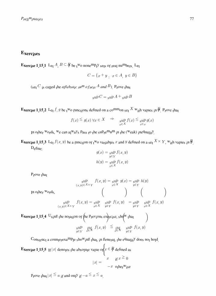
Preliminaries 77
Exercises
Exercise 1.15.1 Let A, B ⊂ IR be two nonempty sets of real numbers. Let
C = x+ y : x ∈ A, y ∈ B
(set C is called the algebraic sum of sets A and B). Prove that
supC = supA+ supB
Exercise 1.15.2 Let f, g be two functions defined on a common set X with values in IR. Prove that
f(x) ≤ g(x) ∀x ∈ X ⇒ supx∈X
f(x) ≤ supx∈x
g(x)
In other words, we can always pass to the supremum in the (weak) inequality.
Exercise 1.15.3 Let f(x, y) be a function of two variables x and y defined on a setX × Y , with values in IR.
Define:g(x) = sup
y∈Yf(x, y)
h(y) = supx∈X
f(x, y)
Prove that
sup(x,y)∈X×Y
f(x, y) = supx∈X
g(x) = supy∈Y
h(y)
In other words,
sup(x,y)∈X×Y
f(x, y) = supx∈X
supy∈Y
f(x, y)
= supy∈Y
supx∈X
f(x, y)
Exercise 1.15.4 Using the notation of the previous exercise, show that
supy∈Y
infx∈X
f(x, y)
≤ infx∈X
supy∈Y
f(x, y)
Construct a counterexample showing that, in general, the equality does not hold.
Exercise 1.15.5 If |x| denotes the absolute value of x ∈ IR defined as
|x| =
x if x ≥ 0
−x otherwise
prove that |x| ≤ a if and only if −a ≤ x ≤ a.

78 APPLIED FUNCTIONAL ANALYSIS
Exercise 1.15.6 Prove the classical inequalities (including the triangle inequality) involving the absolute
values|x| − |y|
≤ |x± y| ≤ |x|+ |y|
for every x, y ∈ IR.
Exercise 1.15.7 Prove the Cauchy–Schwarz inequality
n
i=1
xiyi
≤
n
1
x2i
12
n
1
y2i
12
where xi, yi ∈ IR, i = 1, . . . , n.
Hint: Use the inequalityn
i=1
(xiλ+ yi)2 ≥ 0
for every λ ∈ IR.
Exercise 1.15.8 Use the Cauchy–Schwarz inequality to prove the triangle inequality
d(x,y) ≤ d(x, z) + d(z,y)
for every x,y, z ∈ IRn.
1.16 Open and Closed Sets
We shall now examine several general properties of sets that take on special meaning when they are inter-
preted in connection with IRn. While all of the subsequent ideas make some appeal to the geometrical features
of the real line, they are actually much deeper, and can be easily extended to more general mathematical sys-
tems.
The so-called topology of the real line refers to notions of open sets, neighborhoods, and special classifi-
cations of points in certain subsets of IRn. We discuss the idea of topologies and topological spaces in more
detail in Chapter 4.
Neighborhoods. Let x = (x1, . . . , xn) be a point in IRn. A set A ⊂ IRn is called a neighborhood of point
x iff there exists a ball B(x, ε), centered at x, entirely contained in set A. It follows from the definition that
if A is a neighborhood of x, then every superset B of A (i.e., A ⊂ B) is also a neighborhood of x.

Preliminaries 79
Example 1.16.1
An open ball B(x, r) is a neighborhood of every point belonging to it. Indeed, if y ∈ B(x, r) then
d(x,y) < r and we can select ε such that
ε < r − d(x,y)
Next, choose any z such that d(y, z) < ε. Then we have by the triangle inequality (comp. Exer-
cise 1.15.8)d(x, z) ≤ d(x,y) + d(y, z)
≤ d(x,y) + ε
< r
which proves that B(y, ε) ⊂ B(x, r) (comp. Fig. 1.15).
Figure 1.15
Example 1.16.1. Every open ball is a neighborhood for all its points.
Interior Points. Interior of a Set. A point x ∈ A ⊂ IRn is called an interior point of A iff A is a
neighborhood of x. In other words, there exists a neighborhoodN of x such thatN ⊂ A or, by the definition
of neighborhood, there exists a ball B(x, ε) centered at x entirely contained in A. The collection of all
interior points of a set A is called the interior of A and denoted by int A.
Example 1.16.2
The interior of an open ball B(x, r) coincides with the whole ball. The interior of a closed ball
B(x, r) coincides with the open ball B(x, r) centered at the same point x and of the same radius r.
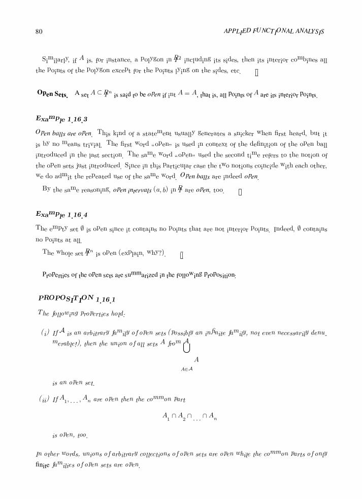
80 APPLIED FUNCTIONAL ANALYSIS
Similarly, if A is, for instance, a polygon in IR2 including its sides, then its interior combines all
the points of the polygon except for the points lying on the sides, etc.
Open Sets. A set A ⊂ IRn is said to be open if int A = A, that is, all points of A are its interior points.
Example 1.16.3
Open balls are open. This kind of a statement usually generates a snicker when first heard, but it
is by no means trivial. The first word “open” is used in context of the definition of the open ball
introduced in the last section. The same word “open” used the second time refers to the notion of
the open sets just introduced. Since in this particular case the two notions coincide with each other,
we do admit the repeated use of the same word. Open balls are indeed open.
By the same reasoning, open intervals (a, b) in IR are open, too.
Example 1.16.4
The empty set ∅ is open since it contains no points that are not interior points. Indeed, ∅ contains
no points at all.
The whole set IRn is open (explain, why?).
Properties of the open sets are summarized in the following proposition:
PROPOSITION 1.16.1
The following properties hold:
(i) If A is an arbitrary family of open sets (possibly an infinite family, not even necessarily denu-
merable!), then the union of all sets A from A
A∈A
A
is an open set.
(ii) If A1, . . . , An are open then the common part
A1 ∩A2 ∩ . . . ∩An
is open, too.
In other words, unions of arbitrary collections of open sets are open while the common parts of only
finite families of open sets are open.

Preliminaries 81
PROOF
(i) Let x ∈ ∪A. By the definition of the union, there exists a set A ∈ A which contains x. But
A is open, which means that there is a neighborhood N of x such that N ⊂ A. But A ⊂ ∪A and
therefore N ⊂ ∪A, which proves that x is an interior point of ∪A. Since x was an arbitrary point
of ∪A, it proves that ∪A is open.
(ii) We shall prove that the common part of two open sets is open. Then the general result follows
by induction. Let A and B be two open sets. If A∩B = ∅ the result is true since the empty set ∅ is
open. Assume that there exists x ∈ A∩B. A is open and therefore there is a ball B(x, ε1) contained
in A. Similarly, there must be a ball B(x, ε2) contained in B. Take ε = min(ε1, ε2). Obviously,
B(x, ε) ⊂ A ∩B
which proves that x is an interior point of A ∩B and therefore A ∩B is open.
Accumulation or Limit Points. Closure of a Set. Let A ⊂ IRn. A point a, not necessarily in A, is called
an accumulation point or a limit point of A if and only if every neighborhood of a contains at least one point
of A distinct from a.
The closure of a set A ⊂ IRn is the set consisting of A and all of the accumulation points of A; i.e., if A is
the set of all accumulation points of a set A, then the set A∪A is the closure of A. The symbolism A is used
to denote the closure of the set A.
Example 1.16.5
Every point y belonging to the sphere of the ball B(x, r), i.e., whose distance from x is exactly r, is
an accumulation point of the ball. Indeed, every ball B(y, ε) (and therefore every neighborhood as
well!) intersects with B(x, r) and therefore contains points from B(x, r).
Other accumulation points of B(x, r) include all the points y from the open ball, d(x,y) < r
(explain, why?). Thus the closure of the open ball B(x, r) coincides with the closed ball B(x, r).
Closed Sets. If a set A ⊂ IRn coincides with its closure, A = A, we say that the set A is closed. In
other words, a set is closed if it contains all its accumulation points.
Example 1.16.6
Consider the set A = x : x ∈ [0, 1) or x = 2 = [0, 1) ∪ 2. The point 1 is an accumulation point
of A, since every neighborhood of 1 contains points in A. However, 2 is not an accumulation point,
since, for example, the neighborhood |x − 2| < 12 contains no points in A other than 2. Clearly, A
is not a closed set, since it does not contain the accumulation point 1; however, every neighborhood

82 APPLIED FUNCTIONAL ANALYSIS
of 1 contains infinitely many points of A. The closure of A is the set A = x : x ∈ [0, 1] or x = 2.
Points such as 2 in the above example for which neighborhoods exist that contain no points of A other than
itself are called isolated points of A.
Before we summarize the essential properties of the closed sets, we shall establish a fundamental link
between the notions of open and closed sets.
PROPOSITION 1.16.2
A set A ⊂ IRn is open iff its complement A = IRn −A is closed.
PROOF Let A ⊂ IRn be open. We should show that IRn−A contains all its accumulation points.
Assume instead that there exists an accumulation point x of IRn−A which does not belong to IRn−A,
i.e., x ∈ A. But A is open, which means that there exists a neighborhood N of x such that N ⊂ A.
But this means that N has no common points with IRn −A and therefore x is not an accumulation
point of A, a contradiction.
Conversely, suppose that A is closed. Again assume instead that there exists a point x ∈ A which
is not an interior point of A. This means that every neighborhood N of x contains points from
outside of A; i.e., from IRn − A and by closedness of A, the point x belongs to A, a contradiction
again.
This relation between open and closed sets, sometimes referred to as the duality principle, is very useful
in proving theorems in topology. As an example we shall use it to prove:
PROPOSITION 1.16.3
(Properties of Closed Sets)
(i) If A is an arbitrary family of closed sets, the common part of all sets A from A
A∈A
A
is also a closed set.
(ii) If A1, . . . , An are closed, then the union
A1 ∪A2 ∪ . . . ∪An
is also closed.

Preliminaries 83
PROOF
(i) By De Morgan’s Laws for arbitrary unions (recall Section 1.4), we have
A
=
A, A ∈ A
Now, if sets A are closed then, by Proposition 1.16.2, their complements A are open. According
to the properties of open sets, the union ∪A is open and then, by the duality principle again, ∩A
must be closed.
We prove property (ii) in exactly the same way.
Example 1.16.7
There are sets in IRn which are neither closed nor open. For instance, if we take a closed ball B(x, r)
and remove any point y from it, we get a set which is neither open nor closed (explain, why?).
It is perhaps more confusing that there are sets which are simultaneously closed and open. Those
include the empty set ∅ and the entire IRn (explain, why?).
Topology of Extended Real Line. Notions of open and closed sets can be extended to IR. Central to the
notion of interior and accumulation points is the concept of neighborhoods for a point. In order to extend
these notions to IR, we simply have to define neighborhoods of ∞ and −∞. We say that a set A ⊂ IR is a
neighborhood of ∞ if it contains an interval (c,∞]. Similarly, a set A ⊂ IR is a neighborhood of −∞ if it
contains an interval (−∞, c]. Once the neighborhoods of both∞ and −∞ have been defined, the definitions
of all remaining topological notions remain identical. For instance, ∞ is an accumulation point of set B if
every neighborhood of∞ contains points from B different from∞. By the definition of neighborhoods, this
is equivalent to say that every B ∩ (c,∞) = ∅ for every c ∈ IR, or simply that B is not bounded from above.
Exercises
Exercise 1.16.1 Prove the properties of the closed sets (Proposition 1.16.3) directly, i.e., using the definition
of a closed set only, without invoking the duality argument.
Exercise 1.16.2 Let intA denote the interior of a set A ⊂ IRn. Prove that the following properties hold:
(i) If A ⊂ B then intA ⊂ intB
(ii) int(intA) = intA
(iii) int(A ∪B) ⊃ intA ∪ intB
(iv) int(A ∩B) = intA ∩ intB
Exercise 1.16.3 Let A denote the closure of a set A ⊂ IRn. Prove that the following properties hold:

84 APPLIED FUNCTIONAL ANALYSIS
(i) If A ⊂ B then A ⊂ B
(ii) (A)¯= A
(iii) A ∩B ⊂ A ∩B
(iv) A ∪B = A ∪B
Exercise 1.16.4 Show the following relation between the interior and closure operations:
intA = A
where A = IRn −A is the complement of set A.
Exercise 1.16.5 Construct examples showing that, in general,
A ∩B = A ∩B
int(A ∪B) = intA ∪ intB
Exercise 1.16.6 Show that if a is an accumulation point of a set A ⊂ IRn, then every neighborhood of a
contains infinitely many points of A. Note that this in particular implies that only infinite sets may have
accumulation points.
Exercise 1.16.7 Prove the Bolzano–Weierstrass Theorem for Sets: if A ⊂ IR is infinite and bounded, then
there exists at least one accumulation point x of set A.
Hint: Use the method of nested intervals:
1. Choose I1 = [a1, b1] ⊃ A. Why is this possible?
2. Divide I1 into two equal intervals, and choose I2 = [a2, b2] as to contain an infinity of elements
A. Why is this possible?
3. Continue this subdivision and produce a sequence of “nested” intervals I1 ⊃ I2 ⊃ I3 ⊃ . . ., each
containing infinitely many elements of set A.
4. Define xn = inf(In∩A), yn = sup(In∩A). Argue that sequences xn, yn converge to a common
limit.
5. Demonstrate that x = y is an accumulation point of set A.
Exercise 1.16.8 Show an example of an infinite set in IR which has no accumulation points.
Exercise 1.16.9 Let A = x ∈ IQ : 0 ≤ x ≤ 1. Prove that every point x ∈ [0, 1] is an accumulation point
of A, but there are no interior points of A.
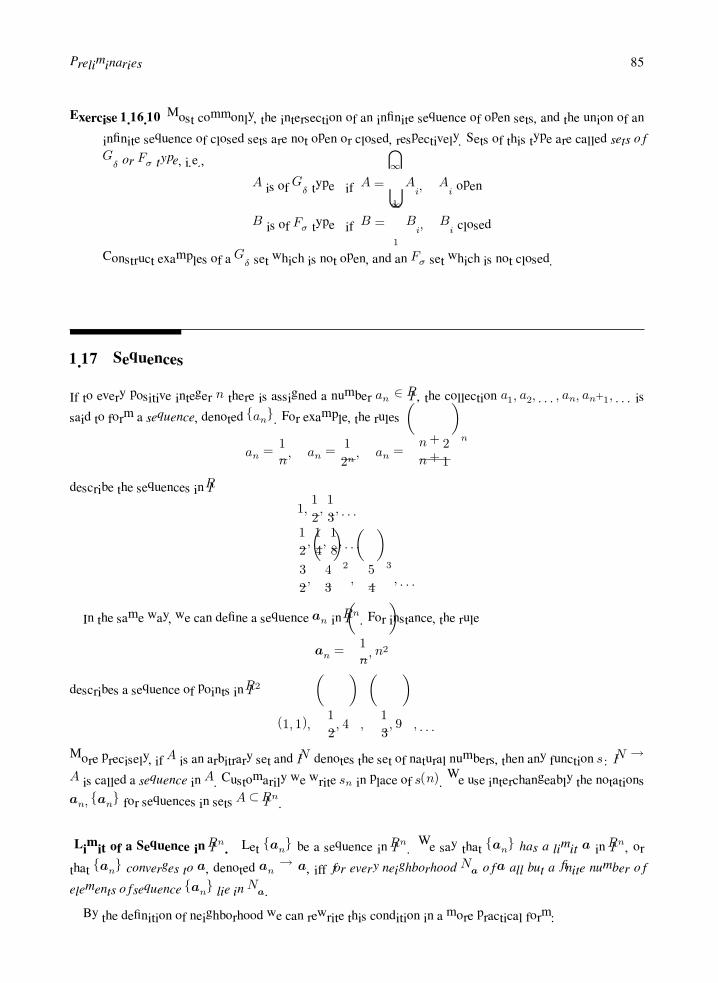
Preliminaries 85
Exercise 1.16.10 Most commonly, the intersection of an infinite sequence of open sets, and the union of an
infinite sequence of closed sets are not open or closed, respectively. Sets of this type are called sets of
Gδ or Fσ type, i.e.,
A is of Gδ type if A =
∞
1
Ai, Ai open
B is of Fσ type if B =
∞
1
Bi, Bi closed
Construct examples of a Gδ set which is not open, and an Fσ set which is not closed.
1.17 Sequences
If to every positive integer n there is assigned a number an ∈ IR, the collection a1, a2, . . . , an, an+1, . . . is
said to form a sequence, denoted an. For example, the rules
an =1
n, an =
1
2n, an =
n+ 2
n+ 1
n
describe the sequences in IR
1,1
2,1
3, . . .
1
2,1
4,1
8, . . .
3
2,
4
3
2
,
5
4
3
, . . .
In the same way, we can define a sequence an in IRn. For instance, the rule
an =
1
n, n2
describes a sequence of points in IR2
(1, 1),
1
2, 4
,
1
3, 9
, . . .
More precisely, if A is an arbitrary set and IN denotes the set of natural numbers, then any function s : IN →
A is called a sequence in A. Customarily we write sn in place of s(n). We use interchangeably the notations
an, an for sequences in sets A ⊂ IRn.
Limit of a Sequence in IRn. Let an be a sequence in IRn. We say that an has a limit a in IRn, or
that an converges to a, denoted an → a, iff for every neighborhood Na of a all but a finite number of
elements of sequence an lie in Na.
By the definition of neighborhood we can rewrite this condition in a more practical form:
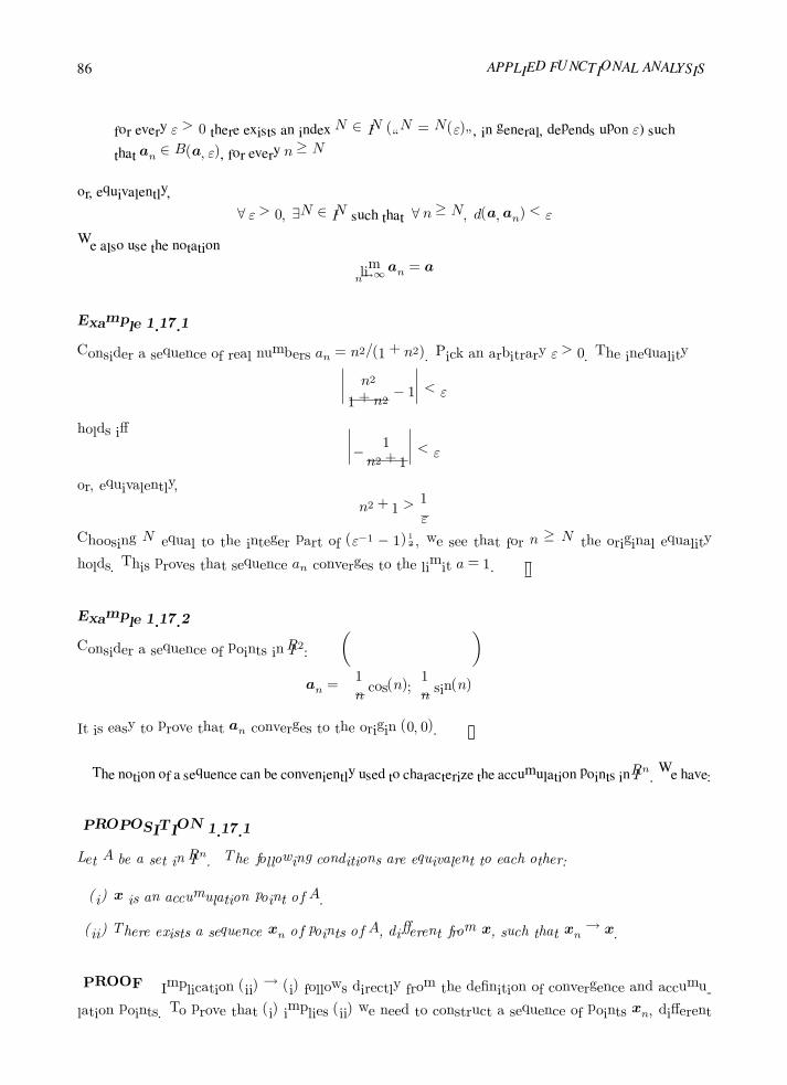
86 APPLIED FUNCTIONAL ANALYSIS
for every ε > 0 there exists an index N ∈ IN (“N = N(ε)”, in general, depends upon ε) such
that an ∈ B(a, ε), for every n ≥ N
or, equivalently,
∀ ε > 0, ∃N ∈ IN such that ∀ n ≥ N, d(a,an) < ε
We also use the notation
limn→∞
an = a
Example 1.17.1
Consider a sequence of real numbers an = n2/(1 + n2). Pick an arbitrary ε > 0. The inequality
n2
1 + n2− 1
< ε
holds iff −
1
n2 + 1
< ε
or, equivalently,
n2 + 1 >1
ε
Choosing N equal to the integer part of (ε−1 − 1)12 , we see that for n ≥ N the original equality
holds. This proves that sequence an converges to the limit a = 1.
Example 1.17.2
Consider a sequence of points in IR2:
an =
1
ncos(n);
1
nsin(n)
It is easy to prove that an converges to the origin (0, 0).
The notion of a sequence can be conveniently used to characterize the accumulation points in IRn. We have:
PROPOSITION 1.17.1
Let A be a set in IRn. The following conditions are equivalent to each other:
(i) x is an accumulation point of A.
(ii) There exists a sequence xn of points of A, different from x, such that xn → x.
PROOF Implication (ii) → (i) follows directly from the definition of convergence and accumu-
lation points. To prove that (i) implies (ii) we need to construct a sequence of points xn, different

Preliminaries 87
from x, converging to x. Let n ∈ IN . Consider a ball B(x, 1n ). It follows from the definition of
the accumulation point that there exists a point in A, different from x, which belongs to the ball.
Denote it by xn. By the construction,
d(xn,x) < ε for every n ≥1
ε+ 1
which finishes the proof.
Given any sequence a1, a2, a3, . . .we can form new sequences of the type a1, a4, a8, . . . or a3, a7, a11,
etc. Such new sequences are called subsequences of the original sequence. More rigorously, we have:
Subsequence. Let s : IN → A and t : IN → A denote two sequences. The sequence t is a subsequence of
s if and only if there exists a one-to-one mapping r : IN → IN such that
t = s r
Example 1.17.3
Let s(n) = 1/n and t(n) = 1/n3. Then s(n) = 1, 12 ,
13 ,
14 , . . . and t(n) = 1, 1
8 ,127 , . . .. Obviously,
t(n) is a subsequence of s(n). To prove this, consider r(n) = n3. Clearly, r is injective.
Thus the injective map r selects particular labels n ∈ IN to be identified with entries in the subsequence
t(n). If ak is a sequence of A ⊂ IRn, we sometimes denote subsequences as having different index labels:
a or ak ⊂ ak.
Cluster Points. Let ak ∈ IRn be a sequence of points in IRn. If ak has a subsequence, say al,
converging to a point a ∈ IRn, we call a a cluster point of the sequence ak. A sequence may have
infinitely many cluster points, a convergent sequence has only one: its limit.
Example 1.17.4
Consider a sequence of real numbers
ak = (−1)k
1 +1
k
Obviously, subsequence a2k (even indices) converges to 1 while the subsequence a2k−1 converges to
−1. Thus ak has two cluster points: +1 and −1.
Sequences in IR. All topological notions discussed for sequences in IR can be extended to IR. A sequence
an ∈ IR converges to ∞ if, for every neighborhood of ∞, almost all elements of an are contained in the

88 APPLIED FUNCTIONAL ANALYSIS
neighborhood. Equivalently,
∀c ∈ IR ∃N = N(c) : n ≥ N ⇒ an > c
In the same way, we define the notion of a sequence converging to −∞. In particular, obviously, all these
notions apply to real-valued sequences an ∈ IR.
Limits Superior and Inferior. The formalism of the extended real line is especially convenient when
discussing the notions of limits superior and inferior. In this paragraph we consider general sequences an ∈ IR
but obviously the whole discussion applies to the particular case of real-valued sequences an ∈ IR. The
notions of limits superior and inferior are very useful as they apply to arbitrary sequences, as opposed to the
notion of the limit which we can use for convergent sequences only.
Let an ∈ IR be a sequence, and let A denote the set of its cluster points. First of all, we notice that set
A is nonempty. Indeed, if sequence an is bounded, the Bolzano–Weierstrass Theorem for Sequences (comp.
Exercise 1.17.2) implies that there exists a subsequence that converges to a real number. On the other side,
if sequence an is not bounded from above, there exists a subsequence ank→ ∞, i.e.,∞ ∈ A. Similarly, if
sequence An is not bounded from below, there exists a subsequence ank→ −∞, i.e., −∞ ∈ A.
Notice that using the language of the extended real analysis, we can reformulate the Bolzano–Weierstrass
Theorem for Sequences stating that every sequence in IR has a convergent (in IR !) subsequence.
As every subset of IR possesses both infimum and supremum, we can define now the notion of limit inferior
and limit superior of the sequence,
lim infn→∞
an = inf A and lim supn→∞
an = supA
In fact, the inf and sup are both attained, i.e.,
lim infn→∞
an = inf A = minA and lim supn→∞
an = supA = maxA
In order to prove this we need to show that we can extract a subsequence xnkconvergent to lim inf an, and
another one convergent to lim sup an. Let us focus on the first case and denote lim inf an =: a. We need to
consider three cases:
Case 1: a = ∞. In this case, a = ∞ is the only cluster point of the sequence. This means that the whole
sequence an converges (“diverges”) to a =∞.
Case 2: a = −∞. It follows from the definition of infimum that, for every number c ∈ IR, we can find a
cluster point ac ∈ A such that ac < c. Therefore, for = c−ac, almost all elements of the subsequence
are in the -neighborhood (ac − , ac + ) of ac. The bottom line is that, for every real number c, there
exists an infinite number of elements of sequence an that are to the left of c. We can now use induction
to construct a subsequence converging to −∞. Set c = −1 and select any n1 such that an1< −1.
Given an1, . . . , ank
, select ank+1in such a way that nk+1 = n1, . . . , nk and ank+1
< c = −(k + 1).

Preliminaries 89
We can always do it, since we have an infinite number of elements of sequence an that are smaller than
any number c. The subsequence ank< −k converges to −∞.
Case 3: a ∈ IR. The reasoning is practically identical to the previous one. Any /2-neighborhood of a must
contain a cluster point a of sequence an. In turn, /2-neighborhood of a must contain almost all
elements of the subsequence converging to a. Consequently, any -neighborhood of a contains an
infinite number of elements of sequence an. We can follow then the procedure above to construct a
subsequence converging to a.
Consider now the set of all values of the sequence an for n ≥ N , denoted an, n ≥ N. Recall that sequence
an is a function from IN into IR. We are talking thus about the image of set N,N + 1, . . . through this
function. Notice that the set need not be infinite. For instance, if sequence an = c = const, the set will
consist of number c only. Define now a new sequence,
bN = infn≥N
an = infan, n ≥ N
Notice subtle details in the notation used above. The first inf above is the infimum of a function (the sequence)
over the set N,N + 1, . . ., and the second inf is the infimum of a subset of IR. For N + 1 > N the set
over which we take the infimum is smaller and, therefore, the new sequence bN is increasing †. Thus, by the
Monotone Sequence Lemma (Exercise 1.17.1), sequence bN is convergent, and
limN→∞
bN = supN
bN = supN
infn≥N
an
We shall demonstrate now that the limit is equal to the limit inferior of the sequence. Let ankbe a subsequence
converging to lim inf an =: a. It follows directly from the definition of sequence bN that
bnk≤ ank
Passing to the limit, we get,
limk→∞
bnk≤ lim
k→∞ank
= a
As the entire sequence bn converges to a limit, its subsequence bnkmust converge to the same limit, and we
have established thus the inequality,
supN
infn≥N
an ≤ lim infn→∞
an
In order to prove the reverse inequality we shall construct a subsequence ankconverging to limN→∞ bN .
As a is the infimum of the set of all cluster points, it must be smaller than limN→∞ bN . It follows from the
definition of bN that, for each N , we can choose nN ≥ N such that
anN≤ bN +
1
N
†Strictly speaking, the sequence is nondecreasing; monotonicity is always understood in the sense of the weak inequality, i.e., bN ≤
bN+1.

90 APPLIED FUNCTIONAL ANALYSIS
Function N → nN may not be an injection and we cannot use it directly to define the desired subsequence.
Starting with n1, we proceed by induction. Given n1, . . . , nk, we take any N > maxn1, . . . , nk and set
nk+1 = nN , where nN has been defined above. As nk+1 ≥ N , nk+1 must be different from n1, . . . , nk. By
construction, we have
ank≤ bnk
+1
nk≤ bnk
+1
k
Passing to the limit with k →∞, we obtain the desired result.
We summarize our findings in the following proposition:
PROPOSITION 1.17.2
(Characterization of Limit Inferior)
Let an ∈ IR be an arbitrary sequence, and let A denote the set of its cluster points. The set A is
nonempty and the following equalities hold:
lim infn→∞
andef= inf A = minA = sup
Ninfn≥N
an
An analogous result holds for the lim sup an, comp. Exercise 1.17.8.
Let us emphasize that the result above allows us in particular to speak about the limit inferior as the smallest
cluster point. Similarly, the limit superior can be understood as the largest cluster point. This identification of
limit superior and limit inferior with the regular limits of certain subsequences allows us to use the notions in
calculus in the very same way as the notion of the limit. Typical properties are summarized in the following
proposition:
PROPOSITION 1.17.3
Let an, bn ∈ IR. The following properties hold:
(i) If an ≤ bn for every n, then
lim inf an ≤ lim inf bn and lim sup an ≤ lim sup bn
(ii) lim inf an + lim inf bn ≤ lim inf(an + bn).
(iii) lim sup(an + bn) ≤ lim sup an + lim sup bn.
PROOF
(i) Pick a subsequence bnksuch that
b = limk→∞
bnk= lim inf
n→∞bn

Preliminaries 91
Since the weak inequality is preserved in the limit, convergent subsequences of the corresponding
subsequence ankhave limits less or equal than b. But this proves that all cluster points of ank
are
less or equal than b and, consequently, the smallest cluster point of an is less or equal than b, too.
Analogously, we prove that the limit superior satisfies the weak inequality, too.
(ii) We have the obvious inequality
infn≥N
an+ infn≥N
bn ≤ an + bn
for every n ≥ N .
Taking the infimum on the right-hand side we get
infn≥N
an+ infn≥N
bn ≤ infn≥N
an + bn
Finally, passing to the limit with n→∞ and using Proposition 1.17.2, we get the required result.
The proof of property (iii) is identical.
Exercises
Exercise 1.17.1 A sequence an ∈ IR is said to be monotone increasing if an ≤ an+1 for all n; it is monotone
decreasing if an+1 ≤ an for all n. Further, a sequence is said to be bounded above if its range is
bounded from above, i.e., there exists a number b such that an ≤ b for all n. Similarly, a sequence an
is bounded below if a number a exists such that a ≤ an for all n.
Prove that every monotone increasing (decreasing) and bounded above (below) sequence in IR is con-
vergent (in IR).
Exercise 1.17.2 Prove the Bolzano–Weierstrass Theorem for Sequences: every bounded sequence in IR has a
convergent subsequence. Hint: LetA be the set of values of the sequence. Consider separately the case
of A being finite or infinite. Use the Bolzano–Weierstrass Theorem for Sets (Exercise 5) in the second
case.
Exercise 1.17.3 Prove that the weak inequality is preserved in the limit, i.e., if xn ≤ yn, xn → x, yn → y,
then x ≤ y.
Exercise 1.17.4 Let xk = (xk1 , . . . , x
kn) be a sequence of points in IR
n. Prove that
limk→∞
xk = x ⇔ limk→∞
xki = xi, for every i = 1, 2, . . . , n
where x = (x1, . . . , xn).
Exercise 1.17.5 Let xk be a sequence in IRn. Prove that x is a cluster point of xk iff every neighborhood of
x contains infinitely many elements of the sequence.

92 APPLIED FUNCTIONAL ANALYSIS
Exercise 1.17.6 Let xk = (xk1 , x
k2) be a sequence in IR
2 given by the formula
xki = (−1)k+i k + 1
k, i = 1, 2, k ∈ IN
Determine the cluster points of the sequence.
Exercise 1.17.7 Calculate lim inf and lim sup of the following sequence in IR:
an =
n/(n+ 3) for n = 3kn2/(n+ 3) for n = 3k + 1n2/(n+ 3)2 for n = 3k + 2
where k ∈ IN .
Exercise 1.17.8 Formulate and prove a theorem analogous to Proposition 1.17.2 for limit superior.
Exercise 1.17.9 Establish the convergence or divergence of the sequences xn, where
(a) xn =n2
1 + n2(b) xn = sin(n)
(c) xn =3n2 + 2
1 + 3n2(d) xn =
(−1)nn2
1 + n2
Exercise 1.17.10 Let x1 ∈ IR be> 1 and let x2 = 2− 1/x1, . . . , xn+1 = 2− 1/xn. Show that this sequence
converges and determine its limit.
1.18 Limits and Continuity
We now examine the fundamental concepts of limits and continuity of functions f : IRn → IRm defined on
IRn. In real analysis, the concept of continuity of a function follows immediately from that of the limit of a
function.
Limit of a Function. Let f : A ⊂ IRn → IRm denote a function defined on a set A ⊂ IRn and let x0 be an
accumulation point of A. Then f is said to have a limit a at the point x0 if, for every ε > 0, there is another
number δ > 0 such that whenever d(x,x0) < δ, d(f(x), a) < ε.
The idea is illustrated in Fig. 1.16a. If x is sufficiently near x0, f(x) can be made as near to a as is desired.
Fig. 1.16b shows a case in which f(x) is discontinuous at x0. Clearly, if we pick a sufficiently small ε > 0,
there exist no point a in the codomain and no δ for which |f(x) − a| < ε whenever |x − x0| < δ. If we
choose x < x0, then |f(x) − a1| < ε whenever |x− x0| < δ; or, if x > x0 then |f(x) − a2| < ε whenever
|x− x0| < δ. Then a1 is called the left limit of f(x) at x0 and a2 is called the right limit of f(x) at x0. The
function f(x) has a limit a at x0 iff a1 = a2 = a, and we write
limx→x0
f(x) = a

Preliminaries 93
Figure 1.16
Continuous and discontinuous functions.
Continuity (The Limit Definition). A function f : A → IR on a set A ⊂ IRn is continuous at the accumu-
lation point x0 ∈ A if and only if
(i) f(x0) exists
(ii) limx→x0
f(x) = f(x0)
If x0 is not an accumulation point of A, we only require (i) for continuity. Note that this in particular implies
that function f is always continuous at isolated points of A.
The definition of continuity can be rewritten without referring to the notion of a limit.
Continuity (ε− δ Definition, Cauchy). A function f : IRn ⊃ A → IRm is continuous at a point x0 ∈ A
(this automatically means that f(x0) exists) iff for every ε > 0 there exists a δ > 0 such that
d(f(x0), f(x)) < ε whenever d(x0,x) < δ,x ∈ A
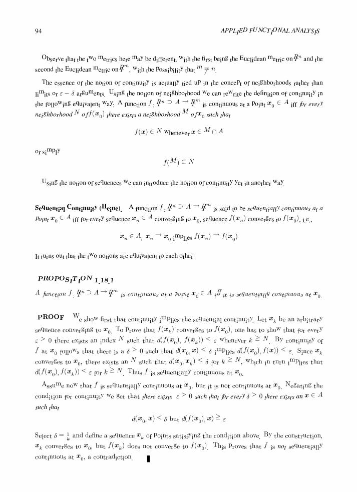
94 APPLIED FUNCTIONAL ANALYSIS
Observe that the two metrics here may be different, with the first being the Euclidean metric on IRn and the
second the Euclidean metric on IRm, with the possibility thatm = n.
The essence of the notion of continuity is actually tied up in the concept of neighborhoods rather than
limits or ε − δ arguments. Using the notion of neighborhood we can rewrite the definition of continuity in
the following equivalent way: A function f : IRn ⊃ A → IRm is continuous at a point x0 ∈ A iff for every
neighborhood N of f(x0) there exists a neighborhood M of x0 such that
f(x) ∈ N whenever x ∈M ∩A
or simply
f(M) ⊂ N
Using the notion of sequences we can introduce the notion of continuity yet in another way.
Sequential Continuity (Heine). A function f : IRn ⊃ A → IRm is said to be sequentially continuous at a
point x0 ∈ A iff for every sequence xn ∈ A converging to x0, sequence f(xn) converges to f(x0), i.e.,
xn ∈ A, xn → x0 implies f(xn)→ f(x0)
It turns out that the two notions are equivalent to each other.
PROPOSITION 1.18.1
A function f : IRn ⊃ A→ IRm is continuous at a point x0 ∈ A iff it is sequentially continuous at x0.
PROOF We show first that continuity implies the sequential continuity. Let xk be an arbitrary
sequence converging to x0. To prove that f(xk) converges to f(x0), one has to show that for every
ε > 0 there exists an index N such that d(f(x0), f(xk)) < ε whenever k ≥ N . By continuity of
f at x0 follows that there is a δ > 0 such that d(x0,x) < δ implies d(f(x0), f(x)) < ε. Since xk
converges to x0, there exists an N such that d(x0,xk) < δ for k ≥ N , which in turn implies that
d(f(x0), f(xk)) < ε for k ≥ N . Thus f is sequentially continuous at x0.
Assume now that f is sequentially continuous at x0, but it is not continuous at x0. Negating the
condition for continuity we get that there exists ε > 0 such that for every δ > 0 there exists an x ∈ A
such that
d(x0,x) < δ but d(f(x0),x) ≥ ε
Select δ = 1k and define a sequence xk of points satisfying the condition above. By the construction,
xk converges to x0, but f(xk) does not converge to f(x0). This proves that f is not sequentially
continuous at x0, a contradiction.

Preliminaries 95
Globally Continuous Functions. Let f : IRn ⊃ A→ IRm be a function. We say that f is globally continu-
ous on A, or shortly, f is continuous on A iff f is continuous at every point of A.
We have the following fundamental characterization of globally continuous functions:
PROPOSITION 1.18.2
Let f : IRn → IRm be a function. The following conditions are equivalent to each other:
(i) f is globally continuous in IRn.
(ii) For every open set G ⊂ IRm, the inverse image f−1(G) by f is open in IRn.
(iii) For every closed set H ⊂ IRm, the inverse image f−1(H) by f is closed in IRn.
The proof of this result is left as an exercise (see Exercise 1.18.1). We shall prove this theorem in Chapter 4
in the context of general topological spaces.
The notion of continuous functions is fundamental in real analysis. Continuous functions satisfy many
important properties which distinguish them from other classes of functions. One of them is the ultimate link
between continuity of functions and the so-called compact sets.
Compact Set. A setK ⊂ IRn is said to be compact iffK is bounded and closed.
Thus, for instance, every closed ball is compact, but a half plane in IR2 is not. Compact sets can be
conveniently characterized using sequences. It turns out that if A is compact then every sequence of points
xk fromA has a subsequence converging to a point x0 inA. We also say thatA is then sequentially compact.
To show that compact sets do indeed have this property, pick an arbitrary sequence xk in A. The sequence
of real numbers xk,1 identified as the first components of points xk is certainly bounded and, therefore, by
the Bolzano–Weierstrass Theorem for Sequences, has a convergent subsequence to an element, say x1 ∈ IR.
Proceeding in the same way, we can extract a subsequence from this subsequence such that also the second
components converge to a number, say x2 ∈ IR, and so on until a subsequence xi is selected such that each
of n components converge to a number xn ∈ IR. But this means (recall Exercise 1.17.4) that the subsequence
xi converges to x = (x1, . . . , xn) ∈ IR. By closedness of A, x must be in A, which proves the result.
This simple result allows us to establish the famous Weierstrass Theorem for functions continuous on
compact sets in IRn.
THEOREM 1.18.1
Let K be a compact set in IRn and f a continuous function defined on K taking on values in IR.
Then f attains both its supremum and infimum on K. In other words, there exist points xmin and

96 APPLIED FUNCTIONAL ANALYSIS
xmax such that
f(xmin) = infK
f , f(xmax) = supK
f
PROOF We shall prove that f attains its maximum on K. The proof for the minimum is
analogous. We first note that the number a = supK
f is an accumulation point of the range of f ,
R(f). If it were not, a ball B(a, ε1) could be found containing upper bounds of R(f) ≤ a but no
points in R(f), and this would contradict the fact that a is the least upper bound. Thus, there exists
a sequence xk ∈ K such that f(xk)→ supK
f (this may include the case when supK
f = +∞, i.e., the
sequence f(xk) is divergent to infinity). Since K is compact and, therefore, sequentially compact as
well, there exists a subsequence, say xi ∈ K, converging to, say, x0 ∈ K. But f is continuous and
therefore f(xi)→ f(x0), which proves that:
1. supK
f is finite, and
2. f(x0) = supK
f .
The notion of compact sets will be studied in a much more general setting in Chapter 4.
Exercises
Exercise 1.18.1 Prove Proposition 1.18.2.
Exercise 1.18.2 Let g f denote the composition of a function f : IRn → IRm and g : IRm → IRk. Prove
that if f is continuous at x0 and g is continuous at f(x0), then g f is continuous at x0.
Exercise 1.18.3 Let f, g : IRn → IRm be two continuous functions. Prove that the linear combination of f, g
defined as
(αf + βg)(x) = αf(x) + βg(x)
is also continuous.
Exercise 1.18.4 Prove the Weierstrass Intermediate Value Theorem:
Let f be a continuous function from IR into IR. Consider a closed interval [a, b] and assume f(a) ≤ f(b).
Then f(x) attains every value between f(a) and f(b).
Exercise 1.18.5 Determine a point x0 ∈ IR at which the following function is continuous:
f(x) =
1− x x is rationalx x is irrational

Preliminaries 97
Exercise 1.18.6 Show that
f(x) =
x sin
1
xx = 0
0 x = 0
is continuous on all of IR.
Exercise 1.18.7 This exercise enforces understanding of the Weierstrass Theorem. Give examples of:
(i) a function f : [0, 1]→ IR that does not achieve its supremum on [0, 1],
(ii) a continuous function f : IR→ IR that does not achieve its supremum on IR.
Elements of Differential and Integral Calculus
1.19 Derivatives and Integrals of Functions of One Variable
For completeness, we now give a brief glimpse at the concepts of differentiation and Riemann integration of
real-valued functions of one real variable. A more elaborate account of these ideas would carry us too far
afield, and some of the more basic theorems are dealt with as exercises.
Derivative of a Function at a Point. Let a be an accumulation point of a set A ⊂ IR and let f be a function
defined from A into IR. A real number K is said to be the derivative of f at a if, for every > 0, there is a
number δ() > 0 such that if x ∈ A and 0 < |x− a| < δ, then
f(x)− f(a)
x− a−K
<
When a number such asK exists, we writeK = f (a).
Alternatively, f (a) is defined as the limit
limx→a
f(x)− f(a)
x− a= f (a)
If we use the classical notations
∆f(a) = f(a+∆x)− f(a)
then also
f (a) = lim∆x→0
∆f(a)
∆x
which is the basis for the classical Leibniz notation
f (a) =df
dx(a)

98 APPLIED FUNCTIONAL ANALYSIS
If f (a) exists, we say that the function f is differentiable at a. If f is differentiable at every point x ∈ A, we
say f is differentiable on A.
PROPOSITION 1.19.1
If a function f is differentiable at a point a ∈ A ⊂ IR then f is continuous at a.
PROOF To show f is continuous at a, we must show that limx→a
f(x) exists and equals f(a).
Pick = 1, and select δ = δ(1) such thatf(x)− f(a)
x− a− f (a)
< 1
∀ x satisfying 0 < |x− a| < δ(1). Using the triangle inequality, we have
|f(x)− f(a)| = |f(x)− f(a) + (x− a)f (a)− (x− a)f (a)|
≤ |f(x)− f(a)− (x− a)f (a)|+ |x− a||f (a)|
≤ |x− a|+ |x− a||f (a)|
Clearly, |f(x) − f(a)| can be made less than if we pick |x − a| < minδ, /(1 + |f (a)|). Hence
limx→a f(x) = f(a), which was to be proved.
Example 1.19.1
The converse of Proposition 1.19.1 is not true. In fact, the function
f(x) =
1 + x x ≤ 01− 2x x > 0
is continuous at x = 0, but not differentiable there. Indeed,
limx→0+
[(f(x)− f(0))/(x− 0)] = 1 whereas limx→0−
[(f(x)− f(0))/(x− 0)] = −2
If f : IR → IR is differentiable at every a ∈ A, a function prescribing for every a ∈ A the derivative of f at
a, denoted f , is called the derivative function of f or simply the derivative of f .
Local (Relative) Extrema of a Function. A function f on a set A ⊂ IR is said to have a local or relative
maximum (minimum) at a point c in A if there exists a neighborhood N of c such that f(x) ≤ f(c)(f(x) ≥
f(c)), for every x ∈ N ∩A.
The following theorem brings the fundamental characterization of local extrema for differentiable func-
tions.

Preliminaries 99
THEOREM 1.19.1
Let f : IR ⊃ A→ IR be differentiable at a point c in the interior of the set A. Suppose f has a local
maximum at c.
Then f (c) = 0.
PROOF Let (c − , c + ) be a neighborhood of c in which the function attains its maximum.
Then, for any x ∈ (c, c+ ),f(x)− f(c)
x− c≤ 0
Passing to the limit with x→ c, we get f (c) ≤ 0. But, at the same time, for x ∈ (c− , c),
f(x)− f(c)
x− c≥ 0
Passing to the limit again, we conclude that f (c) ≥ 0. Hence, f (c) = 0.
An analogous result can be proved for the local minimum.
THEOREM 1.19.2
(Rolle’s Theorem)
Let f be a function continuous on the closed interval [a, b] ⊂ IR and let f be differentiable on
the open interval (a, b). Suppose f(a) = f(b) = 0. Then there exists a point c ∈ (a, b) such that
f (c) = 0.
PROOF If f = 0 ∀ x ∈ (a, b), we can take as point c any point in (a, b). Thus suppose f does
not vanish identically on (a, b). Then f (or −f) assumes some positive values on (a, b). We recall
from the Weierstrass Theorem (Theorem 1.18.1) that a continuous function defined on a compact
set attains its supremum at some point c on this set, and, since f(a) = f(b) = 0( = f(c)), c must
satisfy a < c < b. Now, f (c) exists, by hypothesis, so f (c) must be zero by Theorem 1.19.1.
This brings us to one of the most fundamental theorems of calculus:
THEOREM 1.19.3
(Lagrange Mean-Value Theorem)
Let f be continuous on [a, b] ⊂ IR and let f have a derivative everywhere in (a, b). Then there
exists a point c ∈ (a, b) such that
f(b)− f(a) = (b− a)f (c)

100 APPLIED FUNCTIONAL ANALYSIS
PROOF Let g(x) be defined by
g(x) = f(x)− f(a)−f(b)− f(a)
b− a(x− a)
Clearly, g(x) is continuous on [a, b] and has a derivative on (a, b) and g(a) = g(b) = 0. From Rolle’s
Theorem (Theorem 1.19.2), there is a point c in (a, b) such that g(c) = 0. The assertion of the
theorem follows immediately from this fact.
We now pass on to a review of the concept of integration.
Partitions. A partition P of an interval I = [a, b] is a finite collection of nonoverlapping intervals whose
union is I , generally described by specifying a finite set of numbers, e.g.,
a = x0 ≤ x1 ≤ x2 ≤ · · · ≤ xn = b
For example, if
Ik = [xk−1, xk], 1 ≤ k ≤ n
then P is given by
I =n
k=1
Ik
The quantity
ρ(P ) = maxk|xk − xk−1|
is known as the radius of partition P .
Riemann Sums and Integrals. Let P be a partition of an interval I = [a, b] ⊂ IR and let f be a function
defined on I . The real number
R(P, f) =n
k=1
f(ξk)(xk − xk−1)
where xk−1 ≤ ξk ≤ xk, 1 ≤ k ≤ n, is called the Riemann sum of f corresponding to the partition P =
(x0, x1, . . . , xn) and the choice of intermediate points ξk. The function f is said to be Riemann integrable
on I if for every sequence of partitions Pn converging to zero in the sense that ρ(Pn)→ 0, with an arbitrary
choice of the intermediate points ξk, the corresponding sequence of Riemann sums converges to a common
value J .
The number J is called the Riemann integral of f over [a, b] and is denoted
J =
b
a
f(x)dx =
b
a
fdx
The function f is called the integrand of J .

Preliminaries 101
Example 1.19.2
Let f(x) = 1 if x is rational and let f(x) = 0 if f is irrational. It is easily verified that the limit of
Riemann sum depends upon the choices of ξk. The function f is, therefore, not Riemann integrable.
Necessary and sufficient conditions for a function f to be Riemann integrable will be studied in
Chapter 3. It will turn out that, in particular, every function continuous everywhere except for a
finite number of points is integrable in the Riemann sense. Obviously, the function just considered
does not satisfy this assumption.
THEOREM 1.19.4
(The Mean–Value Theorem of Integral Calculus)
Let f be a continuous function on [a, b]. Then there exists a point c ∈ [a, b] such that
b
a
f(x)dx = f(c)(b− a)
PROOF
If f is constant then the result is trivial. Suppose that f is not constant. By the Weierstrass
Theorem (Theorem 1.18.1), f attains both a minimum and a maximum in [a, b], say at points c1
and c2, respectively.
It follows that the function g(x) defined by
g(x) = f(x)(b− a)−
b
a
f(s)ds
takes on a negative value at c1 and a positive value at c2 (why?). By the Weierstrass Intermediate
Value Theorem (Exercise 1.18.4), g must assume every intermediate value between c1 and c2, in
particular, the zero value, which proves the theorem.
THEOREM 1.19.5
(The First Fundamental Theorem of Integral Calculus)
Let f be continuous on [a, b]. Then the function F (x) defined by
F (x) =
x
a
f(s)ds
is differentiable in [a, b] and F (x) = f(x).
PROOF Let x ∈ [a, b] and ∆x be such that x+∆x ∈ [a, b] as well. By virtue of the Mean-value
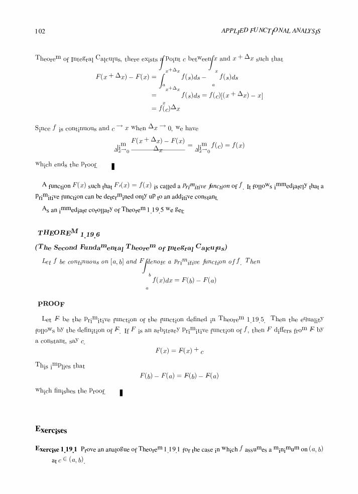
102 APPLIED FUNCTIONAL ANALYSIS
Theorem of Integral Calculus, there exists a point c between x and x+∆x such that
F (x+∆x)− F (x) =
x+∆x
a
f(s)ds−
x
a
f(s)ds
=
x+∆x
x
f(s)ds = f(c)[(x+∆x)− x]
= f(c)∆x
Since f is continuous and c→ x when ∆x→ 0, we have
lim∆x→0
F (x+∆x)− F (x)
∆x= lim
∆x→0f(c) = f(x)
which ends the proof.
A function F (x) such that F (x) = f(x) is called a primitive function of f . It follows immediately that a
primitive function can be determined only up to an additive constant.
As an immediate corollary of Theorem 1.19.5 we get:
THEOREM 1.19.6
(The Second Fundamental Theorem of Integral Calculus)
Let f be continuous on [a, b] and F denote a primitive function of f . Then
b
a
f(x)dx = F (b)− F (a)
PROOF
Let F be the primitive function of the function defined in Theorem 1.19.5. Then the equality
follows by the definition of F . If F is an arbitrary primitive function of f , then F differs from F by
a constant, say c.
F (x) = F (x) + c
This implies that
F (b)− F (a) = F (b)− F (a)
which finishes the proof.
Exercises
Exercise 1.19.1 Prove an analogue of Theorem 1.19.1 for the case in which f assumes a minimum on (a, b)
at c ∈ (a, b).

Preliminaries 103
Exercise 1.19.2 The derivative of the derivative of a function f is, of course, the second derivative of f and
is denoted f . Similarly, (f ) = f , etc. Let n be a positive integer and suppose f and its derivatives
f , f , . . . , f (n) are defined and are continuous on (a, b) and that f (n+1) exists in (a, b). Let c and
x belong to (a, b). Prove Taylor’s formula for f ; i.e., show that there exists a number ξ satisfying
c < ξ < x such that
f(x) = f(c) +1
1!f (c)(x− c) +
1
2!f (c)(x− c)2
+ · · ·+1
n!f (n)(c)(x− c)n +
1
(n+ 1)!f (n+1)(ξ)(x− c)n+1
Exercise 1.19.3 Let f be differentiable on (a, b). Prove the following:
(i) If f (x) = 0 on (a, b), then f(x) = constant on (a, b).
(ii) If f (x) = g(x) on (a, b), then f(x)− g(x) = constant.
(iii) If f (x) < 0 ∀ x ∈ (a, b) and if x1 < x2 ∈ (a, b), then f(x1) > f(x2).
(iv) If |f (x)| ≤M <∞ on (a, b), then
|f(x1)− f(x2)| ≤M |x1 − x2| ∀ x1, x2 ∈ (a, b)
Again, by the Lagrange Mean-Value Theorem,
f(x1)− f(x2) = f (ξ)(x1 − x2)
for some ξ ∈ (x1, x2). Take absolute value on both sides to obtain
|f(x1)− f(x2)| = |f(ξ)| |x1 − x2| ≤M |x1 − x2|
Exercise 1.19.4 Let f and g be continuous on [a, b] and differentiable on (a, b). Prove that there exists a
point c ∈ (a, b) such that f (c)(g(b)− g(a)) = g(c)(f(b)− f(a)). This result is sometimes called the
Cauchy Mean-Value Theorem.
Hint: Consider the function h(x) = (g(b)− g(a))(f(x)− f(a))− (g(x)− g(a))(f(b)− f(a)).
Exercise 1.19.5 Prove L’Hospital’s rule: If f(x) and g(x) are differentiable on (a, b), with g(x) = 0 ∀x ∈
(a, b), and if f(c) = g(c) = 0 and the limitK = limx→c f(x)/g(x) exists, then limx→c f(x)/g(x) =
K.
Hint: Use the result of Exercise 1.19.4.
Exercise 1.19.6 Let f and g be Riemann integrable on I = [a, b]. Show that for any real numbers α and β,
αf + βg is integrable, and
b
a
(αf + βg) dx = α
b
a
f dx+ β
b
a
g dx

104 APPLIED FUNCTIONAL ANALYSIS
Exercise 1.19.7 Let f and g be continuous on [a, b] and suppose that F and G are primitive functions of f
and g, respectively, i.e., F (x) = f(x) and G(x) = g(x) ∀ x ∈ [a, b]. Prove the integration-by-parts
formula: b
a
F (x)g(x) dx = F (b)G(b)− F (a)G(a)−
b
a
f(x)G(x) dx
Exercise 1.19.8 Prove that if f is Riemann integrable on [a, c], [c, b], and [a, b], then
b
a
fdx =
c
a
fdx+
b
c
fdx, a < c < b
Exercise 1.19.9 Let f be a Riemann integrable function defined on [a, b], and let x(u) denote a C1 bijective
map from an interval [c, d] onto [a, b]. Assume, for simplicity, that composition f x is Riemann
integrable on [c, d]. Show that
b
a
f(x) dx =
d
c
f(x(u)) |dx
du| du
1.20 Multidimensional Calculus
Directional and Partial Derivatives of a Function. Let f : IRn → IRm be a function defined on a set
A ⊂ IRn. Equivalently, f can be identified as a composite function f = (f1, . . . , fm) where each of the
component functions fi is a real-valued function defined on A. Let x be an accumulation point of set A and
e denote a unit vector in IRn, i.e., a point e = (e1, . . . , en) ∈ IRn, such that
e21 + e2
2 + . . .+ e2n = 1
The limit
limε→0,ε>0
fj(x+ εe)− fj(x)
ε
if it exists, is called the directional derivative of the j-th component function fj at x in the direction e and is
denoted by
Def j(x)
The directional derivative of f at x in the direction e is defined as
Def(x) = (Def1(x), . . . , Defm(x))
The derivative of the function of a single variable t,
t→ fj(x1, . . . , t(i)
, . . . , xn)
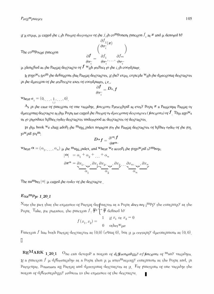
Preliminaries 105
if it exists, is called the i-th partial derivative of the j-th component function fi at x and is denoted by
∂fj∂xi
(x)
The composite function∂f
∂xi=
∂f1
∂xi, . . . ,
∂fm∂xi
is identified as the partial derivative of f with respect to the i-th coordinate.
It follows from the definitions that partial derivatives, if they exist, coincide with the directional derivatives
in the direction of the respective axes of coordinates, i.e.,
∂f
∂xi=Deif
where ei = (0, . . . , 1(i)
, . . . , 0).
As in the case of functions of one variable, functions prescribing at every point x a particular partial or
directional derivative at this point are called the partial or directional derivatives (functions) of f . This allows
us to introduce higher-order derivatives understood as derivatives of derivatives.
In this book we shall adopt the multi-index notation for the partial derivatives of higher order of the fol-
lowing form:
Dαf =∂|α|f
∂xα
where α = (α1, . . . , αn) is the multi-index, and where we accept the following symbols:
|α| = α1 + α2 + . . .+ αn
∂xα = ∂x1, . . . , ∂x1 ∂x2, . . . , ∂x2
. . . ∂xn, . . . , ∂xn
α1 α2 αn
The number |α| is called the order of the derivative .
Example 1.20.1
Note the fact that the existence of partial derivatives at a point does not imply the continuity at the
point. Take, for instance, the function f : IR2 → IR defined by
f (x1, x2) =
1 if x1 or x2 = 0
0 otherwise
Function f has both partial derivatives at (0,0) (equal 0), but it is certainly discontinuous at (0, 0).
REMARK 1.20.1 One can develop a notion of differentiability of functions of many variables.
If a function f is differentiable at a point then it is automatically continuous at the point and, in
particular, possesses all partial and directional derivatives at it. For functions of one variable the
notion of differentiability reduces to the existence of the derivative.

106 APPLIED FUNCTIONAL ANALYSIS
Class of Ck Functions. Let f : IRn → IRm be a function defined on an open set Ω ⊂ IRn. We say that f is
of class Ck(Ω) if all partial derivatives of order less than or equal to k exist, and are continuous on Ω. The
symbols C0(Ω) or C(Ω) are reserved for functions which are just continuous on Ω.
Riemann Integrals in IRn. The notion of the Riemann integral can be generalized to scalar-valued func-
tions in IRn. If (ai, bi) i = 1, . . . , n denotes an open interval in IR, the Cartesian product
σ = (a1, b1)× . . .× (an, bn) ⊂ IRn
is called an (open) cube in IRn.
Assume for simplicity that we are given a function f : IRn → IR defined on a cube E ⊂ IRn. By a partition
P of E we understand a finite family of pairwise disjoint cubes σ ⊂ E such that
E ⊂
σ∈P
σ
where σ denotes the closure of σ,
σ = [a1b1]× . . .× [an, bn]
If a single cube radius is defined as
r(σ) =
n
i
(bi − ai)2
12
the radius of the partition is defined as
r(P ) = maxσ∈P
r(σ)
Choosing an arbitrary (intermediate) point ξσ from every cube σ ∈ P , we define the Riemann sum as
R = R(P, ξ) =
σ∈P
f(ξσ)m(σ)
wherem(σ) denotes the measure (area, volume) of the cube σ defined
m(σ) = (b1 − a1) . . . (bn − an)
The function f is said to be Riemann integrable on E iff for every sequence Pk of partitions such that
r(Pk)→ 0
and for an arbitrary choice of the intermediate point ξσ , the corresponding sequence of Riemann sums
converges to a common value J . The number J is called again the Riemann integral of f over E and is
denoted
J =
E
f dE =
E
f(x) dx =
E
f(x1, . . . , xn) dx1 . . . dxn
It is possible to extend the notion for more general sets E including all open sets in IRn.

Preliminaries 107
We shall return to this and related subjects in Chapter 3.
Exercises
Exercise 1.20.1 Let f : IRn → IRm be a function defined on a set E ⊂ IRn, and x be an interior point of
E. Suppose that f has all its partial derivatives at all x ∈ E, and that a directional derivativeDef(x)
exists, where e = (e1, . . . , en) is a unit vector in IRn. Show that
Def(x) =
n
i=1
∂f
∂xiei
Exercise 1.20.2 Let z = z(t) be a one-to-one function from [a, b] into IR2. The image c of z in IR2 is
identified as a curve in IR2, and the function z, as its parametrization. Assume that z is of class C1.
Let f : IR2 → IR now be a continuous function on IR2. Consider the integral
J =
b
a
f(z(t))
dz1
dt
2
+
dz2
dt
2
dt
Use the result from Exercise 1.19.9 to show that J is independent of the parametrization of curve c.
More precisely, if z is another injective function defined on a different interval [a, b] ⊂ IR, but with the
same image c in IR2 as z(t), then the corresponding integral J is equal to J .
The number J depends thus on the curve c only, and it is known as the line integral of f along c,
denoted by
c
f dc
Exercise 1.20.3 Let Ω be an open set in IR2 with a boundary ∂Ω which is a (closed) C1 curve in IR2. Let
f, g : IR2 → IR be two C1 functions defined on a set Ω1 ⊃ Ω (functions f and g are in particular
continuous along the boundary ∂Ω).
Prove the elementary Green’s formula (also known as the multidimensional version of the integration-
by-parts formula)
Ω
f∂g
∂xidx = −
Ω
∂f
∂xig dx+
∂Ω
fgni ds, i = 1, 2
where n = (n1, n2) is the outward normal unit vector to the boundary ∂Ω.
Hint: Assume for simplicity that the integral over Ω can be calculated as the iterated integral (see
Fig. 1.17), e.g.,
Ω
f∂g
∂x2dx =
b
a
d(x1)
c(x1)
f∂g
∂x2dx2
dx1
and use the integration-by-parts formula for functions of one variable.

108 APPLIED FUNCTIONAL ANALYSIS
Figure 1.17
Exercise 1.20.3. Notation for the iterated integral.
Historical Comments
The most well-known contributor to foundations of contemporary logic and, in particular, mathematical logic,
is probably George Boole (1815–1864), English mathematician and philosopher. Boolean logic has found
extensive applications in electronics and computer hardware. In 1903, Bertrand Russell (1872–1970), En-
glish mathematician and philosopher, along with another English mathematician, Alfred North Whitehead,
published the famous Principia of Mathematica, attempting to establish logic as a foundation of mathemat-
ics. In 1920, a Polish logician, Jan Łukasiewicz (1878–1956), proposed a three-valued logic, leading decades
later to the development of fuzzy logic. Łukasiewicz is also known for his reverse (Polish) notation.
The development of modern set theory is attributed primary to the work of German mathematician, Georg
Cantor (1845–1918). The famous Cantor’s Theorem, discussed in the text, was proved in 1891. The Cantor-
Bernstein-Shroder Theorem was a result of collaboration with two other German mathematicians, Ernst
Schroder(1841–1902) and Felix Bernstein (1878–1956), and it was published in Bernstein’s thesis in 1897.
A second founder of set theory was also a German; Richard Dedekind (1831–1916), was the last student of
Carl Friedrich Gauss (1777–1855) (Chapter 2). Dedekind’s sections and Cantor’s decimal representations are
the two best-known constructs for the real numbers. Cantor and Dedekind built on earlier results of Bernard
Bolzano (1781–1848), a Bohemian mathematician, theologian, philosopher, logician, (and Catholic priest).
Axiomatic set theory was proposed in 1908 by Ernst Zermelo (1871–1953), a German mathematician, and
later complemented by Abraham Fraenkel (1891–1965) from Israel, and Thoralf Skolem (1887–1963) from
Norway.
Venn diagrams were introduced around 1880 by John Venn (1834–1923), a British logician and philoso-
pher.

Preliminaries 109
The Kuratowski-Zorn Lemma was first published in 1922 by Kazimierz Kuratowski (1896–1980), a Polish
mathematician, and in 1935, independently, by Max Zorn (1906–1993), a German-born American mathe-
matician.
The notion of a function was introduced by the giant of calculus, Swiss born Leonhard Euler (1707–1783),
who spent most of his life in Russia and Germany. Among many other contributions, Euler introduced the
number e, the Greek symbolfor summation, and the imaginary unit i (recall Euler’s formula). The precise,
modern definition of a function was worked out by German mathematician Johann Dirichlet (1805–1859).
The terms “injection, surjection, bijection” were introduced by a group of young French mathematicians
associated with Ecole Normale Superieure in Paris, operating under a collective pseudonym of Nicolas
Bourbaki. The group, formed in 1934, published a nine-volume treatise, Elements of Mathematics, which
influenced very much 20th century mathematics. Among others, the group included Henri Cartan, Jean
Dieudonne, Andre Weil and, later, the creator of theory of distributions, Laurent Schwartz (Chapter 5).
The axiomatic theory of natural numbers was formulated by Giuseppe Peano (1858–1932), who published
his famous sets of axioms in 1888. We also owe him our current understanding of mathematical induction. In
1931, an Austrian logician and mathematician, Kurt Godel (1906–1978), published his famous incomplete-
ness theorems stating that any axiomatic, consistent theory of numbers incorporating Peano’s axioms, will
face statements that can neither be proved nor disproved. At the outbreak of WWII, Godel left Vienna and
emigrated to United States.
Modern development of calculus is credited to Sir Isaac Newton (1643–1727) from England, and Gottfried
Leibniz (1646–1716) from Germany. The critical discovery was the fundamental theorem of differential and
integral calculus connecting differentiation with integration.
Augustin-Louis Cauchy (1789–1857), a French mathematician, one of the main contributors to real anal-
ysis, complex analysis, and creator of elasticity theory, is considered to be one of the greatest mathematical
minds that ever lived.
The Taylor series was introduced by a contemporary of Newton, English mathematician and philosopher,
Brook Taylor (1685–1731) in 1715.
Joseph Louis Lagrange (1736–1813), born in Italy, spent most of his life in Prussia and France. He was
one of the main contributors to real analysis, calculus of variations (Euler-Lagrange equations, Lagrange
multipliers) and creator of analytical mechanics. He was among the first to recognize the importance of
Taylor’s series. In 1794, Lagrange became the first professor in Ecole Polytechnique established by Napoleon.
Rolle’s theorem is named after French mathematician, Michel Rolle (1652–1719).
Riemann integrals are named after their creator, Bernhard Riemann (1826–1866) (Chapter 3).


2
Linear Algebra
Vector Spaces—The Basic Concepts
2.1 Concept of a Vector Space
An important abstract mathematical system that embodies a generalization of the familiar concept of a vector
is the vector space. We first cite a formal definition of an abstract vector space and then proceed to identify
the two most significant cases: real and complex spaces.
Definition of an (Abstract) Vector Space. An abstract mathematical system X, +, IF ,+,×, ∗ consisting
of sets X , IF , and operations +, + ×, ∗ is an (abstract) vector space iff
1. X ,+ is an Abelian group with identity 0
2. IF ,+,× is a field, with identities 0 with respect to + and 1 with respect to ×
3. ∗ : IF ×X → X is a binary operation satisfying the conditions
(i) α ∗ (x + y) = α ∗ x + α ∗ y
(ii) (α+ β) ∗ x = α ∗ x + β ∗ x
(iii) α ∗ (β ∗ x) = (α× β) ∗ x
(iv) 1 ∗ x = x
∀ α, β ∈ IF and x,y ∈ X .
We refer to such a system as a vector space X over the field IF (using again X for both the underlying set
and the entire abstract system and using IF for both the field and its underlying set).
The elements x,y, z, . . . ∈ X are called vectors and the operation + on X is vector addition.
The elements α, β, γ, . . . ∈ IF are called scalars and the operation ∗,
IF ×X (α,x)→ α ∗ x ∈ X
111
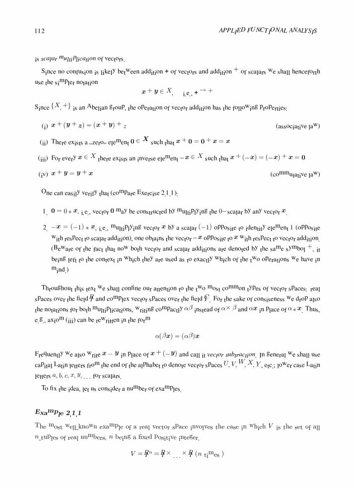
112 APPLIED FUNCTIONAL ANALYSIS
is scalar multiplication of vectors.
Since no confusion is likely between addition + of vectors and addition + of scalars we shall henceforth
use the simpler notation
x+ y ∈ X, i.e., +→ +
Since X,+ is an Abelian group, the operation of vector addition has the following properties:
(i) x+ (y + z) = (x+ y) + z (associative law)
(ii) There exists a “zero” element 0 ∈X such that x+ 0 = 0+ x = x
(iii) For every x ∈ X there exists an inverse element −x ∈ X such that x+ (−x) = (−x) + x = 0
(iv) x+ y = y + x (commutative law)
One can easily verify that (compare Exercise 2.1.1):
1. 0 = 0 ∗ x, i.e., vector 0 may be constructed by multiplying the 0−scalar by any vector x.
2. −x = (−1) ∗ x, i.e., multiplying vector x by a scalar (−1) opposite to identity element 1 (opposite
with respect to scalar addition), one obtains the vector−x opposite to xwith respect to vector addition.
(Beware of the fact that now both vector and scalar additions are denoted by the same symbol +, it
being left to the context in which they are used as to exactly which of the two operations we have in
mind.)
Throughout this text we shall confine our attention to the two most common types of vector spaces: real
spaces over the field IR and complex vector spaces over the field IC. For the sake of consiseness we drop also
the notations for both multiplications, writing compactly αβ instead of α×β and αx in place of α∗x. Thus,
e.g., axiom (iii) can be rewritten in the form
α(βx) = (αβ)x
Frequently we also write x − y in place of x + (−y) and call it vector subtraction. In general we shall use
capital Latin letters from the end of the alphabet to denote vector spaces U, V,W,X, Y , etc.; lower case Latin
letters a, b, c, x, y, . . . for scalars.
To fix the idea, let us consider a number of examples.
Example 2.1.1
The most well-known example of a real vector space involves the case in which V is the set of all
n-tuples of real numbers, n being a fixed positive integer.
V = IRn = IR× . . .× IR (n times )

Linear Algebra 113
Thus an element a ∈ V represents a n-tuple (a1, . . . , an). Given two vectors a and b and a scalar
α we define vector addition and multiplication by a scalar in the following way
a+ b = (a1, . . . , an) + (b1, . . . , bn)def= (a1 + b1, . . . , an + bn)
αa = α(a1, . . . , an)def= (αa1, . . . , αan)
One can easily verify that all the axioms are satisfied.
Example 2.1.2
Most commonly the term “vector” is associated with a pair of points or equivalently a directed
segment of line in a plane or “space.” We define the two operations in the usual way. The vector
addition is constructed using the ancient parallelogram law or in the tip-to-tail fashion as it is shown
in Fig. 2.1. The zero vector is a line segment of zero length and the inverse of a segment a, denoted
Figure 2.1
Vector addition: (a) by the parallelogram law, (b) by the tip-to-tail fashion.
by −a, is a segment of equal length but of opposite direction.
Multiplication of a vector a by a scalar α changes its length by a factor |α| (modulus of α) and
reverses its direction if α is negative, as indicated in Fig. 2.2. For example, −2a is a line segment
twice the length of a, but in a direction opposite to a.
Again, it is easy to see that all the axioms are satisfied.
REMARK 2.1.1 In mechanics we distinguish between a fixed vector with a specified point of
application, a free vector with no point of application, and even sliding vectors with specified lines

114 APPLIED FUNCTIONAL ANALYSIS
Figure 2.2
Multiplication by a scalar.
of action only. Obviously, in our example we deal with free vectors, which more precisely can be
identified with families (classes of equivalence) of fixed vectors possessing the same lines of action,
directions, and magnitudes.
Example 2.1.3
It is a common opinion that every object which can be identified with a directed segment of line
(“an arrow”), i.e., characterized by a magnitude and direction, must be necessarily a “vector.” The
following example of a “vector” of finite rotation contradicts this point of view.
Recall that in three-dimensional kinematics of a rigid body rotating about a point, rotation about
an axis passing through the point can be identified with a “vector” directed along the line of rotation
with a direction specified by the right-hand rule and magnitude equal to the angle of rotation.
According to Euler’s Theorem on Rigid Rotations, a composition of two rotations yields a new
rotation with a corresponding “vector” which can be considered as a natural candidate for the sum
of the two vectors corresponding to the rotations considered. Such “vectors,” however, do not obey
the commutative law (iv), and hence they cannot be identified as vector quantities.
To show this, consider the two finite rotations θ1 + θ2 applied to the block in Fig. 2.3a. Each
rotation has a magnitude of 90 and a direction defined by the right-hand rule, as indicated by the
black arrowhead. The resultant orientation of the block is shown at the right. When these two
rotations are applied in the reverse order θ2 +θ1 as shown in Fig. 2.3b, the resultant position of the
block is not the same as it is in Fig. 2.3a. Consequently, finite rotations do not form a vector space.
REMARK 2.1.2 If smaller, yet finite, rotations had been used to illustrate the example, e.g., 5
instead of 90, the resultant orientation of the block after each combination of rotations would also
be different; however, in this case only by a small amount. In the limit, both orientations are the
same and for that reason we can speak about infinitesimal rotations, angular velocities, or virtual
angular displacements as vectors.

Linear Algebra 115
Figure 2.3
Composition of finite rotations.
Example 2.1.4
Let V be a vector space and E an arbitrary set. Recall that by V E we denote the set of all functions
defined on E with values in V . The family (set) V E can be embodied with the vector structure
provided the two operations are defined as follows:
vector (function) addition:
(f + g)(x)def= f(x) + g(x)
multiplication of a vector (function) by a scalar:
(αf)(x)def= αf(x)
As usual, the same symbol “+” is used to indicate the sum of two functions f and g (the left-hand
side of definition) and the sum of their values at x on the right-hand side. The concept of the
algebraic operations is illustrated in Fig. 2.4. The reader is encouraged to check the axioms. We
emphasize that in this example we have defined operations in V E using operations on vector space
V .

116 APPLIED FUNCTIONAL ANALYSIS
Figure 2.4
Vector addition and multiplication by a scalar in function spaces.
The function vector space V E is the most general example of function (vector) spaces. Usually
we are more specific with assumptions on set E and space V and frequently we incorporate in the
definition some extra assumptions on the regularity of functions considered. If V is chosen as the
space of real (complex) numbers we speak of real- (complex-) valued function . If V = IRn(ICn), we
speak about vector- (complex vector-) valued functions. The following is a very preliminary list of
function (vector) spaces. In all of the definitions Ω ⊂ IRn denotes a domain (an open, connected set)
in IRn.
Ck(Ω) = space of all real- or complex-valued functions defined onΩ of class k meaning functions with derivatives of order kwhich are continuous functions with domain Ω; thus
k = 0 denotes continuous functions;
k = 1, 2, . . . denotes functions differentiable up to k-th
order with k-th order derivatives continuous;
k = ∞ means that all derivatives of any arbitrary order exist ;
k = ω shall denote analytic functions.
Ck(Ω) = denotes space of real (complex) vector-valued functions(usually in IRk, k = 2, 3 in applications) with the deriva-tives of order k continuous on Ω.

Linear Algebra 117
REMARK 2.1.3 The fact that both Ck(Ω) or Ck(Ω) are vector spaces is not an immediate
consequence of Example 2.1.4. Imposing some extra conditions on functions considered, one has to
check that the two operations, vector addition and multiplication by a scalar, are closed with respect
to these conditions. In other words, one has to verify that the sum of two Ck-functions (which a
priori is only a function on Ω and belongs to the space IRΩ) is Ck itself, i.e., falls into the category
of functions considered. (The same concerns multiplication by a scalar, a product of a scalar and a
Ck-function is a Ck-function itself.)
REMARK 2.1.4 It makes only a little sense to speak about Ck-classes for complex-valued
functions of complex variable. It is a well-known fact that (complex) differentiability implies ana-
lyticity (complex analytic functions are called holomorphic). Thus for complex functions Ck, k =
1, 2, . . . ,∞, ω means the same class of functions.
It is often desirable, especially in the study of partial differential equations, to speak of boundary values
of functions defined on the set Ω. Since set Ω is open, the boundary points do not belong to Ω and therefore
functions defined on Ω are not necessarily specified at these points. An attempt to define functions directly
on the closed set Ω in general fails since the notion of differentiability only makes sense for open sets.
To overcome this technical difficulty, we introduce spaces Ck(Ω), k = 0, 1, . . . ,∞. A function f belongs
to the space Ck(Ω) if there exists an open set Ω1, (depending on f ) and an extension f1, such that
1. Ω ⊂ Ω1
2. f1 ∈ Ck(Ω1)
3. f1|Ω = f
According to the definition, a function f from Ck(Ω) can be extended to a function f1 defined on a larger set
containing particularly boundary ∂Ω and values of the extension f1, can be identified as values on f on the
boundary ∂Ω. One can easily verify (see Exercises 2.1.7 and 2.1.8) that Ck(Ω) is a vector space.
Exercises
Exercise 2.1.1 Let V be an abstract vector space over a field IF . Denote by 0 and 1 the identity elements with
respect to addition and multiplication of scalars, respectively. Let −1 ∈ IF be the∗ element opposite to
1 (with respect to scalar addition). Prove the identities
(i) 0 = 0 x, ∀x ∈ V
(ii) −x = (−1) x, ∀x ∈ V
∗It is unique.

118 APPLIED FUNCTIONAL ANALYSIS
where 0 ∈ V is the zero vector, i.e., the identity element with respect to vector addition, and −x
denotes the opposite vector to x.
Exercise 2.1.2 Let IC denote the field of complex numbers. Prove that ICn satisfies the axioms of a vector
space with analogous operations to those in IRn, i.e.,
x+ y = (x1, . . . , xn) + (y1, . . . , yn)def= (x1 + y1, . . . , xn + yn)
α x = α (x1, . . . , xn)def= (α x1, . . . , α xn)
Exercise 2.1.3 Prove Euler’s theorem on rigid rotations. Consider a rigid body fixed at a point A in an initial
configuration Ω. Suppose the body is carried from the configuration Ω to a new configuration Ω1, by a
rotation about an axis l1, and next, from Ω1 to a configuration Ω2, by a rotation about another axis l2.
Show that there exists a unique axis l, and a corresponding rotation carrying the rigid body from the
initial configuration Ω to the final one, Ω2, directly. Consult any textbook on rigid body dynamics, if
necessary.
Exercise 2.1.4 Construct an example showing that the sum of two finite rotation “vectors” does not need to
lie in a plane generated by those vectors.
Exercise 2.1.5 Let Pk(Ω) denote the set of all real- or complex-valued polynomials defined on a set Ω ⊂
IRn(ICn) with degree less or equal to k. Show that Pk(Ω) with the standard operations for functions is
a vector space.
Exercise 2.1.6 Let Gk(Ω) denote the set of all polynomials of order greater or equal to k. Is Gk(Ω) a vector
space? Why?
Exercise 2.1.7 The extension f1 in the definition of a function f from class Ck(Ω) need not be unique. The
boundary values of f1, however, do not depend upon a particular extension. Explain why.
Exercise 2.1.8 Show that Ck(Ω), k = 0, 1, . . . ,∞, is a vector space.
2.2 Subspaces
In most of our studies of vector spaces, we are not concerned with the entire space but also with certain
subsystems called subspaces.
Linear Subspace. Let V be a vector space. A nonempty subsetW of V , sayW ⊂ V , is called a (linear)
subspace of V ifW (with operations restricted from V ) is a vector space (satisfies axioms of the vector space
definition) itself.

Linear Algebra 119
PROPOSITION 2.2.1
A nonempty subset W ⊂ V is a linear subspace of V if and only if it is closed with respect to both
operations: vector addition and multiplication by a scalar, i.e.,
u,v ∈ W ⇒ u+ v ∈ W
α ∈ IR(IC),u ∈ W ⇒ αu ∈ W
PROOF Denote by “+” and “·” the operations in V . If W = W ; +; · is a vector space, then
it must be closed with respect to both operations from the definition of vector space. Conversely,
if W is closed with respect to the operations, then it makes sense to speak about sums u + v and
products αu as elements of W and all axioms which are satisfied in V are automatically satisfied in
W .
Example 2.2.1
Consider a subset Wc of IRn of the form
Wc = x = (x1, . . . , xn) ∈ IRn :
n
i=1
αixi = c
where αi ∈ IR.
Let x,y ∈ Wc. It follows particularly that
αi(xi + yi) =
αixi +
αiyi = 2c
Thus Wc is closed with respect to vector addition if and only if 2c = c, i.e., c = 0. The same holds
for the multiplication by a scalar. Concluding, the set W is a linear subspace of IRn if and only if
c = 0.
Another way to see why c must be equal to zero is to observe that Wc as a vector space must
contain zero vector 0 = (0, . . . , 0). Substituting zero coordinates to the definition of W , we get
immediately that c = 0.
REMARK 2.2.1 For c = 0, Wc can be interpreted as a linear subspace (corresponding to c = 0)
translated in IRn by a vector. Such a subset is called an affine subspace or a linear manifold.
Example 2.2.2
Each of the function spaces defined before on the domain Ω ⊂ IRn can be identified as a linear
subspace of IRΩ (recall Remark 2.1.3).

120 APPLIED FUNCTIONAL ANALYSIS
Example 2.2.3
One of the fundamental concepts in the variational theory of value problems in mechanics is the
notion of the space (set) of all kinematically admissible displacements. Consider, for example, a
membrane occupying a domain Ω ⊂ IR2 with a boundary Γ = ∂Ω consisting of two disjoint parts Γu
and Γt. Recall the classical formulation of the boundary value problem.
Find u = u(x, y), such that
−∆u = f in Ω
u = u0 on Γu
∂u
∂n= g on Γt
In the above ∆ denotes the Laplacian operator (∆ = ∇ ·∇ = ∂2/∂x2 + ∂2/∂y2), ∂u∂n the normal
derivative of u (n is an outward normal unit to Γt), functions f and g specify a given load of the
membrane, inside of Ω and on Γt, respectively, and u0 is a given displacement of the membrane along
part Γu. We call the first boundary condition the essential or kinematic boundary condition since it is
expressed directly in the displacement u, while the second one is called the natural or static boundary
condition . The set of all kinematically admissible displacements is defined as
W = u ∈ Ck(Ω) : u = u0 on Γu
Obviously, W is a subset of the vector space Ck(Ω). The regularity of the solution u is, in this
example, characterized by the order k of the space Ck(Ω) and this order always depends upon the
regularity of the domain Ω, of u0, and of the force data f and g.
In a manner exactly the same as in Example 2.2.1, we prove that W is a linear subspace of C(Ω)
if and only if function u0 is identically equal to zero. In such a case we speak of the space of all
kinematically admissible displacements.
Given two subspaces of a vector space V , we can define their algebraic sum and intersection.
Algebraic Sum of Subspaces. Let X,Y ⊂ V denote two subspaces of the vector space V . The set of all
vectors of the form
z = x+ y
where x ∈ X and y ∈ Y is also a vector subspace of V , denotedX +Y , and called the algebraic sum ofX
and Y .
The algebraic sum should not be confused with the union of subspaces X,Y (X ∪ Y ). The first one
possesses a linear structure while the second one is merely a subset of V .

Linear Algebra 121
Intersection of Subspaces. Contrary to the set operation of the union of sets, the usual intersection opera-
tion preserves the linear structure and the intersection X ∩ Y is a linear subspace of V . Note that X ∩ Y is
never empty since it must contain at least the zero vector.
Algebraic Sum of a Vector and a Subspace. Let x ∈ V and Y be a subspace of the linear space V . The
set
x+ Ydef= x+ y : y ∈ Y
is called the algebraic sum of vector x and subspace Y . The concepts of algebraic sum and intersection are
illustrated in Fig. 2.5.
Figure 2.5
Algebraic sum and common part of subspaces in IR3.
Example 2.2.4
Consider again the set Wc ⊂ IRn defined in Example 2.2.1. Let c = 0 and x denote an arbitrary
element of Wc. One can easily prove that
Wc = x+W0
(recall Remark 2.2.1).
Example 2.2.5
LetW be the set of all kinematically admissible displacements from Example 2.2.3 and letW0 denote
its counterpart for u0 = 0. Finally, let us suppose that function u0 can be extended to a function
denoted by the same symbol but defined on the entire Ω. One can see that
W = u0 +W0

122 APPLIED FUNCTIONAL ANALYSIS
When the common part of two subspaces X and Y consists of zero vector only, their algebraic sum gets a
new name.
Direct Sums. Complements. LetX,Y denote two subspaces of a vector space V such thatX ∩ Y = 0.
In such a case their algebraic sum X + Y is denoted by X ⊕ Y and is called the direct sum of X and Y . In
other words,
X + Y = X ⊕ Y if and only if X ∩ Y = 0
If there exist two subspacesX and Y such that the entire space V is the direct sum ofX and Y , Y is called
a complement of X , conversely, X is a complement of Y .
THEOREM 2.2.1
A linear space V is a direct sum of its two subspaces X and Y , V = X ⊕ Y , if and only if every
vector v ∈ V has a unique representation
v = x+ y
for some x ∈ X and y ∈ Y .
PROOF If V = X ⊕ Y , then V = X + Y and every v ∈ V can be expressed as x + y for
appropriate choices of vectors x ∈ X,y ∈ Y . If, in addition, v = x+ y, where x ∈ X, y ∈ Y , then
x+ y = x+ y
or
x− x = y − y
But x − x ∈ X and y − y ∈ Y ; thus both x − x and y − y belong to both X and Y . However,
X ∩ Y = 0, which implies that both x − x = 0 and y − y = 0. Hence x = x and y = y and v
has a unique representation as the sum x+ y.
Conversely, assume that the representation is unique and take a vector w ∈ X ∩ Y. Then
w = w + 0 = 0+w
where in the first sum w ∈ X,0 ∈ Y and in the second sum 0 ∈ X,w ∈ Y. Since the representation
is unique we must conclude w = 0 and we have X ∩ Y = 0.
Example 2.2.6
Take V = C(Ω) for some bounded domain Ω ⊂ IRn and take
X = u ∈ C(Ω) :
Ω
udΩ = 0
Y = u ∈ C(Ω) : u = const

Linear Algebra 123
Then V = X ⊕ Y . Indeed, if u ∈ V , then u can always be represented as
u = v + w
where w is a constant function, w = meas(Ω)−1
ΩudΩ, and v = u − w belongs to X. Obviously
w ∈ X ∩ Y implies w = 0. The subspace of constant functions is therefore the complement of the
subspace consisting of functions whose mean value on Ω is equal to zero and vice versa.
2.3 Equivalence Relations and Quotient Spaces
Recall that a relation R in a set V has been called an equivalence relation whenever R satisfies three axioms:
(i) xRx (reflexivity)
(ii) xRy ⇒ yRx (symmetricity)
(iii) xRy, yRz ⇒ xRz (transitivity)
Let V be now a vector space. The simplest example of an equivalence relation in V is constructed by taking
a subspaceM ⊂ V and defining the relation RM by
xRMydef⇔ x− y ∈ M
It is easily verified that the three conditions are satisfied. Consequently, we can use the notion of an equiva-
lence class [x] consisting of all elements equivalent to x. In other words
[x] = y ∈ V : y − x ∈ M
which is equivalent to
[x] = x+M
Thus equivalent class [x] can be identified as an affine subspace “parallel” toM , passing through vector x.
SubspaceM , particularly, can be identified as an equivalence class of the zero vector 0.
It is easily verified that the quotient set V/RM is a vector space under the operations of vector addition
and multiplication by a scalar as follows
[x] + [y]def= [x+ y]
α[x]def= [αx]
The quotient space V/RM is denoted V/M and referred to as the quotient space of V modulo M . The
concept of equivalence class [x] = x+M and quotient space V/M is illustrated in Fig. 2.6.

124 APPLIED FUNCTIONAL ANALYSIS
Figure 2.6
Equivalence relation in IR2.
Example 2.3.1
Consider in the space IR2 a subspace
M = x = (x1, x2) ∈ IR2 : α1x1 + α2x2 = 0
(recall Example 2.2.1). M can be identified as a straight line passing through the origin.
Let y = (y1, y2) denote an arbitrary vector. The equivalence class
[y] = x ∈ IR2 : x− y ∈ M
= x : α1(x1 − y1) + α2(x2 − y2) = 0
= x : α1x1 + α2x2 = c, where c = α1y1 + α2y2
is identified as a straight line parallel to M and passing through point y (see Fig. 2.6).
The quotient space IR2/M consists of all such lines parallel to M .
Example 2.3.2
Consider again the membrane problem (recall Example 2.2.3) and suppose that Γu = ∅, i.e., no part
of the membrane boundary is supported. A solution to the corresponding boundary value problem,
called Neumann problem, if it exists, is certainly not unique. Given a solution u(x, y) we easily see
that u+ c, for any c ∈ IR, must be a solution as well.
Identifying the space W of kinematically admissible displacements with the entire space C∞(Ω)
we introduce the following subspace of (infinitesimal, linearized) rigid body motions:
M = u(x, y) : u = const in Ω

Linear Algebra 125
It turns out that the quotient space W/M is a natural candidate space for a solution to the Neumann
problem. Two deflections u and v belong to the same class of equivalence if they differ by a constant
function. We say that the solution of such a membrane problem is determined up to a (linearized
or infinitesimal) rigid body motion.
Example 2.3.3
In continuum mechanics a deformable body is identified with a set Ω satisfying usually some extra
regularity assumptions. The body Ω can occupy different configurations in the space IRn(n = 2, 3)
which may be identified as (open) sets Ωτ in IRn or more precisely by the transformations which map
Ω onto Ωτ :
τ : Ω→ Ωτ ⊂ IRn
If two configurations are considered, say Ωτ1 and Ωτ2 , the composition
τ2 τ−11 : Ωτ1 X → τ2 τ
−11 (X) ∈ Ωτ2
is called a (relative) deformation of configuration τ2 with respect to τ1. One has of course to assume
that both τ1 and τ2 are invertible. Moreover, assuming that the composition τ2 τ−11 is C1, we
introduce the so-called (relative) deformation gradient as
F = ∇χ(X, t), F ki = xk
,i =∂χk
∂Xi
where x = χ = τ2 τ−11 . The composition C = F T F is called the right Cauchy–Green tensor. In
the Cartesian system of coordinates in IRn it takes the form
Cij = xk,ix
k,j
provided the standard summation convention is being used.
Sometimes in place of the deformation it is more convenient to consider the displacement vector
u
u(X) = x(X)−X
and the relative Green strain tensor defined as
2E = C − 1, Eij = Cij − δij
with δij being the usual Kronecker symbol. From the definition of E and C the simple formula
follows:
Eij =1
2(ui,j + uj,i + uk,iuk,j)
We shall define the following relation R in the set S of all configurations τ .
τ1Rτ2def⇔ E = 0

126 APPLIED FUNCTIONAL ANALYSIS
Physically this means that the body is carried from the configuration τ1 to τ2 by a rigid body motion.
We shall prove that R is an equivalence relation.
Toward this goal let us make a few observations first. First of all E = 0 if and only if C = 1.
Second, if τ1, τ2, τ3 denote three configurations and αβF denotes the relative deformation gradient
of configuration τα with respect to configuration τβ , then from the chain rule of differentiation it
follows that31F = 3
2F21F
Recall now that an equivalence relation must be reflexive, symmetric, and transitive. Relation R is
obviously reflexive since the relative deformation gradient of a configuration with respect to itself
equals 1. Next from the identity
31C =
31FT 3
1F =
32F
21FT 3
2F21F =
21FT 3
2C21F
follows that relation R is transitive. Indeed, if τ2Rτ3 then 32C = 1 and 3
1C =
21FT 2
1F = 21C.
Consequently if also τ1Rτ2 then 21C = 1 and finally, 3
1C = 1 which means that τ1Rτ3.
Finally, let τ1Rτ2. Let 21F = F . Obviously 1
2F = F−1 and we have FF−1 = 1, which implies
thatFF−1
T FF−1
=F−1
TF TFF−1 =
F−1
T 21CF
−1 = 1
Since τ1Rτ2 then 21C = 1 and
F−1
TF−1 = 1 which proves that τ2Rτ1. Thus R is reflexive and
therefore R is an equivalence relation.
An equivalence class in this relation can be interpreted as a set of all configurations which are
“connected” by rigid body motions . Thus the quotient set S/R consists of all configurations “up
to a rigid body motion.”
Example 2.3.4
To understand better the notion of the linearized rigid motion let us return now to Example 2.3.3 of
the equivalence relation R in the class of configurations τ . Although the configurations are vector-
valued functions defined on Ω, they do not form a vector space, the reason being for instance that
the only candidate for zero-vector, the zero-function cannot be identified as a configuration (is not
invertible!).
To formulate the problem in terms of vector spaces we shall introduce a reference configuration
τR : Ω → ΩR and consider displacements from that configuration to a given one instead of config-
urations themselves. If u and v are two displacements from ΩR to Ω1 and Ω2 respectively then
v − u prescribes the displacement vector from Ω1 to Ω2 (comp. Fig. 2.7). In a manner identical to
the one in Example 2.3.3, we introduce in the space of displacements defined on ΩR the equivalence
relation: we say that displacement u is related to displacement v,uRv, if the Green strain tensor
corresponding to the displacement v − u vanishes. For the same reasons as before the relation
satisfies the three axioms of equivalence relations.

Linear Algebra 127
Figure 2.7
Reference configuration and concept of displacements.
A natural question arises: Can the introduced relation be induced by a subspace M? The answer
is “no” and there are many ways to verify this. One of them is to notice that if R had been introduced
by a subspace M then the equivalence class of zero displacement would have to coincide with M
and particularly would have to possess the structure of a vector space. This is however not true. To
see this, take two displacements u and v describing rigid body motions, i.e., such that E(u) = 0
and E(v) = 0 and check whether E(u + v) = 0. Due to nonlinearity of E with respect to u the
answer is negative.
The situation changes if we use the linearized geometrical relations, i.e., we replace the Green
strain tensor E with the infinitesimal strain tensor
εij =1
2(ui,j + uj,i)
We leave the reader to check that the equivalence relation generated by the infinitesimal strain tensor
is induced by the subspace of linearized (infinitesimal) rigid body motions (review also Exercises 2.3.2
and 2.3.3). The concept of two equivalence relations is illustrated in Fig. 2.8.
Exercises
Exercise 2.3.1 Prove that the operations in the quotient space V/M are well-defined, i.e., the equivalence
classes [x+ y] and [αx] do not depend upon the choice of elements x ∈ [x] and y ∈ [y].
Exercise 2.3.2 Let M be a subspace of a real space V and RM the corresponding equivalence relation.

128 APPLIED FUNCTIONAL ANALYSIS
Figure 2.8
Concept of two equivalence relations in the space of displacements.
Together with three equivalence axioms (i)-(iii), relation RM satisfies two extra conditions:
(iv) xRy,uRv ⇔ (x+ u)R(y + v)
(v) xRy ⇔ (αx)R(αy) ∀α ∈ IR
We say that RM is consistent with linear structure on V . Let R be an arbitrary relation satisfying
conditions (i)–(v), i.e., an equivalence relation consistent with linear structure on V . Show that there
exists a unique subspaceM of V such that R = RM , i.e., R is generated by the subspaceM .
Exercise 2.3.3 Another way to see the difference between two equivalence relations discussed in Exam-
ple 2.3.3 is to discuss the equations of rigid body motions. For the sake of simplicity let us consider
the two-dimensional case.
(i) Prove that, under the assumption that the Jacobian of the deformation gradient F is positive,
E(u) = 0 if and only if u takes the form
u1 = c1 + cos θx1 + sin θx2 − x1
u2 = c2 − sin θx1 + cos θx2 − x2
where θ ∈ [0, 2π) is the angle of rotation.
(ii) Prove that εij(u) = 0 if and only if u has the following form
u1 = c1 + θx2
u2 = c2 − θx1
Linear Algebra 129
One can see that for small values of angle θ (cos θ ≈ 1, sin θ ≈ θ) the second set of equations can be
obtained by linearizing the first.
2.4 Linear Dependence and Independence, Hamel Basis, Dimension
Linear Combination. Given k vectors x1, . . . ,xk and k scalars α1, . . . , αk, the vector
k
i=1
αixi = α1x1 + . . .+ αkxk
is called a linear combination of the vectors x1, . . . ,xk.
Linear Dependence. We say that a vector x is linearly dependent on vectors x1, . . . ,xk if there exists a
linear combination of xi equal to x, i.e.,
x = α1x1 + . . .+ αkxk
Vectors x1, . . . ,xk are called linearly independent if none of them is linearly dependent upon the remaining
ones. If not, they are called linearly dependent.
PROPOSITION 2.4.1
The following conditions are equivalent:
(i) x1, . . . ,xk are linearly independent
(ii)
k
i=1
αixi = 0⇔ α1 = . . . = αk = 0
PROOF
(i) ⇒ (ii). Suppose to the contrary that
αixi = 0 and that there exists αl = 0. It follows
that
αlxl =
i=l
−αixi
and consequently
xl =
i=l
−αi
αlxi
which proves that xl linearly depends on the remaining xi.

130 APPLIED FUNCTIONAL ANALYSIS
(ii) ⇒ (i). Suppose to the contrary again that there is a vector xl such that
xl =
i=l
βixi
Taking
αi =
βi i = l
−1 i = l
we easily construct the combination
αixi = 0 with not all coefficients equal to zero.
COROLLARY 2.4.1
(i) None of a set of linearly independent vectors x1, . . . ,xk is equal to zero.
(ii) Any subset of linearly independent vectors is linearly independent.
Example 2.4.1
Consider the classical free vectors (recall Example 2.1.2) in three-dimensional space. Three vectors
are linearly dependent if and only if they are coplanar.
Example 2.4.2
Consider the space IRn and a set of vectors
ei = (0, . . . , 1(i)
, . . . , 0) i = 1, . . . , n
Obviously
αiei = (α1, . . . , αn) and therefore if
αiei = 0 then all αi must be zero. By Propo-
sition 2.4.1 vectors ei are linearly independent.
Example 2.4.3
Let Ω ⊂ IR denote an open interval and Pk(Ω) the space of polynomials up to the k-th order defined
on Ω. It is easy to see that the set of monomials 1, x, x2, . . . , xk is linearly independent in Pk(Ω).
So far we have talked about linear dependence or independence of finite sets of vectors only. It is possible
to extend this concept also to infinite sets.
Linear Independence in Infinite Sets. Let V be a vector space and P an arbitrary subset of V . We say
that P is linearly independent if every finite subset of P is linearly independent.

Linear Algebra 131
Example 2.4.4
Let V denote a set of infinite sequences of real numbers x = xi∞1 = (x1, . . .); xi ∈ IR, i = 1, 2, . . .
with a property that in every such sequence only a finite number of elements is different from zero.
Formally we can write:
V = x = xi∞1 , xi ∈ IR, i = 1, 2, . . . : ∃ k = k(x) : xi = 0 ∀i > k
Since infinite sequences are nothing other than real-valued functions defined on the set of positive
integers IN , V can be embodied with natural operations from IRIN . One can easily verify that V is
closed with respect to the operations and therefore V is a vector space (a subspace of IRIN ).
Consider the infinite set of vectors
B = ei, i = 1, 2, . . . where
ei = 0, . . . , 1(i)
, . . ., i = 1, 2, . . .
If A is a finite subset of B then there must be an integer n such that all vectors from A possess zero
components on places with indices greater than n. Consequently
A
αiei =
n
i=1
βiei, where βi =
αi if ei ∈ A
0 otherwise
Consequently, if
A
αiei = (β1, . . . , βn, 0, . . .) = 0
then all coefficients βi, and therefore αi, must vanish too. This proves that set B is linearly inde-
pendent.
Hamel Basis. A linearly independent subset B of a vector space V is called a Hamel basis on V if it is
maximal, i.e., no linearly independent subset S of V exists such that B is a proper subset of S.
Span. A set of vectors P of a vector space V is said to span V if every vector x ∈ V can be expressed as
a linear combination of vectors from P . More precisely, for any vector x there exists a finite subset Px ⊂ P ,
with corresponding coefficients αv such that
x =
v∈Px
αvv
Notice that set P may be infinite but the subset Px is finite, although it may depend upon vector x. In par-
ticular, number of elements of Px may change with x. Notice that vectors v in the linear combination above
serve simultaneously as labels for coefficients αv . This notational departure from using integer indices only
will be very convenient in the proof of Theorem 2.4.1 below. Equivalently, we may extend the summation to
all vectors in P ,
x =
v∈P
αvv

132 APPLIED FUNCTIONAL ANALYSIS
with the understanding that only a finite subset of coefficients αv is different from zero. Infinite sums do not
make sense and are not allowed.
Example 2.4.5
Recall space V of infinite sequences with all but a finite number of terms equal zero, and the set
B = ei, i = 1, 2, . . ., discussed in Example 2.4.4. Set B spans the space V . Indeed, for any
x = xi∞1 ∈ V , there exists a number k(x) such that xi = 0, i > k(x). Consequently,
x =
k(x)
i=1
xiei
THEOREM 2.4.1
(Characterization of Hamel Basis)
The following conditions are equivalent to each other:
(i) B ⊂ V is a Hamel basis of V , i.e., B is a maximal linearly independent subset of V .
(ii) B is linearly independent and spans V .
(iii) For every non-zero vector x ∈ V , there exists a unique finite subset of Bx ⊂ B, with corre-
sponding coefficients αv = 0, v ∈ Bx such that
x =
v∈Bx
αvv
REMARK 2.4.1 Scalars αv in the linear combination above are called the (non-zero) compo-
nents of vector x relative to basis B.
PROOF
(i)⇒ (ii). Let x ∈ V be an arbitrary vector. Since set B is maximal, the superset B ∪ x of
B must be linearly dependent. This means that there exists a finite subset of B ∪ x of linearly
dependent vectors. This subset must include vector x (explain, why?). Let Bx denote all vectors in
the subset, different from vector x. By the linear dependence, there exist numbers αv, v ∈ Bx and
β such that
v∈Bv
αvv + βx = 0

Linear Algebra 133
Again, number β cannot be zero (explain, why?). Solving for x, we get
x =
v∈Bv
−αv
βv
(ii)⇒ (iii). We need to prove uniqueness only. Assume to the contrary that, for a vector x, there
exist two subsets Bix ⊂ B, i = 1, 2 such that
v∈B1x
αvv = x =
v∈B2x
αvv
Consequently,
v∈B1x
αvv −
v∈B2x
αvv = 0
which proves that B1x ∪B2
x ⊂ B is linearly dependent, a contradiction.
(iii)⇒ (i). First we show that B must be linearly independent. First of all, set B cannot contain
the zero vector 0. If it did, we could add term 1 · 0 to the representation of any vector x which
would violate the uniqueness of representation condition. Assume now to the contrary that there
exists a finite subset B0 ⊂ B such that
v∈B0
αvv = 0
Set B0 must have more than one element, otherwise the element would have been the zero vector.
Split B0 into two subsets B0 = B1 ∪B2. We then have
v∈B1
αvv = −
v∈B2
αvv
which proves that vector x =
v∈B1αvv admits two different decompositions, a contradiction.
To prove that B must be maximal, consider an arbitrary vector x. As x admits a representation
in terms of linear combination of vectors from B, set B ∪ x is linearly dependent.
We hasten to point out that the Hamel basis is merely one of many kinds of bases encountered in studying
various mathematical systems. It portrays a purely algebraic property of vector spaces and is intimately
connected with the linear algebraic properties of such spaces. In studying topological properties in Chapter 4,
we again encounter bases of certain spaces, but there we are interested in topological properties, and the
structure of topological bases is quite different from that of the bases considered here. The term basis (or
base) means roughly what we might expect it to: a basis for communication. Once a basis is established and
perfectly understood by all interested parties, we may proceed to describe the properties of the system under
investigation relative to that basis. A reasonable mathematical system always has reasonable properties that
are often useful to know. The particular form in which these properties manifest themselves may well depend
upon what basis we choose to study them.
134 APPLIED FUNCTIONAL ANALYSIS
We emphasize that even in the context of vector spaces the notion of the basis is not unique. In the case
of infinite-dimensional spaces we discuss later in this section, a purely algebraic structure turns out to be
insufficient for our purposes and a topological one must be added. This leads to a new definition of the
basis in certain infinite-dimensional spaces, which we describe later. Contrary to infinite-dimensional spaces,
useful properties of finite-dimensional spaces can be studied within the pure algebraic structure and the notion
of basis is practically unique. The following examples illustrate the concept of Hamel basis.
So long as it is well understood that our aims in this part of our study are purely algebraic, we can drop
the adjective Hamel and simply refer to sets of vectors as possible bases of vector spaces. When the context
requires, we shall be specific about the types of bases.
Example 2.4.6
Consider free vectors in a plane. Let a1,a2 denote two arbitrary, but not collinear vectors. Pick
an arbitrary vector x and project it along the line of action of a1 in the direction of a2 (comp.
Fig. 2.10). Denote the projection by x1 and the corresponding projection along a2 by x2. Obviously
x = x1 + x2. Vectors a1 and x1 are collinear and therefore there must exist a scalar x1, such that
x1 = x1a1. Similarly there exists a scalar x2 such that x2 = x2a2 and consequently
x = x1 + x2 = x1a1 + x2a2
Thus vectors a1,a2 span the entire space. Since none of them can be represented as a product of a
number and the other vector (they are not collinear), they are also linearly independent. Concluding,
any two non-collinear vectors form a basis for free vectors in a plane. The coefficients x1 and x2 are
components of x with respect to that basis.
Similarly, we show that any three non-coplanar vectors form a basis for free vectors in a space.
Example 2.4.7
Consider the space IRn and set of vectors ei considered in Example 2.4.2. Any vector x = (x1, x2, . . . , xn) ∈
IRn can be represented in the form
x =
n
i=1
xiei
Thus vectors ei, i = 1, . . . , n span the entire IRn and since they are linearly independent, they form
a basis. Such a basis is called a canonical basis in IRn.
Example 2.4.8
Monomials from Example 2.4.3 form a basis for the space Pk(Ω).

Linear Algebra 135
Example 2.4.9
Let V be a vector space defined in Example 2.4.4. The set B = ei, i = 1, 2, . . . is linearly
independent and simultaneously spans the space V , so B is a Hamel basis for V .
Example 2.4.10
Consider the vector space whose elements are again infinite sequences of real numbers x = xi∞1 ,
but this time such that∞
1
x2i < +∞. We will encounter this space many times in subsequent
chapters; it is a special vector space, endowed with a norm, and is usually referred to as 2. We are
interested only in algebraic properties now. Obviously the space V from Example 2.4.4 is a subspace
of 2. The set B which has been a Hamel basis for V is not a basis for 2 any more. It is still linearly
independent but it does not span the entire space 2. It spans V , which is only a proper subspace of
2.
It is true that all elements in 2 can be written in the form
x =
∞
i=1
αiei
but such a sum makes no sense in spaces with purely algebraic structure: an infinite series requires
that we specify a mode of convergence and convergence is a topological concept, not an algebraic
one.
We can overcome this difficulty by adding topological structure to 2, and we do just that in
Chapter 4. There we endow 2 with a norm,
x2 =
∞
k=1
|xk|2
12
which allows us to describe not only the “length” of x, but also the “distance” between vectors x
and y in 2. In this particular setting we define as a basis (not a Hamel basis) any countable infinite
set of linearly independent vectors xi∞i=1, such that ∀ x ∈ 2,
∀ ε > 0 ∃N = N(ε) : ||x−
k=1
αkak|| < ε ∀ > N
We will prove that the set B = ei∞1 considered in this sense is a basis for 2.
Besides its practical meaning the notion of the Hamel basis allows us to define the fundamental
concept of the dimension of a vector space and, as a consequence, distinguish between finite- and
infinite-dimensional spaces. To do it, however, we need to prove the two following fundamental
theorems.

136 APPLIED FUNCTIONAL ANALYSIS
THEOREM 2.4.2
Let V be a vector space, B a (Hamel) basis and P ⊂ V an arbitrary linearly independent set. Then
#P ≤ #B
Before we proceed with the proof let us make an important corollary.
COROLLARY 2.4.2
Every two bases in a vector space have the same number of elements or more precisely, the same
cardinal number. Indeed, if B1 and B2 denote two bases, then B2 is linearly independent and
according to the theorem #B2 ≤ #B1. Conversely #B1 ≤ #B1 and the equality holds.
Dimension. The cardinal number of any basis of a vector space V is called the dimension of the space and
denoted dimV .
If dimV = n < +∞, the space is called a finite-dimensional (n-dimensional) space, if not then we speak
of infinite-dimensional vector spaces. Although several properties are the same for both cases, the differences
are very significant. The theory which deals with finite-dimensional spaces is customarily called “linear
algebra,” while the term “functional analysis” is reserved for the case of infinite-dimensional spaces, the
name coming from function spaces which furnish the most common example of spaces of infinite dimension.
By this time a careful reader would have noticed that we have skipped over a very important detail. In
everything we have said so far based on the concept of a basis , we have been implicitly assuming that such
a basis exists in fact in every vector space. Except for a few cases where we can construct a basis explicitly,
this is not a trivial assertion and has to be proved.
THEOREM 2.4.3
Every linearly independent set A in a vector space X can be extended to a (Hamel) basis. In
particular, every nontrivial vector space (X = 0), possesses a basis.
Proofs of Theorems 2.4.2 and 2.4.3 are pretty technical and can be skipped during the first reading. The
fundamental tool in both cases is the Kuratowski–Zorn Lemma.
PROOF Let U be a class of all linearly independent sets containing set A. U is nonempty since
it contains A. We shall introduce a partial ordering in the family U in the following way.
B1 ≤ B2def⇔ B1 ⊂ B2

Linear Algebra 137
Now let B denote a linearly ordered set in family U . We shall construct an upper bound for B.
Toward this goal define set B0 as the union of all sets from the family
B0 =
B∈B
B
Obviously, A ⊂ B0. B0 is linearly independent since every finite subset must be contained in a
certain B and all B’s are linearly independent.
Thus, according to the Kuratowski–Zorn Lemma there exists a maximal element in U which is
nothing else than a (Hamel) basis in X.
To prove the second assertion it suffices to take as A a subset consisting of one, single non-zero
vector.
PROOF When B is finite the proof is standard and does not require the use of the Kuratowski–
Zorn Lemma. Obviously the proof we present holds for both finite- and infinite-dimensional cases.
We shall show that there exists an injection (one-to-one mapping) from P to B. Denote by F a
class of all injections f satisfying the following conditions:
(i) P ∩B ⊂ dom f ⊂ P, im f ⊂ B
(ii) The set (P − dom f) ∪ im f is linearly independent,
where dom f and im f denote the domain and range of funtion f . F is nonempty (explain, why?)
and can be ordered by the following partial ordering in F
f ≤ gdef⇔ dom f ⊂ dom g and g|dom f = f
Let G be a linearly ordered set in the class F . The union of functions f ∈ G, denoted F , is a
well-defined injection satisfying condition (i). Let A = A1 ∪ A2, A1 ⊂ P − domF , A2 ⊂ im F .
It must be an f from F such that A2 ⊂ im f . Obviously A1 ⊂ P − dom (∪f) ⊂ P − dom f and
therefore according to condition (ii), A must be linearly independent.
Thus F is an upper bound for the family G and according to the Kuratowski-Zorn Lemma there
exists a maximal element f in the class F . It is sufficient to show that dom f = P .
Suppose to the contrary that P − dom f = ∅. It implies that also im f = B. Indeed, if it were
im f = B then from the fact that B is a basis and that the set
im f ∪ (P − dom f) = B ∪ (P − dom f)
is linearly independent, it would follow that P −dom f ⊂ B and consequently P −dom f ⊂ P ∩B ⊂
dom f which is impossible.
So pick a vector v0 ∈ B − im f. Two cases may exist. Either v0 is a linear combination of
elements from (P − dom f)∪ im f , or not. In the second case a union of f and (u0.v0), where u0

138 APPLIED FUNCTIONAL ANALYSIS
is an arbitrary element from P −dom f , denoted f1 belongs to family F . Indeed f1 satisfies trivially
condition (i) and the set
(P − dom f1) ∪ im f1,= P − (dom f ∪ u0) ∪ imf ∪ v0
is linearly independent, so f1 is a proper extension of f and belongs to F which contradicts the fact
that f is maximal.
Consider the first case. Vector v0 can be represented in the form
v0 = λ0u0 + . . .+ λnun + µ0w0 + . . .+ µmwm
where u0, . . . ,un ∈ P − dom f , w0, . . . ,wm ∈ im f . One of the numbers λ0, λ1, . . . , λn, say λ0
must be different from zero since in the other case set B would be linearly dependent. Consider
again the extension f1 = f ∪ (u0,v0). If (P − dom f1) ∪ im f1 were linearly dependent then v0
would be a linear combination of elements from (P −dom f)∪ im f −u0 which is impossible since
λ0 = 0. So, again f has the proper extension f1 in the family F and therefore cannot be maximal.
Construction of a Complement. One of the immediate consequences of Theorems 2.4.2 and 2.4.3 is a
possibility of constructing a complement Y to an arbitrary subspace X of a vector space V . Toward this
goal pick an arbitrary basis B forX (which according to Theorem 2.4.3 exists). According to Theorem 2.4.3
basisB can be extended to a basis C for the whole V . The complement space Y is generated by vectors from
C − B. Indeed, X + Y = V and X ∩ Y = 0 due to the linear independence of C. Except for the trivial
case when X = V , subspace X possesses many (infinitely many, in fact) complements Y .
We conclude this section with a summary of the classification of the spaces which we have used in this
chapter according to dimension.
Example 2.4.11
1. Free vectors in a plane form a two-dimensional subspace of a three-dimensional vector space.
2. dim IRn = n, dim ICn = n.
3. dimPk(Ω) = k + 1 if Ω is an interval in IR.
4. Spaces V from Example 2.4.4 and 2 from Example 2.4.10 are infinite-dimensional.
Linear Algebra 139
Linear Transformations
2.5 Linear Transformations—The Fundamental Facts
Each notion of an algebraic structure is accompanied by specific operations, functions which reflect the basic
features of the considered structures. The linear transformation plays such a role for vector spaces.
Linear Transformation. Let V andW be two vector spaces, both over the same field IF . A linear trans-
formation T : V →W is a mapping of V intoW such that the following hold:
(i) T (x+ y) = T (x) + T (y) for every x,y ∈ V .
(ii) T (αx) = αT (x) for every x ∈ V, and every scalar α ∈ IF .
We say that T is additive and homogeneous. One can combine properties (i) and (ii) into the more concise
definition: the transformation T : V →W is linear if and only if
T (αx+ βy) = αT (x) + βT (y)
We have two simple observations:
1. One can easily generalize this law for combinations of more than two vectors
T (α1x+ . . .+ αnxn) = α1T (x1) + . . .+ αnT (xn)
2. If T is linear then an image of zero vector in V must be a necessary zero vector inW , since
T (0) = T (x+ (−1)x) = T (x)− T (x) = 0
The term “transformation” is synonymous with function, map or mapping. One should emphasize however
that the linear transformation is defined on the whole space V , its domain of definition coincides with the
entire V . The term linear operator is frequently reserved for linear functions which are defined in general
only on a subspace of V . Its use is basically restricted to infinite-dimensional spaces.
Example 2.5.1
A function can be additive and not homogeneous. For example, let z = x+ iyi =
√−1denote a
complex number, z ∈ IC, and let T : IC → IC be a complex conjugation; i.e.,
T (z) = z = x− iy

140 APPLIED FUNCTIONAL ANALYSIS
Then
T (z1 + z2) = x1 + x2 − i(y1 + y2) = T (z1) + T (z2)
However, if a = α+ iβ is a complex scalar,
T (az) = αx− βy − i(αy + βx) = aT (z) = αx+ βy + i(βx− αy)
Hence complex conjugation is not a linear transformation.
Example 2.5.2
There are many examples of functions that are homogeneous and not additive. For example, consider
the map T : IR2 → IR given by
T ((x1, x2)) =x2
1
x2
Clearly,
T ((x1, x2) + (y1, y2)) =(x1 + y1)
2
x2 + y2=
x21
x2+
y21
y2
However,
T (α(x1, x2)) =(αx1)
2
αx2= α
x21
x2= αT ((x1, x2))
Example 2.5.3
One of the most common examples of a linear transformation is that associated with the integration
of real-valued functions. Let V = C(Ω).
Define T : V → V
Tf(x) =
Ω
K(x,y)f(y)dy
Function K(x,y) is called the kernel of the integral transformation T and it usually carries some
regularity assumptions to assure the existence of the integral. If, for instance, K is continuous and
bounded then the integral exists and it can be understood as the classical Riemann integral.
One easily verifies that transformation T is linear.
Example 2.5.4
Another common example is associated with the operation of differentiation. Let f(x) be a real-
valued function of real variable x. Then T is defined as follows
Tf(x) = f (x)

Linear Algebra 141
Clearly,(f + g) = f + g
(αf) = αf
where α is a real number. Thus T qualifies as a linear function. As we have mentioned before an
important issue is the domain of definition of T . If we assume for V the space of (continuously)
differentiable functions C1(0, 1) then T is defined on the whole V and we will use the term “transfor-
mation.” If, however, we choose for V , for instance, the space of continuous functions C(0, 1), then
the derivative makes only sense for a subspace of V and we would use rather the term “operator.”
REMARK 2.5.1 In many cases, especially in the context of linear operators we shall simplify
the notion writing Tu in place of T (u) (comp. Examples 2.5.3 and 2.5.4). In general this rule is
reserved for linear transformations or operators only.
Example 2.5.5
Let u : Ω → IR be a real-valued function. We denote by f the operator defined on the set of real
functions on Ω by the formula:
f(u)(x) = f(x, u(x))
where f(x, t) is a certain function. This operator, nonlinear in general, is called the Nemytskii
operator and plays a fundamental role in the study of a broad class of nonlinear integral equations.
If function f is linear in t, i.e., f(x, t) = g(x)t, where g is a function of variable x only, then operator
f becomes linear. For a precise definition, of course, one has to specify more precisely the domain
of f involving usually some regularity assumptions on functions u.
The General Form of Linear Transformation in Finite-Dimensional Spaces. Let V andW be two finite-
dimensional spaces, dimV = n, dimW = m, and let T : V →W denote an arbitrary linear transformation.
Let e1, . . . , en and f1, . . . ,fm denote two arbitrary bases for V andW respectively. Every vector v ∈ V
can be represented in the form
v = v1e1 + . . .+ vnen
where vi, i = 1, . . . , n are the components of v with respect to basis ei. Since T is linear, we have:
T (v) = v1T (e1) + . . .+ vnT (en)
Each of vectors T (ej) belongs to spaceW and therefore has its own representation with respect to basis f i.
Denoting components of T (ej) with respect to basis f i by Tij , i.e.,
T (ej) = T1jf1 + . . .+ Tmjfm =
m
i=1
Tijf i

142 APPLIED FUNCTIONAL ANALYSIS
we have
T (v) =n
j=1
vjT (ej) =
n
j=1
vj
m
i=1
Tijf i =
m
i=1
n
j=1
Tijvjf i
Thus values of T are uniquely determined by matrix Tij . If this matrix is known then in order to calculate
components of T (v) one has to multiply matrix Tij by vector of components vj . In other words, ifw = T (v)
and wi, i = 1, . . . ,m stand for the components of w with respect to basis f i, i = 1, . . . ,m, then
wi =
n
j=1
Tijvj
Writing Tij in the form of a two-dimensional array
T11 T12 T13 . . . T1n
T21 T22 . . . T2n
...
Tm1 Tm2 . . . Tmn
we associate the first index i with the row number, while j indicates the column number. Therefore in order
to multiply matrix Tij by vector vj one has to multiply rows of Tij by vector vj . According to our notation
a j-th column of matrix Tij can be interpreted as components of the image of vector ej , T (ej), with respect
to basis f i. Array Tij is called the matrix representation of linear transformation T with respect to bases ej
and f i. Conversely, if T can be represented in such a form, then T is linear. We will return to this important
issue in Section 2.8.
REMARK 2.5.2 From the proof of Theorem 2.5.1 below follows one of the most fundamental
properties of linear transformations. A linear transformation T is uniquely determined through its
values T (e1), T (e2), . . . for a certain basis e1, e2, . . .. Let us emphasize that this assertion holds for
finite- and infinite-dimensional spaces as well. The practical consequence of this observation is that
a linear transformation may be defined by setting its values on an arbitrary basis.
Example 2.5.6
Let us find the matrix representation of a rotation T in a plane with respect to a basis of two
perpendicular unit vectors, e1 and e2 (see Fig. 2.9). Let θ denote angle of rotation. One can easily
see thatTe1 = cos θe1 + sin θe2
Te2 = − sin θe1 + cos θe2
Thus the matrix representation takes the form:cos θ − sin θ
sin θ cos θ

Linear Algebra 143
Figure 2.9
Rotation in a plane.
Range Space and Null Space of a Linear Transformation. Let T : V → W be an arbitrary linear
transformation from a vector space V into a vector spaceW . Together with the range of T we consider the
kernel of T defined as a subset of V consisting of all elements in V that are mapped into the zero vector 0 of
W . Formally
Ker T = x ∈ V : T (x) = 0
One can easily check that both kernel and range of T form linear subspaces of V and W respectively. We
call them the null space and the range space, denoted N (T ) and R(T ), respectively. If no confusion occurs
we will suppress the letter T and write shortly N andR.
Rank and Nullity. The rank r(T ) of a linear transformation T is the dimension of its range spaceR(T )
r(T ) = dimR(T )
The nullity n(T ) is the dimension of its null space N (T )
n(T ) = dimN (T )
Monomorphism, Epimorphism, Isomorphism. Injective or surjective functions in the context of linear
transformations acquire new names. An injective (one-to-one) linear transformation is called a monomor-
phism or a nonsingular transformation; a surjective (onto) transformation is called an epimorphism. Finally,
a bijective linear transformation carries the name of isomorphism. We have the following simple observation.
PROPOSITION 2.5.1
Let T : V → W be a linear transformation. Then T is nonsingular (monomorphism) if and only if
N (T ) = 0.
PROOF Let x ∈ N (T ), i.e., T (x) = 0. If T is one-to-one, x must be equal to 0 since already
T (0) = 0. Conversely, let N (T ) = 0 and suppose that T (x) = T (y). Then
T (x− y) = T (x)− T (y) = 0

144 APPLIED FUNCTIONAL ANALYSIS
which implies that x− y ∈ N (T ) and consequently x− y = 0 or x = y.
Before we proceed with the next examples we shall prove a fundamental equality relating rank and nullity
of a linear transformation T defined on a finite-dimensional space.
THEOREM 2.5.1
(Rank and Nullity Theorem)
Let V be a finite-dimensional vector space and T : V → W denote a linear transformation from
V into another vector space W . Then
dimV = dimN (T ) + dimR(T )
i.e., the sum of rank and nullity of linear transformation T equals the dimension of space V .
PROOF Denote n = dimV and let e1, . . . , ek be an arbitrary basis of the null space. According
to Theorem 2.4.3, the basis e1, . . . , ek can be extended to a basis e1, . . . , ek, ek+1, . . . , en for the
whole V with vectors ek+1, . . . , en forming a basis for a complement of N (T ) in V . We claim that
vectors T (ek+1), . . . , T (en) are linearly independent and that they span the range space R(T ). To
prove the second assertion pick an arbitrary vector w = T (v). Representing vector v in basis ei, we
getw = T (v1e1 + . . .+ vkek + vk+1ek+1 + . . .+ vnen)
= v1T (e1) + . . .+ vkT (ek) + vk+1T (ek+1) + . . .+ vnT (en)
= vk+1T (ek+1) + . . .+ vnT (en)
since the first k vectors vanish. Thus T (ek+1), . . . , T (en) span R(T ). Consider now an arbitrary
linear combination with coefficients αk+1, . . . , αn such that
αk+1T (ek+1) + . . .+ αnT (en) = 0
But T is linear, which means that
T (αk+1ek+1 + . . .+ αnen) = αk+1T (ek+1) + . . .+ αnT (en) = 0
and consequently
αk+1ek+1 + . . .+ αnen ∈ N (T )
The only vector, however, which belongs simultaneously to N (T ) and its complement is the zero
vector and therefore
αk+1ek+1 + . . .+ αnen = 0
which, since ek+1, . . . , en are linearly independent, implies that αk+1 = . . . = αk = 0 from which in
turn follows that T (ek+1), . . . , T (en) are linearly independent as well.

Linear Algebra 145
Thus vectors T (ek+1), . . . , T (en) form a basis for the range spaceR(T ) and consequently dimR(T ) =
n− k, which proves the theorem.
Theorem 2.5.1 has several simple but important consequences which we shall summarize in the following
proposition.
PROPOSITION 2.5.2
Let V and W be two finite-dimensional spaces and T : V → W denote an arbitrary linear transfor-
mation. Then the following holds
(i) If dimV = n then
T is a monomorphism if and only if rank T = n
(ii) If dimW = m then
T is an epimorphism if and only if rank T = m
(iii) If dimV = dimW then
T is an isomorphism if and only if rank T = n
In particular, in the third case T is an isomorphism if and only if it is a monomorphism or epimor-
phism.
Example 2.5.7
Let Ω ⊂ IR2 be a domain and Pk(Ω) be a space of all polynomials defined on Ω of order less
than or equal to k. One can check that dimPk(Ω) = k(k + 1)/2. Let ∆ =
∂2
∂x2 + ∂2
∂y2
be
the Laplacian operator. Obviously ∆ is linear and maps Pk(Ω) into itself. Since the null space
N (∆) is generated by monomials (1, x, y, xy) and therefore dimN = 4, according to Theorem 2.5.1,
dimR(∆) = k(k + 1)/2− 4.
Example 2.5.8
Let V be a finite-dimensional space, dimV = n and let M be a subspace of V , dimM = m < n.
Let V/M be the quotient space. Introduce the mapping
ι : V x→ [x] ∈ V/M
Obviously ι is linear and its null space coincides with subspace M . Since ι is also surjective we have
dimV/M = dimV − dimM = n−m.

146 APPLIED FUNCTIONAL ANALYSIS
Exercises
Exercise 2.5.1 Find the matrix representation of rotation R about angle θ in IR2 with respect to basis a1 =
(1, 0), a2 = (1, 1).
Exercise 2.5.2 Let V = X ⊕ Y , and dimX = n, dimY = m. Prove that dimV = n+m.
2.6 Isomorphic Vector Spaces
One of the most fundamental concepts in abstract algebra is the idea of isomorphic spaces. If two algebraic
structures are isomorphic (in a proper sense corresponding to the kind of structure considered) all algebraic
properties of one structure are carried by the isomorphism to the second one and the two structures are
indistinguishable. We shall frequently speak in this book about different isomorphic structures in the context
of topological and algebraic properties.
Isomorphic Vector Spaces. Two vector spaces X and Y are said to be isomorphic if there exists an iso-
morphism ι : X → Y , from space X onto space Y .
To get used to this fundamental notion we will first study a series of examples.
Example 2.6.1
Let V be a finite-dimensional (real) space, dimV = n and let a1, . . . ,an denote an arbitrary basis
for V . Consider now the space IRn with the canonical basis ei = (0, . . . , 1(i)
, . . . , 0) and define a linear
transformation ι by setting
ι(ei)def= ai, i = 1, . . . , n
Consequently, if x = (x1, . . . , xn) ∈ IRn, then for v = ι(x)
v = ι(x) = ι
n
1
xiei
=
n
1
xiι(ei) =
n
1
xiai
Thus xi, i = 1, . . . , n can be identified as components of vector v with respect to basis ai. The two
spaces V and IRn are of the same dimension, the map ι is obviously surjective and therefore according
to Proposition 2.5.2 (iii), ι is an isomorphism as well.
Thus we have proved a very important assertion. Every finite-dimensional (real) space V is isomorphic
to IRn, where n = dimV . Similarly complex spaces are isomorphic to ICn. The IRn, frequently called

Linear Algebra 147
the model space, carries all linear properties of finite-dimensional vector spaces and for this reason
many authors of text books on linear algebra of finite-dimensional spaces restrict themselves to
spaces IRn.
Example 2.6.2
Consider the space of free vectors in a plane. By choosing any two noncollinear vectors a1,a2 we
can set an isomorphism from IR2 into the space of free vectors. An image of a pair of two numbers
(x1, x2) is identified with a vector x whose components with respect to a1 and a2 are equal to x1
and x2, respectively (see Fig. 2.10).
ι : IR2 (x1, x2)→ x
Figure 2.10
A system of coordinates in the space of free vectors.
Example 2.6.3
Let (a, b) be an interval in IR and let Pk(a, b) denote the space of polynomials on (a, b) of order less
than or equal to k. Since monomials 1, x, . . . , xk form a basis in Pk, the space Pk is isomorphic to
IRk+1. An image of a vector λ = (λ0, . . . , λk) ∈ IRk+1 is identified with a polynomial of the form
λ0 + λ1x+ λ2x2 + . . .+ λkx
k

148 APPLIED FUNCTIONAL ANALYSIS
Example 2.6.4
Let V be a vector space and X its subspace. Denote by Y a complement of X and consider the
quotient space V/X. Define a mapping ι : Y → V/X as follows
i : Y y → [y] = y +X ∈ V/X
The map ι is trivially linear, is also injective, since the only common element for X and Y is zero
vector, finally is surjective since V = X + Y . Thus the quotient space V/X is isomorphic to an
arbitrary complement of X. The concept of isomorphism ι in context of IR2 is illustrated in Fig. 2.11.
Figure 2.11
Concept of isomorphism between V/X and a complement Y (X ⊕ Y = V ).
Cartesian Products of Vector Spaces. Some of the isomorphisms are so natural that we hardly distinguish
between the corresponding isomorphic vector spaces. For example, let X and Y be two vector spaces. One
can easily verify that the Cartesian product X × Y is a vector space with the following operations:
(x1,y1) + (x2,y2)def= (x1 + x2,y1 + y2)
α(x,y)def= (αx, αy)
Consequently one can consider the space of functions defined on a set Ω with values in X × Y , the space
(X × Y )Ω. Similarly, one can consider first spaces of function XΩ and Y Ω and next their Cartesian product

Linear Algebra 149
XΩ × Y Ω. Spaces (X × Y )Ω and XΩ × Y Ω are different but they are related by the natural isomorphism
ι : (Ω x→ (u(x), v(x)) ∈ X × Y )→
(Ω x→ u(x) ∈ X; Ω x→ v(x) ∈ Y )
The concept can be easily generalized for more than two vector spaces.
Example 2.6.5
Together with the membrane problem discussed in Example 2.2.3, one of the most common examples
throughout this book will be that of boundary-value problems in linear elasticity. Consider, once
again, a domain Ω ⊂ IRn(n = 2 or 3) with the boundary Γ = ∂Ω consisting of two disjoint parts Γu
and Γt (see Fig. 2.12). The classical formulation of the problem is as follows:
Find u = u(x), such that
−div σ(u) =X in Ω
u = u0 on Γu
t(u) = g on Γt
where
u(x) is a displacement of point x ∈ Ω
X denotes body forces
u and g are prescribed displacements and tractions only
σ is the stress tensor (we shall consider precisely the notionof tensors in Section 2.12) of the form
σij = Eijklεkl
where Eijkl denotes the tensor of elasticities and the infinitesimal strain tensor εkl is given by the
formula
εkl =1
2(uk,l + ul,k)
Finally, t(u) denotes the stress vector associated with displacement u by the formula
ti = σijnj
where nj , j = 1, . . . , n denote the components of the outward normal unit to ∂Ω. In both formulas
for σij and ti the standard summation convention has been used: repeated indices are summed
throughout their ranges 1, 2, . . . , n.
One of the first steps toward a variational formulation of this problem is the definition of the set
of kinematically admissible displacements
V = u(x) : u = u0 on Γu
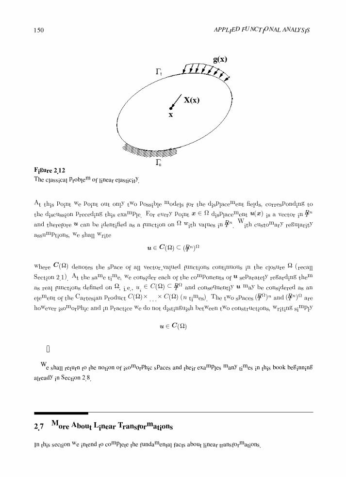
150 APPLIED FUNCTIONAL ANALYSIS
Figure 2.12
The classical problem of linear elasticity.
At this point we point out only two possible models for the displacement fields, corresponding to
the discussion preceding this example. For every point x ∈ Ω displacement u(x) is a vector in IRn
and therefore u can be identified as a function on Ω with values in IRn. With customary regularity
assumptions, we shall write
u ∈ C(Ω) ⊂ (IRn)Ω
where C(Ω) denotes the space of all vector-valued functions continuous in the closure Ω (recall
Section 2.1). At the same time, we consider each of the components of u separately regarding them
as real functions defined on Ω, i.e., ui ∈ C(Ω) ⊂ IRΩ and consequently u may be considered as an
element of the Cartesian product C(Ω)× . . .×C(Ω) (n times). The two spaces (IRΩ)n and (IRn)Ω are
however isomorphic and in practice we do not distinguish between two constructions, writing simply
u ∈ C(Ω)
We shall return to the notion of isomorphic spaces and their examples many times in this book beginning
already in Section 2.8.
2.7 More About Linear Transformations
In this section we intend to complete the fundamental facts about linear transformations.

Linear Algebra 151
Composition of Linear Transformations . Let U, V , and W be vector spaces and let T : U → V and
S : V →W denote two linear transformations from U and V into V andW , respectively. It follows from the
definition of linear transformation that the composition (called also the product) of transformations ST : U →
W defined by
ST (u) = S(T (u))
is also linear.
Let us note that only in the case when the three spaces coincide, i.e., U = V = W , does it make sense to
speak about both compositions ST and TS simultaneously. In general
ST = TS
i.e., composition of linear transformations is generally not commutative.
Inverse of a Linear Transformation . Let V andW be two vector spaces and T : V → W be an isomor-
phism, i.e., a bijective linear transformation. Then the inverse function T−1 : W → V is also linear. Indeed,
let w1 and w2 denote two arbitrary vectors in W . T is bijective so there exist vectors v1 and v2 such that
T (v1) = w1, T (v2) = w2. We have
T−1(α1w1 + α2w2) = T−1(α1T (v1) + α2T (v2))
= T−1(T (α1v1 + α2v2)) = α1v1 + α2v2
= α1T−1(w1) + α2T
−1(w2)
so T−1 is linear.
Projection. We are familiar with the concept of a projection from elementary notions of geometry. For
example, the projection of a directed line segment on a plane can be roughly visualized as the “shadow” it
casts on the plane. For example, a film is used with a movie projector to project a three-dimensional image
on a two-dimensional screen. In much the same way, we speak here of functions that project one linear space
onto another or, more specifically, onto a subspace of possibly lower dimension. What is the essential feature
of such projections? In the case of the shadow produced as the projection of a line, the shadow is obviously
the image of itself; in other words, if P is a projection, and P (v) is the image of a vector v and P , then the
image of this image under P is precisely P (v).
We make these concepts precise by formally introducing the following definition: A linear transformation
P on a vector space V into itself is a projection if and only if
P 2 = P P = P
i.e., if P (v) = w, then P (w) = P (P (v)) = P 2(v) = w.
The following proposition shows that the definition does, in fact, imply properties of projections that are
consistent with our intuitive ideas of projections.

152 APPLIED FUNCTIONAL ANALYSIS
PROPOSITION 2.7.1
(Characterization of a Projection)
The following conditions are equivalent:
(i) T : V → V is a projection.
(ii) There exist subspaces X and Y such that V = X ⊕ Y , and T (v) = x, where v = x + y,x ∈
X,y ∈ Y is the unique decomposition of v.
PROOF (ii) ⇒ (i). Let v = x+ y by the unique decomposition of a vector v. Simultaneously
x = x+ 0 is the unique decomposition of vector x. We have
T 2(v) = T (T (v)) = T (x) = x = T (v), i.e., T 2 = T
(i) ⇒ (ii). Define X = R(T ), Y = N (T ). From the decomposition
v = T (v) + v − T (v)
and the fact that T (v − T (v)) = T (v)− T 2(v) = 0 follows that V = X + Y .
Suppose now that v ∈ R(T )∩N (T ). This implies that there existsw ∈ V such that T (w) ∈ N (T ),
i.e., T (T (w)) = 0. But T (T (w)) = T 2(w) = T (w) = v, so v = 0 which proves the assertion.
COROLLARY 2.7.1
Let X be an arbitrary subspace of V . There exists a (not unique) projection T such that X = R(T ).
Example 2.7.1
Let V be the space of free vectors in a plane. Let X and Y denote two arbitrary, different straight
lines which can be identified with two one-dimensional subspaces of V . Obviously V = X ⊕Y . Pick
an arbitrary vector v and denote by T (v) the classical projection along line X in the direction Y
(see Fig. 2.13). Obviously T 2 = T .
Example 2.7.2
Let V = C(Ω) for some bounded domain Ω in IRn. Define T : f → Tf where Tf is a constant
function given by the formula
Tf = meas(Ω)−1
Ω
f(x)dx
Obviously T 2 = T and therefore T is a projection. For the interpretation of N (T ) and R(T ) see
Example 2.2.6.

Linear Algebra 153
Figure 2.13
Example of a projection.
Linear Transformations on Quotient Spaces. Let V,W be vector spaces and T : V → W denote an
arbitrary linear transformation. SupposeM is a linear subspace of V such thatM ⊂ N (T ). Define
T : V/M →W, T ([v]) = T (v)
Transformation T is well-defined and linear. Indeed let v,w ∈ [v]. It implies that v − w ∈ M and
therefore T (v) − T (w) = T (v − w) = 0, so the definition of T is independent of the choice of w ∈ [v].
Linearity of T follows immediately from linearity of T .
COROLLARY 2.7.2
In the most common case we choose M = N (T ). Then T becomes a monomorphism from V/M into
Y .
Example 2.7.3
Let V = X ⊕ Y and let P denote the projection onto Y in the direction of X, i.e., Pv = y, where
v = x+y is the unique decomposition of vector v. Obviously P is surjective andN (T ) coincides with
X. Thus the quotient transformation P : V/X → Y becomes an isomorphism and the two spaces
V/X and Y—the complement of X, are isomorphic. In other words every equivalence class [x] can
be identified with a common “point” of [x] and Y . The concept is illustrated in Fig. 2.14.
Example 2.7.4
Consider again the membrane problem (recall Examples 2.2.3 and 2.3.2) with Γu = ∅. Let W =
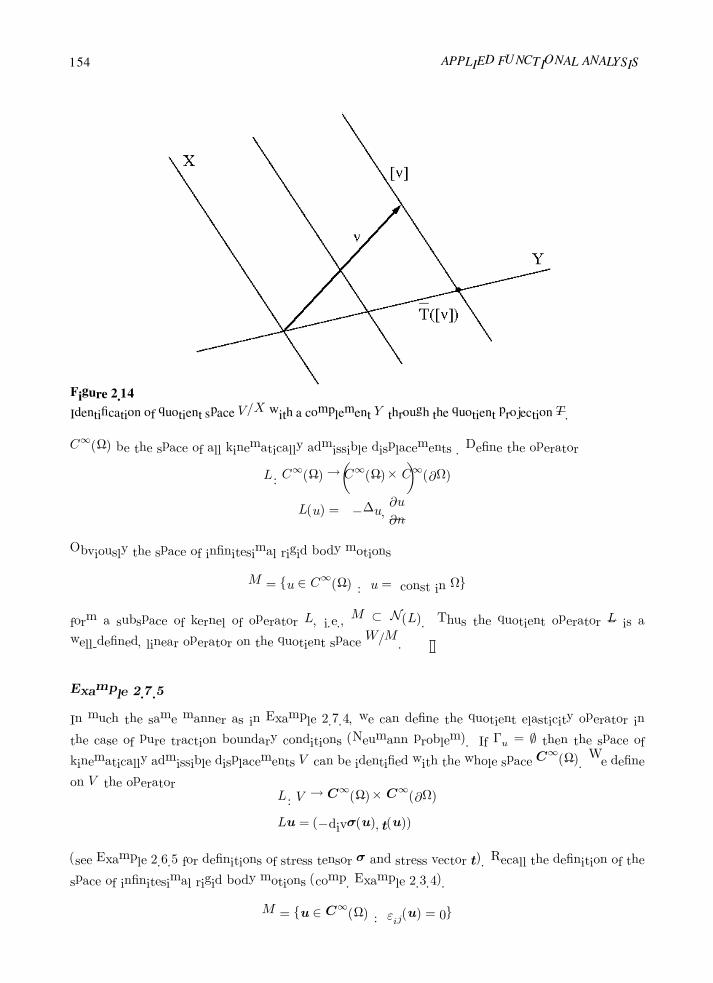
154 APPLIED FUNCTIONAL ANALYSIS
Figure 2.14
Identification of quotient space V/X with a complement Y through the quotient projection T .
C∞(Ω) be the space of all kinematically admissible displacements . Define the operator
L : C∞(Ω)→ C∞(Ω)× C∞(∂Ω)
L(u) =
−∆u,∂u
∂n
Obviously the space of infinitesimal rigid body motions
M = u ∈ C∞(Ω) : u = const in Ω
form a subspace of kernel of operator L, i.e., M ⊂ N (L). Thus the quotient operator L is a
well-defined, linear operator on the quotient space W/M .
Example 2.7.5
In much the same manner as in Example 2.7.4, we can define the quotient elasticity operator in
the case of pure traction boundary conditions (Neumann problem). If Γu = ∅ then the space of
kinematically admissible displacements V can be identified with the whole space C∞(Ω). We define
on V the operatorL : V → C∞(Ω)×C∞(∂Ω)
Lu = (−divσ(u), t(u))
(see Example 2.6.5 for definitions of stress tensor σ and stress vector t). Recall the definition of the
space of infinitesimal rigid body motions (comp. Example 2.3.4).
M = u ∈ C∞(Ω) : εij(u) = 0

Linear Algebra 155
Obviously M ⊂ N (L) and therefore the quotient operator L is well-defined on the quotient space
V/M .
The Space L(X,Y ) of Linear Transformations. We have already learned that for any set Ω the set of
functions defined on Ω with values in a vector space Y, Y Ω forms a vector space. In a very particular case we
can choose for Ω a vector spaceX and restrict ourselves to linear transformations only. A linear combination
of linear transformations is linear as well, so the set of linear transformations from X to Y forms a linear
subspace of Y X . We denote this space by L(X,Y ) or shortly L(X) if X = Y . In the case of X = Y a
new operation can be defined on L(X)–the composition of transformation ST . With this extra operation the
vector space L(X) satisfies axioms of an algebraic structure called linear algebra.
Definition of Linear Algebra. A vector space V over the field IF is called a linear algebra if to vector
addition and multiplication by a scalar a new operation : V × V → V can be added such that the following
axioms hold.(i) (x y) z = x (y z) (associative law)
(ii) (x+ y) z = x z + y z
(iii) z (x+ y) = z x+ z y (distributive laws)
(iv) (αx) y = α(x y) = x (αy)
The first three axioms together with the axioms imposed on the vector addition “+” (comp. Section 2.1)
indicate that with respect to operations “+” and “” V is a ring. Thus roughly speaking V is a linear algebra
(or briefly an algebra) if V is simultaneously a vector space and a ring and the two structures are consistent
in the sense that condition (iv) holds.
Let us check now that the space L(X) satisfies the axioms of linear algebra. Indeed, conditions (i) and
(ii) and the first of equalities in (iv) hold for arbitrary functions, not necessarily linear. In other words the
composition of functions f g is always associative and behaves linearly with respect to the “external”
function f . This follows directly from the definition of the composition of functions. To the contrary, to
satisfy axioms (iii) and the second equality in (iv) we need linearity of f , more precisely, the composition
f g is linear with respect to g if the function f is linear. Indeed, we have
(f (α1g1 + α2g2))(x) = f(α1g1(x) + α2g2(x))
= α1f(g1(x)) + α2f(g2(x))
= (α1(f g1) + α2(f g2))(x)
if and only if function f is linear.
Thus L(X) is an algebra.
Let us finally note that conditions (i)–(iv) and the product of linear transformations itself make sense in a
more general context of different vector spaces. For example, if X,Y , and Z denote three different vector

156 APPLIED FUNCTIONAL ANALYSIS
spaces and f, g ∈ L(Y, Z) and h ∈ L(X,Y ) then
(f + g) h = f h+ g h
Of course, in the case of different spaces we cannot speak about the structure of linear algebra.
The algebraic theory of linear algebras is a separate subject in abstract algebra. We shall not study this
concept further, restricting ourselves to the single example of the space L(X). The main goal of introducing
this definition is a better understanding of the next section which deals with matrices.
Exercises
Exercise 2.7.1 Let V be a vector space and idV the identity transformation on V . Prove that a linear trans-
formation T : V → V is a projection if and only if idV − T is a projection.
2.8 Linear Transformations and Matrices
Most readers are probably familiar with the concept of matrix multiplication and other operations on matrices.
In the most common treatment of this subject, especially in engineering literature, matrices are treated as
tables or columns of objects on which certain simple algebraic operations can be defined. In this section we
shall show the intimate relation between the algebra of matrices and that of linear transformations.
We have already discussed the concept of isomorphic vector spaces: two spaces X and Y are isomorphic
if there exists an isomorphism, i.e., a linear and bijective transformation ι, from X into Y . So far the two
spaces X and Y with their linear structures were given a priori and the bijection ι, when defined, had to be
checked for linearity. One of the most fundamental concepts in abstract algebra is to transfer an algebraic
structure from an algebraic object X onto another set Y through a bijection ι which becomes automatically
an isomorphism. More precisely, let V be a vector space,W an arbitrary set and suppose that there exists a
bijection ι from V ontoW , i.e., we have one-to-one correspondence of vectors from V with elements ofW .
We shall introduce operations inW in the following way:
w1 + w2def= ι(ι−1(w1) + ι−1(w2))
αwdef= ι(αι−1(w))
In other words, in order to add two elementsw1 andw2 inW we have to find their counterparts v1 = ι−1(w1)
and v2 = ι−1(w2) in V first, then add v1 to v2 and next find the image of v1 + v2 through bijection ι. The
concept is illustrated in Fig. 2.15. In the same way we interpret the multiplication by a scalar.

Linear Algebra 157
Figure 2.15
Transfer of vector addition through a bijection ι.
We leave for the reader the lengthy but trivial verification thatW with such defined operations satisfies the
axioms of a vector space. Moreover it follows from the definition of operations in W that ι is linear. Thus
V andW become two isomorphic vector spaces. If additionally V is a linear algebra we can transfer in the
same way the multiplication from V defining the multiplication inW by
w1 w2def= ι(ι−1(w1) ι
−1(w2))
ThenW becomes a linear algebra too, and ι is an isomorphism of two algebras V andW .
For the rest of this section we shall assume that we deal with only finite-dimensional spaces. Studying
linear transformations in Section 2.5, we have found that there exists a one-to-one correspondence between
linear transformations and matrices. More precisely ifX and Y are two vector spaces, dimX = n, dimY =
m, and (e1, . . . , en), (f1, . . . ,fm) denote bases inX and Y respectively, then a transformation T : X → Y
is linear if and only if T is of the form
T (x) =m
i=1
n
j=1
Tijxj
f i
i.e., if y = T (x) is a value of T for x and yi denote the components of y with respect to basis f i, then
yi =n
j=1
Tijxj i = 1, . . . ,m
Recall that the j-th column of matrix Tij indicates components of T (ej) with respect to basis f i, i.e.,
T (ej) =
m
i=1
Tijf i
We shall now use the bijection between linear transformations and matrices to define the operations on
matrices.

158 APPLIED FUNCTIONAL ANALYSIS
Multiplication by a Scalar. Obviously
(αT )(ej) = α(T (ej)) = αm
i=1
Tijf i =m
i=1
(αTij)f i
and therefore we define the product of a scalar α and matrix Tij as a new matrix which is obtained by
multiplying elements of Tij by scalar α.
Matrix Addition. Similarly,
(T +R)(ej) = T (ej) +R(ej) =
m
i=1
Tijf i +
m
i=1
Rijf i =
m
i=1
(Tij +Rij)f i
and consequently we add two matrices element by element.
Matrix Multiplication. Suppose we are given a third vector space Z with a basis (g1, . . . , gl) and two
linear transformations T : X → Y,R : Y → Z with representations Tij and Rki respectively. Let us denote
S = R T and try to calculate the corresponding representation Skj . We have
k=1
Skjgk = S(ej) = R(T (ej)) = R
m
i=1
Tijf i
=
m
i=1
TijR(f i)
=
m
i=1
Tij
k=1
Rkigk =
k=1
m
i=1
RkiTij
gk
and therefore by a direct comparison of both sides we get the product formula for matrices:
Skj =
m
i=1
RkiTij
Thus in order to multiply matrix Tij by matrix Rki we need to multiply rows of Rki by columns of Tij . The
well-known formula gets its natural explanation.
According to our construction the set of matrices m × n with operations defined above forms a vector
space and in the case of square matrices (m = n) has a structure of linear algebra. The two spaces (algebras):
the space (algebra) of linear transformations L(X,Y ) (L(X,X)) and the space of matrices m × n (square
matrices) become isomorphic. All notions and facts concerning transformations may be transferred to matri-
ces and, consequently, everything that is known for matrices may be reinterpreted in terms of corresponding
transformations. We shall return to this one-to-one correspondence many times. For the beginning let us
record a few fundamental facts.
Noncommutativity of Product of Transformations. It is easy to construct two square matrices A and B
such thatn
k=1
AikBkj =n
k=1
BikAkj
(comp. Exercise 2.11.3) and therefore the multiplication of matrices is generally noncommutative. Conse-
quently product of transformations does not commute as well.

Linear Algebra 159
Rank of Matrix. Let T : X → Y be a linear transformation and Tij the corresponding matrix. We define
by the rank of matrix Tij , the rank of corresponding transformation T , i.e., the dimension of the image space
R(T ). We have the following simple observation.
PROPOSITION 2.8.1
Rank of a matrix Tij , i = 1, . . . ,m, j = 1, . . . , n is equal to the maximal number of linearly indepen-
dent column vectors (treated as vectors in IRm).
PROOF Obviously, rank of the corresponding transformation T equals the maximal number of
linearly independent vectors T (ej) where ej denotes a basis in vector space X. Since the column
vectors are precisely the components of T (ej) with respect to basis f i, and IRm is isomorphic with
Y through any basis (f i in particular), the number of linearly independent column vectors must be
precisely equal to the number of linearly independent vectors T (ej), j = 1, . . . , n.
Inverse of a Matrix. Let dimX = dimY = n and let T be an isomorphism, i.e., a one-to-one linear
transformation fromX to Y . Let Tij be a representation of transformation T with respect to bases ej and f i.
Since T is invertible, we may speak about a representation T−1ji of its inverse T−1. Matrix T−1
ji is called the
inverse matrix of matrix Tij . According to the product formula for matrix multiplication we have equivalently
n
k=1
TikT−1kj =
n
k=1
T−1jk Tki = δij
which follows from the definition of the inverse transformation
TT−1 = idY , T−1T = idX
and the fact that the matrix representation for the identity transformation (in every space, with respect to any
basis) can be visualized as the Kronecker’s symbol.
2.9 Solvability of Linear Equations
One of the fundamental problems following the concept of the linear transformation is that of solvability of
linear equations. Suppose we are given spacesX and Y and a linear transformation T : X → Y . For a given
vector y ∈ Y we may ask two fundamental questions:
(i) Does an element x ∈ X exist, such that
Tx = y

160 APPLIED FUNCTIONAL ANALYSIS
(ii) Is such an element unique?
The above equation is called a linear equation for x and the two questions deal with problems of existence
and uniqueness of solutions for one specific “right-hand” y or for every y ∈ Y . Let us record some simple
observations:
(i) If T is an isomorphism, then there exists a unique solution x = T−1y for an arbitrary vector y.
(ii) For a given y there exists a solution x if and only if y ∈ R(T ).
(iii) A solution x is unique if and only if T is injective or equivalently N (T ) = 0.
The trivial observations gain their important interpretation in the context of finite-dimensional spaces. More
precisely if ej , j = 1, . . . , n,f i, i = 1, . . . ,m denote bases in X and Y , respectively, Tij is the matrix
representation of T , the linear equation Tx = y is equivalent to the system of m linear algebraic equations
of n unknowns in the form
T11x1 + T12x2 + . . .+ T1nxn = y1
...
Tm1x1 + Tm2x2 + . . .+ Tmnxn = ym
Let us discuss some particular cases:
1. Number of equations equals number of unknowns, m = n. If matrix Tij is nonsingular, i.e., transfor-
mation T is an isomorphism (which is equivalent to saying that detTij = 0), the system of equations
possesses a unique solution for an arbitrary right-hand side vector yi, i = 1, . . . ,m. In particular for a
homogeneous system of equations (zero right-hand side) the only solution is trivial, the zero vector.
If matrix Tij is singular then N (T ) = 0 and a solution, if it exists, is never unique. Since dimX =
n = dimN (T ) + dimR(T ), dimR(T ) < n and consequently R(T ) ⊆Y (range is a strict subset of
codomain) which implies that the system of equations has a solution only for some right-hand side
vectors y.
A necessary and sufficient condition for existence of solutions may be formulated using the notion of
the rank of matrix. Toward this goal let us note that the range space R(T ) is generated by vectors
T (ej), j = 1, . . . , n and consequently the system has a solution if and only if vector y belongs to
R(T ) or, equivalently, the dimension of a space generated by both vectors T (ej), j = 1, . . . , n and the
vector y equals dimension ofR(T ), i.e., the rank of T . This is equivalent to saying that rank of matrix
Tij must be equal to the rank of the so-called augmented matrix, i.e., matrix Tij with added vector yi:
T11 . . . T1n y1
...
Tm1 . . . Tmn ym

Linear Algebra 161
2. Number of equations is smaller than number of unknowns. From the fundamental identity n =
dimN (T ) + dimR(T ) follows that such a system must be dimN (T ) > 0 and therefore such a
system never has a unique solution. Again, ranks of the matrix Tij and its augmented counterpart can
be compared to determine whether a solution exists.
3. Number of equations is bigger than number of unknowns. Again, it follows from the fundamental
identity that the range space must be a proper subspace of Y , i.e., a solution exists only for some
right-hand sides yi. For a verification we may once again compare the ranks of matrix Tij and Tij
augmented.
The Moore-Penrose Inverse. One way to define a “solution” to the matrix equation Tx = y even when
y /∈ R(T ), is to find an x ∈ X which minimizes the discrepancy between Tx and y measured in the
Euclidean norm,
x ∈ IRn, y − Tx2 → min
where z2 =n
i=1 z2i (norms will be studied in detail in Chapter 5). Differentiating function
F (x1, . . . , xn) =
n
i=1
(yi −
n
j=1
Tijxj)2
with respect to xk, we obtain
∂F
∂xk= 2(yi −
n
j=1
Tijxj)(−
n
j=1
Tijδjk) = 0
or, in the matrix form,
T TTx = T Ty
This system is known as the normal equation for the least-squares problem. If T TT is invertible,
x = T †y
where
T † = (T TT )−1T T
The matrix T † is known as the Moore-Penrose inverse of T . Thus, if T TT is invertible, † we can solve the
system Tx = y at least approximately.
Exercises
Exercise 2.9.1 Equivalent and Similar Matrices. Given matricesA andB, when nonsingular matrices P
andQ exist such that
B = P−1AQ
†This is equivalent to the condition that all singular values of matrix T are non-zero, comp. Example 5.6.2.

162 APPLIED FUNCTIONAL ANALYSIS
we say that the matricesA andB are equivalent. IfB = P−1AP , we sayA andB are similar.
LetA andB be similar n× n matrices. Prove that detA = detB, r(A) = r(B), n(A) = n(B).
Exercise 2.9.2 Let T1 and T2 be two different linear transformations from an n-dimensional linear vector
space V into itself. Prove that T1 and T2 are represented relative to two different bases by the same
matrix if and only if there exists a nonsingular transformation Q on V such that T2 = Q−1T1Q.
Exercise 2.9.3 Let T be a linear transformation represented by the matrix
A =
1 −1 4
0 3 2
relative to bases a1,a2 of IR2 and b1, b2, b3 of IR
3. Compute the matrix representing T relative to
the new bases:
α1 = 4a1 − a2 β1 = 2b1 −b2 +b3
α2 = a1 + a2 β2 = b1 −b3
β3 = b1 +2b2
Exercise 2.9.4 LetA be an n× n matrix. Show that transformations which
(a) interchange rows or columns ofA
(b) multiply any row or column ofA by a scalar = 0
(c) add any multiple of a row or column to a parallel row or column
produce a matrix with the same rank asA.
Exercise 2.9.5 Let a1,a2 and e1, e2 be two bases for IR2, where a1 = (−1, 2),a2 = (0, 3), and
e1 = (1, 0), e2 = (0, 1). Let T : IR2 → IR2 be given by T (x, y) = (3x− 4y, x+ y). Find the matrices
for T for each choice of basis and show that these matrices are similar.
Algebraic Duals
2.10 The Algebraic Dual Space, Dual Basis
Let V denote a vector space over a field IF . A mapping f from V into IF is called a functional on V . If f is
additionally linear (IF is obviously a vector space over itself) we speak of a linear functional on V .

Linear Algebra 163
The Algebraic Dual Space. We recall that ifW is a vector space and A an arbitrary set then the space of
functions defined on A with values inW, denotedWA, forms a new vector space. Since IF is a vector space
over itself, the space of linear functionals on V, L(V, IF ) is a vector space, too. This vector space is denoted
V ∗ and is called the algebraic dual of V .
Example 2.10.1
A familiar example of a linear functional is found in connection with the space of all real-valued
and continuous functions in the closure of a bounded domain Ω ⊂ IRn, the space C(Ω). Since such
functions are Riemann integrable, it makes sense to define a linear transformation T in the form
T (f) =
Ω
g(x)f(x) dx
where g is a given function from C(Ω). Clearly T is a linear functional on C(Ω).
Example 2.10.2
Consider again the space C(Ω). Pick an arbitrary point x ∈ Ω and define a functional
δx(f) = f(x)
This functional, called Dirac’s functional or shortly Dirac’s delta at point x, plays a fundamental
role in the theory of distributions.
More generally, given a finite sequence of points xj ∈ Ω, j = 1, . . . ,m we can define a linear
functional on C(Ω) in the form
T (f) =m
j=1
αjf(xj)
Obviously, T is a linear combination of the corresponding Dirac deltas at points xj .
Example 2.10.3
The Dirac functional can be “applied” to a function or to its derivatives as well. Consider for
instance the space Ck(Ω), a point x ∈ Ω and a multi-index α ∈ IZn, |α| = k. The following is a
linear functional on Ck(Ω):
T (f) = Dαf(x)
The General Form of a Linear Functional in Finite-Dimensional Spaces. Let V be a finite-dimensional
space, dimV = n, with a basis (e1, . . . , en) and consider an arbitrary linear functional f ∈ V ∗. We have
f(v) = f
n
i=1
viei
=
n
i=1
vif(ei) =
n
i=1
fivi

164 APPLIED FUNCTIONAL ANALYSIS
where fidef= f(ei). Conversely, any functional of this form is linear and therefore the formula above con-
stitutes the general form of a linear functional in finite-dimensional space V . Entire information about the
functional is stored in the sequence of n numbers, fi being equal to the values of f on arbitrary basis ei.
As a particular choice for every j = 1, . . . , n we can define a linear functional e∗j by setting
e∗j (ei) = δij
Consequently
e∗j (v) = e∗j
n
i=1
viei
=
n
i=1
vie∗j (ei) =
n
1
viδij = vj
and e∗j can be interpreted as a functional prescribing for a vector v its j-th component with respect to basis
ei.
We have the following simple observation.
PROPOSITION 2.10.1
Functionals e∗j form a basis in dual space V ∗.
PROOF Indeed, every functional f ∈ V ∗ can be represented in the form
f(v) =n
1
vifi =
n
1
e∗i (v)fi
i.e.,
f =n
1
fie∗i
and therefore e∗i span V ∗. To prove the linear independence consider a linear combination
n
1
αje∗j = 0
We have
0 =
n
1
αje∗j
(ei) =
n
1
αje∗j (ei) =
n
1
αjδij = αi
for every i = 1, . . . , n, which proves that e∗j are linearly independent.
Basis e∗jnj=1 is called the dual (reciprocal, biorthogonal) basis to basis ei
ni=1. In particular, Propo-
sition 2.10.1 implies that dimV ∗ = dimV = n. As two finite-dimensional spaces of the same dimension,
V and its dual V ∗ are isomorphic and each linear functional could be identified with a specific element in
V . Such an identification, though possible, is not unique (it depends on a particular choice of a basis). By
choosing to distinguish V ∗ from V we will have a chance to uncover a variety of interesting properties.

Linear Algebra 165
Bilinear Functionals. Given two vector spaces, V andW , we may consider a functional “a” of two vari-
ables
a : V ×W → IF (IR or IC), a(v, w) ∈ IF
Functional a is called bilinear if it is linear with respect to each of the variables separately. In the case when
V = W we speak of bilinear functionals defined on V . The notion can be easily generalized to the case of
multilinear (m-linear) functionals defined on V1 × . . .× Vm or in the case V1 = V2 = . . . = Vm, simply on
V .
Example 2.10.4
Consider again the space C1(Ω). The following are examples of bilinear functionals.
a(u, v) =
Ω
n
i,j=1
aij(x)Diu(x)Djv(x)dx
+
Ω
n
i=1
bi(x)Diu(x)dx+
Ω
c(x)u(x)v(x)dx
a(u, v) = u(x)v(x)
The General Form of a Bilinear Functional in Finite-Dimensional Spaces. Let V andW be two finite-
dimensional spaces, dimV = n, dimW = m, and (e1, . . . , en) and (g1, . . . , gm) denote two bases in V
andW respectively. Let a : V ×W → IR denote an arbitrary bilinear functional. Representing vectors v ∈ V
and w ∈W in the bases we get
a(v,w) = a
n
1
viei,w
=
n
1
via(ei,w)
=
n
1
via
ei,
m
1
wjgj
=
n
1
vi
m
1
wja(ei, gj)
Conversely, setting arbitrary values of a functional a on bases ei, gj we easily check that the functional of
the form above is bilinear. Thus, introducing notation
aij = a(ei, gj)
we get the representation formula for bilinear functionals in finite-dimensional spaces:
a(v,w) =n
i=1
m
j=1
aijviwj
Space of Bilinear Functionals M(X,Y ). Given two vector spaces X and Y , we denote the set of all
bilinear functionals defined on X × Y byM(X,Y ). Obviously a linear combination of bilinear functionals
is bilinear as well and thereforeM(X,Y ) is a vector space.

166 APPLIED FUNCTIONAL ANALYSIS
Duality Pairing. Given a vector space V and its dual V ∗ we define the duality pairing as the functional
V ∗ × V (f,v)→ < f,v >def= f(v) ∈ IR(IC)
It follows from the definition of function addition that the duality pairing is linear with respect to the first
variable and from linearity of functionals f that it is linear with respect to the second variable. Thus the
duality pairing is a bilinear functional on V ∗ × V . Two easy properties follow from the definition.
PROPOSITION 2.10.2
The following properties hold:
(i) < f,v >= 0 ∀v ∈ V implies f = 0.
(ii) < f,v >= 0 ∀f ∈ V ∗ implies v = 0.
We say that the duality pairing is definite.
PROOF
(i) follows trivially from the definition of duality pairing. To prove (ii) assume in contrary that
there exists a v = 0 such that < f,v > = 0 for every f ∈ V ∗. Consider a direct sum
V = IRv ⊕W
where W is a complement of one-dimensional subspace IRv. Setting f(v) = 1, f ≡ 0 on W we extend
f by linearity
f(αv + w) = αf(v) + f(w) = α
and therefore f is a well-defined linear functional on V . Obviously, f(v) = 0, which contradicts the
assumption.
Orthogonal Complement. Let U be subspace of a vector space V . Due to bilinearity of duality pairing,
the set
v∗ ∈ V ∗ : < v∗,v > = 0 for every v ∈ U
is a linear subspace of V ∗. We call it the orthogonal complement of U and denote it by U⊥. Thus
< v∗,v > = 0 for every v∗ ∈ v⊥,v ∈ U
Similarly, ifW is a subspace of V ∗ the set (space) of all such vectors v ∈ V that
< v∗,v > = 0 for every v∗ ∈W
denoted W⊥, is called the orthogonal complement of W . In other words, if W ⊂ V ∗ is the orthogonal
complement of U ⊂ V , then U is the orthogonal complement ofW .

Linear Algebra 167
PROPOSITION 2.10.3
Let vector space X be decomposed into subspaces U and V ,
X = U ⊕ V
Then,
X∗ = V ⊥ ⊕ U⊥
Moreover, if subspace U is finite-dimensional then dimV ⊥ = dimU . In particular, if X is finite-
dimensional then dimU⊥ = dimX − dimU .
PROOF Let x = u + v, u ∈ U, v ∈ V be the unique decomposition for a vector x ∈ X. Given
f ∈ V ∗, define :
g(x) = f(u), h(x) = f(v)
Then g ∈ V ⊥, and h ∈ U⊥, and,
f(x) = f(u) + f(v) = g(x) + h(x)
so X∗ = V ⊥ + U⊥. The common part of V ⊥ and U⊥ is trivial since, if f ∈ V ⊥ ∩ U⊥ then
f(x) = f(u) + f(v) = 0
Assume now that U is finite-dimensional, and that e1, . . . , en is a basis for U . Define e∗i ∈ V ⊥ by
requesting the orthogonality condition,
e∗i (ej) = δij
Functionals e∗i are linearly independent. Indeed, assume that
n
i=1
αie∗i = 0
By evaluating both sides at x = ej , we get
n
i=1
αie∗i
(ej) =
n
i=1
αie∗i (ej) =
n
i=1
αiδij = αj = 0
Notice that, for u ∈ U ,
e∗i (u) = e∗i
n
j=1
ujej
=n
j=1
ujδij = ui
To see that e∗i span V ⊥, take an arbitrary f ∈ V ⊥,
f(x) = f(u+ v) = f(u) = f
n
i=1
uiei
=
n
i=1
uif(ei) =
n
i=1
e∗i (u)f(ei) =
n
i=1
e∗i (x)f(ei)
or, in argumentless notation,
f =
n
i=1
f(ei)e∗i

168 APPLIED FUNCTIONAL ANALYSIS
Bidual Space. Having defined the dual space V ∗ we are tempted to proceed in the same manner and define
the (algebraic) bidual as the dual of the dual space, i.e.,
V ∗∗ def= (V ∗)∗
Proceeding in the same way, we could introduce the “three stars,” “four stars,” etc., spaces. This approach,
though theoretically possible, has (fortunately!) only a little sense in the case of finite-dimensional spaces,
since it turns out that the bidual space V ∗∗ is in a natural way isomorphic with the space V .
PROPOSITION 2.10.4
The following map is an isomorphism between a finite-dimensional vector space V and its bidual V .
ι : V v → V ∗ v∗ →< v∗,v >∈ IR(IC) ∈ V ∗∗
PROOF Due to linearity of v∗ the functional
V ∗ v∗ →< v∗,v >∈ IR(IC)
(called the evaluation at v) is linear and therefore map ι is well-defined. Checking for linearity we
have
v∗ →< v∗, α1v1 + α2v2 > = α1v∗ →< v∗, v1 >+ α2v
∗ →< v∗,v2 >
Map ι is also injective since < v∗,v > = 0 for every v∗ ∈ V ∗ implies that (Proposition 2.10.2) v = 0.
Since all the spaces are of the same dimension, this implies that ι is also surjective which ends the
proof.
Thus, according to Proposition 2.10.4 in the case of a finite-dimensional space V , we identify bidual V ∗∗
with the original space V , “tridual” V ∗∗∗ with dual V ∗, etc. The two spaces V and its dual V ∗ (the “lone star
space”) with the duality pairing < v∗,v > are treated symmetrically.
An Alternative Definition of the Dual Space. For real vector spaces, the duality pairing generalizes the
concept of a scalar (inner) product discussed later in this chapter. For complex spaces, however, the two
notions are at odds with each other as the duality pairing is linear with respect to the second argument,
whereas the inner product is not. In order to alleviate this conflict, we frequently introduce an alternative
definition of the dual space as the space of antilinear functionals. Let V,W be complex vector spaces. A
function A : V →W is said to be antilinear if A is additive and
A(αv) = αAv

Linear Algebra 169
where α denotes the complex conjugate of α. Equivalently,
A(αu+ βv) = αAu+ βAv
A linear combination of antilinear functions is antilinear, so the antilinear functions form a vector space,
denoted L(V,W ). In the particular, the space of antilinear functionals L(V, IC) is frequently identified as the
algebraic dual of space V , denoted by the same symbol V ∗ as before. Obviously, both definitions coincide
with each other for the case of real vector spaces. It is a bit confusing, but one has to figure out from the
context which definition is in use.
The majority of the results discussed in this section remains the same for the new definition of the dual
space. We will point out now to few small differences. The general form of an antilinear functional defined
on a finite-dimensional vector space V will involve now complex conjugates. Indeed, let e1, . . . , en be a
basis for V . We have
f(v) = f(n
i=1
viei) =
n
i=1
vif(ei) =
n
i=1
fivi
where fidef= f(ei). The dual basis functionals e
∗j do not return j-th component of vector v but its complex
conjugate instead,
e∗j (v) = e∗j
n
i=1
viei
=
n
i=1
vie∗j (ei) = vi
Corresponding to notion of a bilinear functional is the concept of a sesquilinear functional. A functional
f : V × W → IC, defined on complex spaces V,W is said to be sesquilinear if it is linear with respect
to the first argument and antilinear with respect to the second argument. We arrive naturally at the notion
when developing various weak formulations for linear boundary-value problems involving complex-valued
solutions, e.g., for vibration or wave propagation problems. By placing the complex conjugate over the test
functions, we obtain sesquilinear rather than bilinear functionals. For instance, the following is a sesquilinear
functional defined on space C1(Ω),
b(u, v) =
Ω
n
i,j=1
aij(x)Diu(x)Djv(x) dx
=
Ω
n
i,j=1
aij(x)Diu(x)Djv(x) dx
The general form of a sesquilinear functional b defined on complex spaces V,W with bases ei, gj will involve
now complex conjugates over components with respect to basis gj ,
b(v,w) =
n
i=1
m
j=1
bijviwj
where bijdef= b(ei, gj).
Finally, the duality pairing will now be a sesquilinear functional,
V ∗ × V (f,v)→< f,v >def= f(v) ∈ IC

170 APPLIED FUNCTIONAL ANALYSIS
All the remaining properties discussed in this section remain unchanged.
Exercises
Exercise 2.10.1 Consider the canonical basis e1 = (1, 0), e2 = (0, 1) for IR2. For x = (x1, x2) ∈ IR2, x1, x2
are the components of x with respect to the canonical basis. The dual basis functional e∗j returns the
j-th component:
e∗j : IR2 (x1, x2)→ xj ∈ IR
Consider now a different basis for IR2, say a1 = (1, 1),a2 = (−1, 1). Write down the explicit formulas
for the dual basis.
Exercise 2.10.2 Let V be a finite-dimensional vector space, and V ∗ denote its algebraic dual. Let ei, i =
1, . . . , n be a basis in V , and e∗j , j = 1, . . . , n denote its dual basis. What is the matrix representation
of the duality pairing with respect to these two bases? Does it depend upon whether we define the dual
space as linear or antilinear functionals?
Exercise 2.10.3 Let V be a complex vector space. Let L(V, IC) denote the space of linear functionals defined
on V , and let L(V, IC) denote the space of antilinear functionals defined on V . Define the (complex
conjugate) map C as,
C : L(V, IC) f → f ∈ L(V, IC), f(v)def= f(v)
Show that operator C is well-defined, bijective, and antilinear. What is the inverse of C?
Exercise 2.10.4 Let V be a finite-dimensional vector space. Consider the map ι from V into its bidual space
V ∗∗, prescribing for each v ∈ V the evaluation at v, and establishing the canonical isomorphism
between space V and its bidual V ∗∗. Let e1, . . . , en be a basis for V , and let e∗1, . . . , e
∗n be the
corresponding dual basis. Consider the bidual basis, i.e., the basis e∗∗i , i = 1, . . . , n in the bidual
space, dual to the dual basis, and prove that
ι(ei) = e∗∗i
2.11 Transpose of a Linear Transformation
Transpose of a Linear Transformation. Let V andW be two vector spaces over the same field IF and T
denote an arbitrary linear transformation from V intoW . Denoting byW ∗ and V ∗ algebraic duals toW and

Linear Algebra 171
V respectively, we introduce a new transformation TT from the algebraic dual W ∗ into algebraic dual V ∗
defined as follows:
TT : W ∗ → V ∗, TT (w∗) = w∗ T
Transformation TT is well defined, i.e., compositionw∗ T defines (due to linearity of both T and functional
w∗) a linear functional on V . TT is also linear. Transformation TT is called the transpose of the linear
transformation T . Using the duality pairing notation we may express the definition of the transpose in the
equivalent way:TTw∗,v
= w∗, Tv ∀ v ∈ V,w∗ ∈W
Let us note that the transpose TT acts in the opposite direction to T ; it maps dualW ∗ into dual V ∗. We may
illustrate this by the following simple diagram:
VT−→ W
V ∗ TT
←− W ∗
A number of algebraic properties of transpose transformations are easily proved:
PROPOSITION 2.11.1
(i) Let T and S ∈ L(V,W ). Then
(αT + βS)T = αTT + βST
(ii) If T ∈ L(U, V ) and S ∈ L(V,W ), then
(S T )T = TT ST
(iii) If idV denotes the identity transformation on V , then
(idV )T = idV ∗
where idV ∗ is the identity transformation on V ∗.
(iv) Let T ∈ L(V,W ) be an isomorphism, i.e., T−1 exists. Then (TT )−1 exists too, and
(TT )−1 = (T−1)T
PROOF The first three assertions follow immediately from the definition of the transpose. For
instance, to prove the second one, we need to notice that
(S T )T (w∗) = w∗ S T = (w∗ S) T = (STw∗) T
= TT (STw∗) = (TT ST )(w∗)
172 APPLIED FUNCTIONAL ANALYSIS
From the second and third statements it follows that
idV ∗ = (idV )T = (T−1 T )T = TT (T−1)T
and similarly
idW∗ = (T−1)T TT
which proves that (TT )−1 exists and is equal to (T−1)T .
PROPOSITION 2.11.2
Let A ∈ L(X,Y ) be a linear transformation with a finite rank.‡ Then
rankAT = rankA
PROOF The result follows from the fundamental equality between the null space of the transpose
operator AT and the orthogonal complement of range of operator A.
y∗ ∈ N (AT ) ⇔ < AT y∗, x >X∗×X= 0 ∀x ∈ X
⇔ < y∗, Ax >Y ∗×Y = 0 ∀x ∈ X
⇔ y∗ ∈ R(A)⊥
Let space Y be decomposed into the range of operator A and an algebraic complement,
Y = R(A)⊕ V
Then, by Proposition 2.10.3 and the relation above,
Y ∗ = V ⊥ ⊕R(A)⊥ = V ⊥ ⊕N (AT )
and dimV ⊥ = dimR(A). But AT restricted to V ⊥ is injective, and it maps V ⊥ onto the whole range
of the transpose. In other words, V ⊥ is isomorphic with the range of the transpose from which the
equality of dimensions follows.
Matrix Representation of a Transpose in Finite Dimensional Spaces . LetX and Y be finite-dimensional
spaces with corresponding bases a1, . . . ,an and b1, . . . , bm, respectively. Let T ∈ L(X,Y ) and let Tij
denote the corresponding matrix representation for T , i.e.,
Tij = b∗i , T (aj)
‡Notice that space Y need not be finite-dimensional.

Linear Algebra 173
A natural question arises: What is a matrix representation of the transpose TT ? The matrix representation
depends obviously on the choice of bases. The natural choice for X∗ and Y ∗ are the dual bases a∗j and b∗i .
Since every basis can be identified with its bidual we have
TTji =
a∗∗j , TT (b∗i )
=TT (b∗i ),aj
= b∗i , T (aj) = Tij
Thus, as we might have expected from previous comments and nomenclature itself, the matrix representation
of transpose TT (in dual bases) is obtained by interchanging rows and columns of the matrix representing T .
If A is the matrix corresponding to T , the one corresponding to TT is the transpose matrix, denoted AT . As
usual, all properties of transformations can be reinterpreted in terms of matrices.
PROPOSITION 2.11.3
(i) Let A,B ∈ Matr(n,m). Then (αA+ βB)T = αAT + βBT .
(ii) Let A ∈ Matr(k, n),B ∈ Matr(n,m). Then (BA)T = ATBT .
(iii) Let 1 be the identity matrix, 1 ∈ Matr (n, n). Then
1T = 1
(iv) Let A ∈ Matr(n, n) and suppose that A−1 ∈ Matr(n, n) exists. Then
(A−1)T = (AT )−1
(v) Let A ∈ Matr(n,m). Then rank AT = rank A.
Exercises
Exercise 2.11.1 The following is a ”sanity check” of your understanding of concepts discussed in the last
two sections. Consider IR2.
(a) Prove that a1 = (1, 0), a2 = (1, 1) is a basis in IR2.
(b) Consider a functional f : IR2 → IR, f(x1, x2) = 2x1 + 3x2. Prove that the functional is linear,
and determine its components in the dual basis a∗1, a∗2.
(c) Consider a linear map A : IR2 → IR2 whose matrix representation in basis a1, a2 is
1 01 2
Compute the matrix representation of the transpose operator with respect to the dual basis.
Exercise 2.11.2 Prove Proposition 2.11.3.

174 APPLIED FUNCTIONAL ANALYSIS
Exercise 2.11.3 Construct an example of square matricesA andB such that
(a) AB = BA
(b) AB = 0, but neitherA = 0 norB = 0
(c) AB = AC, butB = C
Exercise 2.11.4 If A = [Aij ] is an m × n rectangular matrix and its transpose AT is the n × m matrix,
ATn×m = [Aji]. Prove that
(i) (AT )T = A.
(ii) (A+B)T = AT +BT .
(iii) (ABC · · ·XY Z)T = ZTY TXT · · ·CTBTAT .
(iv) (qA)T = qAT .
Exercise 2.11.5 In this exercise, we develop a classical formula for the inverse of a square matrix. Let
A = [aij ] be a matrix of order n. We define the cofactor Aij of the element aij of the i-th column of
A as the determinant of the matrix obtained by deleting the i-th row and j-th column ofA, multiplied
by (−1)i+j :
Aij = cofactor aijdef= (−1)i+j
a11 a12 · · · a1,j−1 a1,j+1 · · · a1n
· · · · · ·ai−1,1 ai−1,2 · · · ai−1,j−1 ai−1,j+1 · · · ai−1,n
ai+1,1 ai+1,2 · · · ai+1,j−1 ai+1,j+1 · · · ai+1,n
· · · · · ·an1 an2 · · · an,j−1 an,j+1 · · · ann
(a) Show that
δij detA =
n
k=1
aikAjk, 1 ≤ i, j ≤ n
where δij is the Kronecker delta.
Hint: Compare Exercise 2.13.4.
(b) Using the result in (a), conclude that
A−1 =1
detA[Aij ]
T
(c) Use (b) to compute the inverse of
A =
1 2 21 −1 02 1 3
and verify your answer by showing that
A−1A = AA−1 = I

Linear Algebra 175
Exercise 2.11.6 Consider the matrices
A =
1 0 4 12 −1 3 0
, B =
−1 412 00 1
, C = [1,−1, 4,−3]
and
D =
23
, E =
1 0 2 3−1 4 0 11 0 2 40 1 −1 2
If possible, compute the following:
(a) AAT + 4DTD +ET
(b) CTC +E −E2
(c) BTD
(d) BTBD −D
(e) EC −ATA
(f) ATDC(E − 2I)
Exercise 2.11.7 Do the following vectors provide a basis for IR4?
a = (1, 0,−1, 1), b = (0, 1, 0, 22)
c = (3, 3,−3, 9), d = (0, 0, 0, 1)
Exercise 2.11.8 Evaluate the determinant of the matrix
A =
1 −1 0 41 0 2 14 7 1 −11 0 1 2
Exercise 2.11.9 Invert the following matrices (see Exercise 2.11.5).
A =
1 −11 2
, B =
4 2 12 4 21 2 2
Exercise 2.11.10 Prove that ifA is symmetric and nonsingular, so isA−1.
Exercise 2.11.11 Prove that ifA,B,C, andD are nonsingular matrices of the same order then
(ABCD)−1 =D−1C−1B−1A−1
Exercise 2.11.12 Consider the linear problem
T =
0 1 3 −22 1 −4 32 3 2 −1
, y =
157

176 APPLIED FUNCTIONAL ANALYSIS
(i) Determine the rank of T .
(ii) Determine the null space of T .
(iii) Obtain a particular solution and the general solution.
(iv) Determine the range space of T .
Exercise 2.11.13 Construct examples of linear systems of equations having (1) no solutions, (2) infinitely
many solutions, (3) if possible, unique solutions for the following cases:
(a) 3 equations, 4 unknowns
(b) 3 equations, 3 unknowns
Exercise 2.11.14 Determine the rank of the following matrices:
T =
2 1 4 70 1 2 12 2 6 84 4 14 10
, T 2 =
1 2 1 3 4 42 0 3 2 1 51 1 1 2 1 3
, T 3 =
2 −1 12 0 10 1 1
Exercise 2.11.15 Solve, if possible, the following systems:
(a)4x1 + 3x3 − x4 + 2x5 = 2
x1 − x2 + x3 − x4 + x5 = 1
x1 + x2 + x3 − x4 + x5 = 1
x1 + 2x2 + x3 + x5 = 0
(b)− 4x1 − 8x2 + 5x3 = 1
2x1 − 2x2 + 3x3 = 2
5x1 + x2 + 2x3 = 4
(c)2x1 + 3x2 + 4x3 + 3x4 = 0
x1 + 2x2 + 3x3 + 2x4 = 0
x1 + x2 + x3 + x4 = 0
2.12 Tensor Products, Covariant and Contravariant Tensors
Let A and B be two arbitrary sets. Given two functionals f and g defined on A and B respectively, we can
define a new functional on the Cartesian product A×B, called the product of f and g, as
A×B (x, y)→ f(x)g(y) ∈ IR(IC)

Linear Algebra 177
In the case of vector spaces and linear functionals, this simple construction leads to some very important
algebraic results.
Tensor Product of Linear Functionals. Given two vector spaces X and Y with their duals X∗, Y ∗, we
define the tensor product of two functions as
(x∗ ⊗ y∗)(x,y) = x∗(x)y∗(y) for x ∈ X,y ∈ Y
It is easy to see that the tensor product x∗ ⊗ y∗ is a bilinear functional on X × Y and therefore the tensor
product can be considered as an operation from the Cartesian product X∗ × Y ∗ to the space of bilinear
functionalsM(X,Y )
⊗ : X∗ × Y ∗ (x∗,y∗)→ x∗ ⊗ y∗ ∈M(X,Y )
PROPOSITION 2.12.1
Let X and Y be two vector spaces. The following properties hold
(i) The tensor product operation
⊗ : X∗ × Y ∗ →M(X,Y )
is a bilinear map from X∗ × Y ∗ into M(X,Y )
(ii) If additionally X and Y are finite-dimensional and ei, i = 1, . . . , n and gj , j = 1, . . . ,m denote
two bases for X and Y respectively, with e∗i , g∗j their dual bases, then the set e∗i ⊗ g
∗j forms a
basis for M(X,Y ).
PROOF
(i) The property follows directly from the definition.
(ii) According to the representation formula for bilinear functionals in finite-dimensional spaces,
we have for a ∈M(X,Y )
a(x, y) =
n
i=1
m
j=1
aijxiyj
=
n
i=1
m
j=1
aije∗i (x)g
∗j (y)
=n
i=1
m
j=1
aij(e∗i ⊗ g
∗j )(x,y)
and therefore
a =
n
i=1
m
j=1
aije∗i ⊗ g
∗j

178 APPLIED FUNCTIONAL ANALYSIS
which means that e∗j ⊗ g∗j spans the space M(X,Y ). To prove linear independence assume that
n
1
m
1
aije∗i ⊗ g
∗j = 0
Taking pairs ek, gl consecutively, we get
0 =
n
1
m
1
aij(e∗i ⊗ g
∗j )(eK , gl)
=n
1
m
1
aije∗i (ek)g
∗j (gl)
=n
1
m
1
aijδikδjl = akl
which ends the proof.
REMARK 2.12.1 It follows from Proposition 2.12.1 that
dimM(X,Y ) = dimX dimY
Tensor Product of Finite-Dimensional Vector Spaces. The algebraic properties of spaceM(X,Y ) give
rise to the definition of an abstract tensor product of two finite-dimensional vector spaces. We say that a
vector space Z is a tensor product of finite-dimensional spacesX and Y , denoted Z = X ⊗ Y , provided the
following conditions hold:
(i) There exists a bilinear map
⊗ : X × Y (x,y)→ x⊗ y ∈ X ⊗ Y
(x⊗ y is called the tensor product of vectors x and y).
(ii) If ej , i = 1, . . . , n and gj , j = 1, . . . ,m are two bases forX and Y respectively, then ei⊗gj is a basis
for X ⊗ Y .
Obviously according to Proposition 2.12.1 for duals X∗ and Y ∗, their tensor product can be identified as
M(X,Y ). But what can we say for arbitrary vector spaces X and Y ? Does their tensor product exist? And
if the answer is yes, is it unique? The following proposition answers these questions.
PROPOSITION 2.12.2
Let X and Y be two finite-dimensional spaces. Then the following spaces satisfy the axioms of tensor
product X ⊗ Y .

Linear Algebra 179
(i) M(X∗, Y ∗)–the space of bilinear functionals on X∗ × Y ∗. The tensor product of two vectors
x⊗ y is identified as
x⊗ y : X∗ × Y ∗ (x∗,y∗)→ x∗(x)y∗(y) ∈ IR(IC)
(ii) M∗(X,Y )–the dual to the space M(X,Y ) of bilinear functionals on X × Y .
x⊗ y : M(X,Y ) f → f(x,y) ∈ IR(IC)
(iii) L(X∗, Y )–the space of linear transformations from dual X∗ to space Y .
x⊗ y : X∗ x∗ → x∗,xy ∈ Y
PROOF Proof follows directly from the definition and is left as an exercise.
So, as we can see, the problem is not one of existence but rather with the uniqueness of the tensor product
X ⊗ Y . Indeed, there are many models of the tensor product; but, fortunately, one can show that all of them
are isomorphic. In other words, no matter which of the models we discuss, as long as we deal with (linear)
algebraic properties only, all the models yield the same results.
Covariant and Contravariant Tensors. One can easily generalize the definition of tensor product to more
than two finite-dimensional vector spaces. In particular we can consider a tensor product of a space X with
itself and its dual.
Let X be a finite-dimensional vector space with a basis e1, . . . , en. Elements of the tensor product
X ⊗ . . .⊗X
⊗ X∗ ⊗ . . .⊗X∗
p times q times
are called tensors of order (p, q). A tensor of order (p, 0) is called a contravariant tensor of order p, a tensor
of order (0, q) is a covariant tensor of order q, and if p > 0, q > 0, the tensor is referred to as a mixed tensor.
Let T be a tensor of order (p, q). Using the summation convention we can write
T = Ti1,...,ipj1,...,jq
ei1 ⊗ . . .⊗ eip ⊗ e∗j1 ⊗ . . .⊗ e∗jq
where e∗j is the dual basis. The quantities Ti1,...,ipj1,...,jq
are called components of tensor T with respect to basis
e1, . . . , en.
Obviously, according to the definition just stated, vectors x ∈ X are identified with contravariant tensors
of order 1 while functionals from the dual space are identified with covariant tensors of order 1.
Let ek, k = 1, . . . , n be a basis inX and x ∈ X denote an arbitrary vector. Using the notation for tensors,
we can write
x = xkek

180 APPLIED FUNCTIONAL ANALYSIS
where xk are components of vectorxwith respect to basis ek. One of the fundamental issues in linear algebra,
especially in applications, is to ask about a transformation formula for vector components when the basis is
changed. Toward establishing such a formula, consider a new basis ej , j = 1, . . . , n with a corresponding
representation for x in the form
x = xjej
Thus we have the identity
xj ej = xkek
Applying to both sides the dual basis functional e∗i , we get
xi = xjδij = xj e∗i , ej =e∗i , x
jej=e∗i , x
kek= e∗i , ekx
k
Introducing the matrix
αi··k = e∗i , ek
we obtain the transformation formula for vector components in the form
xi = αi··kx
k
The matrixα = [αi··k] is called the transformation matrix from basis ek to basis ej . Thus in order to calculate
the new components of vector x we must multiply the transformation matrix by old components of the same
vector.
From the formula for the transformation matrix, it follows easily that
ek = αi··kei
Indeed, applying to both sides functional e∗j , we check that
e∗j , ek
= αi·
·k
e∗j , ei
= αi·
·kδj··i = αj·
·k.
Having found the transformation formula for vectors we may seek a corresponding formula for linear
functionals, elements from the dual space X∗. Using tensor notation, we have for an arbitrary functional
f ∈ X∗
f je∗j = f = fke
∗k
Applying both sides to vector ei, we get
f i = f jδij = f j
e∗j , ei
=f je
∗j , ei
= fke
∗k, ei = e
∗k, ei fk = βk·
·i fk
where
βk··i = e∗k, ei
is the transformation matrix from the new basis ei to the old basis ek. Note that this time in order to obtain
the new components of the functional f , we have to multiply the transpose of matrix β by old components
of f . From the formula for the matrix β, it follows that
e∗l = βl··je
∗j

Linear Algebra 181
Indeed, applying both sides to vector ei we check that
e∗l , ei = βl··j
e∗j , ei
= βl·
·i
Finally, from the definition of transformation matrices it follows that matrix β is the inverse matrix of matrix
α. Indeed, from
ek = αi··kei = αi·
·kβl··iel
follows that
βl··iα
i··k = δl··k
which proves the assertion.
We conclude this section with the statement of a general transformation formula for tensors of an arbitrary
order (p, q). For simplicity let us restrict ourselves, for instance, to a tensor of order (2, 1).
Again, let ei and ek be a new and old basis and e∗i , e
∗k denote their duals. For a tensor T of order (2, 1)
we have
T = Tij·
··kej ⊗ ej ⊗ e∗k
and, simultaneously,
T = T lm···n el ⊗ em ⊗ e
∗n
From the transformation formulas for vectors el, e∗n and the properties of tensor product, it follows that
el ⊗ em ⊗ e∗n = αi·
·lαj··mβn·
·k ei ⊗ ej ⊗ e∗k
or, after substitution into the second formula for T ,
T = αi··ια
j··mβn·
·kTιm···n ei ⊗ ej ⊗ e
∗k
Finally, comparing both formulas for T , we get the transformation formula for components of tensor T
Tij·
··k = αi··lα
j··mβn·
·kTιm···n
Note the difference between the multiplication of contra- and covariant indices of tensor T .
2.13 Elements of Multilinear Algebra
We present foundations of multilinear algebra leading to the definition of determinant and its properties.
182 APPLIED FUNCTIONAL ANALYSIS
Multilinear Functionals. We begin with a generalization of the concept of bilinear functionals to more
variables. Let V1, . . . , Vm bem vector spaces. A functional
V1 × · × Vm (v1, . . . , vm)→ a(v1, . . . , vm) ∈ IR(IC)
is said to be multilinear, if it is linear with respect to each of its m variables. A linear combination of
multilinear functionals is multilinear as well, so them-linear functionals form a vector space. We will denote
it byMm(V1, . . . , Vm). In the particular (most interesting) case when all the spaces are the same, V1 = V2 =
. . . = Vm = V , we will use a shorter notationMm(V ).
In the case of finite-dimensional spaces, similarly to bilinear functionals, the m-linear functionals have a
simple representation. Let e1, . . . , en be a basis for space V . Expanding each of the m arguments in the
basis,
vi =
n
ji=1
vi,jieji
i = 1, . . . ,m
and using the multilinearity of functional a, we obtain the representation:
a(v1, . . . , vm) = a
n
j1=1
v1,j1ej1 , . . . ,
n
jm=1
vm,jmejm
=n
j1=1
. . .
n
jm=1
v1,j1 . . . vm,jma(ej1 , . . . , ejm
)
def= aj1,...,jm
=
n
j1=1
. . .
n
jm=1
aj1,...,jmv1,j1 . . . vm,jm
Notice the need for using double indices to describe the multilinear properties of functionals. The represen-
tation generalizes in an obvious way to the case of different vector spaces, if needed. The entire information
about them-linear functional is thus contained in them-index array aj1,...,jm. Conversely, anym-index array
aj1,...,jmdefines them-linear functional through the formula above. The space ofm-linear functionals is thus
isomorphic with the space ofm-index matrices. In particular, the dimension of the spaceMm(V ) equals the
dimension of the spaces of matrices,
dimMm(V ) = nm
Multilinear Antisymmetric Functionals. Let a(v1, . . . , vm) be anm-linear functional defined on a vector
space V . The functional is said to be antisymmetric if switching any of its two arguments results in the change
of sign,
a(. . . , vi, . . . , vj , . . .) = −a(. . . , vj , . . . , vi, . . .)
This, in particular, implies that if any two arguments are equal, the corresponding value of the functional
must be zero. Turning to the finite-dimensional case, we learn that the matrix representation aj1,...,jmwill
be non-zero only if all indices are different. If the number of variables exceeds the dimension of the space,
m > n, this is clearly impossible and, therefore, the space Mm(V ) for m > n reduces to the trivial space

Linear Algebra 183
(just zero functional only). We shall assume thus thatm ≤ n = dimV . Let j1, . . . , jm ∈ 1, . . . , n denote
any m element subsequence of the n indices, i.e., m variation of n elements. Let i1, . . . , im denote the
corresponding increasing permutation of j1, . . . , jm, i.e.,
1 ≤ i1 ≤ i2 ≤ . . . ≤ im ≤ n
Recall that sequence j1, . . . , jm is an even permutation of sequence i1, . . . , im, if it takes an even number
of elementary permutations § to get from sequence i1, . . . , im to sequence j1, . . . , jm. In a similar way we
define the notion of an odd permutation. Obviously, each permutation is either even or odd. The antisymmetry
property of the functional leads then to a simple observation,
aj1,...,jm=
ai1,...,im if j1, . . . , jm is an even permutation of i1, . . . , im
−ai1,...,im if j1, . . . , jm is an odd permutation of i1, . . . , im
Consequently, all entries in the matrix representation corresponding to the samem combination of n indices
are determined by the entry corresponding to the increasing sequence of indices i1, . . . , im. Therefore, the
number of independent non-zero entries is equal to the number of m combinations of n elements (indices
1, . . . , n).
A linear combination of antisymmetric functionals remains antisymmetric and, therefore, the antisymmet-
ric functionals form a subspace of Mm(V ), denoted Mam(V ). For dimV = n, we have just learned its
dimension,
dimMam(V ) = Cm
n =
nm
=n!
m! (n−m)!=
1 · 2 · . . . · n
1 · 2 · . . . ·m 1 · 2 · . . . · (n−m)
In the particular case ofm = n, the dimension of the space is just one. The representation formula implies
that any n-linear antisymmetric functional is determined uniquely by its value on any basis e1, . . . , en. Let
j = (j1, . . . , jn) denote any permutation of indices 1, . . . , n, and σ(j) denote a number of elementary
permutations yielding j. Then,
a(v1, . . . , vn) = a(e1, . . . , en)
j
(−1)σ(j)v1,j1 . . . vn,jn
In particular, the value of a nontrivial n-linear antisymmetric functional on any basis must be non-zero. Notice
that any permutation is either even or odd. In other words, the factor (−1)σ(j) is independent of a particular
value of σ(j). To make σ(j) unique, we may consider the minimum number of elementary permutations.
Multilinear Symmetric Functionals. In an analogous way we introduce the notion of symmetric function-
als. An m-linear functional defined on a space V is said to be symmetric, if switching any two indices with
each other does not change its value, i.e.,
a(. . . , vi, . . . , vj , . . .) = a(. . . , vj , . . . , vi, . . .)
§By the elementary permutation ofm indices, we mean switching two indices with each other.

184 APPLIED FUNCTIONAL ANALYSIS
The symmetric functionals form another subspace of m-linear functionals, denoted byMsm(V ). In the case
of a finite-dimensional space dimV = n, one can show (comp. Exercise 2.13.1) that
dimMsm(V ) = Cm
n+m−1 =
n+m− 1
m
The rest of this section is devoted to determinants. From now on, we will consider finite-dimensional space
only. In the case of finite-dimensional spaces, the multilinear functionals are frequently called multilinear
forms.
Determinant of a Linear Transformation. Let dimX = n. Let A : X → X be a linear map from the
spaceX into itself. Let a(v1, . . . , vn) denote any nontrivial n-linear functional defined onX . Notice that the
space Man(X) is one-dimensional which implies that a is unique up to a multiplicative constant. Consider
the composition of map A and functional a,
(a− A)(v1, . . . , vn) = (a (A× . . .×A))(v1, . . . , vn) = a(Av1, . . . , Avn)
The composition is also an n-linear functional on V and, due to the fact that dimMan(V ) = 1, it must simply
be a product of the original functional a with a number. We will identify the number as the determinant of
map A, denoted detA,
a− A = detA a
Notice that the definition does not depend upon the choice of functional a. The definition implies immediately
the famous result of Cauchy.
THEOREM 2.13.1
(Cauchy’s Theorem for Determinants)
Let A,B ∈ L(X) be two linear maps defined on a finite-dimensional space X. Then
det(A B) = det(B A) = detA detB
PROOF Let a ∈Man(X) be a nontrivial functional. We have,
a− (B A) = det(B A)a
On the other side,
a− (B A) = (a
− B)
− A = detA (a
− B) = detA detB a
Consequently, det(B A) = detA detB. Similarly, we prove that det(A B) = detB detA as well.
The determinants can be used to characterize linear isomorphisms.

Linear Algebra 185
PROPOSITION 2.13.1
Let A ∈ L(V ) be a linear map defined on a finite-dimensional space V . Then A is a monomorphism
(equivalently, an isomorphism), if and only if detA = 0.
PROOF Let a be a nontrivial n-linear antisymmetric functional defined on V . The equality
defining the determinant of A,
a(Av1, . . . , Avn) = detA a(v1, . . . , vn)
holds for any choice of arguments v1, . . . , vn. If A is not injective, then there exists a non-zero vector
v1 such that Av1 = 0. The left-hand side must then vanish. Complete v1 to a basis v1, . . . , vn in V .
There must be a(v1, . . . , vn) = 0, since a is nontrivial. Consequently, detA = 0.
Conversely, if detA = 0, the right-hand side of the identity above vanishes for any choice of
vectors v1, . . . , vn. Assume in contrary that N (A) = 0. Let Av1, . . . , Avn be a basis for the range
of A that coincides with the whole space V . Consequently, the left-hand side is then non-zero, a
contradiction.
Consider now n arbitrary vectors v1, . . . , vn in space V , and n arbitrary functionals f1, . . . , fn in dual
space V ∗. The expression:¶
< f1, v1 > · . . . · < fn, vn >
defines simultaneously an n-linear functional on space V , and an n-linear functional on dual space V ∗.
Consequently,
< f1, Av1 > · . . . · < fn, Avn >= detA < f1, v1 > · . . . · < fn, vn >
but also,
< f1, Av1 > · . . . · < fn, Avn > =< AT f1, v1 > · . . . · < AT fn, vn >
= detAT < f1, v1 > · . . . · < fn, vn >
Both equalities hold for any choice of vectors vi and functionals fi. We proved thus that the determinant of
the transpose of map A is equal to the determinant of the map.
THEOREM 2.13.2
Let A ∈ L(X) be a linear map defined on a finite-dimensional space X, and let AT ∈ L(X∗) denote
its transpose. Then,
detAT = detA
¶Tensor product of n duality pairings.

186 APPLIED FUNCTIONAL ANALYSIS
Determinant of a Matrix. We can now specialize the theory of determinants to matrices. We will use the
notation for real spaces IRn, but everything applies to the complex space ICn as well. Any square n×nmatrix
A = Aij defines a linear map from IRn into itself,
A : IRn x→ y = Ax ∈ IRn
The matrix can be identified with the matrix representation of the very linear map with respect to the canonical
basis ei = (0, . . . , 1(i)
, . . . , 0)T . In linear algebra, the vectors in IRn are usually written as columns, hence the
use of the transpose operator in the formula for ei. The i-th column of the matrix defines the value of the
operator on the i-th canonical basis vector, Aei. Let a(v1, . . . ,v2) be a nontrivial n-linear antisymmetric
functional defined on IRn, scaled in such a way that it assumes the unit value on the canonical basis, i.e.,
a(e1, . . . , en) = 1. We define the determinant of the matrix A, denoted detA, as the determinant of the
corresponding map A. Consequently,
a(Ae1, . . . , Aen) = detA a(e1, . . . , en) = detA
This implies that the determinant of matrix A is a multilinear, antisymmetric functional of its columns. We
also learn from the very definition that the determinant of the identity matrix is one, det I = 1.
From the fact that the matrix representation of the transpose operator AT (with respect to the dual basis) is
the transpose of the matrix representation of A, we learn the important result that
detA = detAT
Consequently, the determinant is also an n-linear, antisymmetric functional of rows of matrix A. These
observations lead to the explicit formulas for the determinant,
detA =
n
j1=1
. . .
n
jn=1
(−1)σ(j1,...,jn)A1j1 . . . Anjn
=
n
j1=1
. . .
n
jn=1
(−1)σ(j1,...,jn)Aj11 . . . Ajnn
where σ(j1, . . . , jn) is a number of elementary permutations of indices 1, . . . , n to yield j1, . . . , jn.
Finally, reinterpreting Cauchy’s Theorem, we learn that the determinant of the product of two square
matrices is equal to the product of determinants of the matrices.
Exercises
Exercise 2.13.1 Let X be a finite-dimensional space of dimension n. Prove that the dimension of the space
Msm(X) of allm-linear symmetric functionals defined on X , is given by the formula,
dimMsm(X) =
n(n+ 1) . . . (n+m− 1)
1 · 2 · . . . ·m=
(n+m− 1)!
m! (n− 1)!=
n+m− 1
m
Proceed along the following steps.

Linear Algebra 187
(a) Let Pi,m denote the number of increasing sequences ofm natural numbers ending with i,
1 ≤ a1 ≤ a2 ≤ . . . ≤ am = i
Argue that
dimMsm(X) =
n
i=1
Pi,m
(b) Argue that
Pi,m+1 =
i
j=1
Pj,m
(c) Use the identity above and mathematical induction to prove that
Pi,m =i(i+ 1) . . . (i+m− 2)
(m− 1)!
(d) Conclude the final formula.
Exercise 2.13.2 Prove that any bilinear functional can be decomposed into a unique way into the sum of a
symmetric and antisymmetric functionals. In other words,
M2(V ) = Ms2 (V )⊕Ma
2 (V )
Does the result for generalm-linear functional withm > 2 ?
Exercise 2.13.3 Antisymmetric linear functionals are a great tool to check for linear independence of vectors.
Let a be an m-linear antisymmetric functional defined on a vector space V . Let v1, . . . , vm be m
vectors in space V such that a(v1, . . . , vm) = 0. Prove that vectors v1, . . . , vn are linearly independent.
Is the converse true? In other words, if vectors v1, . . . , vn are linearly independent, and a is a nontrivial
m-linear antisymmetric form, is a(v1, . . . , vm) = 0?
Exercise 2.13.4 Use the fact that the determinant of matrix A is a multilinear antisymmetric functional of
matrix columns and rows, to prove the Laplace Expansion Formula. Select a particular column of
matrix Aij , say the j-th column. Let Aij denote the submatrix of A obtained by removing i-th row
and j-th column (do not confuse it with a matrix representation). Prove that
detA =n
i=1
(−1)i+jAij detAij
Formulate and prove an analogous expansion formula with respect to an i-th row.
Exercise 2.13.5 Prove the Kramer’s formulas for the solution of a nonsingular system of n equations with n
unknowns,
a11 . . . a1n
......
...
an1 . . . ann
x1
...
xn
=
b1
...
bn

188 APPLIED FUNCTIONAL ANALYSIS
Hint: In order to develop the formula for the j-th unknown, rewrite the system in the form:
a11 . . . a1n
......
...
an1 . . . ann
1 . . . x1 . . . 0...
...
0 . . . xn(j)
. . . 1
=
a11 . . . b1 . . . a1n
......
an1 . . . bn(j)
. . . ann
Exercise 2.13.6 Explain why the rank of a (not necessarily square) matrix is equal to the maximum size of a
square submatrix with a non-zero determinant.
Euclidean Spaces
2.14 Scalar (Inner) Product, Representation Theorem in Finite-Dimensional Spaces
In this section we shall deal with a generalization of the “dot-product” or inner product of two vectors.
Scalar (Inner) Product. Let V be a complex vector space. A complex valued function from V ×V into IC
that associates with each pair u,v of vectors in V a scalar, denoted (u,v)V or shortly (u,v) if no confusion
occurs, is called a scalar (inner) product on V if and only if
(i) (α1u1 + α2u2,v) = α1(u1,v) + α2(u2,v), i.e., (u,v) is linear with respect to u.
(ii) (u,v) = (v,u), where (v,u) denotes the complex conjugate of (v,v) (antisymmetry).
(iii) (u,u) is positively defined, i.e., (u,u) ≥ 0 and (u,u) = 0 implies u = 0.
Let us note that due to antisymmetry (u,u) is a real number and therefore it makes sense to speak about
positive definiteness. The first two conditions imply that (u,v) is antilinear with respect to the second
variable
(u, β1v1 + β2v2) = β1(u,v1) + β2(u,v2)
In most of the developments to follow, we shall deal with real vector spaces only. Then property (ii) becomes
one of symmetry
(ii) (u,v) = (v,u)
and the inner product becomes a bilinear functional.
Inner Product (Pre-Hilbert, Unitary) Spaces. A vector space V on which an inner product has been
defined, is called an inner product space. Sometimes the names pre-Hilbert or unitary spaces are also used
for such spaces.

Linear Algebra 189
Orthogonal Vectors. Two vectors u and v of an inner product space V are said to be orthogonal if
(u,v) = 0
A number of elementary properties of an inner product follow immediately from the definition. We shall
begin with the Cauchy–Schwarz inequality .
PROPOSITION 2.14.1
(The Cauchy–Schwarz Inequality)
Let u and v be arbitrary vectors of an inner product space. Then
|(u,v)| ≤ (u,u)12 (v,v)
12
PROOF If v = 0, the inequality is obviously satisfied. Suppose v = 0. Then for an arbitrary
scalar α ∈ IC(IR)
0 ≤ (u− αv,u− αv) = (u,u)− α(v,u)− α(u,v) + αα(v,v)
Take α = (v,u)/(v,v). Then α = (u,v)/(v,v) and
(u,u)−|(v,u)|2
(v,v)−|(u,v)|2
(v,v)+|(u,v)|2
(v,v)≥ 0
or
(u,u)(v,v)− |(u,v)|2 ≥ 0
from which the assertion follows.
The Cauchy–Schwarz inequality is a useful tool in many proofs in analysis. For brevity, we shall follow
common practice and refer to it as simply the Schwarz inequality.
Example 2.14.1
Let V = ICn. The following is an inner product on V
(v,w) = ((v1, . . . , vn), (w1, . . . , wn)) =
n
i=1
viwi
In the case of V = IRn the same definition can be modified to yield
(v,w) =n
1
viwi
resulting in the classical formula for a dot product of two vectors in a Cartesian system of coordinates.

190 APPLIED FUNCTIONAL ANALYSIS
The inner product is by no means unique! Within one vector space it can be introduced in many different
ways. The simplest situation is observed in the case of finite-dimensional spaces. Restricting ourselves to
real spaces only, recall that given a basis e1, . . . , en in V , the most general formula for a bilinear functional
a on V (comp. Section 2.10) is
a(v,v) =
n
i,j=1
aijvivj
where aij = a(ei, ej). Symmetry and positive definiteness of a are equivalent to symmetry and positive
definiteness of matrix aij . Thus setting an arbitrary symmetric and positive definite matrix aij , we may
introduce a corresponding inner product on V . The classical formula from Example 2.14.1 corresponds to
the choice of canonical basis in IRn and matrix aij = δij , where δij denotes the Kronecker delta.
Throughout the rest of this chapter we shall restrict ourselves to finite-dimensional spaces.
Suppose we are given an inner product finite-dimensional space V . Choosing a vector u ∈ V we may
define a corresponding linear functional u∗ on V by
u∗,v = (v,u)
The mapping R : V u → u∗ ∈ V ∗ is linear for real vector spaces and antilinear for complex vector
spaces. It is also injective because (v,u) = 0 for every v ∈ V implies u = 0 (pick v = u and make use of
positive definiteness of the inner product). Since both V and its dual V ∗ are of the same dimension, in the
case of real spaces, the map R is an isomorphism and the two spaces are isomorphic. We summarize these
observations in the following theorem.
THEOREM 2.14.1
(Representation Theorem for Duals of Finite-Dimensional Spaces)
Let V be a finite-dimensional vector space with inner product (·, ·). Then for every linear functional
u∗ ∈ V ∗ there exists a unique vector u ∈ V such that
u∗,v = (v,u) ∀ v ∈ V
The map
R : V u −→ u∗ ∈ V ∗
called the Riesz map, establishing the one-to-one correspondence between elements of V and V ∗ is
linear for real and antilinear for complex vector spaces.
PROOF It remains to show only the surjectivity of R in the case of a complex space V . Let u∗
be an arbitrary linear functional on V . Representing u∗ in the form
u∗,v = Reu∗,v+ i Imu∗,v
= f(v) + ig(v)
Linear Algebra 191
we easily verify that both f and g are linear functionals in the real sense. (Every complex vector
space is automatically a real vector space, if we restrict ourselves to real scalars only.) It follows
also from the complex homogeneity of u∗ that
fiv+ ig(iv) = u∗, iv = iu∗,v
= i (f(v) + ig(v))
= −g(v) + if(v)
which implies that f and g are not independent of each other. In fact,
g(v) = −f(iv) ∀ v ∈ V
Decomposing in the same way the scalar product
(v,u) = Re(v,u) + i Im(v,u)
we can easily verify that
1. Re(v,u) is a scalar product in the real sense on V
2. Im(v,u) = −Re(iv,u)
In particular it follows from condition (ii) for inner products that the imaginary part Im(v,u) is
antisymmetric, i.e.,
Im(v,u) = −Im(u,v)
Applying now the representation theorem for real spaces, we conclude that there exists a vector u
such that
Re(v,u) = f(v) ∀ v ∈ V
But making use of the relations between the real and imaginary parts of both functional u∗ and
inner product (v,u), we have
Im(v,u) = −Re(iv,u) = −f(iv) = g(v)
and consequently
(v,u) = Re(v,u) + i Im(v,u) = f(v) + ig(v) = v∗,v
which finishes the proof.
192 APPLIED FUNCTIONAL ANALYSIS
2.15 Basis and Cobasis, Adjoint of a Transformation, Contra- and Covariant Com-
ponents of Tensors
The Representation Theorem with the Riesz map allows us, in the case of a finite-dimensional inner product
space V , to identify the dual V ∗ with the original space V . Consequently, every notion which has been
defined for dual space V ∗ can now be reinterpreted in the context of the inner product space.
Through this section V will denote a finite-dimensional vector space with an inner product (·, ·) and the
corresponding Riesz map
R : V u→ u∗ = (·,u) ∈ V ∗
Cobasis. Let ei, i = 1, . . . , n be a basis and e∗j , j = 1, . . . , n its dual basis. Consider vectors
ej = R−1e∗j
According to the definition of the Riesz map, we have
(ei, ej) = (ei, R
−1e∗j ) =e∗j , ei
= δij
PROPOSITION 2.15.1
For a given basis ei, i = 1, . . . , n, there exists a unique basis ej (called cobasis) such that
(ei, ej) = δij
PROOF For a real space V the assertion follows from the fact that R is an isomorphism. For
complex vector spaces the proof follows precisely the lines of the proof of the Representation Theorem
and is left as an exercise.
Orthogonal Complements. Let U be a subspace of V and U⊥ denote its orthogonal complement in V ∗.
The inverse image of U⊥ by the Riesz map
R−1(U⊥)
denoted by the same symbol U⊥ will also be called the orthogonal complement (in V ) of subspace U . Let
u ∈ U,v ∈ U⊥. We have
(u,v) = Rv,u = 0
Thus the orthogonal complement can be expressed in the form
U⊥ = v ∈ V : (u,v) = 0 for every u ∈ U

Linear Algebra 193
Adjoint Transformations. Let W denote another finite-dimensional space with an inner product (·, ·)W
and the corresponding Riesz map RW . Recalling the diagram defining the transpose of a transformation, we
complete it by the Riesz maps
VT−→ W
↓ RV ↓ RW
V ∗ TT
←− W ∗
and set a definition of the adjoint transformation T ∗ as the composition
T ∗ = R−1V TT RW
It follows from the definition that T ∗ is a well-defined linear transformation from W ∗ to V ∗ (also in the
complex case). We have
(T ∗w,v)V = ((R−1V TT RW )w,v)V =
(TT RW )w,v
= RWw, Tv = (w, Tv)W
which proves the following:
PROPOSITION 2.15.2
Let T ∈ L(V,W ). There exists a unique adjoint transformation T ∗ ∈ L(W,V ) such that
(T ∗w,v)V = (w, Tv)W for every v ∈ V,w ∈W
Reinterpreting all the properties of the transpose of a transformation in terms of the adjoints, we get the
following:
PROPOSITION 2.15.3
Let U, V,W be finite-dimensional spaces with inner products. Then the following properties hold
(i) T, S ∈ L(V,W ) ⇒ (αT + βS)∗ = αT ∗ + βS∗
where α, β are the complex conjugates of α and β if spaces are complex
(ii) If T ∈ L(U, V ) and S ∈ L(V,W ), then
(S T )∗ = T ∗ S∗
(iii) (idV )∗ = idV
(iv) Let T ∈ L(V,W ) be an isomorphism. Then
(T ∗)−1 = (T−1)∗

194 APPLIED FUNCTIONAL ANALYSIS
(v) rank T ∗ = rank T
(vi) Let T ∈ L(V,W ) and Tij denote its matrix representation with respect to bases a1, . . . ,an ∈ V
and b1, . . . , bm ∈W, i.e.,
Tij = < b∗i , T (aj) > = (T (aj), bi)
Then the adjoint matrix (Tij)∗ def
= T ji is the matrix representation for the adjoint T ∗ with
respect to cobases a1, . . . ,an ∈ V and b1, . . . , bm ∈W , i.e.,
(T ∗)ij = (T ∗(bi),aj) = (bi, T (aj)) = (T (aj), bi) = Tji
PROOF Proof follows directly from the results collected in Section 2.11 and the definition of
the adjoint.
Contravariant and Covariant Components of Tensors. Once we have decided to identify a spaceX with
its dual X∗, all the tensor products
X ⊗ . . .⊗X
p times
⊗X∗ ⊗ . . .⊗X∗
q times
such that p + q = k for a fixed k, are isomorphic and we simply speak of tensors of order k. Thus, for
example, for tensors of order 2 we identify the following spaces:
X ⊗X, X ⊗X∗, X∗ ⊗X∗
We do, however, distinguish between different components of tensors. To explain this notion, consider for
instance a tensor T of second order. Given a basis ei and its cobasis ej , we can represent T in three different
ways:
T = T ij.. ei ⊗ ej
T = T i..jei ⊗ e
j
T = T ··ijei ⊗ ej
Matrices T ij·· , T
i··j and T
··ij are called contravariant components of tensor T . It is easy to see that different repre-
sentation formulas correspond to different but isomorphic definitions of tensor product (comp. Section 2.12).
Let ei now denote a new basis and ek its cobasis. Following Section 2.12 we define the transformation
matrix from the old basis to the new basis ek as
αikdef= (ei, ek)
and its inverse–the transformation matrix from the new basis to the old one–as
βikdef= (ei, ek)

Linear Algebra 195
Let T be for instance a tensor of third order and T ij···k denote its mixed components. The following transfor-
mation formula follows directly from the formula derived in Section 2.12.
Tij·
··k = αi··lα
j··mβn·
·kTlm···n
Orthonormal Bases. A basis ei, i = 1, . . . , n is called orthonormal if
(ei, ej) = δij
i.e., vectors ei are orthogonal to each other in the sense of the inner product and normalized, i.e., (ei, ei) = 1.
(Later on, we will interpret ||x|| = (x,x)12 as a norm, a notion corresponding in elementary algebra to the
notion of the length of a vector.)
As an immediate consequence of the definition we observe that for an orthonormal basis, the basis and
its cobasis coincide with each other. Consequently we cannot distinguish between different components of
tensors. They are all the same! The transformation matrix falls into the category of so-called orthonormal
matrices for which
α−1 = αT
i.e., the inverse matrix of matrix α coincides with its transpose. Thus, the inverse transformation matrix
satisfies the equality
βn··k = αk·
·n
and the transformation formula for tensors, for instance, of the third order gets the form
T ijk = αilαjmαnkTlmn
In the case of the orthonormal bases, since we do not distinguish between different components, all the indices
are placed on the same level.
We conclude this section with a fundamental decomposition result for an arbitrary, possibly rectangular
matrix. The result draws on properties of symmetric, positive definite matrices, and fundamental facts con-
cerning eigenvalue problems (both subjects will be studied in detail in a general infinite dimensional setting
in Chapter 6).
Singular–Value Decompositions. Let A be an arbitrarym× n matrix. Consider the n× n square matrix
ATA. The matrix is symmetric ((ATA)T = AT (AT )T = ATA) and positive semidefinite. Indeed, let
(·, ·) denote the canonical inner product in IRn. Then
(ATAx,x) = (Ax,Ax) ≥ 0
Every n × n symmetric matrix possesses exactly n real eigenvalues λi and corresponding eigenvectors vi
that form an orthonormal basis for IRn, i.e., (vi,vj) = δij . For a positive semidefinite matrix, all eigenvalues
are nonnegative and can be organized in a descending order:
λ1 ≥ λ2 ≥ . . . ≥ λr > 0, λr+1 = λr+2 = . . . = λn = 0

196 APPLIED FUNCTIONAL ANALYSIS
Let x ∈ IRn be expanded in basis vj ,
x =
n
j=1
xjvj
Multiplying (in the sense of the scalar product) both sides of the expansion with vector vi, and using or-
thonormality of the basis, we get
(x,vi) =
n
j=1
xj(vj ,vi) =
n
j=1
xjδji = xi
The expansion of x can thus be written in the form:
x =
n
j=1
(x,vj)vj
Notice also that vectors vr+1, . . . ,vn span the null space of operatorA. Indeed,
Avj2 = (Avj , Avj) = (ATAvj ,vj) = (0,vj) = 0
implies thatAvj = 0, for j = r + 1, . . . , n. At the same time, vectorsAvj , j = 1, . . . , r are orthogonal to
each other,
(Avi,Avj) = (ATAvi,vj) = λi(vi,vj) = λiδij
and, therefore, linearly independent. Consequently, vectors Av1, . . . ,Avr provide a basis for range space
R(A) (comp. proof of the Rank and Nullity Theorem). The rank ofA is thus r and the nullity equals n− r.
Consider now an eigenpair (λ,v) ofATA with λ > 0. Applying operatorA to both sides of
ATAv = λv
we obtain
(AAT )(Av) = λ(Av)
SinceAv = 0, λ is also an eigenvalue of matrixAAT with corresponding eigenvectorAv. As
Av2 = (Av,Av) = λ(v,v) = λ
vectorAv is of length√λ, so 1√
λAv represents a unit eigenvector u of operatorAAT . With all observations
concerning ATA applying also to AAT (just use AT in place of A), pairs (λj ,uj = Avj/
λj), j =
1, . . . , r correspond to positive eigenvalues ofAAT . Notice that this is consistent with the fact that rankA =
rankAT . We can always complete the orthonormal vectors u1, . . . ,ur to an orthonormal basis in IRm, with
vectors uj , j = r + 1, . . . ,m providing a basis for the null space of the adjoint operator N (AT ).
We are now ready to establish our decomposition result for matrix A. Let x ∈ IRn be an arbitrary vector.
ExpandingAx in orthonormal basis ui, we get
Ax =
n
i=1
(Ax,ui)ui

Linear Algebra 197
Notice that only the first r terms are non-zero. Indeed,
(Ax,ui) = (x,ATui) = 0 ⇔ i > r
For the non-zero eigenvalues, we also have
(Ax,ui) = (x,ATui) = (x,AT Avi√λi
) =
λi(x,vi)
Values σi =√λi are known as singular values of matrixA (comp. also Example 5.6.2) with corresponding
right singular vectors vi and left singular vectors ui. Our final representation looks as follows
Ax =r
i=1
σi(x,vi)ui
Returning to the notation of Section 2.12, let us denote by u⊗ vT them×n matrix which has in its i-th row
and j-th column the product of the i-th component of u and the j-th component of vT . We have
(u⊗ vT )x = (vTx)u = (x,v)u
so,
Ax = (r
i=1
σiui ⊗ vTi )x
or, using the argumentless notation,
A =
r
i=1
σiui ⊗ vTi
SwitchingA forAT we also have
AT =
r
i=1
σivi ⊗ uTi
The expansions above provide a powerful method of constructing a representation ofA or, interpreted slightly
differently, of decomposing A into the product of component matrices. Let S denote the m × n matrix of
singular values:
S =
σ1 0 0 . . . . . . 0
0 σ2 0 . . . . . . 0
0 0 σ3 . . . . . . 0. . .
σr 00 0
. . .
0
LetU denote them×m matrix whose columns are the eigenvectors uk and let VT denote the n× n matrix
of row vectors vTk :
U =
| | |u1, u2, . . . , um
| | |
V T =
− vT1 −− vT2 −
...
− vTn −

198 APPLIED FUNCTIONAL ANALYSIS
Then the expansionA =
k σkuk ⊗ vTk can be written
A = USV T
This decomposition ofA into the product of component matrices is called the singular-value decomposition
ofA. In the case of a square matrix with r = n = m, the decomposition collapses into
A = USUT
where U is the matrix with columns equal to the eigenvectors of A and S is now the diagonal matrix of
eigenvalues ofA.
Exercises
Exercise 2.15.1 Go back to Exercise 2.11.1 and consider the following product in IR2,
IR2 × IR2 (x, y)→ (x, y)V = x1y1 + 2x2y2
Prove that (x, y)V satisfies the axioms for an inner product. Determine the adjoint of map A from
Exercise 2.11.1 with respect to this inner product.
Historical Comments
Matrices and systems of equations appeared in a Chinese treatise (300 BC–AD 200) by Jiuzhang Suanshu,
The Nine Chapters on the Mathematical Art. This work also contained the first appearance of a determinant
used as a criterion for nonsingularity of a matrix. Determinants of 2 × 2 matrices were used by Italian
mathematician, physician, and astrologer, Gerolamo Cardano (1501–1576) who, in 1545, published solutions
to cubic and quartic equations. The creator of calculus, Gottfried Leibniz (1646–1716) (Chapter 1) used
determinants of larger matrices, and Japanese mathematician, Seki Kowa (1637–1708), in 1683 published
the first systematic study of determinants. A version of Laplace’s expansion formula was developed by
two independent groups of Japanese mathematicians, Tanaka and Iseki, and Seki and Takebe, around 1690–
1710. Swiss mathematician, Gabriel Cramer (1704–1752), in 1750 developed the famous Cramer’s formulas.
The current version of Laplace expansion formula was formulated in 1772 by French mathematician and
astronomer, Pierre–Simon Laplace (1749–1827).
The word “determinant” was introduced by the “Prince of Mathematicians,” German mathematician and
scientist, Carl Friedrich Gauss (1777–1855). It was Gauss who referred to mathematics as “the queen of
sciences.”

Linear Algebra 199
The concept of the product of two matrices is due to French mathematician, physicist, and astronomer
Jacques Binet (1786–1856). Cauchy’s theorem for determinants was announced simultaneously by Binet
and Cauchy (Chapter 1) in 1812. Its generalization to non-square matrices is known as the Binet–Cauchy
formula.
We owe the modern, axiomatic theory of vector spaces to Giuseppe Peano (1858–1932) (Chapter 1).
The word “affine” was coined by Leonhard Euler (1707–1783) (Chapter 1).
The Hamel basis is named after German mathematician, Georg Hamel (1877–1954). The more relevant no-
tions in the context of infinite-dimensional spaces are the concept of an orthonormal basis for Hilbert spaces,
and a Schauder basis for Banach spaces, introduced by Juliusz Schauder (1899–1943), a Polish mathemati-
cian and a member of Lwow School of Mathematics (Chapter 5).
The terms “monomorphism, epimorphism” were introduced by Nicolas Bourbaki (Chapter 1). The word
“tensor” was introduced in 1846 by Irish physicist, astronomer, and mathematician, William Rowan Hamilton
(1805–1865), but its current meaning was established only in 1898 by German physicist, Woldemar Voigt
(1850–1919). A systematic tensor calculus was developed in a monograph published under the name of
Ricci, by an Italian mathematician, Gregorio Ricci–Curbastro (1853–1925) (recall Ricci’s symbol).
Kronecker’s delta is named after German mathematician, Leopold Kronecker (1823–1891).
Dirac’s delta is named after British physicist, Paul Dirac (1902–1984).
The Cauchy-Schwarz inequality should actually be called Cauchy-Bunyakovsky inequality. Its version
for sums was discovered by Augustin-Louis Cauchy (1789–1857) (Chapter 1) in 1821 and, for integrals, by
Russian mathematician, Viktor Yakovlevich Bunyakovsky (1804–1889), in 1859. German mathematician,
Hermann Schwarz (1843–1921) rediscovered it in 1888.


3
Lebesgue Measure and Integration
Lebesgue Measure
3.1 Elementary Abstract Measure Theory
We shall begin our study of Lebesgue measure and integration theory from some fundamental, general no-
tions.
The concept of measure of a set arises from the problem of generalizing the notion of “size” of sets in IR
and IRn and extending such notions to arbitrary sets. Thus, the measure of a set A = (a, b) ⊂ IR is merely
its length, the measure of a set A ⊂ IR2 is its area, and of a set A ⊂ IR3, its volume. In more general
situations, the idea of the size of a set is less clear. Measure theory is the mathematical theory concerned
with these generalizations and is an indispensable part of functional analysis. The benefits of generalizing
ideas of size of sets are substantial, and include the development of a rich and powerful theory of integration
that extends and generalizes elementary Riemann integration outlined in Chapter 1. Now, we find that the
basic mathematical properties of sizes of geometrical objects, such as area and volume, are shared by other
types of sets of interest, such as sets of random events and the probability of events taking place. Our plan
here is to give a brief introduction to this collection of ideas, which includes the ideas of Lebesgue measure
and integration essential in understanding fundamental examples of metric and normed spaces dealt with in
subsequent chapters. We begin with the concept of σ-algebra.
σ-Algebra of (Measurable) Sets. Suppose we are given a setX . A nonempty class S ⊂ P(X) is called a
σ-algebra of sets if the following conditions hold:
(i) A ∈ S ⇒ A ∈ S.
(ii) Ai ∈ S, i = 1, 2, . . . ⇒
∞
1
Ai ∈ S.
Numerous other definitions of similar algebraic structures exist. The letter “σ” corresponds to the countable
unions in the second condition. If only finite unions are considered, one talks about an algebra of sets without
the symbol “σ.”
201

202 APPLIED FUNCTIONAL ANALYSIS
Some fundamental corollaries follow immediately from the definition.
PROPOSITION 3.1.1
Let S ⊂ P(X) be a σ-algebra. The following properties hold:
(i) A1, . . . , An ∈ S ⇒
n
1
Ai ∈ S.
(ii) ∅, X ∈ S.
(iii) A1, A2, . . . ∈ S ⇒
∞
1
Ai ∈ S.
(iv) A1, . . . , An ∈ S ⇒
n
1
Ai ∈ S.
(v) A,B ∈ S ⇒ A−B ∈ S.
PROOF (i) follows from the second axiom and the observation that A1 ∪ . . . ∪An = A1 ∪ . . . ∪
An ∪An ∪ . . .. To prove (ii) pick a set A ∈ S (S is nonempty). According to the first axiom A ∈ S
and therefore from (i), it follows that X = A∪A belongs to S. Consequently, the empty set ∅ as the
complement of the whole X must belong therefore to S as well. The third and the fourth assertions
follow from De Morgan’s Law∞
1
Ai
=
∞
1
Ai
and the last one from the formula
A−B = A ∩B
It is a matter of a direct check of the axioms to prove the following.
PROPOSITION 3.1.2
Let Sι ⊂ P(X) denote a family of σ-algebras. Then the common part
ι
Sι is a σ-algebra as well.
Example 3.1.1
Two trivial examples of σ-algebras are the family consisting of the space X and the empty set ∅
only: S = X, ∅ and the entire family of all subsets of X : S = P(X).

Lebesgue Measure and Integration 203
Example 3.1.2
One of the most significant and revealing examples of σ-algebras in measure theory is provided by
the concept of the probability of a random event. We denote by X the set of elementary events. For
example, X might be the set of possible spots on a die: ·, ··, · · · , ···· ,····· ,
...... . Given each possible
event i a label ei, we can write X = e1, e2, e3, e4, e5, e6. Thus, e4 is the event that when throwing
a die, the face with four spots will arise.
The subsets of a σ-algebra S ⊂ P(X) are identified as random events. In our case simply S = P(X)
and the axioms for a σ-algebra of sets are trivially satisfied. For example, A = (e2, e4, e6) is the
random event that an even face will appear when casting a die, B = (e1, e2, e3, e4, e5) is the event
that face e6 will not appear. The event ∅ ∈ S is the impossible event and X ∈ S is the sure event.
The set of random events provides an important example of a σ-algebra to which all of measure
theory applies but which is not based on extensions of elementary measurements of length, etc.
Definition of a σ-Algebra Generated by a Family of Sets. Let K ⊂ P(X) be an arbitrary family of
sets. We will denote by S(K) the smallest σ-algebra containing K. Such a σ-algebra always exists since
according to Proposition 3.1.2, it can be constructed as the common part of all σ-algebras containingK,
S(K) =S σ-algebra : S ⊃ K
Note that the family of σ-algebras containingK is nonempty since it contains P(X) (comp. Example 3.1.1).
Borel Sets. A nontrivial example of a σ-algebra is furnished by the σ-algebra of so-called Borel sets gen-
erated by the family K of all open sets in IRn. We shall denote this σ-algebra by B(IRn) or simply B. Since
closed sets are complements of open sets, the family of Borel sets contains both open and closed sets. More-
over, it contains also sets ofGδ-type and Fσ-type as countable intersections or unions of open and closed sets
respectively (see Section 4.1).
The algebraic structure of a σ-algebra can be transferred through a mapping from one space onto another.
PROPOSITION 3.1.3
Let f : X → Y be a mapping prescribed on the whole X, i.e., dom f = X. Let S ⊂ P(X) be a
σ-algebra of sets. Then the family
Rdef= E ∈ P(Y ) : f−1(E) ∈ S
is a σ-algebra in Y .
PROOF X = f−1(Y ) ∈ S and therefore Y ∈ R, which proves that R is nonempty. The first
axiom follows from the fact that
f−1(E) = (f−1(E))

204 APPLIED FUNCTIONAL ANALYSIS
and the second from the identity
f−1
i
Ai
=
i
f−1(Ai)
The following corollary follows.
COROLLARY 3.1.1
Let f : X → Y be a bijection and S ⊂ P(X) a σ-algebra. Then the following hold:
(i) f(S)def= f(A) : A ∈ S is a σ-algebra in Y .
(ii) IfK generates S in X , then f(K) generates f(S) in Y .
We shall prove now two fundamental properties of Borel sets in conjunction with continuous functions.
PROPOSITION 3.1.4
Let f : IRn → IRm be a continuous function. Then
B ∈ B(IRm) implies f−1(B) ∈ B(IRn)
Consequently, if f : IRn → IRn is bijective with a continuous inverse, then
f(B(IRn)) = B(IRn)
PROOF Consider the σ-algebra (Proposition 3.1.3 )
R = E ∈ P(IRm) : f−1(E) ∈ B(IRn)
Since the inverse image of an open set through a continuous function is open, R contains the open
sets in IRm and, therefore, it must contain the whole σ-algebra of Borel sets being the smallest σ-
algebra containing the open sets. The second assertion follows immediately from Corollary 3.1.1.
We shall conclude our considerations concerning the Borel sets with the following important result.
PROPOSITION 3.1.5
Let E ∈ B(IRn), F ∈ B(IRm). Then E×F ∈ B(IRn+m). In other words, the Cartesian product of two
Borel sets is a Borel set.
Lebesgue Measure and Integration 205
PROOF
Step 1. Pick an open set G ⊂ IRn and consider the family
F ⊂ IRm : G× F ∈ B (IRn × IRm)
One can easily prove that the family is a σ-algebra. Since it contains open sets (the Cartesian
product of two open sets is open), it must contain the whole σ-algebra or Borel sets. In conclusion,
the Cartesian products of open and Borel sets are Borel.
Step 2. Pick a Borel set F ⊂ IRm and consider the family
E ⊂ IRn : E × F ∈ B (IRn × IRm)
Once again one can prove that the family is a σ-algebra and, according to Step 1, it contains open
sets. Thus it must contain all Borel sets as well, which ends the proof.
Definition of a Measure. The second fundamental notion we shall discuss in this section is the notion of
an abstract measure. Suppose we are given a set (space) X and a σ-algebra of sets S ⊂ P(X).
A nonnegative scalar-valued function µ : S → [0,+∞] is called a measure provided the following two
conditions hold
(i) µ ≡ +∞.
(ii) µ
∞
1
Ei
=
∞
1
µ(Ei)def= lim
N→∞
N
i=1
µ(Ei) for Ei ∈ S pairwise disjoint.
Both axioms are intuitively clear. The first one excludes the trivial case of measure identically equal to +∞;
the second assures that the notion of measure (thinking again of such ideas as length, area, volume, etc.) of
a countable union of pairwise disjoint sets is equal to the (infinite) sum of their measures. If a measure µ is
defined on S, the number µ(A) associated with a set A ⊂ S is called the measure of A, and A is said to be
measurable. Notice that the second condition corresponds to the second axiom in the definition of σ-algebra.
According to it, the infinite sum
∞
1
Ai is measurable and it makes sense to speak of its measure.
Surprisingly many results follow from the definition. We shall summarize them in the following proposi-
tion.
PROPOSITION 3.1.6
Let µ : S → [0,+∞] be a measure. Then the following conditions hold:
(i) µ(∅) = 0.
(ii) µ
n
1
Ei
=
n
1
µ(Ei), Ei ∈ S pairwise disjoint.
206 APPLIED FUNCTIONAL ANALYSIS
(iii) E,F ∈ S, E ⊂ F ⇒ µ(E) ≤ µ(F ).
(iv) Ei ∈ S, i = 1, 2, . . . ⇒ µ
∞
1
Ei
≤
∞
1
µ(Ei).
(v) Ei ∈ S, i = 1, 2, . . . , E1 ⊂ E2 ⊂ . . . ⇒ µ
∞
1
Ei
= limn→∞
µ(En).
(vi) Ei ∈ S, i = 1, 2, . . . , E1 ⊃ E2 ⊃ . . . , ∃m : µ(Em) <∞ ⇒ µ
∞
1
Ei
= limn→∞
µ(En).
PROOF
(i) Since measure is not identically equal +∞, there exists a set E ∈ S such that µ(E) <∞. One
has
µ(E) = µ(E ∪ ∅ ∪ ∅ ∪ . . .) = µ(E) + µ(∅) + µ(∅) + . . .
from which it follows that µ(∅) = 0.
(ii) Let Ei ∈ S, i = 1, . . . , n be pairwise disjoint sets. Completing sequence E to an infinite family
by empty sets, we get
µ
n
1
Ei
= µ (E1 ∪ . . . En ∪ ∅ ∪ ∅ ∪ . . .) =
n
1
µ(Ei)
(iii) Follows immediately from the decomposition F = E ∪ (F − E) and nonnegativeness of
measure.
(iv) One has∞
1
Ei = E1 ∪ (E2 − E1) ∪ . . .
Ek −
k−1
1
Ei
∪ . . .
and, therefore,
µ
∞
1
Ei
=
∞
k=1
µ
Ek −
k−1
1
Ei
≤
∞
1
µ(Ek)
in accordance with (iii).
(v) One has
En = E1 ∪ . . . ∪ En = E1 ∪ (E2 − E1) ∪ . . . ∪ (En − En−1)
and, consequently,
µ(En) = µ(E1) + µ (E2 − E1) + . . .+ µ (En − En−1)
which implies that
limn→∞
µ(En) = µ(E1) +
∞
2
µ (Ei − Ei−1)
Lebesgue Measure and Integration 207
the last sum being equal to
µ
E1 ∪
∞
2
(Ei − Ei−1)
= µ
∞
1
Ei
(vi) Taking advantage of condition (v) we have
µ
Em −
∞
1
Ei
= µ
∞
1
(Em − Ei)
= limn→∞
µ (Em − En)
= limn→∞
(µ(Em)− µ(En))
= µ(Em)− limn→∞
µ(En)
On the other side
∞
1
Ei ⊂ Em, so
µ
Em −
∞
1
Ei
= µ(Em)− µ
∞
1
Ei
Making use of the fact that µ(Em) < +∞ we end the proof.
REMARK 3.1.1 The example of the family of sets in IR,Ei = (i,+∞) and the measure
µ((a, b)) = (b− a) shows the necessity of the assumption µ(Em) < +∞ in assertion (vi).
REMARK 3.1.2 By definition, measures may take on the +∞ value. The set of real numbers
IR enlarged with symbols +∞ and −∞ is called the extended set of real numbers and denoted by IR
IR = IR ∪ −∞ ∪ +∞
Many of the algebraic properties of IR are extended to IR. In particular, by definition
∞+ c = c+∞ =∞ ∀c ∈ IR
−∞+ c = c−∞ = −∞ ∀c ∈ IR
+− ∞ · c =
+− ∞ for c > 0
−+∞ for c < 0
By definition, also
0·+− ∞ = 0
This implies particularly that for any constant 0 ≤ α < +∞ and measure µ, product αµ is a
measure, too (prescribed on the same σ-algebra).
Symbols ∞+ (−∞), −∞+∞ remain undetermined!

208 APPLIED FUNCTIONAL ANALYSIS
Substitution of a Function for a Measure. Let f : Z → X be a bijection, S ⊂ P(X) a σ-algebra and
µ : S → [0,+∞] a measure. One can easily check that the following is a measure on f−1(S) (comp.
Corollary 3.1.1)
(µ f)(E)def= µ(f(E))
Two immediate identities follow.
COROLLARY 3.1.2
(i) µ (f g) = (µ f) g.
(ii) α(µ f) = (αµ) f .
Above, g : Y → Z is a function, and µ (f g) = (µ f) g is a measure defined on (f g)−1(S).
Measure Space. A triple (X,S, µ) consisting of a set (space) X , a σ-algebra S ⊂ P(X) of (measurable)
sets and a measure µ : S → [0,+∞] is called a measure space.
We conclude this section with a number of simple examples.
Example 3.1.3
Let S = ∅, X and µ ≡ 0. Then the triple (X,S, µ) is an example of a trivial measure space.
Example 3.1.4
A natural example of a measure space is furnished by the case of a finite setX,#X < +∞. Assuming
S = P(X), one defines µ(A) = #A. One can easily check that the triple (X,S, µ) satisfies conditions
of measure space.
Example 3.1.5
Returning to Example 3.1.2, let S denote the σ-algebra of random events of a certain type of elementary
events X . A measure p : S → [0,∞] is called a probability iff
0 ≤ p(A) ≤ 1 ∀A ∈ S
with p(X) = 1 (the sure event has probability equal one).
According to Proposition 3.1.6(i), the impossible event has zero probability: p(∅) = 0.

Lebesgue Measure and Integration 209
Example 3.1.6
(Bayesian Statistical Inference)
A triple (Ω, U, P ) is called a probability space if U ⊂ P(Ω) is a σ-algebra, and P : U → [0, 1] is a
measure such that P (Ω) = 1. Class U is called the random events, and P is a probability defined on
U .
Of increasing interest and practical importance is the so-called Bayesian statistics and Bayesian
statistical inference (induction). The approach is based on the Bayes’ Theorem proposed by English
mathematician, Thomas Bayes (1702-1761). The theorem itself is actually trivial. Given a random
event B ∈ U , we define the conditional probability of an event A ∈ U , given that the event B has
occurred, as
P (A/B)def=
P (A ∩B)
P (B)
The definition implies immediately a simple relation, called the Bayes’ formula,
P (H|D) =P (D|H) P (H)
P (D)
The formula can be interpreted as follows. Event H represents a hypothesis and event D represents
data. P (H) is the prior probability of H: the probability that H is correct before the data D was
recorded. P (D|H) is the conditional probability of observing the data D given that the hypothesis
H is true. Probability P (D|H) is called the likelihood. Finally, P (H|D) is the posterior probability:
the probability that the hypothesis is true, given the observed data and the original state of belief
about the hypothesis.
Exercises
Exercise 3.1.1 Prove Proposition 3.1.2.
Exercise 3.1.2 Prove Corollary 3.1.1.
Exercise 3.1.3 Prove the details from the proof of Proposition 3.1.5. Let G ⊂ IRn be an open set. Prove that
the family
F ⊂ IRm : G× F ∈ B(IRn × IRm)
is a σ-algebra in IRm.
Exercise 3.1.4 Let X be a set, S ⊂ PX a σ-algebra of sets in X , and y a specific element of X . Prove that
function
µ(A) :=
1 if y ∈ A0 otherwise
is a measure on S.

210 APPLIED FUNCTIONAL ANALYSIS
3.2 Construction of Lebesgue Measure in IRn
Though many interesting examples of measure spaces are possible, we will focus our attention almost ex-
clusively on the most important case—the concept of Lebesgue measure and Lebesgue measurable sets. The
present section is devoted to one of many possible constructions of it. The two notions: the Lebesgue measure
and Lebesgue measurable sets will be constructed simultaneously.
Partition of IRn. For a given positive integer k we will consider the following partition of the real line
Sk =
ν
2k,ν + 1
2k
: ν ∈ IZ
and the corresponding partition of IRn
Snk =
σ =
ν1
2k,ν1 + 1
2k
× · · · ×
νn2k
,νn + 1
2k
: ν = (ν1, . . . , νn) ∈ IZn
So the whole IRn has been partitioned into half-open, half-closed cubes σ of the same size. The diagonal
length
δk = 2−k√n
will be called the radius of the partition.
Partition of an Open Set. Let G ⊂ IRn be an open set. Given a positive integer k we define a partition of
the open set G as the family of all cubes belonging to the partition of IRn whose closures are contained in G.
Sk(G) = σ ∈ Snk : σ ⊂ G
The union of cubes belonging to Sk(G) will be denoted by
Sk(G) =σ ∈ Sk(G)
The concept of the partition of an open set G is illustrated in Fig. 3.1.
Two immediate corollaries follow:
COROLLARY 3.2.1
(i) The sequence Sk(G) is increasing, i.e.,
Sk(G) ⊂ Sk+1(G)

Lebesgue Measure and Integration 211
Figure 3.1
Concept of the partition of an open set G.
(ii) The set G is a union of its partitions
G =∞
1
Sk(G)
PROOF To prove the second assertion, pick an arbitrary point x ∈ G. Since G is open, there
exists a ball B(x, r) such that B(x, r) ⊂ G. Consider now a partition Sk(G) with k sufficiently small
so δk < r and let σ denote a cube which contains x. It must be σ ⊂ B(x, r) and therefore σ ⊂ G,
which proves that x ∈ Sk(G) for the chosen k. Thus G is contained in the right-hand side which is
trivially contained in G and therefore the two sets are equal.
“Measure” of Open Sets. With every open set G ⊂ IRn we associate a positive number m(G) defined as
follows
m(G) = limk→∞
1
2kn#Sk(G)
where #Sk(G) denotes the number of cubes in the family Sk(G). Note that, with the natural assumption
the measure (volume) of a single cube is 2−kn, the right-hand side of the above definition prescribes as a
natural measure of Sk(G), an approximation of G itself. Considering finer and finer partitions, we make
this approximation better and better, which corresponds to the limit on the right-hand side. Note also that
according to Corollary 3.2.1, the limit (of the increasing sequence of real numbers) always exists and is finite
when G is bounded.

212 APPLIED FUNCTIONAL ANALYSIS
Quotation marks around the word “measure” are intended to emphasize that the family of open sets does
not form a σ-algebra and therefore we cannot speak about a measure in a strict mathematical sense, yet.
Some other simple observations following directly from the definition will be summarized in the following
proposition.
PROPOSITION 3.2.1
Let G and H be open sets. The following properties hold:
(i) G ⊂ H ⇒ m(G) ≤ m(H).
(ii) G ∩H = ∅ ⇒ m(G ∪H) = m(G) +m(H).
(iii) m(G×H) = m(G) ·m(H).
Moreover, for open intervals (ai, bi) ⊂ IR,
(iv) m((a1, b1)× . . .× (an, bn)) = (b1 − a1) . . . (bn − an).
PROOF
(i) Follows from the fact that Sk(G) ⊂ Sk(H).
(ii) Every cube contained with its closure in the union G ∪H must be entirely contained either
in G or in H and therefore Sk(G ∪H) = Sk(G) ∪ Sk(H). (This intuitively simple property follows
from the fact that two points, one from G, another from H, cannot be connected by a broken line
entirely contained in G ∪ H (the notion of connectivity).) Passing to the limit, we get the result
required.
(iii) This follows from the fact that
Sk(G×H) = σ = σ1 × σ2 : σ1 ∈ Sk(G), σ2 ∈ Sk(H)
To prove (iv) one needs to use (iii) and prove that
m((a, b)) = b− a
We leave the proof of this result as a simple exercise.
Before we prove the next property of functionm, we will need to consider the following simple lemma.
LEMMA 3.2.1
Let G be an open set. Then
m(G) = supm(H) : H open,H compact ⊂ G

Lebesgue Measure and Integration 213
PROOF Choose Hk = int Sk(G). Two cases are possible. Either m(Hk) < +∞ for every k or
m(Hk) = +∞, for sufficiently large k. In the first case all Hk must be bounded and, therefore, sets
Hk are compact and contained in G. According to Proposition 3.2.1 (iv) m(Hk) = 2−kn#Sk(G)
which ends the proof. In the second case m(G) = +∞, and one can consider intersections Hkj =
Hk ∩B(0, j) in place of Hk. Obviously Hkj satisfy all the necessary conditions and m(Hkj)→ +∞.
Having Lemma 3.2.1 in hand we can prove the following simple, but technical, proposition.
PROPOSITION 3.2.2
The following hold:
(i) m
∞
1
Gi
≤
∞
1
m(Gi), Gi open.
(ii) infm(G− F ) : F closed ⊂ G = 0 for G open.
PROOF
Part (i). Step 1. We shall prove first that for two open sets G and H
m (G ∪H) ≤ m(G) +m(H)
Toward this goal pick an open set D such that its closure D is compact and contained in G ∪ H.
Sets D−G and D−H are compact and disjoint and therefore they must be separated by a positive
distance ρ > 0. One can easily see that for k such that ρ > δk, one has
Sk(D) ⊂ Sk(G) ∪ Sk(H)
which implies that
#Sk(D) ≤ #Sk(G) + #Sk(H)
and, consequently,
m(D) ≤ m(G) +m(H)
Making use of Lemma 3.2.1, and taking the supremum over all open setsD withD compact contained
in G ∪H, we arrive at the result required.
Step 2. By induction, we have immediately
m
n
1
Gi
≤
n
1
m(Gi), Gi open
Finally, consider a sequence of open sets Gi, i = 1, 2, . . . and an arbitrary open set D such that
D compact, and D ⊂
∞
1
Gi

214 APPLIED FUNCTIONAL ANALYSIS
We will prove in Chapter 4 that every open covering of a compact set contains a finite subcovering, which
implies that there exists an integer n such that
D ⊂
n
1
Gi
Consequently,
m(D) ≤ m
n
1
Gi
≤
n
1
m(Gi) ≤
∞
1
m(Gi)
Taking supremum over sets D we end the proof of part (i).
Part (ii). Case 1. Assume additionally thatG is bounded. Pick an ε > 0. According to Lemma 3.2.1,
there exists an open set H such that
H compact ⊂ G and m(G)− ε ≤ m(H)
Certainly,
H ∩G−H
= ∅ and H ∪
G−H
⊂ G
and, therefore,
m(H) +mG−H
≤ m(G)
so, consequently,
mG−H
≤ m(G)−m(H) ≤ ε
The choice F = H ends the proof of this case.
Case 2. G arbitrary. Consider again the increasing family of balls Bn = B(0, n). Next pick an
ε > 0. For every n set G ∩ Bn is bounded and according to case (1) of this proof, there exists a
closed set Fn such that
m (G ∩Bn − Fn) <ε
2n
A simple calculation shows that
G−∞
n=1
(Bn ∪ Fn) =
∞
1
(G ∩B − Fn)
and, therefore,
m
G−
∞
1
(Bn ∪ Fn)
≤
∞
1
ε
2n= ε
The choice
F =
∞
1
(Bn ∪ Fn)
ends the proof.
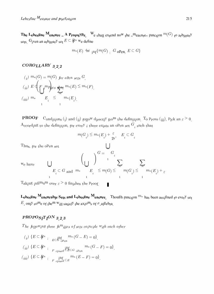
Lebesgue Measure and Integration 215
The Lebesgue Measure – A Prototype. We shall extend now the “measure” function m(G) to arbitrary
sets. Given an arbitrary set E ⊂ IRn we define
m∗(E)def= infm(G) : G open, E ⊂ G
COROLLARY 3.2.2
(i) m∗(G) = m(G) for open sets G.
(ii) E ⊂ F implies that m∗(E) ≤ m∗(F ).
(iii) m∗
∞
1
Ei
≤
∞
1
m∗(Ei).
PROOF Conditions (i) and (ii) follow directly from the definition. To prove (iii), pick an ε > 0.
According to the definition, for every i there exists an open set Gi such that
m(Gi) ≤ m∗(Ei) +ε
2i, Ei ⊂ Gi
Thus, for the open set
G =
∞
1
Gi
we have∞
1
Ei ⊂ G and m∗
∞
1
Ei
≤ m(G) ≤
∞
1
m(Gi) ≤
∞
1
m∗(Ei) + ε
Taking infimum over ε > 0 finishes the proof.
Lebesgue Measurable Sets and Lebesgue Measure. Though function m∗ has been assigned to every set
E, only some of them will satisfy the axioms of σ-algebra.
PROPOSITION 3.2.3
The following three families of sets coincide with each other
(i) E ⊂ IRn : infE⊂G open
m∗ (G− E) = 0.
(ii) E ⊂ IRn : infF closed⊂E⊂G open
m∗ (G− F ) = 0.
(iii) E ⊂ IRn : infF closed⊂E
m∗ (E − F ) = 0.

216 APPLIED FUNCTIONAL ANALYSIS
PROOF
(i) ⊂ (ii). Pick an ε > 0. There exists a G open such that
m∗ (G− E) <ε
4
According to the definition of m∗ there is an open set H such that
G− E ⊂ H and m(H) <ε
2
Making use of Proposition 3.2.2(ii), we can find a closed set F ⊂ G such that
m (G− F ) <ε
2
Obviously, set F −H is closed and
F −H = F ∩H ⊂ F ∩(G ∩ E)
= F ∩ (G ∪ E) = F ∩ E ⊂ E
Finally, for G open and F −H closed, we have
G− (F −H) = G ∩ (F ∪H) = (G− F ) ∪ (G ∩H) ⊂ (G− F ) ∪H
and, according to Proposition 3.2.2(i),
m (G− (F −H)) ≤ m (G− F ) +m(H) < ε
(iii) ⊃ (ii). Pick an ε > 0. There exists an F closed such that
m∗ (E − F ) <ε
4
According to the definition of m∗, there is an open set H such that
E − F ⊂ H and m(H) <ε
2
Consider now the closed set F . According to Proposition 3.2.2(ii), for the open set F there exists
an open set G (equivalently G is closed) such that
G ⊂ F (equivalently F ⊂ G) and m (G− F ) = m (F −G) <ε
2
Finally, for G ∪H open and F closed, we have
m ((G ∪H)− F ) = m ((G− F ) ∪ (H − F )) ≤ m (G− F ) +m(H) < ε
Inclusions (ii) ⊂ (iii) and (iii) ⊂ (ii) follow directly from the definition of m∗.
The family defined in the three different but equivalent ways in Proposition 3.2.3 is called the family
of Lebesgue measurable sets and denoted L(IRn) or compactly L. Intuitively, a Lebesgue measurable set is

Lebesgue Measure and Integration 217
approximated from “inside” by closed and from “outside” by open sets. We shall now prove two fundamental
facts: first that the family L is a σ-algebra containing Borel sets and, second, thatm∗ restricted to L satisfies
axioms of a measure.
THEOREM 3.2.1
The following hold:
(i) L is a σ-algebra, B ⊂ L.
(ii) mdef= m∗|L is a measure.
PROOF
(i) Step 1. Let E ∈ L. F closed ⊂ E ⊂ G open, implies G closed ⊂ E ⊂ F open. Moreover
G− F = F −G and therefore according to Proposition 3.2.3(ii), E ∈ L.
Step 2. Assume Ei ∈ L, i = 1, 2, . . .. Pick an ε > 0. According to the first definition of L, there
exist open sets Gi such that
Ei ⊂ Gi and m∗ (Gi − Ei) <ε
2i
Obviously, G =
∞
1
Gi ⊃
∞
1
Ei is open, and
m∗
∞
1
Gi −
∞
1
Ei
≤ m∗
∞
1
(Gi − Ei)
≤
∞
1
m∗ (Gi − Ei) ≤ ε
In conclusion, L is a σ-algebra. Since it contains open sets it must contain all Borel sets as well.
(ii) Obviously, m ≡ +∞. To prove additivity we shall show first that for E1 and E2 disjoint
m∗ (E1 ∪ E2) ≥ m∗ (E1) +m∗ (E2)
Toward this goal pick an open set G ⊃ E1 ∪E2 and a constant ε > 0. According to the definition of
L, there exist Fi closed ⊂ Ei such that m∗ (Ei − Fi) <ε2 . One can show that there exist two open
sets Gi, both contained in G and separating Fi, i.e.,
Fi ⊂ Gi ⊂ G, Gi disjoint
It follows that
m∗ (F1) +m∗ (F2) ≤ m (G1) +m (G2) = m (G1 ∪G2) ≤ m(G)
and, consequently,
m∗ (E1) +m∗ (E2) ≤ m(G) + ε
Taking infimum over ε > 0 and G open ⊃ E, we arrive at the result required.
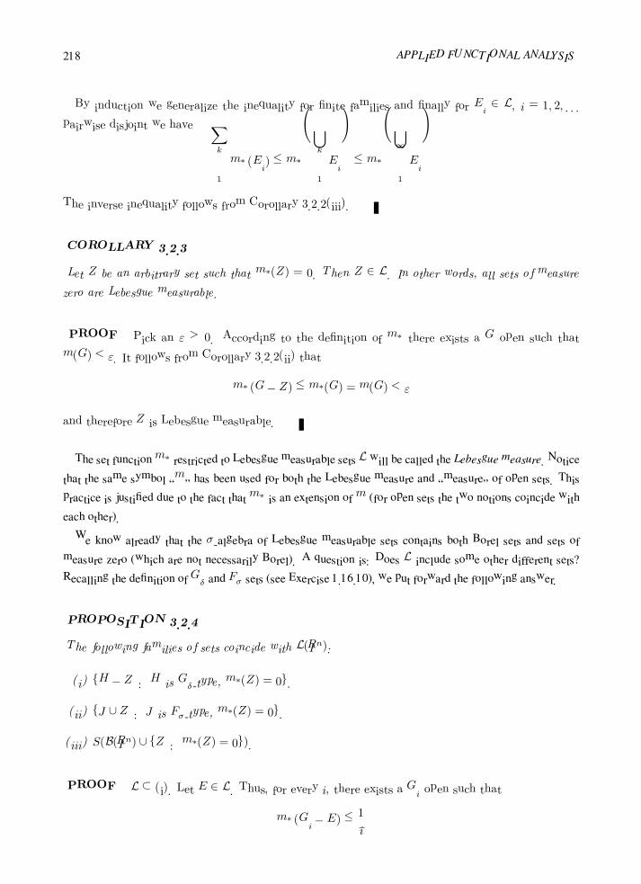
218 APPLIED FUNCTIONAL ANALYSIS
By induction we generalize the inequality for finite families and finally for Ei ∈ L, i = 1, 2, . . .
pairwise disjoint we have
k
1
m∗ (Ei) ≤ m∗
k
1
Ei
≤ m∗
∞
1
Ei
The inverse inequality follows from Corollary 3.2.2(iii).
COROLLARY 3.2.3
Let Z be an arbitrary set such that m∗(Z) = 0. Then Z ∈ L. In other words, all sets of measure
zero are Lebesgue measurable.
PROOF Pick an ε > 0. According to the definition of m∗ there exists a G open such that
m(G) < ε. It follows from Corollary 3.2.2(ii) that
m∗ (G− Z) ≤ m∗(G) = m(G) < ε
and therefore Z is Lebesgue measurable.
The set functionm∗ restricted to Lebesgue measurable sets L will be called the Lebesgue measure. Notice
that the same symbol “m” has been used for both the Lebesgue measure and “measure” of open sets. This
practice is justified due to the fact that m∗ is an extension of m (for open sets the two notions coincide with
each other).
We know already that the σ-algebra of Lebesgue measurable sets contains both Borel sets and sets of
measure zero (which are not necessarily Borel). A question is: Does L include some other different sets?
Recalling the definition of Gδ and Fσ sets (see Exercise 1.16.10), we put forward the following answer.
PROPOSITION 3.2.4
The following families of sets coincide with L(IRn):
(i) H − Z : H is Gδ-type, m∗(Z) = 0.
(ii) J ∪ Z : J is Fσ-type, m∗(Z) = 0.
(iii) S(B(IRn) ∪ Z : m∗(Z) = 0).
PROOF L ⊂ (i). Let E ∈ L. Thus, for every i, there exists a Gi open such that
m∗ (Gi − E) ≤1
i

Lebesgue Measure and Integration 219
Define H =∞
1
Gi (is Gδ-type). Obviously,
m∗ (H − E)) = limk→∞
m
k
1
Gi − E
= 0
and
E = H − (H − E)
from which the result follows. Use Corollary 3.2.3 to prove the inverse inclusion.
Proofs of two other identities are very similar and we leave them as an exercise (comp. Exer-
cise 3.2.2).
Before we conclude this section with some fundamental facts concerning Cartesian products of Lebesgue
measurable sets, we shall prove the following lemma.
LEMMA 3.2.2
Let Z ⊂ IRn, m∗(Z) = 0. Then for every, not necessarily Lebesgue measurable, set F ⊂ IRm
m∗(Z × F ) = 0
PROOF
Case 1. F bounded. There exists a set H open such that m(H) < ∞ and F ⊂ H. Pick an
arbitrary small ε > 0 and a corresponding open set G ⊃ Z such that m(G) < ε. Obviously,
Z × F ⊂ G×H
We have
m∗(Z × F ) ≤ m(G×H) = m(G)m(H) < εm(H)
Case 2. F arbitrary. For Bi = B(0, i), the balls centered at the origin, we have
IRm =
∞
1
Bi
Consequently,
F = F ∩ IRm =
∞
1
(F ∩Bi)
and
F × Z =∞
1
((F ∩Bi)× Z)
The assertion follows now from the fact that a countable union of zero measure sets is of measure
zero, too.
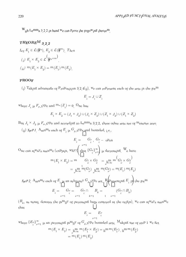
220 APPLIED FUNCTIONAL ANALYSIS
With Lemma 3.2.2 in hand we can prove the following theorem.
THEOREM 3.2.2
Let E1 ∈ L (IRn), E2 ∈ L (IRm). Then
(i) E1 × E2 ∈ LIRn+m
.
(ii) m (E1 × E2) = m (E1)m (E2).
PROOF
(i) Taking advantage of Proposition 3.2.4(ii), we can represent each of the sets in the form
Ei = Ji ∪ Zi
where Ji is Fσ-type and m∗ (Zi) = 0. One has
E1 × E2 = (J1 × J2) ∪ (J1 × Z2) ∪ (Z1 × J2) ∪ (Z1 × Z2)
But J1 × J2 is Fσ-type and according to Lemma 3.2.2, three other sets are of measure zero.
(ii) Step 1. Assume each of Ei is Gδ-type and bounded, i.e.,
Ei =
∞
ν=1
Gνi , Gν
i − open
One can always assume (explain, why?) that Gνi ∞ν=1 is decreasing. We have
m (E1 × E2) = m
∞
1
G1ν ×G2
ν
= limν→∞
mG1
ν ×G2ν
= limν→∞
m(G1ν) lim
ν→∞m(G2
ν) = m(E1)m(E2)
Step 2. Assume each of Ei is an arbitrary Gδ-type set. Representing Ei in the form
Ei =
∞
ν=1
Gνi =
∞
ν=1
Gνi ∩
∞
k=1
Bk =
∞
1
∞
ν=1
(Gνi ∩Bk)
(Bk, as usual, denotes the family of increasing balls centered at the origin), we can always assume
that
Ei =
∞
ν=1
Eνi
where Eνi
∞ν=1 is an increasing family of Gδ-type bounded sets. Making use of step 1 we get
m (E1 × E2) = limν→∞
m (Eν1 × Eν
2 ) = limm (Eν1 ) · limm (Eν
2 )
= m (E1)m (E2)

Lebesgue Measure and Integration 221
Step 3. Assume finally that each of Ei is of the form
Ei = Hi − Zi , Hi −Gδ-type, m∗(Zi) = 0
It follows immediately from Lemma 3.2.2 that
m (H1 ×H2) = m (E1 × E2) +m (E1 × Z2) +m (Z1 × E2) +m (Z1 × Z2)
= m (E1 × E2)
But, simultaneously,
m (H1 ×H2) = m (H1)m (H2) = m (E1)m (E2)
which ends the proof.
Exercises
Exercise 3.2.1 Let F1, F2 ∈ IRn be two disjoint closed sets, not necessarily bounded. Construct open sets
G1, G2 such that
Fi ⊂ Gi, i = 1, 2 and G1 ∩G2 = ∅
Exercise 3.2.2 Complete proof of Proposition 3.2.4.
3.3 The Fundamental Characterization of Lebesgue Measure
Though the construction of Lebesgue measure is at least up to a certain extent very natural and fits our
intuition, an immediate dilemma arises: perhaps there is another “natural” measure we can construct for
Borel sets which does not coincide with Lebesgue measure. The present section brings the answer and
explains why we have no other choice, i.e., why the Lebesgue measure is the only natural measure we can
construct in IRn.
Transitive σ-algebra. Let X be a vector space and S ⊂ P(X) a σ-algebra. We say that S is transitive if
A ∈ S ⇒ A+ a ∈ S for every a ∈ X
In other words, an arbitrary translation keeps us within the family of measurable sets.
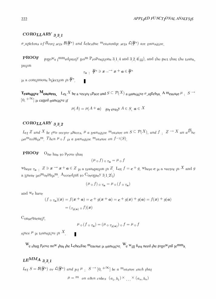
222 APPLIED FUNCTIONAL ANALYSIS
COROLLARY 3.3.1
σ-algebras of Borel sets B(IRn) and Lebesgue measurable sets L(IRn) are transitive.
PROOF follows immediately from Propositions 3.1.4 and 3.2.4(iii), and the fact that the trans-
lation
τa : IRn x −→ x+ a ∈ IRn
is a continuous bijection in IRn.
Transitive Measures. LetX be a vector space and S ⊂ P(X) a transitive σ-algebra. A measure µ : S →
[0,+∞] is called transitive if
µ(A) = µ(A+ a) for every A ∈ S, a ∈ X
COROLLARY 3.3.2
Let Z and X be two vector spaces, µ a transitive measure on S ⊂ P(X), and f : Z → X an affine
isomorphism. Then µ f is a transitive measure on f−1(S).
PROOF One has to prove that
(µ f) τa = µ f
where τa : Z x→ x+a ∈ Z is a translation in Z. Let f = c+ g, where c is a vector in X and g
a linear isomorphism. According to Corollary 3.1.2(i)
(µ f) τa = µ (f τa)
and we have
(f τa)(x) = f(x+ a) = c+ g(x+ a) = c+ g(x) + g(a) = f(x) + g(a)
= (τg(a) f)(x)
Consequently,
µ (f τa) = (µ τg(a)) f = µ f
since µ is transitive in X.
We shall prove now that the Lebesgue measure is transitive. We will first need the following lemma.
LEMMA 3.3.1
Let S = B(IRn) or L(IRn) and let µ : S → [0,+∞] be a measure such that
µ = m on open cubes (a1, b1)× . . .× (an, bn)

Lebesgue Measure and Integration 223
Then
µ = m on S
PROOF
Step 1. µ = m on cubes [a1, b1)× . . .× [an, bn). Indeed,
[a1, b1)× . . .× [an, bn) =
∞
ν=1
a1 −1
ν, b1
× . . .×
an −1
ν, bn
and
m([a1, b1)× . . .× [an, bn)) = limν→∞
m
a1 −1
ν, b1
× . . .×
an −1
ν, bn
= limν→∞
µ
a1 −1
ν, b1
× . . .×
an −1
ν, bn
= µ([a1, b1)× . . .× [an, bn))
Step 2. µ = m on open sets. Let G open. According to Corollary 3.2.1(ii)
G =
∞
1
Si(G)
Consequently,
m(G) = limi→∞
m(Si(G)) = limi→∞
µ(Si(G)) = µ(G)
Step 3. Let E ∈ S and G ⊃ E be an open set. Then
µ(E) ≤ µ(G) = m(G)
Taking infimum over all open sets G containing E, we get
µ(E) ≤ m(E)
In order to prove the inverse inequality we have to consider two cases.
Case 1. E is bounded, i.e.,
E ⊂ σ = [a1, b1]× . . .× [an, bn]
with a proper choice of ai, bi, i = 1, . . . , n. Obviously, σ − E ∈ S and
µ(σ)− µ(E) = µ(σ − E) ≤ m(σ − E) = m(σ)−m(E)
and, therefore, µ(E) ≥ m(E) and
µ(E) = m(E)
Case 2. E arbitrary. Let IRn =
∞
1
Bi (increasing balls centered at the origin). Obviously,
E =
∞
1
(E ∩Bi) , E ∩Bi increasing
224 APPLIED FUNCTIONAL ANALYSIS
and, consequently,
µ(E) = limi→∞
µ (E ∩Bi) = limi→∞
m (E ∩Bi) = m(E)
THEOREM 3.3.1
Let µ be a transitive measure on S = B(IRn) or L(IRn) such that
µ((0, 1)n) = 1
Then µ = m.
LEMMA 3.3.2
Let λ : [0,∞)→ [0,∞) be an additive function , i.e.,
λ(t+ s) = λ(t) + λ(s) for every t, s ≥ 0
Then
λ(ts) = tλ(s) for every t, s ≥ 0
PROOF
Step 1. t = k, a positive integer,
λ(ks) = λ(s+ . . .+ s) = λ(s) + . . .+ λ(s) = kλ(s)
Step 2. t = km , rational, k,m positive. We have
λ(s) = λm
s
m
= mλ
s
m
or, subdividing by m,
λ s
m
=
1
mλ(s)
Consequently,
λ
k
ms
= λks
m
= kλ
s
m
=
k
mλ(s)
Step 3. t ∈ [0,∞). For t = 0 the equality is trivial since
λ(s) = λ(0 + s) = λ(0) + λ(s)
and, therefore, λ(0) = 0. Assume t > 0 and choose an increasing sequence of rational numbers tn
approaching t from the left. We have
tnλ(s) = λ(tns) ≤ λ(ts)

Lebesgue Measure and Integration 225
since t is nondecreasing (it follows from additivity). Passing to the limit on the left-hand side we
get
tλ(s) ≤ λ(ts)
Finally, replacing t by 1/t and s by (ts), we get
1
tλ(ts) ≤ λ(s)
from which the equality follows.
PROOF of Theorem 3.3.1
Consider a cube (a1, b1)× . . .× (an, bn). It follows from transitivity of µ that
µ((a1, b1)× . . .× (an, bn)) = µ((0, b1 − a1)× . . .× (an, bn))
Now, define a function
λ(t) = µ((0, t)× . . .× (an, bn))
λ is additive since
λ(t+ s) = µ((0, t+ s)× . . .× (an, bn))
= µ((0, t)× . . .× (an, bn)) + µ((t, t+ s)× . . .× (an, bn))
= λ(t) + µ((0, s) . . . (an, bn)) = λ(t) + λ(s)
Lemma 3.3.2 implies that
µ((a1, b1)× . . .× (an, bn)) = (b1 − a1)µ((0, 1)× . . .× (an, bn))
and, consequently,
µ((a1, b1)× . . .× (an, bn)) = (b1 − a1) . . . (bn − an) = m((a1, b1) . . . (an, bn))
Lemma 3.3.1 finishes the proof.
Nontrivial Transitive Measures. We shall say that a transitive measure on S = B(IRn) or L(IRn) is non-
trivial if µ((0, 1)n) > 0.
COROLLARY 3.3.3
The following properties hold
(i) Let µ be a nontrivial transitive measure on S = B(IRn) or L(IRn). Then
µ = αm, where α = µ((0, 1)n)

226 APPLIED FUNCTIONAL ANALYSIS
(ii) Let µ and ν be two nontrivial measures on B(IRn) (L(IRn)) and B(IRm) (L(IRm)), respectively.
Then there exists a unique nontrivial transitive measure on B(IRn+m) (L(IRn+m)), called the
tensor product of µ and ν, denoted µ⊗ ν such that
(µ⊗ ν)(A×B) = µ(A)ν(B)
for A ∈ B(IRn) (L(IRn)), B ∈ B(IRm) (L(IRm)).
PROOF
(i) 1αµ is a measure and satisfies the assumptions of Theorem 3.3.1. So 1
αµ = m.
(ii) According to (i) µ = αmIRn , ν = βmIRm , where α = µ((0, 1)n), β = ν((0, 1)m). It implies
µ(A)ν(B) = αβmIRn(A)mIRm(B) = αβmIRn+m(A×B)
The measure on the right-hand side is the unique transitive measure we are looking for.
Substitution of an Affine Isomorphism. Let f : IRn → IRn be an affine isomorphism and E ⊂ IRn
an arbitrary Borel set. According to Proposition 3.1.4(ii), image f(E) is a Borel set as well. The question
arises: What is the relation between measuresm(E) andm(f(E))?. The following theorem brings an answer
providing a fundamental geometrical interpretation for determinants.
THEOREM 3.3.2
Let f : IRn → IRn be an affine isomorphism, i.e.,
f(x) = g(x) + a
where g is a linear isomorphism from IRn into itself and a ∈ IRn.
Then m f is a nontrivial transitive measure on S = B(IRn) or L(IRn) and
m f = | detG|m
where G is the matrix representation of g in any basis in IRn.
PROOF The proof relies on the fundamental result for linear transformations stating that every
linear isomorphism g : IRn → IRn can be represented as a composition of a finite number of so-called
simple isomorphisms gλH,c : IRn → IRn, where H is an n− 1-dimensional subspace of IRn (the so-called
hyperplane), c ∈ IRn and λ ∈ IRn (comp. Exercise 3.3.1). Representing an arbitrary vector x ∈ IRn in
the form
x = x0 + αc, where x0 ∈ H,α ∈ IR

Lebesgue Measure and Integration 227
the action of the simple isomorphism is defined as follows
gλH,c(x) = gλH,c(x0 + αc) = x0 + λαc
In other words, gλH,c reduces to identity on H and elongation along IRc.
Given the result, the proof follows now the following steps.
Step 1. Due to the transitivity of Lebesgue measure m, one can assume a = 0.
Step 2. Let g = g2 g1. Given the result for both g1 and g2, we can prove it immediately for
composition g. Indeed, by Cauchy’s Theorem for Determinants we have
m g = m (g2 g1) = (m g2) g1 = detG1(m g2)
= det G2 det G1 m = det (G2 G1)m = det Gm
where G1,G2,G are matrix representations for g1, g2, and g, respectively. Thus it is sufficient to
prove the theorem for a single simple isomorphism gλH,c.
Step 3. Let gλH,c be a simple isomorphism in IRn and let a1, . . . ,an−1 denote any basis in hyperplane
H. Completing it with an = c, we obtain a basis in IRn. Denoting by e1, . . . , en the canonical basis in
IRn, we construct a linear isomorphism φ : IRn → IRn such that φ(ai) = ei, i = 1, . . . , n. Consequently,
gλH,c can be represented as the composition
gλH,c = φ−1 gλ φ
where
gλ(xi) =
xi, i = 1, . . . , n− 1
λxi, i = n
Consequently,
gλ((0, 1)n) =
(0, 1)× . . .× (0, 1)× (0, λ) for λ > 0
(0, 1)× . . .× (0, 1)× (−λ, 0) for λ < 0
and, therefore, by Theorem 3.2.2(ii),
m(gλ((0, 1)n) = |λ|m((0, 1)n) = | det Gλ|m((0, 1)n)
where Gλ is the matrix representation of gλ.
By Theorem 3.3.1
µ gλ = | det Gλ|µ
for any transitive measure on B(IRn). In particular, by Corollary 3.3.2, we can take µ = m φ−1
and, therefore,
m φ−1 gλ = | det Gλ|µ φ−1
Consequently,
m φ−1 gλ φ = | det Gλ| µ φ−1 φ = | det Gλ| µ

228 APPLIED FUNCTIONAL ANALYSIS
Finally, det Gλ = det GλH,c, where G
λH,c is the matrix representation of simple isomorphism gλH,c
(explain why?) which finishes the proof for Borel sets.
Step 4. In order to conclude it for Lebesgue sets, one has to prove only that affine isomorphism
f prescribes L(IRn) into itself. But, according to Proposition 3.2.4, every Lebesgue measurable set
can be represented in the form∞
i=1
Gi − Z
where Gi are open and Z is of measure zero. Consequently,
f(∞
i=1
Gi − Z) =∞
i=1
f(Gi)− f(Z)
where f(Gi) are open and it remains to prove only that f(Z) is of measure zero. It follows however
from proof of Corollary 3.2.3 that
Z ⊂∞
i=1
Hi, Hi open, m(Hi) <1
i
and, consequently,
f(Z) ⊂
∞
i=1
f(Hi), f(Hi) open
Therefore, according to the just proven result for Borel sets,
m(f(Hi)) = | det G|m(Hi) < | det G|1
where G is the matrix representation of the linear part of f . Consequently m(f(Z)) = 0, which
finishes the proof.
COROLLARY 3.3.4
Let (0, 1)n denote the unit cube in IRn and f(x) = g(x) + a be an affine isomorphism in IRn with G,
the matrix representation of g. Then
m(f((0, 1)n)) = | det G|
Example 3.3.1
(Vitali set)
The use of Axiom of Choice is pivotal in the following example of a Lebesgue non-measurable set
due to Giuseppe Vitali. Consider interval [0, 1) ⊂ IR and the following equivalence relation,
x ∼ ydef⇔ x− y ∈ IQ

Lebesgue Measure and Integration 229
The corresponding equivalence classes form a partition of interval [0, 1). By Axiom of Choice, there
exists a set (the Vitali set) V ⊂ [0, 1) such that it has precisely one element from each equivalence
class. We shall demonstrate that set V is not measurable in the Lebesgue sense.
For each rational number a ∈ [0, 1), consider the corresponding modulo 1 translation Ta : [0, 1)→
[0, 1).
Ta(x) =
a+ x if a+ x < 1a+ x− 1 if a+ x ≥ 1
If V is measurable then Ta(V ) is measurable as well, and both sets have the same measure. Indeed,
a+V can be partitioned into (a+V )∩ [0, 1) and (a+V )∩ [1, 2) where both sets, being intersections
of measurable sets, are measurable. Translation of (a + V ) ∩ [1, 2) by −1 is measurable (explain,
why?) and is of the same measure as (a+ V ) ∩ [1, 2) (Lebesgue measure is transitive).
Definition of set V implies that Ta(V ) ∩ Tb(V ) = ∅ for a, b ∈ IQ, a = b. Indeed, if there were two
different x, y ∈ V such that Ta(x) = Tb(x), then the difference x − y would have to be rational, a
contradiction with the construction of set V . Finally, each x ∈ [0, 1) must belong to some Ta(V ).
Indeed, let [x] be the equivalence class of x and y ∈ [x] the (unique) element of the class selected for
set V . Then, by definition of the equivalence relation, there exists a rational number a such that
x− y = a and, consequently, x = Ta(y) ∈ Ta(V ).
In the end, we obtain a partition of interval [0, 1) into a countable family of sets of equal measure,
[0, 1) =
a∈IQ
Ta(V )
If V were of zero measure, this would imply that [0, 1) is of measure zero as well. On the other side,
if V were of a finite measure, this would imply that [0, 1) is of infinite measure, a contradiction in
both cases.
Exercises
Exercise 3.3.1 Follow the outlined steps to prove that every linear isomorphism g : IRn → IRn is a compo-
sition of simple isomorphisms gλH,c.
Step 1: Let H be a hyperplane in IRn, and let a, b denote two vectors such that a, b,a − b /∈ H . Show
that there exists a unique simple isomorphism gλH,c such that
gλH,c(a) = b
Hint: Use c = b− a.
Step 2: Let g be a linear isomorphism in IRn and consider the subspace Y = Y (g) such that g(x) = x on
Y . Assume that Y = IRn. Let H be any hyperplane containing Y . Show that there exist vectors
230 APPLIED FUNCTIONAL ANALYSIS
a, b such that
g(a) /∈ H
and
b /∈ H, b− g(a) /∈ H, b− a /∈ H
Make use then of the Step 1 result and consider simple isomorphisms g1 and h1 invariant on H
and mapping f(a) into b and b into a, respectively. Prove that
dimY (h1 g1 g) > dimY (g)
Step 3: Use induction to argue that after a finite number of stepsm
dimY (hm gm . . . h1 g1 g) = n
Consequently,
hm gm . . . h1 g1 g = idIRn
Finish the proof by arguing that the inverse of a simple isomorphism is itself a simple isomor-
phism, too.
Lebesgue Integration Theory
3.4 Measurable and Borel Functions
LebesgueMeasurable and Borel Functions. We say that a function ϕ : IRn → IR is (Lebesgue)measurable
if the following conditions hold
(i) dom ϕ is measurable (in IRn).
(ii) The set (x, y) ∈ dom ϕ× IR : y < ϕ(x) is measurable (in IRn+1).
Similarly we say that function ϕ is Borel if its domain is a Borel set and the set defined above is Borel. If no
confusion occurs, we will use a simplified notation y < ϕ(x) in place of (x, y) ∈ E × IR : y < ϕ(x).
Some fundamental properties of measurable and Borel functions are summarized in the following propo-
sitions.
Lebesgue Measure and Integration 231
PROPOSITION 3.4.1
The following properties hold:
(i) E ⊂ IRn measurable (Borel), ϕ : IRn → IR measurable (Borel) ⇒ ϕ|E measurable (Borel).
(ii) ϕi : Ei → IR measurable (Borel), Ei pairwise disjoint ⇒ ϕ =∞
1
ϕi measurable (Borel).
(iii) ϕ measurable (Borel) ⇒ λϕ measurable (Borel).
(iv) ϕi : E → IR measurable (Borel) ⇒ (pointwise) supϕi, inf ϕi, lim supϕi, lim inf ϕi measurable
(Borel). In particular if limϕi exists, then limϕi is measurable (Borel).
PROOF
(i) follows from
(x, y) ∈ E × IR : y < ϕ|E(x) = y < ϕ(x) ∩ E × IR
(ii) follows from
y < ϕ|∪Ei(x) =
i
y < ϕ|Ei(x)
(iii) follows from
y < λϕ(x) = h−1(y < ϕ(x))
where h : (x, y)→ (x, y/λ) is an affine isomorphism.
(iv) It is sufficient to make use of the following identities
y < supi
ϕi(x)
=
i
y < ϕi(x)
y > inf
iϕi(x)
=
i
y > ϕi(x)
and
lim supi→∞
ϕi(x) = infi
supj≥i
ϕj(x)
lim infi→∞
ϕi(x) = supi
infj≥i
ϕj(x)
(comp. also Exercise 3.4.1).
PROPOSITION 3.4.2
Every continuous function ϕ : E → IR, E open, is Borel and therefore measurable, too.

232 APPLIED FUNCTIONAL ANALYSIS
PROOF We have
y < ϕ(x) = g−1(y < z)
where
g : E × IR (x, y)→ (y, ϕ(x)) ∈ IR2
is a continuous function. Since set y < z is open, the set on the left-hand side must be open, too,
and therefore is both Borel and measurable.
We leave as an exercise proof of the following proposition.
PROPOSITION 3.4.3
Let g : IRn → IRn be an affine isomorphism. Then ϕ is measurable (Borel) if and only if ϕ g is
measurable (Borel).
Almost Everywhere Properties. A property P (x), x ∈ E is said to hold almost everywhere on E (often
written “a.e.” on E) if P fails to hold only on a subset of measure zero. In other words
P (x) holds a.e. on A iff P (x) holds for x ∈ A− Z andm(Z) = 0
As an example of an application of the above notion, we have the following simple proposition, proof of
which we leave as an exercise.
PROPOSITION 3.4.4
Let ϕi : E → IR, i = 1, 2 and ϕ1 = ϕ2 a.e. in E. Then ϕ1 is measurable iff ϕ2 is measurable.
Exercises
Exercise 3.4.1 Let ϕ : IRn → IR be a function such that dom ϕ is measurable (Borel). Prove that the
following conditions are equivalent to each other:
(i) ϕ is measurable (Borel).
(ii) (x, y) ∈ dom ϕ× IR : y ≤ ϕ(x) is measurable (Borel).
(iii) (x, y) ∈ dom ϕ× IR : y > ϕ(x) is measurable (Borel).
(iv) (x, y) ∈ dom ϕ× IR : y ≥ ϕ(x) is measurable (Borel).
Exercise 3.4.2 Prove Proposition 3.4.3.
Exercise 3.4.3 Prove Proposition 3.4.4.

Lebesgue Measure and Integration 233
3.5 Lebesgue Integral of Nonnegative Functions
Definition of Lebesgue Integral. Let ϕ : IRn → IR be a nonnegative function. Assume that domain of ϕ,
dom ϕ is measurable (Borel) and define the set
S(ϕ) = (x, y) ∈ dom ϕ× IR : 0 < y < ϕ(x)
One can easily prove that set S(ϕ) is measurable (Borel) if and only if function ϕ is measurable (Borel).
The Lebesgue measure (in IRn+1) of set S(ϕ) will be called the Lebesgue integral of function ϕ (over its
domain) and denoted by
ϕ dm or
ϕ(x) dm(x) or
ϕ(x) dx
Thus
ϕ dm = m(n+1)(S(ϕ))
wherem(n+1) denotes the Lebesgue measure in IRn+1.
If E is a measurable set then the integral of function ϕ over set E is defined as the integral of ϕ restricted
to E, i.e.,
E
ϕ dmdef=
ϕ|Edm = m(n+1)(S(ϕ|E)) = m(n+1)(S(ϕ) ∩ (E × IR))
The concept of the integral is illustrated in Fig. 3.2. The geometrical interpretation is clear.
Figure 3.2
Definition of Lebesgue integral for nonnegative functions. Set S(ϕ|E).
A number of properties follow immediately from the definition and the properties of a measure.
234 APPLIED FUNCTIONAL ANALYSIS
PROPOSITION 3.5.1
All considered functions are measurable and nonnegative. The following properties hold:
(i) m(E) = 0 ⇒
E
ϕ dm = 0.
(ii) ϕ : E → IR,Ei ⊂ E, i = 1, 2, . . . measurable and pairwise disjoint
∪Ei
ϕ dm =
∞
1
Ei
ϕ dm
(iii) ϕ, ψ : E → IR, ϕ = ψ a.e. in E
E
ϕ dm =
E
ψ dm
(iv) c ≥ 0, E measurable
E
c dm = cm(E)
(v) ϕ, ψ : E → IR, ϕ ≤ ψ a.e. in E
E
ϕ dm ≤
E
ψ dm
(vi) λ ≥ 0
(λϕ) dm = λ
ϕ dm
PROOF
(i) follows from the inclusion S(ϕ|E) ⊂ E×IR and the fact thatm(E×IR) = 0 (comp. Lemma 3.2.2).
(ii) is an immediate consequence of measure properties and the decomposition
S (ϕ|∪Ei) =
∞
1
S (ϕ|Ei)
where the sets on the right-hand side are pairwise disjoint.
(iii) follows from (i).
(iv) is a consequence of Theorem 3.2.2 and the formula
S(c) = E × (0, c)
(v) follows from the fact that S(ϕ) ⊂ S(ψ) (except for a set of measure zero).
(vi) For λ = 0 the formula is trivial. For λ > 0 we have
S(λϕ) = 0 < y < λϕ(x) = h(S(ϕ))
where h : (x, y)→ (x, λy) is an affine isomorphism and | deth| = λ. Thus Theorem 3.3.2 implies the
result.
Lebesgue Measure and Integration 235
The following lemma plays a crucial role in the whole integration theory.
LEMMA 3.5.1
Let ϕ, ϕi : E → IR, i = 1, 2, . . . be measurable, nonnegative functions. Then:
(i) ϕi ϕ ⇒
ϕi dm→
ϕ dm.
(ii) ϕi ϕ and ∃j :
ϕj dm < +∞ ⇒
ϕi dm→
ϕ dm.
PROOF
(i) We have
S(ϕ) =∞
1
S(ϕi)
and the family S(ϕi) is increasing. An application of Proposition 3.1.6(v) ends the proof.
(ii) Introduce the set
S1(ϕ) = 0 < y ≤ ϕ(x)
We claim that
ϕ dm = m(S1(ϕ))
Indeed,
S(ϕ) ⊂ S1(ϕ) ⊂ S
1 +1
k
ϕ
which implies that
ϕ dm ≤ m(n+1)(S1(ϕ)) ≤
1 +1
k
ϕ dm
Passing with k to infinity we get the result.
We have now
S1(ϕ) =
∞
1
S1(ϕi)
where S1(ϕi) is decreasing and m(S1(ϕi)) < +∞. Applying Proposition 3.1.6(vi), we end the proof.
We shall prove now two fundamental results of integration theory. Both of them are simple consequences
of Lemma 3.5.1.

236 APPLIED FUNCTIONAL ANALYSIS
THEOREM 3.5.1
(Fatou’s Lemma)
Let fi : E → IR, i = 1, 2, . . . be a sequence of measurable, nonnegative functions. Then
lim inf fi dm ≤ lim inf
fi dm
PROOF We have
infν≥i
fν(x) ≤ fi(x)
and according to Proposition 3.5.1(v),
infν≥i
fν dm ≤
fi dm
Our main objective now is pass to the limit, or more precisely to lim inf, on both sides of this
inequality. On the right-hand side we get simply lim inffi dm. On the left-hand side the sequence
is increasing, so the lim inf coincides with the usual limit. Moreover
1. limi→∞
(infν≥i
fν(x)) = lim infi→∞
fi(x) (comp. Proposition 1.17.2),
2. the sequence on the left-hand side is increasing and therefore according to Lemma 3.5.1,
infν≥i
fν dm→
lim inf fi dm
which ends the proof.
THEOREM 3.5.2
(The Lebesgue Dominated Convergence Theorem)
Let f, fi : E → IR, i = 1, 2, . . . be measurable, nonnegative functions. Assume
(i) fi(x)→ f(x) for x ∈ E, and
(ii) fi(x) ≤ ϕ(x), where ϕ : E → IR is a measurable function such that
ϕ dm < +∞
Then
fi dm→
f dm
PROOF We have
infν≥i
fν(x) ≤ fi(x) ≤ supν≥i
fν(x) ≤ ϕ(x)

Lebesgue Measure and Integration 237
and, consequently,
infν≥i
fν dm ≤
fi dm ≤
supν≥i
fν dm ≤
ϕ dm
Now, looking at the left-hand side
1. lim infi→∞ν≥i
fν = lim infi→∞
fi = limi→∞
fi = f
2. sequence infν≥i
fν is increasing
Thus, according to Lemma 3.5.1(i), the left-hand side converges to
f dm. Similarly for the right-
hand side
1. lim supi→∞ν≥i
f = lim supi→∞
fi = limi→∞
fi = f
2. sequence supν≥i
fν is decreasing
3. all integrals
supν≥i
fν dm are bounded by
ϕ dm
Thus, according to Lemma 3.5.1(ii), the right-hand side converges to
f dm, too, which proves
(The Three Sequences Lemma) that
fi dm→
f dm
REMARK 3.5.1 In both Theorems 3.5.1 and 3.5.2, all pointwise conditions in E may be
replaced by the same conditions but satisfied a.e. in E only (explain, why?).
We will conclude this section with a simple result concerning the change of variables in the Lebesgue
integral.
PROPOSITION 3.5.2
Let g : IRn → IRn be an affine isomorphism, and ϕ : IRn ⊃ E → IR a measurable function.
Then
E
ϕ dm =
g−1(E)
(ϕ g)| det g| dm
PROOF Define the mapping
h : IRn+1 (x, y)→ (g(x), y) ∈ IRn+1

238 APPLIED FUNCTIONAL ANALYSIS
Obviously, h is an affine isomorphism and | deth| = | det g|. Also
h(S(ϕ g)) = S(ϕ)
Thus, according to Theorem 3.3.2,
g−1(E)
(ϕ g)| det g| dm = | det g|m(S(ϕ g))
= (m h)(S(ϕ g)) = m(h(S(ϕ g)))
= m(S(ϕ)) =
E
ϕ dm
3.6 Fubini’s Theorem for Nonnegative Functions
In this section we derive the third fundamental theorem of integration theory – Fubini’s theorem. As in the
previous section, we will restrict ourselves to the case of nonnegative functions only, generalizing all the
results to the general case in the next paragraph. We will start first with the so-called generic case of Fubini’s
theorem.
THEOREM 3.6.1
(Fubini’s Theorem – The Generic Case)
Let E be a set in IRn+m = IRn × IRm. For each x ∈ IRn and y ∈ IRm, we define
Ex = y : (x,y) ∈ E
Ey = x : (x,y) ∈ E
Sets Ex and Ey correspond to sections of set E along y and x “axes” respectively (see Fig. 3.3 for
the geometrical interpretation). The following hold:
(i) If set E is Borel then
1. Ex is Borel for every x;
2. IRn x→ m(m)(Ex) is a Borel function;
3. m(n+m)(E) =
m(m)(Ex) dm(n)(x).
(ii) If set E is measurable then

Lebesgue Measure and Integration 239
1. Ex is measurable a.e. in IRn;
2. IRn x→ m(m)(Ex) (defined a.e.) is measurable;
3. m(n+m)(E) =
m(m)(Ex) dm(n)(x).
(iii) If m(n+m)(E) = 0 then m(m)(Ex) = 0 a.e. in IRn.
Before we start with the proof we will need some auxiliary results. First of all let us recall the very
preliminary definition of cubes introduced in Section 3.2.
σ =
ν1
2k,ν1 + 1
2k
× . . .×
νn2k
,νn + 1
2k
, k = 1, 2, . . .
Now, let us denote by Tk a family consisting of all such sets which are finite unions of cubes σ for a given k
and consider the family T =
∞
1
Tk. We have an obvious
COROLLARY 3.6.1
If A,B ∈ T then A ∪B, A−B ∈ T .
Figure 3.3
Fubini’s Theorem – The Generic Case. Sets Ex and Ey .

240 APPLIED FUNCTIONAL ANALYSIS
m-Class of Sets. A familyM ⊂ P(IRn) will be called an m-class of sets if it is closed with respect to
unions of increasing sequences of sets and intersections of decreasing sequences of bounded sets. In other
words, the following conditions hold:
Ai ∈M , A1 ⊂ A2 ⊂ . . . ⇒
∞
1
Ai ∈M
A1 ∈M , A1 ⊃ A2 ⊃ . . . , Ai bounded ⇒
∞
1
Ai ∈M
We have an immediate
COROLLARY 3.6.2
(i) A σ-algebra of sets is an m-class.
(ii) For every class C there exists the smallest m-class M(C) containing C.
PROOF
(i) follows from definition of σ-algebra and Proposition 3.1.1(iii). To prove (ii) it is sufficient to
notice that a common part of m-classes is an m-class and next consider the common part of all
m-classes containing C (the family is nonempty, why?).
The following lemma is crucial in the proof of Theorem 3.6.1.
LEMMA 3.6.1
The family of Borel sets B(IRn) is the smallest m-class containing family T , i.e.,
B(IRn) =M(T )
PROOF Since B(IRn) as a σ-algebra is an m-class and it contains T , we have immediately
B(IRn) ⊃M(T )
To prove the inverse inclusion we will prove that
1. open sets are contained in M(T );
2. M(T ) is a σ-algebra.
According to Corollary 3.2.1(ii), every open set G =
∞
1
Sk(G) which proves the first assertion. We
claim that in order to prove the second result, it suffices to prove that A,B ∈ M(T ) implies that

Lebesgue Measure and Integration 241
A−B ∈M(T ). Indeed, IRn ∈M(T ) and therefore for A ∈M(T ), complement A = IRn−A belongs
to M(T ). Representing a union of two sets A and B in the form
A ∪B = (A −B)
we see that A,B ∈M(T ) implies that A ∪B ∈M(T ). And finally, from the representation
∞
1
Ai =
∞
i=1
i
k=1
Ak
and the fact that
i
k=1
Ak is increasing, it follows that infinite unions of sets belonging to M(T )
belong to the same class as well. Thus it is sufficient to prove that for A,B ∈ M(T ) the difference
A−B ∈M(T ).
Step 1. Pick an A ∈ T and consider the class
B : A−B ∈M(T )
We claim that the family above is an m-class containing T . Indeed,
1. According to Corollary 3.6.1, it contains T .
2. Let B1 ⊂ B2 ⊂ . . . be an increasing sequence of sets belonging to the class, i.e., A−Bi ∈M(T ).
Moreover, the sets A − Bi are bounded (A is bounded) and sequence A − Bi is decreasing.
Thus
A−∞
1
Bi =
∞
1
(A−Bi) ∈M(T )
3. Let B1 ⊃ B2 ⊃ . . . be bounded. Again, from the identity
A−
∞
1
Bi
=
∞
1
(A−Bi)
follows that
∞
1
Bi belongs to M(T ).
Thus the considered class must contain M(T ) which implies that for A ∈ T , B ∈ M(T ) the
difference A−B ∈M(T ).
Step 2. Pick a B ∈M(T ), and consider the class
A : A−B ∈M(T )
In the identical manner we prove that this is an m-class, and according to Step 1 it containsM(T ).
Thus we have come to the conclusion that A,B ∈ M(T ) implies that A − B ∈ M(T ), which
finishes the proof.
242 APPLIED FUNCTIONAL ANALYSIS
PROOF of Theorem 3.6.1
Part (i). For every x ∈ IRn, define the function
ix : y → (x,y)
Function ix is obviously continuous and Ex = i−1x (E). Thus (comp. Proposition 3.1.4) if E is Borel
then Ex is Borel as well. Now, pick a set E and define the function
ηE : x→ m(m)(Ex)
We shall prove that the family
F =
E Borel : ηE Borel and m(n+m)(E) =
ηE dm(n)
is an m-class containing J .
Step 1. Let E1 ⊂ E2 . . .. Denote E =
∞
1
Ei. Obviously,
Ex =
∞
1
Exi , Ex
1 ⊂ Ex2 ⊂ . . .
Thus, according to Proposition 3.1.6(v),
m(Ex) = limi→∞
m(Exi )
i.e., ηEi(x) → ηE(x) which implies that ηE is Borel (comp. Proposition 3.4.1(iv)) and, due to the
fact that ηEiis increasing, Lemma 3.5.1(i), together with Proposition 3.1.6(v), yield
m(n+m)(E) = limm(n+m)(Ei) = lim
ηEidm(n) =
ηE dm(n)
Step 2. is analogous to Step 1. Pick a decreasing sequence of bounded sets E1 ⊃ E2 ⊃ . . . and
proceed to prove that for E =
∞
1
Ei, ηE is Borel and m(E) =
ηE dm.
Step 3. F contains class J . Indeed, sets E from J are obviously Borel. Now let E ∈ J . One can
always represent set E in the form
E =∞
1
(Ei × Fi)
where Ei are pairwise disjoint cubes σ in IRn and Fi are unions of cubes in IRm. Then
ηE(x) =
m(m)(Fi) if x ∈ Ei
0 otherwise
(see Fig. 3.4 for geometrical interpretation). Thus ηE as a union of Borel functions (explain, why?)
is Borel.

Lebesgue Measure and Integration 243
Figure 3.4
Proof of Theorem 3.6.1. Interpretation of sets E ∈ J .
Finally,
ηE dm(n) =
∞
1
m(n)(Ei)m(m)(Fi) =
∞
1
m(n+m)(Ei × Fi) = m(n+m)(E)
Part (ii). We shall prove first that if E is Borel of measure zero then Ex is of measure zero for
almost all x. Indeed, m(m)(Ex) = ηE(x), and we already know that
ηE dm(n) = m(n+m)(E) = 0
Pick an ε > 0 and consider the set
x : ηE(x) > ε
Obviously,
εm(n)(x : ηE(x) > ε) ≤
ηE dm(n) = 0
which implies that
m(n)(ηE > ε) = 0
Making use of the representation
ηE > 0 =
∞
k=1
ηE >1
k
we get the result.
Now, if E is of measure zero then there exists a Borel set H, also of measure zero, containing E.
Consequently Ex ⊂ Fx, Fx is of measure zero for almost x, and so is Ex.
244 APPLIED FUNCTIONAL ANALYSIS
Part (iii). We leave the proof of this part as a simple exercise. One has to use Proposition 3.2.4
and represent a measurable set E in the form
E = H ∪ Z
where H is Borel and Z if measure zero. Then the proof follows directly from parts (i) and (ii) of
this theorem.
Before we conclude this section with Fubini’s Theorem for functions (which turns out to be a
simple reinterpretation of Theorem 3.6.1), let us take a break and derive some simple but important
observations from the theorem just proved.
COROLLARY 3.6.3
The following properties hold:
(i) Let ϕ : E → IR be a measurable, nonnegative function such that
ϕ dm = 0. Then ϕ = 0 a.e.
(ii) Let ϕ, ψ : E → IR be two measurable, nonnegative functions. Then
(ϕ+ ψ) dm =
ϕ dm+
ψ dm
PROOF (i) According to the Generic Case of Fubini’s Theorem, part (iii),
ϕ dm(n) = m(n+1)(S(ϕ)) = 0
implies that
m(1)(S(ϕ))x = m((0, ϕ(x))) = ϕ(x)
is equal zero for almost all x.
(ii) Consider the isomorphism
g : IRn × IR (x,y)→ (x,−y) ∈ IRn × IR
Obviously, det g = −1 and, therefore,
m(n+1)(g(S(ψ))) = m(n+1)(−ψ(x) < y < 0) =
ψ dm(n)
But g(S(ψ)) and S(ϕ) are disjoint and, therefore,
ϕ dm+
ψ dm = m(n+1)(g(S(ψ)) ∪ S(ϕ))
=
m(1)(g(S(ψ)) ∪ S(ϕ))x dm(n)
=
m(1)((−ψ(x), 0) ∪ (0, ϕ(x)) dm(n)
=
(ϕ+ ψ)(x) dm(n)(x)

Lebesgue Measure and Integration 245
As the final result of this section we state
THEOREM 3.6.2
(Fubini’s Theorem for Nonnegative Functions)
Let f : IRn × IRm ⊃ E (x,y)→ f(x,y) ∈ IR be a nonnegative function of variables x and y. If f
is Borel (measurable) then the following conditions hold
(i) y → f(x,y) is Borel for all x (is measurable for almost all x).
(ii) x→
f(x,y) dm(y) is Borel (measurable).
(iii)
f(x,y) dm(n+m) =
f(x,y) dm(y)
dm(x).
PROOF
(i) dom (y → f(x,y)) = (domf)x and therefore is Borel (measurable) (Theorem 3.6.1). In the
same way
S(y → f(x,y)) = S(f)x
and, therefore, y → f(x,y) is Borel (measurable).
(ii) Apply Theorem 3.6.1 to set S(f) replacing y by (y, z). Thus (ii) follows from Theorem 3.6.1(i)(2)
(ii)(2).
(iii) follows from
f dm(n+m) = m(n+m+1)(S(f)) =
m(m+1)(S(f)x) dm(n)(x)
=
f(x,y) dm(m)(y)
dm(n)(x)
3.7 Lebesgue Integral of Arbitrary Functions
In this section we generalize the notion of Lebesgue integral to the case of arbitrary functions. As a prelimi-
nary step we shall study first the notion of infinite sums.

246 APPLIED FUNCTIONAL ANALYSIS
Infinite Sums. Suppose we are given a sequence ai ∈ IR, i ∈ IN . Note that ai may take the value of +∞
or −∞. For a given number a ∈ IR we define its positive and negative parts as
a+ = maxa, 0 , a− = max−a, 0
Obviously, only one of the numbers is non-zero and
a = a+ − a−
We will define the infinite (countable) sum of ai as
IN
aidef=
∞
i=1
a+i −
∞
i=1
a−i
provided that at least one of the series on the right-hand side is finite (to avoid the undetermined symbol
+∞−∞).
REMARK 3.7.1 Note the significant difference between infinite sums and infinite series. For
instance, the series
∞
1
(−1)i1
iis finite (convergent) but the sum
IN
(−1)i1
iis undetermined.
PROPOSITION 3.7.1
Let ai ∈ IR, i ∈ IN . Suppose that ai = a1i − a2
i , where a1i , a
2i ≥ 0 and one of the series
∞
1
a1i ,
∞
1
a2i
is finite. Then the sum
IN
ai exists and
IN
ai =
∞
1
a1i −
∞
1
a2i
PROOF
Case 1. Both sequences∞
1
a1i ,
∞
1
a21 are finite. This implies that
∞
1
a1i −
∞
1
a2i =
∞
1
a1i − a2
i
=
∞
1
ai
But a+i ≤ a1
i and a−i ≤ a2i which implies that both
∞
1
a+i and
∞
1
a−i are finite, too. Thus for the
same reasons
IN
ai =
∞
1
a+i −
∞
1
a−i =
∞
1
ai

Lebesgue Measure and Integration 247
from which the equality follows.
Case 2. Suppose
∞
1
a1i = +∞ and
∞
1
a2i < +∞. Then, for the same reasons as before
∞
1
a−i <∞
and, therefore,∞
1
a2i − a−i
=
∞
1
a2i −
∞
1
a−i < +∞
If
∞
1
a+i were finite then according to
∞
1
a1i =
∞
1
a+i +
∞
1
a1i − a+
i
=
∞
1
a+i +
∞
1
a2i − a−i
sum∞
1
a1i would have to be also finite which proves that
∞
1
a+i = +∞. Thus both
IN
ai and
∞
1
a2i −
∞
1
a−i are equal to +∞ from which the equality follows. The case
∞
1
a1i < +∞ and
∞
1
a2i = +∞ is proved in the same way.
A number of useful properties of infinite sums will be summarized in the following proposition.
PROPOSITION 3.7.2
Let ai, bi ∈ IR be arbitrary sequences. The following properties hold:
(i)
IN
αai = α
IN
ai for α ∈ IR. Both sides exist simultaneously.
(ii) ai ≤ bi ⇒
IN
ai ≤
IN
bi if both sides exist.
(iii)
IN
(ai+ bi) =
IN
ai+
IN
bi if the right-hand side exists (i.e., both sums exist and the symbols
+∞−∞ or −∞+∞ are avoided).
(iv)
IN
ai
≤
IN
|ai| if the left-hand side exists.
PROOF
(i) Case α = 0 is trivial. Assume α > 0. Then
(αai)+ = αa+
i (αai)− = αa−i
and the equality follows from the definition. Case α < 0 is analogous.

248 APPLIED FUNCTIONAL ANALYSIS
(ii) ai ≤ bi implies that
a+i ≤ b+
i and a−i ≥ b−i
Thus∞
1
a+i ≤
∞
1
b+i and
∞
1
a−i ≥
∞
1
b−i
from which the inequality follows.
(iii) Suppose the right-hand side exists. Then
IN
ai +
IN
bi =
∞
1
a+i −
∞
1
a−i +
∞
1
b+i −
∞
1
b−i
=∞
1
a+i + b+
i
−
∞
1
a−i + b−i
But ai+bi = (a+i +b+
i )−(a−i +b−i ) and a+
i +b+i ≥ 0, a−i +b−i ≥ 0. Thus, according to Proposition 3.7.1,
the sum exists and is equal to the right-hand side.
(iv) Case 1. Both sums
∞
1
a+i and
∞
1
a−i are finite. Then
∞
1
|ai| =
∞
1
(a+i + a−i ) is also finite
and the result follows from the inequality
− |ai| ≤ ai ≤ |ai|
Case 2. If any of the sums is infinite then
∞
1
|ai| = +∞ and the equality follows.
We leave as an exercise the proof of the following:
COROLLARY 3.7.1
Let ai ∈ IR. The sum
IN
ai is finite if and only if
IN
|ai| is finite. In such a case
IN
ai =
∞
1
ai
Definition of Lebesgue Integral for Arbitrary Functions. Let f : IRn → IRn be a measurable function.
Define functions
f+(x) = maxf(x), 0 , f−(x) = max−f(x), 0
According to Proposition 3.4.1, both functions f+ and f− are measurable. We say that function f is inte-
grable and define the integral of f as
f dm =
f+ dm−
f− dm
Lebesgue Measure and Integration 249
if at least one of the integrals on the right-hand side is finite.
In a manner identical to the proof of Proposition 3.7.1, we prove the following:
COROLLARY 3.7.2
Let f : E → IR be measurable and f = f1 + f2 where f1, f2 ≥ 0 are measurable. Assume that at least
one of the integrals
f1 dm,
f2 dm is finite. Then f is integrable and
f dm =
f1 dm−
f2 dm
A number of useful properties will be summarized in the following proposition. Please note the similarities
between integrals and infinite sums.
PROPOSITION 3.7.3
Let functions f and g be measurable. The following properties hold:
(i) m(E) = 0 ⇒
E
f dm = 0
(ii) f : E ⇒ IR, Ei ⊂ E, i = 1, 2, . . . measurable and pairwise disjoint ⇒
∪Ei
f dm =
IN
Ei
f dm
if the left-hand side exists.
(iii) f, g : E → IR integrable, f = g a.e. in E ⇒
E
f dm =
E
g dm
(iv) c ∈ IR, E measurable ⇒
E
c dm = c m(E)
(v) f, g : E → IR integrable, f ≤ g a.e. in E ⇒
E
f dm ≤
E
g dm
(vi) λ ∈ IR, f : E → IR integrable ⇒
E
λf dm = λ
E
f dm
(vii) f, g : E → IR integrable ⇒
E
(f + g) dm =
E
f dm+
E
g dm
if the right-hand side exists and function f + g is determined a.e. in E.

250 APPLIED FUNCTIONAL ANALYSIS
(viii) f : E → IR integrable ⇒
E
f dm
≤
E
|f | dm
(ix) Let g : IRn → IRn be an affine isomorphism. Then
(f g)| det g| dm =
f dm
and both sides exist simultaneously.
PROOF The whole proof follows from the definition of integral, properties of integral of non-
negative functions and properties of infinite sums.
(i) follows from the definition and Proposition 3.5.1(i).
(ii) follows from
∪Ei
f dm =
∪Ei
f+ dm−
∪Ei
f− dm
=∞
1
Ei
f+ dm−
∞
1
Ei
f− dm
=
IN
Ei
f dm (Proposition 3.7.1)
(iii) See Proposition 3.5.1(iii).
(iv) See Proposition 3.5.1(iv).
(v) See Proposition 3.5.1(v).
(vi) See Proposition 3.5.1(vi).
(vii) It follows from Corollary 3.6.3(ii) that
f dm+
g dm =
f+ dm−
f− dm+
g+ dm−
g− dm
=
(f+ + g+) dm−
(f− + g−) dm
But f + g = (f+ + g+)− (f− + g−) and both components are nonnegative, thus, according to
Corollary 3.7.2,
(f+ + g+) dm−
(f− + g−) dm =
(f + g) dm
(viii) follows from the inequalities
−|f | ≤ f ≤ |f |
(ix) Apply the definition of integral and Proposition 3.5.2.

Lebesgue Measure and Integration 251
Summable Functions. Let f : E → IR be an integrable function. We say that f is summable if
f dm is
finite, i.e.,
f dm
< +∞
We leave as an exercise proofs of the following two simple propositions.
PROPOSITION 3.7.4
The following conditions are equivalent:
(i) f is summable.
(ii)
f+ dm,
f− dm < +∞.
(iii)
|f | dm < +∞.
PROPOSITION 3.7.5
All functions are measurable. The following properties hold:
(i) f summable, E measurable → f |E summable.
(ii) f, ϕ : E → IR, |f | ≤ ϕ a.e. in E, ϕ summable → f summable.
(iii) f1, f2 : E → IR summable ⇒ α1f1 + α2f2 summable for α1, α2 ∈ IR.
We conclude this section with three fundamental theorems of integration theory.
THEOREM 3.7.1
(The Lebesgue Dominated Convergence Theorem)
Let:fi : E → IR, i = 1, 2, . . . integrable
fi(x)→ f(x) a.e. in E
|fi(x)| ≤ ϕ(x) a.e. in E, where ϕ : E → IR is summable
Then
1. f is summable, and
2.
fi dm→
f dm.
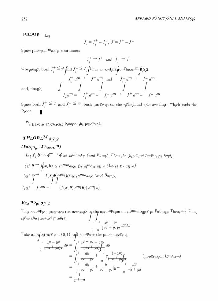
252 APPLIED FUNCTIONAL ANALYSIS
PROOF Let
fi = f+i − f−i , f = f+ − f−
Since function max is continuous
f+i → f+ and f−i → f−
Obviously, both f+i ≤ ϕ and f−i ≤ ϕ. Thus according to Theorem 3.5.2
f+i dm→
f+ dm and
f−i dm→
f− dm
and, finally,
fi dm =
f+i dm−
f−i dm→
f+ dm−
f− dm
Since both f+i ≤ ϕ and f−i ≤ ϕ, both integrals on the right-hand side are finite which ends the
proof.
We leave as an exercise proof of the following:
THEOREM 3.7.2
(Fubini’s Theorem)
Let f : IRn × IRm → IR be summable (and Borel). Then the following properties hold:
(i) y → f(x,y) is summable for almost all x (Borel for all x).
(ii) x→
f(x,y) dm(y) is summable (and Borel).
(iii)
f dm =
(f(x,y) dm(y)) dm(x).
Example 3.7.1
This example illustrates the necessity of the assumption on summability in Fubini’s Theorem. Con-
sider the iterated integral 1
0
1
0
x2 − y2
(x2 + y2)2dydx
Take an arbitrary x ∈ (0, 1) and compute the inner integral,
1
0
x2 − y2
(x2 + y2)2dy =
1
0
x2 + y2 − 2y2
(x2 + y2)2dy
=
1
0
dy
x2 + y2+
1
0
y(−2y)
(x2 + y2)2(integration by parts)
=
1
0
dy
x2 + y2+
y
x2 + y2|10 −
1
0
dy
x2 + y2
=1
1 + x2
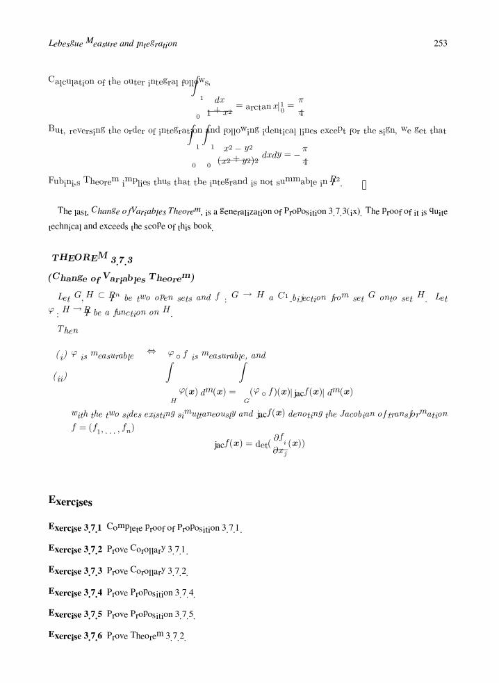
Lebesgue Measure and Integration 253
Calculation of the outer integral follows,
1
0
dx
1 + x2= arctanx|10 =
π
4
But, reversing the order of integration and following identical lines except for the sign, we get that
1
0
1
0
x2 − y2
(x2 + y2)2dxdy = −
π
4
Fubini’s Theorem implies thus that the integrand is not summable in IR2.
The last, Change of Variables Theorem, is a generalization of Proposition 3.7.3(ix). The proof of it is quite
technical and exceeds the scope of this book.
THEOREM 3.7.3
(Change of Variables Theorem)
Let G,H ⊂ IRn be two open sets and f : G → H a C1-bijection from set G onto set H. Let
ϕ : H → IR be a function on H.
Then
(i) ϕ is measurable ⇔ ϕ f is measurable, and
(ii)
H
ϕ(x) dm(x) =
G
(ϕ f)(x)|jacf(x)| dm(x)
with the two sides existing simultaneously and jacf(x) denoting the Jacobian of transformation
f = (f1, . . . , fn)
jacf(x) = det(∂fi∂xj
(x))
Exercises
Exercise 3.7.1 Complete proof of Proposition 3.7.1.
Exercise 3.7.2 Prove Corollary 3.7.1.
Exercise 3.7.3 Prove Corollary 3.7.2.
Exercise 3.7.4 Prove Proposition 3.7.4.
Exercise 3.7.5 Prove Proposition 3.7.5.
Exercise 3.7.6 Prove Theorem 3.7.2.

254 APPLIED FUNCTIONAL ANALYSIS
3.8 Lebesgue Approximation Sums, Riemann Integrals
We continue our considerations on Lebesgue integration theory with a geometrical characterization of the
integral showing particularly the essential difference between Lebesgue and Riemann integrals. We will find
also when the two types of integrals coincide with each other.
Lebesgue’s Sums. Let f : IRn ⊃ E → IR be a measurable function. Pick an ε > 0 and consider a partition
of real line IR
. . . < y−1 < y0 < y1 < . . .
such that y−i → −∞; yi → +∞ and |yi − yi−1| ≤ ε. Define
Ei = x ∈ E : yi−1 ≤ f(x) < yi
Sets Ei are measurable, see Exercise 3.8.2. The series
s =+∞
−∞
yi−1m(Ei), S =
+∞
−∞
yim(Ei)
are called the lower and upper Lebesgue sums, respectively.
We have the following:
THEOREM 3.8.1
Assume additionally that m(E) is finite and consider a sequence εk → 0 with a corresponding family
of partitions and Lebesgue sums sk and Sk. Then
(i) If f is summable then both sk and Sk are absolutely convergent and
lim sk = limSk =
E
f dm
(ii) If one of the Lebesgue’s sums sk or Sk is absolutely convergent, then f is summable and
therefore according to (i), the other sum converges as well and both limits are equal to the
integral.
PROOF
(i) Since Ei are pairwise disjoint one can define the following two functions:
ϕ(x) = yi−1
ψ(x) = yiif x ∈ Ei
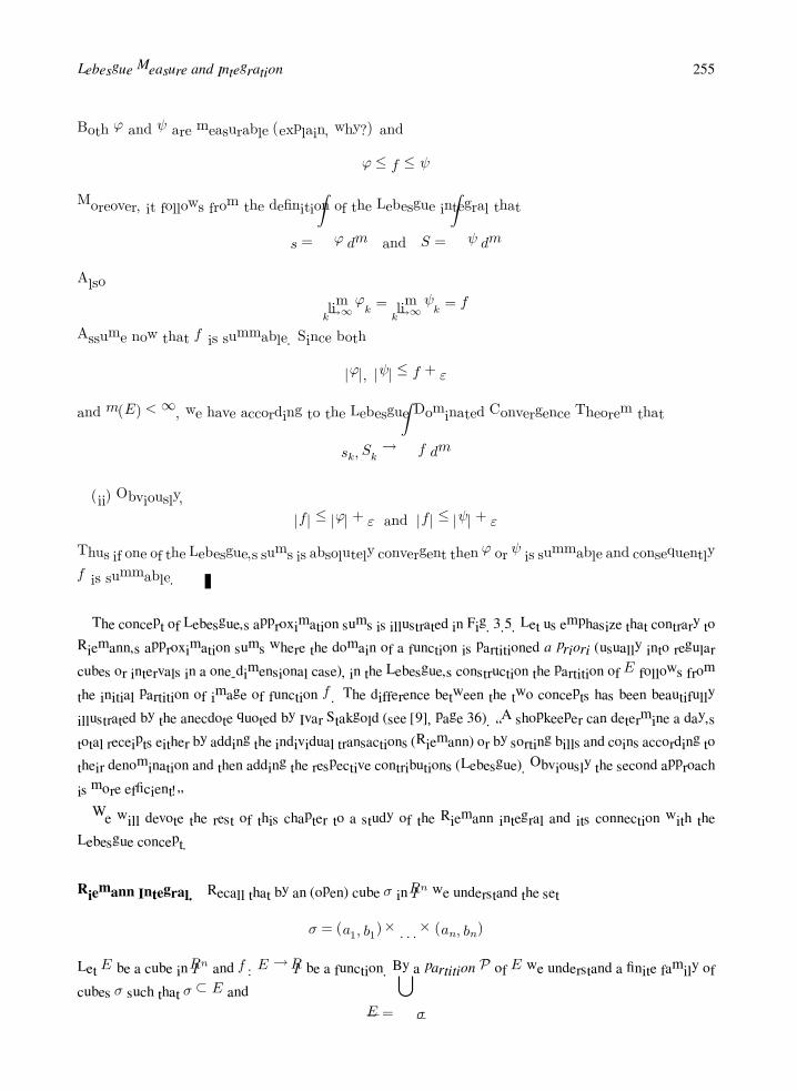
Lebesgue Measure and Integration 255
Both ϕ and ψ are measurable (explain, why?) and
ϕ ≤ f ≤ ψ
Moreover, it follows from the definition of the Lebesgue integral that
s =
ϕ dm and S =
ψ dm
Also
limk→∞
ϕk = limk→∞
ψk = f
Assume now that f is summable. Since both
|ϕ|, |ψ| ≤ f + ε
and m(E) <∞, we have according to the Lebesgue Dominated Convergence Theorem that
sk, Sk →
f dm
(ii) Obviously,
|f | ≤ |ϕ|+ ε and |f | ≤ |ψ|+ ε
Thus if one of the Lebesgue’s sums is absolutely convergent then ϕ or ψ is summable and consequently
f is summable.
The concept of Lebesgue’s approximation sums is illustrated in Fig. 3.5. Let us emphasize that contrary to
Riemann’s approximation sums where the domain of a function is partitioned a priori (usually into regular
cubes or intervals in a one-dimensional case), in the Lebesgue’s construction the partition of E follows from
the initial partition of image of function f . The difference between the two concepts has been beautifully
illustrated by the anecdote quoted by Ivar Stakgold (see [9], page 36). “A shopkeeper can determine a day’s
total receipts either by adding the individual transactions (Riemann) or by sorting bills and coins according to
their denomination and then adding the respective contributions (Lebesgue). Obviously the second approach
is more efficient!”
We will devote the rest of this chapter to a study of the Riemann integral and its connection with the
Lebesgue concept.
Riemann Integral. Recall that by an (open) cube σ in IRn we understand the set
σ = (a1, b1)× . . .× (an, bn)
Let E be a cube in IRn and f : E → IR be a function. By a partition P of E we understand a finite family of
cubes σ such that σ ⊂ E and
E =
σ

256 APPLIED FUNCTIONAL ANALYSIS
Figure 3.5
Interpretation of Lebesgue sums.
Number
r(P) = supσ∈P
r(σ)
where r2(σ) =n
1
(bi − ai)2 will be called the radius of the partition. Choosing for every cube σ ∈ P a
point ξσ ∈ σ, we define the Riemann approximation sum as
R = R(P, ξ) =
σ∈P
f(ξσ)m(σ)
If for every sequence of partitions Pn such that r(Pn) → 0 and an arbitrary choice of points ξ ∈ σ, the
Riemann sum converges to a common limit J then J is called the Riemann integral of function f over cube
E. Function f is said to be Riemann integrable over E.
We have the following fundamental result:
THEOREM 3.8.2
Let E be a cube in IRn and f : E → IR be a bounded function. Then f is Riemann integrable if and
only if f is continuous almost everywhere in E. In such a case Riemann and Lebesgue integrals are
equal to each other:
(Riemann)
f(x)dx = (Lebesgue)
f(x) dm(x)
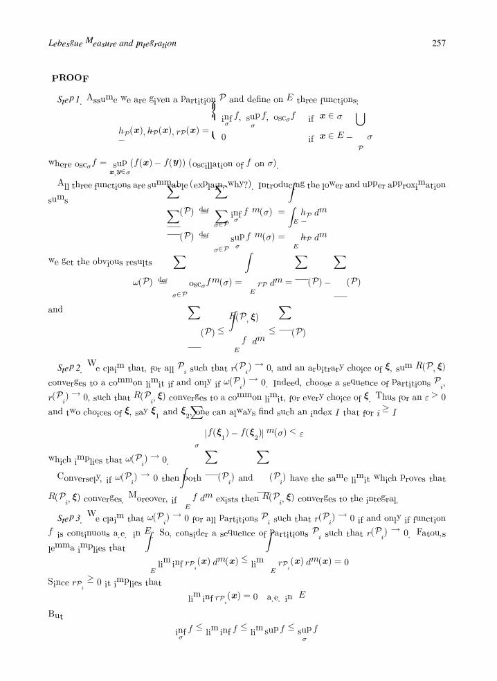
Lebesgue Measure and Integration 257
PROOF
Step 1. Assume we are given a partition P and define on E three functions:
hP(x), hP(x), rP(x) =
infσ
f, supσ
f, oscσf if x ∈ σ
0 if x ∈ E −
P
σ
where oscσf = supx,y∈σ
(f(x)− f(y)) (oscillation of f on σ).
All three functions are summable (explain, why?). Introducing the lower and upper approximation
sums
(P)def=
σ∈P
infσ
f m(σ) =
E
hP dm
(P)
def=
σ∈P
supσ
f m(σ) =
E
hP dm
we get the obvious results
ω(P)def=
σ∈P
oscσfm(σ) =
E
rP dm =
(P)−
(P)
and
(P) ≤
R(P, ξ)
E
f dm≤
(P)
Step 2. We claim that, for all Pi such that r(Pi) → 0, and an arbitrary choice of ξ, sum R(P, ξ)
converges to a common limit if and only if ω(Pi) → 0. Indeed, choose a sequence of partitions Pi,
r(Pi)→ 0, such that R(Pi, ξ) converges to a common limit, for every choice of ξ. Thus for an ε > 0
and two choices of ξ, say ξ1 and ξ2, one can always find such an index I that for i ≥ I
σ
|f(ξ1)− f(ξ2)|m(σ) < ε
which implies that ω(Pi)→ 0.
Conversely, if ω(Pi) → 0 then both
(Pi) and
(Pi) have the same limit which proves that
R(Pi, ξ) converges. Moreover, if
E
f dm exists then R(Pi, ξ) converges to the integral.
Step 3. We claim that ω(Pi)→ 0 for all partitions Pi such that r(Pi)→ 0 if and only if function
f is continuous a.e. in E. So, consider a sequence of partitions Pi such that r(Pi) → 0. Fatou’s
lemma implies that
E
lim inf rPi(x) dm(x) ≤ lim
E
rPi(x) dm(x) = 0
Since rPi≥ 0 it implies that
lim inf rPi(x) = 0 a.e. in E
But
infσ
f ≤ lim inf f ≤ lim sup f ≤ supσ
f

258 APPLIED FUNCTIONAL ANALYSIS
which means that
lim inf f = lim sup f a.e. in E
and, therefore, f is continuous a.e. in E.
Conversely, if f is continuous a.e. in E, then for every x ∈ E except for a set of measure zero
∀ ε > 0 ∃δ > 0 |x− x| < δ ⇒ |f(x)− f(x)| < ε
Thus for x and x belonging to a sufficiently small cube σ containing x
|f(x)− f(x)| ≤ |f(x)− f(x)|+ |f(x)− f(x)| < 2ε
which proves that rP < 2ε a.e. in E. Since ε is arbitrary small, lim rP = 0 a.e. and according to
the Lebesgue Dominated Convergence Theorem
ω(Pi)→ 0
We conclude this section with a rather standard example of a function f which is Lebesgue integrable but
not Riemann integrable.
Example 3.8.1
Consider the function of the Dirichlet type f : (0, 1)→ IR,
f(x) =
3 if x is rational
2 if x is irrational
Then f is continuous nowhere and therefore a Riemann integral does not exist. Simultaneously,
since the set of rational numbers is of measure zero, f = 2 a.e. in (0, 1) and, therefore, the Lebesgue
integral exists and 1
0
f dm = 2
Example 3.8.2
(Cauchy Principal Value Integral)
Common in complex variables and in theory of integral equations is the concept of Principal Value
(PV) integral due to Cauchy. Assume that we are given a function f(x) defined in an open set
Ω ⊂ IRn that is singular at some point a ∈ Ω, i.e., limx→x |f(x)| = ∞. The Cauchy PV (CPV)
integral is defined as follows,
−
Ω
f(x) dx = lim→0
Ω−B(a,)
f(x) dx

Lebesgue Measure and Integration 259
If function f is summable in Ω then CPV integral coincides with the standard Lebesgue integral.
In fact, given any monotone sequence (not necessarily balls) of sets A1 ⊃ A2 ⊃ . . . , shrinking in
measure to zero, we can conclude that
limn→∞
Ω−An
f(x) dx =
Ω
f(x) dx
This follows immediately from the Lebesgue Dominated Convergence Theorem. Defining a sequence
of functions,
fn(x) =
f(x) x ∈ Ω−An
0 otherwise
we observe that fn → f pointwise, and fn are dominated by f that is summable. Thus, in the
case of a singular but summable function, the CPV integral coincides with the Lebesgue integral.
Frequently we say then that function f is weakly singular.
However, the CPV integral may exist even if the Lebesgue integral does not. The simplest example
is function f(x) = 1/x defined on the whole real line IR. Function 1/|x| is not summable over IR but
IR−(−,)
1
xdx =
−
−∞
1
xdx+
∞
1
xdx = 0
and, consequently, the limit defining CPV integral exists and it is equal to zero. Sufficient conditions
under which the CPV integral exists are usually formulated in context of specific applications. For
instance, in the theory of integral equations we encounter integrals of the form
−
Ω
Φ(|x− y|)f(y) dy
where Φ(r) is a function of scalar argument r, singular at zero. Typically, we will try to formulate
then appropriate regularity assumption on a class of functions f(y) for which the CPV integral
exists.
In conclusion, the CPV integral should not be confused with Lebesgue integral. For a specific
singular kernel Φ(r), the CPV integral can also be seen as a distribution, see Chapter 5. There are
other examples of “integrals” that are really not integrals but distributions. For instance, if the
Cauchy integral
−
b
a
f(y)
y − xdy
exists for every x ∈ (a, b), then the derivative
d
dx−
b
a
f(y)
y − xdy =: =
b
a
f(y)
(y − x)2dy
is identified as the Hadamard Finite Part integral. The integral can also be defined directly,
=
b
a
f(t)
(t− x)2dt = lim
ε→0
x−ε
a
f(t)
(t− x)2dt+
b
x+ε
f(t)
(t− x)2dt−
2f(x)
ε

260 APPLIED FUNCTIONAL ANALYSIS
Cauchy Principal Value and Hadamard Finite Part integrals are common in the theory of integral
operators, in particular in the Boundary Element Method.
Exercises
Exercise 3.8.1 Consider function f from Example 3.8.1. Construct explicitly Lebesgue and Riemann ap-
proximation sums and explain why the first sum converges while the other does not.
Exercise 3.8.2 Let f : IRn ⊃ D → IR be a measurable (Borel) function. Prove that the inverse image
f−1([c, d)) = x ∈ D : c ≤ f(x) < d
is measurable (Borel), for any constants c, d.
Lp Spaces
3.9 Holder and Minkowski Inequalities
We will conclude this chapter with two fundamental integral inequalities and a definition of some very im-
portant vector spaces.
THEOREM 3.9.1
(Holder Inequality)
Let Ω ⊂ IRn be a measurable set. Let f, g : Ω→ IR be measurable such that
Ω
|f |p dm and
Ω
|g|q dm, p, q > 1,1
p+
1
q= 1
are finite. Then the integral
Ω
fg is finite, and
Ω
fg dm
≤
Ω
|f |p dm
1p
Ω
|g|q dm
1q
PROOF
Step 1. Since
Ω
fg dm
≤
Ω
|fg| dm =
Ω
|f ||g| dm

Lebesgue Measure and Integration 261
it is sufficient to prove the inequality for nonnegative functions only.
Step 2. Assume additionally that fp = gq = 1 where we have introduced the notation
fpdef=
Ω
|f |p dm
1p
, gqdef=
Ω
|g|q dm
1q
So, it is sufficient to prove that
Ω
fg dm ≤ 1
Denote α = 1/p, β = 1/q = 1 − α and consider function y = xα, α < 1. Certainly the function is
concave. A simple geometrical interpretation (comp. Fig. 3.6) implies that
xα ≤ αx+ (1− α) = αx+ β
Figure 3.6
Concavity of function y = xα, α < 1.
Replacing x with t/v we gett
v
α
≤ α
t
v
+ β
or
tαvβ ≤ αt+ βv
Substituting f1α for t and g
1β for v, one gets
fg =f
1α
α g
1β
β≤ αf
1α + βg
1β
Finally, integrating over Ω, we obtain
Ω
fg dm ≤ α
Ω
fp dm+ β
Ω
gq dm = α+ β = 1

262 APPLIED FUNCTIONAL ANALYSIS
Step 3. If f or g are zero a.e. then both sides are equal zero and the inequality is trivial. So,
assume that both fp and gq are different from zero. Set (normalize)
f =f
fpand g =
g
gq
Obviously, fp = gq = 1 and it is sufficient to apply the result from Step 2.
As an immediate corollary we get:
THEOREM 3.9.2
(Minkowski Inequality)
Let Ω ⊂ IRn be a measurable set and f, g : Ω → IR two measurable functions such that fp and
gp are finite,∗ where p > 1. Then f + gp is also finite and
f + gp ≤ fp + gp
PROOF
Step 1. Since
|f + g| ≤ |f |+ |g|
it is sufficient to prove the inequality for nonnegative functions.
Step 2. One has
Ω
(f + g)p dm =
Ω
f(f + g)p−1 dm+
Ω
g(f + g)p−1 dm ≤
Ω
fp dm
1p
Ω
(f + g)p dm
p−1p
+
Ω
gp dm
1p
Ω
(f + p)p dm
p−1p
since 1/q = (p−1)/p. Dividing both sides by the last factor on the right-hand side, we get the result
required.
Functions Essentially Bounded. Let f : E → IR be a function. We say that f is essentially bounded on E
if there exists a constant c > 0 such that
|f | ≤ c a.e. in E
In other words, there exists a set Z ⊂ E of measure zero such that
|f(x)| ≤ c for all x ∈ E − Z
∗See proof of the Holder inequality for notation.

Lebesgue Measure and Integration 263
Let f : E → IR be essentially bounded. The number
ess supx∈E
|f(x)| = infm(Z)=0
supx∈E−Z
|f(x)|
is called the essential supremum of function f over set E. We introduce the notation
f∞def=
ess sup
x∈E|f(x)| if f is essentially bounded
+∞ otherwise
The following simple observation follows directly from the definition.
PROPOSITION 3.9.1
Let f : E → IR be essentially bounded. Then
|f(x)| ≤ f∞ a.e. in E
PROOF Indeed, let ck be a decreasing sequence of positive numbers such that
ck f∞
The sets
Ck = x ∈ E : |f(x)| > ck
are of measure zero and, therefore, the set
C = x ∈ E : |f(x)| > f∞ =
∞
k=1
Ck
as a countable union of measure zero sets is of measure zero, too.
Lp Spaces. For a given domain Ω in IRn and a positive number p ∈ [1,+∞], we introduce the following set
of functions:
Lp(Ω)def= f : Ω→ IR measurable : fp < +∞
PROPOSITION 3.9.2
Let Ω ⊂ IRn be a measurable set and p ∈ [1,+∞]. The following properties hold:
(i) ||αf ||p = |α|fp for every f ∈ Lp(Ω).
(ii) f + gp ≤ fp + gp for every f, g ∈ Lp(Ω).

264 APPLIED FUNCTIONAL ANALYSIS
PROOF
(i) follows directly from the definitions.
(ii) One has to prove only the case p = 1 and p = ∞ (see Minkowski’s inequality for the other
case). Integrating the inequality
|f(x) + g(x)| ≤ |f(x)|+ |g(x)| for x ∈ Ω
we get the result for p = 1. Also according to Proposition 3.9.1,
|f(x)| ≤ f∞ a.e. in Ω and |g(x)| ≤ g∞ a.e. in Ω
and, therefore,
|f(x) + g(x)| ≤ f∞ + g∞ a.e. in Ω
which ends the proof for p =∞.
COROLLARY 3.9.1
The set Lp(Ω) for p ∈ [1,+∞] is a vector space.
PROOF Indeed, it follows from Proposition 3.9.2 that Lp(Ω) is closed with respect to both
vector addition and multiplication by a scalar which ends the proof.
The Lp spaces form a fundamental class of vector spaces which we shall study throughout most of this
book. To begin with, let us conclude this section with the following proposition investigating the relation
between Lp-functions for a domain Ω of finite measure.
PROPOSITION 3.9.3
Let Ω ⊂ IRn be an open set, m(Ω) < +∞. Then the following properties hold:
(i) Lp(Ω) ⊂ Lq(Ω) for 1 ≤ q < p ≤ +∞.
(ii) If f ∈ L∞(Ω) then f ∈ Lp(Ω) for p ≥ 1 and
limp→∞
fp = f∞
PROOF
(i) Case 1. 1 ≤ q < p < +∞. Apply the Holder inequality for function |f |q and a function g
identically equal 1 on Ω. We have
Ω
|f |q dm
≤
Ω
|f |p dm
qp
Ω
dm
p−1p

Lebesgue Measure and Integration 265
Raising both sides to the power 1/q we get the result.
Case 2. 1 ≤ q < p = +∞ follows directly from Proposition 3.9.1
(ii) If ||f ||∞ = 0 then f = 0 a.e. in Ω and, therefore, ||f ||p = 0 for every p > 1, hence ||f ||p = ||f ||∞.
Assume ||f ||∞ > 0. Pick an ε > 0 and define the set
Ωε = x ∈ Ω : |f(x)| ≥ f∞ − ε
Obviously, m(Ωε) > 0. The following inequality follows:
(f∞ − ε) (m(Ωε))1p ≤ fp ≤ f∞ (m(Ω))
1p
Passing with p to infinity we get
f∞ − ε ≤ lim inf fp ≤ lim sup fp ≤ f∞
from which the result follows.
Exercises
Exercise 3.9.1 Prove the generalized Holder inequality:
uvw
≤ up vq wr
where 1 ≤ p, q, r ≤ ∞, 1/p+ 1/q + 1/r = 1.
Exercise 3.9.2 Prove that the Holder inequality
Ω
|fg| ≤
Ω
|f |p 1
p
Ω
|g|q 1
q
,1
p+
1
q= 1, p, q ≥ 1
turns into an equality if and only if there exist constants α and β such that
α|f |p + β|g|q = 0 a.e. in Ω
Exercise 3.9.3 (i) Show that integral 1
2
0
dx
x ln2 x
is finite, but, for any > 0, integral 1
2
0
dx
[x ln2]1+
is infinite.

266 APPLIED FUNCTIONAL ANALYSIS
(ii) Use the property above to construct an example of a function f : (0, 1) → IR which belongs to
space Lp(0, 1), 1 < p <∞, but it does not belong to any Lq(0, 1), for q > p.
Exercise 3.9.4 Let fn, ϕ ∈ Lp(Ω), p ∈ [1,∞) such that
(a) |fn(x)| ≤ ϕ(x) a.e. in Ω, and
(b) fn(x)→ f(x) a.e. in Ω.
Prove that
(i) f ∈ Lp(Ω), and
(ii) fn − fp → 0.
Exercise 3.9.5 In process of computing the inverse of the Laplace transform,
f(s) =1
s− a
we need to show that the integral est
s− ads
over the semicircle shown in Fig. 3.7 vanishes as R→∞. Use parametrization
s = γ +Reiθ = γ +R(cos θ + i sin θ), θ ∈ (π
2,3π
2)
to convert the integral to a real integral over interval (π2 ,3π2 ), and use the Lebesgue Dominated Con-
vergence Theorem to show that this integral vanishes as R → ∞ (you can think of R as integer).
Historical Comments
The theory of integration starts with the fundament work of German mathematician, Bernhard Riemann
(1826–1866), whom we owe the concept of Riemann approximation sums and Riemann integral. The main
contributors to measure and integration theory were, however, French. Emile Borel (1871–1956), a mathe-
matician and politician, established the foundations of measure theory. The founder of the modern measure
and integration theory, Henri Lebesgue (1875–1941), published his famous thesis in Annali di Matematica
in 1902. Pierre Fatou (1878–1929) was a French mathematician working primarily on complex analytic
dynamics.
Examples of Lebesgue non-measurable sets were constructed by Italian mathematician Giuseppe Vitali
(1875–1932) (comp. Example 3.3.1) and Felix Bernstein (1878–1956) (Chapter 1). Critical in their construc-
tion is the use of the Axiom of Choice.

Lebesgue Measure and Integration 267
Figure 3.7
Contour integration for the inversion of Laplace transform.
Guido Fubini (1879–1943) was an Italian mathematician. He left Italy in 1939 and spent the last four years
of his life teaching at Princeton. A generalization of Fubini’s theorem was worked out by another Italian
mathematician, Leonida Tonelli (1885–1946).
Hermann Minkowski (1864–1909) was a German mathematician specializing in number theory, mathe-
matical physics and the theory of relativity. He taught Einstein in Zurich, and introduced the concept of
space–time. Among his students was Greek mathematician, Constantin Caratheodory (1893–1950) (comp.
Example 4.7.3).
The Holder inequality was dicovered by an English mathematician, Leonard James Rogers (1862–1933)
in 1888 and, independently, a year later by German mathematician Otto Holder (1859–1937).


4
Topological and Metric Spaces
Elementary Topology
4.1 Topological Structure—Basic Notions
When introducing the concept of topology, one faces the common problem of the choice of a particular path
of reasoning, or equivalently, the particular definition of topology. Mathematics is full of such logical or
rather didactic problems. When two statements describing properties of the same object are equivalent to
each other, then one can be selected as a definition, whereas the other can be deduced as a consequence.
For instance, we may call upon the equivalence of the Axiom of Choice and the Kuratowski-Zorn Lemma
discussed in Chapter 1. The two statements are equivalent to each other and, indeed, it is a matter of a purely
arbitrary choice that the Axiom of Choice bears the name of an axiom while the Kuratowski-Zorn Lemma
serves as a theorem. One of course may argue that it is easier to accept intuitively the Axiom rather than the
Lemma, but such reasoning has very little to do with (formal) logic, of course.
The concept of equivalent paths in developing a theory is not new to engineering students. It is well-
known for instance that, under customary assumptions, Newton’s equations of motion, Lagrange equations,
or Hamilton principle are equivalent to each other. It is again the simplicity of Newton’s equations, when
compared with the other formulations, which motivates lecturers to introduce them as axioms or laws and
derive the other results in form of theorems.
Sometimes the choice is less obvious, especially when one does not deal with equivalent statements, but
rather two different approaches leading to the same (in some sense) object. Our discussion on equivalence
of the concepts of equivalence relations and equivalence classes and that of a partition of a set, presented
in Chapter 1, provides a good example. In what sense are these two concepts equivalent? Certainly, an
equivalence relation and a partition of a set are different things! The equivalence of the two concepts may be
summarized making the following points
• Every equivalence relation R on a set X induces the corresponding partition of X into equivalence
classes with respect to relation R
PR = [x]R, x ∈ X
269
270 APPLIED FUNCTIONAL ANALYSIS
• Every partition P of X
Xι, ι ∈ I,
ι∈I
Xι = X
induces the corresponding equivalence relation on X defined as
xRPydef⇔ ∃ι ∈ I : x, y ∈ Xι
• Equivalence relationRPRcorresponding to partition PR corresponds in turn to equivalence relationR,
and coincides with the original relation R, i.e.,
RPR= R
• PartitionPRP corresponding to equivalence relationRP induced by partitionP coincides with partition
P , i.e.,
PRP = P
The final point is that the two structures inX-partition and equivalence relation always coexist and it is only a
matter of convenience or taste as to whether the two objects are constructed inX by setting up an equivalence
relation or introducing a partition.
Exactly the same situation is encountered when introducing the concept of topology, except that it is more
complicated. The complication comes from the fact that there exist more than just two equivalent objects as
in our example with equivalence relations and partitions. Roughly speaking, constructing a topology on a set
X consists in introducing in X several objects like
• open sets
• closed sets
• the interior operation
• the closure operation
• neighborhoods of points x, for every point x ∈ X
and others (this list is by no means complete!). Every two objects from the list are equivalent to each other in
the sense discussed earlier. This means that once any of the objects (with some specific properties to hold, of
course) is introduced in setX , the rest of them will be induced inX automatically, as all these objects always
coexist simultaneously. Often, we say that the topology in X has been introduced, for instance, through
open sets or neighborhoods of points, etc. Some authors go a little bit further and identify the notion of
topology with one of the particular ways of introducing it in X . Thus, depending on one’s taste, the notion
of a topology may be identified with a family of open sets, with systems (filters) of neighborhoods of points
in X , etc. This identification is sometimes confusing, as it leaves the reader with an impression that there is
more than one notion of topology.

Topological and Metric Spaces 271
In our presentation we shall focus on two equivalent ways of introducing a topology in X , one based on
open sets and the other one on neighborhoods of points. The open sets concept is certainly the most common
one in textbooks, whereas introducing a topology by identifying neighborhoods of vectors (points) or just
the zero vector is the most natural and convenient approach in the context of the theory of topological vector
spaces. By showing the equivalence of two approaches, it is then somewhat easier to appreciate other ways
of constructing a topology on a set.
We shall start our considerations with a simple but useful algebraic relation between families of sets.
Stronger and Equivalent Families of Sets. Let X be an arbitrary set and A,B ⊂ P(X) denote two
families of subsets of X . We say that A is stronger than B, denoted A B, if for every set B ∈ B there
exists a set A ∈ A contained in B, i.e.,
A Bdef⇔ ∀B ∈ B ∃A ∈ A A ⊂ B
If A B and B A we say that the two families are equivalent and write
A ∼ B
Example 4.1.1
Let f : A→ B be a function from set A into set B. We introduce the notation
f(A) = f(A) : A ∈ A
i.e., f(A) is the class of all image sets of the function f on sets in the class A. Since f(A) is a class,
we can compare its “strongness” with other classes in the spirit of the symbolism defined above.
This leads us to a simple way of expressing symbolically the idea of continuity of f . Suppose that
Bx = the class of all balls centered at x ∈ X = IRn
Then f : X → Y ⊂ IRm is continuous at x0 ∈ X if, ∀ B ∈ Bf(x0) ∃ a ball A ∈ Bx0such that
A ⊂ f−1(B); i.e., f(A) ⊂ B. Thus, the condition that f is continuous at x0 can be written
f (Bx0) Bf(x0)
Base. A nonempty class of sets B ⊂ P(X) is called a base if the following conditions are satisfied:
(i) ∅ ∈ B
(ii) ∀A,B ∈ B ∃ C ∈ B such that C ⊂ A ∩B

272 APPLIED FUNCTIONAL ANALYSIS
Example 4.1.2
Let X = α, β, γ, ρ. The family of sets
B = α, α, β, α, β, ρ
is a base, as is easily checked.
Example 4.1.3
Every nonempty family of decreasing nonempty sets in IRn is a base. In particular, the family of
balls centered at x0 ∈ IRn
B = B(x0, ε), ε > 0
is a base.
An example of a trivial base is a family consisting of a single nonempty set.
Filter. A nonempty family of sets F ⊂ P(X) is called a filter if the following conditions are satisfied
(i) ∅ ∈ F
(ii) A,B ∈ F ⇒ A ∩B ∈ F
(iii) A ∈ F , A ⊂ B ⇒ B ∈ F
Let A,B ∈ F , but C = A ∩B ⊂ A ∩B. Thus every filter is a base.
Let B ⊂ P(X) be a base. We will denote by F(B) a family of all supersets of sets from the base B, i.e.,
C ∈ F(B) ⇔ ∃B ∈ B B ⊂ C
It follows immediately from the definitions that F = F(B) is a filter. We say that B is a base of filter F or,
equivalently, that B generates F . Note that in particular every filter is a base of itself.
We have the following simple observation:
PROPOSITION 4.1.1
Let B and C denote two bases. The following holds:
B C ⇔ F(B) ⊃ F(C)
In particular two equivalent bases generate the same filter
B ∼ C ⇔ F(B) = F(C)
PROOF The proof follows immediately from definitions.

Topological and Metric Spaces 273
Topology through Open Sets. Let X be an arbitrary, nonempty set. We say that a topology is introduced
in X through open sets if a class X ⊂ P(X) of subsets of X , satisfying the following conditions, has been
identified.
(i) X and ∅ belong to X .
(ii) The union of any number of members of X belongs to X .
(iii) The intersection of any two members (and, therefore, by induction, any finite number of members) of
X belongs to X .
The sets forming X are called open sets, and the family of open sets X is frequently itself called the topology
onX . We emphasize that as long as the three conditions are satisfied, any family X can be identified as open
sets and, at least at this point, the notion of open sets has nothing to do with the notion of open sets discussed
in Chapter 1, except that our abstract open sets satisfy (by definition) the same properties as open sets in IRn
(Proposition 1.16.1). Set X with family X is called a topological space. We shall use the slightly abused
notations (X,X ) or X or simply X to refer to the topological space, it generally being understood that X
is the underlying set for the topology X characterizing the topological space (X,X ). Different classes of
subsets of P(X) will define different topologies on X and, hence, define different topological spaces.
Neighborhoods of a Point. Let x be an arbitrary point of a topological spaceX . The collection of all open
sets A containing point x, denoted Box, is called the base of open neighborhoods of x
Box = A ∈ X : x ∈ A
As intersections of two open sets remain open, conditions for a base are immediately satisfied. Filter Fx =
F(Box) generated by base B
ox is called the filter or system of neighborhoods of point x. Elements of Fx are
called simply neighborhoods of x. Thus, according to the definition, any set B containing an open set A,
containing, in turn, the point x, is a neighborhood of x. Consequently, of course, every neighborhood B of x
must contain x.
Topology through Neighborhoods. Let X be an arbitrary, nonempty set. We say that a topology is intro-
duced on X through neighborhoods if, for each x ∈ X , a corresponding family Fx of subsets of X exists,
called the neighborhoods of x, which satisfies the following conditions:
(i) x ∈ A, ∀A ∈ Fx (consequently elements A of Fx are nonempty)
(ii) A,B ∈ Fx ⇒ A ∩B ∈ Fx
(iii) A ∈ Fx, A ⊂ B ⇒ B ∈ Fx
(iv) A ∈ Fx ⇒
Adef= y ∈ A : A ∈ Fy ∈ Fx

274 APPLIED FUNCTIONAL ANALYSIS
The first three conditions guarantee that family Fx is a filter and, for that reason, Fx is called the filter (or
system) of neighborhoods of point x. Condition (iv) states that the subset of neighborhood A of x, consisting
of all points y for which A is a neighborhood as well, must itself be a neighborhood of point x. Later on
we will reinterpret this condition as the requirement that with every neighborhood A of x, its interior is a
neighborhood of x as well.
Mapping
X x→ Fx ⊂ P(X)
prescribing for each x in X the corresponding filter of neighborhoods is frequently itself called the topology
on X and X is called again a topological space.
We emphasize again that the neighborhoods discussed here, once they satisfy the four axioms, are com-
pletely arbitrary and may not necessarily coincide with the neighborhoods defined earlier using open sets.
In practice, instead of setting Fx directly, we may introduce first bases of neighborhoods Bx of points
x and set the corresponding filters Fx as filters generated by these bases, Fx = F(Bx). More precisely,
families Bx must satisfy the following conditions (see Fig. 4.1 for illustration of condition (iii)):
(i) x ∈ A, ∀A ∈ Bx
(ii) A,B ∈ Bx ⇒ ∃C ∈ Bx : C ⊂ A ∩B
(iii) ∀B ∈ Bx ∃C ∈ Bx : ∀y ∈ C ∃D ∈ By : D ⊂ B
Figure 4.1
Illustration of condition (iii) for a base of neighborhoods.

Topological and Metric Spaces 275
Indeed, the first two conditions imply that Bx is a base and consequentlyFx = F(Bx) satisfy the first three
conditions for filters of neighborhoods of x. To prove the fourth condition, pick an arbitrary A ∈ F(Bx). By
definition of a filter generated by a base, there existsB ∈ Bx such thatB ⊂ A. It follows now from condition
(iii) for the base of neighborhoods that there exists C ∈ Bx such that
y ∈ C ⇒ ∃D ∈ By : D ⊂ B
or, equivalently,
y ∈ C ⇒ B ∈ Fy
which implies
y ∈ C ⇒ A ∈ Fy
Thus, C ∈ Bx is a subset of
A= y ∈ A : A ∈ Fy which implies that
A∈ Fy .
Conversely, let Fx satisfy the four conditions for the filter of neighborhoods of x, and Bx be any base
generating Fx. Obviously, Bx satisfies the first two conditions for the base of neighborhoods and it remains
to show only the third condition. Toward this goal, let B ∈ Bx. Consequently B ∈ Fx and, by condition (iv)
for filters and definition of the base, there exists a C ∈ Bx such that
C ⊂
B = y ∈ B : B ∈ Fy
= y ∈ B : ∃D ∈ By : D ⊂ B
or, in another words,
y ∈ C ⇒ ∃D ∈ By : D ⊂ B
which ends the proof.
We mention also that if Bx is the base of open neighborhoods Box discussed earlier, then condition (iii) for
the base is trivially satisfied as (by definition) open sets are neighborhoods of all their points and, therefore,
it is enough to set C = D = B in condition (iii).
Interior Points. Interior of a Set. Open Sets. Let X be a topological space with topology introduced
through filters Fx, x ∈ X . Consider a set A ⊂ X . A point x ∈ A is called an interior point of A if A
contains x together with a neighborhood C ∈ Fx, i.e.,
∃ C ∈ Fx : C ⊂ A
Equivalently, if the topology is set through bases Bx, A must contain a set B ∈ Bx. Note that a set A is a
neighborhood of all its interior points. The collection of all interior points of A, denoted intA, is called the
interior of set A. Finally, if A = intA, i.e., all points of A are interior, then A is called open. We note that
setA used in condition (iv) for filters was precisely the interior of set A,
A= intA.
The following proposition summarizes the fundamental properties of the open sets defined through neigh-
borhoods.

276 APPLIED FUNCTIONAL ANALYSIS
PROPOSITION 4.1.2
(i) A union of an arbitrary family of open sets is an open set.
(ii) A common part of a finite family of open sets is an open set.
PROOF
(i) Assume that Aι, ι ∈ I are open and let x ∈
ι∈I
Aι. Then x ∈ Aκ for some κ and therefore
there exists a neighborhood C of x such that C ⊂ Aκ and consequently C ⊂
ι∈I
Aι which proves
that every point of ∪Aι is interior. Thus ∪Aι is open.
(ii) Suppose Ai, i = 1, 2, . . . , n are open. Let x ∈
n
1
Ai and let Bi ∈ Fx be a neighborhood of x
such that Bi ⊂ Ai. It follows by induction that
n
1
Bi ∈ Fx as well and consequently
n
1
Bi ⊂
n
1
Ai
which proves that x is interior to
n
1
Ai.
At this point we have shown that any family X of open sets in X induces the corresponding filters Fx
of neighborhoods of points x and conversely, introducing filters Fx (or bases Bx) of neighborhoods in X
implies existence of the corresponding family of open sets.
We emphasize compatibility of the notions introduced in the two alternative ways. Postulated properties
of sets open by definition coincide with (proved) properties of open sets defined through neighborhoods and
postulated properties of sets being neighborhoods by definition are identical with those for neighborhoods
defined through open sets.
In order to prove the equivalence of the two ways of introducing a topology in a set, it remains to show that
(recall the discussion in the beginning of this section):
• open sets induced by neighborhoods coincide with open sets in the original class of open sets of a
topology on a set X ,
• neighborhoods induced by open sets coincide with original neighborhoods in the filters or neighbor-
hood systems of points x ∈ X .
So, let us begin with the first statement. Let X be a family of open sets introduced as sets in the class X
and Box the corresponding bases of open neighborhoods. A set A is open with respect to a topology generated
by Box if all its points are interior, i.e.,
∀x ∈ A ∃Bx ∈ Box Bx ⊂ A

Topological and Metric Spaces 277
This implies that
A =
x∈A
Bx
and, consequently, set A is the union of open (original) sets Bx and belongs to family X , i.e., every open set
in the new sense is also open in the old sense.
Conversely, if A ∈ X then A is a neighborhood of every one of its points, i.e., all its points are interior
points and, therefore, A is also open in the new sense.
In order to prove the second statement, as both original and defined neighborhoods constitute filters, it is
sufficient to show that the two families of sets are equivalent to each other. Thus, let Fx denote the original
filter of neighborhoods and let A be a neighborhood of point x in the new sense. By definition, there exists
an open set B, containing x (i.e., B ∈ Box) such that B ⊂ A. Consequently, by definition of open sets, there
exists an original neighborhood F ∈ Fx such that F ⊂ B and, in turn, F ⊂ A. Thus, the original filter of
neighborhoods is stronger than the new, induced one.
Conversely, let A ∈ Fx. By condition (iv) for filters, A contains intA, which is an open neighborhood of
x in the new sense and consequently, the family of new open neighborhoods is stronger than the original one.
We conclude our discussion on two equivalent ways of introducing a topology in a set X with a short
summary of properties of the interior intA of a set A.
PROPOSITION 4.1.3
(Properties of the Interior Operation)
Let X be a topological space. The following properties hold:
(i) int(intA) = intA
(ii) int(A ∩B) = intA ∩ intB
(iii) int(A ∪B) ⊃ intA ∪ intB
(iv) A ⊂ B ⇒ intA ⊂ intB
PROOF
(i) By definition, intB ⊂ B, so the nontrivial inclusion to be shown is
intA ⊂ int(intA)
But this is a direct consequence of the fourth property for filters. Indeed, if x ∈ intA then there
exists a neighborhood of x, contained in A and, consequently, A itself is a neighborhood of x, i.e.
A ∈ Fx. It follows from the fourth property for filters Fx that B = intA ∈ Fx. Thus, there exists a
neighborhood B of x, namely, B = intA, such that B ⊂ intA and, therefore, x ∈ int(intA).

278 APPLIED FUNCTIONAL ANALYSIS
Proof of the remaining three properties is a straightforward consequence of the definition of interior
and we leave it to the reader as an exercise.
REMARK 4.1.1 Interior (intA) of set A is equal to the union of all open sets contained in A
intA =B ⊂ A : B open
Indeed, by property (iv) of the preceding proposition, B ⊂ A implies B = intB ⊂ intA and,
therefore, the inclusion “⊃” holds. On the other side, x ∈ intA implies that there exists an open
neighborhood Bx of x such that Bx ⊂ A and A can be represented as
A =
x∈B
Bx
so the inclusion “⊂” holds as well.
As the representation above provides for a direct characterization of the interior of a set in terms
of open sets, it serves frequently as a definition of the interior, especially when the topology is
introduced through open sets.
Stronger and Weaker Topologies. It is clear that on the same underlying set X more than one topology
can be introduced. We have the following result:
PROPOSITION 4.1.4
Let X be an arbitrary nonempty set, and X1 and X2 denote two families of open sets with corre-
sponding
• filters of neighborhoods F1x ,F
2x ,
• bases of open neighborhoods Bo1x ,Bo2
x , and
• any other, arbitrary bases of neighborhoods B1x,B
2x.
The following conditions are equivalent to each other
(i) X1 ⊃ X2
(ii) F1x ⊃ F
2x
(iii) Bo1x Bo2
x
(iv) B1x B
2x

Topological and Metric Spaces 279
PROOF Equivalence of conditions (ii), (iii), and (iv) has been proved in Proposition 4.1.1. Note
that in particular Boix ∼ B
ix, i = 1, 2, as the corresponding filters are the same. Let now A ∈ Bo2
x , i.e.,
A be an open set from X2 containing x. By (i), A ∈ X1, and therefore A ∈ Bo1x , which proves that
Bo1x Bo2
x . Consequently, (i) implies (iii). Conversely, if A ∈ X2 then A is an open neighborhood
for each of its points x ∈ A, i.e.,
A ∈ Bo2x ∀x ∈ A
By (iii), for every x ∈ A there exists an open set Bx from X1 such that Bx ⊂ A and consequently
A =
x∈A
Bx
i.e., A can be represented as a union of open sets from X1 and therefore must belong to X1.
In the case described in Proposition 4.1.4, we say that the topology corresponding to X1, or equivalently
F1x , is stronger than topology corresponding to families X2 or F
2x . Note that in particular equivalent bases of
neighborhoods imply the same topology.
Example 4.1.4
Let X = IRn and Bx denote the family of open balls centered at x
Bx = B(x, ε), ε > 0
Bases Bx define the fundamental topology in IRn. Note that this topology can be introduced through
many other but equivalent bases, for instance:
• open balls with radii 1/n,
• closed balls centered at x,
• open cubes centered at x, C(x, ε) =
y :n
i=1
|yi − xi| < ε
,
etc. The key point is that all these families constitute different but equivalent bases and therefore
the corresponding topology is the same.
Example 4.1.5
Let X be an arbitrary, nonempty set. The topology induced by single set bases
Bx = x
is called the discrete topology on X. Note that every set C containing x is its neighborhood in this
topology. In particular every point is a neighborhood of itself.

280 APPLIED FUNCTIONAL ANALYSIS
A totally opposite situation takes place if we define a topology by single set bases Bx = X, for
every x ∈ X. Then, obviously, F(Bx) = X and the only neighborhood of every x is the whole set
X. The corresponding topology is known as the trivial topology on X.
Notice that in the discrete topology every set is open, i.e., the family of open sets coincides with
the whole P(X), whereas in the trivial topology the only two open sets are the empty set ∅ and
the whole space X. Obviously the trivial topology is the weakest topology on X while the discrete
topology is the strongest one.
Example 4.1.6
Let X = α, β, γ, ρ and consider the classes of subsets X:
X1 = X, ∅, α, α, β, α, β, ρ
X2 = X, ∅, β, β, γ, β, γ, ρ
X3 = X, ∅, α, α, β, β, γ, ρ
Now it is easily verified that X1 and X2 are topologies on X: unions and intersections of subsets
from each of the classes are in the same class, respectively, as are X and ∅. However, X3 is not a
topology, since α, β ∩ β, γ, ρ = β ∈ X3.
Neither topology X1 nor X2 is weaker or stronger than the other, since one does not contain the
other. In such cases, we say that X1 and X2 are incommensurable .
Accumulation Points. Closure of a Set. Closed Sets. As in Chapter 1, point x, not necessarily in set A,
is called an accumulation point of set A if every neighborhood of x contains at least one point of A, distinct
from x:
N ∩A− x = ∅ ∀N ∈ Fx
The union of setA and the set A of all its accumulation points, denotedA, is called the closure of setA. Note
that sets A and A need not be disjoint. Points in A which are not in A are called isolated points of A (recall
Example 1.16.6).
PROPOSITION 4.1.5
(The Duality Principle) Let X be a topological space. A set A ∈ P(X) is closed if and only if its
complement A = X −A is open.
PROOF See Proposition 1.16.2.

Topological and Metric Spaces 281
PROPOSITION 4.1.6
(Properties of Closed Sets)
(i) Intersection of an arbitrary family of closed sets is a closed set.
(ii) A union of a finite family of closed sets is closed.
PROOF See Proposition 1.16.3.
REMARK 4.1.2 Note that a set may be simultaneously open and closed! The whole space X
and the empty set ∅ are the simplest examples of such sets in any topology on X.
Sets of Gδ-Type and Fσ-Type. Most commonly, the intersection of an infinite sequence of open sets and
the union of an infinite sequence of closed sets are not open or closed, respectively. Sets of this type are called
sets of Gδ-type or Fσ-type, i.e.,
A is of Gδ-type if A =
∞
1
Gi, Gi open
B is of Fσ-type if B =
∞
1
Fi, Fi closed
Recall that we used this notion already in the context of IRn, in the proof of Fubini’s theorem in the preceding
chapter.
Before listing properties of the closure of a set, we record the relation between the closure and interior
operations.
PROPOSITION 4.1.7
Let A be a set in a topological space X. The following relation holds:
(intA) = (A)
PROOF Inclusion “⊂.” Let x ∈ (intA), i.e., x /∈ intA. Consequently, for every neighborhood
N of x, N ⊂ A or equivalently N ∩A = ∅. Now, either x ∈ A or x /∈ A. If x /∈ A then
N ∩A = N ∩A − x = ∅, ∀N ∈ Fx
which means that x is an accumulation point of A. Thus either x belongs to A or x is its accumu-
lation point and, therefore, in both cases it belongs to the closure of A.
Inclusion “⊃.” Let x ∈ A. Then either x ∈ A or x is an accumulation point of A from outside of
A. If x ∈ A, then x /∈ A and consequently x /∈ intA ⊂ A, i.e., x ∈ (intA). If x is an accumulation

282 APPLIED FUNCTIONAL ANALYSIS
point of A and x ∈ A, then
N ∩A − x = N ∩A = ∅, ∀N ∈ Fx
which implies that x /∈ intA.
PROPOSITION 4.1.8
(Properties of the Closure Operation) The following properties hold:
(i) A = A
(ii) (A ∩B) ⊂ A ∩B
(iii) (A ∪B) = A ∪B
(iv) A ⊂ B ⇒ A ⊂ B
PROOF The proof follows immediately from Propositions 4.1.3 and 4.1.7.
Before we proceed with further examples, we emphasize that all the notions introduced are relative to a
given topology. A set which is open with respect to one topology does not need to be open with respect to
another one; an accumulation point of a set in one topology may not be an accumulation point of the set in a
different topology and so on. It follows, however, directly from the definitions that every interior point of a set
remains interior in a stronger topology and every accumulation point of a set remains its accumulation point
in any weaker topology as well. Consequently, every open or closed set remains open or closed respectively
with respect to any stronger topology.
Example 4.1.7
As we have indicated in the beginning of this section, every topological notion we have introduced
thus far is a generalization of a corresponding definition of elementary topology in IRn provided we
consider an IRn topology induced by bases of balls centered at a point. Thus, the elementary topology
in IRn supplies us with the most natural examples of open, closed, Fσ-type and Gδ-type sets as well.
Example 4.1.8
Though we will study function spaces through most of this book in a more organized fashion, let
us consider a simple example of two different topologies in the space of continuous functions C(0, 1)
on the interval (0, 1).

Topological and Metric Spaces 283
To define the first topology, pick an arbitrary function f ∈ C(0, 1) and consider for a given positive
number ε the set
B(f, ε)def= g ∈ C(0, 1) : |g(x)− f(x)| < ε for every x ∈ (0, 1)
It is easy to check that sets B(f, ε), ε > 0, constitute a base Bf . Bases Bf , f ∈ C(0, 1), generate the
so-called topology of uniform convergence. To set the second topology, pick again a function f and
consider for a given point x ∈ (0, 1) and a positive number ε the set
C(f, ε, x)def= g ∈ C(0, 1) : |g(x)− f(x)| < ε
Next, for finite sequences x1, . . . , xN ∈ (0, 1), define the intersections
C(f, ε, x1, . . . , xN ) =
N
k=1
C(f, ε, xk)
It is again easy to check that sets C(f, ε, x1, . . . , xN ), for ε > 0 and x1, . . . , xN arbitrary but finite
sequences, constitute bases Cf for different f ’s which in turn generate the so-called topology of
pointwise convergence in C(0, 1). Obviously,
B(f, ε) ⊂ C(f, ε, x1, . . . , xN )
for any finite sequence x1, . . . , xN and, therefore, Bf Cf which proves that the uniform convergence
topology is stronger than the topology of pointwise convergence. In particular, any open or closed
set in the pointwise convergence topology is open or closed with respect to uniform convergence
topology as well.
To see that the converse, in general, is not true, consider the set of monomials
A = f(x) = xn, n ∈ IN
We will see later in this chapter that A has no accumulation points in the uniform convergence
topology from outside of A. Thus A is closed with respect to this topology. We claim, however, that
the zero function f(x) ≡ 0 is an accumulation point of A with respect to the pointwise convergence
topology and therefore A is not closed with respect to that topology. To see this, pick an arbitrary
element from the base of neighborhoods of the zero function C(0, ε, x1, . . . , xN ). It is easy to see
that for sufficiently large n
|xnk − 0| < ε, k = 1, . . . , N
and, therefore, f(x) = xn belongs to C(0, ε, x1, . . . , xN ). Consequently,
A ∩ C(0, ε, x1, . . . , xN ) = ∅
which proves that zero function is an accumulation point for A.
284 APPLIED FUNCTIONAL ANALYSIS
Exercises
Exercise 4.1.1 Let A,B ⊂ P(X) be two arbitrary families of subsets of a nonempty set X . We define the
trace A−∩ B of families A and B as the family of common parts
A−∩ B := A ∩B : A ∈ A, B ∈ B
By analogy, by the trace of a family A on a set C, denote A−∩ C, we understand the trace of family A
and the single set family C
A−∩ C := A
−∩ C = A ∩ C : A ∈ A
Prove the following simple properties:
(i) A C, B D ⇒ A−∩ B C
−∩ D.
(ii) A ∼ C, B ∼ D ⇒ A−∩ B ∼ C
−∩ D.
(iii) A ⊂ P(C) ⇒ A−∩ C = A.
(iv) A B ⇒ A−∩ C B
−∩ C.
(v) B ⊂ C ⇒ A−∩ B A
−∩ C.
(vi) A ⊂ P(C) ⇒ (A B ⇔ A B−∩ C).
Exercise 4.1.2 Let A ⊂ P(X) and B ⊂ P(Y ) denote two arbitrary families of subsets of X and Y , re-
spectively, and let f : X → Y denote an arbitrary function from X into Y . We define the (direct)
image of family A by function f , and the inverse image of family B by function f by operating simply
on members of the families,
f(A) := f(A) : A ∈ A
f−1(B) := f−1(B) : B ∈ B
Prove the following simple properties:
(i) A B ⇒ f(A) f(B).
(ii) A ∼ B ⇒ f(A) ∼ f(B).
(iii) C D ⇒ f−1(C) f−1(D).
(iv) C ∼ D ⇒ f−1(C) ∼ f−1(D).
(v) Let domain of function f be possibly only a subset of X . Then f(A) C ⇔ A−∩ domf
f−1(C).

Topological and Metric Spaces 285
Exercise 4.1.3 LetX = w, x, y, z. Determine whether or not the following classes of subsets ofX satisfy
the axioms for open sets and may be used to introduce a topology in X (through open sets).
X1 = X, ∅, y, z, x, y, z
X2 = X, ∅, w, w, x, w, y
X3 = X, ∅, x, y, z, x, y, w, x, y
Exercise 4.1.4 The class X = X, ∅, a, b, a, b, a, b, c, a, b, d satisfies axioms∗ for open sets in
X = a, b, c, d
(i) Identify the closed sets in this topology.
(ii) What is the closure of a, of a, b?
(iii) Determine the interior of a, b, c and the filter (system) of neighborhoods of b.
Exercise 4.1.5 Let A ⊂ P(X) be a family of subsets of a set X . Prove that the following conditions are
equivalent to each other:
(i) ∀A,B ∈ A ∃C ∈ A : C ⊂ A ∩B (condition for a base).
(ii) A A−∩ A.
(iii) A ∼ A−∩ A.
(See Exercise 4.1.1 for notation.)
Exercise 4.1.6 Let X be a topological space. We say that a point x is a cluster point of set A if
N ∩A = ∅, for every neighborhood N of x
Show that point x is a cluster point of A if and only if it belongs to its closure: x ∈ A.
Exercise 4.1.7 Let X be an arbitrary topological space and A ⊂ X and arbitrary set. Show that intA is the
largest open subset of set A, and that closure A is the smallest closed superset of A.
Exercise 4.1.8 We say that a topology has been introduced in a setX through the operation of interior, if we
have introduced operation (of taking the interior)
P(X) A→ int∗A ∈ P(X) with int∗A ⊂ A,
that satisfies the following four properties:
(i) int∗X = X
∗Frequently, we simply say that the class is a topology inX .

286 APPLIED FUNCTIONAL ANALYSIS
(ii) A ⊂ B implies int∗A ⊂ int∗B
(iii) int∗(int∗A) = int∗A
(iv) int∗(A ∩B) = int∗A ∩ int∗B
Sets G such that int∗G = G are identified then as open sets.
1. Prove that the open sets defined in this way, satisfy the usual properties of open sets (empty set,
the whole space are open, unions of arbitrary families, and intersections of finite families of open
sets are open).
2. Use the identified family of open sets to introduce a topology (through open sets) in X and
consider the corresponding interior operation int with respect to the new topology. Prove then
that the original and the new operations of taking the interior coincide with each other, i.e.,
int∗A = intA
for every set A.
3. Conversely, assume that a topology was introduced by open sets X . The corresponding operation
of interior satisfies then properties listed above and can be used to introduce a (potentially differ-
ent) topology and corresponding (potentially different) open sets X . Prove that families X and
X must be identical.
Exercise 4.1.9 We say that a topology has been introduced in a setX through the operation of closure, if we
have introduced operation (of taking closure)
P(X) A→ clA ∈ P(X) with A ⊂ clA
that satisfies the following four properties:
(i) cl∅ = ∅
(ii) A ⊂ B implies clA ⊂ clB
(iii) cl(clA) = clA
(iv) cl(A ∪B) = clA ∪ clB
Sets F such that clF = F are identified then as closed sets.
1. Prove that the closed sets defined in this way, satisfy the usual properties of closed sets (empty set
and the whole space are closed, intersections of arbitrary families, and unions of finite families of
closed sets are closed).
2. Define open sets X by taking complements of closed sets. Notice that the duality argument
implies that family X satisfies the axioms for the open sets. Use then family X to introduce a
topology (through open sets) in X . Consider next the corresponding closure operation A → A

Topological and Metric Spaces 287
with respect to the new topology. Prove then that the original and the new operations of taking
the closure coincide with each other, i.e.,
clA = A
for every set A.
3. Conversely, assume that a topology was introduced by open sets X . The corresponding operation
of closure satisfies then properties listed above and can be used to introduce a (potentially differ-
ent) topology and corresponding (potentially different) open sets X . Prove that families X and
X must be identical.
4.2 Topological Subspaces and Product Topologies
In this section we shall complete the fundamental topological notions introduced in the previous section. In
particular, we demonstrate how a topology on X induces a topology on every subset of X and how two
topologies, one on X , another on Y , generate a topology on the Cartesian product X × Y .
Topological Subspaces. Let X be a topological space and Y ⊂ X be an arbitrary subset of X . Set Y can
be supplied with a natural topology in which neighborhoods are simply the intersections of neighborhoods in
X with set Y . More precisely, for every x ∈ Y we introduce the following base of neighborhoods
BYx = B ∩ Y : B ∈ Bx
where Bx is a base of neighborhoods of x ∈ X . It is easily verified that BYx satisfies the axioms of a base of
neighborhoods. With such an introduced topology set Y is called the topological subspace of X .
PROPOSITION 4.2.1
Let Y be a topological subspace of X and E ⊂ Y a subset of Y . Then
Y E = E ∩ Y
where Y E denotes closure of E in the topological subspace Y .
PROOF
“⊂.” Let x ∈Y E. Then either x ∈ E or x is an accumulation point of E from Y −E. In the first
case x obviously belongs to the right-hand side. In the second case we have
BY ∩ E − x = ∅ for every BY ∈ BYx

288 APPLIED FUNCTIONAL ANALYSIS
or, equivalently,
B ∩ Y ∩ E − x = ∅ for every B ∈ Bx
This implies that
B ∩ E − x = ∅ for every B ∈ Bx
i.e., x is an accumulation point of E in X.
“⊃.” If x ∈ E ∩ Y then x ∈ Y and either x ∈ E or x is an accumulation point of E from outside
of E. It remains to consider only the second case. We have
B ∩ E − x = ∅ for every B ∈ Bx
But (B ∩ Y ) ∩ E = B ∩ (Y ∩ E) = B ∩ E(E ⊂ Y ) and, therefore,
(B ∩ Y ) ∩ E − x = ∅ for every B ∈ Bx
which means that x is an accumulation point of E in Y .
We have the following fundamental characterization of open and closed sets in topological subspaces.
PROPOSITION 4.2.2
Let Y ⊂ X be a topological subspace of X. The following hold:
(i) A set F ⊂ Y is closed in Y if there exists a closed set F1 in X such that F = F1 ∩ Y.
(ii) A set G ⊂ Y is open in Y if there exists an open set G1 in X such that G = G1 ∩ Y .
In other words, closed and open sets in topological subspaces Y are precisely the intersections of open
and closed sets from X with set Y .
PROOF
(i) Assume that F is closed in Y . Then
F = Y F = F ∩ Y
and we can choose simply F1 = F .
Conversely, let F = F1 ∩ Y , where F1 is closed in X. Then
Y F = (F1 ∩ Y ) ∩ Y ⊂ F 1 ∩ Y ∩ Y = F 1 ∩ Y = F1 ∩ Y = F
which proves that F is closed in Y .
(ii) G is open in Y if and only if Y −G is closed in Y . According to part (i), this is equivalent to
saying that there is a closed set F1 in X such that Y −G = F1 ∩ Y .

Topological and Metric Spaces 289
It follows that
G = Y − (Y −G) = Y − (F1 ∩ Y ) = Y ∩ (F 1)
which proves the assertion because G1 = F 1 is open in X.
Example 4.2.1
Let X be the real line IR with the fundamental topology in IR and let Y = (0,∞). Set E = (0, 1] is
closed in Y . Indeed, E = [a, 1]∩Y for any a ≤ 0 and interval [a, 1] is closed in IR. Note that however
E is not closed in the whole IR!
Product Topologies. LetX and Y be two topological spaces. Introducing on the Cartesian productX ×Y
the following bases of neighborhoods,
B(x,y) = C = A×B : A ∈ Bx, B ∈ By
where Bx and By denote bases of neighborhoods of x in X and y in Y , respectively, we generate on X × Y
a topology called the product topology of topologies on X and Y .
Of course, the Cartesian product X × Y , as any set, can be supplied with a different topology, but the
product topology is the most natural one and we shall always assume that X × Y is supplied with this
topology, unless explicitly stated otherwise.
We leave as an exercise proof of the following simple result.
PROPOSITION 4.2.3
Let X and Y be two topological spaces. The following hold:
(i) A is open in X and B is open in Y ⇔ A×B is open in X × Y .
(ii) A is closed in X and B is closed in Y ⇔ A×B is closed in X × Y .
The notion of the product topology can be easily generalized to the case of a Cartesian product of more
than two spaces.
Example 4.2.2
Consider the space IRn+m = IRn × IRm. The following bases of neighborhoods are equivalent to each
other:Bz = B(z, ε), ε > 0
Cz = B(x, ε1)×B(y, ε2), ε1 > 0, ε2 > 0
where z = (x,y),x ∈ IRn,y ∈ IRm.

290 APPLIED FUNCTIONAL ANALYSIS
Thus, the topology in IRn+m coincides with the product topology from IRn and IRm.
Dense Sets. Separable Spaces. A set Y ⊂ X in a topological space X is said to be dense in X if its
closure coincides with X , i.e.,
Y = X
A space X is called separable if there exists a countable set Y dense in X . Equivalently, for every point
x ∈ X and an arbitrary neighborhood B of x, there exists a point y ∈ Y belonging to B (B ∩ Y = ∅).
Example 4.2.3
Rationals IQ are dense in the set of real numbers IR.
Exercises
Exercise 4.2.1 Let A ⊂ P(X), B ⊂ P(X) be families of subsets of X and Y , respectively. The Cartesian
product of families A and B is defined as the family of Cartesian products of sets from A and B
A−× B := A×B : A ∈ A, B ∈ B
Prove the following properties:
(i) A B, C D ⇒ A−× C B
−× D.
(ii) A ∼ B, C ∼ D ⇒ A−× C ∼ B
−× D.
(iii) (f × g)(A−× B) = f(A)
−× g(B).
Exercise 4.2.2 Recall the topology introduced through open sets
X = X, ∅, a, b, a, b, a, b, c, a, b, d
on a set X = a, b, c, d from Exercise 4.1.4.
1. Are the sets a and b dense in X?
2. Are there any other sets dense in X?
3. Is the space X separable? Why?
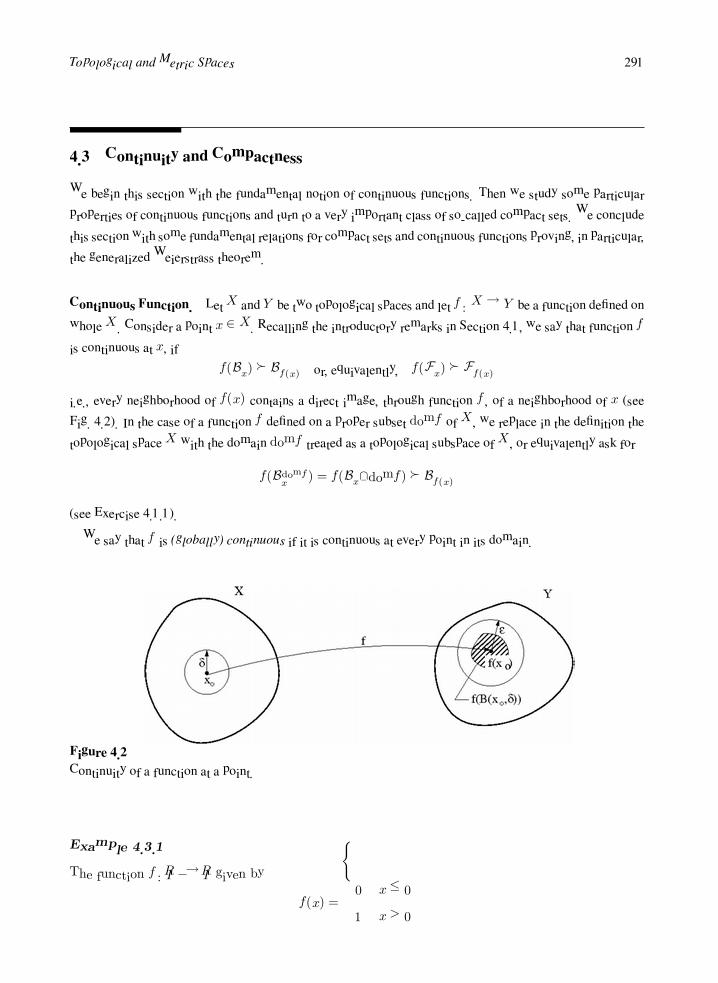
Topological and Metric Spaces 291
4.3 Continuity and Compactness
We begin this section with the fundamental notion of continuous functions. Then we study some particular
properties of continuous functions and turn to a very important class of so-called compact sets. We conclude
this section with some fundamental relations for compact sets and continuous functions proving, in particular,
the generalized Weierstrass theorem.
Continuous Function. LetX and Y be two topological spaces and let f : X → Y be a function defined on
whole X . Consider a point x ∈ X. Recalling the introductory remarks in Section 4.1, we say that function f
is continuous at x, if
f(Bx) Bf(x) or, equivalently, f(Fx) Ff(x)
i.e., every neighborhood of f(x) contains a direct image, through function f , of a neighborhood of x (see
Fig. 4.2). In the case of a function f defined on a proper subset domf of X , we replace in the definition the
topological space X with the domain domf treated as a topological subspace of X , or equivalently ask for
f(Bdomfx ) = f(Bx∩domf) Bf(x)
(see Exercise 4.1.1).
We say that f is (globally) continuous if it is continuous at every point in its domain.
Figure 4.2
Continuity of a function at a point.
Example 4.3.1
The function f : IR −→ IR given by
f(x) =
0 x ≤ 0
1 x > 0

292 APPLIED FUNCTIONAL ANALYSIS
is discontinuous at x = 0 and continuous at any other point. To confirm this assertion notice that for
any ball B = B(0, δ) centered at 0, (B(0, δ) = (−δ, δ)), f(B) contains the number 1 and, therefore,
f(B) cannot be contained in the balls B(0, ε) = B(f(0), ε) for ε < 1.
Example 4.3.2
Let X = 1, 2, 3 and Y = a, b, c, d and consider the following topologies:
X = X, ∅, 1, 2, 1, 2 and Y = Y, ∅, a, b, a, b, b, c, d
Consider the functions F and G from X into Y defined by
F G
F (1) = b G(1) = a
F (2) = c G(2) = b
F (3) = d G(3) = c
The function F is continuous at 1. Indeed, set 1 is a neighborhood of 1 and f(1) = b must be
contained in all neighborhoods of b. Similarly F is continuous at 2. The only two neighborhoods of d
in Y are Y itself and set b, c, d. Both of them contain f(X), with X being the only neighborhood
of 3 in X. Thus function F is continuous. Is function G continuous as well?
The following propositions summarize the fundamental properties of continuous functions.
PROPOSITION 4.3.1
In the following, U, V,X, Y , and Z denote topological spaces.
(i) Let f : X → Y and g : Y → Z be continuous. Then the composition gf : X → Z is continuous
as well.
(ii) Let f : X → Y and g : X → Z be continuous. Then (f, g) : X x → (f(x), g(x)) ∈ Y × Z is
continuous as well.
(iii) Let f : U → X and g : V → Y be continuous. Then the Cartesian product of functions f and
g,
(f × g) : U × V (u, v)→ (f(u), g(v)) ∈ X × Y
is continuous.
PROOF Proof follows immediately from definitions and we leave details as an exercise.
Topological and Metric Spaces 293
PROPOSITION 4.3.2
Let X and Y be two topological spaces and let f : X → Y denote an arbitrary function defined on
the whole X(domf = X). Then the following conditions are equivalent to each other:
(i) f is (globally) continuous.
(ii) f−1(G) is open in X for every G open in Y .
(iii) f−1(F ) is closed in X for every F closed in Y .
PROOF
(i) ⇒ (ii). Let G be an open set in Y and let x ∈ f−1(G). Then f(x) ∈ G and, consequently,
there exists a neighborhood B of f(x) such that B ⊂ G. It follows from continuity at x that there
must be a neighborhood C of x such that f(C) ⊂ B, which implies that
C ⊂ f−1(B) ⊂ f−1(G)
(ii) ⇒ (i). We use the bases of open neighborhoods Box and Bo
f(x). Let G be an arbitrary open set
containing f(x). Then f−1(G) is open, contains x and, therefore, is a neighborhood of x. Trivially,
f(f−1(G)) ⊂ G
which proves that f is continuous at x.
(i) ⇔ (iii) follows by duality arguments from the identity:
f−1(G) = (f−1(G))
PROPOSITION 4.3.3
Let X be a topological space. The following conditions are equivalent.
(i) There exists a nontrivial open partition of X, i.e., there exist nonempty open sets Gi ⊂ X, i =
1, 2, such that G1 ∪G2 = X, G1 ∩G2 = ∅.
(ii) There exists a nontrivial closed partition of X, i.e., there exist nonempty closed sets Fi ⊂
X, i = 1, 2, such that F1 ∪ F2 = X, F1 ∩ F2 = ∅.
(iii) There exists a nonempty subset A, not equal to X, that is simultaneously open and closed.
PROOF It is sufficient to notice that, by duality, sets Gi or Fi, being complements of each other,
must be simultaneously open and closed.

294 APPLIED FUNCTIONAL ANALYSIS
Connected sets. If a space X does not admit an open (or equivalently, closed) partition, we say that X is
connected. A set A ⊂ X is connected if, as a topological subspace of X , is connected.
PROPOSITION 4.3.4
Let A be a connected subset of X, and let f : X → Y be continuous. The f(A) is connected in Y .
PROOF See Exercise 4.3.8.
Hausdorff Spaces. In what follows, we restrict ourselves to a class of topological spaces called Hausdorff
spaces. A topological space X is said to be Hausdorff if for every two distinct points x and y there exist
neighborhoods B of x and C of y such that B ∩ C = ∅. In other words, every two distinct points can be
separated by disjoint neighborhoods. We will see a fundamental consequence of this definition in the next
section when we define the limit of a sequence.
Example 4.3.3
Let X be an arbitrary nonempty set. The discrete topology on X is Hausdorff (explain, why?), the
trivial one is not.
Compact Topological Spaces. Let X be a topological space and G ⊂ P(X) a family of sets. G is said to
be a covering of space X if simply
X =
G∈G
G
Similarly, if G contains a subfamily G0, which is also a covering of X , then G0 is called a subcovering. We
say that covering or subcovering is finite if it contains a finite number of sets. Finally, if all sets of G are open,
then we speak of an open covering.
We have the following important definition. A Hausdorff space X is said to be compact if every open
covering of X contains a finite subcovering. In other words, from every family of open sets Gι, ι ∈ I , I
being an “index set,” such that
X =
ι∈I
Gι
we can extract a finite number of sets G1, . . . , Gk such that
X = G1 ∪ . . . ∪Gk
Now, let B be a base. We say that a point x is a limit point of B if
x ∈
B∈B
B

Topological and Metric Spaces 295
We have the following important characterization of compact spaces.
PROPOSITION 4.3.5
Let X be a Hausdorff space. The following conditions are equivalent to each other:
(i) X is compact.
(ii) Every base in X possesses a limit point.
PROOF
(i)⇒ (ii). Let B be a base in X. It follows from the definition of a base that the family consisting
of closures of sets belonging to B is also a base. Thus, it is sufficient to show that every base of
closed sets possesses a limit point. Let B be such a base and assume, to the contrary, that
B∈B
B = ∅ or, equivalently,
B∈B
B = X
Since sets B are open, they form an open covering of X and, according to the definition of compact
space, we can find sets B1, . . . , Bk such that
B1 ∪ . . . ∪B
k = X
or, equivalently,
B1 ∩ . . . ∩Bk = ∅
But this contradicts the assumption that B is a base, as every finite intersection of elements from a
base is nonempty (explain, why?).
(ii) ⇒ (i). Let G be an open covering of X
X =
G∈G
G
or, equivalently,
G∈G
G = ∅
Define the family B of finite intersections,
G1 ∩ . . . ∩G
k Gi ∈ G
B is a base provided each of the intersections is nonempty. Assume now, contrary to (i), that there
is no finite subcovering in G. This is equivalent to saying that the intersections above are nonempty
and consequently B is a base of closed sets. According to (ii),
G∈G
G = ∅ i.e.,
G∈G
G = X

296 APPLIED FUNCTIONAL ANALYSIS
which contradicts that G is a covering of X.
Compact Sets. A set E in a Hausdorff spaceX is said to be compact if E, as a topological subspace ofX ,
is compact. Let G be a family of open sets in X such that
E ⊂
G∈G
G
We say that G is an open covering of set E in space X . Sets G ∩ E are open in E and, therefore, they form
an open covering of space (topological subspace) E. If E is compact, then there exists a finite subfamily
G1, . . . , Gk such that
E = (G1 ∩ E) ∪ . . . (Gk ∩ E)
or, equivalently,
E ⊂ G1 ∪ . . . ∪Gk
Concluding, a set E is compact if every open covering of E in X contains a finite subcovering.
Similarly, reinterpreting Proposition 4.3.5, we establish that a set E is compact if every base B in E
possesses a limit point in E, i.e.,
B∈B
B ∩ E = ∅
The following proposition summarizes the fundamental properties of compact sets.
PROPOSITION 4.3.6
(i) Every compact set is closed.
(ii) Every closed subset of a compact set is compact.
(iii) Let f : X → Y be continuous and E ⊂ dom f ⊂ X be compact. Then f(E) is also compact.
In other words, a direct image of a continuous function of a compact set is compact.
(iv) Cartesian products of compact sets are compact.
PROOF
(i) Let E be compact and let x be an accumulation point of E. Suppose that x does not belong
to E. Consequently,
B ∩ E = B ∩ E − x = ∅ for every B ∈ Bx
But this means that sets B ∩E form a base in E which, by compactness of E, must possess a limit
point in E, i.e., the set
B∈B
B ∩ E ∩ E
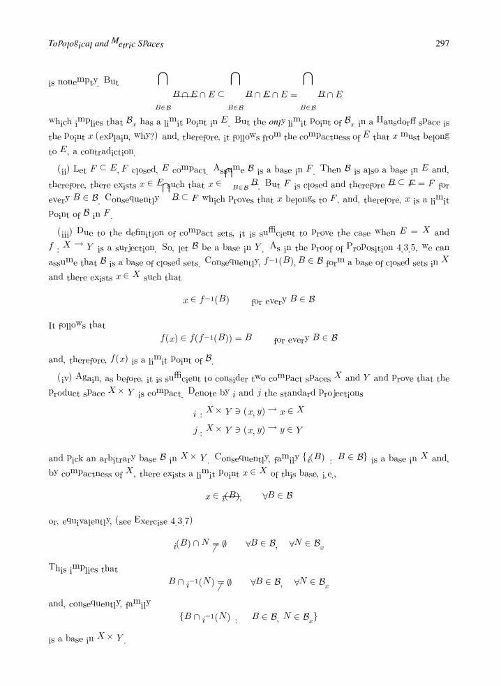
Topological and Metric Spaces 297
is nonempty. But
B∈B
B ∩ E ∩ E ⊂
B∈B
B ∩ E ∩ E =
B∈B
B ∩ E
which implies that Bx has a limit point in E. But the only limit point of Bx in a Hausdorff space is
the point x (explain, why?) and, therefore, it follows from the compactness of E that x must belong
to E, a contradiction.
(ii) Let F ⊂ E,F closed, E compact. Assume B is a base in F . Then B is also a base in E and,
therefore, there exists x ∈ E such that x ∈
B∈B B. But F is closed and therefore B ⊂ F = F for
every B ∈ B. Consequently
B ⊂ F which proves that x belongs to F , and, therefore, x is a limit
point of B in F .
(iii) Due to the definition of compact sets, it is sufficient to prove the case when E = X and
f : X → Y is a surjection. So, let B be a base in Y . As in the proof of Proposition 4.3.5, we can
assume that B is a base of closed sets. Consequently, f−1(B), B ∈ B form a base of closed sets in X
and there exists x ∈ X such that
x ∈ f−1(B) for every B ∈ B
It follows that
f(x) ∈ f(f−1(B)) = B for every B ∈ B
and, therefore, f(x) is a limit point of B.
(iv) Again, as before, it is sufficient to consider two compact spaces X and Y and prove that the
product space X × Y is compact. Denote by i and j the standard projections
i : X × Y (x, y)→ x ∈ X
j : X × Y (x, y)→ y ∈ Y
and pick an arbitrary base B in X × Y . Consequently, family i(B) : B ∈ B is a base in X and,
by compactness of X, there exists a limit point x ∈ X of this base, i.e.,
x ∈ i(B), ∀B ∈ B
or, equivalently, (see Exercise 4.3.7)
i(B) ∩N = ∅ ∀B ∈ B, ∀N ∈ Bx
This implies that
B ∩ i−1(N) = ∅ ∀B ∈ B, ∀N ∈ Bx
and, consequently, family
B ∩ i−1(N) : B ∈ B, N ∈ Bx
is a base in X × Y .

298 APPLIED FUNCTIONAL ANALYSIS
Repeating the same argument with this new base in place of the original base B, we obtain
B ∩ i−1(N) ∩ j−1(M) = ∅ ∀B ∈ B, ∀N ∈ Bx, ∀N ∈ By
But i−1(N) ∩ j−1(M) = N ×M and, consequently,
B ∩ (N ×M) = ∅ ∀B ∈ B, ∀N ∈ Bx, ∀N ∈ By
which implies that (x, y) is a limit point of B. Thus, every base in X × Y possesses a limit point
and, therefore, X × Y is compact.
We conclude this section with two fundamental theorems concerning compact sets. The first one, the
Heine–Borel Theorem, characterizes compact sets in IR.
THEOREM 4.3.1
(The Heine–Borel Theorem)
A set E ⊂ IR is compact iff it is closed and bounded.
PROOF Let E ⊂ IR be compact. According to Proposition 4.3.6(i), it suffices to prove that E is
bounded. Assume to the contrary, that supE = +∞ and consider the family B of sets of the form
[c,∞) ∩ E, c ∈ IR
Obviously, B is a base of closed sets in E and its intersection is empty, which contradicts that E is
compact.
Conversely, to prove that a closed and bounded set E must be compact, it is sufficient to prove
that every closed interval [a,b] is compact. Then E, as a closed subset of a compact set, will also
have to be compact.
So, let B be a base of closed sets in a closed interval [a,b]. First of all, any nonempty, closed,
and bounded set B in IR possesses its maximum and minimum. Indeed, if b = supB then, by the
boundedness of B, b <∞ and it follows from the definition of supremum that there exists a sequence
bn from B converging to b. Finally, it follows from the closedness of B that b ∈ B and therefore
supB = maxB. Analogously inf B = minB.
Denote now
c = infB∈B
(maxB)
It follows from the definition of infimum that for every δ > 0 there exists a set Bδ from base B such
that
maxBδ < c+ δ
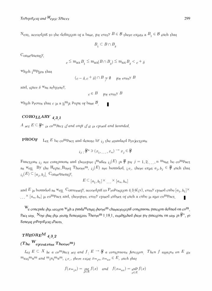
Topological and Metric Spaces 299
Next, according to the definition of a base, for every B ∈ B there exists a B1 ∈ B such that
B1 ⊂ B ∩Bδ
Consequently,
c ≤ maxB1 ≤ max(B ∩Bδ) ≤ maxBδ < c+ δ
which implies that
(c− δ, c+ δ) ∩B = ∅ for every B
and, since δ was arbitrary,
c ∈ B for every B
which proves that c is a limit point of base B.
COROLLARY 4.3.1
A set E ⊂ IRn is compact if and only if it is closed and bounded.
PROOF Let E be compact and denote by ij the standard projections
ij : IRn (x1, . . . , xn)→ xj ∈ IR
Functions ij are continuous and therefore images ij(E) in IR for j = 1, 2, . . . , n must be compact
as well. By the Heine–Borel Theorem, ij(E) are bounded, i.e., there exist aj , bj ∈ IR such that
ij(E) ⊂ [aj , bj ]. Consequently,
E ⊂ [a1, b1]× . . .× [an, bn]
and E is bounded as well. Conversely, according to Proposition 4.3.6(iv), every closed cube [a1, b1]×
. . .× [an, bn] is compact and, therefore, every closed subset of such a cube is also compact.
We conclude this section with a fundamental theorem characterizing continuous function defined on com-
pact sets. Note that this result generalizes Theorem 1.18.1, established there for functions on sets in IRn, to
general topological spaces.
THEOREM 4.3.2
(The Weierstrass Theorem)
Let E ⊂ X be a compact set and f : E → IR a continuous function. Then f attains on E its
maximum and minimum, i.e., there exist xmin, xmax ∈ E, such that
f(xmin) = infx∈E
f(x) and f(xmax) = supx∈E
f(x)

300 APPLIED FUNCTIONAL ANALYSIS
PROOF According to Proposition 4.3.6(iii), f(E) is compact in IR and therefore the Heine–Borel
Theorem implies that f(E) is closed and bounded. Thus, both sup f(E) and inf f(E) are finite and
belong to set f(E) which means that there exist xmin and xmax such that f(xmin) = inf f(E) and
f(xmax) = sup f(E).
Exercises
Exercise 4.3.1 Let X = 1, 2, 3, 4 and consider the topology on X given by a family of open sets,
X = X, ∅, 1, 2, 1, 2, 2, 3, 4
Show that the function f : X → X given by
f(1) = 2, f(2) = 4, f(3) = 2, f(4) = 3
is continuous at 4, but not at 3.
Exercise 4.3.2 Let f : X → Y . Prove that f is continuous iff f−1(B) ⊂ f−1(B) for every B ⊂ Y .
Exercise 4.3.3 Let f be a function mappingX into Y . Prove that f is continuous iff f(A) ⊂ f(A) for every
A ⊂ X .
Exercise 4.3.4 Let X1 and X2 be two topologies on a set X and let I : (X,X1) → (X,X2) be the identity
function. Show that I is continuous if and only if X1 is stronger than X2; i.e., X2 ⊂ X1.
Exercise 4.3.5 Show that the constant function f : X → X, f(x) = c, is continuous relative to any
topology on X .
Exercise 4.3.6 Explain why every function is continuous at isolated points of its domain with respect to any
topology.
Exercise 4.3.7 We say that bases A and B are adjacent if
A ∩B = ∅ ∀A ∈ A, B ∈ B
Verify that bases A and B are adjacent iff A∩B is a base.
Analogously, we say that base A is adjacent to set C if
A ∩ C = ∅ ∀a ∈ A
Verify that base B is adjacent to set C iff family A∩C is a base.
Prove the following simple properties:
(i) A is adjacent to C, A B ⇒ B is adjacent to C.

Topological and Metric Spaces 301
(ii) If family A is a base then (family f(A) is a base iff A is adjacent to domf ).
(iii) Family C being a base implies that (f−1(C) is a base iff C is adjacent to range f(X)).
(iv) If families A,B are adjacent and families C,D are adjacent then families A × C,B × D are
adjacent as well.
Exercise 4.3.8 Prove that the image of a connected set through a continuous function is connected as well.
4.4 Sequences
It turns out that for a class of topological spaces many of the concepts introduced can be characterized in
terms of sequences. In the present section, we define notions such as sequential closedness, continuity,
and compactness and seek conditions under which they are equivalent to the usual concepts of closedness,
continuity, or compactness.
Convergence of Sequences. A sequence of points xn in a topological spaceX converges to a point x ∈ X ,
denoted xn → x, if, for every neighborhood B of x, there exists an index N = N(B) such that
xn ∈ B for every n ≥ N
Sometimes we say that almost all (except for a finite number of) elements of xn belong to B. Equivalently,
we write x = limxn and call x the limit of sequence x. Note once again that this notion is a straightforward
generalization of the idea of convergence of sequences in IRn where the word “ball” has been replaced by the
word “neighborhood.”
Example 4.4.1
Consider the space of continuous functions C(0.1) of Example 4.1.8, with the topology of pointwise
convergence and the sequence of monomials fn(x) = xn. A careful look at Example 4.1.8 reveals
that we have proved there that fn converges to the zero function.
It may seem strange, but in an arbitrary topological space a sequence xn may have more than one limit.
To see this, consider an arbitrary nonempty set X with the trivial topology. Since the only neighborhood of
any point is just the whole space X , every sequence xn ∈ X converges to an arbitrary point x ∈ X . In other
words: every sequence is convergent and the set of its limits coincides with the whole X .
The situation changes in a Hausdorff space where a sequence xn, if convergent, possesses precisely one
limit x. To verify this, assume, to the contrary, that xn converges to another point y distinct from x. Since the
space is Hausdorff, there exist neighborhoods, A of x and B of y such that A ∩ B = ∅. Now let N1 be such

302 APPLIED FUNCTIONAL ANALYSIS
an index that xn ∈ A for every n ≥ N1 and similarly let N2 denote an index for which xn ∈ B for every
n ≥ N2. Thus for n ≥ max(N1, N2) all xn must belong to A ∩B = ∅, a contradiction.
Cluster Points. Let xn be a sequence. We say that x is a cluster point of sequence xn if every neighborhood
of x contains an infinite number of elements of sequence xn, i.e., for every neighborhood B of x and positive
integer N, there exists n ≥ N such that an ∈ B. Trivially, a limit of sequence xn, if it exists, is its cluster
point.
Bases of Countable Type. A base B is said to be of countable type if it is equivalent to a countable base C.
C = Ci, i = 1, 2, . . .
Note that sets of the form
Dk = C1 ∩ C2 ∩ . . . ∩ Ck , k = 1, 2, . . .
form a new countable base D = Dk, k = 1, 2, . . . such that
D1 ⊃ D2 ⊃ . . .
and D ∼ C. Thus, every base of countable type can be replaced with an equivalent countable base of
decreasing sets.
Example 4.4.2
Let X = IRn and let B be a base of balls centered at a point x0
B = B(x0, ε) , ε > 0
Then B is of countable type. Indeed, B is equivalent to its subfamily
C = B(x0,1
k) , k = 1, 2, . . .
PROPOSITION 4.4.1
Let X be a topological space such that, for every point x, base of neighborhoods Bx is of countable
type. Let xn be a sequence in X. Then x is a cluster point of xn iff there exists a subsequence xnk
converging to x.
PROOF Obviously, if xnkconverges to x then x is a cluster point of xn. Conversely, let x be a
cluster point of xn. Let B1 ⊃ B2 ⊃ . . . be a base of neighborhoods of x. Since every Bk contains

Topological and Metric Spaces 303
an infinite number of elements from sequence xn, for every k one can choose an element xnk∈ Bk
different from xn1 , . . . , xnk−1. Since Bk is decreasing, xnl
∈ Bk for every l ≥ k which implies that
xnk→ x.
Sequential Closedness. A set E is said to be sequentially closed if every convergent sequence of elements
from E possesses a limit in E, i.e.,
E xn → x ⇒ x ∈ E
It is easy to notice that closedness implies sequential closedness. Indeed, let xn ∈ E converge to x. This
means that
∀ B ∈ Bx ∃N : xn ∈ B ∀ n ≥ N
It follows that B ∩ E = ∅, for every B ∈ Bx and consequently x ∈ E = E (comp. Exercise 4.1.6).
PROPOSITION 4.4.2
Let Bx be of countable type for every x ∈ X. Then set E ⊂ X is closed iff it is sequentially closed.
PROOF Let x be an accumulation point of E and B1 ⊃ B2 ⊃ . . . denote a base of neighborhoods
of x. Choosing xk ∈ Bk ∩ E − x, we get E xk → x, which implies that x ∈ E.
Sequential Continuity. Let X and Y be Hausdorff spaces and f : X → Y a function. We say that f
is sequentially continuous at x0 ∈ dom f if for every sequence xn ∈ dom f converging to x0 ∈ dom f ,
sequence f(xn) converges to f(x0),
xn → x0 ⇒ f(xn)→ f(x0)
If f is sequentially continuous at every point in its domain, we say that f is (globally) sequentially continuous.
Continuity implies always sequential continuity. To verify this assertion, pick an arbitrary neighborhoodB
of f(x0). If f is continuous at x0 then there is a neighborhood C of x0 such that f(C) ⊂ B. Consequently, if
xn is a sequence converging to x one can find an index N such that xn ∈ C for every n ≥ N , which implies
that f(xn) ∈ f(C) ⊂ B and therefore f(xn)→ f(x0).
The converse is, in general, not true but we have the following simple observation.
PROPOSITION 4.4.3
Let Bx be of countable type for every x ∈ X. Then function f : X → Y is continuous iff it is
sequentially continuous.

304 APPLIED FUNCTIONAL ANALYSIS
PROOF Let B1 ⊃ B2 ⊃ . . . be a base of neighborhoods of x0 ∈ dom f . Assume f is sequentially
continuous at x0 and suppose, to the contrary, that f is not continuous at x0. This means that there
exists a neighborhood C of f(x0) such that
f(Bk) ⊂ C for every Bk
Thus, one can choose a sequence xk ∈ Bk such that f(xk) /∈ C. It follows that xk → x and, simulta-
neously, f(xk) /∈ C for all k, which implies that f(xk) does not converge to f(x0), a contradiction.
Many of the properties of continuous functions hold for sequentially continuous functions as well. For
instance both a composition and Cartesian product of sequentially continuous functions are sequentially con-
tinuous.
Sequential Compactness. One of the most important notions in functional analysis is that of sequential
compactness. We say that a set E is sequentially compact if, from every sequence xn ∈ E, one can extract a
subsequence xnkconverging to an element of E.
The following observation holds.
PROPOSITION 4.4.4
Let E ⊂ X be a compact set. Then
(i) every sequence in E has a cluster point.
If additionally every base of neighborhoods Bx is of countable type then
(ii) E is sequentially compact.
PROOF
(i) Let xn be a sequence in E. The family of sets
Ck = xk, xk+1, xk+2, . . .
is a base in E and, therefore, there must be an x such that
x ∈ Ck for every k
But this means that for every B, a neighborhood of x, and for every k there exists an xnk(nk ≥ k)
such that xnk∈ B. Thus, an infinite number of elements of sequence xn belongs to B.
(ii) This follows immediately from Proposition 4.4.1.
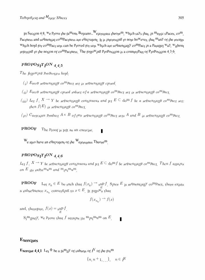
Topological and Metric Spaces 305
In Section 4.8, we prove the famous Bolzano–Weierstrass theorem, which says that, in metric spaces, com-
pactness and sequential compactness are equivalent. It is interesting to note however, that many of the results
which hold for compact sets can be proved for sets which are sequentially compact in a parallel way, without
referring to the notion of compactness. The following proposition is a counterpart of Proposition 4.3.6.
PROPOSITION 4.4.5
The following properties hold:
(i) Every sequentially compact set is sequentially closed.
(ii) Every sequentially closed subset of a sequentially compact set is sequentially compact.
(iii) Let f : X → Y be sequentially continuous and let E ⊂ dom f be a sequentially compact set;
then f(E) is sequentially compact.
(iv) Cartesian product A×B of two sequentially compact sets A and B is sequentially compact.
PROOF The proof is left as an exercise.
We also have an equivalent of the Weierstrass Theorem.
PROPOSITION 4.4.6
Let f : X → Y be sequentially continuous and let E ⊂ domf be sequentially compact. Then f attains
on E its supremum and minimum.
PROOF Let xk ∈ E be such that f(xk)→ supE
f . Since E is sequentially compact, there exists
a subsequence xnkconverging to x ∈ E. It follows that
f(xnk)→ f(x)
and, therefore, f(x) = supE
f .
Similarly, we prove that f attains its minimum on E.
Exercises
Exercise 4.4.1 Let Φ be a family of subsets of IN of the form
n, n+ 1, . . ., n ∈ IN

306 APPLIED FUNCTIONAL ANALYSIS
1. Prove that Φ is a base (the so-called fundamental base in IN ).
2. Characterize sets from filter F(Φ).
3. Let an be a sequence in a topological spaceX . Prove that the following conditions are equivalent
to each other:
(i) an → a0 in X
(ii) a(Φ) Ba0 , and
(iii) a(F(Φ)) Fa0
where Ba0 and Fa0 are the base and filter of neighborhoods of point a0 ∈ X , respectively.
Exercise 4.4.2 Let X be a topological space and an a sequence in X . Let Φ be the fundamental base in IN
from the previous exercise and a : IN n → an ∈ X an arbitrary sequence in X . Prove that the
following conditions are equivalent to each other:
1. a(Φ) Ba0
2. (a α)(Φ) Ba0 , for every injection α : IN → IN
where Ba0is base of neighborhoods of some point a0 ∈ X (sequence an converges to a0 iff its every
subsequence converges to a0).
Exercise 4.4.3 Let xn be a sequence in a topological space X and let Φ denote the fundamental base in IN
(recall Exercise 4.4.1). Prove that the following conditions are equivalent to each other:
1. x0 is a cluster point of xn
2. bases x(Φ)and Bx0are adjacent
4.5 Topological Equivalence. Homeomorphism
Topological Equivalence. In previous chapters, we have frequently encountered the idea of equivalence of
various mathematical systems. We have seen that this idea is extremely important to the theory surrounding
any particular system. For instance, the notion of an isomorphism provides for “algebraic equivalence” of
linear vector spaces or linear algebras: when two such systems are isomorphic, their algebraic properties are
essentially the same. Can a parallel concept of equivalence be developed for topological spaces?
It is natural to ask first what common properties we would expect two “topologically equivalent” topolog-
ical spaces to share. From what we have seen up to this point, the answer is partially clear—the properties
of continuity of functions, convergence of sequences, compactness of sets, etc., should be preserved under
some correspondence (map) between the two spaces. A simple bijection is not enough—it can only establish

Topological and Metric Spaces 307
a one-to-one and onto correspondence of elements in the underlying sets. For example, supposeX,Y, and Z
are topological spaces, and F : X → Z is a continuous function. If X and Y are to be equivalent in some
topological sense, we would expect there to exist a bijection map L : X → Y that preserves the continuity
of F in the sense that F L−1 : Y → Z is continuous, too. In other words, the topological equivalence
we are looking for is attained if the compositions of the bijections L and L−1 with continuous functions are
continuous. Such mappings are called homeomorphisms (not to be confused with homomorphisms discussed
in Chapter 2), and we sum up our observations concerning them by recording the following definition.
Homeomorphic Spaces. Two topological spaces X and Y are said to be homeomorphic (or topologically
equivalent) if and only if there exists a map L : X → Y such that
(i) L is bijective,
(ii) L,L−1 are continuous.
The map L is called a homeomorphism from X to Y .
Any property P of a topological space X is called a topological property if every space homeomorphic to
X also has property P .
REMARK 4.5.1 Note that, in general, continuity of L does not imply continuity of L−1, even
though L is bijective. As an example consider a finite set X, 1 < #X < ∞ with the discrete
topology. Let Y be another finite set such that #Y = #X and let L : X → Y denote a bijection.
Setting the trivial topology in Y , we easily see that L is continuous, while L−1 is not (explain,
why?).
We record some of the fundamental properties of homeomorphic spaces in the following proposition.
PROPOSITION 4.5.1
Let L : X → Y be a homeomorphism. The following properties hold:
(i) E is open iff L(E) is open.
(ii) E is closed iff L(E) is closed.
(iii) E is compact iff L(E) is compact.
PROOF These assertions follow immediately from the corresponding propositions in the previous
sections.

308 APPLIED FUNCTIONAL ANALYSIS
Theory of Metric Spaces
4.6 Metric and Normed Spaces, Examples
We now come to the subject of a special type of topological space that shall be of great importance throughout
the remainder of this book: metric spaces. A metric on a set amounts to a rather natural generalization of the
familiar idea of distance between points.
Metric. Metric Space. Let X be a nonempty set. A function
d : X ×X (x, y)→ d(x, y) ∈ [0,∞)
taking pairs of elements ofX into nonnegative real numbers, is called a metric on the setX if and only if the
following conditions hold:
(i) d(x, y) = 0 if and only if x = y;
(ii) d(x, y) = d(y, x) for every x, y ∈ X;
(iii) d(x, z) ≤ d(x, y) + d(y, z) for every x, y, z ∈ X .
Frequently we refer to d(x, y) as the distance between points x and y. Property (i) of the function d charac-
terizes it as strictly positive and (ii) as a symmetric function of x and y. Property (iii) is known as the triangle
inequality.
The set X with the metric d, denoted X = (X, d), is called a metric space.
Example 4.6.1
Perhaps the most familiar example of a metric space involves the idea of distance between points in
the Euclidean plane. Here X = IR2 and the distance between points x = (x1, x2) and y = (y1, y2) is
defined as follows:
d(x, y) = ((x1 − y1)2 + (x2 − y2)
2)12
Clearly, d(x, y) is symmetric and strictly positive. To prove the triangle inequality (look at Fig. 4.3
for notation) one has to show that
c ≤ a+ b or, equivalently, c2 ≤ a2 + b2 + 2ab
But, it follows from the cosine theorem that
c2 = a2 + b2 − 2ab cos γ ≤ a2 + b2 + 2ab

Topological and Metric Spaces 309
which finishes the proof.
Figure 4.3
Triangle inequality for the Euclidean metric in a plane.
Many of the notions from Euclidean geometry can be easily generalized into the general context of metric
spaces. The (open) ball with center at x and radius ε > 0, denoted B(x, ε), is defined as follows
B(x, ε) = y ∈ X : d(x, y) < ε
IfE is a subset ofX and x is a point, the distance between point x and set E, denoted d(x,E), can be defined
as the smallest distance from x to members of E. More precisely,
d(x,E) = infy∈E
d(x, y)
The number
dia (E) = supd(x, y) : x, y ∈ E
is referred to as the diameter of set E. If dia(E) is finite then E is said to be bounded, if not, then E is
unbounded. Equivalently, E is bounded if there exists a sufficiently large ball which contains E.
Norm. Normed Spaces. Let V be a real or complex vector space. A function
· : V v → v ∈ [0,∞)
prescribing for each vector v a nonnegative real number is called a norm, provided the following axioms
hold:
(i) v = 0 if and only if v = 0;
(ii) λv = |λ| v for every λ ∈ IR(IC),v ∈ V ;
(iii) u+ v ≤ u+ v for every u,v ∈ V .
Axiom (i) characterizes the norm as strictly positive, property (ii) is frequently referred to as homogeneity
and (iii) is known as triangle inequality.
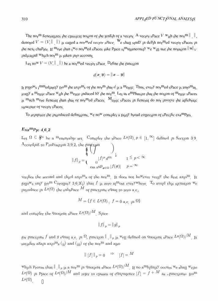
310 APPLIED FUNCTIONAL ANALYSIS
The norm generalizes the classical notion of the length of a vector. A vector space V with the norm · ,
denoted V = (V, · ) is called a normed vector space. We shall study in depth normed vector spaces in
the next chapter. If more than two normed spaces take place simultaneously we will use the notation uV
indicating which norm is taken into account.
Let now V = (V, · ) be a normed vector space. Define the function
d(x,y) = x− y
It follows immediately from the axioms of the norm that d is a metric. Thus, every normed space is automat-
ically a metric space with the metric induced by the norm. Let us emphasize that the notion of metric spaces
is much more general than that of normed spaces. Metric spaces in general do not involve the algebraic
structure of vector spaces.
To reinforce the introduced definitions, we now consider a fairly broad collection of specific examples.
Example 4.6.2
Let Ω ⊂ IRn be a measurable set. Consider the space Lp(Ω), p ∈ [1,∞] defined in Section 3.9.
According to Proposition 3.9.2, the function
fp =
Ω
|f |p dm
1p
1 ≤ p <∞
ess supx∈Ω |f(x)| p =∞
verifies the second and third axioms of the norm. It does not however verify the first axiom. It
follows only from Corollary 3.6.3(i) that f is zero almost everywhere. To avoid this situation we
introduce in Lp(Ω) the subspace M of functions equal to zero a.e.,
M = f ∈ Lp(Ω) : f = 0 a.e. in Ω
and consider the quotient space Lp(Ω)/M . Since
fp = gp
for functions f and g equal a.e. in Ω, function · p is well defined on quotient space Lp(Ω)/M . It
satisfies again axioms (ii) and (iii) of the norm and also
[f ] p = 0 ⇒ [f ] = M
which proves that · p is a norm in quotient space Lp(Ω)/M . If no ambiguity occurs we shall write
Lp(Ω) in place of Lp(Ω)/M and refer to classes of equivalence [f ] = f + M as “functions” from
Lp(Ω).
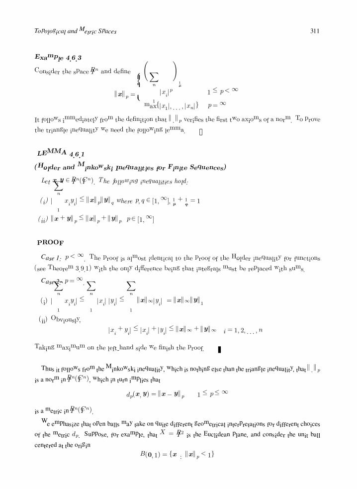
Topological and Metric Spaces 311
Example 4.6.3
Consider the space IRn and define
xp =
n
1
|xi|p
1p
1 ≤ p <∞
max|x1|, . . . , |xn| p =∞
It follows immediately from the definition that ·p verifies the first two axioms of a norm. To prove
the triangle inequality we need the following lemma.
LEMMA 4.6.1
(Holder and Minkowski Inequalities for Finite Sequences)
Let x,y ∈ IRn(ICn). The following inequalities hold:
(i) |
n
1
xiyi| ≤ xpyq where p, q ∈ [1,∞], 1p + 1
q = 1
(ii) x+ yp ≤ xp + yp p ∈ [1,∞]
PROOF
Case 1: p < ∞. The proof is almost identical to the proof of the Holder inequality for functions
(see Theorem 3.9.1) with the only difference being that integrals must be replaced with sums.
Case 2: p =∞.
(i) |
n
1
xiyi| ≤
n
1
|xi| |yi| ≤
n
1
x∞|yi| = x∞y1
(ii) Obviously,
|xi + yi| ≤ |xi|+ |yi| ≤ x∞ + y∞ i = 1, 2, . . . , n
Taking maximum on the left-hand side we finish the proof.
Thus it follows from the Minkowski inequality, which is nothing else than the triangle inequality, that ·p
is a norm in IRn(ICn), which in turn implies that
dp(x,y) = x− yp 1 ≤ p ≤ ∞
is a metric in IRn(ICn).
We emphasize that open balls may take on quite different geometrical interpretations for different choices
of the metric dp. Suppose, for example, that X = IR2 is the Euclidean plane, and consider the unit ball
centered at the origin
B(0, 1) = x : xp < 1

312 APPLIED FUNCTIONAL ANALYSIS
If we take p = 2 (Euclidean norm) then B(0, 1) is the set of points in the unit circle shown in Fig. 4.4(a), if
p =∞ then
d(x, 0) = x∞ = max|x1|, |x2|
and the ball coincides with the unit square shown in Fig. 4.4(b). The unit ball becomes the diamond-shaped
region (a rotated square) shown in Fig. 4.4(c) if p = 1 and, finally, if we select p > 1, B(0, 1) becomes a
figure with curved sides. For example, if p = 3 then B(0, 1) assumes the shape shown in Fig. 4.4(d).
Figure 4.4
Examples of unit balls in IR2 with respect to different metrics.
Lemma 4.6.1 can be easily generalized for the case of infinite sequences.
LEMMA 4.6.2
(Holder and Minkowski Inequalities for Infinite Sequences)
Let x = xi∞1 ,y = yi
∞1 be infinite sequences of real or complex numbers. The following
inequalities hold:

Topological and Metric Spaces 313
(i) |∞
1
xiyi| ≤ xpyp where p, q ∈ [1,∞], 1p + 1
q = 1
(ii) x+ yp ≤ xp + yp p ∈ [1,∞]
provided the right-hand sides are finite. In the above
xp =
∞
1
|xi|p
1p
1 ≤ p <∞
maxi|xi| p =∞
PROOF The proof follows immediately from Lemma 4.6.1. For instance, according to Lemma 4.6.1,
we have
|n
1
xiyi| ≤
n
1
|xi|p
1p
n
1
|yi|q
1q
≤
∞
1
|xi|p
1p
∞
1
|yi|q
1q
Passing with n to infinity on the left-hand side, we get the results required.
Example 4.6.4
(p Spaces)
Guided by Lemma 4.6.2, we introduce the sets of infinite sequences
p = x = (xi)∞1 : xp <∞
According to Lemma 4.6.2, p is closed with respect to the customary defined operations and,
therefore, p are vector spaces. It follows also from the definition of · p and Lemma 4.6.2 that
· p is a norm in p. Thus spaces p, p ∈ [1,∞], are another example of normed and metric spaces.
Example 4.6.5
(Chebyshev Spaces)
Let K ⊂ IRn be a compact set and let C(K) denote, as usual, the space of continuous functions
on K. Recalling that every continuous functional attains its maximum on a compact set, we define
the following quantity
f∞ = supx∈K
|f(x)| = maxx∈K
|f(x)|
One can easily verify that X = C(K) is a normed vector space with the norm ·∞. The ·∞ norm
is referred to as the Chebyshev norm and X is called the Chebyshev space. The resulting metric is

314 APPLIED FUNCTIONAL ANALYSIS
known as the Chebyshev metric. In fact, X can be considered as a subspace of L∞(K) (for continuous
functions the essential supremum coincides with the usual supremum).
It is interesting to interpret the Chebyshev metric graphically by considering the two functions
f(x) and g(x) in Fig. 4.5. Clearly, d(f, g) is the maximum amount f(x) differs from g(x) in the
interval [a, b] as shown.
Figure 4.5
Geometrical interpretation of Chebyshev metric.
We will present now two examples of metric spaces which are not normed spaces.
Example 4.6.6
Let d(x, y) be any metric on a set X. We claim that the function
σ(x, y) =d(x, y)
1 + d(x, y)
is also a metric. Indeed, σ(x, y) = σ(y, x), σ(x, y) = 0 iff x = y. Finally, let a ≤ b be two nonnegative
numbers. It follows thatb
1 + b−
a
1 + a=
b− a
(1 + b)(1 + a)≥ 0
soa
1 + a≤
b
1 + b
Concluding, (a = d(x, z), b = d(x, y) + d(y, z)):
σ(x, z) =d(x, z)
1 + d(x, z)≤
d(x, y) + d(y, z)
1 + d(x, y) + d(y, z)
=d(x, y)
1 + d(x, y) + d(y, z)+
d(y, z)
1 + d(x, y) + d(y, z)
≤ σ(x, y) + σ(y, z)
so the triangle inequality holds, and σ is a metric.

Topological and Metric Spaces 315
It is surprising, but every set E is bounded in the metric σ(x, y). Indeed, for arbitrary x and y,
σ(x, y) =d(x, y)
1 + d(x, y)≤ 1
Example 4.6.7
(The Discrete Metric)
Let X be any set and define the function d(x, y) by
d(x, y) =
1 x = y
0 x = y
It is easily verified that d is a metric, generally referred to as the discrete or trivial metric.
Product Spaces. Let (X, d) and (Y, ρ) be two metric spaces with metrics d and ρ, respectively. The metric
space (Z, σ), where Z = X × Y and
σ((x1, y1), (x2, y2)) = σ(d(x1, x2), ρ(y1, y2))
(where σ is one of the metrics induced by norms in IR2 discussed in Example 4.6.3), is called the product
space of the spaces (X, d) and (Y, ρ). For instance one can define the metric σ as (p = 1)
σ((x1, y1), (x2, y2)) = d(x1, x2) + ρ(y1, y2)
Exercises
Exercise 4.6.1 Let (X, d) be a metric space. Show that
ρ(x, y) = min1, d(x, y)
is also a metric on X .
Exercise 4.6.2 Show that any two norms · p and · q in IRn, 1 ≤ p, q ≤ ∞, are equivalent, i.e., there exist
constants C1 > 0, C2 > 0 such that
xp ≤ C1xq and xq ≤ C2xp
for any x ∈ IRn. Try to determine optimal (minimum) constants C1 and C2.

316 APPLIED FUNCTIONAL ANALYSIS
Exercise 4.6.3 Consider IRN with the l1-norm,
x = (x1, . . . , xN ), x1 =
N
i=1
|xi|
Let x be now any other norm defined on IRn.
(i) Show that there exists a constant C > 0 such that,
x ≤ Cx1 ∀x ∈ IRN
(ii) Use (i) to demonstrate that function
IRN x→ x ∈ IR
is continuous in l1-norm.
(iii) Use Weierstrass Theorem to conclude that there exists a constant D > 0 such that
x1 ≤ Dx ∀x ∈ IRN
Therefore, the l1 norm is equivalent to any other norm on IRN . Explain why the result implies that any
two norms defined on an arbitrary finite-dimensional vector space must be equivalent.
Take now two arbitrary norms. As each of them is equivalent to norm · 1, they must be equivalent
with each other as well.
4.7 Topological Properties of Metric Spaces
Let X = (X, d) be a metric space. Defining, for every x ∈ X , the family Bx of neighborhoods of x as the
family of open balls centered at x
Bx = B(x, ε), ε > 0
we introduce in X a topology induced by the metric d. Thus every metric space is a topological space with
the topology induced by the metric. Two immediate corollaries follow:
(i) Bases Bx are of countable type.
(ii) The metric topology is Hausdorff.
The first observation follows from the fact that Bx is equivalent to its subbase of the form
B
x,1
k
, k = 1, 2, . . .

Topological and Metric Spaces 317
To prove the second assertion consider two distinct points x = y. We claim that balls B(x, ε) and B(y, ε)
where ε = d(x, y)/2, are disjoint. Indeed, if z were a point belonging to the balls simultaneously, then
d(x, y) ≤ d(x, z) + d(z, y) < ε+ ε = d(x, y)
a contradiction.
Thus all the results we have derived in the first five sections of this chapter for Hausdorff topological
spaces with bases of neighborhoods of countable type hold also for metric spaces. Let us briefly review some
of them.
Open and Closed Sets in Metric Spaces. A setG ⊂ X is open if and only if, for every point x ofG, there
exists a ball B(x, ε), centered at x, that is contained in G. A point x is an accumulation point of a set F if
every ball centered at x contains points from F which are different from x, or, equivalently, there exists a
sequence xn points of F converging to x.
Note that a sequence xn converges to x if and only if
∀ ε > 0 ∃ N = N(ε) : d(xn, x) < ε ∀ n ≥ N
Finally, a set is closed if it contains all its accumulation points.
Continuity in Metric Spaces. Let (X, d) and (Y, ρ) be two metric spaces. Recall that a function f : X →
Y is continuous at x0 if
f(Bx0) Bf(x0)
or, equivalently,
∀ε > 0 ∃δ > 0 : f(B(x0, δ)) ⊂ B(f(x0), ε)
The last condition can be put into a more familiar form of the definition of continuity for metric spaces (ε− δ
continuity):
Function f : X → Y is continuous at x0 if and only if for every ε > 0 there is a δ = δ(ε, x0) such that
ρ(f(x), f(x0)) < ε whenever d(x, x0) < δ
Note that number δ generally depends not only on ε, but also upon the choice of point x0. If δ happens to
be independent of x0 for all x0 from a set E, then f is said to be uniformly continuous on E. Let us recall
also that, since bases of neighborhoods are of countable type, continuity in metric spaces is equivalent to
sequential continuity: a function f : X → Y is continuous at x0 if and only if
f(xn)→ f(x0) whenever xn → x0
Suppose now that there exists a constant C > 0, such that
ρ(f(x), f(y)) ≤ Cd(x, y) for every x, y ∈ E

318 APPLIED FUNCTIONAL ANALYSIS
Functions f satisfying such a condition are called Lipschitz continuous on E. Note that every Lipschitz
continuous function on E is also uniformly continuous on E. Indeed, choosing δ < εC (independent of x) we
get
ρ(f(x), f(x0)) ≤ Cd(x, x0) < Cε
C= ε
Example 4.7.1
Let X = Y = IR with the natural metric d(x, y) = |y − x|. Every C1 function f : IR→ IR is Lipschitz
continuous on every closed interval [a,b]. Indeed, according to the Lagrange theorem
f(y)− f(x) = f (c)(y − x) for every a ≤ x < y ≤ b
where c ∈ (x, y) ⊂ [a, b]. But f is continuous and the interval [a, b] is compact in IR so, according to
the Weierstrass Theorem, there exists such an x0, that
C = |f (x0)| = maxa≤c≤b
|f (c)|
Consequently,
|f(y)− f(x)| ≤ C|y − x|
which proves that f is Lipschitz continuous on [a, b].
Example 4.7.2
Choose again X = Y = IR and consider the function
f(x) =1
x, x ∈ (0,∞)
If f were uniformly continuous in (0,∞) then, for every ε > 0, one could choose a δ > 0 such that
|f(x)−f(x0)| < ε whenever |x−x0| < δ. Choose now x0 = 1n , x = 1
2n . Then |f(x)−f(x0)| = 2n−n
while |x − x0| =1
2n . In other words, for sufficiently large n, |x − x0| can be arbitrarily small while
|f(x)− f(x0)| can be arbitrarily large, which proves that 1x is not uniformly continuous.
Example 4.7.3
A nontrivial example of a continuous, nonlinear mapping in function spaces is given by the theorem
of Krasnosel’skii [4].
A mapping g : Ω× IR→ IR, where Ω ⊂ IRn is an open set, is called a Caratheodory mapping of Ω× IR
into IR if:
(i) for every ξ ∈ IR, x→ g(x, ξ) is a measurable function, and
(ii) for almost all x ∈ Ω, ξ → g(x, ξ) is a continuous function.

Topological and Metric Spaces 319
Now, for each measurable function u : Ω→ IR, let G(u) denote the measurable function
Ω x→ g(x, u(x))
Recall that the operator G is called the Nemytskii operator (comp. Example 2.5.5). It turns out
that if G maps Lp(Ω) into Lr(Ω), for some 1 ≤ p, r <∞, then G is continuous in Lp and Lr metrics,
respectively. In other words, a well-defined Nemytskii operator (i.e., mapping Lp(Ω) into Lr(Ω)) is
automatically continuous.
Let us note also that both norm and metric are continuous in metric topology. Indeed, let V = (V, · ) be
a normed space. It follows from the triangle inequality that
x = y + x− y ≤ y+ x− y
or, equivalently,
x − y ≤ x− y
Similarly,
y − x ≤ y − x = x− y
so
|x − y| ≤ x− y
which proves that norm is Lipschitz continuous with constant equal 1.
Similarly, one can show that
|ρ(x, y)− ρ(x, y)| ≤ ρ(x, x) + ρ(y, y)
which proves that metric is Lipschitz continuous with constant equal 1, provided the product spaceX ×X is
supplied with the metric
ρ((x, y), (x, y)) = ρ(x, x) + ρ(y, y)
Dense Sets. Separable Metric Spaces. As in general topological spaces, a set E is dense in a metric space
(X, d), if E = X or, equivalently,
∀x ∈ X ∃xn ∈ E such that xn → x
The space (X, d) is said to be separable if there exists a countable set E dense in X .
Topological Equivalence. Two metric spaces X = (X, d) and Y = (Y, ρ) are topologically equivalent if
X and Y , with topologies induced by metrics d and ρ, are homeomorphic.

320 APPLIED FUNCTIONAL ANALYSIS
PROPOSITION 4.7.1
Let (X, d), (Y, ρ) be metric spaces and L : X → Y be a bijection such that there exist constants
µ1, µ2 > 0 such that
µ1d(x, y) ≤ ρ(L(x), L(y)) ≤ µ2d(x, y)
Then (X, d) and (Y, ρ) are topologically equivalent.
PROOF It follows from the inequality above that both L and L−1 are Lipschitz continuous, and
therefore X and Y are homeomorphic.
REMARK 4.7.1 Note that the inequality
µ1d(x, y) ≤ ρ(L(x), L(y))
implies in particular that L is one-to-one. Indeed, if L(x) = L(y) then d(x, y) = 0, which implies
that x = y.
The converse of Proposition 4.7.1 in general is not true. To see this consider IRn with a metric d induced by
any of the norms discussed in Example 4.6.3 and let σ = d/(1+d) be the metric introduced in Example 4.6.6
on the same underlying setX . It is easy to check that the two metrics are topologically equivalent. Obviously
µ1σ(x, y) ≤ d(x, y) for µ1 = 1
but the second inequality does not hold since d(x, y) may be arbitrarily large while σ remains bounded
(σ ≤ 1).
Thus, the topological equivalence of two metrics defined on the same set X does not imply that they must
be bounded by each other in the sense of the discussed inequalities.
The situation is less complicated in the case of metrics induced by norms. It can be shown that norms
in the same vector space are topologically equivalent (generate the same topology) if and only if they are
bounded by each other. Moreover it turns out that in a finite-dimensional vector space any two norms are
topologically equivalent. This means, in particular, that the norm-induced topology in IRn is unique, i.e., can
be introduced only in one way! These and other facts concerning the normed spaces will be considered in the
next chapter.
Metric Equivalence—Isometries. At this point we have established a notion of topological equivalence
of two metric spaces, but this has been in the broad setting of topological spaces. We also saw that every
metric space is a topological space, so while the notion of topological equivalence does apply to metric
spaces, it provides too general a means of comparison to depict equivalence of purely metric properties, i.e.,
the concept of distance between points. What is needed to construct a more specialized idea is, as usual, a

Topological and Metric Spaces 321
means of comparing points in two metric spaces (e.g., a bijective map from one space onto the other) and
the equivalence of distances between points in each space. These properties are covered by the concept of an
isometry:
Two metric spaces (X, d) and (Y, ρ) are said to be isometric (or metrically equivalent) if and only if there
exists a bijection G : (X, d)→ (Y, ρ) such that
d(x, y) = ρ(G(x), G(y)) for every x, y ∈ X
The mapping G with this property is called an isometry.
Obviously, if G is an isometry then both G and G−1 are Lipschitz continuous with constant 1 and, there-
fore, G is a homeomorphism. Thus two isometric spaces are homeomorphic.
Example 4.7.4
Recall the classical theorem in elementary geometry: Every isometry G : IRn → IRn(n = 2, 3, IRn with
Euclidean metric) is a composition of a translation and a rotation about a point. Equivalently, in
the language of mechanics: A rigid body motion is always a composition of a translation and a
rotation about a point.
Exercises
Exercise 4.7.1 Prove that F : (X,D) → (Y, ρ) is continuous if and only if the inverse image of every
(open) ball B(y, ) in Y is an open set in X .
Exercise 4.7.2 Let X = C∞(a, b) be the space of infinitely differentiable functions equipped with Cheby-
shev metric. Let F : X → X be the derivative operator, Ff = df/dx. Is F a continuous map on X?
4.8 Completeness and Completion of Metric Spaces
Cauchy Sequences. Recall that every convergent sequence (xn) in IR satisfies the so-called Cauchy condi-
tion
∀ε > 0 ∃N : |xn − xm| < ε whenever n,m ≥ N
Roughly speaking, when a sequence converges in IR, the entries xi, xi+1, . . . get closer and closer together as
i increases. In other words
limi,j→∞
|xi − xj | = 0

322 APPLIED FUNCTIONAL ANALYSIS
A sequence which satisfies the Cauchy condition is called a Cauchy sequence. Thus, every convergent se-
quence in IR is a Cauchy sequence. It is well known that the converse is also true. Every Cauchy sequence in
IR is convergent.
The notion of a Cauchy sequence can be easily generalized to a general metric space (X, d). A sequence
(xn) is said to be a Cauchy sequence iff
∀ε > 0 ∃N : d(xn, xm) < ε whenever n,m ≥ N
As in the case of real numbers, every convergent sequence in a metric space (X, d) is a Cauchy sequence. To
see this, suppose that limxn = x0. Since
d(xm, xn) ≤ d(xm, x0) + d(xn, x0)
and d(xm, x0) < ε/2 and d(xn, x0) < ε/2 form,n ≥ some N ,
d(xm, xn) < ε form,n ≥ N
Hence, xn is a Cauchy sequence.
In general, however, the converse is not true. In many cases Cauchy sequences do not converge. We shall
examine this phenomenon here in some detail.
Example 4.8.1
The sequence (1/n) is convergent in IR and therefore is a Cauchy sequence in IR. This implies that
(1/n) is also a Cauchy sequence in any subset of IR, e.g., the interval (0, 1). Clearly, lim 1/n = 0 ∈
(0, 1) and therefore (1/n) is not convergent in (0, 1).
Example 4.8.2
Let X = C([−2, 2]) be the space of continuous functions on the interval [−2, 2] with L1 metric given
by
d(f, g) =
2
−2
|f(x)− g(x)| dx
Consider now the sequence of functions (fn(x)), where
fn(x) =
0 for −2 ≤ x ≤ 1− 1n
nx+ 1− n for 1− 1n ≤ x ≤ 1
1 for 1 ≤ x ≤ 2
(fn) is a Cauchy sequence. Indeed, if m > n, then
d(fm, fn) =
2
−2
|fm(x)− fn(x)| dx =1
2(1
n−
1
m)

Topological and Metric Spaces 323
which tends to 0 as m,n→∞.
However, this sequence does not converge in X. Indeed, suppose that fn → g in L1 metric. It
follows from Fatou’s lemma that 2
−2
lim inf |(fn − g)| ≤ lim inf
2
−2
|(fn − g)| = 0
which implies that g = f = lim inf fn = lim fn a.e. in [−2, 2], where
f(x) =
0 x > 1
1 x ≤ 1
It is easy to see that no such continuous function exists. Thus (fn) is not convergent in X.
When metric spaces do not have deficiencies of the type illustrated in these examples, we say that they are
complete.
Complete Metric Spaces. A metric space (X, d) is said to be complete if every Cauchy sequence in (X, d)
is convergent.
Example 4.8.3
The p normed spaces, p ∈ [1,∞], are complete. To prove this, let (xn) be a Cauchy sequence in p,
i.e., for every ε > 0 there exists an N such that
xn − xm =
∞
i=1
|xin − xi
m|p
1p
for p ∈ [1,∞]
maxi|xi
n − xim| for p =∞
is less than ε, for every m,n ≥ N . This implies that
|xin − xi
m| < ε n,m ≥ N
for every i = 1, 2, . . . and, therefore, xin is convergent for every i = 1, 2, . . .. Denote xi = lim
n→∞xin.
Passing to the limit with n→∞, we get
∞
i=1
|xi − xim|
p
1p
for p ∈ [1,∞]
supi∈IN
|xi − xim| for p =∞
< ε for m ≥ N
which proves that
1. x = (xi) belongs to p; we have from the triangle inequality
xp ≤ x− xnp + xnp ≤ ε+ xnp for any n ≥ N
324 APPLIED FUNCTIONAL ANALYSIS
2. xn converges to x.
Thus, spaces p are complete.
Example 4.8.4
Let K be a compact set in IRn. Consider the space C(K) of continuous functions on K with the
Chebyshev norm
f∞ = supx∈K
|f(x)|
The space C(K) is complete. To prove it, consider a Cauchy sequence (fn) in C(K). Thus, for every
ε > 0, there is an N such that for all x ∈ K
|fn(x)− fm(x)| ≤ fn − fm < ε for m,n ≥ N
Then, for an arbitrary fixed x ∈ K, fn(x) is a Cauchy sequence in IR and therefore convergent to
(say) the number f(x). Passing with n to infinity in the equality above, we get
|f(x)− fm(x)| ≤ ε for m ≥ N
which proves that
f − fm → 0
It remains to prove that f belongs to space C(K).
We show that if fn converges uniformly to f(x), then f(x) is continuous. Pick an ε > 0. It is
clear that
|f(x)− fn(x)| <ε
3for n ≥ some N, for every x ∈ K
Thus|f(x)− f(y)| ≤ |f(x)− fn(x)|+ |fn(x)− fn(y)|+ |fn(y)− f(y)|
< 2ε
3+ |fn(x)− fn(y)| for n ≥ N
Since fn is continuous, there exists δ such that
|fn(x)− fn(y)| <ε
3whenever |x− y < δ
i.e., f is continuous.
Example 4.8.5
Let Ω ⊂ IRn be an open set. The normed spaces Lp(Ω), p ∈ [1,∞] are complete. Consider first the
case p <∞. Let (fn) be a Cauchy sequence in Lp(Ω), i.e.,
∀ε > 0 ∃N : |fn − fmp < ε for n,m ≥ N

Topological and Metric Spaces 325
It follows that one can always extract a subsequence fnksuch that
fnk− fnk−1
p <1
2k, k = 1, 2 . . .
We will show that this subsequence converges to a limit which turns out to be the limit of the entire
Cauchy sequence.
Define
gk = fnk− fnk−1
, k = 1, 2 . . .
and consider the following two series
sk = g1 + g2 + . . .+ gk and Sk = |g1|+ |g2|+ . . .+ |gk|
Notice that
sm =
m
k=1
gk = fnm− fn0
and, therefore, convergence of the k-th partial sum sk will imply (is in fact equivalent to) convergence
of the subsequence fnk.
We have
Ω
(Sk)p = |g1|+ |g2|+ . . .+ |gk|
pp ≤ (|g1p + |g2p + . . .+ |gkp)
p
≤
1
2+
1
22+ . . .+
1
2k
p
≤ 1
For every x ∈ Ω, denote
Sp(x) = limk→∞
Spk(x)
As a nondecreasing sequence of nonnegative numbers, Spk(x) converges to a positive number or to
∞. It follows, however, from Fatou’s lemma (Theorem 3.5.1) that
Ω
Sp =
Ω
limk→∞
Spk ≤ lim
k→inf∞
Ω
Spk ≤ 1
which proves that Sp(x) and, therefore, S(x) is finite a.e. in Ω. In other words Sk(x) converges a.e.
in Ω, which in turn implies that sk(x) converges a.e. in Ω to a finite value, too. Denote
f0(x) = fn0(x) + lim
k→∞sk(x) = lim
k→∞fnk
(x)
We claim that:
1. f0 ∈ Lp(Ω);
2. fn → f0 in the Lp norm.
Indeed, the Cauchy condition and Fatou’s Lemma imply that
Ω
|fm(x)− f0(x)|p ≤ lim inf
k→∞
Ω
|fm(x)− fnk(x)|p < ε

326 APPLIED FUNCTIONAL ANALYSIS
provided m ≥ N . This proves that
fm → f0 in Lp(Ω)
Finally, from the inequality
f0p ≤ fmp + f0 − fmp ≤ fmp + ε
for m sufficiently large, follows that f0 ∈ Lp(Ω). Thus, Lp(Ω), 1 ≤ p <∞, is complete.
Proof of the case p =∞ is very similar to the proof of the completeness of C(K) from the previous
example and we leave it as an exercise.
The following proposition characterizes two fundamental properties of complete spaces.
PROPOSITION 4.8.1
(i) A subspace (Y, d) of a complete metric space (X, d) is complete iff Y is a closed set.
(ii) Let (X, d) and (Y, ρ) be two metric spaces that are isometric to each other. Then (Y, ρ) is
complete iff (X, d) is complete.
PROOF
(i) Assume that Y is closed and let (yn) be a Cauchy sequence in Y . Since yn ∈ X (because
Y ⊂ X), it has a limit y0 in X. However, every convergent sequence in a closed set has a limit in
the set; thus y0 ∈ Y and (Y, d) is complete.
Now assume that (Y, d) is complete. Let y be an accumulation point of Y . Equivalently, there
exists a sequence yn ∈ Y converging to y. As a convergent sequence (in X) yn is a Cauchy sequence
(both in X and in Y ) and therefore it has a limit y0 in Y which, according to the uniqueness of
limits in a metric space, must coincide with y. Thus y ∈ Y .
(ii) Let H : X → Y be an isometry and assume that X is complete. Consider a Cauchy sequence
yn ∈ Y , i.e.,
∀ε > 0 ∃N : ρ(yn, ym) < ε whenever n,m ≥ N
It follows from the definition of isometry that
∀ε > 0 ∃N : d(H−1(yn), H−1(ym)) < ε whenever n,m ≥ N
Hence, H−1(yn) is a Cauchy sequence in X and therefore possesses a limit x in X, which in turn
implies that y = H(x) = lim yn. Thus Y is complete.
The reverse process, interchanging X and Y , shows that if (Y, ρ) is complete, then (X, d) is
complete, and this completes the proof.

Topological and Metric Spaces 327
Notice that all isometric spaces are homeomorphic, but all homeomorphic spaces are not necessarily
isometric (since a homeomorphism need not preserve distances). Hence, it does not follow from Proposi-
tion 4.8.1 that if two spaces are homeomorphic, one is complete if and only if the other is. In other words,
completeness is not necessarily preserved under homeomorphisms. Therefore, completeness is not a topo-
logical property.
Now in the examples of complete and incomplete metric spaces considered earlier, we note that each
incomplete space is “immersed” in a larger metric space that is complete. For example, according to Propo-
sition 4.8.1, any open set in IRn is not complete. But its closure is. In this case we are able to “complete”
the space by merely adding all accumulation points to the set. In more general situations, we will not always
be able to find an incomplete space as the subspace of a complete one, but, as will be shown, it will always
be possible to identify a “larger” space that is very similar to any given incomplete space X that is itself
complete. Such larger complete spaces are called completions of X .
Completion of a Metric Space. Let (X, d) be a metric space. A metric space (X#, d#) is said to be a
completion of (X, d) if and only if
(i) there exists a subspace (Z, d#) of (X#, d#) which is dense in (X#, d#) and isometric to (X, d),
(ii) (X#, d#) is complete.
Thus, (X, d) may not necessarily be a subspace of a completion, as was the case in the example cited
previously, but it is at least isometric to a dense subspace. Hence, in questions of continuity and convergence,
(X, d) may be essentially the same as a subspace of its completion.
The question arises of when such completions exist and, if they exist, how many completions there are for
a given space. Fortunately they always exist, and all completions of a given metric space are isometric (i.e.,
completions are essentially unique). This fundamental fact is the basis of the following theorem.
THEOREM 4.8.1
Every metric space (X, d) has a completion and all of its completions are isometric.
The proof of this theorem is lengthy and involved; so, to make it more digestible, we shall break it into a
number of steps. Before launching into these steps, it is informative to point out a few difficulties encountered
in trying to develop completions of a given space too hastily. First of all, (X, d) must be isometric to a
space (Z, d#) dense in a completion (X#, d#). This suggests that (X#, d#) might consist of the Cauchy
sequences of (X, d) with d# defined as a metric on limit points. This is almost the case, but the problem with
this idea is that if two Cauchy sequences (xn) and (yn) in X have the property that lim d(xn, yn) = 0, then
we cannot conclude that (xn) = (yn) (xn = yn, but lim |xn − yn| = 0). To overcome this problem, we use
the notion of equivalence classes.
328 APPLIED FUNCTIONAL ANALYSIS
We will need two following lemmas.
LEMMA 4.8.1
Let (xn) be a Cauchy sequence in a metric space (X, d). Let (yn) be any other sequence in X such
that lim d(xn, yn) = 0. Then
(i) (yn) is also a Cauchy sequence,
(ii) (yn) converges to a point y ∈ X iff (xn) converges to y.
PROOF
(i) follows from the inequality
d(yn, ym) ≤ d(yn, xn) + d(xn, xm) + d(xm, ym)
(ii) Since
d(xn, y) ≤ d(xn, yn) + d(yn, y)
lim yn = y implies limxn = y. The converse is obtained by interchanging xn and yn.
LEMMA 4.8.2
Let (X, d) and (Y, ρ) be two complete metric spaces. Suppose that there exist two dense subspaces,
X of X and Y of Y which are isometric to each other. Then X and Y are isometric, too.
PROOF Let H : X → Y be an isometry from X onto Y. Pick an arbitrary point x ∈ X.
From the density of X in X it follows that there exists a sequence xn converging to x. Thus (xn)
is a Cauchy sequence which in turn implies that also yn = H(xn) is a Cauchy sequence. From the
completeness of Y it follows that (yn) has a limit y. Define
H(x) = y
We claim that H is a well-defined extension of H. Indeed, let xn be another sequence from X
converging to x. From the triangle inequality
d(xn, xn) ≤ d(xn, x) + d(xn, x)
it follows that lim ρ(H(xn), H(xn)) = lim d(xn, xn) = 0 which, according to the previous lemma,
implies that limH(xn) = y. Thus H(x) is independent of the choice of (xn). Choosing (xn) =
(x, x, . . .) for x ∈ X , we easily see that H(x) = H(x) for x ∈ X . Thus H is an extension of H.

Topological and Metric Spaces 329
Next we prove that H is an isometry. Indeed, we have
d(xn, yn) = ρ(H(xn), H(yn))
for every xn, yn ∈ X . Taking advantage of continuity of metrics d and ρ we pass to the limit with
xn → x and yn → y, getting the result required.
PROOF of Theorem 4.8.1.
Step 1. Let C(X) denote the set of all Cauchy sequences of points in X. We introduce a relation
R on C(X) defined so that two distinct Cauchy sequences (xn) and (yn) are related under R if and
only if the limit of the distance between corresponding terms in each is zero:
(xn)R(yn) iff lim d(xn, yn) = 0
The relation R is an equivalence relation. Indeed, by inspection, R is clearly reflexive and symmetric
owing to the symmetry of metric d. If (xn)R(yn) and (yn)R(zn), then (xn)R(zn), because
d(xn, zn) ≤ d(xn, yn) + d(yn, zn)
and
lim d(xn, yn) = 0 and lim d(yn, zn) = 0 implies lim d(xn, zn) = 0
Hence R is transitive and is, therefore, an equivalence relation.
Step 2. Now we recall that an equivalence relation partitions a set C(X) into equivalence classes;
e.g., [(xn)] is the set of all Cauchy sequences related to (xn) under the equivalence relation R. Let
X# denote the quotient set C(X)/R and let d#([(xn)], [(yn)]) be defined by
d# ([(xn)], [(yn)]) = limn→∞
d(xn, yn)
The function d# is a well-defined metric on X#. By “well defined” we mean that the limit appearing
in the definition of d# exists and is unambiguous. Denoting
sn = d(xn, yn)
we have|sn − sm| = |d(xn, yn)− d(xm, ym)|
= |d(xn, yn)− d(yn, xm) + d(yn, xm)− d(xm, ym)|
≤ d(xn, xm) + d(yn, ym)
from which follows that (sn) is a Cauchy sequence in IR. Since the set of real numbers is complete,
(sn) has a limit s in IR.
To show that this limit does not depend upon which representative we pick from the equivalence
classes [(xn)] and [(yn)], choose
(xn), (xn) ∈ [(xn)] ; (yn), (yn) ∈ [(yn)]

330 APPLIED FUNCTIONAL ANALYSIS
Then|d(xn, yn)− d(xn, yn)| = |d(xn, yn)− d(yn, xn) + d(yn, xn)− d(xn, yn)|
≤ |d(xn, yn)− d(yn, xn)|+ |d(yn, xn)− d(xn, yn)|
≤ d(xn, xn) + d(yn, yn)
By the definition of [(xn)] and [(yn)], d(xn, xn) and d(yn, yn)→ 0 as n→∞. Hence
lim d(xn, yn) = lim d(xn, yn)
Now, by construction, d#([(xn)], [(yn)]) is zero iff (xn) and (yn) belong to the same equivalence
class and in this case [(xn)] = [(yn)]. The symmetry of d# is obvious. From the triangle inequality
d(xn, zn) ≤ d(xn, yn) + d(yn, zn)
for any Cauchy sequences (xn), (yn), (zn), passing to the limit, we obtain
d#([(xn)], [(zn)]) ≤ d#([(xn)], [(yn)]) + d#([(yn)], [(zn)])
Hence, (X#, d#) is a metric space.
Step 3. Suppose that x0 is a point in X. It is a simple matter to construct a Cauchy sequence
whose limit is x0. For example, the constant sequence
(x0, x0, x0, . . .)
is clearly Cauchy and its limit is x0. We can construct such sequences for all points x in X, and
for each sequence so constructed, we can find an equivalence class of Cauchy sequences in X. Let Z
denote the set of all such equivalence classes constructed in this way; i.e.,
Z = z(x) : x ∈ X, z(x) = [(x, x, x, . . .)]
We claim that (X, d) is isometric to (Z, d#). Indeed, for x, y ∈ X
d#(z(x), z(y)) = d#([(x, x, . . .)], [(y, y, . . .)]) = lim d(x, y) = d(x, y)
Hence, z : X → Z is an isometry.
Step 4. (Z, d#) is dense in (X#, d#).
Let [(xn)] be an arbitrary point in X#. This means that (xn) is a Cauchy sequence of points in
X. For each component of this sequence there is a corresponding class of sequences equivalent to a
constant Cauchy sequence in Z; i.e.,
z(x1) = [(x1, x1, . . .)]
z(x2) = [(x2, x2, . . .)]
...
z(xn) = [(xn, xn, . . .)]

Topological and Metric Spaces 331
Consider the sequence of equivalence classes (z(x1), z(x2), . . .) = (z(xn)) in Z. Since (xn) is Cauchy,
we have
limn→∞
d#([(xn)], z(xn)) = limn→∞
( limm→∞
d(xm, xn)) = limn,m→∞
d(xn, xm) = 0
Therefore, the limit of (z(xn)) is [(xn)]. Thus Z is dense in X#.
Step 5. (X#, d#) is complete.
Let (x1,x2, . . .) be a Cauchy sequence in X#. Since Z is dense in X#, for every n there is an
element z(xn) ∈ Z such that
d#(xn, z(xn)) < 1/n
Consequently, d#(xn, z(xn))→ 0. It follows from Lemma 4.8.1 that (z(xn)) is Cauchy which in turn
implies that (xn) is Cauchy in X. Hence, by construction of X#, [(xn)] is a limit of z(xn) (compare
Step 4) and, according to Lemma 4.8.1, of (x1,x2, . . .), too.
Step 6. Uniqueness of the completion .
Let (X0, d0) be another completion of (X, d). It follows from the definition of completion that
both X# and X0 contain dense subspaces which are isometric to space X and therefore are also
isometric to each other. Thus, according to Lemma 4.8.2, X# and X0 are isometric to each other,
too.
This last result completes the proof.
The Baire Categories. It is convenient at this point to mention a special property of complete metric spaces.
A subspaceA of a topological spaceX is said to be nowhere dense inX if the interior of its closure is empty:
intA = ∅. For example, the integers Z are nowhere dense in IR.
A topological space X is said to be of the first category if X is the countable union of nowhere dense
subsets of X . Otherwise, X is of the second category. These are called the Baire categories. For example,
the rationals IQ are of the first category, because the singleton sets q are nowhere dense in IQ, and IQ is the
countable union of such sets. The real line IR is of the second category. Indeed, that every complete metric
space is of the second category is the premise of the following basic theorem.
THEOREM 4.8.2
(The Baire Category Theorem)
Every complete metric space (X, d) is of the second category.
PROOF Suppose, to the contrary, that X is of the first category, i.e.,
X =
∞
1
Mi, int M i = ∅

332 APPLIED FUNCTIONAL ANALYSIS
Replacing Mi with their closures M i, we can assume from the very beginning that Mi are closed.
Hence, complements M i are open.
Consider now the set M1. We claim that
M 1 = X
Indeed, suppose to the contrary that there is an x ∈M 1. Equivalently, there exists a neighborhood
B of x such that B∩M 1 = ∅, which in turn implies that B ⊂M1. Thus x ∈ int M1, a contradiction.
Since M 1 is open, there exists a closed ball
S1 = (x : d(x1, x) ≤ r1) ⊂M 1
centered at a point x1 which, according to the fact that M 1 = X, can be arbitrarily close to any
point of X. Obviously, we may assume that r1 < 1/2.
By the same arguments M 2 contains a closed ball
S2 = x : d(x2, x) ≤ r2
contained in S1 (we can locate center x2 arbitrarily close to any point in X) such that r2 < 1/22.
Proceeding in this way we obtain a sequence Sn of closed balls with the properties
rn < 1/2n, Sn+1 ⊂ Sn, Sn ∩Mn = ∅
Obviously, the sequence of centers xn is a Cauchy sequence and therefore possesses a limit x0. Since
xk ∈ Sn, for every k ≥ n and for every Sn, and Sn are closed, x0 ∈ Sn, for every n, which in turn
implies that x0 ∈
∞
1
Sn and consequently
x0 ∈
∞
1
Sn
=
∞
1
Sn ⊃
∞
1
Mn = X
a contradiction. Hence X is of the second category.
Exercises
Exercise 4.8.1 Let Ω ⊂ IRn be an open set and let (C(Ω), p) denote the (incomplete) metric space of
continuous, real-valued functions on Ω with metric induced by the Lp norm. Construct arguments
supporting the fact that the completion of this space is Lp(Ω).
Hint: See Exercise 4.9.3 and use Theorem 4.8.1.
Exercise 4.8.2 Let xnkbe a subsequence of a Cauchy sequence xn. Show that if xnk
converges to x, so does
the whole sequence xn.

Topological and Metric Spaces 333
Exercise 4.8.3 Prove that in a complete normed space, we have the generalization of the triangle inequality,
|
∞
n=1
xn| ≤
∞
n=1
|xn|
The result should be read as follows: if the series on the right-hand side converges, so does the one on
the left-hand side, and the estimate holds.
4.9 Compactness in Metric Spaces
Since in a metric space every point possesses a countable base of neighborhoods, according to Proposi-
tion 4.4.4, every compact set is sequentially compact. It turns out that, in the case of a metric space, the
converse is also true.
THEOREM 4.9.1
(Bolzano–Weierstrass Theorem)
A set E in a metric space (X, d) is compact if and only if it is sequentially compact.
Before we prove this theorem, we shall introduce some auxiliary concepts.
ε-Nets and Totally Bounded Sets. Let Y be a subset of a metric space (X, d) and let ε be a positive real
number. A finite set
Yε = y1ε , . . . , y
nε ⊂ X
is called an ε-net for Y if
Y ⊂
n
j=1
Byjε, ε
In other words, for every y ∈ Y there exists a point yjε ∈ Yε such that
dy, yjε
< ε
A set Y ⊂ X is said to be totally bounded in X if for each ε > 0 there exists in X an ε-net for Y . If Y is
totally bounded in itself, i.e., it contains the ε-nets, we say that Y is totally bounded. Note that, in particular,
every set Y totally bounded inX is bounded. Indeed, denoting byMε the maximum distance between points
in ε-net Yε
Mε = max d(x, y) : x, y ∈ Yε
we have
d(x, y) ≤ d(x, xε) + d(xε, yε) + d(yε, y) ≤Mε + 2ε for every x, y ∈ Y

334 APPLIED FUNCTIONAL ANALYSIS
where xε and yε are points from ε-net Yε such that
d(x, xε) < ε and d(y, yε) < ε
Consequently, diaY ≤Mε + 2ε, which proves that Y is bounded.
COROLLARY 4.9.1
Every totally bounded (in itself) metric space is separable.
PROOF Consider a family of 1/n-nets Yn and define
Y =
∞
1
Yn
As a union of a countable family of finite sets, Y is countable. Now, it follows from the definition of
ε-net that for a given x ∈ X and for every n = 1, 2 . . . there exists a yn ∈ Yn ⊂ Y such that
d(x, yn) < 1/n
Thus, limn→∞
yn = x, which proves that Y is dense in X.
LEMMA 4.9.1
Every sequentially compact set E in a metric space (X, d) is totally bounded.
PROOF Pick ε > 0 and an arbitrary point a1 ∈ E. If
E ⊂ B(a1, ε)
then a1 is the ε-net for E. If not, then there exists an a2 ∈ E − B(a1, ε). Proceeding in the
same manner we prove that either E contains ε-net of points a1, . . . , an or there exists an infinite
sequence (ai)∞1 such that
d(ai, aj) ≥ ε
This contradicts the fact that E is sequentially compact. Indeed, let (aik) be a subsequence of (ai)
convergent to an element a. Then, for sufficiently large i,
d(a, ai) <ε
3
which in turn implies that
d(ai, aj) ≤ d(ai, a) + d(a, aj) < 2ε
3
a contradiction.

Topological and Metric Spaces 335
PROOF of the Bolzano–Weierstrass Theorem.
Since every subset E of a metric space (X, d) is a metric space itself, it is sufficient to prove that
every sequentially compact metric space is compact. So let (X, d) be a sequentially compact metric
space and let Gι, ι ∈ I be an open covering of X. We claim that there exists an ε > 0 such that
every open ball with radius ε (centered at arbitrary point) is entirely contained in one of the sets
Gι. Indeed, suppose to the contrary that for every n there exists a point an ∈ X such that none of
the sets Gι contains ball B(an, 1/n). Since X is sequentially compact, there exists a subsequence
ankand a point a such that ank
→ a. Obviously, a ∈ Gκ, for some κ ∈ I and therefore there exists
a ball B(a, α) such that
B(a, α) ⊂ Gκ
However, for sufficiently large nk, d(ank, a) ≤ α/2 and simultaneously 1/nk ≤ α/2. It follows that
d(x, a) ≤ d(x, ank) + d(ank
, a) ≤α
2+
α
2= α
for every x ∈ B(ank, 1/nk). Thus
B(ank, 1/nk) ⊂ B(a, α) ⊂ Gκ
a contradiction.
Now, according to Lemma 4.9.1, X is totally bounded. Let Yε be an ε-net corresponding to the
value of ε for which every ball B(yε, ε), yε ∈ Yε, is contained entirely in the corresponding set Gyε
from the covering Gι, ι ∈ I. We have
X =
y∈Y ε
B(y, ε) ⊂
y∈Yε
Gyε
which proves that Gyε, yε ∈ Yε form a finite subcovering of Gι, ι ∈ I. Thus X is compact.
Recall that every (sequentially) compact set is (sequentially) closed. According to Lemma 4.9.1 every com-
pact (or, equivalently, sequentially compact) set in a metric space is totally bounded and therefore bounded.
Thus compact sets in metric spaces are both closed and bounded. The converse, true in IR (the Heine-Borel
Theorem), in general is false. The following is an example of a set in a metric space which is both closed and
bounded, but not compact.
Example 4.9.1
Consider the closed unit ball in the space 2, centered at zero vector:
B = B(0, 1) =
(xi)
∞j=1 :
∞
1
x2i
12
≤ 1

336 APPLIED FUNCTIONAL ANALYSIS
Obviously, B is bounded (dia B = 2). Since B is an inverse image of the closed interval [0, 1] in IR
through the norm in 2 which is continuous, B is also closed. However, B is not compact. To see it,
consider the sequence
ei = (0, . . . , 1(i)
, 0, . . .), i = 1, 2, . . .
Obviously, ei ∈ B and d(ei, ej) =√2, for every i = j. Thus sequence ei cannot be contained in
any finite union of balls with radii smaller than√2 which proves that B is not totally bounded and
therefore not compact, too.
The situation changes if we restrict ourselves to complete metric spaces, replacing the condition of bound-
edness with that of total boundedness.
THEOREM 4.9.2
Let (X, d) be a complete metric space. A set E ⊂ X is compact (equivalently sequentially compact)
if and only if it is closed and totally bounded.
PROOF Every compact set is closed and, according to Lemma 4.9.1, compact sets in metric
spaces are totally bounded.
Conversely, assume that E is closed and totally bounded. We shall prove that E is sequentially
compact. So let (xn) be an arbitrary sequence of points in E and consider a collection of ε-nets
corresponding to choices of ε of ε1 = 1, ε2 = 1/2, . . . , εn = 1/n, . . .. Since E is totally bounded, for
each of these choices we can construct a finite family of balls of radius ε that cover E. For example,
if ε = 1, we construct a collection of a finite number of balls of radius 1. One of these balls, say B1,
contains an infinite subsequence of (xn), say (x(1)n ). Similarly, about each point in the 1/2-net, we
form balls of radius 1/2, one of which (say B2) contains an infinite subsequence of (x(1)n ), say (x
(2)n ).
Continuing in this manner, we develop the following set of infinite subsequences
ε1 = 1
x(1)1 , x
(1)2 , . . . , x
(1)n , . . .
⊂ B1
ε2 = 1/2
x(2)1 , x
(2)2 , . . . , x
(2)n , . . .
⊂ B2
···
εn = 1/n
x(n)1 , x
(n)2 , . . . , x
(n)n , . . .
⊂ Bn
Selecting the diagonal sequence (x(n)n ), we get a subsequence of the original sequence (xn) which
satisfies the Cauchy condition. This follows from the fact that all x(m)m for m ≥ n are contained in
ball Bn of radius 1/n. Since X is complete, x(m)m converges to a point x which, according to the
assumption that E is closed, belongs to E. Thus E is sequentially compact.

Topological and Metric Spaces 337
REMARK 4.9.1 Note that the assumption of completeness of metric space (X, d) in The-
orem 4.9.2 is not very much restrictive since every compact set E in a metric space (X, d) (not
necessarily complete) is itself complete. To see it, pick a Cauchy sequence (xn) in E. As every
sequence in E, (xn) contains a convergent subsequence (xnk) to an element of E, say x0. It follows
from the triangle inequality that
d(x0, xn) ≤ d(x0, xnk) + d(xnk
, xn)
and therefore the whole sequence must converge to x0. Thus E is complete.
REMARK 4.9.2 The method of selecting the subsequence of functions converging on a countable
set of points, used in the proof of Theorem 4.9.2, is known as “the diagonal choice method.” We
will use it frequently in this book.
Precompact Sets. A set E in a topological space X is said to be precompact if its closure E is compact.
Thus, according to the Bolzano-Weierstrass theorem, a set E in IR is precompact iff it is bounded. Looking
back at Theorem 4.9.2, we can characterize precompact sets in complete metric spaces as those which are
totally bounded.
Due to the importance of compact sets, one of the most fundamental questions in functional analysis
concerns finding criteria for compactness in particular function spaces. We shall conclude this section with
two of them: the famous Arzela–Ascoli Theorem formulating a criterion for a compactness in the Chebyshev
space C(K) and the Frechet–Kolmogorov Theorem for spaces Lp(IR).
Equicontinuous Classes of Functions. Let C(X,Y ) denote a class of continuous functions (defined on
the entire X) mapping a metric space (X, d) into a metric space (Y, ρ). Thus f ∈ C(X,Y ) iff
∀x0 ∈ X ∀ε > 0 ∃δ > 0 : d(x0, x) < δ ⇒ ρ(f(x0), f(x)) < ε
Obviously, δ generally depends upon x0, ε and function f . Symbolically, we could write δ = δ(x0, ε, f).
Recall that if δ is independent of x0, δ = δ(ε, f) then f is said to be uniformly continuous .
A subclass F ⊂ C(X,Y ) of functions is said to be equicontinuous (on X) if δ happens to be independent
of f , for every f from the class F . In other words
∀ x0 ∈ X ∀ε > 0 ∃δ = δ(x0, ε) : d(x0, x) < δ ⇒ ρ(f, x0), f(x)) < ε
for every function f ∈ F .
Uniformly Bounded Real-Valued Function Classes. Recall that a function (functional) f : X → IR,
defined on an arbitrary set X , is bounded if there exists a constantM > 0 such that
|f(x)| ≤M for every x ∈ X

338 APPLIED FUNCTIONAL ANALYSIS
A class F of such functions is said to be uniformly bounded if constant M happens to be independent of
function f ∈ F , i.e.,
|f(x)| ≤M for every x ∈ X, f ∈ F
Consider now the Chebyshev space C(K) of continuous functions defined on a compact set K in IRn with
the Chebyshev norm
f = supx∈K
|f(x)|
and the resulting Chebyshev metric
d(f, g) = supx∈K
|f(x)− g(x)|
Thus, class F is uniformly bounded iff F is simply a bounded set in metric space C(K).
LEMMA 4.9.2
(Dini’s Theorem)
Let E be a compact topological space. Suppose we are given a monotone sequence of continuous
functions fn : E → IR converging pointwise to a continuous function f : E → IR. Then fn converges
uniformly to f .
PROOF
Case 1. Sequence fn is increasing.
Suppose, to the contrary, that fn does not converge uniformly to f . Thus there exists an ε > 0
such that the sets
En = x : f(x)− fn(x) ≥ ε
are not empty, for every n = 1, 2, . . .. Thus, as the decreasing family of nonempty sets, En forms a
base of closed sets. According to the compactness of E, there exists an element x0 ∈
∞
1
En, which
in turn implies that
f(x0)− fn(x0) ≥ ε for every n = 1, 2, . . .
which contradicts the fact that fn(x0) converges to f(x0).
Case 2. The proof for decreasing sequences of functions fn is identical.
LEMMA 4.9.3
Every continuous function f : X → Y from a compact metric space (X, d) to a metric space (Y, ρ)
is uniformly continuous.
In particular, every continuous functional defined on a compact metric space must be necessarily
uniformly continuous.

Topological and Metric Spaces 339
PROOF Suppose, to the contrary, that there is an ε > 0 such that for every n there exist points
xn, yn ∈ X such that
d(xn, yn) < 1/n and ρ(f(xn), f(yn)) ≥ ε
Since X is compact, we can choose a subsequence xnkconvergent to a point x in X. Selecting
another convergent subsequence from ynk, we can assume that both xn and yn converge to points x
and y. But d(xn, yn)→ 0 and therefore (comp. Lemma 4.8.1) x = y. On the other side, passing to
the limit with xn → x and yn → y in
ρ(f(xn), f(yn)) ≥ ε
we obtain from continuity of function f and metric ρ that
ρ(f(x), f(y)) ≥ ε
a contradiction.
We have the following
THEOREM 4.9.3
(Arzela–Ascoli Theorem)
A subclass F of C(K) is precompact if and only if
(i) F is equicontinuous, and
(ii) F is uniformly bounded.
PROOF We first prove necessity. Assume F is precompact. Then F is totally bounded in C(K)
which means that, for every ε > 0, we can construct an ε-net Yε = (f1, . . . , fn) in C(K). Denoting
M = max fi∞, i = 1, . . . , n
we have for every f ∈ F
|f(x)| ≤ |f(x)− fk(x)|+ |fk(x)| ≤ ε+M
where fk is a function from ε-net Yε such that
f − fk∞ < ε
Thus F is uniformly bounded.
To prove equicontinuity pick an ε > 0 and consider a corresponding ε3 -net Y ε
3= (f1, . . . , fn). Since
each fi is uniformly continuous (comp. Lemma 4.9.3), there exists a δi such that
|fi(x)− fi(y)| <ε
3whenever x− y < δi

340 APPLIED FUNCTIONAL ANALYSIS
where · denotes any of the norms in IRn. Setting
δ = min δi, i = 1, 2, . . . , n
we have
|fi(x)− fi(y)| <ε
3whenever x− y < δ for every fi ∈ Y ε
3
Now, for an arbitrary function f from F , it follows from the definition of ε-nets that
|f(x)− f(y)| ≤ |f(x)− fi(x)|+ |fi(x)− fi(y)|+ |fi(y)− f(y)|
<ε
3+
ε
3+
ε
3= ε
whenever x− y < δ.
To prove sufficiency we assume that F is uniformly bounded and equicontinuous and show that
every sequence (fn) ⊂ F contains a convergent subsequence. Since every compact set in a metric
space is separable (see Corollary 4.9.1), there exists a countable set K = x1,x2, . . . such that
K = K. Each of the sequences fk(xi)∞k=1 for x1,x2, . . . ∈ K is bounded, so by the diagonal choice
method (see Remark 4.9.2), we can extract such a subsequence fkjthat fkj
(x) is convergent for
every x ∈ K.
Pick an ε > 0. According to equicontinuity of F , there exists a δ > 0 such that
|fkj(x)− fkj
(y)| <ε
3whenever x− y < δ
Let x be an arbitrary point of K. It follows from density of K in K that there is a y ∈ K such
that x− y < δ. Consequently,
|fki(x)− fkj
(x)| ≤ |fki(x)− fki
(y)| +|fki(y)− fkj
(y)|+ |fkj(y)− fkj
(x)|
<ε
3+
ε
3+
ε
3= ε
for ki and kj sufficiently large (fki(y) is convergent and therefore Cauchy). Concluding, for every
x ∈ K, fki(x) is Cauchy in IR and therefore convergent. Denote
f0(x) = limki→∞
fki(x)
It remains to prove that
1. f0 is continuous;
2. fkiconverges uniformly to f0 (in norm · ∞).
It follows from equicontinuity of F that
∀ε > 0 ∃δ > 0 : |fki(x)− fki
(y)| < ε whenever x− y < δ
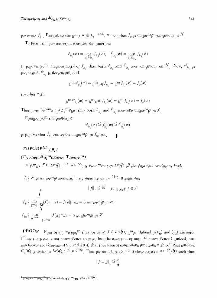
Topological and Metric Spaces 341
for every fki. Passing to the limit with ki →∞, we get that f0 is uniformly continuous in K.
To prove the last assertion consider the functions
ϕki(x) = inf
kj≥ki
fkj(x), ψki(x) = sup
kj≥ki
fkj(x)
It follows from equicontinuity of fkithat both ϕki
and ψkiare continuous on K. Now, ϕki
is
increasing, ψkiis decreasing, and
limϕki(x) = lim inf fki
= lim fki(x) = f0(x)
together with
limψki(x) = lim sup fki
(x) = lim fki(x) = f0(x)
Therefore, Lemma 4.9.2 implies that both ϕkiand ψki
converge uniformly to f .
Finally, from the inequality
ϕki(x) ≤ fki
(x) ≤ ψki(x)
it follows that fkiconverges uniformly to f0, too.
THEOREM 4.9.4
(Frechet–Kolmogorov Theorem)
A family F ⊂ Lp(IR), 1 ≤ p <∞, is precompact in Lp(IR) iff the following conditions hold:
(i) F is uniformly bounded,† i.e., there exists an M > 0 such that
fp ≤M for every f ∈ F
(ii) limt→0
IR|f(t+ s)− f(s)|p ds = 0 uniformly in F ;
(iii) limn→∞
|s|>n
|f(s)|p ds = 0 uniformly in F .
PROOF First of all, we claim that for every f ∈ Lp(IR), limits defined in (ii) and (iii) are zero.
(Thus the issue is not convergence to zero, but the assertion of uniform convergence.) Indeed, one
can prove (see Exercises 4.9.3 and 4.9.4) that the space of continuous functions with compact support
C0(IR) is dense in Lp(IR), 1 ≤ p <∞. Thus for an arbitrary ε > 0 there exists a g ∈ C0(IR) such that
f − gp ≤ε
3
†In other words, F is a bounded set in metric space Lp(IR).

342 APPLIED FUNCTIONAL ANALYSIS
Now, since g is continuous and bounded (explain, why?), by the Lebesgue Dominated Convergence
Theorem, we have
IR|g(t+ s)− g(s)|
pds
1p
→ 0 for t→ 0
and, consequently, Ttg − gp < ε3 for t ≤ some t0, where Tt is the translation operator
Ttg(s) = g(t+ s)
Finally,
f − Ttfp ≤ f − gp + g − Ttgp + Ttg − Ttfp < ε
whenever t ≤ t0, since the norm · p is invariant under the translation Tt. Thus
limt→0
IR|f(t+ s)− f(s)|p ds = 0 for every f ∈ Lp(IR)
The second assertion follows immediately from the Lebesgue Dominated Convergence Theorem and
pointwise convergence of truncations
fn(x) =
f(x) |x| ≤ n
0 |x| > n
to function f .
Assume now that F is precompact. Thus F is totally bounded in Lp(IR) and therefore bounded.
To prove the second assertion consider an ε3 -net (f1, . . . , fn) ⊂ Lp(IR) for F . According to our
preliminary considerations
Ttfi − fip <ε
3whenever t ≤ t0 = t0(fi)
with t0 = t0(fi) depending on fi. By choosing however
t0 = mint0(fi), i = 1, 2, . . . , n
we get
Ttfi − fip <ε
3whenever t ≤ t0
Consequently,
Ttf − fp ≤ Ttf − Ttfip + Ttfi − fip + fi − fp < ε
for t ≤ t0. This proves (ii). Using exactly the same technique we prove that (iii) holds.
To prove the converse we shall show that conditions (i)–(iii) imply total boundedness of F in
C(K) (comp. Theorem 4.9.2).
First of all, condition (ii) is equivalent to saying that
Ttf − fp → 0 uniformly in F

Topological and Metric Spaces 343
Define the mean-value operator as
(Maf)(s) = (2a)−1
a
−a
Ttf(s) dt
It follows from the Holder inequality and Fubini’s Theorem that
Maf − fp =
∞
−∞
a
−a
(2a)−1f(t+ s) dt− f(s)
p
ds
1p
≤
∞
−∞
a
−a
(2a)−1 |f(t+ s)− f(s)| dt
pds
1p
≤ (2a)−1
∞
−∞
(2a)pq
a
−a
|f(t+ s)− f(s)|pdt ds
1p
= (2a)−1+ 1q
a
−a
∞
−∞
|f(t+ s)− f(s)|pds dt
1p
= (2a)−1+ 1q
+ 1p sup|t|≤a
∞
−∞
|f(t+ s)− f(s)|pds
1p
= sup|t|≤a
Ttf − fp
where 1p + 1
q = 1.
Thus, according to (ii)
Maf → f uniformly in F
We shall show now that, for a fixed a > 0, functions Maf, f ∈ F are uniformly bounded and
equicontinuous. It follows from the Holder inequality again that
|(Maf)(s1)− (Maf)(s2)| ≤ (2a)−1
a
−a
|f(s1 + t)− f(s2 + t)| dt
≤ (2a)−1p
a
−a
|f(s1 + t)− f(s2 + t)|pdt
1p
= (2a)−1p Ts1−s2f − fp
But Ttf − fp → 0 while t→ 0 uniformly in f ∈ F and therefore Maf, f ∈ F are equicontinuous.
Similarly,
|(Maf)(s)| ≤ (2a)−1
a
−a
|f(t+ s)| dt ≤ (2a)−1
s+a
s−a
|f(t)| dt
≤ (2a)−1p
s+a
s−a
|f(t)|pdt
1p
≤ (2a)−1p fp
and, therefore,
sups∈IR
|Maf(s)| <∞ uniformly in F
Thus, by the Arzela–Ascoli Theorem, for a fixed n (note that IR is not compact and therefore
we restrict ourselves to finite intervals [−n, n]) and a given ε there exists an ε-net of function
gj ∈ C[−n, n]) such that for any f ∈ Lp(IR)
supx∈[−n,n]
|Maf(s)− gj(s)| < ε for some gj

344 APPLIED FUNCTIONAL ANALYSIS
Denoting by gj the zero extension of gj outside [−n, n], we obtain
IR|f(s)− gj(s)|
pds =
|s|>n
|f(s)|pds+
|s|≤n
|f(s)− gj(s)|pds
≤
|s|>n
|f(s)|pds+
|s|≤n
(|f(s)−Maf(s)|+ |Maf(s)− gj(s)|)pds
≤
|s|>n
|f(s)|pds+ 2p
|s|≤n
|f(s)−Maf(s)|pds
+
|s|≤n
|Maf(s)− gj(s)|pds
Now, pick an arbitrary ε > 0. By condition (iii) we can select an n such that the first term on the
right-hand side is bounded by ε3 uniformly in F . Next, from the inequality
2p
|s|≤n
|f(s)−Maf(s)|pds ≤ 2p f −Maf
pp
follows that we can select sufficiently small “a” such that the second term is bounded by ε3 . Finally,
considering the corresponding ε-net of function gj ∈ C([−n, n]), we have
|s|≤n
|Maf(s)− gj(s)|pds ≤ (sup |Maf − gj |)
p2n ≤ε
3
for ε = (ε/3/2n)1p .
Consequently, for every f ∈ Lp(IR)
IR|f(s)− gj(s)|
pds <
ε
3+
ε
3+
ε
3= ε
for some extensions gj . Thus F is totally bounded in Lp(IR) and therefore precompact in Lp(IR).
REMARK 4.9.3 The mean-value operator Maf can be equivalently defined as
Maf = f ∗ ϕ
where the star ∗ denotes the so-called convolution operation
(f ∗ ϕ)(s) =
IRf(s− t)ϕ(t) dt
provided ϕ is defined as follows
ϕ(t) =
12a for |t| ≤ a
0 otherwise

Topological and Metric Spaces 345
Functions ϕ of this type are called mollifiers and the convolution above is known as the mollification or
regularization of function f . It turns out that by taking more regular mollifiers, we obtain more regular
mollifications. In particular, for a C∞-mollifier the corresponding mollifications are also C∞-functions.
Exercises
Exercise 4.9.1 Let E ⊂ IRn be a Lebesgue measurable set. Function
χE :=
1 x ∈ E0 x /∈ E
is called the characteristic function of set E. Prove that there exists a sequence of continuous functions
φn : IRn → [0, 1], φn ≥ 0, converging to χE in the Lp norm for 1 ≤ p <∞.
Hint: Pick = 1/n and consider a closed subset F of E, and an open superset G of E such that
m(G − F ) < (recall characterization of Lebesgue measurable sets in Proposition 3.2.3(ii))). Then
set
φn(x) = φ(x) :=d(x,G)
d(x,G) + d(x, F )
where d(x,A) denotes the distance from point x to set A
d(x,A) := infy∈A
d(x, y)
Exercise 4.9.2 Let f : Ω → IR be a measurable function. Function φ : Ω → IR is called a simple function
if Ω can be partitioned into measurable sets Ei, i = 1, 2, . . ., and the restriction of φ to each Ei is
constant. In other words,
φ =∞
i=1
aiχEi
where ai ∈ IR and Ei are pairwise disjoint measurable sets. Prove then that, for every > 0, there
exists a simple function φ : Ω→ IR such that
f − φ∞ ≤
Hint: Use the Lebesgue approximation sums.
Exercise 4.9.3 Let Ω ⊂ IRn be an open set. Let f ∈ Lp(Ω), 1 ≤ p < ∞. Use results of Exercise 4.9.1 and
Exercise 4.9.2 to show that there exists a sequence of continuous functions φn : Ω→ IR converging to
function f in the Lp(Ω) norm.
Exercise 4.9.4 Argue that, in the result of Exercise 4.9.3, one can assume additionally that functions fn have
compact support.
Exercise 4.9.5 Let F be a uniformly bounded class of functions in Chebyshev space C[a, b], i.e.,
∃M > 0 : |f(x)| ≤M, ∀x ∈ [a, b], ∀f ∈ F

346 APPLIED FUNCTIONAL ANALYSIS
Let G be the corresponding class of primitive functions
F (x) =
x
a
f(s) ds, f ∈ F
Show that G is precompact in the Chebyshev space.
4.10 Contraction Mappings and Fixed Points
The ideas of a contraction mapping and of the fixed point of a function are fundamental to many questions in
applied mathematics. We shall outline briefly in this section the essential ideas.
Fixed Points of Mappings. Let F : X → X . A point x ∈ X is called a fixed point of F if
x = F (x)
Contraction Mapping. Let (X, d) be a metric space and F a mapping of X into itself. The function F is
said to be a contraction or a contraction mapping if there is a real number k, 0 ≤ k < 1, such that
d(F (x), F (y)) ≤ kd(x, y) for every x, y ∈ X
Obviously, every contraction mapping F is uniformly continuous. Indeed, F is Lipschitz continuous with a
Lipschitz constant k. The constant k is called the contraction constant for F .
We now arrive at an important theorem known as the Principle of Contraction Mappings or Banach Con-
traction Map Theorem.
THEOREM 4.10.1
(Banach Contraction Map Theorem )
Let (X, d) be a complete metric space and F : X → X be a contraction mapping. Then F has a
unique fixed point.
PROOF First, we show that if F has a fixed point, it is unique. Suppose there are two: x = F (x)
and y = F (y), x = y. Since F is a contraction mapping,
d(x, y) = d(F (x), F (y)) ≤ kd(x, y) < d(x, y)
which is impossible. Hence, F has at most one fixed point.
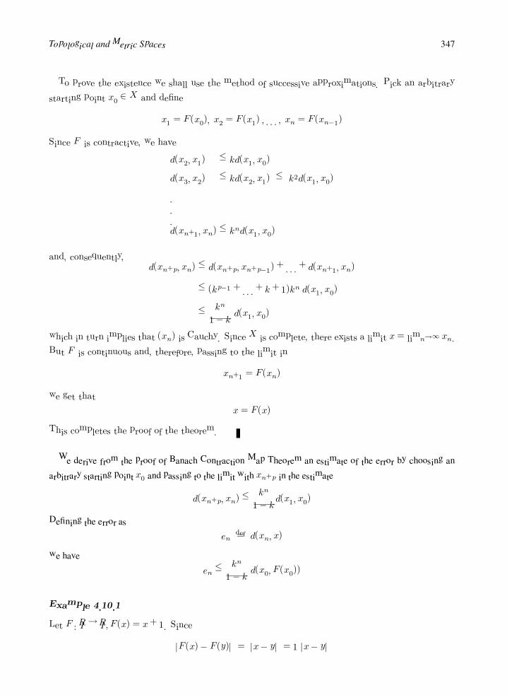
Topological and Metric Spaces 347
To prove the existence we shall use the method of successive approximations. Pick an arbitrary
starting point x0 ∈ X and define
x1 = F (x0), x2 = F (x1) , . . . , xn = F (xn−1)
Since F is contractive, we have
d(x2, x1) ≤ kd(x1, x0)
d(x3, x2) ≤ kd(x2, x1) ≤ k2d(x1, x0)
···d(xn+1, xn) ≤ knd(x1, x0)
and, consequently,d(xn+p, xn) ≤ d(xn+p, xn+p−1) + . . .+ d(xn+1, xn)
≤ (kp−1 + . . .+ k + 1)kn d(x1, x0)
≤kn
1− kd(x1, x0)
which in turn implies that (xn) is Cauchy. Since X is complete, there exists a limit x = limn→∞ xn.
But F is continuous and, therefore, passing to the limit in
xn+1 = F (xn)
we get that
x = F (x)
This completes the proof of the theorem.
We derive from the proof of Banach Contraction Map Theorem an estimate of the error by choosing an
arbitrary starting point x0 and passing to the limit with xn+p in the estimate
d(xn+p, xn) ≤kn
1− kd(x1, x0)
Defining the error as
endef= d(xn, x)
we have
en ≤kn
1− kd(x0, F (x0))
Example 4.10.1
Let F : IR→ IR, F (x) = x+ 1. Since
|F (x)− F (y)| = |x− y| = 1 |x− y|

348 APPLIED FUNCTIONAL ANALYSIS
then k = 1 and F is not a contraction. We observe that F (x) has no fixed point; this fact does
not follow from Theorem 4.10.1, however, which gives only sufficient conditions for the existence of
fixed points. In other words, there are many examples of operators with fixed points that are not
contraction mappings. For example
F (x) = 2x+ 1
is not a contraction mapping, but it has a unique fixed point, x = −1.
Example 4.10.2
Now suppose X = (0, 14 ], F : X → X,F (x) = x2. Thus
|F (x)− F (y)| = |x2 − y2| ≤ (|x|+ |y|) |x− y| ≤1
2|x− y|
Hence, k = 12 and F is a contraction. But F has no fixed points (in X!). This is not a contradiction
of Theorem 4.10.1 because X is not complete.
Example 4.10.3
Let F : [a, b] → [a, b], F differentiable at every x ∈ (a, b) and |F (x)| ≤ k < 1. Then, by the
mean-value theorem, if x, y ∈ [a, b], there is a point ξ between x and y, such that
F (x)− F (y) = F (ξ)(x− y)
Then
|F (x)− F (y)| = |F (ξ)| |x− y| ≤ k|x− y|
Hence F is a contraction mapping.
Example 4.10.4
Let F : [a, b]→ IR. Assume that there exist constants µ and γ such that µ < 1γ and 0 < µ ≤ F (x) ≤
1γ and assume that F (a) < 0 < F (b) (i.e., we have only one zero between a and b). How do we find
the zero of F (x)? That is, how can we solve
F (x) = 0 in [a, b]
To solve this problem, we transform it into a different problem: Consider a new function
F (x) = x− γF (x)
Clearly, the fixed points of F (x) are the zeros of F (x). Observe that
F (a) = a− γF (a) > a
F (b) = b− γF (b) < b

Topological and Metric Spaces 349
Also
F (x) = 1− γF (x) ≥ 0, F (x) ≤ 1− µγ < 1
Hence F transforms [a, b] into itself and | F (x)| ≤ 1 − µγ < 1, for every x ∈ [a, b]. In view of our
results in the previous example, F (x) is a contraction mapping.
Example 4.10.5
(Kepler’s Equations)
In orbital mechanics, we encounter the equation
ξ = η − e sin η
where e is the eccentricity of an orbit of some satellite and η is the central angle from perigee (if
P = period, t = time for perigee, then ξ = 2πt/P ). We wish to solve for η for a given ξ, ξ < 2π.
Toward this end, define
F (η) = η − e sin η − ξ
We must now solve for the zeros of the function F (η). Suppose that 0 ≤ η ≤ 2π; note that
F (0) = −ξ < 0, F (2π) = 2π − ξ > 0. Moreover, 1 − e ≤ F (η) ≤ 1 + e, since F (η) = 1 − e cos η.
Thus, using the results of the previous example, set µ = 1− e, γ = 1/(1 + e), and
F (η) = η −1
1 + eF (η) = η −
1
1 + e(η − e sin η − ξ)
or
F (η) =eη + (ξ + e sin η)
1 + e
Hence
k = 1−1− e
1 + e=
2e
1 + e
We can solve this problem by successive approximations when e < 1.
Example 4.10.6
(Fredholm Integral Equation)
Consider the integral equation
f(x) = ϕ(x) + λ
b
a
K(x, y)f(y)dy
whereinK(x, y) is continuous on [a, b]× [a, b]
ϕ(x) is continuous on [a, b]
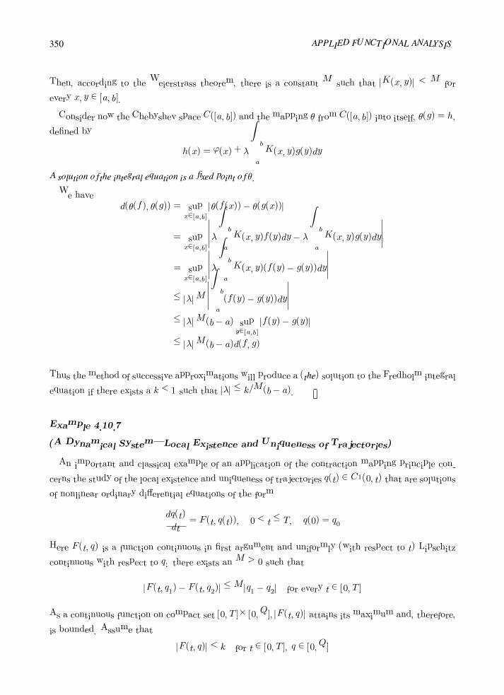
350 APPLIED FUNCTIONAL ANALYSIS
Then, according to the Weierstrass theorem, there is a constant M such that |K(x, y)| < M for
every x, y ∈ [a, b].
Consider now the Chebyshev space C([a, b]) and the mapping θ from C([a, b]) into itself, θ(g) = h,
defined by
h(x) = ϕ(x) + λ
b
a
K(x, y)g(y)dy
A solution of the integral equation is a fixed point of θ.
We haved(θ(f), θ(g)) = sup
x∈[a,b]
|θ(f(x))− θ(g(x))|
= supx∈[a,b]
λ
b
a
K(x, y)f(y)dy − λ
b
a
K(x, y)g(y)dy
= supx∈[a,b]
λ
b
a
K(x, y)(f(y)− g(y))dy
≤ |λ|M
b
a
(f(y)− g(y))dy
≤ |λ|M(b− a) supy∈[a,b]
|f(y)− g(y)|
≤ |λ|M(b− a)d(f, g)
Thus the method of successive approximations will produce a (the) solution to the Fredholm integral
equation if there exists a k < 1 such that |λ| ≤ k/M(b− a).
Example 4.10.7
(A Dynamical System—Local Existence and Uniqueness of Trajectories)
An important and classical example of an application of the contraction mapping principle con-
cerns the study of the local existence and uniqueness of trajectories q(t) ∈ C1(0, t) that are solutions
of nonlinear ordinary differential equations of the form
dq(t)
dt= F (t, q(t)), 0 < t ≤ T, q(0) = q0
Here F (t, q) is a function continuous in first argument and uniformly (with respect to t) Lipschitz
continuous with respect to q: there exists an M > 0 such that
|F (t, q1)− F (t, q2)| ≤M |q1 − q2| for every t ∈ [0, T ]
As a continuous function on compact set [0, T ]× [0, Q], |F (t, q)| attains its maximum and, therefore,
is bounded. Assume that
|F (t, q)| < k for t ∈ [0, T ], q ∈ [0, Q]

Topological and Metric Spaces 351
Now, we select t0 (the time interval) so that t0M < 1, t0 ≤ T and consider the set C in the space
C([0, T ]) of continuous functions on [0, t0]:
C = q : [0, T ]→ IR : |q(t)− q0| ≤ kt0 for 0 ≤ t ≤ t0
As a closed subset of the complete space C([0, T ]), C is complete.
We transform the given problem into the form of a fixed-point problem by setting
q(t) = q0 +
t
0
F (s, q(s))ds
Then, if we set
q0(t) = q0, qn+1(t) = q0 +
t
0
F (s, qn(s))ds
we may obtain a sequence of approximations to the original problem if the integral operator indicated
is a contraction mapping. This method for solving nonlinear differential equations is known as
Picard’s method.
We shall show now that we, in fact, have a contraction mapping. Let q(t) ∈ C. Then denoting
ψ(t) = q0 +
t
0
F (s, q(s))ds
we have
|ψ(t)− q0| =
t
0
F (t, q(t))dt
≤ kt0
Thus the considered mapping maps C into itself.
Moreover
|ψ1(t)− ψ2(t)| ≤
t
o
|F (s, q1(s))− F (s, q2(s))| ds ≤Mt0d∞(q1, q2)
Since Mt0 < 1, the mapping is a contraction mapping. Hence the nonlinear equation has one and
only one solution on the interval [0, t0].
Exercises
Exercise 4.10.1 Reformulate Example 4.10.6 concerning the Fredholm Integral Equation using theLp spaces,
1 < p <∞. What is the natural regularity assumption on kernel function K(x, y)? Does it have to be
bounded?
Exercise 4.10.2 Consider an initial-value problem:
q ∈ C([0, T ]) ∩ C1(0, T )
q = t ln q, t ∈ (0, T )
q(0) = 1
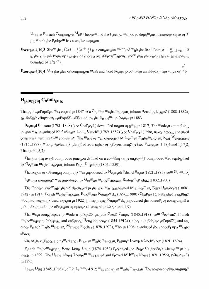
352 APPLIED FUNCTIONAL ANALYSIS
Use the Banach Contractive Map Theorem and the Piccard method to determine a concrete value of T
for which the problem has a unique solution.
Exercise 4.10.3 Show that f(x) = 12 (x+
32 ) is a contraction mapping with the fixed point x = 3
2 . If x0 = 2
is the starting point of a series of successive approximations, show that the error after n iterations is
bounded by 1/2n+1.
Exercise 4.10.4 Use the idea of contraction maps and fixed points to compute an approximate value of3√5.
Historical Comments
The term “topologie” was coined in 1847 by a German mathematician, Johann Benedict Listing (1808–1882).
Its English equivalent “topology” appeared for the first time in Nature in 1883.
Bernard Bolzano (1781–1848) (see Chapter 1) developed notion of limit in 1817. The modern −−δ def-
inition was introduced by Augustin–Louis Cauchy (1789–1857) (see Chapter 1) who, nevertheless, confused
continuity with uniform continuity. The mistake was corrected by German mathematician, Karl Weierstrass
(1815–1897), who is frequently identified as a father of rigorous analysis (see Exercises 1.18.4 and 1.17.2,
Theorem 4.3.2).
The fact that every continuous function defined on a compact set is uniformly continuous was established
by German mathematician, Johann Peter Dirichlet (1805–1859).
The notion of sequential continuity was introduced by Heinrich Eduard Heine (1821–1881) from Germany.
Lipshitz continuity was introduced by German mathematician, Rudolf Lipschitz (1832–1903).
The modern axiomatic theory discussed in the text was established by a German, Felix Hausdorff (1868–
1942) in 1914. Polish mathematician, Kazimierz Kuratowski (1896–1980) (Chapter 1), published a slightly
modified, currently used version in 1922. In particular, Kuratowski introduced the concept of constructing a
topology through the operation of closure (discussed in Exercise 4.1.9).
The main contributors to modern topology include Georg Cantor (1845–1918) from Germany, French
mathematician, physicist, and engineer, Henri Poincare (1854–1912) (father of algebraic topology), and an-
other French mathematician, Maurice Frechet (1878–1973), who in 1906 introduced the concept of a metric
space.
Chebyshev spaces are named after Russian mathematician, Pafnuty Lvovich Chebyshev (1821–1894).
French mathematician, Rene–Louis Baire (1874–1932) presented the Baire Catheogory Theorem in his
thesis in 1899. The Heine–Borel Theorem was stated and proved by Emile Borel (1871–1956), (Chapter 3)
in 1895.
Ulisse Dini (1845–1918) (comp. Lemma 4.9.2) was an Italian mathematician. The notion of equicontinuity
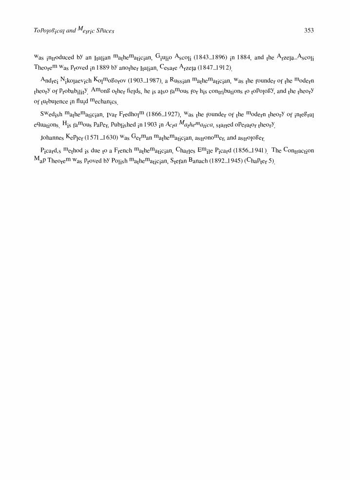
Topological and Metric Spaces 353
was introduced by an Italian mathematician, Giulio Ascoli (1843–1896) in 1884, and the Arzela–Ascoli
Theorem was proved in 1889 by another Italian, Cesare Arzela (1847–1912).
Andrei Nikolaevich Kolmogorov (1903–1987), a Russian mathematician, was the founder of the modern
theory of probability. Among other fields, he is also famous for his contributions to topology, and the theory
of turbulence in fluid mechanics.
Swedish mathematician, Ivar Fredholm (1866–1927), was the founder of the modern theory of integral
equations. His famous paper, published in 1903 in Acta Mathematica, started operator theory.
Johannes Kepler (1571–1630) was German mathematician, astronomer, and astrologer.
Picard’s method is due to a French mathematician, Charles Emile Picard (1856–1941). The Contraction
Map Theorem was proved by Polish mathematician, Stefan Banach (1892–1945) (Chapter 5).


5
Banach Spaces
Topological Vector Spaces
5.1 Topological Vector Spaces—An Introduction
The most important mathematical systems encountered in applications of mathematics are neither purely
topological (i.e., without algebraic structure, such as metric spaces) nor purely algebraic (without topological
structure, such as vector spaces); rather they involve some sort of natural combinations of both. In this
chapter, we study such systems, beginning with the concept of a topological vector space and quickly passing
on to normed vector spaces.
Topological Vector Space. V is called a topological vector space (t.v.s.) iff
(i) V is a vector space (real or complex),
(ii) the underlying set of vectors, also denoted V , is endowed with a topology so that the resulting topo-
logical space is a Hausdorff topological space, also denoted V , and
(iii) vector addition
V × V (u,v)→ u+ v ∈ V
and multiplication by a scalar
IR(or IC)× V (α,u)→ αu ∈ V
are continuous operations.
Example 5.1.1
Every normed vector space is a t.v.s. As normed vector spaces are metric spaces it is sufficient to
prove that both operations of vector addition and scalar multiplication are sequentially continuous.
Let un → u and vn → v. It follows from the triangle inequality that
(un + vn)− (u+ v) ≤ un − u+ vn − v
355

356 APPLIED FUNCTIONAL ANALYSIS
and, consequently, un + vn → u+ v, which proves that vector addition is continuous.
Similarly, if αn → α and un → u then
αnun − αu = αnun − αun + αun − αu
≤ |αn − α|un+ |α|un − u
Since un is bounded (explain, why?), the right-hand side converges to zero which proves that
αnun → αu.
In a topological vector space, translations
Tu : V v → Tu(v)def= u+ v ∈ V
are homeomorphisms. Indeed
1. Tu is a bijection and its inverse is given by T−u
(Tu)−1 = T−u
2. Both Tu and T−u are continuous, since the vector addition is assumed to be continuous.
Similarly, the dilations
Tα : V v → Tα(v)def= αv ∈ V, α = 0
are homeomorphisms as well.
This leads to an observation that, if B0 denotes a base of neighborhoods of the zero vector and Bu is a base
of neighborhoods of an arbitrary vector u, then
Bu ∼ u+ B0
where
u+ B0
def= u+ B : B ∈ B0
Similarly
B0 ∼ αB0 ∀α = 0
where
αB0
def= αB : B ∈ B0
The practical conclusion from these observations is that, when constructing a topological vector space, one
can start by introducing a base of neighborhoods for the zero vector (which must be invariant under multipli-
cation by scalars according to the second of the equivalence relations). One next defines neighborhoods for
arbitrary vectors by “shifting” the base for the zero vector and, finally, verifying that the topological vector
space axioms hold.

Banach Spaces 357
This is precisely the way in which we construct the important case of locally convex topological vector
spaces discussed in the next section.
REMARK 5.1.1 Notice that the continuity of multiplication by a scalar implies automatically
the last condition for a base of neighborhoods of a point (see Section 4.1, discussion on introducing
a topology through neighborhoods):
∀C ∈ Bx ∃C ∈ Bx : ∀y ∈ C ∃D ∈ By : D ⊂ B
Indeed, let B0 be an arbitrary neighborhood of 0. Continuity of multiplication by a scalar implies
that there exists another neighborhood C0 of 0 such that C0 ⊂12B0. For B = x + B0 take now
C = x+ C0 and D = y + C0. Then,
y + C0 ⊂ x+ C0 + C0 ⊂ x+1
2B0 +
1
2B0 ⊂ x+B0
Exercises
Exercise 5.1.1 Let V be a t.v.s. and let B0 denote a base of neighborhoods for the zero vector. Show that B0
is equivalent to αB0 for α = 0.
5.2 Locally Convex Topological Vector Spaces
Seminorm. Let V be a vector space. Recall that a function p : V → [0,∞) is called a seminorm iff
(i) p(αu) = |α|p(u) (homogeneity)
(ii) p(u+ v) ≤ p(u) + p(v) (triangle inequality)
for every scalar α and vectors u,v. Obviously every norm is a seminorm but not conversely.
Example 5.2.1
Let V = IR2. Define
p(x) = p ((x1, x2)) = |x1|

358 APPLIED FUNCTIONAL ANALYSIS
Then p is a seminorm, but not a norm since p(x) = 0 implies that only the first component of x is
zero.
The assumption that seminorms p are nonnegative is not necessary as it follows from the following:
PROPOSITION 5.2.1
Let V be a vector space and p any real-valued function defined on V such that p satisfies the two
conditions for a seminorm. Then
(i) p(0) = 0 and
(ii) |p(u)− p(v)| ≤ p(u− v).
In particular, taking v = 0 in the second inequality one gets p(u) ≥ |p(u)|, which proves that p must
take on only nonnegative values.
PROOF (i) follows from the first property of seminorms by substituting α = 0. Inequality (ii)
is equivalent to
−p(u− v) ≤ p(u)− p(v) ≤ p(u− v)
or, equivalently,
p(v) ≤ p(u− v) + p(u) and p(u) ≤ p(v) + p(u− v)
Both inequalities follow directly from the triangle inequality and homogeneity of seminorms.
Recall that by a ball centered at zero with radius c and corresponding to a particular norm ·, one means a
collection of all vectors bounded by c in the norm. The following proposition investigates properties of more
general sets of this type, using seminorms rather than norms.
PROPOSITION 5.2.2
Let V be a vector space and p a seminorm defined on V . Define
Mcdef= v ∈ V : p(v) ≤ c c > 0
The following properties hold:
(i) 0 ∈Mc
(ii) Mc is convex, i.e.,
u,v ∈Mc ⇒ αu+ (1− α)v ∈Mc for every 0 ≤ α ≤ 1

Banach Spaces 359
(iii) Mc is “balanced”
u ∈Mc, |α| ≤ 1 ⇒ αu ∈Mc
(iv) Mc is “absorbing”
∀u ∈ V ∃α > 0 : α−1u ∈Mc
(v) p(u) = infαc : α > 0, α−1u ∈Mc
PROOF (i) follows from Proposition 5.2.1 (i). Next
p(αu+ (1− α)v) ≤ αp(u) + (1− α)p(v) ≤ αc+ (1− α)c = c
which proves convexity of Mc. Property (iii) is a direct consequence of homogeneity of seminorms.
To prove (iv), it is sufficient to take α = p(u)/c as
p(α−1u) = α−1p(u) = c
Notice that for p(u) = 0 any α > 0 does the job. Finally, α−1u ∈Mc implies that
p(α−1u) = α−1p(u) ≤ c ⇒ p(u) ≤ αc
and the infimum on the right-hand side of (v) is attained for α = p(u)/c.
Locally Convex Topological Vector Space (Bourbaki). Let V be a vector space and pι, ι ∈ I , a family
(not necessarily countable) of seminorms satisfying the following axiom of separation
∀u = 0 ∃κ ∈ I : pκ(u) = 0
We begin by constructing a base of neighborhoods for the zero vector. Consider the family B = B0 of all sets
B of the form
B = B(I0, ε)def= u ∈ V : pι(u) ≤ ε, ι ∈ I0
where I0 denotes any finite subset of I .
The following properties of sets B are easily observed:
(i)
B(I0, ε) =
ι∈I0
M ιε
where
M ιε = v ∈ V : pι(v) ≤ ε
(ii) B(I0, ε) are convex, balanced, and absorbing.

360 APPLIED FUNCTIONAL ANALYSIS
Since sets B are nonempty (why?) and
B(I1, ε1) ∩B(I2, ε2) ⊃ B (I1 ∪ I2,min(ε1, ε2))
it follows that B is a base. Since each of the sets contains the zero vector, the family can be considered as a
base of neighborhoods for the zero vector.
Following the observations from the previous section, we proceed by defining the base of neighborhoods
for an arbitrary vector u = 0 in the form
Budef= u+ B = u+B : B ∈ B
Vector space V with topology induced by bases Bu is identified as a locally convex topological vector space.
To justify the name it remains to show that the topology is Hausdorff and that the operations in V are contin-
uous.
The first property follows from the axiom of separation. Let u = v be two arbitrary vectors. There exists
a seminorm pκ such that
pκ(v − u) > 0
Take 2ε < pκ(v − u) and consider neighborhoods of u and v in the form
u+Mκε , v +Mκ
ε , Mκε = w : pκ(w) ≤ ε
If there were a common element w of both sets then
pκ(v − u) ≤ pκ(v −w) + pκ(w − u) < 2ε
a contradiction.
In order to show that vector addition is continuous we pick two arbitrary vectors u and v and consider a
neighborhood of u+ v in the form
u+ v +B(I0, ε)
We claim that for each u1 ∈ u+B(I0,ε2 ) and v1 ∈ v+B(I0,
ε2 ), u1+v1 is an element of the neighborhood,
which shows that vector addition is continuous. This follows easily from the triangle inequality
pι (u1 + v1 − (u+ v)) ≤ pι(u1 − u) + pι(v1 − v) ≤ ε
for every ι ∈ I0.
Similarly, taking neighborhood of αu in the form
αu+B(I0, ε)
for each α1 ∈ (α− β, α+ β) and u1 ∈ u+B(I0, δ) where we select δ and β such that
βpι(u) ≤ε
2∀ι ∈ I0 and max(|α− β|, |α+ β|)δ ≤
ε
2
Banach Spaces 361
we have
pι (α1u1 − αu) ≤ pι (α1 (u1 − u) + (α1 − α)u)
≤ |α1|pι (u1 − u) + |α1 − α|p(u)
≤ε
2+
ε
2= ε
for every ι ∈ I0, which proves that multiplication by a scalar is continuous.
REMARK 5.2.1 In a nontrivial case the family of seminorms inducing the locally convex
topology must be infinite. If I were finite then we could introduce a single function
p(u) = maxι∈I
pι(u)
which, by the axiom of separation would have been a norm with a corresponding topology identical
to the locally convex topology. Thus, only in the case of infinite families of seminorms do locally
convex topological vector spaces provide us with a nontrivial generalization of normed vector spaces.
Example 5.2.2
Recall the definition of the topology of pointwise convergence discussed in Example 4.1.8. Identifying
with each point x ∈ (0, 1) a corresponding seminorm
px(f)def= |f(x)|
we easily see that the family of such seminorms px, x ∈ (0, 1) satisfies the axiom of separation.
The corresponding topology is exactly the previously discussed topology of pointwise convergence in
C(0, 1).
According to Proposition 5.2.2, for every seminorm p and a constant c > 0, we can construct the corre-
sponding set Mc = Mc(p) consisting of all vectors bounded in p by c and proved to be convex, balanced,
and absorbing. In property (v) from the same proposition we also have established a direct representation of
the seminorm p in terms of the setMc. It turns out that once we have a convex, balanced, and absorbing set,
the set defines a seminorm.
Minkowski Functional. Let M be a convex, balanced, and absorbing set in a vector space V . We define
the Minkowski functional of M as
pM (u)def= infα > 0 : α−1u ∈M

362 APPLIED FUNCTIONAL ANALYSIS
PROPOSITION 5.2.3
The Minkowski functional pM is a seminorm. Moreover
u : pM (u) < 1 ⊂M ⊂ u : pM (u) ≤ 1
PROOF
Step 1. M absorbing implies that set
α > 0 : α−1u ∈M
is nonempty and therefore pM is well-defined (takes on real values).
Step 2. pM is homogeneous.
pM (λu) = infα > 0 : α−1λu ∈M
= infα > 0 : α−1|λ|u ∈M
(M is balanced)
= infβ|λ| : β > 0, β−1u ∈M
= |λ| infβ > 0 : β−1u ∈M
= |λ|pM (u)
Step 3. pM satisfies the triangle inequality.
Let α, β > 0 denote arbitrary positive numbers such that α−1u ∈ M , β−1v ∈ M . By convexity
of Mα
α+ βα−1u+
β
α+ ββ−1v = (α+ β)−1(u+ v)
is also an element of M and consequently
pM (u+ v) = infγ > 0 : γ−1(u+ v) ∈M
≤ α+ β , α−1u ∈M, β−1v ∈M
It remains to take the infimum with respect to α and β on the right-hand side of the inequality.
Finally, the relation between set M and sets of vectors bounded in pM by one follows directly
from the definition of pM .
Thus, by means of the Minkowski functional, one can establish a one-to-one correspondence between
seminorms and convex, balanced, and absorbing sets. We summarize now these observations in the following
proposition.
PROPOSITION 5.2.4
Let V be a topological vector space. The following conditions are equivalent to each other.
Banach Spaces 363
(i) V is a locally convex space topologized through a family of seminorms satisfying the axiom of
separation.
(ii) There exists a base of neighborhoods for the zero vector consisting of convex, balanced, and
absorbing sets.
PROOF (i) ⇒ (ii) follows from the construction of the locally convex topology and Proposi-
tion 5.2.2. Conversely, with every setM from the base we can associate the corresponding Minkowski
functional, which by Proposition 5.2.3 is a seminorm. Since each of the sets is absorbing, the family of
seminorms trivially satisfies the axiom of separation. Finally, by the relation from Proposition 5.2.3
between sets M and sets of vectors bounded in pM , the topology induced by seminorms pM is
identical to the original topology (the bases are equivalent).
We shall use the just established equivalence to discuss a very important example of a locally convex
topological vector space, the space of test functions, in the next section.
Exercises
Exercise 5.2.1 Show that each of the seminorms inducing a locally convex topology is continuous with
respect to this topology.
Exercise 5.2.2 Show that replacing the weak equality in the definition of setMc with a strict one, does not
change the properties ofMc.
Exercise 5.2.3 Show that by replacing the weak equality in the definition of sets B(I0, ε) with a strict one,
one obtains bases of neighborhoods equivalent to the original ones and therefore the same topology.
Exercise 5.2.4 Show that seminorms are convex functionals.
Exercise 5.2.5 Prove the following characterization of continuous linear functionals.
Let V be a locally convex t.v.s. A linear functional f on V is continuous iff there exists a continuous
seminorm p(u) on V (not necessarily from the family inducing the topology) such that
|f(v)| ≤ p(v)

364 APPLIED FUNCTIONAL ANALYSIS
Figure 5.1
Support of a function.
5.3 Space of Test Functions
Functions with Compact Support. Let Ω ⊂ IRn be an open set and f any real- (or complex-) valued
function defined on Ω. The closure of the set of all points x ∈ Ω for which f takes non-zero values is called
the support of f :
supp fdef= x ∈ Ω : f(x) = 0
Note that, due to the closure operation, the support of a function f may include the points at which f vanishes
(see Fig. 5.1).
The collection of all infinitely differentiable functions defined on Ω, whose supports are compact (i.e.,
bounded) and contained in Ω will be denoted as
C∞0 (Ω)
def= f ∈ C∞(Ω) : supp f ⊂ Ω, supp f compact
Obviously, C∞0 (Ω) is a vector subspace of C∞(Ω).
Example 5.3.1
A standard example of a function in C∞0 (IR) is
φ(x) =
exp[1/(x2 − a2)] |x| < a (a ∈ IR)
0 |x| ≥ a

Banach Spaces 365
We shall construct now a very special topology on C∞0 (Ω) turning it into a topological vector space. We
begin with an auxiliary technical lemma.
LEMMA 5.3.1
Let Ω ⊂ IRn be an open set. There always exists a sequence of compact sets Ki ⊂ Ω such that
(i) Ki ⊂ intKi+1 and
(ii)
∞
1
Ki = Ω.
PROOF Consider the set of all closed balls with rational coordinates of their centers and rational
radii, contained in Ω. The set is countable (why?) and therefore can be put into a sequential form
B1, B2, B3, . . .
Also, by the definition of open sets,
∞
1
Bi = Ω and
∞
1
Bi = Ω
where Bi = intBi are the corresponding open balls. Next, set
K1 = B1
K2 = B1 ∪B2
...
Kn = B1 ∪ . . . ∪Bn
Each of sets Ki is compact; they form an increasing sequence (K1 ⊂ K2 ⊂ . . .) and
intKi ⊃i
j=1
intBj =i
j=1
Bj
Consequently∞
i=1
intKi ⊃
∞
i=1
i
j=1
Bj =
∞
j=1
Bj = Ω
As intKi are also increasing (A ⊂ B ⇒ intA ⊂ intB), we have
∞
j=i+1
intKi = Ω , for every i
which proves that for each compact set Ki, sets intKj , j ≥ i+1 form an open covering of Ki. Thus
one can always find a finite number of them covering Ki. Taking the largest one (the sequence intKi
is increasing), we see that for each Ki we can always select an index j > i such that Ki ⊂ intKj
which, by the principle of mathematical induction, finishes the proof.

366 APPLIED FUNCTIONAL ANALYSIS
The Space of Test Functions. Let Ω ⊂ IRn be an open set. For each compact subset K ⊂ intΩ we
introduce the space of C∞ functions with supports inK,
C∞0 (K)
def= u ∈ C∞
0 (Ω) : supp u ⊂ K
Introducing a sequence of seminorms
pn(u) = sup |Dαu(x)| : x ∈ K, |α| = n
we equip C∞0 (K) with the corresponding locally convex topology. With this topology the space C∞
0 (K) is
frequently called the space of test functions with supports in K and denoted D(K).
Let BK denote a corresponding base of convex, balanced, and absorbing neighborhoods for the zero func-
tion 0. Consider now the family B of all nonempty convex, balanced setsW from C∞0 (Ω) such that
∀ compact K ⊂ Ω ∃ V ∈ BK : V ⊂W ∩ C∞0 (K)
PROPOSITION 5.3.1
B is a base of a locally convex topology on C∞0 (Ω).
PROOF First of all, sets W from B are absorbing. Indeed, if u ∈ C∞0 (Ω), then by definition
taking K = supp u, we can find an absorbing set V ∈ BK such that V ⊂ W ∩ C∞0 (K) ⊂ W , which
proves that W is absorbing.
Next, if W1,W2 ∈ B, then simply W = W1 ∩W2 is also an element of B. Indeed, W is convex and
balanced and if Vi ∈ BK , i = 1, 2 denote sets such that
Vi ⊂Wi ∩ C∞0 (K), i = 1, 2
Then, since BK is a base, there exists V ∈ BK such that
V ⊂ V1 ∩ V2 ⊂W1 ∩W2 ∩ C∞0 (K) = W ∩ C∞
0 (K)
which proves that W ∈ B. Finally, B is nonempty as it contains at least the entire space C∞0 (Ω).
The space C∞0 (Ω) equipped with the just-defined topology is called the space of test functions on Ω and
denoted D(Ω).
REMARK 5.3.1 The condition defining base B can be written in a more concise form using
notation from Chapter 4.
BK B ∩ C∞0 (K) for every compact K ⊂ Ω

Banach Spaces 367
This is equivalent to saying that the inclusion
iK : C∞0 (K) → C∞
0 (Ω)
is continuous at zero. The topology of the space of test functions on Ω can be identified as the
strongest topology in C∞0 (Ω) in which all such inclusions are continuous and is frequently called the
inductive topological limit of topologies in D(K).
The space of test functions is a basis for developing the theory of distributions, introduced by L. Schwartz
in 1948. We conclude this section by presenting one of its most crucial properties characterizing convergence
of sequences in D(Ω).
PROPOSITION 5.3.2
Let ϕn be a sequence of functions from D(Ω). The following conditions are equivalent to each other:
(i) ϕn → 0 in D(Ω)
(ii) There exists a compact set K ⊂ Ω such that supp ϕn ⊂ K and Dαϕn → 0 uniformly in K.
PROOF
(ii) =⇒ (i) follows immediately from Remark 5.3.1 and the definition of topology in D(K). To
prove the converse we need only demonstrate the existence ofK. LetKn, n = 1, 2 . . . be the sequence
of compact sets discussed in Lemma 5.3.1 and satisfying
Ki ⊂ intKi+1,
i
Ki
=
i
intKi
= Ω
We proceed by contradicting the existence of such a set K. Accordingly, we can find an index n1
and a corresponding point x1 ∈ Kn1 such that ϕn1(x) = 0. Similarly
∃n2 > n1, x2 ∈ Kn2−Kn1
: ϕn2(x2) = 0
and, by induction,
∃ni > ni−1, xi ∈ Kni−Kni−1 : ϕni
(xi) = 0
Finally, consider the set
W =ϕ ∈ C∞
0 (Ω) : ϕ(xi) < i−1ϕni(xi), i = 1, 2, . . .
We claim that W is an element of B, the base of neighborhoods for the zero vector in D(Ω). Indeed,
W is convex and balanced. Moreover, if K is a compact subset of Ω, there exists a set Ki from the

368 APPLIED FUNCTIONAL ANALYSIS
sequence such that K ⊂ Ki and consequently only a finite number of points xi is in K. This implies
that for every compact K we can always find δ > 0 such that
supx∈K
|ϕ(x)| < δ implies ϕ ∈W
Thus W is a well-defined neighborhood of the zero vector. But this contradicts the convergence of
ϕn to zero vector as for ε = 1 and every i,
ϕni(xi) ≥ i−1ϕni
(xi) =⇒ ϕni∈W
Hahn–Banach Extension Theorem
5.4 The Hahn–Banach Theorem
In this section we establish a fundamental result concerning the extension of linear functionals on infinite-
dimensional vector spaces, the famous Hahn–Banach theorem. The result will be obtained in a general setting
of arbitrary vector spaces and later on specialized in a more specific context.
Sublinear Functionals. Let V be a real vector space. A functional p : V → IR is said to be sublinear iff
(i) p(αu) = αp(u) ∀α > 0
(ii) p(u+ v) ≤ p(u) + p(v) (p is subadditive)
for arbitrary vectors u and v. Obviously, every linear functional is sublinear and every seminorm is sublinear
as well.
THEOREM 5.4.1
(The Hahn–Banach Theorem)
Let X be a real vector space, p : X → IR a sublinear functional on X, and M ⊂ X a subspace of
X. Consider f : M → IR, a linear functional on M (f ∈M∗) dominated by p on M , i.e.,
f(x) ≤ p(x) ∀ x ∈M
Then, there exists a linear functional F : X → IR defined on the whole X such that
Banach Spaces 369
(i) F |M ≡ f
(ii) F (x) ≤ p(x) ∀ x ∈ X
In other words, F is an extension of f dominated by p on the whole X.
PROOF Let us pick an element u0 of X, not in M , and consider the subspace
M1 = M + IRu0 = x =m+ αu0 : m ∈M, α ∈ IR
A possible extension of f to M1 must have the form
F (x) = F (m+ αu0) = F (m) + αF (u0) = f(m) + αc
where we have used linearity of F and cdef= F (u0). We now determine if it is possible to choose c
such that F (x) ≤ p(x) on M1. Then we have extended f to the space M1 of dimension “one larger”
than M . We will have
F (m+ αu0) = f(m) + αc ≤ p(m+ αu0)
and this is equivalent to
f(−α−1m)− p (−α−1m− u0) ≤ c for α < 0
c ≤ p (α−1m+ u0)− f(α−1m) for α > 0
Thus, it is sufficient to check whether a constant c exists such that
f(m)− p(m − u0) ≤ c ≤ p(m + u0)− f(m)
for every m,m ∈M . In other words, is it true that
supm∈M
f(m)− p(m − u0) ≤ infm∈M
p(m + u0)− f(m)
The answer is “yes,” as
f(m) + f(m) = f(m +m) ≤ p(m +m)
= p(m − u0 +m + u0)
≤ p(m − u0) + p(m + u0)
Moving the terms with m to the left side and those with m to the right side and taking the
supremum and infimum, respectively, we get the result required.
Thus, we have shown that the extension F to M1 exists. We could now repeat this process for a
larger space M2 = M1 ⊕ IRu1, etc. Continuing in this way, we would produce an increasing family
of spaces along with corresponding extensions of f dominated by p. The question is whether this
process could be used to eventually cover the whole space.

370 APPLIED FUNCTIONAL ANALYSIS
We proceed by appealing to the Kuratowski-Zorn Lemma: If in a partially ordered set every
linearly ordered subset (a chain) has an upper bound, then there exists a maximum element in the
set.
Step 1. Define a family
F = (Y, fY ) : Y is a subspace of X,M ⊂ Y
fY : Y → IR is a linear extension of f
fY (y) ≤ p(y) ∀y ∈ Y
Thus F is a family of all possible extensions of f along with their domains of definition—subspaces
of X, containing M . According to the first part of this proof, F is nonempty.
Step 2. Introduce a relation on F
(Y, fY ) ≤ (Z, fZ)def⇔ Y ⊂ Z and fZ |Y = fY
It is a simple exercise (see Exercise 5.4.1) that relation “≤” is a partial ordering of F .
Step 3. Let G be a linearly ordered subset of F
G = (Yι, fYι) : ι ∈ I
where I is a set of indices. Recall that G being linearly ordered means that any two elements of G
are comparable with each other, i.e.,
(Y, fY ), (Z, fZ) ∈ G =⇒ (Y, fY ) ≤ (Z, fZ) or (Z, fZ) ≤ (Y, fY )
The question is: Does G have an upper bound in F? Define
Y =
ι∈I
Yι
fY : Y → IR
fY (x)def= fYι
(x), where x ∈ Yι, for some ι ∈ I
It is left as an exercise (see Exercise 5.4.2) to prove that (Y, fY ) is a well-defined upper bound for G.
Step 4. By the Kuratowski-Zorn Lemma, family F has a maximal element, say (Z, fZ). We claim
that it must be Z = X. Indeed, if there were an element left, u0 ∈ X − Z, then by the procedure
discussed in the first part of this proof, we could have extended fZ further to Z ⊕ IRu0, which
contradicts the maximality of (Z, fZ). This finishes the proof.
Exercises
Exercise 5.4.1 Prove that relation ≤ introduced in the proof of the Hahn–Banach Theorem is a partial order-
ing of the family F .

Banach Spaces 371
Exercise 5.4.2 Prove that element (Y, fY ) of F defined in the proof of the Hahn–Banach theorem
1. is well defined, i.e.,
(i) Y is a linear subspace of X and
(ii) value fY (x)def= fYι
(x) is well defined, i.e., independent of the choice of index ι, and
2. is an upper bound for the chain G.
5.5 Extensions and Corollaries
In this section we generalize the Hahn–Banach theorem to the case of complex vector spaces and provide a
number of important corollaries.
We start with a simple corollary.
COROLLARY 5.5.1
Let X be a real vector space, p : X → [0,∞] a seminorm, M ⊂ X a subspace of X and f :→ IR, a
linear functional on M(f ∈M∗) such that
|f(x)| ≤ p(x) x ∈M
Then, there exists a linear extension F : X → IR of f such that
|F (x)| ≤ p(x) x ∈ X
PROOF Obviously, p satisfies assumptions of the Hahn–Banach theorem and
f(x) ≤ |f(x)| ≤ p(x) x ∈M
i.e., f is dominated by p on M . Let F : X → IR be an extension of f to the whole X, dominated
by p, i.e.,
F (x) ≤ p(x) x ∈ X
Replacing x with −x, we get
−F (x) = F (−x) ≤ p(−x) = p(x) x ∈ X
which implies that
−p(x) ≤ F (x) x ∈ X

372 APPLIED FUNCTIONAL ANALYSIS
and, consequently,
|F (x)| ≤ p(x) ∀ x ∈ X
We proceed now with the generalization for complex spaces.
THEOREM 5.5.1
(Bohnenblust–Sobczyk)
Let X be a complex vector space, p : X → [0,∞) a seminorm, M ⊂ X a subspace of X, and
f : M → IC a linear functional on M(f ∈M∗) such that
|f(x)| ≤ p(x) ∀ x ∈M
Then, there exists a linear functional F : X → IC defined on the whole X such that
(i) F |M ≡ f and
(ii) |F (x)| ≤ p(x) ∀ x ∈ X
PROOF Obviously, X is also a real space when the multiplication of vectors by scalars is
restricted to real numbers. Functional f on M has the form
f(x) = g(x) + ih(x) x ∈M
where both g and h are linear, real-valued functionals defined on M . Note that g and h are not
independent of each other, as f is complex-linear, which in particular implies that
f(ix) = if(x)
or
g(ix) + ih(ix) = i(g(x) + ih(x)) = −h(x) + ig(x)
and, therefore,
h(x) = −g(ix) ∀ x ∈M
Also
|g(x)| ≤ |f(x)|=
g(x)2 + h(x)2≤ p(x)
By the preceding corollary, there exists a real-valued linear extension G of g to the whole X such
that
|G(x)| ≤ p(x)
Banach Spaces 373
Define:
F (x) = G(x)− iG(ix) x ∈ X
Clearly, F is an extension of f . To prove that F is complex-linear, it is sufficient to show (why?)
that
F (ix) = iF (x) ∀ x ∈ X
ButF (ix) = G(ix)− iG(iix) = G(ix)− iG(−x)
= iG(x) +G(ix) = i(G(x)− iG(ix))
= iF (x)
It remains to prove that F is bounded by seminorm p on X. Representing F (x) in the form
F (x) = r(x)e−iθ(x), where r(x) = |F (x)|
we have
|F (x)| = eiθ(x)F (x) = Feiθ(x)x
= G
eiθ(x)x
since |F (x)| is real. Finally
Geiθ(x)x
≤Geiθ(x)x
≤ p
eiθ(x)x
≤eiθ(x)
p(x) = p(x)
which finishes the proof.
COROLLARY 5.5.2
Let (U, · U ) be a normed space and let u0 ∈ U denote an arbitrary non-zero vector.
There exists a linear functional f on U such that
(i) f(u0) = u0 = 0 and
(ii) |f(u)| ≤ u ∀ u ∈ U .
PROOF Take p(u) = u and consider the one-dimensional subspace M of U spanned by u0
M = IRu0 (or ICu0) = αu0 : α ∈ IR (or IC)
Define a linear functional f on M by setting f(u0) = u0
f(αu0) = αf(u0) = αu0
Obviously
|f(u)| ≤ p(u) (in fact, the equality holds).

374 APPLIED FUNCTIONAL ANALYSIS
Use the Hahn–Banach theorem to extend f to all of U and thus conclude the assertion.
REMARK 5.5.1 Using the language of the next two sections, one can translate the corollary
above into the assertion that for every non-zero vector u0 from a normed space U , there exists a
linear and continuous functional f such that f = 1 and f(u0) = u0 = 0. f denotes here
a norm on f as a member of the “topological dual space” of U , a concept we shall address more
carefully in Section 5.7 and thereafter. This in particular will imply that the topological duals U
are nonempty. We shall return to this remark after reading the next two sections.
Bounded (Continuous) Linear Operators on Normed Spaces
5.6 Fundamental Properties of Linear Bounded Operators
We developed most of the important algebraic properties of linear transformations in Chapter 2. We now
expand our study to linear transformations on normed spaces. Since the domains of such linear mappings
now have topological structure, we can also apply many of the properties of functions on metric spaces. For
example, we are now able to talk about continuous linear transformations from one normed linear space into
another. It is not uncommon to use the term “operator” to refer to a mapping or function on sets that have
both algebraic and topological structure. Since all of our subsequent work involves cases in which this is so,
we henceforth use the term operator synomously with function, mapping, and transformation.
To begin our study, let (U, · U ) and (V, · V ) denote two normed linear spaces over the same field
IF , and let A be an operator from U into V . We recall that an operator A from U into V is linear if and
only if it is homogeneous (i.e., A(αu) = αAu ∀ u ∈ U and α ∈ IF ) and additive (i.e., A(u1 + u2) =
A(u1) + A(u2) ∀ u1,u2 ∈ U ). Equivalently, A : U → V is linear if and only if A(αu1 + βu2) =
αA(u1) + βA(u2) ∀ u1,u2 ∈ U and ∀ α, β ∈ IF . When A does not obey this rule, it is called a nonlinear
operator. In the sequel we shall always take the field IF to be real or complex numbers: IF = IR or IF = IC.
Recall that the null space, N (A), of a linear operator A : U → V is defined by N (A) = u : Au =
0,u ∈ U and is a subspace of U , and the range R(A) of a linear operator A : U → V is defined to be
R(A) = v : Au = v ∈ V , for u ∈ U and R(A) ⊂ V . We note here that the operator A is one-to-one if
and only if the null space N (A) is trivial, N (A) = 0.
Thus far we have introduced only algebraic properties of linear operators. To talk about boundedness and
continuity of linear operators, we use the topological structure of the normed spaces U and V .
We begin with the fundamental characterization of linear continuous operators on normed spaces.

Banach Spaces 375
PROPOSITION 5.6.1
Let (U, · U ) and (V, · V ) be two normed vector spaces over the same field and T : U → V a
linear transformation defined on U with the values in V (T ∈ L(U, V )). The following conditions are
equivalent to each other
(i) T is continuous (with respect to norm topologies),
(ii) T is continuous at 0,
(iii) T is bounded, i.e., T maps bounded sets in U into bounded sets in V ,
(iv) ∃C > 0 : TuV ≤ CuU ∀ u ∈ U
PROOF
(i) ⇒ (ii) trivial.
(ii) ⇒ (iii) Let A be a bounded set in U , i.e., there exists a ball B(0, r) such that A ⊂ B(0, r). T
being continuous at 0 means that
∀ ε > 0 ∃ δ > 0 : uU < δ ⇒ TuV < ε
Selecting ε = 1 we get
∃ δ > 0 : uU < δ ⇒ TuV < 1
Let u ∈ A and therefore ||u||U ≤ r. Consequentlyδ
ru
U
=δ
ruU ≤ δ
which implies that T
δ
ru
V
≤ 1 ⇒ T (u)V ≤r
δ
which is equivalent to saying that T (A) ⊂ B(0, r/δ) and therefore is bounded.
(iii) ⇒ (iv) From the boundedness of set T (B(0, 1)) follows that
∃C > 0 : uU ≤ 1 ⇒ TuV ≤ C
Consequently, for every u = 0 T
u
uU
V
≤ C
or, equivalently,
T (u)V ≤ C uU
(iv) ⇒ (i) It is sufficient to show sequential continuity. Let un → u. Then
Tun − TuV = T (un − u)V ≤ C un − uU → 0

376 APPLIED FUNCTIONAL ANALYSIS
Operator Norm. According to the definition just given, we can always associate with any bounded linear
operator A : U → V a collection of positive numbers C such that
AuV ≤ C uU ∀ u ∈ U
If we consider the infimum of this set, then we effectively establish a correspondenceN between the operator
A and the nonnegative real numbers
N(A) = inf C : AuV ≤ C uU ∀ u ∈ U
Remarkably, the function N determined in this way satisfies all the requirements for a norm, and we denote
N(A) by A and refer to it as the norm of the operator A:
A = inf C : AuV ≤ C uU ∀ u ∈ U
Notice that passing with C to the infimum in
AuV ≤ C uU
we immediately get the inequality
AuV ≤ A uU
We will demonstrate later that the notation A is justified. First, we develop some alternative forms for
defining A.
PROPOSITION 5.6.2
Let A be a bounded linear operator from (U, ·U ) into (V, ·V ). Then
(i) A = supu∈U
AuVuU
u = 0
(ii) A = supu∈U
AuV , uU ≤ 1
(iii) A = supu∈U
AuV , uU = 1
PROOF
(i) AuV ≤ C uU implies thatAuVuU
≤ C
Thus taking the supremum over all u = 0 on the left-hand side and the infimum over all C’s on the
right side, we get
supu=0
AuVuU
≤ A

Banach Spaces 377
On the other side, for an arbitrary w = 0,
AwVwU
≤ supu=0
AuVuU
def= C0
and, consequently,
AwV ≤ C0 wU
so thatA = infC : AuV ≤ CuU , ∀u ∈ U
≤ C0 = supu=0
AuVuU
This proves (i).
(iii) follows directly from (i) as
AuVuU
=
A
u
uU
V
andu−1
U uU= 1.
(ii) As
AuV ≤ A uU ∀ u
we immediately have
supuU≤1
AuV ≤ A
The inverse inequality follows directly from (iii) (supremum is taken over a larger set).
It is not difficult now to show that the function A satisfies the norm axioms.
1. In view of the definition, if A = 0 , then AuV = 0 for all u. But this is not possible unlessA ≡ 0.
2. λA = supu=0
λAuVuU
= |λ| supu=0
AuVuU
= |λ| A
3. A+B = supu=0
Au+BuVuU
≤ supu=0
AuV + BuVuU
≤ A+ B
4. An additional useful property of the norm of a bounded (continuous) linear operator can be identified:
if AB denotes the composition of two bounded operators, then
ABu ≤ A Bu ≤ A B u
Consequently
AB ≤ A B
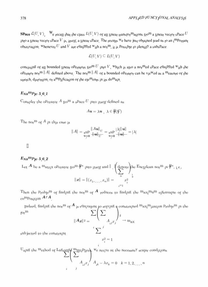
378 APPLIED FUNCTIONAL ANALYSIS
Space L(U, V ). We recall that the class L(U, V ) of all linear transformations from a linear vector space U
into a linear vector space V is, itself, a linear space. The results we have just obtained lead us to an important
observation: whenever U and V are equipped with a norm, it is possible to identify a subspace
L(U, V ) ⊂ L(U, V )
consisting of all bounded linear operators from U into V , which is also a normed space equipped with the
operator norm A defined above. The norm A of a bounded operator can be viewed as a measure of the
stretch, distortion, or amplification of the elements in its domain.
Example 5.6.1
Consider the operator A from a space U into itself defined as
Au = λu , λ ∈ IR(IC)
The norm of A in this case is
A = supu=0
AuUuU
= supu=0
|λ|u
u= |λ|
Example 5.6.2
Let A be a matrix operator from IRn into itself and · denote the Euclidean norm in IRn, i.e.,
x = (x1, . . . , xn) =
n
i=1
x2i
12
Then the problem of finding the norm of A reduces to finding the maximum eigenvalue of the
composition ATA.
Indeed, finding the norm of A is equivalent to solving a constrained maximization problem in the
form
Ax2=
i
j
Aijxj
2
→ max
subjected to the constraint
i
x2i = 1
Using the method of Lagrange multipliers, we arrive at the necessary scalar conditions
i
j
Aijxj
Aik − λxk = 0 k = 1, 2, . . . , n

Banach Spaces 379
where λ is the Lagrange multiplier; equivalently, in vector notation:
ATAx = λx
Thus Ax2 attains its maximum at one of the eigenvectors λ of ATA and consequently
ATAx
x=λx
x= |λ|
which implies that the norm A is equal to the square root of the maximum (in modulus) eigenvalue
of ATA. Square roots µi of the nonnegative eigenvalues of ATA (ATA is positive semidefinite)
µ2i = λi
ATA
are frequently called the singular values of A. For symmetric matrices the singular values of A
coincide with absolute values of eigenvalues of A, since for an eigenvalue λ of A and a corresponding
eigenvector x, one has
ATAx = ATλx = λATx = λAx = λ2x
and, therefore, λ2 is an eigenvalue of ATA = A2.
Consider, for instance, the matrix
A =
2 1
1 2
from IR2 into IR2.
Now, it is easily verified that the eigenvalues of A are
λ1 = 3, λ2 = 1
Clearly, in this particular case
A = max|λ1|, |λ2| = 3
We emphasize that maxλ = A in general. For instance, for matrix
A =
1 1
0 1
the singular values are
µ21,2 =
3±√5
2
and, therefore,
A = max
3−√5
2
12
,
3 +√5
2
12
≈ 1.618
whereas the matrix A has only a single eigenvalue λ = 1.

380 APPLIED FUNCTIONAL ANALYSIS
It is clear, however, that if A : IRn → IRn, then
A = supu=0
Au
u≥ max
1≤i≤n|λi(A)|
where λi(A) are the eigenvalues of A (why?).
Example 5.6.3
We wish to emphasize that the character of the norm assigned to a bounded operator A : U → V
depends entirely on the choice of norms used in U and V .
Suppose, for example, that U = V = IRn and A is identified with a given n × n matrix [Aij ].
Among possible choices of norms for IRn are the following:
u1 =
n
j=1
|uj |, u2 =
n
j=1
|uj |2
12
, u∞ = max1≤j≤n
|uj |
or, more generally,
up =
n
j=1
|uj |p
1p
, 1 ≤ p <∞
Depending upon the choice of norm in U and V , the operation A has a different corresponding norm.
For example,
if A : (IRn, · 1)→ (IRn, · ∞), then
A1,∞ = max1≤i≤n
max1≤j≤n
|Aij |
if A : (IRn, · ∞)→ (IRn, · ∞), then
A∞ = max1≤i≤n
n
j=1
|Aij |
if A : (IRn, · 1)→ (IRn, · 1), then
A1 = max1≤j≤n
n
i=1
|Aij |
and so forth. If the Euclidean norm is used, i.e.,
A : (IRn, ·2) −→ (IRn, ·2)
then
A2 =
ρATA

Banach Spaces 381
where AT is the transpose of A and ρ is the spectral radius of ATA, and the spectral radius of any
square matrix B is defined by
ρ(B) = maxs|λs(B)|
where λs(B) is the s-th eigenvalue of B. When A is symmetric, then
A2 = maxs|λs(A)|
(compare this with the previous example).
Example 5.6.4
(An Unbounded Operator)
Consider the differential operator
Du =d
dx(u(x))
defined on the set of differentiable functions with the norm u = sup |u(x)|, x ∈ [0, 1]. We shall show that
D is not bounded in C[0, 1]. Toward this end, let
un(x) = sin(nx)
Clearly, un = supx∈[0,1]
|un(x)| = 1 for all n, and Dun = n cos(nx), Dun = n. Since un = 1 and
Dun increases infinitely for n → ∞, there is no constantM such that Du < Mu for all u ∈ C[0, 1].
Thus, D is not bounded.
We also note thatD is not defined everywhere in C[0, 1]. However, ifD is considered as an operator from
C1[0, 1] into C[0, 1] with u = max supx∈[0,1]
|u(x)|, supx∈[0,1]
|Du(x)|, then it can be shown to be bounded.
In general, a linear differential operator of orderm with continuous coefficients ai,
(Tu)(x)def=
m
i=0
ai(x)diu
dxi
can be considered as a bounded operator from Cm[0, 1] into C[0, 1] if we select an appropriate norm; e.g.,
u = max0≤k≤m
sup0≤x≤1
|Dku(x)|.
Exercises
Exercise 5.6.1 Verify the assertions given in Example 5.6.3.
Exercise 5.6.2 Show that
A∞,1 ≤
i,j
|Aij |

382 APPLIED FUNCTIONAL ANALYSIS
but construct an example of a matrix for which
A∞,1 <
i,j
|Aij |
Exercise 5.6.3 Let A : (IR2, · a)→ (IR2, · b) and B : (IR2, · a)→ (IR2, · b), where a, b = 1, 2,∞,
be linear operators represented by the matrices
A =
2 13 −2
, B =
4 22 1
Determine A and B for all choices of a and b.
Exercise 5.6.4 Let A be an invertible matrix in IRn × IRn, and µi > 0 denote its singular values (see Exam-
ple 5.6.2). Show that with A calculated with respect to the Euclidean norm in IRn,
A−1 =1
min1≤i≤n
µi
5.7 The Space of Continuous Linear Operators
In this section, we will closer investigate the space L(U, V ) of all continuous operators from a normed space
U into a normed space V . We have already learned that L(U, V ) is a subspace of the space L(U, V ) of all
linear (but not necessarily continuous) operators from U to V , and that it can be equipped with the norm
A = AL(U,V ) = supu=0
AuVuU
In the case of a finite-dimensional space U , the space L(U, V ) simply coincides with L(U, V ) as every linear
operator on U is automatically continuous. In order to show this, consider an arbitrary basis
ei, i = 1, 2, . . . , n
for U and a corresponding norm,
u =
n
i=1
|ui| , where u =
n
1
uiei
As any two norms are equivalent in a finite-dimensional space (recall Exercise 4.6.3), it is sufficient to show
that any linear operator on U is continuous with respect to this particular norm. This follows easily from
AuV =
A
n
1
uiei
≤
n
1
|ui| AeiV
≤max
iAeiV
n
1
|ui|

Banach Spaces 383
REMARK 5.7.1 The notion of the space L(U, V ) can easily be generalized to arbitrary topo-
logical vector spaces U and V . Indeed, if A and B are two continuous linear operators from U to V ,
then αA + βB, because of continuity of the operations of addition and scalar multiplication in V
is also continuous, and therefore the set of all continuous linear operators is closed with respect to
vector space operations. Obviously, in general L(X,Y ) cannot be equipped with a norm topology.
Convergence of Sequences in L(U, V ). A sequence An of operators in L(U, V ) is said to converge
uniformly to A ∈ L(U, V ) if simply An → A in the norm topology, i.e.,
limn→∞
An −A = 0
The sequence An from L(U, V ) is said to converge strongly to A ∈ L(U, V ), denoted Ans→ A, if
limn→∞
Anu−Au = 0 for every u ∈ U
It follows immediately from the inequality
Anu−Au ≤ An −A u
that uniform convergence implies strong convergence. The converse is in general not true.
We will prove now an important assertion concerning the completeness of the space L(U, V ).
PROPOSITION 5.7.1
Let U, V be two normed spaces and V be complete, i.e., V is a Banach space . Then L(U, V ) is
complete, and is therefore also a Banach space.
PROOF Let An ∈ L(U, V ) be a Cauchy sequence, i.e.,
limn,m→∞
An −Am = 0
Since for every u ∈ UAnu−AmuV = (An −Am)uV
≤ An −Am uU
it follows that Anu is a Cauchy sequence in V and by completeness of V has a limit. Define
Audef= lim
n→∞Anu
Then:
Step 1. A is linear. Indeed, it is sufficient to pass to the limit with n → ∞ on both sides of the
identity
An(αu+ βv) = αAn(u) + βAn(v)
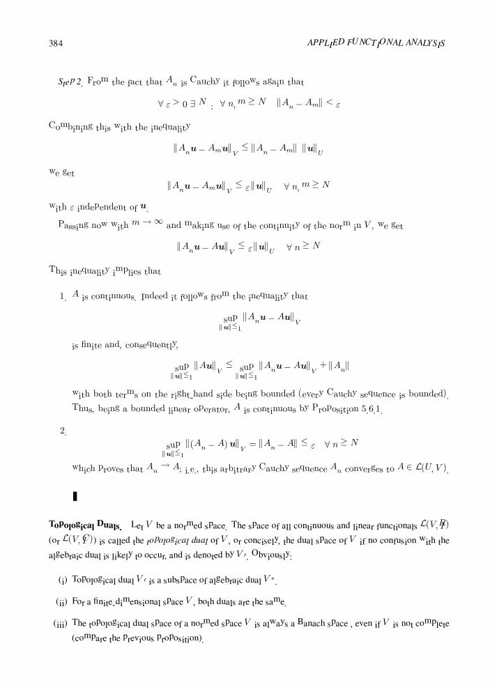
384 APPLIED FUNCTIONAL ANALYSIS
Step 2. From the fact that An is Cauchy it follows again that
∀ ε > 0 ∃ N : ∀ n,m ≥ N An −Am < ε
Combining this with the inequality
Anu−AmuV ≤ An −Am uU
we get
Anu−AmuV ≤ ε uU ∀ n,m ≥ N
with ε independent of u.
Passing now with m→∞ and making use of the continuity of the norm in V , we get
Anu−AuV ≤ ε uU ∀ n ≥ N
This inequality implies that
1. A is continuous. Indeed it follows from the inequality that
supu≤1
Anu−AuV
is finite and, consequently,
supu≤1
AuV ≤ supu≤1
Anu−AuV + An
with both terms on the right-hand side being bounded (every Cauchy sequence is bounded).
Thus, being a bounded linear operator, A is continuous by Proposition 5.6.1.
2.
supu≤1
(An −A)uV = An −A ≤ ε ∀ n ≥ N
which proves that An → A; i.e., this arbitrary Cauchy sequence An converges to A ∈ L(U, V ).
Topological Duals. Let V be a normed space. The space of all continuous and linear functionals L(V, IR)
(or L(V, IC)) is called the topological dual of V , or concisely, the dual space of V if no confusion with the
algebraic dual is likely to occur, and is denoted by V . Obviously:
(i) Topological dual V is a subspace of algebraic dual V ∗.
(ii) For a finite-dimensional space V , both duals are the same.
(iii) The topological dual space of a normed space V is always a Banach space , even if V is not complete
(compare the previous proposition).

Banach Spaces 385
Example 5.7.1
(Neumann Series)
Let A : U → U be a continuous linear operator from a Banach space into itself. We wish to make
use of the topological ideas discussed so far to compute an inverse of the operator
λI −A
if it exists, where λ is a scalar and I is the identity operator. In particular, we recall that geometric
series1
λ− a=
1
λ(1− a/λ)=
1
λ
1 +a
λ+
a2
λ2+ · · ·
converges if a/λ < 1, and we wish to derive a similar expansion for operators
(λI −A)−1 =1
λI +
1
λ2A+
1
λ3A2 + · · ·
(if possible).
Toward this end, consider the series
1
λ
∞
k=0
1
λkAk
by which, as in classical analysis, we understand both the sequence of partial sums
SN =1
λ
N
k=0
1
λkAk
and the limit S = limN→∞
SN , if it exists.
This is called a Neumann series for the operator A. Since A is continuous, so are the compositions
Ak andAk
≤ A
k
From the estimate
SN − SM =
1
λ
N
k=M+1
1
λkAk
≤
1
|λ|
N
k=M+1
1
|λ|kA
k
≤1
|λ|
A
|λ|
M+1 ∞
k=0
A
|λ|
k
for N ≥M
it follows that the sequence SN is Cauchy if
A < |λ|
Since U is complete, so is L(U,U) and therefore SN has a limit, say S ∈ L(U,U).

386 APPLIED FUNCTIONAL ANALYSIS
We proceed now to show that S = (λI −A)−1. We have
(λI −A)SN = (λI −A)1
λ
N
k=0
1
λkAk
=
N
k=0
1
λkAk −
N+1
k=1
1
λkAk
= I −
A
λ
N+1
and, consequently,
(λI −A)SN − I ≤
A
|λ|
N+1
Passing to the limit with N →∞ we get
(λI −A)S − I = 0 ⇒ (λI −A)S = I
which proves that S is a right inverse of λI − A. A similar argument reveals that S(λI − A) = I.
Hence
S = (λI −A)−1
Observe that A < |λ| is only a sufficient condition for (λI − A)−1 to exist and to be continuous.
Cases exist in which (λI −A)−1 ∈ L(U,U), but A ≥ |λ|.
Exercises
Exercise 5.7.1 Show that the integral operator defined by
Au(x) =
1
0
K(x, y)u(y) dy
whereK(x, y) is a function continuous on the square Ω = (x, y) ∈ IR2 : 0 ≤ x, y ≤1, is continuous
on C[0, 1] endowed with the supremum norm, i.e., u∞ = supx∈[0,1] |u(x)|.
Exercise 5.7.2 Let U and V be two arbitrary topological vector spaces. Show that a linear operatorA : U →
V is continuous iff it is continuous at 0.
Exercise 5.7.3 Discuss why, for linear mappings, continuity and uniform continuity are equivalent concepts.
Exercise 5.7.4 Show that the null space N (A) of any continuous linear operator A ∈ L(U, V ) is a closed
linear subspace of U .
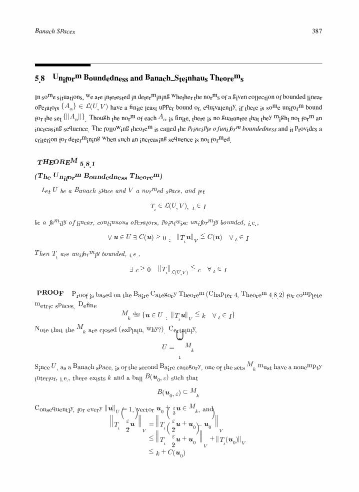
Banach Spaces 387
5.8 Uniform Boundedness and Banach–Steinhaus Theorems
In some situations, we are interested in determining whether the norms of a given collection of bounded linear
operators Aα ∈ L(U, V ) have a finite least upper bound or, equivalently, if there is some uniform bound
for the set Aα. Though the norm of each Aα is finite, there is no guarantee that they might not form an
increasing sequence. The following theorem is called the principle of uniform boundedness and it provides a
criterion for determining when such an increasing sequence is not formed.
THEOREM 5.8.1
(The Uniform Boundedness Theorem)
Let U be a Banach space and V a normed space, and let
Tι ∈ L(U, V ), ι ∈ I
be a family of linear, continuous operators, pointwise uniformly bounded, i.e.,
∀ u ∈ U ∃ C(u) > 0 : TιuV ≤ C(u) ∀ ι ∈ I
Then Tι are uniformly bounded, i.e.,
∃ c > 0 TιL(U,V ) ≤ c ∀ ι ∈ I
PROOF Proof is based on the Baire Category Theorem (Chapter 4, Theorem 4.8.2) for complete
metric spaces. Define
Mkdef= u ∈ U : TιuV ≤ k ∀ ι ∈ I
Note that the Mk are closed (explain, why?). Certainly,
U =
∞
1
Mk
Since U , as a Banach space, is of the second Baire category, one of the setsMk must have a nonempty
interior, i.e., there exists k and a ball B(u0, ε) such that
B(u0, ε) ⊂Mk
Consequently, for every uU = 1, vector u0 +ε2u ∈Mk, and
Tι
ε
2uV=Tι
ε
2u+ u0 − u0
V
≤Tι
ε
2u+ u0
V+ Tι(u0)V
≤ k + C(u0)

388 APPLIED FUNCTIONAL ANALYSIS
for every ι ∈ I, which implies that
Tι ≤2
ε(k + C(u0)) ∀ ι ∈ I
One of the most important consequences of the uniform boundedness theorem is the following Banach–
Steinhaus Theorem examining properties of pointwise limits of sequences of continuous linear operators
defined on Banach spaces.
THEOREM 5.8.2
(The Banach–Steinhaus Theorem)
Let U be a Banach space and V a normed space, and let
Tn ∈ L(U, V )
be a pointwise convergent sequence of continuous linear operators from U to V , i.e.,
∀ u ∈ U ∃ limn→∞
Tnu =: Tu
Then:
(i) T ∈ L(U, V )
(ii) T ≤ lim infn→∞
Tn
PROOF
Step 1. T is linear (essentially follows the proof of Proposition 5.7.1).
Step 2. From the continuity of the norm it follows that
limn→∞
Tn(u)V = TuV , ∀ u ∈ U
Consequently, Tn are pointwise uniformly bounded and, by the Uniform Boundedness Theorem, the
sequence of the norms Tn is bounded.
Step 3. Passing to the lim inf on both sides of the inequality (according to Step 2 the limit is
finite)
TnuV ≤ Tn uU
we get
TuV = limn→∞
TnuV ≤lim infn→∞
TnuU
which proves that

Banach Spaces 389
1. T is bounded
2. T ≤ lim infn→∞
Tn
5.9 The Open Mapping Theorem
Open Functions. Let X and Y be two topological spaces. A function f : X → Y is said to be open iff it
maps open sets in X into open sets in Y , i.e.,
A open in X =⇒ f(A) open in Y
Notice that if f is bijective and f−1 is continuous, then f is open.
The fundamental result of Stefan Banach reads as follows:
THEOREM 5.9.1
(The Open Mapping Theorem)
Let X and Y be two Banach spaces and T a nontrivial continuous linear operator from X onto Y
such that
T ∈ L(X,Y ), and T is surjective
Then T is an open mapping from X to Y , i.e.,
A open in X =⇒ T (A) open in Y
In order to prove the Open Mapping Theorem, we need a preliminary result.
LEMMA 5.9.1
Let X, Y be two normed vector spaces, T a continuous, linear operator from X into Y such that the
range of T , R(T ) is of the second Baire category in Y .
Then, for every A, a neighborhood of 0 in X, there exists D, a neighborhood of 0 in Y , such that
D ⊂ T (A)
In other words, for every neighborhood A of 0 in X, the closure T (A) is a neighborhood of 0 in Y .

390 APPLIED FUNCTIONAL ANALYSIS
PROOF
Step 1. One can always find a ball B = B(0, ε) with radius ε small enough such that
B +B ⊂ A
Step 2. Since, for every x ∈ X, limn→∞
1
nx = 0, there must exist a large enough n such that x ∈ nB.
Consequently,
X =
∞
n=1
(nB)
which implies that
R(T ) =∞
n=1
T (nB)
Step 3. As R(T ) is of the second category, there exists an index n0 such that T (n0B) has a
nonempty interior. But since multiplication by a non-zero scalar is a homeomorphism
T (n0B) = n0T (B) = n0T (B)
and therefore
intT (B) = ∅
which means that there exists a ball B(y0, δ) such that
B(y0, δ) ⊂ T (B)
One can always assume that y0 ∈ T (B), i.e., that y0 = Tx0, for some x0 ∈ B (explain, why?).
Step 4. Consider the ball D = B(0, δ). We have
D = −y0 +B(y0, δ) ⊂ −y0 + T (B)
= T (−x0) + T (B)
= T (−x0 +B)
⊂ T (A)
since −x0 +B ⊂ B +B ⊂ A.
PROOF of the Open Mapping Theorem
Step 1. Denote by Aε and Bε balls centered at 0 in X and Y , respectively.
Aε = B(0, ε) ⊂ X , Bε = B(0, ε) ⊂ Y
Pick also an arbitrary ε > 0 and denote εi =ε2i . By the lemma
∀i ∃ηi : Bηi⊂ T (Aεi
)

Banach Spaces 391
One can always assume that limi→∞
ηi = 0 (explain, why?).
Step 2. Let y ∈ Bη0 . We claim that there exists an element x ∈ A2ε0 such that Tx = y. Indeed,
from the above inclusion, we know that
∃ x0 ∈ Aε0 : y − Tx0Y < η1
It follows that y − Tx0 ∈ Bη1and, by the same reasoning,
∃ x1 ∈ Aε1 : y − Tx0 − Tx1Y < η2
By induction, there exists a sequence xi ∈ Aεisuch that
y − T
n
i=0
xi
Y
< ηn+1
Since
n
k=m+1
xk
X
≤
n
k=m+1
xkX ≤
n
k=m+1
εk ≤
n
m+1
2−k
ε0
the sequence of finite sumsn
k=0
xk
is Cauchy and, by the completeness of X, has a limit x ∈ X. Moreover, by the continuity of the
norm,
xX = limn→∞
n
k=0
xk
X
≤ limn→∞
n
k=0
xkX
≤
∞
0
2−k
ε0 = 2ε0
Finally, passing to the limit with n→∞ we get
y − TxY = 0 =⇒ y = Tx
As y was an arbitrary element of Bη0, we have shown that
Bη0 ⊂ T (A2ε)
Step 3. Let G be a nonempty open set in X and let x ∈ G. By the openness of G, there exists
ε > 0 such that
x+A2ε ⊂ G
Consequently
Tx+Bη0⊂ Tx+ T (A2ε) = T (x+A2ε) ⊂ T (G)
and therefore T (G) is open.
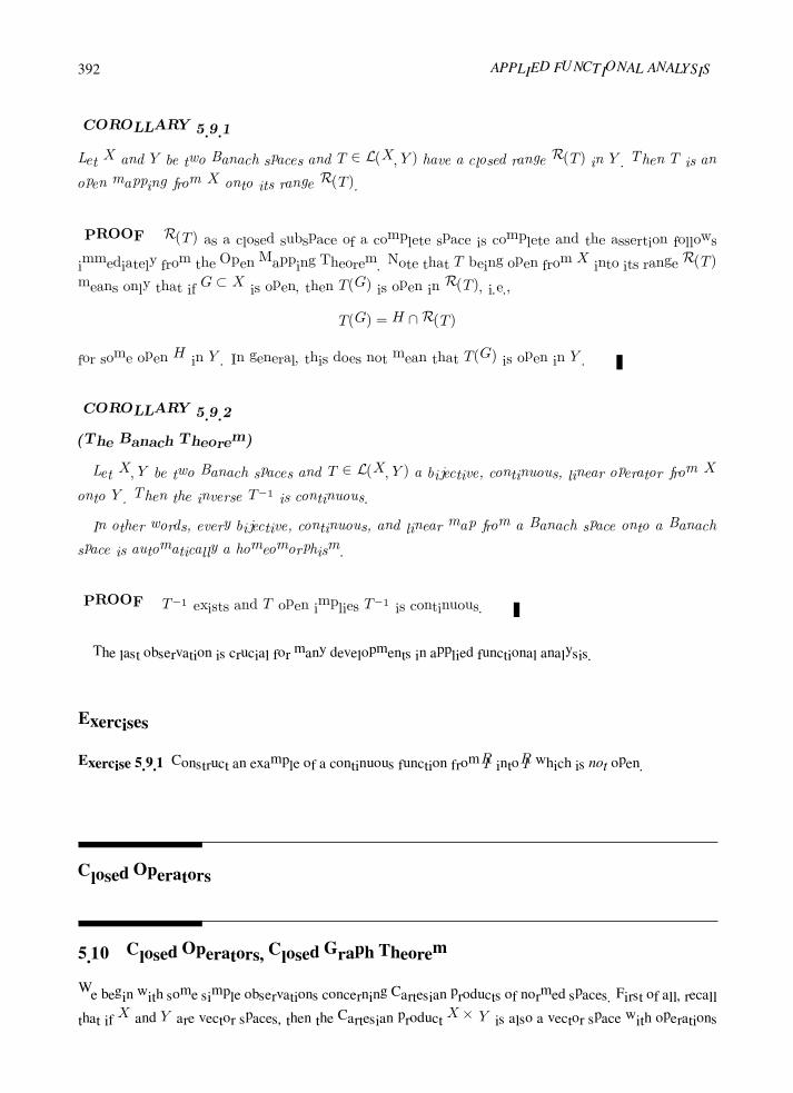
392 APPLIED FUNCTIONAL ANALYSIS
COROLLARY 5.9.1
Let X and Y be two Banach spaces and T ∈ L(X,Y ) have a closed range R(T ) in Y . Then T is an
open mapping from X onto its range R(T ).
PROOF R(T ) as a closed subspace of a complete space is complete and the assertion follows
immediately from the Open Mapping Theorem. Note that T being open from X into its range R(T )
means only that if G ⊂ X is open, then T (G) is open in R(T ), i.e.,
T (G) = H ∩R(T )
for some open H in Y . In general, this does not mean that T (G) is open in Y .
COROLLARY 5.9.2
(The Banach Theorem)
Let X,Y be two Banach spaces and T ∈ L(X,Y ) a bijective, continuous, linear operator from X
onto Y . Then the inverse T−1 is continuous.
In other words, every bijective, continuous, and linear map from a Banach space onto a Banach
space is automatically a homeomorphism.
PROOF T−1 exists and T open implies T−1 is continuous.
The last observation is crucial for many developments in applied functional analysis.
Exercises
Exercise 5.9.1 Construct an example of a continuous function from IR into IR which is not open.
Closed Operators
5.10 Closed Operators, Closed Graph Theorem
We begin with some simple observations concerning Cartesian products of normed spaces. First of all, recall
that if X and Y are vector spaces, then the Cartesian product X × Y is also a vector space with operations

Banach Spaces 393
defined by
(x1,y1) + (x2,y2)def= (x1 + x2,y1 + y2)
α (x,y)def= (αx, αy)
where the vector additions and multiplications by a scalar on the right-hand side are those in the X and Y
spaces, respectively.
If additionallyX and Y are normed spaces with norms · X and · Y , respectively, thenX ×Y may be
equipped with a (not unique) norm of the form
(x,y) =
(xpX + y
pY )
1p 1 ≤ p <∞
maxxX , yY p =∞
Finally, if X and Y are complete, then X × Y is also complete. Indeed, if (xn,yn) is a Cauchy sequence
in X × Y , then xn is a Cauchy sequence in X , and yn is a Cauchy sequence in Y . Consequently both xn
and yn have limits, say x and y, and, therefore, by the definition of the norm inX × Y , (xn,yn)→ (x,y).
Thus, if X and Y are Banach spaces, then X × Y is a Banach space, too.
Operators. Up to this point, all of the linear transformations from a vector space X into a vector space Y
have been defined on the whole space X , i.e., their domain of definition coincided with the entire space X .
In a more general situation, it may be useful to consider linear operators defined on a proper subspace of X
only (see Example 5.6.4). In fact, some authors reserve the name operator to such functions distinguishing
them from transformations which are defined on the whole space.
Thus, in general, a linear operator T from a vector space X into a vector space Y may be defined only on
a proper subspace of X , denoted D(T ) and called the domain of definition of T , or concisely, the domain of
T :
X ⊃ D(T ) x −→ Tx ∈ Y
Note that in the case of linear operators, the domain D(T ) must be a vector subspace of X (otherwise it
would make no sense to speak of linearity of T ).
Still, the choice of the domain is somehow arbitrary. Different domains with the same rule defining T
result formally in different operators in much the same fashion as functions are defined by specifying their
domain, codomain, and the rule (see Chapter 1).
With every operator T (not necessarily linear) we can associate its graph, denoted G(T ) and defined as
graph T = G(T )def= (x, Tx) : x ∈ D(T ) ⊂ X × Y
(recall the discussion in Section 1.9).
PROPOSITION 5.10.1
Let X, Y be two vector spaces and T : X ⊃ D(T )→ Y an operator. Then T is linear iff its graph
G(T ) is a linear subspace of X × Y .
394 APPLIED FUNCTIONAL ANALYSIS
PROOF Assume T is linear and let (x1,y1), (x2, y2) ∈ G(T ), i.e., x1,x2 ∈ D(T ) and y1 = Tx1,
y2 = Ty2.
Consequently, for every α1, α2,
α1x1 + α2x2 ∈ D(T )
and
α1y1 + α2y2 = α1Tx1 + α2Tx2 = T (α1x1 + α2x2)
which proves that
α1 (x2,y2) + α2 (x2,y2) ∈ G(T )
and therefore G(T ) is a linear subspace of X × Y .
Conversely, assume that G(T ) is a vector subspace of X × Y . Let x1,x2 ∈ D(T ) and x =
α1x1 + α2x2. By linearity of G(T )
α1 (x1, Tx1) + α2 (x2, Tx2) = (x, α1Tx1 + α2Tx2) ∈ G(T )
which means that x ∈ D(T ) (thus D(T ) is a linear subspace of X) and
Tx = α1Tx1 + α2Tx2
Closed Operators. Let X and Y be two normed spaces. A linear operator T : D(T ) → Y is said to be
closed iff its graph G(T ) is a closed subspace of X × Y .
It follows from the definition that every linear and continuous operator defined on a closed subspace of X
(in particular the whole X) is automatically closed.
Indeed, if (xn, Txn)→ (x,y), then xn → x and x ∈ D(T ). By continuity of T , Tx = limn→∞
Txn = y.
With every injective operator
T : X ⊃ D(T ) −→ R(T ) ⊂ Y
we can associate an inverse T−1 defined on the rangeR(T )
T−1 : Y ⊃ DT−1
= R(T ) −→ R
T−1
= D(T ) ⊂ X
As the operation
X × Y (x,y) −→ (y,x) ∈ Y ×X
is obviously a homeomorphism, it follows immediately from the definition of closed operators that if T is
closed and injective then T−1 is closed as well.
The following is a simple characterization of closed operators.

Banach Spaces 395
PROPOSITION 5.10.2
Let X and Y be two normed spaces and T a linear operator from D(T ) ⊂ X to Y . The following
conditions are equivalent to each other:
(i) T is closed
(ii) For an arbitrary sequence xn ∈ D(T ), if xn → x and Txn → y then x ∈ D(T ) and Tx = y
PROOF
(i) ⇒ (ii) Since
G(T ) (xn, Txn) −→ (x,y)
and G(T ) is closed, (x,y) ∈ G(T ) which means that x ∈ D(T ) and y = Tx.
(ii) ⇒ (i) Let
G(T ) (xn,yn) −→ (x,y)
Then xn → x and Txn = yn → y which implies that x ∈ D(T ) and Tx = y, or equivalently
(x,y) ∈ G(T ).
Closable Operators. Let X,Y be normed spaces and
T : X ⊃ D(T ) −→ Y
be a linear operator. Operator T is said to be closable (or pre-closed) iff the closure of graph of T , G(T ), in
X × Y can be identified as a graph of a (possibly another) linear operator T . The operator T is called the
closure of T .
PROPOSITION 5.10.3
Let X and Y be normed spaces and T a linear operator from D(T ) ⊂ X to Y . The following
conditions are equivalent to each other:
(i) T is closable
(ii) For an arbitrary sequence xn ∈ D(T ) such that
xn → 0 and Txn → y
implies y = 0

396 APPLIED FUNCTIONAL ANALYSIS
PROOF
(i) ⇒ (ii) xn → 0 and Txn → y means that (xn, Txn)→ (0,y) which implies that
(0,y) ∈ G(T ) = G(T )
and, consequently, y = T (0) = 0 (T is linear).
(ii) ⇒ (i) Step 1. Consider the closure G(T ) and define
D(S) = projection of G(T ) on X
=x ∈ X : ∃ y ∈ Y, (x,y) ∈ G(T )
Then D(S) is a linear subspace of X (explain, why?). We claim that for every x ∈ D(S) there exists
only one (a unique) y such that (x,y) ∈ G(T ).
Indeed, if there were two, say y1 and y2, then there would have to exist two corresponding
sequences x1n and x2
n in D(T ) such that
x1n, Tx
1n
−→ (x,y1) and
x2n, Tx
2n
−→ (x,y2)
Consequently,
xn = x1n − x
2n −→ 0 and Txn −→ y1 − y2
and, by condition (ii), y1 − y2 = 0 or y1 = y2.
Step 2. Define
D(S) x −→ Sx = y ∈ Y, (x,y) ∈ G(T )
For arbitrary x1,x2 ∈ D(S) there exist corresponding sequences x1n, x
2n such that
x1n, Tx
1n
→x1, Sx1
and
x2n, Tx
2n
→x2, Sx2
Consequently
α1x
1n + α2x
2n, T
α1x
1n + α2x
2n
→α1x
1 + α2x2, α1Sx
1 + α2Sx2
which proves that
Sα1x
1 + α2x2= α1Sx
1 + α2Sx2
and therefore S is linear.
COROLLARY 5.10.1
Every linear and continuous operator T from D(T ) in a normed space X to a normed space Y is
closable.
PROOF Let xn → 0 and Txn → y. By continuity of T , Txn → 0 and since T is single-valued,
it must be y = 0. Then the assertion follows from Proposition 5.10.3.

Banach Spaces 397
We conclude this section with the fundamental result concerning closed operators due to Banach.
THEOREM 5.10.1
(Closed Graph Theorem)
Let X and Y be Banach spaces and T a linear and closed operator from X to Y with the domain
of definition coinciding with the whole X, i.e., D(T ) = X. Then T is continuous.
PROOF As X × Y is a Banach space and T is closed, it follows that the graph of T , G(T ) is a
Banach space, too.
Considering the projection
iX : G(T ) −→ X, iX ((x, Tx))def= x
we see that
1. iX is a bijection
2. iX is continuous
Thus, by Corollary 5.9.2 to the Open Mapping Theorem, iX has a continuous inverse i−1X .
Introducing now the second projection
iY : G(T ) −→ Y, iY ((x, Tx))def= Tx
we can represent T in the form
T = iY i−1X
which proves that, as a composition of continuous operators, T must be continuous.
The important message in this theorem is that nontrivial closed operators, i.e., those which are not contin-
uous, are never defined on the entire space X .
Exercises
Exercise 5.10.1 Let A be a closed linear operator from D(A) ⊂ U into V , where U and V are Banach
spaces. Show that the vector space (D(A), · A) where uA = uU + AuV (the so-called
operator norm on D(A)) is Banach.
398 APPLIED FUNCTIONAL ANALYSIS
5.11 Example of a Closed Operator
Distributional Derivatives. Let Ω ⊂ IRn be an open set,α = (α1,. . ., αn) a multi-index and u ∈ Lp(Ω) an
arbitrary Lp-function. A function uα defined on Ω is called the distributional derivative of u, denoted Dαu,
iff
Ω
uDαϕdx = (−1)|α|
Ω
uαϕdx ∀ ϕ ∈ C∞0 (Ω)
where C∞0 (Ω) is the space of test functions discussed in Section 5.3. (It is understood that function uα must
satisfy sufficient conditions for the right-hand side to exist.)
Notice that the notion of the distributional derivative is a generalization of the classical derivative. Indeed,
in the case of a C |α| function u, the formula above follows from the (multiple) integration by parts and the
fact that test functions, along with their derivatives, vanish on the boundary ∂Ω.
Example 5.11.1
Let Ω = (0, 1) ⊂ IR and x0 ∈ (0, 1). Consider a function
u(x) =
u1(x) 0 < x ≤ x0
u2(x) x0 ≤ x < 1
where each of the branches is C1 in the corresponding subinterval, including the endpoints, and
u1(x0) = u2(x0) (see Fig. 5.2). Thus u is globally continuous but may not be C1 (the derivative at
x0 may not exist). For an arbitrary (test) function ϕ ∈ C∞0 (0, 1), we have
1
0
uϕdx =
x0
0
u1ϕdx+
1
x0
u2ϕdx
= −
x0
0
u1ϕdx+ u1ϕ|1x0−
1
x0
u2ϕdx+ u2ϕ|1x0
= −
x0
0
u1ϕdx−
1
x0
u2ϕdx− [u2(x0)− u1(x0)]ϕ(x0)
since ϕ(0) = ϕ(1) = 0.
But u2(x0) = u1(x0) and therefore
1
0
uϕdx = −
x0
0
u1ϕdx+
1
x0
u2ϕdx
Introducing a function
u(x) =
u1(x) 0 < x < x0
c x = x0
u2(x) x0 < x < 1

Banach Spaces 399
Figure 5.2
An example of a function differentiable in the distributional but not classical sense.
where c is an arbitrary constant, we see that
1
0
uϕdx = −
1
0
uϕdx
which proves that u is a distributional derivative of u. As constant c is completely arbitrary in the
definition of u, we remind that the Lebesgue integral is insensitive to the change of the integrand
on a set of measure zero. In fact, in order to be uniquely defined, the distributional derivatives have
to be understood as equivalence classes of functions equal almost everywhere.
Sobolev Spaces. Let Ω ⊂ IRn be an open set, m an integer and 1 ≤ p ≤ ∞. Consider the set of all Lp-
functions on Ω, whose distributional derivatives of order up tom all exist and are themselves Lp-functions:
Wm,p(Ω)def=u ∈ Lp(Ω) : Dαu ∈ Lp(Ω) ∀ |α| ≤ m
It can be easily checked (Exercise 5.11.2) thatWm,p(Ω) is a normed space with the norm
um,p = uWm,p(Ω) =
|α|≤m
Dαu
pLp(Ω)
1p
for 1 ≤ p <∞
max|α|≤m
Dαu
L∞(Ω)
for p =∞
PROPOSITION 5.11.1
Sobolev spaces Wm,p(Ω) are complete and, therefore, Banach spaces .
PROOF Let un be a Cauchy sequence in Wm,p(Ω). The definition of the norm in the space
implies that both functions un and their derivatives Dαun, for every multi-index α, form Cauchy
400 APPLIED FUNCTIONAL ANALYSIS
sequences in Lp(Ω) and therefore, by completeness of Lp(Ω), converge to some limits u and uα,
respectively. It remains only to show that the limits uα are distributional derivatives of the limit u.
This is done by passing with n→∞ in the identity
Ω
unDαϕ dx = (−1)
|α|
Ω
Dαunϕ dx
It follows from the Holder inequality that both sides are linear and continuous functionals of un and
Dαun, respectively, and therefore if un → u and Dαun → uα for n→∞, then in the limit
Ω
uDαϕ dx = (−1)|α|
Ω
uαϕ dx
which proves that uα ∈ Lp(Ω) is a distributional derivative of the limit u ∈ Lp(Ω). This holds for
every |α| ≤ m and therefore u ∈Wm,p(Ω).
For p = 2, the Sobolev spaces have structure of a Hilbert space (we will study that particular case in the
next chapter). A different notation is then used:
Hm(Ω)def= Wm,2(Ω)
At this point we are prepared to give a nontrivial example of a closed operator in Banach spaces.
Example 5.11.2
For an open set Ω ⊂ IRn and 1 ≤ p ≤ ∞, consider the Banach space Lp(Ω) and define the operator
T as:
Tu =
|α|≤m
aαDαu
with domain D(T ) defined as
D(T ) = u ∈ Lp(Ω) : Tu ∈ Lp(Ω)
and derivatives understood in the distributional sense discussed earlier. Here aα are arbitrary
constants, and m > 0. By the construction of the domain D(T ), operator T is well-defined, i.e., it
takes on its values in space Lp(Ω). We will demonstrate now that operator T is closed.
Toward this goal, pick a sequence un ∈ D(T ) and assume that
un → u and Tun =
|α|≤m
aαDαun → w in Lp(Ω)
for some u,w ∈ Lp(Ω). Passing with n→∞ in the identity
Ω
un
|α|≤m
aα(−1)|α|Dαϕ dx =
Ω
|α|≤m
aαDαunϕ dx
for arbitrary test function ϕ ∈ C∞0 (Ω), we learn that

Banach Spaces 401
1. Tu ∈ Lp(Ω)
2. Tu = w
and, therefore, by Proposition 5.10.2, the operator T is closed.
At the same time, in general, the operator T is not continuous, or equivalently bounded, as
can be seen in the particular case of Ω = (0, 1) ⊂ IR, D(T ) = W 1,2(0, 1), and Tu = u. Taking
un(x) =√2n+ 1xn, we easily check that
unL2 = 1 but TunL2 = unL2 = n
2n+ 1
2n− 1−→∞
as n→∞.
Exercises
Exercise 5.11.1 Consider X = L2(0, 1) and define a linear operator Tu = u, D(T ) = C∞([0, 1]) ⊂
L2(0, 1). Show that T is closable. Can you suggest what would be the closure of T ?
Exercise 5.11.2 Show that the Sobolev spaceWm,p(Ω) is a normed space.
Topological Duals, Weak Compactness
5.12 Examples of Dual Spaces, Representation Theorem for Topological Duals of
Lp Spaces
In Section 5.7, for every normed space U , we introduced its topological dual U , defined as the space of all
linear and continuous functionals from U to IR (or IC).
Since there are many linear functionals on U that are not continuous, the topological dual is a smaller space
than the algebraic dual U∗ = L(U, IR) described in Chapter 2, and algebraically L(U, IR) ⊂ L(U, IR). But we
have little need for L(U, IR) in discussions of normed spaces. Unless some specific distinction is needed, we
shall henceforth refer to U as the dual of U .
Let f ∈ U = L(U, IR). As in Chapter 2, it is customary to represent the functional f as a duality pairing;
i.e., we usually write
f(u) = f,u, f ∈ U , u ∈ U

402 APPLIED FUNCTIONAL ANALYSIS
Then the symbol ·, · can be regarded as a bilinear map from U × U into IR or IC.
Now, since f(u) is a real or complex number, f(u) = |f,u|. Hence, in view of what was said about
the norms on spaces L(U, V ) of linear operators, the norm of an element of U is given by
fU = supu∈U
|f,u|
uU, u = 0
Hence we always have
|f,u| ≤ fU uU f ∈ U , u ∈ U
which in particular implies that the duality pairing is continuous (explain, why?).
Before we proceed with some general results concerning dual spaces, we present in this section a few non-
trivial examples of dual spaces in the form of so-called representation theorems. The task of a representation
theorem is to identify elements from a dual space (i.e., linear and continuous functionals defined on a normed
space) with elements from some other space, for instance some other functions, through a representation
formula relating functionals with those functions. The representation theorems not only provide meaningful
characterizations of dual spaces, but are also of great practical value in applications.
The main result we present in this chapter is the representation theorem for the duals of the spaces Lp(Ω),
1 ≤ p <∞.
LEMMA 5.12.1
Let 1 < q ≤ 2. There exists a positive number c > 0 such that
|1 + u|q≥ 1 + qu+ cθ(u) ∀ u ∈ IR
where
θ(u) =
|u|
2|u| < 1
|u|q|u| ≥ 1
PROOF Define
ψ(u)def= |1 + u|
q− 1− qu , u ∈ IR
χ(u)def=
ψ(u)
θ(u), u = 0
As (check it)
limu→0
χ(u) =q(q − 1)
2, lim
|u|→∞χ(u) = 1
it follows from the continuity of χ that there exist positive constants c1, δ,∆ > 0 such that
χ(u) ≥ c1 for |u| ≤ δ or |u| ≥ ∆
At the same time
ψ(u) = q |1 + u|q−1
sgn(1 + u)− q = 0 ⇒ u = 0
Banach Spaces 403
and
ψ(u) = q(q − 1) |1 + u|q−2
⇒ χ(0) > 0
which implies that ψ(u) has a unique minimum attained at 0 (equal 0) and therefore must be
bounded away from 0 for δ < |u| < ∆ (why?). As the function θ(u) is bounded from above in the
same range of u (why?), function χ(u) is bounded away from zero as well, i.e.,
∃ c2 > 0 : χ(u) ≥ c2 for δ < |u| < ∆
It is sufficient now to take c = minc1, c2.
THEOREM 5.12.1
(Representation Theorem for (Lp(Ω))
)
Let Ω ⊂ IRN be an open set and 1 ≤ p <∞. For every linear and continuous functional f defined
on the space Lp(Ω), there exists a unique function ϕ ∈ Lq(Ω), 1p + 1
q = 1, such that
f(u) = f, u =
Ω
ϕu dx ∀ u ∈ Lp(Ω)
Moreover,
f(Lp) = ϕLq
REMARK 5.12.1 Consider the linear mapping
F : Lq(Ω) −→ (Lp(Ω)), ϕ −→ F (ϕ) = f
where f(u) =
Ω
ϕu dx.
Denoting by · p the Lp norm, we have (from the Holder inequality)
|f(u)| =
Ω
ϕu dx
≤ ϕq up
which proves that
(i) F is well-defined and
(ii) F (ϕ) ≤ ϕq.
At the same time taking u = |ϕ|q−1sgn ϕ we check that
(i) u ∈ Lp(Ω)
(ii) f(u) =
Ω
|ϕ|qdx = ϕqup

404 APPLIED FUNCTIONAL ANALYSIS
which proves that F (ϕ) = ϕq.
Thus F defines a linear, norm-preserving (and therefore injective) map from Lq(Ω) into the dual
of Lp(Ω). What the representation theorem says is that all functionals from the dual space are of
this form and, consequently, F is a (norm-preserving) isomorphism between Lq(Ω) and the dual of
Lp(Ω).
PROOF of Theorem 5.12.1.
We shall restrict ourselves to the case of bounded Ω.
Case 1 (a unit cube). Ω = Qdef= (0, 1)N = (0, 1)× . . .× (0, 1) (N times). 2 ≤ p <∞.
Step 1. For an arbitrary positive integer n, divide Q into cubes (with disjoint interiors)
Q(n)k , k = 1, 2, . . . , (2n)N
Let χ(n)k denote the characteristic function of cube Q
(n)k , i.e.,
χ(n)k =
1 on Q(n)k
0 otherwise
Obviously, χ(n)k belong to Lp(Q).
Set
ϕn =
2nN
k=1
1
measQ
(n)k
fχ
(n)k
χ
(n)k =
k
2nNfχ
(n)k
χ
(n)k
Consequently,
Q
ϕnχ(n)k dx =
Q(n)k
ϕndx = fχ
(n)k
and therefore, by linearity of integrals and functional f ,
Q
ϕnu dx = f(u)
for any u, a linear combination of characteristic functions χ(n)k .
Selecting
u =|ϕn|
q
ϕn= |ϕn|
q−1sgn ϕn
upp =
Q
|ϕn|p(q−1)
dx =
Q
|ϕn|qdx
we have
Q
|ϕn|qdx =
Q
ϕnu dx ≤ f up
= f
Q
|ϕn|qdx
1p

Banach Spaces 405
which implies
ϕnq ≤ f
Step 2. ϕn is a Cauchy sequence in Lq(Q). Assume n ≥ m. Applying Lemma 5.12.1 with
u =ϕn − ϕm
ϕm
we getϕn
ϕm
q
≥ 1 + qϕn − ϕm
ϕm+ cθ
ϕn − ϕm
ϕm
which upon multiplying by |ϕm|q and integrating over Q yields
Q
|ϕn|qdx ≥
Q
|ϕm|qdx+ q
Q
|ϕm|q
ϕm(ϕn − ϕm)dx
+ c
Q
|ϕm|qθ
ϕn − ϕm
ϕm
dx
But, selecting u = |ϕm|q
ϕm, we have
Q
|ϕm|q
ϕm(ϕn − ϕm)dx =
Q
(ϕn − ϕm)u dx = f(u)− f(u) = 0
and, therefore,
Q
|ϕn|qdx ≥
Q
|ϕm|qdx+ c
Q
|ϕm|qθ
ϕn − ϕm
ϕm
dx
In particular, sequenceQ|ϕn|
qdx is increasing. Since, according to Step 1, it is also bounded, it
converges to a finite value. Consequently,
limn,m→∞
Q
|ϕm|qθ
ϕn − ϕm
ϕm
dx = 0
Denote now by em,n the collection of all points where
|ϕn − ϕm| ≥ |ϕm| ⇒ θ
ϕn − ϕm
ϕm
=|ϕn − ϕm|
q
|ϕm|q
and by em,n the set of all x for which
|ϕn − ϕm| ≤ |ϕm| ⇒ θ
ϕn − ϕm
ϕm
=|ϕn − ϕm|
2
|ϕm|2
This leads to the decomposition
Q
|ϕm|qθ
ϕn − ϕm
ϕm
dx =
em,n
|ϕn − ϕm|qdx
+
em,n
|ϕn|q−2
|ϕn − ϕm|2dx

406 APPLIED FUNCTIONAL ANALYSIS
Since |ϕn − ϕm| < |ϕn| on em,n we also have
em,n
|ϕn − ϕm|qdx ≤
em,n
|ϕm|q−1
|ϕn − ϕm| dx
=
em,n
|ϕm|
q−12 |ϕn − ϕm|
|ϕm|
q2 dx
≤
|ϕm|q−2
|ϕn − ϕm| dx
12
|ϕm|qdx
12
(Cauchy–Schwarz inequality)
Concluding
Q
|ϕn − ϕm|qdx −→ 0 for n,m −→∞
which means that ϕn is a Cauchy sequence and, by the completeness of Lq(Q), converges to a
function ϕ ∈ Lq(Q).
Remark: In all inequalities above we have implicitly assumed that ϕm = 0. Technically speaking,
one should eliminate from all the corresponding integrals such points and notice that the final
inequalities are trivially satisfied at points where ϕm = 0.
Step 3. For any function u, a linear combination of the characteristic functions χ(m)k
Q
ϕnu dx = f(u) ∀ n ≥ m
Passing to the limit with n→∞
Q
ϕu dx = f(u)
Finally, by the density of the characteristic functions in Lp(Q), the equality holds for any u ∈ Lp(Q).
Case 2. Ω bounded. 2 ≤ p <∞. By a simple scaling argument, Case 1 result holds for any cube
Q ⊂ IRN (not necessarily unit).
Choose now a sufficiently large Q such that Ω ⊂ Q. Extending functions from Lp(Ω) by zero to
the whole Q, we can identify the Lp(Ω) space with a subspace of Lp(Q).
Lp(Ω) ⊂ Lp(Q)
By the Hahn–Banach Theorem, any linear and continuous functional f defined on Lp(Ω) can be
extended to a linear and continuous functional F defined on the whole Lp(Q). According to the
Case 1 result, there exists a function Φ ∈ Lq(Q) such that
Q
Φudx = F (u) ∀ u ∈ Lp(Q)
Define ϕ = Φ|Ω (restriction to Ω). Obviously
Ω
ϕudx = F (u) = f(u) ∀ u ∈ Lp(Ω)
Case 3. Ω is bounded. 1 ≤ p < 2. According to Proposition 3.9.3 , L2(Ω) is continuously embedded
in Lp(Ω) and therefore any linear and continuous functional f defined on Lp(Ω) is automatically

Banach Spaces 407
continuous on L2(Ω). By the Case 2 result, specialized for p = 2, there exists a function ϕ ∈ L2(Ω),
such that
Ω
ϕudx = f(u) ∀ u ∈ L2(Ω)
We will show that
1. ϕ ∈ Lq(Ω),1
p+
1
q= 1
2.
Ω
ϕudx = f(u) ∀ u ∈ Lp(Ω)
Step 1. Assume p > 1.
Define
ϕn(x) =
ϕ(x) if |ϕ(x)| ≤ n
n if |ϕ(x)| > n
and set
un = |ϕn|q−1
sgnϕ
Obviously, functions un are bounded and, therefore, they are elements of Lp(Ω). We have
f(un) =
Ω
ϕundx =
Ω
ϕ |ϕn|q−1
sgnϕ dx ≥
Ω
|ϕn|qdx
At the same time
f(un) ≤ f unp = f
Ω
|ϕn|qdx
1p
So:
Ω
|ϕn|qdx
1q
≤ f
By the Lebesgue Dominated Convergence Theorem (ϕn → ϕ),
ϕq ≤ f
By the density argument (L2-functions are dense in Lp, 1 ≤ p < 2; see Exercise 5.12.1),
Ω
ϕudx = f(u) ∀ u ∈ Lp(Ω)
Step 2. Case p = 1.
Define
en = x ∈ Ω : |ϕ(x)| ≥ n
and set
un =
sgnϕ on en
0 otherwise

408 APPLIED FUNCTIONAL ANALYSIS
Obviously, un ∈ L2(Ω) and
f(un) =
Ω
ϕundx =
en
|ϕ|dx ≥ n meas(en)
At the same time
f(un) ≤ f un1 = f meas(en)
and, therefore,
(n− f) meas(en) ≤ 0
which proves that meas(en) = 0 for n > f and therefore ϕ is essentially bounded.
By the density argument, again the representation formula must hold for all u ∈ L1(Ω).
THEOREM 5.12.2
(Representation Theorem for (p))
Let 1 ≤ p <∞. For every linear and continuous functional f defined on the space p, there exists
a unique sequence ϕ ∈ q, 1/p+ 1/q = 1 such that
f(u) = f, u =
∞
i=1
ϕiui ∀ u ∈ p
Moreover
f(p) = ϕq
and the map
q ϕ→
p u→
∞
i=1
ϕiui
∈ (p)
is a norm-preserving isomorphism from q onto (p).
The proof follows the same lines as for the Lp spaces and is left as an exercise.
REMARK 5.12.2 Note that both representation theorems do not include the case p = ∞. A
separate theorem identifies the dual of L∞(Ω) with so-called functions of bounded variation .
Integral Form of Minkowski’s Inequality. The representation theorem for Lp spaces implies an important
generalization of Minkowski’s inequality which was discussed in Section 3.9. Let Ω ⊂ IRn be an open set
and let, for 1 ≤ p < ∞, · p denote the Lp norm. The triangle inequality for the Lp norm, known as
Minkowski’s inequality,
u+ vp ≤ up + vp

Banach Spaces 409
can easily be generalized by induction to finite sums,
n
i=1
uip ≤
n
i=1
uip
It turns out that the sum can be replaced with an integral.
PROPOSITION 5.12.1
(Integral Form of Minkowski’s Inequality)
Let Ω ⊂ IRn, G ⊂ IRm be open sets, and let v : Ω×G→ IR(IC) be a Lebesgue summable function.
Let 1 ≤ p <∞. The following inequality holds,
Ω
G
u(t,x) dt
p
dx
1p
≤
G
Ω
|u(t,x)|p dx
1p
dt
PROOF Define function
w(x) =
G
u(t,x) dt
For p = 1, the result can be obtained by integrating both sides of the inequality
|w(x)| ≤
G
|u(t,x)| dt
and applying Fubini’s theorem to the right-hand side. Consider now p > 1 and assume that the
right-hand side of the inequality is finite (otherwise, the result trivially holds). Consider space
Lq(Ω), 1/p+ 1/q = 1, and a linear functional defined on Lq(Ω) by function w,
Lq(Ω) v →
Ω
vw dx ∈ IR(IC)
We have,
|
Ω
vw dx| = |
Ω
v(x)
G
u(t,x) dt dx|
= |
G
v(x)
Ω
u(t,x) dx dt| (Fubini’s Theorem)
≤
G
vq
Ω
|u(t,x)|p dx
1p
dx dt (Holder’s inequality)
=
G
Ω
|u(t,x)|p dx
1p
dx dt vq
The functional is thus continuous on Lq(Ω) and, by Theorem 5.12.1, its norm, equal to the Lp norm
of function w(x) must be bounded by the (finite) constant on the right-hand side,
wp ≤
G
Ω
|u(t,x)|p dx
1p
dx dt
which is precisely what we want to prove.
410 APPLIED FUNCTIONAL ANALYSIS
Distributions. The notion of the topological dual understood as the space of linear and continuous func-
tionals can be generalized to any topological vector space. In particular, the dual of the space of test functions
D(Ω) (see Section 5.3) introduced by L. Schwartz, denoted D(Ω), is known as the famous space of distri-
butions. The elements q ∈ D(Ω) are called distributions.
To test continuity of linear functionals defined on D(Ω), we must recall (see Remark 5.3.1) that the topol-
ogy in D(Ω) is identified as the strongest topology in C∞0 (Ω) such that all inclusions
iK : D(K) → D(Ω)
are continuous, for every compact setK ⊂ Ω. Consequently, a linear functional q : D(Ω)→ IR is continuous
if the composition
q iK : D(K) −→ IR
is continuous, for every compact K ⊂ Ω. This leads to the following criterion for continuity: a linear
functional q : D(Ω) → IR is continuous iff to every compact set K ⊂ Ω there corresponds a constant
CK > 0 and k > 0 such that
|q(ϕ)| ≤ CK sup|α|≤k
|Dαϕ(x)| ∀ ϕ ∈ D(K)
x∈K
Using the criterion above, it is easy to check (comp. Exercise 5.12.5), that, for any locally integrable function
f on Ω, i.e., such thatKfdx <∞, on any compact setK ⊂ Ω, the linear functional
C∞0 (Ω) ϕ −→
Ω
fϕdx ∈ IR(IC)
is continuous on D(Ω) and therefore defines a distribution. Distributions of this type are called regular and
are identified with the underlying, locally integrable function f .
Distributions which are not regular are called irregular . The most famous example of an irregular distri-
bution is the Dirac delta functional
δx0, ϕ
def= ϕ(x0)
Theory of distributions exceeds significantly the scope of this book. From a number of remarkable proper-
ties of distributions, we mention only the definition of the distributional derivative, generalizing the notions
discussed in Section 5.11.
For any multi-index α, a distribution qα is called the Dα-derivative of a distribution q, denoted Dαq, iff
qα, ϕ = (−1)|α|q,Dαϕ ∀ ϕ ∈ D(Ω)
Surprisingly enough, it can be proved that every distribution q ∈ D(Ω) possesses derivatives of arbitrary
order.

Banach Spaces 411
Exercises
Exercise 5.12.1 Let Ω ⊂ IRN be a bounded set, and fix 1 ≤ p < ∞. Prove that, for every r such that
p < r ≤ ∞, Lr(Ω) is dense in Lp(Ω).
Hint: For an arbitrary u ∈ Lp(Ω) define
un(x) =
u(x) if |u(x)| ≤ n
n otherwise
Show that
1. un ∈ Lr(Ω) and
2. un − up → 0.
Exercise 5.12.2 Consider IRn equipped with the p-norm,
xp =
n
i=1
|xi|p
1p
1 ≤ p <∞
max1≤i≤n
|xi| p =∞
Prove that
supyp=1
n
i=1
xiyi = xq
where 1/p + 1/q = 1. Explain why the result implies that the topological dual of (IRn, · p) is
isometric with (IRn, · q).
Exercise 5.12.3 Prove Theorem 5.12.2.
Exercise 5.12.4 Let Ω ⊂ IRn be an open set and f : Ω→ IR a measurable function defined on Ω. Prove that
the following conditions are equivalent to each other:
1. For every x ∈ Ω there exists a neighborhood N(x) of x (e.g., a ball B(x, ε) with some ε =
ε(x) > 0) such that
N(x)
|f | dx < +∞
2. For every compactK ⊂ Ω
K
|f | dx < +∞
Functions of this type are called locally integrable and form a vector space, denoted L1loc(Ω).

412 APPLIED FUNCTIONAL ANALYSIS
Exercise 5.12.5 Prove that the regular distributions and the Dirac delta functional defined in the text are
continuous on D(Ω).
Exercise 5.12.6 Consider function u : (0, 1)→ IR of the form
u(x) =
u1(x) 0 < x ≤ x0
u2(x) x0 < x ≤ 1where x0 ∈ (0, 1)
Here u1 and u2 are C1 functions (see Example 5.11.1), but the global function u is not necessarily
continuous at x0. Follow the lines of Example 5.11.1 to prove that the distributional derivative of the
regular distribution qu corresponding to u is given by the formula
(qu) = qu + [u(x0)]δx0
where u is the union of the two branches derivatives u1 and u2 (see Example 5.11.1), δx0 is the Dirac
delta functional at x0, and [u(x0)] denotes the jump of u at x0,
[u(x0)] = u2(x0)− u1(x0)
5.13 Bidual, Reflexive Spaces
The Bidual Space. Let U be a normed space and U its topological dual. Then U equipped with the dual
norm is itself a normed space (always complete, even if U is not) and it also makes sense to speak of the
space of all continuous linear functionals on U . The dual of the dual of a normed space U is again a Banach
space, denoted U and called the bidual of U
U def= (U )
It turns out that any normed space U is isomorphic, in a natural way, to a closed subspace of its bidual U .
To see this, let u ∈ U and f ∈ U . Then f, u = f(u) is a linear functional on U (by the choice of f ).
However, for each fixed u, f, u is also a linear functional on U (by definition of vector space operations
in U ). More precisely, for each u ∈ U , we define a corresponding linear functional Fu on U , called the
evaluation at u and defined as
U f −→ Fu(f)def= f, u ∈ IR(IC)
From the inequality
|Fu(f)| = f, u ≤ uU fU
follows that
FuU ≤ uU

Banach Spaces 413
Moreover, by Corollary 5.5.2 to the Hahn–Banach Theorem, for any vector u ∈ U , there exists a correspond-
ing functional f ∈ U , fU = 1 such that f(u) = u. Let f1 denote such a functional. Then
FuU ≥|Fu(f1)|
f1U =|f1, u|
1= uU
Therefore,
FuU = uU
Summing that up, the linear map F prescribing for each u ∈ U the corresponding element Fu of bidual U
U ∈ u −→ Fu ∈ U
is linear (explain, why?) and norm-preserving. Thus F establishes an isometric isomorphism between any
normed space U and its range in the bidual U . Note that, in general, F is not surjective.
Reflexive Spaces. A normed vector space U is called reflexive if the evaluation map F discussed above is
surjective, i.e., space U is isomorphic and isometric with its bidual U through the evaluation map.
Before we proceed with a number of properties of reflexive spaces, we need to record the following simple
but important lemma:
LEMMA 5.13.1
(Mazur Separation Theorem)
Let U be a normed space and M ⊂ U a closed subspace of U . For every non-zero vector u0 ∈M
there exists a continuous linear functional f on U , f ∈ U , such that
(i) f |M ≡ 0
(ii) f(u0) = u0 = 0
(iii) f = 1
PROOF Consider the subspace M1 = M ⊕ IRu0 (or M ⊕ ICu0) and a corresponding linear
functional f defined on M1 as
f(u) =
0 on M
αu0 for u = αu0, α ∈ IR(IC)
We claim that f is continuous. Indeed, suppose to the contrary that there exists an ε > 0 and
sequences mn ∈M, αn ∈ IR(IC) such that
un =mn + αnu0 → 0

414 APPLIED FUNCTIONAL ANALYSIS
and
|f(un)| = |αn| u0 > ε
By switching from un to −un, we can always assume that αn > 0. Consequently, α−1n < ε−1u0
and
α−1n un = α−1
n mn + u0 −→ 0
which proves that u0 ∈ M = M , a contradiction. Finally, taking p(u) = u we apply the Hahn–
Banach Theorem and extend f to the whole U . From the inequality
|f(u)| ≤ u
and the fact that f(u0) = u0, follows that f = 1.
REMARK 5.13.1 Defining a hyperplane Π as
Π = u ∈ U : f(u) = c
where f ∈ U and c is a constant, we can interpret the discussed result as a separation of the
subspace M from the point u0 by any hyperplane corresponding to the constructed functional f and
any constant 0 < c < u0. Indeed
f(u0) = u0 > c > 0 = f(m) for m ∈M
which means that u0 and M stay on “opposite” sides of the hyperplane. This explains why the
result is interpreted as a separation theorem.
PROPOSITION 5.13.1
(i) Any reflexive normed space must be complete and, hence, is a Banach space .
(ii) A closed subspace of a reflexive Banach space is reflexive.
(iii) Cartesian product of two reflexive spaces is reflexive.
(iv) Dual of a reflexive space is reflexive.
PROOF
(i) By definition, U is isomorphic with the complete space U and therefore must be complete as
well.

Banach Spaces 415
(ii) Let V ⊂ U be a closed subspace of a reflexive space U and let g denote an arbitrary linear
and continuous functional on the dual V , i.e., g ∈ V . Consider now the transpose of the inclusion
map,
i : U f −→ i(f) = f |V ∈ V
prescribing for each linear and continuous functional f on U its restriction to V . Composition g i
defines a linear and continuous functional on U and therefore, by reflexivity of U , there exists an
element u ∈ U such that
(g i)(f) = f, u ∀ f ∈ U
The Hahn–Banach Theorem implies that u must be an element of V , as we now show. Suppose
u ∈ V , then any continuous functional f vanishing on V and taking a non-zero value at u could be
extended to the whole U and consequently f, u = f(u) = 0 but
(g i)(f) = g(f |V ) = g(0) = 0
which is a contradiction.
Question: Where have we used the assumption that V is closed?
(iii) Let Ui, i = 1, 2, be two reflexive spaces and U i , i = 1, 2, their duals. The following map
establishes an isomorphism between the dual of the Cartesian product U1 × U2 and the Cartesian
product of the duals U 1, U
2.
i : (U1 × U2) f −→ i(f) = (f1, f2) ∈ U
1 × U 2
where
f1(u1)def= f ((u1, 0))
and
f2(u2)def= f ((0, u2))
Consequently, if Fi : Ui → U i denote the isomorphisms between U1, U2 and their biduals, then
F1 × F2 : (u1, u2)→ U 1 × U
2 (f1, f2)→ f1(u1) + f2(u2) ∈ IR(IC)
establishes the isomorphism between U1 × U2 and the dual to U 1 × U
2 or equivalently, (U1 × U2).
(iv) Assume F : U → U is an isomorphism and consider the map
G : U f −→ G(f)def= f F−1 ∈ (U ) ∼ (U )
It is a straightforward exercise to prove that G is an isomorphism, too.
REMARK 5.13.2 One can prove that the reflexivity of the dual space U is not only a necessary,
but also a sufficient condition for the reflexivity of a normed space U . The proof considerably exceeds
the scope of this book.

416 APPLIED FUNCTIONAL ANALYSIS
Example 5.13.1
The Lp(Ω) spaces are reflexive for 1 < p < ∞. This follows immediately from the Representation
Theorem for duals of Lp spaces. For 1 < p <∞, the dual of Lp(Ω) is identified with Lq(Ω) and, in
turn, the dual of Lq(Ω) can again be identified with Lp(Ω). Note that the result holds neither for
L1(Ω) nor for L∞(Ω) spaces which are not reflexive.
The same conclusions apply to p spaces.
Example 5.13.2
Every finite-dimensional space is reflexive (explain, why?).
Example 5.13.3
Sobolev spaces Wm,p(Ω) (see Section 5.11) are reflexive for 1 < p <∞.
For proof, it is sufficient to notice that the space Wm,p(Ω) is isomorphic to a closed subspace of
the Cartesian product of reflexive Lp(Ω) spaces:
uα ∈ Lp(Ω), |α| ≤ m :
Ω
uDαϕdx = (−1)|α|
Ω
uαϕdx, ∀ ϕ ∈ C∞0 (Ω)
Indeed, the subspace above can be identified as an image of the operator from Wm,p(Ω) into the
Cartesian product Lp(Ω) × . . . × Lp(Ω) (n times, where n = #|α| ≤ m), prescribing for each
function u all its distributional derivatives.
Exercises
Exercise 5.13.1 Explain why every finite-dimensional space is reflexive.
Exercise 5.13.2 LetWm,p(Ω) be a Sobolev space for Ω, a smooth domain in IRn. The closure inWm,p(Ω)
of the test functions C∞0 (Ω) (with respect to theWm,p norm), denoted byWm,p
0 (Ω),
Wm,p0 (Ω) = C∞
0 (Ω)
may be identified as a collection of all “functions” from Wm,p(Ω) which “vanish” on the boundary
together with their derivatives up tom− 1 order (this is a very nontrivial result based on Lions’ Trace
Theorem; see [6, 8]). The duals of the spacesWm,p0 (Ω) are the so-called negative Sobolev spaces
W−m,p(Ω)def= (Wm,p
0 (Ω))
m > 0
Explain why bothWm,p0 (Ω) andW−m,p(Ω), for 1 < p <∞, are reflexive.
Banach Spaces 417
5.14 Weak Topologies, Weak Sequential Compactness
The topological properties of normed linear spaces are complicated by the fact that topologies can be induced
on such spaces in more than one way. This leads to alternative notions of continuity, compactness, and
convergence for a normed space U .
Weak Topology. Let U be a normed space and let U denote its dual. For each continuous, linear functional
f ∈ U we introduce a corresponding seminorm pf on U defined as
pf (u)def= |f(u)| = |f,u|, f ∈ U
By Corollary 5.5.2, for each u = 0, there exists a functional f ∈ U taking a non-zero value at u, which
implies that the family of seminorms
pf : U → [0,∞), f ∈ U
satisfies the axiom of separation (see Section 5.5). Consequently, the pf seminorms can be used to construct
a locally convex topology on U . We refer to it as the weak topology in contrast to the topology induced by
the norm and called the strong topology.
Indeed, it follows immediately from the definition of locally convex spaces that the weak topology is
weaker than the one induced by the norm. To see this, consider an arbitrary element from the base of neigh-
borhoods for the zero vector in U
B(I0, ε) = u ∈ U : |f(u)| ≤ ε, f ∈ I0
where I0 ⊂ U is finite.
By continuity of functionals f , there exist corresponding constants Cf > 0 such that
|f(u)| ≤ Cfu
Take δ = min εCf
: f ∈ I0 and consider the ball B(0, δ). It follows that
|f(u)| ≤ Cfu ≤ Cfδ ≤ ε, for every f ∈ I0
which proves that B(0, δ) ⊂ B(I0, ε).
Consequently, the base of neighborhoods for the zero vector in the strong topology (the balls) is stronger
than the base of neighborhoods in the weak topology (setsB(I0, ε)). As bases of neighborhoods for non-zero
vectors u are obtained by shifting the base for zero to u, the same property holds for any vector u. This
proves that the norm topology is stronger than the weak one.
418 APPLIED FUNCTIONAL ANALYSIS
Weak* Topology. A third fundamental topology in a normed spaceU can be generated whenU is identified
as the dual of some other normed space V , U = V . For every v ∈ V , seminorms
U f −→ |f,v| = |f(v)| ∈ [0,∞)
trivially satisfy the axiom of separation (explain, why?) and therefore can be used to induce another locally
convex topology, called the weak* (weak “star”) topology on U . As in general elements from V are identified
with a proper subspace of the bidual V = U , the neighborhoods in the weak* topology form a proper
subset of the neighborhoods in the weak topology. Consequently, the weak* topology is weaker than the
weak topology. Notice, however, that the two topologies coincide for reflexive spaces, since V ∼ V .
In this section we study some basic topological properties of weak topologies including the fundamental
notion of weak sequential compactness.
We begin by discussing a simple characterization for the convergence of sequences in the weak topologies.
PROPOSITION 5.14.1
Let U be a normed space and consider the sequences
un ∈ U, fn ∈ U
Then
(i) un converges to u in the strong (norm) topology, denoted un → u, iff
un − uU → 0
(ii) un converges to u in the weak topology, denoted un u, iff
f, un − u −→ 0 ∀ f ∈ U
(iii) fn converges to f in the strong (dual) topology, denoted fn → f , iff
fn − fU → 0
(iv) fn converges to f in the weak (dual) topology, denoted fn f , iff
g, fn − f → 0 ∀ g ∈ U
(v) fn converges to f in the weak* topology, denoted fn∗ f , iff
fn − f, u → 0 ∀ u ∈ U

Banach Spaces 419
PROOF Proof is a straightforward consequence of the definitions and is left as an exercise.
Example 5.14.1
Many weakly convergent sequences do not converge strongly. For any integer n > 0, consider the
partition of unit interval (0, 1) into 2n equal subintervals and a corresponding sequence of functions
ϕn(x) =
1 for (k − 1)2−n ≤ x ≤ k2−n, k even
−1 otherwise
(see Fig. 5.3). Obviously, ϕn ∈ L2(0, 1). We will prove later (see Example 5.14.3) that sequence ϕn
converges weakly in L2(0, 1) to zero function 0. At the same time,
ϕn2L2 =
1
0
ϕ2ndx = 1
and therefore ϕn does not converge strongly to 0.
Example 5.14.2
Recall that L1(a, b) is not reflexive, and L∞(a, b) can be identified with the dual of L1(a, b). Let φn
be a sequence of functions in L∞(a, b). Then φn converges weakly∗ to a function φ0 ∈ L∞(a, b) if
limn→∞
b
a
fφndx =
b
a
fφ0dx, ∀ f ∈ L1(a, b)
The reason that this represents weak∗ convergence is clear: the φn represent continuous linear
functionals on L1(a, b) and L1(a, b) ⊂ (L∞(a, b)) = L1(a, b). Hence we construct a functional on
L1(a, b), using f ∈ L1(a, b), and apply the definition.
The notion of the topological dual, understood as the space of all linear and continuous functionals, can be
generalized to any topological vector space. Keeping this in mind, we could speculate what the topological
dual corresponding to the weak topology would look like. As the weak topology is weaker than the strong
topology, functionals continuous in the weak topology are automatically continuous in the strong topology.
Surprisingly enough, the converse is also true: any strongly continuous and linear functional is also weakly
continuous. This follows from the definition of the weak topology. Assume that U is a normed space, and
f ∈ U , i.e., f is linear and continuous (in norm topology). In order to demonstrate that f is also continuous
in the (corresponding) weak topology, we need to show that
∀ > 0 ∃B(I0, δ) : u ∈ B(I0, δ) ⇒ |f(u)| <
But this is trivially satisfied if we recall the definition of neighborhoods B(I0, ) in the weak topology, and
select I0 = f and δ = .
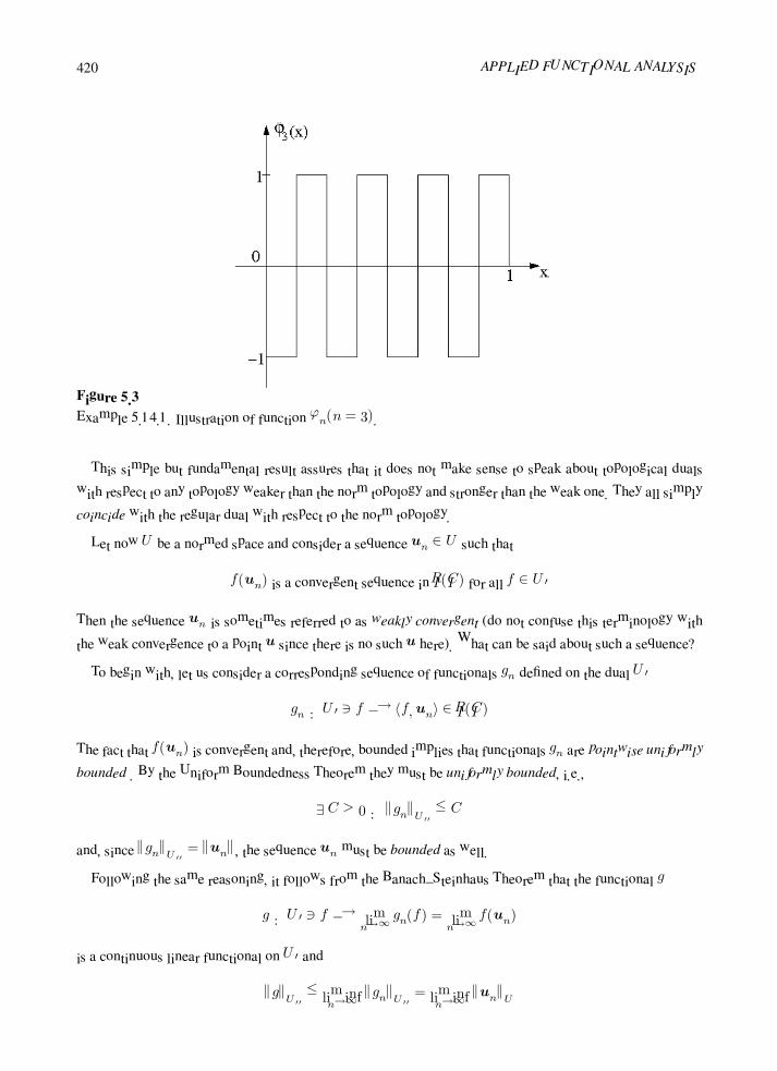
420 APPLIED FUNCTIONAL ANALYSIS
Figure 5.3
Example 5.14.1. Illustration of function ϕn(n = 3).
This simple but fundamental result assures that it does not make sense to speak about topological duals
with respect to any topology weaker than the norm topology and stronger than the weak one. They all simply
coincide with the regular dual with respect to the norm topology.
Let now U be a normed space and consider a sequence un ∈ U such that
f(un) is a convergent sequence in IR(IC) for all f ∈ U
Then the sequence un is sometimes referred to as weakly convergent (do not confuse this terminology with
the weak convergence to a point u since there is no such u here). What can be said about such a sequence?
To begin with, let us consider a corresponding sequence of functionals gn defined on the dual U
gn : U f −→ f,un ∈ IR(IC)
The fact that f(un) is convergent and, therefore, bounded implies that functionals gn are pointwise uniformly
bounded . By the Uniform Boundedness Theorem they must be uniformly bounded, i.e.,
∃ C > 0 : gnU ≤ C
and, since gnU = un, the sequence un must be bounded as well.
Following the same reasoning, it follows from the Banach–Steinhaus Theorem that the functional g
g : U f −→ limn→∞
gn(f) = limn→∞
f(un)
is a continuous linear functional on U and
gU ≤ lim infn→∞
gnU = lim infn→∞
unU

Banach Spaces 421
Thus, if we additionally assume that U is reflexive, then there exists u ∈ U such that
un u and u ≤ lim infn→∞
un
We summarize these observations in the following proposition.
PROPOSITION 5.14.2
Let un be a weakly convergent sequence in a normed space U . Then un is bounded.
If, additionally, U is reflexive, then un converges weakly to an element u ∈ U and
u ≤ lim infn→∞
un
The following sufficient and necessary condition for weak convergence holds.
PROPOSITION 5.14.3
Let un be a sequence in a normed space U . The following conditions are equivalent to each other:
(i) f(un) is convergent ∀ f ∈ U
(ii) a) un is bounded and
b) f(un) is convergent ∀ f ∈ D, where D is a dense subset of U , i.e., D = U .
PROOF It remains to prove (ii) ⇒ (i). Let f ∈ U . By density of D in U , for every ε > 0,
there exists a corresponding fε ∈ D such that f − fεU ≤ ε. It follows that
|f(un)| ≤ |f(un)− fε(un) + fε(un)|
≤ f − fε un+ |fε(un)|
which, in view of the boundedness of un, implies that f(un) is bounded in IR. By compactness
argument in IR, there exists a subsequence unkand a ∈ IR such that
f (unk) −→ a
But again,|f (un)− f (unk
)| ≤ f − fε un
+ |fε (un)− fε (unk)|
+ fε − f unk
implies that the whole sequence must converge to a.

422 APPLIED FUNCTIONAL ANALYSIS
Example 5.14.3
We are now ready to prove that the sequence of functions ϕn from Example 5.14.1 converges weakly
to zero. Toward this goal, recall that piecewise constant functions on the uniform partitions Qn,
(k − 1)2−n, k2n
, k = 1, 2, . . . , 2n, n > 0
form a dense subset in L2(0, 1). On the other hand, for any piecewise constant function u on the
partition Qn, by definition of ϕm
1
0
ϕmu dx = 0 ∀ m > n
and consequently ϕm 0 on the dense subset of L2(0, 1). As ϕn is bounded, it follows from
Proposition 5.14.2 that ϕn 0.
We now proceed with the main result of this section.
THEOREM 5.14.1
(Weak Sequential Compactness)
Let U be a reflexive Banach space and un any sequence of U that is bounded in the norm of U ,
i.e., there exists a constant M > 0 such that
unU ≤M ∀ n
Then there exists a subsequence unk of un that converges weakly to an element u of U such that
u ≤M . In other words, in a reflexive Banach space, closed balls are weakly sequentially compact.
In the proof of the theorem, we will restrict ourselves only to the case of separable spaces. Recall that
a normed space U is separable iff there exists a countable subset of U which is dense in U . We need a
preliminary lemma and a corollary.
LEMMA 5.14.1
If the dual U of a normed space U is separable, then so is U .
PROOF Let D be a countable and dense subset of U . Let Dε0 denote a (countable) subset of
D such that
Dε0 = f ∈ D : 1− ε0 ≤ f ≤ 1
for an ε0 < 1/4. By definition of the dual norm
f = supu=1
|f(u)|

Banach Spaces 423
for each f ∈ Dε0 , there exists a corresponding uf ∈ U , uf = 1, such that
| f,uf | = |f (uf ) | >1
2
We claim that the countable set M of all linear combinations with rational coefficients of functions
uf , f ∈ Dε0 , must be dense in U .
Suppose to the contrary that M = U . Pick u0 ∈ U−M . Then, by the Mazur Separation Theorem
(Lemma 5.13.1), there exists f0 ∈ U such that f0 = 1, f vanishes on M and is non-zero at u0.
Since f0 = 1 and D is dense in U , there exists a sequence fn ∈ Dε0 , converging to f0. We have
1
2< | fn,ufn
| ≤ | fn − f0,ufn |+ | f0,ufn
|
a contradiction, since the right-hand side converges to zero.
COROLLARY 5.14.1
If a normed space U is reflexive and separable, so is the dual U .
PROOF of Theorem 5.14.1
As we have mentioned above, we assume additionally that U is separable. By the preceding
corollary, U is separable, too. Let fj be a countable and dense subset of U . As un is bounded
it follows that
|fj (un)| ≤ fjU unU ≤ fjU M j = 1, 2, . . .
and therefore fj(un) is bounded for every j. By the Bolzano–Weierstrass Theorem and the diagonal
choice method, one can extract a subsequence unksuch that
fj (unk) is convergent for every j
By Proposition 5.14.3, unkis weakly convergent and, by Proposition 5.14.2, there exists an element
u0 ∈ U such that unk u0. Also, by the same proposition
u0 ≤ lim infk→∞
unk ≤M
Example 5.14.4
Let U be a reflexive Banach space and U its dual. Then, for every f ∈ U
fU = maxu≤1
f,u
i.e., there exists an element u ≤ 1 such that fU = f(u).
424 APPLIED FUNCTIONAL ANALYSIS
Indeed, the unit ball B = B(0, 1) is weakly sequentially compact and f is weakly continuous and,
therefore, by the Weierstrass Theorem , f attains its maximum on B.
Exercises
Exercise 5.14.1 Prove Proposition 5.14.1.
Exercise 5.14.2 Let U and V be two normed spaces. Prove that if a linear transformation T ∈ L(U, V ) is
strongly continuous, then it is automatically weakly continuous, i.e., continuous with respect to weak
topologies in U and V .
Hint: Prove first the following:
Lemma: Let X be an arbitrary topological vector space, and Y be a normed space. Let T ∈ L(X,Y ).
The following conditions are equivalent to each other.
(i) T : X → Y (with weak topology) is continuous
(ii) f T : X → IR(IC) is continuous, ∀ f ∈ Y
Follow then the discussion in the section about strongly and weakly continuous linear functionals.
Exercise 5.14.3 Consider space c0 containing infinite sequences of real numbers converging to zero, equipped
with ∞-norm.
c0def= x = xn : xn → 0, x = sup
i|xi|
Show that
(a) c0 = 1
(b) c0 = ∞
(c) If en = (0, . . . , 1(n), . . .) then en → 0 weakly∗ but it does not converge to zero weakly.
Exercise 5.14.4 Let U and V be normed spaces, and let either U or V be reflexive. Prove that every operator
A ∈ L(U, V ) has the property that A maps bounded sequences in U into sequences having weakly
convergent subsequences in V .
Exercise 5.14.5 In numerical analysis, one is often faced with the problem of approximating an integral of
a given continuous function f ∈ C[0, 1] by using some sort of numerical quadrature formula. For
instance, we might introduce in [0, 1] a sequence of integration points
0 ≤ xn1 < xn
2 < · · · < xnj < · · · < xn
n ≤ 1, n = 1, 2, . . .
and set
Qn(f)def=
n
k=1
ank f(xnk ) ≈
1
0
f(x) dx

Banach Spaces 425
where the coefficients ank satisfy the condition
n
k=1
|ank| < M, ∀ n ≥ 1
Suppose that the quadrature rule Qn(f) integrates polynomials p(x) of degree n− 1 exactly; i.e.,
Qn(p) =
1
0
p(x)dx
(a) Show that, for every f ∈ C[0, 1],
limn→∞
Qn(f)−
1
0
f(x)dx
= 0
(b) Characterize the type of convergence, this limit defines in terms of convergence in the space
C[0, 1] (equipped with the Chebyshev norm).
5.15 Compact (Completely Continuous) Operators
We establish here several interesting properties of an important class of operators on normed spaces—the
compact operators. We shall show that compact operators behave almost like operators on finite-dimensional
spaces and they take sequences that only converge weakly and produce strongly convergent sequences.
Compact and Completely Continuous Operators. Recall that a setK in a topological space is said to be
precompact (or relatively compact) iff its closureK is compact.
Consider now two normed spaces U and V and let T : U → V be any (not necessarily linear) operator
from U to V . T is said to be compact iff it maps bounded sets in U into precompact sets in V , i.e.,
A bounded in U ⇒ T (A) compact in V
If, in addition, T is continuous, then T is said to be completely continuous. If V is a Banach space (complete),
then, according to Theorem 4.9.2, T is compact if and only if it maps bounded sets in U into totally bounded
sets in V . This implies that every compact operator is bounded and therefore, in particular, every compact
linear operator is automatically completely continuous. Note also that, since in a finite-dimensional space
boundedness is equivalent to the total boundedness, every bounded operator with a finite-dimensional range
is automatically compact. In particular, every continuous linear operator with a finite-dimensional range is
compact. This also implies that every linear T operator defined on a finite-dimensional space U is compact.
Indeed, T is automatically continuous and the range of T is of finite dimension.

426 APPLIED FUNCTIONAL ANALYSIS
Example 5.15.1
Let U = V = C[0, 1] endowed with the · ∞ norm, and consider the integral operator
(Tu)(ξ)def=
1
0
K(x, ξ)u(x) dx =: v(ξ)
where K(x, ξ) is continuous on the square 0 ≤ x, ξ ≤ 1. We shall show that T is compact. Suppose
SN is a bounded set of functions of C[0, 1] with u ≤ N . Obviously, for u ∈ SN , Tu(ξ) is uniformly
bounded and |Tu(ξ)| ≤ MN , where M = maxx,ξ
|K(x, ξ)|. Since the kernel K(x, ξ) is uniformly
continuous, for each > 0 there exists a δ, such that
|K (x, ξ1)−K (x, ξ2)| <
N
for |ξ1 − ξ2| < δ and ∀ x ∈ [0, 1]. Then
|v (ξ1)− v (ξ2)| ≤
1
0
|K (x, ξ1)−K (x, ξ2)| |u(x)|dx <
for all u ∈ SN . Hence the functions Tu(ξ) are equicontinuous. By Arzela–Ascoli Theorem, the set
T (SN ) with the metric of C[0, 1] is precompact. This proves that the operator T is compact.
Example 5.15.2
Consider again the integral operator from Example 5.15.1, but this time in the L2-setting, i.e.,
A : L2(I)→ L2(I), I = (0, 1),
(Au)(x)def=
1
0
K(x, y)u(y) dy
where kernel function K(x, y) is L2-integrable on I2.
We will prove that K is compact. Toward this goal, consider a sequence of functions un converging
weakly in L2(I) to zero function. Recall that every weakly convergent sequence is bounded, i.e.,
unL2(I) ≤M , for some M > 0. We will demonstrate that the corresponding sequence
vn(x) =
1
0
K(x, y)un(y) dy
converges strongly to zero. Indeed,
1
0
1
0
|K(x, y)|2 dydx <∞
implies that 1
0
|K(x, y)|2 dy <∞ a.e. in x ∈ (0, 1)
In other words, K(x, ·) ∈ L2(I) and, by the weak convergence of un 0,
1
0
K(x, y)un(y) dy → 0 a.e. in x ∈ (0, 1)

Banach Spaces 427
At the same time, by the Cauchy–Schwarz inequality, we obtain
1
0
1
0
K(x, y)un(y) dy
2
dx ≤
1
0
1
0
|K(x, y)|2 dy
1
0
|un(y)|2 dy
≤M2K2L2(I2)
Consequently, sequence
1
0
K(x, y)un(y) dy
2
converges pointwise to zero a.e. in I, and it is dominated by an integrable function. Therefore, by
the Lebesgue Dominated Convergence Theorem,
1
0
1
0
K(x, y)un(y) dy
2
dx→ 0
i.e., vnL2(I) → 0.
Example 5.15.3
Let U be a normed space, u0 be a fixed vector in U and f be a continuous, linear functional on U .
Define the operator T : U → U by
Tu = f(u)u0
Obviously, T is continuous and its range is of dimension 1. Consequently T is compact.
There are many continuous operators that are not compact. For instance, the identity operator on infinite-
dimensional Banach spaces is not compact since it maps the unit ball into itself, and while the unit ball is
bounded, it is not totally bounded, and hence the identity operator is not compact.
The following proposition explains why the linear and compact operators are called completely continuous.
PROPOSITION 5.15.1
A linear and continuous operator T from a reflexive Banach space U to a Banach space V is com-
pact (completely continuous) iff it maps weakly convergent sequences in U into strongly convergent
sequences in V , i.e.,
un u in U ⇒ Tun −→ Tu in V
PROOF
Necessity. Let un converge weakly to u. Suppose that vn = Tun does not converge strongly to
v = Tu. This implies that there exists an ε > 0 and a subsequence vnksuch that vnk
− v ≥ ε.
Now, according to Proposition 5.14.2, unkis bounded and therefore enclosed in a sufficiently large
ball B = B(0, r). T being compact implies that T (B) is compact and therefore sequentially compact,
which means that there must exist a strongly convergent subsequence of vnk, denoted by the same
symbol, convergent to an element v0.

428 APPLIED FUNCTIONAL ANALYSIS
However, every linear and continuous operator is also weakly continuous (see Exercise 5.14.2 )
and therefore vnk v. Since, at the same time, vnk
v0 (strong convergence implies weak
convergence), by the uniqueness of the limit (weak topologies are Hausdorff), v = v0, a contradiction.
Sufficiency. Let A be a bounded set in U . It is sufficient to show that T (A) is sequentially compact.
Let vn = Tun be a sequence from T (A), un ∈ A. Since A is bounded and U reflexive, there must
exist a weakly convergent subsequence unk u. Consequently, vnk
= Tunk→ v = Tu, which
finishes the proof.
REMARK 5.15.1 Notice that reflexivity of U was used only in the “sufficiency” part of the
proof.
In retrospect, one might inquire as to whether the range of a compact operator must be finite-dimensional.
This is not true in general; however, compact operators come close to having a finite-dimensional range.
Indeed, as stated by the following proposition, it can be shown that, for a compact operator T , range T (U)
can be made arbitrarily close to a finite-dimensional subspaceM ⊂ R(T ).
PROPOSITION 5.15.2
Let T : U → V be a compact operator from a Banach space U into another Banach space V . Then,
given > 0, there exists a finite-dimensional subspace M of R(T ) such that
infv∈M
Tu− vV ≤ uU
PROOF Let > 0 be given, and D be the closed unit ball in U . Since T is compact, T (D)
is contained in a compact set, and hence there is an -net in R(T ) ∩ T (D). Let M be the linear
subspace of V generated by this -net. It follows that M is finite-dimensional, and dist (Tu,M) ≤
for all u ∈ D. Then, if u is any point in U , then u/uU ∈ D, and
infv∈M
T
u
uU
− vV
≤
Substituting v = v/uU , we complete the proof.
We conclude this section with a number of simple properties of linear and compact operators.
PROPOSITION 5.15.3
Let U, V,W be Banach spaces and A,B denote linear operators. The following properties hold:
(i) A linear combination of compact operators is compact
A,B : U → V compact ⇒ αA+ βB : U → V compact

Banach Spaces 429
(ii) Compositions of continuous and compact operators are compact
A : U → V compact, B ∈ L(V,W ) ⇒ B A : U →W compact
A ∈ L(U, V ), B : V →W compact ⇒ B A : U →W compact
(iii) A limit of a sequence of compact operators is compact
An : U → V compact, An −AL(U,V )n→∞−→ 0 ⇒ A : U → V compact
In other words, compact operators form a closed subspace in L(U, V ).
PROOF
(i) follows immediately from the definition. (ii) follows from Proposition 5.15.1. To prove (iii),
assume that D is a bounded set in U . It is sufficient to prove that A(D) is totally bounded in V .
Let D be enclosed in a ball B(0, r). Pick an ε > 0 and select n such that An − A ≤ δ = ε2r . Let
Vε = v1, . . . ,vm be theε2 -net for An(D). Then
infiAu− viV ≤ infi Au−AnuV + Anu− viV
≤ A−An uU + infiAnu− viV
≤ε
2rr +
ε
2= ε
for every u ∈ D, which proves that Vε is an ε-net for A(D).
Exercises
Exercise 5.15.1 Let T : U → V be a linear continuous operator from a normed space U into a reflexive
Banach space V . Show that T is weakly sequentially compact, i.e., it maps bounded sets in U into sets
whose closures are weakly sequentially compact in V .
A is bounded in U ⇒ T (A) is weakly sequentially compact in V .
Exercise 5.15.2 Let U and V be normed spaces. Prove that a linear operator T : U → V is compact iff
T (B) is precompact in V for B – the unit ball in U .
Exercise 5.15.3 Use the Frechet-Kolmogorov Theorem (Theorem 4.9.4) to prove that operator T from Ex-
ample 5.15.1 with an appropriate condition on kernel K(x, ξ) is a compact operator from Lp(IR) into
Lr(IR), 1 ≤ p, r <∞.

430 APPLIED FUNCTIONAL ANALYSIS
Closed Range Theorem. Solvability of Linear Equations
5.16 Topological Transpose Operators, Orthogonal Complements
In Chapter 2 we introduced the idea of the transpose of a linear transformation A : X → Y from a vector
spaceX to a vector space Y . The (algebraic) transpose was defined as an operator AT : Y ∗ → X∗ from the
algebraic dual Y ∗ to the algebraic dual X∗ by the formula
AT : Y ∗ → X∗, ATy∗ = x∗ where x∗ = y∗ A
or, in other words,
y∗, Ax = ATy∗,x ∀ x ∈ X,y∗ ∈ Y ∗
where ·, · stands for the duality pairings.
Topological Transpose. The same concept may be developed for continuous linear operators defined on
normed spaces. Let X,Y be two normed spaces and A ∈ L(X,Y ). The topological transpose of A, or
briefly, the transpose of A, denoted A is defined as the restriction of the algebraic transpose AT to the
topological dual Y
A : Y → X : A = AT /Y , Ay = x, where x = y A
or, equivalently,
y, Ax = Ay,x ∀ x ∈ X,y ∈ Y
Note that A is well-defined (takes on values in X ) since the composition y A is continuous.
Notice that in the above definition, the duality pairings are defined on different spaces, i.e., more appropri-
ately, we could write
y, AxY ×Y = Ay,xX×X
The concept of the topological transpose is illustrated in Fig. 5.4.
The following proposition summarizes a number of properties of the transpose (compare Proposition 2.10.1).
PROPOSITION 5.16.1
Let X,Y, Z be normed spaces with their topological duals X , Y , Z . Let A,Ai ∈ L(X,Y ), i = 1, 2,
and B ∈ L(Y, Z). The following properties hold:

Banach Spaces 431
Figure 5.4
Illustration of the algebraic and topological transpose operators.
(i) transpose of a linear combination of operators is equal to the linear combination of their trans-
pose operators:
(α1A1 + α2A2)= α1A
1 + α2A
2
(ii) transpose of a composition is equal to the composition of the transpose operators (with inverted
order)
(B A) = A B
(iii) transpose of the identity operator equals the identity operator on the dual space
(idX)= idX
(iv) if the inverse A−1 exists and is continuous, then A has a continuous inverse, too, and
(A)−1 = (A−1)
(v) AL(X,Y ) = AL(Y ,X)
PROOF Proof of the first four properties follow precisely lines of the proof of Proposition 2.10.1
and is left as a straightforward exercise. To prove (v) see that
|Ay(x)| = |Ay,x| = |y, Ax|
≤ yY AxY
≤ A yY xX

432 APPLIED FUNCTIONAL ANALYSIS
which implies that
AyX ≤ A yY
and, consequently, A ≤ A.
Conversely, by Corollary 5.5.2 to the Hahn–Banach Theorem, for every x = 0, there exists a
functional y ∈ Y such that yY = 1 and y, Ax = AxY . Consequently
AxY = y, Ax = Ay,x ≤ A x
which proves that A ≤ A.
Example 5.16.1
Let A : X → Y be a linear transformation from a finite-dimensional space X into a finite-
dimensional space Y and ei, f j be bases for X and Y , respectively. In Chapter 2 we proved
that if A = Aij is the matrix representation for transformation A with respect to these bases,
then the transpose matrix AT = Aij is the matrix representation for the transpose operator AT
with respect to the dual bases f∗j and e∗i .
A similar property holds in the case of the integral operator A : L2(0, 1)→ L2(0, 1) of the form
Au = v, v(x) =
1
0
K(x, ξ)u(ξ) dξ
where the kernel K(x, ξ) is assumed to be an L2-function on (0, 1)× (0, 1).
Recalling the representation theorem for the duals of Lp spaces, let
f : v →
1
0
wv dx
be an arbitrary linear and continuous functional on L2(0, 1) represented by function w ∈ L2(0, 1).
We have
f,Au =
1
0
wAu dx
=
1
0
w(x)
1
0
K(x, ξ)u(ξ) dξ
dx
=
1
0
1
0
K(x, ξ)w(x) dx
u(ξ) dξ
=AT f, u
where AT f is represented by the L2-function
y(ξ) =
1
0
K(x, ξ)w(x) dx =
1
0
KT (ξ, x)w(x) dx
where
KT (ξ, x) = K(x, ξ)

Banach Spaces 433
Identifying this L2 space with its dual, we see that the transpose of the integral operator A is
obtained by interchanging arguments in the kernel K(x, ξ) in much the same way the transpose
matrix represents transpose of a linear operator on finite-dimensional spaces.
Topological Orthogonal Complements. Let X be a vector space and X∗ its algebraic dual. In Chapter 2
we defined for a subspace Z ⊂ X its (algebraic) orthogonal complement as
Z⊥ = x∗ ∈ X∗ : x∗, z = 0 ∀ z ∈ Z
The same concept can now be generalized to a normed space X . By the topological orthogonal complement
(or simply the orthogonal complement) of a subspace Z ⊂ X , denoted Z⊥, we mean
Z⊥ = x ∈ X : x, z = 0 ∀ z ∈ Z
It is easy to check that Z⊥ is a closed subspace of X .
In the same way we define the orthogonal complement for a subspaceM ⊂ X :
M⊥ = z ∈ X : x, z = 0 ∀ x ∈M
Again,M⊥ is a closed subspace ofX . Note that in defining the orthogonal complement ofM ⊂ X we refer
back to the original space X and not to the bidual X .
Let Z ⊂ X be a linear subspace of a normed spaceX . For every x ∈ Z⊥, by definition of Z⊥, x, z =
0 and therefore by definition ofM⊥ forM = Z⊥
Z ⊂Z⊥⊥
The following proposition formulates a sufficient and necessary condition for the two sets to be equal to each
other.
PROPOSITION 5.16.2
Let Z ⊂ X be a subspace of a normed space X. The following conditions are equivalent to each
other:
(i) Z is closed
(ii) (Z⊥)⊥ = Z
PROOF
(ii) ⇒ (i) follows from the fact that orthogonal complements are closed.
(i) ⇒ (ii) It remains to prove that (Z⊥)⊥ ⊂ Z. Suppose, contrary to the assertion, that there
exists z ∈ (Z⊥)⊥ such that z ∈ Z. By the Mazur Separation Theorem (Lemma 5.13.1) there exists

434 APPLIED FUNCTIONAL ANALYSIS
a linear continuous functional f such that
f |Z = 0 and f(z) = 0
which means that f ∈ Z⊥ and f, z = 0 and therefore z ∈Z⊥⊥
, a contradiction.
Exercises
Exercise 5.16.1 Prove Proposition 5.16.1(i)–(iv).
Exercise 5.16.2 Let U, V be two Banach spaces, and let A ∈ L(U, V ) be compact. Show that A is also
compact. Hint: See Exercise 5.20.2 and recall Arzela–Ascoli Theorem.
5.17 Solvability of Linear Equations in Banach Spaces, The Closed Range Theorem
In this section we shall examine a collection of ideas that are very important in the abstract theory of linear
operator equations on Banach spaces. They concern the solvability of equations of the form
Au = f , A : U −→ V
where A is a linear and continuous operator from a normed space U into a normed space V and f is an
element of V . Obviously, this equation can represent systems of linear algebraic equations, partial differential
equations, integral equations, etc., so that general theorems concerned with its solvability are very important.
The question about the existence of solutions u to the equation above, for a given f , can obviously be
rephrased as
when does f ∈ R(A)?
where R(A) denotes the range of A. The characterization of the range R(A) is therefore crucial to our
problem.
From the definition of the transpose
v, Au = Av,u ∀ u ∈ U,v ∈ V
we have that
v ∈ N (A) ⇔ v ∈ R(A)⊥
which can be restated as
R(A)⊥ = N (A)

Banach Spaces 435
Combining this observation with Proposition 5.16.2, we arrive at the following theorem:
THEOREM 5.17.1
(The Closed Range Theorem for Continuous Operators)
Let U and V be normed spaces and A ∈ L(U, V ) a linear and continuous operator from U to V .
The following conditions are equivalent to each other:
(i) R(A) is closed
(ii) R(A) = N (A)⊥
PROOF The proof follows immediately from Proposition 5.16.2.
In view of this result, the criterion for the solvability of a linear system cab be restated as follows.
COROLLARY 5.17.1
(Solvability of Linear Equations)
Assume A ∈ L(U, V ) and that R(A) is closed in V . Then the linear problem Au = f possesses a
solution if and only if
f ∈ N (A)⊥
It turns out thus to be essential to determine sufficient (and possibly necessary) conditions for the closed-
ness of rangeR(A).
Bounded Below Operators. A linear operator A : U → V from a normed space U to a normed space V
is said to be bounded below iff there exists a constant c > 0 such that
AuV ≥ c uU ∀ u ∈ D(A)
This immediately implies that a bounded below operator possesses a continuous inverse on its range R(A).
Indeed, Au = 0 implies u = 0 and therefore A is injective, and for u = A−1v we get
A−1v
U≤
1
cvV
The following theorem establishes the fundamental result showing equivalence of the closed range with
the boundedness below for injective operators on Banach spaces.

436 APPLIED FUNCTIONAL ANALYSIS
THEOREM 5.17.2
Let U and V be Banach spaces and let A ∈ L(U, V ) be injective. Then the range R(A) is closed if
and only if A is bounded below.
PROOF
Sufficiency. Suppose vn ∈ R(A),vn → v. Does v ∈ R(A)? Let un ∈ U be such that Aun = vn.
But vn − vmV = A(un −um)V ≥ cun −umU . Hence, un − um → 0 as m,n→∞, i.e., un
is a Cauchy sequence. But, since U is complete, there exists u such that un → u in U . Since A is
continuous, Aun → Au = v ∈ R(A); i.e., R(A) is closed.
Necessity. As a closed subspace of the Banach space V , the range R(A) is a Banach space as
well. Thus, A is a continuous, injective operator from U onto R(A) and, by the Banach Theorem
(Corollary 5.9.2 to the Open Mapping Theorem), A has a continuous inverse A−1, i.e.,
A−1v
U≤A−1
vV ∀ v ∈ R(A)
But this is equivalent to A being bounded below.
Thus, for a linear injective operator A, the boundedness below is equivalent to the closedness of the range
R(A) which in turn is equivalent to the criterion for the existence of the solution of a linear system expressed
in terms of the transpose of operator A.
We proceed now with a discussion for noninjective operators A.
Quotient Normed Spaces. Let U be a vector space andM ⊂ U a subspace of U . In Chapter 2 we defined
the quotient space U/M consisting of equivalence classes of u ∈ U identified as affine subspaces of U of the
form
[u] = u+M = u+ v : v ∈M
If, in addition, U is a normed space andM is closed, the quotient space U/M can be equipped with the norm
[u]U/Mdef= inf
v∈[u]vU
Indeed, all properties of norms are satisfied:
(i) [u] = 0 implies that there exists a sequence vn ∈ [u] such that vn → 0. By closedness ofM and,
therefore, of every equivalence class [u] (explain, why?), 0 ∈ [u], which means that [u] = [0] = M is
the zero vector in the quotient space U/M .
(ii)λ[u] = [λu]
= infλv∈[λu]
λv
= |λ| infv∈[u]
v = |λ| [u]

Banach Spaces 437
(iii) Let [u], [v] ∈ U/M . Pick an arbitrary ε > 0. Then, there exist uε ∈ [u] and vε ∈ [v] such that
uε ≤ [u]U/M +ε
2and vε ≤ [v]U/M +
ε
2
Consequently
uε + vε ≤ [u]U/M + [v]U/M + ε
But uε + vε ∈ [u + v] and therefore taking the infimum on the left-hand side and passing to the limit with
ε→ 0, we get the triangle inequality for the norm in U/M .
It also turns out that for a Banach space U , the quotient space U/M is also Banach.
LEMMA 5.17.1
Let M be a closed subspace of a Banach space U . Then U/M is Banach.
PROOF Let [un] be a Cauchy sequence in U/M . One can extract a subsequence [unk] such that
unk+1
− [unk
] ≤
1
2k+2
Next, for every k, select an element vk such that
vk ∈unk+1
− [unk
] =unk+1
− unk
and
vkU ≤unk+1
− [unk
]U/M
+1
2k+2≤
1
2k+1
and consider the sequence
v0 = un1, v1 = un2
, v2 = un3, . . .
The sequence of partial sums Sk =
k
i=0
vi is Cauchy and therefore converges to an element v in U .
At the same timeSk = v0 + v1 + v2 + · · ·vk ∈ [un1
] + [un2− un1
]
+ · · ·unk+1
− unk
=unk+1
which impliesunk+1
− [v]
U/M
≤ Sk − vU → 0
and finally, by the triangle inequality,
[un]− [v] ≤[un]−
unk+1
+
unk+1
− [v]
which proves that the entire sequence converges to [v].
We continue now with the discussion of sufficient and necessary conditions for the range R(A) of an
operator A to be closed.

438 APPLIED FUNCTIONAL ANALYSIS
THEOREM 5.17.3
Let U and V be Banach spaces and let A ∈ L(U, V ) be a linear and continuous operator on U . Then
the range R(A) of A is closed if and only if there exists a constant c > 0 such that
AuV ≥ c infw∈N (A)
u+wU
PROOF Let M = N (A). By continuity of A, M is closed. Consider next the quotient operator
A : U/M [u]→ A[u] = Au ∈ V
A is obviously a well-defined injective operator on a Banach space. Taking the infimum with respect
to w in the inequality:
AuV = AwV ≤ A wU ∀w ∈ [u]
proves that A is also continuous.
The inequality in the theorem can now be reinterpreted as boundedness below of operator A:
A[u]
V≥ c [u]U/M
which reduces the whole case to the previous theorem for injective operators.
COROLLARY 5.17.2
(Solvability of Linear Equations)
Let U and V be Banach spaces and let A ∈ L(U, V ) be a linear and continuous operator such that
AuV ≥ c infw∈N (A)
u+wU , c > 0
Then the linear problem Au = f , for some f ∈ V , has a solution u if and only if
f ∈ N (A)⊥
The solution u is determined uniquely up to elements from the null space of A, i.e., u +w is also
a solution for every w ∈ N (A).
We emphasize that the boundedness below of the quotient operator A provides not only a sufficient condi-
tion for the solvability criterion above (f ∈ N (A)⊥), but it is equivalent to it, as follows from the presented
theorems.
Notice also that the boundedness below is equivalent to the continuity of the inverse operator A−1:
A−1 : V v −→ [u] ∈ U/M

Banach Spaces 439
which is just another way of saying that the solutions u of Au = f should depend continuously on the data,
i.e., the right-hand side f .
Exercises
Exercise 5.17.1 Let X be a Banach space, and P : X → X be a continuous linear projection, i.e., P 2 = P .
Prove that the range of P is closed.
5.18 Generalization for Closed Operators
Surprising as it looks, most of the results from the preceding two sections can be generalized to the case of
closed operators.
Topological Transpose. Let X and Y be two normed spaces and let A : X ⊃ D(A) → Y be a linear
operator, not necessarily continuous. Consider all points (y,x) from the product space Y ×X such that
y, Ax = x,x ∀x ∈ D(A)
where the duality pairings are to be understood in Y × Y and X × X , respectively. Notice that the set is
nonempty as it always contains point (0,0). We claim that y uniquely defines x iff the domain D(A) of
operator A is dense inX . Indeed, assume thatD(A) = X . By linearity of both sides with respect to the first
argument, it is sufficient to prove that
x,x = 0 ∀ x ∈ D(A) implies x = 0
But this follows easily from the density of D(A) in X and continuity of x.
Conversely, assume thatD(A) = X . Letx ∈ X−D(A). By theMazur Separation Theorem (Lemma 5.13.1)
there exists a continuous and linear functional x0, vanishing on D(A), but different from zero at x. Conse-
quently, the zero functional y = 0 has two corresponding elements x = 0 and x = x0, a contradiction.
Thus, restricting ourselves to the case of operators A defined on domains D(A) which are dense in X ,
we can identify the collection of (y,x) discussed above (see Proposition 5.10.1) as the graph of a linear
operator from Y toX , denotedA, and called the transpose (or dual) of operatorA. Due to our construction,
this definition generalizes the definition of the transpose for A ∈ L(X,Y ).
The next observation we will make is that the transpose operator A is always closed. Indeed, consider a
sequence yn ∈ D(A) such that yn → y and Ayn → x. Passing to the limit in the equality
yn, Ax = Ayn,x x ∈ D(A)

440 APPLIED FUNCTIONAL ANALYSIS
we conclude immediately that y ∈ D(A) and Ay = x. Consequently, by Proposition 5.10.2, A must be
closed.
We summarize a number of properties for this generalized operator in the following proposition.
PROPOSITION 5.18.1
Let X,Y, Z be normed spaces with their topological duals X , Y , Z
(i) Let Ai : X ⊃ D → Y , i = 1, 2 be two linear operators defined on the same domain D, dense
in X. Then
α1A1 + α2A
2 ⊂ (α1A1 + α2A2)
i.e., the transpose (α1A1 + α2A2) is an extension of α1A
1 + α2A
2. Note that, by definition,
the sum of the two transpose operators is defined on the common part of their domains.
(ii) Let A : X ⊃ D(A) → Y , B : Y ⊃ D(B) → Z be linear operators with domains dense in X
and Y , respectively, and let R(A) ⊂ D(B) (to make sense for the composition B A). Then
(B A) ⊃ A B
i.e., the transpose (B A) is an extension of the composition A B.
(iii) If A : X ⊃ D(A)→ Y is a linear injective operator with domain D(A) dense in X and range
R(A) dense in Y then the transpose operator A has an inverse and
(A)−1 = (A−1)
PROOF The proof follows directly from the definitions and is left as an exercise (see Exer-
cise 5.18.1).
Consider now again the abstract linear equation of the form
Au = f , A : U ⊃ D(A)→ V, D(A) = U
where A is a closed operator from the dense domain D(A) in a normed space U into another normed space
V . We have the following fundamental result due to Stefan Banach.
THEOREM 5.18.1
(The Closed Range Theorem for Closed Operators)
Let U and V be normed spaces and A : U ⊃ D(A) → V , D(A) = U , be linear and closed. The
following conditions are equivalent to each other:

Banach Spaces 441
(i) R(A) is closed in V
(ii) R(A) = N (A)⊥
PROOF
(ii) ⇒ (i) This follows immediately from the fact that orthogonal complements are always closed.
(i) ⇒ (ii) From the definition of the transpose operator A
v, Au = Av,u ∀ u ∈ D(A), v ∈ D(A)
we havev ∈ N (A) ⇔ v ∈ D(A) and Av = 0
⇔ v, Au = 0 ∀ u ∈ D(A)
⇔ v ∈ R(A)⊥
Thus, as in the case of continuous operators,
R(A)⊥ = N (A)
Applying Proposition 5.16.2 we finish the proof.
As before, we have immediately the same
COROLLARY 5.18.1
(Solvability of Linear Equations)
Let A be a closed operator discussed above, and let the range R(A) of A be closed in V . Then the
linear problem Au = f possesses a solution if and only if
f ∈ N (A)⊥
As in the case of continuous operators, the closedness of the range R(A) turns out to be equivalent to the
boundedness below.
THEOREM 5.18.2
Let U and V be Banach spaces and
A : U ⊃ D(A)→ V
denote a closed, linear operator. The following conditions are equivalent to each other:
(i) R(A) is closed in V

442 APPLIED FUNCTIONAL ANALYSIS
(ii) There exists a positive constant c > 0 such that
AuV ≥ c infw∈N (A)
u+wU
PROOF
Case 1. A injective.
(ii) ⇒ (i) The inequality implies that A is bounded below and therefore its inverse A−1 is con-
tinuous. A being closed and bounded below implies that its domain D(A) is closed and therefore
its range R(A) coincides with the inverse image of D(A) through the continuous inverse A−1 and
therefore must be closed.
(i) ⇒ (ii) If A is closed then A−1 is closed as well and is defined on the closed range R(A) in
V , which can be identified as a Banach space itself. By the Closed Graph Theorem, A−1 must be
continuous which is equivalent to the boundedness below of A.
Case 2. A arbitrary.
As in the proof of Theorem 5.17.3, consider the quotient map
A : U/M ⊃ D( A) [u]→ A[u] = Au ∈ V
where M = N (A).
A few comments are necessary:
1. Null space of a closed operator is closed. Indeed if
D(A) ⊃ N (A) un → u
then Aun = 0 is constant and therefore converges trivially to 0 which, by Proposition 5.10.2,
implies that u ∈ D(A) and Au = 0. Consequently u ∈ N (A), which proves that N (A) is
closed.
2. By Lemma 5.17.1, the space U/M is Banach.
3. The domain D( A) of A is equal to D(A)/M .
4. A is closed. Indeed, let
D( A) [un]→ [u], A[un]→ v
By definition of the norm in U/M one can find a sequence wn ∈ [un] (see Lemma 5.17.1) such
that
wn −→ w ∈ [u]
At the same time A[un] = Awn → v and therefore, by closedness of A
w ∈ D(A) and Aw = v

Banach Spaces 443
Consequently
[u] = [w] ∈ D( A) and A[u] = v
which proves that A is closed.
Finally, it is sufficient to apply the first case result to A.
We conclude this section with the generalization of Corollary 5.17.2.
COROLLARY 5.18.2
(Solvability of Linear Equations)
Let U and V be Banach spaces and let
A : U ⊃ D(A) −→ V, D(A) = U
be a linear, closed operator with the domain D(A) dense in U such that
∃c > 0 : AuV ≥ infw∈N (A)
u+wU ∀u ∈ D(A)
Then the linear problem
Au = f , f ∈ V
has a solution u if and only if
f ∈ N (A)⊥
where A is the transpose of A
A : V ⊃ D(A) −→ U
The solution u is determined uniquely up to elements from the null space of A.
Note that all the comments concluding the preceding section remain valid.
Exercises
Exercise 5.18.1 Prove Proposition 5.18.1.
5.19 Examples
In this section, we give two simple examples from mechanics dealing with the solution of a linear problem
Au = f and showing the interpretation of the solvability condition f ∈ N (A)⊥.

444 APPLIED FUNCTIONAL ANALYSIS
Figure 5.5
A “free” beam loaded with the distributed loading with intensity q(x).
Example 5.19.1
Consider the beam equation
(EIw) = q 0 < x < l
where EI is the stiffness of the beam (product of Young modulus E and cross-sectional moment of
inertia I) and q = q(x) the intensity of the load applied to beam (see Fig. 5.5).
The beam is not supported, and both ends are subjected to neither concentrated forces nor
concentrated moments which, in view of the formulas for the bending moment M and shear force
V :
M = −EIw, V = −(EIw)
translates into boundary conditions
w(0) = w(0) = 0 and w(l) = w(l) = 0
provided we assume for simplicity that EI = const.
We will formulate now the problem in the operator form. Toward this goal we introduce the space
W =w ∈ H4(0, l) : w(0) = w(0) = w(l) = w(l) = 0
consisting of all functions w from the Sobolev space of fourth order H4 satisfying the boundary
conditions. As a closed subspace of H4(0, l) (see Exercise 5.19.1); W is itself a Banach (in fact,
Hilbert) space. Next, we consider the operator A : W → V = L2(0, 1) defined as
Aw = (EIw) = EIw
Obviously, A is both linear and continuous on space W and the whole boundary value problem
reduces to the operator equation
Aw = q
provided we assume that the load q is square integrable.
We continue now by determining the transpose of A. First of all, according to the representation
theorem for Lp spaces, the dual to L2(0, l) can be identified with itself. Consequently, the duality

Banach Spaces 445
pairing is replaced with the L2-product on L2 (see Chapter 2) and the definition of the conjugate
operator A reads as l
0
v(EIw) dx = (v,Aw) = Av, w
∀ w ∈W, v ∈ V = L2(0, 1)
where ·, · stands for the duality pairing between W and its dual and (·, ·) is the L2-product.
Recall that, for a continuous operator A : W → V defined on the whole space W , the topological
transpose A is defined on the whole dual space V . Its value at a particular v is given precisely by
the left-hand side of the formula above.
Next, we determine the kernel (null space) of A. Restricting ourselves first to w ∈ C∞0 (0, l) ⊂W ,
we get l
0
v(EIw) dx = 0 ∀ w ∈ C∞0 (0, l)
which, by the definition of the distributional derivatives, means that v has a distributional derivative
of fourth order, v and that
v = 0
Integration by parts yields now (see Exercise 5.19.2)
l
0
v(EIw) dx =
l
0
vEIw dx+ (vw − vw)|l0
= (vw − vw)|l0 ∀ w ∈W
As there are no boundary conditions on w and w in the definition of W , both w and w may take
arbitrary values at 0 and l, which implies that
v(0) = v(l) = v(0) = v(l) = 0
Consequently
N (A) = v : v(x) = αx+ β, α, β ∈ IR
Notice that the null space N (A) of the transpose operator coincides with the null space N (A) of the
operator itself, interpreted as the space of infinitesimal rigid body motions. Consequently, the necessary
and sufficient condition for the existence of a solution w ∈W
q ∈ N (A)⊥
reduces to l
0
q(x) dx = 0 and
l
0
q(x)x dx = 0
The two conditions above are easily recognized as the global equilibrium equations for the load q
(resultant force and moment must vanish).
Note that the solution u is determined only up to the rigid body motions.

446 APPLIED FUNCTIONAL ANALYSIS
REMARK 5.19.1 It may be a little confusing, but it is very illustrative to see how the same
example is formulated using the formalism of closed operators. Introducing only one space V =
L2(0, l), identified with its dual, we define operator A : V → V as follows:
D(A) = u ∈ L2(0, l) : u ∈ L2(0, l) and u(0) = u(0) = u(l) = u(l) = 0
A = EIu
Notice that domain D(A) coincides with space W from Example 5.19.1. It is an easy exercise to
prove that A is well-defined and closed. By the same calculations as before we find out that
l
0
EIvu dx+ (vu − vu)|l0 = (Av, u) ∀ u ∈ D(A), v ∈ D(A)
This leads to the transpose (adjoint) operator in the form
D(A) = v ∈ L2(0, l) : v ∈ L2(0, l) and v(0) = v(l) = v(0) = v(l) = 0
Av = EIv
Thus the transpose operator A coincides with A itself. Note the difference between the domain of
this and the domain of A from Example 5.19.1.
The rest of the conclusions are the same.
Example 5.19.2
In most applications in mechanics, the solvability condition f ∈ N (A)⊥ admits to a simple physical
interpretation like in the previous example. Now, we shall briefly describe an application to a class
of boundary-value problems in linear elasticity.
A two-dimensional version of the situation is illustrated in Fig. 5.6. An elastic body, occupying
a domain Ω, is subjected to body forces of density f per unit volume and surface tractions g on
a portion Γt of the boundary Γ = ∂Ω of Ω. On the remaining portion of the boundary, Γu, the
displacement vector u is prescribed as zero, u|Γu= 0.
We wish to find the displacement vector field u = u(x) for which the body will be at rest (in
equilibrium) under the action of forces f and g. We obtain the familiar boundary-value problem
Find the displacement u such that
−(Eijkluk,l),j = fi in Ω
subjected to the boundary conditions
Eijkluk,lnj = gi on Γt
ui = 0 on Γu
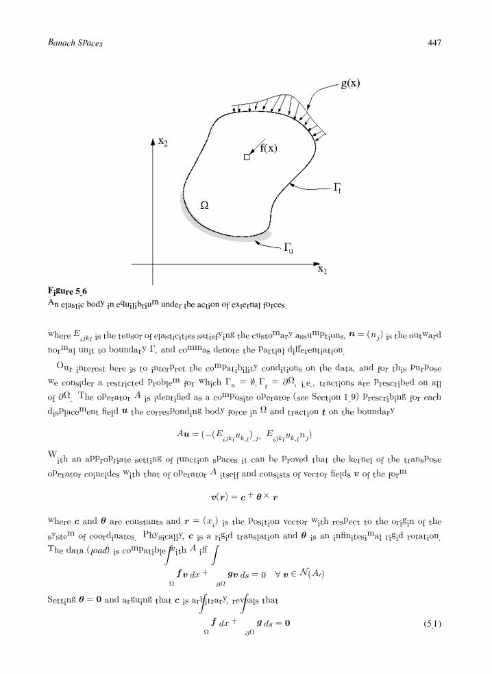
Banach Spaces 447
Figure 5.6
An elastic body in equilibrium under the action of external forces.
where Eijkl is the tensor of elasticities satisfying the customary assumptions, n = (nj) is the outward
normal unit to boundary Γ, and commas denote the partial differentiation.
Our interest here is to interpret the compatibility conditions on the data, and for this purpose
we consider a restricted problem for which Γu = ∅,Γt = ∂Ω, i.e., tractions are prescribed on all
of ∂Ω. The operator A is identified as a composite operator (see Section 1.9) prescribing for each
displacement field u the corresponding body force in Ω and traction t on the boundary
Au = (−(Eijkluk,l),j , Eijkluk,lnj)
With an appropriate setting of function spaces it can be proved that the kernel of the transpose
operator coincides with that of operator A itself and consists of vector fields v of the form
v(r) = c+ θ × r
where c and θ are constants and r = (xi) is the position vector with respect to the origin of the
system of coordinates. Physically, c is a rigid translation and θ is an infinitesimal rigid rotation.
The data (load) is compatible with A iff
Ω
fv dx+
∂Ω
gv ds = 0 ∀ v ∈ N (A)
Setting θ = 0 and arguing that c is arbitrary, reveals that
Ω
f dx+
∂Ω
g ds = 0 (5.1)

448 APPLIED FUNCTIONAL ANALYSIS
whereas setting c = 0 and using arbitrary θ gives
Ω
r × x dx+
∂Ω
r × g ds = 0 (5.2)
We recognize these compatibility conditions as the global equations of equilibrium: (5.1) is the
requirement that the vector sum of external forces vanish, and (5.2) is the requirement that the
moment of all external forces about the origin vanish.
We have thus transformed the local equilibrium equations into global requirements on the data f
and g.
Exercises
Exercise 5.19.1 Prove that the linear mapping (functional)
H1(0, 1) w → w(x0), where x0 ∈ [0, l]
is continuous. Use the result to prove that spaceW in Example 5.19.1 is closed.
Hint: Consider first smooth functions w ∈ C∞([0, l]) and then use the density of C∞([0, l]) in
H1(0, l).
Exercise 5.19.2 Let u, v ∈ H1(0, l). Prove the integration by parts formula
l
0
uv dx = −
l
0
uv dx+ (uv)|l0
Hint: Make use of the density of C∞([0, l]) in H1(0, l).
Exercise 5.19.3 Work out all the details of Example 5.19.1 once again, with different boundary conditions:
w(0) = w(0) = 0 and w(l) = w(l) = 0
(left end of the beam is supported by a pin support).
Exercise 5.19.4 Prove that operator A from Remark 5.19.1 is closed.
Exercise 5.19.5 (A finite-dimensional sanity check). Determine necessary conditions on data f for solutions
to the linear systems of equations that follows to exist. Determine if the solutions are unique and, if
not, describe the null space of the associated operator:
Au = f
Here
A =
1 −1 0
−1 0 1
A =
1 2 −14 0 23 −2 −3
A =
3 1 −1 26 2 −2 49 3 −3 6
Banach Spaces 449
5.20 Equations with Completely Continuous Kernels. Fredholm Alternative
In this last section we would like to study a special class of abstract equations of the form
x− Tx = y
where T is a linear, completely continuous (compact) operator from a Banach spaceX into itself, y is a given
vector fromX , and x is the unknown. Such equations are frequently called equations of the second type and
they are typical in the theory of integral equations. Results presented in this section are essentially due to Ivar
Fredholm, a Swedish mathematician who devoted much of his efforts to the study of these equations.
Introducing the identity operator I : X → X and the corresponding operator A = I − T one could, of
course, rewrite the equation in the usual form
Ax = y
However, the point is that then the special properties of operator T are lost and the general theory for linear
equations presented in the previous sections cannot deliver such strong results as a direct study of the equation
of the second type.
We begin with an essential observation concerning operator A = I − T .
LEMMA 5.20.1
The range R(A) of operator A is closed.
PROOF Let M = N (A) denote the null space of operator A. According to Theorem 5.17.3,
closedness of R(A) is equivalent to the boundedness below of the quotient operator
A : X/M → X, A[x] = Ax
where [x] = x+M denotes the equivalence class of x.
In contrast, assume that A is not bounded below. There exists, then, a sequence of equivalence
classes [xn] ∈ X/M such that
[xn]X/M = 1 and A[xn]
X→ 0
It follows from the definition of norm in the quotient space that there exists a corresponding sequence
of vectors xn ∈ [xn] such that
xnX ≤ [xn]X/M + ε ≤ 1 + ε
450 APPLIED FUNCTIONAL ANALYSIS
for some ε > 0. Consequently xn is bounded, and by the compactness of T , we can extract a
subsequence xnksuch that Txnk
→ x0 strongly for some x0 ∈ X. Consequently,
xnk= (T +A)xnk
→ x0
By the continuity of T , T (xnk)→ T (x0), which proves that
x0 = Tx0 ⇒ x0 ∈M
From the continuity of the map
X x→ [x] ∈ X/M
follows that
[xnk]→ [x0] in X/M
a contradiction since [xnk]X/M = 1 and [x0]X/M = 0.
Before we proceed with the study of further properties of operator A, we stop to prove a simple but
fundamental result which holds in any normed vector space.
LEMMA 5.20.2
(Lemma on Almost Perpendicularity ∗)
Let X be a normed space and X0 a closed subspace of X, different from X. Then, for an arbitrary
small ε > 0, there exists a corresponding unit vector xε, xε = 1 such that
ρ (xε, X0) > 1− ε
PROOF Recall the definition of the distance between a vector x and set (space) X0
ρ(x, X0) = infy∈X0
x− y
As X0 is closed and different from X, there must be a vector x ∈ X separated from X0 by a positive
distance d:
ρ (x, X0) = d > 0
(Otherwise X0 would be dense in X and by closedness would have to coincide with the whole X.)
By definition of the distance ρ(x, X0), for every 1 > ε > 0 there exists a vector x ∈ X0 such that
x− x ≤d
1− ε(> d)
Define
xε =x− x
x− x= a (x− x) , a = x− x
−1
∗Also known as Riesz Lemma.

Banach Spaces 451
Then, for every x ∈ X0, we have
xε − x = ax− ax − x = ax−
x +
x
a
≥ ad >1− ε
dd = 1− ε
sincex +
x
a
∈ X0.
REMARK 5.20.1 If X were a Hilbert space then, taking any unit vector x0 from the orthogonal
complement of X0 (comp. Theorem 6.2.1), we would have
ρ (x0, X0)2= inf
y∈X0
x0 − y2
= infy∈X0
(x0 − y,x0 − y)
= infy∈X0
x02 + 2Re(x0,y) + y
2
= x02 + inf
y∈X0
y2 = 1
where (·, ·) is the inner product in X. This explains the name of the lemma.
COROLLARY 5.20.1
Let X be a normed space. The following conditions are equivalent to each other:
(i) X is finite-dimensional, dimX <∞.
(ii) A set E ⊂ X is compact iff E is closed and bounded.
PROOF Implication (i) ⇒ (ii) follows from the famous Heine–Borel Theorem (Theorem 4.3.1).
To prove (ii) ⇒ (i), assume instead that dimX = ∞. Next, take an arbitrary unit vector x1 and
consider subspace X1 = IRx1(ICx1). By the Lemma on Almost Perpendicularity, there exists a unit
vector x2 such that
ρ (x2, X1) >1
2
and by induction we have a sequence of unit vectors xn such that
ρ (xn, Xn−1) >1
2
where Xn = IRx1 ⊕ . . .⊕ IRxn (ICx1 ⊕ . . .⊕ ICxn). As the unit ball is closed and bounded, according
to (ii) it must be compact and therefore sequentially compact as well. Consequently, we can extract
a converging subsequence xnkwhich, in particular, must satisfy the Cauchy condition, i.e.,
limk,l→∞
xnk− xnl
= 0

452 APPLIED FUNCTIONAL ANALYSIS
a contradiction, since by construction of xn
xnk− xnl
>1
2
We return now to the study of equations of the second type. As a direct consequence of the Lemma on
Almost Perpendicularity , we get the following further characterization of operator A = I − T .
LEMMA 5.20.3
Let An = A . . . A (n times). Then the sequence of null spaces N (An) is increasing:
N (A) ⊂ NA2⊂ . . . ⊂ N (An) ⊂ N
An+1
⊂ . . .
and contains only a finite number of different sets, i.e. there exists an index m such that
N (Am) = N (Am+1) = . . .
PROOF We have
x ∈ N (An)⇐⇒ Anx = 0 ⇒ A (Anx) = 0 ⇒ x ∈ NAn+1
which proves the monotonicity.
Denote Xn = N (An). If Xn = Xn+1 for some n, then Xn+1 = Xn+2 and, consequently Xm =
Xm+1, for any m ≥ n. Indeed,
x ∈ Xn+2 ⇒ An+2x = 0 ⇒ An+1(Ax) = 0
⇒ Ax ∈ Xn+1 ⇒ Ax ∈ Xn
⇒ An(Ax) = 0 ⇒ x ∈ Xn+1
Finally, assume to the contrary that Xn = Xn+1, ∀ n. By the Lemma on Almost Perpendicularity,
there exists a sequence of unit vectors xn such that
xn+1 ∈ Xn+1, xn+1 = 1, ρ (xn+1, Xn) >1
2
Let m > n. Then
Txm − Txn = xm −Axm − (xn −Axn) = xm − x
where we have denoted
x = Axm + xn −Axn
Moreover,
Am−1x = Amxm +Am−1xn −Amxn = 0
Banach Spaces 453
and therefore x ∈ Xm−1, which implies that
Txm − Txn = xm − x >1
2
This leads to a contradiction, since we can extract a subsequence xnksuch that Txnk
converges
strongly to some element in X and, in particular, it satisfies the Cauchy condition
limk,l→∞
Txnk− Txnl
= 0
a contradiction.
LEMMA 5.20.4
The sequence of range spaces An(X) is decreasing
A(X) ⊃ . . . ⊃ An (X) ⊃ An+1 (X) ⊃ . . .
and contains only a finite number of different sets.
PROOF We have
x ∈ An(X) ⇒ ∃ y ∈ X x = Any ⇒ x = An−1(Ay)
⇒ x ∈ An−1(X)
which proves the monotonicity.
Next, An(X) = An+1(X) implies trivially An+1(X) = An+2(X). Finally, assuming to the contrary
that An(X) = An+1(X), the Lemma on Almost Perpendicularity implies again that
∃ xn ∈ An(X), xn = 1, ρxn, A
n+1(X)>
1
2
We get for m > n
Txn − Txm = xn − (Axn + xm −Axm) = xn − x
where
x = Axn + xm −Axm ∈ An+1(X)
and therefore
Txn − Txm = xn − x >1
2
which leads to the same contradiction as in the proof of the previous lemma.
Let m now denote the minimum index n such that An(X) = An+1(X). (If X = A(X), i.e., A is
surjective, thenm = 0.) Denote
Ydef= Am(X) = R (Am) , Z
def= N (Am)

454 APPLIED FUNCTIONAL ANALYSIS
We will continue now with a detailed discussion of the restrictions of operator A to spaces Y and Z.
Step 1.
It follows from the definition of Y that
A(Y ) = A (Am(X)) = Am+1(X) = Am(X) = Y
which proves that operator A takes Y onto Y . It follows also that the restriction of A to Y is one-to-one.
Indeed, assume that Ay = 0 for some y ∈ Y . As y ∈ Am(X) = An(X), n ≥ m; for every n ≥ m there
exists a corresponding x such that y = Anx. Consequently, 0 = Ay = An+1x implies x ∈ N (An+1),
and, for sufficiently large n such thatN (An+1) = N (An), x ∈ N (An), and therefore Anx = y = 0 which
proves that AYis injective.
Operator Am = (I − T )m can be represented in the form
Am = (I − T )m = I − T1
where T1 is a sum of compositions of T and, as such, it is completely continuous. Since the restriction of Am
to Z is zero, we have
T1z = z for z ∈ Z
This implies that any bounded and closed set in Z must be compact. Indeed, if zn is a bounded sequence
in Z, then by the compactness of T1 we can extract a subsequence znksuch that Tznk
→ z0 strongly for
some z0 ∈ Z, which implies that znkitself converges strongly to z. Thus, by Corollary 5.20.1, Z must be
finite-dimensional. When restricted to Z, operator Amaps Z into itself. Indeed, ifm = 0, then A is injective
and the assertion is trivial (Z = 0). Form = 0 and z ∈ Z (Amz = 0), we have
Am(Az) = Am+1z = A (Amz) = 0
Step 2.
By Lemma 5.20.1 applied to operator Am = (I − T )n = I − T1, Space Y must be closed and therefore
is a Banach space. By the Open Mapping Theorem then, restriction A0 = A|Y has a continuous inverse
A−10 : Y → Y . For any x ∈ X we define
y = A−m0 Amx z = x− y
By definition, x = y + z and y ∈ Y . Also,
Amz = Amx−Amy = 0
which proves that z ∈ Z. Due to bijectivity of A0 = A|Y , the decomposition is unique. Indeed, if there were
x = y + z = y1 + z1
for some other y1 ∈ Y , z1 ∈ Z, then it would be
0 = (y − y1) + (z − z1)

Banach Spaces 455
and consequently
Am(y − y1) + (z − z1)
= Am (y − y1) = 0
which, by bijectivity of Am restricted to Y , implies y = y1. Thus space X can be represented as the direct
sum of Y and Z as
X = Y ⊕ Z
Step 3.
Let n denote now the smallest integer k such that NAk= N
Ak+1
. It turns out that n = m.
We first prove that n ≤ m. It is sufficient to show thatNAm+1
⊂ N (Am). Let x ∈ N
Am+1
. Using
the just-proved decomposition x = y + z, we have
0 = Am+1x = Am+1y +Am+1z = Am+1y +A (Amz) = Am+1y
which implies that y = 0 and consequently x = z ∈ N (Am).
To prove thatm ≤ n, consider Anx. We have
Anx = An(y + z) = Any +Anz
= Any = AnAA−1y = An+1y1
because N (An) = N (Am) (m ≥ n) and where y1 = A−1y. Thus An(X) ⊂ An+1(X), which proves that
m ≤ n and consequentlym = n.
Step 4.
Let ΠY and ΠZ denote the (continuous) projections corresponding to the decomposition X = Y ⊕ Z
(comp. Step 2):
ΠY = A−m0 Am, ΠZ = I −ΠY
Defining
TYdef= T ΠY , TZ
def= T ΠZ
we can decompose T into the sum of completely continuous operators TY , TZ :
T = TY + TZ
where, according to the Step 1 results, TY maps X into Y and TZ maps X into Z. In particular, both
compositions TY TZ and TZTY are zero,
TY TZ = TZTY = 0
Finally, the decomposition of T implies the corresponding decomposition of A = I − T
A = (I − TY )− TZ

456 APPLIED FUNCTIONAL ANALYSIS
The first map,Wdef= I − TY = I − T ΠY , turns out to be an isomorphism of Banach spaces. According to
the Open Mapping Theorem, it is sufficient to prove thatW is bijective.
LetWx = 0. Using decomposition x = y + z, y ∈ Y , z ∈ Z, we have
0 = Wx = x− TY y − TY z = y − TY y + z
= Ay + z
which, due to the fact that Ay ∈ Y , implies that Ay = z = 0 and, consequently, y = 0 as well. ThusW is
injective.
To prove surjectivity, pick x ∈ X and consider the correponding decomposition
x = y + z, y ∈ Y, z ∈ Z
Next, define
w = A−10 y + z
We haveWw = w − TΠY
A−1
0 y + z= A−1
0 y + z − TA−10 y
= (I − T )A−10 y + z = AA−1
0 y + z = y + z = x
which proves thatW is surjective.
We summarize the results in the following theorem.
THEOREM 5.20.1
Let X be a Banach space and T : X → X a completely continuous operator taking X into itself.
Define A = I − T , where I is the identity operator on X. Then the following properties hold:
(i) There exists an index m ≥ 0 such that
N (A) ⊆ . . . ⊆ N (Am) = NAm+1
= . . .
A(X) ⊇ . . . ⊇ Am(X) = Am+1(X) = . . .
(ii) Space X can be represented as a direct sum
X = Y ⊕ Z, Ydef= Am(X), Z
def= N (Am)
where Z is finite-dimensional and the corresponding projections ΠY and ΠZ are continuous.
(iii) Operator T admits a decomposition
T = TY + TZ
where TY ∈ L(X,Y ), TZ ∈ L(X,Z) are completely continuous and I − TY is an isomorphism
of Banach spaces.

Banach Spaces 457
COROLLARY 5.20.2
Equation Ax = x− Tx = y is solvable for every y ∈ Y , i.e., operator A is surjective if and only if
A is injective (compare the case of a finite-dimensional space X).
PROOF Consider the case m = 0 in Theorem 5.20.1.
Together with the original equation we can consider the corresponding equation in the dual space X ,
f − T f = g f , g ∈ X
We first show that the structure of the transpose operator is the same as the original one.
LEMMA 5.20.5
Let T be a completely continuous operator from a Banach space X into a Banach space Y . Then
the transpose operator T : Y → X is completely continuous as well.
PROOF Let B be the unit ball in X. Compactness of T implies that T (B) is precompact in
Y . In a complete metric space, precompactness is equivalent to the total boundedness (compare
Exercise 5.20.2). In particular T (B) is bounded, i.e., yY ≤M, ∀y ∈ T (B), for some M > 0.
According to Exercise 5.15.2, it is sufficient to demonstrate that the image of a unit closed ball in
Y through transpose T ,
C := y T : yY ≤ 1
is precompact in X . Consider the corresponding set of restrictions of the linear functionals on the
compact set T (B),
D := y|T (B)
: y ∈ Y , yY ≤ 1
Linear functionals in D are uniformly bounded in C(T (B)). Indeed,
supy∈T (B)
|y(y)| ≤ supy∈T (B)
yY yY ≤ 1 ·M = M
For linear functionals, uniform boundedness implies uniform continuity. By Arzela–Ascoli Theorem,
set D is precompact in C(T (B)).
Let yn T be now an arbitrary sequence in C. Let ynkbe the corresponding subsequence that is
Cauchy in C(T (B)), i.e.
∀ > 0 ∃N k, l ≥ N ⇒ supy∈T (B)
|(ynk− ynl
)(y)| <
Then
supx≤1
|(ynk T − ynl
T )(x)| = supx≤1
|(ynk− ynl
)(Tx)| ≤

458 APPLIED FUNCTIONAL ANALYSIS
which proves that ynk T is Cauchy in X . Consequently, by Exercise 5.15.2, C is precompact in
X .
Thus all conclusions for operator T hold for the transpose operator T as well. We also have
LEMMA 5.20.6
Kernels of operator T and its conjugate T have the same dimension.
dimN (T ) = dimN (T )
PROOF Let A = I − T and let m ≥ 0 be the smallest integer such that N (Am) = N (Am+1).
Since N (A) ⊂ N (Am) and, according to Theorem 5.20.1, N (Am) is finite-dimensional, the kernel
of A, N (A) must be finite-dimensional as well. The same applies to the kernel of the transpose
operator
(idX −A) = idX −A = I −A
where we have used the same symbol I to denote the identity operator in X .
Case: n = dimN (A) ≤ m = dimN (A). Let x1, . . . ,xn be a basis for N (A) and g1, . . . , gm a
basis for N (A). Let next
f1, . . . ,fn ∈ (N (A))∗ = (N (A))
denote the dual basis to x1, . . . ,xn in the (finite-dimensional) dual to kernel N (A). By the Hahn–
Banach Theorem, functionals f1, . . . ,fn can be extended to linear and continuous functionals defined
on the whole space X. Thus
f i,xj = δij i, j = 1, . . . , n
Similarly, let y1, . . . ,ym be a set of linearly independent vectors in X such that
gi,yj = δij i, j = 1, . . . ,m
Define now a new operator R as
R = T + S where Sxdef=
n
k=1
fk(x)yk
As transformation S is also completely continuous (explain, why?), hence R is completely continuous,
too.
We now claim that operator I −R is injective. Indeed,
x−Rx = x− Tx− Sx = Ax− Sx = 0
implies that
Ax−
n
k=1
fk(x)yk = 0
Banach Spaces 459
and, consequently,
gi, Ax −
n
k=1
fk(x) gi,yk = 0 i = 1, . . . , n
or
Agi,x − fi(x) = 0 i = 1, . . . , n
As Agi = 0, this implies that
fi(x) = 0 i = 1, . . . , n
and consequently Ax = 0, i.e., x ∈ N (A). But this implies that x can be represented in the form
x =
n
i=1
aixi
and, since fj(x) = aj = 0, it follows that x = 0. Thus I − R is injective and, by Corollary 5.20.2,
surjective as well. In particular, there exists a solution, say x, to the equation
Ax−
n
k=1
fk (x)yk = yn+1
Applying gn+1 to the left-hand side we get
gn+1, Ax
−
n
k=1
fk (x)gn+1,yk
=Agn+1,x
= 0
whereas, when applied to the right-hand side, it yields
gn+1,yn+1
= 1
a contradiction. Thus it must be that m ≤ n and, consequently, n = m.
Case: n ≥ m is proved analogously using the same arguments for the conjugate operator (see
Exercise 5.20.1).
We conclude our study with the general result concerning equations of the second type with completely
continuous operators, known as the Fredholm Alternative.
THEOREM 5.20.2
(Fredholm Alternative)
Let X be a Banach space and T : X → X a completely continuous operator from X into itself.
Then, either the equations
x− Tx = y in X and g − T g = f in X
are solvable for every y and f and, in such a case solutions x ∈ X and g ∈ X are unique, or else
the homogeneous equations
x− Tx = 0 in X and g − T g = 0 in X

460 APPLIED FUNCTIONAL ANALYSIS
have the same finite number of linearly independent solutions
x1, . . . ,xn ⊂ X and g1, . . . , gn ⊂ X
In such a case, the necessary and sufficient condition for the solutions to exist is
gi,y = 0 i = 1, . . . , n
f ,xi = 0 i = 1, . . . , n
and, if satisfied, the solutions are determined up to the vectors x1, . . . ,xn and g1, . . . , gn, i.e., they
are in the form
x+
n
i=1
aixi, g +
n
i=1
bigi, ai, bi ∈ IR(IC)
where x and g are arbitrary solutions of the original equations.
PROOF The proof follows immediately from Lemma 5.20.6 and Corollary 5.18.2.
Example 5.20.1
(Integral Equations of the Second Type)
Consider the integral equation
u(x)− λ
1
0
K(x, ξ)u(ξ)dξ = v(x), x ∈ [0, 1]
where kernel K(x, ξ) is a real- or complex-valued, continuous function on the (closed) square domain
[0, 1]× [0, 1] and λ ∈ IR(IC). Introducing the Banach space C([0, 1]) with the Chebyshev metric, we
can rewrite the equation in the operator form as
u− λTu = v
where the corresponding integral operator T , considered in Example 5.15.1, was proved to be com-
pletely continuous.
The same problem can be formulated using space X = L2(0, 1). In such a case, the assumption on the
kernel K(x, ξ) can be weakened to the condition that K is an L2-function. It can be proved again (see
Exercise 5.15.3) that operator T is completely continuous. Moreover, as the dual of space L2(0, 1) can be
identified with the space itself, the transposed problem
g − λT g = f
is equivalent to the equation (comp. Example 5.16.1)
g(ξ)− λ
1
0
K(x, ξ) g(x)dx = f(ξ)

Banach Spaces 461
According to the FredholmAlternative, either both equations admit unique solutions for every v, f ∈ L2(0, 1),
or the corresponding homogeneous equations have the same number of n linearly independent solutions
u1, . . . , un, g1, . . . , gn
In such a case, a necessary and sufficient condition for the solutions u and g to exist is
1
0
vgidx = 0 i = 1, . . . , n
for the original problem, and 1
0
fuidx = 0 i = 1, . . . , n
The same conclusions hold for the case of continuous functional v(x), f(x), and kernel K(x, ξ), except
that the second integral equation cannot be directly interpreted as the conjugate problem to the original
equation, for the dual of C([0, 1]) does not coincide with the space itself.
Let us finally mention that values λ ∈ IC for which the original and the transpose equations have no unique
solutions are called the characteristic values of operators T and T .
Exercises
Exercise 5.20.1 Complete the proof of Lemma 5.20.6.
Exercise 5.20.2 LetX, d be a complete metric space and let A ⊂ X . Prove that the following conditions are
equivalent to each other.
(i) A is precompact in X , i.e., A is compact in X .
(ii) A is totally bounded.
(iii) From every sequence in A one can extract a Cauchy subsequence.
Historical Comments
Stefan Banach (1892–1945) was born in Krakow. Upon graduating from Henryk Sienkiewicz Gymnasium in
1910, where he had already become a legend, Banach entered Lwow Polytechnic but he dropped out at the
outbreak of WWI. He was “discovered” two years later by Hugo Steinhaus (student of Hilbert, see Chapter 6)
who called him later his greatest mathematical discovery. After the end of WWI and resurrection of Poland,
following a recommendation of Steinhaus, Banach obtained an assistantship at Jagiellonian University in

462 APPLIED FUNCTIONAL ANALYSIS
Krakow. In 1922, the University of Lwow† accepted his doctoral thesis that contained essentially the foun-
dations of what we know today as theory of Banach spaces. Two years later, Banach became an Assistant of
Antoni Łomnicki (1881–1941) at Lwow Polytechnic (he never formally finished his undergraduate studies)
and, in 1927, he obtained a chair at the same institution. His famous book – Theorie des Operations Lineaires
was published in 1932 in Warsaw.
Banach established the Lwow’s School of Mathematics assembling around himself a group of young Pol-
ish mathematicians that held most of their discussions in a legendary Scottish Cafe (Kawiarnia Szkocka in
Polish). Results of their discussions along with open problems were recorded in the famous “Scottish Book.”
Solutions were awarded with various commodities, including once a live goose. Besides Banach, Stein-
haus, Łomnicki, the group included, among others, Kazimierz Kuratowski (1896–1980) (Chapter 1), Juliusz
Schauder (1899–1943) (Chapter 2), and Stanisław Mazur (1905–1981) (Lemma 5.13.1). ‡
The concept of a distribution was introduced in 1935 by a Russian mathematician, Sergei Lvovich Sobolev
(1908–1989), after whom the Sobolev spaces have been named. The modern theory of distributions was
developed by French mathematician, Laurent Schwartz (1915–2002) during WWII, who also introduced the
term “distribution.” A competing (equivalent to distributions) operational calculus was developed by a Polish
mathematician, Jan Mikusinski (1913–1987).
The Hahn–Banach theorem was named after Austrian mathematician, Hans Hahn (1879–1934) and Banach
who proved it independently in late 1920s, but the first person to prove it was actually another Austrian
mathematician, Eduard Helly (1884–1943), who published the result in 1912. The generalization of the
Hahn–Banach Theorem to complex spaces was done by American mathematicians, Andrew Sobczyk (1915–
1981) and his supervisor, H. Frederick Bohnenblust.
The concept of locally convex topological vector spaces was coined by the Bourbaki group.
†Now Lviv, in Ukraine.‡It was Mazur who offered a live goose as an award for proving that every Banach space has a Schauder basis. The result was proved by
an American mathematician Per Enflo in 1972, and Mazur handed him the goose in a ceremony broadcasted by Polish television.

6
Hilbert Spaces
Basic Theory
6.1 Inner Product and Hilbert Spaces
Much of functional analysis involves abstracting and making precise ideas that have been developed and used
over many decades, even centuries, in physics and classical mathematics. In this regard, functional analysis
makes use of a great deal of “mathematical hindsight” in that it seeks to identify the most primitive features
of elementary analysis, geometry, calculus, and the theory of equations in order to generalize them, to give
them order and structure, and to define their interdependencies. In doing this, however, it simultaneously
unifies this entire collection of ideas and extends them to new areas that could never have been completely
explored within the framework of classical mathematics or physics.
The final abstraction we investigate in this book is of geometry: We add to the idea of vector spaces
enough structure to include abstractions of the geometrical terms direction, orthogonality, angle between
vectors, and length of a vector. Once these ideas are established, we have the framework for not only a
geometry of function spaces but also a theory of linear equations, variational methods, approximation theory,
and numerous other areas of mathematics.
We begin by reminding the definition of scalar product (comp. Section 2.14).
Scalar (Inner) Product. Let V be a vector space defined over the complex number field IC. A scalar-
valued function p : V × V −→ IC that associates with each pair u, v of vectors in V a scalar, denoted
p(u,v) = (u,v), is called a scalar (inner) product on V iff
(i) (u,v) is linear with respect to the first argument
(α1u1 + α2u2,v) = α1(u1,v) + α2(u2,v) ∀ α1, α2 ∈ IC, u1,u2,v ∈ V
(ii) (u,v) is symmetric (in the complex sense)
(u,v) = (v,u), ∀ u,v ∈ V
where (v,u) denotes the complex conjugate of (v,u)
463

464 APPLIED FUNCTIONAL ANALYSIS
(iii) (u,v) is positive definite, i.e.,
(u,u) > 0 ∀ u = 0, u ∈ V
Note that the first two conditions imply that (u,v) is antilinear with respect to the second argument
(u, β1v1 + β2v2) = (β1v1 + β2v2,u)
= β1(v1,u) + β2(v2,u)
= β1(u,v1) + β2(u,v2)
for every β1, β2 ∈ IC, v1,v2 ∈ V .
In the case of a real vector space V , condition (ii) becomes one of symmetry
(u,v) = (v,u) ∀ u,v ∈ V
and then (u,v) is linear with respect to both arguments u and v. Note also that, according to the second
condition
(u,u) = (u,u)
is a real number and therefore condition (iii) makes sense.
Inner Product Spaces. A vector space V on which an inner product has been defined is called an inner
product space. If V is a real vector space, with an inner product, then V is called a real inner product space.
Orthogonal Vectors. Two elements u and v of an inner product space V are said to be orthogonal if
(u,v) = 0
Example 6.1.1
Let V = ICn, the vector space of n-tuples of complex numbers.
v ∈ ICn ⇔ v = (v1, v2, . . . , vn) , vj = αj + iβj 1 ≤ j ≤ n
i =√−1. Then the operation (·, ·) : ICn × ICn → IC, defined by
(u,v) = u1v1 + u2v2 + · · ·+ unvn
where vj = αj − iβj denotes the complex conjugate of vj , is an inner product on ICn, as is easily
verified.
Take n = 2, and consider the two vectors
u = (1 + i, 1 + i) and v = (−2− 2i, 2 + 2i)

Hilbert Spaces 465
These two vectors are orthogonal with respect to the inner product defined previously:
(u, v) = (1 + i) (−2 + 2i) + (1 + i) (2− 2i) = 0
Example 6.1.2
Let V = C[a, b] be the vector space of continuous, complex-valued functions defined on an interval
[a, b] of the real line. Then
(f, g) =
b
a
f(x)g(x) dx
is an inner product on V , wherein g(x) denotes the complex conjugate of g(x).
Let a = 0, b = 1 and consider the functions
f(x) = sinπx+ i sinπx, g(x) = − sin 2πx+ i sin 3πx
These functions are orthogonal; indeed,
1
0
f(x)g(x) dx =
1
0
[− sinπx sin 2πx+ sinπx sin 3πx
− i(sinπx sin 2πx+ sinπx sin 3πx)] dx
= 0 + i0
The essential property of vector spaces with the scalar-product structure is that they form a special subclass
of normed spaces as confirmed by the following proposition.
PROPOSITION 6.1.1
Every inner product space V is a normed space. The mapping
V ∈ u −→ udef= (u,u)
12
defines a norm on V .
PROOF The first two norm axioms (positive definiteness and homogeneity) are automatically
satisfied. The Cauchy–Schwarz inequality (Proposition 2.14.1) can be put to use to verify that
466 APPLIED FUNCTIONAL ANALYSIS
(u,u)12 also satisfies the triangle inequality:
u+ v2= (u+ v,u+ v)
= (u,u) + (u,v) + (v,u) + (v,v)
≤ u2+ 2u v+ v
2
= (u+ v)2
which completes the proof.
It follows that the Cauchy–Schwarz inequality can be rewritten in the form
|(u,v)| ≤ u v
which is reminiscent of the rule for inner products of vectors in the usual Euclidean setting in IR3. In real
inner product spaces, this observation prompts us to define the angle between vectors by
cos θ =(u,v)
u v
REMARK 6.1.1 It follows immediately from the Cauchy–Schwarz inequality that the inner
product is continuous. Indeed, let un → u, vn → v. Then
|(u,v)− (un,vn)| ≤ |(u,v)− (un,v) + (un,v)− (un,vn)|
≤ u− un v+ un v − vn
and the right-hand side converges to zero.
The existence of the norm also gives meaning to the concept of completeness of inner product spaces.
Hilbert Space. An inner product space V is called a Hilbert space if it is complete with respect to the norm
induced by the scalar product.
Every finite-dimensional inner product space is a Hilbert space since every finite-dimensional space is
complete. Obviously, every Hilbert space is a Banach space. The converse, however, is not true.
Unitary Maps. Equivalence of Hilbert Spaces. Let U and V be two inner product spaces with scalar
products (·, ·)U and (·, ·)V , respectively. A linear map
T : U −→ V
is said to be unitary if
(Tu, Tv)V = (u,v)U ∀u,v ∈ U

Hilbert Spaces 467
Note that this implies that T is an isometry
TuV = uU ∀ u ∈ U
and therefore, in particular, it must be injective. If, additionally, T is surjective we say that spaces U and V
are unitarily equivalent. Obviously, both T and T−1 are then continuous and T = T−1 = 1. Also, if U
and V are unitarily equivalent then U is complete if and only if V is complete.
Example 6.1.3
The space 2 consisting of square-summable sequences of complex numbers
2 =
x = xi∞i=1 :
∞
i=1
|xi|2<∞
is a Hilbert space with the scalar product
(x,y) =
∞
i=1
xiyi
Holder’s inequality with p = 2 describes the Cauchy–Schwarz inequality for this space
|(x,y)| ≤
∞
i=1
|xi|2
12
∞
j=1
|yj |2
12
Example 6.1.4
The space Pn of real polynomials p = p(x) of degree less than or equal to n defined over an interval
a ≤ x ≤ b, with the inner product defined as
(p, q) =
b
a
p(x)q(x) dx
is an inner product space. Since Pn is finite-dimensional, it is complete. Hence it is a Hilbert space.
Example 6.1.5
The space L2(a, b) of equivalence classes of complex-valued functions defined on (a, b) whose squares
are Lebesgue integrable is a Hilbert space with inner product
(u, v) =
b
a
u(x)v(x) dx
The integral form of Holder’s inequality describes the Cauchy–Schwarz inequality for L2(a, b) if we
set p = 2.

468 APPLIED FUNCTIONAL ANALYSIS
Example 6.1.6
A nontrivial example of a unitary map is provided by the Fourier transform in space L2(IRn).
We introduce first the space of rapidly decreasing (at ∞) functions, denoted S(IRn), which contains
all C∞(IRn)-functions f such that
supx∈IRn
xβDαf(x)
<∞
for every pair of multiindices α and β. Space S(IRn) includes C∞-functions with compact support
– C∞0 (IRn) and such functions as, e.g., exp(−|x|2).
Similarly to the space of test functions, S(IRn) can be topologized with a locally convex topology.
The corresponding dual, denoted S (IRn), is known as the space of tempered distributions and can be
identified as a subspace of regular distributions.
For a function f ∈ S(IRn), we define the Fourier transform f as
f(ξ) = (2π)−n2
IRne−iξxf(x)dx
where
ξx =
n
i=1
ξixi
The inverse Fourier transform g(x) of a function g ∈ S(IRn) is defined as
g(x) = (2π)−n2
IRneixξg(ξ)dξ
It can be proved that the Fourier transform defines a linear and continuous map F from S(IRn) into
S(IRn) with inverse F−1 exactly equal to the inverse Fourier transform, i.e.,
f = f and g = g
Consequently (substituting −x for x in the inverse transform),
f
(x) = f(−x) andg(ξ) = g(−ξ)
Also,
IRnf(ξ)g(ξ) dξ =
IRnf(ξ)(2π)−
n2
IRne−iξxg(x) dx dξ
=
IRn(2π)−
n2 (
IRne−iξxf(ξ) dξ) g(x) dx
=
IRnf(x)g(x) dx
which, upon observing that ( stands for the complex conjugate)
(f) = (f)

Hilbert Spaces 469
leads to the Parseval relation
IRnf(x)g(x) dx =
IRnf(ξ)g(ξ) dξ
Substituting g = f , we get
fL2 = fL2 for f ∈ S(IRn)
Using the same concept as for the differentiation of distributions, we define next the Fourier transform
of a tempered distribution T ∈ S (IRn) as
T , φdef= T, φ ∀φ ∈ S(IRn)
and its inverse
T , φdef= T, φ ∀φ ∈ S(IRn)
Again, it can be shown that T is an isomorphism between S (IRn) and itself with T being precisely
its inverse.
Let f be now an arbitrary L2-function on IRn and Tf the corresponding regular distribution, i.e.,
Tf , φ =
IRnf(x)φ(x) dx
As the space of rapidly decreasing functions S(IRn) is continuously imbedded in L2(IRn), it follows
from the Cauchy–Schwarz inequality that Tf is a tempered distribution as well. Calculating its
Fourier transform, we get
|Tf , φ| = |Tf , φ| = |
IRnf(x)φ(x) dx|
≤ fL2φL2 = fL2φL2
As S(IRn) is dense in L2(IRn), it follows from the Representation Theorem for the duals to Lp spaces,
that there exists a unique function f ∈ L2(IRn) such that
Tf , φ = Tf , φ ∀φ ∈ S(IRn)
and also
fL2 ≤ fL2
which implies that
f(·)L2 = f(−·)L2 = ˆfL2 ≤ fL2
and therefore, finally,
fL2 = fL2
Function f ∈ L2(IRn) is called the Fourier transform of function f ∈ L2(IRn) and, consequently, the
Fourier transform is identified as the unitary map from L2(IRn) onto itself.

470 APPLIED FUNCTIONAL ANALYSIS
Note the delicate detail concerning the definition: for f ∈ L1(IRn) the Fourier transform can be
defined directly, using the same definition as for the rapidly decreasing functions, but for f ∈ L2(IRn)
cannot, because the kernel e−ixξ is not an L2-function in IRn × IRn!
We conclude this example with the fundamental property of the Fourier transform in conjuction
with differentiation. We have, by definition
Dβφ(ξ) = (2π)−n2
IRne−iξxDβφ(x) dx
Integrating the right-hand side by parts, we arrive at the formula
Dβφ(ξ) = i|β|ξβφ(ξ)
for φ ∈ S(IRn) and consequently, for T ∈ S (IRn) as well.
In other words, Fourier transform converts derivatives of functions (distributions) into products
of transforms and polynomials ξβ! It is this property which makes the transform a fundamental tool
in solving linear differential equations with constant coefficients in the whole IRn.
Example 6.1.7
A special class of the Sobolev spaces Wm,p(Ω), m ≥ 0, 1 ≤ p ≤ ∞, described in Section 5.11,
constitutes one of the most important examples of Hilbert spaces. Let Ω be an open set in IRn. The
space
Hm(Ω)def= Wm,2(Ω) (p = 2)
is a Hilbert space with the scalar product defined as
(u, v)Hm(Ω) =
|α|≤m
(Dαu,Dαv)L2(Ω) =
Ω
|α|≤m
Dαu ·Dαv dx
with the corresponding norm
uHm(Ω) =
Ω
|α|≤m
|Dαu|2dx
12
For example, if Ω ⊂ IR2,
(u, v)H2(Ω) =
Ω
uv +∂u
∂x
∂v
∂x+
∂u
∂y
∂v
∂y+
∂2u
∂x2
∂2v
∂x2
+ 2∂2u
∂x∂y
∂2v
∂x∂y+
∂2u
∂y2
∂2v
∂y2
dx dy
or, if Ω = (a, b) ⊂ IR,
(u, v)Hm(a,b) =
b
a
m
k=0
dku
dxk
dkv
dxkdx

Hilbert Spaces 471
Relation between Real and Complex Vector Spaces. For the remainder of this chapter we will select the
complex vector spaces as a natural context for developing the concepts of the Hilbert spaces theory. This
degree of generality is not only necessary for developing, for instance, the spectral theories, but proves to be
absolutely essential in discussing some problems which simply do not admit “real” formulations (e.g., linear
acoustics equations; see [5]). Obviously, every complex vector space can be considered as a real space when
we restrict ourselves to the real scalars only (compare proofs of the Representation Theorem in Section 5.12
and the proof of the Hahn–Banach Theorem for complex spaces in Section 5.5). Thus, intuitively speaking,
whatever we develop and prove for complex spaces should also remain valid for real spaces as a particular
case. We devote the rest of this section to a more detailed discussion of this issue.
1. Let us start with an intuitive observation that for most (if not all) of the practical applications we deal
with function spaces, e.g., C(Ω), L2(Ω), Hk(Ω), etc. Every space of real-valued functions can be
immediately generalized to the space of complex-valued functions defined on the same domain and
possessing the same class of regularity. For instance, a real-valued square integrable function f defined
as an open set Ω
f : Ω −→ IR,
Ω|f(x)|
2dx <∞
can be identified with a real part of a complex-valued L2-function F
F : Ω −→ IC, F (x) = f(x) + ig(x)
Ω|F (x)|
2dx =
Ω
f2(x) + g2(x)
dx <∞
Most of the time extensions like this are done quite naturally by replacing the absolute value of real
numbers with modulus of complex ones.
2. Any abstract real vector space X can be extended into a complex space by considering pairs (x, y) of
vectors from the real space X . More precisely, we introduce the space
Z = X ×X
with operations defined as
(x1,y1) + (x2,y2)def= (x1 + x2,y1 + y2)
λ(x,y) = (αx− βy, αy + βx)
where λ = α + βi is an arbitrary complex number. It is easy to check that this abstract extension is
linearly isomorphic with the natural extensions of function spaces discussed previously.
3. The complex extension Z of a normed real space X may be equipped with a (not unique) norm,
reducing to the norm on X for real elements of Z. We may set, for instance,
zZ = (x,y)Zdef= (x
pX + y
pX)
1p 1 ≤ p <∞

472 APPLIED FUNCTIONAL ANALYSIS
or
zZ = (x,y)Zdef= max
θx cos θ + y sin θX
etc. While all these norms are different, they prove to be equivalent and therefore all the corresponding
topological properties will be the same. Consequently, any of the presented norms can be used. Again,
for function spaces the norms are usually naturally generalized by replacing the absolute value with the
modulus.
4. The complex extension Z of a real space X with an inner product (·, ·)X can be equipped with a
corresponding product (·, ·)Z reducing to the original one for real elements. More precisely, for z1 =
(x1,y1) and z2 = (x2,y2) we define
(z1, z2)Zdef= (x1,x2)X + (y1,y2)X+ i (x2,y1)X − (x1,y2)X
One can easily check that the above is a well-defined scalar product on complex extension Z. The pre-
sented construction is identical to the definition of the L2-scalar product for complex-valued functions
f and g
(f, g)L2(Ω) =Ω f(x)g(x) dx
=
Ω(Re f Re g + Im f Im g) + i(Im f Re g − Re f Im g) dx
= (Re f,Re g) + (Im f, Im g)+ i(Im f,Re g)− (Re f, Im g)
where (·, ·) denotes the L2-product for real-valued functions.
5. Any linear operator L : X → Y defined on real spaces X and Y can be naturally extended to their
complex extensions by setting
L(x, y)def= (L(x), L(y))
Indeed L is trivially additive and is also homogeneous, since
L(λ(x, y)) = L((αx− βy, αy + βx))
= (L(αx− βy), L(αy + βx))
= (αLx− βLy, αLy + βLx)
= λ(Lx,Ly) = λL(x, y)
where λ = α+ βi is a complex number.
Most of the properties of L transfer immediately to its extension L. For instance
L is continuous ⇒ L is continuous,
L is closed ⇒ L is closed,
L is completely continuous ⇒ L is completely continuous,

Hilbert Spaces 473
etc. For operators L defined on function spaces, the abstract extension L corresponds to natural extensions of
L for complex-valued functions. For example, for a differential operator L = ddx and f ∈ C2(0, 1),
d
dx(f) =
d
dx(Re f) + i
d
dx(Im f)
or in the case of an integral operator L with real kernelK(x, y),
1
0
K(x, y)f(y) dy =
1
0
K(x, y)Re f(y) dy + i
1
0
K(x, y)Im f(y) dy
Let us emphasize, however, that there are operators which are not extensions of real operators, for instance,
L : f −→ if
We conclude this section with an example emphasizing the importance of complex analysis.
Example 6.1.8
Most of the time when designing a time-marching algorithm for evolution equations, we are concerned
with the fundamental issue of linear stability. As an example consider a linear convection equation
with periodic boundary conditions
Find u(x, t), x ∈ [0, 1], t ≥ 0 :
ut + cux = 0, x ∈ (0, 1), t > 0 c = const
u(0, t) = u(1, t), ux(0, t) = ux(1, t), t > 0
u(x, 0) = u0(x)
(6.1)
where ut and ux denote the derivatives with respect to time t and spatial coordinate x, respectively.
As a starting point for discretization in time we assume the following finite difference formula of second
order
u(t+∆t)−∆t2
2utt(t+∆t) = u(t) + ∆tut(t) +O(∆t3) (6.2)
where ∆t is a time interval and utt denotes the second order time derivative. Using next the original differ-
ential equation we represent the time derivatives in terms of spatial derivatives
ut = −cux
utt = −(cux)t = −c(ut)x = c2uxx
(6.3)
which leads to a one-step problem of the form
un+1 −(c∆t)2
2un+1xx = un − c∆tun
x
un+1(0) = un+1(1), un+1x (0) = un+1
x (1)
(6.4)

474 APPLIED FUNCTIONAL ANALYSIS
where un = u(n∆t, ·) is an approximate solution at time level tn = n∆t and the initial condition u0 is used
in place of the zero-th iterate u0. Thus, formally, the time-continuous problem is replaced with a sequence of
the equations above solved for iterates un, n = 1, 2, . . ..
In order to construct a fully discrete scheme, equations (6.4) must be next discretized in the space variable
x. Probably the simplest approach would be to use a uniformly spaced finite difference grid
xl = lh, l = 0, 1, . . . , N,N + 1, h = 1/N (6.5)
with corresponding discrete solution values ul (see Fig. 6.1).
Figure 6.1
Example 6.1.8. A uniform finite difference grid (N = 6) on unit interval (0, 1).
Using the finite difference formulas
ux(lh) = (ul+1 − ul−1) /2h+O(h3)
uxx(lh) = (ul+1 − 2ul + ul−1) /h2 +O(h3)
(6.6)
we replace the differential equations with their finite difference approximations
un+1l −
(c∆t)2
2
un+1l+1 − 2un+1
l + un+1l−1
/h2
= unl − (c∆t)
unl+1 − un
l−1
/2h
(6.7)
The first boundary condition will translate into
uN = u0 (6.8)
and the second one, after the finite difference approximations
ux(0) = (u1 − u0)/h ux(1) = (uN+1 − uN )/h (6.9)
reduces to the condition
uN+1 = u1 (6.10)
Consequently, solution of one time step reduces to solving the system of N simultaneous linear equa-
tions (6.7) for l = 1, . . . , N with values u0 and uN+1 eliminated by conditions (6.8) and (6.10).
Identifying the finite difference representation
unl , l = 1, 2, . . . , N (6.11)

Hilbert Spaces 475
with a vector un ∈ IRN , we introduce a linear operator A prescribing to the solution un at time level n, the
corresponding solution un+1 at the next time level n+ 1.
A : IRN −→ IRN , Aun = un+1
Obviously, A may be identified with a real N ×N matrix Aij .
We say now that the prescribed method is (linearly) stable if all eigenvalues of A are bounded in modulus
by one, i.e.,
|λj | ≤ 1 j = 1, . . . , N
It is at this point where we implicitly replace IRN with its complex extension ICN and extend operator A to
the complex space ICN
A : ICN → ICN , Azn = zn+1
where
zn = (un,vn) and Azn = (Aun, Avn)
This extension to the complex setting is very essential. It will follow from the general spectral theory pre-
scribed at the end of this chapter that there exists a sequence of unit eigenvectors wj ∈ ICN , forming a basis
in ICN . Consequently, any vector z ∈ ICN can be represented in the form
z =N
j=1
zjwj , zj ∈ IC (6.12)
Applying operator A to z we get
Az =N
j=1
zjAwj =N
j=1
zjλjwj
and after n iterations
Anz =N
j=1
zjλnjwj
Thus, if any of the eigenvalues λj is greater in modulus than one, the corresponding component will grow
geometrically to infinity (in modulus) and the solution will “blow up.”
It is interesting to see the difference between real and complex eigenvalues. If λ is a real eigenvalue and
w denotes the corresponding (complex!) eigenvector then both real and imaginary parts of w (if not zero),
u = Re w and v = Im w are eigenvectors of operator A in the real sense. Indeed,
(Au, Av) = A(u,v) = Aw = λw = λ(u,v) = (λu, λv)
implies that both Au = λu and Av = λv.
If |λ| > 1, the loss of stability is observed as a rapid (geometrical) growth of an initial value component
corresponding to the eigenvector u or v. In particular, starting with an initial value u0 equal to the real

476 APPLIED FUNCTIONAL ANALYSIS
eigenvector u (or v if both are different from zero and from each other), after n iterations solution un takes
on the form
un = Anu = λnu
The situation is more complicated if λ is complex. Representing λ in the form
λ = |λ|eiθ = |λ|(cos θ + i sin θ)
we get
λn = |λ|neinθ = |λ|n(cosnθ + i sinnθ)
and, consequently, if w = (u,v) is the corresponding eigenvector
(Anu, Anv) = Anw = λnw = (Re λnu− Im λnv, Im λnu+Re λnv)
= |λ|n(cos(nθ)u− sin(nθ)v, sin(uθ)u+ cos(nθ)v)
which implies that
Anu = |λ|n(cos(nθ)u− sin(nθ)v)
Anv = |λ|n(sin(nθ)u+ cos(nθ)v)
Starting therefore with the real part u of the eigenvalue w, we do not observe the simple growth of u as
in the case of a real eigenvalue but a growth coupled with a simultaneous interaction between the real and
imaginary parts of w. Only for an appropriate phase
nθ ≈ kπ, k = 1, 2, . . . ,
we have
Anu ≈ (−1)k|λ|nu
and a simple amplification of u will be observed.
We conclude this lengthy example intended to show the importance of complex analysis with an evaluation
of eigenvalues and eigenvectors for operator A from our example.
We simply postulate the following form for eigenvectors
wj = wj,lN−1l=0
where
wj,l = ei(j2πxl) = ei2πjlh = eiβj l = (cosβj l, sinβj l) (6.13)
with
βjdef= 2πhj

Hilbert Spaces 477
In particular
eiβj(l+1) + eiβj(l−1) =eiβj + e−iβj
eiβj l
= 2 cosβjeiβj l (6.14)
andeiβj(l+1) − eiβj(l−1) =
eiβj − e−iβj
eiβj l
= 2i sinβjeiβj l
Assuming next
un = wj , un+1 = Awj = λjwj (6.15)
where λj is the corresponding eigenvalue, and substituting (6.13) and (6.14) into (6.7) we get
λj
(1 + d2)− d2 cosβj
= 1− di sinβj
where
d =c∆t
h
Thus
λj =1− di sinβj
1 + d2(1− cosβj)
It is easily checked that the conjugates
λj =1 + di sinβj
1 + d2(1− cosβj)
are also eigenvalues with corresponding eigenvectors which are conjugates of vectors wj .
In particular,
|λj |2 = λj λj =
1 + d2 sin2 βj
(1 + d2(1− cosβj))2=
1 + 4d2 sin2 βj
2cos2
βj
2
(1 + 2d2 sin2 βj
2)2
=1 + 4d2 sin2 βj
2− 4d2 sin4 βj
2
1 + 4d2 sin2 βj
2+ 4d4 sin4 βj
2≤ 1
which shows that our method is stable for an arbitrary time step∆t. Such schemes are called unconditionally
stable.
478 APPLIED FUNCTIONAL ANALYSIS
Exercises
Exercise 6.1.1 Let V be an inner product space. Prove that
(u,w) = (v,w) ∀ w ∈ V
if and only if u = v.
Exercise 6.1.2 (a) Prove the parallelogram law for real inner product spaces
u+ v2 + u− v2 = 2u2 + 2v2
(b) Conversely, let V be a real normed space with its norm satisfying the condition above. Proceed
with the following steps to prove that
(u,v)def=
1
4(u+ v2 − u− v2)
is an inner product on V . Proceed along the following steps.
Step 1. Continuity
un → u, vn → v =⇒ (un,vn)→ (u,v)
Step 2. Symmetry
(u,v) = (v,u)
Step 3. Positive definiteness
(u,u) = 0 =⇒ u = 0
Step 4. Use the parallelogram law to prove that
u+ v +w2 + u2 + v2 + w2 = u+ v2 + v +w2 + w + u2
Step 5. Use the Step 4 identity to show additivity
(u+ v,w) = (u,w) + (v,w)
Step 6. Homogeneity
(αu,v) = α(u,v)
Hint: Use the Step 5 identity to prove the assertion first for α = k/m, where k and m are
integers, and use the continuity argument.

Hilbert Spaces 479
(c) Generalize the result to a complex normed space V using the formula (so-called polarization
formula)
(u,v) =1
4(u+ v2 − u− v2 + iu+ iv2 − iu− iv2)
Compare the discussion on the extension of a scalar product from a real space to its complex
extension.
Exercise 6.1.3 Use the results of Exercise 6.1.2 to show that the spaces p, p = 2 are not inner product
spaces. Hint: Verify the parallelogram law.
Exercise 6.1.4 Let u and v be non-zero vectors in a real inner product space V . Show that
u+ v = u+ v
if and only if v = αu for some real number α > 0 (compare Exercise 3.9.2). Does the result extend to
complex vector spaces?
Exercise 6.1.5 Let un be a sequence of elements in an inner product space V . Prove that if
(un,u) −→ (u,u) and un −→ u
then un −→ u, i.e., un − u −→ 0.
Exercise 6.1.6 Show that the sequence of sequences
u1 = (α1, 0, 0, . . .)
u2 = (0, α2, 0, . . .)
u3 = (0, 0, α3, . . .)
etc., where the αi are scalars, is an orthogonal sequence in 2, i.e., (un,um) = 0 form = n.
Exercise 6.1.7 Let A : U → V be a linear map from a Hilbert space U, (·, ·)U into a Hilbert space V, (·, ·)V .
Prove that the following conditions are equivalent to each other,
(i) A is unitary, i.e., it preserves the inner product structure,
(Au, Av)V = (u,v)U ∀u,v ∈ U
(ii) A is an isometry, i.e., it preserves the norm,
AuV = uU ∀u ∈ U

480 APPLIED FUNCTIONAL ANALYSIS
6.2 Orthogonality and Orthogonal Projections
Orthogonal Complements. Let V be an inner product space and let V be its topological dual. IfM is any
subspace of V , recall that (see Section 5.16) we have defined the space
M⊥ def= f ∈ V : f,u = 0 ∀ u ∈M
as the orthogonal complement of M with respect to the duality pairing ·, ·.
Since V is an inner product space, the inner product can be used to construct orthogonal subspaces of V
rather than its dual. In fact, we also refer to the space
M⊥V
def= v ∈ V : (u,v) = 0 ∀ u ∈M
as the orthogonal complement ofM with respect to the inner product (·, ·).
The situation is really not as complicated as it may seem, because the two orthogonal complements M⊥
andM⊥V are algebraically and topologically equivalent. We shall take up this equivalence in some detail in
the next section. In this section we shall investigate some fundamental properties of orthogonal complements
with respect to the inner product (·, ·). Taking for a moment the equivalence of two notions for the orthogonal
complements for granted, we shall denote the orthogonal complementsM⊥V simply asM⊥.
THEOREM 6.2.1
(The Orthogonal Decomposition Theorem)
Let V be a Hilbert space and M ⊂ V a closed subspace of V . Then
(i) M⊥ is a closed subspace of V .
(ii) V can be represented as the direct sum of M and its orthogonal complement M⊥
V = M ⊕M⊥
i.e., every vector v ∈ V can be uniquely decomposed into two orthogonal vectors m,n
v =m+ n, m ∈M, n ∈M⊥
PROOF
(i) M⊥ is trivially closed with respect to vector space operations and therefore is a vector subspace
of V . Continuity of scalar product implies also thatM⊥ is closed. Indeed, let vn ∈M⊥ be a sequence
converging to a vector v. Passing to the limit in
(u,vn) = 0, u ∈M
Hilbert Spaces 481
we get that (u,v) = 0 for every u ∈M and therefore v ∈M⊥.
(ii) We need to prove that
M ∩M⊥ = 0
and
V = M +M⊥
The first condition is simple. If v ∈M ∩M⊥ then v must be orthogonal with itself
v2= (v,v) = 0
which implies v = 0.
If M = V then the decomposition is trivial
v = v + 0
and M⊥ reduces to the zero vector 0.
Let us assume then that M is a proper subspace of V . We will show that there exists an element
m ∈M realizing the distance between v and the subspace M (see Fig. 6.2), i.e.,
v −m = d = infu∈M
v − u (> 0)
To prove it, consider a minimizing sequence un ∈M such that
d = limn→∞
v − un
We claim that un is Cauchy. Indeed, making use of the parallelogram law (Exercise 6.1.2) we have
un − um2= (un − v) + (v − um)
2
= 2v − um
2+ v − un
2− 2v − un − um
2
= 2v − um
2+ v − un
2− 4
v −
un + um
2
2
≤ 2v − um
2+ v − un
2− 4d2
because (un + um)/2 is an element of M and therefore
d ≤
v −
un + um
2
Consequently if both n,m→∞ then
un − um2−→ 2
d2 + d2
− 4d2 = 0
which proves that un is Cauchy and therefore converges to a vectorm. By closedness of M ,m ∈M .

482 APPLIED FUNCTIONAL ANALYSIS
Figure 6.2
Construction of elementm in the orthogonal decomposition v = m+ n.
Consider now the decomposition
v =m+ (v −m)
It remains to show that n = v −m ∈M⊥. Let m be an arbitrary vector of M . For any α ∈ IR the
linear combination m+ αm belongs to M as well and therefore
d2 ≤ v −m− αm2= n− αm
2= (n− αm,n− αm)
= n2− α(n,m)− α(m,n) + α2 m
2
= d2 − 2αRe(n,m) + α2 m2
Consequently,
−2αRe(n,m) + α2 m2≥ 0 ∀ α ∈ IR
which implies that
Re(n,m) = 0
At the same time,
Im(n,m) = −Re(n, im) = 0
since im ∈M as well.

Hilbert Spaces 483
COROLLARY 6.2.1
(Recall Proposition 5.16.2)
Let V be a Hilbert space and M a vector subspace of V . The following conditions are equivalent
to each other
(i) M is closed.
(ii) (M⊥)⊥ = M .
PROOF
(ii) ⇒ (i) follows from the fact that orthogonal complements are closed.
(i) ⇒ (ii). Obviously, M ⊂ (M⊥)⊥. To prove the inverse inclusion consider an arbitrary
m ∈ (M⊥)⊥ and the corresponding unique decomposition
m =m1 + n
where m1 ∈M and n ∈M⊥. From the orthogonality of m to M⊥ it follows that
0 = (n,m) = (n,m1 + n) = (n,n)
which implies that n = 0 and therefore m =m1 ∈M .
Orthogonal Projections. Let M be a closed subspace of a Hilbert space V . The linear projection PM
corresponding to the decomposition
V = M ⊕M⊥, v =m+ n
and prescribing for any vector v itsm component (recall Section 2.7)
PM : V −→ V, PMvdef= m
is called the orthogonal projection onto the subspace M . Using the nomenclature of Section 2.7, we identify
the orthogonal projection onM as the (linear) projection on M in the direction of its orthogonal complement
M⊥.
In general, there are many projections on M corresponding to various (not necessarily orthogonal) de-
compositions V = M ⊕ N but there is only one orthogonal projection on M corresponding to the choice
N = M⊥.
From the orthogonality of the decomposition
v =m+ n, m ∈M, n ∈M⊥

484 APPLIED FUNCTIONAL ANALYSIS
it follows thatv
2= (v,v) = (m+ n,m+ n) = (m,m) + (n,n)
= m2+ n
2
which implies that
m = PMv ≤ v ∀ v ∈ V
and, consequently, the norm of the orthogonal projection PM ≤ 1. But at the same time, ifM = 0, then
PMm =m ∀m ∈M
and therefore PM = 1.
We summarize the properties of orthogonal projections in the following proposition.
PROPOSITION 6.2.1
Let M be a closed subspace of a Hilbert space V . There exists a linear, bounded operator PM with a
unit norm, PM = 1, prescribing for each v ∈ V a unique element m ∈M such that
(i) v −m = infm∈M
v − u
(ii) v −m ∈M⊥.
Example 6.2.1
Let V = L2(−1, 1) be the space of square-integrable functions on interval (−1, 1) and M denote the
subspace of even functions on (−1, 1)
u ∈M ⇐⇒ u(x) = u(−x) for (almost) all x ∈ (−1, 1)
As the L2-convergence of a sequence implies the existence of a subsequence converging pointwise
almost everywhere (Exercises 6.2.5 and 6.2.6), M is closed. From the decomposition
u(x) =u(x) + u(−x)
2+
u(x)− u(−x)
2
it follows that the orthogonal complement M⊥ can be identified as the space of odd functions on
(−1, 1). Indeed, if u is even and v odd, then 1
−1
u(x)v(x)dx =
0
−1
u(x)v(x)dx+
1
0
u(x)v(x)dx
=
1
0
u(−x)v(−x)dx+
1
0
u(x)v(x)dx
= 0
Operators prescribing for any function u ∈ L2(−1, 1) its even and odd contributions are orthogonal
projections. In particular, functions (u(x) + u(−x))/2 and (u(x) − u(−x))/2 can be interpreted as
the closest (in the L2-sense) even and odd functions to function u.
Hilbert Spaces 485
Exercises
Exercise 6.2.1 Let V be an inner product space andM,N denote vector subspaces of V . Prove the following
algebraic properties of orthogonal complements:
(i) M ⊂ N ⇒ N⊥ ⊂M⊥.
(ii) M ⊂ N ⇒ (M⊥)⊥ ⊂ (N⊥)⊥.
(iii) M ∩M⊥ = 0.
(iv) IfM is dense in V , (M = V ) thenM⊥ = 0.
Exercise 6.2.2 LetM be a subspace of a Hilbert space V . Prove that
M = (M⊥)⊥
Exercise 6.2.3 Two subspaces M and N of an inner product space V are said to be orthogonal, denoted
M ⊥ N , if
(m,n) = 0, ∀m ∈M, n ∈ N
Let V now be a Hilbert space. Prove or disprove the following:
(i) M ⊥ N =⇒M⊥ ⊥ N⊥.
(ii) M ⊥ N =⇒ (M⊥)⊥ ⊥ (N⊥)⊥.
Exercise 6.2.4 Let Ω be an open, bounded set in IRn and V = L2(Ω) denote the space of square integrable
functions on Ω. Find the orthogonal complement in V of the space of constant functions
M =u ∈ L2(Ω) : u = const a.e. in Ω
Exercise 6.2.5 Let Ω ⊂ IRN be a measurable set and fn : Ω → IR(IC) a sequence of measurable functions.
We say that sequence fn converges in measure to a measurable function f : Ω → IR(IC) if, for every
ε > 0,
m(x ∈ Ω : |fn(x)− f(x)| ≥ ε)→ 0 as n→ 0
Let now m(Ω) < ∞. Prove that Lp(Ω) convergence, for any 1 ≤ p ≤ ∞, implies convergence in
measure.
Hint:
m(x ∈ Ω : |fn(x)− f(x)| ≥ ε) ≤
1
ε
Ω|fn(x)− f(x)|p dx
1p
1 ≤ p <∞
1
εess supx∈Ω|fn(x)− f(x)| p =∞

486 APPLIED FUNCTIONAL ANALYSIS
Exercise 6.2.6 Let Ω ⊂ IRN be a measurable set and fn : Ω → IR(IC) a sequence of measurable functions
converging in measure to a measurable function f : Ω → IR(IC). Prove that one can extract a subse-
quence fnkconverging to function f almost everywhere in Ω.
Hint: Follow the steps given below.
Step 1. Show that, given an ε > 0, one can extract a subsequence fnksuch that
m (x ∈ Ω : |fnk(x)− f(x)| ≥ ε) ≤
1
2k+1∀k ≥ 1
Step 2. Use the diagonal choice method to show that one can extract a subsequence fnksuch that
m(x ∈ Ω : |fnk(x)− f(x)| ≥
1
k) ≤
1
2k+1∀k ≥ 1
Consequently,
m(x ∈ Ω : |fnk(x)− f(x)| ≥ ε) ≤
1
2k+1
for every ε > 0, and for k large enough.
Step 3. Let ϕk = fnkbe the subsequence extracted in Step 2. Use the identities
x ∈ Ω : infν≥0
supn≥ν
|ϕn(x)− f(x)| > 0 =
k
x ∈ Ω : infν≥0
supn≥ν
|ϕn(x)− f(x)| ≥1
k
x ∈ Ω : infν≥0
supn≥ν
|ϕn(x)− f(x)| ≥ ε =
ν≥0
x ∈ Ω : supn≥ν
|ϕn(x)− f(x)| ≥ ε
to prove that
m(x ∈ Ω : lim supn→∞
|ϕn(x)− f(x)| > 0)
≤
k
limν→∞
m(x ∈ Ω : supn≥ν
|ϕn(x)− f(x)| ≥1
k)
Step 4. Use the identity
x ∈ Ω : supn≥ν
|ϕn(x)− f(x)| >1
k ⊂
n≥ν
x ∈ Ω : |ϕn(x)− f(x)| >1
k
and the result of Step 2 to show that
m(x ∈ Ω : supn≥ν
|ϕn(x)− f(x)| ≥ ε) ≤1
2ν
for every ε > 0 and (ε-dependent!) ν large enough.
Step 5. Use the results of Step 3 and Step 4 to conclude that
m(x ∈ Ω : limk→∞
fnk(x) = f(x)) = 0
Remark: The Lebesgue Dominated Convergence Theorem establishes conditions under which point-
wise convergence of a sequence of functions fn to a limit function f implies the Lp-convergence.
While the converse, in general, is not true, the results of the last two exercises at least show that the Lp-
convergence of a sequence fn implies the pointwise convergence (almost everywhere only, of course)
of a subsequence fnk.

Hilbert Spaces 487
6.3 Orthonormal Bases and Fourier Series
One of the most important features of Hilbert spaces is that they provide a framework for the Fourier repre-
sentation of functions. We shall now examine this and the related idea of an orthonormal basis in the Hilbert
space (recall Example 2.4.10).
Orthogonal andOrthonormal Families of Vectors. A (not necessarily countable) family of vectors eιι∈I
is said to be orthogonal if
(eι, eκ) = 0
for every pair of different indices ι, κ. If additionally all vectors are unit, i.e., eι = 1, the family is said to
be orthonormal. As every orthogonal family eιι∈I of non-zero vectors can be turned to an orthonormal one
by normalizing the vectors, i.e., replacing eι with eι/eι, there is a limited need for the use of orthogonal
families and for most of the time we will talk about the orthonormal ones only.
Every orthonormal family eιι∈I is linearly independent. Indeed, if one of the vectors, say eκ, could be
represented as a linear combination of a finite subset I0 of vectors from the family:
eκ =
ι∈I0
αιeι, #I0 <∞, I0 ⊂ I
then
eκ2=
ι∈I0
αιeι, eκ
=
ι∈I0
αι (eι, eκ) = 0
is a contradiction.
Orthonormal Basis. An orthonormal family eιι∈I of vectors in a Hilbert space V is called an orthonor-
mal basis of V iff it is maximal, i.e., no extra vector e0 from V can be added such that eιι∈I ∪ e0 will
be orthonormal. In other words,
(eι,v) = 0 ∀ ι ∈ I implies v = 0
We shall examine now closely the special case when the basis is countable, i.e., it can be represented in the
sequential form e1, e2, . . ., the sequence being finite or infinite.
LetM denote the linear span of vectors e1, e2, . . . forming the basis
M = span e1, e2, . . .
The definition of the orthonormal basis implies that the orthogonal complement of M reduces to the zero
vector
M⊥ = 0

488 APPLIED FUNCTIONAL ANALYSIS
which (recall Exercise 6.2.2) implies that
M =M⊥⊥
= 0⊥= V
ThusM is (everywhere) dense in the space V . Consequently, for any vector v ∈ V there exists a sequence
un ∈M converging to v, un → v.
In particular, since any finite-dimensional space is automatically closed, we immediately see that the ex-
istence of a finite orthonormal basis implies that the space V is finite-dimensional. Orthonormal bases then
constitute a special subclass of usual (Hamel) bases in a finite-dimensional Hilbert (Euclidean) space.
Let Vn = span e1, . . . , en denote now the span of first n vectors from the basis and let Pn be the
corresponding orthogonal projection on Vn. We claim that
Pnv → v, for every v ∈ V
Indeed, let un ∈ M be a sequence converging to v. Pick an arbitrary ε > 0 and select an element uk ∈ M
such that
uk − v <ε
2
Let N = N(k) be an index such that uk ∈ VN . We have then for every n ≥ N
Pnv − v ≤ Pnv − Pnuk+ Pnuk − v
≤ Pn v − uk+ uk − v
≤ v − uk+ uk − v ≤ 2ε
2= ε
since Pn = 1 and Pnuk = uk for n ≥ N .
Define now
v1 = P1v, vn = Pnv − Pn−1v
We havev = lim
n→∞Pnv = lim
n→∞P1v + (P2v − P1v) + . . .+ (Pnv − Pn−1v)
= limn→∞
n
i=1
vi =
∞
i=1
vi
Also, representing Pnv ∈ Vn as a linear combination of vectors e1, . . . , en
Pnv = v1ne1 + . . .+ vn−1
n en−1 + vnnen
we see that
Pn−1v = v1ne1 + . . .+ vn−1
n en−1
and, consequently,
vn = Pnv − Pn−1v = vnnen
or simplifying the notation
vn = vnen, for some vn ∈ IC(IR)
Hilbert Spaces 489
Thus, we have found that any vector v ∈ V can be represented in the form of the series
v =
∞
i=1
viei
The coefficients vi can be viewed as the components of v with respect to the orthonormal basis ei.
Example 6.3.1
Vectors
ek =0, . . . , 1(k), . . . , 0
form a (canonical) orthonormal basis in ICn with the canonical scalar product.
Example 6.3.2
(Recall Example 2.4.10)
Vectors
ek =
0, . . . , 1(k)
, . . . , 0, . . .
form a (canonical) orthonormal basis in 2.
Indeed, let v ∈ 2, v = (v1, v2, v3, . . .). Then
(ek,v) = vk
and, therefore, trivially (ek,v) = 0, k = 1, 2, . . . implies that v = 0. Also, since
v =∞
i=1
viei
numbers vi are interpreted as components of v with respect to the canonical basis.
Example 6.3.3
We will prove that functions
ek(x) = e2πikx, k = 0, ±1, ±2, . . .
form an orthonormal basis in L2(0, 1).
Step 1. Orthonormality
(ek, e) =
1
0
ek(x)e(x) dx =
1
0
e2πikxe−2πix dx =
1
0
e2πi(k−)x dx = δkl
Step 2. Let f ∈ L2(0, 1) be a real continuous function on [0, 1]. We claim that
1
0
f(x)ek(x) dx = 0, k = 1, 2, . . .
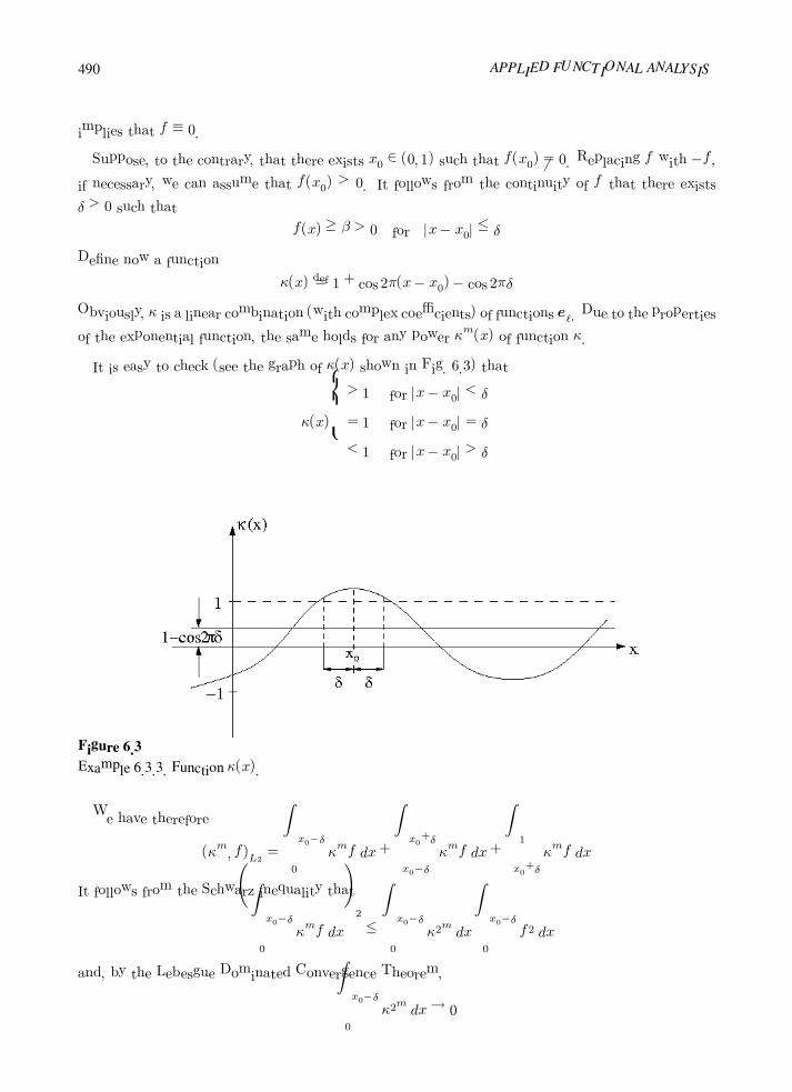
490 APPLIED FUNCTIONAL ANALYSIS
implies that f ≡ 0.
Suppose, to the contrary, that there exists x0 ∈ (0, 1) such that f(x0) = 0. Replacing f with −f ,
if necessary, we can assume that f(x0) > 0. It follows from the continuity of f that there exists
δ > 0 such that
f(x) ≥ β > 0 for |x− x0| ≤ δ
Define now a function
κ(x)def= 1 + cos 2π(x− x0)− cos 2πδ
Obviously, κ is a linear combination (with complex coefficients) of functions e. Due to the properties
of the exponential function, the same holds for any power κm(x) of function κ.
It is easy to check (see the graph of κ(x) shown in Fig. 6.3) that
κ(x)
> 1 for |x− x0| < δ
= 1 for |x− x0| = δ
< 1 for |x− x0| > δ
Figure 6.3
Example 6.3.3. Function κ(x).
We have therefore
(κm, f)L2 =
x0−δ
0
κmf dx+
x0+δ
x0−δ
κmf dx+
1
x0+δ
κmf dx
It follows from the Schwarz inequality that x0−δ
0
κmf dx
2
≤
x0−δ
0
κ2m dx
x0−δ
0
f2 dx
and, by the Lebesgue Dominated Convergence Theorem, x0−δ
0
κ2m dx→ 0

Hilbert Spaces 491
In the same way the last integral converges to zero as well, but the middle one
x0+δ
x0−δ
κmf dx ≥ 2δβ > 0
At the same time, due to the orthogonality of f with e,
(κm, f)L2 = 0
is a contradiction.
The assertion of this step is immediately generalized to complex-valued functions f .
Step 3. Let f ∈ L2(0, 1) be an arbitrary function. By the density of continuous functions in
L2(0, 1), there exists a sequence of continuous functions fn ∈ L2(0, 1) converging to f . Assume now
that
(ek, f) = 0 k = 0, ±1,±2, . . .
In particular, (k = 0)
1
0
f(x) dx = 0. As
1
0
fn(x) dx→
1
0
f(x) dx = 0
we can replace the original functions fn(x) with
fn(x)−
1
0
fn(x) dx
and assume that also
1
0
fn(x) dx = 0.
Now, for each n define the function
gn(x) =
x
0
fn(s)ds
From the Fundamental Theorem of Integral Calculus, it follows that gn is C1 and gn = fn. Conse-
quently 1
0
gn(x)v(x) dx = −
1
0
fn(x)v(x) dx
for every C1 function v(x), since gn(0) = gn(1) = 0.
Passing to the limit, we get
1
0
g(x)v(x) dx = −
1
0
f(x)v(x) dx
for the (continuous) function g(x) =
x
0
f(s)ds. Substituting functions ek(x) for v(x), we draw the
conclusion that
(ek, g) = 0 k = 0, ±1,±2, . . .
492 APPLIED FUNCTIONAL ANALYSIS
By the Step 2 result, g ≡ 0, which implies that
b
a
f(x) dx =f, χ[a,b]
= 0 0 < a < b < 1
for every characteristic function of an interval (a, b) ⊂ (0, 1). Since the span of such characteristic
functions forms a dense subset in L2(a, b) (see Exercise 4.9.2), f must vanish almost everywhere
(Exercise 6.2.1(iv)).
Example 6.3.4
Functionsf0 ≡ 1
fk =√2 cos 2πkx, k = 1, 2, . . .
gk =√2 sin 2πkx, k = 1, 2, . . .
form an orthonormal basis in L2(0, 1).
By a straightforward calculation we check that the functions are orthonormal. To prove that they form a
maximal set, it is enough to see that
f0 = e0, fk =ek + e−k√
2, gk =
ek − e−k
i√2
, k = 1, 2, . . .
where ek, k = 1, 2, . . . are the exponential functions from the previous example.
Note that in contrast to the previous example, functions from this example form an orthonormal basis in
both real and complex L2(a, b) spaces.
Let e1, . . . , en be a finite set of orthonormal vectors in a Hilbert space V and Vn its linear span. It is easy
to derive an explicit formula for the orthogonal projection Pn on the subspace Vn.
Toward this goal, pick an arbitrary vector v ∈ V and represent Pnv in the form of a linear combination of
vectors e1, . . . , en
Pnv = v1e1 + . . .+ vnen
Multiplying both sides by ej in the sense of the scalar product and using the orthonormality of ei, we get
vj = (Pnv, ej)
According to the Orthogonal Decomposition Theorem, however, v can be represented in the form
v = Pnv + (v − Pnv)
where v − Pnv is orthogonal to Vn and therefore
vj = (v, ej)

Hilbert Spaces 493
Thus we end up with the formula
Pnv =
n
j=1
(v, ej)ej
Gram-Schmidt Orthonormalization. Given an arbitrary sequence of linearly independent vectors vi∞i=1
in a Hilbert space V , it is easy to construct a corresponding orthonormal sequence by using the so-called
Gram-Schmidt orthonormalization procedure.
We begin by normalizing the first vector v1
e1def=
v1
v1
Next we take the second vector v2 and subtract from it its orthogonal projection P1v2 on V1 = span e1
e2def= v2 − P1v2 = v2 − (v2, e1)e1
It follows from the linear independence of v1 and v2 that vector e2 is different from zero. We define now e2
by normalizing e2
e2def=
e2
e2
By induction, given n− 1 vectors e1, . . . , en−1, we construct first en by subtracting from vn its orthogonal
projection Pn−1vn on Vn−1 = span e1, . . . , en−1 = spanv1, . . . ,vn−1
endef= vn − Pn−1vn = vn −
n−1
j=1
(vn, ej)ej
and normalize it
endef=
enen
It follows from the construction that vectors ei, i = 1, 2, . . . are orthonormal.
Example 6.3.5
(Legendre Polynomials)
By applying the Gram-Schmidt orthonormalization to monomials
1, x, x2, x3, . . .
in the real L2(a, b), we obtain the so-called Legendre polynomials pn which can be represented in a
concise form as
pn(x) =1
γn
dn
dxn(x− a)n(x− b)n , n = 0, 1, . . .
with constants γn chosen to satisfy pn = 1.
We prove the assertion by induction. For n = 0, p0 ∼ 1(= 1/√b− a). Assume now n > 0.
Obviously, pn is a polynomial of order n. To prove that it coincides with the function en resulting

494 APPLIED FUNCTIONAL ANALYSIS
from the Gram-Schmidt orthonormalization, it is sufficient to show that pn is orthogonal with
p0, . . . , pn−1 or, equivalently, with all monomials xm of order m ≤ n− 1. We have
b
a
xm dn
dxn(x− a)n(x− b)n dx
= −
b
a
mxm−1 dn−1
dxn−1(x− a)n(x− b)n dx
+xm dn−1
dxn−1(x− a)n(x− b)n|
ba
Continuing the integration by parts another m−1 times, we conclude that the integral must vanish.
Let V be an arbitrary Hilbert space. By modifying the proofs of Theorems 2.4.2 and 2.4.3, and using the
Kuratowski–Zorn Lemma, it can be shown that every Hilbert space V has an orthonormal basis and that every
two orthonormal bases in V have precisely the same number of elements (cardinal number). This number is
frequently identified as the dimension of the Hilbert space V (not the same as the dimension of V treated as
a vector space only).
We shall content ourselves here with a much simpler, explicit construction of an orthonormal basis in a
separable Hilbert space.
THEOREM 6.3.1
Every separable Hilbert space V has a countable orthonormal basis.
PROOF Let vn∞n=1 be an everywhere dense sequence in V .
Step 1. Select a subsequence of linearly independent vectors
vnk∞k=1
We proceed by induction. We take first the smallest index n1 such that vn1= 0. Next, assume
that k linearly independent vectors vn1 , . . . ,vnkhave already been selected. Two possible cases may
occur:
Case 1. All remaining vn, n > nk are linearly dependent with the vectors selected so far. In this
case the subsequence of linearly independent vectors will be finite.
Case 2. There exists the smallest index nk+1 > nk such that vectors
vn1 , . . . ,vnk,vnk+1
are linearly independent.
Hilbert Spaces 495
Step 2. Apply the Gram-Schmidt orthonormalization , yielding vectors e1, e2, . . .. Obviously
span (e1, e2, . . .) = span (vn1,vn2
, . . .) = span (v1,v2, . . .)
and, therefore, the span of vectors e1, e2, . . . is dense in V , which implies that e1, e2, . . . is an
orthonormal basis in V .
COROLLARY 6.3.1
A Hilbert space V is separable iff it possesses a countable basis.
PROOF It remains to show sufficiency. Let e1, e2, . . . be an orthonormal basis in V . Accordingly,
any vector v ∈ V can be represented in the form
v =
∞
i=1
viei
the series being finite if V is finite-dimensional. Pick now an arbitrary ε > 0 and select rational
numbers vi (complex numbers with rational real and imaginary parts in the complex case) such that
|vi − vi| ≤ε
2ii = 1, 2, . . .
It follows thatv −
∞
i=1
viei
=
∞
i=1
(vi − vi) ei
≤
∞
i=1
|vi − vi| ei ≤
∞
i=1
ε
2i= ε
which proves that linear combinations of vectors ei, i = 1, 2, . . . with rational coefficients are dense
in V .
Example 6.3.6
We give now without proof three examples of orthonormal bases in different L2 spaces.
1. The Legendre polynomials
pn(x) =
2n+ 1
2
12 1
2nn!
dn
dxn
x2 − 1
n
form an orthonormal basis in L2(−1, 1).
2. The Laguerre functions
φn(x) =1
n!e−x/2Ln(x), n = 0, 1, . . .
where Ln(x) is the Laguerre polynomial
Ln(x) =
n
i=0
(−1)in
i
n(n− 1) . . . (i+ 1)xi
= exdn
dxn
xne−x

496 APPLIED FUNCTIONAL ANALYSIS
form an orthonormal basis in L2(0,∞).
3. The Hermite functions
φn(x) =2nn!
√π− 1
2 ex2/2Hn(x), n = 0, 1, . . .
where Hn(x) is the Hermite polynomial
Hn(x) = (−1)nex2 dn
dxn
e−x2
form an orthonormal basis for L2(−∞, ∞) = L2(IR).
Fourier Series. The existence of an orthonormal basis in a separable Hilbert space provides a very useful
tool in studying properties of the space because it allows us to represent arbitrary elements of the space as
(infinite) linear combinations of the basis functions. Suppose that en∞n=1 is an orthonormal basis for a
Hilbert space V . Taking an arbitrary vector v and representing it in the form of the series
v =
∞
i=1
viei = limN→∞
N
i=1
viei
we easily find the explicit formula for coefficients vi. Orthonormality of vectors ei implies that
N
i=1
viei, ej
= vj for N ≥ j
Passing to the limit with N →∞, we get
vj = (v, ej)
and, consequently,
v =∞
i=1
(v, ei) ei
The series is called the (generalized) Fourier series representation of v ∈ V , and the scalars vn = (v, en) are
called the Fourier coefficients of v relative to the basis ei∞i=1.
Substituting the Fourier series representation for vectors u and v in the scalar product (u,v), we get
immediately
(u,v) =
∞
i=1
uiei,
∞
j=1
vjej
= limN→∞
N
i=1
uiei,
N
j=1
vjej
= limN→∞
N
i=1
uivi =
∞
i=1
uivi =
∞
i=1
(u, ei) (v, ei)
The formula
(u,v) =∞
i=1
(u, ei) (v, ei)

Hilbert Spaces 497
is known as Parseval’s identity. Substituting v = u in particular implies that
u2=
∞
i=1
|(u, ei)|2
Exercises
Exercise 6.3.1 Prove that every (not necessarily separable) nontrivial Hilbert space V possesses an orthonor-
mal basis.
Hint: Compare the proof of Theorem 2.4.3 and prove that any orthonormal set in V can be extended to
an orthonormal basis.
Exercise 6.3.2 Let en∞n=1 be an orthonormal family in a Hilbert space V . Prove that the following condi-
tions are equivalent to each other.
(i) en∞n=1 is an orthonormal basis, i.e., it is maximal.
(ii) u =
∞
n=1
(u, en) en ∀ u ∈ V .
(iii) (u,v) =∞
n=1
(u, en) (v, en).
(iv) u2=
∞
n=1
|(u, en)|2.
Exercise 6.3.3 Let en∞n=1 be an orthonormal family (not necessarily maximal) in a Hilbert space V . Prove
Bessel’s inequality∞
i=1
|(u, ei)|2≤ u
2∀ u ∈ V
Exercise 6.3.4 Prove that every separable Hilbert space V is unitary equivalent with the space 2.
Hint: Establish a bijective correspondence between the canonical basis in 2 and an orthonormal basis
in V and use it to define a unitary map mapping 2 onto V .
Exercise 6.3.5 Prove the Riesz-Fisher Theorem.
Let V be a separable Hilbert space with an orthonormal basis en∞n=1. Then
V =
∞
n=1
vnen :∞
n=1
|vn|2<∞
In other words, elements of V can be characterized as infinite series
∞
n=1
vnen with 2-summable
coefficients vn.

498 APPLIED FUNCTIONAL ANALYSIS
Exercise 6.3.6 Let I = (−1, 1) and let V be the four-dimensional inner product space spanned by the
monomials 1, x, x2, x3 with
(f, g)V =
1
−1
fg dx
(i) Use the Gram-Schmidt process to construct an orthonormal basis for V .
(ii) Observing that V ⊂ L2(I), compute the orthogonal projection Πu of the function u(x) = x4
onto V .
(iii) Show that (x4 −Πx4, v)L2(I) = 0 ∀v ∈ V .
(iv) Show that if p(x) is any polynomial of degree ≤ 3, then Πp = p.
(v) Sketch the function Πx4 and show graphically how it approximates x4 in V .
Exercise 6.3.7 Use the orthonormal basis from Example 6.3.4 to construct the (classical) Fourier series rep-
resentation of the following functions in L2(0, 1).
f(x) = x, f(x) = x+ 1
Duality in Hilbert Spaces
6.4 Riesz Representation Theorem
The properties of the topological dual of a Hilbert space constitute one of the most important collection of
ideas in Hilbert space theory and in the study of linear operators. We recall from our study of topological
duals of Banach spaces in the previous chapter that the dual of a Hilbert space V is the vector space V
consisting of all continuous linear functionals on V . If f is a member of V we write, as usual,
f(v) = f,v
where ·, · denotes the duality pairing on V × V . Recall that V is a normed space equipped with the dual
norm
fV = supv =0
f,v
vV
Now, in the case of Hilbert spaces, we have a ready-made device for constructing linear and continuous
functionals on V by means of the scalar product (·, ·)V . Indeed, if u is a fixed element of V , we may define
a linear functional fu directly by
fu(v)def= (v,u) = (u,v) ∀ v ∈ V

Hilbert Spaces 499
This particular functional depends on the choice u, and this suggests that we describe this correspondence by
introducing an operator R from V into V such that
Ru = fu
We have by the definition
Ru,v = (v,u) = (u,v) ∀ u,v ∈ V
Now, it is not clear at this point whether or not there might be some functionals in V that cannot be repre-
sented by inner products on V . In fact, all we have shown up to now is that
R(V ) ⊂ V
It is a remarkable fact, proven by the Hungarian mathematician Frigyes Riesz, that all functionals in V can
be represented in this way; that is,
R(V ) = V
The statement of this important assertion is set forth in the following theorem (recall the Representation
Theorems in Section 5.12).
THEOREM 6.4.1
(The Riesz Representation Theorem)
Let V be a Hilbert space and let f be a continuous linear functional on V . Then there exists a
unique element u ∈ V such that
f(v) = (v,u) ∀ v ∈ V
where (·, ·) is the scalar product on V . Moreover,
fV = uV
PROOF
Step 1: Uniqueness. Suppose that
f(v) = (v,u1) = (v,u2) ∀ v ∈ V
and some u1, u2 ∈ V . Then (v,u1 − u2) = 0 and upon substituting v = u1 − u2 we get
u1 − u22= 0
which implies u1 = u2.
Step 2: Existence. The case f ≡ 0 is trivial. Assume that f ≡ 0. Since functional f is continuous,
the null space
N = f−10 = ker f = u ∈ V : f(u) = 0
500 APPLIED FUNCTIONAL ANALYSIS
is a closed subspace of V and therefore by the Orthogonal Decomposition Theorem, the space V can
be represented in the form of the direct, orthogonal sum
V = N ⊕N⊥
Pick an arbitrary non-zero vector u0 ∈ N⊥ and define
u =f (u0)
u02 u0
It follows from the choice of u that both functionals f and Ru coincide on N ⊕ ICu0. Indeed,
f(v) = (v,u) = 0 for v ∈ N
and, for v = αu0, α ∈ IC,
(v,u) = (αu0,u) = αf (u0) = f (αu0)
We claim finally that N⊥ is one-dimensional and it reduces to ICu0. We have for any v ∈ V
v =
v −f(v)
f(u)u
+f(v)
f(u)u
Now
f
v −f(v)
f(u)u
= f(v)−f(v)
f(u)f(u) = 0
and, therefore, the first vector belongs to N , which proves that
V = N ⊕ ICu = N ⊕ ICu0
the decomposition being orthogonal (u0 ∈ N⊥). To prove that fV = uV notice that, by means
of Cauchy–Schwarz inequality, for v = 0
|f(v)| = |(v,u)| ≤ v u
and, therefore, fV ≤ uV .
But at the same time,
u2V = (u,u) = f(u) ≤ fV uV
so uV ≤ fV .
COROLLARY 6.4.1
Let R : V → V denote the map from a Hilbert space V onto its dual V such that
Ru,v = (u,v) ∀ u,v ∈ V

Hilbert Spaces 501
Then:
(i) R is an antilinear map from V onto V .
(ii) R preserves the norm, i.e.,
RuV = uV
In particular, in the case of a real Hilbert space V , R is a linear norm-preserving isomorphism
(surjective isometry) from V onto V .
PROOF It remains to show that R is antilinear. But this follows directly from the fact that the
scalar product is antilinear with respect to the second variable:
(v, α1u1 + α2u2) = α1 (v,u1) + α2 (v,u2)
Consequently,
R (α1u1 + α2u2) = α1R (u1) + α2R (u2)
The antilinear operator R described above is known as the Riesz map corresponding to the Hilbert space
V and the scalar product (·, ·) and it is frequently used to identify the topological dual of V with itself in
much the same way as the representation theorems for the Lp spaces were used to identify their duals with
(conjugate) spaces Lq, 1/p+ 1/q = 1.
The Riesz map can be used to transfer the Hilbert space structure to its dual V which a priori is only a
normed (Banach) space. Indeed by a straightforward verification we check that
(f, g)V def=R−1g,R−1f
V
is a well-defined scalar product on V . (Note that the inverse of an antilinear map if it exists, is antilinear,
too.) Moreover, from the fact that R is norm-preserving it follows that the norm corresponding to the just-
introduced scalar product on V coincides with the original (dual) norm on V .
Applying the Riesz representation theorem to the dual space V , we can introduce the Riesz map for the
dual space as
RV : V g → f → (f, g)V ∈ IC ∈ (V )
where (V ) is the bidual of V . Composing R = RV with the Riesz map for the dual space we getRV RV (u)
(f) =
f,RV (u)
V
=R−1
V RV (u), R−1V f
V
=u, R−1
V f
V
= f,u

502 APPLIED FUNCTIONAL ANALYSIS
which implies that the evaluation map mapping space V into its bidual (V ) (see Section 5.13) coincides
with the composition of the two Riesz maps for V and its dual (notice that the composition of two antilinear
maps is linear). Consequently, every Hilbert space is reflexive.
REMARK 6.4.1 It is a bit awkward that the Riesz map is not a linear but antilinear map.
This is a direct consequence of the definition of the inner product that assumes antilinearity with
respect to the second variable. If, however, we adopt the alternative definition of the dual space and
define it as a space of antilinear functionals on V (recall discussion in Section 2.10) , the complex
conjugate in the definition of the Riesz map disappears, and the map is defined as
< Ru,v >= (u,v) ∀v ∈ V
Consequently, the Riesz map becomes linear. All results concerning the dual and the bidual spaces
discussed above remain the same.
We conclude this section with a number of examples illustrating the concept of the Riesz map.
Example 6.4.1
We return one more time to the example of a finite-dimensional inner product space V with a scalar
product (·, ·) studied previously in Chapter 2.
Let e1, . . . , en be an arbitrary (not necessarily orthonormal) basis in V . Using Einstein’s summa-
tion convention we represent two arbitrary vectors x,y ∈ V in the form
x = xkek, y = yjej
Now let f be an arbitrary element of the dual V ∗ = V . It is natural to represent f in the dual
basis e∗1, . . . , e∗n:
f = fie∗i
Assume now that f = Rx where R is the Riesz map from V into its dual V . We have
f ,y = Rx,y = (y,x) =yjej , x
kek= gjky
jxk
where gjkdef= (ej , ek) is the positive definite (so-called Gram) matrix corresponding to basis e1, . . . , en.
At the same time
f ,y =fe
∗, yjej= fy
je∗, ej
= fy
jδj = fjyj
Comparing both expressions, we get
fj = gjkxk
which is precisely the matrix form representation for the equation
f = Rx

Hilbert Spaces 503
As we can see, the Gram matrix can be interpreted as the matrix representation of the Riesz map
with respect to the basis e1, . . . , en and its dual. It can also be explicitly seen that the Riesz map
is antilinear.
Introducing the inverse Gram matrix gkj , we write
gkjfj = xk
or taking into account that gkj = gjk, we get
gjkf j = xk
Consequently, the scalar product in the dual space can be represented in the form
(f ,h)V =R−1h, R−1f
= gjkR−1h
j(R−1f)
k
= gjkgnjhng
kmfm
= δmj gnjhnfm
= gnmfmhn
where h = he∗ and f = fe
∗.
Example 6.4.2
Let V = L2(Ω) with Ω an open set in IRn. We have
Ru, v = (v, u)L2(Ω) =
Ωvu dΩ
and
(Ru,Rv)V = (v, u)V =
Ωvu dΩ
Example 6.4.3
Consider the Sobolev space Hm(Ω) of order m introduced in Example 6.1.7. The closure of functions
C∞0 (Ω) (infinitely differentiable functions with compact support contained in Ω) is identified as a
subspace of Hm(Ω)
Hm0 (Ω)
def= C∞
0 (Ω)Hm(Ω)
By definition, Hm0 (Ω) is closed and, therefore, is a Hilbert space with the scalar product from Hm(Ω)
(u, v)Hm(Ω) =
|α|≤m
ΩDαuDαvdΩ

504 APPLIED FUNCTIONAL ANALYSIS
Intuitively speaking, spaces Hm0 (Ω) consist of all functions from Hm(Ω) which vanish on the bound-
ary together with all derivatives of order up to (inclusively) m− 1. A precise interpretation of this
fact is based on Lions’ Trace Theorem; see [6, 8, 7].
Topological duals of spaces Hm0 (Ω) are identified as Sobolev spaces of negative order
H−m(Ω)def= (Hm
0 (Ω))
Note that, in general, elements from H−m(Ω) are only linear and continuous functionals defined on
Hm0 (Ω) and cannot be identified with functions.
In this example we would like to take a closer look at a particular case of the real space H10 (I),
with I = (−1, 1) ⊂ IR. According to the Sobolev Imbedding Theorem, see [1], the space H1(I) can be
imbedded into the Chebyshev space C(I) of functions continuous on the closed interval I = [−1, 1].
More precisely, there exists a linear and continuous injection
T : H1(I) −→ C(I)
which for functions continuous on I reduces to the identity map. Recall that continuity means that
TuC(I) ≤ C uH1(I) ∀ u ∈ H1(I)
for some C > 0. In particular, this implies that the mapping
H1(I) u −→ (Tu)(x0) x0 ∈ I
is continuous for every point x0 from I.
It may be a little confusing, but most of the time we drop the letter T and write that
H1(I) u −→ u(x0) x0 ∈ I
is continuous. This notational simplification is at least partially justified by the fact that T reduces
to identity for (equivalence classes of) functions from C(I).
Equipped with these observations we redefine the space H10 (I) as
H10 (I)
def=u ∈ H1(I) : u(0) = u(1) = 0
It is not a trivial exercise but it can be shown that H10 (I) defined above coincides with H1
0 (Ω) defined
before, i.e., the closure of functions C∞0 (I) in H1(I).
Notice that due to the continuity of the imbedding map T , H10 (I) is a closed subspace of H1(I)
and therefore it is itself a Hilbert space equipped with the scalar product from H1(I)
(u, v) =
1
−1
uv +du
dx
dv
dx
dx
Hilbert Spaces 505
Continuity of the imbedding implies also that the Dirac functional
δ(v) = v(0)
is a continuous and linear map on H1(I) and therefore on the subspace H10 (I) as well and therefore
is an element of the dual Sobolev space
H−1(I)def=H1
0 (I)
The Riesz map R from H10 (I) onto H−1(I) is defined by
R : u −→ f
f, v = (v, u) =
1
−1
vu+dv
dx
du
dx
dx ∀ v ∈ H10 (I)
Restricting ourselves to test functions v ∈ C∞0 (I), we see that u can be interpreted as a solution to
the distributional equation
−d2u
dx2+ u = f
with boundary conditions u(−1) = u(1) = 0 (see Sections 6.6 and 6.7 for a more detailed discussion
of related issues).
In particular, for f = δ the corresponding solution u = uδ is given by
uδ(x) =
sinh(1 + x)/2 cosh 1 −1 ≤ x ≤ 0
sinh(1− x)/2 cosh 1 0 ≤ x ≤ 1
It follows that
δ2H−1(I) = uδ
2H1(I) =
1
−1
u2δ +
duδ
dx
2
dx =sinh 2
4 cosh2 1
Exercises
Exercise 6.4.1 Revisit Example 6.4.1 and derive the matrix representation of the Riesz map under the as-
sumption that the dual space consists of antilinear functionals.

506 APPLIED FUNCTIONAL ANALYSIS
6.5 The Adjoint of a Linear Operator
In Sections 5.16 and 5.18 we examined the properties of the transpose of linear and both continuous and
closed operators defined on Banach spaces. In the case of Hilbert spaces those ideas can be further specialized
leading to the idea of (topologically) adjoint operators (recall Section 2.15 for a discussion of the same notion
in finite-dimensional spaces).
We set the stage for this discussion by reviewing some notations. Let
U , V be (complex) Hilbert spaces with scalar products (·, ·)U and (·, ·)V , respectively.
U , V denote the topological duals of U and V .
·, ·U and ·, ·V denote the duality pairings on U × U and V × V .
RU : U → U , RV : V → V be the Riesz operators for U and V , respectively, i.e.,
RUu,w = (w,u)U ∀ w ∈ U and
RV v,w = (w,v)V ∀ w ∈ V
(Topological) Adjoint of a Continuous Operator. Let A ∈ L(U, V ), i.e., let A be a linear and continuous
operator from U into V . Recall that the topological transpose operator A ∈ L(V , U ) was defined as
Av = v A for v ∈ V
or, equivalently:
Av,u = v, Au ∀ u ∈ U v ∈ V
The transpose A of operator A operates on the dual V into the dual U . Existence of the Riesz operators
establishing the correspondence between spaces U , V and their duals U , V prompts us to introduce the
so-called (topological) adjoint operator A∗ operating directly on the space V into U and defined as the
composition
A∗def= R−1
U A RV
The relationship between A, A, A∗ and the Riesz maps is depicted symbolically in Fig. 6.4.
As in the finite-dimensional case, it follows from the definitions of A, A∗ and the Riesz maps that
(u, A∗v)U =u, R−1
U ARV vU
= ARV v,uU
= RV v, AuV
= (Au,v)V

Hilbert Spaces 507
Figure 6.4
Topological adjoint of a continuous operator defined on a Hilbert space.
for every u ∈ U, v ∈ V . Note that even though the Riesz operators are antilinear, the adjoint operator A∗
is linear as the composition of linear and antilinear maps is antilinear and the composition of two antilinear
maps is linear.
Example 6.5.1
The adjoint of the integral operator
Au = v, v(x) =
1
0
K(x, ξ)u(ξ) dξ
defined on the real space L2(0, 1) with square-integrable kernelK(x, ξ), considered in Example 5.16.1,
is equal to the integral operator A∗ where
A∗u = v, v(ξ) =
1
0
K(x, ξ)u(x) dx
i.e., the corresponding kernel K∗(x, ξ) = K(ξ, x). Notice that in the complex case a complex
conjugate has to be added, i.e.,
K∗(ξ, x) = K(x, ξ)

508 APPLIED FUNCTIONAL ANALYSIS
Example 6.5.2
Recall that an operator T mapping a Hilbert space U into a Hilbert space V is said to be unitary if
(Tu, Tv)V = (u,v)U ∀ u ∈ U, v ∈ V
Then T is an isometry (in fact, the two conditions are equivalent to each other, compare Exer-
cise 6.1.7) and in particular injective.
Assume additionally that T is surjective, i.e., R(T ) = V . Then the inverse of T coincides with its
adjoint. Indeed, substituting w = Tv in the above equation
(Tu,w)V = (u, T−1w)U ∀u ∈ U, w ∈ V
which implies that T−1 = T ∗.
Conversely, T−1 = T ∗ implies that T is unitary and surjective.
Reinterpreting properties of the transpose operator (recall Proposition 5.16.1), we get
PROPOSITION 6.5.1
Let U , V , W be inner product spaces and let A, Ai ∈ L(U, V ), i = 1, 2, and B ∈ L(V,W ). The
following properties hold.
(i) Adjoint of a linear combination of operators is equal to the linear combination of the corre-
sponding adjoint operators with complex conjugate coefficients
(α1A1 + α2A2)∗= α1A
∗1 + α2A
∗2
(ii) Adjoint of a composition is equal to the composition of the adjoint operators with inverted order
(B A)∗ = A∗ B∗
(iii) Adjoint of the identity operator equals the operator itself
(idU )∗= idU
(iv) If the inverse A−1 exists and is continuous then A∗ has a continuous inverse too, and
(A∗)−1
=A−1
∗
(v) Norm of the adjoint equals norm of the operator
AL(U,V ) = A∗L(V,U)
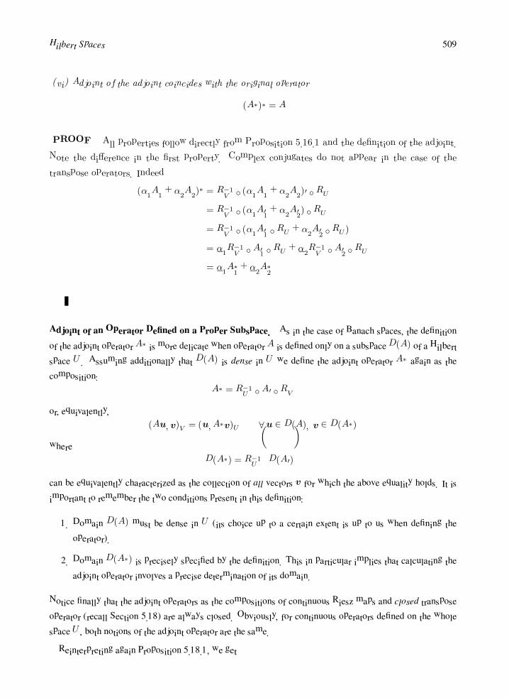
Hilbert Spaces 509
(vi) Adjoint of the adjoint coincides with the original operator
(A∗)∗ = A
PROOF All properties follow directly from Proposition 5.16.1 and the definition of the adjoint.
Note the difference in the first property. Complex conjugates do not appear in the case of the
transpose operators. Indeed
(α1A1 + α2A2)∗= R−1
V (α1A1 + α2A2)RU
= R−1V (α1A
1 + α2A
2) RU
= R−1V (α1A
1 RU + α2A
2 RU )
= α1R−1V A1 RU + α2R
−1V A2 RU
= α1A∗1 + α2A
∗2
Adjoint of an Operator Defined on a Proper Subspace. As in the case of Banach spaces, the definition
of the adjoint operator A∗ is more delicate when operator A is defined only on a subspaceD(A) of a Hilbert
space U . Assuming additionally that D(A) is dense in U we define the adjoint operator A∗ again as the
composition:
A∗ = R−1U A RV
or, equivalently,
(Au,v)V = (u, A∗v)U ∀ u ∈ D(A), v ∈ D(A∗)
where
D(A∗) = R−1U
D(A)
can be equivalently characterized as the collection of all vectors v for which the above equality holds. It is
important to remember the two conditions present in this definition:
1. Domain D(A) must be dense in U (its choice up to a certain extent is up to us when defining the
operator).
2. Domain D(A∗) is precisely specified by the definition. This in particular implies that calculating the
adjoint operator involves a precise determination of its domain.
Notice finally that the adjoint operators as the compositions of continuous Riesz maps and closed transpose
operator (recall Section 5.18) are always closed. Obviously, for continuous operators defined on the whole
space U , both notions of the adjoint operator are the same.
Reinterpreting again Proposition 5.18.1, we get

510 APPLIED FUNCTIONAL ANALYSIS
PROPOSITION 6.5.2
Let U , V , and W be inner product spaces.
(i) Let Ai : U ⊃ D → V , i = 1, 2 be two linear operators defined on the same domain D, dense
in U . Then
(α1A1 + α2A2)∗= α1A
∗1 + α2A
∗2
(ii) Let A : U ⊃ D(A)→ V , B : V ⊃ D(B) → W be two linear operators with domains dense in
U and V , respectively, and let R(A) ⊂ D(B). Then
(B A)∗ ⊃ A∗ B∗
i.e., the adjoint (B A)∗ exists and it is an extension of the composition A∗ B∗.
(iii) If A : U ⊃ D(A) → V is a linear, injective operator with domains D(A) and range R(A)
dense in U and V , respectively, then the adjoint operator A∗ has an inverse and
(A∗)−1
=A−1
∗
All theorems involving the transpose operators on Banach spaces, proven in Sections 5.17 and 5.18, may
be directly reinterpreted in the context of Hilbert spaces with scalar products replacing duality pairings and
the adjoint operators replacing the transpose operators. Reinterpreting for instance Corollary 5.18.2, we get
THEOREM 6.5.1
(Solvability of Linear Equations on Hilbert Spaces)
Let U and V be Hilbert spaces and let
A : U ⊃ D(A) −→ V, D(A) = U, R(A) = R(A)
be a linear, closed operator with the domain D(A) dense in U and range R(A) closed in V . Then
the linear problem
Au = f f ∈ V
has a solution u if and only if
f ∈ N (A∗)⊥
where A∗ is the adjoint of A. The solution u is determined uniquely up to elements from the null
space N (A).
REMARK 6.5.1 Recall (Theorem 5.18.2) that closedness of the range R(A) in V is equivalent
to the condition
AuV ≥ c infw∈N (A)
u+wU ∀ u ∈ D(A), c > 0

Hilbert Spaces 511
This in particular implies that if u is a solution corresponding to f , then
infw∈N (A)
u+wU ≤1
cfV
Symmetric and Self-Adjoint Operators. An operator A defined on a dense subspace D(A) of a Hilbert
space U into itself is said to be symmetric, if A ⊂ A∗, i.e.,
D(A) ⊂ D(A∗) and A∗|D(A) = A
If additionally, the domains of both operators are the same, i.e., A = A∗, then we say that operator A is
self-adjoint.
Obviously, every self-adjoint operator is symmetric, but not conversely. There are numerous examples
of symmetric operators which are not self-adjoint. In the case of a continuous and symmetric operator A
defined on the whole space U however, the adjoint A∗ is defined on the whole U as well, and therefore, A is
automatically self-adjoint.
Note finally that, since adjoint operators are closed, every self-adjoint operator A is necessarily closed.
Example 6.5.3
Integral operator A discussed in Example 6.5.1 is self-adjoint iff
K(x, ξ) = K(ξ, x)
Example 6.5.4
Orthogonal projections in a Hilbert space are self-adjoint. Indeed, let M be a closed subspace of a
Hilbert space V and P the corresponding orthogonal projection on M , i.e., if
u = u1 + u2 where u1 ∈M,u2 ∈M⊥
then Pu = u1. Similarly, Pv = v1, for v = v1 + v2, v1 ∈M , v2 ∈M⊥. We have
(Pu,v) = (u1,v) = (u1,v1 + v2)
= (u1,v1) = (u1 + u2,v1)
= (u,v1) = (u, Pv)
for every u,v ∈ V .

512 APPLIED FUNCTIONAL ANALYSIS
Example 6.5.5
Let V = L2(0, 1) and consider the operator A defined as
D(A) = C∞0 (0, 1) , Au = −
d2u
dx2= −u
It can be proved that the space of test functions C∞0 (0, 1) is dense in L2(0, 1) and therefore it makes
sense to speak about the adjoint of A. It follows from the definition of the adjoint operator that
1
0
(−u)v dx =
1
0
uA∗v dx ∀u ∈ C∞0 (0, 1)
which implies that A∗v = −v in the distributional sense. As the value of A∗v must be in L2, this
implies that for v ∈ D(A∗), v ∈ L2(0, 1).
It can be proved next that v is a C1-function. In particular, we can integrate the first integral by
parts, which yields
1
0
−uv dx =
1
0
uv dx− uv|10 = −
1
0
uv dx− uv|10
Consequently, the domain of operator A∗ is identified as
D(A∗) =v ∈ L2(0, 1) : v ∈ L2(0, 1), v(0) = v(1) = 0
As we can see, D(A) ⊂ D(A∗) but at the same time D(A) = D(A∗) and, therefore, the operator A
is symmetric, but not self-adjoint.
For other examples of self-adjoint operators, we refer the reader to the next section.
Normal Operators. A continuous linear operator A, defined on a Hilbert space V into itself is said to be
normal if it commutes with its adjoint, i.e.,
AA∗ = A∗A
It follows from the definition that all self-adjoint operators are normal. Also, every unitary and surjective
operator is normal as well (see Example 6.5.2).
Example 6.5.6
Let M be a closed vector subspace of a Hilbert space V , and let P be the corresponding orthogonal
projection. Operator A = λP , where λ is a complex number, is self-adjoint iff λ is real, because
A∗ = (λP )∗ = λP ∗ = λP
But
A∗A = AA∗ = λλP = |λ|2P

Hilbert Spaces 513
and, therefore, A is normal for all complex λ.
The following proposition provides an important characterization of normal operators.
PROPOSITION 6.5.3
Let A be a bounded, linear operator on a Hilbert space V . Then A is normal if and only if
Au = A∗u ∀ u ∈ V
PROOF Assume that A is normal. Then
||Au||2 = (Au, Au) = (u, A∗Au) = (u, AA∗u)
= (A∗u, A∗u) = ||A∗u||2
Conversely, assume that ||Au|| = ||A∗u||, for every u ∈ V . By a direct calculation, we easily prove
that (recall Exercise 6.1.2)
(Au,v) =1
4[(A(u+ v),u+ v)− (A(u− v),u− v)
+i(A(u+ iv), u+ iv)− i(A(u− iv),u− iv)]
and, consequently,
(Au,u) = 0 ∀ u ∈ V implies (Au,v) = 0 ∀ u,v ∈ V
which in turn implies that A ≡ 0. But
Au2 = (Au, Au) = (A∗Au,u)
and
A∗u2 = (A∗u, A∗u) = (AA∗u,u)
imply that
((A∗A−AA∗)u,u) = 0 ∀ u ∈ V
and, by the implication above, A∗A−AA∗ = 0.
COROLLARY 6.5.1
Let A be a normal operator on a Hilbert space V . Then
An = An

514 APPLIED FUNCTIONAL ANALYSIS
PROOF First of all, notice that
Anu =AAn−1u
≤ A
An−1u
≤ . . . ≤ Anu
and, therefore, always An ≤ An. We show now that for normal operators the inverse inequality
holds as well. We start with the observation that always
A∗A = A2
Indeed
A2 = supu≤1
(Au, Au) = supu≤1
(A∗Au,u) ≤ supu≤1
(A∗Au u) ≤ A∗A
The inverse inequality follows now from the fact that A∗ = A.
Step 1. A symmetric (self-adjoint), n = 2k. By the result above, we have A2 = A2. By
induction in k, An = An for n = 2k.
Step 2. A normal, n = 2k. Substituting Ak for A, we have
(Ak)∗Ak = Ak2
From the commutativity of A and A∗, it follows that arbitrary powers of A and A∗ commute, and
therefore,
(A∗)kAk = (A∗A)k
But A∗A is symmetric and, by the Step 1 result,
(A∗A)k = A∗Ak = A2k
from which the assertion follows.
Step 3. A normal, n arbitrary. One can always find m such that 2m ≤ n < 2m+1. Denoting
r = 2m+1 − n, we have
An+r = A2m+1
= A2m+1
= An+r ≤ An Ar
and, consequently,
An ≤ An
Exercises
Exercise 6.5.1 Let A be an operator defined on a dense subspace D(A) of a Hilbert space U into a Hilbert
space V . Prove that the adjoint operator A∗ is closed.

Hilbert Spaces 515
Exercise 6.5.2 Prove that the composition BA of two self-adjoint continuous operators A and B is self-
adjoint iff A and B commute, i.e., AB = BA.
Exercise 6.5.3 Prove that for a self-adjoint operator A, (Au,u) is always a real number.
Exercise 6.5.4 Prove that for a self-adjoint, continuous operator A
A = supu≤1
|(Au,u)| = supu≤1
|(u, Au)|
Hint: Make use of the formula for (Au,v) used in the proof of Proposition 6.5.3.
Exercise 6.5.5 Assuming that for a continuous, self-adjoint operator A, the inverse (A+ iI)−1 exists and is
continuous (see Section 6.9), prove that operator
Q = (A− iI)(A+ iI)−1
is unitary.
Exercise 6.5.6 Let A : IC2 −→ IC2 be given by
y1
y2
=
a bc d
x1
x2
What conditions must the complex numbers a, b, c, and d satisfy in order that A be (a) self-adjoint, (b)
normal, and (c) unitary.
Exercise 6.5.7 Prove the Cartesian Decomposition Theorem: Every linear and continuous operator A on a
Hilbert space V can be represented in the form
A = B + iC
where B and C are self-adjoint.
Hint: Define
B =1
2(A+A∗) and C =
1
2i(A−A∗)
Exercise 6.5.8 Prove that if A is bijective and normal, then so is A−1.
Exercise 6.5.9 Determine the adjoints of the following operators in L2(I), where I = (0, 1).
(a) Au = dudx , D(A) = u ∈ L2(I) ∩ C1(I) : u(0) = 0
(b) Au = d2udx2 − u,D(A) = u ∈ L2(I) ∩ C2(I) : u(0) = u(1) = 0
(c) Au = − ddx (x
2 dudx ) + xdu
dx
D(A) = u ∈ L2(I) ∩ C2(I) : u(0) = u(1) = 0

516 APPLIED FUNCTIONAL ANALYSIS
6.6 Variational Boundary-Value Problems
We begin with a simple example of the classical formulation of a boundary problem for the Laplace operator
(Example 2.2.3). Given an open set Ω ⊂ IR2, we look for a function u(x) such that
−∆u = f in Ω
u = u0 on Γu
∂u
∂n= g on Γt
where Γu and Γt are two disjoint parts of the boundary Γ. A mathematical formulation of the problem must
include a precise specification of the regularity of the solution. Usually, minimum regularity assumptions
are desired, admitting the largest possible class of solutions accommodating thus for possible irregular data
to the problem, in our case: the domain Ω, boundary Γ = Γu ∪ Γt, functions f, u0, and g specified in Ω
and on the two parts of the boundary, respectively. Classical regularity assumptions for the problem above
would consist in looking for a solution u in a subspace of C2(Ω) consisting of those functions for which the
boundary conditions make sense, e.g., the space
C2(Ω) ∩ C1(Ω)
It is therefore anticipated that the solution will have second order derivatives (in the classical sense) continu-
ous in Ω and first order derivatives and function values continuous on the whole Ω, including the boundary.
Classical paradoxes with less regular data to the problem (concentrated on impulse forces in mechanics,
resulting in the nonexistence of classical solutions) several decades ago led to the notion of weak or variational
solutions.
Variational Formulation. Multiplying the differential equation by a sufficiently regular function v and
integrating over the domain Ω, we get
−
Ω
∆u v dx =
Ω
fv dx
Integrating the first integral by parts, we get
Ω
∇u∇v dx−
Γ
∂u
∂nv dx =
Ω
fv dx
where ∂u∂n is the normal derivative of u
∂u
∂n=
n
i=1
∂u
∂xini
with ni the components of the outward normal unit vector n.

Hilbert Spaces 517
Substituting g for ∂u∂n on Γt-boundary and eliminating the unknown normal derivative of u on Γu-boundary
by restricting ourselves to functions v vanishing on Γu, we arrive at the formulation
Find u(x) such that u = u0 on Γu, and
Ω
∇u∇v dx =
Ω
fv dx+
Γt
gv ds, for every v = v(x) such that v = 0 on Γu
The problem above is called the variational formulation of the boundary value problem considered, or vari-
ational boundary value problem. Functions v = v(x) are called the test functions.
It is easily seen that the regularity assumptions to make sense for the variational formulation are much less
demanding than in the classical case. Second order derivatives of the solution need not exist, and the first
order derivatives can be understood in the distributional sense.
The two formulations are equivalent in the sense that they yield the same solution u in the case when u is
sufficiently regular. We have shown so far that every classical solution is a variational solution. It remains to
examine when the converse holds, i.e., the variational solution turns out to be the classical one as well.
Toward this goal, we integrate the integral on the left-hand side by parts (it is at this point that we use the
assumption that u ∈ C2(Ω)× C1(Ω)), arriving at the identity
−
Ω
∆u v dx+
Γt
∂u
∂nv ds =
Ω
fv dx+
Γt
gv ds
for every test function vanishing on Γu or, equivalently,
Ω
(−∆u− f)v dx+
Γt
(∂u
∂n− g)v ds = 0 ∀ v, v = 0 on Γu
This in particular, implies that
Ω
(−∆u− f)v dx = 0
for every test function vanishing on the entire boundary. Now, if the set (space) of such functions is dense in
L2(Ω), then
−∆u− f = 0
Consequently, the first integral vanishes for any test function, this time not necessarily vanishing on the whole
boundary, and we arrive at the condition
Γt
(∂u
∂n− g)v ds ∀ v
If again the test functions are dense, this time in the space L2(Γt), then we conclude that
∂u
∂u− g = 0
We say sometimes that we have recovered both the differential equation and the second (Neumann) boundary
condition. Thus, for regular solutions u, the two formulations are equivalent to each other.

518 APPLIED FUNCTIONAL ANALYSIS
Abstract Variational Boundary Value Problems. A precise formulation of the variational boundary value
problem involves a careful specification of regularity assumptions for both the solution u and the test function
v. This usually leads to the selection of function spaces X and Y with a Banach or Hilbert space structure
containing the solution u and test functions v. The essential (Dirichlet) boundary conditions on u and v lead
next to the introduction of
the set of (kinematically) admissible solutions
K = u ∈ X : u = u0 on Γu
and the space of (kinematically) admissible test functions
V = v ∈ Y : v = 0 on Γu
Notice that V is a vector subspace of Y , while K is only a subset of X , unless u0 ≡ 0 ( Example 2.2.3).
More precisely, if an element u0 from X exists which reduces to u0 on the boundary Γu, then K can be
identified as an affine subspace or linear manifold of X , i.e.,
K = u0 + U, where U = u ∈ X : u = 0 on Γu
Finally, the left-hand side of the variational equation in our example is easily identified as a bilinear form of
solution u and test function v and the right-hand side as a linear form (functional) of test function v.
Introducing symbols
b(u, v) =
Ω
∇u∇v dx
l(v) =
Ω
fv dx+
Γt
gv ds
we are prompt to consider an abstract variational boundary value problem in the formFind u ∈ K = u0 + U such that
b(u,v) = l(v) ∀ v ∈ V
The essential question here is what conditions can be imposed so that we are guaranteed that a unique solution
exists, and the solution depends continuously on the linear functional l. This question was originally resolved
for the case U = V (the same regularity assumptions for both solution u and test function v) by Lax and
Milgram. We shall prove a more general form of their classic theorem.
THEOREM 6.6.1
(The Generalized Lax–Milgram Theorem) ∗
Let X be an arbitrary, and Y a reflexive Banach space with corresponding closed vector subspaces
U and V . Let b : X × Y → IR (or IC) be a bilinear functional which satisfies the following three
properties:
∗Also known as Babuska’s Theorem

Hilbert Spaces 519
(i) b is continuous, i.e., there exists a constant M > 0 such that
|b(u,v)| ≤MuXvY ∀ u ∈ X,v ∈ Y
(ii) There exists a constant γ > 0 such that
infu∈U
u=1
supv∈V
v≤1
|b(u,v)| ≥ γ > 0
(iii) supu∈U
|b(u,v)| > 0 ∀ v = 0,v ∈ V
Then, for every linear and continuous functional l on V , l ∈ V , and element u0 ∈ X there exists a
unique solution to the abstract variational problem:
Find u ∈ u0 + U such that
b(u,v) = l(v) ∀v ∈ V
Moreover, the solution u depends continuously on the data: functional l and element u0, in fact
uX ≤1
γlV +
M
γ+ 1
u0X
PROOF
Step 1. u0 = 0. For each fixed u ∈ U , b(u, ·) defines a linear functional Bu on V ,
Bu,vdef= b(u,v) ∀ v ∈ V
and this functional is continuous by virtue of property (i)
|Bu,v| ≤MuU vV = CvV where C = Mu
where the norms on U and V are those from X and Y , respectively.
Linearity of B with respect to the first variable implies also that operator B : U −→ V prescribing
for each u the corresponding linear and continuous functional Bu on V is linear and, by property
(i) again, is continuous, i.e.,
B ∈ L(U, V )
Consequently, the variational problem can be rewritten in the operator form as
Find u ∈ U such that
Bu = l l ∈ V
A simple reexamination of condition (ii) implies that
infu∈U
u=1
BuV ≥ γ > 0

520 APPLIED FUNCTIONAL ANALYSIS
or, in the equivalent form, (explain, why?)
BuV ≥ γuU
which proves that B is bounded below. As both U and V as closed subspaces of Banach spaces X
and Y are the Banach spaces themselves too, boundedness below of B implies that the range R(B)
is closed in V (recall Theorem 5.17.2).
Finally, condition (iii) implies that the orthogonal complement of R(B) (equal to the null space
of the transpose operator B : V ∼ V → U ) reduces to the zero vector 0. Indeed, assume that for
some v = 0
< Bu,v >= 0 ∀ u ∈ U
Then
supu∈U
|B(u,v)| = supu∈U
< Bu,v >= 0
a contradiction with (iii). Notice that the transpose of operator B : U → V is defined on the
dual of V , i.e., the bidual of V . By virtue of the assumption on reflexivity of V , V ∼ V and the
verification of closedness of range R(B) can be done using elements from V only.
Consequently, B is surjective and, since it is bounded below, we have
uU ≤1
γBuV =
1
γlV
where Bu = l.
Step 2. u0 = 0. Substituting u = u0 +w, where w ∈ U , we reformulate the variational problem
into the form Find w ∈ U such that
b(u0 +w,v) = l(v) ∀ v ∈ V
or, equivalently,Find w ∈ U such that
b(w,v) = l(v)− b(u0,v) ∀ v ∈ V
Now, the continuity of b (condition (i)) implies that the right-hand side can be identified as a new,
linear, and continuous functional on V
l1(v)def= l(v)− b(u0,v)
and
l1V ≤ lV +Mu0X
Applying the results of Step 1, we prove that there exists a unique solution w and
wX = wU ≤1
γ(lV +Mu0X)
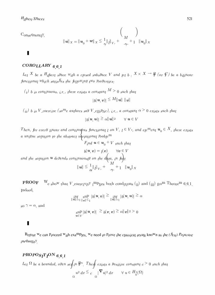
Hilbert Spaces 521
Consequently,
uX = u0 +wX ≤1
γlV +
M
γ+ 1
u0X
COROLLARY 6.6.1
Let X be a Hilbert space with a closed subspace V and let b : X × X → IR (or IC) be a bilinear
functional which satisfies the following two properties:
(i) b is continuous, i.e., there exists a constant M > 0 such that
|b(u,v)| ≤Mu v
(ii) b is V -coercive (some authors say V -elliptic), i.e., a constant α > 0 exists such that
|b(u,u)| ≥ αu2 ∀ u ∈ V
Then, for every linear and continuous functional l on V , l ∈ V , and element u0 ∈ X, there exists
a unique solution to the abstract variational problem
Find u ∈ u0 + V such that
b(u,v) = l(v) ∀v ∈ V
and the solution u depends continuously on the data, in fact
u ≤1
αlV +
M
γ+ 1
u0X
PROOF We show that V -coercivity implies both conditions (ii) and (iii) from Theorem 6.6.1.
Indeed,
infu=1
supv≤1
|b(u,v)| ≥ infu=1
|b(u,u)| ≥ α
so γ = α, and
supu∈V
|b(u,v)| ≥ b(v,v) ≥ αv2 > 0
Before we can proceed with examples, we need to prove the classical result known as the (first) Poincare
inequality.
PROPOSITION 6.6.1
Let Ω be a bounded, open set in IRn. There exists a positive constant c > 0 such that
Ω
u2 dx ≤ c
Ω
|∇u|2 dx ∀ u ∈ H10 (Ω)
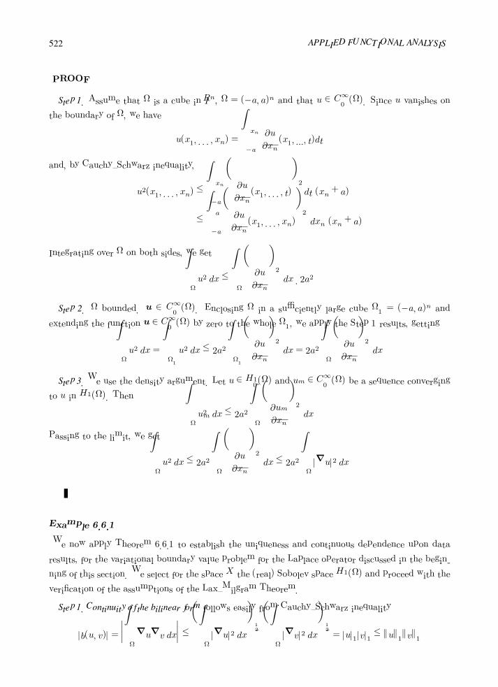
522 APPLIED FUNCTIONAL ANALYSIS
PROOF
Step 1. Assume that Ω is a cube in IRn, Ω = (−a, a)n and that u ∈ C∞0 (Ω). Since u vanishes on
the boundary of Ω, we have
u(x1, . . . , xn) =
xn
−a
∂u
∂xn(x1, ..., t)dt
and, by Cauchy–Schwarz inequality,
u2(x1, . . . , xn) ≤
xn
−a
∂u
∂xn(x1, . . . , t)
2
dt (xn + a)
≤
a
−a
∂u
∂xn(x1, . . . , xn)
2
dxn (xn + a)
Integrating over Ω on both sides, we get
Ω
u2 dx ≤
Ω
∂u
∂xn
2
dx · 2a2
Step 2. Ω bounded. u ∈ C∞0 (Ω). Enclosing Ω in a sufficiently large cube Ω1 = (−a, a)n and
extending the function u ∈ C∞0 (Ω) by zero to the whole Ω1, we apply the Step 1 results, getting
Ω
u2 dx =
Ω1
u2 dx ≤ 2a2
Ω1
∂u
∂xn
2
dx = 2a2
Ω
∂u
∂xn
2
dx
Step 3. We use the density argument. Let u ∈ H10 (Ω) and um ∈ C∞
0 (Ω) be a sequence converging
to u in H1(Ω). Then
Ω
u2m dx ≤ 2a2
Ω
∂um
∂xn
2
dx
Passing to the limit, we get
Ω
u2 dx ≤ 2a2
Ω
∂u
∂xn
2
dx ≤ 2a2
Ω
|∇u|2 dx
Example 6.6.1
We now apply Theorem 6.6.1 to establish the uniqueness and continuous dependence upon data
results, for the variational boundary value problem for the Laplace operator discussed in the begin-
ning of this section. We select for the space X the (real) Sobolev space H1(Ω) and proceed with the
verification of the assumptions of the Lax–Milgram Theorem.
Step 1. Continuity of the bilinear form follows easily from Cauchy–Schwarz inequality
|b(u, v)| =
Ω
∇u∇v dx
≤
Ω
|∇u|2 dx
12
Ω
|∇v|2 dx
12
= |u|1|v|1 ≤ u1v1

Hilbert Spaces 523
where |u|1 and u1 denote the first order Sobolev seminorm and norm respectively, i.e.,
|u|21 =
Ω
|∇u|2 dx =
Ω
2
i=1
∂u
∂xi
2
dx
u21 =
Ω
u2 + |∇u|2
dx = u2
0 + |u|21
with u0 denoting the L2-norm.
Step 2. Continuity of the linear functional l follows from Lions’ Trace Theorem; see [6, 8, 7]. It can be
proved that there exists a linear and continuous operator γ, called the trace operator, from the space
H1(Ω) onto a boundary fractional Sobolev space H12 (∂Ω) continuously embedded and dense in L2(∂Ω)
such that for regular functions u, values of γu coincide with the restriction of u to the boundary Γ,
i.e.,γ : H1(Ω)→ H
12 (Γ), u→ γu
γuH
12 (Γ
≤ CuH1(Ω) ∀ u ∈ H1(Ω)
γu = u|∂Ω ∀ u ∈ C(Ω) ∩H1(Ω)
for some C > 0. At the same time,
uL2(Γ) ≤ uH12 (Γ)
∀ u ∈ H12 (Γ)
so,
γuL2(Γ) ≤ CuH1(Ω) ∀ u ∈ H1(Ω)
As we can see, a “simple” verification of the assumptions of the Lax–Milgram Theorem can get fairly
technical. Assuming now regularity assumptions for data f and g as
f ∈ L2(Ω), g ∈ L2(Γt)
we interpret the linear functional l precisely as follows:
l(v) =
Ω
fv dx+
Γ
gγv ds
where function g has been extended by zero to the whole boundary Γ. It follows now from Cauchy–
Schwarz inequality and the Trace Theorem that l is continuous
|l(v)| ≤
Ω
fv dx
+
Γ
gγv ds
≤ f0v0 + CgL2(Γt)v1
≤f0 + CgL2(Γt)
v1
Step 3. We identify V as the (sub)space of all kinematically admissible functions satisfying the
homogeneous kinematic (Dirichlet) boundary conditions on Γu.
V =v ∈ H1(Ω) : γv = 0 on Γu

524 APPLIED FUNCTIONAL ANALYSIS
Assuming that meas (Γu) > 0, it follows now from the continuity of the trace operator γ and the
restriction operator:
L2(Γ) u→ u|Γu∈ L2(Γu)
that V is a closed subspace of H1(Ω).
Step 4. V -coercivity of the bilinear functional B follows from another very nontrivial result for
the Sobolev spaces, the (Rellich) Compact Imbedding Theorem, see [1], which holds under the
assumption that meas(Γu) > 0.
In the case when Γu coincides with the whole boundary Γ, a simpler argument, based on the
Poincare inequality, can be used. Indeed, by Proposition 6.6.1, we have
|u|21 ≥ εu20 ∀ u ∈ H1
0 (Γ)
and, consequently,
Ω
|∇u|2 dx =1
2|u|21 +
1
2|u|21
≥ε
2u2
0 +1
2|u|21
≥ min
ε
2,1
2
u21
for every u ∈ V = H10 (Ω).
Step 5. Postulating finally that function u0 can be extended to a function u0 defined on the whole
Ω such that u0 ∈ H1(Ω), we conclude, by the Lax–Milgram Theorem, that there exists a unique
solution u to the problem
Find u ∈ u0 + V such that
Ω
∇u∇v dx =
Ω
fv dx+
Γt
gv ds ∀ v ∈ V
where, for simplicity, the symbol of trace operator has been omitted.
Solution u depends continuously on the data. There exists positive constants C1, C2, C3, such
that
uH1(Ω) ≤ C1fL2(Ω) + C2gL2(Γt) + C3u0H1(Ω)
REMARK 6.6.1
1. Regularity assumptions on functions f and g are by no means unique! The only condition
is that whatever we assume of f and g, it must imply that the corresponding functional l
is continuous. In the case of Ω ⊂ IR2, it follows, for instance, from the Sobolev Imbedding
Theorems (see [1]) that one can assume that f ∈ Lp(Ω) with any p > 1.

Hilbert Spaces 525
2. Existence and continuity of the trace operator γ from H1(Ω) into L2(Γ) (then, it is not surjec-
tive) can be proved directly, skipping the technical considerations of fractional Sobolev spaces
on the boundary Γ (see [8]).
Example 6.6.2
In the case of Γu = ∅, i.e., the pure Neumann problem, a solution cannot be unique, as adding
an arbitrary constant c to any solution u produces another solution as well. Application of the
Lax–Milgram Theorem, which implies uniqueness of the solution, requires more caution, and relies
on the concept of quotient spaces.
Step 1. We identify the space V = X as the quotient space H1(Ω)/V0, where V0 is the subspace
consisting of all constant modes (infinitesimal rigid body motions for the membrane problem). As
V0 is isomorphic with IR, we frequently write H1(Ω)/IR.
As a finite-dimensional subspace, V0 is closed and therefore, by the results in Sections 5.17 and 5.18,
the quotient space H1(Ω)/V0 is a Banach space with the norm
[u]H1(Ω)/V0
def= inf
c∈IRu+ cH1(Ω)
The infimum on the right-hand side is in fact attained and by a direct differentiation with respect
to c of the function u+ c2 (of one variable c), we find out that
c = −
Ω
u dx
Thus, the norm of the equivalence class of u coincides with the H1-norm of the representative with
a zero mean value.
[u]H1(Ω)/V0= u1
H where u ∈ [u],
Ω
u dx = 0
By the direct verification of the parallelogram law or polarization formula (comp. Exercise 6.1.2), we
may check that every quotient space which has been obtained from a Hilbert space, is in fact a
Hilbert space itself.
Step 2. We define the bilinear form on the quotient space as
b([u], [v]) =
Ω
∇u∇v dx, u ∈ [u], v ∈ [v]
As the right-hand side is independent of the representantives u, v, the bilinear form is well-defined.
It is also continuous as follows by taking the infimum with respect to u and v on the right-hand side
of the inequality
Ω
∇u∇v dx
≤ u1v1

526 APPLIED FUNCTIONAL ANALYSIS
implies
|b([u], [v])| ≤ infu∈[u]
u1 infv∈[v]
v1 = [u]V [v]V
where V = H1(Ω)/V0.
Step 3. It follows from Cauchy–Schwarz inequality that
Ω
u dx
≤
Ω
u2 dx
12
Ω
dx
12
and, consequently,
Ω
|∇u|2 dx+
Ω
u dx
2
≤
Ω
|∇u|2 dx+meas(Ω)
Ω
u2 dx
≤ max(1,meas(Ω)) u2H1(Ω)
for every u ∈ H1(Ω).
For a class of domains Ω (satisfying the so-called segment property) it follows from the Sobolev
Imbedding Theorems that the inverse inequality (sometimes called the second Poincare inequality)
holds, i.e., there is a positive number C > 0 such that
u2H1(Ω) ≤ C
Ω
|∇u|2 dx+
Ω
u dx
2
for every u ∈ H1(Ω).
This inequality implies immediately that the bilinear form B is coercive on the quotient space.
Indeed, we have
b([u], [u]) =
Ω
|∇u|2 dx ≥1
Cu2
H1(Ω) =1
C[u]2
H1(Ω)/V0
provided u ∈ [u],
Ω
u dx = 0.
The transformation T mapping the closed subspace of functions from H1(Ω) with zero average
onto the quotient space V is identified as an isomorphism of Banach spaces, and can be used to
introduce a scalar product in the quotient space
([u], [v])Vdef= (u, v)H1(Ω)
where u ∈ [u], v ∈ [v], and
Ω
u dx =
Ω
v dx = 0.
Step 4. Continuity of linear functional l. Introducing the linear functional l on the quotient space V
as
l([v]) =
Ω
fv dx+
Γ
gγv ds
where v ∈ [v] and γ is the trace operator, we first of all see that, to be well-defined, i.e., independent
of a particular representative v ∈ [v], the right-hand side must vanish for v = const. This is equivalent
to
Ω
f dx+
Γ
g ds = 0
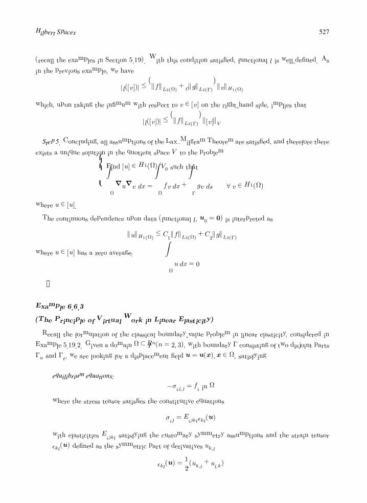
Hilbert Spaces 527
(recall the examples in Section 5.19). With this condition satisfied, functional l is well-defined. As
in the previous example, we have
|l([v])| ≤fL2(Ω) + cgL2(Γ)
vH1(Ω)
which, upon taking the infimum with respect to v ∈ [v] on the right-hand side, implies that
|l([v])| ≤fL2(Γ)
[v]V
Step 5. Concluding, all assumptions of the Lax–Milgram Theorem are satisfied, and therefore there
exists a unique solution in the quotient space V to the problem
Find [u] ∈ H1(Ω)/V0 such that
Ω
∇u∇v dx =
Ω
fv dx+
Γ
gv ds ∀ v ∈ H1(Ω)
where u ∈ [u].
The continuous dependence upon data (functional l, u0 = 0) is interpreted as
uH1(Ω) ≤ C1fL2(Ω) + C2gL2(Γ)
where u ∈ [u] has a zero average:
Ω
u dx = 0
Example 6.6.3
(The Principle of Virtual Work in Linear Elasticity)
Recall the formulation of the classical boundary-value problem in linear elasticity, considered in
Example 5.19.2. Given a domain Ω ⊂ IRn(n = 2, 3), with boundary Γ consisting of two disjoint parts
Γu and Γt, we are looking for a displacement field u = u(x),x ∈ Ω, satisfying
equilibrium equations:
−σij,j = fi in Ω
where the stress tensor satisfies the constitutive equations
σij = Eijklkl(u)
with elasticities Eijkl satisfying the customary symmetry assumptions and the strain tensor
kl(u) defined as the symmetric part of derivatives uk,l
kl(u) =1
2(uk,l + ul,k)

528 APPLIED FUNCTIONAL ANALYSIS
kinematic boundary conditions:
ui = ui on Γu
traction boundary conditions:
ti = qi on Γt
where t = (ti) is the stress vector defined as
ti = σijnj
with n = (nj) the outward normal unit to boundary Γ.
In order to derive a variational formulation for the problem, we pick an arbitrary test function
v = (vi), multiply both sides of the equilibrium equations by vi and integrate over Ω, getting
−
Ω
σij,jvi dx =
Ω
fivi dx
Integrating next first integral by parts, we have
−
Ω
σij,jvi dx =
Ω
σijvi,j dx−
Γ
σijnjvi dS
But, due to the symmetry of the stress tensor,
σij(u)vi,j = σij(u)ij(v)
so, consequently,
Ω
σij(u)ij(v) dx =
Ω
fivi dx+
Γ
ti(u)vi dS
Finally, restricting ourselves only to test functions vanishing on Γu, and using the traction boundary
conditions, we arrive at the variational formulation in the form
Find u = u(x),u = u on Γu such that
Ω
σij(u)ij(v) dx =
Ω
fivi dx+
Γ
qivi dS for every v : v = 0 on Γu
The formulation above is recognized as the classical principle of virtual work in mechanics. Test
function v = v(x) is interpreted as the virtual displacement, the integral on the left-hand side as the
virtual work done by stresses σij(u) on strains ij(v) corresponding to the virtual displacement, and
the integral on the right-hand side as the work of exterior forces.
Thus every solution u to the (classical) boundary value problem is also a solution to the variational
formulation, i.e., it satisfies the principle of virtual work.
Conversely, by reversing the entire procedure, we can show that any regular enough solution of
the variational formulation is a solution in the classical sense as well.
For a precise analysis of the elasticity problem by means of the Lax–Milgram Theorem, we refer
the reader to [2].

Hilbert Spaces 529
Sesquilinear Forms. In the case of complex-valued functions, when deriving the variational formulation,
we frequently prefer to multiply the original equation not by a test function v(x), but rather its complex
conjugate v(x). In the case of the boundary value problem for the Laplace operator, we get
Find u(x)such that u = u0 on Γu and
Ω
∇u∇v dx =
Ω
fv dx+
Γ
gv dS for every v = v(x) vanishing on Γu
Consequently, the functional on the left-hand side is not linear, but antilinear with respect to the second
variable, similarly as in the definition of a scalar product in a complex Hilbert space. Also, the right-hand
side is identified as an antilinear functional of v. The particular advantage of such an approach is that, for
symmetric sesquilinear forms, i.e.,
b(u,v) = b(v,u)
value b(u,u), interpreted most of the time in physical applications as an energy, is real.
It is easily verified that antilinear and continuous functionals share all the properties of linear and con-
tinuous functionals. In particular they form a normed vector space with the norm defined as for the linear
functionals, i.e.,
f = supu≤1
|f(u)| (6.16)
In fact many authors prefer to define the algebraic and topological duals of a complex vector space as the
space of antilinear rather than linear functionals. As a result of such a definition, a few little algebraic
changes follow. For instance, the Riesz map is always linear (not antilinear like in our version), and the map
prescribing for a linear operator A its transpose A is antilinear (comp. properties of adjoint operators on
Hilbert spaces).
All these modifications are very cosmetic in nature as there exists a one-to-one correspondence between
all linear and antilinear functionals defined through the complex conjugate operation. To see it, define the
map J prescribing for each linear functional f : V → IC on a complex vector space V its complex conjugate
J(f) = f defined by
J(f)(u) = f(u)def= f(u) (6.17)
It is a straightforward exercise to check that J is antilinear, bijective and norm preserving.
Using J we can easily reinterpret all results concerning linear functionals in terms of antilinear ones and
vice versa. In particular, we have the following reinterpretation of the Generalized Lax–Milgram Theorem
for sesquilinear forms.
COROLLARY 6.6.2
(The Generalized Lax-Milgram Theorem for Sesquilinear Forms)
Let all assumptions of Theorem 6.6.1 or Corollary 6.6.1 hold, except that b is sesquilinear rather
than bilinear and l is an antilinear, continuous functional on V . Then, all the conclusions hold as
well.
530 APPLIED FUNCTIONAL ANALYSIS
PROOF The proof follows exactly the lines of proof of Theorem 6.6.1. In the first step, we
assume u0 = 0 and reinterpret the variational formulation in the operator form as
Bu = l (6.18)
where B is the operator corresponding to the sesquilinear form
Bu,vdef= b(u,v) (6.19)
The only difference now is that B takes vectors from U into antilinear and continuous functionals
on U . Due to linearity of B in u, B is still a linear operator and consequently the rest of the proof
holds without any change.
Exercises
Exercise 6.6.1 LetX be a Hilbert space and V a closed subspace. Prove that the quotient spaceX/V , which
a priori is only a Banach space, is in fact a Hilbert space.
6.7 Generalized Green’s Formulas for Operators on Hilbert Spaces
As we have seen in the previous chapter, variational boundary value problems can be treated as generaliza-
tions of classical formulations. If a solution to such a variational problem is additionally sufficiently regular
then it is also a solution to the classical formulation. The question now is whether we can interpret all
variational solutions (including those “less” regular as well) as the solutions to the original boundary value
problems, and if the answer is “yes,” then in what sense?
Trace Property. An abstraction of the idea of boundary values of functions from a Hilbert space, exempli-
fied in the Trace Theorem for Sobolev spaces, is embodied in the concept of spaces with a trace property. A
Hilbert space V is said to have the trace property if the following conditions hold
1. V is continuously imbedded in a larger Hilbert space H
V → H
Note that this in particular implies that the topology of H , when restricted to V , is weaker than the
original topology of V .

Hilbert Spaces 531
2. There exists a linear and continuous (trace) operator γ that maps V onto another (boundary) Hilbert
space ∂V such that the kernel of γ, denoted V0, is everywhere dense in H
V0 = H, V0 = kerγ = N (γ)
It follows that the original space V is dense in H as well.
Example 6.7.1
Let Ω be a smooth open set in IRn with boundary Γ and let V = H1(Ω) be the first-order Sobolev
space . Then V satisfies the trace property whereH = L2(Ω), ∂V = H12 (Γ), and γ : H1(Ω)→ H
12 (Γ)
is the actual trace operator.
Let ι denote now the continuous inclusion operator from a Hilbert space V imbedded in a Hilbert spaceH
and let us assume that V is dense in H,V = H . Its transpose ιT maps dual H into dual V and it may be
used to identify H as a subspace of V , provided it is injective. Since
ιT (f) = f ι = f |V
this means that, from the fact that two linear functionals continuous in H coincide on subspace V , should
follow that they are equal to each other on the entire H
f |V = g|V ⇒ f = g f, g ∈ H
But this follows immediately from continuity of f and g and density of V in H . Indeed, let x ∈ H and xn
be a sequence in V converging to x. Then
f(xn) = g(xn)
and in the limit f(x) = g(x), as required.
Frequently space H is identified with its dual H using the Riesz map and, in such a case, called the pivot
space. We shall write shortly then
V → H ∼ H → V
both imbeddings being continuous.
Example 6.7.2
Let Ω be an open set in IRn. Then
H10 (Ω) → L2(Ω) ∼ (L2(Ω)) → H−1(Ω)
and the L2(Ω) space is a pivot space.

532 APPLIED FUNCTIONAL ANALYSIS
Formal Operators and Formal Adjoints. Let U and V be now two Hilbert spaces satisfying the trace
property, with the corresponding pivot spaces G and H and boundary spaces ∂U and ∂V , i.e.,
U → G ∼ G → U V → H ∼ H → V
β : U ∂U γ : V ∂V
U0def= kerβ V0
def= kerγ
U0 → G ∼ G → U 0 V0 → H ∼ H → V
0
All mappings are continuous and symbols → and are used to indicate injective and surjective operations,
respectively.
Consider now a bilinear and continuous functional b defined on U × V . Restricting first functional b to
U × V0 only (think: the test functions v vanishing on the boundary), we consider the corresponding linear
and continuous operator B : U → V 0 defined as
Bu,vV0 = b(u,v) ∀u ∈ U,v ∈ V0
The operator B is called the formal operator associated with the bilinear form. Note the difference between
the formal operator and operator B corresponding to b and considered in the proof of the Lax–Milgram
Theorem.
In a similar manner, by inverting the order of arguments we can consider a corresponding bilinear form b∗
on V × U
b∗(v,u)def= b(u,v)
with the corresponding formal operator B∗ : V → U 0
B∗v,uU0
def= b∗(v,u) = b(u,v) ∀u ∈ U0,v ∈ V
Operator B∗ is known as the formal adjoint of B.
Green’s Formulae. As H is only a proper subspace of V 0 , a value of formal operator Bu cannot be
identified in general with a linear and continuous functional on H .
For some elements u, however, namely for u ∈ B−1(H), the value of formal operator Bu belongs to H
and therefore by the Riesz Representation Theorem
b(u,v) = Bu,vV0 = (v, R−1H Bu)H ∀v ∈ V0
As H is identified with its dual, it is customary to drop the symbol for the Riesz map R−1H and replace the
composition R−1H B with B itself writing
b(u,v) = (v, Bu)H ∀v ∈ V0
where B is understood now as the operator from a subspace of U into H .

Hilbert Spaces 533
But both b(u, ·) and (·, Bu)H now are linear and continuous functionals on the whole V and therefore
their difference
b(u, ·)− (·, Bu)H
can be identified as an element from V , vanishing on V0.
Consider now the boundary space ∂V and trace operator γ : V → ∂V . From the surjectivity of γ follows
that the corresponding operator γ defined on the quotient (Banach!) space V/V0 into ∂V
γ : V/V0 → ∂V
is injective and continuous. Consequently, by the corollary to the Open Mapping Theorem, the inverse γ−1
is continuous as well.
This in particular implies that the boundary space ∂V can be equipped with an equivalent norm of the form
|||w|||∂Vdef= infvV : γv = w
Indeed, taking the infimum in v on the right-hand side of
γv∂V ≤ γvV
we get
γv∂V ≤ γ|||γv|||∂V
At the same time, reinterpreting continuity of γ−1, we get
γ−1(w)V/V0= inf
γv=wvV = |||w|||∂K ≤ γ
−1w∂K
Consider now an arbitrary element w ∈ ∂V and define a linear functional ∂u on ∂V by
∂u,w = b(u,v)− (v, Bu)H
where v ∈ V is an arbitrary element from V such that γv = w. As the right-hand side vanishes for v ∈ V0,
the functional ∂u is well-defined, i.e., its value is independent of the choice of v.
Introducing now a space
UB = u ∈ U : Bu ∈ H
with the (so called operator) norm
uUB
def= (u2
U + Bu2H)
12
we have immediately
|∂u,w| ≤ MuUvV + BuHvH
≤ (MuU + CBuH)vH

534 APPLIED FUNCTIONAL ANALYSIS
Taking infimum in v on the right-hand side we get
|∂u,w ≤ (MuU + CBuH)|||w|||∂V
which proves that ∂u is a continuous functional on ∂V and, at the same time, the operator ∂ : u → ∂u is a
linear and continuous operator from UB into the dual ∂V.
Operator ∂ is called the generalized Neumann operator corresponding to the trace (Dirichlet) operator
γ. The formula defining ∂u is known as the generalized or abstract Green’s formula (of the first type) for
operator B. Exactly the same results can be obtained for the bilinear form b∗(v,u) = b(u,v) and the
corresponding formal adjoint operator B∗.
We summarize the results in the following theorem.
THEOREM 6.7.1
Let U and V denote real Hilbert spaces with the trace properties previously described, and let b
denote a continuous, bilinear form from U ×V into IR with associated formal operators B ∈ L(U, V 0)
and B∗ ∈ L(V, U 0). Moreover, let UB and VB∗ denote the spaces
UBdef= u ∈ U : Bu ∈ H (H ∼ H ⊂ V
0)
VB∗def= v ∈ V : B∗v ∈ G (G ∼ G ⊂ U
0)
with the operator normsu2
UB= u2
U + Bu2H
v2VB∗
= v2V + B∗v2
G
Then there exist uniquely defined operators
∂ ∈ L(UB , ∂V), ∂∗ ∈ L(VB∗ , ∂U
)
such that the following formulas hold
b(u,v) = (v, Bu)H + ∂u, γv∂V u ∈ UB ,v ∈ V
b(u,v) = (u, B∗v)G + ∂∗v, βu∂U u ∈ U,v ∈ VB∗
A schematic diagram illustrating the various spaces and operators is given in Fig. 6.5.
Green’s Formula of the Second Type. As an immediate corollary of Theorem 6.7.1 we get Green’s for-
mula of the second type
(u, B∗v)G = (Bu,v)H + ∂u, γv∂V − ∂∗v, βu∂U
for every u ∈ UB ,v ∈ V ∗B∗ .
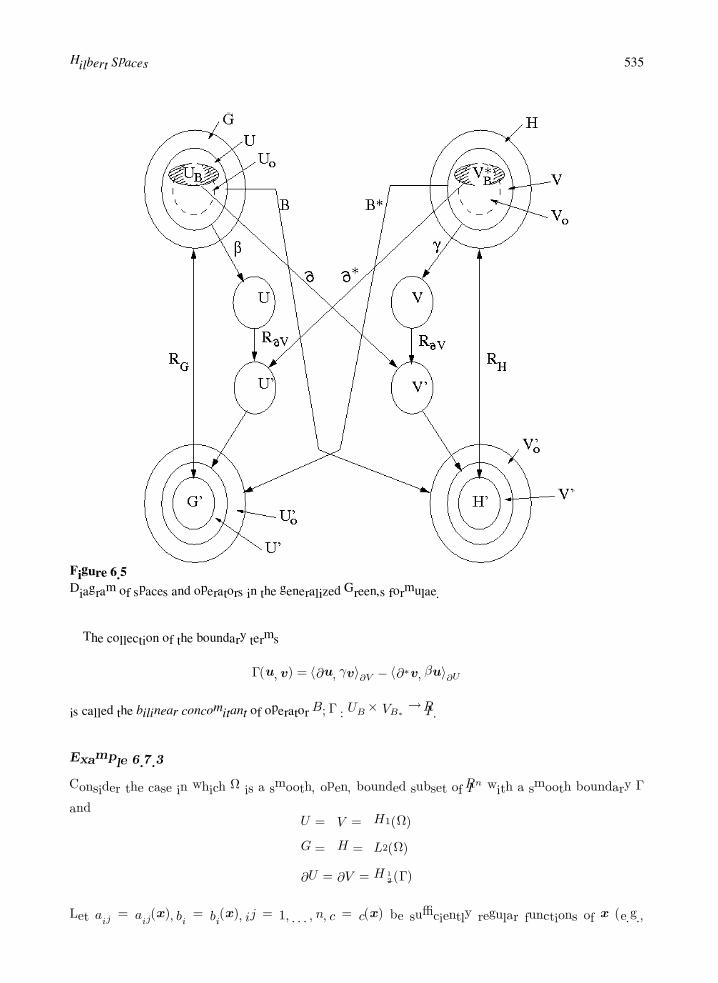
Hilbert Spaces 535
Figure 6.5
Diagram of spaces and operators in the generalized Green’s formulae.
The collection of the boundary terms
Γ(u,v) = ∂u, γv∂V − ∂∗v, βu∂U
is called the bilinear concomitant of operator B; Γ : UB × VB∗ → IR.
Example 6.7.3
Consider the case in which Ω is a smooth, open, bounded subset of IRn with a smooth boundary Γ
andU = V = H1(Ω)
G = H = L2(Ω)
∂U = ∂V = H12 (Γ)
Let aij = aij(x), bi = bi(x), ij = 1, . . . , n, c = c(x) be sufficiently regular functions of x (e.g.,

536 APPLIED FUNCTIONAL ANALYSIS
aij , bi ∈ C1(Ω)), and define the bilinear form b : H1(Ω)×H1(Ω)→ IR by
b(u, v) =
Ω(
n
i,j=1
aij∂u
∂xj
∂v
∂xi+
n
j=1
bj∂u
∂xjv + cuv) dx
Obviously, if u is sufficiently smooth (e.g., u ∈ C2(Ω)) then
b(u, v) =
Ω(−
n
i,j=1
∂
∂xi(aij
∂u
∂xj) +
n
j=1
bj∂u
∂xj+ cu)v dx
+
Γ(
n
i,j=1
aij∂u
∂xjni)v dS
where n = (ni) is the outward normal unit to boundary Γ.
This prompts us to consider the formal operator
B : H1(Ω)→ (H10 (Ω))
= H−1(Ω)
Bu, v = b(u, v) u ∈ H1(Ω), v ∈ H10 (Ω)
to be a generalization of the classical operator
−
n
i,j=1
∂
∂xi(aij
∂
∂xj) +
n
j=1
bj∂
∂xj+ c
Function u belongs to
UB = u ∈ H1(Ω) : Bu ∈ L2(Ω)
if and only if a function f ∈ L2 exists such that
b(u, v) =
Ωfv dx ∀v ∈ H1
0 (Ω)
or, equivalently,
−
n
i,j=1
∂
∂xi(aij
∂u
∂xj) +
n
j=1
bj∂u
∂xj+ cu = f
Note that from this it does not follow that u ∈ H2(Ω)!
Finally, the generalized Neumann operator is interpreted as a generalization of the classical oper-
ator
∂u =n
i,j=1
aij∂u
∂xjni ∂ : UB → H− 1
2 (Γ)
Similarly, for sufficiently smooth v
b(u, v) =
Ωu(−
n
i,j=1
∂
∂xj(aij
∂v
∂xi)−
n
j=1
∂
∂xj(bjv) + cv)dx
+
Γu
n
j=1
(
n
i=1
aij∂v
∂xi+ bjv)nj dS

Hilbert Spaces 537
which prompts for the interpretations
B∗ : H1(Ω)→ H−1(Ω)
B∗v = −
n
i,j=1
∂
∂xj(aij
∂v
∂xi)−
n
j=1
∂
∂xj(bjv) + cv
VB∗ = v ∈ H1(Ω) : B∗v ∈ L2(Ω)
∂∗v =
n
j=1
(
n
i=1
aij∂v
∂xi+ bjv)nj , ∂∗ : VB∗ → H− 1
2 (Γ)
The bilinear concomitant is a generalization of
Γ(u, v) =
Γ(
n
i,j=1
aij∂u
∂xjniv − u
n
j=1
(
n
i=1
aij∂v
∂xi+ bjv)nj) dS
Example 6.7.4
(Interpretation of Solutions to Variational Problems)
Let u be a solution to the variational problem considered in Example 6.6.1
Find u ∈ u0 + V such that
Ω∇u∇v dx =
Ωfv dx+
Γt
gγv dS ∀v ∈ V
where
V = u ∈ H1(Ω) : γu = 0 on Γu
and γ : H1(Ω)→ H12 (Γ) is the trace operator.
The space of traces ∂V , identified as the image of operator γ does not coincide with H12 (Γt) (unless
Γu = ∅!) and is frequently denoted as the space H00(Γt). Functions from H00(Γt) must decay at an
appropriate rate when approaching boundary of Γt, see [6].
Taking v ∈ H10 (Ω) = kerγ in the variational formulation, we get
Ω∇u∇v dx =
Ωfv dx ∀v ∈ H1
0 (Ω)
Consequently, −∆u = f ∈ L2(Ω), which implies that u is in the domain of the generalized Neumann
operator∂
∂n: H1(∆)→ (H00(Γt))
where
H1(∆) = u ∈ H1(Ω) : ∆u ∈ L2(Ω)
538 APPLIED FUNCTIONAL ANALYSIS
From the generalized Green’s formula follows finally that
∂u
∂n, v =
Γt
gv dS ∀v ∈ H00(Γt)
Summing that up, u being a variational solution implies that
1. u is a solution to the differential equation in the distributional sense,
2. u satisfies the Dirichlet boundary condition in the sense of the trace operator
γu = γu0 on Γu
3. u satisfies the Neumann boundary condition in the sense of the generalized Neumann operator
∂u
∂n= g on Γt
Conversely, by reversing the entire procedure, it can be immediately shown that any u satisfying
the conditions above is a solution to the variational problem as well.
All presented results can be immediately generalized to the case of complex Hilbert spaces and sesquilinear
forms with the dual spaces redefined as the spaces of antilinear functionals.
THEOREM 6.7.2
Let U and V denote two complex Hilbert spaces satisfying the trace property with corresponding pivot
spaces G and H, boundary spaces ∂U and ∂V and trace operators β : U → ∂U and γ : V → ∂V
respectively. All dual spaces are defined as spaces of antilinear functionals.
Let b : U×V → IC be a continuous, sesquilinear form with associated formal operators B ∈ L(U, V 0)
and B∗ ∈ L(V, U 0) defined as
Bu,vdef= b(u,v) u ∈ U,v ∈ V0
B∗v,udef= b∗(v,u)
def= b(u,v) v ∈ V,u ∈ U0
Moreover, let UB and VB∗ denote the spaces
UBdef= u ∈ U : Bu ∈ H (H ∼ H ⊂ V
0)
VB∗def= v ∈ V : B∗v ∈ G (G ∼ G ⊂ U
0)
with the operator norms
u2UB
= u2U + Bu2
H
v2VB∗
= v2V + B∗v2
G

Hilbert Spaces 539
Then there exist unique operators
∂ ∈ L(UB , ∂V), ∂∗ ∈ L(VB∗ , ∂U
)
such that the following formulas hold
b(u,v) = (Bu,v)H + ∂u, γv∂V u ∈ UB ,v ∈ V
b(u,v) = b∗(v,u) = (B∗v,u)G + ∂∗v, βu∂U u ∈ U,v ∈ VB∗
or, equivalently,
b(u,v) = (u, B∗v)G + ∂∗v, βu∂U u ∈ U,v ∈ VB∗
As for the real spaces, Green’s formula of the second type follows
(u, B∗v)G = (Bu,v)H + ∂u, γv∂V − ∂∗v, βu∂U
for u ∈ UB ,v ∈ VB∗ .
Exercises
Exercise 6.7.1 Consider the elastic beam equation
(EIw) = q 0 < x < l
with the boundary conditions
w(0) = w(0) = 0 and w(l) = EIw(l) = 0
(a) Construct an equivalent variational formulation, identifying appropiate spaces.
(b) Use the Lax–Milgram Theorem to show that there exists a unique solution to this problem.
Exercise 6.7.2 Consider again the elastic beam equation
(EIw) = q 0 < x < l
with different boundary conditions
w(0) = EIw(0) = 0
EIw(l) = −Ml, (EIw)(l) = Pl
(a) Construct an equivalent variational formulation, identifying appropriate spaces.
(b) Use the Lax–Milgram Theorem to establish existence and uniqueness result in an appropriate
quotient space. Derive and interpret the necessary and sufficient conditions for the distributed
load q(x), momentMl and force Pl to yield the existence result.

540 APPLIED FUNCTIONAL ANALYSIS
Exercise 6.7.3 Let u, v ∈ H2(0, l) and b(·, ·) denote the bilinear form
b(u, v) =
l
0
(EIuv + Puv + kuv) dx
where EI, P , and k are positive constants. The quadratic functional b(u, u) corresponds to twice the
strain energy in an elastic beam of length l with flexural rigidityEI , on elastic foundation with stiffness
k and subjected to an axial load P .
(a) Determine the formal operator B associated with b(·, ·) and its formal adjoint B∗.
(b) Describe the spaces G,H,UB , VB∗ , ∂U, ∂V for this problem. Identify the trace operators.
(c) Describe the Dirichlet and Neumann problems corresponding to operators B and B∗.
(d) Consider an example of a mixed boundary-value problem for operator B, construct the corre-
sponding variational formulation and discuss conditions under which this problem has a unique
solution.
Exercise 6.7.4 Consider the fourth-order boundary-value problem in two dimensions:
∇2∇
2u+ udef=
∂4u
∂x4+ 2
∂4u
∂x2∂y2+
∂4u
∂y4+ u = f in Ω
u = 0,∂u
∂n= 0 on ∂Ω
with f ∈ L2(Ω). Construct a variational formulation of this problem, identifying the appropiate spaces,
and show that it has a unique solution. What could be a physical interpretation of the problem?
Elements of Spectral Theory
6.8 Resolvent Set and Spectrum
The spectral analysis of linear operators is basically a geometric study of the behavior of linear operators
with special regard to the existence of certain inverses. In particular, if A ∈ L(U,U), where U is a Hilbert
space, and if λ is a scalar, we are concerned with the existence of the inverse of the operator (λI − A). In
finite-dimensional spaces, the situation is clear: either (λI −A)−1 exists or it does not. If, for a given scalar
λ, it does not exist, then λ is called an eigenvalue of A, and if dim U = n, there are at most n (distinct)
eigenvalues.
However, when U is infinite-dimensional, there may be infinitely many, indeed a continuum of scalars λ
such that (λI − A)−1 does not exist. If (λI − A)−1 exists, the question arises as to whether it is a bounded

Hilbert Spaces 541
operator or, moreover, whether its domain, equal to the range R(λI − A), is dense in U . None of these
questions arises in the finite-dimensional case. These questions are in the province of the so-called spectral
theory of linear operators. The last part of this chapter presents an introductory account of this theory.
Eigenvalues and Characteristic Values of an Operator. Let U be a normed vector space over the complex
number field IC and let A be a linear operator from a subspace D = D(A) ⊂ U into itself. The problem of
finding scalars λ ∈ IC such that there exists u ∈ D,u = 0 satisfying the equation
(λI −A)u = 0
is called an eigenvalue problem associated with operator A. Any complex scalar λ such that the equality
holds for some non-zero vector u ∈ D is called an eigenvalue of A, and the corresponding non-zero vector u
is called an eigenvector of A corresponding to λ. The null space of the transformation N (λI − A) is called
the eigenmanifold (or eigenspace) corresponding to the eigenvalue λ, and the dimension of the eigenspace is
called the multiplicity of the eigenvalue λ. Note that a scalar λ is an eigenvalue of A if and only if the linear
transformation (λI −A) is singular; in other words, if the null space N (λI −A) is nontrivial.
For non-zero eigenvalues λ, we can rewrite the equation in the form
(I − λ−1A)u = 0
The inverse λ−1 is frequently called the characteristic value of operator A.
Resolvent Set. If operator λI −A has a continuous (bounded) inverse defined on a dense subset of U , i.e.,
if λI −A has a range dense in U , operator
Rλ = (λI −A)−1
is called the resolvent of A and λ is said to belong to the resolvent set r(A) of operator A.
Note that ifA is closed, it follows that λI−A is closed as well, and boundedness ofRλ implies that λI−A
has a closed range in U , and therefore the resolvent Rλ is defined on the whole space U .
Spectrum. The set of all complex numbers that are not in the resolvent set is called the spectrum of the
operator A and is denoted by σ(A). There is a number of situations in which the operator λI − A has no
continuous inverse defined on a dense subset of U . The transformation may not be injective when λ is an
eigenvalue of A. Another possibility is that the inverse may not be defined on a dense subset of U or it may
not be bounded. It is customary to divide the spectrum σ(A) into various categories, depending on which of
these circumstances a given scalar λ fails to be in the resolvent set r(A).
Point (or Discrete) Spectrum. The point spectrum of A is the subset of all λ’s for which (λI − A) is not
one-to-one. That is, the point spectrum, denoted σP (A), is exactly the set of all eigenvalues.

542 APPLIED FUNCTIONAL ANALYSIS
Residual Spectrum. This the subset of all λ’s for which (λI − A) has no range dense in U . The residual
spectrum is denoted by σR(A).
Continuous Spectrum. The continuous spectrum is the subset of all λ’s for which (λI −A) is one-to-one
and has range dense in U , but for which the inverse defined on its range is not continuous. The continuous
spectrum is denoted by σc(A).
From the definitions, it follows that σP (A), σR(A), and σc(A) are pairwise disjoint sets and that
σ(A) = σP (A) ∪ σR(A) ∪ σc(A)
Example 6.8.1
Consider the case in which U = L2(IR) and A is the differential operator
Au =du
dx
with its domain D(A) defined as
D(A) = H1(IR)
The eigenvalue problem associated with A
λu−du
dx= 0
has no non-zero solution as the general solution of the differential equation is
u(x) = Ceλx, C ∈ IC
and u ∈ L2(IR) only if C = 0. Thus the discrete spectrum of A is empty.
To determine the resolvent set of A, assume λ = a+ bi and consider the equation
λu−du
dx= v
for v ∈ L2(IR). Assume the equation above has a solution u ∈ H1(IR). Applying Fourier transforms
to both sides of the equation (comp. Example 6.1.6) yields
(λ− iξ)u(ξ) = v(ξ)
or
u(ξ) =1
a− i(ξ − b)v(ξ) =
a+ i(ξ − b)
a2 + (ξ − b)2v(ξ)
Consequently,
|u(ξ)|2 =1
a2 + (ξ − b)2|v(ξ)|2
and
|du
dx(ξ)|2 =
ξ2
a2 + (ξ − b)2|v(ξ)|2
which allows one to draw the following conclusions.

Hilbert Spaces 543
1. If a = Reλ = 0, then factors
1
a2 + (ξ − b)2,
ξ2
a2 + (ξ − b)2
are bounded and therefore v ∈ L2(IR) implies that both u and dudx are L2-functions which in
turn implies that u ∈ H1(IR). Consequently the range of λI−A is equal to the whole L2(IR). It
follows from the formula for u(ξ) that resolvent Rλ is continuous and therefore the resolvent
set r(A) contains all complex numbers λ with non-zero real part.
2. If a = 0 then factor1
(ξ − b)2
is not bounded and therefore the range of λI−A does not coincide with the whole L2(IR). It is,
however, dense in L2(IR). To see it, pick an L2-function v ∈ L2(IR) and consider a sequence vn
vn(ξ) =
0 if |ξ − b| < 1
n
v(ξ) otherwise
Obviously, vn → v in L2(IR) and the corresponding inverse transform vn converges to v. Thus
functions of this type form a dense subset of L2(IR). From the formula for u and dudx it follows
immediately that vn is in the range of λI −A.
The resolvent Rλ is not, however, continuous. To see it, it is sufficient to consider a sequence
of functions vn ∈ L2(IR) such that
vn(ξ) =
√n for |ξ − b| < 1
2n
0 otherwise
Obviously, vnL2 = vnL2 = 1 and by inspecting the formula for u we see that for the
corresponding sequence of functions un
unL2 →∞
Summing up, the spectrum of operator A consists only of its continuous part, coinciding with the
imaginary axis in the complex plane λ.
Asymptotic Eigenvalues. Let U be a normed space and let A : U ⊃ D(A) → U be a linear operator. A
complex number λ is called an asymptotic eigenvalue if there exists a sequence of unit vectors xn, xn = 1,
such that
(λI −A)xn → 0 for n→∞
Obviously, every eigenvalue λ is asymptotic, as one can select xn = x, where x is a unit eigenvector
corresponding to λ. The following proposition gives a simple characterization of essentially asymptotic
eigenvalues.

544 APPLIED FUNCTIONAL ANALYSIS
PROPOSITION 6.8.1
Let U be a normed space and let A : U ⊃ D(A) → U be a linear operator. Let λ be a complex
number such that λ ∈ σP (A), i.e., λI −A is injective. Then the following conditions are equivalent
to each other:
(i) λ is an asymptotic eigenvalue of A.
(ii) resolvent Rλ = (λI −A)−1 is unbounded.
PROOF
(i) ⇒ (ii). Let xn be a sequence of unit vectors, xn = 1 such that
(λI −A)xn → 0
Put
yn =(λI −A)xn
(λI −A)xn
Then yn = 1 and
Rλyn =xn
(λI −A)xn→ ∞
which proves that Rλ is unbounded.
(ii)⇒ (i). Unboundedness of Rλ implies that there exists a sequence of unit vectors yn, yn = 1,
such that
Rλyn → ∞
Put
xn =Rλyn
Rλyn
Vectors xn are unit and
(λI −A)xn =yn
Rλyn→ 0
which proves that λ is an asymptotic eigenvalue.
Exercises
Exercise 6.8.1 Determine spectrum of operator A : U ⊃ D(A)→ U where
U = L2(IR) D(A) = H1(IR) Au = idu
dx
Hint: Use Fourier transform (comp. Example 6.8.1).

Hilbert Spaces 545
6.9 Spectra of Continuous Operators. Fundamental Properties
In this section we examine some basic properties of operators A taking a (whole) Banach space U into itself.
If A were defined only on a subspace D(A) of U , then, by continuity, A could be automatically extended to
closure D(A) and then, say by zero, to the entire space U . The extension would also have been continuous
and the norm of A, A, would have not changed. Thus whatever we can prove for A defined on the whole
U , could be next reinterpreted for the restriction of A to the original D(A) and, therefore, it makes a very
little sense to “play” with continuous operators A which are defined on proper subspaces only.
We return now to Example 5.7.1 on Neumann series and consider the following sequence of partial sums
SN = I +A+ . . .+AN
The following proposition establishes a simple generalization of the Cauchy criterion of convergence for
infinite series of numbers.
PROPOSITION 6.9.1
Let U be a Banach space and A ∈ L(U,U) and let SN be the corresponding sequence of partial sums
defined above. The following properties hold:
(i) There exists a limit
c = limn→∞
An1n = inf
nAn
1n
(ii) If c < 1 then sequence SN is convergent.
(iii) If c > 1 then sequence SN diverges.
PROOF
(i) Define
a = infnAn
1n
It must be a ≤ A since
An = A . . . A ≤ An
Let > 0 be now an arbitrary small number. By definition of a, there must be an index m such that
Am1m ≤ a+
Set
Mdef= max1, A, . . . , Am−1

546 APPLIED FUNCTIONAL ANALYSIS
As every integer n can be represented in the form
n = knm+ ln, kn ∈ IZ, 0 ≤ ln ≤ m− 1
we obtaina ≤ (An)
1n ≤ (AlnAmkn)
1n
≤ M1n Am
knn ≤M
1n (a+ )
n−lnn
which, upon passing with n→∞, proves that
a ≤ lim inf An1n ≤ lim sup An
1n ≤ a+
from which (i) follows.
(ii) Denote an = An and recall the Cauchy convergence test for series of real numbers
c = limn→∞
(an)1n < 1 ⇒
∞
n=1
an convergent
Assuming that c < 1, we have for N < M
SM − SN = AN+1 + . . .+AM
≤ AN(A+ . . .+ AM−N)
≤ AN
∞
n=1
an → 0 for N →∞
Consequently, SN is a Cauchy sequence and, therefore, is convergent.
(iii) Let c > 1 and assume to the contrary that SN is convergent. From c > 1 it follows that
∃N ∀n ≥ N An1n ≥ 1 + , > 0
Consequently,
An ≥ (1 + )n ≥ 1 for n ≥ N
But, at the same time convergence of SN implies that AN → 0, a contradiction.
Spectral Radius of a Continuous Operator. The number
spr(A) = limn→∞
An1n
is called the spectral radius of operator A. Obviously
spr(A) ≤ A
Let λ ∈ IC be now an arbitrary complex number. Applying the Cauchy convergence criterion to the series
1
λ
∞
k=0
1
λkAk, SN =
1
λ
N
k=0
1
λkAk

Hilbert Spaces 547
we see that SN converges if |λ| > spr(A), and diverges if |λ| < spr(A). Moreover, passing to the limit in
(λI −A)SN − I = (A
λ)N+1
(comp. Example 5.7.1), we prove that for λ < spr(A), SN converges to a right inverse of λI −A.
Similarly, we prove that SN converges to a left inverse and consequently the resolvent
Rλ = (λI −A)−1 =1
λ
∞
k=0
λ−kAk
exists and is continuous for |λ| > spr(A). The whole spectrum of A therefore is contained in the closed ball
centered at origin with radius equal to the spectral radius.
Later on in this section, we outline a much stronger result showing that the spectral radius spr(A) is equal
to the radius of the smallest closed ball containing spectrum σ(A).
Consider now an arbitrary number λ0 from the resolvent set of A, λ0 ∈ r(A) and let λ denote some other
complex number. We have
λI −A = (λ0I −A) + (λ− λ0)I
= (λ0I −A)(I − (λ0 − λ)Rλ0)
= (λ0 − λ)(λ0I −A)((λ0 − λ)−1I −Rλ0)
and, formally,
(λI −A)−1 = (λ0 − λ)−1((λ0 − λ)−1I −Rλ0)−1Rλ0
Applying the Cauchy convergence criterion to
((λ0 − λ)−1I −Rλ0)−1
we immediately learn that, if |λ0 − λ|−1 > Rλ0 or, equivalently, |λ − λ0| < Rλ0
−1, then the inverse
above exists and is continuous. Consequently, resolvent Rλ exists and is continuous as well. Moreover, the
following formula holds
Rλ = (λ0 − λ)−1((λ0 − λ)−1I −Rλ0)−1Rλ0
It follows that the resolvent set r(A) is open and therefore the spectrum σ(A) must be closed. Since it is
simultaneously bounded, it must be compact.
We summarize our observations in the following proposition.
PROPOSITION 6.9.2
Let A be a bounded, linear operator from a Banach space U into itself. The following properties
hold:
(i) Spectrum of A, σ(A), is compact.

548 APPLIED FUNCTIONAL ANALYSIS
(ii) σ(A) ⊂ B(0, spr(A)).
(iii) For every |λ| > spr(A) the corresponding resolvent is a sum of the convergent Neumann series
Rλ =1
λ
∞
k=0
λ−kAk
(iv) For λ, µ ∈ r(A)
Rλ −Rµ = (µ− λ)RµRλ
In particular, resolvents are permutable.
(v) Resolvent set of A is contained in the resolvent set of the transpose operator A
r(A) ⊂ r(A)
(vi) In the case of a Hilbert space U , resolvent of the adjoint operator A∗, r(A∗), is equal to the
image of r(A) under the complex conjugate operation, i.e.,
λ ∈ r(A) ⇔ λ ∈ r(A∗)
PROOF It remains to prove (iv), (v), and (vi).
(iv) We have
Rλ −Rµ = (λI −A)−1 − (µI −A)−1
Multiplying by (λI −A) from the right-hand side and by (µI −A) from the left-hand side, we get
(µI −A)(Rλ −Rµ)(λI −A) = (µI −A)− (λI −A) = (µ− λ)I
which proves the assertion.
(v) We have
((λI −A)−1) = ((λI −A))−1 = (λI −A)−1
Thus if (λI −A)−1 exists and is continuous, then (λI −A) exists and is continuous as well.
Note that for reflexive spaces r(A) ⊂ r(A) = r(A) and therefore r(A) = r(A).
(vi) follows from the identity
((λI −A)−1)∗ = (λI −A∗)−1
We conclude this section with an important geometrical characterization of spectral radius. Only an outline
of the proof is provided as the proof uses essentially means of complex analysis exceeding the scope of this
book.

Hilbert Spaces 549
PROPOSITION 6.9.3
Let A be a bounded, linear operator from a Banach space U into itself. The following characterization
of the spectral radius holds
sprA = limn→∞
An1n = max
λ∈σ(A)|λ|
i.e., spectral radius is equal to the maximum (in modulus) number from the spectrum of A.
PROOF
Step 1. We define the characteristic set of A, denoted ρ(A), as the set of characteristic values of A
ρ(A)def= ρ ∈ IC : ∃u = 0 : (I − ρA)u = 0
Obviously, for λ = 0,
λ−1 ∈ ρ(A) ⇔ λ ∈ σ(A)
The characteristic set ρ(A), as an inverse image of spectrum σ(A) through the continuous map
λ→ λ−1, is closed and obviously does not contain 0.
Step 2. For ρ−1 = λ ∈ r(A) we introduce the resolvent (of the second kind) Bρ, defined as
Bρ = (I − ρA)−1
A direct calculation reveals the relation between the two types of resolvents
Rλ = λ−1I + λ−2Bλ−1
Step 3. Property (iv) proved in Proposition 6.9.2 implies that
Bρ −Bµ = (ρ− µ)BρBµ
Step 4. It follows from Step 3 that resolvent Bρ ∈ L(U,U) is a continuous function of ρ.
Step 5. It follows from Step 3 and Step 4 results that for any x ∈ U and f ∈ U function
φ(ρ) = f,Bρ(x)
is holomorphic in ρ (analytic in the complex sense). Indeed, it is sufficient to show that φ is
differentiable (analyticity in the complex sense is equivalent to the differentiability!). But
φ(ρ) = limµ→ρ
f,Bµ −Bρ
µ− ρ(x) = lim
µ→ρf,BµBρ(x) = f,B
2ρ(x)
Step 6. Consequently, φ(ρ) can be expanded into its Taylor’s series at ρ = 0:
φ(ρ) =
∞
k=0
φ(k)(0)
k!ρk
550 APPLIED FUNCTIONAL ANALYSIS
and, at the same time, from the definition of the spectral radius (comp. Proposition 6.9.1) follows
that
φ(ρ) =∞
k=0
f,Ak+1xρk
Both series, as the same representations of the same function must converge (uniformly!) in the ball
with the same radius. The second of the series converges for
|ρ| < (spr(A))−1 (|λ| = |ρ−1| > spr(A))
while the first one (a standard result from complex analysis) for all ρ from a ball containing no
singular points of φ(ρ), i.e.,
|ρ| < ( maxλ∈σ(A)
|λ|)−1
Consequently, it must be
maxλ∈σ(A)
= spr(A)
Exercises
Exercise 6.9.1 Let X be a real normed space and X × X its complex extension (comp. Section 6.1). Let
A : X → X be a linear operator and let A denote its extension to the complex space defined as
A((u, v)) = (Au,Av)
Suppose that λ ∈ IC is an eigenvalue of A with a corresponding eigenvector w = (u, v). Show
that the complex conjugate λ is an eigenvalue of A as well with the corresponding eigenvector equal
w = (u,−v).
Exercise 6.9.2 Let U be a Banach space and let λ and µ be two different eigenvalues (λ = µ) of an operator
A ∈ L(U,U) and its transpose A ∈ L(U , U ) with corresponding eigenvectors x ∈ U and g ∈ U .
Show that
g,x = 0
6.10 Spectral Theory for Compact Operators
In this section we focus on the special class of compact (completely continuous) operators on Banach and
Hilbert spaces.

Hilbert Spaces 551
Let T be a compact operator from a Banach space X into itself and λ a non-zero complex number. Ac-
cording to the Fredholm Alternative (comp. Section 5.20), operator λI − T or equivalently I − λ−1T has
either a continuous inverse (bijectivity and continuity of A = I − λ−1T implies continuity of A−1 = Rλ !)
or it is not injective and its null space
Xλ = N (I − λ−1T ) = N (λI − T )
has a finite dimension. Consequently, the whole spectrum of T , except for λ = 0, reduces to the point
spectrum σP (T ) consisting of eigenvalues λ with corresponding finite-dimensional eigenspaces Xλ.
The following theorem gives more detailed information on σP (T ).
THEOREM 6.10.1
Let T be a compact operator from a Banach space X into itself. Then σ(T ) − 0 consists of at
most a countable set of eigenvalues λn. If the set is infinite then λn → 0 as n→∞.
PROOF It is sufficient to prove that for every r > 0 there exists at most a finite number of
eigenvalues λn such that |λn| > r. Assume to the contrary that there exists an infinite sequence of
distinct eigenvalues λn, |λn| > r with a corresponding sequence of unit eigenvectors xn
Txn = λnxn, xn = 1
We claim that xn are linearly independent. Indeed, from the equality
xn+1 =
n
k=1
αkxk
follows that
λn+1xn+1 = Txn+1 =n
k=1
αkTxk =n
k=1
αkλkxk
and, consequently,
xn+1 =
n
k=1
αkλk
λn+1xk
As the coefficients αk are unique, there must be λk
λn+1= 1 for some k, a contradiction.
Let Xn denote now the span of the first n eigenvectors xk
Xn = spanx1, . . . ,xn
By Lemma on Almost Perpendicularity, there exists a sequence of unit vectors yn ∈ Xn such that
ρ(yn+1, Xn) >1
2, yn+1 = 1

552 APPLIED FUNCTIONAL ANALYSIS
Let now x ∈ Xn, i.e., x =n
k=1 αkxk. Then
Tx =n
k=1
αkTxk =
n
k=1
αkλkxk ∈ Xn
and, at the same time, denoting Bn = λnI − T
Bnx =
n
k=1
αk(λnI − T )xk =
n
k=1
αk(λn − λk)xk ∈ Xn−1
Thus, for m > n,
T (ym
λm)− T (
yn
λn) = ym −Bm(
ym
λm)− yn +Bn(
yn
λn) >
1
2
since
−Bm(ym
λm)− yn +Bn(
yn
λn) ∈ Xn
At the same time, sequence yn
λnis bounded (|λn| > r) and therefore we can extract a strongly con-
vergent subsequence from T (λ−1n yn), satisfying in particular the Cauchy condition, a contradiction.
For the rest of this section, we shall restrict ourselves to a more specialized class of compact operators –
the normal and compact operators. We begin by recording some simple observations concerning all normal
and continuous operators (not necessarily compact) on a Hilbert space U .
PROPOSITION 6.10.1
Let U be a Hilbert space and A ∈ L(U,U) be a normal operator, i.e., AA∗ = A∗A. The following
properties hold:
(i) For any eigenvalue λ of A and a corresponding eigenvector u, λ is an eigenvalue of A∗ with
the same eigenvector u.
(ii) For any two distinct eigenvectors λ1 = λ2 of A, the corresponding eigenvectors u1 and u2 are
orthogonal
(u1,u2) = 0
(iii) spr(A) = A.
PROOF
(i) If A is a normal operator then A− λI is normal as well and Proposition 6.5.3 implies that
(A− λI)u = (A∗ − λI)u

Hilbert Spaces 553
Consequently,
(A− λI)u = 0 ⇔ (A∗ − λI)u = 0
which proves the assertion.
(ii) We first prove that if λ1 is an eigenvalue of any operator A ∈ L(U,U) with a corresponding
eigenvector u1, and λ2 is an eigenvalue of adjoint A∗ with corresponding eigenvector u2 then (comp.
Exercise 6.9.2)
λ1 = λ2 implies (u1,u2) = 0
Indeed, for λ1 = 0 we have
(u1,u2) = (A(u1
λ1),u2) = (
u1
λ1, A∗u2) =
λ2
λ1(u1,u2)
which implies that (u1,u2) = 0.
We proceed similarly for λ2 = 0. Finally, (ii) follows from the orthogonality result just proved
and property (i).
(iii) follows immediately from Corollary 6.5.1 and the definition of spectral radius.
COROLLARY 6.10.1
Let A be a normal, compact operator from a Hilbert space U into itself. Then the norm of A is equal
to the maximum (in modulus) eigenvalue of A.
PROOF The proof follows immediately from Proposition 6.9.3, Theorem 6.10.1, and Proposi-
tion 6.10.1 (iii).
We are ready now to state our main result for compact and normal operators on Hilbert spaces.
THEOREM 6.10.2
(Spectral Decomposition Theorem for Compact and Normal Operators)
Let U be a Hilbert space and let T ∈ L(U,U) be a compact and normal operator. Let
|λ1| ≥ |λ2| ≥ . . . (→ 0 if infinite)
denote the finite or infinite sequence of eigenvalues of T and P1, P2, . . . the corresponding orthogonal
projections on finite-dimensional eigenspaces
T =
∞
i=1
λiPi
and, for the adjoint operator,
T ∗ =
∞
i=1
λiPi
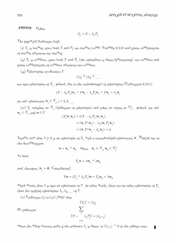
554 APPLIED FUNCTIONAL ANALYSIS
PROOF Define
T1 = T − λ1P1
The following properties hold:
(i) T1 is normal, since both T and P1 are normal (comp. Example 6.5.6) and linear combinations
of normal operators are normal.
(ii) T1 is compact, since both T and P1 (the eigenspace is finite-dimensional!) are compact and
linear combinations of compact operators are compact.
(iii) Eigenvalues of operator T
|λ2| ≥ |λ3| ≥ . . .
are also eigenvalues of T1. Indeed, due to the orthogonality of eigenvalues (Proposition 6.10.1)
(T − λ1P1)ui = Tui − λiP1ui = Tui = λiui
for any eigenvector ui ∈ Ni, i = 2, 3, . . ..
(iv) T1 vanishes on N1 (definition of eigenvalue) and takes on values in N⊥1 . Indeed, for any
u1 ∈ N1 and u ∈ U(T1u,u1) = ((T − λ1P1)u,u1)
= (u, T ∗u1)− λ1(u, P1u1)
= (u, T ∗u1 − λ1u1) = 0
Assume now that λ = 0 is an eigenvalue of T1 with a corresponding eigenvector u. Making use of
the decomposition
u = u1 + u2 where u1 ∈ N1,u2 ∈ N⊥1
we have
T1u = λu1 + λu2
and, therefore, u1 = 0. Consequently,
Tu = (T1 + λ1P1)u = T1u2 = λu2
which means that λ is also an eigenvalue of T . In other words, there are no other eigenvalues of T1
than the original eigenvalues λ1, λ2, . . . of T .
(v) Properties (i) to (iv) imply that
T1 = |λ2|
By induction
T −n
i=1
λiPi = |λn+1|
where the whole process stops if the sequence λi is finite, or |λi+1| → 0 in the infinite case.
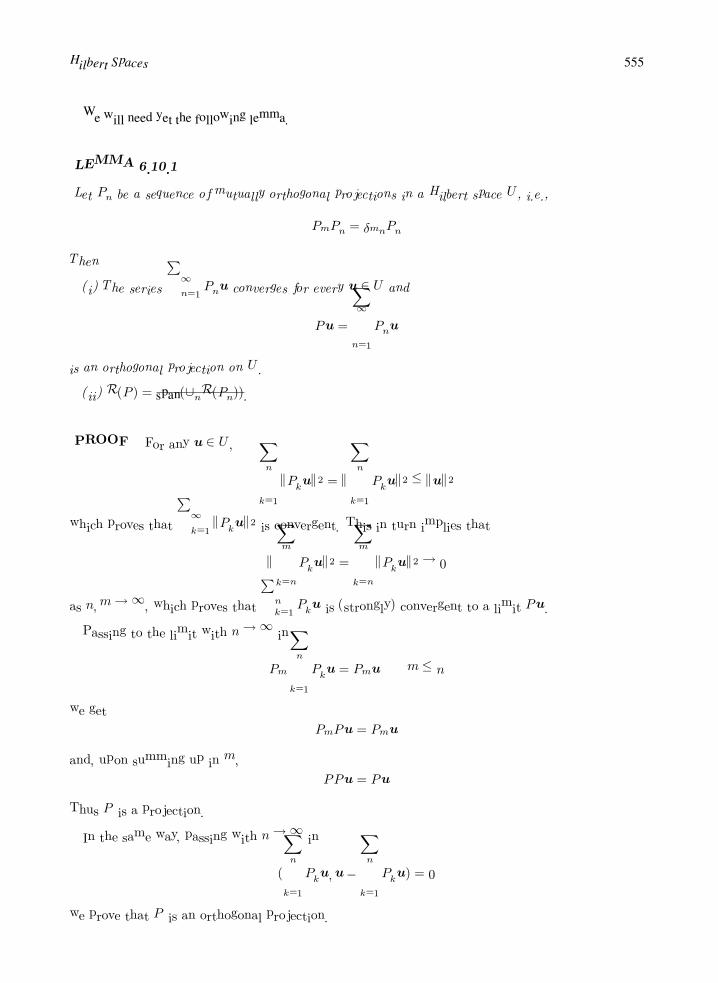
Hilbert Spaces 555
We will need yet the following lemma.
LEMMA 6.10.1
Let Pn be a sequence of mutually orthogonal projections in a Hilbert space U , i.e.,
PmPn = δmnPn
Then
(i) The series∞
n=1 Pnu converges for every u ∈ U and
Pu =
∞
n=1
Pnu
is an orthogonal projection on U .
(ii) R(P ) = span(∪nR(Pn)).
PROOF For any u ∈ U ,
n
k=1
Pku2 =
n
k=1
Pku2 ≤ u2
which proves that∞
k=1 Pku2 is convergent. This in turn implies that
m
k=n
Pku2 =
m
k=n
Pku2 → 0
as n,m→∞, which proves thatn
k=1 Pku is (strongly) convergent to a limit Pu.
Passing to the limit with n→∞ in
Pm
n
k=1
Pku = Pmu m ≤ n
we get
PmPu = Pmu
and, upon summing up in m,
PPu = Pu
Thus P is a projection.
In the same way, passing with n→∞ in
(
n
k=1
Pku,u−
n
k=1
Pku) = 0
we prove that P is an orthogonal projection.

556 APPLIED FUNCTIONAL ANALYSIS
Finally, condition (ii) follows from definition of P .
THEOREM 6.10.3
Let U be a Hilbert space and T be a compact and normal operator from U into itself. Let
|λ1| ≥ |λ2| ≥ . . . (→ 0 if infinite)
denote the sequence of its eigenvalues with corresponding eigenspaces Ni and let N denote the null
space of operator T (eigenspace of λ = 0 eigenvalue). Let Pi, i = 1, 2, . . . denote the orthogonal
projections on Ni and P0 the orthogonal projection on N .
Then the following holds
u =
∞
i=0
Piu
PROOF Let u ∈ N,v ∈ U . Then
0 = (Tu,v) = (u, T ∗v)
implies that R(T ∗) ⊂ N⊥ and, consequently,
N ⊂ R(T ∗)⊥
(comp. Exercises 6.2.1(i) and 6.2.2).
At the same time, for y ∈ R(T ∗)⊥ we have
0 = (y, T ∗x) = (Ty,x) ∀x ∈ U
and, consequently, Ty = 0, i.e., y ∈ N , which all together proves that
N = R(T ∗)⊥
As λi are eigenvalues of T∗ with the same corresponding eigenspaces Ni and the range of T ∗,R(T ∗),
is closed, applying Lemma 6.10.1, we have
u =∞
i=1
Piu for u ∈ R(T ∗)
and, finally,
y = P0u+ (u− P0u) = P0u+
∞
i=1
Pi(u− P0u) =
∞
i=0
Piu

Hilbert Spaces 557
REMARK 6.10.1 The decomposition formula for u is frequently rewritten in the operator form
as
I =∞
i=0
Pi
and called the resolution of identity (see the definition at the end of this section). The essential
difference between the resolution of identity and spectral representation for compact and normal
operators
A =
∞
i=1
λiPi
is the underlying kind of convergence. The first formula is understood in the sense of the strong
convergence of operators, i.e.,n
i=0
Piu→ u ∀u ∈ U
whereas the second one is in the operator norm
n
i=1
λiPi −A → 0
and, in particular, implies the uniform convergence of operator values on bounded sets.
COROLLARY 6.10.2
Let U be a Hilbert space and suppose that a bounded, normal and compact operator T from U into
itself exists such that the null space of T is finite-dimensional. Then U admits an orthonormal basis.
PROOF Let φ1, . . . , φn0 be an orthonormal basis for N , φn0+1, . . . , φn0+n1 an orthonormal basis
for N1, etc.
COROLLARY 6.10.3
Let φ1, φ2, . . . be an orthonormal basis selected in the previous corollary. Then
Tu =∞
k=1
λk(u, φk)φk
where λk repeat themselves if dimNk > 1.
PROOF The proof follows immediately from the Fourier series representation.
Spectral Representation for Compact Operators. LetU, V be two Hilbert spaces and T be a compact (not
necessarily normal!) operator from U into V . As operator T ∗T is compact, self-adjoint, and semipositive-

558 APPLIED FUNCTIONAL ANALYSIS
definite, it admits the representation
T ∗Tu =∞
k=1
α2k(u, φk)φk
where α2k are the positive eigenvalues of T
∗T (comp. Exercise 6.10.1) and φk are the corresponding eigen-
vectors
T ∗Tφk = α2kφk k = 1, 2, . . . α1 ≥ α2 ≥ . . . > 0
Set
φk = α−1k Tφk
Vectors φk form an orthonormal family in V , since
(α−1k Tφk, α
−1l Tφl) = (α−1
k α−1l T ∗Tφk, φl) = (
αk
αlφk, φl) = δkl
We claim that
Tu =∞
k=1
αk(u, φk)φk
Indeed, the series satisfies the Cauchy condition as
m
k=n
αk(u, φk)φk
2 =
m
k=n
α2k|(u, φk)|
2
≤ α2n
m
k=n
|(u, φk)|2 ≤ α2
nu2
Moreover, both sides vanish onN (T ) = N (T ∗T ) (explain why the two sets are equal to each other), and on
eigenvectors φl,∞
k=1
αk(φl, φk)φk =
∞
k=1
αkδlkφk = αlφ
l = Tφl
and, therefore, on the whole space U .
Resolution of Identity. A sequence of orthogonal projections Pn on a Hilbert space U is said to be a
resolution of identity if
(i) Pn is orthogonal to Pm,m = n (PmPn = 0 for allm = n) and
(ii) I =
n Pn (strong convergence of the series is assumed).
The series may be finite or infinite.
Thus, according to Theorem 6.10.3, every compact and normal operator in a Hilbert space generates a
corresponding resolution of identity of orthogonal projections on its eigenspaces Nλ.
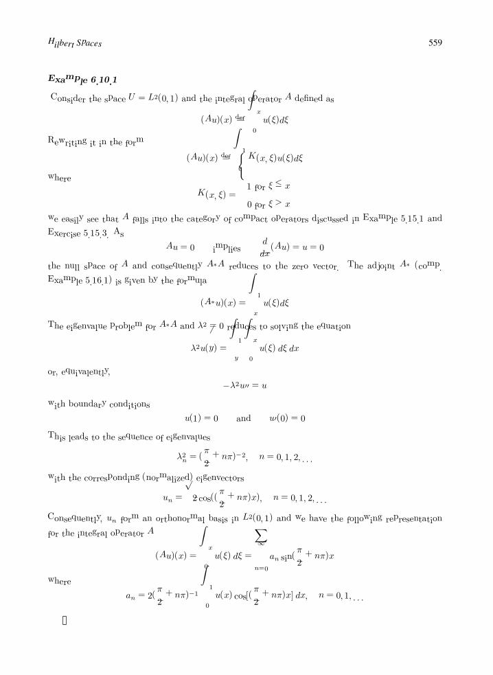
Hilbert Spaces 559
Example 6.10.1
Consider the space U = L2(0, 1) and the integral operator A defined as
(Au)(x)def=
x
0
u(ξ)dξ
Rewriting it in the form
(Au)(x)def=
1
0
K(x, ξ)u(ξ)dξ
where
K(x, ξ) =
1 for ξ ≤ x
0 for ξ > x
we easily see that A falls into the category of compact operators discussed in Example 5.15.1 and
Exercise 5.15.3. As
Au = 0 impliesd
dx(Au) = u = 0
the null space of A and consequently A∗A reduces to the zero vector. The adjoint A∗ (comp.
Example 5.16.1) is given by the formula
(A∗u)(x) =
1
x
u(ξ)dξ
The eigenvalue problem for A∗A and λ2 = 0 reduces to solving the equation
λ2u(y) =
1
y
x
0
u(ξ) dξ dx
or, equivalently,
−λ2u = u
with boundary conditions
u(1) = 0 and u(0) = 0
This leads to the sequence of eigenvalues
λ2n = (
π
2+ nπ)−2, n = 0, 1, 2, . . .
with the corresponding (normalized) eigenvectors
un =√2 cos((
π
2+ nπ)x), n = 0, 1, 2, . . .
Consequently, un form an orthonormal basis in L2(0, 1) and we have the following representation
for the integral operator A
(Au)(x) =
x
0
u(ξ) dξ =
∞
n=0
an sin(π
2+ nπ)x
where
an = 2(π
2+ nπ)−1
1
0
u(x) cos[(π
2+ nπ)x] dx, n = 0, 1, . . .

560 APPLIED FUNCTIONAL ANALYSIS
Exercises
Exercise 6.10.1 Let T be a compact operator from a Hilbert space U into a Hilbert space V . Show that:
(i) T ∗T is a compact, self-adjoint, positive semi-definite operator from a space U into itself.
(ii) All eigenvalues of a self-adjoint operator on a Hilbert space are real.
Conclude that all eigenvalues of T ∗T are real and nonnegative.
6.11 Spectral Theory for Self-Adjoint Operators
We conclude our presentation of elements of spectral theory with a discussion of the very important case of
self-adjoint operators in Hilbert spaces. Most of the presented results exceed considerably the scope of this
book and are presented without proofs. For a complete presentation of the theory we refer the reader to [3].
Let U be a Hilbert space. Recall that an operator A defined on a (dense) domain D(A) ⊂ U into U is
called self-adjoint iff it coincides with its adjoint operator, i.e., A = A∗. For A defined on a proper subspace
only, the equality of operators involves the equality of their domains(!), i.e., D(A) = D(A∗). As adjoint
operators are always closed, every self-adjoint operator is necessarily closed. If domain of A, D(A) equals
the whole space U then, by the Closed Graph Theorem, Amust be continuous. Thus two cases are of interest
only: the case of continuous, i.e., bounded operators defined on the whole space U and the case of closed
operators defined on a proper (dense) subspace D(A) of U . We discuss first the bounded operators.
Spectral Theory for Self-Adjoint Bounded Operators
First of all, as the self-adjoint operators fall into the category of normal operators, all the results concerning
compact and normal operators, studied in the previous section, remain valid. Additionally, all eigenvalues of
A are real. Indeed, if λ is an eigenvalue of A with a corresponding eigenvector u then
λu2 = λ(u,u) = (λu,u) = (Au,u)
= (u, Au) = (u, λu) = λ(u,u) = λu2
and, consequently, λ = λ.

Hilbert Spaces 561
Thus every self-adjoint and compact operator A admits the representation
A =
∞
i=1
λiPi
where |λ1| ≥ |λ2| ≥ . . . is a decreasing (possibly finite) series of real eigenvalues and Pi are the correspond-
ing orthogonal projections on eigenspaces Ni = N (λiI −A).
The observation concerning the eigenvalues of self-adjoint operators can be immediately generalized to
the case of asymptotic eigenvalues, which must be real as well. To see it, let λ be an asymptotic eigenvalue
of a self-adjoint operator A and un a corresponding sequence of unit vectors un, un = 1, such that
(λI −A)un → 0 as n→∞
We have
((λI −A)un,un)→ 0 and (un, (λI −A)un)→ 0
Consequently,
λ = λ(un,un) = (λun,un) = limn→∞
(Aun,un)
and
λ = λ(un,un) = (un, λun) = limn→∞
(un, Aun)
both limits on the right-hand side being equal, which proves that λ = λ.
It can be proved that the asymptotic eigenvalues constitute the whole spectrum of A, i.e., if λ is not an
asymptotic eigenvalue of A, then (λI − A)−1 is defined on the whole U (i.e., R(λI − A) = U ) and is
bounded (comp. Proposition 6.8.1). This result has two immediate consequences:
• self-adjoint operators have no residual spectrum, i.e., σ(A) may consist of point and continuous spec-
trum only!
• spectrum σ(A) is real!
Define now
mdef= inf
u=1Au,u M
def= sup
u=1
Au,u
Both quantities are finite since A = max|m|, |M | (comp. Exercise 6.5.4). It follows immediately from
the definition of an asymptotic eigenvalue that
σ(A) ⊂ [m,M ]
The following theorems formulate the main result concerning spectral representation of self-adjoint oper-
ators.

562 APPLIED FUNCTIONAL ANALYSIS
THEOREM 6.11.1
Let U be a Hilbert space and A a bounded, self-adjoint operator from U into itself. There exists then
a one-parameter family of orthogonal projections I(λ) : U → U, λ ∈ IR, which satisfies the following
conditions:
(i) λ ≤ µ ⇒ I(λ) ≤ I(µ) (the family is increasing).
(ii) I(λ) = 0 for λ < m and I(λ) = I for λ > M .
(iii) function λ→ I(λ) is right-continuous, i.e.,
I(λ) = limµ→λ+
I(µ)
(iv) λ ∈ r(A) (resolvent set of A) iff λ is a point of constancy of A, i.e., there exists a constant
δ > 0 such that I(λ− δ) = I(λ+ δ).
(v) λ ∈ σP (A) (is an eigenvalue of A) iff λ is a discontinuity point of I(λ), i.e.,
limµ→λ−
I(µ) = I(λ)
The inequality of projections in condition (i) of the theorem makes sense for any self-adjoint operators A
and B and is understood as
A ≥ Bdef= A−B ≥ 0 (positive definite)
The family of projections I(λ), λ ∈ IR is known as the spectral family of A.
The following example explains the relation between the spectral family and the resolution of identity
defined in the previous section.
Example 6.11.1
In the case of a compact and self-adjoint operator A on a Hilbert space U , the spectral family I(λ)
can be represented in terms of orthogonal projections P (λ) corresponding to eigenvalues λ as
I(λ) =
µ<λ
P (λ)
where the sum on the right-hand side is finite for λ < 0 and is to be understood in the sense of the
strong convergence of operators for λ ≥ 0 if A has infinitely many eigenvalues.
Given an arbitrary partition Pn
λ0 < λ1 < . . . < λn < λn+1
where λ0 < m and λn+1 > M , we construct now two approximate Riemann-like sums
sn =
n−1
k=0
λk[Iλk+1− Iλk
]

Hilbert Spaces 563
and
Sn =
n−1
k=0
λk+1[Iλk+1− Iλk
]
THEOREM 6.11.2
Let all the assumptions of Theorem 6.11.1 hold. Then for any sequence of partitions Pn, such that
r(Pn) = max |λi+1 − λi| → 0
the corresponding lower and upper sums sn and Sn converge (in the operator norm!) to operator A.
The approximate sums are interpreted as the Riemann–Stieltjes approximation sums and the result is stated
symbolically as
A =
∞
−∞
λ dIλ
=
M
m
λ dIλ
Spectral Theory for Self-Adjoint Closed Operators
We turn now our attention to unbounded operators. Let us begin with a simple result concerning any linear
operator A on a Hilbert space U .
PROPOSITION 6.11.1
Let A be a linear operator on a Hilbert space U . If there is a complex number λ0 in the resolvent set
of A for which the resolvent (λ0I −A)−1 is compact and normal, then
(i) spectrum of A consists of at most countable set of eigenvalues
|λ1| ≤ |λ2| ≤ . . . (→∞ if infinite)
(ii) A can be represented in the form
A =∞
i=1
λiPi
where Pi are the orthogonal projections on eigenspaces Ni corresponding to λi and the conver-
gence of operators is to be understood in the strong sense, i.e.,
Au =
∞
i=1
λiPiu ∀u ∈ D(A)
PROOF Let
|µ1| ≥ |µ2| ≥ . . . (→ 0 if infinite)
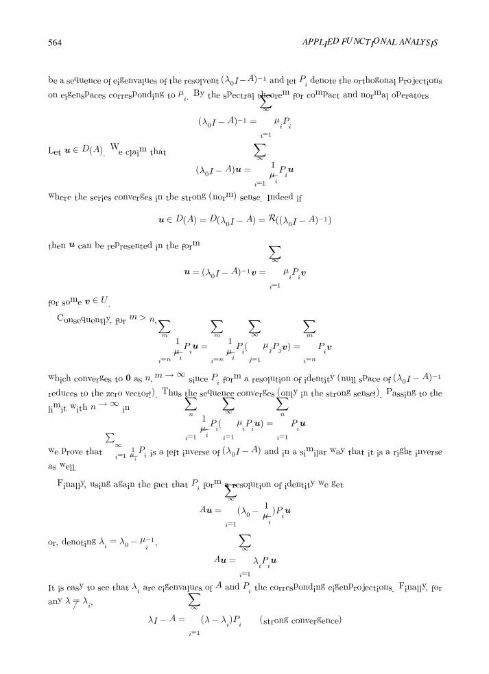
564 APPLIED FUNCTIONAL ANALYSIS
be a sequence of eigenvalues of the resolvent (λ0I−A)−1 and let Pi denote the orthogonal projections
on eigenspaces corresponding to µi. By the spectral theorem for compact and normal operators
(λ0I −A)−1 =
∞
i=1
µiPi
Let u ∈ D(A). We claim that
(λ0I −A)u =
∞
i=1
1
µiPiu
where the series converges in the strong (norm) sense. Indeed if
u ∈ D(A) = D(λ0I −A) = R((λ0I −A)−1)
then u can be represented in the form
u = (λ0I −A)−1v =
∞
i=1
µiPiv
for some v ∈ U .
Consequently, for m > n,
m
i=n
1
µiPiu =
m
i=n
1
µiPi(
∞
j=1
µjPjv) =
m
i=n
Piv
which converges to 0 as n,m→∞ since Pi form a resolution of identity (null space of (λ0I −A)−1
reduces to the zero vector!). Thus the sequence converges (only in the strong sense!). Passing to the
limit with n→∞ inn
i=1
1
µiPi(
∞
i=1
µiPiu) =
n
i=1
Piu
we prove that∞
i=11µiPi is a left inverse of (λ0I −A) and in a similar way that it is a right inverse
as well.
Finally, using again the fact that Pi form a resolution of identity we get
Au =
∞
i=1
(λ0 −1
µi)Piu
or, denoting λi = λ0 − µ−1i ,
Au =
∞
i=1
λiPiu
It is easy to see that λi are eigenvalues of A and Pi the corresponding eigenprojections. Finally, for
any λ = λi,
λI −A =∞
i=1
(λ− λi)Pi (strong convergence)

Hilbert Spaces 565
and using the same reasoning as before we can prove that
(λI −A)−1 =
∞
i=1
(λ− λi)−1Pi
where the boundedness of (λ − λi)−1 implies the boundedness of (λI − A)−1. Thus eigenvalues λi
are the only elements from the spectrum of A.
The proposition just proved not only has a practical importance but also indicates the kind of convergence
in the spectral representation, we can expect in the general case for unbounded operators.
Example 6.11.2
Consider the space U = L2(0, 1) and the differential operator
Au = −d2u
dx2
defined on the subspace
D(A) = u ∈ H2(0, 1) : u(0) = 0, u(1) = 0
(A is actually self-adjoint.)
The inverse of A, equal to the integral operator,
(A−1u)(y) =
1
y
x
0
u(ξ) dξ dx
(comp. Example 6.10.1) was proved to be compact with the corresponding sequence of eigenvalues
µn = (π
2+ nπ)−2 n = 0, 1, 2, . . .
and eigenvectors
un =√2 cos((
π
2+ nπ)x) n = 0, 1, 2, . . .
Consequently,
λn = (π
2+ nπ)2 n = 0, 1, 2, . . .
are the eigenvalues of A and the spectral decomposition takes form
−u(x) =
∞
n=0
an cos((π
2+ nπ)x)
where
an = 2(π
2+ nπ)2
1
0
u(x) cos((π
2+ nπ)x) dx

566 APPLIED FUNCTIONAL ANALYSIS
Continuing our discussion on self-adjoint operators, we first notice that, in the initial considerations in this
section, concerning asymptotic eigenvalues of self-adjoint operators, we have nowhere used the assumption
that the operator was bounded. Moreover, as in the case of bounded operators, one can show that the spectrum
of a self-adjoint operator consists of the asymptotic eigenvalues only and therefore the same conclusions hold:
the residual spectrum is empty and the whole spectrum is real.
We are now ready to state the final result concerning the self-adjoint, unbounded operators (comp. Theo-
rems 6.11.1 and 6.11.2).
THEOREM 6.11.3
(The Spectral Theorem for Self-Adjoint Unbounded Operators)
Let U be a Hilbert space and A an unbounded self-adjoint operator defined on a subspace D(A) ⊂ U
into U . There exists then a one-parameter family of orthogonal projections I(λ) : U → U, λ ∈ IR,
satisfying the following conditions:
(i) λ ≤ µ I(λ) ≤ I(µ) (monotonicity).
(ii) limλ→−∞ I(λ) = 0 and limλ→∞ I(λ) = I (in the strong sense).
(iii) function λ→ I(λ) is right-continuous, i.e.,
I(λ) = limµ→λ+
I(µ)
(iv) λ ∈ r(A) iff λ is a point of constancy of A.
(v) λ ∈ σP (A) iff λ is a discontinuity point of I.
Moreover,
Au =
∞
∞
λ dI(λ)udef= lim
M→∞
M
−M
λ dI(λ)u for u ∈ D(A)
where the convergence is understood in the strong sense and the finite integral is understood in the
sense of the Riemann-Stieltjes integral discussed in Theorem 6.11.2.
Additionally, we have the following characterization for the domain of operator A:
D(A) = u ∈ U :
∞
∞
λ2 dI(λ)u2 <∞
As previously, I(λ) is called the spectral family of operator A.
Functions of Operators. Given the spectral representation of a linear operator A, and a real function φ(λ),
we may define functions of A as
φ(A) =
∞
−∞
φ(λ) dI(λ)

Hilbert Spaces 567
Domain of φ(A) will consist of only those vectors u for which the integral converges (in the appropriate
sense). The same observation applies to the compact and normal operators. Note that, due to the properties
of the spectral family I(λ), operator φ(A) is insensitive to the behavior of φ outside of spectrum σ(A). Thus,
in this sense, all the information about operator A is stored in its spectrum.
Exercises
Exercise 6.11.1 Determine the spectral properties of the integral operator
(Au)(x) =
x
0
1
ξ
u(η) dη dξ
defined on the space U = L2(0, 1).
Exercise 6.11.2 Determine the spectral properties of the differential operator
Au = −u
defined on the subspace D(A) of L2(0, 1),
D(A) = u ∈ H2(0, 1) : u(0) = u(1) = 0
Historical Comments
The creator of theory of Hilbert spaces, German mathematician David Hilbert (1862–1943), was one of the
most universal and influential mathematicians of late 19th and early 20th centuries. Hilbert was born in
Konigsberg. He graduated from Wilhelm Gymnasium in 1880 and in 1882 entered University of Konigsberg
where he met Hermann Minkowski (1864–1909) (Chapter 3), his lifelong friend and collaborator. While in
Konigsburg, both Hilbert and Minkowski were strongly influenced by a young associate professor, Adolf
Hurwitz (1859–1919).
Hilbert defended his doctorate thesis under Ferdinand von Lindemann (1852–1939) and remained at the
university as a professor. In 1895, following the recommendation of influential German geometer, Felix Klein
(1849–1925), Hilbert became the chairman of mathematics department at the University of Gottingen, where
he stayed until his death in 1943.
The mathematicalGotingen School became a legend. Hilbert graduated 69 doctorate students, among them
Felix Bernstein (1878–1956) (Chapter 1), Hermann Weyl (1885–1955), Richard Courant (1888–1972), and
Hugo Steinhaus (1887–1972) (Chapter 5). Hungarian–American mathematician and director of the famous
Institute for Advanced Study at Princeton, John von Neumann (1903–1957), was among Hilbert’s assistants.

568 APPLIED FUNCTIONAL ANALYSIS
At the second International Congress of Mathematicians in Paris, in 1900, Hilbert presented his famous
list of 23 unsolved problems.
Joseph Fourier (1768–1830) was a French mathematician and physicist, one of the first chair holders in
Ecole Polytechnique.
The Gram–Schmidt orthonormalization procedure which appeared in the works of Laplace and Cauchy,
was named after Danish mathematician and actuary, Jørgen Pedersen Gram (1850–1916) and German math-
ematician (student of Hilbert), Erhard Schmidt (1876–1959).
Adrien–Marie Legendre (1752–1833) was a French mathematician. Besides Legendre polynomials (Ex-
ample 6.3.5), he is also remembered for the Legendre transform used in analytical mechanics. Edmond
Laguerre (1834–1886) and Charles Hermite (1822–1901) (see Example 6.3.6) were French mathematicians.
Hermite was the supervisor of Henri Poincare (see below).
Various types of boundary conditions are named after German mathematicians, Johann Dirichlet (1805–
1859) (Chapter 1) and Carl Neumann (1832–1925) (see also Example 5.7.1) and Augustine–Louis Cauchy
(1789–1857) (Chapter 1). The Cauchy boundary condition is also frequently called “Robin boundary condi-
tion” after another French mathematician, Victor Robin (1855–1897).
Jacques Hadamard (1865–1963), a French mathematician, is remembered for his definition of a well-posed
problem: a problem is well posed if it has a unique solution, and the solution depends continuously upon data.
The Lax–Milgram Theorem is named after two contemporary American mathematicians, Peter Lax and
Arthur Milgram. Ivo Babuska is our colleague and professor at The University of Texas at Austin.
Sobolev spaces are named after Sergei Sobolev (1908–1989) (Chapter 5). The trace theorem was proved
by French mathematician, Jacques–Louis Lions (1928–2001), a student of Laurent Schwartz and one of the
most influential mathematicians in second half of 20th century.
The Poincare inequality is named after Henri Poincare (1854–1912), a French mathematician, theoretical
physicist, and philosopher of science. Besides mathematics, Poincare contributed fundamental results to rela-
tivity and celestial mechanics. Hilbert and Poincare were considered to be the most universal mathematicians
of their time.
The Principle of Virtual Work has been known in mechanics for over three centuries. Swiss mathemati-
cians, Johann Bernoulli (1667–1748) and Daniel Bernoulli (1700–1782) are credited with early versions of
the principle for rigid bodies.
The Riesz Representation Theorem was established by Hungarian mathematician, Frigyes Riesz (1880–
1956). Modern spectral theory for self–adjoint operators was developed by Riesz and his collaborator, Bela
Szokefalvi–Nagy (1913–1998).
Thomas Joannes Stieltjes (1856–1894) (Riemann–Stieltjes integral) was a Dutch mathematician.

7
References
[1] H. Adams. Sobolev Spaces. Academic Press, New York, 1978.
[2] G. Duvaout and J. L. Lions. Les Inequations en Mecanique et en Physique. Editions Dunod, Paris,
1972.
[3] T. Kato. Perturbation Theory for Linear Operators. Springer-Verlag, New York, 1966.
[4] M. A. Krasnosel’skii. Topological Methods in the Theory of Nonlinear Integral Equations. Pergamon
Press, New York, 1964.
[5] R. Leis. Initial Boundary Value Problems in Mathematical Physics. Teubner, 1986.
[6] J. L. Lions and E. Magenes. Non Homogeneous Boundary Value Problems and Applications, Vol. 1.
Springer-Verlag, Berlin, 1972.
[7] W. McLean. Strongly Elliptic Systems and Boundary Integral Equations. Cambridge University Press,
2000.
[8] R. E. Showalter. Hilbert Space Methods for Partial Differential Equations. Pitman Publishing Limited,
London, 1977.
[9] I. Stakgold. Green’s Functions and Boundary Value Problems. John Wiley & Sons, New York, 1979.
569
